Powder Technology 288 (2016) 339–353

Contents lists available at ScienceDirect

Powder Technology

j ourna l homepage: www.e lsev ie r .com/ locate /powtec

Experimental and computational study of erosion in elbows due to sandparticles in air flow

Ronald E. Vieira ⁎, Amir Mansouri, Brenton S. McLaury, Siamack A. ShiraziDepartment of Mechanical Engineering, The University of Tulsa, 800 South Tucker Drive, Tulsa, OK 74104, USA

⁎ Corresponding author.E-mail addresses: rev87@utulsa.edu (R.E. Vieira), amir

(A. Mansouri), brenton-mclaury@utulsa.edu (B.S. McLaur(S.A. Shirazi).

http://dx.doi.org/10.1016/j.powtec.2015.11.0280032-5910/© 2015 Elsevier B.V. All rights reserved.

a b s t r a c t

a r t i c l e i n f o

Article history:Received 7 May 2015Received in revised form 13 October 2015Accepted 11 November 2015Available online 12 November 2015

Severe equipment degradation in production piping can occur for gas–solid flows. Advances in modeling andsolid particle erosion simulations are gained through matching computer generated predictions to real-worldexperimental results. This paper presents a comprehensive approach inmodeling and computational study tode-termine erosion in elbows due to sand particles entrained in air. Firstly, utilizing a particle image velocimetry(PIV) technique, the slip velocity between the gas and sand particles in a direct impact geometry has beenmea-sured. Secondly, an erosion equation has been generated based on PIV results and erosion testing of stainless steelin air. Thirdly, erosion patterns are measured in a 76.2 mm ID standard elbow for air-sand flows using a state-of-the-art non-invasive Ultrasonic Technology (UT) device. The metal loss is measured at 16 different locations inthe elbow using dual element ultrasonic transducers. Erosion experiments in the vertical to horizontal elboware performed with gas velocities ranging from 11 m/s to 27 m/s at nearly atmospheric pressure. Two differentsand sizes (150 and 300 μm sand) were used for performing tests. The shapes of the sand are also differentwith the 300 μm sand being sharper than the 150 μm sand. Finally, the new erosion equation has been imple-mented into a commercially available Computational Fluid Dynamics (CFD) code to predict erosion ratios in el-bows for a variety of flow conditions and particle sizes. The predicted CFD erosion magnitudes are comparedwith present and previous UT erosion data in elbows. The comparisons show that CFD predictions are within afactor of two of present and previous UT single-phase erosion data. Four correlations for erosion from literatureare also studied and validated in simulations. The correlation developed and validated in this work can be used topredict the bend lifetime for particular operating conditions.

© 2015 Elsevier B.V. All rights reserved.

Keywords:Gas–solid erosionCFD-based erosion modelingErosion equationErosion in elbowsPIV techniqueUltrasonic testing

1. Introduction

Any industrial process involving the transport of solid particlesentrained in a fluid phase can be subject to erosion damage. Erosionhas been long recognized as a potential source of problems in pneumat-ic and hydraulic transport systems [1–3] and oil and gas production sys-tems [4,5]. Equipment erosion caused by produced sand has long been amajor operating problem in many areas, both in terms of cost of equip-ment replacement and in terms of the risk of pollution and/or firecaused by flowline or equipment cutouts. For example, a number ofdangerous elbow failures occurred in the North Sea on production plat-forms and drilling units between 1993 and 2001 [6]. To make a wellfinancially healthy, flow rates must be high in order to justify the hugeamounts of resources that must be utilized to find and produce oiland gas. Higher throughput is preferred because of the advantage of

-mansouri@utulsa.eduy), siamack-shirazi@utulsa.edu

having higher production rates and lower liquid holdups. The operationmanagers, on the other hand, must run a safe and lowmaintenance op-eration and often they desire lower, moremanageable flow rates. Thesetwo desires conflict and in order to satisfy the owners the operatorsmust work with velocities not of their choosing. The challenge to thedesign engineers is to find the optimum pipeline dimension that offersthe highest throughput while keeping the fluid velocity below the safeoperating limit.

To optimize the design of process equipment and the piping system,it is important to identify the location and magnitude of the maximumerosion rate for single-phase flows in elbows. Additionally, gas andsand experiments allow the qualification ofmeasurement devices to de-termine sand erosion [7]. Medium and high gas velocity flows with lowsand concentrations are expected to remove material from inner wallsin a symmetric pattern. Data captured duringmany gas and sand exper-iments demonstratemaximummeasured erosion patterns and the loca-tion of the maximum erosion rate.

Computational Fluid Dynamics (CFD) based erosion modeling hasmany advantages making it a powerful tool to predict erosion damage.Unlike many simplified erosion models, CFD-based erosion modelingcan be applied to any complex components and can provide great

Fig. 1. Process of generating and validating erosion models.

340 R.E. Vieira et al. / Powder Technology 288 (2016) 339–353

help in developing a simple, timely procedure to predict detailedpatterns of erosion.

The primary goal of this work is to improve and validate CFD-based erosion modeling predictions. The tasks and steps in the pres-ent work are shown in Fig. 1. In order to accomplish the goal, severalsteps have been accomplished. (1) Utilizing a particle imagevelocimetry (PIV) technique, the slip velocity between the gas andsand particles has been determined in a direct impact geometry.(2) Erosion data were collected for stainless steel 316 target materialin air for the same flow geometry. (3) An erosion equation was gen-erated to represent these conditions. (4) Erosion data for the samestainless steel material were collected for the same particle type ina 76.2 mm ID standard elbow using non-invasive ultrasonic trans-ducers. (5) The new erosion equation has been implemented into acommercially available CFD code to predict erosion ratios in elbowsfor a variety of flow conditions and particle sizes. (6) The predictedCFD erosion magnitudes in elbows are compared with present andprevious erosion data, and with four empirical correlations, pro-posed by Oka et al. [8], Zhang et al. [9], Det Norske Veritas (DNV)[10] and Neilson and Gilchrist [11]. These empirical models are wide-ly used in the literature for erosion calculations.

The present work also focuses on low sand concentration (less than2%byweight) and small sizes,which are representative of the situationsencountered in oil and gas productions systems. Therefore, interactionsbetween particles are not considered.

2. Background

2.1. Erosion ratio equations

A wide variety of erosion equations or models has been developedby many investigators [5,12]. There is no universal erosion equationfor all materials to predict erosion rate as erosion is dependent onmany factors. Meng and Ludema [12] concluded that there are four pri-mary mechanisms for which solid particle erosion occurs: cutting wearand plastic deformation, cyclic fatigue, brittle fracture andmelting of thematerials. Besides variation of solid particle erosion mechanisms, manyinvestigators have found that particle speed at impact and incomingangle of the impacting particles should be used to determine erosioncharacteristics [13]. In order to develop an impact angle dependencefunction, erosion tests are usually conducted with particles entrainedin gas flow impacting a target wall, since the impact speed and anglesare similar to the values in the flow stream. Therefore, a deeper under-standing of erosion is obtained by performing small-scale experimentsonmetallic coupons. By performing these experiments, erosion equationsare developed, which are implemented into CFD codes for predictingerosion for a variety of cases.

Finnie [14] developed the one of the earliest erosion equations ero-sion equations for predicting the erosion rate. Finnie [14] suggested

his equation in the form of Eq. (1) and since then several erosion equa-tions in this form were developed.

ER ¼ K FSVnP f θð Þ; ð1Þ

where ER is the erosion ratio that is defined as the amount of mass lostby the wall material due to particle impacts divided by the mass ofimpacting particles, K is a wall material dependent constant, FS is theparticle shape coefficient that has values equal to or less than unity forsharp, semi-round and fully-round sand, VP is the particle impingementvelocity, n is an empirical constant. A range of values between 2 and 3 isrecommended in the literature for the constant n. Based on previous ex-perimental tests conducted at the E/CRC, the value of 2.41 is used as thespeed exponent in the present investigation. f(θ) is an empirical func-tion for incorporating the particle impingement angle.

Ahlert [15] and McLaury [16] at the Erosion/Corrosion ResearchCenter (E/CRC) at the University of Tulsa performed a series of erosiontests to determine the empirical constants in Eq. (1). Ahlert [14] studiedcarbon steel and McLaury [16] studied aluminum. Recently, Okita [17]utilized a small-scale experimental facility to study erosion in a directimpingement geometry using glass beads in air. Erosion models weredeveloped based on air testing for aluminum and stainless steel usingLDV (Laser Doppler Velocimeter) technique for particle velocity mea-surements. For aluminum, erosion models were generated for twotypes of sand: Oklahoma #1 and California 60. These newly developedequations were used to predict erosion rates in CFD. Later, Mansouriet al. [18] performed a series of dry impingement jet tests for normaland oblique configurations. Utilizing a particle image velocimetry(PIV) technique, they determined the slip velocity between the gasand sand particles.

2.2. Experimental work in elbows in air-sand flows

There is not a large amount of published data on erosion problems inthe field. Therefore, it becomes necessary to design and build experi-mental facilities to understand erosion phenomena under controlledconditions and develop and improve erosion predictionmodels. The ex-perimental approach requires using a flowgeometry of interest (such aspipe, elbow, or tee) or a representative elbow specimen to conduct theerosion tests under specific flow conditions. The erosion rate (wallthickness loss per unit time, mm/year) and/or erosion ratio (wall thick-ness loss per unit sand throughput, mm/kg) are then calculated fromthemass loss or thickness loss data, geometry, flow and test conditions.This experimental erosion data can be used to validate erosion models.

The erosion of bends conveying a gas–solid mixture has been inves-tigated by many researchers. Earlier experimental studies were carriedout by Bikbiaev et al. [1–2]. They found that the erosion rate increasesas the inlet gas velocity and curvature ratio increase. Tolle and Green-wood [19] studied the flow of gas/sand mixtures in tubulars for gasvelocities of up to 30 m/s. Both high and low sand concentrations inair were used at different velocities in 50.8 mm standard elbows.Bourgoyne [20] studied experimentally the effect of flow velocity, liquidcontent, and sand concentration in standard elbows. Chen et al. [21]performed experimental erosion tests as well as numerical simulationsin an elbow and a plugged tee with 25.4 mm diameter. Results showedthat particle reboundmodel plays an important role in determining themotion of particles. Mazumder et al. [22] investigated the location andmagnitude of maximum erosion in single-phase flows in a 25.4 mmelbow using aluminum and stainless steel specimens at different fluidvelocities. Themaximum erosion ratio at 34.1 m/s for 150 μm sand par-ticles was measured at 55° from the inlet of the elbow.

Evans et al. [23] carried out an erosion study in high velocity gassystems at high pressure (6.89 MPa) in 101.6 mm long-radius elbows.Intrusive Electrical Resistance (ER) Probes were installed wherethe centerline of the elbow inlet intersects with the elbow surface. Sim-ilarly, extensive empirical information has been gathered at The Tulsa

341R.E. Vieira et al. / Powder Technology 288 (2016) 339–353

University SandManagement Projects (TUSMP) for examining sensitiv-ity of ER probes in airflowwith sand at atmospheric pressure conditionsin 50.8mm ID [24–26] and 76.2mm [26,27] and 101.6 mm [27] elbows.In all of these experiments, standard elbow measurements wereconducted at 45° and 90° to the flow orientation using 150 μm and300 μmsand. Although these ER probe experiments provide valuable in-formation for erosivity trend for many conditions, all these experimentsused ER probes at a fixed location. Also, the intrusive effect of ER probescould affect gas flow parameters inside the elbow.

Eyler [28] studied the erosion pattern generated for gas-sandflow along the long bend of an elbow with r/D = 3.25 in a one-dimensional sense. Ultrasonic and caliper instruments were used to ob-tain readings from 19 locations along the elbows long bend. Maximumwall loss was measured at the 35° position from the inlet to the elbow.Deng [29] studied erosion patterns on bends of pneumatic conveyorsand utilized a handheld ultrasonic probe to determine the extent ofwall loss. Measurements were obtained in a two-dimensional patterninstead of a one-dimensional line along the elbow's long bend. More re-cently, Grubb [7] and Kesana [30] used a novel non-intrusive tempera-ture compensated ultrasonic device to measure the metal loss at 16different locations inside an elbow. Initially, experiments were per-formed with a single-phase carrier fluid (gas-sand) moving in a hori-zontal pipeline. Next, experiments were extended to the horizontalmultiphase slug flow regime. Kesana et al. [31] and Vieira et al. [32]showed that UT technology was successful identifying the erosionpattern on a standard bend.

2.3. CFD-based prediction of sand erosion in elbows

CFD has been used in solid particle erosion studies for many years.Shirazi et al. [33] reported an algorithm to calculate erosion rates in amechanistic approach for awider range of elbow and tee sizeswhich re-lied heavily on computational fluid dynamics for its development.McLaury [15] proposed a generalized erosion prediction procedurethat involves flow simulation, particle tracking, and erosion prediction.Edwards et al. [34] and Zhang [13] developed and improved CFD-based erosion prediction procedures and investigated the erosion ina 90° bend and plugged-tee. Wang and Shirazi [35] developed a CFD-based correlation to predict the erosion ratio between a long radiuselbow and standard elbow. They found that the erosion rate decreasesas the bend radius increases. El-Behery et al. [36] investigated numeri-cally the erosion phenomenon that occurs in 90° and 180° curvedducts. Results showed that the penetration rate increases as the

Fig. 2. Schematic of th

curvature ratio, particle diameter, and inlet gas velocity increase, andas the mass loading ratio and pipe diameter decrease. Pereira et al.[37] found that the combination of the models proposed by Oka et al.[8] for the erosion ratio and Grant and Tabakoff [38] for the coefficientof restitution is the most suitable for the erosion prediction due to par-ticles in an 25.4 mm ID elbow pipe with a 90° curvature angle.

3. Experimental facilities and conditions

3.1. Sand particle velocity measurements

Although erosion rate is influenced by many factors, particle impactspeed is the biggest factor that affects erosion rate. In order to study theeffects of sand particle characteristics (size and shape) on particle veloc-ity, which affect erosion rate, particle velocities of 150 μm and 300 μmsand were measured using Particle Image Velocimetry (PIV) in asmall-scale direct impact test geometry.

Fig. 2 is a schematic of the PIV measurement facility. An electricalcompressor provides the gas flow in the nozzle. The velocity of the gaswas controlled by the valve positioned upstream of the flow meter.Since some gas is normally introduced with sand in the sand injectionnozzle, the flow meter cannot provide the actual gas flow rate and ve-locity that is flowing out of the nozzle. Therefore, a Pitot tube is usedto measure the actual gas velocity at the nozzle exit. The flow meterwas calibrated with the Pitot tube measurements and used only as aguide. The pressure drop at the nozzle creates suction in the feedingtube and draws the sand particles into the nozzle. The mixture of thesand particles and air flow out of the nozzle, and the particle velocityis measured at the intersection of the nozzle jet with the laser sheet.Laser sheet is aligned in theway to have a right anglewith the CCD cam-era. The test section is contained in a box to keep particles from scatter-ing. Two acrylic panels are provided and attached to the box so that thelaser sheet intersects inside the box at the exit of the nozzle from the topwhile the camera captures the images from the side of the box. At theend of the box, there is an outlet for air and particles to escape.

In the present work, the PIV measurements were performedusing a TSI PIV system. The laser source was a pulsed Nd:YAG laserwith 200 mJ/pulse output energy and 532 nmwave length. The imageswere captured by a high resolution (2048 × 2048 pixel) CCD cameraoperating with a 100 mm lens. The synchronizer with 1 ns resolutionautomatically controlled the timing between the laser pulses and cam-era. The post-processing of images was performed using the softwareINSIGHT 4G provided by TSI Inc. The motion of each sand particle was

e PIV test setup.

Fig. 3. Schematic of erosion measurements in air.

342 R.E. Vieira et al. / Powder Technology 288 (2016) 339–353

determined individually, and velocity vectors were obtained 12.7 mmaway from the nozzle exit where the samples were also placed duringerosion tests.

3.2. Direct impact testing (DIT)

Erosion testing of stainless steel 316 (SS316) was conducted using ahigh velocity mixture of sand in air. Measurements were performedunder gas velocities ranging from 28.3 m/s to 112.1 m/s. PIV measure-ments revealed that these gas velocities correspond to average particlevelocities of 8.9 m/s and 35.5 m/s, respectively. In all of the tests, thespecimens were located 12.7 mm from the end of the nozzle. The spec-imens had a rectangular shape with dimensions of 76 mm × 50 mm ×1.5 mm. The density of the material is 7990 kg/m3. The nozzle had thefollowingdimensions: 7mminternal diameter, 8mmexternal diameterand a length of 120 mm (L/D≅17). At each velocity, the measurementswere taken for impact angles of 90, 75, 60, 45, 30, and 15 degrees. Massloss is the test metric, and it is obtained from mass change measure-ments before and after the test. The specimens were weighed using ananalytical balance with an accuracy of 0.0001 g. At each particle speedand angle, the measurements were taken at least 3 times after 300 gor 600 g of 300 μm sand had passed through the nozzle. Erosion ratios

Fig. 4. Experimental facility fo

(kg/kg) are calculated by mass loss of a target coupon (kg) divided bythe total mass of sand throughput (kg). The particle mass flow rate isabout 20 g/min for 300 μm. Each test lasts for about 15min. The test sec-tion was contained in a hood during themeasurements. The test set-upis shown schematically in Fig. 3.

3.3. Erosion studies in elbow

The large-scale erosion tests in a 76.2 mm (3 in.) standard elbowwere performed using the Erosion/Corrosion Research Center (E/CRC)tower-boom loop facility located at The University of Tulsa. The maincomponents of the loop are two diesel compressors, test section, andseparator as shown in Fig. 4. The test section in this large scale facilitycan be modified to accommodate different pipe diameters and canbe oriented between 0° (horizontal) to 90° (vertical). For these experi-ments, the pipe diameter was 76.2mm (3 in.) and 18m long. The elbowis made of stainless steel 316 and has a curvature ratio r/D equal to 1.5.In the present work, all erosion experiments were performed in thevertically upwards inlet and horizontal outlet (V–H) orientation atnear atmospheric pressure conditions (115.1 kPa).

Gas and sand experiments are once-through flow where both thesand and the air are not re-circulated. Air is typically provided by a sin-gle compressor. The sand injection method was achieved by using aninductor sand feeder. The sand feeder is a transparent pipe in which ameasured quantity of sand can be poured from the top. Pressurizedgas from the electrical compressor is used to create a suction force atan inductor nozzle that draws the sand into the test section. The sandrate can be adjusted by controlling the valve on one transparent tube.Gas flow velocities ranging between 11 and 27 m/s propelled sand atrates between 103 kg/day to 256 kg/day. Once the gas flow rate hasbeen established at the desired level, the sand flow control valve isopened so that sand may flow into the loop. When sand injection intothe test section begins, a stopwatch should be used to record the time,and data acquisition should begin. Once the sand injection period isover and the metal loss output has been determined, the experimentis finished; but there is still one task left to complete the experimentalprocedure and that is to clean the entire system. After each experiment,clean water from an open tank is pumped into the test section, whichpushes all remaining sand particles in the test section into the separator.Then, the slurry is pumped from the separator through a filter bag thatretains the sand particles but lets the liquid pass. Once the filtration step

r erosion tests in elbows.

Table 1Experimental flow conditions of erosion experiments in elbow.

Test Q1 P1 P2 T1 T2 VGAS ReG

(#) (m3/s) (Pa) (Pa) (°C) (°C) (m/s) (−)

1 5.43E−03 1.48E + 06 1.06E + 05 48.7 25.4 15 7.60E + 042 5.43E−03 1.48E + 06 1.06E + 05 49.3 25.1 15 7.56E + 043 5.43E−03 1.41E + 06 1.06E + 05 49.0 27.0 15 7.24E + 044 3.87E−03 1.51E + 06 1.05E + 05 48.9 26.4 11 5.62E + 045 5.43E−03 1.48E + 06 1.06E + 05 49.9 26.5 15 7.55E + 046 8.50E−03 1.41E + 06 1.08E + 05 50.9 26.8 23 1.11E + 057 1.04E−02 1.38E + 06 1.08E + 05 51.9 26.5 27 1.31E + 058 3.87E−03 1.51E + 06 1.05E + 05 48.9 25.3 11 5.60E + 049 5.43E−03 1.48E + 06 1.06E + 05 49.9 26.8 15 7.56E + 0410 8.50E−03 1.41E + 06 1.08E + 05 50.9 26.9 23 1.11E + 0511 1.04E−02 1.38E + 06 1.08E + 05 51.9 26.9 27 1.31E + 05

343R.E. Vieira et al. / Powder Technology 288 (2016) 339–353

is complete, both the sand and water are disposed. Finally, the loop isflushed with clean water again to ensure the removal of all sand parti-cles for the subsequent experiments. More detailed information on theexperimental test facility and procedures is provided by Vieira [39].

Local pressure and temperature play a critical role in determiningthe gas density, which consequently changes the gas velocity. Insteadof only considering gas flow rate and test section pipe inner diameter,test section local pressure (P2) and temperature (T2) as well as the

Fig. 5. Location of the transducers o

Fig. 6. Particles used in PIV a

pressure (P1) and temperature (T1) measured after the gas compressorswere considered to calculate the local gas velocity. The final calculationof gas velocity, VGAS, in m/s is shown by Eq. (2).

VGAS ¼ Q1 � P1 � T2 þ 273:15Kð ÞAP � P2 � T1 þ 273:15Kð Þ ; ð2Þ

where: Q1 is the gas flow rate in the gas line near the flowmeter, and APis the cross-sectional area of the pipe test section. In Eq. (2), the absolutepressure and temperature units are in Pascal and Celsius, respectively.Experimental conditions can be found summarized in Table 1:

Erosion rate data has been obtained using state-of-the-art tempera-ture compensated ultrasonic (UT) sensors. Ultrasonic Testing (UT) uti-lizes high frequency sound energy that is used in many industries forflaw detection, thickness measurements, and material characterization.The basic components of UT are the pulser/receiver, transducers, multi-plexer, digitizer and display devices. Transducers utilized in this workare manufactured by Olympus NDT, and the frequency of the transduc-ers used is 10MHz. The resolution of the transducers is 1 μm. Increasingthe frequency of the transducer results in better resolution and shorterwavelengths. In order to take into account the effect of temperature onthe erosion rate measurements, a temperature-compensated post-processor algorithm was applied to the raw data. The temperature ofthe wall is measured from outside of the bend by flush mounting 4

n the standard 76.2 mm elbow.

nd erosion experiments.

Fig. 7. Sand particle velocity vs. air velocity measured 12.7 mm away from the nozzle exit.

344 R.E. Vieira et al. / Powder Technology 288 (2016) 339–353

Resistance Temperature Detector's (RTDs) against the outer elbowwall.The thickness of the pipe wall at the location of interest can be deter-mined by multiplying the velocity of the sound wave in that particularmaterial and the time required to travel through that thickness. Thetransducers which perform the dual role of sending and receiving arecalled dual element transducers. In the present study, the pulse/echotechnique is implemented and therefore dual element transducers areused. Another component of the UT system is the multiplexer, whichis a multichannel switch that enables the user to select the transducerto receive the excitation pulse. A final important component is the dig-itizer which converts the analog signal received by the transducer intodigital output for further analysis. More detailed information on theultrasonic transducer instrumentation is provided by Grubb [7] andKesana [30].

Ultrasonic transducers are arranged in a pattern that permitted theuse of the maximum amount of transducers possible from the custombuilt instrument utilized for this work. The size of the transducersused in this work is 6.35 mm (0.25 in.), which enables a relativelyhigh sensor density on the outside of the elbow. The high sensor densityallows thicknessmeasurements atmultiple locations on the bend. Fig. 5shows the configuration that was used in the experiments.

For erosion tests, a short period of time (in the range of 14 to 85min)is sufficient as the flow is highly erosive. The wall thickness loss obtain-ed at the location of maximum erosion was always higher than0.00254mm (0.1mil). Due to precision improvements in the ultrasonic

Fig. 8. Direct impact tests results f

instrument, this amount of wall material removed during the erosionexperiment was always detectable.

3.4. Sand particles used for PIV measurements and erosion testing

Twodifferent abrasive particleswere utilized for theparticle velocityand erosionmeasurements. California 60mesh is the biggest sized sandparticle. Fig. 6a shows a Scanning Electron Microscope (SEM) image ofthe California 60 sand showing sharp edges. The image of the California60 shows a large variation of particle diameters. From the size distribu-tion, the average diameter of the particle is approximately 300 μm [39].The second sandparticle size used in the experiments is OklahomaNo.1.It is referred to as semi-round sand. Fig. 6b shows an SEM image of theOklahoma No.1 sand. Smooth or rounded edges are visible in the imagethat easily justifies the assignment of the semi-round label. This sandhas an average particle diameter of 150 μm [39]. By conducting theerosion experiments using the Oklahoma No.1 sand, the influence ofparticle shape on erosion can also be studied in addition to the effectsof the particle size. The density of sand used in all cases is assumed tobe 2650 kg/m3.

4. Small-scale tests results and generation of erosion equations

4.1. Sand particle velocity results

The particle velocity measurement results for the 150 μm and300 μm sand are shown and plotted against the gas velocity measuredwith the Pitot tube. Particle velocity was measured by the PIV, and thefluid velocities were measured by the Pitot tube. Fig. 7 shows the parti-cle velocity (VP) versus fluid velocity for the direct impingement geom-etry for 150 μm and 300 μm sand.

As shown in the graph, the particle velocity is directly proportionalto the fluid velocity. The ratio between measured sand particle velocityand gas velocity varied from 0.30 to 0.32. A linear equation was used todetermine the best fitting curve for the data. The data show that there isvery similar slip between fluid and the particles for both particle types.The linear equations were used to determine the gas velocities neces-sary to produce the desired particle velocities during the small-scaleerosion measurements.

4.2. Direct impact test (DIT) results

Erosion rates are measured for stainless steel 316 specimens in air.California 60 (300 μm average size) sand is used as abrasive particles.300 g of sand was injected at the nozzle for the erosion tests that arepresented in this section. After injecting sand, the weight of the coupon

or SS316 in air, 300 μm sand.

Table 3Repeatability of test from UT for VGAS = 15 m/s, 300 μm sand size.

Test VGAS Sandsize

Sandrate

Erosionrate

Erosionratio

UTnumber

UTlocation

Exp.time

(#) (m/s) (μm) (kg/day) (mm/yr) (mm/kg) (#) (°) (min)

1 15 300 154 22.1 3.94E−04 8 47 752 15 300 192 19.3 2.76E−04 8 47 603 15 300 452 58.5 3.55E−04 8 47 15

Data and experimental conditions from eight gas-sand erosion tests can be found summa-rized in Table 4.

Table 4Erosion results using UT for V–H gas-sand flows in 76.2 mm I.D stainless steel elbow.

Test VGAS Sandsize

Sandrate

Erosionrate

Erosionratio

UTnumber

UTlocation

Exp.time

(#) (m/s) (μm) (kg/day) (mm/yr) (mm/kg) (#) (°) (min)

4 11 300 288 16.9 1.61E−04 3 45 605 15 300 103 14.7 3.93E−04 8 47 156 23 300 227 80.3 9.71E−04 8 47 457 27 300 256 129.6 1.39E−03 8 47 148 11 150 254 6.5 7.05E−05 3 45 859 15 150 237 13.2 1.53E−04 8 47 4310 23 150 257 36.2 3.86E−04 8 47 2811 27 150 206 54.0 7.19E−04 3 45 49

Table 2Angle function variables, 300 μm sand (stainlesssteel 316).

Variable Value

n1 0.15n2 0.85n3 0.65Hv (GPa) 1.83f 1.53

345R.E. Vieira et al. / Powder Technology 288 (2016) 339–353

was measured and recorded. Fig. 8 summarizes the erosion ratio inkg/kg versus impact angle for three different impact velocities. Impactparticle velocities of 17.2m/s, 25.2m/s and 32.6m/s and impact particleangles of 15, 30, 45, 60, 75 and 90° were tested. As shown in Fig. 8,higher impact particle velocities yield higher erosion rates for all ofthe impact angles. It is also found that erosion rates are higher forlower impact angles for all the particle velocities. The test resultsrevealed that the maximum erosion ratio occurs at 30° for stainlesssteel. However, Finnie's [14] experimental tests showed that this maxi-mum erosion ratio occurs at 16° for Aluminum. Reviewing other refer-ences indicates that in ductile materials, depending on the type oftarget material and its hardness, this maximum angle might vary from15° to 40°.

Table 5UT Data vs. CFD, V–H orientation, gas-sand flow, 76.2 mm standard elbow, 300 μm and 150 μm

Test VGAS Sand size Sand rate Max. UT data

(#) (m/s) (μm) (kg/day) (mm/year)

1 15 300 154 22.12 15 300 192 19.33 15 300 452 58.54 11 300 288 16.95 15 300 103 14.76 23 300 227 80.37 27 300 256 129.68 11 150 254 6.59 15 150 237 13.210 23 150 257 36.211 27 150 206 54.0

4.3. Generation of erosion equations

Utilizing the information gained through erosion measurements inair, the erosion equation for SS316 is generated. At first, all the experi-mental results are normalized and plotted together in Fig. 8a. Sincethe results are normalized by themaximummeasured ratio, the resultsfrom different particle velocities are close in value to each other whichindicates that particle velocity only affects the erosion equations inmagnitude and not the shape of the erosion versus impact angle profile.

The angle function as shown by Eq. (3) is a modified version of theangle function suggested byOka et al. [8] andwas usedwith parametersn1, n2 and n3, which are chosen tofit the experimental data, and they arelisted in Table 2. The Vicker's hardness for SS316 is approximately1.83 GPa. Since the experimental data are normalized, the angle func-tion must be normalized as well by dividing the function by f, which isthe maximum value of the function. The angle function is plotted to-gether with 300 μm sand experimental data in Fig.8b.

F θð Þ ¼ 1f

sinθð Þn1 1þHvn3 1− sinθð Þ� �n2 : ð3Þ

With the angle function, the entiremodified erosion equation can bedefined based on earlier work at the E/CRC. The erosion equation usedhere takes the basic formof the E/CRC erosion equation (Eq. (1)) for car-bon steels where the value of 2.41 was selected as the speed exponent:

ER ¼ K FSVP2:41 F θð Þ; ð4Þ

where

K ¼ C BHð Þ−0:59; ð5Þ

BH ¼ HV þ 0:10230:0108

: ð6Þ

Since Brinell hardness BH, sharpness factor FS (1.0 for 300 μm sand),impact velocity and angle function are constants for each test condition,the empirical constant C is found by simply dividing the measured ero-sion rate by these constants for each test condition. The total constant Cis calculated by taking an average of the results from the entire set oftest conditions. For SS316 (HV = 1.83 GPa, BH = 178.9) and 300 μmsand, the values of C and K are 4.62 × 10–7 and 2.16 × 10–8, respectively.

5. Sand erosion test results in elbows

5.1. UT results

First, one experiment was repeated three times to examine therepeatability of the UT erosion results under V–H two phase gas/sandconditions. Table 3 shows the repeatability of results for the V–H

sand size.

CFD erosion prediction Pred. over data

(mm/kg) (mm/year) (mm/kg) (−)

3.94E−04 30.3 5.40E−04 1.372.76E−04 37.5 5.36E−04 1.943.55E−04 87.4 5.30E−04 1.491.61E−04 19.9 1.89E−04 1.173.93E−04 20.1 5.35E−04 1.369.71E−04 138.2 1.67E−03 1.721.39E−03 234.6 2.51E−03 1.817.05E−05 7.5 8.10E−05 1.151.53E−04 19.3 2.23E−04 1.463.86E−04 67.0 7.14E−04 1.857.19E−04 69.3 9.23E−04 1.28

Table 6UT Data vs. CFD, H–H orientation, gas-sand flow, 76.2 mm Standard Elbow, 150 μm sand size. Data from Kesana [30].

VGAS Sand size Sand rate UT location Exp. time Max. UT data CFD erosion prediction Pred. over data

(m/s) (μm) (kg/day) (°) (min) (mm/yr) (mm/kg) (mm/yr) (mm/kg)

19 150 39 47 132 6.8 4.76E−04 6.4 4.48E−04 0.9429 150 100 47 180 25.0 6.83E−04 48.8 1.33E−03 1.9533 150 99 47 225 43.5 1.20E−03 67.5 1.86E−03 1.5534 150 98 47 240 63.0 1.76E−03 71.0 1.99E−03 1.13

Table 7Model constants for Det Norske Veritas model.

A1 A2 A3 A4 A5 A6 A7 A8

9.370 42.295 110.864 175.804 170.137 98.398 31.211 4.170

Table 8Comparison of percent bias of present and previous UT data with CFD predictions fordifferent erosion models.

VGAS Sandsize

Max. UTdata

Percent bias

(m/s) (μm) (mm/kg) Presentmodel

Okaet al.

Zhanget al.

DNV Neilson andGilchrist

11 300 1.61E−04 −17.4 52.3 51.8 84.6 81.615 300 3.93E−04 −36.3 47.0 46.7 81.1 82.323 300 9.71E−04 −72.0 35.3 32.2 74.2 81.727 300 1.39E−03 −80.9 33.3 30.3 72.2 82.211 150 7.05E−05 −14.9 13.7 50.7 68.7 61.315 150 1.53E−04 −45.8 −4.2 39.1 58.5 59.323 150 3.86E−04 −85.0 −26.0 26.9 43.6 58.327 150 7.19E−04 −28.4 13.0 47.2 59.6 72.615 300 3.94E−04 −37.1 46.9 46.6 81.1 82.315 300 2.76E−04 −94.2 24.4 22.7 73.1 74.715 300 3.55E−04 −49.3 42.1 39.9 79.4 80.719 150 4.76E−04 5.9 35.4 62.0 72.3 77.229 150 6.83E−04 −94.7 −29.3 23.8 38.2 61.133 150 1.20E−03 −55.0 −1.5 39.8 49.9 70.934 150 1.76E−03 −13.1 26.8 56.2 63.5 79.2

Average −50.0 20.2 41.0 64.3 75.8

346 R.E. Vieira et al. / Powder Technology 288 (2016) 339–353

experiments for VGAS = 15 m/s and 300 μm sand. The average erosionfor the three experiments conducted was 3.42 × 10–4 mm/kg. The ran-dom uncertainty is 1.49 × 10–4 mm/kg which is approximately 44%of the average measured erosion value. From Table 3, it is observedthat the location of maximum erosion was clearly repeated. However,the magnitudes of the erosion were not repeated perhaps due to varia-tions in sand rates. Still, the erosion magnitudes agree within +− 40%

Fig. 9. Erosion rate pattern for gas-sand experiments,

which is reasonable as erosion is a complex process and some variationsin results are anticipated due to sand size and rate variations.

Fig. 9 shows sample results for thewall loss erosion pattern obtainedfrom two erosion tests with gas velocities of 27 m/s and 15 m/s and300 μm sand. Units of measurement are millimeter of wall thicknessloss per year (mm/year). The maximum value of erosion ratio in mm/kgis also shown at the bottom of each figure. The data is displayed at thelocations of the UT probes. Similarly, Fig. 10 shows the results for thewall loss erosion pattern obtained from two experiments with gas veloc-ities of 27 m/s and 15 m/s and 150 μm sand. Similar to previous experi-mental results using UT transducers in gas dominant flows [40], sometransducers mounted at the side and upstream section of the pipe bendmeasure minimal or no metal loss. This discloses that erosion occursmostly on the outer wall of the elbow.

From Figs. 9 and 10, measurements demonstrate that a maximumwall loss rate occurring at the expected hot spot (location of highest ero-sion measured) along the center vertical plane of the vertical–horizontaloriented elbow and in-line with the center axis of the inlet pipe. Everyerosion test had itsmaximumwall loss ratemeasured at either transduc-er location #3 or transducer #8 (See Fig. 5), and those erosion ratesranged from 6.5 mm/year (7.05 × 10–5 mm/kg) to 129.6 mm/year(1.39 × 10–3 mm/kg). It can be observed that the 300 μmparticles create1.9 to 2.5 times greater metal loss compared to the 150 μm particlesdue to the fact that 300 μm sand is much sharper than the 150 μmsand. Fig. 11 demonstrates how the wall thickness loss increases withincreased gas velocity in the V–H flow orientation. Trend lines aredrawn through the data. Based on the erosion results obtained, the ero-sion ratio follows a power law trend as shown in Eq. (7).

ER ∝ VGASn; ð7Þ

where ER is the erosion ratio, VGAS is the gas velocity and n is the velocityexponent. The exponents for both sand sizes are very similar. The expo-nents are approximately 2.39 for 300 μm sand and 2.49 for 150 μm sand.

300 μm sand. Erosion rate is shown in mm/year.

Fig. 10. Erosion rate pattern for gas-sand experiments, 150 μm sand. Erosion rate is shown in mm/year.

347R.E. Vieira et al. / Powder Technology 288 (2016) 339–353

6. CFD validation of erosion equations in standard elbows

In order to validate the erosion equation generated using new PIVmeasurements of sand particles and direct impact tests for stainlesssteel 316 developed in Section 3, 3D Computational Fluid Dynamics(CFD) simulations in elbows are used. Model geometry generation,meshing and simulations were performed using the software FLUENTversion 15.0 developed andmarketed by ANSYS Inc. The CFD-based ero-sion prediction-validation procedure consists of four main sections:flow modeling, particle tracking, erosion calculation and validation.

6.1. Flow modeling, particle tracking and erosion calculation

Flow simulation of the continuous fluid (carrier fluid) is thefirst stepof the CFD-based erosion prediction procedure. FLUENT uses a finitevolume approach to solve the Navier–Stokes equations [41]. The firsttask of flow simulation is to generate the computational grid of the ge-ometry. Fig. 12 shows a schematic diagram of the pipe elbow geometryused in the fluid simulations for 76.2mmelbows (note that the figure isnot drawn to scale). The pipe has an inside diameterD=76.2mm. Flowenters a straight section 1000 mm (≅13D) long. The straight section isfollowed by a 90° elbow section (r/D = 1.5), and then another straightsection of pipe 600 mm (≅8D) in length. The length of upstreamand downstream pipes was chosen because it is possible to refine the

Fig. 11. Effect of gas velocity and sand size on maximum erosion ratio UT measurementsfor gas-sand flow.

mesh without severely increasing the cell count and therefore the com-putational cost of the simulations.

Structured grid types were used for all CFD simulations. The meshused in the simulation was created using only hexahedra, which guar-antees more stability and generates less diffusivity in the simulation.In order to accurately predict erosion, a grid sensitivity and refinementstudy was performed. The mesh resolution used in all simulations isapproximately 1.5 million nodes and is shown in detail in Fig. 13. Notethat the mesh is greatly refined in the vicinity of the pipe wall, inorder to capture the large gradients in the viscous boundary layer. Thecell immediately adjacent to the wall is specified to have a thicknessof 0.4 mm; the cell thickness then gradually increases with distance

Fig. 12. Schematic of the 90° standard 76.2 mm I.D. elbow geometry used for CFDsimulations.

348 R.E. Vieira et al. / Powder Technology 288 (2016) 339–353

from the wall. The boundary layer used was able to provide an averagey+ value of approximately 30 for the first grid point from the wall.

Solution options such as inlet and boundary conditions anddiscretization scheme are specified for each simulation. The flow solu-tion is treated as the steady flow of a viscous and isothermal gas, withthe carrying fluid being air. Gravitational effects are considered for allsimulations (g=9.81m/s2). The density and viscosity of air consideredis ρ=1.2 kg/m3 and μ=1.8 × 10–5 kg/(m-s). The flow velocities at theinlet, as averaged over the pipe cross section, vary from 11m/s to 27m/s.This results in Reynolds number ranging from 7.33 × 105 to 1.72 × 106,which indicates that the flow is expected to be fully turbulent. Thoughturbulent flows are inherently unsteady, it is the prediction of the meanor averaged properties of the flow that is of most interest in erosion cal-culations. For this purpose, it is necessary to augment the underlyingflowequations by a turbulence model. Zhang [13] showed good agreementbetween LDV data from Enayet et al. [42] and predicted velocity and tur-bulence intensity profiles in elbows using a Reynolds stress turbulencemodel. In the present study, the Reynolds Stress Model (RSM) incorpo-rated in ANSYS FLUENT is used as the turbulence model for all simula-tions. In order to achieve the goal of having a near-wall modelingapproach that will possess the accuracy for refined near-wall mesh, anenhanced wall treatment [41] is used along with the turbulence model.

At the inlet to the domain, ANSYS FLUENT's Velocity Inlet boundarycondition is applied. For an impenetrable wall, there can be no flownormal to its surface, and since the flow is treated as viscous, the veloc-ity components tangential to the wall must vanish there as well. The“no-slip” boundary condition, for which all three components of veloc-ity are identically zero at the wall, was used for both the pipe wall andthe surfaces representing the standard elbow. At the outlet, FLUENT'sPressure Outlet boundary condition is applied. This requires that a valuefor the gauge static pressure be provided as well as the turbulence prop-erties. An absolute pressure of 101,325 Pa (atmospheric conditions),which is representative of the large-flow loopexperiments,was specified.The turbulence intensity and hydraulic diameter were set to the samevalues used at the inlet, i.e., 5% and 76.2 mm, respectively.

The process of discretization involves several choices as to howvarious quantities are converted from their continuum to discreterepresentations. ANSYS FLUENT allows the user to pick from several op-tions in this regard. For these simulations, ANSYS FLUENT's “Standard”

Fig. 13.Mesh

scheme is used for the pressure interpolation, and the SIMPLE schemeis used to represent the pressure velocity coupling. In the equationsfor momentum, the non-linear convective terms are discretized usinga spatially second-order accurate upwind scheme; the viscous termsare automatically treated using a second-order accurate scheme.

The predicted flow field is used as input in the particle trackingsection to determine particle trajectories. Particles obtain momentumfrom the carrier fluid, and some of them cross the fluid streamlinesand impact thewall, resulting in erosion. In the particle trackingmodel-ing section, particle impingement information such as impingementspeed, impingement angle, and impingement location as well as im-pingement intensity is obtained. In ANSYS FLUENT, a Discrete RandomWalk (DRW) model is applied to account for the interaction betweenparticles and turbulent eddies. This model assumes that the particlestravel through a succession of turbulent structures that are present inthe flow [41]. Interaction with eddies causes particles to deviate fromthe trajectory. In order to provide a reasonable solution for engineeringapplications, someassumptions aremade for the particle tracking calcu-lations: 1) The presence of the sand particles does not affect the flowand particle interaction is negligible; 2) Solid particles are releasedfrom the inlet of the pipe assuming no slip between the particle andfluid; 3) The particles that are used in the trackingprocedure are consid-ered to be spherical; and 4) the dominant forces acting on the particleare drag force due to the surrounding fluid, buoyancy and added masseffects. It should be noted that since the experimental PIV data showedthat there is a slip between gas and particle velocities, the secondassumption might be a potential source of error in the CFD results. Inorder to validate the particle-tracking option in ANSYS Fluent, Leducet al. [43] compared CFD simulations with experimental results atlow-pressure conditions. It was found that particles can be trackedwith acceptable accuracy.

In order to ensure that a statistically representative set of particleimpingements are obtained, enough particles have to be released fromthe inlet. Chen [21] and Zhang [13] showed that the predicted erosionin elbows and 90° sharp bends becomes independent of the simulatedparticle number when the number is larger than 20,000. In the presentwork, the influence of simulated particle number on the predictedmax-imum erosion rate in the bend has been investigated and verified. Itwasconfirmed that the effect of simulated particle number on the predicted

details.

349R.E. Vieira et al. / Powder Technology 288 (2016) 339–353

maximum erosion rate is negligible for numbers greater that 10,000.When the simulated particle number is larger than 10,000, the overallmaximum erosion rate changes are not significant as particle numberis increased. 100,000 particles were considered to be sufficient, andthe calculation time of the trajectories in CFD simulations is of theorder of a few minutes. Therefore, 100,000 particles were simulated inall subsequent simulations of thiswork. The particle size distribution ef-fect is not examined in the present work. The coefficient of restitutionmodel used was the one proposed by Grant and Tabakoff [38]. In thismodel, it is assumed that the particle rebound is a stochastic processand is subject to statistical variation due to differences in particle sizeand shape. Grant and Tabakoff [38] proposed themean values of the co-efficient of restitution (en and et) and the corresponding standard devi-ations (ɛn and ɛt) as

en ¼ 0:998−1:66θþ 2:11θ2−0:67θ3; ð8Þ

et ¼ 0:993−1:76θþ 1:56θ2−0:49θ3; ð9Þ

εn ¼ 2:15θ−5:02θ2 þ 4:05θ3−1:085θ4; ð10Þ

εt ¼ −0:0005þ 0:62θ−0:535θ2 þ 0:089θ3 ð11Þ

where n and t indicate normal and tangential directions, respectively. θis the incoming particle impact angle. Once a particle hits the pipe wall,the corresponding impingement information is stored and is used laterto calculate erosion in the last step. The erosion modeling relates thisimpingement information to the amount of erosion or mass loss of thewall material. In this work, several erosion models were implementedinto the commercial solver using a User Defined Function (UDF). Inthe CFD simulations, the area-weighted average erosion rates on thetransducer surfaces are calculated. Then, erosion rates are convertedinto thickness loss for comparison with experimental UT data. Assum-ing a material density of 7990 kg/m3 enables the transformation of theCFD erosion units to mm per year (mm/year) through division.

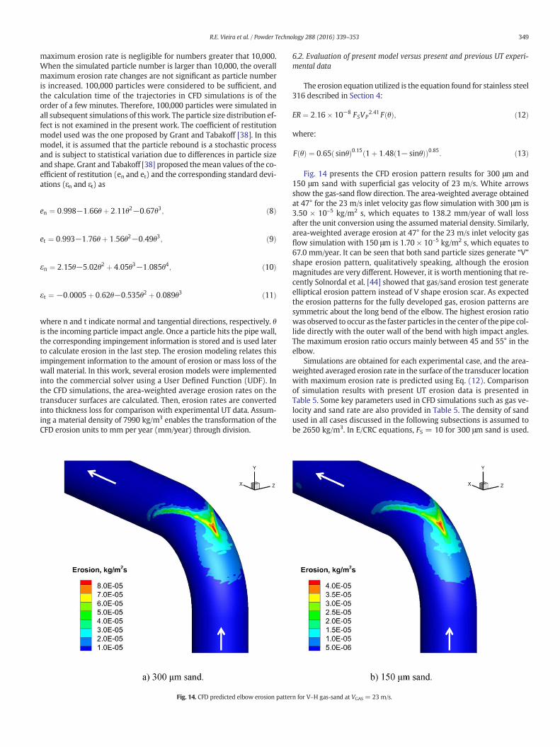
Fig. 14. CFD predicted elbow erosion patter

6.2. Evaluation of present model versus present and previous UT experi-mental data

The erosion equation utilized is the equation found for stainless steel316 described in Section 4:

ER ¼ 2:16� 10−8 FSVP2:41 F θð Þ; ð12Þ

where:

F θð Þ ¼ 0:65 sinθð Þ0:15 1þ 1:48 1− sinθð Þð Þ0:85: ð13Þ

Fig. 14 presents the CFD erosion pattern results for 300 μm and150 μm sand with superficial gas velocity of 23 m/s. White arrowsshow the gas-sand flow direction. The area-weighted average obtainedat 47° for the 23 m/s inlet velocity gas flow simulation with 300 μm is3.50 × 10–5 kg/m2 s, which equates to 138.2 mm/year of wall lossafter the unit conversion using the assumed material density. Similarly,area-weighted average erosion at 47° for the 23 m/s inlet velocity gasflow simulation with 150 μm is 1.70 × 10–5 kg/m2 s, which equates to67.0 mm/year. It can be seen that both sand particle sizes generate “V”shape erosion pattern, qualitatively speaking, although the erosionmagnitudes are very different. However, it is worth mentioning that re-cently Solnordal et al. [44] showed that gas/sand erosion test generateelliptical erosion pattern instead of V shape erosion scar. As expectedthe erosion patterns for the fully developed gas, erosion patterns aresymmetric about the long bend of the elbow. The highest erosion ratiowas observed to occur as the faster particles in the center of thepipe col-lide directly with the outer wall of the bend with high impact angles.The maximum erosion ratio occurs mainly between 45 and 55° in theelbow.

Simulations are obtained for each experimental case, and the area-weighted averaged erosion rate in the surface of the transducer locationwith maximum erosion rate is predicted using Eq. (12). Comparisonof simulation results with present UT erosion data is presented inTable 5. Some key parameters used in CFD simulations such as gas ve-locity and sand rate are also provided in Table 5. The density of sandused in all cases discussed in the following subsections is assumed tobe 2650 kg/m3. In E/CRC equations, FS = 10 for 300 μm sand is used.

n for V–H gas-sand at VGAS = 23 m/s.

Fig. 15. Comparison of CFD erosion ratio predictions to the UT measurements.

350 R.E. Vieira et al. / Powder Technology 288 (2016) 339–353

Similarly, a value of FS = 0.5 is used for 150 μm sand particles. Thevalues of FS are based on Scanning Electron Microscope (SEM) analysisof sand samples [9,39].

Fig. 15a and b show the measured and predicted erosion ratio inmm/kg for 300 μm and 150 μm sand, respectively. The horizontal axisshows the gas velocity in m/s, and the vertical axis shows the erosionrate in mm per year (mm/year). The blue bars in the plot show theCFDpredictedmaximumerosion rates, and the yellowbars are themea-suredmaximum erosion rates. From this plot, it is clear that the predict-ed and themeasured erosionmagnitudes are in a reasonable agreementfor both particles sizes. It is worth mentioning that CFD tends to overpredict the experimental data in all test conditions. The plot andTable 5 show that CFD predictions are within a factor of 2 of the mea-sured UT single-phase erosion data.

Kesana [30] performed UT erosion experiments in the E/CRC large-scale flow loop using gas (single-phase flow) and sand in the horizontalinlet and horizontal outlet (H–H) orientation in a 76.2 mm ID standardelbow. All of the single-phase flow experiments were performed using150 μm sand. The gas velocity varied from 19 to 33 m/s. The test condi-tions and CFD simulation results are listed in Table 6. Fig. 16presents theCFDmodeling results for 300 μmsand in the horizontal orientationwithgas velocity of 34 m/s. The area-weighted average obtained at 47°for the 34 m/s inlet velocity gas flow simulation with 150 μm is1.80 × 10–5 kg/m2 s, which equates to 71.0 mm/year of wall loss Forthe H–H orientation, similar erosion patterns are observed in compari-son with the V–H orientation.

Fig. 17 shows a comparison between CFD predictions and theUT measurements. Similar to the previous comparison, the plot and

Fig. 16. CFD predicted elbow erosion rate pattern for H–H gas-sand at VGAS = 34 m/s,150 μm sand. Experimental conditions from Kesana [30].

Table 6 show that CFD predictions are within a factor of 2 of the mea-sured UT single-phase erosion data.

6.3. Comparison among erosion models

An investigation of four erosion models available in literature isperformed in this work. The predicted CFD erosion magnitudes usingfour empirical correlations proposed by Oka et al. [8], Zhang et al. [9],Det Norske Veritas [10] and Neilson and Gilchrist [11] are comparedwith present and previous UT erosion data in elbows. These modelswere implemented as a UDF into the commercial solver where the pre-dicted area-weighted averaged erosion rate on the transducer surfaceswas converted into erosion rate for comparison with experimentaldata. For all the comparisons, 100,000 computational particles wereinjected in the domain, and the coefficient of restitution model chosenwas the one proposed by Grant and Tabakoff [38].

The correlation proposed by Oka et al. [8] is:

ER ¼ ER90g θð Þ; ð14Þ

where ER90 is the reference erosion ratio at VP= VREF, dP= dREF and θ=90°, where the reference velocity VREF = 104 m/s and the referenceparticle size dREF = 326 μm.

ER90 ¼ KP HVð Þk1 VPð Þk2 dPð Þk3 ð15Þ

where k1, and k3 are empirical exponent factors and k2 is a function ofmaterial hardness and particle properties. KP is an independent factor

Fig. 17. Comparison of CFD erosion ratio predictions to the UT measurements for H–Hgas-sand at VGAS = 34 m/s. Data from Kesana [30].

Fig. 18. Comparison of present and previous UT data with CFD predictions for differenterosion models.

351R.E. Vieira et al. / Powder Technology 288 (2016) 339–353

denoting particle properties such as shape and hardness. HV is theVickers hardness.

The angle function g(θ) in Eq. (14) is defined by the followingexpression:

g θð Þ ¼ sinθð Þn1 1þ HV 1− sinθð Þð Þn2 : ð16Þ

The first term on the right hand side of Eq. (16) represents repeatedplastic deformation, and the second term represents cutting action [5].The constants n1 and n2 are determined by material hardness or otherimpact conditions.

The correlation proposed by Zhang et al. [9] is:

ER ¼ 2:17� 10−7 BHð Þ−0:59 FSVP2:41 F θð Þ; ð17Þ

where:

F θð Þ ¼ 5:4θ−10:11θ2 þ 10:93θ3−6:33θ4 þ 1:42θ5: ð18Þ

Where θ is the particle incidence angle and BHis the Brinell hardnessof the eroded material. FS is the sharpness factor.

Fig. 19. Comparison of present UT Data with CF

The Det Norske Veritas (DNV) model [10] takes the form of:

ER ¼ _mPKNVPnN F θð Þ

f θð Þ ¼X8i¼1

−1ð Þiþ1Aiθπ180

� �i

8><>: ; ð19Þ

where _mP is the mass rate of solid particles, KN and nN are the materialconstants (KN = 2.0 × 10–9, nN = 2.6 for steels) and model constantsof Ai are given in Table 7.

The correlation proposed by Neilson and Gilchrist [11] is:

ER ¼ ERC þ ERD; ð20Þ

in which ERC and ERD represent contributions from cutting and defor-mation, respectively. The cutting erosion is modeled as a function ofthe incidence angle θ.

V2P cos

2θ sinπθ2θ0

2εCθ b θ0

V2P cos

2θ2εC

θ b θ0

8>>>><>>>>:

; ð21Þ

where θ0 is the transition angle, normally set as 45°, and εC is the cuttingcoefficient equal to 3.332 × 107. The deformation erosion is given by:

ERD ¼ max VP sinθ−KD;0ð Þ22εD

; ð22Þ

where εD is the deformation coefficient equal to 7.742 × 107, and KD isthe cut-off velocity, below which no deformation occurs.

In order to compare the results among different erosion models, theconcept of percent bias (PBIAS) is used in this work. Percent bias mea-sures the average tendency of the simulated data to be larger or smallerthan their observed counterparts [45]. The optimal value of PBIAS is 0.0,with low-magnitude values indicating accurate model simulation. Posi-tive values indicatemodel underestimation bias, and negative values in-dicate model overestimation bias [45]. PBIAS is calculated with Eq. (23).The results are presented in Table 8.

PBIAS ¼

Xni¼1

Yidata−Yi

sim� �

� 100

Xni¼1

Yidata

� �

266664

377775; ð23Þ

D predictions along the elbow centerline.

352 R.E. Vieira et al. / Powder Technology 288 (2016) 339–353

whereYiobs is the ith data point for the condition being evaluated,Yi

sim isthe ith simulated value for the condition being evaluated.

From Table 8, it is observed that the negative values of the presentmodel indicate an overall overestimation, with an average percentbias of approximately 50%. On the other hand, all themodels from liter-ature present positive values, which indicate a general underestimationbias. It can be noticed that the Det Norske Veritas [10] and Neilson andGlichrist [11] correlations resulted in much lower erosion when com-pared to the experimental results, whereas the other two correlationsfrom literature displayed values closer to the experimental data. Thecorrelations proposed by Oka et al. [8] and Zhang et al. [9] were theones that showed lowermagnitude percent bias. However, bothmodelsalso underpredict experimental erosion values.

Fig. 18 shows an overall comparison between CFD predictions andthe UT measurements. The horizontal axis shows the measured UTmaximum erosion rates in mm/kg in logarithmic scale, and the verticalaxis shows the CFD predictions also in logarithmic scale. The plot con-firms that CFD predictions with the present model slightly overpredictmeasured UT single-phase erosion data. On the other hand, the fourmodels from literature underpredict the UT data.

Based on the present experimental data, it is also possible to quanti-tatively compare the erosion profile on the outer wall of the elbow as afunction of the curvature angle. The measured values along the center-line of the elbow (Transducers #3, #8, #12 and #15 in Fig. 5) are com-pared with the area-weighted average erosion predictions at theequivalent transducer surfaces in the computational mesh. The mea-sured erosion rate in mm/year along the centerline and the five erosionmodels predictions for two different V–H flow conditions are presentedin Fig. 19.

7. Summary and conclusions

A new erosion model was developed based on previous work con-ducted at the E/CRC. Erosion rates for stainless steel 316 occurring from300 μm sand particles with air were measured in a direct impingementgeometry. Gas velocities were measured with the help of a Pitot tube atthe nozzle exit, and velocities for sand particles were measured usingPIV for the corresponding gas velocities measured with the Pitot tube.

A non-intrusive UT permanent placement temperature compensat-ed ultrasonic wall thickness device was utilized for this work. It wassuccessful identifying the erosion pattern on a standard bend. Locationof highest erosion for single-phase (gas) flow with sand was identifiedaround 45° to the bend. The location of maximum erosion rate was un-altered by increasing the particle size in single-phase flows. It was ob-served that the 300 μm particles create 1.9 to 2.5 times greatererosion rate compared to the 150 μm particles and this was attributedto the fact that 300 μm sand is much sharper. UT results show thatwith an increase in gas velocity there is a power law trend increase inmetal loss in mm/kg. The velocity exponents found for the erosioncurve fit is 2.39 for 300 μm and 2.49 for 150 μm sand, respectively.

A commercial CFD code was utilized to validate the new erosionmodel in elbows. The comparison of predicted and measured erosionrates of 76.2 mm ID SS316 standard elbows showed that CFD predic-tions are within a factor of 2 of present and previous UT single-phaseerosion data found in literature. For both particles sizes, the trends ofpredicted erosion rates are comparable to that of the measured erosionrates. Although CFD over predicts themeasurements for sand in air, it isable to predict the location where maximum erosion rate occurs in theouter section of the elbow. Overall, CFD is capable of being used as atool to predict erosion rates in gas production systems.

Acknowledgments

The authors gratefully acknowledge the financial supports by themember companies of Erosion/Corrosion Research Center (E/CRC) at

the University of Tulsa. The authors also would like to thank Ed Bowers,senior technician at E/CRC, for building the boom loop facility at Univer-sity of Tulsa North Campus.

References

[1] F.A. Bikbiaev, M.I. Maksimenko, V.L. Berezin, V.I. Krasnov, I.B. Zhilinskii, Wear onbranches in pneumatic conveying ducting, Chem. Pet. Eng. 8 (1972) 465–466.

[2] F.A. Bikbiaev, V.I. Krasnov, M.I. Maksimenko, V.L. Berezin, I.B. Zhilinskii, N.T.Otroshko, Main factors affecting gas abrasive wear of elbows in pneumatic convey-ing pipes, Chem. Pet. Eng. 9 (1973) 73–75.

[3] C.L. Flemmer, R.L.C. Flemmer, K. Means, E.K. Johnson, The erosion of pipe bends, The1988 ASME Pressure Vessels and Piping Conference 1988, pp. 93–98.

[4] E.S. Venkatesh, Erosion Damage in Oil and Gas Wells, SPE Paper 15183, 1986.[5] M. Parsi, K. Najmi, F. Najafifard, S. Hassani, B.S. McLaury, S.A. Shirazi, A comprehen-

sive review of solid particle erosion modeling for oil and gas wells and pipelinesapplications, J. Nat. Gas Sci. Eng. 21 (2014) 850–873.

[6] N.A. Barton, Erosion in Elbows in Hydrocarbon Production Systems: Review Docu-ment, Prepared by TÜV NEL Limited for the Health and Safety Executive, ResearchReport 115, UK, 2003.

[7] S.A. Grubb, Development and use of a multi-point temperature compensated highprecision permanent mounted ultrasonic instrument to measure the slug flowerosion pattern in a horizontal standard elbow(PhD. Dissertation) Department ofMechanical Engineering, The University of Tulsa, Tulsa, Oklahoma, USA, 2010.

[8] Y.I. Oka, K. Okamura, T. Yoshida, Practical estimation of erosion damage caused bysolid particle impact, Wear 269 (2005) 102–109.

[9] Y. Zhang, E.P. Reuterfors, B.S. McLaury, S.A. Shirazi, E.F. Rybicki, Comparison ofcomputed and measured particle velocities and erosion in water and air flows,Wear 263 (2007) 330–338.

[10] Recommended Practice RP O501: Erosive Wear in Piping Systems, Revision 4.2,Det Norske Veritas, 2007.

[11] J.H. Neilson, A. Gilchrist, Erosion by a stream of solid particles, Wear 11 (1968)111–122.

[12] H.S. Meng, K.C. Ludema, Wear models and predictive equations: their form andcontent, Wear 181–183 (1995) 443–457.

[13] Y. Zhang, Application and improvement of Computational Fluid Dynamics (CFD) insolid particle erosion modeling(Ph.D. Dissertation) Department of MechanicalEngineering, The University of Tulsa, Tulsa, Oklahoma, USA, 2006.

[14] I. Finnie, Erosion of surfaces by solid particles, Wear 3 (2) (1960) 87–103.[15] K. Ahlert, Effect of Particle Impingement Angle and SurfaceWetting on Solid Particle

Erosion of AISI 1018 Steel(M.S. thesis) Department of Mechanical Engineering, TheUniversity of Tulsa, Tulsa, USA, 1994.

[16] B.S. McLaury, Predicting solid particle erosion resulting from turbulent fluctuationsin oilfield geometries(Ph.D. Thesis) Department of Mechanical Engineering, TheUniversity of Tulsa, Tulsa, USA, 1996.

[17] R. Okita, Effects of Viscosity and Particle Size on Erosion Measurements andPredictions(M.S. thesis) The University of Tulsa, Tulsa, Oklahoma, USA, 2010.

[18] A. Mansouri, H. Arabnejad, S. Shirazi, B. McLaury, A combined CFD/experimentalmethodology for erosion prediction, Wear 332–333 (2015) 1090–1097.

[19] G.C. Tolle, D.R. Greenwood, Design of pipe fittings to reduce wear caused by sanderosion, API OSAPER Project No. 6, Texas A&M Research Foundation, 1977.

[20] A.T. Bourgoyne Jr., Experimental study of erosion in diverter systems due to sandproduction, SPE/IADC Drilling Conference, Society of Petroleum Engineers, 1989.

[21] X. Chen, B.S. McLaury, S.A. Shirazi, Application and experimental validation of acomputational fluid dynamics (CFD)-based erosion prediction model in elbowsand plugged tees, Comput. Fluids 33 (2004) 1251–1272.

[22] Q. Mazumder, S.A. Shirazi, B.S. McLaury, Experimental investigation of the location ofmaximum erosivewear damage in elbows, J. Press. Vessel. Technol. 30 (2008) 011303.

[23] T. Evans, H. Bennett, Y. Sun, J. Alvarez, E. Babaian-Kibala, J. Martin, Studies of inhibi-tion and monitoring of metal loss in gas systems containing solids, Proceedings ofCORROSION 2004, Paper 04362, NACE International, 2004.

[24] M. Pyboyina, Experimental investigation and computational fluid dynamics simula-tions of erosion on electrical resistance probes(M.S. Thesis) Department of Mechan-ical Engineering, The University of Tulsa, Tulsa, Oklahoma, USA, 2006.

[25] P.K. Nuguri, Experimental investigation and modeling of erosion for gas dominantmultiphase flows with sand(M. S. Thesis) Department of Mechanical Engineering,The University of Tulsa, Tulsa, Oklahoma, USA, 2007.

[26] R.M. Dosila, Effects of low liquid loading on solid particle erosion for gas dominantmultiphase flows(M.S. Thesis) Department of Mechanical Engineering, The Univer-sity of Tulsa, Tulsa, Oklahoma, USA, 2008.

[27] C. Fan, Evaluation of solid particle erosion in gas dominant flows using electrical re-sistance probes(M.S. Thesis) Department of Mechanical Engineering, The Universityof Tulsa, Tulsa, Oklahoma, USA, 2010.

[28] R.L. Eyler, Design and analysis of a pneumatic flow loop(M. S., Thesis) West VirginiaUniversity, Morgantown, West Virginia, USA, 1987.

[29] T. Deng, M. Patel, I. Hutchings, M. Bradley, Effect of bend orientation on life andpuncture point location due to solid particle erosion of a high concentration flowin pneumatic conveyors, Wear 258 (2005) 426–433.

[30] N. Kesana, Erosion in multiphase pseudo slug flowwith emphasis on sand samplingand pseudo slug characteristics(Ph.D. Dissertation) Department of Mechanical Engi-neering, The University of Tulsa, Tulsa, Oklahoma, USA, 2013.

[31] N. Kesana, S.A. Grubb, B.S. McLaury, S.A. Shirazi, Ultrasonic measurement of multi-phase flow erosion patterns in a standard elbow, ASME J. Energy Resour. Technol.135 (2013) 032905.

353R.E. Vieira et al. / Powder Technology 288 (2016) 339–353

[32] R.E. Vieira, N.R. Kesana, B.S. McLaury, S.A. Shirazi, Experiments for sand erosionmodel improvement for elbows in gas production, low-liquid loading and annularflow conditions, Proceedings of CORROSION/2014, paper no. 4325, NACE Interna-tional, 2014.

[33] S.A. Shirazi, J.R. Shadley, B.S. McLaury, E.F. Rybicki, A procedure to predict solid par-ticle erosion in elbows and tees, ASME J. Press. Vessel Technol. 117 (1995) 45–52.

[34] J. Edwards, B.S. McLaury, S.A. Shirazi, Modeling solid particle erosion in elbows andplugged tees, ASME J. Energy Resour. Technol. 123 (2001) 277–284.

[35] J. Wang, S.A. Shirazi, A CFD based correlation for erosion factor for long-radiuselbows and bends, ASME J. Energy Resour. Technol. 125 (2003) 26–34.

[36] S. El-Behery, M. Hamed, K.A. Ibrahim, M.A. El-Kadi, CFD evaluation of solid particleserosion in curved ducts, ASME J. Fluids Eng. 132 (2010) 071303.

[37] G.C. Pereira, F.J. de Souza, D. Martins, Numerical prediction of the erosion due toparticles in elbows, Powder Technol. 261 (2014) 105–117.

[38] T. Grant, W. Tabakoff, Erosion prediction in turbomachinery resulting from environ-mental solid particles, J. Aircr. 12 (1975) 471–547.

[39] R.E. Vieira, Sand erosion model improvement for elbows in gas production, multi-phase annular and low-liquid flow(Ph.D. Dissertation) Department of MechanicalEngineering, The University of Tulsa, Tulsa, Oklahoma, USA, 2014.

[40] M. Parsi, R.E. Vieira, N.R. Kesana, B.S. McLaury, S.A. Shirazi, Ultrasonic measurementsof sand particle erosion in gas dominant multiphase churn flow in vertical pipes,Wear 328 (2015) 401–413.

[41] ANSYS Fluent, 12.0/12.1 Documentation, Users Guide Manual, Ansys Inc., 2009[42] M. Enayet, M. Gibson, A. Taylor, M. Yianneskis, Laser-Doppler measurements of

laminar and turbulent flow in a pipe bend, Int. J. Heat Fluid Flow 3 (1982) 213–219.[43] S. Leduc, C. Fredriksson, R. Hermansson, 2005, particle-tracking option in fluent

validated by simulation of a low-pressure impactor, Adv. Powder Technol. 17 (2006)99–111.

[44] C.B. Solnordal, Y.W. Chong, J. Boulanger, An experimental and numerical analysis oferosion caused by sand pneumatically conveyed through a standard pipe elbow,Wear 336 (2015) 43–57.

[45] H. Gupta, S. Sorooshian, P.O. Yapo, Status of automatic calibration for hydrologicmodels: comparison with multilevel expert calibration, J. Hydrol. Eng. 4 (1999)135–143.