This article appeared in a journal published by Elsevier. The attachedcopy is furnished to the author for internal non-commercial researchand education use, including for instruction at the authors institution

and sharing with colleagues.

Other uses, including reproduction and distribution, or selling orlicensing copies, or posting to personal, institutional or third party

websites are prohibited.

In most cases authors are permitted to post their version of thearticle (e.g. in Word or Tex form) to their personal website orinstitutional repository. Authors requiring further information

regarding Elsevier’s archiving and manuscript policies areencouraged to visit:

http://www.elsevier.com/copyright

Author's personal copy

Poverty mapping based on livelihood assets: A meso-level application inthe Indo-Gangetic Plains, India

Olaf Erenstein a,*, Jon Hellin b, Parvesh Chandna c

a International Maize and Wheat Improvement Centre (CIMMYT), NASC, Pusa, New Delhi-110012, Indiab CIMMYT, Apdo Postal 6-641, 06600 Mexico D.F., Mexicoc International Rice Research Institute (IRRI)/Rice–Wheat Consortium for the Indo-Gangetic Plains (RWC), NASC, Pusa, New Delhi-110012, India

Keywords:Poverty mappingLivelihood capitalMulti-dimensional povertyTargetingIndo-Gangetic PlainsIndia

a b s t r a c t

Poverty maps are an increasingly popular mode of visualizing the spatial dimension ofpoverty. They help guide priority-setting and target poverty-alleviation interventions. Theutility of poverty maps can be enhanced by spatially disaggregating the underlying causes ofpoverty. One promising approach explored in this paper is the use of livelihood assets –natural, physical, human, social and financial – the building blocks of sustainable livelihoods.We illustrate the approach by mapping and contrasting poverty and livelihood assets withinthe Indian Indo-Gangetic Plains drawing on district-level indicators and livelihood asset-based principal components. The relatively low poverty incidence in the north-westernplains is associated with an overall favorable livelihood asset base, particularly pronouncedfor natural and financial capitals. There is a marked gradient with poverty increasing east-wards, reflecting a similarly marked decline in livelihood assets. The overall unfavorablelivelihood asset base in the mid-Gangetic Plains of Bihar and Eastern Uttar Pradesh providesa particularly challenging spatial poverty trap. The maps and regional contrasts of povertyand livelihood assets provide a foundation for future research and development work andreiterate the need for cross-sectoral and inter-disciplinary approaches.

� 2009 Elsevier Ltd. All rights reserved.

Introduction

Poverty is a spatially heterogeneous phenomenon, i.e. poor people tend to be clustered in specific places. The geographicvariation in the incidence and magnitude of poverty is often due to factors with spatial dimensions, such as natural resourceendowments, and access to services such as health care and education (Henninger & Snel, 2002). An analysis and under-standing of poverty from a geographical and historical perspective is, hence, an invaluable contribution to the debates aboutthe causes of poverty, and the action required to reduce poverty. Geographers have long analyzed the spatial dynamics ofpoverty, including pioneering work by Green (1994) in Great Britain and Kodras (1997) in the United States of America.Geographers and political scientists from the Indian sub-continent have, likewise, been long engaged in academic debate (e.g.Shrestha, 1997; Yapa, 1996) and empirical research on poverty, inequality and social division in society in both rural (e.g.Krishna et al., 2004; Kundu & Raza, 1982) and urban (e.g. Kundu & Sarangi, 2007) settings.

India is home to 17% of the global population and 33% of the world’s poor (Chen & Ravallion, 2008). Poverty is falling inIndia, even though there is some controversy over the rate at which poverty is declining and concerns that the officialestimates of poverty reduction are too optimistic, particularly for rural India (Erenstein, 2009). What is less controversial isthat poverty remains endemic in rural areas. Indeed, although agriculture’s share in GDP declined from 45% in 1977–1978 to

* Corresponding author. Tel.: þ91 11 2584 2940; fax: þ91 11 2584 2938.E-mail address: o.erenstein@cgiar.org (O. Erenstein).

Contents lists available at ScienceDirect

Applied Geography

journal homepage: www.elsevier .com/locate/apgeog

0143-6228/$ – see front matter � 2009 Elsevier Ltd. All rights reserved.doi:10.1016/j.apgeog.2009.05.001

Applied Geography 30 (2010) 112–125

Author's personal copy

only 28% in 1999–2000 (at constant 1993–1994 prices), agriculture continues to occupy a predominant position in the Indianeconomy and its share of employment declined only from 74% in 1972–1973 to 60% by 1999–2000 (Bhalla & Hazell, 2003).

As part of the wider debate about the causes of poverty and specifically the interventions needed to alleviate poverty,researchers, development practitioners and policy makers are increasingly using poverty maps to visualize the spatialdimensions of poverty (Amarasinghe, Samad, & Anputhas, 2005; Bellon et al., 2005; Bigman & Fofack, 2000; CIESIN, 2006;Elbers, Lanjouw, & Leite, 2008; Henninger & Snel, 2002; Hyman, Larrea, & Farrow, 2005; Kam, Hossain, Bose, & Villano, 2005;Xiaoyun & Remenyi, 2008). Furthermore, poverty maps help guide priority-setting and target poverty-alleviation interven-tions by disentangling the spatial heterogeneity of poverty, informing where there may be a concentration of poverty andidentifying where development efforts may best be directed (Fujii, 2008; Palmer-Jones & Sen, 2006).

The use of poverty maps has been enhanced by a number of factors including: greater availability of relevant data; enhancedaccess to Geographic Information Systems (GIS) and mapping software; and advances in statistical methods of mapping poverty(Henninger & Snel, 2002). Reflecting their popularity, Internet search engines can deliver an array of hits for ‘poverty map’(Google produced 10.8 million hits and Google scholar 156,000 hits on 1/09/2008) and there is a dedicated web-site (http://www.povertymap.net, accessed on 1/09/2008). Mirroring the worldwide trend, there has been an increasing use of povertymaps in India, particularly at the state level (e.g. MSSRF & WFP, 2004; Planning Commission, 2002; Srivastava et al., 2004) andoccasionally at the district-level (e.g. Bansil, 2006; Chaudhuri & Gupta, 2009; Debroy & Bhandari, 2003). Poverty maps have nowalso been used to map urban poverty and to examine the implications for policy targeting (Baud, Sridharan, & Pfeffer, 2008).

A major challenge for poverty mapping remains that both measuring poverty and its mapping are data intensive. Toenhance the utility of poverty maps as a targeting tool, there is a need to seek out the most disaggregated data available(Alderman, Babita, Demombynes, Makhatha, & Ozler, 2002; Minot, 2000). India provides a case in point, where targeting atthe district level as opposed to state level reduces the average target population from 40 to two million. Indeed, the smallerthe target areas the more homogeneous the population in terms of its standard of living, thereby greatly enhancing theefficiency of poverty-alleviation interventions and reducing the leakage to the non-poor (Bigman & Srinivasan, 2002).

The disaggregated data needs have, thus, been a major impediment to the development of poverty maps, particularly inmost developing countries (Bigman & Fofack, 2000). Poverty maps based on light surveys are not accurate and could againresult in substantial leakage of poverty-alleviation interventions (Fofack, 2000). Promising approaches to produce moredetailed poverty maps and reduce targeting errors have been developed (Bigman & Fofack, 2000), and include combiningdifferent survey types (Fofack, 2000; Hentschel, Lanjouw, Lanjouw, & Poggi, 2000) and econometric models (Bigman &Srinivasan, 2002; Bigman, Dercon, Guillaume, & Lambotte, 2000).

Poverty maps are most frequently based on uni-dimensional indicators of poverty (such as monetary income, expenditure,or daily subsistence levels), or of wellbeing (such as life expectancy, child mortality, or literacy), derived from national censusdata or household surveys (Henninger & Snel, 2002). Some have expressed reservations in terms of the data sources and callfor more participatory approaches (Xiaoyun & Remenyi, 2008). Others perceive uni-dimensional poverty measures such asa lack of income or food as too narrow and ignoring other aspects of human deprivation (Erenstein, 2009; Krishnaraj, 2006;Ruggeri Laderchi, Saith, & Stewart, 2003; Saith, 2005; Wagle, 2008).

The utility of uni-dimensional poverty maps can be enhanced by integrating biophysical and socio-economic indicators toprovide a more systematic and analytical picture of human wellbeing and equity (Henninger & Snel, 2002). Multi-dimen-sional poverty maps thereby provide a means for spatially disaggregating the underlying causes of poverty. These providemore immediate pointers to the corresponding policy implications for poverty-alleviation.

One promising approach explored in this paper is to link multi-dimensional poverty maps to the sustainable livelihoodsapproach (DFID, 2007; Ellis, 2000), particularly as the latter provides a coherent framework for defining poverty (Beck & Nesmith,2001). Central to the approach are people’s assets (natural, physical, human, financial and social), the major complementarybuilding blocks for their livelihoods. Poverty is an outcome of people’s livelihoods. Livelihood assets thereby provide both a proxyfor absolute poverty and a broader poverty measure (Erenstein, 2009). Researchers such as Baud et al. (2008), Fujii (2008) andKristjanson, Radeny, Baltenweck, Ogutu, and Notenbaert (2005) have linked poverty mapping to the livelihood approach, but thepractice is still relatively uncommon. This is associated with the difficulty of operationalizing the livelihoods approach in terms ofits measurement. Like other capability approaches to poverty, it still lacks appropriate measurement schemes for practical wide-scale application, partly due to the complexity of identifying and quantifying the contributing elements (Wagle, 2008).

In this paper we assess the potential of livelihood asset indicators for multidimensional poverty mapping at the meso-level. We illustrate the approach by mapping and contrasting poverty and livelihood assets in the Indian Indo-Gangetic Plainsas an empirical case. In the next section we introduce the study area and the data and methods used. The results are presentedin Section 3 and discussed in Section 4. The discussion outlines some of the challenges in enhancing the utility of poverty andasset maps as a regional targeting tool. In Section 5, we draw conclusions from the study.

Material and methods

Study area

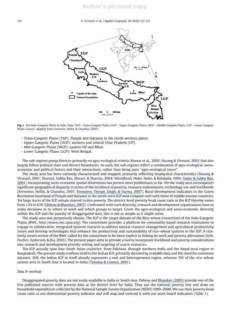
The study area encompasses the Indo-Gangetic Plains (IGP) in India comprising 0.47 million km2 and 280 million ruralinhabitants. The area includes 149 districts in five states across northern India along the Himalayan range: Punjab, Haryana,Uttar Pradesh, Bihar, and West Bengal. The area can be divided into four major sub-regions (Fig. 1):

O. Erenstein et al. / Applied Geography 30 (2010) 112–125 113

Author's personal copy

- Trans-Gangetic Plains (TGP): Punjab and Haryana in the north-western plains.- Upper Gangetic Plains (UGP): western and central Uttar Pradesh (UP).- Mid-Gangetic Plains (MGP): eastern UP and Bihar.- Lower Gangetic Plains (LGP): West Bengal.

The sub-regions group districts primarily on agro-ecological criteria (Kumar et al., 2002; Narang & Virmani, 2001) but alsolargely follow political state and district boundaries. As such, the sub-regions reflect a combination of agro-ecological, socio-economic and political factors and their interactions, rather than being pure ‘‘agro-ecological zones’’.

The study area has been variously characterized and mapped, primarily reflecting biophysical characteristics (Narang &Virmani, 2001; Sharma, Subba Rao, Murari, & Sharma, 2004; Woodhead, Huke, Huke, & Balababa, 1994; Yadav & Subba Rao,2001). Incorporating socio-economic spatial dimensions has proven more problematic so far. Yet the study area encompassessignificant geographical disparity in terms of the incidence of poverty, resource endowments, technology use and livelihoods(Erenstein, Hellin, & Chandna, 2007; Erenstein, Thorpe, Singh, & Varma, 2007). Rural development indicators in the GreenRevolution heartland of Punjab and Haryana in the north-west IGP now compare well with those of middle income countries.Yet large tracts of the IGP remain marred in dire poverty. The district-level poverty head count ratio in the IGP thereby variesfrom 1.5% to 63% (Debroy & Bhandari, 2003). Confronted with such diversity, research and development organizations have tomake decisions as to where to work and which groups to target. Given the agro-ecological and socio-economic diversitywithin the IGP and the paucity of disaggregated data, this is not as simple as it might seem.

The study area was purposively chosen. The IGP is the target domain of the Rice-wheat Consortium of the Indo-GangeticPlains (RWC, http://www.rwc.cgiar.org). The consortium provides a platform for commodity-based research institutions toengage in collaborative, integrated systems research to address natural resource management and agricultural productivityissues and develop technologies that enhance the productivity and sustainability of rice–wheat systems in the IGP. A rela-tively recent review of the RWC called for the consortium to be more explicit in linking its work and poverty alleviation (Seth,Fischer, Anderson, & Jha, 2003). The present paper aims to provide a tool to incorporate livelihood and poverty considerationsinto research and development priority-setting and targeting of scarce resources.

The IGP actually span four South Asian countries: from Pakistan, through northern India and the Nepal terai region toBangladesh. The present study confines itself to the Indian IGP, primarily dictated by available data and the need for consistentdatasets. Still, the Indian IGP in itself already represents a vast and heterogeneous region, whereas 76% of the rice–wheatsystem area in South Asia is located in India (Timsina & Connor, 2001).

Data & methods

Disaggregated poverty data are not easily available in India or South Asia. Debroy and Bhandari (2003) provide one of thefew published sources with poverty data at the district level for India. They use the national poverty line and draw onhousehold expenditures collected by the National Sample Survey Organization (NSSO) 1999–2000. We use their poverty headcount ratio as uni-dimensional poverty indicator and will map and contrast it with our asset-based indicators (Table 1).

Fig. 1. The Indo-Gangetic Plains in India. Note: TGP¼ Trans-Gangetic Plains; UGP¼Upper Gangetic Plains; MGP¼Middle Gangetic Plains; LGP¼ Lower GangeticPlains. Source: adapted from Erenstein, Hellin, & Chandna (2007).

O. Erenstein et al. / Applied Geography 30 (2010) 112–125114

Author's personal copy

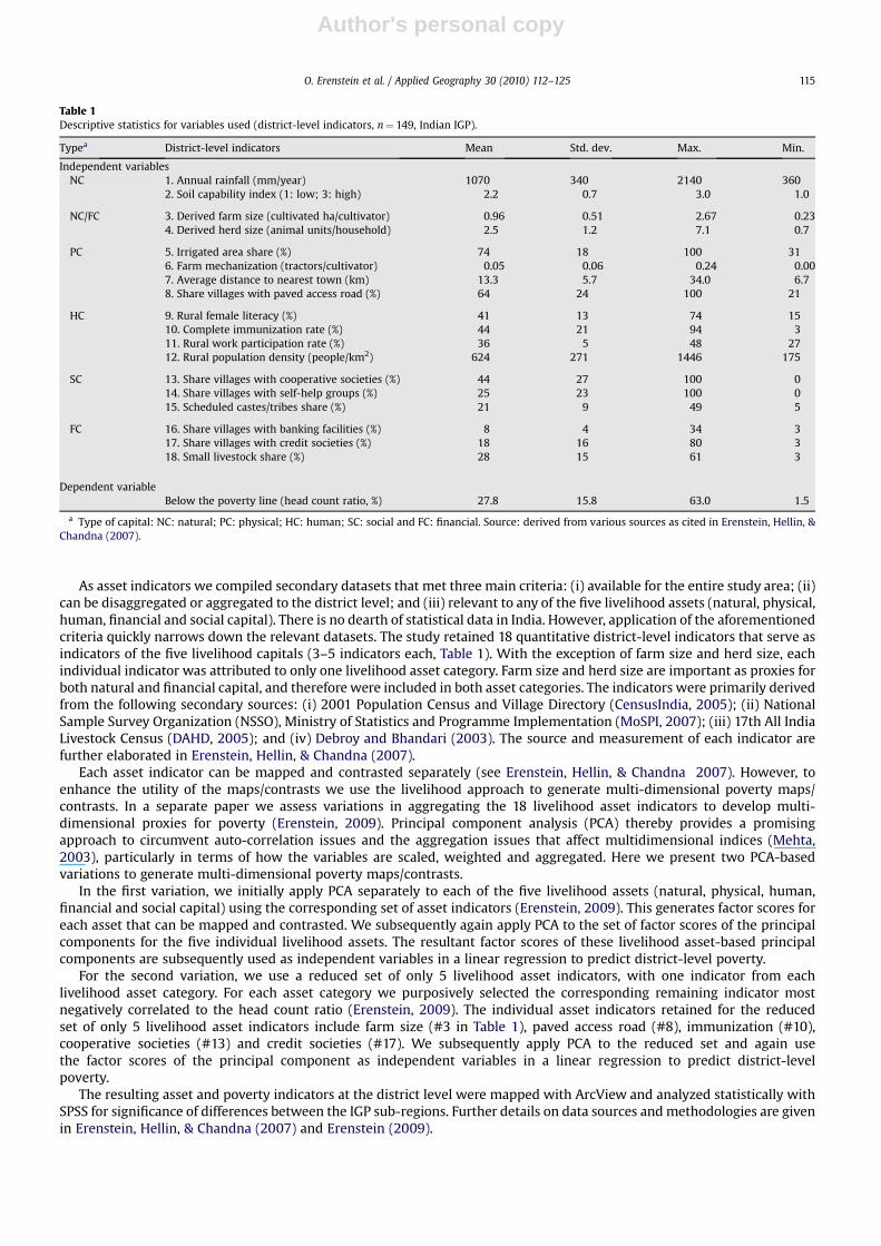
As asset indicators we compiled secondary datasets that met three main criteria: (i) available for the entire study area; (ii)can be disaggregated or aggregated to the district level; and (iii) relevant to any of the five livelihood assets (natural, physical,human, financial and social capital). There is no dearth of statistical data in India. However, application of the aforementionedcriteria quickly narrows down the relevant datasets. The study retained 18 quantitative district-level indicators that serve asindicators of the five livelihood capitals (3–5 indicators each, Table 1). With the exception of farm size and herd size, eachindividual indicator was attributed to only one livelihood asset category. Farm size and herd size are important as proxies forboth natural and financial capital, and therefore were included in both asset categories. The indicators were primarily derivedfrom the following secondary sources: (i) 2001 Population Census and Village Directory (CensusIndia, 2005); (ii) NationalSample Survey Organization (NSSO), Ministry of Statistics and Programme Implementation (MoSPI, 2007); (iii) 17th All IndiaLivestock Census (DAHD, 2005); and (iv) Debroy and Bhandari (2003). The source and measurement of each indicator arefurther elaborated in Erenstein, Hellin, & Chandna (2007).

Each asset indicator can be mapped and contrasted separately (see Erenstein, Hellin, & Chandna 2007). However, toenhance the utility of the maps/contrasts we use the livelihood approach to generate multi-dimensional poverty maps/contrasts. In a separate paper we assess variations in aggregating the 18 livelihood asset indicators to develop multi-dimensional proxies for poverty (Erenstein, 2009). Principal component analysis (PCA) thereby provides a promisingapproach to circumvent auto-correlation issues and the aggregation issues that affect multidimensional indices (Mehta,2003), particularly in terms of how the variables are scaled, weighted and aggregated. Here we present two PCA-basedvariations to generate multi-dimensional poverty maps/contrasts.

In the first variation, we initially apply PCA separately to each of the five livelihood assets (natural, physical, human,financial and social capital) using the corresponding set of asset indicators (Erenstein, 2009). This generates factor scores foreach asset that can be mapped and contrasted. We subsequently again apply PCA to the set of factor scores of the principalcomponents for the five individual livelihood assets. The resultant factor scores of these livelihood asset-based principalcomponents are subsequently used as independent variables in a linear regression to predict district-level poverty.

For the second variation, we use a reduced set of only 5 livelihood asset indicators, with one indicator from eachlivelihood asset category. For each asset category we purposively selected the corresponding remaining indicator mostnegatively correlated to the head count ratio (Erenstein, 2009). The individual asset indicators retained for the reducedset of only 5 livelihood asset indicators include farm size (#3 in Table 1), paved access road (#8), immunization (#10),cooperative societies (#13) and credit societies (#17). We subsequently apply PCA to the reduced set and again usethe factor scores of the principal component as independent variables in a linear regression to predict district-levelpoverty.

The resulting asset and poverty indicators at the district level were mapped with ArcView and analyzed statistically withSPSS for significance of differences between the IGP sub-regions. Further details on data sources and methodologies are givenin Erenstein, Hellin, & Chandna (2007) and Erenstein (2009).

Table 1Descriptive statistics for variables used (district-level indicators, n¼ 149, Indian IGP).

Typea District-level indicators Mean Std. dev. Max. Min.

Independent variablesNC 1. Annual rainfall (mm/year) 1070 340 2140 360

2. Soil capability index (1: low; 3: high) 2.2 0.7 3.0 1.0

NC/FC 3. Derived farm size (cultivated ha/cultivator) 0.96 0.51 2.67 0.234. Derived herd size (animal units/household) 2.5 1.2 7.1 0.7

PC 5. Irrigated area share (%) 74 18 100 316. Farm mechanization (tractors/cultivator) 0.05 0.06 0.24 0.007. Average distance to nearest town (km) 13.3 5.7 34.0 6.78. Share villages with paved access road (%) 64 24 100 21

HC 9. Rural female literacy (%) 41 13 74 1510. Complete immunization rate (%) 44 21 94 311. Rural work participation rate (%) 36 5 48 2712. Rural population density (people/km2) 624 271 1446 175

SC 13. Share villages with cooperative societies (%) 44 27 100 014. Share villages with self-help groups (%) 25 23 100 015. Scheduled castes/tribes share (%) 21 9 49 5

FC 16. Share villages with banking facilities (%) 8 4 34 317. Share villages with credit societies (%) 18 16 80 318. Small livestock share (%) 28 15 61 3

Dependent variableBelow the poverty line (head count ratio, %) 27.8 15.8 63.0 1.5

a Type of capital: NC: natural; PC: physical; HC: human; SC: social and FC: financial. Source: derived from various sources as cited in Erenstein, Hellin, &Chandna (2007).

O. Erenstein et al. / Applied Geography 30 (2010) 112–125 115

Author's personal copy

Results

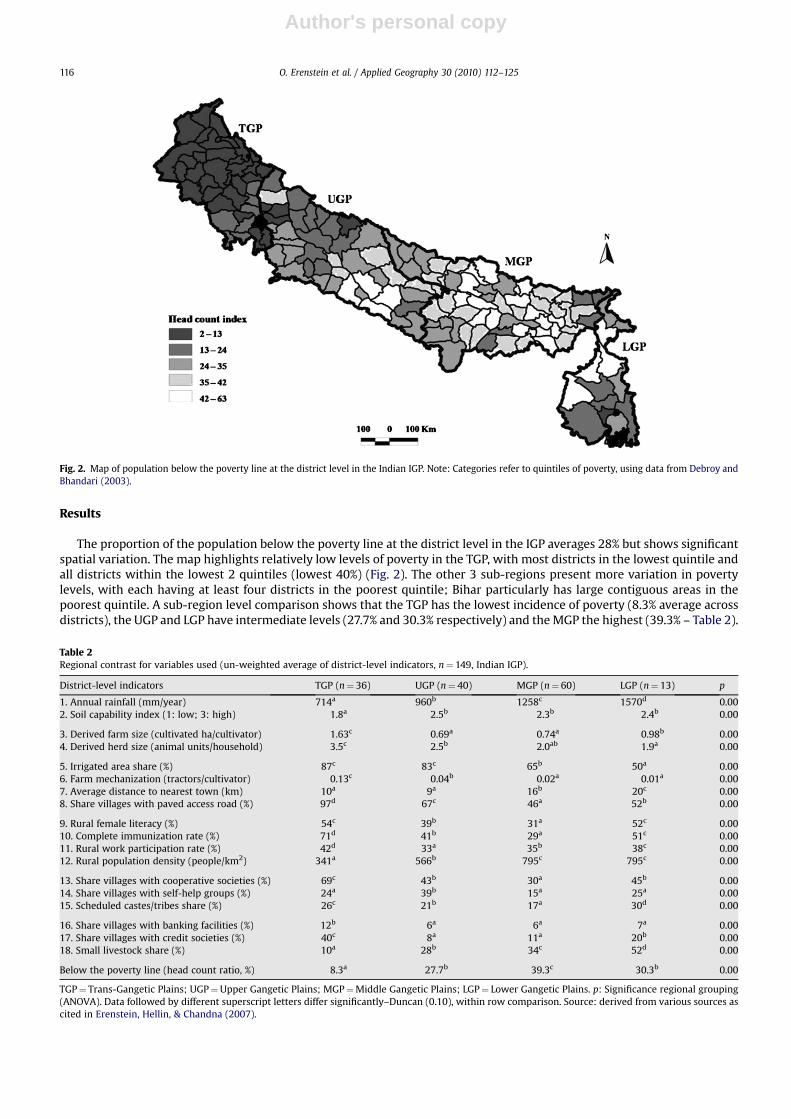
The proportion of the population below the poverty line at the district level in the IGP averages 28% but shows significantspatial variation. The map highlights relatively low levels of poverty in the TGP, with most districts in the lowest quintile andall districts within the lowest 2 quintiles (lowest 40%) (Fig. 2). The other 3 sub-regions present more variation in povertylevels, with each having at least four districts in the poorest quintile; Bihar particularly has large contiguous areas in thepoorest quintile. A sub-region level comparison shows that the TGP has the lowest incidence of poverty (8.3% average acrossdistricts), the UGP and LGP have intermediate levels (27.7% and 30.3% respectively) and the MGP the highest (39.3% – Table 2).

Fig. 2. Map of population below the poverty line at the district level in the Indian IGP. Note: Categories refer to quintiles of poverty, using data from Debroy andBhandari (2003).

Table 2Regional contrast for variables used (un-weighted average of district-level indicators, n¼ 149, Indian IGP).

District-level indicators TGP (n¼ 36) UGP (n¼ 40) MGP (n¼ 60) LGP (n¼ 13) p

1. Annual rainfall (mm/year) 714a 960b 1258c 1570d 0.002. Soil capability index (1: low; 3: high) 1.8a 2.5b 2.3b 2.4b 0.00

3. Derived farm size (cultivated ha/cultivator) 1.63c 0.69a 0.74a 0.98b 0.004. Derived herd size (animal units/household) 3.5c 2.5b 2.0ab 1.9a 0.00

5. Irrigated area share (%) 87c 83c 65b 50a 0.006. Farm mechanization (tractors/cultivator) 0.13c 0.04b 0.02a 0.01a 0.007. Average distance to nearest town (km) 10a 9a 16b 20c 0.008. Share villages with paved access road (%) 97d 67c 46a 52b 0.00

9. Rural female literacy (%) 54c 39b 31a 52c 0.0010. Complete immunization rate (%) 71d 41b 29a 51c 0.0011. Rural work participation rate (%) 42d 33a 35b 38c 0.0012. Rural population density (people/km2) 341a 566b 795c 795c 0.00

13. Share villages with cooperative societies (%) 69c 43b 30a 45b 0.0014. Share villages with self-help groups (%) 24a 39b 15a 25a 0.0015. Scheduled castes/tribes share (%) 26c 21b 17a 30d 0.00

16. Share villages with banking facilities (%) 12b 6a 6a 7a 0.0017. Share villages with credit societies (%) 40c 8a 11a 20b 0.0018. Small livestock share (%) 10a 28b 34c 52d 0.00

Below the poverty line (head count ratio, %) 8.3a 27.7b 39.3c 30.3b 0.00

TGP¼ Trans-Gangetic Plains; UGP¼Upper Gangetic Plains; MGP¼Middle Gangetic Plains; LGP¼ Lower Gangetic Plains. p: Significance regional grouping(ANOVA). Data followed by different superscript letters differ significantly–Duncan (0.10), within row comparison. Source: derived from various sources ascited in Erenstein, Hellin, & Chandna (2007).

O. Erenstein et al. / Applied Geography 30 (2010) 112–125116

Author's personal copy

All of the 18 asset indicators show significant variation across the IGP districts (Table 1), resulting in marked contrastsbetween the 4 sub-regions (Table 2). Overall, the TGP typically has the most favorable indicators and the MGP the least.

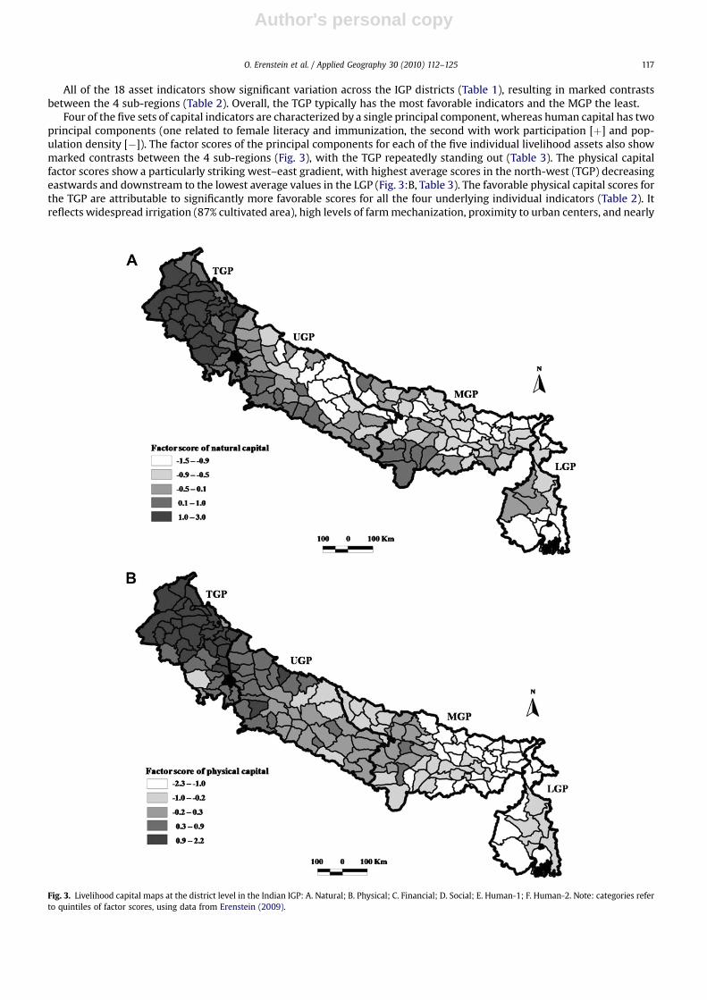
Four of the five sets of capital indicators are characterized by a single principal component, whereas human capital has twoprincipal components (one related to female literacy and immunization, the second with work participation [þ] and pop-ulation density [�]). The factor scores of the principal components for each of the five individual livelihood assets also showmarked contrasts between the 4 sub-regions (Fig. 3), with the TGP repeatedly standing out (Table 3). The physical capitalfactor scores show a particularly striking west–east gradient, with highest average scores in the north-west (TGP) decreasingeastwards and downstream to the lowest average values in the LGP (Fig. 3:B, Table 3). The favorable physical capital scores forthe TGP are attributable to significantly more favorable scores for all the four underlying individual indicators (Table 2). Itreflects widespread irrigation (87% cultivated area), high levels of farm mechanization, proximity to urban centers, and nearly

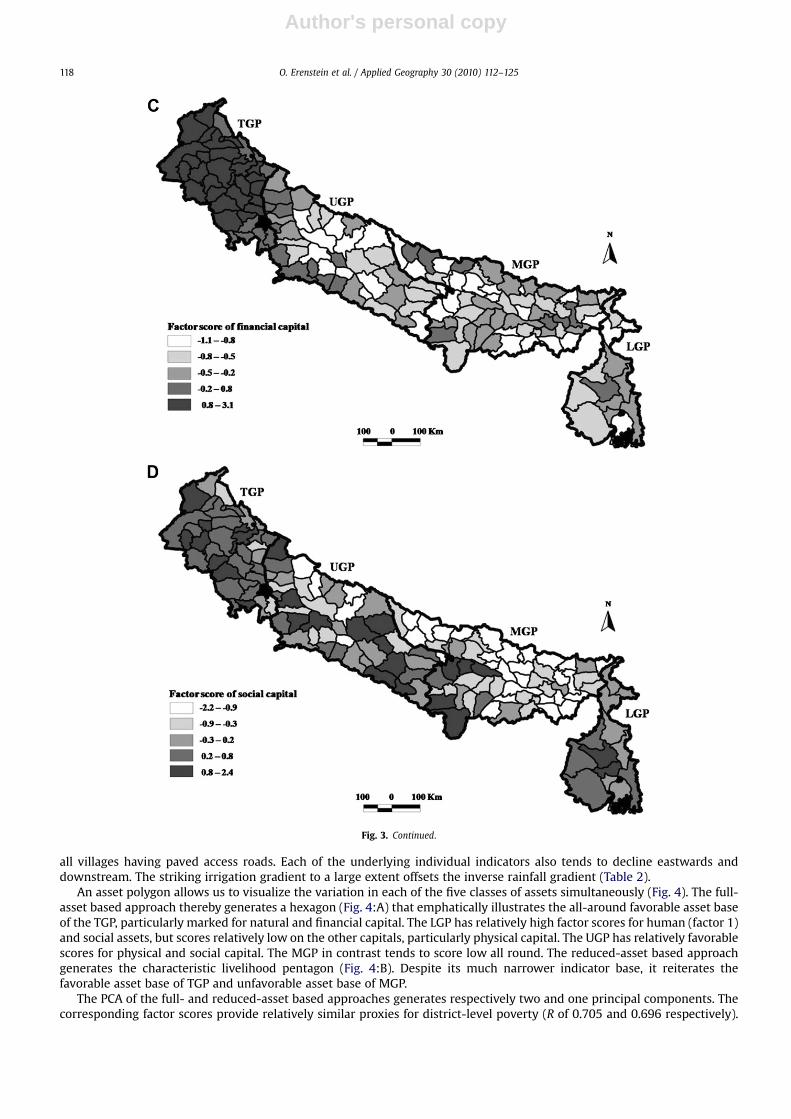
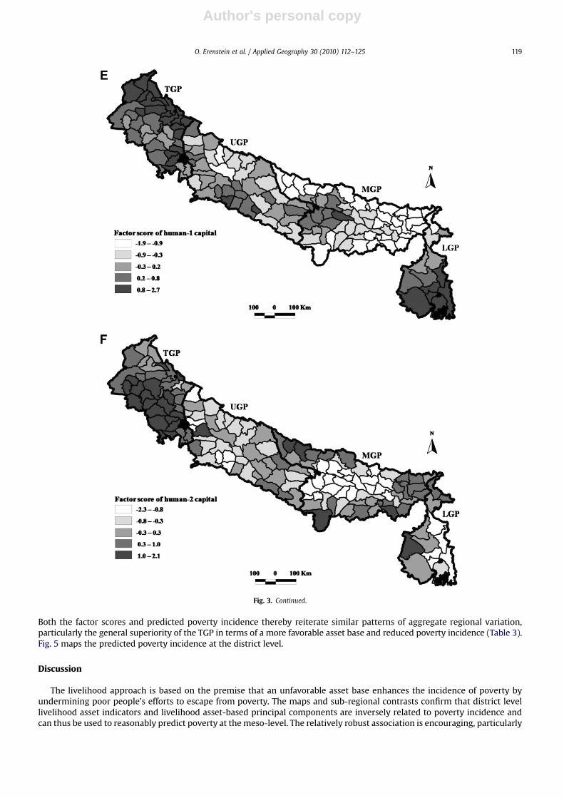
Fig. 3. Livelihood capital maps at the district level in the Indian IGP: A. Natural; B. Physical; C. Financial; D. Social; E. Human-1; F. Human-2. Note: categories referto quintiles of factor scores, using data from Erenstein (2009).

O. Erenstein et al. / Applied Geography 30 (2010) 112–125 117

Author's personal copy

all villages having paved access roads. Each of the underlying individual indicators also tends to decline eastwards anddownstream. The striking irrigation gradient to a large extent offsets the inverse rainfall gradient (Table 2).

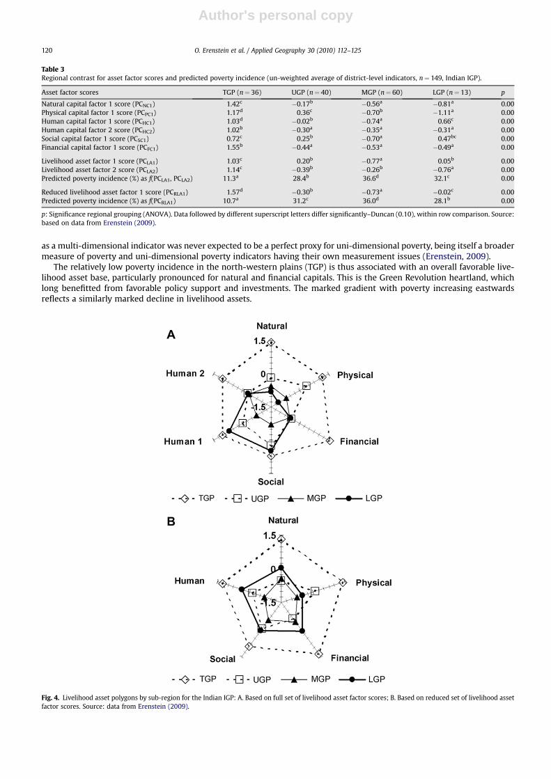
An asset polygon allows us to visualize the variation in each of the five classes of assets simultaneously (Fig. 4). The full-asset based approach thereby generates a hexagon (Fig. 4:A) that emphatically illustrates the all-around favorable asset baseof the TGP, particularly marked for natural and financial capital. The LGP has relatively high factor scores for human (factor 1)and social assets, but scores relatively low on the other capitals, particularly physical capital. The UGP has relatively favorablescores for physical and social capital. The MGP in contrast tends to score low all round. The reduced-asset based approachgenerates the characteristic livelihood pentagon (Fig. 4:B). Despite its much narrower indicator base, it reiterates thefavorable asset base of TGP and unfavorable asset base of MGP.

The PCA of the full- and reduced-asset based approaches generates respectively two and one principal components. Thecorresponding factor scores provide relatively similar proxies for district-level poverty (R of 0.705 and 0.696 respectively).

Fig. 3. Continued.

O. Erenstein et al. / Applied Geography 30 (2010) 112–125118

Author's personal copy

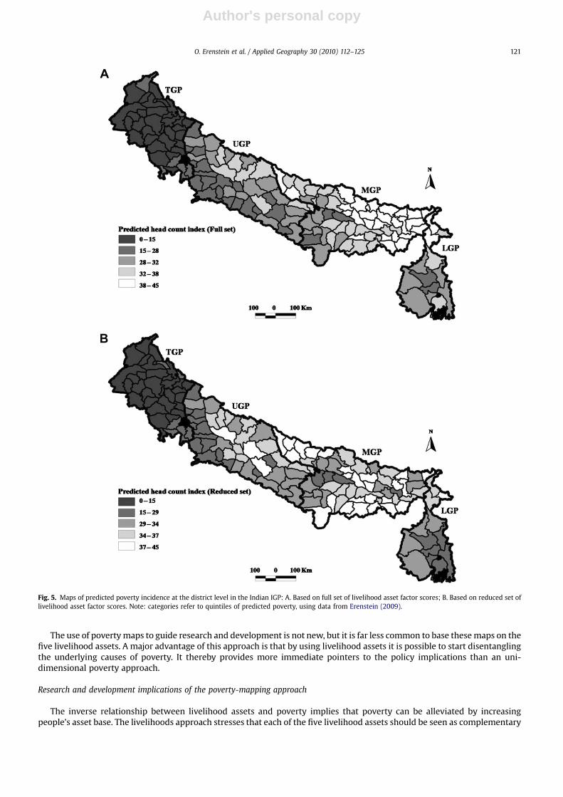
Both the factor scores and predicted poverty incidence thereby reiterate similar patterns of aggregate regional variation,particularly the general superiority of the TGP in terms of a more favorable asset base and reduced poverty incidence (Table 3).Fig. 5 maps the predicted poverty incidence at the district level.

Discussion

The livelihood approach is based on the premise that an unfavorable asset base enhances the incidence of poverty byundermining poor people’s efforts to escape from poverty. The maps and sub-regional contrasts confirm that district levellivelihood asset indicators and livelihood asset-based principal components are inversely related to poverty incidence andcan thus be used to reasonably predict poverty at the meso-level. The relatively robust association is encouraging, particularly

Fig. 3. Continued.

O. Erenstein et al. / Applied Geography 30 (2010) 112–125 119

Author's personal copy

as a multi-dimensional indicator was never expected to be a perfect proxy for uni-dimensional poverty, being itself a broadermeasure of poverty and uni-dimensional poverty indicators having their own measurement issues (Erenstein, 2009).

The relatively low poverty incidence in the north-western plains (TGP) is thus associated with an overall favorable live-lihood asset base, particularly pronounced for natural and financial capitals. This is the Green Revolution heartland, whichlong benefitted from favorable policy support and investments. The marked gradient with poverty increasing eastwardsreflects a similarly marked decline in livelihood assets.

Table 3Regional contrast for asset factor scores and predicted poverty incidence (un-weighted average of district-level indicators, n¼ 149, Indian IGP).

Asset factor scores TGP (n¼ 36) UGP (n¼ 40) MGP (n¼ 60) LGP (n¼ 13) p

Natural capital factor 1 score (PCNC1) 1.42c �0.17b �0.56a �0.81a 0.00Physical capital factor 1 score (PCPC1) 1.17d 0.36c �0.70b �1.11a 0.00Human capital factor 1 score (PCHC1) 1.03d �0.02b �0.74a 0.66c 0.00Human capital factor 2 score (PCHC2) 1.02b �0.30a �0.35a �0.31a 0.00Social capital factor 1 score (PCSC1) 0.72c 0.25b �0.70a 0.47bc 0.00Financial capital factor 1 score (PCFC1) 1.55b �0.44a �0.53a �0.49a 0.00

Livelihood asset factor 1 score (PCLA1) 1.03c 0.20b �0.77a 0.05b 0.00Livelihood asset factor 2 score (PCLA2) 1.14c �0.39b �0.26b �0.76a 0.00Predicted poverty incidence (%) as f(PCLA1, PCLA2) 11.3a 28.4b 36.6d 32.1c 0.00

Reduced livelihood asset factor 1 score (PCRLA1) 1.57d �0.30b �0.73a �0.02c 0.00Predicted poverty incidence (%) as f(PCRLA1) 10.7a 31.2c 36.0d 28.1b 0.00

p: Significance regional grouping (ANOVA). Data followed by different superscript letters differ significantly–Duncan (0.10), within row comparison. Source:based on data from Erenstein (2009).

Fig. 4. Livelihood asset polygons by sub-region for the Indian IGP: A. Based on full set of livelihood asset factor scores; B. Based on reduced set of livelihood assetfactor scores. Source: data from Erenstein (2009).

O. Erenstein et al. / Applied Geography 30 (2010) 112–125120

Author's personal copy

The use of poverty maps to guide research and development is not new, but it is far less common to base these maps on thefive livelihood assets. A major advantage of this approach is that by using livelihood assets it is possible to start disentanglingthe underlying causes of poverty. It thereby provides more immediate pointers to the policy implications than an uni-dimensional poverty approach.

Research and development implications of the poverty-mapping approach

The inverse relationship between livelihood assets and poverty implies that poverty can be alleviated by increasingpeople’s asset base. The livelihoods approach stresses that each of the five livelihood assets should be seen as complementary

Fig. 5. Maps of predicted poverty incidence at the district level in the Indian IGP: A. Based on full set of livelihood asset factor scores; B. Based on reduced set oflivelihood asset factor scores. Note: categories refer to quintiles of predicted poverty, using data from Erenstein (2009).

O. Erenstein et al. / Applied Geography 30 (2010) 112–125 121

Author's personal copy

building blocks. The poverty maps/contrasts illustrate where specific assets are relative weak at the district level and thushelp identify opportunities for strategic policy interventions. For instance, the sub-region level comparisons suggest thatWest Bengal (LGP) would benefit from significant investments in physical capital.

A solid foundation of all five assets is generally needed for livelihood security and to enable people to rise above thepoverty line. Still, there are also significant inter-linkages between types of assets. Most obvious, perhaps, is the significantincrease in irrigation infrastructure (physical capital) in the north-west (TGP) to compensate for meager rainfall (naturalcapital). Another example is that some NGOs in India have promoted micro-finance (financial capital) through women’s self-help groups (social capital) (Ghate, 1999; Premchander, 2003), with India now having one of the largest micro-financeprograms in the world (Krishnaraj, 2006). The overall unfavorable livelihood asset base in the mid-Gangetic Plains of Biharand Eastern UP (MGP) thus provide a particularly challenging spatial poverty trap.

The asset-based poverty maps therefore give an indication of where and on what development initiatives should focus.The asset-based approach complements some of the earlier work. For instance, Fan, Hazell, and Thorat (1999) conclude that toreduce rural poverty the Indian government should give high priority to increasing its spending on rural roads and agri-cultural research and extension, which would also promote the greatest growth in agricultural productivity. Education hadthe third largest impact on rural poverty, whereas irrigation investment had the third largest impact on growth in agriculturalproductivity but only a small impact on rural poverty reduction. Another study, however, highlights the appeal of these lattertwo variables in the design of poverty-targeting programs in India, particularly primary education infrastructure andimproved land productivity through irrigation (Shah & Singh, 2004). The mapping of particular variables and classes oflivelihood assets can help to distinguish where they are most deficient, and, hence, where investment in different typesof asset could have the greatest impact. The mapping thereby enhances the ability to target investments both in terms of typeof assets most needed and more geographical accuracy. The Fan et al. (1999) analysis relied on state-level data, and thedisaggregated maps can therefore help target the proposed investments to the district level. Narrower geographical targetingof poverty-alleviation programs can improve their coverage, reduce leakage to the non-poor, and reduce program costs(Bigman & Srinivasan, 2002, p. 252).

The asset-based poverty maps, therefore, give an indication of where development initiatives to build up different assetsshould focus. Still, the inverse relationship between livelihood assets and absolute poverty does not imply a straightforwardlink between livelihood assets and livelihood outcomes (poverty reduction). A sole focus on assets risks ignoring theunderlying drivers and modifiers that are addressed in the livelihood framework (e.g. DFID, 2007; Ellis, 2000). As Krishna(2003) writes, ‘‘‘poverty’ does not get reduced because growth occurs, or the climate changes, or some structural factor ebbs orgrows in some way. Poverty gets reduced when more households and individuals do the things and take the pathways that lead outof poverty, and fewer individuals take the other pathways that lead into poverty’’. Hence, we need to understand better howlivelihood assets are inter-linked with impact pathways, including the dynamic roles of farmers’ livelihood systems, input–output value chains and associated stakeholders (Dixon, Hellin, Erenstein, & Kosina, 2007). Such insights will contribute to thewider adoption and adaptation of new technologies and knowledge, and so to research and development impacts on povertyin the IGP.

The asset-based poverty maps and regional contrasts provide a foundation for priority-setting and targeting of researchand development work within the IGP. The present approach thereby provides a tool to incorporate livelihood and povertyconsiderations, but does not set priorities as such. Priority-setting depends on an assessment of the value of alternativeinvestments, which captures their relative potential benefits and effectiveness, given existing impact pathways.

Priority-setting and targeting would benefit from a better understanding of the asset–poverty linkages and the trade-offsbetween alternative investments. For instance, land and water resource degradation threaten the longer-term sustainabilityof agricultural production in the TGP, the current cereal bowl (Ladha, Hill, Duxbury, Gupta, & Buresh, 2003). Such ongoingdegradation of the natural capital base undermines future national food security, with implications for the rural and urbanpoor alike. This questions the utility of investment subsidies for drilling wells and pricing rural electricity (for irrigation) atvery low or zero rates (World Bank, 2005), which have contributed to inefficient water use, over-extraction of groundwaterand salinity and water-logging problems. Some stakeholders have called for a shift of the cereal bowl to the eastern region ofthe country, including eastern Uttar Pradesh, Bihar, and West Bengal. The eastern IGP, with its highly fertile soils and relativelyplentiful water supply, can support cereal systems on a more sustainable long-term basis than the western IGP (World Bank,2005). Such a shift and intensification would also have significant positive implications for poverty alleviation. Our mapsmake a number of these relationships spatially explicit and can help guide the discussion and subsequent research anddevelopment initiatives. However, the maps as such remain only one input. Complementary research is still needed to assessrigorously the full implications of such a spatial shift, including the likely impact of climate change. Similarly, our maps canguide but not answer the discussion as to whether agricultural research and development should invest primarily in relativelymarginal areas in the MGP as against the more favorable TGP, and what the relative emphasis should be in terms of themillennium development goals of poverty alleviation and environmental sustainability (RWC, 2006).

A livelihoods approach to poverty reduction entails taking on board variables linked to themes that often do not appear ondisciplinary scientists’ radars. A challenge for agricultural research and development is to accept that the promoted tech-nologies may not always be the key to poverty alleviation. In some cases the most pressing needs may be to improve health(Krishna, Kapila, Porwal, & Singh, 2003) and education. The maps and the livelihood framework, therefore, have the potentialsynergies of cross-sectoral and inter-disciplinary approaches. Hence, for policy makers, the maps can encourage a morejudicious targeting of resources and interventions.

O. Erenstein et al. / Applied Geography 30 (2010) 112–125122

Author's personal copy

Limitations of current approach and possible refinements

Challenging the current approach are the trade-offs between explanatory and interpretational power of asset–poverty link-ages. There is also a danger of information overload in terms of the sheer number of maps and their interpretation (Erenstein,Hellin, & Chandna, 2007). Ideally there would be only one aggregate livelihood asset map supported by five underlying individualasset maps. This can be achieved by using multidimensional indices, but unfortunately these imply a significant loss in explan-atory power (Erenstein, 2009). Principal component analysis (PCA) retains significant explanatory power, but does not necessarilyimply single aggregates. For instance, our full-asset based approach generated two principal components each for human capitaland aggregate livelihood assets. Our reduced-asset based approach did result in a single aggregate for livelihood assets, but losesthe variation associated with other indicators, particularly for capitals that are characterized by more than one principalcomponent (e.g. human capital). We circumvented the lack of a single aggregate for livelihood assets by mapping predictedpoverty. However, such predictions still imply the need for uni-dimensional poverty measures for calibration.

This study draws on and, therefore, is inherently limited by the available secondary data at the district level. The approachcould benefit from a refinement of the indicators used, and other indicators might prove more appropriate in capturingqualitative and quantitative dimensions of livelihood assets (Erenstein, 2009). The approach may also be extended to otherspheres of interest, such as the mapping of ecosystem services (Egoh et al., 2008).

The current study uses the district level as the unit of analysis, primarily dictated by the availability of data. The use of thedistrict level does provide an effective bridge between the micro and macro environments. Still, the use of aggregated asopposed to household-level data does lead to loss in precision due to the livelihood asset heterogeneity within districts,villages, and households (Kristjanson et al., 2005; Minot & Baulch, 2005). District-level data and averages can therefore maskpockets of poverty at lower aggregation levels in well- and poorly-endowed districts alike throughout the IGP. As indicated byBigman and Srinivasan (2002, p. 253), there is a ‘‘wide spread of poverty in all states and districts in India where all too often onefinds a slum next to a fancy apartment building’’. These pockets are not captured by the district-level poverty maps, particularlywhen they exist in otherwise well-off districts, and deserve the attention of policy makers, researchers, and developmentpractitioners. Future studies may want to explore the use of the sub-district as level of analysis, which is do-able given timeand effort and may add to the precision.

The current set of poverty maps are a snapshot of the levels of assets; they do not capture any trends. While the maps arean useful tool, their utility would be enhanced if put in a dynamic perspective and linked to underlying trends. Dependent ondata availability, maps could be generated for different points over time to illustrate the spatial dynamics of individual assets,their relative contribution and linkages to poverty.

Although the case study focuses on the IGP, the approach has wider applicability and could be extended to other areas. Thiswould test the sensitivity of the approach to increased heterogeneity. The IGP encompasses a large geographical area withsignificant diversity, but it is nonetheless a plain area and is probably less heterogeneous than some of the rainfed undulatingor mountainous landscape. Extension of similar studies to other areas may also need to draw on alternative variables thatprove to be more suitable because of data availability, particularly when extending across borders.

Finally, it is also important to appreciate that agricultural-based livelihood systems alone may not be the best way toreduce poverty. For example, research in Rajasthan reported by Krishna (2003) found that diversification of income sourceswas the single most important reason for escaping poverty in this region and that the overwhelming majority of agriculturalhouseholds that had escaped from poverty had successfully diversified their income sources and were no longer reliant onagricultural incomes alone. However, a salutary fact is that in India despite the rapid growth of the non-farm sector, its successin drawing labor from land has been limited (Eswaran, Kotwal, Ramaswami, & Wadhwa, 2009) and, hence, building uplivelihood assets in rural areas is likely to remain the most effective way to reduce poverty.

Conclusion

The livelihood asset-based approach to poverty mapping provides an useful tool to incorporate livelihood and povertyconsiderations into research and development priority-setting and targeting at limited cost. It thereby provides a coherentmulti-dimensional poverty framework and provides immediate pointers to the corresponding policy implications.

Its empirical application to the IGP shows that asset-based poverty maps and regional contrasts provide a foundation forpriority-setting and targeting of research and development work within the area. These help to identify asset bottlenecks andasset-poor districts, to prioritize intervention needs, and to enhance targeting. Having mapped the livelihood assets, we nowneed to better understand the asset–poverty linkages and the trade-offs between alternative investments so as to enhanceresearch and development priority-setting in the IGP.

The approach, therefore, ensures an applied, holistic, and cross-disciplinary approach to priority-setting and targeting. Still,data availability is a major constraint to its wider application, especially in terms of spatial disaggregation and facilitating inter-temporal and cross-border comparisons. Follow-up research can fine tune the approach and address the above challenges.

Acknowledgements

The paper draws from a more elaborate study (Erenstein, Hellin, & Chandna, 2007) and complements a companion paper(Erenstein, 2009). The contributions from individuals to the original study have been acknowledged in the detailed report to

O. Erenstein et al. / Applied Geography 30 (2010) 112–125 123

Author's personal copy

the extent possible. The authors are grateful to reviewers for their comments on an earlier version of this paper. The usualdisclaimer applies.

References

Alderman, H., Babita, M., Demombynes, G., Makhatha, N., & Ozler, B. (2002). How low can you go? Combining census and survey data for mapping povertyin South Africa. Journal of African Economies, 11(2), 169–200.

Amarasinghe, U., Samad, M., & Anputhas, M. (2005). Spatial clustering of rural poverty and food insecurity in Sri Lanka. Food Policy, 30(5-6), 493–509.Bansil, P. C. (2006). Poverty mapping in Rajasthan. New Delhi: Concept.Baud, I., Sridharan, N., & Pfeffer, K. (2008). Mapping urban poverty for local governance in an Indian mega-city: the case of Delhi. Urban Studies, 45(7),

1385–1412.Beck, T., & Nesmith, C. (2001). Building on poor people’s capacities: the case of common property resources in India and West Africa. World Development,

29(1), 119–133.Bellon, M. R., Hodson, D., Bergvinson, D., Beck, D., Martinez-Romero, E., & Montoya, Y. (2005). Targeting agricultural research to benefit poor farmers:

relating poverty mapping to maize environments in Mexico. Food Policy, 30(5–6), 476–492.Bhalla, G. S., & Hazell, P. (2003). Rural employment and poverty: strategies to eliminate rural poverty within a generation. Economic & Political Weekly,

38(33), 3473–3484.Bigman, D., Dercon, S., Guillaume, D., & Lambotte, M. (2000). Community targeting for poverty reduction in Burkina Faso. The World Bank Economic Review,

14(1), 167–193.Bigman, D., & Fofack, H. (2000). Geographical targeting for poverty alleviation: an introduction to the special issue. The World Bank Economic Review, 14(1),

129–145.Bigman, D., & Srinivasan, P. V. (2002). Geographical targeting of poverty alleviation programs: methodology and applications in rural India. Journal of Policy

Modeling, 24(3), 237–255.CensusIndia. (2005). CensusInfo India 2001, Version 2.0. New Delhi: Office of the Registrar General.Chaudhuri, S., & Gupta, N. (2009). Levels of living and poverty patterns: a district-wise analysis for India. Economic & Political Weekly, 44(9), 94–110.Chen, S., & Ravallion, M. (2008). The developing world is poorer than we thought, but no less successful in the fight against poverty. Policy Research working

paper WPS 4703. Washington, DC: World Bank.CIESIN. (2006). Where the poor are: An atlas of poverty. Palisades, NY: CIESIN (Center for International Earth Science Information Network), Columbia

University.DAHD. (2005). Department of Animal Husbandry, Dairying & Fisheries. http://dahd.nic.in/census.htm Accessed December 2005.Debroy, B., & Bhandari, L. (2003). District-level deprivation in the new millennium. New Delhi: Konark Publishers.DFID. (2007). The sustainable livelihoods distance learning guide. http://www.livelihoods.org/info/dlg/Index.htm. Accessed 31.08.07.Dixon, J., Hellin, J., Erenstein, O., & Kosina, P. (2007). U-impact pathway for diagnosis and impact assessment of crop improvement. Journal of Agricultural

Science, 145(3), 195–206.Egoh, B., Reyers, B., Rouget, M., Richardson, D. M., Le Maitre, D. C., & van Jaarsveld, A. S. (2008). Mapping ecosystem services for planning and management.

Agriculture, Ecosystems & Environment, 127(1–2), 135–140.Elbers, C., Lanjouw, P., & Leite, P. G. (2008). Poverty mapping: testing the methodology in Minas Gerais. World Bank Research Digest, 2(3), 1–2.Ellis, F. (2000). Rural livelihoods and diversity in developing countries (1st ed.). New York: Oxford University Press.Erenstein, O. (2009). Livelihood assets as a multidimensional inverse proxy for poverty: A district level analysis of the Indian Indo-Gangetic Plains. Working paper.

New Delhi: CIMMYT.Erenstein, O., Hellin, J., & Chandna, P. (2007). Livelihoods, poverty and targeting in the Indo-Gangetic Plains: A spatial mapping approach. Research Report.

New Delhi, India: CIMMYT/RWC.Erenstein, O., Thorpe, W., Singh, J., & Varma, A. (2007). Crop-livestock interactions and livelihoods in the Indo-Gangetic Plains, India: A regional synthesis.

New Delhi, India: CIMMYT/ILRI/RWC.Eswaran, M., Kotwal, A., Ramaswami, B., & Wadhwa, W. (2009). Sectoral labour flows and agricultural wages in India, 1983–2004: has growth trickled

down? Economic & Political Weekly, 44(2), 46–55.Fan, S., Hazell, P., & Thorat, S. (1999). Linkages between government spending, growth, and poverty in rural India. IFPRI Research Report 110. Washington,

DC: IFPRI.Fofack, H. (2000). Combining light monitoring surveys with integrated surveys to improve targeting for poverty reduction: the case of Ghana. The World

Bank Economic Review, 14(1), 195–219.Fujii, T. (2008). How well can we target aid with rapidly collected data? Empirical results for poverty mapping from Cambodia. World Development, 36(10),

1830–1842.Ghate, P. (1999). Rural credit and self-help groups: micro-finance needs and concepts in India. Economic and Political Weekly, 34(49), 3431–3432.Green, A. E. (1994). The geography of poverty and wealth. Warwick, UK: The Institute for Employment Research, University of Warwick.Henninger, N., & Snel, M. (2002). Where are the poor? Experiences with the development and use of poverty maps. Washington, DC: World Resources Institute/

UNEP/GRID-Arendal.Hentschel, J., Lanjouw, J. O., Lanjouw, P., & Poggi, J. (2000). Combining census and survey data to trace the spatial dimensions of poverty: a case study of

Ecuador. The World Bank Economic Review, 14(1), 147–165.Hyman, G., Larrea, C., & Farrow, A. (2005). Methods, results and policy implications of poverty and food security mapping assessments. Food Policy, 30(5–6),

453–460.Kam, S.-P., Hossain, M., Bose, M. L., & Villano, L. S. (2005). Spatial patterns of rural poverty and their relationship with welfare-influencing factors in

Bangladesh. Food Policy, 30(5–6), 551–567.Kodras, J. E. (1997). The changing map of American poverty in an era of economic restructuring and political realignment. Economic Geography, 73(1), 67–93.Krishna, A. (2003). Falling into poverty: other side of poverty reduction. Economic & Political Weekly, 38(6), 533–542.Krishna, A., Kapila, M., Pathak, S., Porwal, M., Singh, K., & Singh, V. (2004). Falling into poverty in villages of Andhra Pradesh: why avoidance policies are

needed. Economic & Political Weekly, 39(29), 3249–3256.Krishna, A., Kapila, M., Porwal, M., & Singh, V. (2003). Falling into poverty in a high-growth state: escaping poverty and becoming poor in Gujarat villages.

Economic & Political Weekly, 38(49), 5171–5179.Krishnaraj, M. (2006). Food security, Agrarian crisis and rural livelihoods: implications for women. Economic & Political Weekly, 41(52), 5376–5388.Kristjanson, P., Radeny, M., Baltenweck, I., Ogutu, J., & Notenbaert, A. (2005). Livelihood mapping and poverty correlates at a meso-level in Kenya. Food

Policy, 30(5–6), 568–583.Kumar, P., Jha, D., Kumar, A., Chaudhary, M. K., Grover, R. K., Singh, R. K., et al. (2002). Economic analysis of total factor productivity of crop sector in Indo-

Gangetic plain of India by district and region. New Delhi, India: Indian Agricultural Research Institute. Agricultural Economics Research Report 2.Kundu, A., & Raza, M. (1982). Indian economy – The regional dimension. New Delhi: Spectrum Publishers.Kundu, A., & Sarangi, N. (2007). Migration, employment status and poverty: an analysis across urban centres. Economic & Political Weekly, 42(4), 299–306.Ladha, J. K., Hill, J. E., Duxbury, J. M., Gupta, R. K., & Buresh, R. J. (Eds.). (2003). Improving the productivity and sustainability of rice-wheat systems: Issues and

impacts. Madison, Wisconsin, USA: American Society of Agronomy, Crop Science Society of America, Soil Science Society of America.Mehta, A. K. (2003). Multidimensional poverty in India: District level estimates. Manchester: Chronic Poverty Research Centre. CPRC–IIPA Working Paper.

O. Erenstein et al. / Applied Geography 30 (2010) 112–125124

Author's personal copy

Minot, N. (2000). Generating disaggregated poverty maps: an application to Vietnam. World Development, 28(2), 319–331.Minot, N., & Baulch, B. (2005). Poverty mapping with aggregate census data: what is the loss in precision? Review of Development Economics, 9(1), 5–24.MoSPI. (2007). Ministry of Statistics and Programme Implementation. http://mospi.nic.in/ (Accessed 31.08.07).MSSRF, & WFP. (2004). Atlas of the sustainability of food security in India. Chennai: M.S. Swaminathan Research Foundation/World Food Program.Narang, R. S., & Virmani, S. M. (2001). Rice–wheat cropping systems of the Indo-Gangetic Plain of India. New Delhi, India: RWC. Rice–Wheat Consortium Paper

Series 11.Palmer-Jones, R., & Sen, K. (2006). It is where you are that matters: the spatial determinants of rural poverty in India. Agricultural Economics, 34(3), 229–242.Planning Commission. (2002). National human development report 2001. New Delhi: Planning Commission, Government of India.Premchander, S. (2003). NGOs and local MFIs – how to increase poverty reduction through women’s small and micro-enterprise. Futures, 35(4), 361–378.Ruggeri Laderchi, C., Saith, R., & Stewart, F. (2003). Does it matter that we do not agree on the definition of poverty? A comparison of four approaches. Working

Paper No 107. Oxford, UK: Queen Elizabeth House, University of Oxford.RWC. (2006). A research strategy for improved livelihoods and sustainable rice–wheat cropping in the Indo-Gangetic Plains: Vision for 2006–2010 and beyond.

New Delhi, India: Rice–Wheat Consortium for the Indo Gangetic Plains.Saith, A. (2005). Poverty lines versus the poor: method versus meaning. Economic & Political Weekly, 40(43), 4601–4610.Seth, A., Fischer, K., Anderson, J., & Jha, D. (2003). The rice–wheat consortium: An institutional innovation in international agricultural research on the

rice–wheat cropping systems of the Indo-Gangetic Plains (IGP). The Review Panel Report. New Delhi: RWC.Shah, T., & Singh, O. P. (2004). Irrigation development and rural poverty in Gujarat, India: a disaggregated analysis. Water International, 29(2), 167–177.Sharma, S. K., Subba Rao, A. V. M., Murari, K., & Sharma, G. C. (2004). Atlas of rice–wheat cropping system in Indo-Gangetic Plains of India. Bulletin No. 2004-I.

Modipuram, India: PDCSR (ICAR).Shrestha, N. R. (1997). On ‘‘What Causes Poverty? A Postmodern View’’: a postmodern view or denial of historical integrity? The poverty of Yapa’s view of

poverty. Annals of the Association of American Geographers, 87(4), 709–716.Srivastava, S. K., Dutt, C. B. S., Nagaraja, R., Bandyopadhayay, S., Meena Rani, H. C., Hegde, V. S., et al. (2004). Strategies for rural poverty alleviation in India:

a perspective based on remote sensing and GIS-based nationwide wasteland mapping. Current Science, 87(7), 954–959.Timsina, J., & Connor, D. J. (2001). Productivity and management of rice–wheat cropping systems: issues and challenges. Field Crops Research, 69(2), 93–132.Wagle, U. (2008). Multidimensional poverty measurement: Concepts and applications. Berlin: Springer.Woodhead, T., Huke, R., Huke, E., & Balababa, L. (1994). Rice–wheat atlas of India. Los Banos/Philippines/Mexico, D.F./New Delhi, India: International Rice

Research Institute, CIMMYT/Indian Council of Agricultural Research (ICAR).World Bank. (2005). India – Re-energizing the agricultural sector to sustain growth and reduce poverty. New Delhi: Oxford University Press.Xiaoyun, L., & Remenyi, J. (2008). Making poverty mapping and monitoring participatory. Development in Practice, 18(4), 599–610.Yadav, R. L., & Subba Rao, A. V. M. (2001). Atlas of cropping systems in India. Bulletin No. 2001–2. Modipuram, India: PDCSR (ICAR).Yapa, L. (1996). What causes poverty? A postmodern view. Annals of the Association of American Geographers, 86(4), 707–728.

O. Erenstein et al. / Applied Geography 30 (2010) 112–125 125