1 23

Aquaculture InternationalJournal of the European AquacultureSociety ISSN 0967-6120 Aquacult IntDOI 10.1007/s10499-013-9713-y

Potential for production of ‘mini-mussels’in Great Belt (Denmark) evaluated on basisof actual and modeled growth of youngmussels Mytilus edulis

Hans Ulrik Riisgård, Kim Lundgreen &Poul S. Larsen

1 23

Your article is protected by copyright and all

rights are held exclusively by Springer Science

+Business Media Dordrecht. This e-offprint

is for personal use only and shall not be self-

archived in electronic repositories. If you wish

to self-archive your article, please use the

accepted manuscript version for posting on

your own website. You may further deposit

the accepted manuscript version in any

repository, provided it is only made publicly

available 12 months after official publication

or later and provided acknowledgement is

given to the original source of publication

and a link is inserted to the published article

on Springer's website. The link must be

accompanied by the following text: "The final

publication is available at link.springer.com”.

Potential for production of ‘mini-mussels’ in Great Belt(Denmark) evaluated on basis of actual and modeledgrowth of young mussels Mytilus edulis

Hans Ulrik Riisgard • Kim Lundgreen • Poul S. Larsen

Received: 28 June 2013 / Accepted: 17 October 2013� Springer Science+Business Media Dordrecht 2013

Abstract The present study is a first step towards evaluation of the potential for line-

mussel production in the Great Belt region between the Kattegat and Baltic Sea, Denmark.

We present experimental results for actual growth rates of juvenile/adult mussels Mytilus

edulis in suspended net bags in terms of shell length and dry weight of soft parts during

extended periods (27–80 days) in the productive season in the first 6 series of field

experiments, including 4 sites in Great Belt and 2 sites in Limfjorden, Denmark. Data were

correlated and interpreted in terms of specific growth rate (l, % day-1) as a function of dry

weight of soft parts (W, g) by a previously developed simple bioenergetic growth model

l = aW-0.34. Results were generally in good agreement with the model which assumes the

prevailing average chlorophyll a concentration at field sites to essentially account for the

nutrition. Our studies have shown that M. edulis can grow from settlement in spring to

30 mm in shell length in November. We therefore suggest line farming of 30 mm ‘mini-

mussels’ during one growth season, recovering all equipment at the time of harvest and re-

establishing it with a new population of settled mussel larvae at the beginning of the next

season, thus protecting the equipment from the damaging weather of the Danish winter

season. The growth behavior during the fall–winter season was recorded in an additional

7th series of mussel growth experiments on farm-ropes to show the disadvantage of this

period.

Keywords Energy budget � Bioenergetic growth model � Specific growth rate �Doubling time � Chl a � Pelagic biomass � Line-mussels

Electronic supplementary material The online version of this article (doi:10.1007/s10499-013-9713-y)contains supplementary material, which is available to authorized users.

H. U. Riisgard (&) � K. LundgreenMarine Biological Research Centre, University of Southern Denmark, Hindsholmvej 11,5300 Kerteminde, Denmarke-mail: hur@biology.sdu.dk

P. S. LarsenDTU Mechanical Engineering, Fluid Mechanics, Technical University of Denmark, Building 403,2800 Kongens Lyngby, Denmark

123

Aquacult IntDOI 10.1007/s10499-013-9713-y

Author's personal copy

Introduction

Bivalve aquaculture is of increasingly economic importance, and about 50 % of the annual

worldwide harvest of mussels comes from Europe where the main yields of the Atlantic

blue mussel (Mytilus edulis) and the Mediterranean mussel M. galloprovinciales are from

Spain, France, The Netherlands, and Denmark (Smaal 2002; Buck et al. 2010). In Den-

mark, the mussel production mainly comes from fishery on wild stocks of M. edulis in

Limfjorden with annual landings of 80,000–100,000 t in the 1990’s (Kristensen 1997;

Dolmer and Frandsen 2002), resulting in overfishing and a subsequent reduction of the

mussel stock (Kristensen and Hoffmann 2004; Dolmer and Geitner 2004), and in

2006–2008, the mussel fishery declined to about 30,000 tons per year (Dinesen et al. 2011)

which led to restrictions and a national policy that aims at developing a sustainable

production of cultured mussels in balance with the extensive fishery of mussels (Dinesen

et al. 2011). In recent years, the total annual Danish mussel harvest has been around 35,000

tons, with 70 % coming from Limfjorden (data available at http://naturerhverv.fvm.dk/

landings-_og_fangststatistik.aspx?ID=24363). Because eutrophication and seasonal oxy-

gen depletion cause high mortality of bottom-living wild mussels during late summer,

especially in the central parts of Limfjorden, line-mussel farming has recently been

introduced to increase the production of mussels and to mitigate the temporary habit

disturbance of mussel dredging (Dolmer et al. 1999; Ahsan and Roth 2010; Dinesen et al.

2011). An alternative solution to the problems with mussel dredging and farming in the

eutrophicated Limfjorden and other shallow Danish fjords may be the use of more open

and deeper marine areas for cultivation of mussels. Thus, the aim for the MarBioShell

project (2008–2012) has been to evaluate the potential of the Great Belt region between the

Kattegat and the Baltic Sea as a new line-mussel cultivation site to relieve some of the

pressure on the vulnerable Limfjorden and to cover an increasing demand for blue mussels.

Deeper water and faster current speeds in the Great Belt are likely to prevent the envi-

ronmental problems encountered in Limfjorden, although a mean salinity in the Great Belt,

being approximately half of that in Limfjorden, may reduce the growth of mussels. The

wild blue mussels in the Great Belt have never been commercially exploited (no official

landing statistics) and the mussel stocks have not been assessed. The present study is a first

step towards evaluation of the potential for mussel production in the Great Belt region

based on field experiments analyzed and interpreted by a bioenergetic growth model

(BEG) introduced by Clausen and Riisgard (1996) and further developed by Riisgard et al.

(2012a, 2013a) and Larsen et al. (2013). In addition an important by-product of the present

study has been the consequent further testing of the bioenergetic growth model because it

could assist in evaluating the growth potentials at different locations in the Great Belt and

other Danish waters. Further, because the growth model assumes that the prevailing

average chlorophyll a (chl a) concentration accounts for the nutrition, the possible role of

heterotrophic plankton (without chl a) as supplementary diet has been evaluated.

Methods

Bioenergetic growth model

The growth (production) of a mussel may be predicted from the difference between

assimilated food energy and metabolic energy expenses, here limited to the seasonal

growth ignoring energy loss due to spawning. Thus, equating the rate of net intake of

Aquacult Int

123

Author's personal copy

nutritional energy to the sum of various rates of consumption, the energy balance for the

growing organism may be written as (see earlier development by Clausen and Riisgard

1996; Riisgard et al. 2012a, 2013a; Larsen et al. 2013),

G ¼ ½ðF � C � AEÞ � Rm�=a0 ð1Þ

where F is the filtration rate (= clearance, assuming 100 % retention), C the algal con-

centration, AE the assimilation efficiency (AE = 1 - excretion/ingestion, excretion:

feces ? urine, e.g. Jørgensen 1990), Rm the maintenance respiratory rate. The constant a0

(=1.12) follows from the experience that the metabolic cost of growth (i.e., synthesis of

new biomass) constitutes an amount of energy equivalent to 12 % of the growth (biomass

production) (Clausen and Riisgard 1996). Because the filtration rate (F, l h-1) of Mytilus

edulis can be estimated from the dry weight of soft parts (W, g) according to F ¼ a1Wb1 ,

(a1 = 7.45; b1 = 0.66, Møhlenberg and Riisgard 1979) and the maintenance respiratory

rate (Rm, ml O2 h-1) can be estimated according to Rm ¼ a2Wb2 , (a2 = 0.475; b2 = 0.663,

Hamburger et al. 1983), the growth rate may now be expressed as,

G ¼ ðC � AE� a1 � a2ÞWb1=a0 ¼ aWb1 ; ð2Þ

where b1 & b2 = 0.66 has been used. Thus, the resulting semi-empirical BEG for weight-

specific growth rate (l ¼ G=W ¼ aWb1=W ) may now be expressed as

l ¼ aWb; ða ¼ 0:871� C�0:986; b ¼ �0:34Þ; ð3Þ

where units are l in % day-1, W in g dry weight of soft parts, and C in lg chl a l-1.

The constants in Eq. (3) are obtained from use of the cited formulas above for filtration

and respiration, assuming the value of AE = 80 % (although 75 % has been suggested by

Rosland et al. 2009, Table 1 therein), and use of the following conversion factors: (a) 1 ml

O2 = 19.88 J; (b) energy of Rhodomonas salina, equivalent to 1.75 lJ cell-1 (Kiørboe

et al. 1985); (c) 1 mg dry weight of soft parts of M. edulis = 20.51 J (Dare and Edwards

1975); (d) 1 lg chl a l-1 = 1/(1.251 9 10-3) = 799 Rhodomonas salina cells ml-1

(Clausen and Riisgard 1996).

Equations of data analysis

The condition index (CI) of the mussels at given times during growth was calculated from

the dry weight of soft parts (W, mg) and the shell length (L, cm) according to the formula:

CI ¼ W=L3 ð4ÞAccording to the definition, dW/dt = lW, this may be integrated assuming a constant

average value la (day-1) of weight-specific growth rate,

Wt ¼ W0exp latð Þ; ð5Þ

or

la ¼ lnWt � lnW0ð Þ=t ð6ÞTherefore, considering a particular size group of mussels, the mean value of l for

growth from W0 to Wt during period Dt = t - 0 equals the slope of the linear regression

line to a plot of lnW versus t, or according to Eq. (5), as the coefficient in the exponent of

an exponential regression to a plot of W versus t for l constant over the time period. Given

Aquacult Int

123

Author's personal copy

Ta

ble

1C

oo

rdin

ates

of

muss

elg

row

thsi

tes,

Dan

ish

nat

ion

alen

vir

on

men

tal

mon

ito

rin

gst

atio

ns,

wat

erd

epth

,an

dd

ista

nce

/dir

ecti

on

of

mo

nit

ori

ng

stat

ion

sre

lati

ve

tog

row

thsi

tes

for

muss

els

inn

etbag

s(S

erie

s#1

to#6)

or

on

farm

-ropes

(Ser

ies

#7)

Ser

ies

Gro

wth

site

Ab

bre

via

tio

nC

oo

rdin

ates

Mo

nit

ori

ng

stat

ion

Co

ord

inat

esD

epth

Dis

tan

ce,

dir

ecti

on

#1

,#

7K

erte

min

de

Bug

tG

B-K

55�2

5.5

6N

,1

0�4

4.2

0E

ST

53

,cl

ose

toR

om

sø(S

t.1

)5

5�3

0.4

6N

,1

0�5

1.7

2E

32

m1

2.0

km

,N

E

#2

Mu

sho

lmB

ug

tG

B-M

55�2

8.7

4N

,1

1�0

3.1

2E

ST

53

,cl

ose

toR

om

sø(S

t.1

)5

5�3

0.4

6N

,1

0�5

1.7

2E

32

m1

2.3

km

,W

#3

Sv

end

borg

Su

nd

GB

-S5

5�0

0.3

1N

,1

0�4

0.8

3E

Lan

gel

and

ssun

det

(St.

2)

53�0

3.9

6N

,1

0�4

8.1

2E

8.8

m1

0.3

km

,N

E

#4

Kar

rebæ

ksm

inde

Bugt

(Bis

seru

p)

GB

-B55�0

7.3

6N

,1

1�2

9.1

3E

Kar

rebæ

ksm

inde

Bugt

(St.

3)

55�0

6.8

7N

,1

1�4

1.1

6E

9.0

m1

3.0

km

,E

#5

Ris

gar

de

Bre

dnin

g(H

val

psu

nd)

L-H

56�4

2.6

3N

,0

9�1

2.1

5E

Lø

gst

ør

Bre

dnin

g(S

t.4

)5

6�5

7.2

4N

,0

9�0

3.7

5E

7.1

m2

8.2

km

,N

#6

Sal

lin

gS

und

(Gly

ng

øre

)L

-G5

6�4

5.0

3N

,0

8�5

1.6

0E

Sal

lin

gS

un

d(t

emp

./sa

l.)

(St.

5)

56�4

4.5

6N

,0

8�5

0.5

8E

5.5

m1

.4k

m,

SW

Nis

sum

Bre

dnin

g(c

hl

a)

(St.

6)

56�3

6.0

5N

,0

8�2

4.8

9E

6.2

m3

2.0

km

,S

W

Aquacult Int

123

Author's personal copy

several size classes of mussels at a given site, such l-values referred to corresponding

average sizes Wavg = (W0 9 Wt)1/2 leads to an experimentally determined relation of

form:

la ¼ a0Wb0

avg ð7Þ

which may be compared to Eq. (3) for growth according to the model. Finally, given la the

time to double the size in terms of dry weight is obtained from Eqs. (5) or (6) for Wt/

W0 = 2,

s2 ¼ ln2=la ð8Þ

Study areas

Main focus of the present study was on field growth experiments with mussels in net bags

in the Great Belt (Denmark), but in order to evaluate the bioenergetic growth model and

the potential for line-mussel farming in this area, it was found useful to conduct similar

growth experiments in Limfjorden where the environmental conditions are rather different

with regard to levels and changes in salinity, water current speeds, and chl a concentrations

as it appears from the following two sections.

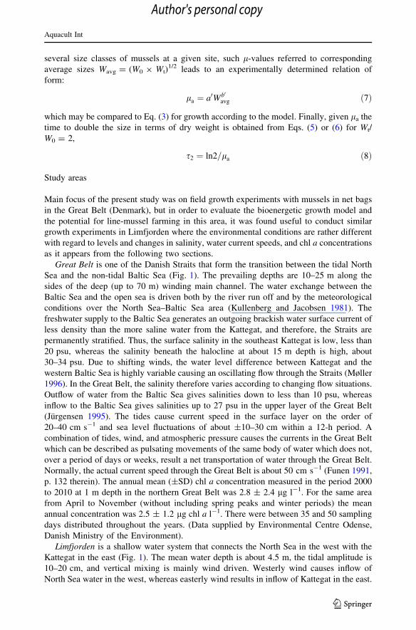
Great Belt is one of the Danish Straits that form the transition between the tidal North

Sea and the non-tidal Baltic Sea (Fig. 1). The prevailing depths are 10–25 m along the

sides of the deep (up to 70 m) winding main channel. The water exchange between the

Baltic Sea and the open sea is driven both by the river run off and by the meteorological

conditions over the North Sea–Baltic Sea area (Kullenberg and Jacobsen 1981). The

freshwater supply to the Baltic Sea generates an outgoing brackish water surface current of

less density than the more saline water from the Kattegat, and therefore, the Straits are

permanently stratified. Thus, the surface salinity in the southeast Kattegat is low, less than

20 psu, whereas the salinity beneath the halocline at about 15 m depth is high, about

30–34 psu. Due to shifting winds, the water level difference between Kattegat and the

western Baltic Sea is highly variable causing an oscillating flow through the Straits (Møller

1996). In the Great Belt, the salinity therefore varies according to changing flow situations.

Outflow of water from the Baltic Sea gives salinities down to less than 10 psu, whereas

inflow to the Baltic Sea gives salinities up to 27 psu in the upper layer of the Great Belt

(Jurgensen 1995). The tides cause current speed in the surface layer on the order of

20–40 cm s-1 and sea level fluctuations of about ±10–30 cm within a 12-h period. A

combination of tides, wind, and atmospheric pressure causes the currents in the Great Belt

which can be described as pulsating movements of the same body of water which does not,

over a period of days or weeks, result a net transportation of water through the Great Belt.

Normally, the actual current speed through the Great Belt is about 50 cm s-1 (Funen 1991,

p. 132 therein). The annual mean (±SD) chl a concentration measured in the period 2000

to 2010 at 1 m depth in the northern Great Belt was 2.8 ± 2.4 lg l-1. For the same area

from April to November (without including spring peaks and winter periods) the mean

annual concentration was 2.5 ± 1.2 lg chl a l-1. There were between 35 and 50 sampling

days distributed throughout the years. (Data supplied by Environmental Centre Odense,

Danish Ministry of the Environment).

Limfjorden is a shallow water system that connects the North Sea in the west with the

Kattegat in the east (Fig. 1). The mean water depth is about 4.5 m, the tidal amplitude is

10–20 cm, and vertical mixing is mainly wind driven. Westerly wind causes inflow of

North Sea water in the west, whereas easterly wind results in inflow of Kattegat in the east.

Aquacult Int

123

Author's personal copy

Between the west and east boundaries, there is a permanent horizontal salinity gradient

having a salinity of 32–34 psu at the connection to the North Sea and 19–25 psu at the

connection to the Kattegat (Wiles et al. 2006; Hofmeister et al. 2009). Limfjorden is

eutrophic, receiving nutrient from the catchment area which is dominated by agriculture.

The western part of Limfjorden is less eutrophicated and less stratified than the central

northern part with intermediate stratified and eutrophic conditions, while the inner central

southern part is strongly stratified and eutrophic which frequently results in oxygen

depletion in the near-bottom water. The key factor determining the extent of oxygen

depletion is the weather conditions during the summer months July through September

where high temperatures coupled with low wind cause severe oxygen depletion, especially

in areas with dense mussel beds (Jørgensen 1980; Dolmer et al. 1999; Møhlenberg 1999;

Møhlenberg et al. 2007; Møller and Riisgard 2007; Maar et al. 2010, Dinesen et al. 2011).

The water currents in Limfjorden are driven by horizontal water density gradients and the

wind. The water current velocity 1 m above the bottom varies typically between \1 and

6 cm s-1, but near the surface, current velocities may be up to 10 cm s-1 (Dolmer 2000a,

b; Maar et al. 2007). The annual mean (±SD) chl a concentration in the period 1982–2006

in the central northern part of Limfjorden (Løgstør Bredning) was 7.5 ± 12.1 lg chl a l-1.

Measurements were taken at 2–3 different depths on the location each day of sampling.

There were between 9 and 29 sampling days distributed throughout the years. Maximum

Fig. 1 Map of Denmark showing the locations for field growth experiments with Mytilus edulis hung up innet bags at different localities in Great Belt (Kerteminde Bugt = GB-K, Musholm Bugt = GB-M,Svendborg Sund = GB-S, Karrebæksminde Bugt = GB-B), and in Limfjorden (Risgarde Bredning(Hvalpsund) = L-H, Salling Sund (Glyngøre) = L-G). Coordinates for mussels growth sites (closedsymbol) and environmental monitoring stations (open symbols, St. 1–6) are presented in Table 1

Aquacult Int

123

Author's personal copy

depth on station was 7.3 m. (Data supplied by Environmental Centre Ringkøbing, Danish

Ministry of the Environment).

Experimental mussels and growth sites

Blue mussels, M. edulis, were collected in Limfjorden (Skive Fjord) and in the Great Belt

(Kerteminde Bugt) (Fig. 1) about 2 weeks before the onset of 6 (Series #1 to #6) field

growth experiments with different size groups of mussels in net bags transferred to various

localities with different chl a concentration levels. In Great Belt, 4 locations: Kerteminde

Bugt (Series #1), Musholm Bugt (Series #2), Svendborg Sund (Series #3), and Kar-

rebæksminde Bugt (Series #4) (Fig. 1) were chosen for growth experiments with mussels

from Kerteminde Bugt between slightly variable periods from 20 July to 8 October

depending on location (Table 1). In Limfjorden, Risgarde Bredning and Salling Sund

(Fig. 1) were chosen, and on these locations, growth experiments with locally collected

mussels were carried out during two periods: (Series #5) July 29 to August 25, 2010 and

(Series #6) July 29 to September 21, 2010 (Table 1).

Before sorting of mussels in size groups, these were kept in aerated 1000-l tanks with

running seawater from the inlet to Kerteminde Fjord (18–22 psu). Mussels were then

cleaned, total shell length measured with a vernier gauge, sorted into 4 size groups (each

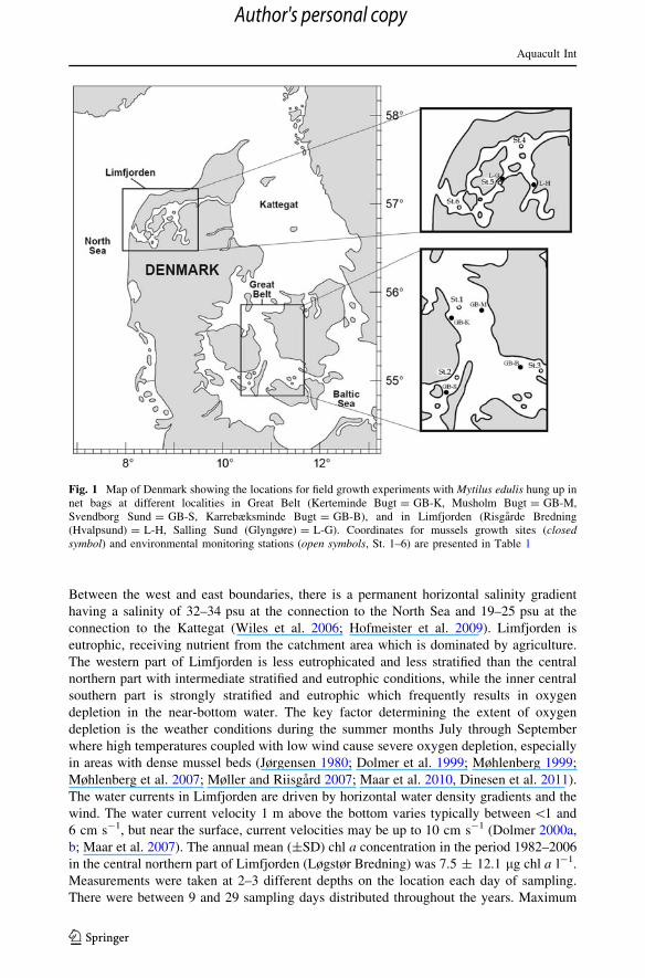
with near identical shell length ±0.4–1.3 mm), and put into net bags (Go Deep Interna-

tional Inc.) before they were transferred to the field location and hung up in a buoy system

(Fig. 2). The net bags were made of polypropylene fibers and cotton strings that rot away

after about 1 week which result in an increase in mask width. This system enables mussels

to settle firmly, and the subsequent disappearance of cotton strings ensure that the shell

opening of the mussels does not become restricted. The widths of the masks for small

mussels (20.8–31.0 mm shell length) were 10 9 10 mm, and for larger mussels

([40.0 mm shell length) were 10 9 15 mm. The net bags were 50 cm long and placed

approximately 1 m apart to avoid entanglement. Subsamples were subsequently collected

with about 14 days interval from the buoy systems and transported to the Marine Bio-

logical Research Centre, Kerteminde, for analysis. Shell length was measured with a

vernier gauge, soft parts removed from the shells, wet weight measured, and then drying

Fig. 2 Buoy system with mussels (Series #1 to #6) in net bags used at 4 locations in Great Belt and 2locations in Limfjorden (see Fig. 1)

Aquacult Int

123

Author's personal copy

Ta

ble

2M

ytil

us

edu

lis

(Ser

ies

#1

to#

6)

Ser

ies

loca

tio

np

erio

dD

t(d

ay)

Chl

a(l

gl-

1)

Tem

p.

(�C

)S

alin

ity

(psu

)L

0(m

m)

Lg

(mm

day

-1)

W0

(mg

)l

(%d

ay-

1)

Wavg

(mg

)s 2

(day

)

Ser

ies

#1

,G

B-K

Ker

tem

ind

eB

ug

t2

8Ju

lto

7O

ct2

01

0

71

3.1

±0

.71

6.0

±3

.51

4.2

±3

.42

0.8

0.1

49

41

.23

.31

38

21

.0

25

.80

.116

79

.92

.51

82

27

.7

30

.80

.104

91

.62

.62

31

26

.7

39

.10

.067

24

2.5

2.0

46

53

4.7

Ser

ies

#2

,G

B-M

Mu

sho

lmB

ug

t2

0Ju

lto

8O

ct2

01

0

80

3.1

±0

.71

6.0

±3

.51

4.2

±3

.42

1.0

0.1

23

41

.72

.99

82

3.9

26

.00

.070

69

.22

.01

52

34

.7

30

.80

.060

11

5.6

1.7

23

04

0.8

39

.00

.040

23

3.7

1.3

35

25

3.3

Ser

ies

#3

,G

B-S

Sv

end

bo

rgS

un

d2

6Ju

lto

13

Sep

20

10

49

3.0

±2

.8a

17

.5±

3.5

15

.4±

1.8

21

.20

.183

41

.23

.61

11

19

.3

25

.90

.135

75

.42

.81

60

24

.8

31

.00

.129

10

5.1

2.9

23

42

3.9

39

.20

.095

19

4.2

2.5

36

82

7.7

Ser

ies

#4

,G

B-B

Kar

rebæ

ksm

inde

Bugt

(Bis

seru

p)

24

Jul

to7

Oct

20

10

75

2.8

±2

.11

7.1

±3

.91

0.7

±1

.12

1.3

0.1

25

42

.92

.47

12

8.9

25

.90

.063

69

.21

.81

08

38

.5

30

.60

.060

10

2.3

1.8

16

83

8.5

40

.0-

0.0

03

20

3.2

1.1

25

96

3.0

Ser

ies

#5

,L

-HR

isg

ard

eB

red

nin

g(H

val

psu

nd

)2

9Ju

lto

25

Au

g2

01

0

27

3.6

±1

.61

8.8

±1

.52

6.9

±0

.82

1.1

0.2

66

41

.25

.28

41

3.3

25

.90

.215

74

.94

.01

29

17

.3

30

.80

.174

10

8.6

3.7

18

01

8.7

39

.40

.100

19

9.8

2.8

29

22

4.8

Aquacult Int

123

Author's personal copy

Ta

ble

2co

nti

nued

Ser

ies

loca

tio

np

erio

dD

t(d

ay)

Chl

a(l

gl-

1)

Tem

p.

(�C

)S

alin

ity

(psu

)L

0(m

m)

Lg

(mm

day

-1)

W0

(mg

)l

(%d

ay-

1)

Wavg

(mg

)s 2

(day

)

Ser

ies

#6

,L

-GS

alli

ng

Su

nd

(Gly

ng

øre

)2

9Ju

lto

21

Sep

20

10

54

3.2

±1

.7b

19

.0±

1.9

29

.4±

1.0

20

.80

.225

49

.73

.11

21

22

.4

25

.90

.221

79

.62

.51

63

27

.7

30

.90

.185

99

.92

.22

00

31

.5

39

.30

.122

17

3.2

2.1

31

03

3.0

aD

ata

are

mea

n(±

SD

)co

nce

ntr

atio

no

fch

la

inth

ep

erio

d2

00

0–

200

9as

no

chl

adat

afr

om

this

loca

tion

wer

eav

aila

ble

for

2010

bch

la

dat

aar

efr

om

Nis

sum

Bre

dnin

gb

ecau

sen

och

la

dat

afr

om

Sal

lin

gS

un

dex

ist

for

this

per

iod

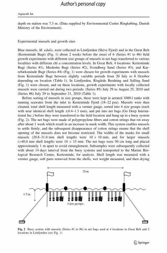
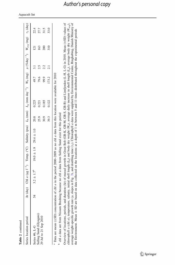
Over

vie

wof

loca

tions,

per

iods,

and

dura

tion

(Dt)

of

muss

elg

row

thin

Gre

atB

elt

(GB

-K,

GB

-M,

GB

-S,

GB

-B)

and

Lim

fjo

rden

(L-H

,L

-G)

in2

01

0.

Mea

n(±

SD

)v

alues

of

chlo

rop

hyll

a(c

hl

a),

tem

per

atu

re,

sali

nit

y,

init

ial

shel

lle

ng

th(L

0)

and

bo

dy

dry

wei

ght

(W0),

aver

age

dai

lyin

crea

sein

shel

lle

ngth

(Lg),

aver

age

bo

dy

dry

wei

gh

t(W

avg),

aver

age

wei

ght-

spec

ific

gro

wth

rate

(l,

slo

pes

inF

ig.

3),

and

do

ub

lin

gti

me

(s2).

Chlo

roph

yll

ad

ata

wer

esu

pp

lied

by

En

vir

on

men

tal

Cen

tre,

Rin

gk

øb

ing

,D

anis

hM

inis

try

of

the

En

vir

on

men

t.M

ean

±S

Dar

eb

ased

on

dat

aco

llec

ted

on

the

loca

tio

ns

ata

dep

tho

f1

mb

etw

een

5an

d1

1ti

mes

dis

trib

ute

dth

roug

ho

ut

the

exp

erim

enta

lp

erio

ds

Aquacult Int

123

Author's personal copy

both shells and soft parts on pieces of tin foil in an oven for 24 h at 90 �C to obtain also the

dry tissue weight.

Environmental data

Data on chl a, salinity, and temperature for the actual mussel growth periods were obtained

from 6 stations monitored by Environmental Centre Ringkøbing (Limfjorden), Environ-

mental Centre Odense, and Environmental Centre Roskilde (Great Belt). Temperature and

(f)

(µ = 2.0)(µ = 2.6)(µ = 2.5)(µ = 3.3)

0

1

2

3

4

5

6

7ln

W

39.06 mm30.82 mm25.78 mm20.82 mm

(a)

(µ = 1.3)(µ = 1.7)(µ = 2.0)(µ = 2.9)

39.04 mm30.80 mm26.01 mm21.00 mm

(b)

(µ = 2.9)(µ = 3.3)

(µ = 3.1)

(µ = 4.0)0

1

2

3

4

5

6

7

lnW

39.17 mm

30.97 mm

25.89 mm

21.16 mm

(c)

(µ = 1.1)

(µ = 1.8)

(µ = 1.8)

(µ = 2.4)

40.02 mm

30.63 mm

25.93 mm

21.25 mm

(d)

(µ = 2.8)(µ = 3.7)(µ = 4.0)

(µ = 5.2)0

1

2

3

4

5

6

7

0 10 20 30 40 50 60 70 80

lnW

Time (d)

39.39mm30.79 mm25.88 mm21.07 mm

(e)

(µ = 2.2)(µ = 2.2)(µ = 2.5)(µ = 3.1)

0 10 20 30 40 50 60 70 80

Time (d)

39.30 mm30.85mm25.92 mm20.78 mm

(f)

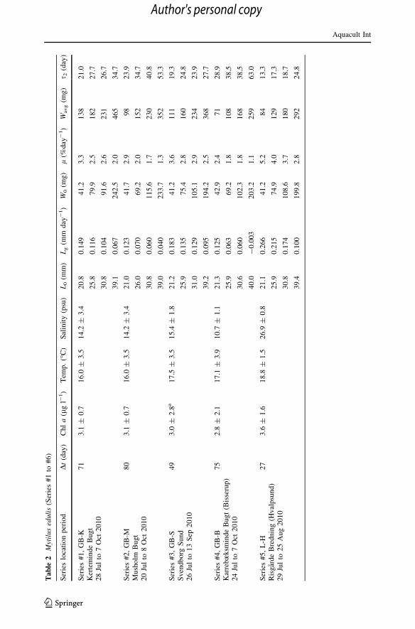
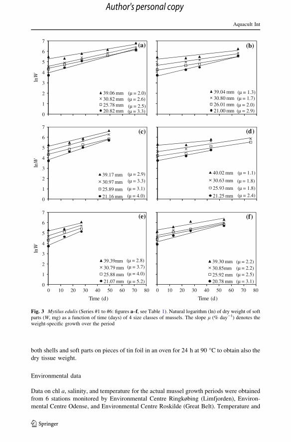
Fig. 3 Mytilus edulis (Series #1 to #6: figures a–f, see Table 1). Natural logarithm (ln) of dry weight of softparts (W, mg) as a function of time (days) of 4 size classes of mussels. The slope l (% day-1) denotes theweight-specific growth over the period

Aquacult Int

123

Author's personal copy

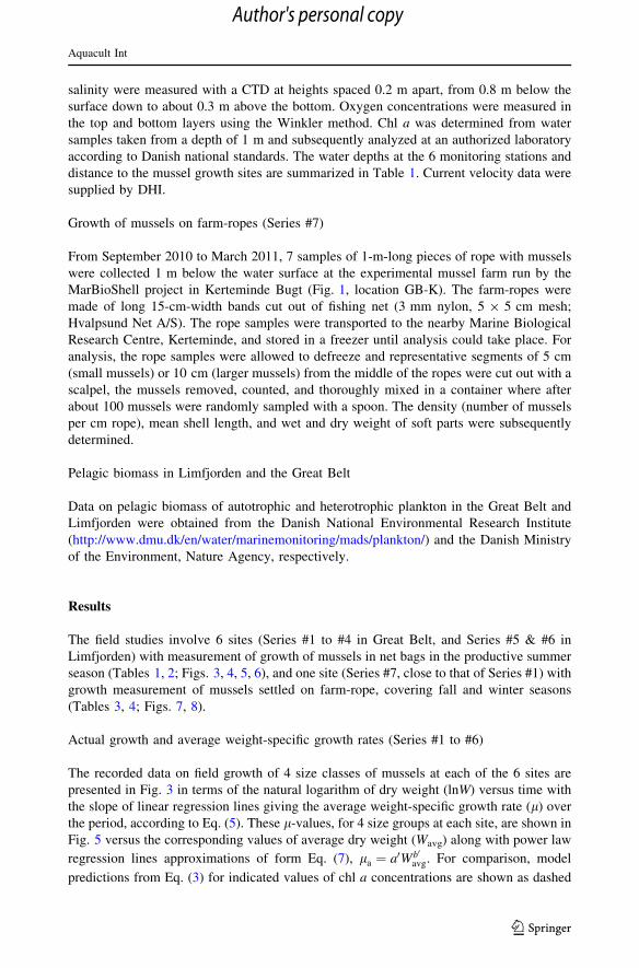
salinity were measured with a CTD at heights spaced 0.2 m apart, from 0.8 m below the

surface down to about 0.3 m above the bottom. Oxygen concentrations were measured in

the top and bottom layers using the Winkler method. Chl a was determined from water

samples taken from a depth of 1 m and subsequently analyzed at an authorized laboratory

according to Danish national standards. The water depths at the 6 monitoring stations and

distance to the mussel growth sites are summarized in Table 1. Current velocity data were

supplied by DHI.

Growth of mussels on farm-ropes (Series #7)

From September 2010 to March 2011, 7 samples of 1-m-long pieces of rope with mussels

were collected 1 m below the water surface at the experimental mussel farm run by the

MarBioShell project in Kerteminde Bugt (Fig. 1, location GB-K). The farm-ropes were

made of long 15-cm-width bands cut out of fishing net (3 mm nylon, 5 9 5 cm mesh;

Hvalpsund Net A/S). The rope samples were transported to the nearby Marine Biological

Research Centre, Kerteminde, and stored in a freezer until analysis could take place. For

analysis, the rope samples were allowed to defreeze and representative segments of 5 cm

(small mussels) or 10 cm (larger mussels) from the middle of the ropes were cut out with a

scalpel, the mussels removed, counted, and thoroughly mixed in a container where after

about 100 mussels were randomly sampled with a spoon. The density (number of mussels

per cm rope), mean shell length, and wet and dry weight of soft parts were subsequently

determined.

Pelagic biomass in Limfjorden and the Great Belt

Data on pelagic biomass of autotrophic and heterotrophic plankton in the Great Belt and

Limfjorden were obtained from the Danish National Environmental Research Institute

(http://www.dmu.dk/en/water/marinemonitoring/mads/plankton/) and the Danish Ministry

of the Environment, Nature Agency, respectively.

Results

The field studies involve 6 sites (Series #1 to #4 in Great Belt, and Series #5 & #6 in

Limfjorden) with measurement of growth of mussels in net bags in the productive summer

season (Tables 1, 2; Figs. 3, 4, 5, 6), and one site (Series #7, close to that of Series #1) with

growth measurement of mussels settled on farm-rope, covering fall and winter seasons

(Tables 3, 4; Figs. 7, 8).

Actual growth and average weight-specific growth rates (Series #1 to #6)

The recorded data on field growth of 4 size classes of mussels at each of the 6 sites are

presented in Fig. 3 in terms of the natural logarithm of dry weight (lnW) versus time with

the slope of linear regression lines giving the average weight-specific growth rate (l) over

the period, according to Eq. (5). These l-values, for 4 size groups at each site, are shown in

Fig. 5 versus the corresponding values of average dry weight (Wavg) along with power law

regression lines approximations of form Eq. (7), la ¼ a0Wb0

avg. For comparison, model

predictions from Eq. (3) for indicated values of chl a concentrations are shown as dashed

Aquacult Int

123

Author's personal copy

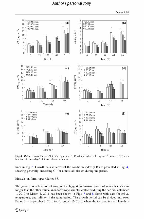
lines in Fig. 5. Growth data in terms of the condition index (CI) are presented in Fig. 4,

showing generally increasing CI for almost all classes during the period.

Mussels on farm-ropes (Series #7)

The growth as a function of time of the biggest 5-mm-size group of mussels (1–5 mm

longer than the other mussels) on farm-rope samples collected during the period September

1, 2010 to March 2, 2011 has been shown in Figs. 7 and 8 along with data for chl a,

temperature, and salinity in the same period. The growth period can be divided into two:

Period I = September 1, 2010 to November 16, 2010, where the increase in shell length is

0

2

4

6

8

10

12

14

16

18C

I(m

g cm

-3)

Time (d)

20.82 mm25.78 mm30.82 mm39.06 mm

(a)

0

2

4

6

8

10

12

14

16

18

CI(

mg

cm-3

)

Time (d)

21.00 mm26.01 mm30.80 mm39.04 mm

(b)

0

2

4

6

8

10

12

14

16

18

CI(

mg

cm-3

)

Time (d)

21.16 mm25.89 mm30.97 mm39.17 mm

(c)

0

2

4

6

8

10

12

14

16

18

CI(

mg

cm-3

)

Time (d)

21.25 mm25.93 mm30.63 mm40.02 mm

(d)

0

2

4

6

8

10

12

14

16

18

CI (

mg

cm-3

)

Time (d)

21.07 mm25.88 mm30.79 mm39.39mm

(e)

0

2

4

6

8

10

12

14

16

18

0 13 27 48 71 0 23 34 65 80

0 17 28 49 0 23 43 75

0 13 27 0 13 27 54

CI(

mg

cm-3

)

Time (d)

20.78 mm25.92 mm30.85 mm39.30 mm

(f)

Fig. 4 Mytilus edulis (Series #1 to #6: figures a–f). Condition index (CI, mg cm-3, mean ± SD) as afunction of time (days) of 4 size classes of mussels

Aquacult Int

123

Author's personal copy

0.277 mm day-1, and Period II = November 16, 2010 to March 2, 2011 with loss of

weight (Fig. 8) but essentially without increase in shell length (Fig. 7b; Table 3). Further

details on weight loss during Period II are given Table 4.

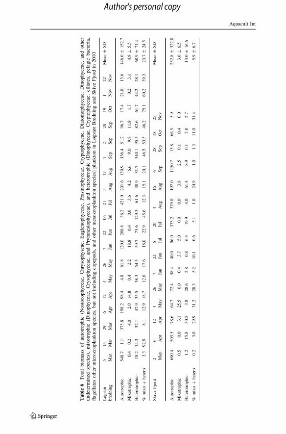
Pelagic biomass

The biomass of autotrophic and heterotrophic plankton in the Great Belt in 1997 and in

Limfjorden in 2010 when also mixotrophic species were quantified are shown in Tables 5

and 6. It appears that the heterotrophic biomass in the Great Belt in 1997 was 3.4 ± 3.3 %

of the total pelagic biomass, whereas the heterotrophic and mixotrophic biomass were

23.7 ± 24.5 % of the total in Løgstør Bredning and 5.9 ± 6.7 % in Skive Fjord, respec-

tively. Although the heterotrophic fraction of the total plankton biomass available for filter-

feeding mussels may at times be relatively high, it seems safe to conclude that the auto-

trophic plankton, which can be quantified by measurement of the chl a concentration,

generally dominates the pelagic microplankton.

Discussion

In the present work, we first present experimental data on the growth of mussels during the

productive summer season and also test to what degree the observed weight-specific

0.1

1.0

10.0

100.0

0.01 0.10 1.00 10.00

µ (%

d-1

)

Wavg (g)

#1 1.49 -0.36 3.1±0.7

#2 0.69 -0.60 3.1±0.7

#3 2.33 -0.22 3.0±2.8*

#4 0.58 -0.54 2.8±2.1

#5 1.60 -0.47 3.6±1.6

#6 1.25 -0.40 3.2±1.7

1.5

2.0

4.0

3.0

Series a' b' chl a (µg l-1)

GB

L

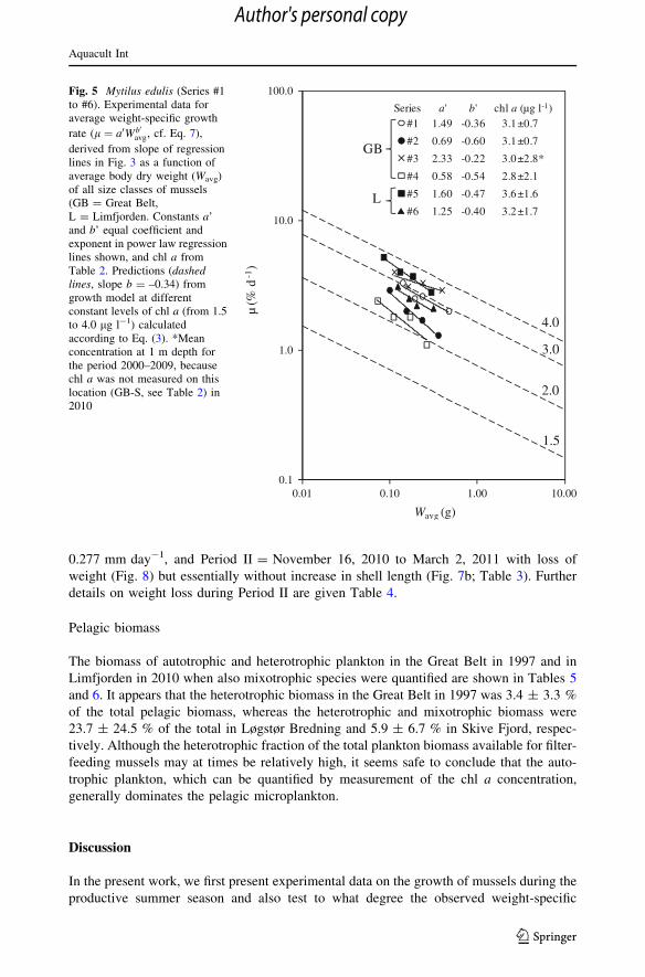
Fig. 5 Mytilus edulis (Series #1to #6). Experimental data foraverage weight-specific growth

rate (l ¼ a0Wb0

avg, cf. Eq. 7),

derived from slope of regressionlines in Fig. 3 as a function ofaverage body dry weight (Wavg)of all size classes of mussels(GB = Great Belt,L = Limfjorden. Constants a’and b’ equal coefficient andexponent in power law regressionlines shown, and chl a fromTable 2. Predictions (dashedlines, slope b = –0.34) fromgrowth model at differentconstant levels of chl a (from 1.5to 4.0 lg l-1) calculatedaccording to Eq. (3). *Meanconcentration at 1 m depth forthe period 2000–2009, becausechl a was not measured on thislocation (GB-S, see Table 2) in2010

Aquacult Int

123

Author's personal copy

growth rate as a function of mussel dry weight can be related to the model expressed by

Eq. (3). We suggest that deviations from either the expected exponent of b = -0.34 or the

constant a expressing the magnitude of growth for the prevailing chl a concentration level

indicate suboptimal growth conditions, although more precise interpretations may not be

possible without supplementary studies.

Figure 5 shows that field data from 6 different sites fall in the general area of prediction

according to the bioenergetic growth model. But in regard to predicted levels of growth

rates for the theoretical and the measured chl a concentrations near the growth sites, there

are some differences. Series #1, #5, and #6 appear close to the model, Series #2 and #4

appear suboptimal, while Series #3 appears to grow faster than predicted by the theory for

the measured chl a concentration near the site.

The reasons for suboptimal growth in Series # 2 and #4 despite high chl a levels may be

suggested by examination of Eq. (1)–(3). Thus, if the b-exponent is essentially that of the

model, this implies b1- and b2-exponents to be near identical (& 0.66), and this leaves the

constants a1, a2, AE, and a0 as sources of suboptimality (or deviations from prerequisites

0

5

10

15

20

25S

alin

ity/

Tem

pera

ture

/Chl

. a

C T S series#1

0

5

10

15

20

25

Salin

ity/

Tem

pera

ture

/Chl

. a

C T S series#2

0

5

10

15

20

25

30

Sal

init

y/Te

mpe

ratu

re T S series#3

0

5

10

15

20

25

30

Sal

init

y/Te

mpe

ratu

re/C

hl.

a

C T S series#4

05

10152025303540

Sal

init

y/Te

mpe

ratu

re/C

hl.

a

C T S series#5

05

10152025303540

Salin

ity/

Tem

pera

ture

/Chl

. a

C T S series#6

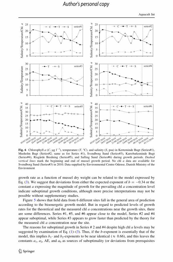
Fig. 6 Chlorophyll a (C, lg l-1), temperature (T, �C), and salinity (S, psu) in Kerteminde Bugt (Series#1),Musholm Bugt (Series#2; same as for Series #1), Svendborg Sund (Series#3), Karrebæksminde Bugt(Series#4), Risgarde Bredning (Series#5), and Salling Sund (Series#6) during growth periods. Dashedvertical lines mark the beginning and end of mussel growth period. No chl a data are available forSvendborg Sund (Series#3) in 2010. Data supplied by Environmental Centre Odense, Danish Ministry of theEnvironment

Aquacult Int

123

Author's personal copy

Ta

ble

3M

ytil

us

edu

lis

(Ser

ies

#7

)

Dat

eD

ayR

op

e(c

m)

nto

tD

ensi

ty(i

nd

.cm

-1)

ns

Ls

(mm

)n

big

5L

big

5

(mm

)W

sp

(mg

)C

I(m

gcm

-3)

Wsh

ell

(mg

)W

C(%

)l (%

day

-1)

01

-09-2

01

00

5.0

11

23

22

51

62

4.4

±1

.62

27

.4±

1.5

3.3

±2

.77

.3±

1.5

16

.1±

11

.16

7.7

±7

.6

18

-09-2

01

01

74

.58

31

18

58

17

.0±

3.2

24

11

.2±

0.9

11

.1±

3.6

7.7

±1

.44

0.8

±1

1.0

76

.2±

3.0

7.1

07

-10-2

01

03

61

0.0

16

83

68

91

11

.6±

4.7

17

18

.1±

2.4

53

.4±

26

.38

.7±

1.4

18

5.2

±7

8.5

78

.1±

2.0

8.3

16

-11-2

01

07

61

0.0

11

45

11

51

55

14

.4±

6.8

10

28

.1±

2.1

19

7.3

±2

1.6

7.0

±0

.67

00

.0±

69

.87

9.8

±1

.33

.3

05

-01-2

01

11

26

9.7

10

66

11

01

24

13

.0±

7.1

92

7.9

±2

.61

71

.9±

28

.66

.6±

1.4

88

4.5

±1

10

.98

1.4

±1

.3-

0.3

02

-03-2

01

11

82

10

.51

46

81

40

19

81

1.6

±6

.58

29

.1±

2.4

14

6.9

±3

7.9

5.1

±1

.38

96

.9±

13

2.8

84

.2±

1.3

-0

.3

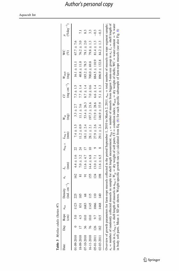
Over

vie

wof

gro

wth

par

amet

ers

for

farm

-rope

muss

els

coll

ecte

din

the

per

iod

Sep

tem

ber

1,

2010

toM

arch

2,

2011.

nto

t=

tota

lnum

ber

of

muss

els

on

rope

segm

ent

sam

ple

;n

s=

num

ber

of

random

lyco

llec

ted

muss

els

insa

mple

for

shel

lle

ngth

mea

sure

men

t;n

big

5=

nu

mb

ero

fm

uss

els

fro

mb

igg

est

5-m

m-s

ize

gro

up

inn

s;L

s=

shel

lle

ng

tho

fm

uss

els

inn

s;L

big

5=

shel

lle

ngth

of

muss

els

inn

big

5;

Wsp

=d

ryw

eig

ht

of

soft

par

ts;

CI

=co

nd

itio

nin

dex

;W

shell

=d

ryw

eig

ht

of

shel

ls;

WC

=w

ater

con

ten

t=

%w

ater

inb

od

yso

ftp

arts

.M

ean

±S

Dar

esh

ow

n.

Wei

gh

t-sp

ecifi

cg

row

thra

te(l

)ca

lcula

ted

from

Eq.

(6)

for

each

spec

ific

subsa

mple

of

farm

-rope

muss

els

(see

also

Fig

.8)

Aquacult Int

123

Author's personal copy

for the growth model) associated with the level of growth. The most obvious candidate for

low level of growth is some degree of reduced filtration rate for the full size range (i.e.,

smaller a1) or increased respiration rate due to, e.g., stress caused by varying salinity (i.e.,

larger a2) (e.g., Strickle and Sabourin 1979; Riisgard et al. 2012b).

The case of Series #3, showing higher growth rates than predicted for the chl a con-

centration measured nearby, could be explained by the rather large experimental uncer-

tainty of data, notably 3.0 ± 2.8 lg l-1, or by the availability of other sources of nutrition

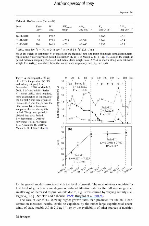
Table 4 Mytilus edulis (Series #7)

Date Time(day)

W(mg)

DWperiod

(mg)DWact

(mg day-1)Rm

(ml O2 h-1)DWest

(mg day-1)a

16-11-2010 0 197.3 0.162 -3.8

05-01-2011 50 171.9 -25.4 -0.508 0.148 -3.4

02-03-2011 106 146.9 -25.0 -0.446 0.133 -3.1

a DWest (mg day-1) = (Rm 9 24 h day-1 9 19.88 J h-1)/(20.51 J mg-1)

Mean dry weight of soft parts (W) of mussels in the biggest 5-mm-size group of mussels sampled from farm-ropes in the winter-starvation period, November 11, 2010 to March 2, 2011 (Fig. 8). Loss of dry weight inperiod between sampling (DWperiod) and actual daily weight loss (DWact) is shown along with estimatedweight loss (DWest) calculated from the maintenance respiratory rate (Rm, see text)

0 20 40 60 80 100 120 140 160 180 200

0

5

10

15

20

25

30

Sal

init

y/Te

mpe

ratu

re/c

hl a

C T S(a) Period I:T = 12.4±2.9C = 3.1±0.8

Period II:T = 3.2±2.6C = 3.3±3.1

Period I:L = 0.277t + 7.255

R² = 0.994

Period II:L = 0.0101t + 27.071

R² = 0.607

0

5

10

15

20

25

30

35

L(m

m)

(b)

Fig. 7 a Chlorophyll a (C, lgchl a l-1), temperature (T, �C),and salinity (S, psu) fromSeptember 1, 2010 to March 2,2011. b Mytilus edulis (Series#7). Mean (±SD) shell length (L,mm) as a function of time (t, d) ofthe biggest 5-mm-size group ofmussels (1–5 mm longer than theother mussels) on farm-ropesamples collected during thisperiod. The growth period isdivided into two: PeriodI = September 1, 2010 toNovember 16, 2010, PeriodII = November 16, 2010 toMarch 2, 2011 (see Table 3)

Aquacult Int

123

Author's personal copy

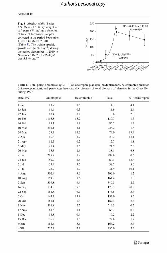
W = -0.475t + 232.82R² = 0.999

W = 4.454e0.053t

R² = 0.950

0

50

100

150

200

250

W(m

g)

Fig. 8 Mytilus edulis (Series#7). Mean (±SD) dry weight ofsoft parts (W, mg) as a functionof time of farm-rope samplescollected in the period September1, 2010 to March 2, 2011(Table 3). The weight-specificgrowth rate (l, % day-1) duringthe period September 1, 2010 toNovember 16, 2010 (76 days)was 5.3 % day-1

Table 5 Total pelagic biomass (lg C l-1) of autotrophic plankton (phytoplankton), heterotrophic plankton(microzooplankton), and percentage heterotrophic biomass of total biomass of plankton in the Great Beltduring 1997

Date 1997 Autotrophic Heterotrophic Total % Heterotrophic

1 Jan 13.7 0.6 14.3 4.1

13 Jan 11.6 0.3 11.9 2.4

27 Jan 10.4 0.2 10.6 2.0

10 Feb 1115.5 15.2 1130.7 1.3

24 Feb 95.1 1.7 96.7 1.7

10 Mar 219.1 4.1 223.2 1.8

24 Mar 59.7 14.3 74.0 19.4

7 Apr 16.6 3.7 20.2 18.1

21 Apr 12.5 0.2 12.7 1.8

6 May 21.4 0.5 21.9 2.3

26 May 35.5 2.6 38.1 6.8

9 Jun 295.7 1.9 297.6 0.6

24 Jun 50.7 9.4 60.1 15.6

3 Jul 35.4 3.3 38.7 8.6

21 Jul 28.7 3.2 31.9 10.1

4 Aug 302.4 3.6 306.0 1.2

18 Aug 159.9 1.6 161.4 1.0

2 Sep 339.8 9.4 349.3 2.7

16 Sep 134.8 35.5 170.3 20.8

22 Sep 164.8 9.7 174.5 5.6

6 Oct 143.7 13.4 157.0 8.5

20 Oct 181.1 6.3 187.4 3.3

3 Nov 516.8 2.5 519.3 0.5

17 Nov 63.6 0.1 63.7 0.2

1 Dec 18.8 0.4 19.2 2.2

15 Dec 76.2 1.5 77.6 1.9

Mean 158.6 5.6 164.2 3.4

±SD 232.7 7.7 235.0 3.3

Aquacult Int

123

Author's personal copy

Ta

ble

6T

ota

lb

iom

ass

of

auto

tro

ph

ic(N

ost

oco

ph

yce

ae,

Ch

ryso

phy

seae

,E

ug

len

op

hy

ceae

,P

rasi

no

ph

yce

ae,

Cry

pto

ph

yce

ae,

Dia

tom

op

hyce

ae,

Din

op

hyce

ae,

and

oth

eru

nd

eter

min

edsp

ecie

s),

mix

otr

op

hic

(Din

op

hy

ceae

,C

ryso

ph

yce

ae,

and

Pry

mn

esio

ph

yce

ae),

and

het

ero

tro

ph

ic(D

inop

hy

ceae

,C

ryp

top

hy

ceae

,ci

liat

es,

pel

agic

bac

teri

a,fl

agel

late

soth

erm

icro

zoopla

nkto

nsp

ecie

s,but

not

incl

udin

gco

pep

ods,

and

oth

erm

esozo

opla

nkto

nsp

ecie

s)pla

nkto

nin

Løgst

ør

Bre

dnin

gan

dS

kiv

eF

jord

in2

01

0

Løgst

ør

bre

dnin

g

5 Mar

15

Mar

29

Mar

6 Apr

12

Apr

4 May

26

May

7 Jun

22

Jun

06

Jul

21

Jul

5 Aug

17

Aug

7 Sep

21

Sep

28

Sep

19

Oct

1 Nov

22

Nov

Mea

n±

SD

Auto

trophic

548.7

1.1

375.8

198.2

98.4

4.8

61.8

120.0

208.8

36.2

421.0

201.6

130.9

136.4

81.2

96.7

17.4

21.8

13.6

146.0

±152.7

Mix

otr

ophic

0.4

0.2

4.0

2.0

14.8

0.4

2.2

18.8

0.4

0.0

3.6

4.2

6.6

9.0

9.8

11.8

1.7

0.2

3.1

4.9

±5.5

Het

erotr

ophic

18.2

14.3

32.1

47.9

35.5

58.3

54.5

59.7

75.6

129.3

61.6

38.9

31.7

340.1

95.5

82.6

61.7

44.2

28.1

68.9

±71.4

%m

ixo

?het

ero

3.3

92.9

8.1

12.9

18.7

12.6

17.6

18.0

22.9

45.6

12.3

15.1

20.1

46.5

53.5

46.2

75.1

60.2

39.3

23.7

±24.5

Skiv

eF

jord

2 May

6 Apr

12

Apr

4 May

26

May

7 Jun

22

Jun

5 Jul

20

Jul

4 Aug

16

Aug

6 Sep

28

Sep

18

Oct

25

Nov

Mea

n±

SD

Auto

trophic

690.4

503.5

78.6

64.7

72.4

58.4

40.0

96.0

373.2

379.0

197.0

1150.7

15.8

66.5

5.9

252.8

±322.0

Mix

otr

ophic

0.5

0.0

3.1

25.5

0.0

0.4

3.7

5.0

0.0

0.0

3.8

2.5

0.1

0.4

0.0

3.0

±6.5

Het

erotr

ophic

1.2

15.8

30.5

3.8

28.6

2.8

0.8

6.4

19.9

4.0

61.4

8.9

0.1

7.8

2.7

13.0

±16.6

%m

ixo

?het

ero

0.2

3.0

29.9

31.2

28.3

5.2

10.1

10.6

5.1

1.0

24.9

1.0

1.3

11.0

31.4

5.9

±6.7

Aquacult Int

123

Author's personal copy

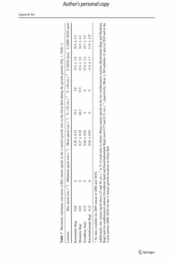
Ta

ble

7M

axim

um

,m

inim

um

,an

dm

ean

(±S

D)

curr

ent

spee

ds

atth

e4

mu

ssel

gro

wth

site

sin

the

Gre

atB

elt

du

rin

gth

eg

row

thp

erio

ds

(Fig

.1,

Tab

le1)

Loca

tion

Max

spee

d(c

ms-

1)

Min

imu

msp

eed

(cm

s-1)

Mea

nsp

eed

(cm

s-1)

%[

25

cms-

1%

[5

0cm

s-1

S(2

01

0)

(psu

)S

(20

08–

20

10

)(p

su)

Ker

tem

ind

eB

ug

t0

.66

00

.20

±0

.14

34

.23

.61

5.4

±3

.81

6.5

±4

.2

Mu

sho

lmB

ug

t0

.87

00

.27

±0

.20

46

.21

5.5

15

.4±

3.8

16

.5±

4.2

Sv

end

bo

rgS

un

d0

.12

00

.04

±0

.02

00

15

.4±

3.2

16

.7±

3.9

Kar

rebæ

ksm

inde

Bugt

0.1

20

0.0

4±

0.0

30

01

1.6

±1

.71

1.9

±1

.8a

aN

odat

aav

aila

ble

for

2009

(mea

nof

2008

and

2010)

Ad

dit

ion

ally

,th

ecu

rren

tsp

eed

abo

ve

25

and

50

cms-

1in

%o

fto

tal

tim

eis

sho

wn.

Mea

ncu

rren

tsp

eed

sat

the

two

no

rther

nm

ost

stat

ion

s(K

erte

min

de

Bu

gt

and

Mu

sho

lmB

ug

t)an

dtw

oso

uth

ern

mo

stst

atio

ns

(Sv

end

bo

rgS

un

dan

dK

arre

bæ

ksm

ind

eB

ug

t)w

ere

0.7

7an

d0

.12

cms-

1,

resp

ecti

vel

y.

Mea

n±

SD

sali

nit

ies

(S,

psu

)in

20

10

and

inth

e3

-yea

rp

erio

d(2

00

8–

20

10

)fo

rth

e4

mu

ssel

gro

wth

loca

tion

sin

Gre

atB

elt

Aquacult Int

123

Author's personal copy

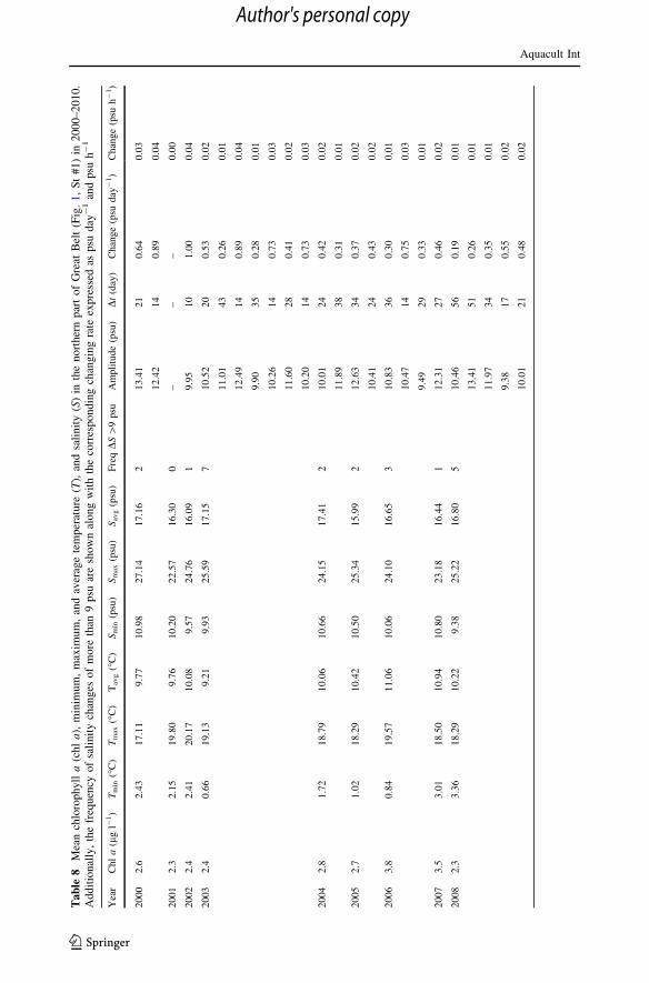
Ta

ble

8M

ean

chlo

rop

hyll

a(c

hl

a),

min

imu

m,

max

imu

m,

and

aver

age

tem

per

ature

(T),

and

sali

nit

y(S

)in

the

no

rther

np

art

of

Gre

atB

elt

(Fig

.1,

St

#1

)in

20

00–

20

10

.A

dd

itio

nal

ly,

the

freq

uen

cyo

fsa

lin

ity

chan

ges

of

mo

reth

an9

psu

are

sho

wn

alo

ng

wit

hth

eco

rres

po

nd

ing

chan

gin

gra

teex

pre

ssed

asp

sud

ay-

1an

dp

suh

-1

Yea

rC

hl

a(l

gl-

1)

Tm

in(�

C)

Tm

ax

(�C

)T

av

g(�

C)

Sm

in(p

su)

Sm

ax

(psu

)S

av

g(p

su)

Fre

qD

S[

9psu

Am

pli

tude

(psu

)D

t(d

ay)

Chan

ge

(psu

day

-1)

Chan

ge

(psu

h-

1)

2000

2.6

2.4

317.1

19.7

710.9

827.1

417.1

62

13.4

121

0.6

40.0

3

12.4

214

0.8

90.0

4

2001

2.3

2.1

519.8

09.7

610.2

022.5

716.3

00

––

–0.0

0

2002

2.4

2.4

120.1

710.0

89.5

724.7

616.0

91

9.9

510

1.0

00.0

4

2003

2.4

0.6

619.1

39.2

19.9

325.5

917.1

57

10.5

220

0.5

30.0

2

11.0

143

0.2

60.0

1

12.4

914

0.8

90.0

4

9.9

035

0.2

80.0

1

10.2

614

0.7

30.0

3

11.6

028

0.4

10.0

2

10.2

014

0.7

30.0

3

2004

2.8

1.7

218.7

910.0

610.6

624.1

517.4

12

10.0

124

0.4

20.0

2

11.8

938

0.3

10.0

1

2005

2.7

1.0

218.2

910.4

210.5

025.3

415.9

92

12.6

334

0.3

70.0

2

10.4

124

0.4

30.0

2

2006

3.8

0.8

419.5

711.0

610.0

624.1

016.6

53

10.8

336

0.3

00.0

1

10.4

714

0.7

50.0

3

9.4

929

0.3

30.0

1

2007

3.5

3.0

118.5

010.9

410.8

023.1

816.4

41

12.3

127

0.4

60.0

2

2008

2.3

3.3

618.2

910.2

29.3

825.2

216.8

05

10.4

656

0.1

90.0

1

13.4

151

0.2

60.0

1

11.9

734

0.3

50.0

1

9.3

817

0.5

50.0

2

10.0

121

0.4

80.0

2

Aquacult Int

123

Author's personal copy

Ta

ble

8co

nti

nued

Yea

rC

hl

a(l

gl-

1)

Tm

in(�

C)

Tm

ax

(�C

)T

av

g(�

C)

Sm

in(p

su)

Sm

ax

(psu

)S

av

g(p

su)

Fre

qD

S[

9psu

Am

pli

tude

(psu

)D

t(d

ay)

Chan

ge

(psu

day

-1)

Chan

ge

(psu

h-

1)

2009

3.1

2.1

519.0

511.1

210.4

824.3

617.6

03

10.5

523

0.4

60.0

2

10.6

261

0.1

70.0

1

11.0

721

0.5

30.0

2

2010

2.7

-0.4

820.9

88.2

310.2

322.4

415.4

23

9.7

029

0.3

30.0

1

9.0

47

1.2

90.0

5

9.4

238

0.2

50.0

1

Aquacult Int

123

Author's personal copy

than phytoplankton, e.g., heterotrophic flagellates, ciliates, and other microzooplankton

that may form part of the in situ diet of mussels (Nielsen and Maar 2007), and further that

mesozooplankton in turbulent water may be ingested by filter-feeding mussels (Davenport

et al. 2000). Thus, growth rates higher than estimated from an energy budget based solely

on chl a may express a possible supplementary ingestion of heterotrophic food.

In case of Series #6, showing growth rates somewhat lower than predicted for the

growth model, a probable explanation is the generally high current speeds at this growth

site in Great Belt (Musholm Bugt). Here, the current speed was higher than 0.25 and

5 cm s-1 for 46.2 and 15.5 % of the time, respectively (Table 7), and according to Wildish

and Miyares (1990) flow-induced inhibition of the filtration rate of blue mussels takes

place in flume flows above 6 cm s-1, and at flows between 25 and 38 cm s-1, the filtration

rate was reduced to only about 12 % of that measured at 6 cm s-1.

Secondly, we study mussel growth during the fall–winter season. Here, the growth of

mussels on farm-ropes (Series #7) shows that the weight-specific growth rate (about

5 % day-1 at about 3–4 lg chl a l-1, Fig. 8) followed model prediction during Period I,

thus suggesting density independent growth of the biggest 5-mm-size group of mussels, but

in Period II when both the chl a concentration and temperature became very low (Fig. 7a),

the mussels were losing weight (Fig. 8), a scenario which is beyond the parameter range

covered by the model. As it appears from Table 4, the actual daily weight loss is signif-

icantly lower (about 7 times) than the estimated weight loss calculated from the mainte-

nance respiration rate assuming this were at the normal level of a fully open mussel. This

indicates that the mussels during Period II may have been partially closed and thus saving

energy by the reduced respiration rate (Jørgensen et al. 1986).

As to the general potential for mussel farming in Danish waters, it is noted that the

variation in chl a, temperature, and salinity in the northern and southern part of Great Belt

during a 10-year period, from beginning of 2000 to end of 2010, have been monitored by

the Danish Nature Agency (Table 8), and the mean salinities in the study period

2008–2010 for the 4 mussel growth locations in Great Belt has been shown in Table 7.

Based on the present study of actual growth of mussels in net bags and on farm-ropes in the

field, it seems reasonable here to make a provisional evaluation of the potential for line-

mussel farming in the Great Belt. The specific growth rates observed in Great Belt compare

quite well with the growth in Limfjorden, although frequently high current speeds at

certain sites in Great Belt may induce inhibition of feeding and thus growth. The observed

variations in salinities, however, are not likely to influence the growth rate of mussels in

Great Belt (Riisgard et al. 2012b, 2013b).

Thus, based on the present bioenergetic growth model and experimental approach, it is

possible to evaluate the potential for optimal line-mussel growth in selected areas of

special interest, especially if supplementary local field measurements of chl a, heterotro-

phic plankton, and current speeds were to be made to fine-adjust the growth model, all

without the need for elaborate growth experiments. Regarding future mussel farming, our

studies have shown that M. edulis can grow from settlement in spring to 30 mm in shell

length in November. However, to reach the traditional consumer size of at least 45 mm, it

will probably take about 18 months, as suggested by Dolmer and Frandsen (2002) for long

line-mussels in Limfjorden, because of the winter period with weight loss and subsequent

re-growth during the next season. It may therefore be suggested to consider a new approach

of line farming of 30-mm mini-mussels during one growth season, from early spring to

November, recovering all equipment at the time of harvest and re-establishing it at the

beginning of the next season for a new population and thus protecting the equipment from

the often damaging weather of the Danish winter season. The new, smaller-sized consumer

Aquacult Int

123

Author's personal copy

0100200300400500600700800900

1000W

(mg)

Time, t (d)

(a)39.06 mm30.82 mm25.78 mm20.82 mm

0100200300400500600700800900

1000

W(m

g)

Time, t (d)

(b)39.06 mm30.82 mm25.78 mm20.82 mm

W = 0.011t2.228

R² = 0.969

0100200300400500600700800900

1000

W(m

g)

Time, t (d)

(c)

39.06 mm30.82 mm25.78 mm20.82 mmPower (All data)

0.94

0.95

0.96

0.97

0 20 40 60 80

R2

ts (d)

µ = 1.345W-0.435

R² = 0.969

1

10

0 20 40 60 80 100 120 140 160 180 200 0 20 40 60 80 100 120 140 160 180 200

0 20 40 60 80 100 120 140 160 180 200 0.01 0.10 1.00

µ (%

d-1

)

W (g)

(d)3.0 µg chl a l-1

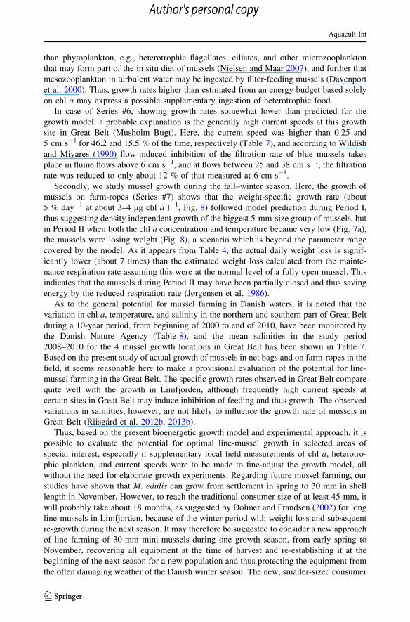
Fig. 9 Mytilus edulis (Series #1). a 4 size groups separated by arbitrary shifts ts = 10, 30, 60, and100 days, respectively; b optimal overlap for shifts ts = 10, 12, 25, and 45 days; c assembled time seriesshifted 30 days to start at ts = 45 days, giving maximal R2 (insert); d resulting relation l(W) calculatedfrom Eq. (10) and compared to growth model at chl a of 3 lg l-1 (dashed)

0.1

1.0

10.0

100.0

µ (%

d-1

)

W (g)

Series a' b' chl a (µg l-1)#1 1.34 -0.44 3.1±0.7#2 0.89 -0.40 3.1±0.7#3 1.88 -0.33 3.0±2.8*#4 0.80 -0.33 2.8±2.1#5 1.96 -0.38 3.6±1.6#6 1.37 -0.42 3.2±1.74.0 µg chl a l-1

3.0

2.0

1.5

GB

L

0.01 0.10 1.00

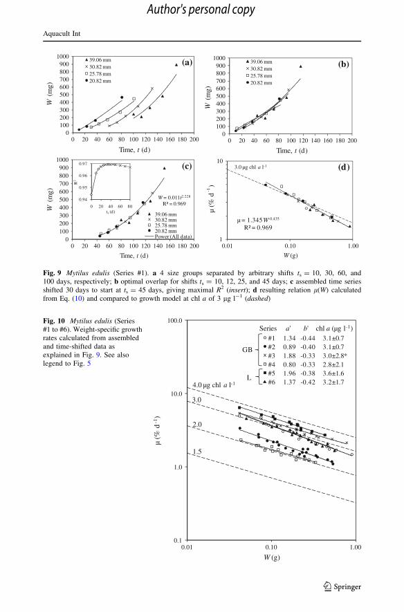
Fig. 10 Mytilus edulis (Series#1 to #6). Weight-specific growthrates calculated from assembledand time-shifted data asexplained in Fig. 9. See alsolegend to Fig. 5

Aquacult Int

123

Author's personal copy

product should be attractive in its own right—like the small French 40-mm ‘bouchot’

mussels for which there is a market (Prou and Goulletquer 2002).

Acknowledgments This work formed part of the MarBioShell project supported by the Danish Agency forScience, Technology and Innovation for the period January 2008 to December 2012. Thanks are due toMads Anker van Deurs and Isabel B. Saavedra for technical assistance, to Lars Birger Nielsen for practicalassistance, to Mads Joakim Birkeland and Flemming Møhlenberg, DHI, for providing current velocity data,and to the Danish Nature Agency, Danish Ministry of the Environment, for providing hydrographical data,and for excellent co-operation, especially with Benny Ludvigsen Bruhn, Bent Jensen, and FlemmingNørgaard. Two anonymous reviewers provided many constructive comments on the manuscript.

Appendix: Note on experimental time series

If an extended time series of data W(t) is available, it is possible to obtain more detail in

terms of how l varies with increasing size W. The first data point in an experimental time

series is normally assigned the arbitrary value of t = 0 at size W0, but on a true time scale

of mussel life this should be some time ts [ 0. We therefore shift the time series W(t) by tsto W(ts ? t) and examine the R2 value of a power law regression to the time-shifted data to

find the shift ts that produces the maximal value of R2. Denoting the power law fit

W ¼ c ts þ tð Þd; ð9Þ

and using the definition l = (1/W) dW/dt, we obtain the estimate of l(W) as

l ¼ 1=Wð Þdc ts þ tð Þd�1¼ d W=cð Þ�1=d¼ a0Wb0 : ð10ÞComparing Eqs. (10)–(3) shows that growth follows the model provided

a0 � dc1=d ¼ a and b0 � �1=d ¼ b.

The time (s2) for doubling the dry weight of soft parts of any given size of mussel may

be estimated by integrating Eq. (5) from W to 2W, assuming a constant mean value of l,

which yields s2 = ln2/l, but this expression gives an underestimate for dry weight W since

l decreases with increasing size. The correct value is obtained by use of Eq. (3) in the

definition (l = (1/W) dW/dt) which integrates to

10

100

1.000.100.01

τ 2(d

)

W (g)

#1 3.1±0.7#2 3.1±0.7#3 3.0±2.8*#4 2.8±2.1#5 3.6±1.6#6 3.2±1.7

Series chl a (µg l-1)

2.0 µg chl a l-1

3.0 4.0

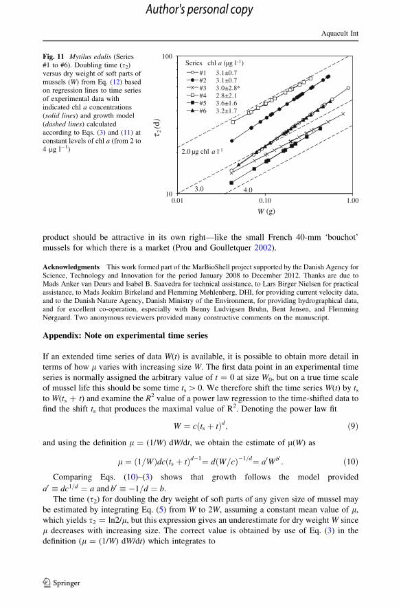
Fig. 11 Mytilus edulis (Series#1 to #6). Doubling time (s2)versus dry weight of soft parts ofmussels (W) from Eq. (12) basedon regression lines to time seriesof experimental data withindicated chl a concentrations(solid lines) and growth model(dashed lines) calculatedaccording to Eqs. (3) and (11) atconstant levels of chl a (from 2 to4 lg l-1)

Aquacult Int

123

Author's personal copy

s2 ¼ 2�b�1� �

�baWb� ��1¼ 0:782=l; ð11Þ

where l is now the model value at W. Similarly, for experimental data correlated by the

power law of Eq. (10) integration yields

s2 ¼ 21=d�1� �

W=cð Þ1=d: ð12Þ

Also, the time (sn) to increase dry weight by an n-factor is obtained by replacing the

number 2 by n in Eqs. (11) and (12).

Weight-specific growth rates and doubling times from assembled time series

Noting the degree over overlap in dry weight among the 4 groups of data at each site, it is

possible to construct one continuous time series covering the full range of sizes at each site.

As explained for the data from Series #1 in Fig. 9, the procedure consists of first separating

the 4 size groups by arbitrary time shifts to facilitate subsequent shifts for optimal overlap

and finally shift the assembled time series to maximize the R2 value of a power law

regression Eq. (9) through the data. Then, the weight-specific growth rate as a function of

dry weight l(W) is calculated from Eq. (10). Such results are presented in Fig. 10 for the

data of Series #1 to #6. The time (s2) to double the dry weight (W) of a given mussel size

calculated from Eq. (12) and based on the analytic equations for regression lines to time

series of experimental data from Series #1 to #6 are shown in Fig. 11 and compared to the

growth model (dashed lines) obtained from Eqs. (11) and (3) corresponding to constant

levels of chl a (from 2 to 4 lg l-1). As a result of the procedure, the data points fall exactly

on the straight lines of the analytic solution but they are nevertheless shown to indicate the

experimental size range corresponding to that of the data in Fig. 10.

Comparing the variation of slopes of regression lines of the size class data l(Wavg)

presented in Fig. 5 to those of the assembled time series l(W) in Fig. 10 suggests a

beneficial smoothing effect of the latter procedure of data reduction. The experimental

design of studying several (4) size groups simultaneously over a limited period of time to

ensure overlapping size ranges is novel to our knowledge and is an efficient approach to

obtain growth histories covering a large size range at the same relatively uniform envi-

ronmental conditions.

References

Ahsan DA, Roth E (2010) Farmers’ perceived risks and risk management strategies in an emerging musselaquaculture industry in Denmark. Mar Resour Econ 25:309–323

Buck BH, Ebeling MW, Michler-Cieluch M (2010) Mussel cultivation as a co-use in offshore wind farms:potential and economic feasibility. Aquactult Econ Manag 14:255–281

Clausen I, Riisgard HU (1996) Growth, filtration and respiration in the mussel Mytilus edulis: no regulationof the filter-pump to nutritional needs. Mar Ecol Prog Ser 141:37–45

Dare PJ, Edwards DB (1975) Seasonal changes in flesh weight and biochemical composition of mussels(Mytilus edulis L.) in Conwy estuary, North Wales. J Exp Mar Biol Ecol 18:89–97

Davenport J, Smith RW, Packer M (2000) Mussels Mytilus edulis: significant consumers and destroyers ofmesozooplankton. Mar Ecol Prog Ser 198:131–137

Dinesen GE, Timmermann K, Roth E, Markager S, Ravn-Jonsen L, Hjorth M, Holmer M, Støttrup JG(2011) Mussel production and water framework directive targets in the Limfjord, Denmark: an inte-grated assessment for use in system-based management. Ecol Soc 16(4):26. doi:10.5751/ES-04259-160426

Aquacult Int

123

Author's personal copy

Dolmer P (2000a) Algal concentration profiles above mussel beds. J Sea Res 43:113–119Dolmer P (2000b) Feeding activity of mussels Mytilus edulis related to near-bed currents and phytoplankton

biomass. J Sea Res 44:221–231Dolmer P, Frandsen RP (2002) Evaluation of the Danish mussel fishery: suggestions for an ecosystem

management approach. Helgol Mar Res 56:13–20Dolmer P, Geitner K (2004) Integrated coastal zone management of cultures and fishery of mussels in

Limfjorden. ICES CM 2004/V:07, DenmarkDolmer P, Kristensen PS, Hoffmann E (1999) Dredging of blue mussels (Mytilus edulis L.) in a Danish

sound: stock sizes and fishery-effects on mussel population dynamic. Fish Res 40:73–80Funen (1991) Eutrophication of coastal waters. Coastal water quality management in the County of Funen,

Denmark, 1976–1990. Funen County Council, Department of Technology and Environment, Oer-baekvej 100, 5220 Odense SO, Denmark, May 1991 pp 288

Hamburger K, Møhlenberg F, Randløv A, Riisgard HU (1983) Size, oxygen consumption and growth in themussel Mytilus edulis. Mar Biol 75:303–306

Hofmeister R, Buchard H, Bolding K (2009) A three-dimensional model study on processes of stratificationand de-stratification in the Limfjord. Cont Shelf Res 29:1515–1524

Jørgensen BB (1980) Seasonal oxygen depletion in the bottom waters of a Danish fjord and its effect on thebenthic community. Oikos 34:68–76

Jørgensen CB (1990) Bivalve filter feeding: hydrodynamics, bioenergetics, physiology and ecology. Olsenand Olsen, Fredensborg

Jørgensen CB, Møhlenberg F, Sten-Knudsen O (1986) Nature of relation between ventilation and oxygenconsumption in filter feeders. Mar Ecol Prog Ser 29:73–88

Jurgensen C (1995) Modelling of nutrient release from sediment in a tidal inlet, Kertinge Nor, Funen,Denmark. Ophelia 42:163–178

Kiørboe T, Møhlenberg F, Hamburger K (1985) Bioenergetics of the planktonic copepod Acartia tonsa:relation between feeding, egg production and respiration, and composition of specific dynamic action.Mar Evol Prog Ser 26:85–97

Kristensen PS (1997) Oyster and mussel fisheries in Denmark. NOAA Tech Rep BNFS 129:25–38Kristensen PS, Hoffmann E (2004) Bestanden af blamuslinger i Limfjorden 1993–2003. DFU report 130-04

(in Danish)Kullenberg G, Jacobsen TS (1981) The Baltic Sea: an outline of its physical oceanography. Mar Pollut Bull

12:183–186Larsen PS, Lundgreen K, Riisgard HU (2013) Bioenergetic model predictions of actual growth and allo-

metric transitions during ontogeny of juvenile blue mussels Mytilus edulis. In: Nowak J, Kozlowski M(eds) Mussels: ecology, life habits and control. Nova Science Publishers, Inc., Newyork, pp 101–122

Maar M, Nielsen TG, Bolding K, Burchard H, Visser AW (2007) Grazing effects of blue mussel Mytilusedulis on the pelagic food web under different turbulence conditions. Mar Ecol Prog Ser 339:199–213

Maar M, Timmermann K, Petersen JK, Gustafson KE, Strom LM (2010) A model study of the regulation ofblue mussels by nutrient loadings and water column stability in a shallow estuary, the Limfjorden.J Sea Res 64:322–333

Møhlenberg F (1999) Effect of meteorology and nutrient load on oxygen depletion in a Danish micro-tidalestuary. Aquat Ecol 33:55–64

Møhlenberg F, Riisgard HU (1979) Filtration rate, using a new indirect technique, in thirteen species ofsuspension-feeding bivalves. Mar Biol 54:143–148

Møhlenberg F, Petersen S, Petersen AH, Gameiro C (2007) Long-term and short-term variability of waterquality in Skive Fjord, Denmark - nutrient load and mussels are the primary pressures and drivers thatinfluence water quality. Environ Monit Assess 127:503–521

Møller JS (1996) Water masses, stratification and circulation. In: Jørgensen BB, Richardson K (eds)Eutrophication in coastal marine ecosystems. Amercian Geophysical Union. Coastal and EstuarineStudies 52:51–66

Møller LF, Riisgard HU (2007) Impact of jellyfish and mussels on algal blooms caused by seasonal oxygendepletion and nutrient release from the sediment in a Danish fjord. J Exp Mar Biol Ecol 351:92–105

Nielsen TG, Maar M (2007) Effects of a blue mussel Mytilus edulis bed on vertical distribution andcomposition of the pelagic food web. Mar Ecol Prog Ser 339:185–198

Prou J, Goulletquer P (2002) The French mussel industry: present status and perspectives. Bull AquacultAssoc Canada 102–3:17–23

Riisgard HU, Lundgreen K, Larsen PS (2012a) Field data and growth model for mussels Mytilus edulis inDanish waters. Mar Bio Res 8:683–700

Riisgard HU, Bøttiger L, Pleissner D (2012b) Effect of salinity on growth of mussels, Mytilus edulis, withspecial reference to Great Belt (Denmark). Open J Mar Sci 2:167–176

Aquacult Int

123

Author's personal copy

Riisgard HU, Pleissner D, Lundgreen K, Larsen PS (2013a) Growth of mussels Mytilus edulis at algal(Rhodomonas salina) concentrations below and above saturation levels for reduced filtration rate. MarBiol Res 9:1005–1017

Riisgard HU, Luskow F, Pleissner D, Lundgreen K, Lopez MAP (2013b) Effect of salinity on filtration ratesof mussels Mytilus edulis with special emphasis on dwarfed mussels from the low saline Central BalticSea. Helgol Mar Res 67:591–598

Rosland R, Strand Ø, Alunno-Bruscia M, Bacher C, Strohmeir T (2009) Applying dynamic energy budget(DEB) theory to simulate growth and bio-energetics of blue mussels under low seston conditions. J SeaRes 62:49–61

Smaal AC (2002) European mussel cultivation along the Atlantic coast: production status, problems andperspectives. Hydrobiologia 484:89–98

Strickle WB, Sabourin TD (1979) Effects of salinity on the respiration and heart rate of the common mussel,Mytilus edulis L., and the black chiton, Katherina tunica (Wood). J Exp Mar Biol Ecol 41:257–268

Wildish DJ, Miyares MP (1990) Filtration rate of blue mussels as a function of flow velocity: preliminaryexperiments. J Exp Mar Biol Ecol 142:213–219

Wiles P, van Duren LA, Hase C, Larsen J, Simpson JH (2006) Stratification and mixing in the Limfjorden inrelation to mussel culture. J Mar Syst 60:129–143

Aquacult Int

123

Author's personal copy