1 23

Archaeological and AnthropologicalSciences ISSN 1866-9557 Archaeol Anthropol SciDOI 10.1007/s12520-013-0155-2

Size prediction in archaeomalacology: theCommon Mussel, Mytilus edulis L., as anexample

Gregory E. Campbell

1 23

Your article is protected by copyright and

all rights are held exclusively by Springer-

Verlag Berlin Heidelberg. This e-offprint is

for personal use only and shall not be self-

archived in electronic repositories. If you wish

to self-archive your article, please use the

accepted manuscript version for posting on

your own website. You may further deposit

the accepted manuscript version in any

repository, provided it is only made publicly

available 12 months after official publication

or later and provided acknowledgement is

given to the original source of publication

and a link is inserted to the published article

on Springer's website. The link must be

accompanied by the following text: "The final

publication is available at link.springer.com”.

ORIGINAL PAPER

Size prediction in archaeomalacology: the Common Mussel,Mytilus edulis L., as an example

Gregory E. Campbell

Received: 3 April 2013 /Accepted: 12 July 2013# Springer-Verlag Berlin Heidelberg 2013

Abstract There are numerous size prediction formulae inarchaeomalacology but (like almost all zooarchaeological for-mulae) only a few account for allometric growth (shape changewith size change, which is almost universal in complex animals)and employ the standard methods developed by statisticians toensure reliable predictions. A general technique for generatingformulae that predict organism size from dimensions of theirarchaeological remains is presented, using an organism that isbadly preserved archaeologically (the CommonMusselMytilusedulis). Allometric growth is fully accommodated, and standardstatistical methods and software are used. Several dimensionscan be used for prediction, and poor predictors are identified anddiscarded. Predictions can be tested for consistency betweenheterogeneous conditions, for statistical soundness, and whetherprediction errors are within tolerable limits.

Keywords Archaeomalacology . Size . Prediction .

Allometry . Multiple linear regression . Mussels

Introduction

Marine molluscs have been used for food by past peoplesaround the world (Antczak and Cipriani 2008; Waselkov1987) for thousands of years (Claasen 1998, pp. 1–2), oftenin vast numbers (see Balbo et al. 2011). Shellfish remains canbe used to trace regional changes over time in cultural com-plexity, human settlement patterns, and population density(e.g. Bailey and Craighead 2003; Fa 2008; Jerardino 2010),role in the diet (Claasen 1998, pp. 183–191), prey selection(e.g. Alvarez-Fernàndez et al. 2011; Jones and Richman 1995;Whitaker 2008), and its effect on the shellfish stock (see Stiner

et al. 1999; Bailey and Milner 2008; Campbell 2008 for analternative).

Marine mussels (bivalves in the family Mytilidae) arevery successful colonisers of stable inter-tidal and shallowsub-tidal shores in temperate waters around the world, oftenforming extensive densely packed beds (Seed and Suchanek1992). Therefore, mussels have been eaten for thousands ofyears (Marean et al. 2007), and prehistoric peoples all aroundthe world ate mussels in large numbers, e.g. South Africa(Steele and Klein 2008; Jerardino et al. 2008), SouthAmerica (Jerardino et al. 1992), New Zealand (Gardner2004) and Pacific North America (Jones and Richman1995; Whitaker 2008). In Atlantic Europe, mussels werelikely consumed before the arrival of anatomically modernhumans (Brown et al. 2011) and continued to be consumedthroughout prehistory (e.g. Gutiérrez-Zugasti et al. 2011).Some historic deposits in this region are composed almostentirely of mussels (e.g. Winder 1980; Light 2005; Campbell2007) indicating specialised mussel processing and trade.Most mussels in Atlantic Europe are the Common MusselMytilus edulis, although some are the Mediterranean speciesM. galloprovincialis or the Baltic speciesM. trossulus, bothof which hybridise withM. edulis where their ranges overlap(Gosling 1992, p. 14). These species and hybrids cannot bediscriminated by eye (Gosling 1992, p. 45), only by multi-variate statistical analyses (Innes and Bates 1999; McDonaldet al. 1991; Verduin 1979).

Archaeological shells are often fragmented (Claasen 1998,pp. 54–67). Shell sizes are required to determine past harvestingstrategies (e.g. Alvarez-Fernàndez et al. 2011; Jones andRichman 1995; Whitaker 2008), the contribution of shellfishto the diet (reviewed by Claasen 1998, pp. 183–191), and thelong-term effects of human predation on wild populations(Bailey and Milner 2008; Campbell 2008). Therefore archae-ologists have had to develop techniques to predict shell sizesfrom dimensions of surviving features (e.g. Faulkner 2010;Jerardino and Navarro 2008; Jerardino et al. 1992, 2001;

G. E. Campbell (*)150 Essex Road, Southsea, Hants, UK PO4 8DJe-mail: g.v.campbell@btinternet.com

Archaeol Anthropol SciDOI 10.1007/s12520-013-0155-2

Author's personal copy

Peacock 2000; Peacock and Seltzer 2008; Randklev et al. 2009;Reitz et al. 1987; Yamazaki and Oda 2009).

Shells of mussels are especially poorly preserved archaeo-logically (Winder 1997, p. 247): deposits containing hundredsof valves usually produce none intact (e.g.Winder 1980; Light2005; Campbell 2007). Thus, techniques have been developedfor archaeological mussel size prediction (Buchanan 1985;Ford 1989; Hall 1980; White 1989). Similar methods recon-struct mussel size from fragments left by fish and bird preda-tion (Hamilton 1992; Lappalainen et al. 2005).

These predictive formulae are not as general or as reliableas possible. Almost none are based on the general biologicalprinciples of shape change with size and growth (Gould1966; Klingenberg 1996) nor are they based on the generalstatistical principles for generating and verifying predictionformulae (Draper and Smith 1981; Sokal and Rohlf 1995).These are general weaknesses in zooarchaeological predic-tion formulae (e.g. von den Dreisch and Boessneck 1974;Noddle 1973). To demonstrate how size prediction might beimproved, these general biological and statistical principleswere applied to the generation of a size-prediction formulawhere poor preservation makes this particularly challenging:in the Common Mussel M. edulis.

Biological and statistical principles

Shape change with size in animals: allometry

In living organisms, shape must vary with size (LaBarbera1989; Seed 1980) because an organism’s volume increasesmuch faster than surface area (Gould 1966) and the balance ofphysical stresses from the environment also shift with changesin size (Vogel 1994, pp. 87, 194; Garcia and da Silva 2006).Since physical stresses differ between habitats, the way inwhich shape changes with size usually differs between habi-tats, even within a species (e.g. Hollander et al. 2006).

Allometry, the study of shape changewith size (Gould 1966),has a long history in biology (Gayon 2000). In its most commonform, ‘simple allometry’ (Gould 1966), the relationship betweendimensions is exponential (Huxley 1932, pp. 4–6):

y ¼ A x bð Þ� �

The multiplicative term (A) is known as the allometriccoefficient, and the exponential term (b) is the allometricexponent (White and Gould 1965). The typical relationshipbetween two dimensions and some other relevant relation-ships are shown in Fig. 1. The allometric exponent (b) is theconstant rate by which the one dimension (y) is outgrowingthe other (x), their instantaneous relative growth rate (Whiteand Gould 1965). Relationships between dimensions are saidto show ‘isometry’ if the exponential component (b) is

exactly one (the ratio of two dimensions is constant), ‘posi-tive allometry’ if (b) is more than one (y is growing fasterthan x), and ‘negative allometry’ if less than one (y growsslower than x) (Gould 1966).

The allometric coefficient (A) is challenging to interpret(White and Gould 1965), but Teissier (1935) recognised it isan average measurement of a dimension (y) at a standardisedreference size (in which the value of x is one in whatevermeasurement unit is used). Therefore, it is similar to a referencedimension in a ‘standard animal’ of zooarchaeology (Albarella2002; Meadow 1999). The allometric coefficient (A) can bethought of as a ‘growth-free size’: it estimates a particulardimension (y) in a very small animal, in which another dimen-sion (x) has yet to grow beyond one unit. The exponent (b) canbe thought of as a correction for growth: it scales up the growthin one dimension (x) to estimate another dimension (y) from itsstandardised, ‘growth-free’ size (A). Estimates of a particulardimension (y) can bemade by ‘correcting’ the growth-free sizefor growth in any number of dimensions:

y ¼ A� x b11

� �� x b22

� �� x b33

� ��⋯

Generating a prediction formula: linear regression

The exponential relationship of ‘simple’ allometry is madelinear if dimensions are transformed into their logarithms(Huxley 1932, p. 4):

log yð Þ ¼ log Að Þ þ b1 log x1ð Þ þ b2 log x2ð Þ þ⋯

Once linear, a formula describing such a relationship can begenerated statistically with linear regression; geometrically, itis the same as fitting a straight line to a cloud of points (Draperand Smith 1981, pp. 1–2; Sokal and Rohlf 1995, pp. 452–521). To predict one variable from others, the formula is fittedusing ordinary least squares (o.l.s.) (Sokal and Rohlf 1995, p.543). Fittingwith o.l.s. gives the line of best prediction, not theline of best fit to the data; the latter requires errors-in-variablesregressions (Fuller 1987, p. 2; Cheng and van Ness 1999, p.1), called Model II regressions in biometry (Sokal and Rohlf1995, p. 457; see Warton et al. 2006 for a review).

Linear regression techniques are highly developed (Draperand Smith 1981; Montgomery et al. 2006; Sokal and Rohlf1995) and can be carried out with commercial statisticalsoftware packages (such as SPSS, SAS or Minitab). It ispossible to predict one variable with many other variables,to identify and eliminate predicting variables that are notworth including, and to determine whether a formula cannotbe used because the fitted lines are not consistent betweencircumstances (for instance, between species or habitats).Once generated, prediction formula must be tested for accu-racy. The distribution of the data used to generate the formulamust satisfy certain conditions. Even if these conditions are

Archaeol Anthropol Sci

Author's personal copy

met, predictions can still be inaccurate and must be tested forvalidity against known values. How to eliminate variables thatdo not predict, to check for consistency, to test whetherregression conditions are met and to test whether predictionsare valid, are explained inmore detail as they are carried out inthe example below.

Materials and dimensions

In December 2008, 464 mussels were collected from a gentlysloping bank of muddy clay at Tab’s Head (52°56′N, 00°05′ E)in TheWash, a large bay on the Norfolk and Lincolnshire coastof eastern England. Samples were collected from each of five

0

10

20

30

40

50

60

70

80

0 10 20 30 40 50 60 70 80 90

y

x

linear

-6

-4

-2

0

2

4

6

8

0 10 20 30 40 50 60 70 80

resi

du

al

yPRED

0

10

20

30

40

50

60

70

80

90

0 10 20 30 40 50 60 70 80 90

y

x

pos' hetero

-20

-15

-10

-5

0

5

10

15

20

0 10 20 30 40 50 60 70 80

resi

du

al

yPRED

0

10

20

30

40

50

60

70

0 10 20 30 40 50 60 70 80 90

y

x

expont'l

-8

-6

-4

-2

0

2

4

6

8

-10 0 10 20 30 40 50 60 70 80

resi

du

al

yPRED

expont'l

a b

c d

e f

linear

pos' hetero

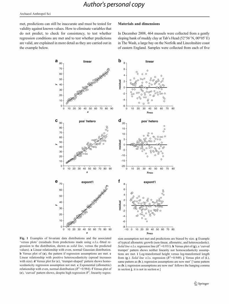
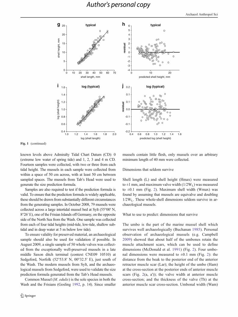
Fig. 1 Examples of bivariate data distributions and the associated‘versus plots’ (residuals from predictions made using o.l.s.-fitted re-gression to the distribution, shown as solid line, versus the predictedvalues). a Linear relationship with even, normal Gaussian distribution.b Versus plot of (a), the pattern if regression assumptions are met. cLinear relationship with positive heteroscedasticity (spread increaseswith size). d Versus plot for (c), ‘trumpet-shaped’ pattern shows homo-scedasticity regression assumption not met. e Exponential (allometric)relationship with even, normal distribution (R2=0.984). f Versus plot of(e), ‘curved’ pattern shows, despite high regression R2, linearity regres-

sion assumption not met and predictions are biased by size. g Exampleof typical allometric growth (non-linear, allometric, and heteroscedastic).Solid line o.l.s. regression line (R2=0.931). h Versus plot of (g), a ‘curvedtrumpet’ pattern shows neither linearity nor homoscedasticity assump-tions are met. i Log-transformed height versus log-transformed lengthfrom (g.). Solid line o.l.s. regression (R2=0.949). j Versus plot of (i.),same pattern as (b.); regression assumptions are now met’ [‘same patternas (b.); regression assumptions are now met’ follows the hanging commain section j, it is not in section e.]

Archaeol Anthropol Sci

Author's personal copy

known levels above Admiralty Tidal Chart Datum (CD): 0(extreme low water of spring tide) and 1, 2, 3 and 4 m CD.Fourteen samples were collected, with two or three from eachtidal height. The mussels in each sample were collected fromwithin a space of 50 cm across, with at least 50 cm betweensampled spaces. The mussels from Tab’s Head were used togenerate the size prediction formula.

Samples are also required to test if the prediction formula isvalid. To ensure that the prediction formula is widely applicable,these should be drawn from substantially different circumstancesfrom the generating samples. In October 2008, 79 mussels werecollected across a large intertidal mussel bed at Sylt (55°00′ N,8°26′ E), one of the Frisian Islands off Germany, on the oppositeside of the North Sea from the Wash. One sample was collectedfrom each of four tidal heights (mid-tide, low-tide, shallow sub-tidal and in deep water at 5 m below low tide).

To ensure validity for preserved material, an archaeologicalsample should also be used for validation if possible. InAugust 2009, a single sample of 50 whole valves was collect-ed from the exceptionally well-preserved mussels in a latemiddle Saxon ditch terminal (context CNE09 10510) atSedgeford, Norfolk (52°53.8′ N, 00°32.5′ E), just south ofthe Wash. The modern mussels from Sylt, and the archaeo-logical mussels from Sedgeford, were used to validate the sizeprediction formula generated from the Tab’s Head mussels.

Common Mussel (M. edulis) is the sole species in both theWash and the Frisians (Gosling 1992, p. 14). Since smaller

mussels contain little flesh, only mussels over an arbitraryminimum length of 40 mm were collected.

Dimensions that seldom survive

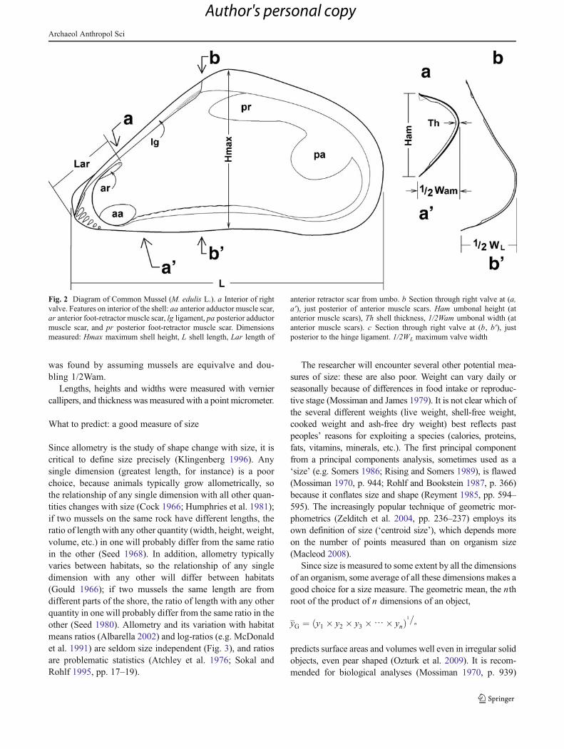
Shell length (L) and shell height (Hmax) were measuredto ±1 mm, and maximum valve width (1/2WL) was measuredto ±0.1 mm (Fig. 2). Maximum shell width (Wmax) wasfound by assuming that mussels are equivalve and doubling1/2WL. These whole-shell dimensions seldom survive in ar-chaeological mussels.

What to use to predict: dimensions that survive

The umbo is the part of the marine mussel shell whichsurvives well archaeologically (Buchanan 1985). Personalobservation of archaeological mussels (e.g. Campbell2009) showed that about half of the umbones retain themuscle attachment scars, which can be used to definedimensions (McDonald et al. 1991) (Fig. 2). Four umbo-nal dimensions were measured to ±0.1 mm (Fig. 2): thedistance from the beak to the posterior end of the anteriorretractor muscle scar (Lar); the height of the umbo (Ham)at the cross-section at the posterior ends of anterior musclescars (Fig. 2(a, a')); the valve width at anterior musclecross-section; and the thickness of the valve (Th) at theanterior muscle scar cross-section. Umbonal width (Wam)

0

5

10

15

20

25

0 10 20 30 40 50 60 70

shel

l hei

ght,

mm

shell length, mm

typical

-4

-3

-2

-1

0

1

2

3

4

5

6

0 10 20

resi

du

al

predicted shell height, mm

0.4

0.6

0.8

1.0

1.2

1.4

1.6

1.0 1.2 1.4 1.6 1.8 2.0

log

(she

ll he

ight

)

log (shell length)

log (typical)

-0.2

-0.1

-0.1

0.0

0.1

0.1

0.2

0.4 0.6 0.8 1.0 1.2 1.4 1.6

resi

du

al

predicted log (shell height)

typicalg h

i j log (typical)

Fig. 1 (continued)

Archaeol Anthropol Sci

Author's personal copy

was found by assuming mussels are equivalve and dou-bling 1/2Wam.

Lengths, heights and widths were measured with verniercallipers, and thickness was measured with a point micrometer.

What to predict: a good measure of size

Since allometry is the study of shape change with size, it iscritical to define size precisely (Klingenberg 1996). Anysingle dimension (greatest length, for instance) is a poorchoice, because animals typically grow allometrically, sothe relationship of any single dimension with all other quan-tities changes with size (Cock 1966; Humphries et al. 1981);if two mussels on the same rock have different lengths, theratio of length with any other quantity (width, height, weight,volume, etc.) in one will probably differ from the same ratioin the other (Seed 1968). In addition, allometry typicallyvaries between habitats, so the relationship of any singledimension with any other will differ between habitats(Gould 1966); if two mussels the same length are fromdifferent parts of the shore, the ratio of length with any otherquantity in one will probably differ from the same ratio in theother (Seed 1980). Allometry and its variation with habitatmeans ratios (Albarella 2002) and log-ratios (e.g. McDonaldet al. 1991) are seldom size independent (Fig. 3), and ratiosare problematic statistics (Atchley et al. 1976; Sokal andRohlf 1995, pp. 17–19).

The researcher will encounter several other potential mea-sures of size: these are also poor. Weight can vary daily orseasonally because of differences in food intake or reproduc-tive stage (Mossiman and James 1979). It is not clear which ofthe several different weights (live weight, shell-free weight,cooked weight and ash-free dry weight) best reflects pastpeoples’ reasons for exploiting a species (calories, proteins,fats, vitamins, minerals, etc.). The first principal componentfrom a principal components analysis, sometimes used as a‘size’ (e.g. Somers 1986; Rising and Somers 1989), is flawed(Mossiman 1970, p. 944; Rohlf and Bookstein 1987, p. 366)because it conflates size and shape (Reyment 1985, pp. 594–595). The increasingly popular technique of geometric mor-phometrics (Zelditch et al. 2004, pp. 236–237) employs itsown definition of size (‘centroid size’), which depends moreon the number of points measured than on organism size(Macleod 2008).

Since size is measured to some extent by all the dimensionsof an organism, some average of all these dimensions makes agood choice for a size measure. The geometric mean, the nthroot of the product of n dimensions of an object,

yG ¼ y1 � y2 � y3 �⋯� ynð Þ1=n

predicts surface areas and volumes well even in irregular solidobjects, even pear shaped (Ozturk et al. 2009). It is recom-mended for biological analyses (Mossiman 1970, p. 939)

Fig. 2 Diagram of Common Mussel (M. edulis L.). a Interior of rightvalve. Features on interior of the shell: aa anterior adductor muscle scar,ar anterior foot-retractor muscle scar, lg ligament, pa posterior adductormuscle scar, and pr posterior foot-retractor muscle scar. Dimensionsmeasured: Hmax maximum shell height, L shell length, Lar length of

anterior retractor scar from umbo. b Section through right valve at (a,a'), just posterior of anterior muscle scars. Ham umbonal height (atanterior muscle scars), Th shell thickness, 1/2Wam umbonal width (atanterior muscle scars). c Section through right valve at (b, b'), justposterior to the hinge ligament. 1/2WL maximum valve width

Archaeol Anthropol Sci

Author's personal copy

because it is the implicit size measure in allometry (Jolicouer1963, p. 497; Mossiman 1970, p. 932). Fa and Fa (2002)found the product of shell length, width and height (equal tothe cube of their geometric mean) estimated mollusc shellvolume well, even in irregular forms. Therefore, the geometricmean of the whole-shell dimensions (GMmax) was the shellsize calculated for all the mussels:

GMmax ¼ Lð Þ Hmaxð Þ Wmaxð Þ½ �1=3

It was this measure of shell size for which accurate pre-dictions were sought in archaeological mussels.

Generating the size prediction formula

Mussels grow with ‘simple’ allometry (Seed 1968), like mostmarine molluscs (e.g. Cabral 2006; Gaspar et al. 2002; Kempand Bertness 1984; Seed 1980). All dimensions were convertedto their common (base 10) logarithms, to make the simpleallometric relationships linear (Huxley 1932, p. 4). This log-transformation also reduces some biases common in biologicaldimensions (compare Fig. 1g with Fig. 1i) which reduce theaccurate use of regression techniques (Sokal and Rohlf 1995,p. 413; Klingenberg 1996).

To generate a shell size prediction formula, a multiple linearregression of the predictors (the log-transformed values ofumbonal dimensions) with log GMmax was carried out, usingo.l.s. fitting. This calculated the intercept (the value of log (A)for simple allometry), the slopes for each predictor (the valueof bi for each log (xi)) and their standard deviations, assumingthe spread around the fitted line is Gaussian normal (e.g.Draper and Smith 1981, pp. 24–28 and 94). The coefficientsof determination (R2) (Sokal and Rohlf 1995, p. 564) and forprediction (R2

PRED) (Montgomery et al. 2006, p. 142) werealso calculated. Coefficient values nearer to one (or 100 %)show a better quality of fit or capacity to predict, while avalue of zero shows no relationship (Draper and Smith1981, p. 206).

Regression was carried out with the General Regressionroutines in Version 16.1.1 of Minitab (©Minitab, Inc., 2010),and statistical tests were carried out with Minitab and withVersion 1.91 of the palaeontological statistical freeware, PAST(Hammer et al. 2001). Differences were considered statisticallysignificant if its probability of occurring (P) was <1 in 20(P<0.05).

Eliminating irrelevant predictors

Methods A form of backward elimination was employed todiscard predictors with no statistically significant relation-ship with log GMmax (Draper and Smith 1981, pp. 305–307). The variation in the predicted quantity (here, logGMmax) that was accounted for by including a predictorvariable in the regression (that predictor’s adjusted meansquare) was calculated. The variation in the predicted quan-tity not accounted for by the regression formula (theregression’s error mean square) was also calculated. Apredictor’s significance was determined by an F test ofits adjusted mean square with the regression error meansquare. The least significant of the non-significant pre-dictors was eliminated, and the regression was repeated,until all remaining predictor variables were significant.These calculations are complex, requiring computer soft-ware for most regressions (Draper and Smith 1981, pp.97–106) and are carried out and presented automaticallyby statistical software.

0.15

0.25

0.35

0.45

0 10 20 30 40 50 60 70

heig

ht /

leng

th

shell length, mm

a

b

0.10

0.15

0.20

0.25

0.30

0 10 20 30 40 50 60 70

log

(hei

ght)

/ lo

g (le

ngth

)

shell length, mmFig. 3 Ratios and log ratios for typical, allometric growth. Same data asfor Fig. 1g. a Height–length ratio versus shell length. b Log-height–log-length ratios versus shell length. Solid line o.l.s.-fitted regression line

Archaeol Anthropol Sci

Author's personal copy

Results The initial regression, using all possible predictors,showed that the relationships of log Th and log Lar with logGMmax were not significant. Removing the least significantpredictor, log Th (F[1, 459]=1.031; P=0.31) and repeating theregression showed that log Lar remained a poor predictor:its relationship with log GMmax was not significant(F[1, 460]=1.58; P=0.21). A further regression, without eitherlog Th or log Lar, showed significant relationships with logGMmax by both log Ham (F[1, 461]=223.5;P=1.8×10

-41) andlog Wam (F[1, 461]=598.3; P=2.6×10

−85). When predictingmussel size, only Ham and Wam need to be measured.

The regression based on significant predictors generated aformula:

log GMmax ¼ 0:4671þ 0:3884 log Ham

þ 0:4719 log Wam

where quality of fit was good (R2=86.9 %) and quality ofprediction was also good (R2

PRED=86.8 %). This formulawas therefore tested for consistency.

Consistency between tidal heights

Methods Mussel shell allometry is known to vary with tidalheight (Buschbaum and Saier 2001; Seed 1968). To deter-mine which of the significant predictors were also consistentpredictors of shell size for all tidal heights, the regressionwas categorised by tidal height (mCD), and the differences infitted slope between categories (the predictor*mCD interac-tions) were tested for significance using F test.

Results The fitted formula using Ham and Wam was consis-tent for all tidal heights. A regression using tidal height(mCD) as a category showed no evidence that the relation-ship of either log Ham or log Wam with log GMmax differedbetween tidal heights: the predictor*mCD interactions werenot significant. Removing the least significant of these inter-actions, that with log Ham (F[1, 449]=0.050; P=0.995), andrepeating the regression showed no evidence that the rela-tionship of log Wam with log GMmax differed between tidalheights: the log Wam*mCD interaction was still not signif-icant (F[4, 453]=1.04; P=0.39).

Consistency between mussel patches

Methods Mussels have a complex, patchy distribution (Seed1969; Tsuchiya and Nishihira 1986): patches differ in musselsize and age distributions (O’Connor and Crowe 2007),encrusting organisms (Buschbaum and Saier 2001), packingdensity and patch age (Bell and Gosline 1997). Therefore, itwas likely that shell allometry varied between shore positions.

To determine which of the significant predictors were alsoconsistent predictors of size for all patches, the regression wascategorised by sample number, and the differences in fittedslope between categories (the predictor*sample number inter-actions) were tested for significance using F tests.

Results The fitted formula using Ham and Wam was consis-tent for all patches. Using sample number as a categoryshowed no evidence that the relationship of either log Hamor log Wam with log GMmax differed with shore position:the variable*sample interactions were not significant.Removing the least significant interaction, that with logHam (F[13, 422]=0.96; P=0.49) and repeating the regressionshowed no evidence that the relationship of log Wam with logGMmax differed between positions: the log Wam*sampleinteraction was not significant (F[13, 435]=1.55; P=0.096).

Satisfaction of regression conditions

Methods Three conditions must hold for linear regression tofit a good prediction line (Sokal and Rohlf 1995, pp. 456–457):linearity (the data lie along a line with no curvature), homo-scedasticity (the spread of the data either side of the line is thesame everywhere along its length), and error-normality (thespread of the data either side of the line is Gaussian normal).

The significant and consistent regression-fitted predictionformula was assessed for linearity and homoscedasticity bycomparing a plot of the residuals (the predicted value minusthe true value, for each individual in a sample) against thepredicted values (a ‘versus plot’) to examples in statistics textsshowing non-linearity, non-normality and heteroscedasticity(e.g. Fig. 1; Draper and Smith 1981, pp. 145–149), whichusually reveals any pattern serious enough to invalidate theformula (Draper and Smith 1981, p. 150). Normality wasassessed by observing whether a histogram of the residualsdeviated seriously from the characteristic Gaussian normal‘bell-shape’ (Sokal and Rohlf 1995, p. 101), and whether anormal quantile plot of the residuals deviated seriously from astraight line (Sokal and Rohlf 1995, p. 118). It was also testedstatistically with the Kolmogorov–Smirnov normality test(Sokal and Rohlf 1995, pp. 708–711).

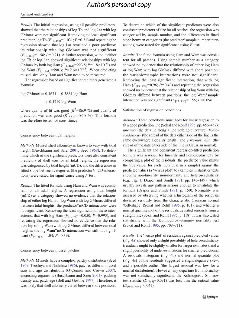
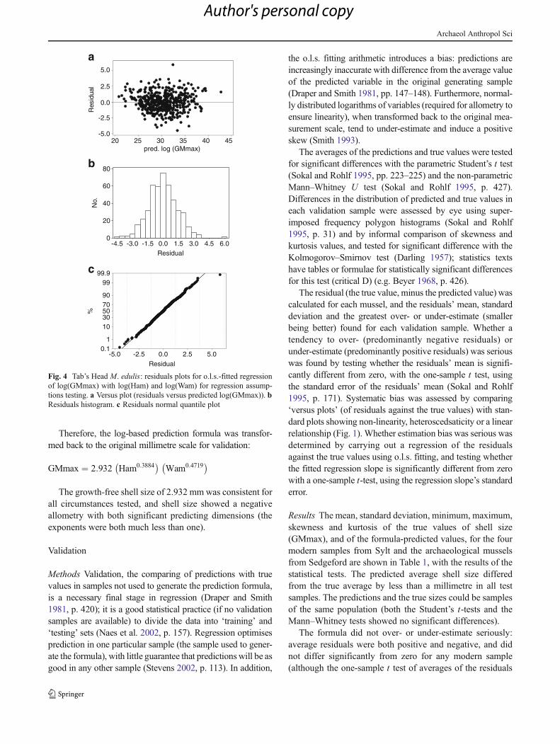
Results The ‘versus plot’ of residuals against predicted values(Fig. 4a) showed only a slight possibility of heteroscedasticity(residuals might be slightly smaller for larger estimates), and aslight possibility of under-estimations for smaller predictions.A residuals histogram (Fig. 4b) and normal quantile plot(Fig. 4c) of the residuals suggested a slight negative skew,and a possible outlier (the largest residual was low for anormal distribution). However, any departure from normalitywas not statistically significant: the Kolmogorov–Smirnovtest statistic (D[464]=0.031) was less than the critical value(D[0.05, 464]=0.041).

Archaeol Anthropol Sci

Author's personal copy

Therefore, the log-based prediction formula was transfor-med back to the original millimetre scale for validation:

GMmax ¼ 2:932 Ham0:3884� �

Wam0:4719� �

The growth-free shell size of 2.932 mm was consistent forall circumstances tested, and shell size showed a negativeallometry with both significant predicting dimensions (theexponents were both much less than one).

Validation

Methods Validation, the comparing of predictions with truevalues in samples not used to generate the prediction formula,is a necessary final stage in regression (Draper and Smith1981, p. 420); it is a good statistical practice (if no validationsamples are available) to divide the data into ‘training’ and‘testing’ sets (Naes et al. 2002, p. 157). Regression optimisesprediction in one particular sample (the sample used to gener-ate the formula), with little guarantee that predictionswill be asgood in any other sample (Stevens 2002, p. 113). In addition,

the o.l.s. fitting arithmetic introduces a bias: predictions areincreasingly inaccurate with difference from the average valueof the predicted variable in the original generating sample(Draper and Smith 1981, pp. 147–148). Furthermore, normal-ly distributed logarithms of variables (required for allometry toensure linearity), when transformed back to the original mea-surement scale, tend to under-estimate and induce a positiveskew (Smith 1993).

The averages of the predictions and true values were testedfor significant differences with the parametric Student’s t test(Sokal and Rohlf 1995, pp. 223–225) and the non-parametricMann–Whitney U test (Sokal and Rohlf 1995, p. 427).Differences in the distribution of predicted and true values ineach validation sample were assessed by eye using super-imposed frequency polygon histograms (Sokal and Rohlf1995, p. 31) and by informal comparison of skewness andkurtosis values, and tested for significant difference with theKolmogorov–Smirnov test (Darling 1957); statistics textshave tables or formulae for statistically significant differencesfor this test (critical D) (e.g. Beyer 1968, p. 426).

The residual (the true value, minus the predicted value) wascalculated for each mussel, and the residuals’ mean, standarddeviation and the greatest over- or under-estimate (smallerbeing better) found for each validation sample. Whether atendency to over- (predominantly negative residuals) orunder-estimate (predominantly positive residuals) was seriouswas found by testing whether the residuals’ mean is signifi-cantly different from zero, with the one-sample t test, usingthe standard error of the residuals’ mean (Sokal and Rohlf1995, p. 171). Systematic bias was assessed by comparing‘versus plots’ (of residuals against the true values) with stan-dard plots showing non-linearity, heteroscedsaticity or a linearrelationship (Fig. 1). Whether estimation bias was serious wasdetermined by carrying out a regression of the residualsagainst the true values using o.l.s. fitting, and testing whetherthe fitted regression slope is significantly different from zerowith a one-sample t-test, using the regression slope’s standarderror.

Results The mean, standard deviation, minimum, maximum,skewness and kurtosis of the true values of shell size(GMmax), and of the formula-predicted values, for the fourmodern samples from Sylt and the archaeological musselsfrom Sedgeford are shown in Table 1, with the results of thestatistical tests. The predicted average shell size differedfrom the true average by less than a millimetre in all testsamples. The predictions and the true sizes could be samplesof the same population (both the Student’s t-tests and theMann–Whitney tests showed no significant differences).

The formula did not over- or under-estimate seriously:average residuals were both positive and negative, and didnot differ significantly from zero for any modern sample(although the one-sample t test of averages of the residuals

454035302520

5.0

2.5

0.0

-2.5

-5.0

pred. log (GMmax)

Res

idua

l

6.04.53.01.50.0-1.5-3.0-4.5

80

60

40

20

0

Residual

No.

5.02.50.0-2.5-5.0

99.999

9070503010

10.1

Residual

%

a

b

c

Fig. 4 Tab’s Head M. edulis: residuals plots for o.l.s.-fitted regressionof log(GMmax) with log(Ham) and log(Wam) for regression assump-tions testing. a Versus plot (residuals versus predicted log(GMmax)). bResiduals histogram. c Residuals normal quantile plot

Archaeol Anthropol Sci

Author's personal copy

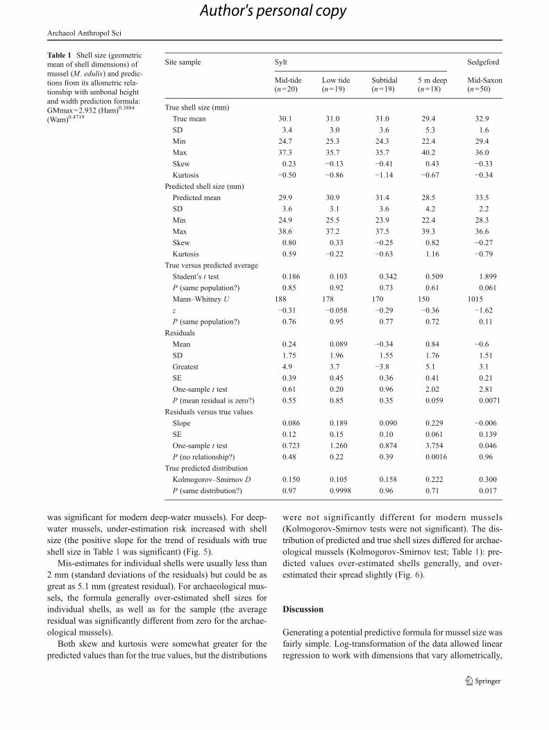
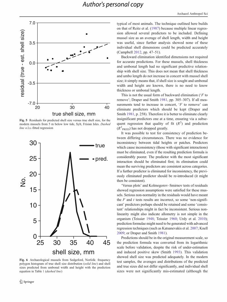
was significant for modern deep-water mussels). For deep-water mussels, under-estimation risk increased with shellsize (the positive slope for the trend of residuals with trueshell size in Table 1 was significant) (Fig. 5).

Mis-estimates for individual shells were usually less than2 mm (standard deviations of the residuals) but could be asgreat as 5.1 mm (greatest residual). For archaeological mus-sels, the formula generally over-estimated shell sizes forindividual shells, as well as for the sample (the averageresidual was significantly different from zero for the archae-ological mussels).

Both skew and kurtosis were somewhat greater for thepredicted values than for the true values, but the distributions

were not significantly different for modern mussels(Kolmogorov-Smirnov tests were not significant). The dis-tribution of predicted and true shell sizes differed for archae-ological mussels (Kolmogorov-Smirnov test; Table 1): pre-dicted values over-estimated shells generally, and over-estimated their spread slightly (Fig. 6).

Discussion

Generating a potential predictive formula for mussel size wasfairly simple. Log-transformation of the data allowed linearregression to work with dimensions that vary allometrically,

Table 1 Shell size (geometricmean of shell dimensions) ofmussel (M. edulis) and predic-tions from its allometric rela-tionship with umbonal heightand width prediction formula:GMmax=2.932 (Ham)0.3884

(Wam)0.4719

Site sample Sylt Sedgeford

Mid-tide(n=20)

Low tide(n=19)

Subtidal(n=19)

5 m deep(n=18)

Mid-Saxon(n=50)

True shell size (mm)

True mean 30.1 31.0 31.0 29.4 32.9

SD 3.4 3.0 3.6 5.3 1.6

Min 24.7 25.3 24.3 22.4 29.4

Max 37.3 35.7 35.7 40.2 36.0

Skew 0.23 −0.13 −0.41 0.43 −0.33

Kurtosis −0.50 −0.86 −1.14 −0.67 −0.34

Predicted shell size (mm)

Predicted mean 29.9 30.9 31.4 28.5 33.5

SD 3.6 3.1 3.6 4.2 2.2

Min 24.9 25.5 23.9 22.4 28.3

Max 38.6 37.2 37.5 39.3 36.6

Skew 0.80 0.33 −0.25 0.82 −0.27

Kurtosis 0.59 −0.22 −0.63 1.16 −0.79

True versus predicted average

Student’s t test 0.186 0.103 0.342 0.509 1.899

P (same population?) 0.85 0.92 0.73 0.61 0.061

Mann–Whitney U 188 178 170 150 1015

z −0.31 −0.058 −0.29 −0.36 −1.62

P (same population?) 0.76 0.95 0.77 0.72 0.11

Residuals

Mean 0.24 0.089 −0.34 0.84 −0.6

SD 1.75 1.96 1.55 1.76 1.51

Greatest 4.9 3.7 −3.8 5.1 3.1

SE 0.39 0.45 0.36 0.41 0.21

One-sample t test 0.61 0.20 0.96 2.02 2.81

P (mean residual is zero?) 0.55 0.85 0.35 0.059 0.0071

Residuals versus true values

Slope 0.086 0.189 0.090 0.229 −0.006

SE 0.12 0.15 0.10 0.061 0.139

One-sample t test 0.723 1.260 0.874 3.754 0.046

P (no relationship?) 0.48 0.22 0.39 0.0016 0.96

True predicted distribution

Kolmogorov–Smirnov D 0.150 0.105 0.158 0.222 0.300

P (same distribution?) 0.97 0.9998 0.96 0.71 0.017

Archaeol Anthropol Sci

Author's personal copy

typical of most animals. The technique outlined here buildson that of Reitz et al. (1987) because multiple linear regres-sion allowed several predictors to be included. Definingmussel size as an average of shell length, width and heightwas useful, since further analysis showed none of theseindividual shell dimensions could be predicted accurately(Campbell 2012, pp. 47–51).

Backward elimination identified dimensions not requiredfor accurate predictions. For these mussels, shell thicknessand umbonal length had no significant predictive relation-ship with shell size. This does not mean that shell thicknessand umbo length do not increase in concert with mussel shellsize; it simply means that, if shell size is sought and umbonalwidth and height are known, there is no need to knowthickness or umbonal length.

This is not the usual form of backward elimination (‘F toremove’; Draper and Smith 1981, pp. 305–307). If all mea-surements tend to increase in concert, ‘F to remove’ caneliminate predictors which should be kept (Draper andSmith 1981, p. 258). Therefore it is better to eliminate clearlyinsignificant predictors one at a time, ensuring via a subse-quent regression that quality of fit (R2) and prediction(R2

PRED) has not dropped greatly.It was possible to test for consistency of prediction be-

tween differing circumstances. There was no evidence forinconsistency between tidal heights or patches. Predictorswhich cause inconsistency (those with significant interactions)must be eliminated, even if the resulting prediction formula isconsiderably poorer. The predictor with the most significantinteraction should be eliminated first; its elimination couldmean the surviving predictors are consistent across categories.If a further predictor is eliminated for inconsistency, the previ-ously eliminated predictor should be re-introduced (it mightthen be consistent).

‘Versus plots’ and Kolmogorov–Smirnov tests of residualsshowed regression assumptions were satisfied for these mus-sels. Serious non-normality in the residuals would have meantthe F and t tests results are incorrect, so some ‘non-signifi-cant’ predictors perhaps should be retained and some ‘consis-tent’ relationships might in fact be inconsistent. Serious non-linearity might also indicate allometry is not simple in theorganism (Teissier 1948; Teissier 1960; Urdy et al. 2010);prediction formulaemight need to be generated with advancedregression techniques (such as Katsanevakis et al. 2007; Knell2009; or Draper and Smith 1981).

Predictions should be in the original measurement scale, sothe prediction formula was converted from its logarithmicscale before validation, despite the risk of under-estimationand induced positive skew (Smith 1993). This validationshowed shell size was predicted adequately. In the moderntest samples, the averages and distributions of the predictedand true sizes did not differ significantly, and individual shellsizes were not significantly mis-estimated (although the

0

5

10

15

20

25

30

25 30 35 40 45

No.

shell size, mm

true

pred.

Fig. 6 Archaeological mussels from Sedgeford, Norfolk: frequencypolygon histogram of true shell size distribution (solid line) and shellsizes predicted from umbonal width and height with the predictionequation in Table 1 (dashed line)

-7.0

-3.5

0.0

3.5

7.0

20 30 40

resi

dual

(tr

ue -

est.

shel

l siz

e)

true shell size, mmFig. 5 Residuals for predicted shell size versus true shell size, for themodern mussels from 5 m below low tide, Sylt, Frisian Isles. Dashedline o.l.s.-fitted regression

Archaeol Anthropol Sci

Author's personal copy

deeper-water mussels tended to be slightly under-estimated,increasingly so for larger shells). Prediction was somewhatpoorer for the archaeological mussels: size was over-estimatedslightly but significantly for individual shells, and this sys-tematic over-estimation was enough to give the predictedvalues a significantly different distribution. The differencebetween true and predicted shell sizes for archaeologicalmussels was shown elsewhere to be due to a difference inumbonal height-width allometry between modern and archae-ological mussels (Campbell 2012, pp. 52–57). This differencemight be due to taphonomic deformation (which thereforeshould be considered a potential source of error in otherzooarchaeological predictions). It might also be due to thearchaeological mussels being M . galloprovincialis , M .trossulus, or a hybrid withM. edulis. If these types ofmussels,and deeper-water M. edulis, are likely to form part of anarchaeological mussel assemblage, size predictions with thisformula should be used with caution. Nevertheless, predictedsizes usually differed from true sizes by less than 2 mm and by5.1 mm at worst.

Carrying out the type of regression outlined here would beuseful for other archaeological shellfish. The ‘umbo-outline’method for determining archaeological sizes for the Pacificmussel M. californianus (White 1989), the basis for manyarchaeological inferences (e.g. Jones and Richman 1995;Whitaker 2008), is prone to error in practice (Bell 2009, p.81), probably because the size-shape relationship in thismussel varies between habitats (Blythe and Lea 2008;Robles et al. 1990). Prismatic band width, used to predictsize in the mussel Choromytilus meridionalis (Buchanan1985), was neither tested for consistency from various hab-itats, nor validated; a trial with some of the Tab’s Headmussels showed prismatic band width was not a useful sizepredictor for M. edulis (Campbell 2012, pp. 97–98). Linearregressions on dimensions without log transformation(Faulkner 2010; Hall 1980; Jerardino and Navarro 2008;Jerardino et al. 1992; Peacock 2000; Peacock and Seltzer2008; Randklev et al. 2009) usually give biased predictions(Reitz and Wing 2008, p. 238), because they are unlikely tohave met the inherent conditions of regression (compareJerardino et al. 2001 Figs. 4 and 5 versus plots with Fig. 1here). Regression without log-transformation also generallyproduce either positive intercepts (implying the predicteddimension exists before the rest of the animal) or negativeintercepts (the rest of the animal existed without that dimen-sion). Quadratic and cubic regressions (e.g. Yamazaki andOda 2009) perform predictions with a single chosen dimen-sion, without checking whether prediction is betterperformed by another dimension or a combination of dimen-sions (and if so, which dimensions should be included).

The regression technique outlined might be useful for otherzooarchaeologists. Sizes or weights of hunted or domesticatedanimals are often required (Albarella 2002; Broughton et al.

2011; Orchard 2005), and many dimensions might be relevant(e.g. von den Dreisch 1976); it would be helpful to knowwhichdimensions are relevant for particular predictions, and whichare not. Also, many terrestrial mammals grow allometrically(Alberdi et al. 1995; Cock 1966; Hofman 1988; Kidwell et al.1952; Lumer 1940; McMahon 1975; Weston 2003), and thephysics of bone means almost all do (Garcia and da Silva2006), so allometry is generally assumed in palaeontology(LaBarbera 1989; Damuth and McFadden 1990). Therefore, itis likely that log-transformation of zooarchaeological measure-ments will be required generally for regression conditions to besatisfied.

Geometric morphometrics (e.g. Drake and Klingenberg2010) and Fourier analysis (e.g. Dommergues et al. 2003;Roy et al. 2001) are increasingly popular because they candescribe shape and its difference between samples clearly.However, they do not examine the chief cause of variation inshape, its change with size. The main practical use of thesetechniques is elucidating which dimensions should beanalysed by regression (Cadrin 2000; Eisenmann andBaylac 2000).

Conclusions

The technique outlined above for generating a predictionformula, eliminating irrelevant predictors and testing it forconsistency, for meeting regression assumptions and for va-lidity should be useful for refining the results of predictions.Formulae can be generated and tested easily with standardcommercial statistical software.

Adequate predictions were made for one of the most poorlypreserved zooarchaeological remains. Validation showed thepredictions accurately reproduced both mean shell size andsize distribution in modern mussels (with a slight tendency tounder-estimate the sizes of larger sub-tidal mussels), and themean shell size in archaeological mussels (with a significantlydifferent distribution). Differences between samples of ar-chaeological M. edulis should be found reliably with thepredictions, but inferences relying on distributions withinsamples will be less reliable. Further research on the causesfor this bias in predicting distribution, and trying the techniquewith other archaeological shellfish (and probably archaeolog-ically important vertebrates), would be worthwhile.

Acknowledgements Ron Jessop and Jason Byrne at the EasternInshore Fisheries and Conservation Authority gave essential assistanceat Tab’s Head. Gary Rossin at the Sedgeford Historical and Archaeo-logical Research Project provided the archaeological mussels, andChristian Buschbaum at the Alfred-Wegener-Institut fűr Polar- undMeeresforschung Wattenmeerstation provided the modern musselsfrom Sylt. James Gallagher, Martin Bell and Rob Hosfield at theUniversity of Reading guided the research. Errors and omissions remainthe sole responsibility of the author.

Archaeol Anthropol Sci

Author's personal copy

References

Albarella U (2002) Size matters: how and why biometry is still impor-tant in zooarchaeology. In: Dobney K, O’Connor T (eds) Bonesand the man: studies in honour of Don Brothwell. Oxbow Books,Oxford, pp 51–66

Alberdi MT, Prado JL, Ortiz-Jaureguizar E (1995) Patterns of body sizechanges in fossil and living Equini (Perissodactyla). Biol J LinnSoc 54:349–370

Alvarez-Fernàndez E, Chauvin A, Cubas M, Arias P, Ontaňón R (2011)Mollusc shell sizes in archaeological contexts in northern Spain(13,200 to 2600 cal BC): new data from La Garma A and LosGitanos (Cantabria). Archaeometry 53:963–985

Antczak A, Cipriani R (eds) (2008) Early Human Impact onMegamolluscs. British Archaeological Reports (International Series)1865, Oxford

Atchley WR, Gaskins CT, Anderson D (1976) Statistical properties ofratios I: empirical results. Syst Zool 25:137–148

Bailey GN, Craighead AS (2003) Late Pleistocene and Holocene coast-al palaeoeconomies: a reconsideration of the molluscan evidencefrom northern Spain. Geoarchaeol Int J 18(2):175–204

Bailey GN, Milner N (2008) Molluscan archives from European pre-history. In: Antczak A, Cipriani R (eds), Early Human Impact onMegamolluscs. British Archaeological Reports (InternationalSeries) 1865, Oxford, pp 111–134

Balbo A, Madella M, Briz Godino I, Álvarez M (2011) Shell middenresearch: an interdisciplinary agenda for the Quaternary and socialsciences. Quat Int 239:147–152

Bell, AM (2009) On the Validity of Archaeological Shellfish Metrics inCoastal California. Unpublished M.A. dissertation, AnthropologyDepartment, California State University, Chico.

Bell EC, Gosline JM (1997) Strategies for life in flow: tenacity, mor-phometry and probability of dislodgement of twoMytilus species.Mar Ecol Prog Ser 159:197–208

Beyer WH (1968) Handbook of tables for probability and statistics.Chemical Rubber Company, Cleveland

Blythe JN, Lea DW (2008) Functions of height and width dimensions inthe intertidal musselMytilus californianus. J Shellfish Res 27(2):385–392

Broughton JM, Cannon MD, Bayham FE, Byres DA (2011) Prey bodysize and ranking in zooarchaeology: theory, empirical evidence, andapplications from the northern Great Basin. Am Antiq 76(3):403–428

Brown K, Fa DA, Finlayson G, Finlayson C (2011) Small game andmarine resource exploitation by Neanderthals: the evidence fromGibraltar. In: Bicho NF, Haws JA, Davis LG (eds) Trekking theshore: changing coastlines and the antiquity of coastal settlement.Springer, Dordrecht, pp. 247–272

Buchanan WF (1985) Middens and mussels: an archaeological enquiry.S Afr J Sci 81:15–16

Buschbaum C, Saier B (2001) Growth of the musselMytilus edulis L. inthe Wadden Sea affected by tidal emergence and barnacle epibionts.J Sea Res 45:27–36

Cabral JP (2006) Shape and growth in European Atlantic Patellalimpets (Gastropoda, Mollusca): ecological implications for sur-vival. Web Ecol 7:11–21

Cadrin SX (2000) Advances in morphometric identification of fisherystocks. Rev Fish Biol Fish 10:91–112

Campbell GE (2007) Appendix G: The marine molluscs. In: Galliou P,Cunliffe B (eds), Les Fouilles du Yaudet en Ploulec’h, Cotesd’Armor 3. http://www.arch.ox.ac.uk/research/research_projects/le_yaudet/appendices

Campbell GE (2008) Beyond means to meaning: using distributions ofshell shapes to reconstruct past collecting strategies. EnvironArchaeol 13(2):111–121

Campbell GE (2009) Southampton French Quarter 1382 Specialist ReportDownload E3: Marine Shell. In Brown R (ed), Southampton FrenchQuarter 1382 Specialist Report Downloads. Oxford ArchaeologyOALibrary EPrints, Oxford. http://library.thehumanjourney.net/42/1/SOU_1382_Specialist_report_download_E3.pdf

Campbell GE (2012) The archaeological potential of fragmentary re-mains of the Common Mussel, Mytilus edulis (L.). UnpublishedM.A. dissertation, Archaeology Department, University of Reading,Reading

Cheng C-L, van Ness JW (1999) Statistical regression with measurementerror. Arnold, London

Claasen C (1998) Shells. Cambridge Manuals in Archaeology.Cambridge University Press, Cambridge

Cock AG (1966) Genetical aspects of metrical growth and form inanimals. Quart Rev Biol 41:131–190

Damuth D, McFadden BJ (1990) Body size in mammalian paleobiolo-gy: estimation and biological implications. Cambridge UniversityPress, Cambridge

Darling DA (1957) The Kolmogorov–Smirnov, Cramér–von Misestests. Ann Math Stat 28(4):823–838

Dommergues E, Dommergures J-L, Magniez F, Neige P, Verrecchia EP(2003) Geometric measurement analysis versus Fourier series anal-ysis for shape characterization using the gastropod shell (Trivia) asan example. Math Geol 35:887–894

Drake AG, Klingenberg CP (2010) Large-scale diversification of skullshape in domestic dogs: disparity andmodularity. AmNat 175:289–301

Draper NR, Smith H (1981) Applied regression analysis. Wiley,Chichester

Eisenmann V, Baylac M (2000) Extant and fossil Equus (Mammalia,Perissodactyla) skulls: a morphometric definition of the subgenusEquus. Zool Scripta 29(2):89–100

Fa DA (2008) Effects of tidal amplitude on intertidal resource avail-ability and dispersal pressure in prehistoric coastal populations:the Mediterranean–Atlantic transition. Quat Sci Rev 27:2194–2209

Fa DA, Fa JE (2002) Species diversity, abundance and body size inrocky-shore Mollusca: a twist in Siemann, Tilman and Haarstad’sparabola? J Molluscan Stud 68:95–100

Faulkner P (2010) Morphometric and taphonomic analysis of granularark (Anadara granosa) dominated shell deposits of BlueMud Bay,northern Australia. J Archaeol Sci 37:1942–1952

Ford PJ (1989) Molluscan assemblages from archaeological deposits.Geoarchaeol Int J 4:157–173

Fuller WA (1987) Measurement error models. Wiley, ChichesterGarcia GJM, da Silva JKL (2006) Interspecific allometry of bone

dimensions: a review of the theoretical models. Phys Life Rev3:188–209

Gardner JPA (2004) A historical perspective on the genus Mytilus(Bivalvia: Mollusca) in New Zealand: multivariate morphometricanalyses of fossil, midden and contemporary blue mussels. Biol JLinn Soc 82:329–344

Gaspar MB, Santos MN, Vasconcelos P, Montiero CC (2002) Shellmorphometric relationships of the most common bivalve species(Mollusca: Bivalvia) of the Algarve coast (southern Portugal).Hydrobiologia 477:73–80

Gayon J (2000) History of the concept of allometry. AmZool 40:748–758Gosling E (1992) Systematics and geographic distribution of Mytilus.

In: Gosling E (ed) The mussel Mytilus: ecology, physiology,genetics and culture. Elsevier, Amsterdam, pp 1–20

Gould SJ (1966) Allometry and size in ontogeny and phylogeny. BiolRev 41:587–640

Gutiérrez-Zugasti I, Andersen SH, Araújo AC, Dupont C, Milner N,Monge-Soares AM (2011) Shell midden research in AtlanticEurope: state of the art, research problems and perspectives forthe future. Quat Int 239:70–85

Archaeol Anthropol Sci

Author's personal copy

Hall M (1980) A method for obtaining metrical data from fragmentarymolluscan material found at archaeological sites. S Afr J Sci76:280–281

Hamilton DJ (1992) A method for reconstruction of zebra mussel(Dreissena polymorpha) length from shell fragments. Can J Zool70:2486–2490

Hammer Ø, Harper DAT, Ryan PD (2001) PAST: paleontologicalstatistics software package for education and analysis. PalaeonElectron 4(1)

Hofman MA (1988) Allometric scaling in palaeontology: a criticalsurvey. Hum Evol 3(3):177–188

Hollander J, Adams DC, Johannesson K (2006) Evolution of adaptationthrough allometric shifts in a marine snail. Evolution 60:2490–2497

Humphries JM, Bookstein FL, Chernoff B, Smith GR, Elder RL, PossSG (1981) Multivariate discrimination by shape in relation to size.Syst Biol 30(3):291–308

Huxley JS (1932) Problems of relative growth. Methuen, LondonInnes DJ, Bates JA (1999) Morphological variation ofMytilus edulis and

Mytilus trossulus in eastern Newfoundland. Mar Biol 133:691–699Jerardino A (2010) Prehistoric exploitation of marine resources in

southern Africa with particular references to shellfish gathering:opportunities and continuities. Pyrenae 41(1):7–52

Jerardino A, Navarro R (2008) Shell morphometry of seven limpetspecies from coastal shell middens in southern Africa. JArchaeol Sci 35:1023–1029

Jerardino A, Castilla JC, Ramirez JM, Hermosilla N (1992) Earlycoastal subsistence in central Chile: a systematic study of themarine invertebrate fauna from the site of Curaumilla-1. Lat AmAntiq 3:43–62

Jerardino A, Navarro R, Nilssen P (2001) Cape rock lobster (Jasuslalandii) exploitation in the past: estimating carapace length frommandible sizes. S Afr J Sci 97:1–4

Jerardino A, Branch GM, Navarro R (2008) Human impacts onprecolonial West Coast marine environments of South Africa. In:Erlandson JM, Rick TC (eds) Human impacts on marine environ-ments: a global perspective. University of California Press, Berkeley,pp 279–296

Jolicouer P (1963) Note: the multivariate generalization of the allometryequation. Biometrics 19(3):497–499

Jones TL, Richman JR (1995) On mussels: Mytilus californianus as aprehistoric resource. N Am Archaeol 16(1):33–58

Katsanevakis S, Thessalou-Legaki M, Karlou-Riga C, Lefkaditou E,Dimitriou E, Verripoulos G (2007) Information-theory approach toallometric growth of marine organisms. Mar Biol 151:949–959

Kemp P, Bertness MD (1984) Snail shape and growth rates: evidencefor plastic shell allometry in Littorina littorea. Proc Natl Acad Sci81:811–803

Kidwell JF, Gregory PW, Guilbert HR (1952) A genetic investigation ofallometric growth in Hereford cattle. Genetics 37:158–174

Klingenberg CP (1996) Multivariate allometry. In: Marcus LF, Corti M,Loy A, Naylor GJP, Slice DE (eds) Advances in morphometrics.Plenum, New York, pp 23–49

Knell RJ (2009) On the analysis of non-linear allometries. Ecol Entomol34:1–11

LaBarbera M (1989) Analyzing body size as a factor in ecology andevolution. Annu Rev Ecol Syst 20:97–117

Lappalainen A, Westerbom M, Heikinkeimo O (2005) Roach (Rutilusrutilus) as an important predator on blue mussel (Mytilus edulis)populations in a brackish water environment, the northern BalticSea. Mar Biol 147:323–330

Light J (2005) Marine mussel shells—wear is the evidence? In: Bar-Yosef Mayer D (ed) Archaeomalacology: molluscs in former en-vironments of human behaviour. Oxbow, Oxford, pp 56–62

Lumer H (1940) Evolutionary allometry in the skeleton of the domes-ticated dog. Am Nat 74:439–467

MacLeod N (2008) Distances, landmarks and allometry. Palaeo-math101 (Palaeontological Association Newsletter 69). Available fromhttp://www.palass.org/modules.php?name=palaeo_mathandpage=21. Accessed 05 Jan 2011

Marean CW, Bar-Matthews M, Bernatchez J, Fisher JE, Goldberg P,Herries AIR, Jacobs Z, Jerardino A, Karkanas P, Minichillo T,Nilssen PJ, Thompson E, Watts I, Williams HM (2007) Earlyhuman use of marine resources and pigment in South Africa duringthe Middle Pleistocene. Nature 449:905–908

McDonald JH, Seed R, Koehn RK (1991) Allozymes and morphomet-ric characters of three species of Mytilus in the Northern andSouthern Hemispheres. Mar Biol 111:323–333

McMahon TA (1975) Allometry and biomechanics: limb bones in adultungulates. Am Nat 109:547–563

Meadow RH (1999) The use of size index scaling techniques for researchon archaeozoological collections from the Middle East. In: BeckerC, Manhart H, Peters J, Schibler J (eds) Historia Animalium exOssibus: Beiträge zur Paläoanatomie, Archäologie, Ägyptologie,Ethnologie und Geschicte der Tiermedizin (Festschrift für Angelavon den Driesch). Verlag Marie Leidorf, Rahden, pp 285–300

Montgomery DC, Peck EA, Vining GG (2006) Introduction to linearregression analysis. Wiley, Chichester

Mossiman JE (1970) Size allometry, size and shape variables withcharacterizations of the lognormal and generalized gamma distri-butions. J Am Stat Assoc 65:930–945

Mossiman JE, James FC (1979) New statistical methods for allometry,with application to Florida red-winged blackbirds. Evolution33(1):444–459

Naes T, Isaksson T, Fearn T, Davies T (2002) A user-friendly guide tomultivariate calibration and classification. NIR Publications,Chichester

Noddle BA (1973) Determination of the bodyweights of cattle from bonemeasurements. In: Matolcsi, J, (ed), Domestikationsforschung undGeschichte der Haustiere, Budapest, pp. 377–389

O’Connor NE, Crowe TP (2007) Biodiversity among mussels: separat-ing the influence of sizes of mussels from the ages of patches. JMar Biol Assoc U K 87:551–557

Orchard TJ (2005) The use of statistical size estimations in minimumnumber calculations. Int J Osteoarchaeol 15(5):351–359

Ozturk I, Ercisli S, Kalkan F, Demier B (2009) Some chemical andphysico-mechanical properties of pear cultivars. Afr J Biotech8(4):687–693

Peacock E (2000) Assessing bias in archaeological shell assemblages. JField Archaeol 27(2):183–196

Peacock E, Seltzer JL (2008) A comparison of multi-proxy data sets forpalaeoenvironmental conditions from freshwater bivalve (Unionid)shell. J Archaeol Sci 35(9):2557–2565

Randklev CR, Wolverton S, Kennedy JH (2009) A biometric techniquefor assessing prehistoric freshwater mussel population dynamics(Family: Uniondae) in north Texas. J Archaeol Sci 36(2):205–213

Reitz EJ, Wing ES (2008) Zooarchaeology. Cambridge UniversityPress, Cambridge, Cambridge Manuals in Archaeology

Reitz EJ, Quitmyer IR, Hale HS, Scudder SJ, Wing ES (1987) Applicationof allometry to zooarchaeology. Am Antiquity 52(2):304–317

Reyment RA (1985) Multivariate morphometrics and analysis of shape.Math Geol 17:591–609

Rising JD, Somers KM (1989) The measurement of overall body size inbirds. Auk 106:666–674

Robles C, Sweetnam D, Eminike J (1990) Lobster predation on mus-sels: shore-level differences in prey vulnerability and predatorpreference. Ecology 71(4):1564–1577

Rohlf FJ, Bookstein FL (1987) A comment on shearing as a method for‘size correction’. Syst Zool 36:356–367

Roy K, Balch DP, Hellberg ME (2001) Spatial patterns of morpholog-ical diversity across the Indo-Pacific: analyses using strombidgastropods. Proc R Soc Lond B 268:2503–2508

Archaeol Anthropol Sci

Author's personal copy

Seed R (1968) Factors influencing shell shape in the mussel Mytilusedulis. J Mar Biol Assoc U K 48:561–584

Seed R (1969) The ecology of Mytilus edulis L. (Lamellibranchiata) onexposed rocky shores II: growth and mortality. Oecologia 3:317–350

Seed R (1980) Shell growth and form in the Bivalvia. In: Rhoads DC,Lutz RA (eds) Skeletal growth of aquatic organisms: biologicalrecords of environmental change. Plenum, London, pp 23–67

Seed R, Suchanek T (1992) Population and community ecology ofMytilus. In: Gosling E (ed) The mussel Mytilus: ecology, physiol-ogy, genetics and culture. Elsevier, Amsterdam, pp 87–168

Smith RJ (1993) Logarithmic transformation bias in allometry. Am JPhys Anthr 90:215–228

Sokal RR, Rohlf FJ (1995) Biometry: the principles and practice ofstatistics in biological research. Freeman, New York

Somers KM (1986) Multivariate allometry and removal of size withprincipal components analysis. Syst Zool 35:359–368

Steele TE, Klein RG (2008) Intertidal shellfish use during the Middleand Later Stone Age of South Africa. Archaeofauna 17:63–76

Stevens JP (2002) Applied multivariate statistics for the social sciences.Erlbaum, Mahwah

Stiner MC, Munro ND, Surovell TA, Tchernov E, Bar-Yosef O (1999)Palaeolithic population growth pulses evidenced by small animalexploitation. Science 283:190–94

Teissier G (1935) Les procédés d’étude de la croissance relative. BullSoc Zool Fr 60:292–307

Teissier G (1948) La relation d’allometrie: sa signification statistique etbiologique. Biometrics 4(1):14–53

Teissier G (1960) Relative growth. In: Waterman TH (ed) The physiol-ogy of Crustacea I: metabolism and growth. Academic, London,pp 537–560

Tsuchiya M, Nishihira M (1986) Islands of Mytilus edulis for smallintertidal animals: effect of Mytilus age structure on the speciescomposition of the associated fauna and community organization.Mar Ecol Progr Ser 31:171–178

Urdy S, Goudemand N, Bucher H, Chirat R (2010) Growth-dependentphenotypic variation of molluscan shells: implications for allome-tric data interpretation. J Exp Zool B Mol Dev Evol 314(4):303–326

Verduin A (1979) Conchological evidence for the separate specificidentity of Mytilus edulis L. and M . galloprovincialis Lmk.Basteria 43(1–4):61–80

Vogel S (1994) Life in moving fluids: the physical biology of flow.Princeton University Press, Princeton

von den Dreisch A (1976) A guide to the measurement of animal bonesfrom archeological sites. Peabody Museum Bulletin 1. HarvardUniversity Press, Cambridge

von den Dreisch A, Boessneck J (1974) Kritische anmerkungenzur wideristhöhenberechnung aus längenma en vor- undf rühgesch ich t l i che r t i e rknochen . Sonderd ruck ausSäugetierkunlich Mitteilungen 22(4):325–348

Warton DI, Wright IJ, Falster DS, Westoby M (2006) Bivariate line-fitting methods for allometry. Biol Rev 81:259–291

Waselkov GA (1987) Shellfish gathering and shell midden archaeology.In: Schiffer M (ed) Advances in archaeological method and theory10. Academic, San Diego, pp 93–210

Weston EM (2003) Evolution of ontogeny in the hippopotamus skull: usingallometry to dissect developmental change. Biol J Linn Soc 80:625–638

Whitaker A (2008) Incipient aquaculture in prehistoric California? Long-term productivity and sustainability vs. immediate returns for theharvest of marine invertebrates. J Archaeol Sci 35(4):1114–1123

White G (1989) A report of archaeological investigations at eleven NativeAmerican Coastal Sites, MacKerricher State Park, MendocinoCounty, California. California State Parks, Sacramento. (Notconsulted: reprinted in Bell 2009).

White JF, Gould SJ (1965) Interpretation of the coefficient in theallometric equation. Am Nat 99:5–18

Winder J (1980) Themarine molluscs. In Holdsworth P (ed), Excavationsat Melbourne Street, Southampton. Council for British Archaeology(Research Report 33). London, pp 121–127

Winder J (1997) Oyster and other marine molluscs. In: Andrews P (ed)Excavations at Hamwic 2: excavations at six dials. Council forBritish Archaeology (Research Report 109), London, p. 247

Yamazaki T, Oda S (2009) Changes in shell gathering in an early agriculturalsociety at the head of Ise Bay, Japan. J Archaeol Sci 36:2007–2011

Zelditch ML, Swiderski DL, Sheets HD, Fink WL (2004) Geometricmorphometrics for biologists: a primer. Elsevier, Amsterdam

Archaeol Anthropol Sci

Author's personal copy