Investigating potential biases in observed and modeled metrics of aerosol-cloud-precipitation...

ACPD10, 29897–29922, 2010

Biases inaerosol-cloud-rain

interactions

H. T. Duong et al.

Title Page

Abstract Introduction

Conclusions References

Tables Figures

J I

J I

Back Close

Full Screen / Esc

Printer-friendly Version

Interactive Discussion

Discussion

Paper

|D

iscussionP

aper|

Discussion

Paper

|D

iscussionP

aper|

Atmos. Chem. Phys. Discuss., 10, 29897–29922, 2010www.atmos-chem-phys-discuss.net/10/29897/2010/doi:10.5194/acpd-10-29897-2010© Author(s) 2010. CC Attribution 3.0 License.

AtmosphericChemistry

and PhysicsDiscussions

This discussion paper is/has been under review for the journal Atmospheric Chemistryand Physics (ACP). Please refer to the corresponding final paper in ACP if available.

Investigating potential biases in observedand modeled metrics ofaerosol-cloud-precipitation interactionsH. T. Duong1, A. Sorooshian1,2, and G. Feingold3

1Department of Chemical and Environmental Engineering, University of Arizona, Tucson,Arizona 85721, USA2Department of Atmospheric Sciences, University of Arizona, Tucson, Arizona 85721, USA3NOAA Earth Systems Research Laboratory, Boulder, Colorado 80305, USA

Received: 29 October 2010 – Accepted: 23 November 2010 – Published: 8 December 2010

Correspondence to: A. Sorooshian ([email protected])

Published by Copernicus Publications on behalf of the European Geosciences Union.

29897

http://www.atmos-chem-phys-discuss.net

http://www.atmos-chem-phys-discuss.net/10/29897/2010/acpd-10-29897-2010-print.pdf

http://www.atmos-chem-phys-discuss.net/10/29897/2010/acpd-10-29897-2010-discussion.html

http://creativecommons.org/licenses/by/3.0/

ACPD10, 29897–29922, 2010


interactions

H. T. Duong et al.

Title Page



Tables Figures

J I

J I

Back Close

Full Screen / Esc



Discussion

Paper

|D

iscussionP

aper|

Discussion

Paper

|D

iscussionP

aper|

Abstract

This study utilizes large eddy simulation, aircraft measurements, and satellite observa-tions to identify factors that bias the absolute magnitude of metrics of aerosol-cloud-precipitation interactions for warm clouds. The metrics considered are precipitationsusceptibility So, which examines rain rate sensitivity to changes in drop number, and5

a cloud-precipitation metric, χ , which relates changes in rain rate to those in drop size.While wide ranges in rain rate exist at fixed cloud drop concentration for different cloudliquid water amounts, χ and So are shown to be relatively insensitive to the growthphase of the cloud for large datasets that include data representing the full spectrumof cloud lifetime. Spatial resolution of measurements is shown to influence both the10

magnitude and liquid water path-dependent behavior of So and χ . Other factors ofimportance are the choice of how to quantify rain rate, drop size, and the cloud con-densation nucleus proxy. Finally, low biases in retrieved aerosol amounts owing to wetscavenging and high biases associated with above-cloud aerosol layers should be ac-counted for. The paper explores the impact of these effects for model, satellite, and15

aircraft data.

1 Introduction

The representation of the physical processes relating aerosol particles, clouds, andprecipitation in general circulation models (GCMs) is characterized by highly uncertainparameterizations (Lohmann and Feichter, 2005). The links between aerosol, clouds,20

and rainfall remain poorly understood owing to the complexity of the processes, mea-surement limitations, and the difficulty in isolating aerosol effects from competing fac-tors such as meteorology. Climate models employ spatial resolution (>100 km) that isfar coarser than the tools used to inform parameterizations of aerosol-cloud processes,including cloud model simulations and observations. Even at the higher spatial resolu-25

tions available with these techniques, there exists large uncertainty in quantifying cloud

29898





ACPD10, 29897–29922, 2010


interactions

H. T. Duong et al.

Title Page



Tables Figures

J I

J I

Back Close

Full Screen / Esc



Discussion

Paper

|D

iscussionP

aper|

Discussion

Paper

|D

iscussionP

aper|

responses to changes in aerosol owing to differences in measurement and data analy-sis techniques (McComiskey and Feingold, 2008; Grandey and Stier, 2010). It is there-fore important to address the source of variability in reported values of aerosol-cloud-precipitation metrics, especially when comparing measurements from in-situ measure-ments, models, and satellite remote sensors.5

The various constructs that are examined in this work are of interest because theyprovide a link between climate model parameterizations and observational and mod-eling studies. For example, the process of collision-coalescence between cloud dropsto form precipitation, termed autoconversion, is represented in GCMs using a param-eterization typically relating rain rate (R) to the amount of liquid water in clouds (i.e.10

liquid water path, LWP) and drop number concentration (Nd) in the form of the follow-ing power law:

R ∼LWPx1Nx2

d (1)

The connection between aerosol and R is contained within the x2 term since Nd isdirectly proportional to aerosol number concentration, Na. Values of x2 range widely15

between −0.8 and −1.75 based on numerous aircraft-based studies in stratocumulusregions (Pawlowska and Brenguier, 2003; Comstock et al., 2004; van Zanten et al.,2005; Wood, 2005; Lu et al., 2009). Such a broad range leads to widely varyingsimulated strengths of the second aerosol indirect effect in climate models, some ofwhich use x2 values ranging between 0 and −1.79 (Quaas et al., 2009).20

The following metrics have recently been introduced as a way to improve the quan-tification and understanding of aerosol-cloud-precipitation interactions (Feingold et al.,2001; Feingold and Siebert, 2009; Sorooshian et al., 2010):

ACI = −∂ lnre

∂ lnα(2)

χ =∂ lnR∂ lnre

(3)25

29899





ACPD10, 29897–29922, 2010


interactions

H. T. Duong et al.

Title Page



Tables Figures

J I

J I

Back Close

Full Screen / Esc



Discussion

Paper

|D

iscussionP

aper|

Discussion

Paper

|D

iscussionP

aper|

So = − d lnRd lnNd

(4a)

S ′o = −d lnR

d lnα(4b)

where re is drop effective radius, α is a cloud condensation nuclei (CCN) proxy,and all partial derivatives are evaluated with macrophysical conditions (e.g. LWP) held5

fixed. ACI relates a change in drop size to an aerosol perturbation, and using basicassumptions, this term is bounded by the range 0–0.33; a value of 0.33 correspondsto complete activation of sub-cloud aerosol into droplets (i.e. α=Nd). A wide range ofACI values has been reported in the literature, with higher values usually associatedwith in-situ and ground-based measurements as compared to satellite remote sensing10

observations (McComiskey and Feingold, 2008); this study showed that a wide range ofradiative forcing estimates (from −3 to −10 W m−2) can result simply from a differencein ACI of 0.05.

The relationship between aerosol perturbations and rain rate can be quantified as theprecipitation susceptibility (So), which relates the precipitation response to a change15

in drop concentration. Alternatively, So can be indirectly obtained by the product ofACI and χ (Sorooshian et al., 2010). Unlike Eq. (4a), the form of the susceptibilityin Eq. (4b) can be quantified using satellite data since Nd can only be inferred fromspace with assumptions, whereas α (in the form of aerosol optical depth or aerosolindex) can be more easily measured. Precipitation susceptibility is useful in that it20

comprises variables that can be observed and it is directly related to the previously-defined x2 value in the autoconversion parameterization employed in climate models(at fixed LWP, So=−x2).

A number of recent studies have shown similar qualitative behavior of So as a func-tion of LWP for shallow cumulus clouds (Jiang et al., 2010; Sorooshian et al., 2009,25

2010), where at low LWP, clouds are relatively insensitive to aerosol as they do nothave a great potential to precipitate, while at larger LWP, clouds can precipitate more

29900





ACPD10, 29897–29922, 2010


interactions

H. T. Duong et al.

Title Page



Tables Figures

J I

J I

Back Close

Full Screen / Esc



Discussion

Paper

|D

iscussionP

aper|

Discussion

Paper

|D

iscussionP

aper|

and they become progressively more sensitive to aerosol perturbations. The precip-itation susceptibility of warm clouds grows with increasing LWP to a maximum, afterwhich it decreases. This represents a shift from a precipitation regime dominated byautoconversion to one of accretion. Sorooshian et al. (2010) showed using model-ing and observational data that χ essentially captures the essence of So behavior as5

a function of LWP, while ACI is approximately invariant with LWP, provided data hasbeen binned by LWP. However, these studies highlighted a number of issues, includingstatistical insignificance of the values of these metrics when calculated using satellitedata (S ′

o), and disagreement in both the absolute values of these metrics, and theirLWP-dependent behavior amongst the various methods (in-situ measurements, mod-10

els, satellite remote sensing).The goal of this study is to directly identify the sources of disagreement in ACI, χ , So

between satellite observations, in-situ observations, and large eddy simulation. We doso by examining the sensitivity of these parameters to a number of factors thought tobias their absolute magnitudes and LWP-dependent behavior. Only warm clouds are15

considered. The paper is structured as follows: (i) overview of experimental methods;(ii) analysis of the sensitivity of aerosol-cloud-precipitation metrics to cloud lifetime andspatial resolution of measurements, method of quantifying aerosol-cloud parameters,using artificially low and high retrieved aerosol concentrations owing to wet scavengingand above-cloud aerosol layers, respectively; and (iii) conclusions.20

2 Experimental methods

2.1 Modeling

The model used in this work is the Regional Atmospheric Modeling System (RAMS,version 6.0) (Cotton et al., 2003), a large eddy simulation (LES) model, coupled to anexplicit bin-resolving microphysical model (Feingold et al., 1996; Stevens et al., 1996).25

The simulations are initialized with a thermodynamic sounding based on data from the

29901





ACPD10, 29897–29922, 2010


interactions

H. T. Duong et al.

Title Page



Tables Figures

J I

J I

Back Close

Full Screen / Esc



Discussion

Paper

|D

iscussionP

aper|

Discussion

Paper

|D

iscussionP

aper|

Rain In Cumulus over Ocean (RICO) field experiment (Jiang et al., 2009, 2010); themodel domain size is 25.6 km×25.6 km×6 km with a horizontal grid spacing of 100 mand vertical grid spacing of ∆z=40 m up to 4 km, and vertically stretched above thatheight with a stretch factor of 1.035. The analysis is restricted to clouds that exhibitlifetimes between 15–45 min. Extensive details on lifetime and areal extent statistics5

for the entire cloud population are provided by Jiang et al. (2010).Two simulations were carried out with initial aerosol concentrations (Na) of 100 cm−3

and 300 cm−3 to represent clean and moderately polluted clouds, respectively. Thesimulations were run for 12 h, but only output from hours 6 and 7 were examined. Indi-vidual clouds were manually tracked over the course of their lifetime, where a cloud10

is defined as having an average LWP exceeding 20 g m−2 and a minimum size of0.3 km×0.3 km. Merging and non-precipitating clouds (R<0.5 mm day−1) are excludedin the analysis. At each minute of a cloud’s life the maximum cloud drop concentration(Nd,max), LWP, maximum drop effective radius (re,max), cloud-top drop effective radius(re,top), and maximum precipitation rate (Rmax) are calculated. These values are then15

averaged over three different spatial resolutions (0.3 km×0.3 km, 0.5 km×0.5 km, and0.7 km×0.7 km) at each sampling time. Note that some clouds were not sufficientlylarge to allow averages over the larger spatial domains. Clouds are categorized intothree regimes based on terciles of lifetime: beginning (0–33% lifetime), middle (33–67% lifetime) and end (67–100% lifetime). ACI, χ , and So are quantified in each cloud20

lifetime category for 15 different LWP bins with midpoints including 50 g m−2, 100 g m−2,and up to 1400 g m−2 in 100 g m−2 increments. LWP bins extend up to 10% around themidpoints (i.e. LWP±10%×LWP) to maintain similar numbers of points in each bin.

2.2 Aircraft measurements

The aircraft measurements derive from the second Marine Stratus/Stratocumulus Ex-25

periment (MASE-II) field campaign during July 2007 off the coast of Monterey, Califor-nia. The objective of MASE-II was to study aerosol-cloud interactions in stratocumulus

29902





ACPD10, 29897–29922, 2010


interactions

H. T. Duong et al.

Title Page



Tables Figures

J I

J I

Back Close

Full Screen / Esc



Discussion

Paper

|D

iscussionP

aper|

Discussion

Paper

|D

iscussionP

aper|

clouds. The flights paths were designed to fly level legs below cloud base, at threelevels in cloud (above-base, mid-level, below-top), and above cloud. Seven flightsare examined here. The measurements and instrument payload are described exten-sively elsewhere (Hersey et al., 2009). Briefly, the forward scattering spectrometerprobe (FSSP; PMS, modified by DMT Inc.) was used to quantify Nd and re, while the5

cloud imaging probe (CIP), part of the cloud/aerosol/precipitation spectrometer pack-age (CAPS; DMT Inc), was used to quantify drizzle rate (R). Maximum values forNd, re, and R were calculated in cloud from the maximum values of each variableover a 2.5 km long stretch of a level leg, which usually lasted 10–15 min (30–45 km atthe aircraft speed ∼50 m s−1). Cloud-top and cloud-base values of various parame-10

ters were obtained by averaging data over the entire below-top and above-base legs,respectively. LWP is quantified as the vertical integration of the liquid water contentmeasured by a PVM-100 probe (Gerber et al., 1994). Data used in calculation of cloudparameters were only taken when LWC exceeded 0.05 g m−3 to avoid biased calcu-lations when breaks appeared in the otherwise solid cloud. A condensation particle15

counter (TSI CPC 3010, Dp≥10 nm) and a passive cavity aerosol spectrometer probe(PCASP; PMS; Dp'100 nm to 2.6 µm) were used to quantify the sub-cloud aerosolnumber concentration (Na).

2.3 Satellite products

For this study, 27 months of data are used from NASA’s A Train constellation of20

satellites beginning from June 2006. The description of all satellite products anddata filtering methodology are described extensively elsewhere (Lebsock et al., 2008;Sorooshian et al., 2010). Briefly, data are only used for warm maritime clouds in con-ditions of single cloud layers. Precipitation rate data are obtained from the Cloud-Sat cloud profiling radar (CPR) (2C-PRECIP-COLUMN product; Haynes et al., 2009)25

within the range of 0.1–5 mm h−1. Collocated aerosol data are obtained from the Mod-erate Resolution Imaging Spectroradiometer (MODIS), specifically the 1◦×1◦ griddedaerosol index (Level 3, MODIS Collection 5) (Remer et al., 2005), which is defined as

29903





ACPD10, 29897–29922, 2010


interactions

H. T. Duong et al.

Title Page



Tables Figures

J I

J I

Back Close

Full Screen / Esc



Discussion

Paper

|D

iscussionP

aper|

Discussion

Paper

|D

iscussionP

aper|

the product of the 0.55 µm aerosol optical depth×0.55/0.867 µm Angstrom exponent.AI serves as a sub-cloud CCN proxy in the analysis. Level 2 MODIS products at 1-kmresolution are used to obtain data for cloud-top drop effective radius (re) and LWP (Plat-nick et al., 2003). In addition, estimates of the lower tropospheric static stability (LTSS)from the European Centre for Medium Range Weather Forecasts (ECMWF) analyses5

that have been matched to the CloudSat footprint (Partain, 2007) are used to quantifyatmospheric stability.

3 Results and discussion

Large eddy simulation output is used in Sects. 3.1 and 3.2 to examine the importanceof cloud lifetime and spatial resolution. Aircraft measurements are used in Sect. 3.310

to discuss the choice of how to quantify aerosol-cloud properties. Satellite data areused in Sects. 3.4 and 3.5 to look at the effect of above-cloud aerosol layers and wetscavenging, respectively.

3.1 Cloud lifetime

Recent work has attempted to parameterize shallow cumulus R in terms of Nd and15

LWP (Jiang et al., 2010). That work showed that the parameterization is significantlyimproved when cloud lifetime is taken into account. Building on those results, we quan-tify the sensitivity of χ and So to cloud lifetime for shallow cumulus clouds using LESoutput. Modeling is used for this effort since satellites provide “snapshots” at one pointin time of a cloud field and therefore there is no direct measurement of what stage of20

a cloud the retrieved data represent. For example, is a cloud with a LWP of 800 g m−2

a budding cloud that is in a growing stage or a decaying cloud that is being depleted ofits liquid water via precipitation?

To determine what effect cloud lifetime will have on So and χ , the dynamicranges of R and re are first evaluated at a representative LWP value (800 g m−2) for25

29904





ACPD10, 29897–29922, 2010


interactions

H. T. Duong et al.

Title Page



Tables Figures

J I

J I

Back Close

Full Screen / Esc



Discussion

Paper

|D

iscussionP

aper|

Discussion

Paper

|D

iscussionP

aper|

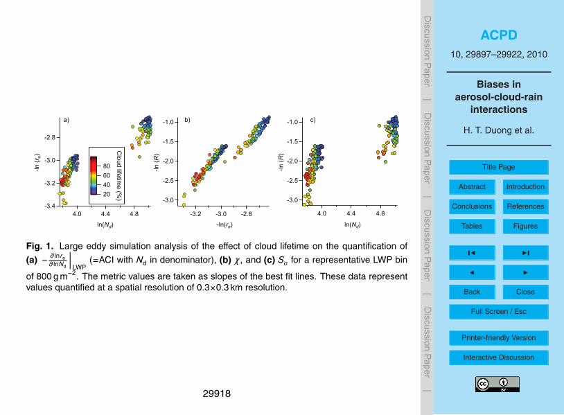
a population of clean and polluted clouds at all stages of their lifetime between 0–100% (Fig. 1). Note that few points are available at the beginning stages of clouds asthey have not yet had sufficient time to reach a LWP of 800 g m−2. The two clustersof points at varying levels of Nd correspond to the “clean” and “polluted” simulations.Precipitation is driven more directly by droplet size rather than Nd, which explains the5

narrower range in R at fixed re as compared to fixed Nd (i.e. R and re are more closelylinked physically than R and Nd). Cloud lifetime is shown to be responsible for the widerange in R at fixed Nd, where clouds near the end of their lifetime are raining mostheavily. The dynamic range in R tends to be wider for the clean clouds versus morepolluted clouds since they have a greater potential to rain owing to larger droplets at10

fixed LWP.Figure 2 illustrates the effect of cloud lifetime on the values of χ and So as a function

of LWP when evaluated at different spatial resolutions. Consistent with previous work,χ and So are non-monotonic functions of LWP and similarly exhibit small values at lowLWP and then increase up to a threshold LWP value after which they decrease. At15

fixed spatial resolution, the absolute values and LWP-dependent behavior of χ and Soare insensitive to whether those values were quantified at lifetimes of 0–33%, 33–67%,67–100%, or 0–100%. From Fig. 1, it is evident that the rare case when lifetime mayhave an important impact on So is when using small datasets that only include clouds inclean and dirty conditions that were at opposite ends of cloud lifetime (clean+growing20

vs. dirty+decaying; clean+decaying vs. dirty+growing). χ will be less sensitive to life-time as there is a relatively small dynamic range in R at a given re as compared to fixedNd conditions.

Remote sensing datasets typically include high volumes of data, so within a partic-ular LWP bin it is expected that clouds across a wide range of lifetimes will be repre-25

sented. Since the results for ACI (not shown), χ , and So are similar for clouds whenanalyzing data for various bins of cloud lifetime (0–33%, 33–67%, 67–100%, and 0–100%), this suggests that when using large datasets the absolute values of ACI, χ , andSo will not be biased to a large extent. The effect of lifetime will likely become more

29905





ACPD10, 29897–29922, 2010


interactions

H. T. Duong et al.

Title Page



Tables Figures

J I

J I

Back Close

Full Screen / Esc



Discussion

Paper

|D

iscussionP

aper|

Discussion

Paper

|D

iscussionP

aper|

important when using small datasets.

3.2 Spatial resolution

An important feature of the LES results in Fig. 2 is the effect of spatial resolution onthe LWP-dependent behavior of χ and So. As the spatial resolution decreases, thepeak values of χ and So shift to lower LWP values. Therefore, the choice of lower spa-5

tial resolution (i.e. 0.7 km×0.7 km versus 0.3 km×0.3 km) has the effect of compressingthe χ–LWP and So–LWP curves to lower LWP values while still maintaining similarabsolute values of χ and So. This effect of spatial resolution can now explain resultsin recent studies (Jiang et al., 2010; Sorooshian et al., 2010) where the precipitationsusceptibility of clouds was shown to exhibit a maximum at varying LWPs, owing to10

quantifying LWP across different spatial scales. Although not shown, ACI is insensi-tive to the choice of spatial resolution since it is relatively constant as a function ofLWP regardless of the size of the spatial resolution. In general, χ and So will likelyexhibit peak values at lower LWP for satellite data (as compared to models and in-situmeasurements) where LWP is averaged over larger spatial scales typically exceeding15

1 km.

3.3 Method of quantifying aerosol-cloud properties

The following analysis assesses the sensitivity of ACI, χ , and, So to the choice ofhow one quantifies the sub-components of these metrics (re, Nd, and R) using aircraftmeasurements from the MASE II study. As an example of why this is important, the20

choice of whether to use cloud column-integrated values of re versus those at cloud-top has previously been shown to influence the value of ACI (Masunaga et al., 2002;Matsui et al., 2004, 2006). Data from seven total cloud cases are examined exhibitinga LWP range between 31–55 g m−2 and an average sub-cloud Na range between 180–1400 cm−3 (using CPC 3010). Cloud base drizzle rates during these cases ranged25

between 0.5–2.7 mm day−1. While the value of re is retrieved with satellite remote

29906





ACPD10, 29897–29922, 2010


interactions

H. T. Duong et al.

Title Page



Tables Figures

J I

J I

Back Close

Full Screen / Esc



Discussion

Paper

|D

iscussionP

aper|

Discussion

Paper

|D

iscussionP

aper|

sensors at cloud-top, the aircraft data are used to quantify this parameter in multipleways including at cloud-top, the maximum in-cloud value, and a column-integrated av-erage. The sub-cloud leg-mean Na value is quantified using a CPC 3010 and a PCASP,while Nd is quantified as a maximum in-cloud value and a column-integrated in-cloudvalue. In addition to column-integrated and maximum values, R is quantified here as5

the leg-mean value above cloud base.

Table 1 shows that ACI values are smaller than − ∂ lnre∂ lnNd

∣∣∣LWP

(=ACI with Nd in denom-

inator), with slight enhancements in ACI when using Na values from the PCASP as

compared to the CPC 3010. ACI values are expected to be lower than − ∂ lnre∂ lnNd

∣∣∣LWP

, with

a reduction approximately equal to the factor “c”: Nd∼Nca (Feingold et al., 2001). The10

values of “c” for these seven cases when using Na (from CPC and PCASP) and Nd,maxare 0.62 and 0.67, respectively, which are close to the ratios of ACI when calculated

using Na as the CCN proxy as compared to Nd,max (0.67–0.76). The − ∂ lnre∂ lnNd

∣∣∣LWP

values

tend to approach 0.33 when using the Nd and re combinations that exhibit the widestrange of values (value range: Nd,max>Nd,col and re,max>re,top>re,col). Similar reason-15

ing explains why values of χ and So (or S ′o) are significantly greater when using Rmax

versus either Rbase or Rcol. These results are consistent with recent work that showedlarger values of ACI for wider ranges of AI (all else fixed) using satellite remote sensingdata (Sorooshian and Duong, 2010).

Why are the values in Table 1 greatest when quantifying the respective sub-20

components in ways that maximize their dynamic range? The strength of the relation-ship between an aerosol perturbation and drop size (or R) at fixed LWP is thought tobe more pronounced when quantifying maximum values of Nd and re (or R) rather thanleg-averaged values that may average out and obfuscate the desired signal. To providefurther support for this explanation, Fig. 3 summarizes the dependence of the parame-25

ters on the level flight leg length over which data were collected (centered around max-imum drop effective radius). It is shown that the maximum values occur at the smallestleg-lengths (<3 km) and level off when the data are averaged over larger spatial scales.

29907





ACPD10, 29897–29922, 2010


interactions

H. T. Duong et al.

Title Page



Tables Figures

J I

J I

Back Close

Full Screen / Esc



Discussion

Paper

|D

iscussionP

aper|

Discussion

Paper

|D

iscussionP

aper|

It is also worth noting that the product of ACI and χ agrees with the directly-quantifiedSo; for example, the product of χ (using re,max and the various rain rates) with 0.31(=ACI with re,max and Nd,max) agrees to within 9% for all three combinations. Thisprovides additional support for the utility of the deconstruction of the So metric intosub-components (Sorooshian et al., 2010) to improve confidence in causal relation-5

ships between aerosol perturbations and the precipitation response of warm cloudsby quantifying an intermediate step with the use of re (or alternatively cloud opticaldepth). Past work has also highlighted the significance of the relationship betweendrop effective radius and precipitation (e.g., Rosenfeld and Gutman, 1994).

3.4 Above-cloud aerosol layers10

Previous work attempted to identify warm oceanic regions between a latitude rangeof ±30◦ with the largest So (Sorooshian et al., 2009) and the largest potential relativereductions in R. It was shown, using a simplified approach, that the greatest predictedrelative reduction in warm rainfall is off the western coast of Africa; it is noted that thisregion did not exhibit the greatest absolute reduction simply because the precipitation15

rates in that region are low. In that work, ∆R was calculated as the product of annualaverage of daily So values (as determined by satellite-retrieved LWP and the So–LWPrelationship from LES output for warm clouds) and d ln(AI), as calculated from the dis-persion (standard deviation/mean) in aerosol index for 2007. However, the assumptionthat a column-integrated value of AI is representative of aerosol impacting a cloud is20

especially problematic in conditions characterized by high above-cloud aerosol con-centrations. In these conditions, AI becomes a poor proxy for sub-cloud CCN. Suchaerosol plumes, which are common during the biomass burning season off the westcoast of Africa, are clearly evident based on CALIPSO observations (e.g., Chand etal., 2009).25

A closer examination of this region off the coast of Africa is carried out to assess thesensitivity of ACI, χ , and S ′

o to using satellite-retrieved aerosol in conditions when rela-tively high concentrations of aerosol reside above the cloud, to represent the sub-cloud

29908





ACPD10, 29897–29922, 2010


interactions

H. T. Duong et al.

Title Page



Tables Figures

J I

J I

Back Close

Full Screen / Esc



Discussion

Paper

|D

iscussionP

aper|

Discussion

Paper

|D

iscussionP

aper|

CCN concentration. The spatial domain of this case study is (5◦ N, 20◦ S; 5◦ E, 35◦ W)and the time duration is between June and October of 2006. CALIPSO is used to iden-tify cases of above-cloud aerosol plumes during all A-Train overpasses when warm rainwas evident based on CloudSat observations. MODIS aerosol data were then filteredto avoid any 1◦×1◦ scenes containing the above-cloud aerosol plumes. The analysis5

of ACI, χ , and S ′o was subsequently carried out both with all of the data and with the

filtered data. The analysis is conducted for 11 LWP bins with up to 10% spacing aroundbin midpoints, which increase in 25 g m−2 increments from 50 to 300 g m−2. The cloudsin this region typically exhibit LTSS values in excess of 20 ◦C, which is indicative ofstratocumulus clouds. Caution was taken to use CloudSat data beginning vertically in10

the lowest clutter-free range gate above the surface, which is between 600 and 840 m(Haynes et al., 2009).

Figure 4a shows that filtering the above-cloud plume data results in an enhancementin the majority of ACI and S ′

o points, which rely on the collocated aerosol data retrievedby MODIS. On average, the enhancement in ACI and S ′

o was 20% and 156%, respec-15

tively, for the LWP range examined. The explanation for the depression of these valuesduring cases of above-cloud plumes likely stems from a cluster of data points at veryhigh aerosol concentrations that obfuscate the desired ACI and S ′

o signals (hypotheti-cally illustrated in Fig. 5), leading to a reduction in their absolute values. Above-cloudaerosol layers present a factor that may lead to lower values of ACI and S ′

o as com-20

pared to surface and aircraft measurements and cloud models that are immune to thisissue. The values of χ tend to be more evenly scattered about the 1:1 line, which ispartly expected as χ does not rely on collocated aerosol data and thus is less sensitiveto above-cloud plumes. On average, there was an 8% enhancement in χ after the datafiltering.25

An issue that cannot be ignored in this discussion is the effect of overlaying aerosollayers on MODIS retrievals of cloud properties such as re and LWP, which are typicallythought to be biased low (e.g., Haywood et al., 2004; Cattani et al., 2006; Bennartzand Harshvardhan, 2007; Wilcox et al., 2009; Coddington et al., 2010). In support of

29909





ACPD10, 29897–29922, 2010


interactions

H. T. Duong et al.

Title Page



Tables Figures

J I

J I

Back Close

Full Screen / Esc



Discussion

Paper

|D

iscussionP

aper|

Discussion

Paper

|D

iscussionP

aper|

the presented analysis, potential biases in re have been shown to be less than 1 µmfor retrievals where the visible reflectance is matched with the 3.7 µm or 2.13 µm re-flectance. Wilcox et al. (2009) report that when the aerosol index obtained from theOzone Monitoring Instrument (OMI) exceeds two, the estimated bias in the averageLWP difference between AMSR-E and MODIS exceeds the instantaneous uncertainty5

in the retrievals. Even after removing the data points in this case study analysis thatexceeded this OMI threshold value (to account for issues in LWP retrievals), the con-clusions of this analysis remain robust.

3.5 Wet scavenging effects

Artificially low aerosol concentrations resulting from wet scavenging can also influence10

the values of ACI, χ , and S ′o. The methodology in a number of studies has included

obtaining data for rain and cloud properties from CloudSat and MODIS with a spatialresolution on the order of 1 km, while aerosol data are retrieved from a significantlylarger spatial domain (1◦×1◦) (Lebsock et al., 2008; Sorooshian et al., 2009, 2010).The effect of wet scavenging is tested using data for the months of June through Au-15

gust (JJA) between 2006–2008 and just the year 2007 within the tropics for shallowcumulus clouds. The Precipitation Estimation from Remotely Sensed Information us-ing Artificial Neural Networks (PERSIANN; Sorooshian et al., 2000) product is used toremove cases of precipitation for a period of time up to a day before a satellite overpasswithin the same 1◦×1◦ domain of MODIS aerosol retrievals. PERSIANN estimates rain-20

fall using geostationary infrared imagery of clouds (e.g., GOES-8, GOES-9/10, GMS-5, Metsat-6/7) and microwave instantaneous rainfall estimates (e.g., TRMM TMI). Theanalysis is performed for 12 LWP bins with up to 10% spacing around bin midpoints,which include 50 g m−2, 100 g m−2, and up to 1100 g m−2 in 100 g m−2 increments. Ap-proximately 20–40% of the points were removed in each LWP bin when accounting for25

the wet scavenging effect.Figure 4b shows that ACI and S ′

o values are scattered around the 1:1 line but withmany points depressed after the PERSIANN filtering. The reduction in ACI and S ′

o

29910





ACPD10, 29897–29922, 2010


interactions

H. T. Duong et al.

Title Page



Tables Figures

J I

J I

Back Close

Full Screen / Esc



Discussion

Paper

|D

iscussionP

aper|

Discussion

Paper

|D

iscussionP

aper|

as a result of the data filtering is likely due to aerosol measurements being biasedlow when wet scavenging is not taken into account. Because wet scavenging tendsto influence the polluted scenes more than clean ones (because there is a greaterpotential to remove more aerosol; Fig. 5), larger aerosol values need to be shiftedto commensurately larger values, which for the same cloud microphysical parameter5

results in weaker ACI/S ′o slopes. Similar to the analysis of artificially high aerosol levels

in Sect. 3.3, the value of χ is less sensitive to the wet scavenging data filtering becauseit does not require aerosol data in its quantification.

4 Conclusions

In previous work we explored the use of various parameters (ACI, χ , and So, defined10

in Sect. 1) that attempt to quantify aerosol-cloud-precipitation processes, and here weassess the sensitivity of such metrics to numerous biasing factors using LES, satelliteobservations, and aircraft measurements. The major results of this work are as follows:

1. The time at which a cloud is sampled, relative to the overall cloud lifetime,could bias estimates of precipitation susceptibility because of the inherent timescale15

for a cloud to produce rainfall. This potential bias was examined for simulated shallowcumulus clouds. The absolute values of χ and So are insensitive to whether thosevalues were quantified at the beginning, middle, or end of cloud lifetime, unless sam-pling conditions were to somehow be biased towards covariance between magnitudeof the aerosol perturbation, and stage of cloud development. Such covariance would20

be unlikely to exist in nature, except perhaps in small datasets. In large datasets, suchas those from satellites, the effects of lifetime will likely be small owing to averagingamongst vast amounts of data representing clouds at varying stages in their lifetime,at their instantaneously measured LWP.

2. The choice and/or limitation of spatial resolution in observational datasets are25

shown to influence the LWP-dependent behavior of χ and So. At low spatial resolution,the curves are compressed towards lower LWP (see Fig. 2); in other words, the point

29911





ACPD10, 29897–29922, 2010


interactions

H. T. Duong et al.

Title Page



Tables Figures

J I

J I

Back Close

Full Screen / Esc



Discussion

Paper

|D

iscussionP

aper|

Discussion

Paper

|D

iscussionP

aper|

at which the maximum values of χ and So are reached occur at lower LWPs. ACI isshown to be relatively constant as a function of LWP and therefore is not as dependenton spatial resolution as χ and So.

3. The absolute magnitudes of So, χ , and ACI are sensitive to the choice of how toquantify the aerosol proxy, re, and R (e.g., cloud-top, maximum, vertically-integrated),5

and to temporal/spatial averaging. Analyses of aircraft data of aerosol-stratocumulusinteractions show that So, χ , and ACI are higher when using values of Nd, re, and Rthat exhibit the widest dynamic ranges over the span of clouds examined. This is mostrelevant to model and aircraft-based studies, where there are many choices for howto quantify these variable values, as opposed to satellite-based data sets where data10

products are more limited.4. The inclusion of cases characterized by above-cloud aerosol plumes, as examined

in a case study off the coast of western Africa, is shown to depress values of ACI andS ′o. This is explained by data points at very high aerosol concentrations that obfuscate

the desired ACI and S ′o signals. Appropriate filtering of these instances shows more15

realistic sensitivity. On the other hand, accounting for low biases in retrieved aerosolamounts as a result of wet scavenging with the use of an artificial neural network algo-rithm is shown in some cases to result in lower values of ACI and S ′

o. An explanationis that wet scavenging tends to influence the polluted scenes more than clean ones,resulting in greater reductions in aerosol abundance during cases with the lowest rain20

rates and drop sizes. The value of χ is relatively insensitive to both factors as it doesnot rely on collocated aerosol data, but only data within cloudy pixels.

While variations are expected in the values of the aerosol-cloud-rain constructs ex-amined here owing to the complexity of these physical interactions and meteorolog-ical feedbacks, it is necessary to understand how much of the variability is due to25

differences in measurement/modeling methodologies and data analysis techniques.The results of this study point to the importance of considering all the issues identi-fied above when comparing results with other independent studies examining aerosol-cloud interactions. For instance, details as basic as how, and at what resolution cloud

29912





ACPD10, 29897–29922, 2010


interactions

H. T. Duong et al.

Title Page



Tables Figures

J I

J I

Back Close

Full Screen / Esc



Discussion

Paper

|D

iscussionP

aper|

Discussion

Paper

|D

iscussionP

aper|

microphysical parameters are calculated may have a major impact on the absolutevalue of the precipitation susceptibility of clouds to aerosol particles. Of the variousparameters relating aerosols to rain in this work, χ is shown to be the least sensitiveto the biasing factors investigated as it does not require collocated aerosol data in itscalculation, which is especially advantageous for satellite studies.5

Acknowledgements. A.S. acknowledges support from an Office of Naval Research YIP Award(N00014-10-1-0811). The aircraft measurements were supported by the Office of Naval Re-search grant N00014-04-1-0018. G.F. acknowledges support from NOAA’s Climate Goal.

References

Bennartz, R. and Harshvardhan: Correction to “Global assessment of marine boundary10

layer cloud droplet number concentration from satellite”, J. Geophys. Res., 112, D16302,doi:10.1029/2007JD00884, 2007.

Cattani, E., Costa, M. J., Torricella, F., Levizzani, V., and Silva, A. M.: Influence of aerosol par-ticles from biomass burning on cloud microphysical properties and radiative forcing, Atmos.Res., 82, 310–327, 2006.15

Chand, D., Wood, R., Anderson, T., Satheesh, S. K., and Charlson, R. J.: Satellite-derived directradiative effect of aerosols dependent on cloud cover, Nat. Geosci., 2, 181–184, 2009.

Coddington, O. M., Pilewskie, P., Redemann, J., Platnick, S., Russell, P. B., Schmidt, K. S.,Gore, W. J., Livingston, J., Wind, G., and Vukicevic, T.: Examining the impact of overlyingaerosols on the retrieval of cloud optical properties from passive remote sensing, J. Geophys.20

Res., 115, D10211, doi:10.1029/2009JD012829, 2010.Comstock, K. K., Wood, R., Yuter, S. E., and Bretherton, C. S.: Reflectivity and rain rate in and

below drizzling stratocumulus, Q. J. Roy. Meteor. Soc., 130, 2891–2918, 2004.Cotton, W. R., Pielke, R. A., Walko, R. L., Liston, G. E., Tremback, C. J., Jiang, H.,

McAnelly, R. L., Harrington, J. Y., Nicholls, M. E., Carrio, G. G., and McFadden, J. P.: RAMS25

2001: current status and future directions, Meteorol. Atmos. Phys., 82(1–4), 5–29, 2003.Feingold, G. and Siebert, H.: In clouds in the perturbed climate system: their relationship to

energy balance, atmospheric dynamics, and precipitation, in: Strungmann Forum Reports,

29913





ACPD10, 29897–29922, 2010


interactions

H. T. Duong et al.

Title Page



Tables Figures

J I

J I

Back Close

Full Screen / Esc



Discussion

Paper

|D

iscussionP

aper|

Discussion

Paper

|D

iscussionP

aper|

2, edited by: Heintzenberg, J. and Charlson, R. J., The MIT Press, Cambridge, MA, 597 pp,2009.

Feingold, G., Kreidenweis, S. M., Stevens, B., and Cotton, W. R.: Numerical simulations of stra-tocumulus processing of cloud condensation nuclei through collision-coalescence, J. Geo-phys. Res., 101(D16), 21391–21402, 1996.5

Feingold, G., Remer, L. A., Ramaprasad, J., and Kaufman, Y. J.: Analysis of smoke impacton clouds in Brazilian biomass burning regions: an extension of Twomey’s approach, J.Geophys. Res., 106, 22907–22922, 2001.

Gerber, H., Arends, B. G., and Ackerman, A. S.: New microphysics sensor for aircraft use,Atmos. Res., 31, 235–252, 1994.10

Grandey, B. S. and Stier, P.: A critical look at spatial scale choices in satellite-based aerosolindirect effect studies, Atmos. Chem. Phys. Discuss., 10, 15417–15440, doi:10.5194/acpd-10-15417-2010, 2010.

Haynes, J. M., L’Ecuyer, T. S., Stephens, G. L., Miller, S. D., Mitrescu, C., Wood, N. B., andTanelli, S.: Rainfall retrieval over the ocean with spaceborne W-band radar, J. Geophys.15

Res., 114, D00A22, doi:10.1029/2008JD009973, 2009.Haywood, J. M., Osborne, S. R., and Abel, S. J.: The effect of overlying absorbing aerosol

layers on remote sensing retrievals of cloud effective radius and cloud optical depth, Q. J.Roy. Meteor. Soc., 130, 779–800, 2004.

Hersey, S. P., Sorooshian, A., Murphy, S. M., Flagan, R. C., and Seinfeld, J. H.: Aerosol hygro-20

scopicity in the marine atmosphere: a closure study using high-time-resolution, multiple-RH DASH-SP and size-resolved C-ToF-AMS data, Atmos. Chem. Phys., 9, 2543–2554,doi:10.5194/acp-9-2543-2009, 2009.

Jiang, H. L., Feingold, G., and Koren, I.: Effect of aerosol on trade cumulus cloud morphology,J. Geophys. Res., 114, D11209, doi:10.1029/2009JD011750, 2009.25

Jiang, H. L., Feingold, G., and Sorooshian, A.: Effect of aerosol on the susceptibility andefficiency of precipitation in trade cumulus clouds, J. Atmos. Sci., 67, 3525–3540, 2010.

Lebsock, M. D., Stephens, G. L., and Kummerow, C.: Multi-sensor observations of aerosoleffects on warm clouds, J. Geophys. Res., 113, D15205, 2008.

Lohmann, U. and Feichter, J.: Global indirect aerosol effects: a review, Atmos. Chem. Phys., 5,30

715–737, doi:10.5194/acp-5-715-2005, 2005.Lu, M.-L., Sorooshian, A., Jonsson, H. H., Feingold, G., Flagan, R. C., and Seinfeld, J. H.:

Marine stratocumulus aerosol-cloud relationships in the MASE-II experiment: precipitation

29914





ACPD10, 29897–29922, 2010


interactions

H. T. Duong et al.

Title Page



Tables Figures

J I

J I

Back Close

Full Screen / Esc



Discussion

Paper

|D

iscussionP

aper|

Discussion

Paper

|D

iscussionP

aper|

susceptibility in Eastern Pacific marine stratocumulus, J. Geophys. Res., 114, D24203,doi:10.1029/2009JD012774, 2009.

Masunaga, H., Nakajima, T. Y., Nakajima, T., Kachi, M., Oki, R., and Kuroda, S.: Physical prop-erties of maritime low clouds as retrieved by combined use of tropical rainfall measurementmission microwave imager and visible/infrared scanner: algorithm, J. Geophys. Res., 107,5

4083, doi:10.1029/2001JD000743, 2002.Matsui, T., Masunaga, H., Pielke Sr., R. A., and Tao, W.-K.: Impact of aerosols and atmospheric

thermodynamics on cloud properties within the climate system, Geophys. Res. Lett., 31,L06109, doi:10.1029/2003GL019287, 2004.

Matsui, T., Masunaga, H., Kreidenweis, S. M., Pielke Sr., R. A., Tao, W.-K., Chin, M., and10

Kaufman, Y. J.: Satellite-based assessment of marine low cloud variability associatedwith aerosol, atmospheric stability, and the diurnal cycle, J. Geophys. Res., 111, D17204,doi:10.1029/2005JD006097, 2006.

McComiskey, A. and Feingold, G.: Quantifying error in the radiative forcing of the first aerosolindirect effect, Geophys. Res. Lett., 35, L02810, doi:10.1029/2007GL032667, 2008.15

Partain, P.: Cloudsat ECMWF-AUX auxiliary data process description and interfacecontrol document, http://www.cloudsat.cira.colostate.edu/dataICDlist.php?go=list&path=/ECMWF-AUX, 2007.

Pawlowska, H. and Brenguier, J. L.: An observational study of drizzle formation in stratocumu-lus clouds for general circulation model (GCM) parameterizations, J. Geophys. Res., 108,20

D15, 8630, doi:10.1029/2002JD002679, 2003.Platnick, S., King, M. D., Ackerman, S. A., Menzel, W. P., Baum, B. A., Riedi, J. C., and

Frey, R. A.: The MODIS cloud products: algorithms and examples from Terra, IEEE T.Geosci. Remote, 41, 459–473, 2003.

Quaas, J., Ming, Y., Menon, S., Takemura, T., Wang, M., Penner, J. E., Gettelman, A., Lohmann,25

U., Bellouin, N., Boucher, O., Sayer, A. M., Thomas, G. E., McComiskey, A., Feingold, G.,Hoose, C., Kristjansson, J. E., Liu, X., Balkanski, Y., Donner, L. J., Ginoux, P. A., Stier, P.,Grandey, B., Feichter, J., Sednev, I., Bauer, S. E., Koch, D., Grainger, R. G., Kirkevag,A., Iversen, T., Seland, Ø., Easter, R., Ghan, S. J., Rasch, P. J., Morrison, H., Lamar-que, J.-F., Iacono, M. J., Kinne, S., and Schulz, M.: Aerosol indirect effects – general cir-30

culation model intercomparison and evaluation with satellite data, Atmos. Chem. Phys., 9,8697–8717, doi:10.5194/acp-9-8697-2009, 2009.

Remer, L. A., Kaufman, Y. J., Tanre, D., Mattoo, S., Chu, D. A., Martins, J. V., Li, R. R.,

29915





http://www.cloudsat.cira.colostate.edu/dataICDlist.php?go=list&path=/ECMWF-AUX



ACPD10, 29897–29922, 2010


interactions

H. T. Duong et al.

Title Page



Tables Figures

J I

J I

Back Close

Full Screen / Esc



Discussion

Paper

|D

iscussionP

aper|

Discussion

Paper

|D

iscussionP

aper|

Ichoku, C., Levy, R. C., Kleidman, R. G., Eck, T. F., Vermote, E., and Holben, B. N.: TheMODIS aerosol algorithm, products, and validation, J. Atmos. Sci., 62, 947–973, 2005.

Rosenfeld, D. and Gutman, G.: Retrieving microphysical properties near the tops of potentialrain clouds by multispectral analysis of AVHRR data, Atmos. Res., 34, 259–283, 1994.

Sorooshian, A. and Duong, H. T.: Ocean Emission Effects on Aerosol-Cloud Interac-5

tions: Insights from Two Case Studies, Advances in Meteorology, 2010, 301395,doi:10.1155/2010/301395, 2010.

Sorooshian, S., Hsu, K. L., Gao, X., Gupta, H. V., Imam, B., and Braithwaite, D.: Evaluation ofPERSIANN system satellite-based estimates of tropical rainfall, B. Am. Meteorol. Soc., 81,2035–2046, 2000.10

Sorooshian, A., Feingold, G., Lebsock, M. D., Jiang, H., and Stephens, G.: On the precip-itation susceptibility of clouds to aerosol perturbation, Geophys. Res. Lett., 36, L13803,doi:10.1029/2009GL038993, 2009.

Sorooshian, A., Feingold, G., Lebsock, M. D., Jiang, H., and Stephens, G.: Deconstructing theprecipitation susceptibility construct: improving methodology for aerosol-cloud-precipitation15

studies, J. Geophys. Res., 115, D17201, doi:10.1029/2009JD013426, 2010.Stevens, B., Feingold, G., Cotton, W. R., and Walko, R. L.: Elements of the microphysical struc-

ture of numerically simulated nonprecipitating stratocumulus, J. Atmos. Sci., 53, 980.1006,1996.

vanZanten, M. C., Stevens, B., Vali, G., and Lenschow, D. H.: Observations of drizzle in noc-20

turnal marine stratocumulus, J. Atmos. Sci., 62, 88–106, 2005.Wilcox, E. M., Harshvardhan, and Platnick, S.: Estimate of the impact of absorbing aerosol

over cloud on the MODIS retrievals of cloud optical thickness and effective radius us-ing two independent retrievals of liquid water path, J. Geophys. Res., 114, D05210,doi:10.1029/2008JD010589, 2009.25

Wood, R.: Drizzle in stratiform boundary layer clouds. Part 1: Vertical and horizontal structure,J. Atmos. Sci., 62, 3011–3033, 2005.

29916





ACPD10, 29897–29922, 2010


interactions

H. T. Duong et al.

Title Page



Tables Figures

J I

J I

Back Close

Full Screen / Esc



Discussion

Paper

|D

iscussionP

aper|

Discussion

Paper

|D

iscussionP

aper|

Table 1. Aircraft measurement summary of the sensitivity of ACI, χ , and So (or S ′o) to the choice

of how the aerosol proxy (Nd or Na), R, and re are quantified. The maximum values (“max”) arequantified as being the average of the 3 points before/after the maximum value (correspond-ing to a level flight length of ∼350 m). Column-integrated values (“col”) represent the verticalintegration of leg-mean values of the respective parameter. Cloud-top and base values (“top”and “base”) represent the leg-mean value below cloud-top and above cloud base, respectively.Na is the leg-mean average of particle concentration below cloud-base, as quantified with botha CPC 3010 (Dp>10 nm) and a PCASP (Dp∼100 nm−2.6 µm). Bold signify that those pointsare not statistically significant with 95% confidence based on the student’s t-test. Numbers inparentheses next to column and row headers correspond to the overall range of those values(Units: Nd and Na=# cm−3; re=µm; R=mm day−1).

Nd,max Nd,col Na from Na from re,max re,col re,top(86–407) (47–229) CPC 3010 PCASP

(187–1360) (54–424)

ACIre,max (8.97–14.0) 0.31 0.24 0.22 0.23re,col (8.26–11.2) 0.18 0.15 0.13 0.13re,top (8.34–12.4) 0.21 0.20 0.14 0.16

So S ′o χ

Rmax (0.75–8.19) 1.23 1.10 0.88 0.90 4.24 4.16 4.20Rcol (0.5–1.60) 0.37 0.44 0.19 0.25 1.31 0.78 0.93Rbase (0.5–2.75) 0.56 0.67 0.33 0.40 1.82 1.05 1.23

29917





ACPD10, 29897–29922, 2010


interactions

H. T. Duong et al.

Title Page



Tables Figures

J I

J I

Back Close

Full Screen / Esc



Discussion

Paper

|D

iscussionP

aper|

Discussion

Paper

|D

iscussionP

aper|

-3.4

-3.2

-3.0

-2.8

-ln (r

e)

4.84.44.0ln(Nd)

-3.0

-2.5

-2.0

-1.5

-1.0

-ln (R

)

-3.2 -3.0 -2.8-ln(re)

-3.0

-2.5

-2.0

-1.5

-1.0

-ln (R

)

4.84.44.0

ln(Nd)

a) b) c)

80604020

Cloud lifetim

e (%)

Fig. 1. Large eddy simulation analysis of the effect of cloud lifetime on the quantification of

(a) − ∂ lnre

∂ lnNd

∣∣∣LWP

(=ACI with Nd in denominator), (b) χ , and (c) So for a representative LWP bin

of 800 g m−2. The metric values are taken as slopes of the best fit lines. These data representvalues quantified at a spatial resolution of 0.3×0.3 km resolution.

29918





ACPD10, 29897–29922, 2010


interactions

H. T. Duong et al.

Title Page



Tables Figures

J I

J I

Back Close

Full Screen / Esc



Discussion

Paper

|D

iscussionP

aper|

Discussion

Paper

|D

iscussionP

aper|

2.8

2.6

2.4

2.2

2.0

1.8

χ

140012001000800600400200

LWP (g m-2)

1.2

1.1

1.0

0.9

0.8

0.7

0.6S

o

140012001000800600400200

LWP (g m-2)

a) b)

0.3 km x 0.3 km: 0-100% life 0-33% life 67-100% life33-67% life: 0.3 km x 0.3 km 0.5 km x 0.5 km 0.7 km x 0.7 km

Fig. 2. Large eddy simulation analysis of the dependence of (a) χ and (b) So on LWP, cloudlifetime, and spatial resolution over which data for aerosol and cloud properties were obtainedfrom the LES output.

29919





ACPD10, 29897–29922, 2010


interactions

H. T. Duong et al.

Title Page



Tables Figures

J I

J I

Back Close

Full Screen / Esc



Discussion

Paper

|D

iscussionP

aper|

Discussion

Paper

|D

iscussionP

aper|

2

3

4

5678

1

2

3

4

5

30252015105Aircraft Leg Length (km)

- ln(re)/ ln(Nd)

So χ

∂∂

Fig. 3. Aircraft measurements showing the dependence of aerosol–cloud-rain relationshipson flight leg length (centered around maximum drop effective radius during a level leg) overwhich data are analyzed. These data represent stratocumulus clouds off the central coast ofCalifornia with a LWP range between 31–55 g m−2.

29920





ACPD10, 29897–29922, 2010


interactions

H. T. Duong et al.

Title Page



Tables Figures

J I

J I

Back Close

Full Screen / Esc



Discussion

Paper

|D

iscussionP

aper|

Discussion

Paper

|D

iscussionP

aper|

a) b)

0.01

2

3

4567

0.1

0.012 3 4 5 6 7 8

0.1

1.0

0.8

0.6

0.4

0.2

0.0

All

data

1.00.80.60.40.2Filtered Data (No Above-Cloud Aerosol Plumes)

1:1 line ACI χ

S'o

2

3

4

5

6789

0.1

2

3

4

5

6789

1

All

data

2 3 4 5 6 7 8 90.1

2 3 4 5 6 7 8 91

PERSIANN Filtered Data

Filled = 2006-2008; Open = 2007 ACI χ S'

o

1:1 line

Fig. 4. Satellite data analysis of the sensitivity of aerosol–cloud-rain metrics to above-cloudaerosol plumes and wet scavenging. (a) Comparison of ACI, χ , and S ′

o with and without above-cloud aerosol plumes off the coast of western Africa. The data represent the time period be-tween June and October 2006. Marker sizes are proportional to LWP (11 LWP bins with up to10% spacing around bin midpoints (LWP±10%×LWP), which increase in 25 g m−2 incrementsfrom 50 to 300 g m−2). (b) Comparison of ACI, χ , and S ′

o with and without filtering of wetscavenging events prior to A-Train overpasses within the same 1◦×1◦ pixel. Marker sizes areproportional to LWP (12 LWP bins with up to 10% spacing around bin midpoints, which include50 g m−2, 100 g m−2, and up to 1100 g m−2 in 100 g m−2 increments). The data represent theJJA months for the three year period including 2006–2008 (filled) and 2007 only (open). Onlypoints are reported in both panels that were statistically significant at 95% confidence (basedon student’s t-test) with and without the data filtering.

29921





ACPD10, 29897–29922, 2010


interactions

H. T. Duong et al.

Title Page



Tables Figures

J I

J I

Back Close

Full Screen / Esc



Discussion

Paper

|D

iscussionP

aper|

Discussion

Paper

|D

iscussionP

aper|

-

ln(R

) or -

ln(r

e)

ln(α)

Wet scavengingevents reduceaerosol abundance

Above-cloudaerosol plumesincrease aerosol abundance

Fig. 5. A visual description of the effect that high and low aerosol concentrations may have onquantification of ACI and S ′

o when using satellite data. The thick solid line represents a hypo-thetical slope when plotting −ln(R) or −ln(re) versus ln(α), which corresponds to ACI and S ′

o,respectively. With above-cloud aerosol plumes, a cluster of points at high levels of ln(α) willreduce the slope (i.e. lower ACI and S ′

o). Low aerosol concentrations as a result of wet scav-enging likely will have a greater impact for the most polluted scenes where there is a greaterpotential to have a reduction in aerosol concentration. This will lead to a higher slope (i.e.higher ACI and S ′

o). The χ metric is relatively insensitive to these effects as it avoids the use ofretrieved aerosol data.

29922





Investigating potential biases in observed and modeled metrics of aerosol-cloud-precipitation...

Documents

Transcript of Investigating potential biases in observed and modeled metrics of aerosol-cloud-precipitation...