A Study on Crude Oil Prices Modeled by Neurofuzzy Networks

Introduction Available methodologies Datasets Experimental setup Numerical results Conclusions

A Study on Crude Oil Prices Modeledby Neurofuzzy Networks

(FUZZ-IEEE 2013)

M. Panella

1L. Liparulo

1F. Barcellona

2R. D’Ecclesia

3

1Dept. of Information Engineering, Electronics and Telecommunications (DIET)2InfoSapienza Centre

3Dept. of Methods and Models for Economics, Territory and Finance (MEMOTEF)

University of Rome “La Sapienza”Email: [email protected]

2013 IEEE International Conference on Fuzzy SystemsJuly 7-10, 2013, Hyderabad, India

Luca Liparulo FUZZ IEEE 2013, July 10, 2013 - Hyderabad, India


Outline

1 Introduction

2 Available methodologies

3 Datasets

4 Experimental setup

5 Numerical results

6 Conclusions



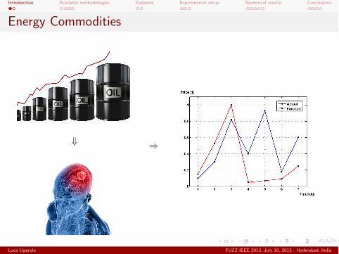
Energy Commodities

+ )



Motivation

To provide a powerful tool to replicate the dynamics of economic andfinancial series.

To apply a new methodology based on a neurofuzzy networks to forecastspecific standard price time series of energy commodities.

To backtest the results and set up risk management strategies.



Available methodologies

Quantitative techniques:

Explanatory methods

Time series based method

+

Forecasting process like a black box

Data-driven approaches to analize time series:

Autoregressive models (AR)

Moving average models (MA)

ARMA and ARIMA models

ARCH and GARCH models

Neural and Neurofuzzy networks



The proposed methodology for prediction (1/3)

We worked with log-prices yt = ln(St) and we considered a standard additivemodel for time series:

yt = µt + "t,

where µt is the deterministic component representing the forecast and "t is arandom variable which takes into account the uncertainty of prediction.

ARMA regression model8<

:µt = f

⇣X(µ)

t ;!(µ)t

⌘

X(µ)t =

⇥yt�1 yt�2 . . . yt�R "t�1 "t�2 . . . "t�M

⇤

where !

(µ)t is equal to the time varying parameter vectors of the regression

function f .




ANFIS (Adaptive Neuro-Fuzzy Inference System) Network Architecture

Fuzzy decision: y(x) =PM

k=1 ↵(k)

(x)y

(k)(x)




Our aim is to prove that ANFIS networks can solve the general regression problemby means of a set of P rules of Sugeno first-order type.

The kth rule, k = 1. . .P , has the following form:

(if yt�1 is B

(k)1 and . . . yt�R is B

(k)R and

"t�1 is B

(k)R+1 and . . . "t�M is B

(k)R+M then

µ

(k)t =

RX

j=1

a

(k)j yt�j +

MX

j=1

a

(k)R+j"t�j + a

(k)0

The structure of the fuzzy inference system is the following one:

µt = f

⇣X(µ)

t

⌘=

PPk=1 µ

(k)t VB(k)

⇣X(µ)

t

⌘

PPk=1 VB(k)

⇣X(µ)

t

⌘.



Datasets (1/2)

We used loarithmic transformed prices of both American and European energycommodities (Crude Oil):

US ! WTI (West Texas Intermediate)

EUR ! BRENT

Input-Output series

Input series (Training phase):8 two-years period from 2001� 2002 to 2008� 2009;

Output series (Testing phase):8 years from 2003 to 2010 (each follows the previous two years)

+

DATASETS

Unique time series for both phases (training and testing), described by data ofthree-year period (from 2001� 2002� 2003 to 2008� 2009� 2010)



Datasets (2/2)

WTI daily log-prices from 2000 to 2012

Brent daily log-prices from 2000 to 2012



Experimental setup (1/3)

Four data-driven modeling techniques are compared in this study:1

LSE (Least-Squares Estimation);2

RBF (Radial Basis Function neural networks), trained using the MatlabTM

software (version R2012a);3

MoG (Mixture of Gaussians neural networks), which are well suited tocomplex and non-convex data;

4ANFIS networks, where the Subtractive Clustering (SUBCL) method is usedfor the rule extraction and the rule parameters are obtained by means of astandard least-squares method coupled with the back-propagationoptimization.

Setup

M = 1 and R = 3 (Rule-of-thumb!)

Training window, NT = 500

Test window, NS = 250




The prediction accuracy is measured by:

Mean Squared Error - MSE

MSE =

1

Ns

X

t

(yt � µt)2

Normalised Mean Square Error - NMSE

NMSE =

Pt (yt � µt)

2

Pt (yt � y)

2

Noise-to-signal ratio or NSR (dB)

) NSRdB = 10 log10

Pt(yt � µt)

2

Pt y

2

Mean absolute percentage error - MAPE

MAPE =

100

Ns

X

t

��yt � µt

yt

��




In the testing phase of theoretical models, it is essential to define some criteria toassess the e�cacy of the chosen model.

In addition to the prediction error estimation, we also evaluated theSTATISTICAL FEATURES of the two series (Actual Vs Forecast)

+

Summarized in the four moments:Mean

Variance

Skewness

Kurtosis



Results analysis 1/5 - 2003



Results analysis 2/5 - 2009



Results analysis 3/5 - Noise-to-Signal Ratio

Year Model WTI (NSR) Brent (NSR)

2003

ANFIS -41.32 -41.57

RBF -35.90 -41.00

MoG -20.57 -36.81

LSE -41.53 -42.00

2004

ANFIS -41.92 -24.16

RBF -35.27 -21.16

MoG -36.25 -19.37

LSE -32.89 -22.15

2005

ANFIS -44.28 -44.52

RBF -29.79 -24.11

MoG -28.22 -14.19

LSE -34.86 -44.67

2006

ANFIS -43.98 -45.85

RBF -35.42 -43.31

MoG -41.02 -20.24

LSE -36.51 -36.56

Year Model WTI (NSR) Brent (NSR)

2007

ANFIS -44.95 -46.02

RBF -35.09 -38.70

MoG -39.68 -42.32

LSE -35.71 -36.71

2008

ANFIS -35.56 -40.18

RBF -24.88 -14.80

MoG -23.94 -32.54

LSE -30.16 -30.55

2009

ANFIS -39.23 -40.51

RBF -33.63 -35.77

MoG -34.81 -36.70

LSE -30.03 -31.58

2010

ANFIS -46.65 -45.78

RBF -46.28 -47.12

MoG -42.93 -43.14

LSE -46.15 -36.97

The ANFIS model provides the best results in terms of NSR and this is ahomogeneous behavior across many years.The prediction performances of ANFIS are essentially better than the linearmodel LSE, which in turn behaves very similarly to the well-known naivepredictor for which yt = yt�1.



Results analysis 4/5 - From 2003 to 2006

Year StatisticWTI Brent

Estim. Actual Estim. Actual

2003

Mean 2.9669 2.9718 2.7643 2.7645

Variance 0.0067 0.0069 0.0088 0.0093

Kurtosis 3.1024 3.1255 2.3691 2.4811

Skewness 0.2533 0.2596 0.5063 0.5547

2004

Mean 3.2599 3.2599 2.8770 2.9508

Variance 0.0203 0.0183 0.0167 0.0219

Kurtosis 2.1745 2.1626 1.7541 2.2098

Skewness 0.3358 0.3369 -0.2293 0.0435

2005

Mean 3.5692 3.5727 3.3251 3.3297

Variance 0.0130 0.0125 0.0208 0.0203

Kurtosis 2.2378 2.2657 2.2683 2.2107

Skewness -0.2982 -0.3218 -0.5999 -0.5857

2006

Mean 3.7224 3.7314 3.4974 3.5018

Variance 0.0051 0.0070 0.0056 0.0068

Kurtosis 1.8276 1.7108 1.8171 1.8207

Skewness -0.0816 0.0545 -0.0973 -0.0988



Results analysis 5/5 - From 2007 to 2010

Year StatisticWTI Brent

Estim. Actual Estim. Actual

2007

Mean 3.7974 3.8043 3.4994 3.5001

Variance 0.0278 0.0293 0.0138 0.0147

Kurtosis 2.1298 2.0256 2.4368 2.3630

Skewness 0.1930 0.2381 -0.1250 -0.1392

2008

Mean 4.0778 4.0999 3.6934 3.6952

Variance 0.0853 0.1137 0.0758 0.0815

Kurtosis 3.7970 3.7757 3.9390 3.8541

Skewness -1.3366 -1.2554 -1.2386 -1.2318

2009

Mean 3.6492 3.6477 3.3228 3.3277

Variance 0.0546 0.0556 0.0275 0.0251

Kurtosis 2.1135 2.3328 1.8815 1.8829

Skewness -0.6866 -0.7792 -0.5744 -0.5590

2010

Mean 3.8943 3.8958 3.5185 3.5285

Variance 0.0018 0.0019 0.0009 0.0010

Kurtosis 1.6653 1.6095 1.9534 1.8746

Skewness 0.0169 0.0614 0.2094 0.1035



Conclusions & Future works

The approach proposed in this paper provides a highly predictive tool forCrude Oil prices, over a one year time horizon.

The quality of the results shows that neurofuzzy networks are extremelyuseful to describe time series with a complex dynamic.

Currently, we are experimenting this approach for the prediction of the returnseries.

We are further investigating more advanced techniques for a more reliableselection of the length of the training period, of the prediction order as wellas of the resultant complexity of the neurofuzzy models.



Thank you!



Proposed algorithm (1/2)

Initialization. Let t = Ts be the first sample to be predicted and find theinitial condition for "k, k = (Ts �NT ) . . . (Ts � 1). We used in this regard anARMA model applied to the samples yk, k = (Ts �NT ) . . . (Ts � 1).

Step 1. At the current value of t, determine the training set to be used forthe model learning. It consists of a matrix where each row is an input-outputpattern that can be used for learning. In fact, the first R+M columns

represent the inputs X(µ)t and the last column is the expected value to be

estimated in correspondence with every pattern. The last row of the trainingset holds the most recent observation.



Proposed algorithm (2/2)

Step 2. Determine, at the current time t, the parameters !(µ)t of the

regression function f , that is the ANFIS model or any other one, by using thetraining set and an appropriate learning algorithm according to the chosenregression model.

Step 3. By means of the parameters !(µ)t determined in the previous Step 2,

apply the ARMA model to forecast the conditional mean µt. Then, let"t = yt � µt, t � t+ 1, and go back to Step 1 if ts +NS , being NS thenumber of samples to be forecast.

Once the iteration is stopped, we have NS samples of conditional means(forecasts) and innovations pertaining to the time interval where prediction iscarried out.


A Study on Crude Oil Prices Modeled by Neurofuzzy Networks

Documents

Transcript of A Study on Crude Oil Prices Modeled by Neurofuzzy Networks