Mixing of Diluted Bitumen and Conventional Crude Oil in ...

Annex 9.C.2: Mixing of Diluted Bitumen and Conventional Crude Oil in Fresh and Marine Environments

Mixing of Diluted Bitumen and Conventional Crude Oil in Fresh and Marine

Environments

by

Hena Farooqi

A thesis submitted in partial fulfillment of the requirements for the degree of

Master of Science

in

Chemical Engineering

Department of Chemical and Materials Engineering

University of Alberta

© Hena Farooqi, 2018

ii

Abstract

With public concern over potential impacts to water environments that could result

from a spill of diluted bitumen during transportation, a study is being conducted to

determine the mixing characteristics of diluted bitumen and conventional crude in fresh

and salt water. The conventional crude (CC) and diluted bitumen (DB1) oils chosen for

this study were selected because of their extensive transportation via pipelines, railways,

and over water and, because of their relative differences in chemical and physical

properties. The mixing behaviour between water and oil depends on the environment, oil

composition and types of water and sediment. To study the relative effects of the

different variables, mixing tests in a rotary agitator were conducted varying the oil (fresh

conventional crude versus fresh diluted bitumen), water (salt versus fresh), temperature

(ambient versus 30oC), sediment (sand versus diatomaceous earth), and mixing speed

(38.7 versus 55.4 RPM, where both speeds were turbulent mixing regime).

To sequentially examine the effects of all of variables, a total of 288 runs would be

needed. However, factorial experimental design with five variables (oil, water, sediment,

temperature and mixing speed) with two levels reduced the number of tests from 288 to

32, the minimum needed to obtain the key information about the effects of all variables

(i.e. 5 factors at 2 levels each). This design allowed the study of 5 main effects, 10 two-

factor interactions, 10 three-factor interactions, 5 four-factor interactions and 1 six-factor

interaction. The data collected for the tests included emulsion formation, and water and

oil mass balances. As well, floating oil was distilled to remove water. The boiling point

iii

(b.p.) >204°C fraction was separated into maltene and asphaltene fractions. Oil was

isolated from the water and sediment phases by carbon disulfide and methylene chloride

extraction. The maltenes and asphaltenes fractions and were then analyzed by high

temperature simulated distillation, and elemental (CHNSO) analyses.

The focus of this work comprised of two objectives; the first objective was to identify

the significant variables in oil-water mixing and, the second objective was to identify the

chemical reasons for the siginicant physical effects identified in the first study. It was

seen that mixing behaviours in salt and fresh water were different, resulting in interesting

patterns for oil loss and sediment interactions for both oils. From the initial variable

screening study, it was found that salt water had the greatest impact on floating oil

recovery with greater recovery of DB1 than CC in salt water; DB1 dispersed more in

fresh water than CC; CC interacted more with sediment than DB1; and, thicker emulsions

were formed when mixing with DB1. Analyses of the oil samples after mixing revealed

the physical properties of each oil along with the presence of bioactivity and effects of

interaction with sediment were causes for the changes that were observed during the

mixing tests. From further analyses of the floating oil and sub fractions of the oil, it was

found that the changes in the boiling point distributions were most significant when

mixing with CC than DB1. There was also greater increase in the asphaltenes content

after mixing with CC along with a greater increase in oxygen content in the asphaltenes

fraction for CC.

Further analyses of the metals content in the asphaltenes fraction, along with analysis

of nuclear magnetic resonance (NMR) and Fourier transform infrared spectroscopy

(FTIR) data would provide insight to the source of oxygen.

iv

Preface

This research was supervised by Dr. Suzanne M. Kresta, Dean of the College of

Engineering, University of Saskatchewan (former Professor with Department of

Chemical and Materials Engineering, University of Alberta) and Dr. Heather D. Dettman,

Natural Resources Canada (NRCan), CanmetENERGY Devon, Alberta.

The funding for this study was provided by NRCan Program of Energy Research and

Development (PERD) and the Interdepartmental Tanker Safety Program. The diluted

bitumen and conventional crude used for the tests were collected from Alberta pipelines

courtesy of the Canadian Association of Petroleum Producers (CAPP).

The analyses of the oil and water samples were carried out at CanmetENERGY

Devon by the Analytical Team (hydrocarbon analyses) and the Environmental Impacts

Team (water analyses), with the exception of the surface tension and interfacial tension

which were performed by Dr. Aleksey Baldygin, with support from his supervisor Dr.

Prashant Waghmare, from the University of Alberta Mechanical Engineering

Department. The rotary agitator tests were conducted by myself at CanmetENERGY

Devon, Alberta. The energy characterization for the rotary agitator jars was completed by

Ramin Memarian and Heather Dettman, “Energy Scaling for Understanding the Effect of

Sand Particles on Aggregate Size of Crude Oils” (unpublished, Appendix A).

The experimental tests, data collection and analysis, and the writing of this thesis are

my original work.

v

Acknowledgements

I would like to express my deepest appreciation to my thesis supervisors, Dr. Suzanne

Kresta from the University of Saskatchewan (former Professor at University of Alberta),

and my project supervisor, Dr. Heather Dettman from CanmetENERGY Devon. Their

knowledge and enthusiasm provided me with the tools I needed to make this learning

process fun and exciting! I will always value their continuous guidance, support and

encouragement.

I would like to recognize the efforts of Dr. Aleksey Baldygin and his supervisor Dr.

Prashant Waghmare, from the University of Alberta Mechanical Engineering

Department, for analyzing the surface tensions and interfacial tensions of the oil and

water samples.

A very special acknowledgment goes out to my colleagues at CanmetENERGY-

Devon for providing the support I needed while I shared my time between the Devon

Research Centre and the University of Alberta. I would like to thank NRCan Program of

Energy Research and Development (PERD) and the Interdepartmental Tanker Safety

Program for funding this study, and the CanmetENERGY Analytical Team and

Environmental Impacts team for the water and hydrocarbon analyses.

Finally, I must express my profound gratitude to my parents for providing me with

the foundation, support and encouragement to engage in further studies with fulltime

work and a family. And to my siblings who have taught me that the challenges we face in

life are only meant to make us stronger. I am grateful to be blessed with three bright,

compassionate and resilient daughters who seamlessly adapted to a new routine for all the

evenings and weekends I had dedicated to completing assignments or writing. Most of

all, I am thankful for the unconditional support and patience from my husband who kept

me motivated and focussed throughout this journey.

vi

Table of Contents

Abstract……… ............................................................................................................................... ii

Preface………................................................................................................................................ iv

Acknowledgements ......................................................................................................................... v

List of Tables……… ..................................................................................................................... ix

List of Figures….. ........................................................................................................................... x

List of Symbols ………................................................................................................................ xiii

Executive Summary ...................................................................................................................... xv

Chapter 1 : Identification of the Significant Variables for Conventional Crude and

Diluted Bitumen Mixing in Fresh and Salt Water using a Factorial

Design of Experiment ........................................................................................... 1

1.1 Abstract................................................................................................................ 1

1.2 Introduction ......................................................................................................... 3

1.3 Experimental........................................................................................................ 8

1.3.1 Selection of oils .......................................................................................... 11

1.3.2 Water type ................................................................................................... 13

1.3.3 Sediment type ............................................................................................. 14

1.3.4 Mixing speed .............................................................................................. 16

1.3.5 Mixing temperature .................................................................................... 16

1.3.6 Factorial design of experiment ................................................................... 16

1.3.7 Experimental method .................................................................................. 17

1.4 Overview ........................................................................................................... 18

1.5 Campaign 1: Variable screening ....................................................................... 20

1.5.1 Normal probability plots for Campaign 1 ................................................... 24

vii

1.5.2 Significant effects on output variables ....................................................... 33

1.6 Campaign 2: Effect of salt water ....................................................................... 46


1.6.2 Parity plots for mixing of diluted bitumen in salt water ............................. 52

1.7 Campaign 3: Mixing in the absence of sediment .............................................. 59


1.7.2 Significant effects when mixing in the absence of sediment ...................... 63

1.8 Conclusions ....................................................................................................... 66

1.9 Acknowledgments ............................................................................................. 67

1.10 Nomenclature .................................................................................................. 67

1.11 References ....................................................................................................... 68

Chapter 2 : Chemical Characterization of Oil after Mixing in Fresh and Salt Water .................. 74

2.1 Abstract.............................................................................................................. 74

2.2 Introduction ....................................................................................................... 76

2.3 Methods ............................................................................................................. 79

2.3.1 Materials ..................................................................................................... 79

2.3.2 Analytical Methods ..................................................................................... 79

2.3.3 Experimental design ................................................................................... 82

2.4 Results ............................................................................................................... 85

2.5 Discussion.......................................................................................................... 99

2.6 Conclusions ..................................................................................................... 108

2.7 Acknowledgments ........................................................................................... 110

2.8 Nomenclature .................................................................................................. 110

2.9 References ....................................................................................................... 111

Chapter 3 : Conclusions, Implications and Recommendations for Future Work ...................... 114

viii

References (all). .......................................................................................................................... 116

Appendix A : Energy Scaling Paper ............................................................................... 123

Appendix B : Standard Operating Procedures ................................................................ 151

B.1 Mixing Tests using a Rotary Agitator ................................................... 151

B.2 Quantification of Oil-Water-Sediment Interactions .............................. 159

Appendix C : Supplementary data .................................................................................. 175

ix

List of Tables

Table 1-1: Mixing speeds and flow regime .................................................................. 8

Table 1-2: Properties of Conventional Crude (CC) and Diluted Bitumen1 (DB1) .... 13

Table 1-3: Particle Size Distribution for Sediment ..................................................... 15

Table 1-4: Variable Levels for Campaign 1 ............................................................... 21

Table 1-5: Contrast Coefficients for Campaign 1 ....................................................... 22

Table 1-6: Design Matrix for Campaign 1 .................................................................. 23

Table 1-7: Variable Levels for Campaign 2 .............................................................. 46

Table 1-8: Contrast Coefficients for Campaign 2 ....................................................... 47


Table 1-10: Variable Levels for Campaign 3 ............................................................ 59

Table 1-11: Contrast Coefficients for Campaign 3 ..................................................... 59

Table 1-12: Design Matrix for Campaign 3 ................................................................ 60

Table 2-1: Variable Levels for Campaign 1 ............................................................... 83


Table 2-3: Properties of Conventional Crude (CC) and Diluted Bitumen (DB1) ..... 87

Table C-1: Change in elemental carbon content from original oil for maltenes and

asphaltenes fractions ....................................................................................................... 175

Table C-2: Change in elemental hydrogen content from original oil for maltenes and


Table C-3: Change in elemental nitrogen content from original oil for maltenes and


Table C-4: Change in elemental sulfur content from original oil for maltenes and


x

List of Figures

Figure 1-1: Physical processes that occur after an oil spill (Source: Global Marine Oil

Pollution Information Gateway, ‘What Happens to Oil in the water’ 2014) ...................... 5

Figure 1-2: Experimental model for determining mixing speeds (Source: Energy

Scaling for Understanding the Effect of Sand Particles on Aggregate Size of Crude Oils;

Memarian, R., Dettman, H.D., internal report) ................................................................... 7

Figure 1-3: Schematic of jar with height of jar (HJ), height of liquid (HL), inside

diameter of jar (DJ,i), outside diameter of jar (DJ,o) and rotation height (HR); top view of

rotary agitator with diameter of jar mounting space (Dm), radius of rotation (N), and

distance between mounting space (DS) ............................................................................... 9

Figure 1-4: Image of the mixing jars mounted on the rotary agitator ......................... 10

Figure 1-5: Environmental Chamber (dimensions in millimeters)

(www.memmert.com/products/incubators/peltier-cooled-incubator/IPP750/) ................. 11

Figure 1-6: Validity of data and hypothesis of normally distributed data. Normal

probability plot of effects for >204oC fraction from Campaign 1 (a) maltenes and (b)

asphaltenes content ........................................................................................................... 20

Figure 1-7: Normal probability plot of effect for (a) recovery of floating oil, and the

effect of water type (b) SW, (c) FW, and mixing temperature of (d) 30oC and (e) ambient

for Campaign 1 ................................................................................................................. 26

Figure 1-8: Normal probability plot of effects for oil in water (g oil/kg water) for

Campaign 1 ....................................................................................................................... 27

Figure 1-9: Normal probability plot of effects for (a) recovery of oil from sediment (g

oil/kg sediment) and effect of oil (b) CC, (c) DB1 and water (d) SW and (e) FW for

Campaign 1 ....................................................................................................................... 28

Figure 1-10 Normal probability plot of effects for (a) average emulsion thickness and

the effect of oil type (b) CC and (c) DB1 and water type (d) SW and (e) FW for

Campaign 1 ....................................................................................................................... 30

xi

Figure 1-11 Normal probability plot of effects for (a) water recovery and the effect of

water type (b) SW and (c) FW and oil type (d) CC and (e) DB1 for Campaign 1 ........... 32

Figure 1-12: Floating oil recovered from salt and fresh water in Campaign 1 .......... 34

Figure 1-13: Oil in salt and fresh water from Campaign 1 ......................................... 36

Figure 1-14: Mixing tests with CC, sand and fresh water at ambient conditions

(20.3oC±2oC) showing oil trapped in the sediment .......................................................... 38

Figure 1-15: Oil recovered from sediment for CC and DB1 from Campaign 1 ......... 39

Figure 1-16: Water recovery in fresh and salt water in Campaign 1 .......................... 41

Figure 1-17: Summary of significant effects from Campaign 1 (a) Oil distribution, (b)

Emulsion thickness and (c) Water recovery ..................................................................... 45

Figure 1-18: Normal probability plot of effects for recovery of floating oil from

Campaign 2 ....................................................................................................................... 48

Figure 1-19: Normal probability plot of effects for (a) DB1 oil in salt water (g oil/kg

water), and effect of sediment, (b) sand and (c) diatomaceous earth for Campaign 2 ..... 49

Figure 1-20: Normal probability plot of effects for (a) recovery of oil from sediment

(g oil/kg sediment) and the effect of sediment, (b) sand and (c) diatomaceous earth for

Campaign 2 ....................................................................................................................... 50

Figure 1-21: Normal probability plot of effects for average emulsion thickness for

Campaign 2 ....................................................................................................................... 51

Figure 1-22: Normal probability plot of effects on water recovery for Campaign 2 .. 52

Figure 1-23: Oil in salt water runs from Campaign 2 ................................................. 53

Figure 1-24: DB1 with salt water and Sand (a) 8.2 RPM and 30oC, (b) 38.7 RPM and

30oC, (c) 2.3 RPM and ambient temperature, and (d) 8.2 RPM and ambient temperature

........................................................................................................................................... 54



Figure 1-26: Normal probability plot of effects for recovery of floating oil from

Campaign 3 ....................................................................................................................... 61

Figure 1-27: Normal probability plot of effects of oil in water (g oil/kg water) for

Campaign 3 ....................................................................................................................... 61

xii

Figure 1-28: Normal probability plot of effects for average emulsion thickness for

Campaign 3 ....................................................................................................................... 62

Figure 1-29: Normal probability plot of effects on water recovery for Campaign 3 .. 63



Figure 2-1: Floating oil boiling point distributions for (a) CC and (b) DB1 tests ..... 88

Figure 2-2: Change in +204ºC fraction maltenes and asphaltenes content from

original oil ......................................................................................................................... 89

Figure 2-3: Boiling point distributions of +204ºC (a) maltenes and (b) asphaltenes

fractions for CC tests ........................................................................................................ 90


fractions for DB1 tests ...................................................................................................... 91

Figure 2-5: Change in oxygen content from original oil for maltenes and asphaltenes

fractions............................................................................................................................. 92

Figure 2-6: Oil loss, +750ºC content, and oxygen content in +204ºC (a) maltenes

fraction and (b) asphaltenes fractions ............................................................................... 94

Figure 2-7: Boiling point distributions of oil extracted from the water for (a) CC and

(b) DB1 tests ..................................................................................................................... 96

Figure 2-8: Boiling point distributions of oil extracted from sediment for (a) CC and

(b) DB1 tests ..................................................................................................................... 98

Figure 2-9: Change in boiling range fractions based on original oil content ............. 99

Figure 2-10: Polarity effect on mixing CC and DB1 in water with sediment .......... 107

xiii

List of Symbols

A sediment (input variable)

B mixing speed (input variable)

b.p. boiling point

C temperature (input variable)

CC conventional crude

D oil (input variable)

DJ,i inside diameter of jar

DJ,o outside diameter of jar

Dm diameter of jar mounting space

DS distance between mounting space

DB1 diluted bitumen

E water (input variable)

FTIR Fourier transform infrared

FW fresh water

HJ height of jar

HL height of liquid

HR rotation height

N radius of rotation

NMR nuclear magnetic resonance

OMA oil mineral aggregates

OSA oil solid aggregates

SW salt water

xiv

Equations:

A represents first main effect, A

C contrast coefficient

fi cumulative frequency at position i of the data value in the ordered list

k number of variables

n number of runs or responses

y output result

xv

Executive Summary

There is much discussion on the transport of diluted bitumen products by pipleline to

Canada’s Western coastal ports (Government of Canada. (2013a), Government of Canada.

(2013b)) where the oil could then be transported via marine tanker or vessel to international

markets. This increased volume of marine tankers poses a high risk for accidental oil spills.

Therefore, there is a need to advance science and broaden our knowledge on the fate and

behaviour of diluted bitumen in water environments. The findings from this study would

provide preliminary information to support science regarding oil spill behaviour information that

could be used to build oil spills models in different mixing conditions for more effective oil spill

response options and strategies.

There were two objectives in this study; the first was to identify key interactions between oil,

water and sediment after an oil spill using a 2k factorial design of experiment, and the second

objective was to carry out a detailed hydrocarbon analyses, including elemental (carbon,

hydrogen, sulfur, nitrogen and oxygen content) and high temperature simulated distillation data.

The five variables that were selected to study their effect on oil, water, sediment mixing;

sediment, mixing speed, mixing temperature, oil type and water type. Each variable was tested

at two levels. The two types of sediments used in the tests were diatomaceous earth and sand to

observe the effect of sediment particle size on the oil distribution. The mixing speeds were

selected to simulate breaking and non-breaking waves while the mixing temperatures were

ambient temperature and 30oC. The higher temperature was chosen to simulate warm water oil

spills. The two oil types used in the mixing tests were a diluted bitumen and conventional crude

for their differences in physical and chemical properties. The diluted bitumen represents the

largest volume of diluted bitumen products transported in pipelines in Canada, and the

conventional crude oil is the conventionally produced light sweet crude for Western Canada.

The water types were fresh water (Devon, AB tap water), and salt water (3.3 wt% NaCl solution

in Devon, AB tap water).

xvi

Chapter 1 of the thesis addresses the first objective of this study which was to determine the

key interactions in oil, water and sediment mixing using a 2k factorial design of experiment. The

mixing of oil, water and sediment was carried out using an end-over-end rotary agitator. The

speeds selected to simulate breaking and non-breaking waves were based on an unpublished

paper by Memarian and Dettman (unpublished) found in Appendix A (“Energy Scaling for

Understanding the Effect of Sand Particles on Aggregate Size of Crude Oils”). Three

experimental campaigns were carried out; Campaign 1 identified the overall interactions between

oil, water and sediment using a 25 design of experiment, Campaign 2 was a 24 design to study the

effect of mixing in breaking and non-breaking waves and, Campaign 3 was a 23 design to study

the effect of oil and water mixing in the absence of sediment. The mixing tests were carried out

using an-end-over end rotary agitator. Four replicate jars with 1:20 ratio of oil to water and 2000

ppm sediment were prepared and mixed for 12 hours. After the mixing, the floating oil as

monitored for emulsion thickness over a period of seven days and the oil, water and sediment

were isolated separately. There were five output variables from each mixing test; floating oil

recovery, amount of oil dispersed in the water, amount of oil in sediment, water recovery and

emulsion thickness. The data from the mixing tests were then analyzed using a 2k design of

experiment where normal probability plots are used to identify significant effects. Parity plots

were also constructed to illustrate the oil distribution. From the Campaign 1 it was found that the

floating oil recovery is higher in salt water than fresh water, at the highest mixing speed diluted

bitumen disperses more in fresh water than conventional crude, conventional crude oil interacts

most with sediment compared to diluted bitumen and thicker emulsions were formed when

mixing with diluted bitumen. When studying the effect of breaking and non-breaking waves in

Campaign 2, the key findings were that at the highest mixing speed diluted bitumen interacts

most with sand in the water column, while at the lower mixing speed diluted bitumen interacts

most with diatomaceous earth in the water column and settles to the bottom of the mixing jars

with sand. From Campaign 3 it was found that in the absence of sediment, conventional crude

disperses more in fresh water than diluted bitumen.

Chapter 2 discusses the second objective of the thesis which includes the analytical results

(elemental and high temperature simulated distillation) of the oil after mixing from Campaign 1.

This information was used to determine the possible causes for the key interactions identified in

Chapter 1. The bulk oil properties provided the necessary information to explain the key

xvii

interactions during mixing, and analyses of the sub-fractions of the oils identified the

significance of polarity of the oils during mixing. A possible cause for a higher oil recovery in

salt water could be due to the ionic effects in salt water along with the oils exhibiting a higher

interfacial tension in salt water, both allowing for greater oil-water separation. Viscosity and oil

composition are important factors that influenced the interaction of oil with water and sediment.

According to Stoffyn-Egli & Lee (2002), oil-mineral-aggregates (OMAs) formation is inversely

proportional to the oil viscosity. Interfacial tension also contributes to the oil-water mixing (Butt

et al., 2006; Israelachvili, 2011). The conventional crude oil used in this study had a lower

viscosity and interfacial tension compared to the diluted bitumen allowing for greater mixing

with the water and sediment. This phenomenon was also observed during the mixing tests with

conventional crude oil. From the elemental results, there was little change in the carbon,

hydrogen, nitrogen and sulfur contents after mixing, however, most change was observed in the

oxygen content after mixing with conventional crude oil. From the mixing tests, it was observed

that the oil type had the greatest impact on the change in oxygen content in the maltenes and

asphaltenes fractions. The greatest increase in oxygen content was observed in the asphaltenes

fraction of the conventional crude, along with the greatest decrease in oxygen content in the

maltenes fraction. There was very little change in the oxygen content for the diluted bitumen

tests after mixing. The increase in oxygen content in the conventional crude fractions suggests

interaction with sediment along with the presence of bioactivity. The most change in the high

temperature simulated distillation data was observed with the conventional crude tests. The

increase in material boiling greater than 750oC in the boiling point distrubution curves, could be

due to the observed increase in oxygen since oxygenated compounds cause a increase in the

heavier boiling fraction.

Chapter 3 proposes future work from this research. Conducting similar mixing tests at cooler

temperatures would provide information related to oil spills in icy waters since the melting sea

ice makes the Arctic routes more accessible. While a major oil spill has yet to occur in the

Arctic, the lack of near by ports and cold weather conditions would make response the more

difficult. Obtaining more information on the fate and behaviour of oil when spilled in icy waters

would provide valuable information to formulate an appropriate response plan in the event of an

oil spill. The diluted bitumen and conventional crude oil used in the mixing tests were fresh oils.

Carrying out mixing tests with weathered oils would provide information on the effect of natural

xviii

weathering processes (evaporation, photo-oxidation) on the mixing behaviour, since weathering

changes the physical and chemical properties of the oil. Studying the effect of water pH on oil-

water-sediment interaction would provide useful information on the changes in the oil

distribution with changes in pH, and the resulting impact on fish and other underwater organisms

in marine and fresh waters.

The findings from this study have shown the effect of salt water and sediment as significant

factors affecting the oil distribution after mixing. Characterization of the changes in the physical

and chemical composition of the oil that occur after oil is spilled on water is beneficial for

building oil spill models for response and remediation. The subsequent impact of an oil spill on

water varies greatly depending on the unique chemical composition of the oil, and the dynamic

water and environment conditions.

1

Chapter 1: Identification of the Significant

Variables for Conventional Crude and

Diluted Bitumen Mixing in Fresh and

Salt Water using a Factorial Design of

Experiment

1.1 Abstract

With public concern over potential impacts to water environments that could result from a

spill of diluted bitumen during transportation, a study is being conducted to determine the mixing

characteristics of diluted bitumen and conventional crude in fresh and salt water. The mixing

behaviour between water and oil depends on the environment, oil composition and types of water

and sediment. To study the relative effects of the different variables, mixing tests in a rotary

agitator were conducted varying the oil (fresh conventional crude versus fresh diluted bitumen),

water (salt versus fresh), temperature (ambient versus 30oC), sediment (sand versus

diatomaceous earth), and mixing speed (38.7 versus 55.4 RPM, where both speeds were

turbulent mixing regime).

To sequentially examine the effects of all of variables, a total of 288 runs would be needed.

However, a factorial experimental design with five variables (oil, water, sediment, temperature

and mixing speed) with two levels reduced the number of tests from 288 to 32, the minimum

needed to obtain key information about the effects of all variables (i.e. 5 factors at 2 levels each).

This design allowed the study of 5 main effects, 10 two-factor interactions, 10 three-factor

interactions, 5 four-factor interactions and 1 six-factor interaction. The data collected for the tests

included emulsion formation, and water and oil mass balances.

The objective of this study is to identify the key interactions that occur between oil, water

and sediment after an oil spill in a marine or fresh water environment. The mixing tests were

conducted using an end-over-end rotary agitator. Three experimental campaigns were carried

2

out. In the first campaign, all variables were tested at two levels as an initial screening test (25

design). The second campaign tested the effect of ionic strength and mixing at lower speeds (24

design). The third campaign tested the effect of mixing in the absence of sediment (23 design).

The results showed that mixing behaviours in salt and fresh water are different, resulting in

interesting patterns for oil loss and sediment interactions for both conventional crude and diluted

bitumen. From this study it was found that there is greater oil dispersion in fresh water,

conventional crude oil interacts more with sediment, floating oil recovery is greater in salt water

compared to fresh water, and in the absence of sediment conventional crude disperses more in

fresh water.

3

1.2 Introduction

The potential increased volume of diluted bitumen product from oil sands being shipped

through sensitive marine environments is a concern to environmental groups and to the general

public. While the chemical composition and physical properties of conventional and non-

conventional petroleum products are available, the behaviour of these oils in a marine

environment is not well understood. Currently when an oil spill occurs, response and clean-up

do not occur until days after the spill due to a lack of understanding of the mixing behaviour

between oil, water and sediment (Gros et al., 2014). Responders to the scene of an oil spill must

have a good understanding of the chemical and physical properties of the oil along with the water

conditions (temperature, mixing intensity, salinity and sediment composition), and how all of

these variables interact, for an effective clean-up response plan. Understanding the risk, fate and

behaviour of Canada’s diluted bitumen when spilled in marine environments is needed to

maintain value of the oil sands and expand to new markets. This study will focus on the

behaviour of conventional crude and diluted bitumen when mixed in fresh and marine

environments.

When oil and water come into contact, several physical processes occur as shown in Figure

1-1. Oil that is exposed to water will initially float on the water (density of Cold Lake diluted

bitumen blend is 0.93 g/ml) (Crude Quality Inc., 2017); however, shortly after the spill the oil

undergoes evaporation, photo-oxidation, spreading, and emulsification as a result of the ambient

conditions which begin to alter the starting oil properties (Kingston, 2002). The lighter

molecular weight compounds present in the oil evaporate which, in turn, increases the density

and viscosity of the original floating oil. Teal (1992) carried out controlled lab studies

monitoring the oil sedimentation process and found that lighter hydrocarbons (benzene through

phenanthrene) underwent evaporation or degradation, while heavier molecules reached the

bottom of the water through sedimentation and photo oxidation (Teal et al., 1992). Spreading

reduces the thickness of the oil slick. The oil-water interfacial tension influences the extent of

spreading and mixing of the oil with water. The lower the interfacial tension between water (salt

water or fresh water) and oil the more mixing can be expected. There must be sufficient mixing

for emulsification to occur (Jenkins et al., 1991). The stability of emulsions can be categorized

as unstable, mesostable, or stable and entrained water is indicative of the oil and water properties

4

(M. Fingas & Fieldhouse, 2003). In an unstable emulsion (containing less than 10% water), the

mixture will separate within a few hours (M. Fingas & Fieldhouse, 2005). The density of a stable

water-in-oil emulsion can increase up to 30% over the density of the starting oil and the viscosity

can increase by a factor of 1000 (Fingas, M., & Fieldhouse, B. (2004), Fingas, M., & Fieldhouse,

B. (2003)). The water content in stable emulsions can be between 60-80% water, thus increasing

the volume from two to five times its original volume (M. Fingas & Fieldhouse, 2005). It has

been observed that for conventional crude oil spills, emulsions may contain 20-80% water with

oil droplets of size 0.1mm or less (Kingston, 2002). Beneath the surface, oil droplets disperse

and dissolve in the water as a result of wave action. Sedimentation can occur when the natural

sediment present in the water interacts with the dispersed oil droplets (Khelifa et al., 2002;

Khelifa et al., 2005; Le Floch et al., 2002; Stoffyn-Egli & Lee, 2002). Approximately 1% of the

lower molecular weight compounds in the spilled oil dissolve into the water column, while other

fractions of the oil are broken into small droplets of size 0.01-1mm in diameter as a result of

wave action (Kingston, 2002). The higher molecular weight compounds detach from the oil and

submerge into the water (International Maritime Organization, 2005; International Towing Tank

Conference, 2011). Sinking of the oil occurs when the oil mineral aggregate (OMA) density

increases such that it can no longer stay suspended in the water column. Biodegradation also

takes place at the oil-water interface when the size and molecular weight of the oil droplets are

small enough for the bacteria to degrade the hydrocarbons, aiding in remediation.

5

Figure 1-1: Physical processes that occur after an oil spill (Source: Global Marine Oil

Pollution Information Gateway, ‘What Happens to Oil in the water’ 2014)

The impact of water salinity is important when predicting behaviour of spills in fresh versus

marine waters. The salinity in freshwaters (ponds, lakes, rivers) is approximately 0-0.5 ppt (parts

per thousand), in brackish waters (estuaries, brackish seas and lakes) it varies between 0.5-30

ppt., while in sea waters it ranges from 30-50 ppt (National Oceanic and Atmospheric

Administration, 2015). The salinity of the water influences oil-water and sediment interaction.

According to studies on the interaction of crude oil (density ranging between 0.85 – 0.99 kg/L)

with mineral solids in fresh and simulated sea water, the interfacial tension of the crude oils in

sea water is less than that in fresh water (Omotoso et al., 2002). With a lower interfacial tension,

the spreading coefficient of the oil would be greater in sea water (King et al., 2014). This

indicates oil spills in sea water spread to a thinner layer than in fresh water. However, according

to Hollebone (2014), the interfacial tension of oils in salt water is greater than the interfacial

tension of oils in fresh water. Laboratory studies suggest OMAs (oil-mineral aggregates) readily

form in salt water compared to fresh water; however, limited data is available to predict the

degree of mineral aggregate formation with varying water salinity levels (Le Floch et al., 2002).

As long as the salinity of the water is greater than 2 ppt, oil spill remediation may be accelerated

by OMA aggregate formation (Le Floch et al., 2002). King, Robinson, Boufadel & Lee (2014)

conducted wave tank studies with sea water from the Bedford Basin (King et al., 2014). They

6

tested the effect of water salinity on the behaviour of oil and found that oil with higher density

had a greater propensity to produce submerged oil-balls that sink with increasing salinity of the

water.

Several oil-water mixing studies have been conducted using swirling (Kaku et al., 2006) and

baffled flasks (Kaku et al., 2006; Venosa & Holder, 2011), and jars in a rotary agitator (M.

Fingas & Fieldhouse, 2003; M. Fingas & Fieldhouse, 2012; M. F. Fingas et al., 2005; Memarian

& Dettman, ). Kaku et al. (2006) studied the effectiveness of dispersants in oil-water mixtures

using swirling and baffled flasks. Mixtures of oil, seawater and dispersant were added to the

swirling flasks and then mixed using an orbital shaker. The experimental setup involved using

150 ml swirling flasks and 200 ml baffled flasks with 120 ml of sample in each flask. After the

mixing and settling periods were completed, water samples were collected to measure the

concentration of oil dispersed in the water. Mixing tests were first carried out in the swirling

flasks (only circular motion), and then again using baffled flasks. The four baffles allowed for 3-

dimensional mixing to increase dispersant effectiveness. Mixing was carried out at five

rotational speeds; 50, 100, 150 175 and 200 RPM, with an orbital diameter of 1.9cm. Venosa

(2011) studied the dispersion of oil in water using 150 ml baffled flasks at speeds of 200 RPM.

The flasks were modified to include a glass stopcock near the bottom of the flask for water

sampling purposes. After mixing and settling times were completed, samples of water were

collected and the dispersed oil was extracted using dichloromethane. Oil-water mixing tests

have also been carried out in cylindrical jars using a rotary agitator. Fingas & Fieldhouse (2003,

2005, 2012) conducted experiments testing the formation of water-in-oil emulsions using a

rotary agitator. The cylindrical jars were 20cm in height and the radius of rotation was about

10cm. Each vessel was filled approximately one quarter full with oil and water (water to oil

ratio, w/o=20). Studies performed by the Government of Canada (2013) to assess oil-sediment

interaction used 2.2 L wide-mouth HDPE bottles and an end-over-end rotary agitator. This study

used 600 ml of water and 30 ml of oil, mixed for 12 hours at 15oC and 55 RPM. A 33 wt%

sodium chloride solution was used to simulate sea water, while reverse osmosis water was used

for fresh water runs. After mixing, the contents of the jars were poured into 1 L graduated

cylinders for observations. A similar study by Memarian and Dettman (internal report),

examined the mixing energy in jars using a rotary agitator and its effect on oil-sediment

interaction. The results from Memarian and Dettman tests were used to generate a model and

7

characterize the mixing flow regimes using the rotary agitator. To derive the model for the water

amplitudes in the jars, tests were initially performed with water. This model was defined by a

sigmoidal curve with a modelling efficiency (EF) of 0.99, as shown in Figure 1-2. The amplitude

at the maximum mixing speed was calculated as the headspace available in the jar when the

water height was 8.5cm (height of liquid). Two additional amplitudes were visually observed

and measured at lower mixing speeds. These five data points are shown in Figure 1-2, and the

amplitudes between these points are defined by the amplitude model data as shown in Table 1-1.

For this study, the mixing speeds were selected within the range of the experimentally derived

data points to ensure mixing was in a well-defined regime. Two mixing speeds were selected

within the non-breaking wave regime and two mixing speeds within the breaking wave flow

regime.

Figure 1-2: Experimental model for determining mixing speeds (Source: Energy Scaling for

Understanding the Effect of Sand Particles on Aggregate Size of Crude Oils;

Memarian, R., Dettman, H.D., internal report)

8

Table 1-1: Mixing speeds and flow regime

Speed of

agitation Observed

Amplitude

(cm)

Modelled

Amplitude

(cm)

Oscillatory

Reynolds

number

Observed

flow

regimes

Kinetic

energy

(J)

Energy

Dissipation

(m2/s3 ) rpm 1/s*

2.3 0.04 0.4** 0.6 96.29 Non-

breaking

waves

0.0002 n/a

8.2 0.14 2** 1.48 1,716 0.004 n/a

16.4 0.27 - 4.7 19,568 Breaking

waves

0.018 1.1× 10–2

21.4 0.36 - 8.38 31,806 0.036 7.8× 10–2

27.3 0.46 - 13.77 47,719 0.064 4.4× 10–1

33.1 0.55 - 18.30 64,093 0.1 1.4

39 0.65 - 21.06 80,415 0.14 3

46.9 0.78 23.3 22.62 104,068 0.24 6.1

54.1 0.9 23.3 23.08 122, 309 0.277 9.7

55.6 0.93 23.3 23.14 125, 700 0.281 10.6

* angular frequency

** measured frequency

This purpose of this work is to identify the key interactions that occur between oil and water

after an oil spill using a 2k factorial design of experiment. The mixing tests were conducted

using an end-over-end rotary agitator. Three experimental campaigns were carried out. In the

first campaign, all variables were tested at two levels as an initial screening test (25 design). The

second campaign tested the effect of ionic strength and mixing at lower speeds (24 design). The

third campaign tested the effect of mixing in the absence of sediment (23 design).

1.3 Experimental

The objective of this work is to determine the key interactions between oil and water after an

oil spill using a factorial design of experiment. The type of oil, water salinity, sediment type,

mixing speed and mixing temperature were selected as the variables for this study, since the

physical changes that occur after an oil spill are influenced by these factors (Gong et al., 2014;

Government of Canada, 2013b; C. P. Huang & Elliott, 1977; Le Floch et al., 2002; R. F. Lee &

Page, 1997; Nordvik et al., 1996; Wei et al., 2003).

Source: Energy Scaling for Understanding the Effect of Sand Particles on Aggregate Size

of Crude Oils; Memarian, R; Dettman, H.D. (internal report)

9

The experimental set up includes an end-over-end rotary agitator and four 2.8 L borosilicate

jars. A schematic of a jar and top view of the rotary agitator is shown in Figure 1-3. Each jar

contained 600.0 ±0.20 ml of water, 30.0 ±0.50 ml of oil and 1.20 ±0.03 g of sediment, giving a

total height of 8.5 ±0.20 cm of water-oil-sediment mixture, and 23.5 cm of headspace. Thirty

millilitres of oil was added to obtain a 5 mm layer of oil on the surface of the water. An image

of the jars mounted on the rotary agitator is shown in Figure 1-4.

Figure 1-3: Schematic of jar with height of jar (HJ), height of liquid (HL), inside diameter of jar

(DJ,i), outside diameter of jar (DJ,o) and rotation height (HR); top view of rotary

agitator with diameter of jar mounting space (Dm), radius of rotation (N), and

distance between mounting space (DS)

10

Figure 1-4: Image of the mixing jars mounted on the rotary agitator

An environmental chamber was used to manually control mixing temperatures, as shown in

Figure 1-5. The rotary agitator was placed in the chamber to control the mixing temperature at

30oC. The chamber working temperature ranges from 0oC – 70oC, with a temperature setting

control accuracy of ±0.1oC.

11

Figure 1-5: Environmental Chamber (dimensions in millimeters)

(www.memmert.com/products/incubators/peltier-cooled-incubator/IPP750/)

1.3.1 Selection of oils

Two types of oils were selected for the mixing tests; a fresh conventional crude (CC) and a

fresh diluted bitumen (DB1) derived from the Athabascan Oil Sands. These oils were collected

from Alberta pipelines courtesy of the Canadian Association of Petroleum Producers (CAPP).

Conventional crude and diluted bitumen were chosen as the two oils for the tests due to their

differences in chemical and physical properties listed in Table 1-2. The density was measured

using a Mettler Toledo Densitometer (ASTM 4052). The kinematic viscosity was measured

according to ASTM D445-01 method. Surface tension was measured using K100 Tensiometer

(KRUSS Scientific Instruments Inc.), while the interfacial tension was measured using a

Spinning Drop Tensiometer (KRUSS Scientific Instruments Inc.) having a capillary inner

diameter of 3.25 mm. For characterization of the fresh oils, each oil was distilled to produce

±204oC boiling point fractions using the ASTM D1160 method. These fractions were generated

to study the effect of the heavier fraction in the oil-water-sediment mixing, as the lighter fraction

containing the volatile components has the potential to evaporate in actual oil spill conditions.

12

This is also a standard boiling range cut point for analytical tests when studying class fractions of

oil (PIONA ASTM D6839 and SARA ASTMD 2770). The maltenes and asphaltene fractions

were separated on the boiling point (b.p.)>204oC fraction by adding pentane as a solvent. The

fraction that was insoluble in pentane was separated as the asphaltene fraction, and the remainder

of the sample was the maltenes fraction. The elemental carbon, hydrogen and nitrogen were

analyzed according to ASTM D5291 and sulfur was determined using ASTM D1552, while the

oxygen content is determined by pyrolysis as suggested by the manufacturer of the Elementar

instrument.

13

Table 1-2: Properties of Conventional Crude (CC) and Diluted Bitumen1 (DB1)

Crude Oil CC DB1

Density (g/ml)

20oC 0.8201 0.9237

25oC 0.8168 0.9203

30oC 0.8130 0.9166

Viscosity (cSt)

20oC 5.1 218.1

25oC 4.2 161.5

30oC 3.7 124.1

Surface tension (mN/m)

20oC 25.5 28.9

Interfacial tension (mN/m)

Fresh water (Devon, AB tap water)

20oC 12.24±0.43 16.58±0.12

30oC 14.16±0.26 16.00±0.09

Salt water (3.3 wt.% NaCl solution)

20oC 7.36±0.08 11.74±0.06

30oC 12.33±0.02 13.94±0.02

+204oC fraction

Maltenes content (%) 98.48 81.86

Carbon (%) 85.89 84.12

Hydrogen (%) 13.05 11.14

Nitrogen (%) 0.08 0.28

Sulfur (%) 0.41 3.98

Oxygen (%) 0.59 0.48

Asphaltenes content (%) 1.52 18.13

Carbon (%) 84.88 81.50

Hydrogen (%) 8.09 7.46

Nitrogen (%) 1.08 1.12

Sulfur (%) 4.21 8.68

Oxygen (%) 1.74 1.23

1.3.2 Water type

Fresh water (FW) and salt water (SW) were used for the mixing tests to determine the effect

of ionic strength on the electrostatic double layer between the negatively charged oil and

sediment particles in water (L. Huang et al., 2012; Le Floch et al., 2002). The fresh water tests

were conducted using Devon, Alberta tap water while a solution of 33 ppt (3.3wt%) sodium

14

chloride (NaCl) solution (Government of Canada, 2013a; Kester & Pytkowicx, 1967; Venosa &

Holder, 2011) was prepared for the salt water tests using the same tap water. The NaCl used for

the tests was obtained from Fisher Scientific with a purity of ≥99.0%.

1.3.3 Sediment type

Two types of sediment were used for the mixing tests; sand and diatomaceous earth. Sand is

mostly silica (90-100%, SIGMA Aldrich MSDS) and is used for many industrial processes, such

as manufacturing of glass and bricks, additive to paints to produce textured surfaces, and for

concrete production. Sand is also used in the oil spill industry to submerge oil spilled on water

as part of the clean-up measures (Boglaienko & Tansel, 2015; Boglaienko & Tansel, 2016;

Boglaienko & Tansel, 2017; Muschenheim & Lee, 2002). Sand particles have a complex

morphology (non-spherical) and, although there are regions of positive and negative charges, it

has an overall negative charge (L. Huang et al., 2012). Diatomaceous earth is the fossilized

remains of microscopic diatoms originating from unicellular algae (Calvert, 1930; Özen et al.,

2015; Tsai et al., 2006). It is found on the bottoms of oceans and lakes and is mined for many

industrial applications (adsorbent, filter and drying agent) due to its high porosity and low

density (Özen et al., 2015). It mainly consists of 85% silica along with alumina (Al2O3) and iron

(Fe2O3), and its size can range from 3 micrometers to 1 millimeter (Calvert, 1930).

Diatomaceous earth has also been proposed for use in marine oil spill clean-up due to its

hydrophilic and oleophilic properties, i.e. it is wet by both water and oil (Özen et al., 2015). The

sand and diatomaceous earth were purchased from Sigma-Aldrich for the tests and were not

surface treated.

The sediment concentration used in the mixing tests was 2000 ppm to simulate extreme

weather conditions with maximum sediment interaction (i.e. storm conditions or in an estuary).

As a reference for fresh and salt water body sediment concentrations, the total suspended solids

(TSS) in the Bay of Fundy is around 9 ppm (Stewart, 2010), the Gulf of Mexico has been

reported to have a sediment concentration ranging between 0.3-1.8 ppm (as cited by Gong et al.

2014), particulate concentration in most oceans is 2 ppm (as cited by Lee and Page 1997), and at

the Devon, Alberta monitoring site for the North Saskatchewan River (NSR) sediment loads

15

average around 100 ppm (Hutchinson Environmental Sciences Ltd., 2014). The suspended

sediment concentration in the Fraser River ranges between 30-440 ppm depending on the

position of the tidal cycle (Bradley et al., 2013). Tests performed by Environment Canada

(2013a) to determine the fate of oil in water used a 10 000 ppm sediment load to simulate coastal

river flows.

The median grain size in the Fraser River Estuary ranges from 250 – 320 µm with little

seasonal variation (Bradley et al., 2013). The particle size distribution of the sand, diatomaceous

earth and a sample of the North Saskatchewan River (NSR) sediment (taken in February 2017 as

a reference for natural sediment size) is presented in Table 1-3, showing that most of the

sediment particles fall in the range of 45-75 microns, while 33% of the mass of diatomaceous

earth is smaller than 45 microns. The sample of the NSR sediment was free from distinctly

larger sediment particles. The particle size distributions for sand, diatomaceous earth and NSR

sediment were determined by sieving the sediment samples through mesh sizes of 250 μm, 150

μm, 106 μm, 75 μm and 45 μm. The percent of sample passing through each sieve was

calculated by subtracting the fraction of sample remaining on each sieve from the initial mass of

the sample.

Table 1-3: Particle Size Distribution for Sediment

Sand Diatomaceous

earth

North

Saskatchewan

River

sediment

Mesh Size

(μm)

Percent Passing (%)

250 27.2 99.9 100.0

150 4.2 99.3 100.0

106 3.7 99.9 99.9

75 3.7 89.6 98.9

45 3.6 67.3 84.5

16

1.3.4 Mixing speed

The rotary mixer speeds were selected based on studies by Memarian and Dettman

(unpublished). This study modelled the energy of mixing in the rotary agitator jars, as shown in

Figure 1-2, to characterize the formation of oil-mineral aggregates for CC and DB1. Based on

the data collected by Memarian and Dettman (unpublished), mixing speeds for this work were

selected in the breaking (38.7 RPM and 55.4 RPM) and non-breaking (2.3 and 8.2 RPM) flow

regime. The speeds chosen were within the upper limit of the breaking wave regime and lower

limit of the non-breaking flow regime to avoid mixing in a region of transitional flow. These

flow regimes were selected to simulate high energy wave conditions and calm wave conditions

that occur in natural bodies of water.

1.3.5 Mixing temperature

Two mixing temperatures were selected for the tests; ambient temperature (average

20.3oC±2oC) and 30oC±0.1oC. Ambient temperature was selected so mixing tests could be

carried out within the laboratory and the 30oC was selected to simulate oil spills in warm

environments. The environmental chamber was used to control only the warmer mixing tests.

1.3.6 Factorial design of experiment

Five main variables were identified in this study: oil, water and sediment types, temperature

and mixing speed. A factorial design of experiments approach is necessary when dealing with

several factors. This approach allows for the fewest number of experiments while identifying

possible variable interactions by allowing all factors to vary in a well ordered way. An initial 2k

unreplicated full factorial design was chosen with all five variables at two levels each, to yield a

minimal number of experiments for maximum information and screen the variables.

Montgomery (2013) suggests selecting extreme values for the high (+) and low (-) levels to

avoid misleading conclusions from experiments with only one set of tests. Hence, the levels for

each variable were chosen at the maximum range. Each variable was represented by a letter: A

17

(sediment), B (mixing speed), C (temperature), D (oil), and E (water), and each variable had two

levels.

With an unreplicated 2k design of experiment, the hypothesis is made that data from the

experiments will follow a normal distribution (Montgomery, 2013). This means the effects that

are negligible will be normally distributed, the significant effects will have non-zero means and

will deviate from the normal distribution, and higher order (multivariable) interactions will

almost certainly be negligible. Therefore, two factor interactions were discarded after

constructing normal probability plots. Factorial designs are used to check for interacting terms

and the likelihood of a three factor interaction is small, unless two of the factors are confounded.

Normal probability plots of the effects for each campaign were constructed to test the hypothesis,

and to identify the significant effects.

The first experimental campaign was carried out to screen the variables with the greatest

impact on mixing, followed by two more campaigns which studied the effect of salt water at a

range of mixing speeds, and the effect of sediment.

1.3.7 Experimental method

The method for jar preparation and rotary agitator mixing was adapted from the Environment

Canada (2013) study where similar mixing tests were performed. Four replicate 2.8 L clear glass

jars (Jar I, II, III, IV) with 1:20 (v/v) ratio of oil to water with 2000 ppm sediment were prepared

for each test. For salt water runs, 33 g/L of NaCl crystals were added to the jars before addition

of oil or sediment and shaken vigorously to dissolve the NaCl. The jars were mounted on the

rotary agitator and set to thermally equilibrate for 4 hours. For runs at 30oC, the rotary agitator

was placed in the environmental chamber to control the temperature. After the thermal

equilibrium period, the jars were agitated for a total of 12 hours, then removed and allowed to

settle for one hour. After the settling period, one jar (Jar IV) was set aside to monitor the

emulsion thickness and observe changes to the jar contents over a period of seven days. The oil,

water and sediment in the remaining three jars (Jars I, II, III) were isolated separately using a

separatory funnel. The water and sediment samples were analyzed to determine the oil content

in both phases.

18

The floating oil from Jars I, II, and III was combined then analyzed for high temperature

simulated distillation analysis shortly after mixing to determine the boiling point distribution of

the oil. After the seven day emulsion test was completed, the oil from Jar IV was added to the

floating oil collected from the respective Jars I, II, III for each test. The total floating oil

underwent distillation to determine water content, and produce two boiling point fractions,

±204oC. The water content provided information on the amount of water trapped in the floating

oil after each mixing condition. The fraction boiling >204oC was further separated into the

maltenes and asphaltenes fraction via the addition of pentane to the oil sample. The amount of

oil in the water phase and on the sediment was determined by carbon disulfide and

dichloromethane extraction.

The output variables for this study were floating oil recovery, oil extracted from water, oil

extracted from sediment, emulsion thickness and water recovery.

1.4 Overview

According to Montgomery (2013), two important components to any experimental problem

are the design of the experiment and the statistical analysis of the data. Analysis of the data from

the experimental campaigns will provide valuable information to determine the fate of oil and

water after an oil spill.

After each set of tests, the single variable effects (main effects) were calculated for each

response variable (output variables) from the experiment. The hypothesis of normality is verified

by normal probability plots. Many statistic software packages are available to generate normal

probability plots, however, in this study the plots were constructed in excel. In order to construct

normal probability plots, the contrast and the effect of each of the main effects and their

interactions must be determined.

The contrast of each main effect and the interactions is determined for each output result

using equation 1 (Montgomery & Runger, 2010).

𝑪𝒐𝒏𝒔𝒕𝒓𝒂𝒔𝒕𝑨 = ∑ (𝑪)𝑨𝒊 𝒚𝒊

𝒏𝒊=𝟏 (1)

19

where A is the first main effect, n is the number of runs, C is the contrast coefficient (either +1 or

-1) and y is the output variable. The effect of each main effect and the interactions is calculated

using equation 2 (Montgomery & Runger, 2010).

𝑬𝒇𝒇𝒆𝒄𝒕𝑨 =∑ (𝑪)𝑨𝒊

𝒚𝒊𝒏𝒊=𝟏

𝟐𝒌−𝟏 (2)

where k is the number of variables. The magnitude and sign of the effect is an indication of its

significance on the output, and in which direction the variable should be adjusted to improve the

output. Once the contrast and effect of each main effect and the interactions are determined, the

effects are sorted from smallest to largest. The ordered cumulative frequency is then calculated

for each effect from equation 3 (Andale Publishing, 2013).

𝒇𝒊 =(𝑖−0.375)

(𝑛+0.25) (3)

where i is the position of the data value in the ordered list and n is the total number of output

responses. From the cumulative frequency (𝒇𝒊), the z-score is obtained using z-score tables.

To identify significant effects of the variables, normal probability plots are used. To

construct a normal probability plot, the effect is plotted against the z-score. If the hypothesis of a

normally distributed data set is accurate, then the data will fall along a straight line. To confirm

the validity of the normal probability distribution hypothesis for a subset of the data, normal

probability plots of the maltenes and asphaltenes content in the b.p. >204oC fraction from the

floating oil (Campaign 1) were constructed. Since high-order interactions occur in an

unreplicated set of tests, it is expected the effects that are negligible will fit along a straight line

with mean zero. The significant effects will deviate from the straight line. In this study, since

the variables are both qualitative and quantitative, the presence of a significant variable will be

indicated by the letter associated with that variable and then the variable level (refer to Section

1.3.6). From Figure 1-6 we can see the data for the maltenes and asphaltenes fits a straight line

with a mean close to zero. The significant effect of D (oil) is clearly an outlier for both the

maltenes and asphaltenes. This is an expected result as the content of maltenes and asphaltenes

in the starting oil will have the greatest effect on the resulting floating oil, validating the

hypothesis. In Figure 1-6a, D has a positive effect (D + level, CC oil) on the maltenes content of

the b.p.>204oC fraction of the floating oil, while in Figure 1-6b D has a negative effect (D –

20

level, DB1 oil) on the asphaltenes content of the 204oC fraction. These results are anticipated

since CC has greater maltenes content than DB1, and DB1 has greater asphaltenes content than

CC (Table 1-2). Based on the clear results shown in Figure 1-6, the use of normal probability

plots was accepted for the screening analysis.

Figure 1-6: Validity of data and hypothesis of normally distributed data. Normal probability plot

of effects for >204oC fraction from Campaign 1 (a) maltenes and (b) asphaltenes

content

The first campaign was designed to do an initial screening of the five chosen variables. The

results from this campaign would identify which variable(s) play a significant role in oil and

water mixing in fresh and marine environments.

1.5 Campaign 1: Variable screening

For Campaign 1, each factor was tested at two levels to give a total of 32 experiments and 31

interactions. The objective of this campaign was to identify the main effects on oil and water

21

mixing. All five variables were tested at two levels as shown in Table 1-4. Each variable was

assigned a letter as an identifier of the effect. Campaign 1 was a 25 factorial design focussed on

mixing in the breaking waves regime.

Table 1-4: Variable Levels for Campaign 1

Effect Variable - level + level

A Sediment Diatomaceous earth Sand

B Mixing Speed 38.7 RPM 55.4 RPM

C Temperature Ambient (20.3oC±2oC) 30oC±0.1oC

D Oil DB1 CC

E Water FW SW

Table 1-5 shows the matrix of contrast coefficients for Campaign 1 with the columns

highlighted in red defining the experimental conditions for each test. It includes all

combinations of each variable and their interactions with each other, where ‘1’ and ‘-1’ (contrast

coefficients) represent the high and low factor levels of each variable (Montgomery, 2013). This

matrix was used to determine the effect of the variables and their interactions on the test

outcomes. An experimental design matrix was then constructed to determine the run sequence

(and run labeling) for each set of runs. The order of the runs was randomized (Table 1-6). In

each run label, the run condition is identified with lower case letters for the input variables

(compared to capital letters for input variable IDs). The presence of a letter indicates that the

variable was tested at the high level (+). The absence of a letter in a run label indicates that the

variable was tested at the lower level (-). The letter ‘L’ indicates that all variables are tested at

the lower level.

22

Table 1-5: Contrast Coefficients for Campaign 1

A B AB C AC BC ABC D AD BD ABD CD ACD BCD ABCD E AE BE ABE CE ACE BCE ABCE DCE DE ADE BDE ABDE ABCDE

-1 -1 1 -1 1 1 -1 -1 1 1 -1 1 -1 -1 1 -1 1 1 -1 1 -1 -1 1 -1 1 -1 -1 1 -1

1 -1 -1 -1 -1 1 1 -1 -1 1 1 1 1 -1 -1 -1 -1 1 1 1 1 -1 -1 -1 1 1 -1 -1 1

-1 1 -1 -1 1 -1 1 -1 1 -1 1 1 -1 1 -1 -1 1 -1 1 1 -1 1 -1 -1 1 -1 1 -1 1

1 1 1 -1 -1 -1 -1 -1 -1 -1 -1 1 1 1 1 -1 -1 -1 -1 1 1 1 1 -1 1 1 1 1 -1

-1 -1 1 1 -1 -1 1 -1 1 1 -1 -1 1 1 -1 -1 1 1 -1 -1 1 1 -1 1 1 -1 -1 1 1

1 -1 -1 1 1 -1 -1 -1 -1 1 1 -1 -1 1 1 -1 -1 1 1 -1 -1 1 1 1 1 1 -1 -1 -1

-1 1 -1 1 -1 1 -1 -1 1 -1 1 -1 1 -1 1 -1 1 -1 1 -1 1 -1 1 1 1 -1 1 -1 -1

1 1 1 1 1 1 1 -1 -1 -1 -1 -1 -1 -1 -1 -1 -1 -1 -1 -1 -1 -1 -1 1 1 1 1 1 1

-1 -1 1 -1 1 1 -1 1 -1 -1 1 -1 1 1 -1 -1 1 1 -1 1 -1 -1 1 1 -1 1 1 -1 1

1 -1 -1 -1 -1 1 1 1 1 -1 -1 -1 -1 1 1 -1 -1 1 1 1 1 -1 -1 1 -1 -1 1 1 -1

-1 1 -1 -1 1 -1 1 1 -1 1 -1 -1 1 -1 1 -1 1 -1 1 1 -1 1 -1 1 -1 1 -1 1 -1

1 1 1 -1 -1 -1 -1 1 1 1 1 -1 -1 -1 -1 -1 -1 -1 -1 1 1 1 1 1 -1 -1 -1 -1 1

-1 -1 1 1 -1 -1 1 1 -1 -1 1 1 -1 -1 1 -1 1 1 -1 -1 1 1 -1 -1 -1 1 1 -1 -1

1 -1 -1 1 1 -1 -1 1 1 -1 -1 1 1 -1 -1 -1 -1 1 1 -1 -1 1 1 -1 -1 -1 1 1 1

-1 1 -1 1 -1 1 -1 1 -1 1 -1 1 -1 1 -1 -1 1 -1 1 -1 1 -1 1 -1 -1 1 -1 1 1

1 1 1 1 1 1 1 1 1 1 1 1 1 1 1 -1 -1 -1 -1 -1 -1 -1 -1 -1 -1 -1 -1 -1 -1

-1 -1 1 -1 1 1 -1 -1 1 1 -1 1 -1 -1 1 1 -1 -1 1 -1 1 1 -1 1 -1 1 1 -1 1

1 -1 -1 -1 -1 1 1 -1 -1 1 1 1 1 -1 -1 1 1 -1 -1 -1 -1 1 1 1 -1 -1 1 1 -1

-1 1 -1 -1 1 -1 1 -1 1 -1 1 1 -1 1 -1 1 -1 1 -1 -1 1 -1 1 1 -1 1 -1 1 -1

1 1 1 -1 -1 -1 -1 -1 -1 -1 -1 1 1 1 1 1 1 1 1 -1 -1 -1 -1 1 -1 -1 -1 -1 1

-1 -1 1 1 -1 -1 1 -1 1 1 -1 -1 1 1 -1 1 -1 -1 1 1 -1 -1 1 -1 -1 1 1 -1 -1

1 -1 -1 1 1 -1 -1 -1 -1 1 1 -1 -1 1 1 1 1 -1 -1 1 1 -1 -1 -1 -1 -1 1 1 1

-1 1 -1 1 -1 1 -1 -1 1 -1 1 -1 1 -1 1 1 -1 1 -1 1 -1 1 -1 -1 -1 1 -1 1 1

1 1 1 1 1 1 1 -1 -1 -1 -1 -1 -1 -1 -1 1 1 1 1 1 1 1 1 -1 -1 -1 -1 -1 -1

-1 -1 1 -1 1 1 -1 1 -1 -1 1 -1 1 1 -1 1 -1 -1 1 -1 1 1 -1 -1 1 -1 -1 1 -1

1 -1 -1 -1 -1 1 1 1 1 -1 -1 -1 -1 1 1 1 1 -1 -1 -1 -1 1 1 -1 1 1 -1 -1 1

-1 1 -1 -1 1 -1 1 1 -1 1 -1 -1 1 -1 1 1 -1 1 -1 -1 1 -1 1 -1 1 -1 1 -1 1

1 1 1 -1 -1 -1 -1 1 1 1 1 -1 -1 -1 -1 1 1 1 1 -1 -1 -1 -1 -1 1 1 1 1 -1

-1 -1 1 1 -1 -1 1 1 -1 -1 1 1 -1 -1 1 1 -1 -1 1 1 -1 -1 1 1 1 -1 -1 1 1

1 -1 -1 1 1 -1 -1 1 1 -1 -1 1 1 -1 -1 1 1 -1 -1 1 1 -1 -1 1 1 1 -1 -1 -1

-1 1 -1 1 -1 1 -1 1 -1 1 -1 1 -1 1 -1 1 -1 1 -1 1 -1 1 -1 1 1 -1 1 -1 -1

1 1 1 1 1 1 1 1 1 1 1 1 1 1 1 1 1 1 1 1 1 1 1 1 1 1 1 1 1

23

Table 1-6: Design Matrix for Campaign 1

Campaign 1 Factor

A B C D E ABCDE

Run Number Sediment Speed Temperature Oil Water Run label

1 - - - - - - L

2 + - - - - + a

3 - + - - - + b

4 + + - - - - ab

5 - - + - - + c

6 + - + - - - ac

7 - + + - - - bc

8 + + + - - + abc

9 - - - + - + d

10 + - - + - - ad

11 - + - + - - bd

12 + + - + - + abd

13 - - + + - - cd

14 + - + + - + acd

15 - + + + - + bcd

16 + + + + - - abcd

17 - - - - + + e

18 + - - - + - ae

19 - + - - + - be

20 + + - - + + abe

21 - - + - + - ce

22 + - + - + + ace

23 - + + - + + bce

24 + + + - + - abce

25 - - - + + - de

26 + - - + + + ade

27 - + - + + + bde

28 + + - + + - abde

29 - - + + + + cde

30 + - + + + - acde

31 - + + + + - bcde

32 + + + + + + abcde

24

After completion of Campaign 1, normal probability plots of the effects were constructed as

part of the initial screening of the significant effects on each of the output variables.

1.5.1 Normal probability plots for Campaign 1

The results for Campaign 1 are presented in several parts, progressing through the variables

which were measured. The first group is the distribution of the oil after mixing: floating oil, oil

in water, and oil on sediment based on a material balance. The second group reflects the

emulsion formation: the emulsion thickness and the water recovery. After presentation of all 5

sets of normal probability plots, the data is replotted as parity plots, comparing the behavior of

diluted bitumen (DB1) to conventional crude (CC). This provides another perspective on the

interaction effects and the dominant effects. Finally, the main effects are reviewed and main

conclusions for campaign 1 are summarized. The reader (you) may find it helpful to use the three

summary figures at the end of this section as they (you) read through the various stages of

analysis.

Floating Oil Recovery. The normal probability plot for the recovery of floating oil from

Campaign 1 is shown in Figure 1-7a. Many complex physical interactions occur during the

mixing of oil, water and sediment. The single variable effects which may be significant in

increasing oil recovery are E at the positive level (salt water) and C at the negative level

(ambient temperture). Complex interactions between B, C, D, and E also seem to occur but this

level of complexity is highly unlikely. To reduce the variable interactions and further study the

effect of water type on the recovery of floating oil, the data was separated into two halves and

the analysis repeated as if two separate studies were done: one in fresh water and one in salt

water. Additional normal probability plots were then constructed. Figure 1-7b and Figure 1-7c

show the remaining variable effects (A, B, C and D) on the recovery of the floating oil in salt and

fresh water, respectively. The effect of C (30oC) reduces oil recovery when mixing in salt water,

but not in fresh water. In the fresh water, the interaction between mixing speed (B) and

temperature (C) appears as negative. A second separation of the data was done for C

(temperature) to explore these observations further. The effects of the remaining variables (A, B,

D, and E) on recovery of floating oil are shown in Figure 1-7d and e for 30oC and ambient

25

conditions, respectively. The effect of E (salt water) will increase oil recovery when mixing at

both temperatures, but is more prominent at ambient mixing. Taking all of the data together and

reviewing the effects and interactions, a number of 4-factor and 3-factor interactions appear in

the plots. Some of these persist, even in smaller data sets, reflecting substantial complexity in the

data. The dominant variables are the type of water (E) and the temperature (C) with mixing

speed (B) appearing only in triple interaction effects.

26

Figure 1-7: Normal probability plot of effect for (a) recovery of floating oil, and the effect of

water type (b) SW, (c) FW, and mixing temperature of (d) 30oC and (e) ambient for

Campaign 1

27

Oil in Water. The significant variables that cause an increase in the amount of oil dispersed

in the water phase are D (DB1 oil) and E (fresh water), as shown in Figure 1-8.

Figure 1-8: Normal probability plot of effects for oil in water (g oil/kg water) for Campaign 1

Oil on Sediment. The factors affecting the amount of oil recovered from sediment are shown

Figure 1-9. The amount of oil recovered from sediment increases with D (CC oil)) along with a

complex interaction between ABC. Water type E (salt water) causes a decrease in oil on

sediment. This point is highlighted in Figure 1-9a since water type has shown to have an effect

on mixing with sediment (multivariable interactions in Figure 1-7a). The effect of oil type and

water type on the oil recovered from sediment for Campaign 1 is shown in Figure 1-9b-e,

respectively. The effect of E (salt water) causes a decrease in the oil on the sediment for both oil

types (Figure 1-9b and c) and the presence of D (CC oil) and A (diatomaceous earth) show up for

both water types (Figure 1-9d and e). However, variable D (CC oil) is not considered significant

due to its close proximity to the rest of the data (normally distributed). Variable A

(diatomaceous earth) is significant in increasing the amount of oil recovered from sediment in

both fresh and salt water.

28

Figure 1-9: Normal probability plot of effects for (a) recovery of oil from sediment (g oil/kg

sediment) and effect of oil (b) CC, (c) DB1 and water (d) SW and (e) FW for

Campaign 1

29

Emulsion Thickness. The emulsion thickness for each run was monitored over a series of

seven days. The significant effects are shown in Figure 1-10. The emulsions thickness is

greatest with D (CC oil) with a small effect of E (salt water). The effect of oil type on the

emulsion thickness was plotted as shown in Figure 1-10b and c. For CC, the interaction of AE is

significant, however, for DB1 variables A (sand) and E (salt water) are single variable effects. In

Figure 1-10d the effect of water type shows that D (DB1 oil) and A (sand) will cause an increase

in emulsion thickness in salt water. In fresh water, D (DB1 oil) is significant and will increase

the emulsion thickness (Figure 1-10e).

30

Figure 1-10 Normal probability plot of effects for (a) average emulsion thickness and the effect

of oil type (b) CC and (c) DB1 and water type (d) SW and (e) FW for Campaign 1

31

Water Recovery. The significant effects on water recovery for Campaign 1 are E (salt water)

and D (CC oil), as shown in Figure 1-11a. The effect of E and D on water recovery are shown in

Figure 1-11b and c, and Figure 1-11d and e, respectively. The effect of D (CC oil) causes an

increased in water recovery in salt water with a little effect on fresh water (Figure 1-11b and c).

Variable E (salt water) clearly causes an increase in water recovery for both CC and DB1 while

A (diatomaceous earth) shows some effect for DB1 (Figure 1-11d and e).

32

Figure 1-11 Normal probability plot of effects for (a) water recovery and the effect of water type

(b) SW and (c) FW and oil type (d) CC and (e) DB1 for Campaign 1

33

1.5.2 Significant effects on output variables

Floating Oil

As shown in Figure 1-7, the main factors that affect the recovery of the floating oil from the

surface of the water are C (ambient temperature) and E (salt water) based on the 32 runs. This

indicates that the mixing at ambient temperatures and the presence of salt ions improve the

recovery of floating oil. The buoyancy of oil is determined by its density while the rate of

spreading and dispersion into the water column is influenced by the viscosity (Government of

Canada, 2013b). As shown in Table 1-2, the density and viscosity for the oils decrease with

increasing temperature, as expected. Studies conducted by Bridie (1980) show that heavier oils

(density around 0.97 g/ml) did not mix as easily in synthetic sea water at 15oC compared to

lighter crude oils (densities between 0.83-0.87 g/ml), which supports our findings of improved

recovery of DB1 in salt water mixing. The effect of E (salt water) is supported by the fact that

water-in-oil emulsion stability decreases with an increase in salt concentration (Butt, Graf, &

Kappl, 2006; Israelachvili, 2011). The higher ionic strength reduces the thickness of the electric

double layer, causing agglomeration of the oil drops (Butt et al., 2006; Halboose, 2010;

Israelachvili, 2011; Trefalt & Borkovec, 2014). From Figure 1-7, the temperature and type of

water both affected the floating oil recovery, with salt water increasing recovery. The effect of

mixing temperature and water type on recovery of floating oil is further illustrated in Figure

1-12. Recovery of DB1 from the surface of salt water is higher than recovery of CC, with all

other mixing conditions constant. In fresh water, the points are distributed around the parity line,

meaning that either CC or DB1 may give higher recovery depending on other factors. This

nicely illustrates the interaction effects and reinforces the importance of revisiting some of the

interactions as potentially significant effects.

34

Figure 1-12: Floating oil recovered from salt and fresh water in Campaign 1

Oil recovered from the water phase

It was observed that D (DB1 oil) and E (fresh water) affect the amount of oil that migrates to

the water phase (Figure 1-8), indicating that mixing DB1 in fresh water will produce the greatest

amount of oil in the water column. This supports the idea that the oil droplets in fresh water

have a higher surface charge density allowing the oil particles to disperse easily due to

electrostatic repulsion (Butt et al., 2006; Israelachvili, 2011; Trefalt & Borkovec, 2014). From

35

Figure 1-13, it can be seen that the greatest amount of DB1 is extracted from the fresh water

column at the higher mixing speed and temperature, with diatomaceous earth. Similar mixing

conditions produce the same result when mixing with CC, but with sand. A study by Lafargue

and Barker (1988) was conducted to understand the effect of the water soluble fractions in crude

oils for the effectiveness of water washing after an oil spill. They found in the four oils studied,

the lighter ends of crude oils were more soluble (saturates and aromatics fractions) (LaFargue &

Barker, 1988). The soluble fractions of oil become a risk to aquatic life (M. Fingas, 2015; Gong

et al., 2014). Detailed analysis of the water soluble components of the oils would provide a

better understanding of the susceptibility of the oil to dispersing/solubilizing in water

environments; however this is beyond the scope of this study.

Colloidally dispersed oil particle sizes range between 1nm - 1μm (Butt et al., 2006;

Israelachvili, 2011), while larger droplets of oil (>~50μm) will resurface (Fingas, M., 2014). The

dispersed oil particle sizes from the mixing tests were not measured, however, similar dispersion

behaviour of a high viscosity oil was observed in the tests carried out by Environment Canada

(2013a). A high mixing speed is necessary to disperse a high viscosity oil which may then

remain dispersed depending on sediment and water salinity conditions (Fingas, M., 2014; Gong

et al., 2014). Further study on oil particle sizes and changes in interfacial stability would provide

more information on the stability of the oil dispersed in the water column.

Due to the presence of ions in salt water, less oil disperses in salt water compared to fresh

water. The influence of the ions causes a decrease in the electric double layer around the

particles in the water allowing them to approach each other and interact (Butt et al., 2006;

Israelachvili, 2011; Lima, De Melo, Baptista, & Paredes, 2013; Trefalt & Borkovec, 2014). The

surface charge density decreases on the negatively charged oil particles which then approach

each other as the energy barrier is reduced and the electrostatic repulsion decreases (Trefalt &

Borkovec, 2014; Butt et al., 2006; Israelachvili, 2011). The Van der Waals attractive force then

becomes the dominating force between the oil particles encouraging separation of the oil from

the water phase (Le Floch et al., 2002).

36

Figure 1-13: Oil in salt and fresh water from Campaign 1

Oil recovered from sediment

Along with oil dispersing into the water column, sediment interaction occurs in the form of

OMAs, also referred to as OSAs (Oil Sediment Aggregates), when oil is spilled in fresh and

marine waters (Le Floch et al., 2002; Lima et al., 2013; Nordvik et al., 1996). Colloidal forces

determine whether particles will attract or repel; van der Waal forces are attractive and almost

37

always present (promote aggregation), and Double Layer forces are repulsive. Most particles in

marine waters have a negative charge including oil particles and silica in sand (C. P. Huang &

Elliott, 1977; Kanicky, Lopez-Montilla, Pandey, & Shah, 2001). According to Stoffyn-Egli &

Lee (2002), the formation of OMAs is dependent on the viscosity of the oil (inversely

proportional to viscosity). Based on the inverse relationship between OMA formation and

viscosity of the oil, it is expected the CC would interact more with sediment, compared to DB1,

since CC has a lower viscosity than DB1 oil. From Figure 1-9, it was found that the effect of D

(CC oil) is the most significant causing an increase of oil on sediment in fresh water. As shown

in Figure 1-14, lab tests revealed that CC becomes trapped within the sediment in fresh water.

However, the OMAs formed are not stable and break upon agitation or sample handling, the

same phenomena experienced during tests performed by Stoffyn-Egli and Lee (2002). Low

viscosity oils used in other studies produced negatively buoyant OMAs causing them to sink

(Gong et al., 2014; Khelifa et al., 2002; R. F. Lee & Page, 1997). To form OMAs, sufficient

polar fractions are needed as this component of the oil increases the adhesion of the oil onto the

sediment (as cited in Gong et al, 2014). The oil composition of CC has a greater maltenes

fraction compared to DB1 and thus interacts more with the sediment.

38

Figure 1-14: Mixing tests with CC, sand and fresh water at ambient conditions (20.3oC±2oC)

showing oil trapped in the sediment

Earlier results suggest a relationship between CC and diatomaceous earth in sedimentation for

both fresh and salt water (Figure 1-9). A parity plot of the results for oil extracted from sediment

data is shown in Figure 1-15. It is evident that CC interacted more with both sediments than

DB1 as all of the data falls above the parity line.

Jar contents were

transferred to a

separatory funnel for

oil, water and sediment

phase separation

39

Figure 1-15: Oil recovered from sediment for CC and DB1 from Campaign 1

Emulsion thickness

Several studies have shown that water-in-oil emulsions are stabilized by the viscous and

elastic forces resulting from the presence of resins and asphaltenes at the interface (Abdel-Rauf,

2012; M. Fingas & Fieldhouse, 2003; M. Fingas, Fieldhouse, & Mullin, 2005; M. Fingas, 2015;

National Research Council, 2003). The floating oil phase was monitored for emulsion thickness

after each mixing test. The jars were maintained at ambient lab conditions over a period of 7

days. It was noted that most of the change in emulsion thickness occurred within the first 24-36

hours after mixing. According to Fingas and Fieldhouse (2005), emulsions are considered stable

40

if there is no change in 5 days at 15oC. The formation of an emulsion can cause volume swell

making oil spill clean-up a difficult task. The most significant effect on emulsion thickness is

the type of oil (DB1 oil), as shown in Figure 1-10a. This emphasizes the importance of oil

properties on the formation of water-in-oil emulsions (Gong et al., 2014; King et al., 2014;

Stoffyn-Egli & Lee, 2002). Oils with higher asphaltene and resin content will produce more

stable water-in-oil emulsions (M. F. Fingas et al., 2005; Nordvik et al., 1996; Poindexter, Chuai,

Marble, & Marsh, 2005; Sjoblom et al., 2003; Wei et al., 2003). When oil is mixed with salt

water, the asphaltenes in the oil form micelles and are adsorbed by electrostatic attraction in the

salt water preventing water particles from coalescing, promoting emulsion formation. The effect

of E, water type, (although not as significant as D, type of oil) is also highlighted as a single

variable effect in Figure 1-10a. The presence of E (salt water) supports the findings that salt

water has an impact on the recovery of the floating oil. The effect of oil type was further

studied. As show in Figure 1-10b, a complex interaction between A and E occurs with CC,

while A (sand) and E (salt water) are significant with DB1. This indicates emulsion formation

with DB1 is most significant in salt water with sand (Figure 1-10c).

Water recovery

The effect of mixing on the water column was also studied in the form of water recovery post

mixing. Water recovery is reduced when water is lost to the formation of water-in-oil emulsions.

Studies have shown that 60-85% of water is lost to form stable emulsions, also referred to as

mousse (M. FINGAS, 1995; M. Fingas & Fieldhouse, 2003; M. Fingas & Fieldhouse, 2008; M.

F. Fingas et al., 2005). From Figure 1-11a, the greatest impact on water recovery for Campaign

1 are variables D (CC oil) and E (salt water). The effect of D (CC oil) is significant in both salt

water and fresh water (Figure 1-11b and c, respectively), while the effect of E (salt water) is

significant for both CC and DB1 (Figure 1-11d and e, respectively). These results are in

agreement with the water salinity effect improving water recovery by destabilizing emulsion

formation (C. P. Huang & Elliott, 1977; Khelifa et al., 2005; Lima et al., 2013). In Figure 1-11e,

the effect of A (diatomaceous earth) also proves important for DB1 runs.

41

A parity plot for water recovery is shown in Figure 1-16, where the water recovery is greater

in salt water for all runs. The variable E (salt water) causes an increase in emulsion thickness

and water recovery (Figure 1-10a and Figure 1-11a, respectively), while D (CC oil) causes an

increase in water recovery and a decrease in emulsion thickness. This implies that DB1 will

produce a thicker emulsion while CC will allow for greater water recovery. Another similarity is

the presence of variable A and E when mixing with DB1. Variable E (salt water) is significant at

the positive level for emulsion thickness (Figure 1-10c) and water recovery (Figure 1-11e), while

A is significance at the positive level (sand) for emulsion thickness (Figure 1-10c) and less

significant at the negative level (diatomaceous earth) for water recovery (Figure 1-11e).

Figure 1-16: Water recovery in fresh and salt water in Campaign 1

42

A summary of the significant effects for the oil distribution, emulsion thickness, and water

recovery from Campaign 1 is shown in Figure 1-17a, b, and c, respectively. The significant

effects identified with a triangular shape are the results from the first level of the normal

probability plots and the circular shapes represent the second level of the normal probability

plots. The input variables are color coded as follows: brown is for type of sediment, green is for

mixing speed, yellow is for temperature, grey is for type of oil and blue is type of water. The

size of each shape represents the magnitude of the effect relative to other effects. The sign below

each shape is an indication if the variable is present at the positive or negative level.

Since the type of water showed the most consistently important effects in Campaign 1, the

salt water data was expanded in a second campaign.

43

(a) Oil Distribution

44

(b) Emulsion Thickness

45

(c) Water Recovery

Figure 1-17: Summary of significant effects from Campaign 1 (a) Oil distribution, (b) Emulsion thickness and (c) Water recovery

46

1.6 Campaign 2: Effect of salt water

After completion of Campaign 1, an additional eight runs were carried out to obtain more

information on the effect of mixing speed and ionic strength. The variable levels for Campaign 2

are shown in Table 1-7. The tests were carried out using diluted bitumen (DB1) in salt water

only, while varying sediment and temperature at two-levels. The new mixing speeds for

Campaign 2 were shifted to the non-breaking wave flow regime. The higher mixing speed data

(breaking waves) from Campaign 1 was combined with Campaign 2 to assess the effect of the

two different flow regimes in order to confirm whether mixing intensity has a significant effect

when dramatically different conditions are present.

Campaign 2 completes a mixed level 24 factorial design with eleven interactions; two

variables were tested at two levels (A, sediment, and C, temperature), and one variable at four

levels (B, mixing speed) while the oil data used on DB1 and water data used only the salt water

runs. Using the method of replacement, the four levels of B were replaced by two 2-level factors

(B1 and B2) (Montgomery, 2013). Any interactions containing both B1 and B2 are ignored since

there is no interaction between the speeds simultaneously. The contrast coefficients and design

matrix are shown in Table 1-8 and Table 1-9, respectively.






D Oil DB1 *

E Water * SW

*: not tested at that level

47


B1 B2

X=speed

@ 4-

levels

C A CA B1C B1A B2C B2A B1CA B2CA

-1 1 x4 -1 -1 1 1 1 -1 -1 -1 1

-1 1 x4 -1 1 -1 1 -1 -1 1 1 -1

1 1 x3 -1 -1 1 -1 -1 -1 -1 1 1

1 1 x3 -1 1 -1 -1 1 -1 1 -1 -1

-1 1 x4 1 -1 -1 -1 1 1 -1 1 -1

-1 1 x4 1 1 1 -1 -1 1 1 -1 1

1 1 x3 1 -1 -1 1 -1 1 -1 -1 -1

1 1 x3 1 1 1 1 1 1 1 1 1

-1 -1 x1 -1 -1 1 1 1 1 1 -1 -1

-1 -1 x1 -1 1 -1 1 -1 1 -1 1 1

1 -1 x2 -1 -1 1 -1 -1 1 1 1 -1

1 -1 x2 -1 1 -1 -1 1 1 -1 -1 1

-1 -1 x1 1 -1 -1 -1 1 -1 1 1 1

-1 -1 x1 1 1 1 -1 -1 -1 -1 -1 -1

1 -1 x2 1 -1 -1 1 -1 -1 1 -1 1

1 -1 x2 1 1 1 1 1 -1 -1 1 -1


Campaign 2 Factor

A B C D E ABCDE

Run Number Sediment Speed Temperature Oil Water Run

label

33 - - - - + + e

34 + - - - + - ae

35 - + - - + - be

36 + + - - + + abe

37 - - + - + - ce

38 + - + - + + ace

39 - + + - + + bce

40 + + + - + - abce

48


Floating Oil Recovery. As shown in Figure 1-18, there is no significant impact of the input

variables on the floating oil recovery.

Figure 1-18: Normal probability plot of effects for recovery of floating oil from Campaign 2

Oil in Water. The significant effects on the amount of oil which remains in the water phase

for DB1 in salt water (Campaign 2) is shown in Figure 1-19. Variable A (sand) has the greatest

effect, along with complex interactions between B, C and A (Figure 1-19a). The results for sand

and diatomaceous earth are separated in Figure 1-19b and Figure 1-19c, respectively. For sand,

increasing the mixing speed increases the amount of oil in the water, while for diatomaceous

earth, the effect is reversed.

49

Figure 1-19: Normal probability plot of effects for (a) DB1 oil in salt water (g oil/kg water), and

effect of sediment, (b) sand and (c) diatomaceous earth for Campaign 2

Oil on Sediment. The significant effects for oil trapped in sediment for Campaign 2 are

shown in Figure 1-20. Sediment type (sand) has the greatest impact on how much DB1 is

recovered from the sediment layer. There were no significant effects when mixing with sand

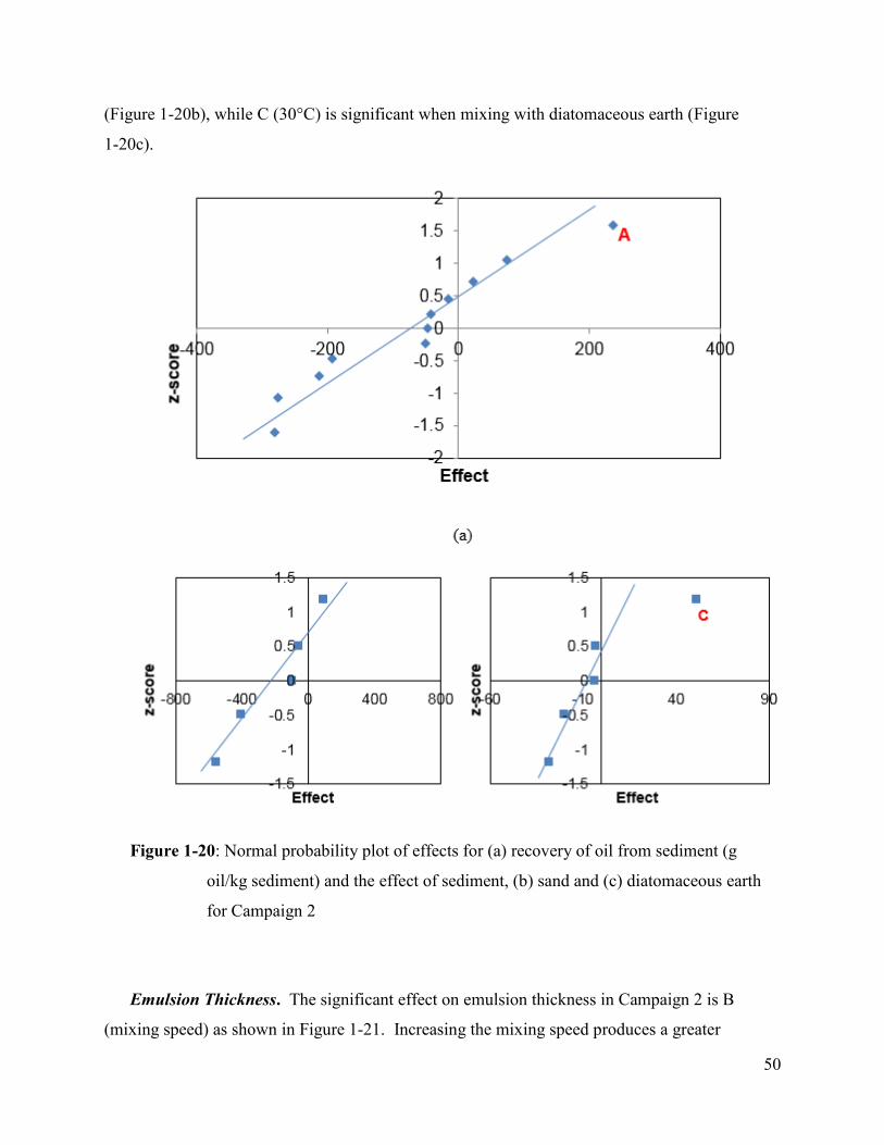
50

(Figure 1-20b), while C (30°C) is significant when mixing with diatomaceous earth (Figure

1-20c).

Figure 1-20: Normal probability plot of effects for (a) recovery of oil from sediment (g

oil/kg sediment) and the effect of sediment, (b) sand and (c) diatomaceous earth

for Campaign 2

Emulsion Thickness. The significant effect on emulsion thickness in Campaign 2 is B

(mixing speed) as shown in Figure 1-21. Increasing the mixing speed produces a greater

51

emulsion thickness, as would be expected. This was not observed in Campaign 1 as the range of

mixing speeds was much smaller.

Figure 1-21: Normal probability plot of effects for average emulsion thickness for Campaign 2

Water Recovery. As shown in Figure 1-22, C (temperature) has the greatest impact on water

recovery in Campaign 2. As the temperature increases, less of the water is recovered and more is

lost to the emulsion layer.

52

Figure 1-22: Normal probability plot of effects on water recovery for Campaign 2

1.6.2 Parity plots for mixing of diluted bitumen in salt water

Floating oil

From Campaign 2, there was no apparent effect of the input variables (Figure 1-18) which

indicates there is no significant impact of different mixing energies on floating oil recovery for

DB1 in SW.

Oil in water

The results from Campaign 2 show the effect of sediment (sand) as significant in increasing

the amount of DB1 dispersing into the water column (Figure 1-19). This is further illustrated in

Figure 1-23 where the greatest amount of oil is recovered from salt water when sand is present in

the system, thus, encouraging the interaction between oil and water during mixing. However, it

53

was noted that the water column almost completely cleared up after the 1-h settling time and oil-

sediment particles settled to the bottom of the jar.

Figure 1-23: Oil in salt water runs from Campaign 2

Lab images taken after mixing DB1 with sand and salt water, at varying mixing speeds

and temperatures, are show in Figure 1-23. These images are taken one day after mixing, and

obvious interactions occurred between the oil and sand at the bottom of each jar. Oil can be

found as dispersed droplets or dissolved oil components interacting with sediment in water

environments. Since oil and mineral particles have a negative surface charge in salt water, and

the presence of ions in the water thins out the electrostatic double layer repulsion between the oil

and mineral particles, the oil then settles at the bottom with the sediment (Gong et al., 2014).

The results of the effect of sediment on the dispersion of DB1 into the water column (Figure

54

1-19b and c) indicate that a high mixing energy is needed for DB1 to adhere to sand while low

mixing energy is required when mixing with diatomaceous earth. Mixing temperature does not

have an effect since oil-sediment interaction is seen at both mixing temperatures in Figure 1-24.

Oil-sediment interaction at the oil-water interface is shown in images Figure 1-24b, c and d. The

lighter OSAs rise to the oil-water surface. This interaction is defined as positively buoyant

OSAs since the oil-sediment particles rise to the oil-water interphase and remain there (Omotoso

et al., 2002).

Figure 1-24: DB1 with salt water and Sand (a) 8.2 RPM and 30oC, (b) 38.7 RPM and 30oC, (c)

2.3 RPM and ambient temperature, and (d) 8.2 RPM and ambient temperature

55

Oil on sediment

In Campaign 2, the most significant effect when mixing DB1 in salt water was A (sand) as

shown in Figure 1-20a. Images to support DB1 and sand interaction are shown in Figure 1-24;

spherical oil drops covered in a layer of sand are settled at the bottom of the jars. The ionic

strength effect, as discussed previously, encourages the interaction between the negatively

charged oil and sand particles. The effect of sediment type on the oil extracted from sediment

phase is shown in Figure 1-20b and c, for sand and diatomaceous earth respectively. No obvious

significant effects are shown in Figure 1-20b for sand, however, C (temperature) in Figure 1-20

implies a relation between diatomaceous earth and warmer mixing temperature on the amount of

oil extracted from the sediment layer.

Emulsion thickness

The main effect when mixing DB1 in salt water is the mixing speed (B + level, higher mixing

speed) as shown in Figure 1-21. Higher mixing energy encourages interaction between the water

and oil phases, trapping more water into the floating oil.

Water recovery

It was found from Campaign 2 that mixing DB1 in salt water with sand will produce a

thicker emulsion, while mixing DB1 in salt water with diatomaceous earth will improve water

recovery. From Figure 1-22, the significant effect on water recovery in Campaign 2 is C

(ambient temperature). At ambient temperature, there would be minimal effect on reducing the

viscosity of DB1 in salt water, which in turn, would minimize oil-water interaction.

A summary of the significant effects on the oil distribution, emulsions thickness and water

recovery is shown in Figure 1-25a, b, and c respectively. Output variables with no main effect

are marked with a ‘•’.

56

The results from Campaign 1 and 2 both show complex interactions between the oil and

sediment. A third campaign was set up with no sediment to isolate some of the other effects.

57


58


(c) Water Recovery


59

1.7 Campaign 3: Mixing in the absence of sediment

A third Campaign was designed with no sediment to isolate its effect on the oil distribution

and emulsion formation (eliminating sediment and mixing at the highest speed, Table 1-10). The

third Campaign was a 23 design, with seven interactions. The temperature (C), oil type (D) and

water type (E) were tested at two-levels.

The contrast coefficients and design matrix for Campaign 3 are shown in Table 1-11 and

Table 1-12, respectively.



A Sediment (No sediment)

B Mixing Speed * 55.4 RPM


D Oil DB1 CC

E Water FW SW

*: not tested at the low level


C D CD E CE DE CDE

-1 -1 1 -1 1 1 -1

1 -1 -1 -1 -1 1 1

-1 1 -1 -1 1 -1 1

1 1 1 -1 -1 -1 -1

-1 -1 1 1 -1 -1 1

1 -1 -1 1 1 -1 -1

-1 1 -1 1 -1 1 -1

1 1 1 1 1 1 1

60


Campaign 3 Factor

A B C D E ABCDE

Run Number Sediment Speed Temperature Oil Water Run

label

41 (no

sediment

added

for these

runs)

+ - - - - b

42 + + - - + bce

43 + - + - + bd

44 + + + - - bcd

45 + - - + + be

46 + + - + - bce

47 + - + + - bde

48 + + + + + bcde


Floating Oil Recovery. The normal probability plot for the floating oil show no significant

effects as shown in Figure 1-26 since the points are almost equally deviated from the straight

line.

61

Figure 1-26: Normal probability plot of effects for recovery of floating oil from Campaign 3

Oil in Water. The water type (fresh water) has the greatest impact on increasing the amount

of oil extracted from the water phase as shown in Figure 1-27.

Figure 1-27: Normal probability plot of effects of oil in water (g oil/kg water) for Campaign 3

62

Emulsion Thickness. No main effects of the variables were identified as significant on the

emulsion thickness formed after mixing in Campaign 3 (Figure 1-28).

Figure 1-28: Normal probability plot of effects for average emulsion thickness for Campaign 3

Water Recovery. As shown in Figure 1-29, no key effects were identified on the water

recovery in the absence of sediment.

63

Figure 1-29: Normal probability plot of effects on water recovery for Campaign 3

1.7.2 Significant effects when mixing in the absence of sediment

In the absence of sediment and mixing at the highest speed, the water type (fresh water) was

identified as the single significant effect which only impacts the amount of oil dispersed into the

water. As expected, oil particles disperse more freely in fresh water than salt water.

A summary of the significant effects for oil distribution, emulsion thickness and water

recovery are shown in Figure 1-30a, b and c, respectively.

64


65


(c) Water Recovery


66

1.8 Conclusions

The idea of deepening Canada’s ties with growing economies in Asia leads towards

the need to better understand the fate and behaviour of oil when spilled in fresh and

marine environments. The interactions that occur between oil, water and sediment after

an oil spill are complex. There is a strong dependence on the composition of the oil,

nature of the sediment particles, ionic strength of the aqueous phase, along with mixing

intensity and temperature.

This study was conducted to identify the main significant effects that occur when

mixing oil, water and sediment under the chosen mixing conditions. From the initial

variable screening tests, it was concluded that the mixing was complex. To simplify the

mixing, the effects of the variables were reduced in subsequent campaigns. It was found

that in the absence of sediment (Campaign 3), the type of water (fresh water) was the

main effect that only impacted the amount of oil dispersed into the water. CC dispersed

more in fresh water than DB1. When studying the impact of mixing speed with DB1 in

salt water (Campaign 2), the type of sediment (sand) had the greatest effect on the

interaction with water and sediment. These two campaigns highlighted the significance of

water type and sediment type in mixing. Similar results were also seen in the overall

screening of the results (Campaign 1) where salt water proved to have the greatest effect

on increasing oil recovery, while in fresh water more DB1 dispersed into the water at the

highest mixing speed. Furthermore, thicker emulsion layers formed with DB1 in fresh

water with sand. Both types of sediment interacted more with CC.

67

1.9 Acknowledgments

The authors would like to thank NRCan Program of Energy Research and

Development (PERD) and the Interdepartmental Tanker Safety Program for funding this

study, and the CanmetENERGY Environmental Impacts Team for the water analyses and

the Analytical Team for the hydrocarbon analyses. We would also like to acknowledge

the Canadian Association of Petroleum Producers (CAPP) for providing the two oils for

this study.

1.10 Nomenclature



b.p. boiling point




DJ,i inside diameter of jar

DJ,o outside diameter of jar

Dm diameter of jar mounting space

DS distance between mounting space

DB1 diluted bitumen


FW fresh water

HJ height of jar

HL height of liquid

68

HR rotation height

N radius of rotation

OMA oil mineral aggregates

OSA oil solid aggregates

SW salt water

Equations:

A represents first main effect, A

C contrast coefficient

fi cumulative frequency at position i of the data value in the ordered list

k number of variables

n number of runs or responses

y output result

1.11 References

Abdel-Rauf, M. E. (2012). Emulsions- composition stability and characterization Chapter

10. http://www.intechopen.com/books/crude-oil-emulsions-composition-stability-

and-characterization/factors-affecting-the-stability-of-crude-oil-emulsions

Andale Publishing. (2013). Normal probability plots.

Boglaienko, D., & Tansel, B. (2015). Instantaneous stabilization of floating oils by

surface application of natural granular materials (beach sand and limestone). Marine

Pollution Bulletin, 91(1), 107-112.

Boglaienko, D., & Tansel, B. (2016). Partitioning of fresh crude oil between floating,

dispersed and sediment phases: Effect of exposure order to dispersant and granular

materials. Journal of Environmental Management, 175, 40-45.

69

Boglaienko, D., & Tansel, B. (2017). Submergence patterns of floating crude oil by

granular particles. Chemical Engineering Journal, 314, 548-553.

Bradley, R. W., Venditti, J. G., Kostaschuk, R. A., Church, M., Hendershot, M., &

Allison, M. A. (2013). Flow and sediment suspension events over low‐angle dunes:

Fraser estuary, Canada. Journal of Geophysical Research: Earth Surface, 118(3),

1693-1709.

Bridie, A. L., Wanders, T. H., Zegveld, W., & Van der Heijde, H B. (1980). Formation,

prevention and breaking of sea water in crude oil emulsions ‘chocolate mousses’.

Marine Pollution Bulletin, 11(12), 343-348.

Butt, H., Graf, K., & Kappl, M. (2006). Physics and chemistry of interfaces John Wiley

& Sons.

Calvert, R. (1930). Diatomaceous earth. J.Chem.Educ, 7(12), 2829.

Crude Quality Inc. (2017). Crude monitor. http://www.crudemonitor.ca/home.php

Dapkunas, S. J., Jillavenkatesa, A., & Lum, L. H. (2001). Particle size characterization.

Fingas, M. (1995). Water-in-oil emulsion formation - a review of physics and

mathematical-modeling. Spill Science & Technology Bulletin, 2(1), 55-59.

Fingas, M. (2015). Diluted bitumen (dilbit): A future high risk spilled material.

Proceedings of Interspill. Edmonton, Alberta, Canada. Spill Science, 24

Fingas, M. (2014). Oil physical properties. Handbook of oil spill science and technology

(Chapter 20) John Wiley & Sons, Inc.

Fingas, M., & Fieldhouse, B. (2003). Studies of the formation process of water-in-oil

emulsions. 47(9-12), 369-396. http://dx.doi.org/10.1016/S0025-326X(03)00212-1

Fingas, M., & Fieldhouse, B. (2005). How to model water-in-oil emulsions. Paper

presented at the 2005 International Oil Spill Conference, IOSC 2005, May 15, 2005

- May 19, 11354-11361.

Fingas, M., & Fieldhouse, B. (2008). Water-in-oil emulsions: Studies on water resolution

and rheology over time. Paper presented at the 31st AMOP Technical Seminar on

Environmental Contamination and Response, June 3, 2008 - June 5, , 1 1-34.

Fingas, M., & Fieldhouse, B. (2012). Studies on water-in-oil products from crude oils and

petroleum products. Marine Pollution Bulletin, 64(2), 272-283.

http://dx.doi.org/10.1016/j.marpolbul.2011.11.019

70

Fingas, M., Fieldhouse, B., & Mullin, J. (2005). Water-in-oil emulsions: How they are

formed and broken. Paper presented at the 2005 International Oil Spill Conference,

IOSC 2005, May 15, 2005 - May 19, 9058-9060.

Fingas, M. F., Fieldhouse, B., Lane, J., & Mullin, J. V. (2005). What causes the

formation of water-in-oil emulsions? Paper presented at the 2005 International Oil

Spill Conference, IOSC 2005, May 15, 2005 - May 19, 9120-9125.

Gong, Y., Zhao, X., Cai, Z., O'Reilly, S. E., Hao, X., & Zhao, D. (2014). A review of oil,

dispersed oil and sediment interactions in the aquatic environment: Influence on the

fate, transport and remediation of oil spills. Marine Pollution Bulletin, 79(1-2), 16-

33. 10.1016/j.marpolbul.2013.12.024

Government of Canada. (2013a). Federal government technical report: Properties,

composition and marine spill behaviour, fate and transport of two diluted bitumen

products from the Canadian oil sands.

http://www.ec.gc.ca/Publications/default.asp?lang=En&xml=D6AB8B67-73F5-

48B6-B3D1-AAE1B06FF9A2

Government of Canada. (2013b). Properties, composition and marine spill behaviour, fate

and transport of two diluted bitumen products from the Canadian oil sands.

(Canadian Federal Government Technical Report No. Cat. No.: En84-96/2013E-

PDF). ISBN 978-1-100-23004-7

Gros, J., Nabi, D., Wurz, B., Wick, L. Y., Brussaard, C. P., Huisman, J., Arey, J. S.

(2014). First day of an oil spill on the open sea: Early mass transfers of

hydrocarbons to air and water. Environmental Science & Technology, 48(16), 9400-

9411.

Halboose, A. T. (2010). Effect of pH and salinity on stability of crude oil water

emulsions. Misan Journal for Academic Studies, 9(17)

Huang, C. P., & Elliott, H. A. (1977). The stability of emulsified crude oils as affected by

suspended particles. Fate and Effects of Petroleum Hydrocarbons in Marine

Organisms and Ecosystems. D.A.Wolfe, Ed., Pergammon Press, 413-420.

Huang, L., Fang, H., & Chen, M. (2012). Experiment on surface charge distribution of

fine sediment. Science China Technological Sciences, 55(4), 1146-1152.

Hutchinson Environmental Sciences Ltd. (2014). North Saskatchewan River: Water

quality and related studies (2007-2012) final report.

71

International Maritime Organization. (2005). Spills of heavy fuel oils - features and

countermeasures. Manual on oil pollution: Combating oil spills (pp. 195). UK:

Polestar Wheatons, Exeter.

International Towing Tank Conference. (2011). Fresh water and seawater properties. (No.

7.5-02-01-03).

Israelachvili, J. N. (2011). Intermolecular and surface forces Academic press.

Jenkins, R. H., Grigson, S. J. W., & McDougall, J. (1991). Formation of emulsions at

marine oil spills and the implications for response strategies. Paper presented at the

Proceedings of the First International Conference on Health, Safety and

Environment in Oil and Gas Exploration and Production Part 2 (of 2), November 11,

1991 - November 14, 437-443.

Kaku, V. J., Boufadel, M. C., Venosa, A. D., & Weaver, J. (2006). Flow dynamics in

eccentrically rotating flasks used for dispersant effectiveness testing. Environmental

Fluid Mechanics, 6(4), 385-406. 10.1007/s10652-006-0003-3

Kanicky, J. R., Lopez-Montilla, J., Pandey, S., & Shah, D. (2001). Surface chemistry in

the petroleum industry. Handbook of applied surface and colloid chemistry (pp. 251-

267) John Wiley and Sons Ltd New York.

Kester, D. R., & Pytkowicx, R. M. (1967). Determination of the apparent dissociation

constants of phosphoric acid in seawater. Limnology and Oceanography, 12(2), 243-

252.

Khelifa, A., Stoffyn-Egli, P., Hill, P. S., & Lee, K. (2002). Characteristics of oil droplets

stabilized by mineral particles: Effects of oil type and temperature. Spill Science and

Technology Bulletin, 8(1), 19-30.

http://www.sciencedirect.com/science/article/pii/S1353256102001172

Khelifa, A., Stoffyn-Egli, P., Hill, P. S., & Lee, K. (2005). Effects of salinity and clay

type on oil–mineral aggregation. Marine Environmental Research, 59(3), 235-254.


King, T. L., Robinson, B., Boufadel, M., & Lee, K. (2014). Flume tank studies to

elucidate the fate and behavior of diluted bitumen spilled at sea. Marine Pollution

Bulletin, 83(1), 32-37.

Kingston, P. F. (2002). Long-term environmental impact of oil spills. Spill Science &

Technology Bulletin, 7(1-2), 53-61. 10.1016/S1353-2561(02)00051-8

72

LaFargue, E., & Barker, C. (1988). Effect of water washing on crude oil compositions.

AAPG Bulletin, 72(3), 263-276.

Le Floch, S., Guyomarch, J., Merlin, F. X., Stoffyn-Egli, P., Dixon, J., & Lee, K. (2002).

The influence of salinity on oil-mineral aggregate formation. Spill Science &

Technology Bulletin, 8(1), 65-71. 10.1016/S1353-2561(02)00124-X

Lee, R. F., & Page, D. S. (1997). Petroleum hydrocarbons and their effects in subtidal

regions after major oil spills. Marine Pollution Bulletin, 34(11), 928-940.

10.1016/S0025-326X(97)00078-7

Lima, E. R., De Melo, B. M., Baptista, L. T., & Paredes, M. (2013). Specific ion effects

on the interfacial tension of water/hydrocarbon systems. Brazilian Journal of

Chemical Engineering, 30(1), 55-62.

Memarian, R., & Dettman, H. D. Energy scaling for understanding the effect of sand

particles on aggregate size of crude oils (unpublished)

Montgomery, D. C. (2013). Design and analysis of experiments (Eighth ed.). Hoboken,

NJ: John Wiley & Sons, Inc.

http://catdir.loc.gov/catdir/enhancements/fy1206/2012000877-t.html

Montgomery, D. C., & Runger, G. C. (2010). Applied statistics and probability for

engineers John Wiley & Sons.

Muschenheim, D. K., & Lee, K. (2002). Removal of oil from the sea surface through

particulate interactions: Review and prospectus. Spill Science & Technology

Bulletin, 8(1), 9-18.

National Oceanic and Atmospheric Administration. (2015). Why is the ocean salty?

Salinity data. http://oceanservice.noaa.gov/facts/whysalty.html

National Research Council. (2003). Oil in the sea III: Inputs, fates, and effects National

Academies Press.

Nordvik, A. B., Simmons, J. L., Bitting, K. R., Lewis, A., & Strm-Kristiansen, T. (1996).

Oil and water separation in marine oil spill clean-up operations. Spill Science &


Omotoso, O. E., Munoz, V. A., & Mikula, R. J. (2002). Mechanisms of crude oil-mineral

interactions. Spill Science & Technology Bulletin, 8(1), 45-54. 10.1016/S1353-

2561(02)00116-0

73

Özen, İ, Şimşek, S., & Okyay, G. (2015). Manipulating surface wettability and oil

absorbency of diatomite depending on processing and ambient conditions. Applied

Surface Science, 332, 22-31.

Poindexter, M. K., Chuai, S., Marble, R. A., & Marsh, S. C. (2005). Solid content

dominates emulsion stability predictions. Energy & Fuels, 19(4), 1346-1352.

Sjoblom, J., Aske, N., Auflem, I. H., Brandal, O., Havre, T. E., Sther, O., Kallevik, H.

(2003). Our current understanding of water-in-crude oil emulsions. Recent

characterization techniques and high pressure performance. Advances in Colloid and

Interface Science, 100-102, 399-473. http://dx.doi.org/10.1016/S0001-

8686(02)00066-0

Stewart, P. L. (2010). Oceanographic measurements - salinity, temperature, suspended

sediment, turbidity, minas passage study Site.

Stoffyn-Egli, P., & Lee, K. (2002). Formation and characterization of oil–mineral

aggregates. Spill Science & Technology Bulletin, 8(1), 31-44.

Teal, J. M., Farrington, J. W., Burns, K. A., Stegeman, J. J., Tripp, B. W., Woodin, B., &

Phinney, C. (1992). The west Falmouth oil spill after 20 years: Fate of fuel oil

compounds and effects on animals. Marine Pollution Bulletin, 24(12), 607-614.

Trefalt, G., & Borkovec, M. (2014). Overview of DLVO theory www.colloid.ch/dlvo

Tsai, W., Lai, C., & Hsien, K. (2006). Characterization and adsorption properties of

diatomaceous earth modified by hydrofluoric acid etching. Journal of Colloid and

Interface Science, 297(2), 749-754.

Venosa, A. D., & Holder, E. (2011). Laboratory-scale testing of dispersant effectiveness

of 20 oils using the baffled flask test. US Environmental Protection Agency, 600-

699.

Wei, Q., Mather, R. R., Fotheringham, A. F., & Yang, R. D. (2003). Characterization of

water-in-crude oil emulsions in oil spill response. Journal of Environmental

Sciences, 15(4), 506-509.

74

Chapter 2: Chemical Characterization of Oil

after Mixing in Fresh and Salt

Water

2.1 Abstract

The unique physical and chemical nature of a crude oil directly impacts its fate and

behaviour when spilled in fresh and salt water environments. The composition of the oil

will determine the extent of mixing, spreading, dispersion and evaporation after an oil

spill. An experimental campaign was conducted in an initial study to identify the

significant variables in oil and water mixing for diluted bitumen and conventional crude

oil (Section 1.5). Mixing behaviours in salt and fresh water were different, resulting in

interesting patterns for oil loss and sediment interactions for both oils. From the first

study of the two oils, the significant physical effects were that salt water had the greatest

impact on floating oil recovery, there is greater oil dispersion in fresh water than salt

water, conventional crude oil interacted more with sediment than diluted bitumen, and a

thicker emulsion layer was formed when mixing with diluted bitumen (Section 1.5) .

In this study, the chemical characteristics of the oil were determined for each fraction

and for different conditions. After each mixing test three fractions were collected; the

floating oil, the water fraction and the sediment. The floating oil was distilled to remove

water and the boiling point (bp) >204°C fraction was separated into maltenes and

asphaltenes fractions. The maltenes and asphaltenes fractions were then analyzed using

high temperature simulated distillation (SimDis), and elemental (carbon, hydrogen,

nitrogen, sulfur, oxygen) analyses. For the water and sediment phases, oil was isolated

first by carbon disulfide, then methylene chloride extraction and analyzed using high

temperature simulated distillation.

75

The purpose of this work was to identify the chemical reasons underlying the

significant physical differences in separation of the oil between the floating oil, oil in

water and the oil attached to sediment – and the associated emulsion formation -

identified in the mixing study.

76

2.2 Introduction

The demand for oil and its derivatives is only increasing with the increasing global

population as a source of energy and as feedstock for the manufacturing of goods. Due to

the limited geographic locations of oil sources, it must be transported from the point of

extraction for use to other countries. Canada recognizes the benefits and opportunities

new markets for oil will bring to the Canadian economy; however, there is much concern

over the risk of transporting oil through coastal waters. In recent years, there have been

several high-profile oil spills in water environments that have captured public interest

(i.e. Gulf of Mexico April 2010, Kalamazoo River July 2010). Oil spills occur as

accidental leaks from drilling rigs, pipelines, tankers, and barges (National Research

Council, 2003). Release of oil and chemicals into fresh and salt waters leads to

environmental and economic damage that can last for decades.

Conventional and non-conventional oil is made up of a wide range of hydrocarbons,

from very volatile compounds such as butane and benzene to more complex heavy

compounds such as asphaltenes, resins and waxes. The main physical properties that

affect the behaviour of oil spilled in fresh or sea water are density and viscosity. The

density will determine whether the oil can sink or float, while the viscosity, along with

the interfacial tension, influence the oil’s resistance to flow or spread over and into the

water. More viscous oils will not spread on nor mix into the water and will not penetrate

soils rapidly. The chemical characteristics of interest in this work are the relative

amounts of volatile components and asphaltenes, both of which influence oil-water

mixing. Oils which form stable water-in-oil emulsions will persist on the water surface,

while oil-in-water emulsions are found below the surface of the water (Wang et al.,

2003). Several studies have been carried out investigating the influence of asphaltenes on

the stability of an emulsion (Czarnecki et al., 2012; M. Fingas & Fieldhouse, 2004; M.

Fingas & Fieldhouse, 2005; M. Fingas & Fieldhouse, 2009; M. Fingas & Fieldhouse,

2012; McLean & Kilpatrick, 1997; Sjoblom et al., 2003; Tchoukov et al., 2014). The

asphaltenes content in diluted bitumen (approximately 13% for Cold Lake Bitumen) is

77

greater than conventional crude oils (approximately 2% for a Mixed Sweet Conventional

Crude) (McLean & Kilpatrick, 1997). Asphaltenes contain compounds that can be found

at the oil-water interface and which tend to act as a mechanical barrier. According to

McLean and Kilpatrick, if the asphaltenes are molecularly dissolved, they will not

contribute to emulsion formation; however, if they are colloidally dispersed they will

form a stable emulsion. According to their studies, resins aid in solubilizing the

colloidally dispersed asphaltenes to form aggregates. They then adsorb on to the oil-water

interface and decrease the interfacial tension (Abdel-Rauf, 2012). Fingas and Fieldhouse

(2004, 2005 and 2009) found emulsions formed have viscoelastic behaviour. Studies

have shown that water-in-oil emulsions are stabilized when resin content in the oil is

slightly greater than the asphaltenes content, however, an excess of resins

(asphaltene/resin ratio >0.6) may lead to instability of the emulsion (M. Fingas &

Fieldhouse, 2009). A study carried out by Czarnecki et al. (2012) examined the

contribution of asphaltenes to emulsion formation by testing properties of a thin oil film

separating two water droplets using the microinterferometric thin liquid film technique.

It was found that only small amounts of surface active agents are present in the

asphaltenes fraction.

When two immiscible liquids are in contact with each other, as in oil and water, an

interfacial area is formed. The fate of oil in water depends on the forces acting between

the oil and water molecules. The interaction energy between atoms and molecules can be

described by the van der Waals attraction forces and electrostatic repulsive forces (Trefalt

& Borkovec, 2014). At close distances between emulsion droplets, there is a strong van

der Waals attraction which increases with decreasing separation distance (attraction

forces varies inversely to separation distance) (Tadros, 2013). Droplets of oil and

sediment particles are negatively charged causing electrostatic repulsion between the oil

and sediment in fresh water. According to the theory of colloidal stability (DLVO

theory), an increase in water salinity reduces the surface charge density of the ions which

in turn weakens the electrostatic repulsion and allows the oil and sediment to aggregate

(Trefalt & Borkovec, 2014). According to the study by Gundlach and Hayes, sedimented

78

oil can sink 15-25 cm into steeper, medium to coarse grain sand beaches (0.25-2.0 mm

size) under high energy environments such as the Atlantic and Pacific coasts (Gundlach

& Hayes, 1978). Studies conducted in the Prudhoe Bay in Alaska found dissolved

hydrocarbons adsorbed onto mineral fines sinking to the bottom of the water column,

while some oil droplets interacted with the suspended particulates in the water to form

stable emulsions (Bragg & Owens, 1994). Sediment particulate concentrations greater

than 100 mg/L are required for oil-particulate suspensions to occur (R. F. Lee & Page,

1997). Water energy (in the form of waves or current) aid in increasing oil surface area

by breaking oil particulates into micron sized particles. The oil particles disperse easier in

the water column allowing solid particulates to adsorb to the surface (K. Lee, 2002; R. F.

Lee & Page, 1997). Tests have been conducted to identify the formation of flocs (masses

of fine oil-mineral particles) when oil is spilled in water and found mineral particles

attach to the oil droplets due to hydrophobic bonding (Omotoso et al., 2002). As long as

the size of the OMA (oil-mineral aggregate) exceeds the electrical double-layer

surrounding the particle, the particle acts as a surfactant preventing the oil droplets from

recoalescing (Stoffyn-Egli & Lee, 2002). The wettability, or contact angle, of a solid

particle determines the stability of the emulsion. When the three-phase contact angle is

slightly less than 90 degrees it will ensure the solid particles are held at the oil-water

interface and stabilize oil-water emulsions (when contact angle is greater than 90 degrees,

water-oil emulsions will be stabilized) (Tambe & Sharma, 1994).

Tests were conducted to identify the key interactions when conventional crude (CC)

and diluted bitumen (DB1) are mixed with water and sediment (Section 1.5). Mixing

tests were carried out in 2.2L borosilicate glass jars using an end-over-end rotary agitator.

The oil distribution after mixing from Campaign 1 of the study outlined in Section 1.5

was quantified by isolating the oil, water and sediment fractions and conducting oil mass

balances.

From the initial screening of the design factors (Campaign 1, Section 1.5), it was

found that salt water had the greatest impact on floating oil recovery. In terms of oil

79

dispersion into the water column, DB1 dispersed more in fresh water than CC at the

highest mixing speed and warmer mixing temperature. It was also found that CC

interacted more with sediment than DB1. A thicker emulsion layer was formed when

mixing with DB1.

The purpose of this study is to identify mechanisms for the significant effects

identified in Campaign 1 (Section 1.5) by conducting detailed hydrocarbon analyses of

the floating oil, and the oil samples isolated from the water and sediment.

2.3 Methods

2.3.1 Materials

The diluted bitumen and conventional crude oils chosen for this study were selected

because of their extensive transportation via pipelines, railways, and over water and,

because of their relative differences in chemical and physical properties (Table 2-3).

These oils were collected from Alberta pipelines courtesy of the Canadian Association of

Petroleum Producers (CAPP). The sand and diatomaceous earth were purchased from

Sigma-Aldrich Canada Co. for the tests and were used as received (more details on

sediment properties are available in Section 1.3.3). The solvents, carbon disulfide and

methylene chloride, used to extract the oil from the water and sediment were also

purchased from Sigma Aldrich Canada Co.

2.3.2 Analytical Methods

Density – ASTM 4052. The density was measured using a Mettler Toledo Digital

Densitometer according to the method recommended by the manufacturer.

80

Kinematic viscosity – ASTM D445-01. The kinematic viscosity was measured using

the Stabinger instrument according to ASTM D445-01 method.

High Temperature Simulated Distillation –ASTM D7169: The boiling range

distribution determination by distillation was simulated by the use of the Agilent 6890N

gas chromatograph and PAC software for processing the data. Boiling points were

assigned to the time axis from a calibration curve obtained under the same

chromatographic conditions by analyzing a known mixture of hydrocarbons covering the

boiling range expected in the sample. From this data, the boiling range distribution up to

750oC was measured. The data was processed first by fixing the mass and then by fixing

the boiling point. The latter method was used to merge the boiling point distribution data

obtained when oil was extracted from the water using the two different solvents based on

the yields from both extractions.

Distillation – ASTM D1160: To remove the water from the floating oil, and create

the ±204ºC fractions, the sample was distilled at reduced pressures. Each fraction was

distilled from the sample, collected, then gravimetrically measured and recorded.

Distillation yields by mass were calculated from the mass of each fraction relative to the

total mass recovery.

Pentane Insolubles (Separation of Asphaltenes & Maltenes fractions) – Modified

ASTM D4055: To isolate the maltenes and asphaltenes fractions, the asphaltenes were

removed from the +204ºC fraction of the oil by precipitation with pentane. A weighed

amount of sample was dissolved in 40 volumes of pentane and sonicated for 60 minutes.

The mixture was then filtered through an 8.0 μm nylon filter membrane under vacuum.

The filter and insolubles were washed, dried and weighed to calculate the insolubles

(asphaltenes). The filtrate was collected and transferred to a rotary evaporator flask and

the pentane is removed by rotary evaporation. The oil obtained was the maltenes

fraction.

81

Carbon, Hydrogen, Nitrogen, Sulfur (CHNS) – ASTM D5291 (CHN) and ASTM

D1552 (S): The carbon, hydrogen, nitrogen and sulfur contents were measured using an

Elementar Variomicrocube Analyzer.

Oxygen (in house): The oxygen contents of the samples were measured by an

Elementar Variomicrocube Analyzer according to the method recommended by the

manufacturer. The repeatability of measurements for this instrument is estimated to be ±

0.2wt%.

Surface tension and Interfacial tension: The surface tension was measured using

K100 Tensiometer (KRUSS Scientific Instruments Inc.) according to the method

suggested by the manufacturer. To determine the interfacial tension between the two oils

(CC and DB1) and the two types of water (salt and fresh) a spinning drop tensiometer

instrument (SDT), manufactured by KRÜSS, was used according to the method

recommended by the manufacturer.

Dean Stark (CanmetENERGY Devon): Another method used to quantitatively

determine the water content of an emulsion, was by Dean Stark extraction at

CanmetENERGY Devon. The solvent used for extraction was toluene. The oil was

extracted from the sample using the modified Soxhlet extractor apparatus by means of

heating toluene so that its vapors washed over the sample, separating the oil from the

water. The water was collected in the water trap, and the oil was collected in the boiling

flask, together with the toluene. The extraction was complete when there was a clear

colorless drip of toluene from the bottom of the thimble, and when the glassware was dry,

indicating that all of the water from the sample has been collected in the water trap.

Solvent extraction of oil in water (CanmetENERGY Devon): To determine the mass

of oil dispersed and dissolved in the water phase after mixing, the oil in the water sample

was first extracted using carbon disulfide followed by extraction with dichloromethane.

The two solvents were used because of their different solubility in oil. Solvent was added

to the separatory funnel containing the oil and water. The solvent-oil layer was separated

82

from the bulk water layer. The vial containing the solvent, oil and any water that may

have been collected during separation was placed in a dry-ice bath to freeze the water.

The solvent-oil layer was transferred to a vial using a syringe and then filtered through a

0.45 μm filter to remove any suspended particulates, then collected for analysis. To

determine the yield of the oil from the carbon disulfide extraction, a drop of the oil and

carbon disulfide was placed on a pre-weighed Whatman glass microfiber filter paper (1.5

μm pore size). The solvent was allowed evaporate and the weight of oil was obtained.

Any remaining oil in the bulk water sample was then extracted using dichloromethane.

The procedure for dichloromethane extraction was the same as carbon disulfide

extraction, except the dichloromethane was evaporated using nitrogen in an evaporation

chamber (TurboVapR LV) to isolate the oil sample. The yield of the oil collected in water

was calculated as g oil/kg water.

Solvent extraction of oil on sediment (CanmetENERGY Devon): To determine the

mass of oil on the sediment, the oil on sediment was extracted with dichloromethane.

Dichloromethane was added to the sediment sample vial (which also contained trace

water). The solvent-oil layer was transferred to a new vial using a syringe, and then

placed in a dry-ice bath to freeze any water that may have entered the syringe. The

solvent-oil layer was then filtered through a 0.45 μm filter to remove any suspended

particulates. The dichloromethane was evaporated using nitrogen in an evaporation

chamber (TurboVapR LV) to isolate the oil sample. The yield of the oil collected from

the sediment was calculated as g oil/g sediment.

2.3.3 Experimental design

The objective of this study was to characterize the floating oil, oil in water and oil on

sediment fractions after the mixing tests performed in Campaign 1 (Section 1.5). All five

variables (sediment, mixing speed, temperature, oil and water) were tested at two levels

as shown in Table 2-1. For each run label, the run condition is identified with lower case

83

letters for the input variables (compared to capital letters for input variable IDs). The

presence of a letter indicates that the variable was tested at the high level (+). The

absence of a letter in a run label indicates that the variable was tested at the low level (-).

The letter ‘L’ indicates that all variables are resent at the lower level (Table 2-2).






D Oil DB1 CC

E Water Fresh Salt

84


Campaign 1 Factor

A B C D E ABCDE

Run Number Sediment Speed Temperature Oil Water Run label

1 - - - - - - L

2 + - - - - + a

3 - + - - - + b

4 + + - - - - ab

5 - - + - - + c

6 + - + - - - ac

7 - + + - - - bc

8 + + + - - + abc

9 - - - + - + d

10 + - - + - - ad

11 - + - + - - bd

12 + + - + - + abd

13 - - + + - - cd

14 + - + + - + acd

15 - + + + - + bcd

16 + + + + - - abcd

17 - - - - + + e

18 + - - - + - ae

19 - + - - + - be

20 + + - - + + abe

21 - - + - + - ce

22 + - + - + + ace

23 - + + - + + bce

24 + + + - + - abce

25 - - - + + - de

26 + - - + + + ade

27 - + - + + + bde

28 + + - + + - abde

29 - - + + + + cde

30 + - + + + - acde

31 - + + + + - bcde

32 + + + + + + abcde

85

A detailed experimental method for the mixing tests is given in Section 1.3.7 and is

summarized here. Four replicate 2.8 L clear glass rotary agitator jars (Jar I, II, III, and

IV) with 1:20 (v/v) ratio of oil to water with 2000 ppm sediment were prepared for each

test. For salt water tests, 33 g/L of sodium chloride (NaCl) crystals were added to the jars

before addition of oil or sediment and shaken vigorously to dissolve the NaCl. The jars

were agitated for a total of 12 hours, then allowed to settle for one hour. After the

settling period, one jar (Jar IV) was set aside to monitor the emulsion thickness and

observe changes to the jar contents over a period of seven days. The oil, water and

sediment in the remaining three jars (Jars I, II, III) were isolated separately using a

separatory funnel. The water and sediment samples were analyzed to determine the oil

content in both phases. Shortly after mixing, the floating oil from Jars I, II, III was

analyzed using high temperature simulated distillation to determine the boiling point

distribution of the oil. After the seven day emulsion test was completed for each test, the

oil from Jar IV was added to the floating oil collected from Jars I, II, and III for each test.

The total floating oil underwent distillation to determine water content, and produce two

boiling point fractions, ±204oC. The water content provided information on the amount

of water trapped in the floating oil after each mixing condition. The fraction boiling

>204oC was further separated into the maltenes and asphaltenes fraction via the addition

of pentane to the oil sample. Elemental (carbon, hydrogen, sulfur, nitrogen and oxygen

content) and high temperature simulated distillation analysis were obtained for the

maltenes and asphaltenes fraction. The oil in the water and sediment was extracted using

carbon disulfide and dichloromethane. These oil samples were analyzed by high

temperature simulated distillation.

2.4 Results

To identify the chemical reasons for the key physical interactions as identified in

Section 1.5, the original oils, conventional crude (CC) and diluted bitumen (DB1), were

analyzed. The densities, viscosities, surface tension and interfacial surface tension results

86

are shown in Table 2-3. The original oils and floating oils were also analyzed by high

temperature simulated distillation for their boiling point distributions as shown in Figure

2-1. During an oil spill the light ends with boiling point less than 204ºC (boiling point,

b.p.<204ºC) would be lost due to evaporation (Zhou, Dettman, & Bundred, 2015).

Consequently, the fraction of oil boiling greater than 204ºC (b.p.>204ºC) was prepared

by distillation for the original and floating oils. To determine whether interactions with

water and sediment would cause changes to the hydrocarbons in the oils, the original oils

and floating oils were separated into two fractions based on polarity; maltenes (pentane

soluble) and asphaltenes (pentane insoluble). Their compositions by elemental analysis

are given in Table 2-3.

For the figures that follow, the naming convention for each of the data points (runs)

include the number sixteen (16) which is used to represent the batch number, followed by

the variable letter(s) (a, b, c, d, e) representing the run condition. As explained in Section

1.5, the presence of a letter indicates that the variable was tested at the high level (+). The

absence of a letter in a run label indicates that the variable was tested at the low level (-).

87

Table 2-3: Properties of Conventional Crude (CC) and Diluted Bitumen (DB1)

Crude Oil CC DB1

Density (g/ml)

20oC 0.8201 0.9237

25oC 0.8168 0.9203

30oC 0.8130 0.9166

Viscosity (cSt)

20oC 5.1 218.1

25oC 4.2 161.5

30oC 3.7 124.1

Surface tension (mN/m)

20oC 25.5 28.9

Interfacial tension (mN/m)

Fresh water (Devon, AB tap water)

20oC 12.24 16.58

30oC 14.16 16.00

Salt water (3.3 wt.% NaCl solution)

20oC 7.36 11.74

30oC 12.33 13.94

+204oC fraction

Carbon (wt.%) 86.65 84.26

Hydrogen (wt.%) 13.04 10.24

Nitrogen (wt.%) 0.03 0.46

Sulfur (wt.%) 0.66 4.33

Oxygen (wt.%) <0.1 0.81

H/C ratio 0.15 0.12

Maltenes content (wt.%) 98.48 81.86

Carbon (wt.%) 85.89 84.12

Hydrogen (wt.%) 13.05 11.14


Sulfur (wt.%) 0.41 3.98

Oxygen (wt.%) 0.59 0.48

H/C ratio 0.15 0.13

Asphaltenes content (wt.%) 1.52 18.13

Carbon (wt.%) 84.88 81.50

Hydrogen (wt.%) 8.09 7.46


Sulfur (wt.%) 4.21 8.68

Oxygen (wt.%) 1.74 1.23

H/C ratio 0.10 0.09

88

Figure 2-1: Floating oil boiling point distributions for (a) CC and (b) DB1 tests

89

After the mixing tests, the maltenes and asphaltenes fractions were also obtained for

the >204ºC fraction of the floating oils. The changes in the maltenes and asphaltenes

content from the original oil are shown in Figure 2-2. The percent change of maltenes

and asphaltenes contents from the original oil is calculated based on the absolute mass of

the maltenes and asphaltenes fractions in the floating oil relative to the mass of the two

fractions in the original oil. As shown in Figure 2-2, the asphaltene content increased in

the CC runs compared to the DB1 tests, while the maltenes content decreased in the CC

runs more than in the DB1 runs. These fractions were then further analyzed for their

elemental composition (carbon, hydrogen, sulfur, nitrogen and oxygen) and boiling point

distributions. The boiling point distributions for the maltenes and asphaltenes for the CC

and DB1 tests are shown in Figure 2-3 and Figure 2-4, respectively.

In Figure 2-3a and Figure 2-4a, there were no high temperature simulated distillation

data available for either original oil maltenes fractions.

Figure 2-2: Change in +204ºC fraction maltenes and asphaltenes content from original

oil

90


fractions for CC tests

91


fractions for DB1 tests

92

From the elemental analysis of the floating oil, minimal changes were observed in the

carbon, hydrogen, nitrogen and sulfur contents, with most changes being found in the

oxygen contents. For this reason, only the oxygen data is shown and the change in the

carbon, hydrogen, nitrogen and sulfur contents can be found in Appendix C. The percent

change from the original oil is calculated based on the absolute mass of the oxygen in the

maltenes and asphaltenes fractions relative to the mass of the oxygen in the two fractions

in the original oil. The change in the oxygen content (by mass) from the original oil for

the maltenes and asphaltenes fractions is shown in Figure 2-5. There is significant

increase in the oxygen content in the asphaltenes fraction for the CC runs compared to

the DB1 runs, while the oxygen content in the maltenes fraction decreased for all CC runs

and increased for most of the DB1 runs.

Figure 2-5: Change in oxygen content from original oil for maltenes and asphaltenes

fractions

In the previous study (Section 1.5), oil losses were observed for some of the runs. As

there were significant variations in the contents of material boiling greater than 750ºC

(Figure 2-3 and Figure 2-4) as well as significant changes in oxygen contents (Figure

93

2-5), the three sets of data for the runs are plotted in Figure 2-6 for the maltenes and

asphaltenes fractions, to observe whether there was a relationship between these factors.

As shown in Figure 2-6, there is more variance in the asphaltene fractions for both oils,

compared to the maltenes fraction.

94

Figure 2-6: Oil loss, +750ºC content, and oxygen content in +204ºC (a) maltenes

fraction and (b) asphaltenes fractions

After each mixing test, the water and sediment were separated from the floating oil.

The oil dissolved and dispersed in the water phase was extracted using carbon disulfide

95

and then dichloromethane. The boiling point distributions for the extracted oils were then

measured. Since two solvents were used for extraction, each oil sample from the water

had two boiling point distributions. The two boiling point distributions were combined

based on the yield of oil from each extraction. The resulting boiling point distribution

curves for the oil isolated from the water phase for the CC and DB1 tests are shown in

Figure 2-7. This shows us that there is greater variance in the boiling point distributions

of the DB1 oil extracted from the water as compared to the CC oil.

96

Figure 2-7: Boiling point distributions of oil extracted from the water for (a) CC and (b)

DB1 tests

97

From the sediment samples collected, the oil on the sediment was extracted using

dichloromethane. The boiling point distribution results for the oil extracted from the

sediment for the CC and DB1 runs are shown in Figure 2-8. There is an increase in the

>750ºC boiling material for the DB1 runs as compared to the CC runs.

Note that there was not enough oil extracted for Run 16-ace and Run 16-ae to obtain

the boiling point distribution for those DB1 runs (Figure 2-8b).

98

Figure 2-8: Boiling point distributions of oil extracted from sediment for (a) CC and (b)

DB1 tests

99

To determine the effects of mixing on the boiling point distribution of the oils, the

data was grouped into four boiling range fractions including initial boiling point (IBP) to

204ºC for naphtha, 204ºC-343ºC for middle distillate, 343ºC-524ºC for gas oil and

524ºC+ for residue. The mass of each boiling range fraction was calculated from the

yields of the floating oil, oil in water and oil from sediment for each test. Once the total

mass of each boiling fraction was determined for a test, the difference with respect to the

original oil content was determined. The change in the mass of each boiling range

fraction after each mixing test is shown in Figure 2-9. The residue fraction increases for

most DB1 runs compared to the CC runs, while there is a decrease in the naphtha, middle

distillate and gas oil fractions for both DB1 and CC.

Figure 2-9: Change in boiling range fractions based on original oil content

2.5 Discussion

Mixing between oil and water in the presence of sediment is a complex phenomenon.

The significant physical effects from the initial screening of the design factors were that

100

salt water had the greatest impact on floating oil recovery with greater recovery of DB1

than CC in salt water; DB1 dispersed more in fresh water than CC; CC interacted more

with sediment than DB1; and a thicker emulsion layer was formed when mixing with

DB1 (Section 1.5). The objective of this study was to analyze the chemical changes of

the oil after mixing to determine if certain components of the oil preferentially dispersed

into one of the three phases.

Floating oil. The conventional method of predicting the behaviour of oil when

spilled on water is by relating the density and viscosity of the oil to that of water. As

long as the density of the oil is less than water, it is expected to float. The density of the

oils used in this study were both less than that of water (Table 2-3), and as expected, the

bulk oil remained floating on the water after mixing. The viscosity of DB1 was

considerably higher than that of CC (Table 2-3), and according to Stoffyn-Egli and Lee

(2002), increasing the viscosity of an oil would reduce interaction with sediment. A

lower viscosity oil would mix more in the water creating more surface area for the oil to

interact with the sediment. This supports our findings that CC, with the lower viscosity,

interacted more with sediment compared to DB1. Although DB1 was found to disperse

more in fresh water than CC, due to its higher viscosity, there was less surface area of

DB1 available to interact with sediment (Stoffyn-Egli & Lee, 2002). Another chemical

property that is used to predict the behaviour between oil and water is the interfacial

tension between the two liquids. The lower the interfacial tension, the greater the

interaction between the oil and water, with the opposite holding true as well (Butt et al.,

2006; Israelachvili, 2011). As shown in Table 2-3, the interfacial tension data between

CC and fresh and salt water is less than that for DB1. This suggests that CC would

interact more in both types of water. However, the mixing tests show that DB1 remained

dispersed more into fresh water than CC, indicating that other variables can have a

significant impact on the mixing. The interfacial tension data can also be used to predict

the behaviour of the starting oils in salt versus fresh water. The interfacial tension for

both CC and DB1 is lower in salt water compared to fresh water (Table 2-3). From this

information alone, it would imply that the oils would mix in salt water more than fresh

101

water, which is supported by the study carried out by Omotoso et al. (2002). However,

according to Hollebone (2014), the interfacial tension of oils in salt water is greater than

the interfacial tension of oils in fresh water. This supports the finding from the first study

where the floating oil recovery was greater in salt water than fresh water as a result of

less interaction with salt water. A higher interfacial tension in salt water also supports the

salting-out effect, or the effect of an ionic solution on oil-water mixing. With increased

salt concentration in the water, the surface charge density of the oil particles decreases

causing less oil dispersion in salt water, allowing for greater oil separation from water

(Le Floch et al., 2002; Stoffyn-Egli & Lee, 2002; Trefalt & Borkovec, 2014). This

phenomenon was discussed in further detail in the initial study in Section1.5. Hollebone

(2014) also suggests that the error in interfacial tension measurements can be as high as

±15%, so these values and their effects should be interpreted with caution.

Another key interaction identified in the initial study was that DB1 formed a thicker

emulsion layer than CC. Even though the surface tension of DB1, and the interfacial

tensions of DB1 with salt and fresh water, are all greater than CC, from the mixing tests it

was found that more water was entrained in DB1 causing the production of a larger

emulsion volume. This could be a result of the nature of mixing a higher viscosity oil in

an end-over-end style agitator, causing entrainment of pockets of water in the oil

resulting in thicker emulsions. These pockets of entrained water were observed during

distillation of the DB1 floating oil, causing bumping of the sample. The entrained

pockets of water could also be attributed to the polarity of DB1. The presence of

heteroatoms and the aromaticity of an oil influences its polarity. DB1 is more polar than

CC (Table 2-3). The higher polarity would foster the mixing with fresh water, while the

higher viscosity would trap pockets of water caused by the rotational mixing in the jars

producing thicker emulsions with DB1. The effect of polarity on the oils mixing in the

water phase is covered later in the discussion.

The high temperature simulated distillation data of the floating oils provides further

information on changes that occur due to mixing. The boiling point distribution data

102

show how the content of the material boiling greater than 750ºC changes after mixing.

The addition of oxygen to the hydrocarbons could result in the boiling points of the

hydrocarbons being higher than 750ºC. However, it is also possible that oxygenated

compounds may not be soluble in the carbon disulfide solvent used in the analysis. This

would result in a greater proportion of material being reported as having greater than

750ºC boiling point. In Figure 2-1a, there is a diverse range of b.p.>750ºC contents for

the CC compared to the DB1 tests (Figure 2-1b), where contents varied from more than

60 wt% of b.p.>750ºC boiling material to less than that of the starting oil. For DB1, there

was less variance with exception of one of the tests, run 16-ab, containing ~70 wt% of

b.p. >750ºC material, while the rest clustered around the same amount as the starting oil.

These results indicate that there are variable quantities of either higher boiling or

insoluble compounds remaining in the CC compared to the starting oil.

The reasons for the significant effects mentioned above were based on the bulk oil

properties which provided partial explanation due to the heterogeneity nature of the oils.

Chemical analyses of the sub-fractions of the oils (below) provided further insight to the

observations.

Since in an actual oil spill scenario there would be losses of the lighter boiling

material in the oil (b.p.<204ºC) (Zhou et al., 2015), it was important to understand the

behaviour of the heavier oil (b.p.>204ºC) that would remain with the water. The analyses

of the boiling fraction b.p.>204ºC produced by distillation of the original and floating

oils, offered information about changes in molecular composition due to conversion to

another fraction or losses from the oil, the presence of biodegradation and interaction

with sediment. As shown in Figure 2-2, there is greater variance in the asphaltenes

contents after mixing, with minimal change in the maltenes contents for the CC tests. For

the DB1 tests there was minimal variance in both the maltenes and asphaltenes contents.

With CC being a lighter oil than DB1, the starting oil will contain more maltenes and less

asphaltenes than DB1 (Gray, 1994), which is consistent with results presented in Table

2-3. An increase in oxygen content in the floating oil could cause the asphaltenes content

103

to increase at the expense of the maltenes fraction. Similar information is also shown in

Figure 2-3a and Figure 2-3b for CC, where there was minimal change in the maltenes

boiling point distributions, but a wider range of b.p.>750ºC contents for the asphaltenes.

The curves to the right of the original CC asphaltenes sample indicate the amount of

material that boils at temperatures greater than 750ºC in the floating oil had reduced after

mixing. Each of these runs were conducted at the warmer mixing temperature, except for

Run 16-d. This implies that mixing at higher temperatures increases the amount of

heavier boiling material (at the expense of the lighter boiling material). The initial

boiling point for Run 16-bd shows the presence of oxygen containing lower boiling

compounds that may have shifted into the asphaltenes after the maltenes were oxidized.

A few DB1 tests saw a slight increase in the asphaltene content: runs 16-e, 16-be, 16-abe

and 16-ce (Figure 2-2), along with an increase in the b.p.>750ºC boiling material ranging

from 30%-60% (Figure 2-4b). The smaller changes for the diluted bitumen are consistent

with the effects seen for CC due to biodegradation as there are greater contents of

susceptible hydrocarbons present in CC compared to the DB1. Bitumen is the result of

biodegradation of crude oil in the reservoir so the most susceptible hydrocarbons for

biodegradation are no longer present.

Changes in the oxygen content in the floating oil could be the result of oxidation of

the hydrocarbons, possibly by biodegradation and/or interaction with the silicon oxide

and aluminum oxide from the sediment. The greatest increase in oxygen occurs in the

asphaltene fractions of the CC tests in runs 16-d, 16-cd and 16-bcd (Figure 2-5). These

three runs were mixed in the presence of diatomaceous earth in fresh water. Runs 16-cd

and 16-bcd were both carried out at the warmer mixing temperature. Warmer mixing

temperatures would encourage biodegradation of the oil. The decrease in the oxygen

content in the maltenes fraction was ~1% and was consistent for all of the CC tests. As

shown in Figure 2-5, the increase in the oxygen content was minimal when mixing DB1

in fresh water (~0.5%) for both the maltenes and asphaltenes fractions, while the oxygen

content increases for runs in salt water in both fractions (up to 1.5%). Oxygen increase

caused by the interaction with sediment would yield an elemental mass balance (carbon,

104

hydrogen, nitrogen, sulfur and oxygen) less than 100% due to the silicon and aluminum

not being measured. This was observed in the asphaltenes fraction for some of the CC

and DB1 tests. Runs 16-cd, 16-acde 16-bcd and 16-d had the greatest increase in

asphaltenes (Figure 2-2), the greatest amount of >750ºC boiling material in the

asphaltene fraction (Figure 2-3b), and also the greatest increase in oxygen content for the

CC tests (Figure 2-5). Interaction with the silicon oxide and alumina oxide in both the

diatomaceous earth (Run 16-cd, Run 16-bcd and Run 16-d) and sand (16-acde) could

cause an increase in oxygen content for these runs as shown in Figure 2-5. All of these

runs had elemental mass balances ranging between 70-85%. This suggests interaction

with sediment could be significant. Metals analyses of these oil samples would provide

more information on the extent of interaction with sediment.

When comparing the oil loss, b.p.>750ºC content, and change in oxygen from

original oil, there is a decrease in the oxygen content in the maltenes fraction for the CC

tests with higher oil loss per run, while the oxygen content increases for the DB1 tests

with lower oil loss in the salt water runs (Figure 2-6a). The amount of material boiling

greater than 750ºC ranges between 0-10% for the CC runs and 2-16% for the DB1 tests.

The increase in oxygen content in the maltenes fractions for the DB1 tests also show an

increase in material boiling greater than 750ºC. Since the range for the axis representing

the change is oxygen content in the maltenes is so narrow (±1%), the observable change

could be within the error of the analysis. The notable increase in oil loss for runs 16-bcd

and 16-abcd was due to oil losses encountered during the mixing tests (leaking jars), so

these results do not represent actual oil loss caused by the mixing condition. As for the

asphaltenes fractions (Figure 2-6b), an increase in oxygen content results in an increase in

the b.p.>750ºC material in the CC oil. This may be a result of the solubility effect of

oxygenated compounds that show up as material boiling >750ºC. The change in oxygen

content varies more in fresh water runs compared to the salt water runs, and is more

pronounced with CC than DB1. This is consistent with CC being more biodegradable

than DB1 (more susceptible hydrocarbons for biodegradation are present). The opposite

can be seen in the DB1 runs; the change in oxygen in the asphaltenes fraction is quite

105

steady around 0.3% in fresh water runs, while the increase in oxygen in the salt water

runs varies between 0.3-1.5% due to the different microbes that exist in fresh versus salt

water. The amount of material that boils >750ºC is greater in the salt water runs with

DB1 compared to the fresh water runs. Less variance was observed with the DB1 tests,

since DB1 contains less available hydrocarbons to undergo biodegradation at the same

rate as CC. The relationship with the amount of oil loss per run is inconclusive as the

results show no obvious trend.

Oil in water and sediment. As shown in Figure 2-7a, most of the CC oil extracted

from the water has less than 10% material boiling greater than 750ºC with the exception

of Runs 16-cde (85%), 16-abcd (65%), and 16-abcde (65%). The runs with the greatest

amount of heavier boiling material in Figure 2-7a were all carried out at the higher

mixing temperature. This implies greater biodegradation at the higher mixing temperature

which then shows up as material boiling greater than 750ºC. It is interesting to note that

runs 16-cde and 16-abcde were both mixed with salt water, yet exhibited the greatest

content of b.p.>750ºC. This implies the effects of other variables may have greater

impact. There is greater variance in the boiling point distributions for DB1 tests extracted

from the water phase (Figure 2-7b). Run 16-ace has almost 85% material that boils

greater than 750ºC while for runs 16-ae, 16-bc and 16-ab the content of the heavier

boiling material is greater than 75%. The greatest content of heavy boiling material for

the CC tests (85%) was when mixed with diatomaceous earth (Figure 2-7a), while the

greatest content of heavy boiling material for the DB1 tests (87%) was when mixed with

sand (Figure 2-7b). From Figure 2-7, it is clear that there is greater variance in the

boiling point distribution results for the DB1 tests than CC tests; this would suggest

presence of oxygenated compounds from biodegradation and/or interaction with

sediment. Additional elemental and metals analyses of the oil isolated from the water

phase would provide more information to further explain the trends of the boiling point

distribution curves.

106

As shown in Figure 2-8a, the oil extracted from the sediment from the CC tests in

Run 16-de had the greatest amount of heavier boiling material (45%) followed by Run

16-acde (30%). Both of these runs were mixed in salt water with the two different

sediments (16-de was mixed with diatomaceous earth and 16-acde mixed with sand).

The content of the material boiling >750ºC for the DB1 oil extracted from the sediment is

greatest for Run 16-a (75%) as shown in Figure 2-8b. It can be seen that DB1 extracted

from the sand in fresh water (Run 16-a) and sand in salt water (Run16-abce) both contain

the greatest amount of material boiling greater than 750ºC, with the difference being the

mixing speed and temperature. The oil for Run 16-ac was extracted using carbon

disulfide, instead of dichloromethane, which is the reason for the low initial and final

boiling points shown in Figure 2-8b as the higher boiling material in the oil was not

extracted from the oil-sediment sample. DB1 tests contain a wider range of b.p. >750ºC

material than the CC tests. Even though greater quantities of CC were extracted from the

sediment in the initial study, the CC oil recovered has less material that boils >750ºC

compared to the DB1 tests. As with the oil extracted from the water, elemental and

metals analyses of the oil from the sediment would provide more information about the

causes for the differences in boiling point curves from the CC and DB1 tests.

The polarity of an oil provides information on the behaviour of the oil when it enters

the water column and interacts with sediment. DB1 is more polar than CC due to the

higher heteroatom content and lower hydrogen to carbon ratio (H/C ratio) in the

b.p.>204ºC fraction as shown in Table 2-3. The higher polarity of DB1 would lead to

greater recovery in salt water because of the ionic effect at the oil-water interface. This

further supports the significant effect observed that there was greater oil recovery in salt

water, with the recovery of DB1 being greater than CC. Subsequently, in fresh water, the

higher polarity of DB1 would cause it to disperse more in fresh water, as was observed as

a significant effect in the mixing tests. On the other hand, CC is less polar than DB1

since it has greater H/C ratio and lower heteroatom content (Table 2-3). As CC is mixed

with the water, smaller oil droplets are formed (due to lower viscosity) allowing for a

greater surface area for the microbes in the water to work at the oil-water interface. This

107

creates a greater opportunity for biodegradation causing a larger increase in oxygen

content (Figure 2-5) and increase in its polarity. The smaller oil droplets would lead to

more interaction with sediment as well. This was observed in the mixing tests (identified

as a significant effect). Based on the effect of the polarity of the two oils, there is greatest

recovery of DB1 in salt water and most dispersion of DB1 in fresh water. This behaviour

is further illustrated in Figure 2-10.

Figure 2-10: Polarity effect on mixing CC and DB1 in water with sediment

Full oil distribution. The mass of each boiling fraction from the floating oil, oil in

water and oil on sediment were combined and then compared to the mass of the boiling

fractions in the original oil (Figure 2-9). Even in a closed system, the naphtha content for

the runs decreased after mixing and was most prominent for the DB1 tests. Since the

108

initial boiling points remained similar for both oils (Figure 2-1), the loss was not

primarily due to evaporation, except for the two DB1 samples that did lose the lightest

hydrocarbons (runs 16-ae and 16-b, Figure 2-1b), which correlate to the losses shown in

Figure 2-9 for the same runs. There is a slight increase in the middle distillate and gas oil

fractions in the CC with fresh water runs, and then decreases with the salt water runs.

This may be a result of partial biodegradation of the residue fraction creating more

middle distillate and gas oil fractions. The greatest amount of residue is found in Run 16-

bd when mixing with CC. Most of the runs with DB1 show an increase in the amount of

residue in the resulting oil, which is not biodegradable. The loss of the naphtha, middle

distillate and gas oil fractions is also greater with the DB1 runs. Interestingly, changes

due to the polarity of the oils, as discussed previously, are not reflected in the overall

boiling point distributions.

2.6 Conclusions

This work focussed on the analysis of the original oil, floating oil and oil from the

water and sediment to understand the causes of the significant physical effects identified

in the first study (Section 1.5). The significant physical effects from the initial screening

of the design factors were that salt water had the greatest impact on floating oil recovery

with greater recovery of DB1 than CC in salt water; DB1 dispersed more in fresh water

than CC; CC interacted more with sediment than DB1; and, a thicker emulsion layer was

formed when mixing with DB1.

The bulk oil properties provided the necessary information to explain the key

interactions during mixing, and analyses of the sub-fractions of the oils identified the

significance of polarity of the oils during mixing. It was found that the floating oil

recovery in salt water was greater than in fresh water, due to the decrease in electrostatic

repulsion between the oil particles caused by the ionic effect in salt water. The interfacial

tension results measured for the bulk oils could not be interpreted according to the

109

literature, possibly due to the heterogeneity of the oils. According to literature, the

interfacial tension of oils in fresh water is less than that in salt water (Hollebone, 2014),

which explains why this behaviour was observed in the initial study. As for the reason

behind thicker emulsions forming with DB1, it was concluded that the density and

viscosity were important factors. With a higher density and viscosity than CC, DB1 did

not mix in to the bulk water as easily and the mixing method (rotary agitation) caused

entrainment of water pockets in the oil. It was also identified from the mixing tests that

DB1 dispersed more in fresh water compared to salt water. The higher viscosity of DB1

compared to that of CC could be the reason why DB1 remained dispersed in the water

column and did not resurface as was observed for CC. Further analyses of the sub-

fractions of the oils revealed that the polarity of the oils, along with the bulk oil

properties, also influenced the extent of interaction with water and sediment. Although

DB1 interacted more with water, CC was found to interact most with sediment due to its

lower viscosity, which is also supported by literature (Stoffyn-Egli & Lee, 2002). It was

found that the changes in the boiling point distributions were most significant when

mixing with CC than DB1. There was also greater increase in the asphaltenes content

after mixing with CC along with a greater increase in oxygen content in the asphaltenes

fraction for CC. This behaviour suggests interaction with sediment and the presence of

bioactivity with CC. Further analyses of the metals content in the asphaltenes fraction,

along with analysis of nuclear magnetic resonance (NMR) and Fourier transform infrared

spectroscopy (FTIR) data would provide insight to the source of oxygen.

More change occurred in the naphtha, middle distillate, gas oil and residue fractions

when mixing with DB1 compared to CC. Mixing DB1 and salt water resulted in more

loss of the naphtha fraction with an increase in the residue fraction.

The results from this work provide further information to the findings from the first

study. The effect of salt water and interaction with sediment have shown to be significant

factors in changes to the oil after mixing. The knowledge of the physical and chemical

changes that occur after oil is spilled on water is beneficial from an oil spill remediation

110

perspective. However, the impact of an oil spill on water varies greatly depending on the

unique chemical composition of the oil, and the dynamic water and environment

conditions.

2.7 Acknowledgments

The authors would like to thank NRCan Program of Energy Research and

Development (PERD) and the Interdepartmental Tanker Safety Program for funding this

study, and the CanmetENERGY Environmental Impacts Team for the water analyses and

the Analytical Team for the hydrocarbon analyses. We would like to recognize the

efforts of Dr. Aleksey Baldygin and his supervisor Dr. Prashant Waghmare, from the

University of Alberta Mechanical Engineering Department, for analyzing the surface

tensions and interfacial tensions of the oil and water samples. We would also like to

acknowledge the Canadian Association of Petroleum Producers (CAPP) for providing the

two oils for this study.

2.8 Nomenclature



b.p. boiling point




DB1 diluted bitumen


FTIR Fourier Transform Infrared Spectroscopy

111

NMR Nuclear Magnetic Resonance

2.9 References

Abdel-Rauf, M. E. (2012). Emulsions- composition stability and characterization chapter

10. Retrieved from http://www.intechopen.com/books/crude-oil-emulsions-

composition-stability-and-characterization/factors-affecting-the-stability-of-crude-

oil-emulsions

Bragg, J. R., & Owens, E. H. (1994). Clay-oil flocculation as a natural cleansing process

following oil spills: Part 1. Studies of shoreline sediments and residues from past

spills. Environment Canada, Ottawa, ON. (Canada). 1, 1-23.


& Sons.

Czarnecki, J., Tchoukov, P., & Dabros, T. (2012). Possible role of asphaltenes in the

stabilization of water-in-crude oil emulsions. Energy & Fuels, 26(9), 5782-5786.

Fingas, M., & Fieldhouse, B. (2004). Formation of water-in-oil emulsions and application

to oil spill modelling. Journal of Hazardous Materials, 107(1-2), 37-50.



- May 19, 11354-11361.

Fingas, M., & Fieldhouse, B. (2009). Studies on crude oil and petroleum product

emulsions: Water resolution and rheology. Colloids and Surfaces A:

Physicochemical and Engineering Aspects, 333(1-3), 67-81.



Gray, R. M. (1994). Upgrading petroleum residues and heavy oils CRC press.

Gundlach, E. R., & Hayes, M. O. (1978). Vulnerability of coastal environments to oil

spill impacts. Marine Technology Society Journal, 12(4), 18-27.

112

Hollebone, B. P. (2014). Oil physical properties. Handbook of oil spill science and

technology (pp. 37-50) John Wiley & Sons, Inc.

Israelachvili, J. N. (2011). Intermolecular and surface forces Academic press.




Lee, K. (2002). Oil-particle interactions in aquatic environments: Influence on the

transport, fate, effect and remediation of oil spills. Spill Science & Technology

Bulletin, 8(1), 3-8. 10.1016/S1353-2561(03)00006-9



10.1016/S0025-326X(97)00078-7

McLean, J. D., & Kilpatrick, P. K. (1997). Effects of asphaltene solvency on stability of

water-in-crude-oil emulsions. Journal of Colloid and Interface Science, 189(2), 242-

253. 10.1006/jcis.1997.4807


Academies Press.



2561(02)00116-0




Interface Science, 100-102, 399-473.



Tadros, T. F. (2013). Emulsion formation and stability John Wiley & Sons.

Tambe, D. E., & Sharma, M. M. (1994). The effect of colloidal particles on fluid-fluid

interfacial properties and emulsion stability. Advances in Colloid and Interface

Science, 52, 1-63.

113

Tchoukov, P., Yang, F., Xu, Z., Dabros, T., Czarnecki, J., & Sjoblom, J. (2014). Role of

asphaltenes in stabilizing thin liquid emulsion films. Langmuir, 30(11), 3024-3033.

Trefalt, G., & Borkovec, M. (2014). Overview of DLVO theory

Wang, Z., Hollebone, B. P., Fingas, M., Fieldhouse, B., Sigouin, L., Landriault, M.,

Weaver, J. W. (2003). Characteristics of Spilled Oils, Fuels, and Petroleum

Products: 1. Composition and Properties of Selected Oils. US EPA Report EPA/600-

R/03, 72

Zhou, J., Dettman, H., & Bundred, M. (2015). A comparative analysis of environmental

behaviour of diluted bitumen and conventional crudes. Paper presented at the

AMOP, 495-516.

114

Chapter 3: Conclusions, Implications and

Recommendations for Future Work

From the first part of the study it was found that mixing with salt water and the

presence of sediment have significant influence the oil distribution after mixing. The

significant physical effects from the initial screening of the design factors were that salt

water had the greatest impact on floating oil recovery with greater recovery of DB1 than

CC in salt water; DB1 dispersed more in fresh water than CC; CC interacted more with

sediment than DB1; and, a thicker emulsion layer was formed when mixing with DB1.

From the second part of the study, the bulk oil properties provided the necessary

information to explain the key interactions during mixing, and analyses of the sub-

fractions of the oils identified the significance of polarity of the oils during mixing. The

effect of viscosity and interfacial tension allowed for greater mixing of conventional

crude into the water increasing interaction with sediment. The most change in elemental

composition after mixing was observed in the conventional crude mixing tests, with the

greatest change occurring in the oxygen content for the maltenes and asphaltene

fractions. Conventional crude oil has a higher hydrogen-to-carbon ration allowing for

more substrate which contains the necessary hydrocarbon chains for biodegradation.

Interaction with sediment and biodegradation of the conventional crude oil would cause a

change in the oxygen content of the floating oil after mixing. Further analyses of the

oxygen containing hydrocarbons (metals content and NMR with FTIR analyses) would

provide more information on the source of the oxygen.

The results from this study are useful not only for reclamation and the effects on

marine life, but also for oil spill responders so they can make a more informed decision

on appropriate oil spill response options and strategies. As shown from the mixing tests,

diluted bitumen and conventional crude oil exhibit quite different mixing behaviours in a

115

water environment. Information on the significant effects on mixing behaviour after an

oil spill would provide valuable information for modelling oil spill behaviour.

Understanding the fate of the oil, would fill key knowledge gaps that currently exist.

More information is required to fully understand the fate and behaviour of oil after an

oil spill under varying environmental conditions. Recommendations for future studies:

Conduct similar mixing tests at cooler temperatures (similar to winter or arctic

conditions) would increase the range between the positive and negative levels

in a factorial design for the temperature variable and provide an insight on the

fate of on oil spills in cooler waters.

Study similar mixing tests on weathered oils since the composition of

weathered and fresh oils differ in their heavier fractions. Accounting for

evaporation will be more representative of spills in open waters.

Studying the effect of water pH on the mixing of oil, water and sediment will

allow for a better understanding on how the varying pH of different bodies of

water will affect oil-water-sediment interaction.

116

References (all)

Abdel-Rauf, M. E. (2012). Emulsions- composition stability and characterization chapter

10. http://www.intechopen.com/books/crude-oil-emulsions-composition-stability-

and-characterization/factors-affecting-the-stability-of-crude-oil-emulsions

Andale Publishing. (2013). Normal probability plots.

Boglaienko, D., & Tansel, B. (2015). Instantaneous stabilization of floating oils by

surface application of natural granular materials (beach sand and limestone). Marine

Pollution Bulletin, 91(1), 107-112.

Boglaienko, D., & Tansel, B. (2016). Partitioning of fresh crude oil between floating,

dispersed and sediment phases: Effect of exposure order to dispersant and granular

materials. Journal of Environmental Management, 175, 40-45.

Boglaienko, D., & Tansel, B. (2017). Submergence patterns of floating crude oil by

granular particles. Chemical Engineering Journal, 314, 548-553.

Bradley, R. W., Venditti, J. G., Kostaschuk, R. A., Church, M., Hendershot, M., &

Allison, M. A. (2013). Flow and sediment suspension events over low‐angle dunes:

Fraser estuary, Canada. Journal of Geophysical Research: Earth Surface, 118(3),

1693-1709.

Bragg, J. R., & Owens, E. H. (1994). Clay-oil flocculation as a natural cleansing process

following oil spills: Part 1. Studies of shoreline sediments and residues from past

spills. Environment Canada, Ottawa, ON. (Canada).1, 1-23.

Bridie, A. L., Wanders, T. H., Zegveld, W., & Van der Heijde, H B. (1980). Formation,

prevention and breaking of seawater in crude oil emulsions ‘chocolate mousses’.

Marine Pollution Bulletin, 11(12), 343-348.


& Sons.

Calvert, R. (1930). Diatomaceous earth. J.Chem.Educ, 7(12), 2829.

Crude Quality Inc. (2017). Crude monitor. http://www.crudemonitor.ca/home.php

117

Czarnecki, J., Tchoukov, P., & Dabros, T. (2012). Possible role of asphaltenes in the

stabilization of water-in-crude oil emulsions. Energy & Fuels, 26(9), 5782-5786.

Dapkunas, S. J., Jillavenkatesa, A., & Lum, L. H. (2001). Particle size characterization.

Fingas, M. (1995). Water-in-oil emulsion formation - a review of physics and

mathematical-modeling. Spill Science & Technology Bulletin, 2(1), 55-59.

Fingas, M. (2014). Oil physical properties. Handbook of oil spill science and technology

(Chapter 20) John Wiley & Sons, Inc.

Fingas, M. (2015). Diluted bitumen (dilbit): A future high risk spilled material.

Proceedings of Interspill. Edmonton, Alberta, Canada. Spill Science, 24

Fingas, M., & Fieldhouse, B. (2003). Studies of the formation process of water-in-oil

emulsions. 47(9-12), 369-396. http://dx.doi.org/10.1016/S0025-326X(03)00212-1



- May 19, 11354-11361.

Fingas, M., & Fieldhouse, B. (2008). Water-in-oil emulsions: Studies on water resolution

and rheology over time. Paper presented at the 31st AMOP Technical Seminar on

Environmental Contamination and Response, June 3, 2008 - June 5, 1 1-34.



http://dx.doi.org/10.1016/j.marpolbul.2011.11.019

Fingas, M., Fieldhouse, B., & Mullin, J. (2005). Water-in-oil emulsions: How they are

formed and broken. Paper presented at the 2005 International Oil Spill Conference,

IOSC 2005, May 15, 2005 - May 19, 9058-9060.

Fingas, M. F., Fieldhouse, B., Lane, J., & Mullin, J. V. (2005). What causes the

formation of water-in-oil emulsions? Paper presented at the 2005 International Oil

Spill Conference, IOSC 2005, May 15, 2005 - May 19, 9120-9125.

Fingas, M., & Fieldhouse, B. (2004). Formation of water-in-oil emulsions and application

to oil spill modelling. Journal of Hazardous Materials, 107(1-2), 37-50.

Fingas, M., & Fieldhouse, B. (2009). Studies on crude oil and petroleum product

emulsions: Water resolution and rheology. Colloids and Surfaces A:

Physicochemical and Engineering Aspects, 333(1-3), 67-81.

118

Gong, Y., Zhao, X., Cai, Z., O'Reilly, S. E., Hao, X., & Zhao, D. (2014). A review of oil,

dispersed oil and sediment interactions in the aquatic environment: Influence on the

fate, transport and remediation of oil spills. Marine Pollution Bulletin, 79(1-2), 16-

33. 10.1016/j.marpolbul.2013.12.024

Government of Canada. (2013a). Federal government technical report: Properties,

composition and marine spill behaviour, fate and transport of two diluted bitumen

products from the Canadian oil sands.

http://www.ec.gc.ca/Publications/default.asp?lang=En&xml=D6AB8B67-73F5-

48B6-B3D1-AAE1B06FF9A2

Government of Canada. (2013b). Properties, composition and marine spill behaviour, fate

and transport of two diluted bitumen products from the Canadian oil sands.

(Canadian Federal Government Technical Report No. Cat. No.: En84-96/2013E-

PDF). ISBN 978-1-100-23004-7

Gray, R. M. (1994). Upgrading petroleum residues and heavy oils. CRC press.

Gros, J., Nabi, D., Wurz, B., Wick, L. Y., Brussaard, C. P., Huisman, J., Arey, J. S.

(2014). First day of an oil spill on the open sea: Early mass transfers of

hydrocarbons to air and water. Environmental Science & Technology, 48(16), 9400-

9411.

Gundlach, E. R., & Hayes, M. O. (1978). Vulnerability of coastal environments to oil

spill impacts. Marine Technology Society Journal, 12(4), 18-27.

Halboose, A. T. (2010). Effect of pH and salinity on stability of crude oil water

emulsions. Misan Journal for Academic Studies, 9(17)

Hollebone, B. P. (2014). Oil physical properties. Handbook of oil spill science and

technology (pp. 37-50) John Wiley & Sons, Inc.

Huang, C. P., & Elliott, H. A. (1977). The stability of emulsified crude oils as affected by

suspended particles. Fate and Effects of Petroleum Hydrocarbons in Marine

Organisms and Ecosystems. D.A.Wolfe, Ed., Pergammon Press, 413-420.

Huang, L., Fang, H., & Chen, M. (2012). Experiment on surface charge distribution of

fine sediment. Science China Technological Sciences, 55(4), 1146-1152.

Hutchinson Environmental Sciences Ltd. (2014). North Saskatchewan River: Water

quality and related studies (2007-2012) final report.

119

International Maritime Organization. (2005). Spills of heavy fuel oils - features and

countermeasures. Manual on oil pollution: Combating oil spills (pp. 195). UK:

Polestar Wheatons, Exeter.

International Towing Tank Conference. (2011). Fresh water and seawater properties. (No.

7.5-02-01-03).

Israelachvili, J. N. (2011). Intermolecular and surface forces. Academic press.

Jenkins, R. H., Grigson, S. J. W., & McDougall, J. (1991). Formation of emulsions at

marine oil spills and the implications for response strategies. Paper presented at the

Proceedings of the First International Conference on Health, Safety and

Environment in Oil and Gas Exploration and Production Part 2 (of 2), November 11,

1991 - November 14, 437-443.

Kaku, V. J., Boufadel, M. C., Venosa, A. D., & Weaver, J. (2006). Flow dynamics in

eccentrically rotating flasks used for dispersant effectiveness testing. Environmental

Fluid Mechanics, 6(4), 385-406. 10.1007/s10652-006-0003-3

Kanicky, J. R., Lopez-Montilla, J., Pandey, S., & Shah, D. (2001). Surface chemistry in

the petroleum industry. Handbook of applied surface and colloid chemistry (pp. 251-

267) John Wiley and Sons Ltd New York.

Kester, D. R., & Pytkowicx, R. M. (1967). Determination of the apparent dissociation

constants of phosphoric acid in seawater. Limnology and Oceanography, 12(2), 243-

252.

Khelifa, A., Stoffyn-Egli, P., Hill, P. S., & Lee, K. (2002). Characteristics of oil droplets

stabilized by mineral particles: Effects of oil type and temperature. Spill Science and



Khelifa, A., Stoffyn-Egli, P., Hill, P. S., & Lee, K. (2005). Effects of salinity and clay

type on oil–mineral aggregation. Marine Environmental Research, 59(3), 235-254.


King, T. L., Robinson, B., Boufadel, M., & Lee, K. (2014). Flume tank studies to

elucidate the fate and behavior of diluted bitumen spilled at sea. Marine Pollution

Bulletin, 83(1), 32-37.

Kingston, P. F. (2002). Long-term environmental impact of oil spills. Spill Science &

Technology Bulletin, 7(1-2), 53-61. 10.1016/S1353-2561(02)00051-8

120

LaFargue, E., & Barker, C. (1988). Effect of water washing on crude oil compositions.

AAPG Bulletin, 72(3), 263-276.






10.1016/S0025-326X(97)00078-7

Lee, K. (2002). Oil-particle interactions in aquatic environments: Influence on the

transport, fate, effect and remediation of oil spills. Spill Science & Technology

Bulletin, 8(1), 3-8. 10.1016/S1353-2561(03)00006-9

Lima, E. R., De Melo, B. M., Baptista, L. T., & Paredes, M. (2013). Specific ion effects

on the interfacial tension of water/hydrocarbon systems. Brazilian Journal of

Chemical Engineering, 30(1), 55-62.

McLean, J. D., & Kilpatrick, P. K. (1997). Effects of asphaltene solvency on stability of

water-in-crude-oil emulsions. Journal of Colloid and Interface Science, 189(2), 242-

253. 10.1006/jcis.1997.4807

Memarian, R., & Dettman, H. D. Energy scaling for understanding the effect of sand

particles on aggregate size of crude oils (unpublished)

Montgomery, D. C. (2013). Design and analysis of experiments (Eighth ed.). Hoboken,

NJ: John Wiley & Sons, Inc.

http://catdir.loc.gov/catdir/enhancements/fy1206/2012000877-t.html

Montgomery, D. C., & Runger, G. C. (2010). Applied statistics and probability for

engineers John Wiley & Sons.

Muschenheim, D. K., & Lee, K. (2002). Removal of oil from the sea surface through

particulate interactions: Review and prospectus. Spill Science & Technology

Bulletin, 8(1), 9-18.

National Oceanic and Atmospheric Administration. (2015). Why is the ocean salty?

Salinity data. http://oceanservice.noaa.gov/facts/whysalty.html


Academies Press.

121

Nordvik, A. B., Simmons, J. L., Bitting, K. R., Lewis, A., & Strm-Kristiansen, T. (1996).

Oil and water separation in marine oil spill clean-up operations. Spill Science &




2561(02)00116-0

Özen, İ, Şimşek, S., & Okyay, G. (2015). Manipulating surface wettability and oil

absorbency of diatomite depending on processing and ambient conditions. Applied

Surface Science, 332, 22-31.

Poindexter, M. K., Chuai, S., Marble, R. A., & Marsh, S. C. (2005). Solid content

dominates emulsion stability predictions. Energy & Fuels, 19(4), 1346-1352.




Interface Science, 100-102, 399-473. http://dx.doi.org/10.1016/S0001-

8686(02)00066-0

Stewart, P. L. (2010). Oceanographic measurements - salinity, temperature, suspended

sediment, turbidity, minas passage study Site.



Tadros, T. F. (2013). Emulsion formation and stability John Wiley & Sons.

Tambe, D. E., & Sharma, M. M. (1994). The effect of colloidal particles on fluid-fluid

interfacial properties and emulsion stability. Advances in Colloid and Interface

Science, 52, 1-63.

Tchoukov, P., Yang, F., Xu, Z., Dabros, T., Czarnecki, J., & Sjoblom, J. (2014). Role of

asphaltenes in stabilizing thin liquid emulsion films. Langmuir, 30(11), 3024-3033.

Teal, J. M., Farrington, J. W., Burns, K. A., Stegeman, J. J., Tripp, B. W., Woodin, B., &

Phinney, C. (1992). The west Falmouth oil spill after 20 years: Fate of fuel oil

compounds and effects on animals. Marine Pollution Bulletin, 24(12), 607-614.

Trefalt, G., & Borkovec, M. (2014). Overview of DLVO theory www.colloid.ch/dlvo

122

Tsai, W., Lai, C., & Hsien, K. (2006). Characterization and adsorption properties of

diatomaceous earth modified by hydrofluoric acid etching. Journal of Colloid and

Interface Science, 297(2), 749-754.

Venosa, A. D., & Holder, E. (2011). Laboratory-scale testing of dispersant effectiveness

of 20 oils using the baffled flask test. US Environmental Protection Agency, 600-

699.

Wang, Z., Hollebone, B. P., Fingas, M., Fieldhouse, B., Sigouin, L., Landriault, M.,

Weaver, J. W. (2003). Characteristics of Spilled Oils, Fuels, and Petroleum

Products: 1. Composition and Properties of Selected Oils. US EPA Report EPA/600-

R/03, 72

Wei, Q., Mather, R. R., Fotheringham, A. F., & Yang, R. D. (2003). Characterization of

water-in-crude oil emulsions in oil spill response. Journal of Environmental

Sciences, 15(4), 506-509.

Zhou, J., Dettman, H., & Bundred, M. (2015). A comparative analysis of environmental

behaviour of diluted bitumen and conventional crudes. Paper presented at the

AMOP, 495-516.

123

Appendix A: Energy Scaling Paper

Energy Scaling for Understanding the Effect of Sand Particles on

Aggregate Size of Crude Oils

Ramin Memarian, Heather D. Dettman

Canmet ENERGY, Natural Resources Canada

Devon, Alberta, Canada

Abstract

The objectives of this study were to identify the variations of energy dissipations in

the jar tests for the rapid mixing of crude oils and to determine whether sand –oil

aggration for conventioal crude oil (CC) are similar to diluted biutmen (DB) derived from

the Alberta oil sands mines. Energy disspation rates were quantified by a predictive

model, defined as a finction of amplitude measure corresponding to the speed

quantity.The comparable rates of energy including 1.1× 10–2 m2s-3, 1.4 m2s-3and 10.6 m2s-

3,which are made up of breaking waves, were used for assessing the role of sand particles

on the agreggation proceses. In the case of CC, sand–CC agreggation appears to be less

affected by varying of energy dissipation. In contrast, the DB is very sensitve to the

change of energy in the test jars. For the DB, high energy dissipation rate yields low

agreggation result even in the percence of increased bulk sand while increasing

dispersion. Hence, the sand-DB agreggation rate should be largely controlled by its

physico-chemical properties not the rate of the energy. A dissipation rate of 1.1×10–2 m2s-

124

3 simulating the field scale energy was found to be effective and optimal to form sand-oil

aggregation for both crude oils tested.

Keywords Energy modeling, amplitude simulation, breaking and non-breaking waves,

oscillatory Reynolds number

1.Introducation

After a spill of crude oil into water, wave action can cause the transport and fate

processes such as oil–sediment aggrgation, settling, emulsion formation and

resuspension To undersatnd the variability in behavior of different crude oils, lab-scale

and test tank studies are being performed. For the lab-scale rotary agitator being used at

CanmetENERGY, the rotation speed, jar geometry, and liquid volume were all found to

influnce the energy dissipation. Fingas (2005) calculated energy dissipations in a swirling

flask and a large 300 L tank and noted that vertical mixing is much lower in the swirling

flask than in the large tank. It is well known that fluid energy plays a significant role in

many chemical - physical processes. Modeling of flow regime will differ based on the

liquid properties and vessel geometry and experiment setting. Also, models can be useful

tools to be able to compare results between different types of test equipment, or

conditions found in open water. Sand–oil aggregates are known to possibly form when

the energy of the water-oil system is high enough. Consequently, it is important for

experiments with rotary agitator equipment, a lab-scale status, to understand when the

conditions of the experiment are in breaking waves. Reynolds number counts have been

applied commonly to integrate three main properties (density, viscosity and speed) of a

flow for identifying its regime. In this way, scientists have developed the distinctive types

of equations to calculate Reynolds number. Ni et al., (2003) suggests that the oscillation

behaviour of fluid in a closed system is defined by the oscillatory Reynolds number, Eq.

(1), as follows

125

Re = 2𝜋 𝑓 𝐴 𝑝𝐷

𝜇 (1)

Where, D = column diameter, m; p = density, kg/m3; µ = viscosity, kg/ms; f =

oscillation frequency, Hz ; A = amplitude length, m. The later describes the wave

behaviour traveling in the jar during rotation. The oscillatory Reynolds number may

characterize the mixing intensity (Ni and Gough, 1997). For laboratory scales, Bache and

Rasool (1996) presented Reynolds number in a form of, Re = Ud/ v where U is the speed

and d is the cylinder diameter and v represents the kinematic viscosity. Thus, they

obtained a wide range of Re up to 10 000 and flow has been considered as a laminar

status for Re < 200. In a given test pipe, for Reynolds number greater than 1000, flow

considers to be a turbulent regime (Cartland and Fitzpatrick, 2007) while at low rate Re <

1000 corresponds to laminar flow (Ni et al., 2003). Earlier, Spriggs (1973) suggests that

laminar flow exists if Re < 2000 and also Re between 2000 and 3000 should be

considered as transient regime. The oscillatory Reynolds number will also specify that for

a system where the oscillation amplitude is zero, no turbulent flow is expected so the

resulting energy dissipation negligible. A rise in the jar volume would result in improved

mixing because it strengthens more corresponding flow in axial and radial directions.

However, the effects of energy dissipation on mineral partials-oil interaction have not yet

been fully evaluated. For instance, under what level of energy is the effect of mixing

likely to be important?

Extensive laboratory attempts have been dedicated for investigating the oil–sediment

aggregation based on their devices, generating different levels of energies and often in

short-time periods. In general, results obtained in laboratory scales are more stable than

that in field scales because of control conditions. However, energy may not predict

accurately oil– mineral particles aggregate rates that, in part, depend on the water

chemistry, oil properties and time. For instance, as the degree of solubility of the oil

components decreases from resins to asphaltenes, thereby stable emulsions are expected

126

to contain more asphaltenes and less resin (Hoshyargar and Ashrafizadeh, 2013). In

response to physical forcing, the rate of turbulent kinetic energy will differ quickly in

time and space by up to several orders of magnitude (Skyllingstad et al., 1999).

Homogenous turbulent is then defined as a flow that statically tends to be unchanging in

time, uniform in space without having preferential direction. The lack of a general

solution to the governing Navier–Stokes equations means that there is no fundamental

theory of turbulent (Bradley et al., 2011). Navier-Stokes equations are known as basic

governing equations for turbulent flow modelling. Energy in terms of kinetic energy is

well known by

Ek = 1

2 𝑚𝑣2 (2)

As seen, the kinetic energy is equal to the half of mass m, kg, multiplied by the square

of speed v, m/s. To estimate the energy dissipation, the energy dissipation could be

proportional to the angular frequency and amplitude length (D’Asaro and Lien, 2007)

according to

∈ ~ 𝜔3A2 (3)

Where ∈ = energy dissipation, m2/s-3; 𝜔 = angular frequency, 1/s; A= amplitude

length, m. The above equation was applied to approximate the energy dissipations over a

desired region in this study.

2. Experiment setup

The experiment setup consists of 2.45 ± 0.05 L jars and a rotary agitator (Fig.1).

Each jar contained 600 mL of water and 28 ± 2 mL of crude oil, a liquid to liquid weight

ratio of 20:1. Two types of fresh crude oils; Mixed Sweet Blend and Cold Lake Blend,

127

were chosen for the assessment because of their highest volume of transportation across

Canada. Mixed sweet blend is a conventional crude oil (CC) and Cold Lake Bend is

classified as diluted bitumen (DB), their density and viscosity are listed in Table 1.

Table 1 Densities and viscosities of fresh crude oils at 25o C*

Name of crude oil Density (g/mL) Viscosity (cSt)

MSB, CC 0.8212 5

CLB, DB 0.9247 219

*Zhou et al., 2015

Sand 50-70 mesh practical size was purchased from Sigma-Aldrich and used in the

amounts of 2000 ppm and 5000 ppm for assessing its aggregation with CC and DB.

After adding the crude oils to the jars, which previously contained the water and arbitrary

chosen sand rates, the samples were agitated using an orbital agitator for a period of 12

hours at room temperature. The agitator is capable of generating the speeds in the range

of from 2.3 to 55.6 rpm. Three constant speeds chosen for study were 16.4, 33.1 and 55.6

rpm to examine the advantage of breaking waves on the aggregation of sand-crude oil.

As suggested by Kaku et al. (2006), density 998.2 kg/ m3 and viscosity 0.001 kg/ ms of

water were taken to account for the Reynolds numbers and to estimate for energy

dissipation as well.

After 12 hours of agitation, the jars were placed on a bench top and remained

undisturbed. The formation of sand- crude oil aggregates was observed and their status

were recoded using a high resolution camera over the course of the test.

128

Fig. 1. Experiment setup, an orbital agitator and a jar sample

3. Results and discussion

3.1. Jar Test as Closed System and Kinetic Energy

First it is required to know how kinetic energy changes during the jar rotation. Here,

as we have a closed system so the water has a reciprocal role in the generation of kinetic

energy, increasing and decreasing with different water volumes in the jar. Although the

water speed in the jar is a function of the speed of the agitator, but decreasing when the

water exceeds a certain height of the jar. At a specific point shown in Fig. 2, adding water

to the jar will have a reverse effect on kinetic energy as there is less space available for

water turnover in the jar. Sufficient speed must be available for turnover of the oil and

water due to agitations of flow and sand loading.

As noted earlier, the water properties are substituted for the density and viscosity of

the fluid mixture to calculate kinetic energy and the resulting dissipation of energy. The

129

total kinetic energy of the water traveling at a distance l (available length in the jar) from

the y- axis can be determined by Eq.(4) is:

K = ½ mv2 = ½ m (l𝜔) 2 = ½ (m l2) 𝜔 2 (4)

Where 𝜃 = m l2 is the moment of the water mass with respect to the y- axis and 𝜔 is

the angular frequency and m is the water mass. To achieve the efficiency maxing

maximum, therefore, we conclude the variables m and l optimized so that the 𝜃 output is

enlarged.

Fig. 2. Relation between θ and water level in jar reflecting mixing efficiency

The arrangement of the θ variable results in a very obvious and characteristic

behavior shown in Fig. 2. As can be seen, the profile of θ through a cross segment of the

water has a nearly parabolic shape. The water level 105 mm having a peak value of 𝜃 =

0.03363 is noted which results in a maximum efficiency of the mixing. If HA and Hw

0.00

0.01

0.02

0.03

0.04

0 50 100 150 200 250 300

Water level in Jar, mm

Ө=

ml

2

Increasi

ng mixing

130

were chosen equal, generation of the kinetic energy as a result could have a lower value

based on the θ analysis. However, in our case Hw = 85 mm, the θ measures a

comparable value of 0.03257.

The indication of 𝜃 provides the potential for generating the kinetic energy, computed

on basis of the different distance plus corresponding mass at which the latter limits the

speed when Hw > 110 cm. In this case, the profile of the speeds begins to lower and

should follow a trend as the θ, similar to that shown in Fig. 2. Hence, the greater the θ

value, the higher the kinetic energy in the jar at highest speed set. In the next part, we can

see l given in Eq. (5) is then defined as maximum possible amplitude in our system.

3.2. Analysis of Amplitudes and Modeling

Through knowledge of the amplitudes, it is possible to afford Eq. (3). Because of

difficulty in measuring the amplitudes for the breaking waves, the models proposed Eq.

(6) and (7) were needed to simulate the amplitudes corresponding to the agitator speeds.

The key observation of the tests was that no change in the patterns of the flows

occurred for speeds higher than 45 rpm. Fig. 3 illustrates these situations and indicates

the internal flow patterns are not amplitude limited. To explore the trend, the proposed

model was to correlate the observed amplitudes with their velocities and then estimating

the quantities of the unknown amplitudes for the other cases (Fig. 4.). In all situations, the

amplitudes tend to enlarge as speed is increased. In practice, the largest waves in the test

jars are these that raise the largest amplitude defined by Eq. (5)

A max = l = HA (5)

131

HA is the jar height that is empty. The maximum amplitude Amax is equal to HA value.

Hence, that maximum excursion is the approximate distance a droplet will travel along

the main axis of the jar in going from the top of the water to the top of the jar or vice-

versa. As a consequence, for the three flow patterns linked to the 46.9, 54.1 and 55.6 rpm,

a maximum amplitude of Amax = 23.3 cm seems to have been reached and presents itself

being responsible for these cases. Low velocities of 2.3 and 8.2 rpm generate identical

amplitudes which measure about 0.4 and 2 cm, respectively (Fig. 3.a and 3.b). For

simplicity, assuming that the components of the velocities (u, v, w) are essentially the

same restricted to homogeneous flows in all situations. Alternatively, the quantity HA

may be defined as the maximum capacity of the jar that the highest energy dissipation

can occur. Since HA > Hw, water in the jar should move at the similar speed as the

agitator. The quantitative model then for amplitude analysis in the jar is one in which the

amplitude of the different speeds is less than A max value. Therefore, we expect that Eq.

(6) serving as the amplitude model can reasonably describe the variation in the amplitude

A =𝐴𝑚𝑎𝑥

1+𝑒𝑥𝑝 [ −( 𝑎𝑆−𝑏 ) ] (6)

Where A is the amplitude in cm and Amax is the ultimate amplitude, defined by Eq. (5)

and the letter a and b are the coefficients to the equation. For this model, the driving force

for generation of the amplitude condition is given by the difference of the ultimate value

and amount that can

132

Fig. 3. Key observations taken as inputs to the model. (a) Wave with A = 0.4 cm for

S = 2.3 rpm. (b) Wave with A = 2 cm for S = 8.2 rpm. Images (c), (d) and (e) show

visually similar patterns, assuming their amplitude being the maximum possible value, A

max = 23.3 cm

133

Fig. 4. Flow patterns of remaining velocities from the breaking waves aimed at

finding their unknown amplitude

exist in the jar. The rate of change of the amplitude with respect to the speed can then be

considered to be proportional to this difference. To assess the proposed model, modeling

efficiency (EF) was applied as suggested by (Bensadoun et al., 2013; Golmohammadi et

al., 2014) that is

EF = ∑ (𝑥𝑖−��)2− ∑ (𝑦𝑖−𝑥𝑖)2𝑛

𝑖=1𝑛𝑖=1

∑ (𝑥𝑖−��)2𝑛𝑖=1

(7)

Where, 𝑥𝑖 and 𝑦𝑖 denote measured and modeled values, �� is the mean of measured

values and n is the number of values considered. If modeled values perfectly match the

measured ones then EF could be equal to unity. Typical values of the unknown

134

amplitudes were obtained to be in the range from 16.4 to 55.6 rpm enclosing the domain

of the breaking waves. Successful application of the sigmoidal model can be proved by

EF = 0.99, implies it has excellent predictability for the five known amplitudes as shown

in Fig. 5. Therefore, this geometry-based model is promising in sizing of the unknown

amplitudes relative to the remaining speeds ranging from 16.4 up to 39 rpm.

Fig. 5. Modeled amplitudes as function of speed. Measured amplitudes and flow

pattern amplitudes analyzed are shown in green and red triangles, respectively.

3.3. Estimate of Energy Dissipation from Kinetic Energy

The value of the energy dissipation is attributable once Reynolds number has

occurred for some time. Of course, it takes more time for non- breaking waves to fully

0

5

10

15

20

25

0 10 20 30 40 50 60

amp

litu

de

(A),

cm

speed (S), rpm

Model Ultimate amplitude

23.3

𝐴 =23.3

1 + 𝑒𝑥𝑝 [− ( 0.16𝑆 − 4 ) ]

EF = 0.99

135

develop along the jar. As seen in Table 2, the two major parameters studied here namely

the amplitudes and their oscillatory Reynolds numbers. Clearly, Reynolds values for the

situation of non-breaking waves are much lower than that for the breaking waves. This is

known as solid body motion, where shear flow or speed gradient is essentially absent

(Venosa et al., 2005). The unknown amplitudes were explored by using the proposed

model and its high EF indicated the level of acceptance.

136

Table 2 Characterized amplitudes and resulting dissipation of energies

Table 2 illustrates the characteristics of the kinetic energies and resultant energy

dissipations obtained by applying equation 2 and 3, respectively. For breaking waves

when aggregation is believed to be formed, the energy dissipation is more efficient with a

value starting at 4.4× 10–1 m2/s3 and increasing to 10. 6 m2/s3. Such wide range of

powerful energies makes the agitator capable of generating various types of aggregates

and also their possible mixtures with fine minerals. With increasing dissipation, the

aggregates formation is believed to be enhanced by speed gradient due to the wave

action. There are significant changes in the dissipation rates of the breaking waves,

suggests that sand-oil aggregation may be regulated by changing of the mixing energy.

137

In spite of such variability, change in the aggregation process between the two first

speeds set (2.3 and 8.2 rpm) may be less pronounced. High energy by itself often is not

sufficient to achieve a desired rate of aggregates. In this regard, longer mixing time

involving higher energies will be required for increasing homogeneity of the mixture to

achieve more the aggregates formation. In ambient conditions, if energy becomes more

strongly increasing such that aggregates are formed, it may be characterized as an

energetic environment such as tidal fronts.

It been has observed that non-breaking waves devoid of turbulence fail to effectively

transport the mixture within the jar. If solvent and solute have the same properties, non-

breaking waves should be practical approach to influence on the mixing results. At an

oceanic scale, different areas of water exhibit characteristic levels of ∈, not uniform in

terms of energy distribution.

Table 3 Some work for energy dissipation recorded in nature

Water body and

location

Dissipation rate

(m2/s3) Reference

Windermere Lake,

U. K ~ 10-5

Simpson et al.,

2015

Columbia River,

Washington State 10-6 − 10-2

Thomson et al.,

2014

Chukchi Sea,

Alaska 4.4 × 10–9− 5 ×

10–7 Shroyer , 2012

Snohomish River,

Washington State 3×10-6 − 2×10-4

Chickadel et

al.,2011

Atlantic Ocean,

North Carolina

coast

10-5 − 10-4 Feddersen et al.,

2007

138

Alpnach Lake,

Switzerland 10-8 − 10-6 Wuest et al., 2000

Atlantic Ocean,

Maryland coast 10-4 − 5×10-4

Drennan et al.,

1996

These areas can be classified into four regions namely (i) open ocean (ii) shelf seas

(iii) costal zones (iv) tidal fronts, ranging from the lowest dissipation to the highest

(Kiørboe and Saiz, 1995). In comparison, the non-breaking cases in Table 2 could be

subject to the ocean where waves mostly are in non-breaking status with negligible

energy at the surface. Inspection of Table 3 shows energy dissipation in nature vary

depending on hydrological conditions, with an overall average of about 10 -5 m2/s3. Li et

al. (2008) have estimated an energy rate of 0.05 m2/s3 of the breaking wave under a wave

tank condition. To compare that rate with a marine scale, Terray et al. 1996 reported that

energy dissipation varies between 10-5 and 10-2 m2/s3 at a wave height of 0.25 m in Lake

Ontario, which is a more close value to that computed for 16.4 rpm. Examination of

performance features of various devices given by Paul et al. (2004) indicates that most of

our energy results fall within the agitated vessel device, whose energy dissipations ranged

from 0.1 up to 100 m2/s3.

3.4. Visualization of sand- oil aggregates and differences

3.4.1. Phase I: test at energy dissipation of 1.1× 10–2

As seen from Fig.6, the aggregates in the jars containing conventional crude are

considerably larger compared to the jars contain diluted bitumen. Increasing the sand

amount increases aggregates formation with less turbidity. At this rate of energy which

breaking waves are initiated, adhesion of the oil products to the jar surface having a

height of 8.5 cm is noticeable. Given the experimental conditions, the result of this

139

dissipation rate which normally found in the water environment could correspond to the

oil spill occurring in nature. Therefore, this phase of the study could be representation of

what occurs in the oil - affected area, specifically in cold waters where volatilization is

slow due to the temperature effect. However, high turbidity is obtained for the jar having

CC with 2000 ppm sand (Fig. 6a) in comparison to the same oil with 5000 ppm sand.

Because the high rate of the sand produces a higher amount of sand- oil aggregates,

resulting in less dispersion. Comparison of this situation with the DB suggests that

chemical products of the CC have entered the water more rapidly because of higher

turbidity seen and if turbidity is an indication in this regard. However, this difference

strongly depends on the viscosity of the crude oils so DB products have tended to flow

and turnover much slower. Oil viscosity alone should be a partial barrier to re-

coalescence of water droplets (Fingas and Fieldhouse, 2006).

For both the crude oils, low turbid results are yielded when the bulk sand was high.

Therefore, the sand particles decreased rather than increased the levels of turbidity in the

test jars. If mineral testing was clay particles that largely differ in its properties, mineral –

oil aggregates and resulting turbidity were different. In this case, effectiveness of clay

particles to decrease water turbidity or increase the aggregation could be questionable to

use for water remediation. Despite the relatively high turbidity observed for CC test, no

considerable difference between the performances of CC vs DB in terms of sand- oil

aggregates exist, specifically when the high rate of the sand is applied (Fig. b and Fig. d).

Changing sand particles from 2000 ppm to 5000 ppm resulted in a higher amount of

spherical aggregation to be formed, which possibly indicates the formation of the stable

species of the aggregates.

140

Fig. 6. Detection of sand- oil aggregates observed at energy dissipation of 1.1× 10–2 m2s-3 CC

with 2000 ppm sand (b) CC with 5000 ppm (c) DB with 2000 ppm and (d) DB with 5000 ppm

sand

Therefore, a possible solution for remediation of shallow and quiescent waters to

lower dispersed oil and turbidity when dealing with oil spill, is that sand particles should

be not only applied to the spill-affected area but properly adjusted to the spill dimensions.

Sedimentation process will be involved further with its drawbacks because of sediment

accumulation that may interfere with hydrologic cycle.

3.4.2. Phase II: test at energy dissipation of 1.4

141

With applying the energy dissipation of 1.4 m2s-3, the results are quite complicated.

Figure 6 illustrates the distribution pattern of sand-oil aggregates varying depending upon

the rate of sand particles. In the absence of the sand, no CC aggregates were observed;

hence CC itself could not sink over the course of this study. The sand-CC aggregate for

the jar containing 2000 ppm sand particles occurred highly variable in size, in which all

of the sand gains had undergone the aggregation process. With 5000 ppm sand, the size

of the sand-CC aggregate increases but more uniform and spherical compared to the prior

case having the concentration 2000 ppm (Fig. 7.a).

For diluted bitumen (DB), the observed effect is less quantifiable and different,

causing most of the sand gains are unaffected. The sand-DB aggregation contains fewer

aggregates as a result of using 2000 ppm sand, which the produced aggregates have

relatively the same size as the sand particles. Small-sized aggregates remain separated

from each other and no longer tend to growth into larger sizes compared to the phase I.

This process of the aggregation makes the oiled particles to have low vertical velocities

for removal in an actual spill. Exposure of DB to 5000 ppm sand did not significantly

affect the sand-DB aggregate size which suggested that there is a large threshold effect of

DB on the aggregation process. The profile of sand-CC aggregates displayed in Figure

6.a is visually comparable to that of dilbit shown in Figure 6.b.

For both cases, there is no submergence of oil products in the absence of the sand

sediment. It is reasonable that the first step to initiate the aggregates to be formed

requires to oil slick breaks up and then generate and raise the dispersion to increasing the

probability of the interaction with sand particles. Second step is that it should have

affinity to adhere to the sand particles, resulting in more stable aggregates. Even though,

the two steps are identical here in our system, but diluted bitumen undergoes a surprising

interaction at high energy applied. The DB aggregation with sand particles is

inappreciable and is limited to the small size of the spherical shaped aggregates and

unlikely to be amorphous (Silva et al., 2015). Also, it could be inferred that flocs

142

experinced a breakage process( Nan et al., 2016). However, the DB results may not be in

agreement with results that showed fine oil droplets facilites formation of more marine

oil snow (MOS) together with a much higher oil content in the resulting MOS ( Fu et al.,

2014).

Fig. 7. Detection of sand- oil aggregates observed at energy dissipation of 1.4 m2s-3. (a) Image of

CC- sand aggregates, large spherical shaped aggregates, caused aggregation of all sand particles.

(b) Images of sand-DB aggregates. Black points represent aggregates which are relatively similar

in size as sand particles. In the case of DB, most sand particles remained unaffected.

143

The prevalence of DB aggregates over the test is due to this fact that less asphaltenes

could be mixed as opposed to resins, and corresponds to the level of the energy applied.

The situation observed for DB should be linked to high contents of resins associated with

less asphaltenes. During the breaking waves known turbulence cascade, DB has formed

two distinct phases; first phase is in the mixing zone and the next phase strongly attached

to the surface of the jar, acts as a stationary media, where it would equilibrate with the

water over the time. Due to high viscosity, about 30 % dilbit has prevented itself from

being mixed and thus did not contribute to the dispersion. However, the mass shearing

between those phases is a kinetic energy rate – response relationship. Given the crucial

role of energy rate in mixing, the qualitative behavior of diluted bitumen tends to be less

affected by increasing sediment than what is seen for conventional crude test.

3.4.3. Phase III: test at energy dissipation of 10.6

At this dissipation of energy 10.6 m2s-3 corresponding to the velocity of 55.6 rpm,

conventional crude oil keeps its tendency to produce more oil-sand aggregates in

comparison to dilbit. Nevertheless, higher water turbidity obtained belongs to the dilbit

rather than conventional crude, different than seen in the two previous tests, phase I and

II. The CC tests have shown a transparent white color and were relatively stable during

the 10-day observation. However it doesn’t constitute a criterion for its toxicity

assessment which significantly varies with PAHs (polycyclic aromatic hydrocarbons)

contents of oil. A full analysis of the chemical compositions of the oil under a given

condition is needed for this propose known as an intense concern in water quality.

The increased dispersivity due to more DB products into the water did not lead to

increased DB- sand aggregates in the jar tests. Not only do higher energies result in lower

DB- sand aggregates, but they increase dispersion of dilbit into the water column which

made the water more turbid. The energy balance then becomes more important since the

sand-DB aggregation may be stimulated by excess energy input. The magnitude of

energy applied, 10.6 m2s-3, could be subject to static mixer devices (Paul et. al., 2004)

144

which is less common in oil spill in nature. However, the residual oil products adhered to

the jar surface after 12-h of agitation was insignificant for both the crude oils tested.

Subtle differences in the turbidity for the DB tests had a negligible effect on their

aggregation process. In Fig 8.c and 8.d, the turbidities are obvious but not identical to the

aggregations of DB tests. Although, conventional crude test generated a lower water

turbidity compared to DB, it had significantly higher sand-oil aggregates but seems to be

less that of phase II. Increasing sand rates from 2000 ppm to 5000 had an inverse effect

on the rate of the aggregates for the CC, almost visible by comparing in Fig. 8.a and 8.b.

Fig. 8. Detection of sand- oil aggregates observed at energy dissipation of 10.6 m2s-3 (a) CC

with 2000 ppm sand (b) CC with 5000 ppm (c) DB with 2000 ppm and (d) DB with 5000 ppm

sand

145

This complex situation should be governed by four parameters in the jars: (1) oil

chemistry (2) dissipation of kinetic energy (3) ratio of oil to water and (4) ratio of oil to

sand. The latter is a major that severely affected the rate of aggregates, because the other

parameters were constant. This possibly indicates that the formation of sand-DB in water

is unstable and highly reversible for DB. Overall and for three phases tested, if the

energy was a major factor in mixing, there would be little difference between the results

for CC and DB with the continuous increased dissipation of energy being applied to the

jars.

4. Conclusions

The study presented here involved in determining the importance of physico-chemical

properties, energy dissipation and sand-to-oil ratio on the sand-oil aggregation in the

agitated vessels. A mathematical model has been developed to simulate the entire set of

the unknown amplitudes, which was required for calculating of the energy dissipations

due to the rotation. The typical rates of energy concern to evaluate the changes in the

aggregations were applied at 1.1× 10–2 m2/s3, 1.4 m2/s3 and 10.6 m2/s3. At the dissipation

rate of 1.1× 10–2 m2/s3, the sand-DB aggregation had the same pattern as the sand-CC

aggregation while has decreased dispersion because of its highly viscous products.

Subsequent increase in the dissipation of the applied energy had disadvantage to sand-DB

aggregation. The sand-DB aggregation drop off quickly as the mixing energy increases,

even in the presence of the high- bulk sand. This indicate that the energy efficiency to

promote increased aggregation beyond that of physico-chemical properties of the crude

oils. Unlike, the performance of the CC appears mostly to be independent of the energy

applied, and a higher rate of bulk sand caused to increase the sand-CC aggregation except

for the energy rate of 10.6 m2/s3. Although no threshold has been detected for the optimal

aggregation, observations suggest that the effective aggregation will occur in the

neighborhood of 1.1× 10–2 m2/s3. The simulation results showed that there exist optimum

146

conditions for sand-to-oil ratio and essential energy rate on the growing aggregation

processes.

147

Acknowledgments

The authors would like to acknowledge support from the Government of Canada’s

Visiting Fellowship Program and Program of Energy Research and Development

(PERD). We are indebted to Dr. Suzanne Kresta for her great guidance.

References

Bache, D.H., Rasool, E., 1996. Measurement of the rate of energy dissipation around

an oscillating grid by an energy balance approach. Chemical Engineering Journal. 63,

105–115.

Bensadoun, A., Monod, H., Angevin, F., Makowski, D., Messéan, A., 2013.

Modeling of gene flow by a Bayesian approach: A new perspective for decision support.

AgBioForum. 17, 213–220.

Bradley, D.I., Fisher, S.N., Guénault, A.M., Haley, R.P., Pickett, G.R., Potts, D.,

Tsepelin, V., 2011. Direct measurement of the energy dissipated by quantum turbulence.

Nature Physics. 7, 473–476.

Cartland, G.M., Fitzpatrick, J.J., 2007. Modelling vortex formation in an unbaffled

stirred tank reactor. Chemical Engineering Journal. 127, 11–22.

Chickadel, C.C., Talke, S.A., Horner-Devine, A.R., Jessup, A.T., 2011. Infrared –

based measurements of speed, turbulent kinetic energy, and dissipation at the water

surface in a tidal river. IEEE Geoscience and Remote letters. 8, 849–853.

D’Asaro, E.A; Lien, R.-C. 2007. Measurement of scalar variance dissipation from

Lagrangian floats, Journal of Atmospheric and Oceanic Technology.24, 1066–1077.

Drennan, W.M., Donelan, M.A., Terray, E.A., Katsaros, K.B., 1996. Oceanic

turbulence dissipation measurements in SWADE. Journal of Physical Oceanography. 26,

808–815.

148

Feddersen, F., Trowbridge, J.H., Williams, J.A., 2007. Vertical structure of

dissipation in the nearshore. Journal of Physical Oceanography. 37, 1764–1777.

Fingas, M., 2005. Energy and work input in laboratory vessels. International oil spill

conference proceedings. 1, 663–669.

Fingas, M., Fieldhouse, B., 2006. A review of knowledge of water-in-oil emulsions.

Proc. 29th AMOP technical seminar. 1, 1–56.

Fu, J., Gong, Y., Zhao, X., O’Relly, S.E., Zhao, D., 2014. Effects of oil and

dispersant on the formation of marine oil snow and transport of oil hydrocarbons.

Environ. Sci. & Technol. 48, 14392-14399.

Golmohammadi, G., Prasher, S., Madani, A., Rudra, R., 2014. Evaluating three

hydrological distributed watershed models: MIKE-SHE, APEX, SWAT. Hydrology. 1,

20–39.

Hoshyargar,V., Ashrafizadeh, S.N., 2013. Optimization of flow parameters of heavy

crude oil-in-water emulsions through pipelines. Industrial & Engineering Chemistry

Research. 52, 1600−1611.

Kaku, V.J., Boufadel, M.C., Venosa, A.D., 2006. Evaluation of mixing energy in

laboratory flasks used for dispersant effectiveness testing. Journal of Environmental

Engineering. 132, 93–101.

Kiørboe, T., Saiz, E., 1995. Planktivorous feeding in calm and turbulent

environments, with emphasis on copepods. Marine Ecology Progress Series. 122, 135–

145.

Li, Z., Lee. K., King, T., Boufadel, M.C., Venosa A.D., 2008. Assessment of

chemical dispersant effectiveness in a wave tank under regular non-breaking and

breaking wave conditions. Mar. Pollut. Bull. 56, 903–912.

Nan, J., Yao, M., Chen, T., Wang, Z.B., Li, Q, G., Zhan, D., 2016. Experimental and

numerical characterization of flocmorphology: role of changing hydraulic retention time

under flocculation mechanisms. Environ Sci Pollut Res. 23, 3596–3608.

149

Ni, X., Gough, P.,1997. On the discussion of the dimensionless groups governing

oscillatory flow in a baffled tube. Chemical Engineering Science. 52, 3209–3212.

Ni, X., Mackley, M.R., Harvey, A.P., Stonestreet, P., Baird, M.H.I., Rama Rao, N.V.,

2003. Mixing through oscillations and pulsations: A guide to achieving process

enhancements in the chemical and process industries. Trans IChemE. 81, 373–383.

Paul, E.L., Atiemo-Obeng, V.A., Kresta, S., 2004. Handbook of industrial mixing:

Science and Practice: John Wiley & Sons, Inc., Publication.

Silva, C.S., de Oliveira, O.M., Moreira, I.T., Queiroz, A.F., de Almeida, M., Silva,

J.V., da Silva Andrade, I.O., 2015. Potential application of oil-suspended particulate

matter aggregates (OSA) on the remediation of reflective beaches impacted by

petroleum: a mesocosm simulation. Environ Sci Pollut Res. 1-13.

Simpson, J.H., Lucas, N.S., Powell, B., Maberly, S.C., 2015. Dissipation and mixing

during the onset of stratification in a temperate lake, Windermere. Limnology and

Oceanography. 1, 29–41.

Shroyer, E.L., 2012. Turbulent kinetic energy dissipation in barrow canyon. Journal

of Physical Oceanography. 42, 1012–1021.

Skyllingstad, E.D., Smyth,W.D., Moum, J.N.,Wijesekera, H.,1999. Upper-ocean

turbulence during a westerly wind burst: A comparison of Large-eddy simulation results

and microstructure measurements. Journal of Physical Oceanography. 29, 5–28.

Spriggs, H.D. 1973. Comments on transition from laminar to turbulent flow.

Industrial & Engineering Chemistry Fundamentals. 12, 286–290.

Terray, E.A., Donelan, M.A., Agrawal, Y,C., Drennan, W.M., Kahma, K.K.,

Williams, A.J., Hwang, P.A., Kitaigorodskii, S.A., 1996. Estimates of kinetic energy

dissipation under breaking waves. Journal of Physical Oceanography. 26,792–807.

Thomson, J., Horner-Devine, A. R., Zippel, S., Rusch, C., Geyer, W., 2014. Wave

breaking turbulence at the offshore front of the Columbia plume. Geophysical Research

Letters. 41, 8987– 8993.

150

Venosa, A.D., Kaku, V.J., Boufadel, M.C., Lee, K., 2005. Measuring energy

dissipation rates in a wave tank. In: Proceedings of 2005 International Oil Spill

Conference, Miami, FL. American Petroleum Institute, Washington, DC.

Wuest, A., Piepke, G., Van Seden, D.C., 2000. Turbulent kinetic energy balance as a

tool for estimating vertical diffusivity in wind-forced stratified waters. Limnology and

Oceanography. 45, 1388-1400.

Zhou, J., Dettman, D.H., Bundred, M., 2015. A comparative analysis of

environmental behaviour of diluted bitumen and conventional crudes, in proceedings of

the 38th AMOP technical seminar on environmental contamination and response,

Environment Canada, Ottawa, ON. 1,495-516.

151

Appendix B: Standard Operating Procedures

B.1 Mixing Tests using a Rotary Agitator

Objective

This procedure outlines the method of preparing oil-water-sediment samples to be

mixed using the rotary agitator. The objective of this test is to monitor the mixing

behaviour of oil, water and sediment.

Note: Conduct rotary agitation test early in the week (i.e., on a Monday) so that

the mixtures can be monitored daily for the remainder of the work week. Most

changes to emulsion thickness occur within two days after mixing. For overnight

mixing, an electronic timer switch is used to start the agitation automatically, but

caution must be taken to ensure that jars are appropriately sealed and fastened to the

agitator to prevent spillage.

Sample information: The samples contain Dilbit/Conventional crude, water and

sediment

Each jar contains: 600 ml water, 30 ml oil, 1.2g sediment (for 2000 ppm sediment

concentration)

Safety Concerns and Personal Protective Equipment

a) Lab coat, gloves and safety glasses are required

b) Ensure area is marked with pylons when rotary agitator is in use.

152

c) Refer to MSDS for diluted bitumen and conventional crude (available on Devon

Digest link to msdsonline.com)

Apparatus and Materials required

1. 2.2 L jars used for rotary agitator

2. Electronic balance

3. Water (tap, deionized)

4. Oil

5. Sediment

6. Teflon tape

7. Electrical tape to seal jar lids before mixing

8. Disposable pipettes

9. Graduated cylinder/beaker to add water to jar

Procedure: Oil, water and sediment tests (12h overnight mixing)

1. If using the environmental chamber, switch power to ON and set desired mixing

temperature.

2. Record run temperature before start of run

3. Set desired mixing speed on agitator and confirm with optical tachometer.

Record at least three consistent readings.

4. Adjust speed dial if necessary to achieve set mixing speed and repeat Step 2.

5. Set timer for mixing start and end time.

6. Plug timer into main outlet and plug agitator into timer.

7. Turn agitator power switch to ON.

8. Label jar with the appropriate descriptors (Year, oil type, Jar number).

9. Apply Teflon tape to rim of jar. Ensure to wrap it over the rim to prevent possible

leaking.

10. Place jar (without lid) on scale and tare.

153

11. Add 600 g of water.

12. Record mass of water added.

13. Obtain density of oil at 20 °C, and calculate the mass of oil required for 30 mL of

oil.

14. Tare scale again (with water in jar).

15. Add the required mass of oil (equivalent of 30 mL).

16. Record the mass of oil added to the jar.

17. If using sediment, weight 1.2g of sediment (2000 ppm concentration).

18. Record the mass of sediment added.

19. Secure lid on jar.

20. Use electrical tape around lid to prevent spillage during mixing.

21. Record water height (WH), and water+oil (Total height = TH).

22. Allow jars to rest for 4 hours to thermally equilibrate.

23. Mount camera on tripod and confirm camera settings are set to automatically take

pictures (see camera instruction manual).

24. Mount jars on rotary agitator.

25. Place pylons to block off area in front of unit while it is running for safety of

other lab personnel.

26. After mixing test is complete, remove jars.

27. Allow jars to rest for 1h.

28. Using an optical tachometer, obtain three readings of mixing speed.

29. Average the readings before mixing (Step 3) and after mixing (Step 28) to obtain

run mixing speed value.

30. Record post-mixing temperature.

31. Average the readings before mixing (Step 2) and after mixing (Step 30) to obtain

run mixing speed value.

32. Record height of water (WH) , and water+oil (Total height = TH) for each jar

33. To monitor emulsion thickness, take daily WH and TH measurements for 7 days

(or increase duration depending on test)

154

34. To separate the oil, water and sediment fractions use a 1L separatory funnel

Clean Up

Note: Do not use an ashing oven to remove oil from jars since any sediment present

therein may anneal to the jar’s surface causing their transparency to deteriorate.

1. Once all desired oil, water and sediment have been removed from the jar, discard

the Teflon tape from around the jar rims.

2. Use toluene to clean jars.

3. Collect all contaminated hydrocarbon waste in an appropriately labelled pail in

G131.

4. Using a spatula, remove the Teflon lining and underlying foam piece from the lid,

then rinse each of these with toluene until the washings run colourless, followed by

methanol and acetone, discarding the washings into an organic waste bottle.

5. Rinse the jar with a small amount of acetone, then dry with a jet of air.

6. Add ~ 20 mL of liquid soap to the jar followed by ~ 1 L of tap water.

7. Cap the jar and agitate well for 1 min.

8. Remove the cap and discard the contents down the drain.

9. Rinse the jar several times with tap water until no more suds are formed.

10. Add 100 mL of deionized water from the carboy in G131to the jar, seal the jar

and agitate for 1 min.

11. Remove the cap and discard the contents down the drain.

12. Rinse the jar with acetone and discard the washings into an organic waste bottle.

13. Scrub with paper towel and minimal toluene to remove any persistent stains.

14. Once the jar’s lid, Teflon liner and foam piece are dry, reassemble the lid.

15. Place the clean jars on the shelf in the lab with the other jars

155

Sediment weight calculation:

For 2000 ppm sediment concentration: (which is equal to 2000/1000000=0.002 wt

sediment/wt of water), multiply mass of water by 0.002 to get mass of sediment to add to

jar (600 g x 0.002 = 1.2 g sediment).

Report: In lab log book keep a record of:

Tare weights of all jars before addition of oil, water and sediment

Mass of water added to each jar

Mass of oil added to each jar

Mass of sediment added to each jar

Weights of jars after oil, water and sediment emptied from jar (to calculate losses)

Record water height (WH) and total height (TH) in lab book and excel file (for

emulsion behaviour)

Before and after mixing temperatures, take average of values to get average run

temperature

Before and after mixing speeds, take average of values to get average run mixing

speed

Consumables and Contacts

Product ID E-mail/Contact info Phone / Fax Address

Jars:

RA-119 Borosilicate

Extraction Bottle 2.2L

David Alff,

Environmental

Equipment Group

215-343-4490 PO Box 537,

Warrington PA 18976

Agitator:

4 Jar: DC-20S/DC

8 Jar: DC-20/DC

David Alff,

Environmental

Equipment Group

215-343-4490 PO Box 537,

Warrington PA 18976

156

Hazard Assessment and Control Report

Job Title or Occupation evaluated:

Rotary agitator jar preparation Task:

Oil-water-sediment

tests jar preparation

Completed by: Hena

Farooqi

Date: August 17, 2015

Location and/or Description of task being evaluated: Lab G131

Environmental factors,

Equipment,

Materials, and harmful substances

being used:

Diluted bitumen, conventional crude

Potential Hazards:

Spills, inhalation and exposure to hydrocarbons

Risk Analysis (scale of 1 to 4):

Frequency – 4 Daily, 3 weekly, 2 monthly, 1 occasionally 3

Incident Probability – 4 probable, 3 occasional, 2 remote, 1 improbable 4

Potential Consequences – 4 Severe, 3 substantial, 2 minor, 1 minimal 1

Degree of Risk = Frequency x Probability x Consequences = 12

(1 to 9 – low risk, 12 to 27 – medium risk, 32 to 64 – high risk)

Engineering controls:

Fume hood (ventilation)

Administrative controls:

SOP, trained lab personnel,

MSDS

PPE:

Nitrile gloves, safety glasses,

NOMEX lab coats, half mask

respirators

Control in place: Yes Yes Yes

Worker:__Hena Farooqi____________ Signature:_____________________

Supervisor:__Heather Dettman____ Signature:_____________________

Manager:____________________ Signature:______________________

Date:___________________

157

Definitions:

Frequency of Exposure – How often is the worker exposed to the hazard? This may be

each time the worker performs the task. (4. daily, 3. weekly, 2. monthly, 1. occasionally)

Incident Probability – How likely is it that exposure will result in loss, such as injury,

illness, property damage, poor work quality or lost production? Consider hazards without

existing control measures in the workplace.

4. Probable – May happen at least once a year

3. Occasional – May happen once every 1 – 5 years

2. Remote – Not likely to happen, but possible once every 5 to 10 years

1. Improbable – Not likely to happen

Potential Consequences – How severe will be the loss at the workplace if the exposure is

not controlled?

4. Severe – Death, serious injury or illness, permanent disability, extreme

property damage

3. Substantial – Lost time injury or illness, temporary disability, substantial

property damage

2. Minor – Medical aid injury, minor illness, minor property damage

1. Minimal – First aid injury

Degree of risk= Frequency x Probability x Consequences

Hazard class:

32 to 64 high risk – take immediate action or implement appropriate controls to lower

the risk to a level as low as reasonably achievable.

12 to 27 medium risk – take timely action to implement appropriate controls to lower

or minimize the degree of risk.

1 to 9 low risk – continued operation is permissible with minimal controls. Monitor

the hazard and take action if the degree of risk increases.

158

Hazard Controls:

Engineering Controls – these are considered first because they are the only control

method that can eliminate the hazard. Examples of engineering controls are elimination,

substitution, isolation, ventilation and safeguards.

Administrative controls – these are focuses on process, procedure and best practices.

Examples include Safe Operation Procedures (SOP), staff rotation, hazard warning sign,

training, codes of practice and maintenance programs.

Personal Protective Equipment – this is frequently used in combination with

Engineering and Administrative controls. PPE must meet accepted standards in

occupational health and safety codes. Examples of PPE are chemical resistant gloves,

respirators, hard hats, lab coats, fire retardant coveralls and proper protective eyewear.

159

B.2 Quantification of Oil-Water-Sediment Interactions

DISCLAIMER

This document and its contents prepared are property of the Government of Canada. This

has been prepared for site specific usage only; CanmetENERGY in Devon, Alberta.

1.0 EXPERIMENTAL INFORMATION

Project:

Fate and Behaviour of Heavy

Oils Spilled in Water Environments

Project Leader: Heather Dettman

Project

Supervisors:

Hena Farooqi

Location: Lab G131 (main)

Lab H106

Lab H102

Lab A161

Lab A163

Chemicals: Dichloromethane (CH2Cl2)

Carbon disulphide (CS2)

Sediments: Diatomaceous earth

Kaolin clay

Sand

2.0 HAZARD IDENTIFICATION AND PREVENTION

2.0.1 Personal Protective Equipment (PPE)

Lab coat, closed toed shoes, long pants, and safety glasses are required at all times in

the labs.

Gloves must be worn when handling chemicals, samples, or contaminated equipment.

160

2.0.2 Conduct

Food and Drinks are not allowed in the lab.

Know the locations of first aid kits, eyewashes, safety showers, and other safety

equipment.

Keep work area and equipment clean, and return all chemicals and equipment to their

proper storage areas after use.

Never directly smell or inhale chemicals. Sample preparation and solvent handling

must be done in the fume hood.

Remove gloves before touching door handles, light switches, keypads, and instrument

controls.

Do not act in any way that could endanger yourself or others.

2.0.3 Handling of Materials

Before working with any material, understand the associated risks and know the

appropriate handling techniques.

1. Volatile organics must be handled in a fume hood with adequate ventilation.

2. If CH2Cl2, CSs, oil, or other solvents spill on your gloves, remove them

immediately and don a new pair.

3. If there is a spill, follow the appropriate cleanup procedure outlined in the MSDS.

4. If the chemicals contact your skin or eyes, immediately flush with water and

consult with Trevor McHarg.

5. Do not return excess materials to stock bottles.

6. Chemicals must be properly disposed of in the designated areas.

7. Close all chemical containers immediately after use.

161

2.0.4 Chemical Hazards

CH2Cl2 (dichloromethane, DCM, or methylene chloride) is a known cancer hazard

and can cause reproductive damage and birth defects. It is an irritant to eyes, skin, and the

respiratory tract. It can cause damage to the central nervous system through inhalation

and should not be handled outside of a fume hood. Due to its ability to pass through

regular laboratory gloves, North Silver Shield gloves are recommended to be worn when

handling DCM. Consult the MSDS for further information. DCM contaminated waste

water also needs to be disposed of in the proper place (to be discussed)

CS2 (carbon disulphide) is extremely flammable and should be kept away from

ignition sources. It must be stored in a flammables cabinet and should be grounded when

working in conditions where static generation is a concern. Due to its vapours, it must not

be handled outside of a fume hood. It is an irritant to eyes, skin, and the respiratory tract,

and can negatively affect the nervous system, reproductive system, and cardiovascular

system. Consult the MSDS for further information.

2.0.5 Physical Hazards

Working in close proximity to a sonicator can cause hearing damage over time. Make

sure you are adequately protected or limit your exposure.

Sharps can puncture gloves and skin, so ensure that care is taken when using them.

Store them in a way in which they will not present a hazard to others, and dispose of

them in the sharps container. If reusing, clean the sharps directly after use.

Dry ice can cause dermal damage when in contact with bare skin. Use insulated

gloves when handling dry ice or materials that have been in contact with it. Allow vials

and other equipment to warm slightly before touching them with nitrile gloves.

Tripping and ergonomic hazards exist in any workplace. Ensure you are aware of

your work environment and how to work safely within it.

162

3.0 GENERAL DESCRIPTION AND PURPOSE

Many factors influence how oil behaves when spilled in aquatic environments.

Sediment, in particular, can influence where the oil resides, how it disperses within the

environment, and the rate at which it biodegrades. To better understand how different oils

interact with sediment, this study will quantify the interactions between oil and sediment.

It will also quantify the interactions between oil and water and look at the amount of oil

within the water column during spill conditions.

4.0 EXPERIMENTAL PROCESS

4.0.1 Preparing Sediment Samples

Sediment samples will be collected in 20mL vials and stored in the fridge until they

are analyzed

4.0.2 Extracting Oil from Sediment

163

Materials:

Material How to label Location

20 mL vial Sample name, smp s,

date

“Oil extraction” drawer in G131

20 mL vial Sample name, sep s,

date


20 mL vial Sample name, dry s,

date


5 mL syringe Sample name, s “Oil extraction” drawer in G131

0.45 µm filter tip Sample name, s “Oil extraction” drawer in G131

42 ashless filter

circle

N/A “Oil extraction” drawer in G131

Aluminum cup Sample name, s “aluminum foil cap” drawer in

blue and yellow fume hood in

H106

Metal pick N/A Fume hood in G131

Metal tweezers N/A Fume hood in G131

Buchner funnel N/A “Oil extraction” drawer in G131

Buchner funnel

rest

N/A “Oil extraction” drawer in G131

Vacuum flask N/A Glass cabinet by fume hood in

G131

Aspirator pump N/A Shelf below counter by sink in

G131

Stand N/A White, open shelf by fumehood

Dry ice holder N/A White, open shelf by fumehood

Dry ice N/A Freezer in H102

Funnels N/A “Oil extraction” drawer in G131

Pipettes N/A White, open shelf by fume hood

Flask DCM In the fume hood in G131

CS2/ CH2Cl2 N/A In the fume hood in G131

Purpose:

Quantify the amount of oil in sediment samples and determine the composition of

the oil interacting with the sediment. The procedure is for one sample only, but multiple

samples can be run at once. From start to finish, including drying, it should take 1-2 days.

164

Procedure:

1. Using the scale in G131, Record the weights of the “smp” vial and the “sep” vial

2. Add 5 mL of dichloromethane (CH2Cl2) to vial “smp”, and weigh and record.

3. Sonicate (operations procedure can be found in section 5.0.1) vial “smp” for 15

minutes. While “smp” is sonicating, bring “dry” vial to A163 and weigh it on the

Mettler Toledo XPE105 microbalance. Due to scale sensitivity to static, touch the

vial to the metal fume hood plate before weighing. If the scale gives you a static

error message, let the “dry” vial sit on the metal plate longer before weighing

again. It may also help to load the balance from the top to avoid the static error

message.

4. While “smp” is still sonicating, bring the filter circles to H106 and place one in an

aluminum cup. Place the filter/aluminum cup in the drying oven (A 104914) for at

least 5 minutes. (*The oven in G132 can be used as well if it is not full) Remove

the filter/aluminum cup from the oven using gloves and immediately weigh the

filter/aluminum cup on the Mettler Toledo AB204 microbalance. The weight will

increase rapidly as the filter absorbs atmospheric moisture, so write down the first

weight that the balance pauses at.

5. Bring the filter/aluminum cup to A163, collect vials “smp” and “dry”, and bring

these to G131.

6. Set up the filter apparatus (see Section 5.0.3) using a Buchner funnel, the Buchner

funnel rest, the aspirator pump, a vacuum flask, and a stand. If a large water layer

is present in vial “smp,” remove it with a pipette (a small water layer will make

later extraction steps easier) and record the amount or water that has been removed

(this can be done using the scale).

7. To filter, remove the filter circle from the aluminum cup and place it in the

Buchner funnel. Turn on the aspirator pump (operating procedure can be found in

section 5.0.4) to create a pressure gradient through the filter. Wet the filter with

CH2Cl2, so that it seals to the funnel, and immediately pour the liquid portion of

the vial on the filter (avoid pouring on the sediment, if possible).

165

8. Once the liquid portion has filtered through, turn off the aspirator pump and break

the vacuum by disconnecting and reconnecting the vacuum hose to the vacuum

flask (this will help prevent the filter circle from getting blocked or freezing due to

the pressure gradient).

9. Add 2 mL of CH2Cl2 to the vial and stir well with a metal pick (or shake vial) to

help remove the remaining oil. Turn the aspirator pump back on and pour the

liquid portion of the vial onto the filter circle.

10. Repeat steps 8 and 9 until no more oil remains in the vial, and any added solvent

stays clear and uncolored.

11. Rinse the filter circle with CH2Cl2 until the rinse CH2Cl2 becomes clear.

12. Turn off the aspirator pump and disconnect it from the vacuum flask.

13. Pour the contents of the vacuum flask (CH2Cl2 filtrate) into the “sep” vial (use a

funnel and a stand, to make pouring easier). Rinse the flask with CS2, pour into the

vial, and repeat until the CH2Cl2 stays clear and uncolored. Weigh the “CH2Cl2-

sep” vial and “smp” vial and record the values.

14. Once you have collected the CH2Cl2 filtrate you can remove the filter and place it

in the aluminum cup.

15. Bring the filter/aluminum cup to H106. Place the filter/aluminum cup in the Fisher

Scientific Isotemp drying oven (A104914). (*The oven in G132 can be used as

well if it is not full)

16. Bring the dry ice holder to H102 and fill 2/3 full with dry ice (amount will increase

if doing multiple samples). Once filled with dry ice, bring it back to G131, and

place the vials “sep” inside so that it is surrounded by dry ice that is above the

liquid layer. Let freeze for 15 minutes.

17. While the vial is freezing, weigh the 5 mL plastic syringe and 0.45 µm filter tip

18. Remove sample, using metal tweezers or protective gloves, and check that the

water layer is frozen. If liquid water is still visible, put the vial back in the dry ice

for 5 minutes.

166

19. Open the vial, and if necessary, use a metal pick to break/move the ice layer aside

so that the syringe can access the oil/CS2 layer.

20. Using the sample syringe, remove the oil/CS2 layer.

21. With the sample still inside, attach the filter tip to the sample syringe and press the

oil/CS2 layer through the filter tip and into the “dry” vial.

22. If the filter clogs at any point, remove the filter and replace it with a new one

(make sure to record the weight of the new filter)

23. If there is still oil/CS2 left in the vial, repeat steps 19-22 until the entire oil/CS2

layer has been removed (if water layer has melted during extraction time, place it

back in the ice to re-freeze it before repeating steps 19-22).

24. Once all the oil/CS2 has been removed from the “sep” vial, set the filter and

syringe aside to dry. Weigh the “sep” vials and “dry” vials and record the values.

Pour the remaining “sep” vial contents into the liquid waste container and dispose

of the vial and lid in the contaminated plastic waste and contaminated glass waste,

respectively.

25. Bring the “dry” vial containing the oil/ CH2Cl2 mixture to A161 and put it into the

nitrogen chamber (operating procedure can be found in section 5.0.2).

26. Once the solvent appears to have dried remove the “dry” vial from the oven and

weigh on the microbalance in A163.

27. Calculate the amount of oil present in the 20 mL vial and give this information,

and the vial, to analytical (H102).

28. Gather the separatory funnel and glass funnels. Rinse them with solvent then

acetone (water if necessary) and allow them to dry overnight

29. The next day, weigh the filter tip(s) and syringe on the scale in G131. Once

recorded, the filter and syringe can be disposed of in the “contaminated plastic”

disposal Labware should be put back in the proper spots in G131.

167

4.0.3 Extracting Oil from Water Samples

Materials:

Material How to label Location

Separatory funnel Sample name, date On counter in G131

Separatory funnel stand N/A On counter in G131

125 mL jar Sample name, sep

wgw, date


125 mL jar Sample name, dry

wgw, date


10 mL syringe Sample name, wgw “Oil extraction” drawer in G131

0.45 µm filter tip Sample name, wgw “Oil extraction” drawer in G131

Metal pick N/A Fume hood in G131

Metal tweezers N/A Fume hood in G131

Dry ice holder N/A White, open shelf by fumehood

Dry ice N/A Freezer in H102

Pipettes N/A White, open shelf by fume hood

Funnels N/A “Oil extraction” drawer in G131

Flask DCM Fume hood in G131

CS2/ CH2Cl2 N/A In the fume hood in G131

Vacuum grease N/A “Oil extraction” drawer in G131

Deionized water N/A Beside the sink in G131

Rag N/A In G131 fume hood, or in rag

box by door

Purpose:

Quantify the amount of oil in the water portion of the sample, and determine the

composition of the oil. The procedure is for one sample only, but multiple samples can

be run at once. From start to finish, including drying, it should take 1-2 days.

Procedure:

1. The water samples are collected in pre-weighed 1L Nalgene bottles and stored in

the fridge in G131 until analysis. Weigh and record the weight of the full Nalgene

to determine the total weight of the water sample.

168

2. Using a funnel, carefully pour the contents of the Nalgene bottle into a 1L

separatory funnel. Add 10mL of CS2 to the Nalgene to rinse it out, and then pour

the oil/CS2 mixture into the separatory funnel. Repeat this step at least 1 more

time, or until the solvent layer is clear.

3. Put a small amount of vacuum grease along the separatory funnel stopper (this

prevents it from getting stuck). Close the separatory funnel, hold it tightly closed

with a rag, and invert/shake it a few times. Turn the separatory funnel upright and

carefully remove the top to vent pressure. Continue shaking and venting until

sample is adequately mixed. Caution: Ensure that the sample has been completely

vented, to remove built-up pressure, before setting sample down or releasing the

stopper. If not properly vented, stopper can pop out and break. Use a large paper

clip if necessary to let the sample vent.

4. Let the separatory funnel settle for at least one hour. During this time, take “dry”

jar to G131 and weigh it and record the weigh.

5. Weigh the “sep” vial, record the weight, and drain the oil/ CS2 layer into the “sep”

vial. Drain a small portion of the water layer into the vial to ensure that all of the

CS2 and oil was collected. Weigh the “sep” vial and record.

6. If there is still oil present in the separatory funnel, repeat steps 2-5 with CH2Cl2

until the entire oil layer has been extracted. If you need to repeat more than once,

the oil/solvent layer can be collected in the same “sep” jar to minimize samples

7. Bring the dry ice holder to H102 and fill 2/3 full with dry ice (amount will

increase if doing multiple samples). Once filled with dry ice, bring it back to

G131, and place jar “sep” inside so that it is surrounded by dry ice that is above

the liquid layer. Let freeze for 15 minutes.

8. While the vial is freezing, weigh the syringes and 0.45 µm filters on the scale in

G131.

9. Remove sample, using metal tweezers, and check that the water layer is frozen. If

liquid water is still visible, put the vial back in the dry ice for 5 minutes.

169

10. Open the vial and use a metal pick to break/move the ice layer aside so that the

syringe can access the oil/ CS2/ CH2Cl2 layer.

11. Using the sample syringe, remove the oil/ CS2/ CH2Cl2 layer.

12. With the sample still inside, attach the filter tip to the sample syringe and press

the oil/ CS2/ CH2Cl2 layer through the filter tip and into the “dry” vial.

13. If the filter clogs at any point, remove the filter and replace it with a new one

(make sure to record the weight of the new filter)

14. If there is still oil/ CS2/ CH2Cl2 left in the vial, repeat steps 10-13 until the entire

oil/ CS2/CH2Cl2 layer has been removed (if water layer has melted during

extraction time, place it back in the ice to re-freeze it before repeating)

15. Once all the oil/ CS2/ CH2Cl2 has been removed from the “sep” vial, set the filter

and syringe aside to dry. Weigh the “sep” vial and “dry” vial and record the

values. Pour the remaining “sep” vial contents into the liquid waste container and

dispose of the vial and lid in the contaminated plastic waste and contaminated

glass waste, respectively.

16. Bring the “dry” vial containing the oil/CS2 mixture to analytical. Let them know

that it is CS2 and that the weight of oil is unknown. Let them know the weight of

CS2 present so that they can calculate the weight of oil.

17. Bring the “dry” vial containing the oil/ CH2Cl2 mixture to A161 and put it into the

nitrogen chamber (operating procedure can be found in section 5.0.2).

18. Once the solvent appears to have dried remove the “dry” vial from the oven and

weigh on the microbalance in A163.

19. Calculate the amount of oil present in the 20 mL vial and give this information,

and the vial, to analytical (H102).

20. Gather the separatory funnel and glass funnels. Rinse them with solvent then

acetone (water if necessary) and allow them to dry overnight

21. The next day, weigh the filter tip(s) and syringe on the scale in G131. Once

recorded, the filter and syringe can be disposed of in the “contaminated plastic”

disposal Lab ware should be put back in the proper spots in G131.

170

5.0 INSTRUMENTATION PROCESS

5.0.1 Sonicator Operations

This applies to the Fisher Scientific FS30H sonicator

1. Check that the water is clean and free of other materials. If needed, drain the

water and refill it with deionized water.

2. If not already in sonicator, place the sample rack in the water bath. Place sample

on the sonicator rack (this step can be omitted if sample vials are too small for the

sonicator rack).

3. Adjust the water height so that it is approximately ¾ of the height of the sample.

4. If power is not already on, switch it on and check that heat switch is turned on.

Turn the dial to desired time.

5. If working in the vicinity of the sonicator, wearing hearing protection is

recommended as the sound waves can cause hearing damage over time.

6. Once time is completed, remove sample and dry it.

5.0.2 Nitrogen Chamber Operations

This applies to the Caliper LifeSciences TurboVap LV

1. Arrange the sample(s) so that the nozzles are positioned over the tops of the open

vials.

2. Ensure that the lid is closed and turn the power on.

3. Use the buttons to increase/decrease the temperature to 45°C.

4. Use the buttons to set the timer. If wanting it to run without following a timer, set

the timer to 00 (recommended).

5. Turn Nitrogen pressure knob till the gauge reads 2.5 psi.

171

6. Press the button corresponding to the row of nozzles that you would like to turn

on (multiple rows can be used at once if there are a large number of samples being

dried at once).

7. Press start and check that the pressure of the nitrogen flow is sufficient.

Increase/decrease the pressure knob until the surface of the samples appears

slightly agitated. This pressure may need to be increased later, once the height of

the vial contents has decreased.

8. When removing samples, press stop, turn off the power, and then lift the lid to

remove samples.

5.0.3 Aspirator Pump Operations

This applies to the Cole-Parmer Instrument Corporation 7049-00 Aspirator Pump

1. Set the aspirator pump on the counter beside the fume hood.

2. Connect the two shorter tubing ends to two outlets on the face of the aspirator

pump. Connect the longest end of the tubing to the vacuum flask.

3. When ready to use, switch the aspirator pump on to start suction.

4. To stop suction, switch off the aspirator pump. Remove the long end of the tubing

from the vacuum flask to release the vacuum created within the vial.

Figure 1

172

6.0 EMERGENCY PROCEDURES

6.0.1 Fire

A pull station is located outside of G131 at the nearest exit door.

Fire extinguishers are located inside G131 (beside the exit door) and in the hall

outside G131.

In the event of a fire alarm, immediately leave the building through the nearest exit.

Go to the closest muster point and await further instructions.

6.0.2 Injury

Emergency medical response, (9) 911, must be alerted for major injuries.

All injuries should be reported to Trevor McHarg.

A first aid kit is located in the hallway outside G131. Incident forms should be filled

out whenever medical supplies are taken from the first aid kit.

6.0.3 Spills

Spill response information can be found in the MSDS of the chemicals being used.

A spill kit is located in the hallway outside of G131.

Alert Trevor McHarg in the event of a spill.

If broken glass is also present, ensure that proper precautions are taken to avoid

injury.

173

6.0.4 Alarms

If a stage 2 alarm sounds, immediately leave the building through the nearest exit. Go

to the closest muster point and await further instructions. This indicated that there is an

emergency in this area of the site or throughout the site.

If a stage 1 alarm sounds be on alert to evacuate the area. This alarm indicates that

there is an emergency in another area of the site.

6.0.5 Eyewash and Safety Shower

An eyewash station is located outside G132 (across from G131). In the event that you

need to use it, start flow of water and gently hold eyelid open. Rinse with water for 15

mins and consult Trevor McHarg.

A safety shower is located outside G132 (across from G131). In the event that you

need to use it, pull handle and stand underneath the flow of water. Contaminated

clothing, unsafe clothing, or clothing that is preventing the affected are from being rinsed,

should be removed. Rinse for 15 minutes and consult Trevor McHarg.

6.0.6 Emergency List

Fire Department (9) 911

RCMP (9) 911

Ambulance (9) 911

Government Security (9) 780-422-3787

Security Desk 8774/8719

Trevor McHarg 8707

174

7.0 MSDS

MSDS for CS2, CH2Cl2, oils, and other solvents will be provided and made accessible

to all G131 workers. It is the worker’s responsibility to become familiarized with these

documents and to review the hazards, prevention, and emergency measures.

175

Appendix C: Supplementary data

The change in elemental carbon, hydrogen, nitrogen and sulfur in the +204C

maltenes and asphaltenes fraction of the floating oil from Campaign 1 is shown in tables

C-1 to C-4, respectively.

Table C-1: Change in elemental carbon content from original oil for maltenes and

asphaltenes fractions

-50

-40

-30

-20

-10

0

10

16

-d16

-ad

16

-bd

16

-abd

16

-cd

16

-acd

16

-bcd

16

-abcd

16

-de

16

-ade

16

-bde

16

-abde

16

-cde

16

-acd

e

16

-bcd

e16

-abcde

16

-L16

-a

16

-b

16

-ab

16

-c

16

-ac

16

-bc

16

-abc

16

-e

16

-ae

16

-be

16

-abe

16

-ce

16

-ace

16

-bce

16

-abce

Ch

an

ge

fro

m o

rig

ina

l o

il (

%)

RunChange in carbon content in maltenes fractionChange in carbon content in asphaltenes fraction

DB1 runsCC runs

Positive value = gainNegative value = loss

176

Table C-2: Change in elemental hydrogen content from original oil for maltenes and


Table C-3: Change in elemental nitrogen content from original oil for maltenes and


-1.0

-0.5

0.0

0.5

1.0

1.5

2.0

2.5

16-d

16-a

d1

6-b

d1

6-a

bd

16-c

d1

6-a

cd

16-b

cd

16-a

bcd

16-d

e1

6-a

de

16-b

de

16-a

bde

16-c

de

16-a

cd

e1

6-b

cd

e1

6-a

bcde

16-L

16-a

16-b

16-a

b16-c

16-a

c16-b

c1

6-a

bc

16-e

16-a

e1

6-b

e1

6-a

be

16-c

e1

6-a

ce

16-b

ce

16-a

bce

Ch

an

ge

fro

m o

rig

ina

l o

il

(%)

RunChange in hydrogen content in maltenes fractionChange in hydrogen content in asphaltenes fraction

DB1 runsCC runs

Positive value = gainNegative value = loss

-1.5

-1.0

-0.5

0.0

0.5

1.0

1.5

2.0

16

-d16

-ad

16

-bd

16

-abd

16

-cd

16

-acd

16

-bcd

16

-abcd

16

-de

16

-ade

16

-bde

16

-abde

16

-cde

16

-acd

e16

-bcd

e16

-abcde

16

-L16

-a16

-b16

-ab

16

-c16

-ac

16

-bc

16

-abc

16

-e16

-ae

16

-be

16

-abe

16

-ce

16

-ace

16

-bce

16

-abce

Ch

an

ge f

rom

ori

gin

al o

il (

%)

RunChange in nitrogen content in maltenes fractionChange in nitrogen content in asphaltenes fraction

DB1 runsCC runsPositive value = gainNegative value = loss

177

Table C-4: Change in elemental sulfur content from original oil for maltenes and


-1.0

-0.5

0.0

0.5

1.0

1.5

16-d

16-a

d1

6-b

d1

6-a

bd

16-c

d1

6-a

cd

16-b

cd

16-a

bcd

16-d

e1

6-a

de

16-b

de

16-a

bde

16-c

de

16-a

cd

e1

6-b

cd

e1

6-a

bcde

16-L

16-a

16-b

16-a

b16-c

16-a

c16-b

c1

6-a

bc

16-e

16-a

e1

6-b

e1

6-a

be

16-c

e1

6-a

ce

16-b

ce

16-a

bce

Ch

an

ge f

rom

ori

gin

al o

il (

%)

RunChange in sulfur content in maltenes fractionChange in sulfur content in asphaltenes fraction

DB1 runsCC runs Positive value = gainNegative value = loss

Mixing of Diluted Bitumen and Conventional Crude Oil in ...

Documents

Transcript of Mixing of Diluted Bitumen and Conventional Crude Oil in ...