The External Cost of European Crude Oil Imports

The External Cost of European Crude Oil Imports

NOTA DILAVORO13.2009

By Andrea Bigano, Mariaester Cassinelli, Fabio Sferra, FEEM, Milan Lisa Guarrera, Sohbet Karbuz, Observatoire Méditerranéen de l'Energie, Sophia-Antipolis, France Manfred Hafner, FEEM, Italy and Observatoire Méditerranéen de l'Energie, Sophia-Antipolis, France Anil Markandya, FEEM, Italy, University of Bath, UK and Basque Centre for Climate Change Research, Bilbao, Spain Ståle Navrud, Department of Economics and Resource Management Norwegian University of Life Sciences, Oslo, Norway

The opinions expressed in this paper do not necessarily reflect the position of Fondazione Eni Enrico Mattei

Corso Magenta, 63, 20123 Milano (I), web site: www.feem.it, e-mail: [email protected]

SUSTAINABLE DEVELOPMENT Series Editor: Carlo Carraro

The External Cost of European Crude Oil Imports By Andrea Bigano, Mariaester Cassinelli, Fabio Sferra, FEEM, Milan Lisa Guarrera, Sohbet Karbuz, Observatoire Méditerranéen de l'Energie, Sophia-Antipolis, France Manfred Hafner, FEEM, Italy and Observatoire Méditerranéen de l'Energie, Sophia-Antipolis, France Anil Markandya, FEEM, Italy, University of Bath, UK and Basque Centre for Climate Change Research, Bilbao, Spain Ståle Navrud, Department of Economics and Resource Management Norwegian University of Life Sciences, Oslo, Norway Summary This paper is the first to assess operational and probabilistic externalities of oil extraction and transportation to Europe on the basis of a comprehensive evaluation of realistic future oil demand-supply scenarios, of the relative relevance of import routes, of the local specificities in terms of critical passages and different burdens and impacts along import routes. The resulting externalities appear reasonable both under the assumption of high future demand and under low demand. Estimates range from 2.32 Euro in 2030 in the low demand scenario to 2.60 Euro in 2010 in the high demand scenario per ton of imported oil. Keywords: Oil Transport, Externalities Oil Spills, Risk Analysis JEL Classification: Q32, Q25, Q41, R40

Address for correspondence: Andrea Bigano Fondazione Eni Enrico Mattei Corso Magenta 63 20123 Milano Italy E-mail: [email protected]

1

The External Cost Of European Crude Oil Imports

31st January 2008

Abstract

This paper is the first to assess operational and probabilistic externalities of oil extraction and transportation to Europe on the basis of a comprehensive evaluation of realistic future oil demand-supply scenarios, of the relative relevance of import routes, of the local specificities in terms of critical passages and different burdens and impacts along import routes. The resulting externalities appear reasonable both under the assumption of high future demand and under low demand. Estimates range from 2.32 Euro in 2030 in the low demand scenario to 2.60 Euro in 2010 in the high demand scenario per ton of imported oil.

Keywords: oil transport, externalities oil spills, risk analysis JEL Classifications: Q32, Q25, Q41, R40

2

1. Introduction

The most recent large scale accidents in oil sea transport (such as the Erika and Prestige accidents)

have highlighted the threats posed by oil spills to the environment, health, economy, and socio-

economic activity, particularly for a world region so dependent from oil imports as Europe. The

associated externalities have been very poorly analysed in previous work and as their impact can

locally be very high, there is a need to deepen the knowledge in this field. Moreover, in order to

assess properly the overall damage cost associated to carrying oil into Europe, these kinds of

damages must be assessed together with the damages routinely caused by this transport activity,

within a consistent framework.

The externalities generated by oil transport are of two kinds. On one hand there are accidental

externalities, caused by accidental oil spills, whose nature is intrinsically stochastic. On the other

hand, there are operational externalities, caused by day to day operations of the ship, which do not

depend upon the occurrence of any uncertain event, and by and large are generated by the discharge

of polluting emissions from the ship engines1.

This study summarises four years of research within the EU FP6 integrated project NEEDS (New

Energy Externalities Developments for Sustainability), and it is the first to provide a comprehensive

evaluation of the external costs associated with importing oil into Europe, on the basis of realistic

future oil demand-supply scenarios, the knowledge of the relative relevance of import routes, the

local specificities in terms of critical passages, the differences in terms of burdens and environmental

and socio-economic impacts along the different routes, and the development of oil spills prevention

and remediation technologies and regulations.

For the first kind of externality, the perception of European citizens of the risks involved in carrying

oil to Europe and the associated risk aversion are particularly important. In order to incorporate all

these features into a consistent evaluation framework, one needs to develop a methodology suitable

to deal with probabilistic externalities. In this perspective, we use an original approach for analyzing

the risks related to oil tanker accidents. This methodology is described in Bigano et al. (2006) and

briefly summarised in the next section.

1 Due to the lack of reliable data we are unable to assess externalities related to the operational discharges of small amounts of oil during cleaning operations. Ship-related oil pollution is attributed mostly to operational discharges, which have consistently overshadowed accidental discharges. However, the majority of these discharges happen either close to the mainland or within port areas and terminal stations, usually resulting in small spills that are dealt with by the local authorities and seldom reported.

3

For the second kind of externality, we follow the Impact Pathway Approach developed in ExternE

(1995) as adopted and further refined within the NEEDS project. This yields geographically

differentiated unit externality values for each pollutant, which take into account the local

specificities of oil producing regions and the likely dispersion paths of air pollutants along the

import routes to Europe.

Finally, the external cost associated with carrying one ton of oil in Europe in 2010, 2020 and 2030 is

evaluated by attaching to each ton oil projected to be transported along the different import routes,

the relevant unit external costs for both probabilistic and operational externalities. The import

volumes projections are derived using an original import–export flows model developed within the

project.

The resulting overall externality values from this exercise appear reasonable both under the

assumption of high demand for oil in the next decades and under assumption of low demand.

Estimates range from 2.32 Euro in 2030 in the low demand scenarios to 2.60 Euro in 2010 in the

high demand scenario per ton of oil transported to Europe.

The rest of this paper is organised as follows. The next section illustrates the methodology and the

main results of the probabilistic externalities assessment. Section 3 describes the methodology and

the results of our unit operational externality evaluations. Section 4 describes how these two kinds of

externalities have been brought together to arrive to an overall assessment of the future externalities

connected to importing one ton of oil into Europe in the coming decades.

4

2. Probabilistic externalities of oil transportation by tanker route

The main methodology for probabilistic externalities assessment including risk aversion has been

described in detail in Bigano et al (2006). The reader is referred to that paper for the details of our

approach. In a nutshell the methodology adopted involves the following steps:

• identify the possible causes of an oil spill;

• evaluate the probabilities related to these types of accidents;

• monetize probabilistic externalities;

• introduce risk aversion and lay risk assessment in a theoretically sound and empirically

founded framework.

The main motivation for applying this methodology is the inadequacy of the traditional approach

(Expert Expected Damage EED). This approach estimates damages by simply monetising expected

consequences, relying on expert judgements about both the probability of consequences and their

magnitude. This approach disregards three fundamental traits of human behaviour when confronted

with situations involving the risk of catastrophic accidents. On one hand, people need more money

to compensate them for taking risks than the actuarial value of these risks (risk aversion). On the

other hand, when confronted with the perspective of being potentially affected by the consequences

of a negative event, people naturally adopt an ex-ante perspective, rather than the ex-post

perspective implicit in standard externality evaluation. Finally, the public and the experts usually do

not share the same information set. This influences the perception of the relevant probabilities.

Hence subjective probabilities held by the public are in general different from probabilities assessed

by the experts (lay vs. expert probabilities). Unless these issues are addressed, the sum of money

estimated as the damage will not match the amount needed to make whole those potentially harmed.

Accidental oil spills from a tanker can be caused by a limited number of accidental event.. The most

likely causes of accidental oil spills are grounding and ship to ship collision. Fire and explosion used

to be significant causes of accident. Their importance is now negligible, due to recent changes in

unloading regulations that prevent the formation of explosive gas mixtures in the hull. Structural

failures, foundering and loading-unloading errors can also cause sizeable spills; in these cases the

human element, which can play a role also in case of grounding and collision, is particularly

important.

5

Our study focuses on groundings, collisions and structural failure & foundering as these are the

most relevant causes of accidents

For each cause of accident the probability that an accident of such kind happens and oil is actually

spilt, are determined applying the Fault Tree Analysis methodology. The Fault Trees were

constructed to show the possible accident trajectory of opportunity which could lead to an oil spill,

and standard probabilities were attributed to the initiator events. These were then combined using

Boolean algebra techniques. The fault trees contains elements which are site specific and elements

which are independent on the location, i.e. they could happen anywhere along the route. The

probabilities associated with the elements dependent on the location are then multiplied by site-

specific weightings to give the relative site probability of this accident trajectory of opportunity.

Weighting factors are based on the physical characteristics, preventive measures taken and level of

spill preparedness of the location2. This allows us to determine the probability that oil is spilt, given

that grounding or a collision or a structural failure has occurred, and the probability that different

amounts of oil are spilt given that oil is lost.

The probabilities of two scenarios are computed:

• the spill occurs and its size is the average one for that kind of accident and

• the spill occurs, is exceptional and 90% of cargo is lost (“Worst Case Scenario”).

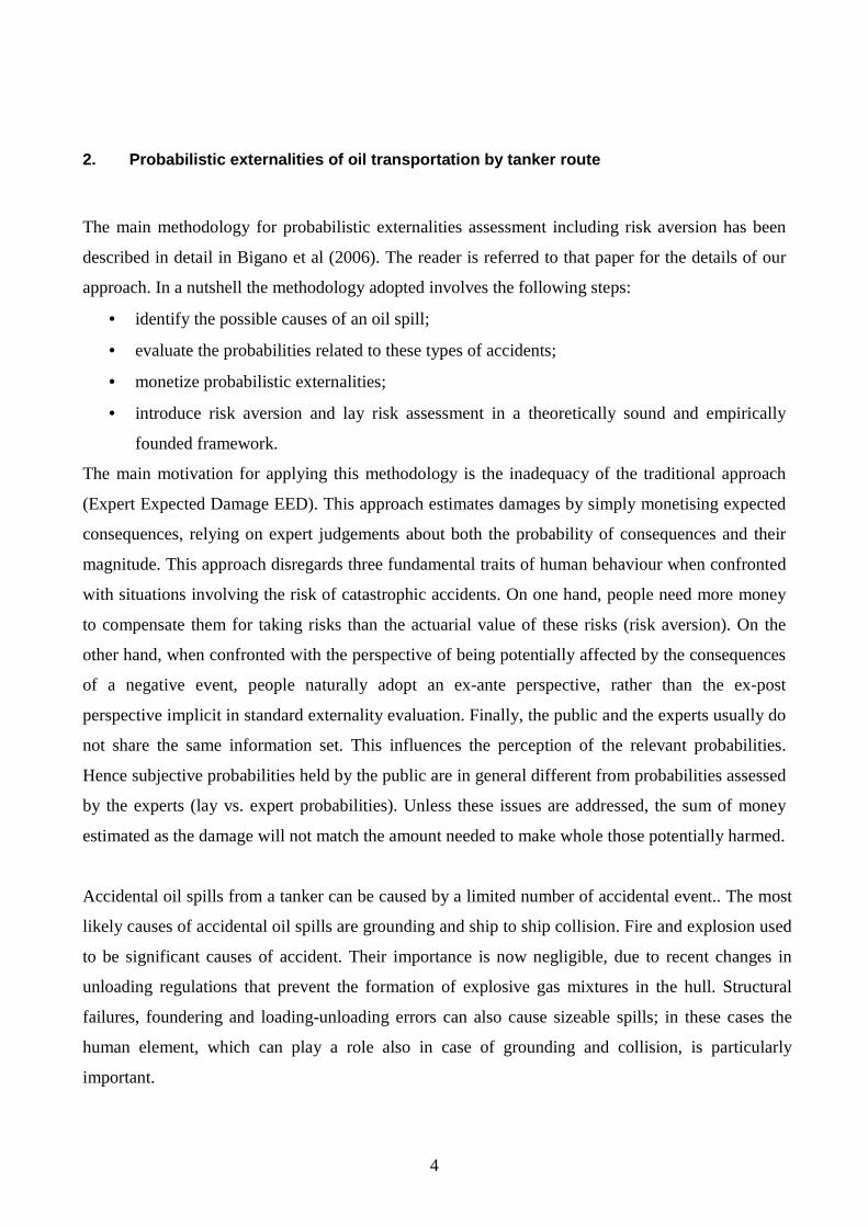
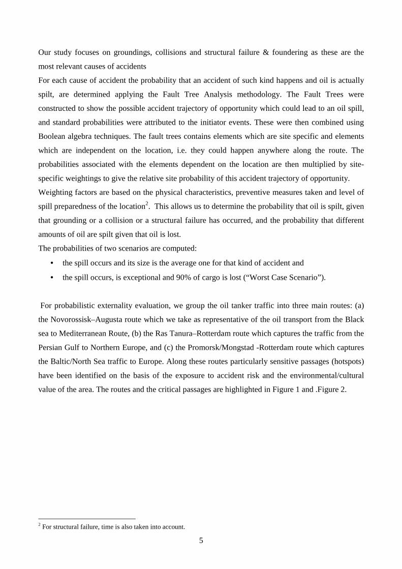
For probabilistic externality evaluation, we group the oil tanker traffic into three main routes: (a)

the Novorossisk–Augusta route which we take as representative of the oil transport from the Black

sea to Mediterranean Route, (b) the Ras Tanura–Rotterdam route which captures the traffic from the

Persian Gulf to Northern Europe, and (c) the Promorsk/Mongstad -Rotterdam route which captures

the Baltic/North Sea traffic to Europe. Along these routes particularly sensitive passages (hotspots)

have been identified on the basis of the exposure to accident risk and the environmental/cultural

value of the area. The routes and the critical passages are highlighted in Figure 1 and .Figure 2.

2 For structural failure, time is also taken into account.

6

Figure 1. Hotspots along the Ras Tanura–Rotterdam-Promorsk/Mongstad routes.

Figure 2. Hotspots along the Novorossisk-Augusta route.

7

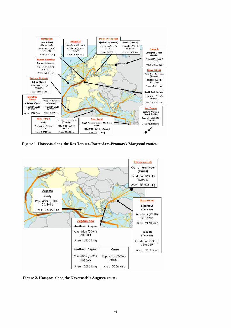
In the following tables the weightings (Table 1 and Table 2) and the probabilities (Table 3 and

Table 4) computed for the critical passages along the selected routes are listed.

Factor Novorossiysk Bosphorus Strait

Aegean Sea

Augusta

Assistance unable to help 2 4 1 1 Non Arrival of Assistance 2 1 4 1 Desired Track Unsafe 4 5 2 4 Grounding Obstacle 4 5 1 4 Other Vessel 3 5 2 3 Vision impairment 3 4 1 1 Erroneous/Untimely Action 1 3 1 1 Bad Weather/Currents 2 4 1 1 Manoeuvre Not Possible 3 4 1 3 Passage Time (hours) 8 20 100 8

Table 1 Estimation of the probabilities of occurrence along the sample routes: the weightings for the

Novorossisk–Augusta route.

8

Factor Ras Tanura

Suez Sicily Strait

Strait of Gibraltar

French finistére

Dover Strait

Baltic Sea

Red Sea

Spanish Finistere

Primorsk

Assistance unable to help 5 4 1 1 1 1 1 4 1 1 Non Arrival of Assistance 3 3 2 1 3 2 1 2 2 2 Desired Track Unsafe 5 4 2 4 3 4 5 3 2 1

Grounding Obstacle 4 5 2 3 1 4 5 3 2 2 Other Vessel 2 4 3 3 2 5 3 3 4 2

Vision impairment 2 2 2 3 2 4 2 2 3 3 Erroneous/Untimely Action 3 4 1 3 1 3 3 3 3 3 Bad Weather/Currents 4 2 2 4 5 4 4 5 4 1 Manoeuvre Not Possible 3 4 2 3 2 4 3 2 2 2 Passage Time (hours) 8 42 20 25 15 20 23 63 14 8

Table 2. Estimation of the probabilities of occurrence along the sample routes: the weightings for the Ras

Tanura–Rotterdam-Promorsk route.

Collision Collision + Spill

Grounding Grounding + Spill

structural failure

structural failure + Spill

(Total) + spill

Novorossiysk

expected 2,57E-04 7,05E-05 2,81E-04 1,05E-04 7,40E-05 7,40E-05 2,50E-04

worst case 2,57E-06 7,05E-07 5,63E-06 2,11E-06 2,52E-05 2,52E-05 2,80E-05

Turkish Straits



Aegean Sea



Augusta



Table 3. Estimation of the probabilities of occurrence along the sample routes: the probabilities for the

Novorossisk–Augusta route.

9

Collision Collision + Spill

Grounding Grounding + Spill

struct failure

struct failure + Spill (Total) + spill

Ras Tanura expected 2,50E-04 6,85E-05 7,15E-04 2,68E-04 7,80E-05 7,80E-05 4,15E-04 worst case 2,50E-06 6,85E-07 1,43E-05 5,36E-06 2,65E-05 2,65E-05 3,26E-05

Suez expected 2,74E-04 7,50E-05 1,01E-03 3,78E-04 7,40E-05 7,40E-05 5,27E-04 worst case 2,74E-06 7,50E-07 2,02E-05 7,56E-06 2,52E-05 2,52E-05 3,35E-05

Sicily expected 2,50E-04 6,85E-05 2,79E-04 1,05E-04 7,40E-05 7,40E-05 2,47E-04 worst case 2,50E-06 6,85E-07 5,58E-06 2,09E-06 2,52E-05 2,52E-05 2,79E-05

Gibraltar expected 2,57E-04 7,05E-05 7,10E-04 2,66E-04 7,80E-05 7,80E-05 4,15E-04 worst case 2,57E-06 7,05E-07 1,42E-05 5,33E-06 2,65E-05 2,65E-05 3,26E-05

French Finisterre expected 2,46E-04 6,72E-05 2,79E-04 1,05E-04 8,00E-05 8,00E-05 2,52E-04 worst case 2,46E-06 6,72E-07 5,58E-06 2,09E-06 2,72E-05 2,72E-05 3,00E-05

Dover Strait expected 2,84E-04 7,76E-05 7,31E-04 2,74E-04 7,80E-05 7,80E-05 4,30E-04 worst case 2,84E-06 7,76E-07 1,46E-05 5,48E-06 2,65E-05 2,65E-05 3,28E-05

Baltic Sea expected 2,57E-04 7,05E-05 7,20E-04 2,70E-04 7,80E-05 7,80E-05 4,18E-04 worst case 2,57E-06 7,05E-07 1,44E-05 5,40E-06 2,65E-05 2,65E-05 3,26E-05

Red Sea expected 2,50E-04 6,85E-05 1,10E-03 4,13E-04 8,00E-05 8,00E-05 5,62E-04 worst case 2,50E-06 6,85E-07 2,20E-05 8,26E-06 2,72E-05 2,72E-05 3,61E-05

Spanish Finisterre expected 2,55E-04 6,98E-05 6,84E-04 2,56E-04 7,80E-05 7,80E-05 4,04E-04 worst case 2,55E-06 6,98E-07 1,37E-05 5,13E-06 2,65E-05 2,65E-05 3,23E-05

Primorsk expected 2,46E-04 6,72E-05 6,42E-04 2,41E-04 7,20E-05 7,20E-05 3,80E-04 worst case 2,46E-06 6,72E-07 1,28E-05 4,81E-06 2,45E-05 2,45E-05 3,00E-05

Table 4. Estimation of the probabilities of occurrence along the sample routes: the probabilities for the Ras

Tanura–Rotterdam-Promorsk route.

In order to monetize the external impacts, we consider three main categories of burdens of

accidental oil spills: tourism, fisheries and natural environment. The steps followed in order to

compute the monetary impacts are illustrated in Figure 3.

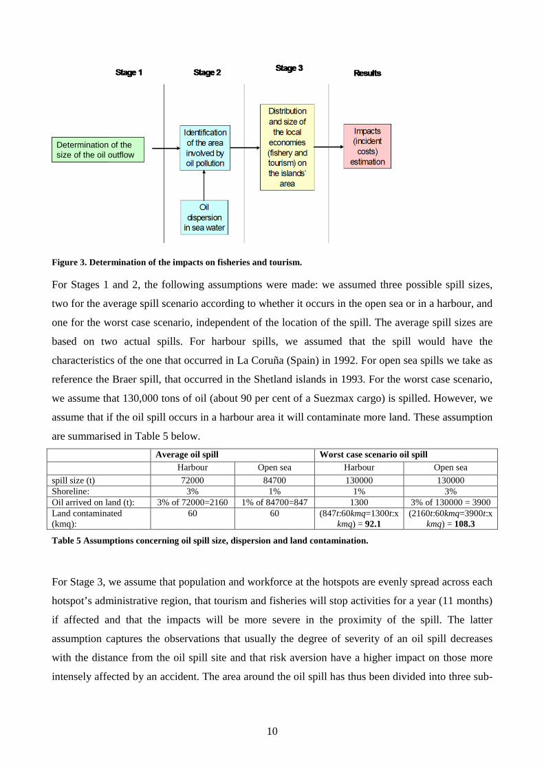
10

Determination of the size of the oil outflowDetermination of the size of the oil outflow

Figure 3. Determination of the impacts on fisheries and tourism.

For Stages 1 and 2, the following assumptions were made: we assumed three possible spill sizes,

two for the average spill scenario according to whether it occurs in the open sea or in a harbour, and

one for the worst case scenario, independent of the location of the spill. The average spill sizes are

based on two actual spills. For harbour spills, we assumed that the spill would have the

characteristics of the one that occurred in La Coruña (Spain) in 1992. For open sea spills we take as

reference the Braer spill, that occurred in the Shetland islands in 1993. For the worst case scenario,

we assume that 130,000 tons of oil (about 90 per cent of a Suezmax cargo) is spilled. However, we

assume that if the oil spill occurs in a harbour area it will contaminate more land. These assumption

are summarised in Table 5 below.

Average oil spill Worst case scenario oil spill Harbour Open sea Harbour Open sea

spill size (t) 72000 84700 130000 130000 Shoreline: 3% 1% 1% 3% Oil arrived on land (t): 3% of 72000=2160 1% of 84700=847 1300 3% of 130000 = 3900 Land contaminated (kmq):

60 60 (847t:60kmq=1300t:x kmq) = 92.1

(2160t:60kmq=3900t:x kmq) = 108.3

Table 5 Assumptions concerning oil spill size, dispersion and land contamination.

For Stage 3, we assume that population and workforce at the hotspots are evenly spread across each

hotspot’s administrative region, that tourism and fisheries will stop activities for a year (11 months)

if affected and that the impacts will be more severe in the proximity of the spill. The latter

assumption captures the observations that usually the degree of severity of an oil spill decreases

with the distance from the oil spill site and that risk aversion have a higher impact on those more

intensely affected by an accident. The area around the oil spill has thus been divided into three sub-

11

areas, with increasing population and decreasing severity of the impacts, according to the

assumptions specified in Table 6 and illustrated in Figure 4.

Land area Impact groups % involved % of oil spill impact

Area 1 Group 1 0.2% 10%

Area 2 Group 2 9.1% 45%

Area 3 Group 3 90.7% 45%

Total 100% 100%

Table 6. Assumptions related to the determination of differentiated impacts on local economies

Area 3

Area 2

Area 1

Oil outflow

shoreArea 3

Area 2

Area 1

Oil outflow

Area 3

Area 2

Area 1

Oil outflow

shoreshore

Figure 4. Vulnerability areas around a oil spill site.

The income likely to be lost has been derived from the sectoral GDP in 2004 of fisheries and

tourism in the administrative regions around the hotspots. It is assumed, in order to avoid

unreasonably high risk premiums that the sectors will never lose their full annual income, but will

be able to count on at least one month’s worth of financial resources. Moreover, sectoral GDPs are

scaled down from the administrative region level to the level of the areas affected by the spill

assuming that workers are distributed evenly in the region and then using the ratio of the workers of

the sectors under scrutiny in the affected area to the total workers of that sector in that

administrative region.

For environmental impacts, we have used the Belgian Coast CV study by Van Bierveliet et al

(2005), as it is the only valuation study in Europe (except the Blücher study in Norway, which is

based on a small sample and a very local spill). The Belgian Coast CV study was based on the

Exxon Valdez study (Carson et al 1992, 2003) which is the prototype study that satisfies the NOAA

Panel guidelines for CV studies (Arrow et al 1993), and which also satisfies the requirements listed

in Söderqvist and Soutukorva (2006). As both of these are national studies, the WTP from these

studies will probably be a lower estimate of WTP among a more affected regional population.

12

However, Belgium is a small country, and therefore there might not be a large difference between

the regional and national WTP. Therefore, we will base the benefit transfer exercise on the Belgian

Coast study, but we also look at the Exxon Valdez study as a consistency check.

Since there are too few CV studies of oil spills to perform a meta analysis, and since we do not have

data on variables needed to perform a value function transfer (as these variables are typically not

available from statistical sources at the policy site, but are typically elicited during a CV survey),

unit transfer is the only available transfer method. However, since income data are available at the

policy sites we perform income adjustments based on GDP measures (national GDP figures, or

regional GDP figures where these are available and the affected population is determined to be

regional rather than national). Even though WTP is determined by many factors, a recent meta

analysis (Bredahl, Jacobsen and Hanley 2007) of 35 CV studies (with a total of 107 WTP estimates)

on 5 continents (80 % of which are from Europe and the US) of WTP for nature protection where

existence values play a major role (which is also the case for WTP to avoid damages to marine and

coastal ecosystems from oil spills), shows that GDP per capita is a significant and good predictor of

WTP. They report that adjusted R2 was 0.53 in a single linear regression between WTP and GDP

per capita (with no constant since at zero income WTP also has to be zero). Often an income

elasticity of WTP equal to 1 is assumed (implicitly) in unit value transfers, but CV studies typically

show an income elasticity of WTP lower than 1 for CV studies of environmental goods, typically in

the 0.3-0.7 range (Kriström and Riera 1996, Höckby and Söderquist 2003, Bredahl Jacobsen and

Hanley 2007). Therefore, we have used an income elasticity of WTP equal to 0.5.

Since the estimated values in the original CV studies are carried out in different years and stated in

different currencies, we convert the different currencies to the same unit in the same year, which we

refer to as 2007-Euros. This is achieved by adjusting the original estimate with the Consumer Price

Index in the study country to 2007, and then converting to euros using Purchasing Power Parities

(PPP) - adjusted exchange rates. The resulting mean WTP per household (as a one-time amount, i.e.

present value) to avoid the described natural resource injuries in these two original CV studies are

presented in Table 7 and Table 8.

Mean WTP/household US, 1991 current prices 97 US, 2007 current prices3 140

Euro, 2007 current prices4 102 Euro, 2007ppp 5 120

Table 7. Exxon Valdez CV study. WTP/household (one-time amount).Sources: Carson et al (1992, 2003)

3 Estimated value on the basis of Consumer Price Index for USA (source: IMF); see e.g. http://investintaiwan.nat.gov.tw/en/env/stats/cpi.html 4 This value is calculated according to the average exchange rate of Euro and US$ in August 5 Estimated value on the basis of 2007-PPPs from OECD: http://www.oecd.org/dataoecd/48/18/18598721.pdf

13

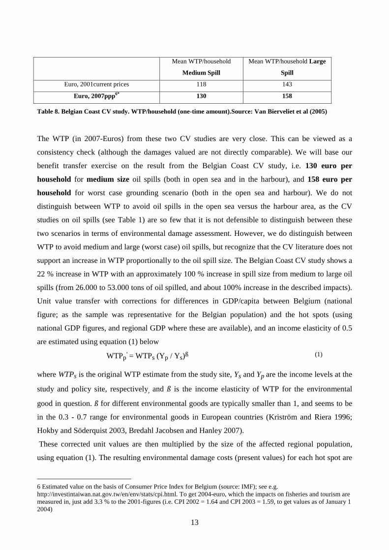
Mean WTP/household

Medium Spill

Mean WTP/household Large

Spill

Euro, 2001current prices 118 143

Euro, 2007ppp6* 130 158

Table 8. Belgian Coast CV study. WTP/household (one-time amount).Source: Van Bierveliet et al (2005)

The WTP (in 2007-Euros) from these two CV studies are very close. This can be viewed as a

consistency check (although the damages valued are not directly comparable). We will base our

benefit transfer exercise on the result from the Belgian Coast CV study, i.e. 130 euro per

household for medium size oil spills (both in open sea and in the harbour), and 158 euro per

household for worst case grounding scenario (both in the open sea and harbour). We do not

distinguish between WTP to avoid oil spills in the open sea versus the harbour area, as the CV

studies on oil spills (see Table 1) are so few that it is not defensible to distinguish between these

two scenarios in terms of environmental damage assessment. However, we do distinguish between

WTP to avoid medium and large (worst case) oil spills, but recognize that the CV literature does not

support an increase in WTP proportionally to the oil spill size. The Belgian Coast CV study shows a

22 % increase in WTP with an approximately 100 % increase in spill size from medium to large oil

spills (from 26.000 to 53.000 tons of oil spilled, and about 100% increase in the described impacts).

Unit value transfer with corrections for differences in GDP/capita between Belgium (national

figure; as the sample was representative for the Belgian population) and the hot spots (using

national GDP figures, and regional GDP where these are available), and an income elasticity of 0.5

are estimated using equation (1) below

WTPp' = WTPs (Yp / Ys)ß (1)

where WTPs is the original WTP estimate from the study site, Ys and Yp are the income levels at the

study and policy site, respectively, and ß is the income elasticity of WTP for the environmental

good in question. ß for different environmental goods are typically smaller than 1, and seems to be

in the 0.3 - 0.7 range for environmental goods in European countries (Kriström and Riera 1996;

Hokby and Söderquist 2003, Bredahl Jacobsen and Hanley 2007).

These corrected unit values are then multiplied by the size of the affected regional population,

using equation (1). The resulting environmental damage costs (present values) for each hot spot are

6 Estimated value on the basis of Consumer Price Index for Belgium (source: IMF); see e.g. http://investintaiwan.nat.gov.tw/en/env/stats/cpi.html. To get 2004-euro, which the impacts on fisheries and tourism are measured in, just add 3.3 % to the 2001-figures (i.e. CPI 2002 = 1.64 and CPI 2003 = 1.59, to get values as of January 1 2004)

14

presented in table 4. To calculate the expected value of the damage costs, these estimates must be

multiplied with the probability of an oil spill occurring.

Hotspot (and affected area)

Ratio of GDP/capita between the hotspot and

Belgium7

Transferred WTP/hh (one-

time) for medium / large

oil spill8

Number of hh in the affected area

Environmental damage costs; if a

medium / large (worst case) oil spill occur; Million euro

Novorossisk (Kraj Krasnodar, Russia)

0.10 (N) 41 / 51 1,830,436 75.0 / 93.4

Aegan Sea (Northern Aegan, Southern Aegan and Crete, Greece)

N. Agean: 0.47 S. Agean: 0.53 Crete: 0.48

89 / 109 95 / 115 90 / 109

N. Agean: 79,231 S. Agean: 116,154 Crete: 231,154

7.1 / 8.6 11.0 / 13.4 20.8 / 25.2

Bosphorus (Istanbul and Kocaeli, Turkey)

0.12 (N) 46 / 55 2,494,405 114.7 / 137.2

Augusta (Sicily, Italy) 0.51 92 / 112 2,005,232 184.5 / 224.6 Ras Tanura (Eastern Province, Saudi Arabia)

0.05 29 / 33 550,845 16.0 / 18.2

Suez Canal (Regions around canal, Egypt)

0.18 55 / 66 386,426 21.3 / 25.5

Sicily Strait (Nabeul Governorate, Tunisia and Sicily, Italy)

Nabuel:0.07 Sicily: 0.51

34 /41 92 / 112

Nabeul : 147,660 Sicily: 2,005,232

5.0 / 6.0 184.5 / 224.6

Strait of Gilbraltar (Andalusia, Spain and Tangier – Tétouan, Morocco)

Andalucia: 0.50

Tangier-Tétouan: 0.03

92 / 112

23 / 27

Andalucia: 2,604,475

Tangier-Tétouan: 466,108

239.6 / 291.7

10.6 / 12.7

Spanish Finistere (Galicia, Spain)

0.52 94 / 114 933,147 87.7 / 106.4

French Finistere (Bretagne, France)

0.77 114 / 139 1,313,428 149.7 / 182.6

Dover Strait (Nord-Pas-de-Calais, France and South East England, UK)

Nord-Pas-de-Calais : 0.69 South East

England : 1.03

108 / 131

132 / 160

Nord-Pas-de-Calais: 1,751,177

South East England: 3,373,025

189.1 / 229.4

445.2 / 539.7

Rotterdam (Zuid-Holland, The Netherlands)

1.01 130 / 158 1,500,844 195.1 / 237.1

Oresund Strait (Sjaelland, Denmark and Scania, Sweden)

Sjaelland: 0.88 Scania: 1.02

122 / 148 131 / 160

Sjaelland: 896,338 Scania: 552,094

109.4 / 132.7 72.3 / 88.3

Primorsk (Leningrad Oblast, Russia)

0.10 (N) 41 /51 596,145 24.4 / 30.4

Mongstad (Hordaland County, Norway)

1.08 135/164 197,206 26.6 / 32.3

Table 9. Recommended environmental damage cost estimates (in 2007-euro) for the hotspots

Based on the results from validity tests of international benefit transfer these estimates could have

errors of + 40 %.

7 Based on regional GDP/capita figures for the hot spots; except in a few cases where only national GDP/capita figures are available (These are marked “N”). GDP per capita in Belgium was 30.600 euro and 31,100 euro in 2004 and 2005, respectively. We divide GDP per capita from the hotspots by one of theses figures (dependent on whether the GDP/capita at the hotspot was from 2004 or 2005) 8 Calculated as WTP/hh to avoid medium/large oil spill from the Belgian Coast CV study in table 3 multiplied by (GDP-ratio) ß ; ß is the income elasticity of WTP equal to 0.5 (see equation (1))

15

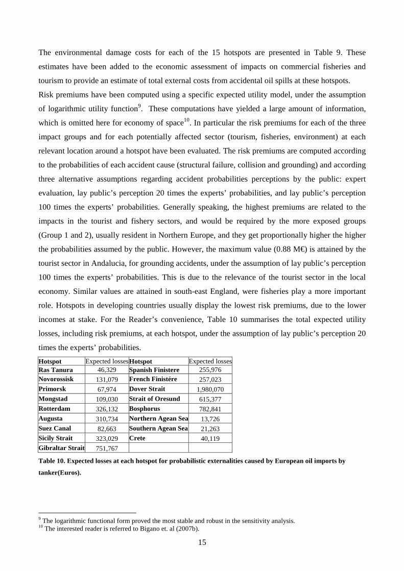
The environmental damage costs for each of the 15 hotspots are presented in Table 9. These

estimates have been added to the economic assessment of impacts on commercial fisheries and

tourism to provide an estimate of total external costs from accidental oil spills at these hotspots.

Risk premiums have been computed using a specific expected utility model, under the assumption

of logarithmic utility function9. These computations have yielded a large amount of information,

which is omitted here for economy of space10. In particular the risk premiums for each of the three

impact groups and for each potentially affected sector (tourism, fisheries, environment) at each

relevant location around a hotspot have been evaluated. The risk premiums are computed according

to the probabilities of each accident cause (structural failure, collision and grounding) and according

three alternative assumptions regarding accident probabilities perceptions by the public: expert

evaluation, lay public’s perception 20 times the experts’ probabilities, and lay public’s perception

100 times the experts’ probabilities. Generally speaking, the highest premiums are related to the

impacts in the tourist and fishery sectors, and would be required by the more exposed groups

(Group 1 and 2), usually resident in Northern Europe, and they get proportionally higher the higher

the probabilities assumed by the public. However, the maximum value (0.88 M€) is attained by the

tourist sector in Andalucia, for grounding accidents, under the assumption of lay public’s perception

100 times the experts’ probabilities. This is due to the relevance of the tourist sector in the local

economy. Similar values are attained in south-east England, were fisheries play a more important

role. Hotspots in developing countries usually display the lowest risk premiums, due to the lower

incomes at stake. For the Reader’s convenience, Table 10 summarises the total expected utility

losses, including risk premiums, at each hotspot, under the assumption of lay public’s perception 20

times the experts’ probabilities.

Hotspot Expected losses Hotspot Expected lossesRas Tanura 46,329 Spanish Finistere 255,976 Novorossisk 131,079 French Finistére 257,023 Primorsk 67,974 Dover Strait 1,980,070 Mongstad 109,030 Strait of Oresund 615,377 Rotterdam 326,132 Bosphorus 782,841 Augusta 310,734 Northern Agean Sea 13,726 Suez Canal 82,663 Southern Agean Sea 21,263 Sicily Strait 323,029 Crete 40,119 Gibraltar Strait 751,767

Table 10. Expected losses at each hotspot for probabilistic externalities caused by European oil imports by

tanker(Euros).

9 The logarithmic functional form proved the most stable and robust in the sensitivity analysis. 10 The interested reader is referred to Bigano et. al (2007b).

16

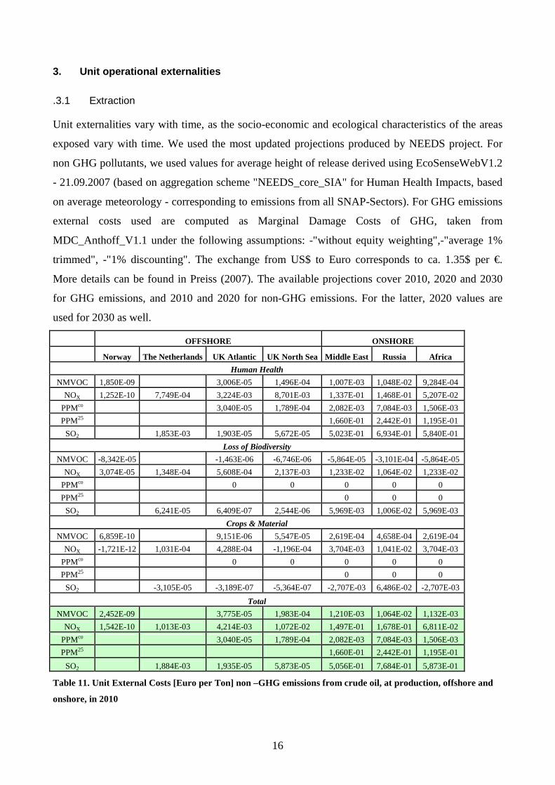
3. Unit operational externalities

.3.1 Extraction

Unit externalities vary with time, as the socio-economic and ecological characteristics of the areas

exposed vary with time. We used the most updated projections produced by NEEDS project. For

non GHG pollutants, we used values for average height of release derived using EcoSenseWebV1.2

- 21.09.2007 (based on aggregation scheme "NEEDS_core_SIA" for Human Health Impacts, based

on average meteorology - corresponding to emissions from all SNAP-Sectors). For GHG emissions

external costs used are computed as Marginal Damage Costs of GHG, taken from

MDC_Anthoff_V1.1 under the following assumptions: -"without equity weighting",-"average 1%

trimmed", -"1% discounting". The exchange from US$ to Euro corresponds to ca. 1.35$ per €.

More details can be found in Preiss (2007). The available projections cover 2010, 2020 and 2030

for GHG emissions, and 2010 and 2020 for non-GHG emissions. For the latter, 2020 values are

used for 2030 as well.

OFFSHORE ONSHORE

Norway The Netherlands UK Atlantic UK North Sea Middle East Russia Africa

Human Health

NMVOC 1,850E-09 3,006E-05 1,496E-04 1,007E-03 1,048E-02 9,284E-04

NOX 1,252E-10 7,749E-04 3,224E-03 8,701E-03 1,337E-01 1,468E-01 5,207E-02

PPMco 3,040E-05 1,789E-04 2,082E-03 7,084E-03 1,506E-03

PPM25 1,660E-01 2,442E-01 1,195E-01

SO2 1,853E-03 1,903E-05 5,672E-05 5,023E-01 6,934E-01 5,840E-01

Loss of Biodiversity

NMVOC -8,342E-05 -1,463E-06 -6,746E-06 -5,864E-05 -3,101E-04 -5,864E-05

NOX 3,074E-05 1,348E-04 5,608E-04 2,137E-03 1,233E-02 1,064E-02 1,233E-02

PPMco 0 0 0 0 0

PPM25 0 0 0

SO2 6,241E-05 6,409E-07 2,544E-06 5,969E-03 1,006E-02 5,969E-03

Crops & Material

NMVOC 6,859E-10 9,151E-06 5,547E-05 2,619E-04 4,658E-04 2,619E-04

NOX -1,721E-12 1,031E-04 4,288E-04 -1,196E-04 3,704E-03 1,041E-02 3,704E-03

PPMco 0 0 0 0 0

PPM25 0 0 0

SO2 -3,105E-05 -3,189E-07 -5,364E-07 -2,707E-03 6,486E-02 -2,707E-03

Total

NMVOC 2,452E-09 3,775E-05 1,983E-04 1,210E-03 1,064E-02 1,132E-03

NOX 1,542E-10 1,013E-03 4,214E-03 1,072E-02 1,497E-01 1,678E-01 6,811E-02

PPMco 3,040E-05 1,789E-04 2,082E-03 7,084E-03 1,506E-03

PPM25 1,660E-01 2,442E-01 1,195E-01

SO2 1,884E-03 1,935E-05 5,873E-05 5,056E-01 7,684E-01 5,873E-01

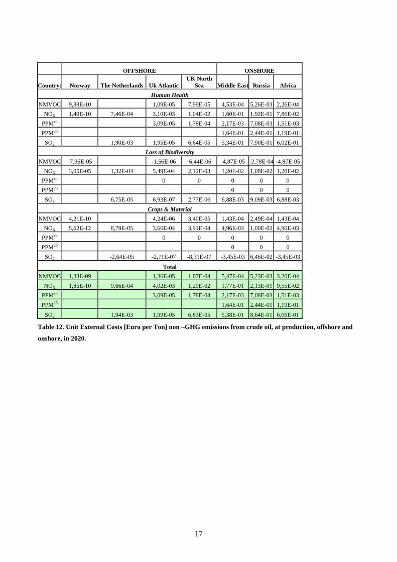
Table 11. Unit External Costs [Euro per Ton] non –GHG emissions from crude oil, at production, offshore and

onshore, in 2010

17

OFFSHORE ONSHORE

Country: Norway The Netherlands Uk Atlantic UK North

Sea Middle East Russia Africa

Human Health

NMVOC 9,88E-10 1,09E-05 7,99E-05 4,53E-04 5,26E-03 2,26E-04

NOX 1,49E-10 7,46E-04 3,10E-03 1,04E-02 1,60E-01 1,92E-01 7,86E-02

PPMco 3,09E-05 1,78E-04 2,17E-03 7,08E-03 1,51E-03

PPM25 1,64E-01 2,44E-01 1,19E-01

SO2 1,90E-03 1,95E-05 6,64E-05 5,34E-01 7,90E-01 6,02E-01


NMVOC -7,96E-05 -1,56E-06 -6,44E-06 -4,87E-05 -2,78E-04 -4,87E-05

NOX 3,05E-05 1,32E-04 5,49E-04 2,12E-03 1,20E-02 1,08E-02 1,20E-02

PPMco 0 0 0 0 0

PPM25 0 0 0

SO2 6,75E-05 6,93E-07 2,77E-06 6,88E-03 9,09E-03 6,88E-03

Crops & Material

NMVOC 4,21E-10 4,24E-06 3,40E-05 1,43E-04 2,49E-04 1,43E-04

NOX 5,62E-12 8,79E-05 3,66E-04 3,91E-04 4,96E-03 1,00E-02 4,96E-03

PPMco 0 0 0 0 0

PPM25 0 0 0

SO2 -2,64E-05 -2,71E-07 -8,31E-07 -3,45E-03 6,46E-02 -3,45E-03

Total

NMVOC 1,33E-09 1,36E-05 1,07E-04 5,47E-04 5,23E-03 3,20E-04

NOX 1,85E-10 9,66E-04 4,02E-03 1,29E-02 1,77E-01 2,13E-01 9,55E-02

PPMco 3,09E-05 1,78E-04 2,17E-03 7,08E-03 1,51E-03

PPM25 1,64E-01 2,44E-01 1,19E-01

SO2 1,94E-03 1,99E-05 6,83E-05 5,38E-01 8,64E-01 6,06E-01

Table 12. Unit External Costs [Euro per Ton] non –GHG emissions from crude oil, at production, offshore and

onshore, in 2020.

18

OFFSHORE ONSHORE

Norway The Netherlands Uk Atlantic UK North Sea Middle East Russia Africa

2010

CO2 0 0 0 0 1,70E-01 5,40E-01 2,67E-01

CH4 4,01E-01 0 4,86E-05 4,86E-05 6,81E-04 2,72E-03 9,74E-04

N2O 1,49E-02 8,23E-03 3,42E-02 3,42E-02 8,90E-03 6,76E-02 1,57E-02

SF6 0 0 0 0 4,99E-07 1,23E-05 4,78E-06

2020

CO2 0 0 0 0 1,83E-01 5,81E-01 2,88E-01

CH4 3,45E-01 0 4,18E-05 4,18E-05 5,86E-04 2,34E-03 8,38E-04

N2O 1,51E-02 8,34E-03 3,47E-02 3,47E-02 9,01E-03 6,85E-02 1,59E-02

SF6 0 0 0 0 5,02E-07 1,23E-05 4,81E-06

2030

CO2 0 0 0 0 1,68E-01 5,33E-01 2,64E-01

CH4 3,09E-01 0 3,74E-05 3,74E-05 5,24E-04 2,09E-03 7,49E-04

N2O 1,24E-02 6,85E-03 2,85E-02 2,85E-02 7,40E-03 5,62E-02 1,31E-02

SF6 0 0 0 0 4,48E-07 1,10E-05 4,30E-06

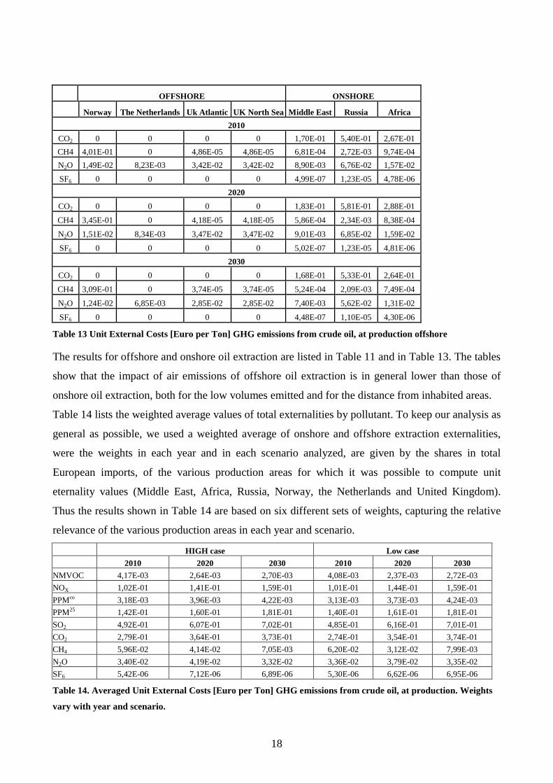
Table 13 Unit External Costs [Euro per Ton] GHG emissions from crude oil, at production offshore

The results for offshore and onshore oil extraction are listed in Table 11 and in Table 13. The tables

show that the impact of air emissions of offshore oil extraction is in general lower than those of

onshore oil extraction, both for the low volumes emitted and for the distance from inhabited areas.

Table 14 lists the weighted average values of total externalities by pollutant. To keep our analysis as

general as possible, we used a weighted average of onshore and offshore extraction externalities,

were the weights in each year and in each scenario analyzed, are given by the shares in total

European imports, of the various production areas for which it was possible to compute unit

eternality values (Middle East, Africa, Russia, Norway, the Netherlands and United Kingdom).

Thus the results shown in Table 14 are based on six different sets of weights, capturing the relative

relevance of the various production areas in each year and scenario.

HIGH case Low case 2010 2020 2030 2010 2020 2030

NMVOC 4,17E-03 2,64E-03 2,70E-03 4,08E-03 2,37E-03 2,72E-03

NOX 1,02E-01 1,41E-01 1,59E-01 1,01E-01 1,44E-01 1,59E-01

PPMco 3,18E-03 3,96E-03 4,22E-03 3,13E-03 3,73E-03 4,24E-03

PPM25 1,42E-01 1,60E-01 1,81E-01 1,40E-01 1,61E-01 1,81E-01

SO2 4,92E-01 6,07E-01 7,02E-01 4,85E-01 6,16E-01 7,01E-01

CO2 2,79E-01 3,64E-01 3,73E-01 2,74E-01 3,54E-01 3,74E-01

CH4 5,96E-02 4,14E-02 7,05E-03 6,20E-02 3,12E-02 7,99E-03

N2O 3,40E-02 4,19E-02 3,32E-02 3,36E-02 3,79E-02 3,35E-02

SF6 5,42E-06 7,12E-06 6,89E-06 5,30E-06 6,62E-06 6,95E-06

Table 14. Averaged Unit External Costs [Euro per Ton] GHG emissions from crude oil, at production. Weights

vary with year and scenario.

19

.3.2 Oil Transportation

Oil pipeline operations can cause negative impacts through the air emissions of compressors at the

pumping stations that propel the oil along the pipeline, and trough the air emissions due to the

escaping of the volatile fractions of the hydrocarbons in the oil. Oil pipelines are listed in the

Ecoinvent database but the fields for air emissions are empty. The only unit emissions record

present in the database are heat emissions and oil spilled in the soil. Alternative LCI data for oil

pipelines could not be found. However, gas pipelines work in a similar fashion, but more energy is

necessary to displace gas rather than oil, since gas must be compressed first. Therefore gas

pipelines’ operational externalities can be considered as an upper bound for oil pipeline

externalities. In particular, according to the database used by the TEAMS model, which computes

well-to-hull LCI data for marine transportation11, on average, one ton of natural gas requires 336

Btu/mile to be moved along a pipeline; crude oil requires about 240 Btu/mile. Therefore, assuming

a linear relationship between energy intensity and emissions, gas pipelines’ emissions should be

multiplied by a factor of 0.714 to yield approximate values for analogous emissions from oil

pipelines. The resulting externalities are listed in the tables below.

2010 2020 2030

NMVOC 5,15E-07 1,19E-08 1,19E-08

CO2 6,91E-10 7,43E-10 6,82E-10

CH4 4,62E-04 1,86E-05 1,66E-05

N2O 0 0 0

SF6 0 0 0

Total GHG 4,62E-04 1,86E-05 1,66E-05

Table 15. Unit External Costs [Euro per Ton]. Emissions from crude oil transport, by long distance pipeline,

NMVOC and GHG-emissions in 2010, 2020 and 2030, Russia.

Externalities due to the operation of oil tankers were originally computed combining Ecoinvent and

Ecosense data. The resulting externalities for 2010 caused by emissions from oil tankers operations

in the regions crossed by the importing routes to Europe are listed in Table 16 and in Table 17

below. Again, externalities not related to GHG emissions vary with the different regions crossed,

due to the different deposition patterns of the pollutants and hence due the different socioeconomic

and environmental characteristics of the regions exposed. The average values have been computed

using as weights the ratio of the lengths of the routes’ legs pertaining the areas listed in the first row

11 More details on the TEAMS model can be found further in this section.

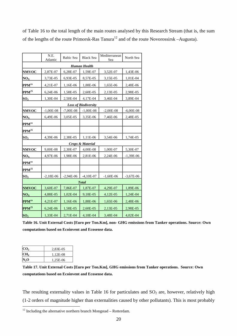
20

of Table 16 to the total length of the main routes analysed by this Research Stream (that is, the sum

of the lengths of the route Primorsk-Ras Tanura12 and of the route Novorossirsk –Augusta).

N.E.

Atlantic Baltic Sea Black Sea

Mediterranean Sea

North Sea

Human Health

NMVOC 2,87E-07 6,28E-07 1,59E-07 3,52E-07 1,43E-06

NOX 3,73E-05 6,93E-05 8,57E-05 3,15E-05 1,01E-04

PPMco 4,21E-07 1,16E-06 1,88E-06 1,65E-06 2,48E-06

PPM25 6,24E-06 1,58E-05 2,60E-05 2,13E-05 2,98E-05

SO2 1,30E-04 2,50E-04 4,17E-04 3,46E-04 3,89E-04


NMVOC -1,00E-08 -7,00E-08 -1,00E-08 -2,00E-08 -6,00E-08

NOX 6,49E-06 3,05E-05 3,35E-06 7,46E-06 2,48E-05

PPMco

PPM25

SO2 4,39E-06 2,38E-05 1,11E-06 3,54E-06 1,74E-05

Crops & Material

NMVOC 9,00E-08 2,30E-07 4,00E-08 1,00E-07 5,30E-07

NOX 4,97E-06 1,98E-06 2,81E-06 2,24E-06 -1,39E-06

PPMco

PPM25

SO2 -2,18E-06 -2,94E-06 -4,10E-07 -1,60E-06 -3,67E-06

Total

NMVOC 3,60E-07 7,86E-07 1,87E-07 4,29E-07 1,89E-06

NOX 4,88E-05 1,02E-04 9,18E-05 4,12E-05 1,24E-04

PPMco 4,21E-07 1,16E-06 1,88E-06 1,65E-06 2,48E-06

PPM25 6,24E-06 1,58E-05 2,60E-05 2,13E-05 2,98E-05

SO2 1,33E-04 2,71E-04 4,18E-04 3,48E-04 4,02E-04

Table 16. Unit External Costs [Euro per Ton.Km], non- GHG emissions from Tanker operations. Source: Own

computations based on Ecoinvent and Ecosense data.

CO2 2,83E-05

CH4 1,12E-08

N2O 1,25E-06

Table 17. Unit External Costs [Euro per Ton.Km], GHG emissions from Tanker operations. Source: Own

computations based on Ecoinvent and Ecosense data.

The resulting externality values in Table 16 for particulates and SO2 are, however, relatively high

(1-2 orders of magnitude higher than externalities caused by other pollutants). This is most probably 12 Including the alternative northern branch Mongstad – Rotterdam.

21

due to the fact that LCI data from Ecoinvent are based on data for old and existing ships. Moreover

the Ecoinvent data at our disposal referred to a generic crude oil tanker, thus not distinguishing

between alternative fuel/engine configurations and sizes of the ship. To overcome these problems

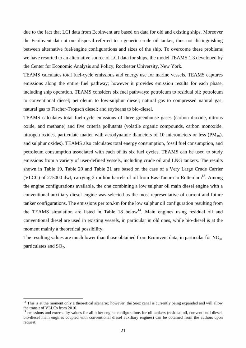
we have resorted to an alternative source of LCI data for ships, the model TEAMS 1.3 developed by

the Center for Economic Analysis and Policy, Rochester University, New York.

TEAMS calculates total fuel-cycle emissions and energy use for marine vessels. TEAMS captures

emissions along the entire fuel pathway; however it provides emission results for each phase,

including ship operation. TEAMS considers six fuel pathways: petroleum to residual oil; petroleum

to conventional diesel; petroleum to low-sulphur diesel; natural gas to compressed natural gas;

natural gas to Fischer-Tropsch diesel; and soybeans to bio-diesel.

TEAMS calculates total fuel-cycle emissions of three greenhouse gases (carbon dioxide, nitrous

oxide, and methane) and five criteria pollutants (volatile organic compounds, carbon monoxide,

nitrogen oxides, particulate matter with aerodynamic diameters of 10 micrometers or less (PM10),

and sulphur oxides). TEAMS also calculates total energy consumption, fossil fuel consumption, and

petroleum consumption associated with each of its six fuel cycles. TEAMS can be used to study

emissions from a variety of user-defined vessels, including crude oil and LNG tankers. The results

shown in Table 19, Table 20 and Table 21 are based on the case of a Very Large Crude Carrier

(VLCC) of 275000 dwt, carrying 2 million barrels of oil from Ras-Tanura to Rotterdam13. Among

the engine configurations available, the one combining a low sulphur oil main diesel engine with a

conventional auxiliary diesel engine was selected as the most representative of current and future

tanker configurations. The emissions per ton.km for the low sulphur oil configuration resulting from

the TEAMS simulation are listed in Table 18 below14. Main engines using residual oil and

conventional diesel are used in existing vessels, in particular in old ones, while bio-diesel is at the

moment mainly a theoretical possibility.

The resulting values are much lower than those obtained from Ecoinvent data, in particular for NOx,

particulates and SO2.

13 This is at the moment only a theoretical scenario; however, the Suez canal is currently being expanded and will allow the transit of VLLCs from 2010. 14 emissions and externality values for all other engine configurations for oil tankers (residual oil, conventional diesel, bio-diesel main engines coupled with conventional diesel auxiliary engines) can be obtained from the authors upon request.

22

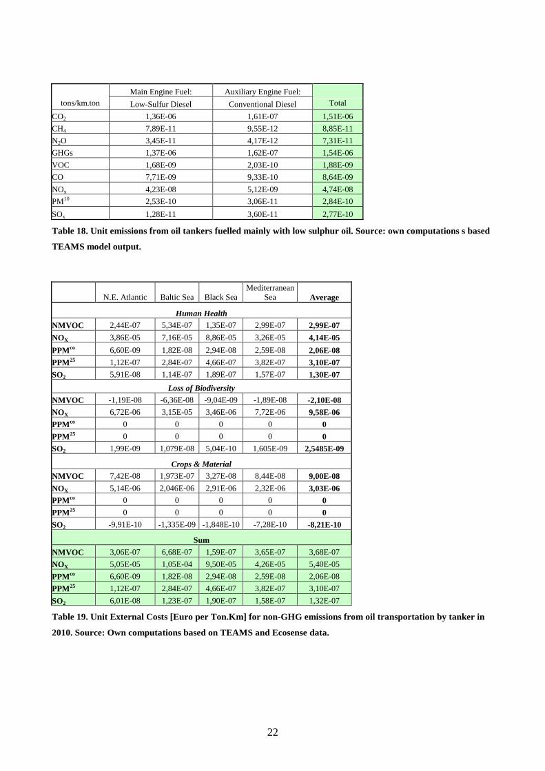
Main Engine Fuel: Auxiliary Engine Fuel: tons/km.ton Low-Sulfur Diesel Conventional Diesel Total

CO2 1,36E-06 1,61E-07 1,51E-06

CH4 7,89E-11 9,55E-12 8,85E-11

N2O 3,45E-11 4,17E-12 7,31E-11

GHGs 1,37E-06 1,62E-07 1,54E-06

VOC 1,68E-09 2,03E-10 1,88E-09

CO 7,71E-09 9,33E-10 8,64E-09

NOx 4,23E-08 5,12E-09 4,74E-08

PM10 2,53E-10 3,06E-11 2,84E-10

SOx 1,28E-11 3,60E-11 2,77E-10

Table 18. Unit emissions from oil tankers fuelled mainly with low sulphur oil. Source: own computations s based

TEAMS model output.

N.E. Atlantic Baltic Sea Black Sea Mediterranean

Sea Average

Human Health

NMVOC 2,44E-07 5,34E-07 1,35E-07 2,99E-07 2,99E-07

NOX 3,86E-05 7,16E-05 8,86E-05 3,26E-05 4,14E-05

PPMco 6,60E-09 1,82E-08 2,94E-08 2,59E-08 2,06E-08

PPM25 1,12E-07 2,84E-07 4,66E-07 3,82E-07 3,10E-07

SO2 5,91E-08 1,14E-07 1,89E-07 1,57E-07 1,30E-07


NMVOC -1,19E-08 -6,36E-08 -9,04E-09 -1,89E-08 -2,10E-08

NOX 6,72E-06 3,15E-05 3,46E-06 7,72E-06 9,58E-06

PPMco 0 0 0 0 0

PPM25 0 0 0 0 0

SO2 1,99E-09 1,079E-08 5,04E-10 1,605E-09 2,5485E-09

Crops & Material

NMVOC 7,42E-08 1,973E-07 3,27E-08 8,44E-08 9,00E-08

NOX 5,14E-06 2,046E-06 2,91E-06 2,32E-06 3,03E-06

PPMco 0 0 0 0 0

PPM25 0 0 0 0 0

SO2 -9,91E-10 -1,335E-09 -1,848E-10 -7,28E-10 -8,21E-10

Sum

NMVOC 3,06E-07 6,68E-07 1,59E-07 3,65E-07 3,68E-07

NOX 5,05E-05 1,05E-04 9,50E-05 4,26E-05 5,40E-05

PPMco 6,60E-09 1,82E-08 2,94E-08 2,59E-08 2,06E-08

PPM25 1,12E-07 2,84E-07 4,66E-07 3,82E-07 3,10E-07

SO2 6,01E-08 1,23E-07 1,90E-07 1,58E-07 1,32E-07

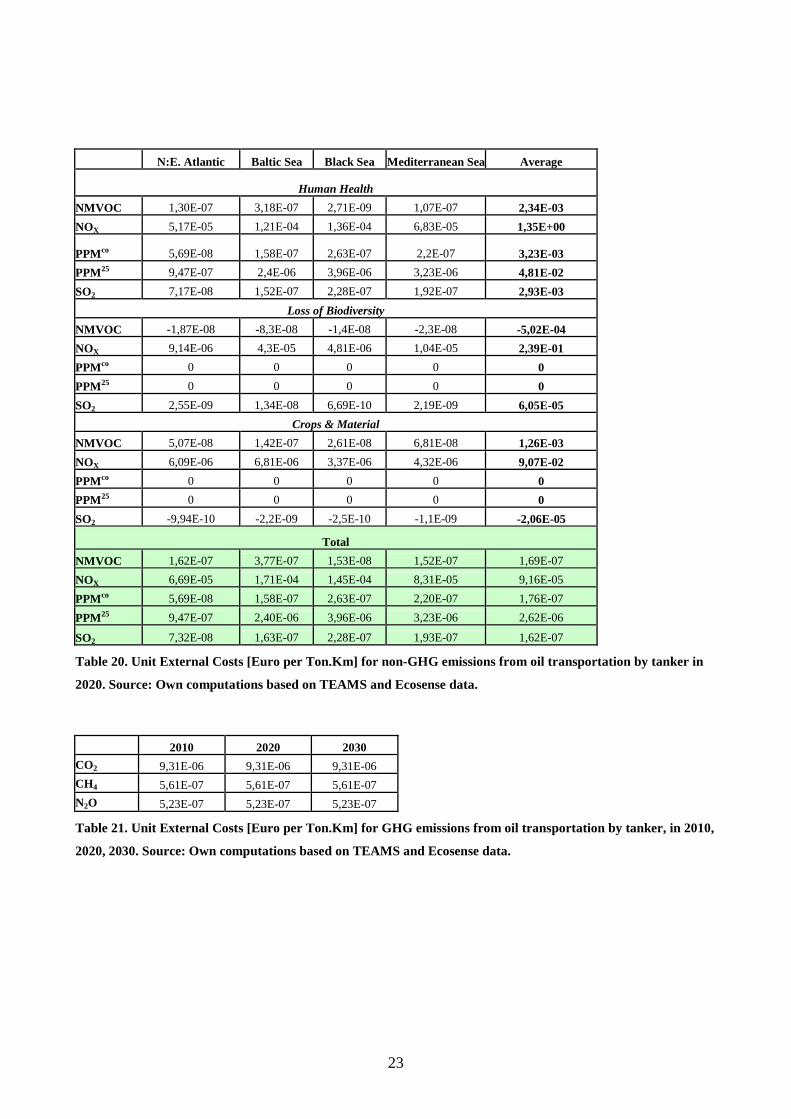
Table 19. Unit External Costs [Euro per Ton.Km] for non-GHG emissions from oil transportation by tanker in

2010. Source: Own computations based on TEAMS and Ecosense data.

23

N:E. Atlantic Baltic Sea Black Sea Mediterranean Sea Average

Human Health

NMVOC 1,30E-07 3,18E-07 2,71E-09 1,07E-07 2,34E-03

NOX 5,17E-05 1,21E-04 1,36E-04 6,83E-05 1,35E+00

PPMco 5,69E-08 1,58E-07 2,63E-07 2,2E-07 3,23E-03

PPM25 9,47E-07 2,4E-06 3,96E-06 3,23E-06 4,81E-02

SO2 7,17E-08 1,52E-07 2,28E-07 1,92E-07 2,93E-03


NMVOC -1,87E-08 -8,3E-08 -1,4E-08 -2,3E-08 -5,02E-04

NOX 9,14E-06 4,3E-05 4,81E-06 1,04E-05 2,39E-01

PPMco 0 0 0 0 0

PPM25 0 0 0 0 0

SO2 2,55E-09 1,34E-08 6,69E-10 2,19E-09 6,05E-05

Crops & Material

NMVOC 5,07E-08 1,42E-07 2,61E-08 6,81E-08 1,26E-03

NOX 6,09E-06 6,81E-06 3,37E-06 4,32E-06 9,07E-02

PPMco 0 0 0 0 0

PPM25 0 0 0 0 0

SO2 -9,94E-10 -2,2E-09 -2,5E-10 -1,1E-09 -2,06E-05

Total

NMVOC 1,62E-07 3,77E-07 1,53E-08 1,52E-07 1,69E-07

NOX 6,69E-05 1,71E-04 1,45E-04 8,31E-05 9,16E-05

PPMco 5,69E-08 1,58E-07 2,63E-07 2,20E-07 1,76E-07

PPM25 9,47E-07 2,40E-06 3,96E-06 3,23E-06 2,62E-06

SO2 7,32E-08 1,63E-07 2,28E-07 1,93E-07 1,62E-07

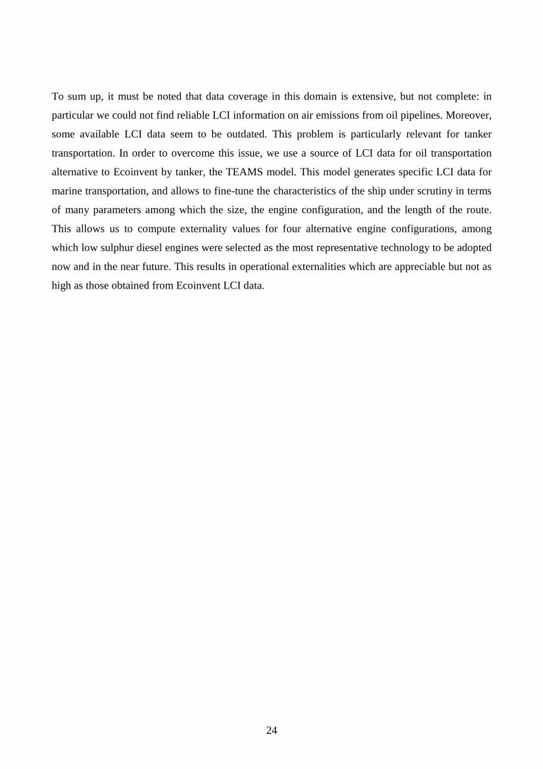
Table 20. Unit External Costs [Euro per Ton.Km] for non-GHG emissions from oil transportation by tanker in

2020. Source: Own computations based on TEAMS and Ecosense data.

2010 2020 2030

CO2 9,31E-06 9,31E-06 9,31E-06

CH4 5,61E-07 5,61E-07 5,61E-07

N2O 5,23E-07 5,23E-07 5,23E-07

Table 21. Unit External Costs [Euro per Ton.Km] for GHG emissions from oil transportation by tanker, in 2010,

2020, 2030. Source: Own computations based on TEAMS and Ecosense data.

24

To sum up, it must be noted that data coverage in this domain is extensive, but not complete: in

particular we could not find reliable LCI information on air emissions from oil pipelines. Moreover,

some available LCI data seem to be outdated. This problem is particularly relevant for tanker

transportation. In order to overcome this issue, we use a source of LCI data for oil transportation

alternative to Ecoinvent by tanker, the TEAMS model. This model generates specific LCI data for

marine transportation, and allows to fine-tune the characteristics of the ship under scrutiny in terms

of many parameters among which the size, the engine configuration, and the length of the route.

This allows us to compute externality values for four alternative engine configurations, among

which low sulphur diesel engines were selected as the most representative technology to be adopted

now and in the near future. This results in operational externalities which are appreciable but not as

high as those obtained from Ecoinvent LCI data.

25

4. Overall assessment of external costs for oil Imports to Europe.

The final step of our externality assessment for the oil chain entails combining the unit externality

values with the scenario projections of oil production and import to Europe for the present and for

selected future years, under reasonable assumptions about energy markets trends. This step was

performed on the basis of oil demand and import flows scenarios developed by the Observatoire

Méditerranéen de l'Energie, and generated overall externality values which ranging from 2.32 Euro

in 2030 in the scenario assuming low demand to 2.60 Euro in 2010 in the High demand scenario

per ton of oil transported to Europe.

The unit externality values described and listed in Section 3 give an overall indication of how much

external damage is caused by producing a ton of oil and by transporting it for one kilometre in the

seas around Europe. However they do not yet give a precise evaluation of how much external cost is

generated by bringing that ton of gas into Europe. More importantly, these values do not allow us to

assess what will be the evolution of these externality costs in the future.

In order to do that, one needs to combine the unit values above with an assessment of the flows of

oil produced for European consumption, and transported to Europe along the main import channels

(pipelines and tanker routes) now and in the future. In principle, this can be done with varying

degrees of refinement and precision. Our procedure is quite accurate but still entails some

simplifying assumptions.

For one thing, “the future” enters into our analyses as three selected years: 2010, 2020 and 2030.

Moreover, we have strived to include as much dynamic elements as possible. In particular, time-

dependent parameters and variables in our computations are the following:

• the volumes of oil extracted and transported to Europe,

• the routes and the transportation modes used to deliver the oil to European consumers,

• the unit externality values for operational externalities15,

• the weights used to compute average operational externalities for the extraction phase16

15 We used the most updated projections produced by NEEDS project. For non GHG pollutants, we used values for average height of release derived using EcoSenseWebV1.2 - 21.09.2007 (based on aggregation scheme "NEEDS_core_SIA" for Human Health Impacts, based on average meteorology - corresponding to emissions from all SNAP-Sectors). For GHG emissions external costs used are computed as Marginal Damage Costs of GHG, taken from MDC_Anthoff_V1.1 under the following assumptions: -"without equity weighting",-"average 1% trimmed", -"1% discounting". The exchange from US$ to Euro corresponds to ca. 1.35$ per €. More details can be found in Preiss (2007). The available projections cover 2010, 2020 and 2030 for GHG emissions, and 2010 and 2020 for non-GHG emissions. For the latter, 2020 values are used for 2030 as well. 16 To keep our analysis as general as possible, we used a weighted average of onshore and offshore extraction externalities, were the weights in each year and in each scenario analyzed are given by the shares in total European

26

• the maintenance standards of oil pipelines17.

However, probabilistic externalities are not allowed to vary between these years. This assumption

has two main motivations. On one hand, the alternative would have involved the addition of further

uncertainty to the computation. In fact, the factors which may influence future probabilistic

externality values are many, spatially differentiated, and very hard to project in the future with any

confidence, at the hot spot level of spatial resolution. Relevant factors, for each hot spot, include:

population size, per capita income, evolution of ecosystems, evolution of the local economy, etc.

On the other hand, the assessment of the likely influence of the upcoming trends in marine

regulation and technology performed within the NEEDS project showed the presence of contrasting

and counterbalancing trends, with a roughly neutral influence on the overall safety standards of the

industry.

Finally, even oil flows may vary according to the assumptions one can make about the main drivers

influencing international energy markets. In order to at least partially capture some of this particular

source of variation, we use two alternative scenarios: one assuming a lower demand level and one

assuming a higher demand level. A reference scenario has not been used in this evaluation exercise,

as it is conceived as instrumental for the derivation of the other two. However it is briefly described

in Section 2 to help illustrating the other scenarios.

For each of these scenarios and for each pollutant, two kind of external costs are computed. On one

hand, as in the case of natural gas, operational externalities along the main import routes and at the

most relevant production sites for European oil imports are computed. Their values are then

averaged to yield externality values, for each pollutant, per ton of oil produced and per ton of oil

imported into Europe. On the other hand, probabilistic externalities are also included using a

specific methodology to be illustrated in more detail below. Finally, external costs pertaining to the

two categories considered are summed up to yield an overall external cost value per ton of oil

imported into Europe in the base year and in each demand scenario.

imports of the various production areas for which it was possible to compute unit eternality values (Middle East, Africa, Russia, Norway, the Netherlands and United Kingdom). Thus the results shown in Table 23 and Table 24 are based on six different sets of weights, capturing the relative relevance of the various production areas in each year and scenario. 17 Pipelines are assumed to reach European standards by 2020.

27

.4.1 Oil demand scenarios

The following is a summary of the main assumptions behind the three demand scenarios used in

this analysis, as depicted in Guarrera and Karbuz (2007), to which the interested reader is referred for

further details.

• Reference Scenario. Crude oil imports are set to increase by 0.3% per year over the next 25

years, reaching 619 Mt in 2030, up from 567 Mt in 2004. While the FSU region and the

Middle East will remain the main exporters to the EU, North Africa and Western Africa will

gain in share. By 2030, the African continent will account for nearly a third of all EU crude

imports up from 17% in 2004. A quarter of all exports to the EU will come from North

African countries alone and especially from Libya and Algeria. Except for pipeline imports

all crude imports to Atlantic and Mediterranean ports increase over time. For Atlantic ports,

crude imports increase from 283 Mt in 2004 to 339 Mt in 2030, while for Mediterranean

ports, crude imports are expected to increase from 197 Mt in 2004 to 208 Mt in 2030. For

pipeline imports, the decrease in share and in total is the consequence of falling Norwegian

crude oil production. Indeed, Norwegian crude oil exports by pipeline exports are expected

to fall from 31 Mt in 2004 to 3 Mt in 2030. All imports through pipeline to the UK will

therefore reduce drastically. However, pipeline oil imports from the FSU region are

increasing rapidly from 56 Mt in 2004 they are forecasted to reach 71 Mt in 2030.

• Low Case Scenario. Compared to the Reference Scenario, in the Low Case Scenario,

import requirements for the EU are expected to be 15% lower in 2030 reaching 526 Mt, 548

Mt in 2020 and 526 Mt in 2030. In 2030, 53% of these imports will come to EU Atlantic

ports, 34% through its Mediterranean ports and 13% directly by pipeline. In 2010 the

difference with the Reference Scenario is not likely to be that great since most of the

policies to be put in place to reduce demand would not yet be effective; in 2020 however, in

the Low Case Scenario, imports are expected to drop by 8% from the Reference Scenario.

Compared with the Reference Scenario, in the Low Case imports would be reduced by more

than 90 Mt in 2030. In the Low Case Scenario, the lesser needs for imports compared with

the Reference Scenario are expected to affect routes unevenly. Indeed, imports from Africa

and the Caspian region will be less pronounced. While the drop in Norwegian oil production

in the Low Case Scenario will still lead to a shift towards other regions, these regions will

not need to contribute as much to oil imports of the EU as in the Reference Scenario. Over

20% less crude will be needed from regions such as Africa (-21%) and Caspian (-28%),

28

while other regions such as Middle East or even Russia, who are already currently

substantial EU trade partners, will see their imports less affected. Compared to the

Reference Scenario, in the Low Case, imports form the Middle East are expected be reduced

by 13% and imports from Russia by less than 7%.

• High Case Scenario. In this scenario, the increase in demand, and thus in imports, will lead

to a supply constraint forcing EU countries to get the oil wherever they can - using the full

extent of routes and pipelines available. In this scenario, the effects of growing demand

would be visible as soon as 2010 due to increasing demand and unchanged production in the

EU; and would therefore lead to immediate increase of imports by 5% compared to the

Reference Scenario. By 2020 the increase in imports in this scenario would be as high as

8%, to reach 681 Mt in 2030 –more than 10% increase compared to the Reference Scenario.

Compared with the Reference Scenario, in the High Scenario, over 60 Mt of additional

crude oil will need to be imported by 2030. Overall, in the High Case Scenario, EU imports

are expected to reach 596 Mt in 2010, 646 Mt in 2020 and 681 Mt in 2030. In 2030, 53% of

these imports will come to EU Atlantic ports, 34% through its Mediterranean ports and 13%

directly by pipeline.

.4.2 Inclusion of probabilistic externalities

Probabilistic externalities, refer, by definition, to damages that may or may not take place in any

given moment and at any given location, in this case along the oil import routes to Europe.

Therefore, any given ton of oil that reaches Europe do not need to cause any damage of this kind

(actually, if it has reached Europe, it has not caused any damage!). However, in its route to Europe,

it stands chances to cause damages by being spilt and not reaching its final destination. Thus the

first step is to define the “probabilistic externality content” of each ton of oil imported. In our study

this is done by looking at this issue in terms of expected utility loss. That is, each ton of oil reaching

Europe brings about a reduction in welfare, which is the utility losses that may be caused by

accidents along the routes to Europe weighted by their probability of occurrence, and including the

discomfort suffered by the affected population for being exposed to such risks.

In principle, each single kilometre along these import routes has such a risk attached, and therefore,

in principle, multiple accidents could happen anywhere along these routes. The complete evaluation

of the exposure of each kilometre of each import route is a daunting task, and thus we had to resort

to some simplifying assumptions.

In particular we assume that a) accidents occur only at well identified “hot-spots” where oil coming

from different exporting countries transits in its way to Europe, and where historical records for oil

29

tanker accidents indicate a significant exposure to accident risk; b) that each ton of oil “collects” its

bits of probabilistic externalities by passing trough the hot spots relevant for the route actually

followed. Thus, for instance, oil imported from Algeria to Southern France will carry attached only

its own shares of probabilistic externalities potentially occurring at the relevant hot spots in western

Mediterranean, but not those occurring, say, in the North Sea.

In practice, probabilistic externalities are allotted to the various routes by dividing their values at the

relevant hotspots along that route by the volume of oil transported along that route in a given year.

This is exemplified in Table 22 below, which shows the computations performed for the case of

Norwegian oil exports to Northern Europe in 2010. In Table 22, the values in the green row are just

the expected losses at the hotspots in the column headings of Table 22, as reported in Table 10,

divided by the total volume of oil imports to Europe projected to pass trough each hotspot in 2010

in the Low demand scenario. To compute the relevant probabilistic externality values, Table 22

multiplies in its blue cells, the externality values per ton (green row) by the volume of oil projected

to leave Norway (orange column) for each European destination (yellow column), but only if the

correspondent hotspot in the column heading pertains to the route from Norway to the destination

country. In this case, only two hotspots are relevant: the departure port of Mongstad and the

destination port of Rotterdam. The blue cells for the remaining hot spots are therefore 0: Norwegian

oil does not need to pass trough Augusta to reach any Northern European destination. Finally, the

last row computes the probabilistic externality per ton of Norwegian oil imported to trough Atlantic

ports by dividing the total probabilistic externalities (blue cells, bold numbers) by the total import

volume in 2010 (orange row, bold number x 1 Million).

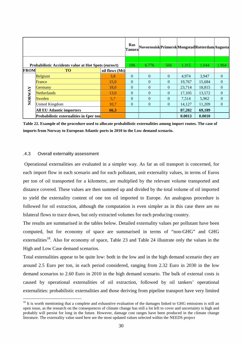
30

Ras Tanura

Novorossisk Primorsk Mongstad Rotterdam Augusta

Probabilistic Accidents value at Hot Spots (euros/t) 186 6.776 566 1.315 1.044 1.964 FROM TO oil flows (Mt)

Belgium 3,8 0 0 0 4,974 3,947 0 France 15,0 0 0 0 19,767 15,684 0 Germany 18,0 0 0 0 23,714 18,815 0 Netherlands 13,0 0 0 0 17,105 13,572 0 Sweden 5,7 0 0 0 7,514 5,962 0 United Kingdom 10,7 0 0 0 14,127 11,209 0

All EU Atlantic importers 66,3 87,202 69,189

NO

RW

AY

Probabilistic externalities in €per ton 0.0013 0.0010

Table 22. Example of the procedure used to allocate probabilistic externalities among import routes. The case of

imports from Norway to European Atlantic ports in 2010 in the Low demand scenario.

.4.3 Overall externality assessment

Operational externalities are evaluated in a simpler way. As far as oil transport is concerned, for

each import flow in each scenario and for each pollutant, unit externality values, in terms of Euros

per ton of oil transported for a kilometre, are multiplied by the relevant volume transported and

distance covered. These values are then summed up and divided by the total volume of oil imported

to yield the externality content of one ton oil imported to Europe. An analogous procedure is

followed for oil extraction, although the computation is even simpler as in this case there are no

bilateral flows to trace down, but only extracted volumes for each producing country.

The results are summarised in the tables below. Detailed externality values per pollutant have been

computed, but for economy of space are summarised in terms of “non-GHG” and GHG

externalities18. Also for economy of space, Table 23 and Table 24 illustrate only the values in the

High and Low Case demand scenarios.

Total externalities appear to be quite low: both in the low and in the high demand scenario they are

around 2.5 Euro per ton, in each period considered, ranging from 2.32 Euro in 2030 in the low

demand scenarios to 2.60 Euro in 2010 in the high demand scenario. The bulk of external costs is

caused by operational externalities of oil extraction, followed by oil tankers’ operational

externalities: probabilistic externalities and those deriving from pipeline transport have very limited

18 It is worth mentioning that a complete and exhaustive evaluation of the damages linked to GHG emissions is still an open issue, as the research on the consequences of climate change has still a lot left to cover and uncertainty is high and probably will persist for long in the future. However, damage cost ranges have been produced in the climate change literature. The externality value used here are the most updated values selected within the NEEDS project

31

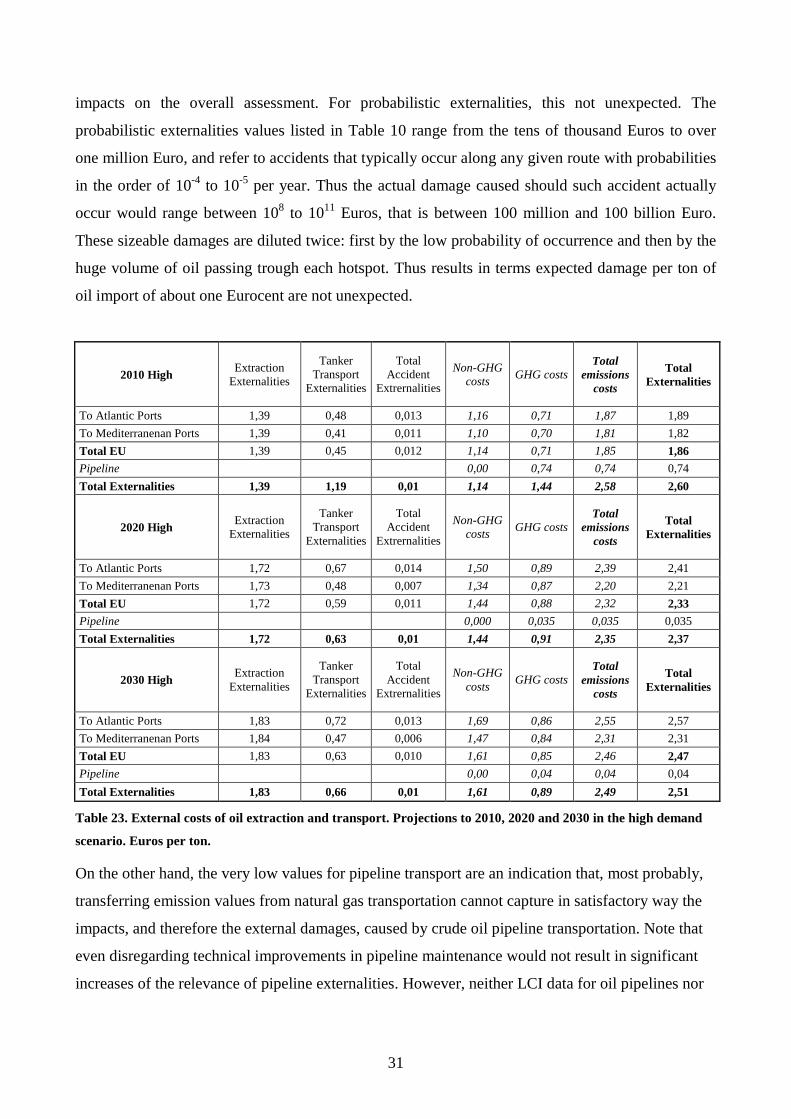
impacts on the overall assessment. For probabilistic externalities, this not unexpected. The

probabilistic externalities values listed in Table 10 range from the tens of thousand Euros to over

one million Euro, and refer to accidents that typically occur along any given route with probabilities

in the order of 10-4 to 10-5 per year. Thus the actual damage caused should such accident actually

occur would range between 108 to 1011 Euros, that is between 100 million and 100 billion Euro.

These sizeable damages are diluted twice: first by the low probability of occurrence and then by the

huge volume of oil passing trough each hotspot. Thus results in terms expected damage per ton of

oil import of about one Eurocent are not unexpected.

2010 High Extraction

Externalities

Tanker Transport

Externalities

Total Accident

Extrernalities

Non-GHG costs

GHG costs Total

emissions costs

Total Externalities

To Atlantic Ports 1,39 0,48 0,013 1,16 0,71 1,87 1,89

To Mediterranenan Ports 1,39 0,41 0,011 1,10 0,70 1,81 1,82

Total EU 1,39 0,45 0,012 1,14 0,71 1,85 1,86 Pipeline 0,00 0,74 0,74 0,74

Total Externalities 1,39 1,19 0,01 1,14 1,44 2,58 2,60


Externalities

Tanker Transport

Externalities

Total Accident

Extrernalities

Non-GHG costs

GHG costs Total

emissions costs

Total Externalities



Total EU 1,72 0,59 0,011 1,44 0,88 2,32 2,33

Pipeline 0,000 0,035 0,035 0,035



Externalities

Tanker Transport

Externalities

Total Accident

Extrernalities

Non-GHG costs

GHG costs Total

emissions costs

Total Externalities



Total EU 1,83 0,63 0,010 1,61 0,85 2,46 2,47

Pipeline 0,00 0,04 0,04 0,04


Table 23. External costs of oil extraction and transport. Projections to 2010, 2020 and 2030 in the high demand

scenario. Euros per ton.

On the other hand, the very low values for pipeline transport are an indication that, most probably,

transferring emission values from natural gas transportation cannot capture in satisfactory way the

impacts, and therefore the external damages, caused by crude oil pipeline transportation. Note that

even disregarding technical improvements in pipeline maintenance would not result in significant

increases of the relevance of pipeline externalities. However, neither LCI data for oil pipelines nor

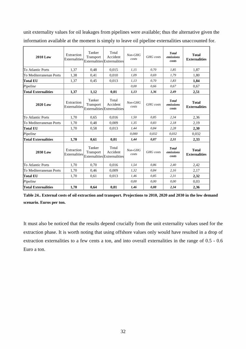
32

unit externality values for oil leakages from pipelines were available; thus the alternative given the

information available at the moment is simply to leave oil pipeline externalities unaccounted for.

2010 Low Extraction

Externalities

Tanker Transport

Externalities

Total Accident

Extrernalities

Non-GHG costs

GHG costs Total

emissions costs

Total Externalities





2020 Low Extraction

Externalities

Tanker Transport

Externalities

Total Accident

Extrernalities

Non-GHG costs

GHG costs Total

emissions costs

Total Externalities





2030 Low Extraction

Externalities

Tanker Transport

Externalities

Total Accident

Extrernalities

Non-GHG costs

GHG costs Total

emissions costs

Total Externalities



Total EU 1,70 0,61 0,013 1,46 0,85 2,31 2,32

Pipeline 0,00 0,00 0,00 0,03


Table 24.. External costs of oil extraction and transport. Projections to 2010, 2020 and 2030 in the low demand

scenario. Euros per ton.

It must also be noticed that the results depend crucially from the unit externality values used for the

extraction phase. It is worth noting that using offshore values only would have resulted in a drop of

extraction externalities to a few cents a ton, and into overall externalities in the range of 0.5 - 0.6

Euro a ton.

33

5. Conclusions

Our assessment covered in detail various aspect of the externalities related to the extraction and

transportation of oil to Europe, in particular the dynamic features related to the foreseeable variation

of oil flows and transport modes, the evolution of the burdens and impacts of operational

externalities, the relative relevance of the various production areas, the likely improvements of

pipeline maintenance standards. The resulting values seem quite low, ranging from 2.32 Euro per

ton in 2030 in the Low demand scenarios to 2.60 Euro in 2010 in the High demand scenario, but

still about 1-2 Euro higher than those originated by the extraction and transportation phases of the

natural gas chain19,. Externalities due to pipeline transport are the main driver of the difference

between the 2010 results and the 2030 results, as maintenance standards of Russian pipelines are

assumed to close the gap with European standards after 2010. Thus, pipeline externalities in 2010

are 25 times higher than those expected in 2030, and this has stronger effect on the overall

externality values than the differences in oil import volumes and exporting countries’ shares

between the two demand scenarios. Assuming that no improvements in the maintenance standards

of Russian pipelines take place, the overall external costs in 2030 would reach 3.05 Euro in the Low

demand scenario, and 3.25 Euro in the High demand scenario. It is not unlikely that more accurate

LCA data for pipelines would have resulted in even higher, but not too high, external costs, as gas

pipeline transport is quite energy intensive and the energy content per cubic meter of oil is higher

than for natural gas and the majority of gas imports to Europe are transported via pipeline20. These

values are however sensitive to the LCA and unit externality assumptions made for the various

phases of the value chain; in particular, the extraction phase, appears to have a strong impact on the

overall assessment.

Notwithstanding the sensitivity of these results to LCA data and to unit externality values per

pollutant, it is clear that these externalities are quite low, both compared to the direct cost of oil and

to the externalities generated by the use of oil as a fuel. Assuming a price of crude oil at destination

of $90 a barrel, the cost of one ton equals to $660 or 447 euros21. The external costs of

transportation then amount to about 0.6% of the cost of the product in 2010. Burning oil for

electricity generation results into a much higher share of external costs over total (external + private

costs). For an average European power plant burning heavy fuel oil the external costs represent on

19 Also assessed within the NEEDS Project. See Bigano et al (2007c). External costs for oil transport are from 35% to 8 times higher (per imported ton) than those for natural gas, depending on the demand scenario considered and on whether Russian pipeline maintenance standards are updated to European standards after 2010. 20 To move one ton of oil by pipeline for one kilometre it takes about 71% of the energy needed to move the same amount of natural gas along the same distance. 21 Assuming an exchange rate of 1.476 Euro per US dollar

34

average about 45% of the total costs, while for power plant using light fuel oil in a gas turbine the

share of external costs over total costs is about 24%.22

The main implication for environmental policy to be drawn from this study is that bringing oil to

Europe is not the most noxious phase of the oil life cycle, as actually using oil as a fuel brings

about, on average, much more serious consequences for the environment and for human health.

However, transporting oil to Europe is an activity which brings about a non negligible probability of

causing very high local damages. The fact that these probabilistic externalities account for a very

small fraction of the total external cost of oil transport, once weighted for their occurrence

probabilities and the volume of oil transported, by no means should be used as a justification for

relaxing pollution prevention and remediation standards in European waters. In fact as our analysis

of probabilistic externalities has demonstrated, the impact on local populations affected can be very

substantial.

22 These shares of private and external costs on total cost of electricity generation are those assessed within the European project CASES (www.feem-project.net/cases ). and reported in Bigano and Porchia (2008).

35

REFERENCES:

Arrow, K.J., R. Solow, E. Leamer, P. Portney, R. Radner and H. Schuman 1993: Report of the NOAA Panel

on Contingent Valuation. Federal Register, 58, 4601-4614 (January 15, 1993).

Bateman, I. J., R. T. Carson, B. Day M. Hanemann et al 2002: Economic Valuation with Stated Preference

Techniques. A Manual. Edward Elgar Publishing, Cheltenham (UK) and Northampton, (MA, USA),

Bergland, O. 1994: Estimating oil spill damages: The case of Blücher. Report to Det Norske Veritas

Research AS, Oslo. December 1994. 36 pp.

Bigano, A. , Cassinelli, M., Markandya, A., Sferra, F.,(2006). The Role of Risk Aversion and Lay Risk in the

Probabilistic Externality Assessment for Oil Tanker Routes to Europe. Fondazione Eni E. Mattei Working

Papers n.149.06, Milan, Italy. (Accepted for publication subject to revision by the Journal of Transport

Economics and Policy).

Bigano, A. , Cassinelli, M., Markandya, A., Sferra, F.,(2007a). Impacts from oil transportation phase of oil

by pipeline and from oil extraction. NEEDS Technical paper 1.6b - RS 1c WP 11.7b, www.needs-

project.org

Bigano, A. , Cassinelli, M., Markandya, A., Sferra, F.,(2007b). Additional potential externalities due to

accidents in the oil chain. Part I: Oil extraction and transportation by tanker route. NEEDS Technical paper

1.7b - RS 1c WP 1, www.needs-project.org

Bigano, A. , Cassinelli, M., Markandya, A., Sferra, F.,(2007b) Burdens, Impacts And Externalities From

Natural Gas Chain. 2.3-2.6. NEEDS Technical paper 1.7b - RS 1c WP 1, www.needs-project.org

Bigano A. and Navrud, S. (2007) Report on the economic evaluation of externalities due to extraction and

transport of oil. NEEDS Technical paper 1.8 - RS 1c WP 1, www.needs-project.org

Bigano A., Porchia, R.(2008) Development of a set of full cost estimates of the use of different energy sources and its comparative assessment in EU countries. CASES deliverable D.6.1, www.feem-project.net/cases.

36

Bredahl Jacobsen, J. and N. Hanley 2007: A global study of income effects in contingent valuation studies of

environmental protection. Paper presented at the 15th Annual Conference of the European Association of

Environmental and Resource Economists, Thessaloniki, Greece, June 27-30th , 18 pp.

Brown, A.J., and B. Haugene (1998): ‘Assessing the Impact of Management and Organizational Factors on

the Risk of Tanker Grounding’, 8th International Offshore and Polar Engineering Conference, ISOPE-98-

HKP-03.

Carson, R. T., R. C. Mitchell, M. Hanemann, R. J. Kopp, S. Presser and P. A. Ruud 2003: 'Contingent

valuation and lost passive use: Damages from the Exxon Valdez oil spill' Environmental and Resource

Economics 25 (3); 257-286.

Commission for the Mining and Other Extractive Industries & Committee on “Borehole Operations (2001):

“Report on Accident Statistics 1991-2000 for the extractive industry related to the borehole operations safety

and health”

Desvousges, W.H, F. R. Johnson and H.S. Banzhaf 1998: Environmental Policy Analysis with Limited

Information.Principles and Applications of the Transfer Method. New Horizons in Environmental

Economics. Edward Elgar, Cheltenham, UK and Northampton, MA, USA.

ECOINVENT Centre: “Ecoinvent Data”. http://www.ecoinvent.ch/

EcoSense Model. http://webeco.ier.uni-stuttgart.de/

ENIscuola: http://www.eniscuola.net/testo.aspx?id=5#11

Etkin, D. S. (2001), ‘Comparative Methodologies for Estimating On-Water Response Costs for Oil Spills’

Interanational Oil Spill Conference, p.1281.

Etkin, D. S. and Schmidt, D. (2004), Modeling Oil Spill Response and Damage Costs, Epa gov (14 September

2005): www.epa.gov/oilspill/etkin2_04.pdf.

ExternE (1995): Externalities of Energy - Vol. 2: Methodology, European Commission DGXII, Luxembourg.

Ferguson, R. (1992): Environmental Costs of Energy Technologies, Accidental Radiological Impacts of Nuclear

Power, CEETES, University of Newcastle.

37

Friend, I., and M. Blume (1975): The Demand for Risky Assets, American Economic Review, 65, 900-922.

Friis–Hansen, P., and O. Ditlevsen (2002): ‘Nature preservation acceptance model applied to tanker oil spill

simulations’, Structural Safety, 25, 1–34.

Gibson P. (2002): “ Oil Spills in U.S. Navigable Waters – 1991-2000”, American Petroleum Institute

Hammond, P. (1981): ‘Ex Ante and Ex Post Welfare Optimality Under Uncertainty’, Economica, 48 (191),

235-250.

Guarrera, L. and Karbuz, S.(2007) Present and future oil flows and routes from producing areas to Europe.

NEEDS Technical paper n°1.2 - RS 1c, www.needs-project.org

Hansen, L.P., and K.J. Singleton (1982): ‘Generalized Instrumental Variables Estimation of Nonlinear

Expectations Models’, Econometrica, 50, 1269-1286.

Hokby S., and T. Söderquist 2003: Elasticities of Demand and Willingness to Pay for Environmental

Services in Sweden, Environmental and Resource Economics 26; 361–383.

Krewitt W., (2002): External cost of energy – do the answers match the questions? Looking back at 10 years

of ExternE. Energy Policy, 30 : 839 – 848.

Kriström B. And P. Riera P.1996: Is the Income Elasticity of Environmental Improvements Less Than One?

Environmental and Resource Economics 7, 45-55.

Lee, R., et al. (1993): Damages and Benefits of the Nuclear Fuel Cycle: Estimation Impacts and Values,

Oakridge National Laboratory, Oakridge USA.

Lindhjem, H. 2006: 20 Years of Stated Preference Valuation of Non-Timber Benefits from Nordic Forests: A

Meta-Analysis, Journal of Forest Economics 12: 251-277, 2007.

Markandya, A., and T. Taylor (1999): The External Costs of Nuclear Accidents, IAEA.

Mehra, R., and E.C. Prescott (1995): ‘The Equity Premium - a puzzle’, Journal of Monetary Economics,15,

1985, 145-161.

38

Navrud, S and R. Ready (eds.) 2007: Environmental Value Transfer: Issues and Methods. Springer,

Dordrect, The Netherlands, 290 pp.

Navrud, S. 2004: Value transfer and environmental policy. Chapter 5 (pp. 189-217) in Tietenberg, T. and H.

Folmer (eds.) 2004: The International Yearbook of Environmental and Resource Economics 2004/2005. A

survey of Current Issues. Edward Elgar Publishing, Cheltenham, UK and Northampton, MA, USA..

Navrud, S. 2007: Benefit Transfer Guidelines – The Methodological Platform. Report from NEEDS RS 3a.

August 2007.

PACE (1992): Environmental Costs of Electricity, PACE University Centre for Environmental Legal Studies.

Prepared for the New York State Energy Research and Development Authority and the US Department of

Energy.

Preiss, Philipp (2007) Technical Paper n° 1.4 - RS 3a“Report on marginal external costs – Preliminary

results” NEEDS deliverable, www.needs-project.org

Preiss, Philipp (2007) Technical Paper n° 1.4 - RS 3a“Report on marginal external costs – Preliminary

results” NEEDS deliverable, www.needs-project.org

RAInews 24: http://www.rainews24.rai.it/ran24/speciali/obiettivo_usa_nuovo/te_petrolio.htm

Ready, R. and S. Navrud 2006: International Benefits Transfer: Methods and Validity Tests. Ecological

Economics 60(2), 429-434.

Rowe,R.D., W.D. Schulze, W.D. Shaw, D. Schenk & L.C. Chestnut 1991: Contingent valuation of natural

resource damage due to the Nestucca oil spill. RCG/Hagler, Bailly, Inc., Boulder, Colorado, USA. Final

report, June 15, 1991.

Safety and Health Commission for Mining and Other Extractive Industry (SHCMOEI) Report On Accident

Statistics: “For The Extractive Industry Related To The Borehole Operations” , (DOC. N° 1587-3-01), EU,

1991-2000. http://ec.europa.eu/employment_social/health_safety/docs/accident_statistics_2000_en.pdf

Sandrea, I, Sandrea, R. (2005) GLOBAL OFFSHORE OIL-1: Exploration trends show continued promise in

world’s offshore basins. Oil & Gas Journal, March 05, 2007, volume 105, issue 9.

39

Söderqvist, T. and Å. Soutukorva 2006: An Instrument for assessing the quality of environmental valuation

studies. Report. Swedish Envioronmental Protection Agency (Naturvårdsverket)

http://www.naturvardsverket.se/bokhandeln/pdf/620-1252-5.pdf

The Center for Energy Analysis and Policy: “TEAMS - The Total Energy and Emissions Analysis for Marine

Systems Model”, Rochester, New York

The Health and Safety Commission: “MHIDAS (Major Hazard Incident Data Service) Database”, Great

Britain

Transneft, http://www.transneft.ru/About/History/Default.asp?LANG=EN

UK Health and Safety Executive (HSE) Industry Sector Profile Onshore Oil Industry 2002/03.

http://www.hse.gov.uk/chemicals/onshoreoi02-03.pdf

Van Bieryliet, K., Le Roy, D. and P.A.L.D. Nunes (2006): ‘An Accidental Oil Spill Along the Belgian Coast:

Results from a CV’, FEEM Working Paper, 41.2006.

Xie, D. (2000): ‘Power Risk Aversion Utility Functions’, Annals of Economics and Finance, 1, 265-282.

NOTE DI LAVORO DELLA FONDAZIONE ENI ENRICO MATTEI

Fondazione Eni Enrico Mattei Working Paper Series

Our Note di Lavoro are available on the Internet at the following addresses: http://www.feem.it/Feem/Pub/Publications/WPapers/default.htm

http://www.ssrn.com/link/feem.html http://www.repec.org

http://agecon.lib.umn.edu http://www.bepress.com/feem/

NOTE DI LAVORO PUBLISHED IN 2009 SD 1.2009 Michael Hoel: Bush Meets Hotelling: Effects of Improved Renewable Energy Technology on Greenhouse Gas

Emissions SD 2.2009 Abay Mulatu, Reyer Gerlagh, Dan Rigby and Ada Wossink: Environmental Regulation and Industry LocationSD 3.2009 Anna Alberini, Stefania Tonin and Margherita Turvani: Rates of Time Preferences for Saving Lives in the

Hazardous Waste Site Context SD 4.2009 Elena Ojea, Paulo A.L.D. Nunes and Maria Loureiro: Mapping of Forest Biodiversity Values: A Plural

Perspective SD 5.2009 Xavier Pautrel : Macroeconomic Implications of Demography for the Environment: A Life-Cycle Perspective IM 6.2009 Andrew Ellul, Marco Pagano and Fausto Panunzi: Inheritance Law and Investment in Family Firms IM 7.2009 Luigi Zingales: The Future of Securities Regulation SD 8.2009 Carlo Carraro, Emanuele Massetti and Lea Nicita: How Does Climate Policy Affect Technical Change? An

Analysis of the Direction and Pace of Technical Progress in a Climate-Economy Model SD 9.2009 William K. Jaeger: The Welfare Effects of Environmental Taxation SD 10.2009 Aude Pommeret and Fabien Prieur: Double Irreversibility and Environmental Policy Design SD 11.2009 Massimiliano Mazzanti and Anna Montini: Regional and Sector Environmental Efficiency Empirical Evidence

from Structural Shift-share Analysis of NAMEA data SD 12.2009 A. Chiabai, C. M. Travisi, H. Ding, A. Markandya and P.A.L.D Nunes: Economic Valuation of Forest

Ecosystem Services: Methodology and Monetary Estimates SD 13.2009 Andrea Bigano, Mariaester Cassinelli, Fabio Sferra, Lisa Guarrera, Sohbet Karbuz, Manfred Hafner, Anil

Markandya and Ståle Navrud: The External Cost of European Crude Oil Imports

The External Cost of European Crude Oil Imports

Documents

Transcript of The External Cost of European Crude Oil Imports