Possible correlation between miocene global climatic changes and magnetic proxies, using neuro fuzzy...

Stud. Geophys. Geod., 54 (2010), 607631 607 © 2010 Inst. Geophys. AS CR, Prague

POSSIBLE CORRELATION BETWEEN MIOCENE GLOBAL CLIMATIC CHANGES AND MAGNETIC PROXIES, USING NEURO FUZZY LOGIC ANALYSIS IN A STRATIGRAPHIC WELL AT THE LLANOS FORELAND BASIN, COLOMBIA

ANA DA SILVA1, VINCENZO COSTANZO-ÁLVAREZ2,*, NURI HURTADO1, MILAGROSA ALDANA2, GERMÁN BAYONA3, OSWALDO GUZMÁN2 AND DIEGO LÓPEZ-RODRÍGUEZ1

1 Laboratorio de Física Teórica de Sólidos, Escuela de Física, Universidad Central de

Venezuela, Caracas, Venezuela ([email protected])

2 Departamento de Ciencias de la Tierra, Universidad Simón Bolívar, Caracas, Venezuela ([email protected], [email protected], [email protected])

3 Corporación Geológica Ares, Bogotá, Colombia ([email protected])

* Corresponding author

Received: February 12, 2010; Revised: May 26, 2010; Accepted: July 10, 2010

ABSTRACT

In this work we have assessed the hybrid algorithm of NeuroFuzzy logic (NFL), to establish a correlation between global climatic changes (benthic foraminiferal δ18O data), experimental S-ratio (factor characterizing stability of remanent magnetization) and magnetic susceptibility (). Magnetic proxies have been measured in 44 samples of the Colombian stratigraphic well Saltarín 1A (distal Llanos foreland basin). and S-ratios were linked to global δ18O data assuming a constant accumulation rate for a 305 meters thick stratigraphic interval flanked by the two palynological age constrains available. This interval encompasses, from top to base, the bottom of the Guayabo formation, the León, and the upper unit of the Carbonera formations (lower to middle Miocene). The best inference is accomplished applying a Takagi-Sugeno-Kan (TSK) fuzzy model with four fuzzy rules and the δ18O, S-ratios and data used in a linear form to train the system. These results are interpreted as the outcome of a significant influence of global climatic changes upon magnetic proxies. A stronger correlation is perhaps prevented by the likely influence of local and regional tectonic events and climatic changes that could have affected the distal segment of the Colombian Llanos foreland basin during Miocene times. We argue that late diagenesis of primary magnetic minerals and the assumption of a constant accumulation rate might have a minor influence on these results.

K e yw ord s : δ18O, magnetic susceptibility, S-ratio, NeuroFuzzy logic

A. Da Silva et al.

608 Stud. Geophys. Geod., 54 (2010)

1. INTRODUCTION

The inference of a relationship, that would allow connecting data of different physical nature in order to characterize distinct systems, is a common practice in geosciences. Linear regression methods are applied to most of these cases in order to establish a possible correlation between the various parameters that are being used. However, the complexities involved in geological and geophysical problems give rise to an increasing dispersion of these data. In such situations, there is not an obvious trend that could be easily adjusted by a single linear or multilinear relationship. This problem has been partially solved in the prediction of permeability, out of porosity data, by dividing the set of experimental points in smaller subunits that correspond to different sedimentary facies, followed by the calculation of a local fitting function for each of these subunits (Finol et al., 2001).

The obvious limitations of the linear regression method, when applied to a set of highly scattered experimental data points, make it necessary to find alternative ways to deal with this kind of intricate problems. Some mathematical approaches apply concepts of neural networks and/or fuzzy logic to handle non-linear relationships between two or more variables (i.e. Helle et al., 2001 and Cuddy and Glover, 2001). In rock magnetism, Urbat et al. (1999) have used fuzzy c-means clustering and non-linear mapping in order to identify and characterize early diagenetic effects in large rock magnetic data sets of the Ocean Drilling Program (ODP) Site 904. Likewise, the NeuroFuzzy logic (NFL) method, a hybrid algorithm that combines fuzzy logic with neural networks, has been previously used in the prediction of complex petrophysical parameters (Hurtado et al., 2008). In most situations, the results obtained have given rise to a set of numerical connections between the different variables involved as well as additional lithological information about an area of particular interest (Finol et al., 2001 and Hurtado et al., 2008, among others).

In this work we employ, for the first time, the NFL hybrid method with the aim of establishing a correlation between magnetic parameters (i.e. S-ratio and/or initial magnetic susceptibility) and benthic foraminiferal δ18O data, as a finite series of flexible local models (Finol and Jing, 2002).

Benthic foraminiferal δ18O values have been taken from the deep-sea oxygen record, based on data compiled from more than 40 Deep Sea Drilling Program (DSDP) and ODP sites by Zachos et al. (2001). It is well known that these δ18O values are linked to the amount of global ice volume released into the oceans and, therefore, to sea level changes. However such major events are somewhat the response to global variations of temperature. Indeed, throughout glacial periods the polar ice sheets grow at expense of atmospheric waters enriched in lighter 16O (low δ18O values). The result is a fall of the sea level and the enrichment of the ocean water in heavier 18O (high δ18O values). Conversely, the dissolution of the ice sheets, during interglacial periods, reinstates the ocean to its initial conditions, namely a rise of the sea level and the decline of global benthic foraminiferal δ18O values. Thus, after the early Oligocene, most of the benthic foraminiferal δ18O values appear to mirror global climate changes by reflecting the variations in Antarctic (eastern and western ice sheets) and Northern Hemisphere ice volume released into the oceans.

Correlation between Miocene Global Climatic Changes and Magnetic Proxies

Stud. Geophys. Geod., 54 (2010) 609

On the other hand, S-ratio and initial magnetic susceptibility have been directly measured on samples from a 305 meters-thick sedimentary sequence that belongs to the stratigraphic well Saltarín 1A (distal Llanos foreland basin in Colombia).

The S-ratio is a rock magnetic index that accounts for the relative contributions of low and high coercivity minerals to the total saturation isothermal remanent magnetization in a sample. In this study, S-ratios have been obtained according to the definition by Bloemendal et al. (1992) and they reflect somehow the variability of redox conditions for different sedimentary environments along the stratigraphic column.

Initial magnetic susceptibility () in sedimentary rocks depends mainly on the concentration of ferrimagnetic minerals (e.g. Ti-magnetite). Since the pioneer works by Shackleton and Opdyke (1973) and Kent (1982), has been widely used, in numerous studies on loess (e.g. Zhu et al., 2001; Retallack et al., 2003; Balsam and Chen, 2004), lake (e.g. Geiss and Banerjee, 1997; Hu et al., 2000) and marine sediments (Alexander et al., 1993; Brachfeld and Banerjee, 2000; Moreno et al., 2002), as a magnetic proxy that reflects global climate cycles.

Kent (1982) has also pointed out that magnetic parameters (i.e. , NRM and/or IRM), measured in deep sea sediments, seem to mirror the variability of carbonate content in these rocks. In turn, such lithological features appear to be finely tuned with global climate changes over long geological time periods. Hilgen (1991) has associated recurring sedimentation, also controlled by carbonate content across five sapropel sections in southern Italy and Greece, to a cyclic pattern of insolation intervals deduced from the astronomical calculations by Laskar (1990). This pattern echoes the position of the Earth’s rotational axis and orbital path (Milankovich cycles). Orbital age calibration has been also applied, in connection with magnetic susceptibility, to obtain a high-resolution astrochronological timescale (e.g. Heller and Liu, 1986; Williams et al., 1997; Lu et al., 1999; Heslop et al., 1999 and Heslop et al., 2000).

In less global terms, past climate variations at low (near equatorial) latitudes are not well understood, mostly because the scarcity of continental tropical sites in which mean annual temperatures (MAT) can be determined. The Llanos foreland basin in eastern Colombia, where the stratigraphic well Saltarín 1A is located, evolved in this kind of geographical setting. The last major episode of large-scale warming was the Middle Miocene Climatic Optimum which lasted for about 23 Ma (14 to 17 Ma), and took place during the long-term cooling of the Neogene (Zachos et al., 2001). One possible assumption is that global warming affected the continental Llanos foreland basin and surrounding areas. However, new research should be conducted to determine these MAT. The stratigraphic interval used for this study partly corresponds to this Middle Miocene Climatic Optimum.

The change from fluvial to lacustrine paleoenvironmental conditions in the Llanos foreland basin, during early and middle Miocene times, has been widely documented in previous works carried out on the Saltarín 1A and other nearby oil wells in Colombia and Venezuela (Bayona et al., 2007, 2008a,b, 2009). These studies also provide evidence for large-scale variations in tectonic subsidence and long-term changes in sediment supply rates. Such conditions, together with climate variations (i.e. Middle Miocene Climatic Optimum) obviously affected the sedimentary filling of a distal continental foreland basin (Bayona et al., 2007, 2008a,b, 2009). Thus, Saltarín 1A seems to be the ideal scenario to

A. Da Silva et al.


asses the possibility of finding, via the NFL method, a relationship between magnetic proxies and global climate changes. Due to the complex geological history of the basin, we would expect that local and regional tectonics and climatic factors would have also had a considerable weight on the record contained by the magnetic proxies.

Several computational trials are required to check for the optimal set of empirical correlations between benthic foraminiferal δ18O data with and S-ratios. If we build the NeuroFuzzy system using only benthic foraminiferal δ18O data and either or S-ratios, we are taking for granted that there is a simple and unique relationship involving each pair of variables. However, and S-ratios could have been independently affected, to a different extent, by local and regional tectonic events as well as by local and global climate changes (Harris and Mix, 2002). Moreover, late diagenesis of primary magnetic minerals probably had variable consequences on the magnetic parameters measured in these samples. Therefore, a better inference of δ18O data should be obtained by considering two mutually complementary magnetic proxies that are not related to each other by a simple univocal and linear way, namely and S-ratio (Frank and Nowaczyk, 2008; Heslop, 2009).

Since the primary, or nearly primary, magnetic record in these rocks might be partially or completely obliterated by tardy alteration effects, it is essential to be cautious in interpreting magnetic variations as global paleoclimate proxies. Therefore, in order to monitor or preclude late digenesis events, we discuss some results of thermomagnetic susceptibility experiments (continuous heating and cooling cycles), scanning electron microscopy (SEM) and energy dispersive X-ray spectroscopy (EDX) analyses, obtained from magnetic separates of some selected samples.

2. SAMPLES AND METHODS

The and S-ratios used in this study were measured for 44 samples from the Colombian stratigraphic well Saltarín 1A (Fig. 1). The samples, provided by Hocol S.A. (Bogotá, Colombia), were taken at approximately every 7 m, between stratigraphic levels 304.75 and 610.20 m (see Table 1). This is about the typical spacing between samples cored for petrophysical and conventional geological analyses (i.e. from 5 up to 15 m).

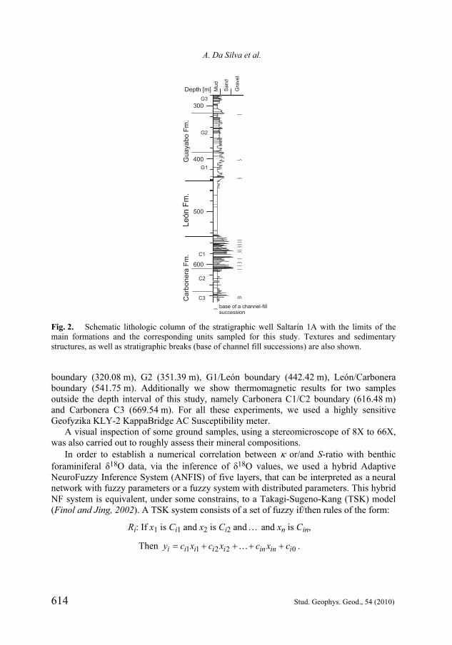
The 305 m depth interval, where we have restricted our study, encompasses mainly the Guayabo formation lower units G1, G2 and G3 (15 samples), León formation (23 samples) and Carbonera formation upper sandstone unit C1 (6 samples), as shown in Fig. 2.

Sedimentological, stratigraphic, biostratigraphic, and provenance analyses carried out in Saltarín 1A allowed the identification of major lithologies and the interpretation of sedimentary conditions for each stratigraphic unit (Bayona et al., 2008a). The lowermost formation is Carbonera that consists of a sandstone unit C3 from a fluvial system, a mudstone unit C2 from a lacustrine system, and a sandstone upper unit C1 (bottom of the studied section), that was accumulated in a fluvial-deltaic system (samples 549.8 to 610.20 m). Over Carbonera lies the León formation (samples 442.42 to 541.75 m), a muddy sequence of sediments from a fresh-water lacustrine system. Finally, on top of Carbonera is the Guayabo formation. According to Bayona et al. (2008a) the main



lithological features of Guayabo’s bottom units G1, G2 and G3 that cap the studied section, are:

G1 (samples from 388.10 to 413.49 m) and G2 (320.08 to 375.33 m): mostly green-colored laminated mudstones grading to sandstones interbedded with light-colored massive mudstones with ferruginous nodules. These lithologies are interpreted as the sedimentation from a fluvio-deltaic system changing to a more continental sediment accumulation in fluvial floodplains.

G3 (304.75 to 315.32 m): mudstones and siltstones accumulated in fluvial flood plains with some evidence of subaerial exposure (light-colored mudstones, formation of ferruginous nodules).

Initial magnetic susceptibility () was measured at room temperature using a Bartington susceptometer. The S-ratio was determined after inducing a high field (ca. 3 T) and an antiparallel low field (ca. 0.03 T) IRM. IRMs were measured in a 2G Enterprises cryogenic magnetometer with a sensitivity of 1011 A/m.

Fig. 1. Geographical setting of the stratigraphic well Saltarín 1A (Llanos Foreland Basin, Colombia).

A. Da Silva et al.


In the profiles of Fig. 3, global δ18O data for benthic foraminifera taken from Zachos et al. (2001), are age-linked to and S-ratios values after assuming a constant accumulation rate for a depth interval flanked by the only two palynological ages available for this stratigraphic well (Carlos Jaramillo, personal communication). These

Table 1. S-ratios, values and corresponding averaged δ18O from benthic foraminifera (Zachos et al., 2001) calculated assuming a constant accumulation rate and an age window of 0.005 Ma. Also shown: age constraints and other analyses performed on selected and additional samples (i.e. SEM/EDX, visual analyses of mineral components and high temperature magnetic susceptibility).

Formation Unit Depth [m] [SI] S-ratio Averaged 18O [‰]

Age Constraints/Analyses

304.75 21.84 0.58 1.33 Top Middle Miocene G3

315.22 17.10 0.38 1.16 --- 320.08 19.53 0.09 2.26 Visual Analyses/High T() 329.85 14.00 0.84 1.08 --- 351.39 27.75 0.87 1.28 High T() 355.30 23.90 0.93 1.15 --- 360.82 23.90 0.92 1.27 --- 370.18 25.59 0.90 1.21 ---

G2

375.33 21.24 0.91 1.07 --- 388.10 20.51 0.84 1.13 --- 395.11 14.97 0.84 0.92 --- 403.39 13.00 0.95 1.23 --- 407.54 21.37 0.94 1.64 ---

GU

YA

BO

G1

413.49 29.84 0.86 1.62 --- 442.42 24.39 0.95 1.59 High T() 444.94 25.35 0.94 1.72 --- 447.97 23.07 0.86 1.71 --- 450.45 19.78 0.99 1.45 --- 453.65 19.81 0.95 1.81 --- 458.85 22.21 0.94 1.67 --- 462.43 46.60 0.94 1.28 --- 475.15 22.94 0.94 1.35 --- 479.55 --- --- --- SEM/EDX 484.35 19.30 0.95 1.90 --- 487.80 23.18 0.94 1.60 --- 492.05 22.45 0.96 1.60 --- 494.14 28.25 0.96 1.78 --- 497.93 22.83 0.96 1.78 --- 511.97 23.66 0.98 1.68 --- 520.35 19.04 0.98 1.48 --- 527.26 16.20 0.95 1.79 --- 531.05 18.83 0.95 1.74 --- 534.44 21.49 0.98 1.90 --- 536.89 12.15 0.95 1.52 ---

LE

ÓN

541.75 31.44 0.94 1.32 High T()



age constrains are at 305 m (top of the middle Miocene, ca. 11.6 Ma) and 610 m (top of the lower Miocene, ca. 16 Ma). The validity of a constant accumulation rate is later revisited in the light of lithostratigraphic evidence and computational results.

The ages of the δ18O were calibrated with the geomagnetic polarity time scale of Berggren et al. (1995). The stratigraphic/temporal resolution of this global collection of δ18O data is less than 103 years for some age intervals. In Zachos et al. (2001), a five-point running mean is used to smooth the raw data. An average curve, showing the main tendencies of global ice volume and sea level changes, is adjusted to these points applying a locally weighted mean. Instead of making use of the rough approximation derived from this curve, we have employed an age window of 5 ka (ca 0.35 m), around the date assigned to each and S-ratio depth level, in order to compute their corresponding average δ18O values. Such a window seems to be the optimal one to minimize the standard deviation of averaged δ18O. Indeed, 5 ka is about a quarter of the shortest (axial precession) Milankovich global climate term. In the depth domain, a precision level of 0.35 m makes sense too, since most of the stratigraphic levels for this well have been given with 2 decimal places of accuracy. Moreover, in the time domain, our sample spacing of about 7 meters corresponds to 105 years, the maximum duration of short term aberrant rapid shifts and extreme climate transients (Zachos et al., 1997 and 2001).

We also carried out scanning electron microscopy (SEM) and energy dispersive X-ray spectroscopy (EDX). Only magnetic separates were used for SEM and EDX analyses. These separates were obtained by applying a hand magnet to a suspension in acetone of finely ground rock. Such small amounts of sample were mixed with ethanol and exposed to an ultrasonic bath for approximately 5 minutes. A drop of this preparation was placed on a thin layer of polyethylene set on a carbon holder, and covered by a carbon film (~ 10 nm). The scanning electron microscope used for SEM studies was a JEOL JSM-6390 and the X-ray probe and energy dispersor was an Oxford Instruments, model 7582.

We show results of some thermomagnetic susceptibility experiments (continuous heating and cooling cycles), performed on selected samples from Guayabo G2/G3

Table 1. Continuation.

Formation Unit Depth [m] [SI] S-ratio Averaged

18O [‰]Age Constraints/Analyses

549.80 21.36 0.61 1.36 --- 561.27 22.45 0.98 1.38 Visual Analyses 564.50 20.28 0.96 1.51 --- 565.14 0.00 0.83 1.52 --- 572.35 1.93 0.96 1.10 --- 579.24 0.00 0.93 1.48 --- 585.10 3.63 0.85 1.93 --- 590.94 4.85 0.92 1.95 --- 596.16 12.27 0.95 1.43 ---

C1

610.20 13.93 0.97 1.77 Top Lower Miocene C2 616.48 --- --- --- High T()

CA

RB

ON

ER

A

C3 669.54 --- --- --- High T()

A. Da Silva et al.


boundary (320.08 m), G2 (351.39 m), G1/León boundary (442.42 m), León/Carbonera boundary (541.75 m). Additionally we show thermomagnetic results for two samples outside the depth interval of this study, namely Carbonera C1/C2 boundary (616.48 m) and Carbonera C3 (669.54 m). For all these experiments, we used a highly sensitive Geofyzika KLY-2 KappaBridge AC Susceptibility meter.

A visual inspection of some ground samples, using a stereomicroscope of 8X to 66X, was also carried out to roughly assess their mineral compositions.

In order to establish a numerical correlation between or/and S-ratio with benthic foraminiferal δ18O data, via the inference of δ18O values, we used a hybrid Adaptive NeuroFuzzy Inference System (ANFIS) of five layers, that can be interpreted as a neural network with fuzzy parameters or a fuzzy system with distributed parameters. This hybrid NF system is equivalent, under some constrains, to a Takagi-Sugeno-Kang (TSK) model (Finol and Jing, 2002). A TSK system consists of a set of fuzzy if/then rules of the form:

Ri: If x1 is Ci1 and x2 is Ci2 and and xn is Cin,

Then 1 1 2 2 0i i i i i in in iy c x c x c x c .

Fig. 2. Schematic lithologic column of the stratigraphic well Saltarín 1A with the limits of the main formations and the corresponding units sampled for this study. Textures and sedimentary structures, as well as stratigraphic breaks (base of channel fill successions) are also shown.



According to the rules above, the output values yi are considered as a linear or constant function of the input variables xj (j = 1, 2, , n). Ri (i = 1, 2, , m) is the i-th fuzzy rule; Ci1, , Cin are the antecedent linguistic variables and ci1, ci2, , cin the consequent parameters.

The ANFIS uses these rules and five neural network layers. Each layer has a particular objective (Hurtado et al., 2009):

The first layer is composed of n membership functions, each implementing a fuzzy decision rule. Its output is the membership function for which the input variable satisfies the associated Cij term.

The second layer computes every possible combination of the n decision rules. The second layer computes every possible combination of the n decision rules.

The third layer normalizes the conjunctive membership functions in order to perceive the inputs.

Fig. 3. Profiles of S-ratio and magnetic susceptibility values between 304.75 m (top Middle Miocene) and 610.20 m (top Lower Miocene) in the stratigraphic well Saltarín 1A. Boundaries between formations (i.e. Guayabo G1, G2 and G3 units and León and Carbonera C1 unit), depth levels corresponding to some selected samples chosen for further detailed analyses and a parallel profile including all global benthic foraminiferal δ18O data in ‰ (after Zachos et al., 2001) are also

shown. Profiles of global δ18O data for benthic foraminifera are linked to and S-ratios values by assuming a constant accumulation rate for a depth interval flanked by the only two palynological ages available for this well. An age window of 0.005 Ma (ca 0.35 m) around the date assigned to each and S-ratio depth level is used to compute their corresponding average δ18O values (at the upper panel: single crosses connected by a dashed line overimposed to the whole δ18O data). This age window minimizes the standard deviation of the averaged δ18O.

A. Da Silva et al.


The fourth layer associates every membership function with an output (the weights are called consequent parameters)

The last layer combines all the individual outputs to obtain the total output (sums evidences).

To train our fuzzy model we used S-ratio or/and values as input variables and δ18O as output variable. We introduced the training data in both, logarithmic and linear forms. In this work, linear, triangular, bell, , and gaussian membership functions were tested.

3. ROCK MAGNETIC CHARACTERIZATION

High temperature susceptibility curves (heating and cooling), for Guayabo samples at 320.08 m (G2/G3 boundary) and 351.39 m (G2) (Figs. 4a and b, respectively) appear to have similar behaviors. However, when the scales of these graphs are blown up for a temperature interval between approximately 100 and 400C (insets in Figs. 4a,b), it is possible to identify, only for sample 351.39 m, a small increase of the magnetic susceptibility, around 220C. This bump, augmented by a logarithmic scale, probably corresponds to the λ transition phase of hexagonal pyrrhotite (Dekkers, 1989). Conversely, such a feature is completely absent in the magnetically weak sample 320.08 m (inset in Fig. 4a). In both cases, the raise of the magnetic susceptibility above 400C, accompanied by the major drop around 580C, implies that secondary magnetite has been formed upon heating. Magnetite formation, at temperatures above 400C, is characteristic of samples like 351.39 m with primary pyrrhotite that irreversibly transforms to magnetite (Dunlop and Özdemir, 1997). Differences in amplitude, for susceptibility changes above 400C,

Fig. 4. Magnetic susceptibility curves (heating and cooling) for samples: a) 320.08 m (located on the boundary between Guayabo units G2 and G3) and b) 351.39 m from the unit G2 within the Guayabo formation. The magnetic susceptibility curve for 320.08 m suggests the presence of hematite. The magnetic susceptibility curve for 351.39 m suggests the presence of hexagonal pyrrhotite with a λ phase above 220C that is not present in 320.08 m (see insets for both samples).



must be related to the presence of distinct primary magnetic phases for each of these two samples (i.e. hematite for 320.08 m and pyrrotite/magnetite for 351.39 m). Besides the formation of secondary magnetite, resulting in such large amplitude rises (Figs. 4a,b), the susceptibility signal at 351.39 m might be enhanced by a Hopkinson peak too.

For the specific case of 320.08 m, visual analyses of mineral compositions show some Fe oxides that have been positively identified as hematite. We argue that this mineral is, perhaps, the chief and primary magnetic phase in these rocks since hematite is stable under oxidizing conditions. In fact, the corresponding S-ratio value, for this depth level, is the lowest of a well-defined negative anomaly (Fig. 3) that spans between 304.75 and 320.08 m (Guayabo’s lower G3 and G2 informal units according to Bayona et al., 2008a). Such an anomaly nearly coincides with a paleoenvironment that includes the presence of oxidized paleosols in G3/G2, between 312.9 to 388 m (Bayona et al., 2008a), and a vastly documented global regression event that occurred at the end of the Serravallian stage (Vail et al., 1977).

Figs. 5a and b show the thermomagnetic curve of sample 442.42 m and the SEM and EDX results for the sample at 479.55 m, both from the León formation. Sample 442.42 m is just at the boundary between the bottom of Guayabo (unit G1) and the top of León. When the temperature scale between 100 and 400C is enlarged, a small rise of the magnetic susceptibility signal, at about 220C, is clearly displayed, followed by a drop at around 325C (inset in Fig. 5a). Once more, as in the case of sample at 351.39 m, this feature suggests the presence of pyrrhotite. The increase of the magnetic susceptibility upon heating, above 400C, followed by a drop around 580C, indicates that magnetite forms in situ and is not a predominant mineral in the original sample.

Sulfur and minute amounts of Fe were also detected, via scanning electron photomicrographs and X-ray energy dispersion spectra, in magnetic separates from sample 479.55 m (Fig. 5b).

The León formation is described as a muddy unit from a fresh-water lacustrine system. It has been extensively reported that, for muddy sediments, accumulated during high water level periods (i.e. warm and humid climate), authigenic formation of magnetic iron sulfides occurs at the very early stages of sedimentation. Fe sulfides form, in these cases, via sulfate reduction and taking advantage of native sulfate and organic carbon (e.g. Sagnotti, 2007; Shouyun et al., 2002; Tric et al., 1991). Accumulation of Fe sulfides is also favored by euxinic lacustrine environments with restricted water circulation, high production of organic matter and relatively high sedimentation rates. The sediments in oxygen depleted bottom waters become rich in organic matter and anoxic because of rapid burial that prevent their oxidation. It seems that, as long as there is a limited amount of sulfide, reactive iron and/or organic matter on hand, iron sulfides such as greigite and pyrrhotite would be preserved with ages that could range from Cretaceous to Holocene (e.g. Babinszki et al, 2007; Otamendi et al., 2006; Weaver et al., 2002, among others). The stability of pyrrhotite is favoured over greigite, in more reducing environments and higher concentrations of H2S (i.e. higher consumption of organic carbon). Since the occurrence of early diagenetic Fe sulfides seems to be produced in muddy lacustrine sediments during interglacial periods, changes of magnetic properties associated to these minerals might be used as environmental proxies (e.g. Babinszki et al., 2007; Mora et al., 2002; Shouyun et al., 2000; Vigliotti et al., 1999; Roberts et al., 1996, among others).

A. Da Silva et al.


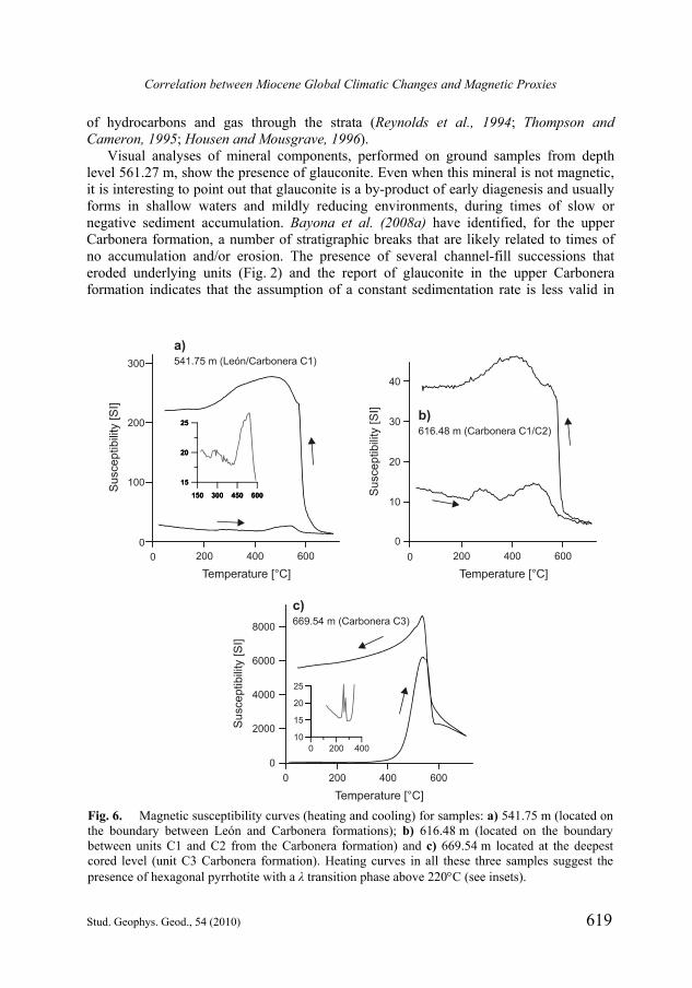
The upper Carbonera formation (unit C1), characterized by sandstones that have accumulated in a fluvial-deltaic system, represents the bottom of our stratigraphic section. Figs. 6a,b,c show the thermomagnetic curves of samples at 541.75 m (León/Carbonera boundary), 616.48 m (Carbonera C1/C2 boundary) and the lowermost level 669.54 m located in Carbonera unit C3 (these last two samples lying outside our studied section). Again, in all these cases, the presence of hexagonal pyrrhotite seems to be revealed by a λ transition phase at about 220C (Dekkers, 1989).

Although Saltarín 1A is a non producer oil well, some impregnations of hydrocarbons have been found in samples from units C1 and C2 from the Carbonera formation casting some doubts about the primary or nearly primary origin of Fe-sulfides in these last three samples (Alejandro Mora, personal communication). Indeed, in some settings, Fe-sulfides have also been reported to form during late diagenesis as a consequence of the diffusion

Fig. 5. a) Magnetic susceptibility curve (heating and cooling) for sample 442.42 m at the boundary between Guayabo and León formations. b) SEM photomicrograph and EDX spectra from magnetic separates of sample 479.55 m. Magnetic susceptibility curve for 442.42 m suggests the presence of hexagonal pyrrhotite with a λ-transition phase above 220C (see inset). SEM and EDX analyses in 479.55 m show the presence of sulfur and minute amounts of Fe.



of hydrocarbons and gas through the strata (Reynolds et al., 1994; Thompson and Cameron, 1995; Housen and Mousgrave, 1996).

Visual analyses of mineral components, performed on ground samples from depth level 561.27 m, show the presence of glauconite. Even when this mineral is not magnetic, it is interesting to point out that glauconite is a by-product of early diagenesis and usually forms in shallow waters and mildly reducing environments, during times of slow or negative sediment accumulation. Bayona et al. (2008a) have identified, for the upper Carbonera formation, a number of stratigraphic breaks that are likely related to times of no accumulation and/or erosion. The presence of several channel-fill successions that eroded underlying units (Fig. 2) and the report of glauconite in the upper Carbonera formation indicates that the assumption of a constant sedimentation rate is less valid in

Fig. 6. Magnetic susceptibility curves (heating and cooling) for samples: a) 541.75 m (located on the boundary between León and Carbonera formations); b) 616.48 m (located on the boundary between units C1 and C2 from the Carbonera formation) and c) 669.54 m located at the deepest cored level (unit C3 Carbonera formation). Heating curves in all these three samples suggest the presence of hexagonal pyrrhotite with a λ transition phase above 220C (see insets).

A. Da Silva et al.


this interval rather than in the León and lower Guayabo units.

4. COMPUTATIONAL RESULTS

The profiles in Fig. 3 show magnetic parameters (S-ratio and ), measured at different depth levels in Saltarín 1A, together with their corresponding average benthic foraminiferal δ18O values. S-ratios and values are subject to local alteration of the sediments reflecting different sedimentary conditions induced by temperature variations. However, from profiles in Fig. 3 alone, there is not an obvious link between S-ratio, and δ18O values.

Fig. 7a,b shows two cross plots for benthic foraminiferal δ18O values versus experimental S-ratio and data, respectively. Linear regression analyses in each case, δ18O = 0.1423 S-ratio + 1.635 (R2 = 0.0068) and δ18O = 0.0025 + 1.635 (R2 = 0.0055), prove unsuitable to find out the complex empirical relationships between these two pairs of parameters. These results prompt us to the use of an alternative non-linear approach (i.e. NFL) to find a family of local fitting functions for different sub groups of experimental data points.

As it was previously indicated, we tested different combinations of these proxies in linear and logarithmic forms, as well as various membership functions. The best results were always accomplished training with the data in linear form and with a Gaussian membership function. Fig. 8 shows the results of our first computational trials by training the net with S-ratio and δ18O data only. In each case, 2, 3 and 4 fuzzy rules (Figs. 8a, b and c, respectively) were employed to monitor a possible improvement of the inference of

Fig. 7. a) Cross plot of experimental S-ratio and global benthic foraminiferal δ18O values in ‰. S-ratios are all the 44 data points measured in Saltarín 1A between depth levels 304.75 m (top Mid Miocene) and 610.20 m (top Lower Miocene). Relationship δ18O = 0.1423 S-ratio + 1.635 (R2 = 0.0068) was obtained using a linear regression analysis. b) The same crossplot using and

global benthic foraminiferal δ18O values. Relationship δ18O = 0.0025 + 1.635 (R2 = 0.0055) was obtained using a linear regression analysis.



global benthic foraminiferal δ18O values. The number of fuzzy rules for the last test (Fig. 8c) is about 10% of the number of data points we have used to train the NFL system.

To quantify the performance of the fitting, we used the R2 correlation between inferred and experimental δ18O data, and the Root Mean-Square Error (RMSE) values calculated according to:

21

1 n

inf expi

RMSE Y Yn

,

where Yinf and Yexp are the inferred and experimental values, respectively, and n is the number of experimental points.

The comparison between δ18O inferred values versus global benthic foraminiferal δ18O values gave rise to R2 = 0.2628 and RMSE = 0.2468‰ using two fuzzy rules, R2 = 0.2905 and RMSE = 0.2421‰ using 3 fuzzy rules, and R2 = 0.4182 and

Fig. 8. Benthic foraminiferal δ18O inference using an adaptative NeuroFuzzy inference system (ANFIS). These results were obtained by training the NeuroFuzzy system with 100% of the experimental S-ratio values and the benthic foraminiferal δ18O data available. Solid lines stand for the inferred data whereas the crosses and dashed lines represent the experimental data. Results of the inference are shown for the three cases: a) 2 fuzzy rules (R2 = 0.2628; RMSE = 0.2468‰), b) 3 fuzzy rules (R2 = 0.2905; RMSE = 0.2421‰) and c) 4 fuzzy rules (R2 = 0.4182; RMSE = 0.2222‰).

A. Da Silva et al.


RMSE = 0.2222‰ using 4 fuzzy rules. The low correlation between inferred and actual data, in these three trials, reveals the inability of the NFL system to predict δ18O proxies by training the net with solely S-ratio experimental values for Saltarín 1A and global benthic foraminiferal δ18O data.

Similar tests were repeated by training the net with experimental data only and their corresponding benthic foraminiferal δ18O values (Fig. 9). δ18O inferred values versus global benthic foraminiferal δ18O gave rise to R2 = 0.0894 and RMSE = 0.2743‰ for two fuzzy rules, R2 = 0.1651 and RMSE = 0.2626‰ for three fuzzy rules, and R2 = 0.1921 and RMSE = 0,2584‰ for 4 fuzzy rules. Once more, the weak correlation between inferred and actual data show the inability of the NFL system to predict δ18O proxies by training the net with experimental values and global benthic foraminiferal δ18O data only.

Fig. 9. Benthic foraminiferal δ18O inference using an adaptative NeuroFuzzy inference system (ANFIS). These results were obtained by training the NeuroFuzzy system with 100% of the experimental magnetic susceptibility () values and the benthic foraminiferal δ18O data available. Solid lines stand for the inferred data whereas the crosses and dashed lines represent the experimental data. Results of the inference are shown for the three cases: a) 2 fuzzy rules (R2 = 0.08935; RMSE = 0.2743‰), b) 3 fuzzy rules (R2 = 0.1651; RMSE = 0.2626‰) and c) 4 fuzzy rules (R2 = 0.1921; RMSE = 0.2584‰).



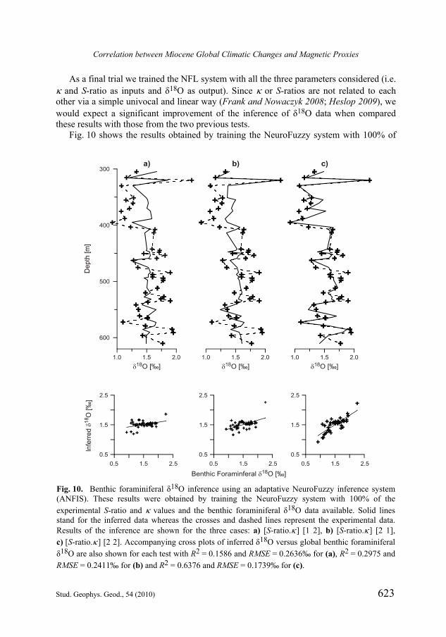
As a final trial we trained the NFL system with all the three parameters considered (i.e. and S-ratio as inputs and δ18O as output). Since or S-ratios are not related to each other via a simple univocal and linear way (Frank and Nowaczyk 2008; Heslop 2009), we would expect a significant improvement of the inference of δ18O data when compared these results with those from the two previous tests.

Fig. 10 shows the results obtained by training the NeuroFuzzy system with 100% of

Fig. 10. Benthic foraminiferal δ18O inference using an adaptative NeuroFuzzy inference system (ANFIS). These results were obtained by training the NeuroFuzzy system with 100% of the

experimental S-ratio and values and the benthic foraminiferal δ18O data available. Solid lines stand for the inferred data whereas the crosses and dashed lines represent the experimental data. Results of the inference are shown for the three cases: a) [S-ratio. ] [1 2], b) [S-ratio. ] [2 1], c) [S-ratio. ] [2 2]. Accompanying cross plots of inferred δ18O versus global benthic foraminiferal δ18O are also shown for each test with R2 = 0.1586 and RMSE = 0.2636‰ for (a), R2 = 0.2975 and RMSE = 0.2411‰ for (b) and R2 = 0.6376 and RMSE = 0.1739‰ for (c).

A. Da Silva et al.


the S-ratio and experimental values and benthic foraminiferal δ18O data available (44 sets of data points). For the first case (Fig. 10a) we considered one membership function for S-ratio data and two for values. This [1 2] combination gives rise to two fuzzy rules (the product of the number of membership functions of the input variables). The corresponding cross plot of inferred and actual values of δ18O reveals a poor inference with a correlation coeficient of R2 = 0.1586 and a RMSE = 0.2636‰. We also tried a [2 1] combination of S-ratio and data (i.e. two fuzzy rules, Fig. 10b). Once more, the corresponding cross plot of inferred and actual values of δ18O reveals a poor inference with a correlation coeficient of R2 = 0.2975 and a RMSE = 0.2410‰. Finally, for the last trial, we used two membership functions for both S-ratio and data ([2 2], four fuzzy rules). The identified TSK model (i.e the membership function values and the four fuzzy rules) are shown in Table 2. As it can be observed in Fig. 10c, a reasonably good correlation was obtained. The R2 (0.6376) and RMSE (0.1739‰) values in Table 2 confirm this observation. This result seems to indicate a link between magnetic proxies, measured in samples from stratigraphic well Saltarín 1A, and global climate changes mirrored by the variability of benthic foraminiferal δ18O data.

Finally we tested how feasible it is the hypothesis of a constant accumulation rate between the two age tie points at 305 and 610 m of depth. We divided the whole interval in 4 subsections of 76.25 m thick each. Two of these subsections, the first and the last, are bond to the first and last ages available. We would expect that the best inference would correspond to the first subsection (305 m/381.25 m), with a progressive worsening of it as long as we move away from the upper age constraint. We have used the same combination [1 2] for S-ratio and for each trial illustrated in Figs. 11a,b,c and d. For each cross plot we have obtained: (a) R2 = 0.9775, RMSE = 0.0502‰ (b) R2 = 0.7713, RMSE = 0.08869‰ (c) R2 = 0.7586, RMSE = 0.0673‰ and (d) R2 = 0.6808, RMSE = 0.1412‰. Notice that the lower correlations correspond to sections b) and d) (381.25 m/457.5 m and 533.75 m/610 m, respectively) that contain some stratigraphic

Table 2. Parameters of the Gaussian membership functions [Δh1/2 Center] and fuzzy rules obtained

by training the NFL using S-ratio and data as input variables to infer δ18O. The RMSE and R2 values are also included.

Membership Functions Parameters

S-ratio Fuzzy Rules RMSE [‰] R2

[0.2400.113] [19.7860.002] 18O = 24.17 (S-ratio) 0.34 + 18.01

[0.2400.113] [19.78846.597] 18O = 28.68 (S-ratio) 0.87 28.26

[0.1051.128] [19.7860.002] 18O = 26.90 (S-ratio) 0.57 + 26.83

[0.1051.128] [19.78846.597] 18O = 37.97 (S-ratio) 0.02 36

0.1739 0.6376



breaks (Bayona et al., 2008a) probably linked to channel fills. Cross-correlation between magnetic parameters and δ18O data would be likely affected by such stratigraphic mismatches at those very subsections. Subsection b has only two of these unconformities whereas subsection d has a total of ten (Fig. 2). As a consequence data dispersion is considerably higher in the latter subsection.

5. DISCUSSION AND CONCLUSIONS

The scattering of data points obtained by plotting global benthic foraminiferal δ18O values, versus either experimental S-ratios (Fig. 7a) or initial magnetic susceptibility

Fig. 11. The consequences of assuming a constant sedimentation rate between 304.75 m and 610.20 m on the inference of benthic foraminiferal δ18O data (in ‰), are assessed by dividing the depth interval in 4 subintervals of about 76.25 m each. The NFL method has been applied in each case using the same combination [S-ratio. ] [1 2] for a), b), c), and d). Accompanying cross plots of inferred δ18O versus global benthic foraminiferal δ18O are also shown for each test with R2 = 0.9775 and RMSE = 0.0502‰ for (a), R2 = 0.7713 and RMSE = 0.0887‰ for (b), R2 = 0.7586 and RMSE = 0.0673‰ for (c) and R2 = 0.6808 and RMSE = 0.1412‰ for (d).

A. Da Silva et al.


(Fig. 7b), illustrates the impossibility of finding a clean cut relationship between these parameters via traditional methods of linear regression analyses.

The complexities of the problem we are dealing with are most likely related to different factors that could introduce random noise to the magnetic proxies, otherwise directly linked to global climatic changes (i.e. δ18O values). Some of these factors are the probable influence of local and regional tectonic events, local climate changes upon sediment composition (Harris and Mix, 2002) and late diagenesis of primary magnetic minerals (Roberts et al., 1996). The hypothesis of a constant accumulation rate, for a 305 m thick stratigraphic sequence in a time period of ca 4.4 Ma, could have also had a consequence upon these results.

Even a non linear approach to this problem, using the hybrid NFL method, requires multiple computational trials to obtain a set of optimal results. We argue that the weak correlation found by training the NFL system with either or S-ratio experimental data and benthic foraminiferal δ18O values (Figs. 8 and 9), is because the origin and properties of the various magnetic minerals in these rocks are independently linked, to different extents, to the several factors that preclude a direct connection of their corresponding magnetic parameters to global climatic proxies.

Since and S-ratio experimental values are not related to each other by a simple univocal and linear way (Frank and Nowaczyk, 2008; Heslop, 2009) it is reasonable to believe that an improved inference of the δ18O data would be obtained by including both magnetic parameters as input in the training of the NFL system. The optimal fitting gives rise to four fuzzy rules in a combination [2 2] of S-ratio and data (Fig. 10c). A correlation factor of R2 = 0.6376 and a root mean squared error RMSE = 0.17389957‰ can be interpreted as the result of a major influence (ca. 64%) of the global climatic changes in the magnetic proxies that we have chosen to infer benthic foraminiferal δ18O data.

We argue that the effect of late diagenesis upon primary magnetic minerals is playing a minor role upon these results. Indeed, an advantage of this cored stratigraphic well is that the rocks analyzed are deep enough to have suffered the effects of tardy weathering. The rock magnetic evidence seems to point out to the primary or nearly primary nature of most of the minerals identified in both Guayabo (G1 and G2 units) and León formations. For instante, hematite in G2 appears to be related to a paleoenvironment that includes the presence of oxidized paleosols and a global regression event at the end of the Serravallian stage. Correspondingly, Fe-sulfides (e.g. pyrrhotite) in León might be the by-product of early diagenesis in muddy lacustrine sediments, during times of humid climate, high production of organic matter, slow bottom water circulation and rapid burial of the sediment load.

However, we have also identified Fe-sulfides (e.g. pyrrhotite) in samples from the upper Carbonera sandstone that could be a late diagenesis by-product formed as a consequence of the diffusion of hydrocarbon through these strata. Oil impregnations recognized in these samples support such a presumption. These upper Carbonera strata also coincide with a glauconite-rich region of multiple unconformities or stratigraphic breaks that most likely represent channel fills (Bayona et al., 2008a).

The presence of amalgamated channel-fill successions at the base of the upper unit of the Carbonera formation (Fig. 2), and the record of fluvial-deltaic sediments whose lower



contact shows evidence of stratigraphic breaks (Bayona et al., 2008a), rules out beforehand the validity of assuming a constant accumulation rate for the upper Carbonera unit. In contrast, the rather uniform muddy lithology of the León formation and lower units of the Guayabo formation allows the assumption of a constant accumulation rate.

Therefore, although erroneous for the whole sequence analyzed, the assumption of constant accumulation rate is a good way to independently assess the effectiveness of the NFL method. In fact, after dividing the stratigraphic section in four intervals of equal thickness, and applying the NFL method to infer δ18O values in each of them, we find that the lower correlation and major dispersion corresponds to this last subsection. Hydrocarbon induced magnetic phases at these levels could have also contributed to such a mismatch.

From the discussion above it is clear that neither late diagenesis nor the assumption of a constant accumulation rate, appear to be critical factors that have had a significant effect upon the NFL inference over most of the stratigraphic sequence that we have studied here.

Local and regional tectonics and climate changes during early and middle Miocene times, at the Colombian Llanos foreland basin, were the main factors that probably prevented a stronger correlation (i.e. over 64%) of S-ratio and data to global climatic proxies. The Miocene succession of the Saltarin 1A at the distal segment of the Llanos foreland basin records changes both in tectonic subsidence rates and in composition/location of source areas (Bayona et al., 2008a). The overwhelming increase of tectonic subsidence rates relative to the decrease of supply of sediments, is recorded in the abrupt contact between the upper sandy unit of the Carbonera formation and the muddy León formation. Bayona et al. (2008b, 2009) interpreted the increase of tectonic subsidence due to the onset of inversion of the whole Eastern Cordillera of Colombia (i.e., flexural subsidence due to orogenic loads) and the effect of large-scale subsidence due to sublithospheric flows associated to the new subduction zone to the west (i.e., dynamic topography subsidence). This change in tectonic conditions also controlled the location of uplifted areas in the distal Llanos basin.

The distal location of uplifted areas due to increasing tectonic subsidence and humid weather favored the flooding of the basin and continue filling with fine-grained terrigenous detritus. Quartzose and subarkosic composition of sandstone beds of the upper unit of the Carbonera formation indicates that sediments were derived from eastward cratonic areas, where intrusive rocks of the Guyana shield crop out. These cratonic regions were totally covered in middle Miocene time by accumulation of the lacustrine sediments of the Leon formation; humid conditions were likely during the time of the Middle Miocene Climatic Optimum. Sandstone beds in the lower Guayabo units document an upsection increase of plagioclase, sedimentary and metamorphic lithic fragments that indicate supply from nearby uplifted blocks located to the south and southeast (Bayona et al. 2008a).

Nevertheless, our novel approach to the assessment of a paleoclimatic problem, applied here to the stratigraphic well Saltarín 1A, shows the scope of the NFL technique in handling geological problems where traditional linear regression methods prove highly limited.

Acknowledgements: Samples were generously provided by Alejandro Mora (Hocol S.A.,

Bogotá). He also made available important unpublished geological and geophysical information. We

A. Da Silva et al.


are grateful to all the people and laboratories that have contributed to this research: specially to Carlos Jaramillo (Smithsonian Tropical Research Institute, Panamá City, Panamá), Wyn Williams and Jennifer Tait (University of Edinburgh, Edinburgh, Scotland), Myriam Rada and Glen Rodríguez (Universidad Simón Bolivar, Caracas, Venezuela), Eduardo Carrillo (Universidad Central de Venezuela, Caracas, Venezuela) and Corporación Geológica ARES (Bogotá, Colombia). This research was partially funded by the Decanato de Investigación y Desarrollo and Dirección de Desarrollo Profesoral both at the Universidad Simón Bolívar (Caracas,Venezuela) via research grants to V. C.-A. and M.A. and by the Consejo de Desarrollo Científico y Humanístico de la Universidad Central de Venezuela (Caracas, Venezuela) via the research project number 03.6377.2006 of N.H.

References

Alexander I., Kroon D. and Thompson R., 1993. Late Quaternary paleoenvironmental change on the northeastern Australian margin as evidenced in oxygen isotope stratigraphy, mineral magnetism and sedimentology. In: McKenzie J.A., Davies P.J. and Palmer-Juslon A. et al. (Eds.), Proc. ODP, Sci. Results, 133, College Station, TX (Ocean Drilling Program), 129161.

Babinszki E., Márton E., Márton P. and Kiss L.F., 2007. Widespread occurrence of greigite in the sediments of Lake Pannon: Implications for environment and magnetostrtigraphy. Palaeogeogr. Palaeoclimatol. Palaeoecol., 252, 626636.

Balsam W., Ji J. and Chen J., 2004. Climatic interpretation of the Luochuan and Lingtai loess sections, China, based on changing iron oxide mineralogy and magnetic susceptibility. Earth Planet. Sci. Lett., 223, 335348

Bayona G., Jaramillo C., Rueda M., Reyes-Harker A. and Torres V., 2007. Paleocene - middle Miocene flexural-margin migration of the nonmarine Llanos forehand basin of Colombia. CT&F Ciencia, Tecnología y Futuro, 3(3), 141160.

Bayona G., Valencia A., Mora A., Rueda M., Ortiz J. and Montenegro O., 2008a. Estratigrafía y procedencia de las rocas del Mioceno en la parte distal de la cuenca antepais de los Llanos de Colombia. Geología Colombiana, 33, 2346 (in Spanish).

Bayona G., Cortés M., Jaramillo C., Ojeda G., Aristizabal J. and Reyes-Harker A., 2008b. An integrated analysis of an orogen-sedimentary basin pair: Latest Cretaceous-Cenozoic evolution of the linked Eastern Cordillera orogen and the Llanos foreland basin of Colombia. Geol. Soc. Am. Bull., 120, 11711197.

Bayona G., Valencia A., de Armas M., Guerrero J., Gomez E., Leyva I., Villamarin P. and Mora A., 2009. Oligocene - Miocene filling of the distal Llanos Basin of Colombia: Interaction of flexural subsidence, intraplate faulting and dynamic topography models. AAPG International Conference and Exhibition, 1518 November 2009, Rio de Janeiro, Brasil, AAPG Search and Discover Article #90100.

Berggren W.A., Kent D.V., Swisher C.C. and Aubry M.-P., 1995. A revised Cenozoic geochronology and chronostratigraphy. In: Berggren W.A., Kent D.V., Aubry M.-P. and Hardenbol J. (Eds.), Geochronology, Time Scales and Stratigraphic Correlation. Society for Sedimentary Geology (SEPM) Spec. Publ., 54, 129212.

Bloemendal J., King J.W., Hall F.R. and Doh S.J., 1992. Rock magnetism of Late Neogene and Pleistocene deep-sea sediments: relationship to sediment source, diagenetic processes and sediment lithology. J. Geophys. Res., 97, 43614375.



Brachfeld S.A. and Banerjee S.K., 2000. Rock-magnetic carriers of century-scale susceptibility cycles in glacial-marine sediments from the Palmer Deep, Antarctic Peninsula. Earth Planet. Sci. Lett., 176, 443455.

Cuddy S.J. and Glover P.W.J., 2001. The application of fuzzy logic and genetic algorithms to oil exploration. In: John R. and Birkenhead R. (Eds.), Developments in Soft Computing. Physica Verlag, Heidelberg, New York, 167174.

Dekkers M.J., 1989. Magnetic properties of natural pyrrhotite II: High and low temperature behaviour of JRS and TRM as function of grain size. Phys. Earth Planet. Inter., 57, 266283.

Dunlop D.J. and Özdemir Ö., 1997. Rock Magnetism - Fundamentals and Frontiers. Cambridge University Press, Cambridge, U.K.

Finol J., Guo Y. and Jing X., 2001. A rule based fuzzy model for the prediction of petrophysical rock parameters. J. Pet. Sci. Eng., 29, 97113.

Finol J. and Jing X.D., 2002. Predicting petrophysical parameters in a fuzzy environment in soft computing for reservoir characterisation and modeling. In: Wong P., Aminzadeh F. and Nikravesh M. (Eds.), Soft Computing for Reservoir Characterization and Modeling. Studies in Fuzziness and Soft Computing, 80, Physica-Verlag, Heidelberg, 183217.

Frank U. and Nowaczyk N.R., 2008. Mineral magnetic properties of artificial samples systematically mixed from haematite and magnetite. Geophys. J. Int., 175, 449461.

Geiss C.E. and Banerjee S.K., 1997. A multi-parameter rock magnetic record of the last glacial-interglacial paleoclimate from south-central Illinois, USA. Earth Plan. Sci. Lett., 152, 203216.

Harris S.E. and Mix A., 2002. Climatic and tectonic influences on continental erosion of tropical South America, 013 Ma. Geology, 30, 447450.

Helle H.B., Bhatt A. and Ursin B., 2001. Porosity and permeability prediction from wireline logs using artificial neural networks: a North Sea case study. Geophys. Prospect., 49, 431444.

Heller F. and Liu T.S., 1986. Plaeoclimatic and sedimentary history from magnetic susceptibility of loess in China. Geophys. Res. Lett., 13, 11691172.

Heslop D., Shaw J., Bloemendal J., Chen F., Wang J. and Parker E., 1999. Submillennial scale variations in east Asian Monsoon systems recorded by dust deposits from the North-Western Chinese Loess Plateau. Phys. Chem. Earth (A), 24, 785792

Heslop D., Langereis C.G. and Dekkers M.J., 2000. A new astronomical timescale for the loess deposits of Northern China. Earth Planet. Sci. Lett., 184, 125139.

Heslop D., 2009. On the statistical analysis of the rock magnetic S-ratio. Geophys. J. Int., 178, 159161.

Hilgen F.J., 1991. Astronomical calibration of Gauss to Matuyama sapropels in the Mediterranean and implication for the Geomagnetic Polarity Time Scale. Earth Planet. Sci. Lett., 104, 226244.

Housen B.A. and Musgrave R.J., 1996. Rock magnetic signature of gas hydrates in accretionary prism sediments. Earth Planet. Sci. Lett., 139, 509519.

Hu S.Y., Wang S.M. and Appel E., 2000. The environmental mechanism of fluctuations of magnetic susceptibility recorded in lacustrine sediments from Jalai Nur, Inner Mongolia. Sci. China Ser. D - Earth Sci., 43, 534540.

A. Da Silva et al.


Hurtado N., Aldana M. and Torres J., 2008. Comparison between neuro-fuzzy and fractal models for permeability prediction. Comput. Geosci., 13, 181186.

Kent D.V., 1982. Apparent correlation of palaeomagnetic intensity and climatic records in deep-sea sediments. Nature, 299, 538539.

Laskar J., 1990. The chaotic motion of the solar system: a numerical estimate of the size of the chaotic zones. Icarus, 88, 266291.

Lu H., Liu X., Zhang F., An Z. and Dodson J., 1999. Astronomical calibration of loesspaleosol deposits at Luochuan central Chinese loess plateau. Palaeogeogr. Palaeoclimatol. Palaeoecol., 154, 237246.

Mora G., Pratt L.M., Boom A. and Hooghiemstra H., 2002. Biogeochemical characteristics of lacustrine sediments reflecting a changing Alpine Neotropical Ecosystem during the Pleistocene. Quat. Res., 58, 189196.

Moreno E., Thouveny N., Delanghe D., McCave N.I. and Shackleton N.J., 2002. Climatic and oceanographic changes in the Northeast Atlantic reflected by magnetic properties of sediments deposited on the Portuguese Margin during the last 340 ka. Earth Planet. Sci. Lett., 202, 465480.

Otamendi A.M., Diaz M., Costanzo-Alvarez V., Aldana M. and Pilloud A., 2006. EPR stratigraphy applied to the study of two marine sedimentary sections in southwestern Venezuela. Phys. Earth Planet. Inter., 154, 243254.

Retallack G.J., Sheldon N.D., Cogoini M. and Elmore R.D., 2003. Magnetic susceptibility of early Paleozoic and Precambrian paleosols. Palaeogeogr. Palaeoclimatol. Palaeoecol., 198, 373380.

Reynolds R.L., Tuttle M.L., Rice C.A., Fishman N.S., Karachewski J.A. and Sherman D.M., 1994. Magnetization and geochemistry of greigite-bearing Cretaceous strata, North Slope Basin Alaska. Am. J. Sci., 294, 485528.

Roberts A.P., Reynolds R.L., Verosub K.L. and Adam D.P., 1996. Environmental magnetic implications of greigite (Fe3S4) formation in a 3 m.y. lake sediment record from Butte Valley, northern California. Geophys. Res. Lett., 23, 28592862.

Sagnotti L., 2007. Iron sulfides. In: Gubbins D. and Herrera-Bervera E. (Eds.), Encyclopedia of Geomagnetism and Paleomagnetism. Springer, Heidelber, 454459.

Schakleton N.J. and Opdyke N.D., 1973. Oxygen isotope and paleomagnetic stratigraphy of equatorial Pacific core V28-238: Oxygen isotope temperatures and ice volumes on a 105-year and 106-year scale. Quat. Res., 3, 3955.

Shouyun H.U., Sumin W., Appel E. and Lei J., 2000. Environmental mechanism of magnetic susceptibility changes of lacustrine sediments from Lake Hulun, China. Sci. China Ser. D - Earth Sci., 43, 534540.

Shouyun H.U., Appel E., Hoffmann V. and Schmahl W., 2002. Identification of greigite in lake sediments and its magnetic significance. Sci. China Ser. D - Earth Sci., 45, 8187.

Thompson R. and Cameron T.D.J., 1995. Paleomagnetic study of Cenozoic sediments in North Sea boreholes: an example of a magnetostratigraphic conundrum in a hydrocarbon producing area. In: Turner P. and Turner A. (Eds.), Paleomagnetic Applications in Hydrocarbon Exploration and Production. Geol. Soc. London Spec. Publ., 98, 223236.



Tric E., Laj C., Jehanno C., Valet J.P., Kissel C., Mazaud A. and Iaccarino S., 1991. Highresolution record of the upper Olduvai polarity transition from Po Valley (Italy) sediments:support for dipolar transition geometry? Phys. Earth Planet. Inter., 65, 319336.

Urbat M., Dekkers M.J. and Vriend S.P., 1999. The isolation of diagenetic groups in marine sediments using fuzzy c-means cluster analyses. In: Tarling D.H. and Turner P. (Eds.), Palaeomagnetism and Diagenesis in Sediments. Geol. Soc. London Spec. Publ., 151, 8593.

Vail P.R., Mitchun R.M.Jr, Todd R.G., Widmier J.M., Thompson S. and Sangree J.R., 1977. Seismic stratigraphy and global changes of sea level. In: Payton C.E. (Ed.), Seismic Stratigraphy - Application to Hydrocarbon Exploration. Am. Assoc. Petrol. Geol. Mem., 26, 49212.

Vigliotti L., Capotondi L. and Torii M., 1999. Magnetic properties of sediments deposited in suboxic-anoxic environments: relationships with biological and geochemical proxies. In: Tarling D.H. and Turner P. (Eds.), Palaeomagnetism and Diagenesis in Sediments. Geol. Soc. London Spec. Publ., 151, 7183.

Weaver R., Roberts A.P. and Barker A.J., 2002. A late diagenetic (synfolding) magnetization carried by pyrrhotite: implications for paleomagnetic studies from magnetic iron sulphide-bearing sediments. Earth Planet. Sci. Lett., 200, 371386.

Willams D.F., Peck J., Karabanov E.B., Prokopenko A.A., Kravchinsky V., King J. and Kuzmin M.I., 1997. Lake Baikal record of continental climate response to orbital insolation during the past 5 million years. Science, 278, 11141117.

Zachos J.C., Flower B.P. and Paul H.A., 1997. Orbitally paced chmate oscillations across the Oligocene/Miocene boundary. Nature, 388, 567570.

Zachos J., Pagani M. , Sloan L., Thomas E. and Billups K. 2001. Trends, Rhythms and Aberrations in Global Climate 65 Ma to Present, Science, 292, 686 - 693.

Zhu R.X., Shi C.D., Suchy V., Zeman A., Guo B. and Pan Y., 2001. Magnetic properties and paleoclimatic implications of loess-paleosol sequences of Czech Republic. Sci. China Ser. D - Earth Sci., 44, 385394.

Possible correlation between miocene global climatic changes and magnetic proxies, using neuro fuzzy...

Documents

Transcript of Possible correlation between miocene global climatic changes and magnetic proxies, using neuro fuzzy...