Detachment in the Khao Kwang Foreland Fold and Thrust Belt ...

Mechanical and petrophysical

properties of the Alum Shale

Detachment in the Khao Kwang

Foreland Fold and Thrust Belt, central

Thailand

Thesis submitted in accordance with the requirements of the University of Adelaide for an Honours Degree in Geology

Rommy Angela Fisher

November 2013

Properties of a shale detachment 1

ABSTRACT

The Alum Shale Detachment within the Khao Kwang Foreland Fold and Thrust Belt

(KKFFTB) has been used as an example to define the nature of the deformational

mechanisms present within detachments. Primarily deformation within the detachment

is brittle, although there are areas of ductile deformation within the higher strain zones.

Electron Back-Scatter Diffraction (EBSD) analysis show strain partitioning from pure

shear to simple shear, which is in support of macrostructural observations. The structure

of this detachment can be separated into three structural zones: 1) Structural Zone 1 is

characterised by metre-to-decametre-scale thrusts, decimetre-scale fault-propagation

folding and no intrusions; 2) Structural Zone 2 is characterised by metre-scale thrusts

and metre-scale intrusions; and 4) Structural Zone 3 is characterised by the simplest

structural geometries; decimetre-to-metre-scale thrusts and minimal intrusions.

Bedding, cleavage and shear planes are all parallel, strike E-W and dip moderately to

the S, throughout the detachment. The deformational intensities observed within fringe

complexes on the micro-scale are intrinsically linked to the decrease in deformational

intensity from Structural Zone 1 to Structural Zone 3.

Electron Back-Scatter Diffraction (EBSD), Source Rock Analyser (SRA) and Total

Organic Carbon (TOC) analysis have constrained the temperature of deformation during

the Indo-Sinian Orogeny (IO) between 150 °C to 200 °C. A structural evolution of the

system has defined six stages based on interpreted structural analysis, Calcite Stress

Inversion Technique (CSIT) and X-Ray Diffraction (XRD) analysis. These stages are:

1) E-W normal fault stress regime during the Asselian; 2) E-W strike-slip fault stress

regime with episodic periods of an E-W thrust fault stress regime that occurred in the

late Permian; 3) intrusions were emplaced, causing contact metamorphism and

temperatures up to 334 °C. 4) A hydrothermal event occurred, causing at least two

generations of veining; 5) formation of the Alum Shale Detachment, and subsequently,

the KKFFTB occurred during the IO from the Late Triassic (250 Ma) to the Early

Jurassic (190 Ma) and; 6) an ENE-WSW thrust fault stress regime occurred after the IO

(190 Ma).

The Alum Shale Detachment has been defined as a thin-skinned type 2a detachment

after Morley et al. (2013), and shows a faulted structural style (Rowan et al. 2004),

based on analysis undertaken herein.

KEYWORDS

Structural Geology, Shale detachment, Khao Khwang Fold-Thrust belt, Thailand,

Petrophysical properties, mechanical properties.


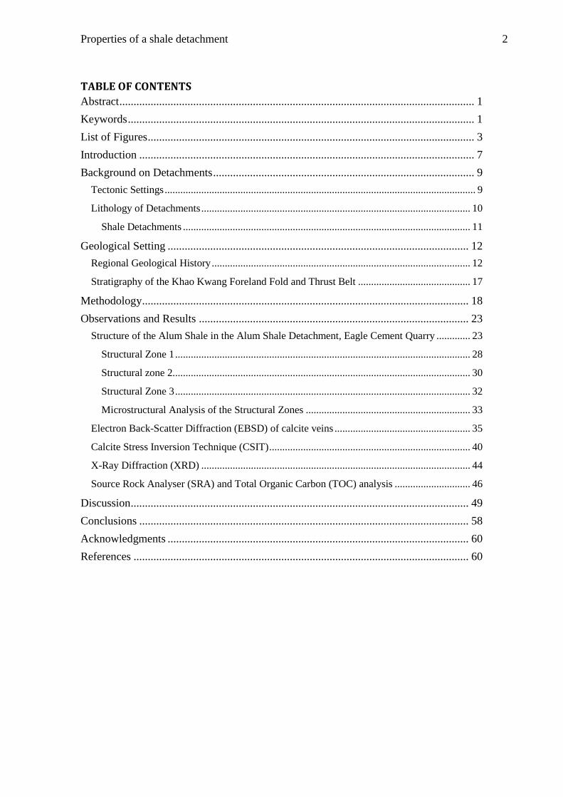
TABLE OF CONTENTS

Abstract ............................................................................................................................. 1

Keywords .......................................................................................................................... 1

List of Figures ................................................................................................................... 3

Introduction ...................................................................................................................... 7

Background on Detachments ............................................................................................ 9

Tectonic Settings ....................................................................................................................... 9

Lithology of Detachments ....................................................................................................... 10

Shale Detachments .............................................................................................................. 11

Geological Setting .......................................................................................................... 12

Regional Geological History ................................................................................................... 12

Stratigraphy of the Khao Kwang Foreland Fold and Thrust Belt ........................................... 17

Methodology ................................................................................................................... 18

Observations and Results ............................................................................................... 23

Structure of the Alum Shale in the Alum Shale Detachment, Eagle Cement Quarry ............. 23

Structural Zone 1 ................................................................................................................. 28

Structural zone 2.................................................................................................................. 30

Structural Zone 3 ................................................................................................................. 32

Microstructural Analysis of the Structural Zones ............................................................... 33

Electron Back-Scatter Diffraction (EBSD) of calcite veins .................................................... 35

Calcite Stress Inversion Technique (CSIT) ............................................................................. 40

X-Ray Diffraction (XRD) ....................................................................................................... 44

Source Rock Analyser (SRA) and Total Organic Carbon (TOC) analysis ............................. 46

Discussion ....................................................................................................................... 49

Conclusions .................................................................................................................... 58

Acknowledgments .......................................................................................................... 60

References ...................................................................................................................... 60


LIST OF FIGURES

Figure 1. Regional location map showing the location of the Sibmasu Block and

Indochina Block in relation to the South China Block, SW Borneo Block and West

Burma Block within Sundaland (Sone & Metcalfe 2008, Morley et al. 2013). ............. 13 Figure 2. Schematic diagram (not to scale) showing the tectonic evolution of mainland

Southeast Asia during the Permian to Early Late Triassic with respect to the Paleo-

Tethys Suture Zone, the Jinghong-Nan-Sra Kaeo Back-Arc Basin Suture and deposition

of the Saraburi carbonate platform. Modified from (Sone & Metcalfe 2008, Metcalfe

2011, Morley et al. 2013) ............................................................................................... 16 Figure 3. Group Stratigraphy of the Saraburi Group (Ueno & Charoentitirat 2011). .... 18 Figure 4. a. Location map showing Saraburi in relation to Bangkok, Thailand. b.

Location map showing the Eagle Cement Quarry NE of Saraburi, Thailand. Image was

taken from Google Maps, 2013. c. Location map indicating the position of the Shale

Quarry within the Eagle Cement Quarry, Thailand. Image was taken from Google

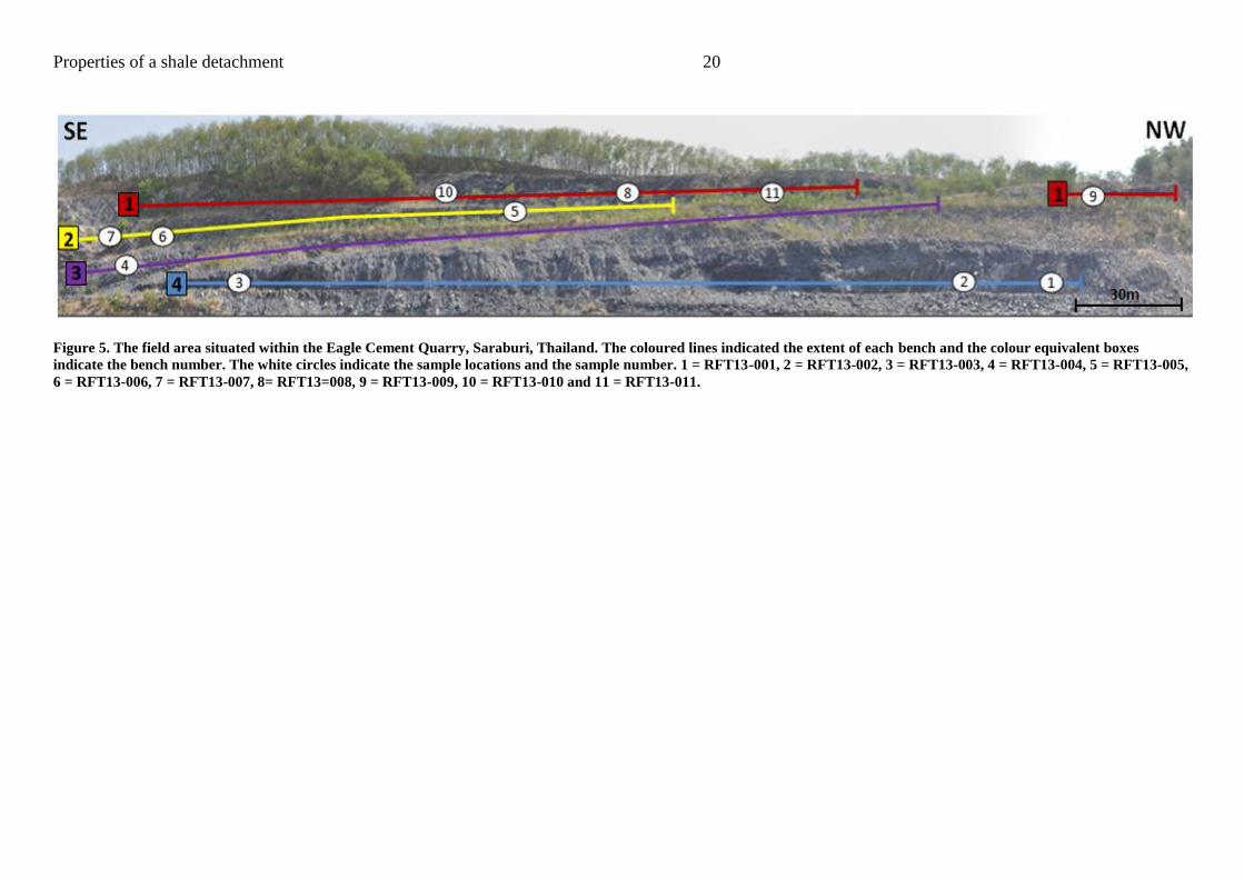
Maps, 2013. .................................................................................................................... 19 Figure 5. The field area situated within the Eagle Cement Quarry, Saraburi, Thailand.

The coloured lines indicated the extent of each bench and the colour equivalent boxes

indicate the bench number. The white circles indicate the sample locations and the

sample number. 1 = RFT13-001, 2 = RFT13-002, 3 = RFT13-003, 4 = RFT13-004, 5 =

RFT13-005, 6 = RFT13-006, 7 = RFT13-007, 8= RFT13=008, 9 = RFT13-009, 10 =

RFT13-010 and 11 = RFT13-011. .................................................................................. 20 Figure 6. Schematic illustration of the affect temperature of deformation has on calcite

twins. Type I represents twinning that occurred at a temperature of deformation below

200°C. Type II, III and IV represents twining that occurred at a temperature of

deformation above 200°C (Ferrill et al. 2004). .............................................................. 21 Figure 7. a. Interpretation of the overall structure within the Shale Quarry, based on the

28 cross-sections. ai. Location of the Thrust 1in Structural Zone 1. aii. Location of

Thrust 2 in Structural Zone 1. aii. Location of Fault-Propagation Fold 1 that has been

reactivated and subsequently, broken through the fold. aiv. Location of Fault-

Propagation Fold 2 in Structural Zone 1. av. Location of the faulted contact in Structural

Zone 3. b. Stereographic projection showing the relationship of poles to bedding, poles

to cleavage and poles to shear planes throughout the area. c. Simplified version of the

overall structure indicating the three structural zones (Structural Zone 1, Structural Zone

2 and Structural Zone 3) in which, the sections have been divided into based on the

structural consistencies. Structural Zone 1 is defined by the blue colouring, Structural

Zone 2 is defined by the orange colouring and Structural Zone 3 is defined by the green

colouring. ........................................................................................................................ 24 Figure 8. a. Stereographic representation of fault planes and slickenlines within the field

area, indicating they tend to show oblique fault movement to either the SW or the E,

throughout the three structural zones. There are 14 fault plane and slickenline

relationships that indicate oblique-slip fault movement. There are three fault plane and

slickenline relationships that indicate strike-slip fault movement and four that represent

dip-slip fault movement. B.Stereographic representation indicating the relationship

between the poles to bedding, poles to cleavage and poles to shear planes within

Structural Zone 1. The total number of bedding measurements uses is 52. The total

number of cleavage measurements used is 50. The total number of shear planes used is

18. c. Stereographic representation demonstrating the relationship between the poles to


bedding, poles to cleavage and poles to shear planes within Structural Zone 2. The total

number of bedding measurements uses is 17. The total number of cleavage

measurements used is 38. The total number of shear planes used is 21. d. Stereographic

representation illustrating the relationship between the poles to bedding, poles to

cleavage and poles to shear planes within Structural Zone 3. The total number of

bedding measurements uses is 45. The total number of cleavage measurements used is

57. The total number of shear planes used is 43. ............................................................ 25 Figure 9. a. Schematic diagram showing an example of the S-C fabrics present

throughout the detachment. b. Photograph illustrating Thrust 1 in section W-X

(Appendix B) in the second bench of the Shale Quarry. Alum Shale forms the hanging

wall and the Khao Khad Limestone forms the footwall. The Alum Shale shows

considerably more recrystallisation and graphitisation closest to the fault. c. Example

from section EE-FF illustrating that thrusts are steepening in succession to the NE. This

section also demonstrates the high level of deformation present within the intrusions. d.

Example from section F-G illustrating that the intrusions present within Structural Zone

3 are highly variable, even within a 20m section. Intrusions can vary from the

decimetre-scale to the metre-scale.’ ............................................................................... 27 Figure 10 a. Antitaxial fringe complex from sample RFT13-004. Core of the fringe

structure is pyrite (Py) with rims of muscovite (Mu) and illite. Photograph was captured

using an Olympus BX51 reflective light microscope in cross-polarised light. b. Highly

deformed antitaxial fringe complexes from sample RFT13-011. Photograph was

captured using an Olympus BX51 reflective light microscope in cross-polarised light. c.

Moderately deformed antitaxial fringe complex from sample RFT13-004. Photograph

was captured using an Olympus BX51 reflective light microscope in cross-polarised

light. d. Undeformed antitaxial fringe complex from sample RFT13-002A. Photograph

was captured using an Olympus BX51 reflective light microscope in cross-polarised

light. ................................................................................................................................ 34 Figure 11 a. Electron Back-Scatter Diffraction (EBSD) map from sample RFT13-002A

with band contrast (BC), a semi-transparent filter and inverse pole figure (IPF)

colouring. b. Pole figure plot for the EBSD map with IPF colouring from sample

RFT13-002A. c. Pole figure plot with contouring of sample RFT13-002A. d. Electron

Back-Scatter Diffraction map from sample RFT13-004 with BC, a semi transparent

filter and IPF colouring. e. Pole figure plot for the EBSD map with IPF colouring from

sample RFT13-004. f. Pole figure plot with contouring of sample RFT13-004. Electron

Back-Scatter Diffraction maps were created using HKL channel 5 software; Tango,

plots were created using Mambo. ................................................................................... 37

Figure 12. a. Electron Back-Scatter Diffraction (EBSD) map from sample RFT13-

002B-1 with band contrast (BC), a semi-transparent filter and inverse pole figure (IPF)


RFT13-002B-1. c Pole figure plot with contouring of sample RFT13-002B-1. d.

Electron Back-Scatter Diffraction map from sample RFT13-002B-2 with BC, a semi

transparent filter and IPF colouring. e. Pole figure plot for the EBSD map with IPF

colouring from sample RFT13-002B-2. f. Pole figure plot with contouring of sample

RFT13-002B-2. Electron Back-Scatter Diffraction maps were created using HKL

channel 5 software; Tango, plots were created using Mambo. ...................................... 38 Figure 13. a. Electron Back-Scatter Diffraction (EBSD) map from sample RFT13-011-1

with band contrast (BC), a semi-transparent filter and inverse pole figure (IPF)



RFT13-011-1. d. Pole figure plot with contouring of sample RFT13-011-1. d. Electron

Back-Scatter Diffraction map from sample RFT13-011-2 with BC, a semi transparent

filter and IPF colouring. e. Pole figure plot for the EBSD map with IPF colouring from

sample RFT13-011-2. f. Pole figure plot with contouring of sample RFT13-011-2.

Electron Back-Scatter Diffraction maps were created using HKL channel 5 software;

Tango, plots were created using Mambo. ....................................................................... 39

Figure 14. Stereographic representation of the principal palaeostresses 1, 2 and 3 and

their relationship to bedding from the first main tectonic stage defined by the Calcite

Stress Inversion Technique. This stage indicates E-W extension, which occurred prior to

deformation. A. Illustrates the principal palaeostresses and their relationship to bedding

at present. B. Illustrates the position of the principal palaeostresses and their

relationship to bedding at the time these conditions occurred........................................ 40


their relationship to bedding from the second main tectonic stage defined by the Calcite

Stress Inversion Technique. This stage indicates an E-W strike-slip regime with strain

partitioning between strike-slip and compression, which occurred prior to deformation.

A. Illustrates the principal palaeostresses and their relationship to bedding at present

from sample RFT13-002. B. Illustrates the position of the principal palaeostresses and

their relationship to bedding at the time these conditions occurred from sample RFT13-

002. C. Illustrates the principal palaeostresses and their relationship to bedding at

present from sample RFT13-005. D. Illustrates the position of the principal

palaeostresses and their relationship to bedding at the time these conditions occurred

from sample RFT13-005. ............................................................................................... 42


their relationship to bedding from the second main tectonic stage defined by the Calcite

Stress Inversion Technique. This stage indicates an ENE-WSW compressional regime

that occurred post-deformation. A. Illustrates the principal palaeostresses and their

relationship to bedding at present from sample RFT13-002. B. Illustrates the principal

palaeostresses and their relationship to bedding at present from sample RFT13-005. .. 43

Figure 17. a. Scatterplot representing the mean temperatures obtained for the illite

crystalinity measurements on the air dried (AD) samples. Calculations used were taken

from the calibrations given by Ji and Browne (2000). b. Scatterplot representing the

mean temperatures obtained for the illite crystalinity measurements on the glycolated

samples (GL). Calibrations after Ji and Browne (2000). ................................................. 45

Figure 18. This figure illustrates the temperatures at which gas, gasoline and kerosene

and diesel, lubricating and heavy oil occur at and their peak. Furthermore it indicates the

subsurface process in which gas, gasoline and kerosene and diesel, lubricating and

heavy oil are likely to form. Based on the SRA and TOC results, samples RFT13-001, -

003, -006, -007, -009 and -010 indicate that they have experienced temperatures of

exceeding 150 °C. ........................................................................................................... 48


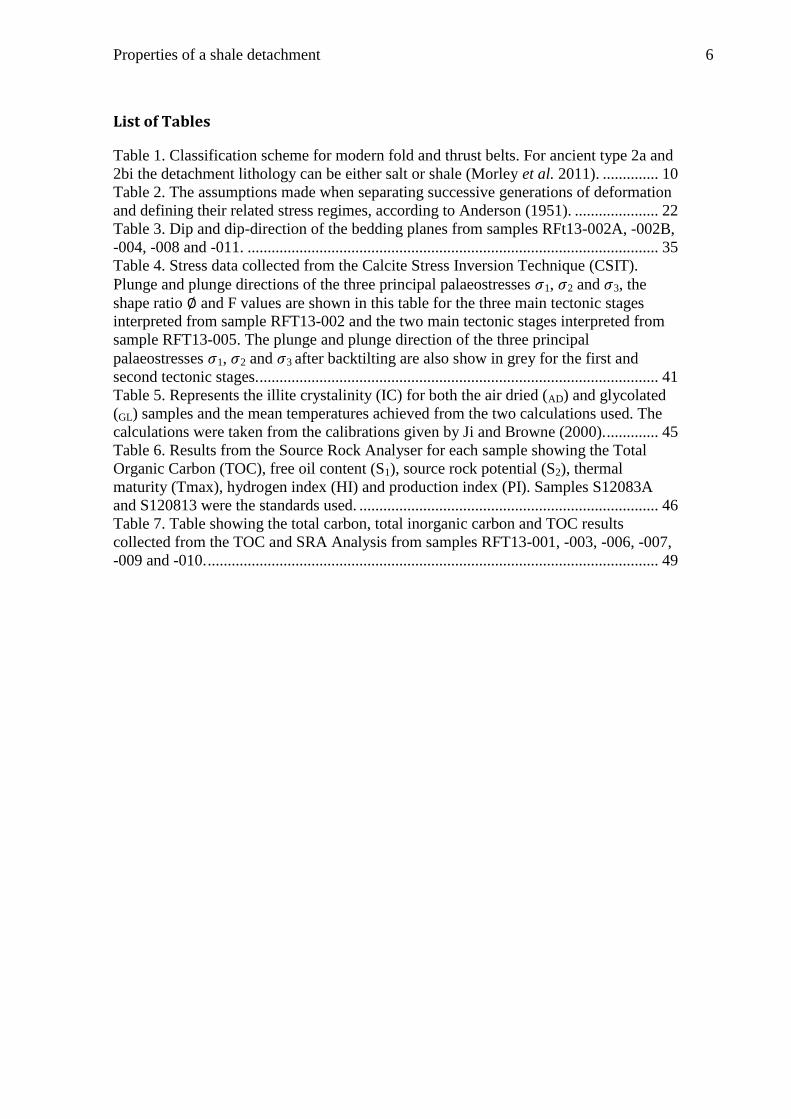
List of Tables

Table 1. Classification scheme for modern fold and thrust belts. For ancient type 2a and

2bi the detachment lithology can be either salt or shale (Morley et al. 2011). .............. 10 Table 2. The assumptions made when separating successive generations of deformation

and defining their related stress regimes, according to Anderson (1951). ..................... 22 Table 3. Dip and dip-direction of the bedding planes from samples RFt13-002A, -002B,

-004, -008 and -011. ....................................................................................................... 35 Table 4. Stress data collected from the Calcite Stress Inversion Technique (CSIT).

Plunge and plunge directions of the three principal palaeostresses 1, 2 and 3, the

shape ratio and F values are shown in this table for the three main tectonic stages

interpreted from sample RFT13-002 and the two main tectonic stages interpreted from

sample RFT13-005. The plunge and plunge direction of the three principal

palaeostresses 1, 2 and 3 after backtilting are also show in grey for the first and

second tectonic stages. .................................................................................................... 41 Table 5. Represents the illite crystalinity (IC) for both the air dried (AD) and glycolated

(GL) samples and the mean temperatures achieved from the two calculations used. The

calculations were taken from the calibrations given by Ji and Browne (2000). ............. 45 Table 6. Results from the Source Rock Analyser for each sample showing the Total

Organic Carbon (TOC), free oil content (S1), source rock potential (S2), thermal

maturity (Tmax), hydrogen index (HI) and production index (PI). Samples S12083A

and S120813 were the standards used. ........................................................................... 46

Table 7. Table showing the total carbon, total inorganic carbon and TOC results

collected from the TOC and SRA Analysis from samples RFT13-001, -003, -006, -007,

-009 and -010. ................................................................................................................. 49


INTRODUCTION

It is generally accepted that shale detachments deform in a highly ductile manner,

similar to salt detachments, for example the Niger Delta, Baram Delta and Mahakham

Delta (Morley & Guerin 1996, McClay et al. 1998, Ajakaiye & Bally 2002, McClay et

al. 2003, Bilotti & Shaw 2005, Briggs et al. 2006). However, more recent studies have

demonstrated that shale detachments are produced by brittle deformation, or a

combination of both brittle and ductile deformation (Ruarri et al. 2009, Hansberry et al.

2013, in prep.).

A detachment is defined as being a zone that separates or decouples the overriding

deforming sediments from the underlying non-deforming sediments (Fossen 2010). In

the past, research has focused on the properties that effect detachments, such as

overpressure, thickness, lithology, temperature, pore pressure, gravity, critical taper

wedge (CTW) geometry and rheology (Hubbert & Rubey 1959, De Jong & Scholten

1973, Fertl 1976, Chapple 1978, Weijermars et al. 1993, Stewart 1999, Schultz-Ela

2001, Rowan et al. 2004). Rheological properties are able to deduce the relationship

between stress and strain and are dependent on the temperature, lithology, state of

strain, fluids and strain rate. Subsequently, temperature, lithology and rheology are all

intrinsically linked (Handin & Carter 1987, Evans & Kohlstedt 1995).

Due to the general consensus that detachments are primarily ductile in nature, many

laboratory models used ductile materials such as air or honey as a substrate to replicate

the behaviour and influence of detachments on fold and thrust belts (FTBs).


Consequently, there is only an understanding of how the geometries in overlying FTBs

form due to ductile deformational mechanisms (De Sitter 1956, Cobbold et al. 2001,

McClay et al. 2003, Dooley et al. 2007).

This study focuses on the Alum Shale Detachment within the Khao Kwang Foreland

Fold and Thrust Belt (KKFFTB), which was active during the Indo-Sinian Orogeny

(IO) (Sone & Metcalfe 2008, Morley et al. 2011). To achieve this, 28 structural cross-

sections were constructed through the Alum Shale in the Shale Quarry within the Eagle

Cement Quarry, Saraburi, Thailand. These cross-sections were used to describe the

structures and their geometries, distribution and dimensions. Electron-Backscatter

Diffraction Analysis (EBSD) was conducted on the calcite veins within the coarser

layers of shales, in order to provide broad deformational temperature constraints and

strain patterns. The Calcite Stress Inversion Technique (CSIT) was used on calcite veins

to measure twins in order to determine the principal palaeostresses, shape ratio and

provide broad temperature constraints on deformation. X-Ray Diffraction (XRD)

analysis was used to determine clay mineralogy of the >2µm sample fraction and illite

crystalinity (IC) in shale samples to ascertain broad temperatures of deformation. The

Source Rock Analyser (SRA) was used to determine kerogen maturity, kerogen type,

hydrogen index, production index and thermal maturity of the sample, which also

provides temperature constraints of deformation. Finally, Total Organic Carbon (TOC)

analysis was used to determine the amount of organic carbon present to provide

additional information on the rheology of the detachment based on the determined

lithology and temperature constraints.


BACKGROUND ON DETACHMENTS

The mechanisms of deformation within detachments has been of long standing interest

within both academia and industry (Morley et al. 2011). Research has focussed on the

geometry of FTBs and the mechanisms of deformation to better constrain an

understanding of FTB formation and evolution (Dahlstrom 1990, McClay et al. 1998,

Ajakaiye & Bally 2002, Butler & McCaffrey 2004, Guzofski et al. 2009, King & Backe

2010a). The features that influence theses mechanisms include: the geological setting,

the lithology of the detachment and CTW geometry (De Jong & Scholten 1973,

Chapple 1978, Butler & McCaffrey 2004, Rowan et al. 2004, Morley et al. 2011). The

CTW is not investigated in the scope of this study.

Tectonic Settings

Fold and thrust belts occur in a variety of geological settings; passive margins,

continental convergence zones and accretionary prisms (Davis et al. 1983, Rowan et al.

2004, Briggs et al. 2009, Hesse et al. 2009, Morley et al. 2011). A classification scheme

has been proposed to distinguish the different types of FTBs based on the primary stress

type, the detachment type (lithology and dip) and the tectonic setting (Table 1) (Morley

et al. 2011).


Table 1. Classification scheme for modern fold and thrust belts. For ancient type 2a and 2bi the

detachment lithology can be either salt or shale (Morley et al. 2011).

Type 1 Type 2

Stress type Predominately/exclusively

near field stress

Mixed near

field and far

field stress

Predominately/

exclusively far field stress

Type 2a Type 2b

Tectonic

setting

Predominately passive

margins. Potentially any type

of setting with a slope to

deepwater

Continental

convergence

zone

Continental

convergence

zone

Accretionary

Prisms

Type 1a Type 1b Type 2bi Type 2bii

Detachment

lithology

Shale Salt Shale Shale Shale

Detachment

dip

Ocean

ward

Land

ward

Oceanward Landward Landward Landward

Lithology of Detachments

Detachments are primarily composed of either salt or shale (Dahlstrom 1990, Rowan et

al. 2004, Morley et al. 2011). The structural styles of FTBs are dependent on the

rheology of the detachment layer, which is intrinsically linked to the lithology

(Weijermars et al. 1993, Rowan et al. 2004). Within salt and shale FTBs, structural

components, such as diapirs, compressional toe region and up-dip growth faults are

similar (Dahlstrom 1990, Rowan et al. 2004). However, the timing of deformation,

location of deformation, structural styles and trigger mechanisms can be very different

(Rowan et al. 2004). The focus of this study is the Alum Shale within the Alum Shale

Detachment of the KKFFTB. Thus, salt detachments are not discussed further.


SHALE DETACHMENTS

Shale detachments within FTBs can be separated into four main categories (Dahlstrom

1969, Morley et al. 2011):

1. Compacted shales with large overpressures.

2. Compacted shales without large overpressures that act as weak, easy slip

horizons due to inherent material weakness.

3. Thick (hundreds of metres-to-kilometre-scale thickness) undercompacted,

overpressured shales that are capable of large-scale viscous flow.

4. Thin (metre-to-decametres thickness) undercompacted shales with high

overpressures.

These large overpressures can be the result of a number of different mechanisms such as

rapid sedimentation, tectonic compaction during shortening, hydrocarbon generation

and strain softening as clay particles rotate during shear and collapse (Morley & Guerin

1996, Osborne & Swarbrick 1998, Kopf & Brown 2003). These processes result in the

removal of the lithostatic support of the overburden (Rowan et al. 2004, Morley et al.

2011).

As the rheological behaviour of overpressured shales is independent of the strain rate,

shales only deform when the deviatoric stress overcomes the strength of the shale

(Weijermars et al. 1993, Rowan et al. 2004). Highly overpressured shale detachments

are more complex than faulted and folded shale detachments and as a result of this they

contain a variety of structural styles (Rowan et al. 2004). This is attributed to the


changes in the degree of overpressure, thickness, lithology, temperature, pore pressure,

gravity, CTW geometry and rheology (Hubbert & Rubey 1959, De Jong & Scholten

1973, Ramberg 1981, Poblet & McClay 1996, Stewart 1999, Schultz-Ela 2001).

There are three major structural styles of shale detached FTBs: faulted shale, folded

shale and highly overpressured shale (mentioned above) (Rowan et al. 2004). Faulted

shale FTBs are characterised by moderate overpressures and an asymmetrical structural

style in the form of basinward-vergent imbricated-thrust faults, fault-propagation folds

and fault-bend folds (Rowan et al. 2004). Folded shale detachments are characterised by

being highly overpressured, with a symmetrical structural style expressed by

symmetrical detachment folds (Dahlstrom 1969, Rowan et al. 2004).

GEOLOGICAL SETTING

Regional Geological History

The territory of modern Thailand forms part of Sundaland, an ancient terrane in SE Asia

(Figure 1) (Metcalfe 1984, 2011, Morley et al. 2013). Sundaland is comprised of five

principal continental blocks – the South China Block, Indochina Block, Sibumasu

Block, West Burma Block and Southwest Burma Block (Figure 1). These blocks make

up the majority of SE Asia (Metcalfe 2011). Thailand is comprised of two of these

principal tectonic blocks – the Indochina Block and the Sibumasu Block (Figure 1)

(Metcalfe 1984, 2011). Both of these blocks originated along the northern margins of

Gondwana (Metcalfe 1984, Sengör 1984, Metcalfe 2011). During the Mesozoic they


drifted north and collided to form Thailand and part of Sundaland (Metcalfe 2011,

Morley et al. 2013). This collisional boundary marks the closure of the Palaeotethys

Ocean and runs approximately N-S through Thailand. However, the exact location of

this collisional boundary is still heavily debated (Metcalfe 2001, 2011, Morley et al.

2013).

Figure 1. Regional location map showing the location of the Sibmasu Block and Indochina Block in

relation to the South China Block, SW Borneo Block and West Burma Block within Sundaland

(Sone & Metcalfe 2008, Morley et al. 2013).


The tectonic evolution of Thailand (Figure 2) can be divided into six major phases

(Sone & Metcalfe 2008, Metcalfe 2011, Morley et al. 2013):

1. Middle Devonian – The Indochina Block rifted from the Indo-Australian margin

of Gondwana and initiated the opening of the Paleotethys Ocean (Metcalfe

2011).

2. Latest Carboniferous - very Early Permian – The subduction of the Paleotethys

Ocean initiated beneath the Indochina Block to the N (Figure 2d). This resulted

in arc magmatism along the margin of the Indochina Block, forming the

Sukhotahi Island Arc system and the Jinghong-Nan Sra Kaeo Back-Arc Basin

by the Asselian (Sone & Metcalfe 2008).

3. Early Permian – The elongate Cimmerian continental strip that the Sibumasu

Block was a part of, separated from eastern Gondwana causing the opening of

the Mesotethys Ocean (Figure 2c) (Metcalfe 2011). Furthermore, an extensive

carbonate platform, the Saraburi Group, developed over the western Indochina

Block, inboard of the Jinghong-Nan Sra Kaeo Back-Arc Basin (Sone &

Metcalfe 2008).

4. Late Permian – The main phase of back-arc compression and the amalgamation

of the Sukothai Island Arc to marginal Indochina occurred (Figure 2b). During

this time the Saraburi Group was uplifted (Sone & Metcalfe 2008).

5. Early Triassic – The first stage of deformation associated with the IO (stage 1)

initiated at 250 Ma. This deformation was associated with the closure of the

Jinghong-Nan Sra Kaeo Back-Arc Basin (Figure 2a). It caused rift basins to be

thrusted and inverted. The end of this stage is marked by the development of the

Khorat Plateau (Indo-Sinian unconformity 1) (Morley et al. 2013).


6. Early Late Triassic - Early Jurassic – The second stage of deformation

associated with the IO (stage 2) initiated at 220 Ma (Morley et al. 2011) . The

Sibumasu Block collided with the continental Sukothai Arc of western

Indochina and as a result the Paleothethys Ocean was completely closed (Figure

2a) (Metcalfe 2011). Subsequently, an extensive accretionary prism of the

Paleotethys Suture Zone formed upon the subducted part of the Sibumasu Block.

It also caused reactivation of the thrusted and inverted rift basins from stage 1 of

the IO (Sone & Metcalfe 2008). Two unconformities, known as Indo-Sinian

unconformities 2 and 3 were formed during this period (Morley et al. 2013).

The KKFFTB was formed during the Early Triassic as part of stage 1 of the IO (Sone &

Metcalfe 2008, Morley et al. 2013). It is located on the western margin of the Indochina

Block (Morley et al. 2013) . At present day, the structural orientation of the FTB is E-

W, contradictory to the N-S trending sutures of the Sukothai and Indochina Blocks, and

the tectonic transport direction is predominately northwards (Morley et al. 2013).


Figure 2. Schematic diagram (not to scale) showing the tectonic evolution of mainland Southeast Asia during the Permian to Early Late Triassic with respect to the Paleo-Tethys

Suture Zone, the Jinghong-Nan-Sra Kaeo Back-Arc Basin Suture and deposition of the Saraburi carbonate platform. Modified from (Sone & Metcalfe 2008, Metcalfe 2011, Morley

et al. 2013)


Stratigraphy of the Khao Kwang Foreland Fold and Thrust Belt

The Saraburi Group is located on the eastern side of the lower Chao Phyraya Central

Plain, stretching southwardly from Nakhon Sawan to Saraburi, and from the western

margin of the Khorat Plateau within the KKFFTB (Bunopas 1992). It is comprised of a

mixture of clastic, siliclastic rocks and carbonate sequences (Bunopas 1982).

Stratigraphically the group overlies the Upper Carboniferous carbonate-clastic and

volcaniclastic sequences and underlies the Permian-Triassic volcanic and volcaniclastic

sequence and/or an Upper Triassic conglomerate (Bunopas 1992). The Saraburi Group

in the area around the Saraburi Province is divided up into three main carbonate

platform dominated facies (Phu Phe, Khao Khad and Khao Khwang Formations) and

three sequences of mixed siliclastic and carbonate sequences (Sap Bon, Pang Asok and

Nong Pong Formations) (Figure 3) (Morley et al. 2013). Previous biostratigraphic

studies have demonstrated that the Saraburi Group was deposited from the Asselian to

Midian (earliest Permian – early Late Permian) (Chonglakmani & Fontaine 1990,

Fontaine & Suteethorn 1992, Dawson 1993, Charoentitirat 2002). These packages are

believed to have been deposited on a continental margin rather than in an interior basin

(Morley et al. 2013).

The stratigraphic relations are poorly constrained throughout the area, consequently

assigning a stratigraphic unit for the Alum Shale is challenging. However, it is proposed

that the Alum Shale lies at the base of the sequence as it has been thrusted over the

younger Khao Khad Formation.


Figure 3. Group Stratigraphy of the Saraburi Group (Ueno & Charoentitirat 2011).

METHODOLOGY

Fieldwork was carried out along four benches in the Shale Quarry within Eagle Cement

Quarry, Saraburi, Thailand (Figures 4c & 5). Saraburi is located approximately

120 kilometres NNE of Bangkok, Thailand (Figure 4a). The Eagle Cement Quarry is

located approximately 25 kilometres NE of Saraburi, Thailand (Figure 4b). The Shale

Quarry within the Eagle Cement Quarry was chosen as the field area because recent

work within the Saraburi Province has identified world-class exposures of the KKFFTB

and its detachment and is easily accessible (Sone & Metcalfe 2008, Morley et al. 2013,

Hansberry et al. in prep.).


Figure 4. a. Location map showing Saraburi in relation to Bangkok, Thailand. b. Location map

showing the Eagle Cement Quarry NE of Saraburi, Thailand. Image was taken from Google Maps,

2013. c. Location map indicating the position of the Shale Quarry within the Eagle Cement Quarry,

Thailand. Image was taken from Google Maps, 2013.

Structural cross-sections were constructed along with sketches, photographs and

samples of shale from the Alum Shale. A total of 11 samples were collected to be used

for EBSD, CSIT, XRD, SRA and TOC analyses.

Samples RFT13-002, -004, -005, -008, -011 were used for EBSD analysis to determine

the grain orientation, grain boundary character and size and texture of calcite grains

(Figure 5). The analysis provided overall preferred orientation of calcite grains and

broad constraints on the temperature of deformation during the IO.


Figure 5. The field area situated within the Eagle Cement Quarry, Saraburi, Thailand. The coloured lines indicated the extent of each bench and the colour equivalent boxes

indicate the bench number. The white circles indicate the sample locations and the sample number. 1 = RFT13-001, 2 = RFT13-002, 3 = RFT13-003, 4 = RFT13-004, 5 = RFT13-005,

6 = RFT13-006, 7 = RFT13-007, 8= RFT13=008, 9 = RFT13-009, 10 = RFT13-010 and 11 = RFT13-011.


Calcite veins from samples RFT13-002 and -005 were used to determine the plunge and

plunge direction of the three principal palaeostresses ( 1, 2 and 3), the shape ratio ( )

and a broad temperature of deformation using the CSIT (Figure 5) (Amrouch et al.

2010, Lacombe 2010). Calcite that has been deformed at low temperatures forms

widespread mechanical e-twinning that records the principal palaeostresses at the time

of deformation (Amrouch et al. 2010). Temperature of deformation can be directly

correlated with the mean calcite twin width. Thin twins are dominant below 200 °C and

thick twins are dominant above 200 °C (Figure 6) (Ferrill et al. 2004, Lacombe 2010,

Amrouch unpubl.).

Figure 6. Schematic illustration of the affect temperature of deformation has on calcite twins. Type

I represents twinning that occurred at a temperature of deformation below 200°C. Type II, III and

IV represents twining that occurred at a temperature of deformation above 200°C (Ferrill et al.

2004).


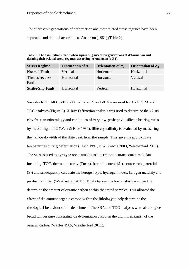
The successive generations of deformation and their related stress regimes have been

separated and defined according to Anderson (1951) (Table 2).

Table 2. The assumptions made when separating successive generations of deformation and

defining their related stress regimes, according to Anderson (1951).

Stress Regime Orientation of 1 Orientation of 2 Orientation of 3

Normal Fault Vertical Horizontal Horizontal

Thrust/reverse

Fault

Horizontal Horizontal Vertical

Strike-Slip Fault Horizontal Vertical Horizontal

Samples RFT13-001, -003, -006, -007, -009 and -010 were used for XRD, SRA and

TOC analyses (Figure 5). X-Ray Diffraction analysis was used to determine the >2µm

clay fraction mineralogy and conditions of very low grade phyllosilicate bearing rocks

by measuring the IC (Warr & Rice 1994). Illite crystallinity is evaluated by measuring

the half-peak-width of the illite peak from the sample. This gave the approximate

temperatures during deformation (Kisch 1991, Ji & Browne 2000, Weatherford 2011).

The SRA is used to pyrolyze rock samples to determine accurate source rock data

including; TOC, thermal maturity (Tmax), free oil content (S1), source rock potential

(S2) and subsequently calculate the kerogen type, hydrogen index, kerogen maturity and

production index (Weatherford 2011). Total Organic Carbon analysis was used to

determine the amount of organic carbon within the tested samples. This allowed the

effect of the amount organic carbon within the lithology to help determine the

rheological behaviour of the detachment. The SRA and TOC analyses were able to give

broad temperature constraints on deformation based on the thermal maturity of the

organic carbon (Waples 1985, Weatherford 2011).


OBSERVATIONS AND RESULTS

Structure of the Alum Shale in the Alum Shale Detachment, Eagle Cement Quarry

A total of 28 cross-sections were constructed from four benches within the Shale Quarry

in the Eagle Cement Quarry, Saraburi, Thailand (Figures 4 & 5). These cross-sections

were constructed based on data collected within the Shale Quarry and quality checked

using photographs and field sketches of each section. Each cross-section was connected

to adjacent cross-sections to provide the overall structure of the detachment (Figure 7a).

The bedding, cleavage and shear planes are all parallel striking E-W and dipping

moderately to the S-SW across the section (Figure 7b). The mean orientation for the

bedding, cleavage and shear planes are 48/182, 51/175 and 47/175, respectively (Figure

7b).

The relationship between the fault planes and slickenlines is oblique and trends to either

approximately 50 ° to 70 ° SW or approximately 20 ° to 40 ° to the E (Figure 8a). This

is observed throughout Structural Zones 1, 2 and 3 (Figure 8a).


Figure 7. a. Interpretation of the overall structure within the Shale Quarry, based on the 28 cross-sections. ai. Location of the Thrust 1in Structural Zone 1. aii. Location of Thrust 2

in Structural Zone 1. aii. Location of Fault-Propagation Fold 1 that has been reactivated and subsequently, broken through the fold. aiv. Location of Fault-Propagation Fold 2 in

Structural Zone 1. av. Location of the faulted contact in Structural Zone 3. b. Stereographic projection showing the relationship of poles to bedding, poles to cleavage and poles to

shear planes throughout the area. c. Simplified version of the overall structure indicating the three structural zones (Structural Zone 1, Structural Zone 2 and Structural Zone 3) in

which, the sections have been divided into based on the structural consistencies. Structural Zone 1 is defined by the blue colouring, Structural Zone 2 is defined by the orange

colouring and Structural Zone 3 is defined by the green colouring.

i

iii

ii

iv

v


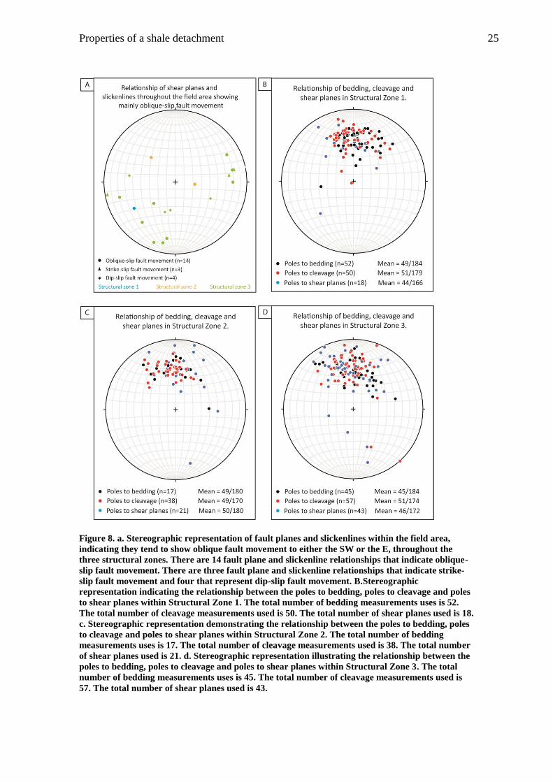
Figure 8. a. Stereographic representation of fault planes and slickenlines within the field area,

indicating they tend to show oblique fault movement to either the SW or the E, throughout the

three structural zones. There are 14 fault plane and slickenline relationships that indicate oblique-

slip fault movement. There are three fault plane and slickenline relationships that indicate strike-

slip fault movement and four that represent dip-slip fault movement. B.Stereographic

representation indicating the relationship between the poles to bedding, poles to cleavage and poles

to shear planes within Structural Zone 1. The total number of bedding measurements uses is 52.

The total number of cleavage measurements used is 50. The total number of shear planes used is 18.

c. Stereographic representation demonstrating the relationship between the poles to bedding, poles

to cleavage and poles to shear planes within Structural Zone 2. The total number of bedding

measurements uses is 17. The total number of cleavage measurements used is 38. The total number

of shear planes used is 21. d. Stereographic representation illustrating the relationship between the

poles to bedding, poles to cleavage and poles to shear planes within Structural Zone 3. The total

number of bedding measurements uses is 45. The total number of cleavage measurements used is

57. The total number of shear planes used is 43.


There is a distinct difference between how deformation is expressed within the Alum

Shale in the lower benches and Khao Khad Limestone in the upper benches. Within the

Alum Shale deformation is expressed on a small scale through a series of decimetre-to-

metre-scale thrusts, duplexes and S-C fabrics within the higher strain zones (Figures 7a

i & ii and 9a). Whereas, the Khao Khad Limestone expresses deformation on a much

larger scale with metre-to-decimetre-scale fault-propagation folding and metre-to-

decimetre-scale thrusts (Figures 7a i, ii, iii & iv).

Strain partitioning is prevalent within the areas of shale exhibiting a higher

deformational intensity; evidence for this is present as S-C fabrics (Figure 9a). The C-

fabric represents pseudo cleavage in the form of decimetre-scale shears, while the S-

fabric is pseudo-bedding (Figure 9a). The general trend of the C-fabric is approximately

40 ° to 50° to the SSW, whereas the general trend of the S-fabric is approximately 60 °

to 80 ° to the S (Appendix A).

Within Structural Zones 2 and 3 several igneous intrusions were observed in the outcrop

of the quarry benches. These intrusions were fine grained, grey-green in colour and

were rich in chlorite and silica. They are likely to be andesitic in composition.


Figure 9. a. Schematic diagram showing an example of the S-C fabrics present throughout the

detachment. b. Photograph illustrating Thrust 1 in section W-X (Appendix B) in the second bench

of the Shale Quarry. Alum Shale forms the hanging wall and the Khao Khad Limestone forms the

footwall. The Alum Shale shows considerably more recrystallisation and graphitisation closest to

the fault. c. Example from section EE-FF illustrating that thrusts are steepening in succession to the

NE. This section also demonstrates the high level of deformation present within the intrusions. d.

Example from section F-G illustrating that the intrusions present within Structural Zone 3 are

highly variable, even within a 20m section. Intrusions can vary from the decimetre-scale to the

metre-scale.’


It appears that across the quarry benches there is considerable variation in the

deformational intensity, which is linked to thrust intensity and lithology. Structural

complexity appears to be greatest closest to the major thrusts and appears to decrease

away from the thrusts, resulting in simpler fold and thrust geometries. Based on this, the

area has been divided into Structural Zone 1, Structural Zone 2 and Structural Zone 3

(Figure 7c).

STRUCTURAL ZONE 1

Structural Zone 1 is approximately 130 metres from the SE and is comprised of the first

and second benches (Figures 5 & 7c). It is defined by metre-to-decimetre-scale thrusts,

decimetre-scale fault-propagation folding and no intrusions. The bedding planes,

cleavage planes and shear planes strike E-W and have a southward dip of between 40 °

and 50 °, which is consistent throughout the field area (Figures 7b & 8b).

The structures observed within the Khao Khad Limestone are incongruent with those

observed within the Alum Shale. These structures occur on a much larger scale

compared with the Alum Shale. Bedding is on the decimetre-to-metre-scale.

Conversely, within the Alum Shale bedding occurs on the centimetre-to-decimetre-

scale. Bedding within the Khao Khad Limestone is generally homogenous, but close to

shear zones bedding is broken and discontinuous; this is also seen within the Alum

Shale. S-C fabrics are prevalent in the more coherent layers of shale near shear zones

(Figure 9a).


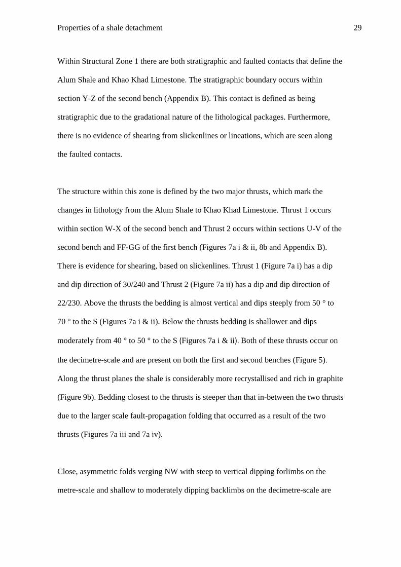
Within Structural Zone 1 there are both stratigraphic and faulted contacts that define the

Alum Shale and Khao Khad Limestone. The stratigraphic boundary occurs within

section Y-Z of the second bench (Appendix B). This contact is defined as being

stratigraphic due to the gradational nature of the lithological packages. Furthermore,

there is no evidence of shearing from slickenlines or lineations, which are seen along

the faulted contacts.

The structure within this zone is defined by the two major thrusts, which mark the

changes in lithology from the Alum Shale to Khao Khad Limestone. Thrust 1 occurs

within section W-X of the second bench and Thrust 2 occurs within sections U-V of the

second bench and FF-GG of the first bench (Figures 7a i & ii, 8b and Appendix B).

There is evidence for shearing, based on slickenlines. Thrust 1 (Figure 7a i) has a dip

and dip direction of 30/240 and Thrust 2 (Figure 7a ii) has a dip and dip direction of

22/230. Above the thrusts the bedding is almost vertical and dips steeply from 50 ° to

70 ° to the S (Figures 7a i & ii). Below the thrusts bedding is shallower and dips

moderately from 40 ° to 50 ° to the S (Figures 7a i & ii). Both of these thrusts occur on

the decimetre-scale and are present on both the first and second benches (Figure 5).

Along the thrust planes the shale is considerably more recrystallised and rich in graphite

(Figure 9b). Bedding closest to the thrusts is steeper than that in-between the two thrusts

due to the larger scale fault-propagation folding that occurred as a result of the two

thrusts (Figures 7a iii and 7a iv).

Close, asymmetric folds verging NW with steep to vertical dipping forlimbs on the

metre-scale and shallow to moderately dipping backlimbs on the decimetre-scale are


observed within Structural Zone 1 (Figures 7a iii & iv). These have the geometry of

fault-propagation faults (Dahlstrom 1969, Chester & Chester 1990, Mitra 1990). The

Fault-Propagation Fold 1 shows reactivation of the fault, as the fault has broken through

the fold (Figure 7a iii). Whereas, Fault-Propagation Fold 2 indicates standard fault-

propagation folding, where the propagating thrust fault loses slip and terminates up

section by transferring its shortening causing a fold to develope at the faults tip (Figure

7a iv) (Dahlstrom 1969, Chester & Chester 1990, Mitra 1990).

STRUCTURAL ZONE 2

Structural Zone 2 is approximately 130 metres from the SE to 230 metres from the SE

and is comprised of the first and second benches (Figures 5 & 7c). It is defined by the

metre-scale thrusts and metre-to-decimetre-scale intrusions. Overall the structure is on a

much smaller scale and appears to be the transition from the structurally complex

Structural Zone 1 to the structurally simple Structural Zone 3. The bedding planes,

cleavage planes and shear planes strike E-W and have a southward dip of approximately

50° (Figure 8c).

There are a number of metre-scale thrusts that occur within Structural Zone 2 (Figure

9c). The dips of these thrusts vary significantly with the majority dipping to the S-SW

and one of two outliers dipping to the NW; these are probably back thrusts or lateral

ramps. Dips of the thrusts range from 22 ° to 83 ° (Figure 9c). There is a general trend

with regards to the large variation in dips, showing that that the thrust planes are

steepening in succession towards the SE and thus propagating to the NW. Section EE-

FF is a good example of this trend and demonstrates that from SE to NW the dips start


at 58 ° and end at 49 °(Figure 9c). Section BB-CC also shows this trend to a lesser

extent (Appendix B).

The shales are more recrystallised and graphitised in close proximity to shear zones in

Structural Zone 2, which is consistent with observations in Structural Zone 1 (Figure

9b). The amount of recrystallisation and graphitisation decreases towards the NW, away

from Thrust 2 in Structural Zone 1. Strain associated with faulting is the dominant

feature when in close proximity to the shear zones and is represented by S-C fabrics

(Figure 9a).

Density of calcite veins significantly increases when in proximity to shear zones.

Calcite veins appear to decrease away from Thrust 2, where they are most prevalent.

Furthermore, the calcite veins are more widespread within the Khao Khad Limestone,

compared to the Alum Shale.

Another key aspect of Structural Zone 2 is the presence of igneous intrusions, which are

not seen within Structural Zone 1. These intrusions vary in thickness on the decimetre-

to-metre-scale in the NW to the metre-scale towards the SE. Intrusions are thicker and

more intensely folding to the SE, which is consistent with the increase deformational

intensity observed within the Alum Shale. A good example of the thicker and more

intensely deformed intrusions is present within section EE-FF (Figure 9c).


STRUCTURAL ZONE 3

Structural Zone 3 spans from 25 metres to 270 metres SE of the third and fourth bench

and from 230 metres to 250 metres from the SE of the first bench (Figures 5 & 7c). It is

defined by the most simple structural geometries, which show bedding striking E-W and

dipping towards the S at between 45 ° and 50 ° (Figure 8d). The thrusts present are on a

much smaller scale compared to those observed in Structural Zones 1 and 2 and range

from the decimetre-to-metre-scale. There are minimal intrusions observed (Appendix

B).

The dominant structural feature throughout this zone is the S-C fabrics that appear

within the Alum Shale and Khao Khad Limestone and are in close proximity to the

intrusions (Figure 9a). These fabrics are observed on a decimetre-scale and demonstrate

that the Alum Shale layers are acting as discrete shear zones (or C-fabric) and the Khao

Khad Limestone layers act as the pseudobedding (or S-fabric) (Figure 9a).

Within section JJ-KK Thrust 3 separates the Alum Shale and Khao Khad Limestone

(Figure 7a v). Thrust 3 is on the metre-scale and has a dip and dip direction of 40/209

(Figure 7a v). This is similar to the dip and dip direction of Thrusts 1 and 2 observed

within Structural Zone 1, which have a dip and dip direction of 30/240 and 22/230,

respectively (Figures 7a i & ii).

The characteristics of the shale lithology within Structural Zone 3 have altered in

comparison to Structural Zone’s 1 and 2. The shale is interlayered and dominated by a


very fine limestone. Towards the NE the lithology changes again to alternating

packages of shale and fine limestone beds that are approximately 20 centimetres thick.

The intrusions that occur within Structural Zone 3 are not as deformed as the intrusions

observed within Structural Zone 2. There appears to be no systematic pattern with

regards to the thickness or continuity of the intrusions throughout this zone. The

thickness can vary from the decimetre-to-metre-scale within a section (Figure 9d).

However, as a general trend the thickness of the intrusions increases towards the NE

from the decimetre-to-metre-scale to the metre-scale.

MICROSTRUCTURAL ANALYSIS OF THE STRUCTURAL ZONES

Samples RFT13-002A, -004, -005, -008 and -011 were used for microstructural analysis

of the shale samples (Figure 5). Within all the samples antitaxial fringe complexes were

observed. The core object of the fringe structures is pyrite and the fringes are muscovite

and illite (Figure 10a). The fringes appear have grown towards the core, and thus are

defined as antitaxial fringes rather than syntaxial fringes, which grow away from the

core (Aerden 1996, Koehn et al. 2000, Bons et al. 2012).The size of the fringe

complexes and degree of deformation varied significantly throughout all the samples.

The observations can be divided based on the abundance of the samples and the degree

of deformation with regards to the sample location and its appropriate structural zone.

Samples RFT13-008 and -011 were collected in Structural Zone 1 and had an

abundance of fringe structures that were highly deformed and varied from 50 m to


>500 m in size (Figures 10b & 7c). Samples RFT13-004 and -005 were collected in

Structural Zone 2 and had slightly smaller structures from 50 m to <200 m that were

moderately deformed (Figures 10c & 7c). Sample RFT13-002A was collected in

Structural Zone 3 and had a minimal amount of very small fringe structures (<50 m)

that were almost completely undeformed (Figures 10d & 7c).

Figure 10 a. Antitaxial fringe complex from sample RFT13-004. Core of the fringe structure is

pyrite (Py) with rims of muscovite (Mu) and illite. Photograph was captured using an Olympus

BX51 reflective light microscope in cross-polarised light. b. Highly deformed antitaxial fringe

complexes from sample RFT13-011. Photograph was captured using an Olympus BX51 reflective

light microscope in cross-polarised light. c. Moderately deformed antitaxial fringe complex from

sample RFT13-004. Photograph was captured using an Olympus BX51 reflective light microscope

in cross-polarised light. d. Undeformed antitaxial fringe complex from sample RFT13-002A.

Photograph was captured using an Olympus BX51 reflective light microscope in cross-polarised

light.


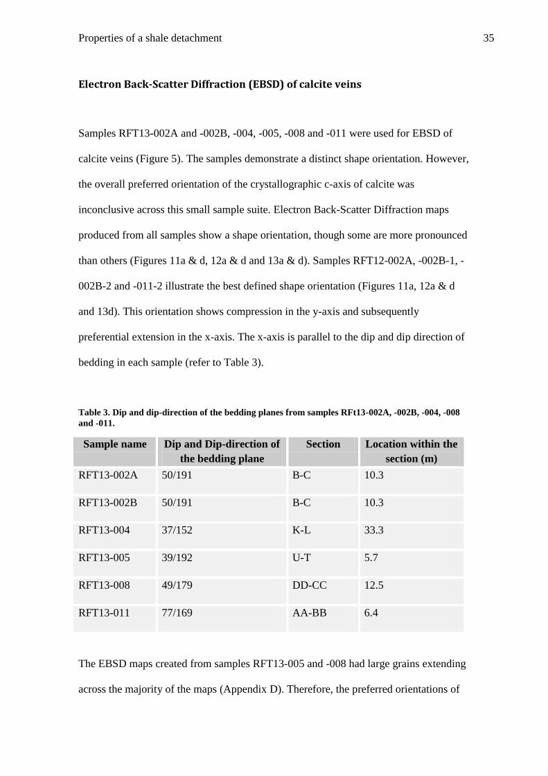
Electron Back-Scatter Diffraction (EBSD) of calcite veins

Samples RFT13-002A and -002B, -004, -005, -008 and -011 were used for EBSD of

calcite veins (Figure 5). The samples demonstrate a distinct shape orientation. However,

the overall preferred orientation of the crystallographic c-axis of calcite was

inconclusive across this small sample suite. Electron Back-Scatter Diffraction maps

produced from all samples show a shape orientation, though some are more pronounced

than others (Figures 11a & d, 12a & d and 13a & d). Samples RFT12-002A, -002B-1, -

002B-2 and -011-2 illustrate the best defined shape orientation (Figures 11a, 12a & d

and 13d). This orientation shows compression in the y-axis and subsequently

preferential extension in the x-axis. The x-axis is parallel to the dip and dip direction of

bedding in each sample (refer to Table 3).

Table 3. Dip and dip-direction of the bedding planes from samples RFt13-002A, -002B, -004, -008

and -011.

Sample name Dip and Dip-direction of

the bedding plane

Section Location within the

section (m)

RFT13-002A 50/191 B-C 10.3

RFT13-002B 50/191 B-C 10.3

RFT13-004 37/152 K-L 33.3

RFT13-005 39/192 U-T 5.7

RFT13-008 49/179 DD-CC 12.5

RFT13-011 77/169 AA-BB 6.4

The EBSD maps created from samples RFT13-005 and -008 had large grains extending

across the majority of the maps (Appendix D). Therefore, the preferred orientations of


the crystallographic c-axis of calcite within these maps are heavily biased because of the

large grains and subsequently have not been included in the overall analysis.

Furthermore, the data produced from sample RFT13-011 is of poor quality and only

indexed a small proportion of the overall map area (Figures 12a & d). Subsequently, the

only data being used from this sample is the shape orientation data (Figures 13a & d)

rather than the orientation of the crystallographic c-axis of calcite (Figures 13c & f).

The pole figure plots were created with and without contouring. The plots with

contouring have been used for interpretation as they are easier to interpret (Figures 11b

& e, 12b & e and 13b & e). There is no systematic pattern to the EBSD data. The peaks

associated with the plots represent between 4 % (Figure 11c) and 19 % (Figure 12c) of

the data. This indicates that there is not a definitive preferred orientation of the

crystallographic c-axis of calcite. There are three general trends observed, which the

peaks illustrate;

1. The orientation of the crystallographic c-axis of calcite is perpendicular to the x-

axis, or bedding plane (Figures 11c and 11e).

2. The orientation of the crystallographic c-axis of calcite is at an oblique angle to

the x-axis or bedding plane (Figures 12c and 12e).

3. The orientation of the crystallographic c-axis of calcite is parallel to the strike of

the bedding plane (Figure 11c).


Figure 11 a. Electron Back-Scatter Diffraction (EBSD) map from sample RFT13-002A with band contrast (BC), a semi-transparent filter and inverse pole figure (IPF) colouring. b.

Pole figure plot for the EBSD map with IPF colouring from sample RFT13-002A. c. Pole figure plot with contouring of sample RFT13-002A. d. Electron Back-Scatter Diffraction

map from sample RFT13-004 with BC, a semi transparent filter and IPF colouring. e. Pole figure plot for the EBSD map with IPF colouring from sample RFT13-004. f. Pole figure

plot with contouring of sample RFT13-004. Electron Back-Scatter Diffraction maps were created using HKL channel 5 software; Tango, plots were created using Mambo.


Figure 12. a. Electron Back-Scatter Diffraction (EBSD) map from sample RFT13-002B-1 with band contrast (BC), a semi-transparent filter and inverse pole figure (IPF) colouring.

b. Pole figure plot for the EBSD map with IPF colouring from sample RFT13-002B-1. c Pole figure plot with contouring of sample RFT13-002B-1. d. Electron Back-Scatter

Diffraction map from sample RFT13-002B-2 with BC, a semi transparent filter and IPF colouring. e. Pole figure plot for the EBSD map with IPF colouring from sample RFT13-

002B-2. f. Pole figure plot with contouring of sample RFT13-002B-2. Electron Back-Scatter Diffraction maps were created using HKL channel 5 software; Tango, plots were created

using Mambo.


Figure 13. a. Electron Back-Scatter Diffraction (EBSD) map from sample RFT13-011-1 with band contrast (BC), a semi-transparent filter and inverse pole figure (IPF) colouring. b.

Pole figure plot for the EBSD map with IPF colouring from sample RFT13-011-1. d. Pole figure plot with contouring of sample RFT13-011-1. d. Electron Back-Scatter Diffraction

map from sample RFT13-011-2 with BC, a semi transparent filter and IPF colouring. e. Pole figure plot for the EBSD map with IPF colouring from sample RFT13-011-2. f. Pole

figure plot with contouring of sample RFT13-011-2. Electron Back-Scatter Diffraction maps were created using HKL channel 5 software; Tango, plots were created using Mambo.


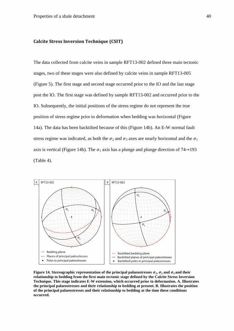
Calcite Stress Inversion Technique (CSIT)

The data collected from calcite veins in sample RFT13-002 defined three main tectonic

stages, two of these stages were also defined by calcite veins in sample RFT13-005

(Figure 5). The first stage and second stage occurred prior to the IO and the last stage

post the IO. The first stage was defined by sample RFT13-002 and occurred prior to the

IO. Subsequently, the initial positions of the stress regime do not represent the true

position of stress regime prior to deformation when bedding was horizontal (Figure

14a). The data has been backtilted because of this (Figure 14b). An E-W normal fault

stress regime was indicated, as both the 2 and 3 axes are nearly horizontal and the 1

axis is vertical (Figure 14b). The 1 axis has a plunge and plunge direction of 74 193

(Table 4).

Figure 14. Stereographic representation of the principal palaeostresses 1, 2 and 3 and their

relationship to bedding from the first main tectonic stage defined by the Calcite Stress Inversion

Technique. This stage indicates E-W extension, which occurred prior to deformation. A. Illustrates

the principal palaeostresses and their relationship to bedding at present. B. Illustrates the position

of the principal palaeostresses and their relationship to bedding at the time these conditions

occurred.


Table 4. Stress data collected from the Calcite Stress Inversion Technique (CSIT). Plunge and

plunge directions of the three principal palaeostresses 1, 2 and 3, the shape ratio and F values

are shown in this table for the three main tectonic stages interpreted from sample RFT13-002 and

the two main tectonic stages interpreted from sample RFT13-005. The plunge and plunge direction

of the three principal palaeostresses 1, 2 and 3 after backtilting are also show in grey for the first

and second tectonic stages.

Stage Sample RFT13-002 Sample RFT13-005

1 2 3 F 1 2 3 F

1 54/321 32/170 14/071 0.5 0.63

72/192 14/346 06/080

2 16/259 73/099 05/351 0.0 0.65 31/264 28/013 46/136 0.8 0.82

14/242 30/147 54/357 16/249 67/022 18/156

3 25/067 21/168 56/293 0.5 1.02 30/060 08/155 59/259 0.5 0.44

The second stage was recorded by both samples and indicates a primarily E-W strike-

slip fault stress regime with episodic periods of an E-W thrust fault stress regime. As

this stage occurred prior to the IO the initial positions of the stress regime do not

represent the true position of stress regime prior to deformation when bedding was

horizontal (Figures 15a & 15c). Subsequently, the data has been backtilted for both

samples (Figures 15b & 15d). The stress regime from sample RFT13-002 indicates that

prior to the IO episodic periods of E-W strike-slip fault stress regime and E-W thrust

fault stress regime were present (Figure 15b), as the shape ratio for 2 and 3 is equal

to zero (Table 4). This indicates that 2 and 3 axes are interchangeable. The plunge and

plunge direction of 1 is 14 242 (Figures 15b). The stress regime from sample RFT13-

005 indicates an E-W strike-slip stress fault regime prior to the IO (Figure 15d). The

shape ratio for 2 and 3 is 0.8, indicating it is only a strike-slip fault stress regime and

unlike sample RFT13-002 (Table 4). The plunge and plunge direction of 1 is 16 249

(Figure 15d).



relationship to bedding from the second main tectonic stage defined by the Calcite Stress Inversion

Technique. This stage indicates an E-W strike-slip regime with strain partitioning between strike-

slip and compression, which occurred prior to deformation. A. Illustrates the principal

palaeostresses and their relationship to bedding at present from sample RFT13-002. B. Illustrates

the position of the principal palaeostresses and their relationship to bedding at the time these

conditions occurred from sample RFT13-002. C. Illustrates the principal palaeostresses and their

relationship to bedding at present from sample RFT13-005. D. Illustrates the position of the

principal palaeostresses and their relationship to bedding at the time these conditions occurred

from sample RFT13-005.


The third stage indicates to ENE-WSW thrust fault stress regime after the IO, as both

the 1 and 2 axes are close to horizontal and the 3 axis is near vertical (Figures 16a &

b). This stage was recorded in both the samples. The plunge and plunge direction of 1

recorded by sample RFT13-002 is 25 067 (Figure 16a). The plunge and plunge

direction of 1 recorded by sample RFT13-005 is 30 060 (Figure 16b). Furthermore,

the shape ratios from each sample were 0.5, confirming that they are the same stress

tensor, even though bedding is different (Table 4).


relationship to bedding from the second main tectonic stage defined by the Calcite Stress Inversion

Technique. This stage indicates an ENE-WSW compressional regime that occurred post-

deformation. A. Illustrates the principal palaeostresses and their relationship to bedding at present

from sample RFT13-002. B. Illustrates the principal palaeostresses and their relationship to

bedding at present from sample RFT13-005.


X-Ray Diffraction (XRD)

Samples RFT13-001, -003, -006, -007, -009 and -010 were used for XRD analysis. The

results of XRD analysis have determined the clay mineralogy of the >2µm sample

fraction and given broad constraints on the maximum temperature of deformation

(Figure 5) (Kisch 1991, Warr & Rice 1994, Ji & Browne 2000).

The clay mineralogy was only determined for samples RFT13-001, -003, -009 and -010

because there was not sufficient illite within samples RFT13-006 and -007. The main

minerals present in all samples were quartz, illite and chamosite. Samples RFT13-009

and -010 also contained paragonite.

Both air dried (AD) and glycolated (GL) samples were prepared for XRD analysis to

determine temperature constraints (Table 5). Sample RFT13-003 was not used as it did

not contain sufficient illite. Samples RFT13-009 and -010 were not used as the half-

peak-width was not able to be calculated accurately due to interference from the

paragonite peaks (Appendix E). The highest temperature recorded from the AD samples

was 319 °C from sample RFT13-007 (Table 5). The lowest temperature recorded by the

AD samples was 314 °C from sample RFT13-006 (Table 5). The GL samples indicate a

wider temperature range; the highest temperature was recorded in sample RFT13-001 at

334 °C and the lowest was recorded in sample RFT13-006 at 321 °C (Table 4). Both the

AD and GL samples have a linear regression with an R2 value of 1, indicating that the

calculations used to plot the data are accurate (Figure 17a & b) (Kisch 1991, Ji &

Browne 2000).


Table 5. Represents the illite crystalinity (IC) for both the air dried (AD) and glycolated (GL) samples

and the mean temperatures achieved from the two calculations used. The calculations were taken

from the calibrations given by Ji and Browne (2000).

Sample

Number

ICAD

(°Δ20)

Calc. 1 Calc. 2 Mean

Temperature

AD(°C)

ICGL

(°Δ20)

Calc

. 1

Calc

. 2

Mean

Temperature

GL(°C)

RFT13-

001

0.202 326 307 316 0.165 334 334 334

RFT13-

006

0.221 324 304 314 0.224 323 319 321

RFT13-

007

0.18 329 310 319 0.179 332 331 331

RFT13-

009

0.61 275 252 264 0.579 258 226 242

RFT13-

010

0.511 287 266 276 0.158 269 242 255

Figure 17. a. Scatterplot representing the mean temperatures obtained for the illite crystalinity

measurements on the air dried (AD) samples. Calculations used were taken from the calibrations

given by Ji and Browne (2000). b. Scatterplot representing the mean temperatures obtained for the

illite crystalinity measurements on the glycolated samples (GL). Calibrations after Ji and Browne

(2000).

R² = 1

310

320

330

340

350

0 0.1 0.2 0.3

Tem

pe

ratu

re (

°C)

ICAD(°Δ20)

Air dried IC (°Δ20) Vs Temperature (°C)

R² = 1

310

320

330

340

350

0 0.1 0.2 0.3

Tem

pe

ratu

re (

°C)

ICGL(°Δ20)

Glycolated IC (°Δ20) Vs Temperature (°C)

A

B


Source Rock Analyser (SRA) and Total Organic Carbon (TOC) analysis

Samples RFT13- 001, -003, -006, -007, -009 and -010 were used for SRA and TOC

analysis (Figure 5). The SRA results were used to determine the kerogen type, kerogen

maturity, hydrogen index and production index and the amount of total carbon,

providing broad temperature constraints on deformation (Table 6). The TOC results

were used to determine the amount of inorganic carbon within the tested samples. Total

carbon results from the SRA data and the amount of inorganic carbon from TOC

analysis were used to determine the TOC content for each sample so that the effect of

detachment rheology could be established.

The SRA results show that there is no potential for hydrocarbon production as the

production index (PI) values range from 0.40 (RFT13-007) to 0.63 (RFT13-010) (Table

6). Economical source rocks for hydrocarbon production generally have PI values of

approximately 400 or over (Waples 1985)

Table 6. Results from the Source Rock Analyser for each sample showing the Total Organic

Carbon (TOC), free oil content (S1), source rock potential (S2), thermal maturity (Tmax), hydrogen

index (HI) and production index (PI). Samples S12083A and S120813 were the standards used.

Sample ID TOC S1 S2 Tmax HI PI

RFT13-001 1.16 0.04 0.05 415.58 4.30 0.44

RFT13-003 0.31 0.03 0.03 349.22 9.69 0.50

RFT13-006 1.37 0.07 0.10 364.18 7.32 0.41

RFT13-007 0.91 0.04 0.06 340.79 6.60 0.40

RFT13-009 1.15 0.03 0.02 325.57 1.74 0.60

RFT13-010 1.64 0.05 0.03 343.45 1.83 0.63

S120813A 0.59 11.76 418.58 0.05

S120813 0.61 11.79 418.52 0.05


The kerogen type and maturity is determined from the Tmax (°C) and hydrogen index

(HI, mgHC/g TOC). To determine the kerogen type and maturity accurately an S2 peak

is required, all of the samples failed to produce this. Subsequently, the kerogen type and

maturity were not calculated. The kerogen type and maturity plots show the distribution

of Tmax within the samples along the x-axis (Appendix F). This data demonstrates that

the samples are overmature and likely to fall within the dry gas window at the end of

catagenisis (Figure 18).

The kerogen quality is determined using TOC and remaining hydrocarbon potential (S2,

mgHC/g), which is based on the S2 peak. As no S2 peak occurred, the kerogen quality is

unable to be determined. The kerogen quality plot shows the distribution of TOC within

the samples along the x-axis (Appendix F). This data demonstrates that the samples are

overmature and likely to fall within the dry gas window at the end of catagenisis (Figure

18).


Figure 18. This figure illustrates the temperatures at which gas, gasoline and kerosene and diesel,

lubricating and heavy oil occur at and their peak. Furthermore it indicates the subsurface process

in which gas, gasoline and kerosene and diesel, lubricating and heavy oil are likely to form. Based

on the SRA and TOC results, samples RFT13-001, -003, -006, -007, -009 and -010 indicate that they

have experienced temperatures of exceeding 150 °C.

The TOC results show that overall the TOC is very low and lies in the range of 0.31 % -

1.64 %. Sample RFT13-010 had the highest percentage of TOC at 1.64 % and sample

RFT13-003 had the lowest percentage of TOC at 0.31 % (Table 7). In all of the samples

the amount of inorganic carbon was lower than the amount of organic carbon. The

highest percentage of total inorganic carbon was 8 %, this was observed in sample

RFT13-003. Whereas, the lowest percentage of total inorganic carbon was 0.97 %

(Table 7), which was observed within sample RFT13-010. There is a clear correlation

between the percentage of TOC and the total percentage of inorganic carbon, which


indicates that the percentage of TOC is directly proportional to the total percentage of

inorganic carbon (Table 6).

Table 7. Table showing the total carbon, total inorganic carbon and TOC results collected from the

TOC and SRA Analysis from samples RFT13-001, -003, -006, -007, -009 and -010.

Sample

Number

Total

Carbon

(%)

Total

Inorganic

Carbon (%)

TOC

(%)

RFT13-001 3.1 1.94 1.16

RFT13-003 8.31 8.00 0.31

RFT13-006 4.71 3.34 1.37

RFT13-007 2.72 1.81 0.91

RFT13-009 3.73 2.58 1.15

RFT13-010 2.61 0.97 1.64

DISCUSSION

Most FTBs that are active at present day occur within deep marine environments, which

are almost completely inaccessible. Subsequently, studies in relation to detachment

zones and their subsequent FTBs have been limited to employing seismic reflection data

and other indirect information. The Alum Shale and Khao Khad Limestone within the

KKFFTB in Thailand have proven to be invaluable at providing insight into the

deformational mechanisms that occur within a shale detachment. These mechanisms

demonstrate a primarily brittle response to stress. This is evident in the complex

thrusting and duplexes that accommodate shortening within the detachment. Detailed

cross-sections from the Shale Quarry show that there is clear evidence of deformational

heterogeneity throughout the outcrop, which is the result of the Alum Shale Detachment

being ordered and systematic. This is contrary to the traditional assumption from


seismics and laboratory modelling that shale detachments are a homogenous ductile

zone (De Sitter 1956, Evamy et al. 1978, Morley & Guerin 1996, McClay et al. 1998,

Cobbold et al. 2001, Ajakaiye & Bally 2002, McClay et al. 2003, Bilotti & Shaw 2005).

The geometries observed within the Alum Shale Detachment comply with the basic

definition of a detachment, as it decouples or separates the deforming interbedded shale

and Khao Khad Limestone sequence within the KKFFTB from the Alum Shale that is

part of the Alum Shale Detachment (Morley et al. 2013). Evidence for brittle

deformation is seen by metre-to-decimetre-scale thrust faulting, metre-to-decimetre-

scale fault-propagation folding and duplexes (Figures 7 a i, ii, iii & iv). Although the

prominent structural features (Thrust’s 1, 2 and 3 and Fault-Propagation Fold’s 1 and 2)

are attributed to brittle deformational mechanisms, there is also evidence for ductile

deformation. The ductile deformational features present within the detachment are the

considerable recrystallisation and graphitisation of the shales in proximity to shear

zones and S-C fabrics (Figures 9a & b). The cause of the significant recrystallisation

and graphitisation within the shales is thought to be due to frictional temperatures and

or fluids facilitating recrystallisation along the shear plane (Passchier & Trouw 2005).

This indicates that for the most part deformation within FTBs is of a brittle nature,

although strain partitioning is occurring within higher strain zones allowing for ductile

deformational features to be present. The formation of S-C fabrics is caused by a need

to accommodate the increase in strain associated with shearing (Figure 9a) (Fossen

2010).


Based on the field observations it is evident that there have been numerous stages of

faulting, allowing for the reactivation of the Thrust 1 in Structural Zone 1, causing the

fault to propagate through the Fault-Propagation Fold 1. Furthermore, faults are

steepening to the SE, indicating that the thrust sheets are in sequence and that

subsequently fault propagation occurred towards the NW (Anderson 1951, Rowan et al.

2004, Fossen 2010).

Microstructural analysis recorded the presence of antitaxial fringe complexes (Figure

10a, b, c, &f). The variation in deformational intensity and abundance is directly linked

to the locations the samples were taken from. Samples RFT13-008 and -011 from

Structural Zone 1 showed abundant fringe complexes that were highly deformed.

Sample RFT13-004 and -005 from Structural Zone 2 were associated with smaller-scale

structures and lower deformational intensities, in comparison to Structural Zone 1.

Sample RFT13-002A from Structural Zone 3 had a minimal amount of structures fringe

complexes, which were mostly undeformed. This indicates that there is a direct

correlation between the deformational intensity on the macro-scale (structures observed

in the Shale Quarry) and the abundance and the deformational intensity on the micro-

scale (fringe complexes).

The observations made based on the structural style of this detachment both differ and

support previous work completed on FTBs. Briggs et al. (2006), Hesse et al.(2009),

Hansberry et al. (2013, in prep.) and have all recorded brittle deformational features in

the form of fault-propagation folds, which are indicative of brittle deformation. ‘Mobile

shales’ have been interpreted throughout history, however recently this interpretation is


less confident (Van Rensbergen & Morley 2003, Maloney et al. 2010, Morley et al.

2011b). There is still strong evidence to suggest ‘mobile shales’ occur in some tectonic

settings. The Niger Delta and NW Borneo are both examples of the existence of ‘mobile

shales’ (Evamy et al. 1978, Morley & Guerin 1996, Briggs et al. 2006, Hesse et al.

2009, King et al. 2010b). However, within both of these FTBs fault-propagation folds

have been noted, indicating that brittle mechanisms are also present (Briggs et al. 2006,

Hesse et al. 2009).

The CSIT results indicate three main tectonic stages, two of which occurred prior to the

IO and the third after the IO. None of the observations recorded in the field show any

evidence of these stress regimes. There could be a number of reasons for this:

The CSIT work was not analysed accurately as the orientations of the twins were

recorded wrong, due to human error. This is unlikely for the second and third

tectonic stages as both samples recorded the same stress regimes.

These structures may have existed, but the rheology of the shale has caused

destruction of the structures over time, due to changes in temperature, stresses,

strain rate, fluids and lithology (Handin & Carter 1987, Evans & Kohlstedt

1995)

The calcite twins record the regional tectonic stress regimes, rather than the local

stress regime (Lacombe et al. 1990). In order for mechanical e-twinning to

occur, calcite is required to experience 10 megapascals (MPa) of constant

critical resolve shear stress (CRSS) (Rowe & Rutter 1990, Craddock et al. 1993,

Lacombe & Laurent 1996, Lacombe 2007). Consequently calcite twins are able

to provide stress and palaeostress determination when macroscopic features are


not observable (Lacombe et al. 1990). Based on this, it is likely that the calcite

twins have recorded the regional tectonic stresses rather than the local ones,

which is why the structures observed within the Shale Quarry do not support the

palaeostresses proposed by the CSIT. Evidence to support this is that as the three

main tectonic stages support the structures that would have been present based

on the regional tectonic evolution of Thailand and the present day regional

structures that trend NNW-SSE (Müller et al. 2008, Sone & Metcalfe 2008,

Keep & Haig 2010, Kundu & Gahalaut 2011, Metcalfe 2011, Morley et al.

2013). Examples where CSIT has recorded the regional stress regime rather than

the local stress regime was recorded by Lacombe et al. (1990) in the north-

eastern side of the Bresse Graben within the Jura Mountains in the Paris Basin

and McQuarrie (2004), in the Zagros FTB, in Iran.

The first main tectonic stage indicates an E-W normal fault stresss regime. This may

have been the result of the Jinghong Nan-Sra Kaeo Back-Arc Basin opening during the

Asselian (Early Permian) (Sone & Metcalfe 2008). The second tectonic stage indicates

an episodic periods of an E-W strike-slip fault stress regime with an E-W thrust fault

stress regime. In relation to the relative timing of all the stages it is plausible that this

stage occurred after the Asselian, but prior to the initiation of the IO (Late Permian-

Early Triassic). Therefore, it is likely that the second stage is associated with the closure

of the Jinghong Nan-Sra Kaeo Back-Arc Basin, in the Late Permian (Sone & Metcalfe

2008). The main tectonic stage that occurred after the IO indicates an ENE-WSW thrust

fault stress regime. This does not support the structural observations recored in that all

of the structures present are dipping to the S and striking E-W. Based on this one can


infer that this stage occurred sometime after the end of the second stage of the IO,

which is thought to have created these structures (190 Ma) (Morley et al. 2011).

As previously mentioned, it is likely that the third tectonic stage is recording the

regional tectonic palaeostresses. Evidence to corroborate this claim is that the E-W

striking orientation of the bedding would not have occurred if the local stresses were an

ENE-WSW thrust fault stress regime (Anderson 1951). Furthermore, it is unlikely the

data has been poorly recorded and analysed as both samples recorded the same stress

tensor, even though the bedding was different (Table 3). A possible cause of this ENE-

WSW thrust fault stress regime from the regional tectonics is the subduction of the

Indo-Australian Plate beneath the western Banda Arc (Kundu & Gahalaut 2011).

Australian continental lithosphere has been colliding with the western Banda arc since 9

- 10 Ma (Keep & Haig 2010), and the current rate of subduction is 60mm/yr (Müller et

al. 2008). The western Banda arc has a NNW-SSE orientation (Kundu & Gahalaut

2011), which corroborates a ENE-WSW maximum horizontal stress ( 1).

Temperatures of deformation during the IO were broadly constrained by EBSD, CSIT,

SRA and TOC data and deformational temperatures prior to the IO by XRD data. The

temperatures constrained using EBSD are inconclusive, due to the lack of a systematic

pattern with regards to the data. This may be due to the different generations of veins

and that only a small sample set was analysed. However, a slight trend was observed

that indicates the orientation of the calcite crystallographic c-axis is parallel to the strike

of the bedding, indicating coaxial progressive flattening. In order for this to occur,

temperatures must have been below 300 °C (Passchier & Trouw 2005). The


temperatures obtained using the CSIT indicate temperatures below 200 °C as the mean

calcite twin width was Type 1; thin twinned (Figure 6) (Ferrill et al. 2004, Lacombe

2010).

The SRA and TOC data indicates that the Alum Shale Detachment and KKFFTB must

have experienced temperatures towards the end of the dry gas window and catagensis,

indicating temperatures of over 150 °C. Therefore, based on the data preserved herein, a

broad deformational temperature constraint of 150 °C to 200 °C occurred during the IO.

These temperatures are consistent with brittle deformational mechanisms, rather than

ductile mechanism, which would give temperatures of over 400 °C (Dragoni 1993).

Temperatures constrained using the XRD data were much higher than the other

temperatures suggested by the EBSD, CSIT, SRA and TOC. The temperatures ranged

between 314 °C to 319 °C for the air dried samples and 321 °C to 334 °C for the

glycolated samples. There are a number of reasons these temperatures could have

occurred, such as contact metamorphism related to igneous intrusions, a major

hydrothermal event, or a combination of the two (Passchier & Trouw 2005). As calcite

grains within both generations of veining record broad temperatures of below 200 °C, it

is unlikely that the temperatures are the result of a major hydrothermal event.

Subsequently, it is more plausible that the temperatures are due to contact

metamorphism from the igneous intrusions. This is supported by the fact that the

intrusions are deformed, and thus, must have been intruded prior to the IO. These

temperatures imply that conditions were in the epizone just below greenschist facies

metamorphism (Passchier & Trouw 2005). A possible source for the igneous intrusions


could be the volcaniclatstic sequences within the Eastern Granitoid Belt, which

persisted from the Carboniferous to the Late Triassic, as they occurred prior to the IO

and throughout the deposition of the Saraburi Group (Bunopas 1982, Charusiri et al.

1993, Morley et al. 2013).

The igneous intrusions have been interpreted as andesitic in composition. Gaetani et al.

(1994) showed that at 1 atmosphere under anhydrous conditions andesitic magmas are

in the liquid phase from 1150 °C to 1210 °C and at 2 Kbar water saturated conditions

andesitic magmas are in the liquid phase from 1000 °C to 1100 °C. Shales have a low

thermal conductivity of approximately 0.7-1.6W/m-1

k-1

, however, this varies due to

composition, overpressures and temperatures (Gilliam & Morgan 1987). Shales low

thermal conductivity explains why the temperatures associated with contact

metamorphism only reached 334 °C, even though the magmas intruding them were

between 1000 °C and 1200 °C. Evidence to support this would be higher temperatures

in samples closer to intrusions. Sample RFT13-001 was taken in close proximity to an

intrusion and records the highest temperatures for the glycolated samples, but not the air

dried samples (Table 5). This indicates that there is no systematic pattern evident from

the sample locations to corroborate this. This is likely to be due to the small sample size

and further studies are required to support this.

Based on field observations, structural interpretation, EBSD, CSIT, TOC, SRA, and

XRD data the following series of events was deduced with regards to the structural

evolution of the Alum Shale Detachment and KKFFTB.


1. E-W normal fault stress regime during the Asselian.

2. E-W strike-slip fault stress regime with episodic periods of an E-W thrust fault

stress regime that occurred in the Late Permian

3. Igneous intrusions were emplaced, causing contact metamorphism and

temperatures up to 334 °C in the Alum Shale.

4. Hydrothermal event occurred in a minimum two stages, resulting in at least two

generations of veining.

5. Formation of the Alum Shale Detachment and subsequently KKFFTB from the

Late Triassic (250 Ma) to the Early Jurassic (190 Ma).

6. ENE-WSW thrust fault stress regime occured after the IO (190Ma).

As with most detachments, the three factors controlling the structural evolution of this

system are the primary stress, tectonic setting and detachment type. The primary stress

type of the Alum Shale Detachment is likely to be a mixture of near and far field

stresses. This is because the macrostructures (structures observed in the Shale Quarry)

are recording the local stresses, whereas the microstructures are recording the regional

stresses (recorded by the CSIT). Subsequently, the detachment can be defined as a type

2 detachment based on the classification scheme from Morley et al. (2011). This

detachment occurs within a foreland basin, therefore, it can be defined as occurring

within a continental convergence zone and is a type 2a detachment (Table 1) (Morley et

al. 2011).

Based on the structural observations the detachment is thin-skinned and has a structural

style of faulted shales, which suggest moderate overpressures (Rowan et al. 2004). The


reason for these moderate overpressures can be attributed to a number of things, but the

most likely is the occurrence of hydrocarbon generation, which is supported in the SRA

and TOC results. Another factor could have been tectonic compaction during

shortening, which is supported by the structural evolution model proposed by Metcalfe

(2011), Morley et al. (2013) and Sone and Metcalfe (2008) and the CSIT results.

CONCLUSIONS

The structural observations of the Alum Shale Detachment within the Shale Quarry of

the Eagle Cement Quarry in Thailand indicate that the deformational mechanisms are

primarily the result of a brittle response to stress. However, ductile deformational

mechanisms are also present, indicating strain partitioning. The structure of this

detachment can be defined by three structural zones. Structural Zone 1 is characterised

by metre-to-decimetre-scale thrusts, decimetre-scale fault-propagation folding and no

intrusions. Structural Zone 2 is characterised by metre-scale thrusts and metre- scale

intrusions. Structural Zone 3 is characterised by the simplest structural geometries;

decimetre-to-metre-scale thrusts and minimal intrusions. Throughout the detachment

bedding, cleavage and shear planes are all parallel and strike E-W and dip moderately to

the S. Microstructural analysis shows that the changes in deformational intensity

recorded by fringe complexes on the micro-scale are intrinsically linked to the decrease

in deformational intensity from Structural Zone 1 to Structural Zone 3.

The temperature of deformation during the IO has been constrained to between 150 °C

and 200 °C based on the EBSD, CSIT, SRA and TOC results. These temperatures are


consistent with brittle deformational mechanisms, rather than ductile ones (Dragoni

1993). The XRD results indicate that temperatures reached a maximum of 334 °C prior

to deformation, which occurred due to contact metamorphism from the igneous

intrusions. Metamorphism is likely to be in the epizone just below greenschist facies.

The structural evolution of this system can be constrained to six major events: However,

only the fifth event is related to the deformation of the Alum Shale Detachment during

the IO. 1) E-W normal fault stress regime during the Asselian, caused by the opening of

the Jinghong Nan-Sra Kaeo Back-Arc Basin; 2) E-W strike-slip fault stress regime with

episodic periods of E-W thrust fault stress regime during the Late Permian, caused by

the closure of the Jinghong Nan-Sra Kaeo Back-Arc Basin; 3) igneous intrusions were

emplaced, causing contact metamorphism and temperatures up to 334 °C in the Alum

Shale; 4) a hydrothermal event occurred in a minimum of two stages, resulting in at

least two generations of veining; 5) formation of the Alum Shale Detachment and

subsequently KKFFTB from the Late Triassic (250 Ma) to the Early Jurassic (190 Ma);

6) ENE-WSW thrust fault stress regime occurred after the IO (190 Ma).

The major controls of the system are the primary stress type, tectonic setting and

detachment type (lithology and dip) (Morley et al. 2013). The detachment system is

defined as being a thin-skinned Type 2a detachment based on Morley et al. (2011) with

a faulted structural style. The moderate overpressures are attributed to the hydrocarbon

generation and tectonic compaction during deformation.


ACKNOWLEDGMENTS

Many people have been invaluable to my research this year with their knowledge and

supervision. My primary supervisor, Dr. Rosalind King, thank you for your wealth of

knowledge, patience and has always having time for me. Dr. Alan Collins, my second

supervisor for his ongoing knowledge and support. Dr. Khalid Amrouch, for his support

and knowledge, especially in regards to the CSIT. Rowan Hansberry, Francesco Arboit

and Dr. Christopher Morley for all their assistance and knowledge in the field. Dr.

Benjamin Wade and Aoife McFadden for all their time and effort at Adelaide

Mircroscopy. Dr. Tony Hall, Dr. Stefan Loehr and Troy Granger for all their assistance

and time spent instructing me on how to use various pieces of equipment in the organic

geochemistry labs and time spent helping me process my data. Special thanks to

Pontifex and Associates for their time spent making my thin sections. Lastly, thank you

to Australian Research Council (ARC) for their generous financial contributions to my

studies.

REFERENCES

AERDEN D. G. A. M. 1996. The pyrite strain fringes from Loudes (France): indicators of Alpine thrust kinematics in the Pyrenees. Journal of Structural Geology 18, 75-91.

AJAKAIYE D. E. & BALLY A. W. 2002. Course Manual and Atlas of Structural Styles on Reflection Profiles from the Niger Delta: Manual. American Association of Petroleum Geologists.

AMROUCH K. unpubl. Contribution of microstructural analysis to the understanding of the folding mechanisms: Examples of folded structures in the USA (Wyoming) and Iran (Zagros). PhD structural geology thesis, Earth and Universe Sciences, University of Pierre & Marie Curie (unpubl.).

AMROUCH K., LACOMBE O., BELLAHSEN N., DANIEL J. & CALLOT J.-P. 2010. Stress and strain patterns, kinematics and deformation mechanisms in a basement-cored anticline: Sheep Mountain Anticline, Wyoming. Tectonics 29, TC1005.

ANDERSON E. M. 1951. The dynamics of faulting and dyke formation with applications to Britain (reprint edition). Hafner Pub. Co.

BILOTTI F. & SHAW J. H. 2005. Deep-water Niger Delta fold and thrust belt modeled as a critical taper wedge: The influence of elevated basal fluid pressure on structural styles. AAPG Bulletin 89, 1475-1491.

BONS P. D., ELBURG M. A. & GOMEZ-RIVAS E. 2012. A review of the formation of tectonic veins and their microstructures. Journal of Structural Geology 43, 33-62.

BRIGGS S. E., CARTWRIGHT J. A. & DAVIES R. J. 2009. Crustal structure of the deepwater west Niger Delta passive margin from the interpretation of seismic reflection data. Marine and Petroleum Geology 26, 936-950.


BRIGGS S. E., DAVIES R. J., CARTWRIGHT J. A. & MORGAN R. 2006. Multiple detachment levels and their control on fold styles in the compressional domain of the deepwater west Niger Delta. Basin Research 18, 435-450.

BUNOPAS S. 1982. Paleogeographic history of western Thailand and adjacent parts of south-east Asia: a plate tectonics interpretation. Geological Survey Division, Department of Mineral Resources.

BUNOPAS S. 1992. Regional Stratigraphic correlation in Thailand. Proceedings of a national conference on geologic resources of Thailand: Potential for future development, Bangkok, Thailand (unpubl.).

BUTLER R. W. & MCCAFFREY W. D. 2004. Nature of thrust zones in deep water sand-shale sequences: outcrop examples from the Champsaur sandstones of SE France. Marine and Petroleum Geology 21, 911-921.

CHAPPLE W. M. 1978. Mechanics of thin-skinned fold-and-thrust belts. Geological Society of America Bulletin 89, 1189-1198.

CHAROENTITIRAT T. 2002. Permian Fusulinoidean biostratigraphy and carbonate development in the Indochina Block of Thailand with their Paleogeoraphic implication. PhD thesis, University of Tsukuba, Tsukuba (unpubl.).

CHARUSIRI P., CLARK A., FARRAR E., ARCHIBALD D. & CHARUSIRI B. 1993. Granite belts in Thailand: evidence from the 40Ar/39Ar geochonological and geological syntheses. Journal of Southeast Asian Earth Sciences 8, 127-136.

CHESTER J. S. & CHESTER F. M. 1990. Fault-propagation folds above thrusts with constant dip. Journal of Structural Geology 12, 903-910.

CHONGLAKMANI C. & FONTAINE H. 1990. The Lam Narai-Phetchabun region: a platform of Early Carboniferous to Late Permian age. Technical Conference on development geology for Thailand into the year 200, Chulalongkorn University, pp. 39-98.

COBBOLD P. R., DURAND S. & MOURGUES R. 2001. Sandbox modelling of thrust wedges with fluid-assisted detachments. Tectonophysics 334, 245-258.

CRADDOCK J. P., JACKSON M., VAN DER PLUIJM B. A. & VERSICAL R. T. 1993. Regional shortening fabrics in eastern North America: Far-field stress transmission from the Appalachian-Ouachita Orogenic Belt. Tectonics 12, 257-264.

DAHLSTROM C. D. A. 1969. Balanced cross sections. Canadian Journal of Earth Sciences 6, 743-757.

DAHLSTROM C. D. A. 1990. Geometric constraints derived from the law of conservation of volume and applied to evolutionary models for detachment folding. AAPG Bulletin 74, 336-344.

DAVIS D., SUPPE J. & DAHLEN F. A. 1983. Mechanics of fold-and-thrust belts and accretionary wedges. Journal of Geophysical Research: Solid Earth 88, 1153-1172.

DAWSON O. 1993. Fusiline foraminiferal biostratigraphy and carbonate facies of the Permian Ratburi Limestone, Saraburi, central Thailand. Journal of Micropalaeontology 12, 9-33.

DE JONG K. A. & SCHOLTEN R. 1973. Gravity and tectonics. Wiley. DE SITTER L. U. 1956. Structural Geology. McGraw-Hill, New York. DOOLEY T. P., JACKSON M. P. A. & HUDEC M. R. 2007. Initiation and growth of salt-based

thrust belts on passive margins: results from physical models. Basin Research 19, 165-177.


DRAGONI M. 1993. The brittle-ductile transition in tectonic bounday zones. Annali Di Geofisica XXXVI, 8.

EVAMY B. D., HAREMBOURE J., KAMERLING P., KNAAP W. A., MOLLOY F. A. & ROWLANDS P. H. 1978. Hydrocarbon habitat of Tertiary Niger Delta. AAPG Bulletin 62, 1-39.

EVANS B. & KOHLSTEDT D. L. 1995. Rheology of Rocks. In: Ahrens T. J. ed., Rock Physics and Phase Relations: A handbook of physcial constans, Vol. 3, pp 148-165, American Geophysical Union, USA.

FERRILL D. A., MORRIS A. P., EVANS M. A., BURKHARD M., GROSHONG R. H. J. & ONASCH C. M. 2004. Calcite twin morphology: a low-temperature deformation geothermometer. Journal of Structural Geology 26, 1521-1529.

FERTL W. H. 1976. Abnormal formation pressure: 382, Elsevier, Amsterdam. FONTAINE H. & SUTEETHORN V. 1992. Permian coals of Southeast Asia and the

bearing of a recent discovery of Lower Permian corals in Northeast Thailand. National Conference on the geologic resources of Thailand: potential for future developement, Bangkok, pp. 346-354. Department of Mineral Resources.

FOSSEN H. 2010. Structural Geology. Cambridge University Press, USA. GAETANI G. A., GROVE T. L. & WILFRED B. B. 1994. Experimental phase relations of

basaltic andesite from hole 839B under hydrous and anhydrous conditions. Texas A&M University Proceedings of the Ocean Drilling Program, scientific results: Lau basin.

GILLIAM T. M. & MORGAN I. L. 1987. Shale: Measurement of thermal properties. Laboratory O. R. N.: 1-147. U.S. Department of Energy, USA.

GUZOFSKI C. A., MUELLER J. P., SHAW J. H., MURON P., MEDWEDEFF D. A., BILOTTI F. & RIVERO C. 2009. Insights into the mechanisms of fault-related folding provided by volumetric structural restorations using spatially varying mechanical constraints. AAPG Bulletin 93, 479-502.

HANDIN J. & CARTER N. 1987. Rheology of Rocks. In: Seyfert C. K. ed., Structral Geology and Plate Tectonics, pp 656-668, Springer, Berlin.

HANSBERRY R. L., KING R., COLLINS A. S. & MORLEY C. K. 2013. Detachments in Shale: Controlling Characteristics on Fold-Thrust Style. EGU General Assembly, Vienna, Ausrtria. Geophysical Research Abstracts.

HANSBERRY R. L., KING R., COLLINS A. S. & MORLEY C. K. in prep. Complex structure of an exposed shale detachment zone: Khao Khwang Fold and Thrust belt, central Thailand. Journal of Structural Geology, 21.

HESSE S., BACK S. & FRANKE D. 2009. The structural evolution of folds in a deepwater fold and thrust belt - a case study from Sabah continental margin offshore NW Borneo, SE Asia. Marine and Petroleum Geology 27, 442-454.

HUBBERT M. K. & RUBEY W. W. 1959. Role of fluid pressure in mechanics of overthrust faulting: I. Mechanics of fluid-filled porous solids and its application to overthrust faulting. Geological Society of America Bulletin 70, 115-166.

JI J. & BROWNE P. R. L. 2000. Relationship between illite crystalinity and temperature in active geothermal systems of New Zealand. Clays and Clay Minerals 48, 139-144.

KEEP M. & HAIG D. W. 2010. Deformation and exhumation in Timor: Distinct stages of a young orogeny. Tectonophysics 483, 3-111.


KING R. & BACKE G. 2010a. A balanced 2D structural model of Hammerhead Delta - Deepwater Fold-Thrust Belt, Bight Basin, Australia. Australian Journal of Earth Sciences 57, 1005-1012.

KING R. C., TINGAY M. R. P., HILLIS R. R., MORLEY C. K. & CLARK J. 2010b. Present-day stress orientations and tectonic provinces of the NW Borneo collisional margin. Journal of Geophysical Research: Solid Earth 115, B10415.

KISCH H. J. 1991. Illite crystallinity: recommendations on sample preparation, X-ray diffraction settings, and interlaboratory samples. Journal of Metamorphic Geology 9, 665-670.

KOEHN D., HILGERS C., BONS P. D. & PASSCHIER C. W. 2000. Numerical Stimulation of fibre growth in antitaxial strain fringes. Journal of Structural Geology 22, 1311-1324.

KOPF A. & BROWN K. M. 2003. Friction experiments on saturated sediments and their implications for the stress state of the Nankai and Barbados subduction thrusts. Marine Geology 202, 193-210.

KUNDU B. & GAHALAUT V. K. 2011. Slab detachment of subducted Indo-Australian plate beneath Sunda arc, Indonesia. Journal of Earth System Science 120, 193-204.

LACOMBE O. 2007. Comparison of paleostress magnitudes from calcite twins with contemporary stress magnitudes and frictional sliding criteria in the continental crust: Mechanical implications. Journal of Structural Geology 29, 86-99.

LACOMBE O. 2010. Calcite twins, a tool for tectonic studies in thrust belts and stalble orogenic forelands. Oil and Gas Science and Technology - Revue de l'IFP Energies nouvelles 65, 809-838.

LACOMBE O., ANGELIER J., LAURENT P., BERGERAT F. & TOURNERET C. 1990. Joint analyses of calcite twins and fault slips as a key for deciphering polyphase tectonics: Burgundy as a case study. Tectonophysics 182, 279-300.

LACOMBE O. & LAURENT P. 1996. Determination of deviatoric stress tensors basd on inversion od calcite twin data from experimentally deformed monophase samples: preliminary results. Tectonophysics 255, 189-202.

MALONEY D., DAVIES R., IMBER J., HIGGINS S. & KING S. 2010. New insights into deformation mechanisms in the gravitationally driven Niger Delta deep-water fold and thrust belt. AAPG Bulletin 94, 1401-1424.

MCCLAY K. R., DOOLEY T. & LEWIS G. 1998. Analog modeling of progradational delta systems. Geology 26, 771-774.

MCCLAY K. R., DOOLEY T. & ZAMORA G. 2003. Analgoue models of delta systems above ductile substrates. Alluvial fans: Geomorphology, Sedimentology, Dynamics 216, 411-428.

MCQUARRIE N. 2004. Crustal scale geometry of the Zagros fold-thrust belt, Iran. Journal of Structural Geology 26, 519-535.

METCALFE I. 1984. Stratigraphy, palaeontology and palaeogeography of the Carboniferous of Southeast Asia. Mem. Soc. Geol. France 147, 107-118.

METCALFE I. 2001. Palaeozoic and Mesozoic tectonic evolution and biogeogrpahy of SE Asia-Australasia. In: Metcalfe I., Smith J. M. B., Morwwod M. & Davidson I. eds., Faunal and Floral Migrations and Evolution of SE Asia-Australasia, pp 15-34, A. A. Balkema, Lisse.


METCALFE I. 2011. Tectonic framework and Phanerozoic evolution of Sundaland. Gondwana Research 19, 3-21.

MITRA S. 1990. Fault-propagation folds; geometry, kinematic evolution, and hydrocarbon traps. AAPG Bulletin 74, 921-945.

MORLEY C. K., AMPAIWAN P., THANUDAMRONG S., KUENPHAN N. & WARREN J. 2013. Development of the Khao Khwang Fold and Thrust Belt: Implications for the geodynamic setting of Thailand and Cambodia during the Indosinian Orogeny. Journal of Asian Earth Sciences 62, 705-719.

MORLEY C. K. & GUERIN G. 1996. Comparison of gravity-driven deformation styles and behavior associated with mobile shales and salt. Tectonics 15, 1154-1170.

MORLEY C. K., KING R., HILLIS R., TINGAY M. & BACKE G. 2011. Deepwater fold and thrust belt classification, tectonics, structure and hydrocarbon prospectivity: A review. Earth-Science Reviews 104, 41-91.

MORLEY C. K., KING R., HILLIS R., TINGAY M. & BACKE G. 2011b. Deepwater fold and thrust belt classification, tectonics, structure and hydrocarbon prospectivity: A review. Earth Science Reviews 104, 41-91.

MÜLLER C., BARCKHAUSEN U., EHRHARDT A., ENGELS M., GAEDICKE C., KEPPLER H., LUTZ R., LÜSCHEN E., NEBEN S., KOPP H., FLUEH E. R., DJAJADIHARDJA Y. S., SOEMANTRI D. D. P. & SEEBER L. 2008. From Subduction to Collision: The Sunda-Banda Arc Transition. Eos, Transactions American Geophysical Union 89, 49-50.

OSBORNE M. J. & SWARBRICK R. E. 1998. Mechanisms for generating overpressure in sedimentary basins: a reevaluation. AAPG Bulletin 81, 1023-1041.

PASSCHIER C. W. & TROUW R. A. J. 2005. Microtectonics (2nd edition). Springer, Germany.

POBLET J. & MCCLAY K. R. 1996. Geometry and kinematics of single-layer detachment folds. AAPG Bulletin 80, 1085-1109.

RAMBERG H. 1981. Gravity, deformation, and the earth's crust: in theory, experiments, and geological application. Academic Press.

ROWAN M. G., PEEL F. L. & VENDEVILLE B. C. 2004. Gravity-Driven Fold Belts on Passive Margins. In: McClay K. R. ed., Thrust Tectonics and Hydrocarbon Systems, pp 157-181, American Association of Petroleum Geologists.

ROWE K. J. & RUTTER E. H. 1990. Palaeostress estimation using calcite twinning: experimental calibration and application to nature. Journal of Structural Geology 12, 1-17.

RUARRI D.-S., MCDONNELL A. & WOOD L. 2009. Characteristics of mobile shale in the deep stratigraphic subsurface. AAPG Annual Convention and Exhibition, Denver, Colorado (unpubl.).

SCHULTZ-ELA D. D. 2001. Excursus on gravity gliding and gravity spreading. Journal of Structural Geology 23, 725-731.

SENGÖR A. M. C. 1984. The Cimmeride orogenic system and tectonics of Eurasia. Geological Society of America Special Paper 195, 82.

SONE M. & METCALFE I. 2008. Parallel Tethyan sutures in mainland Southeast Asia: New insights for Palaeo-Tethys closure and implications for the Indosinian orogeny. Comptes Rendus Geoscience 340, 166-179.

STEWART S. 1999. Geometry of thin-skinned tectonic systems in relation to detachment layer thickness in sedimentary basins. Tectonics 18, 719-732.


UENO K. & CHAROENTITIRAT T. 2011. Carboniferous and Permian, Chapter 6. In: Rudd M. F., Barber A. J. & Crow M. J. eds., The geology of Thailand, p 626, Geological Society of London.

VAN RENSBERGEN P. & MORLEY C. K. 2003. Re-evaluation of mobile shale occurrences on seismic sections of the Champion and Baram deltas, offshore Brunei. Geological Society, London, Special Publications 216, 395-409.

WAPLES D. 1985. Geochemistry in petroleum exploration (Illustrated edition). International Human Resources Development Corp.

WARR L. N. & RICE A. H. N. 1994. Interlaboratory standardization and calibration of clay mineral crystalinity and crystallite size data. Journal of Metamorphic Geology 12, 141-152.

WEATHERFORD 2011. Geochemical services. Rock-sample analysis. Laboratories W.: 16. Weatherford.

WEIJERMARS R., JACKSON M. P. A. & VENDEVILLE B. C. 1993. Rheological and tectonic modelling of salt provinces. Tectonophysics 217, 143-174.

APPENDIX A: Detailed Methodology

1. Fieldwork

The purpose of the fieldwork component was to gather structural data, rock samples, photographs and

sketches within the Eagle Cement Quarry, Saraburi, Thailand. The magnetic declination in Thailand is

0°.

1.1. Structural Data

The structural data was collected from four benches (Figure 1) within the Eagle Cement Quarry

(Table 2). Each bench was divided into sections that are roughly 20m long and were measured out

using a tape measure. Structural data was then collected along the section at known locations. For

each measurement the location was recorded based on the distance along the measuring tape. The

structural measurements collected are provided in Table 1.

Table 1 List of the structural measurements collected and how they were measured.

Structural Measurement How It was measured

Bedding Dip and dip direction

Cleavage Dip and dip direction

Cleavage-bedding intersection Lineation Plunge and plunge direction

Fault Plane Dip and dip direction

Contact between intrusion and shale Dip and dip direction

Fold Hinges Plunge and plunge direction

C-fabrics (bedding) Dip and dip direction

S-fabrics (cleavage) Dip and dip direction

Drag fold hinges Plunge and Plunge direction

Shear Planes Dip and dip direction

Slickenlines Plunge and plunge direction

Conjugate Joint set Dip and dip direction

Kinematic Indicators Shear sense indicators

Veins Dip and dip direction

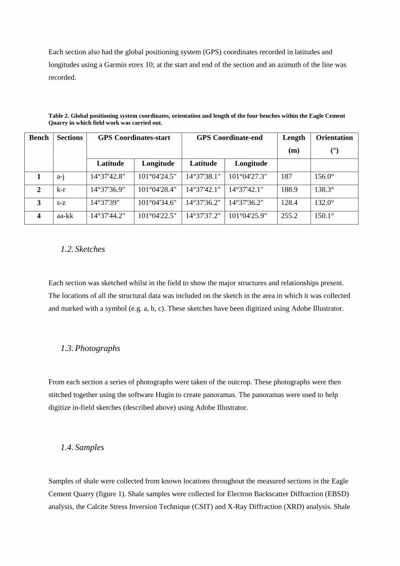
Each section also had the global positioning system (GPS) coordinates recorded in latitudes and

longitudes using a Garmin etrex 10; at the start and end of the section and an azimuth of the line was

recorded.

Table 2. Global positioning system coordinates, orientation and length of the four benches within the Eagle Cement

Quarry in which field work was carried out.

Bench Sections GPS Coordinates-start GPS Coordinate-end Length

(m)

Orientation

(°)

Latitude Longitude Latitude Longitude

1 a-j 14°37'42.8" 101°04'24.5" 14°37'38.1" 101°04'27.3" 187 156.0°

2 k-r 14°37'36.9" 101°04'28.4" 14°37'42.1" 14°37'42.1" 188.9 138.3°

3 s-z 14°37'39" 101°04'34.6" 14°37'36.2" 14°37'36.2" 128.4 132.0°

4 aa-kk 14°37'44.2" 101°04'22.5" 14°37'37.2" 101°04'25.9" 255.2 150.1°

1.2. Sketches

Each section was sketched whilst in the field to show the major structures and relationships present.

The locations of all the structural data was included on the sketch in the area in which it was collected

and marked with a symbol (e.g. a, b, c). These sketches have been digitized using Adobe Illustrator.

1.3. Photographs

From each section a series of photographs were taken of the outcrop. These photographs were then

stitched together using the software Hugin to create panoramas. The panoramas were used to help

digitize in-field sketches (described above) using Adobe Illustrator.

1.4. Samples

Samples of shale were collected from known locations throughout the measured sections in the Eagle

Cement Quarry (figure 1). Shale samples were collected for Electron Backscatter Diffraction (EBSD)

analysis, the Calcite Stress Inversion Technique (CSIT) and X-Ray Diffraction (XRD) analysis. Shale

samples for EBSD were taken from the coarser grained shales that had higher silica and calcite

content. Samples for CSIT were taken from the coarser grained shales. Samples for both EBSD and

CSIT were measured and orientated upon removal from the outcrop. The samples for XRD were

taken from finer grained shales. As each sample was collected, the location was recorded based on the

distance along the measuring tape for the particular section. Where it was possible individual GPS

readings were recorded. However, the resolution of the GPS measurements was often not accurate

enough for this (eg errors of +/- 15m). All shale samples collected approximately the size of a human

fist.

Figure 1. The field area situated within the Eagle Cement Quarry, Saraburi, Thailand. The coloured lines indicated the extent of each bench and the colour equivalent boxes indicate the bench number.

The white circles indicate the sample locations and the sample number. 1 = RFT13-1, 2 = RFT13-2, 3 = RFT13-3, 4 = RFT13-4, 5 = RFT13-5, 6 = RFT13-6, 7 = RFT13-7, 8= RFT13=8, 9 = RFT13-9, 10 =

RFT13-10 and 11 = RFT13-11.

2. Electron Backscatter Diffraction Analysis (EBSD)

Electron backscatter diffraction analysis is used to provide quantitative microstructural information

about the crystallographic nature of metals, minerals, semiconductors and ceramics (Maitland &

Sitzman 2007). It is able to show grain size, grain boundary character, texture, phase identity of the

sample and grain orientation (Maitland & Sitzman 2007). Electron backscatter diffraction maps can

be used to convey the basic character of the samples microstructure visually, with 2D information

about grain size and shape (Humphreys 2001). The EBSD processing software is also able to generate

a variety of additional visual and analytical information as the phase and orientation of each pixel that

is known (Humphreys 2001). This additional information includes (Maitland & Sitzman 2007):

Overall preferred orientation of grains.

Phase distribution throughout the grains.

Character and distribution of grain boundaries.

State of strain and local variations in residual strain within the grains.

For this study I will be using EBSD maps to determine the overall preferred orientation of the grains

and the state of strain and local variations in residual strain within the grains.

2.1. Sample Preparation

Rock samples RFT13- 4, -5, -8 and -11 were orientated and then collected within the Eagle Cement

Quarry, Saraburi, Thailand (figure 1). Each rock sample was sealed in epoxy resin, due to the brittle

nature of the shale and then cut into standard, polished thin sections (76mm by 25mm and ~40microns

thick). The samples were then polished and coated with colloidal silica (detailed below). An Olympus

BX51 reflective light microscope was used to determine the areas that will give the most useful

information when mapped. These areas were characterised by the greatest presence of calcite and then

marked out ready for analysis. A carbon coating was then applied to prevent charge if the sample is

not already conductive.

2.1.1. Thin Section Preparation Procedures

All thin sections were prepared by Pontifex & Associates, using the following procedure:

a. Coat/impregnate surface with an epoxy resin on a hot plate, due to samples brittle tendencies.

b. Cut a small slab from each rock sample that is, approximately 25mm x 55mm, x 8mm thick,

using a 250mm diameter rock-cutting saw blade with a continuous diamond rim.

c. A top surface on the slab, (eventually to be stuck onto a glass slide), is manually ground flat

on a bench-mounted, horizontal diamond grinding wheel Habit-brand, grit size 64.

d. The coarse ground top surface is warmed on a hot plate (at 50oC), and the top coarse-ground

surface is impregnated with an epoxy mix of Araldite LC191 resin, with HY951 hardener,

ratio 8:1.

e. To achieve a finer surface, manually grind this surface using 600 silicon carbon (SiC) grit, on

a zinc-lap or glass plate, using water as a lubricant.

f. This flat finely ground surface is cleaned, checked manually for “perfection”, (if open

porosity is still exposed another veneer of epoxy is applied), is then glued onto a clean, dry

glass slide.

g. Grind to a known thickness, using a UV curing, cyanoacrylate liquid adhesive “Loctite

Impruv 36331”. [Exposure to a UV light of the glued interface through the back of the glass

slide cures the adhesive in 2 to 3 minutes. This is a permanent bond, and the rock (or

eventual wafer) cannot be ever separated from the glass.

h. The block mounted on glass is then cut off using a trim saw with a thin continuous diamond

rimmed sawblade (Diatrenn E2-G), to leave a thickness of about 1mm of the sample slab

(glued onto the glass slide), with the top surface exposed for further processing.

i. The 1mm slab thickness is further ground down on a diamond wheel (Habit D76) held within

a special jig attachment by vacuum, using water as a lubricant. This reduces the slab

thickness stuck on the glass, to a wafer of about 120 micron (0.12mm).

j. The glass slide of known thickness with the glued-on rock wafer, which is then loaded and

held in place on the face of a special jig, and lapped flat on a Logitech machine, to a final

petrographic thickness of the rock wafer, of 30 micron, using 600 SiC grit as the grinding

abrasive, and water as a lubricant.

k. When the Logitech lapping cycle is finished, the quality of the wafer on the glass is assessed,

also optically checked for the required 30 micron thickness, the section is cleaned and

polished.

l. Collodial silica is then applied and the final thin section is again cleaned and labelled. The dip

and dip direction of the bedding is indicated using an arrow on the slide.

2.2. Sample Analysis (Leech 2011)

2.2.1. Sample Loading into SEM

a. Place sample on top edge of the mount.

b. Orientate sample by lining the long axis of the sample parallel to the tilt axis. If elongate

grains are present, orientate the sample by making the smaller dimension of the grains parallel

to the tilt axis. This is due to spatial resolution being lowest in the downhill direction, making

vertical boundaries better resolved than horizontal boundaries.

c. When mounting a sample offset the sample so that the tilt is the closest item to the pole piece.

d. Tilt the stage to 70°, as is determined by Bragg’s Law as being advantageous for resolution.

e. Safe stage movement, it is safe to move the stage so that images move up on screen or left

and right; moving down screen, is dangerous as the pole piece could be hit. Ensure that the

EBSD detector is moved out first before moving the stage to the exchange position.

f. Pump to vacuum, then turn the electron high tension (EHT) on.

g. Calibrate machine: 20kV, maximum aperture = 120 m, high current mode.

h. Set working distance to ~15mm and collect a secondary electron image (SEI) (Obtain SEI

using the Scanning Electron Microscope [SEM]), focus on the m or nm scale.

2.2.2. Inserting the Detector

a. Tilt the stage and move into position under the pole piece so that the EBSD detector can be

inserted into the SEM.

b. Assume the safety stop position hasn’t been set – watch the screen as the detector is inserted

and prepared to hit ‘STOP’ when the detector gets close to the stage. (N.B. Always move the

detector out before moving the stage to the exchange position.

c. The EBSD detector is fully retracted when the display reads zero.

d. Find area to map that was determined using the Olympus BX51 reflective light microscope

and re-focus (a small focus tweak).

e. Perform the dynamic focus.

2.2.3. Dynamic Focus

a. Ensure a low magnification x250.

b. Initiate a slow scan speed for dynamic focus, using a small area raster.

c. Focus image in the centre of the screen.

d. Click ‘control-tab’.

e. Click on a spot and the image will centre.

f. Move green, reduced area box to the top or bottom of the screen.

g. Click ‘dynamic focus’ and change the fluorescence correction factor (FCF) setting (sliding

bar; can be found in scanning/dynamic focus if not already open) until the area within the

reduced area (green box) is in focus.

h. Take it out of reduced area mode.

i. The whole image should be in focus only when you “start scanning” in HKL channel 5

Flamenco software and have collected the SEM image on the Oxford Instruments software

screen.

2.2.4. Using FLAMENCO

a. Open FLAMENCO on Oxford Instruments screen.

b. Insert EBSD detector (see 2.2.2 inserting detector).

c. Acquire SEM image - in secondary electron (SE), click “Read” (upper right,

tilt/magnification/etc.) as a matter of routine.

d. Set Up mode (button in upper left).

e. In electron backscatter diffraction pattern (EBSP) Geometry tab/window: maximize size of

green circle with blue cross indicating centre – a larger area of interest will include more

bands that could potentially be indexed; this is slower, but should result in better indexing.

This is appropriate for less symmetrical phases (geological materials). Do not move the blue

cross.

f. Adjust probe current (coarse-grained [10μm grains]=max. 120μm aperture, high current

mode).

g. Background – turn up probe current, low magnification

Adjust the Timing per frame to adjust the brightness for background reading

(not too bright, not too dim, no pattern visible).

Ensure there is no pattern in the Live EBSP window, if OK, take background.

h. Turn on Spot mode (button in upper left) to get an EBSP (should see a pattern now).

Under Live EBSP, in the Enhancement window, click button to ‘Adjust scale’

(for brightness/contrast).

i. Calibrate:

Centre beam.

Get good EBSP (refer back to 2.2.4.9 above).

Detect bands (increase averaging for good picture).

Eight bands for calibration.

Visually inspect accuracy.

Load phase.

Load calibration file.

Index the number of bands.

Refine a few times - visually inspect for accuracy.

Go to interactive and make sure FLAMENCO is indexing other phases well.

j. Find part of sample with low relief on it at lower magnitude (at high magnitude, you may just

be seeing everything within the narrow swath of focus), use reduced area box, turn on

dynamic focus, then remove reduced area box to check that the entire sample is in focus.

2.2.5. Mapping Steps

a. Save file (new job).

b. Step size needs to be at least 1/5 average grain size, which for my samples the step size was 1.

c. Maximize number of points.

d. Change box size for test - try to go for a tall map vs. wide map to get grain textures quickly

(because of the scanning pattern). For most of my maps the box size varied from 200-200mm

in the x-axis and from 150-350mm in the y-axis.

e. Set: Band Detection (7), Hough Resolution (50), # Reflectors (45 – in the phase box [Match

units]), Frame averaging (4).

f. Add Job and hit Run.

g. Make sure it is indexing all patterns - or if it is not indexing it is because there is no pattern.

h. When happy press menu Job/restart job.

i. Immediately reduce window for 2 mins.

j. Maximize for time per second.

k. Repeat steps g-j with EDS and Image Storage if you want it to get actual time.

l. Enter time in tools/tools/options/time per acquisition.

m. Enter information on new job and get accurate time run for real job.

2.2.6. Drift Prevention

a. Give the stage 1 hour to settle (gravitationally) for higher resolution.

b. Tilt the stage past 70° and then return to 70° to lock gears better.

c. Thick conductive coating can cause drift, ensure carbon paint is used rather than carbon tape.

d. Ensure chamber is as clean as possible and be cautious of insulating wires near tilted sample.

e. Ensure stage grounding is robust.

2.3. Calibration

2.3.1. Energy Source (kV and aperture)

The kV should be set between 10-30kV with a maximum aperture size of 120 m. A calibration of

20kV is generally used for elemental analysis of normal geological materials. A high kV (>30kV)

results in a higher electron yield from the gun and a more efficient scintillation effect on the phosphor

screen, creating crisper patterns, brighter and narrower bands. A lower kV (>15kV) produces better

spatial resolution, less charging and broader bands that clearly show subtle crystallographic

differences between candidate phases and is thus better for phase ID.

3. Calcite Stress Inversion Technique (CSIT)

For the last three decades calcite twins have been used as indicators of stress and strain orientations

and magnitudes of stress and to some extent palaeotemperature or palaeoburial. Etchecopar’s (1984)

calcite stress inversion technique (CSIT) uses computerised inversion of calcite twin data to produce

four of the six parameters of the complete stress tensor (Amrouch et al. 2010, Lacombe 2010). These

parameters are:

1. The plunge and plunge direction of the three palaeo-stresses ( 1, 2 and 3);

2. The shape ratio =

.

3.1. Concept

Within calcite that has been deformed at low temperatures widespread mechanical e-twinning occurs

(Amrouch et al. 2010). Temperature of deformation has been found to correlate directly with mean

calcite twin width, such that thin twins are most dominant below 170°C and thick twins are dominant

above 200°C (Lacombe 2010). The CSIT assumes constant critical resolved shear stress (CRSS) for

twinning and homogeneous state of stress at the grain scale (Lacombe 2010). The process used is very

similar to that used for fault slip data (Etchecopar 1984), as twin gliding along the twinning direction

within the twin plane is geometrically comparable to slip along slickenside lineations within a fault

plane (Lacombe 2010).

3.2. Sample preparation

Samples RFT13-2 and -5 were orientated and then collected within the Eagle Cement Quarry,

Saraburi, Thailand (Figure 1). Each sample was sealed in epoxy resin, due to their brittle nature and

then three standard, polished, covered thin sections (46mm by 25mm and ~40microns thick) were cut

from each sample RFT13-5 and four were cut from RFT13-2. Refer to 3.2.1 for thin section

preparation procedures. . From each sample the thin sections were cut to show orientations of the x, y

and z stress (check with KHALID? Is it supposed to be strain or stress?) axis. Sections 2a and 5a

were orientated in the x-z stress plane and were cut parallel to the dip direction and perpendicular to

the strike (x direction corresponds to the dip direction, for the direction of y and z axis, the rule of the

right hand is used). Sections 2b and 5b were orientated in the y-z stress plane and cut perpendicular to

the bedding and parallel to its strike. Sections 2c, 2d and 5c were orientated in the z-y stress plane and

cut perpendicular to the bedding and to its strike. Sample 2 had two sections 2c and 2d, cut in the z-y

stress plane due to two different generations of calcite veins being present.

Figure 2 This cube represents a hypothetical sample of the perfect planes to cut sections a, b, c and d in samples

RFT13-2 and RFT13-5. The yellow plane represents the hypothetical bedding plane. Sections 2a and 5a were

orientated in an x-z direction and were cut parallel to the dip direction and perpendicular to the strike; this is

represented by the pink plane. Sections 2b and 5b were orientated in a y-z direction and cut perpendicular to the

bedding and parallel to its strike; this is represented by the blue plane. Sections 2c, 2d and 5c were orientated in a z-y

direction and cut perpendicular to the bedding and to its strike sections; this is represented by the yellow plane.

3.2.1. Thin Section Preparation Procedures

All thin sections were prepared by Pontifex & Associates using the following procedure:

a. Steps a-k are the same as section 2.1.1

b. The section is then cleaned and covered with a glass coverslip, using the same UV curing

adhesive as listed above. Again this is a permanent fix, i.e. the coverslip cannot be removed.

c. The final thin section is then again cleaned and labelled.

3.3. Loading the Sample onto the Universal Stage

a. Turn universal stage (U-stage) so that the marker is set to zero.

b. Place 1 drop of glycerine onto the lower hemisphere.

c. Place the thin section on the stage so that the marker on the thin section that runs horizontal is

running east-west (90°-270°) and the marker running diagonally northeast-southwest is in the

top right hand corner.

d. Place 1 drop of glycerine on the thin section.

e. Place the upper hemisphere on top of the thin section with the screw side towards 90°. Screw

upper hemisphere in place.

3.4. Measuring the Samples

a. Find a calcite grain with one of the following characteristics:

1. Two twin planes

2. Two cleavage planes

3. One twin plane and one cleavage plane.

b. Mark the location of the grain on the image of your thin section.

c. Open Calci3.

d. Enter the name of your file, eg RFT22.

e. Enter the date.

f. Press 1 if you are measuring two twin planes.

g. Press 2 if you are measuring two cleavage planes.

h. Press 3 if you are measuring one twin plane and one cleavage plane.

i. To measure a twin plane or cleavage plane align the plane north-south.

j. Tilt the stage to the left or right, so that the plane is visually the thinnest possible.

k. Enter the dip and dip direction of the first twin plane or cleavage plane into Calci3 in the

following format: if the dip and dip direction of the plane is 9/122 and the stage was tilted to

the left, then enter 122 9 ‘G’. If the dip and dip direction of the plane is 08/003 and the stage

was tilted to the right, enter 3 8 ‘D’. Note: the program is in French. ‘G’ represents gauche,

which is the French word for left and ‘D’ represents droite, which is the French word for

right. Press enter.

l. Measure the second plane (twin plane or cleavage plane).

m. Enter the dip and dip direction of the second twin plane into Calci3 and press enter.

n. The program will produce two optical axis which are denoted as ‘axe C1 and C2’. You must

determine, which is the correct optical axis. To do this, align the stage in the dip and dip

direction of both the axis given and push the cross-polariser in. The correct optical axis will

be the plane that is in extinction. Note: both planes can be in extinction; however, one will be

in extinction more than the other.

o. Enter 1 if the first optical axis is in extinction. Enter 2 if the second optical axis is in

extinction.

p. The program will then produce a third twin plane, if you are measuring two twin planes or

three twin planes if you are measuring two cleavage planes or a second and third twin plane,

if you are measuring one twin plane and one cleavage plane.

q. Align the stage in the orientation of the third twin plane (if using two twin planes) and see if

the plane is twinned or untwinned. Do the same for all three twin planes, if measuring two

cleavage planes and the second and third twin plane, if using one twin plane and one cleavage

plane.

r. The program will then ask you if the twin planes are twinned or untwinned. If a twin plane is

twinned enter O, however, if it is untwinned enter N.

s. The program will then ask you how certain you are that the plane is twinned or untwinned.

Enter 100 if you are 100% certain. The following percentages are used as codes to depict the

reason for uncertainty.

Reason for uncertainty Assigned

percentage

Grain is too large 10%

Grain is too small 20%

Grain is too dirty 30%

Dip is too high (generally used if dip is over 45°) 40%

Grain is too deformed 50%

t. Enter 1 if you are happy with the data, this will save the data. Press F if you are unhappy with

the data and need to change anything.

u. Enter 1 again.

v. Repeat steps 1-21 for a minimum of 30 grains per thin section.

3.5. Processing the samples

a. Rotate the original bedding orientation of the sample in the same orientation in which the

twins were measured in. Note the rotations are made around the three euler angles (Kocks et

al. 2000).

b. Enter all measurements for each thin section into separate, appropriately labelled text (txt)

files.

c. Merge each txt file into one txt file and put the angle of the three euler rotations for the

appropriate sections (x-y, y-z, x-z) above their related measurements. Give this file an

appropriate label, e.g. RFT2.

d. Open the parameter file (PARA.txt) and enter the percentage of twinned planes you wish to

create the stress tensor with. Note for the first parameter file it is best to start with between

30-50% of twinned planes.

e. Open Calc.

f. Enter PARA.txt (name of parameters file, which specifies the percentage of twinned planes

you wish to calculate).

g. Enter RFT2.txt (name of the txt file that contains all the measurements).

h. Enter the name of the txt file you wish to create, e.g. RFT2A30. RFT2 = txt file containing

measurements. A= first stress tensor. 50 = percentage of twinned planes being calculated.

i. The program will ask if you wish it exclude outliers, enter N for no.

j. The program will then ask for the average size of the grains measured, enter 100.

k. The program will then ask if you want to create Mohrs circle, enter O for yes.

l. Your txt file will then be created (RFT2A50) and will contain the 1, 2 and 3, shape ratio

( ) and factor of tensor quality (f) values for the appropriate calculation.

m. Repeat steps d-l for between 30-50% of twinned planes or until f=1.5 or above.

n. Record the 1, 2 and 3, and f values for the appropriate calculations.

o. Create stereographic projections of the bedding plane in relation to the 1, 2 and 3 values to

determine which calculation provides the best stress tensor, based on Anderson (1951).

p. Once the best calculation has been chosen, open the txt file created by Calc and remove the

data underneath the 1, 2 and 3, and f values and enter it in the parameter 2 file. This

essentially tells the program to exclude the data that has already provided a stress tensor.

q. Remove all untwinned planes from the first three lines of data. Untwinned planes are

represented with a minus (-) sign. To remove the untwinned planes you must check the txt file

that contains all the data to see how certain you are that the plane is untwinned. The matrix

below is used to determine, which measurement it is and from what thin section it was

measured: The horizontal lines represent the position of the measurement, e.g. whether it is

the first, second or third measurement recorded from the grain. The vertical position

represents, which thin section the grain was measured in, e.g. x-z = thin section 1, y-z = thin

section 2 and x-y = thin section 3. Therefore column one = thin section 1, column 2 = thin

section 2 and column three = thin section 3. So if the value is 613 then the grain would be

from thin section 1, be from the 13th set of measurements and be the third measurement.

Check the certainty of this measurement and if it is not 100% then remove the measurement

from the data PARA2 file.

r. Alter the certainty of the measurement to 100% in the RFT2 file. Once all the appropriate

untwinned measurements have been altered to being twinned planes from the RFT2 file save

the file under a new name, e.g. RFT2M, m= modified.

s. Repeat steps d-p, for parameter 2. Change name in step f to PARA2.txt rather than PARA.txt.

Change name in step g to RFT2M.txt rather than RFT2.txt. Change name in step h to an

appropriate name, e.g. RFT2B50, B= parameter 2.

t. Repeat step q to remove all appropriate untwinned planes and add to the parameter 3 file, in

order to determine a third stress tensor.

u. Once all the appropriate untwinned measurements have been removed save the file under a

new name, e.g. RFT2N, N= second modification.

v. Repeat steps d-p for parameter 3. Change name in step f to PARA2.txt rather than PARA.txt.

Change name in step g to RFT2N.txt rather than RFT2.txt. Change name in step h to an

appropriate name, e.g. RFT2C50, C= parameter 2. Note a third stress tensor may not be

present, depending on the sample.

4. X-ray Diffraction Analysis (XRD)

Measuring clay mineral crystallinity using X-Ray Diffraction (XRD) methods has been used to

determine the conditions of very low-grade metamorphism in phyllosilicate bearing rocks (Warr &

Rice 1994). The selected XRD peak reflections of clay minerals, such as illite chlorite, kaolinite and

pyrophyllite are used to determine these conditions (Warr & Rice 1994). In this study the focus will

be on the illite crystallinity (IC) measured by XRD methods. Illite crystallinity is evaluated by

measuring the half-peak-width of the illite peak from the sample (Warr & Rice 1994). This will give

an approximate temperature of deformation (Warr & Rice 1994).


Samples RFT13- 1, -3, -6, -7, -9 and -10 were collected within the Eagle Cement Quarry, Saraburi,

Thailand (Figure 1). Each sample then underwent the following process:

4.1.1. Crushing the sample using the jaw crusher

a. Procedure is to be undertaken using a clean jaw crusher (method described below) in a clean

laboratory.

b. Rock must be clean and fresh (no texta or weathering).

c. Turn machine on. Ensure gate is locked.

d. Insert sample through the opening on the top of the machine.

e. Close opening by sliding the yellow door across it.

f. Turn off the machine.

g. Release the gate

h. Remove the sample.

i. Place sample on butcher’s paper and transfer into an appropriately labelled bag.

j. Repeat steps b-h for each sample.

4.1.2. Cleaning the Disc Mill

a. Blow all dust and particles off the outside of the jaw crusher, with compressed air.

b. Wipe over outside of machine using ethanol and paper towel.

c. Ensure machine is perfectly dry using compressed air.

d. Open machine.

e. Blow out all dust using compressed air.

f. Wipe tray down using ethanol and paper towel.

g. Ensure it is dry using compressed air.

h. Line tray with butchers paper.

i. Put tray back in machine.

j. Clean the teeth using compressed air, ethanol and paper towel.

k. Brush the teeth down with a wire brush.

l. Use a hack saw to remove any large rock particles wedges between the teeth and the door walls.

m. Close machine. Lock the gate.

4.1.3. Crushing the sample using a ball mill

a. Procedure is to be undertaken using a clean ball mill (method described below) in a clean

laboratory.

b. Remove the ball from the ball mill.

c. Put approximately 200g of previously crushed (using jaw crusher) shale sample into the ball mill.

d. Put the ball on top of the ball mill.

e. Put the lid of the ball will and tighten in place using the knobs.

f. Turn the ball mill on for 1 minute.

g. Set the amplitude to 0.5mm.

h. Remove sample from ball mill.

i. Place sample in appropriately labelled bag.

j. Repeat steps b-i for each sample.

4.1.4. Cleaning the ball mill

a. Wipe over outside of machine using ethanol and paper towel.

b. Open the ball mill.

c. Wipe over the ball using ethanol and paper towel.

d. Wipe over the inside of the ball mills lid using ethanol and paper towel.

e. Wipe over the inside of the ball mill.

f. Close the ball mill.

4.1.5. Sieve crushed sample

a. Procedure is to be undertaken using a clean 250µm sieve in a clean laboratory.

b. Empty contents of previously crushed (using a ball mill) shale sample into a 250µm sieve.

c. Shake the sieve from side to side until all of the 250µm portion has been collected in the bottom

of the sieve.

d. Place 250µm into appropriately labelled plastic bags.

4.1.6. Cleaning the sieve

a. To clean the sieve blow pull apart all three components (the lid, base and mesh).

b. Use compressed air to remove any particles caught in the 250µm mesh.

c. Wipe over the inside and outside of the base and lid of the sieve.

4.1.7. Carbonate Removal Procedure for Clay Purification

a. For each sample place 1.5g of sample into a four 50ml centrifuge vials.

b. Add 10ml of 1M sodium acetate/acetic acid buffer.

c. Loosely screw on cap and place in a water bath at 90°C for approximately 30minutes.

d. Keep a close eye on the samples, if they are reacting too vigorously remove vials and place in a

cold water bath until reaction has slowed.

e. As soon as effervescence stops, remove sample from hot water bath.

f. Fill up vials to 50ml with Deionised water (DIW).

g. Place in centrifuge for 5minutes at 3000RPM and discard supernatant.

h. Repeat steps b-g twice

i. Ca-exchange sample with 10ml of 1M CaC12.

j. Shake sample well, leave for 10minutes.

k. Centrifuge for 5minutes at 3000RPM and discard supernatant.

l. Fill tube up with 50ml DIW and shake sample well.

m. Centrifuge for 5minutes at 3000RPM, discard supernatant.

n. Repeat steps k-l twice.

4.1.8. How to make 1M of sodium acetate/acetic acid buffer with a pH of 5

a. Dissolve 82g of sodium acetate (CH3COONa) in approximately 900ml of deionised water (DIW).

b. Add 45ml of glacial acetic acid.

c. Bring total volume of solution to 1000ml by adding DIW.

4.1.9. Organic Material Removal Step for Clay Purification

a. Adjust the required amount of sodium hypochlorite bleach to a pH of 9.5 using 4M HCl. NOTE:

this needs to be done in the fume hood as it releases a dangerous gas and should not be done on

the day that the solution will be used as the resulting solution is not stable. Use a Calibrated pH

electrode.

b. Dispense 10ml of the pH adjusted bleach into each centrifuge vial.

c. Loosely cap vials, place vials in a plastic rack and place in a 90°C water bath for 15minutes.

d. Remove vials from bath and fill to 50ml with Deionised water (DIW).

e. Centrifuge for 5minutes at 3000RPM.

f. Discard supernatant.

g. Repeat steps b-f until sample no longer reacts upon addition of bleach and have changed colour to

light grey, brown, or redish, indicating complete removal of organic material (OM). This usually

requires 1-3 repeats.

h. After the last bleach repeat, rinse sample with DIW once more.

i. Fill to 50ml with DIW, cap and shake well.

j. Centrifuge for 5minutes at 3000RPM and discard supernatant.

k. Repeat rinse in DIW twice more.

4.1.10. Clay Separation (<2µm) by NaCl method

a. Add 10ml of 1M NaCl solution to each vial.

b. Shake for 10minutes in the end over end shaker.

c. Fill centrifuge tube to 50ml with Deionised water (DIW).

d. Centrifuge for 10minutes at 3000RPM.

e. Carefully pour off supernatant liquid ensuring that none of the material collected at the bottom of

the centrifuge chamber is dislodged.

f. Repeat steps a-e twice or until supernatant is cloudy.

g. Wash material from centrifuge tubes into a labelled 250ml beaker (use one beaker per sample, so

empty 4 centrifuge vials of the same sample into a single beaker).

h. Fill beaker with 150ml of deionised water.

i. Disperse sample in each beaker using the ultrasonic probe.

j. Use the flat tup for 60seconds at 50% amplitude, make sure the tip is immersed in the sample and

does not touch the beaker. NOTE: ensure you clean the probe with a wet tissue between samples

k. Wash the sample into the corresponding centrifuge tubes and make sure they are filled to the 50ml

mark.

l. Shake up all samples before placing them in the centrifuge. Then centrifuge for 4inutes at

900RPM.

m. At this stage the supernatant should be cloudy or discoloured. Carefully pour approximately three

quarters of the supernatant into an appropriately labelled beaker of at least 2 litre capacity (again,

use one beaker per sample).

n. Repeat steps g-m until the supernatant becomes clear. At this stage you have removed all the

<2µm material from your sample. NOTE: Ideally the supernatant should be clear when the

relevant size fraction is collected. The total amount of supernatant is generally 1 litre.

4.1.11. Ca Saturation

a. Flocculate the material collected in the beaker by adding a teaspoon of CaCl2 to each beaker.

Allow the flocculated material to settle overnight and siphon off clear supernatant using the

siphon attached to the vacuum pump.

Pour flocculated material remaining in the beaker into centrifuge tubes and spin at 3000RPm for

20minutes.

b. Carefully discard supernatant (supernatant should be clear).

c. Repeat steps a and b until all material has been transferred from the beaker to the centrifuge tubes.

The final proportion of material will need to be washed from the beaker using DIW from a

squeeze bottle.

4.2. Sample Analysis

a. Fit 5g sample of >2µm clay fraction into the side loader of the Bruker D8 Advance.

b. Turn on Bruker D8 Advance.

c. Radiation is set at Cu 2 , which is the default setting for this machine.

d. Set scanned angle range for between 3.5° 2 - 50° 2 .

e. Set step size to 0.02°.

f. Set dwell time to 1 second

g. Open XRD software – Bruker diffraction evaluation open crystallography database.

h. Peaks created by the samples can then be compared to minerals database with the XRD software

to obtain results.

i. Turn off machine and software.

j. Remove Sample.

k. Repeat steps a-j for each sample.\

5. Total Organic Carbon (TOC) Analysis

Total Organic Carbon (TOC) analysis is being used to determine the amount of organic carbon within

the tested samples. This technique is being used to determine the affects the amount of organic

carbon has on the rheology of the shale within the Eagle Cement Quarry, Thailand during

deformation. In order to get the proportions of carbon and inorganic carbon, two techniques are

required, Elemental Analysis (EA) and Pressure Calcimeter Analysis (PCA). For the EA, CHNX

analysis will be used to determine the mass fractions of carbon, hydrogen and nitrogen for each

sample. PCA will be used to determine the proportion of inorganic carbon within each sample.

5.1. Sample Preparation for Pressure Calcimeter Analysis and Elemental Analysis


Thailand (Figure 1). Each sample then was crushed using a jaw crusher (refer to 4.1.1) and ball mill

(refer to 4.1.3) and then sieved to remove the 250µm portion (refer to 4.1.5).

5.2. Pressure Calcimeter Analysis.

a. Cut micro-centrifuge tubes just above the 1.0ml mark.

b. Add 5ml 4M HCl/3% FeCl2 solution to each glass vial.

c. Weigh out 200mg of each sample into a cut micro-centrifuge tube and place this into a glass vial

containing HCl acid. Make sure that the sample does not come into contact with the acid.

d. Weigh out seven CaCO3 standards (200mg, 150mg, 100mg, 75mg, 50mg, 25mg and 10mg)

and place into vials containing acid.

e. Cap all vials with a rubber stopper and a foil cap, and then crimp the foil using the hand crimper.

f. Once all samples and standards to be tested are capped shake each vial vigorously to ensure that

the entire sample reacts with the acid.

g. Leave the vials sitting for half an hour, shaking them again at 15 minutes.

h. Attach the hose and needle to the manometer.

i. Tear out the centre of the aluminium cap on the first vial, pierce the rubber cap with the needle

and record the maximum pressure vial. Repeat for all vials.

5.2.1. How to prepare 4M HCl with 3% (by weight) ferrous chloride (FeCl2 * 4H2O)

a. Mix 110ml of concentrated (37%; 36.46M) HCl with approximately 500ml of water in a 1L

volumetric flask.

b. Add 30g of ferrous chloride (FeCl2 * 4H2O).

c. Fill to 1L using deionised water.

5.2.2. Sample Processing of PCA

The weight and pressure of the standards and pressure recorded in each sample is used to calculate the

equivalent mass of CaCO3 in each sample. This value needs to be normalized to the exact mass of

sample weighed into each centrifuge tube. This is done in excel. The percentage of CaCO3 from each

sample is then converted into the percentage of inorganic carbon (IC).

5.3. Elemental Analysis (EA)

a. Weigh out 5g of each sample.

b. Place in Aluminium capsule.

c. Insert into the Perkin Elmer Series II CHNS/O Analyser 2400.

d. Turn machine on.

e. Set to Carbon, hydrogen and nitrogen (CHN) mode.

f. Run sample.

g. Run CaCO3 standards for every 5-10 samples, to ensure the results are valid.

6. Source Rock Analyzer (SRA)

I will be using the Source Rock Analyzer (SRA) is used to pyrolyze rock samples to determine

accurate source rock data including, TOC, thermal maturity of the sample (Tmax), free oil content

(S1), the potential of the sample as a source rock (S2) and subsequently calculate the kerogen type,

hydrogen index, kerogen maturity and production index.



Thailand (Figure 1). Each sample then was crushed using a jaw crusher (refer to 4.1.1) and ball mill

(refer to 4.1.3) and then sieved to remove the 250µm portion (refer to 4.1.5).

Source Rock Analysis (SRA) artificial maturation test

a. Take the cap off the crucible and empty the contents. Wear latrex or nitril gloves and handle the

crucible with forceps ensuring not to touch it with your fingers.

b. Weigh approximately 100mg of sample into a crucible. Repeat for all samples.

c. Place cap back on crucible and insert the crucible onto the auto sampler tray. An empty crucible

is normally placed in position one in the autosampler tray, and position two is a daily calibration

standard. Therefore the first sample crucible is placed in position three. Standards are run in

positions 20, 40 60 etc *.

d. In the sequence editor the sample weight, lithology and acquisition type (BLK, STD, TPH) was

recorded.

e. Save data to a known file location.

f. Place the autosampler in the autosampler rack.

g. Check the instrument gas flow rates and make adjustments to gas flows if necessary. The gas flow

rates for air, hydrogen and helium should be as follows:

- Air = 300ml/min

- Hydrogen = 50ml/min

- Helium = 50ml/min

h. Initiate start up, and where prompted load previously saved data file.

i. The autosampler will transfer the crucible from the autosampler tray to the SRA pedestal and

place the sample into the 300˚C oven. The sample is held isothermally at 300˚C for 3 minutes.

During this time, free hydrocarbons are volatilised and detected by the Flame Ionisation Detector

(FID). These hydrocarbons are quantitatively reported as S1 in milligrams of hydrocarbon per

gram of rock.

j. After the isothermal period, the temperature is ramped up at 25˚C/minute to 600˚C. During this

period of increasing temperature, organic hydrocarbons are generated from pyrolitic cracking of

kerogen and other organics within the rock. The generated hydrocarbons are detected by the FID,

labelled as S2 and again reported in milligrams of hydrocarbon per gram of rock. The temperature

which has the maximum release of hydrocarbons by cracking of organics (Tmax) is also recorded.

Data is expressed both as a number (milligrams of hydrocarbon per gram of rock) and in the form

of a pyrogram (Figure 2).

Figure 3: Hypothetical pyrogram generated by the Weatherford SRA, showing S1, S2 and Tmax.

l. Kerogen type, Kerogen maturity hydrogen index (HI) and production index (PI) can be calculated

for the data output by using the following equations, based on the procedure of Espitalie et al.

(1977):

- Kerogen maturity = 0.0180* Tmax -7.16

- Kerogen type = Plot TOC vs S2

- Hydrogen index (mgHC/gTOC) = S2* (100/TOC)

- Production index (mgHC/g sample) = S1/ (S1+S2)

REFERENCES

AMROUCH K., LACOMBE O., BELLAHSEN N., DANIEL J. & CALLOT J.-P. 2010. Stress and strain

patterns, kinematics and deformation mechanisms in a basement-cored anticline: Sheep

Mountain Anticline, Wyoming. Tectonics 29, TC1005.

ANDERSON E. M. 1951. The dynamics of faulting and dyke formation with applications to Britain

(reprint edition). Hafner Pub. Co.

ESPITALIE J., MADEC M., TISSOT B., MENNIG J. & LEPLAT P. 1977. Source rock characterization

method for petroleum exploration. Offshore Technology Conference.

ETCHECOPAR A. 1984. Etude des e´tats de contraintes en tectonique cassante et simulation de

de´formation plastique (approche mathe´matique),. the`se doctorates-sciences thesis,

Sciences, Univ. Sci. et Tech. du Languedoc, Montpellier, France., Univ. Sci. et Tech. du

Languedoc, Montpellier, France. (unpubl.).

HUMPHREYS F. J. 2001. Review Grain and subgrain characterisation by electron backscatter

diffraction. Journal of Materials Science 36, 3833-3854.

KOCKS U. F., TOMÉ C. N. & WENK H. R. 2000. Texture and Anisotropy: Preferred Orientations in

Polycrystals and Their Effect on Materials Properties (Illustrated, reprint edition). Cambridge

University Press, Cambridge, UK.

LACOMBE O. 2010. Calcite twins, a tool for tectonic studies in thrust belts and stalble orogenic

forelands. Oil and Gas Science and Technology - Revue de l'IFP Energies nouvelles 65, 809-

838.

LEECH M. 2011. Instructions for the use of the Oxford Instruments HKL Electron Backscatter

Diffraction (EBSD) and channel 5 software. University S. F. S.: 1-30, San Francisco State

University.

MAITLAND T. & SITZMAN S. 2007. Electron Backscatter Diffraction (EBSD) technique and materials

characterisation examples. In: Zhou W. & Wang Z. L. eds., Scanning Microscopy for

Nanotechnology: Techniques and Applications, pp 41-75, Springer-Verlag New York.

WARR L. N. & RICE A. H. N. 1994. Interlaboratory standardization and calibration of clay mineral

crystalinity and crystallite size data. Journal of Metamorphic Geology 12, 141-152.

APPENDIX B: Cross sections A-B to JJ-KK

13.5

m

NW

SE

013

.5 BA

°E

KEY

°E

KEY

SENW

20m

200 B

C

180

18m

CDSE

NW

°E

KEY

SENW

14m

DE

014

°E

KEY

EF

26.5m

SENW

026

.5

°E

KEY

20m

FGSE

NW 0

20°E

KEY

SENW

20m

GH

020

°E

KEY

Igne

ous

intr

usio

n

KEY

Bedd

ing

Plan

es

Out

line

of s

hale

Thru

st p

lane

Alu

m S

hale

NW

SE

20m

HI

020

°E

Igne

ous

intr

usio

n

KEY

Bedd

ing

Plan

es

Out

line

of s

hale

Thru

st p

lane

Alu

m S

hale

IJ

°E0

35m

SENW

NW

NW

SE

35m

035 L

K°E

KEY

018

18m

MN

SENW

°E

KEY

130

13m

QR

SENW

°E

KEY

019

19m

STSE

NW

°E

KEY

020

.520

.5m

SENW T

U°E

KEY

20.5

0

20.5m

UVSE

NW

°E

KEY

200

SENW

20m

VW

°E

KEY

200

SENW

20m

WX

°E

KEY

130 X

Y

13m

SENW

°E

KEY

015

.415

.4m

YZSE

NW

KEY

Bedd

ing

Plan

es

Out

line

of o

utcr

op

Thru

st p

lane

Khao

Kha

d Li

mes

tone

Alu

m S

hale

°E

020

20m

SENW AA

BB°E

KEY

023

23m

SENW BB

CC°E

KEY

024

.424

.4m

CCDDSE

NW

°E

KEY

023

23m

DD

EE

SENW

°E

KEY

EEFF21

0

21m

SENW

°E

KEY

240

24m

FFGGSE

NW

KEY

Bedd

ing

Plan

es

Out

line

of o

utcr

op

Thru

st p

lane

Khao

Kha

d Li

mes

tone

Alu

m S

hale

°E

0

10.5m

SENW

HH

°E°E

15m

SENW

II

4.5m

KEY

Sect

ions

are

sep

arat

ed b

y a

thru

st

027

.827

.8m

JJKK

SENW

°E

KEY

APPENDIX D: Fault data

Stereographic projections of the relationships

between shear planes and slickenlines.

APPENDIX D: Electron Back-Scatter

Diffraction

Electron back-scatter diffraction maps and

poles to figure plots.

a. Electron back-scatter diffraction (EBSD) map from sample RFT13-002A with band contrast (BC), a semi transparent filter and inverse pole figure (IPF) colouring. b. Pole figure plot for the

EBSD map with IPF colouring from sample RFT13-002A. c. Pole figure plot with contouring of sample RFT13-002A. d. Electron back-scatter diffraction map from sample RFT13-004 with

BC, a semi transparent filter and IPF colouring. e. Pole figure plot for the EBSD map with IPF colouring from sample RFT13-004. f. Pole figure plot with contouring of sample RFT13-004.

Electron back-scatter diffraction maps were created using HKL channel 5 software; Tango, plots were created using Mambo and have been put in a geographic orientation so that x = North.

a. Electron back-scatter diffraction (EBSD) map from sample RFT13-002B-1 with band contrast (BC), a semi transparent filter and inverse pole figure (IPF) colouring. b. Pole figure plot for

the EBSD map with IPF colouring from sample RFT13-002B-1. c Pole figure plot with contouring of sample RFT13-002B-1. d. Electron back-scatter diffraction map from sample RFT13-

002B-2 with BC, a semi transparent filter and IPF colouring. e. Pole figure plot for the EBSD map with IPF colouring from sample RFT13-002B-2. f. Pole figure plot with contouring of

sample RFT13-002B-2. Electron back-scatter diffraction maps were created using HKL channel 5 software; Tango, plots were created using Mambo and have been put in a geographic

orientation so that x = North.

a. Electron back-scatter diffraction (EBSD) map from sample RFT13-005 with band contrast (BC), a semi transparent filter and inverse pole figure (IPF) colouring. b. Pole figure plot for the

EBSD map with IPF colouring from sample RFT13-005. c Pole figure plot with contouring of sample RFT13-005. d. Electron back-scatter diffraction map from sample RFT13-005 with BC, a

semi transparent filter and IPF colouring. e. Pole figure plot for the EBSD map with IPF colouring from sample RFT13-005. f. Pole figure plot with contouring of sample RFT13-005. Electron

back-scatter diffraction maps were created using HKL channel 5 software; Tango, plots were created using Mambo. Plots e and f have been put in a geographic orientation so that x = North.

a. Electron back-scatter diffraction (EBSD) map from sample RFT13-008-1 with band contrast (BC), a semi transparent filter and inverse pole figure (IPF) colouring. b. Pole figure plot for the

EBSD map with IPF colouring from sample RFT13-008-1. c Pole figure plot with contouring of sample RFT13-002B-1. d. Electron back-scatter diffraction map from sample RFT13-008-2

with BC, a semi transparent filter and IPF colouring. e. Pole figure plot for the EBSD map with IPF colouring from sample RFT13-008-2. f. Pole figure plot with contouring of sample RFT13-

008-2. Electron back-scatter diffraction maps were created using HKL channel 5 software; Tango, plots were created using Mambo.


EBSD map with IPF colouring from sample RFT13-008-1. c Pole figure plot with contouring of sample RFT13-008-1. d. Electron back-scatter diffraction map from sample RFT13-008-2 with

BC, a semi transparent filter and IPF colouring. e. Pole figure plot for the EBSD map with IPF colouring from sample RFT13-008-2. f. Pole figure plot with contouring of sample RFT13-008-

2. Electron back-scatter diffraction maps were created using HKL channel 5 software; Tango, plots were created using Mambo and have been have been put in a geographic orientation so that

x = North.


EBSD map with IPF colouring from sample RFT13-011-1. c Pole figure plot with contouring of sample RFT13-011-1. d. Electron back-scatter diffraction map from sample RFT13-011-2 with

BC, a semi transparent filter and IPF colouring. e. Pole figure plot for the EBSD map with IPF colouring from sample RFT13-011-2. f. Pole figure plot with contouring of sample RFT13-011-

2. Electron back-scatter diffraction maps were created using HKL channel 5 software; Tango, plots were created using Mambo and have been have been put in a geographic orientation so that

x = North.

APPENDIX E: X-Ray Diffraction

Clay mineralogy and Illite Crystalinity

Chamosite Illite

Chamosite Quartz

Quartz

0

5000

10000

15000

20000

25000

30000

35000

40000

0 5 10 15 20 25 30 35 40 45 50

Pe

ak In

ten

sity

(C

ou

nts

)

2Theta angle (Coupled 2Theta/Theta)

RFT13-001 clay mineralogy

Chamosite Illite

Chamosite

Quartz

Quartz

0

5000

10000

15000

20000

25000

30000

35000

40000

0 5 10 15 20 25 30 35 40 45 50

Pe

ak In

ten

sity

(C

ou

nts

)



Chamosite Illite

Paragonite

Chamosite

Quartz

Quartz

0

5000

10000

15000

20000

25000

30000

0 5 10 15 20 25 30 35 40 45 50

Pe

ak In

ten

sity

(C

ou

nts

)

2Theta angle (Coupled 2theta/Theta)


Chamosite Illite

Paragonite

Chamosite Quartz

Quartz

0

5000

10000

15000

20000

25000

0 5 10 15 20 25 30 35 40 45 50

Pe

ak In

ten

sity

(co

un

ts)



APPENDIX F: Source Rock Analyzer

Pyrograms and Kerogen Analysis

Pyrogram of sample RFT13-001


0

1000

2000

3000

4000

5000

6000

7000

8000

9000

0

100

200

300

400

500

600

700

0 5 10 15 20

FID

Re

spo

nse

Tem

pe

ratu

re (°

C)

Time (Minutes)

RFT13-001

TEMP

SAMPLE

0

1000

2000

3000

4000

5000

6000

7000

8000

0

100

200

300

400

500

600

700

0 5 10 15 20

FID

Res

po

nse

Tem

per

atu

re (°

C)

Time (Minutes)

RFT13-003

TEMP

SAMPLE



0

2000

4000

6000

8000

10000

12000

0

100

200

300

400

500

600

700

0 5 10 15 20

FID

Re

spo

nse

Tem

pe

ratu

re (°

C)

Time (Minutes)

RFT13-006

TEMP

SAMPLE

0

1000

2000

3000

4000

5000

6000

7000

8000

9000

0

100

200

300

400

500

600

700

0 5 10 15 20

FID

Res

po

nse

(mg/

g)

Tem

pe

ratu

re (°

C)

Time (Minutes)

RFT13-007

TEMP

SAMPLE



0

1000

2000

3000

4000

5000

6000

7000

8000

0

100

200

300

400

500

600

700

0 5 10 15 20

FID

Re

spo

nse

Tem

pe

ratu

re (°

C)

Time (Minutes)

RFT13-009

TEMP

SAMPLE

0

2000

4000

6000

8000

10000

12000

14000

0

100

200

300

400

500

600

700

0 5 10 15 20

FID

Re

spo

nse

Tem

per

atu

re (°

C)

Time (Minutes)

RFT13-010

TEMP

SAMPLE

Pyrogram of standard S120813

Pyrogram of standard S120813A

0

50000

100000

150000

200000

250000

300000

0

100

200

300

400

500

600

700

0 5 10 15 20

FID

Re

spo

nse

Tem

pe

ratu

re (°

C)

Time (Minutes)

S120813

TEMP

SAMPLE

0

50000

100000

150000

200000

250000

300000

350000

0

100

200

300

400

500

600

700

0 5 10 15 20

FID

Re

spo

nse

Tem

per

atu

re (°

C)

Time (Minutes)

S120813A

TEMP

SAMPLE

Kerogen quality plot of samples RFT13-001, -003, -006, -007, -009 and -

010

0

2

4

6

8

10

12

14

16

18

0.0 0.5 1.0 1.5 2.0 2.5 3.0 3.5 4.0 4.5 5.0

RE

MA

ININ

G H

YD

RO

CA

RB

ON

PO

TE

NT

IAL

(S

2,

mg

HC

/g

rock)

TOTAL ORGANIC CARBON (TOC, wt.%)

TYPE II oil-prone

Mixed TYPE II -III

TYPE III gas-prone

Organic Lean

TYPE IV inert

TYPE I oil-prone

Kerogen type plot of samples RFT13-001, -003, -006, -007, -009 and -010

0.00

100.00

200.00

300.00

400.00

500.00

600.00

700.00

800.00

900.00

1000.00

0 10 20 30 40 50 60 70 80 90 100

HY

DR

OG

EN

IN

DE

X (

HI,

mg

HC

/g T

OC

)

OXYGEN INDEX (OI, mg CO2/g TOC)

TYPE I

TYPE II

TYPE IV

TYPE III

Kerogen type and maturity plot (Tmax) of samples RFT13-001, -003, -006, -

007, -009 and -010

0.00

100.00

200.00

300.00

400.00

500.00

600.00

700.00

800.00

900.00

1000.00

400 425 450 475 500

HY

DR

OG

EN

IND

EX

( H

I, m

g H

C/g

TO

C)

Tmax (oC)

TYPE I oil-prone

usually lacustrine

TYPE II oil-prone

usually marine

TYPE II-III oil-gas-prone

Co

nd

en

sate

- Wet G

as Z

on

e

Dry Gas Window

Immature Postmature

TYPE III gas-prone

TYPE IV inert

Mature

Oil Window

Detachment in the Khao Kwang Foreland Fold and Thrust Belt ...

Documents

Transcript of Detachment in the Khao Kwang Foreland Fold and Thrust Belt ...