UNIVERSITY OF CALIFORNIA

Los Angeles

Drug Deals: Policies to Increase the Availability of Effective Medications

A dissertation submitted in partial satisfaction of the

requirements for the degree Doctor of Philosophy

in Management

by

Taylor Courtney Corcoran

2019

c© Copyright by

Taylor Courtney Corcoran

2019

ABSTRACT OF THE DISSERTATION

Drug Deals: Policies to Increase the Availability of Effective Medications

by

Taylor Courtney Corcoran

Doctor of Philosophy in Management

University of California, Los Angeles, 2019

Professor Fernanda Bravo Plaza, Co-Chair

Professor Elisa F. Long, Co-Chair

Two key issues faced by any policy maker in healthcare are providing effective treatments for

ailments and ensuring that these treatments are available to patients. In this dissertation, we use

contract theory, epidemic modeling, and queueing theory to study the effectiveness and availability

of treatment in the context of medicines and vaccines.

In the first essay, “Flexible FDA Approval Policies”, we analyze the problem faced by the Food

and Drug Administration (FDA) of deciding whether to approve or reject novel drugs based on

evidence of their safety and efficacy. Traditionally, the FDA requires clinical trial evidence that

is statistically significant at the 2.5% level, but the agency often uses regulatory discretion when

making approval decisions. Factors including disease severity, prevalence, and availability of existing

therapies are qualitatively considered, but transparent, quantitative guidelines that systematically

assess these characteristics are lacking. We develop a novel queueing model of the drug approval

process which explicitly incorporates these factors, as well as obsolescence, or when newer drugs

replace older formulas. We show that the optimal significance level is higher for diseases with

lengthy clinical trials, greater attrition rates in the development stage, low intensity of research

and development, or low levels of obsolescence among drugs on the market.

Using publicly available data, we estimate model parameters and calculate the optimal signifi-

ii

cance levels for drugs targeting three diseases: breast cancer, HIV, and hypertension. Our results

indicate that the current 2.5% significance level is too stringent for some diseases yet too lenient for

others. A counterfactual analysis of the FDA’s Fast Track program demonstrates that, by bringing

drugs to patients more quickly, this program achieves a level of societal benefit that cannot be

attained by solely changing approval standards.

The second essay, “Contracts to Increase the Effectiveness and Availability of Vaccines”, studies

contractual issues between global health organizations (GHOs) and pharmaceutical companies in

the vaccine supply chain for neglected tropical diseases (NTDs). NTDs are a diverse group of

conditions that affect over 1 billion individuals worldwide but which have historically received

inadequate funding. Current funding mechanisms, such as the Advanced Market Commitment, do

not incentivize pharmaceutical companies to exert costly research and development (R&D) effort

to develop highly efficacious vaccines. We develop a joint game-theoretic and epidemic model that

allows us to study different payment contracts and their impact on the spread of the disease. We

show that traditional wholesale price contracts perform poorly and at best mitigate – diminish the

number of cases – the spread of the disease, while performance-based contracts that directly link

payment to vaccine efficacy have the potential to eliminate – reduce the number of cases to zero –

the disease.

We formulate epidemic models for two NTDs: Chagas, a vector-borne disease most commonly

found in Central and South America, and Ebola. We estimate model parameters and conduct a

numerical analysis in which we explore the performance of each contract under a variety of cost

scenarios. Our results indicate that, when the cost of treating the disease with no vaccine is

sufficiently high, performance-based contracts have the potential to facilitate disease eradication,

but when treatment costs are low, alternate disease containment methods such as vector control or

mass drug administration may be more cost-effective.

iii

The dissertation of Taylor Courtney Corcoran is approved.

Charles J. Corbett

Christopher Siu Tang

Fernanda Bravo Plaza, Committee Co-Chair

Elisa F. Long, Committee Co-Chair

University of California, Los Angeles

2019

iv

DEDICATION

To my parents, for their never-ending support, and to Markov and Fuka, for all the love.

v

Contents

1 Introduction 1

2 Flexible FDA Approval Policies 3

2.1 Introduction . . . . . . . . . . . . . . . . . . . . . . . . . . . . . . . . . . . . . . . . . 4

2.2 Related Literature . . . . . . . . . . . . . . . . . . . . . . . . . . . . . . . . . . . . . 9

2.3 Drug Development Overview . . . . . . . . . . . . . . . . . . . . . . . . . . . . . . . 11

2.3.1 Randomized Controlled Trial Design . . . . . . . . . . . . . . . . . . . . . . . 14

2.3.2 A Statistical Framework for Drug Approval . . . . . . . . . . . . . . . . . . . 15

2.4 A Queueing Framework for the Drug Approval Process . . . . . . . . . . . . . . . . . 16

2.4.1 Queueing Network Model . . . . . . . . . . . . . . . . . . . . . . . . . . . . . 16

2.4.2 Model Analysis . . . . . . . . . . . . . . . . . . . . . . . . . . . . . . . . . . . 20

2.5 Numerical Study . . . . . . . . . . . . . . . . . . . . . . . . . . . . . . . . . . . . . . 24

2.5.1 Parameter Estimation . . . . . . . . . . . . . . . . . . . . . . . . . . . . . . . 25

2.5.2 Case Study: Breast Cancer, HIV, and Hypertension . . . . . . . . . . . . . . 27

2.5.3 Sensitivity Analysis . . . . . . . . . . . . . . . . . . . . . . . . . . . . . . . . 30

2.5.4 FDA Expedited Programs for Serious Conditions . . . . . . . . . . . . . . . . 33

2.5.5 Simulation . . . . . . . . . . . . . . . . . . . . . . . . . . . . . . . . . . . . . 36

2.6 Discussion . . . . . . . . . . . . . . . . . . . . . . . . . . . . . . . . . . . . . . . . . . 38

2.6.1 Limitations . . . . . . . . . . . . . . . . . . . . . . . . . . . . . . . . . . . . . 40

2.6.2 Future Work . . . . . . . . . . . . . . . . . . . . . . . . . . . . . . . . . . . . 41

vi

2.6.3 Conclusions . . . . . . . . . . . . . . . . . . . . . . . . . . . . . . . . . . . . . 41

Appendices 42

A Flexible FDA Approval Policies 43

A.1 Proofs . . . . . . . . . . . . . . . . . . . . . . . . . . . . . . . . . . . . . . . . . . . . 43

A.2 Exponential Assumptions . . . . . . . . . . . . . . . . . . . . . . . . . . . . . . . . . 46

A.3 Parameter Estimation . . . . . . . . . . . . . . . . . . . . . . . . . . . . . . . . . . . 47

3 Contracts to Increase the Efficacy and Availability of Vaccines 56

3.1 Introduction . . . . . . . . . . . . . . . . . . . . . . . . . . . . . . . . . . . . . . . . . 57

3.2 Related Literature . . . . . . . . . . . . . . . . . . . . . . . . . . . . . . . . . . . . . 62

3.3 Model . . . . . . . . . . . . . . . . . . . . . . . . . . . . . . . . . . . . . . . . . . . . 67

3.3.1 Centralized System . . . . . . . . . . . . . . . . . . . . . . . . . . . . . . . . . 72

3.3.2 Lump Sum Contract . . . . . . . . . . . . . . . . . . . . . . . . . . . . . . . . 76

3.3.3 Linear Contract . . . . . . . . . . . . . . . . . . . . . . . . . . . . . . . . . . . 82

3.4 Case Study . . . . . . . . . . . . . . . . . . . . . . . . . . . . . . . . . . . . . . . . . 86

3.4.1 Chagas . . . . . . . . . . . . . . . . . . . . . . . . . . . . . . . . . . . . . . . 87

3.4.2 Ebola . . . . . . . . . . . . . . . . . . . . . . . . . . . . . . . . . . . . . . . . 89

3.4.3 Parameter Values . . . . . . . . . . . . . . . . . . . . . . . . . . . . . . . . . . 91

3.4.4 Numerical Results . . . . . . . . . . . . . . . . . . . . . . . . . . . . . . . . . 94

3.5 Discussion . . . . . . . . . . . . . . . . . . . . . . . . . . . . . . . . . . . . . . . . . . 98

3.5.1 Limitations . . . . . . . . . . . . . . . . . . . . . . . . . . . . . . . . . . . . . 99

3.5.2 Future Work . . . . . . . . . . . . . . . . . . . . . . . . . . . . . . . . . . . . 100

3.5.3 Conclusions . . . . . . . . . . . . . . . . . . . . . . . . . . . . . . . . . . . . . 101

vii

Appendices 102

B Contracts to Increase the Effectiveness and Availability of Vaccines 103

B.1 Notation . . . . . . . . . . . . . . . . . . . . . . . . . . . . . . . . . . . . . . . . . . . 103

B.2 Proofs . . . . . . . . . . . . . . . . . . . . . . . . . . . . . . . . . . . . . . . . . . . . 104

B.3 Numerical Study . . . . . . . . . . . . . . . . . . . . . . . . . . . . . . . . . . . . . . 112

viii

List of Tables

2.1 Summary of key model parameters. . . . . . . . . . . . . . . . . . . . . . . . . . . . . 19

2.2 Parameter estimates for selected diseases. . . . . . . . . . . . . . . . . . . . . . . . . 28

2.3 Optimal policies for selected diseases. . . . . . . . . . . . . . . . . . . . . . . . . . . . 29

2.4 Overview of FDA expedited programs. . . . . . . . . . . . . . . . . . . . . . . . . . . 34

A.1 Drug classifications by disease. . . . . . . . . . . . . . . . . . . . . . . . . . . . . . . 50

A.2 FDA-approved breast cancer drugs. . . . . . . . . . . . . . . . . . . . . . . . . . . . . 51

A.2 FDA-approved breast cancer drugs (continued). . . . . . . . . . . . . . . . . . . . . . 52

A.3 FDA-approved HIV drugs. . . . . . . . . . . . . . . . . . . . . . . . . . . . . . . . . . 52

A.4 FDA-approved hypertension drugs. . . . . . . . . . . . . . . . . . . . . . . . . . . . . 53

A.4 FDA-approved hypertension drugs (continued). . . . . . . . . . . . . . . . . . . . . . 54

A.5 List of FDA-approved drugs that were withdrawn from the market. . . . . . . . . . . 55

3.1 Selected Neglected Tropical Diseases. . . . . . . . . . . . . . . . . . . . . . . . . . . . 58

3.2 Source: Vos et al. (2016) ∗ Disability Adjusted Life Years (DALYs) are a measure ofoverall disease burden which include the number of years lost due to impaired health,disability, or early death. A value of N/A for annual deaths is used to indicate thatdeath from this condition is rare and thus statistics on the number of deaths areunavailable. . . . . . . . . . . . . . . . . . . . . . . . . . . . . . . . . . . . . . . . . 58

3.3 Parameter estimates for Chagas and Ebola. . . . . . . . . . . . . . . . . . . . . . . . 93

3.4 Percent of cost scenarios in which the optimal target falls into each target efficacyregion by contract and disease. . . . . . . . . . . . . . . . . . . . . . . . . . . . . . . 94

B.1 Market size estimation for Chagas disease. . . . . . . . . . . . . . . . . . . . . . . . . 113

B.2 Market size estimation for Ebola. . . . . . . . . . . . . . . . . . . . . . . . . . . . . . 114

ix

B.3 Basic reproduction numbers from literature. . . . . . . . . . . . . . . . . . . . . . . . 114

x

List of Figures

2.1 The FDA drug development and approval process . . . . . . . . . . . . . . . . . . . . 12

2.2 Queueing network representing the drug development and approval process. . . . . . 18

2.3 Example of the sensitivity of the optimal significance level α∗ with respect to theeffectiveness probability p if Proposition 1c is not satisfied. . . . . . . . . . . . . . . . 22

2.4 Comparison of the monetary value and QALYs achieved by different approval policies. 30

2.5 Sensitivity of the optimal approval policy and expected net benefit to the priorprobability p that a drug is effective. . . . . . . . . . . . . . . . . . . . . . . . . . . . 31

2.6 Sensitivity of the optimal approval policy and expected net benefit to the NDAintensity λ . . . . . . . . . . . . . . . . . . . . . . . . . . . . . . . . . . . . . . . . . 32

2.7 Sensitivity of the optimal approval policy and expected net benefit to the averagetime effective drugs spend on the market. . . . . . . . . . . . . . . . . . . . . . . . . 33

2.8 Comparison of the monetary value and QALYs achieved under the current system(with partial Fast Track) and a system with no Fast Track. . . . . . . . . . . . . . . 35

2.9 Expected net benefit from simulation (red line) and base model (black line) forclinical trial assumption relaxations (i) (left) and (ii) (right). . . . . . . . . . . . . . 37

2.10 Expected net benefit from simulation (red line) and base model (black line) forrelaxation of uniform drug class distribution assumption. . . . . . . . . . . . . . . . . 38

2.11 Expected net benefit from simulation (red line) and base model (black line) forlognormally distributed time on market with CV= 0.5 (left), CV= 1 (middle), andCV= 2 (right). . . . . . . . . . . . . . . . . . . . . . . . . . . . . . . . . . . . . . . . 38

A.1 Histograms and qqplots of the duration of phase I, phase II, and phase III clinicaltrials. . . . . . . . . . . . . . . . . . . . . . . . . . . . . . . . . . . . . . . . . . . . . 47

3.1 Possibility of eliminating and mitigating the disease as a function of the target vaccineefficacy t under Assumption 1. . . . . . . . . . . . . . . . . . . . . . . . . . . . . . . 72

3.2 Marginal costs of the centralized problem as a function of the target efficacy. . . . . 73

xi

3.3 First-best target efficacy levels. . . . . . . . . . . . . . . . . . . . . . . . . . . . . . 75

3.4 Marginal costs of the manufacturer’s problem as a function of the target efficacyunder the lump sum contract. . . . . . . . . . . . . . . . . . . . . . . . . . . . . . . 77

3.5 Manufacturer’s best response target efficacy levels t(p1, p2) under the lump sumcontract. . . . . . . . . . . . . . . . . . . . . . . . . . . . . . . . . . . . . . . . . . . 79

3.6 Equilibrium target efficacy levels under the lump sum contract. . . . . . . . . . . . 80

3.7 Marginal costs of the manufacturer’s problem as a function of the target efficacyunder the linear contract. . . . . . . . . . . . . . . . . . . . . . . . . . . . . . . . . . 84

3.8 Compartmental epidemic model for Chagas. . . . . . . . . . . . . . . . . . . . . . . . 89

3.9 Compartmental epidemic model for Ebola. . . . . . . . . . . . . . . . . . . . . . . . . 91

3.10 Total non-procurement costs (R&D, manufacturing, and treatment) under the twoprice contract (black) and the performance-based contract (red) for Chagas (left)and Ebola (right). . . . . . . . . . . . . . . . . . . . . . . . . . . . . . . . . . . . . . 95

3.11 Total per-unit price under the lump sum contract (black) and the linear contract(red) for Chagas (left) and Ebola (right) . . . . . . . . . . . . . . . . . . . . . . . . . 96

3.12 Comparison of the optimal target for Chagas under the lump sum (left) and linear(right) contracts for different values of K1 and K3. . . . . . . . . . . . . . . . . . . 97

3.13 Comparison of the optimal target for Ebola under the lump sum (left) and linear(right) contracts for different values of K1 and K3. . . . . . . . . . . . . . . . . . . . 98

xii

Acknowledgements

Feeling gratitude and not expressing it is like wrapping a present and not giving it.

– William Arthur Ward

First and foremost I am incredibly grateful to my advisors Elisa Long and Fernanda Bravo for their

constant support and guidance throughout all aspects of the PhD. Thank you for showing me how

to be a more eloquent writer, a more creative researcher, and a more engaging speaker. Thank you

both for all of your patience and for always pushing me to be a better student and person.

I also thank the other members of my dissertation committee – Charles Corbett and Chris Tang

– for their thoughtful feedback, which greatly improved the quality of my dissertation. I especially

thank Chris for his guidance on the second chapter and Charles for his insightful questions during

both my ATC and defense.

During my time at UCLA, I was lucky to have been a part of an amazing cohort of fellow

students. I am thankful to Anna Saez De Tejada Cuenca and Araz Khodabakhshian for being

there for me from day one, and for keeping my spirits up throughout the PhD. Thank you to

Prashant Chintapalli for everything you taught me about operations, and for always having a smile

on your face. Thank you to Bobby Nyotta for all the laughs, and to Sean Bruggemann for being

Markie’s favorite dogsitter.

I am incredibly grateful to have joined UCLA at the same time as my childhood friend Auni

Kundu. Thank you for always forcing me to get out of the office, even when I felt like I had too

much work, and thank you for always being there to talk.

Every day that I came into the office, I was greeted with a friendly smile from Bethany Lucas.

Thank you for making me laugh, and for teaching me about being Keto! Thank you also to the

amazing faculty support staff Peter Saephanh, Neli Sabour, and Ameyalli Martinez who went out

xiii

of their way to make my life easier.

My long hours in the office would not have been possible without the support of my amazing

roommates Caroline and Alex. Thank you both for all the food over the years, and for making me

a part of your family. Also thank you to Hazel and Leon for tolerating Markie for so long.

A special thank you is warranted for Price Fishback, Joe Watkins, and Steven Miller for all of

their guidance during my undergraduate years. Thank you all for the countless hours you spent

training me to be a better researcher and teacher, and for writing my letters of recommendation

that helped to provide me with this amazing opportunity.

xiv

Vita

Education

University of California, Los Angeles, 2019Ph.D. Candidate in Management (Decisions, Operations & Technology Management)

University of Arizona, 2014B.S. Mathematics Summa Cum LaudeB.A. Economics Summa Cum Laude

Publications

Miller, Steven J., Taylor C. Corcoran, Jennifer Gossels, Victor Luo, and Jaclyn Porfilio.“Pythagoras at the Bat”. Social Networks and the Economics of Sports. Cham: Springer, 2014.Print.

Becker, Thealexa, Taylor C. Corcoran, Alec Greaves-Tunnell, Joseph R. Iafrate, Joy Jing,Steven J. Miller, Jaclyn D. Porfilio, Ryan Ronan, Jirapat Samranvedhya, Frederick W. Strauch.“Benford’s Law and Continuous Dependent Random Variables”. Annals of Physics (2018).

Working Papers

Bravo, Fernanda, Taylor C. Corcoran, and Elisa Long. “Flexible FDA Approval Policies”. Inpreparation.

Bravo, Fernanda, Taylor C. Corcoran, and Elisa Long. “Contracts to Increase the Efficacy andAvailability of Vaccines”. In preparation.

Conference and Seminar Presentations

Contracts to Increase the Efficacy and Availability of VaccinesPOMS Conference, Washington, D.C., May 2019 (Invited)INFORMS Annual Meeting, Phoenix, Arizona, November 2018 (Invited)POMS Conference, Houston, Texas, May 2018 (Invited)Southern California OR/OM Day, UCLA, May 2018

Flexible FDA Approval PoliciesPOMS Conference, Washington, D.C., May 2019 (Invited)INFORMS Annual Meeting, Phoenix, Arizona, November 2018 (Invited)MSOM Conference, Dallas, Texas, July 2018 (Invited)INFORMS Annual Meeting, Houston, Texas, November 2017 (Invited)INFORMS Health Care Conference, Rotterdam, Netherlands, July 2017 (Invited)Food and Drug Administration Economics Brown Bag Seminar, Webcast, June 2017 (Invited)INFORMS Annual Meeting, Nashville, Tennessee, November 2016 (Invited)

xv

Non-clinical Predictors of Excessive Post-Surgical Length of StayINFORMS Annual Meeting, Philadelphia, Pennsylvania, November 2015

Teaching Experience

Entrepreneurial Opportunities in Medical Technology Winter 2019Organized a poster session for 30 MBA and engineering masters and PhD students; gradedproject assignments; prepared and gave a lecture on FDA device regulation.

Tools and Analysis for Business Strategy Spring 2019Graded homework assignments and exams; held weekly office hours.

Data and Decisions (Full-Time MBA) Fall 2015, Summer 2016, Fall 2017Conducted weekly review sessions for 70 MBA students; graded homework assignments andexams; held office hours upon student request; my overall rating for Summer 2016 was 4.83/5(ratings unavailable before this time).

Data Analysis and Managerial Decisions Under Uncertainty Summers 2016-18(Executive MBA)Conducted review sessions for 30 executive MBA students; assisted with in class assignments;graded midterm and final exams; my overall rating for Summer 2017 was 4.96/5 (ratingsunavailable for the previous summer, rating for Summer 2018 forthcoming in August).

Honors and Awards

CHOM Best Paper Competition 3rd Place Winner (2019)Public Sector OR Paper Competition 1st Place Winner (2018)Pierskalla Finalist (2018)MSOM Best Student Paper Competition Finalist (2018)UCLA Grad Slam Finalist (2018)UCLA Grad Slam Audience Choice Winner (2017)Anderson Doctoral Fellowship (2014-2018)COMAP Mathematical Contest in Modeling Finalist (2014)University of Arizona Department of Economics Outstanding Senior Award (2014)University of Arizona Department of Mathematics Outstanding Senior Award (2014)University of Arizona Mathematics Excellence in Undergraduate Research Award (2014)

xvi

Chapter 1 Introduction

Lack of access to treatment is one of the most complex problems faced by a health system. Initiatives

for improving access are broad, and while many focus on affordability, there are a variety of other

factors that determine whether patients obtain the medicines they need. In this dissertation, we

explore two key components of treatment access: (i) availability – whether treatments exist and if

so, whether they are present in sufficient quantities – and (ii) efficacy/effectiveness – whether the

drug has the desired clinical effect in a controlled setting such as clinical trials (efficacy) or the

extent to which the drug has the desired effect in the the general population (effectiveness).

In the first essay, “Flexible FDA Approval Policies”, we study the problem faced by the Food

and Drug Administration (FDA) of setting type I error thresholds for the approval of novel drugs.

In the second essay, “Contracts to Increase the Efficacy and Availability of Vaccines”, we consider

the problem faced by an altruistic central planner of incentivizing pharmaceutical companies to

develop highly efficacious vaccines for Neglected Tropical Diseases (NTDs). Both chapters examine

the problem of increasing the availability of efficacious/effective medical products from the point of

view of a healthcare policy maker – the FDA in the first essay and a central planner in the second.

While one could additionally take the perspective of the patient or the pharmaceutical company,

we chose to focus on the decisions made by a policy maker that must consider the impact of their

choices on all aspects of the health system.

Each chapter explores ways that the policy maker can increase the availability of drugs or

1

vaccines. In “Flexible FDA Approval Policies”, we propose a disease-specific approval policy that

explicitly depends on characteristics including the severity and prevalence of the disease, the inten-

sity of research and development (R&D) directed towards the disease, and the number of treatments

currently available. By recommending stricter approval standards for diseases with many candidates

in clinical trials and less stringent standards for diseases with a paucity of drugs in development,

our model can incentivize pharmaceutical companies to invest in traditionally under-researched

diseases with few available treatments. In “Contracts to Increase the Efficacy and Availability of

Vaccines”, we compare the advantages of developing a vaccine for NTDs (e.g., savings in treatment

costs) against the costs (e.g, research and development, procurement, and distribution costs). Our

model provides insight regarding the conditions under which a disease may benefit from the in-

troduction of a vaccine (i.e., improved availability), as well as conditions under which the costs of

vaccine development outweigh its benefits.

A key source of uncertainty faced by both policy makers is the effectiveness (efficacy) of drugs

(vaccines). As the FDA is primarily concerned with how drugs perform in the general population,

we consider uncertainty in drug effectiveness in the first chapter. Prior to approval, the FDA does

not know a given drug’s effectiveness, and thus they must take clinical trial evidence into account

when making approval decisions. Relaxing approval standards – accepting drugs with less clinical

evidence demonstrating effectiveness – may increase the chances of approving an effective treatment

for patients, but comes at the risk of approving ineffective treatments. In the second chapter, we

consider uncertainty in drug efficacy as a result of randomness in the vaccine development process.

Due to minimum efficacy standards imposed by the World Health Organization, this uncertainty

impacts whether or not a vaccine will successfully be developed. Furthermore, the realization of

efficacy influences the progression of the epidemic – a highly efficacious vaccine may be able to fully

contain a disease, while a less efficacious vaccine may only be able to mitigate its spread.

2

Chapter 2 Flexible FDA Approval Policies

Abstract

To approve a novel drug therapy, the U.S. Food and Drug Administration (FDA) requires clinical

trial evidence demonstrating efficacy with 2.5% statistical significance, although the agency often

uses regulatory discretion when interpreting these standards. Factors including disease severity,

prevalence, and availability of existing therapies are qualitatively considered, yet current guidelines

fail to systematically consider such characteristics in approval decisions.

New drug approval requires weighing the risks of type I and II errors against the potential ben-

efits of introducing life-saving therapies. Approval standards tailored to individual diseases could

improve treatment options for patients with few alternatives, potentially incentivizing pharmaceu-

tical companies to invest in neglected diseases.

We propose a novel queueing framework to analyze the FDA’s drug approval decision-making

process that explicitly incorporates these factors, as well as obsolescence—when newer drugs replace

older formulas—through the use of pre-emptive M/M/1/1 queues. Using public data encompassing

all registered U.S. clinical trials and FDA-approved drugs, we estimate parameters for three high-

burden diseases: breast cancer, HIV, and hypertension.

Given an objective of maximizing net societal benefits, including health benefits and the mon-

etary value of drug approval/rejection, the optimal policy relaxes approval standards for drugs

targeting diseases with long clinical trials, high attrition during development, or low R&D inten-

3

sity. Our results indicate that the current 2.5% significance level is too stringent for some diseases

yet too lenient for others. A counterfactual analysis demonstrates that the FDA’s Fast Track

program—offering expedited review of therapies for life-threatening diseases—achieves a level of

societal benefit that cannot be attained by solely changing approval standards.

Our study offers a transparent, quantitative framework that can help the FDA issue disease-

specific approval guidelines based on underlying disease severity, prevalence, and characteristics of

the drug development process and existing market.

2.1 Introduction

Since its establishment in 1906, the U.S. Food and Drug Administration (FDA) has approved over

1,500 novel drugs, with total annual sales exceeding $310 billion (Kinch et al., 2014; IMS Health,

2016). When deciding whether to approve a drug, the FDA must consider two key stakeholders:

patients, whose health may be improved or possibly harmed by the drug, and pharmaceutical firms,

which have invested hundreds of millions of dollars into developing the compound. The tension

between providing sick patients with potentially beneficial remedies, while protecting consumers

from harmful adverse events plays a key role in the FDA’s decision-making. Despite undergoing

rigorous evaluation, some FDA-approved drugs are later found to be ineffective or even detrimental

to patients. In September 2004, for example, the anti-inflammatory drug Vioxx developed by Merck

was withdrawn from global markets due to safety concerns after more than 160,000 patients suffered

heart attacks or strokes and 38,000 patients died. Merck lost $25 billion in market capitalization on

the day following the Vioxx recall and $4.85 billion in legal settlements (New York Times, 2007).

In this work, we develop a novel queueing modeling framework to study drug approval decisions.

The model considers the process from compound development through evaluation, FDA approval

or rejection, and obsolescence or market expiry. Our modeling framework can proffer insights for

4

the FDA’s decision-making process, by permitting flexible approval standards based on differences

in disease severity—a measure of a disease’s impact on both mortality (length of life) and morbidity

(quality of life), prevalence—the number of individuals afflicted, intensity of research and develop-

ment (R&D), and the number of alternative treatments available. In this paper, we refer to a drug

as a substance intended to diagnose, cure, treat, or prevent disease; we use this synonymously with

the terms medication, therapy, compound, molecule, or drug candidate. The FDA also regulates

medical devices, which we do not explicitly consider.

Current FDA policy requires pharmaceutical companies to first demonstrate that a candidate

drug displays no evidence of adverse effects—known as drug safety—and second show improvement

in a health outcome related to the target condition—known as drug efficacy. Drug safety and

efficacy are usually established through a series of clinical trials, allowing FDA policy-makers to

weigh the risk of approving an ineffective drug (type I error) against the risk of rejecting an effective

drug (type II error), using statistical hypothesis testing. Traditionally, the probability of type I

error is set to a tolerable level known as the significance level, α, and the probability of type

II error is adjusted through experimental design such as changing the sample size or decreasing

measurement error (Casella and Berger, 2002).

FDA guidelines recommend a constant threshold of α = 2.5% for all diseases (FDA 2017e),

which present both benefits and challenges. By prioritizing diseases equally and holding all drugs

to the same efficacy standard, this policy is impartial. The choice of α = 2.5% is arbitrary, however,

and no compelling rationale exists for why this value was selected (Sterne and Smith, 2001). By

considering only type I errors, this policy ignores the asymmetric costs of type I and type II errors

across diseases. Rejecting an effective drug for mild pain that has many alternative treatment

options, for example, is less costly than rejecting an effective drug for Alzheimer’s disease, for which

few treatments currently exist. A fixed threshold ignores the nuances of clinical trial design (e.g.,

5

rate of new molecule discovery, trial duration, rate of attrition), target population characteristics

(e.g., disease prevalence and severity), and the post-approval market (e.g., availability of other

drugs).

In recognition of the limitations of a fixed threshold, the FDA has introduced programs that

provide the agency with regulatory discretion to address some aspects of (i) disease prevalence, (ii)

disease severity, and (iii) the duration of the drug development and approval process.

(i) One regulatory mechanism that considers disease prevalence is the Orphan Drug Act of

1983. In an attempt to offset the high costs of drug development and incentivize investment in

understudied conditions, Congress established tax credits and market exclusivity rights for drugs

targeting rare, or “orphan” diseases (FDA 2017b). Nevertheless, wide variation exists in rates

of drug development, with common diseases often lacking viable treatments. For example, 1.6

million new cancer diagnoses occur annually in the U.S. and more than 800 cancer-related drugs

are in development; in contrast, Alzheimer’s disease newly afflicts 476,000 people, yet fewer than

80 compounds are in development (PhRMA, 2015b, 2016b). One way to address this imbalance is

via the FDA’s choice of significance level. Raising the significance level, making approval easier,

for diseases with few drugs in development increases the risk of approving an ineffective drug, but

for patients with few alternatives, the benefits of approving more drugs may outweigh the costs.

(ii) The FDA’s consideration of disease severity is indicated in the Federal Code of Regulations,

which states that “patients are generally willing to accept greater risks or side effects from products

that treat life-threatening and severely-debilitating illnesses, than they would accept from products

that treat less serious illnesses” and that “the benefits of the drug need to be evaluated in light of the

severity of the disease being treated” (Code of Federal Regulations, 2018). For example, Lotronex,

a drug used to treat irritable bowel syndrome, was voluntarily withdrawn from the market in 2000

after many patients experienced severe adverse reactions. Based on patient feedback, however, the

6

FDA re-approved Lotronex in 2002 with restricted use (FDA 2016a).

(iii) The FDA introduced four Priority Review programs to address the protracted timeline for

drug development and approval, which typically lasts between ten and fifteen years (FDA 2015).

The Fast Track program facilitates faster trial completion and FDA review of drugs that treat

serious conditions and fill an unmet medical need. Accelerated Approval allows the FDA to base

approval decisions on surrogate endpoints thought to predict clinical benefit (e.g., one surrogate

endpoint for heart disease is cholesterol level). A Breakthrough Therapy designation expedites

the development and review of drugs demonstrating significant clinical improvement over existing

therapies. Finally, Priority Review requires the FDA to take action on a drug application within six

months, compared to ten months under standard review. These programs are designed to benefit

patients, who hopefully gain access to life-saving drugs more quickly, and pharmaceutical firms, who

benefit financially from a shortened development timeline. Despite the benefits of such programs,

a 2013 study found that nearly 45% of newly approved drugs failed to qualify for any expedited

program, leaving room for improvement in the current approval process (Kesselheim et al., 2015).

In this paper, we explore an alternative regulatory policy: vary the FDA’s choice of significance

level for each disease based on characteristics of the drug development process.

In their approval deliberations, the FDA considers other factors including a risk-benefit assess-

ment of the drug, but these are weighed qualitatively (FDA 2017d). By developing a model that

explicitly sets the significance level based on underlying disease characteristics, one can discern the

relative importance of each factor on approval likelihood. Furthermore, the FDA is often accused

of fostering opaque approval policies, and an objective model, in conjunction with existing FDA

analyses, could improve transparency.

The contributions of this paper are as follows:

• We develop a framework to study the drug development process and analyze FDA-approval

7

decisions, accounting for disease severity and prevalence, R&D intensity, trial duration, and

the availability of alternative treatments. We model the development process as a series of

M/M/∞ queues and the post-approval market as a set of M/M/1/1 and M/M/∞ queues.

Our study, to the best of our knowledge, is the first to formulate the drug approval process

as a network of queues.

• We solve for the FDA’s optimal approval policy by disease, assuming they are the primary

decision-maker, to maximize expected societal benefits. These include the health impact ac-

crued from FDA-approved drugs on the market, the monetary value associated with new

drugs, and the costs of approving ineffective (type I error) and rejecting effective (type II

error) drugs. We interpret health impact as the incremental gain in Quality-Adjusted Life

Years (QALYs) associated with novel drugs and monetary value as the change in the mar-

ket capitalization of publicly traded pharmaceutical firms following news of successful drug

approval, rejection, or withdrawal. We show that, in accordance with intuition, the optimal

significance level is higher (easier to approve) for diseases with lengthy clinical trials, high

rates of attrition, and low R&D intensity.

• By constructing a new dataset encompassing all registered clinical trials and FDA drug ap-

provals, we illustrate our approach for three high-burden diseases: breast cancer, HIV, and

hypertension. We show how the optimal significance level relates to characteristics of the

development process and post-approval market. Our numeric results highlight that a one-

size-fits-all significance level for drug approval is sub-optimal on a societal level, and approval

decisions should objectively consider both pre- and post-approval drug characteristics. To

further test model robustness, we simulate the queueing network while relaxing several key

assumptions. Although the expected net benefit is sensitive to our assumptions, the signifi-

8

cance level that maximizes the simulated objective function is relatively robust, differing by

at most 0.004 from the optimal policy.

• We evaluate the existing Fast Track program for breast cancer through a counterfactual

analysis with parameters estimated for a hypothetical approval process without this program.

Our results indicate that, by bringing drugs to market more quickly, Fast Track increases both

health benefits and societal monetary value. Furthermore, we find that Fast Track attains a

level of health benefit that cannot be achieved by solely changing the significance level.

2.2 Related Literature

Drug Development and Approval. Three sources of inefficiency in the current approval process

are the high costs of conducting lengthy clinical trials, frequent attrition during development, and

a lack of transparency by the FDA. The Tufts Centre for the Study of Drug Development (2014)

estimates an average cost of $802 million to $2.5 billion to develop a drug and bring it to market.

Between 2003 and 2011, 7.5% of all novel drugs that initiated clinical trials ultimately gained

approval, with lack of safety and efficacy accounting for more than 60% of failures (Hay et al.,

2014). Additionally, the FDA has been criticized for fostering opaque approval policies. Downing

et al. (2014) examine the strength of clinical trial evidence supporting drug approvals from 2005 to

2012. Despite the FDA’s recommendation that drugs should be tested against an active comparator

or placebo in two randomized, double-blind trials, more than 60% of drugs were approved on the

basis of a single trial, 10% of trials were not randomized, 20% were not double-blind, and 12% did

not use a comparator or placebo. While this demonstrates flexibility in considering a wide range of

trial evidence, it obfuscates the agency’s approval criteria. While these studies are descriptive and

focus on identifying drug approval issues and quantifying their financial or health burden, our work

9

is more prescriptive and presents an objective modeling framework to help inform policy decisions.

Few studies have analyzed the FDA’s decision-making process. One recent paper by Montaz-

erhodjat et al. (2017) uses Bayesian Decision Analysis to show how FDA approval could depend

on disease burden and patient preferences. The authors compute the optimal significance level for

23 cancers and argue that the traditional α = 2.5% is too low for rare cancers with few treatment

options and short survival times, and too high for more common cancers with many treatments

and long survival times. Their choice of significance level depends on trial duration and the rate

of new drug discovery. Our work incorporates these elements of the development pipeline, but also

considers the post-approval market, such as substitution between drugs within a therapeutic class

and obsolescence of older therapies, effects excluded by Montazerhodjat et al. (2017).

Randomized Controlled Trials (RCTs). One bottleneck in the drug approval process is

the required sequence of clinical trials. A large body of research focuses on optimal trial design to

shorten trial duration or minimize the number of volunteers exposed to a potentially unsafe drug.

Ahuja and Birge (2016) dynamically adjust randomization probabilities so that patients are treated

as effectively as possible without compromising the ability to learn about efficacy. Bertsimas et al.

(2015) use discrete linear optimization to construct treatment groups for small samples, allowing

for more powerful statistical inference. Small-sample trial design is important for ethical reasons,

but also logistically, as recruiting a large number of volunteers with a rare disease is challenging.

Montazerhodjat et al. (2017) incorporate the costs of treating patients with a potentially harmful

drug and use expected cost analysis to determine the optimal sample size for a balanced two-arm

RCT. Chick et al. (2018) use a Bayesian, decision-theoretic framework to design multi-arm, multi-

stage trials that allows dynamic patient allocation decisions, based on prior observations. Other

recent studies leverage existing clinical trial data to identify novel drug combinations or patient

groups to target. For example, Bertsimas et al. (2016) use machine learning to predict chemotherapy

10

outcomes in cancer patients and suggest new drug combinations. Gupta et al. (2018) use robust

optimization to identify patient subpopulations to maximize the effectiveness of an intervention.

We do not explicitly model clinical trial design, but instead analyze how disease specifics drive the

optimal significance level, assuming a standard balanced two-arm design.

New Product Development. The journey of a candidate drug from conception through

R&D, testing, regulatory approval, and post-approval market penetration relates to new product

development (NPD), the process of transforming product concepts into commodities. See Krishnan

and Ulrich (2001) and Killen et al. (2007) for a comprehensive review.

Adler et al. (1995) model a product development process as a queueing network, to identify

bottlenecks and find opportunities to reduce time to market for new products. Our work similarly

models the stages of drug development as a sequence of queues, but we also capture characteristics

of the post-approval process, such as obsolescence among drugs. Adler et al. (1995) take the

perspective of a single firm, with the objective of maximizing profit, while we assume the perspective

of the social planner with a goal of maximizing expected societal benefit. Other research focuses on

the marketing stage, examining topics such as how new products compete for market share. Ding

and Eliashberg (2002) use dynamic programming to optimize a portfolio of projects to maximize

expected profit, when the final products target the same market and compete for revenue. They

define the number of projects pursued by a firm as a decision variable, whereas R&D intensity is

an exogenous parameter in our work. Rather than studying market competition for revenue, we

explore the role of obsolescence among FDA-approved drugs targeting the same condition.

2.3 Drug Development Overview

The drug approval process in the U.S. consists of a series of stages, beginning with the discovery

of a potential new pharmaceutical compound and ending with the FDA deciding whether to grant

11

marketing approval to the drug. See Figure 2.1 for a summary and average duration of each stage

(PhRMA, 2015a).

Figure 2.1: The FDA drug development and approval process

PreclinicalAnalysis

Phase I Phase II Phase III Phase IV

INDReview

NDAReview

Experimental(3-6 years)

Clinical Trial Testing(6-7 years)

On Market(13-14 years)

Patent Life(20 years)

Note: For each new compound, the FDA reviews two applications submitted by the pharmaceutical company: anIND (Investigational New Drug) and an NDA (New Drug Application).

The creation of a new drug begins with extensive research on the target disease and identification

of a novel chemical compound intended to treat the illness. Promising candidates are subjected

to preclinical analysis, involving laboratory (in vitro) and animal (in vivo) testing. In addition to

screening for potential safety issues, this testing aims to study how the candidate drug is eventually

metabolized by the human body (pharmacokinetics) and to determine appropriate dosing levels. If

a drug candidate raises no safety concerns, the sponsoring firm can submit an Investigational New

Drug (IND) application to the FDA, presenting a plan for clinical trial testing. The firm may begin

clinical trials within 30 days of filing an IND, provided the FDA does not respond with objections.

Clinical trials usually consist of three phases, designed to test if the candidate drug is both safe

and effective in humans. Phase I entails testing in healthy volunteers to observe the drug’s potential

side effects and pharmacokinetics. If the therapy is well-tolerated in healthy volunteers, the drug

can advance to Phase II, where it is administered to volunteers diagnosed with the target illness

to establish drug efficacy while continuing to monitor side effects, by comparing patients receiving

12

the candidate drug to those treated with a placebo or standard therapy. The final stage of clinical

testing, Phase III, aims to establish efficacy in a large patient cohort, and to assess interactions

with other medications, reactions in different sub-populations, and dosage levels.

At any point during development, the sponsoring firm may withdraw the drug. Typical reasons

for halting development include the inability to demonstrate efficacy, safety concerns, pharmacoki-

netic issues, market competition, and financial considerations (Arrowsmith and Miller, 2013). After

completing Phase III, the firm can submit a New Drug Application (NDA) to the FDA, consisting

of trial results and a proposal for manufacturing and labeling the drug. The FDA performs a risk-

benefit assessment using this information, including data on demonstrated efficacy and reported

adverse events, and decides whether the potential benefits of the medication outweigh its risks.

Firms may be asked to perform additional testing before gaining marketing approval (FDA 2014b).

Drugs that ultimately gain FDA approval may then be legally marketed in the U.S and receive

patenting and exclusivity rights. Patents are granted by the U.S. Patent and Trademark Office and

typically expire 20 years after a sponsoring firm files a patent application. This usually occurs before

the clinical trials begin, although applications can be submitted at any point during development.

Exclusive marketing rights are granted by the FDA, with all new drugs receiving five years of

exclusivity upon approval. Safety and efficacy of approved drugs continue to be monitored during

post-marketing studies (Phase IV), with any adverse events caused by the drug reported to the

FDA (FDA 2016b). Most approved drugs do not cause wide-scale adverse events and thus remain

on the market while the firm continues to manufacture them. In rare cases, drugs with harmful

side effects are withdrawn from the market by the sponsoring firm or the FDA (FDA 2017c).

13

2.3.1 Randomized Controlled Trial Design

RCTs are the gold standard for establishing efficacy of candidate drugs. For simplicity, we assume

that all drugs tested using a two-arm balanced RCT, a common design that randomly assigns par-

ticipants to a treatment or control group, which are equal in size. Individuals in the treatment arm

receive the experimental regimen; those in the control arm receive standard therapy or a placebo.

Before the trial begins, researchers must propose one or more endpoints—outcomes that represent

direct clinical benefit—associated with the target disease that will be monitored throughout the

study (Friedman et al., 2015; Jennison and Turnbull, 2000). For example, one endpoint in oncol-

ogy is five-year progression-free survival. The FDA evaluates drugs using two criteria: safety is

measured by the number and type of adverse events occurring in trial volunteers, and efficacy is

assessed by monitoring one or more disease endpoints and comparing the treatment and control

groups.

We present a standard framework for modeling drug efficacy (Section 2.3.2) drawn from the

statistics literature, but we do not explicitly model drug safety given the multitude of possible

adverse events. According to the FDA, “with the exception of trials designed specifically to evaluate

a particular safety outcome of interest, in typical safety assessments, there are often no prior

hypotheses ... and numerous safety findings that would be of concern” (FDA 2017e). In contrast,

few clinical endpoints are used to assess efficacy. These endpoints must be specified before initiating

the trial and can be objectively measured. We assume that one quantitative primary endpoint

critical to establishing efficacy is monitored. Although multiple primary endpoints may be used in

reality, these endpoints are often merged into a single combined endpoint. Cardiovascular studies,

for example, often consolidate cardiac death, heart attack, and stroke into a single compound

endpoint (FDA 2017e). Finally, we assume that higher endpoint values correspond to better health

14

outcomes, though a range of desirable values could exist.

2.3.2 A Statistical Framework for Drug Approval

Consider a two-armed, balanced, non-adaptive clinical trial with n patients in each arm. Let

x1, . . . , xn denote independent observations of a single quantitative endpoint from patients in the

treatment group, and let y1, . . . , yn denote independent observations from patients in the control

group who receive standard therapy. Assume xi is drawn from a distribution with mean µx and

variance σ2, and yi is drawn from a distribution with mean µy and variance σ2 (Jennison and

Turnbull, 2000). The assumption of equal variance is made for simplicity and can be easily relaxed.

The quantity δ = µx − µy represents the treatment effect of the candidate drug. Our analysis

focuses on superiority trials, which assumes that the experimental drug has no effect or a positive

effect, compared to the standard therapy. We perform the following hypothesis test:

H0 : δ = 0 (drug is ineffective)

H1 : δ > 0 (drug is effective)

We compute the Wald statistic from the observed data:

Zn = (x− y)√In

where x = 1n

∑ni=1 xi and y = 1

n

∑ni=1 yi are the sample means, and In = n

2σ2 is known as the infor-

mation of the sample. By the Central Limit Theorem, Zn is approximately normally distributed

with mean δ√In and variance 1. If the p-value associated with Zn is less than a threshold α, then

H0 is rejected and the drug is deemed effective. If the p-value > α, then H0 cannot be rejected,

and the drug is considered ineffective.

Let the approval policy corresponding to significance level α be defined as follows: candidate

drugs that complete clinical trials and undergo FDA review are approved if p-value < α, and

rejected otherwise. Let p be the prior probability that a candidate drug is actually effective. Given

15

an approval policy α and prior p, we use our statistical model to obtain joint probability expressions:

πAE(α) = [1− Φ(Φ−1(1− α)− δ√In)] p Approved effective (AE) drug (2.1)

πAI(α) = α (1− p) Approved ineffective (AI) drug

πRE(α) = Φ(Φ−1(1− α)− δ√In) p Rejected effective (RE) drug

πRI(α) = (1− α) (1− p) Rejected ineffective (RI) drug

where Φ and Φ−1 are the cumulative distribution function and inverse cumulative distribution

function, respectively, of the standard normal.

In this work, we consider the FDA’s approval decision (i.e., their choice of significance level

α), given a fixed sample size n, rather than simultaneously optimizing for both sample size and

significance level, as in Montazerhodjat et al. (2017). We focus on the choice of significance level

because, in practice, the size of the trial is determined by the pharmaceutical company, taking into

account the costs and feasibility of patient recruitment as well as treatment costs.

2.4 A Queueing Framework for the Drug Approval Process

We introduce a queueing network to model the drug development process from clinical trials to

post-approval (Figure 2.2). A summary of model parameters is provided in Table 2.1.

2.4.1 Queueing Network Model

Assume that candidate drugs begin clinical trials according to a Poisson process with rate λ. We

combine the three phases into a single “clinical trials” queue, rather than consider each phase sep-

arately. This simplifies our analyses and does not change our key insights, as we demonstrate in

the numerical simulation. Drugs either complete clinical trial assessment, or the sponsoring firm

halts the trials early, typically due to financial or pharmacokinetic challenges. Data from clinicaltri-

16

als.gov demonstrate that an exponential distribution approximates total clinical trial duration (see

Appendix A.2 for details). Hence, we model clinical trial duration as an exponential race between

trial completion and abandonment, with rates µCT and µAB, respectively. Drugs advance to FDA

review with probability µCTµCT+µAB

or exit the system with probability µABµCT+µAB

. The net rate at

which drugs enter FDA review is denoted by λ = λ µCTµCT+µAB

and the net trial abandonment rate

is µ = λ µABµCT+µAB

. For simplicity, we assume trial completion and abandonment rates are identical

across drug classes; our model could easily be extended to incorporate class-specific rates.

Modelling a drug candidate’s progression through clinical trials as an M/M/∞ queue with

abandonment has several advantages over simply considering the probability of finishing a trial.

An M/M/∞ queue captures three key elements of all clinical trials: the initiation rate (λ), total

duration (1/µCT ), and abandonment rate (µAB). Each parameter can differ widely across diseases

(see Section 2.5), and our modeling framework can account for this heterogeneity, which would be

lost in a simplified model that only considers the trial completion probability.

After FDA review, a drug is approved if the p-value associated with the clinical trial demon-

strating efficacy is less than the significance level α, and is denied approval otherwise. In our model,

the FDA’s decision is instantaneous, though, in reality, the review process lasts between six months

and two years. This delay could be accounted for by modeling the review stage as an M/M/∞

queue, but would not substantially change our results. In steady state, the output of the FDA

review stage constitutes a thinning of a Poisson process with the following arrival rates:

λAE(α) = λπAE(α), λAI(α) = λπAI(α), λRE(α) = λπRE(α), λRI(α) = λπRI(α). (2.2)

After undergoing FDA review, rejected drugs depart the system, while approved drugs enter

the market. Approved ineffective drugs spend relatively little time on the market as they are more

quickly discontinued by dissatisfied patients. Approved effective drugs typically spend decades

on the market and may, eventually, become obsolete as newer drugs enter the market. Given

17

these differences, we model effective and ineffective FDA-approved drugs separately. Ineffective

drugs are modeled using an M/M/∞ queue, where “service” represents time on the market before

withdrawal, with mean 1/µI . Effective drugs are modeled using a collection ofK parallel preemptive

M/M/1/1 queues with mean service time 1/µE . Each queue represents a therapeutic class and

K denotes the number of unique classes available to treat a particular disease. Upon gaining

FDA approval, we assume that effective drugs are equally likely to be in any of the K classes, for

analytical tractability. However, we relax this assumption in the numerical simulation. Preemption

is designed to account for older drugs becoming obsolete as newer therapies gain approval. Due to

the relatively high market concentration within a drug class—a handful of drugs typically account

for the majority of prescriptions— we consider the case where at most one drug within a class is

on the market. For example, the top five hypertension medications (by market share) belong to

five different drug classes (ACE inhibitors, beta blockers, calcium channel blockers, diuretics, and

angiotensin receptor blockers) and collectively account for more than 50% of the market (Express

Scripts Holding Company, 2017). If a drug class contains two or more comparable drugs, market

share would be divided, but the net benefit to patients would remain largely unchanged. For a

Figure 2.2: Queueing network representing the drug development and approval process.

M/M/∞ µCT

Clinical Trials

New DrugCandidate

Abandonment

λ λ

µ

FDAReview

λAE(α)K

λAE(α)K

λAI(α)

Reject

Approve

M/M/1/1 µEMarket exit

orObsolescence

Effective Drug Class 1

...

M/M/1/1 µEMarket exit

orObsolescence

Effective Drug Class K

M/M/∞ µI Market exit

Ineffective Drugs

Note: λ = λ µCTµCT+µAB

and µ = λ µABµCT+µAB

18

Table 2.1: Summary of key model parameters.

Before FDA review After FDA review

σ Standard deviation of the candidate drug response K Number of unique drug classes on the marketδ Treatment effect of a candidate drug QE Per drug health benefit of an effective drugp Prior probability that candidate drug is effective QI Per drug health cost of an ineffective drugn Clinical trial enrollment CAE Per drug monetary gain of approving effective drugsλ Rate that drugs initiate clinical trials CAI Per drug monetary loss of approving ineffective drugsµCT Rate that clinical trials are completed CRE Per drug monetary loss of rejecting effective drugsµAB Rate that firms abandon clinical trials WTP Willingness to pay per QALY

λ Rate that drugs enter FDA review 1/µE Average market life of an effective drug1/µI Average market life of an ineffective drug

given condition, a drug falls into a single therapeutic class.

For tractability, we analyze the system in steady state with time invariant parameters. We

consider two key components of the FDA’s decision to approve or reject candidate drugs: the health

benefits and monetary value of the drug. The importance of health benefits is explicitly given in the

FDA’s mission statement, which establishes the agency’s role in protecting and advancing public

health (FDA 2018j). Accounting for monetary value is in accordance with the agency conducting

economic analyses of proposed regulations and comparing “both the incremental benefits and costs

associated with increasing the stringency of regulation and the incremental foregone benefits and

cost savings associated with decreasing the stringency of regulation” (FDA 2018f).

We measure health benefits in QALYs to account for a drug’s effects on both length and qual-

ity of life. Consistent with patient health increasing as additional effective treatments become

available—and decreasing if ineffective drugs reach the market—we assign an average health ben-

efit QE per effective drug on the market, and an average health cost QI per ineffective drug.

Additionally, a new drug approval or rejection by the FDA results in market gains or losses (mea-

sured in U.S. dollars) according to perceived changes in the lifetime profitability of the sponsoring

firm. Let CAE denote the average monetary gain associated with approving an effective drug,

and let CAI and CRE , respectively, denote the average monetary losses resulting from approving

ineffective (type I error) and rejecting effective (type II error) drugs. The monetary value of re-

19

jecting an ineffective drug is normalized to zero. To facilitate comparison between health benefits

and monetary values, we multiply QALYs by willingness-to-pay (WTP), the amount that society

values each additional QALY gained (Drummond et al., 2003).

The optimal approval policy α∗ is chosen to maximize the expected net benefit V (α):

α∗ = arg maxα∈[0,1]

V (α) (2.3)

where

V (α) ={

Net health impact ·WTP + Net monetary value}

={(QEE[NE(α)]−QIE[NI(α)]

)WTP + (CAEλAE(α)− CAIλAI(α)− CREλRE(α))

}.

The per drug health benefit or cost is multiplied by the expected number of effective or ineffec-

tive drugs, E[NE(α)] or E[NI(α)], respectively. Letting ψE(α) = λAE(α)/(KµE) and ψI(α) =

λAI(α)/µI , we can write these terms as:

E[NE(α)] =KψE(α)

1 + ψE(α), E[NI(α)] = ψI(α). (2.4)

Each monetary value is multiplied by the corresponding approval or rejection rate, reflecting the

societal benefits (or costs) associated with a new drug. Note that this is a one time gain/loss in

monetary value (e.g., the market value increase of Pfizer upon obtaining approval of Lipitor).

2.4.2 Model Analysis

We first examine the structure of the optimal approval policy to gain insights into how the pre-

and post-review characteristics of a drug affect the FDA’s ultimate approval decision. All proofs

are presented in Appendix A.

The following result shows that the optimal significance level α∗ is unique and is the solution

to a non-linear equation.

Theorem 1. The expected net benefit function V (α) is concave in α, and the optimal policy α∗

20

satisfies the following first order condition:

α∗ = 1− Φ

(1

δ√In

log

(1− pp

CAI +WTP ·QI/µIWTP ·QE/(µE(1 + ψE(α∗))2) + CRE + CAE

)+δ√In

2

). (2.5)

Theorem 1 demonstrates that the optimal approval policy, α∗, weighs the steady-state monetary

losses and health costs of approving ineffective drugs against the monetary gains (losses) and health

benefits of approving (rejecting) effective drugs. Although no closed form expression for the optimal

policy exists, we can analyze the comparative statics of α∗ using the first order condition.

Proposition 1. The optimal approval policy α∗ is

(a) increasing in QE, CAE, CRE, µI , and µAB,

(b) decreasing in QI , CAI , λ, and µCT ,

(c) increasing in p and decreasing in µE under the additional assumption that ψE(α∗) < 1.

Proposition 1 indicates that the optimal approval policy is more stringent for diseases with

many compounds in development (large λ) or short clinical trial durations (large µCT ), and less

stringent for diseases with high attrition rates (large µAB). As expected, drugs with greater health

benefits QE or higher rejection costs CRE (due to a type II error) have easier approval policies

compared to those with higher approval costs CAI (due to a type I error). Prolonging the time that

ineffective drugs might spend on the market 1/µI increases patient harm, thus discouraging FDA

approval.

As the prior probability p of effectiveness increases, or as the average time that effective drugs

spend on the market 1/µE increases, one might expect that it is optimal to approve more drugs.

Proposition 1 states that this intuition only holds under the condition ψE(α∗) = λAE(α∗)/(KµE) <

1. In other words, the rate at which effective drugs in a given class are approved λAE(α∗)/K is less

than the rate of market exit µE . Since we model this market as a collection of M/M/1/1 queues,

21

this condition is not needed for stability; rather it serves to limit crowding in the market. To

understand the relationship between market crowding and non-monotonicity of the optimal policy

(holding all other parameters constant), consider the following example, illustrated in Figure 2.3.

Consider a disease with a high rate of R&D intensity λ, and high health benefits associated

with effective drugs QE relative to the health cost of ineffective drugs QI . For simplicity, suppose

that there is no monetary value associated with approval or rejection, i.e. CAE = CAI = CRE = 0.

To illustrate the non-monotonic behavior of the optimal approval policy, we divide Figure 2.3

into three regions, characterized by the effectiveness probability p and the degree of crowding in

the market among approved effective drugs, E[NE(α)]. In this example, let’s define drugs with a

low effectiveness probability (p < 0.5) as long shots, and those with high effectiveness probability

(p ≥ 0.5) as safe bets. We consider the market crowded if many effective therapies are available

(E[NE(α)] ≈ K) and neglected if few are available (E[NE(α)] << K).

Figure 2.3: Example of the sensitivity of the optimal significance level α∗ with respect to the effectiveness probabilityp if Proposition 1c is not satisfied.

0.000

0.005

0.010

0.015

0.020

0.001 0.010 0.100 1.000Effectiveness Probability

Opt

imal

App

rova

l Pol

icy a

*

RegionI

Optim

alSignificanceLevel𝛼∗

RegionIII

RegionII

EffectivenessProbability𝑝 (logscale)

Note: σ = 1, δ = 0.10, n = 500, λ = 8, K = 1, WTP = 1, QE = 1, QI = 0.1, µE = 0.01, µI = 0.10, CAE = 0,CAI = 0, and CRE = 0. Region I corresponds to 0 ≤ p ≤ 0.005, Region II to 0.005 < p ≤ 0.5, and Region III to0.5 < p ≤ 1.

22

Region I corresponds to diseases with neglected markets and long shot drugs. As the probability

of effectiveness increases—despite its low value—the optimal policy approves more drugs because

of the paucity of effective drugs available to patients. Region II comprises long shot drugs but

a more crowded market. Here, the potential costs of approving an ineffective drug outweigh the

benefits of approving an effective drug, as many alternative drugs are available. Therefore, as the

effectiveness probably p increases, the optimal policy approves fewer drugs. Finally, in Region III,

the market is crowded and each additional effective drug has diminishing marginal benefit, but the

candidate drugs are reasonably safe bets, so each new approval generates a positive expected health

benefit. Hence, the optimal policy in this region is to approve more drugs as p increases.

Our analysis thus far assumes a fixed number of unique drug classes K available to treat a

particular disease. We next examine how the optimal policy changes as K increases, which can be

interpreted as approving a first-in-class drug, one with a new and unique mechanism of action for

disease treatment. First-in-class drugs potentially offer patients a more tolerable set of side effects

or serve a patient population for whom current treatments are inadequate.

Let α∗j denote the optimal policy and let V ∗j denote the optimal expected net benefit when j

drug classes are on the market.

Proposition 2. The optimal approval policies satisfy

α∗0 ≤ α∗1 ≤ · · · ≤ α∗K ≤ · · · ≤ α∗∞

where

α∗0 = 1− Φ

(1

δ√In

log

(1− pp

CAI +WTP ·QI/µICRE + CAE

)+δ√In

2

)(2.6)

and

α∗∞ = 1− Φ

(1

δ√In

log

(1− pp

CAI +WTP ·QI/µIWTP ·QE/µE + CRE + CAE

)+δ√In

2

). (2.7)

Proposition 2 states that the optimal approval policy is non-decreasing in the number of drug

classes K, an intuitive result. As K increases, more opportunities exist for different therapy classes

23

and thus the optimal policy is to ease approval standards to fill the market. While α∗0 is purely

a mathematical lower bound and does not have a direct interpretation in our model, the optimal

policy α∗1 might represent a disease with limited treatment options, such as Alzheimer’s disease or

muscular dystrophy. The upper bound α∗∞ represents the optimal policy for a condition such as

mild pain, for which a multitude of therapies are available.

Changing the number of drug classes on the market affects not only the optimal policy, but also

the expected net benefit from approving and rejecting drugs.

Proposition 3. The optimal expected net benefit functions satisfy

V ∗0 ≤ V ∗1 ≤ · · · ≤ V ∗K ≤ · · · ≤ V ∗∞,

and, for all K ≥ 1 and for any α,

VK+1(α)− VK(α) > VK+2(α)− VK+1(α).

The first result in Proposition 3 shows that, intuitively, increasing the number of drug classes K

generates greater expected net benefit due to additional effective drugs on the market. For diseases

with few drug classes (low K), increasing K with a first-in-class drug approval produces larger

expected gains than for diseases with many existing drug classes (high K). Spurring innovation

in drug development by easing approval standards is particularly beneficial for diseases with few

available treatments.

2.5 Numerical Study

Using publicly available drug approval data, we conduct numerical analyses for three high-burden

diseases: breast cancer, HIV, and hypertension. We compute the optimal approval policies for

each disease, compared to a traditional policy of α = 2.5%. This analysis aims to (i) examine

how characteristics of the drug development process affect the optimal approval policy, and (ii)

24

illustrate how our modeling framework could be used to gain insights about disease-specific approval

recommendations.

2.5.1 Parameter Estimation

We provide an overview of our parameter estimation, with a detailed description and sources in

Appendix B.

Clinical trial parameters. The pre-FDA review parameters are numerically estimated for

each disease using clinical trial data from clinicaltrials.gov and historical drug approval data from

Drugs@FDA. We estimate the clinical trial completion rate µCT using the mean durations of

Phase I-III trials, and then calculate the probability that a drug completes all three phases,

P(Complete clinical trials). The trial abandonment rate is calculated as µCT1−P(Complete clinical trials)P(Complete clinical trials) .

We estimate the NDA submission rate λ using the average rate of drug approval for a disease (com-

puted using exhaustive lists of approved drugs provided in Appendix Tables A.2-A.4) and estimates

for the NDA approval probability from Thomas et al. (2016). The clinical trial initiation rate λ is

estimated using λ and P(Complete clinical trials).

Clinical trial information δ√In is estimated by assuming that the statistical power of the trial—

the probability of approval given the drug is effective—is 90%, assuming a traditional significance

level of α = 2.5%. We calculate the prior probability p that a drug is effective so that the net

approval probability equals estimates given by Thomas et al. (2016), assuming α = 2.5%.

Number of drug classes. We identify classes of drugs that are widely recognized among health

care providers. Next, we use current treatment guidelines to remove classes rendered obsolete by

newer therapies. Lists of all drug classes and references are provided in Appendix Table A.1.

Monetary values. We define the monetary gains and losses CAE , CAI , and CRE as the

average change in market capitalization of pharmaceutical firms in response to the approval of an

25

effective drug, approval of an ineffective drug, and rejection of an effective drug, respectively. We

use published estimates of percent abnormal market returns at the time of initial review, the time

a drug is announced as approvable, the approval (or rejection) announcement day, the day after

the approval announcement, and following market withdrawal (Sarkar and de Jong, 2006; Ahmed

et al., 2002). We estimate monetary values by combining these published estimates with the market

capitalization of pharmaceutical companies to reflect the aggregate monetary gain or loss associated

with a drug approval or rejection decision by the FDA. Note that this gain or loss is incurred once

for each drug that is approved or rejected.

Health impacts. We interpret the per-drug health benefits and costs QE and QI as the change

in QALYs associated with one additional effective or ineffective drug on the market, respectively.

We calculate QE as the incremental per-drug per-person gain in QALYs associated with newly

approved drugs, relative to the prevailing treatment option available at the time of FDA review

(estimated by Chambers et al. (2017)), multiplied by the new drug’s expected market size. We

assume that patients with a particular disease are equally likely to take any of the K drug classes

available. Market size is calculated as either the incidence (for acute diseases) or the prevalence

(for chronic diseases) of the disease being treated, divided by the number of drug classes K, so

that drugs have equal market share. In sensitivity analysis, we relax this assumption and consider

a non-uniform distribution based on historical availability of different drug classes for each disease.

To calculate QI , we assume that the total health cost QI/µI is proportional to the total health

benefit QE/µE . We use the ratio CAI/CAE of the monetary losses of approving ineffective drugs

to the monetary gains of approving effective drugs as our constant of proportionality, with the idea

that the relative stock market reactions of approving and withdrawing a drug may also reflect the

relationship between expected health benefits or costs of approved drugs.

Market durations. The average time that effective drugs spend on the market 1/µE equals

26

the sum of time on patent 1/µPAT and as a generic or off-patent drug 1/µGEN . Assuming that

firms file patents at the start of preclinical analysis (an average of 4.5 years before Phase I trials),

we subtract the time in preclinical work and clinical trials from the 20 year standard patent life

to obtain 1/µPAT (PhRMA, 2015a). To obtain 1/µGEN , we examine FDA records of drugs (novel

and generic) that were discontinued for reasons not related to safety or efficacy between the years

of 2015 and 2017 (FDA 2017a).

The average time that ineffective drugs spend on the market 1/µI is calculated as the average

time until withdrawn drugs are removed, for each disease considered. This is likely an underestimate

as withdrawn drugs often cause patient harm, which may accelerate their removal from the market.

The list of withdrawn drugs and time on the market was obtained from Drugs@FDA and is included

in Appendix Table A.5.

2.5.2 Case Study: Breast Cancer, HIV, and Hypertension

We conduct a numerical study of three high-burden diseases, which collectively accounted for over

10% of all drugs in development in 2016 (Murray et al., 2013; PhRMA, 2016a). Parameter estimates

for each disease are summarized in Table 2.2, with additional details provided in Appendix B

Each year, 250,000 women in the U.S. are diagnosed with breast cancer and more than 40,000

die of the disease. Primary treatment consists of surgery, radiation, and/or chemotherapy and is

typically completed within a year of diagnosis (Breast Cancer Society, 2018). Additional hormone or

targeted therapies may be prescribed for several years after primary treatment to reduce recurrence

risk. Women with metastatic breast cancer may take some form of oncological therapy for the

remainder of their lives.

Currently 1.1 million people in the U.S. are living with Human Immunodeficiency Virus (HIV)

and more than 6,000 die each year (CDC 2019). HIV attacks the body’s immune system, leaving

27

individuals at risk for potentially deadly opportunistic infections. HIV+ patients are prescribed

antiretroviral therapy, which suppresses viral load in the body, slows disease progression, and

substantially prolongs life.

Chronic hypertension, or high blood pressure, afflicts 106 million people in the U.S. and is a

precursor for heart disease, which is responsible for one in every four deaths (CDC 2017). Diagnosed

individuals often take medications to control their blood pressure throughout their life.

Significant heterogeneity exists in the pre-FDA review timeline across these diseases (Table 2).

Breast cancer has the highest R&D intensity λ, but also the highest clinical trial attrition rate µAB

and the longest average trial duration 1/µCT , resulting in an NDA intensity λ of 1.48 drugs per

year. According to Arrowsmith and Miller (2013), this high rate of attrition stems from difficulty

in establishing efficacy for oncology drugs in trials with relatively short durations. In contrast,

hypertension has a low R&D intensity λ of 3.85 drugs per year, but also the lowest attrition rate

and the shortest average clinical trial duration, leading to the highest NDA intensity of 2.34 drugs

per year. The estimated probability p that a drug is effective, conditional on undergoing FDA

Table 2.2: Parameter estimates for selected diseases.

Parameter Breast Cancer HIV Hypertension Source

λ (drugs/year) 9.99 4.80 3.85 clinicaltrials.gov, BIOµCT (drugs/year) 0.08 0.14 0.31 clinicaltrials.govµAB (drugs/year) 0.46 0.28 0.20 clinicaltrials.gov

λ (drugs/year) 1.48 1.60 2.34 BIOp 0.912 0.985 0.933 BIOK (classes) 10 6 9 See Appendix Table A.1CAE (billion $) 0.094 0.094 0.094 Ahmed et al. (2002), Sarkar and de Jong (2006)CAI (billion $) 0.102 0.102 0.102 Ahmed et al. (2002), Sarkar and de Jong (2006)CRE (billion $) 0.023 0.025 0.024 Ahmed et al. (2002), Sarkar and de Jong (2006)QE (QALYs) 2,350 12,650 1,766,670 CDC.gov, Chambers (2017), NCIQI (QALYs) 7,579 23,986 21,975,400 CDC.gov, Chambers (2017), NCIWTP ($/QALY) 100,000 100,000 100,000 Neumann et al. (2014)µE (drugs/year) 0.043 0.039 0.036 FDA.gov, Drugs@FDAµI (drugs/year) 0.128 0.069 0.455 See Appendix Table B6

Note: The clinical trial information δ√In is calculated assuming a 90% statistical power level.

Sources: clinicaltrials.gov (National Library of Medicine and National Institutes of Health, 2018); BiotechnologyInnovation Organization (BIO) (Thomas et al., 2016); Centers for Disease Control and Prevention (2019); Centersfor Disease Control and Prevention (2017c); National Cancer Institute (2018a); FDA (2018a)

28

Table 2.3: Optimal policies for selected diseases.

Breast Cancer HIV Hypertension

Optimal Policy α∗ 4.6% 6.3% 2.3%

review, is similar across the examined conditions, with all estimated values exceeding 0.90.

Substantial variation also exists in the health impact associated with drugs used to treat these

diseases. Hypertension has the greatest societal per-drug health benefit QE , while breast cancer

medications have the least. This is driven by differences in both the incremental QALY gain,

and the much larger market size for hypertension drugs. Hypertension drugs spend more time

on the market under patent protection due to shorter average trial durations, compared to breast

cancer drugs. Historically, ineffective hypertension drugs spend the shortest time on the market,

potentially because blood pressure is easily monitored, leading to faster public awareness of a drug’s

ineffectiveness. The first case of HIV was identified in 1981, which may partly explain the paucity

of drug classes for this disease compared to hypertension and breast cancer, for which treatments

have been in development since the 1950s (Department of Health and Human Services, 2016).

Using the estimated parameter values, we calculate the optimal approval policies α∗ for each

disease (Table 2.3). Our model suggests that a stricter policy is optimal for hypertension drugs due

to the higher rate of NDA submissions λ and the substantial health costs incurred, given its high

prevalence, if an ineffective drug gains FDA approval. In contrast, the optimal threshold for HIV

is less stringent due to the lower NDA intensity, high prior probability of effectiveness p, and lack

of available treatment alternatives.

Figure 2.4 depicts the trade-off between net monetary value accrued (CAEλAE(α)−CAIλAI(α)−

CREλRE(α)) and the health benefits (QALYs) achieved (QEE[NE(α)]−QIE[NI(α)]) for approval

policies ranging from α = 1% (far left point) to α = 10% (far right point). In these plots, moving

29

Figure 2.4: Comparison of the monetary value and QALYs achieved by different approval policies.

MonetaryValue(hundredmillions)

●

●

●

●

●

●● ●

●

●

●

●

●

●

●

●

●

●

●

●

●

16.9

17.0

17.1

17.2

1.00 1.05 1.10 1.15 1.20

𝛼 = 0.025

𝛼∗ = 0.046

●

●

●

●

●

●

●

●

●● ● ● ●

●●●●

●

●

●

●

64.25

64.50

64.75

65.00

1.2 1.3 1.4

●

●

●●

●

●

●

●

●

●

●

●

●

●

●

●

●

●

●

●

●

12900

13000

13100

13200

1.6 1.7 1.8 1.9

𝛼 = 0.025

𝛼∗ = 0.063

QALYs(tho

usands)

ImprovementImprovement

𝛼∗ = 0.023

𝛼 = 0.025

Improvement

Note: Each point on the curve represents a different approval policy α. We vary α from 0.01 (far left point in eachplot) to 0.10 (far right point in each plot).

to the upper right is favorable, as both monetary value and QALYs increase. For each disease,

increasing α from 1% to 10% results in higher monetary value because the marginal gains from

approving effective drugs outweigh the potential losses of approving ineffective or rejecting effective

drugs. Increasing α generates more QALYs initially as more drugs enter the market, but eventually

reduces net QALYs because of market saturation and drug obsolescence. For breast cancer or HIV,

the optimal policy α∗ strictly dominates—offers more societal benefits (33 QALYs for breast cancer,

232 QALYs for HIV) and higher net monetary value ($6 million for breast cancer, $10.5 million for

HIV)—than the status quo policy. The optimal policy for hypertension offers 567 more QALYs,

but slightly lower net monetary value ($1.5 million), in part because the status quo policy is quite

close to the optimal threshold for this disease.

2.5.3 Sensitivity Analysis

We conduct sensitivity analysis of the optimal approval policies and expected net benefit with

respect to the nominal parameter values (Table 2.2), focusing on three key parameters: the prior

30

probability p of effectiveness, NDA intensity λ (which comprises the pre-review parameters λ, µCT ,

and µAB), and the average time effective drugs spend on the market 1/µE .

For each parameter, we plot the value of the expected net benefit as a function of α for different

values of the parameter. On each curve, we indicate the optimal significance level for the given

value of the parameter.

Figure 2.5: Sensitivity of the optimal approval policy and expected net benefit to the prior probability p that a drugis effective.

●

●

●

●

●

●

●

●

●

●

●

●

●

●

●

●

●

●

●

●

●

11000

12000

13000

0.00 0.01 0.02 0.03 0.04 0.05

Effectiveness Probability p

●

0.9

0.8

0.7

0.6

●

●

●

●

●

●

●

●

●

●

●

●

●

●

●

●

●

●

●

●

●

50

55

60

0.00 0.01 0.02 0.03 0.04 0.05

Effectiveness Probability p

●

0.9

0.8

0.7

0.6●

●

●

●

●

●

●

●

●

●

●

●

●

●

●

●

●

●

●

●

●

13

14

15

16

17

18

0.000 0.025 0.050 0.075 0.100

Effectiveness Probability p

●

0.9

0.8

0.7

0.6

Breast Cancer HIV Hypertension

Expe

cted

Net

Ben

efit

(hun

dred

mill

ions

)

Significance Level !

Effectiveness Probability "

Sensitivity to effectiveness probability. We consider a range of p = 0.6 to p = 0.9, assuming

the FDA is most likely to approve drugs for which its prior belief of effectiveness is high. Over this

range, Figure 2.5 shows that the optimal policy is increasing in p for all diseases. Furthermore,

we see that the curvature of the expected net benefit is quite sensitive to the value of p. For

low effectiveness probabilities, the objective function has high curvature, meaning that a deviation

from the optimal policy results in a larger drop in the expected net benefit as compared to high

effectiveness probabilities. As our initial estimates of p are 0.912 (breast cancer), 0.985 (HIV), and

0.933 (hypertension), we can conclude that the objective function is fairly flat around the optimal

policy α∗ for our estimated parameter values.

Sensitivity to NDA intensity. For each disease, we consider three values for the rate of NDA

31

submissions: one value that is similar to the estimated NDA intensity given in Table 2.2, one value

that reflects one fewer NDA submission each year, and one that reflects an additional submission.

As indicated by Proposition 1, the optimal approval policy α∗ is decreasing in λ (Figure 2.6). As

more candidate drugs for a particular disease go up for FDA review, the agency can afford to

be more stringent, given the diminishing marginal returns of additional drugs treating the same

underlying condition joining the market.

For hypertension, an increase in the NDA intensity λ also affects the curvature of the objective.

For low values of λ, there are few drugs going up for approval, and so a deviation from the optimal

significance level α∗ has a small impact on the number of drugs that are ultimately approved and

rejected (and thus the expected net benefit). On the other hand, when λ is high and many NDAs

are being submitted, a small change in the approval policy has a large impact on the number of

approved and rejected drugs.

Figure 2.6: Sensitivity of the optimal approval policy and expected net benefit to the NDA intensity λ

●

●

●

●● ● ●

●●

●●

●●

●●

●●

●●

●●

12000

12500

13000

13500

14000

0.00 0.01 0.02 0.03 0.04 0.05

● 4

3

2

●

●

●● ● ● ● ● ● ● ● ● ● ● ● ● ● ● ● ● ●

40

50

60

70

0.00 0.05 0.10 0.15

● 2.5

1.5

0.5

●

●

●

●● ● ● ● ● ● ● ● ● ● ● ● ● ● ● ● ●

9

12

15

18

21

0.000 0.025 0.050 0.075 0.100

● 2.5

1.5

0.5

Breast Cancer HIV Hypertension

Expe

cted

Net

Ben

efit

(hun

dred

mill

ions

)

Significance Level !

"# = 4

"# = 3

"# = 2

"# = 2.5

"# = 1.5

"# = 0.5

"# = 2.5

"# = 1.5

"# = 0.5

Sensitivity to market duration. As in our analysis of the NDA intensity, we consider three

values of the market duration 1/µE for each disease: the value given in Table 2.2, one value that

reflects five additional years on the market, and one value that reflects five fewer years. For the

32

range of values we consider, the optimal policy is stricter for drugs that spend more time on the

market due in order to avoid overcrowding and increasing the rate of obsolescence among therapies

within the same drug class. Compared to the effectiveness probability p and the NDA intensity

λ, the optimal policy is less sensitive to changes in the average time that effective drugs spend on

the market, and the curvature of the expected net benefit appears to remain the same for different

market durations.

Figure 2.7: Sensitivity of the optimal approval policy and expected net benefit to the average time effective drugsspend on the market.

●

●

●

●

●

●●

● ● ● ● ● ● ● ● ●●

●●

●●

14

15

16

17

18

19

0.000 0.025 0.050 0.075 0.100

● 0.055

0.043

0.55

Breast Cancer

Expe

cted

Net

Ben

efit

(hun

dred

mill

ions

)

Significance Level !

●

●

●

●

●

●

●

●●

●● ● ● ● ● ● ● ● ● ● ●

57.5

60.0

62.5

65.0

67.5

0.00 0.01 0.02 0.03 0.04 0.05

● 0.049

0.039

0.033

HIV

●

●

●

●

●● ● ● ●

●●

●●

●

●

●

●

●

●

●

●

13000

13500

14000

0.00 0.01 0.02 0.03 0.04 0.05

● 0.044

0.036

0.030

Hypertension

1/$% = 23.3

1/$% = 28.3

1/$% = 18.3

1/$% = 25.6

1/$% = 30.6

1/$% = 20.6

1/$% = 27.8

1/$% = 22.8

1/$% = 32.8

2.5.4 FDA Expedited Programs for Serious Conditions

Our framework can be used to examine the FDA’s four expedited programs for serious conditions:

Accelerated Approval, Breakthrough Therapy, Fast Track, and Priority Review. These programs,

whose qualifying criteria and features are summarized in Table 2.4, aim to benefit patients suffering

from serious conditions by reducing the time to bring new drugs to market.

We illustrate our approach for one expedited program (Fast Track), applied to one disease

(breast cancer). Fast Track is chosen because of its impact on both the clinical trial and review

durations, and because the Breakthrough Therapy designation, which similarly reduces these du-

33

rations, was only recently introduced in 2012. Breast cancer is selected because 48% of these drugs

utilize the Fast Track program, compared to 35% for HIV and only 1% for hypertension (Kesselheim

et al., 2015). We perform a counterfactual analysis by estimating parameters of the FDA review

process in the absence of Fast Track, and comparing the monetary value and QALYs obtainable

under this scenario to the current system with Fast Track.

Fast Track aims to reduce the time spent in clinical trials and NDA review, but to not affect

other aspects of the drug development and approval process (FDA 2014a). We model this as an

increase in the clinical trial completion rate µCT , and the per drug monetary gains and losses,

health benefits and costs, market durations, and effectiveness probability are unchanged. Although

Fast Track may seem like an obvious improvement, its potential downsides include approving more

ineffective drugs and increasing drug obsolescence post-approval.

Let µCT denote the clinical trial completion rate under the current system, where 48% of breast

cancer drugs use Fast Track. Let µ0 denote the completion rate if 0% of drugs use Fast Track, and

let µ1 denote the rate if 100% of drugs participate. We denote the current system as partial Fast

Table 2.4: Overview of FDA expedited programs.

Program Qualifying Criteria Features

Accelerated Approval A drug that treats a serious condition and provides a meaningful Approval based on an(1992) advantage over available therapies and demonstrates an effect effect on a surrogate

on a surrogate endpoint likely to predict clinical benefit. endpoint.

Breakthrough Therapy A drug that treats a serious condition and that preliminary Intensive guidance on(2012) evidence indicates may demonstrate substantial improvement drug development;

on a clinically significant endpoint(s) over available therapies. Rolling review.

Fast Track A drug that treats a serious condition and nonclinical or clinical Actions to expedite(1997) data demonstrate the potential to address unmet medical need. development/review.

Priority Review A drug that treats a serious condition and, if approved, would 6-month FDA review(1992) provide a significant improvement in safety or effectiveness. (10-month standard)

Notes: Accelerated Approval was established under the 1992 Code of Federal Regulations, Breakthrough Therapyunder the Food and Drug Administration Safety and Innovation Act of 2012, Fast Track under the Food and DrugAdministration Modernization Act of 1997, and Priority Review under the Prescription Drug User Fee Act of 1992.Source: FDA 2014a.

34

Figure 2.8: Comparison of the monetary value and QALYs achieved under the current system (with partial FastTrack) and a system with no Fast Track.

●

●

●

●●

●

●

●

●

●

16.6

16.8

17.0

17.2

0.95 1.00 1.05 1.10as.numeric(df$noFTcosts)/1e+08

as.num

eric(df$noFTQALYs)/1e+08

MonetaryValue(hundredmillions)

QALYs(tho

usands)

𝛼 = 0.025 (partialFastTrack)

𝛼 = 0.025 (noFastTrack)

Improvement

𝛼 = 0.065(noFastTrack)

Note: The approval policy α for the standard system varies from α = 0.01 (far left point) to α = 0.10 (far rightpoint).

Track. We previously estimated µCT = 0.08 for breast cancer (Section 2.5.2). Assume the duration

of existing clinical trials 1µCT

is a weighted average of the durations with 0% and 100% of drugs on

Fast Track. We set 1µ1

= 0.95 1µCT

based on a report showing that Fast Track reduced total trial

and review time by 5% across all drugs (Tufts Center for the Study of Drug Development, 2008).

Figure 2.8 depicts the trade-off between monetary value and QALYs of varying α between 1%

and 10% (no Fast Track), and the current approval policy (partial Fast Track) with a fixed α = 2.5%.

Compared to no Fast Track, the current system offers greater monetary value and QALYs. In other

words, given a fixed approval policy, adding Fast Track dominates the approval process without

this program. In the absence of Fast Track, no approval policy can achieve the QALYs obtainable

under Fast Track. Eliminating Fast Track while setting α = 6.5% generates similar monetary value

as the current system (because a similar number of drugs are approved/rejected) but significantly

fewer QALYs because drugs spend longer in clinical trials and thus less time on the market.

We assume that Fast Track shortens only the clinical trial completion rate µCT , but this program

could also reduce the prior probability p of drug effectiveness. Shorter clinical trials mean less

35

time to investigate interactions with other medicines or recruit different patient populations, while

shorter FDA review times might mean less time to evaluate trial results. Given a fixed α = 2.5%,

for small changes in p, the current system continues to dominate the approval process with no Fast

Track, both in terms of monetary value and QALYs. However, if p < 0.84 (from p = 0.912), then

an approval system with no Fast Track is preferred.

2.5.5 Simulation

To test the robustness of our queueing model, we conduct a simulation while relaxing several key

assumptions of the base model described in Section 2.4. We focus our analysis on breast cancer

and simulate the drug approval process under various assumptions for a period of 10,000 years, for

significance levels ranging from α = 0.1% to α = 10%. For each value of α, we run 100 iterations

and compute the expected net benefit after a burn-in period of 5,000 years.

Clinical Trials. In the base model, clinical trials are modeled as a single phase with an

exponential race between abandonment and service completion. To test this assumption, we split

the trials into three phases and either (i) model each phase as an exponential race with specific

completion and abandonment rates, or (ii) sample each phase duration using historical breast cancer

trial data from clinicaltrials.gov. In both scenarios, the probability of each phase completion is based

on all oncology drugs given in Thomas et al. (2016). The rate at which drugs initiate clinical trials

is adjusted so that the rate λ of drugs entering NDA review is unchanged.

Figure 2.9 shows the expected net benefit for simulations (i) and (ii), which both closely match

the base model results. The significance level maximizing the simulated objective function is (i)

α = 4.6% and (ii) α = 4.5%, compared to α∗ = 4.6% under the base model, suggesting that our

earlier analysis is robust to structural variations in the pre-review queueing model.

Drug Class Distribution. In the base model, effective drugs that gain FDA approval are

36

Figure 2.9: Expected net benefit from simulation (red line) and base model (black line) for clinical trial assumptionrelaxations (i) (left) and (ii) (right).

Significance Level !

Expe

cted

Net

Ben

efit

(bill

ions

)

CT exponential

0.03 0.04 0.05 0.06 0.071.55

1.60

1.65

1.70

1.75

1.80

1.85

0.000 0.025 0.050 0.075 0.100alpha_vec

objective_ctexp_alpha/1e+09

Expe

cted

Net B

enef

it (b

illio

ns)

Significance Level !

CT historical

0.03 0.04 0.05 0.06 0.07

1.55

1.60

1.65

1.70

1.75

1.80

1.85

0.000 0.025 0.050 0.075 0.100alpha_vec

objective_cthist_alpha/1e+09

Note: The inset plots show the simulated expected net benefit function for α = 2.5% to α = 7.5%.

equally likely to belong to any of the K drug classes on the market. We relax this assumption

by setting the probability distribution across drug classes using historical data on breast cancer

drug approvals (Appendix table A.2). Two of the ten approved drug classes for breast cancer

account for nearly 60% of all approvals: combination chemotherapy (37%) and targeted biological

therapy (20%). This imbalance means that drugs in these two classes are at risk for becoming

obsolete—as newer therapies gain FDA approval—and thus removed from the market prematurely,

before patent expiry. As a result, the remaining eight classes receive relatively few new drugs,

decreasing the expected total number of approved effective drugs and, hence, decreasing expected

net benefits (Figure 2.10). To compensate for this reduction in effective drugs, the significance level

that maximized simulated net benefits increases slightly to α = 5.0%.

Time on Market. Lastly, we relax the M/M/1/1 queueing assumption that the time approved

effective drugs spend on the market is exponentially distributed. We instead use a M/G/1/1 queue

with lognormally distributed time on the market, assuming the same mean. We vary the coefficient

of variation (CV) = σµ in the simulated queue assuming CV= 0.5, CV= 1, or CV= 2.

When CV= 0.5 or CV= 1, the simulated expected net benefit significantly increases, as more

probability mass is placed on longer market durations, increasing health benefits, compared to the

exponential distribution (Figure 2.11). If CV= 2, more mass is placed on shorter market durations,

37

Figure 2.10: Expected net benefit from simulation (red line) and base model (black line) for relaxation of uniformdrug class distribution assumption.

Nonuniform

Significance Level !

Expe

cted

Net

Ben

efit

(bill

ions

)

0.03 0.04 0.05 0.06 0.07

1.3

1.4

1.5

1.6

1.7

1.8

0.000 0.025 0.050 0.075 0.100alpha_vec

objective_nonunif1_alpha/1e+09

The inset plot shows the simulated expected net benefit function for α = 2.5% to α = 7.5%.

leading to fewer health benefits. The preferred significance levels based on these simulations fall

between α = 4.7% and α = 4.9%, relatively close to the optimal policy for breast cancer, α∗ = 4.6%.

Figure 2.11: Expected net benefit from simulation (red line) and base model (black line) for lognormally distributedtime on market with CV= 0.5 (left), CV= 1 (middle), and CV= 2 (right).

Lognormal COV 0.5

Significance Level !

Expe

cted

Net

Ben

efit

(bill

ions

)

0.03 0.04 0.05 0.06 0.071.6

1.8

2.0

2.2

0.000 0.025 0.050 0.075 0.100alpha_vec

objective_lognorm05_alpha/1e+09

Lognormal COV 1

Significance Level !

Expe

cted

Net

Ben

efit

(bill

ions

)

0.03 0.04 0.05 0.06 0.071.6

1.7

1.8

1.9

2.0

0.000 0.025 0.050 0.075 0.100alpha_vec

objective_lognorm1_alpha/1e+09

Lognormal COV 2

Significance Level !

Expe

cted

Net

Ben

efit

(bill

ions

)

0.03 0.04 0.05 0.06 0.071.4

1.5

1.6

1.7

1.8

0.000 0.025 0.050 0.075 0.100alpha_vec

objective_lognorm2_alpha/1e+09

The inset plots show the simulated expected net benefit function for α = 2.5% to α = 7.5%.

2.6 Discussion

Our queueing framework presents a novel scheme for analyzing a disease-specific FDA-approval

policy, accounting for both the pre-review drug development process and post-approval market

characteristics. Our model considers three drivers of the shortfall of therapies available to treat

some diseases: (i) lack of innovation in new drug formulation (i.e., a low arrival rate), (ii) lengthy

clinical trials (i.e., a low service rate), and (iii) frequent attrition during development (i.e., a high

abandonment rate). Over the years, the FDA has introduced multiple expedited programs designed

38

to spur R&D. Our approach could help evaluate their relative health benefits and monetary value

and identify the program(s) best suited to a particular disease to offer the largest societal benefit.

Disease-specific drug approval policies offer a fundamentally different way of addressing imbal-

ances in the number of treatments available to patients. For example, the FDA’s Orphan Drug

Designation aims to increase the research funding allotted to rare diseases by providing incentives,

such as tax credits for clinical trials, to companies developing treatments for these conditions. An-

other way to address low research intensity is to ease approval standards for diseases with few drugs

in the early stages of development (i.e., a low clinical trial arrival rate). This approach could poten-

tially encourage pharmaceutical companies to reduce investment in diseases with many competitor

drugs and instead focus R&D efforts on therapies more likely to gain approval.

Our work relates to Montazerhodjat et al. (2017), who use Bayesian Decision Analysis to find

the significance levels that minimize the expected type I and type II error costs for oncology drugs.

They find an optimal level of 17.6% for breast cancer—seven times higher than the traditional 2.5%.

In contrast, our model recommends a significance level of 4.6% for breast cancer. One driver of

these contrasting results relates to how the post-approval market is modeled. We use an M/M/∞

queue to model ineffective drugs and, in an attempt to incorporate obsolescence, we model effective

drugs with a collection of K M/M/1/1 queues. As a result, our model captures the diminishing

returns of approving additional drugs, and thus recommends stricter approval standards.While

our work accounts for obsolescence within each drug class, Montazerhodjat et al. (2017) ignore

these effects and model effective and ineffective drugs identically, resulting in more lenient approval

policies. Furthermore, the authors focus solely on the health costs of approval decisions, while we

additionally consider the monetary gains or losses, based on stock price movements of the sponsoring

pharmaceutical company, following news of a new drug approval, rejection, or withdrawal.

We focus our analysis on FDA drug approval, but our framework could readily apply to other

39

settings. Drugs developed in the U.S. and Europe both undergo clinical trial testing, but the review

and approval processes differ substantially. All drugs in the U.S. undergo centralized review by the

FDA, whereas in Europe, there are four possible paths to approval: a centralized process overseen

by the European Medicines Agency, application to the regulatory body of a single European Union

(EU) state, application for approval in all EU states following approval in one state, and independent

application in multiple EU states (Van Norman, 2016). Our queueing framework could analyze the

trade-offs of different approval pathways and to compare the European and U.S. systems.

2.6.1 Limitations

Drug efficacy is based on a single quantitative endpoint arising from a balanced, two-arm random-

ized clinical trial. Modern trial designs are often unbalanced, have more than two arms, and involve

multiple endpoints. Our model could be easily adapted for unbalanced trials, but incorporating

multiple arms and endpoints would require a more sophisticated hypothesis testing framework

and queueing model (e.g., incorporating Bonferroni adjustment of the Type I error for multiple

endpoints). Breast cancer trials, for example, often measure tumor size and time until recurrence,

and establishing drug efficacy from these multiple endpoints requires multi-criteria decision-making

(FDA 2017e). Such disease-specific complexity could render our model analytically intractable.

We make several simplifying assumptions regarding FDA decision-making. Qualitative aspects,

such as concerns over trial design or manufacturing capacity, are ignored. We do not consider that

the FDA may ask a firm to revise and resubmit an NDA, which occurs in 30% of reviews (Downing

et al., 2014). We assume that NDA filing and FDA review occur immediately; in reality, these

reviews last six to ten months, on average. Finally, we make several assumptions when computing

expected net benefit: all queues are in steady state, the number of drug classes K is fixed, and

clinical trial attrition rates are equal across drug classes.

40

Employing more complex queueing methodology may provide a more realistic model, but would

likely sacrifice our analytical insights—how specific aspects of drug development affect the optimal

approval policy—that we gain from a more parsimonious model. Simulation results suggest that our

queueing model is relatively robust to several assumptions. A simple model that captures the key

elements of drug development and post-approval market is more interpretable to decision-makers

than a complex model that obscures the rationale behind the optimal approval policy.

2.6.2 Future Work

One natural extension of our approach is to analyze the drug development process using a game

theoretic model with two players: the FDA selects the significance level α, and a pharmaceutical

company selects the clinical trial size n. Conditions under which a firm should not invest in clinical

trials to assess drug efficacy (i.e., n = 0), or when they should conduct additional trials after an

NDA rejection, could be explored. A multi-firm model with competitive (e.g., innovation races) or

cooperative (e.g., clinical trial cost-sharing and joint marketing) players could also be analyzed.

2.6.3 Conclusions

Faced with regulating thousands of drugs in a nation where millions are newly afflicted with severe

diseases, the FDA must find the correct balance between ensuring the safety and effectiveness of

drugs while spurring development of novel therapeutics and bringing life-saving products to market

in a timely manner. Our study offers a transparent, quantitative framework that can provide the

FDA with insights regarding how disease severity, prevalence, and other characteristics of the drug

development process and existing market could change approval standards. Such a model could

augment the complex decision-making and statistical analyses conducted by the FDA, providing a

more customized approach to policy-making.

41

Appendices

42

Appendix A Flexible FDA Approval Policies

A.1 Proofs

We suppress the dependence of various terms on α for readability and only explicitly note it when

needed for clarity. For all derivatives, the variable of differentiation is α unless otherwise specified.

Proof of Theorem 1: To show that V (α) is concave in α, we argue that QEE[NE(α)],

−QIψI(α), CAEλAE(α), −CAIλAI(α), and −CREλRE(α) are all concave functions of α, and thus

the sum of concave functions is concave. Direct computation shows that E[NE(α)] is concave

increasing in ψE(α) and that ψE(α) is concave in α. Thus E[NE(α)] is concave. Establishing

concavity of the remaining terms is similarly straightforward. We note that in the case that α > 0,

−CAIψAI(α) and −CREλRE(α) are strictly concave in α and thus so is V (α). �

Proof of Proposition 1: By the Implicit Function Theorem, we have that

∂α∗

∂x= −

∂V ′(α∗)∂x

∂V ′(α∗)∂α

(A.1)

where x is the parameter of interest. The fact that V (α) is concave in α means the denominator is

negative and thus the sign of ∂α∗

∂x is given by the sign of ∂V ′(α∗)∂x . We use the equation

V ′(α) =

(QE

∂E[NE(α)]

∂ψE

∂ψE(α)

∂α−QI

∂E[NI(α)]

∂ψI

∂ψI(α)

∂α

)WTP (A.2)

+

(CAE

∂λAE(α)

∂α− CAI

∂λAI(α)

∂α− CRE

∂λRE(α)

∂α

)to find the sign of the effect of each parameter on α∗:

43

• sgn

(∂α∗

∂QE

)= sgn

(∂E[NE(α∗)]

∂ψE

∂ψE(α∗)

∂α

)≥ 0 (A.3)

• sgn

(∂α∗

∂QI

)= sgn

(−∂E[NI(α

∗)]

∂ψI

∂ψI(α∗)

∂α

)≤ 0 (A.4)

• sgn

(∂α∗

∂CAE

)= sgn

(∂λAE(α∗)

∂α

)≥ 0 (A.5)

• sgn

(∂α∗

∂CAI

)= sgn

(−∂λAI(α

∗)

∂α

)≤ 0 (A.6)

• sgn

(∂α∗

∂CRE

)= sgn

(−∂λRE(α∗)

∂α

)≥ 0 (A.7)

• sgn

(∂α∗

∂µI

)= sgn

(−QI

∂2ψI(α∗)

∂α∂µI

)≥ 0 (A.8)

• sgn

(∂α∗

∂λ

)= sgn

(WTP ·QE

(∂E[NE(α∗)]

∂ψE

∂2ψE(α∗)

∂α∂λ+∂2E[NE(α∗)]

∂ψ2E

∂ψE(α∗)

∂λ

∂ψE(α∗)

∂α

)(A.9)

−WTP ·QI∂2ψI(α

∗)

∂α∂λ+ CAE

∂2λAE(α∗)

∂α∂λ− CAI

∂2λAI(α∗)

∂α∂λ− CRE

∂2λRE(α∗)

∂α∂λ

)Multiplying both sides by λ > 0 (which does not change the sign) gives

sgn

(λ∂α∗

∂λ

)= sgn

(WTP ·QE

∂E[NE(α∗)]

∂ψE

∂ψE(α∗)

∂α−WTP ·QI

∂ψI(α∗)

∂α+ CAE

∂λAE(α∗)

∂α(A.10)

−CAI∂λAI(α

∗)

∂α− CRE

∂λRE(α∗)

∂α+ WTP ·QE

∂2E[NE(α∗)]

∂ψ2E

ψE(α∗)∂ψE(α∗)

∂α

)= sgn

(WTP ·QE

∂2E[NE(α∗)]

∂ψ2E

ψE(α∗)∂ψE(α∗)

∂α

)≤ 0 (A.11)

The second equality is due to the first order condition for α∗. The sign of the last expression is

negative due to the concavity of E[NE ] with respect to ψE and the fact that ψE is increasing in α.

We claim that ∂α∗

∂µEand ∂α∗

∂p are non-monotonic and that ψE(α∗) < 1 is a sufficient condition to

ensure that ∂α∗

∂µE≤ 0 and ∂α∗

∂p ≥ 0. The proof of this is given by straightforward differentiation:

• sgn

(∂α∗

∂µE

)= sgn

(− λ

µ2E

peΦ−1(1−α∗)δ√In− δ

2In2

(1− ψE(α∗)

(1 + ψE(α∗))3

))(A.12)

• sgn

(∂α∗

∂p

)= sgn

(λeΦ−1(1−α∗)δ

√In− δ

2In2 (WTP ·QE (1− ψE(α∗)) + CAE + CRE) (A.13)

+WTP ·QIλ

µI+ CAI λ

)The condition ψE(α∗) < 1 is sufficient to guarantee that ∂α∗

∂µE≤ 0 and ∂α∗

∂p ≥ 0. �

Proof of Proposition 2: We begin by demonstrating that α∗1 ≤ α∗2 ≤ · · · ≤ α∗K . To do

this, we show that V ′K(α∗K+1) ≤ 0 for any K ≥ 1. The concavity of VK(α) will imply the desired

44

inequality. Consider the following expression, where the notation E[NKE ] and ψKE is used to denote

the expected number of effective drugs when there are K drug classes and the traffic intensity for

each class, respectively:

V ′K(α∗K+1)− V ′K+1(α∗K+1) = WTP ·QE

(∂E[NK

E (α∗K+1)]

∂ψKE

∂ψKE∂α−∂E[NK+1

E (α∗K+1)]

∂ψK+1E

∂ψK+1E

∂α

)(A.14)

= −QEµE

∂λAE∂α

WTP

(1 + ψKE )2(1 + ψK+1E )2

(2ψKEK + 1

+(ψKE )2(2K + 1)

(K + 1)2

)(A.15)

From the optimality of α∗K+1, we know that V ′K+1(α∗K+1) = 0, and thus noting that (A.15) is

negative gives V ′K(α∗K+1) ≤ 0. As this holds for any K, we obtain the desired result. Consider a

system in which K = 0. Applying the same argument as above gives

V ′0(α∗1)− V ′1(α∗1) = −WTP · QEµE

∂λAE∂α

1

(1 + ψ1E)2

(A.16)

Noting that this expression is negative and that V ′0 is concave in α, we see that

α∗0 = 1− Φ

(1

δ√In

log

(1− pp

CAI +WTP ·QI/µICRE + CAE

)+δ√In

2

)≤ α∗1 (A.17)

where α∗0 is found by solving V ′0(α) = 0. Next, consider a system in which K =∞. We demonstrate

that α∗K ≤ α∗∞. Note that E[NKE ] = KλAE

KµE+λAE, and thus taking the limit of this expression as K

goes to infinity gives E[N∞E ] = λAEµE

. Once again, we use the concavity of VK(α) to establish the

result. Consider the following expression:

V ′K(α∗∞)− V ′∞(α∗∞) = WTP ·QE(∂E[NK

E (α∗∞)]

∂ψKE

∂ψKE∂α−∂E[N∞E (α∗∞)]

∂α

)(A.18)

= −WTP · QEµE

λAE∂α

(2ψKE + (ψKE )2

)(A.19)

By the optimality of α∗∞, we have that V ′∞(α∗∞) = 0, and thus V ′K(α∗∞) ≤ 0. As a result, we have

α∗K ≤ α∗∞ = 1− Φ

(1

δ√In

log

(1− pp

CAI +WTP ·QI/µIWTP ·QE/µE + CRE + CAE

)+δ√In

2

)(A.20)

where α∗∞ can be found by solving V ′∞(α) = 0. �

Proof of Proposition 3: We begin by demonstrating that VK(α∗K) ≤ VK+1(α∗K+1), which

first involves showing VK(α) ≤ VK+1(α) for all α. The following calculation shows that this is the

case:

45

VK(α)− VK+1(α) = WTP ·QE(

KλAEKµE + λAE

− (K + 1)λAE(K + 1)µE + λAE

)(A.21)

=−WTP ·QE · λ2

AE

(KµE + λAE)((K + 1)µE + λAE)(A.22)

The series of inequalities VK(α∗K) ≤ VK+1(α∗K) ≤ VK+1(α∗K+1) completes this demonstration.

Next, we show that VK(α∗K) ≤ V∞(α∗∞). To do this, we first show that VK(α) ≤ V∞(α) for all

α as follows:

VK(α)− V∞(α) = WTP ·QE(

KλAEKµE + λAE

− λAEµE

)(A.23)

= −WTP ·QE · λ2

AE

µE(KµE + λAE)(A.24)

The remainder of the proof follows from the series of inequalities VK(α∗K) ≤ V∞(α∗K) ≤ V∞(α∗∞).

Next, we show VK+1(α)− VK(α) > VK+2(α)− VK+1(α) by direct computation:

VK+1(α)− VK(α)− (VK+2(α)− VK+1(α)) (A.25)

= WTP ·QE[(

(K + 1)λAE(K + 1)µE + λAE

− KλAEKµE + λAE

)−(

(K + 2)λAE(K + 2)µE + λAE

− (K + 1)λAE(K + 1)µE + λAE

)]=

2 ·WTP ·QE · µE((K + 1)µE + λAE) ((K + 2)µE + λAE) (KµE + λAE)

�

(A.26)

A.2 Exponential Assumptions

In order to test the assumption that the duration of clinical trials is exponentially distributed, we

downloaded 10,000 (the maximum permitted) phase I, phase II, and phase III clinical trial records

from clinicaltrials.gov with trial start dates from January 2000 to September 2018 (clinical trial

registration was not required before 2000). To ensure that we had a large enough sample size for

our analysis, we examined data for trials targeting any condition rather than limiting ourselves

to the three diseases studied in the paper. Using maximum likelihood estimation, we estimate

exponential distribution parameters for each phase of clinical trials. Figure A.1 shows histograms

and qqplots of the duration of trials in each phase of clinical trials. Note that the curve shown in

46

each histogram is the density of the estimated exponential distribution.

Figure A.1 shows that the distribution of clinical trial durations in each phase is unimodal and

right skewed. Examining the qqplots, we see that our data fits an exponential distribution well

for trials with short durations, but the data has some trials with longer durations than predicted.

For phase I, these are trials that last more than 3 years, while for phase III, these are trials whose

durations exceed 6 years. However, as these trials constitute 4.6% and 1.6% of the phase I and

phase III data, respectively, we believe that the exponential distribution is a reasonable model for

clinical trial duration.

Figure A.1: Histograms and qqplots of the duration of phase I, phase II, and phase III clinical trials.

0.0

0.5

1.0

1.5

0 2 4 6

Time(years)

Den

sity

Histogram Phase I Trial Durations

0.0

0.2

0.4

0.6

0 3 6 9

Time(years)

Den

sity

Histogram Phase II Trial Durations

0.0

0.3

0.6

0.9

0 5 10 15

Time(years)

Den

sity

Histogram Phase III Trial Durations

●●●●●●●●●●●●●●●●●●●●●●●●●●●●●●●●●●●●●●●●●●●●●●●●●●●●●●●●●●●●●●●●●●●●●●●●●●●●●●●●●●●●●●●●●●●●●●●●●●●●●●●●●●●●●●●●●●●●●●●●●●●●●●●●●●●●●●●●●●●●●●●●●●●●●●●●●●●●●●●●●●●●●●●●●●●●●●●●●●●●●●●●●●●●●●●●●●●●●●●●●●●●●●●●●●●●●●●●●●●●●●●●●●●●●●●●●●●●●●●●●●●●●●●●●●●●●●●●●●●●●●●●●●●●●●●●●●●●●●●●●●●●●●●●●●●●●●●●●●●●●●●●●●●●●●●●●●●●●●●●●●●●●●●●●●●●●●●●●●●●●●●●●●●●●●●●●●●●●●●●●●●●●●●●●●●●●●●●●●●●●●●●●●●●●●●●●●●●●●●●●●●●●●●●●●●●●●●●●●●●●●●●●●●●●●●●●●●●●●●●●●●●●●●●●●●●●●●●●●●●●●●●●●●●●●●●●●●●●●●●●●●●●●●●●●●●●●●●●●●●●●●●●●●●●●●●●●●●●●●●●●●●●●●●●●●●●●●●●●●●●●●●●●●●●●●●●●●●●●●●●●●●●●●●●●●●●●●●●●●●●●●●●●●●●●●●●●●●●●●●●●●●●●●●●●●●●●●●●●●●●●●●●●●●●●●●●●●●●●●●●●●●●●●●●●●●●●●●●●●●●●●●●●●●●●●●●●●●●●●●●●●●●●●●●●●●●●●●●●●●●●●●●●●●●●●●●●●●●●●●●●●●●●●●●●●●●●●●●●●●●●●●●●●●●●●●●●●●●●●●●●●●●●●●●●●●●●●●●●●●●●●●●●●●●●●●●●●●●●●●●●●●●●●●●●●●●●●●●●●●●●●●●●●●●●●●●●●●●●●●●●●●●●●●●●●●●●●●●●●●●●●●●●●●●●●●●●●●●●●●●●●●●●●●●●●●●●●●●●●●●●●●●●●●●●●●●●●●●●●●●●●●●●●●●●●●●●●●●●●●●●●●●●●●●●●●●●●●●●●●●●●●●●●●●●●●●●●●●●●●●●●●●●●●●●●●●●●●●●●●●●●●●●●●●●●●●●●●●●●●●●●●●●●●●●●●●●●●●●●●●●●●●●●●●●●●●●●●●●●●●●●●●●●●●●●●●●●●●●●●●●●●●●●●●●●●●●●●●●●●●●●●●●●●●●●●●●●●●●●●●●●●●●●●●●●●●●●●●●●●●●●●●●●●●●●●●●●●●●●●●●●●●●●●●●●●●●●●●●●●●●●●●●●●●●●●●●●●●●●●●●●●●●●●●●●●●●●●●●●●●●●●●●●●●●●●●●●●●●●●●●●●●●●●●●●●●●●●●●●●●●●●●●●●●●●●●●●●●●●●●●●●●●●●●●●●●●●●●●●●●●●●●●●●●●●●●●●●●●●●●●●●●●●●●●●●●●●●●●●●●●●●●●●●●●●●●●●●●●●●●●●●●●●●●●●●●●●●●●●●●●●●●●●●●●●●●●●●●●●●●●●●●●●●●●●●●●●●●●●●●●●●●●●●●●●●●●●●●●●●●●●●●●●●●●●●●●●●●●●●●●●●●●●●●●●●●●●●●●●●●●●●●●●●●●●●●●●●●●●●●●●●●●●●●●●●●●●●●●●●●●●●●●●●●●●●●●●●●●●●●●●●●●●●●●●●●●●●●●●●●●●●●●●●●●●●●●●●●●●●●●●●●●●●●●●●●●●●●●●●●●●●●●●●●●●●●●●●●●●●●●●●●●●●●●●●●●●●●●●●●●●●●●●●●●●●●●●●●●●●●●●●●●●●●●●●●●●●●●●●●●●●●●●●●●●●●●●●●

●●●●●●●●●●●●●●●●●●●●●●●●●●●●●●●●●●●●●●●●●●●●●●●●●●●●●●●●●●●●●●●●●●●●●●●●●●●●●●●●●●●●●●●●●●●●●●●●●●●●●●●●●●●●●●●●●●●●●●●●●●●●●●●●●●●●●●●●●●●●●●●●●●●●●●●●●●●●●●●●●●●●●●●●●●●●●●●●●●●●●●●●●●●●●●●●●●●●●●●●●●●●●●●●●●●●●●●●●●●●●●●●●●●●●●●●●●●●●●●●●●●●●●●●●●●●●●●●●●●●●●●●●●●●●●●●●●●●●●●●●●●●●●●●●●●●●●●●●●●●●●●●●●●●●●●●●●●●●●●●●●●●●●●●●●●●●●●●●●●●●●●●●●●●●●●●●●●●●●●●●●●●●●●●●●●●●●●●●●●●●●●●●●●●●●●●●●●●●●●●●●●●●●●●●●●●●●●●●●●●●●●●●●●●●●●●●●●●●●●●●●●●●●●●●●●●●●●●●●●●●●●●●●●●●●●●●●●●●●●●●●●●●●●●●●●●●●●●●●●●●●●●●●●●●●●●●●●●●●●●●●●●●●●●●●●●●●●●●●●●●●●●●●●●●●●●●●●●●●●●●●●●●●●●●●●●●●●●●●●●●●●●●●●●●●●●●●●●●●●●●●●●●●●●●●●●●●●●●●●●●●●●●●●●●●●●●●●●●●●●●●●●●●●●●●●●●●●●●●●●●●●●●●●●●●●●●●●●●●●●●●●●●●●●●●●●●●●●●●●●●●●●●●●●●●●●●●●●●●●●●●●●●●●●●●●●●●●●●●●●

●●●●●●●●●●●●●●●●●●●●●●●●●●●●●●●●●●●●●●●●●●●●●●●●●●●●●●●●●●●●●●●●●●●●●●●●●●●●●●●●●●●●●●●●●●●●●●●●●●●●●●●●●●●●●●●●●●●●●●●●●●●●●●●●●●●●●●●●●●●●●●●●●●●●●●●●●●●●●●●●●●●●●●●●●●●●●●●●●●●●●●●●●●●●●●●●●●●●●●●●●●●●●●●●●●●●●●●●●●●●●●●●●●●●●●●●●●●●●●●●●●●●●●●●●●●●●●●●●●●●●●●●●●●●●●●●●●●●●●●●●●●●●●●●●●●●●●●●●●●●●●●●●●●●●●●●●●●●●●●●●●●●●●●●●●●●●●●●●●●●●●●●●●●●●●●●●●●●●●●●●●●●●●●●●●●●●●●●●●●●●●

●●●●●●●●●●●●●●●●●●●●●●●●●●●●●●●●●●●●●●●●●●●●●●●●●●●●●●●●●●●●●●●●●●●●●●●●●●●●●●●●●●●●●●●●●●●●●●●●●●●●●●●●●●●●●●●●●●●●●●●●●●●●●●●●●●●●●●●●●●●●●●●●●●●●●●●●●●●●●●●●●●●●●●●●●●●●●●●●●●●●●●●●●●●●●●●●●●●●●●●●●●●●●●●●●●●●●●●●●●●●●●●●●●●●●●●●●●●●●●●●●●●●●●●●●●●●●●●●●●●●●●●●●●●●●●●●●●●●●●●●●●●●●●

●●●●●●●●●●●●●●●●●●●●●●●●●●●●●●●●●●●●●●●●●●●●●●●●●●●●●●●●●●●●●●●●●●●●●●●●●●●●●●●●●●●●●●●●●●●●●●●●●●●●●●●●●●●●●●●●●●●●●●●●●●●●●●●●●●●●●●●●●●●

●●●●●●●●●●●●●●●●●●●●●●●●●●●●●●●●●●●●●●●●●●●●●●●●●●●●●●●●●●●●●●●●●●●●●●●●●●●●●●●●●●●●●●●●●

●●●●●●●●●●●●●●●●●●●●●●●●●●●●●●●●●●●●●●●●●●●●●●●●●●●●●●●●●●●●●●●●●

●●●●●●●●●●●●●●●●●●●●●●●●●●●●●●●●●●●●●●●●●●●●

●●●●●●●●●●●●●●●●●●●●●●●●●●●●●●●●●●●●●●●●●●●●●●●●●●●

●●●●●●●●●●●●●●●●●●●●

●●●●●●●●●

●●●●●●●●●●

●●●

●

●

●

●

●

●

0

5

10

15

0 2 4

theoretical quantiles

sam

ple

quan

tiles

QQPlot Phase I Trial Durations

●●●●●●●●●●●●●●●●●●●●●●●●●●●●●●●●●●●●●●●●●●●●●●●●●●●●●●●●●●●●●●●●●●●●●●●●●●●●●●●●●●●●●●●●●●●●●●●●●●●●●●●●●●●●●●●●●●●●●●●●●●●●●●●●●●●●●●●●●●●●●●●●●●●●●●●●●●●●●●●●●●●●●●●●●●●●●●●●●●●●●●●●●●●●●●●●●●●●●●●●●●●●●●●●●●●●●●●●●●●●●●●●●●●●●●●●●●●●●●●●●●●●●●●●●●●●●●●●●●●●●●●●●●●●●●●●●●●●●●●●●●●●●●●●●●●●●●●●●●●●●●●●●●●●●●●●●●●●●●●●●●●●●●●●●●●●●●●●●●●●●●●●●●●●●●●●●●●●●●●●●●●●●●●●●●●●●●●●●●●●●●●●●●●●●●●●●●●●●●●●●●●●●●●●●●●●●●●●●●●●●●●●●●●●●●●●●●●●●●●●●●●●●●●●●●●●●●●●●●●●●●●●●●●●●●●●●●●●●●●●●●●●●●●●●●●●●●●●●●●●●●●●●●●●●●●●●●●●●●●●●●●●●●●●●●●●●●●●●●●●●●●●●●●●●●●●●●●●●●●●●●●●●●●●●●●●●●●●●●●●●●●●●●●●●●●●●●●●●●●●●●●●●●●●●●●●●●●●●●●●●●●●●●●●●●●●●●●●●●●●●●●●●●●●●●●●●●●●●●●●●●●●●●●●●●●●●●●●●●●●●●●●●●●●●●●●●●●●●●●●●●●●●●●●●●●●●●●●●●●●●●●●●●●●●●●●●●●●●●●●●●●●●●●●●●●●●●●●●●●●●●●●●●●●●●●●●●●●●●●●●●●●●●●●●●●●●●●●●●●●●●●●●●●●●●●●●●●●●●●●●●●●●●●●●●●●●●●●●●●●●●●●●●●●●●●●●●●●●●●●●●●●●●●●●●●●●●●●●●●●●●●●

●●●●●●●●●●●●●●●●●●●●●●●●●●●●●●●●●●●●●●●●●●●●●●●●●●●●●●●●●●●●●●●●●●●●●●●●●●●●●●●●●●●●●●●●●●●●●●●●●●●●●●●●●●●●●●●●●●●●●●●●●●●●●●●●●●●●●●●●●●●●●●●●●●●●●●●●●●●●●●●●●●●●●●●●●●●●●●●●●●●●●●●●●●●●●●●●●●●●●●●●●●●●●●●●●●●●●●●●●●●●●●●●●●●●●●●●●●●●●●●●●●●●●●●●●●●●●●●●●●●●●●●●●●●●●●●●●●●●●●●●●●●●●●●●●●●●●●●●●●●●●●●●●●●●●●●●●●●●●●●●●●●●●●●●●●●●●●●●●●●●●●●●●●●●●●●●●●●●●●●●●●●●●●●●●●●●●●●●●●●●●●●●●●●●●●●●●●●●●●●●●●●●●●●●●●●●●●●●●●●●●●●●●●●●●●●●●●●●●●●●●●

●●●●●●●●●●●●●●●●●●●●●●●●●●●●●●●●●●●●●●●●●●●●●●●●●●●●●●●●●●●●●●●●●●●●●●●●●●●●●●●●●●●●●●●●●●●●●●●●●●●●●●●●●●●●●●●●●●●●●●●●●●●●●●●●●●●●●●●●●●●●●●●●●●●●●●●●●●●●●●●●●●●●●●●●●●●●●●●●●●●●●●●●●●●●●●●●●●●●●●●●●●●●●●●●●●●●●●●●●●●●●●●●●●●●●●●●●●●●●●●●●●●●●●●●●●●●●●●●●●●●●●●●●●●●●●●●●●●●●●●●●●●●●●●●●●●●●●●●●●●●●●●●●●●●●●●●●●●●●●●●●●●●●●●●●●●●●●●●●●●●●●●●●●●●●●●●●●●●●●●●●●●●●●●●●

●●●●●●●●●●●●●●●●●●●●●●●●●●●●●●●●●●●●●●●●●●●●●●●●●●●●●●●●●●●●●●●●●●●●●●●●●●●●●●●●●●●●●●●●●●●●●●●●●●●●●●●●●●●●●●●●●●●●●●●●●●●●●●●●●●●●●●●●●●●●●●●●●●●●●●●●●●●●●●●●●●●●●●●●●●●●●●●●●●●●●●●●●●●●●●●●●●●●●●●●●●●●●●●●●●●●●●●●●●●●●●●●●●●●●●●●●●●●●●●●●●●●●●●●●●●●●●●●●●●●●●●●●●●●●●●●●●●

●●●●●●●●●●●●●●●●●●●●●●●●●●●●●●●●●●●●●●●●●●●●●●●●●●●●●●●●●●●●●●●●●●●●●●●●●●●●●●●●●●●●●●●●●●●●●●●●●●●●●●●●●●●●●●●●●●●●●●●●●●●●●●●●●●●●●●●●●●●●●●●●●●●●●●●●●●●●●●●●●●●●●●●●●●●●●●●●●●●●●●●●●●●●●●●●●●●●●●●●●●●●●●●●●●●●●●●●●●●●●●●●●●●●●●●●●●●●●●●●●●●●●●●●●●●●●●●●●●●●●●●●●●●●●●●●●●●●●●●●●●●●●●●●●●●●●●●●●●●●●●●●●●●●●●●●●●●●●●

●●●●●●●●●●●●●●●●●●●●●●●●●●●●●●●●●●●●●●●●●●●●●●●●●●●●●●●●●●●●●●●●●●●●●●●●●●●●●●●●●●●●●●●●●●●●●●●●●●●●●●●●●●●●●●●●●●●●●●●●●●●●●●●●●●●●●●●●●●●●●●●●●●●●●●●●●●●●●●●●●●●●●●●●●●●●●●●●●●●●●●●●

●●●●●●●●●●●●●●●●●●●●●●●●●●●●●●●●●●●●●●●●●●●●●●●●●●●●●●●●●●●●●●●●●●●●●●●●●●●●●●●●●●●●●●●●●●●●●●●●●●●●●●●●●●●●●●●●●●●●●●●●●●●●●●●●●●●●●●●●●●●●●●●●●●●●●●●●●●●

●●●●●●●●●●●●●●●●●●●●●●●●●●●●●●●●●●●●●●●●●●●●●●●●●●●●●●●●●●●●●●●●●●●●●●●●●●●●●●●●●●●●●●●●●●●●●●●●●●●●●●●●●●●●●●●●●●●●●●●●●●●●●●●●●

●●●●●●●●●●●●●●●●●●●●●●●●●●●●●●●●●●●●●●●●●●●●●●●●●●●●●●●●●●●●●●●●●●●●●●●●●●●●●●●●●●●●●●●●●●●●●●●●●●●

●●●●●●●●●●●●●●●●●●●●●●●●●●●●●●●●●●●●●●●●●●●●●●●●●

●●●●●●●●●●●●●●●●●●●●●●●●●●●●●●

●●●●●●●●●●●●●●●●●●●●●●●●●●●●●●●●●●●●●●●

●●●●●●●●●●●●●●●●●●●●●●●●●

●●●●●●●●●●●●●●●

●●●●●●●●●●●●●●

●●●●●●●

●●●●●●●●●●●

●●●●

●●●●●●●

●●

●

●●

●

●

0

5

10

15

0 5 10

theoretical quantiles

sam

ple

quan

tiles

QQPlot Phase II Trial Durations

●●●●●●●●●●●●●●●●●●●●●●●●●●●●●●●●●●●●●●●●●●●●●●●●●●●●●●●●●●●●●●●●●●●●●●●●●●●●●●●●●●●●●●●●●●●●●●●●●●●●●●●●●●●●●●●●●●●●●●●●●●●●●●●●●●●●●●●●●●●●●●●●●●●●●●●●●●●●●●●●●●●●●●●●●●●●●●●●●●●●●●●●●●●●●●●●●●●●●●●●●●●●●●●●●●●●●●●●●●●●●●●●●●●●●●●●●●●●●●●●●●●●●●●●●●●●●●●●●●●●●●●●●●●●●●●●●●●●●●●●●●●●●●●●●●●●●●●●●●●●●●●●●●●●●●●●●●●●●●●●●●●●●●●●●●●●●●●●●●●●●●●●●●●●●●●●●●●●●●●●●●●●●●●●●●●●●●●●●●●●●●●●●●●●●●●●●●●●●●●●●●●●●●●●●●●●●●●●●●●●●●●●●●●●●●●●●●●●●●●●●●●●●●●●●●●●●●●●●●●●●●●●●●●●●●●●●●●●●●●●●●●●●●●●●●●●●●●●●●●●●●●●●●●●●●●●●●●●●●●●●●●●●●●●●●●●●●●●●●●●●●●●●●●●●●●●●●●●●●●●●●●●●●●●●●●●●●●●●●●●●●●●●●●●●●●●●●●●●●●●●●●●●●●●●●●●●●●●●●●●●●●●●●●●●●●●●●●●●●●●●●●●●●●●●●●●●●●●●●●●●●●●●●●●●●●●●●●●●●●●●●●●●●●●●●●●●●●●●●●●●●●●●●●●●●●●●●●●●●●●●●●●●●●●●●●●●●●●●●●●●●●●●●●●●●●●●●●●●●●●●●●●●●●●●●●●●●●●●●●●●●●●●●●●●●●●●●●●●●●●●●●●●●●●●●●●●●●●●●●●●●●●●●●●●●●●●●●●●●●●●●●●●●●●●●●●●●●●●●●●●●●●●●●●●●●●●●●●●●●●●●●●●●●●●●●●●●●●●●●●●●●●●●●●●●●●●●●●●●●●●●●●●●●●●●●●●●●●●●●●●●●●●●●●●●●●●●●●●●●●●●●●●●●●●●●●●●●●●●●●●●●●●●●●●●●●●●●●●●●●●●●●●●●●●●●●●●●●●●●●●●●●●●●●●●●●●●●●●●●●●●●●●●●●●●●●●●●●●●●●●●●●●●●●●●●●●●●●●●●●●●●●●●●●●●●●●●●●●●●●●●●●●●●●●●●●●●●●●●●●●●●●●●●●●●●●●●●●●●●●●●●●●●●●●●●●●●●●●●●●●●●●●●●●●●●●●●●●●●●●●●●●●●●●●●●●●●●●●●●●●●●●●●●●●●●●●●●●●●●●●●●●●●●●●●●●●●●●●●●●●●●●●●●●●●●●●●●●●●●●●●●●●●●●●●●●●●●●●●●●●●●●●●●●●●●●●●●●●●●●●●●●●●●●●●●●●●

●●●●●●●●●●●●●●●●●●●●●●●●●●●●●●●●●●●●●●●●●●●●●●●●●●●●●●●●●●●●●●●●●●●●●●●●●●●●●●●●●●●●●●●●●●●●●●●●●●●●●●●●●●●●●●●●●●●●●●●●●●●●●●●●●●●●●●●●●●●●●●●●●●●●●●●●●●●●●●●●●●●●●●●●●●●●●●●●●●●●●●●●●●●●●●●●●●●●●●●●●●●●●●●●●●●●●●●●●●●●●●●●●●●●●●●●●●●●●●●●●●●●●●●●●●●●●●●●●●●●●●●●●●●●●●●●●●●●●●●●●●●●●●●●●●●●●●●●●●●●●●●●●●●●●●●●●●●●●●●●●●●●●●●●●●●●●●●●●●●●●●●●●●●●●●●●●●●●●●●●●●●●●●●●●●●●●●●●●●●●●●●●●●●●●●●●●●●●●●●●●●●●●●●●●●●●●●●●●●●●●●●●●●●●●●●●●●●●●●●●●●●●●●●●●●●●●●●●●●●●●●●

●●●●●●●●●●●●●●●●●●●●●●●●●●●●●●●●●●●●●●●●●●●●●●●●●●●●●●●●●●●●●●●●●●●●●●●●●●●●●●●●●●●●●●●●●●●●●●●●●●●●●●●●●●●●●●●●●●●●●●●●●●●●●●●●●●●●●●●●●●●●●●●●●●●●●●●●●●●●●●●●●●●●●●●●●●●●●●●●●●●●●●●●●●●●●●●●●●●●●●●●●●●●●●●●●●●●●●●●●●●●●●●●●●●●●●●●●●●●●●●●●●●●●

●●●●●●●●●●●●●●●●●●●●●●●●●●●●●●●●●●●●●●●●●●●●●●●●●●●●●●●●●●●●●●●●●●●●●●●●●●●●●●●●●●●●●●●●●●●●●●●●●●●●●●●●●●●●●●●●●●●●●●●●●●●●●●●●●●●●●●●●●●●●●●●●●●●●●●●●●●●●●●●●●●●●●●●●●●●●●●●●●●●●●●●●●●●●●●●●●●●●●●●●●●●●●●●●●●●●●●●●●●●●●●●●●●●●●●●●●●●●●●●●●●●●●●

●●●●●●●●●●●●●●●●●●●●●●●●●●●●●●●●●●●●●●●●●●●●●●●●●●●●●●●●●●●●●●●●●●●●●●●●●●●●●●●●●●●●●●●●●●●●●●●●●●●●●●●●●●●●●●●●●●●●●●●●●●●●●●●●●●●●●●●●●●●●●●●●●●●●●●●●●●●●●●●●●●●●●●●●●●●●●●●●●●●●●●

●●●●●●●●●●●●●●●●●●●●●●●●●●●●●●●●●●●●●●●●●●●●●●●●●●●●●●●●●●●●●●●●●●●●●●●●●●●●●●●●●●●●●●●●●●●●●●●●●●●●●●●●●●●●●●●●●●●●●●●●●●●●●●●●●●●●●●●●

●●●●●●●●●●●●●●●●●●●●●●●●●●●●●●●●●●●●●●●●●●●●●●●●●●●●●●●●●●●●●●●●●●●●●●●●●●●●●●●●●●●●●●●●●●●●●●●●●●●●●●●●●●●●●●●●●●●●●

●●●●●●●●●●●●●●●●●●●●●●●●●●●●●●●●●●●●●●●●●●●●●●●●●●●●●●●●●●●●●●●●●●●●●●●●●●●●●●●●●●●●

●●●●●●●●●●●●●●●●●●●●●●●●●●●●●●●●●●●●●●●●●●●●●●●●●●●●●●●●●●●●●●●

●●●●●●●●●●●●●●●●●●●●●●●●●●●●●●●●●●●●●●●●●●●●●●●●●●●●●●●●●●●●●●●●●

●●●●●●●●●●●●●●●●●●●●●●●●●●●●●●●●●●●●●●●●●●●●●●●●●●

●●●●●●●●●●●●●●●●●●●●●●●●●●●●●●●●●●●

●●●●●●●●●●●●●●●●●●●●●●●●●●

●●●●●●●●●●●●●●●●●●●●●●●●●●

●●●●●●●●●●●●●

●●●

●

●●

●

●

●

● ●●

●●

0

5

10

15

0.0 2.5 5.0 7.5

theoretical quantiles

sam

ple

quan

tiles

QQPlot Phase III Trial Durations

A.3 Parameter Estimation

Clinical trial parameters. For each of the diseases (breast cancer, HIV, and hypertension), we

perform an Advanced Search on clinicaltrials.gov with the following field settings: Search Terms:

47

(insert disease here); Study Type: Interventional Studies; Conditions: (insert disease here) ; Inter-

ventions: Drug. All other field settings were left blank. After downloading the data that resulted

from this search, we remove trials that met the following exclusion criterion: (i) Non-drug interven-

tion (Behavioral, Biological, Device, Dietary Supplement, Other, Procedure, Genetic, Radiation),

(ii) Conditions other than the disease of interest, (iii) Enrollment = 0 or NULL, (iv) Study Com-

pletion Date or Study Start Date NULL, (v) Duration of study = 0 or NULL, (vi) Study Start Date

before January 2000 or Study Completion Date after January 2017, (vii) Title or Condition fields

do not indicate relevance of the trial to the disease of interest, (viii) Drug listed in intervention

was not related to treating the disease of interest. Using the trial data that remain after imposing

exclusion criterion (i)-(viii), we estimate the following parameters.

• Rate of clinical trial completion. Let Di denote the mean duration of Phase i trials,

where i =I,II,III. We estimate 1/µCT as DI +DII +DIII.

• Rate of abandonment. Recall that the probability of a drug completing clinical trials is

given by

P(complete clinical trials) =µCT

µCT + µAB(A.27)

For each drug intervention in our data, we define a binary variable Completed Phase III

to be one if there is a Phase III or Phase IV trial associated with that intervention, and

zero otherwise. Our estimate of the probability of completing clinical trials is the mean of

Completed Phase III. Given our estimates of µCT and P(complete clinical trials), we use

equation A.27 to solve for our estimate of µAB.

• Rate of clinical trial initiation and NDA submission. In order to estimate the NDA

submission rate λ and clinical trial initiation rate λ, we first note that the rate λAE + λAI at

which drugs are approved is the product of the rate at which NDAs are submitted λ and the

48

probability that a submitted NDA is approved, P(Approve NDA). We estimate the average

rate λAE + λAI at which drugs were historically approved using exhaustive lists of drugs

approved to treat a disease (Tables A.2 - A.4), and we use estimates for P(Approve NDA)

from Thomas et al. (2016). Using our estimates of λAE + λAI and P(Approve NDA), we

obtain our estimate of λ as λ = (λAE + λAI)/P(Approve NDA). The rate at which drugs

begin clinical trials λ is then estimated as λ = λ/P(Complete clinical trials).

• Clinical trial information. The clinical trial information δ√In is estimated by assum-

ing the statistical power of the trial—the probability of approving a drug conditional on

the drug being effective (given by πAE/p)—is 90%, given a traditional statistical signifi-

cance level of α = 2.5%. Mathematically, our estimate δ√In is chosen to satisfy .90 =

1− Φ(Φ−1(1− 0.025)− δ

√In).

• Effectiveness probability. To estimate the prior probability p that a drug is effective, we

select the value of p that makes the probability of approving a drug in our model equal to

the estimated probability that an NDA is approved, assuming α = 2.5%. Thus our estimate

p satisfies P(Approve NDA) = πAE(α) + πAI(α) =[1− Φ

(Φ−1(1− 0.025)− δ

√In)]p+ (1−

0.025)p.

Monetary Values. To estimate CAE , CAI , and CRE , we multiply the median pharmaceutical

market capitalization Market Cap by the percent change in market capitalization as a result of

approving effective, approving ineffective, and rejecting effective drugs, respectively. We use pub-

lished estimates from Sarkar and de Jong (2006) and Ahmed et al. (2002) of percent abnormal

market returns at the time of initial review rinitial, the time a drug is announced as approv-

able rapprovable, the approval announcement day rapproval day (or the rejection announcement day

rrejection), the day after the approval announcement rday after approval, and following market with-

49

drawal rwithdrawal. We combine these values with the median pharmaceutical market capitalization

to obtain the following monetary value estimates:

CAE = (rinitial + rapprovable + rapproval day + rday after approval) ·Market Cap (A.28)

CAI = CAE − (rwithdrawal) ·Market Cap (A.29)

CRE = (rinitial + rapprovable − rrejection) ·Market Cap · p. (A.30)

Note that the probability p that a drug is effective appears in our estimate for CRE , but not in

our estimates for CAE or CAI . In the case of approved drugs, we assume that it is possible to

distinguish the monetary value of effective and ineffective drugs using the market reaction to drug

withdrawals. In the case of rejected drugs this differentiation is not possible, so instead we multiply

the change in market capitalization by the probability that a drug is effective.

Table A.1: Drug classifications by disease.

Disease Drug Class Source

Breast cancer Alkylating Agents QLHC (2017), NCCN (2016)Anthracyclines QLHC (2017), NCCN (2016)Anti-Estrogen Drugs QLHC (2017), NCCN (2016)Aromatase Inhibitors QLHC (2017), NCCN (2016)Combination Chemo QLHC (2017), NCCN (2016)Ovarian Suppression QLHC (2017), NCCN (2016)Platinum Drugs QLHC (2017)Targeted Biological Therapy (HER-2) QLHC (2017), NCCN (2016)Taxanes QLHC (2017)Vinca Agents QLHC (2017)

HIV Combination Therapy DHHS (2016)Integrase Inhibitors WHO (2016)Non-Nucleoside Reverse Transcriptase Inhibitors WHO (2016)Nucleoside Reverse Transcriptase Inhibitors WHO (2016)Pharmacokinetic Enhancers DHHS (2016)Protease Inhibitors WHO (2016)

Hypertension Angiotensin Converting Enzyme (ACE) Inhibitors AHRQ (2011)Angiotensin II Receptor Blockers (ARB) AHRQ (2011)Antiadrenergics AHRQ (2011)Beta Blockers AHRQ (2011)Calcium Channel Blockers AHRQ (2011)Combination Products AHRQ (2011)Diuretics AHRQ (2011)Other Renin-Angiotensin System Antagonists AHRQ (2011)Vasodilators AHRQ (2011)

Sources: Quantum Leap Healthcare Collaborative (2018); National Comprehensive Cancer Network (2016); Depart-ment of Health and Human Services (2016); World Health Organization (2016); Agency for Healthcare Research andQuality (Townsend et al., 2011).

50

Table A.2: FDA-approved breast cancer drugs.

Drug (Brand Name) Approval Drug Class

Thiotepa (Tepadina) March 1959 Alkylating AgentsCyclophosphamide (Cytoxan) May 2008

Methotrexate (Trexall) Aug 1959 Other ChemotherapyVinblastine (Velban) Aug 1987Vincristine (Oncovin) Apr 1988Fluorouracil 5-FU (Adrucil) Aug 1991Gemcitabine (Gemzar) May 1996Irinotecan (Camptosar) Jun 1996Capecitabine (Xeloda) Apr 1998Temozolomide (Temodar) Aug 1999Ixabepilone (Ixempra) Oct 2007Eribulin (Halaven) Nov 2010Topotecan (Hycamtin) Dec 2010

Megestrol Acetate (Megace) Aug 1971 Other Hormone Therapy

Cisplatin (Platinol) Dec 1978 Platinum DrugsCarboplatin (Paraplatin) Mar 1989

Goserelin (Zoladex) Dec 1989 Ovarian SuppressionLeuprolide (Lupron) Apr 1993Abarelix (Plenaxis) Nov 2003Buserelin (Suprefact) N/A

Paclitaxel (Taxol) Dec 1992 TaxanesDocetaxel (Taxotere) May 1996Paclitaxel (Abraxane) Jan 2005

Vinorelbine (Navelbine) Dec 1994 Vinca Agents

Toremifine (Fareston) May 1997 Anti-Estrogen DrugsTamoxifen (Nolvadex) Feb 2003Raloxifene (Evista) Dec 1997Fulvestrant (Faslodex) Apr 2002

Trastuzumab (Herceptin) Sep 1998 Targeted BiologicsBevacizumab (Avastin) Feb 2004Everolimus (Afinitor) Mar 2009Pertuzumab (Perjeta) Jun 2012Ado-trastuzumab emtansine (Kadcyla) Feb 2013Palbociclib (Ibrance) Feb 2015Tykerb (Lapatinib) Sep 2015Ribociclib (Kisqali) Mar 2017Neratinib maleate (Nerlynx) July 2017

Abemaciclib (Verzenio) Sep 2017 Targeted BiologicsOlaparib (Lynparza) Jan 2018 (Continued)

Zoledronate (Zometa) Aug 2001 Biphosphonate TherapyPamidronate (Aredia) May 2002Alendronate (Fosamex) Feb 2008Denosumab (Xgeva) Jun 2010Ibandronate (Boniva) Apr 2012Risedronate (Actonel) Jun 2014

Doxorubicin (Adriamycin) Dec 1987 AnthracyclinesMitoxantrone (Novantrone) Apr 2006Epirubicin (Ellence) Sep 2008Liposomal Doxorubicin (Doxil) Feb 2013

Anastrozole (Arimidex) Jun 2010 Aromatase InhibitorsExemestane (Aromasin) Apr 2011Letrozole (Femara) Jun 2011

Docetaxel & Cyclophosphamide N/A Combination ChemotherapyDocetaxel, Doxorubicin & Cyclophosphamide N/ADocetaxel & Carboplatin N/APaclitaxel & Capecitabine N/ADocetaxel & Capecitabine N/ADocetaxel & Carboplatin N/APaclitaxel & Carboplatin N/APaclitaxel & Capecitabine N/APaclitaxel & Carboplatin N/AIrinotecan & Temozolomide N/AGemcitabine & Carboplatin N/AIxabepilone & Capecitabine N/A

Sources: National Cancer Institute (2018b); FDA (2018e)

51

Table A.2: FDA-approved breast cancer drugs (continued).

Drug (Brand Name) Approval Drug Class

Doxorubicin & Cyclophosphamide N/A Combination ChemotherapyDoxorubicin, Cyclophosphamide & Paclitaxel N/A (Continued)Doxorubicin, Cyclophosphamide & Docetaxel N/AEpirubicin & Cyclophosphamide N/ACyclophosphamide, Doxorubicin, & Fluorouracil N/ACyclophosphamide, Methotrexate & 5-Flourouracil N/A5-Flourouracil, Doxorubicin & Cyclophosphamide N/A5-Flourouracil, Epirubicin & Cyclophosphamide N/A

Sources: National Cancer Institute (2018b); FDA (2018e)

Table A.3: FDA-approved HIV drugs.

Drug (Brand Name) Approval Drug Class

Zidovudine (Retrovir) Mar 1987 NucleosideDidanosine (Videx) Oct 1991 ReverseStavudine (Zerit) Jun 1994 TranscriptaseLamivudine (Epivir) Nov 1995 InhibitorsAbacavir (Ziagen) Dec 1998 (NRTIs)Didanosine (Videx EC) Oct 2000Tenofovir Disoproxil Fumarate (Viread) Oct 2001Emtricitabine (Emtriva) Jul 2003

Saquinavir (Invirase) Dec 1995 ProteaseIdinavir (Crixivan) Mar 1996 InhibitorsRitonavir (Norvir) Mar 1996Nelfinavir (Viracept) Mar 1997Atazanavir (Reyataz) Jun 2003Fosamprenavir (Lexiva) Oct 2003Tipranavir (Aptivus) Jun 2005Darunavir (Prezista) Jun 2006

Nevirapine (Viramune) Jun 1996 Non-NucleosideDelavirdine (Rescriptor) Apr 1997 ReverseEfavirenz (Sustiva) Sep 1998 TranscriptaseEtravirine (Intelence) Jan 2008 InhibitorsNevirapine (Viramune XR) Mar 2011 (NNRTIs)Rilpivirine (Edurant) May 2011

Lamivudine & Zidovudine (Combivir) Sep 1997 CombinationLopinavir & Ritonavir (Kaletra) Sep 2000 MedicationsAbacavir, Lamivudine & Zidovudine (Trizivir) Nov 2000Abacavir & Lamivudine (Epzicom) Aug 2004Emtricitabine & Tenofovir Disoproxil Fumarate (Truvada) Aug 2004Efavirenz, Emtricitabine & Tenofovir Disoproxil Fumarate (Atripla) Jul 2006Emtricitabine, Rilpivirine & Tenofovir Disoproxil Fumarate (Complera) Aug 2011Cobicistat, Elvitegravir, Emtricitabine Aug 2012& Tenofovir Disoproxil Fumarate (Stribild)Abacavir, Dolutegravir & Lamivudine (Triumeq) Aug 2014Atazanavir & Cobicistat (Evotaz) Jan 2015Cobicistat & Darunavir (Prezcobix) Jan 2015Cobicistat, Elvitegravir, Emtricitabine Nov 2015& Tenofovir Alafenamide Fumarate (Genvoya)Emtricitabine, Rilpivirine & Tenofovir Alafenamide Fumarate (Odefsey) Mar 2016Emtricitabine and Tenofovir Alafenamide (Descovy) Apr 2017Dolutegravir & Rilpivirine (Juluca) Nov 2017Bictegravir & Emtricitabine & Tenofovir & Alafenamide (Bictegravir) Feb 2018

Enfuvirtide (Fuzeon) Mar 2003 Fusion Inhibitors

Maraviroc (Selzentry) Aug 2007 Entry Inhibitors

Raltegravir (Isentress) Oct 2007 IntegraseDolutegravir (Tivicay) Aug 2013 InhibitorsElvitegravir (Vitekta) Sep 2014

Cobicistat (Tybost) Sep 2014 Pharmacokinetic Enhancers

Sources: AidsInfo (2018); FDA (2018b,e)

52

Table A.4: FDA-approved hypertension drugs.

Drug (Brand Name) Approval Drug Class

Reserpine (Raudixin) Mar 1955 AntiadrenergicGuanadrel (Hylorel) Dec 1982Methyldopa (Aldomet) Feb 1986Clonidine (Catapres) Jul 1987Prazosin (Minipress) Sep 1988Guanabenz Apr 1995Phentolamine (Regitine) Mar 1998Terazosin (Hytrin) Mar 1998Doxazosin (Cardura) Oct 2000Guanfacine (Tenex) Oct 2012Phenoxybenzamine (Dibenzyline) Jan 2017Guanethidine (Ismelin) N/A

Deserpidine (Harmonyl) Apr 1957 Angiotensin ConvertingCaptopril (Capoten) Feb 1996 Enzyme (ACE) InhibitorEnalapril (Vasotec) Jan 2001Lisinopril (Prinivil) Jul 2002Moexipril (Univasc) May 2003Benazepril (Lotensin) Feb 2004Fosinopril (Monopril) May 2005Quinapril (Accupril) Jun 2006Trandolapril (Mavik) Jun 2007Ramipril (Altace) Jun 2008Perindopril (Coversyl) Nov 2009Amlodipine & Perindopril (Prestalia) Jan 2015

Chlorothiazide (Diuril) Sep 1958 DiureticsPolythiazide (Renese) Sep 1961Hydrochlorothiazide (Microzide) Jan 1973Furosemide (Lasix) Oct 1981Methyclothiazide Jun 1982Hydroflumethiazide (Saluron) May 1985Amiloride (Midamor) Jan 1986Spironolactone (Aldactone) Jul 1986Triamterene-Hydrochlorothiazide (Dyazide) Dec 1987Atenolol-Chlorthalidone (Tenoretic) Jul 1992Indapamide (Lozol) Jul 1995Bumetanide (Bumex) Nov 1996Metolazone (Zaroxolyn) Dec 2003Torsemide (Demadex) May 2005Ethacrynic Acid (Edecrin) Jul 2015

Deserpidine-Methyclothiazide (Enduronyl) Aug 1961 Combination TherapyReserpine-Polythiazide (Renese-R) Oct 1963Reserpine-Chlorthalidone (Regroton) May 1964Reserpine-Methyclothiazide (Diutensen-R) Sep 1975Reserpine-Hydrochlorothiazide (Hydroserpine) Jan 1977Hydralazine-Reserpine-Hydrochlorothiazide (Hydrap-ES) Sep 1977Hydralazine-Hydrochlorothiazide (Apresazide) Sep 1977Timolol-Hydrochlorothiazide (Timolide) Dec 1981Reserpine-Chlorothiazide (Diupres) May 1982Reserpine-Hydroflumethiazide Mar 1983Reserpine-Trichlormethiazide Apr 1983Methyldopa-Hydrochlorothiazide (Aldoril) Feb 1987Propranolol-Hydrochlorothiazide (Inderide) Apr 1987Spironolactone-Hydrochlorothiazide (Aldactazide) Jul 1987Triamterene-Hydrochlorothiazide (Dyazide) Dec 1987Clonidine-Chlorthalidone (Combipres) Dec 1987Amiloride Hydrochlorothiazide (Moduretic) May 1988Atenolol-Chlorthalidone (Tenoretic) Jul 1992Enalapril-Diltiazem (Teczem) Oct 1996Enalapril Felodipine (Lexxel) Dec 1996

53

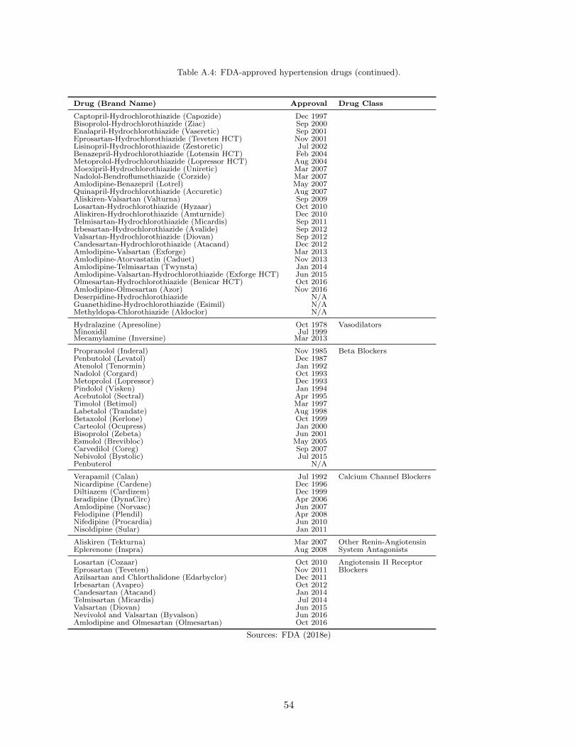
Table A.4: FDA-approved hypertension drugs (continued).

Drug (Brand Name) Approval Drug Class

Captopril-Hydrochlorothiazide (Capozide) Dec 1997Bisoprolol-Hydrochlorothiazide (Ziac) Sep 2000Enalapril-Hydrochlorothiazide (Vaseretic) Sep 2001Eprosartan-Hydrochlorothiazide (Teveten HCT) Nov 2001Lisinopril-Hydrochlorothiazide (Zestoretic) Jul 2002Benazepril-Hydrochlorothiazide (Lotensin HCT) Feb 2004Metoprolol-Hydrochlorothiazide (Lopressor HCT) Aug 2004Moexipril-Hydrochlorothiazide (Uniretic) Mar 2007Nadolol-Bendroflumethiazide (Corzide) Mar 2007Amlodipine-Benazepril (Lotrel) May 2007Quinapril-Hydrochlorothiazide (Accuretic) Aug 2007Aliskiren-Valsartan (Valturna) Sep 2009Losartan-Hydrochlorothiazide (Hyzaar) Oct 2010Aliskiren-Hydrochlorothiazide (Amturnide) Dec 2010Telmisartan-Hydrochlorothiazide (Micardis) Sep 2011Irbesartan-Hydrochlorothiazide (Avalide) Sep 2012Valsartan-Hydrochlorothiazide (Diovan) Sep 2012Candesartan-Hydrochlorothiazide (Atacand) Dec 2012Amlodipine-Valsartan (Exforge) Mar 2013Amlodipine-Atorvastatin (Caduet) Nov 2013Amlodipine-Telmisartan (Twynsta) Jan 2014Amlodipine-Valsartan-Hydrochlorothiazide (Exforge HCT) Jun 2015Olmesartan-Hydrochlorothiazide (Benicar HCT) Oct 2016Amlodipine-Olmesartan (Azor) Nov 2016Deserpidine-Hydrochlorothiazide N/AGuanethidine-Hydrochlorothiazide (Esimil) N/AMethyldopa-Chlorothiazide (Aldoclor) N/A

Hydralazine (Apresoline) Oct 1978 VasodilatorsMinoxidil Jul 1999Mecamylamine (Inversine) Mar 2013

Propranolol (Inderal) Nov 1985 Beta BlockersPenbutolol (Levatol) Dec 1987Atenolol (Tenormin) Jan 1992Nadolol (Corgard) Oct 1993Metoprolol (Lopressor) Dec 1993Pindolol (Visken) Jan 1994Acebutolol (Sectral) Apr 1995Timolol (Betimol) Mar 1997Labetalol (Trandate) Aug 1998Betaxolol (Kerlone) Oct 1999Carteolol (Ocupress) Jan 2000Bisoprolol (Zebeta) Jun 2001Esmolol (Brevibloc) May 2005Carvedilol (Coreg) Sep 2007Nebivolol (Bystolic) Jul 2015Penbuterol N/A

Verapamil (Calan) Jul 1992 Calcium Channel BlockersNicardipine (Cardene) Dec 1996Diltiazem (Cardizem) Dec 1999Isradipine (DynaCirc) Apr 2006Amlodipine (Norvasc) Jun 2007Felodipine (Plendil) Apr 2008Nifedipine (Procardia) Jun 2010Nisoldipine (Sular) Jan 2011

Aliskiren (Tekturna) Mar 2007 Other Renin-AngiotensinEplerenone (Inspra) Aug 2008 System Antagonists

Losartan (Cozaar) Oct 2010 Angiotensin II ReceptorEprosartan (Teveten) Nov 2011 BlockersAzilsartan and Chlorthalidone (Edarbyclor) Dec 2011Irbesartan (Avapro) Oct 2012Candesartan (Atacand) Jan 2014Telmisartan (Micardis) Jul 2014Valsartan (Diovan) Jun 2015Nevivolol and Valsartan (Byvalson) Jun 2016Amlodipine and Olmesartan (Olmesartan) Oct 2016

Sources: FDA (2018e)

54

Table A.5: List of FDA-approved drugs that were withdrawn from the market.

Disease Drug Approval Withdrawal Time on Market

Breast cancer Avastin∗ Feb 2004 Nov 2011 7.8 yearsHIV Hivid Jun 1992 Dec 2006 14.5 yearsHypertension Ticrynafen May 1979 Jun 1982 2.7 yearsHypertension Posicor Jun 1997 Jun 1998 1.0 yearHypertension Valturna Sep 2009 Jul 2012 2.8 years∗ Avastin’s indication for breast cancer was removed but the drug itself remained on the market.Sources: Avastin - Drugsite Trust (2018a), Hivid - FDA (2018i), International Association of Providers of Aids Care(2017), Ticrynafen - Manier et al. (1982), Posicor - Bradbury (1998), Valturna - Drugsite Trust (2018b), FDA (2016b)

55

Chapter 3 Contracts to Increase the Efficacy and Availability of

Vaccines

Abstract

Neglected Tropical Diseases (NTDs) affect 1 in 6 individuals worldwide and disproportionately

occur in low and middle income countries. Existing funding mechanisms, such as Advance Market

Commitments have failed to stimulate investment in these conditions and provide no incentive for

companies to develop a vaccine that exceeds minimum efficacy standards imposed by the World

Health Organization.

The leading NTDs – ascariasis, hookworm, and trichuriasis – affect 1.5 billion individuals,

result in more than 3 million disability adjusted life years lost, and lead to nearly 5,000 deaths

annually. Vaccines with high efficacy – the fraction of a vaccinated population who are immune from

contracting the disease – reduce the number of people who are ultimately infected, and if sufficiently

high, can eliminate the disease altogether in region. Vaccines can result in improved population

health, but developing and administering a vaccine may be prohibitively costly. Two key players

in vaccine markets are Global Health Organizations (GHOs), who procure vaccines for low and

middle income countries, and profit-maximizing manufacturers who develop and produce vaccines.

We develop a joint game-theoretic and epidemic model to study how different performance-based

contracts (i.e., contracts that tie some portion of payment to the vaccine’s resulting efficacy), might

56

simultaneously incentivize pharmaceutical firms to invest in vaccine R&D and GHOs to procure

such vaccines, and the resultant effect on disease spread in a population. We consider two such

contracts: (i) a lump sum contract in which manufacturers receive one per-unit price for exceeding

the minimum efficacy standard and a different (possibly higher) price for a vaccine efficacious

enough to eliminate the disease, and (ii) a contract in which the price is a linear function of vaccine

efficacy.

Compared to wholesale price contracts, which can at best ensure a reduction in the number

of cases, performance-based contracts are able to guarantee disease elimination. We formulate

epidemic models and estimate parameters for two NTDs: Chagas, a vector-borne disease, and

Ebola, which is spread via bodily fluids. The difference in the mode of transmission leads to

epidemic models with fundamentally different structures. Our results indicate that, across a variety

of cost scenarios, the use of a linear contract rather than a lump sum contract results in an average

reduction in R&D and manufacturing costs of 7.5% and 11.3% while only increasing the per-unit

price by 17.5% and 4.1% for Chagas and Ebola, respectively.

Performance-based contracting has been used to improve the overall quality of care in a variety

of health care settings. Recent initiatives have demonstrated the benefits of outcome-based pricing

for drugs, but currently there is no analogous proposal for vaccines. Our work highlights the

potential for these contracts to reduce the burden of disease in the world’s poorest countries.

3.1 Introduction

The control of infectious diseases using vaccines is widely considered to be one of the greatest

public health achievements of the last two centuries (Centers for Disease Control and Prevention,

1999, 2011). Vaccination has eradicated smallpox worldwide, contained cases of polio to just three

nations, and dramatically reduced annual cases of other deadly conditions such as measles and

57

tetanus (Kotar and Gessler, 2013; WHO, 2019a). Despite these successes, billions of individuals

continue to contract infectious diseases, with the number of emerging outbreaks increasing in recent

years. More than 1.6 billion individuals suffer from one or more neglected tropical diseases (NTDs),

a group of 20 conditions identified by the World Health Organization (WHO) that occur primarily

in low-income countries in sub-Saharan Africa, Asia, and Latin America (WHO, 2019b). The term

“neglected” describes the disparity in funding for these conditions (a combined $2.9 billion in 2016)

compared to the “big three” infectious diseases – HIV/AIDS, malaria, and tuberculosis ($11.7

billion, $5.7 billion, and $5.6 billion, respectively, in 2016), which collectively afflict 2.5 billion

people worldwide (WHO, 2018e).

Global health organizations (GHOs) such as Gavi, the Vaccine Alliance or the United Nations

Children’s Fund (UNICEF) play a key role in facilitating disease control in low and middle income

countries. These organizations purchase vaccines in bulk from manufacturers and then provide

these vaccines to countries in an effort to reduce their disease burden. Furthermore, GHOs often

Table 3.1: Selected Neglected Tropical Diseases.

Disease Prevalance Annual Deaths Annual DALYs∗ Transmission Mode

Ascariasis 799 million 4,800 1.3 million Parasitic wormHookworm 450 million N/A 1.6 million Parasitic wormTrichuriasis 435 million N/A 0.3 million Parasitic wormSchistosomiasis 189 million 10,000 1.8 million Parasitic wormLymphatic Filariasis 29 million N/A 1.2 million Parasitic wormRiver Blindness 14 million N/A 0.9 million Parasitic wormChagas Disease 7.2 million 7,000 0.2 million Vector-borneDengue 6 million 37,000 2.9 million Vector-borneLeishmaniasis 4.8 million 13,000 0.9 million Vector-borneTrachoma 3.3 million N/A 0.2 million Bodily fluidsLeprosy < 1 million N/A 0.03 million Bodily fluids

Table 3.2: Source: Vos et al. (2016)∗ Disability Adjusted Life Years (DALYs) are a measure of overall disease burden which include the number of yearslost due to impaired health, disability, or early death.A value of N/A for annual deaths is used to indicate that death from this condition is rare and thus statistics on thenumber of deaths are unavailable.

58

procure and administer medications to treat infected individuals.

In this work, we develop a joint game-theoretic and epidemic model to study contractual issues

between a vaccine manufacturer that invests in the development of a new vaccine for a NTD, and

a GHO that seeks to procure the vaccine on behalf of low and middle income countries. Using

this model, we analyze the impact of different payment contracts on the price and efficacy – the

performance of the vaccine under ideal circumstances, such as those in controlled clinical trials –

of the vaccine, as well as the resulting progression of the underlying epidemic.

Efforts to eradicate NTDs have largely focused on prevention via improvement of sanitation

systems and control of the disease vector (e.g, parasitic worms, flies, or mosquitoes). While these

strategies have proven successful for certain conditions (e.g., guinea worm cases dropped from 3.5

million in 1986 to just 30 in 2017) they have been less effective for others (e.g., cases of dengue

fever have increased in the past 50 years, despite substantial efforts to control its spread) (Bowman

et al., 2016; WHO, 2018b). Some progress has occurred in developing treatments for NTDs (e.g.,

Mectizan for the treatment of river blindness), and mass drug administration (MDA) programs

have focused on providing these therapies to entire communities in affected countries. MDAs,

however, face significant drawbacks, particularly when compared to immunization programs. Drug

treatment does not provide individuals with immunity, meaning that MDA success is critically tied

to community participation rates. If an infected individual chooses not to receive MDA, they can

compromise the health of others by reintroducing the condition to other susceptible individuals.

In contrast, vaccines provide individuals with some degree of protection against the disease, and,

more importantly, contribute to herd immunity, a positive externality that confers some protection

to unvaccinated individuals, as long as a critical vaccination threshold is attained. MDA also needs

to be performed on an annual or semi-annual basis to the entire infected community, a significant

logistical challenge, compared to vaccination, which is typically administered only once or twice

59

during an individual’s lifetime (Cheah and White, 2016).

Despite the public health challenges of MDA programs, there are several reasons why developing

a drug treatment may be a more attractive investment to pharmaceutical companies than a vaccine.

Drugs earn profits over a lifetime of patient use and do not provide immunity to the disease, while

vaccines are administered infrequently and make the overall population less vulnerable to future

infection (Kremer and Snyder, 2003). Companies that invest in vaccine development often focus

on infectious diseases, such as measles or human papillomavirus (HPV), with large markets in

wealthy countries, allowing for recoupment of research and development (R&D) costs via tiered

pricing, in which high-income countries are charged higher prices for the same product than low-

and middle-income nations. NTDs have smaller markets that primarily exist in low- and middle-

income countries, making these settings less attractive to vaccine developers.

In response to the dearth of investment in NTDs, governments and international organizations

have proposed several policy initiatives to incentivize pharmaceutical companies to develop drugs

and vaccines for these conditions. One such initiative is the AMC for pneumococcal vaccine.

Launched in 2009, the AMC aims to eliminate demand uncertainty by guaranteeing the purchase

of a given quantity from manufacturers at a high initial price of $7 per dose for a period of 10 years

in exchange for guaranteed long-term supply at a lower price of $3.50 per dose (Gavi, the Vaccine

Alliance, 2019b). While the pneumococcal vaccine does not target diseases classified as NTDs by

the WHO (the vaccine targets bacteria that cause pneumonia and meningitis), it was selected in

order to demonstrate the AMC’s ability to incentivize the development and production of novel

vaccines. However, the mechanism’s potential for incentivizing new vaccine development is unclear

because the participating manufacturers (GlaxoSmithKline and Pfizer) both committed to supply

doses of each firm’s existing pneumococcal vaccines (Gavi, the Vaccine Alliance, 2019a).

Another challenge with the AMC is that, by setting a price ceiling, it does not reward phar-

60

maceutical companies for developing superior products. The WHO defines a mandatory set of

product attributes (including safety and efficacy) required of vaccines purchased by UNICEF and

other GHOs, as described in each disease’s Target Product Profiles (WHO, 2019c). Under the

current funding mechanism, no incentive exists for companies to exert costly R&D effort to de-

velop a more efficacious vaccine than a competitor, or as required by the WHO. High efficacy

vaccines are desirable not only from a patient perspective, but also from a broader public health

perspective. The higher the efficacy of a vaccine, the lower the critical vaccination threshold, or the

minimum fraction of the population that needs to be vaccinated in order to achieve herd immunity.

If herd immunity is established and maintained in a population for long enough, the disease can

be eliminated — the number of cases falls to zero — in that region. Eradication, or the worldwide

elimination of a disease, brings benefits including savings in healthcare costs, improved population

health, and the ability to redirect resources towards the elimination of other diseases.

In this paper, we propose using performance-based contracts that explicitly link vaccine price

and efficacy to incentivize the development of highly efficacious vaccines that facilitate disease

elimination. Our contributions are as follows:

We develop a joint game-theoretic and epidemic model to study the impact of different payment

contracts between the GHO and manufacturer on the spread of the disease. We incorporate R&D

and manufacturing costs borne by the manufacturer and treatment/vaccine administration costs

borne by the GHO in the case that (i) no vaccine that meets minimum efficacy standards is

produced, (ii) a vaccine is produced that is efficacious enough to mitigate – reduce the number of

cases– but not to eliminate, is produced, and (iii) a vaccine is produced that is efficacious enough to

eliminate the disease. Our study, to the best of our knowledge, is the first to focus on uncertainty

in efficacy in the context of vaccine development.

We analyze two different performance-based contracts in which a per-unit price is paid for a

61

vaccine, conditional on its realized efficacy: (i) a lump sum contract that offers one of two different

per-unit prices depending on whether the vaccine is efficacious enough to mitigate or eliminate, and

(ii) a contract where the payment is a linear function of vaccine efficacy. Our results indicate that

performance-based contracts have two main advantages over wholesale price contracts. First, these

contracts can lead to reduced R&D, manufacturing, and treatment/vaccine administration costs

compared to a wholesale price contract. Second, performance-based contracts have the potential

to achieve disease elimination, while a wholesale price contract can at best ensure mitigation.

We illustrate our joint game-theoretic and epidemic modeling approach for two NTDs: Chagas,

a vector-borne disease found primarily in South and Central America, and Ebola, the majority

of cases of which have occurred in west Africa. We use numerical estimates for each parameter,

where available, and vary others over plausible ranges and compute the optimal per-unit price and

efficacy for the lump sum and linear contracts. Our results show that, across a variety of cost

scenarios, the use of a linear contract leads to an average reduction in non-procurement costs of

7.5% for Chagas and 11.33% for Ebola. Furthermore, we find that, while vaccines purchased under

the linear contract are more expensive per-unit, these additional costs are moderate and translate

to a price increase of 17.5% per unit for Chagas and 4.1% for Ebola.

3.2 Related Literature

Epidemic Modeling and Vaccination. Infectious disease modeling has been widely used to

study how a disease spreads, predict the trajectory of an outbreak (i.e., the total number of infected

individuals or the duration of the epidemic), to evaluate the effectiveness of different public health

interventions (e.g., quarantine, vaccination, treatment) and to optimize resource allocation for

epidemic control (Anderson and May, 1991). A common class of models are compartmental models,

which divide a population into several homogeneous groups (compartments) and use differential

62

equations to describe movement between groups due to disease transmission, recovery, or death.

For example, the SIR model assumes that individuals in the population are either susceptible to

infection, infected and infectious, or removed (either recovered or dead). A key component in the

analysis of these models is the computation of the basic reproduction number, denoted by R0,

which is the expected number of secondary infections caused by a typical infected individual in

an otherwise susceptible population. If R0 < 1, then the disease will be eliminated in the long

run, while if R0 > 1 then the disease remains endemic in the population. Models that include

vaccination derive the basic reproduction number as a function of the vaccine coverage level — the

fraction of the population that is vaccinated — and the vaccine’s efficacy, which is typically defined

in terms of three aspects: take (the fraction of those vaccinated in whom the vaccine has an effect),

degree (the reduction in the probability of infection upon exposure), and duration (the length of

time for which vaccinated individuals are protected from infection) (McLean and Blower, 1993).

In this work, we use variations on the SIR model featuring vaccination with an imperfect

vaccine to evaluate payment contracts between a vaccine manufacturer and a GHO, where different

contracts result in varying levels of vaccine efficacy.

Vaccine Market Coordination. Vaccine markets consist of multiple players with compet-

ing objectives, including profit-maximizing manufacturers (suppliers), group-interested countries

(buyers), public health-oriented global health organizations (procurers), and self-interested indi-

viduals (consumers). A large body of research examines the inefficiencies that arise in vaccine

markets — and potential remedies — when the incentives of one or more players are misaligned; a

comprehensive review is given by Duijzer et al. (2018).

Prior studies have modeled contracts between a vaccine manufacturer and one or more countries,

but typically focus on production yield uncertainty — the number of vaccine doses a manufacturer

produces — and the resulting coverage levels. Deo and Corbett (2009) study Cournot competition

63

between manufacturers in the U.S. influenza vaccine market, in which yield uncertainty impacts the

net production quantity, and hence profits, ultimately deterring a firm from entering the market.

Mamani et al. (2013) study governments’ optimal vaccination coverage levels when cross-border

transmission is possible. The authors find that decentralized decision-making by each country leads

to shortages of vaccines in some countries and excesses in others, and they propose a coordinating

contract to allow for vaccine transfers between countries.

Chick et al. (2008) use a game-theoretic model to study the decisions of a profit-maximizing

vaccine manufacturer that bears the risk of yield uncertainty, and a government seeking to maximize

the health benefits of vaccination less the administration costs. Without intervention, they show

that vaccine coverage is below the societally optimal level, but that this can be remedied with a

cost-sharing contract that shares the risk of yield uncertainty. Chick et al. (2016) extend Chick

et al. (2008) by considering the case where the manufacturer can exert costly effort to fulfill the

demand that was unsatisfied due to yield uncertainty.

Our work differs from Mamani et al. (2013) in that we study a single GHO and a single man-

ufacturer, who decides how much to invest to improve vaccine efficacy, while their work studies

multiple countries, with a manufacturer producing the desired quantity of vaccines with fixed ef-

ficacy. Unlike Deo and Corbett (2009), Chick et al. (2008) and Chick et al. (2016), who consider

yield uncertainty, a risk borne by the manufacturer assuming a quantity-based payment contract,

we allow for uncertain efficacy, which can result in lack of payment to the manufacturer if the

resulting efficacy falls below the WHO’s minimum standard.

Vaccine Pricing and Subsidies. The process of developing, testing, and licensing a new

vaccine is expensive and lengthy, taking an estimated 10 years and between $200 million and $500

million (Serdobova and Kieny, 2006). Given the uncertainty in market demand, relatively smaller

market sizes (as compared to pharmaceuticals) and international pressure to provide vaccines at low

64

prices, firms who decide to pursue vaccine development have an incentive to set high prices in order

to recoup their substantial R&D costs. However, high prices not only create a financial burden for

low- and middle-income countries, they also exacerbate free riding, in which susceptible individuals

forgo vaccination by taking advantage of herd immunity in the population (Harvard Gazette, 2010).

Several papers in the operations management literature explore how these challenges can be resolved

through the use of subsidies to either the manufacturer, consumers, or both.

Arifoglu et al. (2012), Adida et al. (2013), and Arifoglu and Tang (2019) extend the joint game-

theoretic and epidemic model of Chick et al. (2008) to incorporate strategic consumer behavior, and

propose supply-side (manufacturer) or demand-side (individuals) subsidies to resolve inefficiencies

resulting from such strategic behavior. Levi et al. (2016) and Yamin and Gavious (2013) consider

the use of subsidies to increase the consumption of malaria drugs and vaccines, respectively. Unlike

the preceding studies, which use subsidies to increase either the production quantity or consump-

tion of vaccines, we investigate the ability of contracts that link price and efficacy to incentivize

manufacturers to develop highly efficacious vaccines.

Advance Market Commitments. In an AMC, one or more sponsors pre-commit to purchas-

ing a given quantity of vaccines at a guaranteed price, in exchange for the manufacturer agreeing

to a reduced price on additional purchases. The rationale behind an AMC is that it encourages

investment in new vaccines by removing the element of demand uncertainty and ensuring that

manufacturers will recover a large portion of their R&D costs, while at the same time ensuring the

affordability of these vaccines in the long run (Kremer, 2000a,b).

Both Kremer et al. (2015) and Martin et al. (2018) examine the problem of how to optimally

design an AMC, which involves determining the quantity of vaccines that sponsors will commit to

purchase as well as the initial (higher) and long-run (lower) per-unit prices. Similar to an AMC, the

contracts that we examine aim to encourage the development of novel vaccines. However, while the

65

price paid in an AMC is tied to efficacy only through a minimum efficacy threshold, the contracts

proposed in our work explicitly reward manufacturers for developing marginally more efficacious

vaccines. Moreover, neither Martin et al. (2018) nor Kremer et al. (2015) consider the impact

of their proposed contracts on the evolution of the epidemic, while we design performance-based

contracts with the goal of either mitigating or eliminating the disease.

Performance-Based Contracting in Healthcare. Performance-based contracting is a con-

tracting framework in which at least some portion of payment is linked to the evaluation of outputs

or outcomes rather than required inputs, activities or processes (Martin, 2007).

Within the context of performance-based contracting in healthcare, research in the operations

management community has largely focused on contracts between a service provider (e.g., hospital

or clinic) and regulatory bodies (e.g., a government agency), where payment for service is conditional

on patient health outcomes or waiting times. So and Tang (2000) examine a setting in which a health

clinic prescribes medication to a patient and is only reimbursed if the patient’s measured health

score meets a specified threshold. Savva et al. (2018) empirically study how yardstick competition

– a reimbursement scheme in which a provider’s payment is linked to their performance relative to

other comparable providers – performs in service systems such as hospital emergency departments,

where a regulator seeks to incentivize reductions in both costs and waiting time. Jiang et al. (2012)

analyze an outpatient care setting in which a service provider allocates capacity among different

categories of patients in order to meet a waiting-time target. Unlike the majority of research in this

area, which links payment to health outcomes of individual patients or patients within a healthcare

center, our work studies contracts that link payment to vaccine efficacy, which impacts the overall

health of the country.

Outside of healthcare, performance-based contracting has been applied to study after-sales

supply chains (Kim et al., 2007), product reliability (Guajardo et al., 2012) and collaborative

66

services (Roels et al., 2010), among others; see Selviaridis and Wynstra (2015) for an exhaustive

review.

3.3 Model

We propose a joint game-theoretic and epidemic model featuring an immunization supply chain

consisting of a single GHO and a single vaccine manufacturer. Our game-theoretic model consists

of a Stackelberg game between the GHO (the leader), who offers a per-unit price for the vaccine,

and the manufacturer (the follower), who sets a desired, or target, efficacy level. Given the fraction

of the population immunized, the efficacy of the vaccine developed by the manufacturer, and the

underlying disease dynamics, our epidemic model captures the resulting progression of the disease.

We detail the model for a general vaccine, and in Section 3.4 we show how this base model can be

modified for specific diseases. Appendix B.1 provides a summary of the model notation.

We first provide an overview of our model and relevant assumptions. Section 3.3.1 considers a

centralized system in which the GHO and manufacturer operate as a single entity that develops a

vaccine in order to minimize R&D, manufacturing, and treatment/administration costs. Sections

3.3.2 and 3.3.3 consider a decentralized system with a profit-maximizing manufacturer and cost-

minimizing GHO. In Section 3.3.2, we demonstrate the sub-optimal behavior of the wholesale price

contract and analyze the lump sum performance-based contract, while in Section 3.3.3 we consider

the linear performance-based contract.

Immunization Process. Individuals typically receive immunizations through routine immu-

nization – nationally organized programs which seek to vaccinate individuals (typically infants)

according to a defined immunization schedule – or mass vaccination – programs that seek to in-

crease coverage by immunizing large numbers of susceptible individuals, regardless of their age.

Mass vaccination is considered a supplementary activity to routine immunization and is most com-

67

monly used for the influenza vaccine; for these reasons, we assume that all vaccinated individuals

receive their vaccinations via a routine immunization program (Chakrabarti et al., 2019). Given

this assumption, we consider the target population – the intended recipients of the vaccine – to be

newborn babies, as this is the case for the majority of routine immunization programs; nine of the

ten WHO-recommended vaccines are first given shortly after birth, with subsequent doses delivered

three to six months later (WHO, 2018f).

In order to vaccinate a fraction f of the target population of newborns, the GHO purchases

a quantity Q of vaccines from the manufacturer. The resulting fraction immunized (and thus the

corresponding quantity of vaccines ordered) is exogenous and is not a decision made by the GHO;

rather, is a function of factors such as what portion of the population lives in urban areas (it is

logistically more challenging to vaccinate individuals in rural areas), and can range from just 26%

in South Sudan to over 95% in the United States for the DTP3 vaccine (WHO, 2018a). Although

in practice GHOs may order excess vaccines to account for wastage, we assume that the GHO

minimizes costs and thus orders the minimum number of vaccines needed to immunize the fraction

f of the target population.

GHO Actions. The GHO offers a price p(e) per unit for a vaccine with efficacy e, provided

that the vaccine exceeds the minimum efficacy η1. These efficacy standards may be imposed by

recipient countries or by the WHO, which publishes Target Product Profiles detailing the minimum

efficacy required for the prequalification of new vaccines. For example, the WHO’s Target Product

Profile for Zika specifies a minimum efficacy of 70% (WHO, 2017b).

Manufacturer Actions. Taking into account the quantity Q of vaccines demanded by the

GHO and the offered price p(e), the manufacturer invests in developing a vaccine with target efficacy

level t and incurs a corresponding R&D cost that is convex increasing in the target. For analytic

tractability, we consider the case where the R&D cost is quadratic in the target efficacy and is given

68

by rt2. Due to uncertainty in the manufacturing and development process, the realized efficacy

e of the vaccine may differ from its target t. Sources of efficacy uncertainty include (i) patient

reactions to the vaccine caused by genetic factors or previous exposure to the disease (Thomas and

Moridani, 2010), (ii) antigenic variation, or the ability of an infectious agent to alter its makeup

to avoid triggering an immune response in the host (Oyston and Robinson, 2012), (iii) variation in

conferred immunity due to different strains of the disease (WHO, 2018d), or (iv) variation in the

development of the vaccine itself, such as when mutations occur with live attenuated vaccines after

injecting a virus into a foreign host (Shimizu et al., 2004). We consider the realized efficacy e to

be given by t+ ε, where ε ∼ U [−u, u].

Manufacturer Costs and Revenue. If the resulting efficacy exceeds the minimum standard

η1, the manufacturer produces Q doses of the vaccine at a cost c per unit, and receives payment

p(e) per unit. Otherwise, the manufacturer receives no payment and does not produce the vaccine.

GHO Costs. Given the realized vaccine efficacy e, the GHO incurs procurement costs p(e)

per unit and may additionally incur costs associated with administering the vaccine and treating

infected individuals. Equation 3.1 summarizes the administration and treatment costs as a function

of the realized efficacy e. If the realized efficacy falls below the minimum standard η1, the GHO

incurs the lump-sum cost K1 of treating the disease with no vaccine to help attenuate its spread.

If the realized efficacy is above the minimum standard η1, but below the threshold η2 needed

to eliminate the disease in the population, then the GHO incurs the lump-sum cost K2, which

includes the cost of administering the vaccine and treating infected individuals, along with the

payment p(e)Q to the manufacturer. In this case we say that the disease has been mitigated – a

positive number of cases of infection remain in the population, but fewer than if no vaccine were

available – but not eliminated – no cases of infection remain. Finally, in the case that the realized

efficacy is above the threshold η2, the disease is eliminated and thus the GHO bears no cost of

69

treatment and is only responsible for the payment to the manufacturer as well as the lump-sum

cost K3 of administering the vaccine.

GHO’s Administration and Treatment Costs =

K1 if e ≤ η1

K2 if η1 < e ≤ η2

K3 if e > η2

(3.1)

While recipient countries may pay a portion of the total costs, a 2016 analysis by the WHO

found that, in countries with a per-capita GDP of less than $1000 (which tend to have high

rates of NTDs), 78% of routine immunization expenditures and 88% of expenditures on vaccines

were externally funded (WHO, 2016). With this in mind, we focus on the relationship between

the GHO and the vaccine manufacturer, and do not consider the costs incurred by the recipient

country. Furthermore, we assume that the GHO’s vaccine supply is the country’s only source of

immunization for the given disease.

Key Assumptions. We assume that K1 > K2 > K3. The condition K1 > K2 states that

mitigating the disease prevents enough infections to offset the cost of adding the vaccine to the

routine immunization program. In practice this condition likely holds, as vaccination costs are

in general less expensive than disease treatment costs. For example, an analysis of 94 low- and

middle-income countries found that the average per-person cost of a vaccine program is between $2

and $4; in contrast, the average cost to treat a case of dengue fever is $150 (Portnoy et al., 2015a;

Shepard et al., 2016). We note that K2 > K3 by definition, as K2 includes both treatment costs

and administration costs, while K3 only includes administration costs (which are the same in the

case of mitigation and elimination).

In summary, the GHO decides the per-unit vaccine price to minimize societal costs, while the

manufacturer decides the target vaccine efficacy level to maximize their individual profits. We make

a mild assumption on the relationship between parameters introduced above.

70

Assumption 1. The difference between the threshold for elimination η2 and the minimum efficacy

threshold η1 is less than twice the uncertainty in efficacy u.

Assumption 1 states that the difference between the mitigation and elimination thresholds is

small compared to the uncertainty in vaccine production. Recall that the mitigation threshold η1

is the minimum efficacy at which the GHO will purchase the vaccine (which is typically imposed by

the WHO), while the elimination threshold η2 is derived from the epidemiology of the disease and

the fraction f of individuals immunized. The WHO could choose to set a low mitigation threshold

(i.e., accept lower efficacy vaccines), which would have the benefit of providing a vaccine to recipient

countries, but doing so would be costly, would make elimination less likely (compared to a higher

threshold), and, depending on how low the efficacy is, fail to substantially reduce the burden of

disease. Thus Assumption 1 argues that the WHO sets the mitigation threshold η1 relatively close

to the elimination threshold in order to facilitate elimination of the disease.

Figure 3.1 displays the possibility of mitigating (e > η1) or eliminating (e > η2) the disease,

given a target efficacy t. We use the terms “no mitigation/elimination” to indicate that, given

the target efficacy in a region, mitigation or elimination occurs with probability zero. The terms

“possible mitigation/elimination” designate regions where the probability of these events is positive,

but less than one, while “guaranteed mitigation/elimination” is used for regions where these events

occur with probability one. Under Assumption 1, the interval (η1 − u, η1 + u) on which mitigation

is possible and the interval (η2 − u, η2 + u) on which elimination is possible overlap. We use red to

indicate Region I, where no vaccine is produced, orange for Regions II and III, where mitigation is

possible, yellow for Regions IV and V where mitigation is guaranteed, light green for Regions III

and IV where elimination is possible, and dark green for Region V where elimination is guaranteed.

71

Figure 3.1: Possibility of eliminating and mitigating the disease as a function of the target vaccine efficacy t underAssumption 1.

Target efficacy !

Regions:

"! − $ "! + $ "" + $"" − $0 1No vaccine Possible mitigation

Guaranteed eliminationPossible elimination

Guaranteed mitigation

I II III IV V

3.3.1 Centralized System

In order to evaluate the performance of different contracts and determine what target efficacy

level t is desirable, we analyze a centralized system consisting of both the GHO and manufacturer.

In this system, the two decision-makers operate as a single entity that selects a target efficacy t

to minimize the total expected cost of developing and manufacturing the vaccine, as well as the

expected administration and treatment costs. All proofs are presented in Appendix B.2.

The first-best minimizes the total costs for the immunization supply chain:

Π(t) = rt2 +K1P(e < η1) + (cQ+K2)P(η1 < e < η2) + (cQ+K3)P(e > η2)

The centralized cost is a piecewise convex, continuous function of the target efficacy t, but is not

continously differentiable. The marginal cost Π′(t) has a piecewise linear structure, exemplified in

Figure 3.2. Note that all line segments have the same slope 2r, which corresponds to the R&D

costs of developing a marginally more efficacious vaccine. Figure 3.2 displays three vertical shifts

of the line Π′ = 2rt, the magnitude of which are designated by D1, D2, and D3, respectively.

The first shift occurs when t is in Region II (t ∈ (η1−u, η2−u)) where mitigation is possible. In

addition to the known R&D costs incurred on this region, the central planner incurs probabilistic

costs; either K1 in the case of no mitigation, and K2 + cQ if mitigation occurs. On this region, the

marginal increase in the probability of mitigation associated with an increase in the target efficacy t

is 12u . Thus D1 = K1−(K2+cQ)

2u gives the marginal expected savings to the central planner associated

72

with increasing the target t.

The next vertical shift occurs on Region III (t ∈ (η2− u, η1 + u)) on which both mitigation and

elimination are possible. In addition to the R&D cost, the central planner incurs K1 if no mitigation

occurs, K2+cQ if mitigation occurs but elimination does not, and K3+cQ if elimination occurs. On

this region, an increase in the target efficacy t generates two types of marginal expected savings:

K1−(K2+cQ)2u , which compares the costs under mitigation and no mitigation, and K2+cQ−(K3+cQ)

2u

which compares the costs under mitigation but no elimination and elimination. Adding these two

savings gives D2 = K1−K3−cQ2u .

The last shift occurs on Region IV (t ∈ (η1 + u, η2 + u)) where mitigation is guaranteed and

elimination is possible. Because mitigation is guaranteed on this region, the central planner incurs

manufacturing costs cQ as well as the R&D costs. Additionally, the central planner incurs costs

K2 and K3 if elimination does not or does occur, respectively. Thus the marginal expected savings

associated with developing a marginally more efficacious vaccine on this region is D3 = D2 −D1.

Figure 3.2: Marginal costs of the centralized problem as a function of the target efficacy.

!! − # !! + # !" + #!" − #% &

Target efficacy '

Mar

gina

l Cos

t (′

D+,-

,.

Π# = 223

All line segments have the same slope 2r. D1 = K1−K2−cQ2u

, D2 = K1−K3−cQ2u

, D3 = D2 −D1 = K2−K32u

73

While Figure 3.2 shows an example where each of the three shifts translates to a reduction in

marginal costs, we note that in general these shifts can result in either higher (if Di < 0) or lower

(if Di > 0) marginal costs. Given our assumption that K1 > K2 > K3, we have that D3 > 0, but

the sign of D1 and D2 depends on the total manufacturing costs.

Rather than analyzing the centralized system in full generality, we impose sufficient conditions

to ensure that the objective is unimodular and thus has a unique optimum.

Assumption 2. The problem parameters satisfy D2 < 2r(η2 − u).

Assumption 2 states that the centralized costs Π(t) are increasing on Region III in which both

mitigation and elimination are possible, meaning that it is never optimal for the central planner to

choose a target on the interior of this region. Instead, the central planner would prefer to either

lower the target so that only mitigation is possible and save on R&D costs, or raise the target so

that mitigation or elimination is guaranteed and save on treatment costs.

Under Assumption 2, we find that there are a total of four possible optima; Proposition 4

graphically presents these first-best target efficacy levels.

Proposition 4. Under Assumption 2, the centralized problem is unimodular. The first-best target

efficacy levels t∗ are given in Figure 3.3, where t∗i = 0, t∗ii = D12r , t∗iii = D3

2r , and t∗iv = η2 + u.

Figure 3.3 displays the first-best target efficacy levels, where each region is colored according

to the best possible epidemic outcome, using the same color scheme as Figure 3.1. For example,

solution t∗(iii) is in Region IV, where mitigation is guaranteed and elimination is possible. Thus we

color the region associated with this solution light green, which corresponds to the best epidemic

outcome of possible elimination.

We see that, depending on the problem parameters, a variety of targets are possible, ranging

from having no vaccine to eliminating the disease with probability one. Under target t∗(i) (red

74

Figure 3.3: First-best target efficacy levels.

!"

!#!" + 2&((# + ))

!" + 2&((" + ))

!" = !#,">

,#>,.

2&((" − )) 2&((# − ))

2&((# − ))

0(12)∗

0(1)∗

0(11)∗

0(111)∗

t∗(i) = 0, t∗(ii) = D12r

, t∗(iii) = D32r

, and t∗(iv) = η2 + u.

region), no vaccine is produced, and the epidemic progresses as it would without intervention. If

target t∗(ii) (orange region) is selected, then it is possible that the disease will be mitigated, but

the target is too low for elimination. Under target t∗(iii) (light green region) the disease will be

mitigated with probability one, and elimination is possible. Finally, target t∗(iv) (dark green region)

is the minimum value needed to ensure that elimination is guaranteed.

Figure 3.3 highlights how the first-best target efficacy depends on the marginal expected savings

associated with having no vaccine vs mitigation (D1) and the marginal expected savings associated

with having no vaccine vs elimination (D2). We see that the highest targets are associated with

negative values of D1 and positive values of D2, meaning that eliminating the disease is more

attractive from a cost savings perspective than mitigating. Furthermore, we see that, for a fixed

value of D1, increasing D2 may result in a higher target. For example, for low values of D1,

we see that by increasing D2, the optimal target changes from t∗(i) (no vaccine) to t∗(iii) (possible

elimination) to t∗(iv) (guaranteed elimination).

75

3.3.2 Lump Sum Contract

The first contract we consider is a generalization of a wholesale price contract, a popular contract

both among practitioners and academics in the vaccine market setting (Dai et al., 2016; Chick et al.,

2008). In a traditional wholesale price contract, one party purchases a product from another at a

fixed price per unit. The contract we consider differs from a traditional wholesale price contract

in that it is performance-based, meaning that at least some portion of payment is linked to the

evaluation of outputs (Martin, 2007). In particular, given that the efficacy exceeds the minimum

standard, the contract we study offers the manufacturer a per-unit price p1 if the efficacy falls below

the elimination threshold η2, and a different per-unit price p2 if the efficacy exceeds this threshold.

The intuition behind this contract is that, by offering a substantially high price p2, the GHO can

entice the manufacturer to set a target high enough to exceed the elimination threshold.

Under the lump sum contract, the GHO sets the prices p1 and p2 to minimize the expected cost

ΠG of procuring the vaccine, as well as the administration and treatment costs – K1 in the case of

no vaccine, K2 in the case of mitigation, and K3 in the case of elimination – subject to ensuring

that the manufacturer participates (i.e., has a non-negative expected profit). The GHO problem is

as follows:

minp1,p2

ΠG(p1, p2) = K1P(e < η1) + (K2 + p1Q)P(η1 < e < η2) + (K3 + p2Q)P(e > η2)

s.t. ΠM (t(p1, p2)) ≥ 0

Given the prices selected by the GHO, the manufacturer chooses the vaccine efficacy target t to

maximize their expected profits ΠM , which consist of the expected revenues from selling Q units of

the vaccine (p1QP(η1 < e < η2) + p2QP(e > η2)), less the R&D costs rt2 and manufacturing costs

cQ. The manufacturer’s problem is as follows:

maxt∈[0,1]

ΠM (t) = −rt2 + (p1 − c)QP(η1 < e < η2) + (p2 − c)QP(e > η2)

76

We solve the manufacturer and GHO problems by backward induction. Given fixed prices p1

and p2, we solve the manufacturer’s problem to find the optimal target t(p1, p2) as a function of the

contract prices. We then use this characterization of the optimal target to solve the GHO problem

for the optimal prices.

The manufacturer’s profit is piecewise continuous, and the marginal profit Π′M (t) has a piece-

wise linear structure (depicted in Figure 3.4) where all line segments have the same slope −2r,

corresponding to the marginal R&D costs. Figure 3.4 displays three vertical shifts of the line

Π′M = −2rt, which have magnitudes D1, D2, and D3, respectively.

Figure 3.4: Marginal costs of the manufacturer’s problem as a function of the target efficacy under the lump sumcontract.

!" − $ !" + $ !& + $!& − $' "

Target efficacy (

Mar

gina

l Pro

fit) * +

),-

Π/012 = −256

),7

),8

All line segments have the same slope −2r. D1 = (p1−c)Q2u

, D2 = (p2−c)Q2u

, and D3 = D2 − D1.

The quantities D1, D2, and D3 can be interpreted in a similar manner as D1, D2, and D3 in

the centralized system. We see that D1 = (p1−c)Q2u is the marginal expected revenue associated with

an increase in the target efficacy t on Region II, and is obtained by comparing the manufacturer’s

profit when no mitigation occurs (and no vaccine is purchased) versus when mitigation occurs (and

the vaccine is purchased at p1 per unit). The quantity D2 is the marginal expected revenue on

77

Region III and is the sum of the marginal expected increases in revenue associated with mitigation

( (p1−c)Q2u ) and elimination ( (p2−c)Q

2u − (p1−c)Q2u ). Finally, D3 = (p2−p1)Q

2u = D2 − D1 reflects the

marginal expected increase in revenue on Region IV, which compares the profit under the scenarios

when elimination does and does not occur.

Figure 3.4 illustrates an example where each of the three vertical shifts translates to an increase

in marginal profit, but in general these shifts can result in either higher (if Di > 0) or lower (if

Di < 0) marginal profit.

Similarly to the centralized setting, we impose sufficient conditions to ensure that the manufac-

turer’s profit function is unimodular and thus has a unique optimum.

Assumption 3. The problem parameters satisfy D2 < 2r(η2 − u).

Assumption 3 states that the GHO selects prices so that manufacturer’s profit is decreasing on

Region III in which both mitigation and elimination are possible, meaning that the manufacturer

never selects a target on the interior of this region. In other words, this means that the GHO would

rather incentivize the manufacturer to select a lower target so that only mitigation is possible

and save on procurement costs, or incentivize the manufacturer to select a higher target so that

mitigation or elimination is guaranteed and save on treatment costs.

Given Assumption 3, Proposition 5 graphically presents the manufacturer’s best response target

efficacy level as a function of the contract prices p1 and p2.

Proposition 5. Under Assumption 3, the manufacturer’s problem is unimodular. The manufac-

turer’s best response target efficacy levels t(p1, p2) are displayed in Figure 3.5, where t(i)(p1, p2) = 0,

t(ii)(p1, p2) = D12r , t(iii)(p1, p2) = η2 − u, t(iv)(p1, p2) = D3

2r , and t(v)(p1, p2) = η2 + u.

Given the manufacturer’s best response t(p1, p2), the GHO selects the prices p1 and p2 to

minimize its costs, subject to ensuring the participation of the manufacturer. We find that there

78

Figure 3.5: Manufacturer’s best response target efficacy levels t(p1, p2) under the lump sum contract.

!"#

!"# + 2&(() + *)!"# + 2&((# + *)

2&((# − *) 2&(() − *)

2&(() − *)

! - (##, #)) ! --- (##, #))! -- (##, #))! -. (##, #))! . (##, #))

!")

t(i)(p1, p2) = 0, t(ii)(p1, p2) = D12r

, t(iii)(p1, p2) = η2 − u, t(iv)(p1, p2) = D32r

, t(v)(p1, p2) = η2 + u.

are five equilibrium targets tTP that can be obtained, two of which align with the first-best targets.

Proposition 6 details the equilibrium targets and prices. For several target efficacy levels, there are

multiple values of p1 and/or p2 that induce the manufacturer to select this target. For brevity, we

include any additional conditions in Appendix B.2. Figure 3.6 graphically presents the equilibrium

targets and their correspondence with the manufacturer’s best response targets.

Proposition 6. The equilibrium target efficacy level t and prices p1 and p2 under the lump sum

contract are given as follows:

1. t(i) = 0; p1(i) <4ru(η1−u)

Q + c; p2(i) < min{4ru(η2−u)Q + c, 8ruη1

Q + c}

2. t(ii) = 2(η1 − u) ∈ (η1 − u, η2 − u); p1(ii) = 8ru(η1−u)Q + c; p2(ii) < min{8ru(η1−u)

Q + 4ru(η1+u)Q +

c, 4ru(η2−u)Q + c}

3. t(iii) = D14r + η1−u

2 ∈ (η1 − u, η2 − u); p1(iii) = c2 + 2ru(η1−u)+K1−K2

Q ; p2(iii) < min{4ru(η2−u)Q +

c, 4ru(η1+u)Q + c

2 + 2ru(η1−u)Q + K1−K2

Q }

4. t(iv) = η2 − u; p1(iv) = c+ 2ru(η1−u)2

Q(η2−η1) ; p2(iv) < min{4ru(η2−u)Q + c, 4ru(η1+u)

Q + c+ 2ru(η2−u)2

Q(η2−η1) }

79

5. t(v) = D32r ∈ (η1 + u, η)2 + u); p1(v) = c + K2−K3

2Qu

(η2 − u− (K2−K3)

8ru

); p2(v) = c + K2

Q +

K22Qu

((η2 − u)− K2

8ru

)Figure 3.6: Equilibrium target efficacy levels under the lump sum contract.

!" + 2%('( + ))!" + 2%('" + ))

2%('" − )) 2%('( − ))

2%('( − ))

"(,)

-!"

-!" + 2%('( + ))-!" + 2%('" + ))

-!(

"(,,)"(,,,)

"(,.)"(.)

t(i) = 0, t(ii) = 2(η1 − u), t(iii) = D14r

+ η1−u2

, t(iv) = η2 − u, t(v) = D32r

.

Figure 3.6 displays the target efficacy levels under the lump sum contract, where each region

is colored in a similar manner as Figure 3.3, which presents the first-best targets. By comparing

Figures 3.5 and 3.6, we are able to map the manufacturer’s best response target to its resulting

equilibrium target. For example, we see that the best response t(i)(p1, p2) = 0 induces an equilib-

rium target t(i) = 0 which results in no vaccine, while the best response target t(ii)(p1, p2) = D12r

can induce targets t(ii) = 2(η1 − u) or t(iii) = D14r + η1−u

2 which both result in possible mitigation.

The best response t(v)(p1, p2) = η2 + u is not an equilibrium and thus this region is shaded in grey.

From Proposition 6, we see that the lump sum contract is able to achieve the first-best target

D32r (t∗(iii) in Region IV where elimination is possible, but is not able to achieve the lower target D1

2r

(t∗(ii)) in Region II where mitigation is possible. This behavior, where high first-best targets can be

achieved but low ones cannot, is driven by the dual roles that prices in this contract play; prices

80

both shape the value of t and ensure participation of the manufacturer. If the manufacturer’s

best response t(p1, p2) falls below η2 − u (in which case elimination is not possible), then the

contract becomes a function of p1 only as the target is too low for the manufacturer to receive

p2 per unit. On the other hand, when the manufacturer’s best response t(p1, p2) is above η2 − u,

then the manufacturer has a non-zero probability of receiving either price. With this additional

degree of freedom, the contract is able to simultaneously achieve the first-best target and guarantee

participation.

In addition to being unable to achieve the first-best target D12r (t∗ii), the lump sum contract

cannot achieve the highest first-best target η2 + u (t∗(iv)), which is the minimum value needed to

guarantee elimination. While setting the target high enough to guarantee elimination ensures that

the manufacturer earns a per-unit price of p2, it is more profitable for the manufacturer to set a

slightly lower target, save on R&D costs, and gamble that the realized efficacy falls above η2.

Of the four first-best targets, the lump sum is able to induce the manufacturer to select two

of them: t = 0 and t = D32r . As detailed in Proposition 7, it is sometimes possible for the central

planner to select prices p1 and p2 to coordinate the vaccine efficacy target to D12r , but no prices can

incentivize the manufacturer to select the target t = η2 + u. For brevity, all additional conditions

needed are provided in Appendix B.2.

Proposition 7. If D12r ≥ 2(η1−u) and η1 <

η2+u2 , then the lump sum contract with p1 = K1−K2

Q and

p2 < min{4ru(η1+u)Q +p1,

4ru(η2−u)Q +c} coordinates the manufacturer’s target efficacy level D1

2r to the

first-best value D12r . Furthermore, there are no prices p1 and p2 that coordinate the manufacturer’s

target to the first-best level η2 + u.

This result shows that the lump sum contract can sometimes align the decisions of the decen-

tralized system with the first-best decisions, with the notable exception being when the first-best

target is just high enough to guarantee elimination (η2 +u), in which case there are no coordinating

81

prices p1 and p2.

Next, we consider a wholesale price contract, which can be obtained as a special case of the

lump sum contract in which p1 = p2. Under the wholesale price contract, the manufacturer is paid

a per-unit price p1 = p2, provided that the realized efficacy exceeds the minimum threshold η1.

We find that the manufacturer’s profit function under this contract is piecewise continuous and

unimodular. Proposition 8 summarizes the target efficacy levels that can be achieved with this

contract.

Proposition 8. (Wholesale Price Contract) Under a wholesale price contract, there are six possible

equilibrium targets, all of which are at most η1 + u and only one of which (t = 0) aligns with the

first-best targets. Furthermore, there is no price that coordinates the vaccine efficacy target to a

first-best level greater than η1 + u.

Under the wholesale price contract, any target above η1 + u is guaranteed to have a realized

efficacy greater than η1, and thus it is clear that the manufacturer has no incentive to set a high

target, as this contract does not reward the manufacturer for producing vaccines with efficacy

greater than η1.

3.3.3 Linear Contract

The second performance-based contract we consider is a linear contract in which the manufacturer

receives a per-unit price p1 plus a bonus per-unit payment p2e, provided the realized efficacy

exceeds the minimum threshold η1. The intuition behind this contract is that, by rewarding the

manufacturer for producing a marginally more efficacious vaccine, the GHO can incentivize the

manufacturer to set a high efficacy target so as to minimize the number of individuals infected by

the disease.

Under the linear contract, the GHO selects prices p1 and p2 to minimize the expected cost ΠG

82

of procuring the vaccine, as well as the administration and treatment costs, subject to ensuring the

manufacturer’s participation. The GHO problem is as follows:

minp1,p2

ΠG(p1, p2) = K1P(e < η1) +K2P(η1 < e < η2) +K3P(e > η2) + P(e > η1)E[(p1 + p2e)Q|e > η1]

s.t. ΠM (t(p1, p2)) ≥ 0

where t(p1, p2) is the manufacturer’s optimal target level, which is anticipated by the GHO for

given prices p1 and p2.

Given the prices offered by the GHO, the manufacturer selects a target efficacy to maximize

their expected profits ΠM (t), which consist of the expected revenues from selling the vaccine Q(p1 +

p2Ee>η1 [e]), less the R&D costs rt2 and manufacturing costs cQ. The manufacturer’s problem is as

follows:

maxt∈[0,1]

ΠM (t) = −rt2 + Ee>η1 [p1 + p2e− c]QP(e > η1)

We solve the manufacturer and GHO problems by backward induction. Similarly to the lump sum

contract, we find that the manufacturer’s profit is a piecewise concave, continuous function of the

target efficacy t, and the marginal profit Π′G is piecewise linear. However, unlike the lump sum

contract, in which all segments of the marginal profit have the same slope −2r, the slope of the

marginal profit under the linear contract varies, as depicted in Figure 3.7.

From Figure 3.7, we see that the linear contract divides the target efficacy space into three

regions: (0, η1−u), on which no vaccine is produced, (η1−u, η1 +u), on which mitigation is possible

(and elimination is possible if e ≥ η2 − u), and (η1 + u, 1), on which mitigation is guaranteed (and

elimination is guaranteed if e ≥ η2 + u).

On the first region, the target efficacy is too low for the contract to come into play, and thus the

marginal profit curve is just given by Π′M = −2rt. On the second region, the linear contract impacts

the marginal profit in two ways. First, there is a vertical shift of magnitude D1 = (p1−c)Q+p2Qu2u ,

83

which is the expected change in marginal revenue associated with producing a vaccine and receiving

payment p1Q + p2QEe>η1 [e] less the manufacturing costs cQ, compared to producing no vaccine.

Second, the linear contract increases the slope of the marginal profit curve by M = p2Q2u , thus

reducing the marginal cost associated with making a more efficacious vaccine. Finally, on the third

region, for producing a marginally more efficacious vaccine, the manufacturer receives a marginal

performance-based payment of D3 = p2Q and incurs marginal R&D costs 2rt; thus the marginal

profit curve is given by D3 − 2rt.

Figure 3.7: Marginal costs of the manufacturer’s problem as a function of the target efficacy under the linear contract.

!" − $ !" + $ !& + $!& − $' "

Target efficacy (

Mar

gina

l Pro

fit ) *

+′

)-.

)Π0′ = −234

Change in slope:

)-5

)6

D1 = (p1−c)Q+p2Qu2u

, M = p2Q2u

, and D3 = p2Q. The slope on (0, η1 − u) and (η1 + u) is −2r, while the slope on

η1 − u, η1 + u is p2Q2u− 2r.

Given the prices p1 and p2, the manufacturer’s optimal target t(p1, p2) can take one of four

possible values. Proposition 9 presents the targets along with sufficient conditions under which

each target is optimal for the manufacturer.

Proposition 9. The manufacturer’s best response t(p1, p2) under the linear contract is given as

follows:

84

(i) t(p1, p2) = 0 if M < min{2r, ru(η1 + u), 2rη1

(η1 − u)− (p1−c)Q2uη1

}

(ii) t(p1, p2) = D1

2r−D2if 2r(η1−u)

η1− (p1−c)Q

2uη1< M < min{2r, ru(η1 + u), 2r(η1+u)

2u+η1− (p1−c)Q

2u(2u+η1)}

(iii) t(p1, p1) = η1 + u if 2r(η1+u)2u+η1

− (p1−c)Q2u(2u+η1) < M < min{2r, ru(η1 + u)} or 2r < M < r

u(η1 + u)

(iv) t(p1, p2) = D32r if M > max{2r, ru(η1 + u)}

Given the manufacturer’s best response t(p1, p2), the GHO selects optimal prices p1 and p2

to minimize their costs, subject to ensuring that the manufacturer earns a non-negative expected

profit. We find that there are a total of five equilibrium targets t that can be obtained, three of

which agree with the first-best targets. Proposition 10 details the equilibrium targets and prices.

All additional conditions needed are provided in Appendix B.2.

Proposition 10. The equilibrium target efficacy t and prices p1 and p2 under the linear contract

are given as follows:

1. t(i) = 0; p1(i) <(4ru−p2(i)Q)(η1−u)−p2(i)Qu

Q + c; p2(i) < min{4ruQ , 2r(η1+u)

Q }

2. t(ii) = D12r ; p1(ii) = c+

4rut(ii)

Q(t(ii)+u−η1)2(η2

1 − t(ii)u− u2); p2(ii) =4rut(ii)(t(ii)−2(η1−u))

Q(t(ii)+u−η1)2

3. t(iii) = D22r ; p1(iii) = c+

4rut(iii)

Q(t(iii)+u−η1)2(η2

1 − t(iii)u− u2); p2(iii) =4rut(iii)(t(iii)−2(η1−u))

Q(t(iii)+u−η1)2

4. t(iv) = η1+u; p1(iv) = r(η1+u)2

Q −p2(iv)(η1+u)+c; r(η1+u)Qu (3u−η1) < p2(iv) < min{4ru

Q , 2r(η1+u)Q }

5. t(v) = D32u ; p1(v) = c− (K2−K3)2

16ru2Q; p2(v) = K2−K3

2Qu

From Proposition 10, we see that the linear contract is able to achieve every first-best target

except for the highest one, η2 + u. The target η2 + u fails to be an equilibrium of this contract

because, provided that the manufacturer sets this target and guarantees the production of a vaccine

that can eliminate the disease, the GHO has no incentive to set a high price. Unlike lower targets,

where the GHO has an opportunity to lower their costs by encouraging the manufacturer to develop

85

a more efficacious vaccine, at this target, the GHO’s efficacy-related costs are at their lowest, and

they set the price just high enough to ensure the manufacturer’s participation.

While the target η2 + u cannot be achieved as an equilibrium of the linear contract, the central

planner can select prices p1 and p2 to coordinate the manufacturer’s best response target t(p1, p2) =

D32r to the first-best target η2 + u. Proposition 11 provides the coordinating prices.

Proposition 11. The linear contract with p1 ≥ c − r(η2+u)2

Q and p2 = 2r(η2+u)Q coordinates the

manufacturer’s target efficacy level D32r to the first-best value η2 + u.

3.4 Case Study

To illustrate our joint game-theoretic and epidemic model, we conduct a numerical study for two

NTDs: Chagas and Ebola. We compute the equilibrium vaccine prices and resulting efficacy targets

for each disease under the lump sum and linear contracts. The goal of this analysis is to (i) compare

the behavior of the two performance-based contracts for different diseases, and (ii) examine how

differences in infectiousness and cost of disease treatment may require different payment contracts

to incentivize manufacturers to produce high-efficacy vaccines.

For each disease, we introduce a deterministic compartmental model – represented by a system

of nonlinear differential equations – with homogeneous mixing to describe the epidemic’s progres-

sion over time. In epidemiology, partially effective vaccines are typically modeled in one of three

manners: (i) failure in take assumes a vaccine provides perfect immunity to a fraction of those

vaccinated, but provides no protection to the remaining portion, (ii) failure in degree assumes a

vaccine reduces the probability of infection upon exposure in all vaccinated individuals, and (iii)

failure in duration assumes a vaccine offers perfect protection from infection for a period of time,

but subsequently wanes (McLean and Blower, 1993). For tractability, we consider a vaccine with

failure in take (also known as an all-or-nothing vaccine).

86

The purpose of formulating epidemic models for each disease is to compute the basic reproduc-

tion number with vaccination, denoted by Rv, an analogue of the basic reproduction number R0

in the presence of vaccination. This computation is performed using the next generation method,

and the resulting expressions for Rv characterize the relationship between the vaccine efficacy e

and the state of the epidemic (Van den Driessche and Watmough, 2008). If Rv < 1, the disease

is eliminated in the long run, while if Rv > 1 the disease is mitigated but remains endemic (i.e.,

continues to persist in the population). Computations of R0 and Rv are provided in Appendix B.3.

3.4.1 Chagas

An estimated 7.2 million people are infected with Chagas disease worldwide, primarily in rural

areas of Latin America. The disease, responsible for more than 7,000 annual deaths, is caused by

the parasite trypanosoma cruzi, which is transmitted to animals and humans by insects known

as triatominae, or kissing bugs (Vos et al., 2016). Kissing bugs acquire the infection by biting an

infected human or other animal. Among humans, transmission can also occur via blood transfusion,

organ transplantation, or from mother to child, though contracting the disease by these means is

unlikely; for example, the risk of a pregnant or breast-feeding mother transmitting Chagas to her

child is 1-5% (Centers for Disease Control and Prevention, 2018).

Symptoms of Chagas occur in two phases: an acute phase, lasting 8 to 12 weeks, and a chronic

phase, lasting until the infection is cured or the host dies. During the acute phase, symptoms

tend to be absent or mild, and include fever, headaches, and swollen lymph nodes. In 60-70% of

individuals, no further symptoms occur. In the remaining 30-40% of infections, life-threatening

symptoms such as enlargement of the heart ventricles, colon, or esophagus can develop 10-30 years

after the acute phase (Centers for Disease Control and Prevention, 2017a).

To describe the transmission and progression of Chagas disease, we introduce a compartmental

87

epidemic model, summarized in Figure 3.8, consisting of a population of NH humans, who are either

susceptible (SH), in the acute phase of infection (AH), in the chronic phase of infection (IH), or

vaccinated (VH), and a population of NV disease vectors (kissing bugs) that are either susceptible

(SV ) or infected (IV ). The corresponding system of differential equations is given by (3.2).

dSHdt

= (1− ef)µHNH −βV IVNV

SH − µHSH

dAHdt

=βV IVNV

SH − (µH + δA)AH − κAH

dIHdt

= κAH − (µH + δI)IH

dVHdt

= (ef)µHNH − µHVH

dSVdt

= µVNV −(βAAH + βIIH

NH

)SV µV SV

dIVdt

=

(βAAH + βIIH

NH

)SV − µV IV

dNH

dt= −δAAH − δIIH

(3.2)

We assume a per-capita birth rate µH that is equal to the (non-Chagas related) death rate, a

common assumption in the epidemiological literature (Anderson and May, 1991). Of the µHNH

babies born per period, a fraction f are vaccinated with an all-or-nothing vaccine with efficacy

e. Remaining newborns either do not receive a vaccine, or receive a vaccine that fails to provide

protection and thus remain susceptible to the disease. Infected vectors bite susceptible humans

and transmit Chagas at rate βV ; under homogeneous mixing, the rate at which susceptible humans

become acutely infected is βV IVNV

SH . Humans remain in the acute phase for an exponentially

distributed amount of time with mean 1/κ, after which they enter the chronic phase. Acutely and

chronically infected humans die from the disease at rates δA and δI , respectively.

For vectors, we also assume equal birth and death rates µV . Susceptible vectors can contract

Chagas from biting acutely or chronically infected humans, and thus under homogenous mixing,

the rate at which susceptible vectors become infected is(βAAH+βIIH

NH

)SV , where βA and βI are the

transmission rates for acutely and chronically infected humans, respectively.

Proposition 12. The basic reproduction number R0 and the basic reproduction number with vac-

88

Figure 3.8: Compartmental epidemic model for Chagas.

SH AH IH

VH

SV IV

Hosts (Humans)

Vectors (Kissing Bugs)

βV IVNV

SH

(βAAH+βIIH

NH

)SVκAH

µHSH

(1− ef)µHNH

(µH + δA)AH (µH + δI)IH

(ef)µHNH

µHVH

µVNV

µV SV µV IV

cination Rv for Chagas are given as follows:

R0 =

√βV βA

(µH + δA + κ)µV+

βV κβI(µH + δA + κ)(µH + δI)µV

Rv =√

(1− ef)R0

The square root in R0 and Rv arises because it takes two generations – waves of secondary

infection that flow from each previous infection – for an infected human to cause infection in

another human, as the first human must transmit the disease to the vector, which subsequently

bites and infects another human. The first term in R0 is the ratio of the force of infection – the rate

at which susceptibles acquire an infectious disease (βV and βA for humans and vectors, respectively)

– for the acute phase and the rate of removal due to natural death, death from acute infection,

or transition to the chronic phase (µH + δA + κ) and µV for humans and vectors, respectively).

The second term is the ratio of the force of infection ( βV κµH+δA+κ for humans, where κ

µH+δA+κ is the

probability of transitioning from the acute to chronic phase, and βI for vectors) and the rate of

removal (µH + δI and µV for humans and vectors, respectively) for the chronic phase.

3.4.2 Ebola

Ebola virus disease (EVD) is a hemorrhagic fever caused by infection with the Ebola virus that

occurs among humans and other primates. The disease has a high risk of death; since its first

89

recorded outbreak in 1976, there have been 31,099 cases, of which 12,962 resulted in death (WHO,

2018c). Ebola virus spreads through human-to-human transmission via direct contact with bodily

fluids of infected individuals. Symptoms of Ebola typically begin two to three weeks after the

onset of infection, and individuals are not infectious until they develop symptoms. Early indicators

of infection include fever, muscle pain, headache, a sore throat, and general fatigue, while later

symptoms include vomiting, diarrhea, and internal and external bleeding.

To describe the progression of Ebola, we introduce a compartmental epidemic model, summa-

rized in Figure 3.9, comprising a population of N humans, who are either susceptible (S), exposed

but not yet infectious (E), infected and infectious (I), and recovered (R). The corresponding

system of differential equations is given by (3.3).

dS

dt= (1− ef)µN − µS − βI

NS

dE

dt=βI

NS − (µ+ κ)E

dI

dt= κE − (µ+ δ + γ)I

dR

dt= γI − µR

dV

dt= (ef)µN − µV

dN

dt= −δI

(3.3)

As in our previous epidemic models, we assume (i) equal birth and death rates µ and (ii)

vaccination of a fraction f of the µN babies born per period with an all-or-nothing vaccine with

efficacy e. Assuming a homogeneously mixing population, infected individuals transmit the disease

to susceptibles at rate β; thus, the rate of new infections is βIN S. These exposed individuals are

asymptomatic and cannot transmit the disease during an incubation period that is exponentially

distributed with mean 1κ , after which they become infectious. Infectious individuals either recover

(at rate γ) or die from the disease (at rate δ).

Proposition 13. The basic reproduction number R0 and the basic reproduction number with vac-

cination Rv for Ebola are given as follows:

R0 =βκ

(µ+ κ)(µ+ δ + γ)Rv = (1− ef)R0

90

Figure 3.9: Compartmental epidemic model for Ebola.

S E I R

V

βIN S κE γI

µS

(1− ef)µN

µE (µ+ δ)I µR

(ef)µN

µV

The basic reproduction number R0 is the ratio of the force of infection, which consists of the

rate of direct transmission β multiplied by the fraction κµ+κ of individuals that transition from the

exposed to infectious compartments, and the average duration of infectivity 1(µ+δ+γ) before dying

or recovering from the disease.

3.4.3 Parameter Values

We focus our analysis on the geographic regions that have previously experienced an Ebola epidemic,

which is predominantly in west Africa, and the South American countries where Chagas is endemic.

We provide a brief overview of our parameter estimation process.

Epidemic Parameters. The basic reproduction number R0 for each disease is estimated by

collecting R0 values from the epidemiology literature; these values and their sources are summarized

in Appendix Table B.3 . For Chagas, we only use sources that study the disease in South America.

As these values are slightly skewed to the right, we use the median R0 value for each disease.

Market size Q is estimated as the sum of the expected number of infants immunized in each

country in our analysis, given as the product of the births per year and the country’s DTP3 coverage,

a common measure of the strength of a nation’s immunization system (see Appendix Tables B.1

and B.2). The overall vaccination coverage f is computed as the market size Q divided by the

91

aggregate number of births.

We set η1 = 1− ( 1R0

)2 and 1− 1R0

, for Chagas and Ebola, respectively, reflecting the minimum

efficacy needed to eliminate the epidemic (i.e., the critical threshold for herd immunity Rv < 1),

assuming all infants are vaccinated (i.e., f = 1). We define η1 this way under the assumption that

the WHO would not authorize the use of vaccines that cannot eliminate an epidemic, even with

full vaccination coverage. We set η2 = η1f as the efficacy threshold required for elimination if only

the fraction f < 1 of infants are vaccinated.

Manufacturing Cost and Efficacy Variability. We set the manufacturing cost c at $1 per

unit, which is comparable to the range of $1.5 to $3 used in the influenza vaccine literature (Chick

et al., 2008). In order for Assumption 1 to hold, the variability in efficacy u must satisfy u > η2−η12 .

Accordingly, we set u = 0.06 for Chagas and u = 0.07 for Ebola.

Epidemic and R&D Costs. The cost K1 of having no vaccine is estimated as the product

of the number of cases of each disease in the absence of a vaccine and the treatment cost per case.

For Chagas, the number of cases is calculated using estimates from the WHO, and the range of

values for the treatment cost per case are taken from Castillo-Riquelme et al. (2008) (WHO, 2015).

For Ebola, the number of cases is calculated by extrapolating the number of cases from the 2014

epidemic, which reflects a very severe, wide-ranging epidemic, to the countries we study, and the

range of treatment costs per case are taken from Bartsch et al. (2015). The cost K3 of adding the

vaccine the the country’s routine immunization program is calculated as the product of the number

of doses Q and the per-person vaccine distribution cost, estimated by Portnoy et al. (2015b). In

the case that the disease is mitigated, the cost K3 of vaccinating individuals is incurred, and we

assume there is a reduction in the cost of treating infected individuals. Accordingly, we estimate

K2 as K3 + θK1, and we vary θ from 0.10 (a major reduction in infection costs) to 0.90 (a minor

reduction in infection costs). We vary the R&D cost from $100 million to $800 million.

92

Table 3.3: Parameter estimates for Chagas and Ebola.

Parameter Chagas Ebola Sources

R0 2.19 1.79 See Appendix Table B.3Q 5,935,378 5,944,018 See Appendix Tables B.1 and B.2f 0.88 0.77 See Appendix Tables B.1 and B.2η1 0.79 0.44 See Propositions 9 and 10η2 0.90 0.57 See Propositions 9 and 10c ($) 1 1 Assumptionu 0.06 0.07 Assumption 1K1 ($ million) 225-1238 866-1732 WHO (2015), Castillo-Riquelme et al. (2008)

and Bartsch et al. (2015)K2 ($ million) 28-1173 93-1618 AssumptionK3 ($ million) 6-59 6-59 Portnoy et al. (2015b)r ($ million) 100-800 100-800 Assumption

Table 3.3 summarizes our estimated parameter values for both diseases. Chagas has a higher

basic reproduction number R0, driven by the fact that infected individuals infected often live with

the disease for years and have ample opportunities to spread the disease, while Ebola tends to kill

its hosts before they are able to infect others. Although the market size Q for the two diseases is

quite similar, Chagas-affected countries have a higher vaccination coverage f , in part because these

nations tend to be wealthier than Ebola-affected nations. The mitigation and elimination thresholds

η1 and η2 are substantially higher for Chagas as compared to Ebola. This disparity is driven

by the fact that Ebola is transmitted from human to human, meaning that vaccination directly

reduces transmission by preventing individuals from becoming infected and spreading the disease.

In contrast, Chagas is vector-borne, and thus vaccination only reduces transmission indirectly, as

infected kissing bugs are still able to spread the disease. Although Chagas has a larger number

of cases than Ebola (4.5 million vs 216,500), treatment costs per case are significantly cheaper

($50-$275 vs $4000-$8000), resulting in lower epidemic costs K1 and K2 compared to Ebola.

93

3.4.4 Numerical Results

We generate cost scenarios by choosing 50 points uniformly from each interval of costs for K1, K2,

K3, and r, for a total of 504 = 6.25 million scenarios. In our analysis, we only consider scenarios

in which the cost of having no vaccine exceeds the cost of mitigation, which exceeds the cost of

elimination (i.e., K1 > K2 > K3). After removing scenarios that do not satisfy this condition, we

have 4,119,984 cost scenarios remaining for Chagas and 5,451,696 for Ebola.

For each cost scenario, we compute the first-best targets and compare them to the optimal

targets of the lump sum and linear contracts for both diseases. For a given set of parameters, Table

3.4 summarizes how often the first-best and optimal targets for each contract fall into each one of

the five target efficacy regions.

Table 3.4: Percent of cost scenarios in which the optimal target falls into each target efficacy region by contract anddisease.

Disease Contract Region I Region II Region III Region IV Region V

Chagas First-Best 6.26% 0% 0% 1.03% 92.71%Lump Sum 36.61% 0% 63.39% 0% 0%Linear 28.29% 0% 0% 71.71% 0%

Ebola First-Best 0% 0% 0% 0% 100%Lump Sum 0.32% 0% 99.68% 0% 0%Linear 0% 0% 0% 100% 0%

Each region includes its left-most efficacy value and excludes its right-most value. For example, Region I is definedas t ∈ [0, η1 − u).

First, we observe that for the majority (all) of cost scenarios, the first-best targets for Chagas

(Ebola) fall into Region V, in which elimination is guaranteed, though for Chagas we also observe

scenarios in which the central planner does not produce a vaccine (Region I), and in which mitigation

is guaranteed and elimination is possible (Region IV). Compared to first-best, both the lump sum

and linear contracts for both diseases are more likely to result in lower targets over the scenarios

we examined. Specifically, the lump sum contract is more likely to result in having no vaccine or in

94

Figure 3.10: Total non-procurement costs (R&D, manufacturing, and treatment) under the two price contract (black)and the performance-based contract (red) for Chagas (left) and Ebola (right).

Total Cost (hundred millions)

Dens

ity

Chagas

Total Cost (hundred millions)

Dens

ity

Ebola

Lump sumLinear

The dotted line marks the average (with respect to the imposed uniform distribution) total non-procurement costunder each contract.

making a vaccine where both mitigation and elimination are possible (Region III), while the linear

contract either results in no vaccine (for Chagas only) or in a vaccine that is guaranteed to mitigate

and possibly eliminate (Region IV).

Figures 3.10 and 3.11 are created by imposing a discrete uniform distribution over the cost

scenarios in our analysis. Figure 3.10 displays the resulting distribution of total non-procurement

costs (R&D, manufacturing, and treatment) across all cost scenarios under each contract. For both

diseases, we find that, for a given cost scenario, the linear contract always results in lower total non-

procurement costs as compared to the lump sum contract. Across all scenarios, the performance-

based contract results in an average cost reduction of $66 million (7.5%) for Chagas and $2.3

billion (11.3%) for Ebola as compared to the lump sum contract. Per individual immunized, this

is a savings of $11.13 for Chagas and $390.19 for Ebola.

Although the linear contract results in an average reduction in non-procurement costs, vaccines

purchased under this contract tend to be more expensive per unit ($4.36 (17.5%) for Chagas and

$1.78 (4.1%) for Ebola) than under the lump sum contract. However, as shown in Figure 3.11, the

potential range of prices under both contracts is comparable to that of many routine vaccines such

as Hib, which the CDC lists for $9.48 and Varicella, listed for $104.09 (CDC, 2019a).

95

Figure 3.11: Total per-unit price under the lump sum contract (black) and the linear contract (red) for Chagas (left)and Ebola (right)

Dens

ity

Vaccine Price (dollars)

Chagas

Vaccine Price (dollars)

Dens

ity

Ebola

Lump sumLinear

The dotted line marks the average (with respect to the imposed uniform distribution) total vaccine price under eachcontract.

As illustrated in Table 3.4, the lump sum and linear contracts result in optimal targets that

either result in no vaccine (Region I), a vaccine that possibly mitigates and possibly eliminates

(Region III), or (under the linear contract only) a vaccine that is guaranteed to mitigate and

possibly eliminate (Region IV). Figures 3.12 and 3.13 illustrate the sensitivity of the optimal target

under each contract to the cost of having no vaccine K1 and the vaccine administration cost K3.

As in Section 3.4, K2 is set so that K2 = θK1 + K3; we choose a value of θ = 0.5 to illustrate a

situation in which a mitigating vaccine results in a moderate reduction in infection costs.

For both Chagas and Ebola, Figures 3.12 and 3.13 show that low values of K1 are associated

with producing no vaccine, which is line with the notion that if the cost of treating the disease is

sufficiently low, then investing in vaccine development may be prohibitively expensive. For a given

value of K1, increasing the vaccine administration costs K3 eventually causes the costs associated

with developing and distributing a vaccine to outweigh the savings in treatment costs, leading to

no investment in the vaccine. Comparing the left-hand and right-hand plots in both figures, we see

that, over the range of costs examined, the linear contract invests in a vaccine for lower values of

K1 as compared to the lump sum contract, suggesting that this contract may be more successful

at incentivizing manufacturers to invest in diseases with lower treatment costs.

96

Figure 3.12: Comparison of the optimal target for Chagas under the lump sum (left) and linear (right) contracts fordifferent values of K1 and K3.

Chagas lump sum

Adm

inist

ratio

n co

st !"

(hun

dred

mill

ions

)

Treatment costs !# (hundred millions)

Chagas linear

Treatment costs !" (hundred millions)

Adm

inist

ratio

n co

st !#

(hun

dred

mill

ions

)

No vaccineTarget in Region IIITarget in Region IV

K2 = θK1 +K3, where θ = 0.5.

For Ebola, our estimated disease treatment costs K1 (given in Table 3.3) are such that we only

observe optimal targets in Region IV because of the high cost of treating this disease. To more

easily explore the relationship between the optimal target and the treatment and administration

costs, Figure 3.13 varies K1 from $100 million to $900 million, which consists of cost scenarios

under which producing no vaccine is optimal. We note that the white regions in upper left-hand

corner of each plot correspond to cost scenarios that violate the assumption that K1 > K2 > K3

and are thus excluded from our analysis. Figure 3.13 indicates that the optimal targets for Ebola

respond to changes in treatment and administration costs in a similar manner as the targets for

Chagas, and we similarly find that the linear contract invests in a vaccine for lower values of K1

than the lump sum vaccine.

Comparing the right-hand plots in Figures 3.12 and 3.13, we note that both contracts for Ebola

invest in a vaccine for lower values of the treatment cost K1 as compared to Chagas. As the

administration costs K3 are similar for the two diseases, this is not the source of this difference.

Rather, Ebola vaccines can be developed for lower values of K1 because a lower vaccine efficacy is

needed to mitigate/eliminate the disease – and thus the manufacturer incurs lower R&D costs –

due to the fact that Ebola is spread directly between humans instead of indirectly via kissing bugs.

97

Figure 3.13: Comparison of the optimal target for Ebola under the lump sum (left) and linear (right) contracts fordifferent values of K1 and K3.

Ebola lump sum

Adm

inist

ratio

n co

st !"

(hun

dred

mill

ions

)

Treatment costs !# (hundred millions)

Ebola linear

Adm

inist

ratio

n co

st !"

(hun

dred

mill

ions

)

No vaccineTarget in Region IIITarget in Region IV

Treatment costs !# (hundred millions)

K2 = θK1 +K3, where θ = 0.5.

3.5 Discussion

Although our work is among the first to study performance-based pricing to encourage R&D in-

vestment by vaccine manufacturers in developing more efficacious vaccines, performance-based con-

tracting has been widely used in other healthcare settings. In the United States, the Centers for

Medicare & Medicaid Services has implemented several performance-based programs designed to

improve the quality of healthcare; perhaps their best-known program is the Hospital Readmis-

sions Reduction Program, which reduces payments to hospitals that have high rates of avoidable

readmissions for patients experiencing heart attacks, heart failure, or pneumonia. Additionally,

pharmaceutical companies have implemented outcome-based pricing for drugs based on adverse

patient outcomes. For example, in 2017, Amgen agreed to provide health services company Har-

vard Pilgrim with a rebate for the full cost of their cardiovascular drug Repatha in the event that

a patient experiences a heart attack or stoke while using the product (Amgen, 2019). These exam-

ples provide payment to different stakeholders based on the outcomes of a single patient or single

hospital. In contrast, performance-based contracting for vaccine development has the potential to

benefit millions of susceptible individuals and to provide additional indirect protection to others

98

via herd immunity.

Our case study of Chagas and Ebola highlights the key role that the dynamics of the epidemic

play in shaping the optimal target efficacy. In particular, the relationship between the realized

efficacy and the basic reproduction number with vaccination depends on the mode of transmission.

Our results suggests that manufacturers may be more likely to invest in diseases that are spread

directly between humans (such as Ebola and Trachoma, the leading cause of blindness) due to the

fact that, holding all other aspects of the disease constant, lower efficacy levels are needed to ensure

mitigation/elimination as compared to a vector-transmitted disease. As illustrated in Table 3.1,

many prevalent NTDs are transmitted via parasitic worms; our model could be used to analyze

how this mode of transmission impacts the performance of different payment contracts.

We consider vaccine development for NTDs, but our model could be extended to analyze dy-

namic vaccines such as the flu vaccine whose composition (and thus efficacy) changes from year

to year due to genetic drift. Between 2004 and 2018, the vaccine’s efficacy has varied between a

low of 10% during the 2004-2005 season to a high of 60% during the 2010-2011 season. Such an

analysis could consider the annual interaction between governments and vaccine manufacturers as

a repeated game (CDC, 2019b), and contracts that seek to minimize the variability in efficacy or

to raise the expected efficacy over a given time period could be studied.

3.5.1 Limitations

Our work has several limitations. First, we consider a single manufacturer, rather than analyzing a

model with competition among several manufacturers. Additionally, we assume that the manufac-

turer has enough capacity to fulfill all demand. The assumption of sufficient capacity could easily

be relaxed, but incorporating multiple manufacturers would significantly increase the complexity

of our model, as we would have to model the equilibrium market share resulting from competition.

99

Furthermore, unlike other infectious diseases with large global markets that attract multiple phar-

maceutical companies, NTDs have smaller markets and generally suffer from a lack of investment,

meaning that a single manufacturer is likely realistic for our setting.

We also make several assumptions regarding vaccine efficacy. First, we assume that efficacy

follows a uniform distribution, although several other distributions (such as normal or beta) are

possible, and we consider the mitigation cost K2 to be fixed cost rather than a function of the real-

ized vaccine efficacy. Relaxing these assumptions would render our model analytically intractable,

but different assumptions could be explored numerically. Finally, in our numerical analysis, we

consider vaccines that exhibit failure in take, but depending on the disease under consideration,

failure in degree or duration may be more appropriate.

3.5.2 Future Work

Our work prompts several directions for future studies. One extension would involve comparing

performance-based contracts to an AMC, with the goal of identifying conditions under which one

mechanism dominates the other. Under an AMC, a GHO must select (i) an initial high price to

offer for the first Q doses of a vaccine, and (ii) a lower tail price to offer for additional doses, while

manufacturers select their target vaccine efficacy.

There are also additional settings within vaccine markets that may benefit from the use of

performance-based contracts. For example, in an effort to raise immunization rates, Gavi, the

Vaccine Alliance pays healthcare workers a flat price per individual vaccinated during a campaign;

the costs and benefits of alternative payment schemes such as performance-based payment could

be analyzed.

100

3.5.3 Conclusions

Vaccines have revolutionized global health, eradicating diseases that were once commonplace and

preventing millions of premature deaths. Existing funding mechanisms have succeeded in incen-

tivizing the development of vaccines for diseases with large markets in wealthy nations, but different

approaches are needed to encourage the development of products for diseases affecting the world’s

poorest individuals. Innovative payment schemes such as performance-based contracts can help bet-

ter align incentives between GHOs and manufacturers and increase the effort exerted by pharma

companies to develop more efficacious vaccines.

101

Appendices

102

Appendix B Contracts to Increase the Effectiveness and Availabil-

ity of Vaccines

B.1 Notation

General Model Parameters

R0 basic reproduction numberRv basic reproduction number with vaccinationf fraction of newborn infants immunizedQ quantity of vaccines purchased from the manufacturerp(e) per-unit price for a vaccine with efficacy ee realized vaccine efficacyη1 minimum efficacy thresholdt target efficacy level selected by the manufacturerr manufacturer research and development cost rt2

ε uncertainty in vaccine efficacyu variability in vaccine efficacyc per-unit manufacturing costK1 lump sum cost of treating the disease with no vaccineη2 efficacy threshold for disease eliminationK2 lump sum cost of administering a vaccine

and treating infected individuals in the case of mitigationK3 lump sum cost of administering a vaccine in the case of elimination

Centralized System Parameters

Π(t) total costs for the immunization supply chainD1 marginal expected savings to central planner on Region IID2 marginal expected savings to central planner on Region IIID3 marginal expected savings to central planner on Region IVt∗ first-best target efficacy level

103

Lump Sum Contract Parameters

p1 per-unit price for a mitigating vaccinep2 per-unit price for an eliminating vaccine

ΠG expected GHO costst(p1, p2) manufacturer’s best response as a function of contract prices

ΠM expected manufacturer profit

D1 manufacturer’s marginal expected revenue on Region II

D2 manufacturer’s marginal expected revenue on Region III

D3 manufacturer’s marginal expected revenue on Region IV

t optimal target efficacyp1 optimal per-unit price for a mitigating vaccinep2 optimal per-unit price for an eliminating vaccine

Linear Contract Parameters

p1 per-unit base pricep2 per-unit marginal efficacy price

ΠG expected GHO costs

ΠM expected manufacturer profit

D1 vertical shift in manufacturer’s marginal expected revenue on Regions II and III

M change in slope of the manufacturer’s marginal expected revenue on Regions II and III

D2 vertical shift in manufacturer’s marginal expected revenue on Regions IV and V

t optimal target efficacyp1 optimal per-unit base pricep2 optimal marginal efficacy price

B.2 Proofs

Proof of Proposition 4 The objective function for the centralized system can be written asfollows:

Π(t) =

rt2 +K1 if t < η1 − u

rt2 +K1(η1−t+u)

2u + (cQ+K2) (u−η1+t)2u if η1 − u ≤ t < η2 − u

rt2 +K1(η1−t+u)

2u + (cQ+K2) (η2−η1)2u + cQ (u−η2+t)

2u +K3

(u−η2+t2u

)if η2 − u ≤ t < η1 + u

rt2 + cQ+K2η2−t+u

2u +K3

(u−η2+t2u

)if η1 + u ≤ t < η2 + u

rt2 + cQ+K3 if t ≥ η2 + u

104

Taking derivatives, we have

Π′(t) =

2rt if t < η1 − u

2rt+ cQ+K2−K1

2u if η1 − u ≤ t < η2 − u

2rt+ cQ+K3−K1

2u if η2 − u ≤ t < η1 + u

2rt+ K3−K22u if η1 + u ≤ t < η2 + u

2rt if t ≥ η2 + u

The marginal cost on all intervals is linearly increasing in t, and thus the objective function caneither be (i) always decreasing, (ii) decreasing then increasing or (iii) always increasing. A sufficientcondition for (i) is that the marginal cost is negative at the right endpoint of an interval. Sufficientconditions for (ii) are that the marginal cost is negative at the left endpoint and positive at theright endpoint, while a sufficient condition for (iii) is that the marginal cost is positive at the leftendpoint. The objective is increasing on (0, η1 − u) and on (η2 + u, 1) but the behavior on theremaining intervals depends on the problem parameters.

There are eight candidate optimal solutions, which occur either at the boundary of an intervalor when the marginal cost is zero: t = 0, η1 − u, D1

2r , η2 − u, D22r , η1 + u, D3

2r , and η2 + u.We begin by imposing sufficient conditions that ensure the objective is unimodular and thus

has a unique optimum. We note that all of our candidate solutions may be possible optima, withthe exception of η1−u and η2−u. To see that η1−u cannot be optimal, note that the objective isstrictly increasing on (0, η1−u). In order for η2−u to be optimal (and the objective be monotonic),we would need the objective to be decreasing on (η1− u, η2− u) and increasing on (η2− u, η1 + u).

A sufficient condition for the first behavior is given by 2r(η2−u)+ cQ+K2−K1

2u < 0, while a sufficient

condition for the second behavior is given by 2r(η2− u) + cQ+K3−K1

2u > 0. Jointly, these conditionsimply that K3 > K2, which contradicts our assumption that K1 > K2 > K3.

The remaining six solutions and the sufficient conditions needed to ensure the objective isunimodular are given below:

1. t∗ = 0 if 2r(η1 − u) > D1, 2r(η2 − u) > D2, 2r(η1 + u) > D2 −D1

2. t∗ = D12r if 2r(η1 − u) < D1 < 2r(η2 − u), 2r(η2 − u) > D2, and 2r(η1 + u) > D2 −D1

3. t∗ = D22r if 2r(η1 − u) > D1, 2r(η2 − u) < D2 < 2r(η1 + u), and 2r(η1 + u) > D2 −D1

4. t∗ = η1 + u if 2r(η2 − u) > D1, 2r(η1 + u) < D2, and 2r(η1 + u) > D2 −D1

5. t∗ = D32r if . 2r(η1 − u) > D1, 2r(η2 − u) > D2, and 2r(η1 + u) < D2 −D1 < 2r(η2 + u)

6. t∗ = η2 + u if 2r(η1 − u) > D1, 2r(η2 − u) > D2, and 2r(η2 + u) < D2 −D1

Noting that we must have D2 > D1 to ensure that K1 > K2 > K3, we see that if we impose thecondition D2 < 2r(η2 − u), then we are able to fully characterize the optimal solution (see Figure3.3). In imposing this condition, we rule out solutions (3) and (4). The remaining four solutionsand the regions on which they are optimal are presented in Figure 3.3. �

105

Proof of Proposition 2 The manufacturer’s profit function can be written as follows:

ΠM (t) =

−rt2 if t < η1 − u

−rt2 + (p1 − c)Q(u−η1+t

2u

)if η1 − u ≤ t < η2 − u

−rt2 + (p1 − c)Q(η2−η1

2u

)+ (p2 − c)Q

(u−η2+t2u

)if η2 − u ≤ t < η1 + u

−rt2 + (p1 − c)Q(η2−t+u

2u

)+ (p2 − c)Q

(u−η2+t2u

)if η1 + u ≤ t < η2 + u

−rt2 + (p2 − c)Q if t ≥ η2 + u

Taking derivatives, we have

Π′M (t) =

−2rt if t < η1 − u

−2rt+ (p1−c)Q2u if η1 − u ≤ t < η2 − u

−2rt+ (p2−c)Q2u if η2 − u ≤ t < η1 + u

−2rt+ (p2−p1)Q2u if η1 + u ≤ t < η2 + u

−2rt if t ≥ η2 + u

Similar to the centralized problem, we see that the marginal cost on all intervals is linearly de-creasing in t, and so the objective is either (i) always decreasing, (ii) increasing then decreasing,or (iii) always increasing. A sufficient condition for (i) is that the marginal cost is negative at theleft endpoint of an interval. Sufficient conditions for (ii) are that the marginal cost is positive atthe left endpoint and negative at the right endpoint, while a sufficient condition for (iii) is that themarginal cost is positive at the right endpoint. The objective is strictly decreasing on (0, η1 − u)and (η2 + u, 1), but the behavior on the other intervals depends on the problem parameters.

There are eight candidate optimal soultions, which occur either at the boundary of an interval

or when the marginal cost is zero: t = 0, η1 − u, D12r , η2 − u, D2

2r , η1 + u, D32r , η2 + u.

We begin by imposing sufficient conditions that ensure the manufacturer’s profit is unimodularand thus has a unique optimum. We note that all of our candidate solutions may be possibleoptima, with the exception of η1 − u, which cannot be optimal because the objective is strictlydecreasing on (0, η1 − u).

The remaining seven solutions and the sufficient conditions needed to ensure the objective isunimodular for each solution are given below:

1. t(p1, p2) = 0 if D1 < 2r(η1 − u), D2 < 2r(η2 − u), and D2 − D1 < 2r(η1 + u)

2. t(p1, p2) = D12r if 2r(η1 − u) < D1 < 2r(η2 − u), D2 < 2r(η2 − u), and D2 − D1 < 2r(η1 + u)

3. t(p1, p2) = η2 − u if D1 > 2r(η2 − u), D2 < 2r(η2 − u), and D2 − D1 < 2r(η1 + u)

4. t(p1, p2) = D22r if D1 < 2r(η1 − u), 2r(η2 − u) < D2 < 2r(η1 + u), and D2 − D1 < 2r(η1 + u)

5. t(p1, p2) = η1 + u if D1 < 2r(η1 − u), D2 > 2r(η1 + u), and D2 − D1 < 2r(η1 + u)

106

6. t(p1, p2) = D32r if D1 < 2r(η1 − u), D2 < 2r(η2 − u), and 2r(η1 + u) < D2 − D1 < 2r(η2 + u)

7. t(p1, p2) = η2 + u if D1 < 2r(η1 − u), D2 < 2r(η2 − u), and D2 − D1 > 2r(η2 + u)

We note that if we impose the condition D2 < 2r(η2 − u), then we are able to fully characterizethe optimal solution (see Figure 3.5. By imposing this condition, we rule out solutions (4) and (5).The remaining five solutions and the regions on which they are selected by the manufacturer arepresented in Figure 3.5. �

Proof of Proposition 3 For each of the five possible values of the manufacturer’s best responsefunction, we solve the GHO’s problem to find the five possible equilibria t(i) − t(v). We providethe optimal prices p1 and p2, as well as feasibility conditions and individual rationality (IR) andparticipation constraints. The feasibility conditions ensure that the value of the optimal target tlies in the desired range. The IR constraints ensure that t maximizes the manufacturer’s profitand are obtained by ensuring the unimodularity conditions given in Proposition 2 hold. t(i): Ift(p1, p2) = 0, then the GHO’s objective becomes K1, and the participation constraint is satisfied.

The IR constraints give p1(i) <4ru(η1−u)

Q + c, p2(i) <4ru(η2−u)

Q + c, and p2(i) − p1(i) <4ru(η1+u)

Q .

t(ii), t(iii): If t(p1, p2) = D12ru , then the GHO’s problem becomes

minp1,p2

p21

Q2

8ru2+ p1Q

(K2 − cQ

8ru2− (η1 − u)

2u− K1

8ru2

)+K1(η1 + u)

2u− K2(η1 − u)

2u+

(K1 −K2)cQ

8ru2

s.t. p1 ≥8ru(η1 − u)

Q+ c

We see that the objective is a quadratic in p1, subject to a lower bound constraint. Thus we get

p1 = max

{8ru(η1 − u)

Q+ c,

c

2+

2ru(η1 − u)

Q+K1 −K2

2Q

}If 8ru(η1−u)

Q +c ≥ c2 + 2ru(η1−u)

Q + K1−K22Q , then p1 = p1(ii) = 8ru(η1−u)

Q +c and t = t(ii) = 2(η1−u). In

order for t(ii) to be in the range (η1−u, η2−u), we need η1−u < 2(η1−u) < η2−u. This gives the two

conditions η1−u < η2−η1 and η1 < 3u. In order for 8ru(η1−u)Q +c > c

2 + 2ru(η1−u)Q + K1−K2

2Q , we need

3(η1−u) > K1−K2−cQ4ru . The IR constraints give p2(ii) < min{8ru(η1−u)

Q + 4ru(η1+u)Q +c, 4ru(η2−u)

Q +c}.If 8ru(η1−u)

Q + c ≤ c2 + 2ru(η1−u)

Q + K1−K22Q then p1 = p1(iii) = c

2 + 2ru(η1−u)Q + K1−K2

2Q and

t(iii) = K1−K2−cQ8ru + η1−u

2 . In order for t(iii) to be in the range (η1 − u, η2 − u), we need η1 − u <K1−K2−cQ

8ru + η1−u2 < η2 − u. To have c

2 + 2ru(η1−u)Q + K1−K2

2Q > 8ru(η1−u)Q + c, we need K1−K2−cQ

4ru >

3(η1 − u). The IR constraints give p2(iii) < min{4ru(η2−u)Q+ c, 4ru(η1+u)

Q + c2 + 2ru(η1−u)

Q + K1−K2Q }.

t(iv): If t(p1, p2) = η2 − u, then the GHO’s problem becomes

minp1,p2

K1

(η1 − η2 + 2u

2u

)+ (K2 + p1Q)

(η2 − η1)

2u

s.t.p1 ≥ c+2ru(η2 − u)2

Q(η2 − η1)

We see that p1(iv) = c+ 2ru(η2−u)2

Q(η2−η1) , and that this price makes the participation constraint binding.

One IR constraint gives p1(iv) >4ru(η2−u)

Q + c, which simplifies to 2η1 > η2 + u. The remaining IR

constraints give p2(iv) < min{

4ru(η2−u)Q + c, 4ru(η1+u)

Q + c+ 2ru(η2−u)2

Q(η2−η1)

}.

107

t(v): If t(p1, p2) = D32r , then the GHO problem becomes

minp1,p2

p21Q

2

8ru2+p2

2Q2

8ru2− 2p1p2Q

2

8ru2+ p1Q

(η2 + u

2u+

K2

8ru2− K3

8ru2

)+ p2Q

(K3

8ru2− K2

8ru2− η2 − u

2u

)+K2(η2 + u)

2u− K3

2u(η2 − u)

s.t.8ru(p1 − c)Q(η2 + u)

16ru2− 8ruQ(p1 − c)(η2 − u)

16ru2+

(p2 − p1)2Q2

16ru2≥ 0

From the KKT conditions, we find that p2(v)− p1(v) = K2−K3Q and that the participation constraint

is tight. Substituting p2 into the participation constraint and solving for p1 gives p1(v) = c +(η2−u)(K2−K3)

2Qu − (K2−K3)2

16ru2Q. Using the previous relationship, we get p2(v) = c + (η2−u)(K2−K3)

2Qu −(K2−K3)2

16ru2Q+ K2−K3

Q .

In order to ensure that t(v) ∈ (η1 + u, η2 + u), we need η1 + u < K2−K34ru < η2 + u. From the IR

constraints, we need(p1(v)−c)Q

4ru < η1−u and(p2(v)−c)Q

4ru < η2−u. Substituting in our expressions for

p1(v) and p2(v) gives K2−K38ru2

(8ru(η2−u)−K2−K3

8ru

)< η1 − u and K2−K3

8ru2

((η2+u)8ru−K2−K3

8ru

)< η2 − u.

In the case that t(p1, p2) = η2 + u, the GHO’s problem becomes

minp1,p2

K3 + p2Q

s.t. − r(η2 + u)2 + (p2 − c)Q ≥ 0

which has solution p2 = r(η2+u)2

Q + c. However, one of the IR constraints dictates that (p2−c)Q4ru <

η2− u. Substituting in for p2 and rearranging gives (η2− u)2 < −4u2, indicating that t = η2 + u isnot an equilibrium of the lump sum contract. �

Proof of Proposition 4 In order to coordinate the manufacturer’s target efficacy to the first-best value D1

2r = K1−K2−cQ4ru ∈ (η1 − u, η2 − u), we note that the manufacturer’s best response

function on this region is given by D12r = (p1−c)Q

4ru . Thus we can choose p1 = K1−K2Q in order to align

the manufacturer’s best response to the first-best target. For the IR constraints to hold, we need

p2 <4ru(η2−u)

Q + c and p2 <4ru(η1+u)

Q + p1. Finally, in order for the manufacturer’s participation

constraint to hold, we need D12r ≥ 2(η1 − u). However, as the first-best target takes the value D1

2ronly if 2r(η1− u) ≤ D1 ≤ 2r(η2− u), we see that we need 4r(η1− u) ≤ 2r(η2− u), which simplifiesto η1 ≤ η2+u

2 .To see that there are no prices that incentivize the manufacturer to select the target η2+u, recall

that the manufacturer’s participation constraint under this target becomes −r(η2+u)2+(p2−c)Q ≥0, meaning that the central planner must select p2 so that p2 ≥ r(η2+u)2

Q + c. However, in order

for this target to be optimal for the manufacturer, we need p2 <4ru(η2−u)

Q + c. Together, these

conditions require r(η2+u)2

Q + c < 4ru(η2−u)Q + c, which gives (η2−u)2 < −4u2, a contradiction. Thus

no prices exist that can incentivize the manufacturer to select the target t = η2 + u. �Proof of Proposition 5 Under the wholesale price contract, the manufacturer’s problem is

maxt∈[0,1]

ΠM (t) = (p1 − c)QP(e > η1)− rt2

108

which can be rewritten as

ΠM (t) =

−rt2 if t < η1 − u

(p1 − c)Q(u−η1+t

2u

)− rt2 if η1 − u < t < η1 + u

(p1 − c)Q− rt2 if t > η1 + u

Taking derivatives, we have

Π′M (t) =

−2rt if t < η1 − u

(p1−c)Q2u − 2rt if η1 − u < t < η1 + u

−2rt if t > η1 + u

so we see that the manufacturer’s profit is decreasing on (0, η1 − u) and on (η1 + u, 1). Solving forthe manufacturer’s best response function gives

t(p1) =

0 if (p1−c)Q4ru < η1 − u

(p1−c)Q4ru if η1 − u < (p1−c)Q

4ru < η1 + u

η1 + u if (p1−c)Q4ru > η1 + u

Under the wholesale price contract, the GHO’s problem is given as

minp1

ΠG(p1) = K1P(e < η1) + P(η1 < e < η2)(K2 + p1Q) + (K3 + p1Q)P(e > η2)

s.t. (p1 − c)QP(e > η1)− rt2 ≥ 0

The analysis of the GHO’s problem for t(p1) = 0 and part of the analysis for t(p1) = (p1−c)Q4ru (when

t(p1) < η2−u) is identical to cases (i), (ii), (iii) in the proof of proposition 3 because these equilibriaoccur when the target falls below η2− u and the lump sum contract reduces to the wholesale pricecontract. We denote the three equilibria that are shared by these two contracts as (i), (ii), and(iii). We analyze the remaining cases where the manufacturer’s best response falls above η2 − u.

(iv) and (v): If t(p1) = (p1−c)Q4ru and η2 − u < t(p1) < η1 + u, then the GHO’s problem becomes

minp1

p21Q

2

8ru2+ p1Q

(K3

8ru2− cQ

8ru2− η1 − u

2u− K1

8ru2

)+K1cQ

8ru2+K1(η1 + u)

2u+K2(η2 − η1)

2u− (η2 − u)

K3

2u− cQ

8ru2

s.t. p1 ≥8ru(η1 − u)

Q+ c

The objective is quadratic in p1, with a lower bound constraint. Thus

p1 = max

{8ru(η1 − u)

Q+ c,

c

2+

2ru(η1 − u)

Q+K1 −K3

2Q

}

109

If 8ru(η1−u)Q + c ≥ c

2 + 2ru(η1−u)Q + K1−K3

2Q , then p1(iv) = 8ru(η1−u)Q + c and t(iv) = 2(η1 − u). To have

8ru(η1−u)Q + c > c

2 + 2ru(η1−u)Q + K1−K3

2Q we need 3(η1 − u) > K1−K3−cQ4ru . The IR constraints give

η2 − η1 < η1 − u and η1 < 3u.

If 8ru(η1−u)Q + c ≤ c

2 + 2ru(η1−u)Q + K1−K3

2Q , then p1(v) = c2 + 2ru(η1−u)

Q + K1−K32Q and t(v) =

K1−K3−cQ8ru + η1−u

2 . The IR constraint gives 2η2 − η1 − u < K1−K3−cQ4ru < η1 + 3u. In order for

c2 + 2ru(η1−u)

Q + K1−K32Q > c+ 8ru(η1−u)

Q we need 3(η1 − u) < K1−K3−cQ4ru . Combining this constraint

with the IR constraint, we see that we need η1 < 3u.(vi): If t(p1) = η1 + u, then the GHO’s problem becomes

minp1

p1Q+K2

(η2 − η1

2u

)+K3 −

K3

2u(η2 − η1)

s.t. p1 ≥r(η1 + u)2

Q+ c

Thus the GHO’s optimal decision is p1(vi) = r(η1+u)2

Q + c. The IR condition is (p1−c)Q4ru > η1 + u,

which requires η1 > 3u.From the manufacturer’s best response function, it is clear that there is no price p1 that can

coordinate the vaccine efficacy target to a first-best level greater than η1 + u. �Proof of Proposition 6 Under the linear contract, the manufacturer’s profit function can be

written as follows:

ΠM (t) =

−rt2 if t < η1 − u

(p1 − c)Q( t+u−η1

2u

)+ p2Q

(1

4u(t+ u+ η1)(t+ u− η1))− rt2 if η1 − u ≤ t < η1 + u

(p1 − c)Q+ p2Qt− rt2 if t ≥ η1 + u

Taking derivatives gives

Π′M (t) =

−2rt if t < η1 − u

12u(p1 − c)Q+ p2Q

2u (t+ u)− 2rt if η1 − u ≤ t < η1 + u

p2Q− 2rt if t ≥ η1 + u

We note that the marginal profit is piecewise linear in the target efficacy. There are five candidateoptimal solutions, which either occur at the boundary of an interval or when the marginal cost is

zero: t = 0, η1 − u, (p1−c)Q+p2Qu4ru−p2Q , η1 + u, p2Q2r . By imposing the sufficient conditions given in the

proposition, one can show that it is possible to achieve all candidate solutions, with the exceptionof η1− u, which cannot be optimal because the profit function is strictly decreasing on the interval(0, η1 − u). �

Proof of Proposition 7 For each of the four possible values of the manufacturer’s best responsefunction, we solve the GHO’s problem to find the five possible equilibria (i)-(v). We provide theoptimal prices p1 and p2, as well as feasibility conditions and IR and participation constraints.

(i): If t(p1, p2) = 0, then the GHO’s objective becomes K1, and the participation constraint is

satisfied. The IR constraints give p1(i) <(4ru−p2(i)Q)(η1−u)−p2(i)Qu

Q +c and p2(i) < min{

4ruQ , 2r(η1+u)

Q

}.

(ii) and (iii): If t(p1, p2) = (p1−c)Q+p2Qu4ru−p2Q then we have two cases. If η1 − u < t(p1, p2) < η2 − u

then we have solution (ii), while if η2−u < t(p1, p2) < η1 +u we have solution (iii). Under solution

110

(ii), the GHO’s problem becomes

minp1,p2

K1

(η1 + u− t(p1, p2)

2u

)+K2

(u− η1 + t(p1, p2)

2u

)+ p1Q

(u− η1 + t(p1, p2)

2u

)+p2Q

4u(t(p1, p2) + u− η1)(t(p1, p2) + u+ η1)

s.t. (p1 − c)Q(u− η1 + t(p1, p2)

2u

)+p2Q

4u(t(p1, p2) + u− η1)(t(p1, p2) + u+ η1)− r(t(p1, p2))2 ≥ 0

where t(p1, p2) = (p1−c)Q+p2Qu4ru−p2Q . Examining the KKT conditions, we find that the participation

constraint is binding and that t(ii) = D12r . Given this, we can solve a system of linear equations to

find p1(ii) and p2(ii): p1(ii) = c+4rut(ii)

Q(t(ii)+u−η1)2(η2

1− t(ii)u−u2); p2(ii) =4rut(ii)(t(ii)−2(η1−u))

Q(t(ii)+u−η1)2. Checking

the IR conditions, we need p2(ii) < min{4ruQ , 2r(η1+u)

Q }.Under solution (iii), the GHO’s problem becomes

minp1,p2

K1

(η1 + u− t(p1, p2)

2u

)+K2

(η2 − η1

2u

)+K3

(u− η2 + t(p1, p2)

2u

)+ p1Q

(u− η1 + t(p1, p2)

2u

)+p2Q

4u(t(p1, p2) + u− η1)(t(p1, p2) + u+ η1)

s.t. (p1 − c)Q(u− η1 + t(p1, p2)

2u

)+p2Q

4u(t(p1, p2) + u− η1)(t(p1, p2) + u+ η1)− r(t(p1, p2))2 ≥ 0

where t(p1, p2) = (p1−c)Q+p2Qu4ru−p2Q . Examining the KKT conditions, we find that the participation

constraint is binding and that t(iii) = D22r . Given this, we find p1(iii) and p2(iii) by solving a system

of linear equations. We find p1(iii) = c+4rut(iii)

Q(t(iii)+u−η1)2(η2

1−t(iii)u−u2); p2(iii) =4rut(iii)(t(iii)−2(η1−u))

Q(t(iii)+u−η1)2.

Checking the IR constraints, we need p2(iii) < min{

4ruQ , 2r(η1+u)

Q

}.

(iv): If t(p1, p2) = η1 + u, the GHO’s problem becomes

minp1,p2

K2(η2 − η1)

2u+K3

(η1 − η2 + 2u

2u

)+ p1Q+ p2Q(η1 + u)

s.t. (p1 − c)Q+ p2Q(η1 + u)− r(η1 + u)2 ≥ 0

From the KKT conditions, we find that the participation constraint is tight, so p1(iv) and p2(iv)

must be set so that

(p1(iv) − c)Q+ p2(iv)Q(η1 + u) = r(η1 + u)2

. Checking the IR constraints, we either need p2(iii) < min{

4ruQ , 2r(η1+u)

Q

}and

(p1(iii)−c)Q+p2(iii)Qu

4ru−p2(iii)Q>

η1 + u or p2(iii) >4ruQ and p2(iii) <

2r(η1+u)Q .

(v): If t(p1, p2) = p2Q2r then we have two cases. If η1 + u < t(p1, p2) < η2 + u then we can write

the GHO problem as

minp1,p2

K2

2u(η2 + u)− p2QK2

4ru+K3

2u(u− η2) +

K3p2Q

4ru+ p1Q+

p22Q

2

2r

s.t. (p1 − c)Q+p2

2Q2

4r≥ 0

From the KKT conditions, we find that p2(v) = K2−K32Qu and that the participation constraint

111

binds. From this value of p2(v), we have t(v) = K2−K34ru . Plugging in p2(v) to the participation

constraint and solving for p1(v) gives p1(v) = c − (K2−K3)2

16ru2Q. Checking the IR constraints, we need

p2(v) > max{

4ruQ , 2r(η1+u)

Q

}, which reduces to K2

4ru > 2u and K2−K34ru > η1 + u.

If t(p1, p2) > η2 + u, then we can write the GHO’s problem as

minp1,p2

K3 + p1Q+p2

2Q2

2r

s.t. (p1 − c)Q+p2

2Q2

4r≥ 0

From the KKT conditions, we find that the participation constraint is binding and that p2 = 0.Using p2 in the participation constraint gives p1 = c. However, the IR constraints give p2 >

4ruQ ,

so we see that this cannot be an equilibrium. �Proof of Proposition 8 The only central target that is not already achieved by the linear

contract is t = η2 + u. In order to achieve this, we note that the manufacturer’s best response in

this region is given by t(p1, p2) = p2Q2r . Thus if we set p2 = 2r(η2+u)

Q then the manufacturer’s target

becomes η2 + u. Note that with this choice of p2, the IR constraint p2 > max{

4ruQ , 2r(η1+u)

Q

}is

satisfied. Furthermore, to ensure the manufacturer’s participation we simply need to choose p1 so

that p1 ≥ c− r(η2+u)2

Q . �

B.3 Numerical Study

Proof of Proposition 9 To compute R0 and Rv, we use the next generation method, as detailedin Van den Driessche and Watmough (2008). We first compute Rv using our compartmental modelwith vaccination, then we obtain R0 by considering the special case of this system when either thevaccine efficacy e = 0 or when the fraction vaccinated f = 0. Following Van den Driessche andWatmough (2008), we identify 3 disease compartments for Chagas (AH , IH , and IV ), and we letx ∈ R3 be the subpopulations in each of these compartments. We denote by Fi the rate secondaryinfections increase the ith disease compartment and by Vi the rate disease progression, death, andrecovery decrease the ith compartment. We thus have

F =

βV SHIVNV

0

βASV AHNH

+ βISV IHNH

(µH + δA + κ)AH

−κAH + (µH + δI)IH

µV IV

Next, we define F and V to be the 3 × 3 matrices with entries F = ∂Fi

∂xj(y0) and V = ∂Vi

xj(y0)

where y0 is the disease free equilibrium, obtained by setting the disease compartments equal to zeroin (3.2) and solving for the resulting equilibria. For Chagas, the disease free equilibrium is givenby (S0

H , A0H , I

0H , V

0H , N

0H , S

0V , I

0V , N

0V ) = (NH(1− ef), 0, 0, efNH , NH , NV , 0, NV ). This gives

F =

0 0 βV (1− ef)

0 0 0

βAN0V

N0H

βIN0V

N0H

0

V =

µH + δA + κ 0 0

−κ µH + δI 0

0 0 µV

The basic reproduction number with vaccination Rv is the largest eigenvalue of FV −1, and thus

112

we have

Rv =

√βV βA(1− ef)

(µH + δA + κ)µV+

βV κβI(1− ef)

(µH + δA + κ)(µH + δI)µV

To obtain the basic reproduction number in the absence of vaccination R0, we set e = 0 (or,equivalently, f = 0):

R0 =

√βV βA

(µH + δA + κ)µV+

βV κβI(µH + δA + κ)(µH + δI)µV

�Proof of Proposition 10 The computation of R0 and Rv for Ebola closely follows the deriva-

tion of these values for Chagas, as described in the proof of Proposition 9; see this proof for moredetail.

For Ebola, there are two disease compartments, E and I. Following the proof of Proposition 2,we define F ∈ R2 and V ∈ R2 as follows:

F =

βSIN0

V =

(µ+ κ)E

−κE + (µ+ δ + γ)I

Next, we define F and V to be the 2×2 matrices with entries F = ∂Fi

∂xj(y0) and V = ∂Vi

xj(y0) where

y0 is the disease free equilibrium, given by (S0, E0, I0, R0, V 0, N0) = ((1− ef)N, 0, 0, 0, efN,N).

F =

0 β(1− ef)

0 0

V =

µ+ κ 0

−κ µ+ δ + γ

Rv is the largest eigenvalue of FV −1, and is given by

Rv =βκ(1− ef)

(µ+ κ)(µ+ δ + γ)and R0 is obtained by setting e = 0 or f = 0 in the expression for Rv:

R0 =βκ

(µ+ κ)(µ+ δ + γ)�

Table B.1: Market size estimation for Chagas disease.

Country Births/Year DTP3 Coverage

Argentina 760,222 86%Bolivia 256,971 84%Brazil 2,964,149 89%Chile 239,784 93%Colombia 745,699 92%Ecuador 335,406 85%French Guiana 7,039 91%*Guyana 16,005 97%Paraguay 142,676 92%Peru 620,182 83%Suriname 10,262 81%Uruguay 48,512 95%Venezuela 608,523 84%

*regional average was used due to lack of country data.Sources: Chagas Coalitiion (2018); World Bank Group (2019),WHO (2017a)

113

Table B.2: Market size estimation for Ebola.

Country Births/Year DTP3 Coverage

Congo 182,174 69%Democratic Republic of the Congo 3,439,054 81%Gabon 59,765 75%Guinea 456,686 45%Ivory Coast 894,824 84%Liberia 162,389 86%Sierra Leone 264,547 90%South Sudan 451,920 26%Uganda 1,806,416 85%

Sources: Centers for Disease Control and Prevention (2017b); World Bank Group (2019); WHO (2017a)

Table B.3: Basic reproduction numbers from literature.

Disease Country/Region R0 Source

Chagas Brazil 1.25 Massad (2008)Chile 1.52 Canals et al. (2017)

2.86 Canals and Cattan (1992)Columbia 7 Cordovez et al. (2014)

Ebola Democratic Republic of the Congo 1.83 Chowell et al. (2004)1.36 Lekone and Finkenstadt (2006)3.65 Ferrari et al. (2005)

Guinea 1.2552 Shen et al. (2015)1.51 Althaus (2014)1.71 Team (2014)

Liberia 1.54 Webb et al. (2015)1.59 Althaus (2014)1.757 Khan et al. (2015)1.7994 Shen et al. (2015)1.83 Team (2014)1.84 Merler et al. (2015)2.012 Xia et al. (2015)2.49 Lewnard et al. (2014)

Liberia and Sierra Leone 1.80 Meltzer et al. (2014)2.22 Rivers et al. (2014)

Multiple Regions, 2014 Outbreak 1.78 Fisman et al. (2014)1.80 Gomes et al. (2014)

Sierra Leone 1.26 Webb et al. (2015)1.492 Khan et al. (2015)1.6093 Shen et al. (2015)1.78 Rivers et al. (2014)2.02 Team (2014)2.53 Althaus (2014)

Uganda 1.34 Chowell et al. (2004)1.79 Ferrari et al. (2005)

114

Bibliography

Adida, E., Dey, D., and Mamani, H. (2013). Operational Issues and Network Effects in Vaccine Markets. European

Journal of Operational Research, 231(2):414–427.

Adler, P. S., Mandelbaum, A., Nguyen, V., and Schwerer, E. (1995). From Project to Process Management: An

Empirically-Based Framework for Analyzing Product Development Time. Management Science, 41(3):458–484.

Ahmed, P., Gardella, J., and Nanda, S. (2002). Wealth Effect of Drug Withdrawals on Firms and Their Competitors.

Financial Management, pages 21–41.

Ahuja, V. and Birge, J. R. (2016). Response-Adaptive Designs for Clinical Trials: Simultaneous Learning from

Multiple Patients. European Journal of Operational Research, 248(2):619–633.

AidsInfo (2018). FDA-Approved HIV Medicines. Accessed Jan 2019.

Althaus, C. L. (2014). Estimating the Reproduction Number of Ebola Virus (EBOV) During the 2014 Outbreak in

West Africa. PLoS Currents, 6.

Amgen (2019). Amgen And Harvard Pilgrim Agree To First Cardiovascular Outcomes-Based Refund Contract For

Repatha (Evolocumab). Accessed May 2019.

Anderson, R. M. and May, R. M. (1991). Infectious Diseases of Humans: Dynamics and Control. Oxford University

Press.

Arifoglu, K., Deo, S., and Iravani, S. M. (2012). Consumption Externality and Yield Uncertainty in the Influenza

Vaccine Supply Chain: Interventions in Demand and Supply Sides. Management Science, 58(6):1072–1091.

Arifoglu, K. and Tang, C. (2019). A Two-Sided Budget-Neutral Incentive Program for Coordinating an Influenza

Vaccine Supply Chain with Endogenous Supply and Demand under Uncertainty. Working Paper.

Arrowsmith, J. and Miller, P. (2013). Trial Watch: Phase II and Phase III Attrition Rates 2011 to 2012. Nature

Reviews Drug Discovery, 12(8):569–569.

Bartsch, S. M., Gorham, K., and Lee, B. Y. (2015). The Cost of an Ebola Case. Pathogens and Global Health,

109(1):4–9.

115

Bertsimas, D., Johnson, M., and Kallus, N. (2015). The Power of Optimization Over Randomization in Designing

Experiments Involving Small Samples. Operations Research, 63(4):868–876.

Bertsimas, D., OHair, A., Relyea, S., and Silberholz, J. (2016). An Analytics Approach to Designing Combination

Chemotherapy Regimens for Cancer. Management Science, 62(5):1511–1531.

Bowman, L. R., Donegan, S., and McCall, P. J. (2016). Is Dengue Vector Control Deficient in Effectiveness or

Evidence?: Systematic Review and Meta-Analysis. PLoS Neglected Tropical Diseases, 10(3):e0004551.

Bradbury, J. (1998). Posicor Withdrawn Voluntarily from Market by Roche . The Lancet, 9118(351):1791.

Breast Cancer Society (2018). U.S. Breast Cancer Statistics. Accessed Jan 2019.

Canals, M., Caceres, D., Alvarado, S., Canals, A., and Cattan, P. E. (2017). Modeling Chagas Disease in Chile: From

Vector to Congenital Transmission. Biosystems, 156:63–71.

Canals, M. and Cattan, P. (1992). Dynamics of Chagas Infection Transmission in Chile: Model and Simulation.

Revista Medica de Chile, 120(12):1359–1365.

Casella, G. and Berger, R. L. (2002). Statistical Inference. Thomson Learning, Second edition.

Castillo-Riquelme, M., Guhl, F., Turriago, B., Pinto, N., Rosas, F., Martınez, M. F., Fox-Rushby, J., Davies, C.,

and Campbell-Lendrum, D. (2008). The Costs of Preventing and Treating Chagas Disease in Colombia. PLoS

Neglected Tropical Diseases, 2(11):e336.

CDC (2019a). CDC Vaccine Price List. Accessed May 2019.

CDC (2019b). Past Seasons Vaccine Effectiveness Estimates. Accessed May 2019.

Centers for Disease Control and Prevention (1999). Ten Great Public Health Achievements – United States, 1900-

1999. Accessed July 2018.

Centers for Disease Control and Prevention (2011). Ten Great Public Health Achievements — United States, 2001–

2010. Accessed Mar 2019.

Centers for Disease Control and Prevention (2017a). Detailed FAQs. Accessed Apr 2019.

Centers for Disease Control and Prevention (2017b). Ebola Virus Disease Distribution Map: Cases of Ebola Virus

Disease in Africa Since 1976. Accessed Apr 2019.

Centers for Disease Control and Prevention (2017c). Heart Disease Facts. Accessed Jan 2019.

Centers for Disease Control and Prevention (2018). Congenital Chagas Disease . Accessed Apr 2019.

Centers for Disease Control and Prevention (2019). HIV in the United States: At a Glance. Accessed Jan 2019.

Chagas Coalitiion (2018). In Which Countries is Chagas Disease Found. Accessed Apr 2019.

Chakrabarti, A., Grepin, K. A., and Helleringer, S. (2019). The Impact of Supplementary Immunization Activities

116

on Routine Vaccination Coverage: An Instrumental Variable Analysis in Five Low-Income Countries. PLOS One,

14(2):e0212049.

Chambers, J. D., Thorat, T., Wilkinson, C. L., and Neumann, P. J. (2017). Drugs Cleared Through The FDAs Expe-

dited Review Offer Greater Gains Than Drugs Approved By Conventional Process. Health Affairs, 36(8):14081415.

Cheah, P. Y. and White, N. J. (2016). Antimalarial Mass Drug Administration: Ethical Considerations. International

Health, 8(4):235–238.

Chick, S. E., Gans, N., and Yapar, O. (2018). Bayesian Sequential Learning for Clinical Trials of Multiple Correlated

Medical Interventions. Working Paper.

Chick, S. E., Hasija, S., and Nasiry, J. (2016). Information Elicitation and Influenza Vaccine Production. Operations

Research, 65(1):75–96.

Chick, S. E., Mamani, H., and Simchi-Levi, D. (2008). Supply Chain Coordination and Influenza Vaccination.

Operations Research, 56(6):1493–1506.

Chowell, G., Hengartner, N. W., Castillo-Chavez, C., Fenimore, P. W., and Hyman, J. M. (2004). The Basic

Reproductive Number of Ebola and the Effects of Public Health Measures: the Cases of Congo and Uganda.

Journal of Theoretical Biology, 229(1):119–126.

Code of Federal Regulations (2018). Title 21, Volume 5, Subpart E. Accessed Jan 2019.

Cordovez, J. M., Rendon, L. M., Gonzalez, C., and Guhl, F. (2014). Using the Basic Reproduction Number to Assess

the Effects of Climate Change in the Risk of Chagas Disease Transmission in Colombia. Acta tropica, 129:74–82.

Dai, T., Cho, S.-H., and Zhang, F. (2016). Contracting for On-Time Delivery in the US Influenza Vaccine Supply

Chain. Manufacturing & Service Operations Management, 18(3):332–346.

Deo, S. and Corbett, C. J. (2009). Cournot Competition Under Yield Uncertainty: The Case of the US Influenza

Vaccine Market. Manufacturing & Service Operations Management, 11(4):563–576.

Department of Health and Human Services (2016). A Timeline of HIV/AIDS. Accessed Jan 2019.

Ding, M. and Eliashberg, J. (2002). Structuring the New Product Development Pipeline. Management Science,

48(3):343–363.

Downing, N. S., Aminawung, J. A., Shah, N. D., Krumholz, H. M., and Ross, J. S. (2014). Clinical Trial Evidence

Supporting FDA Approval of Novel Therapeutic Agents, 2005-2012. JAMA, 311(4):368.

Drugsite Trust (2018a). Avastin Approval History. Accessed Jan 2019.

Drugsite Trust (2018b). Valturna Approval History. Accessed Jan 2019.

Drummond, M. F., O’Brien, B., Stoddart, G. L., and Torrance, G. W. (2003). Methods for the Economic Evaluation

117

of Health Care Programmes. Oxford Medical Publications, 2nd edition.

Duijzer, L. E., van Jaarsveld, W., and Dekker, R. (2018). Literature Review: The Vaccine Supply Chain. European

Journal of Operational Research, 268(1):174–192.

Express Scripts Holding Company (2017). 2016 Drug Trend Report. Technical report.

FDA (2014). Guidance for Industry Expedited Programs for Serious Conditions: Drugs and Biologics. Accessed Jan

2019.

FDA (2016a). Drug Safety and Availability. Lotronex (Alosetron Hydrochloride) Information. Accessed Jan 2019.

FDA (2016b). FDA Drug Safety Communication: New Warning and Contraindication for Blood Pressure Medicines

Containing Aliskiren (Tekturna). Accessed Jan 2019.

FDA (2017a). FDA Adverse Event Reporting System (FAERS). Accessed Jan 2019.

FDA (2017b). Multiple Endpoints in Clinical Trials Guidance for Industry. Accessed Jan 2019.

FDA (2017c). The FDA’s Drug Review Process: Ensuring Drugs are Safe and Effective. Accessed Jan 2019.

FDA (2018a). Additions/Deletions for Prescription and OTC Drug Product Lists. Accessed Jan 2019.

FDA (2018b). Antiretroviral Drugs Used in the Treatment of HIV Infection. Accessed Jan 2019.

FDA (2018c). Designating an Orphan Product: Drugs and Biological Products. Accessed Jan 2019.

FDA (2018d). Drug Recalls. Accessed Jan 2019.

FDA (2018e). Drugs@FDA. Accessed Jan 2019.

FDA (2018f). Economic Impact Analyses of FDA Regulations. Accessed Jan 2019.

FDA (2018g). Enhancing Benefit-Risk Assessment in Regulatory Decision-Making. Accessed Jan 2019.

FDA (2018h). Fast Track, Breakthrough Therapy, Accelerated Approval, Priority Review. Accessed Jan 2019.

FDA (2018i). HIV/AIDS Historical Time Line 1995-1999. Accessed Jan 2019.

FDA (2018j). What We Do. Accessed Jan 2019.

Ferrari, M. J., Bjørnstad, O. N., and Dobson, A. P. (2005). Estimation and Inference of R0 of an Infectious Pathogen

by a Removal Method. Mathematical Biosciences, 198(1):14–26.

Fisman, D., Khoo, E., and Tuite, A. (2014). Early Epidemic Dynamics of the West African 2014 Ebola Outbreak:

Estimates Derived with a Simple Two-Parameter Model. PLoS Currents, 6.

Friedman, L. M., Furberg, C. D., and DeMets, D. L. (2015). Fundamentals of Clinical Trials. Springer Science and

Business Media, 5th edition.

Gavi, the Vaccine Alliance (2019a). Advance Market Commitment for Pneumococcal Vaccines: Annual Report 1

January-31 December 2017. Accessed Mar 2019.

118

Gavi, the Vaccine Alliance (2019b). How the Pneumococcal AMC Works). Accessed Mar 2019.

Gomes, M. F., y Piontti, A. P., Rossi, L., Chao, D., Longini, I., Halloran, M. E., and Vespignani, A. (2014). Assessing

the International Spreading Risk Associated with the 2014 West African Ebola Outbreak. PLoS Currents, 6.

Guajardo, J. A., Cohen, M. A., Kim, S.-H., and Netessine, S. (2012). Impact of Performance-Based Contracting on

Product Reliability: An Empirical Analysis. Management Science, 58(5):961–979.

Gupta, V., Han, B. R., Kim, S.-H., and Paek, H. (2018). Maximizing Intervention Effectiveness. Working Paper.

Harvard Gazette (2010). Vaccine Vacuum. Accessed May 2019.

Hay, M., Thomas, D. W., Craighead, J. L., Economides, C., and Rosenthal, J. (2014). Clinical Development Success

Rates for Investigational Drugs. Nature Biotechnology, 32(1):40–51.

IMS Health (2016). Medicines Use and Spending in the U.S. A Review of 2015 and Outlook to 2020. Technical

report.

International Association of Providers of Aids Care (2017). Zalcitabine (Hivid, ddC). Accessed Jan 2019.

Jennison, C. and Turnbull, W. (2000). Two-Sided Tests: Introduction. In Group Sequential Methods with Applications

to Clinical Trials. Chapman and Hall/CRC.

Jiang, H., Pang, Z., and Savin, S. (2012). Performance-Based Contracts for Outpatient Medical Services. Manufac-

turing & Service Operations Management, 14(4):654–669.

Kesselheim, A. S., Wang, B., Franklin, J. M., and Darrow, J. J. (2015). Trends in Utilization of FDA Expedited

Drug Development and Approval Programs, 1987-2014: Cohort Study . British Medical Journal, 351:h4633.

Khan, A., Naveed, M., Dur-e Ahmad, M., and Imran, M. (2015). Estimating the Basic Reproductive Ratio for the

Ebola Outbreak in Liberia and Sierra Leone. Infectious Diseases of Poverty, 4(1):13.

Killen, C. P., Hunt, R. a., and Kleinschmidt, E. J. (2007). Managing the New Product Development Project Portfolio:

A Review of the Literature and Empirical Evidence. In Management of Engineering and Technology, Portland

International Center for, pages 1864–1874. IEEE.

Kim, S.-H., Cohen, M. A., and Netessine, S. (2007). Performance Contracting in After-Sales Service Supply Chains.

Management Science, 53(12):1843–1858.

Kinch, M. S., Haynesworth, A., Kinch, S. L., and Hoyer, D. (2014). An Overview of FDA-Approved New Molecular

Entities: 1827-2013. Drug Discovery Today, 19(8):1033–1039.

Kotar, S. and Gessler, J. (2013). Smallpox: A History. McFarland.

Kremer, M. (2000a). Creating Markets for New Vaccines. Part I: Rationale. Innovation Policy and the Economy,

1:35–72.

119

Kremer, M. (2000b). Creating Markets for New Vaccines. Part II: Design Issues. Innovation Policy and the Economy,

1:73–118.

Kremer, M., Levin, J., and Snyder, C. (2015). Designing Advance Market Commitments for New Vaccines. Available

at https://www.dartmouth.edu/ csnyder/AMCDesign33.pdf.

Kremer, M. and Snyder, C. M. (2003). Why are Drugs More Profitable than Vaccines? Technical report, National

Bureau of Economic Research.

Krishnan, V. and Ulrich, K. T. (2001). Product Development Decisions: A Review of the Literature. Management

Science, 47(1):1–21.

Lekone, P. E. and Finkenstadt, B. F. (2006). Statistical Inference in a Stochastic Epidemic SEIR Model with Control

Intervention: Ebola as a Case Study. Biometrics, 62(4):1170–1177.

Levi, R., Perakis, G., and Romero, G. (2016). On the Effectiveness of Uniform Subsidies in Increasing Market

Consumption. Management Science, 63(1):40–57.

Lewnard, J. A., Mbah, M. L. N., Alfaro-Murillo, J. A., Altice, F. L., Bawo, L., Nyenswah, T. G., and Galvani, A. P.

(2014). Dynamics and Control of Ebola Virus Transmission in Montserrado, Liberia: A Mathematical Modelling

Analysis. The Lancet Infectious Diseases, 14(12):1189–1195.

Mamani, H., Chick, S. E., and Simchi-Levi, D. (2013). A Game-Theoretic Model of International Influenza Vaccination

Coordination. Management Science, 59(7):1650–1670.

Manier, J. W., Chang, W. W., Kirchner, J. P., and Beltaos, E. (1982). Hepatotoxicity Associated with Ticrynafen–A

Uricosuric Diuretic. American Journal of Gastroenterology, 77(6).

Martin, L. L. (2007). Performance-Based Contracting for Human Services: A Proposed Model. Public Administration

Quarterly, pages 130–158.

Martin, P., Gupta, D., and Natarajan, K. (2018). Design of Advance Market Commitment Contracts. Available at

SSRN: https://papers.ssrn.com/sol3/papers.cfm?abstractid = 3177663.

Massad, E. (2008). The Elimination of Chagas’ Disease from Brazil. Epidemiology & Infection, 136(9):1153–1164.

McLean, A. R. and Blower, S. M. (1993). Imperfect Vaccines and Herd Immunity to HIV. Proc. R. Soc. Lond. B,

253(1336):9–13.

Meltzer, M. I., Atkins, C. Y., Santibanez, S., Knust, B., Petersen, B. W., Ervin, E. D., Nichol, S. T., Damon, I. K.,

and Washington, M. L. (2014). Estimating the Future Number of Cases in the Ebola Epidemic–Liberia and Sierra

Leone, 2014–2015.

Merler, S., Ajelli, M., Fumanelli, L., Gomes, M. F., y Piontti, A. P., Rossi, L., Chao, D. L., Longini Jr, I. M.,

120

Halloran, M. E., and Vespignani, A. (2015). Spatiotemporal Spread of the 2014 Outbreak of Ebola Virus Disease

in Liberia and the Effectiveness of Non-Pharmaceutical Interventions: A Computational Modelling Analysis. The

Lancet Infectious Diseases, 15(2):204–211.

Montazerhodjat, V., Chaudhuri, S. E., Sargent, D. J., and Lo, A. W. (2017). Use of Bayesian Decision Analysis to

Minimize Harm in Patient-Centered Randomized Clinical Trials in Oncology. JAMA Oncology, 3(9).

Murray, C. J., Abraham, J., Ali, M. K., Alvarado, M., Atkinson, C., Baddour, L. M., Bartels, D. H., Benjamin, E. J.,

Bhalla, K., Birbeck, G., et al. (2013). The State of US Health, 1990-2010: Burden of Diseases, Injuries, and Risk

Factors. JAMA, 310(6):591–606.

National Cancer Institute (2018a). Cancer Stat Facts: Female Breast Cancer. Accessed Jan 2019.

National Cancer Institute (2018b). Drugs Approved for Breast Cancer. Accessed Jan 2019.

National Comprehensive Cancer Network (2016). Guidelines for Patients, Stage 0-Stage IV. Technical report.

National Library of Medicine and National Institutes of Health (2018). CinicalTrials.gov. Accessed Jan 2019.

Neumann, P. J., Cohen, J. T., and Weinstein, M. C. (2014). Updating Cost-Effectiveness: The Curious Resilience of

the $50,000-per-QALY Threshold. New England Journal of Medicine, 371(9):796–797.

New York Times (2007). Merck Agrees to Settle Vioxx Suits for $4.85 Billion. Accessed Jan 2019.

Oyston, P. and Robinson, K. (2012). The Current Challenges for Vaccine Development. Journal of Medical Microbi-

ology, 61(7):889–894.

PhRMA (2015a). Biopharmaceutical Research and Development: The Process Behind New Medicines. Technical

report.

PhRMA (2015b). Medicines in Development for Cancer. Technical report.

PhRMA (2016a). 2016 Profile: Biopharmaceutical Research Industry. Technical report.

PhRMA (2016b). Medicines in Development for Alzheimer’s Disease. Technical report.

Portnoy, A., Ozawa, S., Grewal, S., Norman, B. A., Rajgopal, J., Gorham, K. M., Haidari, L. A., Brown, S. T.,

and Lee, B. Y. (2015a). Costs of Vaccine Programs Across 94 Low-and Middle-Income Countries. Vaccine,

33:A99–A108.

Portnoy, A., Ozawa, S., Grewal, S., Norman, B. A., Rajgopal, J., Gorham, K. M., Haidari, L. A., Brown, S. T.,

and Lee, B. Y. (2015b). Costs of Vaccine Programs Across 94 Low-and Middle-Income Countries. Vaccine,

33:A99–A108.

Quantum Leap Healthcare Collaborative (2018). Breast Cancer Drugs. Accessed Jan 2019.

Rivers, C. M., Lofgren, E. T., Marathe, M., Eubank, S., and Lewis, B. L. (2014). Modeling the Impact of Interventions

121

on an Epidemic of Ebola in Sierra Leone and Liberia. PLoS Currents, 6.

Roels, G., Karmarkar, U. S., and Carr, S. (2010). Contracting for Collaborative Services. Management Science,

56(5):849–863.

Sarkar, S. K. and de Jong, P. J. (2006). Market response to FDA announcements. The Quarterly Review of Economics

and Finance, 46(4):586–597.

Savva, N., Tezcan, T., and Yildiz, O. (2018). Can Yardstick Competition Reduce Waiting Times? Forthcoming in

Management Science.

Selviaridis, K. and Wynstra, F. (2015). Performance-Based Contracting: a Literature Review and Future Research

Directions. International Journal of Production Research, 53(12):3505–3540.

Serdobova, I. and Kieny, M.-P. (2006). Assembling a Global Vaccine Development Pipeline for Infectious Diseases in

the Developing World. American Journal of Public Health, 96(9):1554–1559.

Shen, M., Xiao, Y., and Rong, L. (2015). Modeling the Effect of Comprehensive Interventions on Ebola Virus

Transmission. Scientific Reports, 5:15818.

Shepard, D. S., Undurraga, E. A., Halasa, Y. A., and Stanaway, J. D. (2016). The Global Economic Burden of

Dengue: A Systematic Analysis. The Lancet Infectious Diseases, 16(8):935–941.

Shimizu, H., Thorley, B., Paladin, F. J., Brussen, K. A., Stambos, V., Yuen, L., Utama, A., Tano, Y., Arita, M.,

and Yoshida, H. (2004). Circulation of Type 1 Vaccine-Derived Poliovirus in the Philippines in 2001. Journal of

Virology, 78(24):13512–13521.

So, K. C. and Tang, C. S. (2000). Modeling the Impact of an Outcome-Oriented Reimbursement Policy on Clinic,

Patients, and Pharmaceutical Firms. Management Science, 46(7):875–892.

Sterne, J. A. C. and Smith, G. D. (2001). Sifting the Evidence - What’s Wrong with Significance Tests? British

Medical Journal, 322(8):226–231.

Team, W. E. R. (2014). Ebola Virus Disease in West Africa – The First 9 Months of the Epidemic and Forward

Projections. New England Journal of Medicine, 371(16):1481–1495.

Thomas, C. and Moridani, M. (2010). Interindividual Variations in the Efficacy and Toxicity of Vaccines. Toxicology,

278(2):204–210.

Thomas, D. W., Burns, J., Audette, J., Carroll, A., Dow-Hygelund, C., and Hay, M. (2016). Clinical Development

Success Rates 2006-2015. Technical report, Biotechnology Innovation Organization, Biomedtracker, Amplion.

Townsend, R., Leonard, C., and Lopez de Nava, K. (2011). Utilization of Antihypertensive Drug Classes Among

Medicare Beneficiaries with Hypertension, 2007-2009. Technical report, Agency for Healthcare Research and

122

Quality.

Tufts Center for the Study of Drug Development (2008). Fast Track Designations More Than Doubled During the

Last Five Years. Technical report.

Tufts Centre for the Study of Drug Development (2014). Cost of Developing a New Drug Innovation in the Pharma-

ceutical Industry. Technical report.

Van den Driessche, P. and Watmough, J. (2008). Further Notes on the Basic Reproduction Number. In Mathematical

Epidemiology, pages 159–178. Springer.

Van Norman, G. A. (2016). Drugs and Devices: Comparison of European and U.S. Approval Processes. JACC: Basic

to Translational Science, 1(5):399–412.

Vos, T., Allen, C., Arora, M., Barber, R. M., Bhutta, Z. A., Brown, A., Carter, A., Casey, D. C., Charlson, F. J.,

Chen, A. Z., et al. (2016). Global, Regional, and National Incidence, Prevalence, and Years Lived with Disability

for 310 Diseases and Injuries, 1990–2015: A Systematic Analysis for the Global Burden of Disease Study 2015.

The Lancet, 388(10053):1545–1602.

Webb, G., Browne, C., Huo, X., Seydi, O., Seydi, M., and Magal, P. (2015). A model of the 2014 Ebola Epidemic in

West Africa with Contact Tracing. PLoS Currents, 7.

WHO (2015). Weekly Epidemiological Record. Technical report, WHO.

WHO (2016). Immunization Financing Indicators of the WHO-UNICEF Joint Reporting Form (JRF) . Accessed

Mar 2019.

WHO (2017a). Diphtheria Tetanus Toxoid and Pertussis (DTP3) Immunization Coverage Estimates by Country.

Accessed Apr 2019.

WHO (2017b). WHO/UNICEF Zika Virus Vaccine Target Product Profile for Emergency/Outbreak Use . Accessed

Mar 2019.

WHO (2018a). Diphtheria Tetanus Toxoid and Pertussis (DTP3) Immunization Coverage Estimates by Country.

Accessed Mar 2019.

WHO (2018b). Dracunculiasis (Guinea-Worm Disease). Accessed Mar 2019.

WHO (2018c). Ebola Virus Disease. Accessed Apr 2019.

WHO (2018d). Questions and Answers on Dengue Vaccines. Accessed Apr 2019.

WHO (2018e). R&D Funding Flows for Neglected Diseases (G-FINDER), by Disease,Year and Funding Category.

Accessed Mar 2019.

WHO (2018f). WHO Recommendations for Routine Immunization - Summary Tables. Accessed Apr 2019.

123

WHO (2019a). Does Polio Still Exist? Is it Curable? Accessed Mar 2019.

WHO (2019b). Neglected Tropical Diseases. Accessed Mar 2019.

WHO (2019c). WHO Target Product Profiles (TPPs) . Accessed Mar 2019.

World Bank Group (2019). World Bank Open Data. Accessed Apr 2019.

World Health Organization (2016). Consolidated Guidelines on HIV Prevention, Diagnosis, Treatment and Care for

Key Populations. Technical report.

Xia, Z.-Q., Wang, S.-F., Li, S.-L., Huang, L.-Y., Zhang, W.-Y., Sun, G.-Q., Gai, Z.-T., and Jin, Z. (2015). Modeling

the Transmission Dynamics of Ebola Virus Disease in Liberia. Scientific Reports, 5:13857.

Yamin, D. and Gavious, A. (2013). Incentives’ Effect in Influenza Vaccination Policy. Management Science,

59(12):2667–2686.

124