PLS: A versatile tool for industrial process improvement and optimization

APPLIED STOCHASTIC MODELS IN BUSINESS AND INDUSTRYAppl. Stochastic Models Bus. Ind. 2008; 24:551–567Published online 27 May 2008 in Wiley InterScience (www.interscience.wiley.com). DOI: 10.1002/asmb.716

PLS: A versatile tool for industrial process improvementand optimization

Alberto Ferrer1, Daniel Aguado2,∗,†, Santiago Vidal-Puig1, Jose Manuel Prats1

and Manuel Zarzo1

1Department of Applied Statistics, Operations Research and Quality, Technical University of Valencia,Camino de Vera s/n, 46022 Valencia, Spain

2Department of Hydraulic Engineering and Environment, Technical University of Valencia, Camino de Vera s/n,46022 Valencia, Spain

SUMMARY

Modern industrial processes are characterized by acquiring massive amounts of highly collinear data. Inthis context, partial least-squares (PLS) regression, if wisely used, can become a strategic tool for processimprovement and optimization. In this paper we illustrate the versatility of this technique through severalreal case studies that basically differ in the structure of the X matrix (process variables) and Y matrix(response parameters). By using the PLS approach, the results show that it is possible to build predictivemodels (soft sensors) for monitoring the performance of a wastewater treatment plant, to help in thediagnosis of a complex batch polymerization process, to develop an automatic classifier based on imagedata, or to assist in the empirical model building of a continuous polymerization process. Copyright q2008 John Wiley & Sons, Ltd.

Received 7 May 2007; Revised 14 February 2008; Accepted 15 February 2008

KEY WORDS: classification; fault diagnosis; monitoring; multivariate image analysis; PLS time series;soft sensor

1. INTRODUCTION

Massive amounts of data are routinely collected from processes in modern highly automatedindustries. Extracting useful information from these data is essential for making sound decisions

∗Correspondence to: Daniel Aguado, Department of Hydraulic Engineering and Environment, Technical Universityof Valencia, Camino de Vera s/n, 46022 Valencia, Spain.

†E-mail: [email protected]

Contract/grant sponsor: Spanish Government (MICYT)Contract/grant sponsor: European Union (RDE funds); contract/grant number: CTM2005-06919-C03-03/TECNO

Copyright q 2008 John Wiley & Sons, Ltd.

552 A. FERRER ET AL.

for process improvement and optimization. Nowadays this is a strategic issue for industrial successin the tremendous competitive global market.

Partial-least squares (PLS) regression [1] is a versatile tool with many desirable properties (i)it is able to cope with highly collinear and low rank data, which is not the case of multiple linearregression [2]; PLS allows analysing data with more variables than observations; (ii) PLS providesmodels with high stability of predictions because the risk of overfitting is minimized; (iii) PLSis very efficient in handling missing data and therefore it provides inferential models extremelyrobust to sensor failure and (iv) with the aid of careful data analysis and easy-to-use charts, PLSis able to detect outliers, which improves the quality of the fitted models and reduces the risk ofextrapolation when new observations are projected over the model. All this can be obtained withlow computational requirements.

As commented by Martens and Naes [3], PLS is a term for multivariate modelling methodsderived from Herman Wold’s basic concepts of iterative fitting of bilinear models in several blocksof variables. These concepts arose around 1975 as a practical solution to specific data-analyticproblems in econometrics and social sciences. The most common implementation in econometricshas been one-factor path modelling of multiblock relationships [4].

PLS is a projection method that models the relationship between a response matrix Y and apredictor matrix X. Both matrices are decomposed into smaller ones as follows:

X=A∑

a=1tapTa +E=TPT+E

Y=A∑

a=1uacTa +F=UCT+F

where T and U are the score matrices, P and C are the loading matrices, and E and F are theresidual matrices for X and Y, respectively, for a model with A latent variables determined bycross-validation. The x-scores ta are linear combinations of the X matrix (in the first PLS latentvariable) or X-residual matrix (Xa) (in the ath latent variable)

ta =Xa−1wa, Xa =Xa−1−tapTa

wa being the weight vector for the ath latent variable.This is performed in a way to maximize the covariance between T and U, both related by the

inner relationship

U=TB+H

where B is a diagonal matrix and H is a residual matrix. This allows PLS to be expressed as apredictive model

Y=TBCT+F∗ =XW(PTW)−1

BCT+F∗

where F* is a residual matrix.PLS models can be fitted using all the responses simultaneously, as shown before (PLS2), or

by building one model for each single response (PLS1). In the PLS1 model, the latent subspace isfound by maximizing the covariance between the x-scores ta and one response y (column vectorof the response matrix Y). In general, the more correlated the response variables are, the betterthe performance of PLS2 with respect to PLS1 in terms of predictive accuracy and interpretation.

Copyright q 2008 John Wiley & Sons, Ltd. Appl. Stochastic Models Bus. Ind. 2008; 24:551–567DOI: 10.1002/asmb

INDUSTRIAL PROCESS IMPROVEMENT AND OPTIMIZATION 553

Different algorithms have been proposed for PLS models. The key idea behind them is toreplace the maximum likelihood principles (statistically well sounded but suffering from lack ofapplicability in data-rich environments due to ill-conditioning or singularity problems) by sequentialalgorithmic approaches, based on a series of local least-squares fits. For a more detailed explanationof the different algorithms used and the mathematical and statistical structures of PLS, see, forexample, [3, 5, 6].

PLS can be considered as a prediction/regression method useful for near collinear data. Thereexist a large number of regression methods that have been proposed in the literature for the samepurpose. Some of them treat each response separately (e.g. principal component regression or ridgeregression), while others combine multiple responses by taking advantage of the structure of matrixY (e.g. reduced rank regression or shrunken canonical correlation models, C&W-GCV). Severalauthors have performed comparative studies between all of these competitors via simulation studiesusing prediction errors as performance index [7, 8]. The main findings from these simulation studiesare (i) they often give fairly similar results and (ii) the results are extremely dependent on thesimulations done and, thus, they may not be representative for real data encountered in particularfields. In the discussion of [8], some authors have criticized these simulation studies because theydo not consider other criteria for evaluating the success of a model, such as parsimony, bias,interpretability and diagnosis for outliers, and other data inhomogeneities.

Nevertheless, apart from predictive ability, one of the most appreciated properties of PLS modelsfrom a practitioner’s point of view is model reduction. This PLS property has changed the statisticalparadigm of variable selection to the practitioner paradigm of variable compression. This abilityto discover latent structures seems to function fairly well in practice (especially in data-richenvironments) because this uncovers hidden information and improves model understanding.

PLS was further developed in the field of chemometrics, mainly dealing with problems inhandling spectroscopic data. These techniques produce hundreds of variables (the light absorbanceat different wavelengths) for a set of calibration samples. In this context, PLS provides goodpredictive models by finding those latent variables that present a good correlation with the responsevariables and at the same time explain a fair amount of the spectral variance. However, theresults are poor if the X matrix is characterized by dominant latent components that explain ahigh proportion of the data variance, but are orthogonal to the response variables. Attempting toovercome this limitation, different methods of orthogonal signal correction have been proposed [9].In the context of multivariate statistical process control, the X matrix often presents a multiblockstructure (e.g. a block of variables measuring temperature, another block for pressure, a fewvariables providing information about initial conditions, etc.). In these situations, the traditionalPLS method is sometimes unable to produce good predictive models, and different multiblockalgorithms have been developed [10].

Most successful PLS applications have been reported in chemistry and related disciplines.But this tool is now expanding to many other areas such as business, finance and marketing.A handbook of PLS recently published [11] illustrates the application of this tool in studies ofbusiness performance, brand preference, employee behaviour, customer satisfaction and loyalty.Other PLS applications to improve business strategy can be found in [12–17].

When analysing the large number of variables collected nowadays from modern industrialprocesses, it is usual to find that these variables have different numerical ranges. The numericalrange of a given variable influences its variance (i.e. a large numerical range implies a largevariance) and PLS is variance dependent. Therefore, scaling the raw data is usually required tomake it more suitable for the analysis. Note that the pre-processing can make the difference between



a useful model and no model at all [18]. In the applications that will be presented throughoutthis paper, the raw data were mean centred and scaled to unit variance. In this manner, differentmeasurement units of the collected variables can be handled, thus, giving equal importance a priorito each variable.

By properly arranging the predictor and the response data structure, PLS becomes a strategictool able to adapt to very different scenarios. This is illustrated through several real industrial casestudies in the following sections.

2. PLS: SOFT SENSOR

Nowadays, a large number of process variables can be collected at modern wastewater treatmentplants (WWTPs). On the one hand, these variables can be measured online by means of inex-pensive, robust and low-maintenance sensors, but they do not directly provide information onprocess performance. On the other hand, the process output quality variables that clearly reflectthe WWTP performance are usually measured less frequently in a quality control laboratory. Thereare special probes that allow an online measurement of some key quality variables, but they are notusually employed in small WWTPs because they involve high investments and require importantmaintenance costs.

Analysing samples in a quality control laboratory has several drawbacks: the analyses areexpensive, slow and do not allow an early detection of problems that might appear in the process.Thus, there is a strong interest in taking advantage of the information contained in the processvariables to build empirical predictive models (soft sensors) for monitoring the performance ofa WWTP. In this manner, chemical analyses could be replaced or at least reduced. This is anappealing use of PLS, which has been successfully applied in many different contexts [19–25].This wide variety of examples shows that considerable effort has been placed on applying thismultivariate versatile tool for making the most of the operational data available.

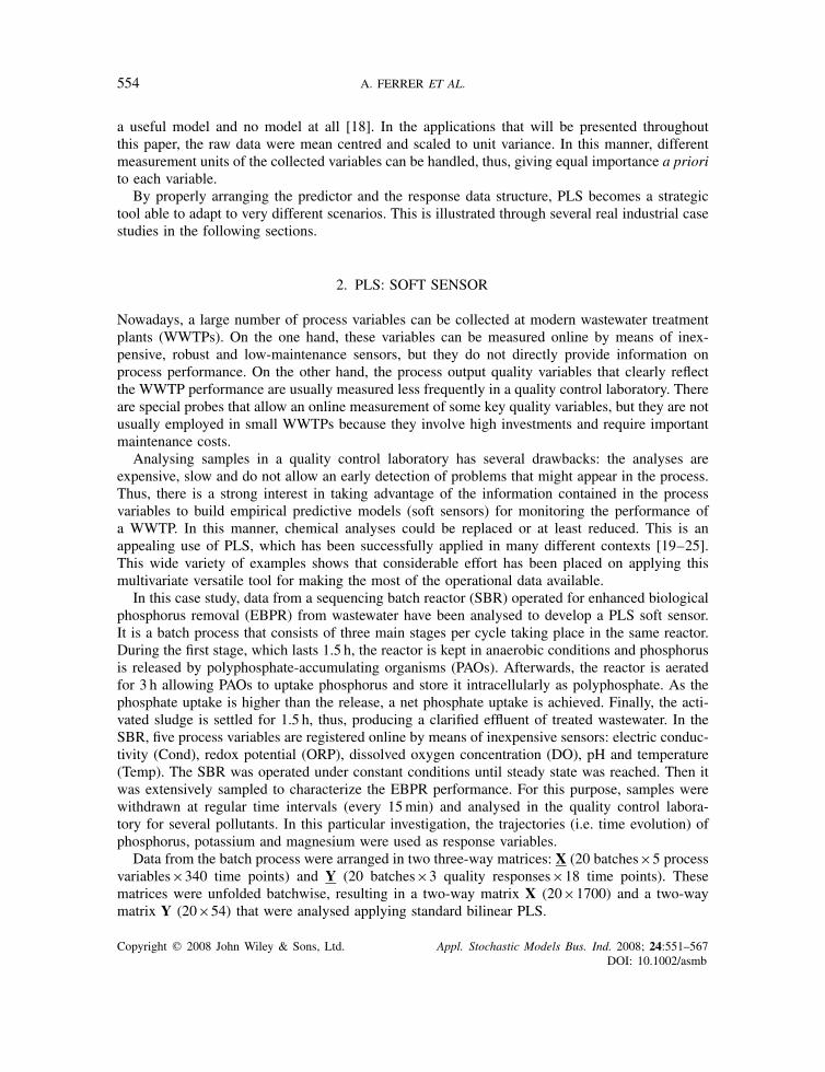
In this case study, data from a sequencing batch reactor (SBR) operated for enhanced biologicalphosphorus removal (EBPR) from wastewater have been analysed to develop a PLS soft sensor.It is a batch process that consists of three main stages per cycle taking place in the same reactor.During the first stage, which lasts 1.5 h, the reactor is kept in anaerobic conditions and phosphorusis released by polyphosphate-accumulating organisms (PAOs). Afterwards, the reactor is aeratedfor 3 h allowing PAOs to uptake phosphorus and store it intracellularly as polyphosphate. As thephosphate uptake is higher than the release, a net phosphate uptake is achieved. Finally, the acti-vated sludge is settled for 1.5 h, thus, producing a clarified effluent of treated wastewater. In theSBR, five process variables are registered online by means of inexpensive sensors: electric conduc-tivity (Cond), redox potential (ORP), dissolved oxygen concentration (DO), pH and temperature(Temp). The SBR was operated under constant conditions until steady state was reached. Then itwas extensively sampled to characterize the EBPR performance. For this purpose, samples werewithdrawn at regular time intervals (every 15min) and analysed in the quality control labora-tory for several pollutants. In this particular investigation, the trajectories (i.e. time evolution) ofphosphorus, potassium and magnesium were used as response variables.

Data from the batch process were arranged in two three-way matrices: X (20 batches×5 processvariables×340 time points) and Y (20 batches×3 quality responses×18 time points). Thesematrices were unfolded batchwise, resulting in a two-way matrix X (20×1700) and a two-waymatrix Y (20×54) that were analysed applying standard bilinear PLS.



The available data set consisted of 20 batches: 15 were used for model fitting and the remainingfor validation. Based on a preliminary study, it was decided to transform the original variablesusing the difference (�) between each variable value and its value at the beginning of the batch.

A PLS-2 model was built using the transformed trajectories of all variables (process and quality).Analysing the weights of the PLS model, it was found that the trajectories with more predictivecontribution were �pH and �Cond. Moreover, the weights of the three quality trajectories weresimilar, thus, indicating a highly positive correlation among them. This result matches the hypothesisof electroneutrality postulated by Comeau et al. [26]: in the EBPR process, both potassium andmagnesium are released and taken up simultaneously with phosphorus and act as counter ions tomaintain electroneutrality inside the bacterial cell.

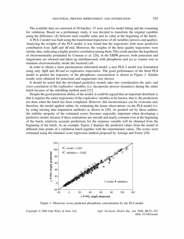
In order to obtain a more parsimonious inferential model, a new PLS-2 model was formulatedusing only �pH and �Cond as explicative trajectories. The good performance of the fitted PLSmodel to predict the trajectory of the phosphorus concentration is shown in Figure 1. Similarresults were obtained for potassium and magnesium (not shown).

It should be noted that the developed predictive models take into consideration the auto- andcross-correlation of the explicative variables (i.e. incorporate process dynamics) during the entirebatch because of the unfolding method used [27].

Despite the good prediction ability of the model, it could be argued that an important drawback isthat it requires the entire trajectories of the explicative variables to be known, that is, the predictionsare done when the batch has been completed. However, this inconvenience can be overcome and,therefore, the model applied online, by estimating the future observations via the PLS model (i.e.by using missing data imputation methods) as shown in [20]. As pointed out by these authors,the stability property of the estimated scores becomes especially important when developing apredictive model, because if these estimations are smooth and nearly constant even at the beginningof the batch, relatively accurate predictions for the response variable will be obtained from thebeginning of the batch. As an example, Figure 2 displays the predicted values from the model atdifferent time points of a validation batch together with the experimental values. The scores wereestimated using the trimmed score regression method proposed by Arteaga and Ferrer [28].

-20

0

20

40

60

80

100

120

-20 0 20 40 60 80 100 120

∆ P-PO4 (mg/l) observed

∆P-P

O4(m

g/l)pr

edicted

model validation

R2y model = 0.951

R2y validation = 0.902

Figure 1. Observed versus predicted phosphorus concentration by the PLS model.



-20

0

20

40

60

80

100

120

0.00 1.50 3.00 4.50Time (h)

∆P-P

O4(m

g/l)

k=1

k=15

k=30

k=90

k=150

k=210

k=270

k=340

P∆ experimental

Figure 2. Experimental and online predicted values of transformed trajectory of phosphorus concentration(�P) in a validation batch. At each time point, the future unknown part of the batch was estimated using

missing data imputation methods [28].

These results successfully illustrate that it is possible to build an efficient soft sensor formonitoring the performance of the SBR. As only data from the inexpensive and low-maintenancesensors installed in the SBR are used as input, the soft sensor can be considered as a cost-effectivetool. Moreover, monitoring the residuals of this model can be useful in detecting outliers andassessing whether the model needs to be updated. These issues are of special relevance in the areaof PLS research and practice as highlighted in different contributions [29–32].

3. BLOCKWISE PLS: BATCH PROCESS DIAGNOSIS

Batch chemical processes are difficult to control. Quality parameters are determined by analyticalmethods once the process finishes, and some of them are often out of quality specification limits.As a consequence, the product has to undergo further processing or standardization steps to achievea proper commercial quality, or maybe has to be sold under a lower-quality category, resultingin a considerable economic impact. To avoid these problems, a common approach is to reduceas much as possible the deviations of process variables from the target trajectories. However, inindustrial conditions this is complicated and not always effective, as quite often process engineersdo not know which are the key critical points of the process that require a more accurate controlto reduce the variability of quality parameters around the nominal value to avoid batches out ofspecifications.

Data from a petrochemical batch polymerization process have been analysed to diagnose thecauses of variability of one of the final quality parameters: the hydroxyl index (IOH), also referredto in the literature as hydroxyl number. This process takes place in four batch stages and thereare 52 electronic sensors that record online different kinds of information such as temperature,pressure, flow, pH, etc. These data are used online for the engineering process control and areroutinely stored in databases (one datum recorded every minute from each sensor). Once the batchfinishes, the hydroxyl index of the polymer (polypropylene oxide) is determined in the laboratory,



and the problem is that about 15% of the batches produced are out of quality specifications. Toprovide a solution, data from 69 historical batches have been analysed in order to identify thecritical points of the process.

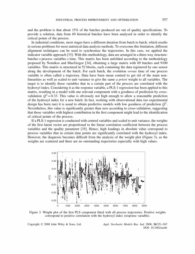
In industrial conditions, most stages have a different duration from batch to batch, which resultsin serious problems for most statistical data analysis methods. To overcome this limitation, differentalignment techniques can be used to synchronize the trajectories. In this case, we applied theindicator variable approach [33]. With this methodology, data are arranged in a three-way structure:batches×process variables×time. This matrix has been unfolded according to the methodologyproposed by Nomikos and MacGregor [34], obtaining a large matrix with 69 batches and 9100variables. This matrix is structured in 52 blocks, each containing the data registered by one sensoralong the development of the batch. For each batch, the evolution versus time of one processvariable is often called a trajectory. Data have been mean centred to get rid of the main non-linearities as well as scaled to unit variance to give the same a priori weight to all variables. Thetarget is to identify those variables that in a certain part of the process are correlated with thehydroxyl index. Considering it as the response variable, a PLS-1 regression has been applied to thismatrix, resulting in a model with one relevant component with a goodness of prediction by cross-validation Q2=0.33. This value is obviously not high enough to allow a reasonable predictionof the hydroxyl index for a new batch. In fact, working with observational data (no experimentaldesign has been run) it is usual to obtain predictive models with low goodness of prediction Q2.Nevertheless, this value is significantly greater than zero according to cross-validation, suggestingthat those variables with highest contribution in the first component might lead to the identificationof critical points of the process.

If a PLS-1 regression is conducted with centred variables and scaled to unit variance, the weightsof the first latent vector are proportional to the linear correlation coefficient between the processvariables and the quality parameter [35]. Hence, high loadings in absolute value correspond toprocess variables that in certain time points are significantly correlated with the hydroxyl index.However, the diagnosis becomes difficult from the analysis of the weight plot (Figure 3), as theweights are scattered and there are no outstanding trajectories especially with high values.

-0.03

-0.02

-0.01

0

0.01

0.02

0.03

0 1000 2000 3000 4000 5000 6000 7000 8000 9000

w*[

1]

Figure 3. Weight plot of the first PLS component fitted with all process trajectories. Positive weightscorrespond to positive correlation with the hydroxyl index (response variable).



As the diagnosis is not clear using the standard methodology of batch processes [36, 37] otheralternatives were tried. Blockwise PLS is a new approach for process diagnosis, following the ideaproposed in a previous paper [35]. Aguado et al. [38] successfully applied this methodology forprocess understanding of a wastewater batch reactor. Starting from the unfolded matrix, a PLSregression is conducted for every block of variables and, for the first component, the associatedlatent variable and its Q2 are calculated. This procedure produces a new matrix of 52 latentvariables that contains the main information in order to predict the IOH. A further analysis ofthis matrix can be carried out to identify stages more correlated with the final quality parameters,outliers, shifts in the process, etc. However, in this case just the analysis of the 52 Q2 valueshighlights the key information.

If the 52 values of Q2 are charted on a normal probability plot, a linear trend is observed(Figure 4), but the highest seven values are slightly separated from the straight line, highlightingthose trajectories most important from a statistical point of view. This result simplifies the diagnosis.The software SIMCA-P used for the analysis considers as threshold of significance for Q2 a valueof about 0.1, but in this case there are 15 values higher than 0.1 that follow the straight line in thenormal probability plot and do not seem to provide relevant information. The pressure during thesecond stage (2PR), the temperature during the first stage (1Ta), the derivative trajectory of thistemperature (1Tad) and the derivative trajectory of pressure (1PRd) are the latent variables withhighest Q2 values.

Regarding the latent variable of pressure (2PR), the highest weights correspond to the beginningof the second stage. During a period of about 20min, the pressure of the batches with highesthydroxyl index (out of specifications) describes a trajectory that tends to be lower than the meantrajectory. The opposite occurs for batches with lowest IOH. Thus, during the beginning of thesecond stage, the pressure has a negative correlation with IOH. The pressure just at the third minuteof this stage is significantly correlated with the hydroxyl index (Figure 5), and similar results areobtained considering other time points. Actually, if a further PLS is conducted with the trajectory

%

-0.1 0 0.1 0.2 0.3 0.40.1

1

5

20

50

80

95

99

99.9 1Tad

1PRd

3Tad

1LEVd

3Tac

2PR

1Ta

Q2

Figure 4. Normal probability plot of 52 Q2 values. Each one corresponds to the first component of a PLSmodel fitted with the block of recorded variables from one of the 52 sensors installed in the process, andconsidering y= IOH. Variable codes are shown for the highest Q2 values that depart from the straight line.The first number corresponds to the stage. 1Tad, 1PRd, 1LEVd are derivative trajectories. The vertical

dashed line is the significance limit considered by the software SIMCA-P.



r2 = 0.578

680

690

700

710

720

730

740

750

760

-0.2 -0.1 0 0.1 0.2 0.3

2PR3centred

I OH

Figure 5. Scatterplot of the hydroxyl index versus the pressure (centred values) in the third minute of thesecond stage (2PR3) for all the 69 batches. The regression line and squared correlation coefficient havebeen calculated discarding the four data with abnormal residuals (shown in asterisks). Horizontal dashed

lines define the tolerance quality interval.

of temperature during this period, it results in Q2=0.6 and hence this multivariate model could beused for online monitoring. Furthermore, these results reveal information regarding the diagnosis:as the correlation appears from the first minutes of the second stage, it seems that the first stageis critical.

With respect to the temperature during the first stage, the highest weights of this latent variable(1Ta) correspond to the final period of the addition of polyalcohol and during the addition of alkalinesolution. Actually, if the original trajectories are checked out, during these periods the batcheswith highest IOH show a trajectory of temperature lower than average. Hence, the temperature inthis stage is correlated with IOH, as it is the pressure in the second stage.

It is important to point out that caution has to be taken when interpreting these correlations.Only if correlation is due to a cause–effect relationship, we can consider those variables as criticalpoints or key process variables whose variability should be reduced to produce a reduction in thevariability of the IOH.

In this case, further studies conducted have pointed out that the flowmeter that controls theaddition of polyalcohol in the first stage seems to be the critical point, and the hypothesis is thatan excessive variability of the mass of polyalcohol used as a reagent seems to be the main causeof variability of IOH. Hence, the advice is to improve the control of this flowmeter in order toachieve a more accurate measure of the mass really added to the tank. From a statistical pointof view, the only way to identify a causal correlation and verify this hypothesis is conducting adesign of experiments (DOE). Blockwise PLS can be an efficient methodology to select the likelykey process variables to run a DOE out of the large amount of original process variables.

4. PLS-DISCRIMINANT ANALYSIS: AUTOMATIC CLASSIFIER BASEDON IMAGE DATA

The classification of parts or objects according to shape, colour or size is common in indus-trial environments. In the case of agricultural products such as fruits, there is a strong interest



in developing automatic systems to classify fruit pieces based on the presence of defects (i.e.phytopathologies and physiopathies that may affect the fruit).

Our example is related to the classification of orange fruit into quality categories based on theseparation of sound pieces from those affected by different defects. In the citric industry, there existsome machines that classify oranges basically in terms of colour and size. These machines do notachieve very good results when trying to discriminate between phytopathologies and physiopathies,probably because colour-based inspection machines try to discriminate between different problemsdealing just with the spectral values of the pixels, but not with the spatial structure of the orangepeel. Despite the big efforts made to improve the machine classification results during the last years,still an important percentage of the fruit introduced in the agricultural cooperatives is inspected andclassified by the human eye, mainly when there is a need to distinguish between some diseases.However, human inspection is not feasible due to its low productivity and lack of reliability forthe classification.

Traditional image analysis classification techniques are based on the extraction of colour ortexture statistics from the images, turning them into just one vector of characteristics that is usedto compare new images with those used to build the models [39]. This is equivalent to considerthe image as a sample from which some variables are measured. The introduction of PLS inthe multivariate image analysis (MIA) field started with the works of Prof. Esbensen [40, 41].Outstanding recognition deserves the work of Prof. MacGregor [42, 43]. Eriksson et al. [44] havealso applied a discriminant version of PLS in a recent work.

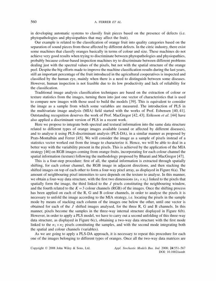
Here we propose to integrate both spectral and textural information into the same data structurerelated to different types of orange images available (sound or affected by different diseases),and to analyse it using PLS-discriminant analysis (PLS-DA), in a similar manner as proposed byPrats-Montalban and Ferrer [45]. We will consider the image as a sample of pixels instead of astatistics vector worked out from the image to characterize it. Hence, we will be able to deal in abetter way with the variability present in the pixels. This is achieved by the application of the MIAstrategy [46] on RGB images coming from orange fruits, incorporating for each colour channel thespatial information (texture) following the methodology proposed by Bharati and MacGregor [47].

This is a four-step procedure: first of all, the spatial information is extracted through spatiallyshifting, for each colour channel, the RGB image in adjacent directions, and then stacking theshifted images on top of each other to form a four-way pixel array, as displayed in Figure 6(a). Theamount of neighbouring pixel intensities to save depends on the texture to analyse. In this manner,we obtain a four-way data structure, with the first two dimensions (n1×n2) linked to the pixels thatspatially form the image, the third linked to the J pixels constituting the neighbouring window,and the fourth related to the K =3 colour channels (RGB) of the images. Once the shifting processhas been applied on each of the R, G and B colour channels, in order to analyse the pixels it isnecessary to unfold the image according to the MIA strategy, i.e. locating the pixels in the samplemode by means of stacking each column of the images one below the other, until one vector isobtained for each of the J shifted images analysed, for the three R, G and B channels. In thismanner, pixels become the samples in the three-way internal structure displayed in Figure 6(b).However, in order to apply a PLS model, we have to carry out a second unfolding of this three-waydata structure, as displayed in Figure 6(c), obtaining a two-way data structure with the first modelinked to the n1×n2 pixels constituting the samples, and with the second mode integrating boththe spatial and colour channels (variables).

As we are going to apply a PLS-DA approach, it is necessary to repeat this procedure for eachone of the images belonging to different types of oranges. Once all the two-way data matrices are



Unfolding 1

J

n2

n1

K

(a) (b) (c)

I=n1×n2

J

K

Unfolding 2

I=n1× n2

JK

YX

X1

X2

X3

(d)

1

0

0

1

0

0

1

001

Figure 6. Scheme of the data structure building procedure for the spectro-textural multivariate image: n1and n2 define the spatial dimensions of the image, which after first unfolding turn into the I sampledimension; K =3 (R, G and B spectral channels); and J is the number of neighbouring pixels saved toinclude the spatial information (texture). (a) Four-way dimensional data structure; (b) three-way internaldata structure; (c) two-way data structure; and (d) stacking process for a three-class PLS-DA model and

creation of the dummy variables.

obtained for each of the orange images to analyse, by stacking them on top of each other, the finaltwo-way data matrix X is created. The final step is to create as many dummy variables as classesof oranges that are to be fitted by the PLS-DA model. This step is accomplished by creating a Ymatrix that contains as many columns as different classes of oranges. For each of these columns,the value 1 is assigned to the pixels belonging to the class linked to that column, and 0 for therest, as shown in Figure 6(d). Usually, one training image per defect is enough for calibrating theclassification model.

Once the data structures have been created, it is possible to build a PLS model. The number ofrelevant components should be determined by means of a cross-validation procedure. Finally, newRGB orange images can be classified by projecting them onto the fitted PLS-DA model, workingout the percentage of pixels over the residual sum of squares (RSS) limit for the fitted model. Ifthis percentage of pixels of the new projected image is higher than the percentage of pixels overthe RSS limit for the training image data set, then the image is classified as not belonging to anyof the modelled classes. On the contrary, if this percentage is lower than the RSS limit, then thenew image is classified as belonging to the class showing an average predicted value for the pixelsclosest to ‘1’.

The application of this procedure for the classification of three types of diseases on a validationimage data set with 67 oranges with several types of diseases gave a 78% success rate in the



classification. As these results were not completely satisfactory, it was decided to project only theimages corresponding to oranges of the same classes as the ones used to build the models. In thismanner, it is not necessary to establish a maximum percentage of pixels over the limit for the RSSstatistic. When considering this alternative, the PLS-DA approach reached up to a 93% successrate in the classification, which is a very good result, always taking into account the limitationsof this alternative.

5. PLS-TIME SERIES: MODEL BUILDING

The objective of this case study is to present the capabilities of PLS time series (PLS-TS) method-ology [18] for the estimate of a transfer function (TF) model of an industrial polymerization processbetween two input variables (X ): reactor temperature (T ) and ethylene flow (E); and two outputvariables (Y ): a quality property of the polymer, Melt Index (MI), and a measure of the processthroughput (APRE). The model can be used for designing predictive controllers. Real data fromthree manufacturing periods provided by a petrochemical company have been investigated.

As the two output variables were slightly correlated, we proceeded to build a TF model for eachoutput variable separately. From the different TF models that can be used to represent the process,the finite impulse response (FIR) model was chosen. This is a simple but non-parsimonious TFmodel, where each output variable at time t , Y j,t ( j =1,2), is expressed as a linear combinationof values at time t and past values of the input variables Xi,t−k (i=1,2, k=0, . . . , L):

Y j,t =2∑

i=1(�i0Xi,t +�i1Xi,t−1+�i2Xi,t−2+·· ·+�i L Xi,t−Li )+� j,t

where Li is the number of lags for input variable Xi related to the inertial properties of the system;the residual part, � j,t , is assumed to be white noise; and Y j,t and Xi,t−k measure the deviations fromsteady state. Other TF models such as, e.g. autoregressive with exogenous variables (ARX) models,which incorporate past measured outputs Y j,t−k as inputs, can also be fitted by PLS-TS [18, 48].

The phases of model building by using PLS-TS methodology are:

• Initial exploratory analysis of data: Study of the nature of the series and their dynamics (auto-and cross-correlation functions); determination of number of differences to obtain stationaryseries and number of lags to consider in the formulation of the model; process fault detection(residual and score plots from preliminary PLS models).

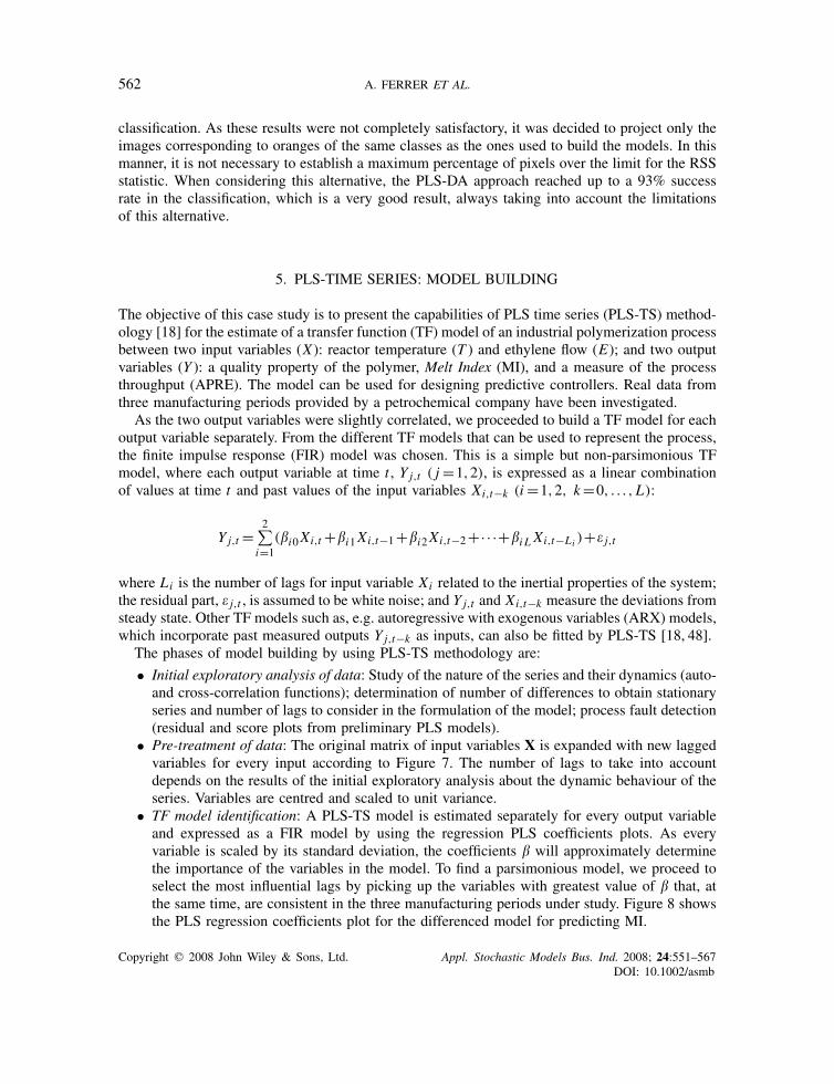
• Pre-treatment of data: The original matrix of input variables X is expanded with new laggedvariables for every input according to Figure 7. The number of lags to take into accountdepends on the results of the initial exploratory analysis about the dynamic behaviour of theseries. Variables are centred and scaled to unit variance.

• TF model identification: A PLS-TS model is estimated separately for every output variableand expressed as a FIR model by using the regression PLS coefficients plots. As everyvariable is scaled by its standard deviation, the coefficients � will approximately determinethe importance of the variables in the model. To find a parsimonious model, we proceed toselect the most influential lags by picking up the variables with greatest value of � that, atthe same time, are consistent in the three manufacturing periods under study. Figure 8 showsthe PLS regression coefficients plot for the differenced model for predicting MI.



L..2

1

x1

•xL

•

•

•

•xn-L

•xn-1

xn

x1

•xL

•

•

•

•xn-L

•xn-1

xn

x1

•xL

•

•

•

•xn-L

•xn-1

xn

x1

•xL

•

•

•

•xn-L

•xn-1

xn

y1

•yL

•

•

•

•yn-L

•yn-1

yn

YX

Figure 7. Overview of the lagging process to create the expanded X matrix. Dropping rows from the topand bottom is carried out to regularize the data structure.

-0.2-0.10.00.10.20.30.40.5

-0.2-0.10.00.10.20.30.40.5

-0.2-0.10.00.10.20.30.40.5

DfE

TIL

DC

1

DfE

TIL

DC

2

DfE

TIL

DC

3

DfE

TIL

DC

4

DfE

TIL

DC

5

DfE

TIL

DC

6

D

fTE

MP

DC

1

D

fTE

MP

DC

2

D

fTE

MP

DC

3

D

fTE

MP

DC

4

D

fTE

MP

DC

5

D

fTE

MP

DC

6

Var ID (Primary)

Campaign 0

DifE

TIL

DC

1

DifE

TIL

DC

2

DifE

TIL

DC

3D

ifET

ILD

C4

DifE

TIL

DC

5

DifE

TIL

DC

6

DifT

EM

PD

C1

DifT

EM

PD

C2

DifT

EM

PD

C3

DifT

EM

PD

C4

DifT

EM

PD

C5

DifT

EM

PD

C6

Var ID (Primary)

Campaign 5

DifE

TIL

DC

1

DifE

TIL

DC

2

DifE

TIL

DC

3

DifE

TIL

DC

4

DifE

TIL

DC

5

DifE

TIL

DC

6

DifT

EM

PD

C1

DifT

EM

PD

C2

DifT

EM

PD

C3

DifT

EM

PD

C4

DifT

EM

PD

C5

DifT

EM

PD

C6

Var ID (Primary)

Campaign 2

Figure 8. PLS coefficient plot of reactor temperature and ethylene flow (differenceddata) as a function of lag number.

• In this case the first two lags for both input variables (DIFETILDC1, DIFETILDC2 andDIFTEMPDC1, DIFTEMPDC2) were included in the model for MI. Following a similarprocedure (not shown), the first two lags for reactor temperature and only the first lag forethylene flow were considered for the APRE model (differenced data).

• If the model contains a high number of highly correlated input variables, a more parsimoniousmodel can be obtained by pruning the original one. The weight plot of the PLS-TS modelwill help to identify the variables that provide redundant information. Owing to the smallnumber of input variables in our study, pruning was not considered.

• Final model estimation: In this case, the estimated model was

∇MIt = �1∇Tt−1+�2∇Tt−2+�3∇Et−1+�4∇Et−2+a1t

∇APREt = �1∇Tt−1+�2∇Tt−2+�3∇Et−1+a2t

where ∇ is the differential operator (∇Xt = Xt −Xt−1).



- 0 .4

- 0 .3

- 0 .2

- 0 .1

0

0 .1

0 .2

0 .3

0 .4

0 .5

1 2 3 4 5 6 1 2 3 4 5 6

- 0 .4

- 0 .3

- 0 .2

- 0 .1

0

0 .1

0 .2

0 .3

0 .4

0 .5

1 2 3 4 5 6 1 2 3 4 5 6

ETHYLENE FLOW TEMPERATURE

(a)

(b)

Figure 9. (a) PLS coefficient plot for ∇MI model and (b) cross-correlation functions between ∇MI and∇E , and between ∇MI and ∇T . Campaign 5.

Figure 10. FIR model (up) versus BJ model (down). Noise � j,t is partiallymodelled in Box–Jenkins methodology.

From this case study, we concluded that:

• PLS-TS can be successfully applied to estimate process dynamics using a variety of TFmodels (FIR, ARX, etc.). The results were consistent with those obtained from using thestatistically well-sounded Box–Jenkins (BJ) methodology [49, 50].

• PLS-TS method provides a pack of very useful graphic tools for the descriptive study of thedata, allowing an easy identification of abnormal periods in the data set. The regression PLS



coefficients plot helps to identify the TF model. This plot is similar to the cross-correlationfunction when the input variables are not correlated. For instance, Figure 9 shows how thePLS coefficient plot for ∇MI model is similar to the cross-correlation functions between∇MI and ∇E, as well as between ∇MI and ∇T in campaign 5.

• Comparing the BJ methodology to FIR and ARX models fitted by PLS-TS, the formerleads to more parsimonious models because noise � j,t can also be modelled (see Figure 10).Nonetheless, PLS-TS may serve as an exploratory tool complementary to the BJ methodology.

• PLS-TS turns out to be a good choice for TF model building in the case of complex multi-input multi-output systems, with inputs and outputs highly correlated, where BJ methodologybecomes practically unfeasible.

6. CONCLUSIONS

Specialized tools for specific problems are easily available in the literature of statistical dataanalysis. Nevertheless, very few techniques are versatile enough to be applied in a very wide rangeof problems (e.g. discrimination, classification, process modelling, process diagnosis and faultdetection) dealing with so many different data structure scenarios (e.g. collinearity, rank deficiency,missing data, etc.), which are typical in complex modern processes.

This is the great virtue of PLS models: the same tool can be used in very different contextsby properly arranging the data structure. This makes PLS an easily transferable tool: a key prop-erty to be successfully applied for problem solving in highly competitive and time-demandingenvironments.

Although the examples illustrated here come from chemometrics environments, where PLS hasbeen widely used in the last years, there is a tremendous potential impact of PLS in other areassuch as marketing, business strategy and the application of statistics in business analysis.

ACKNOWLEDGEMENTS

This research was partially supported by the Spanish Government (MICYT) and the European Union (RDEfunds) under grant CTM2005-06919-C03-03/TECNO. The authors would like to thank E. Molto (InstitutoValenciano de Investigaciones Agrarias-IVIA, Spain) for the orange images data set. The authors arealso grateful to CALAGUA research group (University of Valencia and Technical University of Valencia,Spain) for providing them with the SBR data set. Finally, the authors also wish to acknowledge theanonymous reviewers for their valuable comments and suggestions.

REFERENCES

1. Geladi P, Kowalski BR. Partial least-squares regression: a tutorial. Analytica Chimica Acta 1986; 185:1–17.2. Wold S, Wold H, Dunn WJ, Ruhe A. The collinearity problem in linear regression. The partial least squares

(PLS) approach to generalized inverses. SIAM Journal on Scientific and Statistical Computing 1984; 5:735–743.3. Martens H, Naes T. Multivariate Calibration. Wiley: New York, 2001.4. Wold H. Soft modelling: the basic design and some extensions. In Systems under Indirect Observation, Causality–

Structure–Prediction, Joreskog KG, Wold H (eds). North-Holland: Amsterdam, 1981.5. Helland IS. On the structure of partial least squares. Communication in Statistics—Simulation and Computation

1988; 17(2):581–607.6. Hoskuldsson A. PLS regression methods. Journal of Chemometrics 1988; 2:211–228.7. Frank IE, Friedman JH. A statistical view of some chemometrics regression tools (with Discussion). Technometrics

1993; 35:109–148.



8. Breiman L, Friedman JH. Predicting multivariate responses in multiple linear regression (with Discussion).Journal of the Royal Statistical Society, Series B 1997; 59(1):3–54.

9. Svensson O, Kourti T, MacGregor JF. An investigation of orthogonal signal correction algorithms and theircharacteristics. Journal of Chemometrics 2002; 16:176–188.

10. Westerhuis JA, Kourti T, MacGregor JF. Analysis of multiblock and hierarchical PCA and PLS models. Journalof Chemometrics 1998; 12:301–321.

11. Esposito-Vinzi V, Chin WW, Henseler J, Wang H (eds). Handbook of Partial Least Squares. Concepts, Methodsand Applications in Marketing and Related Fields. Springer: Berlin, 2007.

12. Croteau AM, Bergeron F. An information technology trilogy: business strategy, technological deployment andorganizational performance. Journal of Strategic Information Systems 2001; 10(2):77–99.

13. Guenzi P, Pardo C, Georges L. Relational selling strategy and key account managers’ relational behaviors: anexploratory study. Industrial Marketing Management 2007; 36(1):121–133.

14. Sohn SY, Joo YG, Han HK. Structural equation model for the evaluation of national funding on R&D projectof SMEs in consideration with MBNQA criteria. Evaluation and Program Planning 2007; 30(1):10–20.

15. Joo YG, Sohn SY. Structural equation model for effective CRM of digital content industry. Expert Systems withApplications 2008; 34(1):63–71.

16. Fornell C, Cha J. In Partial Least Squares in Advanced Methods of Marketing Research, Bagozzi RP (ed.).Blackwell: Cambridge, MA, 1994; 52–78.

17. Hulland J. Use of partial least squares (PLS) in strategic management research: a review of four recent studies.Strategic Management Journal 1999; 20:195–204.

18. Eriksson L, Johansson E, Kettaneh-Wold N, Wold S. Multi- and Megavariate Data Analysis (2nd edn). UmetricsAB: Umea, Sweden, 2006.

19. Henriksen H, Naes T, Segtnan V, Aastveit A. Using near infrared spectroscopy for predicting process conditions.A laboratory study from pulp production. Journal of Near Infrared Spectroscopy 2005; 13(5):265–276.

20. Aguado D, Ferrer A, Seco A, Ferrer J. Comparison of different predictive models for nutrient estimation ina sequencing batch reactor for wastewater treatment. Chemometrics and Intelligent Laboratory Systems 2006;84:75–81.

21. Zhang J. Offset-free inferential feedback control of distillation compositions based on PCR and PLS models.Chemical Engineering and Technology 2006; 29(5):560–566.

22. Sharmin R, Sundararaj U, Shah S, Griend LV, Sun YJ. Inferential sensors for estimation of polymer qualityparameters: industrial application of a PLS-based soft sensor for a LDPE plant. Chemical Engineering Science2006; 61(19):6372–6384.

23. Mahani MK, Chaloosi M, Maragheh MG, Khanchi AR, Afzali D. Prediction of acute in vivo toxicity of someamine and amide drugs to rats by multiple linear regression, partial least squares and an artificial neural network.Analytical Sciences 2007; 23(9):1091–1095.

24. Bruwer MJ, MacGregor JF, Bourg WM. Soft sensor for snack food textural properties using on-line vibrationalmeasurements. Industrial and Engineering Chemistry Research 2007; 46(3):864–870.

25. Lee HW, Lee MW, Park JM. Robust adaptive partial least squares modeling of a full-scale industrial wastewatertreatment process. Industrial and Engineering Chemistry Research 2007; 46(3):955–964.

26. Comeau Y, Rabinowitz B, Hall KJ, Oldham KW. Phosphate release and uptake in enhanced biological phosphorusremoval from wastewater. Journal of Water Pollution Control Federation 1987; 59:707–715.

27. Camacho J, Pico J, Ferrer A. Bilinear modelling of batch processes. Part I: theoretical discussion. Journal ofChemometrics 2008; DOI: 10.1002/cem.1113.

28. Arteaga F, Ferrer A. Dealing with missing data in MSPC: several methods, different interpretations, someexamples. Journal of Chemometrics 2002; 16(8–10):408–418.

29. Moller SF, von Frese J, Bro R. Robust methods for multivariate data analysis. Journal of Chemometrics 2005;19(10):549–563.

30. Rousseeuw PJ, Debruyne M, Engelen S, Hubert M. Robustness and outlier detection in chemometrics. CriticalReviews in Analytical Chemistry 2006; 36(3–4):221–242.

31. Furusjo E, Svenson A, Rahmberg M, Andersson M. The importance of outlier detection and training set selectionfor reliable environmental QSAR predictions. Chemosphere 2006; 63(1):99–108.

32. Lee HW, Lee MW, Park JM. Robust adaptive partial least squares modeling of a full-scale industrial wastewatertreatment process. Industrial and Engineering Chemistry Research 2007; 46(3):955–964.

33. Westerhuis JA, Kourti T, MacGregor JF. Comparing alternative approaches for multivariate statistical analysis ofbatch process data. Journal of Chemometrics 1999; 13:397–413.



34. Nomikos P, MacGregor JF. Multivariate SPC charts for monitoring batch processes. Technometrics 1995; 37(1):41–59.

35. Zarzo M, Ferrer A. Batch process diagnosis: PLS with variable selection versus block-wise PCR. Chemometricsand Intelligent Laboratory Systems 2004; 73(1):15–27.

36. Kourti T, MacGregor JF. Process analysis, monitoring and diagnosis using multivariate projection methods—atutorial. Chemometrics and Intelligent Laboratory Systems 1995; 28:3–21.

37. Kourti T, Nomikos P, MacGregor JF. Analysis, monitoring and fault diagnosis of batch processes using multiblockand multiway PLS. Journal of Process Control 1995; 5(4):277–284.

38. Aguado D, Zarzo M, Seco A, Ferrer A. Process understanding of a wastewater batch reactor with block-wisePLS. Environmetrics 2007; 18:551–560.

39. Jain AK, Duin RPW, Mao J. Statistical pattern recognition: a review. IEEE Transactions on Pattern Analysisand Machine Intelligence 2000; 22(1):4–37.

40. Lied TT, Geladi P, Esbensen K. Multivariate image regression (MIR): implementation of image PLSR-first forays.Journal of Chemometrics 2000; 14:585–598.

41. Huang J, Esbensen KH. Applications of the angle measure technique (AMT) in image analysis. Part II: predictionof powder functional properties and mixing components using multivariate AMT regression (MAR). Chemometricsand Intelligent Laboratory Systems 2000; 54:1–19.

42. Yu H, MacGregor JF. Multivariate image analysis and regression for prediction of coating and distribution in theproduction of snack foods. Chemometrics and Intelligent Laboratory Systems 2003; 72:57–71.

43. Liu JJ, MagGregor JF. Modeling and optimization of product appearance: application to injection-molded plasticmodels. Industrial Chemical Engineering Research 2005; 44:4687–4696.

44. Eriksson L, Wold S, Trygg J. Multivariate analysis of congruent images (MACI). Journal of Chemometrics 2005;19:393–403.

45. Prats-Montalban JM, Ferrer A. Integration of colour and textural information in multivariate image analysis:defect detection and classification issues. Journal of Chemometrics 2007; 21:10–23.

46. Geladi P, Grahn H. Multivariate Image Analysis. Wiley: Chichester, U.K., 1996.47. Bharati MH, MacGregor JF. Texture analysis of images using principal component analysis. SPIE/Photonics

Conference on Process Imaging for Automatic Control, Boston, MA, U.S.A., 2000.48. Dayal BS, MacGregor JF. Identification of finite impulse response models: methods and robustness issues.

Industrial and Engineering Chemistry Research 1996; 35:4078–4090.49. Barcelo S, Vidal S, Ferrer A. Case study of comparison of multivariate statistical methods for process modelling.

Third Annual Meeting of European Network for Business & Industrial Statistics (ENBIS), Barcelona, Spain,2003.

50. Box GEP, Jenkins GM, Reinsel GC. Time Series Analysis—Forecasting and Control (3rd edn). Prentice-Hall:Englewood Cliffs, NJ, U.S.A., 1994.


PLS: A versatile tool for industrial process improvement and optimization

Documents

Transcript of PLS: A versatile tool for industrial process improvement and optimization