A Versatile Experimentation Model for Study of Structures ...
283
ISSN 1520-295X A Versatile Experimentation Model for Study of Structures Near Collapse Applied to Seismic Evaluation of Irregular Structures by Dyah Kusumastuti, Andrei M. Reinhorn and Avigdor Rutenberg University at Buffalo, State University of New York Department of Civil, Structural and Environmental Engineering Ketter Hall Buffalo, New York 14260 Technical Report MCEER-05-0002 March 31, 2005 This research was conducted at the University at Buffalo, State University of New York and was supported primarily by the Earthquake Engineering Research Centers Program of the National Science Foundation under award number EEC-9701471.
-
Upload
khangminh22 -
Category
Documents
-
view
2 -
download
0
Transcript of A Versatile Experimentation Model for Study of Structures ...

ISSN 1520-295X
A Versatile Experimentation Model for Studyof Structures Near Collapse Applied to
Seismic Evaluation of Irregular Structures
by
Dyah Kusumastuti, Andrei M. Reinhorn and Avigdor RutenbergUniversity at Buffalo, State University of New York
Department of Civil, Structural and Environmental EngineeringKetter Hall
Buffalo, New York 14260
Technical Report MCEER-05-0002
March 31, 2005
This research was conducted at the University at Buffalo, State University of New York and wassupported primarily by the Earthquake Engineering Research Centers Program of the National Science
Foundation under award number EEC-9701471.

NOTICEThis report was prepared by the University at Buffalo, State University of NewYork as a result of research sponsored by the Multidisciplinary Center for Earth-quake Engineering Research (MCEER) through a grant from the Earthquake Engi-neering Research Centers Program of the National Science Foundation under NSFaward number EEC-9701471 and other sponsors. Neither MCEER, associates ofMCEER, its sponsors, the University at Buffalo, State University of New York, norany person acting on their behalf:
a. makes any warranty, express or implied, with respect to the use of any infor-mation, apparatus, method, or process disclosed in this report or that such usemay not infringe upon privately owned rights; or
b. assumes any liabilities of whatsoever kind with respect to the use of, or thedamage resulting from the use of, any information, apparatus, method, or pro-cess disclosed in this report.
Any opinions, findings, and conclusions or recommendations expressed in thispublication are those of the author(s) and do not necessarily reflect the views ofMCEER, the National Science Foundation, or other sponsors.

A Versatile Experimentation Model forStudy of Structures Near Collapse
Applied to Seismic Evaluation of Irregular Structures
by
Dyah Kusumastuti1, Andrei M. Reinhorn2 and Avigdor Rutenberg3
Publication Date: March 31, 2005Submittal Date: February 7, 2005
Technical Report MCEER-05-0002
Task Numbers 01-2041, 02-2041e and 03-2.6
NSF Master Contract Number EEC-9701471
1 Ph.D. Candidate, Department of Civil, Structural and Environmental Engineering,University at Buffalo, State University of New York
2 Professor, Department of Civil, Structural and Environmental Engineering, Univer-sity at Buffalo, State University of New York
3 Professor Emeritus, Department of Civil and Environmental Engineering, Technion,Israel Institute of Technology, Haifa, Israel
MULTIDISCIPLINARY CENTER FOR EARTHQUAKE ENGINEERING RESEARCHUniversity at Buffalo, State University of New YorkRed Jacket Quadrangle, Buffalo, NY 14261

iii
Preface
The Multidisciplinary Center for Earthquake Engineering Research (MCEER) is a nationalcenter of excellence in advanced technology applications that is dedicated to the reductionof earthquake losses nationwide. Headquartered at the University at Buffalo, StateUniversity of New York, the Center was originally established by the National ScienceFoundation in 1986, as the National Center for Earthquake Engineering Research (NCEER).
Comprising a consortium of researchers from numerous disciplines and institutionsthroughout the United States, the Center’s mission is to reduce earthquake losses throughresearch and the application of advanced technologies that improve engineering, pre-earthquake planning and post-earthquake recovery strategies. Toward this end, the Centercoordinates a nationwide program of multidisciplinary team research, education andoutreach activities.
MCEER’s research is conducted under the sponsorship of two major federal agencies: theNational Science Foundation (NSF) and the Federal Highway Administration (FHWA),and the State of New York. Significant support is derived from the Federal EmergencyManagement Agency (FEMA), other state governments, academic institutions, foreigngovernments and private industry.
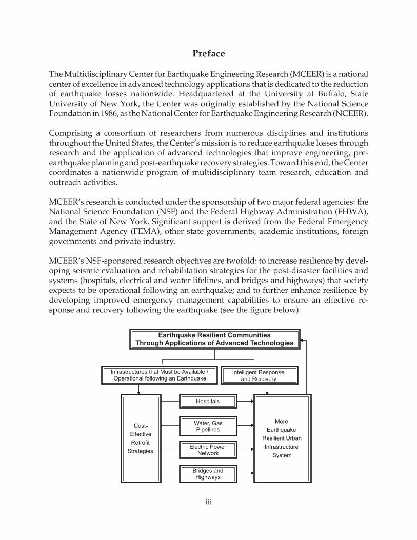
MCEER’s NSF-sponsored research objectives are twofold: to increase resilience by devel-oping seismic evaluation and rehabilitation strategies for the post-disaster facilities andsystems (hospitals, electrical and water lifelines, and bridges and highways) that societyexpects to be operational following an earthquake; and to further enhance resilience bydeveloping improved emergency management capabilities to ensure an effective re-sponse and recovery following the earthquake (see the figure below).
-
Infrastructures that Must be Available /Operational following an Earthquake
Intelligent Responseand Recovery
Hospitals
Water, GasPipelines
Electric PowerNetwork
Bridges andHighways
More
Earthquake
Resilient Urban
Infrastructure
System
Cost-
Effective
Retrofit
Strategies
Earthquake Resilient CommunitiesThrough Applications of Advanced Technologies

iv
A cross-program activity focuses on the establishment of an effective experimental andanalytical network to facilitate the exchange of information between researchers locatedin various institutions across the country. These are complemented by, and integratedwith, other MCEER activities in education, outreach, technology transfer, and industrypartnerships.
This report presents a study of irregular structures near collapse and the development of anexperimental model to study many types of structural systems in the near collapse state. Experienceshows that buildings with irregularities are prone to severe damage from earthquakes, as observed inmany past events. Many analytical studies have been carried out to evaluate irregular structures, butvery few experimental works have been done on this subject. A large number of critical structures, suchas hospitals, often have irregular design due to architectural and functional constraints. This studyprovides an overview of the accuracy of the analytical methods in predicting the structural response.
Equally important in the scope of this research was the design of a structural model for study ofstructural systems near collapse. A versatile reconfigurable structural model was developed to be usedand reused with structures undergoing severe damage to sacrificial elements, thus capable of beingrepaired and further tested without complete collapse. The model was developed with two independentsupport systems: one for gravity loads and one for lateral loads. Loss of the lateral load resisting system,which may happen during earthquakes, does not damage the vertical load resisting system (named also“gravity columns”) and therefore prevents collapse.
This study shows that a separation of lateral and gravity load resisting systems can produce a stablestructure in case of major damage to lateral system, provided that redundancy exists to control lateraldeformations. Such a system can be implemented when retrofitting structures, by weakening theconnections of gravity columns and providing a redundant external lateral load resisting system.Further research and engineering development may assure the success of this potential solution.
v
ABSTRACT
This report presents a study of irregular structures near collapse, aimed to understand better the influence of irregularities and adequacy of simplified techniques of analyses to real behavior of such structures. Experience shows that buildings with irregularities are prone to severe damage as demonstrated in many earthquake occurrences. An experimental study was focused on the validation of the analytical tools for evaluation of seismic response of irregular structures, i.e. setback structures. A number of analytical studies had been carried out to evaluate such structures, but very few experimental works had been done on this subject.
Equally important scope of this study was the design of a structural model for study of structural systems near collapse. A versatile reconfigurable structural model was developed to be used and reused with structures undergoing severe damage to sacrificial elements thus capable to be repaired and further tested without complete collapse. The model was developed with two independent support systems: one for gravity loads and one for lateral loads. Loss of the lateral load resisting system which may happen during earthquakes does not damage the vertical load resisting system (named also “gravity columns”) thus preventing collapse.
The model was designed as a one-third scale three-story three-bay steel frame structure. For the purpose of this study, the irregularity aspect was introduced to the designated model by having two unequal towers creating a setback structure. From dynamic simulation of the analytical model, a ground motion history (Northridge 1996, Rinaldi RS), from the SAC project with 10% probability of exceedence in 50 years in Los Angeles, was selected to perform physical (using shake table testing) and computational simulations.
The gravity columns were equipped with special spherical attachments to enable them to act as pin-connected leaning columns, thus they can resist only vertical load. The beam-column connections were designed to resist only lateral loads, and the tests were conducted on a ‘cruciform’ specimen made of half-beams and half-columns to resemble a sub-assembly having half spans and half stories on each side. Prior to the shake table study of the model structure, several material and component tests were carried out. The actual properties obtained from the material tests were used to refine the analytical models. The “gravity” column and the beam-column connection components were also tested to better understand the behavior of the model structure. The component test results were subsequently used also to refine the analytical model.
Shake table tests of the model structure were conducted by applying a sequence of increasing ground motions. Structural identifications using banded white noise excitations were made in-between the dynamic loadings to monitor changes in the dynamic properties. At the higher ground motion levels, the model behaved inelastically. Damage was recorded in the form of prying effect at the column end plates and a welding failure of a block joint located at the toes of the higher tower where force concentrations due to irregularities were expected. The experimental study showed that the separation of vertical and lateral load resisting systems was satisfactory, the model suffered complete

vi
rupture of its column connections without complete collapse. Most of the structural elements were undamaged and can be used for future research.
Based on the results from the experimental study, analytical studies were conducted, and a number of analytical models were developed following the various stages of the experiments. Progressive knowledge of model properties and refinement of the analytical models improved the accuracy of the simplified model, however, even the approximated results were able to predict mild inelastic behavior. However, none of the models could predict the sudden changes due to the local damages.
This report presents the experimental study and the efforts to simulate it analytically. The report presents also the detailed design of the reconfigurable structural model used in shake table studies.

vii
TABLE OF CONTENTS
SECTION TITLE PAGE
1 INTRODUCTION 1
1.1 Irregular structures 1
1.2 Research objectives 2
1.3 Irregular structures 3
1.4 Irregularities in major health care facilities 5
1.5 Background on irregular structures studies 5
1.6 The present task 7
1.6.1 Benchmark structure 8
1.6.2 Testing procedures 8
1.7 Analytical modeling 8
1.8 Report organization 9
2 VERSATILE MODEL – PRINCIPLES AND LAYOUT 11
2.1. Principles and objectives 11
2.1.1. Model of frame structure 11
2.1.2. Two independent support systems 11
2.1.3. Removable-replaceable lateral load resisting system 12
2.1.4. Undamageable vertical system 12
2.1.5. Floor system 12
2.1.6. Interchangeability: removable and reusable standard elements 12
2.1.7. Implementation of reconfigurable model 13
2.2. Layout and configuration 13
2.2.1. Prototype and scaling for model 13
2.2.2. Model construction 16
2.2.2.1. Layout 17
2.2.2.2. Design considerations 17
2.2.2.3. Components 21
viii
TABLE OF CONTENTS (cont’d)
SECTION TITLE PAGE
2.2.2.3.1. Damageable lateral support system 21
2.2.2.3.2. Beam designs 21
2.2.2.3.3 Column designs 23
2.2.2.3.4 Exterior frame-base connections 25
2.2.2.3.5 Floor system: floor slab 26
2.2.2.3.6 Floor system: floor slab connection 29
2.2.2.3.7 Special connections 29
2.2.2.3.8 Undamageable vertical support system 32
2.2.2.4 Properties of components 34
2.2.3. Model configurations – versatility 35
2.2.3.1. Possible structural configurations: regular and irregular frames 35
2.2.3.2. Examples - four types of structure 35
2.2.4. Example: selected model for irregular structures study 38
2.2.4.1. Objectives of experimental study 38
2.2.4.2. Layout of selected model 38
2.2.4.3. Monitoring the response of selected model 42
2.3 Summary 42
3 ANALYTICAL EVALUATION OF VERSATILE MODEL 43
3.1. Introduction 43
3.1.1. Objectives of evaluation 43
3.1.2. Analytical techniques 43
3.1.2.1. Dynamic time analysis 43
3.1.2.2. Dynamic pushover : incremental dynamic analysis 43
3.1.2.3. Nonlinear spectral, static analysis (spectral demand-capacity
analysis)
43
3.1.3. Analytical models of tested structures 44
ix
TABLE OF CONTENTS (cont’d)
SECTION TITLE PAGE
3.2. Spectral capacity analysis from static nonlinear analysis
(pushover)
44
3.2.1. General description of method 44
3.2.1.1. Components needed for evaluation 44
3.2.1.2. Capacity-Demand Diagram for static nonlinear analysis 45
3.2.2. Inelastic demand spectra based on strength reduction factors 45
3.2.2.1. Elastic spectra derived from dynamic time analysis 45
3.2.2.2. Derivation of R-based inelastic from dynamic time history
analysis
47
3.2.2.3. Derivation of approximate demand spectra from elastic design
spectra
48
3.2.3. Spectral capacity 50
3.2.3.1. General method – loading on inelastic model 51
3.2.3.2. Load distributions for nonlinear analysis: Fixed and adaptive
modes
52
3.2.3.3 Approximation of Capacity Curve 54
3.2.4 Spectral response evaluation 55
3.3. Evaluation of model properties – case study 57
3.3.1. Analysis techniques in evaluation of case study 57
3.3.2 Dynamic time analysis 58
3.3.2.1 Ground motion selection 58
3.3.2.2. Sample results of dynamic analysis 61
3.3.3 Incremental dynamic analysis (dynamic pushover) 62
3.3.4 Spectral capacity analysis 63
x
TABLE OF CONTENTS (cont’d)
SECTION TITLE PAGE
4 EXPERIMENTAL COMPONENT PROPERTIES
EVALUATION
67
4.1. Introduction 67
4.1.1. Brief summary of Section 67
4.1.2. Rationale for choice of the as-built sections 67
4.1.3. Testing procedures for materials, components and connections 67
4.2. Material Properties 68
4.2.1. Properties of beam materials 68
4.2.2. Properties of column materials 69
4.2.3. Summary of material properties 70
4.3 Components – Beams, Columns and Connections 71
4.3.1 Testing setup and test protocol 71
4.3.2. Test procedure 71
4.3.2.1 Test setup 72
4.3.2.2. Instrumentation and calibration 73
4.3.2.3. Test protocol 76
4.3.3. Test Results (sample) 78
4.3.3.1 Stiffness of beam-column connection 78
4.3.3.2 Summary of component test results 80
4.3.3.3 Damage evaluation - prying effects on connection and effect of
load levels
81
4.4 Components - Gravity Columns 84
4.4.1 Testing Setup and Test Protocol 84
4.4.2 Test procedure 84
4.4.2.1. Test setup 84
4.4.2.2. Instrumentation and calibration 85
4.4.2.3 Test protocol 87
xi
TABLE OF CONTENTS (cont’d)
SECTION TITLE PAGE
4.4.2.4 Test Results (Sample) 88
4.4.2.5 Identification of structural stiffness 92
4.5. Summary 93
5 EXPERIMENTAL EVALUATION OF MODEL
STRUCTURE: GLOBAL ASSEMBLY PROPERTIES
IDENTIFICATION
95
5.1 Introduction 95
5.2 Test procedure 96
5.2.1 Test setup 96
5.2.2 Instrumentation and calibration 96
5.2.3 Test protocol 106
5.2.4 Sample test results 107
5.3 Test Interpretation: Identification procedure 109
5.3.1 Dynamic Properties 109
5.3.1.1 Frequencies and Mode Shapes 109
5.3.1.2 Damping Characteristic 112
5.3.2 Structural Stiffness and Damping 113
5.3.2.1 Structural Stiffness 113
5.3.2.2 Structural Damping 114
5.4 Experimental Identification Results – White Noise Excitation 114
5.5 Analytical Identification Results 116
6 SHAKE TABLE TESTING OF SAMPLE STRUCTURE:
IRREGULAR CONFIGURATION
119
6.1. Introduction and Objectives 119
6.2. Test Procedure 119
xii
TABLE OF CONTENTS (cont’d)
SECTION TITLE PAGE
6.2.1. Test setup 120
6.2.2. Instrumentation 120
6.2.3 Testing schedule 120
6.2.4. Sample test results 122
6.3. Data evaluation for Incremental Dynamic Pushover Testing 125
6.3.1. Response to incremental loading 125
6.3.1.1 Global Response: Base Shear vs. Roof Displacement 125
6.3.1.2 Local Response 127
6.3.2 Dynamic Properties during the Dynamic Pushover 130
6.4. Remarks 138
7 COMPARISON OF ANALYTICAL AND
EXPERIMENTAL BEHAVIOR
141
7.1 Introduction 141
7.1.1 Methods of analysis 141
7.1.2 Pre- and post-testing analyses 141
7.1.3 Experimental vs. analytical results 141
7.2 Analytical Models and Techniques 142
7.3 Pre-testing Analysis 145
7.3.1 Procedures 145
7.3.2 Analysis results 145
7.4 Post Test Analysis 147
7.4.1 Modeling and analysis using adjusted material properties 147
7.4.2 Modeling and analysis– prying action 149
7.4.2.1 Connection behavior 149
7.4.2.2 Modeling of connection with semi-rigid connections 150
7.4.2.3 Analysis results 152
xiii
TABLE OF CONTENTS (cont’d)
SECTION TITLE PAGE
7.4.3 Modeling and analysis – final model 155
7.4.3.1 Final Model 155
7.4.3.2 Analysis Results 155
7.5 Comparison of experimental and analytical results 156
7.5.1 Comparison of dynamic properties 156
7.5.2 Comparison of spectral capacity curves – analysis &
experimental
159
7.6 Discussion of analytical vs. experimental results 160
8 CONCLUDING REMARKS 163
9 REFERENCES 167
APPENDIX A UNIT CONVERSIONS 175
APPENDIX B GROUND MOTIONS 177
APPENDIX C DATA ORGANIZATION 199
APPENDIX D SAMPLE DATA RECORDS 207
APPENDIX E FIVE-DEGREE-OF-FREEDOM LARGE SHAKING
TABLE
219
APPENDIX F MULTI AXIS LOAD CELL: DESIGN AND
CONSTRUCTION
223

xv
LIST OF ILLUSTRATIONS
FIGURE TITLE PAGE
2-1 Prototype Layout 13
2-2 Illustration of Model Layout 16
2-3 General Layout of Model A (Floor Plan) 18
2-4 General Layout of Model A (Front Elevation) 19
2-5 General Layout of Model A (Side Elevation) 20
2-6 Typical Exterior Beam 22
2-7 Typical Interior Beam 22
2-8 Typical Column 23
2-9 Typical First Floor Column 24
2-10 Exterior Frame Base Connection 25
2-11 Plan and Side View of Typical Floor Plate 27
2-12 Plan and Side View of Base Plate 28
2-13 Slab Connection 29
2-14 Beam Column Joints 30
2-15 Exterior Frame-Floor Plate Connection 31
2-16 Gravity Column Connection 32
2-17 Gravity Column Details 33
2-18 Possible Layout Arrangements of Models 36
2-19 Case studies for preliminary analysis 36
2-20 General Layout of Model D (First Floor Plan) 39
2-21 General Layout of Model D (Front Elevation) 40
2-22 General Layout of Model D (Side Elevation) 41
3-1 Elastic (a) and inelastic (b) demand diagrams and respective
responses
46-47
3-2 Comparison of approximate and time history based inelastic
spectra
50

xvi
LIST OF ILLUSTRATIONS (cont’d)
FIGURE TITLE PAGE
3-3 Response (capacity) curve from nonlinear analysis 51
3-4 Loads for monotonic nonlinear analysis 52
3-5 Equivalent bi-linear model for strength-deformation capacity 55
3-6 Quantifying inelastic response from inelastic spectra and
capacity diagram
56
3-7 LA16 (Rinaldi) ground motion 58
3-8 Time-scaled (contracted) LA16 ground motion 58
3-9 Roof Displacement Time History for LA16 (PGA = 0.4g) 61
3-10 Incremental Dynamic Analysis Results for LA16 61
3-11 Seismic Demand Spectra for LA16 63
3-12 Static Pushover Analyses 64
3-13 Spectral capacity of model for LA16 ground motion 65
4-1 Stress-Strain Relationship for Beam Element 69
4-2 Stress-Strain Relationship for Column Element 70
4-3 Beam Column Connection Test Specimen 72
4-4 View of Beam Column Connection Test Setup 73
4-5 Beam Column Connection Test 74
4-6 Preliminary Test Schedule for Beam Column Connection
Tests
76
4-7 Test Schedule for Beam Column Connection Tests 76
4-8 Sample Displacement of Beam Column Connection Test
(2.0in amplitude)
78
4-9 Force Displacement Relationship for Beam Column
Connection
79
4-10 Moment-Rotation Relationship for Beam Column
Connection
79
xvii
LIST OF ILLUSTRATIONS (cont’d)
FIGURE TITLE PAGE
4-11 Force-Displacement Relationship of Beam Column
Connection for all tests
80
4-12 Inelastic Response of Beam Column Connection 81
4-13 Prying Effect on Beam Column Connection 82
4-14 Prying Effect Time History 82
4-15 Inelastic Force-Displacement Relationship 83
4-16 Inelastic Moment-Rotation Relationship 83
4-17 View of Gravity Column Test Setup 85
4-18 Gravity Column Test Instrumentation 86
4-19 Test Schedule for Gravity Column Tests 88
4-20 Displacement Time History of Gravity Column Test (elastic
range)
89
4-21 Gravity Column Force-Displacement Relationship (elastic
range)
89
4-22 Gravity Column Moment Rotation Relationship (elastic
range)
90
4-23 Inelastic Sphere Rotation of the Gravity Column 90
4-24 Rotation of Spherical Column End History (inelastic range) 91
4-25 Gravity Column Force-Displacement Relationship (inelastic
range)
91
4-26 Gravity Column Moment Rotation Relationship (inelastic
range)
92
5-1 Model Structure on shake table 95
5-2 Instrument Locations for Identification Test: Front View 101
5-3 Instrument Locations for Identification Test: Side View 102
5-4 Instrument Locations for Identification Test: 1st Floor 103
xviii
LIST OF ILLUSTRATIONS (cont’d)
FIGURE TITLE PAGE
5-5 Instrument Locations for Identification Test: 2nd Floor 104
5-6 Instrument Locations for Identification Test: 3rd Floor 105
5-7 Base Acceleration from White Noise Excitation 107
5-8 Story Accelerations from White Noise Excitation 107
5-9 Story Accelerations from White Noise Excitation 108
5-10 Roof Displacement Time History of White Noise Excitation 108
5-11 Analytical Model with 4 Degrees of Freedom 114
5-12 Dynamic Characteristics of Model Structure 116
5-13 Dynamic Characteristics of Model Structure (cont’d) 117
6-1 View of Model Test Setup 119
6-2 Base Acceleration for LA16 (PGA 0.05 g) 123
6-3 Story Accelerations for LA16 (PGA 0.05 g) 123
6-4 Story Accelerations for LA16 (PGA 0.05 g) 124
6-5 Roof Displacement for LA16 (PGA 0.05 g) 124
6-6 View of Structural Failure 126
6-7 Experimental Base shear vs Roof Displacement 129
6-8 View of Joint Failure 128
6-9 View of Model Test after Failure 129
6-10 View of Prying Effect at Beam Column Connection 129
6-11 Dynamic Characteristics of Model Structure 133
6-12 Dynamic Characteristics of Model Structure 134
6-13 Dynamic Characteristics of Model Structure: Stiffness and
Damping
137
7-1 Tested Model D 142
7-2 Static Pushover Analyses of Model D1 145
xix
LIST OF ILLUSTRATIONS (cont’d)
FIGURE TITLE PAGE
7-3 Static (Inverted Triangle) and Dynamic/Incremental
Pushover Analyses of Model D1
146
7-4 Seismic Demand Spectra for LA16 [Rinaldi (Northridge)
1994]
146
7-5 Spectral capacity of model D1 for LA16 ground motion 148
7-6 Comparison of Static Pushover Analysis (Inverted Triangle)
of Model D2 and D1
149
7-7 Spectral Capacity Analysis of Model D2 149
7-8 Computational model of connectivity of column 150
7-9 Structural Modeling of the Spring 151
7-10 Comparison of Analysis and Experimental Response of
Cruciform Test
152
7-11 Comparison of Static (Inverted Triangle) and Dynamic
Pushover Analysis of Model D3 and D1 with Experimental
Results
153
7-12 Spectral Capacity Analysis of Model D3 154
7-13 Comparison of Static (Inverted Triangle) and Dynamic
Incremental Analyses (LA16) for Model D1 and D4
155
7-14 Spectral Capacity Analysis of Model D4 156
7-15 Initial Dynamic Characteristics of Model Structure 158
7-16 Initial Dynamic Characteristics of Model Structure (cont’d) 159
7-17 Comparison of Static and Dynamic Pushover Analyses 160

xxi
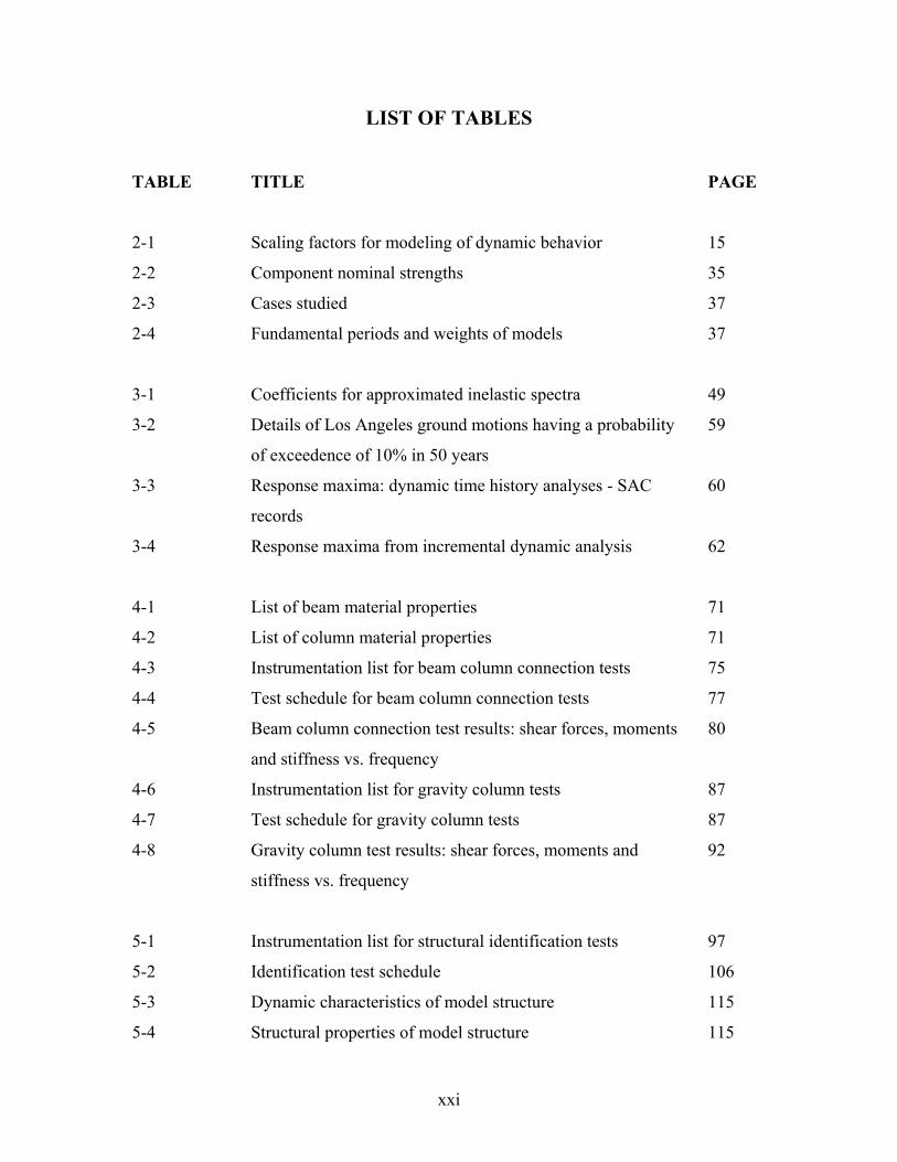
LIST OF TABLES
TABLE TITLE PAGE
2-1 Scaling factors for modeling of dynamic behavior 15
2-2 Component nominal strengths 35
2-3 Cases studied 37
2-4 Fundamental periods and weights of models 37
3-1 Coefficients for approximated inelastic spectra 49
3-2 Details of Los Angeles ground motions having a probability
of exceedence of 10% in 50 years
59
3-3 Response maxima: dynamic time history analyses - SAC
records
60
3-4 Response maxima from incremental dynamic analysis 62
4-1 List of beam material properties 71
4-2 List of column material properties 71
4-3 Instrumentation list for beam column connection tests 75
4-4 Test schedule for beam column connection tests 77
4-5 Beam column connection test results: shear forces, moments
and stiffness vs. frequency
80
4-6 Instrumentation list for gravity column tests 87
4-7 Test schedule for gravity column tests 87
4-8 Gravity column test results: shear forces, moments and
stiffness vs. frequency
92
5-1 Instrumentation list for structural identification tests 97
5-2 Identification test schedule 106
5-3 Dynamic characteristics of model structure 115
5-4 Structural properties of model structure 115
xxii
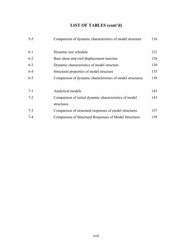
LIST OF TABLES (cont’d)
5-5 Comparison of dynamic characteristics of model structure 116
6-1 Dynamic test schedule 121
6-2 Base shear and roof displacement maxima 126
6-3 Dynamic characteristics of model structure 130
6-4 Structural properties of model structure 135
6-5 Comparison of dynamic characteristics of model structures 138
7-1 Analytical models 143
7-2 Comparison of initial dynamic characteristics of model
structures
143
7-3 Comparison of structural responses of model structures 157
7-4 Comparison of Structural Responses of Model Structures 159
1
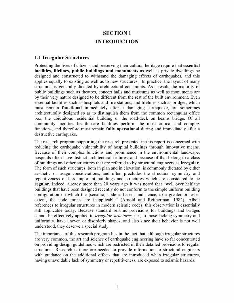
SECTION 1 INTRODUCTION
1.1 Irregular Structures Protecting the lives of citizens and preserving their cultural heritage require that essential facilities, lifelines, public buildings and monuments as well as private dwellings be designed and constructed to withstand the damaging effects of earthquakes, and this applies equally to existing as well as to new structures. In practice, the layout of many structures is generally dictated by architectural constraints. As a result, the majority of public buildings such as theatres, concert halls and museums as well as monuments are by their very nature designed to be different from the rest of the built environment. Even essential facilities such as hospitals and fire stations, and lifelines such as bridges, which must remain functional immediately after a damaging earthquake, are sometimes architecturally designed so as to distinguish them from the common rectangular office box, the ubiquitous residential building or the road-deck on beams bridge. Of all community facilities health care facilities perform the most critical and complex functions, and therefore must remain fully operational during and immediately after a destructive earthquake.
The research program supporting the research presented in this report is concerned with reducing the earthquake vulnerability of hospital buildings through innovative means. Because of their complex functions and prominence in the environmental landscape, hospitals often have distinct architectural features, and because of that belong to a class of buildings and other structures that are referred to by structural engineers as irregular. The form of such structures, both in plan and in elevation, is commonly dictated by either aesthetic or usage considerations, and often precludes the structural symmetry and repetitiveness of less important buildings and structures which are considered to be regular. Indeed, already more than 20 years ago it was noted that “well over half the buildings that have been designed recently do not conform to the simple uniform building configuration on which the [seismic] code is based, and hence, to a greater or lesser extent, the code forces are inapplicable” (Arnold and Reitherman, 1982). Albeit references to irregular structures in modern seismic codes, this observation is essentially still applicable today. Because standard seismic provisions for buildings and bridges cannot be effectively applied to irregular structures, i.e., to those lacking symmetry and uniformity, have uneven or disorderly shapes, and also since their behavior is not well understood, they deserve a special study.
The importance of this research program lies in the fact that, although irregular structures are very common, the art and science of earthquake engineering have so far concentrated on providing design guidelines which are restricted in their detailed provisions to regular structures. Research is therefore needed to provide information to structural engineers with guidance on the additional effects that are introduced when irregular structures, having unavoidable lack of symmetry or repetitiveness, are exposed to seismic hazards.
2
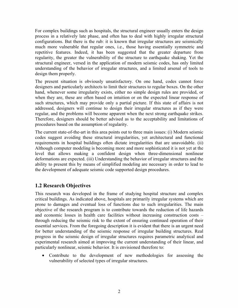
For complex buildings such as hospitals, the structural engineer usually enters the design process in a relatively late phase, and often has to deal with highly irregular structural configurations. But there is the rub: it is known that irregular structures are seismically much more vulnerable that regular ones, i.e., those having essentially symmetric and repetitive features. Indeed, it has been suggested that the greater departure from regularity, the greater the vulnerability of the structure to earthquake shaking. Yet the structural engineer, versed in the application of modern seismic codes, has only limited understanding of the behavior of irregular structures, and a limited arsenal of tools to design them properly.
The present situation is obviously unsatisfactory. On one hand, codes cannot force designers and particularly architects to limit their structures to regular boxes. On the other hand, whenever some irregularity exists, either no simple design rules are provided, or when they are, these are often based on intuition or on the expected linear response of such structures, which may provide only a partial picture. If this state of affairs is not addressed, designers will continue to design their irregular structures as if they were regular, and the problems will become apparent when the next strong earthquake strikes. Therefore, designers should be better advised as to the acceptability and limitations of procedures based on the assumption of regularity.
The current state-of-the-art in this area points out to three main issues: (i) Modern seismic codes suggest avoiding these structural irregularities, yet architectural and functional requirements in hospital buildings often dictate irregularities that are unavoidable. (ii) Although computer modeling is becoming more and more sophisticated it is not yet at the level that allows making a confident design when three-dimensional nonlinear deformations are expected. (iii) Understanding the behavior of irregular structures and the ability to present this by means of simplified modeling are necessary in order to lead to the development of adequate seismic code supported design procedures.
1.2 Research Objectives This research was developed in the frame of studying hospital structure and complex critical buildings. As indicated above, hospitals are primarily irregular systems which are prone to damages and eventual loss of functions due to such irregularities. The main objective of the research program is to contribute towards the reduction of life hazards and economic losses in health care facilities without increasing construction costs – through reducing the seismic risk to the extent of ensuring continued operation of their essential services. From the foregoing description it is evident that there is an urgent need for better understanding of the seismic response of irregular building structures. Real progress in the seismic design of irregular structures requires parametric analytical and experimental research aimed at improving the current understanding of their linear, and particularly nonlinear, seismic behavior. It is envisioned therefore to:
• Contribute to the development of new methodologies for assessing the vulnerability of selected types of irregular structures.
3
• Contribute to the development of simplified nonlinear procedures for modeling, simulation (analysis) and damage prediction of common classes of irregular structures.
The global frame of this research is to contribute towards achieving these objectives by mobilizing the complementary expertise in seismic design and vulnerability assessment with advanced computational simulations and static, quasi-dynamic and shake-table testing, and by applying modern protective systems and strengthening techniques for retrofitting of existing buildings. The achievement of these objectives is being pursued through the realization of several tasks, as outlined subsequently.
1.3 Irregular structures Present State of Knowledge. Most of the engineering knowledge on the seismic response of buildings and bridges has been derived for structures having regular configurations.
Regularity usually means structural symmetry and uniformity, i.e., small variations of assemblages and member dimensions vertically as well as horizontally, continuous lateral and vertical load resistance system, and no abrupt changes in the paths of loads, either vertical or horizontal. It also means diaphragm continuity, i.e. uninterrupted floor slabs in buildings and decks in bridges, practically small variations in mass, strength and stiffness along the building height, and uniform equal-level foundation system.
Irregularity is the absence of some of these features. Past earthquakes have repeatedly shown that structures with irregular configurations suffer greater damage than those with regular ones, and this has been the case even when the former (irregular structures) were well designed and constructed. In regular structures the inelastic demand produced by strong earthquakes is usually well distributed throughout the structures, resulting in wide dispersion of energy dissipation and damage, and, indeed, the concept of structural regularity has been represented as synonymous to uniform damage distribution (Chung, Meyer and Shinozuka, 1987, Mazzolani and Piluso 1996). On the other hand, inelastic behavior in irregular systems tends to concentrate in the zones of irregularity, leading to failure of members there, and thus precipitating progressive structural collapse. Also, some structural irregularities are difficult to model analytically, particularly when elastic analysis is performed, leading to underestimating stress concentrations. Indeed, the role of the many parameters affecting the response of irregular structures is not well understood. It appears that the distinction between regular and irregular structures has been introduced into seismic codes in order to distinguish between cases to which the results of studies on simple models can be extended and to those they cannot. Indeed, this difficulty and the resulting limitations lead seismic regulations to encourage engineers design exclusively structures with regular characteristics, and to discourage, often by means of prohibitive sanctions, irregular ones. Although such practice is good, it is too restrictive and limiting innovative architectural developments.
Whereas it is known that the vulnerability of irregular structures is higher than that of regular ones, the quantification is not a trivial task, particularly since it depends on the limit states that have to be satisfied. The procedures to predict their response should
4
consider the unique modes of failure at discontinuities or in torsion, and their effects on nonstructural components. For this purpose, better understanding of response, which can be achieved through more adequate modeling and extensive parametric studies, will be required. This, in turn, will help define limit states in terms of local damage to a single component or to an assembly thereof (a substructure). This is of particular importance for essential facilities for which the limit state should be “operational”, rather than “life safe” (the latter being the philosophy on which 20th century seismic codes is based). Whereas the vulnerability of some types of irregular structures may be estimated by adjusting presently available techniques, in some other cases the limit states can only be obtained from extensive parametric studies substantiated by well-controlled experiments of substructures or full structural models. Indeed, the paucity of experimental validation and substantiation of theoretical research is a serious limitation of present design approaches, and unless resolved is likely to hamper the updating process of earthquake design procedures and provisions for irregular structures. The recognition of the urgent need to ameliorate this state of affairs is one of the main driving forces behind the present research program.
It has been shown that it is often feasible to design an irregular structure to possess adequate seismic safety. To obtain satisfactory ductile behavior in an irregular structure, it is necessary to consider irregularity in the design process in a rational way, and this in terms of ductility capacity drift, displacement, and strength. To be able to deal with irregularity in these general terms is presently beyond the skills of the structural designer. However, studies seem to suggest that simplified rules for the design of irregular structures formulated to fit within the framework of standard design procedures, yet leading to a reasonably uniform damage distribution, at least for the more common types of irregularity, can be developed. The final definition of these rules, and their calibration by means of extensive analytical simulations and supporting experimental studies, represent the main outcome of the proposed research project.
Furthermore, besides the problems of irregularity in new construction, irregularity effects in existing buildings need also be addressed. The analysis of damage from recent earthquakes shows clearly that among existing structures, irregular structures are the ones most prone to catastrophic failures, and therefore the ones most badly needing rehabilitation. In spite of this evidence, it is still difficult to classify the existing structural heritage in terms of regularity. Once the effects of structural irregularity have become better understood, it will be possible to derive some practical guidelines designed to enforce on them a more regular seismic response. In order to do so it is necessary to examine critically the available provisions for assessment of vulnerability, redesign and retrofit of existing buildings. As there is only limited experience in the application of these provisions, another objective of the proposed research program is the evaluation, by means of case studies, of the proposed procedures for hospital structures. Moreover, the research should address the development of new procedures and recommendations when the provisions fail to address more complex irregular structures. The case studies to be carried out would also be instrumental for the preparation of a critical review of the present approaches to upgrading and retrofit.
5
1.4 Irregularities in Major Health Care Facilities Urban medical centers and large general hospitals usually consist of dense groupings of large, mostly multistory, buildings. The irregularities often encountered in these buildings are (following BSSC, 1989).
• Irregularities of building configuration in both vertical and horizontal planes.
• Combination of setbacks and or wings of different heights, re-entrant corners and structural discontinuities between major structural elements of building, e.g.: weak and/or soft story, higher stories columns stopped at second floor.
• Inadequate connections between structural elements
• Adjacent buildings, often with floors at different levels – pounding
• Modification of structural response by stiff nonstructural elements: short columns, induced eccentricity, and stress concentration.
Note that usually the first two classes are referred to as irregularities, and this designation is adopted in the present report.
Although retrofit of hospitals may not be cost effective, simple solutions avoiding major disruptions and avoiding the undesired effects of irregularities may prove to be useful.
1.5 Background on Irregular Structures Studies As already noted, the seismic behavior of irregular structures is less predictable, and has been less satisfactory than that of regular ones. Whereas there is no evidence to suggest that in general horizontally irregular structures have in past earthquakes fared worse than vertically irregular ones, most of the past research effort has focused on the effects of the former irregularity, namely, plan asymmetry. Less attention has been paid to vertically irregular structures, including to setback ones - which are the subject matter of the present task. This state of affairs may perhaps be attributed to the relative ease of classifying and modeling asymmetric structures, i.e., either as mass or stiffness eccentric on the one hand, and the difficulty in organizing the different types of vertical irregularity into well defined categories. Also, the two noted earthquake engineering pioneers: Rosenblueth (1957) and Housner (1958) were interested in the effects of asymmetry and hence gave a strong impetus to research on seismic torsional effects. Developments in that area were reviewed by Rutenberg (1992, 1997, 2002).
Setback structures form an important sub-class of irregular structures, combining in the general case both vertical and horizontal irregularities. These structures are only vertically irregular when the base and the tower, or towers, are symmetric with respect to the same two axes of symmetry. Yet, when they are monosymmetric and the seismic input is acting only along the axis of symmetry they are only vertically irregular (“symmetric” setback structures), irrespective the number of towers they have. The model studied herein is of this type.
Early studies on setback structures indicated that, due to higher modes effect, the equivalent lateral force procedure is not appropriate and could lead to unconservative
6
designs. Hence, special design rules were devised by seismic codes for “regular” setback structures in order to obviate the need to perform dynamic analysis. However, it was recognized that such rules cannot address the infinite possible combinations of vertical irregularity, and for these structures modal analysis was recommended. It was also recognized that for buildings with small appendages even this approach should be used carefully in view of closely spaced natural periods. A review of relevant studies and code provisions on “symmetric” setback structures up to the mid 1980’s is given by Wood (1986). Later studies on the linear behaviour of setback structures came to similar conclusions.
There are not many studies on the nonlinear seismic behavior of setback structures, and to the knowledge of the authors there are none on multi-tower ones. Pekau and Green (1974) were perhaps the earliest to study the inelastic seismic behavior of setback frame structures. They concluded that large towers (>2/3 of base width) have little effect on response, and that for small towers (width and height) elastic analysis fails to predict the severe tower response.
Higher modes effects above the setback were again observed by Humar and Wright (1977), who showed that simple single mode analysis such as the equivalent lateral load procedure, was insufficiently accurate to predict the response. Humar and Wright (1977), Aranda (1984) - using soft soil records, Sobaih et al (1988), and Shahrooz and Moehle (1990) noted a substantial increase in ductility and drift demands above the setback level relative to uniform buildings. Humar and Wright also noted a substantial increase in shear at the notch. More recently Mazzolani and Piluso (1996) advocated lowering the force reduction factor depending on a “setback irregularity index” they proposed. The response of setback wall-frame structures was studied by Costa et al (1988) and Duarte and Costa (1988). They reported an increase in the ductility demand just above the notch on the order of 2 relative to the reference uniform structures. Some insight into the behavior of symmetric setback frame structures can be gained from Al-Ali and Krawinkler’s (1998) extensive parametric study on vertical irregularities in a symmetric single bay 10-story frame modeled as a discrete shear beam (“column hinge model”). These are represented as variations in the distribution of mass, stiffness and strength along the height. They found that drift and ductility are more sensitive to irregularities in stiffness than in mass, and very strongly affected by variations in strength. Hence they concluded that design should explicitly consider inelastic deformation demand.
The lateral – torsional response of asymmetric setback shear buildings was studied by Duan and Chandler (1995) who proposed a modified equivalent lateral force procedure. However, it is debatable whether shear beam modeling can adequately account for the notch effect. It is interesting to note that the studies of Wood (1986, 1992) and Pinto and Costa (1995) concluded that the response of setback and regular structures did not differ.
The paucity of experimental data on the seismic behavior of irregular structures has already been noted. The only such studies are the shake-table and static tests of Shahrooz and Moehle (1990) and of Wood (1986,1992). Whereas the 1990 study revealed that concentration of damage was to be expected in elements close to the setback level – the notch effect - and proposed procedures to overcome the problem, the 1992 study concluded, as already noted, that the response of setback structures was governed by the first mode, and hence there was no need to devise special rules for their design. The only
7
other shake-table tests were done on a 3-storey steel frame scale model, carried out in the Earthquake Engineering Research Centre of the University of Bristol (De Stefano et al 2001), however, these tests were performed on asymmetric and not setback structures. Therefore it seems to be a need for additional data for setback structures.
Wong and Tso (1994) and Tso and Yao (1995) concluded again that the static code procedure was inadequate, and proposed modification factors to bring the code provision more in line with the expected nonlinear response.
Several studies were very recently reported at the 13th World Conference on Earthquake Engineering in Vancouver. Tena-Colunga (2004) found no evidence for adverse effects due to the presence of regular setback. Romao, Costa and Delgado (2004) came to a similar conclusion, albeit with some exceptions (apparently design not following capacity design principles). The study on structures with regularly stepping setbacks by Birajdar, and Nawawade (2004) is somewhat beyond the scope of the present study.
From this short review it is apparent that the seismic behavior of setback structures, which is manifested in higher modes effects and strain concentrations at the discontinuity (notch), is quite complex and that simple modifications to the present static provisions are unlikely to provide the required safety to setback frame structures.
1.6 The Present Task Within the general framework described in the preceding paragraphs the present task is mainly concerned with irregularities in steel buildings belonging to the class of structures listed as the first and second items in Section 1.4, namely setback structures. In many cases such structures are asymmetric with respect to at least one horizontal axis. Specifically, it involves studying, experimentally as well as analytically, the seismic behavior of vertical irregularities of structures, including one or more setbacks and multiple “towers”. The experimentation is required to produce information on the inelastic behavior of setback structures near collapse. Such behavior dominates the complex effects of vertical irregularity. The following activities are reported herein:
• Develop, design and construct a versatile scale model (referred here also as a reconfigurable model or a “benchmark structure”) capable of sustaining extensive damage without collapse consisting of sacrificial elements - and an undamageable independent gravity load-carrying system, with a view to enabling future experimental studies of different types of irregularity.
• Develop an experimental database for behavior of irregular structures with setback, near collapse.
• Evaluate of existing analytical procedures for quantification of response of irregular structures and contribute to the development of simplified analytical techniques.
This study addressed the first task as a base for the implementation of the second task, where in turn served as a base for the implementation of the third task.
8
1.6.1 Benchmark Structure In order to achieve the overall objectives of the program it is first necessary to design a structural scale model for calibration and qualification of analytical model studies and simulations, i.e., a benchmark structure. To be of practical value it has to be sufficiently versatile so that its variants can represent the types of irregularity that are often encountered in major health care facilities, namely vertical and horizontal irregularities combining setbacks or wings of different heights. At the same time, mainly for comparison purposes, it should also be able to represent the regular counterparts of the irregular model. Moreover, since nonlinear behavior modifies the properties of structural members and their connections it is necessary to design the model structure so that damaged parts can readily be replaced. The choice of steel as the structural material makes this task easier. Furthermore, for ease of assembly and fast replacement of damaged elements, i.e., interchangeability, an effort has been made to standardize the structural elements. Thus, the frames are designed using only two types of beam elements and one column element, and there is only one type of gravity load carrying columns. In fact, the use of two rather than one beam element is due to the decision to have different internal and external spans. A single joint element connects the beams and columns, and identical spherical steel hinges transfer the weight to and from the gravity columns. Full separation of the lateral load resisting system from gravity supporting elements is usually not easy to implement. The decision to do so for the model was motivated by the need for an undamageable vertical load system capable of sustaining the gravity loads under all circumstances of damage to the lateral load resisting system expected in earthquakes. Moreover, the gravity system can provide the framing for installing non-damageable energy dissipation devices and provide restraint in the transverse direction for symmetric models displaying planar behavior. Relieving the lateral load resisting system from gravity loads requires very low fabrication and erection tolerances as well as special detailing of pinned connections to the frame joints.
1.6.2 Testing Procedures The benchmark model is subjected to series of tests to verify its capability to adequately simulate behavior of irregular structures. A careful evaluation of the model is essential to assess its usability. First the materials of beams and columns are tested following ASTM protocol, This is followed by tests of components such as a cruciform subassembly comprising of the beam to column joint block with a half length beam on each side and a half length column above and below it. The performance of gravity columns and their connections is also evaluated. Finally the full model is subjected to a loading sequence consisting of gradually increasing base motion. A complete description of the test procedures for the validation of the benchmark structure model is presented in Sections 4 and 5.
1.7 Analytical Modeling The evaluation of irregular structures relies usually on three dimensional (3-D) finite element models and analysis in elastic range. The seismic codes recommend modeling mildly irregular structures as regular and then performing either elastic modal analysis or nonlinear static analyses. The evaluation of the irregular model in this study is done using
9
nonlinear models subjected to inelastic dynamic analyses or equivalent inelastic static approximations. The structures with severe irregularities undergoing inelastic deformations cannot be analyzed by either modal or nonlinear static analyses as currently available. This report presents the analytical modeling using both nonlinear inelastic dynamic simulations as well as attempts to develop simplified evaluation procedures based on capacity-demand static analysis using adaptable loading shapes (see also Sections 3 and 7).
1.8 Report Organization The general background, motivation for the research program as a whole and its present phase have been presented in this section, as well as a summary of the results obtained so far.
Section 2 presents the principles used for design of the versatile structural model, outlines its layout and configuration considering all constraints, including those set by the shake-table and design requirements, describes the example test specimen, and shows the structural details of each individual structural element.
Section 3 describes the preliminary analytical evaluation of the structural model. First, applicable analytical techniques are described. Second, spectral capacity analysis is performed on the model structure for rapid response evaluation. Third, from the results the global properties of the model are evaluated.
Section 4 evaluates experimentally the structural properties of the model components. First, the testing procedure (“protocol”) for the as-built material properties is described. Then the structural properties of the beams, columns and connections in the exterior frames and the gravity columns, as based on the test results are presented in a tabular form. The effects of the connection imperfections are also described.
Section 5 evaluates the global structural properties of the model. First, the test set up is described in detail. Second, the chosen test protocol is presented. Third, the dynamic identification procedures used are presented and explained. Finally, the results of the experimental identification and analytical evaluation are compared and discussed.
Section 6 presents the shake-table tests and their results for the sample irregular structure. First the test setup, including instrumentation procedure, and the protocol, namely, dynamic pushover, are described. Next, the experimental results of the static and dynamic pushover up-to-failure testing, including global structural and dynamic properties identification, are presented and discussed.
Section 7 compares the experimental and analytical pushover response. Three sets of analytical results are presented: (i) based on a pre-testing model, (ii) based on as-built material properties, and (iii) based on components properties with semi-rigid joints. These are then compared to the experimental results. A discussion of the comparative results follows.
Section 8 is a general summary of research results and the conclusions pointing to further complex issues to be resolved.

11
SECTION 2 VERSATILE MODEL – PRINCIPLES AND LAYOUT
2.1 Principles and Objectives
It is important to understand that the seismic behavior of irregular steel structures is in the inelastic range since many structures are expected to experience some damage under moderate or severe earthquakes. There are very few experimental studies on irregular structures under seismic loading, in particular those experiencing inelastic deformations, and there is a need to ascertain whether standard analytical techniques are applicable to them. Scale models are necessary to simulate typical building construction practices. A reconfigurable scaled model was developed and constructed to simulate various typical irregularities and inelastic behavior without collapse. The development of such versatile structural model is presented in this Section. A typical configuration of such model was tested on the shake table in the University at Buffalo’s Structural Engineering and Earthquake Simulation Laboratory (SEESL). Testing is described in Section 6.
2.1.1 Model of Frame Structure The reconfigurable structural model developed for this study was designed to be a reconfigurable three-story steel structure. A series of different models can be obtained by such reconfiguration. Besides being considered as representative of typical low-rise steel structures in the United States, three story structures are the simplest structures that represent typical multi-story buildings with a ground floor, middle floors, and a top floor. Taking these structures as prototypes, a number of different scaled models consisting of regular and irregular structures were developed.
2.1.2 Two Independent Support Systems The reconfigurable structural model presented herein was designed to have separate lateral and vertical support systems. The lateral support system was designed to be damageable, while the vertical support system is undamageable. The two systems are completely independent. The rationale for having two separate systems is to have damage concentrated in the sacrificial elements while the other elements remain usable. Another reason for the separate support systems is to have a model that can be tested without a need for an additional supporting structure as a fail-safe feature in case of structural collapse. In real construction the complete separation of lateral and vertical support systems is not always realistic, although conventional structural systems are commonly designed with partial separation of gravity load supporting systems, i.e., shear wall for lateral resisting system which only carries a small portion of gravity loads, and leaning gravity columns that still provide some lateral load support for the structural frame. However, the complete separation of the lateral and vertical load resisting systems in this study provides an opportunity to investigate the behavior of the model in the “near collapse” condition. The vertical load system can support gravity loading as long as the

12
lateral load resisting system retains some carrying capacity, which allows sufficient data to be gathered on model behavior, but avoids a complete structural failure, which could be very costly.
2.1.3 Removable-Replaceable Lateral Load Resisting Systems The lateral support system consists of beams and columns similar to those in typical structural frames. However, these are specifically designed to carry only lateral loads. They are designed with beams and columns as sacrificial elements, since damage due to lateral forces is expected to occur in the lateral load resisting system. Therefore, these elements are designed to be removed and replaced easily if structural repair is needed. A special element is used to connect beams and columns to avoid damaging the connection. The connection is rigid and designed to survive any damage to the elements connected to it. The lateral load resisting system differs from one configuration to another. A host of lateral resisting systems can be formed and tested in this versatile model.
2.1.4 Undamageable Vertical System As noted the vertical support system consists of gravity columns only. They can be considered as ‘leaning columns’ since they have no lateral resistance. Since the elements are designed to be undamageable they are reusable. A special connection is used to connect gravity columns to the ground and floor plates. This connection must transfer only axial load and hence is designed to have no shear or moment resistance. More details about the implementation of the gravity columns is presented in section 2.2.2.3.8
2.1.5 Floor System The floor system is also designed to be undamageable. This is mainly due to the need to have very large floor masses in order to satisfy similitude requirements. The steel floor plates are strong and rigid both in plane and out of plane, and hence are reusable. Several requirements were considered in the detailed design of the floor system: dimensional scaling, including model weight, available space of the testing facility, and capacity of the lab for handling of the floor system.
2.1.6 Interchangeability: Removable and Reusable Standard Elements The model was designed so that it could be tested up to a very large inelastic deformation. It was expected that some damage would occur to the structure, but this should be repairable or replaceable easily for the next stage of the experimental program. If additional secondary devices were necessary, they could also be installed with little difficulty. Therefore, model flexibility is a basic requirement for the design. Hence, the removable elements and easy access for placing additional elements and devices were the preferred options for the experimental program. Several design criteria were developed on the basis of these requirements. To ensure ease of assembly and replacement of damaged parts, the model is designed with standardized elements, i.e. two types of
13
beams, two types of columns, one type of gravity columns, and one type of special connection.
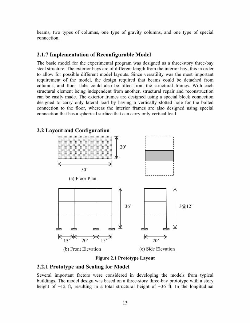
2.1.7 Implementation of Reconfigurable Model The basic model for the experimental program was designed as a three-story three-bay steel structure. The exterior bays are of different length from the interior bay, this in order to allow for possible different model layouts. Since versatility was the most important requirement of the model, the design required that beams could be detached from columns, and floor slabs could also be lifted from the structural frames. With each structural element being independent from another, structural repair and reconstruction can be easily made. The exterior frames are designed using a special block connection designed to carry only lateral load by having a vertically slotted hole for the bolted connection to the floor, whereas the interior frames are also designed using special connection that has a spherical surface that can carry only vertical load.
2.2 Layout and Configuration
15’ 20’ 15’
20’
20’
(c) Side Elevation
(a) Floor Plan
(b) Front Elevation
50’
36’ 3@12’
Figure 2.1 Prototype Layout
2.2.1 Prototype and Scaling for Model Several important factors were considered in developing the models from typical buildings. The model design was based on a three-story three-bay prototype with a story height of ~12 ft, resulting in a total structural height of ~36 ft. In the longitudinal
14
direction the interior bay was selected to be ~20ft. wide, and the exterior bays were ~15ft. The transverse direction width (of the slice of building) was selected to be ~20 ft, giving a planar dimension of 20 ft x 50 ft. The prototype layout is shown in Figure 2.1.
The frame components were made of steel A36 (fy = 36 ksi) and A572/A588 Gr. 50 (fy = 50 ksi) as explained in the next sections. To avoid the need to consider soil-structure interactions, or differential settlements, the structures were assumed to be built on a stiff soil/rock.
To obtain a faithful prediction of response for the prototype structure, the model must be built as close as possible to the prototype, and this should include materials, loads, and especially dimensions. Therefore, precise geometric scale was needed. Since the physical scaled models were to be tested on the shake table in the Structural Engineering and Earthquake Simulation Laboratory (SEESL), at the University at Buffalo, the size of dimensions and mass, as well as the structural sections are controlled by the table constraints. As in any scaled model design some arbitrary decisions are unavoidable. Since the maximum available length for the model is 18ft, and a realistic number of bays is at least three, the resulting geometric scale is about three, which for framed steel structures is perhaps an acceptable minimum. This leads to a reasonable average prototype bay size of 18ft. The available width is circa 6ft. i.e., a single bay which can represent a slice of a longer structure. Thus, the structure was designed to consist of two parallel frames in the longitudinal direction. A regular story height of 12ft is thus scaled to 4ft, allowing up to a 6-story structure within the height constraints of the SEESL.
Based on these requirements, a one-third scale physical model was designed and built for the study. This scale model resulting from these considerations is the largest three story model that could be tested in the laboratory and still satisfy all the geometric constraints, yet would be large enough for obtaining accurate prediction of the response for the prototype structure.
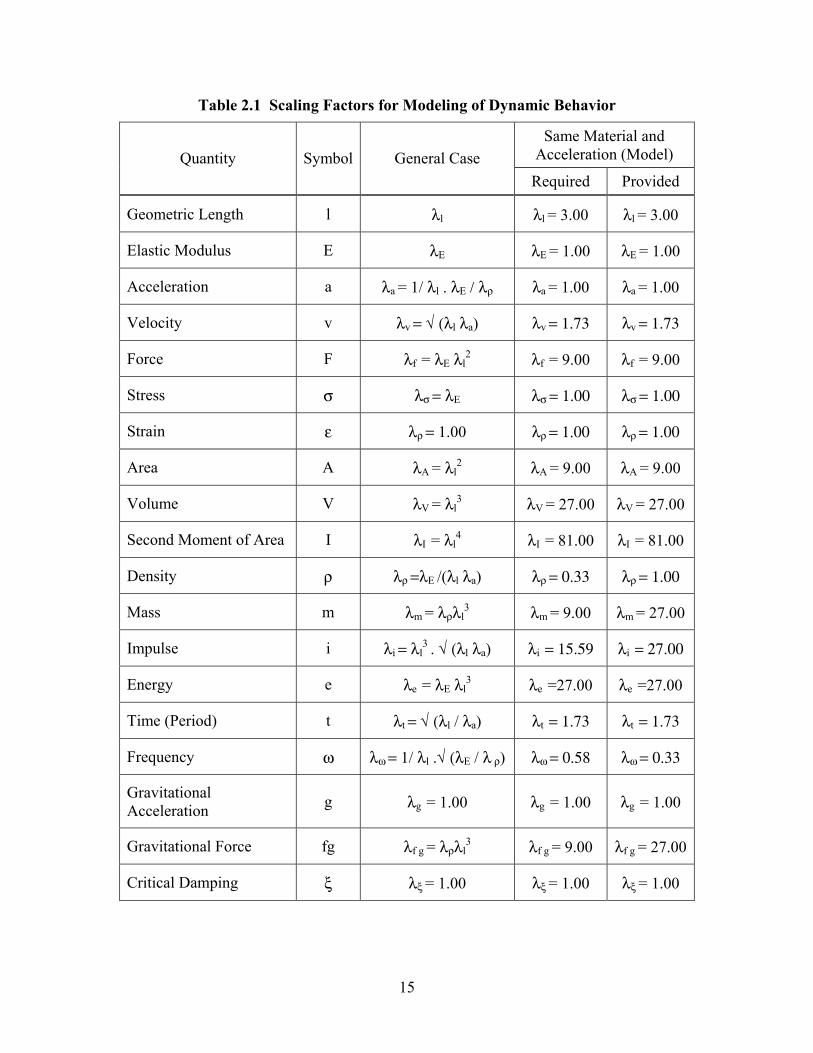
For a scale model using the same material properties and acceleration as the prototype structure, similitude requires to have the mass scaled up by λ2, λ being the geometric scale factor (a similitude table for scaling various parameters for dynamic modeling is given in Table 2.1). Following this requirement, a relatively very heavy floor must be provided. To obviate the need for attached masses – a standard but somewhat cumbersome practice – it was decided to use thick steel plates as floor slabs (3.5” thick) to be pin-connected to the structural frames at the beam-column joints (see detailed description in the next section). Two such plates per floor allow the required flexibility in the geometric configuration of the model. Typical details of alternative structures are shown in Figure 2.18. Note that two 3.5” x 7’ x 10-1/2’ coupled steel plates weigh circa 18 kips, i.e., 54 kips for a three story structure, which is less than the available carrying capacity of the shake table without the foundation block. (The structure and the foundation block together weigh 89 kips while the shake table capability is 110 kips).
15
Table 2.1 Scaling Factors for Modeling of Dynamic Behavior
Same Material and Acceleration (Model) Quantity Symbol General Case
Required Provided
Geometric Length l λl λl = 3.00 λl = 3.00
Elastic Modulus E λE λE = 1.00 λE = 1.00
Acceleration a λa = 1/ λl . λE / λρ λa = 1.00 λa = 1.00
Velocity v λv = √ (λl λa) λv = 1.73 λv = 1.73
Force F λf = λE λl2 λf = 9.00 λf = 9.00
Stress σ λσ = λE λσ = 1.00 λσ = 1.00
Strain ε λρ = 1.00 λρ = 1.00 λρ = 1.00
Area A λA = λl2 λA = 9.00 λA = 9.00
Volume V λV = λl3 λV = 27.00 λV = 27.00
Second Moment of Area I λI = λl4 λI = 81.00 λI = 81.00
Density ρ λρ =λE /(λl λa) λρ = 0.33 λρ = 1.00
Mass m λm = λρλl3 λm = 9.00 λm = 27.00
Impulse i λi = λl3 . √ (λl λa) λi = 15.59 λi = 27.00
Energy e λe = λE λl3 λe =27.00 λe =27.00
Time (Period) t λt = √ (λl / λa) λt = 1.73 λt = 1.73
Frequency ω λω = 1/ λl .√ (λE / λ ρ) λω = 0.58 λω = 0.33
Gravitational Acceleration g λg = 1.00 λg = 1.00 λg = 1.00
Gravitational Force fg λf g = λρλl3 λf g = 9.00 λf g = 27.00
Critical Damping ξ λξ = 1.00 λξ = 1.00 λξ = 1.00
16
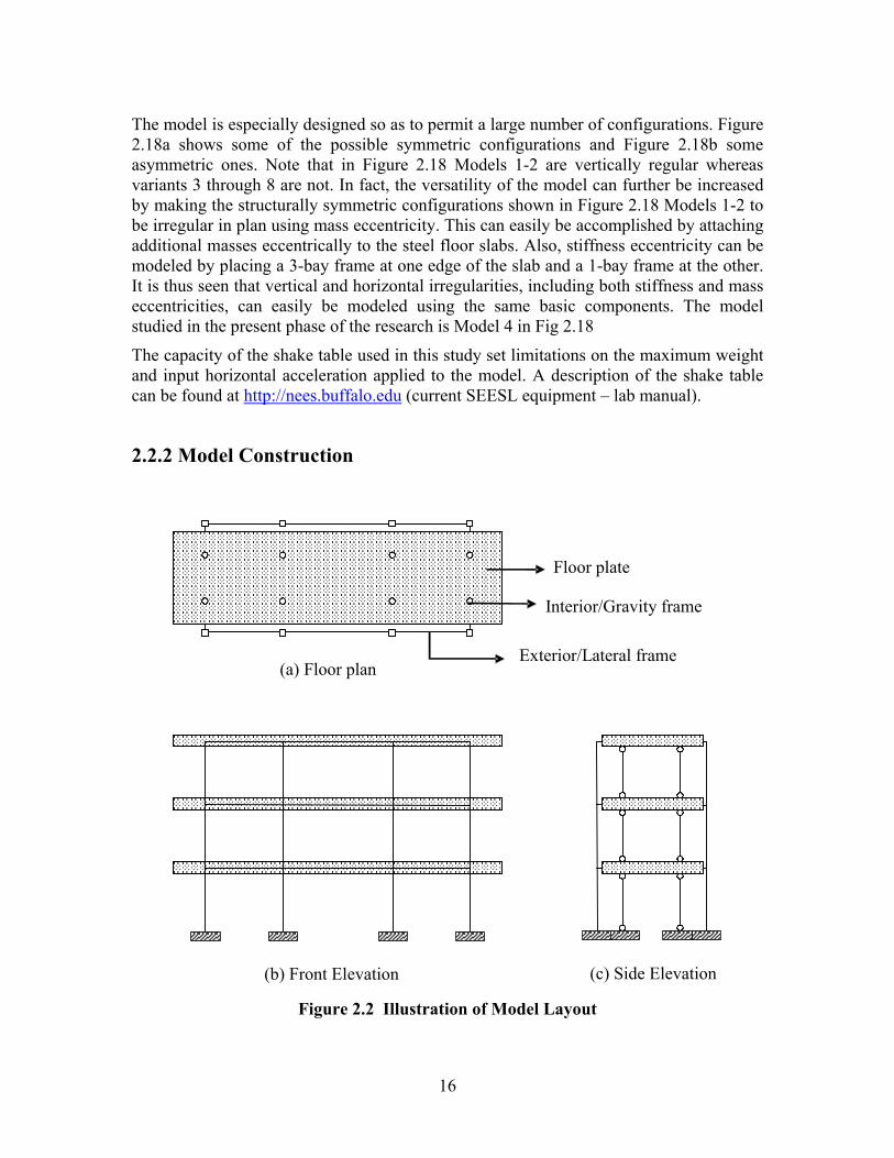
The model is especially designed so as to permit a large number of configurations. Figure 2.18a shows some of the possible symmetric configurations and Figure 2.18b some asymmetric ones. Note that in Figure 2.18 Models 1-2 are vertically regular whereas variants 3 through 8 are not. In fact, the versatility of the model can further be increased by making the structurally symmetric configurations shown in Figure 2.18 Models 1-2 to be irregular in plan using mass eccentricity. This can easily be accomplished by attaching additional masses eccentrically to the steel floor slabs. Also, stiffness eccentricity can be modeled by placing a 3-bay frame at one edge of the slab and a 1-bay frame at the other. It is thus seen that vertical and horizontal irregularities, including both stiffness and mass eccentricities, can easily be modeled using the same basic components. The model studied in the present phase of the research is Model 4 in Fig 2.18
The capacity of the shake table used in this study set limitations on the maximum weight and input horizontal acceleration applied to the model. A description of the shake table can be found at http://nees.buffalo.edu (current SEESL equipment – lab manual).
2.2.2 Model Construction
Interior/Gravity frame
Floor plate
Exterior/Lateral frame (a) Floor plan
(b) Front Elevation (c) Side Elevation
Figure 2.2 Illustration of Model Layout
17
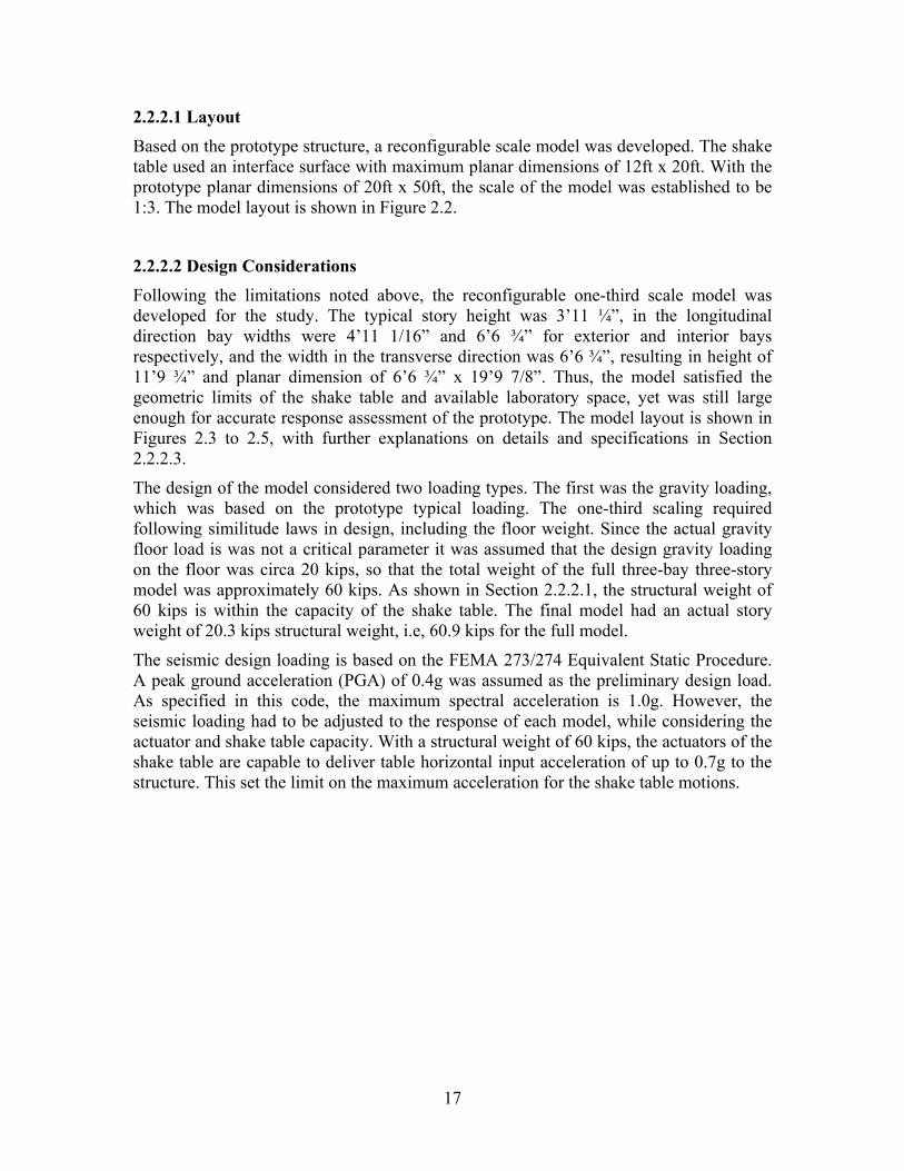
2.2.2.1 Layout Based on the prototype structure, a reconfigurable scale model was developed. The shake table used an interface surface with maximum planar dimensions of 12ft x 20ft. With the prototype planar dimensions of 20ft x 50ft, the scale of the model was established to be 1:3. The model layout is shown in Figure 2.2.
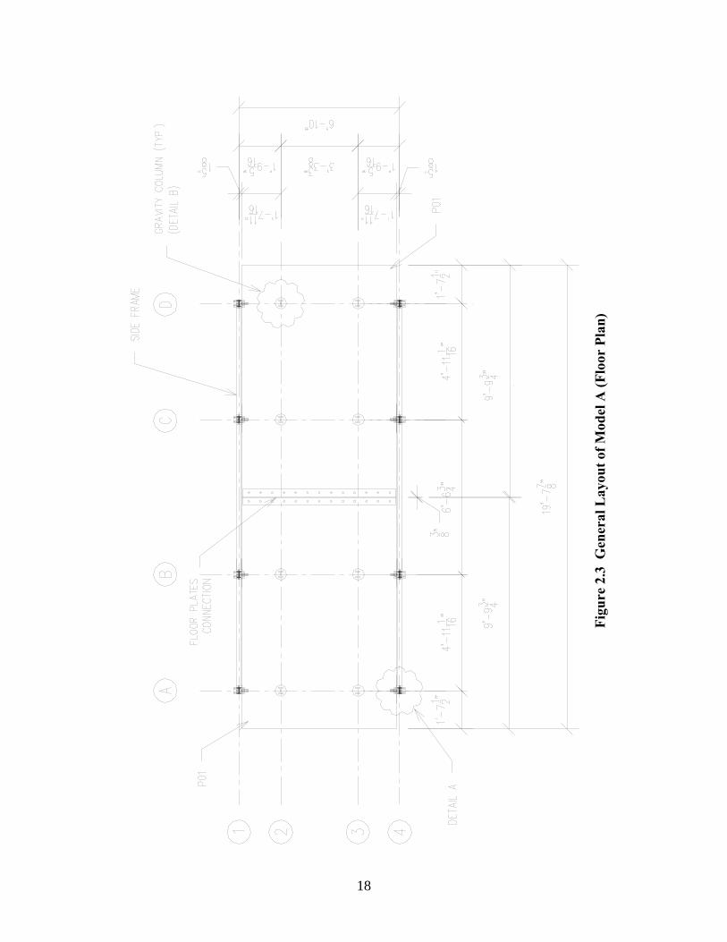
2.2.2.2 Design Considerations Following the limitations noted above, the reconfigurable one-third scale model was developed for the study. The typical story height was 3’11 ¼”, in the longitudinal direction bay widths were 4’11 1/16” and 6’6 ¾” for exterior and interior bays respectively, and the width in the transverse direction was 6’6 ¾”, resulting in height of 11’9 ¾” and planar dimension of 6’6 ¾” x 19’9 7/8”. Thus, the model satisfied the geometric limits of the shake table and available laboratory space, yet was still large enough for accurate response assessment of the prototype. The model layout is shown in Figures 2.3 to 2.5, with further explanations on details and specifications in Section 2.2.2.3.
The design of the model considered two loading types. The first was the gravity loading, which was based on the prototype typical loading. The one-third scaling required following similitude laws in design, including the floor weight. Since the actual gravity floor load is was not a critical parameter it was assumed that the design gravity loading on the floor was circa 20 kips, so that the total weight of the full three-bay three-story model was approximately 60 kips. As shown in Section 2.2.2.1, the structural weight of 60 kips is within the capacity of the shake table. The final model had an actual story weight of 20.3 kips structural weight, i.e, 60.9 kips for the full model.
The seismic design loading is based on the FEMA 273/274 Equivalent Static Procedure. A peak ground acceleration (PGA) of 0.4g was assumed as the preliminary design load. As specified in this code, the maximum spectral acceleration is 1.0g. However, the seismic loading had to be adjusted to the response of each model, while considering the actuator and shake table capacity. With a structural weight of 60 kips, the actuators of the shake table are capable to deliver table horizontal input acceleration of up to 0.7g to the structure. This set the limit on the maximum acceleration for the shake table motions.
Fi
gure
2.3
Gen
eral
Lay
out o
f Mod
el A
(Flo
or P
lan)
18
Fi
gure
2.4
Gen
eral
Lay
out o
f Mod
el A
(Fro
nt E
leva
tion)
19

Fi
gure
2.5
Gen
eral
Lay
out o
f Mod
el A
(Sid
e E
leva
tion)
20

21
2.2.2.3 Components
2.2.2.3.1 Damageable Lateral Support System The Strong Columns Weak Beams concept was applied for the design of the side, lateral load resisting frames. This concept assumes that plastic hinging occurs at beam ends and at the bottom of the first floor columns. Therefore, the general collapse mechanism of the structure is of the ‘Beam-Sway Mechanism’ type. This mechanism is preferred, especially if large displacement ductilities are required.
The preliminary design was carried out to determine the size of sections to be used in the various models, using the chosen S-shape sections for beams and columns. The analysis showed that the S3x5.7 section was suitable for beams and columns for all the models. To make the structure more uniform and replaceable, the beam and column elements were fabricated from this section with two end plates of A572/A588 Gr. 50 steel welded to the S3x5.7 section to connect them to the joints.
2.2.2.3.2 Beam Designs The beams were designed based on the capacity design concept. It was expected that plastic hinges will be developed at both ends to ensure that Beam-Sway Mechanism occurs. Based on the preliminary analysis, S3x5.7 sections made of A36 steel were used for all the beams. The shear and moment capacities for beams are 15.3 kips and 60.5 kips-in, respectively. Typical moment connection end plates were used. Again, design of plates, bolts, and welds was such that connection capacity was larger than beam capacity. A description of the connection is presented subsequently in this report.
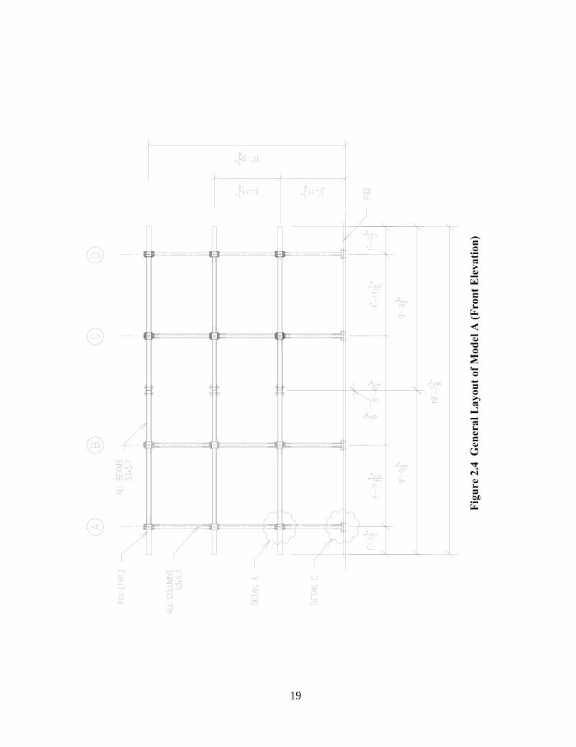
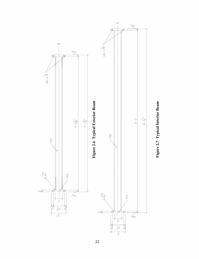
The beams are designed to allow for versatility and interchangeability of damaged parts. Therefore, all details were designed to be typical, including the end plates. However, two different beam lengths were used since the model had two unequal spans. The beam lengths of the interior and exterior spans were made as 6’ – 3 ¼” and 4’ – 7 9/16”, respectively. Typical interior and exterior beams are shown in Figures 2.6 and 2.7 respectively.
Fi
gure
2.6
Typ
ical
Ext
erio
r B
eam
Figu
re 2
.7 T
ypic
al In
teri
or B
eam
22

23
2.2.2.3.3 Column Designs
Figure 2.8 Typical Column
(a
) Ini
tial D
esig
n
(b) M
odifi
ed D
esig
n w
ith In
stru
men
tatio
n
Figu
re 2
.9 T
ypic
al F
irst
Flo
or C
olum
n
24
25
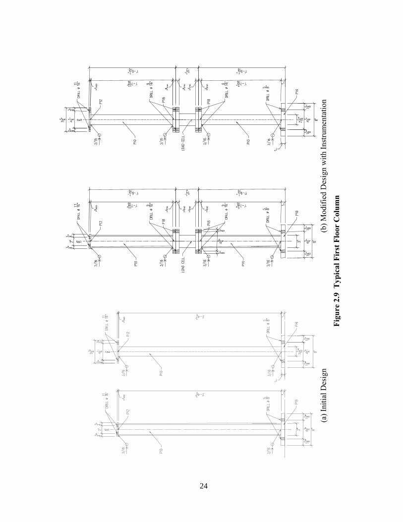
Following the beam designs, the columns are designed to ensure that the Beam-Sway Mechanism will occur. Therefore, plastic hinges were expected to develop only at the base of the structure, i.e. the bottom ends of the first floor columns, and not elsewhere. Preliminary analysis showed that Gr.50 A588/A572 S3x5.7 steel sections were suitable. The shear and moment capacities for columns are 21.3 kips and 84 kips-in, respectively. Again, typical moment connection end plates were used, and plates, bolts, and welds were capacity designed. A description of the connection is given subsequently in this report.
The columns, as the beams, were designed to improve interchangeability of parts. However, due to the need for a different base column connection, two different columns types are used. The typical column design is for the second and higher stories. It has similar connection/end plates at both ends. The typical column designs are shown in Figure 2.8. The typical first floor column has different detailing at the bottom and top ends. Note that modifications were needed for the first floor columns to allow for load cells at their mid height. The initial and modified first floor column designs are shown in Figure 2.9.
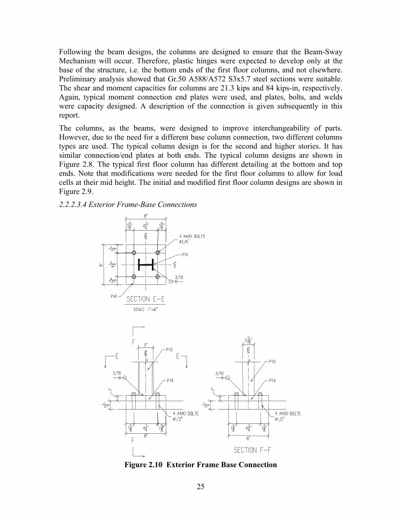
2.2.2.3.4 Exterior Frame-Base Connections
Figure 2.10 Exterior Frame Base Connection
26
The purpose of the exterior frames was to carry the lateral loads. The connection for the exterior frame-base is a typical base plate with a moment connection. The design of plates, bolts, and welds was such that the connection capacity was larger than the column capacity. Therefore, it was expected that the column will fail prior to the connection. The details of the exterior frame base connection are given in Figure 2.10.
2.2.2.3.5 Floor System: Floor Slab
Similitude rules presented earlier in this section required that the floor slab be relatively heavy. A standard practice is to have additional masses on the floor slab. However, this option requires heavy ballast, and a large space. Hence, steel plates were chosen for the model floor slabs. These plates, while providing the necessary weight, occupied very little space in the structure. Steel plates of 31/2” x 7’x 20’ weighting circa 18 kips were chosen based on geometric requirements. Together with the other elements in the structure, this resulted in the needed story weight of circa 20 kips.
Due to the limited capacity of the crane at the delivery dock of the lab facility (15 kips), each plate was divided into 2 equal parts. This was also needed for model versatility. However, if required, the two halves can be connected to form a single floor slab.
The location of gravity columns and connectors was also considered in the slab design. A grid for gravity columns was established as 10", and a grid for the holes for the exterior frames connectors was also 10". Six holes for instrumentation were also prepared in the slab. Based on the location of the holes and the minimum edge distances, the arrangement for the gravity column connections and exterior frames connectors was determined. The design of the floor plates are shown in Figure 2.11.
For the testing the structural model was placed on the shake table using two steel plates acting as the base/floorbed. The plan of the base plate is shown in Figure 2.12.
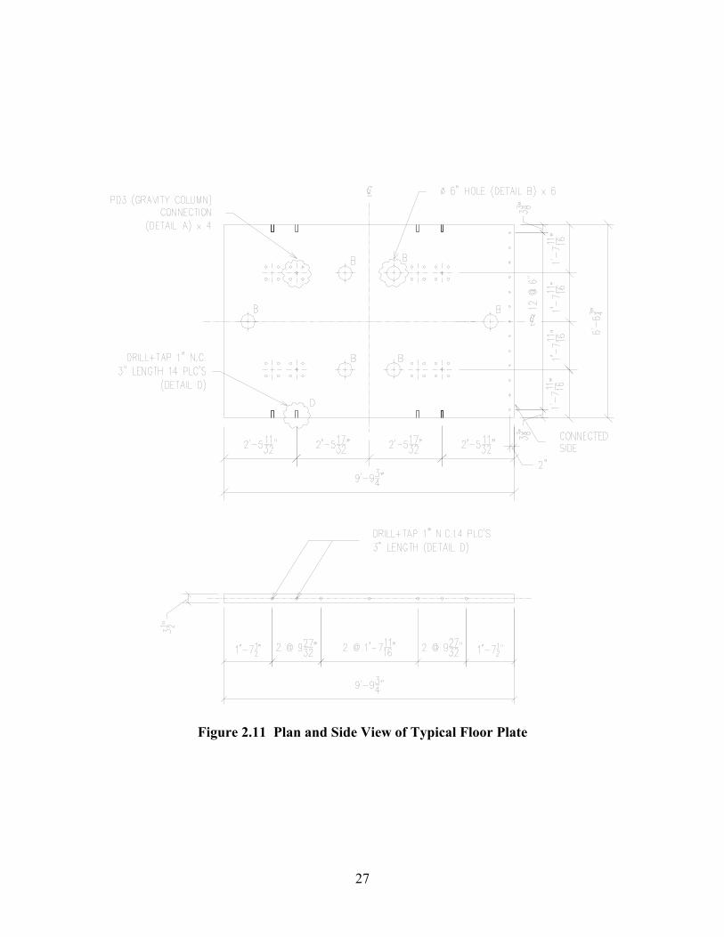
27
Figure 2.11 Plan and Side View of Typical Floor Plate
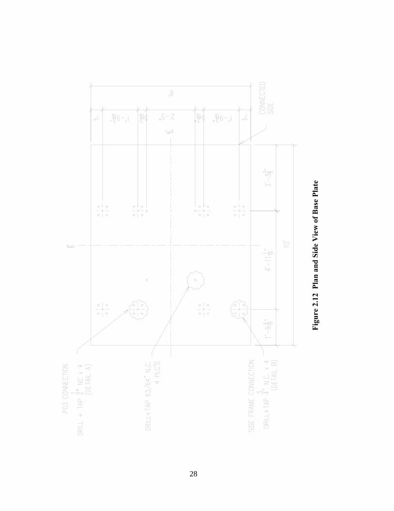
Fi
gure
2.1
2 P
lan
and
Side
Vie
w o
f Bas
e Pl
ate
28
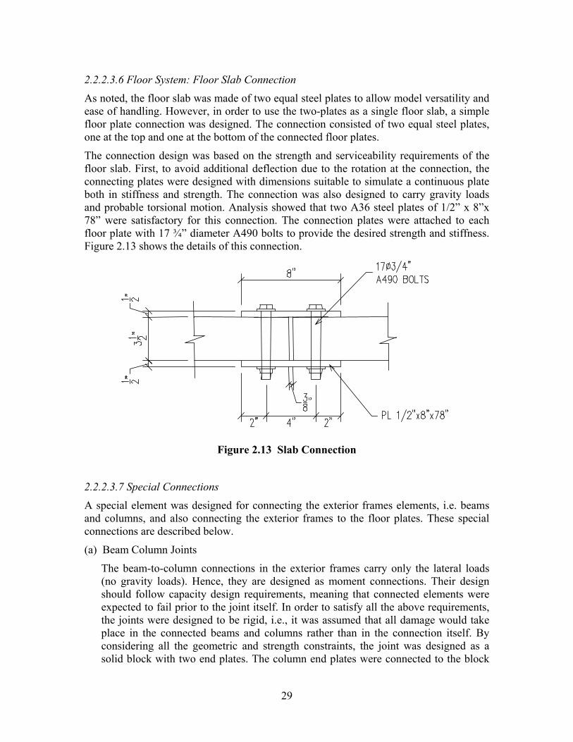
29
2.2.2.3.6 Floor System: Floor Slab Connection
As noted, the floor slab was made of two equal steel plates to allow model versatility and ease of handling. However, in order to use the two-plates as a single floor slab, a simple floor plate connection was designed. The connection consisted of two equal steel plates, one at the top and one at the bottom of the connected floor plates.
The connection design was based on the strength and serviceability requirements of the floor slab. First, to avoid additional deflection due to the rotation at the connection, the connecting plates were designed with dimensions suitable to simulate a continuous plate both in stiffness and strength. The connection was also designed to carry gravity loads and probable torsional motion. Analysis showed that two A36 steel plates of 1/2” x 8”x 78” were satisfactory for this connection. The connection plates were attached to each floor plate with 17 ¾” diameter A490 bolts to provide the desired strength and stiffness. Figure 2.13 shows the details of this connection.
Figure 2.13 Slab Connection
2.2.2.3.7 Special Connections A special element was designed for connecting the exterior frames elements, i.e. beams and columns, and also connecting the exterior frames to the floor plates. These special connections are described below.
(a) Beam Column Joints
The beam-to-column connections in the exterior frames carry only the lateral loads (no gravity loads). Hence, they are designed as moment connections. Their design should follow capacity design requirements, meaning that connected elements were expected to fail prior to the joint itself. In order to satisfy all the above requirements, the joints were designed to be rigid, i.e., it was assumed that all damage would take place in the connected beams and columns rather than in the connection itself. By considering all the geometric and strength constraints, the joint was designed as a solid block with two end plates. The column end plates were connected to the block

30
through these end plates, whereas the beam end plates were connected directly to the block. The design of the solid block included a vertically slotted hole for the connection of the exterior frame to the floor slab. Figure 2.14 shows the details of the connection.
Figure 2.14 Beam Column Joints
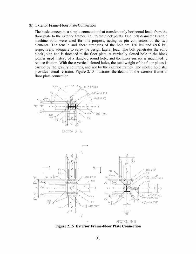
31
(b) Exterior Frame-Floor Plate Connection
The basic concept is a simple connection that transfers only horizontal loads from the floor plate to the exterior frames, i.e., to the block joints. One inch diameter Grade 5 machine bolts were used for this purpose, acting as pin connectors of the two elements. The tensile and shear strengths of the bolt are 120 ksi and 69.6 ksi, respectively, adequate to carry the design lateral load. The bolt penetrates the solid block joint, and is threaded to the floor plate. A vertically slotted hole in the block joint is used instead of a standard round hole, and the inner surface is machined to reduce friction. With these vertical slotted holes, the total weight of the floor plates is carried by the gravity columns, and not by the exterior frames. The slotted hole still provides lateral restraint. Figure 2.15 illustrates the details of the exterior frame to floor plate connection.
Figure 2.15 Exterior Frame-Floor Plate Connection
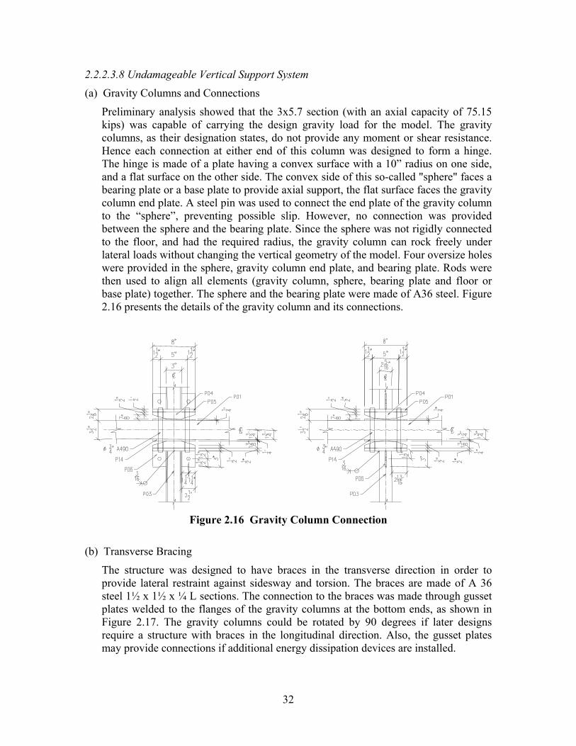
32
2.2.2.3.8 Undamageable Vertical Support System (a) Gravity Columns and Connections
Preliminary analysis showed that the 3x5.7 section (with an axial capacity of 75.15 kips) was capable of carrying the design gravity load for the model. The gravity columns, as their designation states, do not provide any moment or shear resistance. Hence each connection at either end of this column was designed to form a hinge. The hinge is made of a plate having a convex surface with a 10” radius on one side, and a flat surface on the other side. The convex side of this so-called "sphere" faces a bearing plate or a base plate to provide axial support, the flat surface faces the gravity column end plate. A steel pin was used to connect the end plate of the gravity column to the “sphere”, preventing possible slip. However, no connection was provided between the sphere and the bearing plate. Since the sphere was not rigidly connected to the floor, and had the required radius, the gravity column can rock freely under lateral loads without changing the vertical geometry of the model. Four oversize holes were provided in the sphere, gravity column end plate, and bearing plate. Rods were then used to align all elements (gravity column, sphere, bearing plate and floor or base plate) together. The sphere and the bearing plate were made of A36 steel. Figure 2.16 presents the details of the gravity column and its connections.
Figure 2.16 Gravity Column Connection
(b) Transverse Bracing
The structure was designed to have braces in the transverse direction in order to provide lateral restraint against sidesway and torsion. The braces are made of A 36 steel 1½ x 1½ x ¼ L sections. The connection to the braces was made through gusset plates welded to the flanges of the gravity columns at the bottom ends, as shown in Figure 2.17. The gravity columns could be rotated by 90 degrees if later designs require a structure with braces in the longitudinal direction. Also, the gusset plates may provide connections if additional energy dissipation devices are installed.
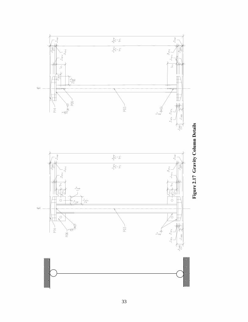
Fi
gure
2.1
7 G
ravi
ty C
olum
n D
etai
ls
33
34
2.2.2.4 Properties of Components The objectives of this study require the model to be tested in the inelastic range. Moreover, the study is aimed to evaluate structures near collapse or at collapse. Therefore, following large ductile deformations, collapse is expected to occur. Since steel can sustain large displacements prior to collapse, developing large ductilities, it was eminently suitable to fulfill the objectives of this study. As noted, the strong column - weak beam approach was implemented in the design since its beam-sway mechanism ensures high structural ductility.
The prototype structures and the model should preferably be of the same material. Hence for both the prototype and model, the material used is A36 steel for beams and A572/A588 Gr.50 steel for columns. From the available steel sections, S-shape sections were chosen for columns and beams. The S-shape sections are believed to be appropriate for small-scale modeling of typical I-shape sections. Preliminary analyses were carried out to determine the suitable S-shape sections for columns and beams. The yield and ultimate strengths were those specified for beams, columns and connection. For A36 steel, the yield strength fy is 36 ksi, and the tensile strength fu is 58 ksi. For A588 Gr.50 steel, the yield strength is 50 ksi, and the tensile strength is 70 ksi.
The axial/tension strengths of structural elements can be evaluated as:
Ty = fy. Ag (yield) (2.1)
Tu = fu Ae (fracture state) (2.2)
Where,
Ty = yield capacity
Tu = tensile strength
Ag = gross area
Ae = effective area
Since there are no holes and no eccentricity of loading, the effective area Ae is the gross area Ag.
The shear strength of structural element can be calculated as:
V = 0.6 fy Aw (2.3)
Where,
V = shear strength
Aw = web area = d·tw
The nominal moment strengths of structural element can be calculated as:
My = Sx fy (2.4)
Mp = Zx fy (2.5)
35
Where,
My = yield moment
Sx = elastic section modulus
Mp = plastic moment
Zx = plastic section modulus
Analysis shows that S3x 5.7 with cross sectional area of 1.67 in2, and Ix of 2.52 in4 is the preferred section for all beams and columns. Table 2.2 summarizes the results of the nominal strength calculations.
Table 2.2 Components’ Nominal Strengths
Tension (kips) Shear (kips) Moment (kips-in) Components
Yield Fracture Shear Yield Plastic
Column N/A N/A 15.3 84.0 97.5
Beam N/A N/A 11.0 60.5 70.2
Gravity Column 83.5 108.6 N/A N/A N/A
2.2.3 Model Configurations – Versatility 2.2.3.1 Possible Structural Configurations: Regular and Irregular Frames The main purpose of the design was to create a versatile model, so that with the same basic components different structural configurations could be assembled. Simple rearrangements of the "basic" model components shown in Figure 2.18a result in two regular structures: 3 and 5 story single-bay frames, and 5 vertically irregular 3-bay structures. Some of the possible layouts for regular and irregular structures are given in Figure 2.18. Other variations of the components are also possible. The reconfiguration uses all or some of the components developed for the basic model.
Horizontal irregularity can be also obtained with same models. The horizontal irregularity (eccentricity) can be obtained by shifting horizontally the mass center of the floors, i.e. by attaching steel strips to the floor slab (above and/or below) at a chosen eccentricity from the axis of symmetry. However, additional attention must be given to the specific effects of eccentricity and limitations of testing facilities such as the maximum horizontal offsets on shake tables.
2.2.3.2 Examples: Four Types of Structures Of the 8 variants shown in Figure 2.18 four cases were studied in some detail in preliminary analyses. The models varied in geometry, as shown in Figure 2.19.
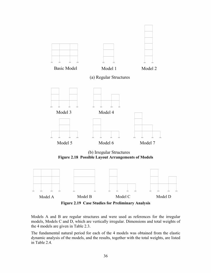
36
Model 1 Model 2
(a) Regular Structures
Model 3 Model 4
Model 5 Model 6 Model 7
Basic Model
(b) Irregular Structures Figure 2.18 Possible Layout Arrangements of Models
Model A Model D Model CModel B Figure 2.19 Case Studies for Preliminary Analysis
Models A and B are regular structures and were used as references for the irregular models, Models C and D, which are vertically irregular. Dimensions and total weights of the 4 models are given in Table 2.3.
The fundamental natural period for each of the 4 models was obtained from the elastic dynamic analysis of the models, and the results, together with the total weights, are listed in Table 2.4.
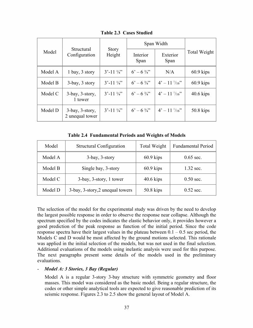
37
Table 2.3 Cases Studied
Span Width
Model Structural Configuration
Story Height Interior
Span Exterior
Span
Total Weight
Model A 1 bay, 3 story 3’-11 ¼” 6’ – 6 ¾” N/A 60.9 kips
Model B 3-bay, 3 story 3’-11 ¼” 6’ – 6 ¾” 4’ – 11 1/16” 60.9 kips
Model C 3-bay, 3-story, 1 tower
3’-11 ¼” 6’ – 6 ¾” 4’ – 11 1/16” 40.6 kips
Model D 3-bay, 3-story, 2 unequal tower
3’-11 ¼” 6’ – 6 ¾” 4’ – 11 1/16” 50.8 kips
Table 2.4 Fundamental Periods and Weights of Models
Model Structural Configuration Total Weight Fundamental Period
Model A 3-bay, 3-story 60.9 kips 0.65 sec.
Model B Single bay, 3-story 60.9 kips 1.32 sec.
Model C 3-bay, 3-story, 1 tower 40.6 kips 0.50 sec.
Model D 3-bay, 3-story,2 unequal towers 50.8 kips 0.52 sec.
The selection of the model for the experimental study was driven by the need to develop the largest possible response in order to observe the response near collapse. Although the spectrum specified by the codes indicates the elastic behavior only, it provides however a good prediction of the peak response as function of the initial period. Since the code response spectra have their largest values in the plateau between 0.1 – 0.5 sec period, the Models C and D would be most affected by the ground motions selected. This rationale was applied in the initial selection of the models, but was not used in the final selection. Additional evaluations of the models using inelastic analysis were used for this purpose. The next paragraphs present some details of the models used in the preliminary evaluations.
- Model A: 3 Stories, 3 Bay (Regular) Model A is a regular 3-story 3-bay structure with symmetric geometry and floor masses. This model was considered as the basic model. Being a regular structure, the codes or other simple analytical tools are expected to give reasonable prediction of its seismic response. Figures 2.3 to 2.5 show the general layout of Model A.
38
- Model B: 1 Bay, 3 Stories - Regular Model B is also a regular structure. The geometric layout of this model is symmetric with one bay and three stories, which can be developed from the basic model by using the mid bay only. The seismic response of Model B can be adequately predicted using codes or other simple analytical tools.
- Model C: 1 Tower/Setback - Irregular Model C is a setback structure, hence irregular. This model is developed from the basic model by removing the mid bay and one of the exterior bays on the second and third floors, thus creating a 3-bay base at first floor level and a tower on one side of the structure. The vertical irregularity can produce additional problems to the structure, such as force concentration at the tower base.
- Model D: 2 Unequal Towers - Irregular Model D is another type of structure with vertical irregularities. This model is also developed from the basic model by removing the mid bay above the first floor and one exterior bay on the third level, thus creating on each side of the model two towers with different heights. It was expected that some additional problems might occur with this configuration, such as a force concentration at the two tower bases, and asymmetry in the mode shapes.
2.2.4 Example: Selected Model for Irregular Structures Study 2.2.4.1 Objective of Experimental Study The main objective of the study was to understand better the seismic behavior of vertically irregular structures. Another objective related only to the physical experimentation was to demonstrate the ability of the example model to monitor it’s response up to collapse without damage to the vertical load resisting system. Model D described in Section 2.2.3 above appeared most suitable, mainly because it combines the quite common setback irregularity together with the multiple tower problem, - often found in hospital buildings (which was one of the main motivations for this research). In other words, this model is believed to be affected by earthquakes in a different way than Model C, due to the presence of two nonsymmetrical towers. When excited in the transverse direction this model combines vertical and horizontal irregularity. However, in the present study, the model was subjected to ground motion only in the longitudinal direction; hence only effects of vertical irregularity were studied.
2.2.4.2 Layout of Selected Model As noted, Model D is a three-bay three-story steel structure with two unequal towers. The structural sections used for beams and columns are S3x5.7. Dynamic analysis was performed on this model, and the fundamental period was found to be 0.52 sec. Figures 2.20 to 2.22 show its general layout.
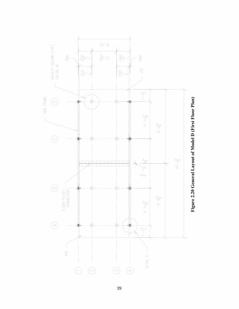
Fi
gure
2.2
0 G
ener
al L
ayou
t of M
odel
D (F
irst
Flo
or P
lan)
39
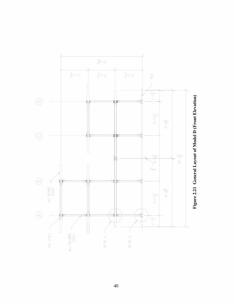
Fi
gure
2.2
1 G
ener
al L
ayou
t of M
odel
D (F
ront
Ele
vatio
n)
40
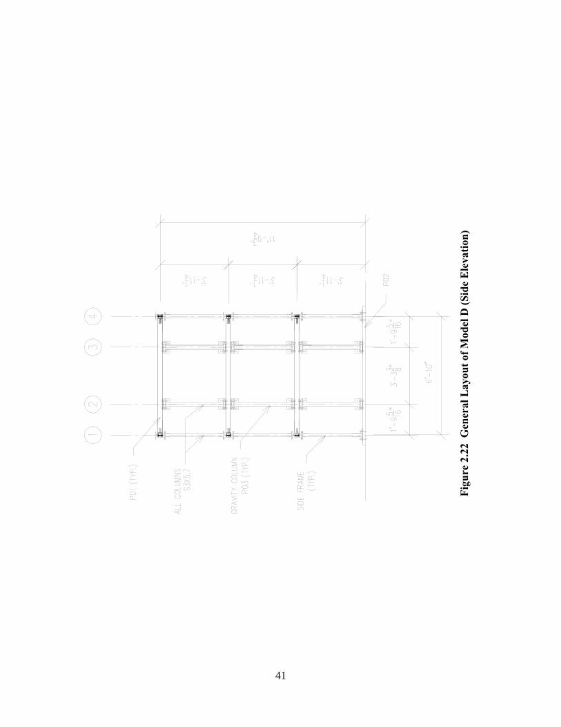
Fi
gure
2.2
2 G
ener
al L
ayou
t of M
odel
D (S
ide
Ele
vatio
n)
41

42
2.2.4.3 Monitoring the Response of Selected Model Several response quantities of the structural model were measured during the experimental study. These quantities are: horizontal and vertical floor accelerations of the base structure and the two towers, floor displacements, relative horizontal movement of the two towers, and the ground floor reactions: moments, shear and axial forces. A detailed description of the instrumentation is presented in Sections 5 and 6.
2.3 Summary
The design of a versatile structural model was presented in this section. The selected model – designated as Model D - was designed so that it can fit within the limitations of capacity of the testing facilities, yet was similar as much as possible to a realistic structure. The versatility of the model consists in the ability to reconfigure it into a large number of alternative variants – regular as well as irregular - that can be built from the same basic components. It was also designed to be easily installed, and easily repaired by replacing damaged parts after severe testing.
The complete designs and structural drawings are presented. The specific features of the basic elements are also described. The properties of materials are described in Section 4, based on specific results obtained from material testing.
43
SECTION 3 ANALYTICAL EVALUATION OF THE VERSATILE MODEL
3.1 Introduction 3.1.1 Objectives of Evaluation In order to better understand the seismic behavior of irregular structures in the inelastic range an experimental program was conducted using the versatile model described earlier. After selecting the model, Model D, a prediction of the structural response was obtained through several types of analysis as described below.
3.1.2 Analytical Techniques Several techniques for the analysis of structures in the inelastic range are available to the engineer, the choice usually depending on the type of building occupancy: (i) dynamic time analysis, (ii) dynamic pushover or incremental dynamic analysis, and (iii) nonlinear static analysis (spectral demand-capacity analysis). 3.1.2.1 Dynamic Time Analysis In the nonlinear dynamic time analysis (Chopra, 2001) the structural model is excited at its base beyond its first yield limit by a historic or artificial ground motion record, or a suite thereof. The effectiveness of the analysis depends on the extent to which the chosen records are consistent with the expected site-specific ground motion. 3.1.2.2 Dynamic Pushover: Incremental Dynamic Analysis Dynamic pushover, or incremental dynamic analysis (IDA), is a procedure in which nonlinear dynamic analyses are performed on the structural model for a given record, or a suite thereof, the PGAs of which are incrementally scaled, i.e., increased, to force the model to the brink of failure or instability (Bracci, 1992; Reichman, 1995; Vamvatsikos and Cornell, 2002, 2004). Roof displacements, or any other response parameter of interest, are plotted vs. the peak ground acceleration (PGA), so that the plot produces a pushover-like curve. The peak values of these parameters are usually of interest, e.g., peak roof displacement, interstory drift, yield level and ultimate capacity of the structure. This method is time consuming, yet, compared with conventional pushover analysis, it offers better accuracy for structures for which higher modes effects are significant, such as tall buildings and irregular structures. 3.1.2.3 Nonlinear Spectral, Static Analysis (Spectral Demand-Capacity Analysis) A different method of analysis was developed and named the Spectral Demand-Capacity Analysis, SDCA (see Reinhorn, 1997). The spectral demand-capacity analysis was developed to provide a simplified tool to estimate the nonlinear structural response under
44
seismic loads. This method offers an insight into the structural behavior by means of matching the seismic demand as expressed in terms of nonlinear response spectra with the capacity given in terms of an “equivalent” single degree of freedom nonlinear force-displacement relationship. This method will be described in some detail in Section 3.2 for sake of completeness. Compared with dynamic time analysis, static analysis involves simpler calculations and hence is often preferred by engineers. However, results from the static analysis are often less accurate, especially for irregular structures and tall buildings dominated by strong participation of higher modes of vibration.
3.1.3 Analytical Models of Tested Structures As described in Section 2.2.4, the example model selected for the experimental study was a three-bay three-story steel structure with two unequal towers designated as model D. The analytical model was developed using two lateral load resisting frames with irregular configuration, as shown in Figures 2.20 to 2.22. The beams and columns in the model are S3x5.7, with A36 steel for beams and A572/A588 Gr.50 steel for columns. The connections between the beams and columns and columns and foundations are assumed rigid. The fundamental natural period of the model was found to be 0.52 seconds, and is within the frequency range of the experimentation equipment. In this study, the analyses using nonlinear properties were performed for the irregular model, both static and dynamic, using the program IDARC Version 5.0 (derived from Valles, et al., 1996).
3.2 Spectral Capacity from Static Nonlinear Analysis (Pushover) The spectral demand-capacity method was developed to answer the need for a simplified analytical tool for predicting the inelastic structural response. A version of this method as developed by Reinhorn (1997) is also described in this report.
3.2.1 General Description of Method 3.2.1.1 Components Needed for Evaluation The spectral demand-capacity analysis (SDCA) utilizes the spectral seismic demand and the structural spectral capacity to approximate the expected dynamic response. The seismic demand is expressed in the form of inelastic response spectrum, which can be obtained for a given ground motion, strength reduction factor R or ductility demand µ and post-elastic hardening ratio α from the elastic response spectrum by means of nonlinear dynamic analysis on a single degree of freedom (1-dof) system. The spectral capacity of the structure takes the form of a force-displacement relationship, as converted to an "equivalent" 1-dof response, and can be obtained from incrementally increased static loading so that the sequence of plastification can be traced. Each component required for conducting the SDCA is described subsequently. Demand spectra can be based either on R or on µ. In this study R-based spectra are used, and hence are presented in some detail.
45
3.2.1.2 Capacity-Demand Diagram for Static Nonlinear Analysis Response spectra are usually defined as frequency or period functions of a response parameter. In the present case the response parameter is the non-dimensionalized spectral acceleration Sa, (i.e., divided by the acceleration of gravity g) vs. the natural period or natural frequency of the system. However, the capacity curve is depicted as acceleration or forces response vs. displacement. Hence, the demand (ground motion) acceleration response spectrum has to be converted to an acceleration-displacement demand diagram by specifying the acceleration response in terms of the spectral displacement Sd rather than of the period T. This conversion is usually done by means of the harmonic relation, namely Sd = [T/(2π)]2Sa. The demand and the capacity curves are plotted on the same diagram, and their intersection can be defined as the actual response of the structure (“performance point”). A detailed description of this procedure is presented below.
3.2.2 Inelastic Demand Spectra Based on Strength Reduction Factors The inelastic spectrum is a function of the ductility of the structure. However, the same inelastic spectrum can be developed as a function of the yield strength or the strength reduction factor R. A description of derivation of spectra based on strength reduction factor is presented in the following section: 3.2.2.1 Elastic Spectra Derived from Dynamic Time Analyses A simple dynamic system will respond to support acceleration (u )g depending on its dynamic properties: mass (m), structural restoring force (Q(u)) and internal viscous damping (c) according to the following equation of motion:
m u(t) cu(t) Q(u(t)) = - m u (t)g+ + (3.1)
where u(t) is the displacement response, and the over-dot indicates the time derivative. The restoring force follows a linear relation for an elastic structure: Q(u) = k u(t) (3.2) Equation 3.1 can also be written as:
u 2 u u uo g+ + = −ξω ωo2 (3.3)
in which ξ0 = c/(2mω0) is the damping ratio and ω0 = natural frequency = 2π/T. The maximum seismic response for a single structure depends on its strength envelope and energy dissipation through hysteretic mechanism. The spectral methods offer a simple way to find the maximum response, if an appropriate spectrum is available. Simple hysteretic 1-dof systems are characterized by an initial stiffness (or period), yield strength, and a secondary stiffness ratio α. Response spectra can be evaluated for displacements, Sd(ωo , ξo ) = max u , absolute accelerations, Sa( ωo , ξo ) = max u ug+ , or for any other desired response quantity, such as the acceleration at maximum displacement, i.e., the pseudo-acceleration. For practical purposes the absolute acceleration response is used to determine the force acting on the support system:
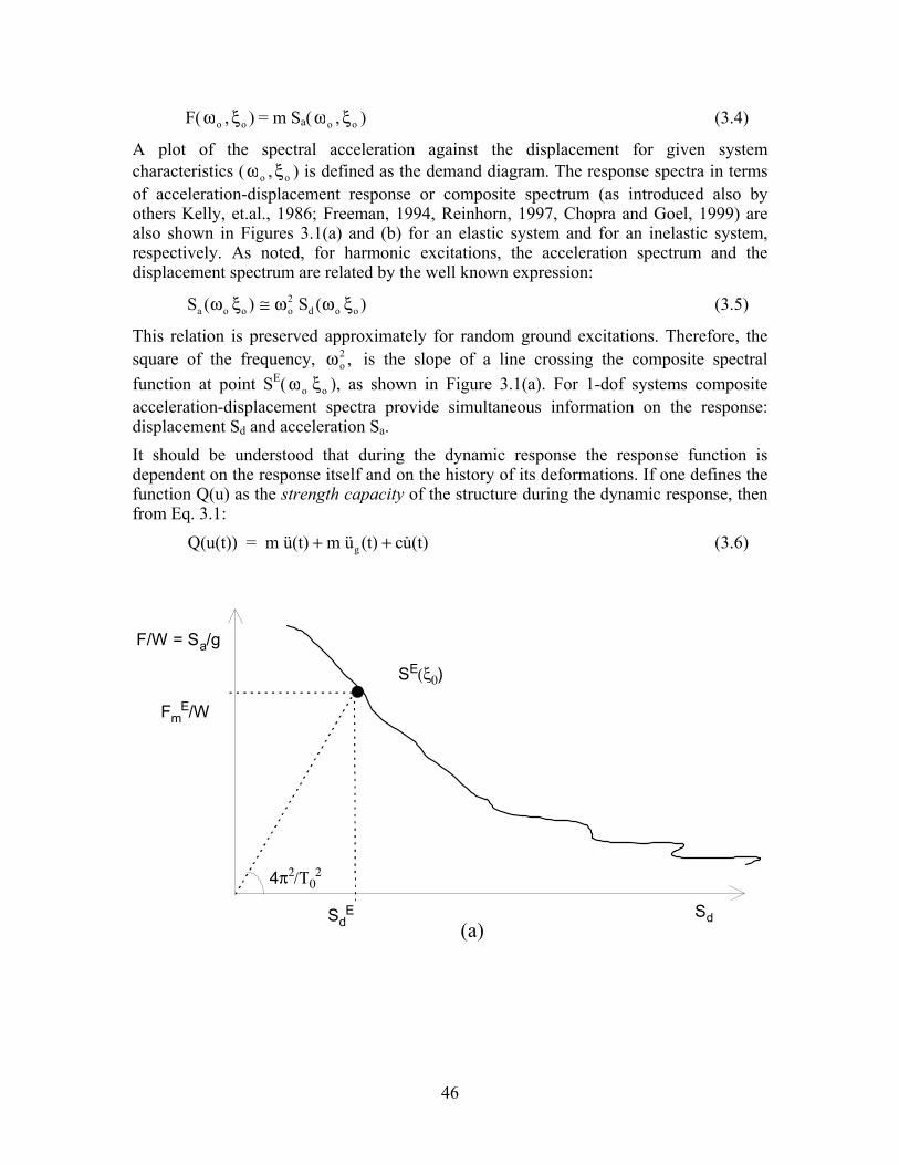
46
F( ωo , ξo ) = m Sa( ωo , ξo ) (3.4)
A plot of the spectral acceleration against the displacement for given system characteristics (ωo , ξo ) is defined as the demand diagram. The response spectra in terms of acceleration-displacement response or composite spectrum (as introduced also by others Kelly, et.al., 1986; Freeman, 1994, Reinhorn, 1997, Chopra and Goel, 1999) are also shown in Figures 3.1(a) and (b) for an elastic system and for an inelastic system, respectively. As noted, for harmonic excitations, the acceleration spectrum and the displacement spectrum are related by the well known expression:
S ( ) S ( )a o o2
d o oω ξ ω ω ξo ≅ (3.5)
This relation is preserved approximately for random ground excitations. Therefore, the square of the frequency, ωo
2 , is the slope of a line crossing the composite spectral function at point SE( ωo ξo ), as shown in Figure 3.1(a). For 1-dof systems composite acceleration-displacement spectra provide simultaneous information on the response: displacement Sd and acceleration Sa. It should be understood that during the dynamic response the response function is dependent on the response itself and on the history of its deformations. If one defines the function Q(u) as the strength capacity of the structure during the dynamic response, then from Eq. 3.1: Q(u(t)) = m u(t) m u (t) cu(t) g+ + (3.6)
S E (ξ0 )
F/W = S a /g
4 π 2 /Τ 0 2
S d
F m E /W
S d E
(a)
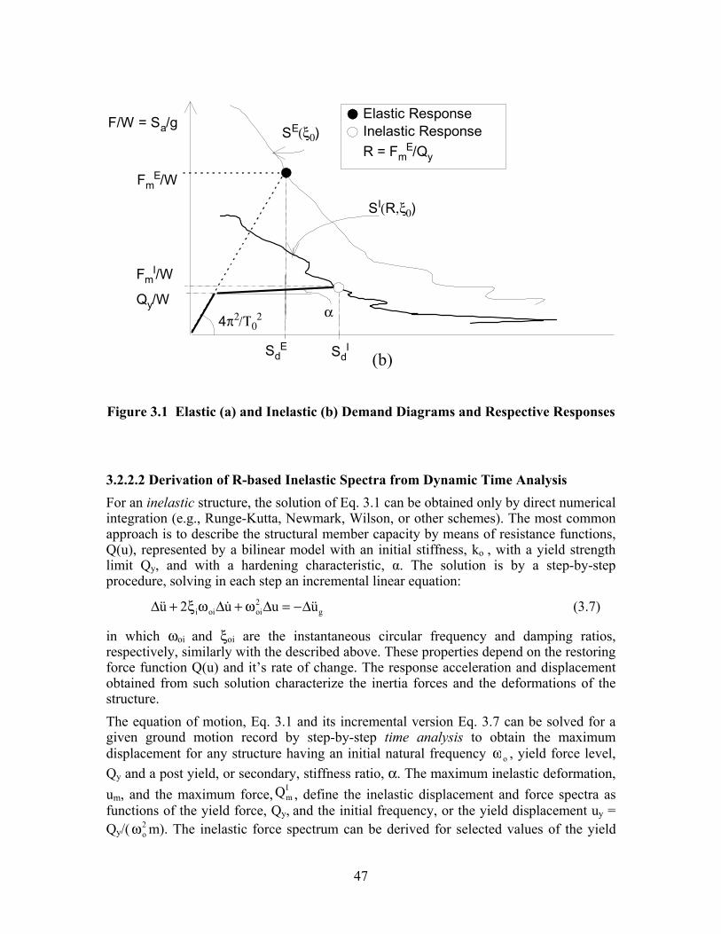
47
S E (ξ 0 ) F/W = S a /g
4 π 2 /Τ 0 2
F m E /W
F m I /W
Q y /W
S I (R ,ξ0 )
S d I S d
E
α
Elastic Response Inelastic Response R = F m
E /Q y
(b)
Figure 3.1 Elastic (a) and Inelastic (b) Demand Diagrams and Respective Responses 3.2.2.2 Derivation of R-based Inelastic Spectra from Dynamic Time Analysis For an inelastic structure, the solution of Eq. 3.1 can be obtained only by direct numerical integration (e.g., Runge-Kutta, Newmark, Wilson, or other schemes). The most common approach is to describe the structural member capacity by means of resistance functions, Q(u), represented by a bilinear model with an initial stiffness, ko , with a yield strength limit Qy, and with a hardening characteristic, α. The solution is by a step-by-step procedure, solving in each step an incremental linear equation:
∆ ∆ ∆ ∆u 2 u u uoi g+ + = −ξ ω ωi oi2 (3.7)
in which ωoi and ξoi are the instantaneous circular frequency and damping ratios, respectively, similarly with the described above. These properties depend on the restoring force function Q(u) and it’s rate of change. The response acceleration and displacement obtained from such solution characterize the inertia forces and the deformations of the structure. The equation of motion, Eq. 3.1 and its incremental version Eq. 3.7 can be solved for a given ground motion record by step-by-step time analysis to obtain the maximum displacement for any structure having an initial natural frequency ωo , yield force level, Qy and a post yield, or secondary, stiffness ratio, α. The maximum inelastic deformation, um, and the maximum force, Qm
I , define the inelastic displacement and force spectra as functions of the yield force, Qy, and the initial frequency, or the yield displacement uy = Qy/( ωo
2 m). The inelastic force spectrum can be derived for selected values of the yield
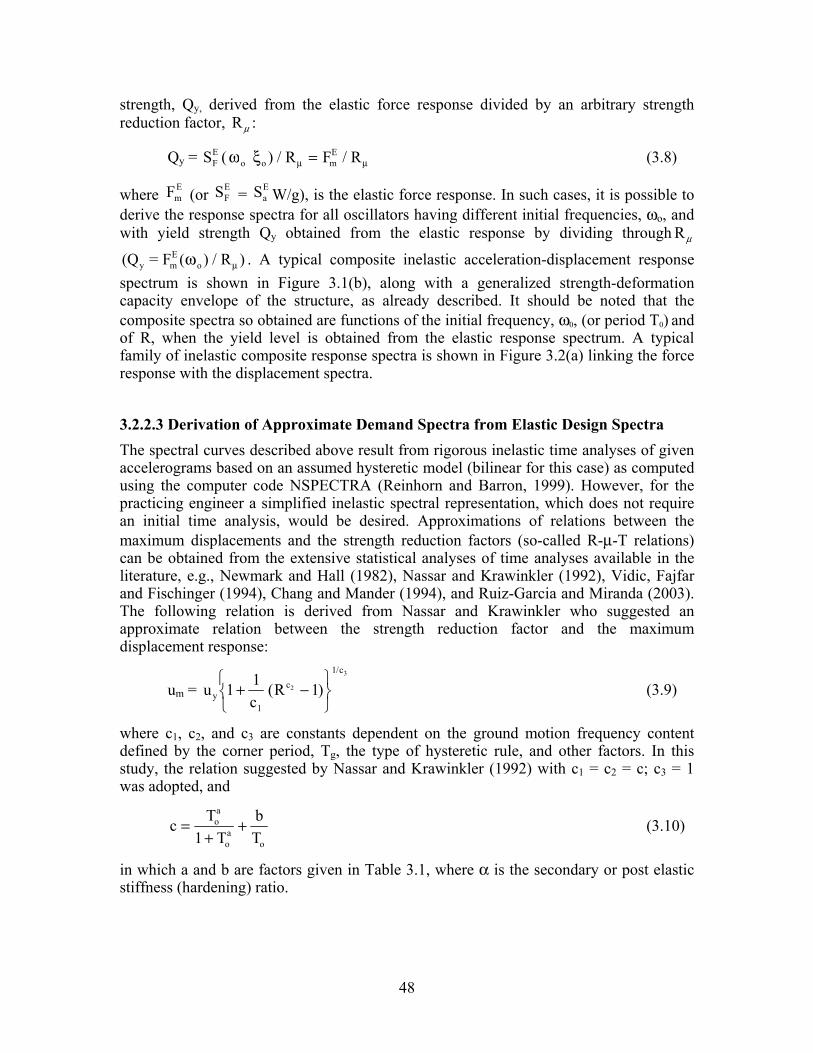
48
strength, Qy, derived from the elastic force response divided by an arbitrary strength reduction factor, Rµ :
Qy = SFE (ωo ξ µ µo m
E) / F / RR = (3.8)
where FmE (or SF
E = SaE W/g), is the elastic force response. In such cases, it is possible to
derive the response spectra for all oscillators having different initial frequencies, ωo, and with yield strength Qy obtained from the elastic response by dividing through Rµ
(Q = F ( ) / Ry mE
oω µ ) . A typical composite inelastic acceleration-displacement response spectrum is shown in Figure 3.1(b), along with a generalized strength-deformation capacity envelope of the structure, as already described. It should be noted that the composite spectra so obtained are functions of the initial frequency, ω0, (or period T0) and of R, when the yield level is obtained from the elastic response spectrum. A typical family of inelastic composite response spectra is shown in Figure 3.2(a) linking the force response with the displacement spectra. 3.2.2.3 Derivation of Approximate Demand Spectra from Elastic Design Spectra The spectral curves described above result from rigorous inelastic time analyses of given accelerograms based on an assumed hysteretic model (bilinear for this case) as computed using the computer code NSPECTRA (Reinhorn and Barron, 1999). However, for the practicing engineer a simplified inelastic spectral representation, which does not require an initial time analysis, would be desired. Approximations of relations between the maximum displacements and the strength reduction factors (so-called R-µ-T relations) can be obtained from the extensive statistical analyses of time analyses available in the literature, e.g., Newmark and Hall (1982), Nassar and Krawinkler (1992), Vidic, Fajfar and Fischinger (1994), Chang and Mander (1994), and Ruiz-Garcia and Miranda (2003). The following relation is derived from Nassar and Krawinkler who suggested an approximate relation between the strength reduction factor and the maximum displacement response:
um = u 1c
Ry1
c1/c
2
3
1 1+ −⎧⎨⎩
⎫⎬⎭
( ) (3.9)
where c1, c2, and c3 are constants dependent on the ground motion frequency content defined by the corner period, Tg, the type of hysteretic rule, and other factors. In this study, the relation suggested by Nassar and Krawinkler (1992) with c1 = c2 = c; c3 = 1 was adopted, and
c T1 T
bT
oa
oa
o
=+
+ (3.10)
in which a and b are factors given in Table 3.1, where α is the secondary or post elastic stiffness (hardening) ratio.
49
Table 3.1 Coefficients for Approximated Inelastic Spectra
α a b
0% 1.0 0.42
2% 1.0 0.37
10% 0.80 0.29
Replacing the deformation in Eq. 3.9 by the spectral value a relation between the approximate inelastic displacement spectrum, Sd
I and the given elastic displacement spectrum, Sd
E can be defined as follows:
S SR
1 1c
(R 1) SRd
I dE
c dE
= + −⎧⎨⎩
⎫⎬⎭
≥µ
µµ
(3.11)
where the reduction factor is defined as: R S WQ g
AE
yµ = .
The inelastic acceleration spectrum, SaI, derived for the bilinear system with a secondary
slope ratio α is given by Reinhorn (1997), and reads:
S SR
1 Sua
I aE
dI
y
= + −⎛
⎝⎜
⎞
⎠⎟
⎡
⎣⎢⎢
⎤
⎦⎥⎥µ
α 1 (3.12)
where, uy = S / RdE
µ
The approximate composite inelastic spectra derived from Eqs. 3.11 and 3.12 can link the elastic composite spectra S Sd
EaE with the reduction factor Rµ , the yield level, Qy, and α.
Composite spectra obtained from Eqs. 3.11 and 3.12 are shown in Figure 3.2(a). It should be noted that the reduction factor Rµ in Eqs. 3.11 and 3.12 depends on the elastic acceleration response and is not a constant for all structures. It should also be noted that the above approximate and simplified composite spectra can be used as substitute for the ones generated rigorously by dynamic time analyses. However, only the rigorously derived inelastic spectra are used in this study.
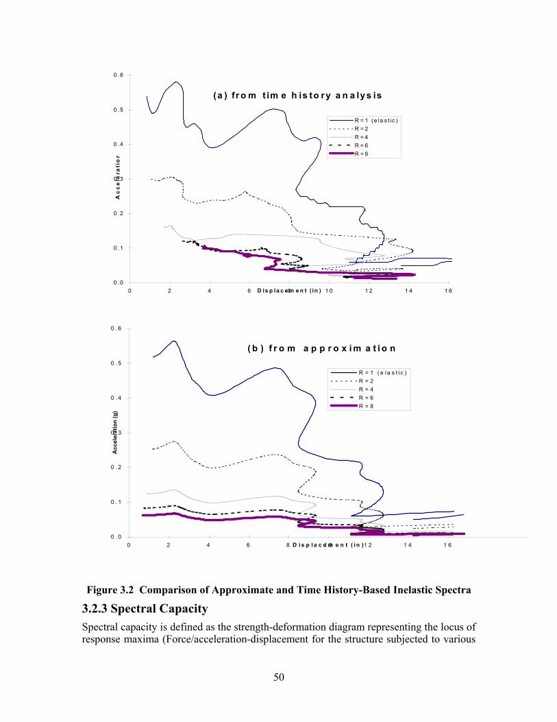
50
(a ) fr o m t im e h is to ry a n a ly s is
0 .0
0 .1
0 .2
0 .3
0 .4
0 .5
0 .6
0 2 4 6 8 1 0 1 2 1 4 1 6D is p la c e m e n t ( in )
Ac
ce
lera
tio
nR = 1 (e la s t ic )R = 2R = 4R = 6R = 8
( b ) f r o m a p p r o x i m a t i o n
0 . 0
0 . 1
0 . 2
0 . 3
0 . 4
0 . 5
0 . 6
0 2 4 6 8 1 0 1 2 1 4 1 6D i s p l a c e m e n t ( i n )
Acc
eler
atio
n (g
)
R = 1 ( e la s t i c )R = 2R = 4R = 6R = 8
Figure 3.2 Comparison of Approximate and Time History-Based Inelastic Spectra
3.2.3 Spectral Capacity Spectral capacity is defined as the strength-deformation diagram representing the locus of response maxima (Force/acceleration-displacement for the structure subjected to various
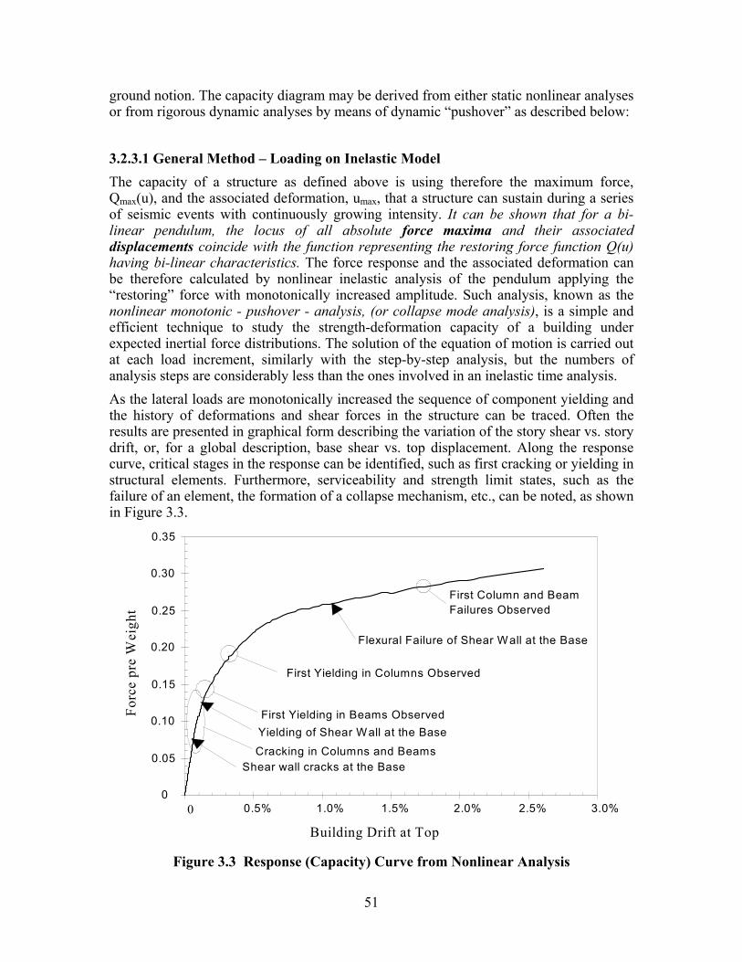
51
ground notion. The capacity diagram may be derived from either static nonlinear analyses or from rigorous dynamic analyses by means of dynamic “pushover” as described below: 3.2.3.1 General Method – Loading on Inelastic Model The capacity of a structure as defined above is using therefore the maximum force, Qmax(u), and the associated deformation, umax, that a structure can sustain during a series of seismic events with continuously growing intensity. It can be shown that for a bi-linear pendulum, the locus of all absolute force maxima and their associated displacements coincide with the function representing the restoring force function Q(u) having bi-linear characteristics. The force response and the associated deformation can be therefore calculated by nonlinear inelastic analysis of the pendulum applying the “restoring” force with monotonically increased amplitude. Such analysis, known as the nonlinear monotonic - pushover - analysis, (or collapse mode analysis), is a simple and efficient technique to study the strength-deformation capacity of a building under expected inertial force distributions. The solution of the equation of motion is carried out at each load increment, similarly with the step-by-step analysis, but the numbers of analysis steps are considerably less than the ones involved in an inelastic time analysis. As the lateral loads are monotonically increased the sequence of component yielding and the history of deformations and shear forces in the structure can be traced. Often the results are presented in graphical form describing the variation of the story shear vs. story drift, or, for a global description, base shear vs. top displacement. Along the response curve, critical stages in the response can be identified, such as first cracking or yielding in structural elements. Furthermore, serviceability and strength limit states, such as the failure of an element, the formation of a collapse mechanism, etc., can be noted, as shown in Figure 3.3.
0
0.05
0.10
0.15
0.20
0.25
0.30
0.35
0 0.5% 1.0% 1.5% 2.0% 2.5% 3.0%
Shear wall cracks at the Base
Yielding of Shear Wall at the Base
Flexural Failure of Shear Wall at the Base
Cracking in Columns and Beams
First Yielding in Beams Observed
First Yielding in Columns Observed
First Column and Beam Failures Observed
Forc
e pr
e W
eigh
t
Building Drift at Top Figure 3.3 Response (Capacity) Curve from Nonlinear Analysis
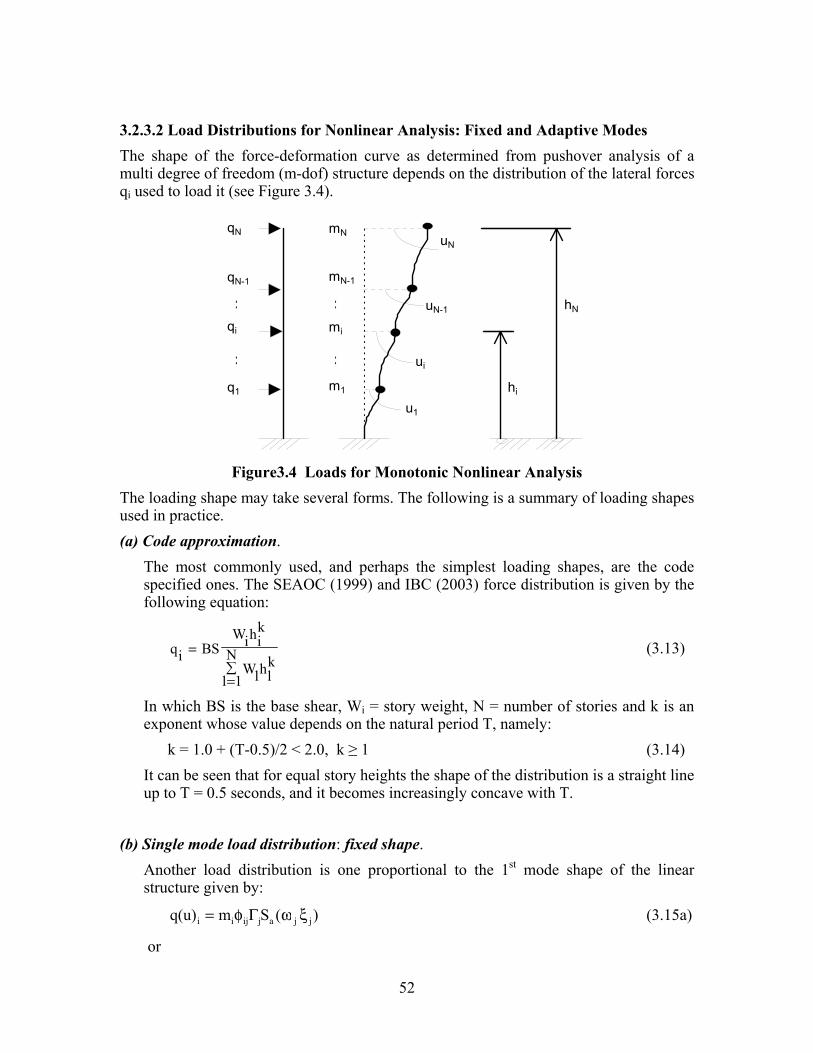
52
3.2.3.2 Load Distributions for Nonlinear Analysis: Fixed and Adaptive Modes The shape of the force-deformation curve as determined from pushover analysis of a multi degree of freedom (m-dof) structure depends on the distribution of the lateral forces qi used to load it (see Figure 3.4).
qN
q1
qi
qN-1
hN
u1
ui
uN-1
uN
hi
mN-1
mi
m1
mN
Figure3.4 Loads for Monotonic Nonlinear Analysis
The loading shape may take several forms. The following is a summary of loading shapes used in practice. (a) Code approximation.
The most commonly used, and perhaps the simplest loading shapes, are the code specified ones. The SEAOC (1999) and IBC (2003) force distribution is given by the following equation:
qi BSWihi
k
Wlhlk
l 1
N=
=∑
(3.13)
In which BS is the base shear, Wi = story weight, N = number of stories and k is an exponent whose value depends on the natural period T, namely: k = 1.0 + (T-0.5)/2 < 2.0, k ≥ 1 (3.14) It can be seen that for equal story heights the shape of the distribution is a straight line up to T = 0.5 seconds, and it becomes increasingly concave with T.
(b) Single mode load distribution: fixed shape. Another load distribution is one proportional to the 1st mode shape of the linear structure given by:
q(u) m S ( )i i ij j a j j= φ ω ξΓ (3.15a)
or

53
q(u) m BS )i i ij j j= φ ( / Γ (3.15b)
in which q, m, φ and Sa are respectively the lateral force, the story mass, the mode shape (herein mass normalized, such that φ j
T M φ j = 1, where T represents transposition and M is the mass matrix), and the modal spectral acceleration response for mode j = 1; Γ j = φ j
T M r is the modal participation factor and r is a vector of units (rT = 1, 1,...1), i = story number.
(c) Multimode load distribution: fixed shape.
This distribution takes into consideration the influence of higher modes, which affect tall buildings, using the following form (Chopra 2000):
q(u) m S srss f si i i1 1 a 1 1 j 1
M
ij j aj= •=
φ ω ξ γΓ ( ) ( ) (3.16)
where srss is the acronym for the square root of the sum of the squares superposition, i.e.:
srss x )j 1
M
j j2 1/2
== ∑( ) (x (3.17)
The terms forming xj are defined as ratios to the respective properties of the first mode: (i) the modal ratios: γ φ φj j ij ij i1and f= =Γ Γ/ /1 and (ii) the spectral ratios for the various modes, defined as saj = Sa ( ω j , ξ j )/Sa (ω1 , ξ1 ) and sdj = Sd (ω j , ξ j )/Sd ( ω1 , ξ1 ) for accelerations and displacements, respectively.
An approximation for these ratios was presented by Valles et al. (1996b). If the base shear is expressed also in terms of the multiple modes:
BS = S srss s12
a 1 1 j 1
M
j2
ajΓ ( ) ( )ω ξ γ•=
(3.18a)
then also the force distribution at each level i can be expressed as:
q(u) m S srss f si i i1 1 a 1 1 j 1
M
ij j aj= •=
φ ω ξ γΓ ( ) ( ) (3.18b)
or after combining Eqs. 3.18a and 3.18b:
( )q(u) BSm srss
srss
f s
sii i1
1
j=1
M
j=1
Mij j aj
j2
aj
= •φ γ
γΓ( )
(3.19)
(d) Adaptive load shapes: single and multimode.
For an inelastic system, the modal characteristics φ j , ω j , Γj, and Saj, change with the formation of plastic hinges and, hence, the terms in Eq. 3.15 change as function of the displacement, u. Therefore, if a monotonic analysis is done, then the dynamic
54
characteristics at every step need to be checked and suitably adjusted. One procedure to accomplish this for the 1st mode load shape was proposed by Bracci et al (1997). Similarly, in the case of multimode approximation the terms in Eq. 3.19 change with the formation of plastic hinges. This adaptive pushover procedure was developed by Bracci et al. (1997), and incorporated in the computer platform, IDARC2D Ver.4.0 (Valles et al. 1996a). Equation 3.19 is the general force distribution, probably the most accurate, but also the most laborious. Evidently, the 1st mode procedure is a particular case of Eq. 3.19.
Several variations of these procedures were proposed and evaluated for typical concrete buildings in the New Madrid area (Valles et al. 1996b), and showed that for a regular building the capacity function, Q(u), resulting from the above monotonic analysis, is only slightly sensitive to the choice of methods described above. 3.2.3.3 Approximation of Capacity Curve The capacity diagram, which may have a curved shape, can be approximated by a set of bilinear curves (e.g. Figure 3.5) for an even more simplified analysis according to (Reinhorn 1997):
Q(u) = Qy · ( ) [ ] u u U u/ ( ) / /u u uy y y− − − −1 1 1α (3.20a)
in which, Qy and uy are the yield strength and displacement, respectively, α=Ky/Ko is the post yield (hardening) stiffness ratio; U[u/uy -1] is a step function [equals 0 for u/uy<1 or equals 1 for u/uy>1]. The same relation can also be described in terms of the ductility ratio, µ = u uy/ as:
Q( µ ) = Qy µ α µ µ− − − −( )( ) ]1 1 1U[ (3.20b)
The bilinear capacity curves are determined by assuming the same post-yielding stiffness, and equal energy to failure as those of their monotonic counterparts. Equating the two energy diagrams to failure leads to:
A12
Q12
(Q Q )(u )m y y u y u y= + + −u u (3.21)
where Am is the work up to failure; and Qy, uy and uu are the yield force, yield deformation, and ultimate deformation of the equivalent bilinear curve. The yield force and displacement can be determined iteratively from the relation:
u u y my y o y
u y
u (Q +Q )-2Au = ; Q =K u
Q -Q (3.22)
for a given post-yielding stiffness y 0 u y u yK (=αK ) where α=(Q - Q )/(u - u ) .
The initial stiffness, K0, and hence the natural period, the yield level, Qy, and the post-yield hardening ratio, α , are the important parameters describing the inelastic behavior, along with the ultimate deformation capacity (uu).
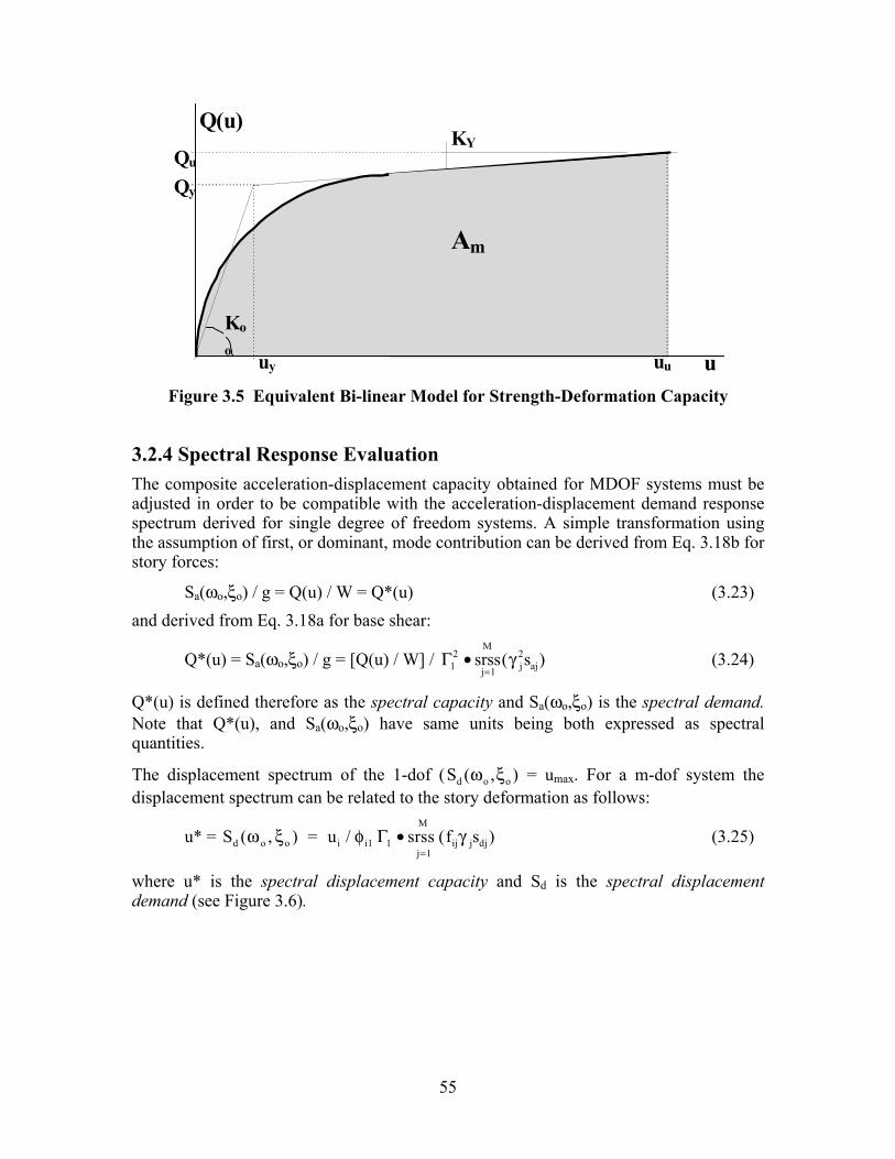
55
K Y
u u
Q(u)
u
Q u
u y
A m
Q y
K o
o
Figure 3.5 Equivalent Bi-linear Model for Strength-Deformation Capacity
3.2.4 Spectral Response Evaluation The composite acceleration-displacement capacity obtained for MDOF systems must be adjusted in order to be compatible with the acceleration-displacement demand response spectrum derived for single degree of freedom systems. A simple transformation using the assumption of first, or dominant, mode contribution can be derived from Eq. 3.18b for story forces:
Sa(ωo,ξo) / g = Q(u) / W = Q*(u) (3.23) and derived from Eq. 3.18a for base shear:
Q*(u) = Sa(ωo,ξo) / g = [Q(u) / W] / Γ12
j 1
M
j2
ajsrss s•=
( )γ (3.24)
Q*(u) is defined therefore as the spectral capacity and Sa(ωo,ξo) is the spectral demand. Note that Q*(u), and Sa(ωo,ξo) have same units being both expressed as spectral quantities.
The displacement spectrum of the 1-dof (S ( , ) d o oω ξ = umax. For a m-dof system the displacement spectrum can be related to the story deformation as follows:
u* = S ( , ) = u / srss f sd o o i i1j 1
M
ij j djω ξ φ γΓ1 •=
( ) (3.25)
where u* is the spectral displacement capacity and Sd is the spectral displacement demand (see Figure 3.6).
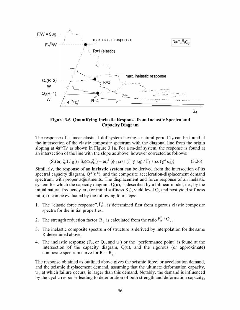
56
R=2
Sd
F/W = Sa/g
FmE/W
Qy(R=2)W
Qy(R=4)W
R=1 (elastic)
R=4
max. elastic response
max. inelastic response
R=FmE/Qy
4 2/Τ02
Figure 3.6 Quantifying Inelastic Response from Inelastic Spectra and
Capacity Diagram
The response of a linear elastic 1-dof system having a natural period T0 can be found at the intersection of the elastic composite spectrum with the diagonal line from the origin sloping at 4π2/T0
2 as shown in Figure 3.1a. For a m-dof system, the response is found at an intersection of the line with the slope as above, however corrected as follows:
(Sa(ωo,ξo) / g ) / Sd(ωo,ξo) = ωo2 φi1 srss (fij γj sdj) / Γ1 srss (γj
2 saj) (3.26) Similarly, the response of an inelastic system can be derived from the intersection of its spectral capacity diagram, Q*(u*), and the composite acceleration-displacement demand spectrum, with proper adjustments. The displacement and force response of an inelastic system for which the capacity diagram, Q(u), is described by a bilinear model, i.e., by the initial natural frequency ω 0 (or initial stiffness K0), yield level Qy and post yield stiffness ratio, α, can be evaluated by the following four steps:
1. The “elastic force response”, FmE , is determined first from rigorous elastic composite
spectra for the initial properties.
2. The strength reduction factor Rµ is calculated from the ratio F QmE
y/ .
3. The inelastic composite spectrum of structure is derived by interpolation for the same R determined above;
4. The inelastic response (Fd, or Qd, and ud) or the "performance point" is found at the intersection of the capacity diagram, Q(u), and the rigorous (or approximate) composite spectrum curve for R = Rµ .
The response obtained as outlined above gives the seismic force, or acceleration demand, and the seismic displacement demand, assuming that the ultimate deformation capacity, uu, at which failure occurs, is larger than this demand. Notably, the demand is influenced by the cyclic response leading to deterioration of both strength and deformation capacity,
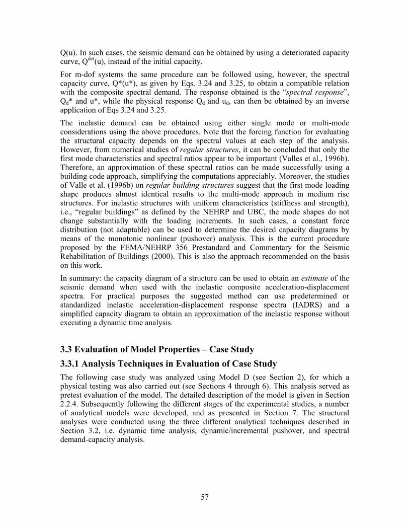
57
Q(u). In such cases, the seismic demand can be obtained by using a deteriorated capacity curve, Qdet(u), instead of the initial capacity. For m-dof systems the same procedure can be followed using, however, the spectral capacity curve, Q*(u*), as given by Eqs. 3.24 and 3.25, to obtain a compatible relation with the composite spectral demand. The response obtained is the “spectral response”, Qd* and u*, while the physical response Qd and ud, can then be obtained by an inverse application of Eqs 3.24 and 3.25. The inelastic demand can be obtained using either single mode or multi-mode considerations using the above procedures. Note that the forcing function for evaluating the structural capacity depends on the spectral values at each step of the analysis. However, from numerical studies of regular structures, it can be concluded that only the first mode characteristics and spectral ratios appear to be important (Valles et al., 1996b). Therefore, an approximation of these spectral ratios can be made successfully using a building code approach, simplifying the computations appreciably. Moreover, the studies of Valle et al. (1996b) on regular building structures suggest that the first mode loading shape produces almost identical results to the multi-mode approach in medium rise structures. For inelastic structures with uniform characteristics (stiffness and strength), i.e., “regular buildings” as defined by the NEHRP and UBC, the mode shapes do not change substantially with the loading increments. In such cases, a constant force distribution (not adaptable) can be used to determine the desired capacity diagrams by means of the monotonic nonlinear (pushover) analysis. This is the current procedure proposed by the FEMA/NEHRP 356 Prestandard and Commentary for the Seismic Rehabilitation of Buildings (2000). This is also the approach recommended on the basis on this work. In summary: the capacity diagram of a structure can be used to obtain an estimate of the seismic demand when used with the inelastic composite acceleration-displacement spectra. For practical purposes the suggested method can use predetermined or standardized inelastic acceleration-displacement response spectra (IADRS) and a simplified capacity diagram to obtain an approximation of the inelastic response without executing a dynamic time analysis.
3.3 Evaluation of Model Properties – Case Study 3.3.1 Analysis Techniques in Evaluation of Case Study The following case study was analyzed using Model D (see Section 2), for which a physical testing was also carried out (see Sections 4 through 6). This analysis served as pretest evaluation of the model. The detailed description of the model is given in Section 2.2.4. Subsequently following the different stages of the experimental studies, a number of analytical models were developed, and as presented in Section 7. The structural analyses were conducted using the three different analytical techniques described in Section 3.2, i.e. dynamic time analysis, dynamic/incremental pushover, and spectral demand-capacity analysis.
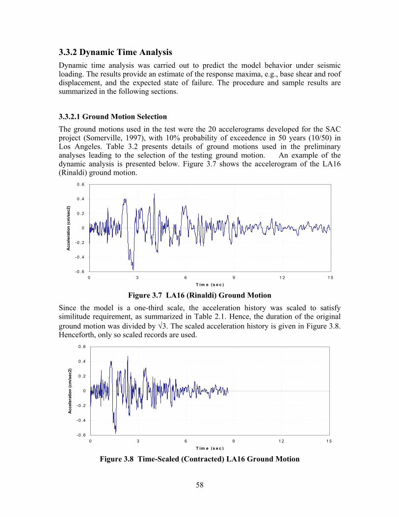
58
3.3.2 Dynamic Time Analysis Dynamic time analysis was carried out to predict the model behavior under seismic loading. The results provide an estimate of the response maxima, e.g., base shear and roof displacement, and the expected state of failure. The procedure and sample results are summarized in the following sections. 3.3.2.1 Ground Motion Selection The ground motions used in the test were the 20 accelerograms developed for the SAC project (Somerville, 1997), with 10% probability of exceedence in 50 years (10/50) in Los Angeles. Table 3.2 presents details of ground motions used in the preliminary analyses leading to the selection of the testing ground motion. An example of the dynamic analysis is presented below. Figure 3.7 shows the accelerogram of the LA16 (Rinaldi) ground motion.
-0 .6
-0 .4
-0 .2
0
0 .2
0 .4
0 .6
0 3 6 9 1 2 1 5
T im e (s e c )
Acc
eler
atio
n (c
m/s
ec2)
Figure 3.7 LA16 (Rinaldi) Ground Motion
Since the model is a one-third scale, the acceleration history was scaled to satisfy similitude requirement, as summarized in Table 2.1. Hence, the duration of the original ground motion was divided by √3. The scaled acceleration history is given in Figure 3.8. Henceforth, only so scaled records are used.
-0 .6
-0 .4
-0 .2
0
0 .2
0 .4
0 .6
0 3 6 9 1 2 1 5
T im e (s e c )
Acc
eler
atio
n (c
m/s
ec2)
Figure 3.8 Time-Scaled (Contracted) LA16 Ground Motion
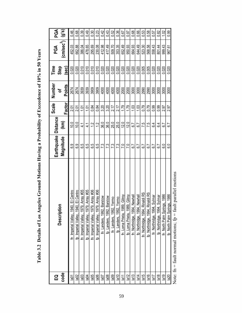
Tab
le 3
.2 D
etai
ls o
f Los
Ang
eles
Gro
und
Mot
ions
Hav
ing
a Pr
obab
ility
of E
xcee
denc
e of
10%
in 5
0 Y
ears
Not
e: fn
= fa
ult n
orm
al m
otio
ns; f
p =
faul
t par
alle
l mot
ions
EQ code
Desc
riptio
nEa
rthqu
ake
Magn
itude
Dist
ance
(km
)
Scale
Fact
or
Num
ber
of P
oint
s
Tim
e St
ep(s
ec)
PGA
(cm
/sec2 )
PGA
(g's)
la01
fn Im
peria
l Vall
ey, 1
940,
El C
entro
6.9
10.0
2.01
2674
0.02
045
2.03
0.46
la02
fp Im
peria
l Vall
ey, 1
940,
El C
entro
6.9
10.0
2.01
2674
0.02
066
2.88
0.68
la03
fn Im
peria
l Vall
ey, 1
979,
Arra
y #0
56.
54.
11.
0139
390.
010
386.
040.
39la0
4fp
Impe
rial V
alley
, 197
9, A
rray
#05
6.5
4.1
1.01
3939
0.01
047
8.65
0.49
la05
fn Im
peria
l Vall
ey, 1
979,
Arra
y #0
66.
51.
20.
8439
090.
010
295.
690.
30la0
6fp
Impe
rial V
alley
, 197
9, A
rray
#06
6.5
1.2
0.84
3909
0.01
023
0.08
0.23
la07
fn L
ande
rs, 1
992,
Bar
stow
7.3
36.0
3.20
4000
0.02
041
2.98
0.42
la08
fp L
ande
rs, 1
992,
Bar
stow
7.3
36.0
3.20
4000
0.02
041
7.49
0.43
la09
fn L
ande
rs, 1
992,
Yer
mo
7.3
25.0
2.17
4000
0.02
050
9.70
0.52
la10
fp L
ande
rs, 1
992,
Yer
mo
7.3
25.0
2.17
4000
0.02
035
3.35
0.36
la11
fn L
oma
Priet
a, 1
989,
Gilro
y7.
012
.01.
7920
000.
020
652.
490.
67la1
2fp
Lom
a Pr
ieta,
198
9, G
ilroy
7.0
12.0
1.79
2000
0.02
095
0.93
0.97
la13
fn N
orth
ridge
, 199
4, N
ewha
ll6.
76.
71.
0330
000.
020
664.
930.
68la1
4fp
Nor
thrid
ge, 1
994,
New
hall
6.7
6.7
1.03
3000
0.02
064
4.49
0.66
la15
fn N
orth
ridge
, 199
4, R
inaldi
RS
6.7
7.5
0.79
2990
0.00
552
3.30
0.53
la16
fp N
orth
ridge
, 199
4, R
inaldi
RS
6.7
7.5
0.79
2990
0.00
556
8.58
0.58
la17
fn N
orth
ridge
, 199
4, S
ylmar
6.7
6.4
0.99
3000
0.02
055
8.43
0.57
la18
fp N
orth
ridge
, 199
4, S
ylmar
6.7
6.4
0.99
3000
0.02
080
1.44
0.82
la19
fn N
orth
Palm
Spr
ings,
198
66.
06.
72.
9730
000.
020
999.
431.
02la2
0fp
Nor
th P
alm S
pring
s, 1
986
6.0
6.7
2.97
3000
0.02
096
7.61
0.99
59
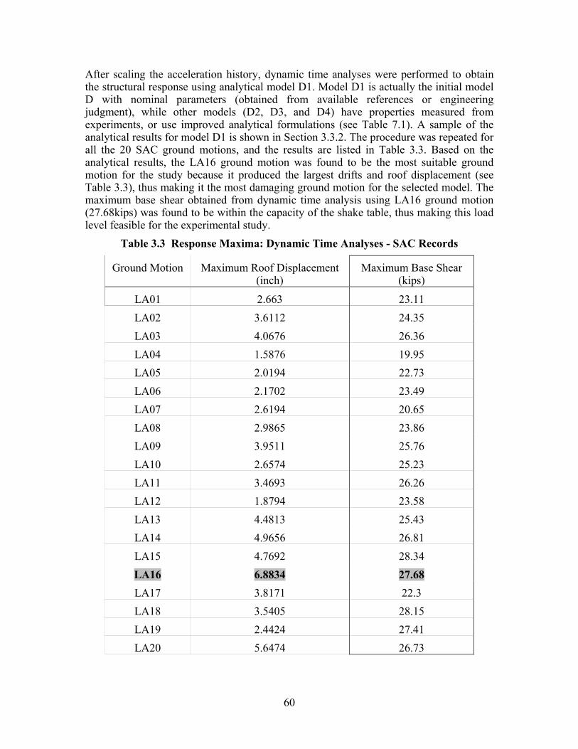
60
After scaling the acceleration history, dynamic time analyses were performed to obtain the structural response using analytical model D1. Model D1 is actually the initial model D with nominal parameters (obtained from available references or engineering judgment), while other models (D2, D3, and D4) have properties measured from experiments, or use improved analytical formulations (see Table 7.1). A sample of the analytical results for model D1 is shown in Section 3.3.2. The procedure was repeated for all the 20 SAC ground motions, and the results are listed in Table 3.3. Based on the analytical results, the LA16 ground motion was found to be the most suitable ground motion for the study because it produced the largest drifts and roof displacement (see Table 3.3), thus making it the most damaging ground motion for the selected model. The maximum base shear obtained from dynamic time analysis using LA16 ground motion (27.68kips) was found to be within the capacity of the shake table, thus making this load level feasible for the experimental study.
Table 3.3 Response Maxima: Dynamic Time Analyses - SAC Records
Ground Motion Maximum Roof Displacement (inch)
Maximum Base Shear (kips)
LA01 2.663 23.11 LA02 3.6112 24.35 LA03 4.0676 26.36 LA04 1.5876 19.95 LA05 2.0194 22.73 LA06 2.1702 23.49 LA07 2.6194 20.65 LA08 2.9865 23.86 LA09 3.9511 25.76 LA10 2.6574 25.23 LA11 3.4693 26.26 LA12 1.8794 23.58 LA13 4.4813 25.43 LA14 4.9656 26.81 LA15 4.7692 28.34 LA16 6.8834 27.68 LA17 3.8171 22.3 LA18 3.5405 28.15 LA19 2.4424 27.41 LA20 5.6474 26.73
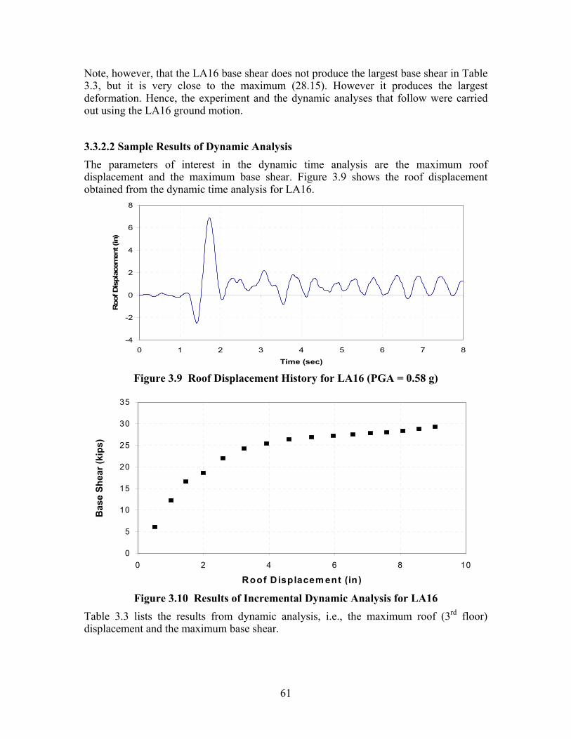
61
Note, however, that the LA16 base shear does not produce the largest base shear in Table 3.3, but it is very close to the maximum (28.15). However it produces the largest deformation. Hence, the experiment and the dynamic analyses that follow were carried out using the LA16 ground motion. 3.3.2.2 Sample Results of Dynamic Analysis The parameters of interest in the dynamic time analysis are the maximum roof displacement and the maximum base shear. Figure 3.9 shows the roof displacement obtained from the dynamic time analysis for LA16.
-4
-2
0
2
4
6
8
0 1 2 3 4 5 6 7 8
Time (sec)
Roo
f Dis
plac
emen
t (in
)
Figure 3.9 Roof Displacement History for LA16 (PGA = 0.58 g)
0
5
10
15
20
25
30
35
0 2 4 6 8 10
Roof D isplacem ent (in)
Bas
e Sh
ear (
kips
)
Figure 3.10 Results of Incremental Dynamic Analysis for LA16
Table 3.3 lists the results from dynamic analysis, i.e., the maximum roof (3rd floor) displacement and the maximum base shear.
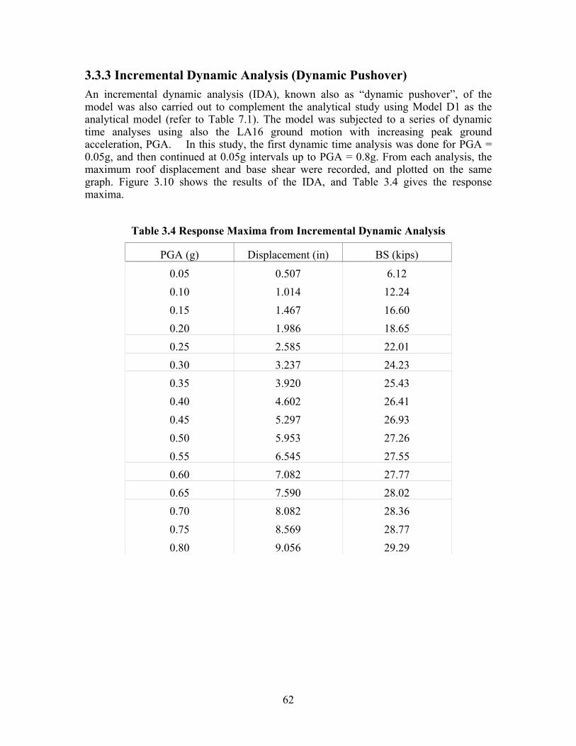
62
3.3.3 Incremental Dynamic Analysis (Dynamic Pushover) An incremental dynamic analysis (IDA), known also as “dynamic pushover”, of the model was also carried out to complement the analytical study using Model D1 as the analytical model (refer to Table 7.1). The model was subjected to a series of dynamic time analyses using also the LA16 ground motion with increasing peak ground acceleration, PGA. In this study, the first dynamic time analysis was done for PGA = 0.05g, and then continued at 0.05g intervals up to PGA = 0.8g. From each analysis, the maximum roof displacement and base shear were recorded, and plotted on the same graph. Figure 3.10 shows the results of the IDA, and Table 3.4 gives the response maxima.
Table 3.4 Response Maxima from Incremental Dynamic Analysis
PGA (g) Displacement (in) BS (kips)
0.05 0.507 6.12 0.10 1.014 12.24 0.15 1.467 16.60 0.20 1.986 18.65 0.25 2.585 22.01 0.30 3.237 24.23 0.35 3.920 25.43 0.40 4.602 26.41 0.45 5.297 26.93 0.50 5.953 27.26 0.55 6.545 27.55 0.60 7.082 27.77 0.65 7.590 28.02 0.70 8.082 28.36 0.75 8.569 28.77 0.80 9.056 29.29

63
3.3.4 Spectral Capacity Analysis (a) Demand spectra In this study, the dynamic analysis to produce the response spectrum was performed using the computer code NSPECTRA (Reinhorn et al, 1998). The response spectra were generated for 5% damping, and 2% post yield stiffness ratio. The results were given for 3 different values of the strength reduction factor, R: R = 1 elastic response spectrum, R = 2 and R = 4. (b) Sample results of demand spectra Figure 3.11 shows an example of the composite spectra developed for the SAC LA16 ground motion for the 3 values of R. The spectrum shown has an almost constant acceleration for a large variety of maximum roof displacement responses.
0
0.4
0.8
1.2
1.6
2
0 2 4 6 8 10Sd (in)
Sa (g
)
R = 1R = 2R = 4
Figure 3.11 Seismic Demand Spectra for LA16
(c) Loading for capacity estimation As noted, the capacity curve is determined from nonlinear pushover analysis, which depends on the lateral load distribution. Therefore, several loading patterns were used in this analysis. The building was modeled and analyzed using Version 4.0 of IDARC-2D (Valles et al, 1996a), using nonlinear static analysis or the monotonic capacity analysis (pushover) option of the above program. Some of the available options in the program for lateral load distribution for pushover analysis are: - Linear/inverted triangular distribution
The lateral load distribution is linear (Eq. 3.13 with the parameter k = 1.0).

64
- Code/generalized power distribution The lateral load distribution follows Eq. 3.13, with the parameter k that controls the shape of the load distribution, calculated as a function of the fundamental structural period. This loading pattern attempts to include higher modes in the structural response.
- Modal adaptive The lateral load distribution was developed to capture the changes in the distribution of lateral forces, based on the structural mode shapes. A general form of the lateral load distribution is given in Eq. 3.16 which considers all modes of vibration. A simplified adaptive modal lateral load distribution can be obtained by using only the first mode (Eq. 3.19).
From several loading patterns, four options were considered and evaluated: linear/inverted triangle, code/generalized power distribution, modal adaptive using 3 modes, and modal adaptive using only the 1st mode. (d) Sample results of spectral capacity
0
5
10
15
20
25
30
35
0 1 2 3 4 5 6 7 8
Displacement (in)
Bas
e Sh
ear (
kips
)
CodeInverted TriangleModal (1 mode)Modal (3 modes)
Figure 3.12 Static Pushover Analyses
Figure 3.12 shows the results of the static pushover analyses of Model D1 using the four loading patterns. These results show that the capacity curve based on code/generalized power distribution almost matches the curve based on the linear/inverted triangle load distribution. Since the model has a predominant period of 0.52 seconds, the k = 1.01 (Eq. 3.14), and hence the code-based load distribution is almost perfectly linear. The adaptive modal load distribution using 3 modes gives, a somewhat different estimate of the structural responses than that using only a single mode.
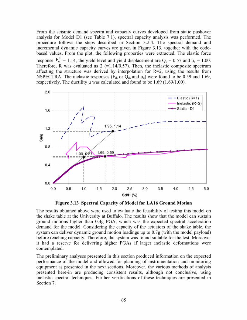
65
From the seismic demand spectra and capacity curves developed from static pushover analysis for Model D1 (see Table 7.1), spectral capacity analysis was performed. The procedure follows the steps described in Section 3.2.4. The spectral demand and incremental dynamic capacity curves are given in Figure 3.13, together with the code-based values. From the plot, the following properties were extracted. The elastic force response Fm
E = 1.14, the yield level and yield displacement are Qy = 0.57 and uy = 1.00. Therefore, R was evaluated as 2 (=1.14/0.57). Then, the inelastic composite spectrum affecting the structure was derived by interpolation for R=2, using the results from NSPECTRA. The inelastic responses (Fd, or Qd, and ud) were found to be 0.59 and 1.69, respectively. The ductility µ was calculated and found to be 1.69 (1.69/1.00).
1.69, 0.591.00, 0.57
1.95, 1.14
0.0
0.4
0.8
1.2
1.6
2.0
0.0 0.5 1.0 1.5 2.0 2.5 3.0 3.5 4.0 4.5 5.0
Sd/H (%)
Sa/g
Elastic (R=1)Inelastic (R=2)Static - D1
Figure 3.13 Spectral Capacity of Model for LA16 Ground Motion
The results obtained above were used to evaluate the feasibility of testing this model on the shake table at the University at Buffalo. The results show that the model can sustain ground motions higher than 0.4g PGA, which was the expected spectral acceleration demand for the model. Considering the capacity of the actuators of the shake table, the system can deliver dynamic ground motion loadings up to 0.7g (with the model payload) before reaching capacity. Therefore, the system was found suitable for the test. Moreover it had a reserve for delivering higher PGAs if larger inelastic deformations were contemplated. The preliminary analyses presented in this section produced information on the expected performance of the model and allowed for planning of instrumentation and monitoring equipment as presented in the next sections. Moreover, the various methods of analysis presented here-in are producing consistent results, although not conclusive, using inelastic spectral techniques. Further verifications of these techniques are presented in Section 7.

67
SECTION 4 EXPERIMENTAL COMPONENT PROPERTIES EVALUATION
4.1 Introduction 4.1.1 Brief Summary of Section Several material and component tests were carried out prior to the full experimental study of the model. The objective of these additional tests was to better understand the behavior of the components, so that the analytical model could be more faithfully represented. Tests of materials of the beams and columns were made. Component tests consisted of the beam to column assembly with its connection, and the gravity column assembly. The testing procedures and results are presented in this section.
4.1.2 Rationale for Choice of the As-built Sections Preliminary analysis indicated that for several reasons the S3x5.7 section was preferable for the frame beams and columns as well as for the gravity columns. First, it resembled the typical I-shape sections used in prototype structures. Second, the section was the smallest one capable of carrying the required load. Third, the section was readily available, therefore making fabrication easier.
The experimental model required that a “strong column - weak beam” concept be implemented. The beam was assumed to be the weaker element; hence most of the damage would occur in it. There are two different ways for achieving this condition, first by reducing the beam cross-section, and second by using lower yield strength steel.
The first approach was not applicable for this model, since the section used was already the smallest available. Indeed, a quick analysis with an alternative having reduced section beams (dog-boned) showed that this technique was difficult to implement, and the results were still unsatisfactory. The only other alternative was to use lower yield strength steel. Therefore, A36 steel was selected for all beams, and A572/A588 Gr. 50 steel for all columns, including the gravity ones.
4.1.3 Testing Procedures for Materials, Components and Connections The model was constructed with steel as the sole material. It was used for the structural frames as well as for the structural weights, in the form of relatively thick steel floor slabs. In this model, different steel properties were used for different elements. As noted, beams and columns are of different steel materials, and each material was tested. Tensile coupon tests were performed to obtain the stress-strain relationship for each material. Based on the results, the tensile strength and ductility could be determined. The static properties of materials were obtained from the testing. Although cyclic properties may prove to be more relevant for high accuracy, the static properties with proper hysteretic models may prove to be sufficient for the approximate modeling, as used in this report.
68
The beam-column connection assembly was tested for its capacity to resist lateral loading. The assembly was prepared with all the elements entering the joint block, resulting in a cruciform with half spans of typical exterior beams on each side, and half height of typical columns at the top and bottom of the connection. Displacement-controlled lateral loads with increasing amplitudes were applied to the specimen, well into the inelastic range. In order to evaluate the structural properties during the component testing, a small lateral displacement was applied between the test steps, which enabled quasi-elastic evaluation of the structural properties. Using this procedure, a complete analysis of the structural properties and the changes they underwent during the tests could be obtained.
The gravity column assembly was tested for its capacity to ‘rock’, meaning ability to sway laterally without developing shear forces or moments. The test procedure was similar to that for the beam column connection assembly, i.e., using a series of displacement-controlled lateral loads, increasing from the elastic to the inelastic range.
4.2 Material Properties A tensile coupon test was performed to the steel material for beams and columns and the material properties were obtained. The test and the results for each material are described below.
4.2.1 Properties of Beam Material The material used for beams was A36 steel i.e. 36 ksi yield strength and 58 ksi ultimate strength. Three tensile coupon tests were performed to check the properties of the material. The tests were carried out per ASTM recommendations and guidelines. A sample of the stress-strain relationship obtained from the tensile coupon test is given in Figure 4.1.
The results from the coupon tests revealed that the beam material had in fact 50 ksi yield strength and 70 ksi ultimate strength. Thus, the beam elements were made from Gr. 50 steel rather than of A36 steel. These new material properties were used for the further analytical studies of the model (see Section 7). Note that in the elastic range, the recording shows minimal output of the same magnitude with the digital error of the instruments. Through proper weighted average the stiffness (modulus of elasticity) could be determined.
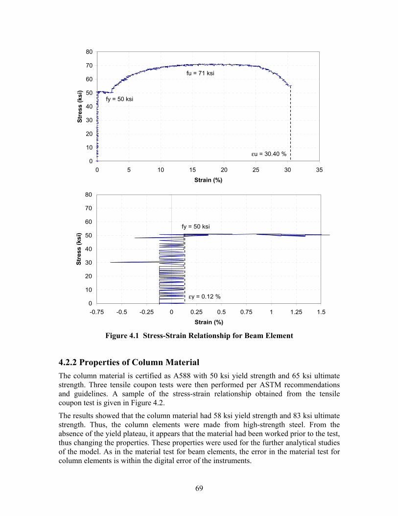
69
0
10
20
30
40
50
60
70
80
0 5 10 15 20 25 30 35
Strain (%)
Stre
ss (k
si)
fy = 50 ksi
fu = 71 ksi
εu = 30.40 %
0
10
20
30
40
50
60
70
80
-0.75 -0.5 -0.25 0 0.25 0.5 0.75 1 1.25 1.5
Strain (%)
Stre
ss (k
si)
fy = 50 ksi
εy = 0.12 %
Figure 4.1 Stress-Strain Relationship for Beam Element
4.2.2 Properties of Column Material The column material is certified as A588 with 50 ksi yield strength and 65 ksi ultimate strength. Three tensile coupon tests were then performed per ASTM recommendations and guidelines. A sample of the stress-strain relationship obtained from the tensile coupon test is given in Figure 4.2.
The results showed that the column material had 58 ksi yield strength and 83 ksi ultimate strength. Thus, the column elements were made from high-strength steel. From the absence of the yield plateau, it appears that the material had been worked prior to the test, thus changing the properties. These properties were used for the further analytical studies of the model. As in the material test for beam elements, the error in the material test for column elements is within the digital error of the instruments.

70
0
10
20
30
40
50
60
70
80
90
100
0 5 10 15 20 25 30
Strain (%)
Stre
ss (k
si)
fy = 58 ksi
fu = 83 ksi
εu = 26.49 %
0
10
20
30
40
50
60
70
80
90
100
-0.75 -0.5 -0.25 0 0.25 0.5 0.75 1 1.25 1.5
Strain (%)
Stre
ss (k
si) fy = 58 ksi
εy = 0.20 %
Figure 4.2 Stress-Strain Relationship for Column Element
4.2.3 Summary of Material Properties Tables 4.1 and 4.2 summarize the material properties as obtained from the test results of the specimens.
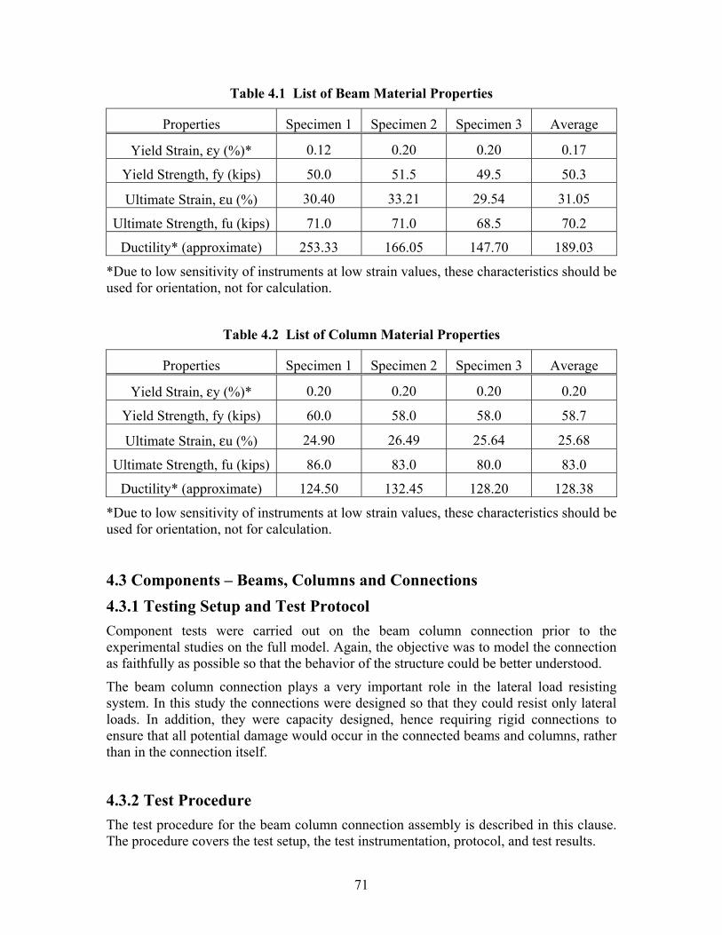
71
Table 4.1 List of Beam Material Properties
Properties Specimen 1 Specimen 2 Specimen 3 Average
Yield Strain, εy (%)* 0.12 0.20 0.20 0.17
Yield Strength, fy (kips) 50.0 51.5 49.5 50.3
Ultimate Strain, εu (%) 30.40 33.21 29.54 31.05
Ultimate Strength, fu (kips) 71.0 71.0 68.5 70.2
Ductility* (approximate) 253.33 166.05 147.70 189.03
*Due to low sensitivity of instruments at low strain values, these characteristics should be used for orientation, not for calculation.
Table 4.2 List of Column Material Properties
Properties Specimen 1 Specimen 2 Specimen 3 Average
Yield Strain, εy (%)* 0.20 0.20 0.20 0.20
Yield Strength, fy (kips) 60.0 58.0 58.0 58.7
Ultimate Strain, εu (%) 24.90 26.49 25.64 25.68
Ultimate Strength, fu (kips) 86.0 83.0 80.0 83.0
Ductility* (approximate) 124.50 132.45 128.20 128.38
*Due to low sensitivity of instruments at low strain values, these characteristics should be used for orientation, not for calculation.
4.3 Components – Beams, Columns and Connections 4.3.1 Testing Setup and Test Protocol Component tests were carried out on the beam column connection prior to the experimental studies on the full model. Again, the objective was to model the connection as faithfully as possible so that the behavior of the structure could be better understood.
The beam column connection plays a very important role in the lateral load resisting system. In this study the connections were designed so that they could resist only lateral loads. In addition, they were capacity designed, hence requiring rigid connections to ensure that all potential damage would occur in the connected beams and columns, rather than in the connection itself.
4.3.2 Test Procedure The test procedure for the beam column connection assembly is described in this clause. The procedure covers the test setup, the test instrumentation, protocol, and test results.
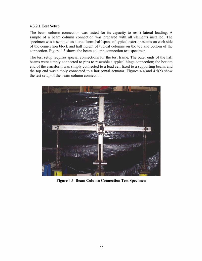
72
4.3.2.1 Test Setup The beam column connection was tested for its capacity to resist lateral loading. A sample of a beam column connection was prepared with all elements installed. The specimen was assembled as a cruciform: half spans of typical exterior beams on each side of the connection block and half height of typical columns on the top and bottom of the connection. Figure 4.3 shows the beam column connection test specimen.
The test setup requires special connections for the test frame. The outer ends of the half beams were simply connected to pins to resemble a typical hinge connection; the bottom end of the cruciform was simply connected to a load cell fixed to a supporting beam; and the top end was simply connected to a horizontal actuator. Figures 4.4 and 4.5(b) show the test setup of the beam column connection.
Figure 4.3 Beam Column Connection Test Specimen

73
Figure 4.4 View of Beam Column Connection Test Setup
4.3.2.2 Instrumentation and Calibration Evidently, the setup for the beam column connection tests requires instrumentation to measure the response of the specimen. Each test instruments is briefly described below. Three five-directional load cells with a capacity of 30 kips in the axial direction, 5 kips for shears X and Y, and 30 k-in for moments about X and Y.
1. Load cell of 20 kips capacity attached to the actuator (calibrated to 0.5 kips/volt).
2. LVDT with a stroke of + 3 in. with sensitivity of 0.6 in./volt
3. Transducers (Temposonics) with + 6 in. calibrated stroke
4. Potentiometers with + 1 in calibrated stroke.
5. Strain gages.
The schematic arrangement of the beam column connection test instrumentation is shown in Figure 4.5. The test data were collected into the SEESL Network through a PC-based interface. Table 4.1 lists the channels used to record the data.

74
(a) Test Setup
(b) Instrumentation
Figure 4.5 Beam Column Connection Test
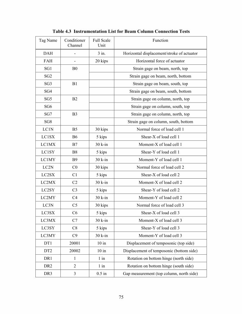
75
Table 4.3 Instrumentation List for Beam Column Connection Tests
Tag Name Conditioner Channel
Full Scale Unit
Function
DAH - 3 in. Horizontal displacement/stroke of actuator
FAH - 20 kips Horizontal force of actuator
SG1 Strain gage on beam, north, top
SG2
B0
Strain gage on beam, north, bottom
SG3 Strain gage on beam, south, top
SG4
B1
Strain gage on beam, south, bottom
SG5 Strain gage on column, north, top
SG6
B2
Strain gage on column, south, top
SG7 Strain gage on column, north, top
SG8
B3
Strain gage on column, south, bottom
LC1N B5 30 kips Normal force of load cell 1
LC1SX B6 5 kips Shear-X of load cell 1
LC1MX B7 30 k-in Moment-X of load cell 1
LC1SY B8 5 kips Shear-Y of load cell 1
LC1MY B9 30 k-in Moment-Y of load cell 1
LC2N C0 30 kips Normal force of load cell 2
LC2SX C1 5 kips Shear-X of load cell 2
LC2MX C2 30 k-in Moment-X of load cell 2
LC2SY C3 5 kips Shear-Y of load cell 2
LC2MY C4 30 k-in Moment-Y of load cell 2
LC3N C5 30 kips Normal force of load cell 3
LC3SX C6 5 kips Shear-X of load cell 3
LC3MX C7 30 k-in Moment-X of load cell 3
LC3SY C8 5 kips Shear-Y of load cell 3
LC3MY C9 30 k-in Moment-Y of load cell 3
DT1 20001 10 in Displacement of temposonic (top side)
DT2 20002 10 in Displacement of temposonic (bottom side)
DR1 1 1 in Rotation on bottom hinge (north side)
DR2 2 1 in Rotation on bottom hinge (south side)
DR3 3 0.5 in Gap measurement (top column, north side)
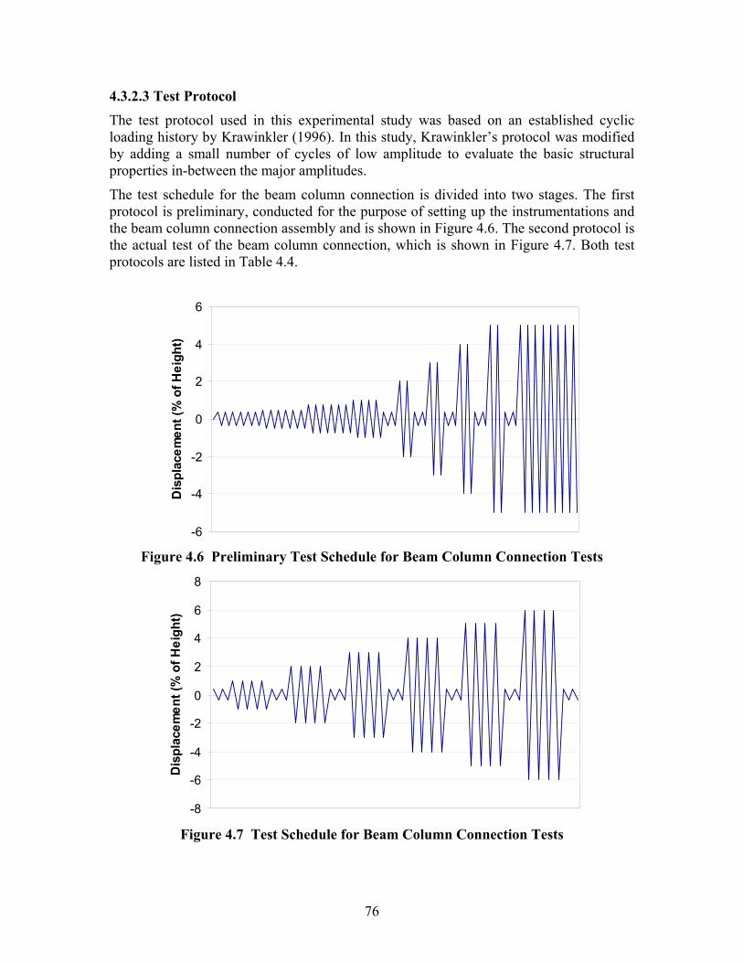
76
4.3.2.3 Test Protocol The test protocol used in this experimental study was based on an established cyclic loading history by Krawinkler (1996). In this study, Krawinkler’s protocol was modified by adding a small number of cycles of low amplitude to evaluate the basic structural properties in-between the major amplitudes.
The test schedule for the beam column connection is divided into two stages. The first protocol is preliminary, conducted for the purpose of setting up the instrumentations and the beam column connection assembly and is shown in Figure 4.6. The second protocol is the actual test of the beam column connection, which is shown in Figure 4.7. Both test protocols are listed in Table 4.4.
-6
-4
-2
0
2
4
6
Dis
plac
emen
t (%
of H
eigh
t)
Figure 4.6 Preliminary Test Schedule for Beam Column Connection Tests
-8
-6
-4
-2
0
2
4
6
8
Dis
plac
emen
t (%
of H
eigh
t)
Figure 4.7 Test Schedule for Beam Column Connection Tests
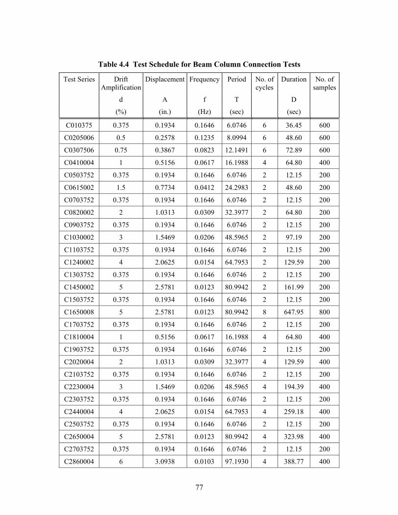
77
Table 4.4 Test Schedule for Beam Column Connection Tests
Test Series Drift Amplification
Displacement Frequency Period No. of cycles
Duration No. of samples
d A f T D
(%) (in.) (Hz) (sec) (sec)
C010375 0.375 0.1934 0.1646 6.0746 6 36.45 600
C0205006 0.5 0.2578 0.1235 8.0994 6 48.60 600
C0307506 0.75 0.3867 0.0823 12.1491 6 72.89 600
C0410004 1 0.5156 0.0617 16.1988 4 64.80 400
C0503752 0.375 0.1934 0.1646 6.0746 2 12.15 200
C0615002 1.5 0.7734 0.0412 24.2983 2 48.60 200
C0703752 0.375 0.1934 0.1646 6.0746 2 12.15 200
C0820002 2 1.0313 0.0309 32.3977 2 64.80 200
C0903752 0.375 0.1934 0.1646 6.0746 2 12.15 200
C1030002 3 1.5469 0.0206 48.5965 2 97.19 200
C1103752 0.375 0.1934 0.1646 6.0746 2 12.15 200
C1240002 4 2.0625 0.0154 64.7953 2 129.59 200
C1303752 0.375 0.1934 0.1646 6.0746 2 12.15 200
C1450002 5 2.5781 0.0123 80.9942 2 161.99 200
C1503752 0.375 0.1934 0.1646 6.0746 2 12.15 200
C1650008 5 2.5781 0.0123 80.9942 8 647.95 800
C1703752 0.375 0.1934 0.1646 6.0746 2 12.15 200
C1810004 1 0.5156 0.0617 16.1988 4 64.80 400
C1903752 0.375 0.1934 0.1646 6.0746 2 12.15 200
C2020004 2 1.0313 0.0309 32.3977 4 129.59 400
C2103752 0.375 0.1934 0.1646 6.0746 2 12.15 200
C2230004 3 1.5469 0.0206 48.5965 4 194.39 400
C2303752 0.375 0.1934 0.1646 6.0746 2 12.15 200
C2440004 4 2.0625 0.0154 64.7953 4 259.18 400
C2503752 0.375 0.1934 0.1646 6.0746 2 12.15 200
C2650004 5 2.5781 0.0123 80.9942 4 323.98 400
C2703752 0.375 0.1934 0.1646 6.0746 2 12.15 200
C2860004 6 3.0938 0.0103 97.1930 4 388.77 400
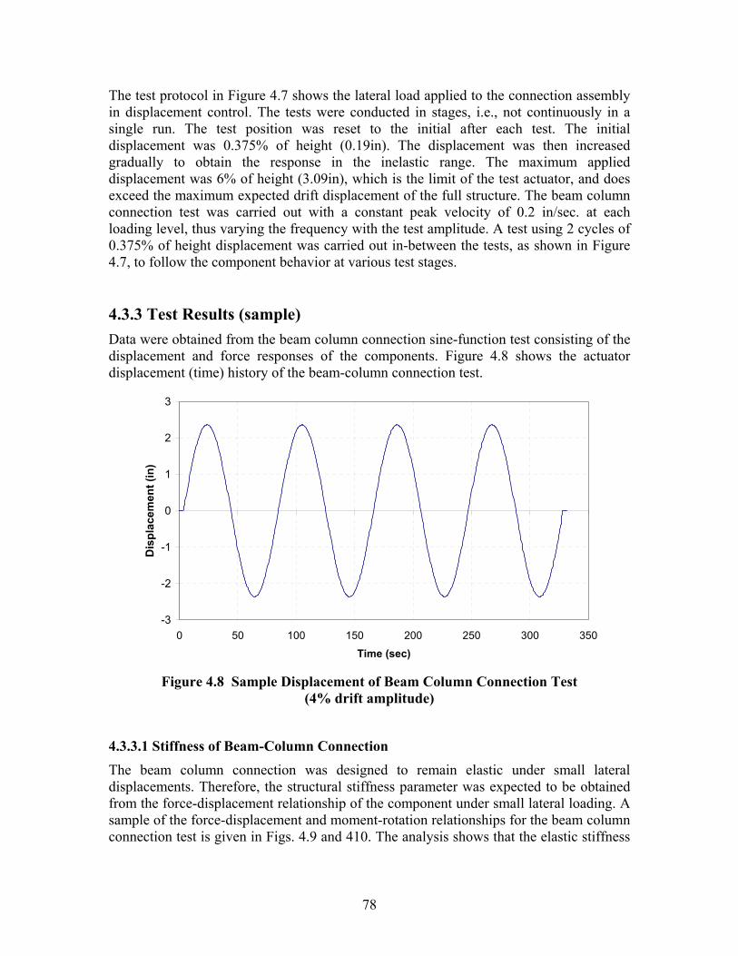
78
The test protocol in Figure 4.7 shows the lateral load applied to the connection assembly in displacement control. The tests were conducted in stages, i.e., not continuously in a single run. The test position was reset to the initial after each test. The initial displacement was 0.375% of height (0.19in). The displacement was then increased gradually to obtain the response in the inelastic range. The maximum applied displacement was 6% of height (3.09in), which is the limit of the test actuator, and does exceed the maximum expected drift displacement of the full structure. The beam column connection test was carried out with a constant peak velocity of 0.2 in/sec. at each loading level, thus varying the frequency with the test amplitude. A test using 2 cycles of 0.375% of height displacement was carried out in-between the tests, as shown in Figure 4.7, to follow the component behavior at various test stages.
4.3.3 Test Results (sample) Data were obtained from the beam column connection sine-function test consisting of the displacement and force responses of the components. Figure 4.8 shows the actuator displacement (time) history of the beam-column connection test.
-3
-2
-1
0
1
2
3
0 50 100 150 200 250 300 350
Time (sec)
Dis
plac
emen
t (in
)
Figure 4.8 Sample Displacement of Beam Column Connection Test
(4% drift amplitude)
4.3.3.1 Stiffness of Beam-Column Connection
The beam column connection was designed to remain elastic under small lateral displacements. Therefore, the structural stiffness parameter was expected to be obtained from the force-displacement relationship of the component under small lateral loading. A sample of the force-displacement and moment-rotation relationships for the beam column connection test is given in Figs. 4.9 and 410. The analysis shows that the elastic stiffness
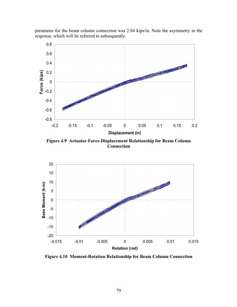
79
parameter for the beam column connection was 2.84 kips/in. Note the asymmetry in the response, which will be referred to subsequently.
-0.8
-0.6
-0.4
-0.2
0
0.2
0.4
0.6
0.8
-0.2 -0.15 -0.1 -0.05 0 0.05 0.1 0.15 0.2
Displacement (in)
Forc
e (k
ips)
Figure 4.9 Actuator Force-Displacement Relationship for Beam Column
Connection
-20
-15
-10
-5
0
5
10
15
20
-0.015 -0.01 -0.005 0 0.005 0.01 0.015
Rotation (rad)
Bas
e M
omen
t (k-
in)
Figure 4.10 Moment-Rotation Relationship for Beam Column Connection
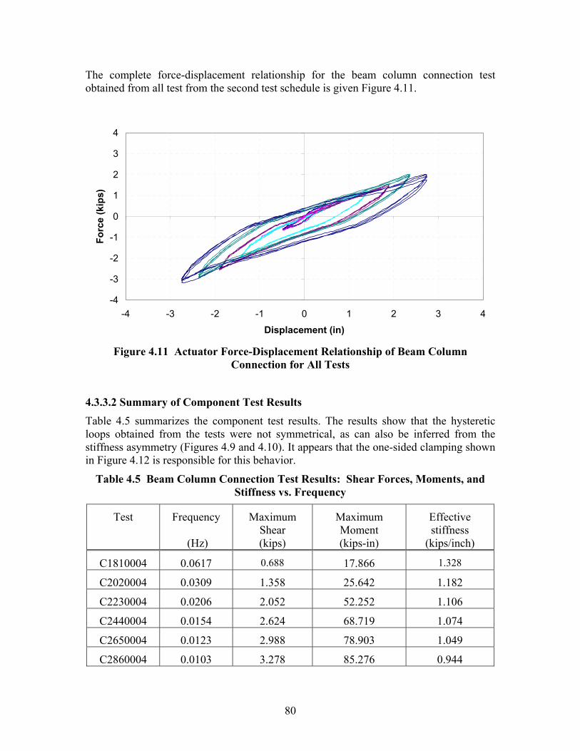
80
The complete force-displacement relationship for the beam column connection test obtained from all test from the second test schedule is given Figure 4.11.
-4
-3
-2
-1
0
1
2
3
4
-4 -3 -2 -1 0 1 2 3 4
Displacement (in)
Forc
e (k
ips)
Figure 4.11 Actuator Force-Displacement Relationship of Beam Column
Connection for All Tests
4.3.3.2 Summary of Component Test Results Table 4.5 summarizes the component test results. The results show that the hysteretic loops obtained from the tests were not symmetrical, as can also be inferred from the stiffness asymmetry (Figures 4.9 and 4.10). It appears that the one-sided clamping shown in Figure 4.12 is responsible for this behavior.
Table 4.5 Beam Column Connection Test Results: Shear Forces, Moments, and Stiffness vs. Frequency
Test Frequency
(Hz)
Maximum Shear (kips)
Maximum Moment (kips-in)
Effective stiffness
(kips/inch)
C1810004 0.0617 0.688 17.866 1.328
C2020004 0.0309 1.358 25.642 1.182
C2230004 0.0206 2.052 52.252 1.106
C2440004 0.0154 2.624 68.719 1.074
C2650004 0.0123 2.988 78.903 1.049
C2860004 0.0103 3.278 85.276 0.944

81
4.3.3.3 Damage Evaluation - Prying Effects on Connection and Effect of Load Levels Test results show that the beam column connection experienced damage under large lateral displacement. Figure 4.12 shows damage to the cruciform. The accumulated damage of the connection to the block took the form of prying of the column end plate, as shown in Figure 4.13. Figure 4.14 shows the history of the raise of the column end plate for the connection test with a drift amplification of 4 percent of the height of the component. Note the asymmetry in prying manifested in Figure 4.14 by the base line shift.
Figure 4.12 Inelastic Response of Beam Column Connection
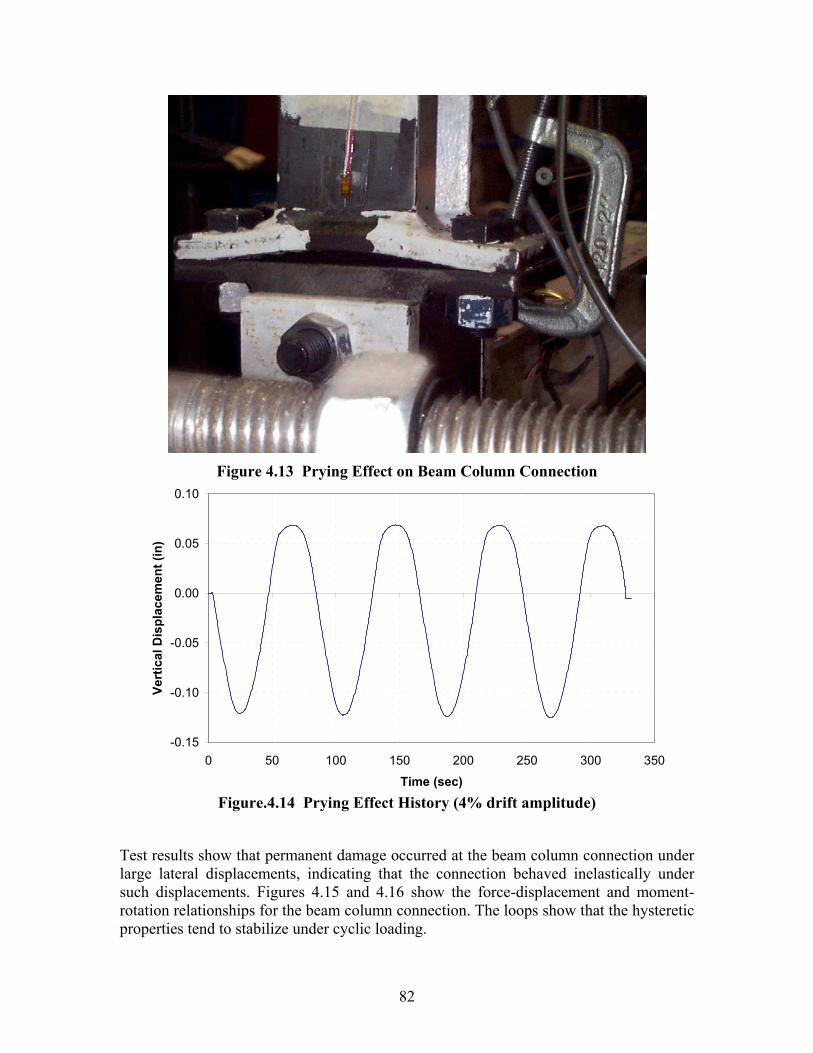
82
Figure 4.13 Prying Effect on Beam Column Connection
-0.15
-0.10
-0.05
0.00
0.05
0.10
0 50 100 150 200 250 300 350
Time (sec)
Vert
ical
Dis
plac
emen
t (in
)
Figure.4.14 Prying Effect History (4% drift amplitude)
Test results show that permanent damage occurred at the beam column connection under large lateral displacements, indicating that the connection behaved inelastically under such displacements. Figures 4.15 and 4.16 show the force-displacement and moment-rotation relationships for the beam column connection. The loops show that the hysteretic properties tend to stabilize under cyclic loading.
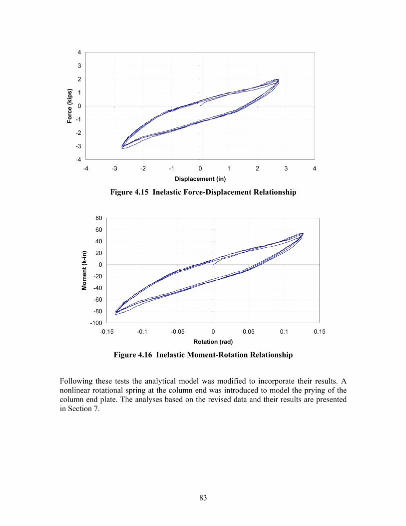
83
-4
-3
-2
-1
0
1
2
3
4
-4 -3 -2 -1 0 1 2 3 4
Displacement (in)
Forc
e (k
ips)
Figure 4.15 Inelastic Force-Displacement Relationship
-100
-80
-60
-40
-20
0
20
40
60
80
-0.15 -0.1 -0.05 0 0.05 0.1 0.15
Rotation (rad)
Mom
ent (
k-in
)
Figure 4.16 Inelastic Moment-Rotation Relationship
Following these tests the analytical model was modified to incorporate their results. A nonlinear rotational spring at the column end was introduced to model the prying of the column end plate. The analyses based on the revised data and their results are presented in Section 7.
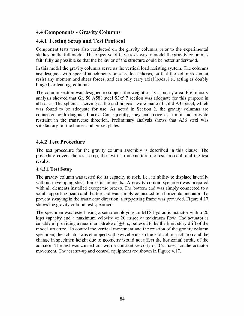
84
4.4 Components - Gravity Columns 4.4.1 Testing Setup and Test Protocol Component tests were also conducted on the gravity columns prior to the experimental studies on the full model. The objective of these tests was to model the gravity column as faithfully as possible so that the behavior of the structure could be better understood.
In this model the gravity columns serve as the vertical load resisting system. The columns are designed with special attachments or so-called spheres, so that the columns cannot resist any moment and shear forces, and can only carry axial loads, i.e., acting as doubly hinged, or leaning, columns.
The column section was designed to support the weight of its tributary area. Preliminary analysis showed that Gr. 50 A588 steel S3x5.7 section was adequate for this purpose in all cases. The spheres - serving as the end hinges - were made of solid A36 steel, which was found to be adequate for use. As noted in Section 2, the gravity columns are connected with diagonal braces. Consequently, they can move as a unit and provide restraint in the transverse direction. Preliminary analysis shows that A36 steel was satisfactory for the braces and gusset plates.
4.4.2 Test Procedure The test procedure for the gravity column assembly is described in this clause. The procedure covers the test setup, the test instrumentation, the test protocol, and the test results.
4.4.2.1 Test Setup The gravity column was tested for its capacity to rock, i.e., its ability to displace laterally without developing shear forces or moments.. A gravity column specimen was prepared with all elements installed except the braces. The bottom end was simply connected to a solid supporting beam and the top end was simply connected to a horizontal actuator. To prevent swaying in the transverse direction, a supporting frame was provided. Figure 4.17 shows the gravity column test specimen.
The specimen was tested using a setup employing an MTS hydraulic actuator with a 20 kips capacity and a maximum velocity of 20 in/sec at maximum flow. The actuator is capable of providing a maximum stroke of +3in., believed to be the limit story drift of the model structure. To control the vertical movement and the rotation of the gravity column specimen, the actuator was equipped with swivel ends so the end column rotation and the change in specimen height due to geometry would not affect the horizontal stroke of the actuator. The test was carried out with a constant velocity of 0.2 in/sec for the actuator movement. The test set-up and control equipment are shown in Figure 4.17.
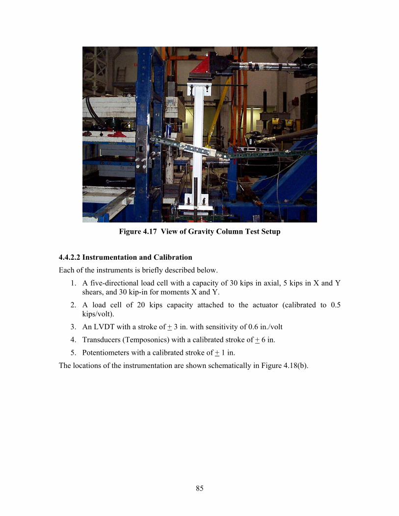
85
Figure 4.17 View of Gravity Column Test Setup
4.4.2.2 Instrumentation and Calibration Each of the instruments is briefly described below.
1. A five-directional load cell with a capacity of 30 kips in axial, 5 kips in X and Y shears, and 30 kip-in for moments X and Y.
2. A load cell of 20 kips capacity attached to the actuator (calibrated to 0.5 kips/volt).
3. An LVDT with a stroke of + 3 in. with sensitivity of 0.6 in./volt
4. Transducers (Temposonics) with a calibrated stroke of + 6 in.
5. Potentiometers with a calibrated stroke of + 1 in.
The locations of the instrumentation are shown schematically in Figure 4.18(b).
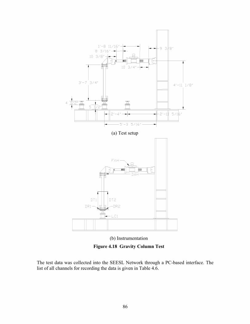
86
(a) Test setup
(b) Instrumentation
Figure 4.18 Gravity Column Test
The test data was collected into the SEESL Network through a PC-based interface. The list of all channels for recording the data is given in Table 4.6.
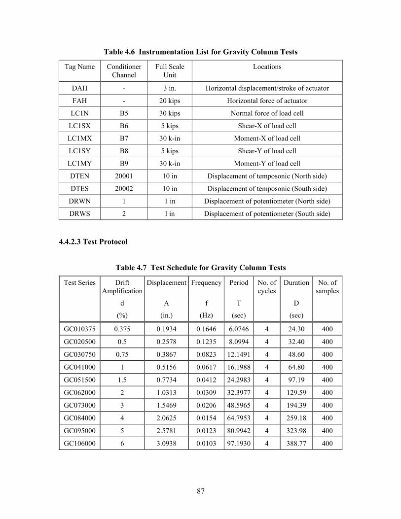
87
Table 4.6 Instrumentation List for Gravity Column Tests
Tag Name Conditioner Channel
Full Scale Unit
Locations
DAH - 3 in. Horizontal displacement/stroke of actuator
FAH - 20 kips Horizontal force of actuator
LC1N B5 30 kips Normal force of load cell
LC1SX B6 5 kips Shear-X of load cell
LC1MX B7 30 k-in Moment-X of load cell
LC1SY B8 5 kips Shear-Y of load cell
LC1MY B9 30 k-in Moment-Y of load cell
DTEN 20001 10 in Displacement of temposonic (North side)
DTES 20002 10 in Displacement of temposonic (South side)
DRWN 1 1 in Displacement of potentiometer (North side)
DRWS 2 I in Displacement of potentiometer (South side)
4.4.2.3 Test Protocol
Table 4.7 Test Schedule for Gravity Column Tests
Test Series Drift Amplification
Displacement Frequency Period No. of cycles
Duration No. of samples
d A f T D
(%) (in.) (Hz) (sec) (sec)
GC010375 0.375 0.1934 0.1646 6.0746 4 24.30 400
GC020500 0.5 0.2578 0.1235 8.0994 4 32.40 400
GC030750 0.75 0.3867 0.0823 12.1491 4 48.60 400
GC041000 1 0.5156 0.0617 16.1988 4 64.80 400
GC051500 1.5 0.7734 0.0412 24.2983 4 97.19 400
GC062000 2 1.0313 0.0309 32.3977 4 129.59 400
GC073000 3 1.5469 0.0206 48.5965 4 194.39 400
GC084000 4 2.0625 0.0154 64.7953 4 259.18 400
GC095000 5 2.5781 0.0123 80.9942 4 323.98 400
GC106000 6 3.0938 0.0103 97.1930 4 388.77 400
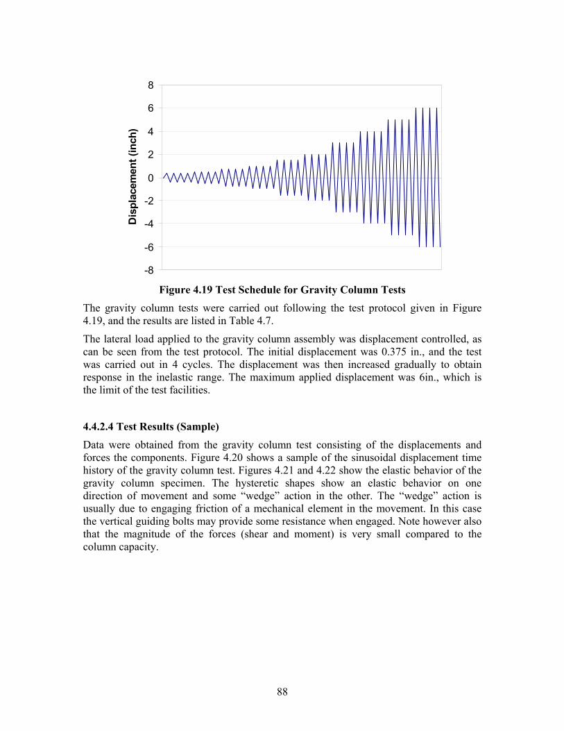
88
-8
-6
-4
-2
0
2
4
6
8
Dis
plac
emen
t (in
ch)
Figure 4.19 Test Schedule for Gravity Column Tests
The gravity column tests were carried out following the test protocol given in Figure 4.19, and the results are listed in Table 4.7.
The lateral load applied to the gravity column assembly was displacement controlled, as can be seen from the test protocol. The initial displacement was 0.375 in., and the test was carried out in 4 cycles. The displacement was then increased gradually to obtain response in the inelastic range. The maximum applied displacement was 6in., which is the limit of the test facilities.
4.4.2.4 Test Results (Sample)
Data were obtained from the gravity column test consisting of the displacements and forces the components. Figure 4.20 shows a sample of the sinusoidal displacement time history of the gravity column test. Figures 4.21 and 4.22 show the elastic behavior of the gravity column specimen. The hysteretic shapes show an elastic behavior on one direction of movement and some “wedge” action in the other. The “wedge” action is usually due to engaging friction of a mechanical element in the movement. In this case the vertical guiding bolts may provide some resistance when engaged. Note however also that the magnitude of the forces (shear and moment) is very small compared to the column capacity.
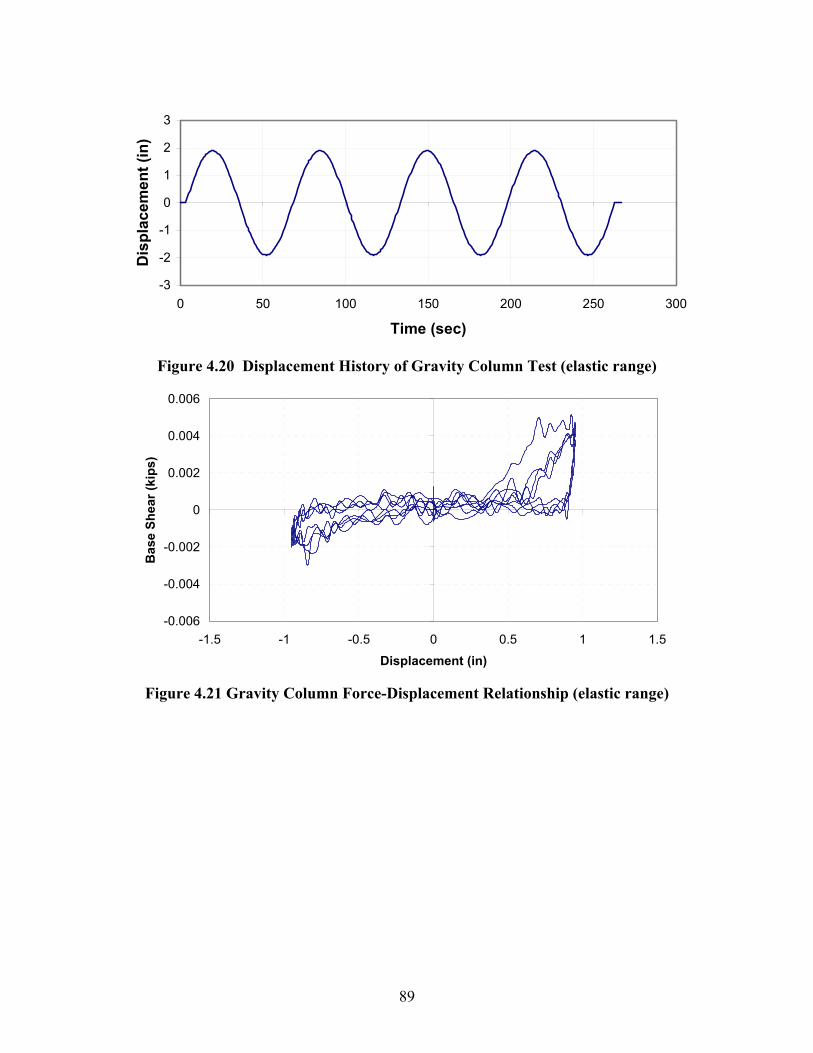
89
-3
-2
-1
0
1
2
3
0 50 100 150 200 250 300
Time (sec)
Dis
plac
emen
t (in
)
Figure 4.20 Displacement History of Gravity Column Test (elastic range)
-0.006
-0.004
-0.002
0
0.002
0.004
0.006
-1.5 -1 -0.5 0 0.5 1 1.5
Displacement (in)
Bas
e Sh
ear (
kips
)
Figure 4.21 Gravity Column Force-Displacement Relationship (elastic range)
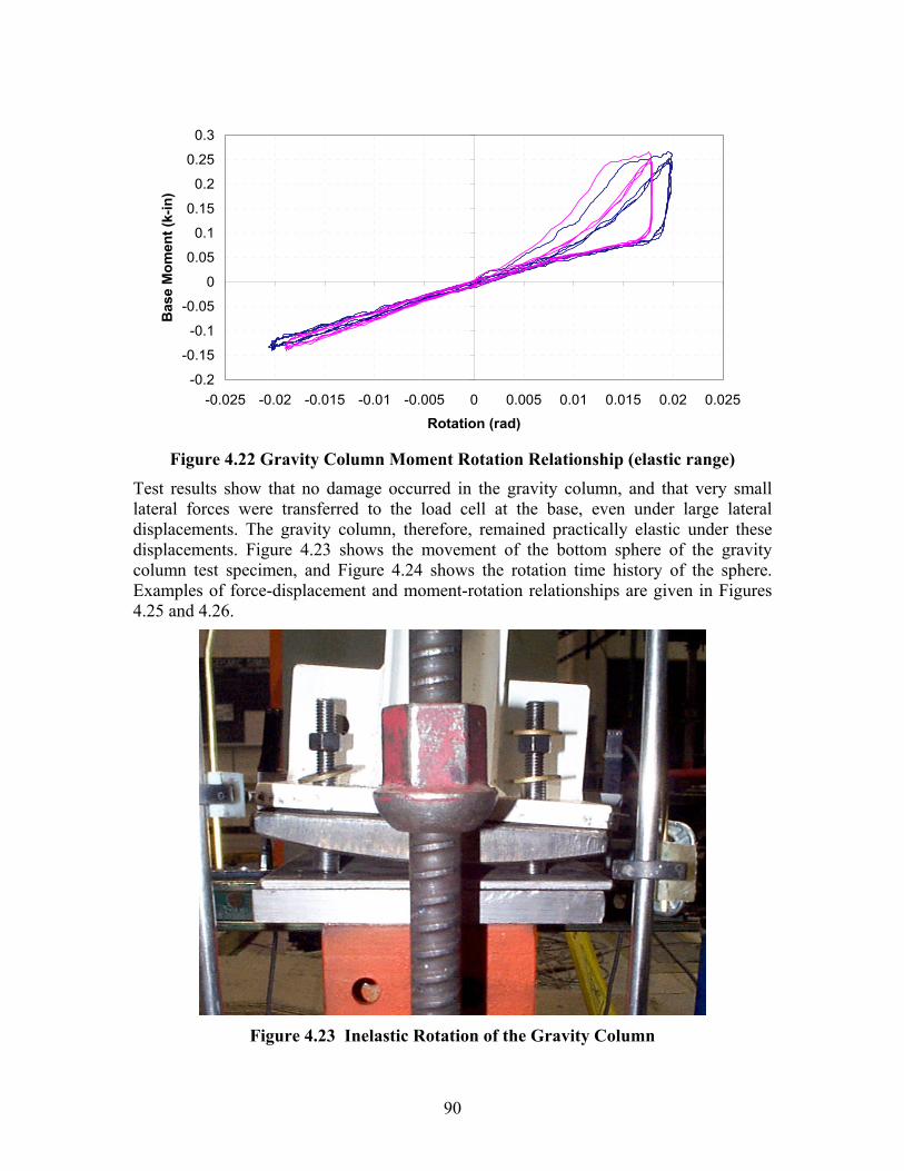
90
-0.2
-0.15
-0.1
-0.05
0
0.05
0.1
0.15
0.2
0.25
0.3
-0.025 -0.02 -0.015 -0.01 -0.005 0 0.005 0.01 0.015 0.02 0.025
Rotation (rad)
Bas
e M
omen
t (k-
in)
Figure 4.22 Gravity Column Moment Rotation Relationship (elastic range)
Test results show that no damage occurred in the gravity column, and that very small lateral forces were transferred to the load cell at the base, even under large lateral displacements. The gravity column, therefore, remained practically elastic under these displacements. Figure 4.23 shows the movement of the bottom sphere of the gravity column test specimen, and Figure 4.24 shows the rotation time history of the sphere. Examples of force-displacement and moment-rotation relationships are given in Figures 4.25 and 4.26.
Figure 4.23 Inelastic Rotation of the Gravity Column

91
-0.15
-0.1
-0.05
0
0.05
0.1
0.15
0 50 100 150 200 250 300
Time (sec) Figure 4.24 Rotation of Spherical Column End History (inelastic range)
-0.015
-0.01
-0.005
0
0.005
0.01
0.015
-4 -3 -2 -1 0 1 2 3 4
Displacement (in)
Bas
e Sh
ear (
kips
)
Figure 4.25 Gravity Column Force-Displacement Relationship (inelastic range)
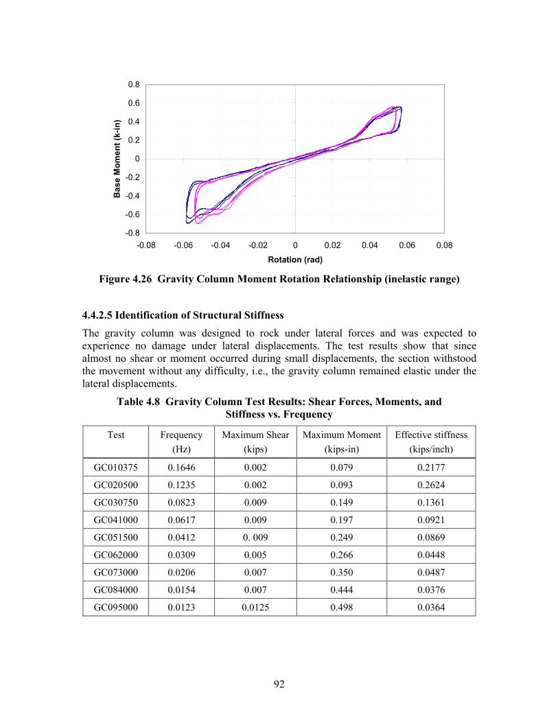
92
-0.8
-0.6
-0.4
-0.2
0
0.2
0.4
0.6
0.8
-0.08 -0.06 -0.04 -0.02 0 0.02 0.04 0.06 0.08
Rotation (rad)
Bas
e M
omen
t (k-
in)
Figure 4.26 Gravity Column Moment Rotation Relationship (inelastic range)
4.4.2.5 Identification of Structural Stiffness
The gravity column was designed to rock under lateral forces and was expected to experience no damage under lateral displacements. The test results show that since almost no shear or moment occurred during small displacements, the section withstood the movement without any difficulty, i.e., the gravity column remained elastic under the lateral displacements.
Table 4.8 Gravity Column Test Results: Shear Forces, Moments, and Stiffness vs. Frequency
Test Frequency (Hz)
Maximum Shear (kips)
Maximum Moment (kips-in)
Effective stiffness (kips/inch)
GC010375 0.1646 0.002 0.079 0.2177
GC020500 0.1235 0.002 0.093 0.2624
GC030750 0.0823 0.009 0.149 0.1361
GC041000 0.0617 0.009 0.197 0.0921
GC051500 0.0412 0. 009 0.249 0.0869
GC062000 0.0309 0.005 0.266 0.0448
GC073000 0.0206 0.007 0.350 0.0487
GC084000 0.0154 0.007 0.444 0.0376
GC095000 0.0123 0.0125 0.498 0.0364
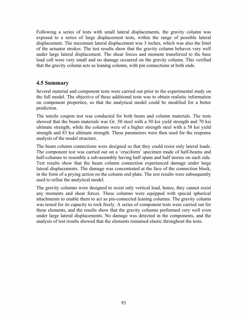
93
Following a series of tests with small lateral displacements, the gravity column was exposed to a series of large displacement tests, within the range of possible lateral displacement. The maximum lateral displacement was 3 inches, which was also the limit of the actuator strokes. The test results show that the gravity column behaves very well under large lateral displacement. The shear forces and moment transferred to the base load cell were very small and no damage occurred on the gravity column. This verified that the gravity column acts as leaning column, with pin connections at both ends.
4.5 Summary Several material and component tests were carried out prior to the experimental study on the full model. The objective of these additional tests was to obtain realistic information on component properties, so that the analytical model could be modified for a better prediction.
The tensile coupon test was conducted for both beam and column materials. The tests showed that the beam materials was Gr. 50 steel with a 50 ksi yield strength and 70 ksi ultimate strength, while the columns were of a higher strength steel with a 58 ksi yield strength and 83 ksi ultimate strength. These parameters were then used for the response analysis of the model structure.
The beam column connections were designed so that they could resist only lateral loads. The component test was carried out on a ‘cruciform’ specimen made of half-beams and half-columns to resemble a sub-assembly having half spans and half stories on each side. Test results show that the beam column connection experienced damage under large lateral displacements. The damage was concentrated at the face of the connection block, in the form of a prying action on the column end plate. The test results were subsequently used to refine the analytical model.
The gravity columns were designed to resist only vertical load, hence, they cannot resist any moments and shear forces. These columns were equipped with special spherical attachments to enable them to act as pin-connected leaning columns. The gravity column was tested for its capacity to rock freely. A series of component tests were carried out for these elements, and the results show that the gravity columns performed very well even under large lateral displacements. No damage was detected in the components, and the analysis of test results showed that the elements remained elastic throughout the tests.


95
SECTION 5
EXPERIMENTAL EVALUATION OF MODEL STRUCTURE: GLOBAL ASSEMBLY PROPERTIES IDENTIFICATION
5.1 Introduction
The identification testing procedure of the benchmark model was performed using shake table experiments in order to observe the structural conditions during the whole experimental study. The structural parameters obtained from the identification tests included natural frequencies, mode shapes, modal participation factors, stiffness matrix, damping matrix, and damping ratios. To obtain these parameters, the model was subjected to a white noise base displacement. The test set-up, test procedure and the theoretical background are presented in this chapter. Experimental results are compared with the analytical predictions and are also discussed in this section.
Figure 5.1 Model Structure on Shake Table
96
5.2 Test Procedure
5.2.1 Test Setup
To run the identification testing, the model was installed on the shake table with all its elements in place. The instruments and measuring devices were then positioned on the finished model. A special frame was placed next to the model to serve as reference. The model was then subjected to a white noise base displacement.
The test setup included model assembly, instrumentation, and preparation of testing facilities, i.e. shake table calibration and compensation. Figure 5.1 shows view of the model structure prior to the identification testing.
5.2.2 Instrumentation and Calibration
Placements of instruments and their calibration are key factors in getting reliable experimental results. The locations, therefore, were chosen so that significant structural responses could be measured. The calibration procedures were conducted for each instrument according to specifications. The instruments used in the identification testing are listed below:
a) Five directional load cells with the following capacities: axial - 30 kips, shears X and Y - 5 kips, moments X and Y - 30 k-in. placed at first story columns for identification of reactions and base shear.
b) Accelerometers (Kulite, Sensotec, and Endevco) with a capacity of + 10 g. placed at all floors to obtain information on the inertia forces and motion detection.
c) Transducers (Temposonics) with a calibrated stroke of + 6 in. for relative and absolute displacements and deformations
d) Potentiometers with a calibrated stroke of + 1 in. for relative and absolute displacements and deformations
A list of all instruments used in the testing is given in Table 5.1. Figures 5.2 to 5.6 show the locations of the instruments for identification testing.
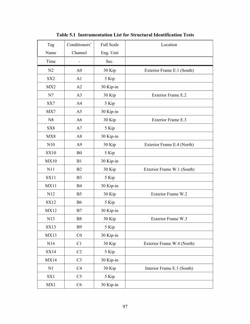
97
Table 5.1 Instrumentation List for Structural Identification Tests
Tag Conditioners’ Full Scale Location
Name Channel Eng. Unit
Time - Sec.
N2 A0 30 Kip Exterior Frame E.1 (South)
SX2 A1 5 Kip
MX2 A2 30 Kip-in
N7 A3 30 Kip Exterior Frame E.2
SX7 A4 5 Kip
MX7 A5 30 Kip-in
N8 A6 30 Kip Exterior Frame E.3
SX8 A7 5 Kip
MX8 A8 30 Kip-in
N10 A9 30 Kip Exterior Frame E.4 (North)
SX10 B0 5 Kip
MX10 B1 30 Kip-in
N11 B2 30 Kip Exterior Frame W.1 (South)
SX11 B3 5 Kip
MX11 B4 30 Kip-in
N12 B5 30 Kip Exterior Frame W.2
SX12 B6 5 Kip
MX12 B7 30 Kip-in
N13 B8 30 Kip Exterior Frame W.3
SX13 B9 5 Kip
MX13 C0 30 Kip-in
N14 C1 30 Kip Exterior Frame W.4 (North)
SX14 C2 5 Kip
MX14 C3 30 Kip-in
N1 C4 30 Kip Interior Frame E.1 (South)
SX1 C5 5 Kip
MX1 C6 30 Kip-in

98
Tag Conditioners’ Full Scale Location
Name Channel Eng. Unit
N3 C7 30 Kip Interior Frame E.2
SX3 C8 5 Kip
MX3 C9 30 Kip-in
N4 D0 30 Kip Interior Frame E.3
SX4 D1 5 Kip
MX4 D2 30 Kip-in
N5 D3 30 Kip Interior Frame E.4 (North)
SX5 D4 5 Kip
MX5 D5 30 Kip-in
N6 D6 30 Kip Interior Frame W.1 (South)
SX6 D7 5 Kip
MX6 D8 30 Kip-in
N9 D9 30 Kip Interior Frame W.2
SX9 E0 5 Kip
MX9 E1 30 Kip-in
N15 E2 30 Kip Interior Frame W.3
SX15 E3 5 Kip
MX15 E4 30 Kip-in
N16 E5 30 Kip Interior Frame W.4 (North)
SX16 E6 5 Kip
MX16 E7 30 Kip-in
DT1 +/- 8" 1st Fl. SE
DT2 +/- 8" 1st Fl. SW
DT3 +/- 10" 2nd Fl. SE
DT4 +/- 15" 2nd Fl. NE
DT5 +/- 10" 2nd Fl. SW
DT6 +/- 8" 2nd Fl. NW
DT7 +/- 10" 3rd Fl. SE
DT8 +/- 10" 3rd Fl. SW
DT9 +/- 6" Base Fl. SE
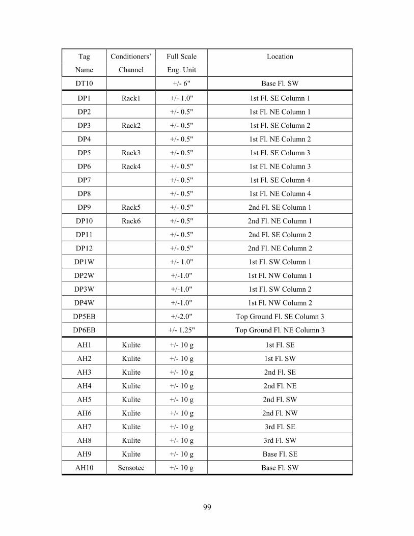
99
Tag Conditioners’ Full Scale Location
Name Channel Eng. Unit
DT10 +/- 6" Base Fl. SW
DP1 Rack1 +/- 1.0" 1st Fl. SE Column 1
DP2 +/- 0.5" 1st Fl. NE Column 1
DP3 Rack2 +/- 0.5" 1st Fl. SE Column 2
DP4 +/- 0.5" 1st Fl. NE Column 2
DP5 Rack3 +/- 0.5" 1st Fl. SE Column 3
DP6 Rack4 +/- 0.5" 1st Fl. NE Column 3
DP7 +/- 0.5" 1st Fl. SE Column 4
DP8 +/- 0.5" 1st Fl. NE Column 4
DP9 Rack5 +/- 0.5" 2nd Fl. SE Column 1
DP10 Rack6 +/- 0.5" 2nd Fl. NE Column 1
DP11 +/- 0.5" 2nd Fl. SE Column 2
DP12 +/- 0.5" 2nd Fl. NE Column 2
DP1W +/- 1.0" 1st Fl. SW Column 1
DP2W +/-1.0" 1st Fl. NW Column 1
DP3W +/-1.0" 1st Fl. SW Column 2
DP4W +/-1.0" 1st Fl. NW Column 2
DP5EB +/-2.0" Top Ground Fl. SE Column 3
DP6EB +/- 1.25" Top Ground Fl. NE Column 3
AH1 Kulite +/- 10 g 1st Fl. SE
AH2 Kulite +/- 10 g 1st Fl. SW
AH3 Kulite +/- 10 g 2nd Fl. SE
AH4 Kulite +/- 10 g 2nd Fl. NE
AH5 Kulite +/- 10 g 2nd Fl. SW
AH6 Kulite +/- 10 g 2nd Fl. NW
AH7 Kulite +/- 10 g 3rd Fl. SE
AH8 Kulite +/- 10 g 3rd Fl. SW
AH9 Kulite +/- 10 g Base Fl. SE
AH10 Sensotec +/- 10 g Base Fl. SW
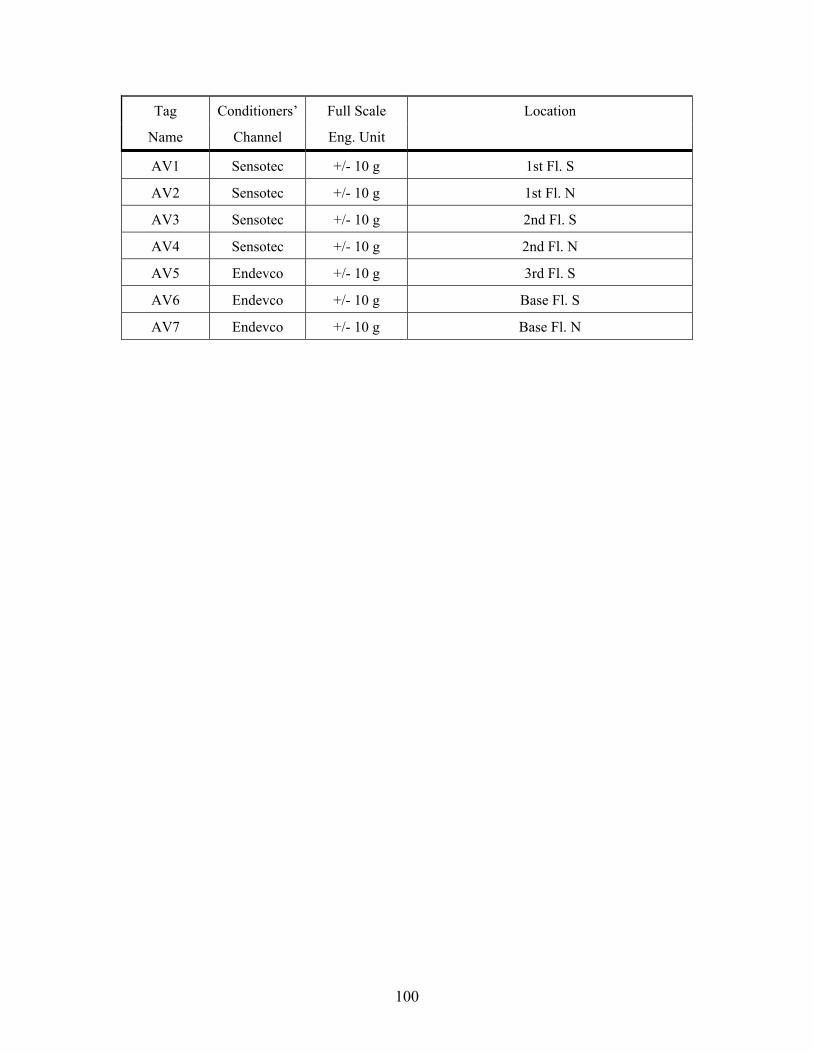
100
Tag Conditioners’ Full Scale Location
Name Channel Eng. Unit
AV1 Sensotec +/- 10 g 1st Fl. S
AV2 Sensotec +/- 10 g 1st Fl. N
AV3 Sensotec +/- 10 g 2nd Fl. S
AV4 Sensotec +/- 10 g 2nd Fl. N
AV5 Endevco +/- 10 g 3rd Fl. S
AV6 Endevco +/- 10 g Base Fl. S
AV7 Endevco +/- 10 g Base Fl. N

Figu
re 5
.2 I
nstr
umen
t Loc
atio
ns fo
r Id
entif
icat
ion
Tes
t: F
ront
Vie
w
N
101

Figu
re 5
.3 I
nstr
umen
t Loc
atio
ns fo
r Id
entif
icat
ion
Tes
t: S
ide
Vie
w
102
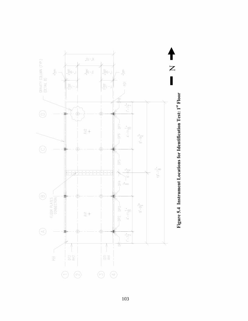
Figu
re 5
.4 I
nstr
umen
t Loc
atio
ns fo
r Id
entif
icat
ion
Tes
t: 1
st F
loor
N
103
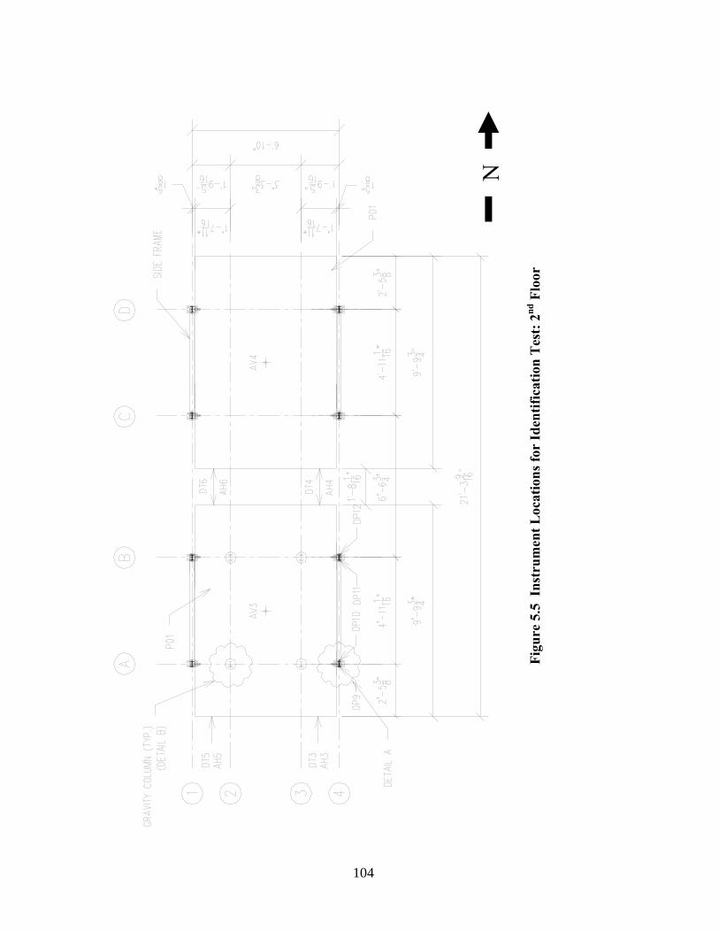
Figu
re 5
.5 I
nstr
umen
t Loc
atio
ns fo
r Id
entif
icat
ion
Tes
t: 2
nd F
loor
N
104
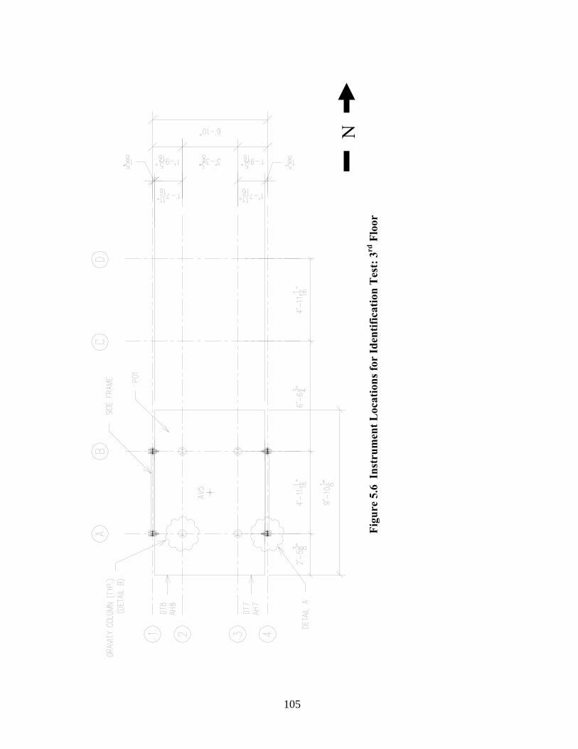
Figu
re 5
.6 I
nstr
umen
t Loc
atio
ns fo
r Id
entif
icat
ion
Tes
t: 3
rd F
loor
N
105
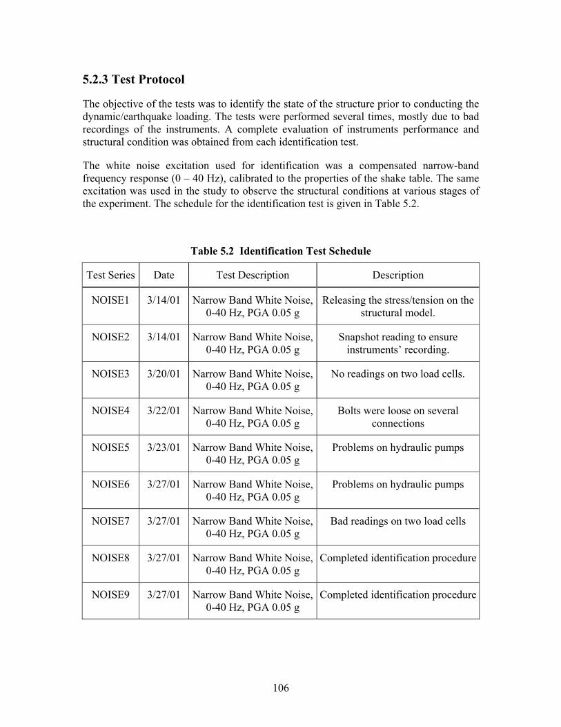
106
5.2.3 Test Protocol
The objective of the tests was to identify the state of the structure prior to conducting the dynamic/earthquake loading. The tests were performed several times, mostly due to bad recordings of the instruments. A complete evaluation of instruments performance and structural condition was obtained from each identification test.
The white noise excitation used for identification was a compensated narrow-band frequency response (0 – 40 Hz), calibrated to the properties of the shake table. The same excitation was used in the study to observe the structural conditions at various stages of the experiment. The schedule for the identification test is given in Table 5.2.
Table 5.2 Identification Test Schedule
Test Series Date Test Description Description
NOISE1 3/14/01 Narrow Band White Noise, 0-40 Hz, PGA 0.05 g
Releasing the stress/tension on the structural model.
NOISE2 3/14/01 Narrow Band White Noise, 0-40 Hz, PGA 0.05 g
Snapshot reading to ensure instruments’ recording.
NOISE3 3/20/01 Narrow Band White Noise, 0-40 Hz, PGA 0.05 g
No readings on two load cells.
NOISE4 3/22/01 Narrow Band White Noise, 0-40 Hz, PGA 0.05 g
Bolts were loose on several connections
NOISE5 3/23/01 Narrow Band White Noise, 0-40 Hz, PGA 0.05 g
Problems on hydraulic pumps
NOISE6 3/27/01 Narrow Band White Noise, 0-40 Hz, PGA 0.05 g
Problems on hydraulic pumps
NOISE7 3/27/01 Narrow Band White Noise, 0-40 Hz, PGA 0.05 g
Bad readings on two load cells
NOISE8 3/27/01 Narrow Band White Noise, 0-40 Hz, PGA 0.05 g
Completed identification procedure
NOISE9 3/27/01 Narrow Band White Noise, 0-40 Hz, PGA 0.05 g
Completed identification procedure
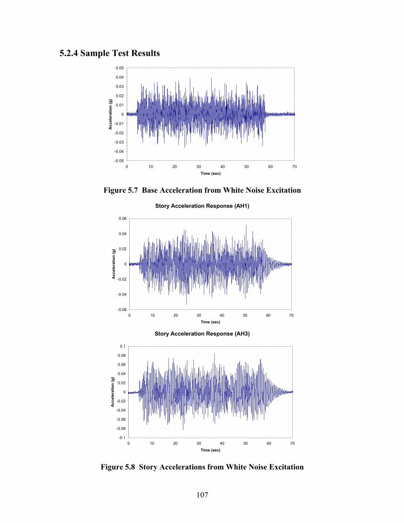
107
5.2.4 Sample Test Results
-0.05
-0.04
-0.03
-0.02
-0.01
0
0.01
0.02
0.03
0.04
0.05
0 10 20 30 40 50 60 70
Time (sec)
Acc
eler
atio
n (g
)
Figure 5.7 Base Acceleration from White Noise Excitation
Story Acceleration Response (AH1)
-0.06
-0.04
-0.02
0
0.02
0.04
0.06
0 10 20 30 40 50 60 70
Time (sec)
Acc
eler
atio
n (g
)
Story Acceleration Response (AH3)
-0.1
-0.08
-0.06
-0.04
-0.02
0
0.02
0.04
0.06
0.08
0.1
0 10 20 30 40 50 60 70
Time (sec)
Acc
eler
atio
n (g
)
Figure 5.8 Story Accelerations from White Noise Excitation
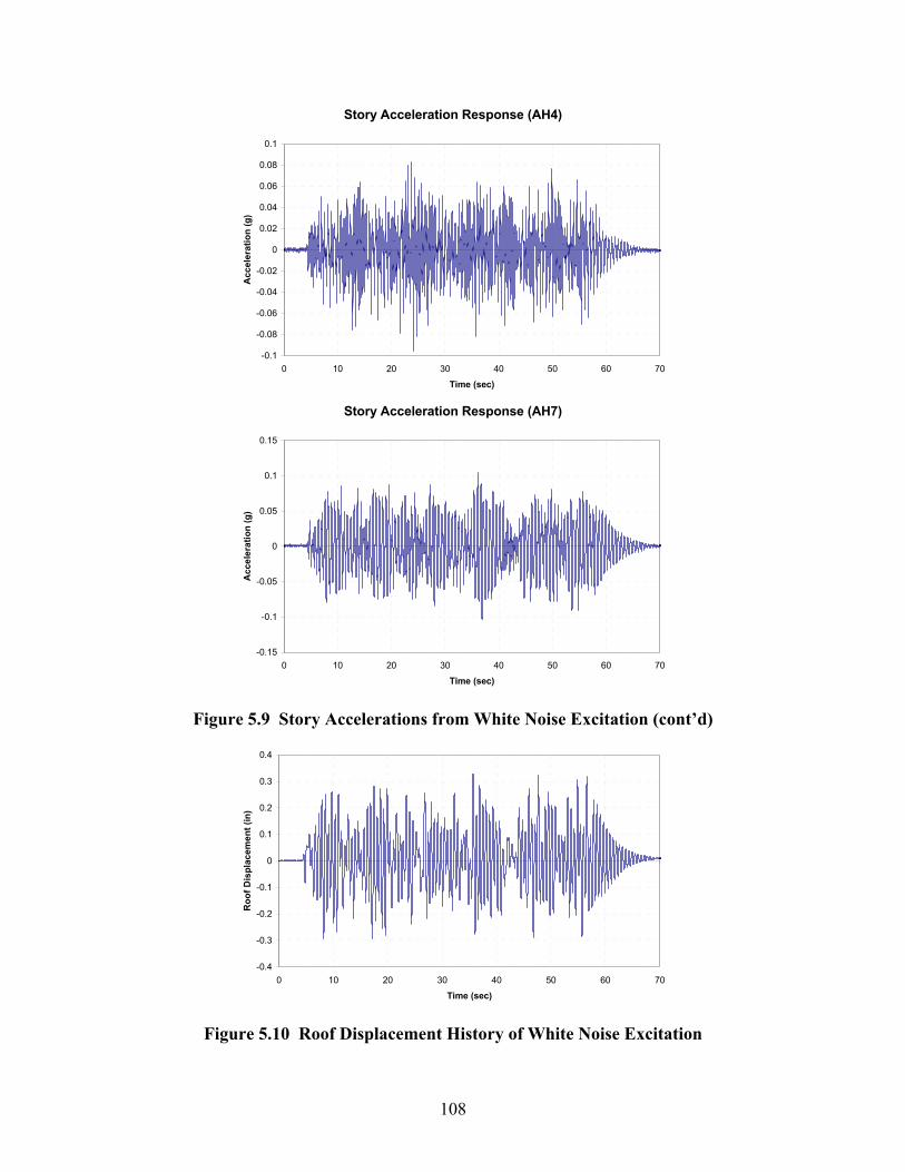
108
Story Acceleration Response (AH4)
-0.1
-0.08
-0.06
-0.04
-0.02
0
0.02
0.04
0.06
0.08
0.1
0 10 20 30 40 50 60 70
Time (sec)
Acc
eler
atio
n (g
)
Story Acceleration Response (AH7)
-0.15
-0.1
-0.05
0
0.05
0.1
0.15
0 10 20 30 40 50 60 70
Time (sec)
Acc
eler
atio
n (g
)
Figure 5.9 Story Accelerations from White Noise Excitation (cont’d)
-0.4
-0.3
-0.2
-0.1
0
0.1
0.2
0.3
0.4
0 10 20 30 40 50 60 70
Time (sec)
Roo
f Dis
plac
emen
t (in
)
Figure 5.10 Roof Displacement History of White Noise Excitation

109
Data were obtained from the identification test consisting of story displacements, story accelerations, and force responses of the structure. Figures 5.7, 5.8 and 5.9 show the base and story acceleration time history of the model. Figure 5.8 shows the roof displacement time history of the taller tower.
5.3 Test Interpretation: Identification Procedures
A simple identification procedure was carried out to identify the dynamic parameters of the model structure (Bracci, 1992). It utilized the structural responses due to a white noise excitation. The procedure to determine the dynamic parameters is presented in Section 5.3.1.
5.3.1 Dynamic Properties
It is useful to relate the accelerations at floor levels to the base acceleration. The transfer function is given in the frequency domain: it is the ratio of the floor acceleration response to the base acceleration. The following derivations evaluate of the dynamic properties using the transfer function.
5.3.1.1 Frequencies and Mode Shapes
The equations of motion for a multi-degree-of freedom (MDOF) structure are usually written as:
)()()()( txmtKxtxCtxM g−=++ (5.1)
where:
M = Structural mass matrix
C = Structural damping matrix
K = Structural stiffness matrix
m = M ⋅ I = Structural mass vector
I = Identity vector
)(txg = Ground acceleration time history
)(tx = Relative displacement time history
)(tx = Relative velocity time history
)(tx = Relative acceleration time history
110
The relative displacement vector can be expressed in terms of the mode shape, Φ, and modal displacement vector, η(t).
)()( ttx η⋅Φ= (5.2)
The equations of motion for a MDOF system can also be written in modal form as follows:
)()()()( txmtKtCtM g−=Φ+Φ+Φ ηηη (5.3)
Equation 5.3 can further be modified to obtain the uncoupled equation of motion for the k-th mode of vibration by multiplying it with the transpose of the k-th mode shape, T
kφ , and utilizing the orthogonality property of the mode shapes:
)()()()( *** txmtKtCtM gTkkkk φηηη −=++ (5.4)
where:
kTkk MM φφ=*
kTkk CC φφ=*
kTkk KK φφ=*
To simplify Eq. 5.4, the mode shapes are normalized such that 1* =kM , implying that 1−Φ=Φ MT
k . The results are then transferred into the frequency domain using the Fourier Transform. Thus, the equation of motion for the k-th mode of vibration can be expressed as:
)()()(2)( 22 ωωηωωηωωξωηω gkkkkkkk xi Γ−=++− (5.5)
where:
ω = requency
kξ = damping ratio for the k-th mode
kω = natural frequency for the k-th mode
MTkk φ=Γ = modal participation factor for the k-th mode
The modal displacements are then obtained from:.
kkk
gkk i
xωωξωω
ωωη
2)(
)( 22 +−⋅Γ
= (5.6)
111
Next, the absolute acceleration for the MDOF system )(ta is given by:
)()()( txtxta g+= (5.7)
Similarly, the absolute acceleration can be expressed in terms of the mode shape. Transferring Eq. 5.7 into the frequency domain:
)()()( 2 ωωφηωω gxa +−= (5.8)
Multiplying Eq. 5.8 by MTkk φ=Γ and introducing the absolute modal acceleration, )(ως ,
for the k-th mode of vibration lead to:
)()()()( 2 ωωηωωως gkkTkk xaM Γ+−=Φ= (5.9)
and substituting Eq. 5.9 into Eq. 5.5 result in:
0)()(2)( 2 =++ ωηωωηωωξως kkkkkk i (5.10)
Thus, the absolute modal acceleration is given by:
)(2
)2()( 22
2
ωωωξωωωωωξως g
kkk
kkkkk x
ii
⋅+−
+⋅Γ−= (5.11)
The absolute modal acceleration can be expressed as the superposition of modes of vibration, as follows:
∑=
⋅=n
kkjkja
1
)]([)( ωςφω (5.12)
where:
=)(ωja absolute acceleration of j-th DOF
n = modes of vibration
jkφ = k-th mass normalized mode shape for j-th DOF
Using Eq. 5.11, the absolute acceleration can then be evaluated as:
)(2
)2()(1
22
2
ωφωωξωωωωωξω g
n
kjk
kkk
kkkkj x
iia ⋅⎥
⎦
⎤⎢⎣
⎡⋅
+−+⋅Γ−= ∑
=
(5.13)
Since the transfer function is the ratio of the acceleration response to the base ground motion, Eq. 5.13 above can be used to obtain the transfer function Hj(ω) for the j-th DOF, namely:
112
2
2 21 1
(2 )( ) ( )2
n nk k k
j k jk k k jkk kk k k
iH Hi
ωξ ω ωω φ ω φω ω ωξ ω= =
⎡ ⎤− += Γ ⋅ = ⋅Γ ⋅⎢ ⎥− +⎣ ⎦∑ ∑ (5.14)
where 2
2 2
(2 )( )2
k k kk
k k k
iHi
ωξ ω ωωω ω ωξ ω− +=
− +
In a structure with small damping ratios and well-separated modes, the above expression will only have significant values at k mω ω= . The natural frequencies of the structure are where the resonance occurs, and they appear as peaks in the transfer function.
Therefore, the peak of the j-th transfer function at the m-th mode of vibration can then be calculated as follows.
21 4
( )2
mj m m jm
m
Hξ
ω φξ
+= Γ ⋅ (5.15a)
From the ratio of two transfer functions:
jm
im
jmmm
immm
mj
mi
hh
HH
φφ
φωφω
ωω =
⋅Γ⋅⋅Γ⋅=
)()(
)()( (5.15b)
Equation 5.15 shows that the peak of the j-th transfer function for the m-th natural frequency is proportional to the amplitude of the m-th mass normalized mode shape for the j-th DOF. Since the modal participation factor and the damping ratio are the same for all degrees of freedom for the k-th mode, the ratio of the peak of the transfer function at the m-th mode is equal to the ratio of the mode shapes at the m-th mode.
Note that the functions in Eq. 5.15 are complex numbers which indicate:
(i) Magnitude ratio is a normalized mode shapes in respect to degree of freedom j. For example, for φjm = 1, the magnitude value is φjm mode shape.
(ii) Phase of the ratio obtained from the imaginary/real ratio indicates the relative sign of the mode shape ratio.
5.3.1.2 Damping Characteristics
The damping characteristics of the structure can be determined using the “half-power” method. The damping ratio for k-th mode of vibration for an elastic structure can be obtained as follows:

113
kk f
ffffff
212
12
12 −=
+−
=ξ (5.16)
where:
f1 = lower frequency where ρf1 = ρfk/√2
f2 = upper frequency where ρf2 = ρfk/√2
fk = natural frequency for k-th mode
ρf1 = amplitude of transfer function at f1
ρf2 = amplitude of transfer function at f2
ρfk = amplitude of transfer function at fk
Thus, a simple application of the transfer function can give a good estimate of the damping characteristics of the model structure.
5.3.2 Structural Stiffness and Damping
5.3.2.1 Structural Stiffness
Using the mass normalized mode shape matrix, the following expression can be written:
Ω=ΦΦ nTn K (5.17)
where:
nΦ = Mass normalized mode shape matrix
K = Structural stiffness matrix
Ω = Diagonal natural frequency matrix [ ]222
21 ,,, nωωω …
kω = k-th natural frequency
The structural stiffness matrix is expressed as follows:
1−− ΩΦΦ= nT
nK (5.18)
From the orthonormality properties:
nT
n MΦ=Φ − (5.19)
MTnn Φ=Φ −1 (5.20)
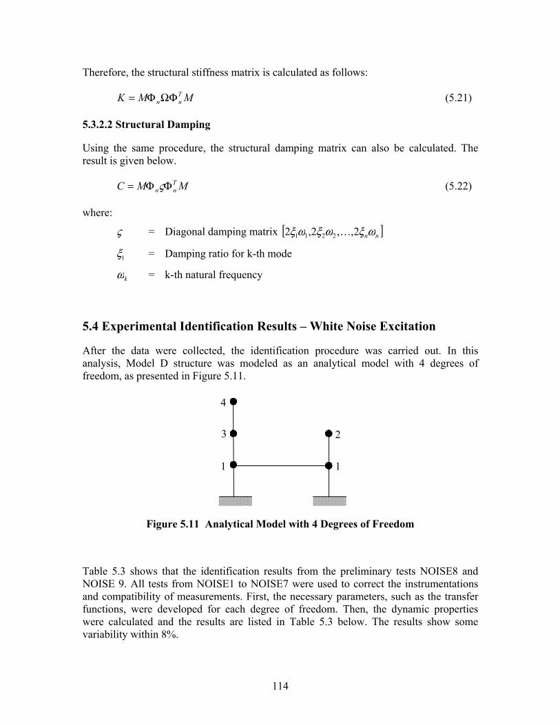
114
Therefore, the structural stiffness matrix is calculated as follows:
MMK TnnΩΦΦ= (5.21)
5.3.2.2 Structural Damping
Using the same procedure, the structural damping matrix can also be calculated. The result is given below.
MMC Tnn ΦΦ= ς (5.22)
where:
ς = Diagonal damping matrix [ ]nnωξωξωξ 2,,2,2 2211 …
1ξ = Damping ratio for k-th mode
kω = k-th natural frequency
5.4 Experimental Identification Results – White Noise Excitation
After the data were collected, the identification procedure was carried out. In this analysis, Model D structure was modeled as an analytical model with 4 degrees of freedom, as presented in Figure 5.11.
1 1
23
4
Figure 5.11 Analytical Model with 4 Degrees of Freedom
Table 5.3 shows that the identification results from the preliminary tests NOISE8 and NOISE 9. All tests from NOISE1 to NOISE7 were used to correct the instrumentations and compatibility of measurements. First, the necessary parameters, such as the transfer functions, were developed for each degree of freedom. Then, the dynamic properties were calculated and the results are listed in Table 5.3 below. The results show some variability within 8%.
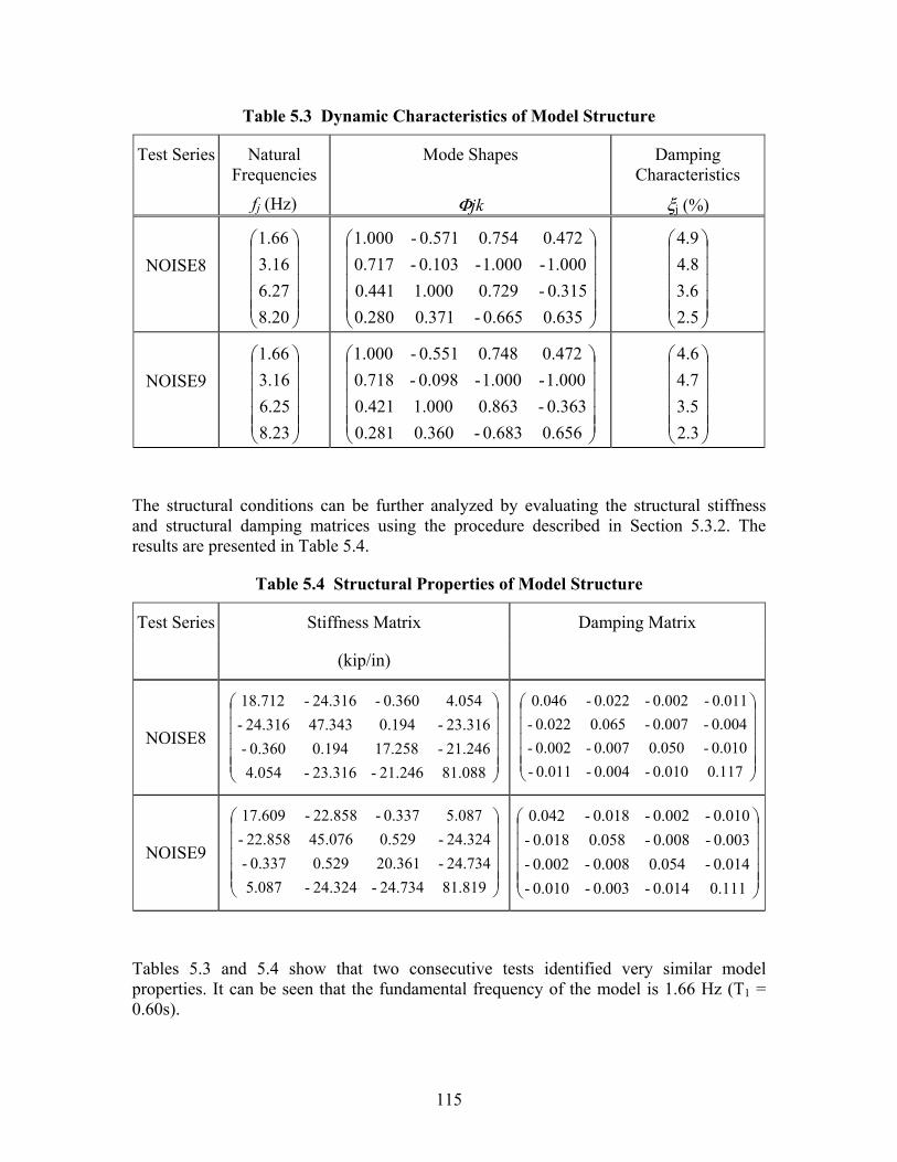
115
Table 5.3 Dynamic Characteristics of Model Structure
Test Series Natural Frequencies
Mode Shapes Damping Characteristics
fj (Hz) Φjk ξj (%)
NOISE8
⎟⎟⎟⎟⎟
⎠
⎞
⎜⎜⎜⎜⎜
⎝
⎛
8.206.273.161.66
⎟⎟⎟⎟⎟
⎠
⎞
⎜⎜⎜⎜⎜
⎝
⎛
0.6350.665-0.3710.2800.315-0.7291.0000.4411.000-1.000-0.103-0.7170.4720.7540.571-1.000
⎟⎟⎟⎟⎟
⎠
⎞
⎜⎜⎜⎜⎜
⎝
⎛
2.53.64.84.9
NOISE9
⎟⎟⎟⎟⎟
⎠
⎞
⎜⎜⎜⎜⎜
⎝
⎛
8.236.253.161.66
⎟⎟⎟⎟⎟
⎠
⎞
⎜⎜⎜⎜⎜
⎝
⎛
0.6560.683-0.3600.2810.363-0.8631.0000.4211.000-1.000-0.098-0.7180.4720.7480.551-1.000
⎟⎟⎟⎟⎟
⎠
⎞
⎜⎜⎜⎜⎜
⎝
⎛
2.33.54.74.6
The structural conditions can be further analyzed by evaluating the structural stiffness and structural damping matrices using the procedure described in Section 5.3.2. The results are presented in Table 5.4.
Table 5.4 Structural Properties of Model Structure
Test Series Stiffness Matrix Damping Matrix
(kip/in)
NOISE8 ⎟⎟⎟⎟⎟
⎠
⎞
⎜⎜⎜⎜⎜
⎝
⎛
81.08821.246-23.316-4.05421.246-17.2580.1940.360-23.316-0.19447.34324.316-4.0540.360-24.316-18.712
⎟⎟⎟⎟⎟
⎠
⎞
⎜⎜⎜⎜⎜
⎝
⎛
0.1170.010-0.004-0.011-0.010-0.0500.007-0.002-0.004-0.007-0.0650.022-0.011-0.002-0.022-0.046
NOISE9 ⎟⎟⎟⎟⎟
⎠
⎞
⎜⎜⎜⎜⎜
⎝
⎛
81.81924.734-24.324-5.08724.734-20.3610.5290.337-24.324-0.52945.07622.858-5.0870.337-22.858-17.609
⎟⎟⎟⎟⎟
⎠
⎞
⎜⎜⎜⎜⎜
⎝
⎛
0.1110.014-0.003-0.010-0.014-0.0540.008-0.002-0.003-0.008-0.0580.018-0.010-0.002-0.018-0.042
Tables 5.3 and 5.4 show that two consecutive tests identified very similar model properties. It can be seen that the fundamental frequency of the model is 1.66 Hz (T1 = 0.60s).

116
5.5 Analytical Identification Results
The objective of the analytical identification procedure was to validate the analytical model (referred as Model D1, see Table 7.1). A structural program (IDARC) was used to conduct the analysis. The program output included the natural frequencies and mode shapes. Hence, they can be compared with the results of the experimental study directly. The comparison of dynamic characteristics obtained from the experimental and the analytical studies is given in Table 5.5, and also illustrated in Figure 5.12.
Table 5.5 Comparison of Dynamic Characteristics of Model Structure
Parameters Experimental Results (NOISE9) IDARC Results (Model D1)
fj (Hz)
⎟⎟⎟⎟⎟
⎠
⎞
⎜⎜⎜⎜⎜
⎝
⎛
8.236.253.161.66
⎟⎟⎟⎟⎟
⎠
⎞
⎜⎜⎜⎜⎜
⎝
⎛
10.347.043.611.91
Φjk
⎟⎟⎟⎟⎟
⎠
⎞
⎜⎜⎜⎜⎜
⎝
⎛
0.6560.683-0.3600.2810.363-0.8631.0000.4211.000-1.000-0.098-0.7180.4720.7480.551-1.000
⎟⎟⎟⎟⎟
⎠
⎞
⎜⎜⎜⎜⎜
⎝
⎛
0.5980.906-0.3340.3120.215-1.0001.0000.4701.000-0.958-0.087-0.7100.4390.7760.616-1.000
0
2
4
6
8
10
12
1 2 3 4Mode
Nat
ural
Fre
quen
cy (H
z) IDARC-D1
NOISE8
NOISE9
(a) Natural frequencies
Figure 5.12 Dynamic Characteristics of Model Structure
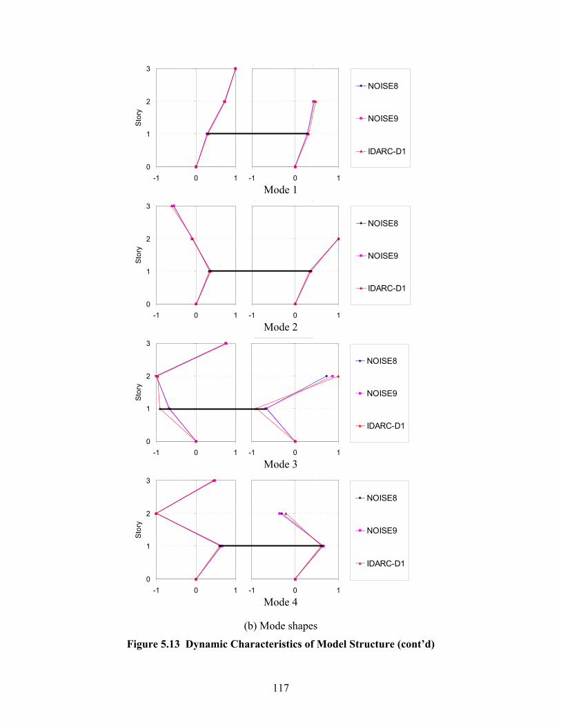
117
0
1
2
3
-1 0 1
Sto
ry
NOISE8
NOISE9
IDARC-D1
-1 0 1
NOISE8
NOISE9
IDARC-D1
Mode 1
0
1
2
3
-1 0 1
Sto
ry
NOISE8
NOISE9
IDARC-D1
-1 0 1
NOISE8
NOISE9
IDARC-D1
Mode 2
0
1
2
3
-1 0 1
Sto
ry
NOISE8
NOISE9
IDARC-D1
-1 0 1
NOISE8
NOISE9
IDARC-D1
Mode 3
0
1
2
3
-1 0 1
Stor
y
NOISE8
NOISE9
IDARC-D1
-1 0 1
NOISE8
NOISE9
IDARC-D1
Mode 4
(b) Mode shapes
Figure 5.13 Dynamic Characteristics of Model Structure (cont’d)

118
The comparison of the dynamic parameters shows that the analytical results of Model D1 are in agreement with the experimental results except for the information related to the third and fourth modes. It was evident that the analytical model was not adequate to predict the model response faithfully. In order to improve the agreement some modifications were made to the analytical model. These, together with the analysis results of the modified model, are presented in Section 7.

119
SECTION 6
SHAKE TABLE TESTING OF SAMPLE STRUCTURE: IRREGULAR CONFIGURATION
6.1 Introduction and Objectives
Testing of the structural model D was carried out to obtaining some insight into the behavior of irregular structures under seismic loading. The dynamic loading, record LA16 (Northridge1994, Rinaldi station), was applied to the model. An incremental dynamic pushover testing (IDPT) was conducted by increasing the amplitude of the dynamic loading up to the verge of structural failure. The structural response was monitored, and the parameters obtained from the procedure included base shear, floor displacements and accelerations. The observed structural damage was instrumental for understanding the effect of irregularities. The test procedure and experimental results are presented in this section, as are some of the basic interpretations.
6.2 Test Procedure
Figure 6.1 View of Model Test Setup
120
6.2.1 Test Setup
The test setup for the dynamic loading was identical to that for the identification procedure (see Section 5). The model was installed on top of the shake table, and then the instruments and measuring devices were positioned on the finished model. A reference frame was placed next to the model and the recorded response was made in respect to this frame.
Figure 6.1 shows the model structure before the dynamic testing.
6.2.2 Instrumentation
As described earlier, the instrument locations for the dynamic loading were identical to the locations for the identification procedure because the structural responses to be measured were similar. In addition, identification testing had also to be carried out during the sample structure test. The instruments used in the dynamic loading were:
a) Five directional load cell with the following capacities: axial - 30 kips, shears X and Y - 5 kips, moments X and Y - 30 k-in.
b) Accelerometers (Kulite, Sensotec, Endevco) with a capacity of + 10 g.
c) Transducers (Temposonics) with a calibrated stroke of + 6 in.
d) Potentiometers with a calibrated stroke of + 1 in.
A list of all instruments used in the experiment is given in Table 5.1. Figures 5.2 to 5.6 show the instrument locations.
6.2.3 Testing Schedule
Following the identification procedure (as described in Section 5), dynamic loading was applied to the model via the 5-DOF shake table (seismic simulator) at University at Buffalo.. A series of ground motions was used to conduct dynamic pushover tests, in order to understand the behavior of such irregular structure under seismic loading. The ground motion selected was LA16 (Rinaldi) earthquake, which was applied to the model in an increasing pattern (see Table 6.1). The first test was set up with a seismic loading of a minor earthquake (PGA = 0.05g) to observe the elastic response of the structure. Following an identification procedure using a white noise excitation, seismic loading with an increased PGA was applied. The test was continued by increasing the PGA at intervals of 0.05g until a state of incipient structural collapse was reached. During the test, the changes in the structural parameters were also obtained by conducting identification tests as outlined in the previous section. The schedule for dynamic tests is given in Table 6.1.
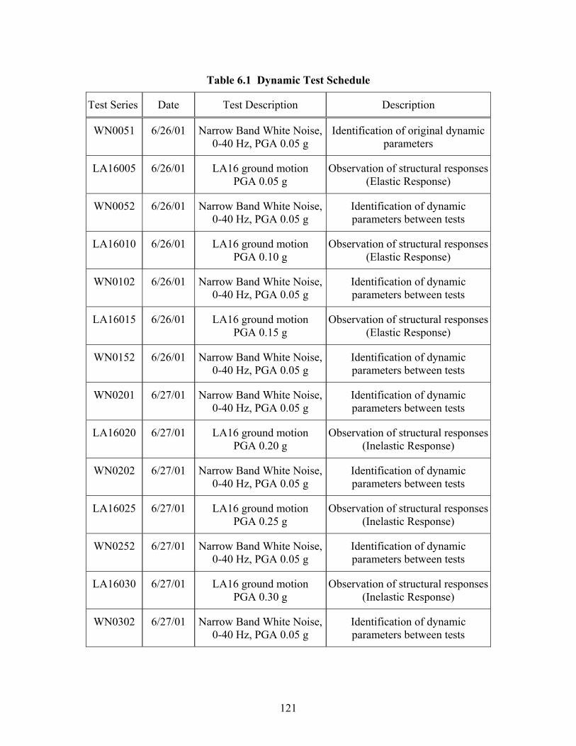
121
Table 6.1 Dynamic Test Schedule
Test Series Date Test Description Description
WN0051 6/26/01 Narrow Band White Noise, 0-40 Hz, PGA 0.05 g
Identification of original dynamic parameters
LA16005 6/26/01 LA16 ground motion PGA 0.05 g
Observation of structural responses (Elastic Response)
WN0052 6/26/01 Narrow Band White Noise, 0-40 Hz, PGA 0.05 g
Identification of dynamic parameters between tests
LA16010 6/26/01 LA16 ground motion PGA 0.10 g
Observation of structural responses (Elastic Response)
WN0102 6/26/01 Narrow Band White Noise, 0-40 Hz, PGA 0.05 g
Identification of dynamic parameters between tests
LA16015 6/26/01 LA16 ground motion PGA 0.15 g
Observation of structural responses (Elastic Response)
WN0152 6/26/01 Narrow Band White Noise, 0-40 Hz, PGA 0.05 g
Identification of dynamic parameters between tests
WN0201 6/27/01 Narrow Band White Noise, 0-40 Hz, PGA 0.05 g
Identification of dynamic parameters between tests
LA16020 6/27/01 LA16 ground motion PGA 0.20 g
Observation of structural responses (Inelastic Response)
WN0202 6/27/01 Narrow Band White Noise, 0-40 Hz, PGA 0.05 g
Identification of dynamic parameters between tests
LA16025 6/27/01 LA16 ground motion PGA 0.25 g
Observation of structural responses (Inelastic Response)
WN0252 6/27/01 Narrow Band White Noise, 0-40 Hz, PGA 0.05 g
Identification of dynamic parameters between tests
LA16030 6/27/01 LA16 ground motion PGA 0.30 g
Observation of structural responses (Inelastic Response)
WN0302 6/27/01 Narrow Band White Noise, 0-40 Hz, PGA 0.05 g
Identification of dynamic parameters between tests
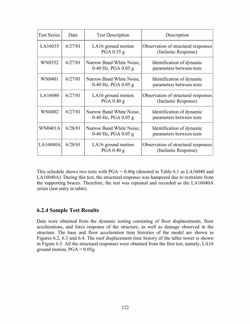
122
Test Series Date Test Description Description
LA16035 6/27/01 LA16 ground motion PGA 0.35 g
Observation of structural responses (Inelastic Response)
WN0352 6/27/01 Narrow Band White Noise, 0-40 Hz, PGA 0.05 g
Identification of dynamic parameters between tests
WN0401 6/27/01 Narrow Band White Noise, 0-40 Hz, PGA 0.05 g
Identification of dynamic parameters between tests
LA16040 6/27/01 LA16 ground motion PGA 0.40 g
Observation of structural responses (Inelastic Response)
WN0402 6/27/01 Narrow Band White Noise, 0-40 Hz, PGA 0.05 g
Identification of dynamic parameters between tests
WN0401A 6/28/01 Narrow Band White Noise, 0-40 Hz, PGA 0.05 g
Identification of dynamic parameters between tests
LA16040A 6/28/01 LA16 ground motion PGA 0.40 g
Observation of structural responses (Inelastic Response)
This schedule shows two tests with PGA = 0.40g (denoted in Table 6.1 as LA16040 and LA16040A). During this test, the structural response was hampered due to restraints from the supporting braces. Therefore, the test was repeated and recorded as the LA16040A series (last entry in table).
6.2.4 Sample Test Results
Data were obtained from the dynamic testing consisting of floor displacements, floor accelerations, and force response of the structure, as well as damage observed in the structure. The base and floor acceleration time histories of the model are shown in Figures 6.2, 6.3 and 6.4. The roof displacement time history of the taller tower is shown in Figure 6.5. All the structural responses were obtained from the first test, namely, LA16 ground motion, PGA = 0.05g.
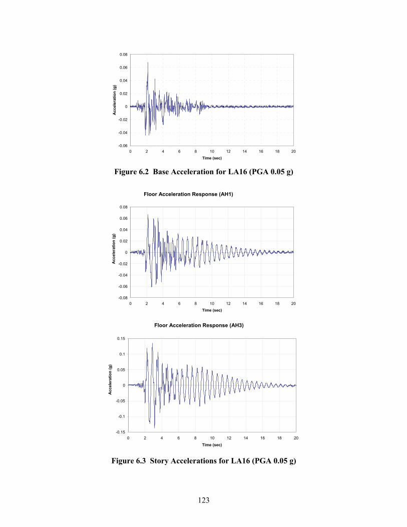
123
-0.06
-0.04
-0.02
0
0.02
0.04
0.06
0.08
0 2 4 6 8 10 12 14 16 18 20
Time (sec)
Acc
eler
atio
n (g
)
Figure 6.2 Base Acceleration for LA16 (PGA 0.05 g)
Figure 6.3 Story Accelerations for LA16 (PGA 0.05 g)
Floor Acceleration Response (AH1)
-0.08
-0.06
-0.04
-0.02
0
0.02
0.04
0.06
0.08
0 2 4 6 8 10 12 14 16 18 20
Time (sec)
Acc
eler
atio
n (g
)
Floor Acceleration Response (AH3)
-0.15
-0.1
-0.05
0
0.05
0.1
0.15
0 2 4 6 8 10 12 14 16 18 20
Time (sec)
Acc
eler
atio
n (g
)
124
Figure 6.4 Story Accelerations for LA16 (PGA 0.05 g) (cont’d)
-1
-0.8
-0.6
-0.4
-0.2
0
0.2
0.4
0.6
0.8
1
0 2 4 6 8 10 12 14 16 18 20
Time (sec)
Roo
f Dis
plac
emen
t (in
)
Figure 6.5 Roof Displacement for LA16 (PGA 0.05 g)
Floor Acceleration Response (AH4)
-0.15
-0.1
-0.05
0
0.05
0.1
0.15
0 2 4 6 8 10 12 14 16 18 20Time (sec)
Acc
eler
atio
n (g
)
Floor Acceleration Response (AH7)
-0.25
-0.2
-0.15
-0.1
-0.05
0
0.05
0.1
0.15
0.2
0.25
0 2 4 6 8 10 12 14 16 18 20
Time (sec)
Acc
eler
atio
n (g
)
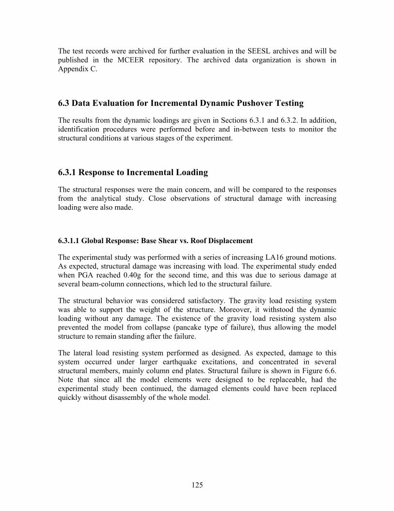
125
The test records were archived for further evaluation in the SEESL archives and will be published in the MCEER repository. The archived data organization is shown in Appendix C.
6.3 Data Evaluation for Incremental Dynamic Pushover Testing
The results from the dynamic loadings are given in Sections 6.3.1 and 6.3.2. In addition, identification procedures were performed before and in-between tests to monitor the structural conditions at various stages of the experiment.
6.3.1 Response to Incremental Loading
The structural responses were the main concern, and will be compared to the responses from the analytical study. Close observations of structural damage with increasing loading were also made.
6.3.1.1 Global Response: Base Shear vs. Roof Displacement
The experimental study was performed with a series of increasing LA16 ground motions. As expected, structural damage was increasing with load. The experimental study ended when PGA reached 0.40g for the second time, and this was due to serious damage at several beam-column connections, which led to the structural failure.
The structural behavior was considered satisfactory. The gravity load resisting system was able to support the weight of the structure. Moreover, it withstood the dynamic loading without any damage. The existence of the gravity load resisting system also prevented the model from collapse (pancake type of failure), thus allowing the model structure to remain standing after the failure.
The lateral load resisting system performed as designed. As expected, damage to this system occurred under larger earthquake excitations, and concentrated in several structural members, mainly column end plates. Structural failure is shown in Figure 6.6. Note that since all the model elements were designed to be replaceable, had the experimental study been continued, the damaged elements could have been replaced quickly without disassembly of the whole model.
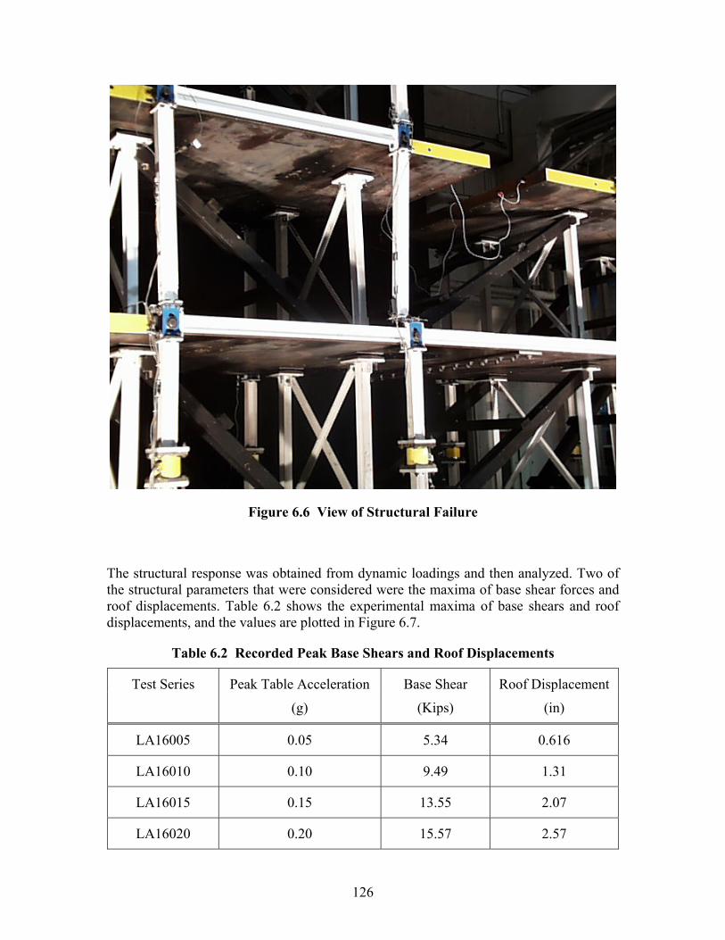
126
Figure 6.6 View of Structural Failure
The structural response was obtained from dynamic loadings and then analyzed. Two of the structural parameters that were considered were the maxima of base shear forces and roof displacements. Table 6.2 shows the experimental maxima of base shears and roof displacements, and the values are plotted in Figure 6.7.
Table 6.2 Recorded Peak Base Shears and Roof Displacements
Test Series Peak Table Acceleration Base Shear Roof Displacement
(g) (Kips) (in)
LA16005 0.05 5.34 0.616
LA16010 0.10 9.49 1.31
LA16015 0.15 13.55 2.07
LA16020 0.20 15.57 2.57
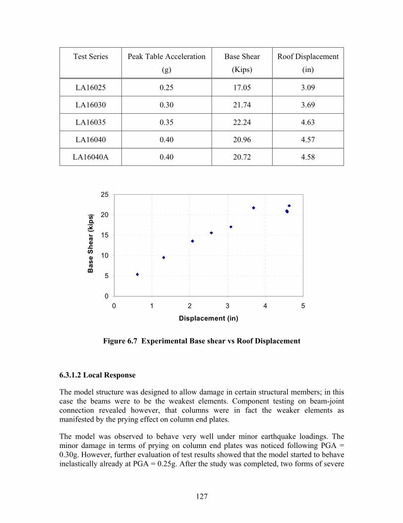
127
Test Series Peak Table Acceleration Base Shear Roof Displacement
(g) (Kips) (in)
LA16025 0.25 17.05 3.09
LA16030 0.30 21.74 3.69
LA16035 0.35 22.24 4.63
LA16040 0.40 20.96 4.57
LA16040A 0.40 20.72 4.58
0
5
10
15
20
25
0 1 2 3 4 5
Displacement (in)
Bas
e S
hear
(kip
s)
Figure 6.7 Experimental Base shear vs Roof Displacement
6.3.1.2 Local Response
The model structure was designed to allow damage in certain structural members; in this case the beams were to be the weakest elements. Component testing on beam-joint connection revealed however, that columns were in fact the weaker elements as manifested by the prying effect on column end plates.
The model was observed to behave very well under minor earthquake loadings. The minor damage in terms of prying on column end plates was noticed following PGA = 0.30g. However, further evaluation of test results showed that the model started to behave inelastically already at PGA = 0.25g. After the study was completed, two forms of severe
)

128
damage were observed at the beam-column joint connections: prying effect on the column end plates and welding failure at the block joint. The last form of damage was unexpected since it was not manifested in the preliminary component testing, and proved to be a more critical factor in the structural failure.
Welding failure of the block joint occurred in two of the connections, creating a separation of the solid block from the block joint end plate. The failure occurred at the toes of the higher tower where force concentrations due to irregularities were expected. Figure 6.8 shows a close up view of the joint failure. Figure 6.9 is a view after the test was completed. The figure shows that the column was completely separated from the solid block joint, yet all bolted connections were still attached properly.
Prying at the column end plates was observed at predicted locations, i.e., where force concentrations occurred. The prying effect was minor compared to the prying in the component test because the story drifts from the dynamic loading were lesser than the limit of the applied displacements in the component test. Figure 6.10 shows the prying effect on the beam column connection located at the outer toe of the lower tower.
Figure 6.8 View of Joint Failure
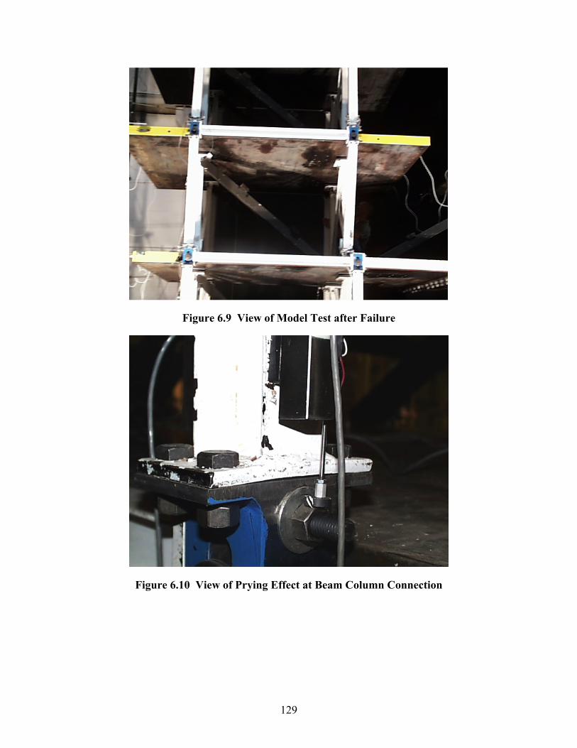
129
Figure 6.9 View of Model Test after Failure
Figure 6.10 View of Prying Effect at Beam Column Connection
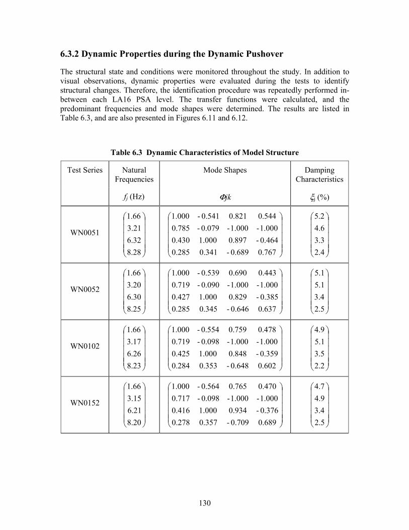
130
6.3.2 Dynamic Properties during the Dynamic Pushover
The structural state and conditions were monitored throughout the study. In addition to visual observations, dynamic properties were evaluated during the tests to identify structural changes. Therefore, the identification procedure was repeatedly performed in-between each LA16 PSA level. The transfer functions were calculated, and the predominant frequencies and mode shapes were determined. The results are listed in Table 6.3, and are also presented in Figures 6.11 and 6.12.
Table 6.3 Dynamic Characteristics of Model Structure
Test Series Natural Frequencies
Mode Shapes Damping Characteristics
fj (Hz) Φjk ξj (%)
WN0051
⎟⎟⎟⎟⎟
⎠
⎞
⎜⎜⎜⎜⎜
⎝
⎛
8.286.323.211.66
⎟⎟⎟⎟⎟
⎠
⎞
⎜⎜⎜⎜⎜
⎝
⎛
0.7670.689-0.3410.2850.464-0.8971.0000.4301.000-1.000-0.079-0.7850.5440.8210.541-1.000
⎟⎟⎟⎟⎟
⎠
⎞
⎜⎜⎜⎜⎜
⎝
⎛
2.43.34.65.2
WN0052
⎟⎟⎟⎟⎟
⎠
⎞
⎜⎜⎜⎜⎜
⎝
⎛
8.256.303.201.66
⎟⎟⎟⎟⎟
⎠
⎞
⎜⎜⎜⎜⎜
⎝
⎛
0.6370.646-0.3450.2850.385-0.8291.0000.4271.000-1.000-0.090-0.7190.4430.6900.539-1.000
⎟⎟⎟⎟⎟
⎠
⎞
⎜⎜⎜⎜⎜
⎝
⎛
2.53.45.15.1
WN0102
⎟⎟⎟⎟⎟
⎠
⎞
⎜⎜⎜⎜⎜
⎝
⎛
8.236.263.171.66
⎟⎟⎟⎟⎟
⎠
⎞
⎜⎜⎜⎜⎜
⎝
⎛
0.6020.648-0.3530.2840.359-0.8481.0000.4251.000-1.000-0.098-0.7190.4780.7590.554-1.000
⎟⎟⎟⎟⎟
⎠
⎞
⎜⎜⎜⎜⎜
⎝
⎛
2.23.55.14.9
WN0152
⎟⎟⎟⎟⎟
⎠
⎞
⎜⎜⎜⎜⎜
⎝
⎛
8.206.213.151.66
⎟⎟⎟⎟⎟
⎠
⎞
⎜⎜⎜⎜⎜
⎝
⎛
0.6890.709-0.3570.2780.376-0.9341.0000.4161.000-1.000-0.098-0.7170.4700.7650.564-1.000
⎟⎟⎟⎟⎟
⎠
⎞
⎜⎜⎜⎜⎜
⎝
⎛
2.53.44.94.7
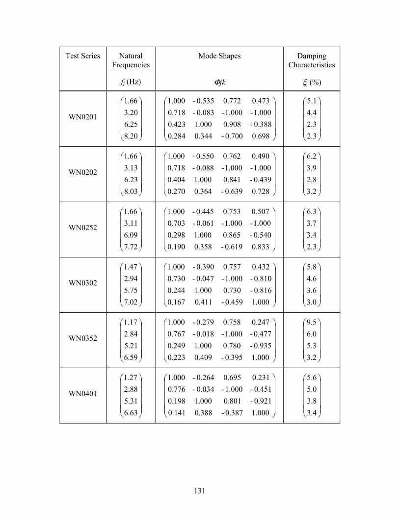
131
Test Series Natural Frequencies
Mode Shapes Damping Characteristics
fj (Hz) Φjk ξj (%)
WN0201
⎟⎟⎟⎟⎟
⎠
⎞
⎜⎜⎜⎜⎜
⎝
⎛
8.206.253.201.66
⎟⎟⎟⎟⎟
⎠
⎞
⎜⎜⎜⎜⎜
⎝
⎛
0.6980.700-0.3440.2840.388-0.9081.0000.4231.000-1.000-0.083-0.7180.4730.7720.535-1.000
⎟⎟⎟⎟⎟
⎠
⎞
⎜⎜⎜⎜⎜
⎝
⎛
2.32.34.45.1
WN0202
⎟⎟⎟⎟⎟
⎠
⎞
⎜⎜⎜⎜⎜
⎝
⎛
8.036.233.131.66
⎟⎟⎟⎟⎟
⎠
⎞
⎜⎜⎜⎜⎜
⎝
⎛
0.7280.639-0.3640.2700.439-0.8411.0000.4041.000-1.000-0.088-0.7180.4900.7620.550-1.000
⎟⎟⎟⎟⎟
⎠
⎞
⎜⎜⎜⎜⎜
⎝
⎛
3.22.83.96.2
WN0252
⎟⎟⎟⎟⎟
⎠
⎞
⎜⎜⎜⎜⎜
⎝
⎛
7.726.093.111.66
⎟⎟⎟⎟⎟
⎠
⎞
⎜⎜⎜⎜⎜
⎝
⎛
0.8330.619-0.3580.1900.540-0.8651.0000.2981.000-1.000-0.061-0.7030.5070.7530.445-1.000
⎟⎟⎟⎟⎟
⎠
⎞
⎜⎜⎜⎜⎜
⎝
⎛
2.33.43.76.3
WN0302
⎟⎟⎟⎟⎟
⎠
⎞
⎜⎜⎜⎜⎜
⎝
⎛
7.025.752.941.47
⎟⎟⎟⎟⎟
⎠
⎞
⎜⎜⎜⎜⎜
⎝
⎛
1.0000.459-0.4110.1670.816-0.7301.0000.2440.810-1.000-0.047-0.7300.4320.7570.390-1.000
⎟⎟⎟⎟⎟
⎠
⎞
⎜⎜⎜⎜⎜
⎝
⎛
3.03.64.65.8
WN0352
⎟⎟⎟⎟⎟
⎠
⎞
⎜⎜⎜⎜⎜
⎝
⎛
6.595.212.841.17
⎟⎟⎟⎟⎟
⎠
⎞
⎜⎜⎜⎜⎜
⎝
⎛
1.0000.395-0.4090.2230.935-0.7801.0000.2490.477-1.000-0.018-0.7670.2470.7580.279-1.000
⎟⎟⎟⎟⎟
⎠
⎞
⎜⎜⎜⎜⎜
⎝
⎛
3.25.36.09.5
WN0401
⎟⎟⎟⎟⎟
⎠
⎞
⎜⎜⎜⎜⎜
⎝
⎛
6.635.312.881.27
⎟⎟⎟⎟⎟
⎠
⎞
⎜⎜⎜⎜⎜
⎝
⎛
1.0000.387-0.3880.1410.921-0.8011.0000.1980.451-1.000-0.034-0.7760.2310.6950.264-1.000
⎟⎟⎟⎟⎟
⎠
⎞
⎜⎜⎜⎜⎜
⎝
⎛
3.43.85.05.6
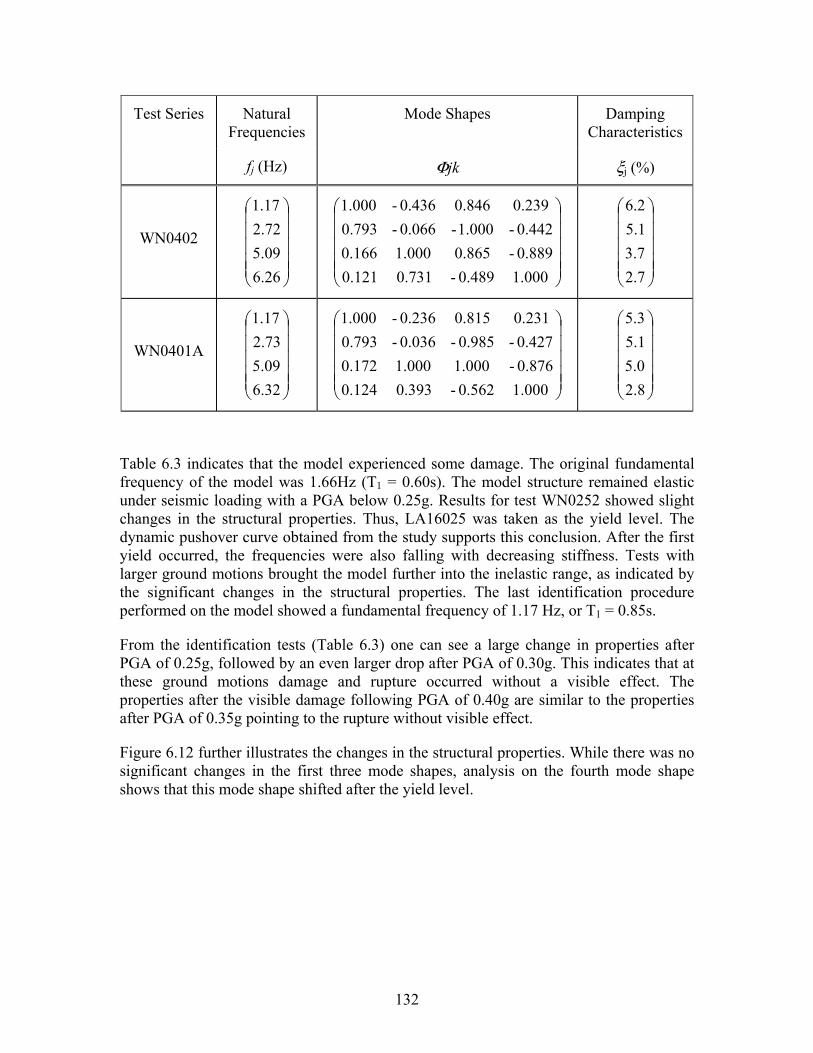
132
Test Series Natural Frequencies
Mode Shapes Damping Characteristics
fj (Hz) Φjk ξj (%)
WN0402
⎟⎟⎟⎟⎟
⎠
⎞
⎜⎜⎜⎜⎜
⎝
⎛
6.265.092.721.17
⎟⎟⎟⎟⎟
⎠
⎞
⎜⎜⎜⎜⎜
⎝
⎛
1.0000.489-0.7310.1210.889-0.8651.0000.1660.442-1.000-0.066-0.7930.2390.8460.436-1.000
⎟⎟⎟⎟⎟
⎠
⎞
⎜⎜⎜⎜⎜
⎝
⎛
2.73.75.16.2
WN0401A
⎟⎟⎟⎟⎟
⎠
⎞
⎜⎜⎜⎜⎜
⎝
⎛
6.325.092.731.17
⎟⎟⎟⎟⎟
⎠
⎞
⎜⎜⎜⎜⎜
⎝
⎛
1.0000.562-0.3930.1240.876-1.0001.0000.1720.427-0.985-0.036-0.7930.2310.8150.236-1.000
⎟⎟⎟⎟⎟
⎠
⎞
⎜⎜⎜⎜⎜
⎝
⎛
2.85.05.15.3
Table 6.3 indicates that the model experienced some damage. The original fundamental frequency of the model was 1.66Hz (T1 = 0.60s). The model structure remained elastic under seismic loading with a PGA below 0.25g. Results for test WN0252 showed slight changes in the structural properties. Thus, LA16025 was taken as the yield level. The dynamic pushover curve obtained from the study supports this conclusion. After the first yield occurred, the frequencies were also falling with decreasing stiffness. Tests with larger ground motions brought the model further into the inelastic range, as indicated by the significant changes in the structural properties. The last identification procedure performed on the model showed a fundamental frequency of 1.17 Hz, or T1 = 0.85s.
From the identification tests (Table 6.3) one can see a large change in properties after PGA of 0.25g, followed by an even larger drop after PGA of 0.30g. This indicates that at these ground motions damage and rupture occurred without a visible effect. The properties after the visible damage following PGA of 0.40g are similar to the properties after PGA of 0.35g pointing to the rupture without visible effect.
Figure 6.12 further illustrates the changes in the structural properties. While there was no significant changes in the first three mode shapes, analysis on the fourth mode shape shows that this mode shape shifted after the yield level.
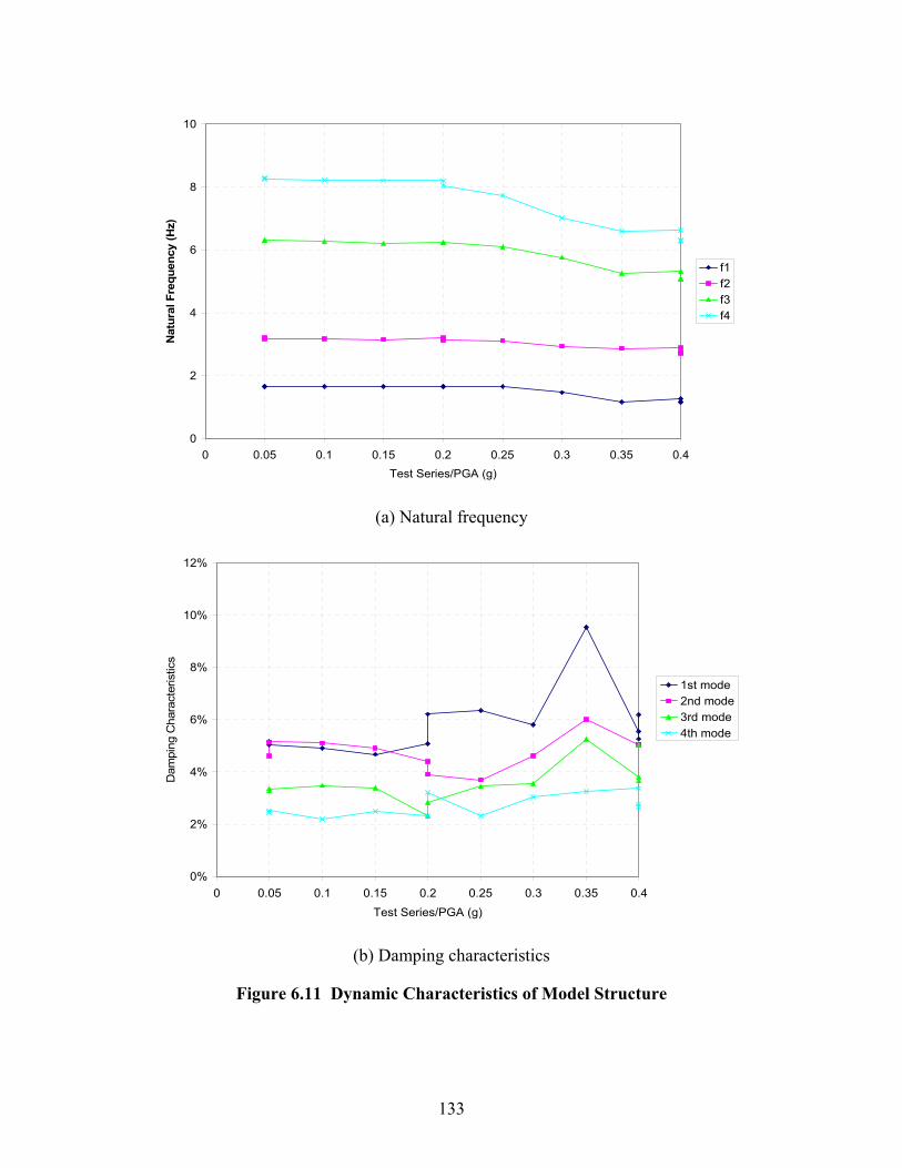
133
0
2
4
6
8
10
0 0.05 0.1 0.15 0.2 0.25 0.3 0.35 0.4Test Series/PGA (g)
Nat
ural
Fre
quen
cy (H
z)
f1f2f3f4
(a) Natural frequency
0%
2%
4%
6%
8%
10%
12%
0 0.05 0.1 0.15 0.2 0.25 0.3 0.35 0.4
Test Series/PGA (g)
Dam
ping
Cha
ract
eris
tics
1st mode2nd mode3rd mode4th mode
(b) Damping characteristics
Figure 6.11 Dynamic Characteristics of Model Structure

134
0
1
2
3
-1 0 1
Sto
ry
WN0051
WN0052
WN0102
WN0152
WN0201
WN0202
WN0252
WN0302
WN0352
WN0401
WN0402
WN0401A-1 0 1
WN0051WN0052WN0102WN0152WN0201WN0202WN0252WN0302WN0352WN0401WN0402WN0401A
Mode 1
0
1
2
3
-1 0 1
Sto
ry
WN0051
WN0052
WN0102
WN0152
WN0201
WN0202
WN0252
WN0302
WN0352
WN0401
WN0402
WN0401A-1 0 1
WN0051WN0052WN0102WN0152WN0201WN0202WN0252WN0302WN0352WN0401WN0402WN0401A
Mode 2
0
1
2
3
-1 0 1
Sto
ry
WN0051
WN0052
WN0102
WN0152
WN0201
WN0202
WN0252
WN0302
WN0352
WN0401
WN0402
WN0401A-1 0 1
WN0051WN0052WN0102WN0152WN0201WN0202WN0252WN0302WN0352WN0401WN0402WN0401A
Mode 3
0
1
2
3
-1 0 1
Sto
ry
WN0051
WN0052
WN0102
WN0152
WN0201
WN0202
WN0252
WN0302
WN0352
WN0401
WN0402
WN0401A-1 0 1
WN0051WN0052WN0102WN0152WN0201WN0202WN0252WN0302WN0352WN0401WN0402WN0401A
Mode 4
(c) Mode shapes
Figure 6.12 Dynamic Characteristics of Model Structure
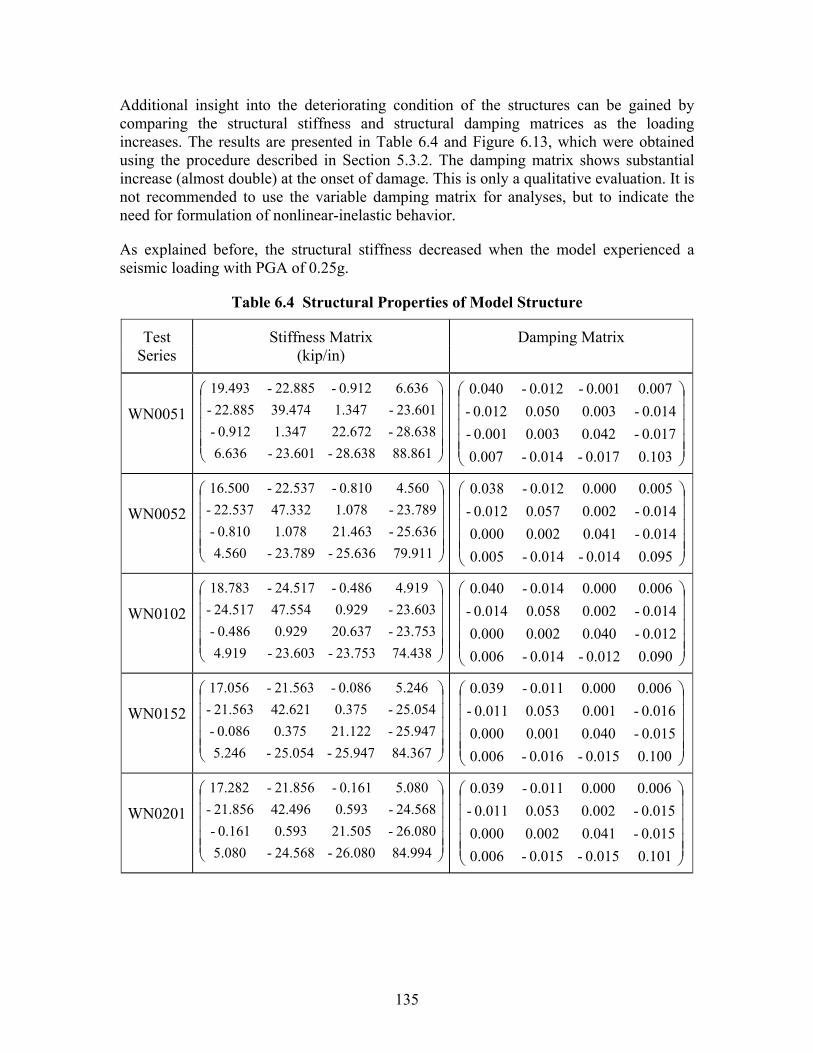
135
Additional insight into the deteriorating condition of the structures can be gained by comparing the structural stiffness and structural damping matrices as the loading increases. The results are presented in Table 6.4 and Figure 6.13, which were obtained using the procedure described in Section 5.3.2. The damping matrix shows substantial increase (almost double) at the onset of damage. This is only a qualitative evaluation. It is not recommended to use the variable damping matrix for analyses, but to indicate the need for formulation of nonlinear-inelastic behavior.
As explained before, the structural stiffness decreased when the model experienced a seismic loading with PGA of 0.25g.
Table 6.4 Structural Properties of Model Structure
Test Stiffness Matrix Damping Matrix Series (kip/in)
WN0051
⎟⎟⎟⎟⎟
⎠
⎞
⎜⎜⎜⎜⎜
⎝
⎛
88.86128.638-23.601-6.63628.638-22.6721.3470.912-23.601-1.34739.47422.885-6.6360.912-22.885-19.493
⎟⎟⎟⎟⎟
⎠
⎞
⎜⎜⎜⎜⎜
⎝
⎛
0.1030.017-0.014-0.0070.017-0.0420.0030.001-0.014-0.0030.0500.012-
0.0070.001-0.012-0.040
WN0052
⎟⎟⎟⎟⎟
⎠
⎞
⎜⎜⎜⎜⎜
⎝
⎛
79.91125.636-23.789-4.56025.636-21.4631.0780.810-23.789-1.07847.33222.537-4.5600.810-22.537-16.500
⎟⎟⎟⎟⎟
⎠
⎞
⎜⎜⎜⎜⎜
⎝
⎛
0.0950.014-0.014-0.0050.014-0.0410.0020.0000.014-0.0020.0570.012-
0.0050.0000.012-0.038
WN0102
⎟⎟⎟⎟⎟
⎠
⎞
⎜⎜⎜⎜⎜
⎝
⎛
74.43823.753-23.603-4.91923.753-20.6370.9290.486-23.603-0.92947.55424.517-4.9190.486-24.517-18.783
⎟⎟⎟⎟⎟
⎠
⎞
⎜⎜⎜⎜⎜
⎝
⎛
0.0900.012-0.014-0.0060.012-0.0400.0020.0000.014-0.0020.0580.014-
0.0060.0000.014-0.040
WN0152
⎟⎟⎟⎟⎟
⎠
⎞
⎜⎜⎜⎜⎜
⎝
⎛
84.36725.947-25.054-5.24625.947-21.1220.3750.086-25.054-0.37542.62121.563-5.2460.086-21.563-17.056
⎟⎟⎟⎟⎟
⎠
⎞
⎜⎜⎜⎜⎜
⎝
⎛
0.1000.015-0.016-0.0060.015-0.0400.0010.0000.016-0.0010.0530.011-
0.0060.0000.011-0.039
WN0201
⎟⎟⎟⎟⎟
⎠
⎞
⎜⎜⎜⎜⎜
⎝
⎛
84.99426.080-24.568-5.08026.080-21.5050.5930.161-24.568-0.59342.49621.856-5.0800.161-21.856-17.282
⎟⎟⎟⎟⎟
⎠
⎞
⎜⎜⎜⎜⎜
⎝
⎛
0.1010.015-0.015-0.0060.015-0.0410.0020.0000.015-0.0020.0530.011-
0.0060.0000.011-0.039

136
Test Stiffness Matrix Damping Matrix Series (kip/in)
WN0202
⎟⎟⎟⎟⎟
⎠
⎞
⎜⎜⎜⎜⎜
⎝
⎛
81.88726.059-22.340-4.79526.059-21.0240.7940.381-22.340-0.79440.66421.579-4.7950.381-21.579-17.468
⎟⎟⎟⎟⎟
⎠
⎞
⎜⎜⎜⎜⎜
⎝
⎛
0.0980.015-0.014-0.0050.015-0.0400.0020.0000.014-0.0020.0520.011-0.0050.0000.011-0.039
WN0252
⎟⎟⎟⎟⎟
⎠
⎞
⎜⎜⎜⎜⎜
⎝
⎛
81.25527.154-19.399-4.57827.154-22.5130.4980.181-19.399-0.49834.39518.678-4.5780.181-18.678-15.597
⎟⎟⎟⎟⎟
⎠
⎞
⎜⎜⎜⎜⎜
⎝
⎛
0.0980.018-0.013-0.0050.018-0.0420.0010.0000.013-0.0010.0470.008-
0.0050.0000.008-0.038
WN0302
⎟⎟⎟⎟⎟
⎠
⎞
⎜⎜⎜⎜⎜
⎝
⎛
73.91427.809-11.041-1.67327.809-23.0280.321-0.34711.041-0.321-23.86214.264-1.6730.34714.264-12.746
⎟⎟⎟⎟⎟
⎠
⎞
⎜⎜⎜⎜⎜
⎝
⎛
0.0970.021-0.008-0.0010.021-0.0420.0000.0000.008-0.0000.0380.006-0.0010.0000.006-0.034
WN0352
⎟⎟⎟⎟⎟
⎠
⎞
⎜⎜⎜⎜⎜
⎝
⎛
68.17828.655-4.485-0.709-28.655-25.3142.402-1.9294.485-2.402-15.0189.592-0.709-1.9299.592-8.645
⎟⎟⎟⎟⎟
⎠
⎞
⎜⎜⎜⎜⎜
⎝
⎛
0.0960.024-0.0000.0000.024-0.0470.003-0.003
0.0000.003-0.0280.004-0.0000.0030.004-0.025
WN0401
⎟⎟⎟⎟⎟
⎠
⎞
⎜⎜⎜⎜⎜
⎝
⎛
69.34226.484-3.850-0.729-26.484-20.3143.616-2.1373.850-3.616-15.6629.086-0.729-2.1379.086-8.040
⎟⎟⎟⎟⎟
⎠
⎞
⎜⎜⎜⎜⎜
⎝
⎛
0.0960.024-0.0000.0000.024-0.0470.003-0.003
0.0000.003-0.0280.004-0.0000.0030.004-0.025
WN0402
⎟⎟⎟⎟⎟
⎠
⎞
⎜⎜⎜⎜⎜
⎝
⎛
69.51126.484-3.068-3.120-26.484-20.8122.762-2.5093.068-2.762-12.2978.377-3.120-2.5098.377-8.796
⎟⎟⎟⎟⎟
⎠
⎞
⎜⎜⎜⎜⎜
⎝
⎛
0.0990.027-0.001-0.008-0.027-0.0470.004-0.0030.0000.004-0.0250.002-0.003-0.0040.002-0.027
WN0401A
⎟⎟⎟⎟⎟
⎠
⎞
⎜⎜⎜⎜⎜
⎝
⎛
69.19628.959-2.666-2.002-28.959-24.5353.027-2.7152.666-3.027-11.0297.251-2.002-2.7157.251-7.367
⎟⎟⎟⎟⎟
⎠
⎞
⎜⎜⎜⎜⎜
⎝
⎛
0.0990.027-0.0000.003-0.027-0.0470.004-0.004
0.0000.004-0.0230.0000.003-0.0040.0000.024
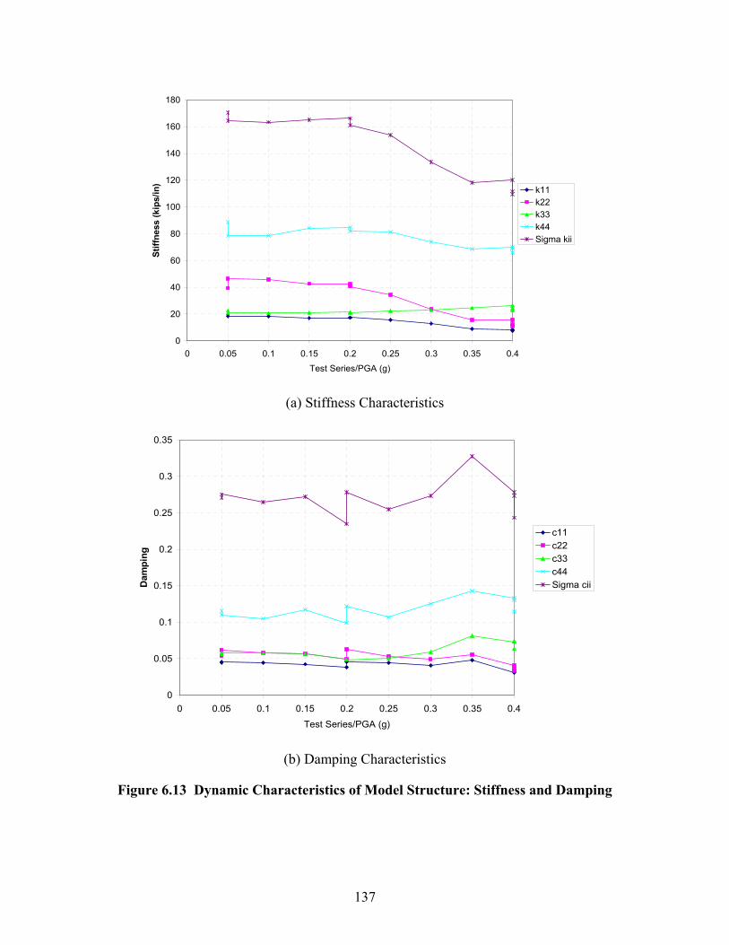
137
0
20
40
60
80
100
120
140
160
180
0 0.05 0.1 0.15 0.2 0.25 0.3 0.35 0.4
Test Series/PGA (g)
Stiff
ness
(kip
s/in
)
k11k22k33k44Sigma kii
(a) Stiffness Characteristics
0
0.05
0.1
0.15
0.2
0.25
0.3
0.35
0 0.05 0.1 0.15 0.2 0.25 0.3 0.35 0.4
Test Series/PGA (g)
Dam
ping
c11c22c33c44Sigma cii
(b) Damping Characteristics
Figure 6.13 Dynamic Characteristics of Model Structure: Stiffness and Damping

138
The preliminary analytical identification procedure was also conducted with the structural program IDARC. The comparison of initial dynamic characteristics obtained from the experimental and the preliminary analytical studies is given in Table 6.5.
Table 6.5 Comparison of Dynamic Characteristics of Model Structures
Parameters Experimental Results (WN0051) IDARC Results
fj (Hz)
⎟⎟⎟⎟⎟
⎠
⎞
⎜⎜⎜⎜⎜
⎝
⎛
8.286.323.211.66
⎟⎟⎟⎟⎟
⎠
⎞
⎜⎜⎜⎜⎜
⎝
⎛
10.347.043.611.91
Φjk
⎟⎟⎟⎟⎟
⎠
⎞
⎜⎜⎜⎜⎜
⎝
⎛
0.7670.689-0.3410.2850.464-0.8971.0000.4301.000-1.000-0.079-0.7850.5440.8210.541-1.000
⎟⎟⎟⎟⎟
⎠
⎞
⎜⎜⎜⎜⎜
⎝
⎛
0.5980.906-0.3340.3120.215-1.0001.0000.4701.000-0.958-0.087-0.7100.4390.7760.616-1.000
The comparison of the initial dynamic parameters showed that the preliminary analytical results were not in agreement with the experimental ones. Therefore, the analytical model had to be modified to better estimate the structural behavior of the model, as described in Section 7.
6.4 Remarks
The model structure was successively excited by a sequence of increasing LA16 (Rinaldi, Northridge 1994) ground motions. The structural response was monitored, and the base shear, floor displacements and accelerations were recorded. Structural damage occurring during the experiment was also observed and interpreted. Structural identifications were made in-between the dynamic loadings to monitor changes in the dynamic properties, i.e., frequencies and mode shapes. The results were also used to obtain more information on the condition of the structure.
Experimental results and visual observation show that the model behaved elastically under minor earthquake loadings. The first yield was experienced at a PGA = 0.20g. as shown in the changes of the natural frequencies and in the stiffness coefficients (Figs 6.11 through 6.13).
The structural failure as visually observed during the test occurred at a PGA = 0.40g Using the frequencies’ changes (see Figs 6.11 through 6.13) one can identify the onset of

139
rupture at 0.35g, before the damage was actually visible. After this test the frequencies remained unchanged.
The changes in the global mode shapes (Fig 6.12) could locate the degrees of freedom affected by the damage, but could not identify which connection rigidly linked to the same degree of freedom actually ruptured.
The separation of vertical and lateral load resisting systems was satisfactory: no significant flexural straining was noted, and a pancake type of collapse was avoided at structural failure, although the lateral load resisting system lost any capacity to support gravity loads.
The model experienced damage in the forms of prying effect at the column end plates and a welding failure of a block joint located at the toes of the higher tower where force concentrations due to irregularities were expected. This welding failure is considered to be the primary cause of the structural failure.

141
SECTION 7 COMPARISON OF ANALYTICAL AND EXPERIMENTAL
BEHAVIOR 7.1 Introduction As well known, analytical results are not always likely to be in full agreement with the experimental ones. This, of course, is due to inability to analytically model the behavior of the tested specimen faithfully throughout the full inelastic range. However, efforts were made to reduce the discrepancies as much as possible. This was achieved by ensuring that the material and component properties, mainly stiffness and strength within the full loading range were determined and incorporated as faithfully as possible in the analytical model. For this purpose material coupon tests were made for the column and beam sections, while sub-assemblies of frame connections – a cruciform composed of two half beams, two half columns and a joint element (e.g. Figure 4.3), and gravity columns specimens were tested and modeled accordingly. The comparisons of the analytical models, as they were refined by further testing, with the experimental results are the subject of this section.
7.1.1 Methods of Analysis As noted in Section 3, several techniques for analysis in the nonlinear range are available: incremental static or pushover analysis - either fixed or adaptive - as the supply, and nonlinear response spectra as demand (spectral demand-capacity analysis), dynamic time history analysis for given level of input motion, and dynamic pushover or incremental dynamic analysis.
7.1.2 Pre- and Post-Testing Analyses Preliminary analyses were carried out prior to the full model experimental study, using different analytical techniques to predict the seismic response of the model using the specified material properties. Since actual properties of materials, and those of multi-element components, are usually different from their specified or nominal values, laboratory testing is always required in order to obtain reliable estimates. Indeed, the material and components test results indicated that this was indeed the case. The analytical model was then modified to incorporate the results of the material and component tests. The resulting new analytical model and the comparison of its response with the experimental results are presented in this section.
7.1.3 Experimental vs. Analytical Results Whereas calibration of material properties was a relatively simple task, faithful modeling of the component behavior in the nonlinear range turned out to be more difficult, since the nonlinearity was mainly manifested in the prying action of the end-plate connecting the column to the beam-column joint block, rather than in plastic hinging of the column

142
ends. In other words, a nonlinear semi-rigid connection model was called for. As is demonstrated subsequently, the chosen spring element, together with the as-built material properties, modeled the actual behavior of the joint, and indeed of the whole specimen, quite satisfactorily.
7.2 Analytical Models and Techniques The computational model representing the tested structures was described in some detail in Section 2, and the analysis techniques were given in Section 3. Several analysis procedures were carried out: the spectral demand-capacity analysis, with various loading patterns, and the incremental dynamic time history or dynamic pushover analysis.
The tested model designated as Model D was described in some detail in Section 2, and is shown again in Figure7.1 (only "Type D")
Figure 7.1 Tested Model D
Using Model D as a typical model layout, four analytical models were then developed for this study. These analytical models are varied in terms of material properties and computational models, following the progress of the experimental study. The analytical models are summarized in Table 7.1, and the structural elements and material properties for each model are presented in Table 7.2.
The models with estimated material properties were analyzed using the nominal values of the materials (based on engineering experience), while the ones with measured material properties were analyzed based on the results from the materials’ coupon experiments or from substructure testing. The modified computational models were developed from the original computational model to accommodate the prying effect in the connections observed in the component tests. Semi rigid connection models were introduced to incorporate the prying effect on the column end plate, which became a dominant factor in the inelastic response.
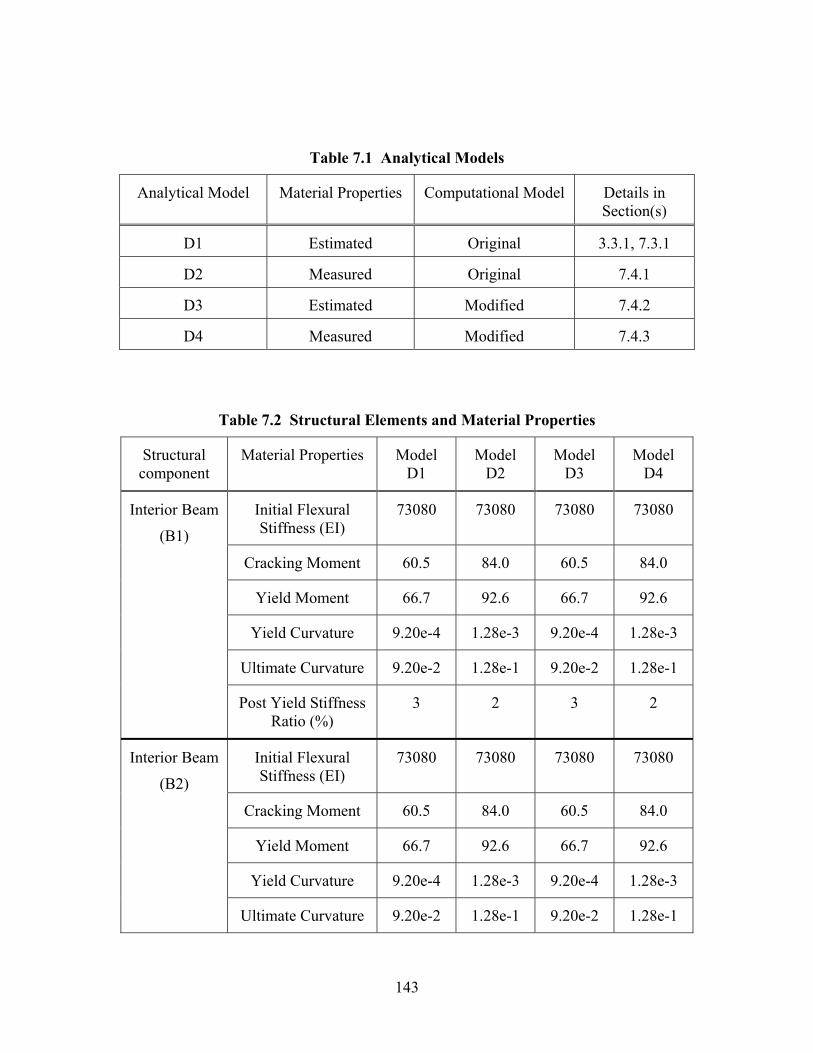
143
Table 7.1 Analytical Models
Analytical Model Material Properties Computational Model Details in Section(s)
D1 Estimated Original 3.3.1, 7.3.1
D2 Measured Original 7.4.1
D3 Estimated Modified 7.4.2
D4 Measured Modified 7.4.3
Table 7.2 Structural Elements and Material Properties
Structural component
Material Properties Model D1
Model D2
Model D3
Model D4
Initial Flexural Stiffness (EI)
73080 73080 73080 73080
Cracking Moment 60.5 84.0 60.5 84.0
Yield Moment 66.7 92.6 66.7 92.6
Yield Curvature 9.20e-4 1.28e-3 9.20e-4 1.28e-3
Ultimate Curvature 9.20e-2 1.28e-1 9.20e-2 1.28e-1
Interior Beam
(B1)
Post Yield Stiffness Ratio (%)
3 2 3 2
Initial Flexural Stiffness (EI)
73080 73080 73080 73080
Cracking Moment 60.5 84.0 60.5 84.0
Yield Moment 66.7 92.6 66.7 92.6
Yield Curvature 9.20e-4 1.28e-3 9.20e-4 1.28e-3
Interior Beam
(B2)
Ultimate Curvature 9.20e-2 1.28e-1 9.20e-2 1.28e-1
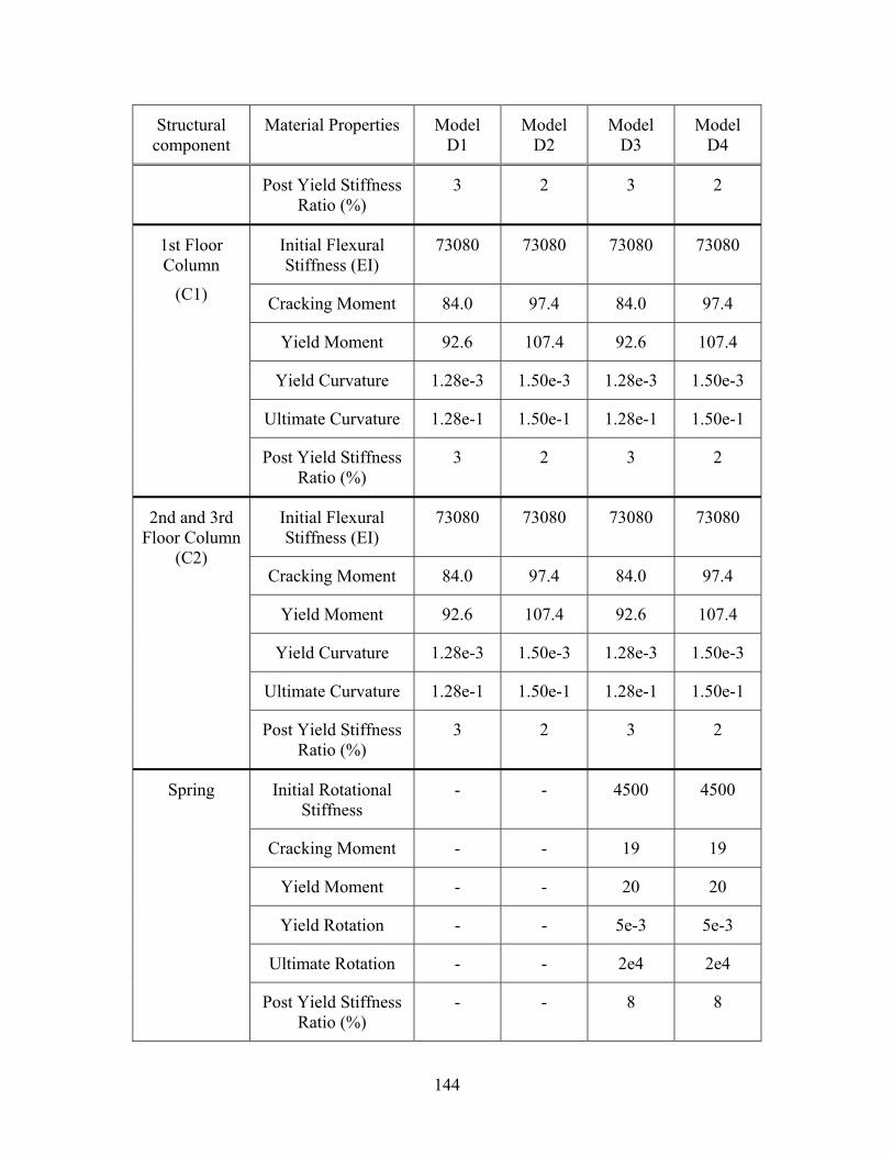
144
Structural component
Material Properties Model D1
Model D2
Model D3
Model D4
Post Yield Stiffness Ratio (%)
3 2 3 2
Initial Flexural Stiffness (EI)
73080 73080 73080 73080
Cracking Moment 84.0 97.4 84.0 97.4
Yield Moment 92.6 107.4 92.6 107.4
Yield Curvature 1.28e-3 1.50e-3 1.28e-3 1.50e-3
Ultimate Curvature 1.28e-1 1.50e-1 1.28e-1 1.50e-1
1st Floor Column
(C1)
Post Yield Stiffness Ratio (%)
3 2 3 2
Initial Flexural Stiffness (EI)
73080 73080 73080 73080
Cracking Moment 84.0 97.4 84.0 97.4
Yield Moment 92.6 107.4 92.6 107.4
Yield Curvature 1.28e-3 1.50e-3 1.28e-3 1.50e-3
Ultimate Curvature 1.28e-1 1.50e-1 1.28e-1 1.50e-1
2nd and 3rd Floor Column
(C2)
Post Yield Stiffness Ratio (%)
3 2 3 2
Initial Rotational Stiffness
- - 4500 4500
Cracking Moment - - 19 19
Yield Moment - - 20 20
Yield Rotation - - 5e-3 5e-3
Ultimate Rotation - - 2e4 2e4
Spring
Post Yield Stiffness Ratio (%)
- - 8 8
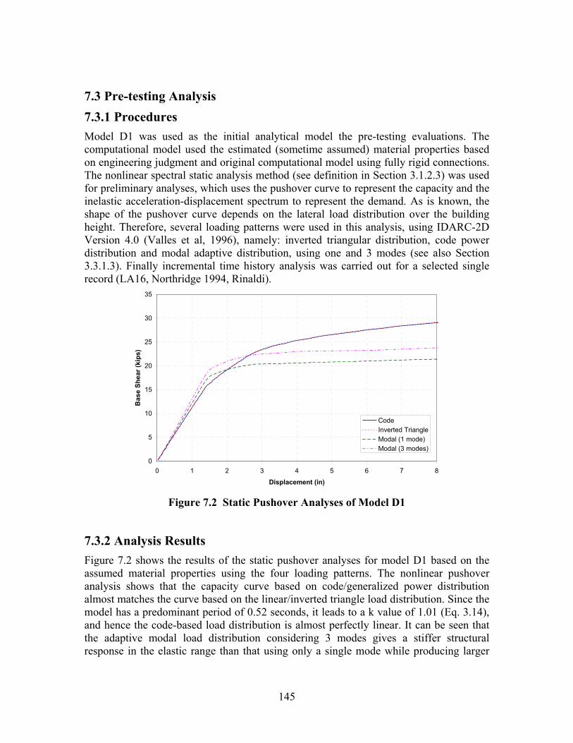
145
7.3 Pre-testing Analysis 7.3.1 Procedures Model D1 was used as the initial analytical model the pre-testing evaluations. The computational model used the estimated (sometime assumed) material properties based on engineering judgment and original computational model using fully rigid connections. The nonlinear spectral static analysis method (see definition in Section 3.1.2.3) was used for preliminary analyses, which uses the pushover curve to represent the capacity and the inelastic acceleration-displacement spectrum to represent the demand. As is known, the shape of the pushover curve depends on the lateral load distribution over the building height. Therefore, several loading patterns were used in this analysis, using IDARC-2D Version 4.0 (Valles et al, 1996), namely: inverted triangular distribution, code power distribution and modal adaptive distribution, using one and 3 modes (see also Section 3.3.1.3). Finally incremental time history analysis was carried out for a selected single record (LA16, Northridge 1994, Rinaldi).
0
5
10
15
20
25
30
35
0 1 2 3 4 5 6 7 8
Displacement (in)
Bas
e Sh
ear (
kips
)
CodeInverted TriangleModal (1 mode)Modal (3 modes)
Figure 7.2 Static Pushover Analyses of Model D1
7.3.2 Analysis Results Figure 7.2 shows the results of the static pushover analyses for model D1 based on the assumed material properties using the four loading patterns. The nonlinear pushover analysis shows that the capacity curve based on code/generalized power distribution almost matches the curve based on the linear/inverted triangle load distribution. Since the model has a predominant period of 0.52 seconds, it leads to a k value of 1.01 (Eq. 3.14), and hence the code-based load distribution is almost perfectly linear. It can be seen that the adaptive modal load distribution considering 3 modes gives a stiffer structural response in the elastic range than that using only a single mode while producing larger
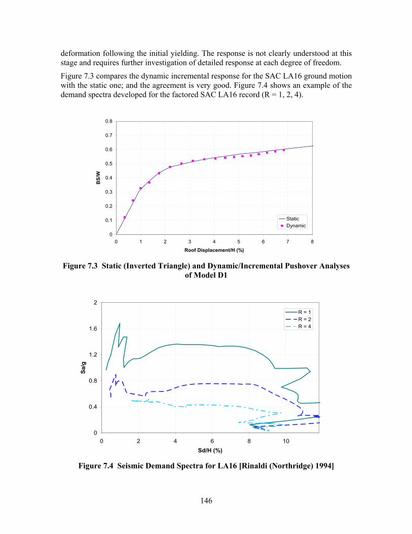
146
deformation following the initial yielding. The response is not clearly understood at this stage and requires further investigation of detailed response at each degree of freedom.
Figure 7.3 compares the dynamic incremental response for the SAC LA16 ground motion with the static one; and the agreement is very good. Figure 7.4 shows an example of the demand spectra developed for the factored SAC LA16 record (R = 1, 2, 4).
0
0.1
0.2
0.3
0.4
0.5
0.6
0.7
0.8
0 1 2 3 4 5 6 7 8
Roof Displacement/H (%)
BS/
W
StaticDynamic
Figure 7.3 Static (Inverted Triangle) and Dynamic/Incremental Pushover Analyses
of Model D1
0
0.4
0.8
1.2
1.6
2
0 2 4 6 8 10Sd/H (%)
Sa/g
R = 1R = 2R = 4
Figure 7.4 Seismic Demand Spectra for LA16 [Rinaldi (Northridge) 1994]
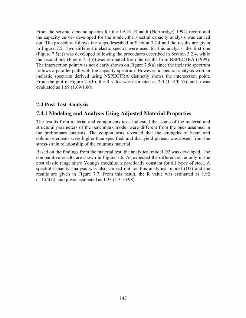
147
From the seismic demand spectra for the LA16 [Rinaldi (Northridge) 1994] record and the capacity curves developed for the model, the spectral capacity analysis was carried out. The procedure follows the steps described in Section 3.2.4 and the results are given in Figure 7.5. Two different inelastic spectra were used for this analysis, the first one (Figure 7.5(a)) was developed following the procedures described in Section 3.2.4, while the second one (Figure 7.5(b)) was estimated from the results from NSPECTRA (1999). The intersection point was not clearly shown on Figure 7.5(a) since the inelastic spectrum follows a parallel path with the capacity spectrum. However, a spectral analysis with an inelastic spectrum derived using NSPECTRA distinctly shows the intersection point. From the plot in Figure 7.5(b), the R value was estimated as 2.0 (1.14/0.57), and µ was evaluated as 1.69 (1.69/1.00).
7.4 Post Test Analysis 7.4.1 Modeling and Analysis Using Adjusted Material Properties The results from material and components tests indicated that some of the material and structural parameters of the benchmark model were different from the ones assumed in the preliminary analysis. The coupon tests revealed that the strengths of beam and column elements were higher than specified, and that yield plateau was absent from the stress-strain relationship of the columns material.
Based on the findings from the material test, the analytical model D2 was developed. The comparative results are shown in Figure 7.6. As expected the differences lie only in the post elastic range since Young's modulus is practically constant for all types of steel. A spectral capacity analysis was also carried out for this analytical model (D2) and the results are given in Figure 7.7. From this result, the R value was estimated as 1.92 (1.15/0.6), and µ was evaluated as 1.33 (1.31/0.98).
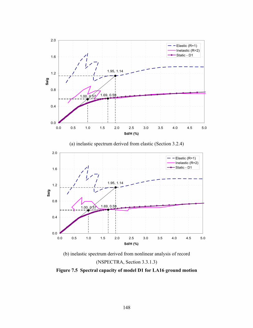
148
1.69, 0.591.00, 0.57
1.95, 1.14
0.0
0.4
0.8
1.2
1.6
2.0
0.0 0.5 1.0 1.5 2.0 2.5 3.0 3.5 4.0 4.5 5.0
Sd/H (%)
Sa/g
Elastic (R=1)Inelastic (R=2)Static - D1
(a) inelastic spectrum derived from elastic (Section 3.2.4)
1.69, 0.591.00, 0.57
1.95, 1.14
0.0
0.4
0.8
1.2
1.6
2.0
0.0 0.5 1.0 1.5 2.0 2.5 3.0 3.5 4.0 4.5 5.0
Sd/H (%)
Sa/g
Elastic (R=1)Inelastic (R=2)Static - D1
(b) inelastic spectrum derived from nonlinear analysis of record
(NSPECTRA, Section 3.3.1.3)
Figure 7.5 Spectral capacity of model D1 for LA16 ground motion
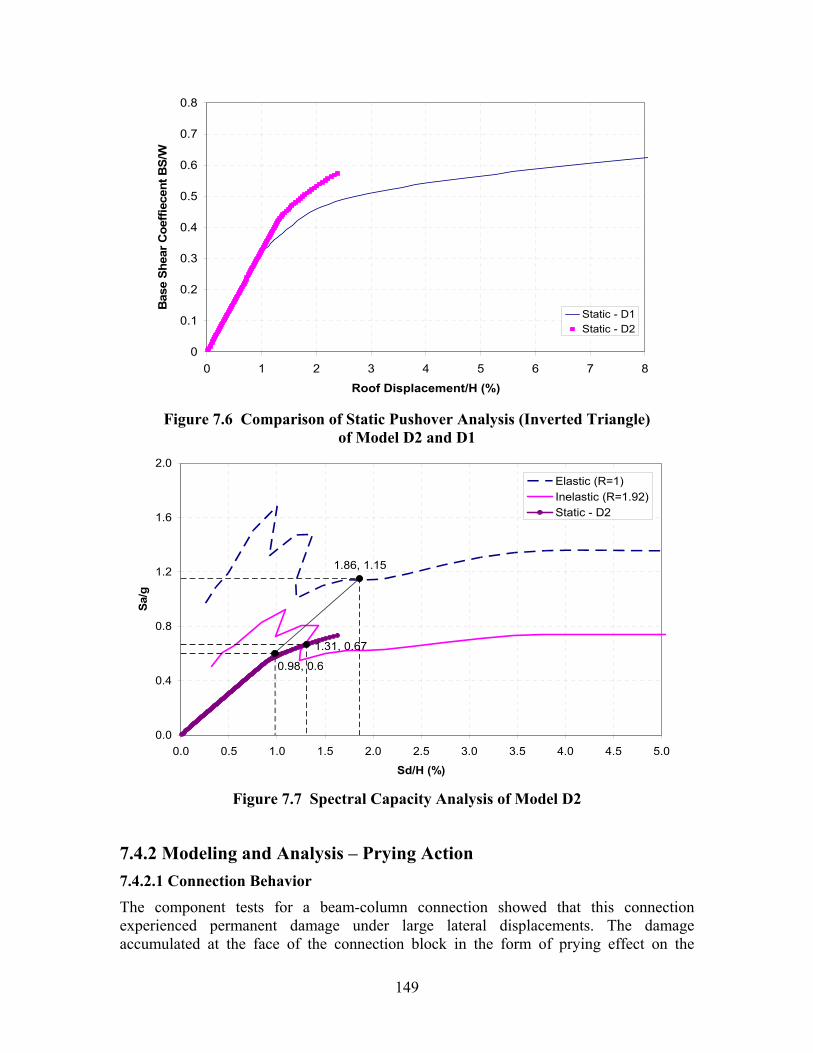
149
0
0.1
0.2
0.3
0.4
0.5
0.6
0.7
0.8
0 1 2 3 4 5 6 7 8
Roof Displacement/H (%)
Bas
e Sh
ear C
oeffi
ecen
t BS/
W
Static - D1Static - D2
Figure 7.6 Comparison of Static Pushover Analysis (Inverted Triangle)
of Model D2 and D1
1.31, 0.67
0.98, 0.6
1.86, 1.15
0.0
0.4
0.8
1.2
1.6
2.0
0.0 0.5 1.0 1.5 2.0 2.5 3.0 3.5 4.0 4.5 5.0
Sd/H (%)
Sa/g
Elastic (R=1)Inelastic (R=1.92)Static - D2
Figure 7.7 Spectral Capacity Analysis of Model D2
7.4.2 Modeling and Analysis – Prying Action 7.4.2.1 Connection Behavior The component tests for a beam-column connection showed that this connection experienced permanent damage under large lateral displacements. The damage accumulated at the face of the connection block in the form of prying effect on the
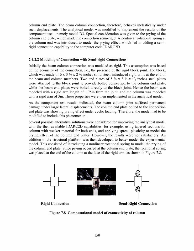
150
column end plate. The beam column connection, therefore, behaves inelastically under such displacements. The analytical model was modified to implement the results of the component tests - namely model D3. Special consideration was given to the prying of the column end plate, which made the connection semi-rigid. A nonlinear rotational spring at the column end was introduced to model the prying effect, which led to adding a semi-rigid connection capability to the computer code IDARC2D.
7.4.2.2 Modeling of Connection with Semi-rigid Connections Initially the beam column connection was modeled as rigid. This assumption was based on the geometry of the connection, i.e., the presence of the rigid block joint. The block, which was made of 6 x 3 ½ x 2 ¾ inches solid steel, introduced rigid arms at the end of the beam and column members. Two end plates of 5 ¾ x 3 ½ x 3/8 inches steel plates were attached to the block joint to provide bolted connection to the column end plate, while the beam end plates were bolted directly to the block joint. Hence the beam was modeled with a rigid arm length of 1.75in from the joint, and the column was modeled with a rigid arm of 3in. These properties were then implemented in the analytical model.
As the component test results indicated, the beam column joint suffered permanent damage under large lateral displacements. The column end plate bolted to the connection end plate was showing prying effect under cyclic loading. Therefore, the model had to be modified to include this phenomenon.
Several possible alternative solutions were considered for improving the analytical model with the then available IDARC2D capabilities, for example, using tapered sections for column with weaker material for both ends, and applying spread plasticity to model the prying effect of the column end plates. However, the results were not satisfactory. An addition to the structural platform was then developed to better model the experimental model. This consisted of introducing a nonlinear rotational spring to model the prying of the column end plate. Since prying occurred at the column end plate, the rotational spring was placed at the end of the column at the face of the rigid arm, as shown in Figure 7.8.
Rigid Connection Semi-Rigid Connection
Figure 7.8 Computational model of connectivity of column
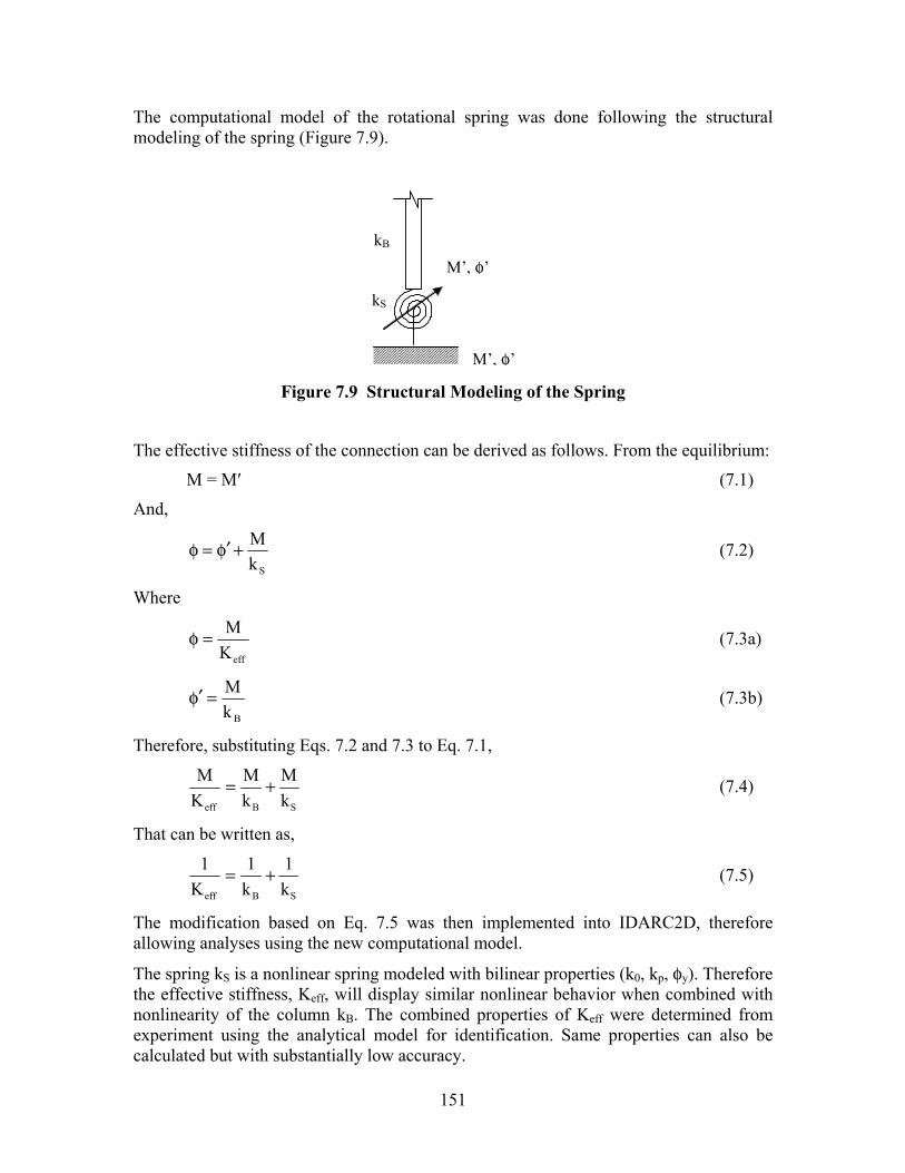
151
The computational model of the rotational spring was done following the structural modeling of the spring (Figure 7.9).
M’, φ’
M’, φ’
kS
kB
Figure 7.9 Structural Modeling of the Spring
The effective stiffness of the connection can be derived as follows. From the equilibrium:
M = M′ (7.1)
And,
Sk
M+φ′=φ (7.2)
Where
effK
M=φ (7.3a)
Bk
M=φ′ (7.3b)
Therefore, substituting Eqs. 7.2 and 7.3 to Eq. 7.1,
SBeff k
MkM
KM += (7.4)
That can be written as,
SBeff k
1k1
K1 += (7.5)
The modification based on Eq. 7.5 was then implemented into IDARC2D, therefore allowing analyses using the new computational model.
The spring kS is a nonlinear spring modeled with bilinear properties (k0, kp, φy). Therefore the effective stiffness, Keff, will display similar nonlinear behavior when combined with nonlinearity of the column kB. The combined properties of Keff were determined from experiment using the analytical model for identification. Same properties can also be calculated but with substantially low accuracy.
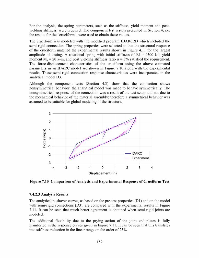
152
For the analysis, the spring parameters, such as the stiffness, yield moment and post-yielding stiffness, were required. The component test results presented in Section 4, i.e. the results for the “cruciform”, were used to obtain these values.
The cruciform was modeled with the modified program IDARC2D which included the semi-rigid connection. The spring properties were selected so that the structural response of the cruciform matched the experimental results shown in Figure 4.11 for the largest amplitude of testing. A rotational spring with initial stiffness of EI = 4500 ksi, yield moment My = 20 k-in, and post yielding stiffness ratio α = 8% satisfied the requirement. The force-displacement characteristics of the cruciform using the above estimated parameters in an IDARC model are shown in Figure 7.10 along with the experimental results. These semi-rigid connection response characteristics were incorporated in the analytical model D3.
Although the component tests (Section 4.3) show that the connection shows nonsymmetrical behavior, the analytical model was made to behave symmetrically. The nonsymmetrical response of the connection was a result of the test setup and not due to the mechanical behavior of the material assembly; therefore a symmetrical behavior was assumed to be suitable for global modeling of the structure.
-3
-2
-1
0
1
2
3
-4 -3 -2 -1 0 1 2 3 4
Displacement (in)
Forc
e (k
ips)
IDARCExperiment
Figure 7.10 Comparison of Analysis and Experimental Response of Cruciform Test
7.4.2.3 Analysis Results
The analytical pushover curves, as based on the pre-test properties (D1) and on the model with semi-rigid connections (D3), are compared with the experimental results in Figure 7.11. It can be seen that much better agreement is obtained when semi-rigid joints are modeled.
The additional flexibility due to the prying action of the joint end plates is fully manifested in the response curves given in Figure 7.11. It can be seen that this translates into stiffness reduction in the linear range on the order of 25%.
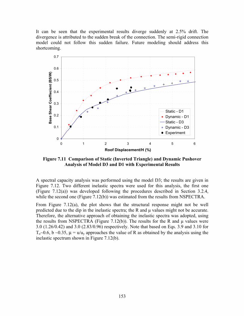
153
It can be seen that the experimental results diverge suddenly at 2.5% drift. The divergence is attributed to the sudden break of the connection. The semi-rigid connection model could not follow this sudden failure. Future modeling should address this shortcoming.
0
0.1
0.2
0.3
0.4
0.5
0.6
0.7
0 1 2 3 4 5 6
Roof Displacement/H (%)
Bas
e Sh
ear C
oeffi
ecie
nt (B
S/W
)
Static - D1Dynamic - D1Static - D3Dynamic - D3Experiment
Figure 7.11 Comparison of Static (Inverted Triangle) and Dynamic Pushover
Analysis of Model D3 and D1 with Experimental Results
A spectral capacity analysis was performed using the model D3; the results are given in Figure 7.12. Two different inelastic spectra were used for this analysis, the first one (Figure 7.12(a)) was developed following the procedures described in Section 3.2.4, while the second one (Figure 7.12(b)) was estimated from the results from NSPECTRA.
From Figure 7.12(a), the plot shows that the structural response might not be well predicted due to the dip in the inelastic spectra; the R and µ values might not be accurate. Therefore, the alternative approach of obtaining the inelastic spectra was adopted, using the results from NSPECTRA (Figure 7.12(b)). The results for the R and µ values were 3.0 (1.26/0.42) and 3.0 (2.83/0.96) respectively. Note that based on Eqs. 3.9 and 3.10 for To~0.6, b ~0.35, µ = u/uy approaches the value of R as obtained by the analysis using the inelastic spectrum shown in Figure 7.12(b).
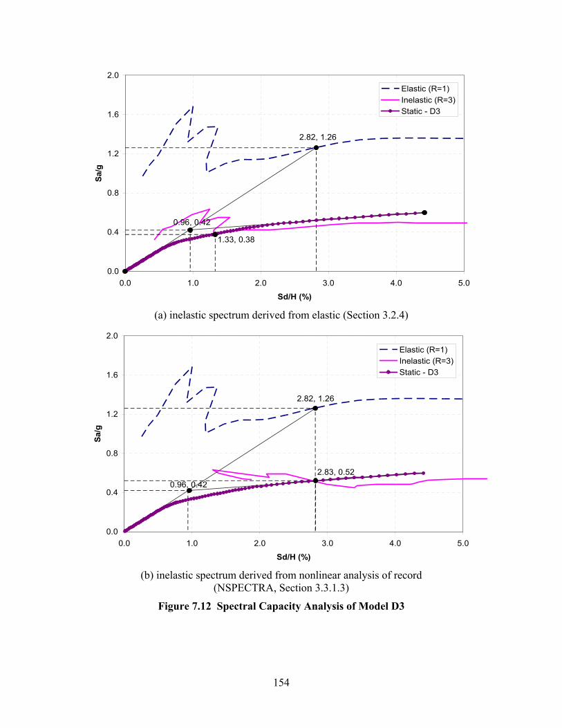
154
1.33, 0.38
0.96, 0.42
2.82, 1.26
0.0
0.4
0.8
1.2
1.6
2.0
0.0 1.0 2.0 3.0 4.0 5.0
Sd/H (%)
Sa/g
Elastic (R=1)Inelastic (R=3)Static - D3
(a) inelastic spectrum derived from elastic (Section 3.2.4)
2.83, 0.52
2.82, 1.26
0.96, 0.42
0.0
0.4
0.8
1.2
1.6
2.0
0.0 1.0 2.0 3.0 4.0 5.0
Sd/H (%)
Sa/g
Elastic (R=1)Inelastic (R=3)Static - D3
(b) inelastic spectrum derived from nonlinear analysis of record
(NSPECTRA, Section 3.3.1.3)
Figure 7.12 Spectral Capacity Analysis of Model D3
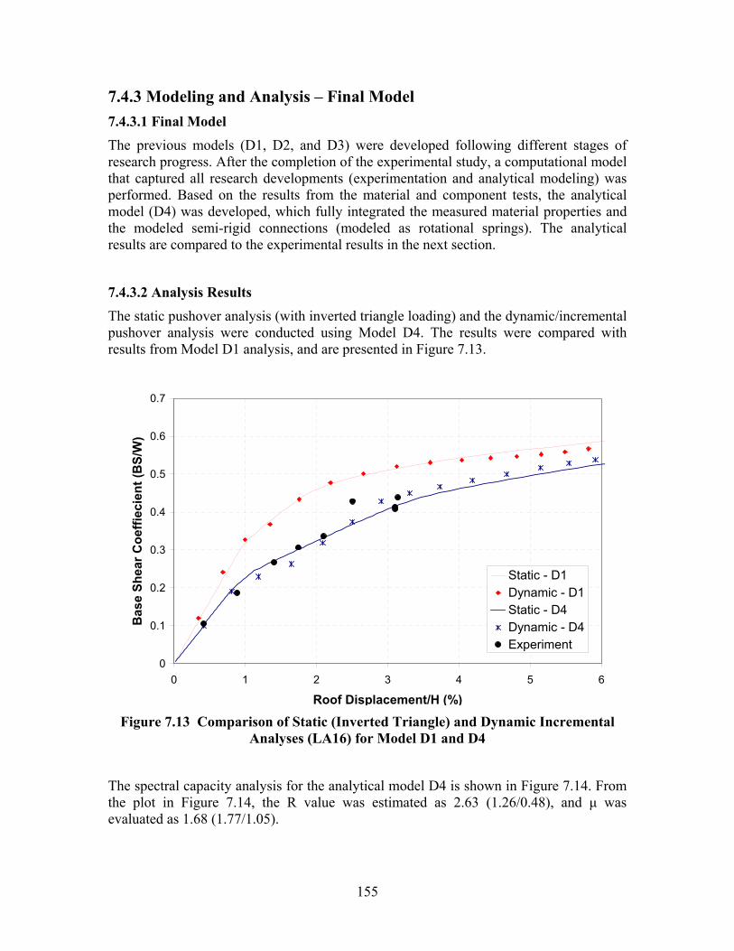
155
7.4.3 Modeling and Analysis – Final Model 7.4.3.1 Final Model The previous models (D1, D2, and D3) were developed following different stages of research progress. After the completion of the experimental study, a computational model that captured all research developments (experimentation and analytical modeling) was performed. Based on the results from the material and component tests, the analytical model (D4) was developed, which fully integrated the measured material properties and the modeled semi-rigid connections (modeled as rotational springs). The analytical results are compared to the experimental results in the next section.
7.4.3.2 Analysis Results
The static pushover analysis (with inverted triangle loading) and the dynamic/incremental pushover analysis were conducted using Model D4. The results were compared with results from Model D1 analysis, and are presented in Figure 7.13.
0
0.1
0.2
0.3
0.4
0.5
0.6
0.7
0 1 2 3 4 5 6
Roof Displacement/H (%)
Bas
e Sh
ear C
oeffi
ecie
nt (B
S/W
)
Static - D1Dynamic - D1Static - D4Dynamic - D4Experiment
Figure 7.13 Comparison of Static (Inverted Triangle) and Dynamic Incremental
Analyses (LA16) for Model D1 and D4
The spectral capacity analysis for the analytical model D4 is shown in Figure 7.14. From the plot in Figure 7.14, the R value was estimated as 2.63 (1.26/0.48), and µ was evaluated as 1.68 (1.77/1.05).
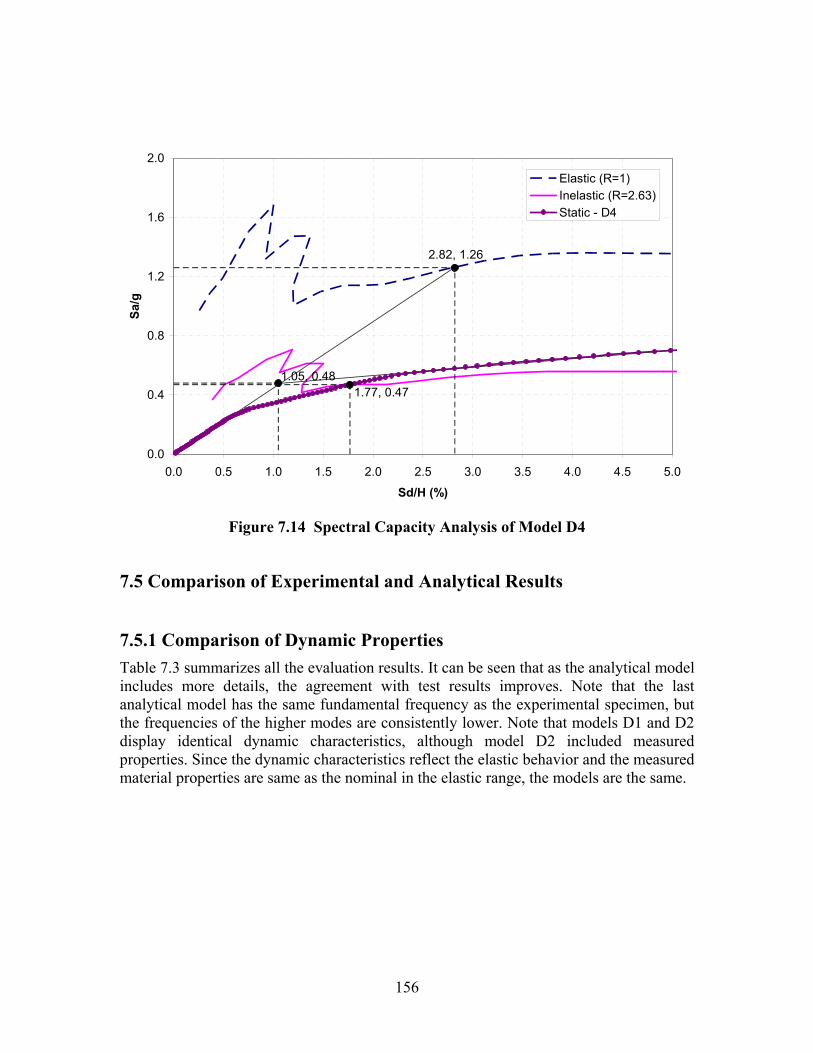
156
1.77, 0.47
2.82, 1.26
1.05, 0.48
0.0
0.4
0.8
1.2
1.6
2.0
0.0 0.5 1.0 1.5 2.0 2.5 3.0 3.5 4.0 4.5 5.0
Sd/H (%)
Sa/g
Elastic (R=1)Inelastic (R=2.63)Static - D4
Figure 7.14 Spectral Capacity Analysis of Model D4
7.5 Comparison of Experimental and Analytical Results 7.5.1 Comparison of Dynamic Properties Table 7.3 summarizes all the evaluation results. It can be seen that as the analytical model includes more details, the agreement with test results improves. Note that the last analytical model has the same fundamental frequency as the experimental specimen, but the frequencies of the higher modes are consistently lower. Note that models D1 and D2 display identical dynamic characteristics, although model D2 included measured properties. Since the dynamic characteristics reflect the elastic behavior and the measured material properties are same as the nominal in the elastic range, the models are the same.
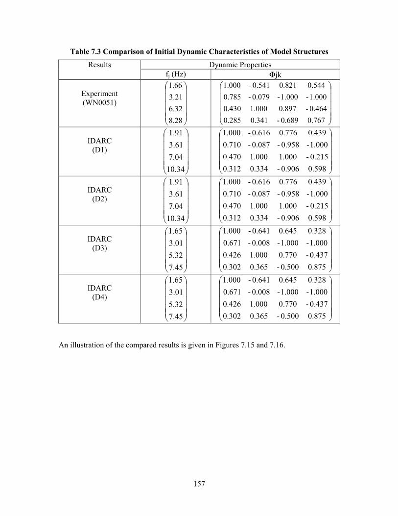
157
Table 7.3 Comparison of Initial Dynamic Characteristics of Model Structures
Dynamic Properties Results fj (Hz) Φjk
Experiment (WN0051)
⎟⎟⎟⎟⎟
⎠
⎞
⎜⎜⎜⎜⎜
⎝
⎛
8.286.323.211.66
⎟⎟⎟⎟⎟
⎠
⎞
⎜⎜⎜⎜⎜
⎝
⎛
0.7670.689-0.3410.2850.464-0.8971.0000.4301.000-1.000-0.079-0.7850.5440.8210.541-1.000
IDARC
(D1)
⎟⎟⎟⎟⎟
⎠
⎞
⎜⎜⎜⎜⎜
⎝
⎛
10.347.043.611.91
⎟⎟⎟⎟⎟
⎠
⎞
⎜⎜⎜⎜⎜
⎝
⎛
0.5980.906-0.3340.3120.215-1.0001.0000.4701.000-0.958-0.087-0.7100.4390.7760.616-1.000
IDARC
(D2)
⎟⎟⎟⎟⎟
⎠
⎞
⎜⎜⎜⎜⎜
⎝
⎛
10.347.043.611.91
⎟⎟⎟⎟⎟
⎠
⎞
⎜⎜⎜⎜⎜
⎝
⎛
0.5980.906-0.3340.3120.215-1.0001.0000.4701.000-0.958-0.087-0.7100.4390.7760.616-1.000
IDARC (D3)
⎟⎟⎟⎟⎟
⎠
⎞
⎜⎜⎜⎜⎜
⎝
⎛
7.455.323.011.65
⎟⎟⎟⎟⎟
⎠
⎞
⎜⎜⎜⎜⎜
⎝
⎛
0.8750.500-0.3650.3020.437-0.7701.0000.4261.000-1.000-0.008-0.6710.3280.6450.641-1.000
IDARC
(D4)
⎟⎟⎟⎟⎟
⎠
⎞
⎜⎜⎜⎜⎜
⎝
⎛
7.455.323.011.65
⎟⎟⎟⎟⎟
⎠
⎞
⎜⎜⎜⎜⎜
⎝
⎛
0.8750.500-0.3650.3020.437-0.7701.0000.4261.000-1.000-0.008-0.6710.3280.6450.641-1.000
An illustration of the compared results is given in Figures 7.15 and 7.16.

158
0
1
2
3
-1 0 1
Sto
ry
Experiment (WN0051)
IDARC - D1
IDARC - D2
IDARC - D3
IDARC - D4
-1 0 1
Experiment(WN0051)
IDARC - D1
IDARC - D2
IDARC - D3
IDARC - D4
Mode 1
0
1
2
3
-1 0 1
Sto
ry
Experiment (WN0051)
IDARC - D1
IDARC - D2
IDARC - D3
IDARC - D4
-1 0 1
Experiment(WN0051)
IDARC - D1
IDARC - D2
IDARC - D3
IDARC - D4
Mode 2
0
1
2
3
-1 0 1
Sto
ry
Experiment (WN0051)
IDARC - D1
IDARC - D2
IDARC - D3
IDARC - D4
-1 0 1
Experiment(WN0051)
IDARC - D1
IDARC - D2
IDARC - D3
IDARC - D4
Mode 3
0
1
2
3
-1 0 1
Sto
ry
Experiment (WN0051)
IDARC - D1
IDARC - D2
IDARC - D3
IDARC - D4
-1 0 1
Experiment(WN0051)
IDARC - D1
IDARC - D2
IDARC - D3
IDARC - D4
Mode 4
(a) Mode shapes
Figure 7.15 Initial Dynamic Characteristics of Model Structure

159
0
2
4
6
8
10
12
1 2 3 4Mode
Nat
ural
Fre
quen
cy (H
z)
IDARC-D1
IDARC-D2
IDARC-D3
IDARC-D4
Experiment(WN0051)
(b) Natural frequencies
Figure 7.16 Initial Dynamic Characteristics of Model Structure (cont’d)
7.5.2 Comparison of Spectral Capacity Curves – Analysis and Experimental The static (inverted triangle) and dynamic/incremental pushover analyses were conducted for all four analytical models, and the results are compared to experimental results. Figure 7.17 shows that the dynamic/incremental pushover analyses are in good agreement with the static pushover analyses for all analytical models. The final analytical model (Model D4) also gave a good estimate of the experimental model, especially in the elastic range.
The results of the spectral capacity analyses for the four analytical models are summarized in Table 7.4.
Table 7.4 Comparison of Structural Responses of Model Structures
Analytical Model uy** Qy Fm
E u* Q* R µ
D1 1.00 0.57 1.14 1.69 0.59 2.0 1.69
D2 0.98 0.60 1.15 1.31 0.67 1.92 1.33
D3 0.94 0.42 1.26 2.82 0.52. 3.00 3.00
D4 1.05 0.48 1.26 1.77 0.47. 2.63 1.68
* Normalized to the first mode (see Eq. 3.24 and 3.25); **Estimated from Eq. 3.22. u is dimensionless parameter of structure’s spectral drift (top displacement per height) F is base shear per weight Q is the spectral shear per weight (= acceleration per g)
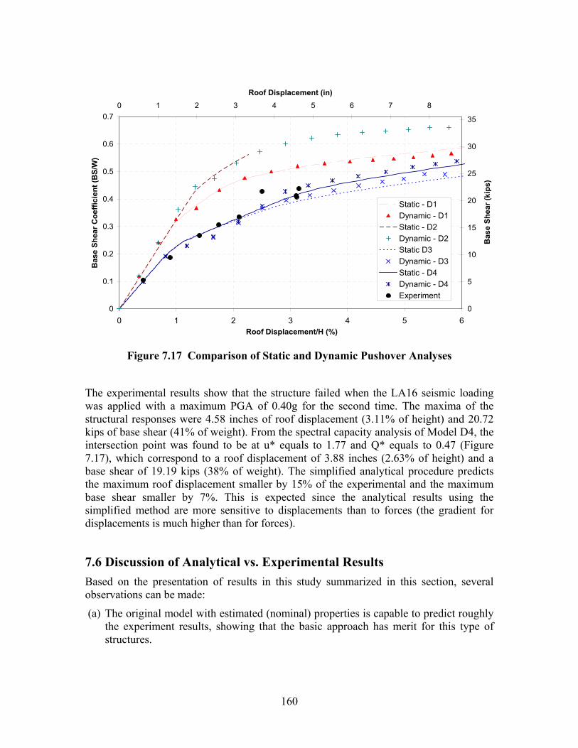
160
0
0.1
0.2
0.3
0.4
0.5
0.6
0.7
0 1 2 3 4 5 6Roof Displacement/H (%)
Bas
e Sh
ear C
oeffi
cien
t (B
S/W
)
0
5
10
15
20
25
30
35
0 1 2 3 4 5 6 7 8
Roof Displacement (in)
Bas
e Sh
ear (
kips
)
Static - D1Dynamic - D1Static - D2Dynamic - D2Static D3Dynamic - D3Static - D4Dynamic - D4Experiment
Figure 7.17 Comparison of Static and Dynamic Pushover Analyses
The experimental results show that the structure failed when the LA16 seismic loading was applied with a maximum PGA of 0.40g for the second time. The maxima of the structural responses were 4.58 inches of roof displacement (3.11% of height) and 20.72 kips of base shear (41% of weight). From the spectral capacity analysis of Model D4, the intersection point was found to be at u* equals to 1.77 and Q* equals to 0.47 (Figure 7.17), which correspond to a roof displacement of 3.88 inches (2.63% of height) and a base shear of 19.19 kips (38% of weight). The simplified analytical procedure predicts the maximum roof displacement smaller by 15% of the experimental and the maximum base shear smaller by 7%. This is expected since the analytical results using the simplified method are more sensitive to displacements than to forces (the gradient for displacements is much higher than for forces).
7.6 Discussion of Analytical vs. Experimental Results Based on the presentation of results in this study summarized in this section, several observations can be made:
(a) The original model with estimated (nominal) properties is capable to predict roughly the experiment results, showing that the basic approach has merit for this type of structures.
161
(b) Measuring the component properties indicated that additional effects, such as prying, needed to be modeled as semi rigid connections, in order to improve accuracy of predictions.
(c) The modified model including the semi-rigid connection action, as observed in both experiments of component properties and in the shake table experiment of the global system, is able to predict better the capacity of the structure as compared to the original model.
(d) An estimate of the maximum displacements and forces can be obtained using the simplified inelastic spectral approach with errors of less than 20%.
(e) The displacement estimates are more sensitive to the method of analysis than the force (acceleration) estimates, due to the expected gradients of each in the inelastic range.
(f) The structure has irregular features, which could not be modeled in detail in the simplified method (i.e., direction of forces/loads in pushover analysis). This may explain some of the differences between the simplified analytical models and the tested results. More refinement of the simplified model is necessary if higher accuracy is desired.
(g) By-and-large the loads determined from the modal spectral analysis, in its present form, do not produce results better than the approximated “inverted triangular” load distribution as suggested by the codes. This applies to both regular and mildly irregular structures. The experimental study could not completely address the influence of severe irregularity in the inelastic range due to premature failure of connections, but produced information for further studies and further analytical modeling.


163
SECTION 8 CONCLUDING REMARKS
A versatile experimental model was developed to be used and reused with structures undergoing severe damage to sacrificial elements thus capable to be repaired and further tested to provide reference information for the required validations. The selected model, a three-story three-bay steel structure designated as Model D, was designed so that it can fit within the limitations of capacity of the testing facilities, yet was similar as much as possible to a realistic structure, which established the one third scaled model. Steel was chosen as the material based on the versatility and the workability. The versatility of the model consists in the ability to reconfigure it into a large number of alternative variants – regular as well as irregular - that can be built from the same basic components. It was also designed to be easily installed, and easily repaired by replacing damaged parts after severe testing. For the purpose of this study, the irregularity aspect was introduced to the designated model by having two unequal towers.
This experimental study focused on the validation of the analytical tools for evaluation of seismic response of irregular structures, i.e. setback structures. A number of analytical studies had been carried out to evaluate such structures, but very few experimental works had been done on this subject. With a large number of critical structures, such as hospitals, which often have irregular design due to architectural and functional constraints, the study provides an overview of the accuracy of the analytical methods in predicting the structural response.
After selecting the model, the prediction of the structural response in the inelastic range was based on several analyses: dynamic time history analysis, dynamic pushover or incremental dynamic analysis, and nonlinear static analysis (spectral demand-capacity analysis). An analytical model was developed, model D1, using the estimated material properties and an original computational model. A selection process was performed to choose the most suitable ground motion for the study. First, the model was subjected to 20 different ground motions from the SAC project with 10% probability of exceedence in 50 years (10/50) in Los Angeles. Based on the results, LA16 ground motion (Northridge 1996, Rinaldi RS) was found to be the most suitable ground motion for the study because it produced the largest drifts and roof displacement (see Table 3.1), thus making it the most damaging ground motion. Therefore, LA16 ground motion was chosen to be the applied ground motion for the experimental study. A spectral capacity analysis was also conducted to have a better understanding of the structural inelastic seismic response, which led to the strength reduction factor (R) of 2, and the ductility (µ) of 1.69 (Figure 3.13).
Prior to the experimental study on the full model, several material and component tests were carried out. The tensile coupon test was conducted for both beam and column materials. The tests showed that the beam materials was Gr. 50 steel with a 50 ksi yield strength and 70 ksi ultimate strength, while the columns were of a higher strength steel with a 58 ksi yield strength and 83 ksi ultimate strength. These parameters were then used for the response analysis of the model structure, and a refined analytical model was
164
developed. The gravity columns were designed to resist only vertical load, hence, they cannot resist any moments and shear forces. These columns were equipped with special spherical attachments to enable them to act as pin-connected leaning columns. The component tests show that the gravity columns performed very well even under large lateral displacements. No damage was detected in the components, and the analysis of test results showed that the elements remained elastic throughout the tests. The beam column connections were designed so that they could resist only lateral loads. The component test was conducted on a ‘cruciform’ specimen made of half-beams and half-columns to resemble a sub-assembly having half spans and half stories on each side. Test results show that the beam column connection experienced damage under large lateral displacements. The damage was concentrated at the face of the connection block, in the form of a prying action on the column end plate. The component test results were subsequently used to refine the analytical model.
After completing the component and material testing, a series of shake table experiments were conducted as the identification testing procedure of the versatile model. The model was subjected to a white noise base displacement, and from the test results, the structural parameters were extracted, which include, natural frequencies, mode shapes, modal participation factors, stiffness matrix, damping matrix, and damping ratios. The comparison of the dynamic parameters shows that the analytical results of Model D1 (estimated property and original computational model) are not in agreement with the experimental results (Table 5.5). It was evident that the structural model used in the analysis was not adequate to predict the model response faithfully. In order to improve the agreement some modifications were made to the analytical model, based on the results from the material and component testing.
The experimental tests were conducted by applying a sequence of increasing LA16 (Rinaldi, Northridge 1994) ground motions, thus attempting to achieve the dynamic pushover analyses results. During the experiment, the structural response was monitored, and the base shear, floor displacements and accelerations were recorded. Structural damage (local and global) was also observed and interpreted. Structural identifications using white noise excitations were made in-between the dynamic loadings to monitor changes in the dynamic properties, i.e., frequencies and mode shapes. The results were also used to obtain more information on the condition of the structure.
Experimental results and visual observation show that the model behaved elastically under minor earthquake loadings. The first yield occurred at a PGA = 0.20g, and at higher ground motion levels the model behaved inelastically. Damage was recorded in the forms of prying effect at the column end plates and a welding failure of a block joint located at the toes of the higher tower where force concentrations due to irregularities were expected. This welding failure is considered to be the primary cause of the structural failure. The structural failure as visually observed during the test occurred at a PGA = 0.40g. Using the frequencies’ changes (see Figs 6.11 through 6.13) one can identify the onset of rupture at 0.35g, before the damage was actually visible. After this test the frequencies remained unchanged.
The changes in the global mode shapes (Fig 6.12) could locate the degrees of freedom affected by the damage, but could not identify which connection rigidly linked to the same degree of freedom actually ruptured.
165
The separation of vertical and lateral load resisting systems was satisfactory. No damage was recorded on the gravity columns, and a pancake type of collapse was avoided at structural failure. Most of the structural elements were undamaged during the experimental study, and these elements can be used for future research. The damaged parts are also replaceable, and if desired, can be rebuilt for future research.
Based on the results from the experimental study, analytical studies were conducted, and a number of analytical models were developed following the various stages of the experiments. The experimental results showed that the original model with estimated (nominal) properties is capable to predict roughly the experimental results. However, to achieve a better agreement with the experimental results, changes were made to include the actual material properties and the additional effects (prying) of the beam-column connection. A complete comparison of various analytical models and experimental results were presented (Figure 7.14) and a new analytical model with a semi-rigid connection gives a better prediction of the capacity of the structure as compared to the original model. Using the new model, the simplified inelastic spectral approach (spectral demand-capacity analysis) can give an estimate of the maximum displacements and forces with errors of less than 20%. The error is slightly larger in the displacement estimates since the method is more sensitive to this parameter in the inelastic range (the method depends on the gradient of the capacity curve).
Finally, the model structure was designed to accommodate inelastic behavior and severe damage without collapse. The model suffered complete rupture of its column connections, without complete collapse. The gravity columns and the redundancy of the system prevented such catastrophic collapse. The model can accommodate multiple configurations which may allow testing in the future of various assemblies of structural systems and protective devises, behaving well in the nonlinear range, near collapse. Although the severe failure in the tested model did not occur in the expected fashion the model proved its capability to test structures near collapse and collect sufficient information to improve computational models.
This study shows that a separation of lateral and gravity load resisting systems can produce a stable structure in case of major damage to lateral system, provided that redundancy exists to control lateral deformations. Such system can be implemented in retrofitting structures, by weakening the connections of gravity columns and providing a redundant external lateral load resisting system. Further research and engineering development may assure the success of such solution.

167
SECTION 9
REFERENCES
Al-Ali, A.K., and Krawinkler, H. (1998) “Effects of vertical irregularities on seismic behavior of building structures”, The John A. Blume Earthquake Engineering Center, Stanford, CA.
Aranda, H. (1984) “Ductility demands for R/C frames irregular in elevation”, Proceedings, 8th World Conference on Earthquake Engineering, Vol. 4, San Francisco, CA, pp. 559-566.
Arnold, C., and Reitherman, R. (1982) “Building configuration and seismic design”, Wiley, NY, 296 pp.
Birajdar, B.G., and Nawawade, S.S. (2004) “Seismic analysis of buildings resting on sloping ground”, Proceedings, 13th World Conference on Earthquake Engineering, Vancouver, B.C.
Bracci, J.M., Kunnath, S.K., and Reinhorn, A.M. (1997) “Seismic performance and retrofit evaluation of reinforced concrete structures”, Journal of Structural Engineering, Vol. 123, No. 1, pp. 3-10.
Bracci, J.M., Reinhorn, A.M., and Mander, J.B. (1995) “Seismic resistance of reinforced concrete frame structures designed for gravity loads: performance of structural system”, ACI Structural Journal, Vol. 92, No. 5, pp. 597-609.
Bracci, J.M., Reinhorn, A.M., and Mander, J.B. (1995) “Seismic retrofit of reinforced concrete buildings designed for gravity loads: Performance of structural model”, ACI Structural Journal, Vol. 92, No. 6, pp. 711-723
Bracci, J M., Mander, J.B., and Reinhorn, A.M. (1992) “Evaluation of seismic retrofit of reinforced concrete frame structures: Part II - Experimental performance and analytical study of a retrofitted structural model”, National Center for Earthquake Engineering Research, Buffalo, NY.
Bracci, J.M., Reinhorn, A.M., and Mander, J.B. (1992) “Seismic resistance of reinforced concrete frame structures designed only for gravity loads: Part I - Design and properties of a one-third scale model structure”, National Center for Earthquake Engineering Research, Buffalo, NY.
Bracci, J.M., Reinhorn, A.M., and Mander, J.B. (1992) “Seismic resistance of reinforced concrete frame structures designed only for gravity loads: Part III - Experimental performance and analytical study of a structural model”, National Center for Earthquake Engineering Research, Buffalo, NY.

168
Bracci, J.M., Reinhorn, A.M., and Mander, J.B. (1995) “Seismic resistance of reinforced concrete frame structures designed for gravity loads: performance of structural system”, ACI Materials Journal, Vol. 92, No. 5, pp. 597-609.
Chang, G.A., and Mander, J.B. (1994) “Seismic energy based fatigue damage analysis of bridge columns: Part II – Evaluation of seismic demand”, National Center for Earthquake Engineering Research, Buffalo, NY.
Chopra, A.K., and Goel, R.K. (1999) “Capacity-demand-diagram methods for estimating seismic deformation of inelastic structures: SDF systems”, Pacific Earthquake Engineering Research Center, Berkeley, CA.
Chopra, A.K., and Goel, R.K. (2001) “A modal pushover analysis procedure to estimate seismic demands for buildings: theory and preliminary evaluation”, Pacific Earthquake Engineering Research Center, Berkeley, CA.
Chopra, A.K., and Goel, R.K. (2000) “Evaluation of NSP to estimate seismic deformation: SDF systems”, Journal of Structural Engineering, Vol. 126, No. 4, pp. 482-490.
Chopra, A.K., and Goel, R.K. (2000) “Building period formulas for estimating seismic displacements”, Earthquake Spectra, Vol. 16, No. 2, pp. 533-536.
Choudhuri, D., Mander, J.B., and Reinhorn, A.M. (1992) “Evaluation of seismic retrofit of reinforced concrete frame structures: Part I - Experimental performance of retrofitted subassemblages”, National Center for Earthquake Engineering Research, Buffalo, NY.
Costa, A.G., Oliveira, C.S., and Duarte, R.T. (1988) “Influence of vertical irregularities on seismic response of buildings”, Proceedings, 9th World Conference on Earthquake Engineering, Vol. V, Tokyo-Kyoto.
De La Llera, J.C., and Chopra, A.K. (1995) “Understanding the inelastic seismic behavior of asymmetric-plan buildings”, Earthquake Engineering and Structural Dynamics, Vol. 24, No. 4, pp. 549-572.
De La Llera, J.C., and Chopra, A.K. (1995) “A simplified model for analysis and design of asymmetric-plan buildings”, Earthquake Engineering and Structural Dynamics, Vol. 24, No. 4, pp. 573-594.
De Stefano, M., Faella, G., and Ramasco, R. (1993) “Inelastic response and design criteria of plan-wise asymmetric systems”, Earthquake Engineering and Structural Dynamics, Vol. 22, pp. 245-259.
De Stefano, M. et al. (2001) “Shaking table tests on scale models of multistorey steel buildings”, “Cable Stayed Bridges, Irregular Bridges and Asymmetrical Structures”, R. Severn and C.A. Taylor eds., ECOEST 2 Report No. 8, LNEC, Lisbon.

169
Duan, X.N., and Chandler, A.M. (1995) “Seismic torsional response and design procedures for a class of setback frame buildings”, Earthquake Engineering and Structural Dynamics, Vol. 24, No. 5, pp. 761-777.
Duan, X.N., and Chandler, A.M. (1993) “Inelastic seismic response of code-designed multistorey frame buildings with regular asymmetry”, Earthquake Engineering and Structural Dynamics, Vol. 22, No. 5, pp. 431-445.
Duarte, R.T., and Costa, A.C. (1988) “Earthquake design of reinforced concrete structures based on local ductility coefficients”, Proceedings, 9th World Conference on Earthquake Engineering, Vol. V, Tokyo-Kyoto.
Fajfar, P. (1999) “Capacity spectrum method based on inelastic demand spectra” Earthquake Engineering and Structural Dynamics, Vol. 28, No. 9, pp. 979-993.
Fajfar, P., and Vidic, T. (1994) “Consistent inelastic design spectra: hysteretic and input energy”, Earthquake Engineering and Structural Dynamics, Vol. 23, No. 5, pp. 523-537.
FEMA 273 (1997) “NEHRP guidelines for the seismic rehabilitation of buildings”, Federal Emergency Management Agency, Washington, D.C.
FEMA 274 (1997) “NEHRP commentary for the seismic rehabilitation of buildings”, Federal Emergency Management Agency, Washington, D.C.
FEMA 356 (2000) “Prestandard and commentary for the seismic rehabilitation of buildings”, Federal Emergency Management Agency, Washington, D.C.
FEMA IG 370 (1989) “Non-structural earthquake hazard mitigation for hospitals and other care facilities”, Federal Emergency Management Agency, Washington, D.C.
Freeman, S.A. (1994) “The capacity spectrum method for determining the demand displacement”, ACI Spring Convention.
Goel, R.K. (1997) “Seismic response of asymmetric systems: energy-based approach”, Journal of Structural Engineering, Vol. 123, No. 11, pp. 1444-1453.
Harasimowicz, A.P., and Goel, R.K. (1998) “Seismic code analysis of multi-storey asymmetric buildings”, Earthquake Engineering and Structural Dynamics, Vol. 27, No. 2, pp. 173-185.
Harris, H.G., and Sabnis, G.M. (1999) “Structural modeling and experimental techniques”, 2nd edition, CRC Press, Boca Raton.
Housner, G.W., and Outinen, H. (1958) “The effect of torsional oscillations on earthquake stresses”, Bulletin of Seismological Society of America, Vol. 48, 1958, pp. 221-229
170
Humar, J.L., and Wright, E.W. (1977) “Earthquake response of steel-framed multistory buildings with setbacks”, Earthquake Engineering and Structural Dynamics, Vol. 5, pp. 15-39.
International Code Council (2000) “International building code 2000”, International Code Council, Falls Church, VA.
Kan, C.L., and Chopra, A.K. (1981) “Torsional coupling and earthquake response of simple elastic and inelastic systems”, Journal of the Structural Division, Vol. 107. No. ST8, pp. 1569-1587.
Kelly, J.M, Buckle, I.G., and Tsai, H.-C. (1986) “Earthquake simulator testing of a base isolated bridge deck”, Earthquake Engineering Research Center, College of Engineering, University of California, 111 pp., Berkeley, CA.
Kilar, V., and Fajfar, P. (1997) “Simple push-over analysis of asymmetric buildings”, Earthquake Engineering and Structural Dynamics, Vol. 26, pp. 233-249.
Krawinkler, H., and Seneviratna, G.D.P.K. (1998) “Pros and cons of a pushover analysis of seismic performance evaluation”, Engineering Structures, Vol. 20, No. 4-6, pp. 452-464.
Krawinkler, H. (1996) “Cyclic loading histories for seismic experimentation on structural components”, Earthquake Spectra, Vol. 12, No. 1, pp. 1-11.
Magliulo, G., Ramasco, R., and Realfonzo, R. (2002) “A critical review of seismic code provisions for vertical irregularity”, Proceedings, 3rd European Workshop on Seismic Behaviour of Irregular and Complex Structures, M. De Stefano & A. Rutenberg, eds., Florence.
Mazzolani, F., and Piluso, V. (1996) “Behaviour and design of set-back steel frames”, Proceedings, European Workshop on Seismic Behaviour of Asymmetric and Setback Structures, R. Ramasco, & A. Rutenberg, eds, University of Naples, Federico II, Anacapri, October.
Mazzolani, F, and Piluso, V. (1997) “Review of code provisions for vertical irregularity”, Proceedings, 2nd International Conference on Behaviour of Steel Structures in Seismic Areas, STESSA '97, Kyoto, Japan, pp. 250-257.
Moehle, J.P., and Alarcon, L.F. (1986) “Seismic analysis methods for irregular buildings” Journal of Structural Engineering, Vol. 112, No. 1, pp. 35-52.
Nassar, A.A., and Krawinkler, H. (1991) “Seismic demands for SDOF and MDOF systems”, The John A. Blume Earthquake Engineering Center, Dept. of Civil Engineering, Stanford University, Stanford, CA.
Newmark, N.M., and Hall, W.J. (1982) “Earthquake spectra and design”, Earthquake Engineering Research Inst, 103 pp., Berkeley, CA.
171
Pekau, O.A., and Green, R. (1974) “Inelastic structures with setbacks”, Proceedings, 5th World Conference on Earthquake Engineering, Rome, Italy, Vol. 2, pp. 1744-1747.
Pinto, D., and Costa, A.G. (1995) “Influence of vertical irregularities on seismic response of buildings”, Proceedings, 10th European Conference on Earthquake Engineering: Vienna, Balkema, Rotterdam.
Reichman, Y., and Reinhorn, A.M. (1995) “Extending the seismic life span of bridges: Analytical evaluation of retrofit measures”, Structural Engineering Review, Vol. 7, No. 3, pp. 207-218.
Reinhorn, A.M. (1997) “Inelastic analysis techniques in seismic evaluation”,”Seismic Design Methodologies for the Next Generation of Codes”, P. Fajfar & H .Krawinkler eds., Balkema, Rotterdam.
Reinhorn, A.M., Barron, R, Valles, R., and Sivaselvan, M.V. (1998) “NSPECTRA Version 2.0: Nonlinear analysis program for inelastic spectra with degradation and deterioration of structural systems. User manual”, University at Buffalo, Buffalo, NY.
Romao, X., Costa, A., and Delgado, R. (2004) “Seismic behavior of reinforced concrete frames with setbacks”, Proceedings, 13th World Conference on Earthquake Engineering, Vancouver, B.C.
Rosenblueth, E. (1957) “Consideration on torsion, overturning and drift limitations”, Proc. SEAOC Conference, Coronado, CA.
Ruiz-Garcia, J., and Miranda, E. (2003) “Inelastic displacement ratios for evaluation of existing structures”, Earthquake Engineering and Structural Dynamics, Vol. 32, pp. 1237-1238.
Rutenberg, A. (1992) “Nonlinear response of asymmetric building structures and seismic codes: state of the art review”, European Earthquake Engineering, Vol. 2, pp. 3-19.
Rutenberg, A. (2002) “EAEE Task Group (TG) 8: Behaviour of irregular and complex asymmetric structures - progress since 1998”, Proceedings, 12th European Conference Earthquake Engineering, London.
Rutenberg, A., and De Stefano, M. (1997) “On the seismic performance of yielding asymmetric multistorey buildings: A review and a case study”, “Seismic Design Methodologies for the Next Generation of Codes”, P.Fajfar & H. Krawinkler eds., Balkema, Rotterdam.
Ryan, K.L., and Chopra, A.K. (2002) “Approximate analysis methods for asymmetric plan base-isolated buildings”, Earthquake Engineering and Structural Dynamics, Vol. 31, No.1, pp. 33-54.

172
Satyarno, I., Carr, A., and Restrepo, J. (1998) “Refined pushover analysis for the assessment older reinforced concrete buildings”, Proceeding, New Zealand National Society for Earthquake Engineering, Wairakei.
SEAOC, Seismology Committee (1999) “Recommended lateral force requirements and commentary”, Structural Engineers Association of California, Sacramento, CA.
Seneviratna, G.D.P.K., and Krawinkler, H. (1997) “Evaluation of inelastic MDOF effects for seismic design”, The John A. Blume Earthquake Engineering Center, Stanford, CA.
Shahrooz, B.M., and Moehle, J.P. (1990) “Evaluation of seismic performance of reinforced concrete frames”, Journal of Structural Engineering, Vol. 116, No. 5, pp. 1403-1422.
Shahrooz, B.M., and Moehle, J.P. (1990) “Seismic response and design of setback buildings” Journal of Structural Engineering, Vol. 116, No. 5, pp. 1423-1439.
Shea, G.H. (1996) “Recommended lateral force requirements & commentary (SEAOC Blue Book) 6th Edition”, Structural Engineers Association of California, Sacramento, CA.
Sommerville, P., et. al. (1997) “Development of ground motion time histories for phase 2 of the FEMA/SAC steel project”, SAC Steel Project Report No. SAC/BD-97/04, SAC Joint Venture, Sacramento, CA.
Tena-Colunga, A. (2004) “Evaluation of the seismic response of slender, setback RC moment-resisting frame building designed according to the seismic guidelines of a modern buiding code”, Proceedings, 13th World Conference on Earthquake Engineering, Vancouver, B.C.
Tso, W.K., and Yao, S. (1994) “Seismic load distribution in buildings with eccentric setback”, Canadian Journal of Civil Engineering, Vol. 21, No. 1, pp. 50-62.
Tso, W.K., and Ying, H. (1990) “Additional seismic inelastic deformation caused by structural asymmetry”, Earthquake Engineering and Structural Dynamics, Vol. 19, No. 2, pp. 243-258, 1990
Valles, R.E., Reinhorn, A.M., Kunnath, S.K., Li, C., and Madan, A. (1996a) “IDARC2D Version 4.0: A computer program for the inelastic damage analysis of buildings”, National Center for Earthquake Engineering Research, Buffalo, NY.
Valles, R.E., Reinhorn, A.M., Madan A. and Barron, R. (1996b), “Seismic evaluation of a low-rise RC building in the vicinity of the New Madrid seismic zone”, National Center for Earthquake Engineering Research, Buffalo, NY.
Vamvatsikos, D., and Cornell, C.A. (2002) “Incremental dynamic analysis”, Earthquake Engineering and Structural Dynamics, Vol. 31, No. 3, pp. 491-514.
173
Vamvatsikos, D., and Cornell, C.A. (2004) “Applied incremental dynamic analysis”, Earthquake Spectra, Vol. 20, pp. 523-553.
Vidic, T., Fajfar, P., and Fischinger, M. (1994) “Consistent inelastic design spectra: strength and displacement”, Earthquake Engineering and Structural Dynamics, Vol. 23, No. 5 , pp. 507-521.
Wong, C.M., Tso, W.K. (1994) “Seismic loading for buildings with setbacks”, Canadian Journal of Civil Engineering, Vol. 21, No. 5, pp. 863-871.
Wood, S.L. (1992) “Seismic response of R/C frames with irregular profiles”, Journal of Structural Engineering, Vol. 118, No. 2, pp. 545-566.

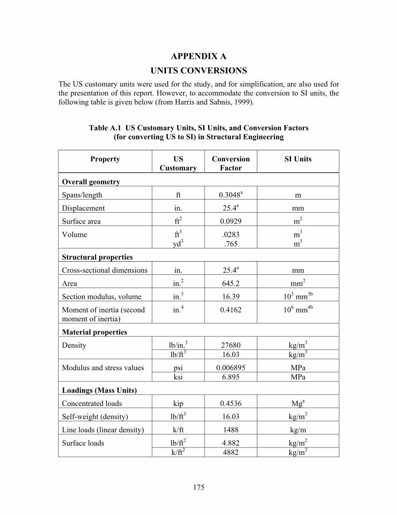
175
APPENDIX A UNITS CONVERSIONS
The US customary units were used for the study, and for simplification, are also used for the presentation of this report. However, to accommodate the conversion to SI units, the following table is given below (from Harris and Sabnis, 1999).
Table A.1 US Customary Units, SI Units, and Conversion Factors (for converting US to SI) in Structural Engineering
Property US Customary
Conversion Factor
SI Units
Overall geometry
Spans/length ft 0.3048a m
Displacement in. 25.4a mm
Surface area ft2 0.0929 m2
ft3 .0283 m3 Volume yd3 .765 m3
Structural properties
Cross-sectional dimensions in. 25.4a mm
Area in.2 645.2 mm2
Section modulus, volume in.3 16.39 103 mm3b
Moment of inertia (second moment of inertia)
in.4 0.4162 106 mm4b
Material properties
lb/in.3 27680 kg/m3 Density lb/ft3 16.03 kg/m3
psi 0.006895 MPa Modulus and stress values ksi 6.895 MPa
Loadings (Mass Units)
Concentrated loads kip 0.4536 Mga
Self-weight (density) lb/ft3 16.03 kg/m3
Line loads (linear density) k/ft 1488 kg/m
lb/ft2 4.882 kg/m2 Surface loads k/ft2 4882 kg/m2
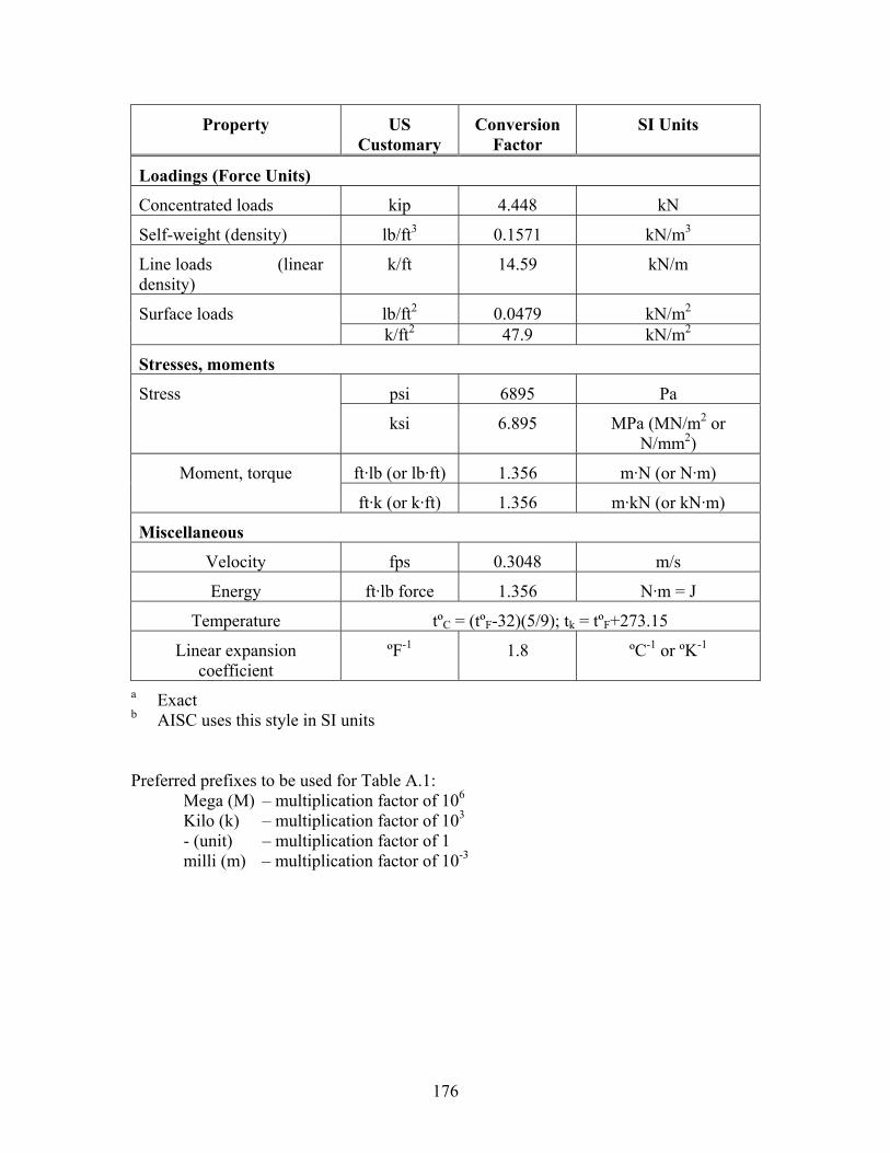
176
Property US Customary
Conversion Factor
SI Units
Loadings (Force Units)
Concentrated loads kip 4.448 kN
Self-weight (density) lb/ft3 0.1571 kN/m3
Line loads (linear density)
k/ft 14.59 kN/m
lb/ft2 0.0479 kN/m2 Surface loads k/ft2 47.9 kN/m2
Stresses, moments
psi 6895 Pa Stress
ksi 6.895 MPa (MN/m2 or N/mm2)
ft·lb (or lb·ft) 1.356 m·N (or N·m) Moment, torque
ft·k (or k·ft) 1.356 m·kN (or kN·m)
Miscellaneous
Velocity fps 0.3048 m/s
Energy ft·lb force 1.356 N·m = J
Temperature tºC = (tºF-32)(5/9); tk = tºF+273.15
Linear expansion coefficient
ºF-1 1.8 ºC-1 or ºK-1
a Exact b AISC uses this style in SI units Preferred prefixes to be used for Table A.1:
Mega (M) – multiplication factor of 106 Kilo (k) – multiplication factor of 103 - (unit) – multiplication factor of 1 milli (m) – multiplication factor of 10-3

177
APPENDIX B GROUND MOTIONS
The ground motions used in this study are the 20 accelerograms developed for the SAC project (Somerville, 1997), with 10% probability of exceedence in 50 years (10/50) in Los Angeles for fault normal motions (marked fn) and fault parallel motions (marked fn), as presented in Table 3.2.
Figures B.1 to B.40 show the acceleration history and the inelastic seismic demand spectra developed for of the accelerograms, used in the preliminary analyses leading to the selection of the testing ground motion. The inelastic response spectra were developed using the computer code NSPECTRA (Reinhorn,et al, 1998). The response spectra were generated for 5% damping, and 2% post yield stiffness ratio. The results were given for 3 different values of the strength reduction factor, R: R = 1 elastic response spectrum, R = 2 and R = 4.
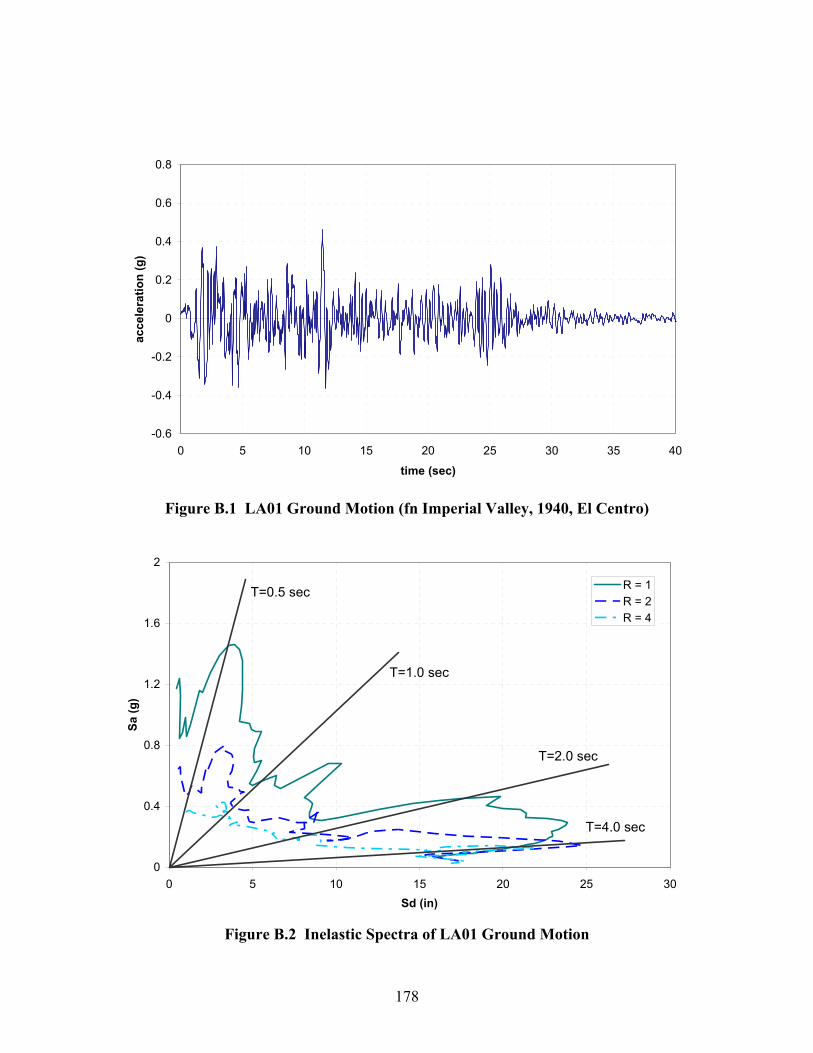
178
-0.6
-0.4
-0.2
0
0.2
0.4
0.6
0.8
0 5 10 15 20 25 30 35 40
time (sec)
acce
lera
tion
(g)
Figure B.1 LA01 Ground Motion (fn Imperial Valley, 1940, El Centro)
0
0.4
0.8
1.2
1.6
2
0 5 10 15 20 25 30Sd (in)
Sa (g
)
R = 1R = 2R = 4
T=0.5 sec
T=1.0 sec
T=2.0 sec
T=4.0 sec
Figure B.2 Inelastic Spectra of LA01 Ground Motion
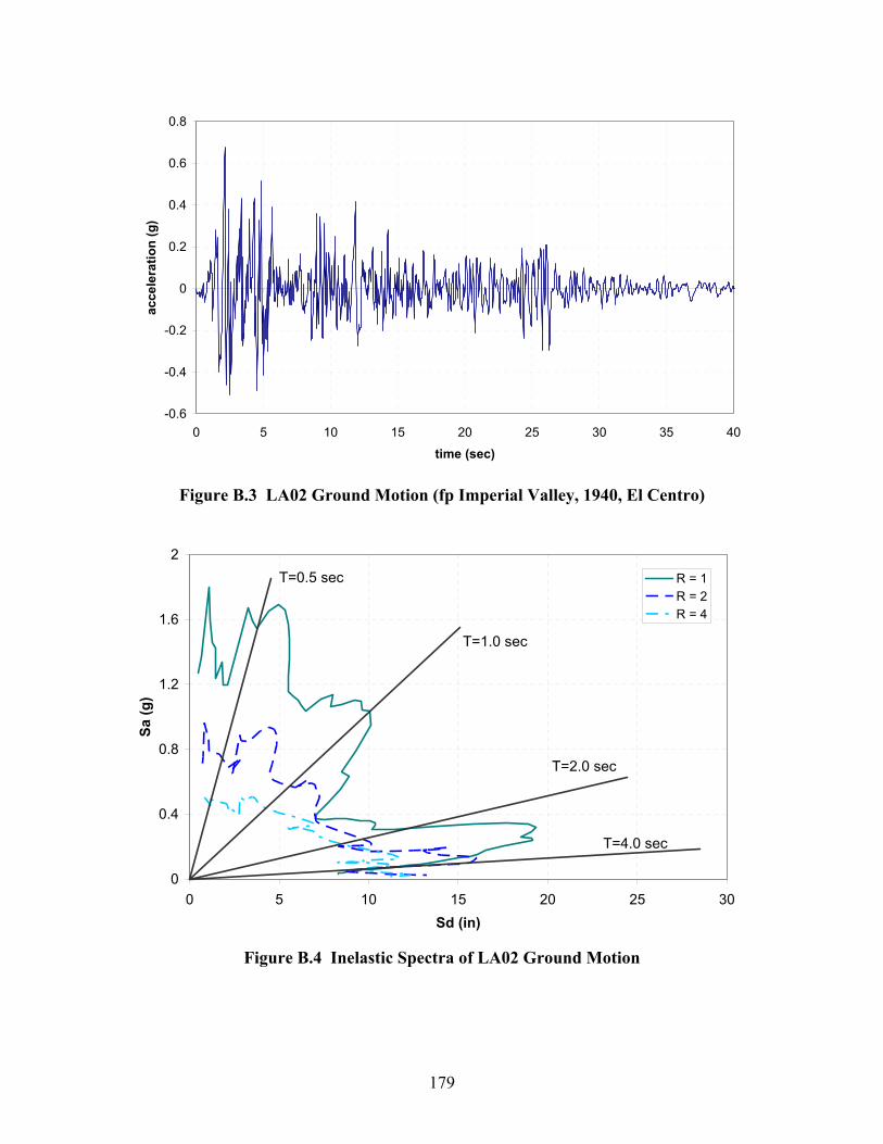
179
-0.6
-0.4
-0.2
0
0.2
0.4
0.6
0.8
0 5 10 15 20 25 30 35 40
time (sec)
acce
lera
tion
(g)
Figure B.3 LA02 Ground Motion (fp Imperial Valley, 1940, El Centro)
0
0.4
0.8
1.2
1.6
2
0 5 10 15 20 25 30Sd (in)
Sa (g
)
R = 1R = 2R = 4
T=0.5 sec
T=1.0 sec
T=2.0 sec
T=4.0 sec
Figure B.4 Inelastic Spectra of LA02 Ground Motion
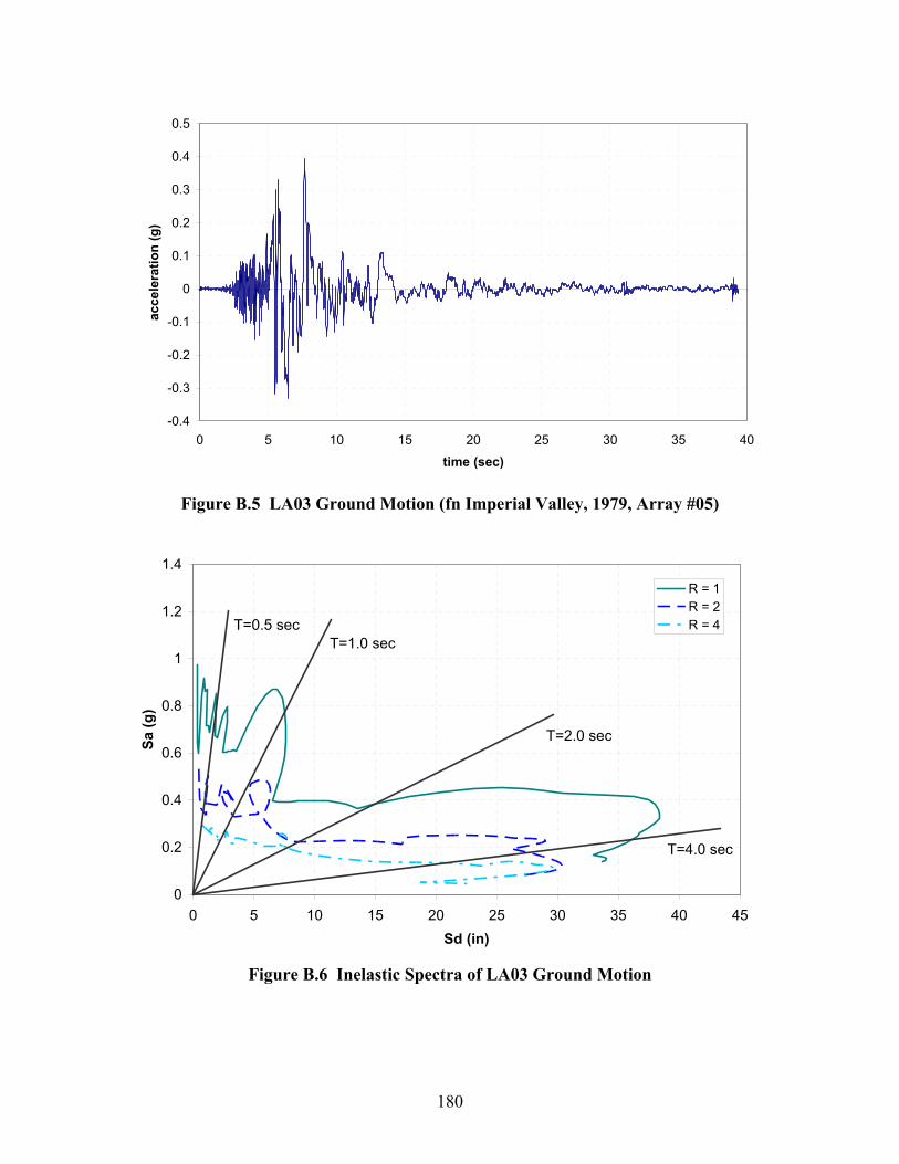
180
-0.4
-0.3
-0.2
-0.1
0
0.1
0.2
0.3
0.4
0.5
0 5 10 15 20 25 30 35 40
time (sec)
acce
lera
tion
(g)
Figure B.5 LA03 Ground Motion (fn Imperial Valley, 1979, Array #05)
0
0.2
0.4
0.6
0.8
1
1.2
1.4
0 5 10 15 20 25 30 35 40 45Sd (in)
Sa (g
)
R = 1R = 2R = 4T=0.5 sec
T=1.0 sec
T=2.0 sec
T=4.0 sec
Figure B.6 Inelastic Spectra of LA03 Ground Motion
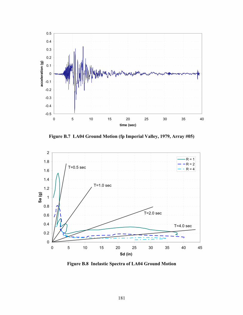
181
-0.5
-0.4
-0.3
-0.2
-0.1
0
0.1
0.2
0.3
0.4
0.5
0 5 10 15 20 25 30 35 40
time (sec)
acce
lera
tion
(g)
Figure B.7 LA04 Ground Motion (fp Imperial Valley, 1979, Array #05)
0
0.2
0.4
0.6
0.8
1
1.2
1.4
1.6
1.8
2
0 5 10 15 20 25 30 35 40 45Sd (in)
Sa (g
)
R = 1R = 2R = 4T=0.5 sec
T=1.0 sec
T=2.0 sec
T=4.0 sec
Figure B.8 Inelastic Spectra of LA04 Ground Motion

182
-0.4
-0.3
-0.2
-0.1
0
0.1
0.2
0.3
0.4
0 5 10 15 20 25 30 35 40
time (sec)
acce
lera
tion
(g)
Figure B.9 LA05 Ground Motion (fn Imperial Valley, 1979, Array #06)
0
0.1
0.2
0.3
0.4
0.5
0.6
0.7
0.8
0.9
1
0 10 20 30 40 50 60Sd (in)
Sa (g
)
R = 1R = 2R = 4
T=0.5 sec
T=1.0 sec
T=2.0 sec
T=4.0 sec
Figure B.10 Inelastic Spectra of LA05 Ground Motion
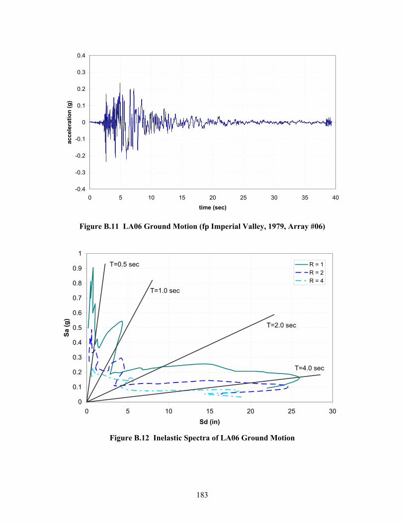
183
-0.4
-0.3
-0.2
-0.1
0
0.1
0.2
0.3
0.4
0 5 10 15 20 25 30 35 40
time (sec)
acce
lera
tion
(g)
Figure B.11 LA06 Ground Motion (fp Imperial Valley, 1979, Array #06)
0
0.1
0.2
0.3
0.4
0.5
0.6
0.7
0.8
0.9
1
0 5 10 15 20 25 30Sd (in)
Sa (g
)
R = 1R = 2R = 4
T=0.5 sec
T=1.0 sec
T=2.0 sec
T=4.0 sec
Figure B.12 Inelastic Spectra of LA06 Ground Motion
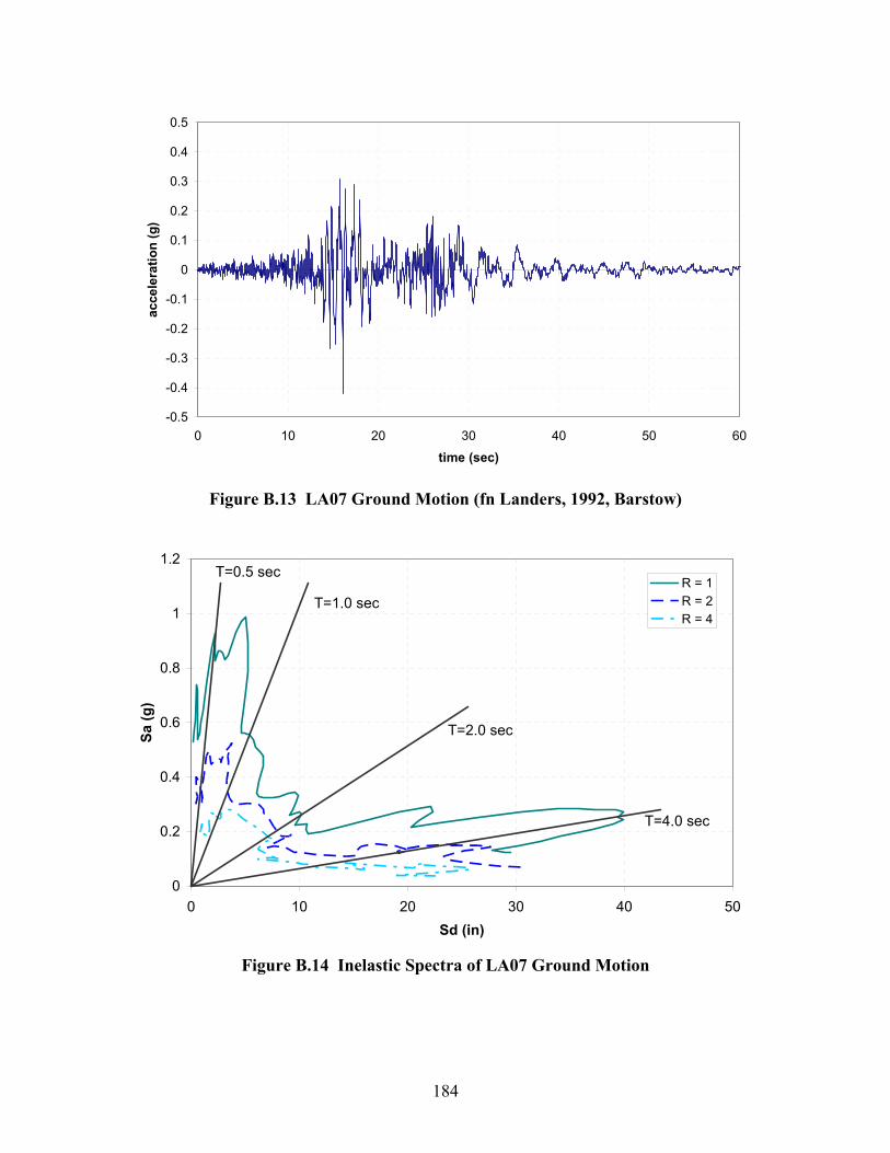
184
-0.5
-0.4
-0.3
-0.2
-0.1
0
0.1
0.2
0.3
0.4
0.5
0 10 20 30 40 50 60
time (sec)
acce
lera
tion
(g)
Figure B.13 LA07 Ground Motion (fn Landers, 1992, Barstow)
0
0.2
0.4
0.6
0.8
1
1.2
0 10 20 30 40 50Sd (in)
Sa (g
)
R = 1R = 2R = 4
T=0.5 sec
T=1.0 sec
T=2.0 sec
T=4.0 sec
Figure B.14 Inelastic Spectra of LA07 Ground Motion
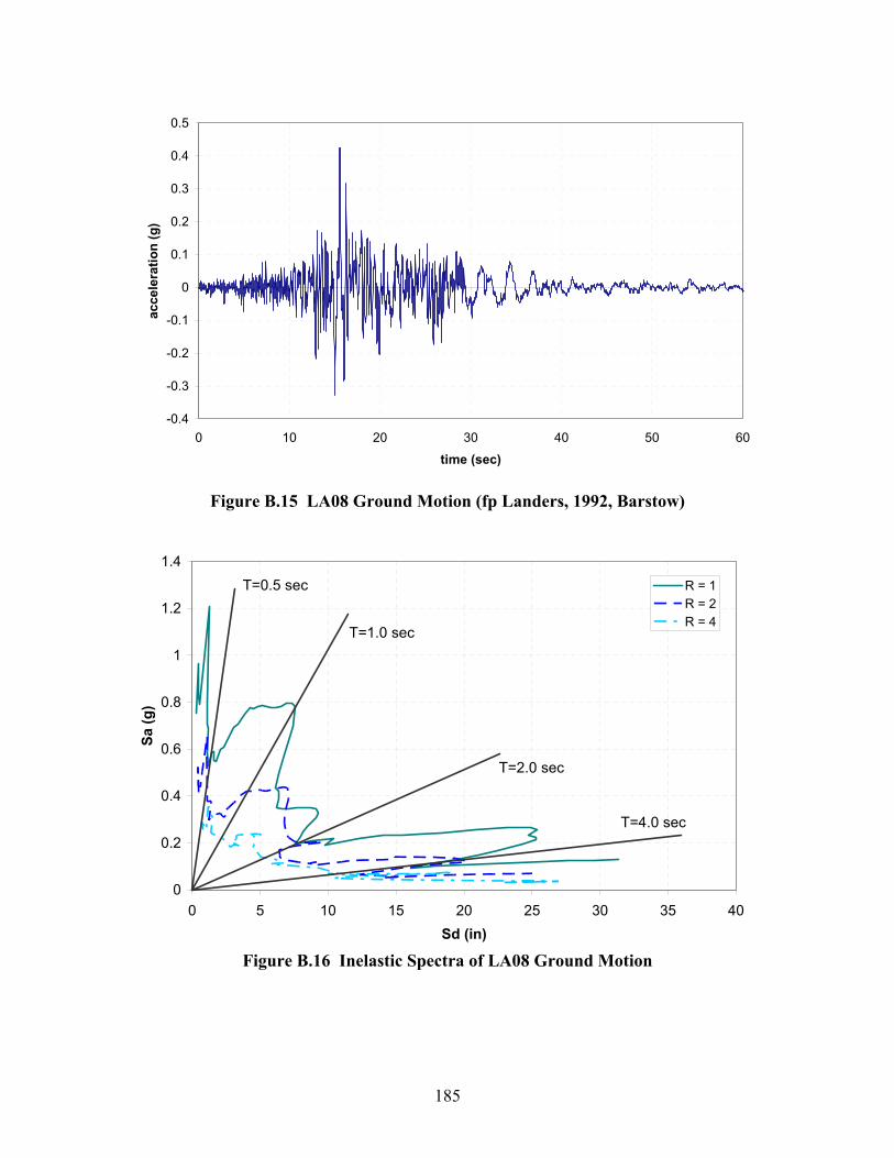
185
-0.4
-0.3
-0.2
-0.1
0
0.1
0.2
0.3
0.4
0.5
0 10 20 30 40 50 60
time (sec)
acce
lera
tion
(g)
Figure B.15 LA08 Ground Motion (fp Landers, 1992, Barstow)
0
0.2
0.4
0.6
0.8
1
1.2
1.4
0 5 10 15 20 25 30 35 40Sd (in)
Sa (g
)
R = 1R = 2R = 4
T=0.5 sec
T=1.0 sec
T=2.0 sec
T=4.0 sec
Figure B.16 Inelastic Spectra of LA08 Ground Motion

186
-0.4
-0.3
-0.2
-0.1
0
0.1
0.2
0.3
0.4
0.5
0.6
0 10 20 30 40 50 60
time (sec)
acce
lera
tion
(g)
Figure B.17 LA09 Ground Motion (fn Landers, 1992, Yermo)
0
0.2
0.4
0.6
0.8
1
1.2
1.4
1.6
0 10 20 30 40 50Sd (in)
Sa (g
)
R = 1R = 2R = 4
T=0.5 sec
T=1.0 sec
T=2.0 sec
T=4.0 sec
Figure B.18 Inelastic Spectra of LA09 Ground Motion

187
-0.4
-0.3
-0.2
-0.1
0
0.1
0.2
0.3
0.4
0 10 20 30 40 50 60
time (sec)
acce
lera
tion
(g)
Figure B.19 LA10 Ground Motion (fp Landers, 1992, Yermo)
0
0.2
0.4
0.6
0.8
1
1.2
1.4
0 10 20 30 40 50Sd (in)
Sa (g
)
R = 1R = 2R = 4
T=0.5 sec
T=1.0 sec
T=2.0 sec
T=4.0 sec
Figure B.20 Inelastic Spectra of LA10 Ground Motion

188
-1
-0.8
-0.6
-0.4
-0.2
0
0.2
0.4
0.6
0.8
1
0 5 10 15 20 25 30
time (sec)
acce
lera
tion
(g)
Figure B.21 LA11 Ground Motion (fn Loma Prieta, 1989, Gilroy)
0
0.5
1
1.5
2
2.5
3
0 5 10 15 20 25 30Sd (in)
Sa (g
)
R = 1R = 2R = 4T=0.5 sec
T=1.0 sec
T=2.0 sec
T=4.0 sec
Figure B.22 Inelastic Spectra of LA11 Ground Motion
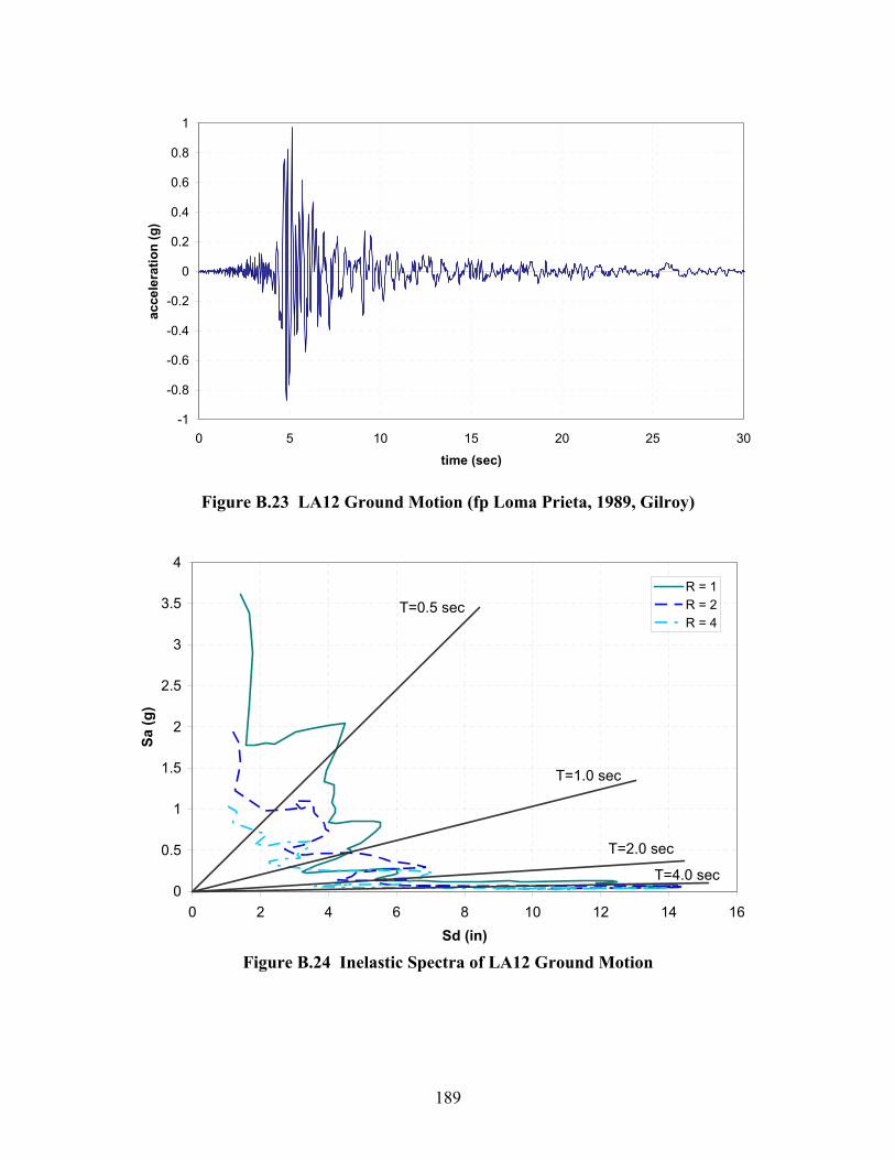
189
-1
-0.8
-0.6
-0.4
-0.2
0
0.2
0.4
0.6
0.8
1
0 5 10 15 20 25 30
time (sec)
acce
lera
tion
(g)
Figure B.23 LA12 Ground Motion (fp Loma Prieta, 1989, Gilroy)
0
0.5
1
1.5
2
2.5
3
3.5
4
0 2 4 6 8 10 12 14 16Sd (in)
Sa (g
)
R = 1R = 2R = 4
T=0.5 sec
T=1.0 sec
T=2.0 sec
T=4.0 sec
Figure B.24 Inelastic Spectra of LA12 Ground Motion
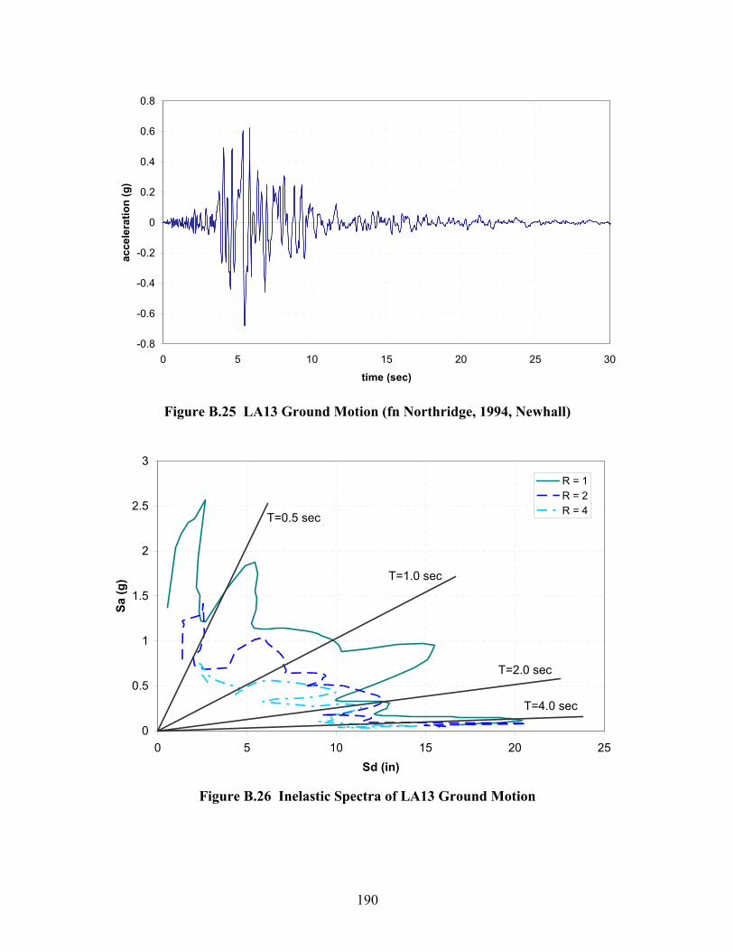
190
-0.8
-0.6
-0.4
-0.2
0
0.2
0.4
0.6
0.8
0 5 10 15 20 25 30
time (sec)
acce
lera
tion
(g)
Figure B.25 LA13 Ground Motion (fn Northridge, 1994, Newhall)
0
0.5
1
1.5
2
2.5
3
0 5 10 15 20 25Sd (in)
Sa (g
)
R = 1R = 2R = 4T=0.5 sec
T=1.0 sec
T=2.0 sec
T=4.0 sec
Figure B.26 Inelastic Spectra of LA13 Ground Motion
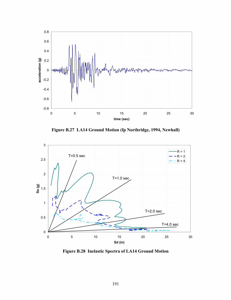
191
-0.8
-0.6
-0.4
-0.2
0
0.2
0.4
0.6
0.8
0 5 10 15 20 25 30
time (sec)
acce
lera
tion
(g)
Figure B.27 LA14 Ground Motion (fp Northridge, 1994, Newhall)
0
0.5
1
1.5
2
2.5
3
0 5 10 15 20 25 30Sd (in)
Sa (g
)
R = 1R = 2R = 4
T=0.5 sec
T=1.0 sec
T=2.0 sec
T=4.0 sec
Figure B.28 Inelastic Spectra of LA14 Ground Motion
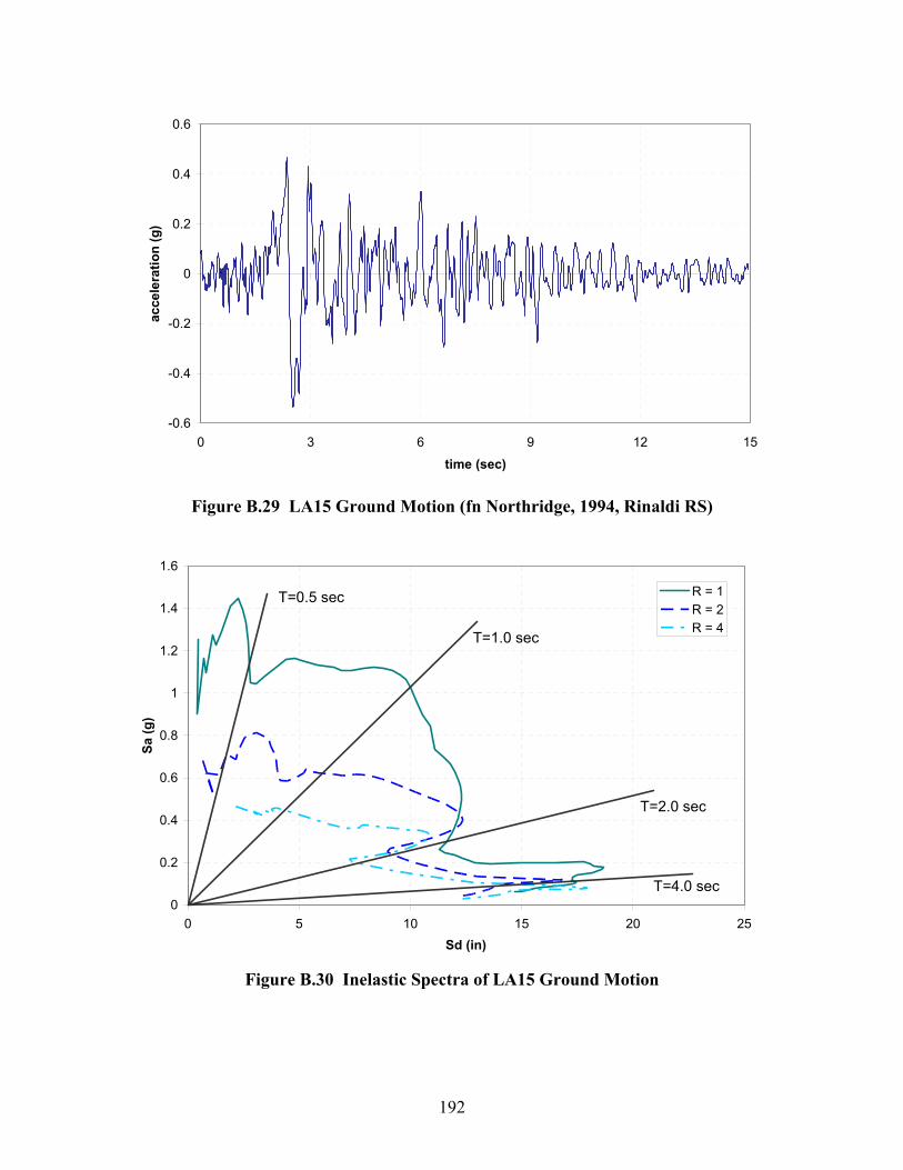
192
-0.6
-0.4
-0.2
0
0.2
0.4
0.6
0 3 6 9 12 15
time (sec)
acce
lera
tion
(g)
Figure B.29 LA15 Ground Motion (fn Northridge, 1994, Rinaldi RS)
0
0.2
0.4
0.6
0.8
1
1.2
1.4
1.6
0 5 10 15 20 25Sd (in)
Sa (g
)
R = 1R = 2R = 4
T=0.5 sec
T=1.0 sec
T=2.0 sec
T=4.0 sec
Figure B.30 Inelastic Spectra of LA15 Ground Motion
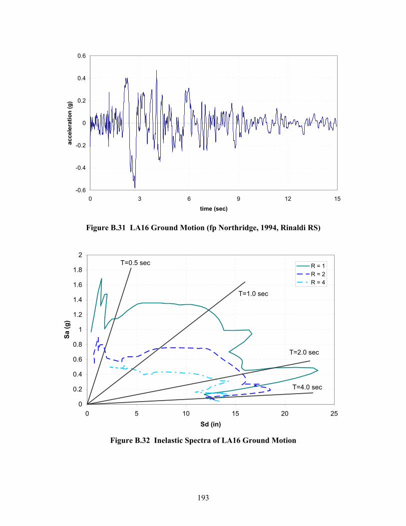
193
-0.6
-0.4
-0.2
0
0.2
0.4
0.6
0 3 6 9 12 15
time (sec)
acce
lera
tion
(g)
Figure B.31 LA16 Ground Motion (fp Northridge, 1994, Rinaldi RS)
0
0.2
0.4
0.6
0.8
1
1.2
1.4
1.6
1.8
2
0 5 10 15 20 25Sd (in)
Sa (g
)
R = 1R = 2R = 4
T=0.5 sec
T=1.0 sec
T=2.0 sec
T=4.0 sec
Figure B.32 Inelastic Spectra of LA16 Ground Motion
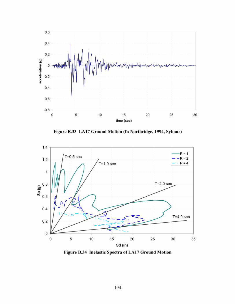
194
-0.8
-0.6
-0.4
-0.2
0
0.2
0.4
0.6
0 5 10 15 20 25 30
time (sec)
acce
lera
tion
(g)
Figure B.33 LA17 Ground Motion (fn Northridge, 1994, Sylmar)
0
0.2
0.4
0.6
0.8
1
1.2
1.4
0 5 10 15 20 25 30 35Sd (in)
Sa (g
)
R = 1R = 2R = 4
T=0.5 sec
T=1.0 sec
T=2.0 sec
T=4.0 sec
Figure B.34 Inelastic Spectra of LA17 Ground Motion
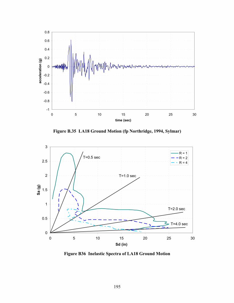
195
-1
-0.8
-0.6
-0.4
-0.2
0
0.2
0.4
0.6
0.8
0 5 10 15 20 25 30
time (sec)
acce
lera
tion
(g)
Figure B.35 LA18 Ground Motion (fp Northridge, 1994, Sylmar)
0
0.5
1
1.5
2
2.5
3
0 5 10 15 20 25 30Sd (in)
Sa (g
)
R = 1R = 2R = 4
T=0.5 sec
T=1.0 sec
T=2.0 sec
T=4.0 sec
Figure B36 Inelastic Spectra of LA18 Ground Motion
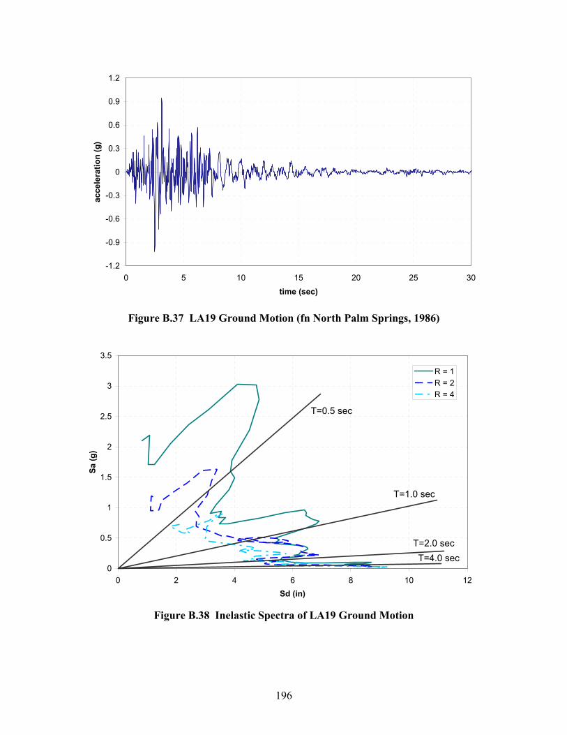
196
-1.2
-0.9
-0.6
-0.3
0
0.3
0.6
0.9
1.2
0 5 10 15 20 25 30
time (sec)
acce
lera
tion
(g)
Figure B.37 LA19 Ground Motion (fn North Palm Springs, 1986)
0
0.5
1
1.5
2
2.5
3
3.5
0 2 4 6 8 10 12Sd (in)
Sa (g
)
R = 1R = 2R = 4
T=0.5 sec
T=1.0 sec
T=2.0 secT=4.0 sec
Figure B.38 Inelastic Spectra of LA19 Ground Motion

197
-1.2
-0.9
-0.6
-0.3
0
0.3
0.6
0.9
1.2
0 5 10 15 20 25 30
time (sec)
acce
lera
tion
(g)
Figure B.39 LA20 Ground Motion (fp North Palm Springs, 1986)
0
0.5
1
1.5
2
2.5
3
3.5
4
0 5 10 15 20 25Sd (in)
Sa (g
)
R = 1R = 2R = 4T=0.5 sec
T=1.0 sec
T=2.0 sec
T=4.0 sec
Figure B.40 Inelastic Spectra of LA20 Ground Motion

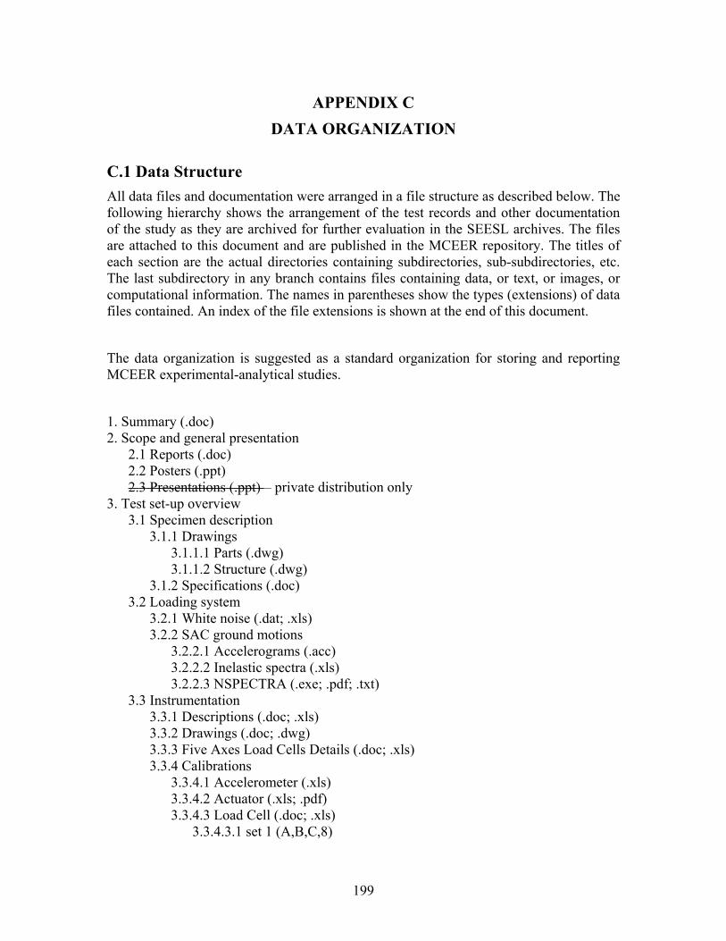
199
APPENDIX C DATA ORGANIZATION
C.1 Data Structure All data files and documentation were arranged in a file structure as described below. The following hierarchy shows the arrangement of the test records and other documentation of the study as they are archived for further evaluation in the SEESL archives. The files are attached to this document and are published in the MCEER repository. The titles of each section are the actual directories containing subdirectories, sub-subdirectories, etc. The last subdirectory in any branch contains files containing data, or text, or images, or computational information. The names in parentheses show the types (extensions) of data files contained. An index of the file extensions is shown at the end of this document.
The data organization is suggested as a standard organization for storing and reporting MCEER experimental-analytical studies.
1. Summary (.doc) 2. Scope and general presentation
2.1 Reports (.doc) 2.2 Posters (.ppt) 2.3 Presentations (.ppt) – private distribution only
3. Test set-up overview 3.1 Specimen description
3.1.1 Drawings 3.1.1.1 Parts (.dwg) 3.1.1.2 Structure (.dwg)
3.1.2 Specifications (.doc) 3.2 Loading system
3.2.1 White noise (.dat; .xls) 3.2.2 SAC ground motions
3.2.2.1 Accelerograms (.acc) 3.2.2.2 Inelastic spectra (.xls) 3.2.2.3 NSPECTRA (.exe; .pdf; .txt)
3.3 Instrumentation 3.3.1 Descriptions (.doc; .xls) 3.3.2 Drawings (.doc; .dwg) 3.3.3 Five Axes Load Cells Details (.doc; .xls) 3.3.4 Calibrations
3.3.4.1 Accelerometer (.xls) 3.3.4.2 Actuator (.xls; .pdf) 3.3.4.3 Load Cell (.doc; .xls)
3.3.4.3.1 set 1 (A,B,C,8)
200
3.3.4.3.1.1 forces (.xls) 3.3.4.3.1.2 crosstalk (.xls)
3.3.4.3.2 set 2 (3,11,12,7) 3.3.4.3.2.1 forces (.xls) 3.3.4.3.2.2 crosstalk (.xls)
3.3.4.3.3 set 3 (9,4,1,3) 3.3.4.3.3.1 forces (.xls) 3.3.4.3.3.2 crosstalk (.xls)
3.3.4.3.4 set 4 (2,14,7,11) 3.3.4.3.4.1 forces (.xls) 3.3.4.3.4.2 crosstalk (.xls)
3.3.4.3.5 set 5 (4,5,9,6) 3.3.4.3.5.1 forces (.xls) 3.3.4.3.5.2 crosstalk (.xls)
3.3.4.3.6 set 6 (12,10,13,2or14) 3.3.4.3.6.1 forces (.xls) 3.3.4.3.6.2 crosstalk (.xls)
3.3.4.3.7 set 7 (2,14,7,11) 3.3.4.3.7.1 forces (.xls) 3.3.4.3.7.2 crosstalk (.xls)
3.3.4.3.8 set 8 (2,14) 3.3.4.3.8.1 forces (.xls) 3.3.4.3.8.2 crosstalk (.xls)
3.3.4.3.9 pictures (.jpg) 3.3.4.4 Potentiometer (.xls) 3.3.4.5 Temposonic (.doc; .xls)
4. Test procedures 4.1 Material/coupon tests
4.1.1 Test schedule (.doc; .xls) 4.1.2 Test implementation (.jpg)
4.2 Component tests 4.2.1 Cruciform (beam-column connection)
4.2.1.1 Test schedule (.doc; .xls) 4.2.1.2 Test implementation (.jpg)
4.2.2 Gravity column 4.2.2.1 Test schedule (.doc; .xls) 4.2.2.2 Test implementation (.jpg)
4.3 Model structure 4.3.1 Test schedule (.doc; .xls) 4.3.2 Test implementation (.jpg; .avi)
5. Test Results 5.1 Material/coupon tests
5.1.1 Beam (.xls) 5.1.2 Column (.xls)
5.2 Component tests 5.2.1 Cruciform (beam-column connection)
201
5.2.1.1 Data (.00x; .dat) 5.2.1.2 DADiSP Labbook
5.2.1.2.1 tests(.pi) 5.2.1.3 Calculation sheet (.xls)
5.2.2 Gravity column 5.2.2.1 Data (.00x) 5.2.2.2 DADiSP Labbook
5.2.2.2.1 gctestA(.pi) 5.2.2.2.2 gctestB(.pi)
5.2.2.3 Calculation sheet (.xls) 5.3 Model structure
5.3.1 Raising shake table and checking instruments (.00x) 5.3.2 Weight of structures (.00x) 5.3.3 Preliminary identification (white noise) (.00x) 5.3.4 Seismic test (.00x)
6. Data processing – Model Structure 6.1 DADISP command files (.dsp) 6.2 Test series
6.2.1 Raising shake table and checking instruments (DADiSP labbook) 6.2.1.1 draise (.pi) 6.2.1.2 lift3 (.pi) 6.2.1.3 lift4 (.pi) 6.2.1.4 load (.pi)
6.2.2 Weight of structures (.xls) 6.2.3 Preliminary identification (white noise)
6.2.3.1 DADiSP labbook 6.2.3.1.1 noise3 (.pi) 6.2.3.1.2 noise4 (.pi) 6.2.3.1.3 noise5 (.pi) 6.2.3.1.4 noise6 (.pi) 6.2.3.1.5 noise7 (.pi) 6.2.3.1.6 noise8 (.pi) 6.2.3.1.7 noise9 (.pi)
6.2.3.2 Model identification (.xls) 6.2.4 Seismic test
6.2.4.1 DADiSP labbook 6.2.4.1.1 LA16O40 (.pi) 6.2.4.1.2 LA160O5 (.pi) 6.2.4.1.3 LA1601O (.pi) 6.2.4.1.4 LA16005 (.pi) 6.2.4.1.5 LA16015 (.pi) 6.2.4.1.6 LA16020 (.pi) 6.2.4.1.7 LA16025 (.pi) 6.2.4.1.8 LA16030 (.pi) 6.2.4.1.9 LA16035 (.pi) 6.2.4.1.10 LA16040 (.pi)

202
6.2.4.1.11 LA16040A (.pi) 6.2.4.1.12 WN0051 (.pi) 6.2.4.1.13 WN0052 (.pi) 6.2.4.1.14 WN0102 (.pi) 6.2.4.1.15 WN0152 (.pi) 6.2.4.1.16 WN0201 (.pi) 6.2.4.1.17 WN0202 (.pi) 6.2.4.1.18 WN0252 (.pi) 6.2.4.1.19 WN0302 (.pi) 6.2.4.1.20 WN0352 (.pi) 6.2.4.1.21 WN0401 (.pi) 6.2.4.1.22 WN0401A (.pi) 6.2.4.1.23 WN0402 (.pi)
6.2.4.2 Model identification (.xls) 7. Analytical predictions
7.1 Idarc2d 5.5 7.2 Idarc-Calculations
7.2.1 Model D1 (Rigid –Estimated Properties) 7.2.1.1 SAC Ground motion (.xls)
7.2.1.1.1 la01 (.dat; .out; .prn; .exe) 7.2.1.1.2 la02 (.dat; .out; .prn; .exe) 7.2.1.1.3 la03 (.dat; .out; .prn; .exe) 7.2.1.1.4 la04 (.dat; .out; .prn; .exe) 7.2.1.1.5 la05 (.dat; .out; .prn; .exe) 7.2.1.1.6 la06 (.dat; .out; .prn; .exe) 7.2.1.1.7 la07 (.dat; .out; .prn; .exe) 7.2.1.1.8 la08 (.dat; .out; .prn; .exe) 7.2.1.1.9 la09 (.dat; .out; .prn; .exe) 7.2.1.1.10 la10 (.dat; .out; .prn; .exe) 7.2.1.1.11 la11 (.dat; .out; .prn; .exe) 7.2.1.1.12 la12 (.dat; .out; .prn; .exe) 7.2.1.1.13 la13 (.dat; .out; .prn; .exe) 7.2.1.1.14 la14 (.dat; .out; .prn; .exe) 7.2.1.1.15 la15 (.dat; .out; .prn; .exe) 7.2.1.1.16 la16 (.dat; .out; .prn; .exe) 7.2.1.1.17 la17 (.dat; .out; .prn; .exe) 7.2.1.1.18 la18 (.dat; .out; .prn; .exe) 7.2.1.1.19 la19 (.dat; .out; .prn; .exe) 7.2.1.1.20 la20 (.dat; .out; .prn; .exe)
7.2.1.2 DPA-LA16 (.xls) 7.2.1.2.1 la16-5%g (.dat; .out; .prn; .exe) 7.2.1.2.2 la16-10%g (.dat; .out; .prn; .exe) 7.2.1.2.3 la16-15%g (.dat; .out; .prn; .exe) 7.2.1.2.4 la16-20%g (.dat; .out; .prn; .exe) 7.2.1.2.5 la16-25%g (.dat; .out; .prn; .exe) 7.2.1.2.6 la16-30%g (.dat; .out; .prn; .exe)
203
7.2.1.2.7 la16-35%g (.dat; .out; .prn; .exe) 7.2.1.2.8 la16-40%g (.dat; .out; .prn; .exe) 7.2.1.2.9 la16-45%g (.dat; .out; .prn; .exe) 7.2.1.2.10 la16-50%g (.dat; .out; .prn; .exe) 7.2.1.2.11 la16-55%g (.dat; .out; .prn; .exe) 7.2.1.2.12 la16-60%g (.dat; .out; .prn; .exe) 7.2.1.2.13 la16-65%g (.dat; .out; .prn; .exe) 7.2.1.2.14 la16-70%g (.dat; .out; .prn; .exe) 7.2.1.2.15 la16-75%g (.dat; .out; .prn; .exe) 7.2.1.2.16 la16-80%g (.dat; .out; .prn; .exe) 7.2.1.2.17 la16-85%g (.dat; .out; .prn; .exe) 7.2.1.2.18 la16-90%g (.dat; .out; .prn; .exe)
7.2.1.3 Pushover (.xls) 7.2.1.3.1 option1(invt triangle) (.dat; .out; .prn; .exe) 7.2.1.3.2 option3(modal) – 1 mode (.dat; .out; .prn; .exe) 7.2.1.3.3 option3(modal) – 3 mode (.dat; .out; .prn; .exe) 7.2.1.3.4 option5(distr) (.dat; .out;, .prn; .exe)
7.2.2 Model D2 (Rigid – Actual Properties) 7.2.2.1 DPA-LA16 (.xls)
7.2.2.1.1 la16-5%g (.dat; .out; .prn; .exe) 7.2.2.1.2 la16-10%g (.dat; .out; .prn; .exe) 7.2.2.1.3 la16-15%g (.dat; .out; .prn; .exe) 7.2.2.1.4 la16-20%g (.dat; .out; .prn; .exe) 7.2.2.1.5 la16-25%g (.dat; .out; .prn; .exe) 7.2.2.1.6 la16-30%g (.dat; .out; .prn; .exe) 7.2.2.1.7 la16-35%g (.dat; .out; .prn; .exe) 7.2.2.1.8 la16-40%g (.dat; .out; .prn; .exe) 7.2.2.1.9 la16-45%g (.dat; .out; .prn; .exe) 7.2.2.1.10 la16-50%g (.dat; .out; .prn; .exe) 7.2.2.1.11 la16-55%g (.dat; .out; .prn; .exe) 7.2.2.1.12 la16-60%g (.dat; .out; .prn; .exe) 7.2.2.1.13 la16-65%g (.dat; .out; .prn; .exe) 7.2.2.1.14 la16-70%g (.dat; .out; .prn; .exe)
7.2.2.2 Pushover (.xls) 7.2.2.2.1 option1(invt triangle) (.dat; .out; .prn; .exe)
7.2.3 Model D3 (Semi Rigid –Estimated Properties) 7.2.3.1 Spring (xls)
7.2.3.1.1 Idarc-cruciform (.dat; .out; .prn; .exe) 7.2.3.2 DPA-LA16 (.xls)
7.2.3.2.1 la16-5%g (.dat; .out; .prn; .exe) 7.2.3.2.2 la16-10%g (.dat; .out; .prn; .exe) 7.2.3.2.3 la16-15%g (.dat; .out; .prn; .exe) 7.2.3.2.4 la16-20%g (.dat; .out; .prn; .exe) 7.2.3.2.5 la16-25%g (.dat; .out; .prn; .exe) 7.2.3.2.6 la16-30%g (.dat; .out; .prn; .exe) 7.2.3.2.7 la16-35%g (.dat; .out; .prn; .exe)
204
7.2.3.2.8 la16-40%g (.dat; .out; .prn; .exe) 7.2.3.2.9 la16-45%g (.dat; .out; .prn; .exe) 7.2.3.2.10 la16-50%g (.dat; .out; .prn; .exe) 7.2.3.2.11 la16-55%g (.dat; .out; .prn; .exe) 7.2.3.2.12 la16-60%g (.dat; .out; .prn; .exe) 7.2.3.2.13 la16-65%g (.dat; .out; .prn; .exe) 7.2.3.2.14 la16-70%g (.dat; .out; .prn; .exe)
7.2.3.3 Pushover (.xls) 7.2.3.3.1 option1(invt triangle) (.dat; .out; .prn; .exe)
7.2.4 Model D4 (Semi Rigid – Actual Properties) 7.2.4.1 DPA-LA16 (.xls)
7.2.4.1.1 la16-5%g (.dat; .out; .prn; .exe) 7.2.4.1.2 la16-10%g (.dat; .out; .prn; .exe) 7.2.4.1.3 la16-15%g (.dat; .out; .prn; .exe) 7.2.4.1.4 la16-20%g (.dat; .out; .prn; .exe) 7.2.4.1.5 la16-25%g (.dat; .out; .prn; .exe) 7.2.4.1.6 la16-30%g (.dat; .out; .prn; .exe) 7.2.4.1.7 la16-35%g (.dat; .out; .prn; .exe) 7.2.4.1.8 la16-40%g (.dat; .out; .prn; .exe) 7.2.4.1.9 la16-45%g (.dat; .out; .prn; .exe) 7.2.4.1.10 la16-50%g (.dat; .out; .prn; .exe) 7.2.4.1.11 la16-55%g (.dat; .out; .prn; .exe) 7.2.4.1.12 la16-60%g (.dat; .out; .prn; .exe) 7.2.4.1.13 la16-65%g (.dat; .out; .prn; .exe) 7.2.4.1.14 la16-70%g (.dat; .out; .prn; .exe)
7.2.4.2 Pushover (.xls) 7.2.4.2.1 option1(invt triangle) (.dat; .out; .prn; .exe)
8. Discussion and recommendations (.doc)
C.2 Types of Files and Programs A vast array of computer codes/programs and different types of files were used in this study. The following list presents various file extensions and specific computer codes that were used to operate/manage the files. Note that while most files created using Windows/Microsoft applications (e.g. MS Word, MS Excel) can be opened with later versions of those application, other files created using specific computer codes (e.g. DADisP) require certain versions to fully operate them.

205
Table C.1 Types of Files and Computer Codes/Program
File extension Types of File Computer Code/Program
.00x Text/data ASCII – Notepad, DADiSP 4.1 (data)
.acc Text/data ASCII - Notepad
.avi Video Windows Media Player
.dat Text/data ASCII - Notepad
.doc Word Microsoft Word
.dsp Command file DADiSP 4.1
.dwg Drawing AutoCAD R14
.exe Program (Executable file)
.jpg Picture Windows Picture
.out Text/data ASCII - Notepad
.pdf PDF Acrobat Reader
.pi Labbook window DADiSP 4.1 (labbook)
.ppt PowerPoint Microsoft PowerPoint
.prn Text/data ASCII - Notepad
.txt Text/data ASCII - Notepad
.xls Excel Microsoft Excel

207
APPENDIX D SAMPLE DATA RECORDS
D1. Text File (.00x; .acc; .dat; .out; .prn; .txt) The following text is a typical IDARC input file (.dat) used in the analytical study. Model - unequal towers Control Data 4 1 0 0 0 0 0 1 Element Types 3 2 0 0 0 0 0 0 0 0 Element Data 10 6 0 0 0 0 0 0 0 Units - in kips 1 Floor Elevations 52.744 99.988 99.988 147.232 Description of Identical Frames 2 Plan Configuration 4 Nodal Weights 1 1 2.115 2.961 2.961 2.115 2 1 0.00 0.00 2.538 2.538 3 1 2.538 2.538 0.00 0.00 4 1 2.538 2.538 0.00 0.00 Material Property Sets 1 Hysteretic Modeling Rules 1 1 2 200.0 0.001 0.001 10 0.5 0.0 1000 0.0 5 1000 1 Column Properties User Input 1 Column Data 1 52.744 0.0 3.375 -1 73080 48430 18626.9 84.00 92.625 1.28e-3 1.28e-1 3 84.00 92.625 1.28e-3 1.28e-1 3 2 47.244 3.375 3.375 -1 73080 48430 18626.9 84.00 92.625 1.28e-3 1.28e-1 3 84.00 92.625 1.28e-3 1.28e-1 3 3 47.244 3.375 3.375 -1 73080 48430 18626.9 84.00 92.625 1.28e-3 1.28e-1 3 84.00 92.625 1.28e-3 1.28e-1 3 Beam Properties 1 Beam Section Data 1 59.055 1.75 1.75 -1 73080 18626.9 60.48 66.69 9.2e-4 9.2e-2 3 60.48 66.69 9.2e-4 9.2e-2 3 2 78.740 1.75 1.75 -1 73080 18626.9 60.48 66.69 9.2e-4 9.2e-2 3 60.48 66.69 9.2e-4 9.2e-2 3
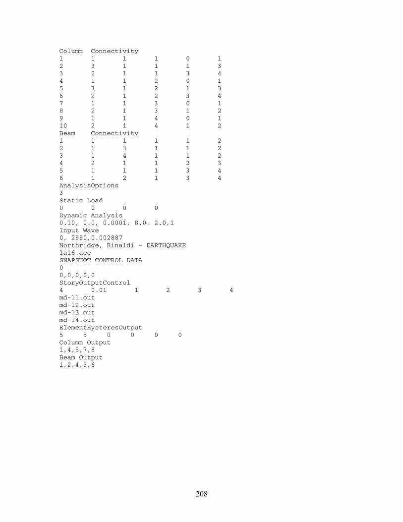
208
Column Connectivity 1 1 1 1 0 1 2 3 1 1 1 3 3 2 1 1 3 4 4 1 1 2 0 1 5 3 1 2 1 3 6 2 1 2 3 4 7 1 1 3 0 1 8 2 1 3 1 2 9 1 1 4 0 1 10 2 1 4 1 2 Beam Connectivity 1 1 1 1 1 2 2 1 3 1 1 2 3 1 4 1 1 2 4 2 1 1 2 3 5 1 1 1 3 4 6 1 2 1 3 4 AnalysisOptions 3 Static Load 0 0 0 0 Dynamic Analysis 0.10, 0.0, 0.0001, 8.0, 2.0,1 Input Wave 0, 2990,0.002887 Northridge, Rinaldi - EARTHQUAKE la16.acc SNAPSHOT CONTROL DATA 0 0,0,0,0,0 StoryOutputControl 4 0.01 1 2 3 4 md-l1.out md-l2.out md-l3.out md-l4.out ElementHysteresOutput 5 5 0 0 0 0 Column Output 1,4,5,7,8 Beam Output 1,2,4,5,6

209
D2. DADiSP Command File (.dsp) The following text is an example of DADiSP command file used to verify the instrumentations and to calculate shear forces.
!================ DADiSP program to check Shear Forces ! ! Adjust the number of windows to the total number of windows needed for calculation ! gotowin(w1) @cr DISPLAYALL @CR IF((NUMWIN>8), REMOVEWIN(NUMWIN-8), ADDWINDOW(8-NUMWIN)) @CR clearall @cr addwindow(24) @cr setprecision(2) @cr moveto(w1) @cr ! ! Loading data series into the worksheet ! ! 1. Loading horizontal accelerations ! loadseries (w1..w4,strcat(getvariable('data'),'.AH1'),strcat(getvariable('data'),'.AH2'),strcat(getvariable('data'),'.AH3'),strcat(getvariable('data'),'.AH4'),1) @CR loadseries (w5..w8,strcat(getvariable('data'),'.AH5'),strcat(getvariable('data'),'.AH6'),strcat(getvariable('data'),'.AH7'),strcat(getvariable('data'),'.AH8'),1) @CR moveto(w9) @cr ! ! 2. Loading Shear Forces from External Frames ! loadseries (w9..w12,strcat(getvariable('data'),'.SX2'),strcat(getvariable('data'),'.SX7'),strcat(getvariable('data'),'.SX8'),strcat(getvariable('data'),'.SX10'),1) @CR loadseries (w13..w16,strcat(getvariable('data'),'.SX11'),strcat(getvariable('data'),'.SX12'),strcat(getvariable('data'),'.SX13'),strcat(getvariable('data'),'.SX14'),1) @CR moveto(w17) @cr ! ! 3. Loading Shear Forces from Internal Frames ! loadseries (w17..w20,strcat(getvariable('data'),'.SX1'),strcat(getvariable('data'),'.SX3'),strcat(getvariable('data'),'.SX4'),strcat(getvariable('data'),'.SX5'),1) @CR loadseries (w21..w24,strcat(getvariable('data'),'.SX6'),strcat(getvariable('data'),'.SX9'),strcat(getvariable('data'),'.SX15'),strcat(getvariable('data'),'.SX16'),1) @CR moveto(w25) @cr

210
! ! Calculating Shear Forces ! 10.152*(w1+w2)+(10.152/2)*(w3+w5)+(10.152/2)*(w4+w6)+(10.152/2)*(w7+w8);Title(BLACK,"Base Shear(Accelerometers)");setvunits("Kips") @cr moveto(w26) @cr W9+W10+W11+W12+W13+W14+W15+W16;Title(BLACK,"Base Shear(External Frames)");setvunits("Kips") @cr moveto(w27) @cr W17+W18-W19-W20+W21+W22+W23-W24;Title(BLACK,"Base Shear(Internal Frames)");setvunits("Kips") @cr moveto(w28) @cr w26+w27;Title(BLACK,"Base Shear(Load Cells)");setvunits("Kips") @cr moveto(w29) @cr w25/w28 @cr moveto(w30) @cr w28*1.3;Title(BLACK,"Base Shear (Corrected, SF = 1.3)");setvunits("Kips") @cr overplot(w25,red) @cr moveto(w31) @cr w30/50.76*100;Title(BLACK,"Base Shear/Weight (Corrected, SF = 1.3)");setvunits("BS/W %") @cr moveto(w32) @cr (w30-w25)/50.76*100;Title(BLACK,"Horizontal Force Error");setvunits("Errs/Wght(%)") @cr sety(-1,1) @cr ! ! Zooms Shear window ! @cr zoom(w32) @cr
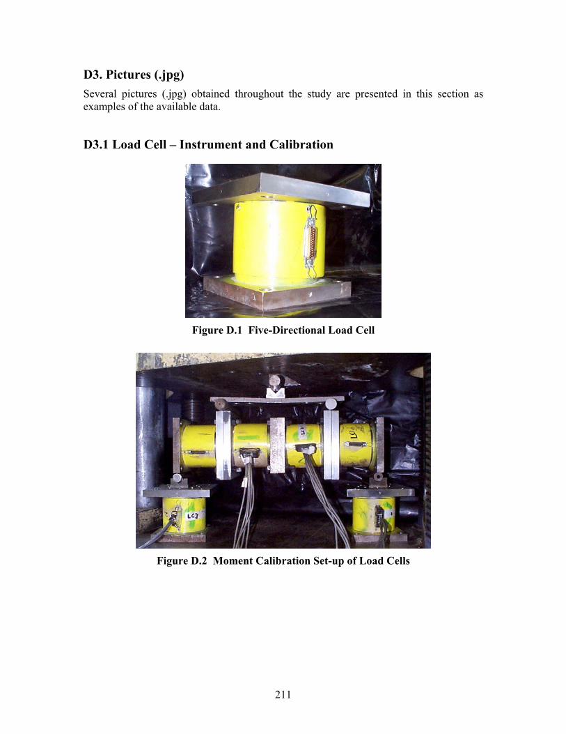
211
D3. Pictures (.jpg) Several pictures (.jpg) obtained throughout the study are presented in this section as examples of the available data.
D3.1 Load Cell – Instrument and Calibration
Figure D.1 Five-Directional Load Cell
Figure D.2 Moment Calibration Set-up of Load Cells
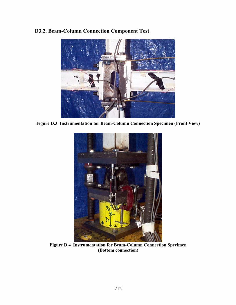
212
D3.2. Beam-Column Connection Component Test
Figure D.3 Instrumentation for Beam-Column Connection Specimen (Front View)
Figure D.4 Instrumentation for Beam-Column Connection Specimen
(Bottom connection)

213
D3.3. Gravity Column Component Test
Figure D.5 Instrumentation for Gravity Column Specimen (Bottom connection)
D3.4. Model Structure D3.4.1 Phase of Construction
Figure D.6 Construction of the Second Floor

214
Figure D.7 Final Stage of Construction
D3.4.2 Details of Structural Elements
(a) (b)
Figure D.8 Beam Column Connections: (a) Exterior and (b) Interior
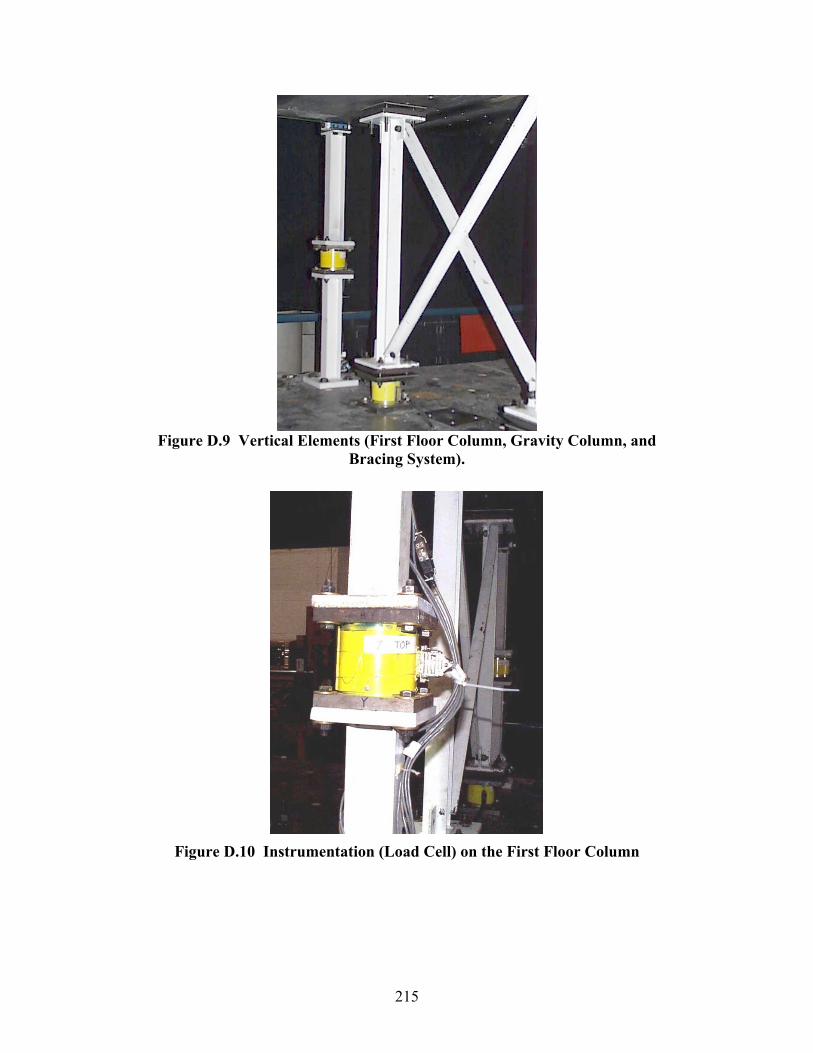
215
Figure D.9 Vertical Elements (First Floor Column, Gravity Column, and
Bracing System).
Figure D.10 Instrumentation (Load Cell) on the First Floor Column
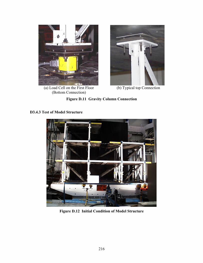
216
(a) Load Cell on the First Floor
(Bottom Connection) (b) Typical top Connection
Figure D.11 Gravity Column Connection
D3.4.3 Test of Model Structure
Figure D.12 Initial Condition of Model Structure
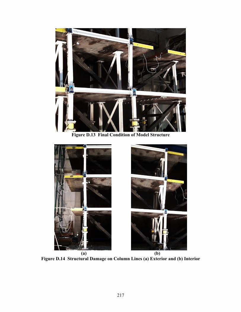
217
Figure D.13 Final Condition of Model Structure
(a) (b)
Figure D.14 Structural Damage on Column Lines (a) Exterior and (b) Interior
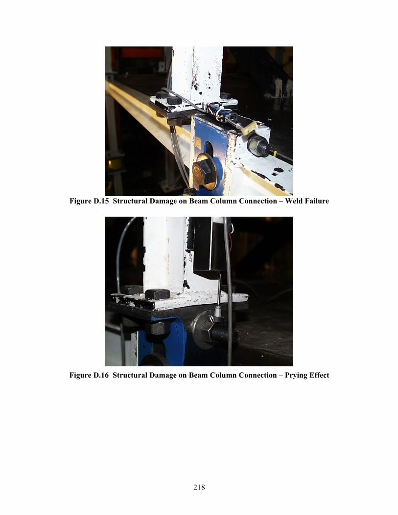
218
Figure D.15 Structural Damage on Beam Column Connection – Weld Failure
Figure D.16 Structural Damage on Beam Column Connection – Prying Effect
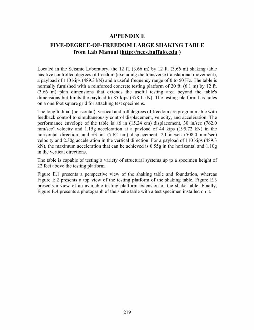
219
APPENDIX E FIVE-DEGREE-OF-FREEDOM LARGE SHAKING TABLE
from Lab Manual (http://nees.buffalo.edu )
Located in the Seismic Laboratory, the 12 ft. (3.66 m) by 12 ft. (3.66 m) shaking table has five controlled degrees of freedom (excluding the transverse translational movement), a payload of 110 kips (489.3 kN) and a useful frequency range of 0 to 50 Hz. The table is normally furnished with a reinforced concrete testing platform of 20 ft. (6.1 m) by 12 ft. (3.66 m) plan dimensions that extends the useful testing area beyond the table's dimensions but limits the payload to 85 kips (378.1 kN). The testing platform has holes on a one foot square grid for attaching test specimens.
The longitudinal (horizontal), vertical and roll degrees of freedom are programmable with feedback control to simultaneously control displacement, velocity, and acceleration. The performance envelope of the table is ±6 in (15.24 cm) displacement, 30 in/sec (762.0 mm/sec) velocity and 1.15g acceleration at a payload of 44 kips (195.72 kN) in the horizontal direction, and ±3 in. (7.62 cm) displacement, 20 in./sec (508.0 mm/sec) velocity and 2.30g acceleration in the vertical direction. For a payload of 110 kips (489.3 kN), the maximum acceleration that can be achieved is 0.55g in the horizontal and 1.10g in the vertical directions.
The table is capable of testing a variety of structural systems up to a specimen height of 22 feet above the testing platform.
Figure E.1 presents a perspective view of the shaking table and foundation, whereas Figure E.2 presents a top view of the testing platform of the shaking table. Figure E.3 presents a view of an available testing platform extension of the shake table. Finally, Figure E.4 presents a photograph of the shake table with a test specimen installed on it.
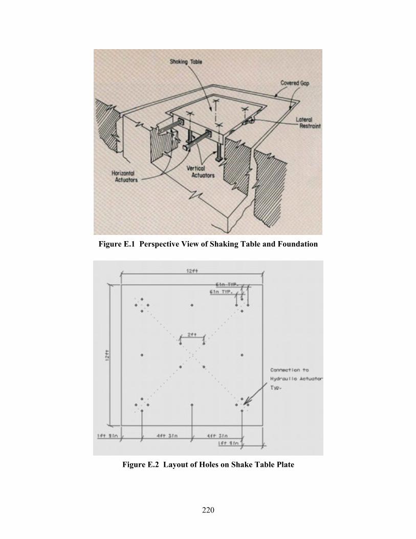
220
Figure E.1 Perspective View of Shaking Table and Foundation
Figure E.2 Layout of Holes on Shake Table Plate
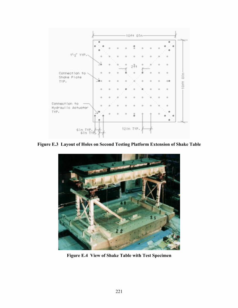
221
Figure E.3 Layout of Holes on Second Testing Platform Extension of Shake Table
Figure E.4 View of Shake Table with Test Specimen

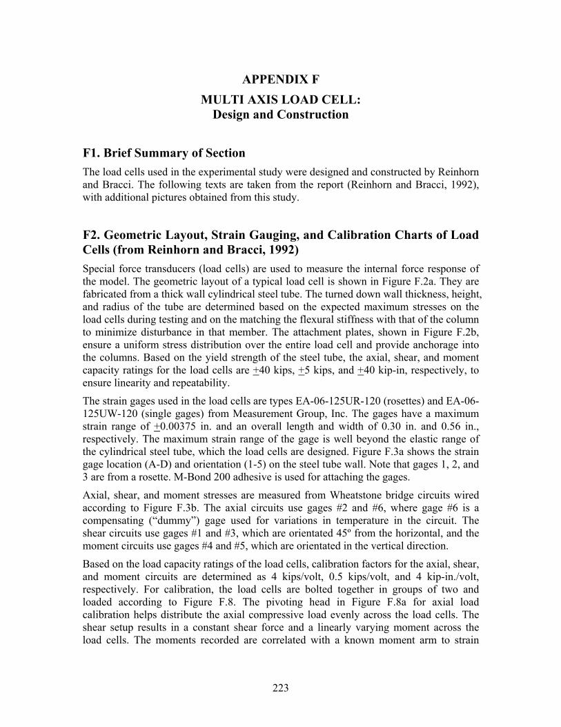
223
APPENDIX F MULTI AXIS LOAD CELL:
Design and Construction
F1. Brief Summary of Section The load cells used in the experimental study were designed and constructed by Reinhorn and Bracci. The following texts are taken from the report (Reinhorn and Bracci, 1992), with additional pictures obtained from this study.
F2. Geometric Layout, Strain Gauging, and Calibration Charts of Load Cells (from Reinhorn and Bracci, 1992) Special force transducers (load cells) are used to measure the internal force response of the model. The geometric layout of a typical load cell is shown in Figure F.2a. They are fabricated from a thick wall cylindrical steel tube. The turned down wall thickness, height, and radius of the tube are determined based on the expected maximum stresses on the load cells during testing and on the matching the flexural stiffness with that of the column to minimize disturbance in that member. The attachment plates, shown in Figure F.2b, ensure a uniform stress distribution over the entire load cell and provide anchorage into the columns. Based on the yield strength of the steel tube, the axial, shear, and moment capacity ratings for the load cells are +40 kips, +5 kips, and +40 kip-in, respectively, to ensure linearity and repeatability.
The strain gages used in the load cells are types EA-06-125UR-120 (rosettes) and EA-06-125UW-120 (single gages) from Measurement Group, Inc. The gages have a maximum strain range of +0.00375 in. and an overall length and width of 0.30 in. and 0.56 in., respectively. The maximum strain range of the gage is well beyond the elastic range of the cylindrical steel tube, which the load cells are designed. Figure F.3a shows the strain gage location (A-D) and orientation (1-5) on the steel tube wall. Note that gages 1, 2, and 3 are from a rosette. M-Bond 200 adhesive is used for attaching the gages.
Axial, shear, and moment stresses are measured from Wheatstone bridge circuits wired according to Figure F.3b. The axial circuits use gages #2 and #6, where gage #6 is a compensating (“dummy”) gage used for variations in temperature in the circuit. The shear circuits use gages #1 and #3, which are orientated 45º from the horizontal, and the moment circuits use gages #4 and #5, which are orientated in the vertical direction.
Based on the load capacity ratings of the load cells, calibration factors for the axial, shear, and moment circuits are determined as 4 kips/volt, 0.5 kips/volt, and 4 kip-in./volt, respectively. For calibration, the load cells are bolted together in groups of two and loaded according to Figure F.8. The pivoting head in Figure F.8a for axial load calibration helps distribute the axial compressive load evenly across the load cells. The shear setup results in a constant shear force and a linearly varying moment across the load cells. The moments recorded are correlated with a known moment arm to strain

224
gages for the moment circuits. The moment setup is a two point loading which creates a constant bending moment with no shear force.
The circuits are connected to 2310 Vishay Signal Conditioning Amplifiers from the Measurement Group, Inc. which filters frequencies above 25 Hz, and varies the amplification (gain) of the incoming signal from the Wheatstone bridge circuit. Calibration charts are developed, typically shown for a particular load cell in Figure F.9, based on several series of loading and unloading for each setup and adjustments in amplification from the conditioners to acquire the appropriate calibration factor. Note, that a loop in the unloading states of testing develops in the moment calibrations. However the initial loading is perfectly linear and returns to zero when the load is fully removed, which implies that the load cell behaves elastically. Therefore the loops were created by some errors in the setup, possibly due to some concentrated yielding or friction which develops in the components of the setup.
It is suggested to move the gages 5 and 4 to the mid-line of the load cell and place the rosette off-center. In case of addition of torque circuit, add a second rosette on each face symmetric to the mid-line to the first rosette and wire the shear circuits to add up all signals from all faces.
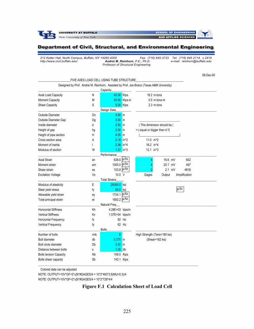
225
08-Dec-00_____________________FIVE AXES LOAD CELL USING TUBE STRUCTURE_______________________________
_________________________________________Capacity_____________ _____________________________________________________Axial Load Capacity N 40.00 Kips 18.2 m-tonsMoment Capacity M 40.00 Kips-in 0.5 m-tons-mShear Capacity S 5.00 Kips 2.3 m-tons_________________________________________Design Data__________ _____________________________________________________Outside Diameter Do 4.50 inOutside Diameter Gap Dg 3.00 in __________________________Inside diameter d 2.50 in | This dimension should be |Height of gap hg 2.00 in <-| equal or bigger than d !!|Height of pipe section H 4.00 in |__________________________|Cross section area A 2.16 in^2 11.0 in^2Moment of inertia I 2.06 in^4 18.2 in^4Modulus of section W 1.37 in^3 12.1 in^3_________________________________________Performance______ _____________________________________________________Axial Strain en 638.6 uSt 4 16.6 mV 602Moment strain em 1005.0 uSt 4 20.1 mV 497Shear strain es 103.8 uSt 2 2.1 mV 4818Excitation Voltage Vo 10.0 V Gages Output Amplification_________________________________________Total Strains_____ _____________________________________________________Modulus of elasticity E 29000.0 ksiSteel yield stress fy 50.0 ksiAllowable yield strain ey 1724.1 uStTotal principal strain et 1650.2 uSt_________________________________________Natural Freq.__ _____________________________________________________Horizontal Stiffness Kh 4.28E+03 kips/inVertical Stiffness Kv 1.57E+04 kips/inHorizontal Frequency fx 92 HzVertical Frequency fy 62 Hz_________________________________________Bolts________________ _____________________________________________________Number of bolts nnb 8 High Strength (Tens=180 ksi)Bolt diameter db 0.375 in (Shear=162 ksi)Bolt circle diameter Db 3.50 inDistance between bolts s 1.00 dbBolts tension Capacity Nb 159.0 KipsBolts shear capacity Sb 143.1 Kips________________________________________________________________________________________________________ Colored data can be adjustedNOTE: OUTPUT=10V*GF=2*uSt*#GAGES/4 = 10*2*463*2.6(MU=0.3)/4NOTE: OUTPUT=10V*GF=2*uSt*#GAGES/4 = 10*2*728*4/4
Designed by Prof. Andrei M. Reinhorn, Assisted by Prof. Joe Bracci (Texas A&M University)
212 Ketter Hall, North Campus, Buffalo, NY 14260-4300 Fax: (716) 645-3733 Tel: (716) 645 2114, x 2419http://www.civil.buffalo.edu/ Andrei M. Reinhorn, P.E., Ph.D. e-mail: [email protected]
Professor of Structural Engineering
µSt
µStµStµSt
µStµSt
Figure F.1 Calculation Sheet of Load Cell
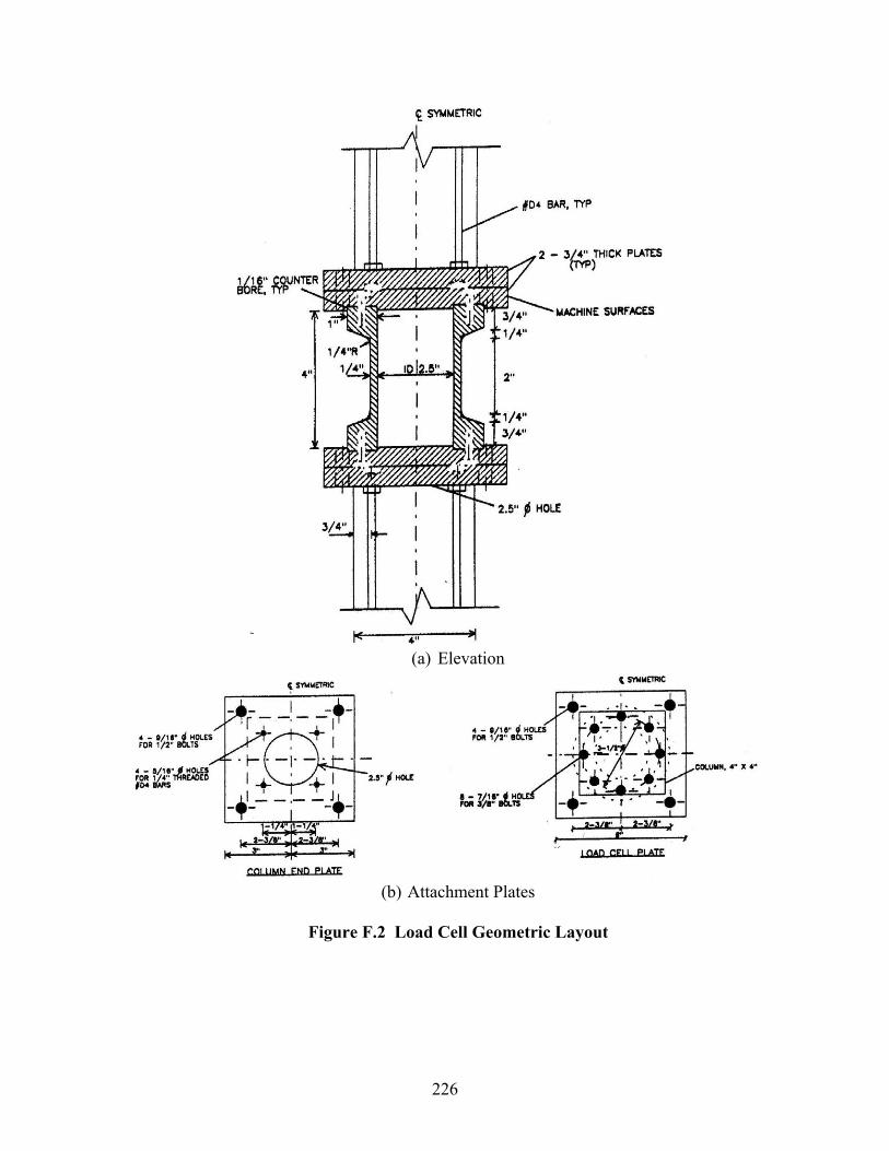
226
(a) Elevation
(b) Attachment Plates
Figure F.2 Load Cell Geometric Layout
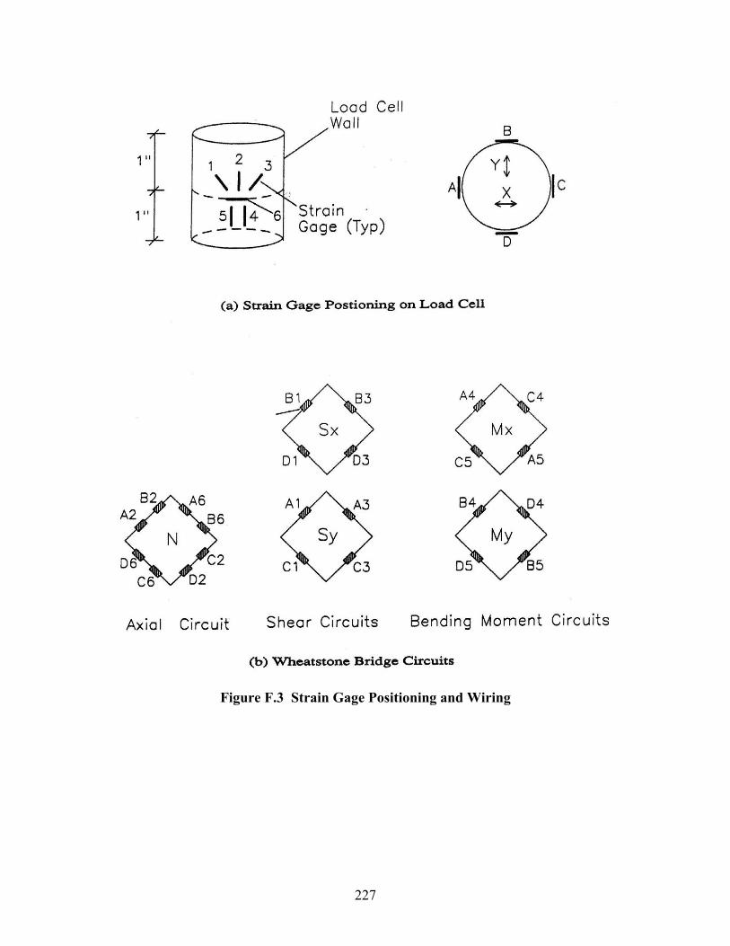
227
Figure F.3 Strain Gage Positioning and Wiring

Fi
gure
F.4
Mai
n C
ircu
its o
f Loa
d C
ells
228
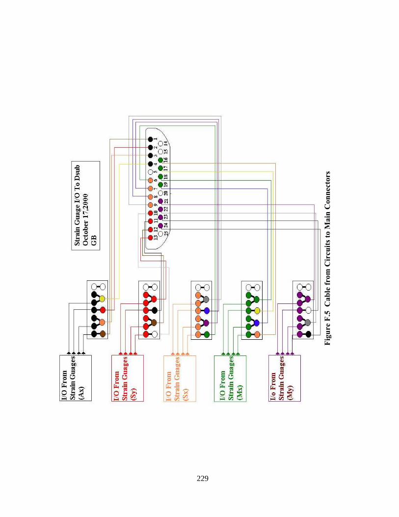
Fi
gure
F.5
Cab
le fr
om C
ircu
its to
Mai
n C
onne
ctor
s
229
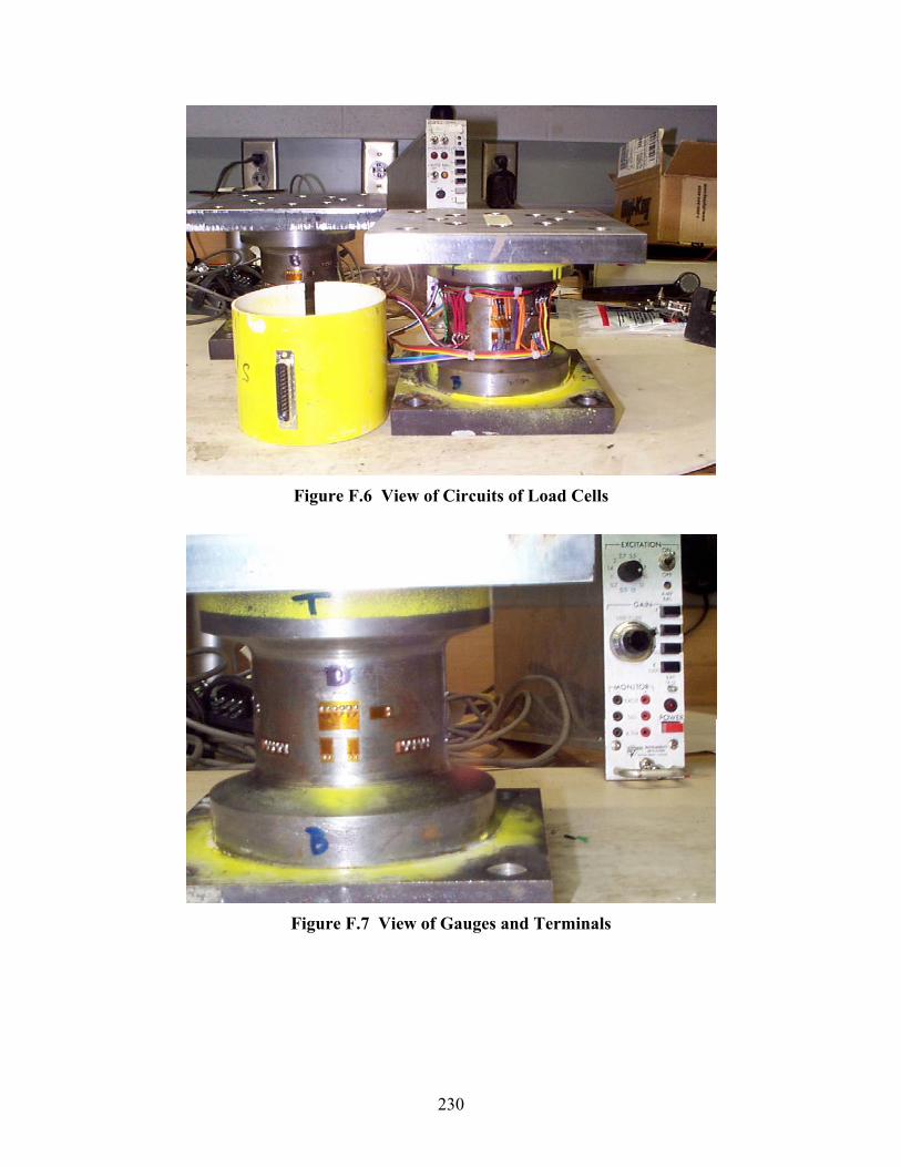
230
Figure F.6 View of Circuits of Load Cells
Figure F.7 View of Gauges and Terminals
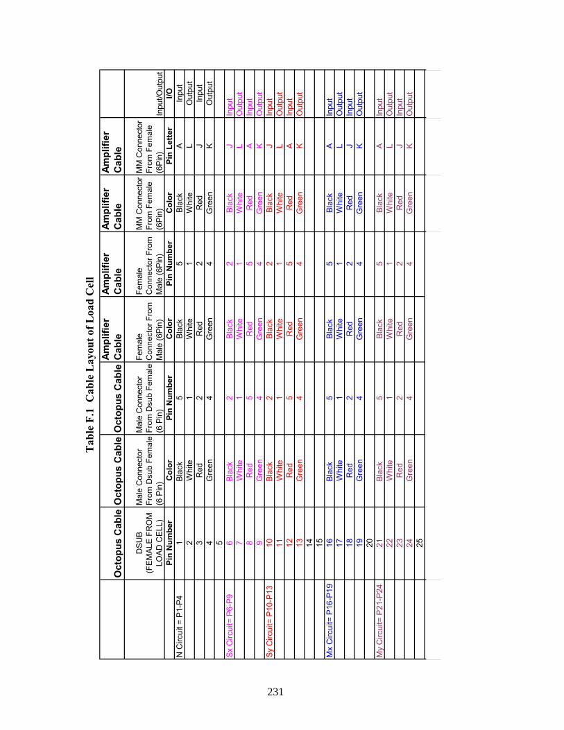
Tab
le F
.1 C
able
Lay
out o
f Loa
d C
ell
Oct
opus
Cab
leO
ctop
us C
able
Oct
opus
Cab
leAm
plifi
er
Ca b
leAm
plifi
er
Cab
leAm
plifi
er
Cab
leAm
plifi
er
Cab
le
DSU
B
(FEM
ALE
FRO
M
LOAD
CE
LL)
Mal
e C
onne
ctor
Fr
om D
sub
Fem
ale
(6 P
in)
Mal
e C
onne
ctor
Fr
om D
sub
Fem
ale
(6 P
in)
Fem
ale
Con
nect
or F
rom
M
ale
(6Pi
n)
Fem
ale
Con
nect
or F
rom
M
ale
(6P
in)
MM
Con
nect
or
From
Fem
ale
(6Pi
n)
MM
Con
nect
or
From
Fem
ale
(6Pi
n)In
put/O
utpu
tPi
n N
umbe
rC
olor
Pin
Num
ber
Col
orPi
n N
umbe
rC
olor
Pin
Lette
rI/O
N C
ircui
t = P
1-P4
1B
lack
5
Bla
ck5
Blac
kA
Inpu
t2
Whi
te1
Whi
te1
Whi
teL
Out
put
3R
ed2
Red
2R
edJ
Inpu
t4
Gre
en4
Gre
en4
Gre
enK
Out
put
5Sx
Circ
uit=
P6-
P96
Bla
ck
2B
lack
2Bl
ack
JIn
put
7W
hite
1W
hite
1W
hite
LO
utpu
t8
Red
5R
ed5
Red
AIn
put
9G
reen
4G
reen
4G
reen
KO
utpu
tSy
Circ
uit=
P10
-P13
10B
lack
2
Bla
ck2
Blac
kJ
Inpu
t11
Whi
te1
Whi
te1
Whi
teL
Out
put
12R
ed5
Red
5R
edA
Inpu
t13
Gre
en4
Gre
en4
Gre
enK
Out
put
14 15M
x C
ircui
t= P
16-P
1916
Bla
ck
5B
lack
5Bl
ack
AIn
put
17W
hite
1W
hite
1W
hite
LO
utpu
t18
Red
2R
ed2
Red
JIn
put
19G
reen
4G
reen
4G
reen
KO
utpu
t20
My
Circ
uit=
P21
-P24
21B
lack
5
Bla
ck5
Blac
kA
Inpu
t22
Whi
te1
Whi
te1
Whi
teL
Out
put
23R
ed2
Red
2R
edJ
Inpu
t24
Gre
en4
Gre
en4
Gre
enK
Out
put
25
231
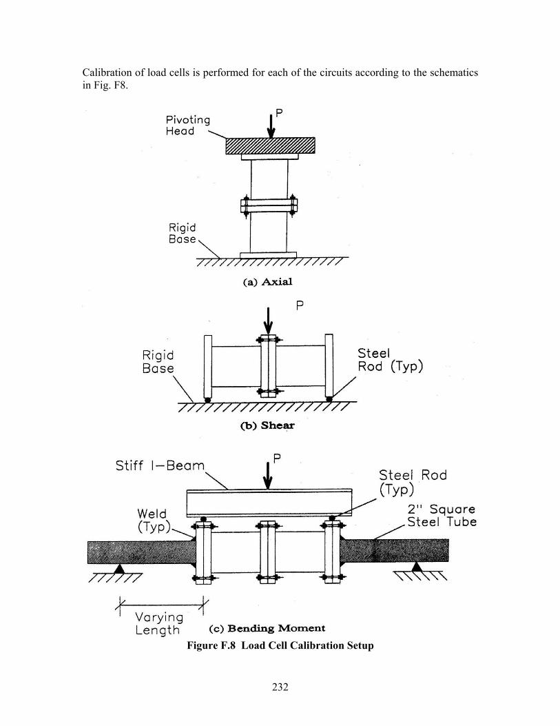
232
Calibration of load cells is performed for each of the circuits according to the schematics in Fig. F8.
Figure F.8 Load Cell Calibration Setup

233
Figure F.9 Actual Load Cell Calibration Setup
An improved calibration set-up is shown in Fig F.9. The set-up is using two axially calibrated load cells as supports and four load cells connected as one beam. The configuration is equivalent with the combined shear and moment calibration schemes shown in Fig F.8 (b) and (c). The two interior load cells (in the center of the beam) are calibrated for moment and the two external (near the supports) are calibrated for shear (and moment) simultaneously. Sample calibration curves (for load cell 8) are shown in Fig F.10. The coupling of measurements shown in the calibration curves is below 1% in most cases except for the moment circuits where the errors are larger. The “error” is a result of the test set-up and should not be corrected in the recordings. (Note that the friction forces in the supports and at location of application of forces are eccentric to the axes of the load cells and introduce both axial loads and moments. See axial coupling N and moment proportionality.). The load cells are sensitive to measure also imperfections in the test set-up. Complete calibration data is found in the repository described in Appendix C.
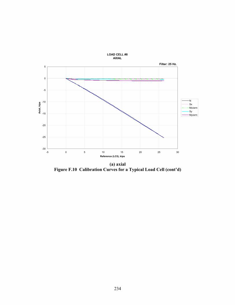
234
LOAD CELL #8AXIAL
-30
-25
-20
-15
-10
-5
0
5
-5 0 5 10 15 20 25 30
Reference (LC5), kips
Axi
al, k
ips N
SxMx/armSyMy/arm
Filter: 25 Hz.
(a) axial
Figure F.10 Calibration Curves for a Typical Load Cell (cont’d)
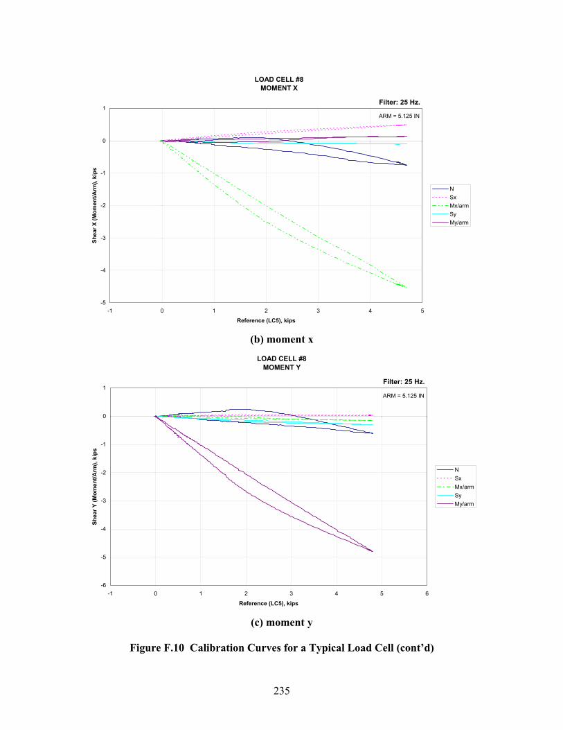
235
LOAD CELL #8MOMENT X
-5
-4
-3
-2
-1
0
1
-1 0 1 2 3 4 5
Reference (LC5), kips
Shea
r X (M
omen
t/Arm
), ki
ps
NSxMx/armSyMy/arm
ARM = 5.125 IN
Filter: 25 Hz.
(b) moment x
LOAD CELL #8MOMENT Y
-6
-5
-4
-3
-2
-1
0
1
-1 0 1 2 3 4 5 6
Reference (LC5), kips
Shea
r Y (M
omen
t/Arm
), ki
ps
NSxMx/armSyMy/arm
ARM = 5.125 IN
Filter: 25 Hz.
(c) moment y
Figure F.10 Calibration Curves for a Typical Load Cell (cont’d)

236
LOAD CELL #8SHEAR X
-6
-5
-4
-3
-2
-1
0
1
2
3
4
5
-1 0 1 2 3 4 5 6
Reference (LC5), kips
Shea
r X, k
ips N
SxMx/armSyMy/arm
ARM = 1.9375 IN
Filter: 25 Hz.
(d) shear x LOAD CELL #8
SHEAR Y
-5
-4
-3
-2
-1
0
1
-1 0 1 2 3 4 5
Reference (LC5), kips
Shea
r Y, k
ips N
SxMx/armSyMy/arm
ARM = 1.9375 IN
Filter: 25 Hz.
(e) shear y
Figure F.10 Calibration Curves for a Typical Load Cell (cont’d)

Formerly the National Center for Earthquake Engineering Research
237
Multidisciplinary Center for Earthquake Engineering Research List of Technical Reports
The Multidisciplinary Center for Earthquake Engineering Research (MCEER) publishes technical reports on a variety of subjects related to earthquake engineering written by authors funded through MCEER. These reports are available from both MCEER Publications and the National Technical Information Service (NTIS). Requests for reports should be directed to MCEER Publications, Multidisciplinary Center for Earthquake Engineering Research, State University of New York at Buffalo, Red Jacket Quadrangle, Buffalo, New York 14261. Reports can also be requested through NTIS, 5285 Port Royal Road, Springfield, Virginia 22161. NTIS accession numbers are shown in parenthesis, if available. NCEER-87-0001 "First-Year Program in Research, Education and Technology Transfer," 3/5/87, (PB88-134275, A04, MF-
A01). NCEER-87-0002 "Experimental Evaluation of Instantaneous Optimal Algorithms for Structural Control," by R.C. Lin, T.T.
Soong and A.M. Reinhorn, 4/20/87, (PB88-134341, A04, MF-A01). NCEER-87-0003 "Experimentation Using the Earthquake Simulation Facilities at University at Buffalo," by A.M. Reinhorn
and R.L. Ketter, to be published. NCEER-87-0004 "The System Characteristics and Performance of a Shaking Table," by J.S. Hwang, K.C. Chang and G.C.
Lee, 6/1/87, (PB88-134259, A03, MF-A01). This report is available only through NTIS (see address given above).
NCEER-87-0005 "A Finite Element Formulation for Nonlinear Viscoplastic Material Using a Q Model," by O. Gyebi and G.
Dasgupta, 11/2/87, (PB88-213764, A08, MF-A01). NCEER-87-0006 "Symbolic Manipulation Program (SMP) - Algebraic Codes for Two and Three Dimensional Finite Element
Formulations," by X. Lee and G. Dasgupta, 11/9/87, (PB88-218522, A05, MF-A01). NCEER-87-0007 "Instantaneous Optimal Control Laws for Tall Buildings Under Seismic Excitations," by J.N. Yang, A.
Akbarpour and P. Ghaemmaghami, 6/10/87, (PB88-134333, A06, MF-A01). This report is only available through NTIS (see address given above).
NCEER-87-0008 "IDARC: Inelastic Damage Analysis of Reinforced Concrete Frame - Shear-Wall Structures," by Y.J. Park,
A.M. Reinhorn and S.K. Kunnath, 7/20/87, (PB88-134325, A09, MF-A01). This report is only available through NTIS (see address given above).
NCEER-87-0009 "Liquefaction Potential for New York State: A Preliminary Report on Sites in Manhattan and Buffalo," by
M. Budhu, V. Vijayakumar, R.F. Giese and L. Baumgras, 8/31/87, (PB88-163704, A03, MF-A01). This report is available only through NTIS (see address given above).
NCEER-87-0010 "Vertical and Torsional Vibration of Foundations in Inhomogeneous Media," by A.S. Veletsos and K.W.
Dotson, 6/1/87, (PB88-134291, A03, MF-A01). This report is only available through NTIS (see address given above).
NCEER-87-0011 "Seismic Probabilistic Risk Assessment and Seismic Margins Studies for Nuclear Power Plants," by Howard
H.M. Hwang, 6/15/87, (PB88-134267, A03, MF-A01). This report is only available through NTIS (see address given above).
NCEER-87-0012 "Parametric Studies of Frequency Response of Secondary Systems Under Ground-Acceleration Excitations,"
by Y. Yong and Y.K. Lin, 6/10/87, (PB88-134309, A03, MF-A01). This report is only available through NTIS (see address given above).
NCEER-87-0013 "Frequency Response of Secondary Systems Under Seismic Excitation," by J.A. HoLung, J. Cai and Y.K.
Lin, 7/31/87, (PB88-134317, A05, MF-A01). This report is only available through NTIS (see address given above).
NCEER-87-0014 "Modelling Earthquake Ground Motions in Seismically Active Regions Using Parametric Time Series
Methods," by G.W. Ellis and A.S. Cakmak, 8/25/87, (PB88-134283, A08, MF-A01). This report is only available through NTIS (see address given above).

Formerly the National Center for Earthquake Engineering Research
238
NCEER-87-0015 "Detection and Assessment of Seismic Structural Damage," by E. DiPasquale and A.S. Cakmak, 8/25/87,
(PB88-163712, A05, MF-A01). This report is only available through NTIS (see address given above). NCEER-87-0016 "Pipeline Experiment at Parkfield, California," by J. Isenberg and E. Richardson, 9/15/87, (PB88-163720,
A03, MF-A01). This report is available only through NTIS (see address given above). NCEER-87-0017 "Digital Simulation of Seismic Ground Motion," by M. Shinozuka, G. Deodatis and T. Harada, 8/31/87,
(PB88-155197, A04, MF-A01). This report is available only through NTIS (see address given above). NCEER-87-0018 "Practical Considerations for Structural Control: System Uncertainty, System Time Delay and Truncation of
Small Control Forces," J.N. Yang and A. Akbarpour, 8/10/87, (PB88-163738, A08, MF-A01). This report is only available through NTIS (see address given above).
NCEER-87-0019 "Modal Analysis of Nonclassically Damped Structural Systems Using Canonical Transformation," by J.N.
Yang, S. Sarkani and F.X. Long, 9/27/87, (PB88-187851, A04, MF-A01). NCEER-87-0020 "A Nonstationary Solution in Random Vibration Theory," by J.R. Red-Horse and P.D. Spanos, 11/3/87,
(PB88-163746, A03, MF-A01). NCEER-87-0021 "Horizontal Impedances for Radially Inhomogeneous Viscoelastic Soil Layers," by A.S. Veletsos and K.W.
Dotson, 10/15/87, (PB88-150859, A04, MF-A01). NCEER-87-0022 "Seismic Damage Assessment of Reinforced Concrete Members," by Y.S. Chung, C. Meyer and M.
Shinozuka, 10/9/87, (PB88-150867, A05, MF-A01). This report is available only through NTIS (see address given above).
NCEER-87-0023 "Active Structural Control in Civil Engineering," by T.T. Soong, 11/11/87, (PB88-187778, A03, MF-A01). NCEER-87-0024 "Vertical and Torsional Impedances for Radially Inhomogeneous Viscoelastic Soil Layers," by K.W. Dotson
and A.S. Veletsos, 12/87, (PB88-187786, A03, MF-A01). NCEER-87-0025 "Proceedings from the Symposium on Seismic Hazards, Ground Motions, Soil-Liquefaction and Engineering
Practice in Eastern North America," October 20-22, 1987, edited by K.H. Jacob, 12/87, (PB88-188115, A23, MF-A01). This report is available only through NTIS (see address given above).
NCEER-87-0026 "Report on the Whittier-Narrows, California, Earthquake of October 1, 1987," by J. Pantelic and A.
Reinhorn, 11/87, (PB88-187752, A03, MF-A01). This report is available only through NTIS (see address given above).
NCEER-87-0027 "Design of a Modular Program for Transient Nonlinear Analysis of Large 3-D Building Structures," by S.
Srivastav and J.F. Abel, 12/30/87, (PB88-187950, A05, MF-A01). This report is only available through NTIS (see address given above).
NCEER-87-0028 "Second-Year Program in Research, Education and Technology Transfer," 3/8/88, (PB88-219480, A04, MF-
A01). NCEER-88-0001 "Workshop on Seismic Computer Analysis and Design of Buildings With Interactive Graphics," by W.
McGuire, J.F. Abel and C.H. Conley, 1/18/88, (PB88-187760, A03, MF-A01). This report is only available through NTIS (see address given above).
NCEER-88-0002 "Optimal Control of Nonlinear Flexible Structures," by J.N. Yang, F.X. Long and D. Wong, 1/22/88, (PB88-
213772, A06, MF-A01). NCEER-88-0003 "Substructuring Techniques in the Time Domain for Primary-Secondary Structural Systems," by G.D.
Manolis and G. Juhn, 2/10/88, (PB88-213780, A04, MF-A01). NCEER-88-0004 "Iterative Seismic Analysis of Primary-Secondary Systems," by A. Singhal, L.D. Lutes and P.D. Spanos,
2/23/88, (PB88-213798, A04, MF-A01).

Formerly the National Center for Earthquake Engineering Research
239
NCEER-88-0005 "Stochastic Finite Element Expansion for Random Media," by P.D. Spanos and R. Ghanem, 3/14/88, (PB88-213806, A03, MF-A01).
NCEER-88-0006 "Combining Structural Optimization and Structural Control," by F.Y. Cheng and C.P. Pantelides, 1/10/88,
(PB88-213814, A05, MF-A01). NCEER-88-0007 "Seismic Performance Assessment of Code-Designed Structures," by H.H-M. Hwang, J-W. Jaw and H-J.
Shau, 3/20/88, (PB88-219423, A04, MF-A01). This report is only available through NTIS (see address given above).
NCEER-88-0008 "Reliability Analysis of Code-Designed Structures Under Natural Hazards," by H.H-M. Hwang, H. Ushiba
and M. Shinozuka, 2/29/88, (PB88-229471, A07, MF-A01). This report is only available through NTIS (see address given above).
NCEER-88-0009 "Seismic Fragility Analysis of Shear Wall Structures," by J-W Jaw and H.H-M. Hwang, 4/30/88, (PB89-
102867, A04, MF-A01). NCEER-88-0010 "Base Isolation of a Multi-Story Building Under a Harmonic Ground Motion - A Comparison of
Performances of Various Systems," by F-G Fan, G. Ahmadi and I.G. Tadjbakhsh, 5/18/88, (PB89-122238, A06, MF-A01). This report is only available through NTIS (see address given above).
NCEER-88-0011 "Seismic Floor Response Spectra for a Combined System by Green's Functions," by F.M. Lavelle, L.A.
Bergman and P.D. Spanos, 5/1/88, (PB89-102875, A03, MF-A01). NCEER-88-0012 "A New Solution Technique for Randomly Excited Hysteretic Structures," by G.Q. Cai and Y.K. Lin,
5/16/88, (PB89-102883, A03, MF-A01). NCEER-88-0013 "A Study of Radiation Damping and Soil-Structure Interaction Effects in the Centrifuge," by K. Weissman,
supervised by J.H. Prevost, 5/24/88, (PB89-144703, A06, MF-A01). NCEER-88-0014 "Parameter Identification and Implementation of a Kinematic Plasticity Model for Frictional Soils," by J.H.
Prevost and D.V. Griffiths, to be published. NCEER-88-0015 "Two- and Three- Dimensional Dynamic Finite Element Analyses of the Long Valley Dam," by D.V.
Griffiths and J.H. Prevost, 6/17/88, (PB89-144711, A04, MF-A01). NCEER-88-0016 "Damage Assessment of Reinforced Concrete Structures in Eastern United States," by A.M. Reinhorn, M.J.
Seidel, S.K. Kunnath and Y.J. Park, 6/15/88, (PB89-122220, A04, MF-A01). This report is only available through NTIS (see address given above).
NCEER-88-0017 "Dynamic Compliance of Vertically Loaded Strip Foundations in Multilayered Viscoelastic Soils," by S.
Ahmad and A.S.M. Israil, 6/17/88, (PB89-102891, A04, MF-A01). NCEER-88-0018 "An Experimental Study of Seismic Structural Response With Added Viscoelastic Dampers," by R.C. Lin, Z.
Liang, T.T. Soong and R.H. Zhang, 6/30/88, (PB89-122212, A05, MF-A01). This report is available only through NTIS (see address given above).
NCEER-88-0019 "Experimental Investigation of Primary - Secondary System Interaction," by G.D. Manolis, G. Juhn and
A.M. Reinhorn, 5/27/88, (PB89-122204, A04, MF-A01). NCEER-88-0020 "A Response Spectrum Approach For Analysis of Nonclassically Damped Structures," by J.N. Yang, S.
Sarkani and F.X. Long, 4/22/88, (PB89-102909, A04, MF-A01). NCEER-88-0021 "Seismic Interaction of Structures and Soils: Stochastic Approach," by A.S. Veletsos and A.M. Prasad,
7/21/88, (PB89-122196, A04, MF-A01). This report is only available through NTIS (see address given above).
NCEER-88-0022 "Identification of the Serviceability Limit State and Detection of Seismic Structural Damage," by E.
DiPasquale and A.S. Cakmak, 6/15/88, (PB89-122188, A05, MF-A01). This report is available only through NTIS (see address given above).

Formerly the National Center for Earthquake Engineering Research
240
NCEER-88-0023 "Multi-Hazard Risk Analysis: Case of a Simple Offshore Structure," by B.K. Bhartia and E.H. Vanmarcke, 7/21/88, (PB89-145213, A05, MF-A01).
NCEER-88-0024 "Automated Seismic Design of Reinforced Concrete Buildings," by Y.S. Chung, C. Meyer and M.
Shinozuka, 7/5/88, (PB89-122170, A06, MF-A01). This report is available only through NTIS (see address given above).
NCEER-88-0025 "Experimental Study of Active Control of MDOF Structures Under Seismic Excitations," by L.L. Chung,
R.C. Lin, T.T. Soong and A.M. Reinhorn, 7/10/88, (PB89-122600, A04, MF-A01). NCEER-88-0026 "Earthquake Simulation Tests of a Low-Rise Metal Structure," by J.S. Hwang, K.C. Chang, G.C. Lee and
R.L. Ketter, 8/1/88, (PB89-102917, A04, MF-A01). NCEER-88-0027 "Systems Study of Urban Response and Reconstruction Due to Catastrophic Earthquakes," by F. Kozin and
H.K. Zhou, 9/22/88, (PB90-162348, A04, MF-A01). NCEER-88-0028 "Seismic Fragility Analysis of Plane Frame Structures," by H.H-M. Hwang and Y.K. Low, 7/31/88, (PB89-
131445, A06, MF-A01). NCEER-88-0029 "Response Analysis of Stochastic Structures," by A. Kardara, C. Bucher and M. Shinozuka, 9/22/88, (PB89-
174429, A04, MF-A01). NCEER-88-0030 "Nonnormal Accelerations Due to Yielding in a Primary Structure," by D.C.K. Chen and L.D. Lutes,
9/19/88, (PB89-131437, A04, MF-A01). NCEER-88-0031 "Design Approaches for Soil-Structure Interaction," by A.S. Veletsos, A.M. Prasad and Y. Tang, 12/30/88,
(PB89-174437, A03, MF-A01). This report is available only through NTIS (see address given above). NCEER-88-0032 "A Re-evaluation of Design Spectra for Seismic Damage Control," by C.J. Turkstra and A.G. Tallin, 11/7/88,
(PB89-145221, A05, MF-A01). NCEER-88-0033 "The Behavior and Design of Noncontact Lap Splices Subjected to Repeated Inelastic Tensile Loading," by
V.E. Sagan, P. Gergely and R.N. White, 12/8/88, (PB89-163737, A08, MF-A01). NCEER-88-0034 "Seismic Response of Pile Foundations," by S.M. Mamoon, P.K. Banerjee and S. Ahmad, 11/1/88, (PB89-
145239, A04, MF-A01). NCEER-88-0035 "Modeling of R/C Building Structures With Flexible Floor Diaphragms (IDARC2)," by A.M. Reinhorn, S.K.
Kunnath and N. Panahshahi, 9/7/88, (PB89-207153, A07, MF-A01). NCEER-88-0036 "Solution of the Dam-Reservoir Interaction Problem Using a Combination of FEM, BEM with Particular
Integrals, Modal Analysis, and Substructuring," by C-S. Tsai, G.C. Lee and R.L. Ketter, 12/31/88, (PB89-207146, A04, MF-A01).
NCEER-88-0037 "Optimal Placement of Actuators for Structural Control," by F.Y. Cheng and C.P. Pantelides, 8/15/88,
(PB89-162846, A05, MF-A01). NCEER-88-0038 "Teflon Bearings in Aseismic Base Isolation: Experimental Studies and Mathematical Modeling," by A.
Mokha, M.C. Constantinou and A.M. Reinhorn, 12/5/88, (PB89-218457, A10, MF-A01). This report is available only through NTIS (see address given above).
NCEER-88-0039 "Seismic Behavior of Flat Slab High-Rise Buildings in the New York City Area," by P. Weidlinger and M.
Ettouney, 10/15/88, (PB90-145681, A04, MF-A01). NCEER-88-0040 "Evaluation of the Earthquake Resistance of Existing Buildings in New York City," by P. Weidlinger and M.
Ettouney, 10/15/88, to be published. NCEER-88-0041 "Small-Scale Modeling Techniques for Reinforced Concrete Structures Subjected to Seismic Loads," by W.
Kim, A. El-Attar and R.N. White, 11/22/88, (PB89-189625, A05, MF-A01).

Formerly the National Center for Earthquake Engineering Research
241
NCEER-88-0042 "Modeling Strong Ground Motion from Multiple Event Earthquakes," by G.W. Ellis and A.S. Cakmak, 10/15/88, (PB89-174445, A03, MF-A01).
NCEER-88-0043 "Nonstationary Models of Seismic Ground Acceleration," by M. Grigoriu, S.E. Ruiz and E. Rosenblueth,
7/15/88, (PB89-189617, A04, MF-A01). NCEER-88-0044 "SARCF User's Guide: Seismic Analysis of Reinforced Concrete Frames," by Y.S. Chung, C. Meyer and M.
Shinozuka, 11/9/88, (PB89-174452, A08, MF-A01). NCEER-88-0045 "First Expert Panel Meeting on Disaster Research and Planning," edited by J. Pantelic and J. Stoyle, 9/15/88,
(PB89-174460, A05, MF-A01). NCEER-88-0046 "Preliminary Studies of the Effect of Degrading Infill Walls on the Nonlinear Seismic Response of Steel
Frames," by C.Z. Chrysostomou, P. Gergely and J.F. Abel, 12/19/88, (PB89-208383, A05, MF-A01). NCEER-88-0047 "Reinforced Concrete Frame Component Testing Facility - Design, Construction, Instrumentation and
Operation," by S.P. Pessiki, C. Conley, T. Bond, P. Gergely and R.N. White, 12/16/88, (PB89-174478, A04, MF-A01).
NCEER-89-0001 "Effects of Protective Cushion and Soil Compliancy on the Response of Equipment Within a Seismically
Excited Building," by J.A. HoLung, 2/16/89, (PB89-207179, A04, MF-A01). NCEER-89-0002 "Statistical Evaluation of Response Modification Factors for Reinforced Concrete Structures," by H.H-M.
Hwang and J-W. Jaw, 2/17/89, (PB89-207187, A05, MF-A01). NCEER-89-0003 "Hysteretic Columns Under Random Excitation," by G-Q. Cai and Y.K. Lin, 1/9/89, (PB89-196513, A03,
MF-A01). NCEER-89-0004 "Experimental Study of `Elephant Foot Bulge' Instability of Thin-Walled Metal Tanks," by Z-H. Jia and R.L.
Ketter, 2/22/89, (PB89-207195, A03, MF-A01). NCEER-89-0005 "Experiment on Performance of Buried Pipelines Across San Andreas Fault," by J. Isenberg, E. Richardson
and T.D. O'Rourke, 3/10/89, (PB89-218440, A04, MF-A01). This report is available only through NTIS (see address given above).
NCEER-89-0006 "A Knowledge-Based Approach to Structural Design of Earthquake-Resistant Buildings," by M. Subramani,
P. Gergely, C.H. Conley, J.F. Abel and A.H. Zaghw, 1/15/89, (PB89-218465, A06, MF-A01). NCEER-89-0007 "Liquefaction Hazards and Their Effects on Buried Pipelines," by T.D. O'Rourke and P.A. Lane, 2/1/89,
(PB89-218481, A09, MF-A01). NCEER-89-0008 "Fundamentals of System Identification in Structural Dynamics," by H. Imai, C-B. Yun, O. Maruyama and
M. Shinozuka, 1/26/89, (PB89-207211, A04, MF-A01). NCEER-89-0009 "Effects of the 1985 Michoacan Earthquake on Water Systems and Other Buried Lifelines in Mexico," by
A.G. Ayala and M.J. O'Rourke, 3/8/89, (PB89-207229, A06, MF-A01). NCEER-89-R010 "NCEER Bibliography of Earthquake Education Materials," by K.E.K. Ross, Second Revision, 9/1/89,
(PB90-125352, A05, MF-A01). This report is replaced by NCEER-92-0018. NCEER-89-0011 "Inelastic Three-Dimensional Response Analysis of Reinforced Concrete Building Structures (IDARC-3D),
Part I - Modeling," by S.K. Kunnath and A.M. Reinhorn, 4/17/89, (PB90-114612, A07, MF-A01). This report is available only through NTIS (see address given above).
NCEER-89-0012 "Recommended Modifications to ATC-14," by C.D. Poland and J.O. Malley, 4/12/89, (PB90-108648, A15,
MF-A01). NCEER-89-0013 "Repair and Strengthening of Beam-to-Column Connections Subjected to Earthquake Loading," by M.
Corazao and A.J. Durrani, 2/28/89, (PB90-109885, A06, MF-A01).

Formerly the National Center for Earthquake Engineering Research
242
NCEER-89-0014 "Program EXKAL2 for Identification of Structural Dynamic Systems," by O. Maruyama, C-B. Yun, M. Hoshiya and M. Shinozuka, 5/19/89, (PB90-109877, A09, MF-A01).
NCEER-89-0015 "Response of Frames With Bolted Semi-Rigid Connections, Part I - Experimental Study and Analytical
Predictions," by P.J. DiCorso, A.M. Reinhorn, J.R. Dickerson, J.B. Radziminski and W.L. Harper, 6/1/89, to be published.
NCEER-89-0016 "ARMA Monte Carlo Simulation in Probabilistic Structural Analysis," by P.D. Spanos and M.P. Mignolet,
7/10/89, (PB90-109893, A03, MF-A01). NCEER-89-P017 "Preliminary Proceedings from the Conference on Disaster Preparedness - The Place of Earthquake
Education in Our Schools," Edited by K.E.K. Ross, 6/23/89, (PB90-108606, A03, MF-A01). NCEER-89-0017 "Proceedings from the Conference on Disaster Preparedness - The Place of Earthquake Education in Our
Schools," Edited by K.E.K. Ross, 12/31/89, (PB90-207895, A012, MF-A02). This report is available only through NTIS (see address given above).
NCEER-89-0018 "Multidimensional Models of Hysteretic Material Behavior for Vibration Analysis of Shape Memory Energy
Absorbing Devices, by E.J. Graesser and F.A. Cozzarelli, 6/7/89, (PB90-164146, A04, MF-A01). NCEER-89-0019 "Nonlinear Dynamic Analysis of Three-Dimensional Base Isolated Structures (3D-BASIS)," by S.
Nagarajaiah, A.M. Reinhorn and M.C. Constantinou, 8/3/89, (PB90-161936, A06, MF-A01). This report has been replaced by NCEER-93-0011.
NCEER-89-0020 "Structural Control Considering Time-Rate of Control Forces and Control Rate Constraints," by F.Y. Cheng
and C.P. Pantelides, 8/3/89, (PB90-120445, A04, MF-A01). NCEER-89-0021 "Subsurface Conditions of Memphis and Shelby County," by K.W. Ng, T-S. Chang and H-H.M. Hwang,
7/26/89, (PB90-120437, A03, MF-A01). NCEER-89-0022 "Seismic Wave Propagation Effects on Straight Jointed Buried Pipelines," by K. Elhmadi and M.J. O'Rourke,
8/24/89, (PB90-162322, A10, MF-A02). NCEER-89-0023 "Workshop on Serviceability Analysis of Water Delivery Systems," edited by M. Grigoriu, 3/6/89, (PB90-
127424, A03, MF-A01). NCEER-89-0024 "Shaking Table Study of a 1/5 Scale Steel Frame Composed of Tapered Members," by K.C. Chang, J.S.
Hwang and G.C. Lee, 9/18/89, (PB90-160169, A04, MF-A01). NCEER-89-0025 "DYNA1D: A Computer Program for Nonlinear Seismic Site Response Analysis - Technical
Documentation," by Jean H. Prevost, 9/14/89, (PB90-161944, A07, MF-A01). This report is available only through NTIS (see address given above).
NCEER-89-0026 "1:4 Scale Model Studies of Active Tendon Systems and Active Mass Dampers for Aseismic Protection," by
A.M. Reinhorn, T.T. Soong, R.C. Lin, Y.P. Yang, Y. Fukao, H. Abe and M. Nakai, 9/15/89, (PB90-173246, A10, MF-A02). This report is available only through NTIS (see address given above).
NCEER-89-0027 "Scattering of Waves by Inclusions in a Nonhomogeneous Elastic Half Space Solved by Boundary Element
Methods," by P.K. Hadley, A. Askar and A.S. Cakmak, 6/15/89, (PB90-145699, A07, MF-A01). NCEER-89-0028 "Statistical Evaluation of Deflection Amplification Factors for Reinforced Concrete Structures," by H.H.M.
Hwang, J-W. Jaw and A.L. Ch'ng, 8/31/89, (PB90-164633, A05, MF-A01). NCEER-89-0029 "Bedrock Accelerations in Memphis Area Due to Large New Madrid Earthquakes," by H.H.M. Hwang,
C.H.S. Chen and G. Yu, 11/7/89, (PB90-162330, A04, MF-A01). NCEER-89-0030 "Seismic Behavior and Response Sensitivity of Secondary Structural Systems," by Y.Q. Chen and T.T.
Soong, 10/23/89, (PB90-164658, A08, MF-A01). NCEER-89-0031 "Random Vibration and Reliability Analysis of Primary-Secondary Structural Systems," by Y. Ibrahim, M.
Grigoriu and T.T. Soong, 11/10/89, (PB90-161951, A04, MF-A01).

Formerly the National Center for Earthquake Engineering Research
243
NCEER-89-0032 "Proceedings from the Second U.S. - Japan Workshop on Liquefaction, Large Ground Deformation and
Their Effects on Lifelines, September 26-29, 1989," Edited by T.D. O'Rourke and M. Hamada, 12/1/89, (PB90-209388, A22, MF-A03).
NCEER-89-0033 "Deterministic Model for Seismic Damage Evaluation of Reinforced Concrete Structures," by J.M. Bracci,
A.M. Reinhorn, J.B. Mander and S.K. Kunnath, 9/27/89, (PB91-108803, A06, MF-A01). NCEER-89-0034 "On the Relation Between Local and Global Damage Indices," by E. DiPasquale and A.S. Cakmak, 8/15/89,
(PB90-173865, A05, MF-A01). NCEER-89-0035 "Cyclic Undrained Behavior of Nonplastic and Low Plasticity Silts," by A.J. Walker and H.E. Stewart,
7/26/89, (PB90-183518, A10, MF-A01). NCEER-89-0036 "Liquefaction Potential of Surficial Deposits in the City of Buffalo, New York," by M. Budhu, R. Giese and
L. Baumgrass, 1/17/89, (PB90-208455, A04, MF-A01). NCEER-89-0037 "A Deterministic Assessment of Effects of Ground Motion Incoherence," by A.S. Veletsos and Y. Tang,
7/15/89, (PB90-164294, A03, MF-A01). NCEER-89-0038 "Workshop on Ground Motion Parameters for Seismic Hazard Mapping," July 17-18, 1989, edited by R.V.
Whitman, 12/1/89, (PB90-173923, A04, MF-A01). NCEER-89-0039 "Seismic Effects on Elevated Transit Lines of the New York City Transit Authority," by C.J. Costantino,
C.A. Miller and E. Heymsfield, 12/26/89, (PB90-207887, A06, MF-A01). NCEER-89-0040 "Centrifugal Modeling of Dynamic Soil-Structure Interaction," by K. Weissman, Supervised by J.H. Prevost,
5/10/89, (PB90-207879, A07, MF-A01). NCEER-89-0041 "Linearized Identification of Buildings With Cores for Seismic Vulnerability Assessment," by I-K. Ho and
A.E. Aktan, 11/1/89, (PB90-251943, A07, MF-A01). NCEER-90-0001 "Geotechnical and Lifeline Aspects of the October 17, 1989 Loma Prieta Earthquake in San Francisco," by
T.D. O'Rourke, H.E. Stewart, F.T. Blackburn and T.S. Dickerman, 1/90, (PB90-208596, A05, MF-A01). NCEER-90-0002 "Nonnormal Secondary Response Due to Yielding in a Primary Structure," by D.C.K. Chen and L.D. Lutes,
2/28/90, (PB90-251976, A07, MF-A01). NCEER-90-0003 "Earthquake Education Materials for Grades K-12," by K.E.K. Ross, 4/16/90, (PB91-251984, A05, MF-
A05). This report has been replaced by NCEER-92-0018. NCEER-90-0004 "Catalog of Strong Motion Stations in Eastern North America," by R.W. Busby, 4/3/90, (PB90-251984, A05,
MF-A01). NCEER-90-0005 "NCEER Strong-Motion Data Base: A User Manual for the GeoBase Release (Version 1.0 for the Sun3)," by
P. Friberg and K. Jacob, 3/31/90 (PB90-258062, A04, MF-A01). NCEER-90-0006 "Seismic Hazard Along a Crude Oil Pipeline in the Event of an 1811-1812 Type New Madrid Earthquake,"
by H.H.M. Hwang and C-H.S. Chen, 4/16/90, (PB90-258054, A04, MF-A01). NCEER-90-0007 "Site-Specific Response Spectra for Memphis Sheahan Pumping Station," by H.H.M. Hwang and C.S. Lee,
5/15/90, (PB91-108811, A05, MF-A01). NCEER-90-0008 "Pilot Study on Seismic Vulnerability of Crude Oil Transmission Systems," by T. Ariman, R. Dobry, M.
Grigoriu, F. Kozin, M. O'Rourke, T. O'Rourke and M. Shinozuka, 5/25/90, (PB91-108837, A06, MF-A01). NCEER-90-0009 "A Program to Generate Site Dependent Time Histories: EQGEN," by G.W. Ellis, M. Srinivasan and A.S.
Cakmak, 1/30/90, (PB91-108829, A04, MF-A01). NCEER-90-0010 "Active Isolation for Seismic Protection of Operating Rooms," by M.E. Talbott, Supervised by M.
Shinozuka, 6/8/9, (PB91-110205, A05, MF-A01).

Formerly the National Center for Earthquake Engineering Research
244
NCEER-90-0011 "Program LINEARID for Identification of Linear Structural Dynamic Systems," by C-B. Yun and M.
Shinozuka, 6/25/90, (PB91-110312, A08, MF-A01). NCEER-90-0012 "Two-Dimensional Two-Phase Elasto-Plastic Seismic Response of Earth Dams," by A.N. Yiagos, Supervised
by J.H. Prevost, 6/20/90, (PB91-110197, A13, MF-A02). NCEER-90-0013 "Secondary Systems in Base-Isolated Structures: Experimental Investigation, Stochastic Response and
Stochastic Sensitivity," by G.D. Manolis, G. Juhn, M.C. Constantinou and A.M. Reinhorn, 7/1/90, (PB91-110320, A08, MF-A01).
NCEER-90-0014 "Seismic Behavior of Lightly-Reinforced Concrete Column and Beam-Column Joint Details," by S.P.
Pessiki, C.H. Conley, P. Gergely and R.N. White, 8/22/90, (PB91-108795, A11, MF-A02). NCEER-90-0015 "Two Hybrid Control Systems for Building Structures Under Strong Earthquakes," by J.N. Yang and A.
Danielians, 6/29/90, (PB91-125393, A04, MF-A01). NCEER-90-0016 "Instantaneous Optimal Control with Acceleration and Velocity Feedback," by J.N. Yang and Z. Li, 6/29/90,
(PB91-125401, A03, MF-A01). NCEER-90-0017 "Reconnaissance Report on the Northern Iran Earthquake of June 21, 1990," by M. Mehrain, 10/4/90, (PB91-
125377, A03, MF-A01). NCEER-90-0018 "Evaluation of Liquefaction Potential in Memphis and Shelby County," by T.S. Chang, P.S. Tang, C.S. Lee
and H. Hwang, 8/10/90, (PB91-125427, A09, MF-A01). NCEER-90-0019 "Experimental and Analytical Study of a Combined Sliding Disc Bearing and Helical Steel Spring Isolation
System," by M.C. Constantinou, A.S. Mokha and A.M. Reinhorn, 10/4/90, (PB91-125385, A06, MF-A01). This report is available only through NTIS (see address given above).
NCEER-90-0020 "Experimental Study and Analytical Prediction of Earthquake Response of a Sliding Isolation System with a
Spherical Surface," by A.S. Mokha, M.C. Constantinou and A.M. Reinhorn, 10/11/90, (PB91-125419, A05, MF-A01).
NCEER-90-0021 "Dynamic Interaction Factors for Floating Pile Groups," by G. Gazetas, K. Fan, A. Kaynia and E. Kausel,
9/10/90, (PB91-170381, A05, MF-A01). NCEER-90-0022 "Evaluation of Seismic Damage Indices for Reinforced Concrete Structures," by S. Rodriguez-Gomez and
A.S. Cakmak, 9/30/90, PB91-171322, A06, MF-A01). NCEER-90-0023 "Study of Site Response at a Selected Memphis Site," by H. Desai, S. Ahmad, E.S. Gazetas and M.R. Oh,
10/11/90, (PB91-196857, A03, MF-A01). NCEER-90-0024 "A User's Guide to Strongmo: Version 1.0 of NCEER's Strong-Motion Data Access Tool for PCs and
Terminals," by P.A. Friberg and C.A.T. Susch, 11/15/90, (PB91-171272, A03, MF-A01). NCEER-90-0025 "A Three-Dimensional Analytical Study of Spatial Variability of Seismic Ground Motions," by L-L. Hong
and A.H.-S. Ang, 10/30/90, (PB91-170399, A09, MF-A01). NCEER-90-0026 "MUMOID User's Guide - A Program for the Identification of Modal Parameters," by S. Rodriguez-Gomez
and E. DiPasquale, 9/30/90, (PB91-171298, A04, MF-A01). NCEER-90-0027 "SARCF-II User's Guide - Seismic Analysis of Reinforced Concrete Frames," by S. Rodriguez-Gomez, Y.S.
Chung and C. Meyer, 9/30/90, (PB91-171280, A05, MF-A01). NCEER-90-0028 "Viscous Dampers: Testing, Modeling and Application in Vibration and Seismic Isolation," by N. Makris
and M.C. Constantinou, 12/20/90 (PB91-190561, A06, MF-A01). NCEER-90-0029 "Soil Effects on Earthquake Ground Motions in the Memphis Area," by H. Hwang, C.S. Lee, K.W. Ng and
T.S. Chang, 8/2/90, (PB91-190751, A05, MF-A01).

Formerly the National Center for Earthquake Engineering Research
245
NCEER-91-0001 "Proceedings from the Third Japan-U.S. Workshop on Earthquake Resistant Design of Lifeline Facilities and Countermeasures for Soil Liquefaction, December 17-19, 1990," edited by T.D. O'Rourke and M. Hamada, 2/1/91, (PB91-179259, A99, MF-A04).
NCEER-91-0002 "Physical Space Solutions of Non-Proportionally Damped Systems," by M. Tong, Z. Liang and G.C. Lee,
1/15/91, (PB91-179242, A04, MF-A01). NCEER-91-0003 "Seismic Response of Single Piles and Pile Groups," by K. Fan and G. Gazetas, 1/10/91, (PB92-174994,
A04, MF-A01). NCEER-91-0004 "Damping of Structures: Part 1 - Theory of Complex Damping," by Z. Liang and G. Lee, 10/10/91, (PB92-
197235, A12, MF-A03). NCEER-91-0005 "3D-BASIS - Nonlinear Dynamic Analysis of Three Dimensional Base Isolated Structures: Part II," by S.
Nagarajaiah, A.M. Reinhorn and M.C. Constantinou, 2/28/91, (PB91-190553, A07, MF-A01). This report has been replaced by NCEER-93-0011.
NCEER-91-0006 "A Multidimensional Hysteretic Model for Plasticity Deforming Metals in Energy Absorbing Devices," by
E.J. Graesser and F.A. Cozzarelli, 4/9/91, (PB92-108364, A04, MF-A01). NCEER-91-0007 "A Framework for Customizable Knowledge-Based Expert Systems with an Application to a KBES for
Evaluating the Seismic Resistance of Existing Buildings," by E.G. Ibarra-Anaya and S.J. Fenves, 4/9/91, (PB91-210930, A08, MF-A01).
NCEER-91-0008 "Nonlinear Analysis of Steel Frames with Semi-Rigid Connections Using the Capacity Spectrum Method,"
by G.G. Deierlein, S-H. Hsieh, Y-J. Shen and J.F. Abel, 7/2/91, (PB92-113828, A05, MF-A01). NCEER-91-0009 "Earthquake Education Materials for Grades K-12," by K.E.K. Ross, 4/30/91, (PB91-212142, A06, MF-
A01). This report has been replaced by NCEER-92-0018. NCEER-91-0010 "Phase Wave Velocities and Displacement Phase Differences in a Harmonically Oscillating Pile," by N.
Makris and G. Gazetas, 7/8/91, (PB92-108356, A04, MF-A01). NCEER-91-0011 "Dynamic Characteristics of a Full-Size Five-Story Steel Structure and a 2/5 Scale Model," by K.C. Chang,
G.C. Yao, G.C. Lee, D.S. Hao and Y.C. Yeh," 7/2/91, (PB93-116648, A06, MF-A02). NCEER-91-0012 "Seismic Response of a 2/5 Scale Steel Structure with Added Viscoelastic Dampers," by K.C. Chang, T.T.
Soong, S-T. Oh and M.L. Lai, 5/17/91, (PB92-110816, A05, MF-A01). NCEER-91-0013 "Earthquake Response of Retaining Walls; Full-Scale Testing and Computational Modeling," by S.
Alampalli and A-W.M. Elgamal, 6/20/91, to be published. NCEER-91-0014 "3D-BASIS-M: Nonlinear Dynamic Analysis of Multiple Building Base Isolated Structures," by P.C.
Tsopelas, S. Nagarajaiah, M.C. Constantinou and A.M. Reinhorn, 5/28/91, (PB92-113885, A09, MF-A02). NCEER-91-0015 "Evaluation of SEAOC Design Requirements for Sliding Isolated Structures," by D. Theodossiou and M.C.
Constantinou, 6/10/91, (PB92-114602, A11, MF-A03). NCEER-91-0016 "Closed-Loop Modal Testing of a 27-Story Reinforced Concrete Flat Plate-Core Building," by H.R.
Somaprasad, T. Toksoy, H. Yoshiyuki and A.E. Aktan, 7/15/91, (PB92-129980, A07, MF-A02). NCEER-91-0017 "Shake Table Test of a 1/6 Scale Two-Story Lightly Reinforced Concrete Building," by A.G. El-Attar, R.N.
White and P. Gergely, 2/28/91, (PB92-222447, A06, MF-A02). NCEER-91-0018 "Shake Table Test of a 1/8 Scale Three-Story Lightly Reinforced Concrete Building," by A.G. El-Attar, R.N.
White and P. Gergely, 2/28/91, (PB93-116630, A08, MF-A02). NCEER-91-0019 "Transfer Functions for Rigid Rectangular Foundations," by A.S. Veletsos, A.M. Prasad and W.H. Wu,
7/31/91, to be published.

Formerly the National Center for Earthquake Engineering Research
246
NCEER-91-0020 "Hybrid Control of Seismic-Excited Nonlinear and Inelastic Structural Systems," by J.N. Yang, Z. Li and A. Danielians, 8/1/91, (PB92-143171, A06, MF-A02).
NCEER-91-0021 "The NCEER-91 Earthquake Catalog: Improved Intensity-Based Magnitudes and Recurrence Relations for
U.S. Earthquakes East of New Madrid," by L. Seeber and J.G. Armbruster, 8/28/91, (PB92-176742, A06, MF-A02).
NCEER-91-0022 "Proceedings from the Implementation of Earthquake Planning and Education in Schools: The Need for
Change - The Roles of the Changemakers," by K.E.K. Ross and F. Winslow, 7/23/91, (PB92-129998, A12, MF-A03).
NCEER-91-0023 "A Study of Reliability-Based Criteria for Seismic Design of Reinforced Concrete Frame Buildings," by
H.H.M. Hwang and H-M. Hsu, 8/10/91, (PB92-140235, A09, MF-A02). NCEER-91-0024 "Experimental Verification of a Number of Structural System Identification Algorithms," by R.G. Ghanem,
H. Gavin and M. Shinozuka, 9/18/91, (PB92-176577, A18, MF-A04). NCEER-91-0025 "Probabilistic Evaluation of Liquefaction Potential," by H.H.M. Hwang and C.S. Lee," 11/25/91, (PB92-
143429, A05, MF-A01). NCEER-91-0026 "Instantaneous Optimal Control for Linear, Nonlinear and Hysteretic Structures - Stable Controllers," by J.N.
Yang and Z. Li, 11/15/91, (PB92-163807, A04, MF-A01). NCEER-91-0027 "Experimental and Theoretical Study of a Sliding Isolation System for Bridges," by M.C. Constantinou, A.
Kartoum, A.M. Reinhorn and P. Bradford, 11/15/91, (PB92-176973, A10, MF-A03). NCEER-92-0001 "Case Studies of Liquefaction and Lifeline Performance During Past Earthquakes, Volume 1: Japanese Case
Studies," Edited by M. Hamada and T. O'Rourke, 2/17/92, (PB92-197243, A18, MF-A04). NCEER-92-0002 "Case Studies of Liquefaction and Lifeline Performance During Past Earthquakes, Volume 2: United States
Case Studies," Edited by T. O'Rourke and M. Hamada, 2/17/92, (PB92-197250, A20, MF-A04). NCEER-92-0003 "Issues in Earthquake Education," Edited by K. Ross, 2/3/92, (PB92-222389, A07, MF-A02). NCEER-92-0004 "Proceedings from the First U.S. - Japan Workshop on Earthquake Protective Systems for Bridges," Edited
by I.G. Buckle, 2/4/92, (PB94-142239, A99, MF-A06). NCEER-92-0005 "Seismic Ground Motion from a Haskell-Type Source in a Multiple-Layered Half-Space," A.P. Theoharis, G.
Deodatis and M. Shinozuka, 1/2/92, to be published. NCEER-92-0006 "Proceedings from the Site Effects Workshop," Edited by R. Whitman, 2/29/92, (PB92-197201, A04, MF-
A01). NCEER-92-0007 "Engineering Evaluation of Permanent Ground Deformations Due to Seismically-Induced Liquefaction," by
M.H. Baziar, R. Dobry and A-W.M. Elgamal, 3/24/92, (PB92-222421, A13, MF-A03). NCEER-92-0008 "A Procedure for the Seismic Evaluation of Buildings in the Central and Eastern United States," by C.D.
Poland and J.O. Malley, 4/2/92, (PB92-222439, A20, MF-A04). NCEER-92-0009 "Experimental and Analytical Study of a Hybrid Isolation System Using Friction Controllable Sliding
Bearings," by M.Q. Feng, S. Fujii and M. Shinozuka, 5/15/92, (PB93-150282, A06, MF-A02). NCEER-92-0010 "Seismic Resistance of Slab-Column Connections in Existing Non-Ductile Flat-Plate Buildings," by A.J.
Durrani and Y. Du, 5/18/92, (PB93-116812, A06, MF-A02). NCEER-92-0011 "The Hysteretic and Dynamic Behavior of Brick Masonry Walls Upgraded by Ferrocement Coatings Under
Cyclic Loading and Strong Simulated Ground Motion," by H. Lee and S.P. Prawel, 5/11/92, to be published. NCEER-92-0012 "Study of Wire Rope Systems for Seismic Protection of Equipment in Buildings," by G.F. Demetriades,
M.C. Constantinou and A.M. Reinhorn, 5/20/92, (PB93-116655, A08, MF-A02).

Formerly the National Center for Earthquake Engineering Research
247
NCEER-92-0013 "Shape Memory Structural Dampers: Material Properties, Design and Seismic Testing," by P.R. Witting and F.A. Cozzarelli, 5/26/92, (PB93-116663, A05, MF-A01).
NCEER-92-0014 "Longitudinal Permanent Ground Deformation Effects on Buried Continuous Pipelines," by M.J. O'Rourke,
and C. Nordberg, 6/15/92, (PB93-116671, A08, MF-A02). NCEER-92-0015 "A Simulation Method for Stationary Gaussian Random Functions Based on the Sampling Theorem," by M.
Grigoriu and S. Balopoulou, 6/11/92, (PB93-127496, A05, MF-A01). NCEER-92-0016 "Gravity-Load-Designed Reinforced Concrete Buildings: Seismic Evaluation of Existing Construction and
Detailing Strategies for Improved Seismic Resistance," by G.W. Hoffmann, S.K. Kunnath, A.M. Reinhorn and J.B. Mander, 7/15/92, (PB94-142007, A08, MF-A02).
NCEER-92-0017 "Observations on Water System and Pipeline Performance in the Limón Area of Costa Rica Due to the April
22, 1991 Earthquake," by M. O'Rourke and D. Ballantyne, 6/30/92, (PB93-126811, A06, MF-A02). NCEER-92-0018 "Fourth Edition of Earthquake Education Materials for Grades K-12," Edited by K.E.K. Ross, 8/10/92,
(PB93-114023, A07, MF-A02). NCEER-92-0019 "Proceedings from the Fourth Japan-U.S. Workshop on Earthquake Resistant Design of Lifeline Facilities
and Countermeasures for Soil Liquefaction," Edited by M. Hamada and T.D. O'Rourke, 8/12/92, (PB93-163939, A99, MF-E11).
NCEER-92-0020 "Active Bracing System: A Full Scale Implementation of Active Control," by A.M. Reinhorn, T.T. Soong,
R.C. Lin, M.A. Riley, Y.P. Wang, S. Aizawa and M. Higashino, 8/14/92, (PB93-127512, A06, MF-A02). NCEER-92-0021 "Empirical Analysis of Horizontal Ground Displacement Generated by Liquefaction-Induced Lateral
Spreads," by S.F. Bartlett and T.L. Youd, 8/17/92, (PB93-188241, A06, MF-A02). NCEER-92-0022 "IDARC Version 3.0: Inelastic Damage Analysis of Reinforced Concrete Structures," by S.K. Kunnath, A.M.
Reinhorn and R.F. Lobo, 8/31/92, (PB93-227502, A07, MF-A02). NCEER-92-0023 "A Semi-Empirical Analysis of Strong-Motion Peaks in Terms of Seismic Source, Propagation Path and
Local Site Conditions, by M. Kamiyama, M.J. O'Rourke and R. Flores-Berrones, 9/9/92, (PB93-150266, A08, MF-A02).
NCEER-92-0024 "Seismic Behavior of Reinforced Concrete Frame Structures with Nonductile Details, Part I: Summary of
Experimental Findings of Full Scale Beam-Column Joint Tests," by A. Beres, R.N. White and P. Gergely, 9/30/92, (PB93-227783, A05, MF-A01).
NCEER-92-0025 "Experimental Results of Repaired and Retrofitted Beam-Column Joint Tests in Lightly Reinforced Concrete
Frame Buildings," by A. Beres, S. El-Borgi, R.N. White and P. Gergely, 10/29/92, (PB93-227791, A05, MF-A01).
NCEER-92-0026 "A Generalization of Optimal Control Theory: Linear and Nonlinear Structures," by J.N. Yang, Z. Li and S.
Vongchavalitkul, 11/2/92, (PB93-188621, A05, MF-A01). NCEER-92-0027 "Seismic Resistance of Reinforced Concrete Frame Structures Designed Only for Gravity Loads: Part I -
Design and Properties of a One-Third Scale Model Structure," by J.M. Bracci, A.M. Reinhorn and J.B. Mander, 12/1/92, (PB94-104502, A08, MF-A02).
NCEER-92-0028 "Seismic Resistance of Reinforced Concrete Frame Structures Designed Only for Gravity Loads: Part II -
Experimental Performance of Subassemblages," by L.E. Aycardi, J.B. Mander and A.M. Reinhorn, 12/1/92, (PB94-104510, A08, MF-A02).
NCEER-92-0029 "Seismic Resistance of Reinforced Concrete Frame Structures Designed Only for Gravity Loads: Part III -
Experimental Performance and Analytical Study of a Structural Model," by J.M. Bracci, A.M. Reinhorn and J.B. Mander, 12/1/92, (PB93-227528, A09, MF-A01).

Formerly the National Center for Earthquake Engineering Research
248
NCEER-92-0030 "Evaluation of Seismic Retrofit of Reinforced Concrete Frame Structures: Part I - Experimental Performance of Retrofitted Subassemblages," by D. Choudhuri, J.B. Mander and A.M. Reinhorn, 12/8/92, (PB93-198307, A07, MF-A02).
NCEER-92-0031 "Evaluation of Seismic Retrofit of Reinforced Concrete Frame Structures: Part II - Experimental
Performance and Analytical Study of a Retrofitted Structural Model," by J.M. Bracci, A.M. Reinhorn and J.B. Mander, 12/8/92, (PB93-198315, A09, MF-A03).
NCEER-92-0032 "Experimental and Analytical Investigation of Seismic Response of Structures with Supplemental Fluid
Viscous Dampers," by M.C. Constantinou and M.D. Symans, 12/21/92, (PB93-191435, A10, MF-A03). This report is available only through NTIS (see address given above).
NCEER-92-0033 "Reconnaissance Report on the Cairo, Egypt Earthquake of October 12, 1992," by M. Khater, 12/23/92,
(PB93-188621, A03, MF-A01). NCEER-92-0034 "Low-Level Dynamic Characteristics of Four Tall Flat-Plate Buildings in New York City," by H. Gavin, S.
Yuan, J. Grossman, E. Pekelis and K. Jacob, 12/28/92, (PB93-188217, A07, MF-A02). NCEER-93-0001 "An Experimental Study on the Seismic Performance of Brick-Infilled Steel Frames With and Without
Retrofit," by J.B. Mander, B. Nair, K. Wojtkowski and J. Ma, 1/29/93, (PB93-227510, A07, MF-A02). NCEER-93-0002 "Social Accounting for Disaster Preparedness and Recovery Planning," by S. Cole, E. Pantoja and V. Razak,
2/22/93, (PB94-142114, A12, MF-A03). NCEER-93-0003 "Assessment of 1991 NEHRP Provisions for Nonstructural Components and Recommended Revisions," by
T.T. Soong, G. Chen, Z. Wu, R-H. Zhang and M. Grigoriu, 3/1/93, (PB93-188639, A06, MF-A02). NCEER-93-0004 "Evaluation of Static and Response Spectrum Analysis Procedures of SEAOC/UBC for Seismic Isolated
Structures," by C.W. Winters and M.C. Constantinou, 3/23/93, (PB93-198299, A10, MF-A03). NCEER-93-0005 "Earthquakes in the Northeast - Are We Ignoring the Hazard? A Workshop on Earthquake Science and
Safety for Educators," edited by K.E.K. Ross, 4/2/93, (PB94-103066, A09, MF-A02). NCEER-93-0006 "Inelastic Response of Reinforced Concrete Structures with Viscoelastic Braces," by R.F. Lobo, J.M. Bracci,
K.L. Shen, A.M. Reinhorn and T.T. Soong, 4/5/93, (PB93-227486, A05, MF-A02). NCEER-93-0007 "Seismic Testing of Installation Methods for Computers and Data Processing Equipment," by K. Kosar, T.T.
Soong, K.L. Shen, J.A. HoLung and Y.K. Lin, 4/12/93, (PB93-198299, A07, MF-A02). NCEER-93-0008 "Retrofit of Reinforced Concrete Frames Using Added Dampers," by A. Reinhorn, M. Constantinou and C.
Li, to be published. NCEER-93-0009 "Seismic Behavior and Design Guidelines for Steel Frame Structures with Added Viscoelastic Dampers," by
K.C. Chang, M.L. Lai, T.T. Soong, D.S. Hao and Y.C. Yeh, 5/1/93, (PB94-141959, A07, MF-A02). NCEER-93-0010 "Seismic Performance of Shear-Critical Reinforced Concrete Bridge Piers," by J.B. Mander, S.M. Waheed,
M.T.A. Chaudhary and S.S. Chen, 5/12/93, (PB93-227494, A08, MF-A02). NCEER-93-0011 "3D-BASIS-TABS: Computer Program for Nonlinear Dynamic Analysis of Three Dimensional Base Isolated
Structures," by S. Nagarajaiah, C. Li, A.M. Reinhorn and M.C. Constantinou, 8/2/93, (PB94-141819, A09, MF-A02).
NCEER-93-0012 "Effects of Hydrocarbon Spills from an Oil Pipeline Break on Ground Water," by O.J. Helweg and H.H.M.
Hwang, 8/3/93, (PB94-141942, A06, MF-A02). NCEER-93-0013 "Simplified Procedures for Seismic Design of Nonstructural Components and Assessment of Current Code
Provisions," by M.P. Singh, L.E. Suarez, E.E. Matheu and G.O. Maldonado, 8/4/93, (PB94-141827, A09, MF-A02).
NCEER-93-0014 "An Energy Approach to Seismic Analysis and Design of Secondary Systems," by G. Chen and T.T. Soong,
8/6/93, (PB94-142767, A11, MF-A03).

Formerly the National Center for Earthquake Engineering Research
249
NCEER-93-0015 "Proceedings from School Sites: Becoming Prepared for Earthquakes - Commemorating the Third
Anniversary of the Loma Prieta Earthquake," Edited by F.E. Winslow and K.E.K. Ross, 8/16/93, (PB94-154275, A16, MF-A02).
NCEER-93-0016 "Reconnaissance Report of Damage to Historic Monuments in Cairo, Egypt Following the October 12, 1992
Dahshur Earthquake," by D. Sykora, D. Look, G. Croci, E. Karaesmen and E. Karaesmen, 8/19/93, (PB94-142221, A08, MF-A02).
NCEER-93-0017 "The Island of Guam Earthquake of August 8, 1993," by S.W. Swan and S.K. Harris, 9/30/93, (PB94-
141843, A04, MF-A01). NCEER-93-0018 "Engineering Aspects of the October 12, 1992 Egyptian Earthquake," by A.W. Elgamal, M. Amer, K.
Adalier and A. Abul-Fadl, 10/7/93, (PB94-141983, A05, MF-A01). NCEER-93-0019 "Development of an Earthquake Motion Simulator and its Application in Dynamic Centrifuge Testing," by I.
Krstelj, Supervised by J.H. Prevost, 10/23/93, (PB94-181773, A-10, MF-A03). NCEER-93-0020 "NCEER-Taisei Corporation Research Program on Sliding Seismic Isolation Systems for Bridges:
Experimental and Analytical Study of a Friction Pendulum System (FPS)," by M.C. Constantinou, P. Tsopelas, Y-S. Kim and S. Okamoto, 11/1/93, (PB94-142775, A08, MF-A02).
NCEER-93-0021 "Finite Element Modeling of Elastomeric Seismic Isolation Bearings," by L.J. Billings, Supervised by R.
Shepherd, 11/8/93, to be published. NCEER-93-0022 "Seismic Vulnerability of Equipment in Critical Facilities: Life-Safety and Operational Consequences," by
K. Porter, G.S. Johnson, M.M. Zadeh, C. Scawthorn and S. Eder, 11/24/93, (PB94-181765, A16, MF-A03). NCEER-93-0023 "Hokkaido Nansei-oki, Japan Earthquake of July 12, 1993, by P.I. Yanev and C.R. Scawthorn, 12/23/93,
(PB94-181500, A07, MF-A01). NCEER-94-0001 "An Evaluation of Seismic Serviceability of Water Supply Networks with Application to the San Francisco
Auxiliary Water Supply System," by I. Markov, Supervised by M. Grigoriu and T. O'Rourke, 1/21/94, (PB94-204013, A07, MF-A02).
NCEER-94-0002 "NCEER-Taisei Corporation Research Program on Sliding Seismic Isolation Systems for Bridges:
Experimental and Analytical Study of Systems Consisting of Sliding Bearings, Rubber Restoring Force Devices and Fluid Dampers," Volumes I and II, by P. Tsopelas, S. Okamoto, M.C. Constantinou, D. Ozaki and S. Fujii, 2/4/94, (PB94-181740, A09, MF-A02 and PB94-181757, A12, MF-A03).
NCEER-94-0003 "A Markov Model for Local and Global Damage Indices in Seismic Analysis," by S. Rahman and M.
Grigoriu, 2/18/94, (PB94-206000, A12, MF-A03). NCEER-94-0004 "Proceedings from the NCEER Workshop on Seismic Response of Masonry Infills," edited by D.P. Abrams,
3/1/94, (PB94-180783, A07, MF-A02). NCEER-94-0005 "The Northridge, California Earthquake of January 17, 1994: General Reconnaissance Report," edited by
J.D. Goltz, 3/11/94, (PB94-193943, A10, MF-A03). NCEER-94-0006 "Seismic Energy Based Fatigue Damage Analysis of Bridge Columns: Part I - Evaluation of Seismic
Capacity," by G.A. Chang and J.B. Mander, 3/14/94, (PB94-219185, A11, MF-A03). NCEER-94-0007 "Seismic Isolation of Multi-Story Frame Structures Using Spherical Sliding Isolation Systems," by T.M. Al-
Hussaini, V.A. Zayas and M.C. Constantinou, 3/17/94, (PB94-193745, A09, MF-A02). NCEER-94-0008 "The Northridge, California Earthquake of January 17, 1994: Performance of Highway Bridges," edited by
I.G. Buckle, 3/24/94, (PB94-193851, A06, MF-A02). NCEER-94-0009 "Proceedings of the Third U.S.-Japan Workshop on Earthquake Protective Systems for Bridges," edited by
I.G. Buckle and I. Friedland, 3/31/94, (PB94-195815, A99, MF-A06).

Formerly the National Center for Earthquake Engineering Research
250
NCEER-94-0010 "3D-BASIS-ME: Computer Program for Nonlinear Dynamic Analysis of Seismically Isolated Single and Multiple Structures and Liquid Storage Tanks," by P.C. Tsopelas, M.C. Constantinou and A.M. Reinhorn, 4/12/94, (PB94-204922, A09, MF-A02).
NCEER-94-0011 "The Northridge, California Earthquake of January 17, 1994: Performance of Gas Transmission Pipelines,"
by T.D. O'Rourke and M.C. Palmer, 5/16/94, (PB94-204989, A05, MF-A01). NCEER-94-0012 "Feasibility Study of Replacement Procedures and Earthquake Performance Related to Gas Transmission
Pipelines," by T.D. O'Rourke and M.C. Palmer, 5/25/94, (PB94-206638, A09, MF-A02). NCEER-94-0013 "Seismic Energy Based Fatigue Damage Analysis of Bridge Columns: Part II - Evaluation of Seismic
Demand," by G.A. Chang and J.B. Mander, 6/1/94, (PB95-18106, A08, MF-A02). NCEER-94-0014 "NCEER-Taisei Corporation Research Program on Sliding Seismic Isolation Systems for Bridges:
Experimental and Analytical Study of a System Consisting of Sliding Bearings and Fluid Restoring Force/Damping Devices," by P. Tsopelas and M.C. Constantinou, 6/13/94, (PB94-219144, A10, MF-A03).
NCEER-94-0015 "Generation of Hazard-Consistent Fragility Curves for Seismic Loss Estimation Studies," by H. Hwang and
J-R. Huo, 6/14/94, (PB95-181996, A09, MF-A02). NCEER-94-0016 "Seismic Study of Building Frames with Added Energy-Absorbing Devices," by W.S. Pong, C.S. Tsai and
G.C. Lee, 6/20/94, (PB94-219136, A10, A03). NCEER-94-0017 "Sliding Mode Control for Seismic-Excited Linear and Nonlinear Civil Engineering Structures," by J. Yang,
J. Wu, A. Agrawal and Z. Li, 6/21/94, (PB95-138483, A06, MF-A02). NCEER-94-0018 "3D-BASIS-TABS Version 2.0: Computer Program for Nonlinear Dynamic Analysis of Three Dimensional
Base Isolated Structures," by A.M. Reinhorn, S. Nagarajaiah, M.C. Constantinou, P. Tsopelas and R. Li, 6/22/94, (PB95-182176, A08, MF-A02).
NCEER-94-0019 "Proceedings of the International Workshop on Civil Infrastructure Systems: Application of Intelligent
Systems and Advanced Materials on Bridge Systems," Edited by G.C. Lee and K.C. Chang, 7/18/94, (PB95-252474, A20, MF-A04).
NCEER-94-0020 "Study of Seismic Isolation Systems for Computer Floors," by V. Lambrou and M.C. Constantinou, 7/19/94,
(PB95-138533, A10, MF-A03). NCEER-94-0021 "Proceedings of the U.S.-Italian Workshop on Guidelines for Seismic Evaluation and Rehabilitation of
Unreinforced Masonry Buildings," Edited by D.P. Abrams and G.M. Calvi, 7/20/94, (PB95-138749, A13, MF-A03).
NCEER-94-0022 "NCEER-Taisei Corporation Research Program on Sliding Seismic Isolation Systems for Bridges:
Experimental and Analytical Study of a System Consisting of Lubricated PTFE Sliding Bearings and Mild Steel Dampers," by P. Tsopelas and M.C. Constantinou, 7/22/94, (PB95-182184, A08, MF-A02).
NCEER-94-0023 “Development of Reliability-Based Design Criteria for Buildings Under Seismic Load,” by Y.K. Wen, H.
Hwang and M. Shinozuka, 8/1/94, (PB95-211934, A08, MF-A02). NCEER-94-0024 “Experimental Verification of Acceleration Feedback Control Strategies for an Active Tendon System,” by
S.J. Dyke, B.F. Spencer, Jr., P. Quast, M.K. Sain, D.C. Kaspari, Jr. and T.T. Soong, 8/29/94, (PB95-212320, A05, MF-A01).
NCEER-94-0025 “Seismic Retrofitting Manual for Highway Bridges,” Edited by I.G. Buckle and I.F. Friedland, published by
the Federal Highway Administration (PB95-212676, A15, MF-A03). NCEER-94-0026 “Proceedings from the Fifth U.S.-Japan Workshop on Earthquake Resistant Design of Lifeline Facilities and
Countermeasures Against Soil Liquefaction,” Edited by T.D. O’Rourke and M. Hamada, 11/7/94, (PB95-220802, A99, MF-E08).

Formerly the National Center for Earthquake Engineering Research
251
NCEER-95-0001 “Experimental and Analytical Investigation of Seismic Retrofit of Structures with Supplemental Damping: Part 1 - Fluid Viscous Damping Devices,” by A.M. Reinhorn, C. Li and M.C. Constantinou, 1/3/95, (PB95-266599, A09, MF-A02).
NCEER-95-0002 “Experimental and Analytical Study of Low-Cycle Fatigue Behavior of Semi-Rigid Top-And-Seat Angle
Connections,” by G. Pekcan, J.B. Mander and S.S. Chen, 1/5/95, (PB95-220042, A07, MF-A02). NCEER-95-0003 “NCEER-ATC Joint Study on Fragility of Buildings,” by T. Anagnos, C. Rojahn and A.S. Kiremidjian,
1/20/95, (PB95-220026, A06, MF-A02). NCEER-95-0004 “Nonlinear Control Algorithms for Peak Response Reduction,” by Z. Wu, T.T. Soong, V. Gattulli and R.C.
Lin, 2/16/95, (PB95-220349, A05, MF-A01). NCEER-95-0005 “Pipeline Replacement Feasibility Study: A Methodology for Minimizing Seismic and Corrosion Risks to
Underground Natural Gas Pipelines,” by R.T. Eguchi, H.A. Seligson and D.G. Honegger, 3/2/95, (PB95-252326, A06, MF-A02).
NCEER-95-0006 “Evaluation of Seismic Performance of an 11-Story Frame Building During the 1994 Northridge
Earthquake,” by F. Naeim, R. DiSulio, K. Benuska, A. Reinhorn and C. Li, to be published. NCEER-95-0007 “Prioritization of Bridges for Seismic Retrofitting,” by N. Basöz and A.S. Kiremidjian, 4/24/95, (PB95-
252300, A08, MF-A02). NCEER-95-0008 “Method for Developing Motion Damage Relationships for Reinforced Concrete Frames,” by A. Singhal and
A.S. Kiremidjian, 5/11/95, (PB95-266607, A06, MF-A02). NCEER-95-0009 “Experimental and Analytical Investigation of Seismic Retrofit of Structures with Supplemental Damping:
Part II - Friction Devices,” by C. Li and A.M. Reinhorn, 7/6/95, (PB96-128087, A11, MF-A03). NCEER-95-0010 “Experimental Performance and Analytical Study of a Non-Ductile Reinforced Concrete Frame Structure
Retrofitted with Elastomeric Spring Dampers,” by G. Pekcan, J.B. Mander and S.S. Chen, 7/14/95, (PB96-137161, A08, MF-A02).
NCEER-95-0011 “Development and Experimental Study of Semi-Active Fluid Damping Devices for Seismic Protection of
Structures,” by M.D. Symans and M.C. Constantinou, 8/3/95, (PB96-136940, A23, MF-A04). NCEER-95-0012 “Real-Time Structural Parameter Modification (RSPM): Development of Innervated Structures,” by Z.
Liang, M. Tong and G.C. Lee, 4/11/95, (PB96-137153, A06, MF-A01). NCEER-95-0013 “Experimental and Analytical Investigation of Seismic Retrofit of Structures with Supplemental Damping:
Part III - Viscous Damping Walls,” by A.M. Reinhorn and C. Li, 10/1/95, (PB96-176409, A11, MF-A03). NCEER-95-0014 “Seismic Fragility Analysis of Equipment and Structures in a Memphis Electric Substation,” by J-R. Huo and
H.H.M. Hwang, 8/10/95, (PB96-128087, A09, MF-A02). NCEER-95-0015 “The Hanshin-Awaji Earthquake of January 17, 1995: Performance of Lifelines,” Edited by M. Shinozuka,
11/3/95, (PB96-176383, A15, MF-A03). NCEER-95-0016 “Highway Culvert Performance During Earthquakes,” by T.L. Youd and C.J. Beckman, available as
NCEER-96-0015. NCEER-95-0017 “The Hanshin-Awaji Earthquake of January 17, 1995: Performance of Highway Bridges,” Edited by I.G.
Buckle, 12/1/95, to be published. NCEER-95-0018 “Modeling of Masonry Infill Panels for Structural Analysis,” by A.M. Reinhorn, A. Madan, R.E. Valles, Y.
Reichmann and J.B. Mander, 12/8/95, (PB97-110886, MF-A01, A06). NCEER-95-0019 “Optimal Polynomial Control for Linear and Nonlinear Structures,” by A.K. Agrawal and J.N. Yang,
12/11/95, (PB96-168737, A07, MF-A02).

Formerly the National Center for Earthquake Engineering Research
252
NCEER-95-0020 “Retrofit of Non-Ductile Reinforced Concrete Frames Using Friction Dampers,” by R.S. Rao, P. Gergely and R.N. White, 12/22/95, (PB97-133508, A10, MF-A02).
NCEER-95-0021 “Parametric Results for Seismic Response of Pile-Supported Bridge Bents,” by G. Mylonakis, A. Nikolaou
and G. Gazetas, 12/22/95, (PB97-100242, A12, MF-A03). NCEER-95-0022 “Kinematic Bending Moments in Seismically Stressed Piles,” by A. Nikolaou, G. Mylonakis and G. Gazetas,
12/23/95, (PB97-113914, MF-A03, A13). NCEER-96-0001 “Dynamic Response of Unreinforced Masonry Buildings with Flexible Diaphragms,” by A.C. Costley and
D.P. Abrams,” 10/10/96, (PB97-133573, MF-A03, A15). NCEER-96-0002 “State of the Art Review: Foundations and Retaining Structures,” by I. Po Lam, to be published. NCEER-96-0003 “Ductility of Rectangular Reinforced Concrete Bridge Columns with Moderate Confinement,” by N. Wehbe,
M. Saiidi, D. Sanders and B. Douglas, 11/7/96, (PB97-133557, A06, MF-A02). NCEER-96-0004 “Proceedings of the Long-Span Bridge Seismic Research Workshop,” edited by I.G. Buckle and I.M.
Friedland, to be published. NCEER-96-0005 “Establish Representative Pier Types for Comprehensive Study: Eastern United States,” by J. Kulicki and Z.
Prucz, 5/28/96, (PB98-119217, A07, MF-A02). NCEER-96-0006 “Establish Representative Pier Types for Comprehensive Study: Western United States,” by R. Imbsen, R.A.
Schamber and T.A. Osterkamp, 5/28/96, (PB98-118607, A07, MF-A02). NCEER-96-0007 “Nonlinear Control Techniques for Dynamical Systems with Uncertain Parameters,” by R.G. Ghanem and
M.I. Bujakov, 5/27/96, (PB97-100259, A17, MF-A03). NCEER-96-0008 “Seismic Evaluation of a 30-Year Old Non-Ductile Highway Bridge Pier and Its Retrofit,” by J.B. Mander,
B. Mahmoodzadegan, S. Bhadra and S.S. Chen, 5/31/96, (PB97-110902, MF-A03, A10). NCEER-96-0009 “Seismic Performance of a Model Reinforced Concrete Bridge Pier Before and After Retrofit,” by J.B.
Mander, J.H. Kim and C.A. Ligozio, 5/31/96, (PB97-110910, MF-A02, A10). NCEER-96-0010 “IDARC2D Version 4.0: A Computer Program for the Inelastic Damage Analysis of Buildings,” by R.E.
Valles, A.M. Reinhorn, S.K. Kunnath, C. Li and A. Madan, 6/3/96, (PB97-100234, A17, MF-A03). NCEER-96-0011 “Estimation of the Economic Impact of Multiple Lifeline Disruption: Memphis Light, Gas and Water
Division Case Study,” by S.E. Chang, H.A. Seligson and R.T. Eguchi, 8/16/96, (PB97-133490, A11, MF-A03).
NCEER-96-0012 “Proceedings from the Sixth Japan-U.S. Workshop on Earthquake Resistant Design of Lifeline Facilities and
Countermeasures Against Soil Liquefaction, Edited by M. Hamada and T. O’Rourke, 9/11/96, (PB97-133581, A99, MF-A06).
NCEER-96-0013 “Chemical Hazards, Mitigation and Preparedness in Areas of High Seismic Risk: A Methodology for
Estimating the Risk of Post-Earthquake Hazardous Materials Release,” by H.A. Seligson, R.T. Eguchi, K.J. Tierney and K. Richmond, 11/7/96, (PB97-133565, MF-A02, A08).
NCEER-96-0014 “Response of Steel Bridge Bearings to Reversed Cyclic Loading,” by J.B. Mander, D-K. Kim, S.S. Chen and
G.J. Premus, 11/13/96, (PB97-140735, A12, MF-A03). NCEER-96-0015 “Highway Culvert Performance During Past Earthquakes,” by T.L. Youd and C.J. Beckman, 11/25/96,
(PB97-133532, A06, MF-A01). NCEER-97-0001 “Evaluation, Prevention and Mitigation of Pounding Effects in Building Structures,” by R.E. Valles and
A.M. Reinhorn, 2/20/97, (PB97-159552, A14, MF-A03). NCEER-97-0002 “Seismic Design Criteria for Bridges and Other Highway Structures,” by C. Rojahn, R. Mayes, D.G.
Anderson, J. Clark, J.H. Hom, R.V. Nutt and M.J. O’Rourke, 4/30/97, (PB97-194658, A06, MF-A03).

Formerly the National Center for Earthquake Engineering Research
253
NCEER-97-0003 “Proceedings of the U.S.-Italian Workshop on Seismic Evaluation and Retrofit,” Edited by D.P. Abrams and
G.M. Calvi, 3/19/97, (PB97-194666, A13, MF-A03). NCEER-97-0004 "Investigation of Seismic Response of Buildings with Linear and Nonlinear Fluid Viscous Dampers," by
A.A. Seleemah and M.C. Constantinou, 5/21/97, (PB98-109002, A15, MF-A03). NCEER-97-0005 "Proceedings of the Workshop on Earthquake Engineering Frontiers in Transportation Facilities," edited by
G.C. Lee and I.M. Friedland, 8/29/97, (PB98-128911, A25, MR-A04). NCEER-97-0006 "Cumulative Seismic Damage of Reinforced Concrete Bridge Piers," by S.K. Kunnath, A. El-Bahy, A.
Taylor and W. Stone, 9/2/97, (PB98-108814, A11, MF-A03). NCEER-97-0007 "Structural Details to Accommodate Seismic Movements of Highway Bridges and Retaining Walls," by R.A.
Imbsen, R.A. Schamber, E. Thorkildsen, A. Kartoum, B.T. Martin, T.N. Rosser and J.M. Kulicki, 9/3/97, (PB98-108996, A09, MF-A02).
NCEER-97-0008 "A Method for Earthquake Motion-Damage Relationships with Application to Reinforced Concrete Frames,"
by A. Singhal and A.S. Kiremidjian, 9/10/97, (PB98-108988, A13, MF-A03). NCEER-97-0009 "Seismic Analysis and Design of Bridge Abutments Considering Sliding and Rotation," by K. Fishman and
R. Richards, Jr., 9/15/97, (PB98-108897, A06, MF-A02). NCEER-97-0010 "Proceedings of the FHWA/NCEER Workshop on the National Representation of Seismic Ground Motion
for New and Existing Highway Facilities," edited by I.M. Friedland, M.S. Power and R.L. Mayes, 9/22/97, (PB98-128903, A21, MF-A04).
NCEER-97-0011 "Seismic Analysis for Design or Retrofit of Gravity Bridge Abutments," by K.L. Fishman, R. Richards, Jr.
and R.C. Divito, 10/2/97, (PB98-128937, A08, MF-A02). NCEER-97-0012 "Evaluation of Simplified Methods of Analysis for Yielding Structures," by P. Tsopelas, M.C. Constantinou,
C.A. Kircher and A.S. Whittaker, 10/31/97, (PB98-128929, A10, MF-A03). NCEER-97-0013 "Seismic Design of Bridge Columns Based on Control and Repairability of Damage," by C-T. Cheng and
J.B. Mander, 12/8/97, (PB98-144249, A11, MF-A03). NCEER-97-0014 "Seismic Resistance of Bridge Piers Based on Damage Avoidance Design," by J.B. Mander and C-T. Cheng,
12/10/97, (PB98-144223, A09, MF-A02). NCEER-97-0015 “Seismic Response of Nominally Symmetric Systems with Strength Uncertainty,” by S. Balopoulou and M.
Grigoriu, 12/23/97, (PB98-153422, A11, MF-A03). NCEER-97-0016 “Evaluation of Seismic Retrofit Methods for Reinforced Concrete Bridge Columns,” by T.J. Wipf, F.W.
Klaiber and F.M. Russo, 12/28/97, (PB98-144215, A12, MF-A03). NCEER-97-0017 “Seismic Fragility of Existing Conventional Reinforced Concrete Highway Bridges,” by C.L. Mullen and
A.S. Cakmak, 12/30/97, (PB98-153406, A08, MF-A02). NCEER-97-0018 “Loss Asssessment of Memphis Buildings,” edited by D.P. Abrams and M. Shinozuka, 12/31/97, (PB98-
144231, A13, MF-A03). NCEER-97-0019 “Seismic Evaluation of Frames with Infill Walls Using Quasi-static Experiments,” by K.M. Mosalam, R.N.
White and P. Gergely, 12/31/97, (PB98-153455, A07, MF-A02). NCEER-97-0020 “Seismic Evaluation of Frames with Infill Walls Using Pseudo-dynamic Experiments,” by K.M. Mosalam,
R.N. White and P. Gergely, 12/31/97, (PB98-153430, A07, MF-A02). NCEER-97-0021 “Computational Strategies for Frames with Infill Walls: Discrete and Smeared Crack Analyses and Seismic
Fragility,” by K.M. Mosalam, R.N. White and P. Gergely, 12/31/97, (PB98-153414, A10, MF-A02).

Formerly the National Center for Earthquake Engineering Research
254
NCEER-97-0022 “Proceedings of the NCEER Workshop on Evaluation of Liquefaction Resistance of Soils,” edited by T.L. Youd and I.M. Idriss, 12/31/97, (PB98-155617, A15, MF-A03).
MCEER-98-0001 “Extraction of Nonlinear Hysteretic Properties of Seismically Isolated Bridges from Quick-Release Field
Tests,” by Q. Chen, B.M. Douglas, E.M. Maragakis and I.G. Buckle, 5/26/98, (PB99-118838, A06, MF- A01).
MCEER-98-0002 “Methodologies for Evaluating the Importance of Highway Bridges,” by A. Thomas, S. Eshenaur and J.
Kulicki, 5/29/98, (PB99-118846, A10, MF-A02). MCEER-98-0003 “Capacity Design of Bridge Piers and the Analysis of Overstrength,” by J.B. Mander, A. Dutta and P. Goel,
6/1/98, (PB99-118853, A09, MF-A02). MCEER-98-0004 “Evaluation of Bridge Damage Data from the Loma Prieta and Northridge, California Earthquakes,” by N.
Basoz and A. Kiremidjian, 6/2/98, (PB99-118861, A15, MF-A03). MCEER-98-0005 “Screening Guide for Rapid Assessment of Liquefaction Hazard at Highway Bridge Sites,” by T. L. Youd,
6/16/98, (PB99-118879, A06, not available on microfiche). MCEER-98-0006 “Structural Steel and Steel/Concrete Interface Details for Bridges,” by P. Ritchie, N. Kauhl and J. Kulicki,
7/13/98, (PB99-118945, A06, MF-A01). MCEER-98-0007 “Capacity Design and Fatigue Analysis of Confined Concrete Columns,” by A. Dutta and J.B. Mander,
7/14/98, (PB99-118960, A14, MF-A03). MCEER-98-0008 “Proceedings of the Workshop on Performance Criteria for Telecommunication Services Under Earthquake
Conditions,” edited by A.J. Schiff, 7/15/98, (PB99-118952, A08, MF-A02). MCEER-98-0009 “Fatigue Analysis of Unconfined Concrete Columns,” by J.B. Mander, A. Dutta and J.H. Kim, 9/12/98,
(PB99-123655, A10, MF-A02). MCEER-98-0010 “Centrifuge Modeling of Cyclic Lateral Response of Pile-Cap Systems and Seat-Type Abutments in Dry
Sands,” by A.D. Gadre and R. Dobry, 10/2/98, (PB99-123606, A13, MF-A03). MCEER-98-0011 “IDARC-BRIDGE: A Computational Platform for Seismic Damage Assessment of Bridge Structures,” by
A.M. Reinhorn, V. Simeonov, G. Mylonakis and Y. Reichman, 10/2/98, (PB99-162919, A15, MF-A03). MCEER-98-0012 “Experimental Investigation of the Dynamic Response of Two Bridges Before and After Retrofitting with
Elastomeric Bearings,” by D.A. Wendichansky, S.S. Chen and J.B. Mander, 10/2/98, (PB99-162927, A15, MF-A03).
MCEER-98-0013 “Design Procedures for Hinge Restrainers and Hinge Sear Width for Multiple-Frame Bridges,” by R. Des
Roches and G.L. Fenves, 11/3/98, (PB99-140477, A13, MF-A03). MCEER-98-0014 “Response Modification Factors for Seismically Isolated Bridges,” by M.C. Constantinou and J.K. Quarshie,
11/3/98, (PB99-140485, A14, MF-A03). MCEER-98-0015 “Proceedings of the U.S.-Italy Workshop on Seismic Protective Systems for Bridges,” edited by I.M. Friedland
and M.C. Constantinou, 11/3/98, (PB2000-101711, A22, MF-A04). MCEER-98-0016 “Appropriate Seismic Reliability for Critical Equipment Systems: Recommendations Based on Regional
Analysis of Financial and Life Loss,” by K. Porter, C. Scawthorn, C. Taylor and N. Blais, 11/10/98, (PB99-157265, A08, MF-A02).
MCEER-98-0017 “Proceedings of the U.S. Japan Joint Seminar on Civil Infrastructure Systems Research,” edited by M.
Shinozuka and A. Rose, 11/12/98, (PB99-156713, A16, MF-A03). MCEER-98-0018 “Modeling of Pile Footings and Drilled Shafts for Seismic Design,” by I. PoLam, M. Kapuskar and D.
Chaudhuri, 12/21/98, (PB99-157257, A09, MF-A02).

Formerly the National Center for Earthquake Engineering Research
255
MCEER-99-0001 "Seismic Evaluation of a Masonry Infilled Reinforced Concrete Frame by Pseudodynamic Testing," by S.G. Buonopane and R.N. White, 2/16/99, (PB99-162851, A09, MF-A02).
MCEER-99-0002 "Response History Analysis of Structures with Seismic Isolation and Energy Dissipation Systems:
Verification Examples for Program SAP2000," by J. Scheller and M.C. Constantinou, 2/22/99, (PB99-162869, A08, MF-A02).
MCEER-99-0003 "Experimental Study on the Seismic Design and Retrofit of Bridge Columns Including Axial Load Effects,"
by A. Dutta, T. Kokorina and J.B. Mander, 2/22/99, (PB99-162877, A09, MF-A02). MCEER-99-0004 "Experimental Study of Bridge Elastomeric and Other Isolation and Energy Dissipation Systems with
Emphasis on Uplift Prevention and High Velocity Near-source Seismic Excitation," by A. Kasalanati and M. C. Constantinou, 2/26/99, (PB99-162885, A12, MF-A03).
MCEER-99-0005 "Truss Modeling of Reinforced Concrete Shear-flexure Behavior," by J.H. Kim and J.B. Mander, 3/8/99,
(PB99-163693, A12, MF-A03). MCEER-99-0006 "Experimental Investigation and Computational Modeling of Seismic Response of a 1:4 Scale Model Steel
Structure with a Load Balancing Supplemental Damping System," by G. Pekcan, J.B. Mander and S.S. Chen, 4/2/99, (PB99-162893, A11, MF-A03).
MCEER-99-0007 "Effect of Vertical Ground Motions on the Structural Response of Highway Bridges," by M.R. Button, C.J.
Cronin and R.L. Mayes, 4/10/99, (PB2000-101411, A10, MF-A03). MCEER-99-0008 "Seismic Reliability Assessment of Critical Facilities: A Handbook, Supporting Documentation, and Model
Code Provisions," by G.S. Johnson, R.E. Sheppard, M.D. Quilici, S.J. Eder and C.R. Scawthorn, 4/12/99, (PB2000-101701, A18, MF-A04).
MCEER-99-0009 "Impact Assessment of Selected MCEER Highway Project Research on the Seismic Design of Highway
Structures," by C. Rojahn, R. Mayes, D.G. Anderson, J.H. Clark, D'Appolonia Engineering, S. Gloyd and R.V. Nutt, 4/14/99, (PB99-162901, A10, MF-A02).
MCEER-99-0010 "Site Factors and Site Categories in Seismic Codes," by R. Dobry, R. Ramos and M.S. Power, 7/19/99,
(PB2000-101705, A08, MF-A02). MCEER-99-0011 "Restrainer Design Procedures for Multi-Span Simply-Supported Bridges," by M.J. Randall, M. Saiidi, E.
Maragakis and T. Isakovic, 7/20/99, (PB2000-101702, A10, MF-A02). MCEER-99-0012 "Property Modification Factors for Seismic Isolation Bearings," by M.C. Constantinou, P. Tsopelas, A.
Kasalanati and E. Wolff, 7/20/99, (PB2000-103387, A11, MF-A03). MCEER-99-0013 "Critical Seismic Issues for Existing Steel Bridges," by P. Ritchie, N. Kauhl and J. Kulicki, 7/20/99,
(PB2000-101697, A09, MF-A02). MCEER-99-0014 "Nonstructural Damage Database," by A. Kao, T.T. Soong and A. Vender, 7/24/99, (PB2000-101407, A06,
MF-A01). MCEER-99-0015 "Guide to Remedial Measures for Liquefaction Mitigation at Existing Highway Bridge Sites," by H.G.
Cooke and J. K. Mitchell, 7/26/99, (PB2000-101703, A11, MF-A03). MCEER-99-0016 "Proceedings of the MCEER Workshop on Ground Motion Methodologies for the Eastern United States,"
edited by N. Abrahamson and A. Becker, 8/11/99, (PB2000-103385, A07, MF-A02). MCEER-99-0017 "Quindío, Colombia Earthquake of January 25, 1999: Reconnaissance Report," by A.P. Asfura and P.J.
Flores, 10/4/99, (PB2000-106893, A06, MF-A01). MCEER-99-0018 "Hysteretic Models for Cyclic Behavior of Deteriorating Inelastic Structures," by M.V. Sivaselvan and A.M.
Reinhorn, 11/5/99, (PB2000-103386, A08, MF-A02).

Formerly the National Center for Earthquake Engineering Research
256
MCEER-99-0019 "Proceedings of the 7th U.S.- Japan Workshop on Earthquake Resistant Design of Lifeline Facilities and Countermeasures Against Soil Liquefaction," edited by T.D. O'Rourke, J.P. Bardet and M. Hamada, 11/19/99, (PB2000-103354, A99, MF-A06).
MCEER-99-0020 "Development of Measurement Capability for Micro-Vibration Evaluations with Application to Chip
Fabrication Facilities," by G.C. Lee, Z. Liang, J.W. Song, J.D. Shen and W.C. Liu, 12/1/99, (PB2000-105993, A08, MF-A02).
MCEER-99-0021 "Design and Retrofit Methodology for Building Structures with Supplemental Energy Dissipating Systems,"
by G. Pekcan, J.B. Mander and S.S. Chen, 12/31/99, (PB2000-105994, A11, MF-A03). MCEER-00-0001 "The Marmara, Turkey Earthquake of August 17, 1999: Reconnaissance Report," edited by C. Scawthorn;
with major contributions by M. Bruneau, R. Eguchi, T. Holzer, G. Johnson, J. Mander, J. Mitchell, W. Mitchell, A. Papageorgiou, C. Scaethorn, and G. Webb, 3/23/00, (PB2000-106200, A11, MF-A03).
MCEER-00-0002 "Proceedings of the MCEER Workshop for Seismic Hazard Mitigation of Health Care Facilities," edited by
G.C. Lee, M. Ettouney, M. Grigoriu, J. Hauer and J. Nigg, 3/29/00, (PB2000-106892, A08, MF-A02). MCEER-00-0003 "The Chi-Chi, Taiwan Earthquake of September 21, 1999: Reconnaissance Report," edited by G.C. Lee and
C.H. Loh, with major contributions by G.C. Lee, M. Bruneau, I.G. Buckle, S.E. Chang, P.J. Flores, T.D. O'Rourke, M. Shinozuka, T.T. Soong, C-H. Loh, K-C. Chang, Z-J. Chen, J-S. Hwang, M-L. Lin, G-Y. Liu, K-C. Tsai, G.C. Yao and C-L. Yen, 4/30/00, (PB2001-100980, A10, MF-A02).
MCEER-00-0004 "Seismic Retrofit of End-Sway Frames of Steel Deck-Truss Bridges with a Supplemental Tendon System:
Experimental and Analytical Investigation," by G. Pekcan, J.B. Mander and S.S. Chen, 7/1/00, (PB2001-100982, A10, MF-A02).
MCEER-00-0005 "Sliding Fragility of Unrestrained Equipment in Critical Facilities," by W.H. Chong and T.T. Soong, 7/5/00,
(PB2001-100983, A08, MF-A02). MCEER-00-0006 "Seismic Response of Reinforced Concrete Bridge Pier Walls in the Weak Direction," by N. Abo-Shadi, M.
Saiidi and D. Sanders, 7/17/00, (PB2001-100981, A17, MF-A03). MCEER-00-0007 "Low-Cycle Fatigue Behavior of Longitudinal Reinforcement in Reinforced Concrete Bridge Columns," by
J. Brown and S.K. Kunnath, 7/23/00, (PB2001-104392, A08, MF-A02). MCEER-00-0008 "Soil Structure Interaction of Bridges for Seismic Analysis," I. PoLam and H. Law, 9/25/00, (PB2001-
105397, A08, MF-A02). MCEER-00-0009 "Proceedings of the First MCEER Workshop on Mitigation of Earthquake Disaster by Advanced
Technologies (MEDAT-1), edited by M. Shinozuka, D.J. Inman and T.D. O'Rourke, 11/10/00, (PB2001-105399, A14, MF-A03).
MCEER-00-0010 "Development and Evaluation of Simplified Procedures for Analysis and Design of Buildings with Passive
Energy Dissipation Systems," by O.M. Ramirez, M.C. Constantinou, C.A. Kircher, A.S. Whittaker, M.W. Johnson, J.D. Gomez and C. Chrysostomou, 11/16/01, (PB2001-105523, A23, MF-A04).
MCEER-00-0011 "Dynamic Soil-Foundation-Structure Interaction Analyses of Large Caissons," by C-Y. Chang, C-M. Mok,
Z-L. Wang, R. Settgast, F. Waggoner, M.A. Ketchum, H.M. Gonnermann and C-C. Chin, 12/30/00, (PB2001-104373, A07, MF-A02).
MCEER-00-0012 "Experimental Evaluation of Seismic Performance of Bridge Restrainers," by A.G. Vlassis, E.M. Maragakis
and M. Saiid Saiidi, 12/30/00, (PB2001-104354, A09, MF-A02). MCEER-00-0013 "Effect of Spatial Variation of Ground Motion on Highway Structures," by M. Shinozuka, V. Saxena and G.
Deodatis, 12/31/00, (PB2001-108755, A13, MF-A03). MCEER-00-0014 "A Risk-Based Methodology for Assessing the Seismic Performance of Highway Systems," by S.D. Werner,
C.E. Taylor, J.E. Moore, II, J.S. Walton and S. Cho, 12/31/00, (PB2001-108756, A14, MF-A03).

Formerly the National Center for Earthquake Engineering Research
257
MCEER-01-0001 “Experimental Investigation of P-Delta Effects to Collapse During Earthquakes,” by D. Vian and M. Bruneau, 6/25/01, (PB2002-100534, A17, MF-A03).
MCEER-01-0002 “Proceedings of the Second MCEER Workshop on Mitigation of Earthquake Disaster by Advanced
Technologies (MEDAT-2),” edited by M. Bruneau and D.J. Inman, 7/23/01, (PB2002-100434, A16, MF-A03).
MCEER-01-0003 “Sensitivity Analysis of Dynamic Systems Subjected to Seismic Loads,” by C. Roth and M. Grigoriu,
9/18/01, (PB2003-100884, A12, MF-A03). MCEER-01-0004 “Overcoming Obstacles to Implementing Earthquake Hazard Mitigation Policies: Stage 1 Report,” by D.J.
Alesch and W.J. Petak, 12/17/01, (PB2002-107949, A07, MF-A02). MCEER-01-0005 “Updating Real-Time Earthquake Loss Estimates: Methods, Problems and Insights,” by C.E. Taylor, S.E.
Chang and R.T. Eguchi, 12/17/01, (PB2002-107948, A05, MF-A01). MCEER-01-0006 “Experimental Investigation and Retrofit of Steel Pile Foundations and Pile Bents Under Cyclic Lateral
Loadings,” by A. Shama, J. Mander, B. Blabac and S. Chen, 12/31/01, (PB2002-107950, A13, MF-A03). MCEER-02-0001 “Assessment of Performance of Bolu Viaduct in the 1999 Duzce Earthquake in Turkey” by P.C. Roussis,
M.C. Constantinou, M. Erdik, E. Durukal and M. Dicleli, 5/8/02, (PB2003-100883, A08, MF-A02). MCEER-02-0002 “Seismic Behavior of Rail Counterweight Systems of Elevators in Buildings,” by M.P. Singh, Rildova and
L.E. Suarez, 5/27/02. (PB2003-100882, A11, MF-A03). MCEER-02-0003 “Development of Analysis and Design Procedures for Spread Footings,” by G. Mylonakis, G. Gazetas, S.
Nikolaou and A. Chauncey, 10/02/02, (PB2004-101636, A13, MF-A03, CD-A13). MCEER-02-0004 “Bare-Earth Algorithms for Use with SAR and LIDAR Digital Elevation Models,” by C.K. Huyck, R.T.
Eguchi and B. Houshmand, 10/16/02, (PB2004-101637, A07, CD-A07). MCEER-02-0005 “Review of Energy Dissipation of Compression Members in Concentrically Braced Frames,” by K.Lee and
M. Bruneau, 10/18/02, (PB2004-101638, A10, CD-A10). MCEER-03-0001 “Experimental Investigation of Light-Gauge Steel Plate Shear Walls for the Seismic Retrofit of Buildings”
by J. Berman and M. Bruneau, 5/2/03, (PB2004-101622, A10, MF-A03, CD-A10).
MCEER-03-0002 “Statistical Analysis of Fragility Curves,” by M. Shinozuka, M.Q. Feng, H. Kim, T. Uzawa and T. Ueda, 6/16/03, (PB2004-101849, A09, CD-A09).
MCEER-03-0003 “Proceedings of the Eighth U.S.-Japan Workshop on Earthquake Resistant Design f Lifeline Facilities and
Countermeasures Against Liquefaction,” edited by M. Hamada, J.P. Bardet and T.D. O’Rourke, 6/30/03, (PB2004-104386, A99, CD-A99).
MCEER-03-0004 “Proceedings of the PRC-US Workshop on Seismic Analysis and Design of Special Bridges,” edited by L.C.
Fan and G.C. Lee, 7/15/03, (PB2004-104387, A14, CD-A14). MCEER-03-0005 “Urban Disaster Recovery: A Framework and Simulation Model,” by S.B. Miles and S.E. Chang, 7/25/03,
(PB2004-104388, A07, CD-A07). MCEER-03-0006 “Behavior of Underground Piping Joints Due to Static and Dynamic Loading,” by R.D. Meis, M. Maragakis
and R. Siddharthan, 11/17/03, (PB2005-102194, A13, A03, CD-A00). MCEER-03-0007 “Seismic Vulnerability of Timber Bridges and Timber Substructures,” by A.A. Shama, J.B. Mander, I.M.
Friedland and D.R. Allicock, 12/15/03. MCEER-04-0001 “Experimental Study of Seismic Isolation Systems with Emphasis on Secondary System Response and
Verification of Accuracy of Dynamic Response History Analysis Methods,” by E. Wolff and M. Constantinou, 1/16/04 (PB2005-102195, A99, E08, CD-A00).

Formerly the National Center for Earthquake Engineering Research
258
MCEER-04-0002 “Tension, Compression and Cyclic Testing of Engineered Cementitious Composite Materials,” by K. Kesner and S.L. Billington, 3/1/04, (PB2005-102196, A08, CD-A08).
MCEER-04-0003 “Cyclic Testing of Braces Laterally Restrained by Steel Studs to Enhance Performance During Earthquakes,”
by O.C. Celik, J.W. Berman and M. Bruneau, 3/16/04, (PB2005-102197, A13, A03, CD-A00). MCEER-04-0004 “Methodologies for Post Earthquake Building Damage Detection Using SAR and Optical Remote Sensing:
Application to the August 17, 1999 Marmara, Turkey Earthquake,” by C.K. Huyck, B.J. Adams, S. Cho, R.T. Eguchi, B. Mansouri and B. Houshmand, 6/15/04.
MCEER-04-0005 “Nonlinear Structural Analysis Towards Collapse Simulation: A Dynamical Systems Approach,” by M.V.
Sivaselvan and A.M. Reinhorn, 6/16/04. MCEER-04-0006 “Proceedings of the Second PRC-US Workshop on Seismic Analysis and Design of Special Bridges,” edited
by G.C. Lee and L.C. Fan, 6/25/04. MCEER-04-0007 “Seismic Vulnerability Evaluation of Axially Loaded Steel Built-up Laced Members,” by K. Lee and M.
Bruneau, 6/30/04. MCEER-04-0008 “Evaluation of Accuracy of Simplified Methods of Analysis and Design of Buildings with Damping Systems
for Near-Fault and for Soft-Soil Seismic Motions,” by E.A. Pavlou and M.C. Constantinou, 8/16/04. MCEER-04-0009 “Assessment of Geotechnical Issues in Acute Care Facilities in California,” by M. Lew, T.D. O’Rourke, R.
Dobry and M. Koch, 9/15/04. MCEER-04-0010 “Scissor-Jack-Damper Energy Dissipation System,” by A.N. Sigaher-Boyle and M.C. Constantinou, 12/1/04. MCEER-04-0011 “Seismic Retrofit of Bridge Steel Truss Piers Using a Controlled Rocking Approach,” by M. Pollino and M.
Bruneau, 12/20/04. MCEER-05-0001 “Experimental and Analytical Studies of Structures Seismically Isolated with an Uplift-Restraint Isolation
System,” by P.C. Roussis and M.C. Constantinou, 1/10/05. MCEER-05-0002 “A Versatile Experimentation Model for Study of Structures Near Collapse Applied to Seismic Evaluation of
Irregular Structures,” by D. Kusumastuti, A.M. Reinhorn and A. Rutenberg, 3/31/05.

University at Buffalo The State University of New York
University at Buffalo, State University of New York
Red Jacket Quadrangle Buffalo, New York 14261
Phone: (716) 645-3391 Fax: (716) 645-3399
E-mail: [email protected] WWW Site http://mceer.buffalo.edu
ISSN 1520-295X