Experimentation and Job Choice

Kate Antonovics

University of California, San Diego

Limor Golan ∗

Carnegie Mellon University

Abstract

This paper examines optimal job choices when jobs differ in the rate at which

they reveal information about workers’ skills. We then analyze how the optimal level

of experimentation changes over a worker’s career and characterize job transitions

and wage growth over the life-cycle. Using the Dictionary of Occupational Titles

(DOT) merged with the National Longitudinal Survey of Youth 1979 (NLSY79), we

then construct an index of how much information different occupations reveal about

workers’ skills and document patterns of occupational choice and wage growth that

are consistent with a tradeoff between information and wages.

1 Introduction

Workers enter the labor market with uncertainty about their skill, but learn through

repeated observation of their on-the-job performance. Since information is valuable in

making future job choices, workers and firms may be willing to trade off current-period

output for additional information. We refer to this tradeoff as experimentation and an-

alyze how the optimal level of experimentation changes over a worker’s career and how

∗We thank Jan Eeckhout, Ronald Goettler, John Kennan, Dirk Krueger, Edward Lazear, Robert

Miller, W. Bentley MacLeod, Victor Rios-Rull, Fallaw Sowell and two anonymous referees for their

helpful comments, and Luis Zuluaga and Juan Vera for excellent research assistance. We also benefited

from discussions with the participants of the SOLE 2004 meeting, the North American Econometrics

Society 2004 meeting, Canadian Economic Theory conference 2005 and the seminar participants at Boston

University, the St. Louis Federal Reserve, Stanford University, UCLA, UCSB and the University of

Wisconsin . This research is supported by the Berkman Development Fund (Carnegie Mellon).

1

experimentation affects job transitions and wage growth over the life-cycle. Then, using

data from the Dictionary of Occupational Titles (DOT) merged with the National Longi-

tudinal Survey of Youth 1979 (NLSY79), we construct an index of how much information

different occupations reveal about workers’ skills and document patterns of occupational

choice and wage growth that are consistent with experimentation.

The theoretical and empirical literature on uncertainty in the labor market primarily

focuses on models of matching (see, for example, Jovanovic (1979) and Miller (1984)) and

models of learning (see, for example, Farber and Gibbons (1996) Gibbons and Waldman

(1999), Neal (1999), Gibbons et al. (2005)). Our model differs from standard matching

models because, in our model, workers’ productivity is not match specific. In addition,

our model differs from standard learning models in that we allow different jobs to convey

different amounts of information about workers’ skills. Two recent papers, Pastorino

(2010) and Papageorgiou (2009), estimate models of experimentation. These papers do

not use an explicit measure of the extent to which different occupations reveal informa-

tion about workers’ skills. Thus, we are able to more directly establish the link between

occupational choice, learning and wage dynamics. Several recent papers also use data

from the DOT to characterize occupations (see, for example, Autor, Levy and Murnane

(2003), Ingram and Neumann (2006), Poletaev and Robinson (2008), Bacolod and Blum

(2010) and Yamaguchi (2010)). These papers, however, do not consider whether em-

ployers can observe whether workers possess the skills needed in a given occupation. In

contrast, our primary goal is to capture the extent to which different occupations are

likely to reveal information about workers’ skills.

In our model, workers choose a job in every period to maximize the expected present

discounted value of lifetime income. In each job, the more output depends upon the

unobserved skill, the more information the job reveals about that skill. For example, this

might correspond to the case in which workers learn more about their ability as a manager

in jobs where output depends on managerial ability. Workers value information because

it increases the probability that they will be assigned to the job at which they are the

2

most productive. Thus, workers experiment, foregoing expected current-period output

in order to learn about their skill. We find that workers are more likely to experiment

at the beginning of their career, when there is considerable uncertainty about skill. The

optimal level of experimentation, however, is initially small, increases as worker’s gain

experience, and then declines as workers become increasingly certain about their skill.

The decline in experimentation at the end of a worker’s career is intuitive; as uncertainty

about workers’ skills falls so too does the value of experimentation. The increase in

experimentation in the early stages of a worker’s career is driven by the fact that when

there is a lot of dispersion in workers’ prior beliefs about their skill, marginal increases

in information do little to increase the probability that workers are correctly assigned to

jobs in the future.1

The tradeoff between information and current output is similar to matching models

(such as Jovanovic (1979) and Miller (1984)). In Miller (1984), the mean and the variance

of the prior distribution of match quality differ across occupations. Since workers learn

about match quality more quickly in high-variance occupations than in low-variance

occupations, workers may be willing to enter into occupations in which expected match

quality is low as long as the prior variance of match quality is high enough. This form

of experimentation primarily takes place early in a worker’s career. Our model differs

because instead of facing a binary decision about whether or not to learn about a specific

match (workers either enter an occupation or they do not), in our model workers choose

both whether to learn and how much to learn.

In addition to characterizing patterns of experimentation over the life cycle, we also

examine our model’s implications for wage dynamics. We show that, unlike most stan-

dard models of wage growth in which wages increase because of either human capital

accumulation or improvements in match quality, in our model, wage growth is also par-

1The fact that patterns of experimentation are often non-monotonic and complex is a manifestation

of the of the famous Radner and Stiglitz (1984) result that the value of information is non-concave. This

result is generalized by Chade and Schlee (2002).

3

tially driven by the eventual decline in experimentation.2 Further, we show that random

productivity shocks can have long-lasting effects on both wages and wage growth. In

particular, workers who receive negative productivity shocks may be reassigned to jobs

that reveal little about their skill and where wage growth is slow. As a result, luck may

lead to different career trajectories, even in the long run. Further, since new information

has the largest effect on prior beliefs when workers are young, productivity shocks have

the largest impact early in workers’ careers.

To test our model’s predictions, we use data from the DOT to create an index that

ranks occupations by the degree to which output depends on unobserved skill, and we

merge this index with occupational work histories from the NLSY79. We show that our

model’s predictions are consistent with observed wage and job mobility patterns in the

NLSY79. We find that workers do not start in jobs that are likely to reveal a great deal

of information about their skill. In addition, although on average workers move into jobs

that depend more on skill, a substantial fraction transitions into jobs that depend less on

skill and, consistent with experimentation, still experience wage increases. In addition,

workers who experiment more at the beginning of their careers have faster wage growth

and greater wage dispersion than do workers who experiment less but earn higher wages,

again suggesting a tradeoff between information and wages.

A handful of other papers also consider experimentation in the labor market. Ortega

(2001) builds a two-period model of job rotation and shows that expected productivity

is higher when firms learn about workers through job rotation rather than through fixed

job assignments. Ortega does not, however, fully characterize the optimal job rotation

policy. Felli and Harris (1996, 2006) and Pastorino (2009) characterize wages and firm

turnover in models of experimentation in a strategic framework in which learning is

inefficient due to competition over scarce talent. In contrast, our paper characterizes

2One exception is Harris and Holmstrom (1982) who examine an environment in which firms provide

risk-averse workers with partial insurance against negative productivity shocks. In their model, wages

rises over workers’ careers because as uncertainty about worker ability falls, so does the cost of insuring

the worker against future wage cuts.

4

the optimal level of experimentation in a non-strategic framework in order to focus on

the trade-off between current-period productivity and information.3 While few papers

consider experimentation in the labor market, there is a large theoretical literature on

optimal experimentation in other contexts. These papers, however, use different payoff

functions and information acquisition processes, and thus their results are not directly

applicable to our setting.

The paper is organized as follows. Section 2 describes the labor market and the struc-

ture of the information in the model. Section 3 characterizes experimentation and job

assignments in a two-period model in order to highlight the tradeoff between information

and current-period output. Then, to characterize job transitions and wage dynamics over

the life-cycle, Section 4 presents the solution to the infinite-horizon problem. Section 5

describes the data. Section 6 presents empirical regularities consistent with our model’s

predictions, and Section 7 concludes.

2 Model

We consider an economy with infinitely-lived, risk-neutral workers and firms with a com-

mon discount factor δ. Workers differ in the set of skills they possess. In principle, this

skill set may be multidimensional and include skills such as creativity, diligence, adapt-

ability, etc.. To focus on essentials, however, we examine a simple scenario in which each

worker has only two skills: a known skill, k, and an unknown skill, θ, both of which are

time-invariant. For simplicity we assume that each firm offers one job. Each job differs

in the extent to which output depends upon k and θ. There are N different type of jobs,

each completely characterized by a given value of α, where α denotes the degree to which

output depends on θ, relative to k. Thus, choosing a job in period t is equivalent to

3Our information structure is similar to Felli and Harris (1996, 2006) in that jobs which depend more

on skill are more informative. Pastorino (2009) explains the patterns of promotions of managers found

in Baker, Gibbs and Holmstrom (1994), considering the case in which high-level jobs are less informative

about ability than low-level jobs.

5

choosing a value of α. Given this choice, we assume output in period t is given by

yt = αtθ + (1 − αt)k + ǫt, (1)

where ǫt is an i.i.d. productivity shock, αt denotes the value of α chosen by the worker

at time t, and αt ∈ {α1, ..., αN }, where α1 = 0, αN = 1 and αr > αs for all r > s. Thus,

there is one job in which output is only sensitive to θ (αN = 1) and one job in which

output is only sensitive to k (α1 = 0). For the rest of the N − 2 jobs, the higher is αj ,

the more output depends on θ.

Information in the model is symmetric; firms and workers have common priors on θ,

k is known to everyone and output is commonly observed. Workers and firms acquire

additional information about a worker’s unknown skill through successive observations

of output. Thus, having observed output, workers and firms calculate

xt =yt − (1 − αt)k

αt= θ +

ǫt

αt, (2)

where xt serves as a signal of the worker’s unobserved skill, θ. The noise in xt is not

independent of a worker’s job choice. In particular, the higher is αt, the higher is the

signal-to-noise ratio and the more information about θ the market is able to extract from

xt. Under the assumption that the prior distribution of θ at time t is normal with mean

µt and variance σ2t and the distribution of ǫt is normal with mean zero and variance σ2

ǫ ,

the posterior distribution of θ is known to be normal with mean µt+1 and variance σ2t+1

where

µt+1 =µtσ

2ǫ̃,t + xtσ

2t

σ2ǫ̃,t + σ2

t

(3)

and

σ2t+1 =

σ2ǫ̃,tσ

2t

σ2t + σ2

ǫ̃,t

(4)

and where σ2ǫ̃,t = σ2

ǫ

α2t

. In addition, µt+1 is itself normally distributed with mean, mt+1

and variance s2t+1 given by:

mt+1 = µt (5)

6

s2t+1 =

σ4t

σ2t + σ2

ǫ̃,t

. (6)

Thus, the posterior mean of θ follows a martingale, and the more information xt reveals

about θ (the higher is α), the higher is the variance of the posterior mean.

Timing in the model is as follows: at the beginning of each period, workers announce

a job choice, firms make take-it-or-leave it wage offers and each worker accepts an offer.

We assume competitive markets and free entry into the labor market.

Given their prior beliefs about θ and given a worker’s job choice, αt, firms pick a wage

policy wt(αt, µt, σ2t ) to maximize the present discounted value of future profit. Workers’

current-period utility is given by Ut = wt, so workers choose αt to maximize the expected

present discounted value of lifetime wages. We assume spot contracts. Thus, given free

entry and symmetric information, wages will equal a worker’s expected productivity in

each period. In addition, it is straightforward to show if firms (instead of workers)

determined job assignments, the equilibrium outcome would be the same (proof available

upon request).

3 Optimal Job Choice in a Two-Period Model

Consider a worker who works for two periods and then retires. Assume there is a con-

tinuum of jobs α ∈ [0, 1]. For simplicity and without loss of generality, assume that

ǫ ∼ N(0, 1). Thus, the worker’s problem can be written:

V (µ1, σ21) = max

αt∈[0,1]α1µ1 + (1 − α1)k + δE1[α2µ2 + (1 − α2)k], (7)

which we can solve recursively beginning from the second period.

Proposition 1 The second period optimal choice of job is given by:

α2(µ2) =

1, if µ2 ≥ k,

0, otherwise.(8)

7

The second-period job assignment is the solution to a static problem in which the worker

maximizes his or her expected wage. Since workers are paid their expected productivity,

they choose the job in which their expected productivity is the highest.

Next, we solve for the optimal assignment in period one. Note that expected produc-

tivity in period two depends on the second-period belief, µ2, which in turn depends on

α1 through x1 (see Equations (2) and (3)). We therefore rewrite the first-period problem

as:

V (µ1, σ21) = max

α1∈[0,1]α1µ1 + (1 − α1)k + δ[Φ(r)k +

∫ ∞

k

µ2f(µ2)], (9)

where r = k−µ1

s2, Φ(·) is the standard normal cumulative density function, and f is the

normal probability density function with mean m2 = µ1 and variance s22 =

α21σ4

1

α21σ2

1+1. The

above equation makes clear that when µ1 < k, there is a cost associated with selecting

α1 > 0 since expected current-period output will be less than k. Thus, when µ1 < k,

workers must weigh the benefit of increasing α1 in terms of expected second-period output

against the cost in terms of expected current-period output.

To see why expected second-period output is increasing in α1, note that the expected

value of any left-truncated normal random variable is increasing in the variance of that

random variable. Thus, since s22 is increasing in α1, we know that expected second-period

output must also be increasing in α1. Intuitively, information is valuable because workers

can insure themselves against the arrival of negative information about θ by selecting

future jobs with α = 0, but can take advantage of the arrival of positive information

about θ by selecting jobs with α = 1.

If a worker chooses to forego expected current-period output in order to gain infor-

mation about θ, then we say that the worker experiments. Proposition 2 establishes that

for any µ1 < k, experimentation is beneficial if there is sufficient uncertainty about a

worker’s skill.

Proposition 2 A worker experiments if µ1 < k, but the worker chooses α1 > 0. For

every −∞ < µ1 < k and any α′

1 > 0, there exists a large enough σ′

such that the value

of experimenting is greater than the value of not experimenting. That is, V (µ, σ′ |α′

1) >

8

V (µ, σl|α1 = 0).

The intuition is that even when θ is believed to be very low, if there is sufficient uncer-

tainty about θ, then the probability that θ > k is high enough that it is worth foregoing

current-period output to gain additional information about θ’s true value.

Next, we characterize the optimal solution. The first order necessary condition for

an interior solution is:

∂φ(r)

∂α1s2 +

∂s2

∂α1φ(r) + (k − µ1)

∂Φ(r)

∂α1=

k − µ1

δ, (10)

where φ(r) is the standard normal pdf.

Thus, in an interior solution, the marginal benefit of experimentation α in terms of

second-period output is equal to the marginal cost in terms of first-period output. Note

that when µ1 > k, the cost of increasing α is negative (the right-hand side of equation

(10) is negative). Thus, when µ1 > k, both first-period and second-period expected

output are increasing in α1, and there will be a corner solution at α1 = 1.

Figures 1 and 2 illustrate the optimal job choice as a function of the state variables,

σ1 and µ1. Holding σ1 constant, the higher is the prior mean of θ, the higher is the

optimal choice of α1. The optimal choice of α1, however, is not always increasing in the

prior variance of θ.4

To understand why there is a non-monotonic relationship between α1 and σ1, recall

that the current-period expected output does not depend on σ21; this implies that the

non-monotonic relationship between σ21 and the optimal choice of α1 must depend solely

on how increases in α1 affect expected future output. In particular, the effect of increasing

α1 on expected future output must be low both when σ21 is small and when σ2

1 is large.

When σ21 is small, the option value of new information is low because new information on

θ is unlikely to have a large impact on the posterior mean of θ. Moreover, the expected

loss of output due to incorrect future job assignments is small because the likelihood

that θ is much different than µ1 is small. To see why the benefit of increasing α1 is also

4The second order conditions were verified due to the non-convexities in these type of problems.

9

small when σ21 is large, recall that an increase in α1 increases expected future output

through its effect on s22, the spread of µ2. As is clear from Equation 6, however, s2

2 is

also increasing in σ21, and the marginal effect of an increase in α1 on s2

2 is small when

σ21 is large. Thus, when there is considerable uncertainty about a worker’s skill, the

spread of µ is large, and experimentation has little value on the margin since increased

information has little effect on the optimal job assignment in the second period. Figure

3 describes the marginal effect of increase α1 on second period output as a function of

σ21 , and Proposition 3 establishes this formally.

Proposition 3 The marginal value of increasing α1 in terms of second-period output

shrinks to zero both as σ1 becomes arbitrarily small and as σ1 becomes arbitrarily large.

That is, limσ1→0∂E[y2]∂α1

= 0, and limσ1→∞∂E[y2]∂α1

= 0.

4 Optimal Job Choice in an Infinite-Period Model

We now extend the model above to incorporate an infinite time horizon so that we can

fully characterize the evolution of wages and job assignments over the life-cycle. We solve

the model numerically and assume that there are a finite number of job “types” (that

is, αt is discrete). Since the worker’s decision problem in period t is the same as their

problem in period 1, except that the worker updates his or her prior beliefs about θ based

on the history of productivity signals, {xt−1, ..., x1}, according to Equations (3) and (4),

the worker’s problem is stationary. Thus, we can write the value function, V (·, ·), as the

solution to a Bellman equation in which the control variable is αt and in which the state

variables, µt and σ2t , describe the prior distribution of θ. That is,

V (µt, σ2t ) = max

αt∈{α1,...,αN}αtµt + (1 − αt)k + δ

∫

V (µt+1, σ2t+1)f(µt+1)dµt+1, (11)

where f denotes the normal probability density function with mean mt+1 and variance

s2t+1; the dependence of σ2

t+1 and s2t+1 on αt and the state variables is given in Equations

4 and 6. The first two terms on the right-hand side of (11) represent expected current-

period output, and the second term represents the continuation value, which incorporates

10

the value of information obtained from observing xt.

Similar to the two-period model, there is a tradeoff between current-period output

and information. In the context of Equation 11, the benefit of increasing αt is reflected in

the continuation value and the fact that s2t+1, the variance of µt+1, is increasing in αt. In

contrast to the two-period model, however, αt also affects the continuation value through

it’s effect on σ2t+1. That is, information affects future patterns of experimentation.

4.1 Job Assignments Over the Life Cycle

In this section, we characterize optimal job assignments and verify that the basic qual-

itative properties of the two-period model hold. We refer to α = 0 as the low-level

job and α = 1 as the high-level job. In addition, we refer to all jobs with α ∈ (0, 1)

as intermediate-level jobs. A key feature of our model is that the productivity signal,

xt, provides information about a worker’s productivity at many jobs. Thus, we cannot

appeal to solution techniques developed in the literature on independent multi-armed

bandit problems (because the “arms” in our problem are dependent).5 Instead, we solve

our problem numerically.6

Figure 4 illustrates optimal job choices in the N -job model when δ = 0.9, k = 7,

σ2ǫ = 1 and α ∈ {0, 0.5, 1}. As the figure reveals, the key features of the two-job model

remain. First, as long as σ2t > 0, there are workers with µt < k who choose either

αt = 0.5 or αt = 1, reflecting the tradeoff between current wages and information.

Second, similar to the two-period model, holding σ2t constant, the higher is the prior

mean of θ, the higher is the optimal choice of αt. Finally, αt may increase as the prior

variance of θ falls. To see this, note that the frontier along which workers are indifferent

between choosing αt = 0.5 and αt = 1 is positively sloped when the prior variance of θ is

relatively high.7 Thus, if young workers are very uncertain about their skills, then fixing

5For further discussion, see Gittins and Jones (1974).6By the contraction mapping theorem, the value function in (11) is unique and can be obtained by

iteration of T . The problem is solved using standard numerical methods.7Notice that the frontier between αt = 0 and αt = 0.5 is an “indifference” curve in which the value

11

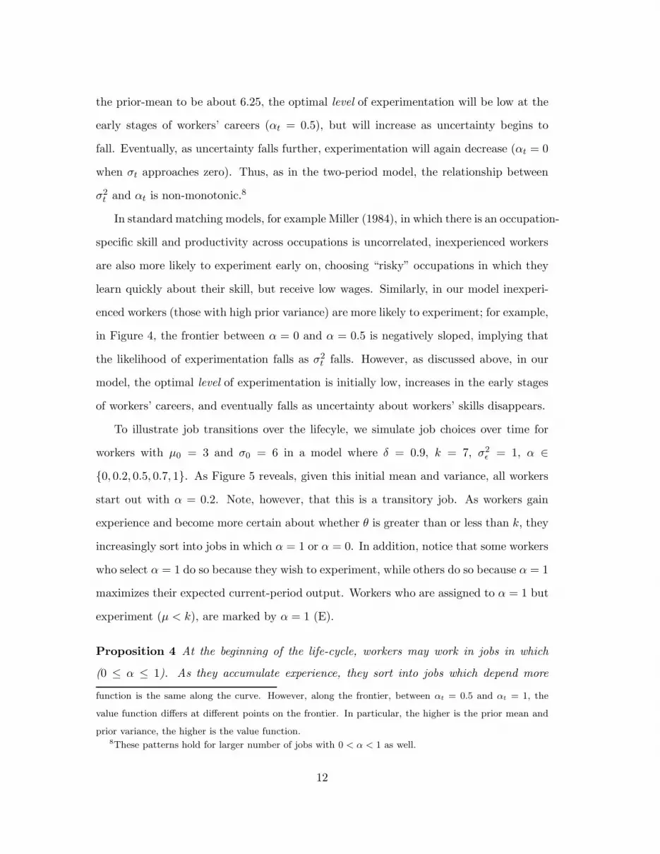
the prior-mean to be about 6.25, the optimal level of experimentation will be low at the

early stages of workers’ careers (αt = 0.5), but will increase as uncertainty begins to

fall. Eventually, as uncertainty falls further, experimentation will again decrease (αt = 0

when σt approaches zero). Thus, as in the two-period model, the relationship between

σ2t and αt is non-monotonic.8

In standard matching models, for example Miller (1984), in which there is an occupation-

specific skill and productivity across occupations is uncorrelated, inexperienced workers

are also more likely to experiment early on, choosing “risky” occupations in which they

learn quickly about their skill, but receive low wages. Similarly, in our model inexperi-

enced workers (those with high prior variance) are more likely to experiment; for example,

in Figure 4, the frontier between α = 0 and α = 0.5 is negatively sloped, implying that

the likelihood of experimentation falls as σ2t falls. However, as discussed above, in our

model, the optimal level of experimentation is initially low, increases in the early stages

of workers’ careers, and eventually falls as uncertainty about workers’ skills disappears.

To illustrate job transitions over the lifecyle, we simulate job choices over time for

workers with µ0 = 3 and σ0 = 6 in a model where δ = 0.9, k = 7, σ2ǫ = 1, α ∈

{0, 0.2, 0.5, 0.7, 1}. As Figure 5 reveals, given this initial mean and variance, all workers

start out with α = 0.2. Note, however, that this is a transitory job. As workers gain

experience and become more certain about whether θ is greater than or less than k, they

increasingly sort into jobs in which α = 1 or α = 0. In addition, notice that some workers

who select α = 1 do so because they wish to experiment, while others do so because α = 1

maximizes their expected current-period output. Workers who are assigned to α = 1 but

experiment (µ < k), are marked by α = 1 (E).

Proposition 4 At the beginning of the life-cycle, workers may work in jobs in which

(0 ≤ α ≤ 1). As they accumulate experience, they sort into jobs which depend more

function is the same along the curve. However, along the frontier, between αt = 0.5 and αt = 1, the

value function differs at different points on the frontier. In particular, the higher is the prior mean and

prior variance, the higher is the value function.8These patterns hold for larger number of jobs with 0 < α < 1 as well.

12

heavily on one of the skills, and in the limit workers either choose α = 1 or α = 0.

The proof is in Appendix A. The intuition for this proposition is clear. The first part

follows directly from the optimal solution (see, for example, Figure 4), and the second part

of the proposition follows from the fact that as t becomes arbitrarily large, σ2t becomes

close to zero for workers who are assigned to αt > 0 (once assigned to αt = 0, workers do

not move). Thus, for these workers, the solution approaches the full information solution

in which αt = 1 if θ > k, and αt = 0 otherwise.

4.2 Wage Growth, Wage Dispersion and Luck

Wage growth in our model occurs as workers learn about θ and sort into the job at which

their expected productivity is the highest. Moreover, since experimentation involves a

loss in expected current-period wages, wage growth is also driven by the eventual decline

in experimentation. To illustrate this, we simulate the wage distribution when k = 7,

µ0 = 6, σ0 = 4, δ = 0.9 and α ∈ {0, 0.2, 0.5, 0.7, 1}, so that the optimal job assignment is

initially α = 0.7. Figure 6 shows the resulting percentiles of the wage distribution for 10

periods into the future. Notice that experimentation initially leads some workers to earn

less than they would earn if they were assigned to α = 0. For example, the wage at the

5th percentile is lower than k = 7 for the first 4 periods, but this bottom tail (any wage

less than k) disappears as workers stop experimenting. In addition, like most learning

models, it shows increasing cohort wage dispersion.

To illustrate the tradeoff between current wage and future earnings, we repeat the

simulation in Figure 7, but set µ0=4.3. Relative to workers with µ0 = 6, these workers

will start with a lower initial α (α0 = 0.2 instead of α0 = 0.7) and will have higher initial

wages (w0 = $6.50 instead of w0 = $6.30). Over time, however, they will have lower wage

growth and wage dispersion.

Our model also suggests that i.i.d. productivity shocks, especially those early in a

worker’s career, have a persistent effect on earnings. It is a common feature of all learning

models that past output realizations affect current beliefs about workers’ skills, and on

13

average, workers who receive positive productivity shocks (ǫt > 0) will have higher wages

than will those who receive negative productivity shocks (ǫt < 0), at least for any finite

time horizon.

In contrast with previous literature, however, in our model, negative productivity

shocks have longer-lasting effects than do positive productivity shocks. Workers who

receive negative productivity shocks are more likely to choose jobs with a low α, and hence

will acquire less information about θ, and will be slower to sort into the job at which

they are the most productive. As a result, workers who receive negative productivity

shocks will not only have lower wages but also slower wage growth. In addition, since

no information is revealed when α = 0, there will always exist a subset of workers for

whom θ is never fully learned, even in the limit.9 Thus, experimentation serves as a

propagation mechanism. Further, the effect of luck is especially pronounced early in

a worker’s career since new information has the largest effect on beliefs when there is

considerable uncertainty about θ.

To see the effect of luck on wages, we assign all workers θ = 8 and simulate the wage

distribution when k = 7, µ0 = 6, σ0 = 4, δ = 0.9 and α ∈ {0, 0.2, 0.5, 0.7, 1}. Given

that θ > k, if θ were known, all workers would be assigned to α = 1 and would earn a

wage of $8. Uncertainty about θ, however, leads to departures from this full-information

outcome, and Figure 8 shows the percentiles of the wage distribution for 10 periods into

the future. Given the parameter values, all workers initially are assigned to α = 0.7 and

earn a wage of $6.50.

Figure 8 demonstrates several points. First, the exceptionally high wages captured

by the 85th and 95th percentiles result from “good luck” (high realizations of ǫ) and the

fact that productivity signals are highly influential early in a worker’s career. Continued

learning, however, leads wages for these individuals to converge to $8, and in the limit, all

workers not assigned to α = 0 earn $8. Second, convergence to a wage of $8 is slower at

the bottom than at the top of the wage distribution because learning is slower for those

9Thus, in the language of Aghion et al. (1991), learning is not adequate.

14

who initially experience bad luck and are assigned to relatively low-α jobs. Third, since

by period 7 the median worker earns a wage close to the true productivity, the long-run

per period wage loss of workers incorrectly assigned to α = 0 is roughly θ−k = 1. Finally,

note that the percentages along the line of k = 7 represent the cumulative probability

of incorrect assignment and that the marginal increase in this probability decreases with

experience. Thus, the probability of incorrect assignment is greatest early in a worker’s

career.

5 Data and Empirical Implementation

To construct the data used in our empirical analysis, we create an index that ranks

occupations by the degree to which output depends on unobserved skills. We then merge

this measure of α with occupational work histories from the National Longitudinal Survey

of Youth 1979 (NLSY79) in order to construct life-cycle patterns of α and wages.

5.1 The Dictionary of Occupational Titles

To construct our measure of α, we rely upon information in the Dictionary of Occupa-

tional Titles (DOT). The DOT provides information on the primary tasks performed in a

given occupation and the worker characteristics necessary for successful job performance.

The occupational characteristics given in the DOT are linked to the 1970 Census three-

digit occupation codes in an augmented version of the April 1971 Current Population

Survey (CPS) compiled by the Committee on Occupational Classification and Analysis

at the National Academy of Sciences. This augmented data file contains occupation codes

from the fourth edition of the DOT, which we update with the 1991 revised fourth edition

of the DOT.10 The data in the DOT are both comprehensive and detailed, describing

over 12,000 occupations along 44 dimensions.

From the DOT, we assemble a list of job characteristics that capture the importance of

hard-to-observe skill to job performance. There are several key features that characterize

10We thank Shintaro Yamaguchi for helping us update to the Revised Fourth Edition.

15

hard-to-observe skill in our model. First, there must be uncertainty about the skill prior

to a worker’s entry into the labor market. Second, observing output only gradually

reveals a worker’s skill, and the more important is the unobservable skill to successful

job performance, the more quickly the skill is revealed. In order to identify occupations

in which hard-to-observe skill is important to job performance, we select occupational

characteristics that indicate the importance of complex tasks. We define complex tasks

as those for which it is hard to write down an explicit algorithm for successful completion.

This is similar to the definition of “nonroutine” tasks in Autor, Levy and Murnane (2003)

and to the definition of “unanalyzable” in Perrow (1967).

Our reasoning is that if a task can be broken into an ordered list of well-defined ac-

tions, then a worker’s ability can be quickly learned by observing his or her performance

at each separate action. In contrast, if it is difficult to explicitly describe how to suc-

cessfully complete a task, then it will be difficult to determine a worker’s skill without

observing his or her on-the-job performance. For example, we classify the DOT variable

“Data” as complex since occupations that score high on this variable involve activities

such as “conducts research to discover new uses for chemical byproducts” and “creates

satirical cartoons based on current news events”–activities for which it would be diffi-

cult to write down step-by-step instructions. In contrast, we classify the DOT variable

“Things” as noncomplex since even occupations that score high on this variable involve

activities for which it is relatively easy to give detailed instructions, such as “prepares

machines for operation”, “verifies the dimensions of parts for adherence to specifications”

and “verifies the accuracy of machine functions”. Further examples are presented in Ta-

ble 1, and a full list of the DOT variables we classify as complex is included in the Data

Appendix.

Using this list of variables, we construct a single summary measure of α using princi-

pal component analysis. Since the DOT variables do not have a natural scale, we follow

Autor, Levy and Murnane (2003) and first transform each DOT variable into a percentile

value corresponding to its ranking in the 1970 distribution of that job attribute in the

16

population. We then calculate the first principal component and predict the first com-

ponent score for each occupation. To ease comparison with our theoretical model, we

normalize this predicted first component score by calculating its percentile ranking and

dividing by 100. This normalized predicted score naturally takes on a value between zero

and one, and higher values indicate a higher level of required skill. We then use this

normalized predicted score as our measure of α.11 At every stage in constructing our

measure of α, we use the sampling weights given in the CPS. Thus, our measure of α best

captures the variation in the occupational characteristics from the DOT for a nationally

representative sample of men in the United States.12

To verify that α captures the importance of unobservable as opposed to observable

skill, we create a measure of the importance of observable skill using variables from

the DOT that we classify as noncomplex and easy-to-observe (and so were not used to

create our measure of α). Just as we did when constructing α, we use PCA to create

a single measure of the importance of observable skill. As it turns out, the ranking of

the occupations in terms of the importance of observable skill is very different from the

ranking of occupations in terms of unobservable skill. To illustrate this point, Table

2 compares occupations that have similar observable skill requirements, but different

measures of α. For example, while both legal secretaries and bank tellers have similar

observable skill requirements, α is higher for legal secretaries than it is for bank tellers

(0.69 vs. 0.52), suggesting that it is harder to observe the skills needed to be a legal

secretary compared to a bank teller.

5.2 The National Longitudinal Survey of Youth 1979

The model we develop focuses on the evolution of αt over the life-cycle. In order to

construct this occupational work history, we use the National Longitudinal Survey of

Youth 1979 (NLSY79), which follows individuals born between 1957 and 1964. We focus

11Our qualitative findings are not sensitive to this normalization.12Results of the principal components analysis are available upon request. The first component explains

52 percent of the variation in the 17 DOT variables we employ.

17

our empirical analysis on males in the cross-sectional sample. Although, the NLSY79

contains information on individuals’ labor force activities for each week from 1978 through

the most recent year in which a respondent was interviewed, we only rely upon labor

market data from 1978 through 2000 because of a switch in occupational coding that

occurred after 2000. If a respondent is not interviewed in a given year (or years), then

at the next interview date, the respondent is asked to go back and retrospectively report

their labor force activities. As a result, the NLSY allows us to construct relatively

complete work histories. The work history data include information on each of up to

five jobs a respondent may have held in a given week, and we define an individual’s

occupation in a given week to be their occupation in the job at which they worked the

most number of hours.

We follow individuals’ occupational histories starting with their first transition to

full-time work after the completion of their highest degree. In particular, following the

completion of their degree, we identify the first week in which the individual is working

at least 10 hours a week and in which they will continue to work at least 10 hours a week

for at least 39 of the next 52 weeks. We then keep a running tab of a worker’s actual

labor market experience and their occupation in each week in which they work.13 In our

empirical analysis, we focus on the first 350 weeks (about 6.7 years) of an individual’s

actual experience in the labor force because attrition from the sample makes it difficult

to construct complete work histories for longer horizons.

We lose 693 respondents because we cannot identify either their highest degree or the

date at which they received their highest degree. We additionally drop 350 respondents

who completed their highest degree prior to the start date of the work history record and

254 observations who complete their highest degree relatively late in the life because we

worry that these workers already may have accumulated substantial labor market expe-

rience that could influence employers’ beliefs about skills. We also drop 239 observations

13In this tabulation, after making the sample selection rules discussed below, we treat individuals with

missing occupation information as being out of the labor force.

18

whose occupational history is relatively incomplete. In particular, we drop individuals

who have more than 150 weeks in which the respondent either is not working or has

missing occupation information during the first 500 weeks following their transition to

full-time work. In other words, we give individuals 500 weeks in which to accumulate

350 weeks of valid occupation information, otherwise we drop them from the sample.

We additionally drop 67 individuals who ever report an hourly wage of either over 100

or under 2. After these restrictions have been made, we are left with 1,360 individuals.

Relative to the initial sample, these individuals have a relatively strong attachment to

the labor market and are relatively young. Table 3 presents basic summary statistics for

our sample.

6 Empirical Findings

In this section, we document patterns in wage growth and job assignments over the life-

cycle, discuss the extent to which our model’s predictions are supported by the data and

relate our findings to existing models of wage dynamics.

Wage and job assignment profiles. We begin by describing the changes in α

and wages over the lifecycle. Figure 9 shows the average value of α by weeks of actual

experience. For college graduates the average value of α in the first week is 0.65, rising

to roughly 0.75 in week 350. Similarly, α increases from about 0.32 to 0.42 for high

school graduates. Figures 10 and 11 present the average hourly wage and the standard

deviation of hourly wages for high school graduates and college graduates. Like previous

studies, we find that both wages and wage dispersion increase over the life cycle. The

above patterns in α and wages are consistent with our model. First, the optimal level

of α is relatively low in the early stages of workers’ careers when there is considerable

uncertainty about workers’ skills, and over time, as workers sort into jobs where they

are more productive, both wages and wage dispersion grow. These findings, however, are

also consistent with theories of on-the-job training in which workers learn how to perform

tasks and accordingly move up the job ladder causing wages to increase over time(e.g.

19

Jovanovic and Nyarko (1997)).

As discussed in section 4.2, workers who experiment will have relatively low initial

wages and high initial α, but will have higher wage growth and wage dispersion than will

workers with high initial wages and low initial α (see, for example, the simulations in

Figures 6 and 7). To look for evidence of this, we regress a worker’s hourly wage in week

t on a worker’s initial job assignment (α0), their initial wage (w0), their experience in

week t and the interaction between experience and both α0 and w0. Columns 1 and 2 of

Table 4 show that for both high school graduates and college graduates, the coefficient on

the interaction between α0 and experience is positive and statistically significant while

the coefficient on the interaction between w0 and experience is negative, suggesting wage

growth is higher for the group of workers who begin their careers in jobs with higher α

and lower wages.

To look for evidence of whether the increase in wage dispersion is higher for workers

with high initial α, we determine the quartile of the distribution of α and the quartile of

the distribution of wages into which each worker falls in week 1. Thus, for each education

category, there are 16 possible bins into which a worker can fall (four α quartiles and

four wage quartiles). We want to know how the change over time in the spread of the

wage distribution within each bin depends on workers’ initial job assignments. Thus,

within each bin, we calculate the difference between the wage at the 90th and the 10th

percentile for every week of actual experience. We then regress this measure of wage

dispersion on the quartile of the initial wage distribution, the quartile of the initial α

distribution, experience, the interaction between experience and the quartile of the initial

wage distribution and quartile of the initial α distribution. Table 5 reports the results

of this regression. The coefficient on the interaction between the quartile of the initial

α distribution and experience is positive and statistically significant, suggesting that the

spread in the distribution of wages grows more quickly for those initially in occupations

with higher α. Note that if jobs with higher α provide more training than do jobs with

lower α, then the above patterns also could be consistent with investment in human

20

capital as opposed to investment in information (see Ben-Porath (1967)).

Job transitions. A key difference, however, between our model and human capital

models is that workers in our model should also transition into jobs that depend less on

the unobserved skill, which we analyze next. In our model, as uncertainty is resolved

and workers experiment less, a fraction of workers should move to jobs with lower α.

Table 6 presents a transition matrix for α where the rows show the decile of α before

the transition, and the columns show the decile of α after the transition. Thus, the

sum of the entries in each row adds up to 100%. The entries below the diagonal capture

transitions into lower deciles while the entries above the diagonal capture transitions into

higher deciles. Clearly a large fraction of all occupational changes involve transitions into

jobs with a lower α.

A key feature of our model is the tradeoff between current wages and information and

the fact that a decline in experimentation can lead to wage increases even for those who

move to occupations with a lower α. Thus, transitions to jobs where output depends

less on hard-to-observe skills may entail wage increases. Table 7 summarizes the mean

change in α and wages for workers who move to higher and lower α jobs. First, note

that the number of job changes is larger in the first 200 weeks after a worker’s entry into

the labor market than it is in weeks 201-350, suggesting a decline in uncertainty and

experimentation. Consistent with our model, we also find that even among those who

transition to lower α jobs, wages increase on average.

The magnitude of the changes in α and wages in Table 7 is large. The absolute value

of the mean change in α for those who change jobs is above 0.2, which is substantial given

that in week 1 the mean of α is 0.43 and the standard deviation is 0.29. In addition, the

mean increase in α associated with a move up is more than twice as large as the entire

increase in the mean of α from week 1 to week 350, suggesting that a substantial fraction

of workers transition to jobs with a lower α. Indeed, we find that between week 1 and

week 350, α declines for roughly 30 percent of the workers in our sample.14 Furthermore,

14For 55 percent of workers α increases, and for 15 percent α doesn’t change.

21

the wage increase for those who move to lower-α jobs is approximately $1.18, which is

large compared to the wage increase for those who do not change jobs and compared to

the overall wage increase of $4.80 for those with α350 < α0.15

Existing theories of learning and sorting (e.g. Gibbons and Waldman (2006), Gibbons

et al. (2005)) that incorporate on-the-job training can explain both why α increases over

time on average (because experience augments the unobserved skill) and why α may

decline for some individuals (some will receive negative information about their skill),

but in those models, wages and α should move in the same direction when workers change

jobs because workers who receive positive information about their skill will move to jobs

where output depends more on skill and earn more, while those who receive negative

information will move to jobs where output depends less on skill and earn less. The

results in Table 7, however, show that α and wages do not always move in the same

direction.

Lifecycle patterns of experimentation and sorting. Our model also predicts

that for workers who experiment (those for whom µt < k but αt > 0), the optimal level of

experimentation is initially low, increases over time, and then eventually declines. This

non-monotonic relationship is difficult to test for because the non-monotonicity only holds

conditional on µt and for µt < k, and because adequate measures of µt are not readily

available as wages reflect both expected skill and job assignments. Nonetheless, while our

analysis is only suggestive, we look for a non-monotonic relationship between experience

and experimentation using workers’ starting wages and the value of α associated with

their first occupation to proxy for µ0, and by focussing on individuals whose wages fall

below a certain threshold to try to isolate individuals for whom µt < k. In particular, for

each week of experience, we only keep individuals whose wage is less than we0, where we

0

is defined to be the average starting wage of workers in education group e ∈ {high school

graduate, college graduate}. We then regress wt on w0, α0, experience and experience

15When we repeat the above analysis for high school graduates and college graduates separately, we

get similar results. Details available upon request.

22

squared.16

Columns 3 and 4 of Table 4 present the regression results. For college graduates, the

coefficient on experience is positive and the coefficient on experience squared is negative

and statistically different from zero. Based on these estimates, Figure 12 shows the

predicted value of α by experience for the median individual with a college degree. It

shows that the overall increase in α between the first week and week 350 is small relative

to the increase between the first week and week 200, when the predicted value of α reaches

its peak. We also find weak evidence of non-monotonicity for high school graduates. In

Column 3, the coefficient on experience squared is still negative, but no longer statistically

different from zero (see also Figure 13).17

Finally, while we also find evidence that workers sort over time into jobs that depend

either more or less on the unobserved skill, we do not find evidence that they sort into

occupations in which α is close to either zero or one, as predicted in Proposition 4. There

are several extensions to our model that could potentially account for this. For example,

if there are switching costs that depend positively on the difference between the value of

α in a worker’s current job and the value of α in the next job, then this will limit sorting.

In addition, if the production function involves complementarities between the observed

and the unobserved skill, then even under full information, workers will not sort into jobs

that depend upon one skill.

16We chose this specification to minimize the mean squared error. The inclusion of higher order terms

of experience does not substantially change the mean square error, and the coefficient on higher order

terms is statistically indistinguishable from zero. In addition, adding higher order terms does not change

any of our qualitative findings.17As discussed above, our model predicts that we should not find any evidence of a non-monotonic

relationship between experience and experimentation for workers with µt > k expected. When we repeat

the analysis in Table 4 for high-wage workers, we find that α is strictly increasing with experience.

23

7 Conclusion

This paper develops a lifecycle model of occupational choice and wage dynamics when

jobs differ in the amount of information they provide about workers’ skills. In this setting,

we show that workers experiment, trading off current-period wages for information. Our

model predicts that the optimal level of experimentation is relatively low at the beginning

of workers’ careers, increases as workers gain experience, and then declines as workers

become increasingly certain about their skill. This eventual decline in experimentation

partially drives wage growth in our model. In addition, experimentation can lead random

productivity shocks, especially when workers are young, to have lasting effects on workers’

career trajectories.

We then use data from the Dictionary of Occupational Titles to construct a measure

of how much information different occupations reveal about workers’ skills and match

this measure to data from the NLSY79. In particular, our measure captures the degree

to which different occupations involve complex tasks, conjecturing that there will uncer-

tainty about workers’ skill in these tasks. We then document patterns of occupational

choice and wage dynamics in the NLSY79. Consistent with our model, we find that

workers tend to start their careers in jobs that reveal relatively little about their skill.

In addition, the more information a worker’s initial job reveals about the worker’s skill,

the faster will be the worker’s wage growth. We also find that a large fraction of workers

transitions into occupations with lower skill requirements and that these transitions are

often accompanied by wage increases, a fact that is hard to reconcile with existing models

of wage dynamics.

We believe our results suggest that experimentation may be an important feature of

the labor market. Nonetheless, we acknowledge that without estimating the fundamen-

tal parameters of a richer model of wage dynamics, we cannot parse out the importance

of experimentation relative to other factors that may explain the wage growth and job

transition patterns in our data. For example, an obvious extension to our model would

be to allow workers to accumulate job-specific human capital and to quantify the impor-

24

tance of experimentation relative to learning by doing, search frictions. We leave these

identification issues and extensions to future work.

References

[1] Aghion, Philippe, Patrick Bolton, Christopher Harris, and Bruno Jullien. 1991. Op-

timal learning by experimentation. Review of Economic Studies 58, no. 4:621-654.

[2] Autor, David H., Frank Levy, and Richard J. Murnane. 2003. The skill content of

recent technological change: An empirical exploration. Quarterly Journal of Eco-

nomics 118, no. 4:1279-1334.

[3] Bacolod, Marigee, and Bernardo Blum. 2010. Two sides of the same coin: U.S.

“residual” inequality and the gender gap. Journal of Human Resources 45, no. 1:197-

242.

[4] Baker, George, Michael Gibbs, and Bengt Holmstrom. 1994a. The internal economics

of the firm: Evidence from personnel data. Quarterly Journal of Economics, 109,

no. 4: 881-919.

[5] ——. 1994b. The wage policy of a firm. Quarterly Journal of Economics 109, no. 4:

921-55

[6] Ben-Porath, Yoram. 1967. The production of human capital and the life cycle of

earnings. The Journal of Political Economy 75, no. 4:352-365.

[7] Chade, Hector, and Edward Schlee. 2002. Another look at the Radner-Stiglitz non-

concavity in the value of information. Journal of Economic Theory 107, no. 2:421-

452.

[8] Farber, Henry, and Robert Gibbons. 1996. Learning and wage dynamics. Quarterly

Journal of Economics 111, no. 4: 1007-47.

25

[9] Felli, Leonardo, and Christopher Harris. 1996. Learning, wage dynamics, and firm-

specific human capital. Journal of Political Economy 104, no. 4:838-868.

[10] Felli, Leonardo and Christopher Harris. 2006. Firm-specific training. CEPR Discus-

sion Paper No. 4580. http://ssrn.com/abstract=607061.

[11] Gibbons, Robert, Lawrence Katz, Thomas Lemieux, and Daniel Parent. 2005. Com-

parative advantage, learning, and sectoral wage determination. Journal of Labor

Economics 23, no. 4: 681-723.

[12] Gibbons, Robert, and Michael Waldman. 1999. A theory of wage and promotion

dynamics inside firms. Quarterly Journal of Economics 114, no. 4:1321-58.

[13] Gibbons, Robert, and Michael Waldman. 2006. Enriching a theory of wage and

promotion dynamics inside firms. Journal of Labor Economics 24, no. 1:59-107.

[14] Gittins, John C., and David M. Jones. 1974. A dynamic allocation index for sequen-

tial design of experiments. In Progress in statistics, ed. Joseph Gani, Karoly Sarkadi

and Istvan Vincze. Amsterdam: North-Holland.

[15] Harris, Milton, and Bengt Holmstrom. 1982. A theory of wage dynamics. Review of

Economic Studies 49, no. 3:315-33.

[16] Ingram, Beth, and George Neumann. 2006. The returns to skill. Labour Economics

13, no. 1: 35-59.

[17] Jovanovic, Boyan. 1979. Job matching and the theory of turnover. Journal of Polit-

ical Economy 87, no. 5:972-990.

[18] Jovanovic, Boyan, and Yaw Nyarko. 1997. Stepping stone mobility. Carnegie

Rochester Conference Series on Public-Policy 46 (June):289-325.

[19] Miller, Robert. 1984. Job matching and occupational choice. Journal of Political

Economy 92, no. 6:1086-1120.

26

[20] Neal, Derek. 1999. The complexity of job mobility among young men. Journal of

Labor Economics 17, no. 2:237-261.

[21] Ortega, Jaime. 2001. Job rotation as a learning mechanism. Management Science

47, no. 10: 1361-1370.

[22] Papageorgiou, Theodore. 2010. Learning your comparative advantages. Unpublished

manuscript, Department of Economics, Pennsylvania State University.

[23] Pastorino, Elena. 2009. Learning in labor markets and job mobility. Unpublished

manuscript, Department of Economics, University of Iowa.

[24] Pastorino, Elena. 2010. Learning and career dynamics: Estimating the value of firm

experimentation. Unpublished manucript, Department of Economics, University of

Iowa.

[25] Perrow, Charles. 1967. A framework for the comparative analysis of organizations.

American Sociological Review 32, no. 2:194-208

[26] Poletaev, Maxim and Chris Robinson. 2008. Human capital specificity: Evidence

from the Dictionary of Occupational Titles and Displaced Worker Surveys, 1984-

2000. Journal of Labor Economics 26, no. 3:387-420.

[27] Radner, Roy, and Joseph Stiglitz. 1984. A nonconcavity in the value of information.

In Bayesian models of economic theory, ed. Marcel Boyer and Richard Kihlstrom.

Amsterdam: Elsevier.

[28] Yamaguchi, Shintaro. 2010. Career progression and comparative advantage. Labour

Economics 17, no. 4:679-689.

27

Appendix A

Proof of Proposition 1

The second period payoff is given by

U2(µ2, σ2) = w2(α2, µ2, σ2) = α2 ∗ E(θ|µ2, σ2) + (1 − α2) ∗ k = α2 ∗ µ2 + (1 − α2) ∗ k

If µ2 > k then w2 = µ2 > α2 ∗ µ + (1−α2) ∗ k. The opposite holds if µ2 < k. If µ = k all

jobs pay the same. Thus, the decision rule is optimal.

Proof of Proposition 2

We need to show that for any α′

1 > 0 and −∞ < µ1 < k, there exists a large enough σ1

such that V (µ1, σ1|α′

1) > V (µ1, σ1|α1 = 0) = k(1 + δ). Using the well-known properties

of a truncated normal distribution, it can be shown that this condition holds iff

s2φ(r) + µ1 + (k − µ1)Φ(r) >(k − µ1)α

′

1 + δk

δ, (12)

where r = µ1−kσ1

. Since µ1 < k, and Φ(r) > 0, it is suffices to show that

s2φ(r) + µ1 >(k − µ1)α

′

1 + δk

δ. (13)

The above equation holds iff

s2 >(k − µ1)(α

′

1 + δ)

δφ(r). (14)

Since

∂φ(r)

∂σ1= exp{(k − µ1)

2(σ21α

21 + 1)

2σ41α

21

}(k − µ1)2(σ2

1α21 + 2)√

2πσ51α

21

> 0,

the right hand side of equation (14) is continuous and decreasing in σ1. In addition,

limσ1→∞(k − µ1)(α

′

1 + δ)

δφ(r)=

√2π(k − µ1)(α

′

1 + δ)

δ.

Further, since

s2 =α1σ

21

√

α21σ

21 + 1

,

the left-hand side of equation (14) is continuous and increasing in σ1 and limσ1→∞s2 = ∞,

there exists σ1 < ∞ such that equation 12 holds.

28

Proof of Proposition 3

It can be shown that ∂φ(r)∂α1

s2 = −(k−µ1)∂Φ(r)∂α1

, thus the first order condition in equation

(10) reduces to

σ21exp{−1

2(σ2

1α21+1)(k−µ1)2

σ41α2

1}

√2π(σ2

1α21 + 1)1.5

=k − µ1

δ. (15)

1.

limσ1→0

σ21exp{−1

2(σ2

1α21+1)(k−µ1)2

σ41α2

1}

√2π(σ2

1α21 + 1)1.5

= limσ1→0

σ21√

2π(σ21α

21 + 1)1.5

∗ limσ1→0

exp{−1

2

(σ21α

21 + 1)(k − µ1)

2

σ41α

21

} =0√2π

∗0 = 0

2.

limσ1→∞

σ21exp{−1

2(σ2

1α21+1)(k−µ1)2

σ41α2

1}

√2π(σ2

1α21 + 1)1.5

= limσ1→∞

σ21

(σ21α

21 + 1)1.5

∗ limσ1→∞

φ(r) = 0 ∗ 1√2π

= 0

Since for any 0 < σ1 < ∞ and 0 < α ≤ 1,σ21exp{− 1

2

(σ21α2

1+1)(k−µ1)2

σ41α2

1}

√2π(σ2

1α21+1)1.5 > 0 and continuous, it

is increasing and eventually decreasing in σ1.

Proof of Proposition 4

1. Suppose that in time t it is optimal for a worker to choose α′ where 0 < α′ < 1 and

stay in that job forever. We know that at time t + n

µt+n =µtσ

2ǫ̃,t + σ2

t

∑n−1i=0 xt+i

σ2ǫ̃,t + nσ2

t

.

Further, by the Law of Large Numbers, we know that

limn→∞

µt+n = limn→∞

1

n

n−1∑

i=0

xt+i = limt→∞

θ +1

n

n−1∑

i=0

ǫt+i

α′ = θ.

Thus, the worker’s problem approaches the benchmark case in which θ is known.

However, when θ is known, workers will optimally choose α = 1 if θ > k and α = 0

otherwise. Thus, in the limit, it cannot be optimal for the worker to stay in a job

in which 0 < α′ < 1.

29

Appendix B

The variables we use in constructing our measure of α are DATA,PEOPLE, GED-

REASONING, GED-MATH, GED-VERBAL, GENERAL LEARNING, VERBAL, NU-

MERICAL, SPATIAL, PERCEPTION, COLOR, EYE-HAND-FOOT, DIRECTING, IN-

FLUENCING, STRESS, EXPRESSING, PEOPLE, JUDGEMENTS.

30

Table 1: Examples of Task Classification for Variables in the DOT

Variable DOT Definition Classification Examples

DATA Describes workers’ relationship to infor-

mation, knowledge, and conceptions re-

lated to data, people or things obtained

by observation, investigation, interpreta-

tion, visualization, and mental creation.

Hard to observe Creates and teaches original dances for bal-

let. Conducts research to discover new uses

for chemical byproducts, and devises new pro-

cedures for preparing organic compounds.

GED-REASONING General reasoning development Hard to observe Arbitrates, advises and administers justice in

a court of law. Plans, organizes and conducts

research for use in understanding social prob-

lems.

DIRECTING Directing, controlling, or planning activ-

ities of others.

Hard to observe Plans, implements, and coordinates programs

to reduce or eliminate occupational injuries,

commands ship to transport passengers.

MANUAL DEXTERITY The ability to move hands easily and

skillfully.

Easy to observe Installs, repairs, maintains, and adjusts, indi-

cating, recording, telemetering, and control-

ling instruments used to measure and control

variables, such as pressure, flow, and temper-

ature.

THINGS Describes workers’ relationship to inan-

imate objects as distinguished from hu-

man being; substances or materials; and

machine tools, equipment, work aids, and

products.

Easy to observe Lays out position of parts on metal, using

scribe and hand tools, repairs and main-

tains production machinery in accordance

with manufacturer’s specifications.

TOLERANCES Adaptability to setting limits, tolerances

or standards.

Easy to observe Weighs, measures, and mixes drugs and other

medicinal compounds.

Note: Definitions and examples taken from The Revised Handbook for Analyzing Jobs, 1991.

31

Table 2: Occupations with Similar Observable Skill Requirements But Different α

High α Low α

Example 1 Optometrists

(.97)

Opticians, and lens

grinders and polishers

(0.56)

Example 2 Painters and sculptors

(0.74)

Photoengravers and

lithographers

(0.50)

Example 3 Dentists

(0.98)

Dental hygienists

(0.62)

Example 4 Electronic engineering

technicians

(0.72)

Automobile mechanics

(0.48)

Example 5 Legal secretaries

(0.69)

Bank tellers

(0.52)

Example 6 Librarians

(0.73)

Proofreaders

(0.55)

Note: The value of α for each occupation is given in parentheses.

32

Table 3: Summary Statistics

High School College All

Alpha 0.364 0.738 0.504

(0.231) (0.229) (0.289)

Wage 11.411 18.463 14.054

(5.384) (8.963) (7.762)

Number of Moves 4102 1787 6236

Number of People 813 464 1360

Number of Observations 264,459 152,899 444,431

Note: Standard deviations in parentheses.

33

Table 4: Wage Growth, Job Assignment and Experience

wt αt

High School College High School College

(1) (2) (3) (4)

Initial wage 0.587*** 0.690*** 0.0006 -0.0007

(0.0368) (0.0513) (0.002) (0.002)

Initial alpha 0.353 0.000329 0.3885*** 0.3933***

(0.520) (1.056) (0.038) (0.042)

Actual experience (in years) 1.008*** 1.492*** 0.0156** 0.0297**

(0.101) (0.235) (0.007) (0.012)

Initial wage x actual experience -0.0511*** -0.0553***

(0.0104) (0.0210)

Initial alpha x actual experience 0.479*** 0.857***

(0.176) (0.315)

Actual experience squared -0.0015 -0.0039**

(0.001) (0.002)

Constant 3.656*** 4.624*** 0.1810*** 0.3955***

(0.356) (0.691) (0.020) (0.033)

Observations 267,921 155,675 102,458 48,833

R2 0.172 0.267 0.132 0.201

Note: Robust standard errors in parentheses.

*** p<0.01, ** p<0.05, , * p<0.1.

34

Table 5: Wage Dispersion and Initial Job Assignment

High School College

(1) (2)

Initial wage quartile -0.0027 -0.1012***

(0.004) (0.006)

Initial alpha quartile 0.0103** -0.1031***

(0.004) (0.006)

Actual experience (in years) 0.0114*** 0.0246***

(0.004) (0.006)

Initial wage quartile x actual experience 0.0063*** -0.0119***

(0.001) (0.002)

Initial alpha quartile x actual experience 0.0126*** 0.0208***

(0.001) (0.002)

Constant 0.7224*** 1.2605***

(0.016) (0.022)

Observations 5,600 5,600

R2 0.340 0.372

Note: Standard errors in parentheses.

*** p<0.01, ** p<0.05, * p<0.1.

35

Table 6: Alpha Transition Matrix for Job Moves

Decile of α in Time t + 1

(0, 0.1] (0.1, 0.2] (0.2, 0.3] (0.3, 0.4] (0.4, 0.5] (0.5, 0.6] (0.6, 0.7] (0.7, 0.8] (0.8, 0.9] (0.9, 1] N

Dec

ile

of

αin

Tim

et

(0, 0.1] 0.197 0.158 0.165 0.150 0.157 0.058 0.059 0.032 0.008 0.017 903

(0.1, 0.2] 0.231 0.103 0.169 0.141 0.149 0.066 0.071 0.039 0.016 0.016 623

(0.2, 0.3] 0.185 0.132 0.167 0.099 0.164 0.072 0.096 0.062 0.012 0.012 666

(0.3, 0.4] 0.168 0.108 0.107 0.100 0.166 0.100 0.075 0.105 0.040 0.030 730

(0.4, 0.5] 0.158 0.112 0.129 0.113 0.149 0.087 0.104 0.083 0.034 0.030 796

(0.5, 0.6] 0.083 0.057 0.083 0.112 0.140 0.081 0.083 0.165 0.116 0.081 508

(0.6, 0.7] 0.077 0.051 0.086 0.084 0.093 0.095 0.120 0.184 0.077 0.135 549

(0.7, 0.8] 0.051 0.027 0.044 0.078 0.087 0.116 0.133 0.212 0.097 0.157 632

(0.8, 0.9] 0.005 0.014 0.019 0.066 0.052 0.109 0.093 0.208 0.153 0.262 366

(0.9, 1] 0.013 0.019 0.017 0.017 0.041 0.093 0.156 0.188 0.188 0.268 463

N 825 551 678 636 799 532 597 719 386 513 6,236

36

Table 7: Changes in Wages and α at Job Transitions

Weeks

[2,50] [51,100] [101.150] [151,200] [201,250] [251,300] [301,350] All

Move Up:

∆wage 1.640 0.909 1.119 1.341 1.431 1.632 0.648 1.256

(4.271) (4.625) (5.487) (4.593) (4.876) (5.948) (5.823) (5.061)

∆alpha 0.251 0.240 0.238 0.221 0.219 0.207 0.225 0.230

(0.184) (0.181) (0.175) (0.172) (0.168) (0.180) (0.169) (0.177)

N 556 555 479 495 435 409 376 3,305

Move Down:

∆wage 1.426 0.948 1.117 1.345 1.217 1.252 0.893 1.179

(5.081) (5.128) (4.332) (6.607) (6.519) (6.447) (5.227) (5.620)

∆alpha -0.219 -0.219 -0.207 -0.222 -0.205 -0.223 -0.209 -0.215

(0.179) (0.175) (0.159) (0.174) (0.175) (0.170) (0.172) (0.172)

N 499 458 464 411 362 391 346 2,931

Stay:

∆wage -0.002 -0.001 0.000 0.000 0.003 -0.003 -0.001 -0.001

(0.338) (0.414) (0.443) (0.542) (0.734) (0.601) (0.709) (0.560)

N 60,559 62,411 62,674 62,912 63,201 63,089 63,349 438,195

Note: Standard errors in parentheses.

37

Figure 1: Optimal α1 as a Function of µ1,

Two-Period Model (k = 7, σ1 = 4)

Figure 2: Optimal α1 as a Function of σ1,

Two-Period Model (k = 7, µ1 = 6)

Figure 3: Marginal Change in Second-Period Output as a Function of σ1 (k = 7, µ1 = 6,

α1 = 5)

38

Figure 4: Optimal Job Choice: Three-Job Model

0.50

1.00

0.00

Expected Productivity, t

Unce

rtai

nty

,

t

4 4.5 5 5.5 6 6.5 7 7.5 80

1

2

3

4

5

6

Figure 5: Job Assignments Over the Life-Cycle When µ0 = 3 and σ0 = 6

� � � � � � � � ���

���

���

���

���

���

���

���

��

��

�

� ������ ��

������ � ��

����������������������������������������������������������������������������

Note: The light gray region shows the likelihood that αt = 1 but µt < k (experimentation)

while the white region shows the likelihood that αt = 1 and µt ≥ k (no experimentation)

.

39

Figure 6: Wage Distribution (α0 = 0.7)

� � � � � � � � �

�

�

�

�

��

��

�

��

��

� ��

��� �� ����

Figure 7: Wage Distribution (α0 = 0.2)

� � � � � � � � �

�

�

�

�

��

��

�

��

��

� ��

��� �� ����

Figure 8: Wage Dispersion Due to Luck

� � � � � � � � �

�

�

�

��

��

��

��

���

��

���

��

� ������ ��

������������������������������

������������������������������������������������������

40

Figure 9: Average α by Actual Experience

!"

#"

$"

""

%"

&"

!"#$%&'("

' "' ('' ("' !'' !"' #'' #"'

%)*+"&$,-'!./!#)!$0/#$1!!234$

%&& 5/6($7)(88&

9%:97$8.$(/6(!.

Figure 10: Average Wage by Actual Experience

!"

!#

!$

!%

!

#"

##

!"#$%"&!$'(#$)***$+,--"./0

" &" !"" !&" #"" #&" '"" '&"

1234"-$567!.(!#2!$'(#$8!!9/0$

1-- :(&;$<2;,,-

=1>=<$,.$;(&;!.

Figure 11: Standard Deviation of Wages by Ex-

perience

!

"

#

$$

%&'()'*)+,-./'&/0(

1 !1 $11 $!1 211 2!1 11 !1

34&5'6+789-*/-(4-+:/(+;--<=>+

366 ?/@A+%4A006

B3CB%+0*+A/@A-*

41

Figure 12: Predicted α by Experience, Low-

Wage Workers, College Graduates

.69

.7.71

.72

.73

.74

Fit

ted

val

ues

0 100 200 300 400

Actual experience (in weeks)

Figure 13: Predicted α by Experience, Low-

Wage Workers, High School Graduates

.22

.23

.24

.25

.26

Pre

dic

ted

Alp

ha

0 100 200 300 400

Actual experience (in weeks)

42