staRdom: Versatile Software for Analyzing Spectroscopic Data ...
19
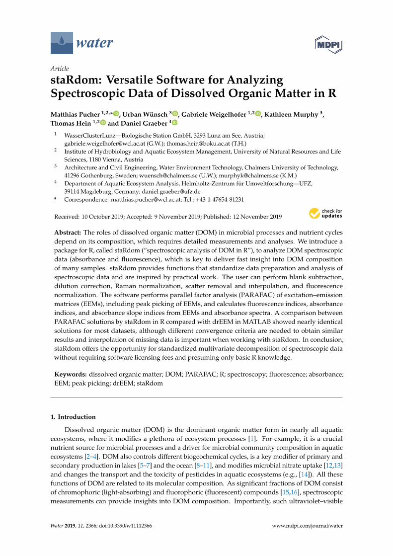
water Article staRdom: Versatile Software for Analyzing Spectroscopic Data of Dissolved Organic Matter in R Matthias Pucher 1,2, * , Urban Wünsch 3 , Gabriele Weigelhofer 1,2 , Kathleen Murphy 3 , Thomas Hein 1,2 and Daniel Graeber 4 1 WasserClusterLunz—Biologische Station GmbH, 3293 Lunz am See, Austria; [email protected] (G.W.); [email protected] (T.H.) 2 Institute of Hydrobiology and Aquatic Ecosystem Management, University of Natural Resources and Life Sciences, 1180 Vienna, Austria 3 Architecture and Civil Engineering, Water Environment Technology, Chalmers University of Technology, 41296 Gothenburg, Sweden; [email protected] (U.W.); [email protected] (K.M.) 4 Department of Aquatic Ecosystem Analysis, Helmholtz-Zentrum für Umweltforschung—UFZ, 39114 Magdeburg, Germany; [email protected] * Correspondence: [email protected]; Tel.: +43-1-47654-81231 Received: 10 October 2019; Accepted: 9 November 2019; Published: 12 November 2019 Abstract: The roles of dissolved organic matter (DOM) in microbial processes and nutrient cycles depend on its composition, which requires detailed measurements and analyses. We introduce a package for R, called staRdom (“spectroscopic analysis of DOM in R”), to analyze DOM spectroscopic data (absorbance and fluorescence), which is key to deliver fast insight into DOM composition of many samples. staRdom provides functions that standardize data preparation and analysis of spectroscopic data and are inspired by practical work. The user can perform blank subtraction, dilution correction, Raman normalization, scatter removal and interpolation, and fluorescence normalization. The software performs parallel factor analysis (PARAFAC) of excitation–emission matrices (EEMs), including peak picking of EEMs, and calculates fluorescence indices, absorbance indices, and absorbance slope indices from EEMs and absorbance spectra. A comparison between PARAFAC solutions by staRdom in R compared with drEEM in MATLAB showed nearly identical solutions for most datasets, although different convergence criteria are needed to obtain similar results and interpolation of missing data is important when working with staRdom. In conclusion, staRdom offers the opportunity for standardized multivariate decomposition of spectroscopic data without requiring software licensing fees and presuming only basic R knowledge. Keywords: dissolved organic matter; DOM; PARAFAC; R; spectroscopy; fluorescence; absorbance; EEM; peak picking; drEEM; staRdom 1. Introduction Dissolved organic matter (DOM) is the dominant organic matter form in nearly all aquatic ecosystems, where it modifies a plethora of ecosystem processes [1]. For example, it is a crucial nutrient source for microbial processes and a driver for microbial community composition in aquatic ecosystems [2–4]. DOM also controls different biogeochemical cycles, is a key modifier of primary and secondary production in lakes [5–7] and the ocean [8–11], and modifies microbial nitrate uptake [12,13] and changes the transport and the toxicity of pesticides in aquatic ecosystems (e.g., [14]). All these functions of DOM are related to its molecular composition. As significant fractions of DOM consist of chromophoric (light-absorbing) and fluorophoric (fluorescent) compounds [15,16], spectroscopic measurements can provide insights into DOM composition. Importantly, such ultraviolet–visible Water 2019, 11, 2366; doi:10.3390/w11112366 www.mdpi.com/journal/water
-
Upload
khangminh22 -
Category
Documents
-
view
0 -
download
0
Transcript of staRdom: Versatile Software for Analyzing Spectroscopic Data ...
water
Article
staRdom: Versatile Software for AnalyzingSpectroscopic Data of Dissolved Organic Matter in R
Matthias Pucher 1,2,* , Urban Wünsch 3 , Gabriele Weigelhofer 1,2 , Kathleen Murphy 3,Thomas Hein 1,2 and Daniel Graeber 4
1 WasserClusterLunz—Biologische Station GmbH, 3293 Lunz am See, Austria;[email protected] (G.W.); [email protected] (T.H.)
2 Institute of Hydrobiology and Aquatic Ecosystem Management, University of Natural Resources and LifeSciences, 1180 Vienna, Austria
3 Architecture and Civil Engineering, Water Environment Technology, Chalmers University of Technology,41296 Gothenburg, Sweden; [email protected] (U.W.); [email protected] (K.M.)
4 Department of Aquatic Ecosystem Analysis, Helmholtz-Zentrum für Umweltforschung—UFZ,39114 Magdeburg, Germany; [email protected]
* Correspondence: [email protected]; Tel.: +43-1-47654-81231
Received: 10 October 2019; Accepted: 9 November 2019; Published: 12 November 2019�����������������
Abstract: The roles of dissolved organic matter (DOM) in microbial processes and nutrient cyclesdepend on its composition, which requires detailed measurements and analyses. We introduce apackage for R, called staRdom (“spectroscopic analysis of DOM in R”), to analyze DOM spectroscopicdata (absorbance and fluorescence), which is key to deliver fast insight into DOM compositionof many samples. staRdom provides functions that standardize data preparation and analysis ofspectroscopic data and are inspired by practical work. The user can perform blank subtraction,dilution correction, Raman normalization, scatter removal and interpolation, and fluorescencenormalization. The software performs parallel factor analysis (PARAFAC) of excitation–emissionmatrices (EEMs), including peak picking of EEMs, and calculates fluorescence indices, absorbanceindices, and absorbance slope indices from EEMs and absorbance spectra. A comparison betweenPARAFAC solutions by staRdom in R compared with drEEM in MATLAB showed nearly identicalsolutions for most datasets, although different convergence criteria are needed to obtain similarresults and interpolation of missing data is important when working with staRdom. In conclusion,staRdom offers the opportunity for standardized multivariate decomposition of spectroscopic datawithout requiring software licensing fees and presuming only basic R knowledge.
Keywords: dissolved organic matter; DOM; PARAFAC; R; spectroscopy; fluorescence; absorbance;EEM; peak picking; drEEM; staRdom
1. Introduction
Dissolved organic matter (DOM) is the dominant organic matter form in nearly all aquaticecosystems, where it modifies a plethora of ecosystem processes [1]. For example, it is a crucialnutrient source for microbial processes and a driver for microbial community composition in aquaticecosystems [2–4]. DOM also controls different biogeochemical cycles, is a key modifier of primary andsecondary production in lakes [5–7] and the ocean [8–11], and modifies microbial nitrate uptake [12,13]and changes the transport and the toxicity of pesticides in aquatic ecosystems (e.g., [14]). All thesefunctions of DOM are related to its molecular composition. As significant fractions of DOM consistof chromophoric (light-absorbing) and fluorophoric (fluorescent) compounds [15,16], spectroscopicmeasurements can provide insights into DOM composition. Importantly, such ultraviolet–visible
Water 2019, 11, 2366; doi:10.3390/w11112366 www.mdpi.com/journal/water

Water 2019, 11, 2366 2 of 19
spectroscopy is fast and cost-efficient, allowing immediate measurements during sampling campaignswith high sample throughput. Although some DOM fractions are not spectroscopically active and itsspectral properties do not resolve fine details of its molecular structure, spectroscopic measurementscan distinguish groups of DOM molecules in a meaningful way [17–19]. DOM spectroscopic propertieshave been shown to discriminate between sources, pathways, and undergone processes in aquaticecosystems [20–24].
While absorbance data have mainly been used to estimate DOC concentrations and to detectthe presence of aromatic compounds in DOM [25,26], fluorescence characteristics, such as theposition, height, and shape of different fluorescence peaks, deliver additional information on DOMcomposition [15]. Electrons within DOM molecules are excited by photons of specific wavelengths andemit light at longer wavelengths due to energy loss (called Stokes shift; [27]). This Stokes shift definesthe wavelength of fluorescence emission relative to the wavelength of excitation, and both depend onthe structure of the excited DOM molecule. Three-dimensional excitation–emission matrices (EEMs)represent the spectroscopic measurements of DOM best [28], showing the complex picture of different,partially overlapping wavelengths of fluorescent light from various DOM molecules. Such EEMs covera wide range of excitation and emission wavelengths (between approximately 200 and 700 nm) andcan easily have more than 3000 data points per sample (e.g., [20]). For such large datasets, multivariateapproaches are required to distinguish between chemically meaningful spectral patterns.
The most common approach for analyzing EEMs is Parallel Factor Analysis (PARAFAC, also calledcanonical decomposition, CANDECOMP) [29–33]. PARAFAC is a statistical model approach thatextracts independent fluorophores from EEMs under ideal conditions [32]. Currently, the most popularsoftware tools used to analyze EEMs by PARAFAC are the drEEM toolbox [32] and its predecessorDOMFluor [34], which both work in a MATLAB software environment. In both cases, the N-waytoolbox calculates the actual PARAFAC model using an alternating least squares (ALS) algorithm [35].Although these toolboxes are released under an open-source license, a commercial license for MATLABis needed to run them.
Due to its open-source nature, the R software environment for statistical computing andgraphics [36] is widely used in ecological research nowadays [37]. In R, a reliable PARAFACtoolbox is the multiway package [38]. The multiway package uses an ALS algorithm similar to N-wayto solve PARAFAC models; however, the initialization procedure is limited in comparison to the onesoffered by the N-way toolbox. Like N-way, multiway is not tailored toward a particular use case andthus requires in-depth knowledge of the R language for its application to spectroscopic data. WhiledrEEM and DOMFluor have addressed this shortcoming, there is no spectroscopy-tailored PARAFACtoolbox available in R.
Besides PARAFAC analysis, many studies investigate specific absorbance spectra and fluorescencepeak heights for analyses of DOM spectroscopic data. The method of “peak-picking” uses fluorescenceintensities at predefined wavelengths or wavelength regions as a proxy for DOM composition [39].In the aquatic sciences, commonly reported peaks include B (tyrosine-like), T (tryptophan-like),A (humic-like), M (marine humic-like), and C (humic-like) [40]. Furthermore, multiple indices are usedto characterize aquatic DOM. Fluorescence-based indices usually use ratios of fluorescence intensities attwo different predefined wavelengths or wavelength ranges, such as the humification index HIX, usedto represent molecular complexity [41], the fluorescence index FI, indicating degree of autochthony [22],and the biological index BIX, showing recent autochthonous contributions [42]. Indices also exist forabsorbance spectra, such as the specific UV absorbance at 254 nm (SUVA254) which indicates degree ofaromaticity [25,43], and spectral slopes and slope ratios, which may relate to molecular size [44].
Data preparation is always necessary prior to PARAFAC modeling or index calculation (Figure 1).For fluorescence, this includes correction of wave dependency of the exciting light, dilution correction,inner-filter effect correction, signal normalization (Raman units or Quinine-sulfate equivalents), removalof Rayleigh scatter and Raman scatter, and outlier checks [32,45,46]. Currently available toolboxesthat facilitate data preparation require either a commercial software environment (drEEM requires

Water 2019, 11, 2366 3 of 19
MATLAB) [32] or a license themselves (Solo/MIA). For R, there is a free package available that canpre-process spectral data (eemR [47]). Until now, this package was not integrated into any PARAFACpackage within R.
The need for a user-friendly software to correct and analyze EEMs was stated earlier [45].We additionally identified the need for free software in a programming environment that ecologistsand biogeochemists are familiar with [37] to reduce the initial hurdle of applying advanced dataanalysis methods. In this paper, we present and test a new package for fast and comprehensivespectroscopic analysis of DOM in R, called staRdom (“spectroscopic analysis of DOM in R”), which issuitable for the demands of both beginners and experienced users. This package combines and extendsexisting R packages, namely the multiway package [38] for PARAFAC and the eemR package [47] fordata preparation and index calculation and provides additional ways for EEM data preparation andabsorbance data analysis. Furthermore, staRdom includes plots and statistics based on establishedprocedures for generating and validating PARAFAC models [32]. Due to its link to the eemR package,staRdom imports ASCII files generated with many fluorescence spectrometers, and accepts genericinput files from less common instruments. staRdom delivers various output formats, including anoption to transfer data to the OpenFluor database for existing PARAFAC models from DOM EEMs [48].This study presents the capabilities of staRdom to analyze the optical properties of DOM and comparesPARAFAC model results and the performance between staRdom (which uses the multiway packagefor model fitting) and drEEM (which uses the N-way toolbox for model fitting).
2. Materials and Methods
The staRdom package provides functions necessary for a detailed analysis of fluorescence andabsorbance data of DOM, providing means for (i) data preparation, (ii) peak picking, calculationsof (iii) fluorescence and (iv) absorbance indices, and (v) PARAFAC analysis. We show commonapproaches in the tutorial (Supplement S2); furthermore, specific functions are available for specificcases. For beginners, (i) data preparation, (ii) peak picking, (iii) fluorescence and (iv) absorbance indexcalculation can also be done using a template, which guides the user through the process. The useronly needs to provide necessary data and parameters in an R Markdown (.rmd) file (plain text, refer toSupplement S1). No knowledge of R programming is necessary, and the calculations are automated.At the end of the analysis, staRdom places tables, plots, and a report of the analyses into a directorydefined by the user. For (i)–(iv) and (v) PARAFAC analysis, all necessary steps and functions can befollowed in the detailed tutorial (supplement S2). The user can either compile a specific R script withhelp from the tutorial or already use the example script and data for exercises and demonstrations.
Below, we introduce the basic features of staRdom including the respective commands of thepresented functions. In the supplementary material, we provide a detailed manual for the version 1.0.26of staRdom. Frequently updated, stable versions of staRdom together with vignettes for up-to-datetutorials and manuals can be downloaded from the staRdom pages on Comprehensive R ArchiveNetwork (CRAN, https://cran.r-project.org/package=staRdom) and newer, experimental versions canbe downloaded from GitHub (https://github.com/MatthiasPucher/staRdom).
The offered functions follow the established concept [32]:
1. Data preparation [47],2. Decomposing EEMs via PARAFAC/CANDECOMP [31,38], and3. Validating the model using a split-half analysis [49], the model fit and visual examination of
the residuals.
In addition, staRdom includes the following features:
1. Calculating fluorescence peaks and indices (tutorials S1 and S2) [47],
◦ autochthonous productivity index/freshness index (BIX) [33,42],◦ classical peaks based on manual peak picking (B, T, A, M, C) [40],
Water 2019, 11, 2366 4 of 19
◦ fluorescence index (FI) [22] and◦ humification index (HIX) [41].
2. Calculating common absorbance (slope) indices:
◦ absorbance at 254 nm (a254) [43],◦ absorbance at 300 nm (a300) [50],◦ ratio of absorbance at 250 to 365 nm (E2:E3) [51],◦ ratio of absorbance at 465 to 665 nm (E4:E6) [52],◦ spectral slope within log-transformed absorption spectra range (S275–295, S350–400, S300–700)
and the ratio of S275–295 to S350–400 (SR) [44],◦ the wavelength distribution of absorption spectral slopes [53] and◦ user-defined values and slopes can be extracted or calculated from the absorbance spectra.
In addition to these functions, staRdom provides experimental analysis approaches to stimulateresearch and offers scientists the opportunity to apply methods that have not yet been investigatedin peer-reviewed publications. For example, staRdom allows recombining PARAFAC componentsfrom different models to project sample data onto a recombined model. We marked such functionsas experimental in the documentation and the tutorial. Whenever possible, staRdom functions usemultiple CPU cores to accelerate the calculation. This parallelization is used for simultaneouslygenerated PARAFAC models with different random initializations as well as for the calculation ofabsorbance parameters and EEM interpolation of different samples.
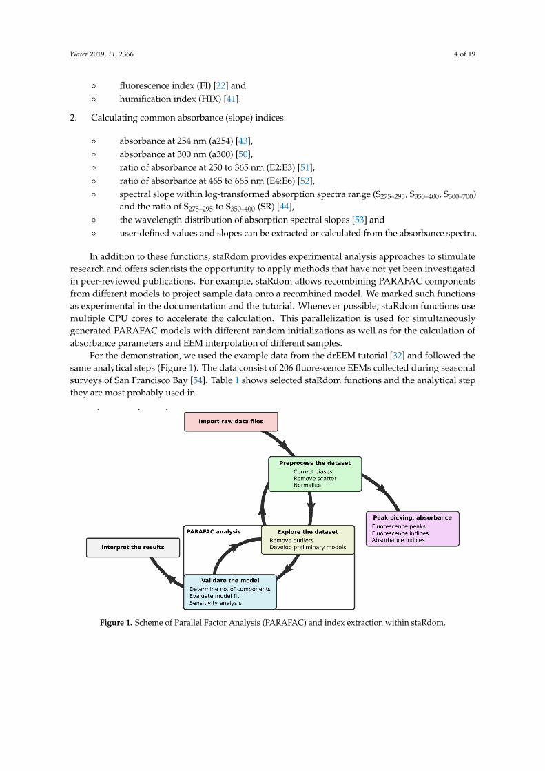
For the demonstration, we used the example data from the drEEM tutorial [32] and followed thesame analytical steps (Figure 1). The data consist of 206 fluorescence EEMs collected during seasonalsurveys of San Francisco Bay [54]. Table 1 shows selected staRdom functions and the analytical stepthey are most probably used in.
Water 2019, 11, x FOR PEER REVIEW 4 of 21
◦ absorbance at 254 nm (a254) [43], ◦ absorbance at 300 nm (a300) [50], ◦ ratio of absorbance at 250 to 365 nm (E2:E3) [51], ◦ ratio of absorbance at 465 to 665 nm (E4:E6) [52], ◦ spectral slope within log-transformed absorption spectra range (S275–295, S350–400, S300–700) and
the ratio of S275–295 to S350–400 (SR) [44], ◦ the wavelength distribution of absorption spectral slopes [53] and ◦ user-defined values and slopes can be extracted or calculated from the absorbance spectra.
In addition to these functions, staRdom provides experimental analysis approaches to stimulate research and offers scientists the opportunity to apply methods that have not yet been investigated in peer-reviewed publications. For example, staRdom allows recombining PARAFAC components from different models to project sample data onto a recombined model. We marked such functions as experimental in the documentation and the tutorial. Whenever possible, staRdom functions use multiple CPU cores to accelerate the calculation. This parallelization is used for simultaneously generated PARAFAC models with different random initializations as well as for the calculation of absorbance parameters and EEM interpolation of different samples.
For the demonstration, we used the example data from the drEEM tutorial [32] and followed the same analytical steps (Figure 1). The data consist of 206 fluorescence EEMs collected during seasonal surveys of San Francisco Bay [54]. Table 1 shows selected staRdom functions and the analytical step they are most probably used in.
Figure 1. Scheme of Parallel Factor Analysis (PARAFAC) and index extraction within staRdom.
Table 1. List of selected staRdom functions and the step of the analysis scheme (Figure 1) that are most probably used.
Step of the Analysis staRdom Functions
Used Purpose of the Function
import raw data eem_read load EEM data absorbance_read load absorbance data
check data consistency
eem_checkdata check presence and names of samples
view data ggeem create single plots eem_overview plot create multiple plots
correct biases abs_blcor absorbance baseline correction
Figure 1. Scheme of Parallel Factor Analysis (PARAFAC) and index extraction within staRdom.

Water 2019, 11, 2366 5 of 19
Table 1. List of selected staRdom functions and the step of the analysis scheme (Figure 1) that are mostprobably used.
Step of the Analysis staRdom Functions Used Purpose of the Function
import raw data eem_read load EEM dataabsorbance_read load absorbance data
check data consistency eem_checkdata check presence and names of samplesview data ggeem create single plots
eem_overview plot create multiple plotscorrect biases abs_blcor absorbance baseline correction
eem_spectral_cor EEM spectral correctioneem_remove_blank subtract blank sampleeem_ife_correction inner-filter effect correction
eem_raman_normalisation,eem_raman_normalisation2 normalize EEM data to Raman units
remove scatter eem_rem_scat remove Rayleigh and Raman scattering of 1st and2nd order
eem_setNA remove noise manuallyeem_interp interpolate missing data
synchronize sample wavelength eem_red2smallest remove all wavelengths that are not present in allsamples
eem_extend2largest create all wavelengths present in any sample in allsamples
correct for sample dilution eem_dilution multiply EEM data by a dilution factorsmooth data eem_smooth smooth EEM data
normalize no dedicated function, argument normalise= TRUE in eem_parafac normalize EEM data
eem_biological_index calculate BIXfluorescence peaks and indiceseem_coble_peaks calculate Coble peaks
eem_fluorescence_index calculate FIeem_humification_index calculate HIX
absorbance indices abs_parms calculate absorbance indices, spectral slopes, andselected ratios
calculate PARAFAC model(preliminary and final) eem_parafac calculate PARAFAC models
view PARAFAC models eempf_compare compare PARAFAC models (with different numbersof components) visually
eempf_comp_load_plot plot single PARAFAC modelsidentify outliers eempf_leverage calculate the leverage of each sample and wavelength
eempf_leverage_plot plot leverageseempf_leverage_ident manually select samples in leverage plots
remove outliers eem_exclude remove samples and wavelengths from the data setevaluate model eempf_convergence extract convergence behavior of a model
eempf_cortable, eempf_corplot show correlation between componentseempf_corcondia calculate the core consistency
sensitivity analysis splithalf, splithalf_plot calculate and plot a split-half validationinterpret the results eempf4analysis export table with component loadings
eempf_report create an analysis report in html formateempf_openfluor export data for openfluor.org
2.1. Data Import
In the first step, users import files written by the fluorometer into staRdom. Currently, staRdomcan read ASCII data from Cary Eclipse, Horiba Aqualog, Horiba Fluoromax-4, Shimadzu, and HitachiF-7000 as well as raw CSV-files.
For absorbance data import, data has to be provided by tables in CSV or TXT format(absorbance_read). A separate table containing dilution factors, Raman areas, or photometer pathlengthsfor each sample can be loaded to provide case-specific information in further analysis.
The function eem_checkdata checks for potential problems with the input data, such as missingdata in samples, duplicate or invalid sample names, wavelength mismatches, and missing samples ineither absorbance or fluorescence data. This data check does not change the original data but points atquestionable characteristics in the data set. This function can be applied at any time in the analysis toensure that the data is still coherent.
2.2. Data Preprocessing
staRdom partially applies functions from eemR [47] and uses additionally developed functions tocorrect EEM data and reduce noise in multiple ways. Here, we follow the same procedures used by

Water 2019, 11, 2366 6 of 19
drEEM as described in Reference [32]. In short, the data are corrected for instrument-specific errors,making spectra comparable among measurements on different instruments and at different time points.Spectral correction factors are used to remove effects of wavelength-dependent shifts of the light sourceor the emission detector (eem_spectral_cor). Raman normalization (eem_raman_normalisation) is appliedto remove instrument-dependent fluorescence intensity factors, such as different light source type,voltage, and light source age [45]. To produce linearity between sample fluorophore concentrationand its fluorescence, the effect of internal light absorbance of the sample, i.e., the inner-filter effect, isremoved (eem_ife_correction). To reduce or remove Rayleigh and Raman scatter a blank can be subtracted(eem_remove_blank) or the known area of the scattering can be removed specifically (eem_rem_scat). Inaddition, users can manually remove EEM data anywhere in the EEMs (eem_setNA). This may proveuseful if noise has been introduced by instrument errors and parts of EEM spectra should be removed.
Missing values produced by scatter or other EEM data removal can be interpolated with differentinterpolation options (eem_interp). The default method used in staRdom is the multilevel B-splineapproximation [55]. It is an accurate method to interpolate smooth but complex surfaces, whichis exactly, what one would expect from a theoretical EEM. We suggest interpolating missing datawhenever possible since the occurrence of non-converging models and models that converge in localminima has been shown to increase along with the proportion of missing values [56]. Therefore,eem_checkdata explicitly calculates the ratio of missing to nonmissing data to warn the user of thispotential risk. To ensure a convenient interpolation in many cases, staRdom offers five differentmethods for interpolation from which the user can choose. The available methods are filling missingvalues with zeros, spline interpolation [55], piecewise cubic hermitean interpolation polynomials inone and two dimensions [57] and linear interpolation. In case of an analysis covering samples ofdifferent origin, samples measured with different instrument settings or array detectors (as used in theHoriba Aqualog), wavelength pairs in the sample set must be synchronized. Synchronization can bedone by either reducing the data to wavelength pairs available in the whole set (eem_red2smallest) oradding and interpolating data that is missing in some samples but present in others (eem_extend2largest).Optionally, EEM data can be smoothed to stabilize results for calculations of fluorescence-based indices(eem_smooth). However, we do not recommend smoothing fluorescence EEM data before applyingPARAFAC. Finally, the dilution of samples can be reverted by applying a dilution factor, where a factorof 2 represents a 1:2 dilution (eem_dilution).
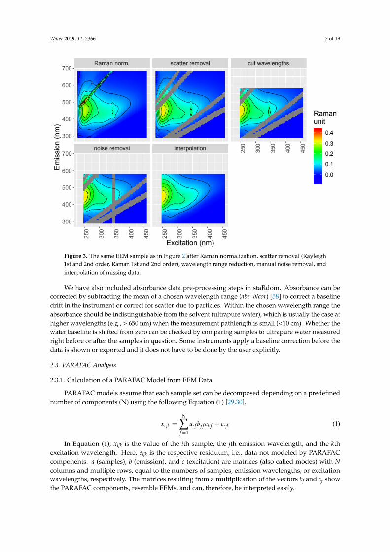
We applied the following corrections to the example data: spectral correction, blank correction,inner-filter effect correction (Figure 2); and subsequently Raman normalization, scatter removal,wavelength cutting to remove spectral parts with low information content and high instrument noise,and interpolation of cut parts (Figure 3).Water 2019, 11, x FOR PEER REVIEW 7 of 21
Figure 2. An excitation–emission matrices (EEM) sample as measured, untreated (original) and after spectral correction with correction factors, blank subtraction with ultra-pure water, and inner-filter effect correction using absorbance data.
Figure 3. The same EEM sample as in Figure 2 after Raman normalization, scatter removal (Rayleigh 1st and 2nd order, Raman 1st and 2nd order), wavelength range reduction, manual noise removal, and interpolation of missing data.
We have also included absorbance data pre-processing steps in staRdom. Absorbance can be corrected by subtracting the mean of a chosen wavelength range (abs_blcor) [58] to correct a baseline drift in the instrument or correct for scatter due to particles. Within the chosen wavelength range the absorbance should be indistinguishable from the solvent (ultrapure water), which is usually the case at higher wavelengths (e.g., > 650 nm) when the measurement pathlength is small (<10 cm). Whether the water baseline is shifted from zero can be checked by comparing samples to ultrapure water measured right before or after the samples in question. Some instruments apply a baseline correction before the data is shown or exported and it does not have to be done by the user explicitly.
Figure 2. An excitation–emission matrices (EEM) sample as measured, untreated (original) and afterspectral correction with correction factors, blank subtraction with ultra-pure water, and inner-filtereffect correction using absorbance data.
Water 2019, 11, 2366 7 of 19
Water 2019, 11, x FOR PEER REVIEW 7 of 21
Figure 2. An excitation–emission matrices (EEM) sample as measured, untreated (original) and after spectral correction with correction factors, blank subtraction with ultra-pure water, and inner-filter effect correction using absorbance data.
Figure 3. The same EEM sample as in Figure 2 after Raman normalization, scatter removal (Rayleigh 1st and 2nd order, Raman 1st and 2nd order), wavelength range reduction, manual noise removal, and interpolation of missing data.
We have also included absorbance data pre-processing steps in staRdom. Absorbance can be corrected by subtracting the mean of a chosen wavelength range (abs_blcor) [58] to correct a baseline drift in the instrument or correct for scatter due to particles. Within the chosen wavelength range the absorbance should be indistinguishable from the solvent (ultrapure water), which is usually the case at higher wavelengths (e.g., > 650 nm) when the measurement pathlength is small (<10 cm). Whether the water baseline is shifted from zero can be checked by comparing samples to ultrapure water measured right before or after the samples in question. Some instruments apply a baseline correction before the data is shown or exported and it does not have to be done by the user explicitly.
Figure 3. The same EEM sample as in Figure 2 after Raman normalization, scatter removal (Rayleigh1st and 2nd order, Raman 1st and 2nd order), wavelength range reduction, manual noise removal, andinterpolation of missing data.
We have also included absorbance data pre-processing steps in staRdom. Absorbance can becorrected by subtracting the mean of a chosen wavelength range (abs_blcor) [58] to correct a baselinedrift in the instrument or correct for scatter due to particles. Within the chosen wavelength range theabsorbance should be indistinguishable from the solvent (ultrapure water), which is usually the case athigher wavelengths (e.g., > 650 nm) when the measurement pathlength is small (<10 cm). Whether thewater baseline is shifted from zero can be checked by comparing samples to ultrapure water measuredright before or after the samples in question. Some instruments apply a baseline correction before thedata is shown or exported and it does not have to be done by the user explicitly.
2.3. PARAFAC Analysis
2.3.1. Calculation of a PARAFAC Model from EEM Data
PARAFAC models assume that each sample set can be decomposed depending on a predefinednumber of components (N) using the following Equation (1) [29,30].
xi jk =N∑
f=1
ai f b j f ck f + ei jk (1)
In Equation (1), xijk is the value of the ith sample, the jth emission wavelength, and the kthexcitation wavelength. Here, eijk is the respective residuum, i.e., data not modeled by PARAFACcomponents. a (samples), b (emission), and c (excitation) are matrices (also called modes) with Ncolumns and multiple rows, equal to the numbers of samples, emission wavelengths, or excitationwavelengths, respectively. The matrices resulting from a multiplication of the vectors bf and cf showthe PARAFAC components, resemble EEMs, and can, therefore, be interpreted easily.

Water 2019, 11, 2366 8 of 19
A PARAFAC model can be calculated using eem_parafac. At a minimum, users need to supply theEEM data and the number of components N. For each N, a model is calculated and the comparisonof peak shapes and model errors between multiple models can help finding the best solution.Optionally, the data can be normalized, which can be helpful if the samples span a wide rangeof DOC concentrations or if the components are highly correlated (see below). The model can beconstrained to non-negativity, smoothness, or unimodality for each mode. Since fluorescence is alwayspositive, non-negativity is commonly assumed for all modes [59]. The known shape of a fluorescencepeak is smooth in emission and excitation modes and unimodal in the emission mode. Unimodalityconstraints are not always used because PARAFAC models typically show plausible results using onlynon-negativity constraints (e.g., [20,32]). Still, imposed unimodality can improve the interpretability ofthe results (e.g., [60,61]). The PARAFAC algorithm uses randomly generated start values. The stepwiseleast-squares approximation can return invalid local minima of the sum-of-squared-error (SSE) insteadof the global minimum. To ensure that the global minimum is identified, several models are calculatedusing different random start values. The convergence tolerance can be set to provide an adjustabletrade-off between accuracy and speed.Water 2019, 11, x FOR PEER REVIEW 9 of 21
Figure 4. Comparing preliminary (outliers still included) and final models with 5 and 6 components. The components were normalized according to their maximum fluorescence (Fmax). Comp. = Component.
Plot functions can show the goodness of fit for the simultaneously calculated models and the components in two views, via matrix plots (Figure 4) and modes plots (not shown). Both are created using the function eempf_compare. These plots provide a quick overview on how well the model fits the data and how physically plausible the components are. Besides, different models can be compared visually. Studies describing shape characteristics of plausible fluorescence peaks [62] and peak shapes of pure substances can also be used to check for plausible shapes [63]. By plotting, different models can be compared visually. Certain model modes and components can also be plotted individually (eempf_comp_load_plot).
2.3.2. Identification of Outliers
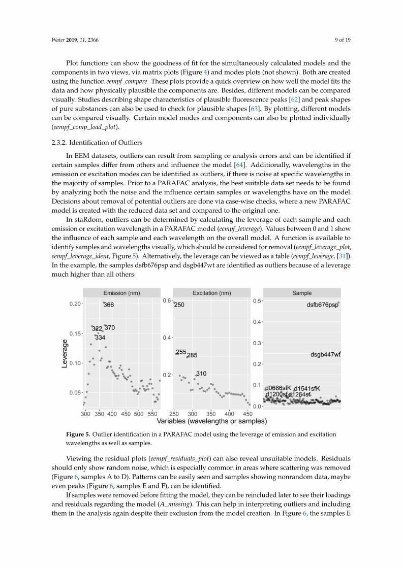
In EEM datasets, outliers can result from sampling or analysis errors and can be identified if certain samples differ from others and influence the model [64]. Additionally, wavelengths in the emission or excitation modes can be identified as outliers, if there is noise at specific wavelengths in the majority of samples. Prior to a PARAFAC analysis, the best suitable data set needs to be found
Figure 4. Comparing preliminary (outliers still included) and final models with 5 and 6 components. Thecomponents were normalized according to their maximum fluorescence (Fmax). Comp. = Component.
Water 2019, 11, 2366 9 of 19
Plot functions can show the goodness of fit for the simultaneously calculated models and thecomponents in two views, via matrix plots (Figure 4) and modes plots (not shown). Both are createdusing the function eempf_compare. These plots provide a quick overview on how well the model fits thedata and how physically plausible the components are. Besides, different models can be comparedvisually. Studies describing shape characteristics of plausible fluorescence peaks [62] and peak shapesof pure substances can also be used to check for plausible shapes [63]. By plotting, different modelscan be compared visually. Certain model modes and components can also be plotted individually(eempf_comp_load_plot).
2.3.2. Identification of Outliers
In EEM datasets, outliers can result from sampling or analysis errors and can be identified ifcertain samples differ from others and influence the model [64]. Additionally, wavelengths in theemission or excitation modes can be identified as outliers, if there is noise at specific wavelengths inthe majority of samples. Prior to a PARAFAC analysis, the best suitable data set needs to be foundby analyzing both the noise and the influence certain samples or wavelengths have on the model.Decisions about removal of potential outliers are done via case-wise checks, where a new PARAFACmodel is created with the reduced data set and compared to the original one.
In staRdom, outliers can be determined by calculating the leverage of each sample and eachemission or excitation wavelength in a PARAFAC model (eempf_leverage). Values between 0 and 1 showthe influence of each sample and each wavelength on the overall model. A function is available toidentify samples and wavelengths visually, which should be considered for removal (eempf_leverage_plot,eempf_leverage_ident, Figure 5). Alternatively, the leverage can be viewed as a table (eempf_leverage, [31]).In the example, the samples dsfb676psp and dsgb447wt are identified as outliers because of a leveragemuch higher than all others.
Water 2019, 11, x FOR PEER REVIEW 10 of 21
by analyzing both the noise and the influence certain samples or wavelengths have on the model. Decisions about removal of potential outliers are done via case-wise checks, where a new PARAFAC model is created with the reduced data set and compared to the original one.
In staRdom, outliers can be determined by calculating the leverage of each sample and each emission or excitation wavelength in a PARAFAC model (eempf_leverage). Values between 0 and 1 show the influence of each sample and each wavelength on the overall model. A function is available to identify samples and wavelengths visually, which should be considered for removal (eempf_leverage_plot, eempf_leverage_ident, Figure 5). Alternatively, the leverage can be viewed as a table (eempf_leverage, [31]). In the example, the samples dsfb676psp and dsgb447wt are identified as outliers because of a leverage much higher than all others.
Figure 5. Outlier identification in a PARAFAC model using the leverage of emission and excitation wavelengths as well as samples.
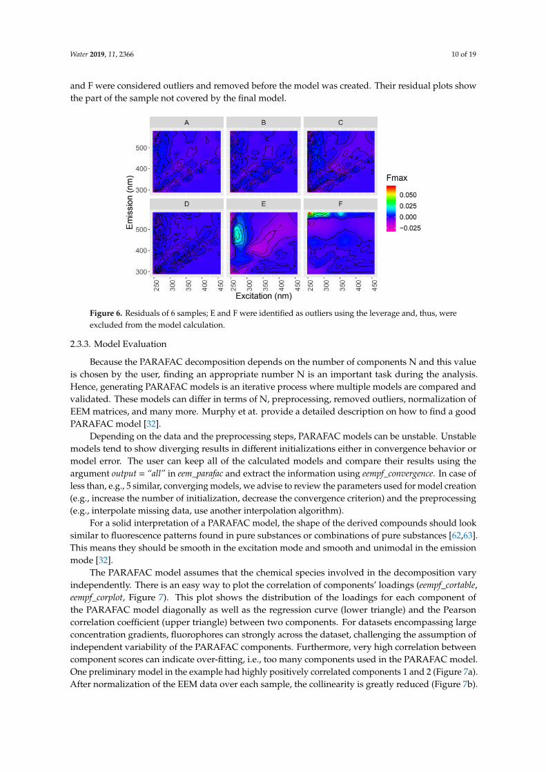
Viewing the residual plots (eempf_residuals_plot) can also reveal unsuitable models. Residuals should only show random noise, which is especially common in areas where scattering was removed (Figure 6, samples A to D). Patterns can be easily seen and samples showing nonrandom data, maybe even peaks (Figure 6, samples E and F), can be identified.
Figure 5. Outlier identification in a PARAFAC model using the leverage of emission and excitationwavelengths as well as samples.
Viewing the residual plots (eempf_residuals_plot) can also reveal unsuitable models. Residualsshould only show random noise, which is especially common in areas where scattering was removed(Figure 6, samples A to D). Patterns can be easily seen and samples showing nonrandom data, maybeeven peaks (Figure 6, samples E and F), can be identified.
If samples were removed before fitting the model, they can be reincluded later to see their loadingsand residuals regarding the model (A_missing). This can help in interpreting outliers and includingthem in the analysis again despite their exclusion from the model creation. In Figure 6, the samples E
Water 2019, 11, 2366 10 of 19
and F were considered outliers and removed before the model was created. Their residual plots showthe part of the sample not covered by the final model.
Water 2019, 11, x FOR PEER REVIEW 10 of 21
by analyzing both the noise and the influence certain samples or wavelengths have on the model. Decisions about removal of potential outliers are done via case-wise checks, where a new PARAFAC model is created with the reduced data set and compared to the original one.
In staRdom, outliers can be determined by calculating the leverage of each sample and each emission or excitation wavelength in a PARAFAC model (eempf_leverage). Values between 0 and 1 show the influence of each sample and each wavelength on the overall model. A function is available to identify samples and wavelengths visually, which should be considered for removal (eempf_leverage_plot, eempf_leverage_ident, Figure 5). Alternatively, the leverage can be viewed as a table (eempf_leverage, [31]). In the example, the samples dsfb676psp and dsgb447wt are identified as outliers because of a leverage much higher than all others.
Figure 5. Outlier identification in a PARAFAC model using the leverage of emission and excitation wavelengths as well as samples.
Viewing the residual plots (eempf_residuals_plot) can also reveal unsuitable models. Residuals should only show random noise, which is especially common in areas where scattering was removed (Figure 6, samples A to D). Patterns can be easily seen and samples showing nonrandom data, maybe even peaks (Figure 6, samples E and F), can be identified.
Figure 6. Residuals of 6 samples; E and F were identified as outliers using the leverage and, thus, wereexcluded from the model calculation.
2.3.3. Model Evaluation
Because the PARAFAC decomposition depends on the number of components N and this valueis chosen by the user, finding an appropriate number N is an important task during the analysis.Hence, generating PARAFAC models is an iterative process where multiple models are compared andvalidated. These models can differ in terms of N, preprocessing, removed outliers, normalization ofEEM matrices, and many more. Murphy et at. provide a detailed description on how to find a goodPARAFAC model [32].
Depending on the data and the preprocessing steps, PARAFAC models can be unstable. Unstablemodels tend to show diverging results in different initializations either in convergence behavior ormodel error. The user can keep all of the calculated models and compare their results using theargument output = “all” in eem_parafac and extract the information using eempf_convergence. In case ofless than, e.g., 5 similar, converging models, we advise to review the parameters used for model creation(e.g., increase the number of initialization, decrease the convergence criterion) and the preprocessing(e.g., interpolate missing data, use another interpolation algorithm).
For a solid interpretation of a PARAFAC model, the shape of the derived compounds should looksimilar to fluorescence patterns found in pure substances or combinations of pure substances [62,63].This means they should be smooth in the excitation mode and smooth and unimodal in the emissionmode [32].
The PARAFAC model assumes that the chemical species involved in the decomposition varyindependently. There is an easy way to plot the correlation of components’ loadings (eempf_cortable,eempf_corplot, Figure 7). This plot shows the distribution of the loadings for each component ofthe PARAFAC model diagonally as well as the regression curve (lower triangle) and the Pearsoncorrelation coefficient (upper triangle) between two components. For datasets encompassing largeconcentration gradients, fluorophores can strongly across the dataset, challenging the assumption ofindependent variability of the PARAFAC components. Furthermore, very high correlation betweencomponent scores can indicate over-fitting, i.e., too many components used in the PARAFAC model.One preliminary model in the example had highly positively correlated components 1 and 2 (Figure 7a).After normalization of the EEM data over each sample, the collinearity is greatly reduced (Figure 7b).

Water 2019, 11, 2366 11 of 19Water 2019, 11, x FOR PEER REVIEW 12 of 21
Figure 7. Components’ loadings from PARAFAC models (a) without and (b) with previous normalization. Diagonally: distributions of the loadings; lower triangle: regression curve between components; and upper triangle: Pearson correlation coefficient between components.
The models are validated using a split-half validation, which is a specific method of cross-validation [32]. A robust model validation requires enough samples (depending on the data approximately 100–200 samples). Split-half validation is realized with the splithalf function in staRdom. Here, models are compared based on different subsets of the original data. The implemented test uses 4 splits, 6 combinations, and 3 tests (S4C6T3): the data are split into four subsets (A, B, C, and D) and recombined to compare one half of the data to the other in different combinations (AB–CD, AD–BC, AC–BD) [32]. The comparison is done visually by plots showing the spectral loadings (splithalf_plot, Figure 8) and by calculating Tucker’s congruence coefficient [65] (TCC) or shift- and shape-sensitive congruence [66] (SSC, splithalf_tcc). Subsets can be automatically generated or manually defined.
Figure 8. Split-half validation of a PARAFAC model. Emission spectra: full line; excitation spectra: dashed line; colors according to models using different sample sub-sets.
The quality of a PARAFAC model can also be tested using the core consistency (eempf_corcondia) [67]. Models specified with an appropriate number of components should have high core consistencies (near 100%), whereas low core consistencies indicate that too many components were specified. The core consistency diagnostic should protect against over-fitting but rigid adherence to guidelines can lead to under-fitted models. For real-life fluorescence datasets, it has been suggested
Figure 7. Components’ loadings from PARAFAC models (a) without and (b) with previousnormalization. Diagonally: distributions of the loadings; lower triangle: regression curve betweencomponents; and upper triangle: Pearson correlation coefficient between components.
The models are validated using a split-half validation, which is a specific method ofcross-validation [32]. A robust model validation requires enough samples (depending on the dataapproximately 100–200 samples). Split-half validation is realized with the splithalf function in staRdom.Here, models are compared based on different subsets of the original data. The implemented test uses4 splits, 6 combinations, and 3 tests (S4C6T3): the data are split into four subsets (A, B, C, and D) andrecombined to compare one half of the data to the other in different combinations (AB–CD, AD–BC,AC–BD) [32]. The comparison is done visually by plots showing the spectral loadings (splithalf_plot,Figure 8) and by calculating Tucker’s congruence coefficient [65] (TCC) or shift- and shape-sensitivecongruence [66] (SSC, splithalf_tcc). Subsets can be automatically generated or manually defined.
Water 2019, 11, x FOR PEER REVIEW 12 of 21
Figure 7. Components’ loadings from PARAFAC models (a) without and (b) with previous normalization. Diagonally: distributions of the loadings; lower triangle: regression curve between components; and upper triangle: Pearson correlation coefficient between components.
The models are validated using a split-half validation, which is a specific method of cross-validation [32]. A robust model validation requires enough samples (depending on the data approximately 100–200 samples). Split-half validation is realized with the splithalf function in staRdom. Here, models are compared based on different subsets of the original data. The implemented test uses 4 splits, 6 combinations, and 3 tests (S4C6T3): the data are split into four subsets (A, B, C, and D) and recombined to compare one half of the data to the other in different combinations (AB–CD, AD–BC, AC–BD) [32]. The comparison is done visually by plots showing the spectral loadings (splithalf_plot, Figure 8) and by calculating Tucker’s congruence coefficient [65] (TCC) or shift- and shape-sensitive congruence [66] (SSC, splithalf_tcc). Subsets can be automatically generated or manually defined.
Figure 8. Split-half validation of a PARAFAC model. Emission spectra: full line; excitation spectra: dashed line; colors according to models using different sample sub-sets.
The quality of a PARAFAC model can also be tested using the core consistency (eempf_corcondia) [67]. Models specified with an appropriate number of components should have high core consistencies (near 100%), whereas low core consistencies indicate that too many components were specified. The core consistency diagnostic should protect against over-fitting but rigid adherence to guidelines can lead to under-fitted models. For real-life fluorescence datasets, it has been suggested
Figure 8. Split-half validation of a PARAFAC model. Emission spectra: full line; excitation spectra:dashed line; colors according to models using different sample sub-sets.
The quality of a PARAFAC model can also be tested using the core consistency (eempf_corcondia) [67].Models specified with an appropriate number of components should have high core consistencies (near100%), whereas low core consistencies indicate that too many components were specified. The coreconsistency diagnostic should protect against over-fitting but rigid adherence to guidelines can lead tounder-fitted models. For real-life fluorescence datasets, it has been suggested that the core consistencydiagnostic is overly severe [31]. Further research is needed to establish the utility of the core-consistencydiagnostic for validating PARAFAC models of natural organic matter EEMs.
2.4. Export and Further Interpretation of Results
For further analysis and interpretation, staRdom offers a table containing the loadings of eachcomponent per sample (eempf4analysis). Peaks and indices from EEM data can be included in this table.

Water 2019, 11, 2366 12 of 19
PARAFAC models can be exported to a file and uploaded to openfluor.org (eempf_openfluor) [48].By doing that, a comparison to published and partly peer-reviewed models is possible and can help ininterpreting the results.
An overview of a model optionally including information, such as applied correction methods,leverages and split-half validation, can be written as an HTML file (eempf_report).
2.5. Toolbox Comparison
We compared the results from multiple PARAFAC models using staRdom (PARAFAC modelcalculated by the multiway package) and drEEM (PARAFAC model calculated by the N-way toolbox).The models were derived from four published datasets, which comprised of marine, lake, and streamsamples from different areas and climate zones and were measured on different instruments fromdifferent ecosystems and/or from different landscapes. Additionally, two datasets consisting of purefluorophore spectra were compared (Table 2).
For each dataset, 3000 PARAFAC models were calculated with convergence criteria varyingbetween 1 × 10⁻⁶ and 1 × 10⁻⁹ for drEEM and between 1 × 10⁻⁸ and 1 × 10⁻¹¹ for staRdom, in steps of1 × 10−1. Different convergence criteria were necessary because the toolboxes use different methodsto monitor convergence, as shown in Equations (2) and (3). Due to this difference, when identicalconvergence criteria are supplied in the function inputs to both staRdom and drEEM, then drEEMreturn models with a smaller modeling error.
staRdom:(SSEn − SSEn−1)∑
X2 ≤ crit (2)
drEEM:(SSEn − SSEn−1)
SSEn≤ crit (3)
SSEn—sum-of-squared-error of nth iterationX—EEM datacrit—convergence criterionFor both toolboxes, the maximum number of iterations was set to 2500, and non-negativity
constraints were applied in all modes. The time until convergence (TUC) was measured by initializing atimer function just before each call to the PARAFAC function and stopping it just after completion of eachcall to the respective PARAFAC functions. The remaining model metrics were supplied by the respectivetoolboxes and included the number of iterations until convergence, and the sum-of-squared-error (SSE)of each model. Lastly, the number of models that reached the iteration limit or stopped due to otherreasons before convergence was compared.
To show the influence of the number of random initializations we used a Monte-Carlo simulation,i.e., the respective number of models was picked from the whole set of models 5000 times randomlyfor each data set and convergence criterion. The sum of TUC of the models in a subset was consideredto equal the calculation time of a set under realistic conditions running on a single CPU core. The bestmodel per subset was used as a representative for this set, to mimic a standard analysis. From withinall models of each data set, the one with the least SSE was used as a reference for model quality.We calculated the TCC to compare each of them with the best models [48]. The TCC is a parameterfor assessing similarity between pairs of fluorescence excitation and emission spectra and rangesbetween 0 (totally different) to 1 (identical). The 99% quantile of SSE within all model subsets with thesame convergence criterion and the same number of initializations was considered being the accuracythat can be achieved using exactly these conditions. Model parameters were accepted as sufficientlyaccurate if the TCCs of all components were at least 0.999. The TCC is a parameter for model similaritybetween 0 (totally different) to 1 (identical). In comparisons between different studies a TCC of 0.95 isconsidered to show a good similarity between two components [48].

Water 2019, 11, 2366 13 of 19
Table 2. Test datasets and important characteristics.
NameNumber of %
Description ReferenceComps 1 Samples Em 2 Ex 3 NA 4
Amino3 3 5 201 61 0 Pure amino acids [31]
Fjord6 6 191 91 44 16.6 Solid-phase extracts of DOMfrom three arctic fjords [68]
Headwater4 4 235 151 43 0Headwater streams, andagricultural catchments,Denmark and Uruguay
[20]
PortSurvey6 6 206 73 42 9.5port and oceanic marine samples
(USA, Pacific coast), drEEMtutorial dataset
[54]
Pure5 5 60 50 40 0 Pure substances with addedartificial noise unpublished
RioEx4 4 58 97 111 0 Photodegradation experiment ofsolid-phase extracted DOM [69]
1 components of the PARAFAC model, 2 emission wavelengths, 3 excitation wavelengths, 4 missing data.
3. Results and Discussion
For five of the six tested datasets, PARAFAC models obtained from both toolboxes were highlysimilar to the best solution with TCCs of at least 0.999 in scores and loadings. For one of the datasets(Fjord6), no convergent models were obtained using staRdom; possible reasons and solutions for thisare missing data (see Section 3.3). Both software tools required different considerations regardingmodel parameters (Figure 9 and Table 3). As such, we identified the convergence criterion, the numberof random initializations and susceptibility toward missing data as important factors during thecomparison of staRdom and drEEM. The impacts of different model parameters on the results arehighly dependent on the data set. In the following, we address particularities and provide suggestionsfor smooth practical work and mitigations of possible problems.Water 2019, 11, x FOR PEER REVIEW 15 of 21
Figure 9. Similarity of PARAFAC models derived using staRdom and drEEM, using different numbers of random initializations and different convergence criteria. Similarity is measured as minimum TCC: the higher the TCC, the more similar are the components.
Table 3. Summary of test performance for five datasets that produced convergent PARAFAC models.
Name Software Convergence Criterion
Initializations Relative error
Minimum TCC
Amino3 staRdom 1 × 10⁻⁸ 10 1.000069 1.0000 drEEM 1 × 10⁻⁸ 10 1.000000 1.0000
Headwater4 staRdom 1 × 10⁻⁹ 10 1.000010 1.0000 drEEM 1 × 10⁻⁷ 10 1.000002 1.0000
PortSurvey6 staRdom 1 × 10⁻¹¹ 30 1.000042 0.9997 drEEM 1 × 10⁻⁷ 10 1.000039 0.9997
Pure5 staRdom 1 × 10⁻¹⁰ 40 1.000071 0.9993
drEEM 1 × 10⁻⁷ 10 1.000056 0.9993
RioEx4 staRdom 1 × 10⁻¹⁰ 30 1.000022 0.9999
drEEM 1 × 10⁻⁷ 20 1.000015 1.0000
3.1. Number of Initializations
Implementing repeated starts of PARAFAC models under identical conditions but with different (random) starting values is common practice to identify a robust least-squares solution. If an
Figure 9. Similarity of PARAFAC models derived using staRdom and drEEM, using different numbersof random initializations and different convergence criteria. Similarity is measured as minimum TCC:the higher the TCC, the more similar are the components.

Water 2019, 11, 2366 14 of 19
Table 3. Summary of test performance for five datasets that produced convergent PARAFAC models.
Name Software ConvergenceCriterion Initializations Relative Error Minimum
TCC
Amino3staRdom 1 × 10⁻⁸ 10 1.000069 1.0000drEEM 1 × 10⁻⁸ 10 1.000000 1.0000
Headwater4staRdom 1 × 10⁻⁹ 10 1.000010 1.0000drEEM 1 × 10⁻⁷ 10 1.000002 1.0000
PortSurvey6 staRdom 1 × 10⁻¹¹ 30 1.000042 0.9997drEEM 1 × 10⁻⁷ 10 1.000039 0.9997
Pure5staRdom 1 × 10⁻¹⁰ 40 1.000071 0.9993drEEM 1 × 10⁻⁷ 10 1.000056 0.9993
RioEx4staRdom 1 × 10⁻¹⁰ 30 1.000022 0.9999drEEM 1 × 10⁻⁷ 20 1.000015 1.0000
3.1. Number of Initializations
Implementing repeated starts of PARAFAC models under identical conditions but with different(random) starting values is common practice to identify a robust least-squares solution. If an insufficientnumber of random initializations is used, a local minimum solution may be identified instead of theglobal least-squares solution.
Our analysis showed good results with staRdom for five datasets assuming 40 initializations(Figure 9). This indicates that it is preferable to start at least 40 models in order to obtain a solution thatis sufficiently stable and close to the global minimum of the PARAFAC modeling error. Users shouldmonitor the error of all solutions and increase the number of random starts, if the best solution is farbetter than the others.
However, an issue was sometimes encountered whereby a proportion of models did not converge.Except in the case of the Fjord6 dataset, multiple convergent solutions were obtained using staRdom anda reasonable model could be obtained from within the subset of models that converged. As a solutionfor slow and incomplete convergence, Reference [56] demonstrated the interpolation of missing data.
staRdom monitors the number of models that converged within the specified number of iterations.By adding the argument output = “all” in the function eem_parafac, eempf_convergence can providedetailed information on the convergence behavior of the model. As a general precaution, eem_parafacalways informs the user if less than 50% of models converged. In response, users can either increasethe number of random starts or specify that models should be calculated until a specified number ofconvergent models have been produced (strictly_converging = TRUE in eem_parafac). This functionwas not applied in the demonstration and the number of models shown in the results containboth convergent and nonconvergent models. drEEM does not currently provide a similar functionfor tracking nonconvergence, but nonconvergence appeared to occur less frequently analyzing thedescribed data sets.
3.2. Convergence Criterion
For the datasets we investigated, staRdom provided a similar modeling error as drEEM as long asthe convergence criterion was increased by two to three orders of magnitude (Figure 9 and Table 3).Therefore, the default convergence criteria are 1 × 10⁻⁶ in drEEM and 1 × 10⁻⁸ in staRdom. As theresults in this study are based on model errors, these differences do not further influence any results ofthe shown PARAFAC models.
3.3. Influence of Missing Data
Only two of the six test datasets (Fjord6 and PortSurvey6) contained missing data correspondingto regions of Rayleigh and Raman scatter, while the remaining datasets were interpolated prior toPARAFAC modeling. It seems likely that for the Fjord6 dataset, a relatively large proportion of missingnumbers (16.6% missing) was a causal or contributing factor explaining why staRdom did not reach

Water 2019, 11, 2366 15 of 19
convergence prior to the maximum number of iterations. It appears that staRdom may be moresensitive to missing data than drEEM, although further tests are needed to determine if this is the case.
Previous studies have shown that missing data should generally be interpolated in order to avoidlocal minima [56]. In order to obtain robust results, we stress the advantage of interpolating areasof Rayleigh and Raman scatter. To support users in finding an interpolation leading to a reasonablePARAFAC model, staRdom offers five different interpolation methods (see Section 2.2). Future studiesand developments in the multiway package should address this issue to improve the convergencebehavior where interpolation is no option for mitigation.
3.4. Time until Model Convergence
Since PARAFAC modeling of large datasets can be time-consuming, the time elapsed until modelconvergence (using parameters as stated in Table 3) using three common CPU architectures (introduced2013–2017) was compared. For both toolboxes, the algorithms reached convergence within similartimespans, even in cases where staRdom calculated with a higher number of initializations (Figure A1).Comparing time elapsed for the oldest to the newest CPU model gives an idea of how modeling speedis affected by improvements in hardware. For the computers tested in this study, improvements inCPU reduced the time until convergence by approximately 50% in MATLAB and 20% in R.
3.5. Outlier Calculation and Split-Half Validation
Both, the outlier identification [31] and the split-half analysis [49] rely on a PARAFAC model.The approaches applied after the PARAFAC algorithm are implemented identically in staRdom anddrEEM, so we limited our tests on the PortSurvey6 dataset only.
For the PortSurvey6 data, outlier identification (Figure 5) and split-half analyses (Figure 8)produced essentially identical outputs using either staRdom or drEEM.
4. Conclusions
We introduced “staRdom”, a new toolbox for the analysis of absorbance spectra and fluorescenceEEMs using the R statistical computing environment. Data preprocessing steps and routines in staRdomare for the most part identical to those available in the established drEEM toolbox for MATLAB.Results from both toolboxes are interchangeable apart from datasets with a relatively high fractionof missing data. The availability of multiway analysis tools in the free R software environment willreduce barriers in spectroscopic research and stimulate advances in DOM biogeochemistry for naturaland engineered systems.
Supplementary Materials: The following are available online at http://www.mdpi.com/2073-4441/11/11/2366/s1,Document D1: Correcting raw data, calculating peaks and indices in EEMS and absorbance (slope) parameters,Document D2: PARAFAC analysis of EEM data to separate DOM components.
Author Contributions: Conceptualization, M.P. and D.G.; methodology, M.P., D.G., U.W., and K.M.; software, M.P.;validation, K.M., G.W., and T.H.; formal analysis, M.P., U.W., and K.M.; investigation, K.M. and D.G.; resources,G.W. and T.H.; data curation, M.P.; writing—original draft preparation, M.P.; writing—review and editing, M.P.,G.W., K.M., U.W., T.H., and D.G.; visualization, M.P.; supervision, D.G. and T.H.; project administration, G.W.;funding acquisition, G.W.
Funding: This research was funded by the Provincial Government of Lower Austria, Nö Forschungs- undBildungs GmbH, within the Science Call 2015 (SC15-002, project ORCA). K.R.M. and U.J.W. acknowledge fundingfrom the Swedish Research Council (FORMAS 2017-00743). M.P. acknowledges funding from the doctoral schoolHuman River Systems in the 21st century (HR21).
Acknowledgments: A very important part of this work was the feedback from users that were interested anddedicated at an early stage already. We would like to thank especially Stefan Preiner, Astrid Harjung, RenataPinto, Ching-Hsuang Lo, Alexandra Tiefenbacher, and Gerardo Gold-Bouchot for testing, asking, and stimulatingthe development. Nora and Christoph Zechmeister contributed to the staRdom logo used in the tutorials.
Conflicts of Interest: The authors declare no conflict of interest. The funders had no role in the design of thestudy; in the collection, analyses, or interpretation of data; in the writing of the manuscript; or in the decision topublish the results.

Water 2019, 11, 2366 16 of 19
Appendix AWater 2019, 11, x FOR PEER REVIEW 18 of 21
Figure A1. Distributions of calculation times for models of five datasets, using staRdom and drEEM on different CPU architectures (CPU speed improves from left to right), with the model specifications defined in Table 3.
References
1 Findlay, S.; Sinsabaugh, R.L. Aquatic Ecosystems: Interactivity of Dissolved Organic Matter; Academic Press: Amsterdam, The Netherlands; Boston, MA, USA, 2003; ISBN 978-0-08-052754-3.
2 Niño-García, J.P.; Ruiz-González, C.; del Giorgio, P.A. Interactions between hydrology and water chemistry shape bacterioplankton biogeography across boreal freshwater networks. ISME J. 2016, 10, 1755–1766.
3 Besemer, K.; Luef, B.; Preiner, S.; Eichberger, B.; Agis, M.; Peduzzi, P. Sources and composition of organic matter for bacterial growth in a large European river floodplain system (Danube, Austria). Org. Geochem. 2009, 40, 321–331.
4 Amaral, V.; Graeber, D.; Calliari, D.; Alonso, C. Strong linkages between DOM optical properties and main clades of aquatic bacteria. Limnol. Oceanogr. 2016, 61, 906–918.
5 Tranvik, L.J. Allochthonous dissolved organic matter as an energy source for pelagic bacteria and the concept of the microbial loop. In Dissolved Organic Matter in Lacustrine Ecosystems: Energy Source and System Regulator; Salonen, K., Kairesalo, T., Jones, R.I., Eds.; Developments in Hydrobiology; Springer Netherlands: Dordrecht, The Netherlands, 1992; pp. 107–114, ISBN 978-94-011-2474-4.
6 Morris, D.P.; Zagarese, H.; Williamson, C.E.; Balseiro, E.G.; Hargreaves, B.R.; Modenutti, B.; Moeller, R.; Queimalinos, C. The attenuation of solar UV radiation in lakes and the role of dissolved organic carbon. Limnol. Oceanogr. 1995, 40, 1381–1391.
Figure A1. Distributions of calculation times for models of five datasets, using staRdom and drEEMon different CPU architectures (CPU speed improves from left to right), with the model specificationsdefined in Table 3.
References
1. Findlay, S.; Sinsabaugh, R.L. Aquatic Ecosystems: Interactivity of Dissolved Organic Matter; Academic Press:Amsterdam, The Netherlands; Boston, MA, USA, 2003; ISBN 978-0-08-052754-3.
2. Niño-García, J.P.; Ruiz-González, C.; del Giorgio, P.A. Interactions between hydrology and water chemistryshape bacterioplankton biogeography across boreal freshwater networks. ISME J. 2016, 10, 1755–1766.[CrossRef] [PubMed]
3. Besemer, K.; Luef, B.; Preiner, S.; Eichberger, B.; Agis, M.; Peduzzi, P. Sources and composition of organicmatter for bacterial growth in a large European river floodplain system (Danube, Austria). Org. Geochem.2009, 40, 321–331. [CrossRef] [PubMed]
4. Amaral, V.; Graeber, D.; Calliari, D.; Alonso, C. Strong linkages between DOM optical properties and mainclades of aquatic bacteria. Limnol. Oceanogr. 2016, 61, 906–918. [CrossRef]
5. Tranvik, L.J. Allochthonous dissolved organic matter as an energy source for pelagic bacteria and the conceptof the microbial loop. In Dissolved Organic Matter in Lacustrine Ecosystems: Energy Source and System Regulator;Salonen, K., Kairesalo, T., Jones, R.I., Eds.; Developments in Hydrobiology; Springer Netherlands: Dordrecht,The Netherlands, 1992; pp. 107–114. ISBN 978-94-011-2474-4.
6. Morris, D.P.; Zagarese, H.; Williamson, C.E.; Balseiro, E.G.; Hargreaves, B.R.; Modenutti, B.; Moeller, R.;Queimalinos, C. The attenuation of solar UV radiation in lakes and the role of dissolved organic carbon.Limnol. Oceanogr. 1995, 40, 1381–1391. [CrossRef]

Water 2019, 11, 2366 17 of 19
7. Fiedler, D.; Graeber, D.; Badrian, M.; Köhler, J. Growth response of four freshwater algal species to dissolvedorganic nitrogen of different concentration and complexity. Freshw. Biol. 2015, 60, 1613–1621. [CrossRef]
8. Amon, R.M.W.; Benner, R. Bacterial utilization of different size classes of dissolved organic matter.Limnol. Oceanogr. 1996, 41, 41–51. [CrossRef]
9. Benner, R.; Biddanda, B. Photochemical transformations of surface and deep marine dissolved organic matter:Effects on bacterial growth. Limnol. Oceanogr. 1998, 43, 1373–1378. [CrossRef]
10. Benner, R. 5-Molecular Indicators of the Bioavailability of Dissolved Organic Matter. In Aquatic Ecosystems;Findlay, S.E.G., Sinsabaugh, R.L., Eds.; Aquatic Ecology; Academic Press: Burlington, ON, Canada, 2003;pp. 121–137. ISBN 978-0-12-256371-3.
11. Babin, M.; Stramski, D.; Ferrari, G.M.; Claustre, H.; Bricaud, A.; Obolensky, G.; Hoepffner, N. Variations inthe light absorption coefficients of phytoplankton, nonalgal particles, and dissolved organic matter in coastalwaters around Europe. J. Geophys. Res. Oceans 2003, 108. [CrossRef]
12. Taylor, P.G.; Townsend, A.R. Stoichiometric control of organic carbon–nitrate relationships from soils to thesea. Nature 2010, 464, 1178. [CrossRef] [PubMed]
13. Wymore, A.S.; Coble, A.A.; Rodríguez-Cardona, B.; McDowell, W.H. Nitrate uptake across biomes and theinfluence of elemental stoichiometry: A new look at LINX II. Global Biogeochem. Cycles 2016, 30, 1183–1191.[CrossRef]
14. Bejarano, A.C.; Chandler, G.T.; Decho, A.W. Influence of natural dissolved organic matter (DOM) on acuteand chronic toxicity of the pesticides chlorothalonil, chlorpyrifos and fipronil on the meiobenthic estuarinecopepod Amphiascus tenuiremis. J. Exp. Mar. Biol. Ecol. 2005, 321, 43–57. [CrossRef]
15. Stedmon, C.A.; Markager, S.; Bro, R. Tracing dissolved organic matter in aquatic environments using a newapproach to fluorescence spectroscopy. Mar. Chem. 2003, 82, 239–254. [CrossRef]
16. Gabor, R.; Baker, A.; McKnight, D.M.; Miller, M. Fluorescence indices and their interpretation. In AquaticOrganic Matter Fluorescence; Cambridge Environmental Chemistry Series; Cambridge University Press:Cambridge, UK, 2014; pp. 303–338.
17. Senesi, N.; Miano, T.M.; Provenzano, M.R. Fluorescence spectroscopy as a means of distinguishing fulvicand humic acids from dissolved and sedimentary aquatic sources and terrestrial sources. In Proceedingsof the Humic Substances in the Aquatic and Terrestrial Environment, Linköping, Sweden, 21–23 August1989; Allard, B., Borén, H., Grimvall, A., Eds.; Springer Berlin Heidelberg: Berlin/Heidelberg, Germany, 1991;pp. 63–73.
18. Stubbins, A.; Lapierre, J.-F.; Berggren, M.; Prairie, Y.T.; Dittmar, T.; del Giorgio, P.A. What’s in an EEM?Molecular Signatures Associated with Dissolved Organic Fluorescence in Boreal Canada. Environ. Sci. Technol.2014, 48, 10598–10606. [CrossRef] [PubMed]
19. Herzsprung, P.; Osterloh, K.; von Tümpling, W.; Harir, M.; Hertkorn, N.; Schmitt-Kopplin, P.; Meissner, R.;Bernsdorf, S.; Friese, K. Differences in DOM of rewetted and natural peatlands - Results from high-fieldFT-ICR-MS and bulk optical parameters. Sci. Total Environ. 2017, 586, 770–781. [CrossRef] [PubMed]
20. Graeber, D.; Boëchat, I.G.; Encina-Montoya, F.; Esse, C.; Gelbrecht, J.; Goyenola, G.; Gücker, B.; Heinz, M.;Kronvang, B.; Meerhoff, M.; et al. Global effects of agriculture on fluvial dissolved organic matter. Sci. Rep.2015, 5, 16328. [CrossRef] [PubMed]
21. Graeber, D.; Lorenz, S.; Poulsen, J.R.; Heinz, M.; von Schiller, D.; Gücker, B.; Gelbrecht, J.; Kronvang, B.Assessing net-uptake of nitrate and natural dissolved organic matter fractions in a revitalized lowland streamreach. Limnologica 2018, 68, 82–91. [CrossRef]
22. McKnight, D.M.; Boyer, E.W.; Westerhoff, P.K.; Doran, P.T.; Kulbe, T.; Andersen, D.T. Spectrofluorometriccharacterization of dissolved organic matter for indication of precursor organic material and aromaticity.Limnol. Oceanogr. 2001, 46, 38–48. [CrossRef]
23. Mopper, K.; Schultz, C.A. Fluorescence as a possible tool for studying the nature and water columndistribution of DOC components. Mar. Chem. 1993, 41, 229–238. [CrossRef]
24. Pullin, M.J.; Cabaniss, S.E. Physicochemical variations in DOM-synchronous fluorescence: Implications formixing studies. Limnol. Oceanogr. 1997, 42, 1766–1773. [CrossRef]
25. Weishaar, J.L.; Aiken, G.R.; Bergamaschi, B.A.; Fram, M.S.; Fujii, R.; Mopper, K. Evaluation of SpecificUltraviolet Absorbance as an Indicator of the Chemical Composition and Reactivity of Dissolved OrganicCarbon. Environ. Sci. Technol. 2003, 37, 4702–4708. [CrossRef] [PubMed]

Water 2019, 11, 2366 18 of 19
26. Spencer, R.G.M.; Aiken, G.R.; Butler, K.D.; Dornblaser, M.M.; Striegl, R.G.; Hernes, P.J. Utilizing chromophoricdissolved organic matter measurements to derive export and reactivity of dissolved organic carbon exportedto the Arctic Ocean: A case study of the Yukon River, Alaska. Geophys. Res. Lett. 2009, 36. [CrossRef]
27. Reynolds, D.M. The principles of fluorescence. In Aquatic organic matter fluorescence; Cambridge EnvironmentalChemistry Series; Cambridge University Press: Cambridge, UK, 2014; pp. 3–34.
28. Warner, I.M.; Patonay, G.; Thomas, M.P. Multidimensional Luminescence Measurements. Anal. Chem. 1985,57, 463A–483A. [CrossRef]
29. Harshman, R.A. Foundations of the parafac procedure: Models and conditions for an “explanatory”multimodal factor analysis. UCLA Work. Pap. Phon. 1970, 16, 1–84.
30. Carroll, J.D.; Chang, J.-J. Analysis of individual differences in multidimensional scaling via an n-waygeneralization of “Eckart-Young” decomposition. Psychometrika 1970, 35, 283–319. [CrossRef]
31. Bro, R. PARAFAC. Tutorial and applications. Chemom. Intell. Lab. Syst. 1997, 38, 149–171. [CrossRef]32. Murphy, K.R.; Stedmon, C.A.; Graeber, D.; Bro, R. Fluorescence spectroscopy and multi-way techniques.
PARAFAC. Anal. Methods 2013, 5, 6557–6566. [CrossRef]33. Fellman, J.B.; Hood, E.; Spencer, R.G.M. Fluorescence spectroscopy opens new windows into dissolved
organic matter dynamics in freshwater ecosystems: A review. Limnol. Oceanogr. 2010, 55, 2452–2462.[CrossRef]
34. Stedmon, C.A.; Bro, R. Characterizing dissolved organic matter fluorescence with parallel factor analysis:A tutorial. Limnol. Oceanogr. Methods 2008, 6, 572–579. [CrossRef]
35. Andersson, C.A.; Bro, R. The N-way Toolbox for MATLAB. Chemom. Intell. Lab. Syst. 2000, 52, 1–4. [CrossRef]36. R Development Core Team. R: A Language and Environment for Statistical Computing; R foundation for
Statistical Computing Vienna: Vienna, Austria, 2019.37. Lai, J.; Lortie, C.J.; Muenchen, R.A.; Yang, J.; Ma, K. Evaluating the popularity of R in ecology. Ecosphere 2019,
10, e02567. [CrossRef]38. Helwig, N.E. CRAN—Package multiway. Available online: https://cran.r-project.org/package=multiway
(accessed on 13 March 2019).39. Aiken, G.R. Fluorescence and dissolved organic matter: A chemist’s perspective: Chapter 2. Aquat. Org.
Matter Fluoresc. 2014, 14, 35–74.40. Coble, P.G. Characterization of marine and terrestrial DOM in seawater using excitation-emission matrix
spectroscopy. Mar. Chem. 1996, 51, 325–346. [CrossRef]41. Ohno, T. Fluorescence Inner-Filtering Correction for Determining the Humification Index of Dissolved
Organic Matter. Environ. Sci. Technol. 2002, 36, 742–746. [CrossRef] [PubMed]42. Huguet, A.; Vacher, L.; Relexans, S.; Saubusse, S.; Froidefond, J.M.; Parlanti, E. Properties of fluorescent
dissolved organic matter in the Gironde Estuary. Org. Geochem. 2009, 40, 706–719. [CrossRef]43. Dobbs, R.A.; Wise, R.H.; Dean, R.B. The use of ultra-violet absorbance for monitoring the total organic carbon
content of water and wastewater. Water Res. 1972, 6, 1173–1180. [CrossRef]44. Helms, J.R.; Stubbins, A.; Ritchie, J.D.; Minor, E.C.; Kieber, D.J.; Mopper, K. Absorption spectral slopes
and slope ratios as indicators of molecular weight, source, and photobleaching of chromophoric dissolvedorganic matter. Limnol. Oceanogr. 2008, 53, 955–969. [CrossRef]
45. Lawaetz, A.J.; Stedmon, C.A. Fluorescence Intensity Calibration Using the Raman Scatter Peak of Water.Appl. Spectrosc. AS 2009, 63, 936–940. [CrossRef] [PubMed]
46. Murphy, K.R.; Butler, K.D.; Spencer, R.G.M.; Stedmon, C.A.; Boehme, J.R.; Aiken, G.R. Measurementof Dissolved Organic Matter Fluorescence in Aquatic Environments: An Interlaboratory Comparison.Environ. Sci. Technol. 2010, 44, 9405–9412. [CrossRef] [PubMed]
47. Massicotte, P. CRAN - Package eemR. Available online: https://cran.r-project.org/package=eemR (accessedon 26 June 2019).
48. Murphy, K.R.; Stedmon, C.A.; Wenig, P.; Bro, R. OpenFluor—An online spectral library of auto-fluorescenceby organic compounds in the environment. Anal. Methods 2014, 6, 658–661. [CrossRef]
49. Law, H.G. Research Methods for Multimode Data Analysis; Praeger: New York, NY, USA, 1984;ISBN 978-0-03-062826-9.
50. Molot, L.A.; Hudson, J.J.; Dillon, P.J.; Miller, S.A. Effect of pH on photo-oxidation of dissolved organic carbonby hydroxyl radicals in a coloured, softwater stream. Aquat. Sci. 2005, 67, 189–195. [CrossRef]

Water 2019, 11, 2366 19 of 19
51. De Haan, H.; De Boer, T. Applicability of light absorbance and fluorescence as measures of concentrationand molecular size of dissolved organic carbon in humic Lake Tjeukemeer. Water Res. 1987, 21, 731–734.[CrossRef]
52. Summers, R.S.; Cornel, P.K.; Roberts, P.V. Molecular size distribution and spectroscopic characterization ofhumic substances. Sci. Total Environ. 1987, 62, 27–37. [CrossRef]
53. Loiselle, S.A.; Bracchini, L.; Dattilo, A.M.; Ricci, M.; Tognazzi, A.; Cózar, A.; Rossi, C. The opticalcharacterization of chromophoric dissolved organic matter using wavelength distribution of absorptionspectral slopes. Limnol. Oceanogr. 2009, 54, 590–597. [CrossRef]
54. Murphy, K.R.; Boehme, J.R.; Brown, C.; Noble, M.; Smith, G.; Sparks, D.; Ruiz, G.M. Exploring the limits ofdissolved organic matter fluorescence for determining seawater sources and ballast water exchange on theUS Pacific coast. J. Mar. Syst. 2013, 111–112, 157–166. [CrossRef]
55. Lee, S.; Wolberg, G.; Shin, S.Y. Scattered data interpolation with multilevel B-splines. IEEE Trans. Vis.Comput. Graph. 1997, 3, 228–244. [CrossRef]
56. Elcoroaristizabal, S.; Bro, R.; García, J.A.; Alonso, L. PARAFAC models of fluorescence data with scattering:A comparative study. Chemom. Intell. Lab. Syst. 2015, 142, 124–130. [CrossRef]
57. Moler, C.B. Numerical Computing with Matlab; Other Titles in Applied Mathematics; Society for Industrial andApplied Mathematics: Philadelphia, PA, USA, 2004; ISBN 978-0-89871-660-3.
58. Li, P.; Hur, J. Utilization of UV-Vis spectroscopy and related data analyses for dissolved organic matter(DOM) studies: A review. Crit. Rev. Environ. Sci. Technol. 2017, 47, 131–154. [CrossRef]
59. Andersen, C.M.; Bro, R. Practical aspects of PARAFAC modeling of fluorescence excitation-emission data.J. Chemom. 2003, 17, 200–215. [CrossRef]
60. Bro, R. Exploratory study of sugar production using fluorescence spectroscopy and multi-way analysis.Chemom. Intell. Lab. Syst. 1999, 46, 133–147. [CrossRef]
61. Bieroza, M.; Baker, A.; Bridgeman, J. Classification and calibration of organic matter fluorescence data withmultiway analysis methods and artificial neural networks: An operational tool for improved drinking watertreatment. Environmetrics 2011, 22, 256–270. [CrossRef]
62. Lakowicz, J.R. Principles of Fluorescence Spectroscopy, 3rd ed.; Springer Science+Business Media: New York,NY, USA, 2006; ISBN 978-0-387-31278-1.
63. Wünsch, U.J.; Murphy, K.R.; Stedmon, C.A. Fluorescence Quantum Yields of Natural Organic Matter andOrganic Compounds: Implications for the Fluorescence-based Interpretation of Organic Matter Composition.Front. Mar. Sci. 2015, 2, 98. [CrossRef]
64. Riu, J.; Bro, R. Jack-knife technique for outlier detection and estimation of standard errors in PARAFACmodels. Chemom. Intell. Lab. Syst. 2003, 65, 35–49. [CrossRef]
65. Tucker, L.R. A method for synthesis of factor analysis studies; Educational Testing Service: Princeton, NJ,USA, 1951.
66. Wünsch, U.J.; Bro, R.; Stedmon, C.A.; Wenig, P.; Murphy, K.R. Emerging patterns in the global distribution ofdissolved organic matter fluorescence. Anal. Methods 2019, 11, 888–893. [CrossRef]
67. Bro, R.; Kiers, H.A.L. A new efficient method for determining the number of components in PARAFACmodels. J. Chemom. 2003, 17, 274–286. [CrossRef]
68. Wünsch, U.J.; Geuer, J.K.; Lechtenfeld, O.J.; Koch, B.P.; Murphy, K.R.; Stedmon, C.A. Quantifying the impactof solid-phase extraction on chromophoric dissolved organic matter composition. Mar. Chem. 2018, 207,33–41. [CrossRef]
69. Murphy, K.R.; Timko, S.A.; Gonsior, M.; Powers, L.C.; Wünsch, U.J.; Stedmon, C.A. PhotochemistryIlluminates Ubiquitous Organic Matter Fluorescence Spectra. Environ. Sci. Technol. 2018, 52, 11243–11250.[CrossRef] [PubMed]
© 2019 by the authors. Licensee MDPI, Basel, Switzerland. This article is an open accessarticle distributed under the terms and conditions of the Creative Commons Attribution(CC BY) license (http://creativecommons.org/licenses/by/4.0/).