Plant Leaf Motion Estimation Using A 5D Affine Optical Flow Model
154
Plant Leaf Motion Estimation Using A 5D Affine Optical Flow Model Von der Fakult¨ at f¨ ur Elektrotechnik und Informationstechnik der Rheinisch-Westf¨ alischen Technischen Hochschule Aachen zur Erlangung des akademischen Grades eines Doktors der Ingenieurwissenschaften genehmigte Dissertation vorgelegt von Diplom-Ingenieur Tobias Schuchert aus Essen Berichter: Univ.-Prof. Dr.-Ing. Til Aach Univ.-Prof. Dr.-Ing. Jens-Rainer Ohm Prof. Dr. Uli Schurr Tag der m¨ undlichen Pr¨ ufung: 09.02.2010 Diese Dissertation ist auf den Internetseiten der Hochschulbibliothek online verf¨ ugbar.
-
Upload
khangminh22 -
Category
Documents
-
view
4 -
download
0
Transcript of Plant Leaf Motion Estimation Using A 5D Affine Optical Flow Model

Plant Leaf Motion Estimation Using A5D Affine Optical Flow Model
Von der Fakultat fur Elektrotechnik und Informationstechnikder Rheinisch-Westfalischen Technischen Hochschule Aachen
zur Erlangung des akademischen Grades einesDoktors der Ingenieurwissenschaften
genehmigte Dissertation
vorgelegt von
Diplom-IngenieurTobias Schuchert
aus Essen
Berichter: Univ.-Prof. Dr.-Ing. Til AachUniv.-Prof. Dr.-Ing. Jens-Rainer OhmProf. Dr. Uli Schurr
Tag der mundlichen Prufung: 09.02.2010
Diese Dissertation ist auf den Internetseiten der Hochschulbibliothek onlineverfugbar.
Forschungszentrum Jülich GmbHInstitute of Chemistry and Dynamics of the Geosphere (ICG)Phytosphere (ICG-3)
Plant Leaf Motion Estimation Using A 5D Affine Optical Flow Model
Tobias Schuchert
Schriften des Forschungszentrums JülichReihe Energie & Umwelt / Energy & Environment Band / Volume 57
ISSN 1866-1793 ISBN 978-3-89336-613-2

Bibliographic information published by the Deutsche Nationalbibliothek.The Deutsche Nationalbibliothek lists this publication in the Deutsche Nationalbibliografie; detailed bibliographic data are available in the Internet at http://dnb.d-nb.de.
Publisher and Forschungszentrum Jülich GmbHDistributor: Zentralbibliothek, Verlag
D-52425 Jülichphone:+49 2461 61-5368 · fax:+49 2461 61-6103e-mail: [email protected]: http://www.fz-juelich.de/zb
Cover Design: Grafische Medien, Forschungszentrum Jülich GmbH
Printer: Grafische Medien, Forschungszentrum Jülich GmbH
Copyright: Forschungszentrum Jülich 2010
Schriften des Forschungszentrums JülichReihe Energie & Umwelt / Energy & Environment Band / Volume 57
D 82 (Diss., RWTH Aachen, Univ., 2010)
ISSN 1866-1793ISBN: 978-3-89336-613-2
The complete volume is freely available on the Internet on the Jülicher Open Access Server (JUWEL) athttp://www.fz-juelich.de/zb/juwel
Neither this book nor any part may be reproduced or transmitted in any form or by any means, electronicor mechanical, including photocopying, microfilming, and recording, or by any information storage andretrieval system, without permission in writing from the publisher.
Abstract
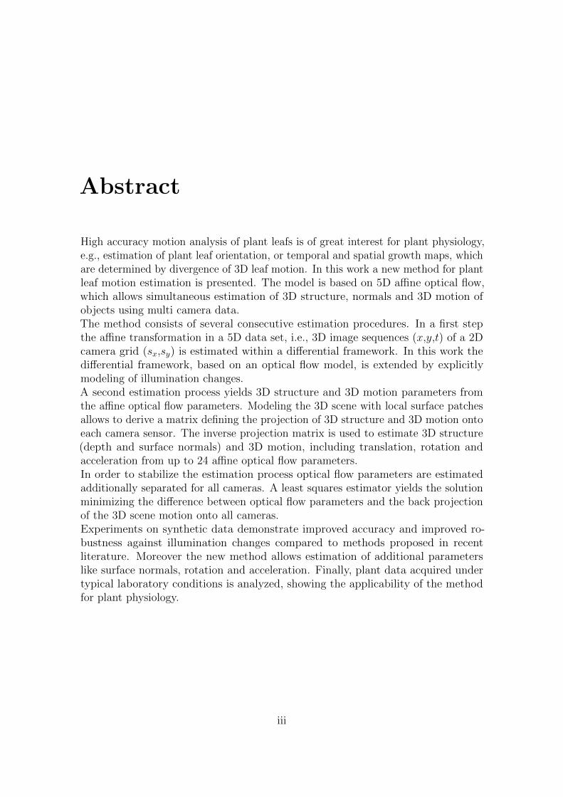
High accuracy motion analysis of plant leafs is of great interest for plant physiology,e.g., estimation of plant leaf orientation, or temporal and spatial growth maps, whichare determined by divergence of 3D leaf motion. In this work a new method for plantleaf motion estimation is presented. The model is based on 5D affine optical flow,which allows simultaneous estimation of 3D structure, normals and 3D motion ofobjects using multi camera data.The method consists of several consecutive estimation procedures. In a first stepthe affine transformation in a 5D data set, i.e., 3D image sequences (x,y,t) of a 2Dcamera grid (sx,sy) is estimated within a differential framework. In this work thedifferential framework, based on an optical flow model, is extended by explicitlymodeling of illumination changes.A second estimation process yields 3D structure and 3D motion parameters fromthe affine optical flow parameters. Modeling the 3D scene with local surface patchesallows to derive a matrix defining the projection of 3D structure and 3D motion ontoeach camera sensor. The inverse projection matrix is used to estimate 3D structure(depth and surface normals) and 3D motion, including translation, rotation andacceleration from up to 24 affine optical flow parameters.In order to stabilize the estimation process optical flow parameters are estimatedadditionally separated for all cameras. A least squares estimator yields the solutionminimizing the difference between optical flow parameters and the back projectionof the 3D scene motion onto all cameras.Experiments on synthetic data demonstrate improved accuracy and improved ro-bustness against illumination changes compared to methods proposed in recentliterature. Moreover the new method allows estimation of additional parameterslike surface normals, rotation and acceleration. Finally, plant data acquired undertypical laboratory conditions is analyzed, showing the applicability of the methodfor plant physiology.
iii

iv

Kurzfassung
Eine detaillierte Bewegungsanalyse von Pflanzenblattern ist fur die Pflanzenphy-siologie von großem Interesse, z.B. die Bestimmung der Blattwinkelstellung oderzeitlich und raumlich hochaufgeloster Blattwachstumskarten, welche sich aus der3-D-Bewegung eines Blattes berechnen lassen. Im Rahmen dieser Arbeit wurde eineneue Methode zur Analyse von Pflanzenblattbewegungen entwickelt. Die Methodebasiert auf dem 5-D-affinen optischen Fluss und ermoglicht die simultane Bestim-mung von 3-D-Struktur, Oberflachennormalen und 3-D-Bewegung eines Objektesaus Multi-Kamerasequenzen.Die Methode basiert auf mehreren, hintereinander ausgefuhrten Schatzungen. Zu-nachst wird die affine Transformation einer Umgebung innerhalb eines 5-D-Daten-satzes, d.h. 3-D-Bildsequenzen (x,y,t) eines 2-D-Kamera-Arrays (sx,sy), mit einemdifferentiellen Ansatz nach dem Prinzip des optischen Flusses bestimmt. Das in dieserArbeit vorgestellte erweiterte Modell des optischen Flusses modelliert auftretendeHelligkeitsanderungen explizit und erhoht somit die Robustheit gegenuber Beleuch-tungsanderungen.Nach Bestimmung der 5-D-optischen Flussparameter werden die 3-D-Struktur unddie 3-D-Bewegung, basierend auf einem sogenannten Surface Patch Model, geschatzt.Die Matrix, die die Projektion der 3-D-Struktur und der 3-D-Bewegung des SurfacePatches auf den jeweiligen Kamerasensor beschreibt, kann mit Hilfe projektiver Geo-metrie bestimmt werden. Die Inverse dieser Projektionsmatrix ermoglicht dann dieErmittlung von 3-D-Struktur (Tiefe und Oberflachennormalen) und 3-D-Bewegung(Translation, Beschleunigung und Rotation) aus den bis zu 24 Parametern des affinenoptischen Flusses.Zur Stabilisierung der Schatzung werden Parameter des optischen Flusses zusatzlichseparat in allen Kameras geschatzt. Ein Least-Squares Schatzer liefert dann dieLosung, welche die Differenz zwischen den einzelnen Parametern des optischen Flus-ses und der Ruckprojektion der 3-D-Bewegung in die einzelnen Kameras minimiert.Experimente mit synthetischen Daten belegen die hohere Genauigkeit und die hohereRobustheit gegenuber Beleuchtungsanderungen im Vergleich zu bekannten Verfah-ren aus der Literatur. Zudem ist die explizite Bestimmung zusatzlicher Parameterwie Oberflachennormalen, Beschleunigung und Rotation moglich. Die erfolgreicheAuswertung von unter normalen Laborbedingungen erhobenen Pflanzensequenzenbelegt die Anwendbarkeit der neuen Methode in der Pflanzenphysiologie.
v

vi

Contents
1 Introduction 1
1.1 Motivation and Approach . . . . . . . . . . . . . . . . . . . . . . . . 2
1.2 Thesis Outline . . . . . . . . . . . . . . . . . . . . . . . . . . . . . . . 3
2 Parameter Estimation of Dynamic Processes 5
2.1 Model Derivation . . . . . . . . . . . . . . . . . . . . . . . . . . . . . 7
2.1.1 Modeling of Flow Fields . . . . . . . . . . . . . . . . . . . . . 8
2.1.2 Model Limitations . . . . . . . . . . . . . . . . . . . . . . . . 10
2.2 Discretization . . . . . . . . . . . . . . . . . . . . . . . . . . . . . . . 11
2.3 Parameter Estimation . . . . . . . . . . . . . . . . . . . . . . . . . . 12
2.3.1 Least Squares . . . . . . . . . . . . . . . . . . . . . . . . . . . 12
2.3.2 Total Least Squares . . . . . . . . . . . . . . . . . . . . . . . . 13
2.3.3 Respecting Known Measurement Errors in Estimation Schemes 17
2.3.4 Robust Estimation . . . . . . . . . . . . . . . . . . . . . . . . 22
2.4 Conclusions . . . . . . . . . . . . . . . . . . . . . . . . . . . . . . . . 29
3 Approaches to 3D Motion Estimation 31
3.1 Scene Flow . . . . . . . . . . . . . . . . . . . . . . . . . . . . . . . . 32
3.2 Range Flow . . . . . . . . . . . . . . . . . . . . . . . . . . . . . . . . 33
3.2.1 The Range Constraint . . . . . . . . . . . . . . . . . . . . . . 33
3.2.2 The Intensity Constraint . . . . . . . . . . . . . . . . . . . . . 34
3.2.3 Range Flow Estimation . . . . . . . . . . . . . . . . . . . . . . 34
3.3 Affine Model . . . . . . . . . . . . . . . . . . . . . . . . . . . . . . . . 35
3.3.1 Derivation of the BCCE . . . . . . . . . . . . . . . . . . . . . 36
3.3.2 Parameter Estimation . . . . . . . . . . . . . . . . . . . . . . 42
3.4 Experiments . . . . . . . . . . . . . . . . . . . . . . . . . . . . . . . . 44
3.4.1 Sinusoidal Pattern . . . . . . . . . . . . . . . . . . . . . . . . 45
3.4.2 Synthetic Cube . . . . . . . . . . . . . . . . . . . . . . . . . . 50
3.4.3 Plant Sequences . . . . . . . . . . . . . . . . . . . . . . . . . . 51
3.5 Conclusions . . . . . . . . . . . . . . . . . . . . . . . . . . . . . . . . 55
vii
CONTENTS
4 Modeling Brightness Changes 574.1 Prefiltering . . . . . . . . . . . . . . . . . . . . . . . . . . . . . . . . 574.2 Brightness Constraints . . . . . . . . . . . . . . . . . . . . . . . . . . 59
4.2.1 The Gradient Constancy Constraint . . . . . . . . . . . . . . . 604.2.2 Combined Intensity and
Gradient Constancy Constraint . . . . . . . . . . . . . . . . . 604.2.3 A Physics-Based Brightness Change Model . . . . . . . . . . . 60
4.3 Extension of 3D Motion Estimation Models . . . . . . . . . . . . . . 634.3.1 Scene Flow . . . . . . . . . . . . . . . . . . . . . . . . . . . . 634.3.2 Range Flow . . . . . . . . . . . . . . . . . . . . . . . . . . . . 634.3.3 Affine Model . . . . . . . . . . . . . . . . . . . . . . . . . . . . 65
4.4 Experiments . . . . . . . . . . . . . . . . . . . . . . . . . . . . . . . . 664.4.1 Evaluation of Brightness Change Models
for the Affine Model . . . . . . . . . . . . . . . . . . . . . . . 664.4.2 Evaluation of Prefilters and Brightness Change
Models for Range Flow . . . . . . . . . . . . . . . . . . . . . . 724.4.3 Comparison of Models . . . . . . . . . . . . . . . . . . . . . . 82
4.5 Conclusions . . . . . . . . . . . . . . . . . . . . . . . . . . . . . . . . 86
5 Modeling Rotation 895.1 Model Derivation . . . . . . . . . . . . . . . . . . . . . . . . . . . . . 90
5.1.1 Surface Patch Model . . . . . . . . . . . . . . . . . . . . . . . 905.1.2 Camera Model . . . . . . . . . . . . . . . . . . . . . . . . . . 905.1.3 Pixel-Centered View . . . . . . . . . . . . . . . . . . . . . . . 905.1.4 Projecting the Pixel Grid to the Surface . . . . . . . . . . . . 915.1.5 Brightness Change Model . . . . . . . . . . . . . . . . . . . . 925.1.6 Combination of Models . . . . . . . . . . . . . . . . . . . . . . 925.1.7 Rotation . . . . . . . . . . . . . . . . . . . . . . . . . . . . . . 945.1.8 The Range Constraint, Zt, b4, and why (5.5) still holds under
Rotation . . . . . . . . . . . . . . . . . . . . . . . . . . . . . . 945.1.9 A 4D-Affine Model . . . . . . . . . . . . . . . . . . . . . . . . 95
5.2 Parameter Estimation . . . . . . . . . . . . . . . . . . . . . . . . . . 965.3 Experiments . . . . . . . . . . . . . . . . . . . . . . . . . . . . . . . . 97
5.3.1 Sinusoidal Pattern . . . . . . . . . . . . . . . . . . . . . . . . 975.3.2 Synthetic Cube . . . . . . . . . . . . . . . . . . . . . . . . . . 1005.3.3 Castor Oil Plant . . . . . . . . . . . . . . . . . . . . . . . . . 102
5.4 Conclusions . . . . . . . . . . . . . . . . . . . . . . . . . . . . . . . . 104
6 5D-Affine Scene Flow Model 1056.1 5D-Affine Model . . . . . . . . . . . . . . . . . . . . . . . . . . . . . . 1056.2 Parameter Estimation . . . . . . . . . . . . . . . . . . . . . . . . . . 1086.3 Experiments . . . . . . . . . . . . . . . . . . . . . . . . . . . . . . . . 108
6.3.1 Sinusoidal Pattern . . . . . . . . . . . . . . . . . . . . . . . . 109
viii

CONTENTS
6.3.2 Synthetic Cube . . . . . . . . . . . . . . . . . . . . . . . . . . 1116.3.3 Castor Oil Plant . . . . . . . . . . . . . . . . . . . . . . . . . 1156.3.4 Tobacco Plant . . . . . . . . . . . . . . . . . . . . . . . . . . . 116
6.4 Conclusions . . . . . . . . . . . . . . . . . . . . . . . . . . . . . . . . 119
7 Conclusions And Outlook 1217.1 Summary and Conclusions . . . . . . . . . . . . . . . . . . . . . . . . 1217.2 Future Work . . . . . . . . . . . . . . . . . . . . . . . . . . . . . . . . 1237.3 Closure . . . . . . . . . . . . . . . . . . . . . . . . . . . . . . . . . . . 125
A Average Angular Error 127
B Synthetic Testsequences 129
Bibliography 133
Curriculum Vitae 141
Acknowledgements 143
ix

x

Chapter 1
Introduction
This thesis presents a new approach for estimation of 3D structure, surface slopesand 3D motion of objects from multi-camera image sequences. In the last yearsmore and more applications using 3D reconstruction and/or motion estimation ofimage sequences are developed. Miniaturization and increasing performance of imageprocessing setups including cameras and signal processing hardware as well as fallingcosts, allow fast and cheap measurements from large to small scale applications.Another important fact is that measurements are non-invasive. Image processingapplications can be found almost everywhere in daily life, starting from motionestimation in consumer hardware such as cameras or entertainment products asSony’s EyeToy [66], to driver assistance systems, surveillance systems, satellite dataproducts, so-called web mapping service applications, like Google Street View [22],and so on. Motion estimation in image sequences is a prerequisite of many imageprocessing algorithms, such as depth reconstruction, 3D motion estimation, tracking,segmentation and coding, to name only few of them. 2D motion in image sequencesis sometimes called optical flow [26]. Several estimation frameworks have beenproposed for optical flow estimation. We may distinguish between differential, oftencalled optical flow based techniques and point/feature correspondence or correlationbased techniques. In this work we focus on differential frameworks, which yield highaccuracy and are developed since the early 80’s [28, 42]. There is rich literature onoptical flow estimation techniques (see e.g., [4, 26, 10, 14, 49]) and many extensionshave been developed. An overview of recent optical flow estimation algorithms ispresented in [3]. Optical flow can be used for depth reconstruction and 3D motionestimation, depending on the images on which the optical flow is determined:
in case of images of different cameras displaced parallel to their sensor planesthe optical flow is inversely proportional to the depth of the 3D point projectedonto the image sensor element,
for consecutive images from one fixed camera the motion seen on the sensor isthe projection of the 3D motion in the scene, the so called Scene Flow.
1

1 Introduction
Considerable work has already been carried out on estimating 3D motion fields. RangeFlow estimation [80, 21] uses solely data from range sensors, whereas Spies et al.[67, 69] incorporate information from both range and image sensors. Reconstructionof Scene Flow and 3D structure from optical flow observed in several cameras hasbeen proposed by [81, 76, 40, 57, 31].
1.1 Motivation and Approach
In this work we focus on plant leaf motion estimation. The Institute of Chemistryand Dynamics of the Geosphere: Phytosphere (ICG-3) at the ForschungszentrumJulich investigates plant leaf motion and growth in order to examine the influenceof environmental change, biotic/abiotic stresses, and light quality and quantityon growth dynamics. For the estimation of plant leaf growth a system based ona single camera was developed by Schmundt and Schurr [59]. There the cameraimages a leaf from the top and the divergence of the calculated velocity field yieldsthe sought growth rate. Typical growth rates of fast growing leaves are below 3%per hour or 0.1%/frame when a typical frame rate of 0.5 frames per minute isassumed [78]. Therefore a suitable estimation technique has to be highly accurate.However, any change in the distance between the camera and the plant leaf causesa diverging optical flow field. This motion cannot be distinguished from growth ofthe leaf. Therefore the leaf is fixed in order to restrict motion to the horizontalplane. The procedure how to fix the leaf in order not to influence overall leaf growthwas thoroughly tested [63]. Nevertheless, fixing leafs influences plants and is notappropriate for screening, i.e., high throughput measurements. In order to estimateplant growth of freely moving plant leaves, 3D structure and motion has to beestimated in high accuracy.
In this work we investigate three 3D motion estimation techniques, namely SceneFlow [74], Range Flow [67] and a technique based on an affine motion model [57](labeled as the Affine Model). All these techniques are based on motion models,which do not allow reliable estimation of plant motion. We extend these models andpropose a novel estimation technique incorporating advantages of all three approaches.The novel affine optical flow-like differential model allows estimation of 3D structureand 3D motion using image sequences of a camera grid. The model is valid forinstantaneously moving cameras observing moving surfaces. This is unlike previouswork (e.g., [41, 37, 1, 79]) where either an observed surface moves, or a camera, butnot both. The model introduced here combines motion estimation in the sequencein camera displacement direction, i.e., disparity, and in time direction, i.e., opticalflow. It is an extension of a model first introduced by Scharr [55] and further refinedand extended in [56, 60]. It allows simultaneous local estimation of 3D motion, 3Dposition and surface normals in a spatio-temporal affine optical flow-like model.
3D motion estimation is used for many different applications, i.e., driver assistance,machine vision or tracking, to name only few of them. Obviously applications have
2

1.2 Thesis Outline
a b c d
X and SX
z
Y a
ndS Y
z
Figure 1.1: Setup for our target application plant growth analysis. A camera grid(a) is simulated using a single camera on a moving stage (b). From images (c) takenfrom vertical view a 3D reconstruction (d) is calculated.
different demands on the estimated 3D motion field, e.g., real-time processing andreliability are basic prerequisites for a driver assistance system, whereas accuracy inthe range of cm may be sufficient.
Although we do not aim at presenting a best method yet, we do have the targetapplication plant leaf growth analysis in mind when designing our experiments.Accuracy in the range of µm is a basic requisite. Plant leaf motion is high comparedto plant leaf growth. In order to estimate growth from the divergence of plant leafmotion these estimates have to be highly accurate and reliable. Moreover many plantspecies have reflective leaf surfaces, i.e., directed illumination may cause specularhighlights. Further plants react on visible light. Nevertheless real-time processingis not necessary, i.e., motion and growth parameter estimation can be done off-line.In order to develop an appropriate method all these requirements have to be takeninto account. For imaging we use a single camera on an x-y-moving stage instead ofa real camera grid. This allows us to use very small baselines, much smaller thancamera dimensions. Obviously images are not taken at exactly the same point intime, which could be accounted for in the discretization of derivative kernels appliedto the images. We neglect this effect here, because plants move slowly enough suchthat time intervals between two images at the same camera position are much largerthan the overall acquisition time for all camera images representing ’one’ point intime. Figure 1.1 shows the setup for our target application, and a rendered image ofa plant obtained with the presented model.
1.2 Thesis Outline
In this work we derive a novel model for 3D depth, slopes and 3D motion estimation.In Chap. 2 we demonstrate the basic elements of motion estimation techniques, i.e.,model derivation, discretization and parameter estimation. We discuss motion modelssuitable for optical flow estimation and optimal filter sets for data discretization.Several estimators are proposed and evaluated on synthetic sequences.
Chapter 3 reviews the 3D motion estimation techniques Scene Flow and RangeFlow. Furthermore the Affine Model is introduced, which is an extension of the
3

1 Introduction
multi-camera model presented by [55]. Range Flow and the Affine Model have alreadybeen proposed for plant leaf emotion estimation, whereas Scene Flow showed highperformance in human motion estimation. We evaluate the performance of the threemodels on synthetic data and on a plant leaf sequence.
None of the models yields the accuracy needed for reliable plant leaf motionestimation. The main reason are illumination changes in the image sequences due tomotion of the leaf or the light source. Chapter 4 therefore shows an investigation ofdifferent approaches to handle varying illumination. Combinations of prefilters andbrightness change constraints are thoroughly tested and a novel brightness changeconstraint, which explicitly models brightness changes is derived.
In Chap. 5 we introduce a new motion model for the Affine Model in orderto estimate rotational motion. Furthermore we extend the model by estimatingadditional affine optical flow parameters. These parameters are used to makesubsequent parameter estimation of 3D structure and 3D motion more robust. Thisextension boils down to be a combination of the Affine Model and Range Flow.
Chapter 6 demonstrates how to integrate Scene Flow in the Affine Model. Thenovel Affine Scene Flow Model combines advantages of all three 3D motion estimationmodels and yields highest accuracies on synthetic sequences as well as on plant leafsequences.
Finally a concluding summary and an outlook on possible future work is given inChap. 7.
4

Chapter 2
Parameter Estimation of DynamicProcesses
Parameter estimation from noisy data is a basic requisite in many image and signalprocessing applications, like line fitting, camera calibration, image matching, signalreconstruction or position detection. In this work we focus on motion estimationon image sensors. The motion seen on a 2D image sensor is called optical flowand describes the change of a value, e.g., brightness or color, in consecutive images.This optical flow may be used as input for subsequent processing steps includingmotion detection, motion compensation, motion-based data compression, 3D scenereconstruction, 3D motion estimation or segmentation,to name only a few of them.In some publications [74, 40] optical flow is referred to as the projection of the 3Dmotion. In fact it is only an approximation of the projected motion. Motion onthe image plane is identified by changes of a certain value, e.g., the intensity forgray value images. Therefore optical flow in an intensity image sequence can onlybe estimated in textured areas or by varying illumination. This leads to problemsfor interpretation of the projected 3D motion. Horn [27] denotes several problemswhen estimating optical flow, e.g., the motion of a rigid sphere. Consider a rigidsphere without texture and homogeneous surface reflectance rotating around an axisthrough its origin. With a constant illumination source, this 3D motion does notgenerate optical flow, because no brightness changes are visible. If the light sourceitself is moving optical flow occurs also when the illuminated object does not move.Other problems for motion estimation are e.g., occlusion, transparent and multiplemotions, aperture problems and correspondence problems.
Figure 2.1 shows two frames of the well known synthetic Yosemite sequence[4], which is very popular as a benchmark for motion estimation techniques. Thesequence was originally generated by Lynn Quam at SRI and shows a flight throughthe Yosemite valley. The optical flow for frame 7 is depicted in Fig. 2.1c. Severaltechniques have been proposed for motion estimation between consecutive frames.Haussecker and Spies [26] distinguished two groups, namely optical flow-based andcorrespondence-based techniques. The definition of optical flow-based is somewhat
5

2 Parameter Estimation of Dynamic Processes
a b c
Figure 2.1: a and b: Frames 5 and 9 of the Yosemite sequence. c: Ground truth flowvectors for frame 7.
misleading, as optical flow is in general defined as the motion in the image, whichis estimated by both techniques. Haussecker and Spies define techniques as opticalflow-based techniques, when the relationship between the temporal variations ofimage intensities or the frequency distribution in the Fourier domain is analyzed,e.g., differential, energy-based, tensor-based and phase-based techniques. Thesetechniques imply compliance with the temporal sampling theorem.In contrast to this, correspondence techniques estimate best matches of featuresbetween two frames. These techniques can be classified into correlation methodsand feature tracking techniques. Whereas correlation techniques find the best matchbased on a so called correlation window, the feature tracking techniques extractfeatures like borders or edges and track them over time.Haussecker and Spies [26] present an extensive study of these two classes of 2D motionestimation techniques. They propose that the tensor based techniques perform bestwith respect to systematic error and noise sensitivity and should be used for subpixeldisplacement estimation. Correspondence based techniques are less sensitive toillumination changes and are capable of estimating long range displacements, wherestandard differential techniques fail. Illumination models for differential techniques[25, 60] and warping techniques (e.g., [13]), which address these disadvantages, havebeen presented recently.Overviews of optical flow-based approaches are given by Barron et al. [4] andHaussecker and Spies [26]. Baker et al. [3] established a set of benchmarks andevaluation methods for optical flow algorithms. This database is freely availableon the web together with results of the most recent optical flow-based techniquesat http://vision.middlebury.edu/flow/. A taxonomy of dense two frame stereocorrespondence based techniques was presented by Scharstein and Szeliski [58].Benchmarks and results of these and more recent techniques are also available onthe web at http://vision.middlebury.edu/stereo/.A complete motion estimation technique is based on an appropriate combination ofa data model, a discretization and an estimator. The result of a motion estimationtechnique depends on all three parts, e.g., combining a highly accurate data modeland an estimator based on statistics not appropriate for the data, leads to reducedaccuracy of estimation results, limited by the estimator.Optical flow estimation techniques are commonly classified into local and global
6

2.1 Model Derivation
methods. Local estimators use data exclusively from a local neighborhood andminimize an energy function based on a local data-model, i.e., the so-called dataterm1. Methods based on these models may be implemented very efficiently andare often more robust under noise compared to global methods [19, 14]. Globalestimators incorporate a prior term on the solution that couples parameters not onlyin a local neighborhood but in the whole data set [39]. In most cases this prior termis a smoothness assumption of the solution, therefore often called smoothness term.The prior term allows to estimate parameters also in regions where the estimationproblem is ill-posed [5], i.e., when the solution a) is not unique, b) does not exist orc) does not depend continuously on the data. However, the prior term may includeany prior knowledge on the solution parameters.Global and combined local/global methods are widely used in recent work and showedhigh performance and accuracy [3]. A drawback of these methods is the prior terminfluencing all parameters, making detailed error analysis difficult. In contrast tothis several error measurements for local methods, e.g., the structure tensor method,have been studied intensively [35].We briefly review differential-based estimation of optical flow. We start by derivingflow models and the discretization of the image space. The second part of thischapter addresses different types of local estimation techniques.
2.1 Model Derivation
Parameter estimation is a part of statistics and includes appropriate mathematicalmodeling of data structures and estimation of constant parameters of this model. Acommon assumption on optical flow is that the image brightness I(x, t) at a pointx = [x, y]T at time t should only change because of motion u = [ux, uy]
T. We get
I(x, t) = I(x + uδt, t+ δt) (2.1)
with optical flow u. Assuming that δt is small we approximate I(x + uδt, t + δt)by its Taylor expansion. Ignoring higher order terms we obtain a gradient basedformulation for the total change of intensity I(x, t) in time
dI =(I(x, t) + ∂I
∂xdx + ∂I
∂ydy + ∂I
∂tdt)− I(x, t)
⇔ dI = ∂I∂x
dx + ∂I∂y
dy + ∂I∂t
dt
⇔ dIdt
= ∂I∂xux + ∂I
∂yuy + ∂I
∂t
(2.2)
with the optical flow components denoted by ux = dx /dt and uy = dy /dt . Equation(2.2) describes brightness changes in the data due to the optical flow and is thereforecalled the brightness change constraint equation (BCCE). A special case of the BCCE
1In literature also named likelihood term [51] or bones [36].
7

2 Parameter Estimation of Dynamic Processes
is the brightness constancy constraint equation (in literature sometimes also calledBCCE), where intensities are assumed constant with time, i.e., dI /dt = 0. Thisresults in
Ixux + Iyuy + It = 0 (2.3)
with partial image derivatives Iq = ∂I∂q
with q ∈ x, y, t. To solve for optical flow u theflow field is modeled for neighboring image points in Sec. 2.1.1. Additional equationsthen allow to solve for u.
2.1.1 Modeling of Flow Fields
In order to solve under-determined constraints like the BCCE (2.2), constraints maybe grouped together over a local neighborhood Λ. The resulting equation systemallows estimation of a constant solution vector (here: optical flow vector u). Theneighborhood Λ should be chosen as small as possible to ensure a local estimate ofoptical flow u. The larger the neighborhood is, the more likely it is that the opticalflow varies in Λ, or that multiple flows occur. On the other hand, Λ should be largeenough to contain enough information to constrain the solution and be robust tonoise. In this section we parameterize the flow vector u assuming a single motion.The most common models are
Local constancy of u(x),
Local smoothness of u(x), i.e., the so-called affine optical flow and
Higher order models of u(x).
Local constancy of u(x) assumes that the flow in a certain neighborhood Λ of xis constant. Assuming brightness constancy (cmp. (2.3)), optical flow u is thendetermined by solving the overdetermined equation system
Ix,1 Iy,1 It,1Ix,2 Iy,2 It,2
......
...Ix,N Iy,N It,N
ux
uy1
=
00...0
(2.4)
for neighborhood Λ with size N .The assumption of locally constant motion is not fulfilled for most motion vectorfields or holds only for small sizes of neighborhood Λ. A more sophisticated motionvector field model is the assumption of local smoothness. Local smoothness and localconstancy are sometimes used synonymously. But in a stricter sense local smoothnessmeans that within a local neighborhood Λ the optical flow field is allowed to varysmoothly. This may be achieved e.g., by means of a Taylor series of u(x) in localcoordinates ∆x = (x − x0, y − y0)
T =: (∆x,∆y)T around the center (x0, y0) of Λ.This is typically called an affine model and estimation boils down to estimating a
8

2.1 Model Derivation
a b c
Figure 2.2: Motion vector field transformations. a: Constant, b: stretching and c:rotation.
larger parameter vector also containing smoothness information, which is constantin a neighborhood. The displacement vector field v is modeled locally by
v = u + A∆x (2.5)
with a 2× 2-matrix A. (x0, y0) is the point for which a displacement vector is to becalculated, usually the center of the neighborhood Λ. Reformulating the brightnessconstancy constraint (2.3) to ∇T
xIu + It = 0 with spatial gradient ∇x = (∂x, ∂y)T
and replacing u by v yields
0 = ∇TxI(u + A∆x) + It
⇔ 0 = ∇TxIu +∇T
xIA∆x + It
⇔ 0 = Ixux + Iyuy + Ix∆xa11 + Ix∆ya12
+ Iy∆xa21 + Iy∆ya22 + It .
(2.6)
Flow vector u represents the translational motion of the center (x0, y0) of Λ. Thematrix A addresses smooth changes of the velocity field in the neighborhood, based onelementary geometric transformations, namely rotation, dilation, shear and stretching.Two examples of vector field transformations are compared to a constant vector fieldin Fig. 2.2.An affine optical flow model describes variations of u by matrix A and linear local
coordinates ∆x. Obviously motion models based on quadratic local coordinates∆x may be used as well. Recently, Li and Sclaroff [40] fit flow vectors to an eight-parameter model corresponding to quadratic motion (cmp. [11]). The optical flowmodel is given by
0 = ∇TxI(u + Aquad∆xquad) + It
⇔ 0 = Ixux + Iyuy + Ix∆xa11 + Ix∆ya12
+ Iy∆xa21 + Iy∆ya22
+ Ix∆x∆ya13 + Ix∆x2a14
+ Iy∆x∆ya23 + Iy∆y2a24 + It
(2.7)
9

2 Parameter Estimation of Dynamic Processes
a b
Figure 2.3: a: Aperture problem, flow not uniquely defined and b: full flow at afeature point.
with
Aquad =
[a11 a12 a13 a14 0a21 a22 a23 0 a24
](2.8)
and xquad = [∆x,∆y,∆x∆y,∆x2,∆y2]T. Quadratic models have also been used toimprove change detection algorithms [29]. There the gray-value distribution within aregion was modeled by a so-called quadratic picture function.
2.1.2 Model Limitations
Using a neighborhood assumption to solve equation (2.2) does not always yield thecorrect flow as shown in Fig. 2.3. The so called aperture problem occurs if there is nochange of the spatial gradient ∇xI in the neighborhood. In this case the minimumnorm solution is the normal flow, pointing parallel to the direction of the spatialgradient. To avoid the aperture problem, either global smoothness assumptions maybe applied or, for local methods, the size of the neighborhood has to be enlarged.However, this may extend the region over motion boundaries, thus that constraintsare no longer consistent. In addition enlarging kernels blurs results. In order toovercome this problem robust statistics [8] may be used. A sophisticated estimatoris presented in Sec. 2.3.Another limitation of differential models is that differentiation in the BCCE (2.2)assumes small motions. Therefore compliance with the temporal sampling theoremis a basic prerequisite. So called multi-grid methods ([72, 8, 49, 65]) help to achievealso larger motions reliably. These methods calculate motion estimates on imagepyramids, but so far are only available for 2 frame algorithms. Motion betweenthe coarsest images is significantly smaller than for the original images and thesampling theorem is fulfilled. The motion estimates from the coarse images are usedto warp the image on the next resolution. The remaining motion vector field typicallyalso fulfills the sampling theorem. In subsequent steps only an incremental motionneeds to be estimated. These steps are repeated till the original image resolution isreached.
10
2.2 Discretization
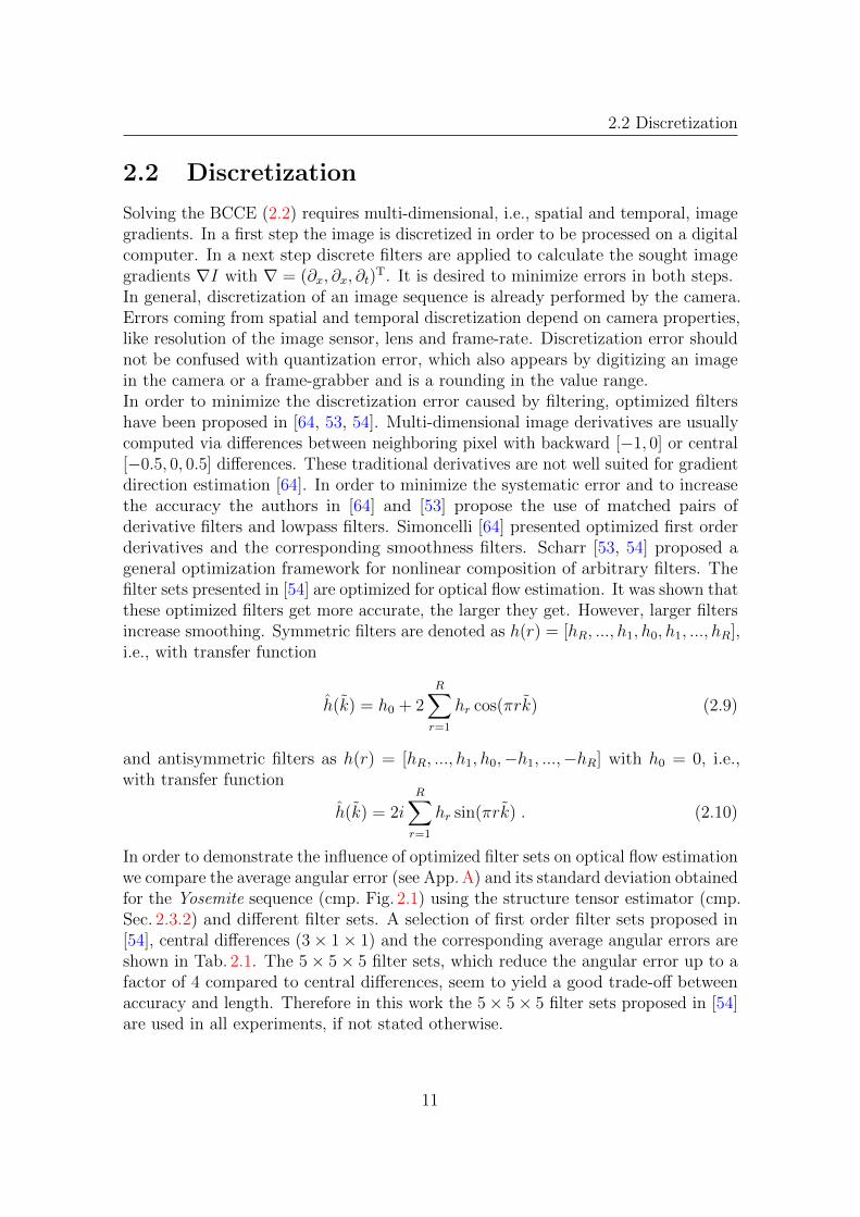
2.2 Discretization
Solving the BCCE (2.2) requires multi-dimensional, i.e., spatial and temporal, imagegradients. In a first step the image is discretized in order to be processed on a digitalcomputer. In a next step discrete filters are applied to calculate the sought imagegradients ∇I with ∇ = (∂x, ∂x, ∂t)
T. It is desired to minimize errors in both steps.In general, discretization of an image sequence is already performed by the camera.Errors coming from spatial and temporal discretization depend on camera properties,like resolution of the image sensor, lens and frame-rate. Discretization error shouldnot be confused with quantization error, which also appears by digitizing an imagein the camera or a frame-grabber and is a rounding in the value range.In order to minimize the discretization error caused by filtering, optimized filtershave been proposed in [64, 53, 54]. Multi-dimensional image derivatives are usuallycomputed via differences between neighboring pixel with backward [−1, 0] or central[−0.5, 0, 0.5] differences. These traditional derivatives are not well suited for gradientdirection estimation [64]. In order to minimize the systematic error and to increasethe accuracy the authors in [64] and [53] propose the use of matched pairs ofderivative filters and lowpass filters. Simoncelli [64] presented optimized first orderderivatives and the corresponding smoothness filters. Scharr [53, 54] proposed ageneral optimization framework for nonlinear composition of arbitrary filters. Thefilter sets presented in [54] are optimized for optical flow estimation. It was shown thatthese optimized filters get more accurate, the larger they get. However, larger filtersincrease smoothing. Symmetric filters are denoted as h(r) = [hR, ..., h1, h0, h1, ..., hR],i.e., with transfer function
h(k) = h0 + 2R∑r=1
hr cos(πrk) (2.9)
and antisymmetric filters as h(r) = [hR, ..., h1, h0,−h1, ...,−hR] with h0 = 0, i.e.,with transfer function
h(k) = 2iR∑r=1
hr sin(πrk) . (2.10)
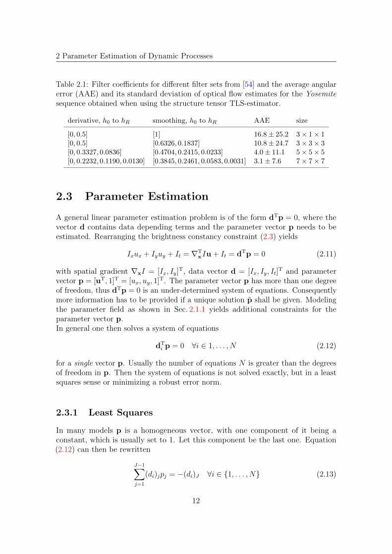
In order to demonstrate the influence of optimized filter sets on optical flow estimationwe compare the average angular error (see App. A) and its standard deviation obtainedfor the Yosemite sequence (cmp. Fig. 2.1) using the structure tensor estimator (cmp.Sec. 2.3.2) and different filter sets. A selection of first order filter sets proposed in[54], central differences (3× 1× 1) and the corresponding average angular errors areshown in Tab. 2.1. The 5× 5× 5 filter sets, which reduce the angular error up to afactor of 4 compared to central differences, seem to yield a good trade-off betweenaccuracy and length. Therefore in this work the 5× 5× 5 filter sets proposed in [54]are used in all experiments, if not stated otherwise.
11
2 Parameter Estimation of Dynamic Processes
Table 2.1: Filter coefficients for different filter sets from [54] and the average angularerror (AAE) and its standard deviation of optical flow estimates for the Yosemitesequence obtained when using the structure tensor TLS-estimator.
derivative, h0 to hR smoothing, h0 to hR AAE size
[0, 0.5] [1] 16.8± 25.2 3× 1× 1[0, 0.5] [0.6326, 0.1837] 10.8± 24.7 3× 3× 3[0, 0.3327, 0.0836] [0.4704, 0.2415, 0.0233] 4.0± 11.1 5× 5× 5[0, 0.2232, 0.1190, 0.0130] [0.3845, 0.2461, 0.0583, 0.0031] 3.1± 7.6 7× 7× 7
2.3 Parameter Estimation
A general linear parameter estimation problem is of the form dTp = 0, where thevector d contains data depending terms and the parameter vector p needs to beestimated. Rearranging the brightness constancy constraint (2.3) yields
Ixux + Iyuy + It = ∇TxIu + It = dTp = 0 (2.11)
with spatial gradient ∇xI = [Ix, Iy]T, data vector d = [Ix, Iy, It]
T and parametervector p = [uT, 1]T = [ux, uy, 1]T. The parameter vector p has more than one degreeof freedom, thus dTp = 0 is an under-determined system of equations. Consequentlymore information has to be provided if a unique solution p shall be given. Modelingthe parameter field as shown in Sec. 2.1.1 yields additional constraints for theparameter vector p.In general one then solves a system of equations
dTi p = 0 ∀i ∈ 1, . . . , N (2.12)
for a single vector p. Usually the number of equations N is greater than the degreesof freedom in p. Then the system of equations is not solved exactly, but in a leastsquares sense or minimizing a robust error norm.
2.3.1 Least Squares
In many models p is a homogeneous vector, with one component of it being aconstant, which is usually set to 1. Let this component be the last one. Equation(2.12) can then be rewritten
J−1∑j=1
(di)jpj = −(di)J ∀i ∈ 1, . . . , N (2.13)
12

2.3 Parameter Estimation
where J is the number of components of p. We rewrite equation (2.13) as
A u = b (2.14)
where we renamed Aij = (di)j, uj = pj with p = (uT, 1)T, and bi = −(di)J forj ∈ 1, . . . , J − 1 and i ∈ 1, . . . , N. One can then solve for u in least squaressense using the Moore-Penrose-pseudo-inverse A+ = (ATA)−1AT
u = A+b . (2.15)
In general ATA is a symmetric positive semi-definite matrix and therefore diagonal-izable. But it is not necessarily invertible as one or more eigenvalues may be (closeto) zero, i.e., ATA may be rank deficient. If this is the case, one may calculate A+ bydiagonalization of ATA and inversion of all non-zero (or large enough) eigenvaluesonly, instead of (ATA)−1 where all eigenvalues are inverted.
If ATA is invertible then solution u is fully determined. If it is not invertiblethen the eigenvectors corresponding to the (very small or) zero eigenvalues spanthe null space Null(ATA) = u|ATAu = 0. This means that solution u is onlydetermined up to an additive arbitrary vector u0 ∈ Null(ATA). Solution u givenin (2.15) is the shortest vector of all possible solutions and therefore is normal toNull(ATA). The solution is then called normal solution. ATA is rank deficient, ifd(xi) (and therefore the intensity signal I(x)) does not vary enough in the localneighborhood Λ. As Λ acts as an aperture on I(x) and is, in the rank deficient case,selected too small with respect to changes in I(x), this phenomenon is sometimescalled aperture problem (cmp. Sec. 2.1.2).
2.3.2 Total Least Squares
As for standard least squares estimation (see Sec. 2.3.1) total least squares parameterestimation solves (2.12) for p. The standard least squares approach assumes thatmatrix A contains no errors, i.e., all errors of (2.14) are confined to b. In case ofsolving (2.11), this assumption is not fulfilled, because both A and b are composed ofimage gradients. In contrast to standard least squares, total least squares addresseserroneous data in A. It is assumed that solution vector p approximately solves allequations in the local neighborhood Λ and therefore dT
i p only approximately equals0. We get
dTi p = ei ∀i ∈ 1, . . . , N (2.16)
with errors ei which have to be minimized by the sought solution p. We definematrix D := [A,b] (cmp. (2.14)) composed of the vectors di via Dij = (di)jfor j ∈ 1, . . . , J (in contrast to A in the least squares case in Sec. 2.3.1) andi ∈ 1, . . . , N. Equation (2.16) becomes Dp = e.
13
2 Parameter Estimation of Dynamic Processes
We minimize e in a weighted 2-norm
||e||2 = ||Dp||2 = pTDTWDp =: pTJp!
= min
⇒ p = arg minp
pTJp(2.17)
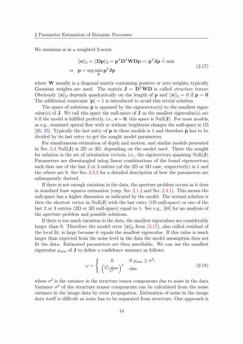
where W usually is a diagonal matrix containing positive or zero weights; typicallyGaussian weights are used. The matrix J = DTWD is called structure tensor.Obviously ||e||2 depends quadratically on the length of p and ||e||2 = 0 if p = 0.The additional constraint |p| = 1 is introduced to avoid this trivial solution.
The space of solutions p is spanned by the eigenvector(s) to the smallest eigen-value(s) of J. We call this space the null-space of J as the smallest eigenvalue(s) are0 if the model is fulfilled perfectly, i.e., e = 0, this space is Null(J). For most models,as e.g., standard optical flow with or without brightness changes the null-space is 1D[26, 25]. Typically the last entry of p in these models is 1 and therefore p has to bedivided by its last entry to get the sought model parameters.
For simultaneous estimation of depth and motion, and similar models presentedin Sec. 3.3 Null(J) is 2D or 3D, depending on the model used. There the soughtfor solution is the set of orientation vectors, i.e., the eigenvectors spanning Null(J).Parameters are disentangled using linear combinations of the found eigenvectors,such that one of the last 2 or 3 entries (of the 2D or 3D case, respectively) is 1 andthe others are 0. See Sec. 3.3.2 for a detailed description of how the parameters aresubsequently derived.
If there is not enough variation in the data, the aperture problem occurs as it doesin standard least squares estimation (cmp. Sec. 2.1.2 and Sec. 2.3.1). This means thenull-space has a higher dimension as indicated by the model. The normal solution isthen the shortest vector in Null(J) with the last entry (1D null-space) or one of thelast 2 or 3 entries (2D or 3D null-space) equal to 1. See e.g., [68] for an analysis ofthe aperture problem and possible solutions.
If there is too much variation in the data, the smallest eigenvalues are considerablylarger than 0. Therefore the model error ||e||2 from (2.17), also called residual ofthe local fit, is large because it equals the smallest eigenvalue. If this value is muchlarger than expected from the noise level in the data the model assumption does notfit the data. Estimated parameters are then unreliable. We can use the smallesteigenvalue µmin of J to define a confidence measure as follows:
ω =
0 if µmin ≥ σ2,(
σ2−µmin
σ2
)2
else.(2.18)
where σ2 is the variance in the structure tensor components due to noise in the data.Variance σ2 of the structure tensor components can be calculated from the noisevariance in the image data by error propagation. Estimation of noise in the imagedata itself is difficult as noise has to be separated from structure. One approach is
14
2.3 Parameter Estimation
using a Laplacian operator and adaptive edge detection following [71].In most cases it does not make a lot of sense to distinguish between full and
normal solutions and cases where model assumptions are not met. Instead reliabilityof an estimated parameter should be calculated by a suitable error analysis (seee.g., [46]). If an aperture problem occurs variance of an estimated parameter in theundetermined direction will be close to infinity. In the following we therefore assumethat enough data variation is present and an error analysis is performed, if needed.
Structure Tensor Method
Optical flow estimation via the structure tensor is discussed in [6, 33, 26]. Therean image sequence I(x) is treated as a volume of scalar, unit-free gray values withx = (x1, x2, x3)T where x3 is time. The single motion model given in (2.3) can thusbe written
∇TI · (uT, 1)T = 0 (2.19)
with data vector d = ∇I and parameter vector p = (uT, 1)T. The data vector canbe calculated by convolving intensity signal I with derivative filters optimized foroptical flow computation (cmp. Sec. 2.2). The structure tensor J = DTWD from(2.17) may then be calculated as
Jρ = Gρ ∗ (∇I∇TI) =
J11 J12 J13
J12 J22 J23
J13 J23 J33
, (2.20)
where weights W are given by a Gaussian filter kernel Gρ with variance ρ2. Thesupport of this kernel defines the local neighborhood Λ. In Sec. 2.3.1 matrix ATAwas used to generate the Moore-Penrose-inverse. Gaussian filtering of ATA yields theupper left 2× 2 submatrix of Jρ and has been used for local orientation estimation in2D data [7, 44]. Eigenvectors ei (i ∈ 1, 2, 3) of Jρ give preferred local orientations,and corresponding eigenvalues µi denote local contrast or gray-value variation alongthese directions. Typically we deal with noisy data, thus part of this contrastcomes from the noise. For independently distributed, additive Gaussian noise ofvariance σ2
n each diagonal entry of Jρ on average is increased by the noise varianceσ2d in the derivative estimates2. As this does not change the eigensystem of Jρ the
structure tensor method is robust under this kind of noise [34]. In addition it can beimplemented efficiently [26].
Eigenanalysis
An eigenvalue analysis of the structure tensor corresponds to a total least squares fitof a locally (on the scale of Gρ) constant displacement vector field to the intensity
2This variance σ2d depends on the noise variance σ2
n and the actual implementation of thederivatives.
15

2 Parameter Estimation of Dynamic Processes
a b
t = 1 t = 2 t = 3 t = 1 t = 2 t = 3
c d
t = 1 t = 2 t = 3 t = 1 t = 2 t = 3
Figure 2.4: The four considered spatio-temporal neighbourhoods. a: no structure, b:point-like structure, c: linear structure and d: no coherent structure.
data (see Sec. 2.1.1 and e.g., [26]). In the following we assume the eigenvaluesµi (i ∈ 1, 2, 3) of Jρ to be sorted in descending order and the correspondingeigenvectors ei to be normalized. Jρ thus can be written
Jρ = (e1, e2, e3)M(e1, e2, e3)T (2.21)
where M is a 3× 3 diagonal matrix with Mii = µi.The noise variance σ2
d is a natural threshold below which an eigenvalue µ can beconsidered to be 0. As illustrated in Fig. 2.4 there are four cases that have to beconsidered:
1. No structure (µ1,2,3 . σ2d): All eigenvalues vanish and no motion can be
estimated.
2. Corner- or point-like structure (µ3 . σ2d; µ1, µ2 > σ2
d): Moving corner- orpoint-like structures result in one-dimensional trajectories and are characterizedby only the third eigenvalue of Jρ vanishing. In this case the displacementvector is easily obtained from e3:
u =1
e3,3
(e3,1 e3,2)T . (2.22)
3. Linear structures (µ2, µ3 . σ2d; µ1 > σ2
d): This is the aperture problem andonly the flow n normal to the intensity structure may be estimated. For thespecial case of optical flow (3D signal I, 1D null-space of J) it can be estimatedfrom e1 (cmp. [68]):
n =−e1,3
e21,1 + e2
1,2
(e1,1 e1,2)T . (2.23)
4. No coherent motion (µ1, µ2, µ3 > σ2d): In this case the local fit of the flow
model (here constant) failed and no sensible motion may be estimated. Thishappens for example in the presence of motion discontinuities.
16

2.3 Parameter Estimation
2.3.3 Respecting Known Measurement Errors in EstimationSchemes
In Sec. 2.3.2 standard total least squares estimation is presented without regardingknown measurement errors, i.e., covariance matrices. In general motion modelcomponents may have different variances, e.g., in the affine motion model (2.6)presented in Sec. 2.1.1. There, gradients are weighted by local coordinates ∆x.Assuming that the gradients have all the same variance σ, the covariance matrix ofan affine model with
d = [Ix, Iy, Ix∆x, Ix∆y, Iy∆x, Iy∆y, It]T
andp = [ux, uy, a11, a12, a21, a22, 1]T
is given by
C(∆x,∆y) = σ2
1 0 ∆x ∆y 0 0 00 1 0 0 ∆x ∆y 0
∆x 0 ∆x2 ∆x∆y 0 0 0∆y 0 ∆x∆y ∆y2 0 0 00 ∆x 0 0 ∆x2 ∆x∆y 00 ∆y 0 0 ∆x∆y ∆y2 00 0 0 0 0 0 1
(2.24)
depending on local coordinates ∆x. In the affine model the local coordinates mayinfluence estimation depending on their scale, because changing the scale directlychanges the covariance matrix. In some computer vision tasks like computationof the fundamental matrix [23] they are scaled in the range [−1; 1]. However, thescale of the local coordinates and therefore the scale of parts of the data vector d,may be set arbitrarily. Then it is desirable to weight parameters according to theircovariances to minimize bias coming from different measurement errors. Re-scalingof variances may avoid these biased estimates [16, 38]. An overview of estimationapproaches incorporating covariances can be found in [16]. In this section we brieflyreview three of the most common techniques, namely
Sampson’s scheme (SMP, [52]),
the Fundamental Numerical Scheme (FNS, [16]) and
First Order Renormalization Version III (FOR III, [38]).
Standard total least squares of Sec. 2.3.2 can be understood as minimizer of theenergy
E =N∑i
pTAip
pTp(2.25)
17

2 Parameter Estimation of Dynamic Processes
for all constraints i in a neighborhood of size N and non-smoothed structure tensor
A = J0. The eigenvector to the smallest eigenvalue ofN∑i
Ai yields pTLS, the solution
of (2.25) as shown in Sec. 2.3.2. The standard total least squares estimator treats alldata as being equally important. However, if information about measurement errorsis available, e.g., the covariance matrix of the affine model (2.24), it is desirable toincorporate this information into the estimation process. Based on the principle ofmaximum likelihood and Kanatani’s work on geometric fitting [38], Chojnacki et al.[16] derived a more sophisticated energy function. The measurement errors for eachconstraint i may be given by a covariance matrix Ci. Then, an approximation of theenergy of a maximum likelihood (AML) estimate can be derived by
EAML =N∑i
pTAip
pTCip. (2.26)
The minimum of (2.26) can be determined by finding pAML with the variationalapproach ∂pEAML = 0, where
∂EAML
∂p= 2Xpp
!= 0 (2.27)
and
Xp =N∑i
Ai
pTCip−
N∑i
pTAip
(pTCip)2 Ci . (2.28)
This equation is non-linear and not every solution of the variational equation is aglobal minimum of EAML.In practice p is calculated numerically. It is assumed that pTLS already is close topAML. Numerical methods with seed pTLS are then likely to converge to pAML.
Fundamental Numerical Scheme
A vector p solves (2.28) if and only if it falls into the null space of matrix Xp. Startingwith pTLS = pk−1 an improved estimate can be obtained by taking the eigenvector tothe smallest eigenvalue of Xpk−1
. This eigenvector most closely approximates the nullspace of Xpk
. When the new solution vector pk is sufficiently close to the previousone pk−1 this iterative procedure is terminated, otherwise k is incremented. Thisminimization scheme is presented in [16] and is the so-called Fundamental NumericalScheme.
18
2.3 Parameter Estimation
Sampson’s Scheme
Another numerically estimation technique for (2.27) is the so-called Sampson’sScheme. There, solution vector p in the denominator of EAML is frozen at a value ξ.The energy to be minimized becomes
ESMP = pTMξp (2.29)
with
Mp =N∑i
Ai
pTCip. (2.30)
Starting with an initial estimate p0 (typically p0 = pTLS) and a stopping criterion,(2.29) may be solved iteratively.It can be shown that Sampson’s Scheme has an inherent systematic bias. This biasmay be avoided by the renormalization technique of Kanatani [38], see below.
First Order Renormalization Scheme
Following [16] the bias of M can be removed with the help of a compensating factorJcom. This leads to
Yp =N∑i
Ai − Jcom(p)Ci
pTCip= Mp − JcomNp (2.31)
where Mp is given by (2.30), and Np is defined by
Np =N∑i
Ci
pTCip, (2.32)
and
Jcom =1
N
N∑i
pTAip
pTCip. (2.33)
The renormalization equation is then
Ypp = 0 (2.34)
analog to the variational equation (2.27). Chojnacki et al. [16] present severalschemes for solving the renormalization equation. Tests showed that the First OrderRenormalization Scheme Version III yields best results regarding accuracy and speed.
19
2 Parameter Estimation of Dynamic Processes
a b
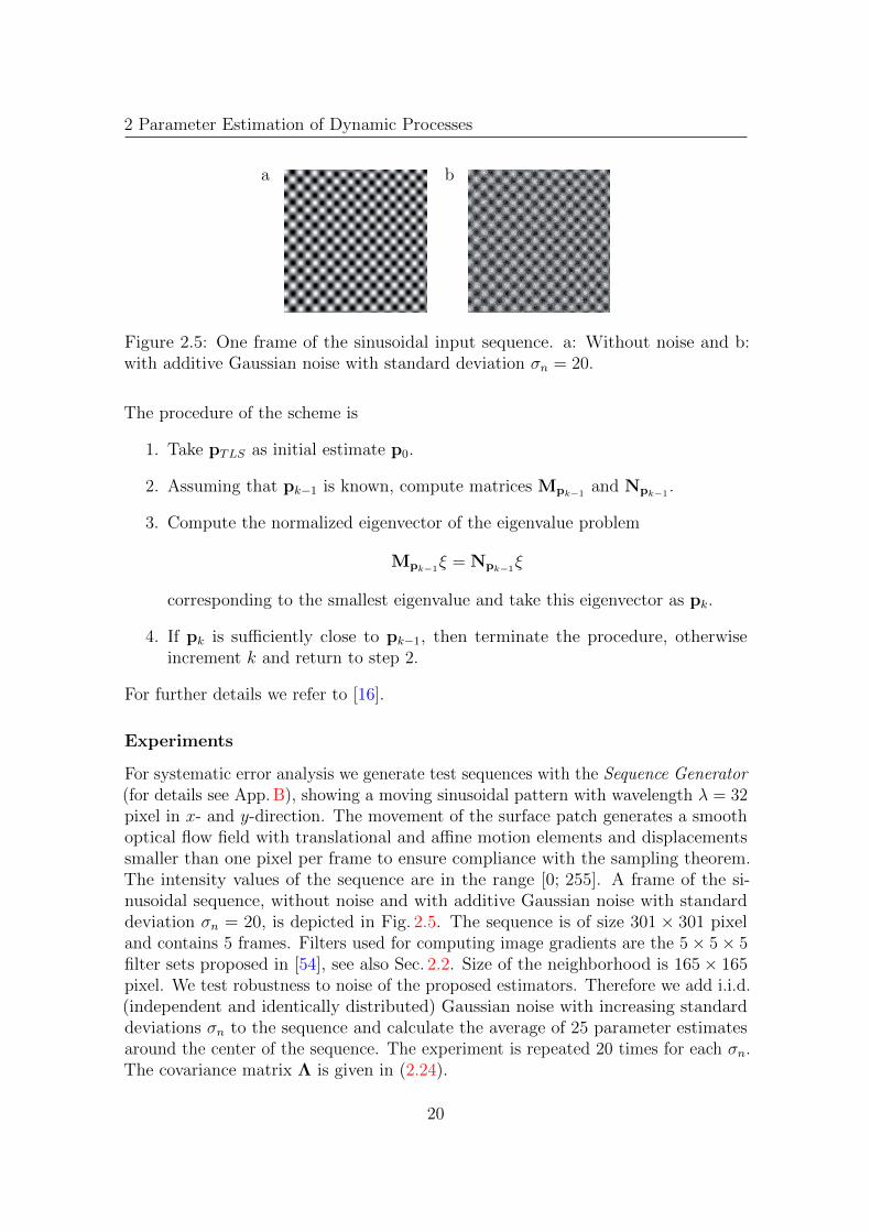
Figure 2.5: One frame of the sinusoidal input sequence. a: Without noise and b:with additive Gaussian noise with standard deviation σn = 20.
The procedure of the scheme is
1. Take pTLS as initial estimate p0.
2. Assuming that pk−1 is known, compute matrices Mpk−1and Npk−1
.
3. Compute the normalized eigenvector of the eigenvalue problem
Mpk−1ξ = Npk−1
ξ
corresponding to the smallest eigenvalue and take this eigenvector as pk.
4. If pk is sufficiently close to pk−1, then terminate the procedure, otherwiseincrement k and return to step 2.
For further details we refer to [16].
Experiments
For systematic error analysis we generate test sequences with the Sequence Generator(for details see App. B), showing a moving sinusoidal pattern with wavelength λ = 32pixel in x- and y-direction. The movement of the surface patch generates a smoothoptical flow field with translational and affine motion elements and displacementssmaller than one pixel per frame to ensure compliance with the sampling theorem.The intensity values of the sequence are in the range [0; 255]. A frame of the si-nusoidal sequence, without noise and with additive Gaussian noise with standarddeviation σn = 20, is depicted in Fig. 2.5. The sequence is of size 301 × 301 pixeland contains 5 frames. Filters used for computing image gradients are the 5× 5× 5filter sets proposed in [54], see also Sec. 2.2. Size of the neighborhood is 165× 165pixel. We test robustness to noise of the proposed estimators. Therefore we add i.i.d.(independent and identically distributed) Gaussian noise with increasing standarddeviations σn to the sequence and calculate the average of 25 parameter estimatesaround the center of the sequence. The experiment is repeated 20 times for each σn.The covariance matrix Λ is given in (2.24).
20

2.3 Parameter Estimation
a b
1.0E-04
1.0E-03
1.0E-02
1.0E-01
1.0E+00
1.0E+01
1.0E+02
1 10 100σ
AAE
TLS*
OLS
1.0E-04
1.0E-03
1.0E-02
1.0E-01
1.0E+00
1.0E+01
1.0E+02
1 10 100σ
AAEAffine
FNS & FOR III
OLS, TLS & SMP
c d
1.0E-04
1.0E-03
1.0E-02
1.0E-01
1.0E+00
1.0E+01
1.0E+02
1 10 100σ
AAE
1.0E-04
1.0E-03
1.0E-02
1.0E-01
1.0E+00
1.0E+01
1.0E+02
1 10 100σ
AAEAffine
OLS TLS FNSSMP FOR III
Figure 2.6: Parameter estimation with standard least squares (OLS), and total leastsquares (TLS∗) techniques. The TLS∗ techniques are standard TLS, FNS, SMP andFOR III. Angular errors of translational (left) and affine (right) motion parametersfor increasing additive Gaussian noise are shown. Scaling of local coordinates withk = 1 (top), i.e., normalized by pixelsize, and with k = 1e− 4 (bottom).
Figure 2.6 shows estimation results of standard least squares (OLS), total leastsquares (TLS) and the proposed numerical schemes for solving the variational equa-tion, namely FNS, SMP and FOR III. The average angular error (App. A) of thetranslational parameters (left) and of the affine motion parameters (right) is shownfor increasing standard deviations σn of additive Gaussian noise. Scaling of localcoordinates may influence estimation (cmp. Sec. 2.3.3). In a standard affine motionmodel (2.6) weights of affine parameters are different to weights of the translationalmotion parameters. In order to examine the influence of different weights, we distin-guish between angular errors of translational and affine motion parameters.Figure 2.6a and b show angular errors using local coordinates scaled by k = 1, i.e.,normalized by pixelsize, ∆x ∈ [−82; 82]. In this case, the standard least squaresapproach (Sec. 2.3.1) yields highest errors for translational motion estimates for high
21

2 Parameter Estimation of Dynamic Processes
noise variances (σn > 20). All other techniques perform similar for translationalmotion. Affine motion parameters are slightly better estimated by schemes incorpo-rating covariance matrices (FNS and FOR III). Standard TLS, OLS and SMP yieldsimilar results.The effect on incorporating covariance matrices is only visible for high noise. Affinemotion parameters for optical flow are typically up to a factor 100 smaller thantranslational motion parameters, i.e., the impact of re-scaling these parameters issmall compared to the overall error. Experiments where incorporation of covarianceinformation yield superior results are ellipse fitting [16] or fundamental matrix esti-mation [17]. There the influence of affine parameters is higher, because the scaling isdifferent, e.g., typically in the range of [−1; 1] for fundamental matrix estimation.Figure 2.6c and d show results of a second experiment where affine parameters arescaled by a factor k = 1e − 4 before estimation, i.e., ∆x ∈ [−0.0082; 0.0082] andre-scaled afterwards. Using this scaling, errors in affine parameters influence errorsin translational parameters much more than using a scaling factor k = 1.In this case, the FNS yields no reliable estimates for neither translational nor affinemotion parameters. Standard TLS and SMP perform similar for small noise variances.For noise with standard deviation σn > 20 SMP is not able to estimate reliablemotion parameters any more. Estimates of OLS and standard TLS yield similarangular errors. However, FOR III estimates show lowest angular errors for noisewith standard deviation σn > 20. The affine parameters are best estimated withOLS and FOR III. Angular errors of SMP and standard TLS are more than oneorder of magnitude higher compared to FOR III for σn > 20.We conclude that the scale, i.e., selected units, of local coordinates has significanteffect on estimation results. Using the FOR III scheme or OLS the effect is negligible,but standard TLS, the SMP scheme and the FNS scheme may yield highly degradedestimation results, if the scaling is not appropriate. The FOR III scheme yieldsoverall highest accuracy for all scaled and unscaled parameters.
2.3.4 Robust Estimation
The presented estimation approaches assume that motion within a local neighborhoodΛ can be determined by a single parameter set, e.g., a single motion vector, if theconstancy assumption (2.3) is used. This motion assumption is violated in commonsituations due to transparency, depth discontinuities, shadows or noise. Robustestimation approaches relax the assumption of single motions. Black and Anandan[9] introduced a robust least squares estimation framework for optical flow to handlediscontinuities and to estimate multiple motion in a spatial neighborhood. A robustρ-function is used to decrease the influence of outliers in the estimation process. Inorder to estimate a second motion another estimation process may be initialized,using only the outliers of the first estimation process. The use of a robust ρ-functionis detailed in the following example.The OLS parameter estimation problem for optical flow is to find a motion vector u
22

2.3 Parameter Estimation
which minimizes energy function E
E(u) =∑
(x∈Λ)
(Ix(x, t)ux + Iy(x, t)uy + It(x, t))2
=∑
(x∈Λ)
((∇T
xI)u + It)2
=∑
(x∈Λ)
ρquad((∇T
xI)u + It) (2.35)
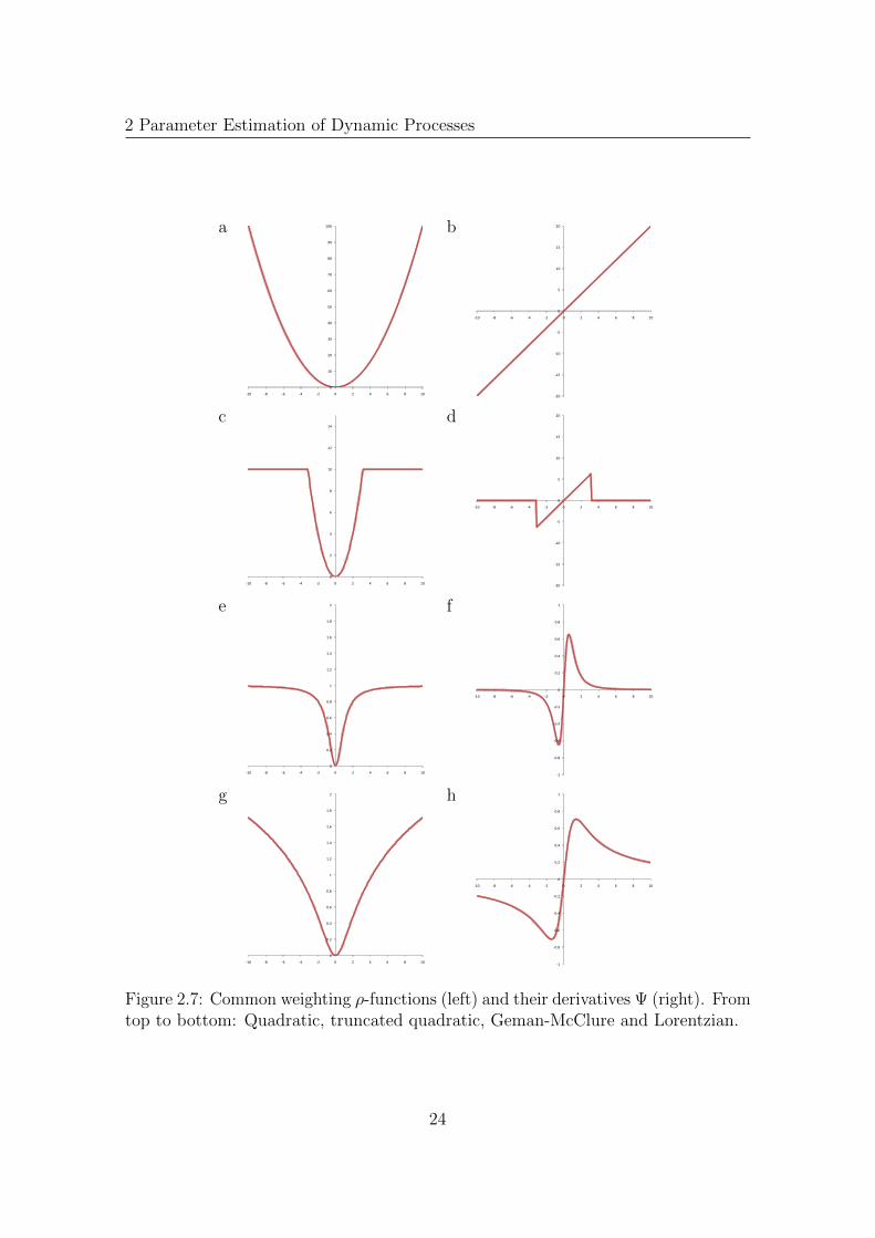
with the quadratic ρ-function ρquad(x) = x2 and neighborhood Λ. This ρ-functionis optimal, when errors in ∇xI are normally distributed. However, the quadraticρ-function assigns high weights to outlying measurements. The so-called influencefunction of a particular ρ-function is used to demonstrate this behavior. The influencefunction characterizes the bias that a particular measurement has on the solution andis proportional to the derivative, Ψ, of the ρ-function. In the least squares case, theinfluence of data points increases linearly and without bound. To increase robustnessa ρ-function should reduce the weight of outliers. The quadratic ρ-function andthree common robust ρ-functions with the corresponding Ψ-functions are depicted inFig. 2.7.The truncated quadratic
ρtq(x, α, λ) =
λx2 if |x| <
√α√λ
α else(2.36)
weights errors quadratically up to a fixed threshold. Beyond that threshold errorsreceive a constant value α. The truncated quadratic is similar to the Huber function[30]. There errors increase linearly beyond the threshold. Other robust functions arethe Geman and McClure [20]
ρgem(x, σ) =x2
σ + x2(2.37)
and the Lorentzian
ρlor(x, σ) = log
(1 +
1
2
(xσ
)2). (2.38)
These robust function have differentiable Ψ-functions
Ψgem(x, σ) =2xσ
(σ + x2)2(2.39)
and
Ψlor(x, σ) =2x
2σ2 + x2, (2.40)
which provide a more gradual transition between inliers and outliers.To make (2.35) more robust, it is reformulated to account for outliers by using a
23
2 Parameter Estimation of Dynamic Processes
a b
0
10
20
30
40
50
60
70
80
90
100
-10 -8 -6 -4 -2 0 2 4 6 8 10 -20
-15
-10
-5
0
5
10
15
20
-10 -8 -6 -4 -2 0 2 4 6 8 10
c d
0
2
4
6
8
10
12
14
-10 -8 -6 -4 -2 0 2 4 6 8 10 -20
-15
-10
-5
0
5
10
15
20
-10 -8 -6 -4 -2 0 2 4 6 8 10
e f
0
0.2
0.4
0.6
0.8
1
1.2
1.4
1.6
1.8
2
-10 -8 -6 -4 -2 0 2 4 6 8 10 -1
-0.8
-0.6
-0.4
-0.2
0
0.2
0.4
0.6
0.8
1
-10 -8 -6 -4 -2 0 2 4 6 8 10
g h
0
0.2
0.4
0.6
0.8
1
1.2
1.4
1.6
1.8
2
-10 -8 -6 -4 -2 0 2 4 6 8 10 -1
-0.8
-0.6
-0.4
-0.2
0
0.2
0.4
0.6
0.8
1
-10 -8 -6 -4 -2 0 2 4 6 8 10
Figure 2.7: Common weighting ρ-functions (left) and their derivatives Ψ (right). Fromtop to bottom: Quadratic, truncated quadratic, Geman-McClure and Lorentzian.
24
2.3 Parameter Estimation
robust ρ-function. We get
E(u) =∑
(x∈Λ)
ρ((∇T
xI)u + It, σ)
(2.41)
with robust function ρ.
Robust Least Squares
Black and Anandan [9] use successive over-relaxation (SOR, cmp. [12]) to find theminimum of (2.41). The iterative update equation for one motion parameter ui atstep n+ 1 is
un+1i = uni − κ
1
T (ui)
∂E
∂ui(2.42)
where κ is an over-relaxation parameter. When 0 < κ < 2 the method can be shownto converge, but the rate of convergence is sensitive to the exact value of κ. Theterm T (ui) is an upper bound on the second partial derivative of E,
T (ui) ≥∂2E
∂u2i
. (2.43)
Typically the objective function is non-convex. To find the globally optimal solutionBlack and Anandan propose to use a robust ρ-function with a parameter whichcontrols the influence of the outliers, e.g., parameter σ. They start with minimizinga convex approximation of the objective function, i.e., high σ, thus outliers are notdown-weighted. Then they successively minimize better approximations of the trueobjective function, i.e., lowering σ, starting from the previous estimated minimum,so that influence of outliers on the estimation process gets less. This approach workswell in practice, but is not guaranteed to converge to the global minimum, becausethe initial estimate may be too far away from the global minimum.
Robust Total Least Squares
Equation (2.41) may be solved in total least squares sense analog to Sec. 2.3.2. Theapproximated maximum likelihood function (2.26) is combined with the robustρ-function by
EAML,Rob =N∑i
ρ
(pTAip
pTCip, σ
). (2.44)
The minimum of the energy EAML,Rob may be found numerically with the schemespresented in Sec. 2.3.2, e.g., FOR III or FNS. Analog to [9] the control parameter σof the robust function should be successively minimized to find the global minimum.
25
2 Parameter Estimation of Dynamic Processes
a b
0
0.5
1
1.5
2
2.5
3
3.5
4
4.5
0 5 10 15 20 25 30
2
2.2
2.4
2.6
2.8
3
3.2
3.4
3.6
3.8
4
0 5 10 15 20 25 30
c d
2
2.2
2.4
2.6
2.8
3
3.2
3.4
3.6
3.8
4
0 5 10 15 20 25 30 -0.025
-0.02
-0.015
-0.01
-0.005
0
0.005
0 5 10 15 20 25 30
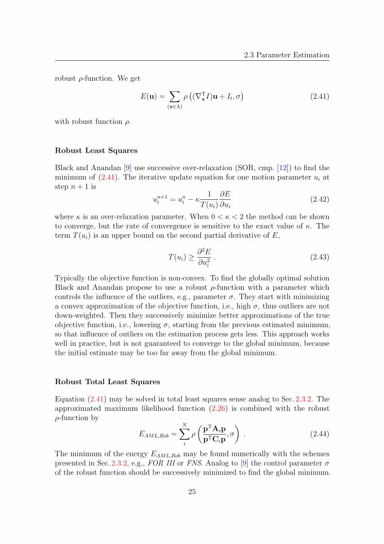
a: and Ground truth translational motion parameters u1 and u2
and Ground truth affine motion parameters a1 = 0 and a2 = 0
b–d: ρ-functions Quadratic Truncated quadratic
Geman-McClure Lorentzian
Figure 2.8: Robust estimation. a: Ground truth values, b: robust estimation withtranslational motion model, c and d: robust estimation with affine motion model. c:Translational motion estimates and d: affine motion estimates.
Robust Estimation for Parametric Motion Models
Finding the global minimum of a robust energy function highly depends on the choiceof the ρ-function and its control parameter σ. The proposed minimization schemeswork well in practice for constant motion models. Difficulties arise when using morecomplex motion models, e.g., an affine motion model (2.6).An experiment investigating the influence of ρ-functions on parameter estimationfor one dimensional optical flow is shown in Fig. 2.8. Figure 2.8a shows the groundtruth optical flow parameters. Translational motion parameters u1 = 4 and u2 = 2are depicted in blue and affine motion parameters a1 = a2 = 0 in red, i.e., puretranslational motion. The data term is given by d1 = [5,−20]T and d2 = [7,−14]T.A motion discontinuity occurs at x = 15. The control parameter for ρgem and ρlor is
26

2.3 Parameter Estimation
a b
0
50
100
150
200
250
0 5 10 15 20 25 30
0
5
10
15
20
25
30
0 5 10 15 20 25 30
ρ-functions: Truncated quadratic, Geman-McClure and Lorentzian
Figure 2.9: Robust estimation. Weights for estimate at x = 23, a: robust estimationwith translational motion model and b: robust estimation with affine motion model.
lowered from σ = 15 to σ = 0.1. The threshold for the truncated quadratic is α = 3and λ = 1. Size of the neighborhood is N = 21.Figure 2.8b shows estimation results using robust total least squares and a constantmotion model. It clearly demonstrates the smoothing effect using the quadraticρ-function, due to high weighting of outliers. The truncated quadratic ρ-functionrecovers a discontinuity, but it is shifted by approx. 6 values and still the motionparameters are slightly smoothed. Using robust functions ρgem or ρlor yield clearlyseparated motion parameters. However, using the ρgem-function proposed by Gemanand McClure also leads to a shift of the discontinuity. The shift of the discontinuitydepends on the difference of the energy functions around the discontinuity, theρ-function and its control parameter, which determines when a parameter is declaredas an outlier. Figures 2.8c and d show estimation results when using an affine motionmodel. Results for translational motion parameters are depicted in Fig. 2.8c, and foraffine motion parameters in Fig. 2.8d. Simultaneous estimation of all parameters of aparametric model leads to erroneous estimates at the motion discontinuity, becausethe iterative estimation process does not converge to the global energy minimum. Alocal minimum solution is not a solely translational motion at one side and outliersat the other side, but a divergent motion. Figure 2.9 shows weights for x = 23, i.e.,near the discontinuity, calculated by the different ρ-functions for the translationaland the affine motion model. Using the translational motion model, the data onthe left side gets high weights and the outliers on the right side are suppressed.Figure 2.9b demonstrates that high weights are assigned to data on both side of thediscontinuity, when an affine motion model is used. This effect occurs regardless ofwhich ρ-function is used.Black and Anandan avoid this kind of erroneous estimates for parametric models bysuccessive estimation of translational and affine model parameters.
27

2 Parameter Estimation of Dynamic Processes
a b c d
Figure 2.10: a and b: First and last frame of a sinusoidal sequence with two affinemotions. The white rectangle depicts the area, where the average angular error isevaluated. c and d: gray value coded ground truth of translational motion parametersin x- and y-direction respectively.
Experiments
In this section we compare the robust estimators Robust TLS, Robust Affine OLS andRobust Affine TLS. Sinusoidal sequences are generated with the Sequence Generator(App. B). Wavelength of the sinusoidal pattern is λx = λy = 8 pixel and sequencesize is 301× 301× 9. In the first experiment two patches move with translationalmotion. In the second experiment both patches have translational and affine motionparameters. The maximum motion in both sequences is less than one pixel perframe. Figure 2.10 shows two frames of the sequence for translational and affinemotion and the gray value coded ground truth optical flow in x- and y- direction.Optical flow values in x-direction are in the range [−0.1, 0.3] and in y-direction in therange [−0.3, 0.3]. Standard deviation of additive i.i.d. Gaussian noise is increasedand for each standard deviation experiments are repeated 10 times. The size of theneighborhood is 65 pixel in x- and y-direction and 5 frames in time and is weightedwith a Gaussian with standard deviation 19 × 19 × 1. All robust estimators usethe Lorentzian (2.38), initialized with σ = 5 and lowered to σ = 0.1. Iterations arestopped after 50 iterations or when change of parameters is below 1E − 08. Theaverage angular error is calculated for a rectangular patch of 151× 11 pixel aroundthe discontinuity (see Fig. 2.10a). Translational and affine angular errors for bothsequences are depicted in Fig. 2.11.Figure 2.11a demonstrates that all estimators perform similar for noise with standarddeviation up to approx. σn = 3. The ordinary least squares estimator performsslightly better compared to the total least squares estimators for higher noise values.In the case of no noise the standard TLS performs best. Affine angular errors aresimilar for both affine estimators, when noise is present. In the noise-free case theOLS approach yields lower affine angular errors.In Fig. 2.11c is shown that the affine TLS approach performs best for low noise(σn < 3), when a sequence contains affine motion parameters. Standard TLS performsbetter than affine OLS for noise with σn < 1. All estimators yield similar results forhigher noise variances. Figure 2.11d demonstrates that affine angular errors of theaffine TLS is up to one orders of magnitude lower than for the affine OLS in the
28

2.4 Conclusions
a b
1.0E-04
1.0E-03
1.0E-02
1.0E-01
1.0E+00
1 2 3 4 5σ
AAE
1.0E-04
1.0E-03
1.0E-02
1.0E-01
1.0E+00
0 1 2 3 4 5σ
AAE
c d
1.0E-04
1.0E-03
1.0E-02
1.0E-01
1.0E+00
0 1 2 3 4 5σ
AAEAffine
1.0E-04
1.0E-03
1.0E-02
1.0E-01
1.0E+00
0 1 2 3 4 5σ
AAEAffine
Robust estimators: TLS, affine OLS [9] and affine TLS
Figure 2.11: Average translational (top) and affine (bottom) angular errors of motionestimates near a discontinuity caused by two translational (left) and two affine (right)moving surface patches (see Fig. 2.10).
noise free case. The TLS estimator yields still slightly better results for noise withσn < 3, for higher standard deviations of noise OLS and TLS perform similar.
2.4 Conclusions
In this section parameter estimation techniques applied to motion estimation basedon optical flow have been presented. A data model based on the brightness constancyconstraint and constant, affine and quadratic motion models for optical flow havebeen introduced. Optimized filters used to calculate image derivatives have beenproposed in Sec. 2.2. Standard local estimation techniques and more sophisticatedlocal estimators incorporating covariance distributions and handling outliers havebeen discussed and compared in Sec. 2.3.Synthetic experiments (cmp. Fig. 2.11) showed that affine modeling of the flow fielddoes only improve estimation results when an appropriate estimator is used. Anaffine TLS estimator yields better results in the low noise case, whereas the leastsquares estimator proposed by Black and Anandan [9] yields only similar or worse
29

2 Parameter Estimation of Dynamic Processes
results than standard TLS. However, in order to ensure reliable estimates the size ofthe local neighborhood has to be increased for affine motion models, because moremotion parameters have to be estimated.Incorporating known measurement errors yields better motion estimates for sequencesheavily corrupted by noise or when the influence of (affine) parameters is high dueto inappropriate scaling of parameters. In this case the First Order RenormalizationScheme Version III (FOR III) showed best performance. Standard TLS yields similarperformance for input data with low noise (σn < 20) and appropriate scaling ofparameters, i.e., scaling factor k = 1.Robust estimation should be used when discontinuities (e.g., caused by noise ormultiple motions) occur in the data. The Lorentzian ρ-function best separated differ-ent parameter near discontinuities. Combinations of parametric motion models androbust estimation techniques may lead to corrupt estimates at motion discontinuities.Successive robust estimation of translational and affine motion parameters can avoidconvergence to local minimum solutions. In synthetic experiments the robust affineTLS outperformed standard TLS and the affine OLS [9] for translational and affinemotion estimation in sequences with discontinuities.
30

Chapter 3
Approaches to 3D MotionEstimation
In literature many models have been introduced for 3D structure and 3D motionestimation. 3D motion is sometimes called Scene Flow, to point out the relationshipto optical flow, or Range Flow, that is 3D motion calculated from range data. Bothmotion estimation techniques, namely optical flow-based and correspondence-based(cmp. Sec. 2), have been used for 3D structure and 3D motion estimation. However,optical flow-based estimation schemes have been shown to yield higher accuracy fordedicated setups [26]. In this work the focus is on optical flow-based estimation. Theso-called Scene Flow technique [74] is one of the most popular 3D motion estimationframeworks. In general this technique may be used for estimation of 3D motion fromone or more cameras and for computing scene structure. However, the flow-basedreconstruction algorithm proposed in [76] can only recover structure where the sceneis actually moving. The 3D motion estimation algorithm has been improved by [40],recently. They incorporate probability distributions from 2D optical flow to makethe estimation of 3D motion more reliable. Range Flow estimation techniques arebased on range image sequences. Spies et al. [67] presented a framework where rangeconstraints on range sequences are combined with optical flow on intensity sequences.Scene Flow and Range Flow techniques solely estimate 3D motion based on alreadyavailable 3D structure information. In contrast [57] presented a multi-camera frame-work for simultaneous estimation of 3D structure and 3D motion. Therefore theparameters of an affine optical flow-based model (cmp. Sec. 2.1.1) are used to solve fordepth, surface slopes and translational motion. The framework has been generalizedin [56] and has been made robust against brightness changes in the data [60]. Furtherimprovements in [62] made the model more robust and incorporated constraints fromRange Flow.In this chapter we review Scene Flow, Range Flow and the Affine Model. We evaluateestimation of depth and slopes with the Affine Model on synthetic test sequencesand on real data. Finally the three motion estimation techniques are compared onsynthetic sequences and real data.
31

3 Approaches to 3D Motion Estimation
3.1 Scene Flow
Vedula et al. [74] define Scene Flow as the 3D motion field of points in the world,just as optical flow is the 2D motion field of points in the image (cmp. Sec. 2.1).Optical flow is the projection of 3D motion onto the image plane of a camera.
Given a 3D point X = (X, Y, Z)T, the projection onto the image plane in camerac is denoted by xc = (xc, yc)
T. The 2D components of xc are
xc =[Pc]1(X, Y, Z, 1)T
[Pc]3(X, Y, Z, 1)T, yc =
[Pc]2(X, Y, Z, 1)T
[Pc]3(X, Y, Z, 1)T(3.1)
where [Pi]j is the jth row of the camera projection matrix Pc [23]. If the camera isnot moving, then the 2D optical flow u = dxc
dtis uniquely determined by
u =∂xc∂X
dX
dt. (3.2)
This equation denotes how optical flow u can be computed for known 3D motionf = dX
dt. Computing 3D motion f from optical flow u requires inverting (3.2). The
problem is, that X depends not only on the optical flow but also on time, indirectlythrough the 3D structure, i.e., X = X(xc(t), t). 3D motion f is given by the totaldifferential of X with respect to time
dX
dt=∂X
∂xc
dxcdt
+∂X
∂t
∣∣∣∣xc
. (3.3)
This means that the motion of a point cannot be calculated solely from optical flow.The second term determines the change of a point on the surface imaged by a fixedpixel, i.e., the motion of X along the ray corresponding to xc. In order to solvefor 3D motion f with (3.3) this motion has to be known. If structure data is notavailable for additional time steps more than one camera viewing the scene is neededto invert (3.2). Assuming that optical flow is known we have two linear constraintsand three unknowns in f . Analog to optical flow (cmp. Sec. 2.1), more than twoequations are needed to solve for 3D motion f , i.e., at least two cameras are needed.The final equation system is
Bf = U , with B =
∂xc,1∂X
∂xc,1∂Y
∂xc,1∂Z
∂yc,1∂X
∂yc,1∂Y
∂yc,1∂Z
∂xc,2∂X
∂xc,2∂Y
∂xc,2∂Z
......
...∂xc,N∂X
∂xc,N∂Y
∂xc,N∂Z
and U =
∂xc,1∂t∂yc,1∂t
∂xc,2∂t...
∂xc,N∂t
(3.4)
for N calibrated cameras. Analog to optical flow, (3.4) may be solved with anytechnique presented in Sec. 2.3. Vedula et al. [75] propose a singular value decompo-
32
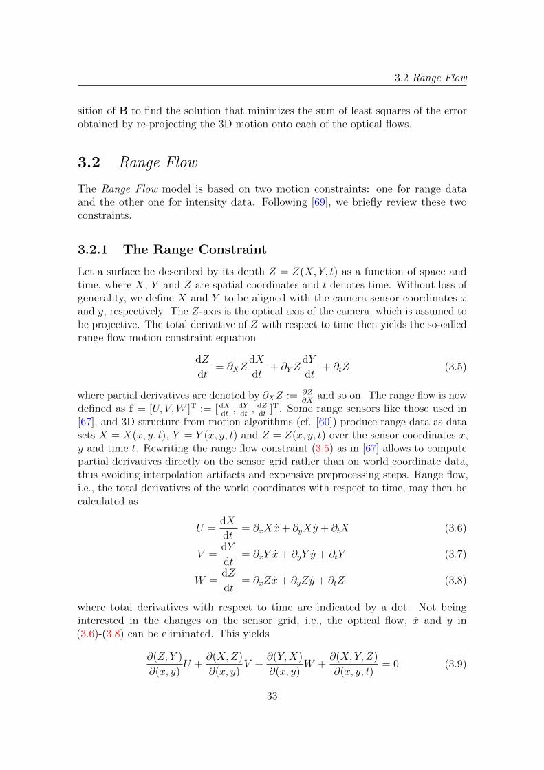
3.2 Range Flow
sition of B to find the solution that minimizes the sum of least squares of the errorobtained by re-projecting the 3D motion onto each of the optical flows.
3.2 Range Flow
The Range Flow model is based on two motion constraints: one for range dataand the other one for intensity data. Following [69], we briefly review these twoconstraints.
3.2.1 The Range Constraint
Let a surface be described by its depth Z = Z(X, Y, t) as a function of space andtime, where X, Y and Z are spatial coordinates and t denotes time. Without loss ofgenerality, we define X and Y to be aligned with the camera sensor coordinates xand y, respectively. The Z-axis is the optical axis of the camera, which is assumed tobe projective. The total derivative of Z with respect to time then yields the so-calledrange flow motion constraint equation
dZ
dt= ∂XZ
dX
dt+ ∂YZ
dY
dt+ ∂tZ (3.5)
where partial derivatives are denoted by ∂XZ := ∂Z∂X
and so on. The range flow is nowdefined as f = [U, V,W ]T := [dX
dt, dY
dt, dZ
dt]T. Some range sensors like those used in
[67], and 3D structure from motion algorithms (cf. [60]) produce range data as datasets X = X(x, y, t), Y = Y (x, y, t) and Z = Z(x, y, t) over the sensor coordinates x,y and time t. Rewriting the range flow constraint (3.5) as in [67] allows to computepartial derivatives directly on the sensor grid rather than on world coordinate data,thus avoiding interpolation artifacts and expensive preprocessing steps. Range flow,i.e., the total derivatives of the world coordinates with respect to time, may then becalculated as
U =dX
dt= ∂xXx+ ∂yXy + ∂tX (3.6)
V =dY
dt= ∂xY x+ ∂yY y + ∂tY (3.7)
W =dZ
dt= ∂xZx+ ∂yZy + ∂tZ (3.8)
where total derivatives with respect to time are indicated by a dot. Not beinginterested in the changes on the sensor grid, i.e., the optical flow, x and y in(3.6)-(3.8) can be eliminated. This yields
∂(Z, Y )
∂(x, y)U +
∂(X,Z)
∂(x, y)V +
∂(Y,X)
∂(x, y)W +
∂(X, Y, Z)
∂(x, y, t)= 0 (3.9)
33

3 Approaches to 3D Motion Estimation
where∂(Z, Y )
∂(x, y)=
∣∣∣∣ ∂xZ ∂xY∂yZ ∂yY
∣∣∣∣ = ∂xZ∂yY − ∂yZ∂xY (3.10)
is the Jacobian of Z, Y with respect to x, y, and so on. Equation (3.9) depends onlyon derivatives in sensor coordinates, and can be calculated easily using derivativekernels. Assuming aligned world and sensor coordinate systems (∂yX = ∂xY = 0),(3.9) reduces to
(∂yY ∂xZ)U + (∂xX∂yZ)V − (∂xX∂yY )W
+ (∂xX∂yY ∂tZ − ∂xX∂tY ∂yZ − ∂tX∂yY ∂xZ) = 0 . (3.11)
3.2.2 The Intensity Constraint
The range constraint is based solely on range data, and, analog to optical flow (cmp.Sec. 2.3.2) the full flow can only be estimated where 3 or more distinct depth planesintersect. Surfaces are sometimes nearly planar, smooth surfaces resulting in apertureproblems almost everywhere when using the range flow constraint only. As proposedin [67], intensity data should therefore be incorporated in addition. Let the intensityof a point remain constant over the observation time interval. Then the so-calledbrightness constancy constraint equation often used for optical flow estimation (see,e.g., [4]) holds. Linearization of this constraint yields
dI
dt= ∂xIx+ ∂yIy + ∂tI = 0 . (3.12)
Eliminating optical flow (x, y) using (3.6) and (3.7) yields
∂(I, Y )
∂(x, y)U +
∂(X, I)
∂(x, y)V +
∂(X, Y, I)
∂(x, y, t)= 0 . (3.13)
The estimated range flow f = [U, V,W ]T has to fulfill both the range flow constraint(3.9) and the intensity constraint (3.13). The intensity constraint is more reliableto provide point-to-point correspondences, and therefore often solves the apertureproblem. Together with the range constraint, it allows to solve for f in places wherethe range constraint alone is insufficient.
3.2.3 Range Flow Estimation
To estimate parameters within a total least squares framework, we closely follow [69].The range constraint (3.11) yields for every pixel an equation of the form dT
rcp = 0with
drc =
[∂ (Z, Y )
∂ (x, y),∂ (X,Z)
∂ (x, y),∂ (Y,X)
∂ (x, y),∂ (X, Y, Z)
∂ (x, y, t)
]T
(3.14)
34

3.3 Affine Model
and parameter vectorp = [U, V,W, 1]T . (3.15)
To solve this equation standard total least squares is used (cmp. Sec. 2.3.2), butany other estimator proposed in Sec. 2.3 could be used as well. As described inSec. 3.2.2 we have more than one constraint for the U and V components of RangeFlow. In the same way as expressing the range constraint by dT
rcp = 0, the intensityconstraint may be expressed by dT
I p = 0, where dI is computed from the observeddata according to
dI =
[∂ (I, Y )
∂ (x, y),∂ (X, I)
∂ (x, y), 0,
∂ (X, Y, I)
∂ (x, y, t)
]T
. (3.16)
As shown in [69], combining the different constraints yields a new structure tensorwhich is simply the weighted sum of the tensor Jrc from the range constraint (3.9),and the tensor JI from the intensity-dependent constraint (3.13). With the weightβ, the overall tensor thus is
J = Jrc + βJI . (3.17)
The weight β may be used to account for different signal-to-noise-ratios in thestructure tensors. Furthermore, the data channels should be scaled to the same meanand variance before they are combined.The optimal estimate of the sought parameter vector is then given by the eigenvectorb corresponding to the lowest eigenvalue of J (cmp. Sec. 2.3.2). As the eigenvectoris only defined up to a scaling factor, the range flow is finally computed by thenormalization (see (3.15)) U
VW
=1
b4
b1
b2
b3
. (3.18)
3.3 Affine Model
Scharr and Kusters [57] introduced a multi-camera extension of the brightnessconstancy constraint model for simultaneous local estimation of 3D motion and 3Dposition. This model has been extended and evaluated for 4 special cases: estimationof depth only using 1D and 2D camera grids, estimation of depth and 3D motion, andestimation of depth and normals in Scharr [55]. Scharr and Schuchert [56] presenteda general framework for this Affine Model. However, in [56] the model is restrictedto surfaces inclined in only one direction, i.e., surface normal n = (ZX , 0,−1)T orn = (0, ZY ,−1)T. We derive a model handling arbitrarily inclined surfaces and asimultaneous estimation technique for all parameters.An image sequence can be interpreted as data in a 3D x-y-t-space. For optical flow
35

3 Approaches to 3D Motion Estimation
estimation in this space a BCCE defines a linear model for the changes of gray valuesdue to local object motion. The result of the calculation is a displacement vectorfield. Assuming the data comes from a single fixed camera displacements comefrom object motion. Assuming a pinhole camera looking at a fixed scene, movingorthogonal to its viewing direction, displacements (then usually called disparities)are anti-proportional to local depth. This is known as structure from camera motion(e.g., [43]).The basic idea for this estimation technique is to interpret camera position s = (sx, sy)as additional dimensions of the data. Hence all image sequences acquired by a 1Dcamera grid can be combined to sample a 4D-Volume in x-y-sx-t-space. If a 2Dcamera grid is used (as e.g., in [45, 77]) we get a 5D-Volume in x-y-sx-sy-t-space.Brightness constancy can be defined in this space as vanishing total differential ofthe intensity data. A camera model is used to project a dynamic surface patch intothe image. This yields equations for x- and y-position of the patch as a function ofcamera position and time. Plugging the linearized total differentials of x and y intothe total differential of the intensity results in the sought model. It boils down tobe an affine optical flow model with 3 dimensions (sx, sy, t) behaving like the timedimension in an usual affine optical flow model (cmp. (2.6) in Sec. 2.1). A detailedderivation can be found below in Sec. 3.3.1.As this linear data model has the same form as usual BCCEs (cmp. Sec. 2.1) nospecial estimation framework has to be established. We use the structure tensormethod (cmp. Sec. 2.3.2 and Sec. 3.3.2), but other methods can be applied as well(e.g., the ones in [4, 26]). But as parameters in the model are mixed motion-, normals-and disparity-parameters, they have to be disentangled. Especially when 2D cameragrids are used multiple independent measurements are present in each model equation.These not only have to be disentangled, but also recombined respecting their errorestimates (cmp. Sec. 3.3.2).
3.3.1 Derivation of the BCCE
In this section we derive a constraint equation describing local brightness changesin the data. To do so we project a geometric model of a moving surface patch ontoa camera sensor plane using a pinhole camera model. This geometric descriptionof moving projected surface elements is then combined with a brightness constancyassumption forming the sought constraint equation.
Surface Patch Model
For each pixel at a given point in time we want to estimate from a local neighborhooddepth, motion and surface normals of a 3D patch imaged at that location. Thuswe use a surface patch valid for the whole neighborhood as object/motion model.This surface element has its center at world coordinate position (X0, Y0, Z0) and ismodeled as a function of time t and local world coordinates (∆X,∆Y ) with X- and
36

3.3 Affine Model
Z
f
P
X
x
y
Y
∆Y
p
sx
sy
∆X
∆x
∆y
x0 imageplane
y0
Figure 3.1: Pinhole projection of a point P using a camera with center at (sx, sy).
Y -slopes ZX and ZY . It moves with velocity U = (UX , UY , UZ)T: XYZ
=
X0 + UX∆t+ ∆XY0 + UY ∆t+ ∆YZ0 + UZ∆t+ ZX∆X + ZY ∆Y
. (3.19)
The surface normal is then n = (ZX , ZY ,−1)T. Velocity U could be further modeledusing translation and rotation for rigid patches (cmp. Chap. 5) or using an affinetransform for deformable patches. We omit this step here for simplicity.
Camera Model
We use a pinhole camera at world coordinate position (sx, sy, 0), looking into Z-direction (cmp. Fig. 3.1) (
xy
)=f
Z
(X − sxY − sy
)(3.20)
where x and y are sensor coordinates and camera position space is sampled equidis-tantly using a camera grid.A local neighborhood for parameter estimation is defined using neighboring pixels.However, we are interested in the local neighborhood given on the 3D surface patchby means of ∆X and ∆Y . We therefore need to derive a relation between local 3D
37

3 Approaches to 3D Motion Estimation
coordinates ∆X and ∆Y and local sensor coordinates ∆x and ∆y. To do so we solvethe pinhole camera model (3.20) of the central camera, i.e., sx = sy = 0, for a 3Dpoint (X, Y, Z) and substitute Z = Z0,0/(1− ZX x0
f− ZY y0
f) with depth Z0,0 at the
principal point (x, y) = (0, 0) (cmp. [23]). We get Xx0,y0
Yx0,y0Zx0,y0
=Z0,0
f
x0
y0
f
1
1− ZX x0f− ZY y0
f
(3.21)
with (x0, y0) being the pixel coordinates where (X, Y, Z) is projected to. Assuminglocal coordinates ∆X constant in time, the total differential of X is given by
∆X =∂X
∂x∆x+
∂X
∂y∆y . (3.22)
Inserting (3.21) in (3.22) yields
∆X∆Y∆Z
=Z0
fcx0,y0
(
1− ZY y0f
)∆x+ ZY
x0f
∆y(1− ZX x0
f
)∆y + ZX
y0f
∆x
ZX∆x+ ZY ∆y
(3.23)
withcx,y = 1− ZX
x
f− ZY
y
f(3.24)
and local neighborhood operators ∆x = x− x0 and ∆y = y − y0 on the image plane.In the case of a fronto-parallel surface, i.e., ZX = ZY = 0, (3.23) boils down to ∆X
∆Y∆Z
=Z0
f
∆x∆y0
. (3.25)
There neighboring points in ∆X and ∆Y directions are projected independent of eachother and of the pixel position (x0, y0) onto the image plane. Figure 3.2 demonstratesthe difference between projection of a fronto-parallel surface and a sloped surface.
Brightness Change Model
Using a camera grid means sampling (sx, sy)-space using several cameras each ofwhich acquires an image sequence. We combine all of these sequences into one 5Ddata set sampling the continuous intensity function I(x, y, sx, sy, t), i.e., intensitylives in a 5D space. We assume that the acquired brightness of a surface element isconstant under camera translation, meaning we are looking at a Lambertian surface.In addition this brightness shall be constant in time, i.e., we need temporally constantillumination, which can be relaxed easily using the approach shown in Chap. 4. We
38

3.3 Affine Model
Figure 3.2: Pinhole projection of a patch. Left: fronto-parallel surface, right: Surfacenot fronto-parallel. We selected huge pixel sizes to demonstrate the effect.
see that brightness is constrained in one temporal and two spatial coordinates. Inother words there is a 3D manifold in our 5D space in which I does not change. Thusthe total differential dI vanishes in this manifold. The brightness model therefore is
dI = Ixdx + Iydy + Isxdsx + Isydsy + Itdt = 0 . (3.26)
Please note that all derivatives and differentials in this equation have physical units.Image coordinates x and y are given in pixel, i.e., the physical length of a sensorelement on the camera chip, typically several µm. Camera coordinates sx and sy aregiven in camera to camera displacements and time t normalized to frames (dependingon the measurement that is typically a fraction of seconds or minutes). This isimportant when interpreting parameters estimated from the model equations.
Combination of the 3 Models
In order to derive a single linear equation from the above models, we first projectthe moving surface element (3.19) to the sensor plane using a pinhole camera (3.20)(
xy
)=f
Z
(X0 + UX∆t+ ∆X − sxY0 + UY ∆t+ ∆Y − sy
). (3.27)
Consequently we can calculate the differentials dx and dy for a fixed surface location(i.e., for constant ∆X and ∆Y cmp. Sec. 3.3.1)(
dxdy
)=f
Z
((UX − UZ xf )dt − dsx(UY − UZ yf )dt − dsy
). (3.28)
39

3 Approaches to 3D Motion Estimation
This equation is nonlinear in the sought 3D parameters. From (3.19) we know that
Z = Z0 + UZ∆t+ ZX∆X + ZY ∆Y= Z0 + UZ∆t+ Z0
fc(ZX∆x+ ZY ∆y) .
(3.29)
We linearize (3.29) via the assumption that UZ∆t is small compared to the overalldepth |Z0| |Uz∆t| and omit UZ∆t in the denominator. Further we can approximate
f
Z≈ f
Z0
− ZXZ0c
∆x− ZYZ0c
∆y (3.30)
assuming |ZX∆x/(fc) + ZY ∆y/(fc)| 1 . This is usually well fulfilled for not toolarge slopes, i.e., ZX and ZY smaller than 5 corresponding to a slope of approximately80 degrees, and normal angle lenses because then c ≈ 1 and ∆x f . In our Sony XC-55 camera pixel size is 7.4µm and focal length f = 12.5mm, i.e., n∆x/f ≈ n0.6 · 10−3
for the nth neighbor pixel.Plugging (3.30) into (3.28), using local coordinates x = x0 + ∆x and y = y0 + ∆y,sorting by differentials and ∆-terms, and ignoring higher order ∆-terms we get
dx =f
Z
[(UX −
x
fUZ
)dt − dsx
]=
f
Z0
(UX −
x0
fUZ
)dt
−[ZXZ0c
(UX −
x0
fUZ
)+UZZ0
]∆xdt
−[ZYZ0c
(UX −
x0
fUZ
)]∆ydt
− f
Z0
dsx +ZXZ0c
∆xdsx +ZYZ0c
∆ydsx
(3.31)
and
dy =f
Z
[(UY −
y
fUZ
)dt − dsy
]=
f
Z0
(UY −
y0
fUZ
)dt
−[ZXZ0c
(UY −
y0
fUZ
)]∆xdt
−[ZYZ0c
(UY −
y0
fUZ
)+UZZ0
]∆ydt
− f
Z0
dsy +ZXZ0c
∆xdsy +ZYZ0c
∆ydsy .
(3.32)
40
3.3 Affine Model
We may now rename the mixed 3D parameters in (3.31) with
dx = uxdt + a11∆xdt + a12∆ydt
+ νdsx + b1∆xdsx + b2∆ydsx(3.33)
and (3.32) withdy = uydt + a21∆xdt + a22∆ydt
+ νdsy + b1∆xdsy + b2∆ydsy .(3.34)
Substituting (3.33) and (3.34) into the brightness change model (3.26) we get thesought affine optical flow-like model for dynamic surface reconstruction
∇I[(
uxdt + νdsxuydt + νdsy
)+
(a11dt + b1dsx a12dt + b2dsxa21dt + b1dsy a22dt + b2dsy
)(∆x∆y
)]+Isxdsx + Isydsy + Itdt = 0 .
(3.35)
We observe that the components of this model are known from the standard affinemodel (2.6) for optical flow, i.e., translations ux, uy, and affine components a11, a12,a21, and a22 in the well known form [18]. Further there are disparity ν and its affineparameters b1 and b2 representing the projections of slopes ZX and ZY . They maybe grouped into two affine optical flow like submodels for depth estimation, i.e., onesubmodel for each camera displacement direction.For a 2D camera grid both depth-submodels, i.e., the submodel with terms containingdsx and the one containing terms with dsy are present. When only a 1D cameragrid is available, say oriented in sx-direction, then terms containing dsy can not beevaluated and are removed by setting dsy = 0. In the remainder of this work we callmodels operating on data of a 2D camera grid a 2D model, the ones referring to a1D camera grid 1D models.
Local Equations for Flow Components
We can now derive the equations connecting flow components with surface patchparameters for the three ”time”-like dimensions dt , dsx and dsy . Flow parameterscoming with dt are
ux = fZ0
(UX − x0
fUZ
)uy = f
Z0
(UY − y0
fUZ
)a11 = −ZX
Z0c
(UX − x0
fUZ
)− UZ
Z0a21 = −ZX
Z0c
(UY − y0
fUZ
)a12 = − ZY
Z0c
(UX − x0
fUZ
)a22 = − ZY
Z0c
(UY − y0
fUZ
)− UZ
Z0
(3.36)The ones coming with dsx or dsy are
ν = fZ0, b1 = ZX
Z0cand b2 = ZY
Z0c. (3.37)
41

3 Approaches to 3D Motion Estimation
All patch parameters are evaluated at a fixed pixel position and point in time.
3.3.2 Parameter Estimation
In this section we present a way to solve for the parameters using two standard leastsquares estimators. We will start by estimating affine flow parameter vectors basedon the structure tensor method (cmp. Sec. 2.3.2). Linear combinations of the solutionvectors are used to disentangle depth and motion parameters. When using a 2Dcamera grid, estimates of depth and surface normals are combined according theircovariance matrices. Finally motion parameters are estimated from affine motionparameters and 3D structure via least squares.
Estimation via Structure Tensor Method
In this parameter estimation method a model with linear parameters pj has to begiven in the form dTp = 0 with data depending vector d and parameter vector p(cmp. Sec. 2.3.2). Equation 3.35 is of this form when identifying
d = (Ix, Iy, Ix∆x, Ix∆y, Iy∆x, Iy∆y, Isx , Isy , It)T
p = (uxdt + νdsx , uydt + νdsy , a11dt + b1dsx , a12dt + b2dsx ,
a21dt + b1dsy , a22dt + b2dsy , dsx , dsy , dt )T .
(3.38)
The parameters for using a 1D camera grid oriented in sx-direction are obtained bysetting dsy = 0
d = (Ix, Iy, Ix∆x, Ix∆y, Iy∆x, Iy∆y, Isx , It)T
p = (uxdt + νdsx , uydt , a11dt + b1dsx , a12dt + b2dsx ,
a21dt , a22dt , dsx , dt )T .
(3.39)
For standard optical flow the null-space is 1D, here it is 2D or 3D, depending on themodel used. Therefore solution vectors are combined to find a minimum solutionvector for the flow in the corresponding direction, i.e., dt , dsx or dsy .
Solving for Flow Components
For our models the solution space of (2.17) is spanned by eigenvectors pi of J (wherei ∈ 1, 2 using a 1D camera grid or i ∈ 1, 2, 3 using a 2D camera grid). Thecomponents (pi)j of these eigenvectors always represent two flow components (cmp.(3.38)), one depending on time and coming together with dt and the other dependingon a camera displacement direction (dsx or dsy ).
We solve for time depending flow parameters (ux, uy, a11, a12, a21, a22) by linearlycombining solution vectors pi such that dt = 1 and dsx = dsy = 0, where dsx , dsy ,
42

3.3 Affine Model
and dt are components 9 to 11, respectively. Components 1 to 8 of the resultingvector then correspond to ux, uy, a11, a12, a21, and a22 respectively.
When using a 1D camera grid dsy already vanishes and we only need to linearlycombine solution vectors pi such that dt = 0 and dsx = 1. Depth related flowparameters ν, b1, b2 then correspond to components 1, 3, and 4, respectively.
When using a 2D camera grid, 2 linear independent eigenvectors with dt = 0can be derived. One with dsx = 1 and dsy = 0, and the other with dsx = 0 anddsy = 1. Thus we could estimate v, b1, and b2 from either of the 2 eigenvectors, butunfortunately the two estimates for each flow parameter are neither identical, norindependent. This becomes clear considering the following example. Assume ourcameras are looking at a striped pattern oriented in y-direction, i.e., parallel to sy.Then a 1D camera grid shifting along x-direction will easily determine depth fromdisparity ν, but a camera grid shifting along y-direction suffers from the apertureproblem and can not determine depth. A 2D camera grid also can only resolvedepth from its sx-movement, but not from sy-movement. In this example the twoestimates are independent. Now think of a striped pattern not oriented along x- ory-direction. The two ν-estimates are now coupled and we need to combine themaccording to their error covariance matrix C. We do so by calculating C followingNestares and Fleet [46], and rotating the representation of sx-sy-space such that Cbecomes diagonal (cmp. Fig. 3.3a). Then the resulting single estimate for ν is a sumof the independent estimates weighted by the inverse of their individual errors
ν =ν1e1 + ν2e2
e1 + e2
(3.40)
where ν1 and ν2 are the two independent disparity estimates and errors e1 = C−0.511
and e2 = C−0.522 with diagonal entries C11 and C22 of the diagonalized covariance
matrix C.Scharr [55] demonstrates the advantages of this approach. On the one hand this
approach solves the aperture problem in one camera displacement direction. In thiscase the error of one estimate becomes infinity and is therefore neglected. On theother hand the estimation accuracy slightly improves, because two estimates are usedinstead of one. Figure 3.3b shows a histogram of disparities νx, νy and ν estimatedfrom a synthetic, sinusoidal test pattern with 10% Gaussian noise added (true valueν = 1). Although there is no aperture problem and the same data has been used forall 3 estimates the histogram of ν (solid line) has less variance than the other twocurves.
Disentangling Surface Patch Parameters
Disentangling the flow parameters into parameters describing the local surface patchmeans solving the nonlinear system of (3.36) and (3.37). We have 6 unknowns(UX , UY , UZ , Z0, ZX , ZY ) and one equation per estimated flow component, i.e., 12constraints. We have an overdetermined system of equations and consequently some
43
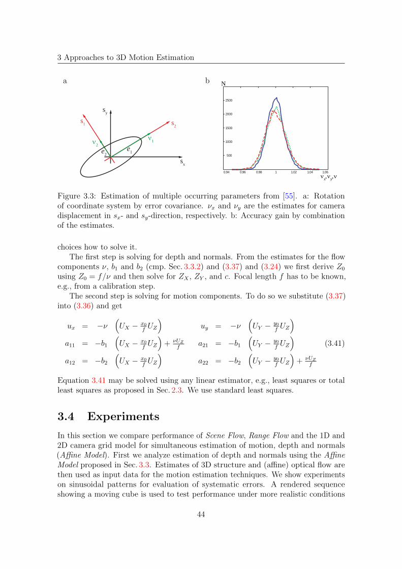
3 Approaches to 3D Motion Estimation
a b
sy
sx
ν2ν1
e1e2
s1 s2
0.94 0.96 0.98 1 1.02 1.04 1.06
500
1000
1500
2000
2500
νx,νy,ν
N
Figure 3.3: Estimation of multiple occurring parameters from [55]. a: Rotationof coordinate system by error covariance. νx and νy are the estimates for cameradisplacement in sx- and sy-direction, respectively. b: Accuracy gain by combinationof the estimates.
choices how to solve it.The first step is solving for depth and normals. From the estimates for the flow
components ν, b1 and b2 (cmp. Sec. 3.3.2) and (3.37) and (3.24) we first derive Z0
using Z0 = f/ν and then solve for ZX , ZY , and c. Focal length f has to be known,e.g., from a calibration step.
The second step is solving for motion components. To do so we substitute (3.37)into (3.36) and get
ux = −ν(UX − x0
fUZ
)uy = −ν
(UY − y0
fUZ
)a11 = −b1
(UX − x0
fUZ
)+ νUZ
fa21 = −b1
(UY − y0
fUZ
)a12 = −b2
(UX − x0
fUZ
)a22 = −b2
(UY − y0
fUZ
)+ νUZ
f
(3.41)
Equation 3.41 may be solved using any linear estimator, e.g., least squares or totalleast squares as proposed in Sec. 2.3. We use standard least squares.
3.4 Experiments
In this section we compare performance of Scene Flow, Range Flow and the 1D and2D camera grid model for simultaneous estimation of motion, depth and normals(Affine Model). First we analyze estimation of depth and normals using the AffineModel proposed in Sec. 3.3. Estimates of 3D structure and (affine) optical flow arethen used as input data for the motion estimation techniques. We show experimentson sinusoidal patterns for evaluation of systematic errors. A rendered sequenceshowing a moving cube is used to test performance under more realistic conditions
44

3.4 Experiments
and with ground truth available. Estimation results on plant leafs demonstrate theperformance of the models on real data.
3.4.1 Sinusoidal Pattern
In the first experiment we compare the influence of the additional estimation ofnormals to the other parameters in the 1D case (via (3.39)) using synthetic data.In a second experiment we test the benefit of a 2D camera grid (3.38) compared tothe 1D camera grid (3.39). The estimated 3D structure is then used to compare themotion estimation techniques.
3D Structure
Scharr [55] investigated properties of basic elements of the Affine Model with respectto filter choices, linearization effects, and noise influence. We use the results here bychoosing 5 cameras, i.e., sampling points in sx, for the 1D grid and 5× 5 cameras forthe 2D grid, because the sx- and sy-derivatives can be calculated with low systematicerror with the filter-sets proposed in [54] (cmp. Sec. 2.2). Noise increases the absoluteerror of the estimated components of the parameter vectors in the structure tensor.Thus image sequences should be acquired such that the estimable signal is maximal.Especially absolute values of displacements, i.e., optical flow components ux and uyas well as disparity v, should be as large as possible. For reasonable camera distancesin the grid disparity is much larger than 1 pixel. Therefore we define a workingdepth with an integer disparity ν0 and preshift our data in sx- and sy-directions suchthat this disparity becomes zero. Then we can estimate disparity reliably in a depthinterval around the working depth, where extremal disparities should not exceed±1 pixel. We select our acquisition configuration accordingly. Please note that thisrestriction is not inherent to the model but is due to the use of the structure tensorand can be relaxed using warping or multi-scale estimators (see e.g., [14, 49]).
As synthetic data we calculate sinusoidal patterns with the Sequence Generatorpresented in App. B. Two example intensity images and the corresponding depthmaps can be found in Fig. 3.4.
1D Grid with and without Normals In order to show the influence of theadditional estimation of surface normals in the 1D camera grid model, we generatenoise free, synthetic sinusoidal images (see above) with varying ZX . The otherparameters were set to λx=λy=λ, α=0, Z0=100 mm, f=10mm, ZY =0 and width ofpixels is 7.4µm. From these sequences with and without additive Gaussian noise weestimate local depth Z for both 1D grid models, and ZX for the model additionallyhandling surface normals. The respective plots can be found in Fig. 3.5 and Fig. 3.6.There ZX is given in degrees, i.e., ZX []= arctan(ZX). Looking at Fig. 3.5 we observethat left and right plots are almost identical. Thus the model with the normalsperforms as stable as the simpler model without normals. This coincides with
45

3 Approaches to 3D Motion Estimation
a b c d
Figure 3.4: Sinusoidal images for the central camera sx=sy=0, origin (X0, Y0) inthe image center, no motion, Z0=100 mm, f=10 mm, ZY =0 using a: λx=λy=16pixel=0.1184 mm, α=0, ZX=1.73=60 and c: λx=8 pixel, λy=80 pixel, α=30,ZX=1=45. b and d are the corresponding ground truth depth maps.
a b
1.0E-06
1.0E-05
1.0E-04
1.0E-03
1.0E-02
1.0E-01
1.0E+00
0 20 40 60 80ZX [°]
Rel. Err of Z0 [mm]
1.0E-06
1.0E-05
1.0E-04
1.0E-03
1.0E-02
1.0E-01
1.0E+00
0 20 40 60 80ZX [°]
Rel. Err of Z0 [mm]
c d
1.0E-06
1.0E-05
1.0E-04
1.0E-03
1.0E-02
1.0E-01
1.0E+00
0 20 40 60 80ZX [°]
Rel. Err of Z0 [mm]
1.0E-06
1.0E-05
1.0E-04
1.0E-03
1.0E-02
1.0E-01
1.0E+00
0 20 40 60 80ZX [°]
Rel. Err of Z0 [mm]
Patterns: λ = 8 pixel λ = 16 pixel λ = 32 pixel
Figure 3.5: Comparison of 1D camera grid models. Relative errors from sinusoidalimages. Left: model without normals, right: model with normals. a and b: noisefree data, c and d: 2.5% Gaussian noise added.
experiments in Sec. 2.3. There we have seen that an affine optical flow model, i.e.,the model with normals, may outperform a standard optical flow model, i.e., themodel without normals. Here we are looking at disparity estimates and very smallaffine motions (b1 = 0.0001 and ν ≈ 0.27, cmp. (3.37)). The improvements dueto the Affine Model are therefore not visible. In the case of noise free syntheticdata, estimates are better for larger wavelengths. For noisy data the influence ofthe wavelength is negligible. Figure 3.6 demonstrates that the absolute error of theestimated ZX is in the range of 0.001 to 0.01 in the noise free case and in the rangeof 0.01 to 10 when 2.5% Gaussian noise is added to the data.
46

3.4 Experiments
a b
1.0E-06
1.0E-05
1.0E-04
1.0E-03
1.0E-02
1.0E-01
1.0E+00
0 20 40 60 80ZX [°]
Abs. Err of ZX [°]
1.0E-03
1.0E-02
1.0E-01
1.0E+00
1.0E+01
1.0E+02
0 20 40 60 80ZX [°]
Abs. Err of ZX [°]
Patterns: λ = 8 pixel λ = 16 pixel λ = 32 pixel
Figure 3.6: 1D camera grid model with normals. Absolute errors of normals calculatedfrom sinusoidal images. a: no noise, b: 2.5% Gaussian noise.
a b c d e
Figure 3.7: a–d: Input patterns with different orientations (α ∈ [0, 30, 60, 90]
degrees), and e: gray-value coded depth map.
1D Grid versus 2D Grid The benefit of a second camera-shift direction isexpected to lie in the reduction of a potential aperture problem. This means, lookingat a strongly oriented pattern, a 1D camera grid can not resolve, e.g., depth if thepattern is oriented along the sx-axis. A 2D camera grid should not encounter thisproblem as depth can be estimated easily in the camera direction normal to thepattern orientation. To test this behavior we generate noisy (σn=2.5%) and noisefree sinusoidal patterns with λx=8 pixel, λy=80 pixel and varying orientation angleα. The other parameters are fixed to be Z0=100 mm, f=10 mm, ZY =1=45, ZX=0.Figure 3.7 shows the four different surface patterns and the gray value coded depthmap. From these sequences we estimate local depth Z, and surface slope ZY andtabulate their standard deviation (see Tab. 3.1).
For the standard deviations we observe that the 1D grid model performs worse forrotated patterns with α = 30 and α = 60 in the noise free case. The estimation ofZY is more sensitive (its a first order derivative), therefore the errors of ZY are evenhigher. In the noisy data case the aperture problem becomes more clearly visiblein the 1D model: estimation of Z0 gets worse for increasing α, ZY is not estimable.The 2D model still gives Z0 reliably, ZY has a high but limited variance.
3D Motion
For systematic error analysis of motion estimates and comparison of the differentmotion models, we generate image sequences showing a moving surface patch with
47

3 Approaches to 3D Motion Estimation
Table 3.1: Comparison 1D and 2D camera grid. Standard deviations calculated fromsinusoidal images. Standard deviations which are significantly higher for the 1Dmodel than for the 2D model are marked red.
α noiseZ0: std. dev. [mm] ZY : std. dev. []
1D 2D 1D 2D
0 0% 0.104 0.104 0.35 0.2930 0% 0.119 0.108 5.40 0.2360 0% 0.140 0.108 5.37 0.1190 0% 0.128 0.104 0.001 0.01
0 2.5% 0.44 0.43 28.1 26.930 2.5% 2.07 0.41 70.1 24.960 2.5% 2.80 0.31 73.3 17.990 2.5% 3.71 0.32 76.7 19.1
a sinusoidal pattern. The parameters of the surface patch are: Z0 = 100 mm,ZX = 0.6=30.96, ZY = 0.5=26.56, UX = 0.00733 mm/frame, UY = −0.00367mm/frame and UZ = 0.06 mm/frame. As we use a simple total least squares estima-tor we kept the optical flow values well below 1 pixel/frame to avoid errors comingfrom the estimator. The synthetic sensor contains 501×501 pixels with width 4.4µm.The focal length of the projective camera is set to f = 12 mm.We compare the performance of the models for surface patches with different inclina-tions and velocities. Furthermore we investigate the effect of additive Gaussian noisewith increasing standard deviation σn, and of two baselines with d1 = 0.01 mm (nearbaseline) and d2 = 0.5 mm (wide baseline). Near baseline needs no preprocessingof the input sequences as the optical flow between camera positions is smaller than1 pixel. For wide baseline we shift the input sequences in camera displacementdirection towards the central camera to get the smallest image motion for the centralpixel (here we have a preshift of 14 pixel). Due to this preprocessing the effectiveimage size is cropped to 301× 301 pixel. For our analysis we compare the averageangular error (App. A) for 3D motion estimates over all pixel N at a minimumdistance of 70 pixel from the nearest image border. To reduce systematic errors weuse the optimized 5× 5× 5 filter sets presented in [54] and a 3D structure tensorweighting matrix W with spatio-temporal size of 65 × 65 pixel and 5 frames andstandard deviation of σW = 19 in space and σW = 1 in time direction. Figure 3.8shows average angular errors for increasing UZ , ZX , and σn for both near (left) andwide (right) baselines. For increasing depth motion UZ and near baseline, errors ofthe Affine Model and Scene Flow are up to one order of magnitude lower than errorsof Range Flow. For wide baseline only errors of the Affine Model increase. Errorsof the other models stay in the same range as for near baseline. In case of large
48

3.4 Experiments
a b
UZ
AAE
1.E-05
1.E-04
1.E-03
1.E-02
1.E-01
1.E+00
-1 -0.5 0 0.5 1UZ
AAE
1.E-05
1.E-04
1.E-03
1.E-02
1.E-01
1.E+00
-1 -0.5 0 0.5 1
c d
1.0E-05
1.0E-04
1.0E-03
1.0E-02
1.0E-01
1.0E+00
1.0E+01
1.0E+02
0 20 40 60 80 100ZX [°]
AAE
ZX [°]
AAE
1.0E-05
1.0E-04
1.0E-03
1.0E-02
1.0E-01
1.0E+00
1.0E+01
1.0E+02
0 20 40 60 80 100
e f
1.0E-02
1.0E-01
1.0E+00
1.0E+01
1.0E+02
0.1 1 10 100σn
AAE
σn
AAE
1.0E-02
1.0E-01
1.0E+00
1.0E+01
1.0E+02
0.1 1 10 100
Models: Scene Flow Range Flow Affine Model
Figure 3.8: Average angular error versus UZ (top), ZX (central) and σn (bottom) fornear (left) and wide (right) baseline.
slopes (up to approx. ZX = 75 degrees) a near baseline setup yields more reliableestimates compared to wide baseline setups using Scene Flow or the Affine Model.For increasing noise and near baseline the Affine Model outperforms Scene Flow andRange Flow by one order of magnitude. Using a wide baseline, errors of Scene Flowand Range Flow are reduced by one order of magnitude. The errors for the AffineModel are similar for both baselines.
For near baseline the Affine Model and Scene Flow perform significantly betterthan Range Flow. For wide baseline Scene Flow yields estimates with lowest errors
49
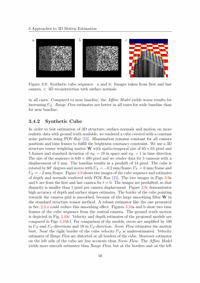
3 Approaches to 3D Motion Estimation
a b c
Figure 3.9: Synthetic cube sequence. a and b: Images taken from first and lastcamera. c: 3D reconstruction with surface normals.
in all cases. Compared to near baseline, the Affine Model yields worse results forincreasing UZ . Range Flow estimates are better in all cases for wide baseline thanfor near baseline.
3.4.2 Synthetic Cube
In order to test estimation of 3D structure, surface normals and motion on morerealistic data with ground truth available, we rendered a cube covered with a constantnoise pattern using POV-Ray [15]. Illumination remains constant for all camerapositions and time frames to fulfill the brightness constancy constraint. We use a 3Dstructure tensor weighting matrix W with spatio-temporal size of 65× 65 pixel and5 frames and standard deviation of σW = 19 in space and σW = 1 in time direction.The size of the sequence is 640× 480 pixel and we render data for 5 cameras with adisplacement of 5 mm. The baseline results in a preshift of 14 pixel. The cube isrotated by 60 degrees and moves with UX = −0.2 mm/frame, UY = 0 mm/frame andUZ = −2 mm/frame. Figure 3.9 shows two images of the cube sequence and estimatesof depth and normals rendered with POV-Ray [15]. The two images in Figs. 3.9aand b are from the first and last camera for t = 0. The images are preshifted, so thatdisparity is smaller than 1 pixel per camera displacement. Figure 3.9c demonstrateshigh accuracy of depth and surface slopes estimates. The border of the cube pointingtowards the camera grid is smoothed, because of the large smoothing filter W inthe standard structure tensor method. A robust estimator like the one presentedin Sec. 2.3.4 could reduce this smoothing effect. Figures 3.10a and b show two timeframes of the cube sequence from the central camera. The ground truth motionis depicted in Fig. 3.10c. Velocity and depth estimates of the proposed models arecompared in Figs. 3.10d-f. For comparison of the models, errors are amplified by 100in UX-and UY -directions and 10 in UZ-direction. Scene Flow estimates the motionbest. Near the right border of the cube velocity UZ is underestimated. Velocityestimates of Range Flow are distorted at all borders of the cube. Moreover estimateson the left side of the cube are less accurate than Scene Flow. The Affine Modelyields more smooth estimates than Range Flow, but at the borders and on the left
50

3.4 Experiments
a b c
d e f
Figure 3.10: Motion estimation of cube moving towards camera. a and b: Firstand last image taken with central camera. c: Ground truth motion. d–f: Scaledmotion estimates with amplified errors for the models Scene Flow, Range Flow andthe Affine Model are depicted, respectively.
side worse results than Scene Flow. A robust estimator may improve estimationresults at borders. Range Flow is more sensible to borders, because it incorporatesderivatives of estimated depth sequences, which already suffer from border problems.
3.4.3 Plant Sequences
In this work the main focus is on plant leaf motion estimation. We show experimentson two different plants, namely Kalanchoe and Castor Oil Plant (Ricinus).
Kalanchoe
The input sequence contains images of 49 camera positions, i.e., a 7 × 7 cameragrid with 0.5 mm camera displacement. Figure 3.11a and b show an image of thecentral camera and depth estimates rendered by POV-Ray [15]. The rendered viewdemonstrates that positions and surfaces of leafs are well reconstructed. Largesmoothing filters (W has spatial size 128 × 128 with σW = 37) have been used,because structures on the leafs are rare. This leads to strong smoothing of the 3Dreconstruction. Structure of small leafs in the center of the plant cannot be estimated.Figure 3.11c and d show a close-up view of the large leaf positioned in the lowerpart in Fig. 3.11a. The rendered view and estimated surface slopes are depicted in
51
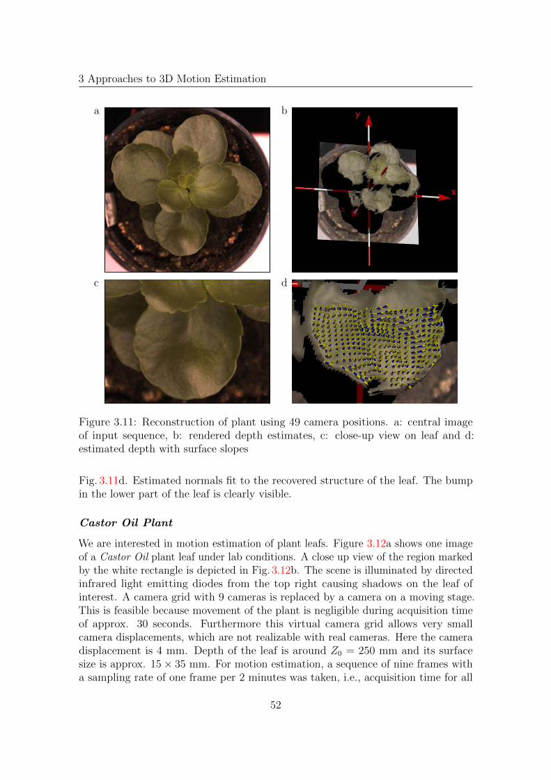
3 Approaches to 3D Motion Estimation
a b
c d
Figure 3.11: Reconstruction of plant using 49 camera positions. a: central imageof input sequence, b: rendered depth estimates, c: close-up view on leaf and d:estimated depth with surface slopes
Fig. 3.11d. Estimated normals fit to the recovered structure of the leaf. The bumpin the lower part of the leaf is clearly visible.
Castor Oil Plant
We are interested in motion estimation of plant leafs. Figure 3.12a shows one imageof a Castor Oil plant leaf under lab conditions. A close up view of the region markedby the white rectangle is depicted in Fig. 3.12b. The scene is illuminated by directedinfrared light emitting diodes from the top right causing shadows on the leaf ofinterest. A camera grid with 9 cameras is replaced by a camera on a moving stage.This is feasible because movement of the plant is negligible during acquisition timeof approx. 30 seconds. Furthermore this virtual camera grid allows very smallcamera displacements, which are not realizable with real cameras. Here the cameradisplacement is 4 mm. Depth of the leaf is around Z0 = 250 mm and its surfacesize is approx. 15× 35 mm. For motion estimation, a sequence of nine frames witha sampling rate of one frame per 2 minutes was taken, i.e., acquisition time for all
52
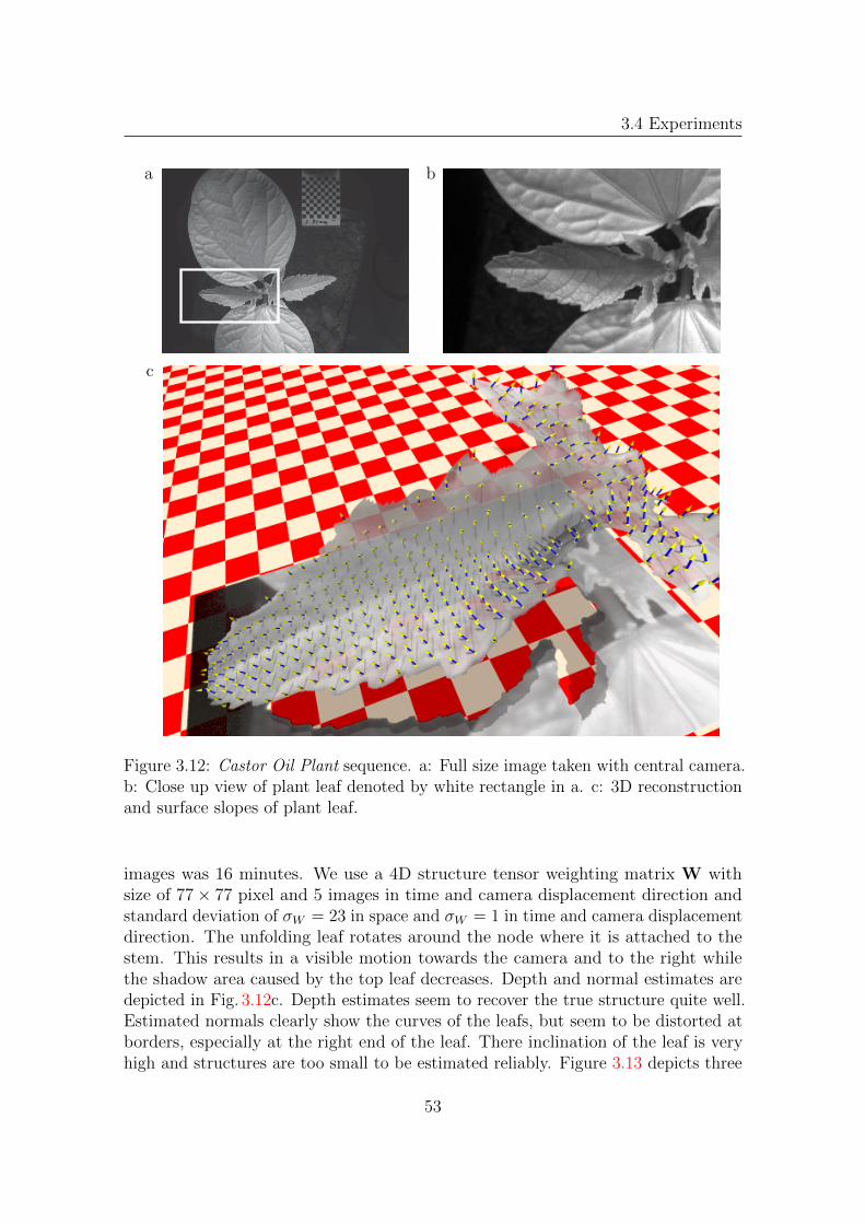
3.4 Experiments
a b
c
Figure 3.12: Castor Oil Plant sequence. a: Full size image taken with central camera.b: Close up view of plant leaf denoted by white rectangle in a. c: 3D reconstructionand surface slopes of plant leaf.
images was 16 minutes. We use a 4D structure tensor weighting matrix W withsize of 77× 77 pixel and 5 images in time and camera displacement direction andstandard deviation of σW = 23 in space and σW = 1 in time and camera displacementdirection. The unfolding leaf rotates around the node where it is attached to thestem. This results in a visible motion towards the camera and to the right whilethe shadow area caused by the top leaf decreases. Depth and normal estimates aredepicted in Fig. 3.12c. Depth estimates seem to recover the true structure quite well.Estimated normals clearly show the curves of the leafs, but seem to be distorted atborders, especially at the right end of the leaf. There inclination of the leaf is veryhigh and structures are too small to be estimated reliably. Figure 3.13 depicts three
53
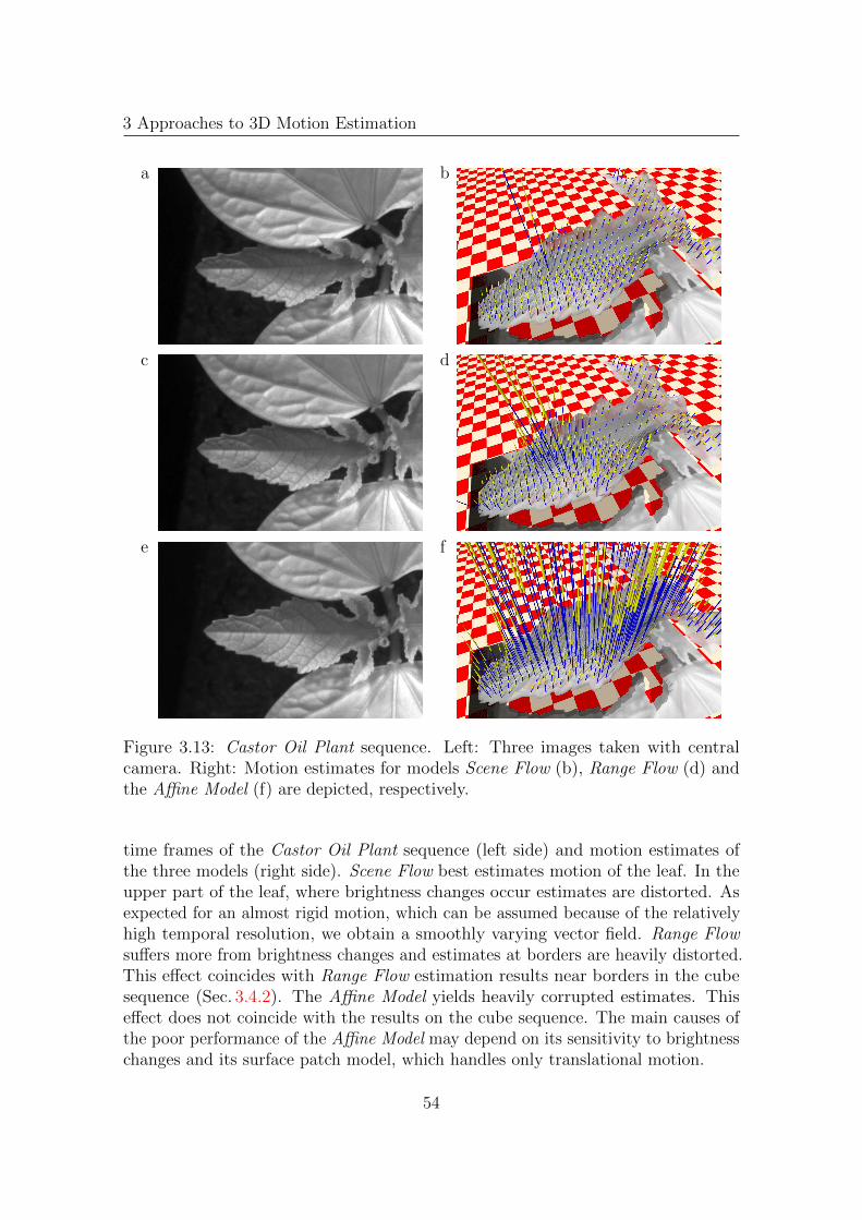
3 Approaches to 3D Motion Estimation
a b
c d
e f
Figure 3.13: Castor Oil Plant sequence. Left: Three images taken with centralcamera. Right: Motion estimates for models Scene Flow (b), Range Flow (d) andthe Affine Model (f) are depicted, respectively.
time frames of the Castor Oil Plant sequence (left side) and motion estimates ofthe three models (right side). Scene Flow best estimates motion of the leaf. In theupper part of the leaf, where brightness changes occur estimates are distorted. Asexpected for an almost rigid motion, which can be assumed because of the relativelyhigh temporal resolution, we obtain a smoothly varying vector field. Range Flowsuffers more from brightness changes and estimates at borders are heavily distorted.This effect coincides with Range Flow estimation results near borders in the cubesequence (Sec. 3.4.2). The Affine Model yields heavily corrupted estimates. Thiseffect does not coincide with the results on the cube sequence. The main causes ofthe poor performance of the Affine Model may depend on its sensitivity to brightnesschanges and its surface patch model, which handles only translational motion.
54

3.5 Conclusions
Table 3.2: Comparison of motion estimation approaches
Scene Flow Range Flow Affine Model
estimated3D motion 3D motion
3D structureparameters & motion
input forall cameras central camera all cameras
intensity data
input for centralall time points all time points
depth data time point
3.5 Conclusions
In this chapter we described three optical flow based approaches for 3D motionestimation. The Affine Model is also capable of structure estimation. The threemodels use different sources and models for motion estimation. A comparison ofthese sources is depicted in Tab. 3.2. The main goal of all methods is to use 2Doptical flow to estimate 3D motion. Whereas pure 3D motion in X- and Y -directionmay be easily explained by optical flow estimates, motion estimation in Z-directionis not uniquely defined by 2D optical flow estimates only. Therefore the 3D motionestimation approaches incorporate additional constraints to solve for 3D motion.Scene Flow combines optical flow estimates in all cameras with depth data for t = 0to estimate 3D motion. On the other hand Range Flow combines optical flow inthe central camera with the change in depth data seen in this camera. The AffineModel uses information of optical flow in the spatial neighborhood (e.g., divergence)to solve for 3D motion.However, Scene Flow and Range Flow use two separate estimators for depth and flowestimation, i.e., depth data is estimated independent from optical flow. The AffineModel combines both estimation processes in one parameter estimation and solvesthen for motion in time or camera displacement by combining solution vectors of thisparameter estimation. The benefit of this estimation approach is that all availableinput data influences estimation of the parameters, whereas the other approachesuse only subsets of the data (cmp. Tab. 3.2). The general structure of Scene Flowand the Affine Model are quite similar. First optical flow components and depth arederived. In a second step these parameters are explained by 3D parameters. Thedifference is that Scene Flow incorporates information of translational optical flow,i.e., two parameters, of different cameras, whereas the Affine Model is based on morethan two optical flow parameters in the central camera.Synthetic experiments on sinusoidal patterns, the synthetic cube sequence and onplant leaf sequences showed that estimation of depth and slopes with the AffineModel yields reliable results for 1D and 2D camera grids. In the experiments we
55

3 Approaches to 3D Motion Estimation
compared the 1D model without normals from [55] to the full model. All parameterscan be estimated as well or better with the full model. The additional parametersdo not lead to instabilities. In addition the 2D model is more robust with respect tothe aperture problem.Scene Flow yields best 3D motion estimates for wide baseline setups. Sinusoidalexperiments showed that for small baselines estimation accuracy of the Affine Modelis comparable to the accuracy of Scene Flow. In case of noisy data and small baselinesthe Affine Model clearly yields best results. Estimates using Range Flow have highestaccuracy only for special cases, e.g., fronto-parallel surface or no depth motion forwide baseline setups.Experiments on the synthetic cube sequence and on plant sequences confirmed resultsfrom the sinusoidal sequences. In addition experiments on the plant leaf sequenceshowed that Scene Flow is quite robust to brightness changes, although it is based onthe brightness constancy constraint. Estimates of Range Flow and especially of theAffine Model are highly corrupted by brightness changes. The Affine Model seems tobe more sensitive to the rotational motion of the leaf. This may come from modelassumptions of translating surface patches. We conclude that Scene Flow works beston real data and is less sensitive in regions where the brightness constancy constraintis not fulfilled. However, in order to get more reliable estimates we have to derivea new approach to handle brightness changes in the data which do not come frommotion. This will be addressed in the following chapter.
56

Chapter 4
Modeling Brightness Changes
Motion estimation approaches as presented in the previous chapter yield good resultsfor objects under homogeneous, diffuse illumination. Problems occur for directed,inhomogeneous illumination, because the brightness constancy constraint (2.3) isnot sufficiently well satisfied anymore. A setup for Range Flow may include anillumination independent range sensor, such as a laser range sensor. This meansthe range constraint is still fulfilled. However, range data estimated by a structurefrom motion approach may also be corrupted. In this chapter we present differentapproaches to handle illumination changes. First we focus on prefiltering the intensitydata, in order to reduce brightness changes coming from changing illumination. Thenwe will present two brightness constraints, which are more robust to brightnesschanges compared to the brightness constancy constraint (see (2.3)), and one novelconstraint, which models brightness changes based on reflectance physics. In thesecond part of this chapter we will integrate these constraints in Range Flow andin the Affine Model and show experimental results for different combinations ofprefilters and constraints. We do not explicitly test brightness handling approacheswith Scene Flow because, as showed in the previous chapter, Scene Flow is basicallya specific estimation method and therefore integration would not yield additionalinsights. Finally the performance of the three models is compared on syntheticsequences with illumination changes and we show improvements on the plant leafsequence.
4.1 Prefiltering
Prefiltering is a well-known technique for illumination change suppression, makingimage data more or less illumination invariant.
Temporal and/or spatial highpass filtering approximately eliminates slow or low-frequent brightness changes in the data. However, faster illumination changes in bothspatial and temporal domain still remain present in the data. In our experiments,
57

4 Modeling Brightness Changes
a b cI(
x,t)
-100
10-2
02
0
5
10
x t
I(x,
t)
-100
10-2
02
0
5
10
x t
I(x,
t)
-100
10-2
02
0
5
10
x t
d e f
I(x,
t)
-100
10-2
02
0
5
10
x t
I(x,
t)
-100
10-2
02
0
5
10
x t
I(x,
t)
-100
10-2
02
0
5
10
x t
g h i
I(x,
t)
-100
10-2
02
0
5
10
x t
I(x,
t)
-100
10-2
02
0
5
10
x t
I(x,
t)
-100
10-2
02
0
5
10
x t
Figure 4.1: Sine wave with increasing illumination, parameter a1 = 0.1, a1,x = 0(left), after highpass (middle) and homomorphic (right) prefiltering (lowpass withσpre = 35). Noise added: (top) no noise, (middle) additive Gaussian noise (σn = 0.5),and (bottom) shot noise (k = 0.5, see (4.31)).
we evaluate highpass filtering according to
I = (1l−Gσpre) ∗ I (4.1)
where Gσpre denotes a spatial Gaussian filter (see, e.g., [32]) with standard deviationσpre, and where 1l is an identity filter whose impulse response equals one everywhere,and where ∗ is convolution.
A more sophisticated approach uses homomorphic filtering [48, 73]. Following [73],we briefly derive a straightforward implementation of homomorphic filtering, whichproved to be very successful in suppressing illumination changes. Homomorphicfiltering is based on modeling the image intensity I(x, y) as being determined byillumination L(x, y) reflected towards the camera by the surfaces of the objectspresent in the scene. The reflectance of the surfaces is denoted by R(x, y). Notethat in this model, both the illumination and the object reflectance are already
58
4.2 Brightness Constraints
projected onto the image plane, i.e., they depend on the sensor coordinates x, y. ForLambertian surfaces, the image intensity can thus be modeled by
I(x, y) ∝ L(x, y) ·R(x, y) . (4.2)
The structure of the scene is represented by the reflectance R(x, y), from which motionneeds to be estimated. A logarithmic point transform converts the multiplicativerelation1 between illumination L and reflectance R into an additive one according to
log(I(x, y)) ∝ log(L(x, y)) + log(R(x, y)) . (4.3)
In a rough approximation, log(L) and log(R) may be considered separated in fre-quency domain, as L(x, y) is assumed to be low-frequent (such that even its harmonicsgenerated by the nonlinear point transform can be neglected), while R and hencelog(R) is regarded as predominantly high-frequent such that it can be extracted by ahighpass filter. In practice, though, the two components overlap. The design of thehighpass filter thus implies a trade off between suppressing brightness changes andloss of relevant signal. After highpass filtering, exponentiation returns an approxi-mation of the sought reflectance component. Note that the nonlinear log-operationturns the camera noise, which, neglecting quantum noise, is often modeled as beingsignal-independent, into signal-dependent noise, which may affect motion parameterestimation. Figure 4.1 illustrates the effects of the proposed prefilters on a 2D signalI(x, t) with exponential temporal brightness changes. Results for linear highpass andhomomorphic prefiltering of the signal for noise-free data (top), for added Gaussiannoise (middle) and for intensity-dependent noise (bottom) are shown (see Sec. 4.4.2for details on intensity dependent noise). Evidently, homomorphic prefiltering re-moves all brightness changes for noise-free data, whereas highpass prefiltering onlyremoves signal offset. Figure 4.1f shows how the nonlinear log-operation leads toincreased noise in regions with small intensity values, especially for t < 0. If thenoise is intensity-dependent like shot noise, homomorphic prefiltering may reducethis effect (Fig. 4.1i). A general possibility to reduce the signal dependence of shotor quantum noise is to subject the data first to a square-root transform [2]. We will,though, not consider this any further here.
4.2 Brightness Constraints
The brightness constancy constraint (2.3) can be replaced by an illumination invariantor illumination insensitive constraint, which can be applied instead of or togetherwith prefiltering the data. In this section we present two standard and one novelconstraint.
1Note that this multiplicative relation is also preserved for cameras with a nonlinear conversionfrom image irradiance to intensity, if the nonlinearity follows a γ-curve.
59

4 Modeling Brightness Changes
4.2.1 The Gradient Constancy Constraint
For the estimation of optical flow, a successful such constraint is to assume thatthe 2D image intensity gradient remains constant along the motion trajectory [49].As gradient computation corresponds to derivative filtering, which is a highpassoperation, this constraint therefore attenuates illumination changes, as discussed inSec. 4.1. This leads to two linearized gradient constancy constraints
dI xdt
= ∂xIxux + ∂yIxuy + ∂tIx = 0 (4.4)
dI ydt
= ∂xIyux + ∂yIyuy + ∂tIy = 0 (4.5)
where lower indices indicate partial derivatives, e.g., Ix := ∂xI.
4.2.2 Combined Intensity andGradient Constancy Constraint
A known drawback of the gradient constancy constraint is that it noticeably reducesstructure in the images and leads to aperture problems. Using both the intensityconstraint and the gradient constraint simultaneously reduces this effect in opticalflow estimation [49]. Doing so leads to three constraint equations ((2.3), (4.4) and(4.5)), which should be satisfied simultaneously.
4.2.3 A Physics-Based Brightness Change Model
A different approach to handle brightness changes is to model these explicitly,and to then estimate both optical flow and brightness change parameters basedon this model. Haussecker and Fleet [25] proposed a generalized formulation ofoptical flow estimation based on models of brightness variation that are caused bytime-dependent physical processes. Brightness changes along a temporal trajectoryx(t) = (x(t), y(t))T. This is described by a parameterized function hI
I(x(t), t) = hI(I0, t,g) (4.6)
where I0 = I(x(0), 0) denotes image intensity at time t = 0 and g = [g1, ..., gn]T
contains n brightness change parameters. Taking the total derivative on both sidesyields
∂xIux + ∂yIuy + ∂tI =d
dthI(I0, t,g) . (4.7)
Assuming brightness constancy, i.e., hI(I0, t,g) = c, (4.7) reduces to (2.3). Figure4.2a shows constant, linear and nonlinear changes of intensity due to brightnesschanges. Given a physical model h for brightness changes, both the optical flow(ux, uy) and the parameter vector g need to be estimated. Several time-dependent
60

4.2 Brightness Constraints
a b
constant
linear
nonlinearI(x,t)-I(x0,t0)
t
x(x-1,t-1)
(x0,t0)(x1,t1)
t
∆X
∆X
I(x,t=t0)
I(x,t=t1)
Figure 4.2: a: Change of intensity values caused by brightness changes (cf. [25])and b: temporal intensity changes caused by illumination changes within a spatialneighborhood with local 3D coordinates ∆X.
brightness change models are proposed in [25], i.e., changing surface orientation,motion of the illuminant, and physical models of heat transport in infrared images.We derive a novel brightness change model [60], which describes spatially varyingtime-dependent illumination changes caused by directed, inhomogeneous illuminationand changing surface orientation. Figure 4.2b illustrates spatially varying intensitychanges in a neighborhood Λ. ∆X and ∆Y are local coordinates of Λ. This modelis able to also describe illumination by spotlights, whereas the models presented in[25] assume that the intensity change of pixels is constant over a local neighborhood.
The cameras convert light intensity L into image intensities I (i.e., gray values). Inorder to derive a model for dI /dt , the temporal changes visible in the data, we lookinto the dependencies of L. We assume that a translating surface patch is illuminatedby a spatially smoothly varying, translating and rotating light source. Direction niof incident irradiance E may vary smoothly with time and space but reflectancedirection nr is kept constant.2 Visible light intensity i.e., reflected radiance L dependson incident irradiance E and on the patch’s bidirectional reflectance distributionfunction (BRDF) B (cmp. e.g., [24]) according to
L(X(∆X,∆Y, t), t,nr) = B(X(∆X,∆Y, t),ni(t),nr)E(∆X,∆Y, t,ni(t)) (4.8)
and the BRDF depends on the material and hence on the position on the surfacepatch as well as the directions of incidence ni and reflectance nr. We assume thatthe material does not change with time and therefore
B(X(∆X,∆Y, t),ni(t),nr) = B(X(∆X,∆Y, 0),ni(t),nr) . (4.9)
If the BRDF is smooth enough, which is typically given at sufficient angular distancefrom specularities, changes due to smoothly changing incidence direction ni(t) can
2Reflectance direction nr obviously also varies with pixel position in the cameras, but we do notuse this extra information.
61
4 Modeling Brightness Changes
be modeled using a smooth function hB(t) with hB(0) = 1
B(X(∆X,∆Y, t),ni(t),nr) = B(X(∆X,∆Y, 0),ni(0),nr)hB(t) . (4.10)
Being spatially inhomogeneous the moving irradiance E changes not only by a timedependent factor, but by a factor also varying smoothly in space
E(∆X,∆Y, t,ni(t)) = E(∆X,∆Y, 0,ni(0))hE(∆X,∆Y, t) . (4.11)
Here again hE(∆X,∆Y, t) is a smooth function with hE(∆X,∆Y, 0) ≡ 1. Plugging(4.10) and (4.11) in (4.8) the reflected radiance L becomes
L(X(∆X,∆Y, t), t) = L(X(∆X,∆Y, 0), 0)hB(t)hE(∆X,∆Y, t) . (4.12)
We assume image intensities I to be proportional to the radiance L, i.e., the charac-teristic curve of the used camera to be linear, and therefore
I(X(∆X,∆Y, t), t) = I(X(∆X,∆Y, 0), 0) exp(hI(∆X,∆Y, t)) (4.13)
where hI(∆X,∆Y, t) := ln(hB(t)hE(∆X,∆Y, t)). The sought temporal derivative of(4.13) is thus
ddtI = I(X(∆X,∆Y, 0), 0) exp(hI(∆X,∆Y, t))
ddthI(∆X,∆Y, t)
= I(X(∆X,∆Y, t), t) ddthI(∆X,∆Y, t) .
(4.14)
The most common assumption in optical flow-like approaches is brightness constancy,boiling down to hI(∆X,∆Y, t) ≡ 0. Haussecker and Fleet [25] derive models forchanging surface orientation and a moving illumination envelope approximating hIas a second order power series respecting temporal changes only
hI(∆X,∆Y, t) ≈ hHF (t,g) :=2∑i=1
giti (4.15)
where g1 and g2 are treated as local constants in the estimation process. Looking atFigs. 4.8f and g we observe that for highest accuracy this is not sufficient. Therefore weintroduce a more accurate approximation of hI explicitly modeling spatial variationsstill respecting hI(∆X,∆Y, 0) ≡ 0
hI(∆X,∆Y, t) ≈ h(∆X,∆Y, t,g) :=2∑i=1
(gi + gi,x∆X + gi,y∆Y ) ti . (4.16)
62

4.3 Extension of 3D Motion Estimation Models
The temporal derivative of h is then
f(∆X,∆Y, t,g) :=d
dth(∆X,∆Y, t,g) =
2∑i=1
i (gi + gi,x∆X + gi,y∆Y ) ti−1 (4.17)
using the notationg = [g1, g2, g1,x, g1,y, g2,x, g2,y]
T . (4.18)
Insertion of f(∆X,∆Y, t,g) into the generalized brightness change constraint(4.7) yields the sought brightness constraint.
Ixux + Iyuy + It − I2∑i=1
i (gi + gi,x∆X + gi,y∆Y ) ti−1 = 0 . (4.19)
4.3 Extension of 3D Motion Estimation Models
In this section we briefly present, how the three models proposed in Chap. 3, namelyScene Flow, Range Flow and the Affine Model are extended to handle the brightnessconstraints different to the brightness constancy constraint (2.3).
4.3.1 Scene Flow
The extension of Scene Flow to handle brightness changes is straightforward. Theconstraints proposed in Sec. 4.2.1, Sec. 4.2.2 or Sec. 4.2.3 replace the brightnessconstancy constraint in (3.4). The equation system is then solved analog to Sec. 3.1.
4.3.2 Range Flow
In this section we show how to extend Range Flow for varying illumination [61] andhow the choice of prefilters and brightness constraints influence estimation results ofRange Flow.
Adaption of Constraints
In order to adapt the gradient constraints in (4.4) and (4.5) for Range Flow theoptical flow ux, uy is eliminated using (3.6) and (3.7) (cmp. derivation of the intensityconstraint (3.13)), yielding
∂(Ix, Y )
∂(x, y)U +
∂(X, Ix)
∂(x, y)V +
∂(X, Y, Ix)
∂(x, y, t)= 0 (4.20)
∂(Iy, Y )
∂(x, y)U +
∂(X, Iy)
∂(x, y)V +
∂(X, Y, Iy)
∂(x, y, t)= 0 . (4.21)
63
4 Modeling Brightness Changes
The combination of gradient and intensity constraint proposed in Sec. 4.2.2 leadsto three constraint equations, viz. (3.13), (4.20) and (4.21), which should be satisfiedsimultaneously by the horizontal and vertical Range Flow components U and V .Adaption of the brightness change model is handled analog. Eliminating the opticalflow (ux, uy) in (4.19) using (3.6) and (3.7) leads to
∂(I, Y )
∂(x, y)U +
∂(X, I)
∂(x, y)V +
∂(X,Y, I)
∂(x, y, t)− Ig1 − Ig1,x∆X − Ig1,y∆Y
− 2Ig2t− 2Ig2,x∆Xt− 2Ig2,y∆Y t = 0 . (4.22)
Estimation of Motion and Brightness Parameters
Estimating the 3D motion from the input data then corresponds to fitting theselected model to the original or, if applicable, prefiltered data. The parametersto be estimated comprise the motion parameters U , V , W for all models and, forthe physics-based brightness change model from Sec. 4.2.3, the brightness changeparameters g1, g1,x, g1,y, g2, g2,x, g2,y in the Taylor series (4.16).
As described in Secs. 3.2.3, 4.2.1, 4.2.2 and 4.2.3 we have more than one constraintfor the U and V components of the Range Flow. In the same way as expressingthe range constraint by dT
rcp = 0, the intensity constraint (3.13) and the gradientconstancy constraints (4.20) and (4.21) may be expressed by dT
Qp = 0, where dQ iscomputed from the observed data according to
dQ =
[∂ (Q, Y )
∂ (x, y),∂ (X,Q)
∂ (x, y), 0,
∂ (X, Y,Q)
∂ (x, y, t)
]T
(4.23)
with Q ∈ I, Ix, Iy selected as appropriate. We adapt all constraints to identicaldimensions by inserting zeros at those positions into the data vector d, whichcorrespond to positions of parameters in the parameter vector p which are not partof the respective constraint. In particular, the physics-based brightness change modelin Sec. 4.2.3 contains motion and brightness change parameters, thus leading to theenlarged parameter vector
p = [U, V,W, 1,gT]T . (4.24)
The data vectors for both the range constraint and the brightness change constrainthave hence to be enlarged correspondingly by appropriate insertion of zeros. Asshown in [69], combining the different constraints yields a new structure tensor whichis simply the weighted sum of the tensor Jrc from the range constraint (3.14), andthe tensors Ji, i = 1, . . . , 4 from the intensity-dependent constraints (3.13), (4.20),
64

4.3 Extension of 3D Motion Estimation Models
(4.21) and (4.22). With the weights βi, the overall tensor thus is
J = Jrc +4∑i=1
βiJi . (4.25)
The weights βi may even be used to switch between the models, and to account fordifferent signal-to-noise-ratios in the structure tensors. Analog to standard RangeFlow, data channels should be scaled to the same mean and variance before they arecombined. Parameter estimation is done analog to Sec. 3.2.3.
4.3.3 Affine Model
In this section we will adapt the brightness change model (4.19) to the Affine Modelpresented in [60] and Sec. 3.3. Combining the brightness change model (4.19) withthe 5D affine flow model (3.26) yields
Ixdx + Iydy + Isxdsx + Isydsy + Itdt − Ifdt = 0 . (4.26)
Inserting differentials dx and dy in (4.26) analog to Sec. 3.3 leads to data vectord and parameter vector p:
d = (Ix, Iy, Ix∆x, Ix∆y, Iy∆x, Iy∆y,
Isx , Isy , It, I, I∆x, I∆y, It, It∆x, It∆y)T
p = (uxdt + νdsx , uydt + νdsy , a11dt + b1dsx , a12dt + b2dsx ,
a21dt + b1dsy , a22dt + b2dsy , dsx , dsy , dt ,
g1dt , g1,xdt , g1,ydt , g2dt , g2,xdt , g2,ydt )T .
(4.27)
where f has been substituted by the novel brightness change model from (4.17) andthe brightness change parameters are
g1 = −g1 g2 = −g2
g1,x = −Z0
fc
(g1,x(1− ZY
y0
f) + g1,yZX
y0
f
)g1,y = −Z0
fc
(g1,xZY
x0
f+ g1,y(1− ZX
x0
f
)g2,x = −Z0
fc
(g2,x(1− ZY
y0
f) + g2,yZX
y0
f
)g2,y = −Z0
fc
(g2,xZY
x0
f+ g2,y(1− ZX
x0
f
)(4.28)
For simpler brightness models or when a 1D camera grid is used (i.e., dsy = 0)terms with non-existing parameters are simply omitted.Parameter estimation is done analog to the standard Affine Model (cmp. Sec. 3.3).
65
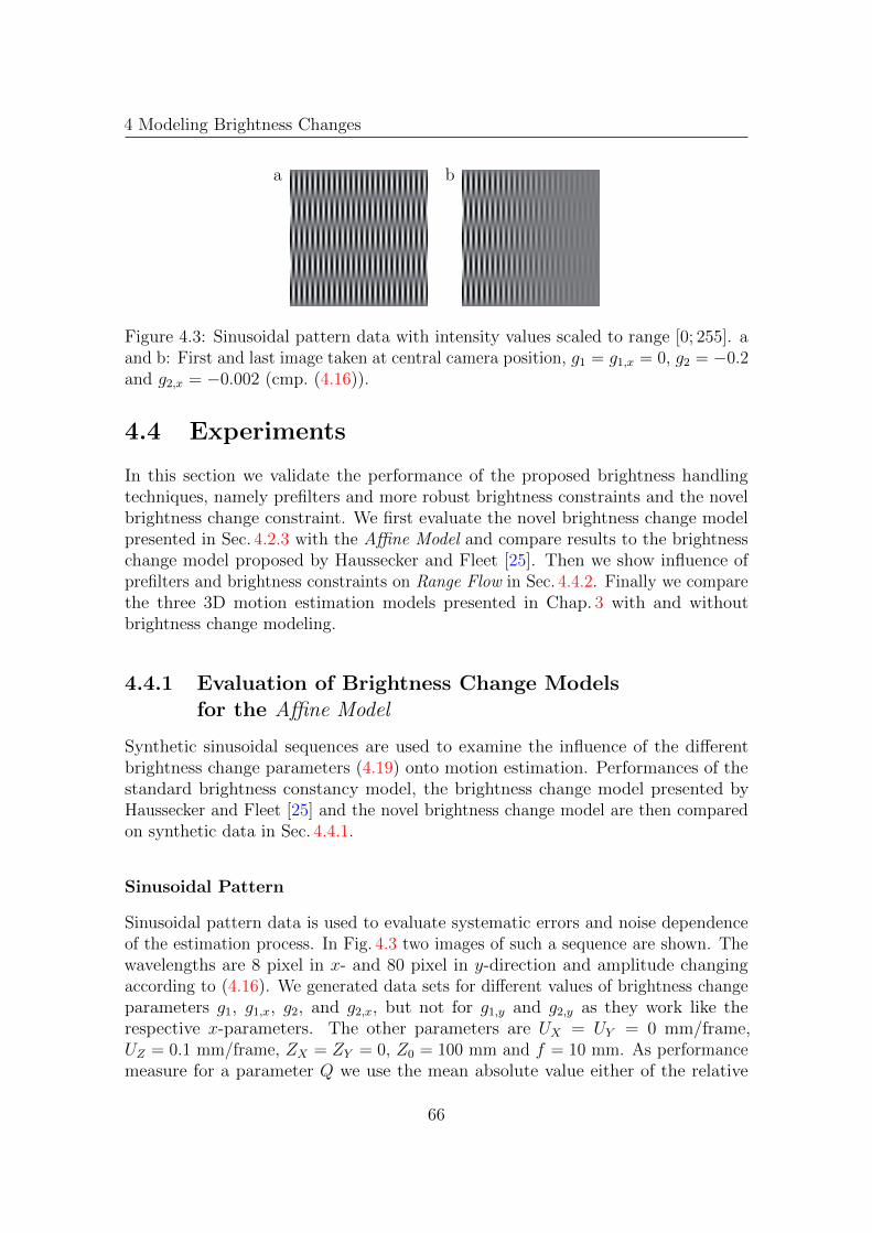
4 Modeling Brightness Changes
a b
Figure 4.3: Sinusoidal pattern data with intensity values scaled to range [0; 255]. aand b: First and last image taken at central camera position, g1 = g1,x = 0, g2 = −0.2and g2,x = −0.002 (cmp. (4.16)).
4.4 Experiments
In this section we validate the performance of the proposed brightness handlingtechniques, namely prefilters and more robust brightness constraints and the novelbrightness change constraint. We first evaluate the novel brightness change modelpresented in Sec. 4.2.3 with the Affine Model and compare results to the brightnesschange model proposed by Haussecker and Fleet [25]. Then we show influence ofprefilters and brightness constraints on Range Flow in Sec. 4.4.2. Finally we comparethe three 3D motion estimation models presented in Chap. 3 with and withoutbrightness change modeling.
4.4.1 Evaluation of Brightness Change Modelsfor the Affine Model
Synthetic sinusoidal sequences are used to examine the influence of the differentbrightness change parameters (4.19) onto motion estimation. Performances of thestandard brightness constancy model, the brightness change model presented byHaussecker and Fleet [25] and the novel brightness change model are then comparedon synthetic data in Sec. 4.4.1.
Sinusoidal Pattern
Sinusoidal pattern data is used to evaluate systematic errors and noise dependenceof the estimation process. In Fig. 4.3 two images of such a sequence are shown. Thewavelengths are 8 pixel in x- and 80 pixel in y-direction and amplitude changingaccording to (4.16). We generated data sets for different values of brightness changeparameters g1, g1,x, g2, and g2,x, but not for g1,y and g2,y as they work like therespective x-parameters. The other parameters are UX = UY = 0 mm/frame,UZ = 0.1 mm/frame, ZX = ZY = 0, Z0 = 100 mm and f = 10 mm. As performancemeasure for a parameter Q we use the mean absolute value either of the relative
66

4.4 Experimentser
ror
ofg 1
1.0E-04
1.0E-03
1.0E-02
1.0E-01
1.0E+00
1.0E+01
1.0E+02
0 0.5 1 1.5 2 2.5
g1,rel
g11.0E-04
1.0E-03
1.0E-02
1.0E-01
1.0E+00
1.0E+01
1.0E+02
0 0.1 0.2 0.3 0.4 0.5
g1,abs
g1,x
erro
rofg 2
1.0E-06
1.0E-05
1.0E-04
1.0E-03
1.0E-02
1.0E-01
1.0E+00
0 0.5 1 1.5 2 2.5
g2,abs
g11.0E-06
1.0E-05
1.0E-04
1.0E-03
1.0E-02
1.0E-01
1.0E+00
0 0.1 0.2 0.3 0.4 0.5
g2,abs
g1,x
novel Haussecker-Fleet-like model
novel spatially and temporally varying model
Figure 4.4: Mean absolute value of relative or absolute error of brightness changeparameters g1 (top) and g2 (bottom) versus the brightness change parameters g1 andg1,x. Noise free data.
error if Qref 6= 0 or of the absolute error if Qref = 0
Qrel =1
N
N∑i
|Qest(i)−Qref (i)||Qref (i)|
Qabs =1
N
N∑i
|Qest(i)−Qref (i)| (4.29)
where the sum runs over all pixels not suffering from border effects and the lowerindices rel stand for ’relative error’, abs for ’absolute error’, est for ’estimated’and ref for ’reference’. Parameter estimation was done according to (3.3.2), withweighting matrix W implemented via a 65-tab Gaussian with standard deviationσW = 16.
The first experiment evaluates systematic error of and cross talk between bright-ness change parameters. Figures 4.4 and 4.5 show errors of g1 and g2 versus brightnesschange parameters g1 and g1,x, and g2 and g2,x respectively. We observe that the
67

4 Modeling Brightness Changeser
ror
ofg 1
1.0E-04
1.0E-03
1.0E-02
1.0E-01
1.0E+00
1.0E+01
1.0E+02
-0.2 -0.1 0 0.1 0.2
g1,abs
g21.0E-04
1.0E-03
1.0E-02
1.0E-01
1.0E+00
1.0E+01
1.0E+02
-0.05 -0.03 -0.01 0.01 0.03 0.05
g1,abs
g2,x
erro
rofg 2
1.0E-06
1.0E-05
1.0E-04
1.0E-03
1.0E-02
1.0E-01
1.0E+00
-0.2 -0.1 0 0.1 0.2
g2,rel
g21.0E-06
1.0E-05
1.0E-04
1.0E-03
1.0E-02
1.0E-01
1.0E+00
-0.05 -0.03 -0.01 0.01 0.03 0.05
g2,abs
g2,x
novel Haussecker-Fleet-like model
novel spatially and temporally varying model
Figure 4.5: Mean absolute value of relative or absolute error of brightness changeparameters g1 (top) and g2 (bottom) versus the brightness change parameters g2,and g2,x. Noise free data.
relative error of g1 is well below 0.5% if g1 < 1 and then moderately raises. This isdue to the fact that temporal derivatives of the data It become less and less accuratewhen exponential behavior of the data becomes more and more prominent. The sameexplanation holds for the linear error increase of g2 with increasing g2. And as localbrightness changes due to g1,x come close to changes due to g1 if g1 = g1,x∆X for thesame local patch, we expect and observe severe cross talk between g1,x and g1, moresevere for the model not containing g1,x. This is also true for g2,x and g2, but therethe cross talk is the same for both models, thus modeling g2,x is of no advantagehere (cmp. Fig. 4.5 bottom). Further g1 is almost independent of g2 and g2,x, as wellas g2 of g1. But while g2 does depend on g1,x if g1,x is not modeled, the error of g2
is about 1 to 2 orders of magnitude smaller if g1,x is modeled (cmp. Fig. 4.4 lowerright). The positive effect on accuracy of the method if g1,x is modeled is even higherfor UZ , as we see next.
68
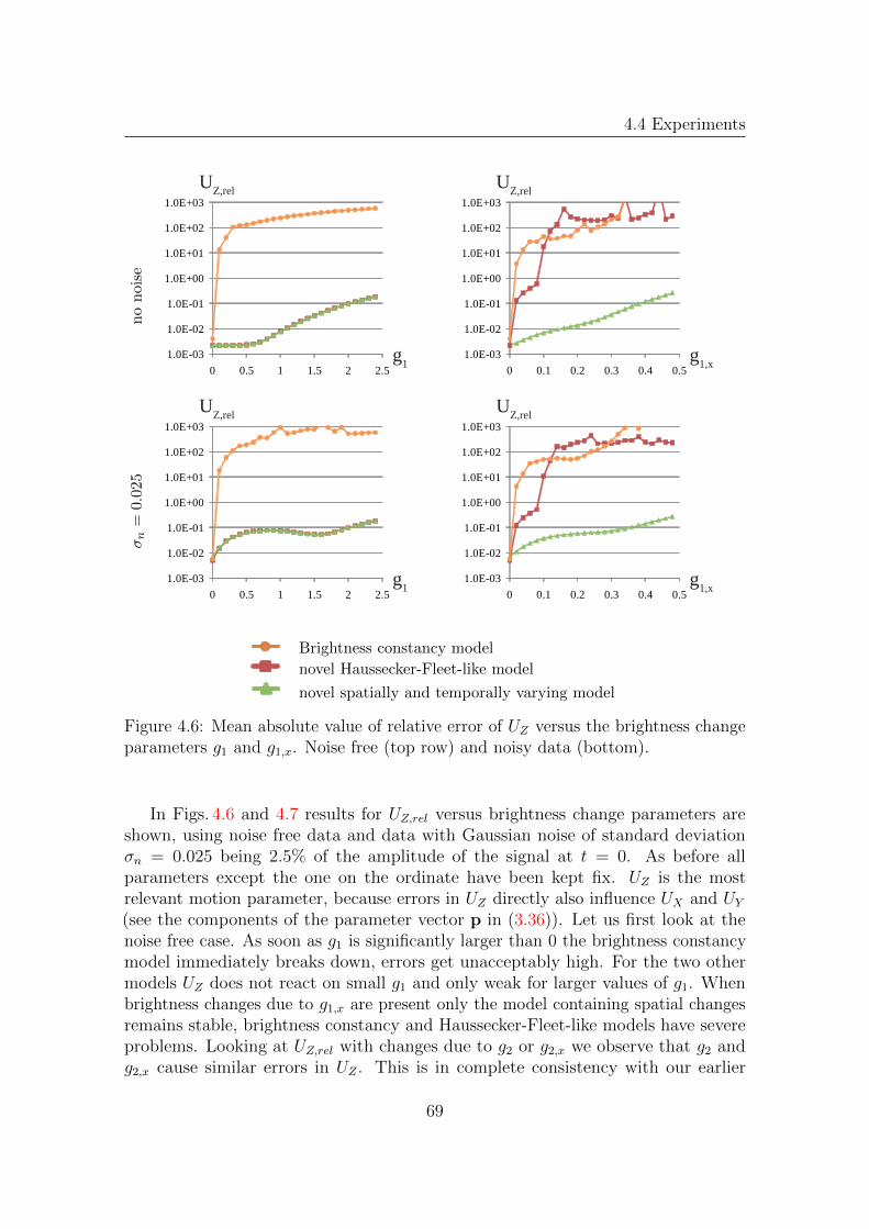
4.4 Experimentsn
on
oise
1.0E-03
1.0E-02
1.0E-01
1.0E+00
1.0E+01
1.0E+02
1.0E+03
0 0.5 1 1.5 2 2.5
UZ,rel
g11.0E-03
1.0E-02
1.0E-01
1.0E+00
1.0E+01
1.0E+02
1.0E+03
0 0.1 0.2 0.3 0.4 0.5
UZ,rel
g1,x
σn
=0.
025
1.0E-03
1.0E-02
1.0E-01
1.0E+00
1.0E+01
1.0E+02
1.0E+03
0 0.5 1 1.5 2 2.5
UZ,rel
g11.0E-03
1.0E-02
1.0E-01
1.0E+00
1.0E+01
1.0E+02
1.0E+03
0 0.1 0.2 0.3 0.4 0.5
UZ,rel
g1,x
Brightness constancy model
novel Haussecker-Fleet-like model
novel spatially and temporally varying model
Figure 4.6: Mean absolute value of relative error of UZ versus the brightness changeparameters g1 and g1,x. Noise free (top row) and noisy data (bottom).
In Figs. 4.6 and 4.7 results for UZ,rel versus brightness change parameters areshown, using noise free data and data with Gaussian noise of standard deviationσn = 0.025 being 2.5% of the amplitude of the signal at t = 0. As before allparameters except the one on the ordinate have been kept fix. UZ is the mostrelevant motion parameter, because errors in UZ directly also influence UX and UY(see the components of the parameter vector p in (3.36)). Let us first look at thenoise free case. As soon as g1 is significantly larger than 0 the brightness constancymodel immediately breaks down, errors get unacceptably high. For the two othermodels UZ does not react on small g1 and only weak for larger values of g1. Whenbrightness changes due to g1,x are present only the model containing spatial changesremains stable, brightness constancy and Haussecker-Fleet-like models have severeproblems. Looking at UZ,rel with changes due to g2 or g2,x we observe that g2 andg2,x cause similar errors in UZ . This is in complete consistency with our earlier
69
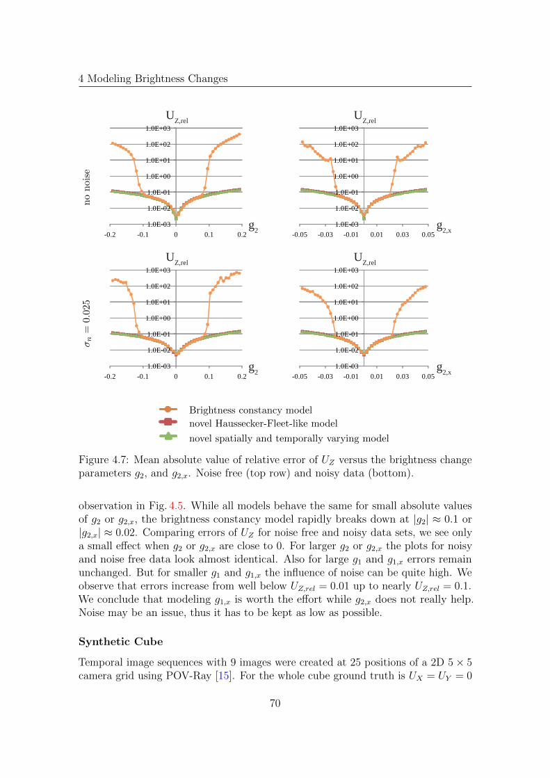
4 Modeling Brightness Changesn
on
oise
1.0E-03
1.0E-02
1.0E-01
1.0E+00
1.0E+01
1.0E+02
1.0E+03
-0.2 -0.1 0 0.1 0.2
UZ,rel
g21.0E-03
1.0E-02
1.0E-01
1.0E+00
1.0E+01
1.0E+02
1.0E+03
-0.05 -0.03 -0.01 0.01 0.03 0.05
UZ,rel
g2,x
σn
=0.
025
1.0E-03
1.0E-02
1.0E-01
1.0E+00
1.0E+01
1.0E+02
1.0E+03
-0.2 -0.1 0 0.1 0.2
UZ,rel
g21.0E-03
1.0E-02
1.0E-01
1.0E+00
1.0E+01
1.0E+02
1.0E+03
-0.05 -0.03 -0.01 0.01 0.03 0.05
UZ,rel
g2,x
Brightness constancy model
novel Haussecker-Fleet-like model
novel spatially and temporally varying model
Figure 4.7: Mean absolute value of relative error of UZ versus the brightness changeparameters g2, and g2,x. Noise free (top row) and noisy data (bottom).
observation in Fig. 4.5. While all models behave the same for small absolute valuesof g2 or g2,x, the brightness constancy model rapidly breaks down at |g2| ≈ 0.1 or|g2,x| ≈ 0.02. Comparing errors of UZ for noise free and noisy data sets, we see onlya small effect when g2 or g2,x are close to 0. For larger g2 or g2,x the plots for noisyand noise free data look almost identical. Also for large g1 and g1,x errors remainunchanged. But for smaller g1 and g1,x the influence of noise can be quite high. Weobserve that errors increase from well below UZ,rel = 0.01 up to nearly UZ,rel = 0.1.We conclude that modeling g1,x is worth the effort while g2,x does not really help.Noise may be an issue, thus it has to be kept as low as possible.
Synthetic Cube
Temporal image sequences with 9 images were created at 25 positions of a 2D 5× 5camera grid using POV-Ray [15]. For the whole cube ground truth is UX = UY = 0
70
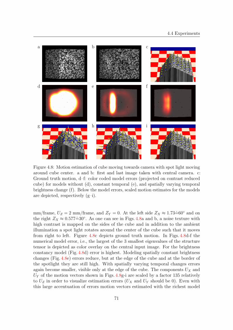
4.4 Experiments
a b c
d e f
g h i
Figure 4.8: Motion estimation of cube moving towards camera with spot light movingaround cube center. a and b: first and last image taken with central camera. c:Ground truth motion, d–f: color coded model errors (projected on contrast reducedcube) for models without (d), constant temporal (e), and spatially varying temporalbrightness change (f). Below the model errors, scaled motion estimates for the modelsare depicted, respectively (g–i).
mm/frame, UZ = 2 mm/frame, and ZY = 0. At the left side ZX ≈ 1.73=60 and onthe right ZX ≈ 0.577=30. As one can see in Figs. 4.8a and b, a noise texture withhigh contrast is mapped on the sides of the cube and in addition to the ambientillumination a spot light rotates around the center of the cube such that it movesfrom right to left. Figure 4.8c depicts ground truth motion. In Figs. 4.8d-f thenumerical model error, i.e., the largest of the 3 smallest eigenvalues of the structuretensor is depicted as color overlay on the central input image. For the brightnessconstancy model (Fig. 4.8d) error is highest. Modeling spatially constant brightnesschanges (Fig. 4.8e) errors reduce, but at the edge of the cube and at the border ofthe spotlight they are still high. With spatially varying temporal changes errorsagain become smaller, visible only at the edge of the cube. The components UX andUY of the motion vectors shown in Figs. 4.8g-i are scaled by a factor 135 relativelyto UZ in order to visualize estimation errors (UX and UY should be 0). Even withthis large accentuation of errors motion vectors estimated with the richest model
71
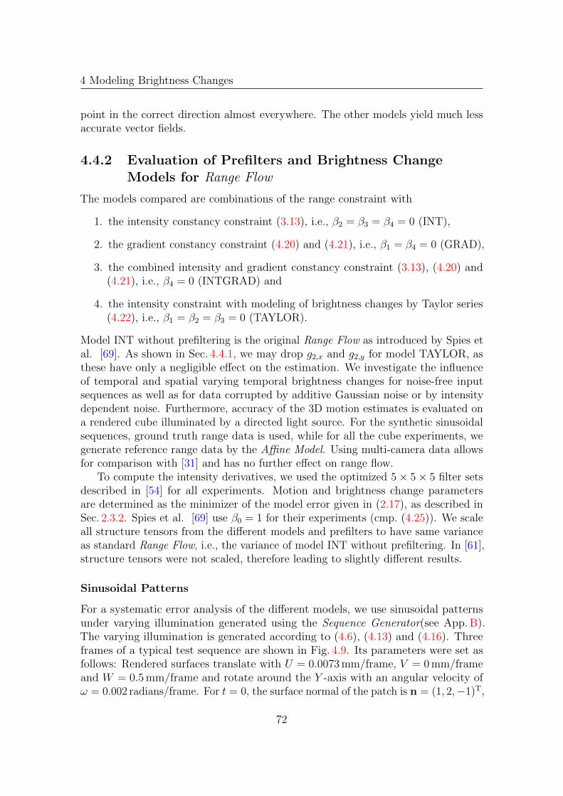
4 Modeling Brightness Changes
point in the correct direction almost everywhere. The other models yield much lessaccurate vector fields.
4.4.2 Evaluation of Prefilters and Brightness ChangeModels for Range Flow
The models compared are combinations of the range constraint with
1. the intensity constancy constraint (3.13), i.e., β2 = β3 = β4 = 0 (INT),
2. the gradient constancy constraint (4.20) and (4.21), i.e., β1 = β4 = 0 (GRAD),
3. the combined intensity and gradient constancy constraint (3.13), (4.20) and(4.21), i.e., β4 = 0 (INTGRAD) and
4. the intensity constraint with modeling of brightness changes by Taylor series(4.22), i.e., β1 = β2 = β3 = 0 (TAYLOR).
Model INT without prefiltering is the original Range Flow as introduced by Spies etal. [69]. As shown in Sec. 4.4.1, we may drop g2,x and g2,y for model TAYLOR, asthese have only a negligible effect on the estimation. We investigate the influenceof temporal and spatial varying temporal brightness changes for noise-free inputsequences as well as for data corrupted by additive Gaussian noise or by intensitydependent noise. Furthermore, accuracy of the 3D motion estimates is evaluated ona rendered cube illuminated by a directed light source. For the synthetic sinusoidalsequences, ground truth range data is used, while for all the cube experiments, wegenerate reference range data by the Affine Model. Using multi-camera data allowsfor comparison with [31] and has no further effect on range flow.
To compute the intensity derivatives, we used the optimized 5× 5× 5 filter setsdescribed in [54] for all experiments. Motion and brightness change parametersare determined as the minimizer of the model error given in (2.17), as described inSec. 2.3.2. Spies et al. [69] use β0 = 1 for their experiments (cmp. (4.25)). We scaleall structure tensors from the different models and prefilters to have same varianceas standard Range Flow, i.e., the variance of model INT without prefiltering. In [61],structure tensors were not scaled, therefore leading to slightly different results.
Sinusoidal Patterns
For a systematic error analysis of the different models, we use sinusoidal patternsunder varying illumination generated using the Sequence Generator(see App. B).The varying illumination is generated according to (4.6), (4.13) and (4.16). Threeframes of a typical test sequence are shown in Fig. 4.9. Its parameters were set asfollows: Rendered surfaces translate with U = 0.0073 mm/frame, V = 0 mm/frameand W = 0.5 mm/frame and rotate around the Y -axis with an angular velocity ofω = 0.002 radians/frame. For t = 0, the surface normal of the patch is n = (1, 2,−1)T,
72

4.4 Experiments
a b c
Figure 4.9: Scaled first (a), central (b) and last (c) frame of sinusoidal sequence withillumination parameters g1 = 0 and g1,x = 0.06.
and the distance of the patch center to the camera is Z0 = 100 mm. The syntheticsensor contains 301×301 pixels of size (0.0044 mm)2. The focal length of the syntheticprojective camera is f = 12 mm. For each experiment, we evaluate the mean absolutevalue of the relative error of U
ERRU =1
N
N∑i
|Uestimated(i)− Ureference(i)||Ureference(i)|
(4.30)
over all pixels i at a minimum distance of 60 pixels from the nearest image border.The structure tensor weighting matrix W is realized by a large, 65-tab Gaussian withstandard deviation σW = 19 in order to reduce systematic errors stemming fromthe phase of the sinusoidal pattern. Prefilters are designed as described in Sec. 4.1,i.e., σpre denotes the standard deviation of the lowpass Gσpre in (4.1). As in [60], wecompare estimation errors of U for increasing illumination parameters g1|g1,x=0 andg1,x|g1=0 to simulate brightness changes. We provide here the errors for U only, aserrors of V and W exhibited very similar behavior. Furthermore, we investigate theinfluence of adding Gaussian noise with σn = 0.025 or shot noise to the intensitydata. The Poisson-distributed shot noise is approximated by adding Gaussian noisewith intensity-dependent standard deviation
σsn = k
√I(x, t)
α(4.31)
with k = 0.025 and α = 1. The sinusoidal pattern for t = 0 has intensity values in therange of 0 ≤ I ≤ 2. To facilitate the evaluation of the effects of prefiltering, we showthe errors for all tested models with and without prefiltering in Fig. 4.10-Fig. 4.13.
In Fig. 4.10, the errors of U for the described models with and without highpassand homomorphic prefiltering are shown over the parameter g1. Highpass prefilteringreduces estimation errors for models INT and INTGRAD. For models GRAD andTAYLOR, using no prefilter yields results as good as using a highpass with standarddeviation σpre > 15 (see (4.1)). Strong filtering, i.e., small σpre, degrades estimationresults for all models. Overall, the model TAYLOR yields the best results for mostcases, only for g1 ≈ 0.3 the model GRAD performs slightly better. Grooves in the
73
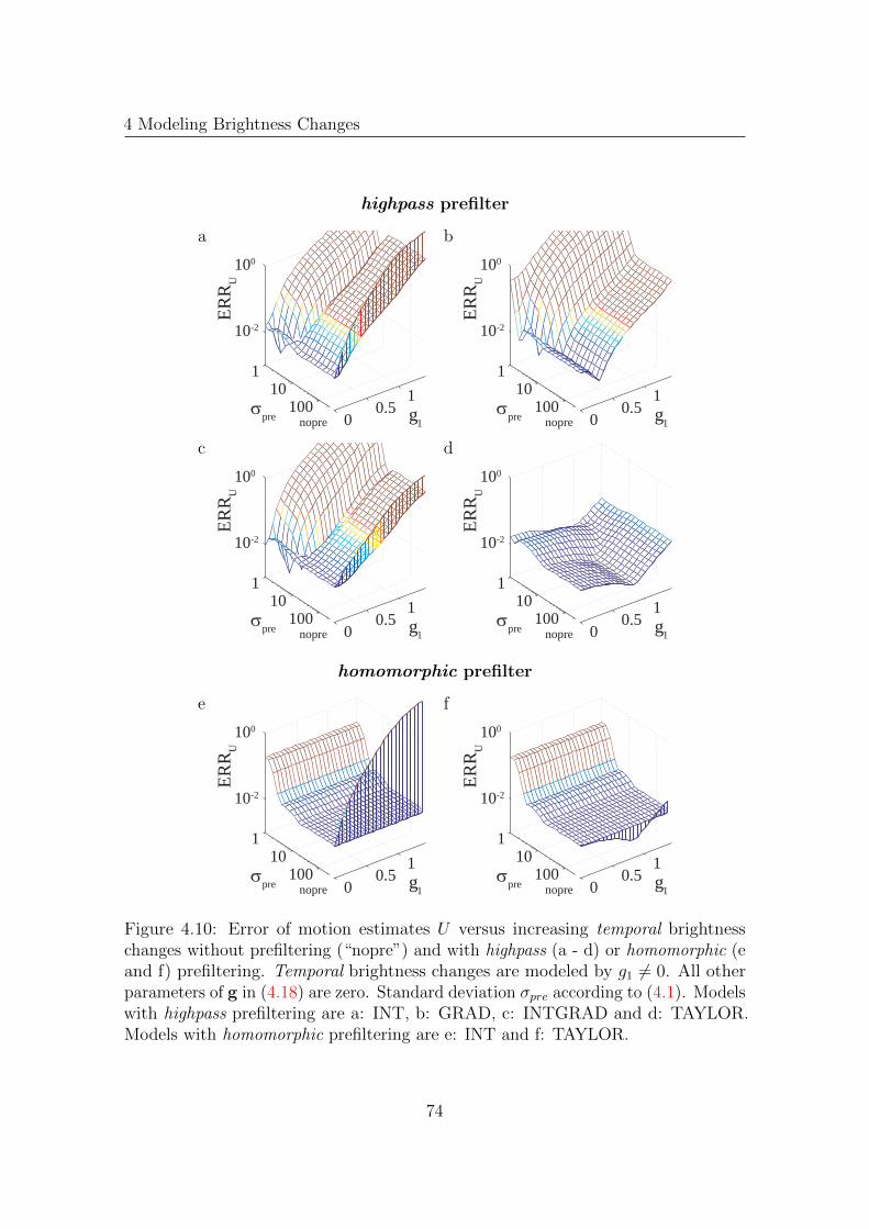
4 Modeling Brightness Changes
highpass prefilter
a b
00.5
1 1
10100
10-2
100
g1σpre
ERR
U
nopre 00.5
1 1
10100
10-2
100
g1σpre
ERR
U
nopre
c d
00.5
1 1
10100
10-2
100
g1σpre
ERR
U
nopre 00.5
1 1
10100
10-2
100
g1σpre
ERR
U
nopre
homomorphic prefilter
e f
00.5
1 1
10100
10-2
100
g1σpre
ERR
U
nopre 00.5
1 1
10100
10-2
100
g1σpre
ERR
U
nopre
Figure 4.10: Error of motion estimates U versus increasing temporal brightnesschanges without prefiltering (“nopre”) and with highpass (a - d) or homomorphic (eand f) prefiltering. Temporal brightness changes are modeled by g1 6= 0. All otherparameters of g in (4.18) are zero. Standard deviation σpre according to (4.1). Modelswith highpass prefiltering are a: INT, b: GRAD, c: INTGRAD and d: TAYLOR.Models with homomorphic prefiltering are e: INT and f: TAYLOR.
74

4.4 Experiments
highpass prefilter
a b
00.1
0.2 1
10100
10-2
100
g1,xσpre
ERR
U
nopre 00.1
0.2 1
10100
10-2
100
g1,xσpre
ERR
U
nopre
c d
00.1
0.2 1
10100
10-2
100
g1,xσpre
ERR
U
nopre 00.1
0.2 1
10100
10-2
100
g1,xσpre
ERR
U
nopre
homomorphic prefilter
e f
00.1
0.2 1
10100
10-2
100
g1,xσpre
ERR
U
nopre 00.1
0.2 1
10100
10-2
100
g1,xσpre
ERR
U
nopre
Figure 4.11: Error of motion estimates U versus increasing spatially varying temporalbrightness changes without prefiltering (“nopre”) and with highpass (a - d) orhomomorphic (e and f) prefiltering. Spatially varying temporal brightness changesare modeled by g1,x 6= 0. All other parameters of g in (4.18) are zero. Standarddeviation σpre according to (4.1). Models with highpass prefiltering are a: INT, b:GRAD, c: INTGRAD and d: TAYLOR. Models with homomorphic prefiltering aree: INT and f: TAYLOR.
75
4 Modeling Brightness Changes
highpass prefilter
a b
00.5
1 1
10100
10-2
100
g1σpre
ERR
U
nopre 00.5
1 1
10100
10-2
100
g1σpre
ERR
U
nopre
c d
00.5
1 1
10100
10-2
100
g1σpre
ERR
U
nopre 00.5
1 1
10100
10-2
100
g1σpre
ERR
U
nopre
Figure 4.12: Same as Figs. 4.10a-d but for data with additive Gaussian noise ofstandard deviation σn = 0.025. Error of motion estimates U versus increasingtemporal brightness changes and highpass prefiltering or without prefiltering (“nopre”).Models are a: INT, b: GRAD, c: INTGRAD and d: TAYLOR.
error surfaces where errors become low, e.g., for model INT at a1 ≈ 0.1 and σpre < 10,may be the result of improved gradients due to brightness changes and are highlypattern dependent. All models perform comparable when applying homomorphicprefiltering. Therefore, we show errors for the models INT and TAYLOR only(Figs. 4.10e and f). Homomorphic prefiltering with σpre > 10 reduces the brightnesschanges efficiently for all values of a1, while prefiltering with σpre < 10 degrades thesignal. For small brightness changes, model TAYLOR performs even better withoutprefiltering.
Figure 4.11 repeats the experiments shown in Fig. 4.10, but with brightnesschanges now being governed by the parameter g1,x instead of g1. This means thatbrightness changes vary now not only temporally, but also spatially.
Evidently, the errors shown in Fig. 4.11 depend more strongly on σpre than thosein Fig. 4.10. Prefiltering with standard deviation of 12 ≤ σpre ≤ 50 yields the bestresults. As before, models GRAD and TAYLOR perform well without prefilter.Figure 4.11e and f show similar behavior for homomorphic prefiltering. Prefilteringwith σpre > 50 degrades the signal for all models but model TAYLOR. For modelTAYLOR, using no prefilter yields best results if g1,x . 0.07.
Figs. 4.12 and 4.13 illustrate the effects of the proposed prefilters on noisy data.
76

4.4 Experiments
homomorphic prefilter
a b
00.5
1 1
10100
10-2
100
g1σpre
ERR
U
nopre 00.5
1 1
10100
10-2
100
g1σpre
ERR
U
nopre
c d
00.5
1 1
10100
10-2
100
g1σpre
ERR
U
nopre 00.5
1 1
10100
10-2
100
g1σpre
ERR
U
nopre
Figure 4.13: Same as Figs. 4.10e and f but for input data with added Gaussiannoise with σn = 0.025 (a and b) or shot noise with k = 0.025 (c and d). Error ofmotion estimates U versus increasing temporal brightness changes and homomorphicprefiltering or without prefiltering (“nopre”). Models are INT (a and c), and TAYLOR(b and d).
In Sec. 4.1, highpass filtering was shown to have no effect on noise distributions incontrast to homomorphic prefiltering. We present errors of U for highpass prefilteringfor added Gaussian noise with standard deviation σn = 0.025 only (Fig. 4.12), becauseresults for shot noise are almost the same. In comparison to the noise-free case, theerrors increased and the grooves in the error surfaces vanished. Overall, the modelTAYLOR yields best results for g1 > 0 and similar results as the other models forg1 ≈ 0.
Figure 4.13 shows how homomorphic prefiltering affects estimation results foradded Gaussian noise and simulated shot noise. As stated above, the nonlinearlog-operation makes originally signal-independent noise signal-dependent. Therefore,homomorphic prefiltering of noisy intensity data with brightness changes g1 > 0.5causes heavily degraded signals. If the noise itself is signal-dependent, such as shotnoise, homomorphic prefiltering performs much better. In both noise experiments,model TAYLOR without prefilter yields the best and most reliable results.
77
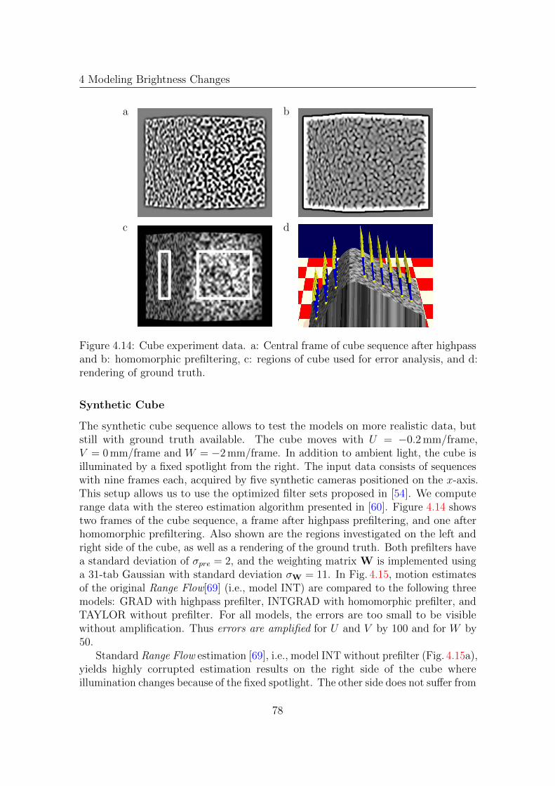
4 Modeling Brightness Changes
a b
c d
Figure 4.14: Cube experiment data. a: Central frame of cube sequence after highpassand b: homomorphic prefiltering, c: regions of cube used for error analysis, and d:rendering of ground truth.
Synthetic Cube
The synthetic cube sequence allows to test the models on more realistic data, butstill with ground truth available. The cube moves with U = −0.2 mm/frame,V = 0 mm/frame and W = −2 mm/frame. In addition to ambient light, the cube isilluminated by a fixed spotlight from the right. The input data consists of sequenceswith nine frames each, acquired by five synthetic cameras positioned on the x-axis.This setup allows us to use the optimized filter sets proposed in [54]. We computerange data with the stereo estimation algorithm presented in [60]. Figure 4.14 showstwo frames of the cube sequence, a frame after highpass prefiltering, and one afterhomomorphic prefiltering. Also shown are the regions investigated on the left andright side of the cube, as well as a rendering of the ground truth. Both prefilters havea standard deviation of σpre = 2, and the weighting matrix W is implemented usinga 31-tab Gaussian with standard deviation σW = 11. In Fig. 4.15, motion estimatesof the original Range Flow[69] (i.e., model INT) are compared to the following threemodels: GRAD with highpass prefilter, INTGRAD with homomorphic prefilter, andTAYLOR without prefilter. For all models, the errors are too small to be visiblewithout amplification. Thus errors are amplified for U and V by 100 and for W by50.
Standard Range Flow estimation [69], i.e., model INT without prefilter (Fig. 4.15a),yields highly corrupted estimation results on the right side of the cube whereillumination changes because of the fixed spotlight. The other side does not suffer from
78

4.4 Experiments
a b
c d
Figure 4.15: Scaled motion estimates with amplified errors for different models: a:INT without prefiltering, b: GRAD with highpass prefiltering, c: INTGRAD withhomomorphic prefiltering, d: TAYLOR without prefiltering. The ground truth isshown in Fig. 4.14d.
illumination changes. Range Flow estimates there are thus much more accurate. Asexpected, estimates are substantially improved by the other models where brightnesschanges are present.
On the left side of the cube all combinations of models and prefilters yield moreor less the same results as original Range Flow.
On its right side, where the brightness changes dominate, applying a highpassprefilter, for instance together with model GRAD (Fig. 4.15b), improves the motionestimates where spatial brightness changes are small, i.e., in the middle of the lightspot. Motion estimates are visibly worse at the borders of the light spot. ModelTAYLOR (Fig. 4.15d) and model INTGRAD yield more uniform and more accuratemotion vectors for the right side of the cube.
Table 4.1 shows numerical errors of the different models for the regions on theleft and right side of the cube (see Fig. 4.14c). We show the average angular error(see App. A) and, since our target application is plant growth estimation, the averagerelative growth rate and their standard deviation. In this experiment, the cube doesnot grow, thus estimated relative growth rates should be zero. According to [70],
79

4 Modeling Brightness Changes
Table 4.1: Average angular error (AAE) in degrees, average relative growth rate(RGR) in percent per frame and their standard deviations of regions on left and rightside of the cube (see Fig. 4.14c). Errors or standard deviations above 1 (AAE) or1%/frame (RGR) are indicated in red, below 0.1 (AAE) or 0.01%/frame (RGR) ingreen.
model prefilterleft region right region
AAE RGR AAE RGR
NO 0.148± 0.074 0.093± 0.092 4.311± 4.024 4.372± 9.211INT HP 0.136± 0.071 0.108± 0.096 0.255± 0.278 0.137± 0.195
HOM 0.132± 0.069 0.111± 0.099 0.061± 0.015 −0.007± 0.054
NO 0.146± 0.075 0.096± 0.095 0.681± 0.719 0.352± 0.627GRAD HP 0.139± 0.070 0.111± 0.098 0.425± 0.455 0.236± 0.321
HOM 0.131± 0.067 0.115± 0.100 0.062± 0.015 −0.007± 0.055
NO 0.150± 0.075 0.095± 0.094 4.764± 4.309 5.055± 10.029INTGRAD HP 0.143± 0.071 0.110± 0.097 0.671± 0.726 0.395± 0.552
HOM 0.132± 0.068 0.113± 0.099 0.062± 0.015 −0.006± 0.053
NO 0.148± 0.074 0.090± 0.094 0.056± 0.014 −0.009± 0.052TAYLOR HP 0.136± 0.071 0.108± 0.096 0.046± 0.015 −0.012± 0.051
HOM 0.132± 0.069 0.111± 0.099 0.061± 0.015 −0.007± 0.054
NO 4.941± 1.812 −0.739± 11.59 2.216± 1.223 −3.36± 8.694[31] HP 8.977± 3.714 −3.20± 15.51 4.041± 4.078 −4.19± 1.557
HOM 8.907± 2.995 −1.83± 13.02 2.093± 0.784 0.347± 7.358
dA =|s(x+1, y)+f(x+1, y)− (s(x, y)+f(x, y))|×|s(x, y+1) + f(x, y+1)−(s(x, y)+f(x, y))|
|s(x+1, y)−s(x, y)|×|s(x, y+1)− s(x, y)|(4.32)
the relative area change dA of a local surface s may be calculated by (4.32), whens(x, y) = [X(x, y), Y (x, y), Z(x, y)]T is parameterized in sensor coordinates x and y,and when the 3D displacement vector field f(x, y) = [U(x, y), V (x, y),W (x, y)]T isgiven. The relative growth rate is determined by RGR = (dA− 1) · 100%.
For the left side of the cube, where no brightness changes are present, all presentedRange Flow models perform comparably. This coincides with the observations inFig. 4.15. On the right side of the cube, where illumination changes are present, ho-momorphic prefiltering results in excellent estimates for all models. Model TAYLORis most robust with respect to prefiltering, whereas results for the other models aremuch more prefilter dependent.
Additionally, we show results obtained by the recent scene flow approach ofHuguet and Devernay [31]. This is essentially a warping technique for stereo camerasequences analogous to the optical flow approach of Papenberg et al. [49]. We apply
80

4.4 Experiments
a b
0.01
0.1
1
10
0.5 5 50
AAE
σW0.01
0.1
1
10
0.5 5 50
AAE
σW
INT without prefiltering GRAD with highpass prefiltering
INTGRAD with homomorphic prefiltering TAYLOR without prefiltering
Figure 4.16: Average angular error of the motion estimates in the left and rightregion, respectively, of the cube for increasing σW of weighting matrix W for differentmodels.
the algorithm as provided by Huguet and Devernay using parameter settings ofthe rotating sphere experiment. Only the weighting parameter γ of the gradientconstraint was increased to γ = 30 in order to reduce the effect of the severe brightnessvariations in the data. The algorithm can handle 4 input images, i.e., two for eachcamera in a stereo setup. We chose the first and the last frame of the two outercameras from the cube data set.
Compared to the original Range Flow of [69], and on the right side of the cube,errors are reduced by approximately a factor of 2. However, on the stronger tiltedleft side of the cube, results are drastically worse than for all other models. Incontrast to the other models, prefiltering does not or not significantly improveresults. Probably incorporating more input data, i.e., more than four images, maysignificantly improve results. This would confirm that using an elaborate estimatoralone does not necessarily help, instead, the whole estimation framework includingappropriate constraints, discretizations and the estimator needs to be optimized.
The cube experiment showed that growth estimates are accurate when homomor-phic prefiltering or model TAYLOR are applied. On the right side of the cube, bestgrowth estimates are well below 0.1%/frame and accurate enough for plant growthstudies where a relative measurement error of approximately 10% is acceptable.However, variances are high, such that spatial resolution is not yet in the desiredrange. In addition, results for the accuracy on the left, stronger tilted side of thecube are not yet sufficient.
In Fig. 4.16, we compare the performance of the different models for different sizesof the neighborhood Λ used in the estimation process. As stated in Sec. 4.3.2, theneighborhood Λ is defined by a normalized Gaussian filter W with standard deviationσW. On the left side of the cube, all models yield similar results for most sizes of W.Only for higher values of σW , model INTGRAD with homomorphic prefiltering yieldsslightly higher errors. For neighborhoods with σW > 25, edges in the data degrade
81

4 Modeling Brightness Changes
estimation results. On the right side of the cube, model INT without prefilteringperforms worst, as expected. Also, model GRAD with highpass prefiltering yieldsunsatisfying results. Model INTGRAD with homomorphic prefiltering and modelTAYLOR without prefilter perform similar and significantly better than the othermodels. The optimal size of filter W is σW . 15.
We conclude that, if the brightness constancy assumption is violated, homomor-phic prefiltering rather than linear highpass prefiltering should be used. Furthermore,the size of the prefilter has a great impact on estimation results and has to be chosencarefully. Nevertheless, even for small neighborhoods modeling brightness changesyields slightly more accurate results than using a model merely attenuating theeffects of brightness changes.
4.4.3 Comparison of Models
So far we extended the three models to handle brightness changes coming from varyingillumination and tested the influence of prefilters and different brightness constraintsSec. 4.4.2 and Sec. 4.4.1. In this section we compare performance of the novelbrightness change model combined with Scene Flow, Range Flow and the Affine Model.Again we do not model brightness change parameters g2,x and g2,y, as these have onlya negligible effect on the estimation (cmp. Sec. 4.4.1). Analog to the experimentsin Sec. 3.4 we show experiments on sinusoidal patterns for evaluation of systematicerrors. A rendered sequence showing a moving cube is used to test performanceunder more realistic conditions and with ground truth available. Estimation resultson plant leafs demonstrate the improved performance of the models on real data.
Sinusoidal Pattern
In the first experiment we compare the influence of the brightness change parametersg1, g1,x and g2 on the average angular error (cmp. App. A). The sinusoidal sequencesare generated with the Sequence Generator (cmp. App. B). The basic parametersfor all experiments are the same as in Sec. 3.4 and we use a wide baseline setup.Brightness change parameters are set to g1 = 0.05, g1,x = 0.01 and g2 = 0.02. Figure4.17 demonstrates the performance of the three models for increasing brightnesschange parameters, while all other parameters are fixed. In general we see that RangeFlow yields lowest angular errors for small brightness changes and for increasingg2. For larger values of g1 or g1,x Scene Flow and the Affine Model perform better.Figure 4.18 depicts average angular errors for fixed brightness changes and increasingUZ (left) and σn (right). For all values UZ 6= 0 Range Flow performs best, whereasScene Flow and the Affine Model perform up to one order of magnitude worse. Thisholds also for low noise sequences. In case of increasing noise Scene Flow yieldslowest errors and Range Flow highest.
82
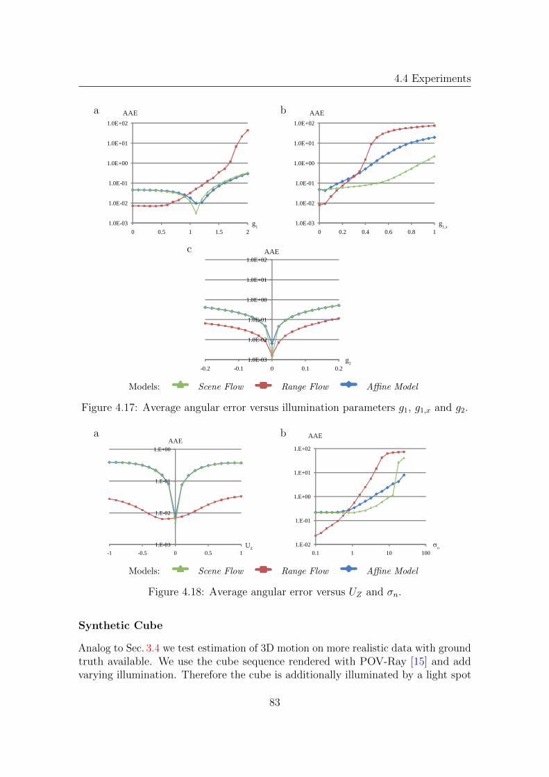
4.4 Experiments
a b
g1
AAE
1.0E-03
1.0E-02
1.0E-01
1.0E+00
1.0E+01
1.0E+02
0 0.5 1 1.5 2g1,x
AAE
1.0E-03
1.0E-02
1.0E-01
1.0E+00
1.0E+01
1.0E+02
0 0.2 0.4 0.6 0.8 1
c
g2
AAE
1.0E-03
1.0E-02
1.0E-01
1.0E+00
1.0E+01
1.0E+02
-0.2 -0.1 0 0.1 0.2
Models: Scene Flow Range Flow Affine Model
Figure 4.17: Average angular error versus illumination parameters g1, g1,x and g2.
a b
1.E-03
1.E-02
1.E-01
1.E+00
-1 -0.5 0 0.5 1UZ
AAE
σn
AAE
1.E-02
1.E-01
1.E+00
1.E+01
1.E+02
0.1 1 10 100
Models: Scene Flow Range Flow Affine Model
Figure 4.18: Average angular error versus UZ and σn.
Synthetic Cube
Analog to Sec. 3.4 we test estimation of 3D motion on more realistic data with groundtruth available. We use the cube sequence rendered with POV-Ray [15] and addvarying illumination. Therefore the cube is additionally illuminated by a light spot
83
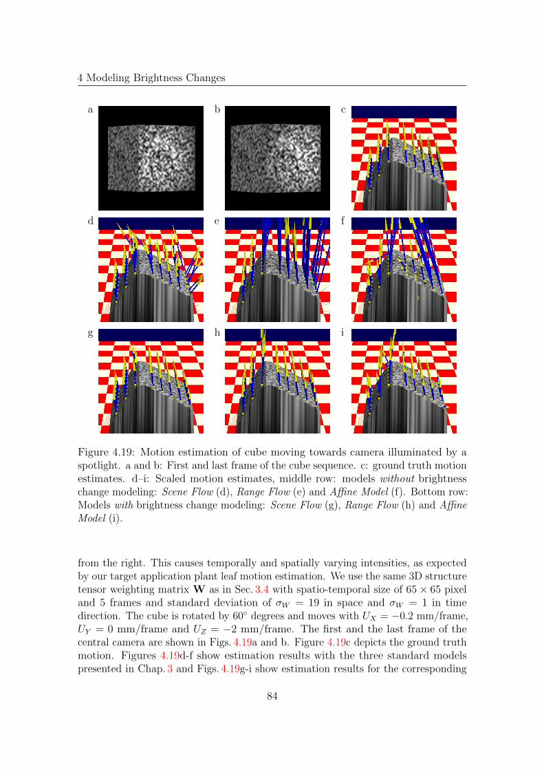
4 Modeling Brightness Changes
a b c
d e f
g h i
Figure 4.19: Motion estimation of cube moving towards camera illuminated by aspotlight. a and b: First and last frame of the cube sequence. c: ground truth motionestimates. d–i: Scaled motion estimates, middle row: models without brightnesschange modeling: Scene Flow (d), Range Flow (e) and Affine Model (f). Bottom row:Models with brightness change modeling: Scene Flow (g), Range Flow (h) and AffineModel (i).
from the right. This causes temporally and spatially varying intensities, as expectedby our target application plant leaf motion estimation. We use the same 3D structuretensor weighting matrix W as in Sec. 3.4 with spatio-temporal size of 65× 65 pixeland 5 frames and standard deviation of σW = 19 in space and σW = 1 in timedirection. The cube is rotated by 60 degrees and moves with UX = −0.2 mm/frame,UY = 0 mm/frame and UZ = −2 mm/frame. The first and the last frame of thecentral camera are shown in Figs. 4.19a and b. Figure 4.19c depicts the ground truthmotion. Figures 4.19d-f show estimation results with the three standard modelspresented in Chap. 3 and Figs. 4.19g-i show estimation results for the corresponding
84

4.4 Experiments
a b
c d
e f
Figure 4.20: Castor Oil Plant sequence. Motion estimates for models without (left)and with (right) brightness change modeling. a and b: Scene Flow, c and d: RangeFlow, e and f: Affine Model.
models with brightness change modeling. Errors of motion estimates are scaled byfactor by 100 in UX-and UY -directions and 10 in UZ-direction. Motion estimates ofmodels without brightness change modeling clearly have higher errors compared tothe models with brightness change modeling. Scene Flow with brightness changemodeling performs best, only at borders estimates are distorted. Brightness changemodeling shows much more effect on Range Flow and the Affine Model comparedto Scene Flow. Nevertheless estimates of Range Flow still suffer from errors andborders and overestimation of UZ . Estimation errors of the Affine Model are higherin X- and Y -direction, but UZ has no significant offset compared to Range Flow.However the Affine Model yields worst results for this data set.
85

4 Modeling Brightness Changes
Castor Oil Plant
The Castor Oil Plant sequence proposed in Sec. 3.4 heavily suffers from changingillumination. Especially at the top of the leaf, where the shadow area decreasesthe standard models yield no reliable estimates. We compare the standard modelsfrom Chap. 3 with the models with brightness change modeling in Fig. 4.20. Motionestimates of Scene Flow already yield almost everywhere reliable results withoutbrightness change modeling. The novel version outperforms the standard version ofScene Flow and no outliers are visible and the estimated velocity field looks evenmore smooth. Also estimates of Range Flow and the Affine Model show significantlymore smooth results with brightness change modeling. However, as for the resultsof the cube sequence, Range Flow yields distorted motion estimates near depthdiscontinuities and the Affine Model yields less reliable estimates.
4.5 Conclusions
In this section, we extended the three 3D motion estimation models described inChap. 3 by different approaches to handle inhomogeneous illumination. We deriveda novel brightness change constraint, where changes are approximated by a powerseries. This model allows to handle changes in reflected radiance due to (1) changesof illumination direction and (2) changes in incoming light intensity caused bymoving inhomogeneous incident irradiance. While the first effect may be modeled byspatially constant temporal changes, the latter one causes spatially variant temporalchanges. In order to test performance of the novel brightness change constraint,it was applied to the Affine Model. The sinusoidal pattern experiments revealthat modeling spatial variations of brightness changes results in increased motionestimation accuracy with respect to g1,x, but not with g2,x (cmp. (4.16)). Motionvector fields of a translating cube illuminated by a moving spotlight have beenestimated using brightness constancy assumption and brightness change model withor without spatial changes. The richest model yields significantly better results thanthe other ones.Based on this conclusion we presented a detailed error analysis for the novel brightnesschange constraint and three different brightness constraints in combination withhighpass or homomorphic prefiltering on synthetic image sequences with RangeFlow. Prefiltering improved estimation results on data when illumination changeswere present, however, the standard deviation σpre of the lowpass used in the filtersshould be large enough. If not, too much signal is lost, resulting in less accuratemotion estimates. Highpass filtering performs well if Gaussian noise or shot noise ispresent. Homomorphic filtering works excellent for shot noise, but errors increasewhen Gaussian noise and strong brightness changes are present. We conclude that,except for this case, well tuned homomorphic prefiltering allows for accurate rangeflow estimation in conjunction with all models. However a wrongly tuned filterseverely corrupts motion estimates. Furthermore, prefiltering increased uncertainty
86

4.5 Conclusions
of motion estimates, as relevant signal is then also affected by the filtering.Modeling brightness changes in Range Flow by the models GRAD or TAYLOR
instead of highpass prefiltering results in motion estimates of same or higher accuracyin almost all scenarios investigated. The model INTGRAD mostly showed resultslying between the results of standard range flow (model INT) and the model GRAD.Generally, best results were achieved by model TAYLOR and, especially whennoise was present, without prefiltering. Only for brightness changes with strongspatial variations, i.e., g1,x 0, and noise-free data homomorphic prefiltering isrecommended. We conclude that suitably modeling brightness changes almost alwaysoutperforms other approaches and increases overall accuracy without tuning ofprefilters.
A comparison of the three 3D motion estimation models using the novel brightnesschange model demonstrated, that for synthetic sinusoidal sequences Range Flowperforms best for low noise and little brightness changes. Scene Flow showed bestperformance for higher noise or larger brightness changes. The Affine Model yieldssame results as Scene Flow for low noise and small brightness changes, but in othercases higher errors. On the cube and the plant leaf sequence Scene Flow performedbest, while Range Flow suffered from outliers near borders. The Affine Model showedmost unreliable results.The Affine Model is based on a translating patch model. This is not true for theplant leaf sequence, because the leaf unfolds and rotates around the point where itis fixed to the stem. In the next section we will extend the Affine Model to handlerotation and introduce additional constraints to make 3D motion estimation morereliable.
87

88

Chapter 5
Modeling Rotation
The Affine Model presented in Sec. 3.3 handles translational motion only. This maylead to severe problems in sequences where objects of interest rotate (cmp. the CastorOil Plant sequence in Fig. 4.20). In this chapter we extend the Affine Model to handlerotational motion. Furthermore we introduce two additional local dimensions to thestandard 2D affine optical flow model, i.e., we model affine transformations not onlyin local image coordinates ∆x and ∆y, but also in local camera displacement ∆s andtime direction ∆t. Analog to the 2D model we identify the additional parameterswith terms depending on scene structure, scene motion, and camera displacement.This 4D affine optical flow model helps to make the second estimation process morereliable, i.e., estimation of 3D motion parameters. The derivation is shown for a 1Dcamera grid only, but extension for a 2D camera grid is analog1.As in Sec. 3.3 we interpret the camera position s as additional dimension of thedata. Hence all image sequences acquired by a 1D camera grid can be combined tosample a 4D-Volume in x-y-s-t-space. Brightness changes in this space are modeledas total differential of the intensity data. A pinhole camera model is used to projecta dynamic surface patch into the image. This yields equations for x- and y-positionof the patch as a function of camera position and time. Plugging the linearized totaldifferentials of x and y into the total differential of the intensity results in the soughtmodel. A crucial point here is the correct handling of neighbor locations. We modelit by back-projection of the pixel grid to the surface in the scene (see Secs. 5.1.3 and5.1.4). A detailed derivation of the modified model can be found in Section 5.1.
In order to evaluate the model we use a parameter estimation procedure asproposed in Sec. 3.3.2. Adaptations needed here are presented in Section 5.2.
Quantitative experiments (Sec. 5.3) use synthetic data with ground truth availablegenerated with the sequence generator presented in App. B. For more realistic sceneswith ground truth available we use another cube sequence rendered by POV-Ray[15] in 8bit-integer accuracy. Finally we demonstrate improvements coming frommodeling rotation on the Castor Oil Plant sequences and compare results to Scene
1In case of a 2D camera model we achieve a 5D affine optical flow model with local cameradisplacement coordinates ∆sx and ∆sy
89

5 Modeling Rotation
Flow and Range Flow.
5.1 Model Derivation
We briefly review the derivation of the Affine Model for translational motion and itsextension to 4D affine optical flow. Afterwards we will model rotational motion ofthe patch.
5.1.1 Surface Patch Model
Following Sec. 3.3 we model a surface patch at world coordinate position (X0, Y0, Z0)as a function of time t by X
YZ
=
X0 + UXt+ ∆XY0 + UY t+ ∆YZ0 + UZt+ ZX∆X + ZY ∆Y
(5.1)
where ZX and ZY are surface slopes in X- and Y -direction for time t = 0 andU = (UX , UY , UZ) is the velocity of the patch. The surface normal is then n =(ZX , ZY ,−1).
5.1.2 Camera Model
We use pinhole cameras at world coordinate positions (s, 0, 0), looking into Z-direction(xy
)=f
Z
(X − sY
)(5.2)
Sensor coordinates x, y are aligned with world coordinates X, Y . Camera positionspace is sampled equidistantly using a 1D camera grid. Modeling steps taken infollowing can also be applied for a 2D camera grid (e.g., [45, 77]), cmp. [62]. Herewe focus on 1D grids and combine data acquired by all cameras into one 4D data setequidistantly sampling the continuous intensity function I(x, y, s, t).
5.1.3 Pixel-Centered View
Parameter estimation at a 4D pixel x0 = (x0, y0, s0, t0) is done using the acquiredimage data I(x) := I(x, y, s, t) in a local neighborhood Λ, with x := (x, y, s, t)T.Consequently we need to know the surface position X for each 4D pixel, i.e., X(x).Using a pinhole camera (5.2) we know(
X(x)Y (x)
)=Z(x)
f
(xy
)+
(s0
). (5.3)
90

5.1 Model Derivation
a b
Z(0)
s=0
image plane
X
xf
X(x) X(x)
ZXX(x)
Z
Z(0)Zt
s=0 s=1
image plane
X
xf
X(x)
U
t=0
t=1Zs
Z
x
Figure 5.1: Relationship between X0, Z(0) (left) and Zt and Zs (right).
In order to derive an expression for Z(x) we fit a tangent plane with surface normaln = (ZX , ZY ,−1)T to the point X(x). The intersection of this tangent plane with theZ-axis is then Z(0, 0, 0, t), and Z(0, 0, 0, t) = Z(0) + Ztt for a constantly translatingplane, where 0 := (0, 0, 0, 0)T. Consequently Z(x) can be expressed as
Z(x) = Z(0) + ZXX(x) + ZY Y (x) + Ztt
⇔ Z(x) = Z(0)+ZXs+Ztt1−ZX
xf−ZY
yf
(5.4)
where we used (5.3) to substitute X(x) and Y (x). Combining (5.3) and (5.4) yields
X(x) = Z(0)+ZXs+Zttf−ZXx−ZY y
xyf
+
s00
. (5.5)
Equation (5.5) extends the formulation in [62], where X only depends on local imagecoordinates x and y. Figure 5.1 depicts the relationship between X(x) and Z(0) fora point in the central camera and frame (Fig. 5.1a) and for varying s and t (Fig. 5.1b).Obviously depth seen at the principal point of a camera changes due to motion ofthe camera or the patch. These changes are addressed by Zs and Zt.
5.1.4 Projecting the Pixel Grid to the Surface
A pixel x in the local neighborhood Λ used for parameter estimation is given byx = x0 +∆x = (x0 +∆x, y0 +∆y, s0 +∆s, t0 +∆t)T. The surface patch center X0 bydefinition is the back projection of the neighborhood center point x0 to the surface.Consequently neighbor points of X0 on the surface given by ∆X = (∆X,∆Y,∆Z)are projections of the cameras pixel grids to the moving surface and we need to
91

5 Modeling Rotation
derive ∆X(∆x). In order to stay on the surface, we model ∆Z = ZX∆X + ZY ∆Y ,cmp. (5.1). Further we know from (5.1) that
∆X = X−X0 −Ut (5.6)
where X is a point on the surface at a given point in time t, X0 is the surface patchcenter at time t0 = 0, and ∆X is the distance between X and the point X0 + Utwhere the patch center moved to. The distance between X and X0 can expressed bythe linearization
X−X0 =∂X
∂x∆x+
∂X
∂y∆y +
∂X
∂s∆s+
∂X
∂t∆t . (5.7)
The partial derivatives of X(x) are (cmp. (5.5))
∂X
∂x=
Z
fc
1− ZY yf
ZXyf
ZX
,∂X
∂y=
Z
fc
ZYxf
1− ZX xf
ZY
∂X
∂s=
1
c
c+ ZXxf
ZXyf
ZX
,∂X
∂t=Ztfc
xyf
(5.8)
where we used the notation
c = 1− ZXx
f− ZY
y
f. (5.9)
Substituting (5.7) and (5.8) in (5.6) yields the sought expression for ∆X(∆x).
5.1.5 Brightness Change Model
We model intensity changes analog to Chap. 4, i.e., dI of a surface element for sucha multi-dimensional data set is
dI = Ixdx + Iydy + Isds + Itdt= I(g1 + g1,x∆X + g1,y∆Y + g2t)dt .
(5.10)
We denote I∗ = ∂I∂∗ for partial derivatives of the image intensities I. In the following
we use notation g = (g1 + g1,x∆X + g1,y∆Y + g2t) for the intensity change function.This brightness change constraint equation (BCCE) models spatially constant andspatially varying brightness changes stemming from varying illumination.
5.1.6 Combination of Models
Following Sec. 3.3 we project the moving surface patch model to the sensor planeusing the pinhole camera model and calculate the differentials dx and dy for a given
92

5.1 Model Derivation
surface location (i.e., for constant ∆X and ∆Y )(dxdy
)=f
Z
((UX − UZ xf )dt − ds
(UY − UZ yf )dt
). (5.11)
This equation is nonlinear in the sought for 3D parameters. Furthermore this equationdepends on ∆X and ∆Y in Z. We simplify it by rephrasing f/Z via the surfacepatch model (5.1), i.e., Z = Z0 +UZ∆t+ZX∆X+ZY ∆Y . Inserting Eqs. (5.6)–(5.9)leads to
f
Z= −ν − b1∆x− b2∆y − b3∆s− b4∆t (5.12)
with ν = − fZ0, b1 = ZX
Z0c, b2 = ZY
Z0c, b3 = f
Z0
ZX
Zc, b4 = f
Z0
Zt
Zc (5.13)
Combination of the proposed models is done analog to [62]. In the first stepEquations (5.12), (5.1) and (5.6)–(5.9) are plugged into (5.11), using local coordinatesx = x0+∆x. Sorting by differentials and ∆-terms, and ignoring higher order ∆-termswe substitute dx and dy in the brightness change model (5.10). This yields
dx = fZ
[(UX − x
fUZ
)dt − ds
]= −ν
(UX − x
fUZ
)dt
−[b1
(UX − x0
f UZ
)+ UZ
Z0
]∆xdt
−[b2
(UX − x0
f UZ
)]∆ydt
−[b3
(UX − x0
f UZ
)]∆sdt
−[b4
(UX − x0
f UZ
)]∆tdt
+ νds + b1∆xds + b2∆yds
+ b3∆sds + b4∆tds
(5.14)
anddy = f
Z
(UY − y
fUZ
)dt
= −ν(UY − y0
f UZ
)dt
−[b1
(UY − y0
f UZ
)]∆xdt
−[b2
(UY − y0
f UZ
)+ UZ
Z0
]∆ydt
−[b3
(UY − y0
f UZ
)]∆sdt
−[b4
(UY − y0
f UZ
)]∆tdt
(5.15)
93
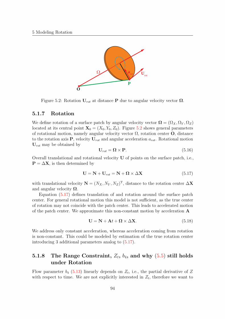
5 Modeling Rotation
UrotarotΩ
PO
Figure 5.2: Rotation Urot at distance P due to angular velocity vector Ω.
5.1.7 Rotation
We define rotation of a surface patch by angular velocity vector Ω = (ΩX ,ΩY ,ΩZ)located at its central point X0 = (X0, Y0, Z0). Figure 5.2 shows general parametersof rotational motion, namely angular velocity vector Ω, rotation center O, distanceto the rotation axis P, velocity Urot and angular acceleration arot. Rotational motionUrot may be obtained by
Urot = Ω×P. (5.16)
Overall translational and rotational velocity U of points on the surface patch, i.e.,P = ∆X, is then determined by
U = N + Urot = N + Ω×∆X (5.17)
with translational velocity N = (NX , NY , NZ)T, distance to the rotation center ∆Xand angular velocity Ω.
Equation (5.17) defines translation of and rotation around the surface patchcenter. For general rotational motion this model is not sufficient, as the true centerof rotation may not coincide with the patch center. This leads to accelerated motionof the patch center. We approximate this non-constant motion by acceleration A
U = N + At+ Ω×∆X. (5.18)
We address only constant acceleration, whereas acceleration coming from rotationis non-constant. This could be modeled by estimation of the true rotation centerintroducing 3 additional parameters analog to (5.17).
5.1.8 The Range Constraint, Zt, b4, and why (5.5) still holdsunder Rotation
Flow parameter b4 (5.13) linearly depends on Zt, i.e., the partial derivative of Zwith respect to time. We are not explicitly interested in Zt, therefore we want to
94

5.1 Model Derivation
express it using parameters we are interested in. We know that UZ := dZ/dt. Thetime derivative of the first equation in (5.4) therefore yields
Zt = UZ − ZXUX − ZYUY (5.19)
for translating planes, i.e., for constant surface slopes ZX and ZY . This is the so-calledrange constraint known from [69] (cmp. (3.5)). Obviously surface slopes change whena surface rotates and the range constraint becomes
Zt = UZ − ZXUX − ZYUY −XZX,t − Y ZY,t (5.20)
ZX,t and ZY,t are first order time derivatives of ZX and ZY .Equation (5.4) was derived for translating surfaces. We model the change in (5.4)
due to rotation by replacing ZX and ZY by their time depending counterparts ZX(t)and ZY (t). We approximate the change of the surface normals by first order Taylorexpansions ZX(t) = ZX(0) + ZX,tt and ZY (t) = ZY (0) + ZY,tt and derive for (5.4)
Z(x) = Z(0) + ZX(t)X(x) + ZY (t)Y (x) + Ztt
⇔ Z(x) −ZX(0)Z(x)xf− ZY (0)Z(x) y
f
= Z(0) + ZXs+ (Zt + ZX,tX(x) + ZY,tY (x))t
⇔ Z(x) =Z(0)+ZX(0)s+(Zt+ZX,tX(x)+ZY,tY (x))t
c
(5.21)
Substituting Zt using (5.20) yields
Z(x) = Z(0)+ZXs+(UZ−ZXUX−ZY UY )tc
⇔ Z(x) = Z(0)+ZXs+Zttc
(5.22)
where now Zt is defined by the standard range constraint, i.e.,
Zt := UZ − ZXUX − ZYUY . (5.23)
We conclude that (5.5) still holds for a first order model of rotational motion, ifZt ignores surface slope changes due to rotation. Consequently Zt in (5.13) alsobecomes Zt.
5.1.9 A 4D-Affine Model
Collecting terms and equations derived so far leads to the sought 4D affine model.We derive it by inserting (5.6) in (5.18), substitution of velocity vector U in (5.14)and (5.15). Ignoring higher order terms yields representations of the elements ofthe 4 dimensional optical flow model (5.24) with parameters (5.25). The partialderivatives of world coordinates in (5.25) are given in (5.8).
95

5 Modeling Rotation
∇TI
( uxdt + νdsuydt
)+
(a11dt + b1ds a12dt + b2ds a13dt + b3ds a14dt + b4ds
a21dt a22dt a23dt a24dt
)∆x∆y∆s∆t
+Isds + Itdt = Igdt(5.24)
ux = −ν(NX − x0
f NZ
)uy = −ν
(NY − y0
f NZ
)a11 = −ν
[ΩY
∂Z∂x − ΩZ
∂Y∂x −
x0
f
(ΩX
∂Y∂x − ΩY
∂X∂x
)− NZ
Z0
]−b1
(NX − x0
f NZ
)a12 = −ν
[ΩY
∂Z∂y − ΩZ
∂Y∂y −
x0
f
(ΩX
∂Y∂y − ΩY
∂X∂y
)]−b2
(NX − x0
f NZ
)a13 = −ν
[ΩY
∂Z∂s − ΩZ
∂Y∂s −
x0
f
(ΩX
∂Y∂s − ΩY
∂X∂s
)]−b3
(NX − x0
f NZ
)a14 = −ν
[ΩY
∂Z∂t − ΩZ
∂Y∂t −
x0
f
(ΩX
∂Y∂t − ΩY
∂X∂t
)+(AX − x0
f AZ
)]−b4
(NX − x0
f NZ
)a21 = −ν
[ΩZ
∂X∂x − ΩX
∂Z∂x −
y0
f
(ΩX
∂Y∂x − ΩY
∂X∂x
)]−b1
(NY − y0
f NZ
)a22 = −ν
[ΩZ
∂X∂y − ΩX
∂Z∂y −
y0
f
(ΩX
∂Y∂y − ΩY
∂X∂y
)− NZ
Z0
]−b2
(NY − y0
f NZ
)a23 = −ν
[ΩZ
∂X∂s − ΩX
∂Z∂s −
y0
f
(ΩX
∂Y∂s − ΩY
∂X∂s
)]−b3
(NY − y0
f NZ
)a24 = −ν
[ΩZ
∂X∂t − ΩX
∂Z∂t −
y0
f
(ΩX
∂Y∂t − ΩY
∂X∂t
)+(AY − y0
f AZ
)]−b4
(NY − y0
f NZ
)(5.25)
5.2 Parameter Estimation
We estimate parameters in three steps. 1. We solve for 4D affine optical flowparameters ν, b1, . . ., b4, ux, uy, a11, . . ., a24 and brightness change parameters g1,g1,x, g1,y and g2 using the total least squares method described in [62]. 2. We solvefor depth Z0, and surface normals ZX and ZY , and Zt using (5.13), where focal lengthf has to be known e.g., from a calibration step. This allows to calculate c from (5.9)and partial derivatives of world coordinates from (5.8). 3. We solve for translationN, and rotation Ω if desired, using the equations in (5.25) or – as reference methods– using Scene Flow from Sec. 3.1 or Range Flow from Sec. 3.2. Acceleration A canonly be estimated up to 1 degree of freedom as we have only 2 equations (the onesfor a14 and a24) for 3 parameters AX , AY , AZ . Equations (5.25) and (5.13) being anoverdetermined system of equations, there are several ways to solve for N and Ωusing a standard least squares estimation scheme. For our experiments we select thefollowing submodels by selecting some or all equations from (5.25) and (5.13), orby removing terms when parameters like rotation or acceleration are not estimated.This is equivalent to not modeling these parameters or setting them to zero.
96
5.3 Experiments
We use the following submodels
2D OF trans. estimates N only, using equations for ux, uy, a11, a12, a21, a22.
2D OF rot. estimates N and Ω using equations for ux, uy, a11, a12, a21, a22.
2D OF trans. and .../2D OF rot. and ... using additional equations indicated bydots (...)
4D OF trans. estimates N only, using all 11 equations containing motion information,10 from (5.25) and 1 from (5.13), i.e., the one for b4.
4D OF rot. estimates N and Ω only, using the 11 equations.
4D OF estimates N, Ω, and A using the 11 equations.
Parameters that are not solved for are set to zero. 4D OF uses two equations morethan 2D OF rot. and a13, a23, b4 but estimates A in addition. We therefore getidentical results for N and Ω using the two models. Thus we do not show results for4D OF in the experiments below.
5.3 Experiments
In a first experiment we use synthetic sinusoidal sequences for systematic erroranalysis. Then performance of different models is compared on more realistic datawith ground truth available, i.e., a translating and rotating cube rendered withPOV-Ray [15]. Finally we show estimation results of a sequence showing a rotatingplant leaf. In all experiments we minimize systematic discretization errors comingfrom derivatives by using optimized 5-tab derivative filter sets presented in [54].
5.3.1 Sinusoidal Pattern
For systematic error analysis we render a surface patch with sinusoidal pattern withthe Sequence Generator (cmp. App. B), where geometry and intensities mimic typicalsettings used in our actual lab experiments with plants. The 32-bit float intensityvalues are in the range [50; 150]. Figure 5.3 shows first and last frame of such an inputsequence with surface patch parameters Z0 = 100 mm, ZX = 0.6, and ZY = −0.5,and motion parameters N ≈ (0.0073,−0.0037, 0.06)T mm/frame and ω = 0.003degree/frame around rotational axis v = (2, 3, 2)T, i.e., Ω = ωv. In each experimentwe vary only one of these parameters. The synthetic sensor contains 501× 501 pixelswith width and height 0.0044 mm. The focal length of the projective camera is setto f = 12 mm. We generate data for 9 cameras, positioned horizontally as a 1D,equidistantly spaced camera grid with displacement of 0.5 mm. In order to keepoptical flow in camera displacement direction below 1 pixel/displacement, we preshiftthe data by 13 pixel/displacement. The effective image size shrinks to 301 × 301
97

5 Modeling Rotation
a b
Figure 5.3: a: First and b: last frame of the input sequence with translation androtation.
pixel due to border effects. Neighborhood Λ is implemented by a Gaussian filter withsize 65× 65× 5× 5 and standard deviations 19× 19× 1× 1 in x, y, s, t-directions.In order to compare performance of models, we use the average angular error (seeApp. A)
AAE =1
N
N∑i=1
arccos(rt(i)
Tre(i))
(5.26)
for N pixel with a minimum distance of 60 pixel to the nearest border, true motionrt and estimated motion re, with r = (NT, 1)T for translation and r = (ΩT, 1)T forrotation.
Figure 5.4 shows average angular errors of translational motion estimates forsequences without (top) and with (bottom) rotation. We show errors for increasingtranslational motion NZ in Figs. 5.4a and c and for increasing standard deviation ofnoise σn in Figs. 5.4b and d. Figures 5.4a and b demonstrate that all models performalmost equally well for sequences without rotation. Scene Flow performs best inalmost all cases. Affine models perform better when using more affine parameters (4DOF trans./rot., and 2D OF rot. and a13, a23, b4). Range Flow performs only slightlybetter than affine models for low noise sequences. In case of rotation (Figs. 5.4c andd) Range Flow and the translational models yield high errors compared to rotationalmodels, Scene Flow again performs best. However, comparing rotational models, 4DOF rot. performs worst. This indicates that modeling A in the equations for a14 anda24 ((5.25)) or not using a14 and a24 (i.e., 2D OF rot. and a13, a23, b4) is beneficial. Incase of noise Scene Flow shows best performance up to σn = 10. Rotational modelsusing 4D affine terms (2D OF rot. and a13, a23, b4 and 4D OF rot.) yield betterresults than the 2D model (2D OF rot.). 4D OF trans. shows considerable betterperformance than Range Flow, despite for NZ = 0 and no noise, and performs asgood as the best rotational models for 1 < σn < 10. In Fig. 5.5 we compare averageangular errors of translational (Fig. 5.5a) and rotational (Figs. 5.5b, c and d) motionparameters for different rotation models. Translational models and Range Flow areshown for reference in Fig. 5.5a. Figures 5.5c and d show angular errors of rotational
98

5.3 Experiments
a b
1.0E-05
1.0E-04
1.0E-03
1.0E-02
1.0E-01
1.0E+00
-1 -0.5 0 0.5 1NZ
AAEN
1.0E-03
1.0E-02
1.0E-01
1.0E+00
1.0E+01
1.0E+02
0.1 1 10 100σn
AAEN
c d
1.0E-05
1.0E-04
1.0E-03
1.0E-02
1.0E-01
1.0E+00
1.0E+01
-1 -0.5 0 0.5 1NZ
AAEN
1.0E-03
1.0E-02
1.0E-01
1.0E+00
1.0E+01
1.0E+02
0.1 1 10 100σn
AAEN
Models:Scene Flow Range Flow 2D OF trans.4D OF trans. 2D OF rot. 2D OF rot. and a13, a23, b44D OF rot.
Figure 5.4: Average angular error (AAE) of N versus increasing NZ (left) and σn(right). a and b: without rotation, c and d: with rotation.
parameters for a rotating sequence and increasing NZ and σn, respectively, i.e., theΩ counterparts of Figs. 5.4c and d.
The figures demonstrate that incorporating the affine parameters a14 and a24 in4D OF rot. without modeling of acceleration significantly increases errors. Figures5.5a and b show average angular errors of translational and rotational parameters forsequences with increasing ω. Rotational models without a14 and a24 perform similarand up to three orders of magnitude better than Range Flow and the translationalmodels, only Scene Flow yields lower errors.
We conclude that modeling rotation yields almost always significantly lower or atleast similar errors as the translational models and Range Flow. Scene Flow performsbest in all cases, but is not able to estimate angular velocity. Using a14 and a24
without modeling acceleration A should be avoided.
99

5 Modeling Rotation
a b
1.0E-04
1.0E-03
1.0E-02
1.0E-01
1.0E+00
1.0E+01
1.0E+02
0.001 0.01 0.1 1ω
AAEN
1.0E-06
1.0E-05
1.0E-04
1.0E-03
1.0E-02
1.0E-01
1.0E+00
1.0E+01
1.0E+02
0.001 0.01 0.1 1ω
AAEΩ
c d
1.0E-05
1.0E-04
1.0E-03
1.0E-02
1.0E-01
1.0E+00
-1 -0.5 0 0.5 1NZ
AAEΩ
1.0E-03
1.0E-02
1.0E-01
1.0E+00
1.0E+01
1.0E+02
0.1 1 10 100σn
AAEΩ
Models:Scene Flow Range Flow 2D OF trans.4D OF trans. 2D OF rot. 2D OF rot. and b42D OF rot. and a13, a23 2D OF rot. and a13, a23, b4 4D OF rot.
Figure 5.5: a: AAE of N versus ω, and AAE of Ω versus b: ω, c: NZ and d: σn.
5.3.2 Synthetic Cube
The synthetic cube sequence allows us to compare models on more realistic datawith ground truth available. The cube is moving with N = (−0.2, 0,−1)T mm/frameand rotates around its Y -axis with ω = 0.4 degrees/frame. The cube is covered witha noise pattern in order to make local estimation reliable. Neighborhood Λ is thesame as for the sinusoidal sequences. The 1D camera grid contains 9 cameras with adisplacement of 5 mm. Figure 5.6a and b show first and last frame of the centralcamera with regions where errors are evaluated. Ground truth motion is depicted inFig. 5.6c.
Figures 5.6d–i show estimation results of Scene Flow, Range Flow, the translationalmodels 2D OF trans. and 4D OF trans. and the rotational models 2D OF rot. and2D OF rot. and a13, a23, b4. The errors are amplified by a factor of 5 for bettercomparison of the models. The estimates of 2D OF trans. clearly show large errors,where estimates on the right side of the cube point in Z-direction, estimates on
100

5.3 Experiments
a b c
d e f
g h i
Figure 5.6: Cube moving towards camera with rotation. a and b: First and lastinput frame with evaluation areas and c: ground truth motion. Motion estimates Nwith amplified errors. d: Scene Flow, e: Range Flow, f: 2D OF trans., g: 4D OFtrans., h: 2D OF rot., and i: 2D OF rot. and a13, a23, b4.
the left side of the cube are not visible because they point inwards the cube. Alsoestimates of the rotational model 2D OF rot. suffer from high and non-uniformerrors. Estimates of Range Flow are more accurate, but distorted near borders ofthe cube. Models 4D OF trans. and 2D OF rot. and a13, a23, b4 yield more accurateresults. Estimates of the translational model are still distorted, mainly on the leftside of the cube. Estimation results of Scene Flow best match the ground truth.
Figure 5.7 shows a rendered top view of the cube with ground truth of therotational parameters and estimation results using models 2D OF rot. and 2D OFrot. and a13, a23, b4. The estimates clearly recover the true motion, where estimatesof 2D OF rot. and a13, a23, b4 are more uniform.Table 5.1 shows angular errors for the regions depicted in Figs. 5.6a and b which
quantitatively confirm the visual impression of the rendered results. 2D OF trans.performs better when b4, a13 and a23, or all three terms are additionally used
101
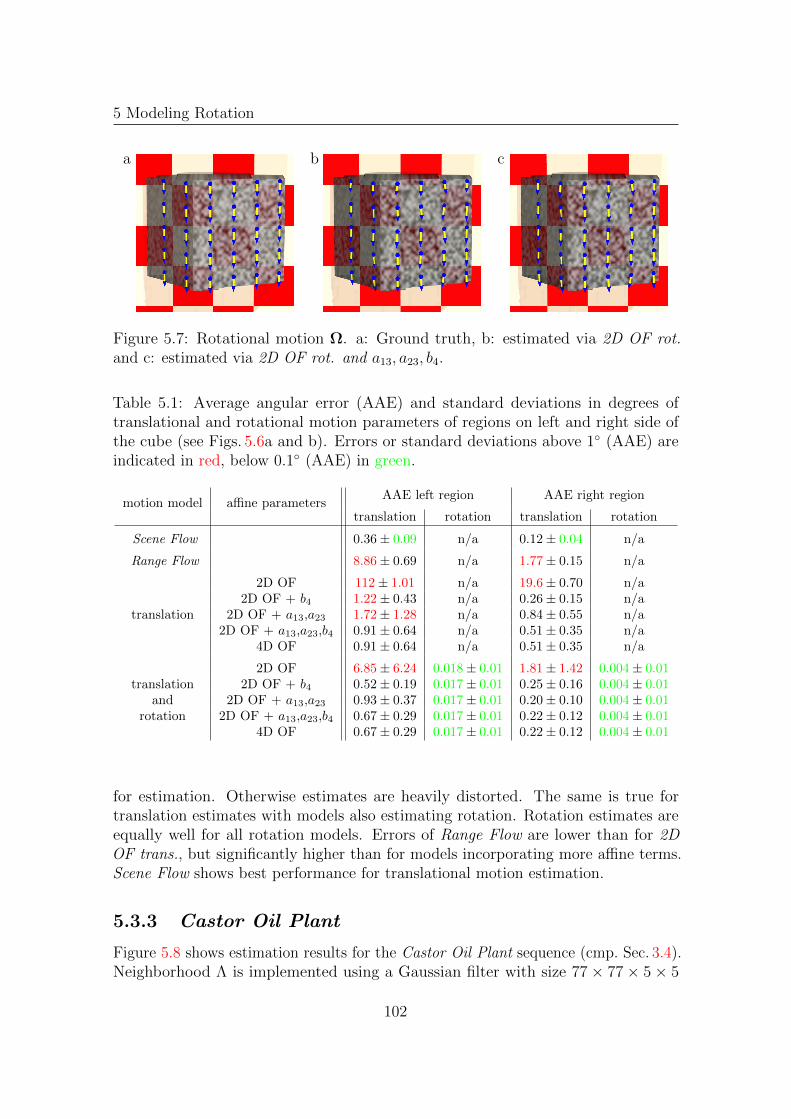
5 Modeling Rotation
a b c
Figure 5.7: Rotational motion Ω. a: Ground truth, b: estimated via 2D OF rot.and c: estimated via 2D OF rot. and a13, a23, b4.
Table 5.1: Average angular error (AAE) and standard deviations in degrees oftranslational and rotational motion parameters of regions on left and right side ofthe cube (see Figs. 5.6a and b). Errors or standard deviations above 1 (AAE) areindicated in red, below 0.1 (AAE) in green.
motion model affine parametersAAE left region AAE right region
translation rotation translation rotation
Scene Flow 0.36± 0.09 n/a 0.12± 0.04 n/a
Range Flow 8.86± 0.69 n/a 1.77± 0.15 n/a
2D OF 112± 1.01 n/a 19.6± 0.70 n/a2D OF + b4 1.22± 0.43 n/a 0.26± 0.15 n/a
translation 2D OF + a13,a23 1.72± 1.28 n/a 0.84± 0.55 n/a2D OF + a13,a23,b4 0.91± 0.64 n/a 0.51± 0.35 n/a
4D OF 0.91± 0.64 n/a 0.51± 0.35 n/a
2D OF 6.85± 6.24 0.018± 0.01 1.81± 1.42 0.004± 0.01translation 2D OF + b4 0.52± 0.19 0.017± 0.01 0.25± 0.16 0.004± 0.01
and 2D OF + a13,a23 0.93± 0.37 0.017± 0.01 0.20± 0.10 0.004± 0.01rotation 2D OF + a13,a23,b4 0.67± 0.29 0.017± 0.01 0.22± 0.12 0.004± 0.01
4D OF 0.67± 0.29 0.017± 0.01 0.22± 0.12 0.004± 0.01
for estimation. Otherwise estimates are heavily distorted. The same is true fortranslation estimates with models also estimating rotation. Rotation estimates areequally well for all rotation models. Errors of Range Flow are lower than for 2DOF trans., but significantly higher than for models incorporating more affine terms.Scene Flow shows best performance for translational motion estimation.
5.3.3 Castor Oil Plant
Figure 5.8 shows estimation results for the Castor Oil Plant sequence (cmp. Sec. 3.4).Neighborhood Λ is implemented using a Gaussian filter with size 77 × 77 × 5 × 5
102

5.3 Experiments
a b
c d
e f
Figure 5.8: Motion estimation results for the plant leaf sequence. a Scene Flow, bRange Flow for varying illumination, c: 2D OF trans., d: 4D OF trans., e: 2D OFrot. and f: 2D OF rot and a13,a23 and b4.
and standard deviation 23× 23× 1× 1 in x, y, s, t-direction.
The leaf rotates around its node where it is attached to the stem. This resultsin a visible motion towards the camera and to the right, while the shadow areacaused by the top leaf decreases. We compare estimation results of the translationalmodel (4D OF trans. and of the rotational models with the estimates from Sec. 4.4,i.e., Scene Flow, Range Flow and the standard translational model (2D OF trans.).Figure 5.8 clearly shows the improvements in motion estimation, when more affineparameters (4D OF trans. and 2D OF rot and a13,a23 and b4) are incorporated inthe estimation. Both models perform visibly better than Range Flow, because theyproduce less outliers. Using the rotational model estimation results are smoother,but Scene Flow still yields more homogeneous results especially in the shadow area
103

5 Modeling Rotation
a b
Figure 5.9: Estimates of angular velocities for the plant leaf sequence. a: 2D OF rot.and b: 2D OF rot and a13,a23 and b4.
of the leaf.Figure 5.9 shows estimation results for angular velocity Ω. Estimates of both
models look heavily distorted. Ground truth is not available, but we assume thatmotion and unfolding of the leaf does not lead to a smooth angular vector field.Nevertheless, outliers are present and demonstrate that the rotational model is notrobust enough for reliable estimation of angular velocity in plant leaf sequences.
5.4 Conclusions
In this chapter we presented a 4D affine optical flow model and how the parametersof this model can be explained by real world parameters. Based on a rigid surfacepatch we modeled translation, acceleration and rotation. The rotational modelimproves estimation results in almost all cases and additionally allows to estimaterotational parameters. Synthetic experiments showed that modeling accelerationis not sufficient to estimate rotation reliably and should therefore not be used ifrotation occurs in the sequence. The 4D Affine Model and its explanation of realworld parameters improved accuracy of motion estimates on synthetic and real datacompared to Range Flow. Scene Flow still yields more reliable results. Therefore theestimation method of Scene Flow should be adapted to the Affine Model. We will dothis in the next section.
104
Chapter 6
5D-Affine Scene Flow Model
In the previous sections we extended the Affine Model to handle (1) sloped surfaces(Sec. 3.3), (2) brightness changes (Sec. 4.3.3), and (3) rotational motion (Chap. 5).The 4D-Affine Model already implicitly includes the range constraint (Sec. 5.1.8) andshowed better performance than Range Flow, although rotation/acceleration couldbe modeled for a neighborhood (Sec. 5.2) only. In this section we will combine theAffine Model with the estimation technique of Scene Flow and derive a formulationfor the complete 5D-Affine Scene Flow Model. Towards this end, we extend thebrightness change model proposed in Chap. 4 to handle brightness changes comingfrom camera motion. This leads to an estimation technique which allows estimationof all parameters including acceleration and/or rotation of patch origins.
6.1 5D-Affine Model
In this section we will extend the Affine Model presented in Sec. 5.1 to handle cameradisplacement in sx and sy direction. In a setup where a spotlight is mounted on thecamera, brightness changes due to motion of the camera occur. We will derive abrightness change model according to Chap. 4 in order to handle brightness changescaused by motion of cameras with fixed spotlights.
In case of camera motion the direction of reflectance changes, i.e., nr becomesnr(sx, sy). This leads to the visible light intensity
L(X(∆X,∆Y, t), sx, sy, t) = B(X(∆X,∆Y, t),ni(t),nr(sx, sy))E(∆X,∆Y, t,ni(t))(6.1)
with the patch’s bidirectional reflectance distribution function (BRDF) B and in-cident light irradiance E (cmp. (4.8)). We model changes of the BRDF due tosmoothly changing reflectance direction nr by smooth functions depending on cameradisplacement, i.e., hB,sx(sx) with hB,sx(0) = 1 and , hB,sy(sy) with hB,sy(0) = 1. We
105

6 5D-Affine Scene Flow Model
obtain
B(X(∆X,∆Y, sx, sy, t),ni(t),nr(sx, sy)) =
B(X(∆X,∆Y, 0, 0, 0),ni(0),nr(0, 0))hB,sx(sx)hB,sy(sy)hB,t(t) .(6.2)
BRDF B depends on three smooth functions hB,sx(sx), hB,sy(sy) and hB,t(t) insteadof hB,t(t) when modeling only temporal changes as in Chap. 4. However, derivationof the visible intensity steps is analog to Chap. 4. This leads to
I(X(∆X,∆Y, t), sx, sy, t) = I(X(∆X,∆Y, 0), 0, 0, 0) exp(hI(∆X,∆Y, sx, sy, t))(6.3)
where
hI(∆X,∆Y, sx, sy, t) := ln(hB,sx(sx)hB,sy(sy)hB,t(t)hE(∆X,∆Y, t)) . (6.4)
The sought temporal derivative of (6.3) is thus
dI = I(X(∆X,∆Y, 0), 0, 0, 0) exp(hI(∆X,∆Y, sx, sy, t))dh I(∆X,∆Y, sx, sy, t)
= I(X(∆X,∆Y, t), sx, sy, t)dh I(∆X,∆Y, sx, sy, t) .(6.5)
We introduce an approximation of hI explicitly modeling spatial variations dueto camera displacement and time still respecting hI(∆X,∆Y, 0, 0, 0) ≡ 0. Themultiplicative behavior between hB,sx , hB,sy and hB,t in (6.4) leads to a sum of powerseries
hI(∆X,∆Y, sx, sy, t) ≈
h(∆X,∆Y, sx, sy, t,g) :=∑
m∈[sx,sy ,t]
2∑i=0
(gm,i + gm,i,x∆X + gm,i,y∆Y )mi .(6.6)
The total derivative of h is then
f(∆X,∆Y, sx, sy, t,g) := dh (∆X,∆Y, sx, sy, t,g)
=∑
m∈[sx,sy ,t]
2∑i=1
i (gm,i + gm,i,x∆X + gm,i,y∆Y )mi−1dm .
(6.7)We substitute sx = sx − sx,0 = ∆sx, sy = sy − sy,0 = ∆sy and t = t − t0 = ∆t in(6.7) and omit higher order terms. We get
f(∆X,∆Y, sx, sy, t,g) =
g1 + g1,x∆X + g1,y∆Y + 2(gsx,2∆sxdsx + gsy ,2∆sydsy + gt,2∆tdt
)(6.8)
106
6.1 5D-Affine Model
withg1 = gsx,1dsx + gsy ,1dsy + gt,1dt
g1,x = gsx,1,xdsx + gsy ,1,xdsy + gt,1,xdt
g1,y = gsx,1,ydsx + gsy ,1,ydsy + gt,1,ydt .
(6.9)
Inserting (6.8) in (5.24) and adding camera displacement directions sx and sy, weobtain the full Affine Model (6.10), where ∇I = (Ix, Iy, I)T and affine parametersare given by (6.12), (6.13). Brightness change parameters can be derived by (6.9)
∇TI
uxdt + νdsx
uydt + νdsy−(gt,1dt + gsx,1dsx + gsy,1dsy
)+ A
∆x∆y∆sx∆sy∆t
+ Isxdsx + Isydsy + Itdt = 0
(6.10)
A =
a11dt + b1dsx a12dt + b2dsx a13dt + b3dsx a14dt + b4dsx a15dt + b5dsxa21dt + b1dsy a22dt + b2dsy a23dt + b3dsy a24dt + b4dsy a25dt + b5dsy
g∆x g∆y g∆sx g∆sy g∆t
(6.11)
ux = −ν(NX − x0
f NZ
)uy = −ν
(NY − y0
f NZ
)a11 = −ν
[ΩY
∂Z∂x − ΩZ
∂Y∂x −
x0
f
(ΩX
∂Y∂x − ΩY
∂X∂x
)− NZ
Z0
]−b1
(NX − x0
f NZ
)a12 = −ν
[ΩY
∂Z∂y − ΩZ
∂Y∂y −
x0
f
(ΩX
∂Y∂y − ΩY
∂X∂y
)]−b2
(NX − x0
f NZ
)a13 = −ν
[ΩY
∂Z∂sx− ΩZ
∂Y∂sx− x0
f
(ΩX
∂Y∂sx− ΩY
∂X∂sx
)]−b3
(NX − x0
f NZ
)a14 = −ν
[ΩY
∂Z∂sy− ΩZ
∂Y∂sy− x0
f
(ΩX
∂Y∂sy− ΩY
∂X∂sy
)]−b4
(NX − x0
f NZ
)a15 = −ν
[ΩY
∂Z∂t − ΩZ
∂Y∂t −
x0
f
(ΩX
∂Y∂t − ΩY
∂X∂t
)+(AX − x0
f AZ
)]−b5
(NX − x0
f NZ
)a21 = −ν
[ΩZ
∂X∂x − ΩX
∂Z∂x −
y0
f
(ΩX
∂Y∂x − ΩY
∂X∂x
)]−b1
(NY − y0
f NZ
)a22 = −ν
[ΩZ
∂X∂y − ΩX
∂Z∂y −
y0
f
(ΩX
∂Y∂y − ΩY
∂X∂y
)− NZ
Z0
]−b2
(NY − y0
f NZ
)a23 = −ν
[ΩZ
∂X∂sx− ΩX
∂Z∂sx− y0
f
(ΩX
∂Y∂sx− ΩY
∂X∂sx
)]−b3
(NY − y0
f NZ
)a24 = −ν
[ΩZ
∂X∂sy− ΩX
∂Z∂sy− y0
f
(ΩX
∂Y∂sy− ΩY
∂X∂sy
)]−b4
(NY − y0
f NZ
)a25 = −ν
[ΩZ
∂X∂t − ΩX
∂Z∂t −
y0
f
(ΩX
∂Y∂t − ΩY
∂X∂t
)+(AY − y0
f AZ
)]−b5
(NY − y0
f NZ
)(6.12)
ν = − fZ0, b1 = ZX
Z0c, b2 = ZY
Z0c
b3 = fZ0
ZXZc , b4 = f
Z0
ZYZc , b5 = f
Z0
ZtZc
(6.13)
c = 1− ZX x0f − ZY
y0f (6.14)
107
6 5D-Affine Scene Flow Model
and the new variables g∆i for i ∈ [x, y, sx, sy, t] by appropriate substitution of ∆Xand ∆Y in 6.8. The partial derivatives of world coordinates can be obtained by (5.8).This notation demonstrates, that the brightness change model has a similar behavioras the standard affine model, but instead of the gradients of the image intensitythe intensity itself is used as input data. Moreover, the novel brightness changemodel introduces only two new affine parameters (gsx,2 and gsy ,2) into the estimationprocess and a new interpretation of the other brightness change parameters (g1, g1,x
and g1,y) compared to the old brightness change model.
6.2 Parameter Estimation
Scene Flow combines translational optical flow estimates from several cameras inorder to solve the aperture problem of Scene Flow (cmp. (3.4)). We extend (3.4) fora 2D camera grid to handle affine optical flow parameters, i.e., parameter b5 anda = (a11, a12, a13, a14, a15, a21, a22, a23, a24, a25)
T. Additional equations constrainingScene Flow then allow to solve for acceleration (AX , AY , AZ)T. We obtain for acamera grid with N calibrated cameras
BV = U ,with V =
NX
NY
NZ
ΩX
ΩY
ΩZ
AXAYAZ
and U =
ux,1uy,1a1
b5,1
ux,2uy,2a2...
b5,N
(6.15)
with affine parameters ai of the optical flow in camera i. Matrix B is created out ofappropriate entries of matrix A and parameters ux, uy as defined in (6.12).Not all parameters of the Affine Model may be available in all cameras. We computethe full model, i.e., with affine parameters containing ∆sx and ∆sy (a13,a14,a23,a24
and b5) only for the central camera. For all other cameras we omit these parametersand get 8 optical flow parameters each.
6.3 Experiments
In a first experiment we use synthetic sinusoidal sequences for systematic erroranalysis. Then performance of different models is compared on more realistic datawith ground truth available, i.e., a translating and rotating cube with varyingillumination in time and camera displacement direction, rendered with POV-Ray[15]. Finally we show estimation results on the previous introduced Castor Oil
108

6.3 Experiments
Plant sequence and another sequence showing a rotating tobacco plant leaf. In allexperiments we minimize systematic discretization errors coming from derivatives byusing optimized 5-tab derivative filter sets presented in [54].In order to test performance of models and influence of acceleration we compareScene Flow and Range Flow with the models1
Affine Model Trans. estimates N using equations ux,uy,a11,a12,a21 and a22, i.e.,standard Affine Model,
Affine Model Trans. Stab. estimates N using all equations from (6.12), and b5,
Affine Model Rot. estimates N and Ω using equations ux,uy,a11,a12,a21 and a22,
Affine Model Rot. Stab. estimates N and Ω using all equations from (6.12), and b5,except a15 and a25,
Affine Scene Flow Model extends the Affine Model Rot. Stab. by additionally usingequations ux,uy,a11,a12,a21 and a22 of all other cameras and
Affine Scene Flow Model Acc. extends the Affine Scene Flow Model by additionallyusing equations a15 and a25 of all cameras and estimates A.
6.3.1 Sinusoidal Pattern
For systematic error analysis we render a surface patch with sinusoidal pattern usingthe Sequence Generator (cmp. App. B). The parameters of the sequence are similarto the parameters used in previous experiments (cmp. Sec. 5.3). Additionally we addacceleration of the patch center A = (0.002,−0.001, 0.003)T mm/frame2. In eachexperiment we vary only one of the parameters. Neighborhood Λ is implemented bya Gaussian filter with size 65× 65× 5× 5 and standard deviations 19× 19× 1× 1in x, y, s, t-directions. In order to compare performance of models, we use theaverage angular error (see App. A) for translational (AAEN ), rotational (AAEΩ) andacceleration (AAEA) parameters.
Figure 6.1 shows average angular errors for sequences with increasing translationalvelocity NZ (left) and with increasing acceleration AZ (right). Figures 6.1a and bdemonstrate that all models based on Scene Flow, i.e., Scene Flow and the AffineScene Flow Model with and without acceleration, perform similar and best of allmodels almost everywhere. Only in case of small patch motion towards the camerathe Affine Model Rot. Stab. performs slightly better. The Affine Model Rot. yieldsbest results when acceleration is large. Range Flow, the Affine Model Trans. Stab.and the Affine Model Trans. yield highest errors in both cases. Models based onScene Flow show high performance also for estimation of rotational parameters (cmp.Figs. 6.1c and d). The Affine Scene Flow Model Acc. performs slightly worse than the
1If not stated differently, all models are extended to handle varying illumination as derived inChap. 4.
109

6 5D-Affine Scene Flow Model
a b
1.0E-04
1.0E-03
1.0E-02
1.0E-01
1.0E+00
1.0E+01
-1 -0.5 0 0.5 1NZ
AAEN
1.0E-04
1.0E-03
1.0E-02
1.0E-01
1.0E+00
1.0E+01
0.0001 0.001 0.01 0.1 1AZ
AAEN
c d
1.0E-05
1.0E-04
1.0E-03
1.0E-02
-1 -0.5 0 0.5 1NZ
AAEΩ
1.0E-05
1.0E-04
1.0E-03
1.0E-02
0.0001 0.001 0.01 0.1 1AZ
AAEΩ
e f
1.0E-05
1.0E-04
1.0E-03
1.0E-02
-1 -0.5 0 0.5 1NZ
AAEA
1.0E-04
1.0E-03
1.0E-02
1.0E-01
1.0E+00
0.0001 0.001 0.01 0.1 1AZ
AAEA
Models:
Scene Flow Range FlowAffine Model Trans. Affine Model Trans. Stab.Affine Model Rot. Affine Model Rot. Stab.Affine Scene Flow Model Affine Scene Flow Model Acc.
Figure 6.1: Average angular error of a and b: translational (AAEN), c and d:rotational (AAEΩ) and e and f: acceleration (AAEA) parameters versus increasingNZ (left) and AZ (right).
110

6.3 Experiments
a b
1.0E-03
1.0E-02
1.0E-01
1.0E+00
1.0E+01
1.0E+02
0.1 1 10 100σn
AAEN
1.0E-03
1.0E-02
1.0E-01
1.0E+00
1.0E+01
1.0E+02
0.1 1 10 100σn
AAEΩ
Models:
Scene Flow Range FlowAffine Model Trans Affine Model Trans StabAffine Model Rot Affine Model Rot StabAffine Scene Flow Model Affine Scene Flow Model Acc.
Figure 6.2: Average angular error of translational (AAEN) and rotational (AAEΩ)parameters versus σn.
model without acceleration. The Affine Model Rot. performs best for high NZ , theAffine Model Rot. Stab. yields worst results. In case of increasing acceleration bothmodels using the estimation technique of Scene Flow perform better than the AffineModel. Figures 6.1 e and f show that the Affine Scene Flow Model Acc. estimatesacceleration reliably for AZ < 0.1.Figures 6.2a and b demonstrate that the increased accuracy of models using the
estimation technique based on Scene Flow also holds under noise. Translational aswell as rotational parameters are best estimated with the Affine Scene Flow Modelfor typical noise values σn < 10. Errors of the other models are similar to the errorsobtained for rotational motion in Chap. 5. The model error is highest for the AffineModel Trans. and Range Flow. The Affine Model Trans. Stab. yields lower errorsand same as the models with rotation for noise values σn > 1. Also the Affine ModelRot. Stab. performs better than the Affine Model without stabilization. In case ofrotational motion it is the other way around. There the Affine Model Rot. yieldslower errors, but the model error is lowest for the Affine Scene Flow Model.We conclude that the Affine Scene Flow Model in general increases stability due tonoise and estimates are more reliable compared to the Affine Model. Estimation ofacceleration is possible and additional estimation of acceleration does not have asignificant effect on the estimates.
6.3.2 Synthetic Cube
The synthetic cube sequence allows to compare models on more realistic data withground truth available. We use a cube sequence similar to the one used in Sec. 5.3,
111

6 5D-Affine Scene Flow Model
a b c
d e f
Figure 6.3: Motion estimation of cube moving towards camera with rotation andillumination changes. a and b: First and last frame of central camera, c: centralframe of central camera with areas used for evaluation, d and e: central frame offirst and last camera, and f: ground truth motion.
i.e., the cube is moving with N = (−0.2, 0,−1)T mm/frame and rotates around itsY -axis with ω = 0.4 degrees/frame. Instead of a static spotlight (cmp. Chap. 4), weadd a spotlight moving with the camera, causing illumination changes in cameradisplacement direction and time. Such a setup is frequently used in robotics, wherecameras and illumination units are placed at a robot’s end-effector. Neighborhood Λis the same as for the sinusoidal sequences. The 1D camera grid contains 9 cameraswith a displacement of 5 mm. Figures 6.4a and b show first and last frame ofthe central camera and Figs. 6.4d and e the central frame of the first and the lastcamera. The brightness changes in time and camera displacement direction areclearly visible. Regions where errors are evaluated are depicted in Fig. 6.3c andground truth motion in Fig. 6.4f. Figures 6.4a-c show motion estimates of thedifferent models using the brightness change model introduced in Chap. 4. Errorsare amplified by a factor of 10 in all directions. The models depicted are the bestfrom the previous experiments, namely Scene Flow, the Affine Model Rot. Stab.and the novel Affine Scene Flow Model. Results look similar for the Affine SceneFlow Model with and without rotation, therefore we depict the Affine Scene FlowModel Acc., only. Figures 6.4d–f show the same models using the new brightnesschange model. The estimates improve for all models. The models based on SceneFlow yield better results compared to the Affine Model. The combined Affine SceneFlow Model shows the most homogeneous motion vector field. For all models most
112

6.3 Experiments
Tab
le6.1:
Average
angu
larerror
oftran
slational
(AAEN
)an
drotation
al(AAE
Ω)
motion
param
etersin
degrees,
averagerelative
growth
rate(R
GR
)in
percen
tp
erfram
ean
dth
eirstan
dard
dev
iations
ofregion
son
leftan
drigh
tsid
eof
the
cub
e(see
Fig.6.3c).
Errors
orstan
dard
dev
iations
above
1
(AA
E)
or1%
/frame
(RG
R)
arein
dicated
inred
,b
elowor
equ
al0.1
(AAE
)or
0.01%/fram
e(R
GR
)in
green.
brigh
tness
motion
mod
elleft
regio
nrigh
tregion
mod
elAAE
NAAE
ΩR
GR
AAE
NAAE
ΩR
GR
Scen
eF
low
0.33±
0.10
n/a
−0.0
013±
0.0410.344
±0.37
n/a
−0.07±
0.28R
an
geF
low
7.16±
0.48
n/a
−0.3
03±
0.26434.32±
44.20
n/a
100
BC
CE
Affi
ne
Mod
elT
ran
s.S
tab.
1.07±
0.73
n/a
0.5
36±
0.0
961.325
±0.853
n/a
−0.29±
0.72(C
hap
.4)
Affi
ne
Mod
elR
ot.
Sta
b.0.5
1±
0.18
0.0047±
0.0
024
0.0094±
0.0881.096
±0.910
0.045±
0.027−
0.23±
0.73A
ffin
eS
cene
Flo
wM
odel
0.32±
0.10
0.0035±
0.0
017
0.0006±
0.0430.410
±0.392
0.028±
0.021−
0.08±
0.28A
ffin
eS
cene
Flo
wM
odel
Acc.
0.32±
0.10
0.0036±
0.0
017
0.0006±
0.0430.410
±0.392
0.027±
0.021−
0.08±
0.28
Scen
eF
low
0.33±
0.10
n/a
−0.0
013±
0.0410.378
±0.40
n/a
−0.063
±0.280
Ran
geF
low
7.15±
0.49
n/a
−0.3
08±
0.2604.63±
1.45n
/a0.433
±0.972
novel
Affi
ne
Mod
elT
ran
s.S
tab.
1.07±
0.73
n/a
0.5
37±
0.0
960.647
±0.477
n/a
−0.044
±0.588
BC
CE
Affi
ne
Mod
elR
ot.
Sta
b.0.5
2±
0.18
0.0047±
0.0
024
0.0
10±
0.0
880.585
±0.597
0.028±
0.0190.009
±0.591
Affi
ne
Scen
eF
low
Mod
el0.3
2±
0.10
0.0035±
0.0
017
0.0006±
0.0430.371
±0.374
0.027±
0.021−
0.057±
0.275
Affi
ne
Scen
eF
low
Mod
elA
cc.0.3
2±
0.10
0.0036±
0.0
017
0.0006±
0.0430.371
±0.374
0.027±
0.021−
0.057±
0.275
113

6 5D-Affine Scene Flow Model
a b c
d e f
g h i
Figure 6.4: Scaled motion estimates of cube sequence with errors amplified. a–c:Motion estimates using the brightness change model proposed in Chap. 6 with modelsScene Flow (a), the Affine Model Rot. Stab. (b), and the Affine Scene Flow ModelAcc. (c). d–f: Motion estimates using the new brightness change model with modelsScene Flow (d), the Affine Model Rot. Stab. (e), and the Affine Scene Flow ModelAcc. (f). g–i: Scaled rotational motion estimates with amplified errors using the newbrightness change model. The Affine Model Rot. Stab. (g), the Affine Scene FlowModel (h) and the Affine Scene Flow Model Acc. (i).
errors occur at borders. The depth reconstruction using the old brightness changemodel fails as expected (cmp. Fig. 6.4a). However, errors of the motion estimates ofScene Flow are lower as expected. This demonstrates that the Scene Flow estimationtechnique is more robust with respect to false depth estimates compared to theAffine Model. Using the Affine Model brightness changes are well compensated alsowith the old brightness change model. As discussed in Sec. 6.1 this may dependon the fact that the model for temporal brightness changes already compensates
114
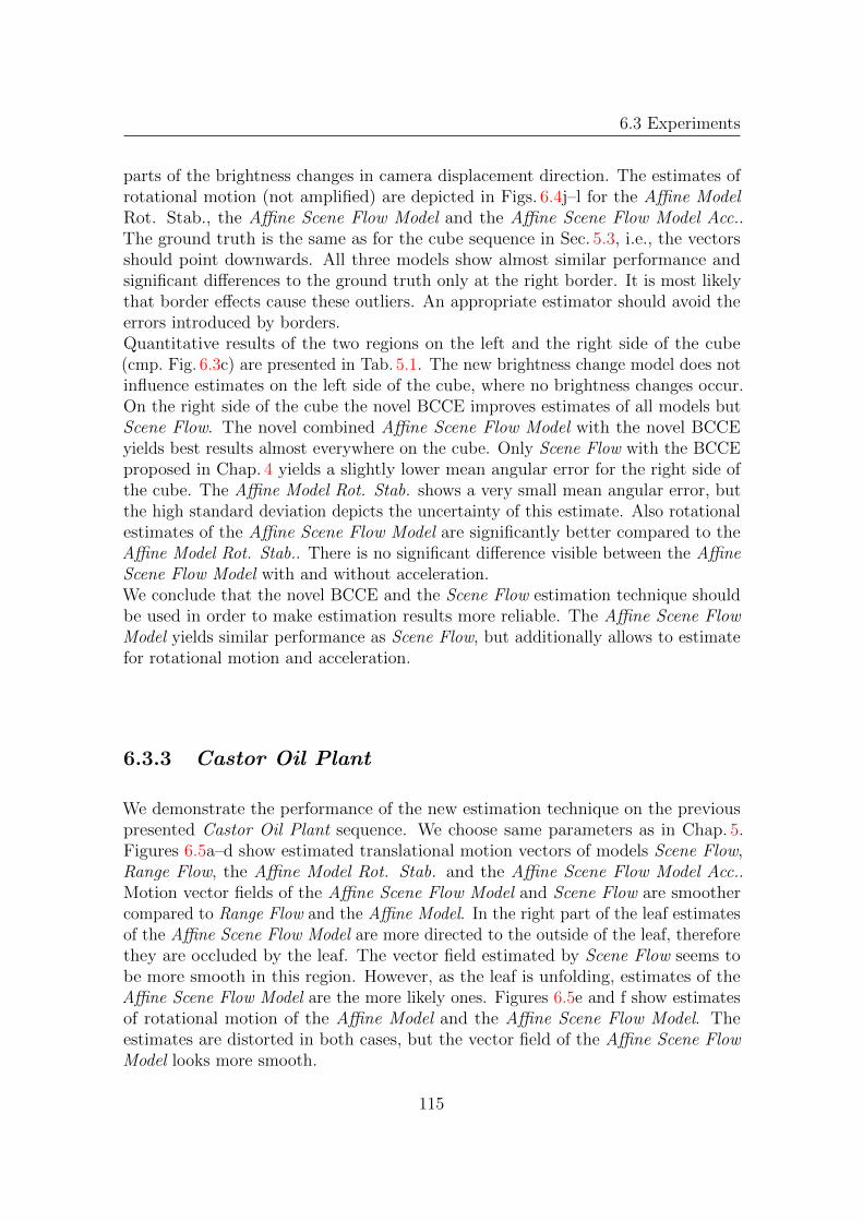
6.3 Experiments
parts of the brightness changes in camera displacement direction. The estimates ofrotational motion (not amplified) are depicted in Figs. 6.4j–l for the Affine ModelRot. Stab., the Affine Scene Flow Model and the Affine Scene Flow Model Acc..The ground truth is the same as for the cube sequence in Sec. 5.3, i.e., the vectorsshould point downwards. All three models show almost similar performance andsignificant differences to the ground truth only at the right border. It is most likelythat border effects cause these outliers. An appropriate estimator should avoid theerrors introduced by borders.Quantitative results of the two regions on the left and the right side of the cube(cmp. Fig. 6.3c) are presented in Tab. 5.1. The new brightness change model does notinfluence estimates on the left side of the cube, where no brightness changes occur.On the right side of the cube the novel BCCE improves estimates of all models butScene Flow. The novel combined Affine Scene Flow Model with the novel BCCEyields best results almost everywhere on the cube. Only Scene Flow with the BCCEproposed in Chap. 4 yields a slightly lower mean angular error for the right side ofthe cube. The Affine Model Rot. Stab. shows a very small mean angular error, butthe high standard deviation depicts the uncertainty of this estimate. Also rotationalestimates of the Affine Scene Flow Model are significantly better compared to theAffine Model Rot. Stab.. There is no significant difference visible between the AffineScene Flow Model with and without acceleration.We conclude that the novel BCCE and the Scene Flow estimation technique shouldbe used in order to make estimation results more reliable. The Affine Scene FlowModel yields similar performance as Scene Flow, but additionally allows to estimatefor rotational motion and acceleration.
6.3.3 Castor Oil Plant
We demonstrate the performance of the new estimation technique on the previouspresented Castor Oil Plant sequence. We choose same parameters as in Chap. 5.Figures 6.5a–d show estimated translational motion vectors of models Scene Flow,Range Flow, the Affine Model Rot. Stab. and the Affine Scene Flow Model Acc..Motion vector fields of the Affine Scene Flow Model and Scene Flow are smoothercompared to Range Flow and the Affine Model. In the right part of the leaf estimatesof the Affine Scene Flow Model are more directed to the outside of the leaf, thereforethey are occluded by the leaf. The vector field estimated by Scene Flow seems tobe more smooth in this region. However, as the leaf is unfolding, estimates of theAffine Scene Flow Model are the more likely ones. Figures 6.5e and f show estimatesof rotational motion of the Affine Model and the Affine Scene Flow Model. Theestimates are distorted in both cases, but the vector field of the Affine Scene FlowModel looks more smooth.
115
6 5D-Affine Scene Flow Model
a b
c d
e f
Figure 6.5: Castor Oil Plant Sequence. Translational motion estimates of modelsScene Flow (a), Range Flow (b), the Affine Scene Flow Model wo ∆t (c) and theAffine Scene Flow Model with ∆t (d). Rotational motion estimates of the AffineModel Rot. Stab. (e) and the Affine Scene Flow Model with ∆t (f).
6.3.4 Tobacco Plant
We show more estimation results using a second plant leaf sequence, imaging atobacco plant leaf. Three frames of the sequence are shown in Figs. 6.6a, c and e.The leaf is marked with spots of watercolor to avoid errors coming from the apertureproblem. The maximal width of the leaf is approximately 20 mm. The leaf rotatesaround the node where it is attached to the stem, causing a visible motion to thecamera and to the left. Moreover it is folding, which leads to slight motion of thesides of the leaf to its center. In the left part of the leaf brightness changes occur dueto shadowing by other leafs. We use a camera on a moving stage to obtain 9 images
116

6.3 Experiments
a b
c d
e f
Figure 6.6: Tobacco leaf sequence. Left: Input frame of the central camera a:t = t0 − 20 min, c: t = t0 min and e: t = t0 + 20 min. b, d and f: Correspondingrendered 3D structure and surface normals estimated with the Affine Model.
from positions with a camera displacement of 1 mm. This leads to a preshift of 26pixel. The images are taken every 2 minutes. The size of the sensor is 1600× 1200pixel with width and height of 0.0044 mm. The focal length is 25 mm. NeighborhoodΛ is realized by a normalized Gaussian with size 121 × 121 × 5 × 5 and standarddeviation σW = 41 × 41 × 1 × 1 in x-y-sx-and t-direction. Figures 6.6b, d and fdepict 3D reconstructions and surface slopes for times t = t0 − 20 min, t = t0 min
117

6 5D-Affine Scene Flow Model
a b
c d
e f
Figure 6.7: Tobacco leaf sequence. a–c: Motion estimates for models Scene Flow,Range Flow and the Affine Model without brightness modeling, d–f: Motion estimatesfor Affine model using ∆sxdt, using ∆sxdt and ∆tdsx and using ∆sxdt, ∆tdsx and∆tdt respectively.
and t = t0 + 20 min obtained by the Affine Model. Reconstructed depth and surfaceslopes clearly recover the true position of the leaf. Furthermore the rotation of theleaf around its node, where it is attached to the stem, is visible.Scaled translational motion estimates of different models are shown in Fig. 6.7.Rendered velocity fields seem most reliable for Scene Flow (a) and the Affine Scene
118

6.4 Conclusions
a b
Figure 6.8: Tobacco leaf sequence. Rotational estimates of a: the Affine Model Rot.Stab. and b: the Affine Scene Flow Model with acceleration.
Flow Model (f). Estimates of Range Flow (b) and the Affine Model (c–e) are overestimated in particular in Z-direction. This behavior was already confirmed formotion estimation in the rotating cube sequence. Range Flow does not handlerotation explicitly, therefore correspondences of the range constraint may fail. Wesuggest that more appropriate choices of βi, i.e., the weighting of the structuretensors, may reduce this effect (cmp. (4.25)). The standard Affine Model is based ona patch model with translational motion only, which estimates motion in Z-directionbased on affine transformations, e.g., divergence. Rotation and folding of the leafleads to visible shrinking of the projection of the leaf. The Affine Model interpretsthis shrinkage as motion away from the camera. The extended models using moreaffine parameters (cmp. Figs. 6.7d and e) yield similar and better approximations ofthe motion vector field.Figures 6.8a and b show estimates of the rotational motion by the Affine Model Rot.Stab. and the Affine Scene Flow Model Acc.. We depict estimates for the AffineScene Flow Model Acc. only, as the model without acceleration yields similar results.The vector field of the Affine Scene Flow Model is more reliable compared to thevector field estimated by the Affine Model. There are less outliers and the directionsof the vectors recover the true rotation and folding of the leaf.
6.4 Conclusions
In this section we proposed a novel BCCE (6.10) and combined the estimationtechnique of Scene Flow with the Affine Model. The brightness change constrainthandles also brightness changes coming from camera displacement and fits well intothe general notation of the Affine Scene Flow Model. Estimation of optical flowparameters in all cameras and combining these parameters with the estimationof the Affine Model yields high accuracy and robustness to noise. Compared toScene Flow the new model yields higher accuracy and moreover allows to estimate
119

6 5D-Affine Scene Flow Model
rotational motion and acceleration parameters reliably. The combination with thenovel BCCE and the Affine Model, i.e., simultaneous estimation of 3D structure,surface slopes and 3D motion, further ensures more accurate 3D surface structureand slope estimation. Experiments on real data demonstrate that the Affine SceneFlow Model yields superior performance compared to Range Flow, the Affine Modeland in some regions also compared to Scene Flow. The tobacco plant leaf sequenceshows that estimation of rotational parameters with the Affine Scene Flow Model ispossible.
120

Chapter 7
Conclusions And Outlook
In this work we presented a highly accurate 3D motion estimation model based onoptical flow, which allows to estimate plant motion reliably. Starting from threebasic models, i.e., Scene Flow, Range Flow and the Affine Model, a new model forsimultaneous estimation of surface structure, slopes and motion has been developedand thoroughly tested. We first summarize results and conclusions of the differentmodels and modifications that have been presented. Finally we discuss possiblefuture work.
7.1 Summary and Conclusions
Motion estimation of dynamic processes has been investigated in Chap. 2. Thetypical estimation process contains at least three important tasks: model derivation,discretization and parameter estimation. First an appropriate model of the data hasto be derived. This model sets the accuracy limits of the estimation process, i.e.,estimation results are only as good as the model fits to the data. In this work severalmotion models for optical flow have been proposed. In typical image sequences affinetransformations of the motion vector field occur, therefore at least an affine motionmodel should be used. An appropriate discretization is needed in order to handleinput data and to compute input parameters, e.g., image gradients. Finally anadequate estimator has to be chosen or developed. Chapter 2 presented several localleast squares estimators with and without handling of covariance information andoutliers. The novel robust total least squares estimator with handling of covarianceinformation showed best performance in estimation of affine model parameters.Chapter 3 reviews three 3D motion estimation models based on optical flow, namelyScene Flow, Range Flow and the Affine Model. Scene Flow and Range Flow need3D structure information for one or more time points in order to estimate 3Dmotion. Scene Flow first computes optical flow in more than two cameras. A secondestimation process yields 3D motion, which re-projections best fit to each of theoptical flows. Range Flow constrains range data of several time points and optical
121

7 Conclusions And Outlook
flow of one camera. A single estimation yields the 3D motion parameters. TheAffine Model starts from multi-camera image sequences. It is based on an affineoptical flow model and allows simultaneous estimation of flow parameters in cameradisplacement direction and time. 3D structure, slopes and 3D motion can be derivedfrom these flow parameters using projective geometry. The Affine Model also allowsestimation of parameters describing the 3D neighborhood, i.e., surface slopes. Thismakes the model appropriate for reliable estimation of highly accurate plant leafmotion. Scene Flow is based on a pinhole camera model similar to the Affine Model,but all parameters in a neighborhood are assumed constant. Synthetic experimentsshowed that the Affine Model yields best results for multi-camera grids with smallbaselines (≈ 0.01 % of depth). For plant measurement setups, where average depthtypically is below 1m, these baselines are physically not realizable with multiplecameras, but with one camera on moving stages. For typical baselines (≈ 0.5 %of depth) Scene Flow yields best results. However, all models fail on plant leafmotion estimation. The main reason is that the models are based on standard opticalflow, which implies brightness constancy. This is well fulfilled for undirected, diffuselight. In a laboratory setup the plant is illuminated by directed infrared LED-lights(cmp. Chap. 3). Therefore motion of the leaf, the light source or the camera causesbrightness changes in the data.In order to handle such brightness changes coming from varying illumination a novelbrightness change constraint has been derived in Chap. 4. The brightness changeconstraint explicitly models temporal and spatially varying temporal brightnesschanges. Motion estimation using the Affine Model with the novel brightness changeconstraint on synthetic data with brightness changes coming from varying illuminationdemonstrated the improved performance. In order to compare the novel BCCE withother approaches an intensive evaluation and comparison with different prefilters(highpass and homomorphic) and brightness constraints using Range Flow has beencarried out. It turns out that if the brightness constancy assumption is violated,homomorphic prefiltering rather than linear highpass prefiltering should be used.Nevertheless, modeling brightness changes yields slightly more accurate results. Thenovel brightness constraint in combination with each of the three estimation modelsyields improved results on the plant leaf sequence. Range Flow showed higher errorsnear borders, while the Affine Model yields worst results compared to the othermodels.In Chap. 5 a 4D-Affine Model has been derived. This model is based on a higherdimensional affine optical flow, which allows estimation of affine transformations infour dimensions, i.e., in local image coordinates and in camera displacement directionand time. It is demonstrated that the affine transformation of the disparity in timeboils down to the Range Flow constraint. Further the motion model of the 4D-AffineModel is extended to handle rotational motion and acceleration. Transformationsof the 3D neighborhood as well as 3D motion are explained by affine optical flowparameters. Tests on synthetic data demonstrated that the new Affine Modeloutperforms Range Flow. However, Scene Flow yields lowest errors. Experiments
122

7.2 Future Work
showed that affine parameters describing transformations of the optical flow in timeshould not be used for estimation, because acceleration parameters are not uniquelydetermined by the affine parameters.A general derivation of a 5D-Affine Model is proposed in Chap. 6. This modelhandles affine transformations in 5D-data, i.e., 2D camera grid sequences, and alsobrightness changes coming from motion of the camera. Further the 5D-Affine Modelis combined with the estimation technique used for Scene Flow. This leads to a highaccuracy 3D motion estimation model (Affine Scene Flow Model), which shows highrobustness. Synthetic experiments demonstrated that the novel Affine Scene FlowModel outperforms all other models, and allows estimation not only of translationalmotion parameters, but also rotational motion and acceleration parameters. Thehigh performance of the model was demonstrated on two real plant leaf sequences.
7.2 Future Work
The 5D-Affine Scene Flow Model has been thoroughly tested on synthetic imagedata and on two real plant leaf sequences. A possible focus in future work may beon establishing an appropriate estimation framework and embed the algorithm intoa measurement system. Apart from practical work we suggest future work on threefundamental parts: the model, the parameter estimation and data acquisition.Although an accurate model based on a moving surface patch has been derived, thefollowing extensions may further improve the accuracy.
The affine optical flow model is based on first order approximations of surfacestructure and motion. Higher order affine models have been proposed for opticalflow computation (cmp. Sec. 2.1.1). Including higher orders of optical flowallows to more accurately approximating 3D parameters, e.g., round surfacesor acceleration of a neighborhood. However, increasing order of the model alsoleads to more parameters which have to be estimated. This could be handledwith a coarse-to-fine technique, where the order of the model is increased, ifthe residual of a simpler model is above a threshold (cmp. [47]).
The Affine Scene Flow Model showed high accuracy in estimating smoothvelocity vector fields on synthetic data. Growth is estimated based on 3Dmotion vectors. Modeling growth explicitly in the affine parameters couldimprove estimation results. Apart from growth other parameters of interest,e.g., reflectance, could be modeled as well.
In this work parameters of the Affine Scene Flow Model are estimated using twostandard least squares estimators. Possible improvements of the estimation processinclude the following:
The parameter estimation of the optical flow parameters is based on standardTLS. It was already shown in Chap. 2 that handling of outliers and incorporation
123

7 Conclusions And Outlook
of covariance information improves estimation. The extension of the AffineScene Flow Model using these estimators is straight forward. The main drawbackof the more sophisticated estimators is their computational complexity. In orderto speed up the estimation algorithm the implementation could be parallelizedand implemented on graphics processing units (GPU), which showed highperformance in optical flow computation recently [50].
Total least squares estimation of optical flow implies motions well below onepixel per frame. A coarse-to-fine multi-grid and/or a warping technique [49, 47]should be integrated in the estimation process in order to allow larger motions.
Most of the best estimators on the popular Middlebury-Benchmark [3] are globalestimators. These estimators allow incorporation of additional constraints likesmoothness of the motion vector field or the equivalence between the derivativeof depth Z and surface normals ZX and ZY . Furthermore direct estimationof 3D parameters without estimating optical flow as an intermediate resultcould be possible. Global estimators yield dense motion vector fields, but erroranalysis is more difficult compared to local estimators.
Although the Affine Model allows simultaneous estimation of optical flowparameters in time and camera displacement direction, two estimation stepsare needed for estimation of 3D parameters. First the 3D structure and surfaceslopes are estimated. 3D motion parameters are then obtained by solving anequation system build up out of the 3D structure information and the affineoptical flow parameters. In order to solve for all parameters simultaneously anonlinear estimator should be developed. This leads to an iterative estimationprocess, where iteratively one parameter set is kept fixed while the otherparameters are estimated.
The two estimation processes in the Affine Scene Flow Model are solvedindependently of each other. Error distributions should be forwarded to thenext estimator or the next estimation process. There are two different errorsto be handled. First the reliability of the different translational and affineflow parameters. In general the translational parameters are more reliablethan the affine parameters, but also affine parameters in camera displacementdirection have different errors compared to affine parameters in time or localcoordinates. Reliability of parameters from different cameras in the SceneFlow estimation technique need to be estimated and used in an appropriateestimation scheme. The incorporation of error distributions may increaserobustness of the estimator, e.g., in case of occlusions and shadowing, as shownfor standard Scene Flow computation in [40].
Experiments, where relative growth is estimated for fixed leafs (cmp. [63]),showed that large temporal averaging filters increase the reliability of growthestimation. Therefore the estimation framework should be extended to include
124

7.3 Closure
temporal averaging of parameters, e.g., plant leaf motion. This may be donein a variational framework, where smoothness constraints on parameter fieldscan be expressed explicitly.
Finally we discuss important issues concerning the acquisition setup:
The developed 5D-Affine Scene Flow Model was tested for short sequences(5-9 frames). In future this algorithm should be used for analysis of long timeleaf motion and/or growth, i.e., more than 100 frames. Therefore a systemhas to be developed, which ensures highly accurate acquisition of input data.Experiments with moving stages showed that accuracy of displacement of ≈ 10µm leads to significant errors that can be clearly detected when using a highlyaccurate estimation scheme like the Affine Scene Flow Model. For instancewhen using a small baseline of 1 mm such inaccuracies lead to an error of1 % which directly influences estimation of disparity and therefore depth Z.Recently 5× 5 camera arrays have been released (see [77]), which allow smalland constant baselines.
Depending on the plant species, leafs may move, bend and fold in all possiblepositions. In order to get most reliable depth and motion estimates the leafshould be imaged fronto-parallel. Furthermore the leafs could move out offocus. Therefore it may be beneficial to track the leaf of interest. We suggestthat a robot arm with a mounted camera array could follow the movements ofthe plant.
7.3 Closure
The main focus of this work was on derivation of a highly accurate model, allowinggrowth estimation of plants. The 5D-Affine Scene Flow Model showed highestaccuracy on synthetic data compared to the three discussed 3D motion estimationmodels. However, a method needs not only a highly accurate model of the data, butalso an appropriate discretization, estimation framework and acquisition setup. Forinstance, using a more sophisticated estimator than standard total least squares,can significantly improve the performance of the method (cmp. Chap. 6, where theestimation technique of Scene Flow is adapted to the Affine Model). In this contextthe derivation of the 5D-Affine Scene Flow Model is an important step in order toestablish a method for plant leaf growth estimation.
125

126
Appendix A
Average Angular Error
The angular error is a common error measure used for optical flow evaluation (cmp.[4, 26]). A 2D motion vector u = [ux, uy]
T can be represented as a normalized
3D vector r = [r1, r2, r3]T/√r2
1 + r22 + r2
3 where u = [r1, r2]T/r3. The angular error
describes the error as an angle in 3D
AE = arccos(rTt re)
(A.1)
with 3D vectors rt and re denoting the true and the estimated flow respectively.The advantage of this error measure is, that it addresses directional and magnitudeerrors simultaneously. However, the angular error measure is biased [26], becausethe relation between relative and angular error depends on the magnitude of themotion vector. That means, that for constant relative error the angular error reachesa maximum for a displacement of 1 pixel per frame. Moreover the angular erroryields different measures for positive and negative deviations from the true value.However, quantitative evaluation of synthetic experiments showed that the angularerror yields a reasonable error measure. The average angular error is defined for aneighborhood of size N by
AAE =1
N
N∑i
arccos(rt(i)
Tre(i))
(A.2)
and may be used also for true 3D motion estimates, e.g., r = [UX , UY , UZ , 1]T. Affinemotion parameters are in general significantly smaller than translational parameters.Therefore angular errors of translational and affine motion parameters should beseparated, because errors in translational parameters would dominate errors in affinemotion parameters.
127

128

Appendix B
Synthetic Testsequences
Synthetic sequences are used for systematic error analysis of 2D optical flow and3D scene flow estimation. We model a camera with perspective projection, butderivation of a sequence for a camera with orthogonal projection is analog. For eachimage sensor element the intersection between the line of sight and the object iscalculated. Therefore the appearance of the object is specified as a translating androtating plane.Following [23] a point X = (X, Y, Z)T in 3D-space is represented in homogeneouscoordinates as a 4D-vector X = (X1, X2, X3, X4)T with X4 6= 0 by
X =X1
X4
, Y =X2
X4
, Z =X3
X4
. (B.1)
Homogeneous coordinates are used to easily represent homogeneous transformationslike affine transformations or perspective projections by a 3× 4 matrix and to carryout calculations in the projective space. Homogeneous points with X4 = 0 representpoints at infinity. For further details on homogeneous representation see [23].The image acquired by a camera is a projection of 3D points X onto a 2D imageplane with points x. This projection can be expressed by a matrix multiplicationof 3D points X with a camera matrix K. Using a projective camera model thecorresponding point x on the image plane can be calculated by
x = K ·X , with K =
f 0 px 00 f py 00 0 1 0
(B.2)
with focal length f and coordinates of the principal point (px, py). The cameramatrix used here is sufficient to model typical CCD cameras, where skew parameteris negligible and aspect ratio is one.
129
B Synthetic Testsequences
The projected 2D point is given by
x =
xy1
=
fZX + px
fZY + py
1
. (B.3)
A rectangular surface patch is defined by a surface normal n = (ZX , ZY ,−1)T
and its central position X0 = (X0, Y0, Z0)T. The patch moves with translational
velocity N and rotates around a vector v = (vX , vY , vZ)T positioned at its centerX0 with angular velocity ω. This yields a combined translational and angularvelocity of U = N + Ω × R for each point xP = (xP , yP )T on the patch withΩ = ωv = (ΩX ,ΩY ,ΩZ)T and distance to the patch center R.The surface of a patch centered at the origin is defined by P0 = (xP , yP , 0, 1)T, wherexP = (xP , yP )T denotes the local position on the patch. Rotation of P0 by two 3× 3rotation matrices and one translation yields coordinates for a patch with sought forposition X0, surface normal n and motion U. Rotation matrix R0 ensures surfacenormal n of the patch for t = 0. Rotation axis is given by q = (ZX ,−ZY , 0)T and
rotation angle is ω0 = arccos(1/√
1 + ZX2 + ZY
2). The second matrix rotates thepatch around a vector v fixed at patch origin X0 with rotational velocity ωt. Thisrotation and translation of the patch are combined in one matrix TR(t). 3D pointson the surface patch are then defined by
Ps = TR(t) ·R0 ·P0 (B.4)
with rotation matrix
R0 =
(R(q, ω0) 0
0T 1
)(B.5)
where
R(q, ω0) = cos(ω0) + q2X (1− cos(ω0)) qXqY (1− cos(ω0))− qZ sin(ω0) qXqZ (1− cos(ω0)) + qY sin(ω0)qY qX (1− cos(ω0)) + qZ sin(ω0) cos(ω0) + q2Y (1− cos(ω0)) qY qZ (1− cos(ω0))− qX sin(ω0)qZqX (1− cos(ω0))− qY sin(ω0) qZqY (1− cos(ω0)) + qX sin(ω0) cos(ω0) + q2Z (1− cos(ω0))
(B.6)
and combined rotational and translational matrix
TR(t) =
(R(v, ωtt) X0
0T 1
). (B.7)
Translational motion N and acceleration A of the patch and displacement S =[sx, sy]
T of the camera is included in XYZ
(t) =
X0 +NXt+ 0.5AXt2 − sxs
Y0 +NY t+ 0.5AY t2 − sys
Z0 +NZt+ 0.5AZt2
. (B.8)
130

a b c
Figure B.1: a: Central image of a sinusoidal sequence, b: gray value coded depthmap and c: rendered patch in 3D with ground truth velocities.
Projection of Ps onto the image plane yields the corresponding points p
p = K ·TR(t) ·R ·P0 . (B.9)
Inversion of (B.9) returns coordinates and motion of the plane given at a certainpixel element on the sensor. Intensity values are mapped onto the surface by
I(xP , yP ) = o+ a cos
(2πxPλ1
)cos
(2πyPλ2
)(B.10)
xP = xP cos(α) + yP sin(α) (B.11)
yP = −xP sin(β) + yP cos(β) (B.12)
Figure B.1 shows an intensity image of a sequence, the gray value coded depth mapZ and a rendered 3D view of a patch with 3D motion vectors. The parameters ofthis inclined surface are Z0 = 100 mm, ZX = 1, ZY = 0, NX = 0.00733 mm/frame,NY = −0.00367 mm/frame, NZ = −0.6 mm/frame, f = 12 mm, λ1 = λ2 = 0.3mm, α = β = 0°, o = 127.5 and a = 127.5. Of course, other intensity data may beprojected onto the surface, e.g., a radial sinus. Motion and acceleration of the planefor each pixel of the sensor is calculated for quantitative error analysis. 3D motion isgiven by
dX
dt= UX = NX + AXt+ ΩY ∆Z − ΩZ∆Y (B.13)
dY
dt= UY = NY + AY t+ ΩZ∆X − ΩX∆Z (B.14)
dZ
dt= UZ = NZ + AZt+ ΩX∆Y − ΩY ∆X (B.15)
131

B Synthetic Testsequences
with Ωi = viω. Optical flow components ux, uy are calculated by projecting the 3Dmotion onto the image plane
ux =f
Z
(UX −
x0
fUZ
)(B.16)
uy =f
Z
(UY −
y0
fUZ
). (B.17)
Affine components of the optical flow are derived by partial derivatives of theoptical flow in the corresponding dimension. Affine flow parameters caused bycamera displacement sx and sy in X-and Y -direction, i.e., disparity ν and its partialderivatives are
ν = − fZ,
∂ν
∂x0
=f
Z2
∂Z
∂x0
,∂ν
∂y0
=f
Z2
∂Z
∂y0
,
∂ν
∂sx=
f
Z2
∂Z
∂sx,
∂ν
∂sy=
f
Z2
∂Z
∂sy,
∂ν
∂t=
f
Z2
∂Z
∂t.
(B.18)
132

Bibliography
[1] G. Adiv, “Determining 3-d motion and structure from optical flow generatedby several moving objects,” IEEE Trans. on Pattern Analysis and MachineIntelligence, vol. 7, no. 4, pp. 384–401, 1985.
[2] H. Arsenault and M. Denis, “Image processing in signal-dependent noise,”Canadian Journal of Physics, vol. 61, pp. 309–317, 1983.
[3] S. Baker, D. Scharstein, J. P. Lewis, S. Roth, M. J. Black, and R. Szeliski, “Adatabase and evaluation methodology for optical flow,” in Intern. Journal ofComputer Vision, 2007, pp. 1–8.
[4] J. L. Barron, D. J. Fleet, and S. S. Beauchemin, “Performance of optical flowtechniques,” Intern. Journal of Computer Vision, vol. 12, pp. 43–77, 1994.
[5] M. Bertero, T. A. Pogcio, and V. Torre, “Ill-posed problems in early vision,”Proc. of the IEEE, vol. 76, no. 8, pp. 869–889, August 1988.
[6] J. Bigun and G. H. Granlund, “Optimal orientation detection of linear symmetry,”in Intern. Conference on Computer Vision, 1987, pp. 433–438.
[7] J. Bigun and G. H. Granlund, “Optical flow based on the inertia matrix of thefrequency domain,” in Proceedings from SSAB Symposium on Picture Processing.Lund University, Sweden: SSAB, March 1988, pp. 132–135, report LiTH-ISY-I-0934, Computer Vision Laboratory, Linkoping University, Sweden, 1988.
[8] M. J. Black, “Robust incremental optical flow,” Ph.D. dissertation, Yale Univer-sity, 1992.
[9] M. J. Black and P. Anandan, “The robust estimation of multiple motions:parametric and piecewise-smooth flow fields,” in Computer Vision and ImageUnderstanding, vol. 63(1), 1996, pp. 75–104.
[10] M. J. Black, D. J. Fleet, and Y. Yacoob, “Robustly estimating changes in imageappearence,” Computer Vision and Image Understanding, vol. 7, no. 1, pp. 8–31,2000.
133

BIBLIOGRAPHY
[11] M. J. Black and A. Jepson, “Estimating optical flow in segmented images usingvariable-order parametric models with local deformations,” IEEE Trans. onPattern Analysis and Machine Intelligence, vol. 18, no. 10, pp. 972–986, 1996.
[12] A. Blake and M. Isard, Active Contours. Springer, 1998.
[13] T. Brox, J. Weickert, B. Burgeth, and P. Mrazek, “Nonlinear structure tensors,”Saarland University, Saarbrucken, Germany, Revised version of Technical ReportNo. 113, 2004.
[14] A. Bruhn, J. Weickert, and C. Schnorr, “Lucas/kanade meets horn/schunck:Combining local and global optic flow methods,” Intern. Journal of ComputerVision, vol. 61, no. 3, pp. 211–231, 2005.
[15] C. Cason, “Persistence of vision ray tracer (POV-Ray), version 3.6, Windows,”www.povray.com, 2005.
[16] W. Chojnacki, M. J. Brooks, and A. van den Hengel, “Rationalising the renor-malisation method of kanatani,” Journal of Mathematical Imaging and Vision,vol. 14, pp. 200–1, 2001.
[17] W. Chojnacki, M. J. Brooks, A. van den Hengel, and D. Gawley, “A newconstrained parameter estimator for computer vision applications,” Image andVision Computing, vol. 22, no. 2, pp. 85 – 91, 2004, statistical Methods in VideoProcessing.
[18] D. J. Fleet and Y. Weiss, “Optical flow estimation,” in Mathematical models forComputer Vision: The Handbook, N. Paragios, Y. Chen, and O. F. (eds.), Eds.Springer, 2005.
[19] B. Galvin, B. Mccane, K. Novins, D. Mason, and S. Mills, “Recovering motionfields: An evaluation of eight optical flow algorithms,” in British Machine VisionConference, 1998, pp. 195–204.
[20] S. Geman and D. McClure, “Statistical methods for tomographic image recon-struction,” Bull. Intern. Statist. Inst., vol. LII-4, pp. 5–21, 1987.
[21] H. Gharavi and S. Gao, “3-d motion estimation using range data,” IEEE Trans.on Intelligent Transportation Systems, vol. 8, no. 1, pp. 133–143, March 2007.
[22] Google, “Google street view,” http://maps.google.com/help/maps/streetview/,2005, google Inc.
[23] R. I. Hartley and A. Zisserman, Multiple View Geometry in Computer Vision,2nd ed. Cambridge University Press, ISBN: 0521540518, 2004.
[24] H. Haussecker, “Interaction of radiation with matter,” in Handbook of ComputerVision and Applications, vol. 1. Academic Press, 1999, pp. 37–62.
134
BIBLIOGRAPHY
[25] H. Haussecker and D. J. Fleet, “Computing optical flow with physical mod-els of brightness variation,” IEEE Trans. on Pattern Analysis and MachineIntelligence, vol. 23, no. 6, pp. 661–673, June 2001.
[26] H. Haussecker and H. Spies, “Motion,” in Handbook of Computer Vision andApplications, 1st ed., B. Jahne, H. Haussecker, and P. Geißler, Eds. AcademicPress, 1999, vol. 2, ch. 13, pp. 309–396.
[27] B. Horn, Robot Vision. McGraw-Hill, 1986.
[28] B. Horn and B. Schunck, “Determining optical flow,” Artificial Intelligence,vol. 17, pp. 185–204, 1981.
[29] Y. Hsu, H. Nagel, and G. Rekers, “New likelihood test methods for changedetection in image sequences,” CVGIP: Graphical Models and Image Processing,vol. 26, no. 1, pp. 73–106, April 1984.
[30] P. J. Huber, “Robust estimation of a location parameter,” The Annals ofMathematical Statistics, vol. 35, no. 1, pp. 73–101, 1964.
[31] F. Huguet and F. Devernay, “A variational method for scene flow estimationfrom stereo sequences,” in Intern. Conference on Computer Vision, 2007.
[32] B. Jahne, Digitale Bildverarbeitung, 3rd ed. Springer, 1993.
[33] B. Jahne, Spatio-temporal image processing, ser. Lecture Notes in ComputerScience. Springer Verlag, 1993.
[34] B. Jahne, “Performance characteristics of low-level motion estimators in spa-tiotemporal images,” in DAGM-Workshop Performance Characteristics andQuality of Computer Vision Algorithms, Braunschweig, September 18, 1997,W. Foerstner, Ed., Univ. Bonn, 1997.
[35] B. Jahne, H. Haussecker, and P. Geissler, Handbook of Computer Vision andApplications, 1st ed. Academic Press, 1999.
[36] S. Ju, M. J. Black, and A. D. Jepson, “Skin and bones: Multi-layer, locallyaffine, optical flow and regularization with transparency,” in IEEE Conferenceon Computer Vision and Pattern Recognition, San Francisco, June 1996, pp.307–314.
[37] K. Kanatani, “Structure from motion without correspondence: general principle,”in Proc. Image Understanding Workshop, 1985, pp. 10 711–6.
[38] K. Kanatani, Statistical Optimization for Geometric Computation: Theory andPractice. Elsevier, 1996.
135
BIBLIOGRAPHY
[39] K. Krajsek and R. Mester, “Marginalized maximum a posteriori hyper-parameterestimation for global optical flow techniques,” in Bayesian Inference and Maxi-mum Entropy Methods In Science and Engineering, Paris, France, November2006.
[40] R. Li and S. Sclaroff, “Multi-scale 3d scene flow from binocular stereo sequences,”Computer Vision and Image Understanding, vol. 110, no. 1, pp. 75–90, 2008.
[41] H. Longuet-Higgins and K. Prazdny, “The interpretation of a moving retinalimage,” Proc. of The Royal Society of London B, 208, pp. 385–397, 1980.
[42] B. Lucas and T. Kanade, “An iterative image registration technique with anapplication to stereo vision,” in Proc. Seventh Intern. Joint Conference onArtificial Intelligence, Vancouver, Canada, August 1981, pp. 674–679.
[43] L. Matthies, R. Szeliski, and T. Kanade, “Kalman filter-based algorithms forestimating depth from image sequences,” Intern. Journal of Computer Vision,vol. 3, pp. 209–236, 1989.
[44] M. Muhlich and T. Aach, “A theory for multiple orientation estimation,” inProc. European Conference on Computer Vision, ser. LNCS, H. Bischof andA. Leonardis, Eds., no. 3952. Springer, 2006, pp. (II) 69–82.
[45] Y. Nakamura, T. Matsuura, K. Satoh, and Y. Ohta, “Occlusion detectablestereo–occlusion patterns in camera matrix,” in IEEE Conference ComputerVision and Pattern Recognition, 1996, pp. 371–378.
[46] O. Nestares, D. J. Fleet, and D. J. Heeger, “Likelihood functions and confidencebounds for Total Least Squares estimation,” in IEEE Conference ComputerVision and Pattern Recognition, 2000.
[47] T. Nir, A. M. Bruckstein, and R. Kimmel, “Over-parameterized variationaloptical flow,” Intern. Journal of Computer Vision, vol. 76, no. 2, pp. 205–216,2008.
[48] A. Oppenheim, R. Schafer, and J. Stockham, T.G., “Nonlinear filtering ofmultiplied and convolved signals,” in Proc. of the IEEE, vol. 56, 1968, pp. 1264– 1291.
[49] N. Papenberg, A. Bruhn, T. Brox, S. Didas, and J. Weickert, “Highly accurateoptic flow computation with theoretically justified warping,” Intern. Journal ofComputer Vision, vol. 67, no. 2, pp. 141–158, April 2006.
[50] T. Pock, M. Unger, D. Cremers, and H. Bischof, “Fast and exact solution oftotal variation models on the gpu,” in CVPR Workshop on Visual ComputerVision on GPU’s, Anchorage, Alaska, USA, Jun. 2008.
136

BIBLIOGRAPHY
[51] S. Roth and M. J. Black, “On the spatial statistics of optical flow,” Intern.Journal of Computer Vision, vol. 74, no. 1, pp. 33–50, 2007.
[52] P. D. Sampson, “Fitting conic sections to ’very scattered’ data: An iterarive re-finement of the bookstein algorithm,” Computer Graphics and Image Processing,vol. 18, no. 1, pp. 97–108, January 1982.
[53] H. Scharr, “Optimal operators in digital image processing,” Ph.D. dissertation,Interdisciplinary Center for Scientific Computing, University of Heidelberg,Germany, 2000.
[54] H. Scharr, “Optimal filters for extended optical flow,” in Complex Motion, 1.Intern. Workshop, Gunzburg, Oct. 2004, ser. Lecture Notes in Computer Science,B. Jahne, E. Barth, R. Mester, and H. Scharr, Eds., vol. 3417. Berlin: SpringerVerlag, 2005.
[55] H. Scharr, “Towards a multi-camera generalization of brightness constancy,” inComplex Motion, 1. Intern. Workshop, Gunzburg, Oct. 2004, ser. Lecture Notesin Computer Science, B. Jahne, E. Barth, R. Mester, and H. Scharr, Eds., vol.3417. Berlin: Springer Verlag, 2007, pp. 78–90.
[56] H. Scharr and T. Schuchert, “Simultaeous estimation of depth, motion and slopesusing a camera grid,” in Vision Modeling and Visualization 2006, L. Kobbelt,T. Kuhlen, T. Aach, and R. Westermann, Eds., Aachen, 2006, pp. 81–88.
[57] H. Scharr and R. Kusters, “A linear model for simultaneous estimation of3d motion and depth,” in IEEE Workshop on Motion and Video Computing,Orlando, USA, December 2002.
[58] D. Scharstein and R. Szeliski, “A taxonomy and evaluation of dense two-framestereo correspondence algorithms,” Intern. Journal of Computer Vision, vol. 47,pp. 7–42, 2001.
[59] D. Schmundt and U. Schurr, “Plant-leaf growth,” in Handbook of Computer Vi-sion and Applications, B. Jahne, H. Haussecker, and P. Geißler, Eds. AcademicPress, 1999.
[60] T. Schuchert and H. Scharr, “Simultaneous estimation of surface motion, depthand slopes under changing illumination,” in Pattern Recognition Symposium ofthe German Association for Pattern Recognition (DAGM), 2007.
[61] T. Schuchert, T. Aach, and H. Scharr, “Range flow for varying illumination,” inEuropean Conference on Computer Vision, vol. 5302/2008. Springer Berlin /Heidelberg, 2008, pp. 509–522.
137

BIBLIOGRAPHY
[62] T. Schuchert and H. Scharr, “An affine optical flow model for dynamic surfacereconstruction,” in Statistical and Geometrical Approaches to Visual MotionAnalysis, ser. Dagstuhl Seminar Proceedings, D. Cremers, B. Rosenhahn,and A. L. Yuille, Eds., no. 08291. Dagstuhl, Germany: Schloss Dagstuhl- Leibniz-Zentrum fur Informatik, Germany, 2008. [Online]. Available:http://drops.dagstuhl.de/opus/volltexte/2008/1620
[63] U. Schurr, A. Walter, S. Wilms, H. Spies, N. Kirchgeßner, H. Scharr, andR. Kusters, “Dynamics of leaf and root growth,” in 12th Intern. Conference onPhotosynthesis, 2001.
[64] E. P. Simoncelli, “Design of multi-dimensional derivative filters,” in IEEE Intern.Conference on Image Processing, Austin TX, 1994, pp. 790–793.
[65] E. P. Simoncelli, E. H. Adelson, and D. J. Heeger, “Probability distributions ofoptical flow,” in IEEE Conference on Computer Vision and Pattern Recognition.Mauii, Hawaii: IEEE Computer Society, Jun 3-6 1991, pp. 310–315.
[66] Sony, “Eyetoy,” www.eyetoy.com, 2005, sony Computer Entertainment Europe.
[67] H. Spies, H. Haussecker, B. Jahne, and J. Barron, “Differential range flowestimation,” in Pattern Recognition Symposium of the German Association forPattern Recognition (DAGM), 1999, pp. 309–316.
[68] H. Spies and B. Jahne, “A general framework for image sequence processing,”in Fachtagung Informationstechnik, 2001, pp. 125–132.
[69] H. Spies, B. Jahne, and J. Barron, “Range flow estimation,” Computer Visionand Image Understanding, vol. 85, no. 3, pp. 209–231, March 2002.
[70] H. Spies, B. Jahne, and J. L. Barron, “Surface expansion from range datasequences,” in Pattern Recognition Symposium of the German Association forPattern Recognition (DAGM). London, UK: Springer-Verlag, 2001, pp. 163–169.
[71] S.-C. Tai and S.-M. Yang, “A fast method for image noise estimation usinglaplacian operator and adaptive edge detection,” in Communications, Controland Signal Processing, 2008. ISCCSP 2008. 3rd Intern. Symposium on, StJulians, 2008, pp. 1077–1081.
[72] D. Terzopoulos, “Image analysis using multigrid relaxation methods,” IEEETrans. on Pattern Analysis and Machine Intelligence, vol. 8, no. 2, pp. 129–139,1986.
[73] D. Toth, T. Aach, and V. Metzler, “Illumination-invariant change detection,” in4th IEEE Southwest Symposium on Image Analysis and Interpretation. Austin,TX: IEEE Computer Society, April 2 - 4 2000, pp. 3–7.
138

BIBLIOGRAPHY
[74] S. Vedula, S. Baker, P. Rander, R. Collins, and T. Kanade, “Threedimensionalscene flow,” in IEEE Intern. Conference on Computer Vision, 1999, pp. 722–729.
[75] S. Vedula, S. Baker, S. Seitz, R. Collins, and T. Kanade, “Shape and motioncarving in 6d,” in IEEE Conference on Computer Vision and Pattern Recognition,2000, pp. 592–598.
[76] S. Vedula, S. Baker, P. Rander, R. Collins, and T. Kanade, “Three-dimensionalscene flow,” IEEE Trans. on Pattern Analysis and Machine Intelligence, vol. 27,no. 3, pp. 475–480, 2005.
[77] ViewPLUS and Point Grey, “ProFUSION 25, 5x5 Camera Array,” http://www.viewplus.co.jp/products/profusion25/ProFUSION25-e.pdf, 2008.
[78] A. Walter, “Raumliche und zeitliche wachstumsmuster in wurzeln und blatterndikotyler pflanzen’,” Ph.D. dissertation, University of Heidelberg, 2001.
[79] A. Waxman, B. Kamgar Parsi, and M. Subbarao, “Closed-form solutions toimage flow equations for 3d structure and motion,” Intern. Journal of ComputerVision, vol. 1, no. 3, pp. 239–258, October 1987.
[80] M. Yamamoto, P. Boulanger, J. A. Beraldin, and M. Rioux, “Direct estimationof range flow on deformable shape from a video rate range camera,” IEEE Trans.on Pattern Analysis and Machine Intelligence, vol. 15, no. 1, pp. 82–89, 1993.
[81] Y. Zhang and C. Kambhamettu, “Integrated 3d scene flow and structure recoveryfrom multiview image sequences,” in IEEE Conference Computer Vision andPattern Recognition, 2000, pp. 2674–2681.
139

140

Curriculum Vitae
Personal Information:
Name Tobias Schuchert
Date of Birth July 23, 1980Place of Birth Essen, Germany
Qualification:
10/2000 - 10/2005 Diploma in Information Technology,TU Dortmund University
11/2005 - 05/2009 PhD Student,Forschungszentrum Julich,ICG-3: Phytosphere, Image Processing GroupandRWTH Aachen University,Institute of Imaging & Computer Vision
since 08/2009 Researcher, Fraunhofer IOSB, Karlsruhe
April 19, 2010
141

142

Acknowledgements
I would like to thank everyone who helped me during my thesis. Inparticular ...
... Prof. Til Aach for supervising my thesis and fruitful discussions,
... Prof. Uli Schurr for great support and interesting insights into plantphysiology,
... Hanno Scharr for giving me this topic, endless discussions on per-spective geometry, estimation processes and illumination modeling,and especially for his guidance and encouragement at all time,
... Richard Poire and Andreas Fischbach for many discussions, manycoffees and many other beverages...,
... Georg Dreissen and all other MaTAs for providing assistance withexperiments and athletic challenges,
... Daniel Gorman for doing experiments with Fred I/II and Steve andhis north American lifestyle,
... all at ICG-3, especially all PhD students, for interesting interdisci-plinary discussions and a positive work environment,
... my friends and especially my family and Anja for their support andpatience.
143