Planktonic foraminifera from modern sediments reflect upwelling patterns off Iberia: Insights from a...

Available online at www.sciencedirect.com

66 (2008) 135–164www.elsevier.com/locate/marmicro

Marine Micropaleontology

Planktonic foraminifera from modern sediments reflect upwellingpatterns off Iberia: Insights from a regional transfer function

Emília Salgueiro a,b,⁎, Antje Voelker a, Fátima Abrantes a, Helge Meggers b,Uwe Pflaumann c, Neven Lončarić d, Raquel González-Álvarez e, Paulo Oliveira f,

Helga B. Bartels-Jónsdóttir a,g, João Moreno h, Gerold Wefer b

a Departamento de Geologia Marinha, Instituto Nacional de Engenharia, Tecnologia e Inovação I.P., (INETI-DGM),Estrada da Portela - Zambujal, Apartado 7586, 2721-866 Alfragide, Portugal

b Fachbereich Geowissenschaften Universität Bremen, Postfach 33 04 40, D-28359 Bremen, Germanyc Institut für Geowissenschaften, Universität Kiel, Olshausenstr. 40, D-24118 Kiel, Germany

d Nederlands Instituut voor Onderzoek der Zee (NIOZ), Postbus 59, 1790 AB, Den Burg, Texel, The Netherlandse Departamento de Xeociencias Mariñas e O.T., Facultade de Ciencias do Mar, Universidade de Vigo, 36310 Vigo, Pontevedra, Spain

f Instituto Nacional de Investigacão Agrária e das Pescas (INIAP), Av. Brasilia, 1449-006 Lisboa, Portugalg Department of Earth Sciences, University of Aarhus, DK-8000 Aarhus C, Denmark

h INETI-DGM former collaborator, Estrada da Portela - Zambujal, Apartado 7586, 2721-866 Alfragide, Portugal

Received 12 June 2006; received in revised form 23 August 2007; accepted 21 September 2007

Abstract

Quantitative and qualitative analyses of planktonic foraminiferal assemblages from 134 core-top sediment samples collected along thewestern Iberianmarginwere used to assess the latitudinal and longitudinal changes in surfacewater conditions and to calibrate a Sea SurfaceTemperature (SST) transfer function for this seasonal coastal upwelling region. Q-mode factor analysis performed on relative abundancesyielded three factors that explain 96% of the total variance: factor 1 (50%) is exclusively defined by Globigerina bulloides, the mostabundant andwidespread species, and reflects themodern seasonal (May to September) coastal upwelling areas; factor 2 (32%) is dominatedbyNeogloboquadrina pachyderma (dextral) andGloborotalia inflata and seems to be associated with the Portugal Current, the descendingbranch of the North Atlantic Drift; factor 3 (14%) is defined by the tropical–sub-tropical species Globigerinoides ruber (white), Globi-gerinoides trilobus trilobus, andG. inflata andmirrors the influence of the winter-time eastern branch of the Azores Current. In conjunctionwith satellite-derived SST for summer and winter seasons integrated over an 18 year period the regional foraminiferal data set is used tocalibrate a SST transfer function using Imbrie & Kipp, MATand SIMMAXndw techniques. Similar predicted errors (RMSEP), correlationcoefficients, and residuals' deviation from SST estimated for both techniques were observed for both seasons. All techniques appear tounderestimate SSToff the southern Iberia margin, an area mainly occupied by warm waters where upwelling occurs only occasionally, andoverestimate SST on the northern part of the west coast of the Iberia margin, where cold waters are present nearly all year round. Thecomparison of these regional calibrations with former Atlantic and North Atlantic calibrations for two cores, one of which is influenced byupwelling, reveals that the regional one attests more robust paleo-SSTs than for the other approaches.© 2007 Elsevier B.V. All rights reserved.

Keywords: planktonic foraminifera; transfer functions; Sea Surface Temperature; upwelling; Iberian margin

⁎ Corresponding author. Departamento de Geologia Marinha, Instituto Nacional de Engenharia, Tecnologia e Inovação I.P., (INETI-DGM), Estradada Portela - Zambujal, Apartado 7586, 2721-866 Alfragide, Portugal. Tel.: +351 214705567; fax: +351 214719018.

E-mail address: [email protected] (E. Salgueiro).

0377-8398/$ - see front matter © 2007 Elsevier B.V. All rights reserved.doi:10.1016/j.marmicro.2007.09.003

mailto:[email protected]

http://dx.doi.org/10.1016/j.marmicro.2007.09.003

136 E. Salgueiro et al. / Marine Micropaleontology 66 (2008) 135–164

1. Introduction

Planktonic foraminifera are one of the most com-monly used tools in paleoceanography because they areseen as “fingerprints” of the water masses in which theylive, behaving as indicators of temperature, salinity, andnutrient content and making it possible to identify pastcirculation through the sedimentary record (Imbrie andKipp, 1971; Kennett, 1982). The uses of sediment trapsand culture experiments have confirmed the importanceof the information that can be derived from the study ofthese organisms. Sediment trap data from upwellingareas have clearly shown that maximum fluxes ofplanktonic foraminifera occur when upwelling is mostintense (e.g., Ortiz and Mix, 1992; Thunell and Sautter,1992; Thunell et al., 1983).

Ever since CLIMAP, the abundance patterns ofplanktonic foraminiferal species in sediments have pro-vided the base for the reconstruction by statistical me-thods of paleoenvironmental parameters, such as SeaSurface Temperature (SST) (e.g., Hutson, 1977; 1980;Imbrie and Kipp, 1971; Malmgren and Nordlund, 1997;Pflaumann et al., 1996; Pflaumann et al., 2003;Waelbroeck et al., 1998). Such techniques are based onthe fundamental assumption that planktonic foraminif-eral fauna assemblages at the seafloor are directly orindirectly related to the SSTabove the respective site (Béand Tolderlund, 1971). However, planktonic foraminif-eral species also respond to other environmentalparameters, such as nutrient availability, light intensity,interspecific competition, and salinity, (Bé, 1977;Hemleben et al., 1989). Le and Shackleton (1994),therefore, proposed the use of a regional calibration andof a selective number of species with known ecologicalcharacteristics to improve the reconstruction of paleoen-vironments. Kucera et al. (2005) also recommendedregional over global calibrations to minimize the noise inthe data and the error of environmental reconstructionsintroduced by the largeness of the area covered by thecalibration data set. The geographical coverage of ca-libration data sets has gained additional importance withthe discovery of cryptic genetic types within morpho-logically defined species of planktonic foraminifera(Huber et al., 1997). These genetic types have specificecological preferences and often restricted geographicalranges (Darling et al., 2003; Darling et al., 2000; deVargas et al., 2001), suggesting that they representdistinct biological species. Kucera et al. (2005) defendthat in theory, if these cryptic species have differentecological characteristics, the use of a regional databasereduces the probability of having different species thathave different ecological preferences within a single

morphotype. For the South China Sea, the advantages ofa regional calibration were reported by Pflaumann andJian (1999).

The Iberian margin (eastern North Atlantic) ischaracterized by seasonal upwelling (May to October)(Fiúza, 1983, 1984; Fraga, 1981; Wooster et al., 1976)associated with high primary productivity that leaves animprint in the sediment beneath these areas, as shown byMonteiro et al. (1983), Abrantes and Sancetta (1985),and Abrantes (1988). Since long these areas represent adifficulty for transfer function techniques and sampleslocated there have often been excluded from calibrationdata sets (Pflaumann et al., 1996).

In this study we use the planktonic foraminiferalcensus data of 134 surface sediment samples from thewestern Iberian margin and satellite-derived SST, whichresolves better the thermal gradient during upwelling inorder to: 1) describe the relationships between actualhydrography/productivity and planktonic foraminiferaassemblages preserved in surface sediments; 2) calibratefor the first time a regional SST transfer function in anupwelling region by minimizing the bias associated withthe absence of sufficient analogs; and 3) reconstruct SSTvariations during the Late Holocene in two box coresfrom the Portuguese margin to evaluate the differentmethods.

For the regional transfer function we tested threecommonly used techniques, Imbrie and Kipp (1971),Modern Analog Technique (MAT; Hutson, 1980), andSIMMAX non-distance-weighted (SIMMAXndw; Pflau-mann et al., 1996). The simultaneous application ofthree different computational approaches to one data-base, allows us to identify the differences in SSTreconstructions that result solely from the use ofdifferent mathematical methods, and find the one thatbest resolves the SST pattern of the seasonal upwellingalong the western Iberian margin.

2. Local hydrographic conditions

The surface ocean circulation along the Iberianmargin, the Portugal Current (PC) system, is character-ized by a broad and slow flow, predominantly with asouthward direction. Close to the coast, however, strongseasonal wind variability causes partial reverse flowpatterns with a southward current in summer and anorthward current in winter (Fiúza, 1984). From May toSeptember, wind-driven coastal upwelling occurs trig-gered by the northerly Portuguese Trade winds blowingnearly parallel to the coast, and cold nutrient-richupwelled water is transported southwards by thePortugal Coastal Current (PCC). During the rest of the

Fig. 1. Sea Surface Temperatures and chlorophyll concentration along the Iberian margin. a) Satellite image, Tiros — N thermal infrared image,obtained during August 1985 (courtesy of A. Fiúza). Sea Surface Temperature (SST) values increase from light (coldest waters) to dark grey (warmestwaters). b) SeaWiFS chlorophyll data for August 8th, 2002 (SeaWiFS Project, NASA/Goddard Space Flight Center). Mean satellite-derived SST(1985–2003) for winter (c) and summer (d) used in this study. Note the different scales in c) and d).

137E. Salgueiro et al. / Marine Micropaleontology 66 (2008) 135–164


year, coastal convergence conditions prevail, especiallyduring the winter period and the most relevant transportmechanism is the northward flowing warm undercur-rent, the Portugal Coastal Countercurrent (PCCC)(Fiúza, 1984; Fiúza et al., 1998).

The upwelled water is fed by the Eastern NorthAtlantic Central Water (ENACW) of either sub-tropical(ENACWst) or sub-polar origin (ENACWsp), whichform the permanent thermocline at water depths belowapproximately 100 m. Depending on the wind strengtheither type can be upwelled. The poleward flowingENACWst is lighter, relatively warmer and saltier thanthe southward flowing ENACWsp and contains lessnutrients. The ENACWst is formed along the Azoresfront during winter and then contributes to the PCCC.The ENACWsp, which flows below the sub-tropicalENACWst, is formed in the eastern North Atlantic at46°N (Fiúza, 1984; Fiúza et al., 1998; Ríos et al., 1992).

When the seasonal coastal upwelling predominates offIberia, the upwelled water forms a cold and nutrient-richwater band along the west coast (Fig. 1) that is generallyabout 50 km wide, as documented off the coast ofPortugal by the analysis of a series of thermal infraredimages (Fiúza, 1983). The different upwelling patterns offIberia are largely determined by the bathymetry, thecoastal morphology, and local wind conditions (northerlywind along the west coast, westerly wind off the southcoast) (Fiúza, 1983). Modulated by topographic featureslike submarine ridges and coastal morphologic capes,filaments and plumes of cold water and high pigmentconcentrations are observed (Álvarez-Salgado et al.,2001; Fiúza, 1983, 1984; Fraga, 1981; Haynes et al.,1993; Sousa and Bricaud, 1992). Such filaments canextend as far as 200 km off Cape Finisterra (43°N), Porto(41°N), near 40°N, and off Lisbon (39°N; Cape Roca).Plumes, also related to coastal morphology, are observedsouth of Capes Espichel and Sines (Fig. 1b). Parallel to thesouth coast off Cape São (S.) Vicente, upwelled watersalong the southern part of thewest coast flow aroundCapeS. Vicente and then continue further to the east over theshelf. Off the Guadiana river (8.6°W), upwelling plumescan also occasionally occur under favorable westerlywind periods (Relvas and Barton, 2002; Sousa andBricaud, 1992).

3. Material and methods

3.1. Calibration data set

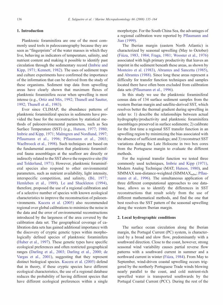
This study incorporates census data of planktonicforaminiferal assemblages from 134 surface sedimentsamples (Fig. 2, Table 1). The samples were collected

along the Iberian margin by Shipeck grab, Van Veengrab, box corer, multi-corer, and kasten corer devicesduring 19 cruises carried out between 1975 and 2004.Most samples are stored at the Departamento deGeologia Marinha, Instituto Nacional de Engenharia,Tecnologia e Inovação I. P. (former Instituto Geológicoe Mineiro), while samples Z5 to Z71 (Table 1) arearchived at the Departamento de Xeociencias Mariñas eO.T., Facultade de Ciencias do Mar, University of Vigo.

The surface samples were weighted and washedthrough a sieve of 74 μm or 63 μmmesh size, but beforethis procedure the first forty six samples (VB-33 to LV-173; Table 1) were preserved in Rose Bengal.

In all samples the fraction 150 μm–2 mm was split toobtain 300–600 specimens and planktonic foraminiferaidentified following the taxonomic criteria of Bé andHamlin (1967), Bé (1977), Kennett and Srinivasan(1983), and Hemleben et al. (1989). Difficulties indiscriminating between the white and pink varieties ofGlobigerinoides ruber in the samples preserved inRose Bengal, were overcome by counting these speciesin the respective non-stained grain size samples. Aftercounting, the relative abundance of each planktonicforaminiferal species was determined.

In this study, the small number of intergrade formsbetween Neogloboquadrina dutertrei and Neoglobo-quadrina pachyderma (dextral) was combined with N.pachyderma (dextral) following Pflaumann et al.(1996). Based on the morphology of the terminalchamber for the species Globigerinoides trilobus, wedistinguished between morphotypes without (G. trilobustrilobus) and with the final sac-like chamber (G. trilobussacculifer). Statistical analysis included 22 species/groups of species with relative abundance equal orhigher than 2% (rounded; Table 2).

Quantitative abundance of planktonic foraminiferawas calculated as number per gram of dry sedimenttaking into account the weight of the original sample andthe number of times the 150 μm fraction was split priorto counting.

Even though we are aware that planktonic forami-nifera inhabit the upper few hundred meters of the watercolumn (e.g., Hemleben et al., 1989), we used modern(summer and winter) satellite-derived SST data tocalibrate the regional transfer function, because theWorld Ocean Atlas (WOA) 2001 data does not resolvethe upwelling features in the study area with enoughdetail. The SST data is based on an integration of dailyPathfinder satellite measurements with a 9 km resolutionfor the period from 1985 to 2003 (version 4.1; dataavailable at: http://podaac-www.jpl.nasa.gov/sst/).Kearns et al. (2000) found that the average difference

http://podaac-www.jpl.nasa.gov/sst/

Fig. 2. Geographical distribution of the 134 surface sediment samples and the 2 box cores (SO83-9GK, M39022-1) used in this study and listed inTable 1. Symbols differentiate between the coring device used. Depth contours drawn are 200 and 500 m and then every 1000 m between 1000 and5000 m. Capes and rivers mentioned in the text are also indicated.


between radiometric ship-based (in situ) and satellite-based Pathfinder SSTs is 0.07±0.31 °C from 219matchups during the low- and midlatitude cruises. Thein situ-Pathfinder differences compared favourablywith the average midlatitude differences between thein situ skin SST and other bulk SSTestimates commonlyavailable for these cruises such as the research vessels'thermosalinograph SST (0.12±0.17 °C) and the weeklyNational Centers for Environmental Prediction optimal-ly interpolated SST analysis (0.41±0.58 °C).

3.2. Calibration techniques

For the regional approach, the relation between theplanktonic foraminifera assemblage and the modern SSTdata was estimated with the same data set from the threemost widely used transfer function techniques forpaleoceanography reconstructions: the Imbrie & Kipp(IK) (Imbrie and Kipp, 1971); the Modern AnalogTechnique (MAT) (Hutson, 1980; Prell, 1985); and theSimilarityMaximum28 (SIMMAX28) (Pflaumann et al.,

Table 1Detailed information on the 134 surface sediment samples and the 2 box cores (SO83-9GK, M39022-1) used in this study including geographicalposition, water depth, cruise and sampling device

Sample Longitude(°W)

Latitude(°N)

Water depth(m)

Cruisename

Device Authorcounts

SSTwinter(°C)

SSTsummer(°C)

VB033 −9.1500 41.3733 140 VIABOA Shipeck grab E. S. 14.1 18.0VB057 −9.2233 41.0867 160 VIABOA Shipeck grab E. S. 14.3 18.2VB060 −8.9050 41.0867 65 VIABOA Shipeck grab E. S. 13.8 18.1VB073 −9.2033 40.8083 140 VIABOA Shipeck grab E. S. 14.3 18.5VB075 −9.0817 40.8100 95 VIABOA Shipeck grab E. S. 14.3 18.4VB094 −9.4917 40.4067 155 VIABOA Shipeck grab E. S. 14.5 18.9VB095 −9.4333 40.4200 145 VIABOA Shipeck grab E. S. 14.5 18.9VB098 −9.1917 40.4300 100 VIABOA Shipeck grab E. S. 14.4 18.8VB106 −9.5150 39.9750 145 VIABOA Shipeck grab E. S. 14.7 19.3VB108 −9.3150 39.9633 120 VIABOA Shipeck grab E. S. 14.5 19.0VB133 −9.4667 39.7150 140 VIABOA Shipeck grab E. S 14.7 19.2VB135 −9.5367 39.7167 155 VIABOA Shipeck grab E. S. 14.8 19.3VB136 −9.8500 39.3000 205 VIABOA Shipeck grab E. S. 14.9 19.3VB138 −9.7833 39.3000 155 VIABOA Shipeck grab E. S. 14.9 19.1VB156 −9.6650 39.0833 94 VIABOA Shipeck grab E. S. 14.8 19.0VB161 −9.7983 39.0833 130 VIABOA Shipeck grab E. S. 14.8 19.1VB164 −9.9417 39.0850 154 VIABOA Shipeck grab E. S. 15.0 19.4VB165 −10.0833 38.8767 415 VIABOA Shipeck grab E. S. 15.1 19.6VB172 −9.7833 38.8667 105 VIABOA Shipeck grab E. S. 15.0 19.2VB176 −9.6300 38.8667 110 VIABOA Shipeck grab E. S. 14.9 18.9LV010 −7.5000 36.9100 405 LIVRA Van Veen grab E. S. 16.3 21.7LV044 −8.1667 36.8667 84 LIVRA Van Veen grab E. S. 15.9 20.9LV051 −8.8667 36.9417 100 LIVRA Van Veen grab E. S. 15.7 20.4LV053 −8.8667 36.9067 110 LIVRA Van Veen grab E. S. 15.8 20.3LV059 −8.4317 36.9000 107 LIVRA Van Veen grab E. S. 15.9 20.6LV072 −8.6667 36.9833 74 LIVRA Van Veen grab E. S. 15.7 20.5LV073 −8.6667 36.9683 80 LIVRA Van Veen grab E. S. 15.8 20.5LV075 −8.6667 36.9333 98 LIVRA Van Veen grab E. S. 15.9 20.5LV078 −8.6667 36.8833 105 LIVRA Van Veen grab E. S. 16.0 20.4LV079 −8.6667 36.8750 110 LIVRA Van Veen grab E. S. 16.0 20.4LV085 −8.9750 37.2500 96 LIVRA Van Veen grab E. S. 15.0 19.8LV087 −9.0417 37.2500 122 LIVRA Van Veen grab E. S. 15.5 19.9LV099 −9.0633 36.8833 157 LIVRA Van Veen grab E. S. 15.8 20.1LV102 −9.0267 37.4150 180 LIVRA Van Veen grab E. S. 15.5 19.7LV119 −8.9500 37.5833 145 LIVRA Van Veen grab E. S. 15.4 19.6LV122 −9.0000 37.5833 172 LIVRA Van Veen grab E. S. 15.5 19.6LV124 −9.0350 37.5883 212 LIVRA Van Veen grab E. S. 15.5 19.6LV125 −9.0533 37.5833 245 LIVRA Van Veen grab E. S. 15.6 19.6LV126 −9.1000 37.5817 305 LIVRA Van Veen grab E. S. 15.6 19.6LV127 −9.1317 37.7417 385 LIVRA Van Veen grab E. S. 15.5 19.5LV131 −8.9900 37.7467 152 LIVRA Van Veen grab E. S. 15.4 19.5LV134 −8.9333 37.7433 130 LIVRA Van Veen grab E. S. 15.0 19.8LV144 −8.9917 37.9142 138 LIVRA Van Veen grab E. S 15.4 19.4LV148 −9.1533 38.0867 335 LIVRA Van Veen grab E. S. 15.5 19.4LV171 −9.0000 38.2133 143 LIVRA Van Veen grab E. S. 15.3 19.4LV173 −8.9333 38.2250 128 LIVRA Van Veen grab E. S 15.1 19.8SO75 09KG −9.8467 37.8433 2331 SONNE75 Box corer E. S 15.7 20.4SO75 13KG −9.2733 37.5550 636 SONNE75 Box corer N. L. 15.7 19.7SO75 15KG −9.4150 37.5750 986 SONNE75 Box corer N. L. 15.7 19.9SO75 25KG −9.5450 37.8550 1300 SONNE75 Box corer N. L. 15.6 20.0SO75 30KG −9.5983 37.4633 1699 SONNE75 Box corer N. L. 15.9 20.4SO75 33KG −9.6417 37.3967 1871 SONNE75 Box corer N. L. 15.9 20.4SO83 07GK −9.7117 37.8400 2010 SONNE83 Box corer E. S. 15.7 20.2SO83 10GK −9.2533 37.8150 498 SONNE83 Box corer N. L. 15.5 19.6SO83 11GK −9.0767 37.8150 267 SONNE83 Box corer N. L. 15.5 19.5PO01(2) −9.1117 37.3267 246 POSEIDON 200-10 Box corer N. L. 15.6 19.8


Table 1 (continued)


Latitude(°N)

Water depth(m)

Cruisename

Device Authorcounts

SSTwinter(°C)

SSTsummer(°C)

PO03(1) −9.3100 37.3250 822 POSEIDON 200-10 Box corer N. L. 15.8 19.9PO05(1) −9.2650 37.8983 550 POSEIDON 200-10 Box corer J. M. 15.5 19.6PO06(1) −9.5033 37.8217 1085 POSEIDON 200-10 Box corer J. M. 15.6 19.9M39002-3 −7.7750 36.0272 1205 METEOR 39/1 Multi-corer N. L. 16.7 22.5M39003-2 −7.2227 36.1108 800 METEOR 39/1 Multi-corer N. L. 16.5 22.5M39004-2 −7.7289 36.2367 967 METEOR 39/1 Multi-corer N. L. 16.5 22.4M39016-2 −7.7056 36.7783 580 METEOR 39/1 Multi-corer N. L. 16.3 21.7M39017-4 −7.4101 36.6500 532 METEOR 39/1 Multi-corer N. L. 16.3 22.2M39021-5 −8.2547 36.6050 900 METEOR 39/1 Box corer N. L. 16.4 21.3M39022-3 −8.2599 36.7117 668 METEOR 39/1 Multi-corer N. L. 16.3 21.0M39023-3 −8.2621 36.7350 728 METEOR 39/1 Box corer N. L. 16.3 21.0M39029-6 −8.2333 36.0497 1918 METEOR 39/1 Multi-corer N. L. 16.7 22.3M39035-3 −9.5010 37.8217 1082 METEOR 39/1 Multi-corer N. L. 15.6 19.9M39058-1 −10.6795 39.0393 1977 METEOR 39/1 Box corer N. L. 15.2 20.5M39059-2 −10.5352 39.0665 1605 METEOR 39/1 Box corer N. L. 15.2 20.3M39070-1 −9.3917 43.6183 1220 METEOR 39/1 Box corer N. L. 13.2 18.2M39072-1 −9.4350 43.7867 2170 METEOR 39/1 Box corer N. L. 13.1 18.4PE151-01A −9.8668 38.7667 133 IBERIA 2000 Box corer E. S. 15.1 19.2PE151-03B −8.8203 36.8522 312 IBERIA 2000 Box corer E. S. 16.0 20.2PE151-04A −7.2792 37.0157 61 IBERIA 2000 Box corer E. S. 15.8 22.1PO287-3-1B −10.4993 39.0738 1505 PALEO I Box corer E. S. 15.2 20.3PO287-5-1B −8.9985 41.3740 87 PALEO I Box corer E. S. 14.0 17.9PO287-8-1B −9.0128 41.2910 88 PALEO I Box corer E. S. 14.0 18.0PO287-13-1B −9.0125 41.1562 81 PALEO I Box corer E. S. 14.0 18.0PO287-15-1B −9.2537 39.7362 111 PALEO I Box corer E. S. 14.5 19.0PO287-19-1B −9.2332 39.8480 101 PALEO I Box corer E. S. 14.5 19.0PO287-21-1B −9.3753 39.9670 128 PALEO I Box corer E. S. 14.6 19.1PO287-26-1B −9.3640 38.5582 96 PALEO I Box corer H. B.-J. 15.0 19.0PO287-27-1B −9.4542 38.6340 85 PALEO I Box corer H. B.-J. 14.9 18.9PO287-28-1B −9.5145 38.6243 105 PALEO I Box corer H. B.-J. 14.9 18.9PO287-33-1B −8.9092 37.6780 119 PALEO I Box corer E. S. 15.1 19.9PO287-34-1B −8.8610 37.6758 90 PALEO I Box corer E. S. 15.1 19.9PO287-40-1B −9.2242 37.6892 493 PALEO I Box corer E. S. 15.6 19.6PO287-41-1B −9.1432 37.6905 380 PALEO I Box corer E. S. 15.6 19.6PO287-44-1B −10.6607 39.0425 1866 PALEO I Box corer E. S. 15.2 20.5PO287-45-1B −10.3742 39.0833 1216 PALEO I Box corer E. S. 15.1 20.1PO201/10-702 −8.6900 43.8433 402 POSEIDON 201-10 Box corer A. V. 13.3 18.6PO201/10-703 −8.7367 43.9667 583 POSEIDON 201-11 Box corer A. V. 13.2 18.6ATL-FP1-04B −9.8750 42.9194 2130 Atalante Multi-corer A. V. 13.5 18.1ATL-FP1-05B −10.1892 42.8361 2953 Atalante Multi-corer A. V. 13.5 18.5ATL-FP1-08A −9.3439 38.0306 987 Foram Prox Multi-corer A. V. 15.5 19.6ATL-FP1-09A −9.7644 37.5283 3124 Foram Prox Multi-corer A. V. 15.9 20.5ATL-FP1-10B −9.6383 37.1933 1863 Foram Prox Multi-corer A. V. 16.0 20.564PE218-16 −8.9333 38.2667 430 Canyons 2003 Multi-corer A. V. 15.3 19.564PE218-21 −9.2672 38.4998 498 Canyons 2003 Multi-corer A. V. 15.0 19.064PE218-22 −9.3296 38.4130 1463 Canyons 2003 Multi-corer A. V. 15.2 19.164PE218-36-1 −9.1584 38.2707 1409 Canyons 2003 Box corer A. V. 15.3 19.364PE225-1-21 −9.5808 38.0833 1742 Canyons 2004 Multi-corer E. S. 15.5 19.964PE225-1-26 −9.4001 39.5990 1118 Canyons 2004 Multi-corer E. S. 14.7 19.364PE225-2-02 −9.3843 38.4330 301 Canyons 2004 Multi-corer E. S. 15.2 19.164PE225-3-03 −9.3266 38.3330 1856 Canyons 2004 Multi-corer E. S. 15.3 19.264PE225-06 −9.9753 38.0080 2945 Canyons 2004 Multi-corer E. S. 15.7 20.464PE225-07 −10.0043 38.1060 4451 Canyons 2004 Multi-corer A. V. 15.6 20.464PE225-25 −10.9999 39.7740 4804 Canyons 2004 Multi-corer A. V. 14.8 20.464PE225-22 −11.1565 39.8980 4975 Canyons 2004 Multi-corer A. V. 14.7 20.364PE225-27 −9.6831 39.5660 1009 Canyons 2004 Multi-corer E. S. 14.8 19.5MD04-2811 −10.1647 37.8040 3162 Privilege Kasten corer E. S. 15.8 20.6

(continued on next page)


Table 1 (continued)


Latitude(°N)

Water depth(m)

Cruisename

Device Authorcounts

SSTwinter(°C)

SSTsummer(°C)

MD04-2814 −9.8577 40.5945 2449 Alienor Kasten corer E. S. 14.5 19.5MD04-2817 −9.7993 42.1618 2365 Alienor Kasten corer A. V. 13.9 18.6M2004-13 −7.3000 36.1940 742 MOUNDFORCE Box corer A. V. 16.5 22.5M2004-28 −7.4010 36.0930 815 MOUNDFORCE Box corer A. V. 16.6 22.5SWIM04-42 SW −7.5278 35.8855 1172 SWIM 2004 SW corer A. V. 16.6 22.6GeoB9014-1 −7.7800 36.5970 716 GAP Multi-corer A. V. 16.4 21.9ZS-5 −9.0496 42.0606 125 Investigador Shipeck grab R. G.-Á. 13.7 17.9ZS-9 −9.1953 41.9887 139 Investigador Shipeck grab R. G.-Á. 13.8 17.9ZS-13 −9.3408 41.9170 192 Investigador Shipeck grab R. G.-Á. 14.0 18.0ZS-17 −9.0322 42.1477 122 Investigador Shipeck grab R. G.-Á. 13.7 17.8ZS-21 −9.1747 42.0751 145 Investigador Shipeck grab R. G.-Á. 13.8 17.8ZS-26 −9.3526 41.9835 244 Investigador Shipeck grab R. G.-Á. 14.0 18.0ZS-30 −9.2323 42.1355 171 Investigador Shipeck grab R. G.-Á. 13.9 17.9ZS-36 −9.0188 42.2358 120 Investigador Shipeck grab R. G.-Á. 13.6 17.7ZS-42 −9.0119 42.3045 104 Investigador Shipeck grab R. G.-Á. 13.5 17.7ZS-51 −9.2715 42.2822 203 Investigador Shipeck grab R. G.-Á. 13.9 17.8ZS-55 −9.1267 42.3481 135 Investigador Shipeck grab R. G.-Á. 13.6 17.7ZS-57 −9.0520 42.3813 105 Investigador Shipeck grab R. G.-Á. 13.5 17.6ZS-63 −9.1153 42.4410 113 Investigador Shipeck grab R. G.-Á. 13.6 17.6ZS-68 −9.2983 42.4268 205 Investigador Shipeck grab R. G.-Á. 13.8 17.7ZS-71 −9.1938 42.4784 123 Investigador Shipeck grab R. G.-Á. 13.5 17.6a SO83-9GK −9.3733 37.8083 900 SONNE83 Box corer N. L./E. S. 15.6 19.7a M39022-1 −8.2599 36.7117 667 METEOR 39/1 Box corer E. S. 16.3 21

Satellite-derived SST as 18 year average for winter and summer (NOAA-1985-2003) and seasonality are also given.E. S.: Emília Salgueiro; N. L.: Neven Lončarić; J. M.: João Moreno; H. B.-J.: Helga Bartels-Jónsdóttir; A. V.: Antje Voelker; R. G.-A.: RaquelGonzález-Àlvarez.a Downcore used in this study.


2003), an improved version of SIMMAX 24 (Pflaumannet al., 1996).

The first two steps of the IK technique, included inthe software package of Sieger et al. (1999) anddescribed in detail by Imbrie and Kipp (1971) andImbrie et al. (1973), were applied in this study. Thefactor analysis (CABFAC, Imbrie and Kipp, 1971) asthe first step, executes a Q-mode factor analysis toidentify statistically significant planktonic foraminiferalassociations (factors) from a large number of species.The communality obtained shows how well a givencombination of species abundances is represented in thecalibration data set. The resulting factor scores indicatethe weight of each species to the respective Q-modefactor. Factor loadings explain the importance of theindividual factors in each sample. The total number offactors was defined by minimizing the remaining“random” variability and by the possibility to relatethe factors to modern hydrographic conditions andplanktonic foraminiferal ecology.

In a second step, a multiple regression analysis wasperformed to fit an empirical equation between factorloadings (independent variables) and modern SST(dependent variables) by multiple linear regression

methods, allowing squared and cross-product terms ofthe factor loadings to enter the equation to account formoderate nonlinearity in the faunal response to theenvironment (Mix et al., 1999).

This technique is based on the assumption thatrelationship between planktonic foraminiferal assem-blages and temperature is maintained through time.Ancient assemblages may, however, deviate significant-ly from the modern fauna and may not be fitted into themodern SST regression model, the so called “no-analogsample problem”, certainly more important in regionallyrestricted areas.

Some years later Hutson (1980) introduced the MATapproach. This technique searches in the calibration dataset for samples that are statistically most similar to theancient assemblage. The SST for the paleo-assemblageis reconstructed as an average of the best modern analogsamples.

In this study the PaleoAnalogs 2.0 program was used(Theron et al., 2004) to identify the best analogs in themodern data set by the square chord distance – pointedout as the best choice for dissimilarity (Prell, 1985) – toselect the 10 least dissimilar samples from the data setand to estimate SST.

Table 2Statistical values for the relative abundance of the important planktonicforaminiferal species in the 134 surface sediment samples

Species Mean Minimum Maximum Standarddeviation

Globigerinella siphonifera 2.7 0.0 8.2 1.8Globigerina bulloides 34.1 1.9 64.8 14.5Globigerinella calida 2.2 0.0 8.1 1.9Neogloboquadrina

dutertrei0.4 0.0 4.6 0.7

Globigerina falconensis 2.8 0.0 11.5 2.2Globigerinita glutinata 6.0 0.1 16.3 3.6Globorotalia hirsuta 1.1 0.0 10.2 1.3Turborotalita humilis 0.4 0.0 4.4 0.9Globorotalia inflata 11.7 2.4 31.9 5.6Pulleniatina

obliquiloculata0.1 0.0 1.8 0.3

Neogloboquadrinapachyderma (sinistral)

1.4 0.0 27.4 3.1

Neogloboquadrinapachyderma (dextral)

18.1 0.7 64.0 12.8

Turborotalita quinqueloba 2.4 0.0 19.8 3.3Globigerinoides rubber

(white)4.6 0.0 30.0 4.9

Globigerinoides rubber(pink)

0.5 0.0 5.6 0.9

Globigerina rubescens 1.7 0.0 9.2 1.9Globigerinoides trilobus

trilobus2.5 0.0 14.5 3.0

Globigerinoides trilobussacculifer

0.4 0.0 3.0 0.7

Globorotalia scitula 0.6 0.0 3.8 0.9Globigerinoides tenellus 0.3 0.0 1.8 0.4Globorotalia

truncatulinoides2.6 0.0 10.9 2.0

Orbulina s.l. 2.0 0.0 13.3 2.6Globigerina digitata 0.1 0.0 1.0 0.2Globigerinoides

conglobatus0.1 0.0 1.0 0.2

Globigerinita uvula 0.0 0.0 0.7 0.1Turborotalita cristata 0.0 0.0 0.9 0.2Globigerinita iota 0.0 0.0 0.8 0.1Globorotalia crassaformis 0.1 0.0 1.2 0.2

Only species with maximum percentages ≥1.8% in the total faunawere used in this study.


Kucera et al. (2005) state that MATcan deal with non-linear relationships between species and environmentalparameter(s), like SST. They also mention that it is astrictly interpolating technique (it cannot extrapolate) and,like all inverse methods, it will tend to perform poorly atthe extremes of the range of the estimated environmentalparameter(s). MAT is completely dependent on the sizeand coverage of the calibration data set, however it is notalways able to benefit from the full information in thereference data set (Kucera and Darling, 2002).

SIMMAX is an improvement of MAT. It differs fromMAT in the way that best analogs are defined and

treated. In SIMMAX, a similarity index based on thescalar product of the normalized faunal percentages anda weighting procedure of the best modern assemblageanalogs according to their inverse geographical distancefrom the most similar ancient samples were incorporat-ed. In this technique, similarity coefficients of the bestanalog can be used, like communality in IK ordissimilarity in MAT, to express how well a givencombination of species abundances is represented in thecalibration data set.

SIMMAX is advantageous to MAT in areas of lowvariability in the calibration data set, where the lack ofchanges in faunal assemblages is supplemented by theinformation on the geographical position of the sample.This approach may also perform better under some no-analog situations as it can handle geographical inconsis-tency among the best analogs (Kucera et al., 2005). Such atechnique generates better results when estimating apaleoenvironment not too different from the modern one,but can introduce an error in the case of migration of thefossil faunal provinces away from the modern centers(Pflaumann et al., 1996), because when it incorporatesgeographic information it slightly violates the stationarityprinciple. Parallel with this distance-weighted SIMMAXestimates option (SIMMAXdw), the program also has thenon-distance-weighted option (SIMMAXndw). Althougha different similarity coefficient is used to select the bestanalog samples, SIMMAXndw is more similar to theclassical MAT technique.

In our upwelling regional data set with highlyvariable hydrographic conditions/planktonic foraminif-eral assemblage and dense sample coverage, if we useSIMMAXdw for the calibration, the technique will preferthe neighboring core-tops and will give less weight tomore distant samples with identical assemblages. Thus,this “transfer function” calibration will be useless forreconstructing any climate state different from that oftoday. Consequently, we use only the SIMMAXndw

option with the 10 best analogs in this study.A validation of each technique to reconstruct modern

SSTwas done by “leave-one-out” cross-validation of themodern data set (Birks, 1995).

To assess the prediction error of all techniques, theroot-mean square of prediction (RMSEP) was calculatedas the square root of the mean of the squared differencesbetween the observed and predicted values for allsamples from the test set.

3.3. Paleo-SST reconstructions

In order to determine potential differences betweenthe techniques, we reconstructed SST in two box cores


from the Portuguese margin: SO83-9GK (37.81°N;9.37°W; 900 m water depth; 38 cm long) retrieved offCape Sines and under the influence of seasonalupwelling; and M39022-1 (36.71°N; 8.26°W; 667 mwater depth; 37 cm long) located off the southern coastand outside of the direct influence of seasonal upwelling(Fig. 2, Table 1). Both cores were sampled continuouslywith a 2 cm resolution, and treated following the surfacesample methodology and taxonomic criteria for quan-titative foraminiferal identification.

Stable isotope measurements were performed on threeplanktonic foraminifera species: Globigerina bulloides,G. ruber (white), and G. inflata. Samples contained onaverage 25 specimens picked from the 250 μm–2 mmfraction and were measured in a Finnigan MAT 252 massspectrometer of the RCOM at Bremen University. The18O/16O ratio is reported in per mil (‰) relative to theVienna Peedee Belemnite (VPDB) standard. Analyticalstandard deviation for δ18O is ±0.07‰.

The paleotemperature equation of Shackleton (1974)was used for the reconstruction of the surface watertemperature based on the isotope values:

T ¼ 16:9� 4:38 d18Oc � d18Ow

� �

þ 0:10 d18Oc � d18Ow

� �2

where T is paleotemperature (°C), δ18Oc=δ18O of plank-

tonic foraminifera carbonate (‰VPDB) and δ18Ow=δ18O

of ambient sea water (‰ VPDB) after conversion fromVSMOW by subtracting 0.27‰ (Hut, 1987). As δ18Ow ofambient sea water we use the average value of 0.63‰,derived from recent water samples collected in the region(at 36°N, −8.5°W; A. Voelker unpublished data). Thisvalue will be used for the paleotemperature reconstructionsof both records.

All investigated data was mapped with the OceanData View program of Schlitzer (2000).

All data presented in this paper will be stored at theWorld Data Centre MARE (http://www.wdc-mare.org).

4. Results

4.1. Planktonic foraminiferal distribution

Planktonic foraminiferal abundance, expressed as thenumber of specimens per gram of dry sediment (#g−1),along the Iberian margin varies by three orders ofmagnitude, from 24 to 31500 #g−1. Values lower than3000 #g−1 are observed along the northwestern innershelf, off the Rias Baixas in Galicia and the majorPortuguese rivers (Minho, Douro, Mondego, andTagus), and in the Iberia abyssal plain (Fig. 3a).

The distribution pattern of total planktonic forami-nifera concentrations mirrors (1) productivity of watersalong the Iberian margin, with concentrations largerthan 8000 #g−1 below the major upwelling zones; (2)the oligotrophic offshore waters with concentrationslower than 3000 #g−1; and also (3) the dilution on thenorthwestern Iberia shelf caused by the presence of acoarse lithic fraction (Monteiro et al., 1980), or by theincreased amount of fine fraction from the riverine inputoff the Rias Baixas and off the major Portuguese rivers.

Twenty eight species/group of species have beenidentified in the planktonic foraminiferal assemblage ofthe 134 surface sediment samples (Table 2). Fourspecies dominate the fauna in the study area: G.bulloides (2–65%), N. pachyderma (dextral) (1–64%),G. inflata (2–32%), and G. ruber (white) (0–30%). G.bulloides (Fig. 3b), the most abundant and widespreadspecies, is distributed with high relative abundances(N30%) near the coast along the western Iberian margin.However, this species also shows the highest percen-tages (50–65%) off the Douro, Tagus and Guadianarivers. N. pachyderma (dextral) (Fig. 3c), the secondmost abundant species, dominates (N20%) the assem-blage along the coast north of 39°N. The highest values(50–64%) are concentrated offshore of the Rias Baixas.G. inflata (Fig. 3d) reveals the highest relativeabundances (N15%) offshore from the G. bulloideshigh abundance band. G. ruber (white), a speciescharacteristic of sub-tropical waters (Fig. 3e), hashighest abundances (N7.5%) off the southern andsouthwestern coasts.

To assess the planktonic foraminiferal data statisti-cally, Q-mode factor analysis of the IK technique wasperformed. On the western Iberian margin, the analysisof 22 species/group of species – the six with percentagesof less than 2% are excluded – results in three factorsthat explain 95.6% of the total variance (Table 3). Factor1 accounts for 49.8% of the total variance and isexclusively defined by G. bulloides (score of 0.98). Thehigh factor loading's distribution is located along thewestern Iberian margin (Fig. 3f), with the highest valuesoff Capes Roca, Espichel and S. Vicente. Factor 2explains 32.2% of the total variance and is dominated byN. pachyderma (dextral) (score of 0.93) and G. inflata(score of 0.31). This factor becomes important north of39°N (Fig. 3g), with high loadings offshore between39.5 and 41.5°N and offshore and nearshore north of41.5°N. Factor 3 describes 13.6% of the total varianceand is defined by G. ruber (white) (score of 0.61), G.trilobus trilobus (score of 0.34) and G. inflata (score of0.52). High factor loadings (Fig. 3h) dominate on thesouthern margin and offshore of the southwestern coast.

http://www.wdc-mare.org

Fig. 3. Spatial distribution patterns of the absolute and relative planktonic foraminifera abundances and the 3 factors resulting from the Q-mode factor analysis along the western Iberian margin. a)number of specimens per gram of dry sediment #g−1. Relative abundances are shown for G. bulloides (b), N. pachyderma (dextral) (c), G. inflata (d), and G. ruber (white) (e). Factor 1 (f), theUpwelling factor, explains 49.8% of the variance. Factor 2 (g; 32.2%) is related to the Portugal Current and factor 3 (h; 13.6%) to the Azores Current Eastern branch.

145E.Salgueiro

etal.

/Marine

Micropaleontology

66(2008)

135–164

Table 3Varimax factor score matrix of the 3 factors as determined by theQ-mode factor analyses of the relative abundance of planktonicforaminifera on the western Iberian margin

Species Factor 1 Factor 2 Factor 3

Upwellingfactor

PortugalCurrentfactor

Azores CurrentEastern branchfactor

G. siphonifera 0.03 −0.02 0.17G. bulloides 0.98 0.10 0.08G. calida 0.06 0.02 0.00N. dutertrei 0.00 0.01 0.01G. falconensis 0.01 −0.03 0.24G. glutinata 0.11 0.03 0.16G. hirsuta −0.02 0.00 0.13T. humilis −0.01 −0.02 0.08G. inflata −0.08 0.31 0.52P. obliquiloculata 0.00 −0.01 0.03N. pachyderma (sinistral) −0.01 0.08 −0.01N. pachyderma (dextral) −0.08 0.93 −0.13T. quinqueloba 0.08 −0.02 0.03G. ruber (white) −0.07 −0.06 0.61G. ruber (pink) −0.01 −0.02 0.09G. rubescens 0.05 0.01 0.02G. trilobus trilobus −0.02 −0.06 0.34G. trilobus sacculifer −0.01 −0.01 0.06G. scitula −0.01 0.00 0.06G. tenellus 0.00 0.00 0.03G. truncatulinoides −0.03 0.05 0.17Orbulina s.l. −0.06 0.04 0.21Variance 49.80 32.18 13.60Cumulative variance 49.80 81.96 95.56

Relevant species are marked in bold.Table 4Results of the regression analyses from the Imbrie & Kipp techniquefor summer and winter temperatures

Variablenumber

Variablename

Regressioncoefficient

Standard error ofregression coefficient

Computedt-value

Winter season7 F1⁎F3 9.997 3.934 2.5416 F1⁎F2 7.673 4.164 1.8434 F2SQ 5.311 2.792 1.90211 F3 −8.654 6.215 −1.3923 F1SQ 7.158 2.103 3.4049 F1 −12.647 5.515 −2.2935 F3SQ 4.883 2.703 1.8068 F2⁎F3 8.835 4.464 1.97910 F2 −12.350 6.512 −1.897Intercept 21.030

Summer season11 F3 −1.095 8.658 −0.1263 F1SQ 5.257 2.929 1.7956 F1⁎F2 4.057 5.800 0.6994 F2SQ 4.983 3.889 1.2817 F1⁎F3 4.320 5.480 0.7888 F2⁎F3 6.523 6.218 1.04910 F2 −9.482 9.070 −1.0459 F1 −7.415 7.681 −0.9655 F3SQ 2.459 3.766 0.653Intercept 22.135


4.2. Modern SST calibrations

The regression equations obtained for the IK regionaltransfer function calibration and the results of SSTestimates and residuals (observed minus estimated SST)obtained in each calibration by the different techniquesare summarized in Tables 4 and 5.

Low communality (≤0.95), high dissimilarity(≥0.20), and low similarity coefficients (≤0.90) forall samples (Fig. 4, 5), were found on the northern coastbetween 43° and 44°N, in the Iberia abyssal plain, on theouter Estremadura promontory (∼39°N, 10–11°W), inthe vicinity of the deeper Lisbon/Setúbal Canyons, andeast of 8°W in the Gulf of Cadiz. The lowest valuescorrespond to samples located outside of the directinfluence of upwelling and located in the Setúbal andNazaré Canyons.

The distribution of the temperature residuals (sum-mer, winter) of each used technique shows nocorrelation with the respective analog index (Fig. 5).Low communality, high dissimilarity and low similarity

coefficients for both seasons do not coincide with highresiduals.

Estimated versus satellite-measured SST, for summerand winter seasons, range from 13° to 23 °C, and aresignificantly correlated (pb0.001) with correlationcoefficients of: 0.85 (summer) and 0.86 (winter) forIK; 0.88 (summer) and 0.91 (winter) for MAT; and 0.86(summer) and 0.88 (winter) for SIMMAXndw (Fig. 6).

In general all techniques display a homogeneousscatter with lower significant deviation, and most of thesamples lie within the root-mean square error ofprediction (RMSEP) for the summer and winter SST.MAT shows lower RMSEP for both seasons (0.59 °C:summer; 0.40 °C: winter) than IK (0.63 °C: summer;0.46 °C: winter) and SIMMAXndw (0.64 °C: summer;0.44 °C: winter).

However, for observed temperatures above 20.6 °Cin summer and 16.2 °C in winter, SST estimates tend tobe too cold (Fig. 6). These sites are located mainly atlatitudes between 36°–37°N, with low communality,high dissimilarity, and low similarity, respectively. Onthe other hand, for observed temperatures lower than18.8 °C in summer and 14 °C in winter, SST estimatesappear to be too warm. These sites are located mainlynorth of 43°N, coincident also with no- or less-analogconditions in the area. These problematic zones are

Table 5Estimated temperature (Est.) with their respective residuals (Resid.) obtained for each sample by the three transfer function techniques used in thisstudy

Station Imbrie & Kipp MAT SIMMAXndw

Winter Summer Winter Summer Winter Summer

SST SST SST SST SST SST

Est. Resid. Est. Resid. Est. Resid. Est. Resid. Est. Resid. Est. Resid.

VB033 13.9 0.2 18.4 −0.4 14.5 −0.4 18.8 −0.8 14.0 0.1 18.5 −0.5VB057 14.2 0.1 18.8 −0.6 14.6 −0.3 19.1 −0.9 14.1 0.2 18.7 −0.5VB060 14.9 −1.1 19.2 −1.1 14.9 −1.1 19.2 −1.1 15.2 −1.4 19.6 −1.5VB073 13.9 0.4 18.0 0.5 14.4 0.0 18.7 −0.2 13.9 0.4 18.2 0.3VB075 14.4 −0.1 18.5 −0.1 14.5 −0.2 18.8 −0.4 14.1 0.2 18.3 0.1VB094 14.3 0.2 18.6 0.3 14.7 −0.1 19.0 0.0 14.4 0.1 18.8 0.1VB095 14.7 −0.2 19.5 −0.6 14.7 −0.2 19.0 −0.1 14.7 −0.2 19.2 −0.3VB098 14.5 −0.1 18.7 0.1 14.6 −0.2 18.9 −0.1 14.2 0.2 18.4 0.4VB106 14.8 −0.1 19.2 0.1 14.6 0.0 18.9 0.4 15.0 −0.3 19.4 −0.1VB108 15.0 −0.5 19.2 −0.2 15.0 −0.5 19.4 −0.4 15.1 −0.6 19.5 −0.5VB133 14.7 0.0 19.0 0.2 14.6 0.1 19.0 0.3 14.8 −0.1 19.1 0.1VB135 15.3 −0.5 19.6 −0.3 14.8 −0.1 19.1 0.2 15.1 −0.3 19.5 −0.2VB136 14.7 0.2 19.2 0.1 14.6 0.2 19.0 0.3 14.6 0.3 19.0 0.2VB138 15.2 −0.3 19.9 −0.8 14.8 0.1 19.1 0.0 14.9 0.0 19.3 −0.2VB156 15.1 −0.3 19.4 −0.4 15.2 −0.4 19.7 −0.8 15.3 −0.5 19.8 −0.8VB161 14.8 0.0 19.1 0.0 14.9 −0.1 19.2 −0.1 14.7 0.1 19.1 0.0VB164 14.9 0.1 19.5 −0.1 14.6 0.3 19.0 0.4 14.7 0.3 19.1 0.3VB165 15.4 −0.3 19.9 −0.3 15.2 0.0 19.6 0.1 15.3 −0.2 19.7 −0.1VB172 15.3 −0.3 19.7 −0.5 15.0 0.0 19.4 −0.2 15.2 −0.2 19.5 −0.3VB176 14.8 0.1 19.1 −0.2 14.7 0.2 19.1 −0.1 14.9 0.0 19.1 −0.2LV010 15.8 0.5 20.2 1.5 15.6 0.7 20.0 1.7 15.5 0.8 20.0 1.7LV044 15.3 0.6 19.7 1.2 15.5 0.4 20.1 0.8 15.4 0.5 20.0 0.9LV051 15.3 0.4 19.7 0.7 15.6 0.1 20.0 0.4 15.6 0.1 20.0 0.4LV053 15.3 0.5 19.8 0.5 15.5 0.3 20.1 0.3 15.6 0.2 20.1 0.2LV059 15.2 0.7 19.7 0.9 15.5 0.3 20.1 0.5 15.5 0.4 20.0 0.6LV072 15.3 0.4 19.7 0.8 15.5 0.2 20.0 0.5 15.2 0.5 19.7 0.8LV073 15.4 0.4 19.9 0.6 15.5 0.2 20.0 0.5 15.6 0.2 20.2 0.3LV075 15.3 0.6 19.8 0.7 15.5 0.3 20.1 0.4 15.5 0.4 20.3 0.2LV078 15.5 0.5 20.0 0.4 15.4 0.5 20.0 0.5 15.4 0.6 20.0 0.4LV079 16.0 0.0 20.5 −0.1 15.5 0.5 20.0 0.4 15.6 0.4 20.0 0.4LV085 15.5 −0.5 19.9 −0.1 15.6 −0.5 20.0 −0.2 15.5 −0.5 20.0 −0.2LV087 15.5 0.0 19.9 0.0 15.6 −0.1 19.9 0.0 15.4 0.1 19.9 0.0LV099 15.8 0.0 20.3 −0.2 15.4 0.4 19.8 0.3 15.6 0.2 20.1 0.0LV102 15.4 0.1 19.8 −0.1 15.4 0.1 19.8 −0.1 15.4 0.1 19.8 −0.1LV119 15.4 0.0 19.9 −0.3 15.5 −0.1 19.9 −0.3 15.4 0.0 19.9 −0.3LV122 15.3 0.2 19.6 0.0 15.3 0.2 19.7 −0.1 15.2 0.3 19.5 0.1LV124 15.5 0.0 19.8 −0.2 15.3 0.3 19.5 0.1 15.3 0.2 19.6 0.0LV125 14.9 0.7 19.2 0.4 15.3 0.3 19.6 0.0 15.0 0.6 19.4 0.2LV126 15.1 0.5 19.5 0.1 15.4 0.2 19.7 −0.1 15.3 0.3 19.5 0.1LV127 15.0 0.5 19.6 −0.1 15.1 0.4 19.5 0.0 15.1 0.4 19.6 −0.1LV131 15.1 0.3 19.3 0.2 15.2 0.1 19.6 −0.1 15.1 0.2 19.4 0.1LV134 15.4 −0.4 19.8 0.0 15.5 −0.5 19.7 0.1 15.4 −0.4 19.8 0.0LV144 15.4 0.0 19.8 −0.4 15.3 0.1 19.7 −0.3 15.2 0.2 19.6 −0.2LV148 14.6 0.9 19.2 0.2 15.1 0.3 19.5 −0.1 15.0 0.5 19.5 −0.1LV171 15.4 −0.1 19.7 −0.3 15.4 0.0 19.7 −0.2 15.2 0.1 19.5 −0.1LV173 15.0 0.1 19.3 0.5 15.3 −0.2 19.7 0.1 15.1 0.0 19.5 0.3SO75 09KG 16.0 −0.3 20.7 −0.3 15.3 0.4 19.9 0.4 15.5 0.2 20.2 0.2SO75 13KG 15.4 0.3 19.8 −0.1 15.7 0.0 20.4 −0.7 15.4 0.3 19.9 −0.1SO75 15KG 15.1 0.6 19.4 0.5 15.5 0.2 20.0 −0.1 15.2 0.5 19.5 0.4SO75 25KG 15.6 0.0 20.2 −0.2 15.7 −0.1 20.3 −0.3 15.6 0.0 20.3 −0.3SO75 30KG 15.6 0.3 20.1 0.3 15.7 0.2 20.2 0.2 15.6 0.3 20.3 0.1

(continued on next page)


Table 5 (continued)





SO75 33KG 15.9 0.0 20.4 0.0 15.9 0.0 20.6 −0.2 15.7 0.2 20.2 0.2SO83 07GK 16.2 −0.5 20.8 −0.6 15.7 0.0 20.4 −0.2 15.6 0.1 20.2 0.0SO83 10GK 14.7 0.8 19.0 0.6 15.0 0.6 19.2 0.4 14.7 0.8 19.0 0.6SO83 11GK 14.8 0.7 19.2 0.3 15.1 0.4 19.2 0.2 14.9 0.6 19.3 0.2PO01(2) 15.3 0.3 19.6 0.2 15.6 0.0 20.0 −0.2 15.5 0.1 19.6 0.2PO03(1) 15.7 0.1 20.1 −0.2 15.8 0.0 20.6 −0.7 15.4 0.4 19.7 0.2PO05(1) 15.1 0.4 19.4 0.2 15.0 0.5 19.2 0.4 15.1 0.4 19.4 0.2PO06(1) 16.1 −0.5 21.2 −1.3 15.8 −0.2 20.7 −0.7 15.7 −0.1 20.7 −0.8M39002-3 16.5 0.2 22.3 0.2 16.3 0.4 21.7 0.8 16.3 0.4 21.8 0.7M39003-2 16.1 0.4 21.9 0.6 16.4 0.1 21.8 0.8 16.4 0.1 22.0 0.5M39004-2 16.4 0.1 21.4 1.0 16.1 0.4 21.0 1.3 16.1 0.4 21.1 1.3M39016-2 16.5 −0.2 21.2 0.5 15.9 0.5 20.5 1.2 15.8 0.5 20.4 1.3M39017-4 16.0 0.3 20.7 1.5 15.9 0.5 20.5 1.7 15.8 0.5 20.5 1.7M39021-5 15.8 0.6 21.4 −0.1 15.9 0.5 20.9 0.4 16.0 0.4 21.1 0.1M39022-3 15.6 0.7 20.1 0.9 15.8 0.5 20.3 0.7 15.5 0.8 20.0 1.0M39023-3 16.2 0.1 20.9 0.1 15.9 0.4 20.6 0.4 15.7 0.6 20.4 0.6M39029-6 16.6 0.1 21.9 0.4 16.2 0.5 21.5 0.8 16.2 0.5 21.4 0.9M39035-3 15.9 −0.3 20.4 −0.5 15.9 −0.2 20.7 −0.8 15.6 0.0 20.0 −0.1M39058-1 15.6 −0.4 20.0 0.5 15.9 −0.7 20.6 −0.1 15.3 −0.1 19.6 0.9M39059-2 15.0 0.2 20.3 0.0 14.9 0.3 19.5 0.8 15.0 0.2 19.8 0.5M39070-1 14.0 −0.8 17.9 0.3 14.2 −0.9 18.7 −0.5 14.6 −1.4 19.0 −0.8M39072-1 14.1 −1.0 18.4 0.0 14.4 −1.3 18.9 −0.5 14.1 −1.0 18.3 0.1PE151-01A 14.9 0.2 19.1 0.1 15.1 0.0 19.3 −0.1 14.7 0.4 18.8 0.4PE151-03B 14.7 1.3 19.0 1.2 15.4 0.6 19.9 0.4 15.2 0.8 19.5 0.7PE151-04A 15.8 0.0 20.3 1.8 15.6 0.2 20.2 2.0 15.7 0.1 20.3 1.8PO287-3-1B 15.2 0.0 19.6 0.7 15.4 −0.2 19.7 0.6 15.1 0.1 19.5 0.8PO287-5-1B 14.4 −0.4 18.6 −0.7 14.1 −0.2 18.3 −0.3 14.2 −0.2 18.4 −0.5PO287-8-1B 14.6 −0.6 18.8 −0.8 14.4 −0.4 18.5 −0.5 14.5 −0.5 18.8 −0.8PO287-13-1B 15.2 −1.2 19.6 −1.6 14.7 −0.7 19.0 −1.0 15.2 −1.2 19.8 −1.8PO287-15-1B 14.6 −0.1 18.8 0.2 15.0 −0.5 19.3 −0.2 14.8 −0.3 18.9 0.1PO287-19-1B 14.5 0.0 18.6 0.4 14.9 −0.4 19.2 −0.2 14.2 0.3 18.3 0.7PO287-21-1B 15.0 −0.4 19.3 −0.2 15.0 −0.4 19.3 −0.2 15.2 −0.6 19.3 −0.2PO287-26-1B 15.2 −0.2 19.8 −0.8 15.0 0.0 19.2 −0.2 15.3 −0.3 19.5 −0.5PO287-27-1B 15.5 −0.6 20.1 −1.2 15.2 −0.3 19.4 −0.5 15.4 −0.5 19.8 −0.9PO287-28-1B 15.4 −0.5 19.9 −1.0 15.1 −0.2 19.2 −0.3 15.4 −0.5 19.8 −0.9PO287-33-1B 15.1 0.0 19.4 0.5 15.2 −0.1 19.5 0.4 15.0 0.1 19.2 0.7PO287-34-1B 15.4 −0.3 19.9 0.0 15.4 −0.3 20.1 −0.2 15.5 −0.4 20.1 −0.2PO287-40-1B 15.3 0.3 19.6 0.0 15.3 0.4 19.6 0.0 15.3 0.3 19.5 0.1PO287-41-1B 15.3 0.3 19.7 −0.1 15.2 0.4 19.5 0.0 15.3 0.3 19.5 0.1PO287-44-1B 15.6 −0.4 20.2 0.3 15.3 −0.1 19.9 0.6 15.2 0.0 19.8 0.7PO287-45-1B 14.1 1.0 18.5 1.6 15.4 −0.3 19.5 0.6 14.6 0.5 19.0 1.1PO201/10-702 14.0 −0.7 18.6 0.0 14.1 −0.7 18.7 −0.2 13.9 −0.6 18.3 0.3PO201/10-703 14.3 −1.1 19.0 −0.4 13.9 −0.7 18.4 0.2 13.9 −0.7 18.3 0.3ATL-FP1-04B 14.3 −0.8 18.9 −0.8 14.1 −0.6 18.8 −0.7 13.9 −0.4 18.6 −0.5ATL-FP1-05B 14.1 −0.6 18.7 −0.2 14.2 −0.8 18.8 −0.3 13.9 −0.4 18.4 0.1ATL-FP1-08A 15.7 −0.2 20.3 −0.7 15.5 0.0 20.0 −0.4 15.5 0.0 19.9 −0.3ATL-FP1-09A 16.7 −0.8 21.9 −1.4 16.1 −0.2 21.3 −0.8 16.1 −0.2 21.1 −0.6ATL-FP1-10B 16.6 −0.6 21.5 −1.0 16.0 0.1 21.1 −0.6 15.8 0.2 20.4 0.164PE218-16 15.3 0.0 19.8 −0.3 15.4 −0.1 19.8 −0.2 15.2 0.1 19.6 −0.164PE218-21 15.4 −0.4 19.9 −0.9 15.0 −0.1 19.2 −0.2 15.4 −0.4 19.8 −0.864PE218-22 15.5 −0.3 20.1 −1.0 15.3 −0.1 19.7 −0.5 15.5 −0.3 20.0 −0.964PE218-36-1 15.2 0.1 19.5 −0.2 15.2 0.1 19.5 −0.2 15.2 0.1 19.7 −0.464PE225-1-21 15.3 0.2 20.2 −0.3 15.6 −0.1 20.0 −0.1 15.6 −0.1 20.1 −0.264PE225-1-26 14.7 0.0 19.1 0.2 15.5 −0.8 19.8 −0.5 15.3 −0.6 19.5 −0.2


Table 5 (continued)





64PE225-2-02 15.4 −0.2 19.9 −0.8 15.5 −0.4 19.8 −0.7 15.3 −0.1 19.7 −0.664PE225-3-03 15.5 −0.2 19.9 −0.7 15.4 0.0 19.7 −0.4 15.4 −0.1 19.9 −0.764PE225-06 15.5 0.2 20.0 0.4 15.4 0.3 20.0 0.4 15.3 0.4 19.8 0.664PE225-07 16.1 −0.5 21.6 −1.2 15.9 −0.3 21.0 −0.6 15.9 −0.3 20.8 −0.464PE225-25 15.8 −1.0 21.1 −0.7 15.2 −0.4 19.8 0.6 15.0 −0.2 20.1 0.364PE225-22 14.9 −0.2 20.2 0.1 15.6 −0.9 20.6 −0.3 14.1 0.6 18.9 1.464PE225-27 14.8 0.0 19.2 0.3 15.0 −0.3 19.5 0.0 14.9 −0.1 19.3 0.2MD04-2811 15.6 0.2 20.3 0.3 15.3 0.5 19.8 0.8 15.0 0.8 19.7 0.9MD04-2814 14.2 0.3 18.8 0.7 14.5 0.0 19.0 0.5 14.1 0.4 18.7 0.8MD04-2817 13.9 0.0 18.5 0.1 14.1 −0.2 18.7 −0.1 13.8 0.1 18.3 0.3M2004-13 15.5 1.0 20.8 1.7 15.1 1.3 19.9 2.6 15.2 1.2 20.1 2.4M2004-28 15.7 0.9 21.0 1.5 15.5 1.1 20.5 2.0 15.5 1.1 20.5 2.0SWIM04-42 SW 16.4 0.2 22.5 0.1 16.3 0.3 21.8 0.8 16.4 0.2 21.9 0.7GeoB9014-1 16.3 0.1 21.8 0.1 16.4 0.0 21.9 0.0 16.4 0.0 22.0 −0.1ZS-5 13.7 0.0 17.8 0.1 13.8 −0.1 17.9 0.0 13.7 0.0 17.9 0.0ZS-9 13.3 0.5 17.5 0.4 13.9 −0.1 17.9 −0.1 13.8 0.0 18.0 −0.1ZS-13 13.7 0.3 18.2 −0.2 14.2 −0.2 18.2 −0.2 13.8 0.2 18.0 0.0ZS-17 14.3 −0.6 18.5 −0.7 13.8 −0.1 17.9 −0.1 14.0 −0.3 18.1 −0.3ZS-21 13.4 0.4 17.1 0.7 13.9 −0.1 17.9 −0.1 13.8 0.0 18.1 −0.3ZS-26 13.4 0.6 17.7 0.3 13.9 0.1 17.9 0.1 13.9 0.1 18.1 −0.1ZS-30 13.5 0.4 17.7 0.2 13.9 0.0 17.9 0.0 13.8 0.1 18.0 −0.1ZS-36 14.0 −0.4 18.1 −0.4 13.8 −0.2 17.9 −0.2 14.0 −0.4 18.1 −0.4ZS-42 13.8 −0.3 17.8 −0.1 13.8 −0.3 18.0 −0.3 14.0 −0.5 18.1 −0.4ZS-51 13.7 0.2 17.8 0.0 13.9 0.0 18.0 −0.2 13.7 0.2 18.1 −0.3ZS-55 13.6 0.0 17.8 −0.1 13.9 −0.2 17.9 −0.2 13.9 −0.2 18.0 −0.3ZS-57 13.8 −0.3 17.8 −0.2 13.8 −0.3 18.0 −0.3 13.8 −0.3 18.0 −0.4ZS-63 13.9 −0.3 18.0 −0.4 13.9 −0.3 18.0 −0.4 13.9 −0.2 18.0 −0.4ZS-68 14.1 −0.3 18.9 −1.2 13.9 −0.1 18.0 −0.3 13.8 0.0 18.1 −0.4ZS-71 13.5 0.0 17.6 0.0 13.7 −0.2 17.8 −0.2 13.8 −0.3 18.0 −0.4


clearly evident when the temperature residuals areplotted versus the satellite temperatures for both seasons(Fig. 7).

The relationship among temperature residuals pro-duced by different techniques and latitude of theindividual sampling sites reveals that the samples areconcentrated around ±1.0 °C with a larger deviationfrom zero in summer (±2.0 °C) than in winter (±1.0 °C),which could be related to the variability of seasonalcoastal upwelling during summer (Fig. 8). All under-estimated SST samples for both seasons are locatedalong the southern Iberian coast and show occasionallytemperature residuals exceeding 1 °C, with PE151-04A(37.02°N, 7.28°W) and PE151-03B (36.85°N, 8.82°W)being the most underestimated samples with IK for thesummer and winter season, respectively, and M2004-13(36.19°N, 7.30°W) for summer and winter with MATand SIMMAXndw.

The area of most overestimated SST is located on thenorthern coast, in the region with the lowest modern

SST. With IK the most overestimated SST for bothseasons is for sample PO287-13-1B (41.16°N, 9.01°W);with MAT VB060 (41.09°N, 8.91°W) for summer andM39072-1 (43.78°N, 9.44°W) for winter with MAT; andPO287-13-1B (41.16°N, 9.01°W) for summer andVB060 and M39070-1 (43.62°N, 9.39°W) for winterwith SIMMAXndw.

4.2.1. Similarity between techniquesFollowing Kucera et al. (2005), the similarities

between the IK, MAT and SIMMAXndw techniqueswere investigated (Fig. 9). The residuals are significant-ly correlated (pb0.001) for all technique pairs. MATversus SIMMAXndw (r=0.85 for summer; r=0.83 forwinter) and SIMMAXndw versus IK (r=0.83 forsummer; r=0.82 for winter) show the highest correla-tion, suggesting that this two techniques alone do notconstitute a sufficiently independent framework. MATand IK are correlated the least (r=0.77 for summer;r=0.73 for winter).

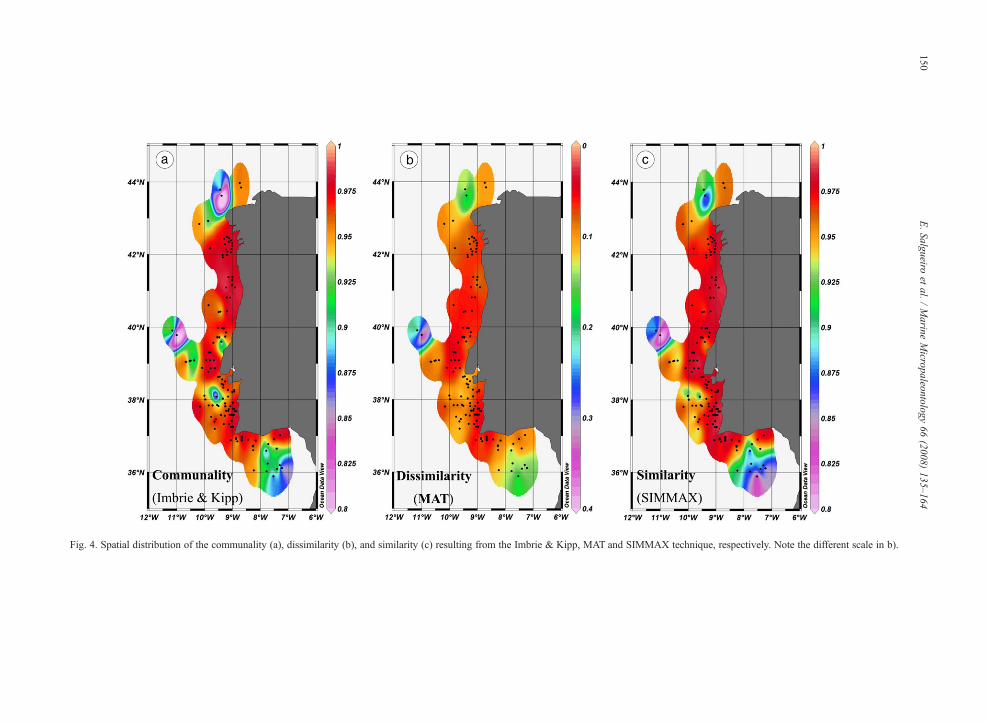
Fig. 4. Spatial distribution of the communality (a), dissimilarity (b), and similarity (c) resulting from the Imbrie & Kipp, MAT and SIMMAX technique, respectively. Note the different scale in b).

150E.Salgueiro

etal.

/Marine

Micropaleontology

66(2008)

135–164

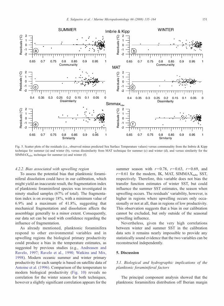
Fig. 5. Scatter plots of the residuals (i.e., observed minus predicted Sea Surface Temperature values) versus communality from the Imbrie & Kipptechnique for summer (a) and winter (b), versus dissimilarity from MAT technique for summer (c) and winter (d), and versus similarity for theSIMMAXndw technique for summer (e) and winter (f).


4.2.2. Bias associated with upwelling regionTo assess the potential bias that planktonic forami-

niferal dissolution could have in our calibration, whichmight yield an inaccurate result, the fragmentation indexof planktonic foraminiferal species was investigated inninety studied samples (67% of total). The fragmenta-tion index is on average 18%, with a minimum value of6.9% and a maximum of 41.8%, suggesting thatmechanical fragmentation and dissolution affects theassemblage generally to a minor extent. Consequently,our data set can be used with confidence regarding theinfluence of fragmentation.

As already mentioned, planktonic foraminiferarespond to other environmental variables and inupwelling regions the biological primary productivitycould produce a bias in the temperature estimates, assuggested by previous studies (e.g., Andreasen andRavelo, 1997; Ravelo et al., 1990; Watkins and Mix,1998). Modern oceanic summer and winter primaryproductivity for each sample is based on satellite data ofAntoine et al. (1996). Comparison of the temperature tomodern biological productivity (Fig. 10) reveals nocorrelation for the winter season for both techniques,however a slightly significant correlation appears for the

summer season with r=0.78, r=0.63, r=0.69, andr=0.61 for the modern, IK, MAT, SIMMAXndw SST,respectively. Therefore, this variable does not bias thetransfer function estimates of winter SST, but couldinfluence the summer SST estimates, the season whenupwelling occurs. The residuals' variability, however, ishigher in regions where upwelling occurs only occa-sionally or not at all, than in regions of low productivity.This observation suggests that a bias in our calibrationcannot be excluded, but only outside of the seasonalupwelling influence.

Nevertheless, given the very high correlationsbetween winter and summer SST in the calibrationdata sets it remains nearly impossible to provide anystatistically sound evidence that the two variables can bereconstructed independently.

5. Discussion

5.1. Biological and hydrographic implications of theplanktonic foraminiferal factors

The principal component analysis showed that theplanktonic foraminifera distribution off Iberian margin

Fig. 6. Comparison between the satellite-derived Sea SurfaceTemperature (SST; 18 year average) data and the SST estimated withthe Imbrie & Kipp (a), MAT (b), and SIMMAXndw techniques forsummer and winter. Solid line represents linear regression line anddashed lines the RMSEP confidence interval. “r” is the correlationcoefficient.


can be explained by three factors. Their biological andhydrographic implications are discussed bellow.

5.1.1. Factor 1: Upwelling factorFactor 1 (Fig. 3f, Table 3) is nearly exclusively

defined by G. bulloides. This species thrives in areas of

nutrient-rich mixing zones and episodic phytoplanktonblooms (e.g., Schiebel et al., 1997; Schiebel et al., 2004;Thiede et al., 1997) and has often been encountered inother upwelling areas (e.g. Curry et al., 1992;Giraudeau, 1993; Ortiz and Mix, 1992; Thunell andSautter, 1992; Thunell et al., 1983).

G. bulloides is the most abundant and widespreadspecies along the Iberian margin. Its distribution pattern(Fig. 3b) matches the satellite-derived SST data (Fig. 1a),high chlorophyll pigment concentrations (Fig. 1b), as wellas the diatom abundance distribution patterns in bothsurface sediments and the water column during a typicalupwelling period (Abrantes and Moita, 1999). Thisindicates a close relationship between the abundance ofthis species and the spatial location of coastal upwelling onthe western Iberian margin. Moreover, the highestpercentages of G. bulloides are located off the mostimportant Portuguese rivers (Douro and Tagus) apparentlyalso reflecting the river nutrient input and related winter/spring season productivity.

Upwelling determines the production patterns observedoff Iberia (Abrantes and Moita, 1999; Prego and Bao,1997). The geographic distribution of the high factorloadings (Fig. 3f) also seems to reflect the upwellingassociated with cold and productive waters close to thecoast, with the highest values off Capes Roca, Espichel andS. Vicente, where upwelling generated plumes first appearunder favorable wind conditions (Fiúza, 1983; 1984). Offthe Guadiana River (8.6°W), the high loading values maybe related to the plume that occurs in the region duringfavorable westerly wind events (Fiúza, 1983; 1984).

Nowadays an important upwelling filament, withcold waters and high primary production, is located offCape Finisterra (Álvarez-Salgado et al., 2001; Hayneset al., 1993). This filament is not reflected by the factor,possibly because our database does not have enoughsamples in this region.

Low factor loadings are observed along the north-western coast off Galicia, where seasonal upwelling alsooccurs during the summer (Fraga, 1981; Tenore et al.,1995). This could be related to: (1) a change in theupwelling source water (ENACWsp instead ofENACWst) and an associated higher abundance ofcold water species like N. pachyderma (dextral) ratherthan G. bulloides; (2) the narrowness of the upwellingband on the Galician coast which practically reaches thecoastline and penetrates into the Rias Baixas (Prego andBao, 1997); (3) the planktonic foraminifera assemblagesin samples located off the Rias Baixas constitute aparautochtonous fauna, due to the frequent shelf-oceanexchange processes in this particular area (Álvarez-Salgado et al., 2003; Nogueira et al., 2003).

Fig. 7. Relationship between the SST residuals of the Imbrie & Kipp (a, b), MAT (c, d), and SIMMAXndw (e, f) techniques versus the satellite-derivedSST for summer and winter, respectively.

Fig. 8. Latitudinal distribution of summer and winter SST residuals from the Imbrie & Kipp technique (a, b), MAT (c, d), and the SIMMAXndw (e, f)methods.


Fig. 9. Assessment of the degree of independence in Sea Surface Temperature estimates produced by Imbrie & Kipp, MAT, and SIMMAXndw

techniques.


5.1.2. Factor 2: Portugal Current factorFactor 2 (Fig. 3g, Table 3) is dominated by N.

pachyderma (dextral) and G. inflata. N. pachyderma(dextral) is considered a sub-polar species by Bé andTolderlund (1971) and Bé (1977) and occurs in watersrelatively colder than preferred by G. bulloides. Ingeneral, it also occupies a deeper habitat in more stablewaters than G. bulloides (thermally stratified upperwater column) just below the thermocline (Fairbankset al., 1982; Marchant et al., 1998). This species has alsobeen associated with upwelling areas (e.g. Giraudeau,

1993; Sautter and Thunell, 1991; Thunell and Sautter,1992; Ufkes and Zachariasse, 1993) occurring inmaximum concentrations during periods of high fertility(diatoms blooms). Isotopic records from sediment trapsin the San Pedro Basin (Thunell and Sautter, 1992)suggest that during upwelling it migrates to shallowerdepths in order to maintain a preferred temperature. Atthe Portuguese margin, N. pachyderma (dextral) is thesecond most important species (Fig. 3c), dominatingalong the coast north of 39°N. The water temperature iscolder (1.5 °C) in the north than in the south all year

Fig. 10. Scatter plots of the SST versus satellite-derived primary productivity for the summer and winter seasons for modern conditions (a, b), Imbrie& Kipp (c, d), MAT (e, f), and SIMMAXndw (g, h) techniques, respectively.


Fig. 11. Paleo-SST reconstructions in core SO83-9GK. Planktonic foraminifera isotope values are shown in (a), and SST derived from planktonicforaminifera isotope values in (b). Paleo-SSTwere calculated with the regional data set (c), the Atlantic data set of Pflaumann et al. (1996) (d), and theNorth Atlantic data set (e; Kucera et al., 2005). Communality, dissimilarity, and similarity from each data set resulting from the Imbrie & Kipp, MAT,and SIMMAXndw are shown in (f), (g), and (h), respectively. For figures (c) to (e), Imbrie & Kipp related results are shown in grey and with triangles;MAT results in black and with squares; and SIMMAXndw results as dashed, black line and with diamonds. For figures (f) to (h), regional data setrelated results are shown in black and with squares, Atlantic data set results in grey and with triangles, and North Atlantic results as dashed, black lineand with diamonds.


round (Fig. 1), not only due to winter circulation, butalso due to the source of the upwelled waters(ENACWsp) during the upwelling season. N. pachy-derma (dextral) appears to reflect this north/southtemperature division, but probably also the increased

fertilization generated by the higher river runoff andnutrient input in the north, which also contribute to ahigher productivity all year round, a pattern similar tothe one of the small forms of the diatom genus Tha-lassiosira (Abrantes and Moita, 1999). In particular, the

Fig. 12. Paleo-SST reconstructions in core M39022-1. Planktonic foraminifera isotope values are shown in (a), and SST derived from planktonicforaminifera isotope values in (b). Paleo-SSTwere calculated with the regional data set (c), the Atlantic data set of Pflaumann et al. (1996) (d), and theNorth Atlantic data set (e; Kucera et al., 2005). Communality, dissimilarity, and similarity from each data set resulting from the Imbrie & Kipp, MAT,and SIMMAXndw are shown in (f), (g), and (h), respectively. In figures (c) to (h) line colors and symbols are conformed with those described forFig. 11.


high percentage of this species off the Rias Baixas couldbe related to the high productivity and well stratifiedwaters in this region associated with the transitionperiod between upwelling and downwelling seasons.Downwelling occurs during winter, when the Portu-guese Coastal Countercurrent (PCCC) (poor in nutri-ents) confines the Rias Baixas waters (with high primary

productivity) to the continental shelf; waters whose“outwelling” is typical and very intense during theupwelling season (Teixeira et al., 2003).

G. inflata is the other major contributor to the factor 2assemblage (Fig. 3d). This species is considered to be atypical indicator of transitional waters (Bé and Tolder-lund, 1971; Deuser et al., 1981; Fairbanks et al., 1980;


Giraudeau, 1993; Ravelo et al., 1990). On thePortuguese margin, higher relative abundances of G.inflata (N15%) (Fig. 4c) occur at the western boundaryof the upwelling front and coincide with oligotrophicwaters in agreement with the transitional assemblage ofBé (1977) and its distribution in the Atlantic database ofPflaumann et al. (2003).

In the eastern North Atlantic, Ottens (1991) found N.pachyderma (dextral) and G. inflata associated withNorth Atlantic Drift waters. This supports our interpre-tation that factor 2 represents the Portugal Current, thedescending branch of the North Atlanic Drift. Due to theupwelling in summer and the coastal poleward flow inwinter, the influence of the Portugal Current is morestrongly felt west of 10°W and in the northwest (Perezet al., 2001), conform with the spatial distribution ofhigh loadings for factor 2 (Fig. 3g).

5.1.3. Factor 3: Azores Current Eastern branch factorFactor 3 (Fig. 3h, Table 3) is defined by high

abundances of the tropical to sub-tropical species G.ruber (white) and G. trilobus trilobus, and also G.inflata.

The geographic distribution of the high abundance oftropical to sub-tropical species (Fig. 3e) and the highestfactor loadings (Fig. 3h) show their dominance on thesouthern margin, where upwelling only occurs occa-sionally (Fiúza, 1983) and offshore of the southwesterncoast, outside of the direct influence of coastalupwelling (well stratified surface waters). These arethe regions most strongly influenced by Azores Currentwaters, either in form of the wintertime PCCC (Pelizet al., 2005) or the ENACWst. The ecology of G.inflata, a non-upwelling, transitional, and oligotrophicspecies, also points to an offshore source.

5.2. Comparison between modern SST calibrations

The IK, MAT, and SIMMAXndw techniques detectedthe lowest affinity coefficients of the best analogsamples outside the direct influence of upwelling.These techniques recognized the same samples in thecalibration data set as no- or less-analogs by the lowcommunality and low similarities index. However, thereis no correlation between temperature residuals (sum-mer, winter) versus communality, similarity or dissim-ilarity, exhibiting that most species abundancecombinations and SST patterns are well represented inthe calibration data set and there is no large error pro-duced by more “exotic” assemblages.

Similar linear correlation coefficients for the esti-mated versus measured satellite-derived SST from 13°

to 23 °C, homogeneous scatters with a lower significantdeviation from the similar RMSEP limits, wereproduced for all techniques and seasons (Fig. 6).However, when other authors (e.g. Chen et al., 2005;Le, 1992; Malmgren et al., 2001; Ortiz and Mix, 1997;Pflaumann et al., 1996; Prell, 1985; Waelbroeck et al.,1998) compared the IK and Modern Analog Techniquesin different study areas, the IK technique consistentlyshowed the worst performance with lower correlationcoefficients and larger RMSEP than the Modern AnalogTechniques. In this study the dense regional data setseems to improve not only the IK (the three factorsexplain 95.6% of the total variance), but also the othertechniques because our observed RMSEPs are lowerthan those found in the literature. If techniques based ondifferent approaches yield similar results, the estimatescan be considered more reliable (Hutson, 1977). On theother hand, if different techniques produce widelydisparate results, the estimates are less reliable, eitherbecause of the presence of no-analog samples or as aresult of secondary modification of the foraminiferalassemblage by calcite dissolution or other processes(Malmgren et al., 2001).

The relationship between temperature residuals andobserved satellite temperature of the single sample sitesfor all three techniques in summer and winter (Fig. 7),also shows that the techniques did not produce anysignificant SST related bias (distribution of the residualvalues around zero). However, there is a general trendfor overestimating warmer SST and for underestimatingcolder SST. This observation is further supported by thetemperature residuals versus latitude distribution. Thelargest positive deviation for all options was foundabove 20.6 °C (summer) and below 16.2 °C (winter)coinciding with samples located between 36° and 37°Nwith low communalities and similarities, and highdissimilarities. The largest negative deviation wasfound below 18.8 °C (summer) and below 14 °C(winter) coincident with samples located north of 41°N,especially north of 43°N, and with low communalityand similarity values. The cause for both deviationsmight be the lack of sufficient modern analogs withsimilar assemblages or the respective temperature rangein the applied database. In general, the largest residualsproduced by the different techniques correspond to thesame sample of the calibration data set (Fig. 8).

All techniques appear to underestimate SST at thesouthern Iberian margin, an area mainly occupied by warmwaters where upwelling occurs only occasionally, andoverestimate SST on the northern part of the Portuguesecoast, where cold waters are mostly present year round.Furthermore, all methods were more successful in


predicting temperatures for the winter season, mostprobably due to the high hydrographic variability causedby the waxing and waning of upwelling features insummer.

When the affinity of the techniques was studied (Fig. 9),MAT and IK showed the lowest correlation, providing anadequate degree of independence among SST estimatesderived from both techniques.

6. Application to paleo-SST reconstructions

All techniques provide a quite similar fit to themodern satellite-derived SST pattern. For paleo-SSTreconstructions using the regional calibrations, however,it might not necessarily be the same, as hydrographicchanges unrelated to upwelling could produce artificial-ly cold or warm SST. So apply the regional calibrationsand to examine the impact of each technique on paleo-SST reconstructions for the Late Holocene, we estimatesSST for two box cores located at the Portuguese marginunder (SO83-9GK) and outside (M39022-1) of directupwelling influence (Fig. 2, Table 1). The box coresSO83-9GK and M39022-1 cover the last 1680 and4290 years, respectively (Salgueiro, 2006). In each core,the estimated SST was compared to SST derived byplanktonic isotope data from the same level. The SSTderived from δ18O of G. bulloides, the most abundantspecies during the summer upwelling, was comparedwith the summer SST, while the SST derived from δ18Ovalues of G. ruber (white) and G. inflata, speciescharacteristic of winter hydrographic conditions, werecompared with the winter SST (Figs. 11a, b and 12a, b).

6.1. SO83-9GK core

IK, MATand SIMMAXndw techniques with a regionalcalibration data set reconstruct downcore the same meanof SSTwith values of ∼19.9 °C for summer and 15.5 °Cfor winter, given that the SST difference between bothtechniques and seasons are inside of RMSEP range of thetechniques. These temperatures for both seasons havesimilar values with modern satellite-derived SST at thissite of 19.7 °C for summer and 15.6 °C for winter.

All methods have low variances (0.1–0) and ampli-tudes of 0.80–1.2 °C for summer (upwelling season) and∼0.8 °C for winter (Fig. 11c). SST estimated by the threetransfer functions more or less agree with the meanisotopic derived SST (G. bulloides: 19.0 °C; G. ruber(white): 20.2 °C; G. inflata: 15.4 °C; Fig. 11b), but withlower amplitudes and a slightly different pattern in somedepths. For example the δ18O derived temperature doesnot show the major warm event detected by all trans-

fer functions in both seasons at 32.5 cm. At this depththe SST rise might be due to a dominant influence ofthe warm winter-time Azores Current, given that theforaminiferal assemblage exhibits a clear increase of sub-tropical species and a decrease ofN. pachyderma (dextral)with a similar relative abundance of G. bulloides.

If we use the calibration data set for the Atlantic(Pflaumann et al., 2003) or just the North Atlantic(Kucera et al., 2005) instead of our regional data set, therange and the variation pattern of the estimated SST bythe three techniques are significantly different (Fig. 11d,e). For both calibration data sets, the IK estimated SSTshow a higher variance (∼0.7 and 0.4 for summer andwinter, respectively) than indicated by the δ18O derivedtemperature, and they are on average 1 °C colder duringboth seasons than the IK SST estimated with ourregional calibration data set. TheMATand SIMMAXndw

show similar variance (∼0.3) for summer, which arecomparable to SST obtained from the planktonicforaminiferal δ18O values, but MAT for winter displaya larger variance (0.6–0.7) than SIMMAXndw (0.2). Bothtechniques show SST reconstructions on average 1 °Cwarmer for both seasons than those of the regionalcalibration data set. For summer, however, the differ-ences are within the RMSEP range. Comparison of thedowncore SIMMAXndw from our regional calibration toSSTs estimated with the other two databases alwaysshow less variation than the other two methods.

The communality and similarity values are lower forthe Atlantic and North Atlantic calibration data sets thanfor our regional calibration data set, so favoring the useof our regional calibration data set (Fig. 11f–h).

6.2. M39022-1 core

The mean satellite-derived SST at this site is 21 °Cfor summer and 16.3 °C for winter.

Downcore SST results calculated by the three methodswith our regional calibration data set, have similar rangesof 20–20.9 °C and 15.5–16.3 °C, low variance (0.1–0),and mean values of∼20.3 °C and∼15.8 °C, for summerand winter, respectively (Fig. 12c). Also at this site, allsamples seems to show consistent SST for both seasons,because the SST differences between the three techniquesfall inside their respective RMSEP ranges and with valuesin same range than the modern satellite-derived SST atthis location.

The downcore variability for the transfer functionbased summer SST ranges from 0.2 to 0.8 °C, whichagrees with the δ18O G. bulloides data (0.7 °C, exceptfor 35 cm depth), while the winter SST vary between 0.2and 0.7 °C, which is slightly lower than the isotopic


values of G. ruber (white) (1.8 °C range) and G. inflata(0.8 °C range) (Fig. 12a, b). However, in the older partof the core, δ18O derived temperature variations deviatefrom the SST estimated by any transfer method or forany season, which appears to be caused by a lack ofsufficient analogs for the hydrographic conditions in theGulf of Cadiz as indicated by the low communality, highdissimilarity, and low similarity values (Fig. 12f–h).

If we estimate the paleo-SST of this core using thecalibration data set from the Atlantic Ocean (Pflaumannet al., 2003) and the North Atlantic (Kucera et al., 2005),the problem of a reduced number of analogs decreases(Fig. 12f–h). The downcore IK SST estimates showagain consistently higher variance values (∼1.0) forboth seasons than implied by the δ18O derivedtemperature variations. In addition, they are on average∼0.1 °C and ∼0.5 °C lower for the summer and winterseasons than the IK SST estimated with the regionalcalibration data set.

For the Atlantic data sets the two modern analogoptions (Fig. 12d, e) produce mean SST of ∼21.5 °Cand ∼17 °C for summer and winter, respectively. Bothtechniques display SST estimated on average 1–1.5 °Ccolder for both seasons than those derived with theregional calibration. MAT has a higher variance (0.4:Atlantic; 0.5: North Atlantic) for summer thanSIMMAXndw (0.1: Atlantic and North Atlantic).SIMMAXndw, on the other hand, displays highervariance for winter (0.2) than for summer (0.1). TheSST trends of both techniques are similar for summer,but differ for winter. In other studies (Malmgren et al.,2001; Pflaumann et al., 1996) the SIMMAX techniquewas considered to yield better predictions of modernSST than MAT and our study confirms this.

6.3. Comparison of techniques and data sets

The regional transfer function calibration for summerand winter produced by all methods and cores show aconsistent mean of SST and a similar variance.

At site SO83-9GK the low temperature variationestimated for each technique (but larger than theRMSEP) during the summer season have a mean SSTvalue equal to the modern SST, which implies none oronly minor intensification of the upwelling during thesummer through time. However at site M39022-1,located outside the modern upwelling area, the calibra-tions underestimate the modern values by 0.7 °C in bothseasons. However, as the sediments used in the transferfunctions represent an average of more than the 18 yearsof derived-satellite SST, these temperatures under-estimations may indicate a predominance of colder

waters during the total time span that is not observed inthe satellite record.

The estimated SST amplitudes for both cores arealways slightly lower but within the range of the δ18Oderived temperature amplitudes. This underestimationof the actual SST variability could be related with apreferential or a lower tolerance of single specie totemperature variability than the assemblage, or mostprobably, as mentioned before, with a lack of relevantanalogs in the calibration database, in which the warm-watersphere of the Azores current is currently poorlyrepresented. Thus the paleo-reconstruction confirmswhat was already indicated by the high residualdeviations for samples in the eastern Gulf of Cadiz(Fig. 12). So one of the future aims is to increase theregional database by adding more warm water analogsfrom the inner and outer Gulf of Cadiz to our data set.

In general, SST estimates by the two modern analogsversions are more closely related than to the IK results,especially in core M39022-1. IK's principal componentanalysis seems to outline the general pattern, but on costof less accuracy. The modern analogs techniques, on theother hand, only focus on the specific pattern in thecalibration data set but produce lower errors. Whenapplied downcore the regional data set brings improve-ments for all techniques, consistent results betweenthem and highest communality and similarities, but inparticular for IK. This is confirmed when we are usingboth Atlantic data sets instead of our regional databasecalculations, because in general all methods result inincreased variance, but IK the most. Furthermore, the IKbased SST estimated with the Atlantic data sets showconsistently higher amplitudes in each core than SSTderived from the planktonic δ18O values. This discrep-ancy is probably caused by factor assemblages that donot reflect the ecological associations of faunas alongthe Iberian margin.

When the SST of core M39022-1 were estimatedwith the Atlantic or North Atlantic databases, the no-analog problem, that affects our regional data set, isdiminished, but not solved because the data sets stillproduce in general low communality and similaritiesdowncore (Fig. 12).

The high correlation between MATand SIMMAXndw

methods (Fig. 9a, b) is not evident in the fossil samplesof either core.

7. Limitations

The limitation of our regional approach is the lack ofanalogs for the colder sub-polar and polar temperaturerange, where N. pachyderma (sinistral) is more abundant.


This species is known to reach high percentages on thewestern Iberianmargin during cold events like theHeinrichevents (Cayre et al., 1999; de Abreu et al., 2003).Consequently, our regional transfer function can only beused to reconstruct SST during interglacial periods.

One way to solve this problem as well as the lack ofwarm analogs would be to include e.g. our data set intoother data set like the North Atlantic reference data setof Kucera et al. (2005).

Another possible approach to solve this calibrationproblem is to follow the Mix et al. (1999) strategy, andlook into past variability along the Portuguese marginsamples to define faunal assemblages that covarythrough time rather than modern samples to defineassemblages that covary geographically with the actualhydrographic conditions.

8. Conclusions

Along the western Iberian margin, G. bulloides is themost abundant and widespread species and its distributionpattern shows a close relationship to the present-day spatialoccurrence of coastal upwelling. Its importance in theplanktonic foraminifera fauna is further highlighted by thefact that the prominent factor 1, upwelling factor, of the Q-mode factor analysis is defined mainly by this species. Theother two factors are interpreted as representing two otherimportant hydrographic features on the Iberian margin: thePortugal Current (factor 2; characterized byN. pachyderma(dextral) andG. inflata) and thewarmEastern branch of theAzores Current (factor 3; defined by G. ruber (white), G.trilobus trilobus, and G. inflata). The geographicalrelevance of the upwelling factor permits to conclude thatthe foraminiferal distribution pattern on the Iberian marginis linked to actual hydrographic conditions, especially tothe various upwelling features.

In an attempt to better reconstruct the seasonally highlyvariable hydrographic conditions along the westernIberian margin, in particular the summer upwellingfeatures, we use the foraminiferal assemblages in 134core-top samples and satellite-derived summer and winterSST to develop a regional transfer function with theImbrie & Kipp (IK), Modern Analog Technique (MAT)and SIMMAX (ndw — without distance weighting).

The regional transfer function calibrations showsimilar predicted errors (RMSEP), similar correlationcoefficients and similar deviation in residuals for bothseasons. All techniques appear to underestimate SST atthe southern Portuguese margin, an area mainly occupiedby warm waters where upwelling occurs only occasion-ally, and to overestimate SST at the northwestern Iberianmargin, where cold waters are mostly present year round.

Furthermore, low communality and similarities areidentified by both methods for the same samples.

When applied downcore, estimated summer andwinter SST for the Late Holocene by all techniques arewithin a similar range and show an average SST thatcoincides with the actual SST at site SO83-9GK, butunderestimate SST at site M39022-1 by 0.7 °C. Thecoherence of the data produced by the differenttechniques is not observed when we reconstruct SSTwith the Atlantic (Pflaumann et al., 2003) and NorthAtlantic (Kucera et al., 2005) data set, where they havefew analogs along the Iberian margin. When the Atlanticdata sets are using instead of our regional database toreconstruct SST in both cores along the Iberia marginthe communality and similarities are decreases.

Currently, our regional data set is underestimatingSSTs in the warmer parts of the Gulf of Cadiz. The lack ofa sufficient number ofmodern analogs is clearly shown bythe differences in the SST variations calculated for coreM39022-1 where the Atlantic and North Atlantic ca-libration data sets yield a higher variability than suggestedby the regional transfer function.

Acknowledgements

We are particularly grateful to the Department ofGeologiaMarinha of INETI, (former IGM), for providingthe sediment samples, and to Ana Margarida Silva andCelia Trindade for technical assistance. We thank IsabelleGil, Susana Lebreiro and Lúcia de Abreu, for collectingsurface samples during various cruises. Lúcia de Abreuand Cristina Lopes gave constructive comments to anearlier version of this manuscript. We thank MichalKucera, and Francisco Sierro for their constructivereviews. This study was funded by the PortugueseFoundation for Science and Technology (FCT), projectINGMAR PLE/4/98 and the fellowship SFRH/BD/11743/2003 to E. Salgueiro. The EU-ARI PALEOSTU-DIES project supported the G. ruber (white) and Glo-borotalia inflata isotope measurements from the SO83-9GK and M39022-1 cores. We are also grateful to theDFG-Research Center Ocean Margins (RCOM) at theUniversity of Bremen for technical support.

References

Abrantes, F., 1988. Diatom assemblages as upwelling indicators insurface sediments off Portugal. Marine Geology 85, 15–39.

Abrantes, F., Moita, M.T., 1999. Water column and recent sedimentdata on diatoms and coccolithophorids, off Portugal, confirmsediment record of upwelling events. Oceanologica Acta 22,319–336.


Abrantes, F., Sancetta, C., 1985. Diatom assemblages in surfacesediments reflect coastal upwelling off Southern Portugal.Oceanologica Acta 8, 7–12.

Álvarez-Salgado, X.A., et al., 2001. Off-shelf fluxes of labile materialsby an upwelling filament in the NW Iberian Upwelling System.Progress in Oceanography 51 (2–4), 321–337.

Álvarez-Salgado, X.A., et al., 2003. The Portugal coastal countercurrent off NW Spain: new insights on its biogeochemicalvariability. Progress in Oceanography 56 (2), 281–321.

Andreasen, D.J., Ravelo, A.C., 1997. Tropical Pacific Oceanthermocline depth reconstructions for the last glacial maximum.Paleoceanography 12 (3), 395–413.

Antoine, D., Andre, J.M., Morel, A., 1996. Oceanic primary production.2. Estimation at global scale from satellite (coastal zone colorscanner) chlorophyll. Global Biogeochemical Cycles 10 (1), 57–69.

Bé, A.W.H., 1977. An ecological, zoogeographic and taxonomicreview of Recent planktonic foraminifera. In: Ramsay, A.T.S.(Ed.), Oceanic Micropaleontology. Academic, San Diego, Cali-fornia, pp. 1–100.

Bé, A.W.H., Hamlin, W.H., 1967. Ecology of recent planktonicforaminifera. Part3: Distribution in the North Atlantic during thesummer of 1962. Micropaleontology 13, 87–106.

Bé, A.W.H., Tolderlund, D.S., 1971. Distribution and ecology ofliving planktonic foraminifera in surface waters of the Atlantic andIndian Oceans. In: Funnel, B.M., Riedel, W.R. (Eds.), TheMicropaleontology of Oceans. Cambridge University Press,New York, pp. 105–149.

Birks, H.J.B., 1995. Quantitative palaeoenvironmental reconstruc-tions. In: Maddy, D., Brew, J.S. (Eds.), Statistical Modelling ofQuaternary Science Data. Technical Guide 5. Quaternary ResearchAssociation, Cambridge, pp. 161–254.

Cayre, O., Lancelot, Y., Vincent, E., 1999. Paleoceanographicreconstructions from planktonic foraminifera off the IberianMargin: temperature, salinity, and Heinrich events. Paleoceano-graphy 14 (3), 384–396.

Chen, M.T., Huang, C.C., Pflaumann, U., Waelbroeck, C., Kucera, M.,2005. Estimating glacial western Pacific sea-surface tempe-rature: methodological overview and data compilation of surfacesediment planktic foraminifer faunas. Quaternary Science Reviews24 (7–9), 1049–1062.

Curry, W.B., Ostermann, D.R., Guptha, M.V.S., Ittekkot, V., 1992.Foraminiferal production and monsoonal upwelling in the Ara-bian Sea: evidence from sediment traps. In: Summerhayes, C.P.,Prell, W.L., Emeis, K.C. (Eds.), Upwelling Systems: EvolutionSince the Early Miocene. Geological Society Special Publication,pp. 93–106.

Darling, K.F., et al., 2000. Molecular evidence for genetic mixing ofArctic and Antarctic subpolar populations of planktonic forami-nifers. Nature 405 (6782), 43–47.

Darling, K.F., Kucera, M., Wade, C.M., von Langen, P., Pak, D., 2003.Seasonal distribution of genetic types of planktonic forami-nifer morphospecies in the Santa Barbara Channel and its paleo-ceanographic implications. Paleoceanography 18 (2). doi:10.1029/2001PA000723.

de Abreu, L., Shackleton, N.J., Schonfeld, J., Hall, M., Chapman, M.,2003. Millennial-scale oceanic climate variability off the WesternIberian margin during the last two glacial periods. Marine Geology196 (1–2), 1–20.

de Vargas, C., Renaud, S., Hilbrecht, H., Pawlovski, J., 2001.Pleistocene adaptive radiation in Globorotalia truncatulinoides:genetic, morphologic, and environmental evidence. Paleobiology27, 104–125.

Deuser, W.G., Ross, E.H., Hemleben, C., Spindler, M., 1981. Seasonalchanges in species composition, numbers, mass, size, and isotopiccomposition of planktonic foraminifera settling into the deepsargasso sea. Palaeogeography, Palaeoclimatology, Palaeoecology33 (1–3), 103–127.

Fairbanks, R.G., Wiebe, P.H., Bé, A.W.H., 1980. Vertical distributionand isotopic composition of living planktonic foraminifera in theWestern North Atlantic. Science 61–63.

Fairbanks, R.G., Sverdlove,M., Free, R.,Wiebe, P.H., Be, A.W.H., 1982.Vertical distribution and isotopic fractionation of living planktonicforaminifera from the Panama Basin. Nature 298 (5877), 841–844.

Fiúza, A.F.G., 1983. Upwelling patterns off Portugal. In: Suess, E.,Thiede, J. (Eds.), Coastal Upwelling its sediment record. PlenumPress, New York, pp. 85–98.

Fiúza, A.F.G., 1984. Hidrologia e Dinamica das Aguas Costeiras dePortugal. Faculdade de Ciências da Universidade de Lisboa,Lisbon. 294 pp.

Fiúza, A.F.G., et al., 1998. Water masses and their circulation offwestern Iberia during May 1993. Deep Sea Research Part I:Oceanographic Research Papers 45 (7), 1127–1160.

Fraga, F., 1981. Upwelling off the Galician Coast, Northwest Spain.In: Richards, F.A. (Ed.), Coastal Upwelling. American Geophys-ical Union, Washington, pp. 176–182.

Giraudeau, J., 1993. Planktonic foraminiferal assemblages in surfacesediments from the Southwest African Continental-Margin. MarineGeology 110, 47–62.

Haynes, R., Barton, E., Pilling, I., 1993. Development, persistence,and variability of upwelling filaments off the Atlantic coast of theIberian Peninsula. Journal of Geophysical Research 98 (C12),22681–22692.

Hemleben, C., Spindler, M., Anderson, O.R., 1989. ModernPlanktonic Foraminifera. Springer-Verlang, Berlin. 363 pp.

Huber, B.T., Bijma, J., Darling, K., 1997. Cryptic speciation in theliving planktonic foraminifer Globigerinella siphonifera (d'Or-bigny). Paleobiology 23 (1), 33–62.

Hut, G., 1987. Stable isotope reference samples for geochemical andhydrological investigations. International Atomic Energy Agency(IAEA), Vienna, Austria, p. 42.

Hutson,W.H., 1977. Transfer-functions under no-analog conditions—experiments with Indian-Ocean planktonic foraminifera. Quater-nary Research 8 (3), 355–367.

Hutson,W.H., 1980. TheAgulhasCurrent during the Late Pleistocene—analysis of modern faunal analogs. Science 207 (4426), 64–66.

Imbrie, J., Kipp, N.G., 1971. A new micropaleontological method forquantitative paleoclimatology: application to a late PleistoceneCaribbean core. In: Turekian, K.K. (Ed.), The late Cenozoic glacialages. Yale University Press, New Haven, Conneticut, pp. 71–181.

Imbrie, J., van Donk, J., Kipp, N.G., 1973. Paleoclimatic investigationof a late Pleistocene Caribbean deep-sea core: comparison ofisotopic and faunal methods. Quaternary Research 3, 10–38.

Kearns, E.J., Hanafin, J.A., Evans, R.H., Minnett, P.J., Brown, O.B.,2000. An independent assessment of Pathfinder AVHRR SeaSurface Temperature accuracy using the Marine AtmosphereEmitted Radiance Interferometer (MAERI). Bulletin of theAmerican Meteorological Society 81 (7), 1525–1536.

Kennett, J., 1982. Marine Geology, Marine Geology. Prentice-HallInc., Englewood Cliffs, pp. 538–559.

Kennett, J.P., Srinivasan, M.S., 1983. Neogene planktonic Foraminif-era. A phylogenetic atlas. Hutchinson Ross Pulbishing Company,Stroudsburg. 263 pp.

Kucera, M., Darling, K.F., 2002. Cryptic species of planktonicforaminifera: their effect on palaeoceanographic reconstructions.

http://dx.doi.org/10.1029/2001PA000723

http://dx.doi.org/10.1029/2001PA000723


Philosophical Transactions of the Royal Society of London SeriesA—Mathematical Physical and Engineering Sciences 360 (1793),695–718.

Kucera, M., et al., 2005. Reconstruction of sea-surface temperaturesfrom assemblages of planktonic foraminifera: multi-techniqueapproach based on geographically constrained calibration data setsand its application to glacial Atlantic and Pacific Oceans.Quaternary Science Reviews 24, 951–998.

Le, J., 1992. Paleotemperature estimation methods: sensitivity test ontwo western Equatorial Pacific cores. Quaternary Science Reviews11, 801–820.

Le, J., Shackleton, N.J., 1994. Reconstructing paleoenvironment bytransfer function: Model evaluation with simulated data. MarineMicropaleontology 24 (2), 187–199.

Malmgren, B.A., Nordlund, U., 1997. Application of artificial neuralnetworks to paleoceanographic data. Palaeogeography Palaeocli-matology Palaeoecology 136, 359–373.

Malmgren, B.A., Kucera, M., Nyberg, J., Waelbroeck, C., 2001.Comparison of statistical and artificial neural network techniquesfor estimating past sea surface temperatures from planktonicforaminifer census data. Paleoceanography 16 (5), 520–530.

Marchant, M., Hebbeln, D., Wefer, G., 1998. Seasonal flux patterns ofplanktic foraminifera in the Peru–Chile Current. Deep-Sea ResearchPart I — Oceanographic Research Papers 45 (7), 1161–1185.

Mix, A.C., Morey, A.E., Pisias, N.G., Hostetler, S.W., 1999.Foraminiferal faunal estimates of paleotemperature: circumventingthe no-analog problem yields cool ice age tropics. Paleoceano-graphy 14 (3), 350–359.

Monteiro, J.H., Dias, J.A., Gaspar, L.C., Possolo, A.M., 1980. Recentmarine sediments of the Portuguese continental shelf. Actualproblems of oceanography in Portugal. JNICT and Nato MarineScience Panel, Lisbon.

Monteiro, J.H., Abrantes, F., Alveirinho-Dias, J.M., Gaspar, L., 1983.Upwelling records in recent sediments from southern Portugal: areconnaissance survey. In: Suess, E., Thiede, J. (Eds.), CoastalUpwelling: Its Sediment Record. Part B; Sedimentary Record ofAncient Coastal Upwelling. NATO Conference Series. Plenum,New York, pp. 145–162.

Nogueira, E., González-Nuevo, G., Morán, X.A.G., Varela, M., Bode,A., 2003. Hydrological structures along the N and NW IberianShelf during the winter–spring transition. 4rd Symposium on theIberian Atlantic Continental Margin. Vigo, Spain, pp. 65–66.

Ortiz, J.D., Mix, A.C., 1992. The spatial distribution and seasonalsuccession of planktonic foraminifera in the California Current offOregon, September 1987–September 1988. In: Summerhayes, C.P.,Prell, W.L., Emeis, K.C. (Eds.), Upwelling Systems: Evolution Sincethe Early Miocene. Geological Society Special Publication, London,pp. 197–213.

Ortiz, J.D., Mix, A.C., 1997. Comparison of Imbrie–Kipp transferfunction and modern analog temperature estimates using sedimenttrap and core top foraminiferal faunas. Paleoceanography 12 (2),175–190.

Ottens, J.J., 1991. Planktic foraminifera as North-Atlantic water massindicators. Oceanologica Acta 14 (2), 123–140.

Peliz, A., Dubert, J., Santos, A.M.P., Oliveira, P.B., Le Cann, B.,2005.Winter upper ocean circulation in theWestern IberianBasin—Fronts, Eddies and Poleward Flows: an overview. Deep-SeaResearch Part I — Oceanographic Research Papers 52 (4),621–646.

Perez, F.F., Castro, C.G., Alvarez–Salgado, X.A., Rios, A.F., 2001.Coupling between the Iberian basin — scale circulation andthe Portugal boundary current system: a chemical study. Deep-

Sea Research Part I — Oceanographic Research Papers 48 (6),1519–1533.

Pflaumann, U., Jian, Z., 1999. Modern distribution patterns ofplanktonic foraminifera in the South China Sea and westernPacific: a new transfer technique to estimate regional sea-surfacetemperatures. Marine Geology 156, 41–83.

Pflaumann, U., Duprat, J., Pujol, C., Labeyrie, L.D., 1996. SIMMAX:a modern analog technique to deduce Atlantic sea surfacetemperatures from planktonic foraminifera in deep-sea sediments.Paleoceanography 11 (1), 15–35.

Pflaumann, U., 2003. Glacial North Atlantic: sea-surface conditionsreconstructed by GLAMAP 2000. Paleoceanography 18 (3), 1065.doi:10.1029/2002PA000774.

Prego, R., Bao, R., 1997. Upwelling influence on the Galician coast:silicate in shelf water and underlying surface sediments.Continental Shelf Research 17 (3), 307–318.

Prell, W.L., 1985. The stability of low-latitude sea-surface tempera-tures: An evaluation of the CLIMAP reconstruction with emphasison the positive SSTanomalies. U.S. Dep. Energy. Spec. Publ. TRO25, Washington, DC, p. 60.

Ravelo, A.C., Fairbanks, R.G., Philander, S.G.H., 1990. Reconstruct-ing tropical Atlantic hydrography using planktonitic foraminiferaand an ocean model. Paleoceanography 5 (3), 409–431.

Relvas, P., Barton, E.D., 2002. Mesoscale patterns in the Cape SãoVicente (Iberian Peninsula) upwelling region. Journal GeophysicalResearch 107 (C10), 28–1-28-23.

Ríos, A.F., Pérez, F.F., Fraga, F., 1992. Water masses in the upper andmiddle North-Atlantic Ocean east of the Azores. Deep-SeaResearch Part A — Oceanographic Research Papers 39 (3–4),645–658.

Salgueiro, M.E.C., 2006. Oceanography and Productivity Conditionson the Iberian Margin: a 150 ky foraminifera record. FachbereichGeowissenschaften Universität Bremen, Bremen. 154 pp.

Sautter, L.R., Thunell, R.C., 1991. Planktonic foraminiferal responseto upwelling and seasonal hydrographic conditions — sedimenttrap results from San-Pedro-Basin, Southern California Bight.Journal of Foraminiferal Research 21 (4), 347–363.

Schiebel, R., Bijma, J., Hemleben, C., 1997. Population dynamics ofthe planktic foraminifer Globigerina bulloides from the easternNorth Atlantic. Deep-Sea Research Part I — OceanographicResearch Papers 44 (9–10), 1701–1713.

Schiebel, R., et al., 2004. Distribution of diatoms, coccolithophoresand planktic foraminifers along atrophic gradient during SWmonsoon in the Arabian Sea. Marine Micropaleontology 51 (3–4),345–371.

Schlitzer, R., 2000. Ocean Data View, http://www.awi-bremerhaven.de/GEO/ODV.

Shackleton, N.J., 1974. Attainment of isotopic equilibrium betweenocean water and the benthonic foraminifera genus Uvigerina:isotopic changes in the ocean during the last glacial. In: C.I.d. C.N.R.S. (Ed.), Les méthodes quantitatives d'étude des variations duclimat au cours du Pléistocène, pp. 203–209.

Sieger, R., Gersonde, R., Zielinski, U., 1999. A new extended softwarepackage for quantitative paleoenvironmental reconstructions.EOS, Transactions of the American Geophysical Union ElectronicSuppl.

Sousa, F.M., Bricaud, A., 1992. Satellite-derived phytoplanktonpigment structures in the Portuguese Upwelling Area. Journal ofGeophysical Research 97 (C7), 11,343–11,356.

Teixeira, I., Figueiras, F.G., Castro, C.G., 2003. Hydrography,microplankton composition and primary production associatedwith the transition period between upwelling and downwelling

http://dx.doi.org/10.1029/2002PA000774

http://www.awi-bremerhaven.de/GEO/ODV

http://www.awi-bremerhaven.de/GEO/ODV


seasons in Galicia waters (NW Spain). 4rd Symposium on theIberian Atlantic Continental Margin. Vigo, Spain, p. 201.

Tenore, K.R., et al., 1995. Fisheries and oceanography off Galicia, NWSpain: mesoscale spatial and temporal changes in physical processesand resultant patterns of biological productivity. J. Geophys. Res. 100(C6), 10943–10966.

Theron, R., et al., 2004. Rapid reconstruction of paleoenvironmentalfeatures using a new multiplatform program. Micropaleontology50 (4), 391–395.

Thiede, J., Nees, S., Schulz, H., DeDeckker, P., 1997. Oceanic surfaceconditions recorded on the sea floor of the Southwest PacificOcean through the distribution of foraminifers and biogenic silica.Palaeogeography Palaeoclimatology Palaeoecology 131 (3–4),207–239.

Thunell, R., Sautter, L.R., 1992. Planktonic foraminiferal faunal andstable isotopic indices of upwelling: a sediment trap study in theSan Pedro Basin, Southern California Bight. In: Summerhayes,C.P., Prell, W.L., Emeis, K.C. (Eds.), Upwelling Systems:

Evolution Since the Early Miocene. Geological Society SpecialPublication, pp. 77–91.

Thunell, R.C., Curry, W.B., Honjo, S., 1983. Seasonal variation in theflux of planktonic foraminifera: time series sediment trap resultsfrom the Panama basin. Earth and Planetary Science Letters 69,44–55.

Ufkes, E., Zachariasse, W.-J., 1993. Origin of coiling differences inliving neogloboquadrinids in the Walvis Bay region, off Namibia,southwest Africa. Micropaleontology 39, 283–287.

Waelbroeck, C., et al., 1998. Improving past sea surface temperatureestimates based on planktonic fossil faunas. Paleoceanography13 (3), 272–283.

Watkins, J.M., Mix, A.C., 1998. Testing the effects of tropicaltemperature, productivity, and mixed-layer-depth on foraminiferaltransfer functions. Paleoceanography 13 (1), 96–105.

Wooster, W., Bakun, A., McLain, D., 1976. The seasonal upwellingcycle along the eastern boundary of the North Atlantic. Journal ofMarine Research 34 (2), 131–141.

Planktonic foraminifera from modern sediments reflect upwelling patterns off Iberia: Insights from a...

Documents

Transcript of Planktonic foraminifera from modern sediments reflect upwelling patterns off Iberia: Insights from a...