HS

Edexcel IAL Physics Unit 6

Summary©

HASAN SAYGINEL

EDEXCEL International Advanced Level

Hasan SAYGINEL HS

Introduction A scientific investigation goes through the following phases:

x Planning ¾ Apparatus ¾ Instruments and techniques ¾ Method

x Implementation and measurements ¾ Significant figures ¾ Readings

x Analysis ¾ Graph ¾ Error and uncertainty ¾ Conclusion

Hasan SAYGINEL HS

A. PLANNING Apparatus

¾ You should produce a list of all the apparatus you will need to take all necessary measurements. Your list must include both the item under investigation and the means to experiment on it.

¾ A diagram will help, so this is a good place to draw your diagram. Make sure that your diagram is clear. Your diagram should show the apparatus assembled as a scientific diagram not an illustration.

Instruments and techniques

Hasan SAYGINEL HS

Method

¾ Write out your method using bullet points. ¾ You should identify the dependent and independent variables. ¾ You should describe the graph you will plot and how you will use to find the value you

require. ¾ You should identify any factors that might affect the outcome and state how you will control

these variables. You should not be too ambitious here but consider only those things that are likely to have a real effect on your work.

Digital Multimeter vs Analogue Ammeter + Voltmeter

Stopwatch vs light gates or sensors and a data logger

Hasan SAYGINEL HS

B. INTERPRETATION AND MEASUREMENTS You should follow your plan but keep in mind what you are trying to find out.

¾ Draw up a table and head each column with the quantity and the unit.

Significant figures

¾ You are going to record what your instruments read and this is usually to 3 s.f. ¾ You should use the least number of significant figures when calculating values for derived

quantities. ¾ Your graph should be as precise as possible. In general, 3 s.f. are needed for plotting the

points, so gradient calculations should also be given to 3 s.f.

Readings

¾ You need to take enough readings to plot a reliable graph. If you expect your graph to be a straight line then you should have six readings. For a curved graph you should take more readings where the graph curves and the readings change rapidly, and take fewer readings when it is straight.

¾ You do not always need to use equal increments of the independent variable.

Critising measurements

¾ Units present or missing in the table ¾ Repetition / at least 6 readings ¾ Inconsistent precision / Inconsistent significant figures ¾ Precision of readings too low

C. ANALYSIS ¾ First, plot your readings on a graph. You must do this by hand without using a software

programme. ¾ You then evaluate your findings and move towards a conclusion.

Graph

¾ Your graph should have the correct axes, as described in your plan, and for giving the axes correct units. The gradient of a graph has no units because the axes are labelled with units and, therefore, you plot pure numbers. Independent variable is usually plotted on the x-axis and the dependent variable on the y-axis. You should have a good reason for plotting the independent variable on the y-axis.

¾ One purpose of a graph is to display data. The data points should occupy at least half of both axes of your graph; you should not include the origin unless you can do so without confirming the points to one corner. The other purpose of a graph is to enable you to take

Hasan SAYGINEL HS

readings from intermediate points (interpolate), so make sure your scale is sensible and easy to read.

¾ Plotting should be accurate. ¾ The best-fit line should have points above and below it and should not necessarily pass

through the origin. ¾ You should describe your graph using appropriate vocabulary. If the graph is a straight line

through the origin then the two variables are directly proportional; if the y-intercept is not zero then you can say there is a linear relationship between the variables. You should also note how close the points are to a straight line.

Error and uncertainty

Error in a reading may be systematic or random. The value of a derived quantity will have an uncertainty that comes from the readings used in the calculation.

Error

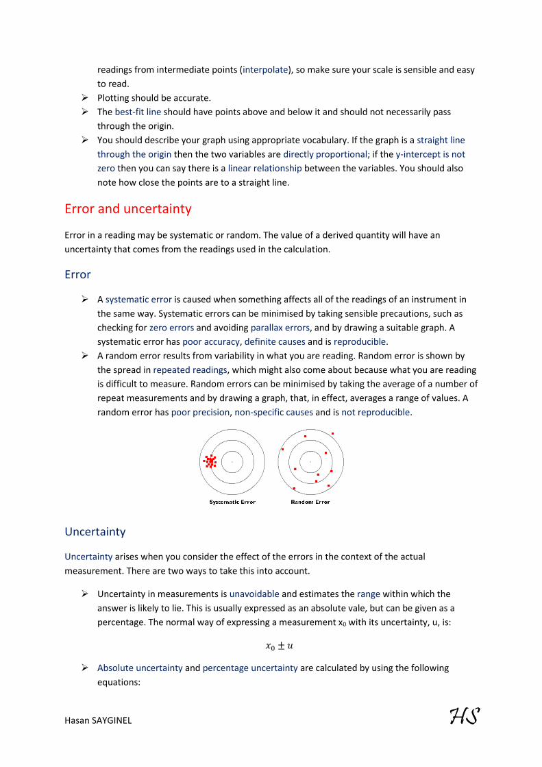
¾ A systematic error is caused when something affects all of the readings of an instrument in the same way. Systematic errors can be minimised by taking sensible precautions, such as checking for zero errors and avoiding parallax errors, and by drawing a suitable graph. A systematic error has poor accuracy, definite causes and is reproducible.

¾ A random error results from variability in what you are reading. Random error is shown by the spread in repeated readings, which might also come about because what you are reading is difficult to measure. Random errors can be minimised by taking the average of a number of repeat measurements and by drawing a graph, that, in effect, averages a range of values. A random error has poor precision, non-specific causes and is not reproducible.

Uncertainty

Uncertainty arises when you consider the effect of the errors in the context of the actual measurement. There are two ways to take this into account.

¾ Uncertainty in measurements is unavoidable and estimates the range within which the answer is likely to lie. This is usually expressed as an absolute vale, but can be given as a percentage. The normal way of expressing a measurement x0 with its uncertainty, u, is:

𝑥0 ± 𝑢

¾ Absolute uncertainty and percentage uncertainty are calculated by using the following equations:

Hasan SAYGINEL HS

𝑚𝑒𝑎𝑛 =𝑥1 + 𝑥2 + ⋯ + 𝑥𝑛

𝑛

𝑢 =𝑥𝑚𝑎𝑥 − 𝑥𝑚𝑖𝑛

2

,where 𝑥𝑚𝑎𝑥 is the maximum and 𝑥𝑚𝑖𝑛 the minimum reading of x. (Ignoring any anomalous readings)

𝑃𝑒𝑟𝑐𝑒𝑛𝑡𝑎𝑔𝑒 𝑢𝑛𝑐𝑒𝑟𝑡𝑎𝑖𝑛𝑡𝑦 =𝑈𝑛𝑐𝑒𝑟𝑡𝑎𝑖𝑛𝑡𝑦𝑀𝑒𝑎𝑛 𝑣𝑎𝑙𝑢𝑒

× 100%

¾ Uncertainties can be combined when 2 or more values with absolute uncertainties are treated.

1-) Multiplying and dividing: The percentage uncertainty in a quantity, formed when two or more quantities are combined by either multiplication or division, is the sum of the uncertainties in the quantities which are combined.

2-) Raising to a power: The percentage uncertainty in xn is n times the percentage uncertainty in x.

Note: The percentage uncertainty in 1𝑥𝑛 is again times the percentage uncertainty in x.

Note: The percentage uncertainty in √𝑥 is half the percentage uncertainty in x.

3-) Multiplying by a constant: The percentage uncertainty is unchanged.

¾ The other way to consider uncertainty is to use a graph. Plot error bars on the graph – these are lines drawn vertically and horizontally from the plot and indicate how much error there is in the reading. Now draw a best-fit line through the data points on the graph and then draw a worst-fit line that just fits through all the error bars. The uncertainty in the gradient is given by the difference between the two gradients.

Conclusion

The aim of the uncertainty calculation is to give a measure of the confidence you can have in your conclusion. The conclusion is the answer to the question in the hypothesis and the uncertainty, informed by your thoughts on errors, will give your results some validity.

As part of your conclusion you need to think about how you might improve the experiment. Your suggestions should reduce the uncertainty and improve your final answer in terms of accuracy and precision.

Hasan SAYGINEL HS

Glossary

Hasan SAYGINEL HS

A2 Physics Experiments 1. Conservation of linear momentum 2. Force and change of momentum 3. Centripetal force 4. Demonstrating a uniform electric field 5. Measuring the force between two charges 6. Measuring the capacitance of a capacitor 7. The efficiency of energy transfer from a capacitor 8. Charging and discharging a capacitor 9. The force on a current-carrying conductor 10. Deflecting electron beams 11. Capturing an induced emf 12. Measuring the specific heat capacity of a solid 13. Measuring the specific heat capacity of a liquid 14. Demonstrating the pressure law 15. Demonstrating Boyle’s law 16. Measuring background radiation 17. Modelling radioactive decay 18. Measuring the activity of a radioactive substance 19. Generating graphs of SHM 20. Forced oscillations 21. Investigating damped oscillations 22. Standard candles

Hasan SAYGINEL HS

1-) Conservation of linear momentum

A. INTRODUCTION The principle of conservation of linear momentum states that in any interaction between bodies, linear momentum is conserved, provided that no external force acts on the bodies. Therefore, the following equation can be applied to two colliding bodies:

𝑚𝑎𝑢𝑎 + 𝑚𝑏𝑢𝑏 = 𝑚𝑎𝑣𝑎 + 𝑚𝑏𝑣𝑏

The purpose of this experiment is to test on this principle using two trolleys (Trolley A and Trolley B) and a friction-compensated slope. As trolley B is stationary initially, and after the collision A and B move off together as a single object the general equation stated above becomes:

𝑚𝑎𝑢𝑎 = (𝑚𝑎 + 𝑚𝑏)𝑣

Therefore, to say that momentum is conserved, the initial momentum of A must be equal to the final momentum of A and B which couple together.

B. SAFETY x Lift the wooden support with care. x To reduce the danger of trolleys falling off the bench, a

means of stopping them safely at the bottom of the runway is needed. An enclosed area or piece of sponge would suffice. The area around the equipment should be kept free of bags, books.

C. APPARATUS x Two trolleys x Two light gates x 0.2 m interrupter card x Pin and cork

x Wooden runway x Means of compensating the runway

for friction.

D. PROCEDURE x Compensate for friction by tilting the runway slightly. Check by giving one trolley a small

push and confirming that it runs down the runway with constant speed. x Trolley A of mass mA is given a push so that, after its release, its interrupter card cuts

through a light beam with the trolley moving at a constant velocity down the friction-

Hasan SAYGINEL HS

compensated slope. The time in the light beam is interrupted is recorded electronically and the (constant) velocity, u, of trolley A is calculated.

x Trolley A has a cork attached with a pin sticking out of it that couples to a cork attached to trolley B of mass mB when A hits B.

x The two now move off together at a constant velocity, v, down the slope; a velocity that is calculated as the interrupter card on trolley A passes through the second light beam.

x The experiment is repeated for differing initial speeds and trolley masses.

E. DATA t1/s t2/s u/m s-1 v/m s-1 Initial momentum/N s Final momentum/N s

0.64 1.28 0.31 0.16 0.27 0.27 0.73 1.45 0.27 0.14 0.24 0.23 0.48 0.95 0.42 0.21 0.36 0.36 0.60 1.20 0.33 0.17 0.29 0.28

F. VALIDITY OF THE STUDY AND IMPROVEMENTS The values of the initial and final momentum are the same (±1%) in each case, indicating that the total momentum has been conserved. The uncertainty is most likely a result of an external resultant force acting on the system which includes air resistance.

The reason behind using an inclined plane: There should be no resultant external forces acting on the system for the momentum to be conserved. There will usually be resistive forces acting on the trolley. These forces can be compensated for by raising the end of the runway so that there is a component of the weight of the trolley acting down the plane. When this force is equal to the frictional forces, the resultant force on the trolley is zero. If the trolley is given a gentle push, it will continue to move down the runway at constant speed, just as it would on a horizontal track with no friction.

Î If the runway were horizontal, the frictional forces would lead to a change in momentum – the total momentum after the collision would be less than that before the collision.

G. CONCLUSION Initial momentum equals final momentum within reasonable accuracy, therefore this experiment has shown that momentum had been conserved in the collision of trolleys.

Hasan SAYGINEL HS

2-) Force and change of momentum

A. INTRODUCTION Newton’s second law establishes the relationship between the resultant force acting on an object and the change of momentum that it causes. An important result that follows from the second law and the definition of the Newton is F = m x a.

Newton’s second law states that:

The rate of change of momentum of an object is proportional to the resultant force acting on it and acts in the direction of the resultant force.

∆𝑝∆𝑡

∝ 𝐹

The definition of the size of the Newton fixes the proportionality constant at one.

The aim of this experiment is to investigate rate of change of momentum using a linear air track.

B. SAFETY x Place a padded box beneath the load so that the floor and masses do not get damaged. x To avoid injuries to feet, do not stand under falling masses.

C. APPARATUS

x Linear air track x Air blower x Rider x Two light gates

x Pulley suitable for fixing to the air track

x Thread x Set of slotted masses

Hasan SAYGINEL HS

D. PROCEDURE The light gates are connected to a suitable data logger and the results can either be interpreted manually or can be fed into a suitable computer programme. They are interpreted manually in this experiment. The following data is required:

x The length l of the card: 200 mm in this experiment x The times for the card to pass through each light gate, t1 and t2 x The time for the car to travel from the first light gate to the second light gate ∆𝑡 x The mass of the trolley mT: 450 g in this experiment

Method

¾ Measure the length of the card. ¾ Carry out the experiment for a particular force and record t1, t2 and ∆𝑡. ¾ Repeat the experiment a couple of times for the same force and calculate the average. ¾ Repeat the experiment for increasing magnitude of forces at 0.1N intervals. Î We need to think carefully about m. The force, which is the weight of the masses

hanging over the pulley has to accelerate the combined mass of the trolley, the masses on the trolley and the masses hanging over the pulley. In order to vary the force and at the same time keep m constant we have to take one of the masses off the trolley and add it to the load each time.

E. DATA The velocity through the first light gate is calculated using the equation: 𝑣1 = 𝑙

𝑡1

The velocity through the second light gate is calculated using the equation: 𝑣2 = 𝑙𝑡2

The change in momentum is then ∆𝑝 = 𝑚(𝑣2 − 𝑣1) = 𝑚∆𝑣 where m is the mass being accelerated.

Hasan SAYGINEL HS

F. REPRESENTATION OF DATA a graph of 𝐹∆𝑡 on the y-axis against ∆𝑣 on the x-axis is plotted.

G. VALIDITY OF THE STUDY AND IMPROVEMENTS Using a linear air track minimises friction.

The experiment should be repeated at each different load combination.

In order to draw a line of best fit, at least 6 points are needed.

H. CONCLUSION A graph of 𝐹∆𝑡 on the y-axis against ∆𝑣 on the x-axis is plotted and a straight line through the origin shows that ∆𝑣 ∝ 𝐹. The gradient is found to be m, then we can say that

𝐹∆𝑡 = 𝑚∆𝑣 or 𝐹 = 𝑚∆𝑣∆𝑡

= 𝑟𝑎𝑡𝑒 𝑜𝑓 𝑐ℎ𝑎𝑛𝑔𝑒 𝑜𝑓 𝑚𝑜𝑚𝑒𝑛𝑡𝑢𝑚

Hasan SAYGINEL HS

3-) Centripetal force

A. INTRODUCTION Consider a body of mass m moving in a circle of radius r at constant speed. While the magnitude of v is constant, its direction is continuously changing; in other words, although the linear speed is constant, the velocity, which is a vector quantity, is always changing.

x The change in velocity means that the mass is accelerating. x Since the magnitude of v remains unchanged, the acceleration must always be

directed at right angles to v, towards the centre of the circle. x The magnitude of the acceleration is given by:

This acceleration is known as the centripetal acceleration.

Using the relation 𝑣 = 𝜔𝑟, centripetal acceleration can also be expressed in terms of the angular speed:

𝑎 = 𝜔2𝑟

By Newton’s second law, a resultant force is required to produce the centripetal acceleration. This resultant force, called the centripetal force, is directed towards the centre of the circle and has a magnitude given by:

𝐹 = 𝑚𝑎 =𝑚𝑣2

𝑟= 𝑚𝜔2𝑟

The aim of this experiment is to verify the equation for centripetal force using a whirling bung.

𝐹 =𝑚𝑣2

𝑟

B. SAFETY x Glass tubing should be smoothed by heat treatment in a Bunsen flame. x Eye protection should be worn, even if the experiment is carried out outdoors.

C. APPARATUS x Rubber bung with a hole through it (mass

75g) x Length of string x Washers

x Stopwatch x Metre ruler x Short length of glass tube with ends

burred over

Hasan SAYGINEL HS

x Access to a balance x Eye protection

D. PROCEDURE x Tie the piece of string to a rubber bung and then thread it through a short length of glass

tube. x Fix a small weight to the lower end of the string. x Whirl the bung round in a horizontal circle while holding the glass tube so that the radius

of the bung’s orbit is constant. x Measure the mass of the bung (m), the total mass of the washers (M), the radius of the

orbit (R) and the time for ten orbits. x Repeat the experiment with different numbers of washers or Repeat the experiment

with different orbit radii or Repeat the experiment with bungs of different masses.

E. DATA - ANALYSIS Calculate the period of the orbit (T), the velocity of the bung in the orbit (𝑣 = 2𝜋𝑅

𝑇) and then

work out the centripetal force (𝐹 = 𝑚𝑣2

𝑅).

Compare this value with the weight of the washers (Mg).

M (g) F = Mg

(N) 10T (s) T (s) R (m) v = 2πR/T

(m/s) mv^2/R 50 0,49 21,9 2,19 0,83 2,38 0,51

100 0,98 16,2 1,62 0,80 3,10 0,90 150 1,47 13,5 1,35 0,93 4,33 1,51 200 1,96 11,2 1,12 0,79 4,43 1,86 250 2,45 10,7 1,07 0,99 5,81 2,56

Hasan SAYGINEL HS

F. REPRESENTATION OF DATA A graph v squared against r can be drawn and that can be used to find the mass of the bung if it is unknown.

G. VALIDITY OF THE STUDY AND IMPROVEMENTS Assumptions

When the supported mass M is in equilibrium,

x There is negligible friction between the glass tube and the string x That the string to the whirling rubber bund is effectively horizontal

Note: Time for 10 rotations is measured instead of 1 in order to reduce the percentage uncertainty in the measurement of the period.

H. CONCLUSION The tension in the string is known. T is equal to the weight of the supported mass M. Tension acts as the centripetal force in this experiment resulting in the circular motion of the rubber bung. The equation for centripetal force is used to calculate the force acting on the bung. In theory tension and centripetal force is equal thus the columns 2 and 6 in the table must be equal. Some values agree. As M gets larger, the agreement between the second and the sixth column becomes weaker which suggests that the system is not frictionless.

Hasan SAYGINEL HS

4-) Demonstrating a uniform electric field

A. INTRODUCTION An electric field is a region in space in which a charged object will experience a force. An electric field is generally represented by drawing field lines or lines of force. Electric field lines are drawn always pointing from positive to negative, like the flow of current. Just like magnetic and gravitational fields, the separation of the lines tells us the relative strength.

Electric field strength can be calculated:

𝐸 =𝐹𝑄

,where F is the force that would act on a positive charge Q placed in the electric field. It should be noted that E is a vector quantity whose direction is that of the force F.

Between a pair of parallel conducting plates that have a potential difference applied across them, the field is uniform, with all field lines perpendicular to the plates. As E is constant, F acting on a charged object should also be uniform.

The aim of this experiment is to demonstrate a uniform electric field using a rod with aluminium foil attached to on of its ends.

B. PROCEDURE x Cut a test strip of aluminium foil, about 20 mm by 5 mm. x Attach it to the bottom of an uncharged insulating rod. x Hold the ruler vertical and lower the end with its foil into the space between two

charged plates. x Move the ruler so that the aluminium foil is at different places between the charged

plates.

C. CONCLUSION If the yield is uniform, the force on the foil will be constant and the aluminium foil will hang at the same angle to the vertical wherever it is placed in the field. If the charges on the plates are reversed, the test strip swings to the same angle the other way.

Hasan SAYGINEL HS

5-) Measuring the force between two charges

A. INTRODUCTION The basic law describing the size of the force F between two point charges Q1 and Q2 is an inverse square law that depends on the distance r between the charges and the size and sign of the charges Q1 and Q2.

𝐹 =𝑘𝑄1𝑄2

𝑟2

The aim of this experiment to measure this force F between two charges.

B. SAFETY x Use a low potential difference.

C. APPARATUS

D. PROCEDURE x The forces are going to be very small, so a sensitive measuring device is required to

register changes in the force as the distance between the charges is changed. x Two conducting spheres, shown in blue, are charged by flicking the negative lower

sphere with woollen cloth and using the positive terminal of a d.c. supply set at about 30V to charge the upper sphere. Spheres are insulated so that they do not lose their charge.

x Readings on the top-pan balance should now be taken for different distances r between the centres of the spheres. One way of recording how this distance changes without touching the charged spheres is to project a shadow of them onto a nearby screen.

Hasan SAYGINEL HS

E. DATA m/g 0.11 0.38 0.62 0.83 1.14 r/cm 12.0 6.4 5.0 4.3 3.7

F. VALIDITY OF THE STUDY AND IMPROVEMENTS One difficulty is that some of the charge on one or both of the spheres may leak away during the experiment.

Another difficulty is the difficulty in measuring the distance r between the centres of the charged spheres.

G. CONCLUSION If 𝑚 ∝ 1

𝑦2⁄ , then the product my2 should be constant. Taking values from the table gives

the following values:

16, 16, 16, 15 and 16 to 2 SF

Hence the product is approximately constant and m is proportional to 1 𝑦2⁄ .

Hasan SAYGINEL HS

6-) Measuring the capacitance of a capacitor

A. INTRODUCTION The capacitance of a capacitor is defined as Q/V where Q is the size of the charge on the plates of the capacitor and V is the potential difference between the plates.

The aim of this experiment is to measure the capacitance on different capacitors.

B. SAFETY Capacitors of more than 1.0 Mf usually have a plus sign marked at one end and a maximum voltage written on them. It is very important in any activity to be sure that the + end of such a capacitor is connected to the positive terminal of the supply and that the maximum p.d. is not exceeded.

C. APPARATUS

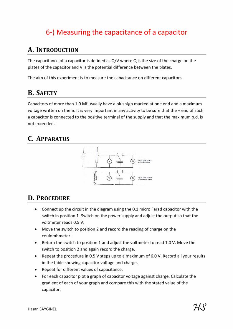
D. PROCEDURE x Connect up the circuit in the diagram using the 0.1 micro Farad capacitor with the

switch in position 1. Switch on the power supply and adjust the output so that the voltmeter reads 0.5 V.

x Move the switch to position 2 and record the reading of charge on the coulombmeter.

x Return the switch to position 1 and adjust the voltmeter to read 1.0 V. Move the switch to position 2 and again record the charge.

x Repeat the procedure in 0.5 V steps up to a maximum of 6.0 V. Record all your results in the table showing capacitor voltage and charge.

x Repeat for different values of capacitance. x For each capacitor plot a graph of capacitor voltage against charge. Calculate the

gradient of each of your graph and compare this with the stated value of the capacitor.

Hasan SAYGINEL HS

E. DATA

Hasan SAYGINEL HS

7-) The efficiency of energy transfer from a capacitor

A. INTRODUCTION Capacitors store energy. The energy transferred, or work done, when a charge ∆𝑄 moves across a potential difference of V is given by ∆𝑊 = 𝑉∆𝑄. When charging capacitors there is a problem in calculating the energy transferred using this formula because the p.d. changes as the capacitor charges!

Fortunately, V is proportional to Q, so the average p.d. is exactly half the final p.d., and we can use:

𝑊 = 𝑉𝑎𝑣𝑄 =12

𝑉𝑚𝑎𝑥𝑄

The aim of this experiment is to use this formula and exploit the principle of conservation of energy in order to calculate the efficiency of energy transfer from a capacitor to a motor which lifts a mass.

B. SAFETY x Fix the motor on the table. x Do not exceed the voltage limit of the capacitor.

C. APPARATUS

Hasan SAYGINEL HS

D. PROCEDURE x The electrical potential energy (EPE) stored in a 10000 𝜇𝐹 capacitor can be

transferred to gravitational potential energy (GPE) by discharging the capacitor through a small electric motor. As the capacitor discharges the current in the motor raises a small mass.

x The mass to be lifted could be a small ball of plasticine with a mass of, say, 8.0 g. the cotton is wound round the spindle of the electric motor and a vertical rule arranged to measure how far the plasticine is lifted. The gain of GPE by the plasticine is mgh so m must be small for measure values of h to be obtained. The capacitance of the capacitor C must, however, be large.

x A series of readings of V the charging voltage and h should be taken as the capacitor is first charged from the variable d.c. power supply and then discharged through the motor.

E. DATA V/V 7.5 9.0 10.5 12.0 h/m 0.27 0.40 0.53 0.71

F. REPRESENTATION OF DATA A graph of mgh (the gain of GPE in joules) against 1

2𝐶𝑉2(the loss of EPE in joules), or simply a graph

of h against V2, could be plotted. If the graph is a straight line through the origin, then ℎ ∝ 𝑉2, or ∆(GPE) is proportional to ∆(EPE).

G. VALIDITY OF THE STUDY The values of mgh and 1

2𝐶𝑉2 will not be equal because the efficiency of the energy transfer is not

100%. Some energy is inevitably lost to internal energy in heating the wires of the circuit and in working against friction in the motor. Over a wide range of values, the efficiency may not be constant and so ∆(GPE) may not proportional to ∆(EPE).

H. CONCLUSION Ideally, ∆(GPE) must be proportional to ∆(EPE). However, there are energy losses from the system due to friction and other forces so this is not the case.

Hasan SAYGINEL HS

8-) Charging and discharging a capacitor

A. INTRODUCTION The charging and discharging of a capacitor follows curved graphs in which the current is constantly changing, and so the rate of change of charge and pd are also constantly changing. These graphs are known as exponential curves. The shapes can be produced by plotting mathematical formulae which have power functions in them.

A data logger must be used in this experiment to display and analyse the potential difference across a capacitor as it charges and discharges through a resistor. Time is too small to collect data as you go.

The purpose of this experiment is to investigate charging and discharging capacitors and their graphs.

B. SAFETY x Ensure that the voltage rating of the capacitor is not exceeded. x Ensure that the electrolytic capacitor has the correct polarity in the circuit.

C. APPARATUS

D. PROCEDURE x The capacitor is charged through the resistor by connecting the switch to contact A.

The capacitor is then discharged through the same resistor by moving the switch to contact B. The p.d. across the capacitor is measured by the voltage sensor and recorded by the data logger. The data can then be analysed by the computer.

Hasan SAYGINEL HS

E. DATA

F. ANALYSIS OF DATA During the first 6 seconds (approximately) the capacitor is being charged through the resistor and the p.d. rises exponentially from zero to just under 6 V. The capacitor then discharges exponentially, becoming almost completely discharged after about 10 seconds.

Equations for the graph:

Charging: V = V0 (1 – e-t/RC)

Discharging: V = V0 e-t/RC

Estimating the capacitance and the uncertainty in the estimate

G. VALIDITY OF THE STUDY AND IMPROVEMENTS The value for the capacitance is only an estimate as it is difficult to read off the times with any accuracy from the graphs. This could be improved by expanding, say, the charging part of the graph so that the time scale was larger, thereby making the times easier to read off.

Hasan SAYGINEL HS

H. CONCLUSION The following equations can be used to calculate the potential difference across a charging and discharging capacitor:

Charging: V = V0 (1 – e-t/RC)

Discharging: V = V0 e-t/RC

Explaining the shape of the following graphs

Hasan SAYGINEL HS

9-) The force on a current-carrying conductor

A. INTRODUCTION The force acting on a current-carrying conductor is perpendicular to both the direction of magnetic field and the direction of current.

The aim of this experiment is to measure the magnitude of this magnetic force with varied current.

B. SAFETY x The power supply should be switched off between readings to avoid the copper wire

getting too hot.

C. APPARATUS

D. PROCEDURE x The balance is first zeroed and the current is then switched on. Having made sure the

horizontal piece of the wire carrying the current lies between the poles of the U-magnet and that the wire is perpendicular to the magnetic field, a series of balance readings m, in grams can be taken for a range of currents I.

x The magnetic force on the wire is, by Newton’s third law, equal in size but opposite direction to the magnetic force on the magnet – and it is this latter force that is registered by a change in the balance reading. The force can then be calculated using F = mg.

x A graph plotted of F against the current I enables a value for the magnetic field strength between the poles of the U-magnet to be deduced. (It is also possible to alter the length l of the horizontal wire in the magnetic field by using a second U-

Hasan SAYGINEL HS

magnet, but such an experiment gives only a rough test of how the force varies with l.)

E. DATA

F. REPRESENTATION OF DATA

G. VALIDITY OF THE STUDY AND IMPROVEMENTS

H. CONCLUSION As the graph is a straight line through the origin, the current in a wire in a magnetic field is directly proportional to the conventional current flowing through it.

Hasan SAYGINEL HS

10-) Deflecting electron beams

A. INTRODUCTION Electric fields

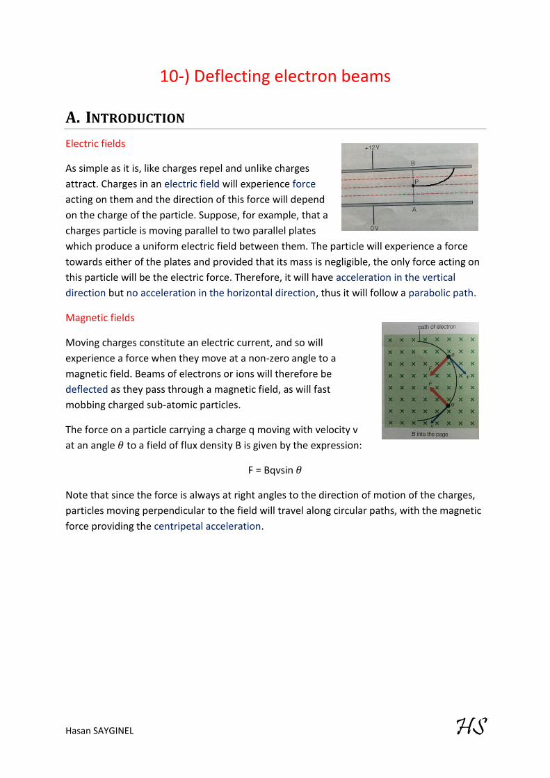
As simple as it is, like charges repel and unlike charges attract. Charges in an electric field will experience force acting on them and the direction of this force will depend on the charge of the particle. Suppose, for example, that a charges particle is moving parallel to two parallel plates which produce a uniform electric field between them. The particle will experience a force towards either of the plates and provided that its mass is negligible, the only force acting on this particle will be the electric force. Therefore, it will have acceleration in the vertical direction but no acceleration in the horizontal direction, thus it will follow a parabolic path.

Magnetic fields

Moving charges constitute an electric current, and so will experience a force when they move at a non-zero angle to a magnetic field. Beams of electrons or ions will therefore be deflected as they pass through a magnetic field, as will fast mobbing charged sub-atomic particles.

The force on a particle carrying a charge q moving with velocity v at an angle 𝜃 to a field of flux density B is given by the expression:

F = Bqvsin 𝜃

Note that since the force is always at right angles to the direction of motion of the charges, particles moving perpendicular to the field will travel along circular paths, with the magnetic force providing the centripetal acceleration.

Hasan SAYGINEL HS

11-) Capturing an induced e.m.f. A short bar magnet is dropped through a coil connected in series with a resistor. A data logger (a device that can capture a changing p.d. thousands of times per second) is connected across this resistor.

The data logger will record the potential difference as it varies across the resistor. The p.d. is equal in size at all times to the e.m.f. induced in the coil.

Apparatus

Data

Explanation of the shape of the graph

x Changing of flux / Cutting of field x Induced e.m.f. is proportional to the rate of change of flux (equation) x Initial increase in e.m.f. as the magnet gets closer to the coil x Negative gradient is when magnet is going through the coil x Magnet’s speed increases as it falls x Negative maximum value is greater than the positive maximum value x Time for second pulse is shorter x The areas of the two parts of the graph will be the same (since N𝜑 is constant)

Hasan SAYGINEL HS

Some questions

Q1 – Explain why the acceleration of the falling magnet is not quite 9.8 m s-2.

The induced e.m.f. produces a current in the coil-resistor circuit. This current in turn produces a magnetic field that will be up out of the coil as the magnet approaches, so repelling the falling magnet – Lenz’s law. Similarly, the falling magnet will be attracted back into the coil as the magnet exits the coil. Both these effects are producing upward forces on the magnet so its acceleration is not quite as big as the free fall acceleration.

Q2 – Describe how the output of the data logger would differ if:

a-) the coil is replaced by a coil with double the number of turns, and

Double the number of turns means that the induced magnetic flux through the coil is doubled. The induced e.m.f. is doubled at each stage of the fall, and so the peaks are each twice as high as they were.

b-) the magnet is dropped from a greater height.

When the magnet is dropped from a greater height the magnetic flux linking the coil changes at a greater rate. Therefore the e.m.f. , is greater and time taken for the magnet to pass through the coil is reduced. The peaks are both higher and narrower.

Hasan SAYGINEL HS

12-) Measuring the specific heat capacity of a solid

A. INTRODUCTION Transferring the same amount of energy to two different objects will increase their internal energy by the same amount. However, this will not necessarily cause the same rise in temperature in both. The increase in temperature can be calculated using the equation:

∆𝐸 = 𝑚𝑐∆𝜃

c, in the equation is the specific heat capacity of the object. This is defined as the amount of energy needed to raise the temperature of 1 kg of a particular substance by 1 K. Different materials have different specific heat capacities because their molecular structures are different and so their molecules will be affected to different degrees by additional heat energy.

The aim of this experiment is to measure the specific heat capacity of a solid using an electrical method.

B. SAFETY Use low voltages.

C. APPARATUS x Aluminium x Heat-resistant mat x Low-voltage heater and a suitable

power supply x Ammeter and voltmeter

x Thermometer x Stopclock x Insulating jacket with a hole for the

thermometer or sensor x Silicone grease

A temperature sensor and a data logger can be used instead of the thermometer and stop clock.

Hasan SAYGINEL HS

D. PROCEDURE x Measure the mass of metal block (m). x Put the thermometer in the small hole in the metal block. Place the heater in the large

hole in the block and switch it on. A small amount of silicone grease in the holes in the block can improve thermal contact. Place the insulating jacket around the apparatus.

x Set the voltage (V) to a convenient value and record this with the value of the current (I). x Measure the initial temperature and start the stopclock (or use a temperature sensor

and data logger). x Record the temperature at one-minute intervals. Switch off the heater when the

temperature reaches 50 °C.

(You may need to adjust the value of I during the experiment so that the power input remains constant.)

E. ANALYSIS Plot a graph of temperature against time and choose a section of the graph where the temperature is rising steadily. In this area find the temperature rise ∆𝜃 in a time ∆𝑡.

Calculate the electrical energy supplied to the heater (𝑉𝐼∆𝑡).

Calculate the specific heat capacity (c) of the metal of your block using the formula:

𝑐 =𝑉𝐼∆𝑡𝑚∆𝜃

where m is the mass of the block.

F. DATA m = 993 g

l = 3.10 A

V = 10.3 V

∆𝑡 = 3.00 minutes

𝜃𝑖 = 21.4°C

𝜃𝑓 = 27.3°C

G. VALIDITY OF THE STUDY AND IMPROVEMENTS Although this quick and practical method provides an accurate estimate of the specific heat capacity, there are several sources of error:

x Energy is absorbed by the heater itself; this is the main source of error and will make the value of c too large because it means that not all the energy supplied is used to raise the temperature of the block of metal.

Hasan SAYGINEL HS

x Energy is transferred to the surroundings, despite the lagging (also making c too large).

x A little energy will be taken by the lagging and the thermometer (again making c too large).

x Inaccuracy of the thermometer, especially ∆𝜃 is fairly small (this could make c too large if ∆𝜃 were too small or too small if ∆𝜃 were too large).

x Inaccuracy of the meters (again, this could affect the value of c either way).

H. CONCLUSION

Hasan SAYGINEL HS

13-) Measuring the specific heat capacity of a liquid

A. INTRODUCTION The aim of this experiment is to measure the specific heat capacity of a liquid using two different experimental set-ups.

B. SAFETY Do not heat the contents of the calorimeter above 50°C.

C. APPARATUS First set-up

x A copper or aluminium calorimeter with a volume between 250 and 400 ml

x Insulating jacket with a hole for the thermometer or sensor

x Electrical immersion heater x Voltmeter and ammeter x Low-voltage power supply (0-12V) x Thermometer (0-50°C) x Stopclock

(A temperature sensor and datalogger can be used instead of the thermometer and stopclock.)

Second set-up

x Expanded polystyrene cup x Thermometer x Heater

x Ammeter and voltmeter x Stopclock

D. PROCEDURE First set-up

x Set up the apparatus as shown in the diagram. x Measure the mass of the calorimeter (mc) and fill it with a

known mass of water (mw). There must be enough water to cover he immersion heater when it is put in the calorimeter. Place the muff over the calorimeter.

x Switch on the heater. Set the voltage (V) to a convenient value and record this with the value of the current (I).

x Measure the initial water temperature (𝜃) using a thermometer and start the stopclock (or use a temperature sensor and datalogger).

Hasan SAYGINEL HS

x Record the temperature at one-minute intervals, stirring just before the thermometer is read.

x Switch off the heater when the temperature reaches 50°C.

Second set-up

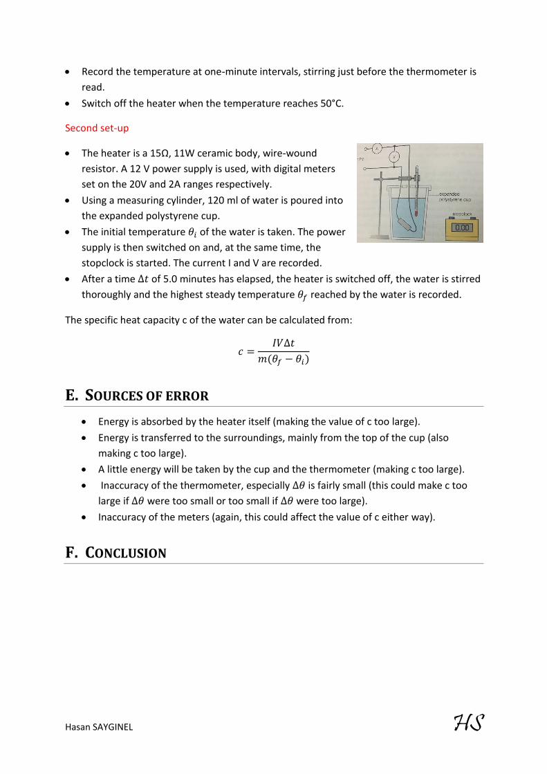
x The heater is a 15Ω, 11W ceramic body, wire-wound resistor. A 12 V power supply is used, with digital meters set on the 20V and 2A ranges respectively.

x Using a measuring cylinder, 120 ml of water is poured into the expanded polystyrene cup.

x The initial temperature 𝜃𝑖 of the water is taken. The power supply is then switched on and, at the same time, the stopclock is started. The current I and V are recorded.

x After a time ∆𝑡 of 5.0 minutes has elapsed, the heater is switched off, the water is stirred thoroughly and the highest steady temperature 𝜃𝑓 reached by the water is recorded.

The specific heat capacity c of the water can be calculated from:

𝑐 =𝐼𝑉∆𝑡

𝑚(𝜃𝑓 − 𝜃𝑖)

E. SOURCES OF ERROR x Energy is absorbed by the heater itself (making the value of c too large). x Energy is transferred to the surroundings, mainly from the top of the cup (also

making c too large). x A little energy will be taken by the cup and the thermometer (making c too large). x Inaccuracy of the thermometer, especially ∆𝜃 is fairly small (this could make c too

large if ∆𝜃 were too small or too small if ∆𝜃 were too large). x Inaccuracy of the meters (again, this could affect the value of c either way).

F. CONCLUSION

Hasan SAYGINEL HS

14-) Demonstrating the pressure law

A. INTRODUCTION When we are looking at the behaviour of gases we have four variables to consider – the mass, pressure, volume and temperature of the gas. These four variables are related by the ideal gas law equation:

𝑝𝑉 = 𝑛𝑅𝑇

In order to investigate how these quantities are related, we need to keep two constant while we see how the other two vary with one another.

The aim of this experiment is to investigate how the pressure of a gas changes when it is heated at a constant volume, thus two factors investigated are pressure and temperature.

B. SAFETY Wear eye protection if your face is to be close to the hot water.

C. APPARATUS x Round-bottomed flask x Temperature sensor and probe x Rubber bung with a short length of

glass tube fitted through it x Length of rubber tubing x Pressure sensor

x Bunsen burner, tripod, gauze and mat

x Glass beaker x Water x Ice x Eye protection

This experiment can be performed either using a thermometer and a pressure gauge or using temperature and pressure sensors with a suitable datalogger. Note that the tube connecting the container of air to the pressure gauge/sensor should be as short and of small an internal diameter as possible to reduce the volume of air inside the tube to a minimum, because this air will not be at the same temperature as that in the flask.

Hasan SAYGINEL HS

D. PROCEDURE x Initially the beaker is packed with ice to get low a starting temperature as possible. x Record the temperature of the water (effectively the temperature of air in the flask) and

the pressure of the air. x Light the Bunsen burner and heat the water slowly. x Record the pressure and temperature of the air at 10-degree intervals until the water

temperature reaches 80°C.

E. ANALYSIS Plot a graph of the pressure of the trapped air (y-axis) against the temperature of the trapped air (x-axis). (Make sure that the pressure you record is the pressure of the trapped air, not just the excess above atmospheric pressure. It is assumed that the temperature of the trapped air will be the same as that of the water in the beaker.

Draw a second graph with the temperature axis showing -300°C to +100°C and find the intercept on the pressure axis. This should be at absolute zero.

Record your value for absolute zero, suggesting any inaccuracies in your experiment and how they might be reduced.

F. VALIDITY OF THE STUDY AND IMPROVEMENTS x Extrapolation x Inaccuracy in thermometer x Uneven heat distribution

G. CONCLUSION As the graph is a straight line through the origin, it shows that

𝑝 ∝ 𝑇 or 𝑝𝑇

= 𝑐𝑜𝑛𝑠𝑡𝑎𝑛𝑡

for a fixed mass of gas at constant volume.

Hasan SAYGINEL HS

15-) Demonstrating Boyle's law

A. INTRODUCTION Boyle’s law states that:

For a constant mass of gas at a constant temperature, the pressure exerted by the gas is inversely proportional to the volume it occupies.

This relationship can be derived from the ideal gas law equation as was the case in the previous experiment.

The aim of this experiment is to verify the relationship between the pressure and volume for a gas.

𝑝𝛼1𝑉

B. SAFETY The apparatus should include a protective plastic screen around the glass tube. However, a safety screen is advisable.

Do not increase the pressure to more than 300 kPa.

C. APPARATUS x Boyle’s law apparatus x Bicycle pump x Length of thick-walled rubber

tubing

x Thermometer x Safety screen

Hasan SAYGINEL HS

D. PROCEDURE x The simple apparatus shown can be used. x The volume V of the fixed mass or air under test is given by the length l of the column air

multiplied by the area of cross section of the glass tube. If the tube is uniform, this area will be constant, so we can assume that 𝑉 ∝ 𝑙.

x The total pressure of the air is read straight off the pressure gauge. x The valve is opened so that the air starts at atmospheric pressure and then the pressure

is increased by means of the foot pump. This pressure is transmitted through the oil and compresses the air.

x The pressure p and the corresponding length l of the air column are recorded for as wide a range of values as possible. --- It is important to leave sufficient time after each change in pressure for the air to reach thermal equilibrium with its surroundings so that its temperature remains constant.

x The measurements of p and l are tabulates, together with values of 1/l.

E. DATA

F. REPRESENTATION OF DATA

G. VALIDITY OF THE STUDY AND IMPROVEMENTS x Constant temperature must be ensured. x Gas should not escape.

Hasan SAYGINEL HS

H. CONCLUSION The graph of p against V is called an isothermal. An isothermal is a curve that shows the relationship between the pressure and volume of a gas at a particular temperature. As this is a straight line through the origin we can deduce that:

𝑝 = 1𝑉

or𝑝 = 𝑐𝑜𝑛𝑠𝑡𝑎𝑛𝑡 × 1𝑉

Giving pV = constant

A convenient way of remembering Boyle’s law for calculations is:

𝑝1𝑉1 = 𝑝2𝑉2

Three different graphs may be drawn which illustrate Boyle’s law and these are shown below along with how each graph would be altered with an increase in temperature.

Hasan SAYGINEL HS

16-) Measuring background radiation

A. INTRODUCTION We live in a radioactive environment and the radiation, which is constantly present in our environment, is called background radiation. There are various sources of background activity. The main natural sources of background radiation are:

x Radioactive gases (mainly radon) emitted from the ground x Radioactive elements in the Earth’s crust – mainly uranium and the isotopes it forms x Cosmic rays from outer space which bombard the Earth’s atmosphere producing

showers of lower-energy particles such as muons, neutrons and electrons x Naturally occurring radioactive isotopes present in our food and drink, and in the air we

breathe

The aim of this experiment is to measure the background count rate.

B. APPARATUS x Geiger – Müller tube and counter x Stopclock

C. PROCEDURE The Geiger-Muller tube detects radiation. Each time it absorbs radiation, it transmits an electrical pulse to a counting machine. This makes a clicking sound or displays the count rate. The greater the frequency of clicks, or the higher the count rate, the more radiation the Geiger-Muller tube is absorbing.

It is easy to determine the average background radiation in your area using a Geiger-Müller tube and counter. As radioactive decay is a random and spontaneous process, the activity in your lab must be measured over a long period of time (30 minutes or more) and then an average calculated. Otherwise, you may find that the measurement is, by chance, particularly high or particularly low and thus does not truly indicate the average over time. For example, if the G – M tube and counter are set to counting for two hours, and the final count is then divided by 7200 seconds, this will give a good approximation to the average over time as the count time is long compared with the typical average count of about 0.5Bq.

Hasan SAYGINEL HS

17-) Modelling radioactive decay

D. APPARATUS x Large beaker x 24 dice

E. PROCEDURE x Twenty-four dice (or small cubes of wood with one face marked with a cross) are shaken

in a beaker and tipped onto the bench. x All the dice that have landed with six uppermost are removed – these are deemed to

have decayed. x The number N of dice remaining are then counted. x This process is repeated until all the dice have decayed. x A graph of N against x (the number of throws) is plotted.

F. DATA

G. REPRESENTATION OF DATA

H. ANALYSIS The curve is not smooth because whether or not a six is thrown is a random event, just like radioactivity. It is instructive to repeat the experiment and average the results, or else combine the results with those of one or more classmates. It will be found that the more results that are combined, the smoother the curve will become.

Hasan SAYGINEL HS

Radioactivity is a random process similar to throwing dice, although it differs from this dice-throwing model insomuch as it is a continuous process and the numbers involved are much, much larger.

“Decay constant” Æ Half-life

I. CONCLUSION AND MODEL OF RADIOACTIVE DECAY Radioactivity differs from the dice-throwing model as it is continuous. The concept of half-life is used to model radioactive decay. Half-life of a particular isotope is the average time for a given number of radioactive nuclei of that isotope to decay to half that number.

As radioactivity is an entirely random process, we can only ever determine an average value of the half-life because it will be slightly different each time we measure it. However, the very large number of nuclei involved in radioactive decay means that our defining equation, -dN/dt = λN is statistically valid.

The graph for radioactive decay is an exponential curve and the equation is:

𝑁 = 𝑁0𝑒−𝜆𝑡

From this equation it can be deduced mathematically that the half-life, 𝑡12⁄ , is related to the

decay constant, λ, by the expression:

𝑡12⁄ =

ln 2𝜆

Hasan SAYGINEL HS

18-) Investigating the absorption of 𝛾-radiation by lead

A. INTRODUCTION Different types of radiation have different penetrating powers and can be stopped by different materials of various length. The absorption of any type of radiation is modelled as an exponential curve and the equation 𝑁 = 𝑁0𝑒−𝜇𝑥.

The aim of this experiment is to investigate the absorption of gamma radiation by several thicknesses of lead.

B. SAFETY x A sealed source should always be used. x The source must be kept in a lead-lined box in a special locked metal cupboard in a

separate store room, labelled with the radioactivity symbol. x Protective gloves should be worn. x Always handle the source with tongs. x Keep as far away from the source as possible. x Keep exposure time to a minimum.

C. APPARATUS x Geiger – Müller (GM) tube, lead and stand x Source holder x Beta source x Pair of long forceps x Counter/scalar and stopclock x Ruler

Hasan SAYGINEL HS

D. PROCEDURE x The thickness of each of the discs is measured with Vernier callipers or a micrometre. x The background count rate is recorded for 5 minutes. This is repeated and the average

value subtracted from subsequent readings. x Once this has been done, the source is put in position and the count N0 with no lead

discs in place is recorded. x The count N is then taken for several thicknesses of x of lead by using the discs, either

singly or in combination, as absorbers. Care must be taken to keep the distance between the source and G-M tube constant.

x A graph of the count rate N against absorber thickness x is initially plotted. x To test whether the graph is an exponential curve, a graph of ln N against x should be

plotted.

E. DATA

F. REPRESENTATION OF DATA

Hasan SAYGINEL HS

G. CONCLUSION The suggested relationship between N and x was:

𝑁 = 𝑁0𝑒−𝜇𝑥

Taking logs of both sides gives,

ln 𝑁 = −𝜇𝑥 + 𝑙𝑛 𝑁0

This is equivalent to y = mx + c. Allowing for a bit of scatter, which is to be expected because of the random nature of radioactive emission, the graph is a straight line of negative gradient, with intercept ln N0. This confirms that the absorption of the gamma radiation varies exponentially with the thickness of the absorber as proposed.

Hasan SAYGINEL HS

19-) Generating graphs of SHM

A. INTRODUCTION Simple harmonic motion is periodic motion about an equilibrium position and all SHMs share two common characteristics:

x The resultant force acting on the oscillating body, and therefore its acceleration, is proportional to the displacement of the body.

x The resultant force, and therefore the acceleration, always acts in a direction towards the equilibrium position.

These conditions are combined into a simple equation:

𝐹 = −𝑘𝑥

X is the horizontal distance from the centre. The motion is a projection of a circular motion so the equations for angular velocity, displacement, frequency and time are equally valid for simple harmonic motion.

When the object is at position A, this projected distance x is equal to the radius of the circle, r, but at position B this distance is shown by OC. This distance can be calculated from:

𝑥 = 𝑟 cos 𝜃

Or: 𝑥 = 𝑟 cos(𝜔𝑡)

In this experiment a spring is used therefore r is replaced with A which denotes the displacement. The equation for SHM is then:

𝐹 = −𝑘𝐴 cos(𝜔𝑡)

The aim of this experiment is to generate graphs of some of the different properties of a system undergoing simple harmonic motion and interpret the graphs mathematically.

B. PROCEDURE This experiment is very simple as a motion sensor and a data logger are used. The set-up shown is arranged. A card is attached to the masses to give a good reflective surface, but may not be needed if the base of the masses is large enough. Typically the data logger

Hasan SAYGINEL HS

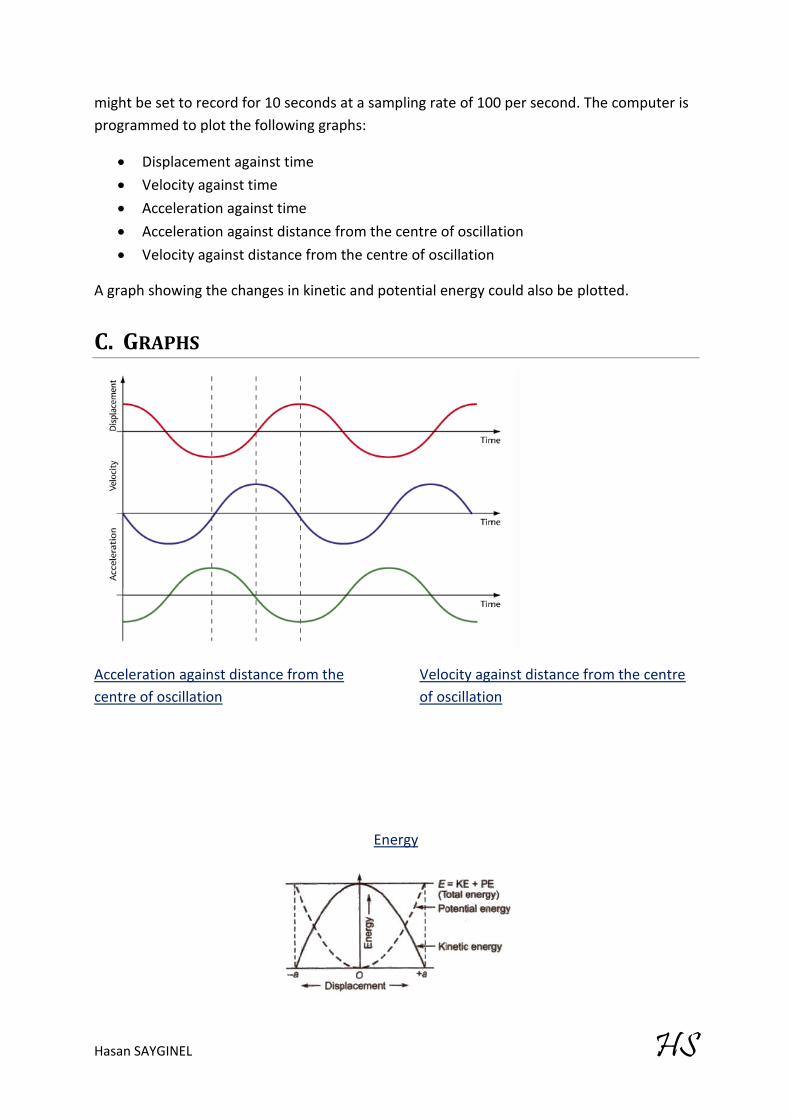
might be set to record for 10 seconds at a sampling rate of 100 per second. The computer is programmed to plot the following graphs:

x Displacement against time x Velocity against time x Acceleration against time x Acceleration against distance from the centre of oscillation x Velocity against distance from the centre of oscillation

A graph showing the changes in kinetic and potential energy could also be plotted.

C. GRAPHS

Acceleration against distance from the centre of oscillation

Velocity against distance from the centre of oscillation

Energy

Hasan SAYGINEL HS

D. INTERPRETATION OF GRAPHS AND CONCLUSION Displacement – time graph

The graph is a typical cosine graph. The equation of the graph is 𝒙 = 𝑨 𝐜𝐨𝐬(𝝎𝒕):

Velocity – time graph

We can calculate the velocity of an oscillator at any moment from the gradient of the displacement – time graph.

Differentiating 𝑥 = 𝐴 cos(𝜔𝑡) gives:

𝒅𝒙𝒅𝒕

= −𝑨𝝎 𝐬𝐢𝐧(𝝎𝒕)

This is the equation of the velocity – time graph. It is sine graph reflected in the x-axis.

Acceleration – time graph

Differentiating the function which represents the velocity – time graph gives the equation of the acceleration – time graph.

𝒅𝟐𝒙𝒅𝒕𝟐 = −𝑨𝝎𝟐 𝐜𝐨𝐬(𝝎𝒕)

Therefore, the acceleration – time graph is a cosine function reflected in the x-axis.

Acceleration against distance from the centre of oscillation

Velocity against distance from the centre of oscillation

Energy graph

Total mechanical energy is conserved and is exchanged between gravitational potential energy and kinetic energy.

Hasan SAYGINEL HS

20-) Forced oscillations

A. INTRODUCTION A free oscillation is one in which no external force acts on the oscillating system except the force that gives rise to the oscillation. Forced oscillations occur if a force is continually or repeatedly applied to keep the oscillation going so that the system is made to vibrate at the frequency of the vibrating source and not at its own natural frequency of vibration.

The aim of this experiment is to investigate how the amplitude of a system subjected to a forced oscillation varies with the driving frequency.

B. SAFETY Wear eye protection.

C. APPARATUS x Spring x Hanging masses x Clamp and stand x Datalogging laptop x Motion sensor x Signal generator x Vibration generator

Hasan SAYGINEL HS

21-) Investigating damped oscillations

A. INTRODUCTION A damped oscillation is one in which energy is being transferred to the surroundings, resulting in oscillations of reduced amplitude and energy. An oscillating system does work against the external forces acting on it, such as air resistance, and so uses up some of its energy. This transfer of energy from the oscillating system to internal energy of the surrounding air causes the oscillations to slow down and eventually die away.

The aim of this experiment is to investigate the oscillations of an air-damped mass-spring system.

B. SAFETY Take care masses do not fall and cause injury.

C. APPARATUS

D. PROCEDURE x Set up the apparatus as shown in the diagram. x The mass on the end of the spring (m) should be chosen so that the period is as long as

possible without damaging the spring. x Record the rest position of the mass. x Pull the mass downwards (by about half the original extension) and release, allowing it to

oscillate. x Record the position of maximum displacement of the mass every 5 oscillations and

hence calculate the amplitude (A) of oscillation each time. x Repeat and take an average for each amplitude.

Hasan SAYGINEL HS

E. GRAPHS

F. SOURCES OF ERROR x Parallax error in amplitude measurement x The stand not perpendicular to the surface

G. CONCLUSION

Hasan SAYGINEL HS

22-) Standard candles

Luminosity and flux

Luminosity is the word astrophysicists use to describe the total output power of a star, unit W.

The electromagnetic wave energy per second per unit area from a star reaching us on Earth is called the radiation flux from the star, symbol F, unit W m-2.

Luminosity (L) and radiation flux (F) are linked by the inverse-square law:

𝐹 𝑜𝑟 𝐼 =𝐿

4𝜋𝑑2

d is the distance from Earth to the star.

Therefore, the following equation can be used to calculate the distance of a star from Earth:

4𝜋𝑑2 =𝐿𝐹

=𝑙𝑢𝑚𝑖𝑛𝑜𝑠𝑖𝑡𝑦

𝑟𝑎𝑑𝑖𝑎𝑡𝑖𝑜𝑛 𝑓𝑙𝑢𝑥

Standard candles

The problem in using the equation to measure how far it is to a star is how to determine the star’s full power output – its luminosity L.

A type of star now called a Cepheid was discovered by Henrietta Leavitt. A Cepheid star has a luminosity that varies with time. Such stars appear more bright and less bright with periods of the order of days. Further, she was able to establish that the maximum luminosity L of a Cepheid star was related to the period T of its luminosity variation. For the first time it was thus possible, by measuring T for a Cepheid star that it is too far away to show any parallax wobble, to know the star’s luminosity. Such stars are valuable standard candles.

A standard candle is a distant star of known (maximum) luminosity.

The process to find the distance d from Earth to a star is therefore:

x Locate a Cepheid variable star x Measure its period T x Find the star’s luminosity L using Leavitt’s T – L data x Measure the radiation flux F from the star at Earth

x Calculate d using 𝑑 = √ 𝐿4𝜋𝐹