Physical mechanisms for sporadic wind wave horse-shoe patterns
247
ISSN: 0997-7546 EJBFEV
-
Upload
independent -
Category
Documents
-
view
3 -
download
0
Transcript of Physical mechanisms for sporadic wind wave horse-shoe patterns

ISSN: 0997-7546 EJBFEV

EUROPEAN JOURNAL OF MECHANICS B/FLUIDS An official medium of publication for EUROMECH - 'European Mechanics Society'
The manuscripts should be sent to one of the Editors-in-Chief
Editors-in-Chief: F. DIAS Institut Non Lineaire de Nice 1361, route des Lucioles 06560 Valbonne, France Tel: + 33 4 92 96 73 07 Fax: + 33 4 93 65 25 17 [email protected]
G. J. F. VAN HEIJST
Eindhoven University of Technolog)' Department of Physics
Fluid Dynamics Laboratory
P.O. Box 513 NL-5600 MB Eindhoven, The Netherlands
Tel.: + 31 40 24 72 722 Fax: + 31 40 24 GA 151
Advisory board T. AKYI.AS Cambridge (USA) G. I. BARENBI.A'ET Berkeley (USA) D. BARTIIl;S-BlHSt:i. Compieguc (France) E H. BUSSE Bayreuth (Germany) C. CuRCICNANI Milano (Italy) H. I. ENE Bucharest (Romania) H. H. pERNllOEZ Berlin (Germany) R. FRIEDRICH München (Germany)
G. P. GAI.DI Fmam (Italy) P. GERMAIN Paris (France) P. HlJERRE Paris (France) G. looss Nice (France) J. JIMENEZ Madrid (Spain) A. V. JOHANSSON Stockholm (Sweden) Y. S. KACHANOV Novosibirsk (Russia) L. Kl.HSER Zürich (Switzerland)
E. KRAUSE Aachen (Germany) H. K. MOFFATT Cambridge (UK) E A. MONKEWITZ Lausanne (Switzerland) R. MoREAU Saint-Martin d'H'eres (France) G. OOMS Rijswijk (Fhe Netherlands) E T. SMITH London (UK) J. So.MMERIA Lyon (France) S. ZAEESK! Paris (France)
The European Journal of Mechanics is abstracted and/or indexed in:
Applied Mechanics Reviews, Current Contents (PC & ES), Mechanics Contents, Mathematical Reviews, Inspec Science Abstracts, Pascal Database, Current Mathematical Publications, Math Sei., Current Contents (EC &T), Science Citation Index, Sei Search, Research Alert, Materials Science Citation Index, Zentralblatt Für Mathemathik.
Associate Editors I. P. CASTRO
University of Surrey Department of Mechanical Engineering Guildford, Surrey GU2 5XH, UK [email protected]
P. LUCHINI
Dipartimento di Ingegneria Aerospaziale Politecnico di Milano Via La Masa 34 20158 Milano, Italy [email protected]
L. G. REDEKOPP
University of Southern California Department of Aerospace Engineering Los Angeles, CA 90089, USA [email protected]
EDITIONS ELSEVIER
23, ruel jnois 75724 Paris cedcx \5. France
hUp://www.elsevier.fY A member of Hlsevier Science
lilitions KciiMitifiques el in helical es Klsevier SAS :m ,-.,^u\ ,le W) ^HXX) ]■ - !W 113 87/ KCS I',« i-;
HARD SCIENCES DEPARTMENT Tel.: 33 1 45 58 90 67 Fax: 33 1 45 58 94 21 Desk editor: Christine Gray Tel.: +33 1 45 58 98 63, [email protected] http://www.elsevier.fr
SUBSCRIPTIONS Tel.: +33 1 45 58 90 67 Fax: +33 1 45 58 94 24. [email protected] Subscription information 1999 - EJM-B/Fluids - Vol 18 - 6 issues - ISSN 0997-7546
France EU* North, Central and South America Rest of the world
EJM-B U FF2 551 □ FF 2 605 O US$ 530 Q FF3 139
EJM-A □ FF 2 944 Q FF 3 005 D US$ 592 Q FF 3 506
EJM-A + EJM-B Q FF4 946 ü FF 5 048 a us$ i oio □ FF5 98I
* Customers resident in the EU (European Union) are liable for VAT (2.19). For tax exemption. VAT registration number must he indicated. Special rales apply for Euromeeh members, please eontact your society. All priees inelude air deiiveiy
Address order and payment to: Editions scientifiques et medicales Elsevier, 23, rue Linois, 75724 Paris cedex 15, France • by cheque or credit card (CB, EuroCard, MasterCard or Visa) indicate number and expiration date • by transfer: CCP Paris n° 30041 00001 1904540 H 020/70
Subscriptions begin 4 weeks after receipt of payment and start with the first issue of the calendar year. Back issues and volumes are available from
the publisher. Claims for missing issues should be made within 6 months of publication.
© 1999 Editions scientifiques et medicales Elsevier, Paris
En application dc la loi du Ier juillet 1992, il est interdit de reproduce, meine partiellement, la presente publication sans l'autorisation de l'editeur ou du Centre francais d'exploitation du droit de copie (20, rue des Grands-Augustins, 75006 Paris). All rights reserved. No part of this publication may be translated, reproduced, stored in a retrieval system or transmitted in any form or by any other means, electronic, mechanical, photocopying, recording or otherwise, without prior permission of the publisher.
lniprimc en France par STEDI President-dirccteur general et directeur de la publication : Catherine Lucet 1, bd Ncy, F-75.018 Paris Commission paritaire n° 0603 T 71133 Depot legal : 5795 - Ä partition Periodicite : 6 nos / an
r
Preface
This special issue of the journal contains a selection of papers presented at the IUTAM Symposium on Three-Dimensional Aspects of Air-Sea Interaction, held in Nice on 17-21 May 1998. This IUTAM symposium, organized jointly by the "Institut Non-Lineaire de Nice" and the "Institut de Recherche sur les Phenomenes Hors Equilibre," covered theoretical, numerical and experimental studies in three-dimensional wave fields. The meet- ing was designed to promote closer interactions among a wide spectrum of experts, including fluid mechanicians, oceanographers and mathematicians and give a new momentum to this field.
The main topics which were considered during the symposium are represented through the selection of papers. These topics are: Wind-waves interactions, wave-wave interactions, wave-current interactions, breaking waves, long waves (surface and internal waves) and remote sensing.
This collection of papers provides a good introduction to a range of challenging problems in three-dimensional aspects of air-sea interaction.
Frederic DIAS and Christian KHARIF
Chairmen of the Symposium
20011130 012 U.S. Government Rights License This work relates to Department of the Navy Grant or Contract issued by Office of Naval Research (ONR) International Field Office- Europe. The United States Government has a royalty-free license throughout the world in all copyrightable material contained herein.
$g fOSi-CQ.-QZ&l

Acknowledgements
We would like to thank all the members of the International Scientific Committee: R. Grimshaw (Monash University, Australia), K. Kirchgässner (Stuttgart Universität, Germany), C. Mei (Massachusetts Institute of Technology, USA), H. Mitsuyasu (Hiroshima Institute of Technology, Japan), K. Moffatt (Isaac Newton Institute, UK), H. Peregrine (University of Bristol, UK), H. Segur (University of Colorado, USA) and V. Zakharov (Landau Institute for Theoretical Physics, Russia).
Special thanks go to all the referees, who did a very careful job in reviewing all the papers which were submitted to this special issue.
The success of the symposium as well as the publication of this volume were made possible through various grants received from IUTAM (International Union of Theoretical and Applied Mechanics), ONR (Office of Naval Research), DGA1 (Delegation Generale pour l'Armement), CNRS (Centre National de la Recherche Scientifique - Departement des Sciences Physiques et Mathematiques et Departement des Sciences Pour PIngenieur), the University of Nice Sophia-Antipolis, AUM (Association Universitaire de Mecanique), the City of Nice, MENRT (Ministere de l'Education Nationale, de la Recherche et de la Technologie), the Conseil General des Alpes Maritimes, the European Community (Commission of the European Communities - Direction Generale XII).
U.S. Government Rights License This work relates to Department of the Navy Grant or Contract issued by Office of Naval Research (ONR) International Field Office- Europe. The United States Government has a royalty-free license throughout the world in all copyrightable material contained herein.
luLe present document a ete etabli en execution du contrat MS N° 97—1106 passe par la direction des systemes de forces et de la prospective (Delegation Generale pour l'Armement)."

REPORT DOCUMENTATION PAGE Form Approved OMB No. 0704-0188
Public reporting burden for this collection of information is estimated to average 1 hour per response, including the time for reviewing instructions, searching existing data sources, gathering and maintaining the data needed, and completing and reviewing the collection of information. Send comments regarding this burden estimate or any other aspect of this collection of information, including suggestions for reducing this burden to Washington Headquarters Services, Directorate for Information Operations and Reports, 1215 Jefferson Davis Highway, Suite 1204, Arlington, VA 22202-4302, and to the Office of Management and Budget, Paperwork Reduction Project (0704-0188), Washington, DC 20503. 1. AGENCY USE ONLY (Leave blank) 2. REPORT DATE
May 1999
3. REPORT TYPE AND DATES COVERED
17-21 May 1998 Conference Proceedings
TITLE AND SUBTITLE
IUTAM Symposium on Three Dimensional Aspects of Air-Sea Interation. 17-21 May 1998.
Nice,
6. AUTHOR(S)
Frederic Dias, Editor
5. FUNDING NUMBERS
7. PERFORMING ORGANIZATION NAME(S) AND ADDRESS(ES)
Institut Non Lineaire de nice 1361, route des Lucioles 06560 Valbonne, France
8. PERFORMING ORGANIZATION REPORT NUMBER
ISSN 00997-7546
9. SPONSORING/MONITORING AGENCY NAME(S) AND ADDRESS(ES)
Office of Naval Research, European Office PSC 802 Box 39 FPO AE 09499-0039
10. SPONSORING/MONITORING AGENCY REPORT NUMBER
11. SUPPLEMENTARY NOTES Published in the European Journal of Mechanics, B/Fluids, Vol. 18 No.3, May-June 1999. Special Issue: Three-Dimensional Aspects of Air-Sea Interaction. Published by Editions Elsevier, 23 rue Linois, 75724 Paris cedex, 15, France for EUROMECH- European Mechanics Society. This work relates to Department of the Navy Grant issued by the Office of Naval Research International Field Office. The United States has a royalty free license throughout the world in all copyrightable material contained herein.
12a. DISTRIBUTION/AVAILABILITY STATEMENT
Approved for Public Release. U.S. Government Rights License, holder. (Code 1,20)
All other rights reserved by the copyright
12b. DISTRIBUTION CODE
12. ABSTRACT (Maximum 200 words)
The special issue of the European Journal of Mechanics contains a selection of papers presented at the IUTAM Symposium on Three-Dimensional Aspects of Air-Sea Interaction held in Nice on 17-21 May 1998. The symposium covered theoretical, numerical and experimental studies in three-dimensional wave fields. The main topics are: wind-waves interactions, wave- wave interactions, wave-current interactions, breaking waves, long waves (surface and internal waves) and remote sensing.
13. SUBJECT TERMS EOARD, Foreign reports, IUTAM, Conference proceedings, Reprints, Remote sensing, Wave propogation,
17. SECURITY CLASSIFICATION OF REPORT
UNCLASSIFIED
18. SECURITY CLASSIFICATION OF THIS PAGE
UNCLASSIFIED
19, SECURITY CLASSIFICATION OF ABSTRACT
UNCLASSIFIED
15. NUMBER OF PAGES
16. PRICE CODE
20. LIMITATION OF ABSTRACT
UL
NSN 7540-01-280-5500 Standard Form 298 (Rev. 2-89) Prescribed by ANSI Std. 239-18 298-102

Eur. J. Mech. B/Fluids © Elsevier, Paris
STATISTICAL THEORY OF GRAVITY AND CAPILLARY WAVES ON THE SURFACE OF A FINITE-DEPTH FLUID
V. ZakharovW [11: L. D. Landau Institute for Theoretical Physics, Moscow 117334, Russia, e-mail: zakharovSitp.ac.ru
(Received 1 December 1998, accepted 2 February 1999)
1. Introduction
In many physical situations, the oscillations of the free surface of a fluid is are a random process in space and time. This is equally correct for ripples in a tea cup as well as for large ocean waves. In both cases the situation must be described by the averaged equations imposed on a certain set of correlation functions. The derivation of" such equations is not a simple problem even on a "physical" level of rigor. It is especially important to determine correctly the conditions of applicability for a given statistical description. For some physical reasons they might happen to be narrow. In this article we discuss the statistical description of potential surface waves on the surface of an ideal fluid of finite depth. We will show that this problem becomes nontrivial in the limit of long waves, i.e. in the case of "shallow water".
The most common tool for the statistical description of nonlinear waves is a kinetic equation for squared wave amplitudes. We will call it the "wave kinetic equation". Sometimes it is called "Boltzmann's equation". This is not exactly accurate. In fact, a wave kinetic equation and Boltzmann's equation are the opposite limiting cases of a more general kinetic equation for particles obeying Bose-Einstein statistics like photons in stellar atmospheres or phonons in liquid helium. It was derived by Peierls in 1929 and can be found now in any textbook on the physics of condensed matter. Both Boltzmann's equation and the wave kinetic equation can be simply derived from the quantum kinetic equation. In spite of this fact, the wave kinetic equation was derived independently and almost simultaneously by Patric, Petchek and others (see Kadomtsev, 1965) in plasma physics and by K. Hasselmann (1962) for surface waves on deep water. It was done in the early sixties. Recall that Boltzmann derived his equation in the last century. Some authors call this equation after Hasselmann. We will use a more general term - "kinetic wave equation".
The pioneers starting from Boltzmann did not care about rigorously justifying the kinetic equation and finding the exact limits of its applicability. This work was done later. Boltzmann's equation was derived in a systematic and self-consisted way by Bogoliubov in 1949. The quantum kinetic equation was studied systematically by the use of diagram technique in fifties.
The wave kinetic equation can be derived and justified In a similar way. It is a lengthy procedure, thus in this short article we will give the final results of the diagram procedure - the kinetic equation and the limits of its validity. We will see that in the case of shallow water the limits are very restrictive.
2. Hamiltonian formalism
We will study weakly-nonlinear waves on the surface of an ideal fluid in an infinite basin of constant depth
h. The vertical coordinate is

328
V. Zakharov
-h<z<T](f), f=(x,y). (2.1)
The fluid is incompressible,
divy = 0 (2.2)
and the velocity V is a potential field,
V = V$, (2.3)
where the potential $ satisfies the Laplace equation
A$ = 0 (2.4)
under the boundary conditions
*U=„ = *(r,t), $z|z=_ft = 0. (2.5)
Let us assume that the total energy of the fluid, H = T + U, has the following expressions for kinetic and potential energies:
T = \ j' dr j\v$)2dz, (2.6)
U = \g f rfdr +a f {y/l + (VT?)2 - l)dr. (2.7)
Here g is the acceleration of gravity, and a is the surface tension coefficient. The Dirichlet-Neumann boundary problem (2.4)-(2.5) is uniquely solvable, thus the flow is defined by fixing
r/ and $. This pair of variables is canonical, so the equation of motion for rj and 9 takes the form (Zakharov, 1968):
dv SH Ö* _SH dt S<$ ' dt Sr] ' [ '
Taking their Fourier transform yields
dt] SH dt>(k) SH (2.9)
dt SV(k)* ' dt Sr](k)* '
Here \E'(fc) is the Fourier transform of \&(f):
$(fc) = JL f ^{r)e-iipdr . (2.10) 27T J
The Hamiltonian H can be expanded in Taylor series in powers of rj:
H = H0 + H1+H2 + --- (2.11)
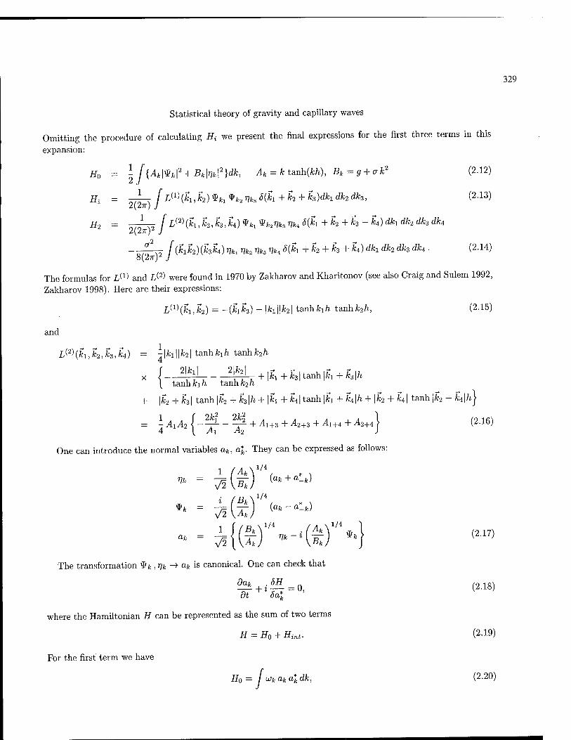
329
Statistical theory of gravity and capillary waves
Omitting the procedure of calculating Hi we present the final expressions for the first three terms in this
expansion:
#o = \ f{Ak\^k\2 + Bk\r,k\2}dk, Ak = k tanh(kh), Bk = g + atf (2.12)
Hl - 2(2 i^ f L^\kl,k2)^k^k^kJ{k1 + k2 + h)dk1dk2dkz, (2.13) 2TT) J
H2 - 2(2 i— /L(2)(fci,h,k3,k4) 9kl *fe%3 Vk4 60S! + k2 + h + h)dkx dk2 dk3 dk4 lit)1 J
—-^- / (hk^ihk^Vk, %2 Vka Vk, S{h + k2 + k3 + k4) dkx dk2 dk3 dk4 . (2.14) 8(27^ J
The formulas for L^ and L& were found in 1970 by Zakharov and Kharitonov (see also Craig and Sulem 1992, Zakharov 1998). Here are their expressions:
L^{kuk2) = -(kik2) - \h\\k2\ tanhhh t&nhk2h, (2.15)
and
L(2\ki,k2,k3,k4) = -|fci||fc2| tanhfci/i tanhfc2ft.
x { gi^L _ 2M + |fc + fc3| tanh \h + fc3|ft ^ tanhfcx/i tanh «2 n
+ |fc2 + A31 tanh \k2 + k3\h + \h + k4\ tanh |fcx + k4\h + \k2 + k4\ tanh \k2 + k4\h\
= 1-A1A2L^--^ + A1+3 + A2+3 + A1+4 + A2+4\ (2.16) 4 { Ai A2 )
One can introduce the normal variables ak, a%. They can be expressed as follows:
Vk V2\Bk
\ 1/4 J (ak+a*_k)
i (Bfl/4
afe = 1 (^V/4%_,^V%4 (2.17)
V2\\AkJ IK \Bk
The transformation <S>k,rjk-+ ak is canonical. One can check that
^+iSJL=0, (2.18) ot 6a*k
where the Hamiltonian H can be represented as the sum of two terms
H = H0 + Hint. (2-19)
For the first term we have
H0= I'ukaka*kdk, (2.20)

330
V. Zakharov
where Uk > 0 is defined by the formula
■ ak aknfi ■
uk = y/AkBk = ^k tanh (kh) (g + ak2).
The second term, Hini, is represented by the infinite series
Hint = , , Y] / V{n'm) (ku... ,kn, 4+1, • • • , kn+m)a*k ■ ■ n\m.\ z—' /
n+m>3J
■ ■ akn+m
(2.21)
x6(ki + h fe„ - kn+i kn+m) dki... dkn+m (2.22)
In the case under consideration we have
V{n'm)(P,Q) = V(m'n)(<2,P), (2.23)
where P — (fcj,... , kn) and Q — (fcn+i, • • • , kn+m) are multi-indices. For more general Hamiltonian systems (in the presence of wind, for instance), the coefficients V^n'm\P,Q)
are complex, and
V{n'm)(P,Q) = V*(m^(Q,P). (2.24)
The condition (2.24) guarantees that the Hamiltonian Hint is real. For surface waves the coefficients can be written as
V^MM - ^{(^y'v.A.fc,-
-t: Ä)%"M>+(^f i(,,H (226)
In this paper we will use only one coefficient of fourth order V^2'2^(P, Q). After a simple calculation we can obtain the following expression for this coefficient:
V^2\kx,k2,h,k4) = --i- JL(2)(-£i, -h,h,kt) + H2\k3,h, -ku-ki) - L^(-h,k3, -k2,kA)
-L^\-kuh,-k2M-L(2\-kM,-kM-L(2\~h2,kA,-kM} (2-27)
-^{(k^Miks,^) + (h,k)(k2,k4) + (kuk4)(h,k3)\ (AklAk^H^\ , lOTT'* I > V £>ki JOk2 Jtik3 tiki J
where
L*Xkuik,ik,h) = I (X4^NK)1/4
i(2)(*i.*2,fc3,A4). (2.28)
331
Statistical theory of gravity and capillary waves
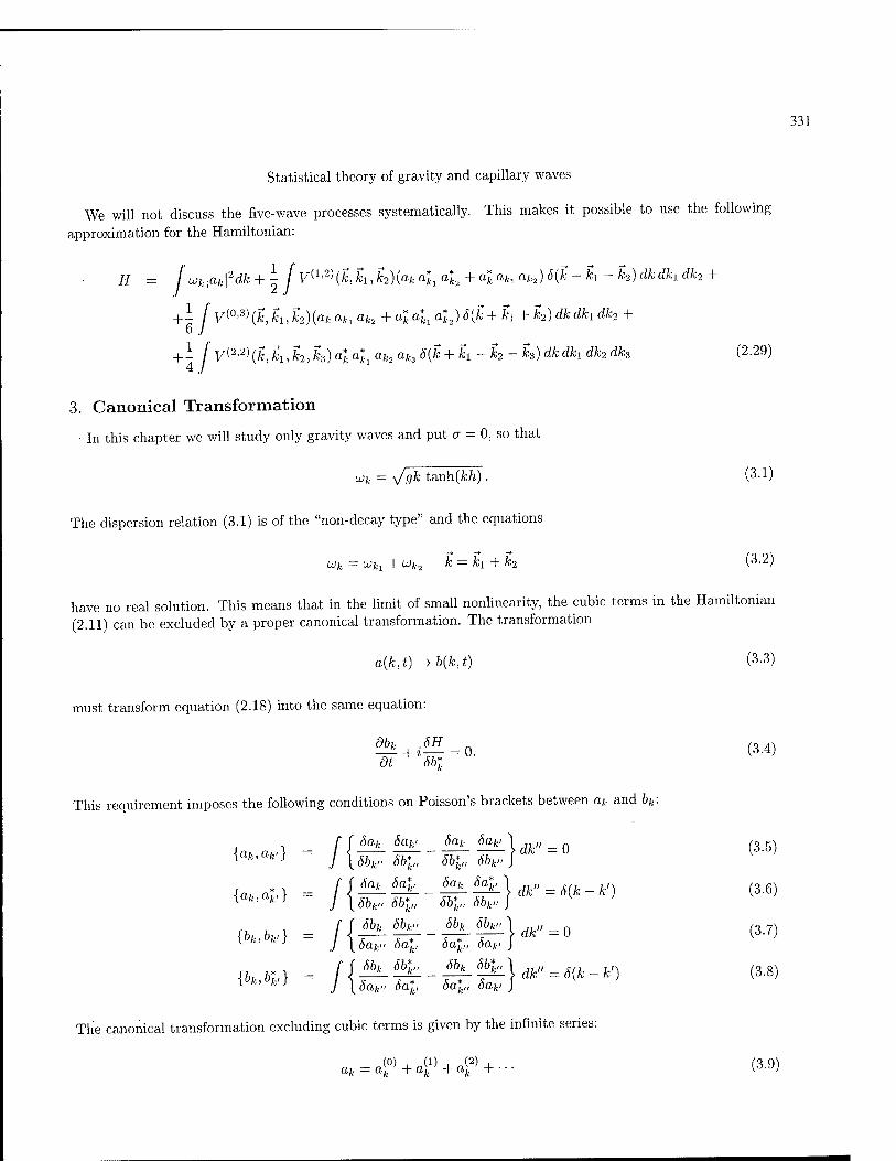
We will not discuss the five-wave processes systematically. This makes it possible to use the following approximation for the Hamiltonian:
H = Iuk\ak\2dk+l- [vt1<2Kk,ki,h){akatlat2+ataklaki)8{k-k1-k2)dkdk1dk2 +
+ 1 fvi°'3\k,kuk2)(akaklak2+alai1at2)S{k + k1+k2)dkdk1dk2 +
+ - f V^2)(jfe, fei, k2, k3) a*k a*kl ak2 ak3 5{k + h - k2 - k3) dkdh dk2 dk3 (2.29)
3. Canonical Transformation
In this chapter we will study only gravity waves and put a = 0, so that
uik = V'gk tanh(fc/i). (3-1)
The dispersion relation (3.1) is of the "non-decay type" and the equations
Wfc = Wifej + Wü2 fc = fci + k2 (3-2)
have no real solution. This means that in the limit of small nonlinearity, the cubic terms in the Hamiltonian (2.11) can be excluded by a proper canonical transformation. The transformation
a(k,t)-> b(h,t) (3-3)
must transform equation (2.18) into the same equation:
^w + iw = 0- (3-4) dt Sb*k
This requirement imposes the following conditions on Poisson's brackets between ak and bk:
<*"> = /{££-£ £}*"=° (3'5)
<"•*> = /{^^-^^}^" = ^-fc,) (3'6)
rhb.l} = [l^S-hl-^pl)dk"=0 (3.7)
lblb*\ = [l^S3lL^^S3z.)dk"=S(k-k') (3.8) iOk,t>vi J \Sak„ 5a*ki Sal„ 8ak, J v
The canonical transformation excluding cubic terms is given by the infinite series:
ak=^+ct?+4) + - (3-9)

332
V. Zakharov
where
(o) ;
„W -
(2)
( T(1)(fc, h,k2) bkl bk2 6(k-k! - k2) dkx dk2 - 2 fr^(k2,k, h) b*ki bk2 6(k + h - k2) dh dk2
+ fr{2\k,kuk2) b*ki b*k2 Stf + kx + k2)dh dk2
r -. - - - _ _ ^ _ = B(k,k1,k2,k3)b*kibk2bk3S(k + k1-k2-k3)dk1dk2dk3 + --- (3.10)
Plugging (3.9) into (3.5)-(3.8), we obtain infinite series in powers of b, b*, which must identically cancel out at all orders except zero.
Let us assume that
r<2>(Mi,A2) = r^(kuk,k2) = T^2\k2,k,k1). (3.ii)
This condition guarantees that (3.11), (3.5)-(3.8) are satisfied at first order in b, b*. Substituting (3.9) into H wc observe that the cubic terms cancel out:
2 [U)k -LOkl -LOk2)
2 [U!k +UJkl +UJk2)
A simple method for the recurrent calculation of B(k,ki,k2,k3) and higher terms in the expansion (3.9) was found by the author in the article (Zakharov, 1998). By the use of this method one can find
B{k,h,k2M = r(1)(fc1,4,fc1-fc2)r(1)(fc3)^4-fc) + r(1)(fc1,fc3,4-fc3)r(1)(fc2,fc,fc2-fc) (3.14)
-T^(k + kuk,h)r^\k2 + h,k2,k3) + r<2>(-£-kuk,h)r^(-k2 - k3,k2,k3)
The series (3.10) should be at least asymptotic. Hence we require
l41}| « IM (3-15)
Let us consider the limit of shallow water as kh —► 0. We will assume also that the wave packet is narrow in angle: ky <C kx. In this limit
cjk^s\k\ M -^{khf+ ■■■), s=y/^h, (3.16)
and
L(1Hk1,k2)~-k1k2, Ak~h\k\\ Bk~g, V^{kMM- ^7= (khh)1/2 (ff^ ■
Denoting ky = q, kx — p and \p\ 3> \q\, one obtains:
■.(^.(p+lSf-iAV). V™,JL,(l)'"lmK)V>. (8.17)

333
Statistical theory of gravity and capillary waves
We will study two opposite cases - wave packets narrow in angle and broad in angle. In both cases we will look only for the leading order terms in 1/kh. For a packet which is very narrow in angle:
a^(p,q) ~ b(p)6(q), a^(p,q) = b{1)(p) 5{q)
The condition (3.15) now reads now
Let a be a characteristic elevation of the free surface, /x = {ka)2, 5 = kh. The condition (3.19) is equivalent to
Hi 63 M«(56, or JV=^=3- «1. (3-20)
N is known as "Stokes number". For wave packets which are broad in angle the condition (3.15) is less restrictive. In this case the denominator
of T^{k,h,k2) is small if all three vectors k,h,k2 are parallel. Let us put k = (p,q), h = (pi,qi), k2 = (P2, -Q2)- Then T^\p,pi,p2, q) has a sharp maximum at q = 0. Performing integration over q yields
6<
The condition
now reads
/•OO I
+ 2/ p1/2(p + Pi)1/2&*(Pi,0)&(P + PiI0)rfpi>+--- (3.21)
|&W(p,0)|«|feW(p,0)| (3.22)
/i « 5\ (3-23)
4. Effective Hamiltonian
After performing the canonical transformation the cubic terms in the Hamiltonian cancel out. In new variables
bk we have
H = H0 + H2 + H3 + --- , (4-1)
H0= [uk\h\2dk, (4-2)
H2 = - IT(k,kuk2M) b*k b*ki bk2 bk3 6(k + h-k2- h) dkdki dk2 dk3 , (4.3)
if3 =

334
V. Zakharov
where
T(k,k,,k2,k3) = \ (f(k,h,k2,k3) + f(kuk,k2,k3) + f(k2,k3,k,h) + f(k3:k2,k,&))
f(k, Ai,k2,k3) = V^2\k, kuk2,k3) + RW(k,h,k2,k3) + R^2\k,kuk2,k3) (4.4)
and
B,^(k,kuk2,k3) =
R^(k,kuk2,k3) = -
V^)(-k-kukX)V{0'3X-k2-h,k2M) uj{—k — ki)-\-uj(k)+u)(k2)
V^2){k + h,k,h)V^2\k2 + k3,k2,h)
V(J-2)(fc,fc2,fc-fc2)V(1|2)(fc3,fc3-fci,fci) V^'2Hk,k3,k ~ k3)V^'2Hk2,k2 - kuh) Wfc-fc2 - UJk + UJk2 Uk-ks - U>k + LOk3
VV<2)(k2,k,k2-k)VW(h,ki-k3,%3) V^ih,^^ - k)V^2\k2,k2 - kuh) Uk2-k +^k - Wfc2 Uk3-k +Uk -0Jk3
(4.5)
(4.6)
In the presence of capillarity, the expression (4.6) makes sense everywhere except in the vicinity of the zeros of the denominators. The width of these vicinities depends on the level of nonlinearity.
The equation of motion (3.4) in new variables takes the form
dt + i tük bk = -- T(k, kuk2,k3) b*ki bk2 bk3 S(k + kx - k2 - k3) dkY dk2 dk3 (4.7)
The term T(k, ki, k2,k3) is defined on the resonance manifold
Wfc + ukl = ujk2 +ujks, k + ki = k2+k3 (4.8)
Further we will omit the wave numbers k and keep only their labels. After a series of transformations the four-wave interaction coefficient T can be simplified into the form
■ - jfl234 = x(^1234 + ^2134),
Tj 1 sA1A2A3A4\i/*
234 167T2
/A1A2A3AA\>
KBiB-zBaBti)
[k'2 B1 +kJB2+ k2 B3 +kJB4- (wj - w3)2 ^1-3 - (wi - w4)
2 AX-A - (wj + w2)2 A 1+2I
+
B,B2B3BA
16TT2 \A1A2A3AA
1
1/4 1
#1-3 £-1,3 £-2,4 +
1 Bi+2
W-1,3 W-2,4
£l.2 £3.4 + «1,2 "3,4
wl+2 - (wl + w2)2
>l-3 - (Wl - UJ3)2 B\-4
T T , U_i,4U-2,3 -t^-1,4 ^-2,3 H 0 1 w
Wf_4 - (WX -W4)^ ■(4.9)
Here
4* = k tanh fc/i, Bk = g + ok2 , Li>2 = -(£1 • fc2) - MM , wfc = ^AkBk. (4.10)

335
Statistical theory of gravity and capillary waves
The expression for u\ t2 is
ui,2 = {fa ■ k2 „l(l + ^)+„2(l
B2 >
AlA2\1/2
W-1,3
+Ei±i W2 ki + Em Wl fc22 + (££) (Wl <* - W?+2)(W1 + W2) B2 Bi \B\B2)
= -Afe)[.,(i+^)-»(i+^i)
ß /AI^N1/
2
1-3 2;2 (4.11)
The above expression is the most general form of four-wave interaction coefficient and is applicable for gravity a well as for capillary waves on an arbitrary depth. It can be simplified in different limiting cases.
In the absence of capillarity a = 0, Bk - g and as
Ul2 = (Wl + u2)<2{fa -k2) + -wiw2(wi+W2 -W1+2) \
U_i,3 = (wi -w3)< -2(fei -fc3) + -wiw3(wi_3 -w\ + ul) > (4.12)
5. Deep water limit
The coefficient of four-wave interaction for pure gravity waves on deep water was calculated by many authors since Hasselmann (1962). We present here a relatively compact expression for this coefficient.
Ti 1
1234 — 12kik2kskA -
16TT2 (hhhh)1/*
-2(wi +w2)2[w3W4((fci -Ä-2) - fcife) +wiw2((fc3 -h) -fafajj ^2
-2(cj! -W3)2 u>2LJ4((ki • Ä-s) + fcifc3) + wiw3((fc2 • M + fefcij] ^2
-2(wi -W4)2 w2w3((fci • fc4) + fc!fc4) +wiw4((fc2 -4) +^2^3)] p-
+ [(fci • k2) + fak2][{fa • A4) + hfa] + [-{fa • £3) + fcifc3][-(*J2 ' A4) + k2h]
+[-{fa ■ fa) + fafa}[-{k2 ■ k3) + fafa]
+4(wi + W2)2
+ 4(a>i - uJi)'
[{fa ■ k2) - fak2][-{k2 ■ fa) + k2fa] 2 [(fc!-fc3)+fclfc3][(fc2-fc4) + fc2fc4 il_i '—. ü — h 4(wi - w3J -2 , _ N2
w2+2 - (a>i + w2)
[(fcl • fc4) + fclfc4][(fc2 ■ £3) + fofcs] w2_4 - (WI - w4)
2
2_3 - (Wl - W3)2
(5.1)
In spite of its complexity the expression (5.1) has an inner symmetry and beauty. It was mentioned that in the one dimensional case the coefficient T1234 cancels out (Dyachenko and Zakharov, 1994). This result was obtained earlier by computer. We will obtain it below "by hand". Another compact expression for T1234 was

336
V. Zakharov
found by Webb (1978). Both expressions coincide on the resonant surface (5.2), but a proof of cancellation of T1234 in a one dimensional geometry is more difficult with the Webb formula.
In the one-dimensional case the resonant conditions
U)2 +UJ2 = Cü3+ UJ3
h +k2 = k3 + fc4 (5.2)
have trivial solutions k3 = hi, k\ = k,2,k3 = fc2, fc4 = k\ describing wave scattering without momentum exchange, and nontrivial solutions providing the momentum exchange. For these solutions the sign of one of the wave vectors is opposite to others. For instance, we can put
fci > 0, k2 < 0, k3 > 0, k4> 0.
In the one-dimensional case most of the terms in (5.1) cancel out, and the expression is simplified down to the form
TriM = -7r-jw1(wiw2W3W.i)1//2| - 3w2w3w4 + u>2(wi +UJ2)2 - LUS(LüI - w3)2 - w4(u>x -w4)
2j (5.3)
The resonant conditions (5.2) can be solved by the parametrization
u1=A(l + Z + e), u2 = M, W3 = A{1 + 0, W4 = A£(l + 0 h = A2(i+t;+e)\ k2 = -A2e, k3 = A2(i+o\ h = A2e(i+o2 (5.4)
By plugging the parametrization (5.4) into (5.3) we get
Tv2U = -^W1(Cü1Lü2üJ3UJ4)2 A3ai + 0 (-3£(1 + 0 + (1 + 03 - 1 - e3) = 0 (5.5)
6. Shallow water limit
The shallow water limit takes place if kh —> 0. In this limit
Ak ->■ k2h Lok -» sk., gh, ~(ki-k2), wi,2 -» s(&i +k2)(ki -k2),
u-i,3 -* -s(h - k3)(ki ■ k3).
The coefficient (4.9) can be simplified into the form
1 1 ■1234
16TT2/I {kxk2k3kAy/2 (ki ■ k2)(k3 ■ fc4) + (&i ■ k3)(k2 • kA) + (ki ■ kA)(k2 ■ k3)
+2
(6.1)
(h ■ k2)(k3 • A4)(fci - k2)2 (h ■ k3)(k2 ■ ki){h - k3)
2 (h ■ k4)(k2 ■ k3)(h - kAf
{ki -k2) -hk2 (ki -k3) -kik3 (ki ■ k4) — kiki 6.2)
The three terms in (6.2) are singular if the vectors ki are parallel. But there is a remarkable fact: these singu- larities cancel and the whole expression (6.2) is a regular continuous function. The cancellation of singularities is a quite nontrivial circumstance. It could be checked by a straightforward calculation.
The singular part of Xi234 can be written as follows:
T, 1 k2k3k4
234 47r2/i (k^hh)1/2 (h + k2f (Ai - h)2 (*i - ktf
fc2(cos02 —1) k3(cos4>3 — 1) ki(coscf>4 — 1) (6.3)

337
Statistical theory of gravity and capillary waves
Here cos(j>i = (fa ■ fa)/fafa. The resonant conditions are:
fa+k2 = fa+fa,
fa + fa COS 4>2 = fa COS (pz + fa COS 04,
fa sin 02 = fa sin (j>3 + fa sin 04 ■
For small angles |<fo| « 1, we can put approximately
cos0i - 1 ~ —^-, sin^i ~
The resonant conditions now become now
k24>j = k3<t>l + fa4>\, fafo = fafo + fafo
The most singular part of T1234 is
1 (fafafa)1'2 J (fa + fa)2 (fa - fa)2 (fa - fa sing fa§\ fa<j>\ '2**h k\'
2 \
But one can check by a direct calculation that
(fci + fa)2 (fa - fa)2 (fa - fa)2
fa(j)\
fafo2 «3 03 fafo\
:0
in virtue of (6.5). Hence the singularities cancel and (6.2) is a regular function. We can calculate T1234 more accurately by putting
T1234 — 1
'16TT2/J (fafafafa)1/2
(fafa)(fafa) + (fafa)(fafa) + (fafa)(fafa)
+ 4s2 (fafa)(fafa)(fa + fa)2 (fafa)(fafa)(fa - fc3)2 (fafa)(fafa)(fa - fa)
U)2+2 - (Wl + W2)2 W2_3 - (Wi - W3)
2 U) 1-4 (wi - w4)2
Here we put
w(fc) = sfc(l-^(fc/i)2)
(6.4)
(6.5)
(6.6)
(6.7)
(6.8)
(6.9)
Now denominators in (6.8) cannot reach zero, but for almost parallel fa they are of order (kh)2 and small if kh -»• 0. As a result, some terms in (6.8) are large, of order I//13, but in fact they cancel each other. The major
terms in (6.8) are
(fa - fa)2 (fa - fa)2
1 sing
1 (fakzfa)1'2 f (fa + fa)2 2^h kY2 \fa[fo2 + h2(fa+fa)2} fa[<j>2 + h2(fa-fa)2} fa[fo\ + h2(fa-faY
= 0(6.10)
The expression (6.10) is identically zero in virtue of (6.5). As /i -» 0 (6.10) goes to (6.7). Cancellations (6.7), (6.10) have a very deep hidden reason - they are consequencies of the integrability of the
KP-2 equations (see Zakharov 1998).

338
V. Zakharov
7. Statistical description
The statistical description of nonlinear wave fields is realized by the correlation function
< «it, •' ■ al.nak„+i ' • ■ akn+m >= Jn'm{h ■■■K,kn+1 ■ ■ ■ kn+m)S(ki H + kn- kn+i kn+m) (7.1)
The presence of ^-functions in (7.1) is a result of spatial uniformity of the wave field. In the same way we can introduce correlation functions for the transformed variables bk:
< b*ky ■ ■ ■ b$nbkn+i ■ ■ ■ bkn+m >= In'm{h ■ ■ ■ kn,kn+1 ■ ■ ■ kn+m)8(ki + ■•■ + £„- kn+1 kn+m) (7.2)
To find the connection between Jn<m and In'm one has to substitute (3.9) into (7.1) and perform the averaging. The following pair of correlation functions is the most important:
< aka*k, > = nk S(k — k1)
<bkb*k,> = Nk6(k-k') (7.3)
Here nk and Nk arc different functions. nk is a measurable quantity, connected directly with observable correlation functions. For instance, from (2.17) we get
/ \ 1/2
I, =< |^|2 >= I I*!) (nk+n.k) = \ g K +n-k) (7.4)
The function Nk cannot be measured directly. It is an important auxiliary tool used in analytical constructions. In most articles on physical oceanography the authors make no difference between nk and Nk. This is a source of persistent and systematic mistakes. We will see that the difference between nk and Nk is especially important on shallow water.
Plugging (3.9) into (7.3) we get:
nk = Nk+ < a<°> 4]>* > + < a!0'* 4" > + < a«1' 41'* > + < af a[J" > + < a£0>* a£a> > + • ■ • (7.5)
Terms < a[. ' a[,' * >, < ak ak > are expressed through triple correlation functions < b*bb > and < bbb >. As far as the cubic terms in the effective Hamiltonian are cancelled, triple correlation is defined by the fifth-order correlation functions and is small and can be neglected. In fact, j(1,2) ~ n5.
The next terms in (7.5) are expressed through quartic correlation. Only one quartic correlation function is really important
< K K, h2 bk3 >= I^^ithMM^k + k, -k2- k3) (7.6)
We study only weakly nonlinear waves and can assume that the stochastic process of surface oscillations is close to Gaussian. Thus we can put approximately
l(2'2\k,h,k2,k3) = NkNk2 6(k - k3) + NkNk3 S(k - k2) (7.7)

339
Statistical theory of gravity and capillary waves
By the use of (7.7) we obtain the following expression:
nk = Nk + 2 flT^ik^nh^N^NkJik-h-k^dhdh
+2 I \T^(k2,k,h)\2Nkl Nk2 S(k + h - k2)dhdk2 +
+2 f \T^(h, k, h)\2 Nkl Nk2 S(k - h + k2) dhdk2 +
+2 f \rW(k, h,k2)\2 Nkl Nk2 S(k + h + h) dkxdk2 - ANk J B(k, h,k, h) Nkl dkx (7.8)
Using the expression (3.14) for B and formulae (3.12), (3.13) we get the final result:
„, = Nk + \[ ly(1'2)(fc.fci^2)|2 { N _ NkN _ NkNk2)ö{k - kx - k2) dhdk2 + 2 J (uk -ujkl -uJk2)
2
+1 r \v^){kMM)? {N N + NkNki _ NkNkjSfc _ fc _ 4)dkldk2 + 2 } (u}kl -wfc -uk2Y
+ i r \v^)(k2,k,fcOl2 { N + NkNk2 _ NkNki)5{k2 _ k- h)dhdk2 + 2 7 (ujk2 -wk -WfcJ2
+1 r |y(0'3)(Mi,fc2)l2 (N N + NkNki + NkNk2)s(k + k1 + k2)dhdk2 (7.9) 2 j (u)k + wkl +uk2y
On deep water all the terms in (7.9) are of the same order, and the difference between nk and Nk is small:
nk
However, in shallow water, denominators in (7.9) are small, and this difference can be dangerously big. The integration in (7.9) for a wave distribution which is broad in angle in the perpendicular direction can be performed explicitly. The last, nonresonant, term in (7.9) must be neglected. It is suitable to present the result in polar coordinates in the fc-plane. The final formula is astonishingly simple:
n(k,9) = N(k,9) + ^ (-)1/2 -±- { jLN(h,9)N{k-h,6)dh + 2 f™ N(h,0)N(k + h,6)dk1} (7.11)
Comparing the leading term with the next terms in (7.11) we obtain
Hk ~ Nk ~ ßßb 8~(kh) (7.12) nk
Then the condition of applicability for a weakly-nonlinear statistical theory of waves on shallow water becomes
li « 85 (7.13)
For a very shallow water, kh ~ 0.1, this condition can practically never be satisfied. But for a moderately shallow water, kh ~ 0.3, it could be satisfied for small amplitude waves, (j, ~ 10~4. In many real situations the corrections in (7.11) are important and cannot be neglected. Generally speaking, the weakly-nonlinear theory has narrow frames of applicability in shallow water.

340
V. Zakharov
8. Kinetic equation
The function nk is usually named "wave action distribution". There is no standard name for the function Nk so far. We will call it "renormalized wave action". It is very important that the kinetic equation is imposed, not on the wave action nk but on the renormalized wave action Nk ■
To derive this equation we can begin from the equation (4.7). It imposes an infinite set of relations on correlation functions. The statistical description means a loss of time reversibility and needs an introduction of negligibly small damping. It can be done by replacing in (4.7)
uu -» wfc + i-yk
Directly from (4.7) we obtain
^ + 2ykNk = f T(k, h,k2,k3) Jm I(k, h,k2,h) S{k + kx-k2- k3)dkLdk2dk3 (8.1)
We will shorten the notation further.
ÖT -^1234 + (»A + T) Ji234 = — ~ / j ^1567 <$l+5-6-7 -^267345 +
+ ^2567 ^2+5-6-7 7i67345 ~ T3567 Ii25467 ^3+5-6-7 - 74567 A25367 Si+5-6^7 >dk5dk6dk7 (8.2)
Here
A = A1234 = -wi - w2 + W3 + W4
T = 71 + 72 + 73 + 74 (8-3)
To make a closure in the system we perform the canonical expansion of the correlation function
/1234 = N1N2(Si3 + £14) + /1234 (8-4)
into
^123456 = NiN2N3(SUS25 + <5l4^26 + ^15^24 + ^15^26 + ^16^24 + <5l6^25) +
+ Ni((I2z56Sl4 + ^1356^24 + ^1256^34) +
+•^5(^2346^15 + ^1346^25 + A246^35) +
+ ^6(72345^16 + ^1345^26 + ^1245^36) + ^123456 (8.5)
The formulae (8.1)-(8.4) are exact. There /1234 and /123456 are the cumulants, irreducible parts of the correlators. Substituting (8.5) into (8.3) and using (8.1) we obtain
^J]234 + (Ȁ + T)71234 = T12M{N2N3N4 + N^Nt - NiN2N3 - JV^A^) + LI + Q (8.6)
Here Q is the right part of the equation (8.2) where the six-point correlator is replaced by a corresponding
cumulant, for instance, 7256347 -> ^256347-
Ä = -uj - uJ2 +1J3 +oJ4, (8.7)

341
(8.8)
Statistical theory of gravity and capillary waves
where ü)(k) is a renormalized dispersion relation
w(Jfe) = w(Jfe) + IT{k,h)Nkl dki, T(k,k1) = T(k,ki,k,k1)
LI is a linear operator:
(LI)i23A = M1234 + M2134 - M3412 - M4312 (8-9)
M1234 = -\N2 [T1256he3i6(l + 2 -5-6)dk5dk6 (8.10)
-?;7V3 /" Ti546 ^2645 5(1 + 5-4-6) dMfo - iN<i / Ti53612635 <J(1 + 5 - 3 - Q)dk5dk6
The system (8.1),(8.6) becomes closed by putting J123456 = 0. It is still very complicated. For further simplifi- cation one has to neglect LI. Sending T -> 0, we finally get
Im Il234 = KT12U{N2N3N4 + #1^4 - W1JV2JV3 - WiJV2JV4) S(Ä)
Substituting (8.9) into (8.1) leads to the final result
dNk
(8.11)
at + 2lkNk=st(N,N,N)
st(N,N,N) = w [ |T1234|2 (N2N3Ni + N^N* - NXN2N3 - JViiV2JV4)
x<5i+2_3-4 8{w\ + ui2 - w3 - L04) dk2dk3dki (8.12)
Due to the inclusion of the frequency normalization, the equation (8.12) is more exact than the "common" wave kinetic equation.
To get the quantum kinetic equation we can use the same procedure, assuming that ofc, ak are noncommu- tative operators of annihilation and creation of quasiparticles.
9. Renormalized dispersion relation
Frequency renormalization is described by the diagonal part of the four-wave interaction coefficient
T(k1,k2)=T(k1,k2,k1,k2)=Tu (9-1)
This "naive" formula presumes the existence of the limit:
T{kuk2)= lim T(ki,ie2,h+#,&■-$ (9-2) |g|-*o
This limit exists and does not depend on the direction of the vector q only in deep water. In the general case, we can obtain from (4.9)
T,„ = - 1 Mi ^2 167I-2 yBiB-i
1 (BXB2
1/2
1/2
2k\Bx + 2k\B2 - (wi + w2)2 Aw - (wi - ui2)
2 Ai_2] (9.3)
32TT2 \A1A2 Bi+2
-^12 + ~2 h\2
W2+2 -{0J1+LJ + 2)2 B 1+2
£-1.2 + -1,2
J2_2 - (Wl - W2)2

342
V. Zakharov
In the absence of capillarity in deep water the expression (9.3) becomes
T12 = -^2 (kll2y/2 I 3kik2 + & ■ h)2 - 4o;1o;2(fe.fc2)(fc1 + k2) +
+2- (Wl + w2)
2 [(& • k2)2 - k2k2} (Wl - w2)
2 [(& • £2)2 + k2k2]
L J_ ,n L J —2 7 ^9 + 2 2 S S2 L } (9-4) Lü(+2 - {üJl + UJ2)
2 Wf_2 - (Wl - Lü2y J
In 'the one-dimensional case the formula (9.4) becomes remarkably simple
_ 1 j k\k2 h < k2 , s Tu~W\ hkl h>k2
(9"5j
The function Ti2 is continuous at k = h, but its first derivative has a jump. This result was published by the author in 1992 (Zakharov, 1992). At k2 = kx
In the presence of capillarity
Ti2->Tn, Tn = ^2fc3- (9-6)
For monochromatic waves we have:
1. b = FS(k-k0), 6u=-T11\F\2 (9.8)
In natural variables
and
2
2 _ 1 fc0 ,p|2 77 = acos(k0x — cot — (f>), a2 = —r \F
lit* LOko
ÖLü 1 2 — ok ,2
w 4 1 - 2ak2 (ka)2 (9.9)
It is in agreement with the classical results of Stokes and other authors. In shallow water the limiting procedure (9.2) needs some accuracy and falls beyond the framework of this article.
10. Kolmogorov spectra
Let us look now for stationary solutions of the kinetic wave equation (8.12). They satisfy the equation
st(N,N,N) = 0 (10.1)
This equation has an ample array of solutions describing direct and inverse cascades of energy, momentum, and wave action. A full description of these solutions has not been done so far. Only very special, isotropic solutions could be found analytically in the case when wk is a power function
iok=a\k\a, (10.2)

343
Statistical theory of gravity and capillary waves
and T(ki, k2, h, kA) is a homogeneous function:
T{tkuek2,ekz,(.kA) = eß' T(kuk2,h,kA) (10.3)
It is assumed that the function T{ki,k2,kz,kA) is invariant with respect to rotation in /c-space. In the general case of water of finite depth uk is not a homogeneous function. As a result, all known analytical
methods are unable to construct any nontrivial (non-thermodynamic) solution of equation (10.1). But in two limiting cases, deep water and very shallow water, some solutions can be found. On deep water
u,k = ^k, a = 1/2, (10.4)
and TfaMMM) is given by the expression (5.1). Apparently, ß = 3. On very shallow water
uk = s\k\, a=l, (10.5)
and T(ki,k2,h,k4) is given by formula (6.2). As far as singularities in (6.2) are cancelled, it is a regular continuous function on the resonant manifold (6.4). Now ß = 2. On a flat bottom the isotropy with respect to rotation is satisfied.
' It is well known (see, for instance, Zakharov, Falkovich and Lvov, 1992) that under conditions (10.2), (10.3) the equation (10.1) has powerlike Kolmogorov solutions
n{2) = a2Q^3k-2J^-d (10.6)
Here d is a spatial dimension (d = 2 in our case). The first one is a Kolmogorov spectrum, corresponding to a constant flux of energy P to the region of small
scales (direct cascade of energy). The second one is a Kolmogorov spectrum, describing inverse cascade of wave action to large scales, and Q is the flux of action. In both cases ar and a2 are dimensionless "Kolmogorov's constants". They depend on the detailed structure of T{k,ki,k2,k3) and are represented by some three- dimensional integrals.
It is known since 1966 (Zakharov and Filonenko, 1966) that on deep water
n (i) aiP^3k-4. (10.7)
For the energy spectrum
Iudu) = u>k nj: dk (10.8)
one obtains
/„-P1/^-4. (10.9)
This result is supported now by many observational data as well as numerical simulations. In the same way on deep water (Zakharov and Zaslavsky, 1982):
nf=a2Qlin-2Zl\ Iu-Q^u,-11^. (10.10)
On a very shallow water a = 1, ß = 2, and we obtain:
„W = a! P1'3 k'w'3 h2'3, J« ~ P1'3 uj-V3 (10.11)
n{2) = ä2Q^3k-3h2^3, I^-Q1/3^1 (10.12)

344
V. Zakharov
Formulae (10.11), (10.12) are new. We must keep in mind that they are applicable only if the condition /z <C ö5
is satisfied.
11. Conclusions
The weakly nonlinear theory of gravity waves has some window of applicability on shallow water. But this window shrinks dramatically when the parameter S = kh tends to zero. For S ~ 0.5 the window is relatively wide, n < 10~2, but for 5 ~ 0.2 it barely exists, p. < 10-4.
On deep water we can neglect the difference between the observed, nk, and renormalized, Nk, wave action. On shallow water the difference could be very important for correct interpretation of observed data. We have to remember that the kinetic equation is written not for real, but for "renormalized" wave action.
Many problems pertaining to the statistical theory of gravity waves on shallow water are still unresolved. The most important problem is finding a Kolmogorov spectra for a fluid of arbitrary depth. From dimensional consideration we can conclude that it has the form
N11] =P1/3k-*F(kh), F-+Ü1, kh ->oo, F-> di (fch)2/3 kh -> 0 (11.1)
The function F(£) is unknown and should be found numerically.
Acknowledgement
This work is supported by the ONR grant N 00014-98-1-0070.
References
[1] W.Craig, C.Sulem and P.L.Sulem, Nonlinear modulation of gravity waves - a rigorous approach, Nonlinearity, vol. 5 (1992), 497-522.
[2] A.Dyachenko, V.Zakharov, Is free-surface hydrodynamics an integrable system? Physics Letters A 190 (1994), 144-148. [3] K.Hasselmann, On the nonlinear energy transfer in gravity-wave spectrum. Part 1. General theory. J. Fluid Mech. 12 (1962),
481-500. [4] B.B.Kadomtsev, Plasma Turbulence, Academic Press, London, 1965. [5] D.J.Webb, Nonlinear transfer between sea waves, Deep-Sea Res. 25 (1978), 279-298. [6] V.E.Zakharov, Stability of periodic waves of finite amplitude on a surface of deep fluid, J. Appl. Mech. Tech. Phys. 2 (1968),
190-198. [7] V.E.Zakharov, Inverse and direct cascade in a wind-driven surface wave turbulence and wave-breaking, IUTAM symposium,
Sydney, Australia, Springer-Verlag, (1992), pp.69-91. [8] V.E.Zakharov, Weakly-nonlinear waves on the surface of an ideal finite depth fluid, Amer. Math. Soc. Transl. (2), vol. 182
(1998), 167-197. [9] V.E.Zakharov and N.Filonenko, The energy spectrum for stochastic oscillation of a fluid's surface, Doklady Akad.Nauk, vol.170 " (1966), 1292-1295.
[10] V.E.Zakharov and V.Kharitonov, Instability of monochromatic waves on the surface of an arbitrary depth fluid, Prikl. Mekh. Tekh. Fiz. (1970), 45-50 (Russian).
[11] V.E.Zakharov and M.M.Zaslavsky, The kinetic equation and Kolmogorov spectra in the weak-turbulence theory of wind waves, Izv. Atm. Ocean. Phys. 18 (1982), 747-753.

Bur. J. Mech. B/Fluids © Elsevier, Paris
ON THE KOLMOGOROV AND FROZEN TURBULENCE IN NUMERICAL SIMULATION OF CAPILLARY WAVES
A. N. PushkarevW W [1]: Arizona Center of Mathematical Sciences, University of Arizona, Tucson, AZ 85721, USA e-mail: andrei8acms.ariZona.edu
(Received 15 September 1998, revised and accepted 15 January 1999)
Abstract - Numerical simulation of dynamical equations for capillary waves excited by long-scale forcing shows the presence of both Kolmogorov spectrum at high wavenumbers (with the index predicted by weak-turbulent theory) and non-monotonic spectrum at low wavenumbers. The value of the Kolmogorov constant measured in numerical experiments happens to be different from the theoretical one. We explain the difference by the coexistence of Kolmogorov and "frozen" turbulence with the help of maps of quasi-resonances. Observed results are believed to be generic for different physical dispersive systems and are confirmed by laboratory experiments. © Elsevier, Paris
1. Introduction
An important issue is the degree of correspondence of wave dynamics in nonlinear dispersive media of infinite and finite extent. This question becomes especially important when the characteristic wavelength of the wave ensemble is comparable with the length of the finite domain and excited waves are weakly nonlinear. Such questions arise during attempts of confirmation of analitical results obtained for dynamical system in infinite domain by numerical simulation of the same dynamical system in the finite region with particular type of boundary conditions. Popular boundary conditions are periodical ones and the following consideration will deal with this particular case of boundary conditions. The result is believed to be true, however, for other types of boundary conditions, such as, zero of the function or its derivative, or their combination, etc.
It is well known that in the limit of low levels of excitations the behavior of an ensemble of waves in nonlinear dispersive systems in infinite domain is described by the kinetic equation for waves [1] and is known as "weak" turbulence. One of the classical examples of the weak turbulence is the system of weakly nonlinear capillary waves on the surface of deep water. One should emphasize that above question of degree of correspondence of the wave dynamics in infinite and finite domain is not only about comparison of numerical simulation and analysis, but also about the role of boundary conditions in laboratory experiments on excitation of capillary waves in finite-size containers [2].
An interaction of the Fourier modes in kinetic equation for capillary waves is performed through the inter- action of triplets of waves which are solution of the system of equations usually referred by "conservation laws"
or "resonances" [1]
UJC + u!.- -u>c =0 (1) fcl «2 «3
fei + k2 = fa (2)
(!) Permanent address: Landau Institute for Theoretical Physics, Russian Academy of Sciences, Russia 117940 GSP-1 Moscow V-334, ul.Kosygina 2

346
A. Pushkarev
where k and w^ are the corresponding wave vector and frequency. The system (l)-(2) always has solutions in the case of continuous spectrum for dispersion relation of capillary
waves
uj; = a2 k2 (3)
known as "decay-type" dispersion relation [1]; a is the coefficient of surface tension. The situation changes, however, in the case of a finite domain. Fourier harmonics of the system with periodic boundary conditions are not continuous functions of the wavenumber anymore, like in the case of infinite domain, but infinite set of values defined at discrete equidistant wavenumbers. The question of existence of solution of the system (l)-(2) turns into, generally speaking, nontrivial number theory problem. Significant breakthrough in classification of existence of solutions of this system for different types of dispersion relations o^ was done by E.Kartashova [3]. It was shown, in particular, that the system (l)-(2) does not have solutions in the case of capillary waves dispersion relation (3) which means that there are no interacting Fourier modes in the kinetic equation for waves in the finite domain in this case.
The situation changes, however, if nonlinear dispersion correction Sk due to finite amplitude of the excited wave is taken into account and capillary wave frequency becomes
tjk = a 2 k 2 + Sk (4)
Conservation laws (l)-(2) are transformed therefore into "quasi-conservation laws" or "quasi-resonances"
Wfci + uk2 - ojk3 = Afclfc2jfc3 (5)
kx + k2 = k3 (6)
Afcjfc2fc3 = <**3 ~ <**1 - <**2 (7)
It is clear that the system (5)-(7) has more degrees of freedom than the system (l)-(2) for solutions to exist due to the parameter Ak1k2k3 which measures the level of excitation of oscillations.
Below we outline the results of direct numerical simulation of the dynamical equations for capillary waves in periodical domain which shows that besides classical Kolmogorov turbulence regime exists another regime of "frozen" turbulence. The "frozen" turbulence regime is explained with the help of "maps" of "quaiziresonances" (5)-(7) which show "allowed" and "prohibited" Fourier modes as a result of the discreteness of the Fourier spectrum due to the periodicity of the boundary conditions.
2, Numerical model
We carried out numerical simulations of weakly nonlinear capillary waves in two-dimensional periodical domain based on discretization of the system of dynamical equation of surface waves on deep water [4] supplied with forcing F? and damping terms Dp:
drjr ^ = [|fc|v] ^ - div(»/V^) - |A| [[|*|V] ?
x *??] ^ + 1^1 ^[[l^XT^X^
+ -2A?
= erdiv
-1*1 l*#
V7] ' * I"-(V^)2+[|A|V'
|A;|^1 - A^ x \A + (VTJ)
1
2 + 2
X T)?\ X J r
X T]F + Df + Ff
(8)
(9)

347
Frozen Turbulence
where T]? = <n(r,t) is the shape of the surface, f= {x,y); ip(f,t) is the velocity potential evaluated on the free
surface. Brackets [...}r denote an expression in i?-space and action of the operator |fc| on the function VF is defined
through Fourier space as
)*H?=^/ifciv*>d* The Fourier component of forcing is defined by
Fg = fj: cos (cjk (I+ R)t) (10)
where wfc is the local linear frequency, R = R(t) is a function of time, taking values randomly distributed between -1 and +1.
For numerical reasons we used an artificial damping D turned on at the wavenumbers k0 = 0.7 -i- 0.9kmax
(the details are not significant for the present paper and can be found in [4]). In the absence of forcing and damping the system (8)-(9) preserves the energy integral H (Hamiltonian)
H = H0 + H1+H2 + ...
Ho = \j[\k\m2 + {9 + o\k\2)\m\2]dk
Hl = ~\h! ^'^^(h +h + h)dkidk2dk3
H2 = TT^y I MkkMWtfkMaS$ + & + ^ + ^dkdhdhdh 4(2
2 lfc"i + H + lfc"i + k"i\ + 1^2 + fa\ + \fo + fci|] - \h\ - \k2\
It is convenient to use the parameter e = Hl^ as a measure of nonlinearity of the system which by the order of magnitude is equal to the average angle of deviation of the liquid surface from the horizontal line |VTJ|.
3. Kolmogorov and "frozen" turbulence
"A series of experiments was carried out with the forcing (10) localized at small wavenumbers. They show that, at low levels of nonlinearity e ~ 10"2, the stationary spectrum of surface elevations is isotropic in angle and transfers a finite energy flux to the large wavenumbers k region.
The plot of the logarithmic derivative (see Fig. 1) shows that in the interval 8 < k < 23 the spectrum can be considered as powerlike Ik = qk~x. The exponential value is close to x ~ 4.8 with q ~ 0.03. This exponential value is in a good agreement with the value of Kolmogorov index " calculated by Zakharov and Filonenko [5], [6] as an exact solution of stationary kinetic equations for waves.
From weak-turbulence theory, q = CexpVP (cr = l), where Cexp is an experimental value of the Kolmogorov constant. Once we have measured the energy flux P, one can calculate Cexp = 1.7 which happens to be different from the theoretical value of Kolmogorov constant Ctheory = 9.85 [4].
Another series of experiments carried out for lower levels of nonlinearity, Hl^ ^ 10~3> nas snown tnat there
is a stationary regime of "frozen" turbulence in the small-wavenumbers region of pumping, with the spectrum exponentially decaying toward high k (see Fig.2). The wave spectrum consists of several dozens of excited low- wavenumber harmonics, possibly exchanging energy between each other, without generating an energy cascade

348
A. Pushkarev
dLogio<\Vk\2> dLogiok
1
2 j
o :
3 -j
4
5 : o
o :
o :
°o°Oo%<?0 -i <» : o : 0
0.0 0.5 1.0 1.5 2.0
Logwk
FIGURE 1. The derivative of the logarithm of the spectrum of spatial elevations with respect to the logarithm of the wavenumber, as a function of the logarithm of the wave number (local value of Kolmogorov index).
•Lo9lO<\Vk\2> -5
FIGURE 2. One half of the spectrum of spatial elevation in the case of "frozen" turbulence
toward high wavenumbers. There is virtually no energy absorption associated with high wavenumbers damping, in this case.
We interpret this regime as generic, associated with wave spectrum discreteness due to periodicity of boundary conditions. The characteristic feature of this regime is formation of ring structures around k = 0 (see Fig. 2).

349
Frozen Turbulence
The numerical experiments described above have demonstrated that the theory of weak turbulence is correct in two-dimensional case, as well as existence of the Kolmogorov spectrum. This result is confirmed by data of laboratory experiments carried out in Department of Physics, UCLA [2].
Still, there are several questions to be answered: 1. Difference of the experimental value of Kolmogorov constant from the theoretical one. 2. Existence of fluxless or "frozen" turbulence regimes at very low levels of short-wave forcing. 3. "Wedding cake" shape of the "frozen" turbulence spectrum (Fig.2) which gives oscillating one-dimensional spectrum after angle-averaging.
4. Maps of quasi-resonances
To understand the answers to above questions we propose the following algorithm of studying of quasi-
resonances. For three vectors
k\ = [klx-l K\y)
k2 — {k2x,k2y)
k3 = (k3x,hy)
conservation laws (5)-(7) transform into
(k\x + fcly)f + (*4 + *!„)* - (fax + hx)2 + (hy + k2y)2)i = Afclfc2
We are building the "map" function Mt{kx,ky) such that
ev ' [0 if Afclfc2 > e
Every map Me(kx,ky) corresponds to the chosen "level" of the turbulence e. The algorithm of building of the map tests if every allowed triplet kuk2,kz has a discrepancy Afclfca less then e. If the answer is "yes" all
points k[, k2, k3 are assigned the value of 1, and 0 otherwise. It is important to note that, generally speaking, a particular map is also a function of the cutoff wavenumber
in Fourier space kcut which is characteristic value of starting of significant high-wavenumber damping. The more is kcuU the more active resonances exist on the map. This is clear from the following consideration. Suppose that absolute value of k\ is much smaller than k2, k3. It is clear that the bigger kcut is, the more possibilities exist to satisfy the condition A < e for any given e.
Fig. 3a, 3b, 3c show the maps of quasiresonances for e = 0.0001, e = 0.01, e = 1.0. White areas correspond to "allowed" Fourier modes while blacks to "prohibited" ones. As one could expect, the richness of resonances grows significantly with e. The picture of resonances on Fig.3a is very poor - direct analysis shows that there are no two different triplets ki,k2,k3 coupling with each other. This case corresponds to the case of pure "frozen" turbulence, because there is no mechanism of energy transfer from one triplet to another, i.e. from low to high
wavenumbers. The picture of resonances on Fig.3b is significantly denser. It was found that there are coupling triplet
of wavevectors in this case able to transfer the energy from low to high wavenumbers, still not many. It is interesting that averaging the map over the angle in Fourier space we get oscillatory one-dimensional "wave spectrum" due to the presence of spectral holes on the corresponding two-dimensional map. It is tempting, but hard to compare these oscillations with low-wavenumber oscillations in laboratory data [2], where some of them are obviously produced by effects of parametric forcing. Still, the tendency of formation of oscillatory spectrum was quite obvious in numerical experiments (see Fig.2) and represents an interesting subject of investigation in laboratory experiments.
;s

350
A. Pushkarev
FIGURE 3. Map of quasi-resonances Me(kx,ky) for (a) e = 0.0001 (b) e — 0.01, (c) e = 1.0. The point kx = 0, ky = 0 is located at the center of the picture. White areas correspond to 1 ("allowed" modes), black area to 0 ("prohibited" modes).
The map of resonances on Fig.3c presents the case of well-developped coupling of resonant triplets. The result of the averaging of the map over the angle does not contain any oscillations. One can expect that the effects of "frozen" turbulence should be minimal in this case being compared to the cases Fig.3a,b which creates better conditions for realization of Kolmogorov regime of turbulence.

351
Frozen Turbulence
5. Conclusion
We performed numerical simulation of weakly turbulent capillary waves which clearly shows existence of Kolmogorov law of the stationary spectrum with the index corresponding to found theoretically from kinetic equation for waves. The value of Kolmogorov constant measured from numerical experiments is happened, however, to be different from the theoretical value.
This difference is caused by the fact that beside Kolmogorov regime there is another, "frozen" regime of turbulence without energy flux from low to high wavenumbers. This mechanism is especially robust at very low levels of turbulence and is observed through anglular symmetric "wedding cake" shaped spectra of turbulence.
The mechanism of "frozen" turbulence can be understood through the analysis of solutions of kinematic three-wave quasi-conservation laws. This analisys was performed numerically by building the maps of quasi- resonanses which show that for small levels of excited waves Fourier space is splitted to the regions of "allowed" and "prohibited" modes. As a result, for very small levels of excitation, there are no coupling triplets of the wavevectors responsible for energy transfer from low to high wavenumbers. The number of "allowed" Fourier modes grows significantly with the increase of the level of excitation or inertial range in Fourier space. As a result, one can expect Kolmogorov regime of turbulence at relatively high levels of excited waves and big enough inertial range in Fourier space. Weak turbulence in bounded systems is therefore, as a rule, the mixture of "frozen" and Kolmogorov turbulence.
The smallness of the experimental value of the Kolmogorov constant suggests that energy flux realized in the numerical experiment is significantly bigger than weak-turbulent flux which could correspond to this constant. Excessive energy flux is, to our mind, caused by narrowness of the intertial range in Fourier space, which makes possible direct (non-cascade) absorbtion of the energy produced in the short wavenumbers region of the
pumping. It is the challenge to build a simplified dynamical numerical model of purely "frozen" turbulence. It can be
based on a numerical algorithm which consists of the solution of dynamical equations coupled with dynamically changing map of allowed modes in time and Fourier space. It is also tempting to observe such "frozen" turbulence in laboratory experiments on excitation of capillary waves in containers which could be observed via detection of ring structures in two-dimensional spectra of surface elevations.
Acknowledgments
This work was supported by the Office of Naval Research of the USA (grant ONR N000 14-98-1-0070) and partially by Russian Basic Research Foundation (grant 94-01-00898). We are using this opportunity to acknowledge these foundations.
Thanks are due to Computational Mechanics Publications for their kind permission to reproduce some parts of this paper which first appeared in [4].
References
[1] Zakharov, V.E., Falkovich G., Lvov V.S, Kolmogorov Spectra of Turbulence I, Springer-Verlag, Berlin, 1992 [2] W.Wright, Raffi Budakian, S.Putterman, Phys.Rew.Lett, V.76, N 24 (1996) [3] Kartashova E, Wave Resonances in Systems with Discrete Spectra, in: V.E.Zakharov (Ed.), Nonlinear Waves and Weak
Turbulence, Advances in the Mathematical Sciences (formerly Advances in Soviet Mathematics), American Mathematical
Society, Providence, Rhode Island, 1998, pp.95-129 [4] Pushkarev A.N., Zakharov V.E., Turbulence of Capillary waves - theory and numerical simulation. Nonlinear Ocean Waves,
Chapter 4, in: W.Perrie (Ed.), Advances in Fluid Mechanics, Vol. 17, Computational Mechanics Publications, Southampton,
Boston, 1998, pp.111-131 [5] Zakharov V.E., Filonenko N.N., The energy spectrum for stochastic oscillation of a fluid surface, Doklady Akademn Nauk SSSR,
170(6), (1996) pp.1292-1295, (in Russian) [6] Zakharov- V.E., Filonenko N.N., Weak turbulence of capillary waves, Journal of Applied Mechanics and Technical Physics, 4,
(1967), pp.506-515

Eur. J. Mech. B/Fluids © Elsevier, Paris
DISCRETIZATION OF ZAKHAROV'S EQUATION
J. H. Rasmussent1] and M. Stiassnie^
[1]: Dept. of Hydrodynamics and Water Resources (ISVA), Tech. Univ. of Denmark, DK-2800 Lyngby [2]: Coastal and Marine Engineering Research Institute (CAMERI), Dept of Civil Engineering, Technion, Haifa 32000, Israel
(Received 11 August 1998, revised and accepted 14 December 1998)
Abstract - In Zakharov's equation the spectral function represents the entire horizontal plane. In practical applications one often has to use a finite number of Fourier-modes that are determined for limited regions of the horizontal plane, but vary from region to region. In this note the Zakharov equation is carefully discretized, and the relationship between the spectral function over the entire wave-number plane and the discrete Fourier-modes is established. The applicability of some special cases of the discretized Zakharov equation is discussed. © Elsevier, Paris
1. Introduction
Zakharov [2] derived an equation describing the slow temporal evolution of the dominant Fourier-components of a weakly nonlinear surface gravity wave-field on deep water. This equation is now known as the Zakharov equation.
In deriving the Zakharov equation the Fourier transform is applied over the entire horizontal plane, resulting in an amplitude spectrum. This spectral function is complex and often quite complicated (i.e. falls within the class of generalized functions). In figure la the modulus of the spectral function is schematically represented by the solid line.
In practice however, (i.e. in field or laboratory applications) the Fourier transform is applied only to a limited region of the horizontal plane, resulting in a discrete amplitude spectrum, which varies from region to region. Another reason to consider a discrete amplitude spectrum is that numerical computations are carried out for discrete numbers.
The above mentioned circumstance raises two major questions: (i) How should one discretize the spectrum? - and more important: (ii) How does the discretization affect the governing Zakharov equation? To answer the above questions, we will first derive a set of governing equations for the slow spatial as well
as temporal evolution of a series of discrete Fourier-modes. As part of the derivation, we establish the relationship between the spectral function (as in figure la) and the
Fourier-modes (as in figure lb). The latter result allows us to establish the relation between the Fourier-modes and the free-surface elevation and potential.
The Zakharov equation is presented in section 2 and discretized in section 3. In section 4 we derive relations between the Fourier-modes and the free-surface elevation and potential. Section 5 includes some special cases of the discretized Zakharov equation and a discussion of their range of applicability.

354
J. Rasmussen, M. Stiassnie
12 16 m 20 24 28 32 36 40
e »
._JL
A^
'— - 1 1 P n H n r . . , , IkJ
FIGURE 1. a) A schematic drawing of the modulus of the spectral function \B(k)\ for an unidirectional wave-field, b) Fourier-modes of the same wave-field. Note that |i?m| = f(km,t, and x), whereas \B(k)\ = f(k,t) only.
2. The Zakharov equation
A generalized complex function is determined from the Fourier transform of the surface elevation, fj, and the Fourier transform of the velocity potential at the free surface, i/>, by
ß(k,t) = 9 v(k,t)+iJ^mt)
2uj(k) 2g (i)
355
Discretization of Zakharov's equation
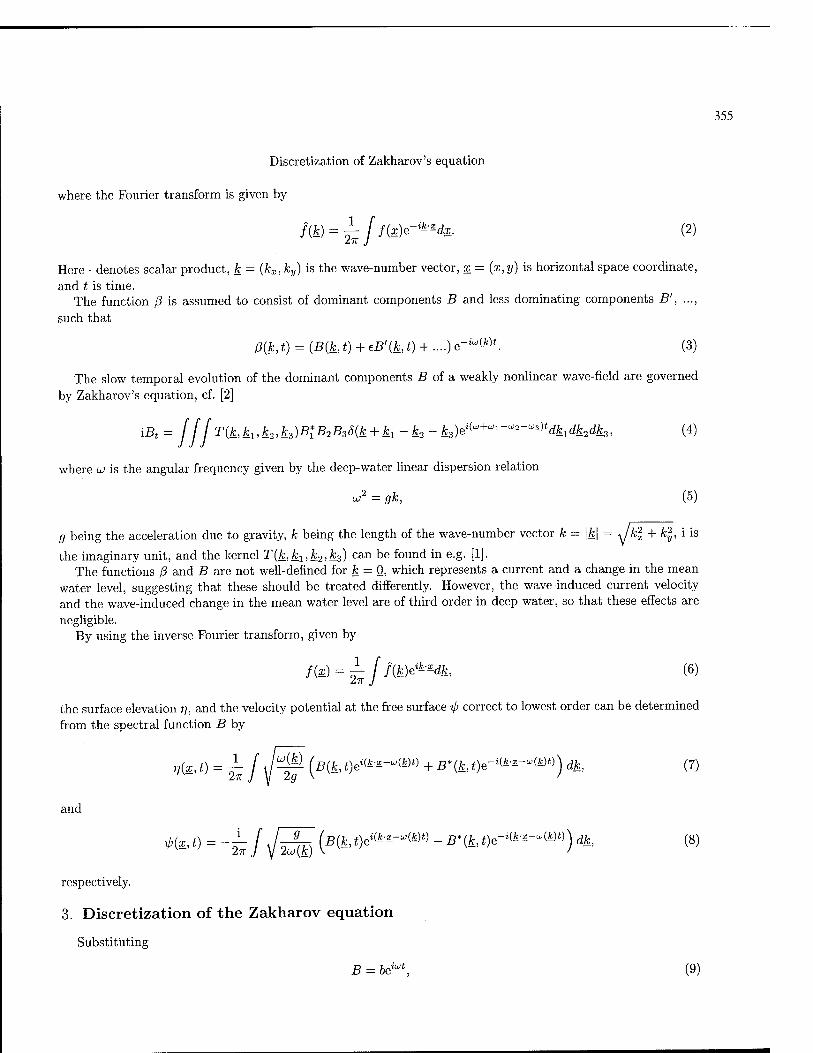
where the Fourier transform is given by
f(k) = ^jf(x)e-i^dx. (2)
Here • denotes scalar product, k — (kx,ky) is the wave-number vector, x = (x,y) is horizontal space coordinate, and t is time.
The function ß is assumed to consist of dominant components B and less dominating components B', ..., such that
ß{k,t) = (B{k,t) + eB'(k,t) + ....)e-iw^t. (3)
The slow temporal evolution of the dominant components B of a weakly nonlinear wave-field are governed by Zakharov's equation, cf. [2]
\Bt = ff[T(k,k1,k2A3)BtB2B36(k + k1-k2-k3)ei^+^-^-^tdk1dk2dk3, (4)
where w is the angular frequency given by the deep-water linear dispersion relation
w2 = gk, (5)
g being the acceleration due to gravity, k being the length of the wave-number vector k = \k\ = ^Jk\ + k%, i is
the imaginary unit, and the kernel T(fc,fc1,fc2>^3) can be found in e.g. [1]. The functions ß and B are not well-defined for k = 0, which represents a current and a change in the mean
water level, suggesting that these should be treated differently. However, the wave-induced current velocity and the wave-induced change in the mean water level are of third order in deep water, so that these effects are negligible.
By using the inverse Fourier transform, given by
f(x) = -^Jf{k)e**dk, (6)
the surface elevation 77, and the velocity potential at the free surface tp correct to lowest order can be determined from the spectral function B by
rffat) = ^j J^ (B^tyik-x-^m) + B'(k,t)e-i&z-'^) dk, (7)
and
V>fe t) = -^f A/3^ {B(k, tytez--"®* - B*(k,Qe-^z-"^) dk, (8)
respectively.
3. Discretization of the Zakharov equation
Substituting
B = bQiut, (9)

356
J. Rasmussen, M. Stiassnie
into the Zakharov equation, equation (4), we find
\{bt +iu)b) = T(k,k1,k2,k3)blb2b36(k + k1 - k2 - k^dk^k^k^. (10)
Applying the inverse Fourier transform, equation (6), on the above expression, we obtain
fi(h+iujb)eik^dk= f j j I T(k,kl,k2,k3)b*1b2h8{k + kl -k2 - k^^dkdkydk^k^ (11)
which simplifies to
J\{bt + icvb)eik^dk = f (JT{kz + k2 - k^k^k^k^blhhe^+^^zdk.dkzdks. (12)
Note that in both sides of the above expression the integrals are over the entire wave-number plane without any restrictions imposed by a Dirac ^-function.
The integral
jf{k,...y^dk, (13)
is now replaced by a sum of a countable number of integrals
W/(fc,..0M*-*Wi)eii'£d*- ■ (14) m,n
Here
*-=(£)• <i5)
are discrete wave-numbers, m, and n are integers that are not simultaneously zero1, A is the increment of the rectangular mesh in the wave-number plane, and h& is a "window"-function given by
, ,, , , [1, \kx -km,n,x\ < A/2 and \ky-km,n,y\ < A/2 M*-*„,,„) = ( 0> otherwise ■ W
Not taking into account m and n simultaneously zero, means that we neglect the effects of current and change in the mean water level, as explained in the previous section.
The role of the hA-function in equation (14) is to pick a single square when calculating the integral; the summation ensures that all squares have been taken into account.
Introducing
K = k-kmn, (17)
expression (14) can be written as
£e*-.n-* j /(fcm,„ + K, ...)hA(K)e^dK. (18)
1Tliis restriction means that our discretized model is unable to treat extremely long waves and background currents.

357
Discretization of Zakharov's equation
Introducing the above into equation (12), we find
J2 ie**—^ f(bt + iio(kmtn + K)6)/iA(K)eifi'£dK (19)
= E E E e^2'"2^31"3^1'"1^//^ mi.ni m2,«2 7713,713
T(tmsin3 + fcm2i„2 - kmuni +K3 + K2- K^kmum + «1 > kmi,n2 + «2,^3 + «S^M«^*»-
Due to the /iA-functions, \K\ of interest is generally much smaller than \kmn\, and thus the interaction coefficient T(kms n3 + km2 „2 -kmuni + K3 + K2-K1,kmuni + Kl,kn2tna + K2,km3,n3 +K3) can be approximated by T(km3tn3 + km2in2-kmuni,kmuni,km2tn2,km3tn3) and moved outside the integration, introducing an error of higher order.
Also due to the /iA-functions and that |K| of interest being much smaller than \kmn\, the angular frequency uj(km n + K) can be replaced by its Taylor expansion
g /m2-2n2 , n2 -2m2 2 Qmn \ 3. . > «(4™,« + fi) = <*»,» + cm ■ * - ^f^ (^7^ + ^T^K»+ m-T^'H +0{K)> (20)
where cfl is the group velocity. Thus equation (19) can be written as
( r fl /m2-2n2 2 n2 - 2m2 2 6mn M^J
(fc + i [«m.» + fi,,ra,„ " fi - 8fcmn(Jmn 1,-^^2-^ + ^+^"«y + ^5+^«««»;] b) ^
EV^ V^ T(h ,7. _jL l. fc fc \ei(im2,n2+im3,~3-&m1,ni)^
/ _, / , J l^m3,n3 +^m2,n2 ^mi,ni'^roi,nii^m2,n2'üm3,ii3^
7711 ,711 7772,712 7773,713
/ (6i/iA(Ki)e4fil'£)* d«i I b2hA(K2y-2-dK2 j ösM^)^3-*£3- (21)
Now it is rather natural to define a square averaged variable as
bm,n = ~j b(km,n + «jÄAteJe^d«. (22)
Spatial derivatives are easily found to
dx = £2 / iK-6^m,n + ä)hA(KV--dK, (23)
and similarly for ^- and higher order derivatives.

358
J. Rasmussen, M. Stiassnie
Hence equation (21) reduces to
E- ik -x I (sum n , ie-"'■" - I + lWm,nOm,n + Qg,m,n ' VOm,n
ig fm2 - 2n2 926m,„ n2 - 2m2 d2bmt„ 6mn d2bm^n
8km,nUm,n \ m2 + n2 dx2 m2 + n2 dy2 m2 + n2 dxdy
= ^ / _, / j / j *■ (,^7713,713 ' f±m2,n2 ~ — mi,n\i— mi,m >—7712,712'— 7713,713/
mi,Til 7712,712 7713,713
0mi,»ll0m2,7l2077l3,7l3e 3' 3 2 2 ' ' • \Z^J
The left as well as the right hand sides of the above expression are complex Fourier series with slowly varying coefficients. The complex exponential-functions of the Fourier series are varying on a fast scale, and their coefficients must match for
fe-M, N — ^7773,713 +^7712,712 _ ^7711 ,711' (25)
where capital indices denote a chosen wave-number. Thus equation (24) reduces to the following set of partial differential equations
.9bM,N , . ■ v7, 1 KL UM,NOM,N + 1CQ M,N ' V6
M,JV at J' '
g [M2-2N2d2bM,N N2 - 2M2 d2bM,N 6MN d2bM,N 8kM,NLOM,N \M2 + N2 Ox2 M2+N2 dy2 M2 + N2 dxdy
= A. 2_j 2—1 /L~i ■* V—JVf,Ar>^77ii,ni'^m2,n2'^m3,7i3)"77ii, m "7712,7i2"m3, 713
7711,711 7712,712 7773,713
Sl< {KM, N +£mi,ni ~~ ^7712,712 ~ — 7713,713)' '^6)
where <$/<(..) denotes Kroneckers 6. Substituting
bM,N = BM,/ve-iWM^', (27)
into the above expression, we finally find
.8BM,N . VR 9 (M2-2N2d2BM,N N2-2M
2O
2BM,N 6MN Ö2
BM,N 1 dt + 1Q° ' VBM
'N
8kM,NUM,N \M2 + N2 dx2 + M2 + N2 dy2 M2 + N2 dxdy
A 2—, l_J Z—l -'v—M.jV'^mi,Til '^7712,712'—7713,713^7711,Til •"7712,712-07713,713
7711,711 7712,712 7713,713
OK\HM,N T^mi.m ^7712,712 ^mz,n3)G > ^°'
which is the main result. In the sequel we call the two first terms on the left hand side "convective terms", the other terms on the left
hand side "dispersive terms", and the terms on the right hand side the "nonlinear terms." The above equation is valid for all pairs of (M, N) and its left hand side has exactly the same structure as
the nonlinear Schrödinger equation.

359
Discretization of Zakharov's equation
Combining equations (9), (22), and (27), we find that the Fourier-modes Bm>n are related to the spectral
function B(k) through
Bm,n = ±f B(km,n + KjAAteJe^*-^«-.-^-''»- >*><&. (29)
4. The relationship between the Fourier-modes and the free surface variables
The relations between the spectral function and the surface elevation and the velocity potential at the free surface as well as the relation between the spectral function and the Fourier-modes are given by equations (7), (8), and (29). It is, however, of practical importance to know the relations between the Fourier-modes and the surface elevation and the velocity potential at the free surface, directly.
To this end we first use equation (9), to find that equations (7), and (8) can be written as
n{x, t) = ^j J^- m t)e** + b'(k, t)e-*s) dk, (30)
and
*fe() - -s/i/SWfc,yM-''(i0e"*1)* (31)
respectively. The surface elevation 77, and the velocity potential at the free surface I/J correct to lowest order are derived
by applying the above discretization technique on equations (30) and (31). First the integrals are written as a sum of a countable number of integrals, i.e. we apply equation (18), resulting in
»»(a.*) = ^Eett--'a/^/h,(&T+fi)(fc(fc')hA(fi)ete'a)<te m,n '
(32)
and
- ^•'"i/^raw&(,Mfi)e,M)*- (33)
Due to the /iA-functions, |K| of interest is generally much smaller than |fcm>n|, and thus the factors of the
form /"(fe^.n+jj) can be repiaCed the leading term in their Taylor expansions
uikm^n + «) _ [Ü- Jm,n
]j 2g M 2g
and so on.
+ 0(K), (34)

360
J. Rasmussen, M. Stiassnie
By moving out constant terms from the integrations and introducing our new variable bm,n, (equation 22), equations (32), and (33) simplify to
(35) m,n ' "
and
<P(x,t) = -^E\/^M-m'"'S-^ne_-m-1 > (36) m.n 2n ~~t V 2wm „
respectively. Using equation (27), we finally find
mn V . " (37)
and
" A 2 /
1>(x,t) = -L_ £ /-JL^ (Broine'^.-^-'--t) - B^^e-'^.»^-"».-«>) , (38)
respectively. The opposite relation is equally important and is derived in the following way. Given the free surface variables r\, and tp in a square with center xQ = (xo>2/o) and side length 2L, these can
be represented by Fourier series expansions
V(x, t)=J2 Hm^mx+n^'L, (39)
where
i pxo+L ryo+L
Hm,n = — / r,{x,t)e-^mx+n»^Ldydx, (40)
and
where
V-fe t) = J2 *m,l.ei(mi+ny),/i
1 (41)
i rx0+L ryo+L
*m,n = -~ / Vfe*)e-i(mx+n!/)7r/L^x, (42)
respectively. Relating the wave-number resolution parameter A to the side-length of the square 2L by
A = j-, (43)

361
Discretization of Zakharov's equation
equations (39), and (41) simplify to
v(x,t) = Y/Hm,neik-^, (44) m,n
^feo = E*^"e*m'n"' (45)
where kmn are discrete wave-numbers given by equation (15), whereas
A2 f Hm,n =^2 J »?(£,*)e-,i—-<fe.
and
A2 f
respectively. Here fA ...dx denotes integration over the above mentioned square. Comparing equation (37) with equation (44), and equation (38) with equation (45), one finds that
TT Akmn-x_A /^m,n („ J(kmn-x-um,nt) , ß* e-i(Km,n-2L-"m,nt)\
and
for all combinations of (m,n).
Adding equation (48) multiplied with V^^ and equation (49) multiplied with y^, we find
A
, 2wm,n V 29 i7r
which gives us
^=SG&W^*"-r"-' <51)
(46)
(47)
(48)
(49)
~Hm njkm,^ + i /^Lli^eiWs = f-^.ne^.-^»-*). (50)
(52)
Insertion of equations (46), and (47) finally gives us
*■- - \ L (\&<>+i\/¥*fe") •■*"—"*- 5. Some special cases of the discretized Zakharov equation
We define the wave-number resolution parameter, S, as the ratio between A and, say, the spectral peak
wave-number kp
«=£. (53)

362
J. Rasmussen, M. Stiassnie
The nonlinearity measure e is estimated by
e = kpa, (54)
where a is a typical amplitude of the wave-field. Both of the above parameters have to be small; e € 1, ä « 1. The nonlinearity parameter e because
waves rarely reach beyond ka = 0.25, since the maximum steepness is limited by breaking. The wave-number resolution parameter S because of the Fourier approach, i.e. the Fourier analysis has to be applied on a length- scale corresponding to a "large" number of peak wave-lengths.
From equation (28) it is seen that the nonlinear terms are of order 0(e3), and from equation (21) it is seen that the dispersive terms are of order 0(eS2), and that the gradient term is of order 0(eS). The order of the time-derivative is either 0(e3) which comes from the Zakharov equation, or 0(eS) which enters from shifting the angular frequency from w to U>M,N- If the leading order of the time derivative is eö the two convective terms combined arc assumed to be of order 0(eS2).
There are three basically different cases depending on how the wave-number resolution parameter 5, and the nonlinearity measure e, compare to each other.
(i) If the wave-number resolution parameter of the spectrum ö is of the same order as the nonlinearity measure e, the convective terms are of order 0(e2) individually, and of order 0(e3) if combined, the dispersive terms are also of order 0(e3), making equation (28) correct to order 0(e3). For this case one has to use the full equation' (28).
(ii) If one takes a dense discretization, i.e.
<5 < e, (55)
there are two possibilities: • If the wave-number resolution parameter of the spectrum S is of order 0(e2), the convective terms become
of order 0(e3) individually as well as combined, but the dispersive terms become of order 0(e5). Thus the governing equation describing the wave-field to leading order simplifies to
i—ßT r- icg • VBM,N = A 2_j 2_^ /__, T{kMtN,kmini,km^n2,km3tnz)BminiBm2<n^Bm3tn3
?ni,rii m2,ri2 m3,ri3
<JK\!i.M,N ^ ^mi.ni ^m2,ri2 —ms,n3 Je ■ \ou)
The above equation is valid for all pairs of (M,N), and is correct to 0(e3). • If, however, the wave-number resolution parameter of the spectrum S is of order higher than 0(e2), say of
order 0(e3), which corresponds to a very dense discretization, all terms with spatial derivatives become of order higher than 0(e3). Thus the governing equation describing the wave-field to leading order reduces to
i TTT = A 2_^ £_^ /—I •''-M,ff!Smi,ni)^m2,ii!'-ra3,n3' i"i,iii"m2Ä-°">3,n3 mj,m m2,ri2 "13,13
brs(k*, *, 4- k -k -fc ')e»(«'M,w+wmi,„1-wm2,„2-wm3,„3)t (57-1
The above system of equations, which is the "naive" discretization of Zakharov's equation, is valid for all pairs of (M,N), and correct to order 0(e3).
(iii) Finally, if the waves have extremely mild steepnesses compared to the wave-number resolution parameter, i.e.
S » e. (58)

363
Discretization of Zakharov's equation
Assuming that the nonlinear measure, e, is of order 0(82), the convective terms are of order 0{83)~ 0(e3/2) individually of order 0{84) ~ 0(e2) in combination, the dispersive terms are of order 0{8 ) ~ 0(e ), and the nonlinear terms are of order 0(e3) ~ 0(56). Thus the governing equation describing the wave-field to leading
order simplifies to
,öBM,N , . T-7 7,
at J
M2 - 2N2 d2BM,N ^ N2 - 2M2 d2BM,N _,_ 6M7V d2BM,N \ = Q ^ ■ +
8kM,Nu>M,N\M2 + N2 dx2 + M2 + N2 dy2 M2 + N2 dxdy
The above equation models the evolution of a linearized wave-field, it is valid for each pair of (M, N) separately, and is correct to order 0(e2) ~ 0((54).
The four different regimes for which the different evolution equations are valid are illustrated in figure 2.
0.001 (».001 0.01
FIGURE 2. Domains of validity of the different equations (indicated on the figure) in the (e, 6)- plane. The diagonal lines are 8 = ep, where p is also indicated in the figure.
6. Discussion and concluding remarks
We found that the discretized Zakharov equation takes different forms depending on the nonlinearity measure, e, and the wave-number resolution parameter, 6. Four different regimes with corresponding discretized equation
were found: • If the wave-number resolution parameter 8, is of order 0(e3) or higher, the "naive" discretization of
' Zakharov's equation, equation (57) holds. • If the wave-number resolution parameter 8, is of order 0(e2), equation (56) holds. • If the wave-number resolution parameter <J, is of order O(e), the full equation (28) holds. • If the nonlinearity measure e, is of order 0(82) or higher, equation (59) holds.

364
J. Rasmussen, M. Stiassnie
The two regimes where equations (28) and (56) hold, are of special interest for a few reasons. They include nonlinear interactions as well as variations in space due to spatial inhomogeneities. This means that these equations are able to model nonlinear wave-wave interactions between modulated wave-trains and wave-packets rather generally. Another reason is that these two regimes together cover a domain in the (e, (5)-plane, which is used for most practical applications, e has typically values in the range from 0.01 to 0.1 and the Fourier analysis is typically applied on a length-scale of 10 to 100 wave-lengths, corresponding to wave-number resolution parameters in the interval from 0.1 to 0.01.
By adding source terms due to wind input and sink terms due to wave-breaking, the discretized Zakharov equation forms a basis for future deterministic wave-forecasting studies.
Acknowledgements
This study was financed by the Danish National Research Foundation, by the Fund for Promotion of Research at the Technion and by the Minerva Center for Nonlinear Physics of Complex Systems. Their assistance is greatly appreciated.
References
[1] STIASSNIE, M. & SHEMER, L. 1984 On modifications of the Zakharov equation for surface gravity waves. J. Fluid Mech., 143, 47-67.
[2] ZAKHAROV, V.E. 1968 Stability of periodic waves of finite amplitude on the surface of a deep fluid. J. Appl. Mech. Tech. Phys., 2, 190-194.

Eur. J. Mech. B/Fluids © Elsevier, Paris
THE EQUILIBRIUM RANGE CASCADES OF WIND-GENERATED WAVES
William PerrieM and Vladimir Zakharov^ [1]: Bedford Institute of Oceanography, Dartmouth, Nova Scotia, Canada, e-mail: wperrie9emerald.bio.dfo.ca
[2]: Landau Institute for Theoretical Physics, Moscow, Russia, e-mail: zakharovflitp.ac.ru
(Received 22 September 1998, revised and accepted 2 February 1999)
Abstract - It was established theoretically by Zakharov and Filonenko (1966) that the direct cascade region of the equilibrium range of the spectrum should follow an /"4 variation. This has since been verified from experimental data, by Toba (1973), Donelan et al (1985) and others. In this study we present a numerical verification of this /~4 variation, assuming physically realistic parameterizations for nonlinear wave-wave interactions, Sni, for energy input to waves by the wind, Sin and removed by wave - breaking dissipation, Sds- © Elsevier, Paris
1. Introduction
Ocean surface waves are generated, grow, evolve and are dissipated according to the spectral wave energy equation
dE[f,9) + CQ ■ V£(/, 0) = Snl + Sin + Sds (1) at J
where /, 9, x and t represent frequency, direction, position and time, respectively. Spectral wave energy is represented by E(f, 9) and wave group velocity is Cg. Nonlinear wave-wave interactions are represented by Sni- The energy input to the waves from the wind is represented by Sin and the dissipation due to wave-breaking is given by Ssds-
There are several challenges that must be confronted in using equation (1) to simulate wave growth and development. For example, although several decades have been invested in the construction of realistic for- mulations for wind input Sin and dissipation Sds, the state-of-the-art parameterizations for these terms still involve many assumptions. This is described in Komen et al. (1994). Although accepted formulations for Sin
and Sds may be valid for specific field experiments (i.e. the Bight of Abaco experiment by Snyder et al. 1981), these parameterizations are not generally valid for more general situations. Examples of the latter conditions are intense, rapidly varying storms with complex spatially and temporally varying wind stress. Even in simple constant wind conditions there is evidence that parameterizations for Sin and Sds are less than perfect. For example, the accepted parameterizations for Sin, Sds and Snh as implemented in the WAM model of Komen et al. (1994), give energy growth curves that differ significantly from observations for short fetches, as shown by Tolman and Chalikov (1996).
The equilibrium range of the spectrum is above the spectral peak, /„, extending from about 1.5 x fp to about 3 xfp. In this region there is an approximate dynamical balance between the so-called direct transfer of energy from lower to higher frequencies, and the so-called inverse transfer of energy from high to lower frequencies. At a specific critical frequency fc in the equilibrium range, the direct and inverse transfers balance. Below fc, there is a net transfer of energy to lower frequencies. In this region, inverse cascades occur. Above fc, there is a

366
W. Perrie, V. Zakharov
net transfer of energy to high frequencies. In this region, direct cascades occur. Following Zakharov (1991), one can associate the direct cascades with wave dissipation Sds and consequent wave attenuation. Inverse cascades can be associated with wind input, £,„, and wave growth. Clearly, inaccuracies in parameterizations for S;„ and Sfis will be reflected by inaccuracies in estimates for the variation of the equilibrium range with frequency. Zakharov (1991) suggested that the direct cascade region follows an /~4 variation, and the inverse cascade region, an /-j3" variation. This paper is concerned with finding the parameterizations for £*„ and Sds which are consistent with an /~4 variation for the direct cascade region of the equilibrium range, as originally predicted by Zakharov and Filonenko (1966), observed by Toba (1973), and reviewed by Zakharov (1991).
In Section 2, we present a brief review of accepted "state-of-the-art" formulations for 5j„ and Sds, for example as implemented in the WAM model of Hasselmann et al. (1988) and Komen et al. (1994). In Section 3, we describe accepted parameterizations of observed spectra, such as Battjes - JONSWAP, as derived by Battjes et al. (1987), and the formulations for Sin and Sds which may be derived from these parameterizations. In Section 4, we consider these S1;« and Sds parameterizations, and we show that they can lead to the existence of equilibrium ranges which have an approximate /~4 variation, with regions of direct and inverse cascades that appear qualitatively consistent with the theoretical estimates of Zakharov and Filonenko (1966) and Zakharov (1991).
2. Overview of Sin and Sds Parameterizations
2.1. WAM Model Formulation
The accepted formulation for wind input Sin, as parameterized in the WAM model of Hasselmann et al. (1988) and Komen et al. (1994), suggests that 5,„ should be represented as
Sin(f,0) = ßu>E(f,6), (2)
where ß is a nondimensional function of seastate maturity and w = 2irf represents angular frequency, which is related to wavenumber k through the deep water dispersion relation u>2 = gk.
In earlier versions, for example WAM (cycle 3), as described by Hasselmann et al. (1988), the formulation for ß is given by
/3 = max|o,0.25e(28^cos(A6l)-lj| (3)
where e = £sL- is the ratio of the densities of air and water and A9 = the difference between the wind and wave Pu,
directions. Janssen (1989,1991), Komen et al. (1994), Tolman and Chalikov (1996) have made revisions to ß, aimed at
simulating the coupling feedback between wind and waves. These modifications have been able to simulate (i) negative wind input when the wind is at large angles to the waves, or slower than the waves, and (ii), smaller overall energy input, because of negative contributions for overdeveloped waves and smaller contributions for waves near full development.
The accepted formulation for wave dissipation Sds, motivated by the earlier studies by Hasselmann (1974) and Komen et al. (1984), as parameterized in the WAM model of Hasselmann et al. (1988) and Komen et al. (1994), suggests that Sds should have the form,
Sds = Cds ~ ' \OtpM
)\l)'°mj.*> «>

367
The equilibrium range cascades of wind-generated waves
where a = m0Qi/g'2, and m0 is the zeroth moment of variance spectrum, Q is the mean radial frequency JjE(w,e)ujdüjde/Etotai, with Etotai the total spectral energy and / is the frequency in Hz. Tuning is achieved by the fitting parameter, Cds, and {a/äPM) is an overall measure of steepness in the wave field.
Variations in this Sds formulation are given by Banner and Young (1994) and Tolman and Chalikov (1996). These alternate Sds formulations result from alternate choices for the other source terms: Sin and Sni. Banner and Young (1994) consider the nonlinear interactions Sni as simulated by Resio and Perrie (1991). Tolman and Chalikov (1996) implement a very detailed, physically well-motivated, wind input Sin parameterization. It is shown in Lin and Perrie (1999) that the Snt formulation by Resio and Perrie (1991) is comparable to the EXACT-NL code of Hasselmann and Hasselmann (1981), and both differ from the DIA code of Komen et al. (1994) in the WAM model. As stated by Komen et al. (1994), all Sds formulations are approximations based on an incomplete understanding of wave - breaking, and represent a tuning of the computer code, so that the resultant simulation of equation (1) produces energy growth and evolution consistent with accepted observations, such as the JONSWAP data of Hasselmann et al. (1973) and Battjes et al. (1987).
2.2. Empirical Formulation
The JONSWAP wave spectra was given a parameterization by Hasselmann et al. (1973) which may be written as
£(/) = a5ff2(27r)-4r5exp^(£) \exp[ (^ (5)
where E(f) is the one - dimensional wave energy, 7 is the peak enhancement factor, a5 is the spectral level of the tail, and aa and ab represent the peak asymmetry, where
o = {a« J"'^' (6) [ ab for / > fp.
Hasselmann et al. (1973) gave parameterizations for fp, 7, a5, aa and ab as functions of dimensionless fetch, xg/Ul
Some years later, Battjes et al. (1987), showed the JONSWAP data is better described by an / 4 fit, using the parameterization,
,(-(*)-) f i-fp
E(f) = a4gU*(2K)-3rieWV^) J^T^n. (7)
Fetch-relations for fp, 7, a4, aa and ab, differ significantly from those derived by Hasselmann et al. (1973). Direct and inverse cascades can be computed in terms of the direct and inverse action transfers, following
Resio and Perrie (1991). For example, inverse transfers, T^ may be written as
rÄK) = / / iC2V ~ H(\ h I -kr)H(kr- I h \)dsdhdh (8)
where C2 the coupling coefficient, |f£|_1 is the Jacobian for the coordinate transformation, resonance con- ditions are kx + k2 + k3 + £4 =0 and wi + w2 + ^3 + w4 = 0, where dsdkydk^ is transformed phase space volume, H is the Heaviside function, and the density function is Dik^k^k^k^) = (n^) + nQcJ) n{k2)n(k3)- (n(fc3) -I- n(fc2)) «(fcjn^).
Using the energy spectra parameterized in equations (5)-(7), Perrie and Lin (1997, 1999) use direct calcula- tions of the direct and inverse cascades from equation (8) to infer constraints on the functional forms for Sin

368
0.006
0.004
0.002
0
-0.002
m -0.004 s <
W. Perrie, V. Zakharov
Snl, Sds + Sinput forTime=0
Time=0 hr, Sin+Sds o Snl -—
Time=6 hr, Sin+Sds + Snl
j ;%JJ*****'*"*:«t:*-V*.-»-
0.05 0.1 0.15 0.2 0.25 0.3 0.35 0.4 0.45 0.5 f(Hz)
FIGURE 1. The variation of Sni and 5,„ + Sds with frequency /, at time t = Ohr and t = 6/ir, where 5j„ and Sds are WAM source terms scaled by 1/100.
and Sds- Motivated by the WAM formulations of equations (2)-(4), which suggest that Sin and Sds have the generic form
Sin + Sds ~ E(f)fm (9)
where m « 2, they suggest that m ~ spectral maturity. Specifically, they suggest that
m = a0 + diifp - A) + a2(fp - B)2 (10)
where a0, a\, a2, A and B are appropriate constants.
3. Equilibrium Range Calculation
3.1. WAM Source Terms
Using the WAM parameterizations for Si„ and Sds, we integrate the kinetic equation (1) in time, neglecting the spatial advective term Cg ■ VE(f,6). These S{n and Sds formulations in equations (2)-(4) are tuned to the discrete interaction approximation (DIA), in the standard WAM model. Because DIA differs significantly from more accurate simulations of the nonlinear wave-wave transfer Sni, such as that of Resio and Perrie (1991), which is used here, it is necessary to rescale these WAM formulations for Sin and SdS in order to get physically realistic results. Thus we reduce Sin and Sds by a factor of 100. Note that this (1/100) scaling gives very small values for Sin + Sds, relative to maximal values for Sni-
This test uses a fine-mesh grid, with 58 frequency bands, 2.5° angular resolution and 15 s timesteps. Initially, fp is 0.15 Hz and fc, the interface between direct and inverse cascades, is about 0.22 Hz. Assumed wind speed is 15 m/s. After 6 hr simulation the spectral peak fp has migrated to lower frequency values and all variables appear physically realistic, as shown in Figure 1. The critical frequency is about 0.17 Hz. In Figure 2, we show the exponential variation of the high frequency region of the spectrum. This shows that starting with the /~5 variation assumed by the JONSWAP parameterization of Hasselmann et al. (1973), the spectrum
evolves to having a distinct equilibrium range at about 1.8/p < / < 2.4/p. The direct cascade region of the

369
The equilibrium range cascades of wind-generated waves
WAM Source Terms: f_p=0.15@t=0, U10=15m/s
+ time=t.01 hour i . ! 1 hour o
;■ ;■ ;:.---''; ■ ■•r-2-noiar""-'""'" ' ; 3 hour +
.-;•'.'.' i : 4 hour ■■'"!' ■■'■. A i »■■!—5-hotir-o
L.v;0 }••;• -••[.. I 6hour
3 I (Hz)/I_p
FIGURE 2. The variation of the equilibrium range exponent m, where E(f) ~ fm as a function of normalized frequency f/fp, with time, up to t = 6/ir, for the spectral evolution of Figure 1.
0.004
0.003
Snl, Sds + Sinput
Time=0 hr, Sin+Sds o /!++ Snl —- /' , Time=5 hr, Sin+Sds + / t J» Snl
-
0.002 / +! + 0 +
-
VI 0.001
0
-0.001
-0.002
o w 75
Q. E LLI
\ I -
-0.003 ill -
-0.004
' > " i t i i
-
0.05 0.1 0.15 0.2 MHz)
0.25 0.3 0.35 0.4
FIGURE 3. As in Figure 1, using the empirical source terms Sj„ and Sds of equations (9)-(10).
equilibrium range has a variation of about f~4. As suggested by Zakharov (1991), the inverse cascade region of the equilibrium range, below fc, has a slightly smaller equilibrium range exponent, in magnitude.
3.2. Empirical Sin and Sas
Using the empirical 5,„ + Sds parameterizations of equations (9)-(10), we repeated the calculation of the previous section, as given in Figures 3-4. Starting with an initial fp « 0.15 and fc w 0.18, we simulate the source terms, Sin + Sds and S„i for 15/ir. It is interesting to note the magnitude of | Sin + Sds | relative to | Sni | in Figure 3, as compared to the WAM test in Figure 1. Similar magnitudes for WAM Sin and Sds terms would give unphysical results.

370
W. Perrie, V. Zakharov
iw4/0c 65nrng+49nang: xlm=1.1, zconst= LARGE
; time=1 hour — !/& 3 hour o
7 hour 9 hour
M hour o - □ .«■Äcjao- 13 hour ■
„A-fgJl Ö
1.5 2 2.5 3 3.5 f (Hz)/I_p
FIGURE 4. As in Figure 2, showing the variation in m as a function of normalized frequency f/fp, with time, up to t = 13/ir.
Figure 4 gives the evolution of the equilibrium range exponent across the spectrum, for this Sin + Sds parameterization, as in Figure 2. Compared to the WAM formulations for Sin and Sds in Figures 1-2, the equilibrium range is much broader and better defined. Figure 4 shows that after a few hours, the direct and inverse cascade regions are formed in the domain 1.4/p < / < 2.8/p. From computations simulating longer times than those of Figure 3, we estimate that fc, marking the interface between direct and inverse cascade regions, is about 2/p. Therefore the equilibrium range variation for the direct cascade region of the spectrum, above fc is approximately /~4. For the inverse cascade region, below fc, the exponent of the equilibrium range variation is slightly smaller in magnitude, which is consistent with Zakharov (1991).
4. Conclusions
The nonlinear wave-wave interactions are responsible for the formation of the equilibrium range, including its direct and inverse cascade regions, with their /~4 and /~^ variations, (Zakharov and Filonenko: 1966 and Zakharov: 1991). A simulation of the kinetic equation (1), using an accurate realistic Sni always gives a well-behaved equilibrium range, a critical frequency fc, defining the interface between direct cascades to high frequencies and inverse cascades to lower frequencies. As pointed out by Zakharov (1991), such dynamical structure is necessary, for conservation of energy and action within the spectrum.
Assuming the existence of nonzero source terms for wind input Sin and dissipation Sds makes the problem difficult because it is easy to specify unphysical Sin and Sds formulations which give unrealistic results. It is difficult to guess physically well-motivated formulations for Sin and Sds which are also consistent with equilib- rium range dynamics. Using the Sni formulation of Resio and Perrie (1991), the WAM formulations for Sin and Sds in their normal form lead to unrealistic effects, after simulations of only a few hours, because WAM Sin
and Sds are tuned to DIA, the parameterization for the WAM 5„;. With more accurate formulations for Sni, new formulations for Sin and Sds are necessary in order to simulate
wave growth relations in a realistic manner. This was the finding of Banner and Young (1994). We have shown that suitable rescaling of WAM Sin and Sds parameterizations can result in a small credible equilibrium range, with associated regions of direct and inverse cascades. However, there are other parameterizations for Sin and Sds which can result in a realistic equilibrium range and regions of direct and inverse cascades. This was shown

371
The equilibrium range cascades of wind-generated waves
in Figures 3-4, for the empirical Sin + Sds formulation of Perrie and Lin (1997, 1999). This formulation was derived from the JONSWAP data, as parameterized by Hasselmann et al. (1973) and Battjes et al. (1987).
Acknowledgements
The wave modeling program at BIO is funded by the Federal Panel on Energy Research and Development (Canada) under Project 534201. This research was also funded by the Wave Prediction Base Enhancement Program of the Office of Naval Research and by the ONR grant N 00014-98-1-0070.
References
[i:
[2
[3:
[4 [5
[6
IT
[8
[9:
[io:
[ii
[12:
[13 [14:
[is:
[ie:
[17:
[is:
[19:
[20:
[21
Banner, M. L. and Young, I. R. 1994: Modeling spectral dissipation in the evolution of wind waves. Part I: Assessment of Existing Model Performance. J. Phys. Oceanogr., Vol. 24, 1550-1571. Battjes, J.A., Zitman, T.J. and L.H. Holthuijsen, 1987: A reanalysis of the spectra observed in JONSWAP. J. Phys. Oceanogr., Vol. 17, 1288-1295. Donelan M. A., Hamilton, J. and Hui, W. H. 1985: Directional spectra of wind-generated waves. Phil. Trans. R. Soc. Lond. A, Vol. 315, 509-562. Hasselmann, K. 1974: On the spectral dissipation of ocean waves due to white-capping. Bound. Layer Meteor., Vol. 6, 107-127. Hasselmann, K.,Barnett, T. P., Bouws, E., Carlson, H., Cartwright, D. E., Enke, K., Ewing, J. A., Gienapp, H., Hasselmann, D. E., Kruseman, P., Meerburg, A., Miller, P., Olbers, D. J., Richter, K., Sell, W., Waiden, H. 1973: Measurements of wind-wave growth and swell decay during the Joint North Sea Wave Project (JONSWAP). Deutsche Hydrograph. Zeit., Erganzungsheft Reihe A (8), Nr. 12. Hasselmann, S. and K. Hasselmann, 1981: A symmetrical method of computing the nonlinear transfer in a gravity-wave spectrum. Hamb. Geophys. Einzelschriften Reihe A: Wiss. Abhand., 52, 138pp. Hasselmann, S. and K. Hasselmann, 1985: Computation and parameterizations of the nonlinear energy transfer in a gravity- wave spectrum. Part I: A new method for efficient computations of the exact nonlinear transfer integral. J. Phys. Oceanogr. Vol. 15, 1369-1377. Hasselmann, S., Hasselmann, K., Komen, G. K., Janssen, P., Ewing, J. A. and Cardone, V., 1988: The WAM model - a third generation ocean wave prediction model, Journal of Physical Oceanography, Vol. 18, 1775-1810. Janssen, P.A.E.M., 1989: Wave-induced stress and the drag of air flow over sea waves. J. Physical Oceanography, Vol. 19, p. 745-754. Janssen, P.A.E.M., 1991: Quasi-linear theory of wind-wave generation applied to wave forecasting. J. Physical Oceanography, Vol. 21, p. 1631-1642. Komen, G. J., L. Cavaleri, M. Donelan, K. Hasselmann, and P. A. E. M. Janssen, 1994: Dynamics and Modelling of Ocean Waves Cambridge University Press, Cambridge, 512pp. Komen, G. J., Hasselmann, S. and Hasselmann, K., 1984: On the existence of a fully developed windsea spectrum, Journal of Physical Oceanography, Vol. 14, 1271-1285. Lin, R. Q. and Perrie, W. 1999: A New Coastal Wave Model. Part IV. Nonlinear Source Function, J. Geophys. Res. (in press). Perrie, W. and R. Q. Lin, 1997: Relating nonlinear cascades to wind input and wave breaking dissipation. In Nonlinear Ocean Waves, Computational Fluid Mechanics, Southampton, pp. 89-110. Perrie, W. and R. Q. Lin, 1999: On parameterizations for wind input and wave-breaking dissipation. Submitted to Ocean Modelling. Resio, D. and Perrie, W. 1991: A numerical study of nonlinear energy fluxes due to wave-wave interactions Part I: Methodology and basic results. J. Fluid Mech. Vol. 223, 603-629. Snyder, R., F. Dobson, J. Elliott and R. Long, 1981: Array measurements of atmospheric pressure fluctuations above surface gravity waves. J. Fluid Mech., Vol. 102, p. 1-59. Toba, Y. 1973: Local balance in the air-sea boundary processes, III. On the spectrum of wind waves. J. Oceanogr. Soc. Japan, Vol. 29, 209-220. Tolman, H. and D. Chalikov, 1996: Source terms in a third-generation wind wave model. J. Phys. Oceanography, Vol. 26, 2497-2518. Zakharov, V. E. 1991: Inverse and Direct Cascade in the Wind- Driven Surface Wave Turbulence and Wave Breaking. In Breaking Waves IUTAM Symposium, M. L. Banner and R. H. J. Grimshaw (Editors), Sydney, Australia, p. 69-91. Zakharov, V. E. and Filonenko, N. N. 1966: The energy spectrum for stochastic oscillation of a fluid's surface. Doklady Akad. Nauk., Vol. 170, 1292-1295.
Eur. J. Mech. B/Fluids © Elsevier, Paris
OBSERVATIONS ON WAVEFORMS OF CAPILLARY AND
GRAVITY-CAPILLARY WAVES
Xin ZhangW
[1] : Scripps Institution of Oceanography, University of California San Diego, La Jolla, California 92093-0230, USA
(Received 22 September 1998, revised and accepted 30 January 1999)
Abstract - Due to extreme conditions in the field, there has not been any observational report on three-dimensional waveforms of short ocean surface waves. Three-dimensional waveforms of short wind waves can be found from integrating surface gradient image data (Zhang 1996a). Ocean surface gradient images are captured by an optical surface gradient detector mounted on a raft operating in the water offshore California (Cox and Zhang 1997). Waveforms and spatial structures of short wind waves are compared with early laboratory wind wave data (Zhang 1994, 1995). Although the large-scale wind and wave conditions are quite different, the waveforms are resoundingly similar at the small scale. It is very common, among steep short wind waves, that waves in the capillary range feature sharp troughs and flat crests. The observations show that most short waves are far less steep than the limiting waveform under weak wind conditions. Waveforms that resemble capillary-gravity solitons are observed with a close match to the form theoretically predicted for potential flows (Longuet-Higgins 1989, Vanden-Broeck and Dias 1992). Capillaries are mainly found as parasitic capillaries on the forward face of short gravity waves. The maximum wavelength in a parasitic wave train is less than a centimeter. The profiles of parasitic wave trains and longitudinal variations are shown. The phenomenon of capillary blockage (Phillips 1981) on dispersive freely traveling short waves is observed in the tank but not at sea. The short waves seen at sea propagate in all directions while waves in the tank are much more unidirectional. © Elsevier, Paris
1. Introduction
Nonlinearity in finite amplitude gravity surface waves of permanent form leads to sharp crests and flat troughs (Stokes, 1880). Wilton (1915) made a pioneering study of nonlinear gravity-capillary waves. Later Crapper (1957) predicted that capillary deep water waves in an inviscid, irrotational flow have profiles characterized by steep troughs and flat crests, the opposite of the nonlinear gravity waveforms. It is an exact closed-form solution for waves of arbitrary amplitude. This prediction has received some visual evidence from laboratory studies by Schooley (1958). For gravity-capillary waves, no exact solutions are known because of the complexity of the equations, but through numerical calculations, Schwartz and Vanden-Broeck (1979) and Hogan (1980) showed that their waveforms are very much like capillaries.
The existence of solitary gravity surface waves of permanent form in shallow water was discovered by Scott Russell (1838) and explained by the approximate theories of Boussinesq (1872), Rayleigh (1876) and Korteweg and de Vries (1895). Solitary capillary-gravity waves in the water of finite depth were discussed with similar approximation by Kawahara (1972), Hunter and Vanden-Broeck (1983), Zufiria (1987), Iooss and Kirchgässner (1990), and Dias and Iooss (1993). In reality the bottom boundary layer due to wall friction is thick compared to fhe water depth. However, this is neglected in the above calculations. For more realistic deep water waves, Longuet-Higgins (1988) first suggested the existence of solitary waves for capillary-gravity waves from a different approach to the nonlinear water wave equations. The subsequent calculations (Longuet-Higgins 1989, 1993, and Vanden-Broeck and Dias 1992) predicted many properties of solitons. Capillary-gravity solitons are predicted

374
X. Zhang
to have a sharp trough similar to periodic capillary waves of finite amplitude with damped oscillations on both sides of the sharp trough. Laboratory observations were reported by Zhang and Cox (1994), Zhang (1995) and Longuet-Higgins and Zhang (1997).
Parasitic capillary waves on the downwind faces of gravity waves propagate as groups (Cox 1958). The linear theory of parasitic waves (Longuet-Higgins 1963) predicts that the wavelengths of parasitic capillaries decrease toward the trough of the long wave on which they ride. It is observed that, in the wind wave tanks (Schooley 1958, and Ebuchi et al 1987), there is a steep dip at the upper end of parasitic capillaries near the long wave crest. From fluid visualizations, Okuda et al (1977) suggested the occurrence of a very strong vortical region at the crest of the gravity wave. Longuet-Higgins (1992) accounted for this phenomenon by including the vorticity introduced by steep capillary waves. Ebuchi et al (1987) concluded, from an observation of 'specular facets' of short wind waves, that there is a streamwise streak structure on the rear face of long waves at a certain wind speed. The wave shape of parasitic capillaries was recently measured in a wind wave tank with surface gradient imaging techniques (Zhang 1995). The waveforms fit the description of the theories. It is also found that the maximum wavelength of parasitic capillaries is less than 1 cm.
Under the influence of wind, there is a wind drift shear layer just below the water surface. Wu (1968) measured a surface drift of about 4% of the mean wind speed, and a thickness of 3-5 mm. The wind drift surface boundary layer is very complicated and the effect on the waveform of very short waves is unknown. It has been shown (Simmen and Saffman 1985) that a uniform vorticity field (a linear shear layer) can change the form of gravity waves.
The discussion so far refers to two-dimensional plane waves propagating horizontally in one dimension. Chen and Saffman (1985) and Dias and Härägu§-Courcelle (1999) calculated the three-dimensional capillary waves that diverge from two-dimensional capillary waves under the influence of nonlinearity. There are virtually no other quantitative measurements of waveforms of very short waves in three dimensions. Our elevation gradient measurements (Zhang and Cox 1994) allow 2-D wave surface reconstruction and provide a way of examining the 3-D waveforms of very short waves in detail.
In this paper, we report the short wind waves we observed in the California coastal water. Due to very different environments and processes involved, it is important to verify short wave behaviors in the field from direct observations. Short wind waves in the ocean are difficult to measure due to the harsh environment. Field observations are rare, and there are no measurements of the waveforms of short waves. The aim of this study is to acquire short wave field data and compare some aspects of very short wind waves between field data and lab data to improve our understanding on the dynamics of short wind waves.
The scattering of microwaves by the sea surface is influenced by Bragg scattering from very short water waves. For ocean surface waves, there are a wide range of wavelengths extending from long swells down to ripples with lengths of the order of a millimeter. Capillarity is dominant in waves with wavelengths shorter than 1.7 cm. The capillaries can be very steep with great curvature which can generate turbulence at and below the surface which contribute to the ocean surface mixing. Short surface waves can be generated and modulated by the wind and longer surface waves. Observing the shapes and structures of short wind waves is of vital importance to our understanding of these processes at the sea surface.
2. Data sets
The water surface is measured by a surface gradient imager that consists of a strobe light source, a color screen and a beam forming lens set underwater, and a photographic recording camera. It records color-coded light beams refracted at the sea surface over an area about of 20 cm x 16 cm. The recorded surface color images can be used to recover the shape of the water surface which is important to study the small scale roughness of the sea surface. Figure 1 shows our raft based optical surface measurement system in operation in Mission Bay, San Diego. The raft consists of a catamaran, 5.4 m long, with the optical equipment supported by two booms extending beyond the bow of the catamaran (on the left). One boom, extending upward into the air, supports anemometers and a mirror to reflect an image of the water surface to a photographic camera mounted just above the bow of the catamaran (see figure 2 for details). The other boom extends underwater and supports an

375
Observations on waveforms of capillary and gravity-capillary waves
FIGURE 1. A raft based optical surface measurement platform in Mission Bay water.
optical system to color code water surface slopes as seen by the photographic camera as well as a PIV system consisting a laser diode array and a CCD camera (not in the drawing). The battery and computer control unit- is mounted near the stern. The controlling computer is operated by a laptop on the mothership nearby through radio communication.
The technique of coding the two dimensional slopes of the water surface at full resolution (Zhang and Cox 1994) can be understood with reference to figure 3. A translucent color screen containing a distribution of hues and saturation of colors is illuminated from below and is at the focus of a Fresnel lens, so that beams of distinctly different colors are projected above the lens. Each colored beam comprises a parallel bunch of rays at an angle to the vertical determined by the location of their origin on the color screen, thus their color. The Fresnel lens set is of sufficiently large diameter (50 cm) and close enough to the water surface (50 cm) so that a circular area on the sea surface about 25 cm in diameter is illuminated by all the color beams. An imaging detector looking down on the sea surface from well above will see only those beams which have been refracted so that the rays are directed towards the detector (essentially parallel to the "optical axis" in the figure). Snell's law of refraction ensures that the color as imaged is determined by the two components of surface slope at each point in the field of view. In this way the slopes of the water surface are color-coded. The dynamical range of the system is limited to water slopes of about 45° by the vertical angles of the parallel beams above the Fresnel lens, and the resolution of small water wavelength is limited by the resolution of the imaging detector. To achieve full resolution to sub millimeter scales and also cover a 25 cm surface diameter with the capability of

376
X. Zhang
Directional wind vane
Mirror ©
0,0
-Anemometers and humidity
sensors
0.5 m
Scale in meters
Fresnel lens to color code water slopes
- color screen
Xenon flash lamp
FIGURE 2. The optical surface slope measurement system is supported by two booms extending beyond the bow of the catamaran.
successive recording at rapid time intervals we have found it necessary to use color photography at a reasonable cost. In this application, a 16 mm movie camera is used. The water surface elevation can be calculated directly from the gradient image (Zhang 1996a).
The camera is mounted just above the bow of the catamaran looking at the sea surface through a mirror on the upper boom. The real distance from the sea surface to the camera is about 365 cm. This is large enough compared with the imaging area of 25 cm. The frame of the booms is rigid to prevent any relative motions among the camera, the mirror, and the under water optical system. Even if there is any small movement, for example 2 cm, it will not introduce appreciable error (very small change in viewing angle), since the distance between the camera and imaging sea surface is two order of magnitude larger.
Environmental data and raft motion is also recorded digitally by a computer. These include pitch, roll and yaw and accelerations of the platform, wind speeds and directions, surface level from a wave staff, air temperature and humidity. Figure 4 shows an example of wind speed collected by two anemometers about 90 cm and 150 cm above the sea surface.
The raft is designed to be towed offshore by a launch that also serves as a mothership. During towing, the booms are tilted to bring the underwater parts up into the air, and the entire boom assembly is then stowed inboard on the raft. When the raft is towed into a measurement station, the booms are lowed down facing the wind, and the raft is allowed to drift freely (or it can be anchored). The data in the paper were collected 5

377
Observations on waveforms of capillary and gravity-capillary waves
/ \ distant camera
light rays
water surface mean water level
color screen
FIGURE 3. Optical principle of gradient detector.
miles from the San Diego coast in November 1997. The wind causes the raft to drift slowly towards the south. The swells coming towards the shoreline are about 15 to 20 m.
3. Waveforms of very short wind waves
3.1. Nonlinear steep capillary-gravity wind waves The dominant features in the surface gradient image data are those of very short waves (less than 5 cm)
because they are steeper than the longer waves. About 30% of the images that contain more or less capillaries with slope greater than 40° degrees (near the maximum measurement range of 45°). The maximum slopes of the longer gravity waves, however, are only in the range of 10° to 15°. The change in surface elevation is due to the energetic long waves, whereas the large change in surface slopes is largely contributed by the short waves. For these steep short waves, one would expect that nonlinearity is important. The nonlinear waveforms featuring narrow, sharp troughs and broad, flat crests are observed present with these steep short waves as in laboratory cases. Figure 5 shows a surface image in which the steepness, the magnitude of surface gradient, is represented by the brightness (intensity). The slopes at wave crests and troughs are low, thus dark, and slopes on forward or backward phases are high thus bright in the image. In the image, the sharp troughs are seen as thin lines or curves in contrast to the flat crests of short waves. Although steep nonlinear short waves are present in the light wind condition here, they are sparse, and spatially intermittent. The energy dissipation by this intermittent short wave field can exceed the dissipation by an assumed uniform distributed short waves field with the same mean slopes, for energy is proportional to square of wave slope. The statistical description of very short wind waves, such as probability distribution function, may have to be considered differently from longer waves due to their stronger nonlinearity and intermittency. In some applications, for example, remote

378
X. Zhang
Wind speed m/s
FIGURE 4. An example of in situ wind speed records. The dark lines correspond to the upper anemometer while the light lines correspond to the lower anemometer.
sensing of ocean surfaces through radar backscatter, one has to be very cautious in interpreting the statistical quantities of short waves, such as the mean square slopes (MSS), and wavenumber or frequency spectrum. Most of the steep short waves in this set of image data are parasitic capillaries. Other steep waves are those solitary capillary-gravity waves, and on rare occasions, irregular random short waves.
3.2. Parasitic capillaries
The existence of parasitic capillaries on the forward face of gravity waves is persistent in laboratory wind wave tanks at all wind speeds, even on purely mechanically generated waves. Parasitic waves are generated at the crests of long waves (Longuet-Higgins 1963, 1992). In resonating with the orbital velocity and gradient of orbital velocity of underlying long waves (Zhang 1995), they extract energy from the underlying long waves to work against the strong viscous dissipation (which is proportional to the square of wavenumber). Otherwise, short waves would be very short lived at a low wind speed. The favorable conditions for the parasitic capillaries arc the existence of 10 to 100 cm steep gravity waves. Under the short fetch conditions in laboratory wind tanks, these short gravity waves are dominant, and parasitic waves are very important in dissipating wave energy and contributing to the small scale of surface roughness.
Parasitic capillaries in this data set are still dominant features among the steep short waves. The wavelengths of the parasitic capillaries are mainly in a range of 1 mm to 1 cm as shown in figure 6. The data of this wavelength histogram plot are collected by measuring the wavelength of each wavelet of all the parasitic wave trains found in our image data set.
Images of parasitic capillaries on long and short gravity waves are shown in figures 7 and 8. The wavelength decays from the crest towards the trough of the underlying waves, so do the slopes. In each parasitic wave train, the wavelength of the first wavelet (the nearest to the carrying wave crest) is the longest, varying from 0.5 cm to 1 cm or more. The shorter the first wavelet is, the steeper it is. The slopes of wavelets over 1 cm are very small. The parasitic wave trains starting with the extremely short wavelet are those associated with

379
Observations on waveforms of capillary and gravity-capillary waves
FIGURE 5. Top: A color-coded sea surface slope image of size 20.7 cm x 14.5 cm. Bottom: Surface steepness in brightness.

380
X. Zhang
FIGURE 6. The wavelength distribution of parasitic capillaries.
incipient breaking (Banner and Phillips 1974) of the underlying waves as can be seen from the image data (Figure 9). The small-scale breaking of gravity waves can thus be detected by the change in wavelength of the parasitic waves. The steeper the carrying waves are, the shorter the starting parasitic wavelets, the steepest being those about 0.5 cm to 0.7 cm long. As the carrying waves steepen, the parasitic waves are compressed and become shorter wavelets as a result of increasing surface flow speed at the incipient breaking crest. The viscous dissipation limits the further growth of extremely short waves. The wavelength of the wavelets in a parasitic wave train decreases quickly for the first few wavelets, then the change diminishes gradually. There is little difference in wavelengths of the last few wavelets. In each of the parasitic capillary trains, there are more short wavelets than longer ones, which is why the shorter wavelet counts are enhanced in figure 6.
The parasitic waves are locally parallel to the underlying wave crests. Locally, they have a narrow angular distribution which limit the triad wave-wave interactions, for the triad resonant condition requires a much wide angular distribution (McGoldrick 1965). However, four wave-wave resonant interactions are possible for the narrow spectral capillaries (Zhang 1995). The wave trains are also propagating in the long wave orbital motion field which is inhomogeneous. These nonlinear waves can be visually detected in some instances (figure 9) when waves focus and defocus in the interaction process and form surface caustics in the direction of propagating waves (Peregrine and Smith 1979).
3.3. Solitary capillary-gravity waves
Another important observed phenomenon is the isolated steep dips which resemble solitons of capillary- gravity waves. These solitary waves propagate slower than the free linear waves, and are dissipated twice as fast as those of linear waves by viscosity (Longuet-Higgins 1997). They are extremely short lived without continuous forcing. A weak pressure disturbance at the speed of the solitary waves proved to be very effective in generating these solitons (Longuet-Higgins and Zhang 1997). Thus, any small disturbance of air pressure advected along with the wind field is capable of resonantly generating the capillary-gravity solitary waves, if the velocity difference between the orbital velocity of the underlying long wave and wind speed is less than the minimal linear wave speed, Cm;„, as illustrated in figure 10. In a coordinate moving with the long wave phase speed C, but in the opposite direction, the long wave orbital velocity, U0, is minimum near the crest and maximum at the trough. The wind profile decays towards the water surface. At the critical layer wind speed, \JW, is zero; that is wind speed matches the wave speed. The wind speed further reduces hear the surface. A favorable condition for the existence of the capillary-gravity solitary waves then is U0 — Uw < Cmin.

381
Observations on waveforms of capillary and gravity-capillary waves
I" i*
ÄF:
](HIB
(Dani BHQB
FIGURE 7. An example of parasitic wave trains. The wave trains are riding on a gravity wave of longer than the image size (about 20.7 cm x 16.5 cm). The bottom surface elevation image corresponds to the central part area of the top image which is outlined.

382
X. Zhang
0.6 -
0.4 1 1.5 2 2.5 3 3.5 4 4.5 5 5.5 6
cm
cm
FIGURE 8. Parasitic wave on 10 cm short gravity waves. The image size is 20.7 cm x 14.5 cm. Two surface height profiles marked in the image are plotted below the image.

383
Observations on waveforms of capillary and gravity-capillary waves
,S
1|»|
mm FIGURE 9. Incipient wave breaking and parasitic wave focusing and defocusing. The crest of a gravity wave just begins breaking in the bottom part of the picture where parasitic waves are compressed by higher local orbital velocity of the breaking crest. The focusing and defocusing a narrow band parasitic wave train due to nonlinearity can be observed as longitudinal caustics across the parasitic wave train.
Figure 11 shows an image of wave surface gradient from our data set. There is an isolated short line of sharp gradient change in the upper middle part of the image. We take a surface profile (vertically across the isolated short line) along the section as shown in figure 11 and plot it below the image. This profile fits remarkably well with the profile of Longuet-Higgins' soliton of phase speed lSOigT/p)1^. The whole trough length of the wave structure is of about 2.5 cm which is large in comparison with the width of the steep dip of less than 0.5 cm. In the left part of the gradient image of Figure 12, there is a soliton with a very long trough.
3.4. Three dimensionality of very short waves The parasitic waves are, locally, quasi two dimensional and parallel to the carrying wave phase. Most of the
analytic and numerical calculations on parasitic waves are only two-dimensional and are good approximations, especially to explore the dynamics. A more realistic model could include a narrow spectrum presentation of capillaries to reflect their three-dimensionality.
The troughs of capillary-gravity solitary waves in our data set are generally rather short, in the range of 1 to 2 cm. The examples shown above are the longest found. The theoretical and numerical studies on these solitary waves are so far still limited in two-dimensional space. However, it seems the theories do provide an adequate prediction. The random short waves, as shown in figure 5, are much more three-dimensional. The three-dimensional pattern of waveforms is similar to those of nonlinear capillary-gravity waves that were calculated by Chen and Saffman (1985) and Dias and Härägu§-Courcelle (1999). In these calculations, the
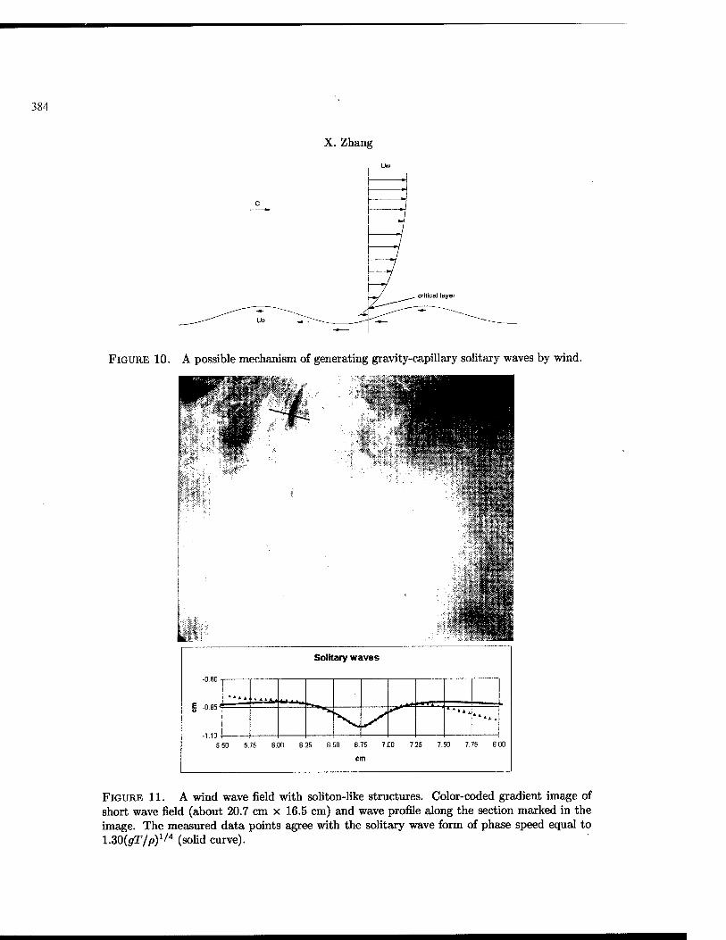
384
X. Zhang
FIGURE 10. A possible mechanism of generating gravity-capillary solitary waves by wind.
Solitary waves
| -0.85«
-1.10 ■ 5.
■^rrl *'•*.
50 5. 75 6.00 6.25 6.50 6.75 7.00 7.25 7.50 7.75 B.
cm
DO
FIGURE 11. A wind wave field with soliton-like structures. Color-coded gradient image of short wave field (about 20.7 cm x 16.5 cm) and wave profile along the section marked in the image. The measured data points agree with the solitary wave form of phase speed equal to 1.30(g/T/p)1/4 (solid curve).

385
Observations on waveforms of capillary and gravity-capillary waves
1.5
cm 1 ---v.-;v~-*
0.5
Solitary wave
5.5 6 6.5 cm
7.5
FIGURE 12. The image of a long trough solitary wave and its profile.
external forcing and nonuniformity of the medium are not considered. The wave patterns and waveforms of nonlinear capillary-gravity waves are very different from the three-dimensional waveform of nonlinear gravity waves (Su 1982). These short random waves are probably directly generated or strongly forced by wind.
4. Wave number spectra
The wavenumber spectrum of short waves is estimated from averaging all the image data. The first order 2-D Slepian window is multiplied with image slope data before FFT calculations to eliminate the effect of image size (Zhang 1994). This window function has a steep spectral cut-off which is critical, since the spectrum has a wide range of values (seven order of magnitude). The spectral leakage of the window (< 10~n) has to be less than the minimum value of estimated spectral value.
To the first order, the wavenumber spectrum of wave energy density of gravity-capillary waves, E{ k), is related to its slope spectrum, S( k ), by
E(i) = l/2(pgk2 + T)S(t)
where p, g, and T are water density, gravity acceleration, and surface tension respectively. The omnidirectional spectrum of energy density is defined as the integral of 2-D energy density spectrum over all directions. It

386
X. Zhang
omnidirectional wavenumber spectra
rad/cm
FIGURE 13. Omnidirectional wavenumber spectra of energy density of very short wind waves. The dark blue curve is the spectrum calculated from the sea surface data set. The other curves are the laboratory data from Zhang (1994).
is plotted in figure 13 (the dark blue curve) against laboratory measurements (Zhang 1994). The high spatial frequency noise of the optical apparatus is higher than that of laboratory as shown in the figure. The higher noise level is due to the film resolution. The spectral shape of capillaries (k > 2-n rad/cm) is similar to the laboratory measurements which is dominated by parasitic capillary waves. The spectral dip in the capillary-gravity range (near k = 2 rad/cm) is much less pronounced. This can be explained as follows: the capillary blockage (Phillips 1981) is less important in the field than in the lab. In the short fetch laboratory condition, the short gravity waves are extremely steep. The less pronounced energy spectral dip could be due to a larger energy flux due to triad wave-wave interactions (Valenzuela and Laing 1972). It could also be due to the pronounced parasitic peak. The two-dimensional wavenumber slope spectrum is shown in Figure 14. The angular distribution of field data is much wider than that of laboratory measurements (Zhang 1994) which is expected.
Short wind waves spectra have also been measured in the coastal waters with scanning laser slope gauges (Hwang et al 1996 and Hara et al 1998). The slope gauges are based on same optical geometry as the slope imaging technique (Zhang 1996b). The imaging technique measures surface area simultaneously while the scanning scheme scans the surface points rapidly in various ways. The wavenumber ranges of spectra measured by Hwang et al (1996) and Hara et al (1998) are about 1< k < 16 rad/cm and 0.5 < k < 8 rad/cm respectively. Hwang et al (1996) found a characteristic change in spectral power law at a wavenumber about 9 rad/cm or a wavelenght of 0.7 cm. This is about the maximum wavelength of the parasitic capillaries. The spectral shapes in the two regions of k<9 and k»9 rad/cm are reasonably smooth and can be represented by power-law functions of wavenumber fc, -1 and -3 for the slope spectra. The capillary wave spectral shape is consistent with our measurement, a typical parasitic capillary wave spectrum (Zhang 1995). For k<9 rad/cm, all measured spectra show very different behavior from the laboratory measurements. Apparently, the capillary blockage (Phillips 1981) is less important in the field.

387
Observations on waveforms of capillary and gravity-capillary waves
FIGURE 14. Two-dimensional wavenumber spectrum.
5. Conclusions and future work
The three dimensional waveforms of capillary-gravity and capillary waves are observed at sea during a recent experiment in California coastal waters. The waveforms are compared with laboratory observations. They are resoundingly similar to the laboratory observations. It is very common, among steep short wind waves, that waves in the capillary range featuring sharp troughs and flat crests. Waveforms that resemble capillary-gravity solitons are observed with a close match to the form theoretically predicted for potential flows. Capillaries are mainly found as parasitic capillaries on the forward faces of short gravity waves. The maximum wavelength in a parasitic wave train is less than a centimeter. The profiles of parasitic wave trains and longitudinal variations are shown. The phenomenon of capillary blockage (Phillips 1981) on dispersive freely traveling short waves is observed in the tank but not at sea. The short waves seen at sea propagate in the all the directions while the waves in the tank are much more unidirectional.
However, statistical distributions of very short wind waves are not that as close resemble as the local wave properties. One should be cautious to extend statistics of laboratory short wave data directly to the field conditions. Systematic field experiments at different wind conditions are required to understand the statistics of these very short wind waves.
References [1] Banner, M. L. and Phillips, O. M. 1974 On the incipient breaking of small scale waves. J. Fluid Mech. 65, 647-656. [2] Boussinnesq, J. 1872 Thforie des ondes et des remous qui se propagent le long d'un canal rectangulaire horizontal. J. Math.
Pure Appl. 17, 55-108. [3] Chen, B. and Saffman, P. G. 1985 Three-dimensional stability and bifurcation of capillary and gravity waves on deep water.
Stud. Appl. Math. 72, 125-147. [4] Crapper, G. D. 1957 An exact solution for progressive capillary waves of arbitrary amplitude. J. Fluid Mech. 96, 417-445. [5] Cox, C. S. 1958 Measurement of slopes of high-frequency wind waves. J. Marine Res., v.16, No.3 : 199-225. [6] Cox, C. S. and Zhang, X. 1997 Optical methods for study of sea surface roughness and microscale turbulence, SPIE, Vol. 3172,
165-172. [7] Dias, F. and Harägu§-Courcelle, M. 1999 On the transition from two-dimensional to three-dimensional water waves, Stud.
Appl. Math, (in press). [8]"Dias, F. and Iooss, G. 1993 Capillary-gravity solitary waves with damped oscillations. Physica D 65, 399-423. [9] Ebuchi, N., Kawamura, H. and Toba, Y. 1987 Fine structure of laboratory wind-wave surfaces studies using an optical method.
Boundary-Layer Meteorology 39, 133-151. [10] Hara, T., Bock, E. J., Edson, J. B., and McGillis, W. R. 1998 Observation of short wind waves in coastal waters. J. Phys.
Oceanogr. 28, 1425-1438

388
X. Zhang
[11] Hwang, P. A., Atakturk, S., Sletten, M. A., and Trizna, D. B. 1996 A study of the wavcnumber spectra of short water waves in the ocean. J. Phys. Oceanogr. 26, 1266-1285 Hogan, S. J. 1980 Some effects of surface tension on steep water waves. Part 2. J. Fluid Mech. 96, 417-445. Hunter, J. K. and Vanden-Broeck, J. M. 1983 Solitary and periodic gravity-capillary waves of finite amplitude. J. Fluid Mech.
134, 205-219 Iooss, G. and Kirchgässner, K. 1990 Bifurcation d'ondes solitaires en presence d'une faible tension superficielle. C. R. Acad.
Sei. Paris 311 I, 265-268 Kawahara, T. 1972 Oscillatory solitary waves in dispersive media. J. Phys. Soc. Japan 33, 260-264 Korteweg, D. J. and deVries, G. 1895 On the change of form of long waves advancing in a rectangular canal, and on a new
type of long stationary waves. Phil. Mag. 39, 422-443. Longuet-Higgins, M. S. 1963 The generation of capillary waves by steep gravity waves. J. Fluid Mech. 16, 138-159.
1988 Limiting forms for capillary-gravity waves, J. Fluid Mech., 194, 351-375 1989. Capillary-gravity waves of solitary type on deep water. J. Fluid Mech. 200, 451-478. 1992 Capillary rollers and bores. J. Fluid Mech. 240, 659-679. 1993 Capillary-gravity waves of solitary type and envelop solitons on deep water. J. Fluid Mech. 252,
[IS! [13:
[H:
[15: [16
[17: [is: [19 [20' [21
[22:
[23 [24
[2, [26'
[28
[29' [3<y
[31 [32:
[33:
[34:
[35
[36: [37 [38
[39
[40:
[41 [42:
[43]
Longuet-Higgins, M. S. Longuet-Higgins, M. S. Longuet-Higgins, M. S. Longuet-Higgins, M. S. 703-711 Longuet-Higgins, M. S. and Zhang, X. 1997 Experiments on capillary-gravity waves of solitary type on deep water. Phys.
Fluids. 9/7, 1963-1968 McGoldrick, L. F. 1965 Resonant interactions among capillary-gravity waves. J. Fluid Mech. 21, 305-331. Okuda, K., Kawai, S. and Toba, Y. 1977 Measurements of skin friction distribution along the surface of wind waves. J.
Oceanogr. Soc. Japan 33, 190-198. Phillips, O. M. 1981 The dispersion of short wavelets in the presence of a dominant long wave. J. Fluid Mech. 107, 465-485. Peregrine, D. H. and Smith, R. 1979 Nonlinear effects upon waves near caustics, Phil. Trans. A292, 241-370. Rayleigh, Lord 1976 On waves. Phil. Mag. 1, 257-279. Russell, J. S. 1838 Report of the committee on waves. Proc. Brit. Ass. Adv. Sei., Liverpool 1837. London. John Murray,
417-496. Schooley, A. II. 1958 Profiles of wind-created water waves in the capillary-gravity transition region. J. Mar. Res. 16, 100-108. Schwartz, L. W. and Vanden-Broeck, J.-M. 1979 Numerical solution of the exact equations for capillary-gravity waves. J. Fluid
Mech. 95, 119-39. Simmen, J. A. and Saffman, P. G. 1985 Steady deep-water waves on a linear shear current. Stud. Appl. Math. 73, 35-57. Stokes, G. G. 1880 Supplement to a paper on the theory of oscillatory waves, in Mathematical and Physical Paper, 1. Cambridge
University Press, 1880, 197-229. Su, M.-Y., 1982, Three-dimensional deep-water waves, Part I, Experimental measurement of skew and symmetric wave patterns,
J. Fluid Mech. 124, 73-108 Valcnzuela, G. R. and Laing M. B. 1972 Nonlinear energy transfer in gravity-capillary wave spectra, with applications, J Fluid
Mech. 54, 507-520. Vanden-Broeck, J.M. and Dias, F. 1992 Gravity-capillary solitary waves in water of infinite depth and related free surface
flows. J. Fluid Mech. 240, 549-557. Wilton, J. R. 1915 On ripples Phil. Mag. (6) 29, 688-700. Wu, J. 1968 Laboratory studies of wind-wave interactions. J. Fluid Mech. 34, 91-111. Zhang, X. and Cox, C. S. 1994 Measuring the two dimensional structure of a wavy water surface optically: A surface gradient
detector. Experiments in Fluids 17, 225-237. Zhang, X. 1994 Wavenumber spectrum of very short wind waves: An application of 2-D Slcpian windows to the spectral
estimation. J. Atmos. Oceanic Tech. 11, part 2, 489-505 Zhang, X. 1995 Capillary-gravity and capillary waves generated in a wind wave tank: Observations and theories, J. Fluid
Mech. 289, 51-82. Zhang, X. 1996a An algorithm for calculating water surface elevations from surface gradient image data, Exp. Fluids 21, 43-48. Zhang^ X. 1996b Optical mapping of fluid density interfaces: Concepts and implementations, Rev. Scientific Instr. Vol.67, No.
5, 1858-1868 Zufiria, J. A. 1987 Symmetry breaking in periodic and solitary gravity-capillary waves on water of finite depth. J. Fluid Mech.
184, 183-206

Eur. J. Mech. B/Fluids
(c) Elsevier, Paris
THREE-DIMENSIONAL EVOLUTION OF WIND WAVES FROM GRAVITY-CAPILLARY TO SHORT GRAVITY RANGE
G. CaulliezW and F. Collard [1]: Institut de Recherche sur les Phenomenes Hors Equilibre, Marseille, France, e-mail: guilOpollux.irphe.univ-mrs.fr
(Received 25 October 1998, revised and accepted 23 January 1999)
Abstract - We report the first systematic laboratory observations of 3-D features of wind waves at early stages of wave field development. The experiments performed in the large IRPHE-Luminy wind-wave tank provided instantaneous reconstruction of the decimeter-scale water surface motions based on simultaneous imaging of the wave slopes in two perpendicular directions. Five essentially distinct regimes in the 3-D evolution of the dominant waves have been identified. Each regime is characterized by different types of 3-D wave patterns associated with specific ranges of wave scale and wave steepness. The likely scenario of the evolution and the possible physical mechanisms of the pattern formation are discussed. © Elsevier, Paris
1. Introduction
Three-dimensional features of wind-wave field developing at sea surface are indeed of principal importance for progress in the basic understanding of air-sea interaction processes and for remote sensing applications. This particular aspect of the wind-wave field evolution has been poorly studied yet inasmuch as the description provided by classical tools used in most observations, i.e. single-point measurements coupled with spectral analysis, is inadequate for getting such an insight. However, following the early works by Cox and Munk [4] and Stilwell [12] on analysis of sun glitter at the sea surface, the rapid development of high performance technology during the last decade, both in optics and data processing, has made realistic the use of optical imaging techniques to obtain a complete description of the 3-D properties of wind wave fields. Thus, stereo- photographic techniques have been recently developed for imaging large scale water surface motions at sea (Banner [1]; Shemdin et al [9]) while in laboratory, light refraction techniques have been used for spatial measurements of small-scale wave slopes in one or two perpendicular directions (Jahne and Riemer [6]; Zhang and Cox [14]). These investigations yielded a rather precise description of the two-dimensional wave slope spectra respectively near the dominant peak and at high wave numbers but were confined to a few wind and fetch conditions. Also, due to the relatively small size of wave slope-imaging systems used for observations, a first preliminary type analysis of the waveforms and the wave patterns shaping the water surface was conducted only for short capillary-gravity wind waves or parasitic capillaries generated by micro-breaking (Zhang [13]).
In this paper, we present a laboratory study carried out to investigate systematically the 3-D aspects of the evolution of the dominant wind waves propagated at the water surface at the early stages of wave field development, i.e. for waves from gravity-capillary to short gravity range. This study aims more specifically at characterizing the 3-D wave patterns which shape the water surface at the different stages of the wind wave evolution and then, at determining the conditions of their emergence as function of both the "external" param- eters as wind speed or fetch and the "intrinsic" wave parameters as wavelength or wave steepness. Accordingly, the two-color visualization system developed to measure simultaneously both wave slope components over a large water surface area will be first described briefly. Then, the typical 3-D wave patterns to be associated

390
G. Caulliez, F. Collard
video camera
v;s;;;;;s;;;//7777777. B
WIND
V/////M
^AvAV/w/k/^ lighting box W////S////S.
TTl
fetch -»
FIGURE 1. Schematic view of the large IRPHE wind-wave facility and the experimental ar- rangement used for imaging wave slopes at the water surface.
with different stages in the 3-D wind wave field evolution will be identified and investigated in more detail. The conditions for which the different regimes are observed as well as the basic wave parameters which control this evolution will be also specified. To conclude, a realistic scenario likely to describe the 3-D wave field evolution will be suggested.
2. The experimental procedure
The optical wave slope-measuring system adopted for wave visualization was based upon the method developed by Jahne and Riemer [6] which utilizes the light refraction at the water surface. The unique performance features of our system are first the ability to image the water surface slopes simultaneously in two perpendicular directions and second the large (compared to other installations) size of the spot allowing quality measurements. The essence of the system could be briefly discussed as follows. The light source is made of a square box (110 x 110 x 20 cm3) illuminated from the downwind and crosswind side-walls by two long cylindrical luminescent tubes equipped with reflectors. The box contains an aqueous suspension of latex particles providing the scattering of the light in the box. A light source with two perpendicular gradients in brightness of two different colors is obtained by inserting two pass-band optical filters between the lamps and the scattering volume respectively. A 3-CCD video camera mounted at the top of the facility looking vertically downward allows to monitor the water surface motions. When waves are present at the water surface, the two-color images of the light source are directly modulated as a function of the two components of the wave slope. The latter at any point of the images are then derived by means of a simple ray tracing model. The special arrangement performed to increase the size of the images available for measurements is described in Shrira and Caulliez [11]. Here let us just mention that an image of size 85 x 85 cm2 could be used for quantitative wave slope measurements for all wave conditions under consideration in this paper, with a relative error in slope less than 5%.
Wave observations were carried out in the large IRPHE wind-wave tank, 40 m long, 2.6 m wide and 1.0 m deep, as schematically shown in Fig. 1. Measurements of the water surface motions made by means of the wave slope imaging system described above and two capacitance wave gauges located at the immediate vicinity of the light box were complemented by measurements of the air surface flow structure using a set of velocity sensors (hot wires and Pitot tube). The wind speed will refer hereafter to the air potential flow velocity. The wave visualization system and the other measuring devices were set up at a fixed position in the water tank, at a distance of 28 m from the entrance, and the desired fetch was obtained by varying the length of the air-water junction plate. Special care was taken to ensure the uniformity of the wind at the entrance of the water tank

391
Three-dimensional evolution of wind waves
and the undisturbed development of the air surface boundary layer above the water surface. For this purpose a special flexible device was used to make smooth the transition between the solid wall at the edge of the air tunnel and the water surface. In these experiments, the wind and fetch conditions were chosen both to investigate the 3-D evolution of the dominant waves with fetch for several wind speeds and to observe waves of definite wavelength in various wind conditions.
For each condition, the images viewed by the video camera were digitized in real time by a RGB data acquisition board at intervals of 1 s and recorded directly on a PC computer. These images were coded into 256 x 350 pixels format (the longitudinal and transverse directions respectively) and 256 light intensity levels for each color channel. Then, for further analysis, the wave slope images were smoothed with a linear 2D low-pass filter of 2 pixels cut-off in scale in order to reduce the gaussian noise introduced by the data acquisition board at high wavenumbers (Jahne [5]). Average two-dimensional wavenumber slope spectra were computed from 100 independent images by means of a classical 2-D FFT algorithm after application of a Hanning window, and then remapped over a (k, '&) grid by means of a sub-grid algorithm. Integration of the spectra over the dominant peak provides too a direct estimation of the dominant wave steepness. To better identify the 3-D wave patterns, the instantaneous images of the water surface motions were also reconstructed from both slope images using an elaborated integration method (Kimmoun et al. [7]).
3. The experimental results
3.1. The main stages of the evolution
The qualitative investigations based on visual observations and photographs or by looking at the individual wave slope images have first shown that three-dimensional wave patterns are the dominant feature of the wind wave field at the early stages of development. The first quantitative results obtained by means of two-dimensional spectral analysis of the wave slope images then enabled us to distinguish five stages in the wind wave evolution depending on wavelength and wave steepness and directly associated with different 3-D coherent wave patterns. An illustration of the wave field features at these different stages is given in Figs. 2 where a side view of the wave field, an image of the water surface elevations reconstructed from wave slope images, and the contour lines of the 2-D wave slope spectra plotted both in a (k, 6) plan and in a sequence of constant-k plans, are displayed respectively for five typical wind and fetch conditions.
The first stage of the 3-D wind wave field evolution has been first detected by visual observations and photographs at relatively large fetches and very low wind speeds. As clearly seen in Fig. 2-la, these wave motions shape the water surface into quite regular rhombic patterns resulting in a striking way from the growth of two quasi-monochromatic oblique waves. These waves correspond to the initial waves generated by wind in the tank for wind speeds below 4 m/s. They are observed at moderate to large fetches when the water surface still looks smooth. The (k, 0) wave slope spectrum shows that the wave field energy is mainly confined in a narrow band of wavenumbers independent on the wave propagation direction, but is distributed quite uniformly over a wide range of angles lying symmetrically on both sides of the wind direction (Figs. 2-lc and 2-ld). Although the images of the water surface motions show waves propagating roughly at ± 30° to the wind (Fig. 2-lb), no preferential angles could be seen in the spectra at this stage of evolution, looking practically flat from -30° to +30°. This peculiar shape of the spectra could be ascribed to the rather small signal to noise ratio observed in these conditions and related to the large time and space intermittence of the initial wind-generated waves propagating on the water surface as well-defined groups of few wavelengths or periods only. This intermittence is particularly noticeable in the time sequences of the water surface elevations observed in these conditions (Fig. 3a). The wavelength of these initial wind waves, is controlled by the wind speed and falls into range 4 to 10 cm. As it was shown previously (Ricci and Caulliez [8]), these wavelengths correspond to the scales of the most spatially-amplified wind waves at such light winds.
At wind speeds exceeding 4 m/s, the spatial growth of the initial wind waves at the entrance of the water tank becomes very rapid and the domain corresponding to the growth of the initial wind waves is localized in the first meter of the tank, just downwind of the air-water junction plate. The characteristic scales of the

392
G. Caulliez, F. Collard
a)
m^m,^ .-Art« - ■
1 *■«&:<
E.W
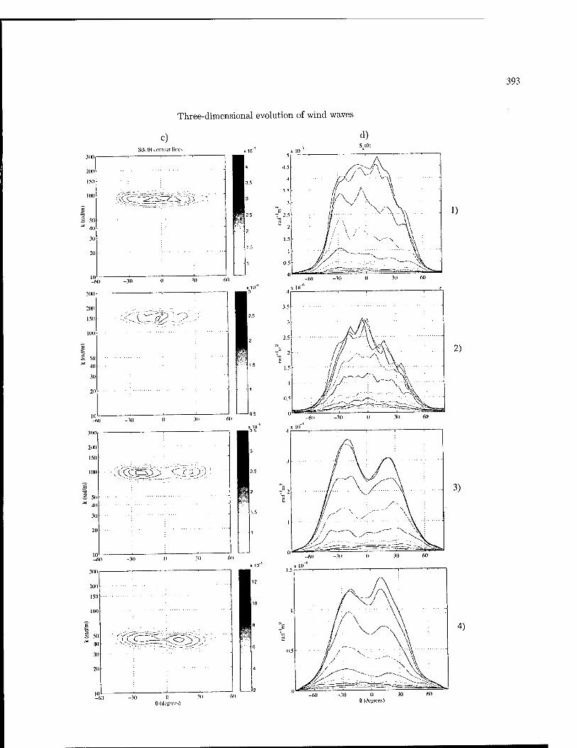
Three-dimensional evolution of wind waves
393
0(decrees)

394
G. Caulliez, F. Collard
1»)
p^'*'
ii in ?n 10 m 50 f,o
FIGURE 2 : see the facing page
most amplified wind waves decrease sharply as well, reaching values smaller than 4 cm in wavelength. At this stage of development (called stage "0" hereafter), the visual observations suggest that the 3-D character of the initial waves is not so well-pronounced. However, the wave field displays there a great inhomogeneity of the order of the wave scales themselves, caused by the laminar-turbulent transition of the drift current (Caulliez et al. [3]). Therefore, quantitative wave slope measurements are difficult to make and especially to interpret in such conditions.
The second stage of the 3-D wave evolution was observed at wind speeds higher than 4 m/s when the initial wind waves fully develop, i.e. just before the start of the frequency and wavenumber downshift phenomenon (i.e. the decrease with fetch of the dominant wave frequency and wavenumber). As illustrated in Figs. 2-2a and 2-2b, the water surface, looking uniformly rough is entirely ruffled by small-scale capillary-gravity waves of high steepness. These waves are shaped with typical round crests and sharp troughs. The random distribution in space of such short-crested waves, quite noticeable just by looking by unaided eye at the water surface, is reflected in the shape of the wave slope spectra, which are of significant broadness both in k and 6 (Fig. 2-2c). At this stage of evolution, the angular distribution of the spectral energy density at the dominant wavenumber is maximal for the along-wind direction, but still remains wide, S/t(#) keeping large values for angles up to ± 30° (Fig. 2-2d).
The third stage of the 3-D evolution of the wind waves concerns waves of scales similar to the initial waves observed at very low wind speeds (stage I). As shown in Fig. 2-3a, the wave field exhibits noticeable 3-D wave patterns as well, but surprisingly, these rhombic patterns emerge gradually out of the random short capillary- gravity wave field described above (stage II). This phenomenon occurs when the dominant wavelength starts to increase. In a very similar way, the 3-D patterns are formed by two symmetric oblique waves propagating at angles close to ± 30° to the wind direction (Fig. 2-3b). The gravity-capillary wave profiles of significant steepness here are distorted by conspicuous trains of capillary waves localized on the forward face of the crests. The wave slope spectra then display two well-pronounced peaks centered more or less symmetrically at about ± 25° (Figs. 2-3c and 2-3d). The existence of such distinguishable peaks suggests essentially coherent nature of the 3-D wave patterns observed at this stage of development.
For wind speeds exceeding 4 m/s the next, i.e. the fourth, stage of wind wave evolution corresponds to the development of steep short-crested gravity waves of wavelength ranging approximately between 10 and 20 cm, as shown in Figs. 2-4a and 2-4b. This stage occurs in a well-defined range of fetches specified by the wind speed. The wave field exhibits rather regular and well-pronounced 3-D patterns shaping the water surface as rhombi, pentagons or hexagons, but the length and the orientation of the ridges forming the 3-D patterns varies widely in space. In fact, the configuration of the patterns looks dependent on the local steepness which changes significantly both in space and time due to the persistence of well-pronounced wave groups

395
Three-dimensional evolution of wind waves
<1) Si til
150
1(1(1
r tr:~'_> >
/\
.A ^■'
5)
-Ml H '" <',)
Odl'i'iivil
FIGURE 2 Illustration of the wind wave features at the five stages of the 3-d evolution: 1) stage I (U = 2.5 m/s; X = 26 m); 2) stage II (U = 6 m/s, X = 2 m); 3) stage III (U = 5 m/s, X = 6 m); 4) stage IV (U = 6 m/s, X = 9 m); 5) stage V (U = 5 m/s, X = 18 m); a) Side view of the wind wave field, with the wind blowing from right to left; b) Image of the water surface elevations (scale in cm) obtained by reconstruction from both wave slope images, with the wind blowing from right to left; c) Contour lines of the (k, 9) wave slope spectrum for the different energy levels indicated in the right scale (scale in m2 rad"1); d) Contour lines of the (k, 6) wave slope spectrum in the succession of constant-k plans k; = (1 + 0.1 i) kpeak with kpeak = 83.5, 137, 92, 43, 30 rad/m respectively and i = 0,1,2,...,9.
(Fig. 3d). In particular, it seems that the occurrence of the first micro-breakings would be at the origin of the pentagon pattern formation (such a pattern is particularly well visible in Fig. 2-5b). To a certain extent, these various features give to the wave field a random and rather rough aspect. However, two peaks can be easily distinguished in the two-dimensional wavenumber spectra of the wave slope images (Figs. 2-4c and 2-4d), indicating the coherency of the 3-D wave patterns is still large there. Note that for such longer waves, the peaks are found at smaller angles, about ± 20° or less, and are generally less symmetric.
The last, fifth, stage of the 3-D evolution of the wave field occurs when the dominant waves reach a certain energy equilibrium resulting from the balance between the wind input to wave motions and the wave dissipation due to breaking or micro-breaking and nonlinear transfer to larger scales. This stage is observed for short gravity waves of wavelength as small as 12 cm at low wind speeds, but longer than 25 cm for the highest wind speeds. The wave field is then composed both of short-crested waves and long-crested waves distributed randomly and forming intermittent 3-D wave patterns of different shape at the water surface (Figs. 2-5a and 2-5b). The 3-D aspect of the wave field is also emphasized by the existence of small-scale wavetrains generated by micro- breaking waves or crescent-shaped breaking waves and propagating in transverse direction to the wind. This noticeable evolution of the wave field 3-D features is well depicted by the drastic change in the shape of the wave slope (k 6») spectra (Figs. 2-5c and 2-5d). The latter exhibit now only one smooth peak at the dominant wave number,' centered at zero angle. Compared to the individual peaks observed previously, this peak is broader in k and 9. This corroborates the large variability in scale, in shape and in wave direction of the dominant waves
at this stage of evolution.
3.2.. The main characteristics of the dominant waves To better specify the wave parameters which control the 3-D wave field evolution described above and then
to attempt to determine the physical processes involved, a detailed analysis of the mean dominant wave features has been performed for the whole set of experiments. As this has never been described before in such a large

396
E o
G. Caulliez, F. Collard
0 2 4 6 8 10 12 14 16 18 2 U.2 i 111 1 l I i | i 'l i
0.1 "Lllliiiliinu mi ll. ill lii ihf 1 Uli lllllhlllll ll ll «lllllf Im ah ilii .JifL.iiiLl Jll.l illJi. ill llll If 0 iiiiiw m |UM| li lil Mwf MB mmM if IMWl
0.1 || ipi'Mpi K|i 'I) pi1 l«ll "II i'iii II film ifiiii
i
| if yiiM|j i
'I'r |i| pi i
I IJI|||i|''||HI| i
|'If! I 1 1
a)
b)
c)
d)
e)
FIGURE 3. Time series of the water surface elevations measured by a capacitance wave gauge set up at the immediate vicinity of the light box for different wind and fetch conditions char- acteristic of the five stages of the 3-D wave field evolution: a): U = 2.5 m/s, X = 26 m (stage I) ; b): U = 6.0 m/s, X = 2 m (stage II) ; c): U = 5.0 m/s, X = 6 m (stage III) ; d): U = 6.0 m/s, X = 9 m (stage IV) ; e): U = 5.0 m/s, X = 18 m (stage V) .
wind-wave tank due to the lack of appropriate measuring techniques, the parallel evolution of the wavelength and the wave steepness of the dominant waves was investigated as function of fetch and wind speed (Figs. 4 and 5). First, these results highlight that the wavelength increases only slowly with fetch when the dominant waves lie in the gravity-capillary domain (A < 8 cm). However, for short gravity waves this growth enhances rapidly, fitting remarkably linear dependence on fetch of slope increasing with wind. The evolution of the wave steepness with fetch confirms that the wave field reaches rapidly a kind of dynamical equilibrium at larger fetches whatever the wind conditions, except for the lowest wind speed (2.5 m/s), where a significant steepness increase may hold at 26 m fetch. Note the fact, that at large fetches the linear increase of the dominant wavelength is not affected by the occurrence of the wave energy saturation.
The spectral analysis made above shows very clearly that at a given wind and fetch condition, the wavenumber of the dominant waves does not vary with the wave propagation direction, and this holds whatever the conditions. Therefore, the mean 3-D features of the dominant waves are better described by the angular distribution function Y(#) obtained by the integration of the spectral energy density of the wave slopes over the dominant peak k- domain. The simplest single quantity to characterize this distribution is the angular dispersion defined here as the average angle at which Y(0) reaches half of its maximum value. This parameter is found to be higher than

397
Three-dimensional evolution of wind waves
10 15 fetch(m)
FIGURE 4. Evolution with fetch of the dominant wavelength observed in the large IRPHE wind-wave tank for the various wind conditions investigated.
fetch (m)
FIGURE 5. Evolution with fetch of the dominant wave steepness observed in the large IRPHE wind-wave tank for the various wind conditions investigated.
FIGURE 6. Evolution with fetch of the angular dispersion of the dominant waves observed in the large IRPHE wind-wave tank for the various wind conditions investigated.

398
G. Caulliez, F. Collard
30° for the most, of the experimental conditions we investigated with a maximum close to 45° at the intermediate fetches (Fig. 6). The highest values of the angular dispersion concern the gravity-capillary waves of wavelength 4 to 10 cm observed at small to moderate wind speeds.
As just inferred above but clearly shown in Figs. 7a-d, the shape of the dominant wave angular distribution shows large similarities for waves of comparable wavelength but measured in different experimental conditions. In particular, the gravity-capillary waves of 4 cm wavelength or less observed at stage II are characterized by a wide and round-shaped curve centered approximately in the wind direction (Fig. 7a). Such a distribution has to be associated with the typical random and short-crested aspect of the small-scale waves developing at the water surface. On the contrary, the angular distribution of the relatively 'long' gravity-capillary waves in the wavelength range 4 - 10 cm observed both in stages I and III is practically flat within the angle sector of approximately ± 30° when the wave steepness is small at low wind speeds (Fig. 7b). When the wave steepness is higher (ak > 0.08), the angular distribution exhibits two well-pronounced peaks located at two symmetric angles close to ± 30°. In this case, the short-crested character of the wave field is due to two oblique wavetrains propagating at about ± 30° to the wind direction and forming relatively regular rhombic patterns at the water surface. For short gravity waves of wavelengths in the range approximately 10 to 20 cm observed at stage IV the angular distribution still exhibits two peaks, but the particular shape of this function, such as the peak sharpness and the peak separation, is controlled by the combined evolution of the wavelength and the wave steepness (Fig. 7c). At the last stage of development when the wave field reaches an equilibrium characterized by the saturation of the wave steepness growth with fetch (stage V), the shape of the angular distribution of the short gravity waves changes completely (Fig. 7d). This function displays now only one smooth peak centered approximately at zero angle, indicating that these wind waves with intermittent long crests mainly propagate at small angles to wind.
These results corroborate undoubtedly the existence of five essentially distinct stages in the 3-D evolution of the wave field generated by wind at limited fetches, as displayed in Fig. 8. Furthermore, they indicate that the parameters which control this evolution, and, consequently, the balance between the different processes responsible for energy transfer to dominant waves, are mainly related to the wave scale and to a less extent to the wave steepness.
This analysis then enables us to determine rather precisely the ranges of wavelength and wave steepness to be associated with these five stages of evolution (Fig. 9). However, it should be mentioned that the boundaries of domains are not sharp and are, in fact, smooth transitions from one stage to the other. Note that it is likely that these boundaries might be slightly modified by a change in an external parameter of secondary importance for the wave development, as, for instance, the drift current development or the air flow turbulence.
The main features of the dominant wave field which characterize the different stages of the three-dimensional evolution are also summarized in Table 1. The table is effectively splitted into two: the upper one is for winds below 4 m/s, while the lower one is for wind exceeding this threshold. There is qualitative difference between the two cases: in the former case, no waves of wavelength smaller than 4 cm can be generated by wind as the wind input is not high enough to allow the growth of short gravity waves of significant steepness before the energy saturation.
4. Discussion and conclusion
The most striking aspects of the three-dimensional evolution of the wind wave field we have described above lie essentially in: i) the generation at very low wind speed (U < 4 m/s) of two oblique waves propagating symmetrically at ± 30° to the wind. These motions observed at stage I correspond to the initial waves generated by wind at the water surface; ii) the development at higher wind speeds of two oblique waves propagating at angles close to ± 30° to the wind direction which emerge from a well-developed but randomly-distributed capillary-gravity wave field of shorter scales, that characterizes the stage III.

399
Three-dimensional evolution of wind waves
1 1 1 ! 1
: 'v
;/. iL^ : : ;/ \ '■ : \
': : v :
' : y : \..x ; )■'
l :
■ f /
J x '■
\
, ..V .;
U = 5m/s - X = 2m U = 6m/s - X = 2m
—^ r i i i i —1
6 (degrees)
K10"5 b) 3.5 U = 6m/s -
U = 5m/s - x = 4m , X = 6m '
;/ \ U = 5m/s - X = 4m
3 U = 2.5m/s - X = 26m
1 \ / ^ : .
2.5
i -" :\
2 i ■ \
1.5 / /
i / V V
0.5 :./ /
1 J i /
V
\\ - -
FIGURE 7. Angular energy distribution of the dominant waves Y(0) estimated from the wave slope images for various wind and fetch conditions characteristic of the five stages of the 3-d wind wave field evolution (A is given for the lowest to highest curves): a) stage II ( A = 3.5 cm; A = 4.2 cm ), b) stage I and stage III ( A = 7.4 cm; A = 4.6 cm; A = 6.7 cm; A = 6.5 cm ), c) stage IV ( A = 11.7 cm; A = 14.3 cm; A = 18.7 cm ), d) stage V ( A = 13.3 cm; A = 20.9 cm; A = 20.9 cm; A = 27.0 cm, A = 26.6 cm ).
In both cases, these wave motions form rhombic patterns of similar shape at the water surface, although their wave steepness can differ by the factor of 3 or 4. Their wavelength falls into a very specific range of scales, namely, between 4 and 10 cm, and then belongs entirely to the gravitational branch of the gravity-capillary wave k-domain located just below the minimum of the phase velocity even if accounted for the correction due to the current. Their typical angular energy distribution is rather flat at low steepness but strictly bimodal at higher steepness, and, most remarkably, without any distinguishable component in the along-wind direction
(Fig. 7b). Let us examine the possible mechanisms of formation of these well-pronounced 3-D wave patterns. First,
the particular conditions of emergence of such 3-D wave patterns of definite scales suggest immediately that some resonant wave-wave interaction processes may be at their origin. However, it is well-known that resonant triad interaction processes can lead to the formation of oblique waves from disturbances generated by wind in the along-wind direction for waves belonging to the capillary branch of the capillary-gravity waves. When the

400
G. Caulliez, F. Collard
regime type of waves A (cm)
ak fetch evol
Y(0) "peak
u <
I initial smooth capillary-gravity waves
4- 10 increase
flat -30° to +30°
4 m/s
V random long-crested gravity waves
> 10 saturation
1 peak «0°
lb initial wind-generated capillary-gravity waves
<4 «0.01
U II short capillary-gravity waves of rough aspect
<4 increase
1 peak «0°
> III two oblique "long" capillary-gravity waves
4- 10 increase
2 peaks ± 30°
4 IV steep short-crested gravity waves
> 10 > 0.12 increase
2 peaks [0°,± 30°]
m/s V random long- and short- crested gravity waves
> 12 saturation
1 peak «0°
TABLE 1
12 r-r
15 fetch (m)
FIGURE 8. Schematic diagram showing the respective domains in wind speed and fetch associ- ated with the different stages of the 3-D wind wave field evolution observed in the large IRPHE wind-wave facility (the symbols indicate the different wind and fetch conditions investigated).
effect of the drift current on the dispersion relation is taken into account, these waves prove to be of scales no longer than 5 cm (Shrira and Caulliez [11]). Thus, such process which may occur in cascade would be rather the best candidate to explain the formation of the 3-D wave field of rough aspect observed at stage II. Second, the nonlinear wave-current interactions have to be also considered in the context of this work. These processes are essentially of the same nature as those responsible for the generation of Langmuir circulations inside the upper water shear layer but due to the feedback of water circulations on surface waves, they lead to the formation of

401
Three-dimensional evolution of wind waves
10 15 20 dominant wavelength (cm)
25 30
FIGURE 9. Evolution with the dominant wavelength of the dominant wave steepness observed for the various wind conditions investigated. The dashed bold lines indicate the limits in wavelength and wave steepness of the different stages of the 3-D wind wave field evolution.
short-crested waves (Shrira [10]). However, we found from previous observations that the growth of the 3-D initial waves observed at stage I is associated with the development of a laminar-turbulent transition in the drift current (Caulliez et al. [3]). In addition, visualizations have shown that the development of Langmuir-like circulations in water occurs only for higher wind speeds and shorter fetches. Such results would discard a priori this nonlinear wave-current interaction process as the main mechanism responsible directly for the 3-D wave pattern formation at stage I of evolution, as very likely at stage III.
The above considerations suggest, that the emergence of two oblique waves in the range of wavelengths from 4 to 10 cm should be rather searched into the development of some nonlinear wave-wave interactions specific for this range of scales. The existence of such a selective mechanism, not investigated or not even clearly identified yet, would be strongly supported by the very sharp decrease of the angular energy distribution observed for the angles larger than those of the peaks (see Fig. 7b).
The next stage in the 3-D evolution of the wave field is characterized by the formation of steep short-crested gravity waves as found at larger fetches (stage IV). These still steepening waves, of wavelengths between 10 cm and 20 cm, develop only at moderate to high wind speeds. The wave angular energy distribution exhibits two peaks, but the distance between the peaks decreases gradually. The rate of decrease accelerates with slowing down of the wave steepness growth. Finally, the last stage of 3-D wave evolution (stage V) was found associated with the energy saturation of the wave field. At this stage, the dominant wavelength still increases, whereas the wave steepness growth practically stops. Simultaneously, the shape of the 3-D patterns becomes more variable, associated both with long-crested and short-crested waves propagating in random directions at small angles to the wind. The wave field is characterized by an angular energy distribution exhibiting only one central peak.
The coupled evolution with wind and fetch of the wavelength, the wave steepness and the angular dispersion of the waves observed both in stage IV and in stage V suggests that the development of the wave field is controlled there by the competition between two phenomena: i) the wind which tends to amplify the dominant waves or smaller-scale disturbances in the along-wind direction at a higher rate, through linear or nonlinear instability mechanisms (Belcher [2] and personal communication); ii) an yet to be identified nonlinear wave-wave or wave-current interaction mechanism which redistributes the

402
G. Caulliez, F. Collard
wave energy over a broader angular spectrum. The efficiency of such process would depend directly on the wave steepness growth, that constitutes a peculiarity of interest for further understanding.
To conclude, the whole set of the findings and considerations given above enables us to suggest a specific scenario to describe the 3-D evolution of the wind wave field at the early stages of wave development. First, the whole 3-D evolution of the wind wave field appears essentially controlled by the emergence at short fetches of two oblique waves, of wavelengths in the range 4 to 10 cm, propagating at about ± 30° to the wind direction and forming quite regular rhombic patterns at the water surface. This regime would originate from the development of some nonlinear wave-wave interaction mechanism specific to this range of scale. Further investigations are carried on now to identify this mechanism more precisely. Then, when the dominant wavelength moves to short gravity domain, the wave field preserves for high enough wind speed a well-pronounced 3-D feature characterized both qualitatively, by its short-crested aspect and quantitatively, by a bimodal angular energy distribution. This regime occurs as long as the wave steepness increases significantly. It would be the result of opposing action of the intense wind forcing which causes simultaneously a higher growth of the wave disturbances in the along- wind direction with a large steepness increase, the latter keeping the nonlinear wave-wave interaction processes very effective. At last, when the energy saturation is reached, the wave motions relax to a broad-band angular spectrum wave field of random aspect. Its 3-D feature would be the result of a rather complex interplay between the wind action and the nonlinear wave-wave and wave-current interactions.
Acknowledgements
We would like to express sincere thanks to V. Shrira for the helpful discussions we shared during the course of this work and his valuable comments on the first draft of the manuscript. We gratefully acknowledge US ONR for financial support under grant N-00014-94-1-0532.
References
[I] Banner M.L., Jones I.S.F., Trinder J.C., 1989, Wavenumber spectra of short gravity waves, J. Fluid Mech. 198, 321-344. [2] Belcher S. E., 1999, Wave growth by non-separated sheltering, Eur. J. Mech. B/Fluids this issue, 121-136. [3] Caulliez G., Ricci N., Dupont R., 1998, The generation of the first visible wind waves, Phys. Fluids 10, 4, 757-759. [4] Cox C, Munk W.H., 1954, Statistics of the sea surface derived from sun glitter, J. Marine Res. 13, 2, 198-227. [5] Jahne B., 1993, Digital Image Processing: Concepts, Algorithms and Scientific Applications., Springer-Verlag, Berlin. [6] Jahne B., Riemer K.S., 1990, Two-dimensional wave number spectra of small-scale water surface waves, J. Geophys. Res. 95,
11531-546. [7] Kimmoun O., Branger H., Kharif C. 1999, On short-crested waves: experimental and analytical investigations, Eur. J. Mech.
B/Fluids (to appear). [8] Ricci N., Caulliez G., 1994, Characteristic scales of the initial wind-generated waves, C. R. Acad. Sei. Paris II 318, 1591-1598. [9] Shemdin O.H., Tran H.M., Wu S.C., 1988, Directional measurements of short ocean waves with stereophotography, J. Geophys.
Res. 93, 13891-901. [10] Shrira V.l., 1998, Wind wave nonlinear interactions owing to drift current: formation of the angular spectrum, wave groups
and Langmuir circulations, in: Perrie (ed), Nonlinear Ocean Waves, Computational Mechanics Publications, Southampton,
163-200. [II] Shrira V., Caulliez G., 1998, Three-dimensional water wave patterns in gravity and gravity-capillary range, O.N.R. report. [12] Stilwell D. J., 1969, Directional energy spectra of the sea from photographs, J. Geophys. Res. 74, 8, 1974-1986. [13] Zhang X., 1995, Capillary-gravity and capillary waves generated in a wind wave tank: observations and theories, J. Fluid
Mech. 289, 51-82. [14] Zhang X, Cox OS., 1994, Measuring the two dimensional structure of a wavy water surface optically: a surface gradient
detector, Exp. Fluids 17, 225-237.

Eur. J. Mech. B/Fluids © Elsevier, Paris
LARGE-SCALE VORTICITY GENERATION BY BREAKERS IN SHALLOW AND DEEP WATER
D. H. Peregrine!1]
[1]: School of Mathematics, Bristol University, University Walk, Bristol BS8 1TW, England, e-mail: D.H.PeregrineQbristol.ac.uk
(Received 18 September 1998, revised and accepted 3 February 1999)
Abstract - Water wave breaking is of considerable importance in the transfer of momentum, and in other transfers, between the atmosphere and oceans. Typically breaking occurs on deep water as events that have finite duration and finite spatial extent. Near shore lines most of the water motions are dominated by breaking waves. Recent work on the generation of vorticity by breaking waves and bores in the surf zone on beaches is considered and typical vortical structures are briefly discussed. Consideration of deep water breaking leads to the proposal that the end result of a breaking event in deep water may be a coherent structure within the resulting current field. Such a structure is topologically equivalent to half a vortex ring. © Elsevier, Paris
Introduction
The role of eddies in surf zone currents, and the generation of their vorticity are discussed in Peregrine (1995, 1998), with the latter paper giving a quantitative measure of vorticity generation by bores. The aim of this paper is to give an indication of the implications of this vorticity generation from three-dimensional waves, i.e. breaking waves of finite crest length, for the structure of surf-zone currents; and to extend the discussion to the effects of deep water breakers. Wave breaking on coastal beaches, due to waves propagating into shallower water, is so commonplace that no introduction is necessary. On deeper water breaking is less common and usually stimulated by the wind.
When wind blows over the ocean surface it is frequently generating water waves. These waves usually sustain a significant density of transient breakers. Sometimes these breakers are large enough to be seen as white caps. More commonly, if not almost all the time, there are smaller breakers, micro-breakers where the effects of capillarity are strong enough to prevent air entrainment but insufficient to prevent development of small scale turbulent patches similar to those created by larger breakers. Banner & Peregrine (1993) review the topic of wave breaking on deep water: the discussion below spans the whole range of breakers.
For ocean wave studies wave breaking is most commonly thought of as the cause of dissipation when wave growth and decay is being predicted, e.g. Komen et al (1994). However, whether one views the fluid dynamics on the scale of a wave, or on an oceanic scale, one of the most significant features of breaking is that it transfers momentum from the relatively well-organised motions of surface waves into a turbulent flow that represents a large part of the wave-induced currents; or, taking one step back up the chain of momentum transfer, these also represent the wind-induced currents. Breaking is also of considerable importance in the transfer of momentum from wind to waves, which is the dominant part of the wind stress (Banner & Melville 1976). It is clear that greater understanding of the dynamics of the breaking process is important for ocean and atmosphere dynamics.
The usual way to model the transfer of momentum from waves to currents is to average over the wave motion, assuming the waves to be sufficiently regular for this to be appropriate. The resulting equations have a momentum transfer term, that is known as radiation stress following its development by Longuet-Higgins &
404
D. H. Peregrine
Stewart, (1964), e.g. see Phillips (1977), or Leblond & Mysak (1978). These averaged equations include mean currents and mean pressures: a standard way of studying fluid motion. However, an alternative way of analysing flows is to consider their vorticity. In the somewhat simpler environment of waves breaking in shallow water on a beach Peregrine (1998) has discussed vorticity generation. An outline of that work is given below. The vorticity from breakers of finite crest length, and duration, is discussed for shallow water waves. These results guide a further discussion of deep water breakers which indicates that their legacy is a vortical structure, which has a noticeably longer life time than the breakers themselves. In that case such structures may be among the typical coherent structures of near-surface wind driven currents.
Note: the vorticity that is being discussed here is not the vorticity caused directly by the breaking of the wave and the subsequent organised and turbulent motions on the scale of the wave crest. Rather, we are concerned with vertical vorticity on a larger scale (horizontal currents), at the scale of the crest length or wave length of the wave, such as is important in describing mean currents generated by breakers.
Vorticity generation by bores in shallow water
The simplest dynamic model for waves breaking on a beach of gentle slope is for shallow water. The equations for finite amplitude shallow water waves, e.g. see Stoker (1957), permit waves to steepen until the necessary approximation of gentle surface slopes is no longer valid. In practice, if the variation of surface elevation is large enough compared with the depth, waves break shortly after they steepen significantly. Thus, if details of the breaking and the associated turbulent motions are on shorter length and time scales than are of immediate interest, the breaking event can be modelled as the development of a surface and current discontinuity in the shallow water equations. Such discontinuities are bores and are dynamically consistent if mass and momentum are conserved.
For the development of wave generated currents it is these longer scales that are most relevant. Modelling of waves on a beach with the shallow water equations plus bores has developed from early numerical models (Keller, Levine & Whitham, 1960; Hibberd & Peregrine; 1979) to more effective one-dimensional models (Kobayahsi & Wurjanto, 1992; Watson, Peregrine & Toro, 1992). Only now are models with two horizontal dimensions and bores being used in this area (Peregrine & Bokhove, 1998). However, comparisons with experiment described in Barnes, Peregrine & Watson (1994) show that although details of wave breaking are poorly modelled the overall generation of currents is well described.
Kelvin's circulation theorem can be derived for the shallow water equations, as can the conservation, following fluid particles, of potential vorticity: (vorticity)/(total waterdepth). However, both of these properties require that the flows be represented by continuous and differentiable functions. The development of bores introduces a new feature: the discontinuity of velocity and depth that represents a bore gives a rate of change of circulation in any material circuit that cuts through the bore unless it has another section through the bore in the opposite direction at a point where the bore has the same properties. It is clear that velocity, and hence circulation along a line, is changing most rapidly at bores. By considering the effect of a bore on a material circuit over a small time interval Peregrine (1998) derives the rate of change of circulation due to one intersection with the bore. It turns out to have a magnitude equal to the rate of energy dissipation in the bore at that point, divided by the water density. This neat result has the nice feature that to a large extent the rate of dissipation is related to the visible strength of a bore in terms of the intensity of splashing and air entrainment.
However, here we need to discuss the large-scale vorticity generation. Peregrine (1998) derives a formula for the generation of vorticity by considering the change in vertical vorticity, Q, that occurs in an infinitesimal material circuit as it passes through a bore. This was originally found by Pratt (1983) using the shallow water equations and bore relations. The result, at a bore that has an increase in water depth from hi to h2, is AÜA + AttD. Here AftA is the change in vorticity due to the vertical stretching of fluid elements:

405
Vorticity generation by breakers
(a) (b) (c)
FIGURE 1. Shallow water bore of finite length: depicted by an irregular heavy line. Vorticity generated by the breaker denoted by circular arrows, (a) Shortly after the formation of the bore by wave breaking, (b) A little time later, (c) Just after cessation of breaking at the shoreline.
where ft is the original vorticity of the fluid element. This part represents no change in the potential vorticity. The motion of the bore, over running water in front of it gives the change of vorticity
AOn = 2h2 dED gihi-h)3
where ED — gh1{hi+h2)\ dy ' 4fti/i2
is the dissipation rate at the bore divided by fluid density. As may be seen a bore with uniform properties, such that ED is constant, conserves potential vorticity. On
the other hand if the bore varies due to non-uniformities in ED, then new potential vorticity is generated. Non-uniformities in ED come from variations in the water depths hx and h2, either because of non-uniformities in the bed, or because of variations along the wave crest. The effect of bed non-uniformities is discussed in Peregrine k Bokhove (1998) with numerical examples. Here we discuss along-crest variations. In particular, for any finite length breaking wave crest the most rapid along-crest variation is at the ends where there is usually an abrupt demarcation between the breaking crest and an unbroken water surface.
Shallow water examples of finite breaking wave crests
Figure 1 is a sketch of the evolution of vorticity due to a breaker crest of finite length. In figure 1(a) the wave has recently started breaking and the vertical vorticity is being most strongly generated at the margins of the breaker. Once vorticity is generated it is convected with the fluid particles. However, the motion of the water is influenced by the vorticity. As is well known the 'free' end of a vortex sheet rolls up: for example the starting vortex from an airfoil at incidence, or from the edge of a plate caused to move perpendicular to its plane. Thus once the breaker has moved on, in figure 1(b), vorticity is still being generated, but the trailing vorticity is beginning to roll up. Further on where the breaking has ceased, the whole strip of vorticity can roll up as sketched in figure 1(c). However, at this point there are various possible scenarios.
In shallow water on a beach breaking doesn't usually cease until the wave meets the shoreline, or else meets deeper water as when passing over a bar to an inshore trough in the bed. In either case the vortex arising from each side of the crest begins to move according to its environment. If no other current structures are around and the vortices are not near the shoreline, they influence each other and proceed onward in the wave's direction as a vortex pair. On the other hand if they are near the shore line, they have an effective image in the shoreline which acts to move each vortex parallel to the shore such that their separation increases. [The action of an effective image of a vortex over a sloping bed near the shore line can be modelled with the family of axisymmetric vortices that has Hill's spherical vortex as a limiting member: see Peregrine (1998).]

406
D. H. Peregrine
6 a) 4
FIGURE 2. A gap in the breaking of a bore and its vorticity. Conventions and stages as in figure 1.
If the breaking wave crest is not very long, so that the strips of vorticity that are generated are much longer than the spacing between them, a more complex rolling up of the vorticity is likely. For example, when a ring vortex is generated by expelling fluid from a sharp edged tube there is a maximum size of vortex generated. Such experiments are described and discussed by Gharib, Rambod & Shariff (1998).
On beaches wave crests are usually so organised that they are rather long and the greatest variation in the breaking comes from a gap in a breaking crest. As such a gap propagates with a wave the ends of the breakers leave strips of vorticity that can roll up as sketched in figure 2. This time if two vortices form and migrate under their mutual influence they move in a direction opposite to the that of wave propagation. This is a relatively common feature on beaches. Just occasionally such a vortex pair becomes visible due to having formed in a region with suspended matter and then moved with that water into a clear region. More commonly they are registered as causing an intermittent rip current. Once again if the spacing between the vortex strips is much shorter than their length the flow is not so simple. The two strips, even if they become convoluted, then form the boundaries of a longer lasting rip current.
Deep water breakers
As yet there is no simplifying model of breakers in deep water like that of a bore in shallow water. However, if one looks at a surface layer of water, in either case, the surging forward of the water in a breaker can be expected to have the same qualitative effect as it transfers momentum from the wave motion to form currents. Thus the sketches in figures 1 and 2 should bear some resemblance to the surface motions due to deep water breakers. Given the usual character of deep water waves with relatively short wave crests it is only figure 1 that has relevance. However, such a picture of the flow is incomplete. Vortex lines can not end within the interior of the fluid. For shallow water they easily reach the bottom. For deep water they must return to the surface. Thus the only sensible interpretation of figure 1 for a deep water breaker is that the vortex lines for the two vortices must be connected beneath the water surface. A sketch is given in figure 3.
There is no difficulty in appreciating the vortex connection between the two vortices since the surface water in a breaker must induce an appropriate shear relative to the undisturbed water beneath it, as in Peregrine & Svendsen's (1978) description of the breaker turbulence as being like a mixing layer between two flows. The turbulence left by the breaker spreads downward to give the vorticity the same, larger, length scale as the trailing vortices. The same shear beneath the surface occurs for breakers in shallow water, but before the shear spreads to the larger scale relevant to the currents it has met the bed where vorticity is absorbed. The current length scale is usually many times the water depth in the surf zone.

407
Vorticity generation by breakers
FIGURE 3. A sketch of the current field derived from a deep water breaking wave shortly after
the event.
A following paper of the Symposium, Nepf k Wu (1998) gave a description of measurements of the current generated by a three-dimensional breaker which corroborates and quantifies the description given here.
Discussion
On a beach the currents are almost two-dimensional. The general properties of two-dimensional flows, especially the flow of enstrophy to larger scales leads one to expect that vortices/eddies are dominant and long lasting. There are good numerical examples of such behaviour (Özkan-Haller & Kirby, 1998), but identifying eddies from measurements made at a restricted number of points is difficult. Sancho & Svendsen (1998) give evidence of eddies in laboratory experiments. Thus further detailed study of these shallow water flows is continuing.
For deep water waves, the above discussion suggests that the residual flow after a typical finite breaking event is something like half a vortex ring with the diameter in the free surface. It seems likely that such a flow may last significantly longer than both the lifetime of a breaker and a typical wave period. Thus it might be seen as a coherent structure within a wind driven current field. In the longer term such a vortex ring structure is likely to be much less durable than the eddies in two-dimensional flows. Presumably as it becomes more diffuse it suffers three-dimensional distortions in the ambient current field. The vertical shear can stretch it out, and eventually it contributes to that shear. A interesting question is the relationship of such structures to the longitudinal-roll type of flows, known as Langmuir vortices, that are frequently seen in wind-driven seas. See Thorpe (1995) for a review of motions in a wind-driven sea.
While there is no problem in identifying the current with a vortex ring structure generated from a three- dimensional deep water breaking wave in a laboratory, it is very much harder it the field. The waves do not break to order. The vortex structure when at its most coherent and strongest is likely to be of a similar scale to the wavelength so that any current measurement needs to be extricated from the currents due to passing waves as well as other current structures. Even so it is worth pursuing these ideas further to complete the chain of momentum transfer from wind to waves, to breakers, to vortex structures, to the mean wind-driven current.
Acknowledgement
Financial support is acknowledged from the Commission of the European Communities, Directorate Gen- eral XII: Science, Research and Development under MAST contract MAS3-CT97-0081, Surf and Swash Zone Mechanics (SASME), and from the U.S.Office of Naval Research with the NICOP grant N00014-97-1-0791.
References
[1]- Banner, M.L. & Peregrine, D.H. 1993, Breaking waves in deep water. Ann. Rev. Fluid Mech. 25, pp.373-397. [2] Barnes,'-T., Peregrine, D.H. & Watson, G. 1994, Low frequency wave generation by a single wave group, Proc. Internat.
Sympos. Waves - Physical and Numerical Modelling, Eds. Isaacson, M. & Quick, M., pp.280-286. [3] Gharib, M., Rambod, E. & Shariff, K. 1998, A universal time scale for vortex ring formation. J. Fluid Mech. 360, 121-140. [4] Hibberd, S. & Peregrine, D.H. 1979, Surf and run-up on a beach. J. Fluid Mech. 95, 323-345.

408
D. H. Peregrine
[5] Keller, H.B., Levine, D.A. k. Whitham, G.B. 1960, Motion of a bore over a sloping beach. J. Fluid Mech. 7, 302-316. [6] Kobayashi, N. &o Wurjanto, A. 1992, Irregular wave setup and run-up on beaches. J. Waterways, Port Coastal & Ocean Engng.
ASCE, 118, 368-386. [7] Komen, G.J., Cavaleri, L., Donelan, M., Hasselman, K., Hasselman, S. &: Janssen P.A.E.M. 1994, Dynamics and modelling of
ocean waves. Cambridge Univ. Press, xxi+532 pp. [8] Leblond, P.H. & Mysak, L.A. 1978, Waves in the ocean. Elsevier, vi+602 pp. [9] Longuet-Higgins, M.S., and Stewart, R.W., 1964, Radiation stresses in water waves; a physical discussion, with applications.
Deep-Sea Res., 11, 529-562. [10] Nepf, H.M. & Wu, C.H. 1998, Experimental investigation of the turbulent wake generated beneath a 3D breaker. IUTAM
Symposium on Three-dimensional aspects of air-sea interaction, Nice, France, May 1998 (Abstract only). [11] Özkan-Haller, H.T., and Kirby, J.T., 1998, Nonlinear evolution of shear instabilities of the longshore current: a comparison of
observations and computations. Submitted to J. Geophys. Res. [12] Peregrine, D.H. 1995, Vorticity and eddies in the surf zone, Proc. Coastal Dynamics '95, ASCE. Gydnia, 460-464. [13] Peregrine, D.H. 1998, Surf zone currents. Theor. & Computational Fluid Dynamics 10, 295-309. [14] Peregrine, D.H. & Bokhove, 1998, Vorticity and surf zone currents. Proc. 26th Internat. Conf. Coastal Engng. ASCE, Copen-
hagen [15] Peregrine, D.H. & Svendsen, L.A. 1978, Spilling breakers, bores and hydraulic jumps, Proc. 16th Inter. Conf. Coastal Engng.
1 pp.540-550. [16] Phillips, O.M. 1977, The dynamics of the upper ocean. 2nd ed. Cambridge University Press, viii+336 pp. [17] Pratt, L.J., 1983,, On inertial flow over topography. Part 1. Semigeostrophic adjustment to an obstacle. J. Fluid Mech. 131,
195-218. [18] Sancho, F.E.P. and Svendsen, I.A., 1998, Shear waves over longshore nonuniform barred beaches. Proc. 26th Inter. Conf.
Coastal Engng. [19] Stoker, J.J., 1957, Water waves. New York, Interscience, xxviii+567 pp. [20] Thorpe, S.A. 1995 Dynamical processes of transfer at the sea surface. Prog. Oceanog. 35, 315-352. [21] Watson, G., Peregrine, D.H. & Toro, E.F. 1992, Numerical solution of the shallow-water equations on a beach using the
weighted average flux method, Computational Fluid Dynamics '92, 1, pp. 495-502.
Eur. 3. Mech. B/Fluids © Elsevier, Paris
THREE-DIMENSIONAL DISPERSION OF MOMENTUM IN WAVE-INDUCED NEARSHORE CURRENTS
Uday Putrevu^ and lb A. Svendsen^
[1] : NorthWest Research Associates, 14508 NE 20th Street, Bellevue, WA 98007, USA. [2]: Center for Applied Coastal Research, University of Delaware, Newark, DE 19716, USA.
(Received 20 October 1998, revised and accepted 5 January 1999)
Abstract - In this paper we consider the circulation induced by waves breaking near a coast. We show that the vertical nonuniformity of the wave-averaged horizontal velocities leads to mixing-like terms for the horizontal velocity in the depth-integrated equations of momentum. The mechanism is analogous to Taylor's (1953, 1954) shear-dispersion mechanism for solutes in a shear flow. The results presented here are an extension of the results found by Svendsen & Putrevu (1994) to the general case of unsteady flow over an arbitrary bottom topography. © Elsevier, Paris
1. Introduction In a previous paper (Svendsen & Putrevu 1994, SP94 hereafter), we considered the case of steady wave-
driven longshore currents on an alongshore-uniform coast and found that the vertical nonuniformity of the currents leads to a mixing-like term in the depth-integrated alongshore momentum equation. The mechanism by which this happens is analogous to the shear-dispersion mechanism found by Taylor (1953, 1954) for the lateral spreading of solutes in a shear flow.
For the case considered in SP94, the lateral mixing caused by the shear-dispersion mechanism was an order of magnitude larger than the turbulent lateral mixing, even inside the surf zone (e.g., Figure 1). This result suggests that the dispersive mixing will be a major contributor to the total lateral mixing in the nearshore region. Therefore, it is desirable to extend the results of SP94 to the general case of unsteady circulations induced by waves breaking over an arbitrary bottom topography. This paper presents such an extension.
Recently, Smith (1997) presented a rather general derivation of the shear dispersion of momentum using a multi-mode representation of the flow. The principal difference between our work and that of Smith's is that we specifically concentrate on nearshore flows driven by breaking waves. Unlike in Smith's case, the short-wave- induced volume flux is an important component of the flows we are interested in. (For a zero wave-induced volume flux, our results are similar to those of Smith.) Another (less important) difference is that our style of calculation is quite different from that of Smith and leads to a result that is somewhat more general than that given by Smith even for the case in which there is no wave-induced volume flux. However, it is also shown that the extra terms we obtain (relative to Smith's results) are likely to be small in most situations. Finally, in Smith's derivation special attention is needed to allow for a no-slip condition at the bed. Here we instead allow for a slip velocity at the bed. However, the solution can, in principle, be readily extended to incorporate the
no-slip condition at the bed. The present paper is organized as follows. Section 2 discusses the depth-integrated, short-wave-averaged
equations of continuity and momentum for the case in which the short-wave-averaged horizontal velocities are allowed to vary with the vertical coordinate. The evaluation of the extra terms that arise from the vertical

410
U. Putrevu, I. A. Svendsen
FIGURE 1. Variations of the turbulent mixing (solid line) and dispersive mixing (dashed line) coefficients as a function of the nondimensional cross-shore distance for the case of steady longshore currents on an alongshore-uniform coast (from Putrevu & Svendsen 1992).
nonuniformity of the short-wave-averaged horizontal velocities forms the subject of Sections 3 and 4. Section 5 discusses the implications of the results derived in Section 4. The final section is devoted to concluding remarks.
2. Depth-integrated, short-wave-averaged equations
We start with the depth-integrated, short-wave-averaged equations of continuity and horizontal momentum which allow for the short-wave-averaged velocities to vary with the vertical. These equations are derived following the steps given in Phillips (1977) or Mei (1989) and are minor extensions of the equations given therein [eqs. 3.6.4 and 3.6.11 of Phillips (1977, pp. 61-62) and eqs. 2.50 and 2.51 of Mei (1989, p. 463)]. (Phillips and Mei only considered situations where the short-wave-averaged velocities are uniform over the vertical.)
Following Phillips (1977)1 we split the instantaneous horizontal velocity into four components
W« = u' + Uwa + Va + Via (1)
where u'a is the turbulence component, uwa is the wave component (whose short-wave-averaged value is zero be- low trough level), and Va and Via are two components of the short-wave-averaged velocity. The first component, Va {Ua in Phillips' notation), is uniform over depth and is given by
~ 1 AC Va = - ua hJ-h0
dz (2)
1 There arc some differences in the way Phillips and Mei define their variables [see Svendsen &: Putrevu (1996) for a discussion].

411
Three-dimensional dispersion of momentum
where z is the vertical coordinate (measured from the still water level). In the above, an overbar denotes averaging over a short-wave period, /i0, C, and (t represent the still water depth, instantaneous water surface elevation, and the elevation of the wave trough level, respectively and h = h0 + ( represents the total depth.
The second component of the short-wave-averaged velocity, Vla, accounts for the vertical variation and
satisfies
/ Viadz = - Uwa dz = -Qwa
J-ho Ht (3)
where Qwa is short-wave-induced volume flux. (In terms of Phillips' variables, this component is analogous to Üa - UQ.) Notice that, in addition to representing the vertical variation of Va, the depth-averaged value of Via is the part of the short-wave-averaged motion that compensates for the volume flux due to the short wave motion. Figure 2 shows the definitions of the two components of the short-wave-averaged velocity. Note that the decomposition of the velocity field is not unique. We have found that the decomposition used here is the most convenient one to use for the present problem. Other forms of decomposing the velocity also lead to the same result but the calculations are more complicated.
V(z)= V + V,(z)
FIGURE 2. Sketch showing the definitions of V, Vla{z), and V{z). Compare this figure with Figure 3.3 of Phillips (1977).
In terms of these variables, the depth-integrated, short-wave-averaged equations read
dt dxa V a ) (4)

412
U. Putrevu, I. A. Svendsen
and
d_ dt
- \VJiJ + -g— VaVßh+ / ViaVi0 dz + (uwaVlß + Viauwß) dz
ldTaß ldSaß d( p axß p oxß oxa
^L + iSL. =0 P P
(5)
where r^, T^ , Saß, and Taß are the surface shear stress, the bottom shear stress, the short-wave-induced radiation stress, and the depth-integrated Reynolds' stress, respectively. In the above, we have assumed that the scales associated with the turbulent motion are such that averaging over the short waves also gives a suitable average over the turbulence. This is a reasonable assumption and is commonly made in the analysis of circulations induced by breaking waves.
In (5) the radiation stress is defined by
f ! 2 Saß = / (puwauwß +pöaß) dz - -pgh25aß J-hn l (6)
where p is the total pressure and daß is the Kronecker delta function. This definition of the radiation stress is slightly different from the one used by Phillips (1977, eq. 3.6.12, p. 62).
Note that since we have allowed for a time variation in (4) and (5), these equations model both mean currents and long waves.
In this work, we concentrate on nearshore flows whose main driving force is the gradient of the radiation stress. We specifically exclude wind-driven flows. Thus, we will neglect surface stresses in the following. Furthermore, we assume that the first integral in (3) may be simplified as follows
/ J-i V\adz / Viadz = -Qwa
J-ho (7)
which implies that we assume that V\a is approximately constant in the interval ( to (. Since we are specifically excluding wind-driven flows, this is a reasonable approximation that does not change the characteristics of the results. (7) also implies that the integrals involving V\ in (5) may be written as
/ VicViß dz+ (z J-ho hi
yV\ß + ViaUwß) dz I Vla J-ho
V\ß dz+ Viß(QQwa + Vla(QQWß (8)
Thus, in the following, we will consider the simplified form of the momentum equation given below
d_ 8t
(V.h) + £j- V„VBh + J V,„V,„ dz + V,e(OQm + Vla{QQn,ß
p OXß p OXß OXa p (9)
The terms involving Vi in (9) represent the effects of the vertical nonuniformity of the short-wave-averaged velocities, and it is these terms that give rise to the dispersive mixing. The goal of the following is to express the dispersive terms in terms of Va and the short-wave-related quantities (Saß, Qwa, uwa, etc.) so that (4) and (9) reduce to equations in which the only unknowns are C and Va. The benefit of reducing (4) and (9) to equations in which the only unknowns are £ and Va is that by doing so we can incorporate the effects of three-dimensionality in two dimensional calculations.

413
Three-dimensional dispersion of momentum
The first step in the calculation of the dispersive terms is the determination of the vertical structure of Via
which is discussed in the next section.
3. Vertical structure of Via
To derive the equation governing the vertical structure of Via, we start with the horizontal momentum
equation
dua d . . d . -1 dp nm
dt dxß dz p oxa
where p is the instantaneous pressure. Introducing (1) into the above and averaging over a wave period leads to
^ + ^ + JL (VlaVlß + vavß + vlavß + vlßva + ü^ü^ß + K^r0) dt dt dxß \ '
+ ^(vlaW + VaW + +ü^^ + ^) = ^g^ (11)
We assume that the the short-wave-averaged pressure is hydrostatic
P = P9(C-z) (12)
and that the Reynolds' stresses may be modeled using an eddy viscosity closure as follows
(W° + d-Yß.) (13) ,,' „,' U>ß = -Vt\-dx-ß
+ dx-a
- -*(^+£) where vt is an eddy viscosity and Va is the total short-wave-averaged velocity (= Va + VXa). Previous studies have shown that such a closure predicts the vertical structure of the nearshore currents reasonably accurately [e.g., Svendsen & Hansen (1988) for cross-shore currents and Svendsen & Putrevu (1994) for longshore currents].
With these assumptions the equation governing V\a reduces to
dVia d ( dVla\ (dVa ~dVa JK_ / -&r-Tz[Vt-dr)= -[-dT+Vßdz-ß+9dxa
+fa
>^-«g^ff+^ d
dxß \dxß dxa)J """ dz y*dxa J 9 ( dW\ ein + 7T- "t-=— (16)
In the above, we have used the local continuity equation (dVa/dxa + dW/dz = 0) and defined fa (which is the local contribution to the radiation stress) by
_ duwpuwa dwwuwa (Y7\ ia~ dxß
+ dz

414
U. Putrevu, I. A. Svendsen
Using (4), the depth-integrated momentum equation (9) may be written as
-ldSaß T% 1 8Taß 8Va - 8Va d( -Kr + V7?- h g-x— at oxß oxa
(18) can be used to rewrite (16) as
ph dxp ph ph dxp
1 d h dxß
I Via J-ho
Viß dz + Vlß(C)Qwa + Vla(QQwß (18)
dVla d 8t dz V dz
i 1 9Saß |
\ ph dxß
ill ph]
dVQ f/dVia dVa dVla dVla Vß— h Viß- h Viß— h w—~-
oxß oxß oxß dz
/ ViaViß dz + Viß{OQwa + Via{QQwß J-ho
v dVa + dVß\ dxß dxa)
d_ f dW\ dz \ dxa) ' ph
1 dTaß\ ~>h dx,ß J
(19)
Note that upto this point the only assumption that has been made is that the short-wave-averaged pressure is hydrostatic.
Equation 19 governs the vertical structure of Vlo,. Here we will solve (19) by applying an initial condition and the following conditions in the vertical
Vf dVla dz z=-hn
'a
9 V\OL &% ^CWCt (20)
This will lead to a solution for Via in which Va will appear as an unknown parameter. We intend to use this solution in combination with the depth-integrated equations by substituting the result for Vla into (9). Together with the continuity equation (4), this step will lead to a system of equations in which the only unknowns are ( and Vn- It is worth noticing that when we solve (19) by specifying the conditions (20), the resulting solution for Via will also automatically satisfy the correct condition for the shear stress at the surface (r5 = 0 in our case). This is a consequence of the fact that (19) represents the correct local momentum balance at any vertical location, and, at the same time, incorporates the information about the depth integrated total balance, which was introduced through the elimination of some of the terms in (19) using the depth-integrated equation (9).
To clearly expose the sizes of the various terms on the RHS of (19), we introduce the following non-dimensional variables
h = hh /?,*, z = hb z*, xa = L xa, t = T t*
Via-6cb V{a, (-Shb (*, Saß = 6pclhb Saß, fa = 5pc2h /*, Qwa = S cbhb Q*wa
Va = K a K, W = (K + S) ^cb W*, T^ = (K + S)fw pel T£*, i/j = e hbcb v*t (21)
where T is a typical time scale of the short-wave-averaged motions, hb (~ lm) is a typical vertical length scale, L (~ 100m) is a typical horizontal length scale, and cb = \fg~hb is a typical wave celerity. In the above, all starred quantities are expected to be order 1. The nondimensional parameters (5,K,e,fw) that appear in some of the definitions represent the sizes of the physical quantities measured in terms of the chosen scales. S (~ 0.1)

415
Three-dimensional dispersion of momentum
represents the size of the short-wave-induced quantities; e represents the size of vt/hy/gh in the nearshore region; fw (~ 0.01) is the friction factor; and K (with typical values between 0 and 0.3) represents the size of the current.
In terms of these dimensionless variables (19) may be written as
L dV{a
cbT dt
eL_d_ hb dz*
* w r la
* dz* = 1 + 11 + 111 (22)
where
7 =
II =
III =
1 9S*aß _ fw(n + 6)L^ Ja "+" -■ Tr" h* dx 0
- dV* r/* ""la dV* dV*
w'dx*ß
+6 i a h* dx ß
r V?aV?ß dz*+ V*ß{C*)Ql,a + V*a{C)Qlß J-hX
C(K + S)hb J d I 8x L
d
dxß
0
dV* + dV*ß
dx*ß dx* +
dz* * fdW*
öc
dx*.
dvß \ . dVn . vvß
dx*
(23)
(24)
(25)
The definitions of the scales imply that eL/hb ~ 1. For both longshore currents and undertow on an alongshore uniform beach, the second term on the LHS of (22) is of the same order of magnitude as the combination of terms in I. It is therefore consistent to assume that the combination of the terms in I and the second term on the LHS of (22) are of the same order of magnitude. L/cbT is an independent parameter - it is zero for steady flows and will be an order one quantity for the fastest of the infragravity motions. For generality, this parameter is assumed to be order 1 here.
For K,S -C 1, the terms represented by II on the RHS of (22) are an order of magnitude smaller than the terms represented by I. Finally, the terms represented by III are much smaller than those represented by I and II. To keep the solution as general as possible, we assume from here on that K ~ 6. (The cases K «; S and K > S form subsets of the solution given below.)
Equation 22 suggests that V*Q may be solved using a perturbation expansion of the type
•(o) (i) VL = v£»> + 6V.T + (26)
*(o) with Via governed by
L dVlT eL d ( d^ cbT dt hb dz* I ' dz*
1 dS*aß
h* dx*ß Ja
fw(n + S)L Bt
6hb Ta (27)
The conditions associated with (27) are
MS (o)
"* dz
and an appropriate initial condition.
) =M*±£T*; r v,T dz = -Q*wa (28)

416
U. Putrevu, I. A. Svendsen
In the steady case the V^ problem described above is completely analogous to the familiar undertow problem (Svendsen 1984): V^} is forced by the local imbalance between the depth-averaged and local values of the forcing and, integrated over depth, T^y compensates for the short-wave-induced volume flux. Thus, V^J may be interpreted as a generalized, time-varying undertow.
The V*a problem reduces to the following
L dV^i] eL d
cbT dt hh dz*
öy*(i)' * w " la
' dz* Vß dx*ß +V^ dx*0
W.dVll0) y*(0)dVl*0)
dz* lß dx*ß
+ l__ö_ h* dxt
6C
— hn ViTKP d**+ v^HmQla + v.TisoQ
subject to the conditions
wß
(29)
..dv; (i)
dz* = 0,
z=-h* J-ha dz* =0 (3Q)
and an initial condition. Below we discuss the solutions for V^J and V{;J.
3.1. Solution for V{ (o)
,(0) (0) 5o Here we outline the solution for V{J. Returning to dimensional variables, the equation governing V{a! is
dt
(0)' d dV£ dz dz
= Fa (31)
where Fa represents the difference between the depth-averaged and local values of the forcing on a fluid element and is given by
Fa 1 dSaß
ph dxß f + —
ph (32)
The conditions associated with (31) are
dvm Vf dz
~ — ha
f Via dz = -Qwa J-h0
(33)
and an appropriate initial condition. The solution for v}„ can be derived by dividing V^ into a part that satisfies the inhomogeneous conditions
(33) and an additional contribution V^' \ Hence,
T/(o) _ -Qu + illr dA_i f r
p \J-ho vt hJ_hoJ_ ho ut / (34)

417
Three-dimensional dispersion of momentum
Substitution of (34) into (31) leads to the following equation for V^'1'
d (Qwa\ 1 9 dt dz \ dz
= Fa + dt\h pdt
■B ( [' M_ _ I fC [" M dz a \J-ho vt h]_hJ_ho ut j
(0,1) The conditions on V^a' are
vt dz = 0,
z= — ho J — hn
dz = 0
along with an appropriate initial condition. The solution for V"/"'1* is given by (see Appendix A)
<'" = v£Hz,t)
J_ho Vt J-ho dt h J-ho J-ho Vt J-ho dt
+ rz, fz2 1 ,*, 92v£\z4,t) /z i rz\ rZ2 j rZ3
-h0 vt J-ho J-ho Vt J-ho
1 f f" A f"1 f 1 f h J_ho J_ho Vt J-ho J-ho Vt J-
8t2
23 d2V&\zA,t)
ho dt2
dzi dz3 dz2 dz\
dz4 dzz dz2 dz\dz
+ ...
(35)
(36)
(37)
where
r - r R{°)(z2,t) dz2 dzj.+1 [ [ - r R(°xz2,t) dZ2 dZl ^ J-ho vt J_ho n J_ho J_ha vt J-ho
Fa + d (Qwa\ 1_9
" pdt dt\h T° \J-.ho vt hJ_hoJ_ho vt
Z
(38)
(39)
Note that VJ°\z,t) is the quasi-steady solution for v£°'^ (it represents the steady state response to the
instantaneous value, i?i°\ of the forcing). Also note that each successive term in the expansion (37) is of magnitude hl/v0T times the previous term (where v0 is the magnitude of the eddy viscosity). Thus, if
h2b/v0T < 1 (40)
(a condition that is satisfied for short-wave-averaged motions in the nearshore, e.g., infragravity waves), then VJ°\z,t), the quasi-steady solution given by (38), represents the first approximation to the complete solution.
Finally the solution for V^ is obtained by substituting (37) into (34). In the following, we assume that the .(0,1) (o) solutions for Vjy ' and V{;a' are known.

418
U. Putrevu, I. A. Svendsen
3.2. Solution for V^J
The problem for V^ is identical to the Vr/°'1) problem, and a solution can be obtained by the method outlined in Appendix A. Defining,
(0)
*><*<> ■ A^^^^^t *oy
l a h dx,ß
fv^Mf dz+ V$(QQwa + v£\0Qv,ß Jo
(41)
wc can write the solution for V^J as
v™=- r - r HL15^,*) ^2 ^i+11 r - r ^M dZ2 ^ dZ+H.o.T.
J-ho vt J_ho h J_ho J_ho vt J-h0
(42)
where H.O.T. represents the higher order terms given by the integrals similar to those in (37). Equation 42, with the higher order terms neglected, will be used in the calculations below. Thus, the results below represent the first approximation to the complete result. We expect that this approximation will, in most cases, be sufficiently accurate.
4. Results for the integrals
The integrals required in (9) can now be calculated as follows
/' VlaVlß dz+Vlß(()Qwa + Vla(0Qwß = / V£]V$ dz+ V^{l)Qwa + V^(0Qwß J-ho ■'-ha
J-ho V '
+V§{QQwa + v£\()Qwß + 0{V^f (43)
Substitution of the results for V^ leads to the following result as the first approximation for the integrals (Appendix B)
/ ViaViß dz + Vlß(QQwa + Vla(C)Qwß = Maß + Aaß5Vs J-ho
(44)
where the tensors A, B, D, and M are defined in Appendix B (equations 96-99). Substituting (44) into (9) we get
d_ dt M+^(^^+^^+Ä(^+pM^)+9/i£+!;
d dxß
T h n dVa + n dv<> JL(hBa WL) =o dxß \ aß dx6 )
(45)
419
Three-dimensional dispersion of momentum
Thus, as in SP94, we find that the vertical variation of the short-wave-averaged horizontal velocities leads to mixing-like terms in the depth-integrated momentum equation. An attractive feature of this result is that the resulting dispersion tensor can be readily calculated. This is important because, as in SP94, the lateral mixing caused by the shear dispersion mechanism is expected to dominate the lateral mixing in the nearshore even in the presence of turbulence from breaking waves.
Equations 6.1a-c of Smith (1997) are analogous to our (44). There are a few differences between these two sets
of equations. The most important difference is that in our case the vertical integral of V{a' is non-zero whereas it is zero in Smith's case. A second difference is that we have a few extra terms (the Bap and Aap$ terms) that Smith does not have. Smith does not get these terms because he essentially neglects the terms VpdVia/dxp and WdVia/dz in (29) and assumes that dVß/dxß = 0. As shown in the next section, the consequences of these simplifications are likely to be minor.
Before proceeding further, we note that the expression for the dispersion tensor, Daß, can be rewritten in a form that is similar to the one given in Fischer et al. (1979) for the dispersion of solutes. To do that, we define
p = f v™ dz' and q = [C - f V$ dz" dz' J-ho Jz vt J-ho
(46)
so that
Lwy**) uy» *) * - -Lr* (4?) 11< i h
Pltho + I 1dP (48) J—i -ho
\ i <] I v f <] dz"dz'dz h J-ho Jz n J-ho
(49)
The boundary terms vanish since p(-h0) = q(() = 0. Therefore,
Daß = I f V^ f I [' yif dz» dz' dz h J-ho Jz vt J-h0
(50)
The structure of the expression (50) for the dispersion tensor is similar to that given in Fischer et al. (1979, eq. 4.64) for the dispersion of solutes in a two-dimensional shear flow, showing the close analogy between the shear-dispersion of momentum considered here and the shear-dispersion of solutes initially considered by Taylor and expanded on by others [see Fischer et al. (1979, Chapter 4) for a discussion of the solute dispersion problem].
5. Discussion
The results derived above show that the vertical nonuniformity of the short-wave-averaged velocities leads to mixing-like terms in the depth-integrated momentum equation. The mechanism by which this happens (the combination of vertical mixing and horizontal advection) is identical to Taylor's (1953, 1954) shear dispersion mechanism for solutes; the results summarized by Fischer et al. are generalizations of Taylor's results to two horizontal dimensions.
Equation (45) shows that the Maß term modifies the radiation stress term2, the Aaß5 term modifies the convective acceleration term, and the Daß and Baß terms modify the lateral mixing term. Below, we estimate
2Probably a more natural interpretation of the Maß term is that it is analogous to the momentum correction factor of hydraulics. The interpretation chosen here essentially follows from Phillips (1977). In fact, Phillips defines the radiation stress (eq. 3.6.12, p.

420
Maß- ~ V?h ~ Ql h
Aaß8
Baß r " Daß ~ Ql
U. Putrevu, I. A. Svendsen
the importance of these modifications by first estimating the size of the various tensors and then comparing these sizes to the magnitude of the terms they modify. Based on the second of the conditions (28) we use the estimate v}°} Qwa/h [see also (34)]. In the calculations, we also use the following estimates (which are reasonable for typical nearshore conditions): vt ~ 0.01hy/gK, Qw ~ 0.1H2^/gh/h, H ~ 0.6h, h ~ 1 m, L ~ 100 m. The various tensors have the following magnitudes
(51)
(52)
(53)
As mentioned above, the Maß term may be thought of as modifying the radiation stress term. Thus, it is reasonable to estimate the importance of the Maß term by comparing its size with the typical size of Saß. Using the estimates mentioned earlier, we have
MQ/3 ~ 0.01 r^n gh2 « Saß ~ O.lgh2 (54)
Thus, we expect that the effect of the Maß term will be small. Next, let us consider the AQßs term. This term modifies the convective acceleration term and has a magnitude
AaßöVs ~ &- (55)
where V is a typical value of the current. In comparison, the convective acceleration term has the following magnitude
VaVßh~ hV2 (56)
Therefore, as long as
9 »r?V^10-3 (57) s[gh \h J L
the Aaßö will not modify the convective acceleration term significantly. Since, nearshore currents typically have sizes that satisfy (57), we expect that the modification of the convective acceleration term due to the AaßS term will be minor.
To discuss the effects of the Baß term, it is convenient to first rewrite this term using the continuity equation
(4) as
^^7 1=^(^1 + ^^) ^ .JL hBa ??i\_d_ dx,ß l aß dxs ) dxß
Thus, the Baß term modifies both the temporal and convective acceleration terms. Therefore,_we have to compare d/dxß(Baßd(/dt) term with the VadC,/dt and d/dxß(BaßV6dh/dxs) with the d/dxß(VaVßh) term to
,(0) 62) by including a term (-pQwaQwß/h) that represents the first approximation to Maß. In particular, if we use Vla = -Qwa/h,
we get Saß% lp" = Saß + Maß.

421
Three-dimensional dispersion of momentum
estimate the importance of the Baß term. We have
dxß \ aßdt) \h) L T V '
whereas
Comparing (59) and (60), we deduce that the Vad(/dt term will dominate over the Baßd(/dt term as long as (57) is satisfied. A comparison of d/dxß(BaßVsdh/dxs) with the convective acceleration terms leads to a similar result.
Therefore, we expect that the modifications caused by the AaßS, Maß, and Baß terms will be small under typical nearshore conditions. In contrast, we expect that the effect of the Daß terms will be significant. The Daß terms modify the turbulent lateral mixing. Thus, we have to compare the size of Daß with vt to estimate the importance of this additional lateral mixing. We have
„ Wwa^jwß i->a0 ~
Vt (jj h^h»vt (61)
Therefore, the lateral mixing due to the Daß terms will dominate the total lateral mixing in the nearshore region.
Based on the analysis above, we conclude that the primary effect of the vertical nonuniformity of the short- wave-averaged horizontal velocities is an enhanced level of lateral mixing in the depth-integrated momentum equation, and that this enhanced mixing is primarily provided by the Daß terms.
6. Concluding Remarks
In this paper we extended the results of SP94 to the general case of unsteady flow over an arbitrary bottom topography. The results show that the vertical nonuniformity of the short-wave-averaged horizontal velocities leads to mixing-like terms for the horizontal velocity in the depth-integrated equations of momentum. An order of magnitude analysis shows that the lateral mixing effect caused by the vertical nonuniformity will dominate over the turbulent mixing.
All the discussions in this paper have dealt with circulations induced by short-waves in the nearshore region. However, the equations derived here for shear dispersion of momentum, as well as the primary conclusion that the vertical nonuniformity of the horizontal velocities leads to enhanced horizontal mixing, will hold for a number of other flows modeled by depth-integrated equations. In that context, it is interesting to notice that Blumberg & Mellor (1987) observed a similar effect for mesoscale phenomena in the coastal ocean in their numerical experiments using a three-dimensional model. Describing their results, they write, "The relatively fine vertical resolution used in the applications resulted in a reduced need for horizontal diffusion because horizontal advection followed by vertical mixing effectively acts like horizontal diffusion in a real physical sense." Our interpretation of this statement is that by using a fine vertical resolution in their fully three-dimensional model Blumberg & Mellor represented the vertical variations of the horizontal velocities sufficiently accurately. Hence, the nonlinear terms in their equations automatically provided the lateral mixing calculated in this paper.
Acknowledgements
This work was funded by the U.S. Office of Naval Research, Coastal Sciences [Contracts N00014-95-C-0011 and N00014-96-C-0075 (UP), and N00014-95-C-0075 (IAS)].

422
U. Putrevu, I. A. Svendsen
Appendix A. Derivation of the solution for V/a'
The solution for v/°'^ for the case in which the eddy viscosity does not vary with the vertical coordinate can be found in the following way. For convenience, we define
where f = z + h0 and consider the problem of solving
T_a \J-h0 vt hJ_hoJ_ho vt J (62)
dV™ PV&V _ at -^^e- = R^t]
subject to
av; (0,1)
d£ 0,
€=0 Jo # = o, v£1\z,t = o) = o
(63)
(64)
where a zero initial condition has been assumed for defmiteness. The solution of the above is (Carslaw & Jaeger 1959, eq. 20, p. 32)
V1i0
a'1\U)=^~[V*(^T,t-T)} dT
where V* is the solution to the version of (63) with "steady" forcing given by
8V* 82V* (0)
subject to
dV* ) =0, /V* de = 0, V(Z,T,t = 0)=0 / e=o Jo
The solution for V* may be expressed as follows:
V*(Z,T,t) = v;(t,T) + Vt'(£,T,t)
where the subscripts s and t represent steady and transient parts, respectively. V* is given by
V;(€,T) = — t f1 R2H&,T) dttdsi + fl- [ f f1 i&°>(6,r) d& ^ df vi Jo Jo ni>t Jo Jo Jo
(65)
(66)
(67)
(68)
(69)
Note that V* is a quasi-steady solution which represents the steady state response to the instantaneous value
of the forcing R^H^t)- Vt*(£,T,t) is the solution to the homogeneous problem
8V* d2Vt* dt Vt oe (70)

423
Three-dimensional dispersion of momentum
satisfying the conditions
^n = o, [hv; de = o, v;&T,t = o) = -v;(£,T) (7i) #£ yc=o Jo
The solution for the problem for Vt*(£,T,t) described by (70) subject to the conditions (71) can be written
as
v;{t,T,t) = f;4")(T)cos (jf^j exp(-Ani) (72)
where A„ = n2n2vt/h2 and A{a\T) is given by
A(n){T) = llj\0S(^ V;({,T)dt; (73)
Substitution of (69) and (72) into (65) leads to the following solution for v/"'1*
V™ = _ f; An cos (^) £ A™ (T) exP [-A„(i - T)} dT (74)
(74) is the exact solution for V1(°'1). However, this form of the solution is not very transparent. The following
manipulations are aimed at expressing (74) in a more transparent form. Integrating (74) by parts and neglecting a term proportional to exp(-A„i), on the grounds that it decays
after a sufficiently long time, leads to
V™ = - £ cos (^) 4") (t) + ± cos (=££) jf ^ exp [-Xn(t - T)] dT (75)
Substituting for AI"}(£) in the first summation on the RHS of (75) we get
n=l n—1
= C(£,i) (77)
so that
V&15 = T/;(^*) + EC0S(!Ti)X^exp[-A"(^T)]dr (78)
The second term on the RHS in the equation above can be transformed as follows. Integrating the second term by parts and again neglecting a term proportional to exp(-Ani) we get
~ /n7r£\ ftdAin) . w+ „,,.„ ^> /»TTA h2 dAJn)
^ fnnt\ h2 f* d2A{^ ' E cos {-r) ^^l-^T- «P [-An(t - T)] dT
n=l (79)

424
U. Putrevu, I. A. Svendsen
We can express the first summation on the RHS of (79) in terms of V*(^,t) as follows. Let
rwrA h2 dA%
n=l x '
(n)
Using (73) we then have
2 rh _2 ~ /UTTA h2 f
2vt dt
nnZA dVa*(ti,t) COS I —7— ) 7^ d£i
(80)
(81)
Differentiating the above twice leads to
32Gi
dC
which when integrated twice gives
^SCOSW/o cos l —r— I -rC «6
i dv;(t,t) vt dt
^u^r^^-un:3^ d& d& df
(82)
(83)
(84)
The constant of integration [the last term on the RHS of (84)] follows from the fact that (81) implies that the integral of of Gi over depth is zero. [(81) also implies that <9Gi/<9£ is zero at the bed.] Thus,
Ecoshr /n ^r-exphAji(^T)]dT = * y« /* av,*(&,t)
Jo Jo Jo dt di2 dfi ^
^ (mrZ\ h2 f d2A^
n=l h ) n2w2ist J0 dT2
(85)
The process of integrating by parts can be continued indefinitely to lead to the following result
y(0,D ' la
1 + —
1 517(6,*) dt d& #i df
+ -7 « ffc /"& r«3 Ö217(^4,*)
Jo Jo Jo Jo dt2 d£4 d£3 d& dCi
-hi ii i i —»*—* **>*<* (86)

425
Three-dimensional dispersion of momentum
The structure of the result above suggests a more general solution. For cases in which h2b/v0T < 1 (where v0
is a typical value of the eddy viscosity), the d/dt term in
«£»_»k«^ _*«.«.„ at dt d£
(87)
is smaller than the second term on the LHS. Solving (87) using a straightforward perturbation expansion leads to (37). The condition h2Ju0T < 1 is satisfied for short-wave-averaged motions (e.g., infragravity waves) in the
nearshore. Finally note that the solution presented here ignores the slow time variation of h in (64). The error caused
by this neglect is of order 5 and is small.
Appendix B. Derivation of the integrals
Here we describe the calculations that lead to (44). First, we have (using the definition for Qwa)
t v?M? dz + v£(OQwß = f [v£>(z) - V^(C)] V$ dz
From (42) we have
which implies that
/ J -h0
V£{z)
V^(z)-v£(Q=f±[ RQdz"dz' Jz ut J-ho
= f (f R, dz") ( [' V$< dz' J-ho \J-ho / \J-ho
-dz Vt
(89)
(90)
(91)
Therefore
t vlavlß dz+vlß(OQwa + vla(OQwß = / v™v$ dz+vSHoQva + vgiOQv.ß J-ho J-ho^
<(/>^(/>'°w)^ (92)
Substituting
«■ ■ -(-# + <€ „«£_„««£ dz 'lc5 dxs
+ 1 d hdxs
f Vl>$ dz+V$\QQwa + v£HQQv>s J-ho
(93)

426
U. Putrevu, I. A. Svendsen
where the vertical velocity W is given by
W (^<»(-w)^+(,»+„g+/;^- (94)
into (92) leads to
/ ViaVip dz + Viß(OQWQ + Vla(OQwß = Maß + AaßsVs ■I-h0
-fl Uöß Q H L>6u Q r £>aQ Q— \ OXs OXs OXs
(95)
where
AaßS ~ 1/-*„.* y-fco to* to, ^ \Lhydz )dz +
I - f J-ho vi \J-ho
(0) '* ^ ö/i0^
dz* 9z' dz' (/%£W') *
ÖK(0)
—/»o
ygW') d^ +
-Da/3
/^[/^•^(/I'S1*-)*
(96)
(97)
(98)

427
Three-dimensional dispersion of momentum
M, aß = f v}y$ dz+ vS\oQwa+v^(OQwß J —ho
+f i (r <'(-/.» J-ha Vt \J-ho
(/>«-') dz
LML^)iL^> (99)
In (100) above Ia is defined by
/« = 1 d hdxp
[ V£>V$ dz+V§\OQwa + v£\OQ J-ho
wß (100)
References [I] Blumberg, A.F. & Mellor, G.L. 1987 A description of a three-dimensional coastal ocean circulation model. Three Dimensional
Coastal Ocean Models (ed. N.S. Heaps), 1-16, AGU. [2] Carslaw, H.S. & Jaeger, J.C. 1959 Conduction of heat in solids. Oxford University Press. [3] Fischer, H.B., List, E.J., Koh, R.C.Y., Imberger, J. & and Brooks N.H. 1978 Mixing in Inland and Coastal Waters. Academic
Press. [4] Mei, C.C. 1989 The applied dynamics of ocean surface waves. World Scientific. [5] Phillips, O.M. 1977 The dynamics of the upper ocean. Cambridge University Press. [6] Putrevu, U. & Svendsen, I.A. 1992 A mixing mechanism in the nearshore region. Proc. 23rd International Conference on Coastal
Engineering, 2758-2771. [7] Smith, R. 1997 Multi-mode models of flow and of solute dispersion in shallow water. Part 3. Horizontal dispersion tensor for
the velocity, J. Fluid Mech., 352, 331-340. [8] Svendsen, I.A. 1984 Mass flux and undertow in a surf-zone. Coastal Engineering, 8, 347-365. [9] Svendsen, I.A. & Lorenz, R.S. 1989 Velocities in combined undertow and longshore currents. Coastal Engineering, 13, 55-79. [10] Svendsen, I.A. & Putrevu, U. 1994 Nearshore mixing and dispersion. Proc. Roy. Soc. Lond., A 445, 561-576. [II] Svendsen, I.A. & Putrevu, U. 1996 Surf zone hydrodynamics. Advances in Coastal and Ocean Engineering, 2, 1-78. [12] Taylor, G.I. 1953 Dispersion of soluble matter in solvent flowing slowly through a tube. Proc. Roy. Soc. Lond., A 219, 186-203. [13] Taylor^ G.I. 1954 The dispersion of matter in a turbulent flow through a pipe. Proc. Roy. Soc. Lond., A 219, 446-468.

Eur. J. Mech. B/FJuids © Elsevier, Paris
IS THE SUPPRESSION OF SHORT WAVES BY A SWELL A THREE-DIMENSIONAL EFFECT?
Alexander M. BalkM
[1]: Department of Mathematics, University of Utah, Salt Lake City, Utah 84112, USA
(Received 16 September 1998, revised and accepted 28 December 1998)
Abstract - We consider the phenomenon of suppression of short waves by a long wave, observed by Mitsuyasu in 1966. The recently proposed [1] essentially 3-D explanation of this phenomenon is reviewed and compared with more traditional 2-D explanations. Several physical implications of this 3-D explanation are suggested and the experimental verification is discussed. © Elsevier, Paris
1. Introduction
More than thirty years ago H. Mitsuyasu [2] noticed the following quite strange phenomenon, that still puzzles scientists. He performed experiments with a large water tank (70m long, 8m wide, and 3m deep). A blower, suspended above the water surface, could produce a wind wave field on the water surface. A wave paddle located at one side of the tank could generate a longer wave (the opposite side of the tank had an absorbent beach in order not to deal with reflected waves). The wind-generated waves were about 4-5 times shorter than the mechanically generated waves. Mitsuyasu compared the energy spectrum of the surface wave field in two situations: (1) when only the blower produced waves (the paddle was at rest); and (2) when the wave field was produced by the blower and by the paddle working simultaneously. He found that under the same wind conditions (i.e. same wind from the blower) the energy of the short-wave field was noticeably smaller in the case of the working wave paddle than in the case of the resting one. This appears quite strange: the working wave paddle puts some extra energy into the system, and we could expect a larger excitation of the system. Instead, the short wave field calms down.
In 1974 Phillips and Banner [3] suggested a possible explanation of this phenomenon. It is well known that a wind blowing for some time generates the so called drift current (under the water surface). Phillips and Banner argued that the presence of the drift current and the long wave causes short waves to break at lower amplitudes, and therefore the short wave field turns out to be smaller in the presence of the long wave.
Phillips and Banner considered the 2-D situation (1-D water surface), and the subsequent studies of this phenomenon were concentrated on the 2-D case. The experiments were often performed in narrow water tanks, whose width did not exceed lm while their length exceeded 10m (see e.g. Kusaba and Mitsuyasu [4], Yuen [5], and Cheng and Mitsuyasu [6]). The theoretical developments in the understanding of this phenomenon were also often based on the 2-D models (Caponi and Saffman [7] and Morland [8]).
Recently Balk [1] suggested another possible explanation of this phenomenon, which is essentially three- dimensional; the proposed mechanism of the suppression can work only in 3-D situations (2-D water sur- face). Though the phenomenon may look like two-dimensional, it actually could possess some hidden three-
dimensionality.

430
A. Balk
The goal of the present note is to point out at some physical implications of the 3-D mechanism and at some experiments that could distinguish whether the phenomenon of the suppression is due to the 2-D or 3-D effects. In Section 2 we review the 3-D mechanism and in Section 3 formulate its physical implications.
2. The mechanism
In order to obtain a quantitative model, we assume that the waves have sufficiently small amplitudes, so that we can take advantage of the wave kinetic equation
-7^- = / -Ri234<5(ki + k2 - k3 - k4)<5(wi + w2 - w3 - w4) x (1)
x[nin3n4 + 11211,3124 — nin2n3 — nin2n4](ik2£flc3(ik4.
Here Wk is the dispersion law; for the deep-water gravity waves w(k) = \fk (k — |k|); n^ = £k/w(k) is the wave action spectrum (eu. is the energy spectrum). We use the following notational contractions: w; = w(ki), rii = nki (i = 1,2,3,4); fii234 = -R(ki,k2,k3,k4). The kernel R is positive and is determined by the form of the medium's nonlinearity.
We assume (as was in the experimental setting) that the amplitudes of the short waves are much smaller than the amplitude of the long wave, characterized by some wave vector po- More precisely, the wave action spectrum n^ has a sufficiently sharp peak at k = p0, so that the main contribution to the "collision integral" (1) comes from the region where two of the integration vectors k2,k3,k4 are "close" to the vector p0. Then the kinetic equation (1) can be reduced to a differential equation. This calculation is presented in [1]; here we only note that when k2 and k4 are close to p0, the frequency (^-function in (1) becomes
JMki) + w(k2) - w(k3) - w(k4)] = <5Kkx) - w(k3) + g£(p„) • (k2 - k4)] =
= ÄMkj) - w(k3) - |^(po) ■ (ki - k3)] = s[Q{k!) - n(k3)]
where
fi(k)=w(k)-^(Po)-k (2)
is the dispersion law of the short waves in the frame of reference moving with the group velocity of the long wave. Hence the wave action spectrum n^ of the short-wave field evolves along the level lines of the function
(2)
0(k) =C = const. (3)
In other words, the time derivative of the spectrum n^ on each curve (3) depends only on the values of the spectrum n^ on the same curve; it is independent of the spectrum n^ on other curves (3). In the case of gravity waves, the curves (3) are shown in figure 1.
Thus the intensive long wave causes the wave action of the short wave field to redistribute along the curves (3), i.e. roughly speaking, in the direction orthogonal to the direction of propagation of the long wave. Here the three-dimensionality is crucial.
The differential equation, to which the wave kinetic equation is reduced, is actually an equation of one- dimensional diffusion. To write down this equation, we transfer from the Cartesian coordinates k = (£, rj) to the variables Q, = Cl(£,r)), 7]\
dn(il,V,t)_ du d \D{ü:V)dn on dt
d drj dt <9£ drj [ ' dij
(4)

431
Is the suppression of short waves by a swell a three-dimensional effect?
-5 -3-2-101234 ALONG the direction of the propagation of the long wave
FIGURE 1. In the case of deep-water gravity waves fl(k) = (£2 + r]2)\ - jj^£ where f, JJ are components of the wave vector k respectively along and across the direction of propagation of the long wave. The diffusion of nk occurs in the k = (£, ?7)-plane along these curves fi(k) = const (the units are chosen such that po — 1).
here the derivatives with respect to t] are calculated for a fixed 0. The diffusion coefficient D(Cl,ri) is given by
the following formula
D(Q,,ri) = E(k,p0lk,po) 8Ü
d£ / u2np+q/2np_q/2rfpö!M, where q
dCl/dr) = I -u „„ ,„:, u
dsi/df
The diffusion leads to the equipartition of the wave action on each of the curves (3). In the absence of dissipation, the total wave action on each of the curves (3)
M(C) = I nk6{n(k) - C)dk (5)
remains constant. Since the curves (3) are not closed and go to infinity, the distribution nk vanishes with time. One may say that the long wave is sweeping the short waves to the region of large |k| where they dissipate, and thereby, the long wave suppresses the short-wave field.
3. Physical Implications
In real situations the wave kinetic equation could be not applicable (since the kinetic description of the inter- action between the short wave field and the train of long waves might require an extremely small nonlinearity level). However, the mechanism of suppression remains qualitatively the same: the long wave causes redistribu- tion of the wave action of the short-wave field in the direction transversal to the direction of the propagation of the long wave. The curves may "smear" out, and the redistribution may take place in the longitudinal direction

432
A. Balk
as well, but at a slower rate than in the transversal direction. Herewith the simple diffusion may be replaced by some complicated relaxation process.
Thus the 3-D mechanism could be rejected or confirmed by the experiments in wide water tanks (like the one in the original Mitsuyasu's experiment [2]). One should measure the 2-D spectrum of the surface height (in longitudinal and transversal directions). According to the 3-D mechanism (see Section 2), the turning on the wave paddle (the presence of an intensive long wave) should lead to the spreading of the spectrum of the short wave field in the transversal direction. The short wave field almost one-dimensional in the beginning would become essentially two-dimensional.
We should note that the proposed mechanism can take place only if the long wave is sufficiently intensive, such that the dynamics of short waves is mainly due to the (nonlocal) interaction with the long wave train, while other interactions can be neglected. For example, the local cascade interactions could actually lead to the intensification of the short wave field due to the flux of energy from the long wave to the short waves. Which interaction is dominant is determined by the actual form of the spectrum. Paper [1] gives some estimates.
It is interesting that the long wave, actually, supplies energy to short waves, but this gain of energy makes them dissipate faster. Indeed, on each of the curves (3), the total wave action (5) is conserved and is transported to the region of higher wave numbers k, and therefore, to higher energies w(k) and higher dissipation. One can say, using the language of social analogy, that the long wave promotes short waves to the positions with higher salaries (higher energies), but this makes them die sooner (dissipate faster).
Since the long wave gives some of its energy to the short waves, the amplitude of the long wave should attenuate faster if it passes through the short-wave field. This effect was indeed observed by Mitsuyasu [2].
It would be also informative to perform experiments in wide (3-D) water tanks with various angles between the wind from the blower and the long wave generated by the paddle. According to the proposed 3-D mechanism the effect should be qualitatively independent of this angle in 3-D tanks (as well as in field observations).
The 3-D mechanism has a general physical nature. It is not related to a drift current and shows that the phenomenon of suppression of short waves by a long wave can be observed in experiments with different physical systems.
References
[1] A. M. Balk, The suppression of short waves by a train of long waves, J. Fluid Mech. 315 (199C) 139-150. [2] H. Mitsuyasu, Interactions between water waves and wind, Rep. Res. Inst. Appl. Mech., Kyushu University, 14 (1966) 67-88. [3] O. M. Phillips and M. L. Banner, Wave breaking in the presence of wind drift and swell, J. Fluid Mech. 66 (1974) 625-640. [4] T. Kusaba and H. Mitsuyasu, Nonlinear instability and evolution of steep water waves under wind action, Rep. Res. Inst. Appl.
Mech., Kyushu University, 33 (1986) 33-64. [5] II. G. Yuen, Some recent experimental results on the effects of long waves on short waves under wind, in: A. R. Osborne
Nonlinear topics in ocean physics (North Holland), 1988, pp. 915-922. [6] Z. Cheng and H. Mitsuyasu, Laboratory studies on the surface drift current induced by wind and swell, J. Fluid Mech. 243
(1992) 247-259. [7] M. Caponi, M. and P. Saffman, Effect of Wind and Shear on Surface Waves, Naval research reviews 4 (1996) 63. [8] L. C. Morland, The growth of wind waves at the crests and troughs of a low amplitude swell, Phys. Fluids, 9 (1997) 1657.

Eur. J. Mech. B/Fluids © Elsevier, Paris
GLOBAL DYNAMICS IN THE SIMPLEST MODELS OF THREE-DIMENSIONAL WATER-WAVE PATTERNS
Sergei I. Badulin W and Victor I. Shrira ^ [1]: P.P.Shirshov Institute of Oceanology of Russian Academy of Sciences, 36, Nakhimovsky prospekt, Moscow 117851, Russia
[2]: Department of Applied Mathematics, University College Cork, Cork, Ireland
(Received 26 October 1998, revised and accepted 5 February 1999)
Abstract - We explore the idea that periodic or chaotic finite motions corresponding to attractors in the simplest models of resonant wave interactions might shed light on the problem of pattern formation. First we identify those dynamical regimes of interest which imply certain specific relations between physically observable variables, e.g. between amplitudes and phases of Fourier harmonics comprising the pattern. To be of relevance to reality, the regimes must be robust.
The issue of structural stability of low-dimensional dynamical models is central to our work. We show that the classical model of three-wave resonant interactions in a non-conservative medium is structurally unstable with respect to small cubic interactions. The structural instability is found to be due to the presence of certain extremely sensitive points in the unperturbed system attractors. The model describing the horse-shoe pattern formation due to non-conservative quintet interactions [11] is also analyzed and a rich family of attractors is mapped. The absence of such sensitive points in the found attractors thus indicates the robustness of the regimes of interest. Applicability of these models to the problem of 3-D water wave patterns is discussed. Our general conclusion is that extreme caution is necessary in applying the dynamical system approach, based upon low-dimensional models, to the problem of water wave pattern formation. © Elsevier, Paris
1. Introduction
Recent progress in mathematical modelling of pattern formation in various media is mainly based upon analysis of some low-dimensional models (see e.g. [3]). Commonly, such models are derived by means of an asymptotic procedure heavily exploiting smallness of nonlinearity and retaining the leading order nonlinear terms only. Other essential steps are a priori selection of a small number of effectively interacting normal modes and the assumption of spatial uniformity for continuous systems. The resulting low-dimensional system of ODEs constitutes a model which is the starting point for the dynamical system approach.
In the purely conservative case these models predict a mere periodic exchange of energy between different modes specified entirely by the initial conditions. Taking into account non-conservative effects enormously enriches the dynamics. The main new feature of non-conservative systems is the so-called auto-oscillations, broadly understood as periodic, multi-periodic and, sometimes, chaotic asymptotic regimes. In contrast to conservative systems, these regimes depend weakly or not at all on initial conditions. They correspond to some attractors in the system phase space. The cornerstone of the dynamical system approach is the mapping of such attractors and domains of their attraction as a function of the system parameters and thus obtaining an understanding of the large-time asymptotics of the system global dynamics. The existence of certain regular attractors is often interpreted as an indication of the existence of the patterns, while the specific relationships among the field variables typical for particular regimes prescribe the specifics of the patterns.
However, the relationship between the particular regimes of the sets of ODEs constituting a model and experimentally observed relevant patterns is not straightforward. The dynamical system approach aimed at

434
S. I. Badulin, V. I. Shrira
studying global dynamics is commonly applied to a given dynamical system derived by means of an asymptotic expansion under certain assumptions, which are quite often valid for some particular regimes only. To be able to relate such a particular regular regime to the experimentally observed patterns one should ensure, (i) the robustness of the regime within the framework of the given dynamical system, and (ii) the structural stability of the system itself.
The issue of structural stability of the dynamical systems and particular regimes we address in the present work has not got the attention it merits. More specifically, we study global dynamics within the framework of two dynamical systems relevant to the problem of water wave pattern formation. For the regimes of interest we will try to find out
(i) Whether and when the higher order nonlinear terms, commonly neglected in the model derivation, could be of qualitative importance (the issue of model structural stability)?
(ii) Whether and when consideration could be confined to some particular regimes (to some sub-spaces in the phase space) despite the fact that the model proves to be inadequate for description of global dynamics?
The questions are very general indeed. However, in the present work we confine our consideration to the two simplest models which describe the formation of 3-D water wave patterns.
First we consider the most well-known of the non-trivial low-dimensional models, that of non-conservative three-wave resonant interaction (see e.g. [4,10,15]). It is relevant to all weakly-nonconservative media, where the dispersion law for the small-amplitude waves w(K) permits resonant processes of the type
Ki + Kj = Ko (1)
wr(Ki) +wr(Kj) « wr(K0)
where K; are the wave-vectors of plane quasi-monochromatic waves, ur are real parts of the frequencies, and nonlinear and non-conservative effects (dissipation/amplification) are small, being of the same order of smallness e as the wave amplitude. The complex amplitudes ai = a(K) of the spatially uniform quasi-monochromatic waves involved into such triad interaction are governed by the classical model [4,10]
iäo = Uai<i2 + iroa0
iäi = Uaoal + il^ai (2) ia2 = Ua\a0 + ir2a2
where U and r» are the nonlinear interaction coefficient and dissipation (Ti < 0) / amplification (F; > 0) rates, respectively. In the context of the water waves the amplification is due to wind, while negative Fi is due to the combined action of different types of dissipation (turbulence in the water and in the air and sink into smaller scales). At the leading order the variables a* in Eq.(2) are either Fourier harmonics of primitive variables (surface elevation, velocity potential) or their linear combinations. The resonant conditions (1) can be satisfied for the water waves in the capillary and capillary-gravity ranges (see Fig.la).
We show that perturbation of the classic three-wave resonant model (2), by taking into account small higher- order (cubic) self-interaction terms, leads to dramatic changes in the dynamics. This structural instability of the three-wave system is explained by the fact that some parts of the phase trajectories "controlling" transition between different regimes are very sensitive to small perturbations of the system.
The second model of 3-D patterns we focus upon was proposed in [11] to explain characteristic crescent water wave patterns (the so-called "horse-shoes"), first experimentally observed by Su et al. [12,13]. The "horse-shoe" model describes wave dynamics due to quintet resonant interactions of the type
Kx+K2 = 3K0 (3)
wr(Ki) + wr(K2) « 3wr(K0)
with input into the main wave K0 oriented alongwind and dissipation of two oblique satellites Kx, K2 (see sketch in Fig.lb). The simplest version of such a model, when two satellites are assumed symmetric and equal,

435
Global dynamics of three-dimensional water-wave patterns
0 0.2 0.4 0.6 0.8 1
FIGURE 1. Geometric configuration of resonant interactions (a) — for three-wave resonant interaction of gravity-capillary waves for various Bond numbers B of the shortest wave a. For each B the oblique resonant components b and c lie on the corresponding oval curve; (b) — for five-wave resonant interaction of deep water gravity waves. The central downwind wave is a, the oblique satellites are b and c.
reads [11]
At = SWA2B2 sin $ +TAA
Bt= -WBA3 sin $ +TBB
$t = A + PA2 + QB2 +W(9AB2 - 2A3) cos $
(4)
Here A and B are moduli of the central and satellite harmonics respectively, while a and ß are their phase angles and $ = 3a - 2/3. The expressions for the coefficients are given in [11]. The model, being much more complex and richer than the three-wave one, does not permit effective analytical study. Nevertheless, it proves to be possible to map the attractors and identify the regular regimes which could be responsible for the pattern formation. The regimes of interest prove to be free from the "sensitive points" thus indicating the system's structural stability.
The work is organized as follows. In § 2 we analyse the model of resonant gravity-capillary triad. We show that taking into account small self-interaction leads to qualitative changes in the system dynamics; in particular, it alters the sequence of the system bifurcations. In § 3 the "horse-shoe" model is analyzed and dynamical regimes of physical interest are identified. A sequence of bifurcations of the system is outlined as well. Discussion is centred on the applicability of the results for water wave pattern formation.

436
S. I. Badulin, V. I. Shrira
2. Three-wave model for gravity-capillary waves
Consider an extension of the classical three-wave resonant model (2) modified by taking into account small higher-order (cubic) self-interaction terms [15]. We cast it in terms of real amplitudes and phases as follows
A= UBCsm$ + TAA;
B = -UACsm$ + TBB;
C = -UABsm<f> + rcC;
i> = 8 + U(BC/A - AB/C - AC IB) cos $ +VAA2 + VBB
2 + VCC2.
(5)
where A,B,C are real amplitudes of wave components in (2), while the phases of the components enter the equations as a unique combination $ = (f>A - §B - <\>c- The parameter S = to0 - wi - w2 is a linear frequency mismatch. Three-wave resonance coefficient U = [/(1)(K0,Ki,K2) and self-interaction coefficients VA,VB,VC
can be found in [9] for the case of gravity-capillary waves. We assume T^ > 0 (generation) and TB,TC < 0. The additional terms in the system (5) as compared to the classical model (2) are due to the self-interaction and are 0(e) small in comparison to all the others.
In the absence of generation/dissipation the system (5) allows for three conservation laws and is integrable. The solutions in terms of elliptic functions describe periodic exchange of energy between three components of the system (e.g. [4]) but will play no role in our further analysis.
We consider only the symmetric case, i.e. assume B = C and TB = TC- It is commonly assumed [4,15] that the full system (5) tends quite rapidly to the symmetric state B = C and, thus, we can confine our consideration to the system of just three ODEs.
Introducing non-dimensional variables based on the decay rate TB
r=\TB\t- Ä = A\rB\/U; B = B\TB\/U. (6)
(r is "new" time) and the transformation [14]
X = icos$; y = isin$; Z = B2. (7)
we arrive at the following dynamical system
X = jX -5Y + 2XY -PY(X2 + Y2) - QYZ
Y= 6X + 7Y + Z -2X2 + PX(X2 + Y2) + QXZ (8)
Z = -2Z - 2YZ.
The main advantage of transformation (7) to variables X, Y, Z lies in the fact that it leads to ODEs with polynomial right-hand sides which are more convenient for analysis. Note also the relation of variables X, Y, Z in Eq.(8) to the variables a*(k) in (2): X and Y are just real and imaginary parts respectively of the main harmonic amplitude a0, while Z is the second harmonic modulo squared. In these variables shrinking of the phase volume, which characterises the degree of "dissipativeness" of the system, is especially easily to find. Indeed, one straightforwardly obtains from (8)
divRiis = divx = II + II + If = 2(7 - 1) (9)
The nonlinear terms are conservative and drop out. Thus, at 7 ~ 1, when generation is balanced by dissipation, the system (8) is close to conservative ones. For 7 < 1 the phase volume shrinks and attractive subspaces can exist in the phase space.

437
Global dynamics of three-dimensional water-wave patterns
The case P = 0,Q = 0 corresponds to the classical model (2) studied in detail both analytically and numerically [4,14,16].
In the extended model (8) the cubic coefficients P and Q are additional parameters and the system dynamics does depend on their values. However we, in line with the previous studies ( e.g. [16]), focus on the dependence on the single parameter 7 = TA/^B considering other parameters P, Q and ö fixed. The particular importance of 7 can be seen from (9) that shows that the phase volume evolution is specified entirely by the single parameter 7. Our goal is to show a drastic effect of small but non-zero additional parameters P, Q on the system dynamics and, in particular, on the bifurcation sequence of the system dynamical regimes in terms of 7, while a detailed study of the influence of the cubic terms goes beyond the framework of the present work.
Vyshkind & Rabinovich [14] have found a way to advance analytically in constructing solutions to the three- wave resonance model utilizing the two-scale temporal structure of these solutions. This approach is based on a very simple and attractive idea, that phase volume shrinking can be strongly anisotropic in the dissipative system. The system can exhibit its "conservative features" in one direction, while its "non-conservative nature" can prevail in an orthogonal subspace. This idea was further considerably developed in [5-7].
2.1. Scaling. Two-scale evolution
The most interesting dynamical regimes correspond to relatively small values of 7 [5,16]. This fact was used in [5,14] to construct "conservative" and "non-conservative" subspaces for the model (2). Assuming 7 < 1, we first scale solutions as follows [14]
X~0(1); y~0(l); Z~0(7) (10)
This means that X, Y evolve in "fast-time" regime while small Z varies slowly and its variation can be taking into account by averaging "fast-time" dependence on X and Y. The corresponding "fast-time" equations for X, Y possess conservation law. One obtains a simple rotation in the {X, Y) plane. Nonlinearity of the governing equations (5) is responsible for this rotation only. The amplitudes of both harmonics A and B are not changing in this approximation and the phase angle $ evolves gradually. The "fast-time" approach remains valid as long as the right-hand sides of the equations for X and Y in (8) are not small. For the case of small self-interaction and small 7 the RHS vanishes near the plane
Xt = 8/2
where transition to "slow" regime of motion occurs [14]. The "slow" evolution of the system is confined to the vicinity of the plane X « X* in phase space. This fact greatly simplifies dynamics and allows one to describe it analytically. Amplitudes A and B and phase angle $ vary dramatically in this regime and these variations are due to joint effect of dissipation and nonlinearity.
Consider first, in more detail, the classical three-wave system, i.e. with zero self-interaction terms P and Q. It is easy to see that the system has just two stationary points. The trivial stationary state X0 = Y0 = Z0 = 0 is a saddle-focus. The corresponding eigenvalues are
Aj = -2; A2,3=7±W- (n)
The second stationary point is located at
X1=8/(2--y); Ki = -1; Z1=j[l+82/(2-1)2}. (12)
and its eigenvalues in the limit 6 -> 0 take the form
Ai = 7 - 2; A2,3 = \ (7 ± V72 + 87) (13)

438
S. I. Badulin, V. I. Shrira
FIGURE 2. Phase trajectory for the classical model of three-wave resonance illustrating an attractor corresponding to a limit cycle. Parameters: 7 = 0.25, <5 = -0.2.
One can see from (11,13) that as 7 diminishes, the stationary points become less unstable and, this can explain qualitatively the series of the system bifurcations to multi-periodic cycles and, eventually, to "strange" attractor.
The above tentative qualitative consideration is justified by direct simulations. Fig. 2 illustrates a solution to (8) with P = Q = 0 shown in the X, Y, Z phase space. Its parameters correspond to those given in [16] for two- periodic limit cycle (7 = 0.1, 8 = -0.2). Initial conditions are taken in the proximity of non-trivial stationary state (12), but the form of the attractor does not depend on initial conditions. Periodic motion corresponding to the attractor is confined to the half-space X < X» = 8/2. This is of prime importance in the context of wave pattern formation: the phase difference between the high-frequency harmonic A and low-frequency one D always remains in a specific angle sector, which implies the wave fronts of corresponding oscillating wave patterns are crescent-shaped and always oriented forward.
Taking into account small self-interaction parameters P, Q does not affect the fact of existence of attractors but can, as we demonstrate below, change dramatically their forms.
2.2. Example of bifurcation sequence for three-wave model with self-interaction
Consider again the system (8) with nonzero 0(e) self-interaction terms, P^O and Q ^ 0. The system preserves the same trivial stationary state X0 = Y0 = Z0 = 0 and a slightly shifted non-trivial fixed point (12). The new fixed point (X2,Y2,Z2) comes from infinity
X2 (2-7VGP + 7Q); y2«=-l; Z2*j(y-2)2/(P + 7Q)2 (14)
Explicit expressions for the instability exponents at this point can be easily obtained for the case 6 = 0, P = 0. Since our simulations show that this case contains all qualitative effects of the complete model (8) we confine ourselves mainly to its consideration. The type of the new fixed point is specified by solutions of the characteristic equation
A3 +c2A2 + C1A + C0 =0 (15)

439
Global dynamics of three-dimensional water-wave patterns
with coefficients
c0 = 2(7 - 2)3/(7Q2); C! = (7 - 2)2(72 + 27 + 2)/(7
2Q2); c2 = 2(1 - 7).
Approximate solutions to Eq.(15) can be easily found
A! =2T(2-7)/(72+27 + 4); (16)
•^2,3 = (73 + 272 - 4)/(7
2 + 27 + 4)± i(7 - 2)V72 + 27 +4/(Q7).
As it is seen from Eq.(16) for 7 < 1 the stationary point is a saddle-focus. In the unstable direction the instability rate Ai is of order of unity, while the attraction rate is given by real part of A2,3- Near this point trajectories are turning around very rapidly (Im(A2,3) ~ Q"1)- A priori, one may expect the effect of such a stationary point to be negligible since the point comes from infinity and is well separated from the regimes of interest, the distance to the reference frame origin being of order Q~2 while exponents A; are of order of unity. However, our simulations show that in the presence of this new stationary point the system dynamics changes qualitatively. This should not be misinterpreted as a direct influence of the new fixed point. It is better to say that the effect of cubic nonlinearities results at the same time in emerging of the new fixed point and small deformation of the phase space structure in the domain where the bounded regimes under consideration occur. We stress that the cubic nonlinearities always remain small for these regimes.
As an example we present here a sequence of the bifurcations of the system. For the calculations we fix the parameters 6 = -0.2, Q = 0.01, P - 0 and change generation/dissipation rates 7 only, to compare with the established results for the unperturbed case. At 7 = 0.25 we have again one-periodic limit cycle (see Fig. 3), but essentially distinct from one for Q = P = 0 shown in Fig. 2. The "fast" motion is now confined to X > 6/2 that is to the opposite half-space compared to its counterpart with the same parameters in the classical model. This implies, in particular, that the corresponding gravity-capillary "horse-shoe" patterns will be oriented backward most of the time, in contrast to the forward orientation predicted by the classical model. This qualitative change of attractors occurs when the cubic terms are very small; indeed the threshold value of the coefficient was found to be Q = 2.65 ■ 10"4.
This extraordinary sensitivity of the system effectively means structural instability of the classical three- wave model, although not precisely in the classical sense: there is a very small but finite threshold. This structural instability is due to the fact that the system has exponentially diverging segments of trajectories and is accumulating perturbations near the points of transition from the "fast" to "slow" regimes. Since the attractors correspond to large-time system asymptotics such an accumulation of perturbations may result in dramatic consequences. It should be noted also that in contrast to the attractors of the classic system, which are very sensitive to noise, the new attractors appear in our simulations to be much more robust.
Generally speaking, demonstration of just one example, of the type exhibited by Figs. 2, 3 is already sufficient to claim structural instability of the classical three-wave model. This makes the results of all earlier mappings of the regimes within its framework irrelevant and raises the question about the true sequence of the regimes. Below we briefly outline a few interesting points in a"true" bifurcation sequence derived within the framework of the model with self-interaction, the details of which will be reported elsewhere.
Two-periodic limit cycle appears at 7 = 0.1525, it corresponds to temporally alternating (forward - backward) wave pattern geometry. One part of the cycle resembles the case of Fig. 2 with X < X*, another part corresponds to "backward" patterns with X > X*. After a series of bifurcations to multi-periodic and chaotic ("strange attractor") regimes a robust one-periodic attractor (limit cycle) appears at 7 = 0.125 corresponding to forward oriented wave patterns (see Fig. 2).
At 7 = 0.075 we encounter a particular case when two different limit cycles, corresponding to the opposite orientation of wave patterns, emerge depending on the initial conditions (Fig. 4). Further reducing the parameter 7 leads to a new series of bifurcations for limit cycles with backward orientation of wave patterns.
The presented examples do not only show clearly structural instability of the classical three-wave model with respect to unavoidable small self-interaction terms, but also illustrate the richness of "true" attractors

440
S. I. Badulin, V. I. Shrira
z .
FIGURE 3. Phase trajectory illustrating limit cycle in the model of three-wave resonance with self-interaction. Parameters are the same as in Fig.2 7 = 0.25,(5 = -0.2, Q = 0.01. Stress that the one-periodic limit cycle orientation is opposite to that of the previous figure.
in a bifurcation sequence and thus potential richness of the corresponding family of 3-D wave patterns. Our conclusion on the system structural instability is in line with the results of [5], where extreme sensitivity of the classical three-wave model with respect to external noise was found for small 7 and attributed to the presence of exponentially diverging segments of trajectories in the system attractor. In fact, the effect of cubic terms may be viewed as that of a sign-definite persistent perturbation. Not suprisingly, because of the sign-defmitness and persistence the influence of cubic terms is more pronounced and is not confined to the range of small 7.
3. The "horse-shoe"pattern model
The analysis carried out above for the three-wave model with self-interaction was facilitated essentially by the fact that the type of "new" remote stationary point of the system was always the same (saddle-focus) in the whole parameter domain. For the model (4) we consider in this section the situation is much more complicated — both the number of stationary points and their types depend on the system parameters, moreover, the number of "control" parameters increases.
In the spirit of the previous section, upon rescaling variables
r = \TB\t; Ä=(TB/W)1'3A; B = {TB/W)1/*B. (17)
and performing the transformation (6), one arrives at the following system with polynomial right-hand sides
X = -yX - 6Y - 6XYZ + 2XY(X2 + Y2) ■ Y = SX + 7F + 3Z(Y2 + 2.X2) - 2X2(X2
Z = 2Z-2YZ(X2+Y2).
e-1 [Y(X2 + Y2) + RYZ] ; - Y2) + e-1 [X(X2 + Y2) + RXZ] ; (18)
Non-dimensional parameters of self-interaction are 1/e = -P/(W2rB)1/3 and R = Q/P w 4.69/(W2rß)1/3. Here e is a rescaled parameter still proportional to wave amplitude at fixed dissipation rate, while coefficients P = 0.0812 and Q = 0.0376 are universal constants for deep-water waves under this scaling.

441
Global dynamics of three-dimensional water-wave patterns
FIGURE 4. Coexistence of two different attractors in the three-wave model with self-interaction (7 = 0.075,5 = -0.2, Q - 0.01). (a) — Attractor of the "classical three-wave" type limit cycle emerges out of initial conditions X = 0.25, Y - -1,Z = 0.29. (b) — Initial conditions X = 0.25, Y — -1, Z = 0.31 evolve into attractor typical of the model with self-interaction.
Our first step is to determine properties of the stationary points as a function of the system parameters and then proceed with analysis of the system dynamics.
The trivial stationary point, X0 = Y0 = Z0 = 0, is a saddle-focus as in the previous cases (see Eq.ll). For non-trivial stationary states it can easily be found
XN =
Here Y* obeys the cubic equation
flfr-e-1 [1 + 07/(3^)]. 37-2 ZN = -7/(3yiv).
^+r^£"37-+2Q7/(3p)])y-+i=°
(19)
(20)

442
S. I. Badulin, V. I. Shrira
a) 0.3
0.2
0.1
b)
10 15 20 o
U.D . r— r
0.4 .
0.3 ■
0.2 .
0.1 ■ UM . . 0.2 0.4 0.6 0.8
y FIGURE 5. Stationary points in the horse-shoe model. Domains correponding to three station- ary points are shaded. Two cross-sections of the 3-D parameter space are given, (a) At fixed 6 = 14. (b) At fixed 7 = 0.25.
The three-dimensional space of parameters 5,7 and e can be subdivided into domains depending on the number of real roots of Eq.(20). Cross-sections of these domains for fixed values of 7 and 5 are presented in Fig. 5. In unshaded domains of parameters there is only one stationary state. When this state is stable the wave dynamics of the corresponding wave pattern is quite simple — the system eventually reaches this stationary state from rather wide domain of initial conditions. In our study this case, as a rule, corresponds to very high wave amplitudes (ak > 0.3) and, thus, is of limited physical interest.
In the shaded domain of parameters shown in Fig. 5 there are three fixed points in addition to the trivial equilibrium XQ = Y0 = ZQ = 0. All possible combinations of these points of different types are of importance for our study. Generally, there always exists one stable point, corresponding to very high wave amplitudes. When there is also an additional stable fixed point (Fig. 6), the phase space is divided into two domains of attraction and the final state of the system depends essentially on its initial conditions. The stationary point A shown in Fig. 6 corresponds to steepness (ak) « 0.25. Another stable stationary point has unrealistically high wave steepness sa 2.5 and is not shown in the figure. Note that these two stationary points are always in opposite quadrants of the plane (X,Y). This implies quite different phase relations between the central harmonic and the satellites. Thus, within the framework of the model the final state of the system can depend strongly on the initial phase relations. Depending on the initial conditions the system can evolve either into a stationary state A, adequately described by the model, or to states lying beyond the applicability of the model.

443
Global dynamics of three-dimensional water-wave patterns
-0.4
FIGURE 6. An example of phase trajectory in the horse-shoe model attracted by a stationary point A located at 7 = 0.3,5 = 11.8, £ = 0.09. The case corresponds to wave steepness
(ak) « 0.25.
At a certain range of parameters the stable stationary point A shown in Fig. 6 loses its stability and a limit cycle, corresponding to stable periodic motion, becomes the only attractor as is shown in Fig. 7. Some important features of these dynamical regimes are worth stressing:
• They appear at smaller wave amplitudes as compared to stable stationary states considered above and have larger domains of attraction;
• The limit motions occur in a relatively narrow range of amplitudes and angles $.
Further bifurcations lead to stable multi-periodic limit cycles (Fig. 8). Typical of the presented examples is a strong dependence of the dynamics on the initial states of the system.
Depending on the initial conditions the system can evolve to a state beyond the model validity, thus indicating necessity of the improvement by means of more realistic description of the non-conservative processes. In fact, the effect of nonlinear dissipation owing to wave breaking should be incorporated into the model to extend its range of validity, which is unlikely to be done in a remotely rigorous way in the foreseeable future. Despite the mentioned shortcomings of the model some of the regimes described adequately within the framework of the model do have chances to be related to those observed in numerical simulations and experimental studies of 3-D water wave patterns.

444
S. I. Badulin, V. I. Shrira
-l.l-i
FIGURE 7. An example of phase trajectory in the horse-shoe model approaching one-periodic limit cycle at 7 = 0.3,6 = 13.6, e = 0.07. The case corresponds to wave steepness (ak) s« 0.2.
4. Discussion
In the present study we demonstrated immensely rich dynamics in the simplest models of wave resonant interaction. Depending on the relatively small number of parameters the dynamics can be periodic or aperiodic in a finite domain of the system phase space. Can the found regimes describe the real 3-D water wave patterns?
For the situations described by the three-wave model our answer is — very unlikely. The simplest toy-model was used to demonstrate danger of common dynamical system approach which starts with a given model. The classic three-wave model is quite correctly derived asymptotically to be valid at time spans 0(e_1). However to describe its asymptotic behaviour at large times, it proves to be necessary to take into account small self- interaction terms as if we were attempting to describe 0(e~2) evolution. The main gap between the results of the three-wave models and water wave reality lies in the very fact which makes them so attractive for analysis, the low number of modes. Except for very special situations created intentionally in laboratory experiments, the number of interacting modes does not remain confined to just a few.
The perspectives of the applicability of the "horse-shoe" model results look brighter, despite the proven struc- tural instability of the model with respect to inclusion of extra modes [1] and the discussed above shortcomings in the description of generation/dissipation. Some of the found regimes might prove robust even within the framework of full hydrodynamic equations, since the range of amplitude variations specific to the particular

445
Global dynamics of three-dimensional water-wave patterns
-0.6
-0.7
Y -0.8
-0.9
X
0.14
0.12
0.1 >33K-U 0.08
-0.6
0.5
X
FIGURE 8. An example of two-periodic limit cycle in the horse-shoe model: 7 13.85, e = 0.07. The case corresponds to wave steepness (ak) « 0.2.
= 0.3,6 =
regime may ensure essentially the same low-modal character of field evolution due to the selection mechanism found in [1]. No simulation test of this kind has been carried out so far.
In brief, our main conclusion is that extreme caution is recommended in applying predictions of the low- dimensional models to the problem of 3-D water wave pattern formation.
Acknowledgments
The work was supported by the US Office of Naval Research (Grant N00014-94-1-0532) and by the Russian Foundation for Basic Research (Grant No. 98-05-64714).
References [1] Annenkov, S. k. Shrira, V. 1999 Physical mechanisms for sporadic wind-wave horse-shoe patterns Eur. J. Mech. B/Fluids this
- issue, 137-148. [2] Badulin-, S. I., Shrira, V. I., Kharif, C. & Ioualalen M., 1995, On two approaches to the problem of instability of short-crested
water waves J. Fluid Mech. 303, 297-325. [3] Bowman, C, & Newell, A.C., 1998 Natural patterns and wavelets Rev. Mod. Phys., 70, 289-301. [4] Craik, A. D. D., 1985, Wave interactions and fluid flows, Cambridge University Press, 322.

446
S. I. Badulin, V. I. Shrira
[5] Hughes D. W. & M. R. E. Proctor, 1990, Chaos and the effect of noise in a model of three-wave mode coupling Physica D 46, 163-176.
[6] Hughes D. W. & M. R. E. Proctor, 1990, A low-order model of the shear instability of convection: chaos and the effect of noise Nonlincarity 3, 127-153.
[7] Hughes D. W. & M. R. E. Proctor, 1992, Nonlinear three-wave interaction with non-conservative coupling two and three dimensions J. Fluid Mech. 244, 583-604.
[8] Krasitskii, V. P., 1990, Canonical transformation in a theory of weakly nonlinear waves with a nondecay dispersion law Zh. Eksp.Teor. Fiz. [Sov. Phys. JETP] 71 (5), 921-927.
[9] Krasitskii V.P., 1994, On reduced Hamiltonian equations in the nonlinear theory of water surface waves J. Fluid Mech. 272, 1-20.
[10] Rabinovich, M. I. & Trubetskov, D. J., 1989, Oscillations and Waves in Linear and Nonlinear Systems. (Kluwer Academic Publishers, Dordcrecht-Boston-London).
[11] Shrira, V. I., Badulin, S. I. & Kharif C, 1996, A model of water wave "horse-shoe" patterns J. Fluid Mech. 318, 375-404. [12] Su, M.-Y., Bergin, M., Marler, P. & Myrick, R., 1982, Experiments on non-linear instabilities and evolution of steep gravity-
wave trains, J. Fluid Mech. 124, 45-72. [13] Su, M.-Y., 1982, Three-dimensional deep water waves. Part I. Experimental measurements of skew and symmetric wave
patterns, .7. Fluid Mech. 124, 73-108. [14] Vyshkind, S.Ya. & Rabinovich, M. I., 1976, The phase stochastization mechanism and the structure of wave turbulence in
dissipative media. Sov. Phys., J. Exp. Theor. Phys. 44, 292-299. [15] Weiland J. k. Wilhelmson H., 1977, Coherent Nonlinear Interaction of Waves in Plasmas, Pergamon Press, 1977. [16] Wersingcr J.-M., Finn J. M. & Ott E., 1980, Bifurcation and "strange behavior" in instability saturation by nonlinear three-
wave mode coupling, Phys.Fluids, 23, 1142-1154. [17] Zakharov, V. E., 1968, Stability of periodic waves of finite amplitude on the surface of a deep fluid J. Appl. Mech. Tech. Phys.
(U.S.S.R.) 9, 86 94.

Eur. J. Mech. B/Fluids © Elsevier, Paris
WAVE GROWTH BY NON-SEPARATED SHELTERING
S.E. BelcherW
[1]: Department of Meteorology, University of Reading, Reading RG6 6BB, U.K.
(Received 5 October 1998, revised and accepted 4 January 1999)
Abstract - Atmospheric boundary layer flow over surface water waves of small slope is analysed with a new heuristic method that clearly shows the underlying physical mechanisms. In this method we consider how the wave displaces mean streamlines in the air flow. Turbulence in the air flow is found to affect the flow over the wave only in a thin inner region that lies close to the interface. The streamline displacement at the top of this inner region has three contributions: displacement over the undulating wave surface; a Bernoulli contribution associated with pressure variations over the wave (which is associated with higher wind speeds at the waves crests and lower wind speeds in the troughs); and a displacement caused by the turbulent stresses in the air flow. The displacement caused by turbulent stresses is a factor (ut/Ui)2 smaller than the other two contributions (u, is the friction velocity and Ui is the wind speed at the top of the inner region), but is important because it leads to the winds being slightly faster on the upwind side of the wave crest compared to in the lee and to the streamline-displacement pattern being shifted slightly downwind of the wave crest. This then leads to a small surface pressure difference across the wave crest and thence wave growth. This is the non-separated sheltering mechanism. The solutions obtained here using physically-based heuristic arguments are in full agreement with those calculated using formal asymptotic methods by Belcher & Hunt (1993) and Cohen & Belcher (1999). The understanding gained from the new method suggests a nonlinear correction to the formula for wave growth that tends to reduce the wave growth rate for steeper waves, in agreement with computations. © Elsevier, Paris
1. Introduction
Jeffreys (1925) put forward the sheltering mechanism of wind-induced growth of surface water waves, whereby the air flow is assumed to separate in the lee of the wave crest leading to a pressure difference across the wave crests, which Jeffreys showed leads to wave growth. Hence Jeffreys found the wave growth rate in terms of an undetermined parameter, which he called the sheltering coefficient.
More recently, understanding developed in studying atmospheric boundary layer flow over hills (e.g. Hunt, Leibovich & Richards 1988; Belcher, Newley & Hunt 1993) has been used to further our understanding of boundary layer flow over waves, and in particular their wind-induced growth. Most ocean waves have gentle slopes and separation does not occur, and the recent studies show how for these gentle waves turbulent stresses in the air flow lead to a reduction in wind speed in the lee, so that streamlines reach their maximum vertical displacement slightly downwind of the wave crest (see figure 1). There is then an associated pressure difference across the wave and so also wave growth. Hence over waves of small slope, and no separation, there is a non-separated sheltering that leads to growth of the waves (Belcher & Hunt 1993; Miles 1993, 1996; van Duin 1996b; Zou 1998). This mechanism, which is associated with turbulence in the wind, complements the celebrated critical-layer mechanism of wave growth first analysed by Miles (1957), which is an inviscid shear-flow instability. There have been studies of how the non-separated sheltering and the critical-layer mechanisms act together (Miles 1993, 1996; Belcher, Hunt & Cohen 1998), but no definitive conclusions have been reached. These
developments have been reviewed recently by Belcher k Hunt (1998).

448
Outer Region
Inner Region
FIGURE 1. Schematic of the flow geometry. Notice how there is sheltering in the lee, with the maximum displacement of the streamline slightly downwind of the wave crest
The detailed and rigorous analyses of non-separated sheltering over slow waves (Belcher & Hunt 1993) and fast waves (Cohen & Belcher 1999) is mathematically involved. The purpose of this paper, therefore, is to develop a more heuristic method, with no intention of rigour, but which sheds light on the physical processes responsible for non-separated sheltering. The present method is based on analysing the displacement of streamlines over the wave and is based on the elegant formalism introduced by Miles (1993). Belcher, Hunt & Cohen (1998) have recently shown how the critical-layer mechanism of wave growth can be understood within a similar framework. Hence the present study represents a step towards analysing together the effects of non-separated sheltering and the critical layer. Finally, a general advantage of more heuristic methods is that they distinguish the key physical assumptions from the mathematical assumptions and so can help to show how the results can be extended to more general situations, and here the new analysis suggests how the results can be generalised for waves of moderate slope, when nonlinear effects are significant.
In §2 the streamline displacement is defined and the basic linear model of the air flow is formulated. In §3 the displacement of streamlines is calculated and in particular the contribution to the streamline displacement from the turbulent stress is evaluated. The results are then used in §3.4 to determine the pressure at the wave surface and turbulent stress at the wave surface. The physical interpretation of these calculations is given in §3.5. The wave growth rate is calculated in §4. Finally in §4.2 a nonlinear correction is suggested for the growth rate formula.
2. Formulation of the physical model
Define the basic flow, which occurs in the limit of vanishing waves when the interface is flat and located at z = 0. In the basic flow the wind blows in the positive ^-direction with a logarithmic velocity profile, namely ÜB = (ii*/K) \n (z/ZQ), where n is the von Karman constant (taken here to be 0.4), and z0 is the roughness parameter. The shear stress in this basic flow, TB, is constant with height and equal to «*, in a normalisation where the density of the air is one (so that the density of water is pw/pa), and where M* is the friction velocity. We calculate the linear changes to this basic flow caused by a two-dimensional wave of small slope that travels along the air-water interface in the wind direction. Then it is sufficient to consider sinusoidal water waves described by zs = Re {ae'kx~ct}, where a is the wave amplitude, k is the wavenumber, and the wave slope is ak < 1.
449
Wave growth by non-separated sheltering
2.1. Formulation in streamline coordinates
Calculations are performed in a reference frame moving with the wave crests, when at leading order the basic wind profile is simply displaced over the wave surface and can be written
UB = —ln{(z-8)/zo}-c. (2-1)
Here s is the vertical displacement of a mean streamline from its position in the unperturbed flow. Following Miles (1993), perturbations to the airflow induced by the travelling wave are analysed in terms of s(£,7?), where X] is the height of the undisturbed streamlines from the undisturbed water surface. The streamfunction, ij>, is then given by tp = J UB (r])dr). Tne following analysis of air flow over the waves is then performed in a streamline coordinate system, (£,77), defined by
x = Z, z = i] + s{^ri).
The horizontal and vertical components of the wind over the wave, u and v, written in terms of this streamline coordinate system, are
« = UB+Ü=, UB}Vl nUB(l-ds/dr)), (2-2) 1 + as I or)
= ,, = us^dsm w (23) 1 + ds I or)
where the approximate forms are for waves of small slope. Upper case letters with subscripts B denote variables associated with the basic flow, and an overbar denotes basic-state variables measured in the laboratory frame, otherwise the reference frame moves with the wave crests. The symbols ü and w denote the wave-induced perturbations to the horizontal and vertical velocity.
If the Reynolds-averaged momentum equations are transformed into the streamline coordinate system and then linearised for small wave-induced perturbations, then the horizontal and vertical momentum equations are
du dp dr ( }
UR^. = ^ + ^L (2.5) UB di 8r) +dC K '
which show the power of the streamline coordinate system, namely that the advective rates of change are only in the ^-direction, i.e. along the streamlines. Here, f is the wave-induced turbulent shear stress; the wave-induced normal turbulent stresses are neglected in the analysis here because their effects are smaller than the dominant terms calculated (Townsend 1972).
The boundary condition on u at the wave surface is the no-slip condition, so that the wave-induced flow must match the tangential velocity associated with the orbital motions in the water, us. The boundary condition on w ensures that the surface is a streamline, i.e. w(z0) = Dzs/Dt. Hence
ü = üs, w = -cdzs/d£ on rj = z0. (2-6)
This shows a second advantage of the streamline coordinates, namely that boundary conditions can be applied actually at the boundary, rather than being linearised onto a horizontal surface. In addition, the wave-induced flow decays to zero far above the air-water interface, i.e.
u,w->0 as krj -> 00. (2.7)

450
S. Belcher
2.2. Modelling the wave-induced turbulent stress
As Townsend (1972) and others have argued, to model the wave-induced turbulent stress faithfully, the flow in the air needs to be divided into two regions (figure 1). In an inner region that lies close to the wave surface the turbulence approaches an equilibrium with the mean-flow velocity gradient and so a mixing-length model can be used. In an outer region the turbulence is advected over the wave too quickly for it either to adjust to the mean velocity gradient or for it to transport significant momentum vertically. The wave-induced turbulent stresses in the outer region can be calculated using rapid-distortion theory (Britter, Hunt & Richards 1981; Belcher & Hunt 1993), which shows that they are small and so can be neglected compared with the pressure gradient forces in (2.4) and (2.5). These arguments are reviewed fully in Belcher & Hunt (1998), and have been shown to be consistent with measuremrents by Mastenbroek et al. (1996).
The height dividing the inner and outer regions, n = lu is determined from scaling arguments by balancing the time it takes for an eddy to be advected over the wave with the time it takes for an eddy to decorrelate. This procedure leads to k being determined implicitly from
kk = 2Kutl\Ui\, (2.8)
where [/,; = Un(k), so that for a logarithmic wind profile
kli\\n{li/z0) - KC/U*\ = 2K2. (2.9)
In summary then, in the inner region n < h the mixing-length model is used to describe the wave-induced stress, namely
?mi = 2KM*??<9ü/(9?7. (2-10)
and in the outer region the wave-induced stress is set to zero. A model for f can be formed over the whole depth of the air flow by interpolating between the two extremes,
f = fmie-kr>/sn, (2.11)-
where 0 < n < 1 is a model constant, 5 = u*jU\ and U\ = Uß{k~l). The wave-induced stress is then forced to zero in an overlap between the inner and outer regions.
Now, as figure 2 shows, the height of the inner region, Zj, varies with the wind and wave speeds, encapsulated in the ratio c/u*. In particular for slow waves, c/u* less than about 10, and for fast waves, c/u* greater than about 20, the inner region is a thin layer so that kk < 1. Furthermore, in these limits the critical layer does not play a dynamical role in the air flow because it is very close to the surface for slow waves (Belcher & Hunt 1993) and because it is very far from the surface for fast waves (Cohen & Belcher 1999). The growth of small-amplitude waves is then dominated by the non-separated sheltering as shown next.
3. Perturbed flow in the inner and outer regions
Here we derive the solution for the streamline displacement following a heuristic method, based on ideas originally developed by Hunt & Richards (1984) for flow over hills and extended by Belcher & Hunt (1998). The method is valid whenever the inner region is thin, and so the solutions found here apply both to slow and to fast waves. The results of the heuristic calculations developed here will be compared with the formal asymptotic solutions found for slow waves by Belcher & Hunt (1993) and for fast waves by Cohen & Belcher (1999).
3.1. Streamline displacement in the inner region
Consider the streamline displacement, s(£,rj), at the 'top' of the inner region, at n = k, denoted here by Si(£). The location of the displaced streamline is k + Si(£). To estimate the magnitude of Si(£,) rearrange (2.2),
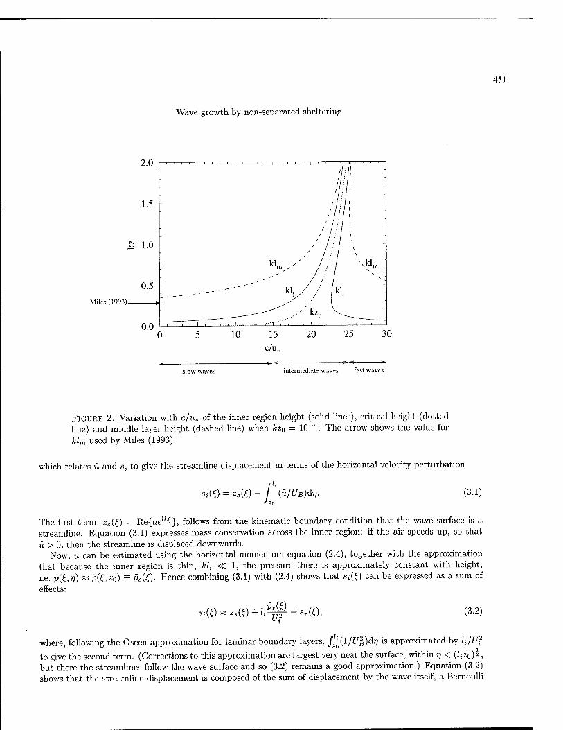
Wave growth by non-separated sheltering
451
2.0 -1 I ' ' ' ' 1 ' ' ' ));«
1:1 It'll :
1.5 „
1:1 1:1
1 ■ 1 - 1 I : 1 .
1 ' ' : -
£ 1.0 - / j : J > V
0.5 ilec (locn) ^
-
^y' /// N
0.0 1 .... 1 ■ —r-V", , , , 1 , , , , 1 ——:
10 15 20 25 30
c/u„ -■<: >-
slow waves intermediate waves fast waves
FIGURE 2. Variation with c/w* of the inner region height (solid lines), critical height (dotted line) and middle layer height (dashed line) when kz0 = 1CT4. The arrow shows the value for klm used by Miles (1993)
which relates ü and s, to give the streamline displacement in terms of the horizontal velocity perturbation
Si(0 = zs(0- [\ü/UB)dr,. J Zo
(3.1)
The first term, zs(£) = Re{aeifc^}, follows from the kinematic boundary condition that the wave surface is a streamline. Equation (3.1) expresses mass conservation across the inner region: if the air speeds up, so that ü > 0, then the streamline is displaced downwards.
Now, ü can be estimated using the horizontal momentum equation (2.4), together with the approximation that because the inner region is thin, kk < 1, the pressure there is approximately constant with height, i.e. p(£,T?) « p(€,-z0) = psiO- Hence combining (3.1) with (2.4) shows that Sj(£) can be expressed as a sum of effects:
Si(0KZs(0+li^+8r(0, (3.2)
where, following the Oseen approximation for laminar boundary layers, J^(l/{/|)dj7 is approximated by k/Uf
to give the second term. (Corrections to this approximation are largest very near the surface, within rj < (hz0) 2, but there the streamlines follow the wave surface and so (3.2) remains a good approximation.) Equation (3.2) shows that the streamline displacement is composed of the sum of displacement by the wave itself, a Bernoulli

452
S. Belcher
variation of streamline height associated with pressure variations, and a displacement caused by the change in shear stress across the inner region, which is given by
r(t)=f^T{f,(0-fi(0}<it- (3.3)
Hence, deceleration of the air by a change in wave-induced shear stress across the inner region, fs - fj, leads to reduced air speeds and hence upward streamline displacement.
3.2. Evaluation of sT
As explained in §2.2, the wave-induced stress is negligibly small in the outer region. Furthermore, as explained in §3.1, in the inner region the pressure is approximately constant with height. Hence in an overlap between the inner and outer regions, where both approximations apply, the momentum equation (2.4) yields
u(Z,v)*-Ps(0/UB{ri), (3.4)
so that when r/ RS £,;, ü « —ps/Ui. Within the inner region the turbulent stresses act to reduce this streamwise velocity perturbation to satisfy
the surface boundary condition (2.6). Hence the inner region acts as an internal boundary layer. To a crude approximation this leads to a logarithmic variation of ü with height from its value at the surface, üs(£) at T] = z0, up to its value at the top of the inner region, r\ « h. Then, if the wave-induced surface stress is fs, the wave-induced velocity has the form
1 (fs/u*) , . . u « - ^-^ ln(ry/2;o) + us
But matching this with the solution (3.4) for ü at r\ K, k yields
ÄKAh-if
ln(li/z0) {Hi - üs}
Z/KiUb*
ln(h/zo)lU, rPs . _ -, {TT + M-
(3.5)
(3.6)
The more detailed solutions (Belcher & Hunt 1993; Cohen & Belcher 1999) show how the logarithmic velocity profile near the surface joins smoothly with the inviscid solution above the inner region. However, the solution for the surface stress given in (3.6) agrees with the value obtained from the formal asymptotic analysis (Cohen & Belcher 1999 equations 5.41 and 5.42).
In addition, the wave-induced stress at r\ « k is calculated from the solution (3.4) for ü to give
TV ^ KJU jf: dü
1 dr] ZifciXhif
U'BVJ) 1 uf Ps(0 2^P.(0- (3.7)
Hence it follows from (3.3), (3.6) and (3.7), that
*T(Z)
ikUf
ZiKiUif.
Ui ln(li/z0) + 2ui I _ .,. 2KU
-Jjf]Ps(0 + ln(k/zo) us(0 d£
ZlKlUL*; + 2ul
UiWh/z0) U, Ps(0 + \n(h/zo) fi«(0 (3.8)
when zs = aeifc?. This expression, which is valid both for fast and slow waves, is extremely interesting, because it shows how the frictional effect of the Reynolds shear stress in the inner region gives rise to a phase shift in the streamline displacement: the maximum in the streamline displacement is shifted a small distance (downwind for slow waves, upwind for fast waves) away from the wave crest, to k£ — 0(ul/Uf).

453
Wave growth by non-separated sheltering
Outer Region
"'.Tinner Region
FIGURE 3. Non-separated sheltering over slow waves
3.3. Streamline displacement in the outer region
As explained in §2.2, in the outer region, the shear stress gradient is smaller than the pressure gradients, so that, in the outer region, (2.4) and (2.5) combine to give an inviscid equation for the streamline displacement, namely
d2s d + Uß'de ' dvV^driJ u%¥\ (3.9)
For a logarithmic basic flow (2.1), the basic velocity profile in this equation can be taken to be approximately constant with height (because U'B/kUB is small when kr] « 1). The dynamics in the outer region (3.9) then reduces to potential flow
^1 ^1 ߣ2 ßjj2 0 so that stzs0e-kr>eikZ, (3.10)
The constant s0 is determined by matching this solution with the streamline displacement at the top of the inner region, si; given in (3.2). Now, from (3.10), S{£,T)) « s0{l - kr]}, which matches (3.2) if
So — zs + ST- (3.11)
Hence, to this leading-order approximation, the streamline displacement in the outer region decays exponentially from its value at the top of the inner region: no further phase shift is generated by the shear stress in the outer region. As far as the outer region is concerned the flow is over a wave whose surface is given by zs + sT, which is shifted slightly downwind of the crest of the water surface (see figure 3).
3.4. The wave-induced pressure
The wave-induced pressure can be calculated conveniently from the vertical momentum equation (2.5) with the boundary condition that the wave-induced pressure far from the surface is zero, so that
*-fK 9f\A (3.12)
so that we might think of the streamwise pressure gradient, dp/d£, driving the wave-induced flow and the vertical pressure gradient responding to the vertical structure of the resulting wave-induced flow.

454
S. Belcher
We saw above in §3.3 that in the outer region the streamline displacement is determined approximately by potential flow, with solution (3.10), so that the wave-induced horizontal and vertical velocities, calculated from (2.3) and (2.2), are respectively
Ü = -UBks0e-k'iei'*, w = UB\ks0e-krie^, (3.13)
and the wave-induced shear stress, calculated from (2.11) is
f = {2Ku,j?öü/a7?}e-*"/*Beift£ « - 2KU,UB k2s0ve-kr,/s'^, (3.14)
which therefore decays to zero over the same length scale as the damped mixing-length model. Turning back to the pressure variation itself, these solutions for w and f can be substituted into the integral
(3.12), which yields
p(£, 1]) = -e[ki / { Ulk2s0e-k7i - 2KU.UB '^3S0V e~kv/sn } dr?. (3.15)
The first term in (3.15) represents the inviscid part of the wave-induced pressure and can be written V2ks0elk^,
where /•OO
V2(kV) = / Ut,e-*dT), (3.16)
(here rj = kij) is the square of a weighted average wind speed. Miles (1993) calculates the solution for V(z0) explicitly for a logarithmic basic wind profile. However a more general method can be used to estimate V for arbitrary basic wind profiles if (3.16) is integrated by parts:
V2 POO
[-Ule-%+ 2(UBU'B/k)e-Mfl, (3.17)
Now the second term is smaller than the first term because U'B/kUB is small over most of the outer region. However, towards the surface this ratio increases until it is equal to one at height lm, defined implicitly by
klm w \U;n/kUm\, so that k2l2m\ \n(lm/z0) - nc/u*\ = 1, (3.18)
for a logarithmic basic velocity profile. The subscript 'm' is used to denote this level because lm corresponds to the height of the middle layer defined by Hunt et al. (1988). Variation of lm with C/M* is shown in figure 2; also marked is the value obtained by Miles (1993). For slow and fast waves klm is small and so the pressure changes from rj = lm to the surface are a factor klm smaller than p(lm). Hence ps as p(lm). Furthermore, the foregoing arguments suggest that p(lm) « V2(lm)ks0e'k^, and also that V2(lm) w U^ (where Um = UB(lm)) since klm < 1. Hence the inviscid contribution to the surface pressure is approximately U^ksoe1^.
The second term in (3.15) arises from horizontal variations in the wave induced stress in the outer region and can be integrated to give a surface value of -2KU^Um82n\ksQ. Hence the damping of the mixing-length model leads to a small variation of pressure with height.
The pressure at the wave surface is therefore given by
Ps w [-Ul{kzs + ksT} + 2KuMm62nik{zs + sT}]eikS
= _££**, ji_i^/3je'*«. (3.19)
Here ß = /3Z„ -f /?,-,,, + ß0, which represent contributions from: the streamline displacement caused by the shear stress in the inner region, which has two components the contribution caused by the undulating wave surface,

455
Wave growth by non-separated sheltering
ßZa, and the contribution from the varying surface velocity, ßüs; and the pressure variation across the outer region, which gives ß0. If products of small terms are neglected, then from (3.8) the values of these contributions are
ßz 2Ul + Wl U2
Uf [Ui(ut/K)HU/zo) ' U, 2 i J
um-c\ r c = 2[t^) \2-w^ (3-20)
g. - ^ ^- = -2(UJn~C)2^, (3.21)
= 2K62nUm =2KS2II (Urn^c] (322)
u* { u* )
These expressions agree with the solutions found using formal asymptotic methods by Cohen & Belcher (1999), equations (5.37) and (5.38).
Results from the foregoing analysis can be used to evaluate the wave-induced shear stress at the wave surface, which is written fs = Re{kzsul{j + ie)eifc?}. In the following 7 only is required. There are two contributions to 7, namely from the undulating wave surface, denoted ^Zs, and from the varying surface velocity, denoted 7,1,. The result (3.6), together with the solution (3.19) for the surface pressure, show that they are given to leading order by
2KUJ = 2(Um-c)2 2KUS _ 2c lz"~ UiUJn{li/z0) (Üi-cjÜi' lu' ujn{h/z0)kzs Ui'
These results will be useful in §4 below, when the wave growth rate is calculated.
3.5. Discussion
The solutions derived here are valid provided the inner region is a thin layer, so that kU < 1. The conditions required to keep kh <§: 1 are established in Cohen k Belcher (1999) and correspond to slow waves, with KC/U*
of order one (so that in practice c/u* < 15), and to fast waves, with c/Ui of order one (so that in practice c/u* > 25). That the same reasoning has led to results applicable to these two regimes is noteworthy. The solutions are not valid in the intermediate regime, which corresponds to wind-wave systems with 15 < c/u* < 25, because the inner region is no longer thin and also because the critical height is of the same order as the depth of the inner region, so that Ui « c and the governing equation is singular. Resolution of this singularity requires explicit analysis of the critical layer, which is beyond the scope of this paper.
The analysis shows that the streamline displacement at the top of the inner region has three contributions: a displacement by the undulating wave surface, a displacement associated with pressure variations along the streamline (which tends to be negative at the wave crest, where the pressure is lowest and the air speeds are highest) and finally a displacement, sT, due to the wave-induced stress change across the inner region. The solution (3.8) shows that sT is a factor u*/Ui smaller than the other two terms and so the streamline displacement at the top of the inner region is largely independent of the turbulent stress. In the outer region the wave-induced stress is negligible and so again, the streamline displacement, which towards the surface matches the value at the top of the inner region, is largely independent of the turbulent stress and to a good approximation is just exponential decay.
Although small, sT is important. It is related, via (3.3), to the integral along a streamline of the change in wave-induced stress across the inner region. Hence, as an air parcel moves along a streamline the frictional deceleration from the change in wave-induced turbulent stress leads to an accumulated displacement of the streamline and hence the maximum streamline displacement is downwind of the wave crest. Belcher & Hunt (1993) called this process non-separated sheltering. For slow waves, the basic flow in the inner region is from left to right, i.e. in the same direction as the wave propagates, and so the displacement in the streamlines is to the right of the wave crest (figure 3), but for fast waves the basic flow is from right to left, i.e. against the direction

456
S. Belcher
Outer Region
Inner Region
FIGURE 4. Non-separated sheltering over fast waves
of propagation, and the streamlines are also displaced slightly to the left (figure 4). This small displacement of streamlines at the top of the inner region also means that streamlines in the outer region are displaced slightly downwind of the wave crest. The pressure perturbation that develops in the outer region then has its minimum displaced downwind of the wave crest, which leads to the contribution to the surface pressure denoted by ßZs. Orbital motions at the wave surface also lead to a change in wave-induced stress across the inner region that is negative and leads to a sheltering displacement of the streamline at the top of the inner region upwind of the wave crest. This process leads to a small shift in the surface pressure denoted by ßüs. Finally, in the lower part of the outer region a small wave-induced pressure gradient develops to balance the small wave-induced stress gradient. This leads to an additional shift in the surface pressure minimum away from the wave crest, namely
ßo. There are interesting differences between the sheltering for fast and slow waves. When the waves are slow
the surface stress is positive, fs > 0, and the stress at the top of the inner region is negative, n < 0. Hence the change in stress, fs - n, is large, so there is a strong sheltering effect and substantial values of ßZa. In contrast, when the waves are fast the wind near the surface is against the direction of wave propagation so the wave- induced surface stress is negative, fs < 0. The stress at the top of the inner region remains negative, f» < 0. The net change in stress across the inner region is therefore much smaller and the sheltering is weaker. The orbital velocity at the wave surface tends to displace streamlines upwind of the wave crests and the magnitude of the effect increases with the strength of the orbital velocites, and so also with increasing wave speed, c. Finally, the contribution to ß from the pressure variations at the bottom of the outer region, where the mixing-length model is being damped to zero, is positive for slow waves and negative for fast waves.
4. Growth and decay of the waves
The wave-induced pressure and stress do work at rate Sw at the wave surface, which then leads to an energy flux into or out of the wave motions, thence leading to wave growth or decay. Following Davis (1972) and Belcher & Hunt (1993), this evolution can be studied by forming an equation for the rate that the stress does work at the surface. If only the leading-order quadratic terms are retained then three sources of working contribute to Sw, namely
Sw = (öijüiTij) = {-c{-ps + f33s}dzs/d£) + (fsüs), (4.1)
where ( ) denotes average over a wavelength, d^ is the wave-induced stress tensor, and rij = (-dzs/d£, 1) is the normal to the surface (to the leading-order approximation). The kinematic boundary condition ws = Dzs/Dt = -cdzs/dx was used in evaluating the first term on the right of (4.1). The contribution from the

457
Wave growth by non-separated sheltering
normal turbulent stress term is small, -c(f33sdzs/d£) (Belcher & Hunt 1993; Mastenbroek 1996). Hence only two terms need to be evaluated.
The first term, c(psd;zs/d£}, can be evaluated using the solution for the asymmetric surface pressure (3.19)
to yield
c(psdzs/dO = ^(akfulcß, (4.2)
where ß is given by (3.22). The second term in (4.1), (fsüs), can be evaluated once the horizontal motions at the surface are specified. For deep water gravity waves when üs = Re{akcelki} this term gives
(fsüs) = \iahfulc~i, (4.3)
where 7 is given in (3.23). The wavelength-averaged energy in waves on deep water is E = \(pwlpa)ga2 (with the current normalisation
that the density of air is one) so that
^ = £±(l±)2a{ß + 7), (4.4)
E pw \ c J
where a = ck is the radian wave frequency. For a homogeneous wave field and in the absence of other processes affecting development of the waves dE/dt = Sw, so that the wave energy grows or decays exponentially in time, with an e-folding time given by the reciprocal of the right hand side of (4.4).
4.1. The growth rate coefficient ß + 7 The factor, denoted here (ß + j), has been intensely debated in the literature. Figure 5 shows that the present
solutions agree well with Mastenbroek's (1996) fully nonlinear computations, with full second-order closure for the stress, for both fast and slow waves. The theory shows both the same variation with c/u* and also the same variation with the relative roughness kz0. Agreement between the computations and the theory is particularly satisfying because Belcher & Hunt (1998) have argued that the damped mixing-length model used here captures the essence of the physics parameterised in a full second-order closure. The results in figure 5 support this claim. Separate evaluation of the contributions to the growth-rate coefficient shows that it is the contribution from ßZa, i.e. the contribution from sheltering, that dominates for slow waves (in agreement with Belcher & Hunt 1993). In the slow-wave regime the results computed by Mastenbroek are larger than the theoretical values as c/u* approaches its maximum value for slow waves. At these larger values of c/u* the inner region becomes too thick for the present approximations to apply and also the critical-layer mechanism might be contributing to wave growth at these more intermediate wave speeds. The present work also shows that it is the contribution from jZs, i.e. working of the wave-induced shear stress at the surface, that dominates for fast waves (the sheltering term is small for fast waves as explained in §3.5). The fast-wave theory agrees well with the computations when kz0 = HT3 and 20 < c/u* < 25.
Figure 5 also shows comparisons of values of the growth-rate coefficient from the theory with values from laboratory and open-ocean experiments collated by Plant (1984). The data lie in the slow- and intermediate-wave regimes. As has been reported by others (e.g. Mastenbroek et al. 1996; Belcher & Hunt 1998) the theoretical values are smaller than the measurements. We can offer no new explanation of this, except to point out that the values measured by Shemdin & Hsu (1967) do lie close to the theory. This is significant because Shemdin & Hsu measured growth of wind-ruffled paddle-generated waves - a configuration that is close to the configuration modelled in the present theory. In contrast the remaining measurements in figure 5 inferred the growth rate of purely wind-generated waves, which are strongly influenced by nonlinear wave-wave interactions and wave breaking (e.g. Phillips 1977 §4.6). In addition the values of wave growth from Snyder et al. (1981) (the open squares in figure 5) were obtained from measurements of the momentum flux to the waves, and so these data

458
S. Belcher
80
70
60
50
40
Cc^°
0
-10
-20
PD
D D D
r? D DDft D
ü D
D D ü D „ D % D
OO O \P% cta an D Sl - D D D D
▼=*%=*^
10 15 c/u«
20 25 30
FIGURE 5. Values of the wave growth rate coefficient from the theory when kz0 = 10~4 (filled triangles) and comparisons with values computed numerically by Mastenbroek (1996) (joined open circles) and data collated by Plant (1982) (other symbols)
need to be treated with some caution. Some previous studies (e.g. Miles 1993) have reported better agreement with the data, but such claims have been made based on models that parameterise the shear stress with a mixing-length model throughout the inner and outer regions. As argued in §2.2, the mixing-length model is appropriate only in the inner region. Belcher & Hunt (1993) and others have shown that using the mixing-length model in the outer region leads to spuriously large values of the growth rate.
4.2. A nonlinear correction to the wave growth
The expression obtained here for the e-folding time of the waves scales on v%, the surface stress in the basic-state wind profile. The present analysis shows that this basic-state wind stress controls the strength of the non-separated sheltering. It is important to recognise that this u* is not the total stress that would be measured above a wave: the total stress measured above a wind-wave system, riof, is obtained by integrating the wave-induced stress tensor along a streamline rj = constant, and is thus found to have two components
Ttotiv) =n(v) + TW(V), (4.5)
where rt = (r/j+f) is the averaged turbulent stress and TW(TI) — -(üw) is the wave-induced stress (e.g. Townsend 1972).

459
Wave growth by non-separated sheltering
At the surface TW(Z0) = rs = (psdzs/df), where 77 is the form drag (Phillips 1977), which can be evaluated from (3.19) and (3.22) to give
rf = \{akfßul. (4-6)
Furthermore, the solutions for ü and w in the outer region show that TW is zero above the inner region. Hence the wave-induced stress decays from its surface value to zero above the inner region.
When averaged over a wavelength the streamwise momentum equation (the nonlinear counterpart of (2.4)) shows that the total stress is constant with height (Townsend 1972). Hence, since TW decreases with height, to maintain rtot constant with height, rt must increase with height and be larger in the outer region than in the inner region. In practice the inner region is so thin (figure 2) that measurements of the stress are likely to be taken in the outer region, where n is larger than its surface value.
The analysis presented in §3 shows clearly that it is the turbulent stress that generates the non-separated sheltering and thence forces wave growth. Hence, following the spirit of the argument of Makin, Kudryavtsev k Mastenbroek (1995), in their calculation of the drag of the sea surface, we can suggest a nonlinear correction to the wind-input term Sw, namely that the factor of w2. in (4.4) and (4.6) is replaced by the surface value of the averaged turbulent stress, Tt{z0) which is given by
rt(zo) = not - TW{Z0) = Ttot - \{akfßul -> Ttot - Aakfßn (4.7)
so that
2V ' ^ * r
1 , \ß(.akf
The wind input of energy then becomes
Sw . Pa ß + 1 Ttot /49\ E ~ Pwl + \{akYß c2 '
where Ttot is the turbulent stress that would be measured in the outer region. Van Duin (1996a) obtained a similar equation based on a rigorous, weakly nonlinear, analysis of the air flow over slow waves. Here we have shown that the nonlinear correction arises for both slow and fast waves, and it arises because the wave absorbs momentum from the air flow, i.e. there is a wave-induced stress, which depletes the turbulent stress near the surface, thereby leaving a reduced level of turbulent stress near the surface to force the non-separated sheltering.
It is clear from (4.9) that nonlinear effects reduce the growth rate of steeper waves, which is consistent with the numerical calculations of Gent k Taylor (1976) and Mastenbroek (1996). Figure 6 shows the variation of a related quantity, namely the form drag, with wave slope for a rigid wavy wall, with c/u* = 0. It is clear from the figure that the nonlinear theory (4.8) lies much closer to the computations than the linear theory (4.6), particularly when ak > 0.2. The theoretical curves are truncated when ak = 0.3 because the air flow is expected to separate for higher slopes. The strength of the nonlinear effects depend on the factor \{ak)2ß, and thus depends on c/u*. For slow waves, with small values of c/u», ß « 20 so that nonlinear effects become appreciable when ak « l/(/?)= ~ |, in agreement with the plots in figure 6. Mitsuyasu & Honda (1982) measured the growth rate of paddle-generated water waves and found that in their range of 0.03 < ak < 0.2 (assuming that their H equals 2a) the growth rate was insensitive to the wave slope, again in rough agreement with figure 6. For fast waves, with large values of c/u*, ß « -1 and much larger slopes are required for the nonlinear effects to be significant. We expect ocean waves that lie in the fast-wave regime, for example swell, to have low slopes and hence we conclude that the nonlinear effects are likely to be negligible for fast waves. Finally, we do not expect the present form of the nonlinear correction to be valid when the waves break, because

460
S. Belcher
1.0
0.9
0.8
0.7
0.6
ij0.5 e
0.4
0.3
0.2
0.1
0.0
;
1 >'• i 11111111111. i 1 " " 1II. 11111 11 11:
I- 1
: : : • :
- / / .D"' 4
; / -. - / - \ / u : : / / :
r 1 y/
/ // i
I >□' j
j- tS--' i
L<rr (Jf_ , , , . i 1^
0.0 0.1 0.2 0.3 0.4 0.5 0.6 0.7
ak
FIGURE 6. Variation of the form drag with wave slope for c/u* = 0. Dashed line: linear theory; solid line: nonlinear theory; open squares: nonlinear numerical calculations with full second order closure from Belcher et al. (1993); filled circles: measurements of Zilker & Hanratty (1979) over solid wavy wall.
then the air flow separates and the streamlines no longer follow the wave surface as they are assumed to do in the present analysis. Nevertheless, the present formula should be valid up until breaking.
5. Conclusions
We have developed a heurstic analysis of the air flow over waves in the limits of slow waves, when c/u* < 15, and of fast waves, when c/u* > 25. Previously published formal asymptotic solutions (Belcher & Hunt 1993; Cohen & Belcher 1999) have shown that non-separated sheltering is the primary mechanism responsible for the growth and decay of these waves. The critical-layer mechanism is, at most, of secondary importance in these parameter regimes.
The heuristic analysis developed here aimed to understand more deeply the physical processes behind non- separated sheltering. The analysis has shown how the streamline displacement at the top of the inner region is controlled by three processes: displacement over the undulating wave surface, a Bernoulli displacement associated with pressure variations, and a small, but important, asymmetric displacement due to the turbulent shear stress. This asymmetric displacement of streamlines leads to deceleration of the wind in the lee of the wave, i.e. to a non-separated sheltering. Above the inner region, in the outer region, the streamline displacement remains in phase with the streamline at the top of the inner region: no further asymmetry is produced because the wave-induced shear-stress gradient there is too weak. A pressure perturbation then develops in the outer region that has its minimum displaced downwind of the wave crest. This pressure perturbation together with

461
Wave growth by non-separated sheltering
the surface stress perturbation does work at the wave surface and leads to growth of slow waves and decay of
fast waves. The present approach shows clearly how the change in value of the shear stress across the inner region
controls the strength of the non-separated sheltering. This observation suggested a nonlinear correction wherein the surface value of the turbulent stress is used in the equation for the energy flux. This surface value of the turbulent stress is smaller than the value aloft in the outer region because some of the momentum in the inner region is absorbed as wave-induced stress, which leads to a correction to the energy flux that increases as the square of the wave slope. The strength of the nonlinear correction also scales on ß, the part of the growth rate coefficient that is determined by the surface pressure. Since ß is larger for slow waves than for fast waves we conclude that slow waves are more likely to be affected by this nonlinear process than fast waves.
Finally, in the intermediate range of 15 < c/u* < 25 the critical-layer mechanism may well be important in addition to non-separated sheltering, although we note the comment of Mastenbroek (1996) that he found no evidence of a critical-layer mechanism contributing to wave growth in his numerical calculations. To date there has been no local analysis of both non-separated sheltering and the critical-layer mechanisms. Miles (1996) develops an integral analysis, but this mathematical method might exaggerate the critical-layer effects. There is hope that the present formulation, wherein the streamline displacement is analysed, can shed light onto this mathematically-difficult intermediate regime, because Belcher et al. (1998) have shown how an inviscid critical layer can be analysed in this framework.
Acknowledgements
It is a pleasure to thank Julian Hunt for useful discussions and suggestions during the course of this work. Funding for this work was provided partly by the EC under the ASPEN project, contract ENV4-CT97-0460 and partly by DERA under contract LSC/2034/222.
References
[1] BELCHER, S. E. & HUNT, J. C. R. 1993 Turbulent shear flow over slowly moving waves. J. Fluid Mech. 251, 109-148. [2] BELCHER! S. E. & HUNT, J. C. R. 1998 Turbulent flow over hills and waves. Ann. Rev. Fluid Mech. 30, 507-538. [3] BELCHER' S. E., HUNT, J. C. R. & COHEN, J. E. 1998 Turbulent shear flow over growing waves To appear in Proc. I.M.A. con-
ference on wind-wave interactions. Eds. S. Sajjadi, N.H. Thomas, J.C.R. Hunt. Oxford. [4] BELCHER, S. E., NEWLEY, T. M. J. & HUNT, J. C. R. 1993 The drag on an undulating surface induced by the flow of a turbulent
boundary layer. J. Fluid Mech. 249, 557-596. [5] BRITTER, R. E., HUNT, J. C. R. fe RICHARDS, K. J. 1981 Air flow over a 2-d hill: studies of velocity speed up, roughness effects
and turbulence.' Q. J. R. Met. Soc. 107, 91-110. [G] COHEN, J. E. & BELCHER, S. E. 1999 Turbulent shear flow and fast moving waves. J. Fluid Mech. In press [7] DAVIES, R. E. 1972 On prediction of turbulent flow over a wavy boundary. J. Fluid Mech. 52, 287-306. [8] DUIN, C. A. VAN 1996a An asymptotic theory for the generation of nonlinear surface gravity waves by turbulent air flow.
J. Fluid Mech. 320, 287-304. [9] DUIN, C.A. VAN 1996b Rapid-distortion turbulence models in the theory of surface-wave generation. J. Fluid Mech. 329,
147-153. [10] GENT, P. R. & TAYLOR, P. A. 1976 A numerical model of the air flow above water waves. J. Fluid Mech. 77, 105-128. [11] HUNT' J. C. R., LEIBOVICH, S. & RICHARDS, K. J. 1988 Turbulent shear flow over low hills. Q. J. R. Met. Soc. 114, 1435-1471. [12] HUNT', J. C. R. & RICHARDS, K. J. 1984 Stratified airflow over one or two hills. Boundary-Layer Met. 30, 223-259. [13] JEFFREYS, H. 1925 On the formation of water waves by wind. Proc. R. Soc. Lond. A 107, 189-206. [14] MAKIN, V.K., KUDRYAVSTEV, V.N., & MASTENBROEK, C. 1995 Drag of the sea surface. Boundary Layer Meteorol. 73,
159-182. [15] MASTENBROEK, C. 1996 Wind-wave interaction, PhD thesis, Delft Technical University. [16] MASTENBROEK, O, MAKIN, V.K., GARAT, M.H. & GIOVANANGELI, J.P. 1996 Experimental evidence of the rapid distortion
of the turbulence in the air flow over water waves. J. Fluid Mech. 318, 273-302. [17] -MILES, J. W. 1957 On the generation of surface waves by shear flows. J. Fluid Mech. 3, 185-204. [18] MILES, J.W. 1993 Surface-wave generation revisited. J. Fluid Mech. 256, 427-441. [19] MILES, J.W. 1996 Surface-wave generation: a viscoelastic model. J. Fluid Mech. 322, 131-145. [20] PHILLIPS, O.M. 1977 The Dynamics of the Upper Ocean. C.U.P. [21] PLANT, W. J. 1984 A relationship between wind shear stress and wave slope. J. Geophys. Res. 87, C3, 1961-1967.

462
S. Belcher
[22] SIIEMDIN, O. II. & IIsu, E. Y. 1967 The dynamics of wind in the vicinity of progressive water waves. J. Fluid Mech. 30, 403-416. [23] SNYUER, R. L., DODSON, F.W., ELLIOT, J. A., LONG, R. B. 1981 Array measurements of atmospheric pressure fluctuations
above gravity waves. J. Fluid Mech. 102, 1-59. [24] TOWNSEND, A. A. 1972 Flow in a deep turbulent boundary layer disturbed by water waves. J. Fluid Mech. 55, 719-735. [25] Zou, Q.P. 1998 A viscoelastic model for turbulent flow over undulating topography. J. Fluid Mech., 355, 81-112. [26] ZILKUR, D. P. & HANRATTY, T. J. 1979 Influence of a solid way boundary on turbulent flow. Part 2 separated flows. J. Fluid
Mech., 90, 257-271.

Eur. J. Mech. B/Fluids © Elsevier, Paris
PHYSICAL MECHANISMS FOR SPORADIC WIND WAVE HORSE-SHOE PATTERNS
Sergei Yu. AnnenkovW and Victor I. Shrirat2'
[1]: P.P.Shirshov Institute of Oceanology, 36 Nakhimovsky prosp., Moscow 117218, Russia, e-mail: sergeSvave.sio.rssi.ru [2]: Department of Applied Mathematics, University College Cork, Cork, Ireland, e-mail: shrirafflucc.ie
(Received 16 October 1998, revised and accepted 10 February 1999)
Abstract - We consider three-dimensional crescent-shaped patterns often seen on water surface in natural basins and observed in wave tank experiments. The most common of these 'horse-shoe-like' patterns appear to be sporadic, i.e., emerging and disappearing spontaneously even under steady wind conditions. The paper suggests a qualitative model of these structures aimed at explaining their sporadic nature, physical mechanisms of their selection and their specific asymmetric form. © Elsevier, Paris
Introduction
Patterns of spectacular crescent-shaped form, resembling horse-shoes, can be often seen on water surface in natural basins. These patterns are very important from the ocean science perspective, since they modify the airflow above the surface and thus affect the air-sea momentum transfer. They also change in a specific way the radar scattering from the sea surface, and, last but not least, they require conceptually new models to describe statistically the wind-wave field dynamics in their presence [11]. On the other hand, the phenomenon is of true interest from the viewpoint of nonlinear science, as a new non-trivial scenario of pattern formation having no close analogues in the very rich literature on patterns (e.g. [3]).
Though no field studies of the horse-shoe patterns are known, among their main features inferred from common observations are [11]:
(i) wave fronts are of crescent-shaped form and are alxuays oriented forward, (ii) the patterns appear quickly after the onset of a fresh wind, at early stages of wave development charac-
terized by high wave steepness; (iii) the patterns might be localized in space and time, but exist over space- and timescales greatly exceeding
the basic wave wavelength and period. A number of experiments carried out in wave tanks ( [4,13]), and wind-wave facilities ( [4,8,10]), both in the
presence and absence of wind, made it possible to reproduce the patterns in their ideal form under controlled conditions and to measure their parameters. It has been established that the inception mechanism of the horse- shoes is due to McLean's class II instability (five-wave decay) of the plane basic wave. It was also found that wave steepness above a certain threshold is necessary for their inception. However, the specific mechanisms of the pattern formation remain unidentified.
A possible scenario of the emergence of the patterns was suggested in [11]. The authors made the assumption that the single symmetric pair with the largest linear growth rate due to McLean's class II instability prevails, while all other pairs within the instability domain may be ignored. Consideration of the simple three-wave problem comprising a basic wave and the fastest growing pair of satellites demonstrated the formation of patterns that indeed render the specific geometry closely resembling the observed horse-shoe forms, but only under a
464
S. Yu. Annenkov, V. I. Shrira
special relation between the phases of the interacting waves. However, in the conservative case, no preference for phases was found. Instead, the phase of a satellite during the cycle of its growth and subsequent decay rotates through all the possible values, giving a full range of various three-dimensional patterns of all orientations with overall distribution being symmetric in up- and downwind directions, in an apparent contradiction to the observations. However, it was shown that non-conservative effects, inserted into the system but small enough to preserve the Hamiltonian structure to the required order, allow the system to evolve to a steady state with the geometric form of the free surface with the required characteristics.
The model of [11] used the rather crude assumption (based on the experimental evidence [4]) that the class II instability of the fundamental can be adequately represented by the selection of a single symmetric pair of oblique satellites. Although the domain of the five-wave instability is 0(ez) narrow (e being the measure of the basic wave steepness), it is still continuous and there is no a priori reason to confine the consideration of this instability to a single pair of satellite harmonics. Moreover, this approach completely neglects the sideband satellites growing due to the Benjamin-Feir instability. On the other hand, from the experimental viewpoint, the most often observed crescent-shaped patterns are sporadic and seem to be far from equilibrium. Besides that, the patterns have been also observed in the tank experiments without wind (e.g. [13]) where no equilibria are possible. All this prompts us to reexamine the basic assumptions of [11] and to look for a new robust mechanism able to create the essentially non-stationary, relatively short-lived patterns of the same geometry.
We consider the general situation when the class II instability gives rise to many pairs of oblique satellites, with Benjamin-Feir (class I) satellites being also taken into account. Since these questions constitute a problem evidently not tractable by analytical means, an extensive numerical study of possible evolution scenarios was undertaken. For this purpose, a novel numerical method recently developed by the authors [1] has been used. This method, based on the perturbed integrodifferential Zakharov equation, allows one to trace the long-term evolution of a sufficiently large number of interacting modes, both in a conservative system and in the presence of weak non-conservative effects included via the insertion of small (of the order of the five-wave interaction term) linear damping and forcing terms.
The numerical analysis allowed us to establish the basic facts concerned with the long-time evolution of five-wave instability. First, even the system with the initially large number of degrees of freedom appears to follow, at least locally, the evolution scenario of a low-dimensional system. This means that in a generic situation only very few of the linearly unstable modes (often different modes at different moments of time) would grow considerably. Moreover, under the effect of weak dissipation this small number of grown modes is normally reduced to just single pair. This suggests the existence of a nonlinear selection mechanism which is enhanced by dissipation. This mechanism reduces considerably the number of grown modes, at the same time noticeably enlarging their maximal amplitude. Evolution of the system is shown to result in the formation of sporadic crescent-shaped patterns on the free surface with steep front slopes and flattened rear ones, closely resembling the observed horse-shoe patterns. The patterns' dynamics is found to be determined mainly by quintet interactions, while the presence of Benjamin-Feir modulation does not alter it qualitatively.
The selection mechanism has been identified as follows: each growing pair of oblique satellites 'pushes' all other pairs out of the narrow instability domain by creating nonlinear frequency shift. Normally, one pair prevails, so that most of the time the evolution closely corresponds to that of the three-wave system. At the same time, the presence of other pairs of satellites is shown to lead to phase asymmetry: a growing satellite pair has the required ('correct') phase value, while the phases of decaying ones are unstable, so that the frequency shifts caused by the weak interaction with other modes set them into rapid rotation. As a result, pronounced horse-shoe like patterns develop at each cycle of such intermittent regime. The described mechanism does not require the presence of non-conservative effects as a prerequisite. Nevertheless, weak dissipation is shown to significantly facilitate observation of the patterns, due to prolonged satellites' growth and elimination of noise.
1. Basic equations and the numerical model
We consider three-dimensional potential gravity waves on the free surface of an incompressible fluid of infinite depth. Wave slopes are supposed to be of the order of a small parameter e. Dynamics then is governed, up to

465
Sporadic wind wave horse-shoe patterns
the order e4, by the integrodifferential equation
: ° = (u!0 + l'7o)^0 + / Vbl23^2Mo+l-2-3dki
+ / ^01234&i&2&3&4^0+l-2-3-4dki234 + 2 / ^43210&i&2&3Mo+l+2-3-4 dki2:
1-^7 = (Wo + 170)00+ / l/O1230i0203'JO+l-2-3dki23 Öt J (1)
00+1+2-3-4 UK1234
derived by [15] (see also [6]) and extended to the order e4 by [7]; for our purposes, equation (1) is modified by the presence of small (of the order e4) non-conservative effects. Here, 6(k) is a canonical complex variable, cj(k) = (</fc) is the linear dispersion relation, k = |k|, 7(k) stands for 0(e3) damping/growth rate, integration in (1) is performed over the entire k-plane. The compact notation used designates the arguments by indices, e-9- V0123 = Vr(k,ki,k2,k3), £0+1-2-3 = S(k + ki - k2 - k3), dki23 = dkidk2dk3, asterisk means complex conjugation, t is time. The canonical variable 6(k) is linked to the Fourier-transformed primitive physical variables y(k,£) and r;(k,i) (free-surface potential and surface elevation, respectively) through an integral- power series ( [7]). All details of the lengthy procedure of derivation of (1), as well as the expressions for the kernels V, W can be found in [7].
Equation (1) is the so called reduced equation, that is, it takes into account only resonant (or nearly reso- nant) interactions between free modes, leaving incomparably fewer interactions to consider than in conventional physical-space models. In other words, much of the complexity of the original hydrodynamic equations goes to coefficients that indeed have very cumbersome algebraic form. More advantages of (1) as a basis for a numerical study can be pointed out ( [2]). Though the idea to use this equation, upon proper discretization, to study the evolution of a number of discrete modes seems natural ( [5]), there were few attempts at implementation of such a numerical scheme.
In the present work, the recently proposed novel numerical approach ( [1]) is used. Given the initial state of the fluid (functions tp(x,y,0), rj(x,y,0)), Fourier transformation and integral power series expansion are used to obtain the initial value of complex amplitude 6(k,0). Then the function 0 is discretized in k-space, being replaced by a set of complex variables bm = 6(km), m = 1,2,...N. Next, all the coefficients V and W are calculated and stored. For the subsequent integration in time, the discretized version of (1) is used. Finally, the obtained fluid state is transformed back to physical variables.
When the non-conservative effects are negligible for the timescales under consideration, (1) is a Hamiltonian system and time integration is performed with a symplectic algorithm, otherwise the system is integrated by the more conventional Runge-Kutta scheme. All the details of the proposed algorithm are given in [1].
2. Instability of a single basic wave: evolution scenarios
The model of [11] is confined to the consideration of only three harmonics in the Zakharov equation. In reality, of course, neither the basic wave nor the satellites are monochromatic. In this section we will focus upon the latter, i.e. we will consider nonlinear evolution of many satellites generated by a single basic wave due to quintet interactions, while the effects of non-monochromaticity of the basic wave are briefly considered in §5.
2.1. Three-wave model
Consider a system comprising only three waves (N = 3) with the amplitudes a, b, c and wavevectors k„, kt, kc satisfying the condition 3k„ = k;, + kc, where a denotes the basic wave, 0, c are the satellites, assumed initially small, k = (kx,ky). Without the loss of generality
kn = (l,0), k6 = (|+p,9), kc = (|-p,-g). (2)
It is implied that the waves a, b. c form a nearly resonant quintet, that is
Zu)a-^,,-ujc<ü(£:i). (3)

466
S. Yu. Annenkov, V. I. Shrira
Thus, this combination of waves represents the simplest possible case of quintet interactions. Equation (1) for this case takes the form
at = -i(w„ + i-ya)a - i [Vannn|a|2 + 2Vnbab\b\2 + 2Vacac\c\2] a - 3iJF6crtanbc (a2)" bt = -i(w(, + i"fb)b - i ct = -i(uic + ryc)c
2Vrotn6|a|2 + Vbbbb\b\2 + 2V(,c6c|c|2| b - iWbcaaac*a3, (4)
2Vacnc\a\2 + 2Vbcbc\b\2 + Vcccc\c\2] c - iWbcaaab*a3.
Performing the transformation
a = Aexp(-ia), b = Bexp(—iß), c = C exp(-i~f),
system (4), for initially equal and symmetric satellites, reduces to the form
At = 3WbcaaaA2B2 sin $ + TaA,
Bt = -WbcanaA3B sin $ + TbB, (5)
$t = 6 + PA2 + MB2 + WbcaaaA(9B2 - 2Ä2) cos $,
where the parameters are
5 = 3ua - ujb - ioc, rn=wa7n, rb=cüb7b, P = 3Vaaaa - 2Vabab - 2VaCac, M — §Vabab + 6Vacac - 4Vbcbc - Vbbbb - Vc cccc-
Variable $ (the phase of the pair of satellites relative to the fundamental) is defined as $ = 3a — ß — 7; $ and sometimes sin$ below will be referred to as 'the phase', for brevity.
The specific form of a surface elevation pattern is mainly prescribed by the value of $. If —n + 2irn < $ < 0 + 2im, the patterns have their convex sides oriented downwind, the best resemblance with the observed patterns being at $ = — TT/2 + 2im. For simplicity we will refer to such phases as negative and will omit the period 2im hereafter. The phases in the range 0 < $ < n correspond to the opposite orientation. However, as was noted by [11], if rn = Tb = 0, then (5) is a reversible Hamiltonian system, so that it passes in a symmetric manner through all the values of <J>. Thus, the system shows a variety of three-dimensional patterns with no preference for orientation. This means that a model of horse-shoe patterns cannot be built upon the basis of such a conservative three-wave system.
Still, a closer inspection of this system is useful for further progress in understanding (see [2] for more detailed analysis). Suppose that Fn = Tb = 0. If the initial amplitudes of the satellites are infinitesimal, then the trajectories of the system (5) are close to the separatrix originating and ending at two stationary saddle points
-iS + PA2
B = 0, A = A0, $ = <50 = ± cos 2WA3
For definiteness, and also because this ensures the maximal instability ( [12]), we choose 6 = — PAQ, and then $0 = ±7r/2. An example of a triad evolution for such a case is presented in figure 1, for the initial value of phase <]> equal to —n/2. The dynamics is periodic; the phase, rotating counterclockwise, stays most of the time close to the two values $ = ±7r/2 with quite fast transition in between, zero phase corresponding to the point of the deepest modulation. When the satellites are small compared to the fundamental, all the trajectories in (B, <3?) plane are in the vicinity of the saddle points. Since the trajectories in the vicinity of the saddle (B = 0, $ = — 7r/2) are divergent in B, there is a convergence of the trajectories in $, while in the neighbourhood of the second saddle (B = 0, $ = 7r/2) the trajectories converge in B but diverge in $. This implies that if we perturb the system the trajectories corresponding to growing satellites will tend to preserve their phase, while those corresponding to decaying satellites will experience large variations of the phase, and thus become unstable.'
These simple facts give insight into more complicated situations. Even a small perturbation can change the phase and thus the whole system dynamics near the point <5 = +ir/2. Thus, the long periods in the

0.8
A, ° .6
sin <£> o
Sporadic wind wave horse-shoe patterns
\A
1000 2000 3000 4000 5000
/ i\ n 1000 2000 3000 4000 5000
FIGURE 1. Evolution of the conservative three-wave system (2) with p = 3/2 and q = 1.54, for the basic wave steepness 0.21. Time is measured in u>-1, where w is the basic wave frequency.
467
neighbourhood of $ = +7r/2 and potential instability of these segments of trajectories indicate a possible structural instability of the three-wave system.
With the inclusion of small non-conservative effects (for wind waves, it is natural to assume that Fa > 0, T(, < 0), the similar two saddles are preserved. Numerical simulations (see [2]) show that the evolution becomes slightly asymmetrical since the growth of satellites is slower and their subsequent decay is faster. The point of maximum corresponds to a certain negative value of phase. Still, simulations demonstrate that there are still relatively long periods of the phase being close to the potentially unstable value +ir/2, which suggests the non- conservative three-wave system to remain potentially structurally unstable and thus might be too oversimplified to serve as a model of the formation of horse-shoe patterns.
2.2. Multiple class II satellites
In reality, a fundamental wave of a finite amplitude possesses finite size domains of instability with respect to four- and five-wave processes in the wavevector space (see [9]; [5], Fig. 6.6), so that simultaneous growth of many pairs of satellites (strictly speaking, continuum of satellites) should occur. Nonlinear dynamics of such continuum of linearly growing satellites is simulated by a large number of unstable satellites. Since our primary interest is in three-dimensional dynamics, in this section we focus upon the situations where the satellites were taken in the five-wave (class II) instability domain and stable part of fc-plane only. The effect of finite bandwidth of the basic wave spectrum and, in particular, role of the Benjamin-Feir instability are briefly addressed in §5.
For the numerical study, a system comprising a basic wave with wavevector ko = (1,0) and N pairs of oblique satellites with wavevectors kj,j+i = (§ ±pj,±qj), j = 1,2,... ,N was selected. In the experiments discussed in this section, N = 42, and both symmetric (with respect to kx-&xis) and non-symmetric oblique harmonics within and in the neighbourhood of the instability domain were represented; see [2] for details. Three different values for the initial steepness of the fundamental (0.13, 0.17 and 0.21) were used. The satellites were put initially small, with amplitudes of the order O(10~2) relative to the amplitude of the fundamental; no essential dependence on the exact value of satellites' initial amplitude was revealed. Initial phase of all the satellites was again prescribed at the value most favourable for growth (—7r/2). Evolution in time was traced for about 103
periods of the basic wave. We again emphasize that at this stage the Benjamin-Feir instability was excluded.

468
A, °-4-
/ 0.2
-1
sin <£> o. 2
S. Yu. Annenkov, V. I. Shrira
1000 2000 3000 4000 5000 6000 7000 8000 9000 10000
A/IMA A, rwun AA i^—mf I
:IWU/NA /AAA rm 0
t 1000 2000 3000 4000 5000 6000 7000 8000 9000 10000
FIGURE 2. Evolution of the conservative system consisting of a basic wave and 42 pairs of initially small satellites. For three most unstable pairs, evolution of phase is shown.
An example of conservative evolution of the system is presented in figure 2. The plot demonstrates two distinct features of the class II instability with respect to multiple satellites. First, most of the modes located in the linear instability domain do not attain considerable amplitudes, stagnating at a quite low level. Only a few modes at each moment can grow inattenuated, though this behaviour is displayed by different modes at different moments. Second, the evolution of the phases of these growing modes differs noticeably from that of the isolated three-wave system. In particular, it becomes essentially asymmetric. When the mode is growing, its phase keeps close to —ir/2, as in the three-mode case; the maximum of the satellite amplitude again corresponds to zero phase, but soon after reaching the maximum of the amplitude, the phase typically starts to change much more rapidly, while the amplitude decreases and tends to stagnate at a quite low level. However, this behaviour is not always well pronounced for all growing pairs during the course of the conservative evolution, thus allowing one to consider it only as a tendency.
Meanwhile, these features, observed in the large number of runs of the numerical model, are much more pronounced in the more realistic weakly non-conservative case (figure 3). Only one pair of satellites attains considerable amplitude, while its phase remains in the neighbourhood of — ir/2 nearly all the time, except for the brief excursion soon after maximum of amplitude. The above features do not exhibit noticeable dependence on the amplitude of the basic wave provided the growth rates due to inviscid class II instability exceed the dissipation.

0.8 r
0.6
A, 0A
B 0.2
1 r
1 r
sinO
469
Sporadic wind wave horse-shoe patterns
3 t 1000 2000 3000 4000 5000 6000 7000 8000 9000 10000
•AMA l\r, :m± 1 I L
AAAA 0 1000 2000 3000 4000 5000 6000 7000 8000 9000 10000
FIGURE 3. As in figure 2, with non-conservative effects included (Fa = 5 • 10~°wa, Tj = 5-10-*ujtj = l,... ,N).
2.3. Summary and discussion
While three-wave systems, with small non-conservative effects, exhibit nearly symmetric behaviour with respect to different values of phase, inclusion of one or more additional pairs of satellites drastically enhances the asymmetry. The phase of a satellite during its growth and near the maximum of amplitude remains close to —7r/2; the phase of the decaying one in most cases becomes indeterminate.
The important role of dissipation requires some special comments. First, the dissipation is essential in the initial selection, since only the modes with maximal growth rates and initial phases close to —7r/2 can survive. Second, its presence results in shifting the phase at the point of the satellite maxima: the phase remains negative at the maximum and in its neighbourhood. Thus, the phases of modes whose amplitudes exceed a certain threshold, are always negative, and therefore the wave fronts are oriented forward. Such sporadically appearing and disappearing surface patterns closely resemble the observed horse-shoe ones.
The most nontrivial fact established numerically is that the evolution in multi-dimensional system remains effectively low-dimensional. It is well known that a nonlinear system characterized at an initial moment by a certain finite number of excited modes can evolve in accordance with two opposite scenarios. If nonlinearity prevails (in a certain sense) over dissipative effects, the number of excited modes of the system tends to grow with time, in the opposite limit the effective number of active modes in the system decreases and the system often falls into a low-modal attractor. At first sight the latter scenario seems to be the case. It is easy to find

470
S. Yu. Annenkov, V. I. Shrira
the rate of contraction of the phase volume v
N N
and it is indeed negative when the integral dissipation exceeds the input Tn. This is the case N N
E r&i + E rc
for all our simulations when non-conservative effects were taken into account. However, the distinct tendency towards low-dimensional dynamics is revealed even in the case of purely Hamiltonian dynamics! Though this seems to contradict the preservation of the phase volume, the contraction of the phase volume in physically important segments of the phase space is exactly compensated by its expansion in other segments. For instance, confinement of the phases of the growing and grown modes is accompanied by the rapid phase rotation of all other modes. If one focuses attention on the subspace of interest, say the modes with amplitudes exceeding a certain small threshold, the rest of phase space will provide a kind of nonlinear dissipation for the chosen subspace.
3. Selection mechanism
Numerical results discussed suggest that there exists a certain nonlinear mechanism responsible for the selection of modes and the eventual formation of horse-shoe patterns, which can be revealed by an analysis of simple low-modal systems.
A monochromatic wave of amplitude a and wavevector ka = (1,0) is known to be unstable with respect to pairs of oblique satellites with wavevectors k(,, kc satisfying (2), if a certain condition on p, q implied by (3) is fulfilled. Within the framework of the Zakharov equation, the corresponding condition can be easily obtained in an explicit form [2]:
4W'£nnJä|(i - (a - i(7t - 7c))2 > (lb + 7c)
2, (6)
where a = S + P|ä|2, 5 is the initial value for o. According to such a linearized theory, all the initially small oblique satellites in the instability domain grow exponentially, with the rate
Re{\fwLaa\ä\6 - Or - i(7«, - 7c))2 - (76 + 7c)2}
If only one pair is present, its evolution is governed by (5); the process is recurrent, linearized system being valid as an approximation on each cycle in the neighbourhood of the point of the smallest amplitude of the satellites.
The presence of just one extra pair makes the problem much more difficult. However, numerical analysis of the evolution of a system comprising two pairs of satellites typically shows a relatively simple scenario of evolution (detailed analysis is presented in [2]). In most cases the simultaneous growth of both pairs does not occur. Instead, the modes grow in alternance: after the initial linear stage of instability one of harmonics stagnates at a quite low amplitude level, while the other one continues to grow, attains considerable amplitude and decays. At this stage, the presence of the other pair of harmonics does not seem to affect the system behaviour at all, except for a rather remarkable fact that the maximum of amplitude of the growing pair in the presence of the stagnating one is somewhat enlarged. Further on, the process is approximately repeated with the other pair of satellites, so that most of time the evolution appears to be close to that of the three-wave system.
In principle, an approximate solution can be obtained by constructing the asymptotic solution for each stage of the evolution and matching the resulting expansions. Consider, as the simplest non-trivial model, a five-wave system with just two pairs of satellites, using the notation (k&, kc) for the first pair and (k,/, ke) for the second

471
Sporadic wind wave horse-shoe patterns
one, so that 3k„ = kb+kc = krf+k<., and the frequency mismatches 3u>a-ujb-uc and 3w„-wrf-we are both of the order of e3. Since our primary interest lies in the selection process, consider the system for the stage B ~ D <C A, A being the amplitude of the fundamental, B and D of the satellites. Provided that the two pairs lie close to the point of the maximum linear growth rate in k-plane, one may put Wbcaaa - Wdeaaa = W = 0(e ), while all the other coefficients of the governing system are of the order s2. However, in virtue of (6), or its analogue with dissipation taken into account, the total initial frequency mismatch with the nonlinear frequency shifts caused by the basic wave, 6j + PjA{0)2 is of the order of the largest term due to the quintet interaction, i.e., 0(e3). Introducing r = Wt as a slow timescale, the typical ratio of amplitudes of satellites and the fundamental at the point where selection occurs B/A ~ D/A =/xasa new small parameter and retaining only the leading order terms in /i2, we obtain the system governing the case of two unstable pairs:
AT = 2»A2B2 sin $1 + 3A2D2 sin $2 + taA, BT = -A3B sin$i +tbB DT = -A3Dsm<$2 + tdD
_[^±PiV] + PaA(A»-V) ;Mg_2A, W
*2r =
W e g
Wee'
where A0 = A(0), f = T/W, Pj, Nj are the new 0(1) coefficients. System (7) enables one to understand the mechanism of the selection process. At the initial stage of evolution,
when B2/A2 «I fi and D2/A2 «: y,, the linear regime is realized: both pairs of satellites grow, provided that $! and $2 are both negative. When the satellites attain a certain threshold amplitude, the second terms in the right-hand sides of the phase equations in (7) become of order 0(1). The signs of these frequency-shifting terms are such that each pair tends to push the phase of the other pair from the value which is favourable for the growth of amplitude, until one of the phases starts to rotate, preventing, the subsequent growth of the corresponding pair. Afterwards, only one of the pairs grows, while the other one, with the rapidly rotating phase, is decaying. The presence of the small parameter in the denominator of the frequency-shifting terms specifies the characteristic threshold level of the satellite amplitude where the selection occurs: B ~ D ~ y/eA. One can describe this mechanism as the 'rivalry' between the pairs, so that each one, while growing, pushes the other one out of the resonance with the fundamental via the frequency shift.
We already mentioned the interesting effect exhibited by the simulations: the maximal amplitude of the remaining pair noticeably exceeds that of the same pair in the isolated three-wave system. In other words, small satellites act like a catalyst enhancing the energy exchange between the growing satellite and the fundamental. This fact can be easily explained by comparison of (7) with the single-pair system. The growth of, say, B in (5) is controlled by the change of the amplitude of the fundamental: when A diminishes, the variation of the frequency shift PX{A
2 - A^/W becomes large and positive (since Px < 0), leading to the counterclockwise rotation of phase. Meanwhile, in the corresponding phase equation in (7) jVx < 0, so that the term NiD2 is always negative, and thus tends to compensate the effect of the frequency shift for this pair, while the similar term in the other phase equation drives the phase of the second pair out of equilibrium. Hence, the effect tends to stabilize the phase of the first pair at the value that is favourable for growth, eventually resulting in the increase of the maximal amplitude.
4. Effects due to the finite width of the spectrum of the basic wave
An actual wave field is continuous, so that the consideration of the process of interaction of monochromatic waves should be regarded as an approximation to the interaction of finite bandwidth wavepackets. In particular, the basic wave spectrum bandwidth cannot be less than e. The most important effect in this respect is clearly the presence of the modulational (Benjamin-Fcir) instability of the fundamental wavepacket. Does the presence of much faster (0(e)"'2) and more energetic four-wave (class I) processes preserve intact the evolution scenarios

472
S. Yu. Anncnkov, V. I. Shrira
A, B
t 0 1000 2000 3000 4000 5000 6000 7000 8000 9000 10000
sin <E> o ^/n^n MM, 0 1000 2000 3000 4000 5000 6000 7000 8000 9000 10000
FIGURE 4. As in figure 3, with a pair of Benjamin-Feir satellites included.
established above? As a first approximation, the effect of the modulational instability can be modeled just by adding of one or more pairs of additional initially small satellites k,-± = (1 ± Aj, 0), j = 1, 2,..., where k0 = (1,0) is the basic wave central wavevector, Aj lie within the domain of the Benjamin-Feir instability (see, e.g. [5]).
Based on numerous simulations in wide range of the parameters involved (one sample is given in figure 4) we conclude that qualitatively, the account of the finite bandwidth of the basic wave does not alter the already established scenarios of field evolution on e~3-timescale, although quantitatively the effect could be quite noticeable.
It has been previously suggested by [14] that the class I processes, which have shorter characteristic time of development, may trigger the class II instability. Our results do not support this hypothesis. Moreover, in accordance with [12], the presence of the class I instability imposing fast oscillations to the amplitudes and phases of the fundamental and class II satellites appears to inhibit five-wave processes. Qualitatively this fact can be easily explained, averaging the equations over fast Benjamin-Feir oscillations: the 'averaged phase' of the satellite will always differ from the optimal one.
5. Discussion
Numerical and analytical consideration carried out above has enabled us to establish a number of properties referring to the formation of three-dimensional wind wave patterns on the free surface.
We have shown that nonlinear evolution of five-wave instability in the generic case can be adequately repre- sented as a low-dimensional process. Though at a linear stage all linearly unstable harmonics do grow simul- taneously, most of them cannot attain considerable amplitudes. Instead, at a nonlinear stage the subsequent

473
Sporadic wind wave horse-shoe patterns
growth is arrested by the selection mechanism: nonlinear frequency shifts lead in most cases to the competition among the satellites, so that they tend to push each other out of the resonance zone. Since this zone is quite narrow, eventually only a small number (typically, a single pair) of satellites survives.
Existence of this mechanism leads to several important consequences. First, it means that the developed class II instability remains essentially low-modal, at least at characteristic times of the order of modulation cycle. This greatly simplifies the theoretical study of the five-wave decay of a basic wave, being also in agreement with observations ( [4]). Second, the harmonics pushed out by a growing satellite at some value of their amplitude (that can be easily estimated) take part in the formation of noise, thus allowing one to introduce the concept of natural noise level. Third, the mechanism controls the effective phase of a growing satellite in such a way that it remains negative for growing and grown satellites and is indeterminate (rapidly changing) for decaying ones. This gives a scenario for the emergence of horse-shoe patterns on the water surface: at each moment a certain pair of harmonics grows with a fixed phase corresponding to the orientation of the patterns downwind, while the phases of all other satellites are rapidly rotating. According to this scenario, the formation of patterns occurs rather rapidly, with the characteristic time of the class II instability and each particular 'individual modulation' exists for a about the same characteristic time period. This correctly describes the character of the observed sporadic patterns. Moreover, the scenario explains the long remaining enigmatic fact of horse-shoe pattern observations even in the tanks without wind: given the finite size of all installations just a fraction of the first modulation cycle is typically available. Furthermore, in full agreement with the tank observations, the mechanism works only for the steepness of the basic wave exceeding a certain level. Such a threshold character of the process is clearly attributed to the rate of dissipation. It is important to note, however, that apart from this threshold, no essential qualitative dependence of dynamics on the amplitude of the basic wave was noted. The role of the dissipation is more diverse. It creates the important phase shift of grown modes, making the phase at the maxima of the satellite amplitude negative, and, besides that, strongly enhances the phase dynamics asymmetry by prolonging growth and shortening sharply decay time of the satellites. However, steep gravity waves under the action of wind are likely to develop breakers which obviously require much more sophisticated description of nonlinear non-conservative mechanisms compared to the extremely simple generation/dissipation model used in this work. Account of nonlinear non-conservative mechanisms will certainly enrich the dynamics, nevertheless, we expect that qualitatively the basic physics established here will remain intact.
Thus, the simple model considered gives a qualitative description of the sporadic horse-shoe phenomenon which is consistent with the observations.
Acknowledgement
The work was supported by US Office of Naval Research (Grant N 00014-94-1-0532) and Russian Foundation for Basic Research (Grant N 98-05-64714).
References
[1] Annenkov, S.Yu. and Shrira, V.l., New numerical method for surface waves hydrodynamics based on the Zakharov equation, J. Fluid Mech., submitted.
[2] Annenkov, S.Yu. and Shrira, V.l., Sporadic wind wave horse-shoe patterns, Nonlin. Proc. Geophys., to appear. [3] Bowman, C. and Newell, A.C., Natural patterns and wavelets, Rev. Mod. Phys. 70, 289-301, 1998. [4] Caulliez G. and Collard F., (in preparation), 1999. [5] Craik, A.D.D., Wave Interactions and Fluid Flows, Cambridge University Press, 1986. [6] Crawford, D.R., Saffman, P.G., and Yuen, H.C., Evolution of a random inhomogeneous field of nonlinear deep-water gravity
waves, Wave Motion 2, 1-16, 1980. [7] Krasitskii, V.P., On reduced Hamiltonian equations in the nonlinear theory of water surface waves, J. Fluid Mech. 272,
1-20, 1994. "[8] Kusaba, T. and Mitsuyasu, H., Nonlinear instability and evolution of steep water waves under wind action, Rep. Res. Inst.
Appt. Mech. Kyushu University 33, No. 101, 33-64, 1986. [9] McLean, J.W., Instabilities of finite-amplitude water waves, J. Fluid Mech. 114, 315-330, 1982.
[10] Melville, W.K., The instability and breaking of deep-water waves, J. Fluid Mech. 115, 165-185, 1982.

474
S. Yu. Anncnkov, V. I. Shrira
[11] Shrira, V.l., Badulin, S.I., and Kharif, C, A model of water wave 'horse-shoe' patterns, J. Fluid Mech. 318, 375-404, 1996. [12] Stiassnie, M. and Shemcr, L., Energy computations for evolution of class I and class II instabilities of Stokes waves, J. Fluid
Mech. 174, 299-312, 1987. [13] Su, M.-Y., Bergin, M., Marler, P., and Myrick, R., Experiments on non-linear instabilities and evolution of steep gravity
wave trains, J. Fluid Mech. 124, 45-72, 1982. [14] Su, M.-Y. and Green, A.W., Coupled two- and three-dimensional instabilities of surface gravity waves, Phys. Fluids 27
2595-2597, 1984. [15] Zakliarov, V.E., Stability of periodic waves of finite amplitude on the surface of a deep fluid, J. Appl. Mech. Tech. Phys.
(USSR.) 9, 86-94, 19G8.

Eiir. .1. Mcch. D/Fluids © Elsevier, Paris
GENERATION AND EVOLUTION OF OBLIQUE SOLITARY WAVES IN SUPERCRITICAL FLOWS
Xue-Nong ChenW [1]: Mathematisches Institut A, Universität Stuttgart, Germany, e-mail: chenSmatheraatik.uni-stuttgart.de
(Received 8 October 1998, revised 7 February 1999, accepted 23 February 1999)
Abstract - It is considered that a thin strut sits in a supercritical shallow water flow sheet over a homogeneous or
very mildly varying topography. This stationary 3-D problem can be reduced from a Boussinesq-type equation into a KdV equation with a forcing term due to uneven topography, in which the transverse coordinate Y plays a same role
as the time in original KdV equation. As the first example a multi-soliton wave pattern is shown by means of N-soliton solution. The second example deals with the generation of solitary wave-train by a wedge-shaped strut on an even bottom. Whitham's average method is applied to show that the shock wave jump at the wedge vertex develops to a cnoidal wave train and eventually to a solitary wavetrain. The third example is the evolution of a single oblique soliton over a periodically varying topography. The adiabatic perturbation result due to Karpman & Maslov (1978) is applied. Two coupled ordinary differential equations with periodic disturbance are obtained for the soliton amplitude and phase.
Numerical solutions of these equations show chaotic patterns of this perturbed soliton. © Elsevier, Paris
1. Introduction
This paper contains a theoretic investigation of the problem of generation of oblique solitary waves by a fixed slender obstacle and their evolution over an even or uneven bottom. This problem has a particular bearing on, and was suggested by, the behaviour of ships moving at supercritical speeds in still water of restricted depth, and may be more directly related to a variety of problems involving shallow water, such as river flow past obstacles. The critical speed is known to be y/g"h^, which is the speed of the wave with infinitely large wave length, and the depth Froude number U can be understood as the ratio of mean flow speed to critical speed. Supercritical flow means U > 1. For the sake of simplicity we study here only the case of a thin obstacle which is fixed on the bottom and extends with vertical sides all the way from free surface to the bottom. For definiteness we refer to the thin obstacle as a strut.
It is well known that the problem of the strut shallow water flow under the linear and nondispersive as- sumptions is entirely congruent to the aerodynamics of a 2-D thin wing. The depth Froude number plays the same role as the Mach number in the aerodynamics. The strut in a supercritical flow will generate oblique shock waves like a supersonic wing. The first solution appears to have been given by Michell in his famous wave-resistance paper (Michell 1898), not only for subcritical but also for supercritical cases. In the sixties and seventies the theory has been developed for practical purpose. Tuck (1966) presented a linear technique of matched asymptotic expansions for a slender ship in shallow water, where the dispersion effect was still excluded. Lea & Feldman (1972) partly took account of nonlinearity and used an established numerical method of transonic flow for computing the steady transcritical motion of ships. Later on Mei (1976) extended this
- The author, being financially supported by an applied mathematics research project (03-KI7ST1-4) sponsored by the Ger- man Federal Ministry of Education, Science, Research and Technology (BMBF), thanks Professor Dr. K. Kirchgässner for his
encouragements.

476
X.-N. Chen
work to include t,he dispersion effect in the transcritical range while dealing with the steady problem. One of his results is that a thin strut can generate an oblique solitary wave, if its shape is suitably chosen. In the meantime Karpnian (1975, p. 92) studied the problem of flow around a 2-D thin body in a dispersive medium, especially for supersonic cases. More theoretic understandings of generation and evolution of solitons are achieved.
On the other side, the dynamic behaviour of solitons under perturbations becomes a hot topic. Two en- lightening reviews in this field were given by Abdullaev (1989) and Kivshar & Malomed (1989). Most of works are based on the so-called inverse-scattering perturbation, of which a most protruding special case is the adiabatic approximation. Thereby the original problems of partial differential equations are reduced into finite- dimensional dynamic systems in terms of amplitude, phase and speed of solitons. The reduced systems reflect more or less the physical phenomena. As a concrete example, the author of this paper discovered theoretically as well as experimentally, see Chen & Wei (1994, 1996), that a nonlinear Schrödinger equation-type soliton does chaotic motions in time under perturbations. There is another type of chaos of solitons, namely, in space. From dynamic system's point of view, if a soliton, seen as a homoclinic orbit, is disturbed by some periodic effects, the chaos can occur. The reason is following. The stable and unstable manifolds of Poincare maps stemming from the same saddle point can intersect at other point else, so that a Smale horseshoe is formed and, this means that, the set of Poincare maps becomes a Cantor one. Melnikov's integral can judge whether both manifolds intersect. Kirchgässner (1991) showed by means of Melnikov's integral that if a capillary gravitational solitary wave is disturbed by a stationary periodic pressure, spatial chaotic wave patterns can be formed. One of reduced cases of the problem concerned in this paper can be also analysed in the same way.
In this paper we consider a supercritical shallow water flow past a thin strut, which is fixed on a homogeneous or very mildly varying topography. The strut generates oblique water waves that are similar to shock waves in supersonic flow but dissimilarly evolve eventually to solitary waves due to the balance of dispersive and nonlinear effects. We start with a stationary Boussinesq-type equation, namely a Kadomtsev-Petviashvili (KP) equation, and reduce it into a KdV equation, in which the transverse coordinate Y plays the same role as the time in a usual KdV equation. Three cases are investigated: generation of N-soliton wave pattern by a semi-infinite thin strut on an even bottom; generation of solitary wave-train by a wedge-shaped strut on the even bottom as well; and evolution of a single oblique soliton over a periodically varying topography. In the first case the well-known N-soliton solution of the KdV equation is used to show a multi-soliton wave pattern. In the second case Whitham's average method is applied to show that the shock wave jump at the wedge vertex will develop to a cnoidal wave train and eventually to a solitary wavetrain, which is the same solution as that of stepwise initial value problem of KdV equation studied by Zakharov et al. (1980). In the third case, i.e. an oblique soliton over an uneven topography, the adiabatic perturbation result due to Karpman & Maslov (1978) is applied. Two coupled ordinary differential equations with periodic disturbance are obtained for the soliton amplitude and phase. Numerical solutions of these equations show chaotic motions of this perturbed soliton. Although the reduced model, KdV equation, holds both for finite and infinite struts, the case calculations in this paper do not apply to the finite struts that generate trailing oscillating waves and appear in most physical problems.
2. Formulation
Let's consider a strut sits in a shallow water flow sheet over an inhomogeneous bottom and a constant incident stream U runs in the negative x-direction. The strut is relatively still to the bottom, so the problem can be simplified to be stationary. If the incident stream velocity U* is larger than the critical value \fg*h^, the wave pattern generated by a strut is similar to shock wave pattern by a thin aerofoil at a supersonic speed. But-because there is the dispersion effect in shallow water, the wave pattern has its own nature. Dimensional variables are marked by asterisks "*".
The study begins with the shallow water model formulated in Chen & Sharma (1994, Eq. 19). Here the uneven bottom effect is taken into account additionally but only up to its first order, since the variation of bottom

477
Generation and evolution of oblique solitary waves
is assumed to be very mild. In terms of standard normalisation of variables by shallow water approximation,
(x,y)=ß(x*,y*)/K, z = z*/h*0, t = ßt* y/sTh*/h*0,
C=il ?=-££==, P=-~TZ, h = h*/h*0, b = ßb*/(eh*), (1) eh*0 eh*0^j% P*9*K
the problem is governed by a Boussinesq-type equation, or called stationary extended Kadomtsev-Petviashvili (eKP) equation, in the field
// oh(x v) (1 - U2)lfXX + Ifyy + eU<PX<Pyy + ^ l^VVx* + 3EU^X^XX + 2EU' (f>Xyif<y = EU ^ (2)
and the boundary condition on the side walls of strut y = ±eb(x)/2,
^ = ±0) = ^—, (3)
where e and \i are two smallness parameters that are defined as the ratios of typical wave amplitude to mean water depth and mean water depth to typical wave length, ip is depth-averaged velocity potential and b(x) is the normalised width of strut. The elevation ( of free surface and the pressure p are expressed approximately as
.2
C(x,y) = U<px + 0(ß2,e), p(x,y,z) = EQ - z + ^ [(1 + E()
2 - (1 + *?] V2C + 0{E^
2). (4)
Without loss of generality we set E — ß2. Because of symmetry of the problem, we need only to consider the half plane y > 0. For supercritical speed
U > 1 and \JU2 - 1 = 0(1), on the ground that the causal waves are downstream we can apply a characteristic transformation for the field y > 0,
^x + yx/fT^T, Y = -0==. (5)
Then via
(2) and (3) become
a a d f-—-3 E Ö = ^pZ~l° +
dx df dy v of JW^TdY'
^3rr3 ^TT* Udh^-yy/lP^l,y) ,. V>t-Y + 2U VW* + Q
U <PKK = 2 äl '
and the boundary condition at Y = +0,
U db(x) ,„,
««•y = +0> = -i^rf <7)
It is clear that the problem is a standard initial-value problem of the KdV equation if the forcing term on the right-hand side is ignored and ^ is seen as the unknown variable. The variable Y plays the same role as time in the original KdV equation. The problem was extensively investigated. For some specially localised initial

478
X.-N. Chen
profiles, from which multiple solitons evolve, it can b'e solved in closed form by the well-known inverse scattering method. For more general initial profile or.perturbed KdV problems it can be analysed by various asymptotic methods. For instance, two well-known ones are Whitham's average method (1965, 1967, 1974) for wavetrains and the adiabatic method, e.g. see Abdullaev (1989) and Kivshar & Malomed (1989), for perturbed solitons.
This reduction approach was first applied in a similar model equation for the problem of body flow in a dispersive medium by Karpman (1975, § 22). It shows here that all solutions of the KdV equation are approximate solutions of the stationary extended KP equation. Since the KdV equation is easy to solve, this reduction is very useful in the context of this paper. Despite easiness of its numerical solution, the problem of closed struts of finite extent can be thereby analysed asymptotically, see Karpman (1975) and Drazin & Johnson (1989). The wave pattern generated by a finite strut can be easily imagined with help of a solution of initial value problem of KdV equation, whose initial profile looks like a lying "S". For instance, the numerical result shown in Fig. 21.3 of Karpman (1975, p.93) can be interpreted that the forebody generates multiple solitons, meanwhile the afterbody makes an oscillating wave train behind. Both soliton and oscillating wave trains extend along the characteristic lines obliquely downstream to infinity.
The solutions in this paper are restricted to concern only solitary waves. Thus the struts considered should be of infinite extent. In the following three sections the above mentioned methods are applied and three different kinds of 3-D wave patterns generated by struts are demonstrated. The first two cases deal with even bottom and the last case concerns uneven bottom.
3. Wave pattern of N-soliton solution
The strut can be so chosen that it generates single soliton or multi solitons. To show this phenomenon we directly employ results given in the book by Drazin & Johnson (1989). Via a transformation
(6) becomes the standard form of KdV equation, which in spite of the forcing term /, differs from (4.7) in Drazin & Johnson (1989) only in a minus in front of the nonlinear term,
, u*dh{x,T) UT + Quux + uxxx = /, / = -g -QX— \J)
with the "initial condition" due to (7)
U4 db(x) .in. u(X,T = 0) = . „ -^-L. (10)
^ 8\/£/2 - 1 dx
So now if h{X,T) - 1, i.e. / = 0, and the "initial condition" is taken as
*W = -W + Vf^s^A, - *„), (12) dx U'1 Uz
then N solitons will evolve asymptotically from this initial single-peak wave packet. For N = 1 we have single soliton solution
<Pi{Z,Y) = ^Sech2^Z-4Y-x0). (13)
i.e. the strut is of the form

Generation and evolution of oblique solitary waves
479
y
0.8 0.6 ^^ 0.4 N.
0.2 \^_ ■10 10
— x
FIGURE 1. Strut shape and its wave pattern resulting from the double-soliton solution as e = 0.08, x0 = 7, U = 2 and N = 2.
This solution was first found by Mei (1976) for supercritical strut flow problem and called oblique solitary wave. More general for TV = 2, from (4.36) in Drazin & Johnson (1989), we have the double-soliton solution
<Pdt,Y) 48 3 + 4cosh[2(£ - x0) - 8Y]V6/U2 + cosh[4(£ - x0) - 64Y}y/Q/U2
U3 [3cosh(£ -xo- 28Y)\/6/U2 + cosh(3(£ - x0) - 36Y)y/E/U2]'
It is asymptotic wave form for Y —>• +00 can be given as
(14)
^(^i') = 7j3sech Jp 2(£ - x0 - 16Y) - ±log3 + ^ech2^ (C-a:o-4F) + -log3 (15)
The N-soliton solution belongs to so-called reflectionless initial profiles. For more general choice of u(x,0), one-may not solve it in closed form, but one can easily solve it numerically or analyse it asymptotically, see Drazin & Johnson (1989, p. 81). Here we selected parameter values e = 0.08, xn = 7, U = 2 and TV = 2 and display the strut shape (12) and the wave pattern ( = Utp^ of the double-soliton solution (14) in true perspective in Figure 1.

480
X.-N. Chen
U >1
FIGURE 2. Oblique shock wave generated by a wedge-shape strut
Since the KdV equation is invariant under the transformation
u->Au, X->X/VÄ, T-+T/(AVÄ),
its solutions can be multiplied by an arbitrary positive factor A and correspondingly the variables A' and T are divided by \fÄ and A\fÄ. This means, the higher (lower) the solitary waves become, the narrower (wider) they are.
4. Wave pattern generated by a wedge-shaped strut
Now we consider a wedge-shaped strut on an even bottom. Let's first look at the simplest case, where both effects of nonlinearity and dispersion are neglected. Therefore the governing equation (2) becomes the wave equation for the case of U > 1,
(1 - U2)ipxx + ipyy = 0, (16)
and for the symmetric wedge-shaped strut flow the boundary condition (3) becomes
dtP, ,m f 0. x >0,
(16) has characteristic solutions ip(x + yy/U2 - 1) and <p{x - yVU2 - 1). The physical solution is determined by the boundary condition, under consideration of the causality effect. For y > 0, it is
dx(^y) dy{x,y)/vu i_| const^ x + yV-—r.^^ (18)
This solution is schematically shown in Figure 2. That is a typical oblique shock wave solution in 2-D super- sonic aerofoil flows. This stepwise shock wave stems from the wedge vertex and keeps permanent along the characteristic line.
The question is now how this shock wave evolves if the nonlinear and dispersive effects are taken into account. Since now the supercritical problem is already reduced into the initial value problem of KdV equation, it is possible to solve this problem of wedge-shaped strut in closed form.
4.1. Whitham's average method
The normal velocity on the strut sidewall is approximately constant. This means the "initial condition" (7) is not localised but constant in the semi-infinite line. Therefore the inverse scattering method is not available for this problem. Nevertheless we can use Whitham's average method to solve this problem.

481
Generation and evolution of oblique solitary waves
Generally Whitham (1974) proposed the average variational approach for evolution of nonlinear dispersive wavetrains. As an example applied to KdV equation, he derived the modulation equations for the cnoidal wavetrain. The modulation equations are hyperbolic and there are three invariants along the characteristic lines. A more direct derivation was suggested by Manakov (1978) (see Zakharov et al 1980), that substituting the cnoidal wave solution into the KdV equation, while the parameters seen as functions of slow time and space, and integrating the equation over the periods of time and space will yield same modulation equations. The method was called direct perturbation method by some people and also corresponds to the general sense of "adiabatic approximation". In the following we state briefly the result of Whitham's method and the solution of stepwise initial value problem of KdV equation due to Zakharov et al (1980).
The problem concerned here becomes the standard form of KdV equation (9) with the stepwise initial condition
The constant initial value «o has been given by unit without loss of generality, because the smallness parameter e is still free and can be evaluated correspondingly later on.
4.1.1. Cnoidal Waves We are looking for the solution in the form of
u(X, T) = u(0), <d = X- CT. (20)
Then (9) becomes
—Cu$ + Quu$ + u$tfi) — 0. (21)
There are two immediate integrals
-Cu + 3u2 + u$# + B = 0,
-Cu2 + 2M3 + u% + 2Bu - 2A = 0.
We rewrite the last equation and define a cubic polynomial P3 as
-^ul=u3-^u2 + Bu-A:=P3{u). (22)
The zeros p, q, r of the cubic polynomial P3, shown in Figure 3, i.e.,
P3(u) = (u - p)(u - q)(u - r), p>q>r, (23)
can be used as new variables in place of .4, B, U. The relations between the coefficients and roots of the cubic polynomial are,
Q p + q + r = —, pq+pr + qr = B, pqr = A. (24)
Since the left-hand side of (22) is negative, the right-hand side must be negative too for a real solution u. So the solution u must lie between the two zeros p and q which correspond to the heights of the crest and the trough, respectively.

482
FIGURE 3. Roots of the cubic polynomial P3.
Equation (22) can be integrated in terms of an elliptic integral by introducing
u = pcos2 ip + qsin2 ip, ip = ip($).
We insert (25) into (22). The left hand side becomes
--ul = -2(p- qfipl cos2 ip sin2 ip,
and the right hand side becomes
P3 = — (p - q)2 cos2 ip sin2 ip \p - r - (p — q) sin2 ip].
Thus we have
tä = ^{p-r)[\-msm2ip], m := —-.
Integrating the above equation, we get and define
FU>,m) Jo T/T m sin2 ip v2
= ±—=y/p- r ■d,
(25)
(26)
(27)
(28)
(29)
where F is the incomplete elliptic integral of the first kind. The above relation can be regarded as an implicit equation for ip as a function of ■d, and inversely it defines
cos?/; = Cn [-pVp- r A,™], sinV» = Sn [—?=i/p- r i?,m], v2 v2
where Cn and Sn are the Jacobi elliptic cosine and sine functions. From Eq. (25) we have the expression
(30)
= q + {p - q)Cl)?[-j=y/p=r 0,171 (31)
At this point it is useful to express the quantities concerned in terms of elliptic integrals. We introduce three variables, wave amplitude a, modulus m of elliptic integrals and average elevation ß, where m is defined in (28)

483
Generation and evolution of oblique solitary waves
and a and ß are defined as
p-q a :=
2 ' (32)
where
= K(m)-E(m) m
and Kim) and E(m) are the complete elliptic integrals of first and second kinds, respectively. If we rather use a, m and ß as basic variables, we have
p = ß + 2a^, q = ß + 2a(^-lY r = ß + 2a(^-±\ (34)
and from (31)
u = q + 2aCn-[,/-tf, m]=p- 2aSn2[,/-t?,m] = r + — Dn2[, &, ml. (35)
Since cos?/; is periodic in 27r, then Cn(z,m) is periodic in 4K(m) and Cn2(z,m) in 2K(m). The wave number (27r/wavelength) and phase velocity are given by
■nJa k - jk> w
C = 2(p + q + r)=6ß + 4a(~-^p-y (37)
4.1.2. Modulation Equations
In the theory developed by Whitham (1965, 1967, see his book of 1974), it is assumed that the solution is given locally by the uniform solution (31) or (35) but that parameters p, q, r, or a, m, ß, are now slowly varying functions of A' and T. Then partial differential equations can be obtained for these functions by an appropriate averaging of the original equation. The motivation of the whole approach is discussed in great detail in Whitham (1965) and the averaged equations are obtained in various examples. However, the procedure can be simplified and given deeper significance by the so-called averaged variational principle cf. Whitham (1974).
Here we just rewrite the equations given by Whitham (1974, pp.565-570)
(q + r)T + VP{q + r)x = 0, (38)
(p + r)T + VQ{p + r)x =0, (39)
(p + q)T + VR{p + q)x =0. (40)

484
X.-N. Chen
The three R.icmann invariants are
P = q + r, Q=p + r, R=p + q, (41)
the three characteristic lines, given names by P, Q, R, are
dXP _ T/ dxQ _ T/
dXR _ v fAO-,
where
„ 4aK 4aK
4a(l-m)K 4a(l - m)K VQ-
C~ m(K-D) =C" E-{l-m)K' (44)
4o(l - m)/f 4a(l-m)A" Vä
= C - m(ml> - *) ^ ' (45)
In general the velocities Vp, VQ, VR are distinct and Vp < VQ < VR. Thus the system is hyperbolic. The limits m —> 0 and m —> 1 are both singular in that two of the velocities become equal. The limiting equations are then not strictly hyperbolic, although, due to the uncoupling of one of the equations, they may still be solved by integration along characteristics.
4.2. Simple-wave solution
By means of Whitham's equations, Zakharov, et al (1980) studied the stepwise initial value problem of KdV equation and obtained its asymptotic solution. The main results are stated here in a new way.
If a Riemann invariant is varying and others are constant throughout, the solution is enormously simplified. Such solution is called simple wave solution. In some sense it is a kind of self-similar solution. In this problem there is a simple-wave solution that corresponds to the asymptotic state of evolution of the initial stepwise profile, for which we are interested. We will see that one of Riemann invariants Q can vary from P to R. Therefore it is naturally believed that the oscillating range will be bounded on one side by X~(T), where Q = P, the amplitude a and modulus m are zero, and on the other side by X+{T), where Q = R and consequently m = 1. Since X+(T) > X~(T), we call X+{T) and X~(T) leading and trailing fronts, respectively.
Setting
T = X/T
and seeing P, Q and R only as functions of r, the modulation equations (38)-(40) then become
d{P^R) ■[(Vp,VQ,VR)-r]=0. (46)
By virtue of simple-wave solution, we reasonably choose
P = const, R, = const, but Q ^ const. (47)
Then from (46) for Q we have
VQ = r. (48)

485
Generation and evolution of oblique solitary waves
In terms of r, following boundary conditions should be satisfied. On the leading front T = T+
,
m{T+) = 1, i.e. Q = R (49)
and due to continuity of u,
U{T+) = 0, or ß{r+) = 0. (50)
On the trailing front T = r~,
o(r-) =0, i.e. Q = P (51)
and due to continuity of u,
u(r-) = l, or/3(r-) = l. (52)
It is clear that there are no oscillating waves before the leading front and after the trailing front, i.e.
p = q = 0, as T > T+, (53)
and
a(r) = 0, U(T) = 1, as T <T~. (54)
The leading-front conditions (49), (50), (53) yield, based on the fact that D(m)/K(m) - 1 -> 0 as m -> 1,
9 = r> 0 = ß(r = r+) = q = P/2,
i.e.
P = 0. (55)
The trailing-front conditions (51), (52), (54) yield
p = q, l = ß(r = T-)=p = R/2,
i.e.
R = 2. (56)
From (34) we get
P = R- — = 0, Q = P + 2a, m
i.e.
a = m, Q = 2m. (57)
C and /3 arc evaluated as
C = P + Q + R = 2 + 2m, ß = 1 + m - 2mD(m)/K{m) = m - 1 + 2E(m)/K{m). (58)

486
X.-N. Chen
-4
0.8
Q-r-S a = m ..•
0.4
0.2
2 4 T
1.5
0.5
2 4 T
FIGURE 4. The wave amplitude a = m, modulus m, average elevation ß and wave number A; as functions of r.
From (55), (56), (57), we get surprisingly simple expressions for p, q and r,
p=l + m, 9=1 —m, r — m — \. (59)
They can be also obtained by substituting expressions for a and ß in (57) and (58) into (34), where all Jacobi elliptic functions disappear. Finally Eq. (48) with the expression (44) gives an algebraic equation for m(r),
2(1 +m) 4m(l - m)K{m)
E(m) - (1 - m)K{m) (60)
Thus (58), (59), (60) and (31) provide the solution of the problem (9) with / = 0 and (19). The equation (60) is solved numerically, where m = 1 and m = 0 determine the leading and trailing fronts, that are r+ = 4 and T~ = -6. For r < r~ or r > r+, we take m = 0 or m = 1, respectively. Figure 4 shows a = m, ß and it as functions of r between r~ and r+.
The nature of waves near the leading and trailing fronts can be nevertheless ascertained analytically. Ap- proximate formulas are listed below for K(m) and E{m) asm-^0 and m ->■ 1. For m being small,
TS/ \ ""/i m 9 2
_,. . 7T., m 3 2 i««-(l-T-_m' + ..
Foi' 1 — 7M > 0 being small
K(m)-E(m)Kl(j + ±m2 + ■■■).
K(rn) « - In 2 1 -m'

487
Generation and evolution of oblique solitary waves
E(m) » l + 1(1 _ m) An —^- - 1 4 \ 1 - m
Near the trailing front m —>• 0, (60) yields
—6 + 9m w T.
This gives
T~ = —6, and r — T~ = 9m = 9a,
and means the amplitude a tends to zero linearly with respect to r — r~. Near the leading front m —> 1, (60) yields
. !/i M 16 4 (1 - m) In « r
2V ; 1-m
This means
T+ = 4, and T
+ — T = -(1 — m) In ■
2V y 1-m
It can be written approximately as r+ — r > 0 but small,
2(r+ - r) TO~lnl/(r+-r)'
Therefore (36) yields that the wave number tends to zero as m —> 1 according to following rule,
, „ 2TT
~ In l/(r+ - T)
and the second equation in (58) gives the local average elevation ß — ü:
4 ß-- lnl/(r+ -r)'
When r = r+, /3(T) itself is zero and continuous at this point, but its derivative is infinitely large and therefore discontinuous at this point. We say there is a weak discontinuity on the leading front.
In order to express the solution in terms of true physical coordinates, we fall back on the transformations (5) and (8), and then we have
_ X _ j[ _ x + yVU2 - 1 T ~ T ~ Y ~ eyl^lp^l '
This gives
er
y VU2-i - VU2 - 1. (61)
The oscillating wave train is bounded by the leading and trailing fronts, which are expressed in terms of true spatial coordinates as
x^ ET^1 i - VU2 - 1, (62)
VÜ2^!

488
X.-N. Chen
FIGURE 5. 3-D wave generated by a wedge-shaped strut in a supercritical stream in the case of U = \/2 and e = 0.1.
where r+ = 4 and r~ = —6. The half vertex angle 8 of the wedge-shaped strut is related with the small parameter e, if the initial step of
u is unit. From (3) and (10) we have
„ dy e db 8VU2 - 1 tanö = ^ = 2^=£—IP—
(63)
The approximate wave elevation £ = Utpx is associated with u as
C = jp «■ (64)
For U = y/2 and e = 0.1, then tan 0 = 0.2 and ( = \/2u. The wave pattern is evaluated and demonstrated by the software Mathematica. Figure 5 shows the 3-D wave
pattern generated by the wedge-shaped strut in true perspective for U = \/2 and e = 0.1. Two wave profiles at y = 3 and y = 30 are shown in Figure 6. As seen clearly a solitary wavetrain evolves from the initial stepwise profile, which is confined within the two characteristics r~ and T
+. Ahead of T+
there is no disturbance due to causality, while behind T" there is a constant disturbance, namely, a plateau. The reason for the plateau is the constant slope of wedge. The solution is believed to be true for the asymptotic state of large y, but questionable for small y. This is because of the limitation of the average method, by which only slow modulation can be taken account for.

489
Generation and evolution of oblique solitary waves
FIGURE 6. Wave profiles at y = 3 and 30.
5. Single oblique solitary wave perturbed by topography
In this section the evolution of a single oblique soliton over an uneven topography is studied. The single soliton solution of homogeneous KdV equation of (9) is in the form of
u = 2/c2 sech2z, z = K(X — x)- (65)
This soliton is generated by a suitably chosen thin strut like in Section 3. The perturbation due to the topography is assumed to be so small that the single soliton form keeps approximately unchanged. According to the adiabatic approximation due to Karpman & Maslov (1978), if the KdV equation is perturbed by a small forcing term / in (9), the amplitude K and phase \ of the single soliton are governed by averaged equations
KT dzf sech'z, (66)
1 f00 1 XT = 4K
2 - —- / dzf sech22;(z + - sech 2z).
4ft J-oo 2 (67)
5.1. ODEs for K and x
The topography is assumed to be varying periodically, i.e. the forcing term is in the form of
/ = A sin aX cos vT.
Then the integrals in (66) and (67) can be carried out by using following results of definite integrals:
f°° sin bz , 7T , b-K „ , r ,, / dz = — tanh—, Rec> \Imb\ J_00 sinhcz c 2c
/
cos bz , ft , bn _, ,,- ,, dz = — sech —, Rec > \lmb\ coshcz c 2c
f z sech2z sm(cz)dz = — [7rccoth(7rc/2) — 2]

490
X.-N. Chen
from Prudnikov et al. 1986 p. 467-668, and
r J — c
seen2 z cos czdz = sinh(7rc/2)
from Holmes (1980). After straightforward manipulations we get two nonlinear ordinary differential equations for K and x,
O-KA COS VT sin av , . ,.„ .. , s KT = -7-5——- csch (air/(2K)) , 68
, 9 A cos VT
4KJ
where
cos a\h (a/tt) + - sin axh (a/n) (69)
/°° 7T r C7T s'm(cz) z sech2zdz = — C7rcoth —— 2
-00 2 L 2
. > f00 , „ , 9 , C7T , a Or , C7T C7T C7T , C7T /.,(c = a/K) := / coscz sechz.zsech*';z az = — tanh — — tann —- + IT sech— — csch-—.
~v ' ' 7_0O 2 4 2 8 4 2 4
5.2. Numerical solutions
We choose an example of a = 1, 1/ = 0.6, ^4 = 0.1 and solve the ODEs (68) and (69) numerically by Mathematica. Figure 7 shows orbits in the phase plane (K, k) in the ranges of T — 0 — 150 and T = 100 — 120. Figure 8 shows the soliton amplitude and phase (position) versus T.
The perturbation of the so chosen topography is very small. The amplitude K varies from 1 to 0.975, i.e. within 2.5 %, see two upper plots in Figure 8, and the perturbation effect on the phase \ is so small that it cannot be recognised in the plot of x vs- T in the left-lower part of Figure 8. In order to see the effect we have to draw a plot of Ax(T) — x(T) — x(T) in a large magnifying power, shown in the right-lower part of Figure 8, where x m a linear fitting function, which passes through two points of (100,x(100)) and (120,x(120)).
It is seen clearly from Figures 7 and 8 that the soliton does chaotic motions in such a way that it varies in amplitude and phase. The physical scene is that a strut generates a solitary wave that extends obliquely into infinity and varies in amplitude and peak-position irregularly. Because of limitation of the adiabatic approximation, neither the waves generated by the uneven topography nor their effect on the soliton has been taken into account.
It is worth notice that one can show the existence of chaos near a homoclinic orbit analytically, if the reduced case is an ODE problem. Kirchgässner (1991) showed by means of Melnikov's integral that a soliton under a stationary periodic perturbation yields a spatial chaotic wave pattern. The reduced case in this problem, which may be similarly analysed, corresponds to a stationary forced KdV equation with an additional shift term Cux- This means for certain oblique soliton the topography have to be so chosen that its contours are straight and parallel to soliton's. Nevertheless we do not have any analytic methods in general for PDE problems.
6. Conclusions
Three examples of the supercritical strut flow problem are solved by applying three different methods: the generation of oblique multi-soliton wave pattern by the inverse scattering method; the generation of solitary- wave train by a wedge-shaped strut by Whitham's average method; and the evolution of an oblique single soliton over a periodically varying topography by the adiabatic approximation method.

491
0.04 ■
0.02
-0.02
-0.04
Generation and evolution of oblique solitary waves
0.04
0.02
-0.02
-0.04
(a) T = 0 - 150 (b) T = 100 - 120
FIGURE 7. Phase portraits in the plane (K,K).
l •
0.98
0.975
0.015
120
FIGURE 8. Soliton amplitude n and phase (position) x or &X vs- T.
References
[1] ADDULI.AEV F. KII., 1989 Dynamical chaos of solitons and nonlinear periodic waves. Phys. Rep. 179, 1-78. [2] CHEN X:-N., WEI R.-.I., 1994 Dynamic behaviour of a non-propagating soliton under a periodically modulated oscillation. .7.
Fluid Mcch. 259, 291-303.

492
X.-N. Chen
[3] CHEN X.-N., SIIARMA S. D., 1994 Nonlinear theory of asymmetric motion of a slender ship in a shallow channel. 20st Symp. on Naval Hydrodynamics, Santa Barbara, California, pp.386-407, ed. E. P. Rood, US Office of Naval Research.
[4] CHEN X.-N., WEI R.-J., 199(5 Chaotic motion of a non-propagating soliton through a period-doubling route. U,th Int. Symp. on Nonlinear Acoustics, pp.353-361, ed. R. J. Wei, Nanjing Univ. Press.
[5] CHEN X.-N., SHARMA S. D., 1996 On ships at supercritical speeds. 21st Symp. on Naval Hydrodynamics, Trondheim, Norway, pp.715-726, ed. E. P. Rood, US Office of Naval Research.
[6] DRAZIN P. G., JOHNSON R. S., 1989 Solitons: An Introduction, Cambridge Univ. Press. [7] HOLMES P. .]., 1980 Averaging and chaotic motions in forced oscillations. SIAM J. Appl. Math. 38, 65-80; Errata and addenta.
SI AM J. Appl. Math. 40, 167-168. [8] KARPMAN V. I., 1975 Nonlinear Waves in Dispersive Media. \22 Flow around a thin body in a dispersive medium. Pergamon
Press, pp. 92-101. [9] KARPMAN V. I., MASLOV E. M., 1978 Perturbation theory for solitons. Sov. Phys. JEPT 46, 281-291.
[10] KiRCHGÄssNER K., 1991 Struktur nichtlinearer Wellen — ein Modell für den Übergang zum Chaos. Rheinisch-Westfälische Akademie der Wissenschaften, Nr. 393.
[11] KIVSHAR Y. S., MALOMED B., 1989 Dynamics of solitons in nearly integrable systems. Reviews of Modern Physics 61, 763-915. [12] LEA G. K., FELDMAN J. P., 1972 Transcritical flow past slender ships. Proc. 8th Symp. on Naval Hydrodynamics, Office of
Naval Research. [13] MEI C. C, 1976 Flow around a thin body moving in shallow water. J. Fluid Mech. 77, 737-752. [14] MICHELL J. H., 1898 The wave resistance of a ship. Phil. Mag. (5) 45, 106-123. [15] PRUDNIKOV A. P., BRYCHKOV YU. A., MARICHEV O. I., 1986 Integrals and Series, Volume 1: Elementary Functions, Translated
by N. M. Queen. Gordon and Breach Science Publishers. [16] TUCK E. O., 1966 Shallow-water flows past slender bodies. X Fluid Mech. 26, 81-95. [17] WHITHAM G. B., 1965 A general approach to linear and nonlinear dispersive waves using a Lagrangian. J. Fluid Mech. 22,
273-283. [18] WHITHAM G. B., 1967 Nonlinear dispersion of water waves. J. Fluid Mech. 27, 399-412. [19] WHITHAM G. B., 1974 Linear and Nonlinear Waves, Wiley, New York. [20] ZAKIIAROV B.E., MANAKOV C.B., NOVIKOV C.P., PITAEVSKI L.P., 1980 Soliton Theory. Nauka, Moscow.

Eur. J. Mcch. B/Fluids (c) Elsevier, Paris
A NEW FRAMEWORK FOR STUDYING THE STABILITY OF GENUS-1 AND GENUS-2 KP PATTERNS
Thomas J. Bridges!1]
[1]: Dept Mathematics and Statistics, Univ. of Surrey, Guildford, Surrey GU2 5XH, England, e-mail: t .bridgesOmcs. surrey .ac.uk
(Received 2 October 1998, revised and accepted 21 December 1998)
Abstract - The Kadomtsev-Petviashvili equation - or KP equation - is a model equation for waves that are weakly two-dimensional in a horizontal plane, and models water waves in shallow water with weak three-dimensionality. It has a vast array of interesting genus-A; pattern solutions which can be obtained explicitly in terms of Riemann theta functions. However the linear or nonlinear stability of these patterns has not been studied. In this paper, we present a new formulation of the KP model as a Hamiltonian system on a multi-symplectic structure. While it is well-known that the KP model is Hamiltonian - as an evolution equation in time - multi-symplecticity assigns a distinct symplectic operator for each spatial direction as well, and is independent of the integrability of the equation. The multi-symplectic framework is then used to formulate the linear stability problem for genus-1 and genus-2 patterns of the KP equation; generalizations to genus—k with k > 2 are also discussed. © Elsevier, Paris
1. Introduction
The Kadomtsev-Petviashvili (KP) equation was one of the first model equations proposed for three-dimensional ocean patterns (two horizontal space dimensions; one vertical direction) (Kadomtsev-Petviashvili,1970). It was first proposed to study the transverse instability of the KdV solitary wave. It was later found to be completely integrable and to have a large class of periodic and quasi-periodic patterns (cf. Dubrovin, 1981 and references therein). In particular there is a large class of genus-fc solutions for A; = 1,2,... which can be expressed explicitly in terms of Riemann theta functions. A hypothesis in the derivation of the KP equation is that the waves are primarily uni-directional in a horizontal plane with weak two dimensionality. However comparison of the solutions of the KP with experiments has shown that these patterns are accurate representations of the multi-periodic and quasi-periodic patterns that appear on the ocean surface in shallow water, even at large amplitude and with significant two-dimensionality (cf. Segur k Finkel, 1985, Hammack et al., 1995, Dubrovin et al., 1997 and references therein).
An open question about these genus-/c patterns of the KP model is whether they are stable or not as solutions of the model equation. The only results as far as we are aware are for genus-1 patterns of the integrable KP model: in §8.3.1 of Infeld & Rowlands, 1990, a stability analysis of genus-1 patterns is given using an averaged Lagrangian and the Whitham modulation equations. In §3 a different formulation of the stability problem for genus-1 patterns is given that extends to patterns of higher genus. In §4 we present a formulation of the stability problem for genus-2 patterns and the sketch how the theory extends to higher genus patterns.
In this paper we will concentrate on formulating the stability problem. The calculations necessary to evaluate the instability criteria proposed here may be formidable, even when the basic state is known explicitly in terms of theta functions, and this will be considered elsewhere.
The basis for the analysis is a new multi-symplectic formulation of the KP equation and its generalizations. Multi-symplecticity is a framework which assigns a distinct symplectic operator to each space direction and
494
T. Bridges
time, and is a natural Hamiltonian structure for pattern formation in conservative systems: symplectic pattern formation (cf. Bridges, 1997a,1997b,1998). Multi-symplecticity is not to be confused with bi-Hamiltonianism or multi-Hamiltonianism which associate more than one symplectic structure in the time direction only, and are associated with integrable systems. A multi-symplectic structure is distinct from integrability; for example, the complete equations governing the water-wave problem have a multi-symplectic structure (cf. Bridges, 1996) and it is unlikely that the water-wave problem is completely integrable except in special cases.
2. Multi-symplectic structure of the KP equation
In this section we show that the KP equation and the generalized KP model can be given a new characteri- zation as a Hamiltonian system on a multi-symplectic structure.
The starting point is the generalized KP equation
(2ut + dxf(u) + uxxx)x + auyy - 0 (2.1)
where a is a non-zero parameter, f(u) is some smooth function and the 2 multiplying ut is added for notational convenience (it can be eliminated by scaling t). The KP model relevant for gravity water waves is recovered by taking a = 3 and /(u) = 3M
2 (cf. Segur & Finkel, 1985: equation (1.8)). The case where f(u) = um with m an
integer or rational number has been studied extensively by Wang et al., 1994 and de Bouard & Saut, 1997. Introduce new variables
Z=fq')eMixRA. (2.2)
These coordinates will be used to reformulate the generalized KP equation as a system of first-order PDEs, and are defined as follows. Define qi, q-2, q3 and p3 by
ue. d d2 d u = p3 = g-q-2 = 0-j<7i and q3 = — p3 . (2.3)
def
Define p\, p> and p.\ by
dt dx dy
,, x . dq2 dq3 dq4 . . V, = /fe) + ^ + -^-^ (2-4)
_ d<72 1 dq4
dy a dx
Then the KP equation (2.1) is equivalent to
dpA dp3 dpi ^-=0 and -K-=0. (2.0 ox dy ox
This can be verified by substituting (2.2)-(2.4) into the two equations in (2.5). Combining these equations leads to a system of eight first-order partial differential equations which can be
written in the form
MZt + KZX + LZU = VS{Z), ZGl8, (2.6)

495
where
M =
and
where
Stability of genus-1 and genus-2 KP patterns
'00000 0 0 0 " " 0 0 0 0 -1 0 0 0 0 0 0 0 0 0 -1 0 0 0 0 0 0 -1 0 0
0 0 0 0 0 0 0 0 0 0 0 0 0 0 -1 0 0 0 0 0 0 0 0 0 0 0
0 0
0 0
0 0 : K =
0 1
0 0
0 0 0 0
0 0
0 0
0 0
-1 0
0 0 0 0 0 0 0 0 0 1 0 0 0 0 0 0 0 10 0 0 0 0 0 0 0 1 0 0 0 0 0 0 0 0 0 0 0 0 0 _ 0 0 0 1 0 0 0 0
" 0 0 0 0 0 0 0 0 " 0 0 0 0 0 0 0 —a 0 0 0 0 0 0 0 0 0 0 0 0 0 0 1 0
L = 0 0 0 0 0 0 0 0 5
0 0 0 0 0 0 0 0 0 0 0 -1 0 0 0 0 0 a 0 0 0 0 0 0
S(Z) = Piq-2 + P2P3 + \°v\ - |?3 - Ffa)>
F(u = /" Jo
f(s)ds.
This system is multi-symplectic in the following sense. Each of three skew-symmetric matrices M, K and L can be identified with closed two forms. Let
t1) = dp3 A dg2 , w(2) = ^2 dPj A d(7j and w - d?4 A d^3 + adP* A d<?2
j=i
Then the three matrices M, K and L are defined by
,(D (U,V) = (MU,V), J2>{U,V) = (KU,V) and J3)(U,V) = (LU,V).
where U, V are any vectors in Each of the two forms u/j) j
and (•, •) is the standard Euclidean inner product on E8. 1,2,3 is closed (since they are constant) and therefore they are pre-symplectic
forms on Rs, and on subspaces where they are non-degenerate, they are symplectic forms. In other words:
l\J» ), (R8,JV) and (!4,u/3>)
are three distinct symplectic manifolds. Moreover, each is associated with a different direction: w(1> is associated with time; w(2) is associated with the i-direction and w<3) is associated with the y-direction. Because of the ordering of the coordinates, the two form w(2) is in standard form for a symplectic form on Rs.
A significant aspect of the formulation (2.6) is that the phase space is /mrte-dimensional, whereas a classical Hamiltonian formulation in the time direction only requires specification of a function space and involves an in/mite-dimensional phase space. It is the abstract form of the equations (2.6) that is the basis for the present analysis. In other words the KP equation and the generalized KP model are completely characterized by the function S(Z), and the three skew-symmetric operators M, K and L - all defined on a finite-dimensional space.
Note that multi-symplecticity is a different concept from bi-Hamiltonianism or multi-Hamiltonianism. Bi- Hamiltonian structures associate two distinct symplectic structures with the time direction only and are a

496
T. Bridges
precursor to integrability. On the other hand, multi-symplecticity associates a distinct symplectic struc- ture with each independent space and time direction and is independent of integrability of the PDE. Multi- symplecticity is a natural dynamical systems framework for pattern formation in conservative systems (cf. Bridges, 1996,1997a,1997b,1998).
3. Genus-1 patterns
A genus—1 pattern of the KP equation is a solution of (2.6) of the form
Z(x,y,t) = Z(9) with 6 = KX +£y+ u)t + 8° . (3.1)
Substitution of this form into (2.6) results in
[wM + KK + £L]Z0 = V5(Z), (3.2)
or
JZg = VS(Z), with J =OJM + KK + £L. (3.3)
When K. ^ 0 the skew-symmetric matrix J is non-degenerate; hence the system (3.3) can be viewed as a classical Hamiltonian system on Rs, and periodic travelling waves correspond to periodic orbits of this Hamiltonian system.
Another view of solutions of (3.2)-(3.3) which we will find useful is as critical points of a constrained variational principle. Since M, K and L are skew-symmetric, the operators M9e, K.dg and ~Ldo are symmetric operators on a space of periodic functions and therefore each can be characterized as the gradient of a functional. Let
A(Z) = ^i(MZe,Z)d6, B(Z) = \ <f(KZ0, Z)dß, C(Z) = \ (f(LZ0, Z) d9 , (3.4a)
where § dO = ~ j~n dd; equivalently,
A(Z) = i iuj{1)(Z„,Z)dO, B{Z) = | Iu{'2){Zg,Z)d9, C(Z) = \ I J3)(Ze,Z)d8. (3.46)
Define the set
1(1) = { Z G C'tS1,«8) : A(Z) = h , B(Z) = h and C(Z) = J3 , /£l3}, (3.5)
where C^S1,^8) is the space of all continuously differentiable 27r—periodic eight-component functions. Then genus—1 patterns can be characterized as critical points of the functional S = § S d9 restricted to the set !(/), with ui, K and £ as Lagrange multipliers. The Lagrange functional is
T{Z, uj, K, £) = S(Z) - w A(Z) - K B{Z) -£C(Z). (3.6)
With the values of the constraint sets considered specified, the critical point, Z(6; Ii} I>, h), is a function of 9 as well as the parameters Ii, 1-2, h-
Classical Lagrange multiplier theory then leads to the identities
OS dS dS , . UJ = —, K = — , £= ^-r-. (3.7)
Oh alo ah

497
Stability of genus-1 and genus-2 KP patterns
The constrained variational principle is said to be non-degenerate precisely when
det
duj du du fth dh dh OK OK OK
dk dk dil L dh dh 9/3
?0. (3.8)
Using the identities (3.7) the non-degeneracy condition has the equivalent form
det[Hess/(<S)] = det Sn S12 <5l3
<$21 S22 <$23
«^31 S32 S33
7^ 0, where d2s öij ~ aw* (3.9)
This system is now in standard form to apply the instability theory for periodic travelling waves in (Bridges, 1997a, §4). Theorem 4.1 and Corollary 4.2 give conditions on the entries of the matrix in (3.9) for instability. This theory applies whether the original equation is integrable or not. However, when the system is integrable, for example when f(u) is a quadratic polynomial, explicit solutions for these waves can be written down and therefore the entries of the matrices (3.8) and (3.9) can be explicitly constructed.
One issue that has not been considered here, which may effect the stability result, is the role of meanflow. It is well-known that mean flow effects in oceanography can stabilize an otherwise unstable wavetrain; an example of this is the stabilization of the Benjamin-Feir instability as the wave travels into shallow water (see Whitham, 1974, §16.9 for a discussion of the effect of meanflow on stability of the Stokes wave).
The KP model for weakly 3D gravity waves in shallow water (i.e. the KP model with a = 3 and f(u) = 3u2) has a restricted form of meanflow. In the multi-symplectic framework, meanflow can be characterized as flow along a group orbit. In other words, to include meanflow effects, it is important to identify the symmetries and conservation laws of the KP model and include them in the construction and linear stability analysis of genus-1 KP patterns. Examples of how meanflow can be incorporated into a multi-symplectic framework - and affect stability - are in (Bridges, 1995) and (Bridges, 1996).
4. Genus-2 patterns
A genus-2 pattern of the KP equation is a solution of (2.6) of the form
Z{x,y,t) = Z{9U92) with 0, = KJX + £jy + wjt + 0° , 3 = 1,2.
Substitution of this form into (2.6) results in
(4.1)
jj ^_ + J2 _ = V5(Z), where Jj = WjM + KjK + Ißj. ■901 '90,
(4.2)
Although the skew-symmetric matrices Ji and J2 are non-degenerate when K\ and K2 are non-zero, the system (4.2) is no longer a classical Hamiltonian system. However it retains the multi-symplectic structure and the variational principle for genus-1 patterns carries over in a straightforward way.
For j = 1,2, let
Aj(Z) = ±fu>W(Zej,Z)d9, Bj{Z) = \jj2\Zaj,Z)dB, C^Z) = | j' JV{Z9.,Z)M, (4.3)
/here
/■"-(s)'/" f *'*
498
T. Bridges
Define the set
1(1) = {Ze Cl{T\ I8) : Aj{Z) = hj-2 , B(Z) = hj-x and C(Z) = I3j } , (4.4)
where C71 (TT2, M8) is the set of all continuously differentiable 2?r x 27r-periodic eight-component functions and
/ = /!,... ,/6£l6.
Then genus-2 patterns can be characterized as critical points of the functional S — § S d6 restricted to the set 1(1), with Lüj, Kj and £j, j — 1,2 as Lagrange multipliers. The Lagrange functional is
T(Z,u, K,t) = S(Z) - £>,- Aj(Z) + KJ Bj(Z) + ed Cj(Z)). J=l
With the values of the constraint sets considered specified, the critical point, Z(Q\I\, ■6'i, 6-2 as well as the parameters I\,... , I6 ■
Classical Lagrange multiplier then leads to the identities
as U>i
as as dhj-x' j ~ di3
J = 1,2. dhj-2 ' 013j-l ' 013j
The constrained variational principle is said to be non-degenerate precisely when
(4.5)
, IQ), is a function of
(4.6)
det ö/i
#o. (4.7)
Using the identities (4.6) the non-degeneracy condition has the equivalent form
iSn ••• 1S16
det
Sßi S, 66
as /0, where 5« = -^ (4.8)
This variational principle holds for any genus-2 solution of a system of the form (2.6), and is therefore independent of integrability of the PDE. According to the variational principle, a genus-2 pattern is specified by the eight parameters: two phases 6\ and 0g in (4.1) and values h,... , h of the six constraint sets. Alternatively, the six Lagrange multipliers could be fixed. In general the twelve parameters h,... , h,u\,... , li are arranged in dual pairs:
(h,UJl), (h,u2), (h,Ki), (h,n2), (hJi), (hJ2)-
In the specification of a genus-2 pattern, one of each pair can be fixed (with the other determined by the solution).
When f(u) is a quadratic function of M, the KP equation is completely integrable and the genus-2 patterns can be expressed explicitly in terms of theta functions (cf. Dubrovin, 1981, Segur and Finkel, 1985). In this case, the genus-2 pattern is specified in terms of a Riemann matrix and the phases and is non-degenerate when a certain 4x4 matrix (denoted by M in (Segur and Finkel, 1985, equation (4.12))) is non-degenerate (Dubrovin, 1981), (Segur and Finkel, 1985). We conjecture that - in the integrable case - the non-degeneracy condition of Dubrovin and the condition (4.6) are equivalent.
The stability of genus—2 patterns can be formulated as follows. Let
Z(x,y,t) = Z(8l,e2;I) + V(8l,02,t),

499
Stability of genus-1 and genus-2 KP patterns
and substitute into (2.6) and linearize about Z:
MVt+J1Vx+J2Vy = D2S(Z)V. (4.9)
With a spectral ansatz: \'(9i,82,t) = extV(6i,62,t), the system (4.9) is reduced to the spectral problem
J1Vx+J2Vy = D2S(Z)V-\MV. (4.10)
The analysis of this spectral problem is difficult because the coefficients are doubly periodic (i.e. toral) and the operator may not have closed range (see discussion in Bridges, 1998). Therefore we proceed formally and make the "Floquet ansatz"
V(81,02,\) = ei^+a^U(61,e2,\,a1,a2).
Then the function U satisfies
CU = XMU + ia1JlU + ia2J2U, (4.11)
with c=D2s^-^w1-
hk- (4-12)
The system (4.11) is the basis for the stability theory. Formally, if there exists a 2ir x 27r-periodic function U satisfying (4.11) for some (aua2) £ E2 with A £ C and Re(A) > 0, we say that the genus-2 patterns are linearly unstable. An instability result for |QI|
2 + |a2|
2 << 1 can be obtained by noting that dg/Z and dg7Z are in the kernel of C. If we assume that the kernel of £ is not larger (i.e. we neglect KP meanflow effects and assume that the kernel is not degenerate) then the right-hand side of (4.11) can be projected onto the kernel of C leading to a dispersion relation for (A, 01,02) when these parameters are sufficiently small. An analysis of this type for multi-phase patterns of arbitrary systems with a multi-symplectic structure is given in (Bridges, 1998). The full details of the application of this theory to the KP model will be given elsewhere.
5. Concluding Remarks
In this paper, aspects of the formulation of the stability problem for genus—1 and genus—2 patterns of the KP equation and the generalized KP model were presented. The starting point for the analysis was a new formulation of the KP model as a Hamiltonian system on a multi-symplectic structure. An advantage of the multi-symplectic formulation is that abstract results can be applied to deduce sufficient conditions for instability, and new instability criteria can be deduced based on the structural properties of the equations alone.
While there some results in the literature on the stability of genus—1 patterns, even for the full water-wave problem, and results on the stability of solitary waves (cf. Wang et al., 1994 and de Bouard and Saut, 1997), the stability of genus—2 patterns of the KP equation is an open problem. The theory of §4 coupled with an explicit form for the genus—2 pattern provides a relatively straightforward framework for checking instability for |QI| and |o->| small.
The analysis of §4 formally extends with minor modification to genus—k patterns for k any (finite) natural number. In this case there are k phases of the form (4.1) and the left-hand side of (4.2) has k terms. The variational principle with Lagrange functional (4.5) also extends in a straightforward way. There are k phases and 3k constraint sets for a total of 4k parameters specifying the genus-fc pattern. The stability framework also extends, but in general one can expect small divisors. The main problem with small divisors is that the operator C in §4 (and its generalization for k > 2) does not have close range and so the Fredholm alternative does not rigorously apply. On the other hand, when the system is completely integrable, we conjecture that the small divisor issue can be eliminated and then the analysis of the stability equation (4.11) (and its generalization to genus—A; patterns) is exact and rigorous.

500
References
T. Bridges
[1] DE BOUARD, A., SAUT, J. C, 1997 Symmetries and decay of the generalized Kadomtsev-Petviashvili solitary waves, SIAM J. Math. Anal. 28, 1064-1085.
[2] BRIDGES, T. .1., 1995 Multi-symplectic structures, Boussinesq equations and periodic travelling waves, Proceedings of the IUTAM Symposium on Nonlinear Waves in Fluids, (EDS. A. MIELKE & K. KIRCHGäSSNER), World Scientific: Singapore.
[3] BRIDGES, T. J., 1996 Periodic patterns, linear instability, symplectic structure and mean-flow dynamics for three-dimensional surface waves, Phil. Trans. Roy. Soc. Lond. A354, 533-74.
[4] BRIDGES, T. J., 1997a Multi-symplectic structures and wave propagation, Math. Proc. Camb. Phil. Soc. 121, 147-190. [5 BRIDGES, T. .)., 1997b A geometric formulation of the conservation of wave action and its implications for signature and the
classification of instabilities, Proc. Roy. Soc. Lond. A453, 1365-1395. [6] BRIDGES, T. J., 1998 Toral-equivariant partial differential eqttations and quasiperiodic patterns, Nonlinearity 11, 467-500. [7] DUBROVIN, B; A., 1981 Theta functions and nonlinear equations, Russ. Math. Surveys 36, 11-92. [8] DUDROVIN, B. A., FLICKINGER, R., SEGUR, H., 1997 Three-phase solutions of the Kadomtsev-Petviashvili equation, Stud.
Appl. Math. 99, 137-203. [9] HAMMACK, J., MCCALLISTER, D., SCHEFFNER, N., SEGUR, H., 1995 Two-dimensional periodic waves in shallow water. Part
2. Asymmetric waves, J. Fluid Mech. 285, 95-122. [10] KADOMTSEV, B. B., PETVIASHVILI, V. I., 1970 On the stability of solitary waves in weakly dispersive media, Sov. Phys. Dokl.
15, 539-541. [11] INFELD, I., ROWLANDS, G., 1990 Nonlinear Waves, Solitons and Chaos, Cambridge University Press. [12 SEGUR, H., FINKEL, A., 1985 An analytical model of periodic waves in shallow water, Stud. Appl. Math. 73, 183-220. [13 WHITIIAM, G. B., 1974 Linear and Nonlinear Waves, Wiley-Interscience Publishers: New York. [14] WANG, X. P., ABLOWITZ, M. J., SEGUR, H., 1994 Wave collapse and instability of solitary waves of a generalized Kadomtsev-
Petviashvili equation, PhysicaD 78, 241-265.

JSiir. J. Mach. B/Fluids © Elsevier, Paris
SELF-CHANNELLING OF SURFACE WATER WAVES IN THE PRESENCE OF AN ADDITIONAL SURFACE PRESSURE
A. Il'ichevt1! [1]: Steklov Mathematical Institute, Gubkina Str. 8 117966 Moscow GSP-I, Russia
(Received 15 August 1998, revised and accepted 3 February 1999)
Abstract - Nonlinear instability of long periodic waves of a small amplitude on a surface of a water layer of finite depth either subjected to surface tension or in the presence of an elastic ice-sheet floating on the water surface is treated. Wave processes in both cases are assumed to be described by a model equation which generalizes the Kadomtsev-Petviashvili equation to the presence of higher order dispersive effects. The treatment is based on the analysis of the Benjamin-Feir type instability, governed by the Davey-Stewartson equations for slowly varying in time and space complex amplitudes of periodic waves. The homogeneous periodic wave is shown to be unstable under perturbations, transversal to a direction of wave propagation. Such kind of instability leads to a formation of a lattice of essential wave-guides, i.e. waves, periodic in the direction of propagation and localized in the transversal direction. Some natural effects of ice damage, which can be explained with the help of such an instability, are discussed.© Elsevier, Paris
1. Introduction
Wave propagation on a water surface in the presence of higher dispersive effects, caused either by surface tension or by an elastic ice-sheet drew considerable attention in the literature. The problem is attractive both as a theoretical subject as well as due to its importance to applications. From the theoretical point of view models of gravity-capillary and water-ice (fiexural-gravity) waves allow application of refined mathematical tools for studying wave phenomena (see e.g., [6-8]). Unlike the gravity-capillary case, where comparison of theoretical results, obtained from the non-viscous description, and experimental data is hard to perform (see e.g., [1]), fiexural-gravity waves have large practical significance. From the engineering standpoint there are questions of stress control in the ice cover in the neighbourhoods of facilities built upon ice, break-up of ice in off-shore regions, performance of ice-breakers, etc.
One of the first questions with regard to any water model is that of its stability, in particular, of the stability of periodic wave patterns taking place in the model. Unstable periodic waves can not represent a physical end state. Linear stability analysis for such waves yields exponentially growing with time perturbations. Though, taking into account a nonlinearity, may lead to a formation of new bounded wave patterns, which are different from the initial periodic wave.
The equation considered here
dtxV + dx(vdxv) + sdixV + d6
xr1 + d2yr1 = 0, s = ±1, (1.1)
where t, x, y, are dimensionless temporal and spatial variables, correspondingly, r\ - dimensionless surface deviation, is a generalisation of the Kadomtsev-Petviashvili (KP) equation. The equation (1.1) is derived in [5] from the full 3D system of Euler's equations for long gravity-capillary waves of small amplitude when the
- Supported by a Research Fellowship from the Alexander von Humboldt Foundation.

502
A. Il'ichev
dimensionless Bond number b is close to 1/3, and also for surface water waves in the presence of an elastic ice-plate. In both cases a liquid of finite depth is considered. For large enough surface tension (b > 1/3), s = —1. For b < 1/3 and in flexural-gravity case s = 1. The deflection of the elastic ice-sheet, floating on the water surface, is governed by the equations of the theory of thin plates, namely, the Kirchoff-Love elastic plate model is used for ice. The experiments, reported in [10], show that the ice sheet exhibits an elastic behaviour for a wide set of physically relevant conditions.
We examine here the nonlinear instability of homogeneous periodic wave train with respect to perturbations which are transversal to a direction of propagation. Such kind of instability is called self-channelling (see e.g., [9]), and leads to a formation of essential wave-guides, periodic in the direction of propagation of the initial wave and localized in the transversal direction.
We proceed as follows. In section 2 we derive from (1.1) the Davey-Stewartson equations for amplitude- envelopes and show that these equations yield the instability of homogeneous periodic wave patterns, leading to the self-channelling. Section 3 contains our conclusion and a discussion of effects of break-up of shore-fast ice. We explain this phenomenon by self-channelling under the ice cover of incident periodic waves. Some possible extensions of instability analysis given here are also discussed. In Appendix the subcritical wave-guide-type solution of (1.1), indicating the presence of the instability in question, is obtained. To get this solution, the centre-manifold reduction of the dynamical system, describing the travelling wave-type solutions of (1.1) is used. The flow on the centre-manifold is then put in normal form. The normal form system corresponds to the simple bifurcation from the quiescent state, and can be integrated explicitly to any algebraic order with respect to the small parameter (wave amplitude). The persistence for the full system of the solutions of the normal form system in the case in question is a known fact (see e.g., [8]).
2. The Davey-Stewartson equations. Self-channelling of periodic waves.
2.1. Derivation of the Davey-Stewartson equations. Wave-guide solutions.
We proceed by seeking asymptotic solution of (1.1) of the form
7] = eA(T, X, Y) exp iO + e2A2(T, X, Y) exp 2i0 + c.c + e2A0(T, X, Y) + 0(e3), (2.1)
where
9 = k(x-Vt), V = Vi-e2, T = etX = ex, Y = ey,
e is a small parameter, A and A% are slowly varying complex amplitudes, Ao is a real function, corresponding to a mean flow and V\ is the critical speed. Next we collect the terms proportional to exp(i#). At leading order in e the dispersion equation V\ = — k2 + k4 is satisfied. At the order e2 one gets
where u> = V\k, and prime denotes the differentiation with respect to the wavenumber k. The equality (2.2) suggests the change of variables X -> X — to (k)T, r = eT, which we use later on, preserving notation X for the combination X — u> (k)T. At the order e3 we get
f)A r)2 A 82 A F)2 A ik^ - k2A + (-6k2 + 15*4)^ + ^Qf ~ k^MA* + AAo) + W^=0' (2-3)
where asterisk denotes complex conjugation. Collecting the terms at e4 leads to
**> + ^-|# + ^=0 (2.4) dXOT dX2,J ' dY2

503
Self-channelling of surface water waves
The equation (2.4) to the required order is equivalent to
as
d2A0 ,d2A0
dXdT ~ U dX2
Collecting the terms proportional to e2 exp(2i0) one gets
A A2A
+ 0(e).
(2.5)
where A < 0 for k > 1/VE is given in Appendix. Finally, substituting (2.5) into (2.3) we arrive at the Davey-Stewartson equations
iAT -kA+ YAXX - JAW2 - kAA° + lÄYY = ° -J (k)A0Xx + \A\\X + AOYY = 0, (2.6)
where subscripts r, X and Y denote differentiation with respect to the corresponding variables. The equations (2.6) have the particular solution A = ^(Y)expiuX, A0 - 0, where ^(Y) is a real function,
satisfying
*(y) = A1*(y) + A*3(F), A1=k2 + '^-^1 (2.7)
where dots denote differentiation with respect to Y. The localized solution of (2.7) is given by
*(F) = rfcW-^sechv/ÄTy. (2.8)
For any u this solution requires Ai > 0, or k > i/3/10 > l/\/5. The parameter v defines an arbitrary amplitude of (2.8). Comparison of (A.9), (A.10) with (2.7), (2.8) yields for v = 0(e)
2.2. Instability analysis
Introducing the new real variables given by A = aexpiip one obtains from (2.6)
aT + —(2axipx + aipxx) + -j-faypY + <#VY) = 0 it Al
-aipT - ka+ —{aXx - aip2x) - —a3 - kA0a + -(ayy - aipY) = 0
-w'Aoxx + (a2)xx + AOYY = 0. (2.9)
The solution of (2.9) corresponding to a plane periodic wave, has the form
a = a0 = const, if> = ip° = (-fc-(a°)2T>> ^o = 0.

504
A. Il'ichev
As a terminology, we call this solution homogeneous periodic wave, because it does not depend on the transversal coordinate Y. Substituting
a = a° + 6a, ip = ip° + Sip, A0 = 6A0,
into (2.9) and assuming
6a = aiexpi(K||X + KJ_Y - fir), 6ip = a2expz(K||X + K±Y - fir),
6A0 = ot$ expi(K\\X + n±Y - fir),
where a*, i=l,2,3 are constants, we get the dispersion relation for (2.9)
«! = \ (»*i+4)'+(«°»2 (^F4 + *) (""*'+2^) ■ <210)
First we note, that the equation (2.10) contains the self-modulational instability, which is governed by the "embedded" in (1.1) Kawahara equation for plane waves
dtV + Vdxv + d3xf) + d5
xr, = 0.
This instability leads to a decay of periodic wave into a sequence of envelope solitary waves for k G (\/3/10, \/3/5) [2]. It means, that periodic waves considered here, for a given range of wave lengths are subjected to the self- modulation with respect to longitudinal perturbations, which are parallel to the direction of propagation of such a wave (K± = 0).
In the present paper we focus our attention on homogeneous transverse perturbations, i.e when K\\ = 0, and perturbations do not depend on the X coordinate. The dispersion equation (2.10) then takes the form
Wave numbers K.J., obeying (2.11) and lying inside the segment [K,max,KQ), where K2mnx = -(a0)2A and K.g =
-2(a°)2A, /cmax < KO, correspond to exponentially growing with time perturbations. The value of KQ gives the threshold of instability, i.e. for all KJ_ > K0, the periodic wave in question is stable. From (2.11) one gets the maximal growth rate of perturbations: fi(/cmax) = -(a°)2A/fc.
For perturbations, depending only on Y, assuming
6a(Q,Y) = a°Ä{Y), «fy(0, Y)=0,
where, without any loss of generality A(Y) is set to be even, we get the initial value problem
6aTT - 2—^-A6aYY + -ß6aYYYY = 0
6a(0, Y) = a°A(Y), 6aT(0, Y) = 0. (2.12)
The initial value problem (2.12) can be easily solved. Its solution is given by
oo
6a(T, Y) = -!- / R(K) COS[KY - fi(/c)r] d/t, (2.13) 27T J

505
Self-channelling of surface water waves
where
R(K) = 2o° f A{Y) cos KY dY, fi(/c) = ^ ^K2-K
2.
o
To analyse the asymptotic behaviour of (2.13) for large time we follow [9]. This analysis, in fact, describes the linear stage of evolution of perturbations, and therefore we are restricted to a bounded value of time. Yet, this value may be taken large enough, if we deal with small initial perturbations A(Y). In our analysis we distinguish the domains of different behaviour of (2.13): Y « K0T and Y » K0T. In other words, we consider the evolution of perturbations in the vicinity of the origin Y = 0 and far from the origin. In the first domain, using the method of steepest descent, one finds that for large r the main contribution to the integral (2.13) is given by the mode, determined by the condition dQ/dn = 0. This equation has the root given by K = Kmax, and the dominant term of the asymptotic reads
Sa(r, Y) ~ C exp[KmaxT] cos f —^=- + A
with constants C and A to be determined from the Cauchy data. Therefore, in the first domain we have the exponential growth of perturbations with the maximum growth rate Kmax. The group speed of these perturbations equals to zero.
At large values of \Y/(K0T)\ an asymptotic expression for (2.13) may be found with the help of the stationary phase method. The wave numbers for dominant modes, then, are given by dQ{K,)/dK = \Y/T\. This equation has the roots
k 1 K2T2
> K0, K2 = l + -j^> K0.
Therefore, for large r, (2.13) is given by the combination of two modes. These waves are stable (KI,2 > /c0), and propagate with the nonzero group speed.
Thus the scenario of the evolution of perturbations at the initial stage is as follows (for general description see e.g., sec 28, 29 in [9]). In the central region we have the large scale modulations with wave numbers lying in a small neighbourhood of Kmax. These waves are close to steady waves with zero group velocity. For increasing r, the linear approximation is no more valid, and the exponential growth of amplitudes is damped by nonlinearity. The depth of modulations increases with time and the contribution of nonlinearity forces the modulated wave to decay into localized waves, described by (2.8). The width of the region of instability in question enlarges with r, as the modulation wave propagates from the boundary of this region with speeds, growing for increasing Y. For large enough absolute values of Y (in the region \Y\ » K0T) one has the stable wave packets, with wavenumbers KI,2 greater than the value of the threshold of instability K0. These waves propagate away from the origin with the group speed which is equal to \Y/T\.
The development of instability of homogeneous in the y-direction periodic waves, subject to transverse perturbations implies also some peculiarities of evolution of weakly non-homogeneous initial disturbances. As an example, we consider here the initial disturbance of the form
^(t = 0,y) = a°/(f), /(O-+0, as |£| -> 0, (2.14)
where /(£) is a dimensionless function, normalised such that max / = 1. If the width of this wave is much greater than the width of the corresponding solitary wave (2.8), i.e L » I, then (2.14) has to decay with time into a sequence of parallel solitary waves, which form are similar to that one, given by (2.8). Thus, the initial surface wave, which is periodic in x, and depends on y via (2.14), decays into several parallel "channels".

506
A. Il'ichev
The surface deviation for each "channel" is determined from (2.8) and (2.1). The shape of the "channel" is qualitatively similar to that one presented in Fig.3 in Appendix.
3. Conclusion and discussion
The outcome of the analysis presented here concerns the instability properties of periodic waves on a water surface in the presence of additional surface pressure. This pressure is caused either by capillary effects or by an elastic ice-sheet floating on the surface of a water layer. The waves under consideration are assumed to be of a small amplitude and to have a size, which considerably exceeds the depth of the water layer. More precisely, let us introduce two small parameters in the problem governed by full Euler's equations: ei = T}Q/H
and e2 = H2/A2, where 770 is a characteristic wave amplitude, H - the depth of the water layer and A is a characteristic wave length in the rr-direction. Assuming E\ = 0{EI) for water waves beneath the elastic ice sheet and E\ = 0(e|) for gravity-capillary waves with the Bond number close to 1/3, one obtains, that the surface deviation r\ obeys the equation (1.1) for waves, propagating in one direction (for details see [5]). The above mentioned surface effects cause the additional dispersion, which is given by the term with the sixth derivative in (1.1).
In this work we focus our attention on the instability of waves, periodic in the direction of propagation and either homogeneous or having large enough support in the transversal direction. We consider the instability with respect to a particular type of perturbations, which are transversal to the direction of propagation along the x-axis and homogeneous in x. The periodic waves subjected to such a kind of perturbation is found to decay into a sequence of parallel wave guides or "channels". Each of these wave guides represents the wave, propagating in the x-axis direction and localized in the transversal direction (the 7/-axis direction).
It was observed in reported in [11] experiments, performed in St. Anthony Bight, Newfoundland, that incoming sea waves can cause break-up of seemingly robust fast ice, which is destroyed in just a few hours by waves incident on the ice edge from open sea. In [3] it was shown, that the pressure and bending momentum achieve their maximal values on crests of waves, propagating under the elastic ice-sheet. In practice, ice is expected to be cracked near the points of high pressure formation. Figure 1 in [11] shows, that cracking of shore-fast ice occurs at uniform intervals, resulting in the formation of floating strips of approximately equal width. This regular structure of shore-fast ice break-up can be explained by self-channelling of incident from clean water, normally to the ice edge, periodic wave. When such a wave comes under the ice cover, it can decay, due to self-channelling, into a sequence of parallel wave guides, having the same direction of propagation as the incident wave. Localisation of these wave guides has a regular character, i.e. their crests are situated at an approximately equal distance from each other. The maximal pressure, formed at crests of such a lattice of wave-guides, can result in the appearance of parallel cracks in ice, which are situated at uniform intervals in the direction transversal to that one of wave propagation.
The presence of self-channelling in the wave processes governed by equation (1.1) is indicated by existence of the wave guide solution (A.11) of (1.1). This solution represents a subcritical travelling wave having the greater amplitude for the smaller speed. This property of the wave in question suggests the following physical mechanism of the development of instability of a homogeneous wave. If the amplitude of a linear wave increases in some point, it causes the decrease of the speed of the wave in this point, which, in its turn, provokes the further increase of the amplitude. The process is repeated until the growth of the amplitude is compensated by dispersive and nonlinear effects. The final stage of evolution of the initially homogeneous wave is given by waves, belonging to the wave family, parametrised by v
7] = 2e^!(Y)TZeexpwXexpik(x-Vt) + 0(iJ,), V = Vy + fi, e2 = -fi, /j. < 0 (3.1)
where xl'(Y) is determined via (2.8). The wave (A.11) is a member of (3.1) for v = 0. We have considered a particular type of perturbations which propagate along the y axis direction. There
are a lot of other unstable directions "hidden" in the dispersion equation (2.10). Among them one finds the :i:-axis direction. This fact makes it possible to suppose, that the wave-guide solution can be destroyed by

507
Self-channelling of surface water waves
perturbations, propagating along the z-axis, and that the equation (2.6) may admit the travelling waves, totally- localised in space. These waves are expected to represent the final stage of evolution of periodic wave under nonhomogeneous oblique perturbations. The instability analysis in this case is more involved, and is planned to be a subject of the forthcoming investigation.
Appendix A. Wave-guide solution of (1.1)
We consider travelling wave solutions of (1.1), propagating with a speed V in the z-direction, having the form T] — rj(x - Vt,y). These solutions satisfy
dyyi) - VdxxV + dx(r,dxri) + sd4xV + d6
xr, = 0 (A.l)
where the former notation x for the combination x - Vt is preserved. Assume V = Vi+p where Vi is some fixed value of the speed to be specified below, and fi is a small parameter. We choose y as an unbounded dynamical variable. Consequently, the equation (A.l) can be written in the form of the dynamical system
77 = 771
771 = Vrflv - sdtv - din + fxdln - (dxV)2 - 770*77, (A.2)
where dot denotes differentiation with respect to y. Then (A.2) may be represented as follows
w = Aw + T((J.,w), (A.3)
with
w = {77,771}', ■*=( v^.^.ge J), n^) = {0,ßdlV-(dxV)2-Vd2xr]Y. (A.4)
Here A is the linearised about the quiescent state right hand side of (A.2), and T gives the nonlinear terms. The system (A.3)-(A.4) is a reversible one, i.e. All = -11 A, T(fj.,1Zw) = -ftJFQu, w), where V, = diag{l, -1}. Note, that the system (A.3)-(A.4) has also two extra symmetries: translational Taw(x, •) = w(x + a, •) and reflectional <Sw(x, •) = w(-x, •). Yet, we need only reversibility for our analysis. We seek solutions of (A.l) which are 2/-periodic in the i-direction and even in x. To obtain the dispersion relation we make use of the substitution 77 = exp[cry] cos(nkx), k = n/l, n G N+, ITGC Then the spectrum of the operator A consists of eigenvalues satisfying
a2 = -Vn2k2 - sn4k4 + neke. (A.5)
Due to the reversibility and the fact that the operator A is real, the eigenvalues are symmetric about real and imaginary axis on the complex er-plane.
A bifurcation occurs when eigenvalues of A arrive at the imaginary axis in pairs. Therefore we put a = i q. By the argument above it suffices to consider q > 0. Then (A.5) takes the form
f(q) = q2 = Vn2k2 + sn4k4 - n6k6 = g(n). (A.6)
The eigenvalues are coming to the imaginary axis when the graph f(q) touches the horizontal line g(n), n £ N+
(see Fig.l). The first bifurcation takes place when the line g(l) touches the graph /(</) at q = 0. Such kind of bifurcations was investigated previously in [4] for the KPI equation, i.e. for s = -1. For KPII (s = 1) this bifurcation does not take place, because all g(n) are greater than zero for any speed V and, consequently there are infinitely many imaginary eigenvalues. But in our case of the generalized KP equation the bifurcation is

508
FIGURE 1. The comparative location of the polynomial f(q) and the levels g(n) for s — 1, V < Vi.
H<0 H = 0 n>o
FIGURE 2. Dynamics of critical eigenvalues for V = Vj + /J, additional double zero eigenvalue is omitted.
possible for s = 1 as well. Further we restrict our analysis to the case s = 1, which covers also the flexural- gravity waves. For s — 1 the bifurcation in question takes place if k > 1/y/E. It is also easy to verify that for such k g(n) > g(n + 1). From (A.6) we deduce that the first bifurcation occurs when V = V\ = —k2 + k4. Note that a new pair of eigenvalues comes to the imaginary axis (i.e. a new bifurcation takes place) when the graph of the polynomial f(q) touches the next "level" g(n), parallel to the g-axis. The eigenvalues then diverge along the imaginary axis. The multiplicity of the moving eigenvalues is one, due to the fact that we consider only even in x solutions. The dynamics of eigenvalues coming for the first time to the imaginary axis is shown in Fig.2
Remark A.l. Note, that zero is an eigenvalue for any speed V, due to the invariance 77 —>■ 77 + const, V —> V + const, and it is double due to reversibility. This zero eigenvalue increases the dimension of the centre manifold by 2. However, both these 2 additional dimensions can be eliminated by using the identities
/ 771 dx = 0, / 77 dx = a
-1 -1
const.

509
Self-channelling of surface water waves
where the constant in the last equality is set to 0, which is the case for solitary waves. These equalities are obtained by integrating (A.l) with respect to x over the period. For details see [5].
Next define the spaces
X = H3exH°, y,=HlxHl
where H™ denotes the Sobolev spaces of 2Z-periodic and even functions. We claim also that our solutions should satisfy the indentities in the Remark.
The linear operator A is closed in Xi with dense domain ^, and since the embedding 3^ C Xi is compact, A has a compact resolvent. Therefore, the spectrum of A consists only of discrete eigenvalues with no finite point of accumilation.
From (A.4) it follows that the nonlinear term T in (A.3) is smooth as a map T : E x Xi -» Xt. Then the version of the centre manifold reduction given in [12] can be applied, provided the following lemma holds.
Lemma A.2. Denote by W the closure in Xt of the range of T. Then there exist a constant C > 0 and q>0 such, that for any q G R, \q\ > q the following inequality holds:
IIM-t9)_1||w-»*, < T-y
The proof of this lemma is completely analogous to that one of lemma 4.1 in [5], and we omit it here. Then we can apply the centre manifold reduction theorem, and obtain that all small bounded solutions of
(A.3) are of the form
w = a0ip0 + aivi +$(^,a0,ai), (A.7)
where ipo, tpi are the generalized eigenvectors of A, associated to the double zero critical eigenvalue: A<po = 0, A<f[ = (fo and $ is a nonlinear function of its arguments. The amplitudes a0 and ai satisfy the reduced system:
öo = ai, di = f(n,a0,ai), (A.8)
where / is a nonlinear function of its arguments. The system (A.8) can be put in normal form
äo = ai
äi = -k2fj,a0 + ßal + 70Q + O(fia0, OQ), (A.9)
where the coefficients ß and 7 are found to be
ß = 0> 7 = f' A=6Ö^)<0- The localized solution of (A.9) is then given by
So = ±kj— sech fcvÄ + 0(/*)- (A-10) V 7
From (A.7), coming back to the old notation for the spatial variable, one gets the expression for the surface deviation r\:
7] = ±kJ^- sech ky/\^\ycos{kx - VI*) + 0(/0- (A.ll)

510
A. Il'ichev
FIGURE 3. Shape of the surface wave of elevation.
The shape of the wave of elevation is presented in Fig.3. This wave is a subcritical one, i.e. its speed V is less than the critical speed V\ (fi < 0).
References
Benjamin T.B., 1982, The solitary wave with surface tension, Q. Appl. Maths, 40, 231-234 Grimshaw R., Malomed B., Benilov E., 1994, Solitary wave with damped oscillatory tails: an analysis of the fifth order Korteweg-de Vries equation, Physica D 77, 473-485 Forbes L.K., 1986, Surface waves of large amplitude beneath an elastic sheet. Part 1. High order series solution, J. Fluid Mech. 188, 409-428 Härägus, M., Kirchgässner K., 1995, Breaking the dimension of a steady wave: some examples. In Nonlinear dynamics and pattern formation in the natural environment, A. Doelman, A. van Harten eds., Pitman Research Notes In Mathematics Series 335, 119-129 Härägusj-Courcelle M., Il'ichev A., 1998, Three-dimensional solitary waves in the presence of additional surface effects, Eur. J. Mech. B/Fluids 17, 739-768 Il'ichev A., Kirchgässner K., 1998, Nonlinear water waves beneath an elastic ice sheet, Universität Stuttgart, Bericht 98/19, SFB 404: Mehhrfeldprobleme in der Kontinuumsmechanik Iooss G., Kirchgässner K., 1990, Bifurcation d'ondes solitaires en presence d'une faible tension superficielle, C.R. Acad. Sei. Paris 311, 265-268 Iooss G., Kirchgässner K., 1992, Water waves for small surface tension: an approach via normal form, Proc. Roy. Soc. Edinburgh 122A, 267-299 Karpman V.l., 1975, Nonlinear waves in dispersive media, Pergamon Press Müller A., Ettema B., 1984, Dynamic response of an icebreaker hull to ice breaking. In Proc. IAHR Ice Symp., Hamburg, II, 287-296 Squire V.A., 1984, On the critical angle for ocean waves entering shore fast ice, Cold. Reg. Sei. Tech., 10, 59-68 Vanderbauwhede A., Iooss G., 1992, Center manifold theory in infinite dimensions, Dynamics Reported, 1, New Series, 125-163

Eur. J. Mech. B/Fluids © Elsevier, Paris
PARAMETRIC EXCITATION OF FLEXURAL-GRAVITY EDGE WAVES IN THE FLUID BENEATH AN ELASTIC ICE SHEET WITH A CRACK
A.MarchenkoW [1]: General Physics Institute of Russian Academy of Sciences, 117942 Moscow, Vavilova str. 38, Russia
(Received 6 October 1998, revised and accepted 6 February 1999)
Abstract - The properties of elastic-gravity oscillations of deep water beneath a thin elastic plate with a crack are investigated in the paper. The dependence of the reflection and transition coefficients of the waves through the crack on wave frequency and incident angle are found. The shape of the fluid surface deformed by edge waves, propagating along the crack and decreasing exponentially away from the crack, is investigated in the vicinity of the crack. The asymptotic equations describing the parametric excitation of counterpropagating edge waves by flexural-gravity waves which hit the crack at normal incidence are derived. © Elsevier, Paris
Introduction
This work is devoted to the investigation of the properties of flexural-gravity waves on the surface of deep water beneath a thin elastic plate with a crack. It is assumed that this model reflects some properties of flexural-gravity oscillations of floating ice cover. Ice cracks are typical structural irregularities of sea ice cover (Zubov, 1943). They are formed permanently in the ice under the influence of internal stresses, induced by external mechanical (wind, water waves, pressure from surrounding ice cover) and thermodynamic factors. The investigation, carried out in the paper, gives answers on the questions about the degree of influence of one rectilinear crack in the ice on plane flexural-gravity wave and about the existence of new modes of flexural- gravity waves in this system.
As a rule, the appearance of new wave modes in inhomogeneous and unbounded media is related to the formation of open waveguides. The waveguides can be formed in the regions where the group velocity of the waves, propagating in the waveguide direction, has a local minimum. The ocean shelf zone and underwater ridge are typical examples of open waveguides for surface gravity waves (Stokes, 1846; Ursell, 1951). Waveguides modes of surface waves are named edge waves. The energy of the edge waves is localized in the vicinity of the waveguide and the amplitude of the edge waves is decreasing exponentially away from the waveguide. Akylas (1983), Miles (1991), Pierce and Knobloch (1994) have investigated the interactions of counterpropagating edge waves in the shelf zone, the wave radiation in the open ocean induced by nonlinear edge wave interactions, and the parametric excitation of counterpropagating edge waves under the influence of gravity waves coming from the open ocean at normal incidence.
All the effects mentioned above are examples of parametric wave interactions in Faraday systems. The first experimental investigations of parametric excitation of capillary-gravity waves by external vibrating sources were carried out by Faraday (1831). The incident waves are analogues of the vibrating source in the problems of parametric excitation of edge waves in open waveguides. The investigation of these effects for the flexural-gravity waves has not been carried out before.
Some difficulties in the investigation of nonlinear interactions of edge waves are related with finding short asymptotic equations, which describe the processes. Using standard techniques of multiscale expansions, which

512
' A. Marchenko
have been used for finding well known equations of KdV or NSE types, is not possible in the case under consideration. It is related with the existence of an additional space scale, which characterizes the damping of edge waves by moving off the waveguide. These difficulties can be overcome by using averaging techniques in the space direction normal to the waveguide. In this work the other approach, based on the Wiener-Hopf methodology, is developed.
Let us mention some work on the linear theory of flexural-gravity waves, propagating in the fluid beneath an inhomogeneous ice cover. The main interest in this field is the calculation of the propagation of surface gravity waves, coming from the open ocean, through the ice edge beneath an ice cover. Waves which penetrate beneath an ice cover can produce the fracture of the ice cover and moreover influence the structure of the marginal zone of drifting sea ice. In the simplest model, the edge of the ice is a horizontal straight line separating the open water from the ice covered water. It is assumed that monochromatic gravity waves come from the open water to the ice edge, interact with it, then partially penetrate beneath the ice cover and partially reflect from the edge. The natural approach for the calculation of this process is the Wiener-Hopf technique (Noble, 1958), which gives the solution of the problem analytically. Solutions of this problem were found by Heins (1948) (the problem about wave diffraction on a dock), Weitz and Keller (1950) (the ice cover is a continuum composed of noninteracting mass points), Evans and Davies (1968) (the ice cover is modeled by a thin elastic plate).
In spite of the Wiener-Hopf methodology the numerical investigation of these analytical solutions is quite complicated. Therefore considerable progress in the investigation of this problem was achieved in another way, relating to the numerical solution of an integral equation for the velocity potential of the fluid. This approach was developed in the work of Fox and Squire (1990, 1994). Later this methodology was used for the investigation of plane gravity wave diffraction on floating elastic bands of finite width (Meylan and Squire, 1994).
The use of the Wiener-Hopf methodology turned out to be most effective for the solution of problems dealing with the propagation of hydroacoustic (Kouzov, 1963) and flexural-gravity (Marchenko, 1993) waves in the fluid beneath a thin elastic plate with rectilinear crack. In this case the factorization in the Wiener-Hopf method is trivial. The solution has a simple analytic form and depends on several free constants. This ambiguity is removed by the definition of the amplitude of the waves, transporting the energy from infinity to the crack, and contact-boundary conditions at the crack edges. It is interesting that solutions can be constructed in this case, when flexural-gravity waves, transporting the energy from infinity to the crack and from the crack into infinity, are absent (Marchenko, 1997a). The condition for the existence of these solutions is the dispersion equation for edge waves, propagating along the crack.
Marchenko and Semenov (1994) proved the existence of edge waves, propagating along the crack in a thin elastic plate, floating on the surface of shallow water. The natural surface oscillations of the water in an ice channel have been investigated in the paper of Marchenko (1997b) also in the approximation of shallow water. The ice channel is modeled by an infinite cut with parallel edges in the floating thin elastic plate. It was shown that the dispersion curve of the first natural mode of the channel is transformed into the dispersion curve of edge waves, propagating along the crack, when the channel width tends to zero. The existence of symmetric edge waves, propagating along a rectilinear crack in an elastic sheet, floating on the surface of deep water, has been proved in the paper of Marchenko (1997a).
In the present paper the properties of known analytical solutions (Marchenko, 1997a), describing the flexural- gravity oscillations of deep water beneath a thin elastic plate with a crack, are investigated numerically. The theory of weakly nonlinear wave interactions is developed on the basis of these analytical solutions. The paper is organized as follows. In § 1 the closed system of equations and boundary conditions, describing the potential motion of the fluid in the system, is formulated. The question about possible forms of contact-boundary conditions at the crack edges is discussed. In § 2 the structure of the solutions of the linearized problem is investigated in the plane of the parameters: wave frequency and wave number in the crack direction. The dependence of the modulus of the transmission coefficient of the wave through the crack on the frequency and the incident angle of the wave is constructed. The shape of the fluid surface, deformed by edge waves in the vicinity of the crack, is investigated numerically for two wave frequencies. In § 3 the technique of asymptotic expansions is used to find simpler equations, describing multimode interactions in the system under consideration

513
Parametric excitation of flexural-gravity edge waves
is used. The equations, describing the parametric excitation of counterpropagating edge waves by the normal incident flexural-gravity waves, are derived. In the conclusion a possible application of the results obtained in this paper for the description of the wave dynamics of a sea ice cover is discussed.
1. Basic equations
In dimensionless variables the full system of equations, describing the potential motions of deep water beneath an elastic plate, consists of the Laplace equation for the velocity potential of the fluid
d2
(A + -^)<p = 0, z < erj, (1.1)
the boundary conditions on the lower surface of the plate
! + .^ = g.! + £(W + (£)V,+,-,.-o,,-., (1.2)
and the condition of vanishing of fluid motion at large depth: tp -> 0 z -¥ — oo. Here the following symbols are considered: ip is the velocity potential of the fluid, z — erj(t, x, y) is the equation
of the fluid surface, p is the pressure in the fluid beneath the elastic plate, pa is the external atmosphere pressure, x, y are the horizontal coordinates, z, t are the vertical coordinate and the time, A = V2 is two dimensional Laplace operator, V = (d/dx, d/dy). The small dimensionless parameter e is equal to the ratio of typical wave amplitude a to typical wave length I.
Assumed that the change of elastic energy of the plate T is equal to the work of the pressure
5T = / (p - Pa)Srjdxdy. (1.3)
This equation is not explicit, since the change of kinetic energy of the plate is not taken into account. The motivation of this assertion is related to the assumption, that the kinetic energy change of the plate is smaller than the change of fluid kinetic energy in the system under consideration. This assumption is satisfied if the typical horizontal scale of the motion and the fluid depth are much larger than the thickness of the plate.
The elastic energy of the plate is equal to
T = Th + Tn, (1.4)
where
dxdy. 2Th = / D^fdxdy, Tn = JD(1- U) [(^) - ggj
The dimensionless rigidity of the elastic plate is defined by the formula
r, V ^ Eh* D = —, V = I*' I2(l-v2)pwg'
where E and v are the Young's modulus and the Poisson's ratio of the plate, h is the thickness of the plate, pw
is fluid density and g is acceleration due to the gravity. Furthermore it is assumed that / = P1/4 and D = 1. Assume that there is a straight linear crack in the elastic plate, and that the crack line coincides with the
horizontal line x = 0. Let us calculate the variation ST, taking into account that the variation 6r] is equal to

514
A. Marchenko
zero at infinity. We have
ST = f 6r]A2r]dxdy + A++AJ+A++ A" , (1.5)
where the letters Af and A^ denote the work of transverse shears and bending moments at the crack edges
OO 00
Af = I F^rjdy, A± = j ?±x„,i„. A± — I jyf± -dy.
The transverse shears and the bending moments are defined by the following formulas
From (1.3) and (1.5) we have
P ~ Pa = A 77. (1.6)
If the crack edges are free and external forces and moments do not act on them, then the following contact- boundary conditions hold at the crack edges:
F± = M± = 0. (1.7)
In the system under consideration the energy dissipation is absent. It is assumed that the source of wave perturbations of the fluid is at infinity and has a constant intensity. Let us define the density of total energy of the fluid and the plate by the following formula
E = P + T + Jr,
where the densities of potential V and kinetic T energy are equal to
(1.8)
p-^.r. -uh'<n dz.
The law of total energy balance has the form
dt v-n, (1.9)
(1.10)
where II is the vector of energy flux
er)
U= f Vip^dz + D(AV^ - ^VAr?) + D(l - u)A,
—00
A ~ \dxdy dtdy dy2 dtdx' dxdy dtdx dx2 dtdy) '
The vector A defines the flux of tension energy of the plate, induced by its flexural deformations. One can see that A is different from zero if the bending deformations are two dimensional. This cannot be realized without the tension of the neutral surface of the plate.

515
Parametric excitation of flexural-gravity edge waves
The influence of the plate is the appearance of an additional linear term A'77 in the dynamical boundary condition (1.2) and a typical length scale I, which defines the typical scale of flexural deformations for which the influence of gravity force as well as elastic forces, acting on the fluid by the plate, are of the same order. The contact-boundary conditions depend on the Poisson's ratio v explicitly only if the deformations are two dimensional. This fact follows from the Kirchhoff-Love hypotheses and Hook's law, which have been used to derive the equations of the classic theory of thin elastic plates (Timoshenko and Woinowsky-Kriger, 1959).
The Kirchhoff-Love hypotheses define the structure of flexural deformations inside the plate. In some practical applications the data about the structure of these deformations can be absent. In these cases using these hypotheses is not fully justified. On the other hand the hypothesis that the density of the elastic energy T of the plate depends on the curvature K of plate surface is more natural. From this, it follows that T = DK
for small flexions of the plate, where the proportionality factor D is the rigidity of the plate and K ta A27j. In this approach the divergent term Fn is absent in the expression for the total energy density. The associated contact-boundary conditions at the crack edges have the form (1.7), where it is supposed that v = 1.
Both approaches are equivalent when the flexion of the plate does not depend on y. Furthermore the problem dealing with oblique reflexion and transmission of flexural-gravity waves through the crack in an elastic plate will be considered. It will be shown that the properties of the solution of this problem essentially depend on the value of the coefficient v in contact-boundary conditions.
2. The solution of the linear problem of flexural-gravity oscillations of deep water beneath an elastic plate with a crack
Consider the flexural-gravity oscillations of small amplitude in deep water beneath an elastic plate with a straight linear crack. Assume that the dependence of the velocity potential and the perturbation of fluid surface on t and y is given by the following formulas
<p = 4>(x,z)eie, n = C,{x)eie, 9 = ut - kyy. (2.1)
The equations for finding the functions cf> and £ follow from the equations (1.1) and (1.2) by setting e = 0 and have the form
a? + e? ' k'i * = "•z K °' (2 2)
*•*+<■+(£-»0'£>=»■*<-£■«-* Solutions of the equations (2.2), which are bounded and continuous in the region z < 0, are written in the
region I: w > ^*(ky) (see fig.l) in the following form
CXI
0 = ^(a+eik°x + a-e-ik°xyXoZ + ^ / -^U^+^dfc, (2.3) Ao 2ir J K(UJ, A)
— oo
oo
C = a+eikoX + a-e-ikax + -!- f ^^eikxdk ZTT J K(iJ,X)
— oo
and in the region II (see fig.l) in the form
oo oo
tor ftRe«i+AS(flfc c i ? AftM * 2TT J K(Lü,X) S
2TT J K{UJ,X) V '

516
0
A. Marchenko
CO //
1.2 1 yr' -SS .^> -^>
0.8 ^^
0.4 y^ II / K f y
0.2 0.4 0.6 0.8 1
FIGURE 1. The regions I and II of qualitatively different behavior of the solutions, describing the flexural-gravity oscillations of deep water beneath an elastic plate with a crack. The con- tinuous curve is described by the equation u — u>t(ky). The dotted curve is related to edge waves.
I Irak
-kl • IfCy
~kQ k0 Re k
-L -iky • ke
II
•
Imk
.1 lie iky •
kQ
• -ke
Re& -k0
-iky • ke
FIGURE 2. The location of the roots of the dispersion relation in the plane of the complex variable it, when the frequency w is in the regions I and II shown in fig.l. The bold lines denote the cuts of the two-sheeted Riemann surface.
Here the following notation has been used:
u,(ky) = yjkv(l + k*), K(W,A) = W2-A(1 + A
4),
A(jfc) = yjk2 + k°y, A0 = X(k0), P3(k) = J]anA:n, an = const. n=0
In the region I the dispersion equation K(UJ,\) = 0 has two real roots k = ±k0 for any given value of ky. These roots become imaginary when the frequency w moves from region I to region II. The existence of the real roots of the dispersion equation means the existence of plane monochromatic waves with frequency u> and real wave vectors k+ = (k0,ky) and k~ = (-k0,ky), transporting the energy from infinity to the crack and from the crack to infinity. The dispersion equation in the regions I and II has also four complex roots k — ±ke and k = ±k* for any given value ky. The location of the roots of the dispersion equation in the complex plane k is shown in fig. 2.
The contour of integration in formulas (2.3) and (2.4) coincides with the real axis k. The integrals in formulas (2.3) must be interpreted in the sense of principal value. The integrals are calculated by the residues of the integrand expressions in the complex plane k. It is necessary to take into account the fact that the function \{k) is defined on a two-sheeted Riemann surface. The sheet, where 5RA > 0, is used in the solutions (2.3) and (2.4). The cuts of the sheet coincide with the semiaxis |5/c| > ky and are marked in fig.2 by bold lines.

517
Parametric excitation of flexural-gravity edge waves
The solutions in the analytic form (2.3) and (2.4) are found by using the Wiener-Hopf methodology (Marchenko, 1993). One can see that the function <f>(x,z) is continuous in the region of fluid motion. The function £(x) can have discontinuities at the point x = 0. The possibility of the existence of discontinuities is due to the degree of the polynomial Ps(fc) and the asymptotics of the integrand expressions as |fc| -> oo.
From the formulas (2.3) and (2.4) it follows that the solutions in the regions I and II depend respectively on six and four free constants a* and an. These constants must be chosen so that according to equations (1.7) the contact-boundary conditions
lim ir(-lr*-v'ki)(= lim (TTT -vkl) C = o (2-5)
are satisfied. The formulas (2.3) describe the diffraction of plane flexural-gravity waves on the straight linear irregularity
in the elastic plate. In the case where contact-boundary conditions have the form (2.5), the irregularity is the crack. The solution is the superposition of incident and reflected plane waves and diffracted perturbation, which is localized in the vicinity of the irregularity. The amplitudes A+ and A" of the waves, transporting the energy from +oo and -co respectively, are defined by the formulas
A+=a+ + ^F(k0), A' =a~ - ^F(-k0) (2.6)
where F(k) = iAP3(fc)(ö«/öA;)-1. The amplitudes B+ and B~ of the waves, transporting the energy from the irregularity into +oo and —oo,
are equal to
B+=a+ + ±F(-ko), B- = a" - ^Ffo).
The asymptotic behavior of the expressions (2.3) is given by the formulas
<j, = l^L{A+eikoX + B+e-ikox), C = A+eik°x + B+e~ik°x, x -» oo, (2.7)
(j> = l-^(A-e-ikox + B~eikax), C = A'e-ikoX + B'eik°x, x -> -oo. Ao
One can see that the solution (2.3) at |x| —> oo is the superposition of real monochromatic waves, propagating in the fluid beneath a homogeneous elastic sheet without irregularities. These waves are described by the formulas (2.1), where
0 = 2¥-Aeikx+xlk)z, C = Aeikx (2.8)
and k — ±k0. The formulas (2.1) and (2.8) describe complex waves, if k is one of the complex roots of the dispersion equation.
Define the average energy flux of the wave with wave number k, related to the x direction, by the formula
2ir/ky {Ux) = h I Uxdy (2-9) 0
where the vector of energy flux II is defined in (1.10).

518
A. Marchenko
8.7 0
FIGURE 3. The dependence of the modulus of the transmission coefficient on the wave frequency u) and the angle 6 of wave incidence on the crack. The coefficient v is equal to 0.34.
Let us substitute the real part of the solution, defined by the formulas (2.1) and (2.8), in the formulas (1.10) and then in the definition (2.9). With accuracy up to square terms in the amplitude A, one can find that (nx) = 0 if k is a complex root of the dispersion equation, and
(Tlx) = -cg(£r), c9 = -±£ (2.10)
in the region I, where k = ±k0. The quantity cg is equal to the projection of the group velocity of the wave on the x-axis. The quantity (£r) is the energy of real monochromatic waves, averaged over their period in the y direction
Since the energy of dissipation is absent in the system, the energy flux of the waves, transporting the energy to infinity is equal to the energy flux of the waves transporting the energy from infinity to the irregularity. Therefore, using the definitions (2.7) and (2.9) one can find
|.4+|2 + |A-|2 = |5+|2 + |BT.
If only one wave transports the energy from -co to the irregularity, then
A~ = 1, A+ = 0.
(2.11)
(2.12)
After substituting the formulas (2.3) into the equations (2.5) one finds a system of four linear algebraic equations with respect to the six free constants a± and an. Adding to this system the equations (2.6) and (2.12), we have an inhomogeneous system of six linear algebraic equations for the six free constants a± and an.
The transmission and reflection coefficients are equal to T = B+ and R = B~ respectively. From the law of total energy balance (2.11), it follows that
|T|2 + |#|2 = 1, TR* + RT* =0. (2.13).
The dependence of the modulus of the transmission coefficient \T\ on wave frequency w and incident angle a, defined by the formula sin a = ky/X0, is performed in fig. 3. It is assumed that the Poisson's ratio v = 0.34. This value is the typical value of the Poisson's ratio of the ice in natural conditions. One can see that the dependence of \T\ on a is non monotone for a given value of the wave frequency to. The quantity \T\ is closed

519
Parametric excitation of flexural-gravity edge waves
8.7 0
FIGURE 4. The dependence of the modulus of the transmission coefficient on the wave frequency uj and the angle 6 of wave incidence on the crack. The coefficient u is equal to 1.
to unity when a = a« « 0.457T. The quantity \T\ does not depend practically on u for u> > 3. If a -¥ TT/2, then ko -> 0, T -» 0 and R -> — 1. One can see that the sum of the incident and reflected waves tends to zero in this case. Therefore the full solution of the problem tends to zero as a -» 7r/2 also.
In fig. 4 the dependence of \T\ on the wave frequency u and incident angle a is shown for v — 1. One can see that the dependence of \T\ on a is monotone for a given value of the wave frequency u>. Therefore the process of wave diffraction at the crack strongly depends on the value of the coefficient v in the contact-boundary conditions.
Let us consider the properties of the solution (2.4), describing the flexural-gravity oscillations in region II. After substituting (2.4) into (2.5) we find a homogeneous system of four linear algebraic equations with respect to the four free constants an. One can show that the determinant A(w,fcy) of the system is real in region II. For the existence of non zero solutions of this system, its determinant has to be equal to zero:
A{u,ky) = 0. (2.14)
Any pair of real quantities ui and ky, satisfying the equation (2.14), defines the frequency and the wave number of the edge wave propagating along the crack. The edge wave transports the energy along the crack, its amplitude decreases exponentially away from the crack. The curve in the plane (w, ky) defined by the equation (2.14) is the dispersion curve of edge waves.
The numerical calculations show that only one branch of the dispersion curve of edge waves exists in the plane (w,kv). This branch, which is related to symmetric edge waves, begins at the origin and lies in a small vicinity of the curve UJ = ut(ky). The qualitative shape of this branch is shown in fig. 1 by the dotted line.
If the condition (2.14) holds, then all constants an can be expressed through one constant Ae, which defines the amplitude of edge wave at x = 0. The qualitative shape of the fluid surface, deformed by the edge wave with wave number ky = ke, is shown in fig. 5 in the vicinity of the crack. The function £(x) is shown in fig.6 for the values us = 0.6(a) and w = 1(b). The amplitude of the edge wave is normalized to unity. One can see that there are two typical length scales l\ and Z2> characterizing the shape of the edge wave profile in the x direction. The length h, characterizing the scale of damping, is much greater than the wave length 2ir/ky in the y direction. The scale h « 2n/ke defines the distance from the crack edge to the point where the value of \d2£/dx'2\ is maximum.
Thus, it is shown that two modes of flexural-gravity waves exist in deep water beneath an elastic plate with a crack. The asymptotic behavior of the solutions of the first mode away from the crack is associated with plane flexural-gravity waves, transporting the energy from infinity to the crack and from the crack to infinity. The second mode corresponds to symmetric edge waves, propagating along the crack and damping exponentially as they move away from the crack. The waves of various modes do not interact in the linear approximation. Below

520
A. Marchenko
FIGURE 5. The qualitative form of the fluid surface, deformed by the edge wave in the vicinity of the crack.
we will investigate the weakly nonlinear interactions of various wave modes in the system, which lead to energy exchange between them.
3. Parametric excitation of edge waves
Assume that the velocity potential ip and the perturbation of the fluid surface r\ depend not only on the fast space variables x, y, z and time t, but also on the slow time r = et. Let us write the following asymptotic expansions
<p = X^v«, v = X]5"7?" (3.1) n=0 n=0
where each function <pn satisfies the Laplace equation, the condition <pn —> 0 at z -» — oo and some conditions at z = 0.
Let us also consider the following expansions to transform the boundary conditions (1.2) on the fluid surface z = er] into conditions on the plane z = 0,
dip Yz = £(«»> „ 0»+V
z=ev n=0 dzn+l
dip ' at ■=en n=0
dtdzr' (3.2)
2 = 0
Substitute the formulas (3.1) and (3.2) into the conditions (1.2) and set D = 1. At order e one finds
d'Vo , ,, , A3,0Vo _ „ drjo _dip0
at* ( ' dz ** ' at dz + " '
(3.3)
(3.4)

521
Parametric excitation of flexural-gravity edge waves
375 450
1 | 1 |
0.9
0.8 |
0.7 ] "^ 1
0 2.5 5 7.5 10 12.5 15
50 100 200 250 300
FIGURE 6. The shape of the fluid surface, deformed by the edge wave in the vicinity of the crack. The frequency of the edge wave is: w = 0.6 (a) and w = 1 (b).
pd> where the functions Fj, ' and F^ ' are defined by the formulas (i)
Fl1' = -2 aVo i a dtdr 2 dt ^ + <™" + (£ + (1 + A'^V^oV^o), (3.5)
F,«1» = -V(„oVv,o)-^.

522
A. Marchenko
Let us assume that the solution in the linear approximation is the superposition of the incident wave at the crack, the reflected wave, the transmitted wave and two counterpropagating edge waves. This superposition can be represented in the form
JBj. <p0 = faelt" + <t>+ee
w+< + ..e— +<p-eel»-'+C.C.
Vo = Qei0' + C+ee^ + (-eeie-< + C.C.
(3.6)
where 6j = 2w(0)i and 6±e = towt + ky0)y. The functions fa and (/ are defined by the formulas (2.3), where we
set LJ = 2w<°\ ky = 0 and P3(fc) = £iUoanfc"- The functions <j)±e and <±e are defined by the formulas (2.4),
where u, = wC), ky = ±ky0) and P3(k) = £4
n=0 a^kn. It is assumed that the quantities a±e are functions of the slow time r. Moreover da±e/dr = 0(e), while
da±/dr = 0(e2) and dafjdr = 0{e2). Therefore the dependence of the coefficients a* and a'n on r is not taken into account at order e.
After substituting the expansions (3.6) into (3.5), we find that the functions F), and Fj, are represented by the expansions
F'1' = F^e»' + FVt+eeie+' + Fv,.ee
ie-' + C.C. + ■■■
F™ = Fvjeie' + Fr,t+ee
w+< + Fn^eei9-< + C.C. + ■■■
(3.7)
where the terms defining the solution in the linear approximation (see the formulas (3.6)) are written out. The other terms of the expansions are denoted by the dots. The functions FVt±e are defined by the formulas
<J,±c = E da±e <-'2
~dr «li^l f fc"e' T n J K(üJ(
{
dk +a+(atrA±n(x)+a-(aryA±n(x) W,A)
n,771=0
FvAx) = £ <ra~eATn(x).
+ X a'm(arrA±mn(x)
(3.S i=0
The coefficients A%n, A±n, A±mn(x) and Afn(x) can be simply calculated by substituting the expressions (3.6) - (3.8) into the formula (3.5). Each of them is bounded, damps exponentially at \x\ -» oo and can have discontinuities as the point x — 0.
The functions F,h±c and F,h, depend on a±, arn, a*e and da±e/dt in the same way as the functions FVi±e
and F^j. Their Fourier images do not have singularities on the real axis of the spectral parameter k. From this, it follows that the dependence of the functions tp\ and rji on a±, ar
n, a±c and da*e/dt is represented by formulas similar to (3.8) with accuracy 0(e). In particular, one can write
Vl = Qljei6> + Ci.+ee
ifl+' + Ci.-ee"- + C.C. + ■ ■ (3.9)
where
C, = X <ea~eBr(x), (3.10) /I,TU=0
C i,±<- E ;i=0 L
da ±c 2-B"(i) + a+(a*eyB$n(x) + a~(a^)* B±n(x)
dr + J2 a!n{a?yB±mn{x).
n,771=0
Each of the coefficients Dn(x), B±n(x), B±n{x), B±mn(x) and B?n(x) is bounded, damps exponentially as \x\ -> oo and can have discontinuities at the point x = 0. The dots in the formula (3.9) mean that in the

Parametric excitation of flexural-gravity edge waves
expansion for the function 771 only the terms denning the solution in the linear approximation (see the formulas (3.6)) are written out.
From the formulas (3.1), (3.6), (3.9) and (3.10) follows the expression for the perturbation of fluid surface. With accuracy 0(e) we have
V = (0 + eCi,/)eiö; + (C+e + £Ci,+e)eie+< + (C-e + eCi,-e)eie-' + C.C. + ■ ■ (3.11)
where the meaning of the dots is the same as in the formula (3.9). Let us substitute the expression (3.11) into the contact-boundary conditions (1.7), multiply the resulting
equations by e~i0' and then average them over the fast time t. Repeat the averaging, by multiplying the contact-boundary conditions by e~t6+' and e~t6-'. We have as a result
.us«. &{0+£(ij) = Mo h{Q+eCi-7) = °' (3.12)
lim x->±0 £-*<*?■>* 5?-"'«0,)! (C±e+eCl,±e)=0.
Taking into account the formulas (2.3), (2.4) and (3.10) one can find that the twelve equations (3.12) have the following form
523
i+C++a-C- + J2<CLn+e £ 4VC=°. m,n=0
I>neQ,n+££ n=0 n=0
da±e
Z-Dj>n + a+(a?rD+ + a-(a?yDr dr
(3.13)
3
+ e J2 aIm(a^)'Df^n = 0,j = l,---,4
(3.14) m,n=0
where all the coefficients, denoted by the letters C and D with subscripts and superscripts, are some real numbers.
The system of twelve equations (3.13) and (3.14) consists of fourteen unknown functions a±, a'n and a^e
(n — 0 - 3) and must be completed by the equations (2.6), which define the amplitudes Ä^ of the waves, transporting the energy from infinity to the crack.
In the linear approximation the equations (2.6) and (3.13) form the linear system of algebraic equations, the solution of which defines the linear dependence of the constants a± and aJ
n on the wave amplitudes A±. In the special case, where only one wave transports the energy from —00 to the crack, the constants a± and a!
n are proportional to the amplitude A~
a± = c^A , a'n = c'nA J A- (3.15)
In the linear approximation the equations (3.14) form two homogeneous systems of linear algebraic equations with determinants equal to zero (see the equation (2.14)). The solution of these systems can be written in the form
,±e cnA ±e (3.16)
where A±e are the amplitudes of the edge waves and c„ are the proportionality factors. After substituting the expressions (3.15) and (3.16) into (3.14) one can find the equations of the parametric
excitation of counterpropagating edge waves by normally incident flexural-gravity waves on the crack
dA±e
dr = aA (A^e)*, a = const. (3.17)

524
A. Marchenko
The solution of (3.17) has the following form
A±e = A^eerT, y=\aA-\2.
One can see that the increment of the growth of edge wave amplitudes is proportional to the energy of the wave normally incident on the crack. The extension of the edge waves will change the reflection coefficient of the wave incident on the crack. This change will be of order one, when the amplitude of the edge wave will be of order l/\/e. At that time the assumption about the independence of the coefficients a± and a!
n on the slow time r loses its meaning and the theory is not longer applicable.
Conclusions
It is shown that the transmission coefficients of the flexural-gravity waves through the crack strongly depend on the coefficient v in the contact-boundary conditions at the crack edges. In the special case where the classic model of thin elastic plate constructed on the basis of the Kirchhoff-Love hypotheses and Hook's law is used, the dependence of the modulus of the wave transition coefficient on the incident angle of the wave a at the crack is non monotone for a given value of wave frequency. The wave reflection from the crack is essentially absent, when a = a» « 0.457T . The use of other models of the floating plate can lead to a monotonic form of this dependence.
In natural conditions the existence of this effect can induce a preferred filtration of flexural-gravity waves in an anisotropic ice cover with a given orientation of the cracks. In this case the coefficient v in the contact-boundary conditions, which is the large scale analogue of the Poisson's ratio, can be defined by the angle between the crack direction and the direction of wave numbers, related to slowly damped flexural-gravity waves.
The existence of the angle a» is the consequence of the form of contact-boundary conditions at the crack edges only. The value of the angle a* does not depend on the value of the ice rigidity D. In this sense this effect is different from the effect of the existence of critical angle of wave incidence at the edge of a half infinite floating elastic plate (Squire et al., 1995), the existence of which depend on the properties of the dispersion equations for gravity waves and flexural-gravity waves. Recall that if the angle of wave incidence at the ice edge is larger than the critical value, then the wave transition coefficient is equal to zero.
In the case of wave diffraction at the crack the transition coefficient tends to zero, when the incident angle of the wave tends to ir/2. Therefore the cracks, which are parallel to the wave vectors of flexural-gravity waves, strongly scatter the wave energies. Apparently, the existence of space nonhomogeneity directed along the cracks can induce the transmission of the wave energy into the energy of edge waves, running along the cracks.
The curvature of the surface of elastic plate, deformed by the edge wave in the vicinity of the crack, has sharp maxima on a distance approximately equal to the wave length. This effect can reduce the fracture of ice edges in the vicinity of the crack. Note that the formulas (2.4), describing symmetric edge waves, can also describe edge waves propagating along a vertical wall. The vertical wall can model the side of a ship or shelf construction. The edge waves excitation near the shelf construction can induce the fracture of the ice in the vicinity of the wall and stipulate moreover the lowering of ice pressure on the wall.
Acknowledgement
The work was supported by the Russian Foundation for Basic Research under Project Code 99-01-01150 and INTAS under Project Code 95-0435.
References
[1] Akylas T.R., 1983, Large-scale modulations of edge waves, J. Fluid. Mech., 132, 197-208. [2] Evans D.V., Davies T.V., 1968, Wave-ice interactions. Rep. 1313. Davidson Lab. Stevens Inst. Technol. Hoboken. NJ. [3] Faraday M., 1831, Pliilos. Trans. R. Soc, 299, 1965.

525
Parametric excitation of flexural-gravity edge waves
[4] Fox C, Squire V.A., 1990, Reflection and transmission characteristics at the edge of shore fast sea ice, J. Geoph. Res., 5(C7), 11629-11639.
[5] Fox C, Squire V.A., 1994, On the oblique reflexion and transmission of ocean waves from shore fast sea ice, Phil. Trans. R. Soc, A 347, 185-218.
[6] Heins A.E., 1948, Water waves over a channel of finite depth with a dock. Amer. J. Maths., 70, 730-748. [7] Kousov D.P., 1963, Diffraction of plane hydro acoustic waves on the crack in an elastic plate, J. Applied Mathematics and
Mechanics (PMM), 1963, 27(6), 1037-1043. [8] Marchenko A.V., 1993, Surface wave diffraction at a crack in ice cover, Izv. RAN, Fluid and Gas Mechanics (Fluid Dynamics),
2, 93-102. [9] Marchenko A.V., Semenov A.Yu., 1994, Edge waves in a shallow water beneath an ice cover with a crack, Izv. AN SSSR, Fluid
and Gas Mechanics (Fluid Dynamics), 1, 185-189. [10] Marchenko A.V., 1997a, Flexural-gravity wave diffraction at linear irregularities in an ice sheet, Izv. RAN, Fluid and Gas
Mechanics (Fluid Dynamics), 4, 97-112. [11] Marchenko A.V., 1997b, Resonance interaction of waves in an ice channel, J. Applied Mathematics and Mechanics (PMM),
1997, 61(6), 931-940. [12] Meylan M., Squire V.A., 1994, The response of ice floes to ocean waves, , J. Geoph. Res., 99(C1), 891-900. [13] Miles J., 1991, Nonlinear asymmetric excitation of edge waves, IMA J. Appl. Maths., 46, 101-108. [14] Noble B., 1958, Methods based on the Wiener-Hopf technique, L.: Pergamon Press. [15] Pierce R.D., Knobloch E., Evolution equations for counterpropagating edge waves. J. Fluid Mech., 264, 137-163. [16] Squire V.A., Dugan J.P., Wadhams P., Rottier P.J.,Liu A.K., 1995, Of ocean waves and sea ice, Annu. Rev. Fluid. Mech., 27,
115-168. [17] Stokes G.G., 1846, Report on recent researches in hydrodynamics, Rep. 16th meet. Brit. Assoc. Adv. Sei., L.: Murray, 1-20. [18] Timoshenko S., Woinowsky-Kriger S., 1959, Theory of elastic plates and Shells. 2nd ed., McGraw-Hill, New-York, U.S.A. [19] Ursell F., 1951, Trapping modes in the theory of surface waves, Proc. Cambridge Phil. Soc, 47. [20] Weitz M., Keller J.B., 1950, Reflection of water waves from floating ice in water of finite depth, Comm. Pure Appl. Math., 3,
305-318. [21] Zubov N.N., 1943, Arctic Ice, IzdatePstvo Glavsevmorputi, Moscow. (English translation, AD 426 972, U.S. Nav. Oceanogr.
Office, Nat. Tech. Inform. Serv., Springfield, Va.)

Eur. J. Mcch. B/Fluids
(c) Elsevier, Paris
A NON-PERIODIC SPECTRAL METHOD WITH APPLICATION TO NONLINEAR WATER WAVES
Yehuda Agnon^ and Harry B. Binghami2]
[1]: Coastal and Marine Engineering Research Institute, Department of Civil Engineering, Technion, Haifa 32000, Israel [2]: Dept. of Mathematical Modelling, Technical University of Denmark, Building 21/305 Lyngby 2800, Denmark
(Received 20 September 1998, revised and accepted 15 January 1999)
Abstract - Spectral methods are very efficient and powerful for solving periodic problems. A new spectral method is developed for problems with no spatial periodicity, and demonstrated for water waves. The method splits the potential into the sum of a prescribed non-periodic component and an unknown periodic component. Computed results are compared with experiments by Shemer et al (1998). © Elsevier, Paris
1. Introduction
Pseudo-spectral methods utilize the computational efficiency of the FFT algorithm to solve differential and pseudo-differential equations in spatially periodic domains. Here we use the case of water waves to introduce a method for applying these methods to non-periodic situations. Computing the nonlinear propagation of dispersive waves over a bathymetry and around vessels is required in many studies of coastal and offshore applications. Realistic problems pose a challenge to existing methods. In solving irrotational flow problems, the velocity potential can be expanded in terms of a set of basis functions which individually satisfy the Laplace equation. The coefficients of the series are then determined such that the sum satisfies the boundary conditions. The number of degrees of freedom, which typically corresponds to a set of values of the function (or its derivatives) at boundary points is much smaller than the number of points that would be required if the fluid volume was discretized. This corresponds to the lower dimension of the boundary. The basis functions can be polynomials, such as used in Boussinesq and high-order Boussinesq equations (Madsen and Schäffer, 1998). They can be singular Green's functions, such as used in boundary integral methods, or they can be Fourier functions (Dommermuth and Yue, 1987; West et al, 1987), or Bessel functions etc. See Tsai and Yue (1996) for a review. Fourier functions have several advantages: The functions and their derivatives are easy to compute, they are nonsingular, a small number of functions yields high accuracy (nearly exponential convergence), and they can be efficiently computed via a fast Fourier transform (FFT). For N grid points, the computational cost is O(TVlogiV), which is similar to Boussinesq methods and compares favorably to other methods which are typically at least 0(N2). Their apparent disadvantages seem to be: They impose periodicity and the medium is assumed to be homogeneous (constant mean depth).
Most of the methods used are subject to a trade-off between computational efficiency, and dispersivity. Boussi- nesq methods are efficient, corresponding to sparse algebraic systems, but have limited dispersion. Boundary integral methods use full systems which are computationally demanding. The FFT algorithm enables us to solve certain full systems (Fourier transforms) in an efficient manner, maintaining full dispersivity. In the present work we overcome one apparent disadvantages of Fourier methods in the following way. The boundary value problem is decomposed into a "sum of two problems" - a simple "steady flow" type solution which allows "wave-maker" or radiation conditions to be satisfied at the lateral control surfaces, and a periodic potential
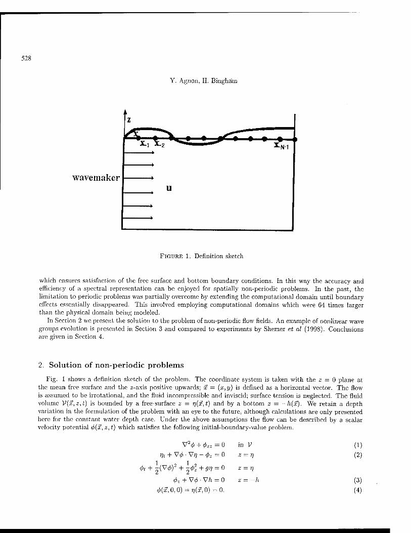
528
Y. Agnon, H. Bingha'm
wavemaker
FIGURE 1. Definition sketch
which ensures satisfaction of the free surface and bottom boundary conditions. In this way the accuracy and efficiency of a spectral representation can be enjoyed for spatially non-periodic problems. In the past, the limitation to periodic problems was partially overcome by extending the computational domain until boundary effects essentially disappeared. This involved employing computational domains which were 64 times larger than the physical domain being modeled.
In Section 2 we present the solution to the problem of non-periodic flow fields. An example of nonlinear wave groups evolution is presented in Section 3 and compared to experiments by Shemer et al (1998). Conclusions are given in Section 4.
2. Solution of non-periodic problems
Fig. 1 shows a definition sketch of the problem. The coordinate system is taken with the z = 0 plane at the mean free surface and the z-axis positive upwards; x = (x,y) is defined as a horizontal vector. The flow is assumed to be irrotational, and the fluid incompressible and inviscid; surface tension is neglected. The fluid volume V(x,z,t) is bounded by a free-surface z = rj{x,t) and by a bottom z = —h{x). We retain a depth variation in the formulation of the problem with an eye to the future, although calculations are only presented here for the constant water depth case. Under the above assumptions the flow can be described by a scalar- velocity potential <j)(x, z, t) which satisfies the following initial-boundary-value problem.
V2<£ +
Vt + V0 • Vr] -
= 0 = 0
<t>z + V0 • V/i = 0
f/>(f,0,0) =r/(£,0) = 0.
in V
z = rj
Z = T]
z = —h
(1) (2)
(3)
(4)

529
A non-periodic spectral method with application to nonlinear water waves
In the above equations
V = (^,—), u = (u,v)=V<p, w = <pz, (5)
In order to use a Fourier-spectral method to solve this problem, the domain V is enclosed within a set of control surfaces which, for illustration, are taken to be the vertical planes at x — 0, x = L, y — 0, and y = M. On these control surfaces, boundary conditions of the following form are applied:
N3
Ün-^ClUl (6) (=1
where N$ is the total number of degrees of freedom distributed over the control surface, un is the velocity normal to each control surface 6;; i = 1,2,3,4, and the Ui are functions of time and of the horizontal coordinate. The Ui are chosen to represent a wave-maker/absorber or a matching to another computational domain. In general Ui may have a vertical structure, which can be included in the solution. However, in many applications there is no interest in resolving this structure, which is essentially responsible for evanescent modes that decay exponentially away from the boundary. For simplicity, we demonstrate the method for Ui that are independent of z.
The velocity potential is decomposed into the following sum of potentials:
0 = 01 + 02 (7) N3
& = X>02i- (8)
The potentials <j)>i are chosen to satisfy the Laplace equation, and the boundary conditions on the bottom and control surfaces, Equation (6) and Equation (3). Note that the problem for <jf>2 is under-determined, making the choice somewhat arbitrary. It is convenient to take 02 to be quadratic in x,y and z, corresponding to steady flow fields, in which case the consequent horizontal velocity is independent of z. As an example, take </>2i to be the solution for the two dimensional flow with u = 0 on x = 0, y = 0, and y — M; but u = U(t) at x = L. This is simply a corner flow, and the solution up to 0(S7h) is
V02i = y (x - 2(z + h)Vh, 0, -(z + h + xVh)). (9)
Where on an even bottom V/i vanishes, yielding:
<!>21 = ~{x2-{z + hY) (10)
Similar solutions can be used for the remaining </>2; corresponding to uniform flows through the other three vertical control boundaries. If U has spatial structure over the control surface, U = U0(t)f(y,z), 4>2 can be pre-solved for the lateral boundary conditions, producing a set of time-independent response functions which may then be used in the solution, at each time step.
Having chosen the appropriate form of Equation (6) to account for a wavemaker at one end and ensure the radiation of waves at the other end, for example, the other part of the potential <j>\, represents a flow in a closed basin, with a prescribed potential on the free surface.

530
Y. Agnon, H. Bingham
z^^yi \ \yy^zyyy / 7 ^^^ / \ ^-^_ —^^ /
__^^ ^^__ ___^ - (c) -
1 1 1 1 1 II _ L. 1
FIGURE 2. Illustration of the components of the potential for a simple wave: (a) Streamlines of fa-, (b) Streamlines of fa, (c) Streamlines of fa + fa.
We study the case of constant water depth. Since fa has zero flux through the boundaries, we may expand it in the following form.
Ni N2
- 2_^ Z^amn m=l n=\
/V, N2
cosh kmn(z + h) cosh kmnh
cos (kmn ■ x)
"fa = 2__, 2~l~kmnamn—---■- i.—:— sin(/cmn • x)
m—1 n=l Nl Nn
cosh kmnh
, _ s^ \T u sinhfcmn(z4-/i) ,, _, (pi- — y / 1 Kmn Q"mn u , £ COS [Kmn -X),
m=ln=l cosh kmnh
(11)
(12)
(13)
idiere
kmn — ( ) Ji and A;TOn — |/cn IT re
(14)
The decomposition of the potential is shown schematically in Fig. 2, which sketches the streamlines of each of the flows that correspond to fa-, fa and fa-+fa, due to a wavemaker on the left end and a reflecting wall at the right end. The complete potential fa- + fa must satisfy the remaining boundary conditions. Upon substituting

531
A non-periodic spectral method with application to nonlinear water waves
Equation (7) into the free-surface conditions we obtain
Vt = -V(fa+fa)-VV + 4>lz + faz 2 = r? (15)
fat = -fat - ^{h + <t>i))2 - 2(^1= + <hz)2 -9V z = V
as the conditions for fa. In order to solve for the evolution of the velocity potential, we need to solve for the evolution of the N =
Ni x N% functions amn(t) and for the N3 functions fat. N collocation points are distributed on a regular grid over the free surface. At the free surface points, Equations (7) and (11) through (13) relate amn to fa The fai functions are determined from the lateral boundary condition Equation (6), using the pre-solved "steady flows". This completes the solution of Laplace equation. To proceed, Equations (15) are marched in time to find the new time values of <j> and 77. The derivatives of fa are known since fa is known in functional form. The derivatives of fa are given in Equations (12, 13) in terms of the coefficients amn. This makes the evaluation of the derivatives efficient and accurate. The gradient of 77 can be derived by finite differences or a variant of the FFT. Since this quantity enters only through nonlinear terms in the free-surface condition, the accuracy of its evaluation can meet lower requirements than those satisfied by the potential. As described above the method is fully nonlinear, and the dominant workload comes from building and inverting an N x N matrix at every time step; and is thus of 0(N3). The solution in this form represents an extension to non-periodic problems of [2]. As long as an effective means of pre-conditioning can be developed, the resultant linear system can, in principle, be solved iteratively reducing the workload to 0(N2). An alternative, however, is to expand the values of fa and its derivatives on the free surface in a Taylor series about the value on the still water level, thus producing a method correct up to some fixed order of nonlinearity, M. In this case, the FFT may be used to reduce the work load to 0(MNlogN). The method is described by Dommermuth and Yue (1987) and we briefly review it here.
Let us write 0 in a perturbation series in the nonlinearity parameter e (which is the order of the wave steepness):
M
) (16) = E^(
where fa'*'1 = O(e'). The value of fa'1 (and its derivatives) on the free surface (2 = 77) can be evaluated from a Taylor series about z = 0:
*i-.i-ESJ!5Ä» (17) «=1 j=Q J'
(and similar expressions for its derivatives). Thus, we may use these expressions to march Eq. (2) in time, and obtain the values of 77 and of fa = faz = 77)
at the following time step. In order to continue the procedure, we then need to find fa1'1 on z = 0, at the new time step. Collecting terms at each order in Eq. (17), we may evaluate a sequence of equations for 4>il=0) '■
<U = ^s (18) ;-i
and Co) = - E ||^r=o)< ' = 2' 3< ->M- W
where; after evaluating </>[l'=o) at eacn order, we use a fast cosine transform to determine the coefficients amn, thus knowing fa and its derivatives at z = 0 in terms of FFT's. We then proceed to the next order in nonlinearity.

532
Y. Agnon, H. Bingham
3. The evolution of wave groups
In order to demonstrate the performance of the non-periodic High Order Spectral method, we have chosen a relatively simple problem. The evolution of wave-groups (with narrow spectra) on an even bottom has recently been studied experimentally and numerically by Shemer et al (1998). The waves are generated at one end of a flume by a wave-maker and propagate along the flume until they are damped at its end. Their nonlinear interaction is studied by recording the waves at a few locations along the flume. Their study addressed the demodulation (or focusing) which occurs within the group. The effect depends on the dispersiveness of the waves, which depends on whether the ratio of wavelength to water depth is larger or smaller than a critical value. When the waves are steeper, this nonlinear evolution is more intense. These features of the wave evolution are successfully predicted by the cubic Schroedinger equation which was used by Shemer et al as a model equation. The main aspect which can not be predicted by the cubic Schroedinger equation, due to its structure, is the development of asymmetry in the wave-groups (and the wave spectrum). They suggest some models that can be used in deep water and others which are valid in fairly shallow water {eg the Korteveg - de Vries equation.) Here we compare the predictions of the non-periodic spectral model with the measurements of Shemer et al for one experiment. Both the focusing and the development of asymmetry are successfully described by the model.
In order to absorb the waves at the end of the flume, it is possible to use an active wave-absorber, which is just a wave-maker. Active wave-absorbers are very efficient in absorbing linear waves. Absorption of nonlinear waves is most effectively done by a combination of active absorption and a damping zone applied to a portion of the free-surface. So far, we have only implemented the damping free surface condition (often referred to as a sponge layer) which requires an extended computational domain. Present day sponge layers require about a full wavelength for effective absorption. Work on an improved sponge layer is in progress.
The characteristics of the waves studied are as follows: Water depth: h = 60 cm; peak wave period: T = 0.7 s. This corresponds to a peak wavenumber: k = 8.21 m_1. The wave-maker stroke is given by:
s = s0 exp(-«/5T)2) cos(2nt/T)
where -16T < t < 16T. The maximum wave steepness at x = 0.24 m is kamax = 0.246, where amax = {Vpcak + Vtrouah)/2- The computational wave-maker was matched to the experiments by adjusting s0 to obtain the correct kn,max at x = 0.24 m. In Fig. 3 are shown the measured and the computed time records of the surface elevation, at the locations: x = 0.24 m and x = 8.67 m. We see that the model faithfully captures the focusing of wave energy as well as the onset and growth of asymmetry in the waveform. The measurements were taken after many wave periods, after a quasi-steady state has been reached. The computations results are plotted shortly after the motion started. This avoided the appearance of small reflected waves, which should be eliminated by improved absorption.
4. Conclusions
A method for the solution of non-periodic problems by a pseudo-spectral technique has been developed and demonstrated for water waves. The method is based on writing the potential as a superposition of a component that is chosen to satisfy the lateral boundary conditions and a spatially periodic component, with no flux through the lateral boundaries. The latter is computed most efficiently through the FFT algorithm.
The efficiency of the method makes it an attractive tool for the study of complex problems. It can also be used for the intensive! computations required for Monte-Carlo simulations of stochastic problems. Further extension of the High Order Spectral method to a topography with large depth variations is the next important step in its development.

A non-periodic spectral method with application to nonlinear water waves
533
Band-pass filtered signal
Raw signal
20 25
Time, s
@
30 35 <0 45
\ Band-pass filtered signal
—( ._...,, ) f-
| Raw signal
1 1 1 1
20 25 30
Time, s
(b) (d)
15 20 25 30 35 <0 45 205 210 215 220 225 230 235 2<0
FIGURE 3. (a) The measured wave elevation at x = 0.24 m. (b) The computed wave elevation at x = 0.24 m. (c) The measured wave elevation at x - 8.67 m. (d) The computed wave elevation at x = 8.67 m.
Acknowledgements
We thank Profs. Lev Shemer and Eliezer Kit from Tel-Aviv University for kindly providing us with their experimental results. This research was supported by the Danish National Research Foundation. Their support is greatly appreciated.
References
[1] Dommermuth D.G., YUK D.K.P., 1987. A high-order spectral method for the study of nonlinear gravity waves, ./. Fluid Meek.
184, 2G7-288.

534
Y. Agnon, H. Bingham
[2] Fenton J.D., Rienecker M.M., 1982. A Fourier method for solving nonlinear water-wave problems: application to solitary-wave interactions, J. Fluid Mech. 118, 411-443.
[3] Madsen P.A., Schärfer H.A., 1998. Higher order Boussinesq-type equations for surface gravity waves - derivation and analysis. Phil. Trans. R. Soc, Series A, London, 356, 3123-3184.
[4] Shemer L., Kit E., Jiao Hai Ying, Eitan O., 1998. Experiments on nonlinear wave groups in intermediate water depth. Journal of Waterway Port Coastal and Ocean Engineering - ASCE, 124:(6), 320-327.
[5] Tsai W., Yue D.K.P., 1996. Computation of nonlinear free-surface flows. Annu. Rev. Fluid. Mech., 28, 249-278. [6] West B. J., Brueckner K.A., Janda R.S., Milder M., Milton R.L., 1987. A new numerical method for surface hydrodynamics.
J. Geophys. Res. 92, 11, 803-824.

JEur. J. Mcch. B/Fluids (c) Elsevier, Paris
ADJUSTMENT PROCESSES AND RADIATING SOLITARY WAVES IN A
REGULARISED OSTROVSKY EQUATION
R. H. J. GrimshawW [1]: Dept Mathematics and Statistics, Monash University, Clayton, Victoria 3168, Australia, e-mail: Roger.GrimshawOsci.monash.edu.au
(Received 15 September 1998, revised and accepted 16 December 1999)
Abstract - The Ostrovsky equation is an adaptation of the Korteweg-de Vries equation widely used to describe the effect of rotation on surface and internal solitary waves. It has been shown that the effect of rotation is to destroy such solitary waves in finite time due to the emission of trailing radiation. Here this issue is re-examined for a regularised Ostrovsky equation. The regularisation is necessary to remove an anomaly in the Ostrovsky equation whereby there is a discontinuity in the mass field at the initial moment. It is demonstrated that in the regularised Ostrovsky equation there is a rapid adjustment of the mass which is transported a large distance in the opposite direction to that in which the solitary wave propagates. © Elsevier, Paris
1. Introduction
Internal solitary waves are an ubiquitous feature of the ocean (and are also commonly occurring in the atmosphere). In the oceanic environment, they are generally generated by the interaction of currents, often of tidal origin, with topography, and are readily observed through satellite remote sensing techniques. Although they are internal to the ocean, their surface currents are usually sufficiently strong to significantly modulate the wind-wave field.
Recently there has been some interest in the effect of the earth's rotation on these waves (see the review by Grimshaw et. al, [1]). In the simplest approximation, the effects of rotation are described by the so-called Ostrovsky equation [2], presented here in dimensionless form
ut + 3uux +-uxxx = e v, (1)
= u. (2)
The parameter e represents the effects of rotation. Although this is a planar equation, the rotational terms are a manifestation of the Coriolis force which of course introduces a three-dimensional aspect to the evolution of the waves. When e = 0 , equation (1) reduces to the familiar KdV equation which supports the well-known solitary wave solution. But for e > 0 , it can be shown that there are no exact steady solitary wave solutions [3, 4]. Instead, if the KdV solitary wave is used as an initial condition for (1), it will decay to zero in finite time due to the emission of trailing radiation [5].
One of the interesting features of the Ostrovsky equation (1) and (2), is that for any localised solution (i.e. u -> 0 as Ixl -t oo) the mass is zero for any t > 0 , that is
M /CO
udx = 0 (3) -CO

536
R. Grimshaw
Indeed, if u -> 0 as |x| -> oo , then (1) shows that v -» 0 as \x\ -> oo also, and then the result (3) follows from (2). This is the case, even when the initial condition,
u = UQ{X) at t = 0 (4)
is such that the initial mass
Mr /oo
uQ dx (5) -oo
is not zero. The physical explanation is that just at the initial moment, an infinitely long wave of zero height, but finite mass, propagates to negative infinity with infinite speed (see the discussion in Grimshaw et. al 1998b for instance).
Our main aim in this paper is to examine this anomalous situation in more detail by introducing a regularising parameter S , so that equation (2) is replaced by
- S2vt + vx = u . (6)
The physical motivation for this is discussed by Grimshaw and Melville [6]. Recently Ablowitz and Wang [7] introduced a related regularisation for the Kadmotsev-Petviashvili equation, where a similar issue regarding the mass arises.
Briefly, in physical terms, equation (2) describes the momentum balance in the direction transverse to the wave propagation direction (i.e. the x-direction). In essence, u can be regarded as the fluid velocity in the re- direction, which in the weakly nonlinear long wave approximation, is equivalent to the vertical wave displacement at leading order, while v is the fluid velocity in the transverse direction. In equation (2) the acceleration term is calculated in the frame of reference moving with the linear long wave speed, and so is represented only by —vx, whereas in equation (6) this same acceleration term retains an additional time evolution with respect to this frame of reference, and so is represented by S2vt - vx, where S is a small parameter. It is now clearly necessary to specify an additional initial condition
v — vo{x) at t = 0 (7)
for the regularised Ostrovsky equations (1) and (6). In Sections 2 and 3 of this paper we analyse the effect of this regularisation in the limit as S ->• 0 . Our asymptotic analysis is somewhat similar to that of Ablowitz and Wang [7]. Because the essential aspects of the issue relating to the mass occur also in the linearised long wave version of (1) and (6), these are considered first in Section 2, where the exact solution for the initial conditions (4) and (7) can readily be constructed. Then in Section 3, we consider the full system (1) and (6) and use a boundary-layer analysis to demonstrate that the mass is transported to large negative xona timescale of 0(S/e) , as 6 -> 0 .
Before proceeding, to these detailed analyses, we note that it can be readily shown from (1) and (6) that
Mtt + ^ M = 0 . (8)
Thus the mass M oscillates at the frequency e/5 , which we can identify as the inertial frequency in physical terms. The solution of (8) is clearly
M = M0 cos{et/5) + e5M, sm(et/6), (9)
where Mi = j"^° t'o (■'•') dx . Note that M has no formal limit as 8 —> 0 . In Section 4 we return to the issue of the fate of a KdV solitary wave, when used as an initial condition for
the regularised Ostrovsky equation (1) and (6). We show that to a large extent, the analysis of Grimshaw et.
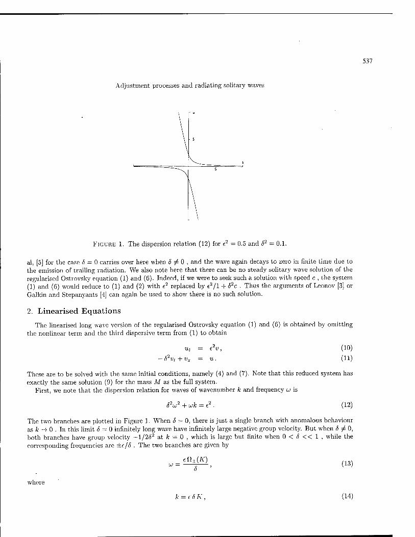
537
Adjustment processes and radiating solitary waves
FIGURE 1. The dispersion relation (12) for e2 = 0.5 and d2 = 0.1.
al, [5] for the case <5 = 0 carries over here when 6 ^ 0 , and the wave again decays to zero in finite time due to the emission of trailing radiation. We also note here that there can be no steady solitary wave solution of the regularised Ostrovsky equation (1) and (6). Indeed, if we were to seek such a solution with speed c , the system (1) and (6) would reduce to (1) and (2) with e2 replaced by e2/l + S2c . Thus the arguments of Leonov [3] or Galkin and Stepanyants [4] can again be used to show there is no such solution.
2. Linearised Equations
The linearised long wave version of the regularised Ostrovsky equation (1) and (6) is obtained by omitting the nonlinear term and the third dispersive term from (1) to obtain
-82vt vx
= e v,
= u.
(10)
(11)
These are to be solved with the same initial conditions, namely (4) and (7). Note that this reduced system has exactly the same solution (9) for the mass M as the full system.
First, we note that the dispersion relation for waves of wavenumber k and frequency ui is
62
UJ~ + u>k — e (12)
The two branches are plotted in Figure 1. When 6 = 0, there is just a single branch with anomalous behaviour as k -> 0 . In this limit 6 = 0 infinitely long wave have infinitely large negative group velocity. But when 5^0, both branches have group velocity -1/262 at k = 0 , which is large but finite when 0 < <5 << 1 , while the corresponding frequencies are ±e/<5 . The two branches are given by
efi±(Ä") (13)
where
k = e8K , (14)

538
R. Grimshaw
and
ü±(I<) = -\K±(I + \K2
1/2
(15)
Note that Cl+(K) = -fl-(K) . The solution of the initial value problem for equations (10) and (11) is
/OO /-00
a+(k)eik*-iQ+WTdk+ / a-(k)eikx-in-lK)Tdk, -OO J— OO
f — n+(K)a+(k) eikx-iQ+(K)T df, + r J — c eS £l-(K)a-(k)
(16)
eikx-iQ-{K)T dk, (17)
where
T = et
The amplitudes a±(k) are determined from the initial conditions. It is readily shown that
e6v0(k)+inT(K)ü0{k)
where
a±{k)
(ü0(k),v0(k)) =
Ti[n+(K)-^(K)} '
2TT (u0(k),vo(k)) exp(—ikx)dx.
(18)
(19)
(20)
Because (u0(k),vo(k)) are real-valued, it is readily shown that a+(k) = a-(k) . Next, we consider this solution in the limit when the regularising parameter 5 -> 0 , while the rotational
parameter e. remains fixed, with e > 0 . First, we note that the temporal development is completely defined in terms of the variable T (18), and so the solution develops on the short timescale where t is 0(S/e) . Hence the limit <S -> 0 can be replaced here by T -» oo . This limit can now be readily obtained using the method of stationary phase. It is not necessary here to present all details, but we note the salient points. First, the stationary phase condition can be expressed as
£ = n±'(Ä-): (21)
where X — e 5 x.
Since the group velocity Q± (K)/52 is large and negative, each of these branches represents a wave which has propagated to large negative x. Next we note that in this limit u is 0(6) , while v is 0(1). The amplitudes are given by (19) where as 6 —> 0 ,
(wo,£0) 2TT (Mo.Mi (22)
Here we recall that (M0,Mi) are defined by (5) and (9), and represent the initial mass in (u,v) . Thus these waves are responsible for transporting the mass to large negative x.
Of particular interest is the nature of the solution in the region where x remains of 0(1) while T -> oo . From the stationary phase condition (21), this requires ü± (K) to be O(eS) , and then from the dispersion relation

539
Adjustment processes and radiating solitary waves
(15) it follows that K -* oo for the first branch, while K -+ -oo for the second branch. Thus, as K ->■ oo ,
Ü+(K) ~ A'"1 , tl+'(K) ~ -•R'"2 and so -^ is 0(l/\/eS) , while o+(fc) ~ ?70(fc) . Similarly, as K -> -oo , ft_(K) ~ K"1 , VtJ(K) ~ -.K~2 , and a_(Jfe) ~ u0(fc) . In these same limits, a±(fc) are 0(5) respectively. It
follows that,
/oo u0(k) exp(ikx - ie2t/k) dk, (23)
-OO
where V-V-JT denotes the principal value. But the right-hand side of (23) is precisely the exact solution of equations (lfjfand (11) when <5 = 0 , which satisfies the initial condition (4). The corresponding solution for v is obtained from (23) by replacing u0(k) with u0(k)/ik. It can be shown that the asymptotic solution (23) satisfies the zero mass condition (3).
In summary, we can conclude that for the system (10) and (11), there is a temporal boundary layer of 0(5), which propagates in the negative x-direction a distance of 0(1/eS). This wave is responsible for the mass M, and hence for the expression (9). The remaining part of the solution remains in the region where x is 0(1), and to within an error of 0(6), satisfies the reduced system (10) and (11) with <5 = 0.
3. Matching to the Temporal Boundary Layer
Here we shall consider the full regularised Ostrovsky equations (1) and (6), with the initial conditions (4) and (7), in the limit as the regularising parameter 6 -> 0 , with e > 0 held fixed. It is clear from the analysis of the linearised long wave equations in the previous section that there is a temporal boundary layer of 0(S/e) just after the initial time t = 0 . Further, the spatial domain at this time can be broken down into two segments, a near-field segment where x is 0(1), and a far-field segment where x is 0(l/e6) and is negative.
To describe the second segment of this temporal boundary layer, we introduce the scaled variables T = et/S
(18) and X = eSx (21), and put
u = 5U, V = ev. (24)
With this scaling, the equations (1) and (6) become
UT + 3 62UUx + ^e263Uxxx = V, (25)
-VT + VX = U. (26)
The initial conditions (4) and (7) become
U = Uo(X) = ±u0 (£\ , at T = 0, (27)
V = ev0 (^] , at T = 0. (28)
Taking the limit as <5 -> 0 , we now see that to within an error of 0(62) , equations (25) and (26) reduce to
while the initial conditions become
UT = V, VT + VX = U,
(29)
U = eMQ5(X), at 1 = 0, 1 (30)
V = 5e2Mi5(X), at T = 0.
540
R. Grimshaw
Here we let 6(.) denote the Dirac ^-function. We see that equations (29) are just, after rescaling, the linearised long wave equations (10) and (11) discussed in the previous section. But importantly, the initial conditions (4) and (7) are now reduced to (30), consistent with the result (22). Thus the solution of (29) and (30) is, after rescaling, just (16) and (17) with (üo,i>o) given by (22). This demonstrates that, just as in the linearised long wave system of §2, the mass is carried to large negative xin a time of ö(S/e) at a speed of ö(ö~2) .
In the first segment of the temporal boundary layer, we again rescale the time variable to T = et/5 but now retain x, to get
UT+*(3uux + \uxxx) = e5v,
(31) • e 5 VT + vx — u.
The initial conditions (4) and (5) are unchanged. However, it is immediately apparent that in the limit 5 -4 0 this system cannot satisfy the initial conditon (7) for v. Hence, it is necessary to introduce an even finer time scale,
T=j2- (32)
We now get
uT + 52 (3uux + \uxxx) - e282v,\ } (33)
- VT + vx = u. )
With an error of 0(62) . the solution of the initial value problem of the system (33) is
u = u0(x),
and v — v0(x + T) + f*+ru0(x )dx (34)
Thus, on this very short time scale, we see that u is unchanged to 0(82) , while v consists of a steady part together with a wave propagating to large negative x. Indeed, we see that,
v —> / 110(^)^1 as T -4 00. (35) J 00
We can now return to the system (31), whose initial condition as T —> 0+ is just the solution (34) of the system (33) as r -KM. Thus, to O(S), we see that the solution of (31) is just u = Uo(x), with v given by (35).
Next, it is necessary to match the solutions in the first and second segments spatially, on the temporal boundary layer timescale. Thus, in the first segment we observe that as x —> —00, u —> 0, but v —> —Mo. Since u = SU is 0(5) in the second segment, this is consistent for the dependent variable u, while for the dependent variable v it implies that V —> —eMo as X —► 0_, at least for T > 0 This latter requirement is readily confirmed from the solution of the system (29), with the initial conditions (30), which can be obtained from the analysis of the previous section.
It is now apparent that, within the temporal boundary layer, the mass M (3), is given by
M = Mo + N,
■ (36) where N = f U dx. J—oo

541
Adjustment processes and radiating solitary waves
Here M0 is the mass in the first segment, and N that in the second segment. It is readily shown form (29) and the condition V -> -e.M0 as X -> 0_ , that
NTT + N = -Af0, T>0. (37)
Of course, the expressions (36) and (37) are completely equivalent to the exact expression (9), and confirm that the time evolution of the mass is due to the waves generated in the second segment. This last comment also implies that, although the above analysis would seem to suggest that u remains time-independent, to 0(5), within the temporal boundary layer in the first segment, this cannot hold eventually as T -> oo. Indeed, this is precisely the implication of the solution (23) of the linearised long wave problem in the first segment.
The final step in this section is to consider the near-field segment where x is 0(1), on the time-scale where t is 0(1) , and t > 0 . In the limit when the regularising parameter 5 ->• 0 with e fixed, it is readily apparent that we obtain the Ostrovsky equations (1) and (2). However, the initial condition is now obtained by matching with the solution in the temporal boundary layer as T -> co . It is readily seen that the appropriate initial condition is just (4) for u, and no initial condition is required for v. It also now follows that for the system (1) and (2), the zero mass condition holds for all t > 0 , even although M0 ^ 0 in general.
4. Radiation damping of a solitary wave
Next we re-examine the fate of a KdV solitary wave due to the effect of rotation, considered by Grimshaw et. al [5] for the Ostrovsky equations (1) and (2). Here, we consider the same problem but for the regularised equations (1) and (6). Thus we now assume that 0 < e2 << 1 , and construct an asymptotic theory valid as e _» o, with the regularising parameter S kept fixed, albeit at a small value. This is in marked contrast to the previous sections, where we kept e fixed, and let 6 -> 0 . Nevertheless, it turns out that the radiation damping of a solitary wave proceeds very much as in the case 8 = 0 , and hence we need give only a brief outline here.
The asymptotic solution consists of three parts, an "inner" solution in the solitary wave region, a "near- field" radiation solution which co-propagates with the solitary wave, and a "far-field" radiation field. Thus, the "inner" solution is described in terms of the variables
T = e2t, 0 = x- c{T)dT . (38) Jo
We put
u = u^(e,T) + e2u^(e,T) + ... v = vW(9,T) + t2vW{9,T) + ..., } (39) c = c<°> + e2 c'1» + ...
and readily find that the leading term corresponds to the KdV solitary wave,
u(0> = Asech2(\/l0),
i/°> = v/I
l + 52A
c<°> = A.
[l-tanh(v/Iö)] , (40)
At the next order we obtain a linear equation for u(1) ,
0 \ (41)
{l + S*A)vgW-uM = S2 c(D v„W - S2 «r<°> . J

542
R. Grimshaw
The compatibility condition for ir1' is that
f J — f
u(o) (_ Ur(o) + vW) d8 = 0.
Using the expressions in (40) we readily find that (42) becomes
dT U 1 + S2A
for which the solution is
A1'2(1 + ±82A)=T0-T.
(42)
(43)
(44)
Thus, just as in the case S = 0 , the amplitude A decreases to zero in finite time, and is extinguished at T = T0. Note that T0 = A0
1^2 (1 + | S2 A0) where A0 is the initial amplitude. The "near-field" radiation zone is the region immediately behind the solitary wave. First we note that, as
0 -* -co , u(0) -> 0 , while
26» and w(0) ->
2VÄ (45)
VI (1 + 6* A)' """ " ' 1 + S2A'
These provide the matching conditions for the "near-field" radiation, which is described by
u = eU(X,T), v = V(X,T), X = e8 (46)
where we recall that T and 6 are defined in equation (38). At the lowest order, the "near-field" equations are
-AUX = V + i/°>, (1+S2A)VX = U.
(47)
Note that although u'0) -» 0 in the "near-field" radiation zone, we must retain t/°) in the expression for v. Eliminating V, we get
AUxx + U lu^(X/e) 2VC4
1 + PA e l + S2A 1 + 62A S(X). (48)
Here S(X) denotes the Dirac «^-function. The matching condition is eU(X -> 0) ~ e2 u^ (9 -» -oo), and from (45) we see that U -> 2 X/y/Ä (1 + <52 4) as X -» 0_, while of course £/ = 0 for A > 0 . Thus the solution of equation (48) is, in A' < 0 ,
U = sin A
VT+WA
The corresponding solution for v is, in total, V + i/0' , or
U = . cos s/T+WÄ
y/A(l+S2A) (49)
X
y/A{\ + S*A) (50)

543
Adjustment processes and radiating solitary waves
Next, the "far-field" radiation zone is unsteady, and best represented in the original variables x and t . Thus with u = e U , v = V as in the "near-field" zone (see (46)), we obtain at the lowest order,
Ut = eV> \ (51) -S2Vt + Vx = eU. } (51)
This is just the regularised linear long wave equations (10) and (11), and hence have the same dispersion relation (12). The structure of the radiated wave field is readily found using the well-known symptotic theory of slowly- varying wave trains (e.g. Whitham, [8]), and the analysis follows the same path as that described in Grimshaw et. al [5] for the case 5 = 0 . The solution is thus described by the space-time rays
§=<*>'(*), (52) at
where w(fc) is determined from the dispersion relation (12). On each ray the local frequency w and wavenumber k remain constant, being determined by their values at the solitary wave trajectory dxs jdt - A(t) . Here, we use the "near-field" solutions to infer that the wavenumber k at the solitary wave trajectory is e/y/A{l + ö2 A) (see (49)), from which it follows that the phase speed is A (the solitary wave speed), while the group velocity is - A/(I + 2 S2 A) . Energy conservation determines the wave amplitude in the radiated field, where the wave amplitude at the solitary wave trajectory is found from the "near-field" solution (49) and is 2e/\/l + ö2 A .
Finally, we return to the issue of the mass, being the main focus of this paper. It is readily verified that for this asymptotic solution, the mass M (3) satisfies equation (8). Since the mass of the solitary wave itself is 2 \/A , it follows immediately that it is the radiated field which firstly has a term exactly cancelling this mass, and secondly contains the terms required to produce the inertial oscillations in the mass (cf. (9)).
References
[1] R.H.J. Grimshaw, L.A. Ostrovsky, V.l. Shrira and Yu. A. Stepanyants, Nonlinear surface and internal gravity waves in a rotating ocean, Nonlinear Processes in Geophysics 19 (1998) 289-338.
[2] L.A. Ostrovsky, Nonlinear internal waves in a rotating ocean, Okeanologiya, 18 (1978) 181-191 (in Russian); (English transla-
tion, Oceanology 18 119-125). [3] A.I. Leonov, The effect of the earth's rotation on the propagation of weak nonlinear surface and internal long oceanic waves,
Ann. NY Acad. Sei., (1981) 373 150-159. [•!] V.M. Galkin and Yu. A. Stepanyants, On the existence of stationary waves in a rotating fluid, Prikl. Mat, Mekl. 55 (1991)
1051-1055 (in Russian); (English translation, J. Appl. .Maths. Mech. 55 939-943). [5] R.H.J. Grimshaw, J-M He and L.A. Ostrovsky, Terminal damping of a solitary wave due to radiation in rotational systems,
Stud. Appl. Math. 101 (1998) 197-210. [6] R. Grimshaw and W.K. Melville, On the derivation of the modified Kadomtsev-Petviashvili equation, Stud. Appl. Math. 80
(1989) 183-202. [7] M..J. Ablowitz and X-P Wang, Initial time layers and Kadomtsev-Petviashvili-type equations, Stud. Appl. Math. 98 (1997)
121-137. [8] G.B. Whitham, Linear and nonlinear waves, Wiley NY, 1974 636 pp.

Bur. J. Mcch. B/Fluids © Elsevier, Paris
THREE-DIMENSIONAL SURFACE WAVES PROPAGATING OVER LONG
INTERNAL WAVES
J.R. Stocker and D.H. Peregrine* M
[1]: School of Mathematics, University of Bristol, University Walk, Bristol BS8 1TW, England
(Received 15 September 1998, revised and accepted 12 December 1998)
Abstract - A non-uniform current, such as may be generated by long internal waves, interacts with short surface waves and causes patterns on the sea surface that are of interest. In particular, regions of steep breaking waves may be relevant to specular radar scattering.
A simple approach to modelling this problem is to take a set of short, surface waves of uniform wavenumber on the sea surface, as may be caused by a gust of wind. The direction of propagation of the surface waves is firstly taken to be the same as that of the current, and surface tension and viscous effects are neglected. We have a number of methods of solution at our disposal: linear (one-dimensional) ray theory is simple to apply to the problem, a nonlinear Schrödinger equation for the modulated wave amplitude, modified to include to effect of the current, can be used and solutions can be found using a fully nonlinear irrotational flow solver. Comparisons between the 'exact' nonlinear calculations for two dimensions (which are too complicated/ computationally intensive to be extended to three dimensions) compare well with the two approximate methods of solution, both of which can be extended, within their limitations, to model the full three-dimensional problem; here we present three-dimensional results from the linear ray theory.
By choosing such a simple (although we consider physically realistic) initial state of uniform wavenumber short waves and assuming a sinusoidal surface current, we can reduce the two-dimensional problem to dependence on three non-dimensional parameters.
In three-dimensions, we consider an initial condition with a uniform wavetrain at an angle a say, to the propagating current, thus introducing a fourth parameter into the problem. Extension of the linear ray theory from one space to two space dimensions is numerically quite simple since we maintain uniformity in the direction perpendicular to the current, and the only difficulty lies with the presentation of results, due to the large number of variables now present in the problem such as initial wavenumber, angle of propagation, position in (x, y, i) space etc. In this paper we present just one solution in detail where waves are strongly refracted and form two distinct foci in space-time. There is a collimation of the short waves with the direction of the propagating current. © Elsevier, Paris
1. Introduction
Non-uniform currents interact with short surface waves and the resultant patterns on the sea surface are of interest. In particular, regions of steep breaking waves may be relevant to specular radar scattering. The scale of these currents may be very large, such as those generated by tidal flow over the edge of the continental shelf, or else relatively small, such as flow into an estuarine channel.
Two substantial review papers have been published in this research field. Firstly, Peregrine [1] was concerned with both large and small scale currents, currents varying with depth, and turbulence. Jonsson [2] took more of an engineer's - as opposed to an applied mathematician's - view of wave-current interactions, discussing both ocean and coastal areas.
- * Author to whom correspondence should be addressed, e-mail: d.h.peregrinefflbris.ac.uk, tel:+44(0) 117 928 7971, fax:+44(0)117 928 7999.

546
J.R. Stocker, D.H. Peregrine
This paper concerns itself with the particular interaction between short surface waves and a surface current generated by long internal waves. The problem considered is similar to that discussed by Gargett and Hughes [3]. They chose a constant frequency initial condition for the short surface waves, and considered the effect of the current in time. We take a constant wavenumber initial condition which, due to the Doppler shift caused by the current, involves a whole range of frequencies initially and in time, leads to focussing of the waves by the current. We consider this to be a more generic form of initial condition.
The two-dimensional problem is discussed in Donato, Peregrine and Stocker [4] (hereafter referred to as DPS). A simple, linear, two-layer model was used for the internal wave which gives a sinusoidal surface current. The surface current is incorporated into a fully nonlinear irrotational flow solver (first used by Dold and Peregrine, [5]) to obtain surface profiles which show the effect in time of the current on the short waves. The effect of variation of current magnitude, length of the initial short surface waves and initial steepness are discussed. Ray theory is used for the linear problem to discuss focussing of the short waves, and surface profiles were generated for comparison with results from the fully nonlinear irrotational flow solver. Ray theory (which is presented in this context by Crapper, [6]) is based on the assumption that wave properties vary slowly in time. This leads to solutions which are valid away from those regions where neighbouring rays cross, that is, at caustics and foci.
As the extension of the fully nonlinear irrotational flow solver to three dimensions is computationally im- practical (at present), we use linear ray theory to obtain three-dimensional solutions. To set the scene, we first briefly present solutions for two dimensions; that is, we take the direction of the surface waves to be that of the (uni-directional) surface current. Then, we consider the three-dimensional situation where the short waves are initially at an angle to the propagating current. As there are many parameters now present in this problem, in the present paper, we restrict ourselves to the discussion of a case where the waves are strongly refracted i.e. they focus, and they initially propagate, relative to the current, at an angle of 7r/6 to the current. This particular case is of interest in that two foci form, whereas at small angles to the current only one focus forms, as in the two-dimensional problem.
Another method which can be extended to model the three dimensional problem is to consider a modulated, weakly nonlinear wavetrain. Its amplitude and phase are described by a nonlinear Schrödinger equation modified to include to a large-scale weak surface current. Solutions generated using this nonlinear equation are valid when the surface waves form part of a single, slowly varying wave train and are therefore only useful prior to focussing or wave breaking.
Note that our model does not allow any current modification by the surface waves. That is, we allow the surface current to remain sinusoidal for all time. Some theoretical approaches do include the wave-current coupling, for example Rizk & Ko [7], and it would be possible here, but this is not the focus of our attention.
In section 2 we discuss the model used, and reduce the problem to a four-parameter problem. A discussion of the ray theory method used is briefly given in section 3. Justification for the use of ray theory is given in section 4 by comparison with the fully nonlinear potential solver in two dimensions. Section 5 shows results using the three-dimensional ray theory when the current and initial short surface waves are at an angle of 7r/6 to each other. Our conclusions are given in section 6.
2. Model
The model used is the same as that described in DPS so this account is brief. The fluid is taken to be inviscid and incompressible and the short surface waves considered are taken to be long enough such that surface tension effects can be neglected but short enough to be locally independent of any density stratification. A simple, linear, two-layer model for the internal wave is used. This results in a sinusoidal form for the internal wave, and the corresponding surface current. We take an (£i,x2,y,t) coordinate system, where y is measured vertically upwards, xi and x2 are on the 'sea' surface and t is time. The frequency and wavenumber of the internal wave are taken to be ft and (K, 0) respectively and are related by
Pi + P2 coth Kh\

547
Three-dimensional wave-current interactions
surface
internal wave
111111 M 11 I M I I I I I I
Rn minimum zero surface surface
N« current 4- current 4- y/
RJ maximum surface
xS current
Kxx
FIGURE 1. Streamlines in the two-layer internal-wave model.
where g is the acceleration due to gravity and pi and pi are the densities of the upper and lower layers respectively. The uni-directional current is aligned along the i\ axis with surface current, U_= (C/i,0) where Uy = Uc cos(f('xi — fit) and Uc being the maximum magnitude of the current.
Although here we have considered a two-layer model, our analysis and results are also valid for any plausible density stratification where the uppermost streamline is sinusoidal. In addition, we assume that the surface waves themselves have no effect on the stratification, as they are short enough such that the upper layer can be considered deep. However, in time, the large scale modulation induced by a non-uniform wavetrain may change the form of the internal wave. It is possible to add in a linear perturbation to model this change in waveform, but for this unsteady problem of initially constant wavenumber, we do not expect to see any large effects due to this modulation, and so have not included such effects here.
For presenting some of the results, we move into a frame of reference (xi,x2,i) moving with the phase speed V of the surface current, where x\ = xi — Vt. In this frame of reference the current becomes steady: Ui(xi,x-2) = Uccos(Kxi) — V and we give streamlines of the flow in a vertical section in figure 1. Also, note that length and time are non-dimensionalised with \/K and \JgK respectively.

548
J.R.. Stocker, D.H. Peregrine
The initial condition considered on the 'sea' surface is a uniform wavetrain of wavenumber fco and amplitude «o at time t = 0 and an angle a0 to the propagating current. As the short, surface waves are propagating over long internal waves, |fc_o| = k0 is taken to be very much greater than K. The uni-directional nature of the propagating current together with this simple initial condition combine to imply uniformity in the x2 -direction and hence the wavenumber component in the ^-direction remains constant, fc2 = k0sina0.
By choosing such a simple (although we consider it to be physically sensible, for example after a gust of wind) initial state and assuming a sinusoidal surface current, we can reduce this three dimensional problem to four non-dimensional parameters: two velocity ratio parameters, 9 and 7 defined by
where g is acceleration due to gravity, k0 and cv are the initial wavelength and phase speed respectively of the short waves, V is the phase speed of the internal wave and Uc is the maximum magnitude of the surface current. The third parameter is the initial steepness of the short surface waves which is just a simple multiplier for linear theory, and the fourth is a0, the angle between the propagating current and the initial wavenumber of the short waves. Taking a0 = 0 reduces the problem to a three parameter problem which models the two dimensional case.
An alternative initial condition, considered in the two-dimensional case by Gargett and Hughes [3], is the case of considering the frequency, w, to be initially constant everywhere. This simplifies the analysis as the frequency remains constant along rays. It is a physically realistic initial condition, for example in the case of a free surface wave packet approaching a region of surface current. In this constant frequency case, for certain physical parameters, waves are trapped in a region between two caustics either side of the position of maximum current. At this point of maximum current, waves travelling with the current are propagating much faster than those against the current. That is, there is a region of both very short and very long waves superposed at the point of maximum current. This is discussed further in DPS.
In this paper we give particular attention to waves which are strongly refracted and focus in space-time. That is, we choose to show results for only one value of (0,7) = (0.122,2.416). These values correspond to, for example, 300 short waves on an internal wave of wavelength 120 m, pycnocline depth 6 m, with density difference of the two layers 2.5 parts per thousand and a surface current of strength approximately 0.04 m/s. An investigation into how the two-dimensional wave properties vary in the (0,7) phase plane is given in DPS.
3. Method of solution
Ray theory assumes that at any particular point the solution locally looks like an infinite periodic plane wavetrain so that any variations in wave amplitude, a, frequency w and wavenumber k are slow.
The short surface wave dispersion relation is:
(w - U-k)2 = gk (3)
where Jfc = |fc| is the wavenumber of the short waves and w is the frequency. This is solved along with the ray equations:
^ = U + cgk (4) dt
where c.,, is the group velocity for surface waves in the absence of a current, k = k/k, and d/ctt defines differentiation along a ray. In our case where we have moved in to a frame of reference where the current is steady, U= (Uc cos(A'xi) - V, 0) and x- (xi, x2)- The frequency, w, is then constant along each particular ray - the value being defined by the initial conditions - and values for the wavenumber, k, along the rays are obtained

549
Three-dimensional wave-current interactions
by solution of (3) and (4). We generate surface profiles using the conservation of wave action equation to obtain wave amplitude, and a phase equation, both of which are valid along the rays. Details are omitted and the reader is once again referred to DPS. Representations of the free surface are generated from this information and results can be compared in the two-dimensional case to those from a fully nonlinear potential solver which has been adapted to include a sinusoidal surface current. Details of this latter code are given in Dold and Peregrine [5] and the alterations made to include the current are given in DPS.
4. Two-dimensional results
Figure 2 shows a space-time ray diagram for the values of (#,7) = (0.122,2.416). Two wavelengths and over one period of the internal wave are shown. The maximum and minimum values of the surface current are indicated by lines ( ) and ( ) respectively. Note that these results are given in the fixed frame of reference (xi,t). The rays are seen to focus at approximately t = 65, and the points of ray reflection in the frame of reference moving with the phase speed of the internal wave are indicated by an asterix. Figure 3 shows the corresponding results from the fully nonlinear code, and it is clear the linear ray theory predicts the focussing and corresponding steepness of the waves well 2. Here we have started the nonlinear calculations with 20 waves of steepness a0k0 = 0.01. This is due to the fact that it is computationally impractical to compute hundreds of short waves - the values of Uc and V have been adjusted in the calculation to correspond to the physical situation described in section 2 with the same values of 0 and 7. The fully nonlinear code calculates solutions up to 'wave breaking'; that is, until there are insufficient points in regions of high surface curvature to obtain solutions within the accuracy required. However, as the results we present in this paper are from linear ray theory, we restrict ourselves to the less steep waves which do not break. Further calculations and discussions of the steeper waves are to be found in DPS.
The profiles shown in figure 3 have been given a vertical exaggeration of 40:1, and the regions Rj and Ru from the streamline pattern in figure 1 are indicated. As we have chosen values of 6 and 7 which correspond to waves that are strongly refracted, we can see in region fij, where the streamlines are diverging, the waves become longer and less steep. Conversely in region Rn, where the streamlines are converging, the waves become shorter and steeper. This intuitive simplification of how the surface current effects the short waves is useful in explaining some of the three-dimensional effects we find later.
As mentioned previously, in regions where neighbouring rays meet, ray theory breaks down as variation in wave properties is too rapid: the wave action equation predicts infinite amplitudes. We therefore present results with a cut-off steepness value, taken to be ak = 0.40. The results could be improved by including diffractive effects using Airy functions at caustics and the Pearcey cusp function at the focus (for example, see Marston [8] for further details). Since we have exact solutions such as in figure 3, this extension is not followed here.
Figure 4(a) compares the fully nonlinear results (full line) with the linear ray theory results (dotted line), for non-dimensional time t = 60. We see that the comparison is good away from the region just before the focus where the amplitude predicted by the ray theory is too large. Figure 4(b) makes the same comparison at t = 106, some time after the focus. Here the waves tend to be in the same place for both the linear and nonlinear results, but the waves outside the caustics in the nonlinear case are less steep than predicted by ray theory implying that nonlinear self focussing may be acting on the energy between the caustics. Figure 4(c) shows the region between the caustics in more detail. The steep group of waves close to the left hand caustic has travelled faster in the nonlinear case which is to be expected as steeper waves travel faster than small amplitude linear waves. Also, the short waves just outside the left hand caustic are not predicted by ray theory, although matching using an Airy function does predict a wave profile of this type (Peregrine, [1]).
We conclude that the linear ray theory gives good results where waves are not too steep and in regions away from rapid variations in wave properties. Therefore we have some confidence in results from three-dimensional ray theory calculations which cannot be compared to a fully nonlinear model.
-Note that, figures 2 and 3 correspond to figures 4 and 5 in DPS.

550
J.R. Stocker, D.H. Peregrine
maximum zero surface surface current current
\ I
minimum surface current caustics
100 -
focus —>
Kxi
FIGURE 2. Ray diagram: the frame of reference is fixed, surface current = Uccoa{x — 0.093£) and (6»,7) = (0.122,2.416).

Three-dimensional wave-current interactions
551
maximum surface current
zero surface current
minimum surface current Ri
\ I S / Rn
100
Kxi
FIGURE 3. Fully nonlinear results: standard case. The frame of reference is fixed. Surface current = Ur oos(z - 0.093t), (0,7) = (0.122,2.416), initial steepness of 20 waves is a0k0 = 0.01 and vertical exaggeration 40:1.

552
(a) 0.004
0.002
-0.004 0
(c) °-°04
0.002
J.R. Stocker, D.H. Peregrine
Kxx
Kxx
Kxx
FIGURE 4. Comparing linear and nonlinear results: surface current = t/ccos(:E — 0.093£), (0,7) = (0.122,2.416), fully nonlinear results ( ), linear ray theory results ( ), initial steepness of 20 waves is oofco = 0.01, (a) t = 60, (b) t = 106 and (c) t = 106 showing more detail between the caustics.
5. Three-dimensional results
In three dimensions, we now consider an initial condition with a uniform wavetrain with wavenumber, k, at an angle a0 say, to the current direction, thus introducing a fourth parameter into the problem. The coordinate system is shown in figure 5. From equation (4), we note that rays are only perpendicular to the crests in the absence of a current. Extension of the linear ray theory from one space to two space dimensions is numerically quite simple, especially since we have uniformity in the ^-direction, and the only difficulty lies with the presentation of results, due to the large number of variables now present in the problem such as initial wavenumber, angle of propagation, position in (xi,X2,t) space etc. Results presented are for the same values of (0,7) as for the two dimensional case, except that now aa = i"/6.

Three-dimensional wave-current interactions
k= {ky,k2)
= fc(cosQO)Sina0)
U=(Ui,0)
Xi
FIGURE 5. Initial wavetrain with crests an angle a0 to the surface current direction.
553
As the current propagates only in the xy-direction, the wavenumber, k2 in the 19-direction remains constant, as mentioned earlier. Without loss of generality we consider only the rays from x2 = 0 since variation in the x-2-direction only arises from the different initial phases of the waves as x2 varies. Figure 6 shows a ray diagram for a0 = TT/6 and (8,-/) = (0.122,2.146) for the rays starting from Kxy e [0,2TT] and x2 = 0. Note that this ray diagram is presented in a moving frame of reference as opposed to figure 2, which is presented in a fixed frame of reference. The rays have focussed in two regions indicated by C/ and C//.
The focus in region Ci looks very similar to the type of focus we found in the two-dimensional case. We could think of the situation as qualitatively similar to having an initial wavenumber of ki in the indirection, giving an effective 7 to be {g/ky)? /V ~ 2.60 i.e. a larger value of 7 which means we expect the focus to occur later (according to the work given in DPS). This is indeed the case here.
The second focus in region C// is expected following the work of Peregrine and Smith [9] on steady wave fields. In figure 7 of their paper on nonlinear effects near caustics, they show part of the linear dispersion relation for waves on a uni-directional current U(x)i. This figure shows that for a range of values of k2g/ui2, two caustics form, as opposed to the usual one in this steady situation. The two caustics are of different - 'R' and 'S' - types, and we expect this situation to be related to that here, where we get one or two foci depending on our value of a0. This is a topic for further investigation.
The colour variation on figure 6 indicates the angle a between the direction of the propagating current, and the wavenumber k. The basic behaviour of a can be explained in terms of the focussing and defocussing effect of the surface current generated by the internal wave. The wavenumber in the x2-direction remains constant for all time. In the region Kxi e [0,7r] the current has a focussing effect which also increases the wavenumber, fci, in the .redirection, which in turn decreases the angle a i.e. the waves turn towards the direction of the propagating current. As the phase speed of the waves relative to the water decreases as the wavenumber increases, the waves in this region are slowed down. Conversely, in the region Kxy € [7r,27r], the surface current has a defocussing

554
J.R. Stocker, D.H. Peregrine
<_ t = 160 (figure 9)
«_ * = 110 (figure 8)
t = 70 (figure 7)
Scale:
IB. a = 0
a =
•"--■•S'"i ' ""■
Kxi
■W88Bfr]
a = $
FIGURE 6. Ray diagram in the (x\,t) plane showing the variation of angle a (with (0,7) (0.122,2.416) and a0 = TT/6).

555
Three-dimensional wave-current interactions
effect, in the xi-direction, k\ decreases and the waves become longer. The value of a is increased and these long waves turn away from the direction of the propagation current.
Figures 7 to 9 show representations of the 'sea' surfaces corresponding to figure 6 for times: t = 70, t = 110 and t = 160 respectively in a frame of reference moving with the internal wave. These times are indicated on figure 6. The grey scale is chosen to show the waves with small steepnesses where we are confident about the predictions by linear ray theory. As ray theory predicts infinite values for amplitudes in regions where neighbouring rays cross, a cut off value for wave steepness is taken in figures 7 to 9 at ak = 0.40, as in our two-dimensional results. Regions where steepnesses exceed this value are shown in white. In practice, these are regions where nonlinear and/or diffractive effects are important. Black lines on figures 7 to 9 indicate the troughs of the waves. That is, in regions Ci and Cu indicated on figure 6, where there are three overlapping wave trains, there are three sets of lines.
Figure 7 shows the surface predicted by linear ray theory at t = 70, a time just prior to the first focus. The effect of the current on the wavenumber magnitude and direction of the surface waves is clearly seen. At Kx\ ~ 1, the waves are being focussed. That is, they have become shorter and steeper - we note that steeper waves are indicated on these figures by a sharp black/white contrast. In addition, the direction of these focussing waves has changed from at t = 0 - they have moved so as to propagate more in the direction of the propagating current. Conversely away from this region where Kx\ £ [ir, 2n], the waves have become longer and less steep. Also, as indicated by the colour variation on figure 6, the waves have turned away from the direction of the propagating current.
Figure 8 shows the surface at t = 110. This is a time shortly after the first focus and before the second focus. Region Cj indicated on on this figure is a region of three overlapping wavetrains. The easiest way to comprehend this wave formation is to once again refer to the ray diagram, figure 6. One wave train - 'on top' - enters region C/ from the right. These waves have the smallest value of a, i.e. they have turned to propagate almost in the direction with the current; they are the shortest waves. The second wave train enters 'below' from the left; this is made up of longer waves which have propagated from the region Kx\ 6 [7r,27r], and are travelling with larger a values i.e. away from the current direction. The third wavetrain is generated from the 'fan' of rays which comes from the focus and adjacent caustics. These rays have less energy and have less effect on the form of the final surface pattern - they merely modulate the criss-cross pattern formed by the other two wave trains. The resultant pattern in region C/ is actually easier to see at a later time when the area covered is larger, as shown in figure 9. In a physical situation, one would expect to see a region of steep waves where a set of longer waves propagating at an angle to the direction of the current meets a set of shorter waves almost collimated with the current. At Kx\ ~ 7r, a second focus made up of longer waves is forming. These long waves are steeper than the surrounding waves and they are propagating at a large angle to the direction of the current.
Figure 9 shows the surface at t = 160 after the second focus has formed. There are now two regions of three overlapping wavetrains. The form of the focus in region C/ is as discussed for figure 8, but the region is now much larger. Region Cu is formed of longer waves overlapping, so the crests of the resultant waves are of a different form. In this case, the wavetrain made up of the shorter waves enters from the left and the longer waves enter from the right. The crests in region C/ are short and thin, whereas the crests in region Cu are more circular. Note that this figure more clearly shows the phase jump of ±n/2 at the caustics by the discontinuities in the black lines indicating the position of the wave troughs.
Figures 7 to 9 are an attempt to give snapshots of the surface at one time. The underlying wavetrains are of course moving. If two non-collinear wavetrains are superposed, the surface pattern is such that there is another moving frame of reference in which the surface is stationary. This is generally not the case for the superposition of waves in the focussing region formed of three wave trains here, in regions C/ and Cu, which are essentially unsteady wave patterns when viewed on the wave scale. However, the relative unsteadiness of these two regions is different. Region Ci is a fast modulation of the shorter waves (seen to the left of the focussing region) and will therefore be moving less quickly than region Cu which is, conversely, a slow modulation of the longer waves (again seen to the left).

556
.J.R. Stocker, D.H. Peregrine
k > ho and o < no
Kx-,
k < fco and n > a0
i
A'.r,
Scale: current direction
;; = -0.005 ;/ = 0.00 ;/ = 0.005
FIGURE 7. Wave surface at time. / = 70 (with (0,7) = (0.122,2.410), o„ = ~/G and a0k0 = 0.01).
6. Conclusion
After utilising a fully nonlinear potential solver to justify the use of the linear ray theory in two dimensions, we have presented three-dimensional results showing wave-current interactions using this method. We have

557
Three-dimensional wave-current interactions
region Cj 3 overlapping wave trains
a second focus approaching mack» up from longer waves
Kx->
Kx, current direction
FIGURE 8. Wave surface at time t = 110 (with {0,-y) = (0.122,2.410), n„ = TT/G and a0k0 = 0.01).
restricted our presentation to one case, taking an initial angle of o() = 7r/0 between the direction of the propagating current and a set of short surface waves of constant wave-number; the strength of current and number of initially short waves we have chosen was a situation where, in the two dimensional case, the waves were strongly refracted and a focus formed. Tin; main result we see is that in the region of converging streamlines of the surface current, two foci form. The first focus is of a similar form to that found in the two dimensional case consisting of very short waves, whereas the second is made up longer waves. The short waves are collimated by the current variation, and the longer waves propagate» away from the direction of the current. The explanation

558
J.R. Stockor, D.H. Peregrine
3 overlapping 3 overlapping region Cf. wave trains region C'n: wave trains
(shorter waves) (longer waves)
4 4-
K.r-
K.r,
region Ci (continued as
periodic)
4-
current, direction
FIGURE 9. Wave surface at time /. = 160 (with (#,7) = (0.122,2.410), a0 = 7r/6 and a0k0 = 0.01).
given for the wave behaviour in three; dimensions is roughly explained iti terms of the convergence and divergence of the surface current.
Consideration of a. wider range of initial angles shows that there is a range of o() within (0,7r/2) which will give two foci for certain values of the velocity ratio parameters (0,7)- Tin; approach of Peregrine and Smith [9] on steady caustics in two dimensions should help to explain this phenomena, and this is the subject of further work which also includes t he use of a current-modified nonlinear Schrödinger equation to model nonlinear effects in two and three; dimensions pre-focussing.

559
Three-dimensional wave-current interactions
Since the wave refraction depicted here occurs within a single wavelength of the underlying internal wave, it is unlikely that the type of wave patterns obtained depend strongly on the precise, sinusoidal current variation that is chosen. Indeed, focussing is a generic property of ray solutions, and hence we can expect focussed wave regions such as those shown here to arise on other unsteady current fields. Note the two different types, one representing a collimation of short waves towards the current direction and the other giving a strongly three-dimensional and unsteady surface pattern.
Acknowledgments
We would like to acknowledge the financial support of the D.E.R.A. and Alice Donato and Mark Jervis for their work on the fully nonlinear code.
References
[1] Peregrine, D.H. Interaction of water waves and currents. Adv. in Appl. Mech. 16 (1976) 9-117. [2] Jonsson, J.J. Wave-current interactions. The Sea. Ocean Engineering Science 9, Part A (Eds. B. le Mihauti & D.M. Haine),
Wiley-Interscience, 1990, pp.65-120. [3] Gargett, A.E. & Hughes, B.A. On the interaction of surface and internal waves. J. Fluid Mech. 52 (1972) 179-191. [4] Donato, A.N., Peregrine, D.H. k. Stocker, J.R. The focussing of surface waves by internal waves, J. Fluid Mech. 384 (1999)
27-58. [5] Dold, J.W. & Peregrine, D.H. An efficient boundary-integral method for steep unsteady water waves. Numer. Meth. for Fluid
dynamics II (Eds. K.W.Morton & M.J.Baines), Oxford University Press, 1986, pp.671-679. [6] Crapper, G.D. Introduction to water waves. Ellis Horwood Ltd, 1984. [7] Rizk, M.H. & Ko, D.R.S. Interaction between small-scale surface waves and large-scale internal waves. Phys. Fluids 21 (1978)
1900-1907. [8] Marston, P.L. Geometrical and catastrophe optics methods in scattering, in: High frequency pulse scattering (Eds. A.D.
Pierce h R.N. Thurston), Physical Acoustics vol. XXI, Academic press, 1992 pp.1-234. [9] Peregrine, D.H. & Smith, R. Nonlinear effects upon waves near caustics. Phil. Trans. A 292 (1979) 341-370.
561
Eur. J. Mech. B/Fluids, 18, n° 3, 561-564, 1999
Book reviews
L'espace chaotique (Chaotic Space) by P. Berge, Y. Pomeau, C. Vidal (Hermann, Paris, 1998, 176 pp.)
FF 180, paperback, ISBN 2 705 66345 2.
Systematic discovery of deterministic chaos in hydrodynamical instabilities is arguably the most important progress made recently in theoretical fluid mechanics. The wonderful previous book by the same authors, "Order in Chaos" is a fascinating introduction to this new field, and is in part remarkable because of the constant stress on physical intuition, despite the frequent use of rigorous and advanced mathematical concepts. This unique flavor in one of the first books on chaos was widely acclaimed.
The new book is a successful application of the same style to spatio-temporal chaos. This relatively new area of non-linear dynamics arises from two features: spatial extension or spatial patterns, and "ordinary" chaos in time-dependent systems. Taking into account spatial effects is a first step towards the rigorous analysis of fully-developed turbulence, the ever-elusive, fascinating goal of fluid mechanics. In that sense the study of spatially-extended chaotic systems is one more stage in the search for a theory of turbulence, just as chaos has been in the sixties and seventies. Admittedly this step does not yet lead us beyond relatively low Reynolds numbers, but the results are rich in physical content.
Despite its rigorous base in non-linear science, the book may be read without specialized preliminary knowledge. Some fundamental concepts and paradigms are reviewed, such as the Rayleigh-Benard instability in extended systems. Two appendices on temporal chaos make the reading of this book possible without any knowledge of the previous book by the same authors.
The authors discuss many experimental cases, such as the plane Poiseuille and Couette flows, as well as less-well known flows: Faraday instability, hydrothermal waves and printer's instability. Moreover a purely mathematical case is treated as an appendix: Kuramoto's equation, a partial differential equation holding the same paradigmatic status for spatio-temporal chaos as Lorenz's equation in the temporal case.
These cases are characterized by spatial patterns diverse in their details but which all show coexistence of regular and irregular regions. This alternating pattern of laminarity and chaos is itself variously organized. In some cases chaos invades space in a sort of disordered way: spatio-temporal intermittency arises, to which a large part of the book is devoted.
Spatio-temporal intermittency is nowadays intensely studied. The phenomenon has all the specific aspects of transition to chaos in spatially-extended systems and involves delicate experiments. One thus starts from a system of great complexity, such as the Navier-Stokes equations, with thermal and surface effects, boundary conditions, a geometrical structure, and one arrives, in a surprising and yet unexplained way, at empirically verified laws that may be derived from very simple models. For instance, the directed-percolation model may be constructed from two states only (to be compared with the complexity of a solution of the Navier-Stokes equation) and the local chaotic dynamics may be viewed as a simple probabilistic law describing the transition between the two states of the system. It is amazing that this simple probabilistic law reproduces the statistical behavior of the fluid-mechanical system.
Although the subject involves many subtle theoretical concepts, the mathematical and technical developments are reduced to the minimum, and physical intuition is everywhere preferred. The book is abundantly illustrated
EUROPEAN JOURNAL OF MECHANICS - B/FLUIDS. VOL. 18, N° 3, 1999
0997-7546/99/03/© Elsevier, Paris

562
Book reviews
without ever becoming flashy. A newcomer will easily and pleasantly discover the field. But there is a second possible reading of this book: it is a manifesto of the particular viewpoint of the authors on the field. Thus one may find general remarks on the validity of variational approaches, on the equations most often used to describe these systems such as the Ginzburg-Landau equations, or else statements on the important features of flows in transition to developed turbulence. The underlying idea is that there is a kind of thermodynamic picture adapted to chaotic systems, in which the transition to chaos is a phase transition. However the precise domain of applicability of these thermodynamics remains to be found. Nevertheless it allows us to derive most of the qualitative description of the transition to turbulence. This duality of viewpoints, both introductory and subtle makes this nice little book an excellent reference for the beginner as well as the specialist.
S. Zaleski LMM/UPMC
Universite Pierre et Marie Curie 75252 Paris, France
Hydrodynamics and nonlinear instabilities, edited by C. Godreche, P. Manneville (Cambridge University Press, 1998, 681pp.) £ 85.00, US$ 100.00, hardcover ISBN 0 521 45503 0.
The study of hydrodynamics has fascinated theorists since the early days of science and it is not hard to see why. Here is a subject which is not only concerned with many everyday phenomena, but which is in the main susceptible to experiments that do not demand the GDP of a small nation to construct. The governing equations are accepted by all as applying accurately to the vast majority of situations, but while they are easy to write down, their full solution is elusive. Their difficulty stems from their nonlinearity, and the fields of boundary layer theory, bifurcation theory, exponential asymptotics and nonlinear dynamics have all received a powerful impetus from the effort of trying to get to grips with their complexities. The present volume, a joint effort by a distinguished group of French scientists, is principally concerned with these and other theoretical tools, while remaining very much in touch with the experimental basis of the subject. There are five long chapters; an overview of hydrodynamics (Castaing), on instabilities in extended closed and open flows (Huerre & Rossi), a discussion of asymptotic methods (Hakim), an extensive treatment of pattern-forming instabilities (Fauve) and flames and explosions (Joulin & Vidal). There is a nice introduction by Manneville emphasising the importance of the link between experiments and their description in terms of nonlinear theoretical models. The chapters are self-contained, and each aims to give a pedagogical description of its subject, accessible to graduate students, while still discussing up-to-date topics that have not yet been exhaustively studied. In my view, while inevitably the style of the chapters is somewhat nonuniform, the book succeeds pretty well in its aim, and I would recommend it as important reading for students embarking on a research career in hydrodynamics.
Chapter 1 gives an enthusiastic introduction to the Navier-Stokes equations and explains the physics behind them. There are sections on low Reynolds number flow (including a discussion of wakes), the energetics of turbulence, boundary layers, flow measurement, dimensional analysis and (the author's favourite) a statistical mechanical description of turbulence. This is all covered in just over 50 pages! Inevitably the pace is very rapid, and each part can only be considered a taster to encourage more detailed study. Chapter 2 is a comprehensive study of instabilities of shear flows, including spatially developing flows. There is a detailed discussion of Rayleigh's equations and viscous stability theory, and an explanation of the absolute stability criterion for such flows, though some very recent work on nonlinear effects is not included. There are also very useful sections on elliptical instabilities and on nonlinear travelling wave states on e.g. Poiseuille flow, whose instabilities are more relevant to turbulent breakdown than those of the basic state.
EUROPEAN JOURNAL OF MECHANICS - B/FLUIDS, VOL. 18, N° 3, 1999

563
Book reviews
Chapter 3 exhibits a complete change of style. The author gives a number of interesting examples with fluid mechanical relevance showing the power of several asymptotic techniques that he has helped to develop. There is a nice description of two-scale analysis and boundary-layer methods, and a very readable and full discussion of exponential asymptotics, as applied to several problems including the Saffman-Taylor experiment. Motions of fronts and the existence of localised states are also discussed, though as yet there has been little investigation of the latter other than in simple evolution equation models. Chapter 4 deals with the nonlinear aspects of pattern-forming instabilities; those that lead to cellular structures or to travelling waves with a definite wavelength at onset. The emphasis throughout is on generality; although e.g. the particular problem of Rayleigh-Bfnard instability is discussed explicitly, the main thrust is towards developing generic equations governing the various forms of pattern dynamics, and investigating which of their properties are robust and generalisable. In keeping with the book's pedagogical character, the treatment of secondary instabilities of rolls is restricted to the discussion of Eckhaus/zigzag type instabilities, which can be understood as phase instabilities arising out of translational symmetries of the primary pattern. There is no discussion of the (admittedly very complicated) 'convective textures' theories of Cross, Newell, Passot and others, which emphasise the role of weakly damped mean flows in destabilising patterns at low Prandtl numbers. Nonetheless, I found this chapter (which is the one closest to my interests), to be extremely valuable. The final article concerns flames and detonations, another subject that has not been widely disseminated in fluid mechanics texts. The authors have assembled some lovely pictures, and have given a wide ranging description of the theory, and of model equations such as that of Sivashinsky that seem to give a good description of flame fronts in a variety of situations. There is also a clear treatment of piston-type problems, though I am surprised that Lighthill's book "Waves in Fluids" which has a very thoughtful section on these problems was not given as a reference. This last chapter reads more like a review article than the others; reflecting perhaps the rapid development of the subject. Only in the future will it be possible to assign their true importance to the various models described.
In summary, I very much enjoyed reading this book, and learned much from it. While the articles are quite separate, each with its own bibliography, there is adequate cross-referencing and a global index. The quality of the English puts to shame the works of many native speakers! I expect that it will find a wide readership among theoretical hydrodynamicists, and will still be useful well into the next century.
M.R.E. Proctor DAMTP
University of Cambridge Cambridge CB3 9EW, UK.
Asymptotic theory of separated flows, edited by V.V. Sychev, A.I. Ruban, V.V. Sychev, G.L. Korolev (Cambridge University Press, 1998, 334p.) £ 30.00, US$ 49.95, hardcover ISBN 0 521 45530 8.
This book seems, to this reviewer at least, to be one of the best such contributions in the area of separated flow theory. It is written by four Russian experts, all of whom were together at the central aero-hydrodynamic institute in Zhukovskii and made exciting and substantial efforts and progress in the area over many years. The successive chapter headings indicate the scope and emphasis of the presentation: the theory of separation from a'smooth surface; flow separation from corners of a body contour; flow in the vicinity of the trailing edge of a thin airfoil; separation at the leading edge of a thin airfoil; the theory of unsteady separation; the asymptotic theory of flow past blunt bodies; numerical methods for solving the equations of interaction. The beautiful theory(ies) and computation(s) of separation are decribed very well in excellent English.
EUROPEAN JOURNAL OF MECHANICS - B/FLUIDS, VOL. 18, N° 3, 1999

564
Book reviews
The review had to search hard for aspects which might, or should, be criticised/questioned. First, is the scope fairly comprehensive and are the quoted references readily available? The answer appears to be yes, by and large (see also the fifth point below). Excellent Russian of Soviet works in the area are included, of course and as necessary, along with excellent Western ones; the most important of the latter in the literature are mostly incorporated, although some are omitted, for example on alternative numerical methods (chapter 7), and others are relegated below later Russian works, for example on nonsymmetric trailing-edge separation in chapter 3. These factors are perfectly understandable and acceptable, however, and form a minor quibble at most. Also, by way of comparison with other recent contributions, analogous criticisms could probably be levelled at the chapters on high Reynolds number asymptotic theories by Rothmayer & Smith in the Handbook of Fluid Dynamics, published in 1998 by CRC Press. Second, are too many or too few details presented (the theory is relatively difficult and subtle, after all) ? The reviewer feels that the authors have achieved about the right balance and is happy to congratulate them on it. Third, is the material up to date ? Again the answer seems to be mostly yes, at least up to approximately two or three years ago perhaps. That is a reasonable gap, although some parts of the theory are still in quite rapid development currently. Fourth, are codes presented for the interested reader, in what is, in its most interesting range, a fully nonlinear subject which requires careful computation? No, but once more that is understandable, or at least debatable. Most researchers in the area have developed (and promote) their own reliable numerical methods and codes and are unlikely to adopt others without a clear benefit. Nevertheless this might be re-addressed in a re-issue. The Handbook chapters mentioned above also do not present sample codes. Fifth, is the subject matter exclusively on aerodynamics? Yes, there is nothing on internal flows in pipes or channels for example and other contexts where separation is significant. Neither is theory covered on three-dimensional flows, on compressibility effects or on turbulent motions. This may smack of a severe restriction, at first, but in practice it makes for a very wholesome and satisfying presentation of the central theory and its solution properties.
Finally, is there likely to be a large readership for the book? This reviewer hopes so, and recommends the book highly to both newcomers and those experienced in the field.
F.T. Smith University College
London WC1 EGBT, UK.
EUROPEAN JOURNAL OF MECHANICS - B/FLUIDS, VOL. 18, N° 3, 1999

CALENDAR
1999
EUROMECH Colloquium 406 Image Processing Methods in Applied Mechanics 6-8 May, 1999, Warsaw, Poland
4th International Conference on Theoretical and Computational Acoustics 10-14 May, 1999,Trieste, Italy
Professor T. Kowalewski Polish Academy of Sciences, IPPT PAN Center of Mechanics, Swietokrzyska 21 PL-00-049 Warsaw Tel.: +48-22-826 9803, Fax: +48-22-826 9815 E-mail: [email protected]
A. Marchetto, Conf. Secretariat ICTA 99 Osservatorio Geofisico Sperimentale PO Box 2011, Opicia, 1-34016 Trieste, Italy E-mail: [email protected]
INI/ERCOFTAC Workshop on Direct and Large- Eddy Simulation 12-14 May, 1999, Cambridge, United Kingdom
1999 SIAM Annual Meeting 12-15 May, 1999, Atlanta, Georgia, USA
International Parallel CFD Conference 23-26 May, 1999, Williamsburg, VA, USA
Fifth SIAM Conference on Applications of Dynamical Systems 23-27 May, 1999, Snowbird, Utah, USA
H. Hughes Isaac Newton Institute 20, Clarkson Road, Cambridge CB3 0EH United Kingdom E-mail: [email protected] www.newton.cam.ac.uk/programs/trb01.html
SIAM 3600 University City Science Center Philadelphia, PA 19104-2688, USA Tel.: +1-215-382 9800, Fax: +1-215-386 7999 E-mail: [email protected] www.siam.org/meetings/an99/
Web page: www.parcfd.org
SIAM 3600 University City Science Center Philadelphia, PA 19104-2688, USA Tel.: +1-215-382 9800, Fax: +1-215-386 7999 E-mail: [email protected] www.siam.org/meetings/an99/
4th International Symposium on Engineering Turbulence Modelling and Measurements 24-26 May, 1999, Corsica, France
Professor W. Rodi, Dr. D. Laurence Institut für Hydromechanik, Univ. Karlsruhe, Kaiserstr. 12, D-76128 Karlsruhe, Germany Tel.: +49-721-608 3535 Fax: +49-721-608 2202 or 4290 E-mail: [email protected]

566
7th Annual Conference of the CFD 30 May - 1 June, 1999, Halifax, Canada
Professor J. Militzer CFD99 Conference Secretariat Department of Mechanical Engineering Dalhousie University, P.O. Box 1000 Halifax, Nova Scotia, B3J 2X4, Canada Tel.: +1-902-494 3947, Fax: +1-902-423 6711 E-mail: [email protected]
EUROMECH Colloquium 395 Coastal, Estuarine and River Forms 2-4 June, 1999, Enschede, The Netherlands
IUTAM Symposium on Segregation in Granular Flows 5-10 June, 1999, Cape May, New Jersey, USA
2nd AFOSR International Conference on DNS and LES 7-9 June, 1999, New Brunswick, New Jersey, USA
International Conference on Fluxes and Structures in Fluids 10-12 June 1999, St. Petersburg, Russia
18th International Congress on Instrumentation in Aerospace Simulation Facilities (ICIASF) 14-17 June, 1999, Toulouse, France
Professor HJ. de Vriend University of Twente, P.O. Box 217 NL-7500 AE Enschede, The Netherlands Tel.: +31-53-489 4320, Fax: +31-53-489 4040 E-mail: [email protected]
Professor A.D. Rosato Mechanical Engineering Department, New Jersey Institute of Technology University Heights, Newark, NJ 07102, USA Fax:+1-201-642 4282
Professor D.D. Knight Dept. of Mechanical and Aerospace Engineering Rutgers Univ. - The State Univ. of New Jersey 98 Brett Road, Piscataway, NJ 08854-8058, USA Tel.: +1-732-445 4464, Fax: +1-732-445 3124 E-mail: [email protected]
Professor Yu.D. Chashechkin Institute for problems in Mechanics, RAS 101 Prospect Vernadskogo, Moscow 117526 Russia Tel + 7-095 434 0192, Fax: + 7-095 938 2048 E-mail: [email protected]
A. Mignosi, ONERA/ DMAE B.P. 4025, 2, Avenue Edouard Belin F-31055 Toulouse Cedex 4, France Tel.: +33-5-62 25 28 08, Fax: +33-2-62 25 25 83
Parallel CFD Workshop 16-18 June, 1999, Istanbul, Turkey
Web page: www3.itu.edu.tr/-parcfdws/
ERCOFTAC/IAHR/COST Workshop on Refined Turbulence Modelling 17-18 June, 1999, Helsinki, Finland
Turbine 99 - Workshop on Draft Tube Flow 20-23 June 1999, Porjus, Sweden
P. Rautaheimo Antti Hellsten Tel: +358.9.451.3679, Fax: +358.9.451.341? E-mail: [email protected] www.cfdthermo.hut.fi/workshop99.html
Professor H. Gustavsson LuTH, Div. of Fluid Mechanics S-971 87Lulea, Sweden E-mail: [email protected]

567
Symposium on Intermittency in Turbulent Flows and Other Dynamical Systems 21-24 June, 1999, Cambridge, United Kingdom
EUROMECH Colloquium 396 Vortical Structures in Rotating and Stratified Fluids 22-25 June, 1999, Cortona, Italy
J.C. Vassilicos Isaac Newton Institute 20, Clarkson Road, Cambridge CB3 OEH United Kingdom E-mail: [email protected] www.newton.cam.ac.uk/programs/trb01.html
Dr. R. Verzicco Universitä di Roma „La Sapienza« Dipartimento di Meccanica e Aeronautica Via Eudossiana 16,1-00184 Roma, Italy Tel.: +39-6-4458 5794, Fax: +39-6-484 854 E-mail: [email protected] .it
1999 ASME Mechanics and Materials Conference 27-30 June, 1999, Blacksburg, VA, USA
NAFFMC 4th International Symposium on Fluid Flow Measurement 28-30 June, 1999, Denver, CO, USA
Symposium on Future Strategies towards Understanding and Prediction of Turbulent Systems 29-30 June, 1999, Cambridge, United Kingdom
17tn AIAA Applied Aerodynamics Conference 14th AIAA Computational Fluid Dynamics Conference 30th AIAA Fluid Dynamics Conference 30tn AIAA Plasmadynamics and Lasers Conference 33rd AIAA Thermophysics Conference 28 June -1 July, 1999, Norfolk, Virginia, USA
R.C. Batra Dept. of Eng. Sei. and Mechanics Virginia Techn. Blackburg, VA 24061 USA Web page: www.esm.vt.edu/mmconf
W. Studzinski NOVA Research & Technology Center, 2928-16th Street, NE, Calgary, Alberta T2E 7K7, Canada Web page: [email protected]
G.F. Hewitt & M.W. Reeks Isaac Newton Institute 20, Clarkson Road, Cambridge CB3 OEH United Kingdom E-mail: [email protected] www.newton.cam.ac.uk/programs/trb01.html
Conference General Chair: Dr. A.A. Hassan American Institute of Aeronautics and Astro- nautics, Alexander Bell Drive, Suite 500 Reston, VA 20191-4344, USA Tel.: +1-703-264 7500, Fax: +1-703-264 7551 Web Site: http://www.aiaa.org
15th Annual Conference on Liquid Atomization and Spray Systems 5-7 July, 1999, Toulouse, France
6th International Congress on Sound and Vibration 5-8 July, 1999, Copenhagen, Denmark
Secretariat ILASS'99 ONERA-Centre de Toulouse 2 Av. Edouard Belin, BP 4025 F-31055 Toulouse Cedex, France Tel.: +33-5 62 25 25 82, Fax: +33-5 62 25 25 83
Professor F. Jacobsen Department of Acoustic Technology Technical University of Denmark, Bldg. 352 DK-2800 Lyngby, Denmark Tel.: +45-4588 1622, Fax: +45-4588 0577 E-mail: [email protected], http://icsv6.dat.dtu.dk
568
The Fourth International Congress on Industrial and Applied Mathematics 5-9 July, 1999, Edinburgh, United Kingdom
7*n International Workshop on the Physics of Compressible Turbulent Mixing 5-9 July 1999, St. Petersburg, Russia
ICIAM '99 Congress Secretariat c/o Meeting Makers, 50 George Street UK-Glasgow Gl 1QE, United Kingdom Tel.:+44-141-553 1930, Fax:+44-141-552 0511 E-mail: [email protected]
Professor E. Meshkov web page: www.vniief.ru/mix99
IUTAM Symposium on Nonlinear Wave Behaviour in Multi Phase Flow 7-9 July, 1999, Notre Dame, Indiana, USA
Professor H.C. Chang Dept. of Chemical Engrg., Univ. of Notre Dame Notre Dame, IN 46556, USA Fax:+1-219-631 8366
Technologies and Combustion for a Clean Environment 12-15 July, 1999, Lisbon, Portugal
Professor M.G. Carvalho Instituto Superior Tecnicö, Mech. Eng. Dept. Av. Rovisco Pais, P-1096 Lisbon Codex Tel.: +351-1-841 7372/ 841 7186 Fax: +351-1-847 5545/ 726 2633 E-mail: [email protected]
Forum on High Speed Jet Flows V ASME/JSME Fluids Engineering Conference 18-23 July, 1999, San Francisco, California, USA
22nd International Symposium on Shock Waves 18-23 July 1999, London, United Kingdom
7th International Conference on Numerical Ship Hydrodynamics 19-22 July, 1999, Nantes, France
Dr. G. Raman Dynacs Inc., NASA Lewis Res. Ctr. Group 2001 Aerospace Parkway, Brookpark, OH 44142 Tel.: +1-216-977 1102, Fax: +1-216-977 1269 E-mail: [email protected]
Professor R. Hillier Department of Aeronautics, Imperial College London, UK E-mail: [email protected] or [email protected]
Professor J. Piquet LMF/UMR 6598, Ecole Centrale de Nantes lruedelaNoe, B.P. 92101 UK-44072 Nantes Cedex 3, France Fax: +33-2-40 37 25 23 E-mail: [email protected]
IUTAM Symposium on Scaling Laws in Sea Ice Mechanics and Sea Ice Dynamics 27-30 July, 1999, Potsdam, New York, USA
2n(J International Symposium on Computational Technologies for Fluid/Thermal/Chemical Systems with Industrial Applications 1-5 August, 1999, Boston, Massachusetts, USA
Professor P.J. Dempsey & H.H. Shen Department of Civil Environmental Engrg. Clarkson University Potsdam, NY 13699-5710, USA Fax:+1-315-268 7985
Symp Web-site: http://www.netcom.com/~vvk E-mail addresses: USA and Canada: [email protected] Japan and Pacific Rim: [email protected] Europe and rest of the world: [email protected]

569
XXVIII International Association for Hydraulic Research 22-27 August, 1999, Graz, Austria
4tn International Symposium on Experimental and Computational Aerthermodynamics of Internal Flows 31 August - 2 September, 1999, Dresden, Germany
8tn International Symposium on Computational Fluid Dynamics 5-10 September, 1999, Bremen, Germany
Professor H. Bergmann Technische Universität, Mandellstrasse 9/1 A-8010 Graz, Austria
Professor Dr.-Ing. R. Grundmann Institute for aerospace Engineering Dresden University of Technology D-01062 Dresden, Germany Tel.: +49-351-463 8086, Fax: +49-351-463 8087 E-mail: [email protected] http://www.tu-dresden.de/mw/ilr/ilr.html
ISCFD '99 ZARM, Universität Bremen Am Fallturm, D-28359 Bremen, Germany Tel.: +49-421-218 4786, Fax: +49-421-218 2521 E-mail: [email protected]
14th International Symposium on Airbreathing Engines (XIVISABE) 5-10 September, 1999, Florence, Italy
Professor F. Martelli Director Ph.D. School of Energetics, Dept. of Energetics „S.Stecco«, Univ. of Florence Via S. Marta, 3,1-50139 Florence Tel.: +39-55-471 925/479 6237 Fax: +39-55-479 6342 E-mail: [email protected]
Turbulence and Shear Flow Phenomena First International Symposium 12-15 September, 1999, Santa Barbara, California, USA
Professor S. Banerjee Department of Chemical Engineering University of California, Santa Barbara Santa Barbara, CA 93106-5080, USA Tel.: +1-805-893 3456, Fax: +1-805-893 4731 E-mail: [email protected]
EUROMECH Colloquium 391 Wind Tunnel Modelling of Dispersion in Environmental Flows 13-15 September, 1999, Prague, The Czech Republic
IUTAM Symposium on Laminar - Turbulent Transition 13-17 September, 1999, Sedona, Arizona, USA
ll*n European Drag Reduction Meeting 15-17 September, 1999, Prague, Czech Republic
3fd International Workshop on Particle Image Velicometry 16-18 September, 1999, Santa Barbara, USA
Dr. Z. Janour Inst. of Thermomechanics, Dolejskova 5, CZ-182 00 Prague 8, The Czech Republic Tel.: +420-2-6605 3273, Fax: +420-2-858 4695 E-mail: [email protected]
Professor W. Saric Arizona State Univ., Tempe, AZ 85287, USA Fax: +1-602-965 1382
Professor J. Poliert Technical University, 166 29 Praha 6 Czech Republic E-mail: [email protected]
CD. Meinhardt Mechanical & Environmental Eng. Dept., University of California-Santa Barbara CA 93106 USA E-mail: [email protected]

570
"Turbulence Modulation and Control" Advanced Course Coordinator: A. Soldati 20-24 September, 1999, Udine, Italy CISM, Palazzo del Torso, Piazza Garibaldi 18
1-3310 Udine, Italy Tel: +39-0432248511, Fax: +39-0432248550 E-mail: [email protected]
GAMM Conference on Numerical Methods in Fluid Mechanics 27-28 September, 1999, Kirchzarten (Black Forest)
Professor Dr. D. Körner Institut für Angewandte Mathematik Univ. Freiburg, D-79104 Freiburg, Germany Tel.: +49-761-203 5637 or 5640 Fax: +49-761-203 5632 E-mail: [email protected]
EUROMECH Colloquium 398 Fluid-Structure Interaction in Ocean Engineering 11-15 October, 1999, Hamburg, Germany
Professor Dr.-Ing. E. Kreuzer Technische Universität Hamburg-Harburg Arbeitsbereich Meerestechnik II - Mechanik Eissendorfer Str. 42, D-21073 Hamburg, Tel.: +49-40-7718 3020, Fax: +49-40-7718 2028 E-mail: [email protected]
Internal Combustion Engine Division of ASME 1999 fall technical conference 16-20 October, 1999, Ann Arbor, USA
Dr. I.B. Celik Mechanical and Aerospace Engineering Dept. West Virginia University, Morgantown WV 26506-6106 USA Tel: + 1 304 293 3111, Fax: +1 304 293.6689 E-mail: [email protected]
IUTAM Symposium on Geometry and Statistics of Turbulence 1-5 November, 1999, Tokyo, Japan
Professor T. Kambe Department of Physics, University of Tokyo Hongo, Bunkyo-ku, Tokyo 113, Japan Fax:+81-3-3814 9717
EUROMECH Colloquium 403 Turbulence in High Speed Compressible Flows 2-4 November, 1999, Poitiers, France
Professor J.P. Bonnet Lab. d'Etudes Aerodynamiques, CNRS 191 C.E.A.T., 43, route de FAerodrome F-86036 Poitiers Tel.: +33-5-49 53 70 31, Fax: +33-5-49 53 70 01 E-mail: [email protected]
52nd Annual Meeting of APS Meeting Division of Fluid Dynamics 21-23 November, 1999, New Orleans, Louisiana, USA
Professor M. Gad-el-Hak Dept. of Aerospace & Mechanical Engineering University of Notre Dame Notre Dame, IN 46556, USA E-mail: [email protected]
International Conference on Computational Fluid Dynamics in Process Industries 6-8 December 1999, Melbourne, Australia
Phil. Schwarz CSIRO Minerals, Box 312 Clayton South, Vic. 3169, Australia E-mail: cfd@minerals .csiro.au Web page: www.minerals.csiro.au

2000
571
EUROMECH Colloquium 408 Interactive Dynamics of Convection and Solidification March, 2000, Nottingham, UK
EUROMECH Colloquium 411 3C Stereo and Holographic PIV Application to Turbulence Measurements 12-14 April, 2000, Rouen, France
Professor D.S. Riley Department of Theoretical Mechanics University of Nottingham, University Park UK-Nottingham NG7 2RD, UK Tel.: +44-115-951 3835, Fax: +44-115-951 3837 E-mail: [email protected]
Doc. Michel Trinite CORIA-UMR6614 Universite et INSA de Rouen F-76821 Mont Saint Aignan Cedex Tel.: +33-2-35 14 65 58, Fax: +33-2-35 70 83 84 E-mail: [email protected]
VECPAR'2000 4th International Meeting on Vector and Parallel Processing 21-23 June, 2000, Porto, Portugal
EUROMECH 8th European Turbulence Conference 27-30 June, 2000, Barcelona, Spain
7th International Conference on Air Distribution in Rooms 9-12 July, 2000, Reading, UK
Viagens Abreu Sa VECPAR'2000, Dept. de Congressos, Av. Dos Aliados 207, 4000-067 Porto, Portugal Tel: + 351-2-204-3570, Fax: +351-2-204-3693 E-mail: [email protected] Web page: www.fe.up.pt/vecpar2000/
Universität Politecnica de Catalunya Universidad de Zaragoza
ROOMVENT 2000 Dept. of Construction, Management & Engineering, The University of Reading, Whiteknights, Reading RG6 6AW, UK Tel: +44 118 931 8198, Fax: +44 118.931.3856
10th International Symposium on Applications of Laser Techniques to Fluid Mechanics 10-13 July, 2000, Lisbon, Portugal
16th IMACS World Congress 2000 on Scientific Computation, Applied Mathematics and Simulation 21-22 August, 2000, Lausanne, Switzerland
9th (Millennium) International Symposium on Flow Visualization 22-25 August 2000, Edinburg, Scotland, UK
Professor M. Heitor Institute Superior Tecnico Portugal 1049-001 Lisboa, Portugal Fax:+351-849 61 56 E-mail: [email protected]
Professor. R. Owens DGM-IMHEF-LMF, Swiss Federal Institute of Technology, CH-1015 Lausanne, Switzerland Fax: +4121-693-3646 E-mail: [email protected] Web page: IMACS2000.epfl.ch
Professor I. Grant Edingburgh, Scotland EH10 5PJUK Tel: +44-1314478800, Fax: +44-1314478660 E-mail: [email protected]

572
20th International Congress of Theoretical and Applied Mechancis, ICTAM 2000 27 August-2 September, 2000, Chicago, Illinois, USA
Professor J.W. Phillips Dept. of Theoretical and Applied Mechanics University of Illinois at Urbana-Champaign 216 Talbot Laboratory, 104 South Wright Street USA-Urbana, IL 61801-2983 Tel.: +1-217-333 2322, Fax: +1-217-244 5707 E-mail: [email protected]
European Congress on Computational Methods in Applied Sciences and Engineering - ECCOMAS 2000 11-14 September, 2000, Barcelona, Spain
Congress Secretariat, SEMNI Edificio C-l, Campus Norte (UPC) C/Gran Capitän, s/n, E-08034 Barcelona, Spain Tel.: +34-93-401 6487, Fax: +34-93-401 6517 E-mail: [email protected]
EUROMECH 4th European Fluid Mechanics Conference - EFMC2000 19-23 November 2000, Eindhoven, The Netherlands
Professor G.J.F. van Heijst Fluid Dynamics Laboratory Eindhoven University of Technology 5600 MB Eindhoven, The Netherlands Tel: +31-40 2473110, Fax: +31-40 2464151 E-mail: info@emfc2000 .tue .nl

EUROPEAN JOURNAL OF MECHANICS B/FLUIDS
INSTRUCTIONS TO AUTHORS
AIMS AND SCOPE Papers submitted for publication must contain original research results, be clearly written and meet a high scientific standard. The manuscript must not have been published before (except in the form of an abstract or as part of a lecture, review or thesis). The text must be written in good English. The authors must secure the rights of reproduction of any material that has previously been published elsewhere. Althouqh investigations in well estabiished areas are within the scope of the journal, recent developments and innovative ideas are particularly welcome. The 'EJM/B-Fluids' publishes papers in all fields of fluid mechanics. Theoretical, computational and experimental papers are equally welcome. Mathematical methods be they deterministic or stochastic, analytical or numerical, will be accepted provided they serve to clearly solve identifiable problems in t uid mechanics, and provided the significance of the results is explained. Similarly, experimental papers must add physical insight to the understanding of fluid mechanics. Manuscripts should be sent to one of the Editors-in-Chief (address on the inside front cover).
GENERAL PRESENTATION Four complete copies of the manuscript should be submitted. The manuscript should be double-spaced, with margins of at least 3.5 cm at the top, bottom and sides for editor's comments. The pages should be numbered. The layout should be presented as follows: title page, abstract, introduction, main text, results, conclusion, acknowledgements, references, figure captions, tables, figures. The total length of the manuscript should not exceed the equivalent of 20 pages when printed. Section headings should be numbered following the international numbering system (1.; 1.1.; 1.1.1., etc.). Tables and figures, with their captions, should not appear in the text, but be placed together on separate sheets at the end of the manuscript. Abbreviations should be punctuated. Uppercase letters should be accented; small capitals should not be used. . ..,,_.,■ ,nTr -r v < . t ,u After the article has been accepted for publication, the authors are encouraged to forward the revised version on disk to the editor (RTF or 1EX format tor the text, and, if possible, TIFF format-300 dpi-for the figures). The publication of the text and black and white figures is free of charge. The publisher will be pleased to send you a quote for colour reproduction.
Title page The title paqe should include the following: the title of the article, which should be concise but explicit, the surname and forenames (in full) of each author, the department and institution where the study was carried out, telephone and fax numbers and e-mail address of the corresponding author (this author being identified by an asterisk), a short title (running head) of no more than 45 characters, including spaces.
Abstracts The abstracts (not more than 200 words each) should be in a suitable form for abstracting services. Paragraphs, footnotes, references, cross-references to figures or tables and undefined abbreviations should be avoided.
Keywords Up to five key words should be provided to assist the reader and facilitate information retrieval. Keywords may be taken from the title, abstract or text. The plural form and uppercase letters should be avoided. Keywords should be written in bold lowercase letters, separated by slashes.
Parameters and units Only ISO symbols always written in italic, should be used for the various parameters. SI units should be used throughout, and should always be written in roman and separated from the numerical value by a space (whatever the language). The p in pgor pm is always in roman. The symbol for litre is L and that tor minute is min For temperatures please note the use of °C and °F but K. As the Angström (1 A = 10"10 m) is not an SI unit, it should be replaced by the nanometre (1 nm'= 10~9 rn) or by the picometre (1 pm = 10~12 m): 1 A = 0.1 nm = 100 pm. Multiple units should be written with negative superscripts (for example, 25mg'l_-1'S-1). The list of notations should appear just before the first paragraph of full text.
Equations and numbers Equations should be carefully typed with attention paid to exponents and subscripts. Those that are referred to in the text [in the form: equation (1) for example] should be numbered using Arabic numerals, in brackets, on the right-hand margin. Punctuation should not be used at the end of an equation. Particular care should be taken to distinguish between the number zero (0) and the letter O; the number one (1) and the letter I, the Roman letter v and the Greek letter nu (v). The decimal logarithm should be written 'log' and the natural log In'. The abbreviation of the exponential function is a roman e (for example, e ; or exp (tor example exp (iß + u)) In expressions of the type dxdr, the letter d (derivative function) is always written in roman, whereas the physical parameter (x or f) is always in italics. Numbers are written in numerals when they are followed by units, these being represented by their SI symbols (10 % but a few percent). In numerals, each group of three letters should be separated by a space (except for dates and postal codes).
References The references are cited in the text followed by an Arabic numeral enclosed in square brackets. They are numbered in order of their citation in the text. In the reference list, the references appear in numerical order, preceded by the appropriate number enclosed in square brackets. Wherever possible the authors' names should be mentioned in the text too. All entries in the reference list must correspond to references in the text and vice versa. When authors are cited, the spelling of the authors names must be exactly the same as in the reference list. . ... , , i -i~.i « u- u The titles of journals should be abbreviated according to the standardised rules (cf. 'ISI', 'Current Contents, Physical Abstracts, for instance). Titles for which no abbreviation is given should be written in full. Examples are given below of the layout and punctuation to be used in the references. • Article (all authors must be mentioned) . „.„„„,,„ 0._ 11] Nagara M., Nonlinear solutions of modified plane Couette flow in the presence of a transverse magnetic field, J. Fluid Mech. 307 (199b) 231-243. [2] Gaster M.,On the effects of boundary-layer growth on flow stability, J. Fluid Mech. 66 (1974) 465-480.
[3] Proctor M.R.E., Gilbert A.D., Lectures on Solar and Planetary Dynamos, Cambridge University Press, Cambridge, 1994.
[4] d'Almeida A., Gatignol R„ Boundary conditions for discrete models of gases and application to Couette flows, in: Leutloff D., Srivastava R.C. (Eds.), Computational Fluid Dynamics, Springer-Verlag, Berlin, 1995, pp. 115-130. ... ,,„„,„ „♦„ i A list of all the other possibilities (journal supplements, proceedings of a congress, accepted articles, edited books, translations, theses, patents, standards, etc.) is available on request from the Editorial Board.
Illustrations (figures and tables) Illustrations (one original and two good copies) should be numbered in Arabic numerals for figures and Roman numerals for tables, and should be referred to in the text by their number (figure 1 table I). Lettering (symbols, numbers, etc.) should not differ from figure to figure and should be of sufficient size to remain leqible after reduction (letters 1-2 mm high after reduction to either one or two column format). Figures should be presented in the form of drawings on drawing or tracing paper or as sharp glossy prints. Half-tones should contain good contrast and should be originals (i.e. not already reproduced); line drawings should have a white background. Photographs should be presented in the form of plates to be reproduced without reduction (maximum size 12 x 19 cm or 16.5 x 24 cm for 'full page' illustrations The lettering (height 1-2 mm) should not be placed any closer to the edges than 1 cm. Graphs should include only the co-ordinate axes with unit divisions or the major mesh lines. The figure captions should be explicit so that the illustrations are comprehensible without reference to the text, and should be presented together on a separate sheet at the end of the paper. As many details as possible should be included in the captions rather than in the figures themselves Authors are responsible for the cost of reproduction of colour figures. Tables should not exceed 84 characters per line (140 rt in landscape format). The title of each table should be written above the corresponding table. Figures and tables published elsewhere cannot be accepted without the prior consent of the publisher and the author(s). . The Editorial Board retains the right of returning, before evaluation, manuscripts to authors who do not comply with these recommendations. The author is advised to keep one manuscript and a set of figures.
PROOFS AND REPRINTS Proofs will be sent to the author indicated on the title page. They should be carefully corrected and returned to the publisher within 48 hours of reception. If this period is exceeded the galleys may be printed with the editor's corrections only. Should substantial changes in the original manuscript be requested (other than typographical errors), they will be made at the author's expense. Twenty-five reprints per contribution are available free of charge. An order form for additional reprints will accompany the proofs.
COPYRIGHT When the article is published the author is considered to have transferred copyright to the publisher. Requests for reproduction should be sent to the publisher.

EUROPEAN JOURNAL OF MECHANICS
B FLUIDS An official medium of publication for EUROMECH "European Mechanics Society"
Eur. J. Mech. B/Fluids, 18, n° 3, 1999
F. Dias, C. Kharif Preface 325 Acknowledgements 326
V. Zakharov Statistical theory of gravity and capillary waves on the surface of a finite-depth fluid 327
A.N. Pushkarev On the Kolmogorov and frozen turbulence in numerical simulation of capillary waves 345
J.H. Rasmussen, Discretization of Zakharov's equation 353 M. Stiassnie W. Perrie, V. Zakharov The equilibrium range cascades of wind-generated waves ... 365 X. Zhang Observations on waveforms of capillary and gravity-capillary
waves 373 G. Caulliez, F. Collard Three-dimensional evolution of wind waves from gravity-
capillary to short gravity range 389 D.H. Peregrine Large-scale vorticity generation by breakers in shallow and
deep water 403 U. Putrevu, Three-dimensional dispersion of momentum in wave- I.A. Svendsen induced nearshore currents 409 A.M. Balk Is the suppression of short waves by a swell a three-
dimensional effect? 429 S.I. Badulin, V.l. Shrira Global dynamics in the simplest models of three-dimen-
sional water-wave patterns 433 S.E. Belcher Wave growth by non-separated sheltering 447 S.Y. Annenkov, Physical mechanisms for sporadic wind wave horse-shoe V.l. Shrira patterns 463 X.-N. Chen Generation and evolution of oblique solitary waves in
supercritical flows 475 T.J. Bridges A new framework for studying the stability of genus-1 and
genus-2 KP patterns 493 A. Il'ichev Self-channelling of surface water waves in the presence of
an additional surface pressure 501' A. Marchenko Parametric excitation of flexural-gravity edge waves in the
fluid beneath an elastic ice sheet with a crack 511 Y. Agnon, A non-periodic spectral method with application to nonlinear H.B. Bingham water waves 527 R.H.J. Grimshaw Adjustment processes and radiating solitary waves in a
regularised Ostrovsky equation 535 J.R. Stocker, Three-dimensional surface waves propagating over long D.H. Peregrine internal waves 545
Book reviews 561 Calendar 565
ELSEVIER