
Photonic band edge effects in finite structures and applications to chi(2) interactions
44
Preface Photonic crystals, periodic dielectric arrays in one, two or three dimensions that selectively transmit or reflect light at various wavelengths, are the phys- ical basis of beautiful natural phenomena. For example, colors in butterfly wings result from the selective reflection of the spectral components of sun- light from periodic dielectric structures that form on the surface of the but- terfly wing. In the laboratory periodic optical arrays in the form of diffraction gratings have been used for over a hundred years to separate the various col- ors in a light beam. In this book we will concentrate on nonlinear phenomena in photonic crystals. The light wavelengths of interest are in the visible and infrared region of the spectrum. The dielectric periodicity scale size in pho- tonic crystals is a fraction of the light wavelength, periods of a few tenths of a micron. The name “photonic crystal” and the exciting growth of photonic crystal research began with the work of Eli Yablonovitch and his group in the late 1980s. They began with basic concepts and experiments in the microwave regime where the 3D structures are easily fabricated. At present fabrication techniques with spatial resolutions in the sub-micron regime are flourishing, resulting in an explosion of new photonic bandgap structures in the visible and infrared. This book describes the initial research in nonlinear photonic crystals. This new research direction results from the growth, intersection and overlap of research in the fields of nonlinear optics and photonic crystals. Intense laser sources and confinement of light to small spatial regions in photonic crystals allows us to generate optical fields that make significant nonlinear changes in the dielectric constants in photonic crystals. This means that we can wavelength tune the photonic crystal reflection and transmission bands by simply varying the intensity of the incident light. Light with wavelengths near the period of a photonic crystal slows down since it is reflected back and forth between the periodic dielectric layers in- stead of being transmitted directly through the material. Since this slowing down depends strongly on the light wavelength, different colors propagate with much different velocities, i.e. there is strong dispersion near a photonic bandgap. The combination of this linear dispersion and nonlinear change in dielectric constant with the light intensity combine to form a new class of
-
Upload
independent -
Category
Documents
-
view
3 -
download
0
Transcript of Photonic band edge effects in finite structures and applications to chi(2) interactions

Preface
Photonic crystals, periodic dielectric arrays in one, two or three dimensionsthat selectively transmit or reflect light at various wavelengths, are the phys-ical basis of beautiful natural phenomena. For example, colors in butterflywings result from the selective reflection of the spectral components of sun-light from periodic dielectric structures that form on the surface of the but-terfly wing. In the laboratory periodic optical arrays in the form of diffractiongratings have been used for over a hundred years to separate the various col-ors in a light beam. In this book we will concentrate on nonlinear phenomenain photonic crystals. The light wavelengths of interest are in the visible andinfrared region of the spectrum. The dielectric periodicity scale size in pho-tonic crystals is a fraction of the light wavelength, periods of a few tenths ofa micron.
The name “photonic crystal” and the exciting growth of photonic crystalresearch began with the work of Eli Yablonovitch and his group in the late1980s. They began with basic concepts and experiments in the microwaveregime where the 3D structures are easily fabricated. At present fabricationtechniques with spatial resolutions in the sub-micron regime are flourishing,resulting in an explosion of new photonic bandgap structures in the visibleand infrared.
This book describes the initial research in nonlinear photonic crystals.This new research direction results from the growth, intersection and overlapof research in the fields of nonlinear optics and photonic crystals. Intenselaser sources and confinement of light to small spatial regions in photoniccrystals allows us to generate optical fields that make significant nonlinearchanges in the dielectric constants in photonic crystals. This means that wecan wavelength tune the photonic crystal reflection and transmission bandsby simply varying the intensity of the incident light.
Light with wavelengths near the period of a photonic crystal slows downsince it is reflected back and forth between the periodic dielectric layers in-stead of being transmitted directly through the material. Since this slowingdown depends strongly on the light wavelength, different colors propagatewith much different velocities, i.e. there is strong dispersion near a photonicbandgap. The combination of this linear dispersion and nonlinear change indielectric constant with the light intensity combine to form a new class of

VI Preface
soliton phenomena. Soliton light pulses retain their shape as they propagatein spite of the strong dispersion that quickly broadens the pulse in time at lowintensities. In fact the new solitons, called “gap solitons” or “Bragg solitons”have many unique properties. For example, gap solitons can propagate at anyvelocity, even zero velocity. A related nonlinear spatial soliton can form inperiodic waveguide arrays where the nonlinear change in the dielectric con-stant at high light intensities can compensate for the diffractive spreading ofthe light beam.
The new physical phenomena being discovered in nonlinear photonic crys-tals almost certainly will lead to advances in optical devices and applicationsin optical systems. This will require advances in fabrication of the photoniccrystals and improvements in the nonlinear response of the composite mate-rials. Examples of optical device function include pulse shaping, pulse com-pression, and pulse regeneration. Optical buffers that store light for extendedperiods and allow random acccess to the stored data are important opticaldevices needed for many applications. Optical buffers are far from competi-tive with electronic memory devices at present. Nonlinear photonic crystalsmay allow for significant advances in optical buffering devices by using res-onantly stored light in dielectric array defects. Switching of optical pulsesand optical data streams is most often accomplished today by converting theoptical pulses to electrical pulses, processing the electrical pulse trains withelectronic circuitry and then converting the processed electrical pulses back tolight. All-optical switches based on nonlinear photonic crystal are now beingexplored for low power, low cost alternatives to the optical-electronic-opticaltechniques. Optical parametric amplification enhanced by dielectric arrays isanother important possible application.
Semiconductor optical amplifiers (SOAs) are one of the leading materialsfor nonlinear photonic crystal applications. SOAs have large nonlinearities forwavelengths near the semiconductor electronc bandgap and they have gainto compensate for losses in the optical circuits. As described in Chap. 13 anumber of very important applications are being developed based on SOAswith distributed feedback periodic dielectric arrays including optical switches,optical regeneration, wavelength conversion and optical memories. Alternatenonlinear materials and new glass microstructed fibers described in this bookoffer new solutions the problem of achieving low power all-optical devices witha broad range of applications.
The book is divided into four parts that deal with different aspects ofnonlinear photonic crystals. After the introduction, Part 1 (Nonlinear Pho-tonic Crystal Theory) presents the theoretical framework for describing non-linear optics in Bragg gratings and photonic crystal structures. Chapter 2presents the general theoretical formulation for nonlinear pulse propagationin periodic media, focusing on third-order nonlinearity in photonic crystalswith weak index modulations. In this weak modulation limit the well knownnonlinear coupled mode equations are derived. Chapter 3 explores polariza-

Preface VII
tion effects in nonlinear periodic structures. Intriguing nonlinear phenomenathat rely on the interplay of the underlying periodicity with the nonlinearityand intrinsic birefringence of the material are described. Raman gap soli-tons are theoretically investigated in Chap. 4. Raman gap solitons are stable,long-lived quasistationary excitation that can exist within the grating evenafter the pump pulse has passed. By solving the modified nonlinear cou-pled mode equations numerically it is shown that slow Raman gap solitonscan propagate with velocities as low as 1 percent of the speed of light. InChap. 5 self-transparency and localization in gratings with quadratic nonlin-earity are described. In Chap. 6 photonic band edge effects in finite gratingstructures are described and applications involving χ(2) interactions are sug-gested. Chapter 7 introduces the theory of parametric photonic crystals alongwith the concept of the simultons, i.e. simultaneous solitary wave solutions.
Part 2 (Nonlinear Fiber Grating Experiments) describes experiments onnonlinear pulse propagation effects in one-dimensional photonic crystalsformed as Bragg gratings in optical fibers. In Chap. 8 some of the initialexperiments are described that demonstrate optical pulse compression andsoliton propagation in nonlinear Bragg gratings. Chapter 9 describes experi-ments demonstrating gap soliton propagation in optical fiber Bragg grating.In Chap. 10 theoretical and experimental aspects of cross-phase modulationeffects in nonlinear Bragg grating structures are reviewed. This includes ex-perimental demonstrations of the optical “push-broom” effect where lightpulses can be compressed by using cross-phase modulation from a secondpulse.
Part 3 (Novel Nonlinear Periodic Systems) deals with novel nonlinearperiodic structures and materials. Chapter 11 reviews recent progress in de-veloping new material systems for nonlinear periodic devices. In particularthis chapter deals with chalcogenide glasses that exhibit a third-order opticalnonlinearity between 100 and 1000 times larger than that of silica. Chapter 12reviews experimental and theoretical aspects of nonlinear pulse propagationin air-silica microstructured optical fibers. Although these microstructuredfibers are not necessarily periodic and may not exhibit a photonic bandgap,they represent an exciting new class of nonlinear material that is openingmany new research directions. Chapter 13 reviews experimental studies ofnonlinear effects in periodic structures integrated within semiconductor op-tical amplifiers. Chapter 14 looks to the future possibility of atomic solitonsin optical lattices where the role of light and material are reversed. The basicformalism leading to the formulation of nonlinear atom optics is described.Dark solitons and their connection to vortices and superfluidity are also dis-cussed. The chapter concludes with a theoretical description of gap solitons(atomic wavefunctions) in optical lattices.
Part 4 (Spatial Solitons in Photonic Crystals) five describes spatial soli-ton effects in waveguide arrays and nonlinear photonic crystals. Experimentsdemostrating spatial solitons in nonlinear array waveguides are described in

VIII Preface
Chap. 15. Finally, in Chapter 16 nonlinear propagation effects in 2D and 3Dphotonic crystal structures are studied theoretically including spatially local-ized light states.
We are delighted to have been able to participate in the early experimentsin this field and edit this book. This book has contributions from many ofthe world leaders in this field. We appreciate their time and resources thatwent into this book. There are many others that contributed ideas to thisbook and helped us to understand the concepts in this field. In particularwe would like to thank Demetrios Christoduolides and John Joannopolis fortheir inspiration and leadership in this field. Preparation of the manuscriptfor this book was greatly facilitated by Adelheid Duhm at Springer. We wouldalso like to thank Shirley Slusher and Susan Eggleton for their loving supportand encouragement.
Murray Hill, New Jersey, Richart SlusherJuly 2002 Benjamin Eggleton

Contents
1 IntroductionR.E. Slusher, B.J. Eggleton . . . . . . . . . . . . . . . . . . . . . . . . . . . . . . . . . . . . . . 1
1.1 History . . . . . . . . . . . . . . . . . . . . . . . . . . . . . . . . . . . . . . . . . . . . . . . . . . 51.2 Applications . . . . . . . . . . . . . . . . . . . . . . . . . . . . . . . . . . . . . . . . . . . . . . 81.3 Future Directions and Challenges . . . . . . . . . . . . . . . . . . . . . . . . . . . . 91.4 Book Outline . . . . . . . . . . . . . . . . . . . . . . . . . . . . . . . . . . . . . . . . . . . . . 10References . . . . . . . . . . . . . . . . . . . . . . . . . . . . . . . . . . . . . . . . . . . . . . . . . . . . . 10
Part I Nonlinear Photonic Crystal Theory
2 Theory of Nonlinear Pulse Propagationin Periodic StructuresA. Aceves, C.M de Sterke, M.I. Weinstein . . . . . . . . . . . . . . . . . . . . . . . . . . 15
2.1 Introduction . . . . . . . . . . . . . . . . . . . . . . . . . . . . . . . . . . . . . . . . . . . . . . 152.2 Gratings at Low Intensities . . . . . . . . . . . . . . . . . . . . . . . . . . . . . . . . . 162.3 Gratings at High Intensities . . . . . . . . . . . . . . . . . . . . . . . . . . . . . . . . . 252.4 Nonlinear Schrodinger Limit . . . . . . . . . . . . . . . . . . . . . . . . . . . . . . . . 27References . . . . . . . . . . . . . . . . . . . . . . . . . . . . . . . . . . . . . . . . . . . . . . . . . . . . . 30
3 Polarization Effectsin Birefringent, Nonlinear, Periodic MediaS. Pereira, J.E. Sipe . . . . . . . . . . . . . . . . . . . . . . . . . . . . . . . . . . . . . . . . . . . . . 33
3.1 Introduction . . . . . . . . . . . . . . . . . . . . . . . . . . . . . . . . . . . . . . . . . . . . . . 333.2 Derivation of the Equations . . . . . . . . . . . . . . . . . . . . . . . . . . . . . . . . . 35
3.2.1 The Linear Coupled Mode Equations . . . . . . . . . . . . . . . . . . 363.2.2 Dispersion Relation for the Linear CME . . . . . . . . . . . . . . . 383.2.3 Effective Birefringence . . . . . . . . . . . . . . . . . . . . . . . . . . . . . . . 403.2.4 Nonlinearity . . . . . . . . . . . . . . . . . . . . . . . . . . . . . . . . . . . . . . . 433.2.5 The Coupled Nonlinear Schrodinger Equations . . . . . . . . . 45
3.3 Numerical Simulations and Experimental Results . . . . . . . . . . . . . . 483.3.1 Three Regimes of Propagation . . . . . . . . . . . . . . . . . . . . . . . . 493.3.2 Approximate Solution for Polarization Evolution . . . . . . . . 523.3.3 Frequency Dependent Polarization Instability . . . . . . . . . . 54

X Contents
3.3.4 Logic Gates using Birefringence . . . . . . . . . . . . . . . . . . . . . . . 553.4 Conclusion . . . . . . . . . . . . . . . . . . . . . . . . . . . . . . . . . . . . . . . . . . . . . . . 59References . . . . . . . . . . . . . . . . . . . . . . . . . . . . . . . . . . . . . . . . . . . . . . . . . . . . . 60
4 Raman Gap Solitons in Nonlinear Photonic CrystalsH.G. Winful, V.E. Perlin . . . . . . . . . . . . . . . . . . . . . . . . . . . . . . . . . . . . . . . . . 61
4.1 Introduction and Brief History . . . . . . . . . . . . . . . . . . . . . . . . . . . . . . 614.2 Propagation Equations . . . . . . . . . . . . . . . . . . . . . . . . . . . . . . . . . . . . . 644.3 Ultraslow and Stationary Raman Gap Solitons . . . . . . . . . . . . . . . . 654.4 Distributed-Feedback Fiber Raman Laser . . . . . . . . . . . . . . . . . . . . . 694.5 Conclusion . . . . . . . . . . . . . . . . . . . . . . . . . . . . . . . . . . . . . . . . . . . . . . . 70References . . . . . . . . . . . . . . . . . . . . . . . . . . . . . . . . . . . . . . . . . . . . . . . . . . . . . 71
5 Self-transparency and Localization in Gratingswith Quadratic NonlinearityC. Conti, S. Trillo . . . . . . . . . . . . . . . . . . . . . . . . . . . . . . . . . . . . . . . . . . . . . . . 73
5.1 Introduction . . . . . . . . . . . . . . . . . . . . . . . . . . . . . . . . . . . . . . . . . . . . . . 735.2 Stopbands Originating from Linear
Versus Nonlinear Periodic Properties . . . . . . . . . . . . . . . . . . . . . . . . . 745.3 Self-transparency in the Stationary Regime . . . . . . . . . . . . . . . . . . . 79
5.3.1 The Models . . . . . . . . . . . . . . . . . . . . . . . . . . . . . . . . . . . . . . . . 805.3.2 In-gap Self-transparency . . . . . . . . . . . . . . . . . . . . . . . . . . . . . 825.3.3 Out-gap Dynamics in Quadratic DFBs . . . . . . . . . . . . . . . . 845.3.4 Regularity Versus Disorder in Quadratic DFBs . . . . . . . . . 84
5.4 Moving Solitons in the Bragg Grating . . . . . . . . . . . . . . . . . . . . . . . . 855.5 Moving Solitons in a Nonlinear-Gap . . . . . . . . . . . . . . . . . . . . . . . . . 925.6 The Copropagating Case: Polarization Resonance Solitons . . . . . . 975.7 Stability of Localized Excitations . . . . . . . . . . . . . . . . . . . . . . . . . . . . 995.8 Conclusions and Further Developments . . . . . . . . . . . . . . . . . . . . . . . 102References . . . . . . . . . . . . . . . . . . . . . . . . . . . . . . . . . . . . . . . . . . . . . . . . . . . . . 103
6 Photonic Band Edge Effects in Finite Structuresand Applications to χ(2) InteractionsG. D’Aguanno, M. Centini, J.W. Haus, M. Scalora, C. Sibilia,M.J. Bloemer, C.M. Bowden, M. Bertolotti . . . . . . . . . . . . . . . . . . . . . . . . . 107
6.1 Introduction . . . . . . . . . . . . . . . . . . . . . . . . . . . . . . . . . . . . . . . . . . . . . . 1076.2 The PBG Structure as an “Open Cavity”:
Density of Modes (DOM) and Effective Dispersion Relation . . . . . 1086.3 Group Velocity, Energy Velocity,
and Superluminal Pulse Propagation . . . . . . . . . . . . . . . . . . . . . . . . . 1166.4 χ(2) Interactions and the Effective Medium Approach . . . . . . . . . . 1226.5 Examples: Blue and Green Light Generation . . . . . . . . . . . . . . . . . . 1256.6 Frequency Down-Conversion . . . . . . . . . . . . . . . . . . . . . . . . . . . . . . . . 1276.7 Effective Index Method . . . . . . . . . . . . . . . . . . . . . . . . . . . . . . . . . . . . 128

Contents XI
6.8 Equations of Motion and Pulse Propagation Formalism. . . . . . . . . 1306.9 Conclusions . . . . . . . . . . . . . . . . . . . . . . . . . . . . . . . . . . . . . . . . . . . . . . . 136References . . . . . . . . . . . . . . . . . . . . . . . . . . . . . . . . . . . . . . . . . . . . . . . . . . . . . 138
7 Theory of Parametric Photonic CrystalsP.D. Drummond, H. He . . . . . . . . . . . . . . . . . . . . . . . . . . . . . . . . . . . . . . . . . . 141
7.1 Introduction . . . . . . . . . . . . . . . . . . . . . . . . . . . . . . . . . . . . . . . . . . . . . . 1417.2 The Parametric Gap Equations . . . . . . . . . . . . . . . . . . . . . . . . . . . . . 143
7.2.1 One-dimensional Maxwell Equations . . . . . . . . . . . . . . . . . . 1437.2.2 Bragg Grating Structure . . . . . . . . . . . . . . . . . . . . . . . . . . . . . 1447.2.3 Grating Equations . . . . . . . . . . . . . . . . . . . . . . . . . . . . . . . . . . 1457.2.4 One-dimensional Dispersion Relation . . . . . . . . . . . . . . . . . . 146
7.3 Hamiltonian Method . . . . . . . . . . . . . . . . . . . . . . . . . . . . . . . . . . . . . . . 1487.3.1 Linear Part of the Hamiltonian and Mode Expansion . . . . 1497.3.2 Transverse Modes . . . . . . . . . . . . . . . . . . . . . . . . . . . . . . . . . . . 1507.3.3 Longitudinal Modes . . . . . . . . . . . . . . . . . . . . . . . . . . . . . . . . . 151
7.4 The Effective Mass Approximation . . . . . . . . . . . . . . . . . . . . . . . . . . 1537.4.1 Nonlinear Part of the Hamiltonian . . . . . . . . . . . . . . . . . . . . 154
7.5 Simulton Solutions . . . . . . . . . . . . . . . . . . . . . . . . . . . . . . . . . . . . . . . . 1567.5.1 Higher Dimensional Solutions . . . . . . . . . . . . . . . . . . . . . . . . 1587.5.2 Stability . . . . . . . . . . . . . . . . . . . . . . . . . . . . . . . . . . . . . . . . . . . 1607.5.3 The EMA and Stability . . . . . . . . . . . . . . . . . . . . . . . . . . . . . 1617.5.4 Material Group Velocity Mismatch . . . . . . . . . . . . . . . . . . . . 1617.5.5 Higher Dimensional Stability . . . . . . . . . . . . . . . . . . . . . . . . . 162
7.6 Conclusions . . . . . . . . . . . . . . . . . . . . . . . . . . . . . . . . . . . . . . . . . . . . . . . 162References . . . . . . . . . . . . . . . . . . . . . . . . . . . . . . . . . . . . . . . . . . . . . . . . . . . . . 164
Part II Nonlinear Fiber Grating Experiments
8 Nonlinear Propagation in Fiber GratingsB.J. Eggleton, R.E. Slusher . . . . . . . . . . . . . . . . . . . . . . . . . . . . . . . . . . . . . . 169
8.1 Introduction . . . . . . . . . . . . . . . . . . . . . . . . . . . . . . . . . . . . . . . . . . . . . . 1698.2 Linear Properties of Fiber Bragg Gratings . . . . . . . . . . . . . . . . . . . . 171
8.2.1 Fiber Bragg Gratings . . . . . . . . . . . . . . . . . . . . . . . . . . . . . . . 1718.2.2 Polarization Properties of Fiber Bragg Gratings . . . . . . . . 175
8.3 Nonlinear Properties of Fiber Bragg Gratings . . . . . . . . . . . . . . . . . 1778.3.1 Nonlinear Coupled Mode equations . . . . . . . . . . . . . . . . . . . 1778.3.2 Bragg Solitons . . . . . . . . . . . . . . . . . . . . . . . . . . . . . . . . . . . . . . 1798.3.3 Modulational Instability . . . . . . . . . . . . . . . . . . . . . . . . . . . . . 1818.3.4 Nonlinear Polarization Effects . . . . . . . . . . . . . . . . . . . . . . . . 181
8.4 Experimental Apparatus . . . . . . . . . . . . . . . . . . . . . . . . . . . . . . . . . . . 1838.5 Experimental Results . . . . . . . . . . . . . . . . . . . . . . . . . . . . . . . . . . . . . . 186
8.5.1 Linear Regime . . . . . . . . . . . . . . . . . . . . . . . . . . . . . . . . . . . . . . 186

XII Contents
8.5.2 Fundamental Soliton Regime . . . . . . . . . . . . . . . . . . . . . . . . . 1888.5.3 Modulational Instability Experiments . . . . . . . . . . . . . . . . . 1928.5.4 Nonlinear Polarization Dependent
Propagation Experiments . . . . . . . . . . . . . . . . . . . . . . . . . . . . 1938.6 Conclusions and Future Directions . . . . . . . . . . . . . . . . . . . . . . . . . . . 197References . . . . . . . . . . . . . . . . . . . . . . . . . . . . . . . . . . . . . . . . . . . . . . . . . . . . . 198
9 Gap Solitons Experiments within the Bandgapof a Nonlinear Bragg GratingN.G.R. Broderick . . . . . . . . . . . . . . . . . . . . . . . . . . . . . . . . . . . . . . . . . . . . . . . 201
9.1 Introduction . . . . . . . . . . . . . . . . . . . . . . . . . . . . . . . . . . . . . . . . . . . . . . 2019.2 Experimental Observation of Nonlinear Switching
in an 8 cm Long Fibre Bragg Grating . . . . . . . . . . . . . . . . . . . . . . . . 2029.2.1 Characterisation
of an All-optical Grating Bases AND Gate . . . . . . . . . . . . . 2059.2.2 Discussion of Early Results . . . . . . . . . . . . . . . . . . . . . . . . . . 208
9.3 Switching Experiments in Long Gratings . . . . . . . . . . . . . . . . . . . . . 2089.3.1 Results for a 20 cm Long Fibre Grating . . . . . . . . . . . . . . . . 2089.3.2 Switching in a 40 cm long Fibre Grating . . . . . . . . . . . . . . . 2129.3.3 Discussion of Results . . . . . . . . . . . . . . . . . . . . . . . . . . . . . . . . 213
9.4 Nonlinear Effects in AlGaAs Gratings . . . . . . . . . . . . . . . . . . . . . . . . 2149.5 Discussion and Conclusions . . . . . . . . . . . . . . . . . . . . . . . . . . . . . . . . . 217References . . . . . . . . . . . . . . . . . . . . . . . . . . . . . . . . . . . . . . . . . . . . . . . . . . . . . 218
10 Pulsed Interactions in Nonlinear Fiber Bragg GratingsM.J. Steel, N.G.R. Broderick . . . . . . . . . . . . . . . . . . . . . . . . . . . . . . . . . . . . . 221
10.1 Introduction . . . . . . . . . . . . . . . . . . . . . . . . . . . . . . . . . . . . . . . . . . . . . . 22110.2 Mathematical Description . . . . . . . . . . . . . . . . . . . . . . . . . . . . . . . . . . 222
10.2.1 Linear Properties . . . . . . . . . . . . . . . . . . . . . . . . . . . . . . . . . . . 22310.2.2 Nonlinear Effects . . . . . . . . . . . . . . . . . . . . . . . . . . . . . . . . . . . 225
10.3 Elements of Optical Pulse Compression . . . . . . . . . . . . . . . . . . . . . . 22810.3.1 Conventional Pulse Compression . . . . . . . . . . . . . . . . . . . . . . 22910.3.2 Compression in Fiber Bragg Gratings . . . . . . . . . . . . . . . . . 229
10.4 XPM Compression in Fiber Gratings: The Optical Pushbroom . . 22910.4.1 Transmitted Field . . . . . . . . . . . . . . . . . . . . . . . . . . . . . . . . . . 23110.4.2 Minimum Power Requirements . . . . . . . . . . . . . . . . . . . . . . . 232
10.5 Experimental Results . . . . . . . . . . . . . . . . . . . . . . . . . . . . . . . . . . . . . . 23310.5.1 CW Switching . . . . . . . . . . . . . . . . . . . . . . . . . . . . . . . . . . . . . . 23510.5.2 Pulsed Experiments: Realizing the Optical Pushbroom . . 23610.5.3 Backward-Propagating Pushbrooms . . . . . . . . . . . . . . . . . . . 23810.5.4 Discussion on Experimental Results . . . . . . . . . . . . . . . . . . . 239
10.6 Parametric Amplification in Fiber Gratings . . . . . . . . . . . . . . . . . . . 24010.6.1 Material Dispersion . . . . . . . . . . . . . . . . . . . . . . . . . . . . . . . . . 240


6 Photonic Band Edge Effectsin Finite Structures and Applicationsto χ(2) Interactions
G. D’Aguanno, M. Centini, J.W. Haus, M. Scalora, C. Sibilia,M.J. Bloemer, C.M. Bowden, and M. Bertolotti
6.1 Introduction
An intense investigation of electromagnetic wave propagation phenomenaat optical frequencies in periodic structures has occurred over the past twodecades. Usually referred to as photonic band gap (PBG) crystals [1], the es-sential property of these structures is the existence of allowed and forbiddenfrequency bands and gaps, in analogy to energy bands and gaps of semi-conductors. An early paper by Armstrong and co-workers [2] and a secondby Bloembergen and Sievers [3] outlined the advantage of periodic dielectricstructures to achieve phase matching. The further advantage of band edgeenhancement and group velocity changes had not been worked out at thattime.
Many applications have been envisioned in one-dimensional systems,which usually consist of multilayer, dielectric stacks or patterned waveguides.The proposed devices include a nonlinear optical limiter [4] and an opticaldiode [5]; a photonic band edge laser [6]; a true-time delay line for delay-ing ultra-short optical pulses [7]; a high-gain optical parametric amplifier fornonlinear frequency conversion [8]. More recently, new applications have beenproposed with transparent metal-dielectric layers [9] and all-optical switching[10]. Some demonstrations of the potential applications of these structuresin higher dimensional systems have been highlighted recently with the real-ization of photonic crystal fibers [11], and in the microwave regime with thedevelopment of a PBG structure for applications to antenna substrates [12].
Second harmonic generation (SHG) in PBG structures has been experi-mentally observed under different circumstances. As an example, SHG wasobserved in a centrosymmetric, crystalline lattice of dielectric spheres [13];in a semiconductor microcavity [14]; and near the band edge of a ZnS/SrFmultilayer stack [15]. From a theoretical point of view, the study of nonlinearoptical interactions in PBG structures has been undertaken mainly in regardto soliton-like pulses (often referred to as gap-solitons) in cubic χ(3) [16] andquadratic χ(2) media [17]. One of the most intriguing aspects related to theχ(2) response of PBG crystals that is of interest for a number of applications isthe possibility of significantly increasing the conversion efficiency of nonlinearprocesses. We cite the enhancement of SHG as the simplest and well-known

108 G. D’Aguanno et al.
parametric nonlinear process, although in general our discussion is valid evenfor more complicated multi-wave mixing processes. The processes that wediscuss owe their increased efficiency to the simultaneous availability of: (a)exact phase matching conditions; and (b) enhancement of the fields withfrequencies tuned to transmission resonances near the photonic band edge.These unusual conditions were first reported in [8], where it was numericallydemonstrated that by pumping a 20-period, GaAs/AlAs multilayer stack ap-proximately 10 microns in length with a 3-micron wavelength pump pulseone could generate short, picosecond SH pulses at a wavelength of 1.5 mi-crons, with power levels enhanced by two to three orders of magnitude withrespect to the output from an equivalent length of an exactly and ideallyphase-matched bulk GaAs (or AlAs) material.
Recently, we theoretically investigated the possibility of nonlinearintensity-dependent phase shifts in a structure similar to that of [8]. In ourresearch we developed devices with a nonlinear phase shift of order π ina structure approximately 10 microns in length, with threshold intensitiesof only a few tens of MW/cm2 [18]. Also recently, a theoretical descriptionbased on the introduction of an effective medium describing the PBG struc-ture as a whole was used [19] in order to explain the results of [8] in termsof appropriate phase matching conditions.
Although it is generally agreed that phase matching conditions and strongfield localization are responsible for the enhancement of nonlinear interactionsnear the band edge, here we set out to review how these effects specificallyinfluence nonlinear field dynamics in structures of finite length, i.e., with theintroduction of entry and exit interfaces. We note that the conditions that wediscuss in this paper are those where the spatial extent of incident pulses mayexceed the spatial extent of a typical structure by several orders of magnitude,as in [8]. The circumstances that arise in this case are not the same as thosethat are typically considered [16,17], where the structure may be much longercompared to the spatial extent of the pulse, and we will discuss the respectiveroles of phase matching conditions and high field localizations available nearthe band edge. These roles will become clear as the formalism is developed,and will help us identify the reasons behind the remarkable predictions ofenhancement of SHG [8,19] and recently reported cascading processes [18].
6.2 The PBG Structure as an “Open Cavity”:Density of Modes (DOM)and Effective Dispersion Relation
Our analysis begins by considering a one-dimensional, finite,N−period struc-ture consisting of pairs of alternating layers of high and low linear refractiveindices. The layer thicknesses are a and b respectively; L = a+b is the lengthof the elementary cell (see inset of Fig. 6.1a), and for N periods the length of

6 Photonic Band Edge Effects in Finite Structures 109
0
0.2
0.4
0.6
0.8
1.0
0.56 0.57 0.58 0.59 0.60 0.61
∆ω∆ω∆ω∆ωII∆ω∆ω∆ω∆ωI
ω/ωω/ωω/ωω/ω0000
|t|2
(b)
0
1
0.5
|t|2
Λ
NΛ
ba
II I
ω/ω
(a)
0
0.2
0.4
0.6
0.8
1.0
1.51.0
Fig. 6.1. a Transmission vs normalized frequency for a 20-period structure,half/quarter- wave stack. The indices of refraction are na = 1 and nb = 1.42857. Thelayers have thicknesses a = λ0/(4na) and b = λ0/(2nb), λ0 = 1 µm, ω0 = 2πc/λ0.Inset: schematic representation of the structure. b The labels ‘I’ and ‘II’ identifythe first and the second transmission resonance, respectively, near the first orderband-gap, with respective bandwidths ∆ωI and ∆ωII
the structure is L = Nλ. We assume the structure is surrounded by air. Un-der the monochromatic plane-wave approximation, the Helmholtz equationfor the evolution of the electric field in a lossless PBG structure is:
d2Φω
dz2+ω2
c2εω(z)Φω = 0 , (6.1)
110 G. D’Aguanno et al.
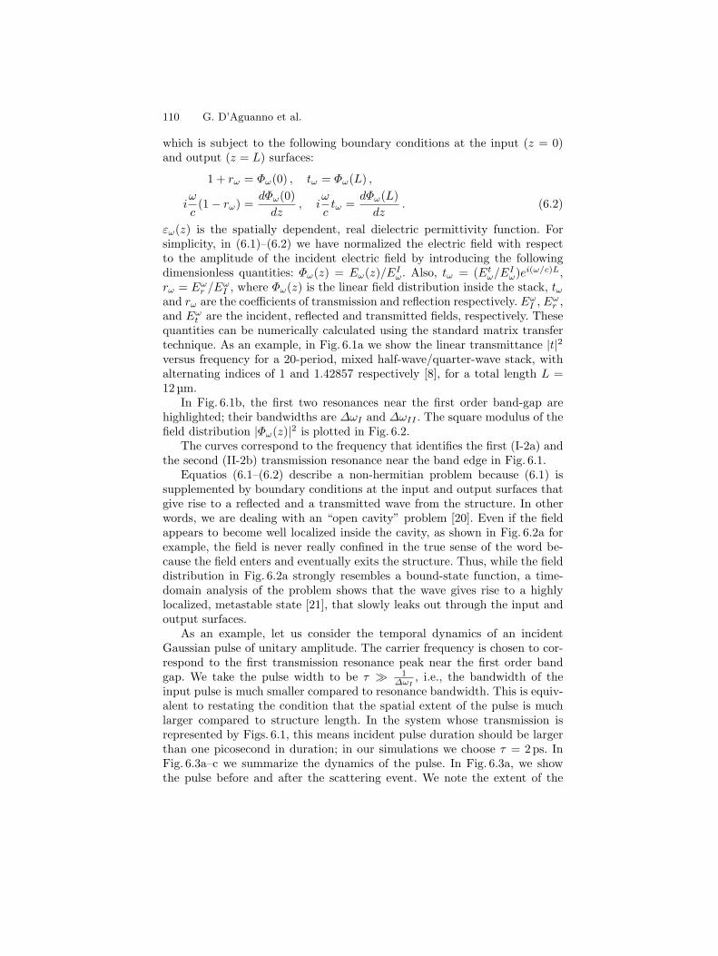
which is subject to the following boundary conditions at the input (z = 0)and output (z = L) surfaces:
1 + rω = Φω(0) , tω = Φω(L) ,
iω
c(1− rω) =
dΦω(0)dz
, iω
ctω =
dΦω(L)dz
. (6.2)
εω(z) is the spatially dependent, real dielectric permittivity function. Forsimplicity, in (6.1)–(6.2) we have normalized the electric field with respectto the amplitude of the incident electric field by introducing the followingdimensionless quantities: Φω(z) = Eω(z)/EI
ω. Also, tω = (Etω/E
Iω)e
i(ω/c)L,rω = Eω
r /EωI , where Φω(z) is the linear field distribution inside the stack, tω
and rω are the coefficients of transmission and reflection respectively. EωI , E
ωr ,
and Eωt are the incident, reflected and transmitted fields, respectively. These
quantities can be numerically calculated using the standard matrix transfertechnique. As an example, in Fig. 6.1a we show the linear transmittance |t|2versus frequency for a 20-period, mixed half-wave/quarter-wave stack, withalternating indices of 1 and 1.42857 respectively [8], for a total length L =12µm.
In Fig. 6.1b, the first two resonances near the first order band-gap arehighlighted; their bandwidths are ∆ωI and ∆ωII . The square modulus of thefield distribution |Φω(z)|2 is plotted in Fig. 6.2.
The curves correspond to the frequency that identifies the first (I-2a) andthe second (II-2b) transmission resonance near the band edge in Fig. 6.1.
Equatios (6.1–(6.2) describe a non-hermitian problem because (6.1) issupplemented by boundary conditions at the input and output surfaces thatgive rise to a reflected and a transmitted wave from the structure. In otherwords, we are dealing with an “open cavity” problem [20]. Even if the fieldappears to become well localized inside the cavity, as shown in Fig. 6.2a forexample, the field is never really confined in the true sense of the word be-cause the field enters and eventually exits the structure. Thus, while the fielddistribution in Fig. 6.2a strongly resembles a bound-state function, a time-domain analysis of the problem shows that the wave gives rise to a highlylocalized, metastable state [21], that slowly leaks out through the input andoutput surfaces.
As an example, let us consider the temporal dynamics of an incidentGaussian pulse of unitary amplitude. The carrier frequency is chosen to cor-respond to the first transmission resonance peak near the first order bandgap. We take the pulse width to be τ 1
∆ωI, i.e., the bandwidth of the
input pulse is much smaller compared to resonance bandwidth. This is equiv-alent to restating the condition that the spatial extent of the pulse is muchlarger compared to structure length. In the system whose transmission isrepresented by Figs. 6.1, this means incident pulse duration should be largerthan one picosecond in duration; in our simulations we choose τ = 2ps. InFig. 6.3a–c we summarize the dynamics of the pulse. In Fig. 6.3a, we showthe pulse before and after the scattering event. We note the extent of the

6 Photonic Band Edge Effects in Finite Structures 111
0
4
8
1 2
0 4 8 1 2
z (µm)
0 4 8 10
2
4 (b)2Φ
2Φ (a)
z (µm)
Fig. 6.2. Square modulus of the field distribution corresponding to the frequencythat identifies the first transmission resonance a labeled I in Fig. 6.1, and the secondtransmission resonance b labeled II in Fig. 6.1) away from the band edge
pulse with respect to structure length. In Fig. 6.3b, the center of the pulsehas reached the structure. At this instant we identify what we earlier referredto as a localized metastable state. Examination of the figure shows that inthis quasi-monochromatic regime, the field distribution inside the stack isvery similar to the field distribution shown in Fig. 6.2a, which was calculatedusing the stationary Helmholtz equation and its related boundary conditions(6.1)–(6.2). The inset of Fig. 6.3b shows the pulse in its entirety, as it crossesthe PBG structure. The large spike visible in the inset corresponds to thefield profile of the figure. Finally, in Fig. 6.3c we compare the localization ofthe 2 ps pulse with the localization of a 200 fs pulse. In this latter case, thespatial extent of the pulse is of the same order as structure length, and as aresult the field appears to become far less localized inside the structure. So,the ability to resolve individual resonances places strict conditions that arenecessary in order to first excite and then observe the localized metastablestates that we show in Figs. 6.2a and 6.3b. In short, then, in studying thephysics of the photonic band edge [4–9,18,19,22], we set out to explore thepeculiar but remarkable properties of those particular metastable states that

112 G. D’Aguanno et al.
transiently manifest themselves as strongly localized fields, with large localfield intensities.
Even if the field appears to become well localized inside the cavity, asshown in Fig. 6.3 for example, the field is never really confined in the truesense of the word because the field must first enter and eventually exit thestructure. Thus, while the field distribution in Fig. 6.3 strongly resembles abound-state function, a time-domain analysis of the problem shows that thewave first enters the structure, gives rise to a highly localized, metastablestate [21], and then slowly leaks out through the input and output surfacesas shown in Fig. 6.3. As a result, the problem does not admit true eigenstates,intended in the traditional sense, i.e., a complete basis of expansion in thespace between z = 0 and z = L. However, the problem admits metastable,or quasi-stationary states that by virtue of their localization properties canbe associated with an effective DOM. One way to define a proper DOM forstructures of finite length is to resort to the spatially averaged electromag-netic energy density. For the field distribution Φω(z), which is expressed indimensionless units, we define the DOM as (see appendix A):
ρ(ω)E ≡ 1
2L
∫ L
0
[εω(z) |Φω|2 + c2
ω2
∣∣∣∣dΦω
dz
∣∣∣∣2]dz . (6.3)
In general, the DOM should reflect the localization properties of the fieldinside the structure. Our definition in (6.3) does so in that it establishesa clear link between large field localization and large values of the DOM.We decompose the field in the form: Φω(z) = |Φω(z)|eiθ(z). It follows that|Φω|2 dθ
dz is a conserved quantity admitted by (6.1). Integrating (6.3) by parts,and using the boundary conditions (6.2), the expression for the DOM takeson the following, more suggestive form:
ρω =1Lc
∫ L
0εω(z) |Φω|2 dz − 1
LωIm(rω) . (6.4)
There is an alternative definition of the DOM, as discussed in [22], namelyρω = 1
Ldϕt
dω , where ϕt is the phase of the transmission function, defined astω = |tω|eiϕt . In Fig. 6.4, the DOM is shown for the 20-period structure ofFig. 6.1; it is clearly largest at each transmission resonance, where |t|2 = 1,and it reaches an absolute maximum at the transmission peak nearest tothe band edge. There, the corresponding field becomes well localized overthe entire structure – see Fig. 6.2. The solid line corresponds to the DOM ascalculated by the definition given in (6.3), and the dotted line correspondsto the DOM as calculated using the definition. The two different definitionsyield the same results in the pass-band, and show only a modest quantitativedifference inside the band gap (see inset of Fig. 6.4). Although quantitativedifferences are slight, our definition given in (6.3) is much more appealingfrom a physical and a conceptual point of view because it establishes a clear

6 Photonic Band Edge Effects in Finite Structures 113
Inte
nsit
y
0
0.2
0.4
0.6
0.8
1.0
PBG
Incident Pulse
0-1000-2000-3000
L=12µµµµm
Transmitted Pulse
300020001000
(a)
0
4
8
12
1260 3 9
z (µm)
0
4
8
12
z (µm)
Inte
nsit
y
-1000 0 1000
(b)
z (µm)
0
4
8
12
0 4 8 12
Inte
nsit
y
z (µm)
(c)
Fig. 6.3. a 2-ps incident Gaussian pulse and the structure. Note the spatial extentof the pulse with respect to structure length is to scale. b Internal field profilewhen the peak of the pulse reaches the structure. Inset : the pulse is shown in itsentirety. The large spike visible in the inset corresponds to the field profile of thefigure. Note that most of the pulse is located outside the structure. c Pulse hasexited the structure. d Metastable states for 2-ps (Fig. 6.3b) (thin line) and for the200-fs pulses (thick line). Note that the longer pulse is much more localized thanthe shorter pulse due to the different frequency bandwidth

114 G. D’Aguanno et al.
0
2
4
6
8
0.6 0.7 0.8
0.20
0.25
0.30
0.625 0.650 0.675 0.700
ω/ω0
DO
M (
in u
nits
of
1/c)
Fig. 6.4. Density of modes for the PBG structure of Fig. 6.1 calculated using (6.3)(solid line) and using the phase of the transmission function (dotted line). Inset :inside of the gap is magnified. In this case, the difference is about 10% at center-gap
direct link between the localization properties of the metastable states andthe concept of the DOM, and because it can be applied much more easilyin a three-dimensional geometry. This link does not directly follow from thedefinition given in [22] in terms of the transmission function.
Once the DOM ρω has been defined, it is then possible to find an effectivedispersion relation for a generic, finite structure, not necessarily multilayered,in the usual way. The real part of the effective dispersion relation kr(ω) isthe solution of the following first order linear differential equation:
dkr(ω)dω
= ρω (6.5)
supplemented by the condition kr(0) = 0. We note that that kr(−ω) =−kr(ω) as a consequence of the parity of the DOM. The imaginary partof the dispersion relation is calculated by invoking the causality principlethrough the Kramers-Kronig relations:
ki(ω) = − 2πP
∫ ∞
0
Ωkr(Ω)Ω2 − ω2 dΩ (6.6)
thus obtaining the effective dispersion relation for the finite PBG structure:
k(ω) = kr(ω) + ikr(ω) . (6.7)
Following [19], we can also introduce an effective index as:
k(ω) =ω
c[nr(ω) + inr(ω)] . (6.8)

6 Photonic Band Edge Effects in Finite Structures 115
1.2
1.3
1.4
0.5 0.6 0.7 0.8 0.9
Re(
n eff)
Band gap
(a)
0
0.04
0.08
0.12
0.5 0.6 0.7 0.8 0.9
ω/ω0
Im(n
eff
f)
(b)
ω/ω0
Fig. 6.5. a Real part of the effective index for a 2-(long dashes) and 20-period(solid curve) structure; dispersion relation for the infinite structure (short dashes).In the inset the band edge is magnified. b Imaginary part of the effective index,same as a, without the 2-period curve
Both real and imaginary parts of the effective index of refraction are plot-ted in Fig. 6.5a–b for a 2-and a 20-period structure, and compared with thedispersion relation of the infinite structure. We note that the real part ofthe index displays anomalous dispersion inside the gap. The imaginary com-ponent is small and oscillatory in the pass-bands; it attains its maximumat the center of each gap, where the transmission is a minimum, and it isidentically zero at each transmission resonance. The figures show that theeffective dispersive properties are modified by the number of periods (geo-metrical dispersion), and rapidly converge to the infinite-structure band edgeby increasing N . However, we emphasize that the dispersion that we find dis-plays clear oscillatory behavior outside the gap, unlike the infinite structure,since in the quasi-monochromatic regime that we are studying individualresonances can always be resolved.

116 G. D’Aguanno et al.
Although our effective index model has been developed principally in con-nection with finite, periodic structures, as we mentioned earlier its validity isgeneral because it holds for any kind of structure, periodic or not. The advan-tages that this approach afford will become clearer in the next sections, whenwe apply the model to the study of nonlinear quadratic interactions. Sufficeit to say for the time being that the effective index approach can simplify theproblem of calculating the conversion efficiency for χ(2) interactions in PBGstructures, because in the effective index picture the fields “see” an effectivebulk material with a well-defined dispersion relation.
6.3 Group Velocity, Energy Velocity,and Superluminal Pulse Propagation
Recent experimental studies of one-dimensional have highlighted particu-larly interesting linear properties of pulses propagating in structures of finitelength. Examples are the measurement of superluminal group velocities atmid-gap frequencies [23], and the measurement of low group velocities nearthe band edge of a semiconductor heterostructure [7]. These effects originatewith the remarkable but peculiar dispersive properties of finite multi-layerstacks which we have highlighted above, and discussed at length in [19]. Theconcept of group velocity is particularly critical when applied to an absorbing(or gain), homogeneous dielectric material because Vg may be greater thanc, and it can even be negative in some circumstances. These topics were dis-cussed at length in a seminal book by Brillouin [24], in 1970 by Loudon [25],and by Garret and McCumber [26]. The physical relevance of Vg regardingpulse propagation with superluminal or negative group velocities was exper-imentally studied by Chu and Wang [27], who measured the transmissiontime of a laser pulse tuned at a GaP:N resonance. Recently, Peatross et al.[28] have theoretically shown that in the context of an absorbing, homoge-nous material, the group velocity may still be meaningful even for broadbandpulses, and when Vg is superluminal or negative. In [28], the group velocityis related to pulse arrival time via the time expectation integral over thePoynting vector.
In the cited references [24–28] the work deals with pulse propagation inabsorbing, homogenous dielectric material. More recently, Wang et al. [29]used gain assisted linear dispersion to demonstrate superluminal light propa-gation in atomic cesium: the group velocity of a laser pulse under conditionsof anomalous dispersion in the presence of gain can exceed c as a result ofclassical interference between the different frequency components. Here, wediscuss the case in which a 1-D PBG structure displays anomalous effectiveindex behavior not as a result of gain or absorption, but as a result of scat-tering. More importantly, in our case the presence of entry and exit interfacesplay a crucial role in determining the definition of the group velocity and itsrelationship with the energy velocity. In contrast, boundary conditions in the

6 Photonic Band Edge Effects in Finite Structures 117
sense of an entry and an exit interface can play no role in the determinationof either group or energy velocity in inhomogeneous, periodic structures ofinfinite length. Our simple and straight forward analysis shows that thereare significant conceptual, qualitative, and quantitative differences betweenenergy and group velocities in finite structures in contrast to the case of infi-nite structures. In fact, for a periodic, infinite structure a unique dispersionrelation exists between Kβ (the Bloch vector) and ω. The group velocity.V
(ω)g is defined as V (ω)
g = 1/[dKβ/dω], and it can be demonstrated thatV
(ω)g = V
(ω)E [30].
In order to discuss the case of 1-d, finite PBG structures, we considerplane monochromatic waves, and Eqs. ([1,2]). The averaged energy velocity,which measures energy flow across the sample, is defined as the ratio of thespatial average of the Poynting vector to the spatial average of the energydensity within the same volume [30], which in our 1-d geometry is given by:
V(ω)E =
1LRe
[ic2
ω
∫ L
0 ΦωdΦ∗
ω
dz dz]
12L
∫ L
0
[εω(z) |Φω|2 + c2
ω2
∣∣dΦω
dz
∣∣2] dz . (6.9)
Integrating by parts, and using the boundary conditions (6.2), the energyvelocity V (ω)
E takes a form that involves both the transmittance |tω|2 and theimaginary part of the reflectivity rω of the stack:
V(ω)E =
c |tω|21L
∫ L
0 εω(z) |Φω|2 dz − cLω Im(rω)
. (6.10)
The second term in the denominator indicates that the energy is generallynot equally shared by the electric and magnetic components, and becomesidentical only at each peak of transmittance, where rω vanishes. In Fig. 6.6we depict V (ω)
E for a 20 and 100-period stack, and compare with the V (ω)E (for
infinite structures, V (ω)g coincides with V
(ω)E ) of an infinite structure made
with the same elementary cell. We find that the energy velocities of the in-finite and finite structures do not converge to one another by increasing thenumber of periods. This is due to the fact that in the monochromatic ap-proximation it is always possible to resolve each transmission resonance, andhence its curvature, even if more periods are added. In this regime, incidentpulses are propagating through the structure tuned at one transmission res-onance, for example, with their bandwidth significantly smaller comparedto resonance bandwidth. Put another way, the spatial extent of the pulseis orders magnitude greater then the physical length of the structure. As aresult, the pulse samples all internal and external interfaces simultaneously,it is delayed and in the end completely transmitted, with minimal distortionor scattering losses [7]. Therefore, the interaction should more properly bereferred to as a scattering event.

118 G. D’Aguanno et al.
0.55 0.56 0.57 0.58 0.59 0.60 0.61
ω/ω0
0.0
0.1
0.2
0.3
0.4
0.5
0.6
0.7
VE (
in u
nit
s o
f c)
N
N=100
N=20
→∞
Fig. 6.6. V (ω)E for a 20-period (short dashes), 100-period (solid line), and infinitestructure (long dashes) vs frequency. Increasing the number of periods, the energyvelocity does not converge to the results obtained using the dispersion of the infinitestructure. The elementary cell is composed of a combination of half-wave/quarter-wave layers. The indices of refraction are na = 1 and nb = 1.42857; the respectivethicknesses are a = λ0/(4na) and b = λ0/(2nb), with λ0 = 1 µm, ω0 = 2πc/λ0
To better clarify this situation, we consider the case of a short pulse in-cident on a structure several pulse widths in length. If the spatial extent ofthe pulse is so short that it traverses the structure without simultaneouslysampling both entry and exit interfaces, then we may expect that the dis-continuity at the entrance and exit interfaces will not significantly affect thedynamics [31]. This is shown in Fig. 6.7, where we plot V (ω)
E as calculated inthe quasi-monochromatic limit via (6.3), and also as numerically calculatedfor an incident gaussian pulse 150 fs in duration tuned in the passband of a100-period structure. The energy (group) velocity of the infinite structure isalso shown in the figure. The comparison between the length of the structureand pulse width is made in the inset. As the inset shows, the structure isseveral pulse widths in length. As a result, the energy velocity of the pulsepropagating inside this structure approximates better the energy velocity ofthe infinite structure (Bloch’s velocity). The energy velocity of the pulse doesnot show the same sharp cut off near the band edge we observe for both theinfinite and the 100-period structures because the pulse is ultrashort, andeven if the carrier frequency is tuned inside the gap a good fraction of the en-ergy is still trasmitted. We find the same degree of convergence only if pulsewidth and structure length are significantly increased simultaneously, so thatthe pulse can better resolve the frequencies near the band edge, but still fitswell inside the structure, as in the inset. In Fig. 6.8, the total momentumand energy inside the 100-period structure depicted in Fig. 6.7 are shown asa function of time. The total electromagnetic momentum for the pulse inside

6 Photonic Band Edge Effects in Finite Structures 119
0.55 0.56 0.57 0.58 0.59 0.60 0.61
Normalized Frequency
0.0
0.2
0.4
0.6
0.8
En
erg
y V
elo
city
Pulse
N= ∞
N=100
Fig. 6.7. V (ω)E vs frequency for 150fs incident pulse (solid line), and monochromaticregime (dotted line). The monochromatic wave regime is also obtained using pulsesat least several tens of picoseconds in duration. The dashed line corresponds toBloch’s velocity for the infinite structure. The structure is similar to that outlinedin Fig. 6.1, but contains 100 periods. Inset: the 100-period structure is approxi-mately 60 microns in length, while the spatial extent of the FWHM of the pulse isapproximately 20 microns
the structure can be written as follows:
g(t) =1c2S(t) =
1c2
∫ L
0Eω(z, t)×Hω(z, t)dz . (6.11)
The total energy is given by:
U(t) =∫ L
0
[εω(z) |Eω(z, t)|2 + c2
ω2 |Bω(z, t)|2]dz . (6.12)
As the pulse enters the structure, there is a rapid rise in both energy andmomentum, which settle to constant values once the whole pulse travels insidethe structure. When the pulse is totally inside, both group and energy veloc-ities are equal and given by Bloch’s velocity. However, even if the structure islong, it is nevertheless finite, and so the pulse must eventually exit, leadingto a reduction of energy and a reversal in sign in the total momentum. Oncethe momentum becomes negative, we track the first pulse reflected from theexit interface. In fact the momentum undergoes several sign reversals, untilall the energy has left the structure. From Fig. 6.3 it should be evident thatthe energy velocity can equal Bloch’s velocity only after the entire pulse hasentered and remains inside the structure, while in general the time-averagedenergy velocity will be different.

120 G. D’Aguanno et al.
0 100 200 300
Time (in unit of λ/c)
-1.0
1.0
3.0
5.0
7.0
9.0
11.0
13.0
g(t
) &
U
(t)
Bloch velocity regions
g(t)
U(t)
Fig. 6.8. Total energy (dashed) and momentum (solid) inside the structure for thepulse shown in the inset of Fig. 6.2. Both momentum and energy increase as thepulse traverses the entry boundary. The energy velocity for the entire process, i.e.,the ratios of the areas under the curves, which is a measure of energy flow throughthe structure in both directions, cannot be the same as Bloch’s velocity, whichmonitors only the velocity of the transmitted pulse. Multiple reflections inside thestack leads to ringing in reflection and transmission from the structure
With these considerations in mind, we define the tunneling time in aquasi-monochromatic regime, consistent with our approach, as:
τω =1c
∫ L
0εω(z) |Φω|2 dz − 1
ωIm(rω) . (6.13)
This definition of tunneling time, derived by imposing boundary conditionson our finite structure and directly suggested by (6.4) and (6.10), is the elec-tromagnetic analogue of Smith’s “dwell time” [32], which addresses electronwave packet tunneling times through a potential barrier. According to Smith,a quantum particle spends a mean time proportional to
∫ L
0 |Ψ(z)|2 dz in theregion of space between 0 and L, which is just the probability of finding theparticle within the same region of space. Following Bohm [21], we use theconcept of electromagnetic energy density, instead of the quantum probabil-ity density, to define the tunneling time (see appendix A): Equation (6.13)states that the time the field spends inside the structure is proportional to theenergy density integrated over the volume. The term −Im(rω)/ω representsthe difference in energy between the electric and magnetic components, andit has no counterpart in the quantum case. Equation (6.13) thus establishesa clear link between large delay times and field localization, as experimen-tally verified for pulse propagation near the band edge [7]. One may alsodefine a group velocity associated with the delay of the transmitted pulse asV
(ω)g ≡ L/τω. In the eyes of an observer, this definition of group velocity is an

6 Photonic Band Edge Effects in Finite Structures 121
extremely useful and powerful concept. However, we remind the reader thatwe are not considering propagation in a uniform medium, where a true groupvelocity can be defined. Our system consists of a pulse whose spatial extentcan be orders of magnitudes larger compared to the length of the structure,which is therefore entirely contained within the pulse [7]. As a consequence,the dynamics can only properly be described as a scattering event, with anassociated tunneling time.
Once a convenient group velocity has been defined in the manner indi-cated, (6.13) can finally be recast in the following simple form:
V(ω)E = |tω|2 V (ω)
g . (6.14)
Equation (6.14) is a strikingly simple new result that makes it clear that forfinite structures the tunneling velocity Vg and the energy velocity VE are thesame only at each transmission resonance, and can be very different from eachother, especially at frequencies inside the gap. The implications of (6.14) areeven more profound and far reaching if we consider superluminal tunnelingbehavior. We begin with the assertion that the energy velocity can nevertake on values greater than c, namely V (ω)
E ≤ c. From (6.14) it immediatelyfollows that the tunneling velocity satisfies V (ω)
g ≤ c/ |tω|2. That is, the simplerequirement that the energy velocity should be subluminal does not preventsuperluminal tunneling times. In fact, this inequality places an unambiguousupper limit on the tunneling velocity that can be achieved without violating therequirement that the energy velocity remain subluminal. Based on these simpleconsiderations, statements regarding superluminal pulse propagation shouldalways be qualified by the energy velocity and transmittance. In Fig. 6.9 weplot V (ω)
g and V(ω)E versus frequency for the 20-period structure of Fig. 6.1.
Inside the gap, the group velocity becomes superluminal, while the energyvelocity always remains causal. In this case, minimum transmittance can be aslow as 1 part in 105. We note that the maximum superluminal group velocityis approximately 5.5 times the speed of light in vacuum (see Fig. 6.10), farbelow the upper limit imposed by the condition that the energy velocityshould remain subluminal.
In Fig. 6.5 we compare the tunneling velocity calculated using (6.6), andthe tunneling velocity calculated using the phase time. The group velocitycorresponds to the inverse of the DOM, which has already been shown inFig. 6.4. While in the pass band the two methods yield similar results, ourmethod gives slightly higher estimates (10%, as in Fig. 6.4) for the maximumsuperluminal velocity compared to the method of the phase time. This dif-ference corresponds to a time delay of the order of 1 fs, which is small butmeasurable [25]. The integration of the equations of motion in the time do-main yield results consistent with our predictions, namely a group velocityof approximately 5.5 c for pulses tuned inside the gap.

122 G. D’Aguanno et al.
0.55 0.56 0.57 0.58 0.59 0.60
ω/ω0
0.0
0.5
1.0
1.5
Vg
, VE
(in
un
its
of c
); t
2
t2
Vg
VE
(N=20) VE
(N= ∞)
Fig. 6.9. V (ω)g (thin solid line), V (ω)E (thick solid line), |t|2 (dashes) for the 20-period structure described in the caption of Fig. 6.1. In the gap, the group velocitybecomes superluminal. At resonance, V (ω)g = V
(ω)E , and V
(ω)g is a minimum. The
group velocity for the infinite structure is also depicted (dotted line) for comparison
0.55 0.60 0.65 0.70 0.75 0.80ω/ω0
0
1
2
3
4
5
6
Vg (
in u
nit
s o
f c)
Fig. 6.10. V (ω)g as calculated using the definition of tunneling times given in (6.4)(solid line) and as calculated using the definition of phase time (dashed line)
6.4 χ(2) Interactionsand the Effective Medium Approach
The equations that describe the interaction of a fundamental and a SH field ina PBG structure have been discussed in [8], in a regime referred to the SlowlyVarying Envelope Approximation in Time, or SVEAT. Operating under theassumption that field envelopes are allowed to vary rapidly in space but not intime, i.e., the temporal evolution of the field envelope proceeds slowly withrespect to the optical cycle, it can be shown that the equations of motion

6 Photonic Band Edge Effects in Finite Structures 123
reduce to [8]:
εΩ∂
∂τEΩ(ξ, τ) =
i
4πΩ∂2
∂ξ2EΩ(ξ, τ) (6.15)
− ∂
∂ξEΩ(ξ, τ) + iπ [εΩ − 1]ΩEΩ + i8π2Ωχ(2)E2ΩE
∗Ω
and
ε2Ω∂
∂τE2Ω(ξ, τ) =
i
4π2Ω∂2
∂ξ2E2Ω(ξ, τ) (6.16)
− ∂
∂ξE2Ω(ξ, τ) + iπ [ε2Ω − 1] 2ΩE2Ω + i8π22Ωχ(2)E2
Ω .
In (6.16), Ω = ω/ω0, ξ = z/λ0, and τ = ct/λ0. The spatial coordinatez has been conveniently scaled in units of a reference wavelength λ0, andω0 = 2π/λ0; the time is then expressed in units of the corresponding opticalperiod. It is evident that the large refractive index contrast preempts a moregeneral slowly varying envelope approximation, or SVEA. However, if thediscussion is restricted to pulses whose duration far exceeds a few opticalcycles, then (6.16,6.17) are more than adequate.
Alternative options to the numerical integration of (6.16,6.17) also existin the form of more approximate solutions. One approach is based on thehypothesis that the modulation of the linear dielectric permittivity functionis small with respect to the averaged dielectric permittivity of the structure:εω = εω + ∆εω(z), where |∆εω(z)| εω (shallow grating limit). Conse-quently, the fields are expanded in terms of forward and backward propagat-ing modes of the equivalent linear bulk medium. As a result, mode amplitudesare slowly modulated by the combined action of nonlinear coupling and theweak longitudinal variation of the refractive index [33]. The second approachis based on the expansion of the fields using Bloch states of the correspond-ing infinite linear structure. The grating may be of arbitrary depth, and theexpansion coefficients are slowly modulated by the action of the quadraticcoupling [34]. In the shallow grating limit, this method yields coupled modeequations identical to those that result using the first approach.
In this work, we propose an alternative approach based on our effectivemedium model that it is useful when strong localization effects and the ap-pearance of metastable states of the kind discussed above come into play. Themethod that we propose can also be applied to intrinsically disordered layeredstructures, where translational invariance cannot be invoked, and analyticalsolutions would be almost impossible to find. We write the coupled modeequations for the nonlinear quadratic interactions in a finite PBG structureof length L as if the interaction were taking place in a bulk material of thesame length L, but with an effective dispersion relation given by (6.8). Inthe case of two monochromatic waves at fundamental frequency (FF) ω andsecond harmonic frequency (SH) 2ω, each tuned at a peak of transmittance

124 G. D’Aguanno et al.
where the imaginary part of the effective dispersion relation (6.12) is zero[19], the coupled mode equations written for the effective medium are:
d
dzAω = i
ω
nreff(ω)c
deffA2ωA∗ωe
i∆keffz (6.17)
andd
dzA2ω = i
ω
nreff(2ω)c
deffA2ωe
−i∆keffz , (6.18)
where ∆keff(ω) = kr(2ω) − 2kr() is the effective phase mismatch calculatedusing the real part of the effective dispersion relation (6.12); nr
eff is thereal part of the effective index; and deff is the effective nonlinear couplingcoefficient defined as:
deff =1L
∫ L
0d(2)(z)|Φω(z)|2|Φ2ω(z)|dz , (6.19)
where d(2)(z) is the quadratic coupling function. It is overlapped with thesquare modulus of the FF and the modulus of SH. The value of the effectivenonlinear coupling coefficient strictly depends on the localization properties ofthe FF field. From (6.4), at the peak of transmittance ρω = 1
Lc
∫ L
0 εω(z) |Φω|2×dz. As a consequence, deff is enhanced by a factor proportional to the DOMwhen the FF field is localized inside the nonlinear layers
deff ∝ ρωd(2)layer , (6.20)
where is d(2)layer is the actual second order susceptibility of the nonlinear layer.Now that we have developed all the major components of the model, we
mention its fundamental limitations. Coupled mode (6.17) cannot give de-tailed information about the actual nonlinear dynamics of the fields insidethe structure. This is evident if we recall that our approach to the problemconsists in substituting the finite PBG structure with an equivalent lengthof bulk material and an effective dispersion relation given by (6.12). In otherwords, we cannot expect that this model will yield both reflected and trans-mitted components. This can only be achieved if we resort to the numericalintegration of (6.16), as was done in [8]. However, the solutions of (6.17) yieldremarkably accurate energy conversion efficiencies when compared to the con-version efficiencies calculated by integrating (6.16). By establishing the va-lidity of the model with a direct comparison with the numerical integrations,conversion efficiencies can then be calculated very efficiently by resorting tothe coupled mode (6.17). As an example, for second harmonic generation un-der the non-depleted pump approximation, we obtain the expression for theconversion efficiency h in analogy with the conversion efficiency calculatedfor bulk materials:
η =8π2d2effL
2Ip[nr
eff(ω)]2nreff(2ω)ε0cλ2
sin c2(∆keffL
2
), (6.21)

6 Photonic Band Edge Effects in Finite Structures 125
where Ip = 12ε0cn
reff(ω)|Aω|2 is the scaled input pump intensity. Equation
(6.17) clarifies the role played by the linear FF metastable state inside thestructure in the enhancement of the effective nonlinearity deff . When the FFmetastable state overlaps well the nonlinear layers, we expect an enhancementof the conversion efficiency approximation proportional to ρ2ω:
η ≈[ρωd
(2)layerL
]2Ip sin c2
(∆keffL
2
). (6.22)
In order to compare with an equivalent length of quadratic bulk material wecan define, from (6.19), a figure of merit (FM) as:
η = L2
[deff
d(2)layer
]2sin c2
(L
2Lc
), (6.23)
where Lc = (1/∆keff) is either one coherence length in the case of bulkmaterial, or the effective coherence length calculated via the effective indexneff in the case of a PBG structure.
6.5 Examples: Blue and Green Light Generation
In order to highlight the potential of 1-D PBG structures for nonlinear fre-quency conversion processes, we discuss a new type of blue laser that couldoperate in the 400 nm range. The device is composed of 30-periods alternat-ing SiO2/AlN layers, to form a quarter-wave/ half-wave stack similar to thatdescribed in the previous section. With a reference wavelength of 0.52 mi-crons, the total length of the structure is approximately 6 microns. The AlNlayers are assumed to have a nonlinear coefficient of about 10 pm/V. The FFbeam is assumed to be incident at an angle of 300 degrees with respect tothe surface of the structure. In Fig. 6.11, we show the linear transmittance ofthis structure. The FF frequency, at 800 nm, is tuned to the first transmis-sion resonance near the first order band gap, where the corresponding linearmode is well localized, and a high density of modes (DOM) is achieved. TheSH frequency is tuned to 400 nm, which corresponds to the second resonancepeak near the second order gap, as indicated on Fig. 6.11. We note that weare using experimentally available data for both materials, and that aligningthe resonances as prescribed can be done by varying the thickness of thelayers, i.e., by adjusting the geometrical dispersion of the structure [19]. Thestructure is exactly phase-matched in the sense of the effective index [19].Through (6.23) we calculate the SH conversion efficiency as a function of theinput FF intensity, and show the results in Fig. 6.12. We find a conversionefficiency of approximately 15% in a single pass through the device, with in-put power levels of 40GW/cm2. Although this intensity may seem high, westress that the structure is only 30 periods long, and only 6 microns length.

126 G. D’Aguanno et al.
0
0.20.2
0.40.4
0.60.6
0.80.8
1.01.0
0.40.4 0.50.5 0.60.6 0.7 0.80.8
SH pump
λ (µm)
|t|t|2
Fig. 6.11. Transmittance for 30-period PBG structure composed of alternatinglayers of SiO2/AlN, quarter- wave/ half-wave stack respect to a reference length of0.53 microns. The FF field (pump) and SH field (generated) are phase matched
0.05
0.15
0.25
0 20
IInω
conv
ersi
on e
ff ici
enc y
40 60
(GW/cm2)
Fig. 6.12. Second harmonic conversion efficiency vs the input pump intensity underundepleted pump approximation (dotted line) and in the case of pump depletion(continuous line) 30-periods alternating SiO2/AlN. A conversion efficiency of ap-proximately 15% is reached for input pump intensity of 40GW/cm2
To test the validity of the effective medium model we perform a full numer-ical integration of the nonlinear coupled wave equations as discussed in [8].We plot the results in Fig. 6.13, where we show the total energy convertedfrom the FF to the SH field as a function of time. The conversion efficiencyobtained numerically is approximately equal to what the effective mediummodel predicts. The conversion efficiency could be dramatically improved,and thresholds lowered, by increasing the number of periods. To concludethis section, we point out that a semiconductor multilayer stack composedof AlGaAs/AlAs has been fabricated and tested according to the criteriathat exploit the simultaneous availability of high density of modes and phasematching conditions. The results are in good agreement with the effectiveindex predictions and will soon be published [35].

6 Photonic Band Edge Effects in Finite Structures 127
0 1000 2000
time (in units of λref/c)
Ene
rgy
0
32
24
16
8
Pump Energy
SH Energy
(a.u
.)
Fig. 6.13. Energy converted from the pump to the SH field as function of the time.λref corresponds to a wavelength of 1 µm. We pump with a 2-ps pulse incident fromthe left, with 40GW/cm2 of peak input intensity. The conversion efficiency, givenby the amount of energy converted to SH divided the total amount of initial energyin the FF, is approximately (4/30) ≈ 13%, in good agreement with that predictedby the effective medium model
6.6 Frequency Down-Conversion
In this section we extend the analysis we began with the introduction ofan effective dispersion relation for the finite structure by examining in somedetail another important aspect of nonlinear frequency conversion, that isdown-conversion processes. Using the effective index approach, we first derivesimple phase matching conditions for three-wave coupling, and then test themby numerically integrating the equations of motion in the time domain. Wespecifically set out to explore the possibility of generating near- and far-infrared radiation through a three-wave mixing process in micron-sized PBGstructures because there is a conspicuous absence of small-volume, reliable,coherent radiation sources in that range. The amplification of sum-frequencygeneration was recently reported [36] for pumps that were tuned near theband edge of a one-dimensional structure. In [36] the authors show that theincrease in the density of modes near the band edge can lead to the generationof 400 nm radiation at a rate that was approximately one order of magnitudehigher compared to the case where the pumps where not tuned near the bandedge. However, no particular care was exercised in that case to make sure thatphase matching conditions that we describe in [19] were satisfied. Therefore,we predict that if the scheme we propose for phase matching is implementedin a one-dimensional geometry, enhancements will be much larger.
As we have seen, the typical 1-D structure that we consider consists ofalternating layers of high and low index materials. We assume that two pumpfields, for example, at ω1 (λ = 1 micron) and ω2 (λ = 1.5 microns), areincident normally on the structure, and that their interaction mediated by

128 G. D’Aguanno et al.
a χ(2) process generates a down-converted signal at a third frequency ω3(λ = 3 microns). Initially there is no ω3 signal. The specific wavelengths thatwe use here are not crucial, and are only used for illustrative purposes. It willbecome clear later, as we also showed previously [19], that both material andgeometrical dispersion can be combined to produce exact phase matchingconditions for a variety of situations, a fact that highlight the flexibility ofthese devices.
The approach that we pursue is as follows: first, we design a multilayerstack, and determine its linear phase properties using the effective index for-mulation. We seek appropriate tuning of all the fields with respect to theirrespective band edges in order to simultaneously optimize and combine phasematching conditions with high DOM [19]. Then, we integrate the nonlinear,coupled equations of motion in the time domain. For clarity and complete-ness, we briefly outline both the effective index approach and the integrationmethod that we use.
6.7 Effective Index Method
We now review a method based on a formulation of the effective dispersionrelation that is derived from the phase properties of the transmission function[22] that allows us to evaluate the effective refractive index for a multilayeredstructure. We note that this method yelds results that are nearly identicalto the more general approach highlighted in the previous sections. Using thematrix transfer method [19,37], we define a general transmission function forany structure as follows:
t = x+ iy =√Teiϕt , (6.24)
where√T is the transmission amplitude, ϕt = tan−1(y/x)±mπ is the total
phase accumulated as light traverses the medium, and m is an integer number.In analogy with the propagation in a homogeneous medium, we can expressthe total phase associated with the transmitted field as
ϕt = k(ω)D = (ω/c)neff(ω)D , (6.25)
where k(ω) is the effective wave vector, and neff is the effective refractiveindex that we attribute to the layered structure whose physical length is D.As described in [19], we obtain the following expression of the effective indexof refraction:
neff =c
ωD
[ϕt − i
2ln(x2 + y2)
]. (6.26)
Equation (6.26) suggests that at resonance, where T = x2 + y2 = 1, theimaginary part of the index is identically zero. We can also define the effective

6 Photonic Band Edge Effects in Finite Structures 129
index as the ratio between the speed of light in vacuum and the effective phasevelocity of the wave in the medium. We have k(w) = ω
c neff(ω). This is theeffective dispersion relation of the finite structure. For periodic structures, thephase matching conditions are automatically fulfilled if the fields are tuned atthe right resonance peaks of the transmission spectrum. Using the formalismintroduced in [22], the expression for the effective index for the N-periodsfinite structure can be recast as follow [19]:
neff =c
ωNa
tan−1 [z tan(Nβ) cot(β)] + Int
[Nβ
π+12
]π
, (6.27)
where β is the Bloch’s phase for an infinite structure having the same iden-tical unit cell as the finite structure in question. Equation (6.27) containsadditional information regarding the location of the resonances where phase-matching for a three wave mixing (TWM) process can occur. For illustra-tion purposes, we consider a 20-period, mixed half-wave/eighth-wave periodicstructure. We choose this arrangement because it allows easy tuning of allthe fields near their respective band edges, thus allowing us to simultaneouslyaccess a high density of modes for all fields. We note that this arrangementis not unique, in that higher or lower order band edges can be combinedto yield the phase matching conditions, within the context of the effectiveindex approach outlined in [19]. We assume that two pump fields are tunedat ω3 = 3ω, ω2 = 2ω; the interaction via a χ(2) process then generates adown-converted signal at a third frequency ω1 = ω (λ = 3 microns). First,we tune the field of frequency ω1 at the first resonance near the first orderband edge; this insures a high density of modes. We have [19]:
β1 =π
N(N − 1) . (6.28)
Then, we tune the field ω2 at the first resonance near the second order bandedge, once again securing a high density of modes; we have:
β2 =π
N(2N − 1) . (6.29)
We now impose the phase-matching condition for the TWM process, namely:
K3(ω3)−K2(ω2)−K1(ω1) = 0 . (6.30)
Substituting (6.28) and (6.29) into (6.30), we obtain
β3 =π
N(3N − 2) , (6.31)
which is the value of the Bloch’s phase that will correspond to the field atfrequency ω3. This means that phase-matching conditions will be satisfiedfor this structure if the thickness of the layers are combined with materialdispersion such that the first pump field (3ω) is tuned to the second resonance
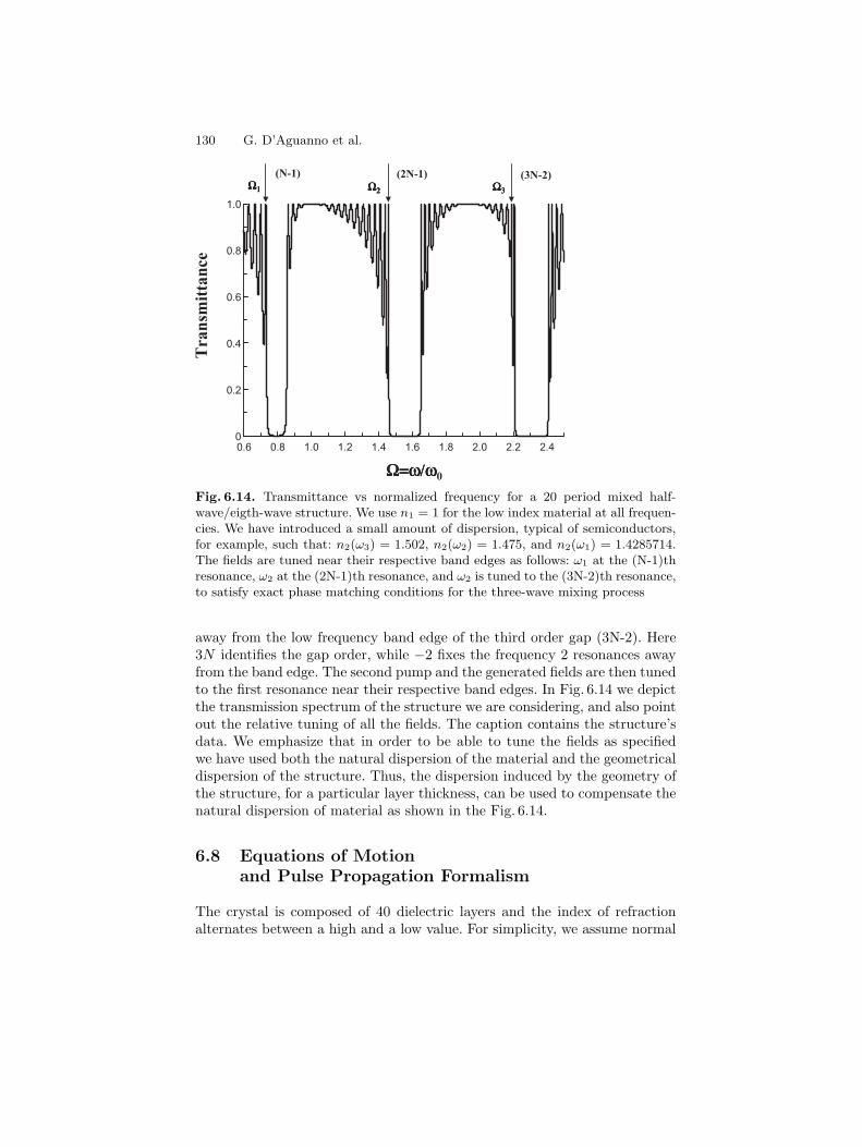
130 G. D’Aguanno et al.
0
0.2
0.4
0.6
0.8
1.0
0.6 0.8 1.0 1.2 1.4 1.6 1.8 2.0 2.2 2.4
Tra
nsm
itta
nce
Ω=ω/ωΩ=ω/ωΩ=ω/ωΩ=ω/ω0
(N-1) (2N-1) (3N-2)ΩΩΩΩ1111 ΩΩΩΩ2222 ΩΩΩΩ3333
Fig. 6.14. Transmittance vs normalized frequency for a 20 period mixed half-wave/eigth-wave structure. We use n1 = 1 for the low index material at all frequen-cies. We have introduced a small amount of dispersion, typical of semiconductors,for example, such that: n2(ω3) = 1.502, n2(ω2) = 1.475, and n2(ω1) = 1.4285714.The fields are tuned near their respective band edges as follows: ω1 at the (N-1)thresonance, ω2 at the (2N-1)th resonance, and ω2 is tuned to the (3N-2)th resonance,to satisfy exact phase matching conditions for the three-wave mixing process
away from the low frequency band edge of the third order gap (3N-2). Here3N identifies the gap order, while −2 fixes the frequency 2 resonances awayfrom the band edge. The second pump and the generated fields are then tunedto the first resonance near their respective band edges. In Fig. 6.14 we depictthe transmission spectrum of the structure we are considering, and also pointout the relative tuning of all the fields. The caption contains the structure’sdata. We emphasize that in order to be able to tune the fields as specifiedwe have used both the natural dispersion of the material and the geometricaldispersion of the structure. Thus, the dispersion induced by the geometry ofthe structure, for a particular layer thickness, can be used to compensate thenatural dispersion of material as shown in the Fig. 6.14.
6.8 Equations of Motionand Pulse Propagation Formalism
The crystal is composed of 40 dielectric layers and the index of refractionalternates between a high and a low value. For simplicity, we assume normal

6 Photonic Band Edge Effects in Finite Structures 131
dispersion, with n2(ω) = 1.4285, n2(2ω) = 1.475, n2(ω) = 1.502, and n1 = 1(air) at all frequencies. We assume we are operating in a region where lossescan be neglected, and the nonlinear material is distributed in the high indexlayers only, with χ(2) ≈ 100 pm/V. We note that this particular choice of theactive layer location is not crucial, and has been chosen because at the lowfrequency band edges the fields localize in the high index layers. Therefore,one might envision a scheme for tuning the pumps at the high frequency bandedge, which would require relocation of the nonlinear material to those layers.From a computational point of view, one may choose any configuration.
For a reference wavelength λ0, corresponding to a frequency ω0, the layershave thicknesses a = λ0
8n1and b = λ0
2n2, respectively. A range of frequencies is
reflected, as shown in Fig. 6.14, where we plot the transmittance as a functionof the scaled frequency Ω = ω/ω0, where ω0 = 2π/λ0. We now describe inmore details the process of arriving at coupled nonlinear equations of motionthat are then integrated in the time domain. We begin by writing Maxwell’sequation for the total electric field, in Gaussian units:
∂2
∂z2E(z, t)− n2(z)
c2∂2
∂t2E(z, t) =
4πc2
∂2
∂t2PNL(z, t) . (6.32)
Here, PNL is the total nonlinear polarization. Without loss of generality, thefields can arbitrarily (and conveniently) be decomposed as follows:
E(z, t) =j=3∑j=1
Ej(z, t)ei(kjz−wjt) + c.c. (6.33)
and
P (z, t) =j=3∑j=1
Pj(z, t)ei(kjz−wjt) + c.c. (6.34)
This decomposition highlights the fields’ angular frequencies. Then we assumethat ω1 = ω, ω2 = 2ω, ω3 = ω1 + ω2 with k1 ≡ k = ω
c , k2 = 2ω/c, andk3 = 3ω/c. The nonlinear polarization takes the following form:
PNL(z, t) = χ(2)E2(z, t) = 2χ(2)[E∗
1E2+E∗2E3 ei(kz−wt)
+E∗1E3+
12E21ei(2kz−2wt) + E1E2ei(3kz−3wt)
]+ c.c. , (6.35)
where E1, E2 and E3 are the fields at the frequencies ω1, ω2, and ω3, respec-tively. While we can assume initial left- or right-propagating pump pulses(2ω and 3ω), the generated signal at frequency ω is initially zero everywhere.The direction of propagation of the spontaneously generated field, and theexact nature of the quasi-standing wave inside the structure, are dynami-cally determined by the nature of the initial and boundary conditions, pump
132 G. D’Aguanno et al.
frequency tuning with respect to the band edge, and the distribution of non-linear dipoles inside the structure. We are also considering propagation inthe presence of large index discontinuities, and so we retain all second-orderspatial derivatives. However, we assume that pulse envelopes have a durationthat is always much greater than the optical cycle, thus allowing the applica-tion of the SVEAT only [5–8,38]. The equations of motion for the fields canthen be derived by substituting (6.33)–6.35) into (6.32), and by applying theSVEAT. The choice of wave vectors that we highlighted above corresponds toan initial condition consistent with pump fields initially propagating in freespace, located away from the structure. Any phase modulation effects thatensue from propagation, i.e., multiple reflections and nonlinear interactions,are fully accounted for in the dynamics of the field envelopes, which main-tain their general form. The inclusion of all second-order spatial derivativesin the equations of motion means that reflections are accounted for to allorders, without any approximations. Details on the propagation method canbe found in [5–8,38]. Therefore, assuming that pulses never become so shortas to violate SVEAT (usually this means a few tens of optical cycles, if prop-agation distances are on the order of pulse width, as in our case. Neglectingthe second-order temporal derivative leads to pulse spreading if the pulse isallowed to propagate over long enough distances), neglecting all but the low-est order temporal contributions to the dynamics, and using the nonlinearpolarization expansions of (6.35), we have:
n22Ω(ξ)
∂
∂τE2Ω(ξ, τ) = i
8πΩ∂2
∂ξ2E2Ω(ξ, τ)− ∂
∂ξE2Ω(ξ, τ)
+iπ[n22Ω(ξ)− 1
]2ΩE2Ω + i16π2Ωχ(2)(ξ)
E∗ΩE3Ω+
12E2Ω
(6.36)
and
n23Ω(ξ)
∂
∂τE3Ω(ξ, τ) = i
12πΩ∂2
∂ξ2E3Ω(ξ, τ)− ∂
∂ξE3Ω(ξ, τ)
+iπ[n23Ω(ξ)− 1
]3ΩE2Ω + i24π2Ωχ(2)(ξ)EΩE2Ω (6.37)
and
n2Ω(ξ)
∂
∂τEΩ(ξ, τ) = i
4πΩ∂2
∂ξ2EΩ(ξ, τ)− ∂
∂ξEΩ(ξ, τ)
+iπ[n2Ω(ξ)− 1]ΩE2Ω + i8π2Ωχ(2)(ξ) E∗
ΩE2Ω+E∗2ΩE3Ω . (6.38)
From (6.35)–(6.38) it is apparent that since we are considering harmonicsof a fundamental field, there will be multiple contributions to the nonlinearsource terms which might otherwise be ignored in the usual rotating waveapproximation. In (6.38)-(6.39), Ω = ω/ω0, ξ = z/λ0, and τ = ct/λ0. Thespatial coordinate z has been conveniently scaled in units of λ0; the time isthen expressed in units of the corresponding optical period. As we will see

6 Photonic Band Edge Effects in Finite Structures 133
ξξξξ (z/λλλλ0)
Inte
nsit
y (a
.u.)
0
15000
30000
45000
60000
75000
392.5 395.0 397.5 400.0 402.5 405.0
0
5000
10000
15000
-500 -250 0 250
Fig. 6.15. Snapshot of the generated field at λ = 3 µm in both forward and back-ward directions. The field leaves the structure as the incident pulses exit to theright, and the interaction comes to an end. Inset: field intensity profile inside thestructure at the instant the peaks of the incident pulses reach the structure
below, forward and backward field generation can occur. Equations (6.36)–(6.38) are then integrated using a modified beam propagation method basedon the split-step algorithm [5–8,38].
In Fig. 6.15 we depict the generated field at frequency ω. The figure showsthat pulses are generated in both the forward and backward directions. Theinset shows the field distribution inside the structure at the instant the peakof the incident pulse(s) has reached the center of the structure, and it stronglyresembles the linear field profile calculated at the same frequency using thematrix transfer method in the linear case. This follows from the fact that weare dealing with deep gratings, where index discontinuities can be of orderunity. As a result, no noticeable band shifts occur [19]. In Fig. 6.16 we plotthe total energy as a function of time for all the fields, as the incident pulsetraverses the structure. We define the total energy as:
Wj(τ) =14π
∫ ∞
−∞n2j (ξ) |Ej(ξ, τ)|2 dξ . (6.39)
We note that both the fundamental and second harmonic fields experiencegain at the expense of the third harmonic signal; that the third harmonicpump pulse becomes significantly depleted during a single pump pass; andthat the total energy remains conserved, as expected. We stress the factthat with a χ(2) of 100 pm/V and input pump field intensities of order of100MW/cm2 we are able to reach the pump depletion regime with a structureapproximately 10 microns (for λ0 = 1 micron) in length. Increasing structure

134 G. D’Aguanno et al.
W(τ τττ
) (a
.u.)
τ (ct/λ0)
ω
3ω
2ω
0
1x10⁹
2x10⁹
3x10⁹
0 175 350 525 700
Fig. 6.16. Electromagnetic energy as function of time for all the three fields. Wenote: a depletion of the third harmonic frequency (alternate short-long dashes);b amplification of the second harmonic frequency (dashes); and c generation of thefundamental signal (solid line)
length can further decrease pump thresholds as a result of a correspondingincrease of the density of modes for each of the pump fields.
In Fig. 6.17 we compare the energy output of our structure with that ofa structure with the same length of an exactly phase matched, dispersionlessbulk medium. We also compare with the energy output of an unmatched bulkmaterial of the same length, and whose refractive indices at ω1, ω2, and ω3 aretaken to be n(ω1) = 1.4285714, n(ω2) = 1.475, n(ω3) = 1.502, i.e., no phasematching conditions of any kind are introduced. The conversion efficiencyobtained with the 20 period structure is approximately two orders of mag-nitude larger compared to the conversion efficiency of the unmatched bulk,and approximately 10 times better than the conversion efficiency of an exactlyphase-matched bulk whose index of refraction is chosen to be n = 1.475 at allfrequencies, thanks to the simultaneous availability of phase matching con-ditions and field localization inside the structure. These results are obtainedusing incident pulses whose duration in approximately 160 optical cycles,which corresponds to approximately 1 ps. Our calculations also show thatthe conversion efficiency drops significantly if the phase matching conditionsshown in Fig. 6.14 are not satisfied. The amount of dispersion we introducedin our sample in order to achieve phase matching conditions is typical ofthe dispersion present in ordinary semiconductor materials (5–10%), as ourFig. 6.12 shows.
The dashed curve in Fig. 6.17 is calculated using slightly different pumptuning conditions that result in another possible phase-matching scheme, andhighlights the flexibility of the system. Referring to Fig. 6.14, tuning the thirdand second harmonic fields to the (3N-3) and (2N-2) resonances causes the

6 Photonic Band Edge Effects in Finite Structures 135
104
105
106
107
108
109
200 300 400 500 600 700
ττττ (ct/λλλλ0)
W(τ τττ
) (a
.u.)
PBG
Phase-Matched Bulk
Unmatched Bulk
10x
120x
Fig. 6.17. Electromagnetic energy as function of time for the fields generated fromthe PBG structure depicted in Fig. 6.1 (solid line), and an exactly phase matchedbulk of the same length (short dashes) with a refractive index n = 1.475. We observethat the conversion efficiency is enhanced by approximately one order of magnitude.We also show the energy attainable with the same length of unprocessed, unmatchedbulk material, i.e., the refractive indices for the fields are those specified for the highindex layers of Fig. 6.1 (lower curve, with alternating long-short dashes). The higherdashed curve represents the energy output by tuning the fields to the (3N − 3),(2N −2) and (N −1) resonances. In this case, an unusual set of circumstances, i.e.,simultaneously phase matched fundamental-second harmonic interaction, and threewave mixing process, cause slightly better conversion efficiency, even if the densityof modes is smaller for the pump fields as depicted in Fig. 6.15. In both cases thePBG performs approximately 100 times better compared to the unmatched bulk
phase matching condition for generation at the fundamental frequency tooccur at the (N-1) resonance. The figure suggests that while the density ofmodes is smaller for both pump fields, the conversion efficiency increases dueto the following, highly unusual set of circumstances: the conditions are rightfor a double phase-matched interaction. The first is between the fundamentaland second harmonic fields, while the second is satisfied for all the fields,according to (6.28). Clearly, these conditions take on a special meaning for up-conversion processes, simultaneous phase-matched second and third harmonicgeneration in particular. These conditions were first discussed by Akhmanov[37] for three-wave mixing in a phase matched bulk material. However, to ourknowledge the ability to achieve simultaneous phase matching conditions forall fields is impossible in bulk materials. The use of geometrical dispersionin the structure to compensate for material dispersion has essentially solveda long-standing problem that can lead to a new class of efficient, compact,nonlinear frequency conversion devices.

136 G. D’Aguanno et al.
6.9 Conclusions
In summary, we have shown that there are nontrivial conceptual, qualitativeand quantitative differences between energy and group velocities in structuresof finite length, as exemplified in our (6.18). These considerations have nat-urally lead us to develop the concept of a new tunneling time, which we callthe electromagnetic analogue of Smith’s tunneling time, that can be usefulto understand the limits and meaning of what is referred to as superluminalpulse propagation under general conditions. The only requirements for thevalidity of our theory are that the scattering potential should be real, andthe bandwidth of the incident pulses should be much narrower than a typi-cal resonance bandwidth near the band edge, e.g., [5]. We note that the lastrequirement is also necessary for the definition of a phase time [20]. How-ever, the tunneling time predicted by our (6.6) is formally and conceptuallynot the same as the phase tunneling time, by a measure that depends onthe interplay between electric and magnetic components. These differencesmay be accentuated depending on the circumstances, i.e., structure length,frequency, boundary conditions.
We have developed a useful effective index model that can be used todescribe the effective dispersive properties of finite structures and it that canbe useful also for the study of nonlinear interactions in finite PBG structures[19]. In particular, we have analyzed the properties of nonlinear quadraticinteractions near the photonic band edge by studying the linear properties offinite PBG structures and by introducing the concept of an effective medium.We arrive at nonlinear coupled-mode equations that are formally similar tothe equations for quadratic interactions in bulk materials, scaled by the ap-propriate coupling coefficients that define the multilayer stack. These equa-tions predict energy conversion rates that are in agreement both with thosepredicted by an integration of the coupled wave equations in the time domainand with the experimental results.
We have shown a new method to achieve efficient nonlinear infrared para-metric generation in one-dimensional PBG structures. We predict conversionefficiencies well in excess of two orders of magnitude compared to bulk mate-rials of the same length, and approximately one order of magnitude comparedto an exactly phase matched bulk medium. We take advantage of the simul-taneous availability of high field localization inside a multilayer stack whentuned near band edge resonances, and the engneering of exact phase match-ing conditions brought about by a combination of material and geometricaldispersion. In our view, these unusual circumstances make PBG structuresthe best candidates for micron-sized nonlinear frequency converters based onquadratic nonlinearities.

6 Photonic Band Edge Effects in Finite Structures 137
Appendix
The definition of DOM given in our (6.3) can be justified in analogy with thequantum mechanical properties of massive particles. The probability that aquantum particle can be found with a momentum between k and (k+ δk)is given by
dP (k) = Ψ∗(k)Ψ(k)dk , (6.40)
where Ψ(k) is the wave function of the quantum particle in the momentumrepresentation. Mapping (6.40) into the frequency domain can be accom-plished with knowledge of the dispersion relation. That is, if k = k(ω), themapping P (k) −→ p(ω) and Ψ(k) −→ ψ(k) leads to:
dp(ω) = ψ∗(ω)ψ(ω)ρωdω , (6.41)
where ρω = dkdω is the DOM. From (6.41) we formally obtain the expression
for the DOM in the following form:
ρω =dp(ω)dω
c|ψ|2 , (6.42)
where ρω is the dimensionless DOM expressed in units of 1/c: ρω = cρω.Note that dp(ω) is only proportional, and not equal, to the probability thata quantum particle can be found with an energy between ω and (ω + δω)and because in general the mapping of the functions from k-space into thefrequency domain via the dispersion relation does not correspond to a unitarytransformation.
Following Bohm [21], in the case of classical electromagnetic fields, i.e.,when many quanta of light are excited in a coherent state and the classicallimit is approached [40], we may resort to the electromagnetic energy densitywhich in this case plays a role analogous to that played by the probabilitydensity in the case of massive, quantum particles. In fact, in the classicallimit, the electromagnetic energy density Uω is proportional to the meannumber of photons in the range from ω to (ω + δω) [21]. Keeping theseconsiderations in mind, we express the DOM for the finite 1-D PBG structureas the spatially averaged electromagnetic energy density, which in our caseplays a role analogous dp(ω)/dω, as in (6.42). The normalization factor foundin (6.42), c|ψ|2, is then replaced by the energy density of the incident field|EI
ω|2. We therefore write the dimensionless DOM as:
ρ ≡12L
∫ L
0
[εω(z) |Eω|2 + c2
ω2
∣∣dEω
dz
∣∣2] dz|EI
ω|2. (6.43)

138 G. D’Aguanno et al.
Introducing the dimensionless field distribution inside the PBG structure asΦ(z) = Eω(z)/EI
ω, we obtain:
ρ ≡ 12L
∫ L
0
[εω(z) |Φω|2 + c2
ω2
∣∣∣∣dΦω
dz
∣∣∣∣2]dz , (6.44)
from which our definition in (6.3) in the text follows.
Acknowledgments. Two of us (G.D. and M.C.) are grateful to the USArmy European Research Office for financial support. JWH was supportedby NSF grant ECS-9630068. This work was also supported by the OPENEsprit project ANLM. We also thank Neset Akozbek and Omar El Gwaryfor helpful discussions relating to this work.
References
1. P. Yeh, Optical Waves in Layered Media John (Wiley & Sons, New York Chich-ester 1988); E. Yablonovitch: Phys. Rev. Lett. 58, 2059 (1987); S. John: Phys.Rev. Lett. 58, 2486 (1987); J. Maddox: Nature 348 481 (1990); E. Yablonovitchand K.M. Leung: Nature 351, 278 (1991); J. Martorell and N.M. Lawandy:Phys. Rev. Lett. 65, 1877 (1990); Development and Applications of MaterialsExhibiting Photonic Band Gaps, edited by C.M. Bowden, J.P. Dowling, andH.O. Everitt, special issue of J. Opt. Soc. Am. B 10, 279 (1993); J. Mod. Opt.41, 171 (1994), special issue on photonic band gaps, edited by G. Kurizki andJ.W. Haus; J.D. Joannopoulos, R.D. Mead, and J.N. Winn, Photonic Crystals(Princeton University Press, Princeton 1994)
2. J.A. Armstrong, N. Bloembergen, J. Ducuing, and P.S. Pershan: Phys. Rev.127, 1918 (1962)
3. N. Bloembergen and A.J. Sievers: Appl. Phys. Rev. Lett. 17, 483 (1970)4. M. Scalora, J.P. Dowling, C.M. Bowden, and M.J. Bloemer: Phys. Rev. Lett.
73, 1368 (1994)5. M. Scalora, J.P. Dowling, M.J. Bloemer, and C.M. Bowden: J. Appl. Phys. 76,
2023 (1994)6. J.P. Dowling, M. Scalora, M.J. Bloemer, and C.M. Bowden: J. Appl. Phys. 75,
1896 (1994)7. M. Scalora, R.J. Flynn, S.B. Reinhardt, R.L. Fork, M.D. Tocci, M.J. Bloe-
mer, C.M. Bowden, H.S. Ledbetter, J.M. Bendickson, J.P. Dowling, and R.P.Leavitt: Phys. Rev. E 54, 1078 (1996)
8. M. Scalora, M.J. Bloemer, A.S. Manka, J.P. Dowling, C.M. Bowden, R.Viswanathan, and J.W. Haus: Phys. Rev. A 56, 3166 (1997)
9. M. Scalora, M.J. Bloemer, A.S Pethel, J.P. Dowling, C.M. Bowden, and A.S.Manka: J. of Appl. Phys. 83, 2377 (1998)
10. G. D’Aguanno, E. Angelillo, C. Sibilia, M. Scalora, and M. Bertolotti: J. Opt.Soc. Am. B 17, 1188 (2000)
11. J.C. Knight, T.A. Birkes, P.S. Russell, and J.P. De Sandro: J. Opt. Soc. Am.A 15, 748 (1998)

6 Photonic Band Edge Effects in Finite Structures 139
12. E. Yablonovitch: Microwave Journal Vl, 66 (1999)13. J. Martorell, R. Vilaseca, and R. Corbalan: Appl. Phys. Lett. 70, 702 (1997);
J. Martorell, R. Vilaseca, and R. Corbalan: Phys. Rev. A 55, 4520 (1997); J.Martorell, R. Vilaseca, and R. Corbalan: J. Opt. Soc. Am. B 15, 2581 (1998)
14. C. Simonneau, J.P. Debray, J.C. Harmand, P. Vidakovic, D.J. Lovering, andJ.A. Levenson: Opt. Lett. 23, 1775 (1997)
15. A.V. Balakin, D. Boucher, V.A. Bushev, N.I. Koroteev, B.I. Mantsyzov, P.Masselin, I.A. Ozheredov, and A.P. Shurinov: Opt. Lett. 24, 793 (1999)
16. W. Chen and D.L. Mills: Phys. Rev. Lett. 58, 160 (1987); J.E. Sipe and H.G.Winful: Opt. Lett. 13, 132 (1988); S. John and N. Akozbek: Phys. Rev. Lett.71, 1168 (1993); C.M. de Sterke, D.G. Salinas and J.E. Sipe: Phys. Rev. E 54,1969 (1996); B.J. Eggleton, R.E. Slusher, C.M de Sterke, P.A. Krug, and J.E.Sipe: Phys. Rev. Lett. 76, 160 (1996)
17. C. Conti, S. Trillo, and G. Assanto: Phys. Rev. Lett. 78, 2341 (1997)18. G. D’Aguanno, M. Centini, C. Sibilia, M. Bertolotti, M.Scalora, M. Bloemer,
and C.M. Bowden: Opt. Lett. 24, 1663 (1999)19. M. Centini, C. Sibilia, M. Scalora, G. D’Aguanno, M. Bertolotti, M. Bloemer,
C.M. Bowden, and I. Nefedov: Phys. Rev. E 60, 4891 (1999)20. A.E. Siegman: Phys. Rev. A 39, 1253 (1989); P.T. Leung, W.M. Suen, C.P.
Sun, and K. Young: Phys. Rev. E 57, 6101 (1998)21. D. Bohm Quantum Theory (Dover Publications, 1989) pp. 283–295; ibid. pp. 9–
10; ibid. pp. 97–9822. J.M. Bendickson, J.P Dowling, and M. Scalora: Phys. Rev E 53, 4107 (1996);
C. Sibilia, I. Nefedov, M. Bertolotti; and M. Scalora: J. Opt. Soc. Am. B 1947(1998)
23. A.M. Steinberg, P.G. Kwiat, and R.T. Chiao: Phys. Rev. Lett. 71, 708 (1993)24. L. Brillouin,Wave Propagation and Group Velocity (Academic Press, New York
1960)25. R. Loudon: J. Phys. A 3, 283 (1970)26. C.G.B. Garret and D.E. McCumber: Phys. Rev. A 1, 305 (1970)27. S. Chu and S. Wong: Phys. Rev. Lett. 48, 738 (1982)28. J. Peatross, S.A. Glasgow, and M. Ware: Phys. Rev. Lett. 84, 2370 (2000)29. L.J. Wang, A. Kuzmich, and A. Dogariu: Nature 406, 277 (2000)30. A. Yariv and P. Yeh, Optical Waves in Crystals (Wiley & Sons, New York
Chichester 1984)31. P.S.J. Russell: J. Mod. Optics 38, 1599 (1991); C.M. De Sterke and J.E. Sipe:
J. Opt. Soc. Am B 6, 1722 (1989)32. For a review article on the definition of tunneling times see: E.H. Hauge and
J.A. Stoevneng: Rev. Mod. Phys 61, 917 (1989); see also R.T. Chiao and A.M.Steinberg, Progress in Optics, edited by E. Wolf, Vol. XXXVII, (1997) p. 345
33. J.W. Haus, R. Viswanathan, M. Scalora, A.G. Kalocsai, J.D. Cole, and J.Theimer: Phys. Rev. A. 57, 2120 (1998) (and references therein)
34. C.M. de Sterke and J.E. Sipe: Phys. Rev. A 38, 5149 (1988); A. Arraf and C.M.de Sterke: Phys. Rev. E 58, 7951 (1998) (and references therein)
35. Y. Dumeige et al., to appear in Applied Physics Lett.36. V. Balakin, V.A. Bushuev, B.I. Mantsyzov, P Masselin, I.A. Ozheredov, and
A.P. Shkurinov: JETP Letters 70, 725 (1999)37. M. Born and E. Wolf, Principles of Optics, 5th Edn., (Oxford, Pergamon Press)38. M. Scalora and M.E. Crenshaw: Opt. Commun. 108, 191 (1994)

140 G. D’Aguanno et al.
39. S.A. Akhmanov and R.V. Khokhlovnce, (Gordon and Breach, New York 1972).Translated from the original Russian edition: Problemy Nelineinoi Optiki,Academy of Sciences of the USSR, 1964
40. R. Loudon, The Quantum Theory Of Light, 2nd Ed., (Oxford University Press,1984)