Projectagon-Based Reachability Analysis for Circuit-LevelFormal Verification

by

Chao Yan

B.Sc., Peking University, 2003

M.Sc., The University of British Columbia, 2006

A THESIS SUBMITTED IN PARTIAL FULFILLMENT

OF THE REQUIREMENTS FOR THE DEGREE OF

Doctor of Philosophy

in

THE FACULTY OF GRADUATE STUDIES

(Computer Science)

The University Of British Columbia

(Vancouver)

September 2011

c© Chao Yan, 2011

Abstract

This dissertation presents a novel verification technique for analog and mixed sig-

nal circuits. Analog circuits are widely used in many applications include con-

sumer electronics, telecommunications, medical electronics. Furthermore, in deep

sub-micron design, physical effects might undermine common digital abstractions

of circuit behavior. Therefore, it is necessary to develop systematic methodologies

to formally verify hardware design using circuit-level models.

We present a formal method for circuit-level verification. Our approach is

based on translating verification problems to reachabilityanalysis problems. It

applies nonlinear ODEs to model circuit dynamics using modified nodal analysis.

Forward reachable regions are computed from given initial states to explore all

possible circuit behaviors. Analog properties are checkedon all circuit states to

ensure full correctness or find a design flaw. Our specification language extends

LTL logic with continuous time and values and applies Brockett’s annuli to spec-

ify analog signals. We also introduced probability into thespecification to support

practical analog properties such as metastability behavior.

We developed and implemented a reachability analysis tool COHO for a sim-

ple class of moderate-dimensional hybrid systems with nonlinear ODE dynamics.

COHO employsprojectagonsto represent and manipulate moderate-dimensional,

non-convex reachable regions. COHO solves nonlinear ODEs by conservatively

approximating ODEs as linear differential inclusions. COHO is robust and effi-

cient. It uses arbitrary precision rational numbers to implement exact computation

and trims projectagons to remove infeasible regions. To improve performance and

reduce error, several techniques are developed, includinga guess-verify strategy,

hybrid computation, approximate algorithms, and so on.

ii

The correctness and efficiency of our methods have been demonstrated by the

success of verifying several circuits, including a toggle circuit, a flip-flop circuit, an

arbiter circuit, and a ring-oscillator circuit proposed byresearchers from Rambus

Inc. Several important properties of these circuits have been verified and a design

flaw was spotted during the toggle verification. During the reachability computa-

tion, we recognized new problems (e.g.,stiffness) and proposed our solutions to

these problems. We also developed new methods to analyze complex properties

such as metastable behaviors. The combination of these methods and reachability

analysis is capable of verifying practical circuits.

iii

Table of Contents

Abstract . . . . . . . . . . . . . . . . . . . . . . . . . . . . . . . . . . . . ii

Table of Contents . . . . . . . . . . . . . . . . . . . . . . . . . . . . . . iv

List of Tables . . . . . . . . . . . . . . . . . . . . . . . . . . . . . . . . . viii

List of Figures . . . . . . . . . . . . . . . . . . . . . . . . . . . . . . . . ix

Abbreviations . . . . . . . . . . . . . . . . . . . . . . . . . . . . . . . . xii

Acknowledgments . . . . . . . . . . . . . . . . . . . . . . . . . . . . . . xiv

1 Introduction . . . . . . . . . . . . . . . . . . . . . . . . . . . . . . . 1

1.1 Background and Motivation . . . . . . . . . . . . . . . . . . . . 1

1.2 Problem Statement . . . . . . . . . . . . . . . . . . . . . . . . . 7

1.3 Contributions . . . . . . . . . . . . . . . . . . . . . . . . . . . . 7

1.4 Organization . . . . . . . . . . . . . . . . . . . . . . . . . . . . . 9

2 Related Work . . . . . . . . . . . . . . . . . . . . . . . . . . . . . . . 11

2.1 Formal Verification of AMS Circuits . . . . . . . . . . . . . . . . 11

2.1.1 Equivalence Checking . . . . . . . . . . . . . . . . . . . 12

2.1.2 Model Checking . . . . . . . . . . . . . . . . . . . . . . 13

2.1.3 Proof-Based and Symbolic Methods . . . . . . . . . . . . 16

2.2 Reachability Analysis of Hybrid Systems . . . . . . . . . . . . .17

2.2.1 Models . . . . . . . . . . . . . . . . . . . . . . . . . . . 18

2.2.2 Specification Languages . . . . . . . . . . . . . . . . . . 20

2.2.3 Representation Methods . . . . . . . . . . . . . . . . . . 22

iv

2.2.4 Solving Dynamics . . . . . . . . . . . . . . . . . . . . . 28

2.2.5 Reducing System Complexity . . . . . . . . . . . . . . . 32

2.2.6 Summary and Reachability Analysis Tools . . . . . . . . 33

2.3 Verified Circuits . . . . . . . . . . . . . . . . . . . . . . . . . . . 36

2.3.1 A∆−Σ Modulator . . . . . . . . . . . . . . . . . . . . . 37

2.3.2 A Tunnel Diode Oscillator . . . . . . . . . . . . . . . . . 39

2.3.3 Voltage Controlled Oscillators . . . . . . . . . . . . . . . 41

2.3.4 A Biquad Lowpass Filter . . . . . . . . . . . . . . . . . . 43

2.4 Prior Research of COHO . . . . . . . . . . . . . . . . . . . . . . 44

2.5 Summary . . . . . . . . . . . . . . . . . . . . . . . . . . . . . . 47

3 Circuit Verification as Reachability . . . . . . . . . . . . . . . . . . 49

3.1 Phase Space and Reachability Based Verification . . . . . . .. . 49

3.2 Circuit Examples . . . . . . . . . . . . . . . . . . . . . . . . . . 51

3.2.1 The Yuan-Svensson Toggle . . . . . . . . . . . . . . . . . 51

3.2.2 A Flip-Flop . . . . . . . . . . . . . . . . . . . . . . . . . 52

3.2.3 An Arbiter . . . . . . . . . . . . . . . . . . . . . . . . . 52

3.2.4 The Rambus Ring Oscillator . . . . . . . . . . . . . . . . 54

3.3 Modeling Circuits as ODE Systems . . . . . . . . . . . . . . . . 56

3.3.1 Circuit Models . . . . . . . . . . . . . . . . . . . . . . . 56

3.3.2 Circuit-Level Models Based on Simulations . . . . . . . . 59

3.4 Specification . . . . . . . . . . . . . . . . . . . . . . . . . . . . 61

3.4.1 Extended LTL . . . . . . . . . . . . . . . . . . . . . . . 61

3.4.2 Probability for Metastable Behaviors . . . . . . . . . . . 64

3.4.3 Brockett’s Annuli . . . . . . . . . . . . . . . . . . . . . . 66

3.5 Specification Examples . . . . . . . . . . . . . . . . . . . . . . . 69

3.5.1 Arbiters . . . . . . . . . . . . . . . . . . . . . . . . . . . 70

3.5.2 The Yuan-Svensson Toggle . . . . . . . . . . . . . . . . . 73

3.5.3 Flip-Flops . . . . . . . . . . . . . . . . . . . . . . . . . . 74

3.5.4 The Rambus Ring Oscillator . . . . . . . . . . . . . . . . 76

3.6 Implementation . . . . . . . . . . . . . . . . . . . . . . . . . . . 77

3.6.1 Linearization Methods . . . . . . . . . . . . . . . . . . . 78

3.6.2 Modeling Input Behaviors . . . . . . . . . . . . . . . . . 80

v

4 Reachability Analysis in COHO . . . . . . . . . . . . . . . . . . . . . 85

4.1 Reachability Analysis . . . . . . . . . . . . . . . . . . . . . . . . 85

4.1.1 COHO Hybrid Automata . . . . . . . . . . . . . . . . . . 85

4.1.2 Reachability Algorithm . . . . . . . . . . . . . . . . . . . 87

4.2 Projectagons . . . . . . . . . . . . . . . . . . . . . . . . . . . . . 90

4.2.1 Manipulating Projectagons via Geometry Computation. . 92

4.2.2 Manipulating Projectagons via Linear Programming . .. 94

4.2.3 Projectagon Faces . . . . . . . . . . . . . . . . . . . . . 95

4.3 Computing Continuous Successors . . . . . . . . . . . . . . . . . 96

4.3.1 Advancing Projectagon Faces . . . . . . . . . . . . . . . 96

4.3.2 COHO Linear Program Solver and Projection Algorithm . 100

4.3.3 Computing Forward Reachable Sets . . . . . . . . . . . . 105

4.4 Improvements . . . . . . . . . . . . . . . . . . . . . . . . . . . . 108

4.4.1 Reducing Projection Error . . . . . . . . . . . . . . . . . 110

4.4.2 Guess-Verify Strategy . . . . . . . . . . . . . . . . . . . 111

4.4.3 Reducing Model Error . . . . . . . . . . . . . . . . . . . 112

4.4.4 Hybrid Computation . . . . . . . . . . . . . . . . . . . . 113

4.4.5 Approximation Algorithms . . . . . . . . . . . . . . . . . 114

4.5 Implementation . . . . . . . . . . . . . . . . . . . . . . . . . . . 116

4.6 Summary and Discussion . . . . . . . . . . . . . . . . . . . . . . 120

5 Examples . . . . . . . . . . . . . . . . . . . . . . . . . . . . . . . . . 122

5.1 Verification of AMS Circuits . . . . . . . . . . . . . . . . . . . . 122

5.1.1 Simulation and Verification . . . . . . . . . . . . . . . . 122

5.1.2 Reachability Computations . . . . . . . . . . . . . . . . . 124

5.1.3 Checking Properties . . . . . . . . . . . . . . . . . . . . 125

5.2 The Yuan-Svensson Toggle . . . . . . . . . . . . . . . . . . . . . 126

5.2.1 The Reachability Computation . . . . . . . . . . . . . . . 128

5.2.2 Verifying the Output Brockett’s Annulus . . . . . . . . . 131

5.3 A Flip-Flop Circuit . . . . . . . . . . . . . . . . . . . . . . . . . 132

5.4 An Arbiter Circuit . . . . . . . . . . . . . . . . . . . . . . . . . . 136

5.4.1 Reachability Computation . . . . . . . . . . . . . . . . . 138

5.4.2 Stiffness . . . . . . . . . . . . . . . . . . . . . . . . . . . 138

vi

5.4.3 Results . . . . . . . . . . . . . . . . . . . . . . . . . . . 142

5.4.4 Metastability and Liveness . . . . . . . . . . . . . . . . . 146

5.5 The Rambus Ring Oscillator . . . . . . . . . . . . . . . . . . . . 149

5.5.1 Static Analysis and Reachability Computation . . . . . .150

5.5.2 Implementation . . . . . . . . . . . . . . . . . . . . . . . 153

5.5.3 Results . . . . . . . . . . . . . . . . . . . . . . . . . . . 157

6 Conclusion and Future Work . . . . . . . . . . . . . . . . . . . . . . 162

6.1 Contributions . . . . . . . . . . . . . . . . . . . . . . . . . . . . 162

6.2 Future Research . . . . . . . . . . . . . . . . . . . . . . . . . . . 166

6.2.1 AMS Verification . . . . . . . . . . . . . . . . . . . . . . 166

6.2.2 Improve Performance of COHO . . . . . . . . . . . . . . 169

6.2.3 Hybrid Systems and Others . . . . . . . . . . . . . . . . 171

Bibliography . . . . . . . . . . . . . . . . . . . . . . . . . . . . . . . . . 172

Appendices . . . . . . . . . . . . . . . . . . . . . . . . . . . . . . . . . . 195

A Geometrical Properties of Projectagons . . . . . . . . . . . . . . .. 196

A.1 Non-Emptiness Problem is NP-Complete . . . . . . . . . . . . . 196

A.2 Removing Infeasible Regions . . . . . . . . . . . . . . . . . . . . 201

A.3 Minimum Projectagons . . . . . . . . . . . . . . . . . . . . . . . 203

B Soundness of COHO Algorithms . . . . . . . . . . . . . . . . . . . . 205

vii

List of Tables

Table 2.1 Comparison of Reachability Analysis Tools . . . . . .. . . . 35

Table 2.2 Verified Circuits . . . . . . . . . . . . . . . . . . . . . . . . . 38

Table 5.1 Reachability Summary of Toggle Verification . . . . .. . . . . 129

Table 5.2 Reachability Summary of Latch Verification . . . . . .. . . . 135

Table 5.3 Verification Times . . . . . . . . . . . . . . . . . . . . . . . . 161

viii

List of Figures

Figure 1.1 Motivation . . . . . . . . . . . . . . . . . . . . . . . . . . . 6

Figure 2.1 Representation Examples . . . . . . . . . . . . . . . . . . . .23

Figure 2.2 The First Order∆−Σ Modulator . . . . . . . . . . . . . . . . 37

Figure 2.3 Tunnel Diode Oscillator . . . . . . . . . . . . . . . . . . . . 40

Figure 2.4 Tunnel Diode’s I-V Characteristic . . . . . . . . . . . .. . . 40

Figure 2.5 Simulations of the Tunnel Diode Oscillator . . . . .. . . . . 41

Figure 2.6 A Differential VCO Circuit . . . . . . . . . . . . . . . . . . . 42

Figure 2.7 A RF VCO Circuit . . . . . . . . . . . . . . . . . . . . . . . 42

Figure 2.8 A Opamp-Based VCO Circuit . . . . . . . . . . . . . . . . . 42

Figure 2.9 A Ring VCO Circuit . . . . . . . . . . . . . . . . . . . . . . 42

Figure 2.10 A Second Order Biquad Lowpass Filter . . . . . . . . . .. . 43

Figure 3.1 Waveforms of Inverters . . . . . . . . . . . . . . . . . . . . . 50

Figure 3.2 Phase-Space View . . . . . . . . . . . . . . . . . . . . . . . 50

Figure 3.3 Toggle Circuit . . . . . . . . . . . . . . . . . . . . . . . . . . 51

Figure 3.4 State Transition Diagram . . . . . . . . . . . . . . . . . . . .51

Figure 3.5 Latch Circuit . . . . . . . . . . . . . . . . . . . . . . . . . . 52

Figure 3.6 Flip-Flop . . . . . . . . . . . . . . . . . . . . . . . . . . . . 52

Figure 3.7 Arbiter Circuit . . . . . . . . . . . . . . . . . . . . . . . . . 53

Figure 3.8 Uncontested Requests . . . . . . . . . . . . . . . . . . . . . 53

Figure 3.9 Contested Requests . . . . . . . . . . . . . . . . . . . . . . . 53

Figure 3.10 The Rambus Ring Oscillator . . . . . . . . . . . . . . . . . .54

Figure 3.11 Expected Oscillation Mode . . . . . . . . . . . . . . . . . .. 55

Figure 3.12 Forward Inverters Too Large . . . . . . . . . . . . . . . . .. 56

ix

Figure 3.13 Cross-Coupling Inverters Too Large . . . . . . . . . .. . . . 56

Figure 3.14 Transistors: Switch-Level Models . . . . . . . . . . .. . . . 57

Figure 3.15 Device Models . . . . . . . . . . . . . . . . . . . . . . . . . 57

Figure 3.16 Kirchoff’s Laws . . . . . . . . . . . . . . . . . . . . . . . . . 58

Figure 3.17 A Brockett’s Annulus . . . . . . . . . . . . . . . . . . . . . . 67

Figure 3.18 Discrete Specification for an Arbiter . . . . . . . . .. . . . . 70

Figure 3.19 Continuous Specification for an Arbiter . . . . . . .. . . . . 72

Figure 3.20 Specification for a Toggle Circuit . . . . . . . . . . . .. . . 73

Figure 3.21 Specification for a Flip-Flop . . . . . . . . . . . . . . . .. . 75

Figure 3.22 Specification for a Rambus Ring Oscillator . . . . .. . . . . 76

Figure 3.23 Input Transitions without the Dwell Time Requirement . . . . 81

Figure 3.24 Input Transitions with the Dwell Time Requirement . . . . . . 83

Figure 4.1 Hybrid Automaton for the Toggle Circuit . . . . . . . .. . . 86

Figure 4.2 Approximate a Reachable Tube Based on Reachable Sets . . . 89

Figure 4.3 A Three-Dimensional “Projectagon” . . . . . . . . . . .. . . 90

Figure 4.4 Polygon Operations . . . . . . . . . . . . . . . . . . . . . . . 94

Figure 4.5 Maximum Principle . . . . . . . . . . . . . . . . . . . . . . . 97

Figure 4.6 Projection Algorithm . . . . . . . . . . . . . . . . . . . . . . 103

Figure 4.7 Projectagon Faces to be Advanced . . . . . . . . . . . . . .. 110

Figure 4.8 Approximated Projection Algorithm . . . . . . . . . . .. . . 116

Figure 4.9 Architecture of COHO . . . . . . . . . . . . . . . . . . . . . 118

Figure 5.1 Verified Toggle Circuit . . . . . . . . . . . . . . . . . . . . . 126

Figure 5.2 Behavior of a Toggle . . . . . . . . . . . . . . . . . . . . . . 127

Figure 5.3 The Invariant Set of Toggle Circuit . . . . . . . . . . . .. . . 131

Figure 5.4 Brockett’s Annulus ofz . . . . . . . . . . . . . . . . . . . . . 133

Figure 5.5 Brockett’s Annulus ofq . . . . . . . . . . . . . . . . . . . . 133

Figure 5.6 Verified Latch Circuit . . . . . . . . . . . . . . . . . . . . . . 134

Figure 5.7 The Output Specification of Latch Circuit . . . . . . .. . . . 136

Figure 5.8 The Output Specification of Flip-Flop . . . . . . . . . .. . . 137

Figure 5.9 Verified Arbiter Circuit . . . . . . . . . . . . . . . . . . . . .137

Figure 5.10 Verification of Arbiter: Mutual Exclusion . . . . .. . . . . . 143

x

Figure 5.11 Verification of Arbiter: Handshake Protocol . . .. . . . . . . 143

Figure 5.12 Verification of Arbiter: Brockett’s Annuli . . . .. . . . . . . 144

Figure 5.13 Reachable Regions Whenr1 andr2 are High . . . . . . . . . 147

Figure 5.14 Verified Two-Stage Rambus Ring Oscillator . . . . .. . . . . 149

Figure 5.15 Common-Mode Convergence toVdd/√

2 . . . . . . . . . . . 158

Figure 5.16 Eliminating the Unstable Equilibrium . . . . . . . .. . . . . 159

Figure 5.17 Computing the Invariant Set . . . . . . . . . . . . . . . . .. 160

Figure A.1 Reduction from a 3SAT Problem to a Non-Emptiness Problem 199

Figure A.2 A 3-D Example of Removing Infeasible Regions . . . .. . . 202

Figure B.1 Computation offb and fh. . . . . . . . . . . . . . . . . . . . 206

Figure B.2 Computing Height of Faces to be Advanced. . . . . . . .. . 206

xi

Abbreviations

Abbreviations Full Names Definitions

ACTL A Universal Fragment of CTL page 21

AnaCTL Analog CTL page 21

AMS Analog and Mixed Signal page 1

APR Arbitrary Precision Rational page 93

ASL Analog Specification Language page 22

BDD Binary Decision Diagram page 27

BLF Biquad Lowpass Filter page 43

CDD Clock Difference Diagram page 27

CTL Computation Tree Logic page 20

CTL-AT Analog and Timed CTL page 21

DBM Difference Bound Matrix page 27

∆ΣM ∆−Σ Modulator page 37

DTTS Discrete-Trace Transition System page 20

FIFO First In First Out page 3

HA Hybrid Automaton page 18

HIOA Hybrid Input Output Automaton page 19

ICTL Integrator CTL page 21

LDHA Linear Dynamical Hybrid Automaton page 19

LDI Linear Differential Inclusion page 78

LHA Linear Hybrid Automaton page 19

LHPN Labeled Hybrid Petri Net page 19

LP Linear Programming or Linear Program page 100

xii

LTL Linear Time Temporal Logic page 20

MITL Metric Interval Temporal Logic page 21

NHA Nonlinear Hybrid Automaton page 19

ODE Ordinary Differential Equation page 28

ODI Ordinary Differential Inclusion page 28

ORH Oriented Rectangular Hull page 26

PDE Partial Differential Equation page 32

PIHA Polyhedral Invariant Hybrid Automaton page 20

PLL Phase-Locked Loop page 3

PSL Accellera Property Specification Lan-

guage

page 20

PVT Process Voltage Temperature page 60

RRO Rambus Ring Oscillator page 54

RTCTL Real Time CTL page 21

SAV Simulation Aid Verification page 20

SMT Satisfiability Modulo Theory page 36

SRAM Static Random Access Memeory page 6

SRE System of Recurrence Equations page 16

STL Signal Temporal Logic page 21

TA Timed Automaton page 18

TCTL Timed CTL page 21

TDO Tunnel Diode Oscillator page 39

THPN Timed Hybrid Petri Net page 19

VCO Voltage Controlled Oscillator page 41

xiii

Acknowledgments

First and foremost, I must acknowledge Dr. Mark Greenstreetfor his guidance,

kindness, and patience during this work. I feel very fortunate to have been men-

tored by a supervisor with such keen insight. I would like to thank the members of

my supervisory committee: Alan Hu and Ian Mitchell. I would also like to thank

the members of my examining committee: William Evans, EldadHaber, and War-

ren Hunt. Without their contribution and direction, this thesis would not have been

what it is now.

I would not have developed a solution for a new research topicwithout many

helpful discussions with experts from different areas and experiences from both

academic and industry. Many thanks to Kevin Jones, Kathryn Mossawir, Tom

Sheffler and the verification group in Rambus Inc for the industry experience and

providing practical verification problems. This thesis also profits from the collab-

oration with members of the TIMA lab, France: Laurent Fesquet, Florent Ouchet,

and Katell Morin-Allory. Finally, I am very grateful to WillEvans and Chen Grief

at UBC, Oded Maler, Thao Dang as well as Goran Frehse at IMAG, Chris Myers at

University of Utah, David Dill at Standford University, Bruce Krogh at CMU, and

Haralampos Stratigopoulos at TIMA for their very helpful insights on reachability

analysis, analog design, and numerical computation.

xiv

To my parents, for their endless support and patience.

xv

1

Introduction

1.1 Background and Motivation

Computing technology permeates nearly all aspects of modern life, from desk-

top and laptop computers through cellphones and embedded computing devices

in everything from automobiles and consumer appliances to life saving medical

equipments. Continuing advances in these products relies on the successful design

of new integrated circuits with ever increasing capabilities. The design process for

these chips has become extremely complicated due to the large number of tran-

sistors (now well over a billion) on a single chip and the increasing use of com-

bined digital and analog circuits on the same chip. A single error in a design can

be extremely costly to correct, requiring design changes, making new masks, and

fabricating new chips. The delay in time-to-market from such errors can cause a

project to fail. Thus, there is a large need for better designverification techniques

that can be used before a chip is fabricated.

This thesis develops new methods for circuit verification. Verification at the

circuit-level is import for several reasons. First,analog and mixed signal(AMS)

circuits are widely used in electronic devices,e.g.,cellphones, GPS, and DSPs.

Second, physical effects affect transistor behavior in deep submicron processes de-

signs; therefore, low-level phenomena (e.g.,leakage currents) must be considered

even for digital circuits. Third, circuit-level bugs account for a growing percentage

of critical bugs in real circuits. Digital design has becomea relatively low error

1

process because there are systematic specifications, design flows, and test method-

ologies using gate and higher level abstractions. However,AMS designs rely on

designers’ intuition and expertise and lack a systematic validation flow. Further-

more, circuit-level bugs generally require re-spins and are expensive to fix. For

example, Intel discovered a design flaw in the 6-Series chipset, which is code-

named Cougar Point, and is used in systems with Sandy Bridge processors [7].

The SATA (Serial-ATA) ports within the chipset are susceptible to degradation over

time, which could impact performance or functionality of storage devices such as

hard drives. The problem in the chipset was traced back to a transistor in the 3Gbps

PLL clocking tree. The transistor has a very thin gate oxide to turn it on with a very

low voltage. However, the leakage current of the transistoris higher than expected

because the transistor is biased with too high of a voltage. The leakage current can

increase over time and cause bit errors on a SATA link. Transfers retry if there

is an error which degrades the performance and results in failure on the 3Gbps

ports. The transistor is a vestige of an earlier design retained in an engineering

oversight, and it can be completely disabled without any illeffect. However, to

disable the transistor, the entire chip set (or motherboard) has to be replaced. This

design flaw has lead to a recall with an estimated cost of aboutone billion to repair

and replace affected materials and systems in the market. Furthermore, the delay

of the widely anticipated Sandy Bridge processors has a significant effect on sales

for major hardware vendors,e.g.,Apple and its MacBook Pro, and also on sales of

software,e.g.,Windows.

Simulation is the most widely used method to validate both digital and analog

circuits. This is because simulation can find errors (especially trivial bugs) quickly,

and the simulation results make sense with respect to designer intuition, and thus

can help to identify the sources of bugs. However, simulation based methods have

several limitations. First, simulation only provides incomplete coverage and can-

not guarantee the correctness of the circuit. Simulation only covers some input sig-

nals, incomplete states and a limited number of operating conditions. Therefore,

fabricated chips may fail to work even if the circuit passed all simulations before

tape-out. For example, the 6-series chipset described above passed all of Intel’s

internal qualification tests as well as all of the OEM qualification tests. These tests

include functionality, reliability and behavior at various conditions, such as high-

2

/low temperature, and high/low voltage. However, the simulation coverage was

still not high enough to find the degradation bug. This is especially true for deep

sub-micron process designs and AMS designs as the number of corner cases is

huge. For example, the PLL circuit designed in [205] has three feedback paths:

an analog proportional path, a digital integral path, and anadditional software

control-loop. The digital part can be precisely controlledby hundreds of inputs

from the software part. It is impossible to simulate all combinations of the control

signals. Second, simulation is often based on highly abstracted models and ideal

conditions, which might be unverified especially for analogcircuits. Therefore,

circuit-level bugs, such as wiring errors and simple parametric faults (wire resis-

tance too high, too much cross-talk,etc.), can go undetected even if the simulations

(with the abstract model and ideal condition) were exhaustive! Designers have to

use these abstractions and assumptions; otherwise, the simulation is too slow (typ-

ically several weeks or longer [215]). For example, it is generally very expensive

to simulate the start-up behavior of analog circuits because the start-up time is too

long. Therefore, simulations are typically performed fromuser-specified, ideal ini-

tial states. However, these assumption are not checked and might cause re-spins of

chips. Take a ring-oscillator from Rambus Inc as an example [129]. Researchers

reported that the circuit failed to start to oscillate in fabricated chips. The bug

eluded detection because all initial states used in simulations were in the oscilla-

tion orbit. Furthermore, it is extremely difficult for designers to find appropriate

parameters of simulations to expose circuit-level bugs. For example, Greenstreet

designed a FIFO circuit based on the C-element circuit [82, Chapter 4.4]. An

analog timing race problem was found in the fabricated chip:leakage caused a

signal to drop slightly below the threshold voltage of PMOS transistors. This led

to unintended oscillations that prevented the FIFO from being initialized properly.

Similar to showing correct start-up, it is also important toshow that analog circuits

can make mode transitions properly. Such transitions occur, for example, when a

CPU changes its operating voltage and frequency. Other AMS circuits can include

updates of digital control values several times per second or more to track changes

in operating conditions. These transitions bring the circuit temporarily out of its

intended operating range, but the simulation time to verifythat the circuit correctly

settles at the intended operating point may be prohibitive.Again, alternatives to

3

simulation based validation are needed. Because of these limitations of simula-

tion based methods, it is necessary to develop formal techniques for circuit-level

verification.

Formal verificationconservatively models a design, specifies correct behav-

iors, and automatically determines if all possible behaviors of the model are cor-

rect. Formal methods which employ gate-level models have been well-studied and

applied in industry, such as equivalence checking, model checking and theorem

proving. For example, STE (symbolic trajectory evaluation) has been used in Intel

for several years [182]. The success of digital formal verification motivates the

work of extending formal methods to the continuous domain.

However, there are several new challenges ofcircuit-level formal verification.

First of all, formal methods require specification languages to describe the behav-

ior of circuits and properties to be verified. Precise specifications are not obvious

in traditional analog design practice. For analog circuits, many interacting physi-

cal effects and details must be considered. Currently, the work of analog design is

largely an art: highly dependent on intuition and experience. Furthermore, analog

circuits are often designed to work in a particular context and lack precise descrip-

tions. It is challenging to extend specification methods fordigital formal methods

to analog circuits. While temporal logics have been very successful for formally

specifying properties of digital designs; most such logicsare based on a discrete

notion of time and discrete states. However, analog properties require continuous

time and states to be described in the specification. There are also many proper-

ties which are difficult to express by current methods, especially many properties

of interest are not time-domain properties,e.g.,frequency, and transfer functions.

As another example, the properties of circuits with metastable behaviours cannot

be expressed by most current specification methods because they do not support

probability which are necessary for specifying metastablebehaviors.

Another new issue is to develop novel verification techniques. Circuit-level

models are generally described by nonlinear ordinary differential equations, which

in general do not have closed form solutions. Numerical methods must be applied

to solve complex dynamics. Therefore, it is unlikely that symbolic methods can

produce accurate results with general models. It is also very expensive to solve

nonlinear ODEs using numerical methods, thus, efficient ODEsolvers are neces-

4

sary. To make the verification sound, over-approximated results are required which

exclude most available numerical integrators. Furthermore, state explosion be-

comes a problem in representing and manipulating moderate-to high-dimensional

continuous space. Typical analog circuits have tens of (or more) nodes which cor-

responds to phase spaces with tens of dimensions. However, current representation

methods have either expensive operators (e.g.,polytopes) or large approximation

errors (e.g.,hyper-rectangles), and thus are not capable of representing moderate-

dimensional regions efficiently. A new challenge is that theregions for all possible

circuit states are generally non-convex. For example, different converging rates

often lead trajectories to hyperbolic (i.e., “banana-like”) shapes. This makes it

difficult to develop an efficient representation method.

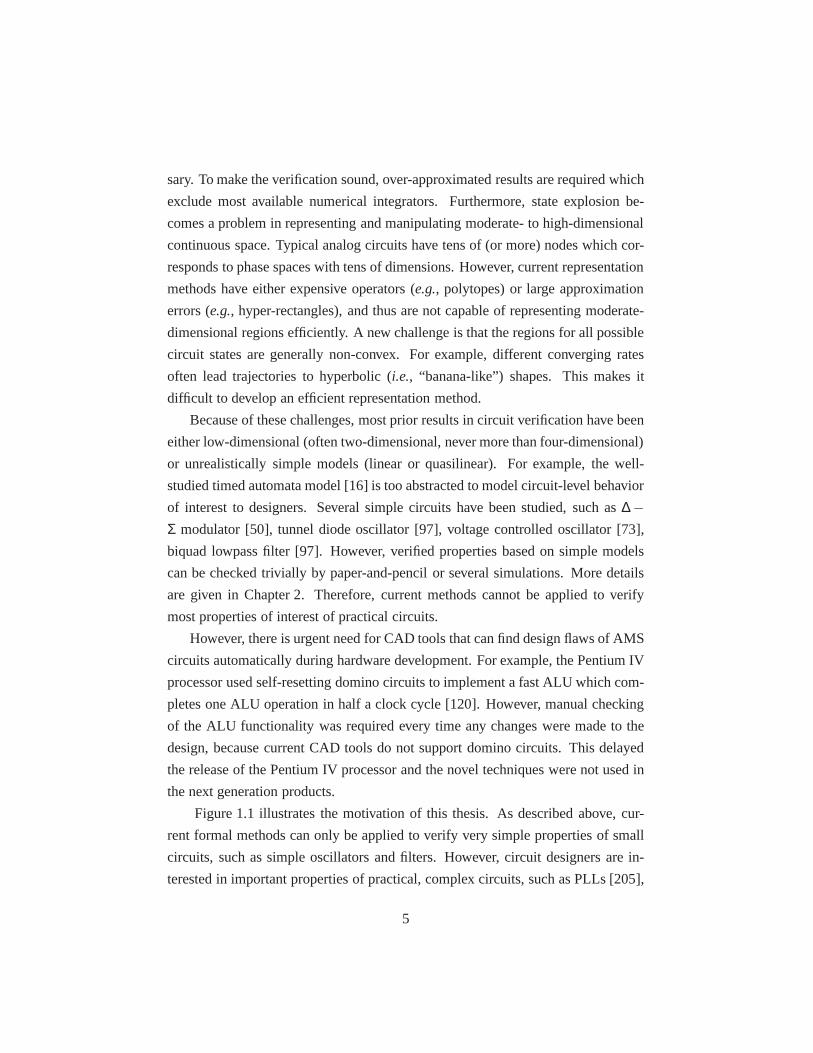
Because of these challenges, most prior results in circuit verification have been

either low-dimensional (often two-dimensional, never more than four-dimensional)

or unrealistically simple models (linear or quasilinear).For example, the well-

studied timed automata model [16] is too abstracted to modelcircuit-level behavior

of interest to designers. Several simple circuits have beenstudied, such as∆−Σ modulator [50], tunnel diode oscillator [97], voltage controlled oscillator [73],

biquad lowpass filter [97]. However, verified properties based on simple models

can be checked trivially by paper-and-pencil or several simulations. More details

are given in Chapter 2. Therefore, current methods cannot beapplied to verify

most properties of interest of practical circuits.

However, there is urgent need for CAD tools that can find design flaws of AMS

circuits automatically during hardware development. For example, the Pentium IV

processor used self-resetting domino circuits to implement a fast ALU which com-

pletes one ALU operation in half a clock cycle [120]. However, manual checking

of the ALU functionality was required every time any changeswere made to the

design, because current CAD tools do not support domino circuits. This delayed

the release of the Pentium IV processor and the novel techniques were not used in

the next generation products.

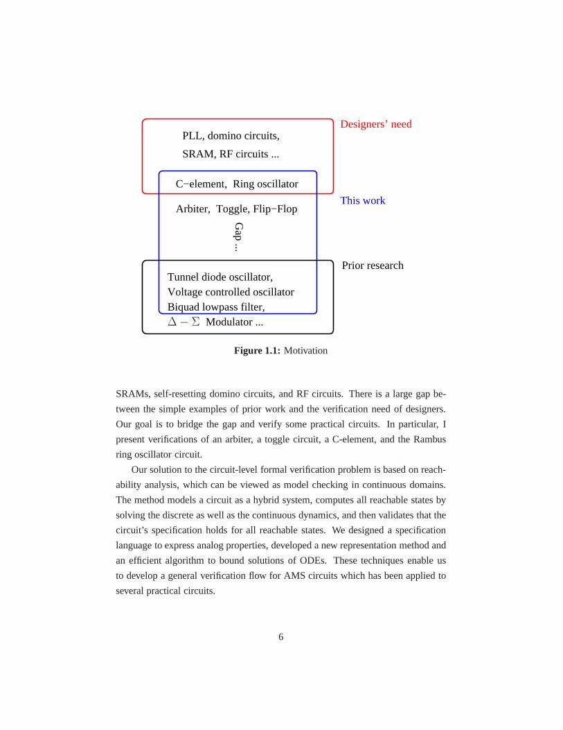
Figure 1.1 illustrates the motivation of this thesis. As described above, cur-

rent formal methods can only be applied to verify very simpleproperties of small

circuits, such as simple oscillators and filters. However, circuit designers are in-

terested in important properties of practical, complex circuits, such as PLLs [205],

5

Gap ...

PLL, domino circuits,

SRAM, RF circuits ...

Designers’ need

C−element, Ring oscillator

Arbiter, Toggle, Flip−Flop

Tunnel diode oscillator,Voltage controlled oscillatorBiquad lowpass filter,

Prior research

This work

Modulator ...∆− Σ

Figure 1.1: Motivation

SRAMs, self-resetting domino circuits, and RF circuits. There is a large gap be-

tween the simple examples of prior work and the verification need of designers.

Our goal is to bridge the gap and verify some practical circuits. In particular, I

present verifications of an arbiter, a toggle circuit, a C-element, and the Rambus

ring oscillator circuit.

Our solution to the circuit-level formal verification problem is based on reach-

ability analysis, which can be viewed as model checking in continuous domains.

The method models a circuit as a hybrid system, computes all reachable states by

solving the discrete as well as the continuous dynamics, andthen validates that the

circuit’s specification holds for all reachable states. We designed a specification

language to express analog properties, developed a new representation method and

an efficient algorithm to bound solutions of ODEs. These techniques enable us

to develop a general verification flow for AMS circuits which has been applied to

several practical circuits.

6

1.2 Problem Statement

Circuit-level verification is necessary to spot critical bugs before fabrication for

both AMS designs and deep sub-micron designs. Extending digital formal methods

to continuous domains requires novel techniques for modeling circuits, specifying

analog signals and desired properties, and solving non-linear dynamics to compute

circuit states.

Reachability analysis is a promising method for formal verification using circuit-

level models. To verify significant properties of large circuits, it is important to de-

velop efficient and accurate methods to support moderate-dimensional (e.g.,5-20)

systems with highly non-linear dynamics and non-convex reachable regions.

1.3 Contributions

This thesis demonstrates the feasibility of formally verifying circuit behaviors for

circuits modeled by non-linear, ordinary differential equations. This verification is

performed using projectagon-based reachability analysis.

In particular, this thesis explores reachability analysistechniques and provides

a reachability computation tool COHO for formal verification of digital or analog

circuits. This thesis makes contributions in the followingareas:

• We proposed techniques for modeling and specifying analog circuits and

their behaviors, which make it possible to perform circuit verification through

reachability analysis.

– We developed a method to model a circuit as a system of non-linear

differential equations (ODEs) automatically. Transistors are modeled

using a simple, table-based method, and other devices can besupported

similarly.

– We applied Brockett’s annulus to specify a family of analog signals.

Based on it, we presented an extended LTL logic that supportsdense

time and continuous state to specify analog properties of circuits. We

also introduced probability into the logic to describe circuit properties

such as metastability behaviors.

7

– We proposed a framework to convert verification problems to reacha-

bility computation problems by a method that we believe could be per-

formed automatically. We also suggested several techniques to obtain a

good trade-off between performance and error during the computation.

• We designed and implemented a robust and efficient reachability computa-

tion tool, COHO, for moderate-dimensional, non-linear, hybrid systems.

– We useprojectagonsto represent moderate-dimensional, non-convex

regions. We avoid performing operations with exponential complex-

ity on the high-dimensional objects. Instead, all operations are imple-

mented using efficient algorithms on the two-dimensional projections

or by linear programming on convex approximations of projectagon

faces.

– Highly non-linear dynamic systems are over-approximated by linear

differential inclusions which are solved efficiently. Linearization is per-

formed locally for each face of a projectagon to reduce approximation

error.

– We applied interval computation and arbitrary precision rational arith-

metic to develop a robust linear program solver and projection algo-

rithm which are essential to make COHO numerically stable. We also

proposed novel algorithms to reduce computation error and improve

performance of the reachability computation, including interval clo-

sure and an approximate LP solver.

– The COHO tool has been released to the public research community1.

• We have formally verified practical circuits including bothsynchronous and

asynchronous digital circuits, and analog circuits.

– We verified the Yuan-Svensson toggle circuit [217]. The output of the

toggle should transition once for every two transitions of the clock in-

put; in particular, the output makes a low-to-high or high-to-low transi-

tion for each rising transition of the clock. We found an invariant subset

1Available onhttp://coho.sourceforge.net

8

of circuit states and verified that all trajectories in this set have a period

twice that of the clock signal [210, 211]. Because the outputand clock

signal satisfy the same specification, an arbitrarily largeripple-counter

can be composed by using the output of one toggle to drive the input

of another one. This verification also revealed that we had neglected to

add keepers circuits to the design to ensure correct operation in spite of

the leakage currents in deep sub-micron designs. Once we added these

keepers, COHO verified the design.

– We showed that the output of a pass-gate latch circuit is stable when

its clock signal is at logical low value. Further, we demonstrated that

a flip-flop consisting of two latches works properly. The clock-to-q

delay and maximum clock frequency of this flip-flop have also been

measured.

– We formally specified and verified both safety and liveness properties

of a two-input, asynchronous arbiter circuit [212, 213]. Inthis verifi-

cation, we encountered thestiffnessproblem for reachability compu-

tations and proposed two solutions. We showed that all trajectories of

the arbiter are safe, and we extend the method from [160] to show that

the arbiter is live for all trajectories except for a set of measure zero.

– The Rambus oscillator challenge was posed by researchers from Ram-

bus, Inc [129]. The challenge is to show that a differential ring os-

cillator with an even number of stages starts properly from all initial

conditions. We combined static analysis and reachability computation

to find the conditions under which the circuit can oscillate as expected

from all initial states.

1.4 Organization

The thesis is organized as follows:

• Chapter 2 describes prior research in circuit verification and reachability

analysis. It also explores related formal verification methods and reacha-

bility analysis techniques as well as developed tools. Several circuits are

9

presented as verification examples to show abilities and limitations of avail-

able verification methods. Prior research on COHO is also presented at the

end of this chapter.

• Chapter 3 presents our framework for translating a circuit verification prob-

lem to a reachability analysis problem. It describes methods to construct

an ODE model from circuit netlists and obtain table-based models for tran-

sistors based on simulations. It also presents our specification method for

analog signals and properties which is based on Brockett’s annulus construc-

tion and LTL logic. It introduces circuit examples used in this dissertation

and provides formal specifications of properties to be checked. It also de-

scribes implementation issues that arise when computing linearized models

and modeling input signals.

• Chapter 4 describes our reachability analysis tool COHO. It first describes

the hybrid automata based interface and gives a high-level description of the

reachability analysis algorithm. It then presents detailsof the projectagon

representation method and operations on it. Based on these operations, al-

gorithms to compute continuous successors are developed, including solv-

ing linear differential inclusions, computing projections and constructing a

feasible projectagon. Techniques and approximation algorithms to improve

performance and accuracy are also discussed. Several implementation issues

such as the architecture of the COHO system are described at the end.

• Chapter 5 describes the digital and analog circuits that we have verified. It

first presents the general process for circuit verification using COHO and then

provides four examples: the toggle circuit, the flip-flop, the arbiter, and the

Rambus ring oscillator.

• Chapter 6 concludes the thesis and proposes future researchtopics.

10

2

Related Work

This chapter presents a survey of prior research related to AMS circuit verifica-

tion. Section 2.1 gives an overview of formal methods and discusses their pros

and cons. This includes equivalence checking, model checking and theorem prov-

ing. As reachability analysis is a promising and widely usedtechnique for model

checking, Section 2.2 presents existing solutions for its main challenges: model-

ing, specification and reachability computation. Section 2.2 also describes methods

to reduce system complexity and compares currently available tools. Section 2.3

presents applications of these techniques, mainly focusing on four circuits that

have been widely used as benchmarks. In addition to others’ work, Section 2.4 de-

scribes the development of COHO by others and myself prior to my Ph.D. program.

Section 2.5 summarizes both the contributions and the unresolved issues from prior

research.

2.1 Formal Verification of AMS Circuits

This section explores existing formal techniques for verifying circuits using ana-

log models. In practice, nearly all designers rely on simulations using SPICE and

similar programs to validate their AMS designs. Many extensions have been made

to the basic circuit simulation programs to improve simulation performance such

as Monte Carlo simulation (Spectre [1]) and fast Spice (Ultrasim [2]), increase

coverage [54], monitor simulation and check properties automatically (i.e., run-

11

time verification) such as AMT (Analog Monitoring Tool) [150, 151, 163] and

others [43, 59, 60, 138, 179, 220], or apply conservatively approximated models

such asFSPICE [193]. However, none of these tools can guarantee full coverage.

Formal techniques provide full coverage by considering alltrajectories of a circuit

starting from all possible initial conditions, and under all admissible variations on

parameter values. Like digital verification, formal methods for AMS circuits can

be grouped into three classes:equivalence checking, model checkingandproof-

based methods. To be sound, both equivalence checking and model checking must

determine all reachable circuit states in order to perform comparisons or verify

properties. Computing the complete reachable space is, in general, an undecidable

problem unless the system dynamics are extremely simple [12, 109, 137, 173].

Therefore, approximation techniques must be applied.Discretizationmethods dis-

cretized the continuous state space into a discrete one, forwhich reachable sets

can be computed by well-developed digital verification tools. On the other hand,

reachability analysisapproaches try to find a reasonable approximated result using

efficient methods to represent continuous regions and solvecontinuous dynamics.

Theorem-proving based methods attempt to avoid the state-space explosion prob-

lem by constructing a formal proof. However, the problems they are addressing are

still undecidable. Furthermore, it relies on human insightand effort to create such

a proof.

2.1.1 Equivalence Checking

Equivalence checking determines whether two systems are equivalent according to

some criteria such as input/output behaviors. In [188], Steinhorst and Hedrich pro-

posed an equivalence checking method for analog circuits based on their system

dynamics. Given two circuits, the method samples their state spaces, constructs a

linear mapping between sampled points in each small region,transforms dynamics

into a canonical state space, and checks if they are the same to within some toler-

ance. Another approach was developed in [178] for comparingtwo VHDL-AMS

designs. It applies rewriting rules and pattern matching tosimplify analog compo-

nents and uses classical SAT/BDD equivalence checkers for digital components.

12

2.1.2 Model Checking

Model checking is a powerful technique for determining whether a mathematical

model of a system meets a specification automatically. The first practical successes

of model checking were for discrete systems, and this has motivated extending

these techniques to handle designs with continuous models.There are two main ap-

proaches:discretizationwhich approximates continuous models by discrete ones,

andreachability analysiswhich solves continuous dynamics directly.

Discretization

The idea ofdiscretizationtechniques is to convert a model checking problem in a

continuous space to a discrete problem by discretizing space and time. Typically,

these approaches partition the entire state space into hyper-rectangles, calculate

transitions between these boxes using simulations or approximation techniques,

and generate a finite-state system such as finite-state machines, transition systems,

or graphs. Conventional model checking algorithms can be applied to these dis-

crete systems. Refinement is used when the approximation error is large.

The first work using circuit-level models was by Kurshan and McMillan [133].

The algorithm first partitions the continuous state space representing the charac-

teristics of transistors into fixed size hyper-cubes and divides continuous time into

uniform time steps. Input signals are divided similarly butonly logic low and high

regions are used with the assumption of instantaneous transitions. Second, the al-

gorithm computes the transition relation between these hyper-cubes using the lower

and upper bounds of the continuous dynamics. The final constructed model is ver-

ified against properties defined byω-language using a language containment tool,

COSPAN [96]. The partition is refined manually and the procedure is repeated if

the verification fails. A similar technique is used in [56] tocheck AnaCTL specifi-

cations1. However, transitions are constructed using SPICE simulations.

The simple approach for discretization proposed by Kurshanand McMillan

has been generalized in the AMCHECK [97, 98] tool by Hartonget al. AMCHECK

makes several improvements on Kurshan and McMillan’s approach. First, it uses a

1Specification languages in this section, including AnaCTL,CTL, CTL-AT, CTL-AMS, and ASL,will be described in Section 2.2.2.

13

varied time step rather than a constant one. Second, refinement is performed auto-

matically on the initial uniform partitions. This procedure is continued recursively

until behaviors of every box are uniform which is defined based on the length and

direction of vector fields. Third, they proposed three algorithms for computing the

transition relation between boxes. The first method computes an overestimated so-

lution by interval analysis. The second approach uses simulations from a number

of test points. The method used in Kurshan’s work is a specialcase of this ap-

proach, which exploits the fact that the transistor drain-to-source current is mono-

tonic. This is valid for the device models used in practice and allows Kurshan

and McMillan to use the lower and upper corner values to boundthe dynamics.

The third approach makes the second process rigorous using Lipschitz constants

of nonlinear functions. However, similar to Kurshan’s work, it also assumes that

the values of input signals do not change at all or change instantaneously over the

whole input value range. AMCHECK converts the nonlinear analog systems to a

transition graph on which CTL specifications can be verified.The transition graph

is augmented with delay information in [81]. Therefore, properties specified by

CTL-AT [81] or ASL [187] can be checked. A similar tool MSCHECK is imple-

mented in [126] where properties are specified by CTL-AMS.

Discretization methods leverage the extensive work in developing model check-

ers for digital designs. However, the number of hyper-rectangles in the discretiza-

tion increases exponentially with the number of dimensions. Refinement strategies

increase the number of hyper-rectangles, and this increasecan be dramatic. There-

fore, discretization methods are only suitable for small circuits.

Reachability Analysis

Reachability analysiscompletely explores the state space of a system by solving

both the continuous and discrete dynamics. There are two main types of analysis.

Forward reachabilitystarts with initial states and follows trajectories forward in

time. Backward reachabilitystarts with target states and follows trajectories back-

ward in time. In this dissertation, we distinguish two different kinds ofreachable

regionsthat a reachability algorithm might generate: areachable setis the set of

states occupied by trajectories at some specified time, and areachable tubeis the

14

set of states traversed by those same trajectories over all times in a closed or un-

bounded interval. Forward and backward versions of both reachable sets and tubes

can be specified.

A general framework of reachability algorithms can be obtained based on fixed-

point computations. In each iteration, a new (forward) reachable set is computed

by applying thepostc and postd operators to the current reachable setS, where

postd(S) is thediscrete successordefined as the set of states reachable by taking a

transition from a state inS, andpostc(S) is thecontinuous successordefined as the

set of states that result by letting time elapse without state transitions. The compu-

tation of postd is the same as for discrete model checking. Therefore, solving the

continuous dynamics of thepostc operator is, in general, the biggest challenge and

the most expensive step of reachability analysis for continuous or hybrid systems.

Various of techniques have been proposed which will be discussed in Section 2.2.4.

The reachable tube over this time step is usually overestimated based on reachable

setsS and postc(S), e.g., the bloated convex hull ofS and postc(S). Backward

reachability analysis is performed similarly usingprec and pred operators. For-

ward algorithms terminate when no new reachable states are found. Conversely,

backward algorithms terminate when no further restrictions of the safety set are

found. However, termination of algorithms is not guaranteed even for highly re-

stricted models [109]. Thus, each of these algorithms must fail for some inputs.

This failure could be a failure to terminate, an incorrect rejection of a correct de-

sign, or an incorrect acceptance of an incorrect design. In averification context,

it is important that the particular limitations of a particular tool are clearly and

correctly identified.

There are several reachability analysis tools for systems with continuous state

and/or time that have been developed in recent years. We listthese tools here for

the discussion in the remainder of this chapter. Detailed features of these tools will

be presented in Section 2.2 and summarized in Section 2.2.6.These tools include

MOCHA [18], UPPAAL [20], KRONOS[216], TAXYS [30, 45], RED [203] for real

time systems; HYTECH [104], PHAVER [70], LEMA [144] for hybrid systems

with constant dynamics, and HYPERTECH [107], D/DT [48], CHECKMATE [40]

for hybrid systems with linear or non-linear dynamics. There are also several

tools that have been developed by researchers in the controlcommunity includ-

15

ing VERISHIFT [31], TOOLBOXLS [159] and zonotope based analysis [77, 79].

In [75], Frehse and Ray present a tool framework, SPACEEX, to integrate and

compare different algorithms and features. Some constraint based solvers such

as HYSAT [116], HSOLVER [177] have also been used in circuit verification.

Most circuit behaviors can be modeled by nonlinear dynamics, with non-deter-

minism as needed to account for uncertainties in the model, parameter values, in-

put, and operating conditions; thus, reachability analysis has the potential of verify-

ing complex properties of real circuits. However, these dynamics,e.g.,differential

equations, generally do not have closed form solutions. Therefore, approximation

techniques must be applied. Furthermore, reachability tools suffer from the state-

space explosion problem. In addition to solving complex dynamics, all model

checking methods require formal models for circuits and properties to be verified.

Solutions to these challenges will be discussed in Section 2.2.

2.1.3 Proof-Based and Symbolic Methods

Theorem provingestablishes design properties by using formal deduction based on

a set of inference rules. In addition to deductive based methods, induction and

symbolic based methods have also been proposed to verify circuits. In [76], Ghosh

and Vemuri used the higher-order-logic proof checker PVS toverify DC and small

signal behaviors of synthesized analog circuits. They usedpiece-wise linear ap-

proximation to model each component, and a subset of VDHL-AMS language to

specify properties. A similar but more elaborate approach was taken by Hanna

in [94] for digital systems with analog-level abstraction.The circuit behavior is

characterized by conservative rectilinear [95] or piece-wise linear predicates over

the voltages and currents at the devices’ terminals. Al Sammaneet al. [180] trans-

formed circuits to system of recurrence equations (SRE) by rewriting rules, and

proved correctness using an induction based verification strategy. The work was

extended in [219], where Taylor approximations and interval arithmetic were ap-

plied in a bounded model checker to generate the SRE model andcheck properties.

In principle, symbolic theorem proving methods do not suffer from the state-

space explosion problem of model checking techniques. However, they require

substantial human insight and intervention. First, they require a formalization of

16

the underlying theory. Embedding calculus including dynamical systems theory

and circuit modeling into a theorem prover would be a huge undertaking. Second,

we would still face the problem that the models do not have symbolic solutions,

i.e., most ODEs do not have solutions in terms of polynomials and elementary

functions. Therefore, approximation techniques must be applied even if we use a

theorem prover. Then, all of the questions of how to represent high-dimensional

regions, how to approximate solutions to ODEs, and how to bound reachable sets

would still apply. Furthermore, many problems are not decidable. There is no

guarantee that a proof (or counterexample) exists, or that the human and theorem-

prover can find it if does.

Discretization, reachability analysis, and theorem proving offer three basic ap-

proaches for formally verifying properties of circuits. Inthis thesis, we focus on

reachability methods. We will show that by using a suitable representation of re-

gions in the continuous state space, reachability computations can overcome the

state-space explosion problems that have restricted discretization methods to low-

dimensional models. Furthermore, reachability methods donot face the need of

finding symbolic solutions to ODEs, and thus can be used with realistic circuits

more readily than the theorem proving based methods that we have seen.

2.2 Reachability Analysis of Hybrid Systems

As described in the previous section, reachability analysis, which models AMS cir-

cuits as hybrid systems, is a promising technique for practical circuit verification.

This section presents reachability analysis techniques and tools. Any verification

method must start with a model and a specification, which translates a physical

problem into a mathematical problem. Typically, models build on well understood

abstractions such as automata or Petri nets with extensionsto incorporate continu-

ous dynamics. Section 2.2.1 examines various models that have been developed by

the hybrid-systems community. Section 2.2.2 goes on to lookat specification meth-

ods, for example, extensions of traditional temporal logics to systems with contin-

uous state. Most prior work has focused on verifying safety properties of hybrid

systems; this amounts to computing (over-approximations of) the regions that can

be reached by the model. Such computations require a tractable way to represent

17

multi-dimensional regions and a way to compute the evolution of such regions ac-

cording to the continuous dynamics of the system. Section 2.2.3 describes many of

the most common representations for multi-dimensional regions, and Section 2.2.4

presents algorithms for advancing these regions accordingto continuous dynamics.

The challenges of representing and manipulating multi-dimensional objects moti-

vates developing methods to reduce the complexity of the models and analysis.

Section 2.2.5 describes such methods. Other surveys of tools for hybrid systems

can be found in [22, 28, 185, 201, 221].

2.2.1 Models

This section introduces some commonly used models for hybrid systems, including

hybrid automata, hybrid Petri nets and transition systems.Methods of extracting

continuous dynamics from circuit netlists are summarized at the end of this section.

A formal model for hybrid systems is aHybrid Automaton (HA)[9, 105]. Hy-

brid automata have several similar definitions from different research groups. In-

formally, a hybrid automaton is a finite state machine augmented with continuous

variables and dynamic equations. It consists of a graph in which eachvertex, also

calledlocation, or mode, is associated with a set of ordinary differential equations

(ODEs),x= f (x), or ordinary differential inclusions (ODIs), ˙x∈ F(x), that define

the time driven evolution, referred to asrate, derivativeor flow, of continuous vari-

ables. A stateconsists of a location and values for all continuous variables. The

edgesof the graph, also calledtransitions, allow the system to jump between loca-

tions, thus changing the dynamics, and instantaneously modifying variable values

according to ajump condition. The jump may only take place when variable val-

ues satisfy a certain condition, specified by aguard, associated with each transition.

The modified values for continuous variables after the transition are also referred

to as thereset map. The system starts from one or more locations labeled asinitial

and may only remain in a location as long as the variable values are in a region

called theinvariant associated with the location.

Hybrid automata can be classified by their associated dynamics. Timed Au-

tomata (TA)[12] are a simple class of hybrid automata in which all continuous

variables have a derivative of+1, i.e., they are “clocks”.Linear Hybrid Automata

18

(LHA) [100] represent dynamics using linear differential inequalities of the form

Ax ≤ b. However, TA or LHA are generally not expressive enough to accurately

model systems with complex dynamics, especially nonlinearAMS circuits. A

more powerful model isLinear Dynamical Hybrid Automata (LDHA)2 which has

linear dynamics, such as linear ODEs or linear differentialinclusions. Nonlinear

Hybrid Automata (NHA)support arbitrary nonlinear differential equations. The

reachability problemof hybrid automata is to determine if a target state is reach-

able from an initial state. It is undecidable even for quite simple automata such

as LHAs [12]. More results about decidability of hybrid automata can be found

in [109, 137, 173]. Thus, verification procedures for hybridautomata must use

approximate algorithms. We examine trade-offs made in making these approxima-

tions when we describe various tools in the remainder of thischapter.

Hybrid automata are widely used by many tools, such as TAs by KRONOS[57],

LHAs by HYTECH [105], LDHAs byD/DT [25], and NHAs by TOOLBOXLS [194].

Models employed by other tools are listed in Table 2.1. A complex automaton is

usually approximated by several simpler ones. For example,UPPAAL [140] and

HYTECH [105] developed methods to transform LHAs to TAs, and PHAVER [70]

approximates LDHAs by LHAs.

Several similar modeling frameworks have been used by reachability analysis

tools. For example, the linearHybrid Input Output Automata (HIOA)[74] used in

PHAVER extends LHAs by specifying some variables as inputs and outputs. Hy-

brid Petri netscombine discrete Petri nets and continuous Petri nets.Timed Hybrid

Petri Nets (THPN)[147] and enhancedLabled Hybrid Petri Nets (LHPN)[146]

are employed in LEMA. However, rates of continuous variables in THPNs or

LHPNs are either constant values or interval values, hybridPetri nets with com-

plicated dynamics have not been studied.Transition systems[149] consist of a

set of finite or infinite states, a transition relation and a set of initial states. They

are widely used to abstract away continuous behaviors of hybrid automata in the

abstraction-refinement strategy which will be discussed inSection 2.2.5. For ex-

ample, CHECKMATE [41] constructs aDiscrete-Trace Transition System (DTTS)

from its Polyhedral Invariant Hybrid Automaton (PIHA)model in a bisimulation

2It is called linear hybrid systems in some papers.

19

based model checking algorithm.

To model an analog or mixed-signal circuit, continuous dynamics must be ex-

tracted from its netlist in advance. The first approach is based onmodified nodal

analysis. For example,bond graphsare used to describe a circuit in [58], from

which ODEs can be generated automatically. Another approach is based on tableau

data from simulation traces. For example, LEMA uses aSimulation Aided Verifi-

cation (SAV)[145] method to generate LHPN models automatically. The method

partitions the state space into boxes based on user providedthresholds and calcu-

lates bounds of dynamics from the simulation data.FSPICE [193] also uses conser-

vative tables which represent the I-V relationships of circuit devices by intervals.

The first approach is similar to the one used in simulators andis well-studied.

However, the second approach can handle uncertain inputs, PVT variations, distur-

bances and noise. It is especially attractive for small circuits. For large systems, an

intractably large number of simulations are often requiredto obtain a reasonable

coverage.

In summary, formal models for circuits are often constructed by deriving the

continuous dynamics from the netlist using modified nodal analysis, and then cre-

ating a hybrid automaton to partition the trajectories of the model into bundles

of interest. We follow this framework in our tool as shown in Section 3.3 and

Section 4.1.

2.2.2 Specification Languages

Having examined some of the most common methods for modelinghybrid systems,

we now consider how the analog properties can be specified. Temporal logics are

the most popular formalism for specifying properties of digital circuits, such as

Linear Time Temporal Logic (LTL), Branching Time Temporal Logic(e.g.,CTL).

TheAccellera Property Specification Language(PSL, a.k.a. IEEE P1850) [64] is a

specification language that contains LTL and CTL as subsets and is supported by

various commercially available verification tools. These discrete temporal logics

can be applied directly to represent properties of a hybrid system. For example,

Kurshanet al. usedω-languages to specify properties of the transition graph in

their discretization based algorithm [133]. CHECKMATE checks properties spec-

20

ified by ACTL [40, 89], which is a universal fragment of CTL without existential

paths.

However, conventional temporal logics are based on discrete time and state and

cannot express properties with continuous variables and dense metric time. There-

fore, several researchers have extended temporal logics with time and real-valued

variables. Generally, timed logic is obtained by putting constraints on temporal

operators to limit their scope in time. For example,Real Time CTL (RTCTL)[63]

uses superscripts to bound the maximum number of permitted transitions along a

path. Timed CTL (TCTL)[8] puts subscripts on the temporal operators to limit

the lower or upper bound of accumulated time over paths.Metric Interval Tempo-

ral Logic (MITL)3 [13] constrains the LTL temporal operators with time intervals.

On the other hand, continuous space is supported by introducing real-valued vari-

ables and predicates to the logic. For example,Analog CTL (AnaCTL)[56] adds

propositions based on linear predicates over continuous variables to CTL. Simi-

larly, PSL has been extended to support continuous space by using linear pred-

icates in the boolean layer [179]. However, these logics still use discrete time.

Temporal logics that support both dense time and continuousstate space have also

been developed.Analog and Timed CTL (CTL-AT)[81, 98] constrains temporal

operators by intervals and expresses continuous regions bylinear predicates.CTL-

AMS[125] extends CTL-AT by supporting unconstrained time (or the time interval

is [0,∞]) over temporal operators.Continuous-Time CTL (CT-CTL)[220] extends

TCTL with predicates. Signal Temporal Logic (STL/PSL)[150, 152] combines

MITL with linear predicates which map analog signals to boolean variables. Fur-

thermore,Integrator CTL (ICTL)[100] supports accumulated time by introducing

integrator variables. These extensions have been applied in many tools. For ex-

ample, LEMA [199] uses TCTL, HYTECH [16] and PHAVER [70] uses ICTL.

Table 2.1 on page 35 lists some of the main tools from the research literature along

with the temporal logics that they support.

Although these temporal logics can express many important properties of hy-

brid systems, they cannot specify many analog properties directly. Therefore,

designer-oriented languages have been proposed. AnaCTL supports waveform

3It is calledMITL[a,b] in some papers.

21

propositions by comparing signal values with reference waveforms provided by

equations or tables generated by users. STL specifies continuous variables by par-

tial functions and supports operations on signals such as concatenation, projec-

tion, and comparison with a reference signal. STL/PSL [163]extends STL with

a layered approach in the fashion of PSL. It uses an analog layer to reason about

continuous signals directly.Mixed-Signal Assertion Language (MSAL)[138] is

based on PSL and supports digital, analog and software properties. However, these

languages are for assertion based verification and only cover signal-based proper-

ties. TheAnalog Specification Language (ASL)[187, 189] is designed for describ-

ing properties of analog systems over a continuous region. For an operator and

a bounded region, it applies the operator to every point in the region and calcu-

lates the range of values based on interval arithmetic. It also supports operations

such as derivative computation, oscillation and start-up time. It is compatible with

CTL-AT and has been implemented in AMCHECK.

There are some other methods, such astimed regular expression[21], and the

method proposed in [74] which constructs a LHA for a property. However, most

specification techniques are still based on temporal logics. Digital temporal logics

have been extended to express properties of real-time systems but are not yet pow-

erful enough to express most properties of interest for AMS circuits. For example,

we are not aware of any specification approaches that formalize frequency domain

properties which are very important for circuit analysis. Many of these extended

logics are for signal-based properties and thus cannot be applied to reachability

analysis based verification directly. It is still a major challenge to make the analog

verification as fully automated as the current state of the art for digital model check-

ing tools. Furthermore, temporal logics are not familiar tomost circuit designers.

Therefore, more expressive designer-oriented languages are needed.

2.2.3 Representation Methods

Given a mathematical model and a formal specification, reachability analysis com-

putes reachable regions according to the model and checks ifall these regions sat-

isfy the specification. This requires techniques to represent multi-dimensional re-

gions and algorithms to compute the evolution of these regions according to the

22

a. polytope b. convex polytope

template

d. template polyhedra e. rectangle

c. flow pipe

g. orthogonal polyhedra

f. ORH

b

a

h. zonotope i. ellpsoid

Figure 2.1: Representation Examples

model. In this section, we describe approaches to representing multi-dimensional

regions, and Section 2.2.4 examines algorithms for computing reachable sets ac-

cording to continuous dynamics.

The representation of regions in continuous state spaces iscrucial for reach-

ability algorithms as it usually determines the efficiency of algorithms and ac-

curacy of results. This section describes several commonlyused representation

methods along with operations on them. We first explore geometry based meth-

ods, including polytopes which have the advantage of accuracy, hyper-rectangles

or intervals aimed to maximize efficiency, zonotopes which are closed under sev-

eral important operations, and ellipsoids. Figure 2.1 illustrates these methods by

a simple two-dimensional example. We then examine some symbolic data struc-

tures, including widely used BDD-like structures and support functions. The op-

23

erations used in reachability analysis include union, intersection, and intersection

with hyperplanes. Some reachability algorithms also require theMinkowski sum

operation. The Minkowski sum of two setsA and B in Euclidean space is de-

fined as the result of adding every element of A to every element of B, i.e., the set

A⊕B= {a+b|a ∈ A,b∈ B}. The selection of a good representation depends on

reachability algorithms, complexities of dynamics, trade-off of performance and

accuracy, and so on. Exact representation is generally impossible due to the com-

plexity of the geometry or dynamics. Therefore, approximation is widely used. For

many reachability analysis algorithms, the errors from approximating the reachable

region accumulate over successive time steps of the computation. This is known as

thewrapping effect.

Polytopes

Polytopescan represent a bounded convex or non-convex region with arbitrarily

small errors. However, the space and time complexity of operations on non-convex

polytopes are generally exponential with the number of dimensions. Therefore,

convex polytopesare used in practical tools. There are two commonly used repre-

sentations for convex polytopes: theinequality representationand theframe rep-

resentation. The first approach represents a half-plane by a linear inequality; thus

some operations such as intersection can be implemented efficiently by manipulat-

ing system of inequalities. The second approach representsan object by points and

rays and has other efficient operations such as convex hull. Translations between

these two representations can be computed by several algorithms [39, 143].

Convex polytopes are generally used to represent reachablesets for TAs or

LHAs which have exact reachability algorithms. Both HYTECH and PHAVER

employ convex polytopes, furthermore, HYTECH also supports unbounded regions

by widening[9] or extrapolation[102] techniques. HYTECH uses Halbwachs’ li-

brary [92, 93] for polytope operations which uses limited precision rational num-

bers. Therefore, HYTECH suffers from the overflow problem. To overcome the

limitation, PHAVER uses the Parma polyhedra library [27] which supports arbi-

trary precision rational numbers. For more complex dynamical systems, reachable

regions cannot be represented exactly and the wrapping effect must be considered.

24

CHECKMATE developed aflow pipe representation [41], which is essentially a

convex polytope with the inequality representation, to over-approximate reachable

tubes estimated from simulation traces. It avoids the wrapping effect by restarting

simulations from initial regions in each step.

When a system has non-linear dynamics, a line-segment can evolve to a more

general curve. Accordingly, polytopes are not closed underevolution with non-

linear dynamics, and approximations must be used. In principle, these approxima-

tions can be made arbitrarily precise by using a polytope with enough faces, but

the space and time required to represent and operate upon such polytopes quickly

become intractable.Template polyhedra[181] have been proposed to limit the

complexity of reachable sets. These are polytopes whose inequalities have fixed

expressions (template) but with varying constant terms. Therefore, the number of

faces of a template polyhedron does not increase with successive time steps. How-

ever, it can produce large approximation errors, and it is a challenging problem to

find a good template4.

Rectangles

Polytope-based representations are accurate but expensive. At the other extreme,

thehyper-rectanglerepresentation optimizes performance at a cost of large approx-

imation errors. The space complexity of hyper-rectangles is linear with the number

of dimensions, and the time complexities of operations on hyper-rectangles are

typically small. Many interval arithmetic algorithms use interval-valued variables

where the valid solution is equivalent to a hyper-rectangle. For example, HYPER-

TECH [107] uses an interval based ODE solver. HYSAT [66] also applies interval

arithmetic to solve nonlinear constraints and ODEs.

Several variations of hyper-rectangles have been developed to improve accu-

racy. D/DT developed techniques based on orthogonal polyhedra [33]. Orthogonal

polyhedra represent a region as the union of a finite number ofuniform or non-

uniform hyper-rectangles. This representation allows arbitrarily small approxima-

tion errors by using sufficiently small hyper-rectangles, but the number of rectangle

needed to represent a region grows rapidly with decreasing hyper-rectangle size.

4Flow pipes are essentially template polyhedra where the template is computed from simulationresults.

25

The Oriented Rectangular Hull (ORH)representation [191] reduces approxima-

tion error by rotating a rectangle to an orientation that is chosen according to the

dynamics of the system. The space complexity of ORH is quadratic with the num-

ber of dimensions. However, ORH is not closed under operations such as union

and intersection. Theface region[167, 172] representation over-approximates a

n-dimensional region by the convex hull of a set of(n−1)-dimensional hyper-

rectangular faces with one dimension fixed to a constant value.

Zonotopes

A zonotope is a polytope which can be represented as the Minkowski sum of seg-

ments. The order of a zonotope is defined as the ratio of the number of segments

to the number of dimensions. Particularly, a hyper-rectangle5 is a special zono-

tope with order 1. Zonotopes have many attractive features.First, they are closed

under linear transformations and Minkowski sum operations, and there are effi-

cient algorithms for implementing these operations. Second, the representation is

very compact. However, zonotopes have two main drawbacks. First, the order of

zonotopes increases after each Minkowski sum operation. Toreduce the order of a

zonotope, an efficient algorithm was proposed in [77] to compute an approximation

of the zonotope. However, the approximation causes wrapping effect errors. Sec-

ond, it is expensive to compute the intersection of a zonotope and a hyperplane. An

efficient approximate algorithm was proposed in [78] by projecting the zonotope

onto two-dimensional planes.

Ellipsoids

A promising representation from the control community isellipsoids [134]. A

d-dimensional ellipsoid is specified by a center point and itsd axis vectors. Al-

gebraically, an ellipsoid can be described as the set of all points x satisfying6:

xTAx≤ 1. This is similar to an oriented hyper-rectangle that can beexpressed by

systems of inequalities:Ax≤ 1. Like the ORH representation, the space com-

plexity for the ellipsoidal representation is quadratic inthe number of dimensions,

5More generally, zonotopes of order 1 are the set of parallelepipeds.6The mathematical formxT Ax≤ 1 is for ellipsoids centered at the origin; a more general form is

(x−xc)TA(x−xc)≤ 1.

26

and the time complexity of ellipsoidal operations is also polynomial. Furthermore,

a reachable region can be approximated with an arbitrarily small error through

intersection (union) of a family of external (internal) ellipsoids. Operations on

ellipsoids are implemented in the Ellipsoidal Toolbox [135] and in [31].

Symbolic Data Structures

In addition to geometry based representations, symbolic functions have also been

used in reachability analysis tools. For example, TOOLBOXLS uses implicit sur-

face functions to represent sets [161]. An implicit surfacefunction for a subset of

a given state space is a scalar function defined over the entire state space whose

value is negative inside the subset, positive outside, and zero on the boundary.

Implicit surface functions can represent sets with an interior exactly; however, rep-

resentation of the implicit surface function itself often requires an amount of data

(e.g.,function values on a grid) which increases exponentially with dimension. A

support function[90], employed in the SPACEEX tool, is a function that bounds

the maximum value on all possible directions. They can represent a convex set

with arbitrary precision and have efficient algorithms for union, Minkowski sum as

well as affine transformation operations. However, it lacksan efficient intersection

operation. An over-approximation can be computed based on the projection con-

cept [90] which is similar to the algorithm for zonotopes [78]. The well-developed

BDDs and BDD-like structures are also used in reachability analysis tools, includ-

ing Difference Bound Matrices (DBMs)[146] in LEMA, Multi-Terminal BDDs

(MTBDDs)[126] in MSCHECK, Clock Difference Diagrams (CDDs)[20] in UP-

PAAL, Clock Restriction Diagrams (CRDs)[200], andHybrid-Restriction Dia-

grams (HRDs)[202] in RED.

Summary

The choice of representation for reachable regions has a strong impact on the ef-

ficiency of analysis techniques. Prior representations have various trade-offs be-

tween the complexity of the model and the number of dimensions of a region that

can be efficiently represented. To support complicated, non-linear dynamics, these

methods are restricted to low-dimensional models. Conversely, some represen-

27

tations such as zonotopes [79] and support functions [71] have been used with

higher-dimensional models, but these applications have been restricted to linear,

and piecewise-linear models. Furthermore, most prior methods can only represent

convex regions. The exceptions to this are level sets and collections of hyper-

rectangles that are only practical for representing low-dimensional sets. The tra-

jectories that arise from circuit models are often roughly hyperbolic, and this gives

rise to non-convex reachable regions, where the non-convexity is critical to verify-

ing the circuits. There remains a need for ways to represent moderate-dimensional

(e.g.,ten to twenty dimensions), non-convex regions with nonlinear dynamics.

2.2.4 Solving Dynamics

One of the most challenging aspect of computing reachable regions is solving con-

tinuous dynamics. Commonly used dynamics for hybrid systems includeOrdinary

Differential Equations (ODEs), Ordinary Differential Inclusions (ODIs), Differ-

ential Algebraic Equations (DAEs)and Difference Equations (DEs). Usually,

ODEs are used to describe deterministic dynamics; and ODIs are used to describe

non-deterministic dynamics (e.g., inputs, and noise) or to conservatively approx-

imate complicated dynamics. DEs are used for discrete-timesystem and can be

solved easily in many cases. DAEs are generally solved by transforming them to

ODEs, for example, they are converted to the semi-explicit form in [50]. Therefore,

this section focuses on computing the forward reachable setpostc(S) as shown in

Section 2.1.2 with dynamics modeled by ODEs or ODIs.

ODEs includeclock ODEsof the formx= 1, constant ODEsof the formx= c,

linear ODEsof the form x = Ax+ b, andnonlinear ODEsof the form x = f (x).

Two commonly used ODIs areconstant ODIsof the form x ∈ [cl ,ch] or Ax ≤ b

andlinear ODIsof the formx∈ Ax+U , whereU is a set or region used to model

uncertainty, non-determinism or errors. Table 2.1 on page 35 lists the forms of

dynamics supported by many of the tools reported in the research literature. We

first describe reachability algorithms for constant dynamics briefly as they can be

solved efficiently and exactly. We then describe methods forsolving linear ODEs

or ODIs, including theoptimal controland theMinkowski summethods. We focus

on nonlinear ODEs because they are used to model AMS circuits. We survey

28

related techniques to compute approximated solutions, includinghybridizationand

level sets.

Constant ODEs and Constant ODIs

Mathematical solutions exist for some simple dynamics, including clock ODEs,

constant ODEs, and constant ODIs. Therefore, reachable regions are generally

computed exactly for TAs and LHAs by either symbolic manipulation or geometric

operations. Model checking algorithms for TAs and LHAs can be found in [8, 110,

112, 201] and are used in several tools including UPPAAL [139], KRONOS [32],

LEMA [198, 199], HYTECH [122], and PHAVER [73].

Linear ODEs and Linear ODIs

The solution of a linear ODE, ˙x = Ax, is x(t) = eAtx(0). However, the problem

of finding reachable sets for ODIs is more difficult. The challenge lies in the un-

certainty setU . Typically, U has the form of a hyper-rectangle or other convex

polytope. The vertex ofU that leads to an extremal trajectory can change during

a time-step. Exact computation of the extremal trajectories is difficult; thus, prac-

tical tools use various forms of over-approximation. Two approaches have been

developed for computing a conservative approximationR of forward reachable set

with linear ODIs. The first method,optimal control, is based on the maximum

principle of the optimal control theory [197]. This method finds the optimal input

u∗(t) which leads to the boundary ofR and numerically computes the integration.

The optimal input for a hyperplane with normal vectord is a functionu∗(t), where

at timet, u∗(t) is a valueu∈U that maximizese−ATtd ·u. The second method is

based onMinkowski sumand approximates the reachable region by the Minkowski

sum of a regionR and an error regionE as the equationR∈ R⊕E. The region

R is computed using the autonomous dynamics ˙x = Ax (i.e., Ri+1 = eAδ tRi) and

the error regionE accounts for the influences of inputs or disturbances. The er-

ror region can be bounded using error analysis. For example,for any nonlinear

ODE with Lipschitz constantL, the radiusr of the error regionE is bounded by

r = ||R− R|| ≤ µ2 (e

Lδ t −1), µ = maxu∈U ||u||, which is proved by the fundamental

inequality theorem from the theory of dynamical systems [23].

29

An example of the first approach is theD/DT tool [197]. It assumes the uncer-

tain setU is a bounded convex polytope and finds the optimal input by linear pro-

gramming. The zonotope based method in [77] uses the Minkowski sum method.

It constrains setU as a hyper-rectangle, and approximates the error regionE as

a hyper-rectangle and consequently a zonotope with radiusr = e||A||δ t−1||A|| µ . Based

on this method, a reachability algorithm was developed in [79] which is free of

the wrapping effect. VERISHIFT also employs the Minkowski sum approach and

approximates the error regionE using the Hausdorff semi-distance of reachable

sets [31].

Nonlinear ODEs

Unlike linear ODEs, nonlinear ODEs do not, in general, have closed-form solu-

tions; thus approximation techniques must be applied. Thehybridizationmethod

partitions the state space into small regions and bounds thenonlinear dynamics by

simple ODIs in each region. Theset integrationmethod extends numerical inte-

gration to reachability analysis by interval arithmetic and Taylor expansion. The

constraint basedapproach transforms ODEs to constraints which can be solvedby

constraint solvers. Other methods such aslevel set, flow pipeand methods for some

special classes of nonlinear ODEs are presented at the end ofthis section.

The idea ofhybridizationis to (over-)approximate complex dynamics by sim-

pler ones which can be solved efficiently. The approximationis calculated in

a small region in order to obtain small error. Therefore, thehybridization pro-

cedure usually consists of two steps: partitioning the state space of the system

into small regions, and computing an (over-)approximationof the solution. Of-

ten, the state space is discretized into disjoint regions, such as hyper-rectangles

or simplexes [24]. To obtain a conservative result, nonlinear ODEs are over-

approximated by ODIs. The commonly used ODIs are constant ODIs or linear

ODIs, which can be solved as described above. As the method isbased on discretiz-

ing the state space, refinement strategies can be applied. Globally, the dynamics of

the approximated system changes when moving from one regionto another. There-

fore, the intersection of reachable sets and the region boundary must be computed

as the initial set for the reachability computation in the next region. Dynamic hy-

30

bridizationwas presented in [51] to avoid possibly expensive intersection computa-

tions. Rather than partitioning the state space into distinct regions, this method gen-

erates overlapped regions. However, it may compute a forward reachable set twice

with different approximated dynamics in two adjacent regions. The hybridization

approach has been applied in several tools.D/DT developed two classes of approx-

imate systems: the piecewise affine [23] system based on simplex regions and the

piecewise multi-affine [24] system based on hyper-rectangular regions. In [53],

the orientation of simplex regions is adapted to achieve better time efficiency for

affine hybridization. The idea of constructing hybridization domains bases on the

dynamics has been extended to more general nonlinear dynamics in [55]. D/DT

also presented aface liftingmethod [52] which calculates the maximum derivative

of the nonlinear dynamics in a small neighborhood of each face of an orthogo-

nal polyhedra. Constant ODIs are applied in PHAVER [70], HYTECH [105] and

LEMA [148].

Set integrationcomputes all possible trajectories from a set of initial points by

using intervals to represent the initial points and using interval arithmetic through-

out the algorithm. ADIODES [186] used in HYPERTECH [107, 174] is an example

of this approach. ADIODES approximates a nonlinear ODE by using its Tay-

lor expansion with its remainder. The wrapping effect is a serious problem for

interval-arithmetic based methods such as set integration.

Closely related to set integration areconstraint-based methods. Here, the ap-

proach is to represent an integration algorithm by a series of constraints. Then,

properties of trajectories can be verified by solving the constraint systems. For ex-

ample, Hickeyet al. [118, 119], developed theConstraint Logic Programming

(Functions) (CLP(F))which combines constraint languages programming with

interval arithmetic. It transforms ODEs to constraints based on Taylor expan-

sions. HSOLVER [177] converts nonlinear ODEs to constraints without differen-

tial operators. HYSAT [62] integrates set integration and CLP(F) methods into

its iSAT [65, 66] constraint solver. As with set integration, the constraint solvers

rely on interval arithmetic for much of their computation, and these methods suffer

from serious errors due to the wrapping effect.

There are several other approaches for solving nonlinear ODEs. Thelevel

set [161] method solves nonlinear ODEs based on the theorem thatthe solution

31

of a particular Hamilton JacobianPartial Differential Equation(PDE) corresponds

to the boundary of the reachable region of a nonlinear ODE. However, PDEs are

even more difficult to solve than ODEs, and the number of grid points increases

exponentially with the number of dimensions. CHECKMATE developed theflow

pipe technique based on simulations. It samples several points in the initial region,

runs simulations from these points until time pointstk and tk+1, and computes a

convex hull of all simulation points. To contain the real reachable tube, the convex

hull is bloated outward. The bloat distance is bounded by error analysis assum-

ing the ODE is a Lipschitz continuous function [40, 42]. Thisapproach is free of

the wrapping effect and allows parallel simulations. However, the bloat distance

is largely over-estimated, and the approximation error increases rapidly with the

number of system dimensions. Several techniques have been developed for some

special forms of nonlinear ODEs. For example, a projection based method was pro-

posed in [24] to solve multi-affine systems. Polynomial systems are solved in [49]

by using Taylor expansions in the integration. There are also some techniques to

analyze properties of nonlinear dynamics, such as barrier certificates [170], poly-

nomial invariants [192] and Lyapunov functions [36, 128].

2.2.5 Reducing System Complexity

In order to apply reachability analysis to high-dimensional, nonlinear hybrid sys-

tems, it is important to reduce system dimensionality and the complexity of the

system dynamics. There are two main approaches, namelyabstractionandmodu-

lar analysis.

The abstractionmethod maps a given model into a less complex model that

retains the behaviors of interest. It is usually based on anabstract-verify-refine

paradigm: build an abstract model, compute transitions, and check desired proper-

ties; if the abstract model is too coarse to analyze the specified properties, it can be

refined, and the checking process is repeated. The abstraction step tries to trans-

form an infinite state system into a finite state system by grouping together states

that have similar behaviors. Such a grouping of states is usually implemented based

on partitioning the state space into hyper-rectangles [177] or regions according to

a set of predicates [11]. The computation of transitions between abstract states is

32

generally based on reachability analysis as described in Section 2.2.4. For exam-

ple, CHECKMATE [41] uses the flow pipe method to compute over-approximated

quotient transition systemsin each iteration of its modifiedbisimulation proce-

dure algorithm [99, 136]. Other examples are available in PHAVER [73] and

D/DT [11]. Lazy abstractionwas proposed in [108] which builds and refines an

abstract model on demand to improve performance. One framework of lazy ab-

straction isCounterexample Guided Abstraction Refinement (CEGAR)which has

been extended to hybrid systems in [44]. CEGAR has been applied in CHECK-

MATE [190], PHAVER [73] andD/DT[10].

Modular analysisor compositional reasoningis a divide-and-conquer mecha-

nism for decomposing a verification problem of a large systeminto subtasks for

each individual component of the system. Modular analysis examines parts of the

system and verifies properties of the entire system in a deductive way. A partic-

ularly effective form of compositional reasoning isAssume-Guarantee Reasoning

(AGR), which analyzes a subsystem using the specification of a subsystem as an

assumption that can be made about its behavior when verifying other subsystems.

AGR has been studied in [15, 111, 114, 115] and applied in PHAVER [67, 72].

2.2.6 Summary and Reachability Analysis Tools

This section presented the four main challenging problems that must be addressed

in the design of a reachability analysis tool: 1) constructing mathematical models

for the system to be verified; 2) formally specifying the properties to be verified;

3) representing reachable regions and 4) solving nonlineardynamics. We explored

the prevalent techniques for these four problems and also discussed methods to re-

duce system complexities. Representing reachable regionsand solving continuous

dynamics are crucial when performing reachability analysis of complex systems.

Many representations of multi-dimensional regions have been proposed based on

geometric objects and symbolic functions. However, most ofthem do not work

efficiently for systems with more than three dimensions, andthey do not address

the problem of representing non-convex regions. There are widely used methods

to solve linear ODEs and linear ODIs, whereas approximationtechniques such as

hybridization must be applied to solve nonlinear ODEs. Furthermore, standard

33

mathematical models for circuits and their properties are necessary to apply reach-

ability analysis tools to verify AMS circuits. Hybrid automata are a widespread

formal model for hybrid systems, and there are general methods to extract contin-

uous dynamics from circuit netlists. Discrete temporal logics have been extended

to continuous domain. However, there remains much work to bedone to develop

a logic that can express the full range of properties needed for analog designs, and

can be integrated in reachability algorithms.

This section described techniques of many reachability analysis tools. We sum-

marize features of these tools in Table 2.17. Tools for real-time systems are well-

developed, including MOCHA [18], UPPAAL [20, 29], KRONOS [57, 216], and

RED [200, 202, 203]. These tools typically model systems using clock variables

and timed automata, specify properties by timed temporal logics (e.g., TCTL),

and represent reachable regions by BDD-like structures. Inaddition to verifica-

tion, they usually also support simulation, parametric analysis, counterexample

generation and so on. HYTECH [103, 107, 113] (The HYbrid TECHnology Tool)

is one of the earliest tool for hybrid systems modeled by LHAs; it was devel-

oped by Henzingeret al. The earliest prototype was implemented based on sym-

bolic computation in MATHEMATICA [16]. The second version [101] represented

reachable regions by convex polytopes to improve performance. The third ver-

sion [103] reimplemented the whole system in C++. It was further extended to

support nonlinear dynamics based on interval ODEs solver asHYPERTECH [107].

In this dissertation, the term “HyTech” is used to refer to the third version unless

otherwise stated. It also supports parametric analysis anddiagnostic error gen-

eration [106]. However, it is limited to simple (e.g., linear and low-dimensional)

hybrid systems because it uses limited precision rational numbers for exact compu-

tation. To solve the overflow problem, Frehseet al. employed arbitrary precision

rational numbers and implemented the PHAVER [68, 70] tool. They also imple-

mented a separate engine for assume-guarantee reasoning [69, 72]. LEMA [144]

(LHPN Embedded/Mixed-signal Analyzer) is a verification tool specified for AMS

circuits developed by Scott Littleet al. It models AMS circuits as Petri net based

models which are compiled from VHDL-AMS codes or generated from simulation

7Details of our tool COHO will be presented in Chapter 3 and Chapter 4.

34

Tool Model Spec Representation Linear Nonlinear Reduction OthersMOCHA Reactive

module [14]ATL [17] BDD clock ODEs [18] AGR [114] diagnostic trace [18]

UPPAAL TA [140] TCTL [29] CDD [20] clock ODEs diagnostic trace [20]KRONOS TA [57] TCTL [216] symbolic [32] clock ODEs forward & backward

[216]RED TA [201],

LHA [202]TCTL [204] CRD [200],

HRD [202]constant ODIs parametric analysis of

LHA [203]HYTECH LHA [105] ICTL [16] symbolic [16],

convex polytope[102]

constant ODIs[100]

hybridization[105]

diagnostic error, para-metric analysis [103]

PHAVER linear HIOA[74]

ICTL [70] convex polyhe-dron [70]

constant ODIs[70]

hybridization[70]

f/b refinement[73], AGR[67, 72]

same algorithm withHYTECH

LEMA THPN[147],LHPN [146]

TCTL [199] DBM [146] constant ODIs[144]

hybridization[148]

SAV [148]

HYPERTECH NHA [107] ICTL [16] interval [107] set integration[107]

extension of HYTECH

D/DT LDHA [25] orthogonal poly-hedron [33]

linear ODIs[197]

hybridization[23, 24], facelifting [52]

CEGAR [10]

CHECKMATE PIHA,DTTS [41]

ACTL [40] flow pipe [41] linear ODEs [42] flow pipe [40,42]

CEGAR [190]

VERISHIFT LDHA [31] ellipsoid [134] linear ODIs [31]Zonotope LDHA [79] zonotope [77] linear ODIs [77]SPACEEX LDHA [75] support func-

tions [75]development platform

TOOLBOXLS NHA [194] level set [161] level set [161]HYSAT NHA [116] interval [66] constraint based

[62]BMC [65]

HSOLVER NHA [177] interval [176] constraint based[176]

abstractionrefinement [177]

COHO NHA Brockett’sannulus, LTL

projectagon linear ODIs hybridization AGR

Table 2.1: Comparison of Reachability Analysis Tools

35

traces automatically. It implemented three engines: a DBM based model checker,

a BDD based model checker and a SMT based bounded model checker. These

tools (i.e., HYTECH, PHAVER, LEMA) support constant dynamics directly and

nonlinear dynamics by hybridization.

More complicated dynamics are supported byD/DT, CHECKMATE, VER-

ISHIFT, TOOLBOXLS, SPACEEX, etc. D/DT [23, 48] is a reachability analysis

tool developed originally by Thao Dang. It represents reachable regions by or-

thogonal polyhedra and solves linear ODIs by the maximum principle method and

nonlinear ODEs by face-lifting. Later extensions include support for hybridiza-

tion [23, 24] and CEGAR [10, 11]. CHECKMATE [40, 184] is a Matlab based tool

for modeling, simulating and verifying properties of nonlinear systems, developed

by Krogh et al. It models systems by PIHAs, which are converted to transition

systems by a modified bisimulation procedure, and applies the flow pipe technique

to estimate transitions between abstract states. TOOLBOXLS [159, 161] is a MAT-

LAB toolbox for level set methods, developed by Mitchell. It represents reachable

regions by level sets and solves nonlinear ODEs directly by converting them to

PDEs. VERISHIFT [31] is a bounded time reachability analysis tool for LDHAs

and represents reachable regions by ellipsoids. SPACEEX [75] is a development

platform from Verimag labs on which several different verification algorithms are

implemented. The current implementation includes the PHAVER scenario which

uses the PHAVER algorithm and the LGG scenario which computes reachable sets

of linear systems using support functions. HYSAT [62, 66, 116] is a satisfiabil-

ity checker for nonlinear arithmetic constraints and a bounded model checker for

hybrid systems. SAT solving techniques and interval-basedarithmetic constraint

solving have been integrated in its iSAT algorithm. HSOLVER [176, 177] is a sim-

ilar verification system based on the constraint solver, RSOLVER [175].

2.3 Verified Circuits

The verification methods and tools presented in Section 2.1 and Section 2.2 have

been applied to verify some circuit examples. Table 2.2 summarizes these exam-

ples. In short, equivalence checking and proof-based methods have only been ap-

plied to verify simple circuit elements, such as NAND gates [188] and TTL logic

36

gates [95]. Simulation based tools includingFSPICE and AMT have been applied

to relatively larger circuits such as the DDR2 memory interface [130], and the

Rambus ring oscillator (RRO) [193]. Both discretization and reachability analysis

are restricted to simple circuits (e.g.,2-3 variables) and simple properties. To show

the capabilities of these verification methods, we describethe four, simple circuits

that have been widely used as benchmarks by researchers in the formal methods

community: aΣ−∆ modulator (∆ΣM), a tunnel diode oscillator (TDO), avoltage

controlled oscillator (VCO), and abiquad lowpass filter (BLF).

2.3.1 A∆−Σ Modulator

Figure 2.2: The First Order∆−Σ Modulator

Figure 2.2 shows the block diagram of a first order∆−Σ modulator (∆ΣM) [26].

The ∆ΣM is an analog-to-digital converter circuit which takes an analog value as

input and encodes it into a digital value. The difference between analog and dig-

ital values is called the quantization error. The modulatoruses anintegrator to

sum the error based on a feedback loop. When the accumulated error reaches a

certain threshold, the quantizer switches the value of the output. Theorder of the

modulator is given by the number of integrators it uses. These integrators and

feedback loop perform noise shaping that moves most of the quantization error

out of the frequency range of interest. Thus, higher-order modulators can achieve

a desired resolution with a lower sample rate (or higher resolution with the same

sample rate). However, they can beunstable. One form of this instability is that

the integrator output values can exceed their specified range. Such saturation can

compromise the quality of the analog-to-digital conversion.

Ignoring noise, PVT variation,etc., an ideal model of the∆ΣM circuit is lin-

37

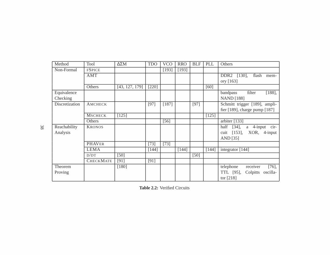
Method Tool ∆ΣM TDO VCO RRO BLF PLL OthersNon-Formal FSPICE [193] [193]

AMT DDR2 [130], flash mem-ory [163]

Others [43, 127, 179] [220] [60]EquivalenceChecking

bandpass filter [188],NAND [188]

Discretization AMCHECK [97] [187] [97] Schmitt trigger [189], ampli-fier [189], charge pump [187]

MSCHECK [125] [125]Others [56] arbiter [133]

ReachabilityAnalysis

KRONOS half [34], a 4-input cir-cuit [153], XOR, 4-inputAND [35]

PHAVER [73] [73]LEMA [144] [144] [144] integrator [144]D/DT [50] [50]CHECKMATE [91] [91]

TheoremProving

[180] telephone receiver [76],TTL [95], Colpitts oscilla-tor [218]

Table 2.2: Verified Circuits

38

ear and all dynamics are monotonic functions. Therefore, the extreme value of

integrators can be found by considering finite number of corner cases. Computing

worst case trajectories is an optimization problem. In [50], Danget al. modeled a

third-order modulator as a discrete-time hybrid automatonwith four variables and

checked the stability problem using mixed integer linear programming. Their re-

sults show that the modulator circuit is stable up to 30 stepsfor some input signals

and initial states. In [91], Guptaet al. studied the same problem using a reachabil-

ity analysis approach by applying a discrete-time version of the CHECKMATE tool.

They reported initial conditions and input values under which saturation levels can

be reached. In [222], a method was presented for bounding thestate variables

of a second order∆ΣM. The method uses a piecewise-affine equation to model

the circuit, employs polygons to represent circuit states,and finds an invariant set

in state-space using either an analytic or algorithmic approach. Symbolic meth-

ods have been applied to prove the stability of the circuit orfind counterexamples

in [180]. The modulator circuit has been used as an example ofmany simulation-

based methods. For example, Sammaneet al. applied their symbolic monitoring

algorithm [179] to the third-order modulator and Jesseret al. applied assertion-

based verification to the first order modulator. In [43], Clarke et al. applied their

random input generator to the third-order modulator and measured the probability

of stability failure within a bounded time.

2.3.2 A Tunnel Diode Oscillator

Figure 2.3 shows the tunnel-diode oscillator (TDO) circuitthat has been studied by

many verification researchers. It consists of a capacitor, an inductor, and a tunnel

diode. An ideal LC oscillator can oscillate forever if the initial current through

inductor or voltage across the capacitor is non-zero. However, the parasitic resis-

tance of the inductor makes the oscillation decay exponentially. The tunnel diode

compensates for the parasitic resistance because it has negative resistance charac-

teristics at low voltages. As shown in Figure 2.4, the current through the tunnel

diode decreases as the voltage is increased in its negative resistance region.

Oscillation conditionsof oscillator circuits refer to all conditions that ensure

the circuit oscillates stably. These conditions include circuit parameters and ini-

39

Figure 2.3: Tunnel DiodeOscillator

−0.1 0 0.1 0.2 0.3 0.4 0.5 0.6−1

−0.5

0

0.5

1

1.5

2

2.5x 10

−3

Forward Voltate

For

war

d C

urre

nt

negative resistance

Figure 2.4: Tunnel Diode’s I-V Characteris-tic

tial node voltages. The circuit can be modeled by a two-variable system,i.e., the

voltageVc across the capacitor and the currentIl through the inductor. All DC

equilibrium points can be computed based on the I-V characteristic of the tun-

nel diode and the inductor. Then two simulations can bound the stable oscillation

region because trajectories cannot cross and there is no chaotic behaviors in a two-

dimensional system. Figure 2.5 shows the equilibrium point, the stable orbit and

two simulations: a trajectory spiraling out from near the equilibrium point, and one

spiraling in from outside of the stable orbit.

Reachability regions of the TDO circuit have been computed by AMCHECK [97],

PHAVER [73], CHECKMATE [91], and LEMA [144]. The stable oscillation prop-

erty can be verified by checking whether the currentIl cycles above an upper bound

and below a lower bound periodically. In [97], Hartonget al. applied AMCHECK to

find an invariant set that contains the oscillation orbit. Onthe other hand, CHECK-

MATE combined reachability analysis over finite time horizon andLyapunov func-

tion to show the stability over infinite time [91]. A condition where the oscillation

may die out was also found. In [220], Zakiet al. checked the property by mon-

itoring circuit behaviors generated by an interval based simulator. HYTECH can-

not complete the verification due to arithmetic overflow errors [144]. Two further

properties were studied by Frehseet al. [73]. They used a monitor automaton to

40

−4 −3 −2 −1 0 1 2 3 4−2

−1.5

−1

−0.5

0

0.5

1

1.5

2

x2

equilibrium point

stable orbit

Figure 2.5: Simulations of the Tunnel Diode Oscillator

measure cycle amplitude variations and period jitters during the reachability com-

putation in PHAVER. However, this makes the reachability computation much

slower (> 20x) and there is no jitter in the simple circuit model which doesnot

include noise. A forward/backward refinement strategy [73]was used to reduce

the memory usage, but this increases the running time further.

2.3.3 Voltage Controlled Oscillators

A voltage controlled oscillator (VCO) is an oscillator whose oscillation frequency

is controlled by a voltage input. Two kinds of VCOs have been considered in the

formal verification literature: differential, LC VCOs (Figure 2.6, Figure 2.7) and

RC ring VCOs (Figure 2.8, Figure 2.9). The differential VCOsare constructed us-

ing a parallel inductor and capacitor combination whose impedance is very large at

the resonant frequency. The MOSFET transistors form two inverters in a positive

feedback loop, and the circuit will oscillate at a frequencyclose to the resonant

frequency of the inductor and capacitor if the gain of the inverters at this frequency

is sufficient to overcome the parasitic losses of the rest of the circuit. The capac-

itances are controlled by an input voltage which changes theresonant frequency

and hence the oscillation frequency. The ring VCOs are basedon a ring with an

41

Figure 2.6: A Differential VCOCircuit (Fig.3 of [73])

Vdd

Vss

Vbias

V− V+

Figure 2.7: A RF VCO Circuit(Fig.13 of [193])

C1

R1

C2 R2

gVin

Figure 2.8: A Opamp-Based VCOCircuit (Fig.4 of [187])

Cload

Vout

Vin

Figure 2.9: A Ring VCO Circuit(Fig.3 of [56])

odd number of inverters. The oscillation frequency is controlled by changing the

delay of the inverters by adjusting their output current.

The differential VCO as shown in Figure 2.6 has three continuous variables8

and its dynamics is less contractive than the TDO circuit. Therefore, the reachabil-

ity computation of this VCO circuit is more challenging. Forexample, PHAVER

failed to find an invariant set because of large over-approximation error [73]. To

8There are four variables:VD1, VD2, IL1 andIL2 in Figure 2.6. Noting the sum ofIL1 andIL2 is aconstant valueIb, the circuit can be modeled by three-state equations.

42

solve the problem, Frehseet al. developed an abstraction-refinement technique

which performs forward as well as backward reachability andrefines models in a

smaller region if the verification fails.FSPICE has been applied to simulate a sim-

ilar differential VCO as shown in Figure 2.7 and analyze the oscillation frequency

by periodic steady state analysis. Discretization methodshave been applied to ring

VCOs. In [187], Steinhorstet al. applied their AMCHECK tool to compute the

period of the VCO circuit as shown in Figure 2.8. Similarly, Dastidaret al. ap-

plied discretized models and showed that the circuit in Figure 2.9 oscillates when

parameter values such as transistor widths have appropriate values.

2.3.4 A Biquad Lowpass Filter

Lowpass filter

Figure 2.10: A Second Order Biquad Lowpass Filter

Figure 2.10 shows a biquad low-pass filter which consists of an operational

amplifier and a feedback capacitor. The dynamics of the circuit are not linear,

thus, nonlinear models, corresponding to saturating the operational amplifier out-

put voltage and current capabilities, must be applied in order to accurately analyze

the circuit. However, from the transfer function of the circuit, it is easy to see that

the circuit passes low-frequency signals but attenuates signals with frequencies

higher than its cutoff frequency.

One property that has been studied is the absence of overshoot in the filters

C1,C2, i.e., uC1,uC2 never exceed their steady state values. This property can be

verified by computing reachable regions of the circuit and checking the bounds of

uC1 anduC2. In [97, 98], Hartonget al. used a linear operational amplifier with

finite gain and unlimited bandwidth. They partitioned the entire three-dimensional

(i.e., ui ,uC1,uC2) state space into boxes and computed transitions between them by

43

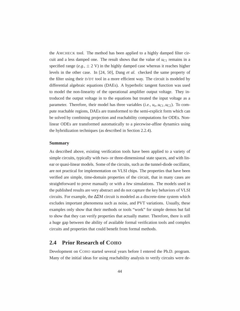
the AMCHECK tool. The method has been applied to a highly damped filter cir-

cuit and a less damped one. The result shows that the value ofuC1 remains in a

specified range (e.g.,± 2 V) in the highly damped case whereas it reaches higher

levels in the other case. In [24, 50], Danget al. checked the same property of

the filter using theirD/DT tool in a more efficient way. The circuit is modeled by

differential algebraic equations (DAEs). A hyperbolic tangent function was used

to model the non-linearity of the operational amplifier output voltage. They in-

troduced the output voltage in to the equations but treated the input voltage as a

parameter. Therefore, their model has three variables (i.e., uo,uC1,uC2). To com-

pute reachable regions, DAEs are transformed to the semi-explicit form which can

be solved by combining projection and reachability computations for ODEs. Non-

linear ODEs are transformed automatically to a piecewise-affine dynamics using

the hybridization techniques (as described in Section 2.2.4).

Summary

As described above, existing verification tools have been applied to a variety of

simple circuits, typically with two- or three-dimensionalstate spaces, and with lin-

ear or quasi-linear models. Some of the circuits, such as thetunnel-diode oscillator,

are not practical for implementation on VLSI chips. The properties that have been

verified are simple, time-domain properties of the circuit,that in many cases are

straightforward to prove manually or with a few simulations. The models used in

the published results are very abstract and do not capture the key behaviors of VLSI

circuits. For example, the∆ΣM circuit is modeled as a discrete-time system which

excludes important phenomena such as noise, and PVT variations. Usually, these

examples only show that their methods or tools “work” for simple demos but fail

to show that they can verify properties that actually matter. Therefore, there is still

a huge gap between the ability of available formal verification tools and complex

circuits and properties that could benefit from formal methods.

2.4 Prior Research of COHO

Development on COHO started several years before I entered the Ph.D. program.

Many of the initial ideas for using reachability analysis toverify circuits were de-

44

veloped by Mark Greenstreet. This led to the idea of using projection-based reach-

ability analysis which was developed by Mark Greenstreet and his students from

1997 to 2003. I joined this effort with my M.Sc. research in 2005 where I im-

plemented numerically robust methods for COHO’s linear program solver. This

re-engineering finally provided COHO with the robustness needed to be used with

some hybrid system examples and enabled the research described in this disserta-

tion. The remainder of this section gives a more detailed description of the work

on COHO that preceded my Ph.D. research.

As described in Section 2.1.2, Kurshan and McMillan published the first paper

reporting the formal verification of circuits using ODE models. This was followed

by a series of papers [83–85] that introduced the idea of using Brockett’s annuli

as the basis for abstraction mappings from continuous to discrete signals, and gave

the first examples of projection-based representations to obtain a tractable repre-

sentation of moderate-dimensional objects. In [83], theseprojections were onto

rectilinear polygons. For each bloated face,i.e., a hyper-rectangle, the maximum

outward derivative was computed easily as the first-order model is a convex func-

tion9. A fourth-order Runge-Kutta integrator was used to integrate ODEs to move

forward each face. The toggle circuit that we examine in Section 3.2.1 was verified

as a proof-of-concept example. Manual model reduction was employed to obtain

a three-dimensional system by ignoring capacitances at some nodes and rewriting

the ODEs to be an integration with respect to the input clock voltage rather than

time.

The use of rectilinear projectagons in [83] resulted in large over approxima-

tions that prevented the verification of other circuits. In 1997, Greenstreet and

Mitchell proposed a generalization of the projection-based method to use gen-

eral, non-convex polygons. These ideas were implemented inthe first version of

COHO [86] where the numerical integration and LP solver were implemented in

MATLAB , and the geometric operations were implemented in JAVA . They manually

constructed circuit models using the modified nodal analysis techniques described

in Section 3.3. The tool was demonstrated using some simple examples [87]. How-

ever, it was observed that the linear programs associated with projectagons are

9This motivates the idea offace liftingandorthogonal polyhedraof D/DT. However, orthogonalpolyhedra do not use the projecting idea and limit vertices of rectilinear polygons as fixed grid points.

45

often highly ill-conditioned, and this prevented the use ofCOHO on more compli-

cated examples.

In 2000, Greenstreet, Laza, and Varah recognized that the structure of linear

programs associated with projectagons can be exploited to produce an efficient and

robust implementation of the Simplex algorithm. Laza developed these ideas in his

M.Sc. thesis [142] including the error analysis of the algorithm and a preliminary

implementation in COHO. However, Laza’s implementation only handled uses of

the LP solver for optimization, but did not support projection operations. In the

summer of 2003, Karen Brennan studied the COHO codes and wrote a proposal for

using Laza’s algorithms for all linear programming based operations.

From 2005 to 2006, I re-engineered the COHO software and solved the nu-

merical problems of COHO to make it more robust [208]. Interval arithmetic was

applied to both the LP solver and the geometry computation engine. The interval-

based LP solver [214] overestimated the optimal value and was also integrated with

a new projection function. However, the LP solver may not findthe correct optimal

basis if the LP is ill-conditioned, which may generate largeapproximation errors

in the projection operations. These enhancements made it possible to apply COHO

to two hybrid system examples [208].

To summarize, the work on COHO preceding my Ph.D. research established the

basic algorithms for projectagon based reachability analysis and showed that these

methods had promise for circuit verification. However, manyquestions needed to

be answered and problems needed to be solved to show that these methods are use-

ful in practice. First of all, we needed a systematic way of specifying the properties

that we wanted to verify about circuits. Next, trying these methods on real circuits

revealed places where COHO’s algorithms introduced unacceptable approximation

errors. By revising these algorithms, I have reduced the errors to enable verification

of real circuits. In some cases, this required developing new data structures and al-

gorithms to replace or complement those used in the originalCOHO. Finally, the

run-time for COHO’s algorithms tended to be very large, limiting the application

of the tool. I made many improvements to the efficiency of COHO by reformulat-

ing the details of the reachability problem, developing newalgorithms, and tuning

the existing implementation. These contributions are described in the remaining

chapters of this dissertation.

46

2.5 Summary

This chapter explored formal methods of analog verification, especially reachabil-

ity analysis, and their application to circuit examples. This provides background

for the methods and tools in this dissertation: Section 2.1 describe the main ap-

proaches used in prior work on circuit verification: equivalence checking, model

checking and theorem-proving based approaches. We argued that reachability anal-

ysis is the most promising of these approaches, and Section 2.2 described the var-

ious algorithms and data-structures that have been used in reachability analysis

tools. Then, Section 2.3 described circuits and their properties that have been veri-

fied using these techniques. The circuits that have been considered have been very

simple, and the properties that have been verified often reflect the capabilities of

the tools more than the concerns of designers.

Verifying relevant properties of practical circuits will require capabilities that

are well beyond those of current tools. High-dimensional (e.g.,> 4) regions should

be represented and manipulated efficiently because most practical analog circuits

have tens to hundreds of nodes. Existing methods use representations that either

have expensive operations (e.g.,polytopes) or have large approximation error (e.g.,

hyper-rectangles). Because many circuits have highly non-convex reachable re-

gions, it is important to support non-convex regions otherwise the wrapping effect

will often generate false-negative results. It is necessary to support nonlinear dy-

namics because ODEs extracted from circuits are neither linear nor even weakly

non-linear. Most current methods are very expensive (e.g.,representation methods

do not scale) or have large approximation errors (i.e., they only work for mod-

els with linear or nearly-linear dynamics). Furthermore, tight approximations are

required to verify complicated systems without false-negatives. Therefore, we de-

velop an efficient, robust, and accurate reachability analysis tool for moderate-

dimensional, nonlinear hybrid systems which will be presented in Chapter 4.

In addition to a powerful reachability computation tool, itis also important to

convert circuit verification problems to reachability analysis automatically. This

includes constructing mathematical models from circuit netlists and formally spec-

ifying analog properties. Although there exist many techniques for modeling and

specification as shown in Section 2.2.1 and Section 2.2.2, most available tools do

47

not support circuit verification tasks directly,i.e., users have to create mathemat-

ical models for circuits and check properties manually. Therefore, we propose a

general solution to model and specify AMS circuits in Chapter 3.

48

3

Circuit Verification as

Reachability

This chapter describes our method for translating circuit verification problems to

reachability analysis problems. Section 3.1 presents the phase-space representa-

tion of circuit behaviours and our verification strategy. Section 3.2 provides a set

of real circuits that we use as a testbench suite for verification methods. Section 3.3

describes how to model circuits as ODE systems and Section 3.4 presents our meth-

ods to specify analog signals and properties. Finally, someimplementation issues

are discussed in Section 3.6.

3.1 Phase Space and Reachability Based Verification

Circuit simulators usually present circuit behaviours to designers as waveforms,

i.e.,signal voltages as functions of time. Thephase-spacerepresentation provides

another view of circuit behaviors which is well-suited for use in formal verifica-

tion. In the phase-space representation, each circuit state is represented by a unique

point, and the set of all possible states is represented as a high-dimensional region.

For most of the circuits that we consider, the state of the circuit can be repre-

sented by the voltage on each node of the circuit. Thus, the dimensionality of the

phase space is the same as the number of nodes for these circuits. For example,

an inverter circuit has an input node and an output node, thusits phase space is

49

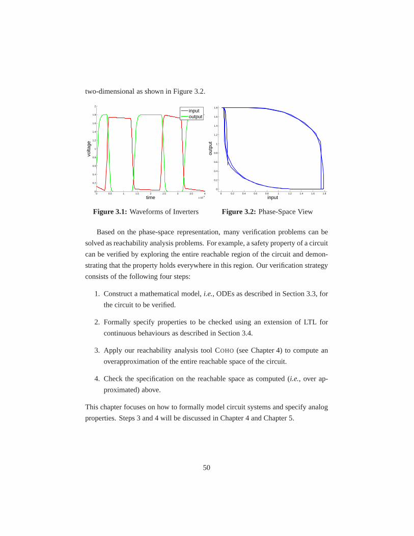
two-dimensional as shown in Figure 3.2.

0 0.5 1 1.5 2 2.5 3 3.5 4

x 10−9

0

0.2

0.4

0.6

0.8

1

1.2

1.4

1.6

1.8

2

time

volta

ge

inputoutput

Figure 3.1: Waveforms of Inverters

0 0.2 0.4 0.6 0.8 1 1.2 1.4 1.6 1.8

0

0.2

0.4

0.6

0.8

1

1.2

1.4

1.6

1.8

input

outp

utFigure 3.2: Phase-Space View

Based on the phase-space representation, many verificationproblems can be

solved as reachability analysis problems. For example, a safety property of a circuit

can be verified by exploring the entire reachable region of the circuit and demon-

strating that the property holds everywhere in this region.Our verification strategy

consists of the following four steps:

1. Construct a mathematical model,i.e.,ODEs as described in Section 3.3, for

the circuit to be verified.

2. Formally specify properties to be checked using an extension of LTL for

continuous behaviours as described in Section 3.4.

3. Apply our reachability analysis tool COHO (see Chapter 4) to compute an

overapproximation of the entire reachable space of the circuit.

4. Check the specification on the reachable space as computed(i.e., over ap-

proximated) above.

This chapter focuses on how to formally model circuit systems and specify analog

properties. Steps 3 and 4 will be discussed in Chapter 4 and Chapter 5.

50

x

y zxx

yy zz

φ

φ

φ

φx

y zxx

yy zz

Figure 3.3: Toggle Circuit

0 0 1 10123

101

0 1 01 1 00 0 1

4 0 1 10

step x y zφ

of toggle elementStable state

Φxyz

x

y

z

HLHL

HLHH

LLHH

LLLH

HLLH

HHLH

HHLL

HHHL

LHHL LLHL

Transient stateof toggle element

xyzΦ

Figure 3.4: State Transition Diagram

3.2 Circuit Examples

In this dissertation, we use four circuits as examples of circuit verification prob-

lems. Our testbench includes a toggle circuit, a flip-flop, anarbiter and a ring

oscillator. It covers synchronous circuits (toggle and flip-flop), asynchronous cir-

cuits (arbiter) and analog circuits (oscillator). It also contains circuits with no

inputs (oscillator), one input (toggle), two inputs that can change at arbitrary time

with respect to each other (arbiter) and two inputs whose transitions must occur

according to a specified timing relationship (flip-flop).

3.2.1 The Yuan-Svensson Toggle

Figure 3.3 shows a toggle circuit that was originally published by Yuan and Svens-

son [217]. The operation of this circuit can be understood byusing a simple switch

model starting from a state where theφ input is low. In this case,y is driven high;

z is floating; andx is the logical negation ofz. Figure 3.4 shows the state transition

diagram for the toggle starting from the state wherez is high whenφ is low – the

other case, withz high, is reached on step 2 of the figure. Note that from step 2 to

3 in the figure, all three ofx, y andz change values. This is a critical race for the

toggle. As a consequence, if the rise time or fall time forφ are too large, the toggle

will fail.

We specify the behavior of the toggle as a safety property. Inparticular, there

is an invariant subset ofRd such that all trajectories in this set have a period twice

51

that of the clock signal. Another property is to show that theinput clock and output

signal satisfies the same specification in order to constructa ripple-counter.

3.2.2 A Flip-Flop

d

φ

φ

q

φ

φq

Figure 3.5: Latch Circuit

φ

d

qq

φ

φ

φ

φ φφ

φ

Figure 3.6: Flip-Flop

A latch is a circuit that has two stable states and thereby is capable of serving

as one bit of memory. Figure 3.5 shows a static, transparentpass-gate latch[207,

Chapter 7.3]. The output of the latch circuit holds its old value when the clock

signal φ is low and is set to the value of the input whenφ is high. Flip-flops

are typically implemented as master-slave devices. Figure3.6 shows a D flip-flop

which consists of two latches. The flip-flop only updates its output value on the

rising edge of the clock signalφ . However, the output value may not be stable if

the input signal changes on the rising edge ofφ .

The input specification of the flip-flop requires that the input value cannot

change during the rising transition of the clock signalφ . The output of the flip-

flop must guarantee that the output signal is stable within a specified time after

the rising clock edge. Other interesting properties includes the maximum clock

frequency and the lower (upper) bounds of the clock-to-q delay.

3.2.3 An Arbiter

An arbiter is a circuit that provides mutually exclusive access to a resource for some

set of clients. We consider an asynchronous arbiter with twoclients as shown in

Figure 3.7(a). The two clients interact with the arbiter using a four-phase hand-

shake protocol: clienti raisesr i to request the privilege; the arbiter raisesgi to

grant clienti the privilege; when the client is done with the privilege, itlowersr i ;

and finally the arbiter lowersgi to complete the handshake.

52

y

g g

yxx

xyg

xy g

client 2client 1

b. Gate−level implementation

a. As a "black box"

c. Transistor−level implementation

x1NAND1

mf1

NAND2

x2

z1

g1

r1

z2

g2

r2

mf2

r1

NAND1

MF1

g1

NAND2

MF2

g2

r2x2x1

r2

g2

r1

g1

Figure 3.7: Arbiter Circuit

Figure 3.7(b) shows an implementation of an arbiter based ona SR-latch us-

ing a pair of cross-coupled NAND gates (see [155, Fig. 5]). Asillustrated in

Figure 3.8, whenr1 and r2 are both low, the NAND gate outputs,x1 andx2 are

both driven high, and themetastability filters(to be described shortly),MF1 and

MF2 will drive the grant signalsg1 andg2 low. If requestr1 is asserted (i.e. driven

to a high value), then thex1 will go low andg1 will go high to grant the request.

If r2 makes a request whiler1 holds the grant, then the request fromr2 will be

blocked. In particular,x2 will remain high even whenr2 goes high becausex1 is

low. When the first client drops,r1, x1 will go high andg1 will go low; if there

is a pending request onr2, thenx2 will go low in response to the rising ofx1, and

this will causeg2 to go high. The arbiter operates in an analogous manner ifr2 is

asserted well-beforer1.

x1

x2

g1

g2

grant

requestr1

r2 blocked

pending request

grant

Figure 3.8: Uncontested Requests

x1

x2

g1

g2

r1

r2

concurrent requests

metastable region

resolved

Figure 3.9: Contested Requests

As shown in Figure 3.9, if both requests,r1 andr2 are asserted at roughly the

53

same time, then signalsx1 andx2 will both start to fall. This results in a falling

input for each NAND-gate and the consequent possibility of metastability if the

two NAND-gates reach a balance point with their outputs at anintermediate level

between the power supply voltage and ground. This conditioncan persist for an

arbitrarily long time [38, 154, 183] but eventually resolves (with probability one)

to a state with one ofx1 or x2 going high and the other going low. The metasta-

bility filters (MF1 andMF2 in Figure 3.7(c)) prevent the outputs of the arbiter from

changing until metastability resolves.

The metastability filter is a modified inverter. Consider circuit MF1. The gates

of the transistors in the inverter are connected tox1. Unlike a traditional inverter,

the source of the PMOS pull-up is connected tox2. With this configuration, the

pull-up transistor remains in cut-off untilx1 is at least the PMOS threshold voltage

belowx2. This preventsg1 from moving any significant amount above ground until

client 1 has clearly won the arbitration.

The arbiter must satisfy the handshake protocol and guaranteemutual exclu-

sion, i.e., signalsg1 andg2 may not both be high at the same time. Obviously,

it would be desirable if the arbiter were guaranteed to eventually issue a grant

when a request is pending. It is well known that a real arbitercannot satisfy this

requirement along with the safety requirements described above (see, for exam-

ple, [154, 157]).

3.2.4 The Rambus Ring Oscillator

cc cc

fwd

fwd

cc cc

fwd

fwd

cc cc

fwd

fwdX1

Xn+1

X2

Xn+2

Xn

X2n

Figure 3.10: The Rambus Ring Oscillator

Figure 3.10 shows a differential ring oscillator. The oscillator consists of an

even number of stages,n; and each stage has twoforward (labeledfwd in the figure)

54

inverters connected by a pair ofcross-coupling(labeledcc) inverters. Consider an

initial state wherexi is high if i is odd andi < n, or i is even andi > n, andxi is

low otherwise. As shown in Figure 3.11, if the forward inverters are strong enough

to overpower the cross-coupled inverters, thenxi will be excited to make a high-

to-low transition andxn+1 will be excited to make a low-to-high transition. This

will lead to a state where signalsx2 andxn+2 are excited to change, and so on.

The cross-coupled inverters ensure that the rising and falling transitions happen

at roughly the same time. In particular, ifxi transitions earlier thanxn+i , then the

inverter fromxi to xn+i will accelerate the transition ofxn+i , while the inverter from

xn+i to xi will retard the transition ofxi .

HH

H LL

L

cc

fwd

fwd

cccc cc

fwd

fwd

cc cc

fwd

fwd

cc cc

fwd

fwd

x x xx1

x x xx5

2 3 4

6 7 8

x1

x

x3

x

2

4

Figure 3.11: Expected Oscillation Mode

Researchers reported that some implementations of the circuit did not oscillate

as described above in real, fabricated chips. They posed a verification problem of

showing that the oscillator starts from all initial conditions for a particular choice

of transistor sizes. Furthermore, they posed an additionalproblem of determining

the sizes of the inverters that guarantee that the circuit will enter a stable oscillating

condition from any initial condition.

The failure occurred when the forward and cross-coupling inverters do not

have comparable strength. If the forward inverters are muchlarger than the cross-

coupling inverters (as shown in Figure 3.12), then the circuit acts like a ring of 2n

55

fwd

fwd

cc cc

H

H

fwd

fwd

cc cc

H

H

fwd

fwd

cc cc

L

L

fwd

fwd

cc cc

L

L

Figure 3.12: Forward Inverters TooLarge

H

fwd

fwd H

LH

LH

LL fwd

fwd

fwd

fwd

fwd

fwd

cccc

cccc

cccc

cccc

Figure 3.13: Cross-CouplingInverters Too Large

inverters and will settle to one of two states:

State 1: x1,xn+1,x3,xn+3, · · · ,xn−1,x2n−1 are high, and

x2,xn+2,x4,xn+4, · · · ,xn,x2n are low.

State 2: x1,xn+1,x3,xn+3, · · · ,xn−1,x2n−1 are low, and

x2,xn+2,x4,xn+4, · · · ,xn,x2n are high.

(3.1)

Conversely, if the cross-coupling inverters are much larger than the forward ones

(as shown in Figure 3.13), then the circuit acts liken separate static latches and has

2n stable states.

3.3 Modeling Circuits as ODE Systems

This section describes how we obtain ODE models from circuitschematics (or

equivalently, netlists). Section 3.3.1 describes the qualitative operation of n-channel

and p-channel MOSFETs, the basic building block of most integrated circuits. We

then describe our use of modified nodal analysis to derive ODEs from the circuits;

this process is essentially the same one that is used by most circuit simulators. De-

vice models for state-of-the art processes are very complicated with a large num-

ber of parameters. Rather than implementing these models inour codes, we use

a table-driven approach described in Section 3.3.2. The tables are generated using

standard circuit simulators. Thus, we use the same models for formal verification

as the circuit designers are using for simulations.

3.3.1 Circuit Models

We construct mathematical models based on nonlinear ODEs from circuit netlists.

The circuits that are used on chips are typically composed oftransistors, capaci-

56

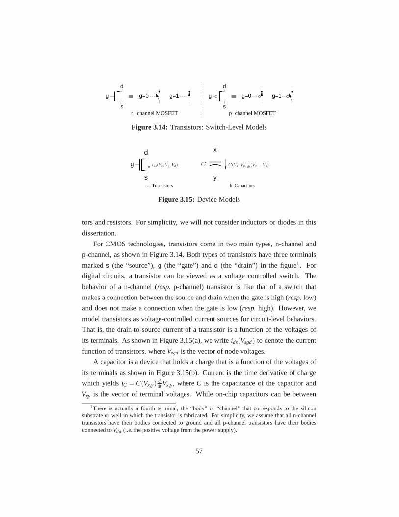
s s

d

g

d

g g=0 g=1 g=0

n−channel MOSFET p−channel MOSFET

g=1

Figure 3.14: Transistors: Switch-Level Models

d

s

g

x

ya. Transistors b. Capacitors

Cids(Vs, Vg, Vd) C(Vx, Vy)ddt

(Vx − Vy)

Figure 3.15: Device Models

tors and resistors. For simplicity, we will not consider inductors or diodes in this

dissertation.

For CMOS technologies, transistors come in two main types, n-channel and

p-channel, as shown in Figure 3.14. Both types of transistors have three terminals

markeds (the “source”),g (the “gate”) andd (the “drain”) in the figure1. For

digital circuits, a transistor can be viewed as a voltage controlled switch. The

behavior of a n-channel (resp.p-channel) transistor is like that of a switch that

makes a connection between the source and drain when the gateis high (resp.low)

and does not make a connection when the gate is low (resp.high). However, we

model transistors as voltage-controlled current sources for circuit-level behaviors.

That is, the drain-to-source current of a transistor is a function of the voltages of

its terminals. As shown in Figure 3.15(a), we writeids(Vsgd) to denote the current

function of transistors, whereVsgd is the vector of node voltages.

A capacitor is a device that holds a charge that is a function of the voltages of

its terminals as shown in Figure 3.15(b). Current is the timederivative of charge

which yields iC = C(Vx,y)ddtVx,y, whereC is the capacitance of the capacitor and

Vxy is the vector of terminal voltages. While on-chip capacitors can be between

1There is actually a fourth terminal, the “body” or “channel”that corresponds to the siliconsubstrate or well in which the transistor is fabricated. Forsimplicity, we assume that all n-channeltransistors have their bodies connected to ground and all p-channel transistors have their bodiesconnected toVdd (i.e. the positive voltage from the power supply).

57

m3 m4

m2

m1 s

g

g dd

d

ss

g

s

dg

b

x

a

b. NANDa. KCL

Cx

Cz

z

iC = i1 + i2i1

i2C

Figure 3.16: Kirchoff’s Laws

arbitrary pairs of nodes and have capacitances that depend on node voltages, for

simplicity we model capacitances as being to ground and having constant values

independent of node voltages. Likewise, we omit resistances for simplicity and

brevity but note that they can be treated as voltage-controlled current sources in a

manner analogous to our treatment of transistors describedabove.

Given models for all devices of a circuit, we construct a nonlinear ODE model

for the whole system using standard nodal analysis techniques based on Kirchoff’s

current law (KCL). As depicted in Figure 3.16(a), KCL statesthat the sum of all

currents flowing into a node must be equal to zero. LetV be the vector whose

elements are the voltages of nodes of the circuit of interest, which consists ofVi for

input nodes andVo for internal and output nodes. LetIds be a function from vectors

of node voltages to vectors of transistor currents. Letn be the number of nodes of

the circuit andm be the number of transistors. LetM ∈ Rn×m be the connectivity

matrix for transistors to nodes:

M(i, j) =

+1, if the source of transistorj is connected to nodei

−1, if the drain of transistorj is connected to nodei

0, otherwise

Finally, letC be the diagonal matrix whereC(i, i) is the capacitance from nodei to

ground. We now have:ddt

Vo =C−1M Ids(V). (3.2)

58

This gives us the time derivative function for all internal and output nodes of the

circuit we wish to verify. The ODE models for external inputsare determined using

a Brockett’s annulus abstraction which will be described inSection 3.4.3.Let us take the NAND gate shown in Figure 3.16(b) as an example. In this

circuit, we haveV = [Vss,Vdd,Va,Vb,Vx,Vz] and Ids = [im1, im2, im3, im4]. By KCL,we obtain:

−im3(Vdd,Va,Vx)− im4(Vdd,Vb,Vx)− im2(Vz,Vb,Vx)−CxddtVx = 0

im2(Vz,Vb,Vx)− im1(Vss,Va,Vz)−CzddtVz = 0,

which yields

ddtVx = − 1

Cx(im3(Vdd,Va,Vx)+ im4(Vdd,Vb,Vx)+ im2(Vz,Vb,Vx))

ddtVz = − 1

Cz(im2(Vz,Vb,Vx)− im1(Vss,Va,Vz)).

When constructing the ODE model, we impose the physically realistic require-

ment that all circuit nodes have some non-zero capacitance to ground, which en-

sures that the diagonal matrixC is positive definite and therefore invertible. These

assumptions avoid complexity while retaining the key features of realistic circuits.

More generally, the procedure we described above provides ageneral way for a

verification researchers to obtain a system of non-linear ODEs from a schematic

diagram; in other words, a schematic is simply syntactic sugar for a system of

ODEs according to this interpretation.

3.3.2 Circuit-Level Models Based on Simulations

We now describe how we obtain theids functions. Of course, there are plenty of

textbooks that present models for transistors (for example[123, 207]). However,

these are simplifications of the models that are used in industry for real fabrication

processes. These simplified models provide designers with intuition to understand

qualitative circuit behaviors, but they do not provide the accuracy to verify detailed

behaviors. For the latter, designers rely on the models usedby commercial cir-

cuit simulators such as HSPICE or Spectre [1]. In other words, circuit simulators

provide the interface between device modeling experts and circuit design experts.

In the same manner, we did not write our own code to implement state-of-the-art

59

transistor models. Instead, we use the HSPICEsimulator to obtain tables ofids data

on a relatively fine grid and use bilinear (or other kinds of) interpolation to com-

pute transistor currents. The key advantage of this approach is its simplicity and

generality. We can generate accurate models for any processwith vendor provided

SPICE models. Furthermore, our table is interval value based, that is, the lower

and upper bounds of the current are provided for each grid point. COHO generates

differential inclusions from the ODE circuit models; thus,we can incorporate the

intervals from the tables in the differential inclusion to ensure that our verification

includes the exact SPICE model in the set of behaviors that it considers. Further-

more, we can use wider intervals in the table to model PVT variations, add error

bounds to the device models themselves,etc.

Compared with other simulation-aided verification techniques such as the one

used in LEMA [148], our approach has the benefit that we only simulate a small

number of basic devices,e.g., transistors, instead of the whole circuit or macro-

models. Therefore, it is much easier to simulate more cornercases in order to

obtain a higher coverage. Our table-based method can be applied similarly to ob-

tain accurate models of circuit capacitance, resistance orinductances. It has not

been implemented but it is an obvious future work.

We extended our table-based approach to create macro modelsfor small cir-

cuit blocks (see Section 5.4 for an example). However, the number of grid points

increases exponentially as the number of device terminals increases. For example,

the tables for transistors have three indices, one each for the source, gate and drain

voltages, and we sampled these on a relatively fine grid of 0.01V for the 180nm

CMOS process. This means that each table has 1813 ≈ 6×106 entries. A four-

dimensional table using the same grid would have about 109 entries which would

consume a prohibitively large amount of memory and cause high cache miss-rates.

Therefore, we developed apolynomial tabletechnique which uses a coarser grid

and uses a higher-order polynomial to approximate the current function with ac-

ceptable errors. We found that second-order polynomials generally provided suf-

ficient accuracy for our verification work, thus each entry ofthe table holds the

coefficients for the quadratic polynomial model. Using thistechnique, the table

with a 0.1V grid only holds roughly 106 values for a four-terminal device2, which

2A three-variable quadratic has ten coefficients, and a tablewith a 0.1V grid has roughly 194 ≈

60

is quite practical.

3.4 Specification

Section 3.3 described how to construct a mathematical modelfor a circuit. This

section describes our approach for specifying circuit properties. We extend linear

temporal logic (LTL) to continuous time and values to specify analog properties.

Atomic propositions in this logic correspond to regions of the circuit’s state space.

A particular class of such regions that is of interest to our work are the regions that

can be specified using Brockett’s annulus construction – such regions correspond

to the intuitive notion of a signal being “digital”.

3.4.1 Extended LTL

To specify circuit-level properties of circuits, we generalize conventional temporal

logics to formulas with continuous time and values. Our specification language

is based onlinear-time temporal logic (LTL)[168] rather than CTL for simplic-

ity because we are mainly interested in safety properties and only use universal

quantifiers. The approach to support dense time is very similar to MITL [16] as

described in Section 2.2.2. We then introduce continuous variables to describe con-

tinuous trajectories similar to the approach used in STL/PSL [150]. The novelty of

our method is that we introduce probability into the logic for specifying important

circuit properties such as metastable behaviors.

Given a set of statesS, we call p anatomic propositionif it is a function from

statesS to booleans (i.e., p : S→ {0,1}). A trace t is an infinite sequence of

valuations inS: t = t1t2 · · · , where∀i ∈ R+, ti ∈ S. We sayp is a LTL formula that

is satisfied for tracet if p(t1) is true. If p andq are LTL formulas, then¬p is the

formula that holds iffp does not hold, andp∧q is the formula that holds if bothp

andq holds. Other boolean operators are just syntactic sugar forcombinations of¬and∧. Thus, we will usep∨q≡ ¬(¬p∧¬q) andp⇒ q≡ ¬p∨q for disjunction

and implication.

Based on atomic propositions and logical operators defined above, temporal

operators of the discrete LTL are defined as:

105 entries. Therefore, there are roughly 106 numbers in the four-dimensional table.

61

N p next p holds in the next state.

� p always shorthand forp∧ (N � p); p holds this and all subse-

quent states.

♦ p eventually shorthand for¬(�¬p); p holds in this or some future

state.

p U q until shorthand forp∧ (q∨N (p U q)); p holds in this state

and continues to hold until a state in whichq holds.

p W q weak until shorthand for(p U q)∨ � p; p holds in the current state

and continues to hold forever or until a state in whichq

holds.

pU⇒q imply until shorthand forp⇒ (p U q); if pholds in the current state,

p will continue to hold until a state in whichq holds.

pW⇒q imply weak

until

shorthand forp ⇒ (p W q); if p holds in the current

state,p will continue to hold forever or until a state in

which q holds.

In order to specify analog properties of circuits, we define LTL-like formulas

for continuous trajectories and introduce a few basic concepts from probability

theory into the logic.

The state of a circuit is represented by ad-dimensional vector of real num-

bers; we say thatd is the dimensionof the model. We writeV to denote this

d-dimensional state space of the circuit, anddV to denote thed-dimension time-

derivative of the state. The circuit is modeled as adifferential inclusion: if A⊆ V

andx∈ A then

x ∈ F(A), (3.3)

wherex denotes the derivative ofx with respect to time. In other words,F : V →dV maps regions of the state space to regions of the derivative space. By using

an inclusion rather than an equation, the time derivative ofthe circuit is not fully

determined. Deterministic circuit models (even HSPICE) are only approximations

of reality, the differential inclusion model solves the problem and could model

non-deterministic behavior of the environment, such as theordering, timing, and

62

details of the waveform shape for input transitions. A behavior of the circuit is a

function from time (the non-negative reals) to states that starts in the initial region

and satisfies the derivative relation. Such a behavior is called a trajectory, and a

circuit is characterized by the (infinite) set of trajectories allowed by its model:

Φ(Q0,F) = {φ : R+ → V | (φ(0) ∈ Q0) ∧ (∀t ∈R+. φ(t) ∈ F({φ(t)}))}, (3.4)

where we assumeφ(t) is C1. For our circuit models, signal voltages are bounded

by simple invariants of the formgnd≤ V ≤ vdd. Therefore,dV

dt is bounded and

φ (t) is defined for allt ≥ 0 if φ ∈ Φ(Q0,F). Our continuous model for circuits is a

tuple,(Q0,F), whereQ0 ⊆ V is the initial region for the model, andF : 2V → 2dV

is the time-derivative relation.

We extend LTL to specify continuous behaviors. Letφ : R+ → V be a trajec-

tory, and define

shift(φ , t0)(t) = φ(t + t0). (3.5)

If φ is a trajectory andS is a continuous LTL formula (defined below), we write

φ |= S iff S is satisfied byφ . For a modelM = (Q0,F), we writeM |= S iff ∀φ ∈Φ(Q0,F), φ |= S.

A continuous LTL formula has a set of atomic propositionsP. These propo-

sitions can correspond to subsets ofV ; for P⊆ V , a trajectoryφ |= P iff φ(0) ∈ P.

To specify properties related to variable derivatives suchas the Brockett’s annulus

in the next section, we also support atomic propositions corresponding to subsets

of V ×dV . For P ⊆ V ×dV , φ |= P iff (φ(0), φ (0)) ∈ P. Our continuous-time

logic has no equivalent to the next-state operator; instead, we define¬, ∧, � and

U directly on trajectories:

φ |= ¬S ≡ φ 6|= S (3.6)

φ |= S1∧S2 ≡ (φ |= S1)∧ (φ |= S2) (3.7)

φ |= �[t l ,th]S ≡ ∀t ∈ [tl , th]. shift(φ , t) |= S (3.8)

φ |= ♦[t l ,th]S ≡ ∃t ∈ [tl , th]. shift(φ , t) |= S (3.9)

φ |= S1 U[t l ,th] S2 ≡ (φ |= S1) ∧ ∃t2 ∈ [tl , th]. (shift(φ , t2) |= S2)∧ (3.10)

(∀0≤ t1 < t2. shift(φ , t1) |= S1).

63

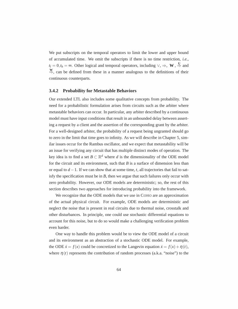
We put subscripts on the temporal operators to limit the lower and upper bound

of accumulated time. We omit the subscripts if there is no time restriction,i.e.,

tl = 0, th = ∞. Other logical and temporal operators, including∨, ⇒, W ,U⇒ and

W⇒, can be defined from these in a manner analogous to the definitions of their

continuous counterparts.

3.4.2 Probability for Metastable Behaviors

Our extended LTL also includes some qualitative concepts from probability. The

need for a probabilistic formulation arises from circuits such as the arbiter where

metastable behaviors can occur. In particular, any arbiterdescribed by a continuous

model must have input conditions that result in an unboundeddelay between assert-

ing a request by a client and the assertion of the corresponding grant by the arbiter.

For a well-designed arbiter, the probability of a request being ungranted should go

to zero in the limit that time goes to infinity. As we will describe in Chapter 5, sim-

ilar issues occur for the Rambus oscillator, and we expect that metastability will be

an issue for verifying any circuit that has multiple distinct modes of operation. The

key idea is to find a setB⊂ Rd whered is the dimensionality of the ODE model

for the circuit and its environment, such thatB is a surface of dimension less than

or equal tod−1. If we can show that at some time,t, all trajectories that fail to sat-

isfy the specification must be inB, then we argue that such failures only occur with

zero probability. However, our ODE models are deterministic; so, the rest of this

section describes two approaches for introducing probability into the framework.

We recognize that the ODE models that we use in COHO are an approximation

of the actual physical circuit. For example, ODE models are deterministic and

neglect the noise that is present in real circuits due to thermal noise, crosstalk and

other disturbances. In principle, one could use stochasticdifferential equations to

account for this noise, but to do so would make a challenging verification problem

even harder.

One way to handle this problem would be to view the ODE model ofa circuit

and its environment as an abstraction of a stochastic ODE model. For example,

the ODEx= f (x) could be concretized to the Langevin equation ˙x= f (x)+η(t),

whereη(t) represents the contribution of random processes (a.k.a. “noise”) to the

64

dynamics at timet. Often, in the treatment of stochastic ODEs,η(t) is assumed

to be Gaussian, but this raises a problem in our verification context: for any bound

M and any time interval∆T, the integral ofη(t) over the interval∆T has some

non-zero probability of being greater thanM. Thus, any signal could be perturbed

by any amount. This means that noise, with some small but non-zero probability,

could cause any digital circuit to fail, and no properties can be verified. From a

practical perspective, we’ll note that noise-margin analysis is an area where ex-

tensive research has been done (e.g. [132, 141, 223]), and regard the details of

noise-margin analysis as beyond the scope of the current dissertation. Instead, we

will assume that the noise margins are sufficient so that the probability of failure

of a logic gate is so small that it can be ignored. In particular, we will assume

thatη(t) is bounded. We also assume that all nodes of the circuit are perturbed by

noise, and that these perturbations are independent for different nodes and different

times. We will say that such a noise model is “reasonable”. With this approach,

we will say that a specification,S, is satisfied “almost-surely” (or “with probability

one”) if S is satisfied almost-surely for any stochastic ODE with a “reasonable”η .

In this case, the bounded noise,η , of the stochastic model provides the underlying

randomness that allows us to consider the probability of various events.

An alternative approach is to stay with an ODE model for the circuit and its

environment but to assume that there exists a probability distribution of the initial

states for trajectories. We require the ODE model to beC2, in which case solutions

of the ODE are unique. Thus, the initial state of the circuit and its environment

determine the entire trajectory. We will not specify the details of the probability

distribution of the initial states, but we will again require it to be “reasonable.” If

the model for the circuit and its environment hasd variables, the state space for

the model isRd. If B is a measurable set, we write‖B‖ to denote the Lesbesgue

measure ofB (intuitively, ‖B‖ is the volume occupied byB), and we writeµ(B)to denote the probability measure ofB. We say thatµ is “reasonable” ifµ(B) is

zero for any setB for which ‖B‖ is zero. With this approach, we will say thatS is

satisfied “almost-surely” (or “with probability one”) if itis satisfied for all trajec-

tories except for those starting from points in a setZ with ‖Z‖= 0. In practice, this

amounts to showing that at any timet, all “bad” trajectories must lie on a manifold

whose dimensionality is less than that of the full-system. Thus, nearly-all small

65

perturbations to such a trajectory would move it off of the manifold so as to obtain

a behavior that satisfies the specification.

We conjecture that these two mechanisms of introducing probability into our

logic are equivalent. In particular, the “cone” arguments that we use for the arbiter

and the oscillator circuits appear to be robust to the introduction of a noise com-

ponent,η , into the model. However, we do not have a proof of this equivalence.

Thus, we will use the second approach to define “almost-surely” for our version of

LTL. If our conjecture is true, then the “almost-surely” results extend to the more

physical notion of randomness of the first approach as well.

We define analmost surelyversion of the LTL “always” operator as shown

below:

φ |= �ZS ≡ (φ |= (�S)∨ ((φ ∈ Z) ∧ (‖Z‖= 0)), (3.11)

where the term((φ ∈ Z)∧ (‖Z‖ = 0)) is treated as an atomic proposition in the

formula. In other words,φ satisfies�ZS iff S holds everywhere alongφ or if φis in a negligible set,Z. This means that the probability ofSholding everywhere

along φ is equal to 1. Note that there is oneZ for all trajectories, and only a

negligible subset of the trajectories are inZ. Furthermore, we only have to show

the existence of a negligibleZ that contains all of the failure trajectories. It is not

necessary to construct the set explicitly. In fact, in many cases finding the exact

set may be very difficult or even uncomputable, but showing its existence can be

straightforward.

3.4.3 Brockett’s Annuli

To specify analog signals, we make extensive use of Brockett’s annulus construc-

tion [37] as shown in Figure 3.17. When a variable is in region1, its value is con-

strained but its derivative may be either positive or negative. Thus, region 1 of the

annulus specifies a logically low signal: it may vary in a specified interval around

the nominal value for low signals. When the variable leaves region 1, it must be

increasing; therefore, it enters region 2. Because the derivative of the variable is

positive in region 2, it makes a monotonic transition leading to region 3. Regions 3

and 4 are analogous to regions 1 and 2 corresponding to logically high and mono-

66

VV

VV

1h

1l

0h

0l

x

VV

VV

1h

1l

0h

0l

x

2

43

1

dx/dt

x

V V V V0l 0h 1l 1h

t

x

1 2 3 4t

A "typical" trajectory A "ricochet" trajectory

The Annulus

Figure 3.17: A Brockett’s Annulus

tonically falling signals respectively. This provides a topological basis for discrete

behaviors – the hole in the middle of the annulus forces rising and falling transi-

tions to be unambiguous – regions 2 and 4 of the annulus admit signals with the

same levels, but are distinguished by the value of the signal’s time derivative. This

construction forbids a signal from making a partial transition to some value in re-

gion 2 or 4 and then returning to where it came from without making a complete

transition.

Furthermore, the horizontal radii of the annulus define the maximum and mini-

mum high and low levels of the signal (i.e.V0l ,V0h,V1l , andV1h in Figure 3.17). The

maximum and minimum rise time for the signal correspond to trajectories along the

upper-inner and upper-outer boundaries of the annulus respectively. Likewise, the

67

lower-inner and lower-outer boundaries of the annulus specify the maximum and

minimum fall times. For simplicity, we often specify a Brockett’s annulus using

two ellipses as shown below:

(v−v0i )2

a2i

+ v2

b2i

= 1(v−v0o)

2

a2o

+ v2

b2o

= 1

v0i =V0h+V1l

2 ai =V1l−V0h

2

v0o =V0l+V1h

2 ao =V1h+V0l

2 ,

(3.12)

wherebi andbo are the minor radii of inner and outer rings. Trajectories corre-

sponding to the inner and outer boundaries of the annulus aresine waves. How-

ever, it is not the case that these waves give upper and lower bounds of the signal

period. First, a signal may remain in regions 1 or 3 for an arbitrarily long time.

Furthermore, the signal is not required to spend any time in regions 1 or 3. The

minimum period signal corresponds to a “ricochet” trajectory as depicted by the

solid curve in the right most plot of Figure 3.17. The period of such a signal is

much less than that of the sine wave corresponding to the outer boundary of the

annulus (the dashed curve). To exclude “ricochet” trajectories, we add constraints

specifying the minimum low timetl and minimum high timeth, i.e., the minimum

duration of sojourns in region 1 and 3. Therefore, we specifya Brockett’s annulus

by B(V0l ,V0h,V1l ,Vlh,bi ,bo,tl ,th) (or B(V,b,t) for short). To express that a signalx satisfies

the annulusB(V,b,t), we include propositions of the formB(V,b,t)(x) in the set of

atomic propositions for our continuous LTL from Section 3.4.1.

This Brockett’s annulus construction allows a large class of signals to be de-

scribed in a simple and natural manner. Given any trajectory, x(t) that is contained

in the interior of the annulus, any trajectoryx′(t) that is obtained from a small,

differentiable perturbation ofx(t) is also in the annulus. This is in contrast with

traditional circuit simulators that test a circuit for specific stimuli such as piece-

wise linear or sinusoidal waveforms. Thus, a Brockett’s annulus can be given that

contains all trajectories that will occur during actual operation, something that tra-

ditional simulation cannot achieve. Of course, such an annulus also includes trajec-

tories that will never occur during actual operation. Thus,this abstraction is sound

in that false positives are excluded, but false negatives could, in principle, occur.

68

In our experience, the Brockett’s annulus abstraction has not been a cause for false

negatives.

A Brockett’s annulus provides the mapping from continuous trajectories to dis-

crete traces. We writeBi(x) to indicate that variablex is in regioni of the annulus,

andBi, j(x) to indicate that it is in regioni or region j. If a trajectory is in region

B1 for variablex, then its discrete abstraction is unambiguously low (i.e. false);

likewise if it is in regionB3, then it is clearly high. If the trajectory is in regionB2

(resp. B4), then itmaybe treated as high (resp. low), but it is not required to do

so until the signal enters regionB3 (resp. B1). We say that a signal makes a rising

transition when it enters region 2 of its Brockett’s annulusand a falling transition

when it enters region 4. Because Brockett’s annuli impose minimum rise and fall

times for signals, the number of rising and falling transitions is countable. Further-

more, this mapping connects the discrete specification and continuous specification

in Section 3.4.1.

A Brockett’s annulus also provides a method to specify inputsignals and calcu-

late the time derivative to construct a mathematical model of a circuit. For regions

1 and 3, the derivative is bounded by the outer ring. For regions 2 and 4, extra infor-

mation of the current discrete region is required to distinguish positive or negative

derivatives as they share the same level signals. Therefore, the ordinary differential

inclusion (ODI) model of the input signals is

ddt

Vi = f (Vi ,B(V,b,t),s), (3.13)

wheres is the index of the current discrete region. Equation 3.2 andEquation 3.13

give a formal model for a circuit and its environment.

3.5 Specification Examples

We applied our LTL and Brockett’s annulus based method to formally specify prop-

erties of circuits in Section 3.2. In the following, we first describe how to define a

discrete specification for an arbiter, and how to translate it to a continuous specifi-

cation. Then we present continuous specifications for othercircuits.

69

Initially:∀i ∈ {1,2}. ¬ri ∧¬gi

Assume(environment controlsr1 andr2):

∀i ∈ {1,2}. �(riW⇒gi) ∧ �(¬ri W⇒¬gi) ∧

�(giU⇒¬ri)

Guarantee(arbiter controlsg1 andg2):Handshake:

∀i ∈ {1,2}. �(¬giW⇒ri) ∧ �(gi

W⇒¬ri)Mutual Exclusion:

�¬(g1 ∧ g2)Liveness:

∀i ∈ {1,2}. (� (riU⇒gi))∧ (�(¬ri U⇒¬gi))

Figure 3.18: Discrete Specification for an Arbiter

3.5.1 Arbiters

Figure 3.18 gives an LTL specification for a discrete arbiterusing an assume-gua-

rantee approach [114] for separating the assumptions made about the clients, from

the requirements for the arbiter. The “assume” clause describes what the environ-

ment can do: it can only modifyr1 andr2, and it must do so in a way that satisfies

the formulas in the assume clause. Conversely, the “guarantee” clause describes

what the arbiter must do: it can only modifyg1 andg2, and it must do so in a way

that satisfies the formulas in the guarantee clause.

In English, the specification says that if the clients observe the four-phase hand-

shake protocol, then the arbiter will observe the protocol and ensure that grants are

mutually exclusive. The “initially” section states that initially, neither client is mak-

ing a request and the arbiter is issuing no grants. The “assume” section describes

the expected behavior of the clients. For example,�(r iW⇒gi) states that once a

client makes a request, it will continue to assert the request until the arbiter asserts

the corresponding grant. In other words, a client may not withdraw a pending re-

quest. The specification uses the weak-until,W because the environment is not

responsible for issuing a grant. Likewise, the clause�(¬r iW⇒¬gi) states that when

a client has withdrawn a request, it must wait until after thearbiter has lowered the

70

corresponding grant signal before the client can make another request. This spec-

ification does not require clients to make requests. This is deliberate: the arbiter

should function correctly even if one or both of its clients never make a request.

On the other hand, the clause�(giU⇒¬r i) states that once a request is granted, the

request must be eventually withdrawn. Without this requirement, we would not be

able to require that all requests are eventually granted, asone client could hold the

grant forever.

The “guarantee” section describes the required behavior ofthe arbiter. The

clause�(¬giW⇒r i) states that the arbiter may not issue a grant until after the cor-

responding request has been made. Likewise,�(giW⇒¬r i) states that the arbiter

must continue to issue a grant until the environment withdraws the request. As in

the “assume” section, we use the weak until because the arbiter is not responsible

for ensuring that the clients eventually lower their requests. The mutual exclusion

clause states that both grants cannot be issued at the same time. The liveness prop-

erties state that all requests must eventually be granted, and a grant must be lowered

following the lowering of the request. Due to metastability, no physical arbiter can

guarantee both safety and liveness for contested requests [154, 157]. We address

these issues in our specification of the continuous arbiter below.

To specify a continuous arbiter, we use a Brockett’s annulusto identify regions

of the state space,V × dV that correspond to true or false values of the atomic

propositions (such asr1) from the discrete specification, and we modify the live-

ness conditions to use an almost-surely formulation for situations with contested

requests. Of course, uncontested requests and releases of requests should receive

responses for all trajectories and not just a subset with probability 1.

To show that contested requests are granted (almost-surely), we follow the ap-

proach of [160]. Their approach introduced a concept called“α − insensitivity.” It

excludes clients which are feedback controllers and thereby trap the arbiter in its

metastable region by exquisite design or unimaginable coincidence. This constraint

on the clients is expressed by requiring that the clients be relatively insensitive to

variations of the two grant signals when waiting for a grant.In real circuits, “ac-

cidentally” designing clients that act as feedback controllers would be extremely

far-fetched. We are much better off worrying about the approximations used in

HSPICE models and other more probable causes of failure. Thus, in our continu-

71

Initially:∀i ∈ {1,2}. B1(r i)∧B1(gi)

Assume(environment controlsr1 andr2):

∀i ∈ {1,2}. �(B3(r i)W⇒B2,3(gi)) ∧ �(B1(r i)

W⇒B4,1(gi)) ∧�(B3(gi)

U⇒B4,1(r i))Guarantee(arbiter controlsg1 andg2):

Handshake:

∀i ∈ {1,2}. �(B1(gi)W⇒B2,3(r i)) ∧ �(B3(gi)

W⇒B4,1(r i))Mutual Exclusion:

�¬(B2,3(g1) ∧ B2,3(g2))Liveness:

∀i ∈ {1,2}. (Parameters: tr , t f ∈R+)

α-ins ⇒ (�Z(B3(r i)U⇒B2,3(gi)))

∧ (B3(r i)U[0,tr ]⇒ (B2,3(gi)∨B3(r∼i)))∧ (�(B1(r i)

U[0,tf ]⇒ B4(gi)))

Figure 3.19: Continuous Specification for an Arbiter

ous specification, we assume thatα-insensitivity holds and writeα-ins to denote

this α-insensitivity assumption. On the other hand, a faulty design could produce

an arbiter with a “dead-zone” where the circuit could hang and never resolve con-

tested grants. Thus, it is important to include the almost-surely liveness condition

to ensure the correctness of a proposed design.

Figure 3.19 shows our specification for the behavior of an arbiter with a con-

tinuous model. Here, we wrote∼ i to denote 3− i, and thusr∼i denotes the “other”

request. For the most part, this is a direct translation of the discrete specification

from Figure 3.18 to a continuous one using the Brockett’s annulus construction

to provide the required atomic propositions for the continuous version. The only

other change was that we rewrote the first clause of the liveness condition from the

discrete specification with two clauses. The first liveness clause for the continuous

specification,

α-ins ⇒ (�Z(B3(r i)U⇒B2,3(gi))),

says that if the clients satisfy theα-insensitivity requirement described above, then

all requests are eventually granted except for those in a setof trajectories,Z, where

72

Initially:B1(φ)∧B3(z)

Assume(environment controlsφ ):�B(V,b,t)(φ)

Guarantee(toggle controlsz):Switch:

∀i ∈ {1,3}� (B1(φ)∧Bi(z)∧ (z′ = i)

W⇒ B2(φ)∧Bi(z)∧ (z′ = i)) ∧� (B2(φ)∧Bi(z)∧ (z′ = i)

U⇒ B2,3(φ)∧Bi,i+1,4−i(z)∧ (z′ = i)) ∧� (B2,3(φ)∧Bi,i+1,4−i(z)∧ (z′ = i)

U⇒ B3(φ)∧B4−i(z)∧ (z′ = i)) ∧� (B3(φ)∧B4−i(z)∧ (z′ = i)

W⇒ B4(φ)∧B4−i(z)∧ (z′ = i)) ∧� (B4(φ)∧B4−i(z)∧ (z′ = i)

U⇒ B1(φ)∧B4−i(z)∧ (z′ = i)) ∧� (B1(φ)∧B4−i(z)∧ (z′ = i)

W⇒ B1(φ)∧B4−i(z)∧ (z′ = 4− i))Brockett’s Annulus:

�B(V,b,t)(z)

Figure 3.20: Specification for a Toggle Circuit

Z has zero probability. To verify this condition, we do not have to explicitly con-

struct the setZ, we simply have to prove that such a set exists. The second clause of

the liveness section states that uncontested requests are eventually granted, and that

grants are always withdrawn after the corresponding request is withdrawn. These

correspond directly to the discrete specification, and say that the continuous arbiter

should respond in a bounded time (tr , t f for grant and withdrawn respectively) in

situations where metastability is avoidable.

3.5.2 The Yuan-Svensson Toggle

Figure 3.20 presents our specification for a toggle such as the one that was shown

in Figure 3.3. The “initially” section describes the initial state of the toggle:φ is

low andz is high. The “assume” section says that the input clockφ must satisfy

a given Brockett’s annulusB(V,b,t). The “guarantee” section describes the state

transition diagram as shown in Figure 3.4. This property ensures the period of the

output signalz is twice that of the clock signalφ . It says that the outputz makes

73

one low-to-high or high-to-low transition for each period of the clock input. For

example, ifz is low whenφ is low, z must remain stable untilφ enters region

2 of a Brockett’s annulus; thenz can transit to high value via regions 1,2 and

3, and the transition must be completed beforeφ entering region 3; the value of

z holds during the falling transition ofφ . The auxiliary variablez′ records the

value ofzof the previous period. The auxiliary variable is implemented by neither

the environment nor the toggle. It is added by the specification and is implicitly

existentially quantified: if there exists a function,z′ : R+ → bool such that the

LTL formulas of the specification are satisfied, then the specification is satisfied.

Because a signal specified by a Brockett’s annulus can stay aslow or high for an

arbitrary long time, we applyW⇒ rather than

U⇒ in the first, fourth, and sixth clauses.

The specification also requires that the output signalzsatisfies the same Brockett’s

annulusB(V,b,t).

3.5.3 Flip-Flops

Figure 3.21 shows a specification for a flip-flop circuit such as the one that was

shown in Figure 3.6. It says that if the data inputd meets its set-up and hold criteria,

then the outputq updates its value after the clock-to-q delay. The “parameters”

section presents three parameters used in the specification: tsetup, thold andtclk2q for

set-up time, hold time and clock-to-q delay time respectively. Note that the set-up

and hold time could be negative in physical flip-flops, we do not requiretsetupand

thold to be positive parameters.

The “assume” section presents input specifications for the clock φ and data

input d. The “Brockett’s annuli” clause requires that bothφ andd satisfy given

Brockett’s annuli. The “set-up & hold criteria” clause states that the value ofd

is held steady for at leasttsetup time before the clock event and for at leastthold

time after the clock event.B2(φ) ⇒ � [0,thold]B1,3(d) says that whenφ is in B2, d

must remain inB1 or B3 for the nextthold time units. This clause specifies the hold

requirement whenthold is positive. B2,4(d) ⇒ � [0,tsetup]B1(φ) says that that ifd is

not stable,φ may not enterB2 for the nexttsetuptime units. This clause specifies the

set-up requirement fortsetup≥ 0. The set-up and hold requirements fortsetup< 0

or/andthold < 0 can be specified similarly as shown in the “set-up & hold criteria”

74

Parameters:tsetup∈ R, thold ∈R, tclk2q ∈ R

+.Assume(environment controlsφ andd):

Brockett’s Anulli:�B(V1,b1,t1)(φ)∧ �B(V2,b2,t2)(d)

Set-up & Hold Criteria:�((tsetup≥ 0)∧B2,4(d)⇒ � [0,tsetup]B1(φ)) ∧�((thold ≥ 0)∧B2(φ)⇒ � [0,thold]B1,3(d)) ∧�((tsetup≤ 0)∧B2(φ)⇒ � [0,−tsetup]B1,3(d)) ∧�((thold ≤ 0)∧B2,4(d)⇒ � [0,−thold]B3(φ))

Guarantee(flip-flop controlsq):Stable Output:

∀i ∈ {1,3}�(B1(φ)∧Bi(d)

W⇒ (B1(φ)∧Bi(d)∧ (d′ = i))∨ (B1(φ)∧¬Bi(d))) ∧�(d′ = i)

W⇒ B1(φ) ∧�(B3(φ) ⇒ ♦ [0,tclk2q]Bd′(q)) ∧�(B3(φ)∧Bd′(q)

W⇒ B4(φ)∧Bd′(q)) ∧�(B4,1(φ) ⇒ B1,3(q))

Figure 3.21: Specification for a Flip-Flop

section.

The “guarantee” section states that ifφ has not had a rising edge in the past

tclk2q time, thenq has the same value thatd had the last timeφ enteredB2. To

record the value ofd in the past, we use an auxiliary variabled′ like we did for the

toggle specification. The first clause of the “guarantee” sections says that whenφis in B1 andd in B1 or B3, eitherd′ will eventually record the value ofd or d transits

to other regions. Combined with the set-up requirements,d′ records the value ofd

whenφ enteredB2 the last time in the past.(d′ = i)W⇒B1(φ) says that the value of

d′ is held whenφ is not inB1. The remainder of this section states thatq must has

the same value withd′ after the clock-to-q delay.B3(φ)⇒ ♦ [0,tclk2q]Bd′(q) says that

whenφ is in B3, q must update its value tod′ in the nexttclk2q time units. The last

two clauses say that the value ofq is held steady beforeφ entersB2 in the future.

75

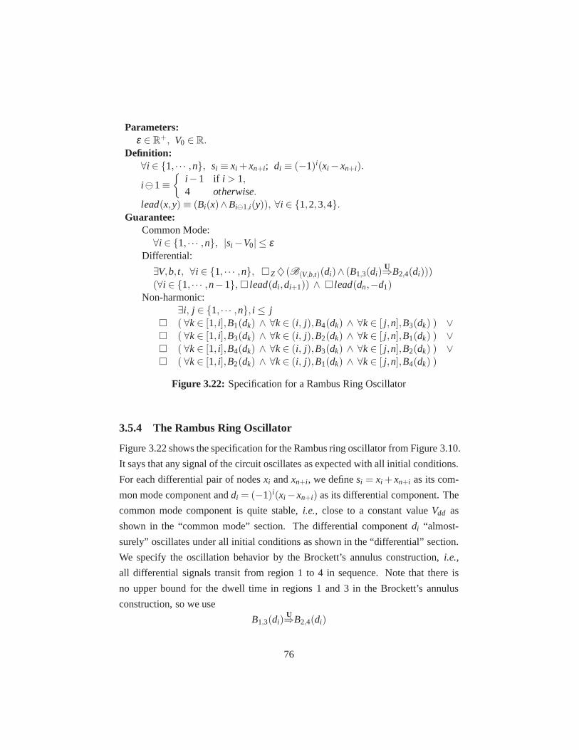
Parameters:ε ∈ R

+, V0 ∈ R.Definition:

∀i ∈ {1, · · · ,n}, si ≡ xi +xn+i; di ≡ (−1)i(xi −xn+i).

i ⊖1≡{

i −1 if i > 1,4 otherwise.

lead(x,y) ≡ (Bi(x)∧Bi⊖1,i(y)), ∀i ∈ {1,2,3,4}.Guarantee:

Common Mode:∀i ∈ {1, · · · ,n}, |si −V0| ≤ ε

Differential:

∃V,b, t, ∀i ∈ {1, · · · ,n}, �Z♦(B(V,b,t)(di)∧ (B1,3(di)U⇒B2,4(di)))

(∀i ∈ {1, · · · ,n−1},� lead(di ,di+1)) ∧ � lead(dn,−d1)Non-harmonic:

∃i, j ∈ {1, · · · ,n}, i ≤ j� ( ∀k∈ [1, i],B1(dk) ∧ ∀k∈ (i, j),B4(dk) ∧ ∀k∈ [ j,n],B3(dk) ) ∨� ( ∀k∈ [1, i],B3(dk) ∧ ∀k∈ (i, j),B2(dk) ∧ ∀k∈ [ j,n],B1(dk) ) ∨� ( ∀k∈ [1, i],B4(dk) ∧ ∀k∈ (i, j),B3(dk) ∧ ∀k∈ [ j,n],B2(dk) ) ∨� ( ∀k∈ [1, i],B2(dk) ∧ ∀k∈ (i, j),B1(dk) ∧ ∀k∈ [ j,n],B4(dk) )

Figure 3.22: Specification for a Rambus Ring Oscillator

3.5.4 The Rambus Ring Oscillator

Figure 3.22 shows the specification for the Rambus ring oscillator from Figure 3.10.

It says that any signal of the circuit oscillates as expectedwith all initial conditions.

For each differential pair of nodesxi andxn+i , we definesi = xi +xn+i as its com-

mon mode component anddi = (−1)i(xi −xn+i) as its differential component. The

common mode component is quite stable,i.e., close to a constant valueVdd as

shown in the “common mode” section. The differential component di “almost-

surely” oscillates under all initial conditions as shown inthe “differential” section.

We specify the oscillation behavior by the Brockett’s annulus construction,i.e.,

all differential signals transit from region 1 to 4 in sequence. Note that there is

no upper bound for the dwell time in regions 1 and 3 in the Brockett’s annulus

construction, so we use

B1,3(di)U⇒B2,4(di)

76

to force the trajectory to leave stable regions within a bounded time. However,

differential signals may not oscillate if the initial stateis an equilibrium point,

that is, currents of all transistors are zeros. Under this circumstance, the circuit

is not stable and diverges to oscillation mode with small disturbances. We apply

the similar “almost-surely” version always operator to denote that all equilibrium

points are in a negligible set. Furthermore, we specify the relationship between

adjacent variablesdi anddi+1 by the “lead” function. We say the value ofdi “leads”

the value ofdi+1 because of the forward inverters of the stage3. Whendi is low,

it makesdi+1 low or start to fall; anddi+1 cannot rise beforedi starts to rise. We

use theB1(di)∧B1,4(di+1) clause to exclude the case thatdi+1 is in B2,3 whendi is

in B1. Similarly, we define the valid value ofdi+1 whendi is in other regions, as

shown in the “definition” section. Note that we use−d1 in the last “lead” function

because the signal is swapped at the end of the ring.

Whenn is large, harmonic behaviors can appear if the circuit is notwell de-

signed. Under this mode, the circuit may oscillate with a faster frequency than

expected. For example, the circuit may oscillate with frequency 3f where f is the

designed frequency. We specify that there is only one transition phase in the ring

for the non-harmonic property. The first clause of the “non-harmonic” specifica-

tion says that there is only one high-to-low or low-to-high transition in the middle

of the ring . The first phaseB1dk states that all signals in the beginning of the ring

are low; the second phaseB4dk states that all signals in the middle of the ring are

falling from high to low; and the third phase states that all signals in the end of the

ring are high. The second clause describes a low-to-high transition in the middle

of the ring, similar to the first clause. Similarly, the last two clauses are for when

transitions occur in the beginning or in the end of the ring.

3.6 Implementation

The previous two sections described how circuits can be modeled using non-linear

ODEs and an extension of LTL with continuous time and values for specifying cir-

cuit properties. This section describes how we convert the nonlinear ODEs to linear

3Whenn= 2, d1 andd2 are symmetric and it is improper to say thatd1 leadsd2. Therefore, the“lead” clause does not apply to two-stage Rambus ring oscillators.

77

differential inclusions, and how we incorporate input signals that are described by

Brockett’s annuli into our reachability computations. These transformations make

the modeling and specification methods described earlier inthis chapter practical

for the reachability methods that will be described in chapter 4.

3.6.1 Linearization Methods

The nonlinear model from Equation 3.13 and Equation 3.2 usually cannot be solved

efficiently by reachability analysis tools. Therefore, we compute a linear differen-

tial inclusion (LDI) to over-approximate the ODE model for efficient computation

as:

ddt

Vi ∈ AiVi +bi ±ui (3.14)

ddt

Vo ∈ AoV +bo±uo, (3.15)

whereVi refers to input voltages,Vo refers to voltages of other ODE nodes,Ai is the

linear coefficient for input signals,bi is the constant term,ui is the error term, and

Ao,bo,uo are coefficients for ODE nodes. Because input signals are specified by

Brockett’s annuli, the time derivativeddtVi only depends on its own voltage value

Vi . The time derivative of ODE nodesddtVo depends on voltages of all nodes.

We have developed two algorithms for computing Equation 3.14 for input sig-

nals specified by Brockett’s annuli. The first algorithm findsa linear approximation

with minimizedL2 norm error term based on the least squares method. Given an

input signalv specified byB(V,b,t) (defined in Equation 3.12), and a range of value

[vl ,vh], the algorithm constructs a linear approximation ˙va as

minE = min∫ vh

vl(va− vm)

2dv

va = AvV +bv

vm =biai

√a2

i −(v−voi )2+ boao

√a2

o−(v−voo)2

2 .

(3.16)

This optimization problem can be solved by the least squaresmethod as

[

Av

bv

]

=

[

∫ vhvl

v2 dv∫ vh

vlv dv

∫ vhvl

v dv∫ vh

vldv

]−1[ ∫ vhvl

vmv dv∫ vh

vlvm dv

]

. (3.17)

78

With this linear approximation, the error bound can be foundby calculating error

terms of pointsvl , vh andve = v0− a2Av√a2A2

v+b2. However, the least squares method

minimizes theL2 norm rather than theL1 norm. Therefore, the constant termbv is

adjusted at the end to balance the lower and upper error bounds.

On the other hand, the second algorithm minimizes theL1 norm based on linear

programming. The algorithm first conservatively approximates the annulus by two

polygonspi andpo. Then it finds the best linear approximation by solving a linear

program:min uv s.t.

v ∈ Avv+bv±uv

v ∈ [vl ,vh, pix, pox],

(3.18)

wherepix(pox) denotes signal values of vertices ofpi(po).

Linear differential inclusions as shown in Equation 3.15 for ODE nodes can be

computed by either the least squares based method or LP basedmethod similarly.

From Equation 3.2, we can see that it suffices to linearize thecurrent function of

transistors to create a linear model. The linear approximation can be obtained by

solving a linear program similar to Equation 3.18 which minimizes the error term

with conditions that the linear inclusion is valid for all grid points of our table-

based models as described in Section 3.3.2. However, this LPusually contains a

huge number of constraints, each of which corresponds to onegrid point. Because

the LP approach is impractical for most problems, only the least-squares method

was implemented. Similar with Equation 3.16, the least-squares method finds the

best linear approximation according to theL2 norm of the error term and adjusts the

constant term at the end. This method can work with bothids tables and polynomial

tables.

Given anids table as described in Section 3.3.2, our algorithm computesa lin-

ear inclusion for a region specified by a user-provided linear program. The al-

gorithm first finds the bounding box of the region, collects all grid points in the

box, and computes a linear fit using the least squares method.Given the linear fit,

our algorithm then computes the error term by evaluating theerror function over

all grid points. The time to compute the linear coefficients is constant by apply-

ing pre-computed sums of tabulated data. Evaluating the error term dominates the

79

computation.

For polynomial tables, the current function is approximated by a quadratic

polynomial as described in Section 3.3.2. The least squaresmethod is implemented

similar to the one forids tables. However, we have two improvements. First, we use

the linear program to trim hyper-cubes to reduce error and improve performance.

Second, noting quadratic polynomials are Lipschitz functions and the Lipschitz

constants can be computed efficiently, we over-estimate theerror term using the

Lipschitz constant and under-estimate the error by evaluating the error function on

several sampled points. Therefore, the lower and upper bounds of the error in each

hyper-cube can be efficiently computed. With the error bound, most hyper-cubes

can be pruned without evaluating the exact error. This process can be refined to

narrow down the error bound. Because the polynomial-interpolation tables are on

a much coarser grid than the rawids data, the algorithm for polynomial tables is

more efficient than the one fori ids tables.

3.6.2 Modeling Input Behaviors

In order to obtain conservative results, it is necessary to compute circuit states

under all possible input transitions. As described in Section 3.4.3, input signals can

be specified by Brockett’s annuli. However, regions 2 and 4 ofan annulus admit

signals with the same range,i.e., they are indistinguishable without information of

time derivative of the signal. Therefore, reachability computations of regions 2 and

4 must be separated.

As mentioned in Section 3.4.3, a Brockett’s annulus has fourregions that cor-

respond to logic low, rising, high and falling signals. Continuous input trajectories

can be mapped to discrete sequences,i.e., iteration of low, rising, high and falling

stages. Therefore, transitions of one input signal can be modeled by fourstates

denoted asB1,B2,B3,B4. For a circuit with only one input signals, all possible cir-

cuit behaviors can be obtained by computing reachable regions within these four

states. Reachability analysis is performed in each stateBi with its initial regions.

In each computation step, forward reachable regions are sliced by the hyperplane

which is the boundary between the current stateBi and the next stateBi+1 (e.g.,

v= 0.2). These slices are accumulated, and the result is used as the initial region

80

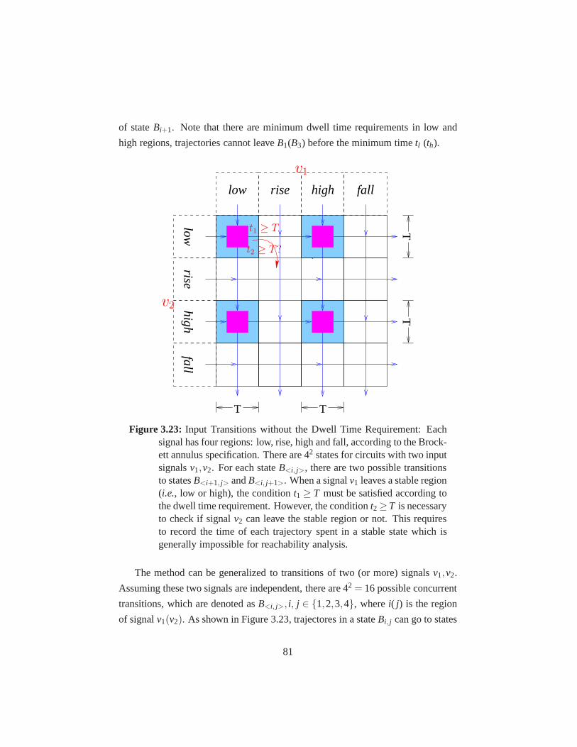
of stateBi+1. Note that there are minimum dwell time requirements in low and

high regions, trajectories cannot leaveB1(B3) before the minimum timetl (th).

T T

TT

low rise high fall

low

riseh

igh

fall

t2 ≥ T?

t1 ≥ T

v1

v2

Figure 3.23: Input Transitions without the Dwell Time Requirement: Eachsignal has four regions: low, rise, high and fall, accordingto the Brock-ett annulus specification. There are 42 states for circuits with two inputsignalsv1,v2. For each stateB<i, j>, there are two possible transitionsto statesB<i+1, j> andB<i, j+1>. When a signalv1 leaves a stable region(i.e., low or high), the conditiont1 ≥ T must be satisfied according tothe dwell time requirement. However, the conditiont2 ≥T is necessaryto check if signalv2 can leave the stable region or not. This requiresto record the time of each trajectory spent in a stable state which isgenerally impossible for reachability analysis.

The method can be generalized to transitions of two (or more)signalsv1,v2.

Assuming these two signals are independent, there are 42 = 16 possible concurrent

transitions, which are denoted asB<i, j>, i, j ∈ {1,2,3,4}, wherei( j) is the region

of signalv1(v2). As shown in Figure 3.23, trajectores in a stateBi, j can go to states

81

Bi+1, j , andBi, j+1. Accordingly, reachable regions are sliced by two hyperplanes to

compute initial regions for statesBi+1, j , andBi, j+1: one hyperplane is the boundary

between stateBi, j and stateBi+1, j (e.g., v1 = 0.2), and the other is for statesBi, j

andBi, j+1 (e.g., v2 = 1.6). In case two signals are not independent, not all states

are reachable. For example, statesB2,4 andB4,4 are forbidden for a flip-flop circuit

because of the timing constrains between the data input and the clock signal.

However, transitions of two inputs are more complicated when considering the

minimum dwell time requirement. We assume that the minimum dwell time is

T for regions 1 and 3 of two annuli, otherwise, we can setT as the minimum

value of them. Due to the minimum dwell time requirement, anytrajectory in

stateB<1,1> must satisfy the constraintt1 ≥ T before entering stateB<2,1>, where

t1 is the time of signalv1 spent in the stable (low or high) region,i.e., the time

of the trajectory spent in all statesB<1,∗>. Similarly, any trajectory cannot enter

B<1,2> until the second signalv2 has stayed in region 1 for at leastT time. As

illustrated in Figure 3.23, when trajectories enter stateB<2,1>, the conditiont2 ≥ T

may be satisfied or not. For trajectories where the conditionis satisfied, they can

enter stateB<2,2> immediately or at any time; for trajectories where the condition

is not satisfied and will not be satisfied before entering state B<3,1>, they cannot

goto stateB<2,2>; for other trajectories, they could go to stateB<2,2> after the

time when the conditiont2 ≥ T becomes to be true. This introduces a challenge

to reachability analysis. It is generally impossible to record the exact time of each

trajectory during reachability computation4. Therefore, it requires infinite number

of reachability computation to obtain the accurate result:e.g., v2 has stayed in

the low region for a timetl ≤ T whenv1 leaves the low region. It is similar for

trajectories in statesB<1,3>,B<3,1> andB<3,3>.

We employ a conservative approximation technique to solve this problem. It

first measures the maximum rising timetmax from the inner bound of the annulus

and then usesT ′ = T− tmaxas the dwell time requirement of the logic low region5.

When trajectories leaveB<1,1> and enterB<2,1>, the new conditiont1 ≥ T ′ must

be satisfied. At the same time, the conditiont2 ≥ T is also checked. If it is satisfied,

4A finite-bisimulation cannot be constructed even though it can be done for timed automata. Thisis because our linear ODIs models have much more complicateddynamics than timed automata.

5T is usually much larger thantmax for circuit signals.

82

T T

TT

t1 ≥ T ′ t2 ≥ T ′t1/2 ≥ T ′ t2/1 ≤ T ′

t1 ≥ T ′

t2 ≤

T′

t2 ≤

T

t2 ≥

T′

v1

v2

Figure 3.24: Input Transitions with the Dwell Time Requirement: We over-approximate valid trajectories by relaxing the time requirement fromT to T ′ = T − tmax. All trajectories are grouped by the conditiont1/2≥T ′: solid arrows denote trajectories in which both signals satisfythe time requirement and dashed arrows denote trajectoriesin whichonly one signal satisfies the time requirement. With this approxima-tion technique, all possible trajectories are computed within a finitenumber of reachability computations.

83

trajectories are allowed to enterB<2,2> at any time. This is an over-approximation

becauset2 ≥ T may not be true. Otherwise, trajectories must stay inB<2,1> and

go toB<3,1>. This is becauset2 ≥ T can not be satisfied when trajectories are in

stateB<2,1>. By applying this method, all reachable regions in stateB<2,1> are

over-approximated by two reachability computation. The first one is for the case

when botht1 andt2 are greater thanT ′, and the second one is for the case when

only one of two signals is greater thanT ′.

The reachability computation phase is illustrated in Figure 3.24. The solid ar-

rows denote transitions of trajectories in the first case, and dashed arrows denote

transitions of trajectories in the second case. Whenever a signal transits from the

low (high) region to the rise (fall) region, the corresponding time requirement must

be satisfied, and trajectories are grouped into two sets by the time requirement of

the other signal. For example, when trajectories leavesB<1,1> to B<2,1>, the con-

dition t1 ≥ T ′ must be satisfied. And forward reachable regions are partitioned into

two sets by the conditiont2 ≥ T ′. For the first set where the condition is satisfied,

reachability computations are performed in statesB<2,1> andB<2,2>. Noting tra-

jectories can enterB<3,1> and then go toB<3,2> immediately becauset2 ≥ T ′ is

true. However, signalv1 must stay in the high region forT ′ time; therefore, dashed

arrows are used inB<3,2>. For the second set where the condition is voilated, only

one reachability computation is performed in stateB<2,1>. After leavingB<2,1>,

trajectories must stay inB<3,1> because botht1 and t2 are smaller thanT ′. It is

similar for trajectories originated from statesB<1,3>,B<3,1> or B<3,3>. From this

analysis, we can see that there are totally 32 reachability computations as shown in

Figure 3.24.

This approach can be extended to higher dimensions for circuits with more

than two inputs. To reduce over-approximation error,tmax in the equation ofT ′

can be replaced by smaller values such astmax/2. However, this requires to par-

tition regions 2 and 4 correspondingly, which increases thenumber of states and

reachability computations.

84

4

Reachability Analysis in COHO

COHO is a reachability analysis tool for computing reachable regions of moderate-

dimensional, nonlinear hybrid systems. The reachability algorithm is described in

Section 4.1. The representation and computation of continuous successors are pre-

sented in Section 4.2 and Section 4.3. Section 4.4 describestechniques to improve

computation time and reduce approximation error. Implementation issues are dis-

cussed in Section 4.5. Finally, Section 4.6 summarizes COHO and compares our

approach with other related techniques.

4.1 Reachability Analysis

4.1.1 COHO Hybrid Automata

In order to analyze hybrid systems, we need a formal model to describe both

continuous dynamics and discrete transitions. COHO uses a general hybrid au-

tomaton to model hybrid systems. A COHO hybrid automatonis a tupleM =

(Q,X,F,T, I ,G,R,S0) where

• Q is a finite set ofdiscrete states.

• X ⊆ Rn is thecontinuous state space, wheren is the number of continuous

variables.S= Q×X is thestate spaceof the system.

• I : Q→ 2X is a collection ofinvariants. I(q) is the condition that the continu-

85

ous variables must satisfy when the automaton is in the stateq. The condition

is described by a system of COHO inequalities,e.g.,(x1 ≤ 1)∨ (x1+2x2 ≥10) (see Section 4.2.2).

• F : Q → ((X → Rn)∪ (X → 2Rn)) is a set ofcontinuous dynamics. For each

stateq, the evolution of continuous variables is governed by the deterministic

or non-deterministic dynamicsF(q).

• T ⊆Q×Q is a set ofdiscrete transitions. Each transitiont = (q,q′) identifies

asource state qand atarget state q′.

• G : Q → (2X → {0,1}) assigns each state aguard conditionfor specifying

the pre-condition of discrete transitions. Given the current reachable region

x in a stateq, the conditionG(q)(x) determines if discrete transitions are

triggered or not.

• R : T → (2X → 2X) is a collection ofreset maps. For each transitiont, R(t)

alters the continuous variables in the source stateq, which will be used in

the target stateq′.

• S0 ⊆ Q×X is the initial region of the automaton. It consists of a set of

discrete statesQ0 ⊆ Q and a set of initial regions for these discrete states

X0 = Q → 2Rn.

L R

HF

t ≥ tdwell

t ≥ tdwell

0 ≤ φ ≤ 0.2 0.2 ≤ φ ≤ 1.6

0.2 ≤ φ ≤ 1.6 1.6 ≤ φ ≤ 1.8

Figure 4.1: Hybrid Automaton for the Toggle Circuit

Figure 4.1 shows the hybrid automaton that we use when verifying the tog-

gle circuit as described in Section 3.2.1 as an example. It has four discrete states

L,R,H,F which correspond to Brockett’s annulus regions (i.e., low, rise, high, fall,

86

respectively), and seven continuous variablesX = {φ ,x,y,z,xx,yy,zz} which cor-

respond to the circuit nodes as shown in Figure 3.3. For each discrete state, the

invariant labeled in Figure 4.1 constraint the range of the clock variableφ . The

continuous dynamics are defined by ODEs extracted from the circuit as described

Section 3.3. There are four transitions:(L,R),(R,H),(H,F),(F,L). For transitions

(R,H) and(F,L), the guard condition is simply the invariant conditions,i.e.,a tra-

jectory leaves stateR or F onceφ no longer satisfies the invariant. The other two

transitions,(L,R) and(H,F) can only occur after the minimum dwell time in state

L or H has elapsed as required by the Brockett’s annulus construction. The reset

map is set to be an identify function. The initial discrete state isR and the initial

value of continuous variables is estimated based on simulations whenφ switches

from stateL to stateR.

4.1.2 Reachability Algorithm

We now turn to analyze behaviors of a hybrid automatonM . A trajectory of the

hybrid automaton is a functions:R+ →S that specifies the evolution of the system

state according to time. A state ofM can change in two ways:discrete evolution

where the system changes the discrete state andcontinuous evolutionwhere contin-

uous variables change according to the dynamics. Thereachable regionof M is the

set of all trajectories it can generate. In this dissertation, we usereachable setto de-

note the system states at a specified timet from an initial region, and usereachable

tubeto denote the region that is reachable prior to or at timet from the initial region.

We only support forward reachability analysis. In principle, backward reachability

can be implemented by negating the continuous dynamics [158]. However, mod-

eling non-linear dynamics requires using over-approximations in the reachability

computation to ensure soundness when verifying safety properties. The approx-

imations that we use make COHO only useful for forward analysis where circuit

dynamics tend to be well-damped.

Algorithm 1 shows the framework of our reachability analysis algorithm used

in COHO. Given a hybrid automatonM and its initial regionS0, it explores discrete

and continuous successors until no new reachable region found. In the algorithm,

we use a setQ to record all reachable discrete states and a setS to record reach-

87

Algorithm 1 : Reachability Algorithm of Hybrid Systems in COHO.

Input : a COHO hybrid automatonM = (Q,X,T,F, I ,G,R,S0),G = {C,L}, S0 = {Q0,X0}

Output : reachable regions of the hybrid automaton

begin1

Q= Q0;2

while q = pop(Q)do3

S0 = X0(q), I(· · · ) = Ø;4

while C(q) do5

Si+1 = postc(Si);6

S[i,i+1] = bloat(convex(Si ,Si+1), ||x||∆t);7

if L (q) then8

for each gate g ofI(q) do9

I(g) = union(intersect(S[i,i+1] ,g∩ I(q)), I(g));10

end11

end12

end13

for each transition t= (q,q′,g) of T do14

push(Q,q′);15

I(g) = R(t)(I(g));16

X0(q′) = union(X0(q′), I(g));17

end18

end19

end20

able regions in each state.Q is initialized byQ0 (line 2) and updated by adding

unvisited states (lines 14,15,18) following discrete transitions. For each stateq, S

is initialized by its initial regionX0(q) (line 4). Forward reachable sets (line 6) and

reachable tubes (line 7) are computed iteratively from the initial region. The com-

putation of reachable sets is the most challenging task which will be described in

Section 4.3 and Section 4.4. The algorithm depends stronglyon the method used

to represent continuous regions, and Section 4.2 presents the projectagon repre-

sentation that is central to COHO. The reachable tube is approximated (line 7) by

a bloated convex hull of reachable sets as illustrated in Figure 4.2. All reachable

regions of the hybrid automatonM are computed once the algorithm terminates.

88

||x||∆t Si+1

Si

S[i,i+1]

Figure 4.2: Approximate a Reachable Tube Based on Reachable Sets

As described above, each stateq has an associated initial regionX0(q). To

compute it efficiently (lines 14-18), we useslicesto record trajectories that cross

state boundaries. A slice is the intersection of a reachabletube and a hyperplane.

Each condition of invariantI(q) defines such a hyperplane, which is also called a

gate, of the stateq1. Slicing is performed in each computation step and the results

are stored in a setI (line 10). The accumulated result is applied to update the

initial region of successor states after the reset map (lines 16,17). With the concept

of slice, a transition is implemented as a tuplet = (q,q′,g) whereg is the gate

of source stateq (line 14). Accordingly, the guard conditionG(q) consists of a

continuous functionC(q) and aslicing functionL(q). The continuous function

determines when to terminate the reachability computation(line 5) and the slicing

function decides when to compute and record slices (lines 8-12) in each state. Take

the automaton as shown in Figure 4.1 as an example: trajectories can leave state

Rat any time; therefore, reachability computation stops when all trajectories leave

this state and slicing is performed in each computation step. However, in state

H, the continuous function always returns true until a fixed-point is reached and

slicing is performed only after the minimum dwell time has elapsed.

89

z

xy

z

yx

z

yx

z

Projections

MaximalReachableSpace

y

x

Figure 4.3: A Three-Dimensional “Projectagon”

4.2 Projectagons

Projectagonsare a data structure for representing high-dimensional polyhedra by

their projections (projection polygons)onto two-dimensionalplanes, where these

projection polygons are not required to be convex. Conversely, a full-dimensional

polyhedron can be obtained from its projections by back-projecting each projection

polygon into aprism and computing the intersection of these prisms as shown

in Figure 4.3. More formally, letS ∈ Rn be an-dimensional polyhedra,B =

{u1, · · · ,un} be an orthogonal basis,L ⊆ {(uX ,uY)|uX ∈ B,uY ∈B,X 6=Y} be a

set of planes. Ifl = (uX(l),uY(l)) ∈ L is a plane, we writepl = pro j(S, l) to denote

the projection ofS onto this plane:

pro j(S, l) = {(xX(l),xY(l))|(x1, · · · ,xn) ∈S}. (4.1)

1In the current implementation of COHO, all gates of the guard condition are “exactly” on theboundary of the invariant regions.

90

We useP= {pl |l ∈L} to denote the collection of all projections and writeprism(pl )

to denote the inverse projection ofpl back into the full-dimensional space:

prism(pl ) = {(x1, · · · ,xn) ∈ Rn|(xX(l),xY(l)) ∈ pl}. (4.2)

The projectagon of a polyhedronS with planesL is SL(S) where:

SL(S) =⋂

l∈Lprism(pro j(S, l)). (4.3)

In addition to thisgeometric representation SL(S) where a projectagon is repre-

sented by a collection of projection polygons, we also provide aninequality rep-

resentation EL(S) for projectagons in Section 4.2.2 where the convex hull of a

projectagon is over-approximated by a system of linear inequalities. Operations

on projectagons are implemented based on these two representations which will be

presented in Section 4.2.1 and Section 4.2.2. To convert from the geometric rep-

resentation to a system of linear constraints, we compute the convex hull of each

projection polygon as described in Section 4.2.1. To convert from a system of lin-

ear constraints back to projection polygons, we project thefeasible region of the

constraints onto the appropriate plane(s) described laterin Section 4.3.2.

Projectagons can represent non-convex polyhedra efficiently, which is not sup-

ported by most other techniques discussed in Section 2.2.3.However, projectagons

are not a canonical representation (see Appendix A). Furthermore, there are many

polyhedra (even convex ones) that cannot be represented by projectagons exactly.

For example, indentations on the surface of the full-dimensional polyhedron will be

filled; likewise, many perforated objects and knot-like objects can only be approx-

imated. However, an attractive feature of this approach is it always overestimates

the original polyhedron; in particular, it is straightforward to show that:

S⊆ SL(S). (4.4)

The approximation error also depends on the set of planesL used. Generally speak-

ing, approximation error decreases when the number of planes increases, which lies

in the range of[⌈n2⌉,

n(n−1)2 ].

91

The projectagon representation offers several advantagesover other approaches.

First, projection polygons capture circuit designers’ intuitive notion of how a cir-

cuit works. Typically, the behavior of each signal is determined by a small number

of other signals. Pairing a node with each of its controllingnodes naturally cap-

tures the causal behavior of the circuit. Because most circuits have limited fan-in

and fan-out, the number of such pairs,i.e.,planes, is proportional to the number of

nodes in the circuit. Second, the geometric representationcan capture important

non-convexities of the reachable space and provides efficient implementations of

key operations including intersection and union. These operations are described

in Section 4.2.1. Furthermore, representing the convex hull of a projectagon as a

system of linear inequalities allows us to use methods from linear programming to

manipulate projectagons which are discussed in Section 4.2.2. This is particularly

useful for operations that work on one face of the projectagon at a time, and we

approximate the face by its convex hull even though the complete projectagon may

be non-convex. Finally, ignoring degeneracies, faces of a projectagon correspond

to edges of its projection polygons. Section 4.2.3 presentsan efficient method to

enumerate all projectagon faces which is an important step for the reachability al-

gorithm in Section 4.3.3.

4.2.1 Manipulating Projectagons via Geometry Computation

The geometric representation of projectagons only tracks two-dimensional pro-

jections rather than full-dimensional polyhedra. Therefore, exponential time and

space operations on full-dimensional polyhedra can be avoided because the opera-

tions needed for reachability computations can be implemented based on polyno-

mial time operations on the two-dimensional projection polygons. For example,

intersection and union of two projectagons can be computed by

intersection(S1L,S

2L) =

⋂

l∈Lintersection(p1

l , p2l ) (4.5)

union(S1L,S

2L) ⊆

⋂

l∈Lunion(p1

l , p2l ). (4.6)

Two other operations required by COHO are convex hull and projectagon simpli-

fication. COHO’s reachability computation tends to increase the number ofver-

92

tices of each projection polygon at each time-step. As described below, polygon

simplification introduces small over-approximations to keep the polygon degrees

manageable. Like intersection and union, both convex hull and projectagon sim-

plification can be computed on a per-projection-polygon basis as indicated below:

convexhull(SL) ⊆⋂

l∈Lconvexhull(pl ) (4.7)

simplify(SL,ε)∆=

⋂

l∈Lsimplify(pl ,ε). (4.8)

The intersection of a projectagon and a hyperplane can be implemented similarly.

However, the intersection of a projection polygon and the corresponding projec-

tion of a hyperplane is a segment. To keep projectagons closed under intersection

with hyperplanes, we use a projectagon to conservatively over approximate the

intersection, which will be described with details in Section 4.3.3.

There are efficient algorithms and well-developed tools forpolygon opera-

tions [171]. However, we found that COHO requires robust implementations of

these operations for polygons with nearly parallel edges and similar difficulties.

To achieve this, we implemented a new geometry computation package based on

arbitrary precision rational (APR)numbers to provide robust implementations es-

pecially for ill-conditioned problems. For the union operation, our algorithm first

computes all intersection points of two or more polygons using thesweep-lineal-

gorithm [171, Chapter 7.2]. It then finds the union of these polygons by walking

from the lower-left-most point in the anti-clock wise orderand always selecting the

right most edge on each intersection point. An example is shown as green arrows

in Figure 4.4(a). The algorithm for the intersection operator is similar except it

chooses the left most edge on each intersection point, illustrated as yellow arrows

in Figure 4.4(a). To simplify a polygon, our algorithm finds an over-approximated

polygon by either deleting a concave vertex or replacing twoconsecutive, con-

vex vertices with a single vertex of the polygon as shown in Figure 4.4(b) and

Figure 4.4(c) respectively.

93

(a) Union/Intersection of polygons

(b) Remove a concave vertex.

(c) Replace two convex vertices with one.

Figure 4.4: Polygon Operations

4.2.2 Manipulating Projectagons via Linear Programming

The geometric representation can represent non-convex regions accurately. How-

ever, it is not efficient for some operations, such as theproject operation of non-

convex polyhedra, and the intersection of prisms. On the other hand,convex projec-

tagonshave an inequality representation which represents a half-plane by a linear

inequality. This representation has an attractive featurethat it corresponds to the

constraints of alinear programwhich makes it possible to manipulate convex pro-

jectagons using techniques from linear programming. Therefore, we also employ

an inequality representation to describe the convex hulls of projectagons and obtain

efficient algorithms for several operations.

The convex hull of a projectagon, which can be approximated efficiently using

Equation 4.7, is described by a COHO constraint systemin the inequality represen-

tationEL(S). A COHO constraint system is a system of inequalities of the form:

EL(S) = Px≤ q=⋂

l∈L{Pl xl ≤ ql |∀x∈ convexhull(pl )}, (4.9)

where the matrixP, called a COHO matrix, has only one or two non-zero elements

in any row, because each COHO inequalitycorresponds to a polygon edge. Like-

wise, a COHO equality is a linear equality constraint that involves onlyone or two

variables. The special structure of the COHO matrix is exploited to develop an

efficient LP solver in [208, 214].

The inequality representationEL(S) conservatively approximates the convex

94

hull of the original polyhedron as

S⊆ convexhull(S)⊆ EL(S). (4.10)

This representation is used to implement the bloating operator by moving each

half-plane outward as

bloat(SL,∆d)⊆ bloat(EL(S),∆d) = Px≤ q+∆d. (4.11)

It is also used to implement the project operator in Section 4.3.2, represent pro-

jectagon faces, compute bounding boxes of projectagons,etc. The intersection of

prisms represented by inequalities is trivial by the conjunction of all COHO in-

equalities.

4.2.3 Projectagon Faces

Finding projectagon faces is an important operation because all computations are

performed on projectagon faces in Algorithm 4 of Section 4.3.3. Fortunately, pro-

jectagon faces correspond to edges of projection polygons.Therefore, ife is a

projection edge on the planel , its corresponding projectagon facef (e, l) is

f (e, l) = prism(e)⋂

SL(S). (4.12)

The prism corresponding to an edge,prism(e) can be described by one COHO

equality and two COHO inequalities. However, it is difficult to compute the inter-

section of a projectagon and these inequalities. We use the inequality representa-

tion instead to compute a conservative result:

f (e, l)⊆ prism(e)⋂

EL(S). (4.13)

The result is accurate for convex projectagons. However, for non-convex pro-

jectagons, the approximation error can be very large. Therefore, we developed

an interval closuretechnique for finding a more accurate representation of projec-

tagon faces. The interval closure calculation is based on interval constraint prop-

agation. It interprets a non-convex polygon as constraintsof continuous variables

95

and views each polygon edge as defining interval bounds for the two variables of

the projection. The algorithm then applies these intervalsto other polygons that

include one of these variables in their basis to obtain bounds of other variables.

This process continues until no further tightening of the interval bounds is possible

or the progress is below a threshold. The algorithm is simple, fast and signifi-

cantly reduces the approximation error when the projectionpolygons are highly

non-convex. The interval closure based projectagon faces can be expressed as:

f (e, l)⊆ prism(e)⋂

EL(S)⋂

intervalClosure(e,SL(S)). (4.14)

4.3 Computing Continuous Successors

This section presents our algorithm for computing continuous successors used in

Algorithm 1. First, the method to move projectagon faces forward in time is shown

in Section 4.3.1. Second, advanced faces are projected ontotwo-dimensional planes

to maintain the structure of projectagons, as described in Section 4.3.2. Finally,

the algorithm for computing continuous successors is presented in Algorithm 4 of

Section 4.3.3 and the feasibility problem of projectagons is discussed.

4.3.1 Advancing Projectagon Faces

As shown in Algorithm 4 (line 13), an essential step of computing continuous suc-

cessors is to advance projectagon faces according to nonlinear dynamics. A projec-

tagon face is represented by a COHO constraint system as described in Section 4.2.3.

In this section, we consider the problem of computing an over-approximationδt(S)

of the reachable set at timet from an initial regionS, which is described by a COHO

constraint systemPx≤ q. Nonlinear dynamics are conservatively approximated by

a linear differential inclusion (LDI) of the form

x= Ax+b±u, (4.15)

where theu term defines a uncertainty setU for which we use a hyper-rectangle.

These non-deterministic dynamics are approached with themaximum principle

from optimal control theory [197]. The key idea is to find acritical value u∗ ∈U

96

for each face ofSwhich moves its corresponding hyperplane furthest outward. A

face fi of S is represented by an inequality from the COHO constraint system as

Pix≤ qi , (4.16)

wherePi is the ith row of COHO matrix P and qi is the ith element of vectorq.

Equation 4.16 also defines a halfspace where~n= PTi is theoutward normalof the

corresponding hyperplane.

a b c

U

u∗(t)

~n(t)S

f

u∗

u1

~n

~n(t)

δt(f) S

f1

f2

f3

u∗

1

u∗

2

p

p∆t

Figure 4.5: Maximum Principle. a) the normal~n(t) is determined by the lin-ear system; b) find critical value by linear programming c) redundantfaces can reduce approximation error.

By integrating Equation 4.15, we have

xu(t) = eAtx(0)+ (eAt − I)A−1b+∫ t

0eA(t−s)u(s)ds.

We remark that all initial points satisfy the COHO constraint systemPx(0) ≤ q;

therefore, we have

Pie−At ·xu(t) ≤ qi +Pi(I −e−At)A−1b+

∫ t

0Pie

−As·u(s)ds. (4.17)

As illustrated in Figure 4.5(a), we can see that the evolution of the normal tofidoes not depend on the uncertainty termu, and is only governed by the linear term

as

~n(t) = e−ATtPTi . (4.18)

To bound all trajectories with all possible values of the uncertainty termu, we

97

maximize the integration in Equation 4.17 as

~nT(t)xu(t) ≤ qi +Pi(I −e−At)A−1b+maxu:[0,t]→U∫ t

0(~nT(s)u(s))ds. (4.19)

It is straightforward to computeqi +Pi(I −e−At)A−1b, and we now derive a bound

for the integral.

maxu:[0,t]→U

∫ t

0~nT(s)u(s)ds

= maxu:[0,t]→U

∫ t

0~nTe−Asu(s)ds

= maxu:[0,t]→U

∫ t

0~nT

(

∞

∑k=0

(−As)k

k!

)

u(s)ds

≤ maxu:[0,t]→U

∫ t

0~nT

(

m

∑k=0

(−As)k

k!

)

u(s)ds

+ maxu:[0,t]→U

∫ t

0~nT

(

∞

∑k=m+1

(−As)k

k!

)

u(s)ds

(4.20)

wherem is chosen to set the degree of the approximation of the matrixexponen-

tial. In practice,‖At‖, is small, andm= 1 or m= 2 will produce a very small

overapproximation. Let

G = maxu:[0,t]→U

∫ t

0~nT

(

m

∑k=0

(−As)k

k!

)

u(s)ds

H = maxu:[0,t]→U

∫ t

0~nT

(

∞

∑k=m+1

(−As)k

k!

)

u(s)ds

(4.21)

For smallm, G can be computed exactly by considering one component ofu at a

time. To boundH, observe

H = maxu:[0,t]→U

∫ t

0~nT

(

∞

∑k=m+1

(−As)k

k!

)

u(s)ds

≤ maxu:[0,t]→U

∫ t

0‖~nT‖

∥

∥

∥

∥

∥

m

∑k=0

(−As)k

k!

∥

∥

∥

∥

∥

‖u(s)‖ds

= t‖~n‖(

e‖At‖−m

∑k=0

‖At‖k

k!

)

‖U‖

(4.22)

98

This provides an overapproximation of the solution to Equation 4.19 providing the

bound we want for the most outward foward faceδt( fi). Thus, the forward reach-

able region is bounded by

δt(S)⊆⋂

fi∈S

δt( fi). (4.23)

The actual implementation of COHO is based on an earlier approximation that

we derived but that can be underapproximate. The COHO code is based on the

assumption that the critical value does not change during the time step and ap-

proximating the forward regionδt(S). With this assumption, the integral is under-

approximated slightly as:

∫ t

0~nT(t)u∗(s)ds ≈ max

u∈U

∫ t

0~nT(s)uds

= |Pi(I −e−At)A−1|u.

Therefore, the forward reachable region is bounded by a COHO advanced con-

straint of the form:

PEx ≤ q

E = e−At

q = q+P(I −E)A−1b+ |P(I −E)A−1|u,(4.24)

where the matrixE is a linear operator for moving a point at the end of a time

step back to the original point at the beginning of the time step. We ran some

experiments to quantify the effect of this under-approximation for the examples

described in Chapter 5. In all cases, any under-approximation wasvery small,

and we are convinced that the over-approximations in other parts of COHO ensure

that, in practice, the overall computation is an overapproximation as desired. Both

approximation methods have the advantage that they are relatively efficient because

only matrix operations rather than numerical integration are involved during the

computation.

Finally, we add redundant faces to the initial regionSto reduce approximation

error. As illustrated in Figure 4.5(c), a vertexp lies on two facesf1 and f2, how-

99

ever, the critical valuesu∗1 andu∗2 of these two faces are not necessarily the same.

Therefore, the intersection pointp∆t of the two forward faces is not reachable from

the pointp. The redundant facef3 can trim unreachable regions and thus reduce

overapproximation error.

4.3.2 COHO Linear Program Solver and Projection Algorithm

COHO makes extensive use of linear programs (LPs) which have either COHO

constraint systems from Equation 4.9 or COHO advanced constraint systems from

Equation 4.24. This section presents an overview of our linear program solver and

projection algorithm based on my Master’s work [208]. The linear programs used

on COHO can be written as

minx

dT ·x, s.t.

P ·E ·x ≤ q,(4.25)

whereP · x ≤ q is a COHO constraint system whose feasible region is a convex

projectagon,d is the cost vector, andE is an optimal backward time step operator

for LDI models. Because time steps are relatively small,E is well-conditioned,

and E−1 can be easily computed. We refer to a linear program in the form of

Equation 4.25 as a COHO linear program.

There are two main approaches for solving linear programs:interior point al-

gorithms [156, 164] and theSimplexalgorithm [80]. However, the inherent ill-

conditioning of interior point methods compounded the problem of badly condi-

tioned linear programs and prevented their successful application. On the other

hand, the Simplex algorithm is typically formulated to operate on standard form

linear programs. Astandard formlinear program has the form [165]:

min cT·x, s.t. Ax≤ b. (4.26)

To retain the special structure of COHO matrices, we convert a COHO LP to its dual

100

form [165] asmin

y−qT·y, s.t.

PT ·y = E−Td

y ≥ 0.

(4.27)

The COHO dual LP is a standard form linear program. Therefore, it can be solved

by the Simplex algorithm. By theduality theorem[196, Chapter 5], the primal

and dual linear programs have the same optimal value and optimal basis; thus, the

COHO LP can also be solved.

Simplex is a greedy algorithm. It repeatedly selects a subset of the columns

of PT called thebasis. Let PTB

denotePT restricted to a basisB. Simplex solves

for yB = P−TB

·d and determines if the basis can be modified so as to improve the

cost. This step is calledpivotingwhich replaces a column in the basis with a new

column to obtain a more favorable basis. Simplex pivots to reduce the cost until

the optimal basis is found.

Algorithm 2 : COHO LP Solver (lpsolve(LP))

Input : LP(P,q,d,E): a COHO LP of the form: mindTx,s.t.PEx≤ qOutput : B: optimal basis,pt: optimal point,v: optimal value

begin1

A=−PT; b=−E−Td; c=−q;2

dLP= lp standard(A,b,c);3

B = BigM(dLP);4

repeat5

cb = A−TB

cB;6

j = argmini 6∈B(ci −AT:,icb < 0);7

t0 = A−1B

b; t j = A−1B

A:, j ;8

k= argmini∈Bt0,it j,i

;9

B = replace(B,k, j);10

until B= null ;11

pt= E−1P−1B

qB; v = dTpt;12

end13

COHO uses a modified Simplex algorithm as shown in Algorithm 2. It first con-

verts COHO LPs to the dual forms (lines 2,3) and computes an initial feasible basis

101

based on theBig M method[196, Chapter 2.3] (line 4). It uses a standard pivoting

algorithm (lines 6-10). However, COHO computes the Simplex tableau from the

input data for each pivot which is different from most implementations where the

tabulea is updated based on its predecessor [80]. This modification avoids accumu-

lated error because only a vector of integers specifying thebasis is passed through

each pivot. The algorithm is as efficient as the traditional implementation based on

rank-1 updates of the tableau, because COHO’s solver exploits the structure of the

COHO matrixP to obtain a linear time algorithm for solving linear systemson lines

6, 8 and 12. More details of the linear system solver are described in [208, 214].

To maintain the projectagon structure, advanced faces in Equation 4.24 need to

be projected onto two-dimensional planes to compute projections for constructing

a new projectagon. Likewise, projectagons are re-projected to remove infeasible

regions which will be discussed in Section 4.3.3. Therefore, an important opera-

tion in COHO is finding the projected polygonof a convex region described by

a COHO constraint systemPx≤ q or COHO advanced constraint systemPEx≤ q

onto a plane defined by two orthogonal axes(~x,~y). We call this problem theprojec-

tion problemand present an algorithm based on linear programming for projection

problems with COHO constraint systems and extend it to problems with COHO

advanced constraint systems.

The idea behind our projection algorithm in Algorithm 3 is tosolve COHO LPs

maxx∈Rn

(~xcosθ +~ysinθ) ·x s.t.Px≤ q, (4.28)

for all θ from 0 to 2π and use the optimal points to construct the projected polygon.

It is unnecessary and impossible to solve Equation 4.28 for every possible value of

θ . Instead, COHO only solves one LP for each edge of the projected polygon,

where the optimal direction~xcosθ +~ysinθ is also the normal vector of the edge.

The normal vector of a polygon edge is computed based on the optimal basis

of the COHO LP in Equation 4.28. Our Simplex based solver works on its dual

problem:

miny∈R+m

q·y s.t.PTy=~xcosθ +~ysinθ ,y≥ 0. (4.29)

When the solver finds a solution to Equation 4.29, it also findsan optimal basis

102

B and an optimal pointpt = P−TB

(~xcosθ +~ysinθ) whose elements are all non-

negative. By increasing the value ofθ to some critical value, the basisB will no

longer be optimal for the optimization direction~xcosθ +~ysinθ . The critical value

of θ is the oneθnext (line 11) at whichpt acquires a negative element, and the

corresponding direction is orthogonal to the polygon edge that is from the current

optimal vertex to the new optimum. Each successive value ofθ can be determined

by a single linear system solve in linear time. Similarly, the normal vector of

the edge from the previous optimal vertex to the current one can be computed by

decreasing the value ofθ to θprev (line 10) as shown in Figure 4.6(a).

θ

ǫ is too large

θ + ǫ

θprev θnext

Figure 4.6: Projection Algorithm:a) finding θnext andθprev from the optimalbasis;b) both blue vertices are optimal for the normal vector;c) an edgeis skipped whenε is too large.

However, using the normal of a polygon edge as the optimal direction may not

find the expected optimal basis, because several projectagon vertices may corre-

spond to the same projection polygon vertex as illustrated in Figure 4.6(b). There-

fore, we increase the value ofθ by a small amountε (line 5) to force the LP solver

to find the correct optimal basis and optimal point. However,this may skip some

edges and produce under-approximated results as shown in Figure 4.6(c). We de-

tect this scenario by comparing the value ofθ andθprev. If there is no edge has

been skipped in the step,θprev must equal toθ . Otherwise, the mean value ofθ and

θprev is used as the new optimization direction (line 12) to repeatthe computation.

The algorithm is generalized to projection problems with COHO advanced con-

straint systems for projecting a time advanced projectagonP ·E · x≤ q. Although

the feasible region of a COHO advanced constraint system is not a projectagon

in the standard coordinateC , it can be represented as a projectagon of the form

P · x ≤ q in the new coordinateE−1C . Therefore, the problem is converted to

103

projectP·x≤ q on to a subspace with basis vectorsE−1~x, andE−1~y (lines 2,3,16).

The algebraic and geometric explanations of this coordinate transformation can be

found in [208].

Algorithm 3 : COHO LP Projection Algorithm (lpproject(PEx≤ q,~x,~y))Input : COHO advanced constraints:PEx≤ qInput : projection plane(~x,~y)Output : p: projection onto (~x,~y) plane

begin1

~x= E−1~x; ~y= E−1~y;2

~y=~y− ~x·~y||~x|| ; ~x=

~x||~x|| ; ~y=

~y||~y|| ;3

for θ = 0,θ ≤ 2π do4

θopt = θ + ε ;5

repeat6

d =~xcos(θopt)+~ysin(θopt); lp = lp standard(P,q,d);7

[B,pt,v] = lp solve(lp);8

ζ = P−TB

~x; η = P−TB

~y;9

θprev= maxi∈[1,n](argθ min(ζi cosθ +ηi sinθ = 0∧ θ < θopt));10

θnext= mini∈[1,n](argθ min(ζi cosθ +ηi sinθ = 0∧ θ > θopt));11

θopt =θ+θ prev

2 ;12

until θ = θprev ;13

θ = θnext; p= p+ pro ject(pt,~x,~y);14

end15

p= convexhull(p); p= E−1p;16

end17

As we can see, the correctness of the LP solver depends on correct pivots and

the projection algorithm relies on correct computation ofθprev andθnext. However,

numerical error of floating point arithmetic may result in anincorrect pivot and fail

to find an optimal solution in the Simplex algorithm, especially for ill-conditioned

COHO LPs. Therefore,arbitrary precision rational (APR)arithmetic is applied in

the LP solver and the projection algorithm to make COHO robust. If APR methods

were applied to all of COHO’s computations, the resulting implementation would

be very slow. As described in Section 4.4.4, COHO uses interval-based methods

where their accuracy is sufficient and resorts to APR only when necessary.

104

4.3.3 Computing Forward Reachable Sets

Algorithm 4 shows the procedure of computing a forward reachable set in COHO.

Because the system dynamics are bounded, trajectories are continuous and can-

not cross. Therefore, trajectories starting on projectagon faces provide bounds for

trajectories starting in the interior. Accordingly, the algorithm first finds all pro-

jectagon faces using the interval closure approximation inSection 4.2.3 (line 4).

Then it calculates a linear differential inclusion (LDI) model for each face and

computes a step size∆t (lines 5-7,10). To ensure soundness, it uses a conserva-

tive strategy to compute the model and step size based on a constraint that any

point in the projectagon can move by at most a user-provided distance∆d along

any axis-parallel direction. It bloats each face outward by∆d (line 5) and approxi-

mates the system dynamics by a LDI in the bloated face (line 6). Based on the LDI

model, it computes the maximum derivative in the bloated face by solving two sets

(∀i ∈ {1, · · · ,n}) of linear programs (line 7) as

min/maxxi , s.t.

x ≤ Ax+b+u

−x ≤ −(Ax+b−u)

Px ≤ q,

(4.30)

which can be solved by the LP solver in Section 4.3.2. The stepsize is calculated

by computing the maximal value∆t = ∆dmax|xi | (line 10) which guarantees that the

reachable tube is bounded by the bloated face during this step [0,∆t].

Given LDI models and a step size, projectagon faces are advanced by using

Equation 4.24 (line 13). To maintain the structure of projectagons, all advanced

faces are projected onto two-dimensional planes using the method described in

Section 4.3.2. However, each advanced face must be projected onto all planes of

the original projectagon (line 15). Intuitively, this is because the projectagon can

rotate during this step and any face can become an external face for any plane. Fi-

nally, a new projectagon for the forward reachable set is constructed by computing

the union of all projected polygons on the same plane and simplifying the result to

reduce space complexity (lines 19-22).

During the computation above, projection polygons are computed indepen-

105

Algorithm 4 : Algorithm for Computing Forward Reachable SetInput : SL: current reachable set represented by a projectagonInput : ∆d: maximum moving distance allowedOutput : S∆t

L : the forward reachable set after time step∆t

begin1

for each projection pdo2

for each edge edo3

fe = prism(e)∩EL, fe = fe∩ intervalClosure(e,SL) if fe 6= /0;4

f be = bloat( fe,∆d);5

modele = modelcreate( f be );6

|x|e = l p solve( f be ,modele);7

end8

end9

∆t = mine∈SL∆d

max|x|e ;10

for each projection pdo11

for each edge edo12

f ∆te = l p f orward( fe,modele,∆t);13

for each plane l∈ L do14

polyle = l p pro ject( f ∆t

e ,~xl ,~yl );15

end16

end17

end18

for each plane l∈ L do19

p∆tl = poly unione∈SL (polyl );20

p∆tl = poly simpli f y(p∆t

l );21

end22

S∆t0 =

⋂

l∈L prism(p∆tl ); E∆t

0 =⋂

l∈L prism(convexhull(p∆tl ));23

repeat24

for each plane l∈ L do25

polyil = l p pro ject(E∆t

i−1,~xl ,~yl );26

pil = poly intersect(pi−1

l , polyil );27

pil = poly simpli f y(pi

l );28

end29

S∆ti =

⋂

l∈L prism(pil ); E∆t

i =⋂

l∈L prism(convexhull(pil ));30

until ||E∆ti−1−E∆t

i || ≤ ε ;31

S∆tL = S∆t

i ; E∆tL = E∆t

i−1;32

end33

106

dently for each plane. Therefore, it is possible that there are infeasible regions

of one projection to other projections,i.e., the prism from this region does not

intersect with other prisms of other polygons. The infeasible regions of the new

projectagon may lead to incomplete boundaries in the next step when working on

an infeasible face. To solve the problem, all projection polygons must be clipped

to make them feasible to each other. Section A.1 shows that the problem of de-

termining whether a projectagon constructed from a set of non-convex polygons

is non-empty is NP-complete. Thus, we accept that a practical algorithm must be

based on heuristics and/or approximations.

We relax the problem of removing infeasible regions as clipping a projectagon

such that each of its projections is feasible to the inequality representation of the

projectagon,i.e., convex hulls of other projections. The algorithm is based onthe

projection algorithm in Section 4.3.2. As shown in line 23 ofAlgorithm 4, the

inequality representation of the new projectagon is constructed from the convex

hulls of projection polygons. This representation can include non-tight or redun-

dant constraints from infeasible edges. To obtain a canonical representation, we

project the COHO constraint system onto all planes (line 26) and construct a new

set of inequalities from the projected polygons. It is easy to show that all these pro-

jected polygons are feasible to each other. Therefore, the intersection of an original

projection and its corresponding updated projected polygon (line 27) is still feasi-

ble to the new inequality representation. This algorithm clips a projectagon and

makes it feasible to its inequality representation.

The inequality representation must be refined because the intersection makes

a projectagon polygon smaller but also changes its convex hull. The convex hulls

of intersected polygons are computed and the inequality representation is recon-

structed at the end of each step (line 30). This procedure is repeated until all convex

hulls are fixed. However, it may take infinite number of steps to converge to the

stable projectagon2. To solve the problem, we stop the computation after a certain

number of iterations or the progress is smaller than a threshold (line 31). We do

not update the inequality representation in the last step (line 32). Therefore, the

inequality representation at the end is an over-approximation rather than an exact

2An example is provided in Section A.2.

107

representation of the convex hull of the projectagon.

This method has been applied in Algorithm 4 to make the boundary complete.

It ensures that projections of any new projectagon are feasible to its inequality rep-

resentation. As show in line 4, we use Equation 4.14 to obtaina tighter approxima-

tion of a projectagon face if the face is feasible; otherwise, we use Equation 4.13

to approximate the projectagon face to ensure the approximation is not empty. To

control space complexity, intersected polygons are also simplified (line 28). How-

ever, only concave vertices can be removed because replacing two convex vertices

with one can enlarge the convex hull and make it infeasible tothe inequality repre-

sentation.

Noting that we can add arbitrary COHO constraint systems to the inequality

representation during the projecting step (line 26), the algorithm is extended to

compute the intersection of a projectagon and a COHO constraint system. Actually,

the intersection of a projectagon and a hyper-plane required in Algorithm 1 is over-

approximated by the intersection of the projectagon and a bloated hyper-plane.

This is because the intersection of a projectagon and hyper-plane is not a full-

dimensional projectagon. By bloating the hyperplane slightly, we avoid the need

to handle special cases for objects that are not full-dimensional, and this makes the

implementation much simpler.

4.4 Improvements

The algorithm described above is numerically stable; however, the reachability

computation can be very expensive especially for high-dimensional systems. Fur-

thermore, the over-approximated result may be too large to verify a correct system

successfully. To improve performance and accuracy, several new algorithms have

been developed as shown in Algorithm 5. Section 4.4.1 presents a method which

projects advanced faces onto one plane to reduce projectionerror and improve per-

formance (line 7). Section 4.4.2 proposes a guess-verify strategy for increasing the

step size and reducing error (lines 2-17). More techniques to reduce model error

are discussed in Section 4.4.3 (lines 9-12,18-21). To improve performance, hybrid

computation is applied as described in Section 4.4.4 and approximate algorithms

are applied as shown in Section 4.4.5 (line 11).

108

Algorithm 5 : Improved Algorithm for Computing Forward Reachable SetInput : SL: current reachable set represented by a projectagonInput : ∆d, ∆t: bloat amount and step size of the previous stepOutput : S∆t

L : the forward reachable set after time step∆t

begin1

repeat2

update∆d and∆t;3

for each projection pdo4

for each edge edo5

fe = prism(e)∩EL∩ intervalC(e,SL) || prism(e)∩EL;6

fe = (bloat( fe,∆d)∩EL) || heighten( fe,∆d);7

modelse = modelcreate(bloat( fe,∆d));8

for each model me ∈ modelse do9

f ∆te = l p f orward( fe,me,∆t);10

polyse(i) = l p pro jA( f ∆te ,~xp,~yp);11

end12

polye = poly intersect(polyse);13

∆d′ = max(ph bloatAmt( fe, polye),∆d′);14

end15

end16

until ∆d′ ≤ ∆d ;17

repeat18

∆d = ∆d′;19

repeat lines 8−14;20

until ||∆d−∆d′|| ≤ ε ;21

for each plane l∈ L do22

p∆tl = poly simpli f y(poly unione∈SL (polyl ));23

end24

S∆t0 =

⋂

l∈L prism(p∆tl ); E∆t

0 =⋂

l∈L prism(convexhull(p∆tl ));25

repeat26

for each plane l∈ L do27

polyil = l p pro ject(E∆t

i−1,~xl ,~yl );28

pil = poly simpli f y(poly intersect(pi−1

l , polyil ));29

end30

S∆ti =

⋂

l∈L prism(pil ); E∆t

i =⋂

l∈L prism(convexhull(pil ));31

until ||E∆ti−1−E∆t

i || ≤ ε ;32

S∆tL = S∆t

i ; E∆tL = E∆t

i−1;33

end34

109

4.4.1 Reducing Projection Error

In Algorithm 4, each advanced face must be projected onto allplanes in order to

ensure soundness. This approach is very expensive with large projection error.

Projecting an advanced face back to the plane for the original edge is usually much

more accurate than projecting onto other planes. This is because the face has much

tighter constraints of variablesXl andYl , i.e., an edge, than other variables, and

the linear differential inclusion model has a smaller errorterm for these two vari-

ables. Although the value ofXl andYl variables can be affected by other variables

as the face may rotate during a step, the correlation is usually much smaller espe-

cially when the step size is very small. Therefore, it is attractive to only project an

advanced face back onto its own plane.

∆d

∆d

a b c

Figure 4.7: Projectagon Faces to be Advanced: a) Extreme trajectory from aface which does not correspond to an edge of the plane; b) Bloat theface inward; c) Increase the height of the face.

However, this method does not consider all possible trajectories as illustrated

in Figure 4.7(a). To ensure soundness, there are two approaches as shown in

Figure 4.7(b) and Figure 4.7(c)3. The first approach bloats a face inward by a

distance∆d which captures all boundaries that can lead to extreme points of pro-

jected polygons, because any point in the projectagon cannot move more than∆d

distance along any direction. The second approach increases the height of the face

by ∆d to block any extreme trajectory from other faces because theextreme trajec-

tory must cross the heightened face. The bloated face or heightened face are used

to create linear differential models and to be advanced in each step. Both meth-

3The correctness of our approach is proved in Appendix B.

110

ods significantly improve the performance. The second technique has relatively

smaller error than the first one because the bloated face enlarges the region ofXl

andYl variables directly whereas the heightened face only increases the range of

other variables that have smaller impact onXl andYl .

4.4.2 Guess-Verify Strategy

Choosing a good pair of step size∆t and bloat amount∆d is important to obtain

good performance and small error. If the bloat amount is too small, COHO will

take very small time steps resulting in long execution timesand reachable regions

that are overly conservative because of the error from the projection phase. Con-

versely, if the bloat amount is too large, then the non-linearity error (theu term

in Equation 4.15), will be large, causing another kind of over approximation and

small time steps. In Algorithm 4, the step size is computed using theℓ∞ norm of the

derivatives. Therefore, it is usually very pessimistic andmuch smaller than what

would actually be safe for the given bloat amount. When a faceis advanced, the

successor of the face at the end of a time step of Algorithm 4 often lies well inside

the bloated face.

Noting the fact that the pair of step size and bloat amount arevalid as long as

the advanced face lies inside the bloat region used to createthe LDI model4. A

guess-verifystrategy was developed which tries to guess a pair of step size ∆t and

bloat amount∆d based on the data from previous steps. At the end of each step,

the method checks that the estimated bloat is sufficient for the estimated step size.

If not, it updates the bloat amount and/or step size and repeats the computation. In

addition to enabling larger time steps, the guess-verify strategy speeds up the com-

putation of each step by eliminating the step-size calculation phase of Algorithm 4

(lines 7,10).

The verify step is based on computing thereal bloat amount∆d′ and comparing

it with the estimated bloat amount∆d. The basic operation of computing a forward

reachable set is to move forward a face that corresponds to a projection edgeeand

4Soundness requires that the reachable tube from the face throughout the time step[0,∆t] mustremain in the bloated region. In order to obtain a simple implementation, we only consider reachablesets at time 0 and∆t for efficiency in the implementation. There is a potential unsoundness if atrajectory goes outside the bloat region and re-enters the bloat by the end of the time step.However,this happens rarely because the step size is generally tiny and our inclusion dynamics are linear.

111

project back the advanced face onto its own plane, resultingin a projected polygon

p. To check if the assumption that every point can move along any axis direction

by at most∆d, the maximum moving distances alongXe andYe must be computed

based on the edgee and the projected polygonp. This is computed by solving a

linear program.min∆d′, s.t.

Px ≤ b+ |P| ·∆d′

Ax ≤ b,

(4.31)

wherePx≤ q is the COHO constraint system that describes the face, andAx≤ b is

the constraint from the convex polygonp. By assuming each point on the face can

move by at most∆d′ along each axis direction, the region reachable during the time

step[0,∆t] is bounded byPx≤ b+ |P| ·∆d′. Therefore, solving this linear program

finds the minimum bloating amount that ensures the polygonp is contained in the

bloated face.

4.4.3 Reducing Model Error

A large fraction of the approximation error of the reachability computation is from

the linearization error during generating linear differential inclusion models,i.e.,

the u term in Equation 4.15. Although the guess-verify strategy reduces the ac-

cumulated error by decreasing the number of steps, bloated faces or heightened

faces make the error term larger. In the current research, I have devised, imple-

mented, and evaluated several techniques to reduce the magnitude of the over-

approximations used by COHO.

In Algorithm 4, all variables are bloated equally. However,in a dynamic sys-

tem, it is common that some variables change much faster thanothers. For ex-

ample, in digital circuits, a few signals will be in transition at any given time and

the others will be relatively stable. This results in excessive bloating for the stable

signals. To achieve an acceptable step size, the bloat for fast changing signals must

be relatively large. When the same bloat is used for all variables, the bloat for slow

changing signals is excessive, leading to much larger errorterms in the differential

inclusion than necessary. Likewise, when a signal is changing, it is generally either

clearly rising or clearly falling. Thus, a large bloat is only needed in one direction,

112

allowing the total bloat for these variables to be reduced bynearly a factor of two.

We implementedasymmetric and anisotropic bloating. Asymmetric bloating al-

lows the positive and negative bloats for a variable to be different. Thus, bloating

can adapt to the direction in which a signal is making a transition. Anisotropic

bloating allows each variable to have its own bloat amount. Thus, bloating can

adapt according to which variables are changing and which are stable. This ap-

proach allowed a significant increase (e.g.,4x) in the typical step size. As an added

benefit, the smaller total bloat reduced the error terms in the differential inclusion,

allowing COHO to compute tighter bounds on the reachable regions.

At the end of each step, areal bloat amount∆d′, which is the smallest valid

bloat for the step size, can be calculated as used in the guess-verify strategy. It

is smaller than the bloat amount∆d hence it can be used to refine models. These

refined models also make it easier to guess an accurate bloat amount for the next

step and consequently reduce the number of guesses.

Another approach to obtain more accurate models is to usemultiple modelsat

the same time. The intersection of several linear differential inclusions provides a

tighter bound of the non-linear dynamics. As a result, each face must be advanced

and projected several times. The intersection of projectedpolygons from different

models is used to generate a more accurate forward reachableset. Of course, this

method also increases the total running time. It is appealing especially for circuit

verification because it can prevent non-physical behaviors. For example, if the

drain voltage is greater than the source voltage, the current of NMOS transistor is

always positive, but negative current may be introduced during the modeling phase.

An extra constant differential inclusion can be added to eliminate projectagon re-

gions corresponding to these non-physical, negative currents.

4.4.4 Hybrid Computation

To make the algorithm robust, we applied APR numbers in the LPsolver as de-

scribed in Section 4.3.2. We also use APR in the geometric computations and the

projection function. Although all rational numbers are rounded to floating point

numbers at the end of each step, it is still very expensive to use APR numbers for

all computations. In practice, APR numbers are only necessary for ill-conditioned

113

problems which happen rarely. Ahybrid computationstrategy is used to solve this

problem by applying both interval computation and APR arithmetic. Most com-

putations are performed using interval arithmetic which computes upper and lower

bounds of the result and detects ill-conditioned problems.If the interval computa-

tion fails, the APR package is used to recomputed an exact solution. This hybrid

computation method improves the performance significantly. Prior to using APR,

COHO runs would often fail due to ill-conditioned computations,and these errors

occurred in many places in the COHO code. The hybrid interval/APR approach

provided a simple implementation that has eliminated theseerrors from COHO.

Therefore, it has been applied to the LP solver, and the geometry package. The

projection function is implemented entirely with APR as most of time are spent on

solving LPs.

The method was generalized to support floating point numbers, interval num-

bers and APR numbers. The Simplex algorithm with floating point numbers can

solve most of the LPs and find the exact optimal basis. To speedup the compu-

tation, the LP solver uses ordinary double-precision arithmetic for each pivot. It

then verifies that each pivot succeeded in reducing the cost function first by using

interval arithmetic, and in the infrequent event that this fails, COHO uses APR. If

the pivot failed to reduce the cost, it repeats the pivot stepwith interval arithmetic

or APR. Likewise, at the end of the algorithm, it tests the optimality of the solu-

tion by verifying that it is feasible in both the primal and dual LPs, again using

interval arithmetic first and APR if the result from the interval calculation is incon-

clusive. In this way, we obtain the certainty of APR while performing nearly all

calculations using ordinary, double-precision arithmetic. The most efficient algo-

rithm can often be obtained by the strategy which uses floating point numbers for

ordinary computation, uses interval numbers to validate the result and uses APR

for ill-condition problems. Of course, other combinationsof floating point, interval

and APR numbers can also be applied.

4.4.5 Approximation Algorithms

Even with the hybrid computation method, solving LPs and projecting advanced

faces is still one of the most expensive computations in COHO. To improve perfor-

114

mance further, we developed more efficient algorithms to compute approximated

results.

Noting that most of the LPs to solve occur in the projection algorithm, the LP

solver is improved by taking advantage of the special properties of these LPs. As

shown in Section 4.3.2, whenθ in Equation 4.28 and Equation 4.29 is increased to

force a pivot to the next edge of a projected polygon, the standard form LP becomes

infeasible. Traditional formulations of Simplex assume a feasible basis; thus, the

original algorithm restarted the LP solver to establish feasibility for each edge of

the projection of each face. However, only a single pivot is required to re-establish

feasibility in the absence of degeneracies. Accordingly, we modified our LP solver

to try each column ofPT to determine if its introduction into the optimal basis of

the previous LP achieves optimality. This requires a singlelinear-system solve for

each column tried which can be performed inO(n) time due to the special struc-

ture of COHO’s LPs. We found that this optimization works for about 80% ofthe

projection polygon edges which resulted in a significant improvement in perfor-

mance. The rather high failure rate is because the prisms whose intersection forms

the projectagon are orthogonal to each other, leading to a higher rate of degeneracy

than for typical LPs. A more efficient method was also developed to find the initial

feasible basis for the Simplex algorithm. It tries to find constraints with only one

non-zero coefficient for each variable, which is easy to find as all constraints of

COHO LPs have only one or two non-zero coefficients, and constructs a feasible

basis from these candidates.

The projection of an advanced face at the end of a time step canhave clusters

of very closely spaced vertices separated by much larger gaps. These clusters arise

from near degeneracies in the COHO LPs. To avoid a rapid growth in the number of

vertices in the projection polygon, COHO performs a simplification step where the

projection polygon is replaced by an enclosing polygon of smaller degree. Con-

sequently, every vertex but one in a cluster will be discarded by the simplification

process, but the projection algorithm expended a significant amount of compu-

tation time to determine these vertices. In the new implementation as shown in

Algorithm 6, we avoid this extra work by enforcing a lower bound on the change

of θ at each step of the projection algorithm as shown in Algorithm 3. The approx-

imate algorithm skips over vertices if the normals of the consecutive polygon edges

115

θ + ǫθ

θnext

θprev

Figure 4.8: Approximated Projection Algorithm. The red polygon is anunder-approximation and the blue polygon is an over-approximation ofthe projection.

are nearly parallel. Thus, the polygon obtained from the revised projection algo-

rithm could be an under-approximatione.g.,the red polygon in Figure 4.8, which

would violate the soundness requirement for COHO. Conversely, we can use each

vertex from the projection algorithm to define a half plane, and construct the poly-

gon defined by the intersection of these half-planes. The resulting polygon is an

over-approximation, illustrated as the blue polygon in Figure 4.8. COHO computes

both polygons. If their areas differ by more than a preset tolerance, COHO reverts to

computing the exact projection polygon. Otherwise it uses the over-approximation.

4.5 Implementation

The COHO tool is implemented in MATLAB and JAVA with a layered architecture

as shown in Figure 4.9. It consists of four layers. The top layer converts circuit ver-

ification problems into reachability analysis problems as described in Chapter 3. It

constructs one or more hybrid automata based on the circuit structure described in

MSPICEand extracts circuit dynamics in order to compute LDI models. The sec-

ond layer,i.e., theHybrid Automatapackage, implements the reachability analysis

algorithm described in Section 4.1. The projectagon representation described in

116

Algorithm 6 : Approximated Projection Algorithm(lpprojA(PEx≤q,~x,~y))Input : COHO advanced constraints:PEx≤ qInput : projection plane(~x,~y)Input : error toleranceτOutput : p: projection onto (~x,~y) plane

begin1

~x= E−1~x; ~y= E−1~y;2

~y=~y− ~x·~y||~x|| ; ~x=

~x||~x|| ; ~y=

~y||~y|| ;3

for θ = 0,θ ≤ 2π do4

d =~xcos(θ)+~ysin(θ); lp = lp standard(P,q,d);5

[B,pt,v] = lp solve(lp);6

pl = pl + pro ject(pt,~x,~y);7

planes= planes+ plane create(θ ,v);8

θopt = θ + ε(τ); d =~xcos(θopt)+~ysin(θopt); lp =9

lp standard(P,q,d);[B,pt,v] = lp solve(lp);10

pl = pl + pro ject(pt,~x,~y);11

ζ = P−TB

~x; η = P−TB

~y;12

θprev= maxi∈[1,n](argθ min(ζi cosθ +ηi sinθ = 0∧ θ < θopt));13

θnext= mini∈[1,n](argθ min(ζi cosθ +ηi sinθ = 0∧ θ > θopt));14

if θprev> θ then15

planes= planes+ plane create(θprev,v);16

end17

θ = θnext;18

end19

pl = convexhull(pl ); pu = plane intersect(planes);20

if area(pu)−area(pl )area(pl )

≤ τ then21

p= E−1pu;22

else23

p= l p pro ject(PEx≤ q,~x,~y);24

end25

end26

117

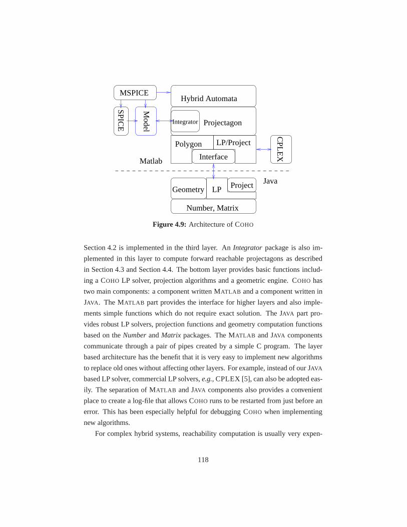
Hybrid Automata

ProjectagonIntegrator

Model

CP

LEX

Number, Matrix

ProjectLPGeometry

Polygon LP/Project

InterfaceMatlab

Java

SP

ICE

MSPICE

Figure 4.9: Architecture of COHO

Section 4.2 is implemented in the third layer. AnIntegrator package is also im-

plemented in this layer to compute forward reachable projectagons as described

in Section 4.3 and Section 4.4. The bottom layer provides basic functions includ-

ing a COHO LP solver, projection algorithms and a geometric engine. COHO has

two main components: a component written MATLAB and a component written in

JAVA . The MATLAB part provides the interface for higher layers and also imple-

ments simple functions which do not require exact solution.The JAVA part pro-

vides robust LP solvers, projection functions and geometrycomputation functions

based on theNumberandMatrix packages. The MATLAB and JAVA components

communicate through a pair of pipes created by a simple C program. The layer

based architecture has the benefit that it is very easy to implement new algorithms

to replace old ones without affecting other layers. For example, instead of our JAVA

based LP solver, commercial LP solvers,e.g.,CPLEX [5], can also be adopted eas-

ily. The separation of MATLAB and JAVA components also provides a convenient

place to create a log-file that allows COHO runs to be restarted from just before an

error. This has been especially helpful for debugging COHO when implementing

new algorithms.

For complex hybrid systems, reachability computation is usually very expen-

118

sive and the approximation error is large. Therefore, it is crucial to achieve a

good trade-off between performance and accuracy in order tosuccessfully ver-

ify a system. COHO offers several implementations of every function, optimized

for performance or precision. First, it supports two kinds of representation meth-

ods: non-convex projectagonand convex projectagon. The general projectagon

representation has the smallest representation error especially for nonlinear sys-

tems. However, the convex projectagon method is much fasterbecause many op-

erations can be implement more efficiently, such as the unionof convex polygons.

Therefore, it is often used in the first time of reachability computation to obtain

an estimated result quickly. The approximation error is usually acceptable, oth-

erwise, the computation is refined using the non-convex projectagons. Second,

COHO supports three methods for finding a bloat amount and step size pair: fixed

bloat amount, fixed time step, andguess-verify. The first and second options use

a user provided bloat amount or step size to compute a valid step size or bloat

amount, and the guess-verify method is described in Section4.4.2. Third, it sup-

ports several methods for finding projectagon faces which are used to build LDI

models and to be advanced. COHO can either advance each face and project back

onto all planes represented in Section 4.2.3, or advance bloated faces or height-

ened face and project onto its own plane only as described in Section 4.4.1. In

addition to these methods, it also supports a much faster technique which creates

only one LDI model for a projectagon and advances the whole projectagon rather

than working on each face. However, this method has larger approximation error

and does not work for non-convex projectagons. Another option is to advance each

projectagon face and only project back onto its own plane. This method can gen-

erate the most accurate result. Although it is not sound in theory, it works well

in practice because approximation errors from other steps,such as modeling and

projecting steps, make the result conservative enough to contain all possible trajec-

tories. Finally, there are some other parameters provided to control the computation

precision, such as tolerance values used for simplifying a polygon or computing an

approximated projected polygon. These options make it possible to use different

strategies in states of a hybrid automaton. For example, we can optimize for run-

ning time in states where the system converges quickly and optimize for accuracy

otherwise. Furthermore, it makes COHO more robust by switching to another set

119

of options and repeating the computation when an error or exception is found in a

step.

4.6 Summary and Discussion

We have devised techniques for reachability analysis of hybrid systems and imple-

mented them in the COHO tool. It supports moderate-dimensional systems based

on the projectagon representation which reduces the numberof dimensions by pro-

jecting high-dimensional polyhedra onto two-dimensionalplanes. It also supports

nonlinear systems by approximating continuous dynamics bylinear differential

inclusions. The COHO tool is robust and has been used to verify properties of sev-

eral circuits as will be described in the next chapter. The main improvements that

we developed to provide this robustness were the use of a combination of interval

arithmetic and arbitrary precision rational arithmetic throughout the linear program

solver and geometric engine. We also developed new techniques to remove infea-

sible regions from projection polygons, which is necessaryfor the robustness of

the implementation. Reachable sets computed by COHO are accurate for several

reasons. First, non-convexpolyhedra can be represented byprojectagons directly,

and all faces can be computed accurately by the interval closure technique. Second,

all computations are performed on projectagon faces ratherthe whole projectagon.

Therefore, small approximation error is achieved during the modeling and project-

ing steps. Furthermore, several techniques have been developed to reduce model-

ing error including model refinement, multiple models, and aguess-verify strategy.

COHO is also efficient because it employs many techniques including hybrid com-

putation, guess-verify, and an approximated LP solver as well as the projection

function. COHO also supports trade-offs between performance and accuracyand

handles exceptions automatically.

There are several related techniques and tools, includingD/DT [48], CHECK-

MATE [40], and PHAVER [70]. Compared with other representation techniques,

the projectagon representation is more accurate because itsupports non-convex re-

gions and works on individual faces. Similarly, orthogonalpolyhedra [33] works

on each face in the face lifting technique and represents non-convex regions by

the union of fixed-grid hyper-rectangles. It can be viewed that intervals or hyper-

120

rectangles are the results of projecting polyhedra onto onedimensional lines and

projectagons are the results of projecting polyhedra onto two-dimensional planes.

The projecting idea can be generalized to three or higher dimensional subspaces.

It might be helpful to represent circuit states more precisely because the dynamics

of one circuit node usually depends on more than two variables. However, ma-

nipulating moderate-dimensional, non-convex polyhedra is much more expensive,

therefore, this technique has not been studied. Hybridization strategy has been

widely used to solve nonlinear dynamics. We adopted this approach and optimized

it to reduce approximation errors by computing LDI models for each face. This

on-the-fly approach is more accurate but also more expensivethan computing only

one model for a fixed-grid region as used in other tools,e.g.,D/DT [24]. The LDI

model is much more precise than the constant differential inclusion model used in

many tools, including LEMA [148] and PHAVER [70]. On the other hand, solving

constant differential inclusion is much easier. Furthermore, we found it is helpful

to use both linear DI models and constant DI models to reduce modeling error.

APR numbers are also used in PHAVER [70] for exact computation. However, we

have not found that the hybrid computation technique is applied in PHAVER or

other similar tools.

There are some research directions to improve COHO. First, the normal of each

advanced face can be estimated based on the maximum principle in Section 4.3.1.

It can help to simplify the new projectagon at the end of each step. As a result,

the number of projectagon faces is roughly constant. A similar approach is used

by template polyhedra [181] in order to control the space complexity. However,

the template is fixed in the template polyhedra representation whereas it is updated

automatically in the projectagon representation. Furthermore, parallel computa-

tion is a promising technique to speedup COHO significantly as there are many

parallelisms in the projectagon based computation.

121

5

Examples

With methods described in Chapter 3 and Chapter 4, we can construct mathemati-

cal models for circuits and compute reachable regions usingthe tool COHO. This

chapter applies these techniques to the circuits presentedin Section 3.2 to demon-

strate correctness and effectiveness of our methods and tools. We first present a

general framework for defining verification problems, computing reachable regions

and checking properties in Section 5.1. Then we show experimental examples with

greater details and verification results in the following sections.

5.1 Verification of AMS Circuits

To formally verify a property of a given circuit, we propose aframework which

consists of three steps.

1. Simulate the circuit and the property

2. Compute reachable regions of the circuit

3. Check the property based on the result of reachability analysis.

The remainder of this section describes each step.

5.1.1 Simulation and Verification

Generally, we simulate the circuit to be verified before attempting verification.

This has several advantages. First, simulation can find obvious errors with less

122

effort and computation than formal verification. Second, the simulation result can

be used to approximate the initial condition of formal verification. For example,

we use simulation traces to estimate Brockett’s annuli for input signals of a circuit

such that its outputs satisfy properties of interest. During the process of verifying

the circuit, we often compare simulation traces and reachable regions to find the

most critical computation steps such that we can obtain a good trade-off between

performance and approximation error during reachability analysis.

We have developed a MATLAB package, MSPICE, to describe the netlist of

a circuit and simulate the circuit. While the simulation speed is an order-of-

magnitude slower than a dedicated simulator such as HSPICE, MSPICE gives the

user much greater flexibility and access to the numerical computations of the sim-

ulation. This allows, for example, inputs to be generated asrandom trajectories

that satisfy their given Brockett’s annuli. With this framework, we use the same

models (see Section 3.3.2) for simulation and verification.This makes it possible

to compare the results of MSPICE and COHO, where the simulation result is an

under-approximation of possible circuit states and the reachable region computed

by COHO is an over-approximation. This guides us when choosing which methods

to use to reduce the over-approximations computed by COHO. Furthermore, when

developing new reachability techniques in COHO, the comparison with simulation

results is helpful for identifying and correcting errors inthe algorithms or their im-

plementations. However, the integrator of MSPICE requires that the functions to

be integrated be continuous. To make the models in Section 3.3.2 continuous, we

smooth out interpolated values by a weighted cosine window.For example, letg0,

g1, . . . be a set of continuous functions wheregi is the one fori−1≤ x≤ i+1, the

interpolated functionf (x) is

f (x) ≈ wm(x−⌊x⌋)g⌊x⌋(x−⌊x⌋)+wm(x−⌈x⌉)g⌈x⌉(x−⌈x⌉)wm(x) = 1

2 +116 (9cos(πx)−cos(3πx)) .

(5.1)

This 3-term cosine window method makesf (x) aC3 function becausedk

dxk w(1) =

0,∀k ∈ [0,3]. Higher orders of smoothness can be obtained by applying more co-

sine terms in the cosine window function.

123

5.1.2 Reachability Computations

Reachability computations are often quite slow,e.g., it may take several days to

complete the computation for a 6-dimensional system. Therefore, it is crucial to

partition the reachability computation into several phases and perform the compu-

tations in parallel. To make the computation in each phase independent of the other

phases, we apply anassume-guaranteestrategy. For each phase, weassumethat

the circuit state is bounded by a regionRi and compute forward reachable regions

from Ri. At the end, weshowthat all assumptions are correct based on reachable

regions computed in all phases to establish an invariant set. Usually, we partition

the reachability computation based on input transitions asshown in Section 3.6.2.

As described in Section 3.6.2, the reachability computation for a circuit with one

input can be partitioned into two phases which correspond tothe rising and falling

stages of the input signal. For a circuit with two inputs, thereachability computa-

tion as shown in Figure 3.24 is usually partitioned into fourphases: the first phase

starts from the stateB<1,1> and ends in the stateB<3,3>; the second phase is from

the stateB<1,3> to the stateB<3,1>; the third phase is from the stateB<3,1> to the

stateB<1,3>; and the last phase is from the stateB<3,3> to the stateB<1,1>. This

strategy enables us to complete the verification, debug the model, and address is-

sues of over approximation in a reasonably timely manner. Italso makes it easier

to find phases with large approximation errors and consequently optimize COHO

for accuracy to avoid false-negatives. Similarly, we can speed up reachability com-

putation for phases in which circuit states converge quickly.

We can further partition one state of the hybrid automaton used in COHO into

several states byslicing signals. For example, instead of computing the reachable

region for a signalx in the region of[0,1] in one state, we can slice the signal by

the face wherex= 0.5 and then solve reachability problems for states wherex is

in the range of[0,0.5] and [0.5,1.0]. The slicing strategy avoids computing LDI

models (see Equation 4.15) for large regions and thus reduces approximation error.

It could also improve the performance of reachability computation which depends

on the size of the initial region. By increasing the number ofstates of the hybrid

automaton used in COHO, slicing enables more parallelism. However, it also intro-

duces extra computation and approximation,e.g.,intersection of reachable regions

124

and slicing faces. From the experimental results, we found it is a good choice to

slice a signal in 0.2 volt intervals for several designs in a 180nm, 1.8 volt CMOS

process.

5.1.3 Checking Properties

Based on the reachable regions computed above, we can check properties of inter-

est. For example, we can compute the Brockett’s annulus for agiven signal based

on the reachable region and its ODE model as shown in Equation3.2. Finding an

invariant set of the reachable region is very helpful to showsafety properties and

liveness properties. In the current implementation, most properties specified by

the logic in Section 3.4 are checked by manually inspecting the reachable regions

computed by COHO. We will talk about details for each verification example in the

following sections.

By default, we use circuit models for the TSMC 1.8V 180nm bulkCMOS

process. For a circuit, the Brockett’s annulus for each input signalss is specified

by B(0,0.15,1.65,2.0,1.5e10,2e10,1e−9) . However, when computing the linear differential

inclusion model as described in Section 3.6.1, we increase the maximum low value

from 0.15V to 0.2V and lower the minimum high value from 1.65Vto 1.6V to

ensure the derivative is strictly positive in region 2 and negative in region 4. For

example, we compute a linearized model in Brockett regionB1 for 0≤ s≤ 0.2 as

if V0h were 0.2V, and use the original Brockett’s annulus for 0.2≤ s≤ 1.6 which

ensures that COHO sees a clearly positive value for ˙s in regionB2. It is similar for

regionsB3 andB4. This method over-approximates the input and is thus sound.

It is possible that COHO is unable to verify that the outputs of some circuits

satisfy a desired Brockett’s annulus due to COHO’s approximation error. Buffer-

ing the output with an inverter provide a very simple model without changing the

circuit behavior. An inverter functions as a Brockett’s annulus transformer. The

inverter can take a slow input transition and turn it into a faster output transition,

because of the inverter’s gain. Conversely, it can take a very fast input transition

and produce a slower output transition because the inverterhas a maximum slew

rate. The filtering effect removes reachable regions that COHO computed due to

approximation errors. This trick usually does not increasethe number of dimen-

125

K

K

K

36

qz

10

10

10

φ

φ

φ

φx

y z

6

10

10

10

xx

yy zz

6

6

10

10 10

10

20

Figure 5.1: Verified Toggle Circuit

sions of the reachability computations, because the decomposition strategy can be

applied to partition the circuit and perform two separate reachability computations

for the original circuit and the inverter.

5.2 The Yuan-Svensson Toggle

Figure 5.1 shows the toggle circuit that we verified. Transistors are labeled with

their shape factors and the capacitor on theq output represents a load equivalent to

the gate capacitance of transistors with a total shape factor of 36; this is the load

that the toggle places on its clock input. We use this load to verify that the output

of one toggle can drive the clock input of another to implement a ripple counter.

The verification that we present resembles an earlier verification result by Green-

street [83]. There are several significant differences between our approach and the

earlier work. Most significantly, Greenstreet ignored internal nodes,i.e., xx, yy,

andzz, and reduced the system further to three dimensions by changing variables.

We include these internal nodes in our model, which results in a seven-dimensional

state space. Second, we model the drain-source currents of the transistors based on

tabulated data obtained from HSPICE as described in Section3.3.2, and thus our

results are based on the BSIM-3 models implemented by HSPICE for the TSMC

180nm process. In contrast, [83] used a simple, first-order,long-channel MOSFET

model that neglected leakage currents and other important properties of transis-

tors in a deep-submicron technology. Using a realistic model forced us to address

126

−1 −0.8 −0.6 −0.4 −0.2 0 0.2 0.4 0.6 0.8 1−1

−0.8

−0.6

−0.4

−0.2

0

0.2

0.4

0.6

0.8

1

Φ↑

Φ↓

Φ↑

Φ↓

X

Y

Figure 5.2: Behavior of a Toggle

other real-world issues, most notable of which was the leakage currents of the

transistors. Thus, we added “keepers” to nodesx, y and z (illustrated by “k” in

Figure 5.1). While such practicalities can seem like a nuisance from a formal veri-

fication perspective, they show that our approach is solidlyconnected to the issues

that challenge circuit designers for deep submicron processes. Like COHO, [83]

used projection polygons to represent reachable regions. However, these polygons

were restricted to have axis-parallel edges. In contrast, we use projectagons to rep-

resent reachable regions and the algorithms from Chapter 4 that are more efficient

and more accurate for reachability analysis. We also verified that the output signal

satisfies the same Brockett’s annulus specification as we useto specify the input

clock, φ .

We specify the behavior of the toggle circuit using the safety properties given in

Figure 3.20. We use COHO to find an invariant subset ofRd such that all trajecto-

ries in this set have a period twice that of the clock signal. This notion can be visu-

alized using a Poincare section [166] as illustrated in Figure 5.2. Letφ be the con-

tinuous signal corresponding toΦ, and letc be some constant withV0h < c<V1l .

Consider the intersection of the invariant set with theφ = c hyperplane. These

intersections form a Poincare map [166]. We verify that these intersections form

four disjoint regions (two for risingφ crossingc, and two falling crossings), and all

trajectories must visit these four regions in the same order. Thus, theφ = c plane

127

partitions the invariant set of the continuous model into four disjoint regions that

map to the four discrete states of the discrete model.

5.2.1 The Reachability Computation

Our specification for the toggle requires it to have an invariant set that has twice

the period of the input clock,φ . Accordingly, our reachability calculation is carried

out for two periods ofφ . Applying the assume-guarantee strategy, we break each

of these periods into two phases: one for the rising transition ofφ and the time that

φ is high; and the other for the falling transition and the low time. We estimate a

bounding hyper-rectangle for the end of each phase based on the simulation results.

With these estimates, we divide the task of verifying the toggle into four separate

proof obligations where each obligation is of the form:

Assumethat the circuit state is in hyper-rectangleYi at the end of phase

i.

Showthat the circuit state will be in hyper-rectangleYi+1 at the end of

phasei +1.

Let

Btoggle = B(0,0.15,1.65,2.0,2e10,3e10,1e−9) , (5.2)

and set the Brockett’s annulus of the clock signal toBtoggle. We start each phase

with the projectagon for the starting hyper-rectangle and note the bounding hyper-

rectangle of the projectagon for the reachable region at theend of each phase as

shown in Table 5.1. Table 5.1 also lists the projection polygons that we used for

each phase. These were chosen with two considerations. First, we chose projec-

tions that correspond to logical dependencies between changing signals. Thus, in

the first phase whenz changes, we includez vs. zzandz vs. x (because the falling

edge ofzenables a rising edge ofx). Second, we included at least one polygon for

each variable to bound the resulting projectagon in all dimensions.

The linear model forφ has large errors if the interval forφ is too large. Thus,

we “sliced” the space into regions corresponding to 0.1 volt wide intervals forφ .

It is simple to show that the circuit model has an invariant that all node voltages

are between 0 volts (i.e. ground) and 1.8 volts (i.e.Vdd) and thatxx≥ x, yy≤ y

128

Start and end hyper-rectangle for each phasePhase φ x y z xx yy zz1, start 0.2 [0.000,0.100] [1.700,1.800] [1.700,1.800] [0.000,1.0] [0.000,0.100] [0.000,0.100]1, end 1.6 [0.000,0.002] [1.790,1.800] [0.000,0.014] [1.788,1.8] [0.000,0.004] [0.000,0.001]2, start 1.6 [0.000,0.100] [1.700,1.800] [0.000,0.100] [1.700,1.8] [0.000,0.100] [0.000,0.100]2, end 0.2 [1.795,1.800] [1.758,1.800] [0.000,0.043] [1.795,1.8] [1.152,1.736] [0.000,0.003]3, start 0.2 [1.750,1.800] [1.750,1.800] [0.000,0.050] [1.750,1.8] [0.800,1.800] [0.000,0.040]3, end 1.6 [0.000,0.001] [0.000,0.005] [1.703,1.800] [1.785,1.8] [0.000,0.002] [0.843,1.740]4, start 1.6 [0.000,0.100] [0.000,0.100] [1.700,1.800] [1.700,1.8] [0.000,0.100] [0.800,1.800]4, end 0.2 [0.000,0.100] [1.700,1.800] [1.700,1.800] [0.000,1.0] [0.000,0.100] [0.000,0.100]

Projection polygons for each phasePhase Polygons1 x vs.xx, x vs.z, zvs.zz, zvs.xx, φ vs.y, φ vs.yy2 x vs.xx, x vs.y, x vs.yy, y vs.yy, φ vs.z, φ vs.zz3 x vs.xx, x vs.y, x vs.yy, y vs.yy, y vs.z, y vs.zz, zvs.zz, zvs.z, zvs.xx, φ vs.z4 x vs.xx, y vs.yy, y vs.z, y vs.zz, zvs.zz, φ vs.z

Table 5.1: Reachability Summary of Toggle Verification

129

andzz≤ z. We added these extra invariants to COHO to tighten the bounds COHO

computes. Phase 3 was the most challenging phase to verify. In this phase,φ goes

from low-to-high, and all three ofx, y, andz change their values, in the ordery ↓→ z↑ → x ↓. The greatest challenge arose becausez can start its rising transition

while y is still falling. As seen in Table 5.1, we used ten projectionpolygons

for this phase instead of the six that were used in the other phases to improve

accuracy. We found that onceφ was high (i.e., greater than 1.6 volts), it was

helpful to slice the value ofy. We used 0.1 volt wide slices fory as it fell from 1.3

volts to 0.1 volts. We slicedz in the same manner but found that it was unnecessary

to slicex. Furthermore, the transistor model from Section 3.3 can produce large

error bounds that include currents that flow against the drain-to-source voltage.

These non-physical behaviours allowed by the model caused COHO to fail to verify

the toggle. We solved the negative current problem by addinga transistor model

that simply determines the minimum and maximum drain-to-source current (i.e.,a

constant differential inclusion) for the region around thecurrent face. While this

model has a large error-term, it never predicts a current of the wrong sign. The

two models produce two different over approximations of thereachable region. At

the end of each time step, we compute the intersection of the two projectagons to

obtain a tighter bound on the reachable space than either alone. More details are

described in [210, 211].

However, we found that the values of all nodesx,y, andzresulted in large inter-

vals during the reachability computation of the toggle circuit without the “keepers”

as shown in Figure 5.1. This is caused by leakage currents of transistors. For ex-

ample, when the input clockφ is low, x is low andy is high, nodez is floating

because both its upper P-channel and lower N-channel transistors are not conduct-

ing. The leakage currents of these N-channel and P-channel transistors allow the

value ofz to be a tiny value of arbitrary sign. Becauseφ can be low for an arbitrar-

ily long time, COHO correctly finds that the possible values forzdiverge to include

any value between the power supply voltage and ground. This failure shows that

leakage currents must be considered in deep sub-micron designs even for “simple”

circuits such as the toggle circuit. Therefore, we added small “keeper” circuits to

nodesx,y andzduring the verification.

130

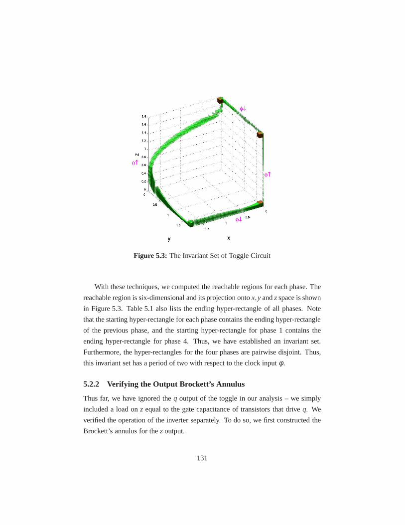
Figure 5.3: The Invariant Set of Toggle Circuit

With these techniques, we computed the reachable regions for each phase. The

reachable region is six-dimensional and its projection onto x,y andzspace is shown

in Figure 5.3. Table 5.1 also lists the ending hyper-rectangle of all phases. Note

that the starting hyper-rectangle for each phase contains the ending hyper-rectangle

of the previous phase, and the starting hyper-rectangle forphase 1 contains the

ending hyper-rectangle for phase 4. Thus, we have established an invariant set.

Furthermore, the hyper-rectangles for the four phases are pairwise disjoint. Thus,

this invariant set has a period of two with respect to the clock input φ .

5.2.2 Verifying the Output Brockett’s Annulus

Thus far, we have ignored theq output of the toggle in our analysis – we simply

included a load onz equal to the gate capacitance of transistors that driveq. We

verified the operation of the inverter separately. To do so, we first constructed the

Brockett’s annulus for thezoutput.

131

At each time step of the verification described above, we determined the reach-

able combinations ofzandz. We note that ˙z is negative monotonic inzand positive

monotonic inzz. Thus, the extremal values of ˙z vs. z occur on the boundary of the

z vs. zzprojection. For each edge of thez vs. zzprojection, COHO computes the

linearized circuit model and uses this model to find the reachable combinations of

z andz. From these, we construct a Brockett’s annulus that is satisfied byz andz.

Figure 5.4 shows the result;z does not satisfies the same Brockett’s annulus as we

used to specifyφ .

We then perform a separate reachability analysis for the output inverter. The

input to this circuit is modeled by the Brockett’s annulus for z as computed by

COHO above. We then use COHO to compute the reachable space forz and q,

and use the method above to compute the reachable region for ˙q vs. q as described

above forzandz. Figure 5.5 shows the result;q clearly satisfies the constraints that

we used forφ . Thus, these toggles can be composed to form an arbitrarily large

ripple-counter as desired.

5.3 A Flip-Flop Circuit

Figure 5.6 gives the latch circuit that we have verified. Transistors as well as in-

verters are labeled with their shape factors. The capacitoron outputq represents

a load equivalent to the load of inputd. Therefore, we can useq as the input of

another latch circuit to compose a master-slave flip-flop as shown in Figure 3.6.

We use a large inverter (8:4) to generate theφ signal.

Unlike the toggle circuit, the latch circuit has two inputs:the clock signalφand the data inputd. To model input transitions of two inputs, we employ the

method presented in Section 3.6.2. The input specification requires thatd must be

stable whenφ is falling. Therefore, statesB<4,2> andB<4,4> are removed from

the reachability computation. Noting that the reachable regions also depend on the

initial states of internal nodes, two reachability problems with the same input signal

and clock are solved for each of the two different latch states. Therefore, there

are six independent phases to compute the reachable regionsusing the assume-

guarantee strategy:

1: FromB<1,1> to B<3,3> with i1 = low.

132

0 0.2 0.4 0.6 0.8 1 1.2 1.4 1.6 1.8 2−4

−3

−2

−1

0

1

2

3

4x 10

10

Figure 5.4: Brockett’s Annulus ofz. The blue polygons show the computedBrockett’s annulus of signalz. The black lines show the polygonal ap-proximation of the Brockett’s annulus ofφ .

0 0.2 0.4 0.6 0.8 1 1.2 1.4 1.6 1.8−4

−3

−2

−1

0

1

2

3

4x 10

10

q (volt)

qdot

(vo

lt/se

cond

)

Figure 5.5: Brockett’s Annulus ofq

133

8

12

4

8:4

8:4

12

φ

φ

φ

q

φ

i1

i2

d

Figure 5.6: Verified Latch Circuit

2: FromB<1,1> to B<3,3> with i1 = high.

3: FromB<1,3> to B<3,1> with i1 = low.

4: FromB<1,3> to B<3,1> with i1 = high.

5: FromB<3,1> to B<1,3> with i1 = low.

6: FromB<3,3> to B<1,1> with i1 = high.

Table 5.2 lists the projection polygons used for reachability computation. It

also provides the initial region of each phase. After the computation of all phases,

we combine the results to check our initial estimations. Forexample, to check the

initial region of phase 1, we compute the union of the ending hyper-rectangles of

phases 3 and 6 becausei1 is low in these two phases. It is similar for other phases.

Figure 5.7 shows the value ofq with respect to the Brockett’s annulus of clock

φ . This plot shows thatq is clearly low or high whenφ is in region 1. This proves

that if input d is stable when clockφ is falling, then outputq is also stable when

φ is clearly low. Furthermore, it shows that the minimum duration time tl andthcan be as low as 0.27ns based on the reachable regions. Therefore, the highest

frequency is about 1.3GHz considering the rising/falling time as defined by the

input specification.

We also verified several properties of the flip-flop circuit asshown in Figure 3.6.

Based on the properties of the latch circuit, it is obvious that the outputq of the

master latch of the flip-flop is stable whenφ is rising. That is, the inputq of the

slave latch does not change whenφ is rising. Therefore, we can conclude that the

outputq of the slave latch is stable whenφ is low by applying the property of the

134

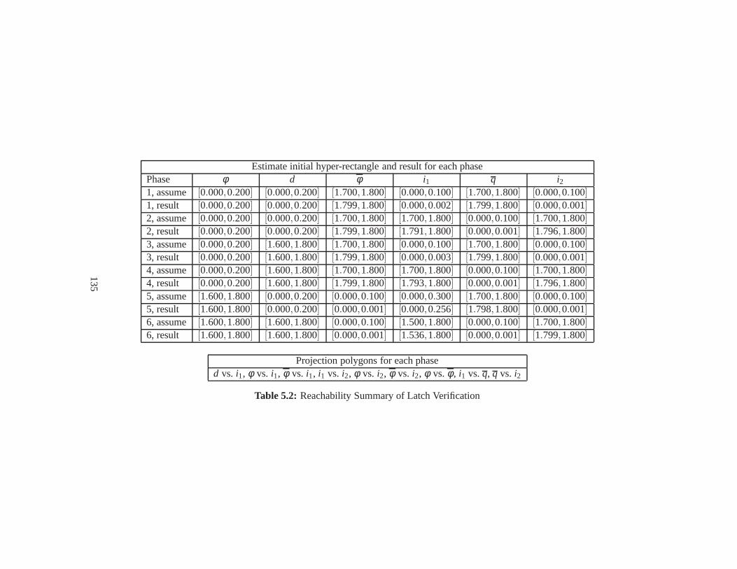
Estimate initial hyper-rectangle and result for each phasePhase φ d φ i1 q i21, assume [0.000,0.200] [0.000,0.200] [1.700,1.800] [0.000,0.100] [1.700,1.800] [0.000,0.100]1, result [0.000,0.200] [0.000,0.200] [1.799,1.800] [0.000,0.002] [1.799,1.800] [0.000,0.001]2, assume [0.000,0.200] [0.000,0.200] [1.700,1.800] [1.700,1.800] [0.000,0.100] [1.700,1.800]2, result [0.000,0.200] [0.000,0.200] [1.799,1.800] [1.791,1.800] [0.000,0.001] [1.796,1.800]3, assume [0.000,0.200] [1.600,1.800] [1.700,1.800] [0.000,0.100] [1.700,1.800] [0.000,0.100]3, result [0.000,0.200] [1.600,1.800] [1.799,1.800] [0.000,0.003] [1.799,1.800] [0.000,0.001]4, assume [0.000,0.200] [1.600,1.800] [1.700,1.800] [1.700,1.800] [0.000,0.100] [1.700,1.800]4, result [0.000,0.200] [1.600,1.800] [1.799,1.800] [1.793,1.800] [0.000,0.001] [1.796,1.800]5, assume [1.600,1.800] [0.000,0.200] [0.000,0.100] [0.000,0.300] [1.700,1.800] [0.000,0.100]5, result [1.600,1.800] [0.000,0.200] [0.000,0.001] [0.000,0.256] [1.798,1.800] [0.000,0.001]6, assume [1.600,1.800] [1.600,1.800] [0.000,0.100] [1.500,1.800] [0.000,0.100] [1.700,1.800]6, result [1.600,1.800] [1.600,1.800] [0.000,0.001] [1.536,1.800] [0.000,0.001] [1.799,1.800]

Projection polygons for each phased vs. i1, φ vs. i1, φ vs. i1, i1 vs. i2, φ vs. i2, φ vs. i2, φ vs.φ , i1 vs.q, q vs. i2

Table 5.2: Reachability Summary of Latch Verification

135

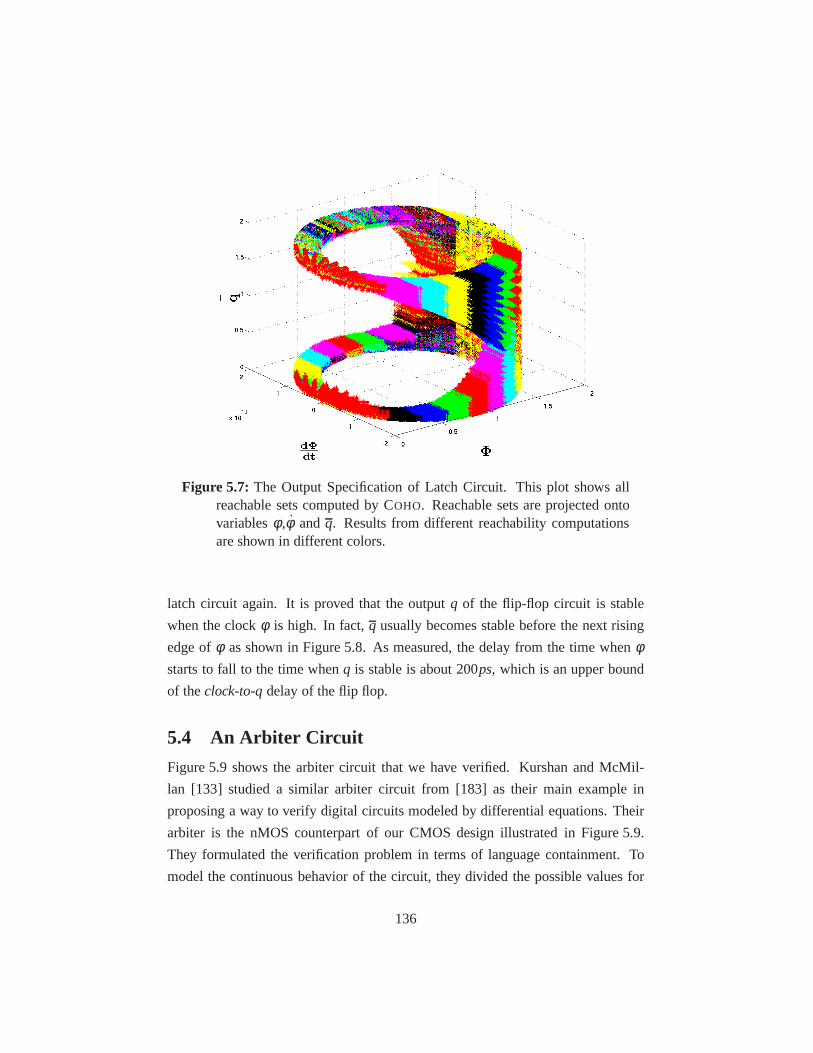
Figure 5.7: The Output Specification of Latch Circuit. This plot shows allreachable sets computed by COHO. Reachable sets are projected ontovariablesφ ,φ andq. Results from different reachability computationsare shown in different colors.

latch circuit again. It is proved that the outputq of the flip-flop circuit is stable

when the clockφ is high. In fact,q usually becomes stable before the next rising

edge ofφ as shown in Figure 5.8. As measured, the delay from the time when φstarts to fall to the time whenq is stable is about 200ps, which is an upper bound

of theclock-to-qdelay of the flip flop.

5.4 An Arbiter Circuit

Figure 5.9 shows the arbiter circuit that we have verified. Kurshan and McMil-

lan [133] studied a similar arbiter circuit from [183] as their main example in

proposing a way to verify digital circuits modeled by differential equations. Their

arbiter is the nMOS counterpart of our CMOS design illustrated in Figure 5.9.

They formulated the verification problem in terms of language containment. To

model the continuous behavior of the circuit, they divided the possible values for

136

φ

φ

φ

d

qq

φ

φφ

φ

φ

φ

φ

d

d can not change

q is stable

q is stable

Figure 5.8: The Output Specification of Flip-Flop

y

g

yxx

g

6 6

2 2

1 1

6 6

2:1 2:1

6 6 6 6

12 12

g1

g1

NAND1

mf1 mf2

NAND2

r2x2x1

z1 z2

g2

g2

r1

Figure 5.9: Verified Arbiter Circuit

each continuous state variable into 10 to 20 intervals, and computed the set of

reachable hyper-rectangles using such a grid. Although thetotal number of possi-

ble hyper-rectangles is large, Kurshan and McMillan used COSPAN to construct

the reachable space, and the next hyper-rectangle relationis only computed for

reachable hyper-rectangles. Unlike our Brockett’s annulus approach for specifying

137

signal transitions, Kurshan and McMillan model the inputs as making instanta-

neous transitions. These transitions were allowed at arbitrary times that satisfied

the handshake protocol. More details of our approach are presented in [212, 213].

5.4.1 Reachability Computation

Rising transitions of the request signals for the two clients can occur concurrently.

These requests can start at different times and have different rise-times. Verifying

correct operation of the arbiter requires accounting for all allowed transitions of

the inputs, including overlapping ones. We applied the method in Section 3.6.2 to

model all input transitions. We excluded the stateB<4,4> noting that there must be

a failure of the arbiter or its clients if both requests are falling at the same time –

this would imply that either the arbiter had violated the mutual-exclusion require-

ment or that at least one client had violated the handshake protocol. By exploiting

the symmetry of the arbiter and its clients, we solve only onereachability prob-

lem to compute reachable regions of statesB<i, j> andB< j,i>. In order to reduce

approximation error, we partitioned the rise and fall regions of the Brockett’s an-

nulus into seven subregions by employing the slicing technique from Section 5.1.

This results in 136 states to perform the complete reachability computation for the

arbiter.

Following the guidance in Section 5.1.2, we divided the 136 reachability prob-

lems into three phases using the assume-guarantee strategyfrom Section 5.1

1: FromB<1,1> to B<3,3>.

2: FromB<3,1> to B<3,1>.

3: FromB<3,3> to B<1,1>.

5.4.2 Stiffness

We encounteredstiffnessproblems when verifying the arbiter circuit. A system

of ordinary differential equations, ˙x = f (x) is said to bestiff if the Jacobian off

is an ill-conditioned matrix. That is,‖λmax/λmin‖ is large whereλmax (λmin) is

the largest (smallest) magnitude eigenvalue of the Jacobian matrix Jacf (x). For

circuits, stiffness occurs when nodes have vastly different time-constants. This

138

occurs in the arbiter where nodesz1 andz2 have much smaller capacitances than

the other nodes in the circuit.

The stiffness problems make it difficult for COHO to find a good choice of the

time step size in the reachability computation. As described in Chapter 4, COHO

has two principle causes of over approximation. First, there is an over approxima-

tion when producing a linear differential inclusion for a non-linear ODE as shown

in Equation 4.15. Second, over approximations are introduced when projecting the

reachable region for a face back down to the basis for the projection polygon. For

the arbiter, if COHO chooses a large time step (suitable for the nodes other thanz1

andz2), then the linearization errors forz1 andz2 will be large, creating large over

approximations for the voltages of these nodes. As the currents flowing through

the n-channel devices drivingx1 andx2 are quite sensitive toz1 andz2, this leads

to large over approximations forx1 andx2. Conversely, if COHO uses times steps

that are small enough to obtain tight bounds forz1 andz2, the accumulated projec-

tion and simplification errors will be large for the other nodes. Thus, the goals of

minimizing the approximation errors due to linearizing themodel and minimizing

the errors arising from projection and polygon simplification are in tension with

each other. For any choice of time step size, we found that COHO produced false-

negatives (failure to verify a correct circuit).

Circuit simulators such as HSPICE handle stiffness by usingimplicit integra-

tion algorithms. However, we are unaware of any formulationof an implicit algo-

rithm that is compatible with a forward reachability computation such as used in

COHO. As other reachability tools use similar methods, we expectthat they will

have similar problems if they attempt to verify common CMOS designs. This con-

jecture is supported by the absence of published results forformal verification of

stiff systems. We implemented two methods to solve the stiffness problem. The

first solution was to follow the example of typical designersand treat nodesz1 and

z2 as if they had no capacitance. The other solution was based ona change of

variables and constraining the reachability computation with an externally verified

invariant. More details are presented in the remainder of this section.

139

Simplified Model

We first used a simplified model of the arbiter circuit to complete the reachability

computation. This method side-stepped the problems of stiffness by treating nodes

z1 andz2 as if they had no capacitance. With this assumption, the voltage on these

nodes is always exactly the value that balances the currentsflowing through the

upper and lower n-channel transistors of each NAND gate. Thus, we created a

model for a nMOS tetrode with source connected to ground, gates connected tor1

andx2, and drain connected toz1, and another such tetrode for the two pull-down

transistors forz2. This simplification reduced the ODE model from six dimensions

down to four and eliminated the stiffness issues. This assumption is reasonable as

the internal nodesz1 andz2 have much smaller capacitances than other nodes of

the circuit. In fact, many designers would instinctively ignore the contributions of

these tiny capacitors. However, the verification is incomplete. For example, we

note that with optical proximity rules, the spacing betweenseries-connected tran-

sistors is growing relative to other circuit dimensions forsub-100nm processes. If

the capacitances of these nodes are ignored, it is impossible to determine when they

have become large enough to cause a circuit failure. Therefore, we implemented

another solution to include internal nodes in our model.

Changing Variables and External Invariants

In order to reduce approximation error, we employed two techniques. First, we

replaced variablesz1 andz2 by two new variables which converge to zero rapidly.

Second, we applied an externally verified invariant to constrain reachable regions.

The remainder of this section presents our modifications to COHO’s reachability

computation that allow it to compute tight overapproximations.

When either transistor connected to nodez1 is conducting,z1 tends to converge

very quickly to a small neighborhood near its equilibrium value; however, the pre-

cise value of the equilibrium varies widely according to thevalues ofr1, x1 and

x2. For any choice of values for the voltages ofr1, x1 andx2, there is a unique

voltage forz1 such that ˙z1 = 0. This is because the current fromx1 to z1 through

the upper transistor is determined by the voltages of nodesx1, x2 andz1 and is neg-

ative monotonic in the voltage of nodez1. Likewise, the current fromz1 to ground

140

through the lower transistor is determined by the voltages of nodesz1 andr1 and

is positive monotonic in the voltage of nodez1. These properties hold for any re-

alistic transistor model. Thus, given values for the voltages on nodesr1, x1 andx2,

there is a unique voltage for nodez1 such that these two currents are equal. This

is the voltage at which ˙z1 = 0, and we call this voltage theequilibrium voltageand

denote it byq1(r1,x1,x2). We defineq2(r2,x2,x1) in the analogous manner.

We replacez1 and z2 in the circuit’s ODE withu1 = z1 − q1(r1,x1,x2) and

u2 = z2−q2(r2,x2,x1) respectively. Whenever a transistor drivingz1 is conducting,

u1 tends rapidly to zero, and it is much easier to show thatu1 converges to zero than

to show thatz1 converges to a moving target. Likewise foru2 andz2. This change

of variables formalizes the designer’s intuition that the capacitance of nodesz1 and

z2 “usually won’t matter.” The chain rule yields:

u1 = z1−(

∂q1∂ r1

r1+∂q1∂x1

x1+∂q1∂x2

x2

)

. (5.3)

Although z1 is not a state variable of the modified ODE, it can be reconstructed

by noting thatz1 = u1+q1(r1,x1,x2), and then ˙z1 can be determined based on the

values forr1, x1, z1 and x2. In our implementation, we use a four-dimensional

table, indexed by the values ofu1, r1, x1 andx2 to compute values for ˙x1 and u1.

This table accounts for all four transistors of the NAND gatethat producesx1 and

the capacitance on nodesx1 andz1. By including x1 in the table, we eliminate the

need to reconstructz1 or calculateq1. By directly computing ˙u1 andx1, we avoid

reconstructingz1 with large error bound intervals that would then propagate to the

other quantities. The same construction applies for computing u2 andx2.

With the change of variables described above, COHO still encountered a prob-

lem at the rising edge ofr1. If r1 is low andr2 is high, thenx2 will be low, and

both transistors connected to nodez1 will be in cut-off. In this case, the equilib-

rium voltage forz1 is determined by balancing the small leakage currents of the

two transistors. Thus,u1 can have a large value whenr1 is low. Following a rising

edge ofr1, u1 should go quickly to zero. However, COHO’s over approximations

from whenr1 was low led it to a region from which it could not establish this con-

traction. In fact, the range foru1 blew up to cover the entire interval from 0 toVdd,

and led to continuous states that violated the specificationfrom Figure 3.19.

141

We solved this problem by manually establishing a simple invariant. The intu-

ition behind this invariant is that based on the leakage currents for our implemen-

tation in the TSMC 180nm, 1.8V CMOS process, we can determinethat nodez1

eventually settles to 1.45V ifr1 = 0 andx2 =Vdd, and this is an upper bound for

z1. By symmetry the same bound applies toz2, from which we postulated the in-

variants−1.45≤ u1 ≤ 1.45V and 0≤ z1 ≤ 1.45V . It is straightforward to establish

this invariant by computing the values of ˙u1, u2, z1, andz2 on the boundary faces

of this region to show that trajectories on these faces flow inward. We constrained

the projectagons computed by COHO to satisfy these simple, externally verified

invariants.

5.4.3 Results

Using the methods described above, COHO computed an invariant region for the ar-

biter. This set allows us to establish the correct operationof the arbiter as described

below.

Safety Properties

Mutual Exclusion:

Figure 5.10 shows the verification of mutual exclusion. Part(a) of the figure

shows all reachable states; clearlyg1 andg2 are never both high. In fact, the region

where they both reach values near 0.5V only occurs when one grant is falling and

the other is rising as the arbiter transfers a grant that one client released and the

other has requested. Figure 5.10.b shows the reachable space for g1 andg2 when

falling transitions of the grant signals are excluded. Thisshows that the separation

of grants is very distinct.

Handshake Protocol:

In a similar fashion, projecting the reachable space onto the signalsg1 and r1

as shown in Figure 5.11 demonstrates thatg1 entersB2 only when r1 is in B3.

Likewise g1 entersB4 when r1 ∈ [0.0,0.22]. When r1 ∈ [0.2,1.6], r1 < 0, thus

r1 ∈ B4. This shows thatg1 starts to fall only when the discrete abstraction ofr1

is a logically low signal. Thus, the grants both rise and fallin accordance with the

handshake protocol.

142

0 0.5 1 1.50

0.2

0.4

0.6

0.8

1

1.2

1.4

1.6

1.8

g1

g2

0 0.5 1 1.50

0.2

0.4

0.6

0.8

1

1.2

1.4

1.6

1.8

g1

g2

a.g1 vs. g2 (includingB4) b. g1 vs. g2 (excludingB4).

Figure 5.10: Verification of Arbiter: Mutual Exclusion. The left plot showsall reachable sets projected onto variablesg1 andg2, where the blueregions are reachable sets computed by COHO and the red regions arecomputed by circuit symmetry. The right plot shows reachable spacefor g1 andg2 when falling transitions of the grant signals are excluded.

0 0.2 0.4 0.6 0.8 1 1.2 1.4 1.6 1.80

0.2

0.4

0.6

0.8

1

1.2

1.4

1.6

1.8

request

gran

t

g1 vs. r1

Figure 5.11: Verification of Arbiter: Handshake Protocol. The blue polygonsshow the reachable sets projected onto variablesg1 and r1, and thearrows illustrate the handshake protocol.

143

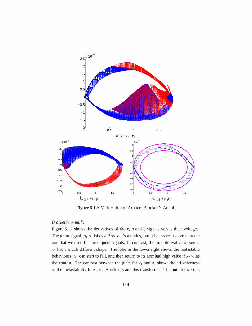
0 0.5 1 1.5−2

−1.5

−1

−0.5

0

0.5

1

1.5

2

2.5x 10

10

a. x1 vs. x1

0 0.5 1 1.5−2.5

−2

−1.5

−1

−0.5

0

0.5

1

1.5

2x 10

10

0 0.5 1 1.5−2

−1.5

−1

−0.5

0

0.5

1

1.5

2x 10

10

b. g1 vs. g1 c. g1 vsg1

Figure 5.12: Verification of Arbiter: Brockett’s Annuli

Brockett’s Annuli:

Figure 5.12 shows the derivatives of thex, g andg signals versus their voltages.

The grant signal,g1 satisfies a Brockett’s annulus, but it is less restrictive than the

one that we used for the request signals. In contrast, the time-derivative of signal

x1 has a much different shape. The lobe in the lower right shows the metastable

behaviours:x1 can start to fall, and then return to its nominal high value ifx2 wins

the contest. The contrast between the plots forx1 andg1 shows the effectiveness

of the metastability filter as a Brockett’s annulus transformer. The output inverters

144

that produceg1 andg2 further improve the transitions to produce the plot shown

in part c where the reachable space computed by Coho is indicated by the blue

polygons, and the pink ellipses show the Brockett’s annulusused for the request

signals. With this output buffering, the output signals satisfy the original input

annulus.

Liveness Properties

Initialization:

We used COHO to compute the reachable space whenr1 andr2 were both low (i.e.

in regionB1) starting from a state wherex1, x2, g1 andg2 could be anywhere in

[0,1.8]. COHO establishes that within 200ps,x1 andx2 enter[1.6V,1.8V ] (i.e. B3),

andg1 andg2 enter[0.0V,0.2V ] (i.e. B1). Thus, the arbiter can be initialized simply

by not asserting any requests for a short time – no additionalreset signal is needed.

Uncontested Requests:

We consider the reachable space with the additional restriction that r2 remains

within regionB1 (i.e. a logically low value). COHO shows thatg1 is asserted within

343 ps ofr1 rising (i.e. enteringB2). This shows that the arbiter is guaranteed to

respond to uncontested requests within a bounded amount of time.

Contested Requests:

If r1 andr2 are asserted at nearly the same time, the arbiter may exhibitmetastable

behavior and may remain in a metastable state for an arbitrarily long period of time.

COHO can show that metastability can only occur in the hyper-rectangle where:

r1 ∈ B3 x1 ∈ [0.55,1.3] g1 ∈ B1

r2 ∈ B3 x2 ∈ [0.55,1.3] g2 ∈ B1.(5.4)

Outside of this region, the dot product of the derivative vector with the final sta-

ble state of granting client 1 or granting client 2 is unambiguous. Section 5.4.4

explores liveness under metastable conditions in greater detail.

Reset:

COHO shows that if clienti has a grant and lowers its request signal then the arbiter

lowers the grant for clienti within 270 ps. This shows that the arbiter satisfies the

liveness requirement for withdrawing grants.

145

Fairness:

If client i wins a grant while the other client is making a request and subsequently

client i drops its request, then Coho shows that the other client receives a grant

within 420 ps. This shows that the other client receives at most one grant while the

current client has a pending request; therefore, this simple arbiter is fair.

Using COHO, we have verified all properties of the arbiter from the specifica-

tion given in Figure 3.19 except for the clause

α-ins ⇒ (�Z(B3(r i)U⇒B2,3(gi))).

This property concerns the behaviour of the arbiter under metastable conditions,

and we describe our technique for verifying this property inthe next section.

5.4.4 Metastability and Liveness

Metastable behavior in digital circuits has been studied since Chaney and Molnar’s

original paper on synchronizer failures [38]. Hurtado [124] analyzed metastability

from a dynamical systems perspective. Seitz [183] gave a nice introduction to

metastability issues, and Marino [154] provided a fairly comprehensive treatment.

When both requests are asserted concurrently, the arbiter may enter a metastable

condition that can persist for an arbitrarily long time. Thus, it is not possible to

prove that all behaviours when both requests are simultaneously asserted will even-

tually lead to granting a client. On the other hand, with a properly designed arbiter,

the probability of no grant being issued when both requests are asserted should

decrease exponentially with time. This implies that the probability of a liveness

failure should go to zero as the settling time goes to infinity. If the arbiter works

for all situations except for some set with a probability measure of zero, then we

say that the circuit worksalmost surely[169, Chapter 2.6]. Our approach is to

use COHO to bound the reachable space when both requests are asserted. Most

of this space can be shown to quickly resolve to granting one client or the other.

For a small region near the metastable point, such progress can’t be demonstrated,

and we use the method from [160] to show that this metastable region is exited

with probability one. The remainder of this section describes these steps in greater

detail.

146

0 0.2 0.4 0.6 0.8 1 1.2 1.4 1.6 1.80

0.2

0.4

0.6

0.8

1

1.2

1.4

1.6

1.8

0→ 1

→ 2

M

2

1

x1

x 2

Figure 5.13: Reachable Regions Whenr1 andr2 are High

To verify liveness when both requests are asserted, we first use COHO to com-

pute the reachable state after both requests are asserted. Figure 5.13 shows the

outcome of this analysis. The square marked0 indicates the initial region forx1

andx2 when r1 and r2 are both in regionB1. COHO then determines the reach-

able space for all low-to-high transitions ofr1 andr2 allowed by their Brockett’s

rings. After bothr1 andr2 have been in regionB3 for a while, COHO shows that

the state is in the union of the regions labeled1, 2, → 1, → 2, andM . Region

1 is wherex1 has gone low, and grantg1 will be asserted. COHO shows that all

trajectories in region→ 1 converge to region1 in bounded time and thus lead to

asserting grantg1. Likewise, from regions2 and→ 2 lead to assertingg2. Region

M contains the metastable point. Because trajectories on thestable manifold for

the metastable point remain in regionM indefinitely, COHO cannot verify that all

such trajectories eventually lead to issuing a grant.

We now show that the arbiter is live in the almost-sure sense.We first make a

147

change of variables. Let

w− = x1−x2, w+ = x1+x2. (5.5)

We will write Mw to denote the regionM in (w−,w+) coordinates. As shownin [160], almost-all trajectories diverge from regionM if we can find constantsc,d > 0 such that for all points(w−

1 ,w+1 ) and(w−

2 ,w+2 ) with w−

1 < w−2 ,

((w+2 −w+

1 )≤ c(w−2 −w−

1 )) ⇒ w−2 − w−

1 ≥ d(w−2 −w−

1 )

(w+2 > w+

1 )∧ ((w+2 −w+

1 ) = c(w−2 −w−

1 )) ⇒ w+2 − w+

1 ≤−d(w−2 −w−

1 )

(w+2 < w+

1 )∧ ((w+2 −w+

1 ) = c(w−2 −w−

1 )) ⇒ w+1 − w+

2 ≤−d(w−1 −w−

2 ).

(5.6)

Basically, this condition ensures that if at some time,t0 two trajectories differ

only by theirw− components, then they must exponentially diverge; this ensures

that one of them must leave regionM . This implies that the set of trajectories that

remain inM indefinitely must have a Lesbesgue measure of zero, which yields the

desired almost-surely result.

We now present a simple test that ensures that the conditionsfrom Equation 5.6

hold. For any pointw∈ Mw, let J(w) be the Jacobian operator for the ODE model

projected onto the(w−,w+) space:

J(w) =

[

∂ w−∂w−

∂ w−∂w+

∂ w+

∂w−∂ w+

∂w+

]

. (5.7)

Now, define:µ = min

w∈M(J(w)(1,1),−J(w)(2,2))

h1 =

(

maxw∈M

|J(w)(1,2)|/J(w)(1,1)

)−1

h2 = maxw∈M

−|J(w)(2,1)|/J(w)(2,2).

(5.8)

The conditions of Equation 5.6 are satisfied if

(µ > 0) ∧ (h1 > h2), (5.9)

whereµ , h1 andh2 are defined as in Equation 5.8. This is straightforward to show

by integration along the line segment from point(w−1 ,w

+1 ) to point(w−

2 ,w+2 ) from

Equation 5.6. We applied these tests to show that trajectories will leave regionM

148

cc cc

fwd

cc cc

fwd

fwdfwd

2:1

2:1

2:1

2:1(2:1)*r (2:1)*r

(2:1)*r (2:1)*r

X3 X4

X2X1

Figure 5.14: Verified Two-Stage Rambus Ring Oscillator. It consists of for-ward inverters (labeled asf wd) and cross-couple inverters (labeled ascc). The ratio of cross-couple inverter size and forward inverter size isdenoted asr.

almost-surely.

In summary, we have verified both safety and liveness properties of the ar-

biter circuit. We also showed that the metastability filtersfunction as a Brockett’s

annulus transformer. During the verification, we found the challenging stiffness

problem and proposed two solutions. We applied a method based on dynamical

systems theory to prove that the arbiter circuit satisfies its liveness properties in the

almost-surely sense, which cannot be demonstrated by reachability analysis alone.

5.5 The Rambus Ring Oscillator

Figure 5.14 shows the two-stage ring oscillator that we verified. The circuit was

proposed by researchers at Rambus [129] as a verification challenge, and they noted

that some implementations of the circuit had failed in real,fabricated chips. There-

fore, they posed the problem of showing that the oscillator starts from all initial

conditions for a particular choice of transistor sizes. Although [88] establishes a

condition to ensure that the oscillator is free from lock-up, there is still the possibil-

ity that the circuit could oscillate at a harmonic of the intended frequency, display

chaotic behavior, or have some other steady-state behaviorother than the intended

oscillation. We solved these problems for the two-stage Rambus oscillator shown

in Figure 5.14. In the circuit, all inverters have the same size and signal nodes

149

are denoted asx1,x2,x3,x4. With the circuit states computed by COHO, we have

shown that the two stage oscillator with any possible initial condition oscillates in

the specified mode with probability one.

5.5.1 Static Analysis and Reachability Computation

Our verification proceeds in three main phases:

1. The oscillator shown in Figure 5.14 is a differential design: nodesX1 andX3

form a “differential pair” and likewise for nodesX2 andX4. The first phase

of the verification shows that each of these differential pairs can be treated

as a single signal. This symmetry reduction of the state space simplifies the

subsequent analysis.

2. Any oscillator must have at least one equilibrium point. Using the methods

from [88], we can show that any such equilibrium points are unstable; how-

ever, we note that any trajectory that starts on the stable manifold for such

an equilibrium point will lead to a non-oscillating behaviour. In other words,

for anyoscillator circuit, there must exist an infinite set of initial conditions

for which the circuit will fail to oscillate. Fortunately, this failure set can

have a lower dimensionality that the full state space. Thus,the second phase

of the verification shows that this occurs with probability zero.

3. The first two phases show that most initial conditions leadto a fairly small

subset of the full phase space. In the final phase, we divide the remaining

space into small regions, and use existing reachability methods to show that

the oscillator starts up properly from each such region.

The remainder of this section describes the dynamical systems issues associated

with each of these phases. Section 5.5.2 describes our verification method based

on these observations.

We model the oscillator circuit from Figure 5.14 using non-linear ordinary dif-

ferential equations (ODEs) obtained by standard, modified nodal-analysis methods

as described in Section 3.3. This gives us an equation of the form:

x = f (x), (5.10)

150

wherex is a vector of node voltages. Letd be the dimensionality ofx. We assume

that f is C2 which guarantees that Equation 5.10 has a unique solution for any

initial state,x(0).

Differential Behaviour

NodesX1 andX3 in the oscillator from Figure 5.14 form a “differential pair” and

likewise for nodesX2 andX4. Let xi denote the voltage on nodeXi. Thedifferential

componentof the differential pair isx1− x3, and thecommon modecomponent is

x1+x3. When the oscillator is operating properly, the common modecomponents

are roughly constant and the oscillation is manifested in the differential compo-

nents. LetV+0 be the nominal value for the common mode components. We show

that for a relatively smallVerr, if |x1+x3−V+0 |>Verr, then d

dt (x1+x3) and(x1+x3)

have opposite signs. This shows that that the common mode component forX1 and

X3 converges to withinVerr of the nominal value. Likewise forX2 andX4 by circuit

symmetry.

Equilibrium Points and Their Manifolds

If the circuit is an oscillator, then the dynamical system described by Equation 5.10

must have a periodic attractor. This is a periodic orbit inRd such that any trajectory

that starts in some open neighbourhood of this orbit must asymptotically converge

to the orbit. For any periodic attractor, there must be an associated equilibrium-

point [121, Chapter 13], i.e. a pointxep for which f (xep) = 0. If this equilibrium

point is an attractor, then its basin of attraction is a set ofinitial conditions for

which the circuit will not oscillate. Otherwise, the equilibrium point may be a

saddle point, in which case it has an associated stable manifold. This manifold

is a set of points that form a surface with a dimensionality< d such that trajec-

tories starting anywhere on this manifold converge toxep. In this case, the set of

initial conditions that lead toxep has zero volume in the full-dimensional space,

and the probability of starting at one of these points is zero. More technically,

the failure set associated with this equilibrium point isnegligible (with respect to

the Lesbegue measure) and trajectories diverge from the neighbourhood ofxep al-

most surely[169, Chapter 2.6]. We use the terminologyalmost surelyto indicate

151

something that has probability one, andalmost allto indicate the entire state space

minus a negligible set.

This dynamical systems perspective provides a critical observation about oscil-

lators:every oscillator circuit has a set of initial conditions forwhich it fails to os-

cillate. Direct application of continuous state-space model checkers (e.g. [69, 97])

to the oscillator start-up problem will identify regions where trajectories might stay

forever (or the reachability computation used was unsound). Because we cannot

show that the set of failure states is empty, we must settle for showing that it is neg-

ligible. This is sufficient in practice, as designers are notworried about a design

that fails with probability zero. To perform this verification, we need reachability-

modulo-measure-theory. We describe such a method below.

To verify the oscillator, we extend the technique describedin Section 5.4.4.

The basic idea is straightforward. Letxeq be an equilibrium point of Equation 5.10,

f (xeq) = 0. Lety1 . . .yk andzk+1 . . .zd be orthonormal vectors and letB be a simple

region. If there is some constant,µ > 0, such that for every point,b, in B,

yi · ∂ f∂yi

(b) > µ , ∀i ∈ 1. . .k

zj · ∂ f∂zj

(b) > −µ , ∀ j ∈ k+1. . .d,(5.11)

then it can be proved [160] that almost all trajectories inB leaveB. The intuition

is that trajectories that start from points that differ onlyin their y1...k components

must diverge from each other.

Reachability Computation

The verification problem that we consider is to show that a Rambus ring oscillator

with a particular choice of transistor sizes will oscillatein its fundamental mode

from nearly all initial conditions. We do this by first showing differential opera-

tion and then showing that almost all trajectories diverge from the stable manifold

of the unstable equilibrium point. These first two phases show that trajectories

from almost all initial conditions lead to a relatively small part of the state space.

Furthermore, this small part of the state space has the common mode components

of both differential signal pairs withinVerr of V+0 . This allows us to rewrite the

152

differential equation model from Equation 5.10 as a differential inclusion [105]:

u ∈ F(u), (5.12)

whereu is the vector[x1 − x3,x2 − x4]. By using an inclusion,F accounts for

all values of the common mode components inV+0 ±Verr. Reducing the four-

dimensional state space of the original problem to a two-dimensional space makes

the exploration of trajectories from all remaining start conditions straightforward.

By showing that all such trajectories lead to an oscillationin the fundamental

mode, we solve the first part of the challenge problem from [129]: we show that

for a particular choice of transistor sizes, the circuit will start oscillation from al-

most all initial conditions. Extending the approach to handle the second part of the

challenge is straightforward. To ensure sound verification, all of the steps of the

verification use over approximations of the circuit model. We can use these uncer-

tainty terms to model a range of size ratios between the forward and cross-coupled

inverters. Thus, we will show that the oscillator starts up properly for any ratio of

transistor sizes in a relatively wide interval.

5.5.2 Implementation

As with the previous examples, our verification is for a design in the TSMC 180µ1.8V CMOS process.

Differential Operation

This verification phase starts by changing the coordinate system to one based on

the differential and common mode representation of signals. Then, a static analysis

of the trajectory flows allows most of the common-mode subspace to be eliminated

from further consideration.

153

Let u be the circuit state in “differential” coordinates:

u = M−1x

M =

√2

2

1 0 1 0

0 1 0 1

−1 0 1 0

0 −1 0 1

.(5.13)

We assume each of nodesX1, X2, X3 andX4 can independently have initial voltages

anywhere in[0,1.8]V. Thus, the differential components,u1 andu2, are initially in

±0.9√

2, and the common mode components,u3 andu4, are initially in [0,1.8√

2].

To establish differential operation, we divide the range ofeach of theu vari-

ables inton intervals, creatingn4 cubes. We construct a graph,G = (V,E) to

represent the reachability relationship between these cubes. Letvi, j,k,ℓ be a vertex

corresponding to theith interval foru1, the jth interval foru2 and so on. There is an

edge fromv to w if f allows a flow out of the cube forv directly into the cube for

w, and there is a self-loop forv if each component off is zero somewhere inv. The

key idea is that if vertexG has no incoming edges, then any trajectory that starts in

the corresponding cube will eventually leave that cube, andno trajectories will ever

enter the cube. Such a cube can be eliminated from further consideration. Thus, we

only need to consider cubes whose vertices are members of cycles. These vertices

can be identified inO(V +E) = O(n4) time. With a direct implementation of this

computation, constructingG dominates the entire time for verifying the oscillator.

To obtain a more efficient computation, we first note that the goal is to establish

differential operation. It is sufficient to project the vertices ofV onto the common-

mode components of the differential signals and show that most vertices can be

eliminated from further consideration. LetG′ = (V ′,E′) wherev′k,ℓ corresponds to

the kth interval ofu3 and theℓth interval ofu4. There is an edge inE′ from v′k1,ℓ1

to v′k2,ℓ2iff there is an edge inE from vi, j,k1,ℓ1 to vi, j,k2,ℓ2 for somei and j. Clearly,

G′ overapproximates reachability. Thus, if a vertex ofG′ has no incoming edges,

then all of the corresponding vertices inG must have no incoming edges as well.

Computing the edges inE′ requires examining all of the edges ofE, but subsequent

operations on the graphG′ are much faster than those onG.

154

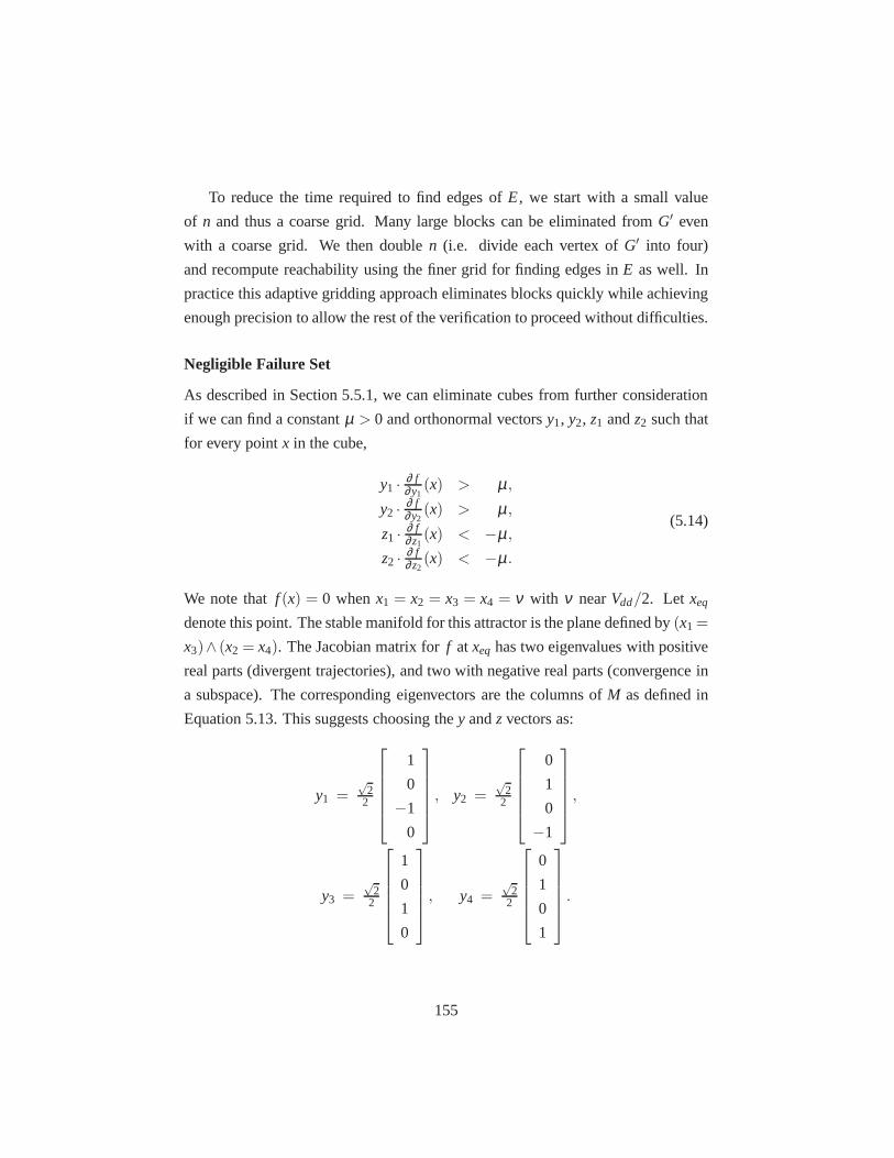
To reduce the time required to find edges ofE, we start with a small value

of n and thus a coarse grid. Many large blocks can be eliminated from G′ even

with a coarse grid. We then doublen (i.e. divide each vertex ofG′ into four)

and recompute reachability using the finer grid for finding edges inE as well. In

practice this adaptive gridding approach eliminates blocks quickly while achieving

enough precision to allow the rest of the verification to proceed without difficulties.

Negligible Failure Set

As described in Section 5.5.1, we can eliminate cubes from further consideration

if we can find a constantµ > 0 and orthonormal vectorsy1, y2, z1 andz2 such that

for every pointx in the cube,

y1 · ∂ f∂y1

(x) > µ ,y2 · ∂ f

∂y2(x) > µ ,

z1 · ∂ f∂z1

(x) < −µ ,z2 · ∂ f

∂z2(x) < −µ .

(5.14)

We note thatf (x) = 0 whenx1 = x2 = x3 = x4 = ν with ν nearVdd/2. Let xeq

denote this point. The stable manifold for this attractor isthe plane defined by(x1 =

x3)∧ (x2 = x4). The Jacobian matrix forf atxeq has two eigenvalues with positive

real parts (divergent trajectories), and two with negativereal parts (convergence in

a subspace). The corresponding eigenvectors are the columns of M as defined in

Equation 5.13. This suggests choosing they andzvectors as:

y1 =√

22

1

0

−1

0

, y2 =√

22

0

1

0

−1

,

y3 =√

22

1

0

1

0

, y4 =√

22

0

1

0

1

.

155

While we chose they andz vectors based on the manual analysis of the dynamics

of the oscillator sketched above, we believe that this process could be automated.

Equilibrium points can be found by standard root-finding methods, and the eigen-

values and eigenvectors can be computed using standard numerical linear algebra

routines.

Having choseny andzvectors, we now check each remaining cube in the state

space to determine if it satisfies the conditions of Equation5.141. This requires

computing bounds on the partial derivatives off . The convexity (and concavity)

of transistor currents with respect to node voltages allowsthe range of possible

partial derivatives of transistor currents with respect tonode voltages to be deter-

mined from the end-points of the intervals for these voltages. By our simplification

of using constant capacitances,f is a linear function of transistor drain-to-source

currents. Thus, we can combine the intervals for the partialderivatives of transistor

currents to obtain over-approximations of the intervals for partial derivatives off .

At the end of this phase, the number of cubes to consider for the final reachabil-

ity analysis has been reduced to a small fraction of the original. More importantly,

cubes that contain or are near the unstable equilibrium point of the oscillator have

been safely eliminated. This allows a reachability computation from the remaining

cubes to complete the verification.

Proper Oscillation

Noting that the common mode voltagesu3 andu4 are restricted to a small region

as shown in Figure 5.15, we eliminate these two variables by replacing the differ-

ential equation model for the circuit with a differential inclusion. This reduces the

state space from four dimensions to two which enables efficient reachability com-

putation. Figure 5.16 shows the region that remains to be verified. We divide this

region into its inner and outer boundaries, and a collectionof “spokes” as shown

in Figure 5.17. The computation has three parts:

1. Starting from each “spoke”, show that all trajectories starting at that spoke

eventually cross the next spoke.

1The details of our method for establishing the inequalitiesfrom Equation 5.14 are described in[209]

156

2. Show that all trajectories starting from the inner or outer boundary eventually

cross the next spoke.

3. Starting from one spoke, compute the reachable set until it converges to a

limit set.

The first two show that all trajectories converge to the same attractor. This means

that all initial conditions lead to a unique mode of oscillation. The final step tight-

ens the bound on this unique mode.

5.5.3 Results

As described earlier, our verification is for designs in the TSMC 0.18µ process.

All transistors in the designs that we considered have gate lengths of 0.18µ . For

all inverters, we use pMOS devices that are twice as wide as the nMOS devices.

All forward inverters have transistors of the same size, andlikewise for the cross-

coupled inverters. In the following,r denotes the ratio of the cross-coupled inverter

size to the forward inverter size. This section first presents the verification of an

oscillator withr = 1. Then, the oscillator is verified for 0.875≤ r ≤ 2.0.

The verification routines were implemented using Matlab with COHO used for

the final reachability computation. All times were obtainedrunning on a dual Xeon

E5520 (quad core) 2.27GHz machine with 32GB of memory; however, the com-

putations described here are all performed using a single core.

Verification with Equal-Size Inverters

The first phase of the verification establishes differentialoperation. Initially, the

computation partitions the space for each of theui variables into 8 regions, creating

a total of 84 = 4096 cubes to explore. After eliminating cubes that have no incom-

ing or self-circulating flows, the remaining cubes are subdivided and rechecked un-

til there are 64 intervals for each variable. Figure 5.15 shows the remaining cubes

projected onto the common-mode variables,u3 andu4 at the end of this phase.

With 8 intervals per region, there are 752 cubes under consideration (18% of

the total space). With each subdivision, the number of cubesremaining increases

by a factor of roughly 4.6, and thus the volume of the space under consideration

157

0 0.5 1 1.5 2 2.50

0.5

1

1.5

2

2.5

u3

u 4

Figure 5.15: Common-Mode Convergence toVdd/√

2. The first phase of ver-ification shows that the common mode components are roughly con-stant. It eliminates cubes that have no incoming or self-circulatingflows. This plot shows the remaining cubes projected onto thecommon-mode variablesu3 andu4.

drops by about a factor of roughly 0.29. With 64 intervals perregion, 74676 cubes

remain (0.45% of the total space). The decrease in the volumeis steady, suggesting

that further reductions would be possible with more iterations. However, the time

per iteration increases with the number of cubes under consideration, and the time

for this phase dominates the total verification time. Thus, for verifying this circuit,

there is no incentive to further refine the region bounding the common-mode signal.

The second phase of the verification eliminates the unstableequilibrium and

cubes near this equilibrium’s stable manifold. It starts with the 74676 cubes from

the previous phase and performs the computation steps described in Section 5.5.2.

Figure 5.16 shows the remaining cubes projected onto the differential variables,u1

andu2 at the end of this phase. This phase eliminates roughly half of the remaining

cubes, leaving 38384 cubes for analysis by the final phase.

The final phase starts with the 38384 cubes from the second phase. As de-

scribed in Section 5.5.2, we divide these cubes into 16 wedges divided by “spokes”

in theu1×u2 projection. For each such wedge, it is sufficient to show thatall tra-

jectories starting on the boundary of the wedge lead to points inside the next wedge

158

−1 −0.5 0 0.5 1

−1

−0.5

0

0.5

1

u1

u 2

Figure 5.16: Eliminating the Unstable Equilibrium. The second phase elimi-nates the unstable equilibrium and cubes near the stable manifold. Thisplot shows the remaining cubes projected onto the differential vari-ablesu1 andu2.

in the clockwise direction. This is shown with three reachability computations per

wedge:

1. Show that all trajectories starting from cubes on the leading spoke (counter-

clockwise boundary of the wedge) cross the trailing spoke (clockwise bound-

ary) in the interior of the wedge. These spokes are drawn in magenta in

Figure 5.17.

2. Show that all trajectories starting from cubes on the inner boundary cross the

trailing spoke. These cubes are drawn in green in Figure 5.17.

3. Show that all trajectories starting from cubes on the outer boundary cross the

trailing spoke. These cubes are also drawn in green in Figure5.17.

With 16 wedges, we perform 48 reachability computation runs. At this point, the

oscillator is verified.

We also ran a longer reachability computation starting froma spoke and com-

pleting two complete cycles of the oscillation. The second cycle starts from a

smaller region that the first and establishes tighter boundson the limit cycle. The

159

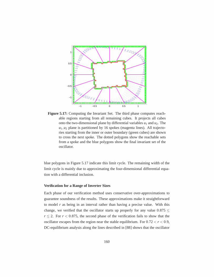
−1 −0.5 0 0.5 1

−1

−0.5

0

0.5

1

Figure 5.17: Computing the Invariant Set. The third phase computes reach-able regions starting from all remaining cubes. It projectsall cubesonto the two-dimensional plane by differential variablesu1 andu2. Theu1,u2 plane is partitioned by 16 spokes (magenta lines). All trajecto-ries starting from the inner or outer boundary (green cubes)are shownto cross the next spoke. The dotted polygons show the reachable setsfrom a spoke and the blue polygons show the final invariant setof theoscillator.

blue polygons in Figure 5.17 indicate this limit cycle. The remaining width of the

limit cycle is mainly due to approximating the four-dimensional differential equa-

tion with a differential inclusion.

Verification for a Range of Inverter Sizes

Each phase of our verification method uses conservative over-approximations to

guarantee soundness of the results. These approximations make it straightforward

to modelr as being in an interval rather than having a precise value. With this

change, we verified that the oscillator starts up properly for any value 0.875≤r ≤ 2. For r < 0.875, the second phase of the verification fails to show that the

oscillator escapes from the region near the stable equilibrium. For 0.72< r < 0.9,

DC-equilibrium analysis along the lines described in [88] shows that the oscillator

160

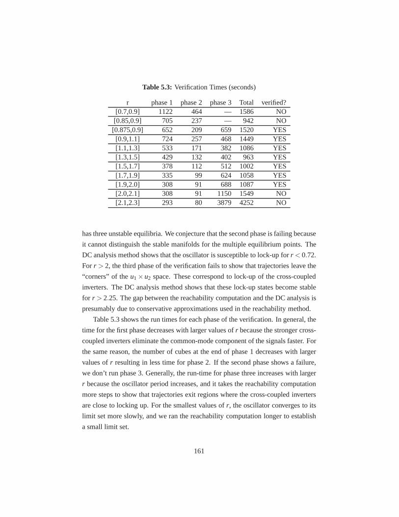
Table 5.3: Verification Times (seconds)

r phase 1 phase 2 phase 3 Total verified?[0.7,0.9] 1122 464 — 1586 NO[0.85,0.9] 705 237 — 942 NO[0.875,0.9] 652 209 659 1520 YES[0.9,1.1] 724 257 468 1449 YES[1.1,1.3] 533 171 382 1086 YES[1.3,1.5] 429 132 402 963 YES[1.5,1.7] 378 112 512 1002 YES[1.7,1.9] 335 99 624 1058 YES[1.9,2.0] 308 91 688 1087 YES[2.0,2.1] 308 91 1150 1549 NO[2.1,2.3] 293 80 3879 4252 NO

has three unstable equilibria. We conjecture that the second phase is failing because

it cannot distinguish the stable manifolds for the multipleequilibrium points. The

DC analysis method shows that the oscillator is susceptibleto lock-up forr < 0.72.

For r > 2, the third phase of the verification fails to show that trajectories leave the

“corners” of theu1×u2 space. These correspond to lock-up of the cross-coupled

inverters. The DC analysis method shows that these lock-up states become stable

for r > 2.25. The gap between the reachability computation and the DC analysis is

presumably due to conservative approximations used in the reachability method.

Table 5.3 shows the run times for each phase of the verification. In general, the

time for the first phase decreases with larger values ofr because the stronger cross-

coupled inverters eliminate the common-mode component of the signals faster. For

the same reason, the number of cubes at the end of phase 1 decreases with larger

values ofr resulting in less time for phase 2. If the second phase shows afailure,

we don’t run phase 3. Generally, the run-time for phase threeincreases with larger

r because the oscillator period increases, and it takes the reachability computation

more steps to show that trajectories exit regions where the cross-coupled inverters

are close to locking up. For the smallest values ofr, the oscillator converges to its

limit set more slowly, and we ran the reachability computation longer to establish

a small limit set.

161

6

Conclusion and Future Work

This dissertation has addressed formal verification of analog and mixed signal cir-

cuits. Our approach is based on translating verification problems to reachability

analysis problems by modeling circuit dynamics as ODEs and specifying ana-

log properties based on Brockett’s annuli and a LTL-based logic with continuous

time and values (see Chapter 3). Reachable circuit states are computed by COHO,

which is a reachability analysis platform for nonlinear, moderate-dimensional hy-

brid systems. COHO employs projectagons to represent and manipulate moderate-

dimensional, non-convex objects and bounds the solution ofnonlinear ODEs by

approximating ODEs by differential inclusions (see Chapter 4). The correctness

and efficiency of our solution have been demonstrated by the success of verifying

several synchronous, asynchronous, and analog circuits (see Chapter 5). Our work

has extended the application of formal methods to practicalanalog circuits and also

motivates many future research topics.

6.1 Contributions

We proposed a reachability based solution to circuit verification. It represents cir-

cuit states by moderate-dimensional regions and computes all circuit states using

COHO. COHO is a sound, efficient and robust reachability analysis tool for nonlin-

ear, moderate-dimensional systems. Our approach has successfully verified several

real circuits.

162

We employed a MNA (modified nodal analysis) based technique to model a

circuit by a system of nonlinear ODEs. The drain-to-source current functions for

transistors are obtained by HSPICE simulations. This simple and general method

can generate accurate models for any process and any device.We developed a poly-

nomial model which applies quadratic polynomials to approximate current func-

tions in order to support larger devices with more terminals. We also developed

a cosine-window interpolation method to ensure the smoothness of these models,

and so enable us to use the same model for both simulation and verification.

To formally specify analog properties, we introduced simple extensions to LTL

to support dense time and continuous variables. We also introduced probability into

the logic to express nondeterministic properties such as metastability behaviours.

We applied the Brockett’s annulus construction to specify afamily of signals and

map between continuous trajectories and discrete behaviors.

With the mathematical model and specification method, we applied reachabil-

ity analysis to compute forward reachable regions from initial states. We developed

new algorithms to provide robust and efficient manipulationof the projectagon data

structure originally proposed in [86] to represent and manipulate high-dimensional,

non-convex regions. A projectagon maintains two structures: the geometric rep-

resentation which projects a high-dimensional object ontotwo-dimensional sub-

spaces, and the inequality representation which applies linear inequalities to bound

the convex hull of the object. The geometric representationreduces the number of

dimensions of the object and implements operations on high-dimensional objects

based on efficient polygon operations, such as unions and intersections of two pro-

jectagons. On the other hand, the inequality representation can implement some

operations more efficiently based on linear programming anda new interval clo-

sure operation; these operations are used to find bounds on variables and project

high-dimensional faces onto the projection planes of the projectagon.

We developed an efficient and robust algorithm to compute thesuccessor of a

projectagon with dynamics described by ODEs based on the algorithm from [87].

Our implementation advances projectagon faces rather thanthe entire projectagon

because trajectories starting on these faces establish bounds for trajectories start-

ing anywhere in the projectagon. We made several improvements to the algorithm

from [87]. First, we use the maximum principle to bound solutions of linear dif-

163

ferential inclusions; this ensures the soundness of our version. Second, we devel-

oped a completely new algorithm for projecting advanced faces onto the projection

planes; thereby solving many of the robustness issues of theversion from [87].

This algorithm is based on linear programming and requires exact solution of lin-

ear programs. We implemented an exact linear program solverwhich uses arbi-

trary precision rational numbers to guarantee the optimal solution and employs

an efficient (O(n)-time) linear system solver to improve performance. Third,the

early version of COHO from [87] would fail in the presence of “infeasible vertices”

which arose when over approximations in projecting a face produced a vertex in a

projection polygon that fails to satisfy the constraints implied by other projections.

We solved this problem of infeasible vertices by iteratively trimming projection

polygons produced by the projection algorithm.

We developed several algorithms to improve performance andreduce approxi-

mation errors. The multiple-model and asymmetric bloatingmethods reduce mod-

eling error and exclude non-physical trajectories. The guess-verify strategy de-

creases the number of steps by adaptively guessing a larger,valid step size. We de-

veloped approximate algorithms for our LP solver and projection operation which

improved performance significantly. We developed a hybrid implementation of the

LP solver that combines floating-point interval arithmeticand arbitrary-precision-

rational (APR) computations. The LP solver performs most ofits computation

using floating point arithmetic, but can detect when critical round-off errors occur.

In the latter case, the computation is repeated with APR arithmetic. In practice,

this provides the speed of hardware-supported floating point computations with

the robustness and soundness of APR.

With the techniques and algorithms described above, we implemented COHO,

a sound, robust, efficient and accurate reachability analysis tool for nonlinear,

moderate-dimensional hybrid systems. Furthermore, we developed a framework

to verify analog and mixed signal circuits using continuousmodels. First, we pro-

vided a standard, easy-to-use interface for the tool. With this interface, reachability

computation for a circuit can be formally described by a hybrid automaton. We also

provided a technique to model input transitions for circuits with multiple input sig-

nals. The method models all possible trajectories using a finite number of automata

states for either independent or related input signals.

164

We applied our methods to verify synchronous, asynchronousand analog cir-

cuits. We found an invariant set for a toggle circuit and verified that its output and

input satisfy the same specification, thus a ripple counter can be constructed using

this toggle circuit. We verified that the output of a flip-flop circuit satisfies a Brock-

ett’s annulus if its input specification is satisfied. We alsomeasured the clock-to-q

delay and the maximum frequency of the flip-flop. We verified both safety and live-

ness properties of an asynchronous arbiter circuit. However, a challenging stiffness

problem was encountered during the reachability computation. We presented two

techniques that can addressed the stiffness problem. First, we simplified the cir-

cuit by a model-reduction technique proposed in [83] that eliminates nodes with

small capacitances1. Our second technique involved a change of variables of the

ODEs in a way that made the stiffness more manageable along with introducing a

simple invariant to reduce approximation error. This invariant was established by

static analysis techniques. We also developed a method based on dynamical sys-

tem theory to show the probability of staying in the metastable region is zero. The

Rambus ring oscillator is a real circuit from industry. We combined static analysis

and reachability computation to show that the circuit always oscillates as expected

from all initial conditions except for a set of measure zero.The success of these

verifications demonstrated the robustness and efficacy of our algorithms and the

COHO tool.

From these verification experiences, we learned several lessons. First, it is pos-

sible and necessary to apply circuit-level models to formalverifications. We could

not find the potential flaw of the toggle circuit caused by leakage currents if we

only used digital models. Second, stiffness is a problem forreachability analysis.

We believe that stiffness will arise in many circuit verification problems because it

is common for nodes to have capacitances and associated timeconstants that differ

by several orders of magnitude. Although stiffness has beenthoroughly addressed

in the context of numerical integration and simulation[47], the difficulties caused

by stiffness for reachability computations do not appear tohave been previously

studied. Furthermore, we found that formal verification techniques can be made

more powerful by combining static analysis with reachability analysis. For ex-

1In [83], the reduction technique was motivated by a need to reduce the dimensionality of thestate space rather than our use of the reduction to avoid problems of stiffness.

165

ample, metastable behaviours cannot be analyzed solely by reachability analysis.

Finally, the application of interval computation and APR numbers are essential for

the robustness of COHO.

In summary, we have developed methods for systematically modeling circuits

based on non-linear models in a way that captures the phenomena of state-of-the-

art device models and is suitable for formal verification. Wegave an extension

of LTL for specifying circuit properties. We have made numerous improvements

to COHO, introduced new analysis techniques, and proven the soundness of these

techniques. We have demonstrated the efficacy of these techniques by verifying

significant properties of real circuits from the literature. These results demonstrate

the feasibility of formally verifying digital and analog circuit behaviors using pro-

jectagon based reachability analysis.

6.2 Future Research

While our research has demonstrated that properties of realistic circuits can be

formally verified, this work also raises many questions and motivates many fu-

ture research topics. To fully realize the potential of formal methods for analog

models, we expect to make improvements to the reachability methods pioneered in

COHO including supporting a wider range of device models, using parallel compu-

tation to speed-up the verification, and working on formal specification techniques

that in turn should help to automate many aspects of the verification process. To

verify larger circuits and a wider range of properties, we believe that reachabil-

ity techniques should be complemented by other methods including small-signal

analysis, static analysis, and parameterized verification. The reachability analysis

techniques that we have developed could also be applied to a wide range of prob-

lems including control theory, biological systems, and hybrid systems as well. We

describe each of these in greater detail below.

6.2.1 AMS Verification

To verify an AMS circuit, designers and verifiers need an expressive specification

language that will allow them to communicate the essential properties of the cir-

cuit. Specifications formalize the correct circuit behaviors and provide a uniform

166

interface for CAD tools such that they can be compared or integrated with other

tools. Unambiguous specifications are also a key prerequisite for design re-use. It

is attractive to extend the specification method in this thesis to include properties

that are commonly used by designers to describe analog circuits such as gain, fre-

quency, and bandwidth. A key challenge here is that these arenaturally described

as frequency-domain properties, whereas formal verification tools have generally

focused on time-domain based analysis. What are sound semantics for frequency-

domain properties when the underlying circuit models are non-linear?

With clearly defined specifications, we should be able to automate much of the

verification process for analog circuits. Currently, we check most of the properties

to be verified by manually inspecting the reachable regions computed by COHO.

If we have specifications with clear, mathematical interpretations, then it should

be possible to automatically generate the reachability problems that COHO or an-

other tool must solve, and then check the results using interval computation and

linear programming techniques. Standard specifications are also helpful to tightly

integrate simulation and verification. In particular, we could use optimal control

methods to try to construct counter-example trajectories that correspond to veri-

fication failures. Conversely, if such a trajectory cannot be found, we could use

the “gap” between the simulation trajectories and the computed reachable space

to guide where additional computational effort should be invested to reduce the

over-approximations of the reachability computation.

Our verification examples described in Chapter 5 show that non-linear reach-

ability computations, static invariant computations, andsmall-signal linear anal-

ysis can be used as complementary techniques to build a verification framework

that is much more powerful that the sum of its parts. For example, tools such as

HYSAT [116] and HSOLVER [177] can be used to derive static constraints on the

feasible regions of non-linear dynamical systems that could then be used by tools

such as COHO to compute tighter bound on the dynamically reachable space. We

envision producing a “satisfiability modulo non-linear dynamics” that could be ap-

plied to AMS circuits and other hybrid systems. Furthermore, the integration of

these algorithms enable users to obtain a good trade-off between performance and

accuracy during the verification. For example, reachability computation by COHO

can solve nonlinear dynamics accurately but the computation is expensive. On

167

the other hand, static analysis by HYSAT or HSOLVER offers greater efficiency.

We tried this idea in the verification of the Rambus oscillator and arbiter circuits.

However, there remain many opportunities to further integrate these approaches.

Most analog circuits are examples of a small number (≤ 20) of basic types of

cells, such as A/D (D/A) converters, amplifiers, oscillators, and phase-comparators.

Therefore, it may be practical to developpoint verificationtools and specification

techniques for the most commonly used types of analog components and structures.

For example, oscillators, with two or three typical structures, are a good starting

point.

A promising approach for verifying large AMS circuits is to take advantage of

common circuit structures. It is common to have multiple stages or a large num-

ber of identical elements in an analog circuit. For example,ladder structures that

implement a unary encoding of a control value are common in analog and mixed

signal designs. The PLL design from [205] constructs the capacitors that set the

resonant frequency by using hundreds of replicas of the samestructure to ensure

monotonic response to the feedback and control paths under PVT variations. Pa-

rameterized verificationis a promising technique to verify large circuits with such

structure. It has the potential to simplify the circuit model and make it practical to

verify analog circuits with hundreds of nodes.

Another promising approach to verifying AMS circuits is to apply small sig-

nal analysis techniques to characterize (nearly) linear behaviors at the intended

operating point and use reachability analysis to show large-scale convergence to

this linear behavior. Although the semiconductor devices exhibit highly non-linear

large-signal behaviors, nearly all analog circuits are designed to operate with nearly

linear transfer functions when viewed from the appropriatedomain [131]. In fact,

designers usually describe the behavior of their circuits in terms of these linear,

small-signal responses. However, analog designs can fail when unforeseen combi-

nations of large-signal, non-linear behaviors prevent thecircuit from reaching the

intended operating point. Such failures can occur at start-up or during mode transi-

tions. Reachability analysis can be applied to identify stable operating regions and

show that a circuit has the intended global convergence properties. One example of

this approach is the Rambus ring-oscillator described above. For the Rambus ring-

oscillator, we noted that convergence can only be shownalmost surely. We expect

168

that this will be the case for most analog circuits. Thus, keytopics for future re-

search include developing systematic ways of showing almost-surely convergence

for a wide range of analog circuits, and developing model-reduction techniques –

such as showing differential operation of the oscillator – that will make the reach-

ability computations tractable for realistic circuits.

Designers frequently employ digital circuits to tune out the non-idealities of

analog circuits, such as PVT variations. This motivates integrating digital for-

mal verification with circuit-level verification. Techniques such as assume-guaran-

tee [114] could be applied to first check individual analog and digital blocks and

then prove properties of the whole circuit.

6.2.2 Improve Performance of COHO

COHO is quite slow,e.g., it may take several days to complete the reachability

computation for an analog circuit with more than six nodes. Roughly speaking,

COHO has three main performance bottlenecks: 1) determining theerror terms

for linear differential inclusions, 2) projecting feasible regions of linear constraint

systems onto projection planes, and 3) computing bounds on node voltages for

device model evaluations. For example, approximately 30% of total runtime is

spent on computing the bounding box of a projectagon (bottleneck 3). Each of

these tasks offers abundant parallelism, thus the performance can be improved by

parallel computation, such as GPGPUs and multi-threaded programming described

below.

COHO has computations that are highly-data parallel, such as theproblem of

finding worst-case errors for linear differential inclusions (bottleneck 1). These

computations are natural candidates for GPGPUs (general purpose GPUs). A GPU

usually has hundreds of simple processors which are specialized for compute-

intensive applications. Therefore, it can process data-parallel computation more

efficiently than a CPU with high frequency. In the past, exploiting the parallelism

offered by GPUs was complicated because a programmer neededto know the ar-

chitecture and programming details of the particular GPU that they were using.

Many GPUs now provide a general programming interface,e.g., the CUDA [6]

programming model supported by many Nvidia GPUs.

169

COHO could also take advantage of multi-threaded programming. The COHO

implementation is partitioned into two components: the MATLAB process imple-

ments the basic reachability algorithms and the JAVA process implements compu-

tationally intensive geometric and linear programming operations. The MATLAB

process can generate a large number of independent problemsfor all of the projec-

tagon faces and put these problems into a pool. These problems include projecting

full-dimensional polyhedra onto two-dimensional planes (bottleneck 2), comput-

ing the bounding box of a projectagon (bottleneck 3), and reachability computa-

tions on projectagon faces. Asynchronously, the JAVA process can create multiple

threads and assign an idle thread to each problem. As the current COHO only uses

one process, this approach can speed up computations significantly without vastly

modifying the current implementation.

Currently, the computation of node voltage bounds (bottleneck 3) is done with

by solving linear programs using CPLEX [5]. For this arrangement, the paral-

lelism is limited by the number of CPLEX licenses available.Alternatively, we

could solve these linear programs using our JAVA methods. While our JAVA code

is not as fast as CPLEX, we can increase the throughput by multi-threaded pro-

gramming as described above. At today’s prices, processor nodes are sufficiently

less expensive than CPLEX licenses that the parallel JAVA approach is more cost-

effective. This gap will almost certainly continue to widenfor the foreseeable

future.

In addition to these three bottlenecks, COHO has many other operations where

task and data level parallelism is readily available. For example, reachability com-

putations in many automata states can be performed independently. We believe that

COHO and verification problems are excellent candidates for parallel computation.

The computation in COHO could also be improved by developing more efficient

algorithms. For example, the bounding box of a projectagon is currently computed

by linear programming. It could also be obtained by applyingthe interval closure

method (see Section 4.2.3) on projection polygons. An interval tree [46, Chapter

14.3] is an efficient data structure to implement the algorithm. The new algorithm

could be implemented in the JAVA process and thus be parallelized. As another ex-

ample, the current implementation generates a complete polygon for the projection

of each time-advanced face. Most edges of this polygon are discarded when com-

170

puting the union of these “face polygons” to produce a projection polygon and in

the simplification operations. It may be possible to modify the projection operation

to only compute the edges that will be used by the next time-step.

6.2.3 Hybrid Systems and Others

Our reachability analysis algorithms and tools can be applied to other hybrid sys-

tems or biological systems that are modeled by ODEs. Unlike traditional sim-

ulation methods, the formal approach accounts for all system behaviors and can

thereby guarantee correctness. This is important for security-critical systems, such

as public transport systems. For example, the airplane collision problem has been

studied in [195] and a helicopter control system has been studied in [71]. As COHO

supports moderate-dimensional, nonlinear systems and computes accurate results,

we believe our methods can be applied to these and more complicated systems.

171

Bibliography

[1] Spectre simulator from Cadence.→ pages11, 59

[2] Ultrasim simulator from Cadence.→ pages11

[3] Formal Methods in Computer-Aided Design, 7th International Conference,FMCAD 2007, Austin, Texas, USA, November 11-14, 2007, Proceedings.IEEE Computer Society, 2007.→ pages193

[4] Proceedings of the 13th Asia South Pacific Design AutomationConference,ASP-DAC 2008, Seoul, Korea, January 21-24, 2008. IEEE, 2008.→ pages184, 193

[5] CPLEX 12.1 user’s manual, 2009.→ pages118, 170

[6] NVIDIA CUDA programming guide, 2010. Version 3.2.→ pages169

[7] The source of Intel’s Cougar Point SATA bug. AnandTech, January 2011.→ pages2

[8] Rajeev Alur, Costas Courcoubetis, and David L. Dill. Model-checking forreal-time systems. InLICS, pages 414–425. IEEE Computer Society, 1990.→ pages21, 29

[9] Rajeev Alur, Costas Courcoubetis, Nicolas Halbwachs, Thomas A.Henzinger, Pei-Hsin Ho, Xavier Nicollin, Alfredo Olivero,Joseph Sifakis,and Sergio Yovine. The algorithmic analysis of hybrid systems. TheoreticalComputer Science, 138(1):3 – 34, 1995. Hybrid Systems.→ pages18, 24

[10] Rajeev Alur, Thao Dang, and Franjo Ivancic. Counterexample-guidedpredicate abstraction of hybrid systems.Theor. Comput. Sci.,354(2):250–271, 2006.→ pages33, 35, 36

172

[11] Rajeev Alur, Thao Dang, and Franjo Ivancic. Predicate abstraction forreachability analysis of hybrid systems.ACM Trans. Embedded Comput.Syst., 5(1):152–199, 2006.→ pages32, 33, 36

[12] Rajeev Alur and David L. Dill. A theory of timed automata. TheoreticalComputer Science, 126(2):183 – 235, 1994.→ pages12, 18, 19

[13] Rajeev Alur, Tomas Feder, and Thomas A. Henzinger. Thebenefits ofrelaxing punctuality.J. ACM, 43(1):116–146, 1996.→ pages21

[14] Rajeev Alur and Thomas A. Henzinger. Reactive modules.Logic inComputer Science, Symposium on, page 207, 1996.→ pages35

[15] Rajeev Alur and Thomas A. Henzinger. Modularity for timed and hybridsystems. In Antoni W. Mazurkiewicz and Jozef Winkowski, editors,CONCUR, volume 1243 ofLecture Notes in Computer Science, pages74–88. Springer, 1997.→ pages33

[16] Rajeev Alur, Thomas A. Henzinger, and Pei-Hsin Ho. Automatic symbolicverification of embedded systems.IEEE Transactions on SoftwareEngineering, 22:181–201, 1996.→ pages5, 21, 34, 35, 61

[17] Rajeev Alur, Thomas A. Henzinger, and Orna Kupferman. Alternating-timetemporal logic.J. ACM, 49(5):672–713, 2002.→ pages35

[18] Rajeev Alur, Thomas A. Henzinger, Freddy Y. C. Mang, Shaz Qadeer,Sriram K. Rajamani, and Serdar Tasiran. MOCHA: Modularity in modelchecking. InCAV ’98: Proceedings of the 10th International Conferenceon Computer Aided Verification, pages 521–525, London, UK, 1998.Springer-Verlag.→ pages15, 34, 35

[19] Rajeev Alur and George J. Pappas, editors.Hybrid Systems: Computationand Control, 7th International Workshop, HSCC 2004, Philadelphia, PA,USA, March 25-27, 2004, Proceedings, volume 2993 ofLecture Notes inComputer Science. Springer, 2004.→ pages184, 189, 191

[20] Tobias Amnell, Gerd Behrmann, Johan Bengtsson, Pedro R. D’Argenio,Alexandre David, Ansgar Fehnker, Thomas Hune, Bertrand Jeannet,Kim Guldstrand Larsen, M. Oliver Moller, Paul Pettersson,Carsten Weise,and Wang Yi. UPPAAL - now, next, and future. In Franck Cassez,ClaudeJard, Brigitte Rozoy, and Mark Dermot Ryan, editors,MOVEP, volume2067 ofLecture Notes in Computer Science, pages 99–124. Springer, 2000.→ pages15, 27, 34, 35

173

[21] Eugene Asarin, Paul Caspi, and Oded Maler. Timed regular expressions.J.ACM, 49(2):172–206, 2002.→ pages22

[22] Eugene Asarin, Thao Dang, Goran Frehse, Antoine Girard, Colas LeGuernic, and Oded Maler. Recent progress in continuous and hybridreachability analysis. InIn Proc. IEEE International Symposium onComputer-Aided Control Systems Design. IEEE Computer. Society Press,2006.→ pages18

[23] Eugene Asarin, Thao Dang, and Antoine Girard. Reachability analysis ofnonlinear systems using conservative approximation. In Oded Maler andAmir Pnueli, editors,HSCC, volume 2623 ofLecture Notes in ComputerScience, pages 20–35. Springer-Verlag, 2003.→ pages29, 31, 35, 36

[24] Eugene Asarin, Thao Dang, and Antoine Girard. Hybridization methodsfor the analysis of nonlinear systems.Acta Inf., 43(7):451–476, 2007.→pages30, 31, 32, 35, 36, 44, 121

[25] Eugene Asarin, Thao Dang, and Oded Maler. d/dt: A tool for reachabilityanalysis of continuous and hybrid systems. In5th IFAC SymposiumNonlinear Control Systems (NOLCOS) , 2001. [ACH + 95, pages 3–34,2001.→ pages19, 35

[26] P. M. Aziz, H. V. Sorensen, and J. vn der Spiegel. An overview ofsigma-delta converters.Signal Processing Magazine, IEEE, 13(1):61 –84,January 1996.→ pages37

[27] Roberto Bagnara, Elisa Ricci, Enea Zaffanella, and Patricia M. Hill.Possibly not closed convex polyhedra and the parma polyhedra library. InSAS ’02: Proceedings of the 9th International Symposium on StaticAnalysis, pages 213–229, London, UK, 2002. Springer-Verlag.→ pages24

[28] Erich Barke, Darius Grabowski, Helmut Graeb, Lars Hedrich, StefanHeinen, Ralf Popp, Sebastian Steinhorst, and Yifan Wang. Formalapproaches to analog circuit verification. InDATE, pages 724–729. IEEE,2009.→ pages18

[29] Gerd Behrmann, Alexandre David, and Kim Guldstrand Larsen. A tutorialon Uppaal. In Marco Bernardo and Flavio Corradini, editors,SFM, volume3185 ofLecture Notes in Computer Science, pages 200–236. Springer,2004.→ pages34, 35

174

[30] V. Bertin, Etienne Closse, M. Poize, Jacques Pulou, Joseph Sifakis,P. Venier, Daniel Weil, and Sergio Yovine. TAXYS=esterel+kronos. a toolfor verifying real-time properties of embedded systems. InDecision andControl, 2001. Proceedings of the 40th IEEE Conference on, volume 3,pages 2875–2880 vol.3, 2001.→ pages15

[31] Oleg Botchkarev and Stavros Tripakis. Verification of hybrid systems withlinear differential inclusions using ellipsoidal approximations. InHSCC’00: Proceedings of the Third International Workshop on Hybrid Systems:Computation and Control, pages 73–88, London, UK, 2000.Springer-Verlag.→ pages16, 27, 30, 35, 36

[32] Ahmed Bouajjani, Stavros Tripakis, and Sergio Yovine.On-the-flysymbolic model checking for real-time systems. InIEEE Real-TimeSystems Symposium, pages 25–. IEEE Computer Society, 1997.→ pages29, 35

[33] Olivier Bournez, Oded Maler, and Amir Pnueli. Orthogonal polyhedra:Representation and computation. InSchuppen (Eds.), Hybrid Systems:Computation and Control, LNCS 1569, pages 46–60. Springer, 1999.→pages25, 35, 120

[34] Marius Bozga, Hou Jianmin, Oded Maler, and Sergio Yovine. Verificationof asynchronous circuits using timed automata.Electronic Notes inTheoretical Computer Science, 65(6):47 – 59, 2002. Theory and Practice ofTimed Systems (Satellite Event of ETAPS 2002).→ pages38

[35] Marius Bozga, Oded Maler, Amir Pnueli, and Sergio Yovine. Someprogress in the symbolic verification of timed automata. In OrnaGrumberg, editor,CAV, volume 1254 ofLecture Notes in ComputerScience, pages 179–190. Springer, 1997.→ pages38

[36] M. S. Branicky. Multiple lyapunov functions and other analysis tools forswitched and hybrid systems.Automatic Control, IEEE Transactions on,43(4):475 –482, apr 1998.→ pages32

[37] R. W. Brockett. Smooth dynamical systems which realizearithmetical andlogical operations. In Hendrik Nijmeijer and Johannes M. Schumacher,editors,Three Decades of Mathematical Systems Theory: A CollectionofSurveys at the Occasion of the 50th Birthday of J. C. Willems, volume 135of Lecture Notes in Control and Information Sciences, pages 19–30. sv,1989.→ pages66

175

[38] T. J. Chaney and Charles E. Molnar. Anomalous behavior of synchronizerand arbiter circuits.IEEETC, C-22(4):421–422, April 1973.→ pages54,146

[39] N. V. Chernikov. Algorithms for discovering the set of all solutions of alinear programming problem.Computational Mathematics andMathematical Physics, pages 283–293, 1968.→ pages24

[40] Alongkrit Chutinan.Hybrid System Verification Using Discrete ModelApproximations. PhD thesis, Carnegie Mellon University, 1999.→ pages15, 21, 32, 35, 36, 120

[41] Alongkrit Chutinan and Bruce H. Krogh. Verification of infinite-statedynamic systems using approximate quotient transition systems.AutomaticControl, IEEE Transactions on, 46(9):1401–1410, September 2001.→pages19, 25, 33, 35

[42] Alongkrit Chutinan and Bruce H. Krogh. Computational techniques forhybrid system verification.Automatic Control, IEEE Transactions on,48(1):64–75, January 2003.→ pages32, 35

[43] Edmund M. Clarke, Alexandre Donze, and Axel Legay. Statistical modelchecking of mixed-analog circuits with an application to a third orderdelta-sigma modulator. In Hana Chockler and Alan J. Hu, editors,HaifaVerification Conference, volume 5394 ofLecture Notes in ComputerScience, pages 149–163. Springer, 2008.→ pages12, 38, 39

[44] Edmund M. Clarke, Ansgar Fehnker, Zhi Han, Bruce H. Krogh, JoelOuaknine, Olaf Stursberg, and Michael Theobald. Abstraction andcounterexample-guided refinement in model checking of hybrid systems,2003.→ pages33

[45] Etienne Closse, Michel Poize, Jacques Pulou, Joseph Sifakis, PatrickVenter, Daniel Weil, and Sergio Yovine. TAXYS: A tool for thedevelopment and verification of real-time embedded systems. In CAV ’01:Proceedings of the 13th International Conference on Computer AidedVerification, pages 391–395, London, UK, 2001. Springer-Verlag.→ pages15

[46] Thomas H. Cormen, Clifford Stein, Ronald L. Rivest, andCharles E.Leiserson.Introduction to Algorithms. McGraw-Hill Higher Education,2nd edition, 2001.→ pages170

176

[47] Germund G. Dahlquist. A special stability problem for linear multistepmethods.BIT Numerical Mathematics, 3:27–43, 1963.10.1007/BF01963532.→ pages165

[48] Thao Dang.Verification and Synthesis of Hybrid Systems. PhD thesis,Institut National Polytechnique de Grenoble, 2000.→ pages15, 36, 120

[49] Thao Dang. Approximate reachability computation for polynomialsystems. In Hespanha and Tiwari [117], pages 138–152.→ pages32

[50] Thao Dang, Alexandre Donze, and Oded Maler. Verification of analog andmixed-signal circuits using hybrid system techniques. In Alan J. Hu andAndrew K. Martin, editors,FMCAD, volume 3312 ofLecture Notes inComputer Science, pages 21–36. Springer, 2004.→ pages5, 28, 38, 39, 44

[51] Thao Dang, Colas Le Guernic, and Oded Maler. Computing reachablestates for nonlinear biological models. In Pierpaolo Degano and RobertoGorrieri, editors,CMSB, volume 5688 ofLecture Notes in ComputerScience, pages 126–141. Springer, 2009.→ pages31

[52] Thao Dang and Oded Maler. Reachability analysis via face lifting. InThomas A. Henzinger and Shankar Sastry, editors,HSCC, volume 1386 ofLecture Notes in Computer Science, pages 96–109, London, UK, 1998.Springer-Verlag.→ pages31, 35

[53] Thao Dang, Oded Maler, and Romain Testylier. Accurate hybridization ofnonlinear systems. In Karl Henrik Johansson and Wang Yi, editors,HSCC,pages 11–20. ACM ACM, 2010.→ pages31

[54] Thao Dang and Tarik Nahhal. Randomized simulation of hybrid systemsfor circuit validation. InFDL, pages 9–15. ECSI, 2006.→ pages11

[55] Thao Dang and Romain Testylier. Hybridization domain construction usingcurvature estimation. InProceedings of the 14th international conferenceon Hybrid systems: computation and control, HSCC ’11, pages 123–132,New York, NY, USA, 2011. ACM.→ pages31

[56] Tathagato Rai Dastidar and P. P. Chakrabarti. A verification system fortransient response of analog circuits using model checking. In VLSI Design,pages 195–200. IEEE Computer Society, 2005.→ pages13, 21, 38, 42

[57] C. Daws, Alfredo Olivero, Stavros Tripakis, and SergioYovine. The toolKRONOS. InProceedings of the DIMACS/SYCON workshop on Hybrid

177

systems III : verification and control, pages 208–219, Secaucus, NJ, USA,1996. Springer-Verlag New York, Inc.→ pages19, 34, 35

[58] William Denman, Har’El Z., and Ivan Sutherland. A bond graph approachfor the constraint based verification of analog circuits.Proc. Workshop onFormal Verification of Analog Circuit (FAC08), pages pp. 1–28., July 2008.→ pages20

[59] Zhi Jie Dong, Mohamed H. Zaki, Ghiath Al Sammane, Sofiene Tahar, andGuy Bois. Checking properties of pll designs using run-timeverification.Proc. IEEE International Conference on Microelectronics (ICM’07), 2007.→ pages12

[60] Zhi Jie Dong, Mohamed H. Zaki, Ghiath Al Sammane, Sofiene Tahar, andGuy Bois. Run-time verification using the VHDL-AMS simulationenvironment.Proc. IEEE Northeast Workshop on Circuits and Systems(NEWCAS’07), 2007.→ pages12, 38

[61] Magnus Egerstedt and Bud Mishra, editors.Hybrid Systems: Computationand Control, 11th International Workshop, HSCC 2008, St. Louis, MO,USA, April 22-24, 2008. Proceedings, volume 4981 ofLecture Notes inComputer Science. Springer, 2008.→ pages180, 189

[62] Andreas Eggers, Martin Franzle, and Christian Herde.SAT modulo ODE:A direct SAT approach to hybrid systems. In Sung Deok Cha, Jin-YoungChoi, Moonzoo Kim, Insup Lee, and Mahesh Viswanathan, editors, ATVA,volume 5311 ofLecture Notes in Computer Science, pages 171–185.Springer, 2008.→ pages31, 35, 36

[63] E. Allen Emerson, Aloysius K. Mok, A. Prasad Sistla, andJai Srinivasan.Quantitative temporal reasoning.Real-Time Systems, 4(4):331–352, 1992.→ pages21

[64] Harry Foster, Erich Marschner, and Yaron Wolfsthal. IEEE 1850 PSL: Thenext generation, 2005.→ pages20

[65] Martin Franzle and Christian Herde. HySAT: An efficient proof engine forbounded model checking of hybrid systems.Formal Methods in SystemDesign, 30(3):179–198, 2007.→ pages31, 35

[66] Martin Franzle, Christian Herde, Tino Teige, Stefan Ratschan, and TobiasSchubert. Efficient solving of large non-linear arithmeticconstraintsystems with complex boolean structure.Journal on Satisfiability, BooleanModeling and Computation, 1:209–236, 2007.→ pages25, 31, 35, 36

178

[67] Goran Frehse. Compositional verification of hybrid systems with discreteinteraction using simulation relations. InComputer Aided Control SystemsDesign, 2004 IEEE International Symposium on, pages 59–64, September2004.→ pages33, 35

[68] Goran Frehse.Compositional Verification of Hybrid Systems UsingSimulation Relations. PhD thesis, Radboud Universiteit Nijmegen, October2005.→ pages34

[69] Goran Frehse. PHAVer: Algorithmic verification of hybrid systems pastHyTech. pages 258–273. Springer, 2005.→ pages34, 152

[70] Goran Frehse. PHAVer: Algorithmic verification of hybrid systems pastHyTech. Int. J. Softw. Tools Technol. Transf., 10(3):263–279, 2008.→pages15, 19, 21, 31, 34, 35, 120, 121

[71] Goran Frehse, Scott Cotton, Rajarshi Ray, Alexandre Donze, OlivierLebeltel, Rodolfo Ripado, Antoine Girard, Colas Le Guernic, and OdedMaler. Spaceex: Scalable verification of hybrid systems. 2011. submitted.→ pages28, 171

[72] Goran Frehse, Zhi Han, and Bruce H. Krogh. Assume-guarantee reasoningfor hybrid i/o-automata by over-approximation of continuous interaction.In Decision and Control, 2004. CDC. 43rd IEEE Conference on, volume 1,pages 479–484 Vol.1, December 2004.→ pages33, 34, 35

[73] Goran Frehse, Bruce H. Krogh, and Rob A. Rutenbar. Verifying analogoscillator circuits using forward/backward abstraction refinement. InDATE’06: Proceedings of the conference on Design, automation and test inEurope, pages 257–262, 3001 Leuven, Belgium, Belgium, 2006. EuropeanDesign and Automation Association.→ pages5, 29, 33, 35, 38, 40, 41, 42

[74] Goran Frehse, Bruce H. Krogh, Rob A. Rutenbar, and Oded Maler. Timedomain verification of oscillator circuit properties.Electr. Notes Theor.Comput. Sci., 153(3):9–22, 2006.→ pages19, 22, 35

[75] Goran Frehse and Rajarshi Ray. Design principles for anextendableverification tool for hybrid systems. InADHS’09, volume 3, part 1, 2009.→ pages16, 35, 36

[76] Abhijit Ghosh and Ranga Vemuri. Formal verification of synthesizedanalog designs.Computer Design, International Conference on, 0:40,1999.→ pages16, 38

179

[77] Antoine Girard. Reachability of uncertain linear systems using zonotopes.In Morari and Thiele [162], pages 291–305.→ pages16, 26, 30, 35

[78] Antoine Girard and Colas Le Guernic. Zonotope/hyperplane intersectionfor hybrid systems reachability analysis. In Egerstedt andMishra [61],pages 215–228.→ pages26, 27

[79] Antoine Girard, Colas Le Guernic, and Oded Maler. Efficient computationof reachable sets of linear time-invariant systems with inputs. In Hespanhaand Tiwari [117], pages 257–271.→ pages16, 28, 30, 35

[80] Gene H. Golub and Charles F. Van Loan.Matrix computations (3rd ed.).Johns Hopkins University Press, Baltimore, MD, USA, 1996.→ pages100, 102

[81] Darius Grabowski, Daniel Platte, Lars Hedrich, and Erich Barke. Timeconstrained verification of analog circuits using model-checkingalgorithms.Electr. Notes Theor. Comput. Sci., 153(3):37–52, 2006.→pages14, 21

[82] Mark R. Greenstreet.STARI: A Technique for High-BandwidthCommunication. PhD thesis, Princeton University, 1993.→ pages3

[83] Mark R. Greenstreet. Verifying safety properties of differential equations.In Proceedings of the 1996 Conference on Computer Aided Verification,pages 277–287, New Brunswick, NJ, July 1996.→ pages45, 126, 127, 165

[84] Mark R. Greenstreet and Peter Cahoon. How fast will the flip flop? InProceedings of the First International Symposium on Advanced Researchin Asynchronous Circuits and Systems, pages 77–86, Salt Lake City,November 1994. IEEE Computer Society Press.→ pages

[85] Mark R. Greenstreet and Xuemei Huang. A smooth dynamical system thatcounts in binary. InProceedings of the 1997 International Conference onCircuits and Systems, volume II, pages 977–980, Hong Kong, June 1997.IEEE. → pages45

[86] Mark R. Greenstreet and Ian Mitchell. Integrating projections. InHSCC’98: Proceedings of the First International Workshop on Hybrid Systems,pages 159–174. Springer Verlag, 1998.→ pages45, 163

[87] Mark R. Greenstreet and Ian Mitchell. Reachability analysis usingpolygonal projections. InHSCC ’99: Proceedings of the Second

180

International Workshop on Hybrid Systems, pages 103–116, London, UK,1999. Springer-Verlag.→ pages45, 163, 164

[88] Mark R. Greenstreet and Suwen Yang. Verifying start-upconditions for aring oscillator. InGLSVLSI ’08: Proceedings of the 18th ACM Great Lakessymposium on VLSI, pages 201–206, New York, NY, USA, 2008. ACM.→pages149, 150, 160

[89] Orna Grumberg and David E. Long. Model checking and modularverification. In Jos C. M. Baeten and Jan Friso Groote, editors, CONCUR,volume 527 ofLecture Notes in Computer Science, pages 250–265.Springer, 1991.→ pages21

[90] Colas Le Guernic and Antoine Girard. Reachability analysis of hybridsystems using support functions. In Ahmed Bouajjani and Oded Maler,editors,CAV, volume 5643 ofLecture Notes in Computer Science, pages540–554. Springer, 2009.→ pages27

[91] Smriti Gupta, Bruce H. Krogh, and Rob A. Rutenbar. Towards formalverification of analog designs. InProceedings of 2004 IEEE/ACMInternational Conference on Computer Aided Design, pages 210–217,November 2004.→ pages38, 39, 40

[92] Nicolas Halbwachs. Delay analysis in synchronous programs. InCAV ’93:Proceedings of the 5th International Conference on Computer AidedVerification, pages 333–346, London, UK, 1993. Springer-Verlag.→ pages24

[93] Nicolas Halbwachs, Pascal Raymond, and Yann-eric Proy. Verification oflinear hybrid systems by means of convex approximations. InSAS, pages223–237. Springer-Verlag, 1994.→ pages24

[94] Keith Hanna. Automatic verification of mixed-level logic circuits. InGanesh Gopalakrishnan and Phillip Windley, editors,Formal Methods inComputer-Aided Design, volume 1522 ofLecture Notes in ComputerScience, pages 530–530. Springer Berlin / Heidelberg, 1998.→ pages16

[95] Keith Hanna. Reasoning about analog-level implementations of digitalsystems. InFormal Methods in System Design, volume 16, pages 127–158.Springer Netherlands, 2000.→ pages16, 37, 38

[96] R. H. Hardin, Z. Har’EI, and Robert P. Kurshan. COSPAN.Lecture Notesin Computer Science, Computer Aided Verification, 1102/1996:423–427,1996.→ pages13

181

[97] Walter Hartong, Lars Hedrich, and Erich Barke. Model checkingalgorithms for analog verification. InDAC ’02: Proceedings of the 39thannual Design Automation Conference, pages 542–547, New York, NY,USA, 2002. ACM.→ pages5, 13, 38, 40, 43, 152

[98] Walter Hartong, Lars Hedrich, and Erich Barke. On discrete modeling andmodel checking for nonlinear analog systems. InCAV ’02: Proceedings ofthe 14th International Conference on Computer Aided Verification, pages401–413, London, UK, 2002. Springer-Verlag.→ pages13, 21, 43

[99] Thomas A. Henzinger. Hybrid automata with finite bisimulatioins. InICALP ’95: Proceedings of the 22nd International Colloquium onAutomata, Languages and Programming, pages 324–335, London, UK,1995. Springer-Verlag.→ pages33

[100] Thomas A. Henzinger. The theory of hybrid automata. InVerification ofDigital and Hybrid Systems, volume Vol.170, pages 265–292. Springer,2000.→ pages19, 21, 35

[101] Thomas A. Henzinger and Pei-Hsin Ho. HyTech: The Cornell HYbridTECHnology tool. InHybrid Systems II, LNCS 999, pages 265–293.Springer-Verlag, 1995.→ pages34

[102] Thomas A. Henzinger and Pei-Hsin Ho. A note on abstract-interpretationstrategies for hybrid automata. InHybrid Systems II, volume 999 of LNCS,pages 252–264. Springer-Verlag, 1995.→ pages24, 35

[103] Thomas A. Henzinger, Pei-Hsin Ho, and Howard Wong-toi. HyTech: Thenext generation. InIn Proceedings of the 16th IEEE Real-Time SystemsSymposium, pages 56–65. IEEE Computer Society press, 1995.→ pages34, 35

[104] Thomas A. Henzinger, Pei-Hsin Ho, and Howard Wong-toi. A user guideto HyTech, 1995.→ pages15

[105] Thomas A. Henzinger, Pei-Hsin Ho, and Howard Wong-toi. Algorithmicanalysis of nonlinear hybrid systems.IEEE Transactions on AutomaticControl, 43:225–238, 1996.→ pages18, 19, 31, 35, 153

[106] Thomas A. Henzinger, Pei-Hsin Ho, and Howard Wong-toi. HyTech: Amodel checker for hybrid systems.Software Tools for Technology Transfer,1:460–463, 1997.→ pages34

182

[107] Thomas A. Henzinger, Benjamin Horowitz, Rupak Majumdar, and HowardWong-toi. Beyond HyTech: Hybrid systems analysis using intervalnumerical methods. Inin HSCC, pages 130–144. Springer, 2000.→ pages15, 25, 31, 34, 35

[108] Thomas A. Henzinger, Ranjit Jhala, Rupak Majumdar, and Gregoire Sutre.Lazy abstraction. InPOPL, pages 58–70, 2002.→ pages33

[109] Thomas A. Henzinger, Peter W. Kopke, Anuj Puri, and Pravin Varaiya.What’s decidable about hybrid automata? InJournal of Computer andSystem Sciences, pages 373–382. ACM Press, 1995.→ pages12, 15, 19

[110] Thomas A. Henzinger, Orna Kupferman, and Moshe Y. Vardi. Aspace-efficient on-the-fly algorithm for real-time model checking. In UgoMontanari and Vladimiro Sassone, editors,CONCUR, volume 1119 ofLecture Notes in Computer Science, pages 514–529. Springer, 1996.→pages29

[111] Thomas A. Henzinger, Marius Minea, and Vinayak S. Prabhu.Assume-guarantee reasoning for hierarchical hybrid systems. In MariaDomenica Di Benedetto and Alberto L. Sangiovanni-Vincentelli, editors,HSCC, volume 2034 ofLecture Notes in Computer Science, pages275–290. Springer, 2001.→ pages33

[112] Thomas A. Henzinger, Xavier Nicollin, Joseph Sifakis, and Sergio Yovine.Symbolic model checking for real-time systems.Information andComputation, 111(2):193–244, 1994.→ pages29

[113] Thomas A. Henzinger, Jorg Preu, and Howard Wong-toi. Some lessonsfrom the HyTech experience. InIn Proceedings of the 40th AnnualConference on Decision and Control, pages 2887–2892. IEEE Press, 2001.→ pages34

[114] Thomas A. Henzinger, Shaz Qadeer, and Sriram K. Rajamani. You assume,we guarantee: Methodology and case studies. In Alan J. Hu andMoshe Y.Vardi, editors,CAV, volume 1427 ofLecture Notes in Computer Science,pages 440–451. Springer, 1998.→ pages33, 35, 70, 169

[115] Thomas A. Henzinger, Shaz Qadeer, Sriram K. Rajamani,and SerdarTasiran. An assume-guarantee rule for checking simulation. ACM Trans.Program. Lang. Syst., 24(1):51–64, 2002.→ pages33

183

[116] Christian Herde, Andreas Eggers, Martin Franzle, and Tino Teige. Analysisof hybrid systems using HySAT. InICONS ’08: Proceedings of the ThirdInternational Conference on Systems, pages 196–201, Washington, DC,USA, 2008. IEEE Computer Society.→ pages16, 35, 36, 167

[117] Joao P. Hespanha and Ashish Tiwari, editors.Hybrid Systems:Computation and Control, 9th International Workshop, HSCC2006, SantaBarbara, CA, USA, March 29-31, 2006, Proceedings, volume 3927 ofLecture Notes in Computer Science. Springer, 2006.→ pages177, 180

[118] Timothy J. Hickey. Analytic constraint solving and interval arithmetic. InPOPL, pages 338–351, 2000.→ pages31

[119] Timothy J. Hickey and David K. Wittenberg. Rigorous modeling of hybridsystems using interval arithmetic constraints. In Alur andPappas [19],pages 402–416.→ pages31

[120] G. Hinton, M. Upton, D. J. Sager, D. Boggs, D. M. Carmean, P. Roussel,T. I. Chappell, T. D. Fletcher, M. S. Milshtein, M. Sprague, S. Samaan, andR. Murray. A 0.18−µ CMOS IA-32 processor with a 4-GHz integerexecution unit.Solid-State Circuits, IEEE Journal of, 36(11):1617 –1627,November 2001.→ pages5

[121] Morris W. Hirsch and Stephen Smale.Differential Equations, DynamicalSystems, and Linear Algebra. Academic Press, 1974.→ pages151

[122] Pei-Hsin Ho.Automatic Analysis of Hybrid Systems. PhD thesis, CornellUniversity, Ithaca, NY, USA, August 1995.→ pages29

[123] David A. Hodges, Horace G. Jackson, and Resve A. Saleh.Analysis andDesign of Digital Integrated Circuits in Deep Submicron Technology.McGraw Hill, 2004.→ pages59

[124] Marco Hurtado.Structure and Performance of Asymptotically BistableDynamical Systems. PhD thesis, Sever Institute, Washington University,Saint Louis, MO, 1975.→ pages146

[125] Alexander Jesser.Mixed-Signal Circuit Verification Using Symbolic ModelChecking Techniques. PhD thesis, University of Frankfurt a.M., Germany,ISBN 978-3-89963-841-7, October 2008.→ pages21, 38

[126] Alexander Jesser and Lars Hedrich. A symbolic approach for mixed-signalmodel checking. InASP-DAC[4], pages 404–409.→ pages14, 27

184

[127] Er Jesser, Stefan Lammermann, Er Pacholik, Lars Hedrich, Jurgen Ruf,Thomas Kropf, Wolfgang Fengler, and Wolfgang Rosenstiel. Analogsimulation meets digital verification a formal assertion approach formixed-signal verification, 2008.→ pages38

[128] M. Johansson and A. Rantzer. Computation of piecewisequadraticlyapunov functions for hybrid systems.Automatic Control, IEEETransactions on, 43(4):555 –559, apr 1998.→ pages32

[129] Kevin D. Jones, Jaeha Kim, and Victor Konrad. Some “real world”problems in the analog and mixed-signal domains. InProc. Workshop onDesigning Correct Circuits, April 2008. → pages3, 9, 149, 153

[130] Kevin D. Jones, Victor Konrad, and Dejan Nickovic. Analog propertycheckers: a DDR2 case study.Form. Methods Syst. Des., 36(2):114–130,2010.→ pages37, 38

[131] Jaeha Kim, M. Jeeradit, Byongchan Lim, and M. A. Horowitz. Leveragingdesigner’s intent: A path toward simpler analog CAD tools. In CustomIntegrated Circuits Conference, 2009. CICC ’09. IEEE, pages 613 –620,September 2009.→ pages168

[132] A. Korshak. Noise-rejection model based on charge-transfer equation fordigital CMOS circuits.IEEE Transactions on Computer Aided Design,23(10):1460–1465, October 2004.→ pages65

[133] Robert P. Kurshan and Kenneth L. McMillan. Analysis ofdigital circuitsthrough symbolic reduction.Computer-Aided Design of Integrated Circuitsand Systems, IEEE Transactions on, 10(11):1356–1371, November 1991.→ pages13, 20, 38, 136

[134] Alexander B. Kurzhanski and Istvan Valyi.Ellipsoidal Calculus forEstimation and Control. Birkhauser Boston, 1 edition edition, September1996.→ pages26, 35

[135] Alex A. Kurzhanskiy and Pravin Varaiya. Ellipsoidal toolbox. TechnicalReport UCB/EECS-2006-46, EECS Department, University of California,Berkeley, May 2006.→ pages27

[136] Gerardo Lafferriere, George J. Pappas, and Shankar Sastry. Hybrid systemswith finite bisimulations. InHybrid Systems V, pages 186–203, London,UK, 1999. Springer-Verlag.→ pages33

185

[137] Gerardo Lafferriere, George J. Pappas, and Sergio Yovine. Decidablehybrid systems. Technical report, Department of Mathematical Science,Portland State University, Portland, OR, 1998.→ pages12, 19

[138] Stefan Lammermann, Jurgen Ruf, Thomas Kropf, Wolfgang Rosenstiel,Alexander Viehl, Alexander Jesser, and Lars Hedrich. Towardsassertion-based verification of heterogeneous system designs. InDATE,pages 1171–1176. IEEE, 2010.→ pages12, 22

[139] Kim Guldstrand Larsen, Paul Pettersson, and Wang Yi. Compositional andsymbolic model-checking of real-time systems. InRTSS ’95: Proceedingsof the 16th IEEE Real-Time Systems Symposium, page 76, Washington, DC,USA, 1995. IEEE Computer Society.→ pages29

[140] Kim Guldstrand Larsen, Paul Pettersson, and Wang Yi. UPPAAL in anutshell.STTT, 1(1-2):134–152, 1997.→ pages19, 35

[141] P. Larsson and C. Svensson. Noise in dynamic CMOS circuits. IEEEJournal of Solid State Circuits, 29(6):655–662, June 1994.→ pages65

[142] Marius Laza. A robust linear program solver for projectahedra. Master’sthesis, Univerisity of British Columbia, 2001.→ pages46

[143] H. Le Verge. A note on chernikov’s algorithm. Technical report, IRISA,1992.→ pages24

[144] Scott Little.Efficient Modeling and Verification of Analog/Mixed-SignalCircuits Using Labeled Hybrid Petri Nets. PhD thesis, University of Utah,2008.→ pages15, 34, 35, 38, 40

[145] Scott Little and Chris J. Myers. Abstract modeling andsimulation aidedverification of analog/mixed-signal circuits.Formal Verification of AnalogCircuits (FAC) ’08, 2008.→ pages20

[146] Scott Little, Nicholas Seegmiller, David Walter, Chris J. Myers, andTomohiro Yoneda. Verification of analog/mixed-signal circuits usinglabeled hybrid Petri nets. InICCAD ’06: Proceedings of the 2006IEEE/ACM international conference on Computer-aided design, pages275–282, New York, NY, USA, 2006. ACM.→ pages19, 27, 35

[147] Scott Little and David Walter. Verification of analog and mixed-signalcircuits using timed hybrid Petri nets.Automated Technology forVerification and Analysis, 3299 of LNCS:426–440, November 2004.→pages19, 35

186

[148] Scott Little, David Walter, Kevin D. Jones, and Chris J. Myers.Analog/mixed-signal circuit verification using models generated fromsimulation traces.Automated Technology for Verification and Analysis,Lecture Notes in Computer Science, 4762:114–128, 2007. Springer, Berlin.→ pages31, 35, 60, 121

[149] John Lygeros. Lecture notes on hybrid systems, January 2003. Departmentof Engineering, University of Cambridge.→ pages19

[150] Oded Maler and Dejan Nickovic. Monitoring temporal properties ofcontinuous signals. In Yassine Lakhnech and Sergio Yovine,editors,FORMATS/FTRTFT, volume 3253 ofLecture Notes in Computer Science,pages 152–166. Springer, 2004.→ pages12, 21, 61

[151] Oded Maler, Dejan Nickovic, and Amir Pnueli. Checkingtemporalproperties of discrete, timed and continuous behaviors. InArnon Avron,Nachum Dershowitz, and Alexander Rabinovich, editors,Pillars ofComputer Science, volume 4800 ofLecture Notes in Computer Science,pages 475–505. Springer, 2008.→ pages12

[152] Oded Maler and Amir Pnueli. Extending PSL for analog circuits. Technicalreport, PROSYD: Property-Based System Design, 2005.→ pages21

[153] Oded Maler and Sergio Yovine. Hardware timing verification usingKRONOS.Israeli Conference on Computer-Based Systems and SoftwareEngineering, 0:23, 1996.→ pages38

[154] L. R. Marino. General theory of metastable operation.IEEETC,C-30(2):107–115, February 1981.→ pages54, 71, 146

[155] Alain J. Martin. Programming in VLSI: From communicating processes todelay insensitive circuits. In C. A. R. Hoare, editor,University of TexasYear of Programming Institute on Concurrent Programming.Addison-Wesley, 1989.→ pages53

[156] Sanjay Mehrotra. On the implementation of a primal-dual interior pointmethod.SIAM Journal on Optimization, 2(4):575–601, 1992.→ pages100

[157] Michael Mendler and Terry Stroup. Newtonian arbiterscannot be provencorrect. InProceedings of the 1992 Workshop on Designing CorrectCircuits, January 1992.→ pages54, 71

187

[158] Ian Mitchell. Comparing forward and backward reachability as tools forsafety analysis. In Alberto Bemporad, Antonio Bicchi, and Giorgio C.Buttazzo, editors,HSCC, volume 4416 ofLecture Notes in ComputerScience, pages 428–443. Springer, 2007.→ pages87

[159] Ian Mitchell. The flexible, extensible and efficient toolbox of level setmethods.J. Sci. Comput., 35(2-3):300–329, 2008.→ pages16, 36

[160] Ian Mitchell and Mark R. Greenstreet. Proving Newtonian arbiters correct,almost surely. InProceedings of the Third Workshop on Designing CorrectCircuits, Bastad, Sweden, September 1996.→ pages9, 71, 146, 148, 152

[161] Ian Mitchell and Claire J. Tomlin. Level set methods for computation inhybrid systems. InHSCC ’00: Proceedings of the Third InternationalWorkshop on Hybrid Systems: Computation and Control, pages 310–323,London, UK, 2000. Springer-Verlag.→ pages27, 31, 35, 36

[162] Manfred Morari and Lothar Thiele, editors.Hybrid Systems: Computationand Control, 8th International Workshop, HSCC 2005, Zurich, Switzerland,March 9-11, 2005, Proceedings, volume 3414 ofLecture Notes inComputer Science. Springer, 2005.→ pages180, 189

[163] Dejan Nickovic and Oded Maler. AMT: A property-based monitoring toolfor analog systems. In Jean-francois Raskin and P. S. Thiagarajan, editors,FORMATS, volume 4763 ofLecture Notes in Computer Science, pages304–319. Springer, 2007.→ pages12, 22, 38

[164] J. Nocedal and S. Wright.Numerical Optimization, pages 395–417.Springer Series in Operations Research, Springer Press, 1999. → pages100

[165] Christos H. Papadimitriou and Kenneth Steiglitz.CombinatorialOptimization: Algorithms and Complexity. Prentice Hall, EnglewoodCliffs, NJ, 1982.→ pages100, 101

[166] Thomas S. Parker and Leon O. Chua.Practical Numerical Algorithms forChaotic Systems. sv, New York, 1989.→ pages127

[167] W. Kopke Peter.The Theory of Rectangular Hybrid Automata. PhD thesis,Cornell University, August 1996.→ pages26

[168] Amir Pnueli. The temporal semantics of concurrent programs.TheoreticalComputer Science, 13:45–60, 1981.→ pages61

188

[169] David Pollard.A User’s Guide to Measure Theoretic Probability.Cambridge University Press, 2001.→ pages146, 151

[170] Stephen Prajna and Ali Jadbabaie. Safety verificationof hybrid systemsusing barrier certificates. In Alur and Pappas [19], pages 477–492.→pages32

[171] Franco P. Preparata and Michael I. Shamos.Computational Geometry: AnIntroduction. Texts and Monographs in Computer Science. Springer, 1985.→ pages93, 198

[172] Joerg Preussig, Stephan Kowalewski, Howard Wong-toi, and Thomas A.Henzinger. An algorithm for the approximative analysis of rectangularautomata. In Anders P. Ravn and Hans Rischel, editors,FTRTFT, volume1486 ofLecture Notes in Computer Science 1486, pages 228–240.Springer, 1998.→ pages26

[173] Anuj Puri and Pravin Varaiya. Decidability of hybrid systems withrectangular differential inclusion. InCAV ’94: Proceedings of the 6thInternational Conference on Computer Aided Verification, pages 95–104,London, UK, 1994. Springer-Verlag.→ pages12, 19

[174] Nacim Ramdani, Nacim Meslem, and Yves Candau. Reachability ofuncertain nonlinear systems using a nonlinear hybridization. In Egerstedtand Mishra [61], pages 415–428.→ pages31

[175] Stefan Ratschan. Efficient solving of quantified inequality constraints overthe real numbers.ACM Trans. Comput. Log., 7(4):723–748, 2006.→pages36

[176] Stefan Ratschan and Zhikun She. Safety verification ofhybrid systems byconstraint propagation based abstraction refinement. In Morari and Thiele[162], pages 573–589.→ pages35, 36

[177] Stefan Ratschan and Zhikun She. Constraints for continuous reachability inthe verification of hybrid systems. In Jacques Calmet, Tetsuo Ida, andDongming Wang, editors,AISC, volume 4120 ofLecture Notes inComputer Science, pages 196–210. Springer, 2006.→ pages16, 31, 32,35, 36, 167

[178] A. Salem. Semi-formal verification of VHDL-AMS descriptions. InCircuits and Systems, 2002. ISCAS 2002. IEEE InternationalSymposiumon, volume 5, pages V–333–V–336 vol.5, 2002.→ pages12

189

[179] Ghiath Al Sammane, Mohamed H. Zaki, Zhi Jie Dong, and Sofiene Tahar.Towards assertion based verification of analog and mixed signal designsusing PSL. InFDL, pages 293–298. ECSI, 2007.→ pages12, 21, 38, 39

[180] Ghiath Al Sammane, Mohamed H. Zaki, and Sofiene Tahar.A symbolicmethodology for the verification of analog and mixed signal designs. InRudy Lauwereins and Jan Madsen, editors,DATE, pages 249–254. ACM,2007.→ pages16, 38, 39

[181] Sriram Sankaranarayanan, Thao Dang, and Franjo Ivancic. Symbolicmodel checking of hybrid systems using template polyhedra.In C. R.Ramakrishnan and Jakob Rehof, editors,TACAS, volume 4963 ofLectureNotes in Computer Science, pages 188–202. Springer, 2008.→ pages25,121

[182] Carl-Johan H. Seger, Robert B. Jones, John W. O’Leary,Thomas F.Melham, Mark Aagaard, Clark Barrett, and Don Syme. An industriallyeffective environment for formal hardware verification.IEEE Trans. onCAD of Integrated Circuits and Systems, 24(9):1381–1405, 2005.→ pages4

[183] Charles L. Seitz. System timing. InIntroduction to VLSI Systems (CarverMead and Lynn Conway), chapter 7, pages 218–262. Addison Wesley,1979.→ pages54, 136, 146

[184] B. Izaias Silva, K. Richeson, Bruce H. Krogh, and Alongkrit Chutinan.Modeling and verifying hybrid dynamical systems using CheckMate. InProceedings of the4th International Conference on Automation of MixedProcesses (ADPM 2000), pages 323–328, September 2000.→ pages36

[185] B. Izaias Silva, Olaf Stursberg, Bruce H. Krogh, and S.Engell. Anassessment of the current status of algorithmic approachesto theverification of hybrid systems.40th Conference on Decision and Control,December 2001.→ pages18

[186] O. Stauning.Automatic Validation of Numerical Solutions. PhD thesis,Danmarks Tekniske Universitet, Kgs., Lyngby, Denmark, 1997. → pages31

[187] Sebastian Steinhorst and Lars Hedrich. Model checking of analog systemsusing an analog specification language. InDATE, pages 324–329, NewYork, NY, USA, 2008. ACM.→ pages14, 22, 38, 42, 43

190

[188] Sebastian Steinhorst and Lars Hedrich. Advanced methods for equivalencechecking of analog circuits with strong nonlinearities.Form. Methods Syst.Des., 36(2):131–147, 2010.→ pages12, 36, 38

[189] Sebastian Steinhorst, Er Jesser, and Lars Hedrich. Advanced propertyspecification for model checking of analog systems. InANALOG06, 2006.→ pages22, 38

[190] Olaf Stursberg, Ansgar Fehnker, Zhi Han, and Bruce H. Krogh.Specification-guided analysis of hybrid systems using a hierarchy ofvalidation methods. InIn Proc. IFAC Conference ADHS. Elsevier, 2003.→pages33, 35

[191] Olaf Stursberg and Bruce H. Krogh. Efficient representation andcomputation of reachable sets for hybrid systems. InIn HSCC2003, LNCS2289, pages 482–497. Springer, 2003.→ pages26

[192] Ashish Tiwari and Gaurav Khanna. Nonlinear systems: Approximatingreach sets. In Alur and Pappas [19], pages 600–614.→ pages32

[193] Saurabh K. Tiwary, Anubhav Gupta, Joel R. Phillips, Claudio Pinello, andRadu Zlatanovici. First steps towards SAT-based formal analogverification. InICCAD ’09: Proceedings of the 2009 InternationalConference on Computer-Aided Design, pages 1–8, New York, NY, USA,2009. ACM.→ pages12, 20, 37, 38, 42

[194] Claire J. Tomlin, Ian Mitchell, Alexandre M. Bayen, ReM. Bayen, andMeeko Oishi. Computational techniques for the verificationand control ofhybrid systems. InProceedings of the IEEE, pages 986–1001, 2003.→pages19, 35

[195] Claire J. Tomlin, Ian Mitchell, Alexandre M. Bayen, and Meeko Oishi.Computational techniques for the verification of hybrid systems.Proceedings of the IEEE, 91(7):986–1001, 2003.→ pages171

[196] Robert J. Vanderbei.Linear Programming: Foundations and Extensions.Springer, second edition edition, 2001.→ pages101, 102

[197] Pravin Varaiya. Reach set computation using optimal control. InProc. KITWorkshop, pages 377–383, 1998.→ pages29, 30, 35, 96

[198] David Walter, Scott Little, and Chris J. Myers. Bounded model checking ofanalog and mixed-signal circuits using an SMT solver.Automated

191

Technology for Verification and Analysis, Lecture Notes in ComputerScience, 4762:66–81, 2007. Spring, Berlin.→ pages29

[199] David Walter, Scott Little, Nicholas Seegmiller, Chris J. Myers, andTomohiro Yoneda. Symbolic model checking of analog/mixed-signalcircuits. InASP-DAC ’07: Proceedings of the 2007 Asia and South PacificDesign Automation Conference, pages 316–323, Washington, DC, USA,2007. IEEE Computer Society.→ pages21, 29, 35

[200] Farn Wang. Efficient verification of timed automata with BDD-like datastructures.STTT, 6(1):77–97, 2004.→ pages27, 34, 35

[201] Farn Wang. Formal verification of timed systems: A survey andperspective. InProceedings of the IEEE, page 2004, 2004.→ pages18, 29,35

[202] Farn Wang. Symbolic parametric safety analysis of linear hybrid systemswith BDD-like data-structures.IEEE Trans. Software Eng., 31(1):38–51,2005.→ pages27, 34, 35

[203] Farn Wang. REDLIB for the formal verification of embedded systems. InISoLA, pages 341–346. IEEE, 2006.→ pages15, 34, 35

[204] Farn Wang, Geng-Dian Hwang, and Fang Yu. TCTL inevitability analysisof dense-time systems. In Oscar H. Ibarra and Zhe Dang, editors,CIAA,volume 2759 ofLecture Notes in Computer Science, pages 176–187.Springer, 2003.→ pages35

[205] Ping-Ying Wang, J. H. C. Zhan, Hsiang-Hui Chang, and H.M. S. Chang. Adigital intensive fractional-N PLL and all-digital self-calibration schemes.Solid-State Circuits, IEEE Journal of, 44(8):2182 –2192, August 2009.→pages3, 5, 168

[206] David S. Watkins.Fundamentals of Matrix Computations. John Wiley &Sons, Inc, New York, NY, USA, 1991. 0-471-61414-9.→ pages197

[207] Neil H. E. Weste and David Harris.CMOS VLSI Design: A Circuits andSystems Perspective. Addison-Wesley, 3rd edition, 2004.→ pages52, 59

[208] Chao Yan. Coho: A verification tool for circuit verification by reachabilityanalysis. Master’s thesis, The University of British Columbia, August2006.→ pages46, 94, 100, 102, 104

192

[209] Chao Yan and Mark Greenstreet. Metastability analysis of Rambus ringoscilator. Technical Report in preparation, Computer Science Department,University of British Columbia, 2011.→ pages156

[210] Chao Yan and Mark R. Greenstreet. Circuit level verification of ahigh-speed toggle. InFMCAD [3], pages 199–206.→ pages9, 130

[211] Chao Yan and Mark R. Greenstreet. Faster projection based methods forcircuit level verification. InASP-DAC[4], pages 410–415.→ pages9, 130

[212] Chao Yan and Mark R. Greenstreet. Verifying an arbitercircuit. InAlessandro Cimatti and Robert B. Jones, editors,FMCAD, pages 1–9,Piscataway, NJ, USA, November 2008. IEEE Press.→ pages9, 138

[213] Chao Yan, Mark R. Greenstreet, and Jochen Eisinger. Formal verificationof arbiters.The 16th IEEE International Symposium on AsynchronousCircuits and Systems, May 2010.→ pages9, 138

[214] Chao Yan, Mark R. Greenstreet, and Marius Laza. A robust linear programsolver for reachability analysis. InProceedings of the First InternationalConference on Mathematical Aspects of Computer and InformationSciences (MACIS), pages pp231–242, Beijing, China, July 2006.→ pages46, 94, 102

[215] Chao Yan and Kevin D. Jones. Efficient simulation basedverification byreordering.DVCon, February 2010.→ pages3

[216] Sergio Yovine. Kronos: A verification tool for real-time systems.International Journal on Software Tools for Technology Transfer,1:123–133, 1997.→ pages15, 34, 35

[217] J. Yuan and C. Svensson. High-speed CMOS circuit technique. Solid-StateCircuits, IEEE Journal of, 24(1):62–70, February 1989.→ pages8, 51

[218] Mohamed H. Zaki.Techniques for the Formal Verification of Analog andMixed- Signal Designs. PhD thesis, Department of Electrical and ComputerEngineering, Concordia University, September 2008.→ pages38

[219] Mohamed H. Zaki, Ghiath Al Sammane, Sofiene Tahar, andGuy Bois.Combining symbolic simulation and interval arithmetic forthe verificationof AMS designs. InFMCAD [3], pages 207–215.→ pages16

[220] Mohamed H. Zaki, Sofiene Tahar, and Guy Bois. A practical approach formonitoring analog circuits. In Gang Qu, Yehea I. Ismail, Narayanan

193

Vijaykrishnan, and Hai Zhou, editors,ACM Great Lakes Symposium onVLSI, pages 330–335. ACM, 2006.→ pages12, 21, 38, 40

[221] Mohamed H. Zaki, Sofiene Tahar, and Guy Bois. Formal verification ofanalog and mixed signal designs: A survey.Microelectronics Journal,39(12):1395 – 1404, 2008.→ pages18

[222] Bo Zhang, M. Goodson, and R. Schreier. Invariant sets for generalsecond-order low-pass delta-sigma modulators with DC inputs. InCircuitsand Systems, 1994. ISCAS ’94., 1994 IEEE International Symposium on,volume 6, pages 1 –4 vol.6, may-2 jun 1994.→ pages39

[223] V. Zolotov, D. Blaaw, S. Sirichotiyakul, M. Becer, C. Oh, R. Panda,A. Grinshpon, and R. Levy. Noise propagation and failure criteria for VLSIdesigns. pages 587–594, November 2002.→ pages65

194

Appendices

195

A

Geometrical Properties of

Projectagons

In the dissertation, we focused on the application of projectagons in reachability

analysis as described in Section 4.2. However, there are many interesting geomet-

rical problems of projectagons. We summarize them in this appendix.

A.1 Non-Emptiness Problem is NP-Complete

Problem Non-Emptiness Problem:Given ad-dimensional projectagonP repre-

sented byns projection polygons, is the feasible region of the projectagon empty

or not? The feasible region is the set of points whose projections lie in all pro-

jection polygons. We assume each projectagon polygonpi corresponds to a two-

dimensional planesi and hasni vertices. We usen = ∑ns

i=1 ni to denote the total

number of polygon vertices ofP. The coordinates of vertices are rational numbers

where both numerators and denominators can be represented by at mostk bits.

We first show that the feasible region of a projectagon is not empty iff the

projectagon contains at lease one point whose coordinates are “small” numbers.

Lemma A.1.1 If a d-dimensional projectagonP is feasible and the coordinates of

all vertices are rational numbers using at most k bits, it must contain at least one

feasible point which can be represented by O(n3k)-bit rational numbers.

196

Let us definebt(a) as the minimum number of bits required to represent a value

a, i.e., bt(a) = ⌈log(a)⌉. From the definition, it is easy to see:

bt(n

∑i=1

vi) ≤ maxi∈{1,···n}

(bt(vi))+ log(n) (A.1)

bt(n

∏i=1

vi) ≤n

∑i=1

bt(vi) (A.2)

If the feasible region ofP is non-empty, the region is a high-dimensional poly-

hedron, and all polyhedron vertices are intersections of hyper-planes. As described

in Section 4.2, each hyper-plane corresponds to one polygonedge. Therefore, co-

ordinates of a polyhedra vertices are the solution of a linear system:i.e., Ax= b,

whereA is a COHO matrix.

It is obviously that all numbers ofA and b can be represented byO(k)-bit

numbers. This is because each constraint of the linear system corresponds to one

polygon edge and values ofAi andbi are computed from twok-bit vertices. Using

the least common multiple of denominators of all rational numbers ofA and b,

the linear systems can be translated to an equivalent integer linear systemAx= b.

By Equation A.2, the least common multiple uses at mostO(d2)k bits, thus, all

integers ofA andb can be represented byO(d2k) bits1.

By Cramer’s rule [206, Chapter 1.8], the solution of the linear systemAx= b

can be expressed as

xi =det(Ai)

det(A)i = 1· · ·d, (A.3)

wheredet(A) denotes the determinant of matrixA, andAi is the matrix formed by

replacing theith column ofA by the column vectorb. The determinate of matrixA

is defined as

det(A) = ∑σ∈Sd

sgn(σ)d

∏i=1

Ai,σi , (A.4)

1There are at most 2d non-zero elements in the COHO matrix. Therefore, all integers ofA andbare at mostO(dk) bits.

197

whereσ is a permutation of the set{1,2, · · ·d} andSd is the set of all permutations.

By Equation A.2, the product∏di=1 Ai,σi in Equation A.4 is at mostO(d3k) bits

large because because all number ofA andb uses at mostO(d2k) bits. Similarly,

by Equation A.1 the value ofdet(A), which is the sum ofd! number of products,

are at mostO(d3k+dlog(d)) = O(d3k) bits. Therefore, the solutionx are rational

numbers whose numerators and denominators uses at mostO(d3k) bits.

Theorem A.1.2 The non-emptiness problem of projectagons is NP-complete.

Proof We shall next show that the non-emptiness problem is in NP by showing that

it has polynomial certifications and it is NP-hard by constructing a polynomial-time

reduction from the 3-SAT problem.

=⇒The non-emptiness problem is in NP.

From Lemma A.1.1, the non-emptiness of a projectagon can be solved by

checking all points whose coordinates uses at mostO(d3k) bits. Given such a

point pt, we show there is a polynomial time certification. By the definition of

projectagons, the pointpt is insideP iff the two-dimensional projection ofpt onto

each projection plane is contained by the corresponding projection polygon ofP.

It is well known that the algorithm that checks if a two-dimensional point inside

a polygon has time complexityO(ni) [171, Chapter 2.2.1] whereni is the num-

ber of polygon vertices. Becausept uses at mostO(d3k)-bit, the total running

time T of the containment testing procedure on all projection planes is at most

T = ∑ns

i=1(O(ni) ·O(d3k)) = O(nd3k). Because the size ofP is |P| = o(nk), we

haveT = o(|P|4). Therefore, the certification can be verified in polynomial time

thus the non-emptiness problem is in NP.

⇐= The non-emptiness problem is NP-hard.

Given a 3-SAT problemS with n variablesx1, . . . ,xn andm clauses, a corre-

sponding projectagonP can be constructed within a polynomial time as follows:

1. Create a variableXi, j for all i, j ∈ {1, . . . ,n}, i < j.

2. Create a projection plane for each pair of variablesXi, j ,Xk,l wherei < j <

k< l for all i, j,k, l ∈ {1, . . . ,n}. On each plane, place 16 squares with unit

length as shown in Figure A.1. Each cell denotes one possibleassignment to

198

11100100

00

01

10

11

11100100

00

01

10

11

0 1 2 3 4

1.00.8

1

0.6

Projection Polygons

0 43210

1

2

3

4

0 43210

1

2

3

4

2λ 2λ 2λ λλ

break cycleconnect isolated regions

2λ2λ

Xi,j

Y

Z

Y

Xi,j

Xk,l

Xi,j

Xk,l

∀i, j, k, l ∈ {1, ...n}, i<j <k <l

∀i, j ∈ {1, ...n}, i< j

Figure A.1: Reduction from a 3SAT Problem to a Non-Emptiness Problem

199

variablesxi ,x j ,xk,xk in the 3-SAT problemS. All cells are labeled as feasible

at the beginning.

3. For each clause ofS with three variables, find all planes that contains these

variables (at mostn−3 planes) and remove all cells correspond to the unsat-

isfiable states of the clause from all these planes.

4. Construct a simple polygon that contains all feasible cells left at the end of

previous steps. Feasible regions resulted from above step may contain sepa-

rated regions as shown in the top-left figure of Figure A.1 or loops as shown

in the top-right figure of Figure A.1. Simple polygons can be contracted by

either connecting isolated regions by thin bridges with length 2λ (λ ≪ 1) or

breaking cycles by removing thin ditches as shown in Figure A.1.

5. Add the projectagon planes and projection polygons as shown in the bottom

figures of Figure A.1.

The projectagon has(n

2

)

+2= O(n2) variables and(n

4

)

+(n

2

)

+1= O(n4) pro-

jection planes. Obviously, step 1 costsO(n2) time, step 2 costsO(n4) time. The

running time of step 3 is at mostO(m·n4) when all projection planes are checked

for all clause. Step 4 is completed inO(n2) time because each polygon can be con-

structed in constant time2. Step 5 costsO(n2) time. Therefore, the transformation

is polynomial-time (O(|S|4).

We now claim that the projectagonP, as constructed above, has non-empty

feasible region iffS is satisfiable. For suppose thatS has a satisfiable assignment

to variablesx1, . . . ,xn, and the satisfiable assignment corresponds to a feasible re-

gion for all variablesXi, j . On each projection plane, the square corresponds to the

projection of the feasible region are not removed in step 3. Therefore,P is not

empty at the end because it must contain a part of the feasibleregion (boundaries

are trimmed byλ in step 4).

For theif part, suppose thatP has a non-empty feasible region; then the fea-

sible region must contains at least one cell that corresponds to an assignment to

variablesx1, . . . ,xn. Projection polygons constructed in step 5 requires all variables

2Step 4 can be pre-computed as there are only 216 possible results.

200

Xi, j must be away from integer variables by at leastλ . This eliminates “false” fea-

sible regions caused by bridges in step 4. Therefore, the assignment corresponds

to the feasible region satisfiesS.

Therefore, a procedure for transforming a 3-SAT problem to anon-emptiness

problem have been presented. The construction of the non-emptiness problem can

be carried out in polynomial time. The non-emptiness problem is also in NP as

proved above; hence it is NP-complete.

Corollary A.1.3 Projectagon is not a canonical representation method.

Apparently, there are more than one projectagon to represent the empty region.

A.2 Removing Infeasible Regions

As described in Section 4.3.3, the infeasible region of a projectagon must be re-

moved in each step of COHO’s reachability analysis. We presented an algorithm to

over-approximate the feasible projectagon as described inAlgorithm 4 (lines 23-

32). In each iteration of the algorithm, each projection polygon is clipped accord-

ing to the constraints from convex hulls of other projectionpolygons. However,

this procedure might take infinite number of iterations. We present an example

here.

The example is 3-dimensional with three projection planes:(x,y),(y,z) and

(x,z). As shown in Figure A.2 (Step 0), three projection polygons are:

(x,y) =[

(0,0) (1,0.5) (0,1) (0.5,0.5)]

(y,z) =[

(0,0) (1,0.5) (0,1) (0.5,0.5)]

(x,z) =[

(0.2,0) (1,0.5) (0.2,1) (0.5,0.5)]

From the(x,z) projection polygon, the range of the value ofx can be computed eas-

ily as [0.2,1]. Therefore, projection polygons on planes(x,y) and(y,z) are clipped

according to our algorithm in Algorithm 4. Figure A.2 (Step 1) shows the trimmed

projection polygons (blue color polygons). At the end, the values ofx,y andz are

201

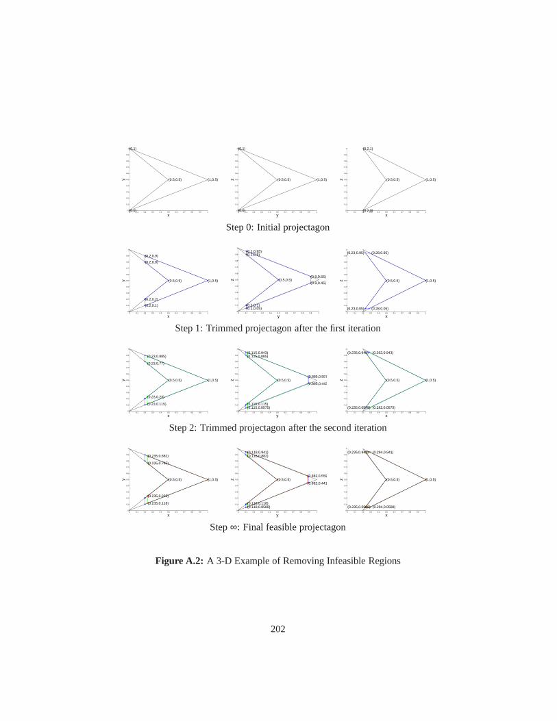
0 0.1 0.2 0.3 0.4 0.5 0.6 0.7 0.8 0.9 10

0.1

0.2

0.3

0.4

0.5

0.6

0.7

0.8

0.9

1

x

y

(0,0)

(1,0.5)

(0,1)

(0.5,0.5)

0 0.1 0.2 0.3 0.4 0.5 0.6 0.7 0.8 0.9 10

0.1

0.2

0.3

0.4

0.5

0.6

0.7

0.8

0.9

1

y

z

(0,0)

(1,0.5)

(0,1)

(0.5,0.5)

0 0.1 0.2 0.3 0.4 0.5 0.6 0.7 0.8 0.9 10

0.1

0.2

0.3

0.4

0.5

0.6

0.7

0.8

0.9

1

x

z

(0.2,0)

(1,0.5)

(0.2,1)

(0.5,0.5)

Step 0: Initial projectagon

0 0.1 0.2 0.3 0.4 0.5 0.6 0.7 0.8 0.9 10

0.1

0.2

0.3

0.4

0.5

0.6

0.7

0.8

0.9

1

x

y

(0.2,0.2)

(0.2,0.1)

(1,0.5)

(0.2,0.9)

(0.2,0.8)

(0.5,0.5)

0 0.1 0.2 0.3 0.4 0.5 0.6 0.7 0.8 0.9 10

0.1

0.2

0.3

0.4

0.5

0.6

0.7

0.8

0.9

1

y

z

(0.1,0.1)(0.1,0.05)

(0.9,0.45)

(0.9,0.55)

(0.1,0.95)(0.1,0.9)

(0.5,0.5)

0 0.1 0.2 0.3 0.4 0.5 0.6 0.7 0.8 0.9 10

0.1

0.2

0.3

0.4

0.5

0.6

0.7

0.8

0.9

1

x

z

(0.23,0.05) (0.28,0.05)

(1,0.5)

(0.28,0.95)(0.23,0.95)

(0.5,0.5)

Step 1: Trimmed projectagon after the first iteration

0 0.1 0.2 0.3 0.4 0.5 0.6 0.7 0.8 0.9 10

0.1

0.2

0.3

0.4

0.5

0.6

0.7

0.8

0.9

1

x

y

(0.23,0.23)

(0.23,0.115)

(1,0.5)

(0.23,0.885)

(0.23,0.77)

(0.5,0.5)

0 0.1 0.2 0.3 0.4 0.5 0.6 0.7 0.8 0.9 10

0.1

0.2

0.3

0.4

0.5

0.6

0.7

0.8

0.9

1

y

z

(0.115,0.115)(0.115,0.0575)

(0.885,0.443)

(0.885,0.557)

(0.115,0.943)(0.115,0.885)

(0.5,0.5)

0 0.1 0.2 0.3 0.4 0.5 0.6 0.7 0.8 0.9 10

0.1

0.2

0.3

0.4

0.5

0.6

0.7

0.8

0.9

1

x

z

(0.235,0.0575) (0.292,0.0575)

(1,0.5)

(0.292,0.943)(0.235,0.943)

(0.5,0.5)

Step 2: Trimmed projectagon after the second iteration

0 0.1 0.2 0.3 0.4 0.5 0.6 0.7 0.8 0.9 10

0.1

0.2

0.3

0.4

0.5

0.6

0.7

0.8

0.9

1

x

y

(0.235,0.235)

(0.235,0.118)

(1,0.5)

(0.235,0.882)

(0.235,0.765)

(0.5,0.5)

0 0.1 0.2 0.3 0.4 0.5 0.6 0.7 0.8 0.9 10

0.1

0.2

0.3

0.4

0.5

0.6

0.7

0.8

0.9

1

y

z

(0.118,0.118)(0.118,0.0588)

(0.882,0.441)

(0.882,0.559)

(0.118,0.941)(0.118,0.882)

(0.5,0.5)

0 0.1 0.2 0.3 0.4 0.5 0.6 0.7 0.8 0.9 10

0.1

0.2

0.3

0.4

0.5

0.6

0.7

0.8

0.9

1

x

z

(0.235,0.0588) (0.294,0.0588)

(1,0.5)

(0.294,0.941)(0.235,0.941)

(0.5,0.5)

Step∞: Final feasible projectagon

Figure A.2: A 3-D Example of Removing Infeasible Regions

202

narrowed down to[0.23,1], [0.1,0.9] and[0.05,0.95], respectively. Similarly, pro-

jection polygons are clipped in the second iteration as shown in Figure A.2 (green

color polygons in Step 2). At each iteration, the values ofx,y andz are narrowed

down to smaller intervals. However, the progress of each step becomes smaller

and smaller. In each iteration, the value ofx shrinks from[a,1] to [4+3a20 ,1] and

converges to[ 417,1] in the limit. Similarly, the values ofy andzconverge to[ 2

17,1517]

and[ 117,

1617], respectively. The red color polygons in Figure A.2 (Step∞) shows the

feasible projectagon. Therefore, approximation algorithms are applied in COHO.

A.3 Minimum Projectagons

Definition Minimum Projectagons: Given a high-dimensional regionR, its mini-

mum projectagon is a projectagon with minimum projection polygons whose fea-

sible region contains R,i.e., the projectagon does not containR if any part of any

projection polygon is removed. If the feasible region is exactly R, we call the

projectagontight; otherwise, we call itnon-tight.

Problem Unique Minimum Projectagon Problem: Given a regionR, is the mini-

mum projectagon unique?

We believe the minimum projectagon is unique. However, we donot have a proof

of the uniqueness problem now. We believe the minimum projectagon can be ob-

tained by clipping infeasible regions.

Corollary A.3.1 If the minimum projectagon is unique, the minimum projectagon

is a canonical representation.

Problem Feasibility Problem: Given a projectagon, make it feasible to its geome-

try representation,i.e.,projection polygons are feasible to each other.

We presented an algorithm to make a projectagon feasible to its inequality rep-

resentation in Section 4.3.3. The algorithm may take infinity number of itera-

tions to obtain the exact result as shown in Section A.2. Therefore, approximation

techniques are applied in the COHO implementation as shown in Algorithm 4 (in

Section 4.3.3). However, it is still an open problem to make aprojectagon feasible

203

to its geometry representation. In fact, the non-emptinessproblem is NP-complete

as proved in Section A.1. Therefore, we believe approximation techniques must be

applied in any implementation. A possible approach is to partition a non-convex

projectagon into convex pieces, make each convex projectagon feasible, and com-

pute the union of feasible convex pieces.

Problem Closure Problem: If P is a minimum projectagon, isconvex(P) a mini-

mum and tight result? IfP1 andP2 are two minimum projectagons, is the intersec-

tion intersect(P1,P2) a minimum and tight result? How about the union?

Apparently, the union of two minimum projectagons is neither minimum or tight

as the union operation returns over-approximated results.We believe the results of

intersection and convex hull operations are minimum and tight. However, they are

also open problems.

204

B

Soundness of COHO Algorithms

This appendix proves the soundness of two algorithms presented in Section 4.4.1.

These algorithms project an advanced face onto one corresponding projection plane

to reduce projection errors. To ensure soundness, the face to be advanced are either

bloated inward byfb in the first approach or enlarged on all other directions byfhin the second approach.

As described in Section 4.3.3, all trajectories from the current projectagon

move by at most∆d on each direction in the time step[0,∆t]. With this assumption,

if the value of fb is no less than 2∆d as shown in Figure B.1(a), the soundness of

the first approach can be proved easily. Because all points ona projectagon face

can move inward by at most∆d, the advanced face on time∆t must be outside

the blue face as shown in Figure B.1. Similarly, all trajectories that may reach

points outside the blue face must has distance smaller than∆d from the blue face.

Therefore, all such trajectories are included in the bloat face illustrated as red re-

gions in Figure B.1(b). Hence, the first approach guaranteesall approximations are

conservative.

In the second approach, the height of face is increased byfh = 2∆d+h(2∆d),

whereh(2∆d) is computed by the interval closure algorithm as shown in Figure B.2.

Figure B.1(b) provides an example for the computation offh. We first bloat a face

corresponds to an edgee inward by 2∆d, then apply the interval closure algorithm

described in Section 4.2.3 to find the height of the bloated face. The height is

increased further by 2∆ as extra guards like we used in the first approach.

205

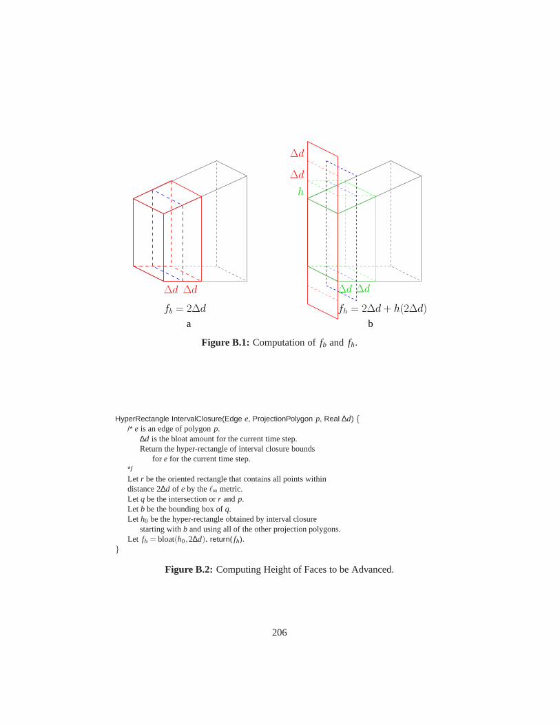
a b

∆d ∆d

∆d

∆d

∆d ∆d

h

fb = 2∆d fh = 2∆d + h(2∆d)

Figure B.1: Computation offb and fh.

HyperRectangle IntervalClosure(Edge e, ProjectionPolygon p, Real ∆d) {/* e is an edge of polygonp.

∆d is the bloat amount for the current time step.Return the hyper-rectangle of interval closure bounds

for e for the current time step.*/Let r be the oriented rectangle that contains all points withindistance 2∆d of e by theℓ∞ metric.Let q be the intersection orr andp.Let b be the bounding box ofq.Let h0 be the hyper-rectangle obtained by interval closure

starting withb and using all of the other projection polygons.Let fh = bloat(h0,2∆d). return( fh).

}

Figure B.2: Computing Height of Faces to be Advanced.

206

To establish the soundness of the interval closure method from Figure B.2,

we consider a projectagon, and assume that one of the projection planes has the

basis(x,y). We show that all points reachable from the projectagon by the end

of the timestep are contained in the(x,y) projection polygon at the end of the

timestep. Letp be an arbitrary point of the projection polygon at the beginning

of the timestep. Ifp is further than 2∆ from the boundary of the(x,y) projection

polygon at the beginning of the timestep, then any point reachable frompat the end

of the timestep will be inside the time advanced polygon, because trajectories from

p can move by at most∆d units outward and points on the boundary of projection

polygon can move by at most∆d units inward during the timestep.

Otherwise, lete be an edge of the(x,y) projection polygon that is within dis-

tance 2∆d of p. By construction, the bloated face containsp. Accordingly, the

constructed face to be advanced has feasible regions that extend by 2∆ in all of the

other dimensions beyond the nearby (i.e. within 2∆) points of projectagon. These

extensions create a “parapet” to ensure that trajectories from faces for other projec-

tion polygons cannot “escape” this polygon. In particular,the face may shrink by

at most∆d along any dimension (illustrated as blue regions in Figure B.1(b)), and

any point can only reach other points that are within distance ∆d (by theℓ∞) metric

of itself. Thus, to reach a point outside of the(x,y) polygon, a trajectory fromp

would have to touch the feasible region for one of the faces arising from the(x,y)

polygon. This means that points reachable fromp are also reachable from the face

that it touched, and therefore project to points on the(x,y) plane that are inside the

time advanced projection polygon.

The values offb and fh to ensure soundness are generally much larger than

necessary. In the implementation of COHO, parameters are provided to users for

obtaining trade-offs between approximation errors and soundness in theory. From

our experiences,∆d is a reasonable value for bothfb and fh.

207