AUTOMATIC FRAME LENGTH, FRAME OVERLAP AND HIDDEN

MARKOV MODEL TOPOLOGY FOR SPEECH RECOGNITION OF

ANIMAL VOCALIZATIONS

by

Anthony D. Ricke

A thesis

submitted to the Faculty

of the Graduation School,

Marquette University,

in Partial Fulfillment of

the Requirements for

the Degree of

Masters of Science in Computing

Milwaukee, Wisconsin

December, 2006

c© Anthony D. Ricke 2006

Preface

Automatic Speech Recognition (ASR) is a useful tool that can facilitate the research

and study of animal vocalizations. The use of human speech-based signal processing

techniques for animal vocalizations has several pitfalls. Animal vocalizations may

not share the same spectral or temporal characteristics as human speech. As a re-

sult, the typical ASR assumptions concerning the best frame length, frame overlap

and HMM topology may not be suitable for various animal vocalizations. This paper

proposes a technique for estimating the frame length, frame overlap and HMM topol-

ogy from a single, clean, example animal vocalization. Multiple trials are run using

the proposed technique, against the vocalizations of two distinct animal species: the

Norwegian Ortolan Bunting (Emberiza Hortulana) and the African Elephant (Lox-

odonta Africana). The results are examined, and the technique provides reasonable

estimates for the frame length, the frame overlap and the HMM topology, given the

quality of the example vocalizations. Specific recommendations are made for the

continuation of this research into a usable tool for animal researches.

ii

Acknowledgments

I thank all of the people that made this work possible; including, but not limited to,

the following people:

To my wife, Denise, for her love and support and for graciously accepting

my absence from our living room every evening for the last year.

To my children, Logan and Zoe, for gracing our lives.

To my adviser, Dr. Michael Johnson, for his guidance, mentoring and

teaching on this project.

To my committee members, Dr. Richard Povinelli and Dr. Craig Struble

for agreeing to be on my committee.

To Patrick Clemins, Jidong Tao and Marek Trawicki, for their work on

animal vocalizations of the African Elephant and the Ortolan Bunting.

To my parents, James and Kathleen, and to the Holy Trinity, for provid-

ing me with the gifts that make my life’s work possible.

Finally, I thank Sun Tzu, for teaching me how to live purposefully:

“Withdraw like a mountain in movement, advance like a rainstorm. Strike

and crush with shattering force; go into battle like a tiger.”[1]

iii

iv

I dedicate this work to my wife Denise, my son Logan and my daughter Zoe, whom

are living examples of courage, unbounded energy and enthusiasm, respectively.

Table of Contents

Preface ii

Acknowledgments iii

Table of Contents v

1 Introduction 11.1 Motivation . . . . . . . . . . . . . . . . . . . . . . . . . . . . . . . . . 2

1.1.1 Spectral Estimation . . . . . . . . . . . . . . . . . . . . . . . . 31.1.2 Frame length, Frame Overlap and Spectral Stationarity . . . . 41.1.3 Hidden Markov Model Topology Selection . . . . . . . . . . . 5

1.2 Present Status of the Problem . . . . . . . . . . . . . . . . . . . . . . 61.2.1 Variable Frame-Rate Analysis . . . . . . . . . . . . . . . . . . 61.2.2 Automated HMM Topology . . . . . . . . . . . . . . . . . . . 7

1.3 Proposed Solution . . . . . . . . . . . . . . . . . . . . . . . . . . . . . 81.4 Contributions of this Work . . . . . . . . . . . . . . . . . . . . . . . . 121.5 Plan of Thesis . . . . . . . . . . . . . . . . . . . . . . . . . . . . . . . 12

2 Background and Related Work 142.1 Speech Processing Overview . . . . . . . . . . . . . . . . . . . . . . . 14

2.1.1 Automatic Speech Recognition Theory . . . . . . . . . . . . . 142.1.2 Statistical Modeling . . . . . . . . . . . . . . . . . . . . . . . 152.1.3 Applications to Animal Vocalizations . . . . . . . . . . . . . . 20

2.2 Spectral Estimation Theory . . . . . . . . . . . . . . . . . . . . . . . 222.2.1 Discrete Fourier Transform . . . . . . . . . . . . . . . . . . . . 222.2.2 Time-Frequency Distributions . . . . . . . . . . . . . . . . . . 252.2.3 Estimating Instantaneous Frequency . . . . . . . . . . . . . . 32

2.3 Summary of Existing Methods . . . . . . . . . . . . . . . . . . . . . . 392.3.1 Variable Frame Rates and Frame Sizing . . . . . . . . . . . . . 392.3.2 Automatic Hidden Markov Model Topology . . . . . . . . . . 40

3 Proposed Method 423.1 Theory . . . . . . . . . . . . . . . . . . . . . . . . . . . . . . . . . . . 42

3.1.1 Frame Length Estimation . . . . . . . . . . . . . . . . . . . . 423.1.2 Frame Overlap Estimation . . . . . . . . . . . . . . . . . . . . 473.1.3 HMM Topology Estimation . . . . . . . . . . . . . . . . . . . 48

3.2 Data Collection . . . . . . . . . . . . . . . . . . . . . . . . . . . . . . 50

v

vi

3.2.1 Elephant Vocalizations . . . . . . . . . . . . . . . . . . . . . . 503.2.2 Ortolan Bunting Vocalizations . . . . . . . . . . . . . . . . . . 51

3.3 Methods . . . . . . . . . . . . . . . . . . . . . . . . . . . . . . . . . . 513.3.1 Overview . . . . . . . . . . . . . . . . . . . . . . . . . . . . . 523.3.2 Frame Length and Overlap Estimation . . . . . . . . . . . . . 563.3.3 HMM Topology Estimation . . . . . . . . . . . . . . . . . . . 60

3.4 Testing Procedures . . . . . . . . . . . . . . . . . . . . . . . . . . . . 633.5 Results . . . . . . . . . . . . . . . . . . . . . . . . . . . . . . . . . . . 64

3.5.1 Instantaneous Frequency Estimation . . . . . . . . . . . . . . 653.5.2 Trials . . . . . . . . . . . . . . . . . . . . . . . . . . . . . . . 723.5.3 Effects Across Species Trial . . . . . . . . . . . . . . . . . . . 80

4 Summary 934.1 Observations . . . . . . . . . . . . . . . . . . . . . . . . . . . . . . . . 934.2 Conclusions . . . . . . . . . . . . . . . . . . . . . . . . . . . . . . . . 1004.3 Further Research Recommendations . . . . . . . . . . . . . . . . . . . 102

Bibliography 103

A Software 108A.1 Overview . . . . . . . . . . . . . . . . . . . . . . . . . . . . . . . . . . 108A.2 Languages . . . . . . . . . . . . . . . . . . . . . . . . . . . . . . . . . 108A.3 Libraries . . . . . . . . . . . . . . . . . . . . . . . . . . . . . . . . . . 108A.4 Tools . . . . . . . . . . . . . . . . . . . . . . . . . . . . . . . . . . . . 109

Approval Page 110

List of Tables

3.1 Instantaneous Frequency vs. Mean Frequency . . . . . . . . . . . . . 653.2 Best-Fit Parameters Trial . . . . . . . . . . . . . . . . . . . . . . . . 81

vii

List of Figures

2.1 Example Left-to-Right HMM . . . . . . . . . . . . . . . . . . . . . . 162.2 Ortolan Bunting Syllable F . . . . . . . . . . . . . . . . . . . . . . . 182.3 Syllable F - 3 State Example . . . . . . . . . . . . . . . . . . . . . . . 192.4 Syllable F - 15 State Example . . . . . . . . . . . . . . . . . . . . . . 202.5 Bin Window for DFT . . . . . . . . . . . . . . . . . . . . . . . . . . . 24

3.1 Stationary Signal . . . . . . . . . . . . . . . . . . . . . . . . . . . . . 433.2 Non-stationary Signal, Inside FFT Bin . . . . . . . . . . . . . . . . . 443.3 Non-stationary Signal, Outside FFT Bin . . . . . . . . . . . . . . . . 443.4 Algorithm Overview . . . . . . . . . . . . . . . . . . . . . . . . . . . 533.5 Preprocessing and Feature Estimation . . . . . . . . . . . . . . . . . . 533.6 Feature Segmentation . . . . . . . . . . . . . . . . . . . . . . . . . . . 553.7 frame length and Overlap Estimation Overview . . . . . . . . . . . . 573.8 Estimate HMM States Overview . . . . . . . . . . . . . . . . . . . . . 613.9 Stationary Frequency ωi Estimate . . . . . . . . . . . . . . . . . . . . 663.10 Linearly-Increasing Frequency ωi Estimate . . . . . . . . . . . . . . . 673.11 Step-Increasing Frequency ωi Estimate . . . . . . . . . . . . . . . . . 683.12 Bunting Syllables . . . . . . . . . . . . . . . . . . . . . . . . . . . . . 693.13 Instantaneous Frequency of the Bunting Syllables . . . . . . . . . . . 703.14 Elephant Vocalizations . . . . . . . . . . . . . . . . . . . . . . . . . . 713.15 Instantaneous Frequency of the Elephant Vocalizations . . . . . . . . 723.16 Ortolan Bunting Frame Length Trials . . . . . . . . . . . . . . . . . . 733.17 African Elephant Frame Length Trials . . . . . . . . . . . . . . . . . 743.18 Ortolan Bunting Frame Overlap Trials . . . . . . . . . . . . . . . . . 763.19 African Elephant Frame Overlap Trials . . . . . . . . . . . . . . . . . 773.20 Ortolan Bunting HMM States Trials . . . . . . . . . . . . . . . . . . 783.21 African Elephant HMM States Trials . . . . . . . . . . . . . . . . . . 793.22 HMM State Bounds for Syllable A . . . . . . . . . . . . . . . . . . . 823.23 HMM State Bounds for Syllable B . . . . . . . . . . . . . . . . . . . . 823.24 HMM State Bounds for Syllable C . . . . . . . . . . . . . . . . . . . 833.25 HMM State Bounds for Syllable D . . . . . . . . . . . . . . . . . . . 833.26 HMM State Bounds for Syllable E . . . . . . . . . . . . . . . . . . . . 843.27 HMM State Bounds for Syllable F . . . . . . . . . . . . . . . . . . . . 843.28 HMM State Bounds for Syllable G . . . . . . . . . . . . . . . . . . . 853.29 HMM State Bounds for Syllable H . . . . . . . . . . . . . . . . . . . 853.30 HMM State Bounds for Syllable J . . . . . . . . . . . . . . . . . . . . 863.31 HMM State Bounds for Syllable U . . . . . . . . . . . . . . . . . . . 86

viii

ix

3.32 HMM State Bounds for Croak 1 . . . . . . . . . . . . . . . . . . . . . 873.33 HMM State Bounds for Croak 2 . . . . . . . . . . . . . . . . . . . . . 873.34 HMM State Bounds for Rumble 1 . . . . . . . . . . . . . . . . . . . . 883.35 HMM State Bounds for Rumble 2 . . . . . . . . . . . . . . . . . . . . 893.36 HMM State Bounds for Rev 1 . . . . . . . . . . . . . . . . . . . . . . 893.37 HMM State Bounds for Rev 2 . . . . . . . . . . . . . . . . . . . . . . 903.38 HMM State Bounds for Snort 1 . . . . . . . . . . . . . . . . . . . . . 903.39 HMM State Bounds for Snort 2 . . . . . . . . . . . . . . . . . . . . . 913.40 HMM State Bounds for Trumpet 1 . . . . . . . . . . . . . . . . . . . 913.41 HMM State Bounds for Trumpet 2 . . . . . . . . . . . . . . . . . . . 92

4.1 HMM State Bounds for Syllable C . . . . . . . . . . . . . . . . . . . 954.2 HMM State Bounds for Syllable B . . . . . . . . . . . . . . . . . . . . 954.3 HMM State Bounds for Trumpet 2 . . . . . . . . . . . . . . . . . . . 964.4 HMM State Bounds for Croak 2 . . . . . . . . . . . . . . . . . . . . . 974.5 HMM State Bounds for Rumble 1 . . . . . . . . . . . . . . . . . . . . 994.6 HMM State Bounds for Trumpet 1 . . . . . . . . . . . . . . . . . . . 100

Chapter 1

Introduction

Automatic speech recognition (ASR) systems model speech signals as a sequence

of encoded symbols that form a message. To decode a speech signal, a typical

ASR system converts the continuous sound signal into a sequence of equally spaced

and equally sized frames. Then, the system encodes each frame into a parameter

vector. The parameter vector sequence is a precise representation of the speech

signal if the original speech signal is stationary inside of each frame [2]. Typical ASR

systems utilize a 30 millisecond frame size with 50% frame overlap. This technique

creates a series of frames with a wideband spectrum that is suited for capturing

temporal changes in the speech signal; i.e., these frames have narrow widths and

they provide better temporal resolution than frequency resolution [3]. Finally, the

ASR systems that utilize a hidden Markov model (HMM) for decoding the paramter

vectors typically model each phoneme using a 3-state HMM.

This model works fairly well for human vocalizations, but it has several short-

comings. First, this model assumes that the speech signal is stationary inside of each

frame. Second, this model utilizes a common frame size for all phonemes; hence, it

assumes that the degree of stationarity for each phoneme is the same. Finally, a

3-state HMM has a state for the transition into the phoneme, a state for the the

“body” of the phoneme, and a state for the transition out of the phoneme. When

used for any possible phoneme, this simplistic model disregards any detailed tempo-

ral characteristics of each phoneme; therefore, it assumes that the detailed temporal

1

2

characteristics of the phoneme are insignificant. All of these assumptions are essen-

tially false, but practical for an English language speech recognition system.

1.1 Motivation

Understanding animal communications is an important task for the preservation of

animal populations in the wild, and for the care and maintenance of domestic animal

populations. Marquette University has started a project, in association with other

animal research organizations, to use human speech signal processing techniques

to aid in the study of animal vocalizations. The goal of this project, called the

“Dr. Dolittle” project, is to create a robust signal-processing framework for pattern

analysis and classification of animal vocalizations.

The application of the human ASR model to animal vocalizations poses several

challenges. First, animal vocalizations may not share the same frequency ranges as

human speech; therefore, the typical choices for frame length may not be suitable for

animal vocalizations. To further complicate the issue, the researches that utilize ASR

techniques on animal vocalizations must study the vocalizations for each distinct

species to determine the frequency range of the signal and to select a frame length

best suited for that frequency range. Second, the temporal characteristics of an

animal vocalization pattern may require the use of a frame overlap that is vastly

different than the typical 50% used by human ASR systems. Finally, the temporal

characteristics of an animal vocalization pattern may be significant to the recognition

of that vocalizations pattern; for example, one type of bird call may contain a warble

that distinguishes it from another type of bird call. As a result, the 3-state HMM

3

model is often inappropriate. One needs a more complex HMM model to adequately

represent a temporally complex vocalization pattern.

The solution to these problems is the motivation of this work; i.e., the purpose

of this work is to develop a method for estimating frame length, frame overlap, and

HMM topology based on a single example for a particular vocalization pattern. This

section describes the problem in detail, as it pertains to the motivation of this work.

1.1.1 Spectral Estimation

The Fourier transform of a discrete-time sequence is called the Discrete-Time Fourier

Transform, or DTFT. For a discrete-time signal, s[n], the DTFT, S(ejω), is defined

as

S(ejω) =∞∑

n=−∞

s[n]e−jωn. (1.1)

The discrete-time signal s[n] provides a reasonable estimate of the spectrum of

the continuous-time signal s(t), if the continuous-time signal is band limited inside

the Nyquist sampling frequency [3].

Practically, the use of the DTFT is not feasible. The continuous-time signal s(t)

is defined for −∞ < t < ∞; therefore, the discrete-time signal s[n] is extends to

infinity and is defined for −∞ < n < ∞. Likewise, the DTFT is a continuous-

frequency function and it is not tractable. Instead, most systems sample a finite-

length sequence from the signal and use the Discrete Fourier Transform to discover

the frequency content of the sequence [3].

The Discrete Fourier Transform, or DFT, is a discrete-time Fourier transform

4

that is only applicable to a finite-length sequence. It is defined as

S[k] = S(ejω)|ω=2πk/N =N−1∑n=0

s[n]e−j2πkn/N . (1.2)

Typically, one computes the DFT using the Fast Fourier Transform.

When using the DFT, one makes the assumption that the spectrum of the signal is

stationary within the window of the DFT. This assumption is important for several

reasons. First, the signal is a random process. To properly estimate all of the

statistical properties from a single realization of a finite length of a random process,

that random process must be ergodic [3]. Second, The DFT is a windowed version

of the discrete-time Fourier transform (DTFT). Since the DTFT transforms the

continuous signal s[n] to the frequency spectrum S(ejω) using s[n] for −∞ < n <∞,

the spectrum of s[n] must be stationary and ergodic, by the definition of the DTFT.

Accordingly, the signal inside of the window of the DFT must be stationary for the

outcome of the DFT to be accurate.

1.1.2 Frame length, Frame Overlap and Spectral Stationarity

In practice, the assumption of spectral stationarity is false for human and animal

vocalizations. Animals and humans communicate information by changing the struc-

ture, and the pitch, of a vocalization over time. Speech processing applications per-

form a DFT using overlapping frames to reduce the amount of non-stationarity in

each frame, and to capture the temporal aspects of the vocalization. Typically, one

selects the size of the frames based on phonetics and research, followed by multiple

adjustments to achieve the best performance from the recognition system. Simi-

lar methods are used for selecting the amount of frame overlap. A typical speech

5

processing system will set the frame overlap to 50% of the frame length to capture

the temporal apsects of the changing spectrum. This amount of frame overlap pro-

vides reasonable temporal resolution without a detailed analysis of the frequency

changes of the vocalization.

One of the problems with using speech processing techniques on animal vocaliza-

tions is the variety of animal species under study. Each species has its own unique

vocalization mechanisms and frequency ranges. Guessing at an acceptable frame

length and frame overlap appropriate for the frequencies ranges for each species is

tedious and prone to error. Ideally, a system would automatically change the frame

length and frame change based on the changing spectral content of the vocalization.

This approach would optimize the temporal and spectral resolution in the features

by reducing the amount of non-stationarity in each frame. This type of system adds

a heavy computational load to the speech recognition task; hence, it may be cost

prohibitive. A better solution for selecting the frame length and frame overlap is to

estimate the frame length from a single example sound of a particular phoneme. One

motivation for this study is the development of a method for automatically estimat-

ing the frame length and frame overlap for a particular human phoneme or animal

vocalization pattern.

1.1.3 Hidden Markov Model Topology Selection

In automatic speech recognition systems, one typically utilizes a three-state left-to-

right model when modeling a phoneme [2]. The first state represents the ingress into

the phoneme. The second state represents the steady-state portion of the phoneme,

and the third state represents the egress out of the phoneme. This model is simple,

6

but it may not properly model the temporal changes for all types of vocalization

patterns; especially when the pitch of the phoneme changes during the vocalization.

Ideally, a system would examine a single example sound for a particular phoneme and

automatically estimate the HMM topology from the characteristics of that sound.

One motivation for this study is the development of a method for automatically

estimating the HMM topology required to model a a particular human phoneme or

animal vocalization pattern, using an example sound.

1.2 Present Status of the Problem

Research on variable frame rates, variable frame lengths and automated model topol-

ogy for animal vocalizations is novel; however, previous work exists [4, 5, 6] for the use

of these techniques on digital processing of speech signals. This work centers around

variable frame-rate analysis and automated HMM topology, and it is described in

the sections that follow.

1.2.1 Variable Frame-Rate Analysis

Variable frame-rate analysis research concentrates on selecting the frames in an ut-

terance that provide the highest information gain between frames. The foundation

of variable frame-rate analysis is frame picking. Frame picking is a method, where

the system measures the distance between frames and to remove frames from the

observation sequence when the distance between the frames is lower than a preset

threshold. Frame picking uses either a euclidean distance or frame entropy as a

distance metric [4, 5], and it is designed to be utilized in a real-time system. In

7

a similar fashion, the work of Potamitis, Fakotakis and Kokkinakis discussed vary-

ing the sampling of the frequency spectrum using the spectral characteristics of the

signal (e.g., spectral slope) [6] with a similar “sample picking” technique.

These methods are focused on reducing the total number of frames that represent

a sound by selecting a subset of the total fames based on a selection criterion. They

utilize a fixed frame length, and they don’t attempt to estimate a suitable frame

length based on the time and frequency description of the signal. As a result, these

methods are inappropriate solutions to the aforementioned problem; i.e., they cannot

provide an estimate of the frame length and frame overlap for a single vocalization.

1.2.2 Automated HMM Topology

Research on automated model topology centers around techniques for trimming the

number of states, state transitions and mixtures per state. One group of researchers

used Bayesian Information Criterion (BIC) for selecting the number of states and

the number of mixtures per state [7]. Using the BIC to automatically trim the

HMM topology requires choosing the prior probabilities for both the structure of

the model and the parameters for the model. Currently, the choice of the prior

probability is either subjective or guided by a data set [8]. Other researchers have

used a simple algorithm for estimating the HMM topology with the minimum number

of states and state transitions.This algorithm trains a set of candidate topologies,

prunes a state transition from each topology from each candidate and calculates the

probability of the data given the model, p(X|M), for each candidate topology. The

algorithm selects the topology with the highest p(X|M). This process continues

until the algorithm contains a model with a single state. Then, the algorithm plots

8

the p(X|M) for each output topology. The algorithm selects the topology at the

point in the curve where the p(X|M) begins to drop. This is the model that has the

highest p(X|M) with the fewest number of states and transitions [9].

None of this research adequately addresses the problem of estimating the initial

HMM topology for the model. This task is left to researcher before applying these

algorithms. Since the motivation of this thesis is to estimate an initial HMM topology

for a particular vocalization pattern, the aforementioned techniques are inappropriate

solutions for the motivation of this thesis; however, these techniques are appropriate

for reducing the number of HMM model parameters after the algorithm estimates

the initial HMM topology.

1.3 Proposed Solution

The solution to these problems is to estimate the frame length, frame overlap and

HMM topology as part of the configuration of the model for ASR. The goal of

this solution is to perform this estimation using a single example vocalization of a

particular vocalization pattern type. This work uses three different approaches to

achieve this goal.

First, the solution estimates the frame length at the current time instant by

measuring the rate of change of the instantaneous frequency over time and by limiting

the amount of change in the instantaneous frequency inside of the current frame. The

solution segments the signal once the slope of the instantaneous frequency breeches

a specific threshold.

The solution estimates the frame overlap for this frame, Wi, by calculating the

9

mean of the instantaneous frequency and the mean of the instantaneous bandwidth

(i.e, the variance of the instantaneous frequency or the instantaneous frequency

spread) over a frame of fixed length. It uses a statistical Student’s t-test to esti-

mate the locations in the observation sequence where the instantaneous frequency

and instantaneous bandwidth are statistically different from the preceding frame.

This process is repeated for the entire vocalization. The solution estimates the

frame length for the next frame, Wi+1, followed by the amount of overlap for proceed-

ing frame, Wi+2, etc.. After estimating the frame length and frame overlap for the

entire vocalization, the solution estimates the average frame length and the average

frame overlap by calculating the sample mean of the frame length and overlap over

the entire vocalization pattern.

Next, the solution estimates the HMM topology for a vocalization pattern using

a similar technique as estimating the average frame overlap; however, it utilizes

three features when estimating the HMM topology: the instantaneous frequency,

the instantaneous bandwidth, and the instantaneous signal power. The solution

estimates the instantaneous signal power using the average frame length and frame

overlap previously estimated. Then, the solution uses the statistical distribution of

the first difference of the three features to estimate the bounds of each HMM state.

To estimate these boundaries, the solution performs a two-sample Student’s t-test.

The purpose of the statistical test is to reject the hypothesis that the signal at time-

instant t + 1 belongs to the statistical distribution of the current HMM state. In

this case, the solution must use a smaller α risk for the t-test to allow for multiple

frames per each HMM state.

The common parameter in each of these three methods is the instantaneous

10

frequency of the signal. Instantaneous frequency is an intuitive concept. We are

surrounded by examples of it in our environment: the change in pitch in a bird

call, the gradual change of color in a rainbow, and the changing frequency of water

dripping from a faucet [10]. Naturally, it is plausible to utilize the instantaneous

frequency of an animal vocalization, along with the instantaneous bandwidth, as

the necessary evidence for estimating the spectral content of a sound at each time

instant, and as the necessary evidence for estimating the frame length, frame overlap

and HMM topology for that vocalization.

The proposed solution uses the instantaneous frequency to automatically deter-

mine the frame length, frame overlap, and HMM topology for an animal vocaliza-

tions. The algorithm utilizes the rate of change of the instantaneous frequency to

estimate the average frame length for a particular vocalization pattern, and it esti-

mates the best frame length as the size where the rate of change of the instantaneous

frequency stays within 50% of the corresponding DFT bin width. Once the the rate

of change of the instantaneous frequency exceeds 50% of the DFT bin width, the

algorithm uses the Student’s t-test to find the location of the start of the next frame.

As a result, when animal vocalization consists of a largely varying instantaneous fre-

quency, the solution estimates a high frame overlap. When the animal vocalization

consists of a constant instantaneous frequency, the solution estimates a lower frame

overlap.

Finally, the proposed solution uses the instantaneous frequency, instantaneous

frequency bandwidth and the instantaneous signal power to select the number of

HMM states for a particular animal vocalization. It converts these three features

into a series of feature vectors and it takes the first difference of these feature vectors.

11

Then, the algorithm utilizes a two-sample Student’s t-test to find the boundaries

between frames. In this case, the α error for the t-test is set at an lower setting to

allow for a large number of frames to fit into the feature vector distribution for a

single state. It estimates the sample mean and sample covariance over the boundary

of the null hypothesis and over the boundary of the alternative hypothesis, and it

uses these two statistical measures when performing the t-test.

To evaluation this solution, the author compares the output of the estimations

for frame length, frame overlap and HMM topology to the HMM model parameters

utilized by prior work with the same animal vocalizations. In addition, he examines

the evidence for each sound and concludes if the algorithm operated in a logical

fashion. It is not expected that the output of this work will make a significant

improvement to a task like speaker identification. Rather, the goal is to provide

a reasonable estimate of the frame length, frame overlap and HMM topology so

researchers can create HMM models without extensive manual analysis of the animal

vocalizations.

During the evaluation, the author uses animal vocalizations from two different

animal species: the African Elephant (Loxodonta Africana) and the Ortolan Bunting

(Emberiza Hortulana L). Previous work [11, 12] utilized these animal vocalizations to

perform automatic speaker identification on animal vocalizations. These two species

were selected because they are vastly different in both spectral content and temporal

content. African Elephant vocalizations have a fundamental frequency between 7 Hz

and 200 Hz [12], which is below the the voice frequency band (300 Hz - 3 kHz) [13].

Ortolan Bunting songs range between 1.9 and 6.7 kHz; hence, these vocalizations

are inside of, to just above, the voice frequency band [14]. In addition, the African

12

Elephant has vastly different vocalization mechanisms that the Ortolan Bunting;

therefore, the temporal characteristics of the vocalization patterns for each species

is vastly different.

1.4 Contributions of this Work

The contributions of this work are threefold:

1. The development of a method to automatically estimate the average frame

length using the instantaneous frequency of an example sound.

2. The development of a method to automatically estimate the average frame

overlap using the instantaneous frequency of an example sound, and a previ-

ously selected frame length.

3. The development of a method to automatically estimate the number of HMM

states using the instantaneous frequency of an example sound, and a previously

selected frame length and frame overlap.

1.5 Plan of Thesis

Chapter 2 reviews the literature relevant to variable frame overlap and optimal HMM

topology, and it reviews the background of using framed sound signals with a statis-

tical model for the purpose of sound identification and labeling. Chapter 3 presents

the proposed method for automatic frame overlap selection, automatic frame length

selection and Hidden Markov Model topology; including the procedures used for test-

13

ing the method and the results obtained from those procedures. Finally, Chapter 4

presents the conclusions of this work and prospects for further research.

Chapter 2

Background and Related Work

This chapter presents the basic concepts required to understand the remainder of

the thesis. Section 2.1 provides overview of techniques used in speech processing and

their application to processing animal vocalizations. Section 2.2 provides an overview

of Spectral Estimation theory, with a detailed discussion on instantaneous frequency

and instantaneous bandwidth. Finally, section 2.3 discusses existing methods for

automatic frame length and HMM topology estimation.

2.1 Speech Processing Overview

This section provides a brief overview of the theory behind ASR and it discusses

the challenges of using speech processing techniques on animal vocalizations; specif-

ically, it discusses the challenges of applying ASR techniques on African Elephant

vocalizations and Ortolan Bunting vocalizations.

2.1.1 Automatic Speech Recognition Theory

Speech recognition systems are built upon an assumption that human speech is a

realization of a message that is encoded as a series of one or more symbols [2]. Using

this assumption, a speech recognition system decodes the speech signal x(t) into a

sequence of symbols that represent some type of meaning. To accomplish this task,

the SR system divides the speech signal into a series of short-time successive frames

14

15

that are usually overlapped [15]. Since speech is composed of acoustic waves that

change over time, most of the information in the speech signal is encoded in the

frequency domain. As a result, the decoding process consists of transforming frames

of speech into the frequency domain, extracting spectral-based features from each

frame, and selecting the labeled sound that has the highest probability of matching

a series of frames. Most modern systems utilize a Hidden Markov Model to decode

a series of speech frames into some type of meaning. The details behind Hidden

Markov Models are covered in the next section. Detailed information on the theory

of speech processing can be found in [16] and [17].

2.1.2 Statistical Modeling

Modern ASR systems utilize the Hidden Markov Model (HMM) to decode the noisy

speech signal into units of meaning. A HMM is a stochastic signal model where

the input into the model (i.e., the speech signal) is modeled as a random stochastic

process. This section gives a brief overview of HMMs. It concentrates on the areas

pertinent to this thesis; namely, the effects of the number of states on the detection

of speech signals. It assumes that the reader has an understanding of stochastic

processes and Markov processes. For a detailed description of Markov processes,

HMMs, and the application of HMMs to ASR, see [18]

An HMM is a model of a Markov chain where the states of the Markov chain are

not observable, but its effect on the output of another set of stochastic processes is

observable. Consider a process that consists of a fix number of discrete states that

can describe the process at any time (see Figure 2.1). Each state has an associated

probability density, or mixture of densities, that describe the occupation probability

16

for a particular observation (e.g., b1(Ot)). Furthermore, such a process has transition

between each state, and each of the state transitions has an associated transition

probability (e.g., a23). These transitions include a transition from a state to itself,

so the process can remain in the same state over multiple observations (e.g., a22). If

this process is a first order Markov chain, the probabilistic description of the process

is limited to the current state and the predecessor state.

Figure 2.1: Example Left-to-Right HMM

Elements of an HMM

If the output of this stochastic process is the set of states at each instant in time and

each state corresponds to an observable event, the process is called an observable

Markov model. If the output of this stochastic process is simply the observable

events over time, and the underlying Markov chain is hidden, the process is called a

hidden Markov model. Given this description, such a model is characterized by five

elements [18]:

1. N, The number of states in the model.

2. M, The number of distinct observation symbols per state. When the observa-

tions are continuous, M = ∞.

17

3. A, The state transition probability distribution. A = {aij}

4. B, The observation symbol probability distribution in state j, B = {bj(k)}.

The observation symbol probability distribution is a continuous probability

distribution that is typically assumed to be a single Gaussian distribution, or

a mixture of Gaussian distributions.

5. Π, The initial state distribution, π = {πi}

A compete description of an HMM requires the specification of two model pa-

rameters (N and M), the specification of three probability measures A, B and π,

and the specification of observation symbols. For speech processing, the observation

symbols are described as a vector of speech features in the real numbering system;

therefore, this model parameter does not apply. The only tasks that remain are to

define the number of states for the model, and to specify the probability measures

A, B and π. Typically, the person designing the HMM model selects the number

of states as appropriate for the signal. Then, the HMM model is trained using a

training set of data and the Baum-Welch algorithm. This is a specialized expec-

tation maximum algorithm that maximizes the likelihood of observation sequence

given the model (P (O|λ)). Then, the trained HMM model is useful for decoding a

sequence of observations into a sequence of states [18].

ASR systems utilize a specialized variant of the HMM model, called the left-right

model or the Bakis model [18]. With this model, it is only possible to transition

forward in time; therefore, state transitions always move from the left to the right

or connect to the same state (see Figure 2.1). This variant of the HMM is suited for

modeling signals whose statistical properties change over time; i.e., non-stationary

18

signals like speech signals and animal vocalizations. The left-right HMM is capable

of capturing temporal aspects of the signal during training and decoding.

Decoding Speech

The purpose of using an HMM for speech processing is to decode the sequence of

observations, i.e., the feature vectors extrapolated from the speech signal, into a se-

quence of Markov states. Each state in the HMM contains an observation probability

distribution; therefore, each state in the HMM must represent a specific temporal

range of the signal. For example, consider the signal in Figure 2.2.

Figure 2.2: Ortolan Bunting Syllable F

This signal starts with a small silence region. At about 20 ms, it transitions into

a sound with a constant frequency and increasing in power; then, the first sound

stops and the second sound begins at 65 ms. This sound consists of an oscillating

pitch and increasing power. A three-state HMM may model the silence region as

one state, the first portion of the sound as a second state, and the second portion of

the sound as the third state (see Figure Figure 2.3). To model the second portion of

the sound, the statistical distribution for the pitch must be fairly wide to properly

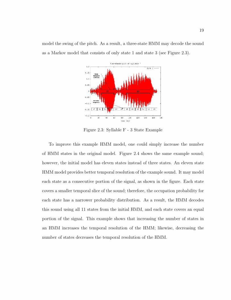
19

model the swing of the pitch. As a result, a three-state HMM may decode the sound

as a Markov model that consists of only state 1 and state 3 (see Figure 2.3).

Figure 2.3: Syllable F - 3 State Example

To improve this example HMM model, one could simply increase the number

of HMM states in the original model. Figure 2.4 shows the same example sound;

however, the initial model has eleven states instead of three states. An eleven state

HMM model provides better temporal resolution of the example sound. It may model

each state as a consecutive portion of the signal, as shown in the figure. Each state

covers a smaller temporal slice of the sound; therefore, the occupation probability for

each state has a narrower probability distribution. As a result, the HMM decodes

this sound using all 11 states from the initial HMM, and each state covers an equal

portion of the signal. This example shows that increasing the number of states in

an HMM increases the temporal resolution of the HMM; likewise, decreasing the

number of states decreases the temporal resolution of the HMM.

20

Figure 2.4: Syllable F - 15 State Example

2.1.3 Applications to Animal Vocalizations

Applying ASR techniques to animal vocalizations reveals additional challenges. The

first challenge is the frequency range of the signal. The human ear can hear frequen-

cies between 20 Hz and 20,000 Hz, but most of the information in intelligible speech

ranges between 500 Hz and 2500 Hz [19]; however, the unvoiced phonemes contain

frequencies that can exceed 10,000 Hz. Animal vocalizations will have frequency

ranges that are partially outside of this band. For example, the African elephant

has vocalizations with a fundamental frequency between 7 Hz and 200 Hz [20]. As

a result, an ASR system must utilize longer frame sizes during encoding to capture

these lower frequencies. There are two possible solutions to this problem. Either

the ASR must adapt its frame length based on the fundamental frequency of the vo-

calization, or the system designer must adjust the frame length based on the target

vocalization type for the ASR system.

The next challenge is the changing pitch of a vocalization. Humans communi-

cate information using phonemes, and most of the phonemes have a fundamental

21

frequency that is stable for most of the duration duration of the phoneme. For

example, the phoneme /aa/ is expressed with stationary fundamental frequency in

the English language, as in the word father [16]. In contrast, animal vocalizations

may vary in fundamental frequency over an equivalent linguistic unit; e.g., the ’a’

syllable of the Ortolan Bunting changes its fundamental frequency rapidly over the

sound. The result is that the ASR system must utilize a different frame overlap when

processing certain animal vocalizations; otherwise, the ASR system cannot capture

the temporal changes in the vocalization accurately.

Currently, researchers at Marquette University have applied ASR techniques to

solve the speaker identification problem for the Ortolan Bunting and the African

Elephant. Originally, the researchers used a frame length of 25 ms, a frame overlap

of 15 ms and a 3-state single-mixture Gaussian model for each syllable for solving

the Ortolan Bunting speaker identification problem. The researchers used the same

parameters for solving the Ortolan Bunting song-type classification problem [21].

Currently, the researchers are using smaller, 5 ms, frames and longer HMM topologies

(around 15 states).

Likewise, researchers used a frame length of 300 ms, a frame overlap of 100 ms

and a 3-state single-mixture Gaussian model for solving African Elephant speaker

identification problem. They used the rumbles for speaker identification problem,

and these rumbles are often in the infrasound range (≈ 10 Hz); therefore, they

required longer frame lengths. The researchers used a frame length of 60 ms and a

frame overlap of 20 ms for the call classification experiments [20].

22

2.2 Spectral Estimation Theory

This section presents a summary of spectral estimation theory, as it applies to au-

tomatic frame length, frame overlap and Hidden Markov Model topology. First, it

reviews the properties and assumptions of the discrete Fourier transform. Then, it

presents the concept of frequency as a density function, and it describes the basic

theory on instantaneous frequency and instantaneous bandwidth. Finally, it dis-

cusses the basis of the method used to estimate the instantaneous frequency for this

research.

2.2.1 Discrete Fourier Transform

There are multiple methods for estimating the power spectrum for a signal. One of

the most common methods is called the periodogram. This method uses the Discrete

Fourier Transform, or DFT, of a frame of a signal to estimate the power spectrum.

The periodogram takes an N-point sample of the signal, s[n], at equally spaced

intervals and transforms the discrete time signal into the discrete frequency signal,

S[ejω], using the DFT:

S[k] = S(ejω)|ω=2πk/N =N−1∑n=0

s[n]e−j2πkn/N . (2.1)

The periodogram is defined as

P (fk) = 1N2 |S(k)|2 : ∀k = 0, 1, 2, ..., N

2(2.2)

for the discrete case [22]. For each sample, or bin, the DFT calculates the power

spectrum for equally spaced frequencies between 0 Hz (DC) and one-half the sampling

frequency (Fs).

23

fk ≡ kN∆

= FskN

: ∀k = 0, 1, ..., N2

(2.3)

Equation 2.3 defines the frequency of each sample, or bin, in the power spectrum.

Since the DFT only operates over the Nyquist interval (one-half of the sampling

frequency), the above equation only defines bins for frequencies from 0 Hz to the

Nyquist frequency. Traditionally, each bin is thought to represents the power of the

spectrum at the frequency of that bin. For example, when the FFT reports a specific

power at the bin for 10 Hz, it is thought that this is the power of the spectrum of the

signal at 10 Hz. Actually, each bin in the power spectrum covers a narrow window of

the frequency spectrum, and equation 2.3 refers to the center of that narrow window.

Each bin has a width of Fs

N, and the power of the spectrum represents the average

power over the width of the bin.

Since each bin is a window of the power spectrum, each bin has a window function.

The window function for each bin is defined as [22]

w(s) =1

N2

[sin(πs)

sin(πs/N)

]2

. (2.4)

where w(s) is the window function and s is defined as the frequency offset, in bins.

Figure 2.5 provides an example of this window function. Notice that the window

has most of its strength from the center of the bin frequency (the main lobe), and

that it does gain additional power from adjacent bin frequencies (side lobes). The

side lobes of this window function results in significant leakage of spectral power

from one frequency bin to another bin in the spectrum estimate.

Various windowing functions are used to reduce the effects of leaking when es-

timating power spectra. See the literature for additional information on data win-

24

Figure 2.5: Bin Window for DFT

dowing for use with the DFT.

When estimating power spectrum, there are few important concepts to remember:

1. The definition of the DFT assumes that the signal is stationary over the DFT;

i.e., that it does not change it’s spectral content or its power content over the

window.

2. Each frame of the signal must be windowed before performing the DFT, to

reduce the spectral leakage from adjacent frames.

3. The frame length for the DFT must be long enough to provide a good average

of the fundamental frequency of the underlying signal. A frame length of at

least two pitch periods is desirable [3].

25

2.2.2 Time-Frequency Distributions

Naturally, signals are described in the time-domain. The simplest form of a time-

varying signal is the sinusoid:

s(t) = a cos(ω0t).

With a sufficient understanding of the continuous Fourier transform and the

discrete Fourier transform, one can transform a signal from the time-domain into

the frequency domain:

S(ω) = F{s(t)} = F{a cos(ω0t)} = π[δ(ω − ω0) + δ(ω + ω0)].

This is sufficient for signals that are truly stationary in time; however, most real-

world signals are not. A general purpose model for a non-stationary signal is more

practical

s(t) = a(t) cosϑ(t) = A(t)ejϕ(t), (2.5)

where the amplitude, a(t), and the phase, ϑ(t), are time-varying functions. Like-

wise, one may use the Fourier integral to transform the time-domain function into a

frequency domain function

S(ω) =1√2π

∫s(t)e−jωtdt. (2.6)

This is often called the spectrum. One can write this equation in terms of the

spectral amplitude and phase,

26

S(ω) = B(ω)ejψ(ω), (2.7)

where B(ω) is called the spectral amplitude and ψ(ω) is called the spectral phase,

which are frequency-varying functions.

This model has a problem with ambiguity. Since both the amplitude and the

phase of the signal vary with time, there are an infinite number of pairs of amplitude

and phase that could define s(t) [10]. Time-frequency distributions are one of the

primary tools for studying and resolving a solution to this model. This section of the

paper provides a brief introduction into the concepts that describe time-frequency

distributions, discusses the concept of instantaneous frequency and instantaneous

bandwidth, and explains one of the methods utilized to estimate the instantaneous

frequency of a real signal.

Functions of the Signal as a Density Function

To understand time-frequency distributions, one must first understand that the time-

varying signal and the frequency-varying spectrum can be represented as densities,

similar to a probability density. For example, to calculate the total energy of the

time-varying signal, simply integrate the absolute value of the signal squared over

all time

E =

∫|s(t)|2 dt. (2.8)

Likewise, the total energy of the frequency-varying signal is a similar integral

E =

∫|S(ω)|2 dω. (2.9)

In both cases, the absolute value of the signal squared, |s(t)|2 for time and |S(ω)|2

for frequency, is called the energy density. In the time domain, this is called the

27

energy density or instantaneous power. In the frequency domain, this is called the

energy density spectrum. This is analogous to the circuit definition of the energy

density being proportional to the voltage squared or to the sound wave definition

of the energy density being proportional to the pressure squared [10]. Notice that

|s(t)|2 isn’t precisely the energy density because it is not normalized properly. To

normalize the energy density, divide the |s(t)|2 by the total energy of the signal;

however, the rest of this paper presents |s(t)|2 and |S(ω)|2 as the energy density to

keep the equations uncluttered.

Mean Frequency and Mean Time

Since, |s(t)|2 is the energy density, one can use the density function to calculate

expectations of the signal. For example one can calculate the mean time of the

signal as

〈t〉 =

∫t |s(t)|2 dt. (2.10)

The mean time can give an indication of where the signal is concentrated in time.

Of course, for a infinitely varying signal, like a continuous sine wave, the solution to

the integral is infinity because the density never converges.

The spread of a density, i.e., the standard deviation, is another interesting statistic

T 2 = σ2t =

∫(t− 〈t〉)2 |s(t)|2 dt =

⟨t2

⟩− 〈t〉2 . (2.11)

The standard deviation is an indication of the concentration of the density around

the mean. The standard deviation of the time of the signal is an indication of the

duration of the signal, since in time 2σ2t , most of the signal will have gone by.

28

In a similar fashion, one may define the mean frequency and mean frequency

spread of the frequency domain of a signal as

〈ω〉 =

∫ω |S(ω)|2 dω (2.12)

and

B2 = σ2ω =

∫(ω − 〈ω〉)2 |S(ω)|2 dω =

⟨ω2

⟩− 〈ω〉2 . (2.13)

By definition, the mean frequency, 〈ω〉, is an indication of the average frequency

of the signal for the duration of the signal and the mean frequency spread, σ2ω , or the

bandwidth, is an indication of the frequency range of the signal. Note that bandwidth

does not indicate where these frequencies exist in time. To understand where the the

frequencies existed in time, a measurement of the frequency over time is required.

One such measurement, usually derived from a time-frequency distribution, is the

instantaneous frequency.

Instantaneous Frequency

The instantaneous frequency is defined by [10] as the derivative of the phase from

equation 2.5. In this paper, it is denoted as

ωi(t) = ϕ′(t) (2.14)

The rest of this section provides the mathematics used to derive the instantaneous

frequency and to show the relationship between the instantaneous frequency and

the derivative of the phase. Here, the instantaneous frequency is derived from the

definition of the mean frequency.

It is possible to calculate the mean frequency without ever entering the frequency

domain. This is done using a Hermitian operator for the frequency

29

W =1

j

d

dt(2.15)

The definition of the mean frequency is transformed into a time-domain version,

that contains the frequency operator, as follows

〈ω〉 =

∫ω |S(ω)|2 dω (2.16)

=

∫ωS∗(ω)S(ω)dω (2.17)

=

∫ω[

1√2π

∫s∗(t)ejωtdt][

1√2π

∫s(t′)e−jωt

′dt′]dω (2.18)

=1

2π

∫ ∫ ∫ωs∗(t)ejωtdt s(t′)e−jωt

′dt′dω (2.19)

=1

2π

∫ ∫ ∫ωs∗(t)s(t′)ej(t−t

′)ωdt′ dt dω. (2.20)

Since

∂

∂tejω(t−t′) = jωej(t−t

′)ω,

then

1

j

∂

∂tejω(t−t′) = ωej(t−t

′)ω

and

〈ω〉 =1

2πj

∫ ∫ ∫s∗(t)s(t′)

∂

∂tej(t−t

′)ωdt′ dt dω. (2.21)

(2.22)

Since

δ(t) =1

2π

∫e±jkxdx,

30

〈ω〉 =1

j

∫ ∫s∗(t)s(t′)

∂

∂tδ(t− t′)dt′ dt (2.23)

=1

j

∫ ∫s∗(t)

∂

∂tδ(t− t′)s(t′)dt′ dt. (2.24)

Since ∫δ(t− t0)x(t)dt = x(t0);

therefore,

〈ω〉 =1

j

∫ ∫s∗(t)

∂

∂tδ(t− t′)s(t′)dt′ dt (2.25)

=1

j

∫s∗(t)

∂

∂ts(t)dt (2.26)

〈ω〉 =

∫s∗(t)

1

j

d

dts(t)dt. (2.27)

This can be further simplified by first considering the transform

Ws(t) = WA(t)ejϕ(t) =1

j

d

dtA(t)ejϕ(t) (2.28)

=1

j

(A(t)

d

dtejϕ(t) + ejϕ(t) d

dtA(t)

)(2.29)

=1

j

(A(t)jϕ′(t)ejϕ(t) + ejϕ(t)A′(t)

)(2.30)

=

(A(t)ϕ′(t)ejϕ(t) +

1

jejϕ(t)A′(t)

)(2.31)

=

(s(t)ϕ′(t) +

1

j

A′(t)

A(t)s(t)

)(2.32)

=

(ϕ′(t) +

1

j

A′(t)

A(t)

)s(t). (2.33)

Using this transform, the mean frequency is

31

〈ω〉 =

∫s∗(t)

1

j

d

dts(t)dt (2.34)

=

∫s∗(t)

(ϕ′(t) +

1

j

A′(t)

A(t)

)s(t)dt (2.35)

=

∫A(t)e−jϕ(t)

(ϕ′(t) +

1

j

A′(t)

A(t)

)A(t)ejϕ(t)dt (2.36)

=

∫ (ϕ′(t) +

1

j

A′(t)

A(t)

)A2(t)dt. (2.37)

Note that the integrand of the second term integrates to zero; therefore,

〈ω〉 =

∫ϕ′(t) |s(t)|2 dt =

∫ϕ′(t)A2(t)dt. (2.38)

This result is interesting. It states that one can obtain the mean frequency by

integrating the density with ϕ′(t) over all time. By definition, this must be the

instantaneous value that we are averaging. In this case, we are calculating the

mean frequency and the ϕ′(t), the derivative of the phase, is accordingly called the

frequency at each time instant, or the instantaneous frequency, ωi(t) [10].

Instantaneous Frequency Spread (Instantaneous Bandwidth)

According to equation 2.38, the average of the instantaneous frequency is the mean

frequency; i.e., 〈ωi〉 = 〈ω〉. It follows that the spread of the instantaneous frequency

is defined as [10]

σ2IF =

∫(ϕ′(t)− 〈ωi〉)2 |s(t)|2 dt (2.39)

=

∫(ϕ′(t)− 〈ω〉)2 |s(t)|2 dt. (2.40)

32

This is given the appellation instantaneous bandwidth. Cohen expands this fur-

ther to show that the instantaneous bandwidth is always less than or equal to the

frequency bandwidth; i.e., σIF ≤ B [10]. This is interesting because the instanta-

neous frequency can move outside the bounds of the frequency bandwidth, but it

must only do so for short durations in time and not significantly impact the overall

spread of the instantaneous frequency. See the work of Cohen [10] for additional de-

tails on using the derivative of the phase of the signal as the instantaneous frequency.

Also, see the work of Boashash [23] for alternative explanations of the instantaneous

frequency.

2.2.3 Estimating Instantaneous Frequency

There are various techniques for estimating the instantaneous frequency. According

to [24], there are eight categories of instantaneous frequency estimation techniques:

1. Discrete-Time IF Estimation

2. Smoothed Versions of the Phase Difference Estimator

3. Zero-Crossing IF Estimation

4. Adaptive IF Estimation

5. Estimation based on the Moments of TFD’s

6. Estimation based on the Peak of TFD’s

7. Time-Varying AR Model Based IF Estimation

8. Enhancement of IF Laws Through the Application of Tracking Algorithms

33

This work utilizes the method of estimating the IF based on the peak (maximum) of

the time-frequency distribution called the Wigner distribution (method #6). This

section of the paper describes the theory behind the instantaneous frequency esti-

mation technique developed by Katkovnic and Stankovic [25, 26].

Estimating Instantaneous Frequency - Wigner Distribution

The Wigner distribution, based on the continuous waveform, is defined as [27]

WDx(t, ω) =

∫x(t+

τ

2)x∗(t− τ

2)e−jωτdτ. (2.41)

The Pseudo-Wigner distribution (WD) for the discrete time waveform, is defined

as

WDh(t, ω) =∞∑

n=−∞

wh(nT )x(t+ nT )x∗(t− nT )e−j2ωnT . (2.42)

where wh(nT ) = T/h ·w(nT/h) and w(t) is a real-valued symmetric window, w(t) =

w(−t). The width of the window wh(nT ), is denoted by h > 0 and it is assumed

that w(t) has a finite length. That is, w(t) = 0 for |t| > 1/2 [25].

Estimating the instantaneous frequency using the maximum of the WD is a simple

process. First, window a portion of the signal using a lag window of a fixed size.

Then, estimate the WD and find its maximum. The maximum is the instantaneous

frequency at time instant t. Move the lag window forward in time, t + 1, estimate

the WD and find its maximum. Repeat this process for the entire signal.

When estimating the IF using this method, the bias and variance estimation are

very dependent on the lag window width. Stankovic and Katkovnik developed an

algorithm for estimating the instantaneous frequency using the Wigner distribution

with an adaptive window width. In this algorithm, sliding pair-wise confidence

34

intervals are used to estimate the optimal, dyadic window width for the Wigner

distribution [25, 26]. The author utilized their method for IF estimation. The rest of

this section describes their method. First, the following section describes the problem

of optimizing the window width for the Wigner distribution; then, it describes their

algorithm for estimating the IF from the signal using an adaptive window width.

Estimating Instantaneous Frequency - Window Width Optimization

Consider the problem of estimating the instantaneous frequency, ω(t) = ϕ′(t), from

a noisy, digital, signal

x(n) = s(n) + e(n), (2.43)

with s(n) being the uncorrupted signal and e(n) being white noise from a complex-

valued Gaussian source with real and imaginary parts of equal variance σ2ε/2. As-

suming that the instantaneous frequency is estimated using the maximum of a time-

frequency distribution, the goal is to find a symmetric lag window that minimizes

the estimation error for the instantaneous frequency. Let ∆ω(t) = ω(t) − ω(t) be

the estimation error. The mean squared error E(∆ω(t))2 is used to characterize the

accuracy of the estimate at time instant t. If the estimation errors are small, then,

for a wide variety of time-frequency representations, the MSE can be represented in

the following form:

E(∆ω(t))2 =V

hm+B(t)hn, (2.44)

where h is a window of the symmetric lag window (ω(t) = 0 for |t| > h/2); the vari-

ance of estimation is σ2(h) = Vhm and the bias of estimation is bias(t, h) =

√B(t)hn.

The window width h depends directly on the number of samples h = N/T and T

is the sampling interval. V and B(t) are dependent on the IF estimation technique

35

used. For the Wigner Distribution with a rectangular window m = 3, n = 4, and

V = 6σ2εT/A

2 [26].

Since the MSE in equation 2.44 has a minimum with respect to h, the correspond-

ing optimal value of h is hopt = [mV/(nB(t))]1/(m+n); however, this formula is not

useful because it contains the bias parameter B(t) that depends on the derivatives

of the IF. The goal is to develop an algorithm that produces the optimal discrete

window length without using the bias for the estimate of the IF. Assuming that the

bias is positive, the following holds:

bias(t, hopt) =

√m

nσ(hopt). (2.45)

Since the IF estimate ωh(t) is a random variable distributed around ω(t), we may

write the following inequality:

|ω(t)− (ωh(t)− bias(t, h))| ≤ kσ(h). (2.46)

The next paraphrased statement describes the algorithm for determining the op-

timal window width for estimating the instantaneous frequency without ever knowing

the bias. It only uses the instantaneous frequency estimate and the variance of the

IF estimate [26].

Let H be a set of dyadic window width values. Assume that the

optimal window width for a given instant t belongs to this set, hopt ∈ H.

Define the upper and lower bounds of the confidence intervals Ds =

[Ls, Us] of the IF estimates as

Ls = ωhs(t)− (k + ∆k)σ(hs)Us = ωhs(t) + (k + ∆k)σ(hs), (2.47)

36

where ωhs(t) is an estimate of the IF, with the window width h = hs and

σ(hs) is its variance.

Let the window width hs+ be determined as a window corresponds to

the largest s (s = 1, 2, . . . , J) when two successive confidence intervals

still intersect, i.e., when

Ds ∩Ds+1 6= ∅ (2.48)

is still satisfied.

Then, there exists values of k and ∆k such that Ds ∩Ds+1 6= ∅ and

Ds+1 ∩ Ds+2 = ∅ for s = s+, when hs+ = hopt, with the corresponding

probability P (k) ' 1 that |ω(t)− (ωh(t)− bias(t, h))| ≤ kσ(h) is satis-

fied.

The proof is provided in [26] and is omitted.

Estimating Instantaneous Frequency - Algorithm

Assuming that the amplitude of the signal A and the standard deviation of the signal

σe are known, find the optimal dyadic window, hs+ from the set of possible dyadic

windows

H = hs|h1 < h2 < h3 < . . . < hJ . (2.49)

Note that hs is a symmetric lag window, hs = 2NsT , around the current time instant,

t.

For every time instant, t, use the following procedure:

1. Calculate the Wigner Distribution for all hs ∈ H. Estimate the instantaneous

37

frequency from the frequency bin with the maximum power

ωhs(t) = arg

[maxω∈Qω

WDhs(ω, t)

].

2. Calculate the upper and lower bounds of the confidence intervals

Ls(t) = ωhs(t)− (k + ∆k)σ(hs) (2.50)

Us(t) = ωhs(t) + (k + ∆k)σ(hs), (2.51)

where σ(hs) is defined as

σ(hs) =

√6σ2

e

|A|2

(1 +

σ2e

2|A|2

)T

h3s

. (2.52)

Assuming a Gaussian distribution for the noise, use k = 2 to set the confidence

intervals to have the probability of P(2) = 0.9454 of inequality

|ω(t)− (ωh(t)− bias(t, h))| ≤ |bias(t, h)|+ kσ(h) (2.53)

σ2(h) = var(∆ωh(t)) (2.54)

=6σ2

e

|A|2

(1 +

σ2e

2|A|2

)T

h3s

. (2.55)

3. The optimal window length, hs+ , is the window length with the largest s(s =

1, 2, . . . , J) when the previous confidence intervals and the current confidence

intervals still intersect

[Ls−1(t), Us−1(t)] ∩ [Ls(t), Us(t)] 6= ∅; (2.56)

that is, when

∣∣ω(hs)(t)− ωhs−1(t)∣∣ ≤ 2k[σ(hs) + σ(hs−1)] (2.57)

38

still holds true. The s+ is the largest value of s where the confidence interval

segments, Ds−1 and Ds, have a point in common for s ≤ J . The optimal

window length is

h(t) = hs+(t)

and ωh(t)(t) is the instantaneous frequency estimator for the data-driven win-

dow at time instant t.

4. The Wigner distribution for the optimal window length is

WD+(ω, t) = WDh(t)(ω, t). (2.58)

This process is repeated at every time instant in the signal [25].

In this work, the values of A and σ2e are estimated from each window of the data

using the estimators provided in [25]

A2 + σ2e =

1

N

N∑n=1

|x(nT )|2 . (2.59)

This sum is calculated over all N observations of a frame. The variance is estimated

as the median of the first difference of the signal

σer ={median(|xr(nT )− xr((n− 1)T )| : n = 2, . . . , N)}

0.6745(2.60)

σei ={median(|xi(nT )− xi((n− 1)T )| : n = 2, . . . , N)}

0.6745(2.61)

σ2e = (σ2

er + σ2ei)/2. (2.62)

Then, the power of the uncorrupted signal is easily estimated by solving equation

2.59.

39

2.3 Summary of Existing Methods

This section presents a brief summary of the existing methods found in the literature

on the focus areas of this thesis: variable frame rates in speech processing, automatic

HMM topology, optimal frame sizing and instantaneous frequency estimation. Each

section gives a brief overview of the the existing methods and compares those meth-

ods to our target solution.

2.3.1 Variable Frame Rates and Frame Sizing

Prior research on variable frame-rate analysis is primarily focused on the use of a

specific distance metric to calculate the distance between speech frames and remove

frames that are close in distance [28, 29, 30, 31, 5]. In the works of Ponting, Peeling

and Russel [[28], [29], and [30]], the system computes the distance between the last

retained feature vector and the current feature vector. When this distance is below

a predefined threshold, the frame is discarded but its duration is retained and added

as a feature in the retained feature vector. Then, the system trains the HMM’s

using the additional duration feature. This style of HMM is appropriately named

a duration sensitive topology. These techniques show improvements over fixed-rate

speech processing; however, the duration sensitive topology provides only marginal

improvement over simple variable frame-rate analysis [28].

The work of Zhu and Alwan [31] expands on the frame selection concept by

utilizing an energy weighted Euclidean distance of the Mel-Frequency Cepstral Co-

efficients as its distance metric. This method uses the energy weighting to discard

frames that exhibit changes between frames, but the frames are low in energy. Fu-

40

ture work by the same authors [5] provides another variant of the frame selection

solution by calculating the entropy of each frame and by selecting frames which ex-

ceed a specific frame-picking threshold. Both of these techniques exhibit improved

performance over the fixed rate results.

The work of Potamitis, Fakotakis and Kokkinakis [6] approached the variable

frame-rate analysis problem as an optimization problem. This work utilized the

Wigner distribution, a time-frequency distribution, to find the optimal time-varying

window. The optimization criterion was to minimize the expectation of the sum

of the variance and squared bias. This results in a solution that varies the frame

length and frame overlap to provide a set of optimally smoothed spectral vectors

for features. The results of this work failed to show significant improvement over a

conventional estimator, using a dynamic time warping speech recognizer.

The aforementioned solutions require additional calculations during the speech

recognition process; in contrast, the author proposes a solution that estimates the

initial frame length and frame overlap (i.e., frame rate) using the change in the

spectral slope over the phoneme.

2.3.2 Automatic Hidden Markov Model Topology

The literature on Hidden Markov Model topology focuses on optimization of existing

topologies using various algorithms. Li, Biem, and Subrahmonia [7] approach the

problem of HMM topology optimization as a model selection problem; where a single

model is selected from a group of candidate models. These works used the Bayesian

Information Criterion (BIC) to select the HMM model with the optimal configura-

tion. The researchers trained multiple HMM models, with varying configurations,

41

and selected the configuration that yields the highest value. A second paper by

Biem, Subrahmonia and Ha [8] used a similar approach, but the researchers used the

HMM-Oriented Bayesian Information Criterion (HBIC) to find the optimal HMM

topology. In both methods, the configurations varied in the number of states and

the number of mixtures per state.

Vasko, El-Laroudi and Boston [9] approach the problem in a different fashion.

They select the model that gives the maximum probability of the data given the

model p(X|M). Starting with a trained HMM, their algorithm prunes a single HMM

state transition from the model. After pruning a state transition, the algorithm

calculates the probability of the data given the model. It repeats this process, pruning

a different HMM state transition each time, until it creates a set of all possible

models with a single state transition pruned. The algorithm selects the model that

maximizes the p(X|M). This process is repeated, until the algorithm prunes the

original model down to a single state. Then, the algorithm selects the single model

that maximizes the p(X|M).

Chapter 3

Proposed Method

This chapter presents the proposed method for automatic estimation of frame length,

frame overlap and HMM topology for animal vocalizations. First, it discusses the

theory behind the automatic estimation methods. Next, it presents the animal vo-

calization data used for experimentation. Then, it describes the algorithm used to

perform the automatic estimation. Finally, it describes the results of the experiments

and compares those results to the frame length, frame overlap and HMM topology

used in the previous experiments.

3.1 Theory

3.1.1 Frame Length Estimation

The goal of frame length estimation is to estimate the length of the frame that

contains a stationary signal and that contains enough samples for proper frequency

resolution. Typically, a frame length of several pitch periods is desirable to resolve

the harmonics of pitch frequencies [3]. Given that a signal processing system uses

the DFT to transform the discrete time signal into the frequency domain, the spec-

trogram of the signal has some tolerance to a non-stationary signal. That tolerance

is subject to the width of the DFT frequency bins. A DFT with a small number

of samples has large frequency bins; therefore, it can tolerate a larger change in

frequency content of the signal over the DFT frame without having the energy of

42

43

the FFT leaking in to neighboring bins. Likewise, a DFT with a larger number

of samples has smaller frequency bins and it has less tolerance to a non-stationary

signal. For example, when a signal is stationary the instantaneous frequency stays

completely inside of a single FFT bin, as shown in Figure 3.1.

Figure 3.1: Stationary Signal

When a signal is not stationary, the instantaneous frequency line has some spe-

cific slope through a particular frame. Figure 3.2 provides an example of an non-

stationary signal where the change in the instantaneous frequency is slight enough

to remain inside the bounds of the FFT bin.

Signals that are highly non-stationary (i.e., in the context of the instantaneous

frequency changing over a single frame) have rapid changes in the instantaneous

frequency over a single frame. Figure 3.3 provides an example of the instantaneous

frequency of such a signal. In this case, the instantaneous frequency change exceeds

the bounds of the FFT bin, and the FFT cannot accurately represent the signal

using the current frame length.

Let x be a discrete-time signal for a particular animal vocalization, sampled with

44

Figure 3.2: Non-stationary Signal, Inside FFT Bin

Figure 3.3: Non-stationary Signal, Outside FFT Bin

45

a sampling rate of Fs. Let ωi be the estimation of the instantaneous frequency for

the animal vocalization from the discrete-time signal, x. Each discrete instant in ωi

represents the maximum-power frequency component of the signal x at time instant

t. At that same instant, an FFT window of length N has a frequency resolution

of Fs/N . Let m be the slope of the instantaneous frequency curve (m = ∆ωi/∆t).

When the signal is stationary, the instantaneous frequency of the signal will remain

stationary, and the slope the instantaneous frequency of the signal will equal zero.

Given these definitions, the maximum allowable change in frequency over a frame,

where the instantaneous frequency remains inside the bounds of a single FFT bin

(i.e., signal remains stationary inside of the frame), is defined as:

|m|N =FsN

(3.1)

or

|m|N2

Fs= 1. (3.2)

Let ρ be the ratio of the change of the instantaneous frequency in the window

over the FFT bin size,

ρ =|m|N2

Fs. (3.3)

It is desirable to keep the change of the instantaneous frequency to less than 1/2 of

the bin size; therefore, one may limit ρ to less than 1/2. Making this ratio dependent

on the mean instantaneous frequency, ωi of the signal, we have:

46

ωi ∼=kFsN

(3.4)

kωi=

NωiFs

; (3.5)

therefore,

ρ =|m|Nkωi

Fs(3.6)

=|m|N2ωi

Fs2 . (3.7)

This is the ratio of instantaneous frequency slope, m, that is sensitive to the

mean instantaneous frequency of the frame. When the instantaneous frequency is

high, this ratio is less sensitive to changes in the instantaneous frequency. When

the instantaneous frequency is low, the ratio is more sensitive to changes in the

instantaneous frequency.

Alternative Approaches

Initially, the author attempted to estimate the frame length using two different

approaches. First, the author attempted to estimate the optimal frame length by

deriving an minimum mean squared estimator. This approach failed because one

cannot take the first derivative of the DFT of a frame of the signal with respect to

the length of the frame.

Next, the author attempted to use an adaptive segmentation technique [32] based

on the estimate of the noise in the signal modeled by an autoregressive process. This

technique made segmentation decisions using the Akaike criterion or a generalized

likelihood ratio test. It utilized a recursive least squares (RLS) algorithm to estimate

47

the variance in the signal, and it used this variance when it made segmentation

decisions. The author did not use this method in the final work because the RLS

easily tracked the changes in the instantaneous frequency and it was never forced to

segment the signal. As a result, the author could not use the adaptive segmentation

technique to estimate the frame length of the signal using the instantaneous frequency

as the primary feature.

3.1.2 Frame Overlap Estimation

The goal of frame overlap estimation is to estimate the frame overlap which provides

the best temporal resolution of the time-frequency distribution. To provide the best

temporal resolution, the system must overlap each frame at the point where the

signal becomes non-stationary. One measurement of the stationarity of the signal is

the change in the instantaneous frequency and instantaneous frequency bandwidth.

Let ωi be the estimation of the instantaneous frequency for the animal vocalization

from the discrete-time signal, x, and let σ2ωi

be the bandwidth of the instantaneous

frequency. Let W0 be the current frame in the signal and W1 be the next frame in

the signal. One can estimate the best frame overlap location by estimating the mean

and standard deviation of the instantaneous frequency and instantaneous frequency

bandwidth for frames W0 and W1. At each time instant, perform a Student’s t-test

to reject the following hypothesis:

H0 : ξ{ωi(W0)} = ξ{ωi(W1)}. (3.8)

Since the instantaneous frequency bandwidth represents the variance of the in-

stantaneous frequency distribution function, use it as the variance in the Student’s

48

t-test [33]:

T =√N

(ξ{ωi(W0)} − ξ{ωi(W1)})σ2ωi

, (3.9)

where N is the sample size for the frame W0, ξ{ωi(W0)} and ξ{ωi(W1)} are the

sample means, and ξ{σ2ωi} is the average instantaneous frequency bandwidth for

frame W0. Reject the null hypothesis, H0, if and only if

|T | > t(α/2,v). (3.10)

The variable v represents the degrees of freedom for the test; i.e., v = N − 1 for

a single sample Student’s t-test.

If the test does not reject the null hypothesis, slide W1 forward in time by one

sample and repeat the statistical test. If the test rejects the null hypothesis, this is

the location of the best frame overlap.

3.1.3 HMM Topology Estimation

The goal of the HMM topology estimation is simply to estimate the number of HMM

states for the sample animal vocalization. This goal is further simplified because ASR

systems utilize left-to-right HMMs. As a result, the HMM topology estimation needs

to estimate only the number of states in the HMM.

Let ωi be the estimation of the instantaneous frequency for the animal vocaliza-

tion from the discrete-time signal, x, let σ2ωi

be the estimate of the instantaneous

frequency bandwidth, and let Ei be the estimate of the instantaneous signal power.

Let X0 be the time span of the current HMM state and X1 be the time span of the

next HMM state; where, each time span is an integer number of overlapping frames

49

of a fixed duration. One can estimate the time duration of a single HMM state by

estimating the mean and standard deviation of ωi, σ2ωi

, and Ei for the time spans

X0 and X1 and either accepting or rejecting the hypothesis that the time span X1

is statistically equivalent to time span X0. When the system rejects this hypothesis,

it holds the boundary for the HMM state X0 and starts a new boundary for the

next HMM state. When the system does not reject this hypothesis, it moves the

boundary for the HMM state X0 to include the time span X1 and it creates a new

X1 that spans a fixed number of frames.

For this statistical test, the system assumes that ωi, σ2ωi

and Ei are statistically

independent for simplicity, and it performs a two-sided Student’s t-test [34]:

T =(ξ{ωi(X0)} − ξ{ωi(X1)})√

s20/N0 + s2

1/N1

, (3.11)

where N0 and N1 and the sample sizes for the time spans X0 and X1, ξ{ωi(X0)} and

ξ{ωi(X1)} are the sample means, and s20 and s2

1 are the sample variances. Reject the

null hypothesis, H0, if and only if

|T | > t(α/2,v). (3.12)

The variable v represents the degrees of freedom for the two-sample Student’s

t-test:

v =(s2

0/N0 + s21/N1)

2

(s20/N0)2/(N0 − 1) + (s2

1/N1)2/(N1 − 1). (3.13)

In this case, three individual statistical tests are performed using the random

processes ωi, σ2ωi

and Ei. The algorithm treats each of these random processes

as statistically independent; therefore, the results of the three t-tests are logically

50

AND’ed to determine if the system should reject the null hypothesis. The system

rejects the null hypothesis if any one of the three statistical tests reject the null

hypothesis and it does not reject the null hypothesis when all three statistical tests

fail to reject the null hypothesis.

3.2 Data Collection

This study utilized data collected from previous work [11, 12] to verify the efficacy

of the algorithm. Researchers at Disney’s Animal KingdomTM in Orlando, FL

collected the Elephant vocalization data used in [11], and researchers in County

Hedmark, Norway collected the Norwegian Ortolan Bunting vocalization data used

in [12]. The details of the data collection for the elephant vocalizations and the

Ortolan Bunting vocalizations are provided in the sections that follow.

3.2.1 Elephant Vocalizations

As described in [12], each elephant involved in the data collection at Disney’s Animal

KingdomTM was fitted with a custom collar that contained a microphone and an

RF radio. The radio broadcasts the audio to the elephant barn where it was recorded

on DAT tapes. Then, the audio was passed through anti-aliasing filters and stored

digitally at a sampling rate of 7518 Hz. More information on the data collection

procedure is located in the works of Leong et. al. [20].

For these experiments, two clean examples of five call types were selected from

the entire set of elephant vocalizations. These vocalizations were selected because

they were vocalizations with a minimal amount of noise, and this set of vocalizations

51

provides a good representation (50%) of the types of vocalizations utilized by the

African Elephant [12].

3.2.2 Ortolan Bunting Vocalizations

As described in [11], researchers collected the Norwegian Ortolan Bunting vocal-

ization data from County Hedmark, Norway in May of 2001 and 2002. The entire

sample population in this data collection contains vocalizations from 150 different

males. Each vocalization is divisible into fundamental units called syllables. The

Ortolan Bunting communicates using a set of 20 distinct syllables which are joined

in sequences, creating multiple song types. These syllables are analogous to the pho-

netic units used in human speech. Additional information on the data collection is

located in [21].

For these experiments, the set of ten clean syllables (a, b, c, d, e, f, g, h, j and

u) were selected from the song data set. These vocalizations were selected because

they were vocalizations with a minimal amount of noise and they exemplify a broad

variety of the vocalizations used by the Ortolan Bunting.

3.3 Methods

The algorithm uses the instantaneous frequency, instantaneous frequency bandwidth

and the instantaneous signal power as the three features from the vocalizations for

the estimation of the frame length, frame overlap and the HMM topology. The

algorithm estimated the instantaneous frequency using the techniques developed by

Katkovnik and Stankovic [25, 26]. This method is explained in Section 2.2.3 of the

52

background of this paper.

Because the estimation of instantaneous frequency utilized in this study is time-

consuming, the system calculates instantaneous frequency and the instantaneous

frequency bandwidth using a stand-alone module and stores these features for later

retrieval. This technique saves the time required to estimate the features at every

run of the algorithm. In addition, the stand-alone module stores the following in-

formation: the sampling rate, the window sizes used by the algorithm from [25, 26],

the mean frequency at each aforementioned window and the mean frequency spread

(bandwidth).

3.3.1 Overview

The algorithm is divided into two major sub-processes: feature estimation and fea-

ture segmentation. Figure 3.4 shows the two major sub-processes, with the major

components of each sub-process.

Feature Estimation

The first sub-process, Feature Estimation, is divided into two major components:

“preprocessing” and “estimate instantaneous frequency and bandwidth”. The “pre-

processing” section is further sub-divided into its component steps, as seen in Figure

3.5.

The algorithm begins by reading a waveform file. The data from the waveform

file is normalized using a zero mean technique. Then, the signal is converted into a

complex signal using the Hilbert transform. Next, the algorithm estimates the largest

frame length by sampling the signal at the midway point, computing the FFT, and

53

Figure 3.4: Algorithm Overview

Figure 3.5: Preprocessing and Feature Estimation

54

estimating the bandwidth of the FFT. The largest frame length is set to two times

the period of the lowest frequency in the FFT bandwidth. The largest frame length

is utilized by the algorithm as a limit on the window sizes for the instantaneous

frequency estimation.

After the algorithm finishes preprocessing the signal, it begins estimating the

instantaneous frequency, the instantaneous frequency spread, or bandwidth, and the

instantaneous signal power. The algorithm estimates the instantaneous frequency

and instantaneous frequency bandwidth utilizing the method defined in [25, 26] and

further described in Section 2.2.3. Finally, the estimation process returns the two

features (instantaneous frequency and instantaneous frequency bandwidth), along

with the window sizes estimated during the instantaneous frequency estimation, to

the parent process.

Feature Segmentation

The second sub-process, Feature Segmentation, is divided into three major compo-

nents: estimate segments, estimate HMM states and persist HMM files. The process

of estimating segments is further sub-divided into three additional sub-processes:

trim features, estimate segments, estimate mean frame length and overlap, as seen

in Figure 3.6

The algorithm begins by loading the previously estimated features. If the features

for the current sound file were never persisted, the algorithm estimates these features

from the current sound file and persists them. The algorithm trims the first n

features from beginning and the end of the feature matrix, where n is one-half of the

first window width from the instantaneous frequency estimation process. Next, the

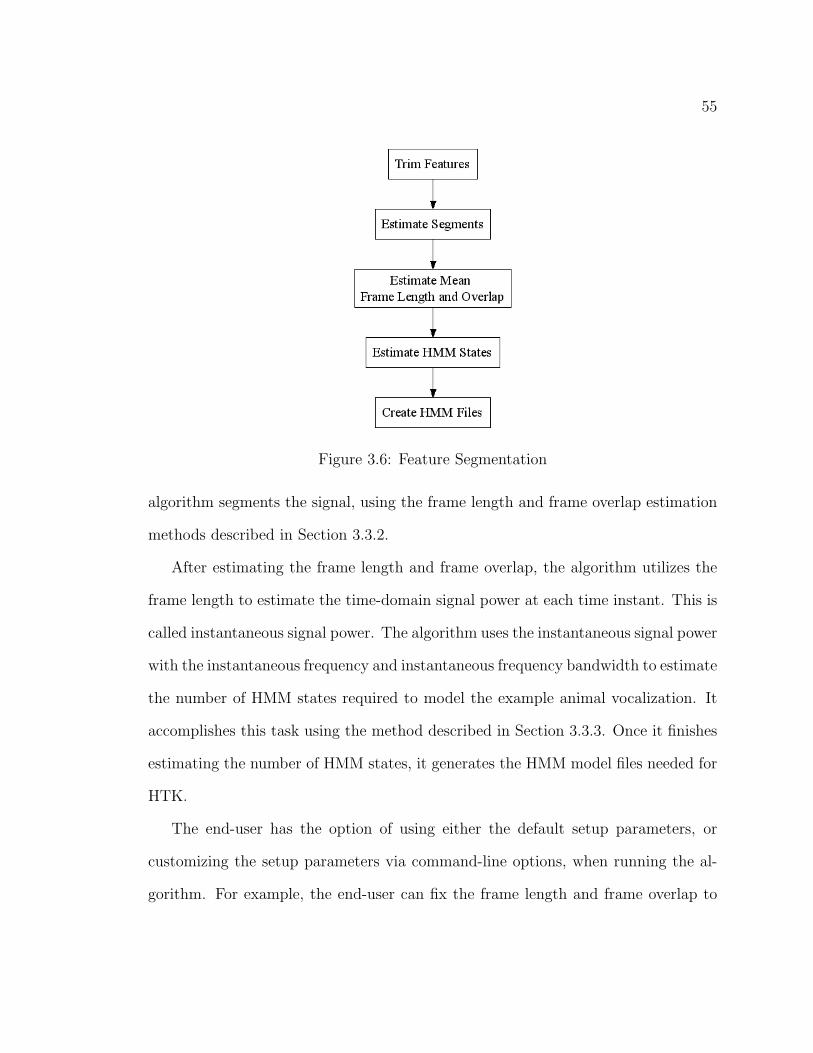
55

Figure 3.6: Feature Segmentation

algorithm segments the signal, using the frame length and frame overlap estimation

methods described in Section 3.3.2.

After estimating the frame length and frame overlap, the algorithm utilizes the

frame length to estimate the time-domain signal power at each time instant. This is

called instantaneous signal power. The algorithm uses the instantaneous signal power

with the instantaneous frequency and instantaneous frequency bandwidth to estimate

the number of HMM states required to model the example animal vocalization. It

accomplishes this task using the method described in Section 3.3.3. Once it finishes

estimating the number of HMM states, it generates the HMM model files needed for

HTK.

The end-user has the option of using either the default setup parameters, or

customizing the setup parameters via command-line options, when running the al-

gorithm. For example, the end-user can fix the frame length and frame overlap to

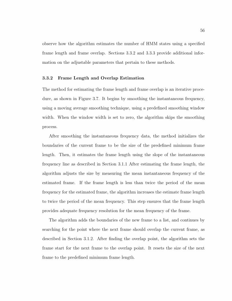
56

observe how the algorithm estimates the number of HMM states using a specified

frame length and frame overlap. Sections 3.3.2 and 3.3.3 provide additional infor-

mation on the adjustable parameters that pertain to these methods.

3.3.2 Frame Length and Overlap Estimation

The method for estimating the frame length and frame overlap is an iterative proce-

dure, as shown in Figure 3.7. It begins by smoothing the instantaneous frequency,

using a moving average smoothing technique, using a predefined smoothing window

width. When the window width is set to zero, the algorithm skips the smoothing

process.

After smoothing the instantaneous frequency data, the method initializes the

boundaries of the current frame to be the size of the predefined minimum frame

length. Then, it estimates the frame length using the slope of the instantaneous

frequency line as described in Section 3.1.1 After estimating the frame length, the

algorithm adjusts the size by measuring the mean instantaneous frequency of the

estimated frame. If the frame length is less than twice the period of the mean

frequency for the estimated frame, the algorithm increases the estimate frame length

to twice the period of the mean frequency. This step ensures that the frame length

provides adequate frequency resolution for the mean frequency of the frame.

The algorithm adds the boundaries of the new frame to a list, and continues by

searching for the point where the next frame should overlap the current frame, as

described in Section 3.1.2. After finding the overlap point, the algorithm sets the

frame start for the next frame to the overlap point. It resets the size of the next

frame to the predefined minimum frame length.

57

Figure 3.7: frame length and Overlap Estimation Overview

58

Estimating Frame Length

The algorithm estimates the frame length by implementing the theory described in

Section 3.1.1. In brief, the algorithm begins by setting the size of the current frame

to the minimum frame length. Then, it executes the following procedure to estimate

the frame length:

1. Using linear regression, estimate the slope of the instantaneous frequency line

over the current frame.

2. Calculate the ratio of the change in the instantaneous frequency over the size

of the FFT bin, ρ = |m|N2ωi

F 2s

.

3. If this ratio, ρ, is greater that the limit, τρ, this is the end of the current frame.

4. Otherwise, increase the frame length by a single sample and restart this process.

The algorithm continues this process until the slope of the instantaneous fre-

quency line exceeds the limit defined by the system parameters.

There is a problem with this technique. When a signal is stationary, the ωi of the

signal is stationary and the slope of the instantaneous frequency is at or near zero.

This results in the algorithm increasing the frame length until the calculation of the

linear regression becomes cost prohibitive. To overcome this problem, the algorithm

decimates the ωi of the signal after it increases the frame length beyond a specific size.

Since this region of the instantaneous frequency is stable, the algorithm can average

each pair of samples without loosing accuracy on the slope of the instantaneous

frequency line.

59

The algorithm begins to decimate the instantaneous frequency of the signal when

the frame length exceeds 1024 sample points. At each boundary of 1024 sample

points, the algorithm increases the decimation rate; therefore, when the frame length

increases from 1024 points to 1025 points, the decimation rate increases from 1 point

decimation (i.e., no oversampling) to two-point decimation (i.e., average pairs of

samples).

Estimating Frame Overlap

The algorithm estimates the frame overlap by implementing the theory described

in Section 3.1.2. In brief, the algorithm begins this process by creating a frame of

the same size as the current frame. It initializes this frame, called the sliding frame

(W1), to start at the same location as the start of the current frame (W0). Then, it

executes the following procedure to estimate the frame overlap:

1. Estimate the mean instantaneous frequency, ξ{ωi(W0)} and the mean instan-

taneous bandwidth, ξ{σ2ωi

(W0)} for the current frame.

2. Estimate the mean instantaneous frequency, ξ{ωi(W1)}, for the sliding frame.

3. Perform a one sample Student’s t-test. The null-hypothesis for this statistical

test is ξ{ωi(W0)} = ξ{ωi(W1)}; where the statistic ξ{σ2ωi

(W0)} is the variance

for the null-hypothesis. Use the number of samples in frame W0, minus one,

as the degrees of freedom for the test. Make the alpha risk for the t-test, ταZ1,

a variable parameter into the algorithm.

4. If the statistical test fails, reject the null-hypothesis. The sliding frame, W1,

is no longer statistically equivalent to the stationary frame, W0. This is the

60

location of the overlap point.

5. If the statistical test passes, accept the null-hypothesis. This sliding frame,

W1, is still statistically equivalent to the stationary frame, W0. Move the

frame forward in time by a single sample, and rerun this procedure.

The algorithm continues this process until either it rejects the null-hypothesis

or until the sliding frame slides past the end of the current frame; i.e., until the

algorithm reaches 0% overlap.

3.3.3 HMM Topology Estimation

The method for estimating the HMM topology is an iterative procedure, as shown

in Figure 3.8. The algorithm begins to estimate the HMM topology by first normal-

izing the data by the covariance matrix of all of the features. The formula for this

conversion is

xnorm = (x− ξ{x})Σ−1 (3.14)

where, x is a matrix of feature vectors and Σ is the covariance matrix where the

features are assumed to be independent; i.e., Σ = I[σ21, σ

22, ..., σ

2N ].

Once the algorithm normalizes the data, it begins the process of estimating the

HMM topology. The algorithm uses the parameter for the minimum number of

frames per state, the frame length, and the frame overlap to initialize the decision

index (idecision = Nframes/state ∗ (Nlength(wi) − Noverlap(wi)). Let W0 represent the

temporal region of the signal for the current state. This temporal region is comprised

of a series of overlapping frames, and w1 represents the frame just outside of the

61

Figure 3.8: Estimate HMM States Overview

62

region W0. Then, using these definition, the algorithm estimates the HMM topology

as follows:

1. Estimate the mean and variance of the features in the region of the signal

matrix bound by W0. This region ends at the decision index.

2. Estimate the mean and variance of the features for the next frame from the

signal matrix. This frame starts at the decision index.

3. Perform a statistical test. The null-hypothesis is that the mean feature vector

of the next frame (w1) is statistically equivalent to the mean feature vector of

the current state (W0); i.e., that the next frame belongs within the statistical

boundaries of the existing state.

(a) For each feature, perform a two-sample statistical t-test to reject the null-

hypothesis. Make the alpha risk for the t-test, ταZ2, a variable parameter

into the algorithm.

(b) All t-tests must pass (i.e., they must not reject the null-hypothesis) for

the next frame to be considered part of the current frame.

4. If the statistical test passes, include the next frame as part of the current state.

Increment the decision index by the frame length minus the frame overlap

(idecision = idecision + (Nlength(wi) −Noverlap(wi))) and repeat this procedure.

5. If the statistical test fails, store the bounds of the current frame in a list. In-

crement the decision index to end of the initial size of the next state (idecision =

idecision +Nframes/state ∗ (Nlength(wi) −Noverlap(wi))) and repeat this procedure.

63

The algorithm continues this process until the decision index plus the frame

length exceeds the number of feature vectors in the feature matrix.

3.4 Testing Procedures

The goal of this project is to design a method for estimating the frame length, frame

overlap and HMM topology given a single example animal vocalization. There are

multiple possible solutions for this problem; a gold standard dataset does not exist

for this project. Instead, numerous example animal vocalizations from two animal

species with vastly different vocalization mechanisms were analyzed; i.e., the African

Elephant and the Ortolan Bunting, as described in Section 3.2.

As a result of the lack of a gold standard for this method, the method was verified

using the following procedure:

1. For each animal vocalization in the dataset, estimate the instantaneous fre-

quency and instantaneous bandwidth a priori and persist these features for

future processing. Plot a graph of the instantaneous frequency, the instanta-

neous bandwidth and the signal over time for each vocalization.

2. For each animal vocalization in the dataset, estimate the frame length, frame

overlap and HMM topology, as appropriate, by running the following experi-

ments:

(a) Estimate the HMM parameters when fixing the frame overlap to 50%

of the estimated frame length. Run four trials for each example animal

vocations. Utilize a τρ limit on the ratio of 0.5, 0.75, 1.0 and 2.0 for each

64

trail. Fix the alpha risk z-score. ταZ2, for the HMM states decision to 30.

Record all results.

(b) Estimate the HMM parameters while fixing the frame length to the length

utilized in the original experiments for the vocalization. Run four trials

for each example animal vocations. Utilize a z-score for the frame overlap

alpha risk, ταZ1, of the statistical test of 1.0, 2.0, 3.0 and 6.0 for each trail.

Record all results.

(c) Estimate the the HMM parameters while fixing the frame length and

frame overlap to the values utilized in the original experiments for the

vocalization. Run four trials for each example animal vocations. Utilize

a z-score for the HMM topology alpha risk, ταZ2, of the statistical test of

3.0, 6.0, 15.0 and 30.0 for each trial. Record all results.

3. For each animal vocalization in the dataset, perform a best case estimation

using the best parameters from the above test procedure. Record all results.

For each experiment, provided the estimates of the frame length, frame over-

lap and HMM topology estimation. In addition, provide a plot of the HMM state

boundaries versus the instantaneous features used by the method.

3.5 Results

The results of this work are divided into three sections. The first section reviews

the original animal vocalizations and their conversion into instantaneous frequency.

The second section reviews the results of the aforementioned experiments. The third

65

section presents the selection of the parameters for the comparison of the effects of

the parameters across species.

3.5.1 Instantaneous Frequency Estimation

This work verified the instantaneous frequency, ωi, estimation using three simulated

sound files, where the instantaneous frequency was known before the estimation. In

each test case, the system plots the instantaneous frequency against the expected ωi

and against the mean frequency of a set of overlapping windows of the spectrogram

of the signal. The test estimates the mean frequency, 〈ω〉, over time using a frame

length of 128 samples (128 ms) and a frame overlap of 96 samples (96 ms). The test

simulates all of the sound files at a rate of 1000 sps.

Table 3.1 shows the mean-squared error of the ωi estimate and of the 〈ω〉 estimate

for each test. Looking at these results, it is obvious that the method used to estimate

the instantaneous frequency is superior to using the mean frequency to estimate the

frequency over time.

Test ωi MSE 〈ω〉 MSEStationary Signal 1.881 7.294

Linearly Increasing Signal 5.192 18.165Staircase Signal 1.995 29.909

Table 3.1: Instantaneous Frequency vs. Mean Frequency

Figure 3.9 provides the results of the instantaneous frequency estimation of a

pure sine wave at a constant frequency. In this case, the mean frequency moves

around the expected value, but the ωi is stable at a value slightly off of the expected

stable frequency of 44Hz.

66

Figure 3.9: Stationary Frequency ωi Estimate

67

Figure 3.10 shows the results of the linearly-increasing example. In this case, the

instantaneous frequency curve follows the actual frequency throughout the plot, but

the estimate is slightly lower than the actual frequency at each time instant. The

mean frequency tends to bounce along the line of the actual frequency with values

slightly higher that the actual frequency.

Figure 3.10: Linearly-Increasing Frequency ωi Estimate

Figure 3.11 shows the result of the system estimating the ωi from a file with a step

increase in the signal frequency. Here, the instantaneous frequency estimation follows

the actual frequency closely; while, the mean frequency estimate cannot handle the

instantaneous changes from one frequency “step” to another. From these examples,

68

it is evident that the instantaneous frequency techniques used in this work provide

a satisfactory ωi estimation.

Figure 3.11: Step-Increasing Frequency ωi Estimate

Next, let’s review the estimation of the instantaneous frequency from the Ortolan

Bunting vocalizations. Figure 3.12 provides a time-series plot of all ten Ortolan

Bunting syllables used in this work. With the exception of the ‘u’ syllable, these

sounds are very clean, with an excellent signal-to-noise ratio (SNR).

Likewise, Figure 3.13 provides the instantaneous frequency estimates for each

of the Ortolan Bunting syllables. Overall, the instantaneous frequency estimation

provides a fairly smooth waveform for all of the Ortolan Bunting syllables.

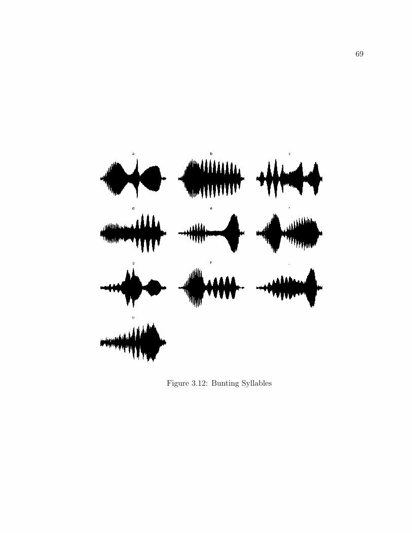
69

Figure 3.12: Bunting Syllables

70

Figure 3.13: Instantaneous Frequency of the Bunting Syllables

71

Finally, let’s review the estimation of the instantaneous frequency from the

African Elephant vocalizations. Figure 3.14 provides a time-series plot of all ten

African Elephant vocalizations used in this work. Likewise, Figure 3.15 provides

Figure 3.14: Elephant Vocalizations

the instantaneous frequency plots of the African Elephant vocalizations. With these

sounds, the SNR is much lower than the Ortolan Bunting syllables. Also, the plots

“Croak 1”, “Rumble 1”, “Rumble 2”, “Trumpet 1” and “Trumpet 2” all have some

very high instantaneous frequency content that is not characteristic of the animal

vocalization. In all of the elephant vocalizations, there is the constant presence of

72

white noise that may cause these IF spikes. Also, the trumpet vocalizations contain

a large amount of silence before and after the vocalization. This silence appears as

high-frequency spikes in the IF estimation plots.

Figure 3.15: Instantaneous Frequency of the Elephant Vocalizations

3.5.2 Trials

Frame Length Trials

The results of the frame length trials are provided in Figures 3.16 and 3.17. As

expected, the length of the average frame in the sound is a function of the algorithm

parameter, τρ (denoted as rho in the figures). With the exception of a single outlier,

73

the frame lengths for the Ortolan Bunting syllables are grouped between 8 ms and

25 ms. The frame lengths for the African Elephant vocalizations are divided into two

groups. The first group represents the low-frequency vocalizations (croak, rumble

and rev). For these vocalizations, the frame lengths are long- between 125 ms and

1000 ms. The second group represents the high-frequency vocalizations (snort and

trumpet) and the frame lengths are shorter, ranging between 15 ms and 100 ms.

Recall that the frame overlap is fixed to 50% of the frame length for these trials.

Figure 3.16: Ortolan Bunting Frame Length Trials

74

Figure 3.17: African Elephant Frame Length Trials

75

Frame Overlap Trials

The results of the frame overlap trials are provided in Figures 3.18 and 3.19. Again,

the amount of the frame overlap is a function of the alpha risk for the Student’s t-test,

ταZ1, as expected. The amount of frame overlap increases as the alpha risk Z-score

increases. The alpha risk parameter had a stronger impact on the frame overlap for

the Ortolan Bunting syllables than the African Elephant vocalizations. Recall that

the frame length was fixed to 300 ms for the African Elephant vocalizations and 5

ms for the Ortolan Bunting vocalizations. In either case, the frame overlap stays

near 100% of the frame length unless the alpha risk Z-score is increased to a very

high value.

HMM Topology Trials

Finally, the results of the HMM topology trials are provided in Figures 3.20 and

3.21. As expected, the number of HMM states is a function of the alpha risk for the

two-sample Student’s t-test, ταZ2. The number of HMM states decrease as the alpha

risk Z-score increases. In both the African Elephant vocalizations and the Ortolan

Bunting vocalizations, the number of HMM states converge to 1 when the alpha

risk Z-score is set to the highest value (45). The number of HMM states is fairly

stationary for the Africa Elephant vocalizations over all alpha risk Z-scores; while,

the number of HMM states fluctuates from above 30 states to below 20 states for

the Ortolan Bunting syllables, as the Z-score changes from 15 to 30.

76

Figure 3.18: Ortolan Bunting Frame Overlap Trials

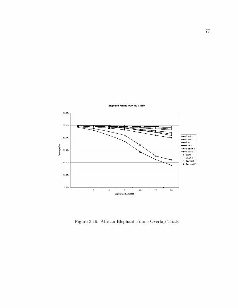
77

Figure 3.19: African Elephant Frame Overlap Trials

78

Figure 3.20: Ortolan Bunting HMM States Trials

79

Figure 3.21: African Elephant HMM States Trials

80

3.5.3 Effects Across Species Trial

The results of the “across species parameters” are provided in detail below. For each

trial, the algorithm parameters were set as follows, based on the knee of each of the

fixed parameter curves:

τρ = 0.5 (3.15)

ταZ1= 15.0 (3.16)

ταZ2= 30.0 (3.17)

(3.18)

The results of this test are summarized in Table 3.2. Figures 3.22 through 3.31

provide the time-series plots of the HMM state boundaries against the instantaneous

frequency, instantaneous bandwidth and the instantaneous signal power for the Or-

tolan Bunting vocalizations. The horizontal axis of each plot indicates the time of

the sound and the vertical axis indicates the z-score for the three features. Before

generating these plots, the author normalized each feature by calculating the z-score

of each feature (z = fracx− xσ). The author normalized each feature to allow all

three features to be discernible on a single graph.

Figures 3.32 through 3.41 provide the time-series plots of the HMM state bound-

aries against the instantaneous frequency, instantaneous bandwidth and the instan-

taneous signal power for the African Elephant vocalizations. The horizontal and

vertical axis of these graphs are the same as the Ortolan Bunting graphs.

81

Vocalization Frame Length (ms) Frame Overlap (ms) # HMM StatesBunting Syllable A 26.4 26.3 8Bunting Syllable B 51.3 51.1 8Bunting Syllable C 18.5 18.0 7Bunting Syllable D 31.3 30.7 6Bunting Syllable E 20.7 20.4 8Bunting Syllable F 29.6 29.3 4Bunting Syllable G 14.6 14.3 9Bunting Syllable H 24.0 23.9 6Bunting Syllable J 18.3 18.0 7Bunting Syllable U 11.7 11.4 3Elephant Croak 1 111.8 109.2 23Elephant Croak 2 672.7 666.6 14

Elephant Rumble 1 1076.7 1069.7 13Elephant Rumble 2 444.6 436.0 22

Elephant Rev 1 670.4 413.2 1Elephant Rev 2 784.8 366.0 1

Elephant Snort 1 82.1 80.7 4Elephant Snort 2 105.5 94.0 8

Elephant Trumpet 1 49.9 41.2 22Elephant Trumpet 2 74.7 70.0 11

Table 3.2: Best-Fit Parameters Trial

82

Figure 3.22: HMM State Bounds for Syllable A

Figure 3.23: HMM State Bounds for Syllable B

83

Figure 3.24: HMM State Bounds for Syllable C

Figure 3.25: HMM State Bounds for Syllable D

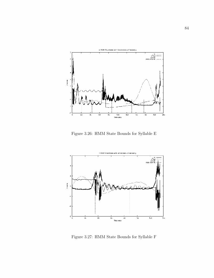
84

Figure 3.26: HMM State Bounds for Syllable E

Figure 3.27: HMM State Bounds for Syllable F

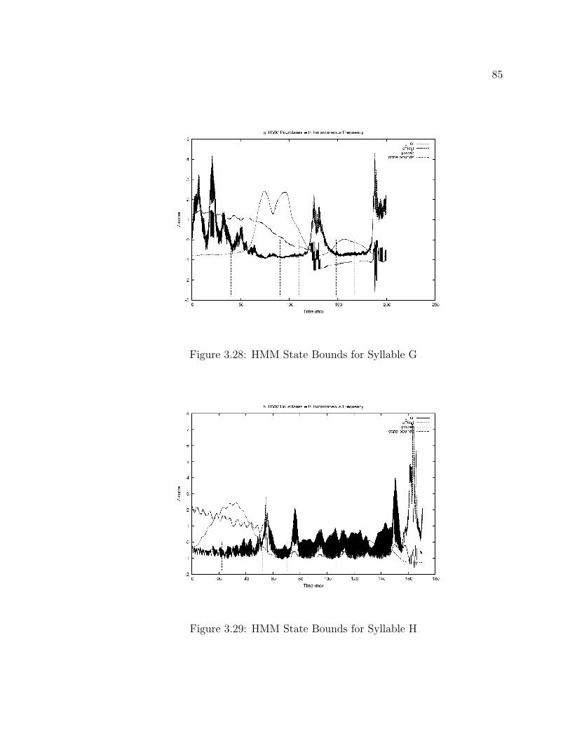
85

Figure 3.28: HMM State Bounds for Syllable G

Figure 3.29: HMM State Bounds for Syllable H

86

Figure 3.30: HMM State Bounds for Syllable J

Figure 3.31: HMM State Bounds for Syllable U

87

Figure 3.32: HMM State Bounds for Croak 1

Figure 3.33: HMM State Bounds for Croak 2

88

Figure 3.34: HMM State Bounds for Rumble 1

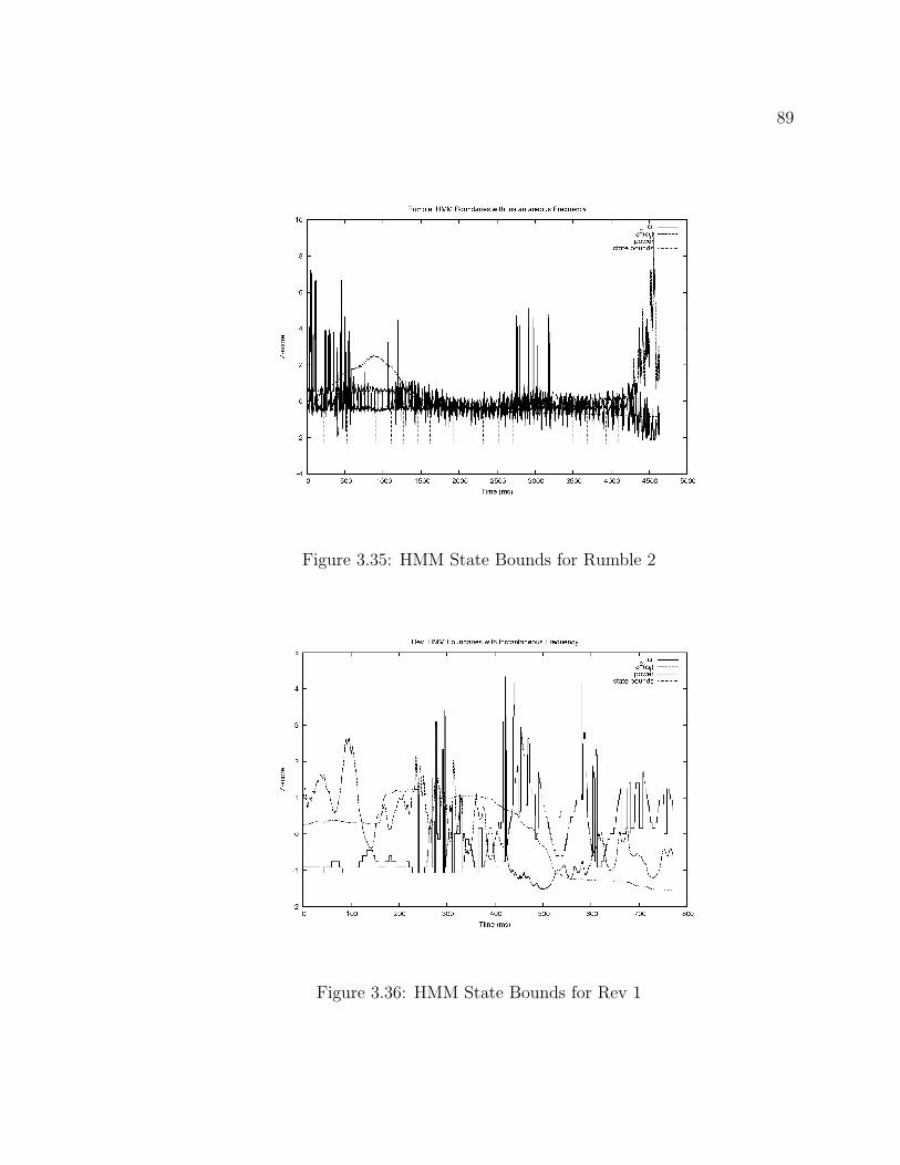
89

Figure 3.35: HMM State Bounds for Rumble 2

Figure 3.36: HMM State Bounds for Rev 1

90

Figure 3.37: HMM State Bounds for Rev 2

Figure 3.38: HMM State Bounds for Snort 1

91

Figure 3.39: HMM State Bounds for Snort 2

Figure 3.40: HMM State Bounds for Trumpet 1

92

Figure 3.41: HMM State Bounds for Trumpet 2

Chapter 4

Summary

4.1 Observations

The overall results of the algorithm are encouraging. All of the three algorithm

parameters, τρ, ταZ1and ταZ2

, have the desired effect on their portion of the algo-

rithm. Increasing the ratio τρ causes a corresponding increase in the frame length

for both the African Elephant vocalizations and the Ortolan Bunting vocalizations.

Increasing ταZ1for the Student’s t-test for the frame overlap estimation causes a cor-

responding decrease in the frame overlap because the distribution of the signal that

belongs to the current frame is increased as the alpha risk decreases (an increase in

the z-score causes a decrease in the tails of the t-distribution). Likewise, increasing

ταZ2for the two-sample Student’s t-test for the HMM topology estimation causes a

corresponding decrease in the number of HMM states overlap because the distribu-

tion of the signal that belongs to the current HMM state is increased as the alpha

risk decreases. In addition, the algorithm estimated the frame length, frame overlap

and the number of HMM states fairly well for both the Ortolan Bunting syllables

and the African Elephant vocalizations.

Frame Length

The algorithm performs well when estimating the frame lengths for both the Ortolan

Bunting syllables and the African Elephant vocalizations. First, examine the frame

93

94

length estimates for the Ortolan Bunting. The frame length estimates for the Bunting

range from 12.7 ms to 31.5 ms when τρ = 0.5 for the Frame Length Trials (3.16),

and the original experiments for the Ortolan Bunting used a frame length of 25 ms

[11].

The algorithm uses the instantaneous frequency and the instantaneous bandwidth

when estimating the frame length; therefore, only the pitch of the animal vocalization

can affect the estimated frame length. Examine the syllable with the minimum

frame length (C - Figure 3.12). The instantaneous frequency is stable throughout

the sound, but the instantaneous bandwidth continuously varies, as shown in Figure

4.1. As a result, the algorithm estimates narrow frame lengths. Now, examine the

instantaneous signal power for this vocalization. It continuously varies throughout

the sound. If the algorithm could also consider signal energy for estimating the frame

length, it might generate even narrower frames.

Conversely, examine the syllable with the maximum frame length (B - Figure

3.12). Both the instantaneous frequency and the instantaneous bandwidth have large

stretches of stability in this sound (see Figure 4.2); hence, the algorithm estimates

a longer frame length than the syllable C. Again, examine the instantaneous signal

power for this vocalization. It varies at a faster rate than the instantaneous signal

power from syllable C. If the algorithm considered signal energy for estimating the

frame length, it might generate even narrower frames.

The algorithm performs similarly with the African Elephant vocalizations. The

frame length estimate for the Elephant vocalizations range from 32.5 ms to 610.9

ms when τρ = 0.5 for the Fixed Frame Length trials (3.17), and the original ex-

periments for the African Elephant vocalizations used frame lengths of 60 ms for

95

Figure 4.1: HMM State Bounds for Syllable C

Figure 4.2: HMM State Bounds for Syllable B

96

the call classification experiments and 300 ms for the speaker identification experi-

ments [12]. Examine the vocalization with the minimum frame length (see Trumpet

2 - Figure 3.14). The instantaneous frequency and bandwidth for this vocalization

are extremely unstable, and corrupted with noise. Also, there is a large amount

of silence before and after the vocalization, which accounts for the volatility in the

instantaneous frequency estimation (see Figure 4.3). If the algorithm trimmed out

the silence regions, it would estimate larger frames for this vocalization. Conversely,

if the algorithm utilized the instantaneous signal power during the frame length es-

timation, it would generate shorter frames because the instantaneous signal power

constantly varies during the vocalization.

Figure 4.3: HMM State Bounds for Trumpet 2

Conversely, examine the vocalization with the maximum frame length (see Croak

2 - Figure 3.14). The instantaneous frequency and bandwidth for this vocalization

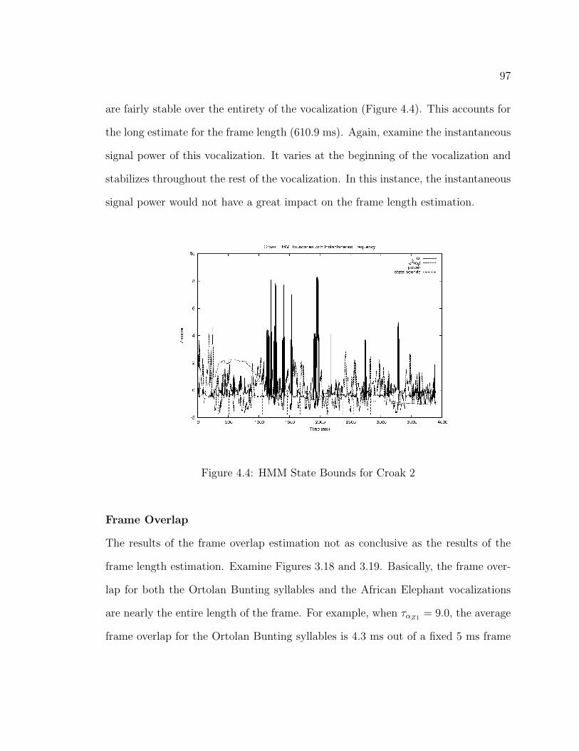
97

are fairly stable over the entirety of the vocalization (Figure 4.4). This accounts for

the long estimate for the frame length (610.9 ms). Again, examine the instantaneous

signal power of this vocalization. It varies at the beginning of the vocalization and

stabilizes throughout the rest of the vocalization. In this instance, the instantaneous

signal power would not have a great impact on the frame length estimation.

Figure 4.4: HMM State Bounds for Croak 2

Frame Overlap

The results of the frame overlap estimation not as conclusive as the results of the

frame length estimation. Examine Figures 3.18 and 3.19. Basically, the frame over-

lap for both the Ortolan Bunting syllables and the African Elephant vocalizations

are nearly the entire length of the frame. For example, when ταZ1= 9.0, the average

frame overlap for the Ortolan Bunting syllables is 4.3 ms out of a fixed 5 ms frame

98

(87% overlap), and the the average frame overlap for the African Elephant vocal-

izations is 276.6 ms out of a fixed 300 ms frame (92% overlap). These numbers are

reasonable due to the variability in the instantaneous frequency of the sounds; how-

ever, it is unclear if this large amount of overlap will improve the results of speaker

identification or call classification.

HMM Topology

The algorithm provides interesting results for the HMM topology estimation. Ex-

amine Figure 3.20 and Figure 3.21. The estimates for the number of HMM states

converge after the ταZ1≥ 30.0. Interestingly, the vocalizations with a higher fun-

damental pitch (i.e., the Ortolan Bunting syllables, the Elephant Trumpet and the

Elephant Snort) have fewer states that the vocalizations with a lower fundamental

pitch. The reasons for this are two-fold:

1. The vocalizations with a higher fundamental pitch have a better SNR.

2. The vocalizations with a higher fundamental pitch have an instantaneous band-

width that is stationary as compared to the vocalizations with a lower funda-

mental frequency.

The algorithm estimates a fairly high number of states for these low-frequency

vocalizations. For example, the algorithm estimates 30 states for “Rumble 1” while

it estimates only 15 states for syllable B. Examine the time-frequency plot for “Rum-

ble 1” (see Figure 4.5). In this case, the instantaneous frequency of the vocalization

is complete unstable. Its distribution is so broad that it cannot impact the seg-

mentation of the frames into states; however, the instantaneous bandwidth and the

99

instantaneous signal power have less variance and contribute more to the decision

process.

Figure 4.5: HMM State Bounds for Rumble 1

Next, examine the time-frequency plot for syllable B (see Figure 4.2). In this

case, the instantaneous frequency, instantaneous bandwidth and the instantaneous

signal power of the vocalization have a low variance. As a result, the algorithm

estimates HMM state boundaries at logical points in the signal; i.e., at points where

the instantaneous frequency changes direction.

Finally, examine the time-frequency plot for the “Trumpet 1” Elephant vocaliza-

tion (Figure 4.6). This vocalization contains obvious silence regions before and after

the vocalization. These regions account for 15 out of the 22 total estimated states.

Also, this vocalization is fairly noisy and the noise accounts for the high variance in

the instantaneous frequency estimate. Again, the silence regions and the background

100

Figure 4.6: HMM State Bounds for Trumpet 1

noise of the signal have significant impact on the estimate of the HMM topology.

4.2 Conclusions

The purpose of this work is to develop a method for frame length estimation, frame

overlap estimation and HMM topology estimation based on a single example for a

particular vocalization pattern. This work utilized the instantaneous frequency and

instantaneous bandwidth of the vocalization as the features necessary to estimate

the frame length and frame overlap for a particular vocalization type. In addition,

this work utilized instantaneous frequency, bandwidth and signal power to estimate

the HMM topology for a particular vocalization type. It used vocalizations from two

different animal species, the African Elephant and Ortolan Bunting, to verify the

101

performance of the algorithm.

This results of this technique are promising. The algorithm provided reasonable

estimates for frame length, frame overlap and HMM topology when the algorithm

parameters were fixed to the same values for both animal species. Noise and silence

regions negatively impacted the results. Ideally, the algorithm should be presented

with sounds that have a high SNR and that have minimum silence regions. Con-

versely, this tool must be robust and should handle sound examples that are less

than ideal.

In addition, the algorithm needs improvements in the area of frame length and

frame overlap estimation. Specifically, the algorithm must utilize both the pitch

of the vocalization (instantaneous frequency and instantaneous bandwidth) and the

energy of the vocalization (instantaneous signal power) when it segments the signal

for the frame length and frame overlap estimates. If the algorithm used instanta-

neous signal power in conjunction with instantaneous frequency and instantaneous

bandwidth it would estimate frame lengths that fit both the frequency characteristics

and the energy characteristics of the signal, and it would estimate frame overlaps

that fit the temporal aspects of the time-frequency distribution and the time-power

distribution of the signal. Despite these shortcomings, this research shows that it

is possible to estimate frame length, frame overlap and HMM topology using fixed

decision parameters across multiple species. Further research recommendations are

provided below.

102

4.3 Further Research Recommendations

This research can be extended to improve the frame length and frame overlap esti-

mates, to make the algorithm more resilient to questionable example vocalizations,

and to make the algorithm easier to use. With these goals in mind, the following

items are recommended for future research projects:

• Trim, or ignore, the silence regions. These cause the instantaneous frequency

to increase which impacts the results of the frame length and frame overlap

estimations.

• Include the instantaneous signal power in the decision mechanism for the frame

length and frame overlap estimations.

• Use a two-sample Student’s t-test on the first difference of the signal when

performing the frame overlap estimation.

• Add a noise tracking mechanism to the algorithm to remove background noise

from the signal.

• Investigate using the feature selection techniques described by Figueirdo [35,

36] to reduce the number of features needed for the HMM topology estimation.

• Automatically generate all the necessary HTK files to facilitate the use of its

results.

• Provide a clean GUI that shows the results of the estimation process in a similar

fashion to the temporal plots in the Discussion section of this thesis.

Bibliography

[1] Zhuge Liang and Liu Ji. Mastering the Art of War. Shambhala, 1989.

[2] J. Young, G. Evermann, M. Gales, H. Thomas, D. Kershaw, G. Moore, J. Odell,

D. Ollason, D. Povey, V. Valtcho, and P. Woodland. The HTK Book (for HTK

Version 3.3). Cambridge University Engineering Department, 2005.

[3] Sanjit K. Mitra. Digital Signal Processing: a Computer-Based Approach.

McGraw-Hill, 1998. ISBN: 0-07-042953-7.

[4] M. Russell. A segmental hmm for speech pattern modeling. In IEEE Interna-

tional Conference on Acoustics, Speech, and Signal Processing, 1993. ICASSP-

93, pages 449–502, April 1993.

[5] Q. Zhu H. You and A. Alwan. Entropy-based variable frame rate analysis of

speech signals and its application to asr. In Proceedings from ICASSSP, 2004,

pages 549–552, 2004.

[6] I. Potamitis, N. Fakotakis, , and G. Kokkinakis. Speech recognition based on

feature extraction with variable rate frequency sampling. In Proceedings of 4th

International Conference on Text, Speech and Dialog, pages 329–333, 2001.

[7] Danfeng Li, Alain Biem, and Jayashree Subrahmonia. Hmm topology opti-

mization for handwriting recognition, acoustics, speech, and signal processing.

In Proceedings of the IEEE International Conference on Acoustics, Speech, and

Signal Processing, 2001. (ICASSP ’01), pages 1521–1524, 2001.

103

104

[8] A. Biem, J.-Y. Ha, and J. Subrahmonai. A bayesian model selection criterion

for hmm topology optimization. In Proceedings of ICASSP, Orlando, pages

989–992, 2002.

[9] Raymond C. Vasko Jr, Amro El-Laroudi, and J. Robert Boston. An algo-

rithm to determine hidden markov model topology. In Proceedings of the IEEE

International Conference on Acoustics, Speech, and Signal Processing, 1996.

(ICASSP-96), pages 3577–3580, May 1996.

[10] L. Cohen. Time-frequency analysis. Prentice-Hall, Inc., 1995. ISBN: 0-13-

594532-1.

[11] M. Trawicki, M. Johnson, and T. Osiejuk. Automatic song-type clasification

and speaker identification of norwegian ortolan bunting (emberiza hortulana).

In IEEE International Conference on Machine Learning in Signal Processing

(MLSP), September 2005.

[12] P. Clemins and M. Johnson. Application of speech recognition to african ele-

phant vocalizations. In Proceedings of 2003 IEEE International Conference on

Acoustics, Speech, and Signal Processing, pages 484–487, 2003.

[13] Wikipedia. Electromagnetic spectrum — wikipedia, the free encyclopedia, 2006.

[Online; accessed 24-June-2006].

[14] T.S. Osiejuk, K. Ratynska, J.P. Cygan, and D. Svein. Song structure and reper-

tori variation in ortolan bunting (emberiza hortulana l.) from isolated norwegian

population. Annales Zoologici Fennici, 40:3–16, February 2003.

105

[15] Russell J. Niederjohn and James A. Heinen. Speech intelligibility enhancement

in high levels of wideband noise. Annual Review of Communications, pages

903–912, 1994-95.

[16] Ben Gold and Nelson Morgan. Speech and Audio Signal Processing. John Wiley

and Sons, Inc., 2000. ISBN: 0-471-35154-7.

[17] D. Jurafsky and J.H. Martin. Speech and Language Processing. Prentice Hall,

2000. ISBN: 0-13-095069-6.

[18] Lawrence R. Rabiner. A tutorial on hidden markov models and selected applica-

tions in speech recognition. Proceedings of the IEEE, pages 257–286, February

1989.

[19] Steven E. Schoenherr. Dynamic range, 2006. [Online; accessed 19-November-

2006].

[20] K. M. Leong, Ortolani A., K. D. Burks, J. D. Mellen, and A. Savage. Quantify-

ing acoustic and temporal characteristics of vocalizations for a group of captive

african elephants (Loxodonta africana). Bioacoustics, 13(3):213–232, 2003.

[21] T.S. Osiejuk, K. Ratynska, J. P. Cygan, and D. Svein. Song structure and

repertoire variation in ortolan bunging (Emberiza hortulana L.) from isolated

norwegian population. Annales Zoologici Fennici, 40:3–16, 2003.

[22] W.H. Press, B.P. Flannery, S.A. Teukolsky, and W.T. Vetterling. Numerical

Recipes in C: The Art of Scientific Computing. Cambridge University Press,

1992. ISBN: 0-521-43108-5.

106

[23] Boualem Boashash. Estimating and interpreting the instantaneous frequency of

a signal–part 1: Fundamentals. Proceedings of the IEEE, pages 520–39, April

1992.

[24] Boualem Boashash. Estimating and interpreting the instantaneous frequency of

a signal–part 2: Algorithms and applications. Proceedings of the IEEE, pages

540–68, April 1992.

[25] V. Katkovnic and L. Stankovic. Instantaneous frequency estimation using the

wigner distribution with varying and data-driven window length. IEEE Trans-

actions on Signal Processing, 46(9):2315–2325, September 1998.

[26] L. Stankovic and V. Katkovnic. Algorithm for the instantaneous frequency esti-

mation using time-frequency distributions with adaptive window width. IEEE

Signal Processing Letters, 5(9):224–227, September 1998.

[27] O’Neill J.C., Flandrin P., and W.J. Williams. On the eistence of discrete wigner

distributions. IEEE Signal Processing Letters, 6(12):304–306, December 1999.

[28] K. M. Ponting and S. M. Peeling. The use of variable frame rate analysis in

speech recognition. Computer Speech and Language, 5:169–179, 1991.

[29] S. M. Peeling and K. M. Ponting. Variable frame rate analysis in the arm con-

tinuous speech recognition system. Speech Communication, 10:155–162, 1991.

[30] M. J. Russell et. al. The arm continuous speech recognition system. In Proceed-

ings of ICASSP, pages 69–72, 1990. Albuquerque, NM, USA.

107

[31] Q. Zhu and A. Alwan. On the use of variable frame rate analysis in speech

recognition. In Proceedings of ICASSP, pages 1783–1786, 2000.

[32] Maciej Niedzwiecki. Identification of Time-varying Processes. John Wiley and

Sons, LTD, 2000. ISBN: 0 471 98629 1.

[33] Papoulis A. and Unnikrishna Pillai S. Probability, Random Varianbles and

Stochastic Processes. McGraw-Hill, 2002. ISBN: 0-07-112256-7.

[34] NIST/SEMATECH. Nist/sematech e-handbook of statistical methods, 2006.

[Online; accessed 29-August-2006].

[35] Mario A.T. Figueiredo Martin H.C. Law and Anil K. Jain. Simultaneous feature

selection and clustering using mixture models. IEEE Transactions on Pattern

Analysis and Machine Intelligence, 26:1154–1166, September 2004.

[36] Mario A.T. Figueiredo. Adaptive sparseness for supervised learning. IEEE

Transactions on Pattern Analysis and Machine Intelligence, 25:1150–1158, Sep-

tember 2003.

Appendix A

Software

A.1 Overview

This appendix provides a very brief overview of the technologies utilized during the

development of the software for this thesis project.

A.2 Languages

C++ and Python are the major programming languages used in this project. The

Python code implements the command-line interpretation and reporting of data and

results. The C++ code is embedded into the Python system and it provides the signal

processing portions of the algorithm. In addition, Octave is used as a replacement

to Matlab, to prototype ideas before porting to C++ for speed. Python and Octave

are open-source projects. For additional information, please see the following web

sites:

• www.python.org - For the Python programming language.

• http://www.gnu.org/software/octave/ - For the Octave programming language.

A.3 Libraries

The GNU Scientific Libraries (GSL) are the primary source for scientific functions;

like, FFT’s and line fitting algorithms. This library is easily linked into the C++

108

109

code for the signal processing tasks of the algorithm. GSL is an open-source project.

Please visit http://www.gnu.org/software/gsl/ for additional information on this

package.

A.4 Tools

Multiple tools were used to make the source code and document the results of the

algorithm; including:

• Automake, Autoconf and Libtool - Open-source build management tools.

• CppUnit - Open-source unit testing tool set.

• CVS - Open-source source code control system.

• Graphviz - Open-source graphing program.

• Gnuplot - Open-source plotting tool.

• Dia - Open-source drawing tool.

• LATEX- Open-source typesetting tool.

• TeXnicCenter - IDE for LATEX

These are the major tools. Other tools were used, but are not included here to

save space and time!

Marquette University

This is to certify that we have examined

this copy of the

masters thesis by

Anthony D. Ricke

and have found that it is complete

and satisfactory in all respects.

The thesis has been approved by:

Thesis Director, Dr. Michael T. JohnsonDepartment of Electrical and Computer Engineering

Dr. Richard PovinelliDepartment of Electrical and Computer Engineering

Dr. Craig StrubleDepartment of Mathematics, Statistics and Com-puter Science

Approved on

110