Phanerozoic trends in the global geographic disparity ofmarine biotas

Arnold I. Miller, Martin Aberhan, Devin P. Buick, Katherine V. Bulinski,Chad A. Ferguson, Austin J. W. Hendy, and Wolfgang Kiessling

Abstract.—Previous analyses of the history of Phanerozoic marine biodiversity suggested that thepost-Paleozoic increase observed at the family level and below was caused, in part, by an increase inglobal provinciality associated with the breakup of Pangea. Efforts to characterize the Phanerozoichistory of provinciality, however, have been compromised by interval-to-interval variations in themethods and standards used by researchers to calibrate the number of provinces. With thedevelopment of comprehensive, occurrence-based data repositories such as the Paleobiology Database(PaleoDB), it is now possible to analyze directly the degree of global compositional disparity as afunction of geographic distance (geo-disparity) and changes thereof throughout the history of marineanimal life. Here, we present a protocol for assessing the Phanerozoic history of geo-disparity, and weapply it to stratigraphic bins arrayed throughout the Phanerozoic for which data were accessed fromthe PaleoDB. Our analyses provide no indication of a secular Phanerozoic increase in geo-disparity.Furthermore, fundamental characteristics of geo-disparity may have changed from era to era inconcert with changes to marine venues, although these patterns will require further scrutiny in futureinvestigations.

Arnold I. Miller, Devin P. Buick, Katherine V. Bulinski,* Chad A. Ferguson, and Austin J. W.Hendy.** Department of Geology, University of Cincinnati, Cincinnati, Ohio 45221. E-mail:arnold.miller@uc.edu

Martin Aberhan and Wolfgang Kiessling. Museum fur Naturkunde, Leibniz Institute for Research onEvolution and Biodiversity at the Humboldt University Berlin, Invalidenstrasse 43, D-10115 Berlin,Germany

*Present Address: Department of Chemistry and Physics, Bellarmine University, Louisville, Kentucky 40205

Accepted: 13 April 2009

Introduction

After more than a quarter-century ofintensive investigation, the Phanerozoic tra-jectory of global marine diversity remains as acentral theme in macroevolutionary investi-gations with respect to the relationshipamong diversity trends at different ecologi-cal/geographic scales and the extent of thepost-Paleozoic increase exhibited at the fam-ily level and below. Depending on one’s pointof view, depictions of raw diversity trajecto-ries (e.g., Valentine 1969; Sepkoski 1981;Sepkoski 1997) are biologically trustworthy(Sepkoski et al. 1981), or they grossly overes-timate (Raup 1972, 1976) or underestimate(Jackson and Johnson 2001) the extent of theCenozoic increase. Attempts to statisticallycorrect for sampling heterogeneities amongPhanerozoic stratigraphic intervals (e.g., Mill-er and Foote 1996; Alroy et al. 2001) have,themselves, led to concerns about the artifac-

tual effects of secular trends in community-level attributes and even interval durationswith respect to the palette of analyticalmethods used for these purposes (Bush et al.2004; Stanley 2007), although Alroy et al.(2008) have recently offered a new perspec-tive on this question.

A possible alternative to assessing globaldiversity trends through aggregate summa-tion at the global level is to evaluate seculartransitions at key hierarchical levels, and thento combine the contributions of each of theseconstituents to develop a global trajectory.Although intended for a somewhat differentpurpose, Sepkoski’s (1988) pioneering assess-ment of diversity trends at the within-com-munity (alpha) and between-community (be-ta) levels for the Paleozoic Era was a step inthat direction. Sepkoski’s analysis, however,was limited primarily to Paleozoic assem-blages from the paleocontinent of Laurentia,

**Present Address: Department of Geology and Geophysics, Yale University, New Haven, Connecticut 06520

Paleobiology, 35(4), 2009, pp. 612–630

’ 2009 The Paleontological Society. All rights reserved. 0094-8373/09/3504–0008/$1.00

with beta diversity analyzed by combiningtogether in a single onshore-offshore ‘‘gradi-ent’’ all of the assemblages contained within agiven stratigraphic interval. The possiblecontribution to global diversity added bygeographic differentiation among biotas wasdiscussed by Sepkoski but not analyzed, andhe downplayed the likelihood of its impor-tance, at least for the Paleozoic, following ondiscussions of Paleozoic global provincialityprovided by Valentine et al. (1978) and others.In the end, Sepkoski was unable to accountfor the significant gulf between synoptic,global diversity numbers and the summedcontributions provided by his assessments atthe alpha and beta levels.

The possible relationship between globalbiodiversity and Phanerozoic trends in globalprovinciality was addressed more directly byValentine and colleagues (e.g., Valentine 1970;Valentine et al. 1978), who argued that thesubstantial post-Paleozoic rise in diversity atthe family level and below, including apossible order-of-magnitude rise at the spe-cies level, was paralleled and fueled by anequally profound increase in the number ofmarine faunal provinces, associated with thebreakup of the supercontinent of Pangea.More recently, however, Bambach (1990)and others have noted that Valentine’s tabu-lations of provinciality through time, whichwere derived from assessments in the litera-ture, were compromised by the use ofdifferent standards by workers who focusedon different parts of the stratigraphic column.

If we assume, as seems reasonable, that thereis a relationship between the degree of globalprovinciality and the degree of compositionalsimilarity or disparity among biotas arrayedaround the world, then we can directly quantifysecular changes, if any, in global compositionaldisparity without attempting to designateprovinces. With the development of geograph-ically resolved, occurrence-based fossil datarepositories such as the Paleobiology Database(PaleoDB; http://paleodb.org/), it is nowpossible to numerically assess, for marinebiotas, Phanerozoic trends in geo-disparity,defined here as the degree of global compositionaldisparity among coeval biotas as a function ofgeographic distance. The purpose of this paper is

to present a methodological framework for ananalysis of this kind, and to provide the initialresults of a Phanerozoic-scale assessment usingdata reposited in the PaleoDB for an aggregateset of genera belonging to a major cross-section of taxa from Sepkoski’s (1981) threeevolutionary faunas. Although these analysesraise several new questions in their own right,they nevertheless suggest that, on a globalscale, there has not been a secular, global-scale increase in geo-disparity through thePhanerozoic.

Methods

Data.—Genus-level occurrence data fromintervals spanning the Phanerozoic weredownloaded from the PaleoDB on 17 Septem-ber 2008; genera with qualified names wereexcluded (e.g., names preceded by ‘‘aff.,’’‘‘cf.,’’ ‘‘sensu lato,’’ or a question mark, orcontained inside of quotation marks), as wereinformal names; taxonomic updates availablein the PaleoDB were applied to genusidentifications, and subgenera were elevatedto genus rank.

All genera belonging to the followinghigher taxa were included in the downloads:Trilobita, Brachiopoda, Bivalvia, and Gastrop-oda. Collectively, these higher taxa provide arepresentative cross-section of major elementsfrom each of Sepkoski’s evolutionary faunasand are among the higher taxa most consis-tently cataloged throughout the Phanerozoicin the PaleoDB. Previous studies limited tosimilar subsets of the marine biota (e.g.,Miller and Foote 1996) suggest that aggregategenus-diversity trajectories for these highertaxa capture major attributes of the Phanero-zoic trajectory exhibited by the marine biotaas a whole. With respect to the Cenozoic inparticular, most previous analyses of diversi-ty trajectories have been dominated over-whelmingly by bivalves and gastropods (seeBush and Bambach 2004), so the focus here onthe same groups seems especially appropriate(but see later section, ‘‘Remaining Issues andFuture Work’’).

Stratigraphic Binning of Collections.—In gen-eral, depictions of Phanerozoic global diver-sity trends in the literature are resolvedstratigraphically to the level of stage or

PHANEROZOIC GEO-DISPARITY 613

substage. Although it would obviously bedesirable in the present analyses to maintainsimilar resolution, the coverage of datareposited in the PaleoDB at the time that theywere downloaded were rather limited forsome stages. As an alternative, therefore, wefollowed the convention of Alroy et al. (2008)and other recent studies, by using a set ofPaleoDB-designated stratigraphic/temporalbins that average about 11 million years induration (Table 1). The bins used here spanthe entire Phanerozoic except for the earliestCambrian (Cambrian 1), which was notincluded because it does not contain sufficientdata. Some of the bins encompass a singlestage, but others are broader in extent. Asindicated by the wide variation in the numberof occurrences of genera and other samplingattributes recognized for each interval, bin-to-bin coverage in the PaleoDB is uneven.Although it is likely that some of thisvariability, such as the increasingly largesamples for Cenozoic bins, directly mirrorsthe availability of material from the fossilrecord, other aspects, such as the smallnumber of occurrences for some Carbonifer-ous bins, reflect the need to further enhancethe acquisition of data for these intervals.Nevertheless, as we will show below, severalstratigraphic bins arrayed throughout thePhanerozoic have adequate coverage for ourpurposes, and those with more limitedcoverage do not impart unusual or uniquesignals with respect to the central questionsaddressed here.

Geographic Binning of Collections into Sam-ples.—For all analyses presented here, Pa-leoDB collections (i.e., faunal lists) in a givenstratigraphic interval were combined togetherinto samples by superimposing a 5u latitudeby 5u longitude grid on the global paleogeo-graphic distribution of collections, estimatedby using Christopher Scotese’s Paleomaprotations (Scotese personal communication2001), provided by the PaleoDB when dataare downloaded. All collections occurringwithin a given 5u 3 5u cell constituted asample. Under the protocol used for accessingdata from the PaleoDB in the present study,multiple occurrences of species for a givengenus in a PaleoDB collection were not

recognized, so that all genera in a collectionwere credited with a single occurrence. In theaggregation of collections into samples, how-ever, genera were credited with multipleoccurrences if they occurred in two or moreof the collections in a 5u 3 5u cell; genera thatwere particularly common or widespreadduring a given stratigraphic interval, indeed,had the propensity to occur in multiplePaleoDB collections within a single cell.

Given that the area covered by a 5u 3 5u cellvaries as a function of latitude, with asystematic decrease toward higher latitudes,it is important to ask whether this geographic-binning protocol might, in itself, compromisethe analyses. With this in mind, we analyzeda limited set of stratigraphic intervals dis-persed throughout the Phanerozoic both byusing an alternative, equal-area binning pro-tocol (i.e., a protocol that holds the area of abin fixed as a function of latitude), and byvarying the areas of individual grid cells asmuch as fourfold. In all cases, the effects onour analytical results were barely discernable.This may reflect, in part, the relative paucityof data from high latitudes (.60u N or S),where the distortion would be most signifi-cant. Furthermore, in cases where substantialdata were available from high latitudes (e.g.,high southern latitudes for the Ordovician),the data tended to be highly concentrated in afew regions, which in itself would tend tominimize the effects of differences in the scaleof geographic-binning because highly con-centrated data would likely fall in the samegeographic bin regardless of the protocolused.

Quantification of Similarity.—All analysesdescribed below were conducted with com-puter programs written and executed inPowerBasic Console Compiler for Windows,Version 5. At the heart of these analyses wasthe quantification of similarity between sam-ple pairs as a function of the distancesbetween them; as illustrated later, highsimilarity is indicative of low disparity, andlow similarity is reflective of high disparity.To quantify pairwise faunal similaritiesamong 5u 3 5u cells within an interval, twodifferent similarity coefficients were used inthe present study:

614 ARNIE MILLER ET AL.

1. Assessment with quantified data. Pairwisecomparisons of samples were first conductedusing the Quantified Czekanowski’s coefficient(Sepkoski 1974):

C~2 S min x1k, x2kð Þ= S x1kzS x2kð Þ,where x1k is the number of occurrences of thekth genus in one of the cells, x2k is the numberof occurrences of the kth genus in the othercell, and min (x1k, x2k) selects the lesser of thetwo values. Only cells with at least 50occurrences were included in these analyses.Because the Quantified Czekanowski’s coef-ficient is sensitive to variations in sample size(i.e., the number of occurrences in each cell),and these differences were probably notbiologically meaningful in most instances,the number of occurrences for each genus ina given cell were transformed by recastingthese values as proportions of the aggregatenumber of occurrences in the cell. The use ofthe Quantified Czekanowski’s coefficient cou-pled with percent transformation is knownwidely in the ecological literature as propor-tional similarity.

As an alternative to data transformation,we investigated the use of sampling-stan-dardization to mitigate differences in samplesize. It was determined with simulations,however, that sampling standardization isnot appropriate in this instance, despite itsintuitive appeal. In our simulations, samplesinitially of different sizes were drawn ran-domly from the same simulated pool ofspecies in which relative abundances wereassigned to species on the basis of a log-normal distribution. When the larger samplewas rarefied down to that of the smallersample, the calculated similarity of the sam-ples tended to decrease, rather than increase,relative to similarity values based on simpletransformation to proportions. We neverthe-less conducted an additional set of analyseson our data in which sampling-standardiza-tion was used, and found that it made littledifference in the end: although samplingstandardization tended to reduce calculatedsimilarity values, it did so predictably anduniformly, and had little effect on the geo-graphic and stratigraphic trajectories present-ed below.

2. Assessment based on presence/absence.Although it is often considered desirable toinclude a quantitative representation of taxo-nomic dominance in the calculation of simi-larity between sample pairs, this inevitablyplaces heavy emphasis on the few commontaxa that tend to dominate most samples. Inthe present study, this may be problematicalbecause the Phanerozoic is thought to havebeen characterized by a secular increase in thenumber of endemic, possibly rare, taxa thatcould have been the main sources of in-creased provinciality posited for the Cenozoic(Valentine 1969; Campbell and Valentine1977). By de-emphasizing uncommon generain the calculation of similarity, the QuantifiedCzekanowski’s coefficient might thereforeoverlook the principal contributors to in-creased Cenozoic geo-disparity. To assess thispossibility, pairwise similarities among sam-ples were also calculated based only on thepresence or absence of genera, using thebinary version of the Jaccard coefficient,which has been used previously in studiesof beta diversity (e.g., Sepkoski 1988):

J~m= mzazbð Þ,where m is the number of genera present inboth samples (the number of ‘‘matches’’), a isthe number of genera uniquely present inone sample, and b is the number of generauniquely present in the other sample. Be-cause multiple occurrences of genera wereignored in this analysis, the minimumthreshold for inclusion of a 5u 3 5u cell inthis analysis was reduced from 50 occurrenc-es to 20. Importantly, uncommon generacontained within a given cell thereforeprovided the same contribution to the calcu-lation of Jaccard similarity as commongenera, enhancing the opportunity to capturethe effects of a secular increase, if any, in thenumber of uncommon, possibly endemic,genera. Furthermore, as with the QuantifiedCzekanowski’s coefficient, it was determinedthat sampling standardization was inappro-priate.

Graphical Representation of Geo-Disparity.—The central goal of this study was to assessthe degree of similarity among the biotas of agiven stratigraphic interval with respect to

PHANEROZOIC GEO-DISPARITY 615

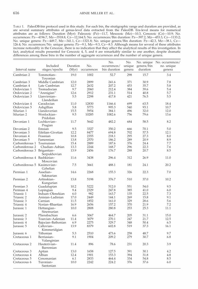
TABLE 1. PaleoDB-bin protocol used in this study. For each bin, the stratigraphic range and duration are provided, asare several summary attributes of genus-level data extracted from the PaleoDB. Era-level means for numericalattributes are as follows: Duration (Myr): Paleozoic (Pz)—11.7, Mesozoic (Mz)—10.3, Cenozoic (Cz)—10.9; No.occurrences: Pz—4196.7, Mz—3518.8, Cz—12,164.5; No. occurrences/Bin duration: Pz—397.2, Mz—453.3, Cz—1133.2;No. unique genera: Pz—449.7, Mz—341.1, Cz—1321.8; No. unique genera/Bin duration: Pz—42.3, Mz—38.1, Cz—126.4; No. occurrences/No. unique genera: Pz—9.1, Mz—9.3, Cz—8.3. Although means for several of these attributesincrease noticeably in the Cenozoic, there is no indication that they affect the analytical results of this investigation. Infact, analytical results presented for Cenozoic 4, 5, and 6 are remarkably similar to one another, despite dramaticdifferences among these bins in the number of aggregate occurrences and the number of unique genera.

Interval nameIncluded

stages/epochsDuration

(Myr)No.

occurrences

No.occurrences/bin duration

No.uniquegenera

No. uniquegenera/bin

duration

No. occurrences/no. unique

genera

Cambrian 2 Tommotian–Toyonian

19.0 1002 52.7 298 15.7 3.4

Cambrian 3 Middle Cambrian 12.0 2899 241.6 371 30.9 7.8Cambrian 4 Late Cambrian 12.7 2632 207.2 453 35.7 5.8Ordovician 1 Tremadocian 9.7 2060 212.4 384 39.6 5.4Ordovician 2 ‘‘Arenigian’’ 12.6 2912 231.1 514 40.8 5.7Ordovician 3 Llanvirnian–

Llandeilian5.5 2298 417.8 421 76.5 5.5

Ordovician 4 Caradocian 11.0 12830 1166.4 699 63.5 18.4Ordovician 5 Ashgillian 5.8 5773 995.3 540 93.1 10.7Silurian 1 Llandoverian 15.5 5954 384.1 496 32.0 12.0Silurian 2 Wenlockian–

Pridolian9.5 10285 1082.6 756 79.6 13.6

Devonian 1 Lochkovian–Pragian

11.7 5642 482.2 684 58.5 8.2

Devonian 2 Emsian 9.5 3327 350.2 666 70.1 5.0Devonian 3 Eifelian–Givetian 12.2 8477 694.8 702 57.5 12.1Devonian 4 Frasnian 10.8 2355 218.1 295 27.3 8.0Devonian 5 Famennian 13.8 2570 186.2 289 20.9 8.9Carboniferous 1 Tournaisian 15.4 2889 187.6 376 24.4 7.7Carboniferous 2 Chadian–Asbian 13.3 2244 168.7 296 22.3 7.6Carboniferous 3 Brigantian–

Serpukhovian13.9 2456 176.7 288 20.7 8.5

Carboniferous 4 Bashkirian–Moscovian

11.6 3438 296.4 312 26.9 11.0

Carboniferous 5 Kasimovian–Gzhelian

7.5 3661 488.1 181 24.1 20.2

Permian 1 Asselian–Sakmarian

14.6 2268 155.3 326 22.3 7.0

Permian 2 Artinskian–Kungurian

13.8 5198 376.7 510 37.0 10.2

Permian 3 Guadalupian 10.2 5222 512.0 551 54.0 9.5Permian 4 Lopingian 9.4 2329 247.8 385 41.0 6.0Triassic 1 Induan–Olenekian 6.0 982 163.7 135 22.5 7.3Triassic 2 Anisian–Ladinian 17.0 2449 144.1 269 15.8 9.1Triassic 3 Carnian 11.5 1852 161.0 329 28.6 5.6Triassic 4 Norian–Rhaetian 16.9 2656 157.2 370 21.9 7.2Jurassic 1 Hettangian–

Sinemurian10.0 2808 280.8 253 25.3 11.1

Jurassic 2 Pliensbachian 6.6 3067 464.7 205 31.1 15.0Jurassic 3 Toarcian–Aalenian 11.4 3079 270.1 247 21.7 12.5Jurassic 4 Bajocian–Bathonian 6.9 2275 329.7 348 50.4 6.5Jurassic 5 Callovian–

Kimmeridgian13.9 8379 602.8 519 37.3 16.1

Jurassic 6 Tithonian 5.3 2510 473.6 258 48.7 9.7Cretaceous 1 Berriasian–

Valanginian9.1 1904 209.2 279 30.7 6.8

Cretaceous 2 Hauterivian–Barremian

11.4 896 78.6 231 20.3 3.9

Cretaceous 3 Aptian 13.0 1658 127.5 391 30.1 4.2Cretaceous 4 Albian 12.4 1901 153.3 394 31.8 4.8Cretaceous 5 Cenomanian 6.1 2833 464.4 334 54.8 8.5Cretaceous 6 Turonian–

Santonian10.0 2242 224.2 376 37.6 6.0

616 ARNIE MILLER ET AL.

their distances from one another. For thispurpose, in all cases where a similarity valuewas determined for a 5u 3 5u cell pair, thegreat-circle distance between the cells wasalso determined. Then, for each stratigraphicinterval, similarity values were grouped into2000-km distance bins, and mean similaritiesof each group were illustrated graphically forsequential distance bins. Results for differentstratigraphic intervals were superimposed,facilitating direct comparisons among them.As an alternative means of assessing seculartrends in similarity, time-series depictions ofsimilarity were also produced for severaldistance bins.

Finally, to better understand the nature ofgeo-disparity on a global scale, we construct-ed paleogeographic maps for each strati-graphic interval to illustrate secular changesin the fundamental nature of paleobiogeo-graphic distributions. On each of these maps,a line was drawn between the centroids ofany 5u 3 5u cell pair for which a similarityvalue had been calculated; the line was color-coded to reflect the similarity value. As willbe demonstrated below, these maps werevaluable for diagnosing the effects of thesecular Phanerozoic decline in the importanceof epicontinental seas and the concomitantincrease in the data derived from open-oceanfacing settings.

Results and Discussion

Geo-disparity versus Distance.—Mean pair-wise similarities between 5u 3 5u cells inrelation to the distances between them areillustrated in Figure 1 for the Ordovician 4

stratigraphic bin (Caradocian), based on theQuantified Czekanowski’s coefficient. Thisinterval was chosen as an initial exemplarnot only because it is well sampled, but alsobecause it captures the culmination of theOrdovician Radiation and establishment ofthe Paleozoic Evolutionary Fauna, whichdominated seafloors for the remainder of thePaleozoic Era (Sepkoski 1981). Not surpris-ingly, there is a strong inverse relationshipbetween similarity and distance, althoughthis levels off at distances of about 8000 km.The small increase observed in the 14,000–16,000 km distance bin relates to slightlyelevated similarities between a few locales inSouth China and cells in Avalonia andBaltoscandia.

An initial comparison of similarity versusdistance in Paleozoic versus Cenozoic strati-graphic bins is also presented in Figure 1,where similarity values for the youngestPhanerozoic bin, Cenozoic 6 (late Miocene–Pleistocene), are compared directly withvalues for Ordovician 4. As with the Ordovi-cian, there is a drop-off with distance in theCenozoic example that levels off at about8000 km. Over the range of distances ana-lyzed, Ordovician 4 similarities were signifi-cantly greater than those for Cenozoic 6 fordistances of 6000 km and less, but there waslittle variation at greater distances, except fora small difference in the aforementioned14,000–16,000 km interval. As we will illus-trate later, the greater mean similaritiesamong Ordovician-4 biotas at distances lessthan 4000 km, and especially less than2000 km, may reflect an ‘‘epicontinental-sea

TABLE 1. Continued.

Interval nameIncluded

stages/epochsDuration

(Myr)No.

occurrences

No.occurrences/bin duration

No.uniquegenera

No. uniquegenera/bin

duration

No. occurrences/no. unique

genera

Cretaceous 7 Campanian 12.9 3622 280.8 486 37.7 7.5Cretaceous 8 Maastrichtian 5.1 18225 3573.5 716 140.4 25.5Cenozoic 1 Paleocene 9.7 5212 537.3 890 91.8 5.9Cenozoic 2 Ypresian–Lutetian 15.4 5668 368.1 860 55.8 6.6Cenozoic 3 Bartonian–

Priabonian6.5 6873 1057.4 1029 158.3 6.7

Cenozoic 4 Oligocene 10.9 8539 783.4 997 91.5 8.6Cenozoic 5 Early–Middle

Miocene11.4 16731 1467.6 1819 159.6 9.2

Cenozoic 6 Late Miocene–Pleistocene

11.6 29964 2585.3 2336 201.6 12.8

PHANEROZOIC GEO-DISPARITY 617

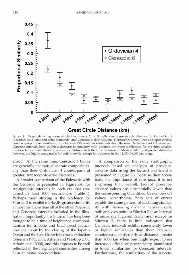
effect.’’ At the same time, Cenozoic 6 biotasare generally not more disparate composition-ally than their Ordovician 4 counterparts atgreater, transoceanic-scale distances.

A broader comparison of the Paleozoic withthe Cenozoic is presented in Figure 2A, forstratigraphic intervals in each era that con-tained at least 8000 occurrences (Table 1).Perhaps most striking is the tendency forSilurian 2 to exhibit markedly greater similarityat most distances than all of the other Paleozoicand Cenozoic intervals included in the illus-tration. Importantly, the Silurian has long beenthought to be a time of heightened cosmopol-itanism for trilobite and brachiopod faunas,brought about by the closing of the IapetusOcean and the Late Ordovician mass extinction(Sheehan 1975, 2008; Adrain and Westrop 2000;Adrain et al. 2000), and this appears to be wellreflected in the heightened similarities amongSilurian biotas observed here.

A comparison of the same stratigraphicintervals based on analyses of presence-absence data using the Jaccard coefficient ispresented in Figure 2B. Because they accen-tuate the importance of rare taxa, it is notsurprising that, overall, Jaccard presence-absence values are substantially lower thanthe corresponding Quantified Czekanowski’svalues. Nevertheless, both sets of curvesexhibit the same pattern of declining similar-ity with increasing distance between cells;both analyses point to Silurian 2 as an intervalof unusually high similarity; and, except forSilurian 2, there is little indication thatCenozoic intervals exhibit consistently loweror higher similarities than their Paleozoiccounterparts, particularly at distances greaterthan 6000 km when one might expect to seeincreased effects of provinciality manifestedin lower similarities for Cenozoic intervals.Furthermore, the similarities of the trajecto-

FIGURE 1. Graph depicting mean similarities among 5u 3 5u cells versus great-circle distance for Ordovician 4(Caradoc; solid lines and solid diamonds) and Cenozoic 6 (late Miocene–Pleistocene; dotted lines and open circles),based on proportional similarity. Error bars are 95% confidence intervals about the mean. Note that the Ordovician andCenozoic intervals both exhibit a decrease in similarity with distance, but mean similarities for the three smallestdistance bins are significantly greater for Ordovician 4 than for Cenozoic 6. Mean similarity at greater distances,however, are highly comparable for both intervals, except for distances in the 14,000–16,000 km range.

618 ARNIE MILLER ET AL.

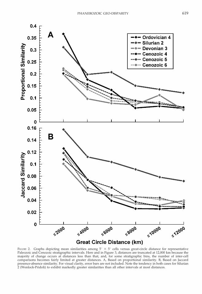
FIGURE 2. Graphs depicting mean similarities among 5u 3 5u cells versus great-circle distance for representativePaleozoic and Cenozoic stratigraphic intervals. Here and in Figure 3, distances are truncated at 12,000 km because themajority of change occurs at distances less than that, and, for some stratigraphic bins, the number of inter-cellcomparisons becomes fairly limited at greater distances. A, Based on proportional similarity. B, Based on Jaccardpresence-absence similarity. For visual clarity, error bars are not included. Note the tendency in both cases for Silurian2 (Wenlock-Pridoli) to exhibit markedly greater similarities than all other intervals at most distances.

PHANEROZOIC GEO-DISPARITY 619

ries for Cenozoic 4, 5, 6 are particularlystriking, given the dramatic differences inoverall sampling among these three bins(Table 1). This attests to a strong signal inthe data that appears impervious to thesesample-size differences.

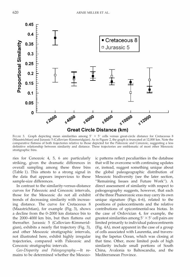
In contrast to the similarity-versus-distancecurves for Paleozoic and Cenozoic intervals,those for the Mesozoic do not all exhibittrends of decreasing similarity with increas-ing distance. The curve for Cretaceous 8(Maastrichtian), for example (Fig. 3), showsa decline from the 0–2000 km distance bin tothe 2000–4000 km bin, but then flattens outthereafter. Jurassic 5 (Callovian–Kimmerid-gian), exhibits a nearly flat trajectory (Fig. 3),and other Mesozoic stratigraphic intervals,not illustrated here, exhibit highly irregulartrajectories, compared with Paleozoic andCenozoic stratigraphic intervals.

Geo-Disparity and Paleogeography.—It re-mains to be determined whether the Mesozo-

ic patterns reflect peculiarities in the databasethat will be overcome with continuing updatesor, instead, suggest something unique aboutthe global paleogeographic distribution ofMesozoic biodiversity (see the later section,‘‘Remaining Issues and Future Work’’). Adirect assessment of similarity with respect topaleogeography suggests, however, that eachof the three Phanerozoic eras may carry its ownunique signature (Figs. 4–6), related to thepositions of paleocontinents and the relativecontributions of epicontinental-sea biotas. Inthe case of Ordovician 4, for example, thegreatest similarities among 5u 3 5u cell pairs arelimited primarily to individual paleocontinents(Fig. 4A), most apparent in the case of a groupof cells associated with Laurentia, and travers-ing the Iapetus Ocean, which was closing atthat time. Other, more limited pods of highsimilarity include small portions of SouthChina, Avalonia to Baltoscandia, and theMediterranean Province.

FIGURE 3. Graph depicting mean similarities among 5u 3 5u cells versus great-circle distance for Cretaceous 8(Maastrichtian) and Jurassic 5 (Callovian–Kimmeridgian). As in Figure 2, the graph is truncated at 12,000 km. Note thecomparative flatness of both trajectories relative to those depicted for the Paleozoic and Cenozoic, suggesting a lessdefinitive relationship between similarity and distance. These trajectories are emblematic of most other Mesozoicstratigraphic bins.

620 ARNIE MILLER ET AL.

FIGURE 4. Proportional similarities plotted on paleogeographic maps for Ordovician 4 (A), Cretaceous 8 (B), andCenozoic 6 (C) with color-coded lines connecting centroids of 5u 3 5u cells when both cells exceed the 50-occurrencesthreshold required for calculation of similarity between the cell pair. Only similarities $0.30 (red) and $0.20 to ,0.30(orange) are depicted. For Ordovician 4, the majority of these linkages are observed for cells in close proximity to oneanother (e.g., among nearby cells on Laurentia or across the closing Iapetus Ocean). By contrast, most such linkages forCenozoic 6 are transoceanic (note the linkages between eastern and western North American and eastern Asia).Cretaceous 8 includes some linkages that are in close proximity and others that are transoceanic.

PHANEROZOIC GEO-DISPARITY 621

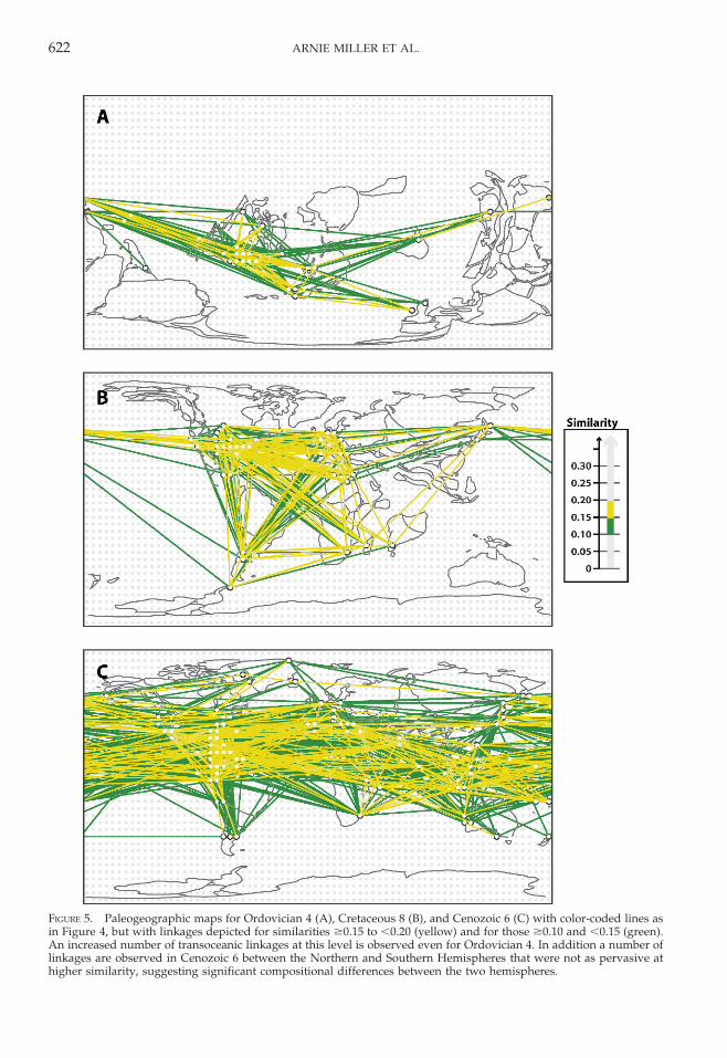
FIGURE 5. Paleogeographic maps for Ordovician 4 (A), Cretaceous 8 (B), and Cenozoic 6 (C) with color-coded lines asin Figure 4, but with linkages depicted for similarities $0.15 to ,0.20 (yellow) and for those $0.10 and ,0.15 (green).An increased number of transoceanic linkages at this level is observed even for Ordovician 4. In addition a number oflinkages are observed in Cenozoic 6 between the Northern and Southern Hemispheres that were not as pervasive athigher similarity, suggesting significant compositional differences between the two hemispheres.

622 ARNIE MILLER ET AL.

FIGURE 6. Paleogeographic maps for Ordovician 4 (A), Cretaceous 8 (B), and Cenozoic 6 (C) with color-coded lines asin Figures 4 and 5, but with linkages depicted for similarities $0.05 to ,0.10 (blue) and for those .0.0 and,0.05 (violet).

PHANEROZOIC GEO-DISPARITY 623

By contrast, for Cenozoic 6 (Fig. 4C), agreater proportion of the high-similaritylinkages between cells are transoceanic, al-though a set of strong links can also beobserved at smaller distances, in the Caribbe-an Sea and elsewhere. In particular, highsimilarities are observed across the Pacificand Atlantic Oceans between biotas of west-ern and eastern North America and easternAsia. The pattern for Cretaceous 8 (Fig. 4B)resembles a kind of ‘‘hybrid’’ of the Ordovi-cian and Cenozoic examples: a preponder-ance of high similarity among cells of theNorth American coastal plain and Europe–North Africa, coupled with linkages acrossthe expanding Atlantic Ocean.

At lower levels of similarity (Figs. 5, 6), anincreasing number of transoceanic links areobserved among biotas in all intervals. Inter-estingly, links for Cenozoic 6 between severallocalities in the Northern and SouthernHemispheres that are not observed at highersimilarities can be observed at these lowerlevels, suggesting compositional disparitybetween the hemispheres. This almost cer-tainly reflects the confinement of majoroceanic circulation cells to the Northern andSouthern Hemispheres, which would tend toinhibit biotic dispersal between the twohemispheres.

An ‘‘epicontinental-sea effect’’ illustratedfor Laurentia in particular in Ordovician 4(Fig. 4A) may explain the tendency of mostPaleozoic intervals to exhibit greater simi-larities than their Cenozoic counterparts atsmaller distances (Fig. 2). At the same time,the lack of high-similarity links at greaterdistances among Paleozoic 5u 3 5u cell pairsmay reflect a relative scarcity of data in thePaleoDB for Paleozoic shallow ocean-facingsettings, given the likelihood that much ofthe area covered by these settings for thePaleozoic was subsequently subducted. Col-lectively, these patterns serve as remindersof a pair of secular trends in the sedimen-tary record: a growth in the contribution ofstrata from shallow, ocean-facing settingsand a decline in strata representative ofepicontinental seas. Whereas the latter ap-parently relates to an actual loss of epicon-tinental seas through the Phanerozoic, the

former is in part a preservational artifact,and should probably be incorporated moreroutinely into future analyses of Phanero-zoic biodiversity (Allison and Wells 2006;Peters 2007).

Secular Trends in Geo-Disparity.—Phanero-zoic trends in geo-disparity are illustrated inFigures 7 (Quantified Czekanowski’s coeffi-cient) and 8 (Jaccard coefficient) for three of thedistance bins included in Figures 1–3: 0–2000 km, 2000–4000 km, and 8000–10,000 km.These three intervals were chosen to provide asense of how the trajectory varies, if at all, inrelation to the distance between 5u 3 5u cells.Values for some stratigraphic bins are notprovided because the available data at thedistances in question are insufficient to quan-tify geo-disparity (for a given distance bin, atleast two pairwise comparisons between 5u 3

5u cells were required). In addition, similarityvalues in these figures decrease upward toreflect increasing geo-disparity.

With respect to transitions between adja-cent stratigraphic bins, the trajectories shouldbe viewed as preliminary because these fine-scale variations may relate to bin-to-bintransitions in data quality and coverage thatwill be investigated in our future analyses; forsome potentially critical transitions (e.g.,Triassic 1, immediately following the end-Permian mass extinction), the data remaininsufficient to quantify geo-disparity. Atbroader scales, however, the pattern is likelyto be meaningful even now because many ofthe stratigraphic bins throughout the Phaner-ozoic, including those highlighted earlier,contain large numbers of occurrences arrayedamong 5u 3 5u cells at a range of distancesfrom one another. Overall, neither the analy-sis based on the Quantified Czekanowski’scoefficient nor that based on the Jaccardcoefficient exhibits a substantial Phanerozoicincrease in geo-disparity. There is some hintof an increase about midway through theCenozoic (in particular for the 8000–10,000 km distance bin) but, in itself, thiswould be insufficient to drive a majorPhanerozoic increase in global diversity.Furthermore, similarity values for the Ceno-zoic are well in line with those for several

624 ARNIE MILLER ET AL.

FIGURE 7. Time-series depictions, based on proportional similarity, of mean geo-disparity through the Phanerozoicamong 5u 3 5u cells for three of the distance bins included in Figures 1–3: 0–2000 km (A), 2000–4000 km (B), and 8000–10,000 km (C). These distances were chosen to illustrate similarities among samples that are relatively closely spaced(A and B), such as cells confined to the same epicontinental sea or continental coastline, as well as others approachingtransoceanic distances (C). At greater distances, the paucity of data available for inter-cell comparisons in severalstratigraphic bins makes it difficult to construct a meaningful time series. Values are illustrated only in cases where twoor more comparisons between cells were available for a given stratigraphic bin. Note that similarity values decreaseupward in these figures, reflecting an upward increase in geo-disparity.

PHANEROZOIC GEO-DISPARITY 625

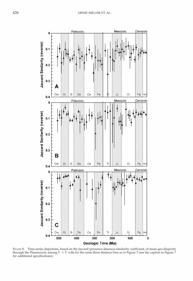
FIGURE 8. Time-series depictions, based on the Jaccard (presence-absence) similarity coefficient, of mean geo-disparitythrough the Phanerozoic among 5u 3 5u cells for the same three distance bins as in Figure 7 (see the caption to Figure 7for additional specifications).

626 ARNIE MILLER ET AL.

other Paleozoic and Mesozoic intervals, anddo not exhibit a unique set of values.

Remaining Issues and Future Work

Although several tantalizing patterns havebeen observed in our analyses to date, ourmain goal in this paper was to convey theimportance of investigating and dissectingsecular trends in geo-disparity, and to presentan analytical protocol that we will continue torefine in the future. In this spirit, it isimportant to consider a number of issues thatwill be addressed as our investigationsunfold. Furthermore, many of these issuesare broadly relevant to a range of potentialfuture investigations of the geographic andenvironmental textures of Phanerozoic diver-sity, and, so, are worth reviewing in detail.

Geo-Disparity versus Beta Diversity.—Al-though environmental gradients inevitablyincorporate a geographic dimension, geo-disparity should not be viewed as synony-mous with beta (‘‘between-community’’) di-versity. From a theoretical standpoint, com-positional partitioning along environmentalgradients may occur for reasons (e.g., bioticinteractions) that are entirely different thanthose responsible for geo-disparity (e.g.,biogeographic barriers). From an operationalstandpoint, the finest geographic scale ana-lyzed herein, the distance between centroidsof adjacent 5u 3 5u cells, may be too coarse tocapture disparity associated with a typicalenvironmental gradient. To analyze betadiversity trends, it would be appropriate tofocus on portions of the world for a givenstratigraphic interval where paleoenviron-mental data and density of sampling areadequate to assess compositional disparitydirectly along the gradients. This could beaccomplished by adapting the numericalmethods presented here, or, if sampling isadequate and appropriate, by applying addi-tive-partitioning methods (Layou 2007; Patz-kowsky and Holland 2007).

Geographic and Secular Variations in Paleoen-vironment.—Dovetailing on the issue of geo-disparity versus beta diversity, it is importantto recognize that differences in compositionamong cells need not simply reflect theirdistances from one another, but could also

reflect differences in their aggregate environ-mental characteristics. Some cells, for example,might encompass a larger proportion ofcarbonate-rich settings, whereas others mightbe more siliciclastic-rich, factors that are nowthought to significantly influence biodiversityon a global scale (Miller and Connolly 2001;Foote 2006; Kiessling and Aberhan 2007). Ifthese differences are distributed nonrandomlywithin and among cells, they could ‘‘disrupt’’an otherwise straightforward relationship be-tween disparity and distance, which, amongother things, may explain the unusual patternsexhibited in our analyses of the Mesozoic todate. It is now well understood that there wasa secular Phanerozoic decline in the availabil-ity of carbonate environments and a concom-itant increase in siliciclastic settings (Walker etal. 2002; Peters 2008), with what was likely aunique mixture of both settings in the Meso-zoic Era. With this in mind, it will be importantto map the geographic distributions of carbon-ate-rich and siliciclastic-rich settings, as well asother environmental attributes throughout thePhanerozoic, to assess the extent to which theyaffect geo-disparity or impart their own,unique signatures on the history of Phanero-zoic diversity.

Secular Variations in the Availability of Datafrom Shallow, Ocean-Facing Settings.—Earlier,we considered the possible importance to geo-disparity of the secular transition from epicon-tinental-sea to ocean-facing settings. Althougha large proportion of ocean-facing shallow-water settings associated with Paleozoic pa-leocontinents ultimately succumbed to sub-duction, there were several noteworthy early-to mid-Paleozoic areas separated from paleo-continents that contained open-ocean-facingfossil biotas. Many of these were small terranesthat sometimes contained faunas composition-ally distinct from their epicontinental counter-parts (e.g., Harper 1992; Owen et al. 1992;Harper et al. 1996). Additional examples,which are also relatively small in area, includethe Mediterranean Province, a set of islands athigh southern latitude marginal to the Paleo-zoic supercontinent of Gondwana, whichtoday constitute large portions of central andsouthern Europe and northern Africa; andAvalonia, which included much of present-

PHANEROZOIC GEO-DISPARITY 627

day England and Wales. There is evidence ofsignificant terrane accretion during the Paleo-zoic onto large continental platforms (Cocksand Torsvik 2007), suggesting a secular loss inthe availability of unique terrane biotas as thePaleozoic progressed. In any case, althoughthe collective areal coverage of these regionsmay not have been as extensive as coevalcontinental areas, they often contain abundantfossil biotas. At present, although there is goodcoverage in the PaleoDB for parts of Avaloniaand the Mediterranean Province, some ter-ranes are not well represented, and a concertedeffort will be undertaken in the future toaugment their coverage.

Geographic Patchiness during the Mesozoic.—As with the global secular transition fromcarbonates to siliciclastics, the Mesozoic erawas characterized by a relatively equitablemix of epicontinental-sea and ocean-facingsettings, as opposed to the epicontinental-sea-dominated record of the Paleozoic, or theincreasingly ocean-facing-dominated recordof the Cenozoic. Not only might this in itselfhave contributed to the unique patternsobserved for the Mesozoic (e.g., Fig. 3), butthe comparatively patchy interspersion ofepicontinental seas, ocean-facing environ-ments, and landmasses evident on Mesozoicglobal paleogeographic maps might also haveaffected the relationship between disparityand distance. Landmasses intermittently lo-cated throughout the faunally rich Tethyanrealm, for example, may have served asregional barriers to dispersal, thereby reduc-ing similarity between geographically proxi-mate regions. This possibility can be investi-gated by focusing on the nature ofcompositional variation within these regions.

Data Quality.—There have long been con-cerns that large databases such as Sepkoski’scompendia (Sepkoski 1982, 1992, 2002) andthe PaleoDB contain numerous taxonomicinconsistencies and that these, in turn, com-promise analyses based on these data. Al-though this might ultimately prove to be thecase for studies conducted at relatively finespatial or temporal scales, comparative anal-yses to date of standardized and vetted datacorrected by taxonomic specialists versus the‘‘raw’’ data contained in the aforementioned

sources (e.g., Adrain and Westrop 2000;Wagner et al. 2007) indicate, that, for theanalysis of broad-scale Phanerozoic patterns,the corrected data do not yield signalsappreciably different from the uncorrecteddata. This may not be the case for studiesinvestigating spatial variations in coverage,however, and the effect of taxonomic dataquality on the analysis of geo-disparity will beinvestigated further in the future.

Genus versus Species-Level Patterns.—Be-cause Valentine’s hypothesis of a relationshipbetween increased Cenozoic diversity andprovinciality focused on the species level(Valentine 1970; Valentine et al. 1978), itmight reasonably be asked whether the hy-pothesized Cenozoic increase in endemismmight only be expressed at the species level,and therefore would not be recognizable in thegenus-level analyses conducted here. If thedata permit it in the future, it would beworthwhile to conduct species-level analyses.Nevertheless, Valentine himself conveyed tworeasons why the genus, and perhaps even thefamily, level should afford sufficient acuity todiagnose a Cenozoic increase in geo-disparity,if it occurred. First, there is evidence that thebasic, underlying structure of provinciality inthe present day diagnosed at the species levelcan also be recognized at the genus and familylevels (Campbell and Valentine 1977). Second,as Valentine (1969) recognized in his earliestanalyses of Phanerozoic diversity trends, thepattern of diversification observed changesfundamentally between the taxonomic levelsof order and family. At the family level andbelow, a post-Paleozoic diversity increase isrecognized that is not apparent at the orderlevel and above. Valentine suggested that theincreases observed at the family throughspecies levels, though inevitably accentuatedas one moves down the taxonomic hierarchy,were all products of the same underlyingdynamic.

The Taxonomic Spectrum.—The focus in thisinitial analysis was on the members of alimited, but representative, cross-section ofmajor higher taxa from each of Sepkoski’sthree Phanerozoic evolutionary faunas. Al-though we might expect the marine biota as awhole to exhibit Phanerozoic-scale patterns

628 ARNIE MILLER ET AL.

similar to those observed here, it is possiblethat this would not be the case. Furthermore, itis important to compare and contrast geo-disparity among different higher taxa, particu-larly in cases where there is reason to believethat the taxa in question have different paleo-ecological or paleogeographic attributes, havenot been adequately sampled in some regionsincluded in the PaleoDB, or are known to haveoccupied different environmental regimesthroughout all or most of the Phanerozoic.Obvious examples of this last case are thecorals; as major representatives of reef andother hard-substrate environments since thePaleozoic, corals provide an opportunity tocompare and contrast level-bottom and reefassociations. Following on the analyses ofKiessling and Aberhan (2007), it will also befruitful to parse the data with respect to avariety of paleoenvironmental and paleogeo-graphic parameters, as suggested earlier, orfundamental differences in the biological prop-erties of taxa, such as their life habits (e.g.,benthonic versus nektonic groups) or, for taxaamong which these properties are known, thenature of their developmental stages (e.g.,planktotrophic versus non-planktotrophic lar-vae), which are now thought to be among theimportant macroevolutionary attributes of taxa(Jablonski 1986; Peterson 2005).

Stratigraphic Acuity.—Given the limiteddata available for some Phanerozoic stagesand substages, we adopted the somewhatcoarser PaleoDB binning scheme, as describedearlier. Because geo-disparity should, by defi-nition, be viewed as a property of bioticdistributions at a given point in time, it wouldobviously be desirable to work with time slicesthat are as constrained as possible, and we lookforward to working at a finer stratigraphic scalein the future. There is little reason to believe,however, that the secular patterns observed inthe present study, in particular the lack of asignificant increase in geo-disparity during theCenozoic relative to the Paleozoic, wouldchange appreciably with a different stratigraph-ic-binning scheme. All else being equal, if astratigraphic bin encompasses a longer tempo-ral interval, we would expect the apparent levelof geo-disparity to be artificially increasedbecause the interval would incorporate a

greater degree of evolutionary turnover; theopposite would be the case with a shorter-duration bin. In our study, the average tempo-ral durations of the Cenozoic bins were notappreciably different from those of the Paleo-zoic, so any such overprint should be minimal.

At the same time, we might expect a similareffect related to the well-documented seculardecline in turnover rates through the Phaner-ozoic (e.g., Raup and Sepkoski 1982; Alroy2008; among many others): all else being equal,a Paleozoic bin might encompass a greaterdegree of taxonomic turnover than a Cenozoicbin of roughly equal duration, and this mightartifactually inflate the measured geo-disparityof Paleozoic bins relative to the Cenozoic. Thispossibility will have to be investigated further.

We presented this extended discussion ofoutstanding issues not only because they needto be addressed to fully come to grips withPhanerozoic diversity trends, but also becausethey convey the underlying complexity ofglobal diversity trends over the sweep of thePhanerozoic. We are confident that theseissues can be addressed in future work,allowing for the routine incorporation of apaleogeographic component into quantitativeassessments of global diversity trends. Withthe continued growth of databases and ana-lytical tools to underpin these investigations,we look forward to the very real possibility ofunderstanding the relationship among Phan-erozoic diversity trends at several levels of thegeographic and ecological hierarchies.

Acknowledgments

We thank the members of the marineworking group of the Paleobiology Databasefor many helpful discussions over the yearsabout paleogeographic aspects of the history ofglobal biodiversity. We also thank U. Merkel,in particular, for diligent data entry; and R. A.Cooper and P. M. Novack-Gottshall for theirvery helpful comments on an earlier draft ofthis paper. Funding was provided by theNational Aeronautics and Space Administra-tion’s Program in Exobiology and Evolution-ary Biology (A.I.M.), the National ScienceFoundation’s Program in Biocomplexity(A.I.M.), and VolkswagenStiftung (W.K.). Thisis Paleobiology Database Publication No. 97.

PHANEROZOIC GEO-DISPARITY 629

Literature Cited

Adrain, J. M., and S. R. Westrop. 2000. An empirical assessment of

taxic paleobiology. Science 289:110–112.

Adrain, J. M., S. R. Westrop, B. D. E. Chatterton, and L. Ramskold.

2000. Silurian trilobite alpha diversity and the end-Ordovician

mass extinction. Paleobiology 26:625–646.

Allison, P. A., and M. R. Wells. 2006. Circulation in large ancient

epicontinental seas: what was different and why? Palaios

21:513–515.

Alroy, J. 2008. Dynamics of origination and extinction in the

marine fossil record. Proceedings of the National Academy of

Sciences USA 105:11536–11542.

Alroy, J., C. R. Marshall, R. K. Bambach, K. Bezusko, M. Foote,

F. T. Fursich, T. A. Hansen, S. M. Holland, L. C. Ivany,

D. Jablonski, D. K. Jacobs, D. C. Jones, M. A. Kosnik, S. Lidgard,

S. Low, A. I. Miller, P. M. Novack-Gottshall, T. D. Olszewski,

M. E. Patzkowsky, D. M. Raup, K. Roy, J. J. Sepkoski Jr., M. G.

Sommers, P. J. Wagner, and A. Webber. 2001. Effects of

sampling standardization on estimates of Phanerozoic marine

diversification. Proceedings of the National Academy of

Sciences USA 98:6261–6266.

Alroy, J., M. Aberhan, D. J. Bottjer, M. Foote, F. T. Fursich, P. J.

Harries, A. J. W. Hendy, S. M. Holland, L. C. Ivany, W.

Kiessling, M. A. Kosnik, C. R. Marshall, A. J. McGowan, A. I.

Miller, T. D. Olszewski, M. E. Patzkowsky, S. E. Peters,

L. Villier, P. J. Wagner, N. Bonuso, P. S. Borkow, B. Brenneis,

M. E. Clapham, L. M. Fall, C. A. Ferguson, V. L. Hanson, A. Z.

Krug, K. M. Layou, E. H. Leckey, S. Nurnberg, C. M. Powers, J.

A. Sessa, C. Simpson, A. Tomasovych, and C. C. Visaggi. 2008.

Phanerozoic trends in the global diversity of marine inverte-

brates. Science 321:97–100.

Bambach, R. K. 1990. Late Palaeozoic provinciality in the marine

realm. In C. R. Scotese and W. S. McKerrow, eds. Palaeozoic

palaeogeography and biogeography. Geological Society of

London Memoir 12:307–323.

Bush, A. M., and R. K. Bambach. 2004. Did alpha diversity

increase during the Phanerozoic? Lifting the veils of tapho-

nomic, latitudinal, and environmental biases. Journal of

Geology 112:625–642.

Bush, A. M., M. J. Markey, and C. R. Marshall. 2004. Removing

bias from diversity curves: the effects of spatially organized

biodiversity on sampling-standardization. Paleobiology 30:666–

686.

Campbell, C. A., and J. W. Valentine. 1977. Comparability of

modern and ancient marine faunal provinces. Paleobiology

3:49–57.

Cocks, L. R. M., and T. H. Torsvik. 2007. Siberia, the wandering

northern terrane, and its changing geography through the

Palaeozoic. Earth-Science Reviews 82:29–74.

Foote, M. 2006. Substrate affinity and diversity dynamics of

Paleozoic marine animals. Paleobiology 32:345–366.

Harper, D. A. T. 1992. Ordovician provincial signals from

Appalachian-Caledonian terranes. Terra Nova 4:204–209.

Harper, D. A. T., C. MacNiocaill, and S. H. Williams. 1996. The

palaeogeography of early Ordovician Iapetus terranes: an

integration of faunal and palaeomagnetic constraints. Palaeo-

geography, Palaeoclimatology, Palaeoecology 121:297–312.

Jablonski, D. 1986. Background and mass extinctions: the

alternation of macroevolutionary regimes. Science 231:129–133.

Jackson, J. B. C., and K. G. Johnson. 2001. Paleoecology:

measuring past biodiversity. Science 293:2401–2404.

Kiessling, W., and M. Aberhan. 2007. Environmental determi-

nants of marine benthic biodiversity dynamics through

Triassic–Jurassic time. Paleobiology 33:414–434.

Layou, K. M. 2007. A quantitative null model of additive diversity

partitioning: examining the response of beta diversity to

extinction. Paleobiology 33:116–124.

Miller, A. I., and S. R. Connolly. 2001. Substrate affinities of higher

taxa and the Ordovician Radiation. Paleobiology 27:768–778.

Miller, A. I., and M. Foote. 1996. Calibrating the Ordovician

radiation of marine life: implications for Phanerozoic diversity

trends. Paleobiology 22:304–309.

Owen, A. W., D. A. T. Harper, and M. Romano. 1992. The

Ordovician biogeography of the Grangegeeth terrane and the

Iapetus suture zone in eastern Ireland. Journal of the Geological

Society, London 149:3–6.

Patzkowsky, M. E., and S. M. Holland. 2007. Diversity partition-

ing of a Late Ordovician marine biotic invasion: controls on

diversity in regional ecosystems. Paleobiology 33:295–309.

Peters, S. E. 2007. The problem with the Paleozoic. Paleobiology

33:165–181.

———. 2008. Environmental determinants of extinction selectiv-

ity in the fossil record. Nature 454:626–629.

Peterson, K. J. 2005. Macroevolutionary interplay between

planktic larvae and benthic predators. Geology 33:929–932.

Raup, D. M. 1972. Taxonomic diversity during the Phanerozoic.

Science 177:1065–1071.

———. 1976. Species diversity in the Phanerozoic: an interpreta-

tion. Paleobiology 2:289–297.

Raup, D. M., and J. J. Sepkoski Jr. 1982. Mass extinctions in the

marine fossil record. Science 215:1501–1503.

Sepkoski, J. J., Jr. 1974. Quantified coefficients of association and

measurement of similarity. Journal of the International Asso-

ciation for Mathematical Geology 6:135–152.

———. 1981. A factor analytic description of the Phanerozoic

marine fossil record. Paleobiology 7:36–53.

———. 1982. A compendium of fossil marine families. Milwau-

kee Public Museum, Milwaukee.

———. 1988. Alpha, beta, or gamma: where does all the diversity

go? Paleobiology 14:221–234.

———. 1992. A compendium of fossil marine animal families, 2d

ed. Milwaukee Public Museum, Milwaukee.

———. 1997. Biodiversity: past, present, and future. Journal of

Paleontology 71:533–539.

———. 2002. A compendium of fossil marine animal genera.

Bulletins of American Paleontology 363:1–560.

Sepkoski, J. J., Jr., R. K. Bambach, D. M. Raup, and J. W. Valentine.

1981. Phanerozoic marine diversity and the fossil record.

Nature 293:435–437.

Sheehan, P. M. 1975. Brachiopod synecology in a time of crisis

(Late Ordovician–Early Silurian). Paleobiology 1:205–212.

——— . 2008. Did incumbency play a role in maintaining

boundaries between Late Ordovician brachiopod realms?

Lethaia 41:147–153.

Stanley, S. M. 2007. An analysis of the history of marine animal

diversity. Paleobiology 33:1–55.

Valentine, J. W. 1969. Patterns of taxonomic and ecological

structure of the shelf benthos during Phanerozoic time.

Palaeontology 12:684–709.

———. 1970. How many marine invertebrate fossil species? A

new approximation. Journal of Paleontology 44:410–415.

Valentine, J. W., T. C. Foin, and D. Peart. 1978. A provincial model

of Phanerozoic marine diversity. Paleobiology 4:55–66.

Wagner, P. J., M. Aberhan, A. Hendy, and W. Kiessling. 2007. The

effects of taxonomic standardization on sampling-standardized

estimates of historical diversity. Proceedings of the Royal

Society of London B 274:439–444.

Walker, L. J., B. H. Wilkinson, and L. C. Ivany. 2002. Continental

drift and Phanerozoic carbonate accumulation in shallow-shelf

and deep-marine settings. Journal of Geology 110:75–87.

630 ARNIE MILLER ET AL.