PERFORMANCE OPTIMIZATION OF ENGINEERING ... - CORE

PERFORMANCE OPTIMIZATION OF ENGINEERING

SYSTEMS WITH PARTICULAR REFERENCE TO

DRY-COOLED POWER PLANTS

by

Antonie Eduard Conradie

Dissertation presented for the Degree of Doctor of Philosophy (Mechanical Engineering)

at the University of Stellenbosch.

Promoters: Prof. D.G. Kroger (Mechanical Engineering Department)

Dr. J.D. Buys (Mathematics Department)

Department of Mechanical Engineering

University of Stellenbosch

South Africa

January 1995

1

DECLARATION

I, Antonie Eduard Conradie, the undersigned, hereby declare that the work contained in this

dissertation is my own original work and has not previously, in its entirety or in part, been submitted

at any university for a degree.

Signature: oate: .J..'. .... l~.':':(!l·JUL .....

Stellenbosch University https://scholar.sun.ac.za

11

SYNOPSIS

Computer simulation programs were developed for the analysis of dry-cooling systems for power

plant applications. Both forced draft direct condensing air-cooled condensers and hyperbolic natural

draft indirect dry-cooling towers are considered.

The results of a considerable amount of theoretical and experimental work are taken into account to

model all the physical phenomena of these systems, to formulate the problems in formal mathematical

terms and to design and apply suitable computational algorithms to solve these problems effectively

and reliably.

The dry-cooling systems are characterized by equation-based models. These equations are

simultaneously solved by a specially designed constrained nonlinear least squares algorithm to

determine the performance characteristics of the dry-cooling systems under fixed prescribed

operating conditions, or under varying operating conditions when coupled to a turbo-generator set.

The solution procedure is very fast and effective.

A capital and operating cost estimation procedure, based on information obtained from dry-cooling

system component manufacturers and the literature, is proposed. Analytical functions express the

annual cost in terms of the various geometrical and operating parameters of the dry-cooling systems.

The simulation and the cost estimation procedures were coupled to a constrained nonlinear

programming code which enable the design of minimum cost dry-cooling systems at fixed prescribed

operating conditions, or dry-cooling systems which minirpize the ratio of total annual cost to the

annual net power output of the corresponding turbo-generator set. Since prevailing atmospheric

conditions, especially the ambient temperature, influence the performance of dry-cooling systems,

wide fluctuations in turbine back pressure occur. Therefore, in the latter case the optimal design is

based on the annual mean hourly frequency of ambient temperatures, rather than a fixed value.

The equation-based models and the optimization problems are simultaneously solved along an

infeasible path (infeasible path integrated approach). The optimization model takes into

consideration all the parameters that may affect the capital and operating cost of the dry-cooling

systems and does not prescribe any limits, other than those absolutely essential due to practical

limitations and to simulate the systems effectively. The influence that changes of the constraint limits

and some problem parameters have on the optimum solution, are evaluated (sensitivity analysis).


ill

The Sequential Quadratic Programming (SQP) method is used as the basis in implementing nonlinear

optimization techniques to solve the cost minimization problems. A stable dual active set algorithm

for convex quadratic programming (QP) problems is implemented that makes use of the special

features of the QP subproblems associated with the SQP methods. This QP algorithm is also used as

part of the algorithm that solves the constrained nonlinear least squares problem This particular

implementation of the SQP method proved to be very reliable and efficient when applied to the

optimization problems based on the infeasible path integrated approach.

However, as the nonlinear optimization problems become large, storage requirements for the Hessian

matrix and computational expense of solving large quadratic programming (QP) subproblems

become prohibitive. To overcome these difficulties, a reduced Hessian SQP decomposition strategy

with coordinate bases was implemented. This method exploits the low dimensionality of the

subspace of independent decision variables. The performance of this SQP decomposition is further

improved by exploiting the mathematical structure of the engineering model, for example the block

diagonal structure of the Jacobian matrix. Reductions of between 50-90% in the total CPU time are

obtained compared to conventional SQP optimization methods. However, more :function and

gradient evaluations are used by this decomposition strategy.

The computer programs were extensively tested on various optimization problems and provide fast

and effective means to determine practical trends in the manufacturing and construction of cost

optimal dry-cooling systems, as well as their optimal performance and operating conditions in power

plant applications.

The dissertation shows that, through the proper application of powerful optimization strategies and

careful tailoring of the well constructed optimization model, direct optimization of complex models

does not need to be time consuming and difficult.

Recommendations for further research are made.

KEYWORDS

Dry-cooling; Power plants; Engineering optimization; Computer simulation; Cost estimation;

Sequential Quadratic Programming; Quadratic Programming; Nonlinear Least Squares; Sensitivity

analysis.


lV

OPSOMMING

Rekenaar simulasie programme is ontwikkel vir die analise van droeverkoelingstelsels soos aangetref

in die kragstasienywerheid. Beide geforseerde trek direkte lugverkoelde kondensors en hiperboliese

natuurlike trek indirekte koeltorings word beskou.

Die resultate van 'n groot hoeveelheid teoretiese en eksperimentele werk word in ag geneem om die

fisiese gedrag van die stelsel te modelleer, die probleme wiskundig korrek te formuleer en om

geskikte algoritmes te ontwikkel en toe te pas vir die e:ffektiewe oplossing van die probleme.

Droeverkoelingstelsels word gekarakteriseer deur vergelyking-gebaseerde wiskundige modelle. 'n

Beperkte nie-lineere kleinste k:wadrate algoritme is ontwikkel om hierdie vergelykings gelyktydig op

te los. Met hierdie metode kan die werkverrigting van droeverkoelingstelsels tydens vaste, sowel as

veranderlike bedryfstoestande bepaal word. Laasgenoemde geval kom voor tydens die koppeling

van die droeverkoelingstelsel met 'n turbogenerator eenheid.

'n Kapitaal- en bedryfskoste beramingsmetode, gebaseer op inligting uit die droeverkoelings

nywerheid en literatuur, word voorgestel. Analitiese funksies druk die jaarlikse koste in terme van

die verskillende geometriese- en bedryfs parameters van die droeverkoelingstelsels uit.

Die simulasie en kosteberamingsmetodes word gekoppel aan 'n nie-lineere optimeringskode vir die

ontwerp van minimum koste droeverkoelingstelsels tydens vaste bedryfstoestande, of vir die ontwerp

van stelsels om die verhouding van totale jaarlikse koste tot netto jaarlikse energie uitset van die

turbogenerator eenheid waaraan die verkoelingstelsel gekoppel is, te minimeer. Aangesien heersende

atmosferiese toestande, veral die omgewingstemperatuur, die werkverrigting van die

droeverkoelingstelsels beinvloed, fluktueer die temgdruk van die turbine oor 'n wye gebied.

Gevolglik word die optimum ontwerp in hierdie geval gebaseer op die jaarlikse gemiddelde uurlikse

frek:wensie van die omgewingstemperatuur en nie op 'n vaste waarde nie.

Die wiskundige modelle en die optimeringsprobleme word gelyktydig opgelos langs 'n me

toelaatbare pad (nie-toelaatbare pad geintegreerde benadering). Die optiJneringsprosedure neem al

die veranderlikes in ag wat die kapitaal- en bedryfskoste beinvloed en skryf geen grense voor,

behalwe die wat absoluut noodsaaklik is weens praktiese oorwegings. Die invloed wat die

versteuring van die grense van beperkings en sommige probleemparameters het op die optimum

oplossing, word ook ondesoek ( sensitiwiteitsanalise ).


v

Die "Sequential Quadratic Programming" (SQP) metode word gebruik as die basis vrr die

implementering van die nie-lineere optimeringstegnieke om die minimum koste probleme op te los.

'n Stabiele duale aktiewe basis algoritme vir konvekse kwadratiese programmerings probleme word

geiinplimenteer. Hierdie algoritme maak gebruik van die spesiale kenmerke van die SQP-metode se

kwadratiese subprobleme en word ook gebruik as deel van die oplosmetode vir die beperkte nie

lineere kleinste kwadrate probleem Die SQP-metode is baie betroubaar en effektief tydens die

oplossing van die optimerinsprobleme gebaseer op die nie-toelaatbare pad geintegreerde benadering.

Die verlangde storingskapasiteit vir die Hessiaan matriks en die berekeningskoste vir die oplos van

die kwadratiese subprobleme word egter onaanvaarbaar hoog soos die dimensie van die optimerings

probleme toeneem Hierdie probleme word oorkom deur die implementering van 'n gereduseerde

Hessiaan SQP dekomposisie strategie wat gebruik maak van koordinaat basisse. Die metode benut

die lae dimensie van die subruimte van onafb.anklike veranderlikes. Die werkverrigting van die

metode word verder verbeter deur die benutting van die wiskundige struktuur van die simulasie

mode~ byvoorbeeld die blokdiagonale struktuur van die Jakobiaan matriks. 'n Vermindering van

tussen 50-90% in die totale berekeningstyd, in vergelyking met konvensionele SQP-metodes, word

ondervind. Die SQP dekomposisie strategie maak egter van meer iterasies en funksie evaluasies

gebruik.

Die rekenaarprogramme is deeglik getoets op 'n verskeidenheid van optimeringsprobleme en

voorsien 'n baie effektiewe metode om tendense vas te stel vir die ontwerp en vervaardiging van

minimum koste droeverkoelingstelsels. Die optimale werkverrigting en bedryfstoestande vir die

stelsels, wanneer toegepas in die kragstasienywerheid, kan ook bepaal word.

Die proefskrif toon aan dat die effektiewe toepassing van kragtige optimeringstegnieke en die

benutting van die wiskundige struktuur van die optimeringsprobleem tot gevolg het dat komplekse

probleme nie noodwendig moeilik hoef te wees en 'n groot hoeveelheid tyd in beslag hoef te neem

nie.

Aanbevelings vir vedere navorsing word gemaak.

TREFWOORDE

Droeverkoeling; Kragstasie; Ingenieursoptimering; Rekenaar simulasie; Kosteberaming; "Sequential

Quadratic Programming"; Kwadratiese programmering; Nie-Iineere kleinste kwadrate; Sensitiwiteits

analise.


VI

ACKNOWLEDGMENTS

I would like to acknowledge the valued contnbutions and support of the following persons and

organizations:

My promoters, Prof D. G. Kroger and Dr. J.D. Buys for their enthusiasm, guidance and

support throughout the project;

The other lecturers in the Mechanical Engineering Department and my fellow-students for

many interesting and useful discussions;

The personnel of the engineering library and the computer center for their assistance;

The Foundation for Research Development, Water Research Commission, and Harry Crossley

Trust for their financial support;

My family and friends for their moral support and encouragement;

My Creator, for His presence and motivation.


vu

TABLE OF CONTENTS

DECLARATION

SYNOPSIS

KEYWORDS

OPSOMMING

TREFWOORDE

ACKNOWLEDGMENTS

TABLE OF CONTENTS

NOMENCLATURE

CHAPTERl

INTRODUCTION

1.1 Introduction

1.2 The dry-cooling system optimization problem

1.3 Scope of the work

1.4 Closing remarks

CHAPTER2

SURVEY OF LITERATURE

2.1 Introduction

2.2 Mathematical optimization: an overview

2.3 Application of optimization in engineering

2.4 Optimal design of dry-cooling systems and air-cooled heat exchangers

CHAPTER3

FORMULATION AND MODELING OF THE PERFORMANCE

EVALUATION AND OPTIMIZATION PROBLEMS

3.1 Introduction

3.2 Problem formulation

3.3 Problem modeling (simulation)

3.4 Application of problem formulation and modeling

3.5 Closing remarks

1

11

111

1V

v

vi

vu

X1

1.1

1.2

1.3

1.5

2.1

2.1

2.28

2.34

3.1

3.1

3.3

3.4

3.10


Vll1

CHAPTER4

DRY-COOLING SYSTEM ECONOMIC AND COST ANALYSIS:

DEFINITION OF THE OBJECTIVE FUNCTION

4.1 Introduction

4.2 Economic concepts

4.3 Cost estimation

4.4 Dry-cooling system cost estimation

4.5 Dry-cooling system capital cost estimation

4.6 Dry-cooling system operating cost estimation

4.7 Cost oflost performance

4.8 Total cost

4.9 Closing remarks

CHAPTERS

COMPUTATIONAL ALGORITHMS TO SOLVE THE PERFORMANCE


5.1 Introduction

5.2 Performance evaluation

5.3 Optimization

5.4 Scaling

5.5 Closing remarks

CHAPTER6

COMPUTER PROGRAMS

6.1 Introduction

6.2 Program structure and implementation

6.3 Performance evaluation

6.4 Optimization

6.5 Computer programs

6.6 Closing remarks

CHAPTER7

NUMERICAL RESULTS AND DISCUSSION

7 .1 Introduction

7.2 Numerical examples and results

4.1

4.1

4.2

4.10

4.11

4.18

4.22

4.25

4.25

5.1

5.1

5.3

5.11

5.11

6.1

6.1

6.3

6.4

6.5

6.7

7.1

7.1


lX

7. 3 Discussion

7.4 Closing remarks

CHAPTERS

CONCLUSIONS AND RECOMMENDATIONS

8.1 Introduction

8.2 Summary of conclusions and recommendations

REFERENCES

ENGINEERING REFERENCES

MATHEMATICAL REFERENCES

APPENDIX A

PROPERTIES OF FLUIDS

APPENDIXB

PERFORMANCE CHARACTERISTICS OF FINNED TUBES

APPENDIXC

FORCED DRAFT DIRECT AIR-COOLED CONDENSERS

APPENDIXD

NATURAL DRAFT INDIRECT DRY-COOLING TOWERS

APPENDIXE

DRY-COOLING SYSTEM COST ESTIMATION

APPENDIXF

SOLUTION OF SYSTEMS OF NONLINEAR EQUATIONS BY USING A

CONSTRAINED NONLINEAR LEAST SQUARES APPROACH

APPENDIXG

DUAL ACTIVE SET ALGORITHM FOR CONVEX QUADRATIC

PROGRAMMING PROBLEMS

APPENDIXH

SUCCESSIVE QUADRATIC PROGRAMMING ALGORITHM

7.9

7.18

8.1

8.1

R.l

R.12

Al

B.l

C.l

D.l

E.l

F.l

G.l

H.l


x

APPENDIX I

DECOMPOSITION OF LARGE-SCALE SUCCESSIVE QUADRATIC


APPENDIXJ

SCALING AND POST-OPTIMALITY ANALYSIS

APPENDIXK

FORCED DRAFT DIRECT AIR-COOLED CONDENSERS:

PROGRAM INPUT AND OUTPUT

APPENDIXL

NATURAL DRAFT INDIRECT DRY-COOLING TOWERS:


I. l

J. l

Kl

L.l


A

A

A

a

a

B

b

b

c C(x)

C(x)

c

c(x)

c(x)

de

d

E

Ey

e

exp

F

F(x)

f

f\x)

f(x)

G

G(x)

xi

NOMENCLATURE

2 Area, m

Set of active constraints

Matrix, matrix of constraint normals, Jacobian matrix

Coefficient, or constant

Vector (usually a column vector)

Approximation for the Hessian matrix (B ~ G)

Coefficient, or constant

Vector

Cost, $, or coefficient

Constraint functions

Vector of constraint functions

Constant

Constraint function

Vector of constraint function

Specific heat at constant pressure, J/kgK

Diagonal matrix

Diameter, m, or minimum of primal problem

Hydraulic or equivalent diameter, m

Vector

Energy

Characteristic pressure drop parameter, m - 2

Escalation rate, %, effectiveness, or constant

Exponent, ex, e =natural base oflogarithms = 2.7182818285 ...

Correction factor, or force, N

Objective function

Friction factor, or constant

Objective function

Vector function

Mass velocity, kg/sm2

Hessian matrix, or matrix


g

g(x)

H

H

h

h

h(x)

h(x)

I

J(x)

K

K

k

L

L(x,A)

.en M

m

N

Ny

n

p

X11

Gravitational acceleration, ml s2, or constant

Gradient vector

Height, m

Approximate inverse of the Hessian matrix (H ~ G-1)

Heat transfer coefficient, WI m 2K, or step length

Error (x(k) - x*)

Equality constraint

Vector of equality constraints, or vector

. Unit matrix

Interest rate, %

Latent heat, J/kg

Jacobian matrix

Loss coefficient, or correction factor

Convex set

Thermal conductivity, W /mK, or iteration counter

Length, m

Lagrange function

loge

Mass per unit length, kg/m, or Molecular weight, kg/mole

Mass flow rate, kg/s, or number of constraints

Revolutions per second, s -l

Characteristic heat transfer parameter, m-1

Number of variables, or number

Pitch, m, or power, W

P(g(x),cr) Penalty function

P Matrix

p .Pressure, N/m2

~p Pressure differential, N/m2

Q Heat transfer rate, W

Q Orthogonal matrix

Q( x) Quadratic form

q Heat flux, W/m2


q(x)

R

Ry

r

r

s s s

s

T

T

t

u u u

u

v v

v

w w w

w

x x

x

y

y

y

z z

{}

Xll1

Quadratic function

Universal gas constant, J/kgK, or thermal resistance, m 2KJW

Characteristic flow parameter, m -l

Radius, m

Vector

Shape factor, or sensitivity

Matrix

Search direction

Tip clearance, m

Temperature, °C or K

Reversed lower triangular matrix

Thickness, m

Overall heat transfer coefficient, WI m 2K

Upper triangular matrix

Lagrange multiplier

Vector of Lagrange multipliers, or vector

3 3 Volume flow rate, m Is, or volume, m

Velocity, mis, or Lagrange multiplier

Vector of Lagrange multipliers, or vector

Width, m, or weighting factor

Hessian of the Lagrange function

Humidity ratio, kg moisture/kg dry air

Vector

Mole fraction

Co-ordinate, variable

Vector of decision variables ( x 1, x2 , ... , xn)

Basis matrix

Co-ordinate, variable

Vector of variables

Basis matrix

Co-ordinate

Set


xiv

IHI Norm of a vector or matrix

11 Absolute value

[a,b] Closed interval

E Element in set

~ Not element in set

(a,b) Open interval

0 Zero vector

v First derivative operator (8/Bx.i)

vx Partial derivative operators with respect to x

vz Second derivative operator ( 82 /8xi8xj)

ox, oA Correction to x, A

!Rn n-dimensional space

=> Implies

GREEK SYMBOLS

a Step length, or scalar parameter, or fraction

ae Kinetic energy coefficient

~ Scalar

y Constant

y Correction

o Correction

L1 I>iff erential

i:: Surface roughness, small positive constant, or convergence tolerance

11 Efficiency

11 Correction

S Constant

e Angle, 0' or parameter

A. Lagrange multiplier, scalar

A Vector of Lagrange multipliers

µ Dynamic viscosity, kg/ms

v Scalar

~ Length ratio, or feasibility variable


xv

7t Pi= 3.1415926535 ...

p Density, kg/m3, or constant

(j Area ratio

(j Penalty parameter

2: Summation

't Time, s

 Angle, 0

(x) y= (x)

'P(x) Merit function

DIMENSIONLESS GROUPS

Frn Densimetric Froude number, pv2 /(L1pLg)

Re Reynolds number, pvL/µ or pvd/µ for a tube

Eu

Nu

Euler number, Llp j ( pv2)

Nusselt number, hL/k or hd/k for a tube

Pr Prandtl number, µcp /k

SUBSCRIPTS

a Air, or assembly, or annual, or based on airside area

abs Absolute

av Mixture of dry air and water vapor, or average

A Set of active constraints

b Bundle, or bellmouth, or blade

c Contraction, or casing, or condensate, or construction

ct Cooling tower

etc Cooling tower contraction

cte Cooling tower expansion

d Diameter, or diagonal, or downstream

dep Dependent variables

D Drag, or D' Arey

db Drybulb

do Downstream

e Electricity, or effective, or expansion

XV1

eff Effective

em Electric motor

eq Equality constraints

F Fan

f Fin, or fuel, or fiiction

Fb Fan bays

Fd Fan drive system

fix Fixed

fl Fin leading edge

Fr Fan rows

fr Frontal

ft Fin tip, or finned tube

g Gross, or galvanizing

gen General

h Hydraulic, or hub, or header

he Heat exchanger 1 Inlet, or inside

id Ideal

indep Independent variables

meq Inequality constraints

ISO Isothermal

J Jetting

1 Lower, or longitudinal, or land

1m Logarithmic mean

m Mean, or model, or maintenance

max Maximum

mm Minimum

n Net, or normal

0 Outlet, or outside

p Pump

pl Plenum, or platform

pv Piping and valves

r Root,. or row


XVl1

s Static, or screen, or shell, or steam, or steel

sd Steam duct

sr Speed reducer

t Throat, or tube, or transversal, or total, or turbine, or tower, or tip

T Temperature

tb Tubes per bundle

tg Turbo-generator

tgc Turbo-generator-condenser

ts Tower support, or tube cross-section

u Upper, or unit

up Upstream

v Vapor

V Volumetric

w Water, or walkway, or wall

wb Wetbulb

wp Water passes

ws Wiring and switching

Y Range space

z Co-ordinate

Z Null space

e Inclined

SUPERSCRIPTS

* T

(k)

Optimum solution point

Transpose of vector or matrix

Iteration k

ABBREVIATIONS AND ACRONYMS

ABC

ACC

ACHE

AI

BFGS

Activity based costing

Air-cooled condenser

Air-cooled heat exchanger

Artificial intelligence

Broyden-Fletcher-Goldfard-Shanno method


CPU

DALR

DFP

FCR

IBM

LHS

LP

max

mm

NFEVAL

NITER

NLP

NLS

PC

QP

QPCPU

RAM

RHS

SBL

SI

SQP

TOT CPU

TTD

Central processing unit

Dry adiabatic lapse rate

Davidon-Fletcher-Powell method

Fixed charge rate

International business Machines

Left-hand side

Linear programming

Maximum

Minimum

XVlll

Number of function and gradient evaluations

Number of major SQP iterations

Nonlinear programming

Nonlinear least squares

Personal computer

Quadratic programming

CPU time related to QP problem solution

Random access memory

Right-hand side

Surface boundary layer

International system of units (Systeme International d'Unites)

SequentiaVsuccessive quadratic programming

Total CPU time

Terminal temperature difference


1.1

CHAPTERl

INTRODUCTION

1.1 INTRODUCTION

All the engineering disciplines are increasingly using some form of optimization to comply with the

demands in the planning, design, analysis and control of projects. Financial pressures towards cost

effectiveness are increasing, resources are becoming limited and the restrictions imposed by social,

environmental and technological requirements are much more stringent today. The recognition that

optimization can be of invaluable assistance in aiding the intuition, skill and experience of the

engineer in these actions can be widely seen in the present-day literature.

During the last twenty five years considerable numerical work has been done to show that nonlinear

programming (optimization) methods can be used to optimize various engineering problems. Most

optimization problems are so large and complex that efficient solution methods are essential in

solving these problems. Engineering applications, like other practical areas, make special demands

on optimization codes. As a direct result, various new optimization techniques and modifications to

existing techniques have been developed to satisfy these needs.

A great step forward has been the development of Sequential Quadratic Programming (SQP)

methods, which solve a sequence of simplified quadratic subproblems containing linearizations of the

nonlinear constraints, yet capturing the essential features of the original problem. For optimization

of complex, computationally intensive models with a small to moderate number of variables, SQP

consistently requires fewer function evaluations to complete the optimization per iteration than other

nonlinear optimization algorithms. SQP methods have been very successfully applied to various

engineering and scientific problems.

In engineering applications the particular model to be optimized may possess a special structure. By

adapting the basic SQP algorithm to exploit this model structure, a tailored SQP algorithm is

obtained which performs (computationally) significantly better than the original method. Thus,

through the application of powerful optimization strategies and careful tailoring of the model,

engineering optimization problems can be efficiently solved.


1.2

1.2 THE DRY-COOLING SYSTEM OPTIMIZATION PROBLEM

Most industrial processes require the rejection of low-quality waste heat. In particular, steam.

electric plants reject heat at approximately twice the rate at which electricity is generated. For a long

time designers found once-through and evaporative cooling (open-cycle cooling systems) an efficient

means to reject waste heat at a low cost. However, water shortages and stringent environmental

regulations forced designers to consider less efficient and more expensive air-cooling, or dry-cooling

as it is often termed (closed-cycle cooling systems). Dry-cooled plants offer potential economic

advantages due to plant siting flexibility. Both natural draft and mechanical draft dry-cooling towers,

equipped with air-cooled heat exchangers (extended airside surface area), are used.

The cooling system is a significant cost. item in the power plant and affects the performance of the

entire power cycle. If the cooling system does not provide adequate cooling, the overall plant

efficiency decreases with serious economic consequences (e.g. decreased electricity production), i.e.

a cost-performance trade-off exists. The selection of waste heat rejection systems for steam-electric

power plants involves a trade-off among environmental, energy and water conservation, and

economic factors, while achieving the required cooling rate.

The heat rejection performance of the dry-cooling tower and the thermodynamic performance of the

turbine are the two most significant factors in the operation of a dry-cooling system The complex

relationships which exist between the condensing system and the turbine must be determined in order

to predict the performance of a combination of the turbo-generator-condenser system Since the

performance of a particular dry-cooling system and the turbine which it serves are so closely related

the complete condensing system and the turbine can best be considered as one integral unit in studies

of economic comparisons for various combinations of dry-cooling towers and turbines.

It is therefore necessary to simulate and evaluate the performance and costs of dry-cooling systems

at specified operating conditions and when coupled to a turbo-generator set. To remain competitive,

the performance and design of these cooling systems should be optimized. In the present study two

types of nonlinear optimization problems, related to natural draft indirect dry-cooling towers and

forced draft direct air-cooled condensers as found in steam-electric power plant applications will be

addressed:

(1) Design a dry-cooling system that satisfies the prescribed operating conditions at the minimum

annual cost (combination of capital and operating cost).


1.3

(2) Design a dry-cooling system at a particular location for the minimum ratio of annual cost

(combination of capita~ fuel and operating cost) to annual net energy output of the turbo

generator set it is coupled to.

The SQP method is used as the basis in implementing optimization techniques to minimize the

objective functions (annual cost or annual cost/kWh electricity generated) in the design of dry

cooling systems for steam-electric power plants.

1.3 SCOPE OF THE WORK

In order to apply numerical solution techniques of optimization theory to engineering problems, it is

necessary to cover the following steps:

(1) Formulate the problem to be optimized in terms of the decision variables, objective function

and the imposed constraints. The decision variables characterize the possible designs or

operating conditions of the system The objective function provides a criterion on the basis of

which the performance or design of the system can be evaluated to select the optimum

outcome. The constraints represent all the restrictions placed on the design or performance of

the system

(2) Construct the mathematical representation of the real system, called the model The model

consists of all the elements that must be considered in calculating a design or in predicting the

performance of an engineering system It describes the manner in which the problem variables

are related and the way in which the objective function is influenced by the decision variables.

(3) Select a suitable optimization algorithm that will effectively and reliably solve the problem

The basic algorithm can be modified to satisfy specific needs. Choose or prepare an efficient

computer implementation of this algorithm Prepare the problem for solution and perform the

computer runs to obtain numerical answers.

(4) Examine the solution and perform a post-optimality (sensitivity) analysis to critically evaluate

the solution behavior to changes in model parameters, assumptions and constraints.

The different chapters and the corresponding appendices follow the general procedure outlined

above and illustrate how each step is performed on the engineering optimization problems

investigated in this dissertation.

Chapter 2 contains a comprehensive survey of literature on topics such as the basic fundamental

concepts from optimization theory, basic solution techniques for unconstrained and constrained


1.4

optimization, the application of optimization in engineering and the optimal design of air-cooled heat

exchangers and dry-cooling systems.

Chapter 3 describes the process of formulating and modeling an engineering optimization problem

and apply these techniques to dry-cooling systems for use in power plants. The results of a

considerable amount of theoretical and experimental work from various sources are included in this

study (Appendices A, B, C, D) to model all the physical phenomena of these systems and to

formulate these problems in formal mathematical terms.

Chapter 4 contains the dry-cooling system economic analysis as well as the capital and operating cost

estimating techniques that are used to set up the objective function required by the economic

optimization. Appendix E contains the proposed dry-cooling system cost estimation model.

The methods for solving the dry-cooling system performance evaluation and optimization problems

as well as the post-optimality analyses are described in Chapter 5. Detailed discussions, derivations

and modifications of these algorithms are described in Appendices F, G, H, I and J. Different

solution strategies are derived, investigated and implemented in order to improve the efficiency of

the solution process when applied to engineering problems. These methods are tailored to take

advantage of the special features of the problems.

Chapter 6 describes the different computer programs that were developed to implement all the

procedures described in the above chapters and appendices. These programs deal with both forced

draft direct air-cooled condensers and natural draft indirect dry-cooling towers with particular

reference to power plant applications. The programs are capable of performing performance

evaluation, design, cost and optimization calculations.

Chapter 7 illustrates the performance of the different computational algorithms described in Chapter

5 and implemented in the various computer programs discussed in Chapter 6. Two interesting

examples on dry-cooling system performance evaluation, cost estimation, design and performance

optimization are formulated and solved to illustrate the various capabilities of the programs and to

compare the performance of the solution techniques. Printouts of program input and output are

listed in Appendices K and L. The program results and performance of the solution methods are

interpreted and discussed.

The dissertation concludes with Chapter 8. Conclusion and recommendations are summarized to

emphasize what has been learned from this investigation and how this study can be extended for

future applications.


1.5

1.4 CLOSING REMARKS

In this dissertation we investigate and apply the methodology applicable to the efficient solution of

engineering optimization problems, as well as the computational and mathematical techniques that

will expedite the solution of application problems.

One of the goals of the study is to demonstrate the applicability of optimization methodology to

engineering problems and to introduce the powerful tool of mathematical optimization techniques

which can be applied to the various engineering practices. Although similar motivation underlies

optimization algorithms for almost all problems, it is very efficient to exploit the specialized

properties of a particular problem, as shown in this dissertation.

The other goal is to perform a detailed economic optimization study on dry-cooling systems as found

in power plants. The aim of this study is to develop computer programs which enable the user to

very effectively obtain certain trends in the manufacturing and construction of cost-optimal dry

cooling systems, as well as their optimal performance and operating conditions. The results of these

programs are strongly dependent on the quality of the input data.

The optimum engineering solution must not be confused with the ultimate minimum cost solution,

for the ultimate answer may be that which provides significant non-quantifiable benefits of an

engineering or socio-economic nature.

This study forms an integral part of an on-going research program on dry-cooling performed in the

Department of Mechanical Engineering at the University of Stellenbosch.


2.1

CHAPTER2

SURVEY OF LITERATURE

2.1 INTRODUCTION

This chapter evolves around the topic of the engineering application of numerical optimization

techniques. It is not the aim to discuss all the different applications of the optimization concepts and

techniques in this chapter. However, by discussing the :fundamental principles and the basic

techniques that can be used, the powerful tool of optimization is introduced which can be applied to

various engineering practices.

In the first section the basic concepts from optimization theory are reviewed. Various definitions and

solution techniques to the unconstrained and constrained optimization problems are described.

These concepts provide the mathematical basis for the understanding of some algorithms to be

discussed in later chapters. The rest of the chapter contains a literature survey on the application of

optimization in engineering. A general overview of this topic is presented first to identify some

problems where optimization has been used effectively. Thereafter, the discussion is limited to the

optimal design of dry-cooling towers and air-cooled heat exchangers to review the concepts used

and to gain some insight into these problem formulations and solutions. These literature surveys will

provide valuable background for the investigation to be conducted.

2.2 MATHEMATICAL OPTIMIZATION: AN OVERVIEW

Introduction

The primary purpose of this section is to give a general overview of the mathematics involved in the

process of optimization and to gain a basic knowledge of the many underlying principles involved in

this field of study. It is not the purpose of this discussion to present a detailed analysis of all the

methods and to discuss all the possible variations and refinements; references are cited for this

purpose. Results from optimization theory are stated without formal proofs of the relevant

theorems.

General problem statement

The general form of a mathematical optimization (programming) problem may be written as

([81Gllm, 83MC1m, 84LU1m, 87FL1m])


2.2

Minimize f(x) x

objective function

subject to the constraints

equality constraints (2.1)

ci ( x) ;:?: 0, i = meq + 1, ... , m inequality constraints

where x = ( x 1, x2 , ... , xn) is a vector of variables, called the decision variables.

The functions f{x) and ci (x), i = l, ... ,m are real-valued functions used to formulate the problem in

terms of the decision variables. Note that simple bounds on the variables such as

~ ~ ~ ~ ~u ,i = 1, ... ,n, are included in the inequality constraints of problem (2.1). These bounds

can also be treated separately in order to gain algorithmic advantages. The solution of this problem,

referred to as x*, is found when the objective function is minimized and the constraints are satisfied.

If any point x satisfies all the constraints stated in problem (2.1) it is said to be a feasible point and

the set of all such points is referred to as the feasible region. Some problems may not have any

constraints (m = 0) and are called unconstrained optimization problems in contrast with the

constrained optimization problem stated above. The entire decision space is feasible for

unconstrained optimization problems.

The above form of stating the optimization problem is not unique and various other statements

equivalent to this are presented in the literature [87FLlm]. For example, maximization problems are

easily handled by the transformation

maximumf(x) = - minimum(-f(x)) x x

(2.2)

The objective and the constraint functions may be linear or nonlinear functions of the variable x and

these functions may be implicit or explicit in x. If the objective and the constraint functions are linear

in the variables x, then the problem is called a linear programming problem If any of these functions

are nonlinear the problem is called a nonlinear programming problem However, except for special

classes of problems (non-smooth optimization) it is required that these functions are smooth, that is

continuous and twice continuously differentiable in x [87FLlm]. The general problem formulation

covers most types of problems having continuous decision variables, real valued constraint functions

and a single real valued objective function. The condition that some variables xi take only discrete

values are not covered. This type of condition is covered in integer programming [81 Gllm,


2.3

87FL1m, 89NElm]. Practical procedures to treat problems with discrete or integer variables are

discussed in [81Gllm, 89AR1e].

The existence of a general problem statement does not imply that all distinctions among problems

should be ignored. It is highly advantageous to determine the special problem characteristics that

allow it to be solved more efficiently by a specific solution method. The most obvious distinctions

between problems involve variations in the mathematical characteristics of the objective and the

constraint functions. Significant algorithmic advantage can be taken of these characteristics.

The following important points should be noted about the general problem statement:

( 1) The number of independent equality constraints must be less than or equal to the number of

variables, i.e. meq :::; n. When meq > n the system of equations is over-determined; either

there are some redundant equality constraints or the formulation is inconsistent. If meq < n an

optimum solution of the problem is possible. When meq = n no optimization of the problem is

necessary because solutions of the system of equality constraints are the only candidates for the

optimum.

(2) There is no restriction on the number of independent inequality constraints. Some inequality

constraints may be strictly satisfied (as equalities) at the optimal solution and are referred to as

active constraints. The inactive constraints remain as strict inequalities at the optimal solution.

The total number of active constraints (equality and active inequality constraints) at the optimal

solution is usually less than or at least equal to the number of variables as mentioned

previously. The active inequality constraints at the optimal solution are not known beforehand

and are determined during the optimization process. A constraint is said to be violated if it is

not satisfied. Furthermore, the theory used to solve these problems requires linear

independence of the gradients of the active constraints at the optimum point.

(3) The objective :function can be scaled by a positive constant or a constant can be added to it

without changing the optimum solution point x*. The value of the objective function will,

however, change. Similarly the constraints can be scaled by any positive constant without

affecting the feasible region and the optimum solution.

Fundamental concepts

A thorough knowledge of linear algebra (vector and matrix operations) and basic calculus is essential

mathematical background for optimization theory. Therefore, some of the most important

2.4

fundamental concepts will be stated. In general it will be assumed that the problem functions, i.e.

f{x) and ci (x), are twice continuously differentiable.

(1) Global and local minima [81Gllm, 84LU1m, 87FL1m, 89AR1e]

A function f{x) has a global (absolute) minimum at x* if f{x*)::::; f{x) for all x in the feasible region.

A function f{x) has a local (relative) minimum at x* if f{x*) ::::; f{x) for all x in some small

neighborhood of x* in the feasible region.

(2) Gradient vector [81Gllm, 84LU1m, 87FL1m, 89AR1e]

The gradient off{x) at any point xis defined as the vector of first partial derivatives

Vf(x) =[af(x) af(x) ... af(x)JT = g(x) axl ax2 axn (2.3)

where the superscript T denotes transpose of the row vector. Geometrically, the gradient vector is

normal to the tangent plane at x and points in the direction of maximum increase in the function.

Points satisfying Vf(x) = 0 are called stationary points.

(3) Hessian matrix [81Gllm, 84LU1m, 87FL1m, 89AR1e]

If f{x) is twice continuously differentiable, then there exists a matrix of second partial derivatives, the

Hessian matrix, defined as

n2f(x) =[82f(x)]= G(x) v ax.ax. i = 1, ... ,n and j = 1, ... ,n . 1 J

(2.4)

This matrix is square and symmetric.

(4) Jacobian matrix [83DE1m, 84LU1m, 87FL1m]

If f(x) = (f1(x),f2(x), ... ,fm(x))T, the Jacobian matrix of the vector function is defined as

(2.5)

and is an x m matrix, the columns of which are the gradient vectors of fi.

(5) Taylor series expansion [81Gllm, 84LU1m, 87FL1m, 89ARle]

The Taylor series expansion of a smooth function in the neighborhood of any point xis

(2.6)


2.5

Most methods for optimizing nonlinear differentiable functions of continuous variables rely heavily

upon Taylor series expansions. When only the first two terms on the right hand side of equation

(2.6) are used and the higher order terms are neglected, a linear approximation to the function is

obtained. Similarly the first three terms on the right hand side represent a quadratic approximation.

(6) Form and definiteness of a matrix [81Gllm, 84LU1m, 87FL1m, 89AR1e]

For a symmetric matrix A, a quadratic form may be defined as Q(x) = xT Ax. Quadratic forms may

be either positive, negative or zero for any fixed x.

Q(x) is positive definite when xT Ax> 0 for all x ;f::. 0.

Q(x) is positive semidefinite when xT Ax~ 0 for all x, and Q(x) = 0 for at least one x ;f::. 0.

Similar definitions for negative definite and negative semidefinite are obtained by reversing the sense

of the inequality. A quadratic form which is positive for some vectors x and negative for others is

called indefinite.

A symmetric matrix A is often referred to as positive definite, positive semidefinite, negative definite,

negative semidefinite or indefinite ifthe quadratic form associated with A is positive definite, positive

semidefinite, negative definite, negative semidefinite or indefinite, respectively. Methods for

checking definiteness are discussed in the above-mentioned references.

These concepts are the keys to the necessary and sufficient optimality conditions discussed in the

next section.

Optimality conditions

It is possible to check mathematically if x* is a local minimum point of problem (2.1 ). The

conditions that must be satisfied at the optimum point are called the necessary conditions. However,

there can be non-optimum points that also satisfy the necessary conditions. The sufficient conditions

provide a means to distinguish between optimum and non-optimum points. The necessary and

sufficient conditions for unconstrained and constrained optimization are as follows:

(1) Unconstrained optimization [81Gllm, 83MC1m, 84LU1m, 87FL1m, 89ARle, 89DE1m]

The location of a local minimum point for an unconstrained optimization problem is determined by

the nature of the objective function. The first order necessary condition states that if f(x) has a local

minimum at x*, the gradient vector is zero, i.e. Vf(x*) = 0. The second order necessary condition

states that if f(x) has a local minimum at x*, then the Hessian matrix is positive semidefinite or

positive definite at x*. If the Hessian matrix is positive semidefinite it is necessary to examine higher


2.6

order derivatives to determine whether x* is a local minimizer or not. The second-order sufficient

condition states that if the Hessian matrix is positive definite at the stationary point x*, then x* is a

local minimum point for the function fl:x).

The above-mentioned necessary and sufficient conditions characterize a local minimum point and are

obviously not sufficient to verify a global minimum point. In order to find the global optimum point

of an unconstrained objective function, one first has to solve for all the local optimum points and

then choose the best solution amongst these local optima. Additional assumptions, such as

convexity, on the objective function are necessary to guarantee a global solution. Only a few

solution methods for global optimization have been developed thus far and there is still a lot to be

done before this field of study is complete. For a detailed discussion on this subject consult

[89Rllm] and the references given therein. Simple practical advice to obtain a global solution is to

solve the problem from different starting points and take the best local solution that is obtained

[84VAle, 87FLlm].

(2) Constrained optimization [81Gllm, 83MClm, 84LUlm, 87FLlm, 89ARle, 89Gllm]

Both the nature of the objective function and the constraints play a prominent role in determining the

optimum solution of a constrained optimization problem Of fundamental importance for nonlinear

programming theory and the development of constrained optimization algorithms is the Lagrange

function, i.e.

m

L( x, A) = f(x) - L A.ici (x) i=l

(2.7)

where A = ( A.1, A.2 , ... , A.m) are the Lagrange multipliers associated with the constraints of problem

(2.1).

Before we can state the necessary conditions for a constrained optimum point, we need to define

what is meant by a regular point of the feasible region. A point x* satisfying the constraints is called

a regular point of the feasible region if the gradient vectors of all the active constraints are linearly

independent. Linear independence means that no two gradients are parallel to each other, and no

gradient can be expressed as a linear combination of the others.

The first order necessary conditions, often referred to as the Kuhn-Tucker conditions, can be stated

as follows:


2.7

If x* is a local minimizer of problem (2.1) and if x* is a regular point for the feasible region thereof:

then there exist Lagrange multipliers A* such that x* and A* satisfy the following system of

equations when (x, A)= (x*, A*):

m

V xL(x,A) = 0 or Vf(x) = :~::).iVci(x) i=l

ci(x) = 0, i = 1, ... ,meq

ci(x) 2:: 0, i = meq + 1, ... ,m

"-i 2:: 0, i = meq + 1, ... , m

A.ici(x)=O, i=l, ... ,m

(2.8)

From the conditions stated in equation (2.8), it can be seen that at x* the gradient vector of the

objective function is a linear combination of the gradients of the constraints with the Lagrange

multipliers as the scalar parameters of the linear combination. Furthermore, the Lagrange multipliers

of the active inequality constraints must be greater than or equal to zero. The Lagrange multipliers

of the equality constraints have no sign restriction.

The constraint and objective function curvature play an important role in evaluating the second order

conditions. The second order necessary conditions can be stated as follows:

Let x* satisfy the first order necessary conditions stated in equation (2.8). The Hessian matrix of the

Lagrange function at ( x*, A*) is

m

V~L(x*, A*)= V2f(x *)- L "-i* V2ci (x *)

i=l

(2.9)

A feasible direction, s, is defined as follows: V cf ( x *) s = 0, i E A . Thus, for a small move in this

direction all the active constraints (equality and active inequality constraints) are not violated.

The second order necessary condition for a local minimizer is that

s v;L(x*,A *) s 2:: 0 (2.10)

for all non-zero feasible directions at any feasible point x*. This condition states that the Lagrange

function must have non-negative curvature for all feasible directions at x*. Any point that does not

satisfy the second order necessary conditions cannot be a local minimum point.


2.8

The second order sufficient conditions can be stated as follows: Let x* satisfy the first order

necessary conditions stated in equation (2.8). The Hessian matrix of the Lagrange function at x* is

defined by equation (2.9). Let there be a non-zero direction, s, satisfying

Vcf(x*)s=O fori= 1, ... , meq

VcT (x *) s = 0 for i = meq + 1, ... , m with A.i > 0 (active inequality constraints)

Also let

VcT (x *) s:?: 0 for i = meq + 1, ... , m with \ = 0 (inactive inequality constraints)

If it is found that

s V~L(x*,A *) s > 0 (2.11)

for all such vectors s, then x* is an isolated local minimum point (isolated means that there are no

other minimum points in the neighborhood of x*). Thus, if the Hessian of the Lagrange function is

positive definite, the sufficiency conditions for an isolated local minimum point are satisfied. The

second order sufficient condition should be interpreted in the sense that the Lagrange function

projected on the subspace of the binding constraints is locally convex.

To treat the subject of global optimality for constrained optimization problems one needs to consider

the topics of convexity and convex programming problems. The first fundamental concept is that of

a convex set. A convex set K is a collection of points (vectors x) defined by the property that for all

x0 , x 1 E K, it follows that for any scalar A. E [O, 1 ], the point

(2.12)

is also contained in K. The other fundamental idea is that of a convex function. A convex function

ftx) is defined on a convex set K, i.e. the independent variables must lie in a convex set. A convex

function ftx) is defined by the condition that for any x0 , x1 EK, and any scalar A. E [0,1], it follows

that

(2.13)

It can be proved that a function ftx) defined on a convex set K is convex if and only if the Hessian

matrix of the function is positive semidefinite or positive definite at all the points in the set K. A

strictly convex function is one for which the Hessian matrix is positive definite for all the points in

the set K. A concave function is defined as one for which -f{x) is convex.


---2.9

A convex programming problem is an optimization problem of the form shown in equation (2.1) in

which f(x) is convex, the equality constraints are linear, and the inequality constraints are concave. It

can be shown that the set defined by the constraints is a convex set. Examples of convex

programming problems are linear programming (LP) and quadratic programming (QP) problems (the

Hessian of the latter must at least be positive semidefinite). A fundamental property of a convex

programming problem is that any local minimum x* is a global minimum; furthermore, if V 2f(x) is

positive definite, x* is unique. Another very useful property of the convex programming problem is

that if f( x) is a convex objective function defined on a convex feasible region, the first order (Kuhn

Tucker) conditions are necessary as well as sufficient to characterize a global minimum point.

The analytical methods discussed in the preceding section are sometimes very cumbersome to use in

practical applications. In practice one is not given a point and asked to check if the optimality

conditions are satisfied. However, a thorough knowledge of optimality conditions is important to

understand the performance and implementation of various numerical solution methods discussed in

the next section. Optimality conditions are not algorithms; they are used to motivate algorithms and

the corresponding convergence proofs.

Solution methods

Numerical methods to solve nonlinear optimization problems are of an iterative nature. An initial

estimate for the optimum point is chosen and the estimate is improved in an iterative manner until,

either some user-supplied convergence criteria become satisfied or the optimality conditions are

satisfied. Almost all iterative optimization algorithms have the following main steps [84VAle,

87FLlm, 89ARle]:

( 1) Determine a search direction. This process can involve function and gradient evaluations, the

solution of a set of linear equations, or the solution of linear or quadratic programming

subproblems.

(2) Solution of the subproblem Several methods are available to solve the subproblem

(3) A step size along the search direction. This usually involves evaluation of functions along the

search direction.

The basic underlying principle in solving a nonlinear programming problem is that of replacing a

difficult problem by an easier, solvable one. This leads to the formulation and solution of a sequence

of subproblems, each of which is related to the original problem in a known way. The subproblems

are based on local models of the objective and constraint functions (if present). The most common


2.10

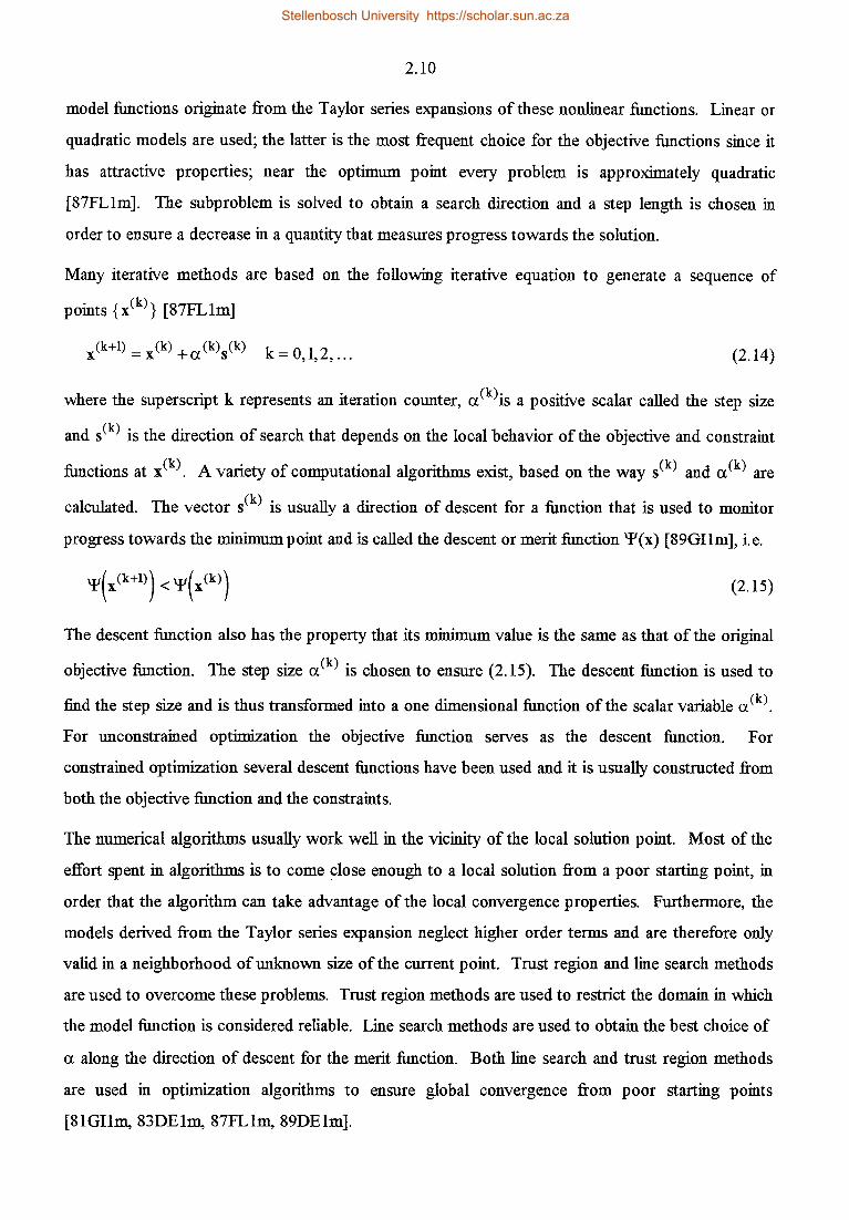
model functions originate from the Taylor series expansions of these nonlinear functions. Linear or

quadratic models are used; the latter is the most frequent choice for the objective functions since it

has attractive properties; near the optimum point every problem is approximately quadratic

[87FL1m]. The subproblem is solved to obtain a search direction and a step length is chosen in

order to ensure a decrease in a quantity that measures progress towards the solution.

Many iterative methods are based on the following iterative equation to generate a sequence of

points { x(k)} [87FLlm]

(2.14)

where the superscript k represents an iteration counter, a(k)is a positive scalar called the step size

and s(k) is the direction of search that depends on the local behavior of the objective and constraint

functions at x(k). A variety of computational algorithms exist, based on the way s(k) and a(k) are

calculated. The vector s(k) is usually a direction of descent for a function that is used to monitor

progress towards the minimum point and is called the descent or merit :function 'I'(x) [89Gllm], ie.

(2.15)

The descent :function also has the property that its minimum value is the same as that of the original

objective function. The step size a(k) is chosen to ensure (2.15). The descent function is used to

find the step size and is thus transformed into a one dimensional function of the scalar variable a(k).

For unconstrained optimization the objective function serves as the descent function. For

constrained optimization several descent functions have been used and it is usually constructed from

both the objective function and the constraints.

The numerical algorithms usually work well in the vicinity of the local solution point. Most of the

effort spent in algorithms is to come close enough to a local solution from a poor starting point, in

order that the algorithm can take advantage of the local convergence properties. Furthermore, the

models derived from the Taylor series expansion neglect higher order terms and are therefore only

valid in a neighborhood of unknown size of the current point. Trust region and line search methods

are used to overcome these problems. Trust region methods are used to restrict the domain in which

the model function is considered reliable. Line search methods are used to obtain the best choice of

a along the direction of descent for the merit function. Both line search and trust region methods

are used in optimization algorithms to ensure global convergence from poor starting points

[81Gllm, 83DElm, 87FLlm, 89DE1m].


2.11

An algorithm is said to be convergent if it approaches a minimum point starting from a given starting

point x(O)_ Convergence to a local minimum point irrespective of the starting point is called global

convergence. A convergent algorithm usually has a descent function that monitors progress towards

the minimum The rate of convergence of an algorithm is usually measured by the number of

iterations and function evaluations, or the CPU time taken to obtain an acceptable solution.

Most optimization methods are iterative and generate a sequence of estimates of the optimum point

x*. The rate at which this sequence converges can be defined in terms of the error

h(k) ={x(k) _x*) (2.16)

If h(k) ~ 0 (convergence) and the errors behave according to (87FLlm, 89DElm]

llh(k+l)ll/llh(k)llP ~ v, v~ O (2.17)

then the order of convergence is defined to be p-th order. The most important cases are p = 1 (first

order or linear convergence) and p = 2 (second order or quadratic convergence). Jn practice local

quadratic convergence is quite fast as it implies that the number of significant digits in x(k) as an

approximation to x* roughly doubles at each iteration once x(k) is near x*. Linear convergence can

be quite slow and much better results can be obtained when the rate constant, v, tends to zero. This

is known as superlinear convergence and algorithms with this property are also quickly convergent in

practice.

Another important feature of an algorithm is the convergence test which is required to terminate the

iterations. These tests have a major effect on the efficiency and reliability of the optimization

process. Some of the termination criteria that are used, are the maximum number of iterations or

function evaluations, the absolute or relative change in the objective function or decision variables,

or satisfaction of the optimality conditions (84VAle, 87FLlm].

Jn practical problems it may often be cumbersome to calculate the derivatives of a complex function

analytically. Jn such cases it is possible to approximate the gradient vector or the Hessian matrix of a

function by means of finite differences (forward difference, central difference, backward difference)

[81Gllm, 83DElm, 87FLlm, 89ARle, 89DElm]. The finite difference steps must be chosen large

enough in order to minimize the finite precision cancellation errors, as well as small enough to ensure

that the difference produce a good approximation to the derivative. If step sizes are properly

selected, then finite difference methods give reliable results. The main disadvantage of these

derivative approximations is the computational effort in evaluating them if the function evaluations


2.12

are expensIVe. However, finite differences will not require more computational effort if the analytical

derivatives of a complicated function require the same effort to evaluate as the function itself

Some of the most important solution methods for unconstrained and constrained nonlinear

programming will now be discussed.

( 1) Unconstrained optimization

The early methods of optimization required the use of function values only (zero order methods) and

were very reliable, easy to program and can often deal effectively with discontinuous functions and

discrete values of the decision variables. However, these methods require many function

evaluations, even for simple problems. The main difficulty in the formulation of these methods is

how to search effectively for the optimum point. The different methods perform their searches in a

random or in an ordered manner. Various methods are discussed and referred to in [83REle,

84VAle, 87FLlm, 88EDle]. The rest of the section will deal with techniques that use the

mathematical nature of the problem in order to make the search for the optimum point as efficient as

possible.

Iterative methods are composed of a search direction subproblem and a step size calculation, also

referred to as the one dimensional line search problem The line search involves the reduction of a

multiple variable function to a function of one variable, the step size, and then finding the minimum

point of the one dimensional problem, i.e.

(2.18)

where a(k) is the step length and s(k) is the search direction. If we assume that a search direction

s(k) is known at the current point x(k), the descent function reduces to a function of one variable.

This function 'P(a) = '¥( x(k) +a s(k)) is assumed to be unimodal, i.e. its minimum exists and is

unique in the interval of interest [87FLlm, 89AR1e]. Analytical methods can be used to determine

the value a* that minimizes '¥ (a). However, analytical methods may become cumbersome and

therefore we rather turn to numerical methods which are in themselves iterative. The line search

problem involves the finding of the interval [O,a (k)] in which the required a* lies, and then the

reduction of this interval until the desired accuracy for locating a(k) is reached. These methods can

be grouped into polynomial approximations (use function values and derivative information) and

those which require function evaluations only [87FLlm]. The latter methods contain interval

searches like the golden section search and the Fibonnaci section search. Any continuous function


2.13

can be closely approximated by passing a polynomial of sufficient order through it and its minimum

can be found explicitly. The minimum point of the approximating polynomial is often a good

estimate of the exact minimum of'P(a) (equation (2.18)). Accurate line searches are very expensive

to carry out and researchers developed a set of conditions for terminating the line search which

would allow low accuracy line searches whilst still forcing global convergence [83DElm, 87FLlm].

The line search thus aims to find a step a(k) which gives a significant reduction in 'P(a) on each

iteration and which is not close to the extremes of the interval [O,a (k)].

In the following paragraphs various algorithms are presented for calculating the search direction, s.

These methods are categorized as first order methods and second order methods.

First order methods utilize gradient information, supplied either analytically or by finite difference

computations. The steepest descent method [81Gllm, 84LUlm, 87FLlm, 89ARle] is the simplest

and probably the best known method for unconstrained optimization. In this method the search

direction, s(k), is taken as the negative of the gradient of the objective function, i.e. s(k) = -g(x(k)),

and presents the direction of maximum decrease in f{x). The convergence rate of this method is very

poor due to the fact that the method does not utilize information from previous iterations. The

steepest descent directions are also orthogonal to each other. This method is therefore not

recommended for general applications and its principal importance is that it usually forms the

starting point for more sophisticated first order methods.

The conjugate gradient [81Gllm, 83MClm, 84LUlm, 87FLlm, 89ARle] method requires a simple

modification to the steepest descent algorithm that substantially improves its rate of convergence

compared to the steepest descent method. The conjugate gradient directions, however, are not

orthogonal to each other, but tend to cut diagonally through the orthogonal steepest descent

directions. The initial search vector is the steepest descent vector and afterwards the conjugate

direction is defined as

(k+l) ( (k+l)) + r.tCk) (k) s =-g x I-' s (2.19)

Information about previous iterations is carried forward in the optimization process by 13. The

conjugate gradient algorithm finds the minimum of a positive definite quadratic function having n

variables in n iterations. For general functions it is recommended that the iterative process is


2.14

restarted every (n+ 1) iterations if the minimum has not been found by then. This method is based on

the calculation of both f{x) and g(x) and only requires storage of n-dimensional vectors (no n 2 -

dimensional arrays). This property makes the method very useful for computation of large

dimensional problems.

Second order methods make use of the second derivatives of the objective function. Newton's

method is the classical second order method [81Gllm, 83DE1m, 83MC1m, 84LU1m, 87FL1m,

89AR1e, 89DE1m]. The idea behind this method is that the function f{x) to be minimized, is

approximated locally by a quadratic function and this approximate function is minimized exactly.

Near x(k\ the function f{x(k)) can be approximated by the second order Taylor series expansion

given in a slightly different form

(2.20)

This method requires first and second order derivatives of f{x) at any point. Equation (2.20) has a

unique minimizer if G(x(k)) is positive definite and Newton's method is only well defined in these

circumstances. By applying the first order necessary condition to equation (2.20), the k-th iteration

ofNewton's method can be written as

S t (k+l) (k) + (k) e x =x s (2.21)

This involves the solution of a n x n system of linear equations. Considerable computational effort is

usually needed to calculate the Hessian matrix. The classical method uses a step size of one in the

search direction. For a true convex quadratic function this method will find the solution in only one

iteration. Since G(x(k)) may not be positive definite when x(k) is far from the solution, the classical

method is not suitable as a general purpose algorithm. If G( x(k)) is positive definite, the method can

be made globally convergent when Newton's method is used in combination with a line search. The

main difficulty, however, is in modifying this algorithm when G( x(k)) is not positive definite. A

multiple of a unit matrix can be added to G(x(k)) to make it positive definite [44LE1m, 63MA1m],

thus giving the search direction a bias towards the steepest descent vector -g(x(k)). The search

direction is then computed from

(2.22)


2.15

When the scalar A,(k) is large the effect of G(x(k)) essentially gets neglected and s(k) is essentially

the steepest descent direction. As the iterative process proceeds, A, is reduced. When A, (k) becomes

sufficiently small the Newton direction is obtained. If s(k) does not reduce the descent function,

A, (k) is increased and the direction is recomputed.

Line search and trust region methods are used to make Newton's method globally convergent while

retaining its excellent local convergence properties [81Gllm, 83DE1m, 87FL1m, 89DE1m]. In line

search methods the quadratic model is used to compute the search direction and then a step length is

chosen. In a trust region method a trial step length h (k) is chosen and then the quadratic model is

used to select a step of at most this length, i.e.

(2.23)

The trial step length is considered an estimate of the region of validity of the Taylor series expansion.

These methods are generally applicable and globally convergent and retain the convergence rate of

Newton's method. Trust region methods are characterized by solving equation (2.22) in order to

determine s(k). The scalars h (k) and A, (k) are related to each other. Such methods were first

suggested by Levenberg [44LE1m] and Marquardt [63MA1m] in the context of nonlinear least

squares problems. The trust region can be adjusted during the iterations and should be as large as

possible subject to a certain measure of agreement between the actual and approximated function.

Both trust region and line search methods appear in modem software and neither appears to be

consistently superior to the other in practice.

The main disadvantage of Newton's method, even when modified to ensure global convergence, is

that the second derivative matrix, G(x(k)), must be evaluated. Furthermore, Newton's method does

not use information from previous iterations. A class of methods that overcomes these

disadvantages is the quasi-Newton (variable metric) methods [81Gllm, 83DE1m, 83MC1m,

84LU1m 84VA1e, 87FL1m, 89AR1e, 89DE1m]. They require only first derivatives and previously

calculated information to approximate the Hessian matrix or its inverse during each iteration. This

approximation is updated during each iteration and these methods have convergence characteristics

similar to second order methods. During updating, the properties of positive definiteness and

symmetry are preserved. The initial matrix can be any positive definite matrix and is usually chosen

as the unit matrix I. Two of the most popular methods are the Davidon-Fletcher-Powell method


2.16

(DFP) and the Broyden-Fletcher-Goldfarb-Shanno method (BFGS) [87FLlm]. The DFP method

builds up the approximate inverse of the Hessian (H ;::;J G-1) of f\x) using only first derivatives.

(k+l) - (k) o(k)o(k)T H(k)y(k) y(k)TH(k)

HDFP - H + dk)T (k) + (k)T (k) (k) u y y H y

(2.24)

where

(2.25)

(2.26)

In the BFGS method the Hessian rather than its inverse is updated at every iteration

(2.27)

where o(k) and y(k) are defined by equation (2.25) and (2.26) respectively. The BFGS method has

been found to work well in practice. Certain conditions must be complied with, in order to keep the

updates positive definite [87FLlm].

If f(x) is the sum of squares of nonlinear functions, special advantages can be taken of the problem

structure to find the minimum solution [74LAlm, 81Gllm, 83DElm, 87FLlm, 89DElm]. The

objective function of this so-called nonlinear least squares problem is written as

m

f(x) = 0.5Lfi (x)2 = f(x)T f(x)

i=l

and its derivatives are given by

g(x) = J(x)f(x)

m

G(x) = J(x)J(x) T + Lfi (x)V' 2fi (x) i=l

(2.28)

(2.29)

(2.30)

Problems of this type occur in nonlinear parameter estimation when fitting model functions to data.

When m > n, least squares solutions to over-determined systems of equations are computed by

minimizing (2.28). Exact solutions can be obtained for well-determined problems ifm = n. Equation

(2.29) can be used with quasi-Newton methods or both equations (2.29) and (2.30) can be used with

a modified Newton method. A good approximation to G(x) can be obtained by assuming that the

last term on the right hand side of equation (2.30) is small (small residual problem), i.e.


2.17

G(x) ~ J(x)J(x) T (2.31)

Whereas a quasi-Newton method might take n iterations to estimate G(x) satisfactorily, here the

approximation is immediately available. The basic Newton method becomes the Gauss-Newton

method when (2.31) is used to approximate G(x). The k-th iteration of the basic Gauss-Newton

method can be written as

S t (k+l) (k) + (k) e x =x s (2.32)

The basic Gauss-Newton method is not necessarily globally convergent or sometimes not even

locally convergent on problems that are very nonlinear or on large residual problems. This algorithm

can be improved in two ways to make it locally and globally convergent, i.e. using it with line search

(damped Gauss-Newton) or with a trust region strategy (refer to equation (2.22)). The trust region

method is usually referred to as the Leven.berg-Marquardt method [44LElm, 63MAlm].

. .

Unconstrained optimization methods can also be used to solve nonlinear constrained problems

[81Gllm, 83MClm, 83REle, 84LUlm, 84VAle, 87FLlm, 89ARle, 89Gllm]. The basic idea is to

construct a composite :function using the objective and the constraint :functions. This composite

:function also contains penalty parameters that penalize it for constraint violations. Mathematically

the problem can be stated as

Minimize ( x, er) = f ( x) + P( c( x ), er) x

(2.33)

where er is the penalty parameter and P is a real valued :function (penalty :function) whose form

depends on the method used.

The composite :function is constructed for a set of penalty parameters and solved using any of the

unconstrained optimization techniques. The penalty parameters are then adjusted, the composite

:function is redefined and then minimized. The process is continued until no improvement in the

estimated optimum point is obtained; thus the term sequential unconstrained minjmizing techniques

identifies these methods. These methods are often called transformation methods because a

constrained problem is transformed into an unconstrained one. Examples of these methods are the

penalty (exterior) and barrier (interior) :function methods as well as the multiplier (augmented

Lagrangian) methods.

2.18

The transformation methods conclude the discussion of the most important classes of unconstrained

optimization solution methods. The techniques used in solving constrained problems rely heavily on

the techniques for solving unconstrained problems.

(2) Constrained optimization

In this section methods used for directly solving the original constrained problem (primal methods)

will be discussed. The algorithms for unconstrained and constrained optimization are based on the

same iterative philosophy. There is one important difference for constrained problems however;

constraints must be taken into account while determining the search direction as well as the step size.

Furthermore, the starting point may be feasible or non-feasible with regard to the constraints.

Different procedures for treating these issues give rise to different optimization algorithms.

An important concept that should be addressed is the status of the inequality constraints at the

optimum solution. Active inequality constraints can be treated as equality constraints and the

remaining inequality constraints can be ignored (locally). These inactive constraints can be perturbed

by small amounts without affecting the local solution. Equality constraints must be exactly satisfied

at the solution. Active constraints at any point x (k) are defined by the index set

(2.34)

called the active set (working set), so that any constraint is active at x(k) if x(k) is on the boundary

of its feasible region [87FL lm]. Equality constraints are always present in the active set. If A* is

known, the problem can be solved as an equality constrained problem. When inequality constraints

are present the active set A* is unknown and must be predicted by some strategy in the solution

method. The predicted A (k) is used to compute the search direction and to change the active set as

the iterations proceed. A(k) usually changes during each iteration, except when x(k) is near x*. It

should be remembered that the constraints active at the solution are significant in the optimality

conditions and that an algorithm will only succeed if the correct active set is identified. An active set

strategy is ea.sier to define for problems with linear constraints than those with nonlinear constraints

(refer to [81Gilm]) and only the basic ideas involved in problems with linear constraints will be

discussed. Linear constraints are of the form

c·(x) = a-:rx- b· I I I (2.35)

Assume that a feasible point x(k) and a predicted active A(k) set are known. Next, the search

direction s(k) can be computed. Two situations are now possible: /


2.19

(1) The point x(k) +s(k) may violate a constraint, or several of them, not currently in the active

set. Thus A (k) is not the correct active set and to remain feasible, a step length 0 ~ a (k) ~ 1 is

determined such that a (k) is the largest step that retains feasibility. A constraint that becomes

exactly satisfied at x(k) +a(k)s(k) is added to the active set and A(k) is enlarged. A new search

direction is computed with this modified active set.

(2) The feasible point x(k) +s(k) is the minimizer of the objective function and A(k) is treated as a

set of equality constraints. The Lagrange multipliers of the active inequality constraints are

then calculated to determine if the solution is a Kuhn-Tucker point. If the minimum of these

multipliers is greater than or equal to zero, a feasible solution is found. Otherwise, the

inequality constraint with the smallest Lagrange multiplier is removed from the active set

(A(k)is reduced) and thus becomes inactive. A new search direction is computed with this

modified active set.

For linear]y constrained problems, the largest step size a (k) to retain feasibility during iteration k is

obtained from solving

T (k) b· -a· x 1 1 (2.36)

If a (k) < 1 is obtained, then a new constraint becomes active and its index is added to the active set

A (k). Various matrices must be updated during the adding and dropping of constraints from the

active set [84Gllm].

This description outlines the strategies involved in a primal active set method for quadratic

programming, because only feasible iterates are allowed. Dual active set methods are also used

where it is not required to satisfy primal feasibility during each iteration [83G01m, 85P01m,

87FL1m]. For more detail regarding active set methods (e.g. the conditions under which the correct

active set will be predicted), the reader should consult Gill, Murray and Wright [81 Gllm, 89Gllm]

and Fletcher [87FL1m] as well as the references stated therein.

Constrained optimization can be categorized into two parts, 1.e. nonlinear or linear objective

functions with linear constraints and linear or nonlinear objective functions with nonlinear

constraints. The simplest type of constrained optimization is the linear programming (LP) problem

This subject is quite well developed and several textbooks and journal articles on the topic are

available, e.g. [81Gllm, 84LUlm, 84VAle, 87FLlm, 89ARle, 89GOlm]. LP problems are the

2.20

most thoroughly developed and understood optimization problems. Many optimization problems of

practical interest are not of this form and linear programming is often overlooked in favor of the

nonlinear programming optimization methods. However, linear programming techniques often form

the basis for the development of more complex nonlinear programming algorithms and sometimes it

is even possible to simplify a nonlinear programming problem by means of linearization and solve it

with linear programming techniques [87FLlm, 89GIIm].

The simplex method is the earliest method for solving LP problems. The basic idea ofthis method is

to proceed from one basic feasible solution to another in such a way as to continually decrease the

value of the objective function until a minimum is reached. This method is still used today but in

more sophisticated forms, e.g. the revised simplex method [84LU1m]. A LP problem is an example

of a convex programming problem and if an optimum solution exists, it is also the global solution.

The optimum solution will always lie on the boundary of a feasible region, i.e. there are always some

constraints active at the solution. LP problems can always be solved in a finite number of steps.

The quadratic programming (QP) problem involves the minimization of a quadratic objective

function subject to linear constraints. QP is of great interest in its own right, and also plays an

important role in the solution of general nonlinear programming problems as a direction finding

subproblem A QP problem may be stated as follows [81Gllm, 87FL1m, 89Gllm]:

quadratic objective function

subject to the linear constraints

T ( T ) aix=bi, i=l, ... ,meq Aeqx=b linear equality constraints (2.37)

linear inequality constraints

where G is symmetric, Y'q(x) = Gx + g and V' 2 q(x) = G. If the Hessian matrix G is positive

semidefinite and the active constraints are linearly independent, x* is the global solution, and if G is

positive definite, x* is also unique (convex programming problem). When G is indefinite, then local

solutions which are not global can occur. QP problems can always be solved in a finite number of

steps.

Equality constrained QP problems can be solved, mainly by usmg matrix manipulations and

computations. The most straightforward method is to use the equality constraints to eliminate

variables and then to minimize the resulting quadratic function. Fletcher [87FL1m] also presents a

generalized elimination method with its various variations for solving these kinds of problems.


2.21

Elimination methods reduce the constrained problem to an unconstrained problem that must be

solved for a minimizer. By using the feasibility and optimality conditions for problem (2.37), one is

able to derive the solution x * and the associated Lagrange multipliers /\. * by the method of Lagrange

multipliers for equality constraint problems (refer to equation (2.8)). This method is discussed in

detail in Fletcher [87FL1m] and Gill et al. [89Gllm] and may be implemented either by null space or

the range space methods.

QP problems containing inequality constraints are usually solved by active set methods as previously

discussed (refer to [81Gllm, 83G01m, 85P01m, 87FL1m, 89Gllm]). The direction of movement

is towards the solution of the corresponding equality constrained problem The main difficulty in

these methods is the prediction of the correct active set of constraints at the solution. If the correct

active set is identified, the problem is solved as an equality constrained quadratic problem that

involves many matrix calculations. It is therefore important to find an effective means of updating

the relevant matrices when the set of active constraints changes [81 Gllm]. A number of solution

methods for QP problems that are extensions of the simplex method for linear programming have

also been suggested [87FL1m, 89AR1e].

Another class of linearly constrained problems are those in which the objective function is general.

These problems can in general no longer be solved :finitely like linear and quaQ.ratic programming

problems and the solution is obtained in the limit of some iterative sequence { x (k)}. The equality

constrained problem can be handled by generalized elimination methods as discussed for quadratic

programming. Inequality constrained problems can be handled by means of active set methods. In

quadratic programming the point x (k) either solves the equality constrained problem or a previously

inactive constraint becomes active. In the more general case the solution of the equality constrained

problem is only located in the limit of a sequence of iterations with the same active set. The line

search procedure is also more complicated and the step length must not exceed an upper limit in

order to retain feasibility. More detail of the general linearly constrained optimization problem can

be found in Fletcher [87FL1m].

Nonlinear programming (NLP) problems arise when both the objective function and the constraints

are nonlinear and is the most difficult of all the smooth optimization problems. The earliest methods

used in solving these problems were the sequential minimization methods or transformation methods

discussed in the section covering the topic of unconstrained optimization. NLP problems can also be

solved by using exact penalty functions in which the minimizer of the penalty function and the

solution of the NLP problem coincide. Sequential processes are not necessary to find the minimizer


2.22

of this exact penalty function. The most popular exact penalty function is the non-smooth or non

differentiable Li-penalty function [87FLlm? 89Gllm]. Smooth exact penalty functions are also

possible.

NLP problems can also be solved by methods based directly on the first order optimality conditions

stated in equation (2.8) [81GI1~ 84LU1~ 84VA1e, 87FL1~ 89AR1e, 89Gllm]. These methods

perform well in the neighborhood of the solution. The idea of a quadratic model is very important in

the most successful methods for unconstrained optimization. In constrained optimization the

curvature of the Lagrange function should be considered and a quadratic model constructed thereof

The original nonlinear constraints are approximated as linear constraints (linearization by means of a

Taylor series expansion). A sequence of approximations x(k) and A(k) to the optimum solution

vector, x*, and the optimum Lagrange multipliers, A*, are generated in the process.

For the derivation of the quadratic subproble~ only the equality constrained problem will be

considered. Inequality constraints can be easily incorporated into the subproblem The subproblem

is derived by writing the first order necessary conditions for the equality constrained problem and

then it is solved by Newton's method for nonlinear equations. Each iteration of Newton's method

can then be interpreted as the solution of a quadratic subproblem We assume in the following

derivations that all . the functions are twice continuously differentiable and gradients of all the

constraints are linearly independent.

The Kuhn-Tucker condition of the equality constrained problem states that

V L(x* A*) = O x,A ' (2.38)

where derivatives are evaluated both with regard to x and A. A linear Taylor series expansion ofVL

about x(k) and A(k) gives rise to the system

[ w<k) -A~~)] [8x(k)] = [-g(k) +A~~) A(k)]

-A (k)T 0 s:: A(k) (k) eq Ui\ C

(2.39)

where A~~) is the Jacobian matrix of the equality constraint normals evaluated at x(k), W(k) is the

Hessian matrix of the Lagrange function, A(k+l) = A(k) +8A(k)and x(k+l) = x(k) +8x(k). Equation

(2.39) can be converted into a slightly different form to solve for A(k+l) and 8x(k)

[ w<k) -A~~)] [ ox<k)] = [-g<k)]

-A (k)T 0 A (k+l) (k) eq 1\ C

(2.40)

2.23

Initial approximations of x (k) and A (k) are required and the iterative procedure is continued until the

convergence criteria are satisfied. Just as with Newton's method for unconstrained optimization it is

possible to restate the problem in terms of one in which the subproblem involves the minimization of

a quadratic function, defined as

Minimize q(k) (8x(k)) = 0.5 cSx(k)TwCk)oxCk) +gCk)Tox(k) + f(k) ox

subject to the linearized constraints

(2.41)

The Kuhn-Tucker conditions of problem (2.41) are given by equation (2.40). If the Hessian matrix

of the Lagrange function is positive definite on the subspace defined by {ox: A~~)T ox (k) = 0}, then

ox(k) minimizes equation (2.41). The QP subproblem for the general nonlinear constrained problem

can thus be defined as

Minimize q(k)(ox) = 0.5 ox T(k)w(k)ox(k) +gTox(k) + f(k) ox


A(k)T s:: (k) + (k) > O meq uX C _

(2.42)

For given initial estimates x(l) and A(1), problem (2.42) can be solved to obtain ox(k)' and A(k+l) is

the vector of Lagrange multipliers of the linear constraints. Update x(k) according to x(k+l) = x(k) +

<ix (k) and continue this iterative process until convergence is reached. Thus, the nonlinear

programming problem as defined by equation (2.1) can be solved by iteratively solving the quadratic

subproblem defined by equation (2.42). This method of solving the nonlinear constrained

programming problem is known as the sequential/successive quadratic programming (SQP) method

or recursive quadratic programming (RQP) method.

A major disadvantage of the method is that second order derivatives of all the constraints and the

objective function must be evaluated to construct the Hessian matrix of the Lagrange function.

However, a major breakthrough was made when it was discovered that this matrix can be

approximated by using only first order information [76HA1m, 77HAlm, 78P01m, 78P03m]. The

idea is similar to that used for Hessian matrix updating in the quasi-Newton methods for

2.24

unconstrained optimization. Both the DFP and the BFGS updating methods have been suggested. It

is sometimes preferred to use the direct updating method given by the BFGS method. It is important

to note that the updated Hessian should be kept positive definite, because then the resulting

quadratic subproblem remains strictly convex. The standard BFGS updating method can lead to an

indefinite or singular Hessian. Powell [78POlm] suggested a modification to the standard formula

to overcome this difficulty so that the solution to the subproblem is always well defined.

The derivation of QP based methods is based on conditions that hold only in a small neighborhood of

the optimum and hence the significance of the quadratic subproblem is questionable when the current

iterate is far from x* (A is far from A*). SQP methods converges locally at second order. In order

to ensure that x(k+l) is a better point than x(k), the solution of the quadratic subproblem can be

interpreted as a search direction. The next iterate is defined by equation (2.14), where s(k) is the

solution to the quadratic subproblem and a (k) is a step length chosen to yield a sufficient decrease in

a merit function 'I' that measures progress towards x*. Typically, a merit function is a combination

of the objective and the constraint functions. Several different choices of merit functions have been

used, namely quadratic penalty functions, exact penalty functions, and augmented Lagrangian

functions [81Gllm, 87FL1m, 89Gllm]. The most successful implementations of the SQP methods

use a modified BFGS updating method and either the Li-exact penalty function or the augmented

Lagrangian function. SQP methods are widely regarded as the most effective general methods of

solving constrained NLP problems. These methods perform well in practice, even on problems that

were formerly regarded as difficult.

Sequential linear constrained methods [89Gllm] minimize the Lagrange function subject to the

linearization of the nonlinear constraints. A quadratic model of the Lagrange function is not

constructed as in the case of the SQP methods, but the objective function is a general approximation

to the Lagrange function. Thus, the subproblem involves the minimization of a general nonlinear

function subject to linear constraints. These methods are widely used for large scale problems,

because general purpose techniques for solving large scale linear constrained problems are better

developed than general methods for large scale quadratic problems. However, issues like global

convergence proofs, the definition of the objective function, the use of merit functions and the

detection of inefficient computations are not yet satisfactorily solved.

There exist other methods to solve NLP problems as well. Sequential linear programming (SLP)

methods [81Gllm, 84VA1e, 89AR1e] are based on the idea of linearizing (Taylor series) both the

objective and the constraint functions about the current x(k) and then to solve the resulting LP


2.25

subproblem by means of efficient LP methods. This process is repeated until the optimum solution is

achieved. The main difficulty of this method is that the solution of the LP subproblem will lie at a

vertex of the linearized constraint set. This method can also give rise to non-feasible solutions and is

recommended only when the curvature effects are negligible. For highly nonlinear programming

problems these methods converge slowly and become unreliable. It is therefore recommended to

rather use SQP methods that contain curvature information and possess excellent convergence

properties.

Feasible direction methods [81Gllm, 84LU1m, 84VA1e, 87FLlm, 89ARle] are based on the

concept of moving from one feasible solution to an improved feasible solution. The feasible search

direction that is calculated from the solution of a linear or quadratic programming subproblem

reduces the value of the objective function and remains strictly feasible for a small step size. The

disadvantages of this method are that a feasible starting point must be known and equality constraints

are not easily implemented. However, these methods will work well in interactive mode [85BE1e].

Gradient projection [81Gllm, 84LU1m, 84VA1e, 87FL1m, 89AR1e] methods were developed in

order to calculate the search direction without solving a linear or quadratic subproblem The search

direction vector is obtained from an explicit expression and is much easier to compute than in the

case of the feasible direction methods. Non-feasible points are corrected by a series of correction

steps to move back into the feasible region. Numerically, the method does not perform well and can

be very inefficient, but is well suited for an interactive process [85BE1e, 89AR1e].

Reduced gradient methods [81Gllm, 84LU1m, 84VA1e, 87FL1m, 89ARle] are based on variable

elimination in that some variables are eliminated by using the constraints currently satisfied as

equalities. The problem then becomes unconstrained in the remaining variables. The search

direction is found, such that for any small move the current active constraints remain precisely active.

If some active constraints are not precisely satisfied due to the nonlinearity of these functions, the

Newton-Raphson method is used to retur:il to the constraint boundary. Both equality and inequality

nonlinear constraints can be treated. There is a definite relationship between reduced gradient

methods and gradient projection methods [81Gllm, 85BE1e]. Special algorithms must be used to

handle arbitrary starting points to obtain a feasible starting point in the feasible direction, gradient

projection and the reduced gradient methods.

There are many other types of optimization solution techniques that were developed to address

certain problem characteristics. Here are some examples:


2.26

(1) Integer programming is the study of optimization problems in which some of the variables are

required to take on integer values.

(2) Network programming treats network flow problems such as encountered in many real life

physical processes.

(3) Geometric programming is a nonlinear programming technique that deals with problems whose

functions are all generalized polynomials. Its development was stimulated by the development

of minimization techniques for engineering design.

( 4) Non-differentiable optimization optimizes a function which fails to have derivatives for some

values of the variables. Standard differentiable calculus must be replaced by methods that treat

these problems effectively.

(5) Multiobjective (multicriterion) optimization deals with multiple criteria optimization problems.

( 6) Stochastic programming considers problems in which some degree of uncertainty exists about

the values assigned to certain parameters and these are given a probabilistic representation.

These special classes of problems will not be discussed in detail and the interested reader can consult

Fletcher [87FL1m] and Nemhauser et al. [89NElm] and the numerous references therein to obtain

further information.

Duality

The concept of duality occurs widely in constrained mathematical programming [84LU1m, 84VA1e,

87FL1m]. The purpose of duality is to provide an alternative formulation of a mathematical

programming problem which either has computational advantages or theoretical significance. Dual

methods do not attack the original constrained problem, referred to as the primal problem, directly

hqt instead attack an alternate problem, the dual problem, whose unknowns are the Lagrange

multipliers. At the dual solution point the values of the multiplier vector A* are associated with the

solution of the primal problem, x*. The dual problem is thus related to the optimality conditions of

the primal problem The objective function used in the dual methods are related to the Lagrangian

function (equation (2. 7) ).

Any function f(x,y) is said to have a saddle point at (x*,y*) if the following condition holds:

f(x*,y) s f(x*,y*) s f(x,y*) for all (x,y) (2.43)

The function f(x,y) exhibits a minimum with respect to x and a maximum with respect toy. In the

case of the Lagrangian function, the point ( x* ,A*) is known to be a saddle point representing a


2.27

minimum with respect to x and a maximum with respect to A. If it is assumed that the Hessian of the

Lagrangian function is positive definite at the solution of the primal problem, x can be expressed in

terms of A in the neighborhood of (x*,A *). Thus we can define the Lagrangian function in terms of

A alone as

L(A) =min L(x,A) x

(2.44)

~

for a fixed A and subject to no constraints. But L(A) ~ d for A in the neighborhood of A*, where d

is the minimum of the primal problem stated in equation (2.1 ). Thus, A* is the solution of the

problem

maximize L( x, A) /\.

subject to (2.45)

V xL(x,A) = 0 and Ai~ 0, i = meq + l, ... m

This formulation is known as the dual optimization probleni and the simple bounds on the variables·

make it easier to solve. In the case of the QP problem stated in equation (2.37), its dual can be

written as (A contains the constraint normals ofboth the equality and the inequality constraints)

Maximize 0.5xTGx+gTx -AT(ATx-b) x,A

subject to

Gx+g-AA=O

Ai~ O, i = IDeq + 1, ... ,m

or

subject to

Ai ~ O , i = meq + 1, ... , m

(2.46)

(2.47)

Furthermore, the minimum of the primal and the maximum of the dual function values are equal at

(x*,A *). If one is able to solve the primal problem, then the dual variables A* can be retrieved.

Similarly, it may be possible in some cases to solve the dual problem and then retrieve the optimum

primal solution, x*. The theory regarding duality is locally as well as globally (convex programming

problems) applicable. Duality cannot be used as a general purpose solution technique and great care


2.28

must be exercised, because in some cases the dual problem may have a solution from which one is

not able to retrieve the primal solution. Dual methods have been used extensively in LP problems as

a very efficient solution technique and are also used in QP and general NLP problems.

Closing remarks

Many methods and their variations for constrained optimization have been developed and evaluated.

References such as Gill et al. [81Gllm], Dennis and Schnabel [83DE1m], Luenberger [84LU1m],

and Fletcher [87FL1m] should be consulted.

The preceding discussion attempts to give a general overview of the basic mathematical

programming techniques (optimization) and the theory involved in order to develop some

'understanding for the relative merits of the methods. The reader is referred to the references stated

for more information on the theoretical development as well as the various modifications and

refinements to ensure efficiency and numerical stability of these methods for practical use.

There is no one optimization technique that will solve all problems satisfactorily. Various methods

exist which have all been modified in some or other way to take advantage of some problem

characteristic or to avoid some unacceptable behavior in order to create more efficient solution

techniques. Optimization problems can be categorized into different standard problem types.

Solution algorithms can be formulated for each of these. It is the user's task to determine into which

category his/her problem fits, and then to apply the appropriate optimization subroutine. Therefore

one must have a basic understanding of the underlying principles of the various methods available.

2.3 APPLICATION OF OPTIMIZATION IN ENGINEERING

Many scientific and engineering problems can be posed in terms of optimization, i.e. seeking the

optimum value of an objective function by varying some parameters. The regular use of optimization

to solve practical problems started during and after World War TI and was made possible by the

creation of computer technology and the development of the simplex method to solve LP problems.

LP is still one of the most widely used optimization techniques.

With the development of the computer technology, researchers were able to solve problems that

were previously regarded as theoretically interesting, because of the amount of computational power

necessary to solve them Enormous progress has been made over the years in developing efficient

optimization algorithms for solving nonlinear optimization problems and to enhance the performance

of existing ones. Furthermore, these developments have led to the solution of real-world problems

that were previously regarded as "unsolvable". The quasi-Newton methods for unconstrained


2.29

optimization problems and the SQP methods for nonlinear optimization problems form part of the

success story. In spite of all these developments, there are still problems that are intractable and

cannot realistically be solved today [91WRlm].

As more and more of the optimization algorithms became known to the engineering and scientific

communities, they were applied or adapted to exploit the structure of particular problems. The

successful solution of real-world problems motivates problem formulators to seek and solve larger

and more complicated problems in the same or closely related areas. The application of optimization

in engineering is a very dynamic and relevant research topic as will be subsequently discussed.

Several publications cover the theoretical development and the applications of optimization

algorithms, for example, Mathematical Programming, Journal of Optimization Theory and

Applications, SIAM Journal on Control and Optimization, Engineering Optimization, International

Journal for Numerical Methods in Engineering, Journal of the Operations Research Society,

Computers and Chemical Engineering, and many more.

Engineering versus mathematical optimization

Engineers and mathematicians view optimization in different ways. Mathematical optimization

assumes that a problem can be formulated in formal mathematical terms and much of the theoretical

and algorithmic development concentrates on methods for locating the solution as accurately and

efficiently as possible. Engineers look from a very problem orientated viewpoint in which they

require sensible, reliable and economic designs or plans to fulfill functional requirements. Engineers

often experience difficulties in formulating the real-world problems in precise mathematical terms

(equation (2.1) refers). The proper formulation (mathematical transcription) of a problem is an

important step in the optimization of any system The problem formulation process requires

identification of the decision variables, an objective function and the constraints of the system for its

reliable performance. It is critically important to formulate a problem by properly modeling the

physical system If the model of the system is inaccurate or its formulation is incorrect, the

optimization process can lead to strange results, or no results at all.

Once the problem is transcribed into the form stated in equation (2.1), it can be solved by means of

the numerical optimization methods available. Even if this is possible, it may sometimes occur that

the problem formulation does not fit into one of the categories studied by mathematicians. The

engineer is more than willing to accept a good approximation for the optimum as long as it can be

obtained without too much effort. To perform engineering optimization in a very effective way, the

engineer needs a solid background in engineering fundamentals, matrix algebra, a basic knowledge of


2.30

numerical optimization algorithms (underlying principles) and computer programming. Textbooks,

like those published by Leitmann [62LEle, 67LEle], Fox [71FOle], Haug and Arora [79HA2e],

Reklaitis et al. [83REle], Vanderplaats [84VAle], Edgar and Himmelblau [88EDle], Arora

[89ARle], provide valuable background on the principles that govern engineering optimization. The

formulation of the optimization problem and the scrutinizing (verifying) of the results are the links

between mathematical optimization and engineering.

The application of optimization in engineering is not limited to specific numerical optimization

methods, but covers the whole spectrum of linear programming, constrained and unconstrained

nonlinear programming, network programming, integer programming, multiobjective optimization,

geometric programming, and stochastic programming just to name a few. Although engineering

optimization is basically concerned with the application of existing techniques, new techniques have

been developed that originate directly from the physical sciences, e.g. geometric programming

[80ECle, 85Rlle]. Optimization methods are fundamentally interdisciplinary in nature and one

cannot in general dedicate a specific method to a specific engineering discipline. Some methods,

however, are better suited to specific problems than others.

Engineers are sometimes confronted with problems or decisions in which more than one objective

must be satisfied [83CLle]. Multiobjective optimization methods are used to make the right

decision in these conflicting situations. The theory and application of multiobjective optimization

and decision making are discussed in detail in Osyczka [840S 1 e] and Reeves and Lawrence

[92REle]. Due to its relevance, multiobjective optimization and decision making is a very active

research topic and the interested reader should consult the above-mentioned references and the

references contained therein for further information.

Numerical optimization techniques have been applied widely to solve a great number of different

engineering problems in the various application fields of design, planning and control.

Optimal design

Engineering design has emerged as a major field of application for numerical optimization

techniques. Numerical optimization is to provide a computer tool to aid the designer in his/her task.

In the past the conventional design process has more than once lead to uneconomical designs. The

designer was able to freely use his experience and intuition in making decisions. The optimum design

process forces the designer to identify a set of design variables, an objective function to be

optimized, and constraint functions for the system and as such gain a better understanding of the

problem Human interaction is an essential part of the optimum design process and it is performed in


2.31

a more formal and organized way than in the conventional design process. The design process is

more organized, using trend information in a very systematized way. Computers play a very

important role in the optimal design process, introducing more accuracy, efficiency and allow us to

understand the behavior of complex systems.

The basic principles of optimal design are discussed in, for example, Avriel et al. [73AV1e ],

Vanderplaats [84VA1e], Arora and Thanedar [86AR2e] and Arora [89ARle] and various design

applications are illustrated. Major contributions in the field of optimum design originate from

structural optimization, process equipment design, and mechanical design. A wide variety of design

applications (in various engineering disciplines) to illustrate the integration of optimization as part of

the design process can be found in, for example [71F01e, 73AV1e, 78Wlle, 79AV1e, 79HA2e,

83RE1e, 84BEle, 84VA1e, 85BE1e, 85GEle, 86AR1e, 86AR2e, 86LI1e, 86THle, 88AR1e,

88ED1e, 88TSle, 89AR1e, 91PEle, 92Blle]. The articles and textbooks give useful hints to assist

the designer when faced with a practical design optimization problems. It is clearly illustrated that an

efficient design process should allow for the designer's experience, intuition and creativity to go

hand in hand with the optimization technique.

Optimal control

The optimal control problem is to find a time dependent feedback control function that assures

optimal behavior of a system during its dynamic performance. The system has active elements that

sense change in the output and the system controls get automatically adjusted to correct the situation

and optimize a measure of performance. On the other hand, optimal design concerns the design of a

system and its elements in order to optimize an objective function; the system then remains fixed for

its entire life. The solution of optimal control problems relies heavily on the theory of calculus of

variations and optimal control theory [62LE1e, 67LEle, 79HA2e, 87FRle]. Optimal control theory

considers problems that cannot be solved by the calculus of variations.

Optimal control problems can also be transformed into optimum design methods and solved by the

same numerical optimization methods [89AR1e, 92Blle]. Control problems can be found in all the

different engineering disciplines and were particularly relevant in many of the complex military and

space programs that were initiated during the 1960's [87FR1e]. Optimal control problems are

experienced in aerospace systems (e.g. trajectory optimization) [62LE1e, 67LEle, 87HA2e,

93BE1e], process engineering (e.g. reactor design and nonsteady-state processing) [92Blle],

Operations Research and Economics (e.g. economical planning) [87FR1e], and the dynamic response


2.32

control of both mechanical and structural systems (e.g. precision control of machines, control of

structures under wind loads and earthquakes etc.) [79HA2e, 89ARle].

Optimal planning

Optimization techniques play a vital role in effective planning, scheduling, and control of projects and

production processes. The processes of planning, control and scheduling are in themselves

optimum-seeking processes. The efficient use and proper scheduling of expensive human resources

and equipment results in creating more with less input, resulting in great economical benefit

[91GL1e]. Plant layout, plant and warehouse location, product distribution, operations planning,

production and working schedules are just a few examples of the problems that can be addressed.

Special numerical techniques have been developed to aid management to perform planning and

control tasks in a more effective manner [92H01e]. The role that optimization plays in these

activities is illustrated both theoretically and practically in [87FR1e, 91HU1e, 92H01e]. Clearly, the

logical approach of mathematical optimization is very useful when applied to the many rational

problems in decision-making.

Algorithms and software

The application of optimization in engineering needs efficient and robust algorithms. Researchers in

the area of mathematical programming are constantly working on this aspect to develop and

implement new algorithms and to improve old ones. Both general-purpose and specialized

algorithms (and software) are needed to aid engineers in performing optimal design, control and

planning. Software development for engineering applications is, however, lagging behind the

mainstream of mathematical programming development.

Special-purpose algorithms and software are mostly needed to solve real-world problems. The

various engineering disciplines have specialized software to address their specific needs [84VA1e,

88ED1e, 89ARle]. Some general purpose design optimization software is becoming available, e.g.

ADS (Automated Design Synthesis - Vanderplaats [86VA1e]) and !DESIGN (Interactive Design

Optimization of Engineering Systems - Arora [88AR1e, 89AR1e]). Some other codes are discussed

by Reklaitis et al. [83RE1e], Belegundu and Arora [85BE1e], and Edgar and Himmelblau [88ED1e].

Software that implements the various optimization algorithms discussed in section 2.2 is readily

available. Some general-purpose libraries are available that contain subroutines implementing these.

Examples are the NAG-library, IMSL-library and the Harwell-library. Furthermore, these libraries

also contain the implementation of various other mathematical routines, e.g. linear algebra. The use

of the general-purpose libraries is the only resort when specialized software to perform the task is


2.33

not available. The user is responsible for the proper interaction between engineering problem

formulation and modeling and the mathematical solution process. The main program and the other

routines written by the user can become very complex and are prone to errors, so extreme care must

be exercised during program development. This method of applying optimization to engineering

requires that the user has some knowledge of the algorithm in use. Guide-lines on use of general

purpose software are discussed in Arora [89ARle].

Artificial intelligence .

The use of artificial intelligence (Al) in engineering design, planning and control is a fairly new

development. Artificial intelligence concentrates on emulating human reasoning in order to solve

problems. Al algorithms analyze the methodology of how a human being solves a problem and

translates the thought process to the computer. The computer then approaches the human reasoning

process to solve the problem in contrast to executing an ordered set of instructions as found in

traditional computer programming. Expert systems (knowledge-based systems), neural networks,

and fuzzy logic are alternative approaches within the artificial intelligence field. Artificial intelligence

can couple the reasoning and judgment of the human mind with the power, speed and memory of the

computer to solve various engineering problems. The general application of artificial intelligence to

engineering problems is discussed in Arora and Baenziger [86AR1e], Winstanley [91Wlle], Gero

[92GE1e], Rowe [92R01e] and the references cited therein. The application of artificial intelligence·

in engineering is of great importance, especially the fact that the decision-making power of an expert

can be emulated to perform optimal tasks.

Closing remarks

The various numerical optimization techniques present the engineer with a means to determine the

best possible solution on a theoretical basis. Intangible factors and practical considerations may

change the final recommendation to other than the calculated optimum It is up to the engineer to

apply proper judgment to take into account these practical factors. Thus, theoretic~ and economic

principles must be combined with the understanding of the practical problems that will arise.

The preceding discussion presents just a few examples to illustrate how optimization techniques can

be implemented in the engineers' never-ending search for improved ways of doing things. The

references cited in this section are intended to serve as an introduction into the field of the

application of optimization in the different engineering disciplines. Substantial literature exists for

future education in this topic and more research and knowledge than presented here is required to


2.34

fully understand these topics . Tue references contained in these books and articles can be used as

further sources of information.

2.4 OPTIMAL DESIGN OF DRY-COOLING SYSTEMS AND AIR-COOLED HEAT

EXCHANGERS

In this section literature relevant to the optimal design of dry-cooling systems and air-cooled heat

exchangers are reviewed. Tue discussion on dry-cooling system optimization will be cast primarily in

the context of power plant cooling to coincide with the illustration of the engineering optimization

application of the present investigation.

Irreversibility and Thermoeconomic design optimization of heat exchangers

Tue second law of Thermodynamics involves the fact that real processes proceed in a certain

direction and not in the opposite direction due to the thermodynamic irreversibilities that exist.

London [82LO 1 e] gives a list of irreversibilities that exist in energy conversion systems. The second

law further leads to a property, called entropy, which enables us to treat it quantitatively in terms of

·the operating conditions for processes. Bejan [89BEle] states that if we are serious about

constructing efficient energy systems and conserving energy, we have no other choice but to design

for less and less entropy production.

The basic design problem is to determine the thermodynamically optimum size or operating regime

of a certain engineering system, where by optimum we mean the condition in which the system

destroys the least exergy (useful energy} while still performing its :fundamental engineering :function

[87BEle, 89BEle]. Tue destruction of exergy is intimately tied to the generation of entropy in the

various components of a .system Tue loss of exergy, or irreversibility, provides a generally

applicable quantitative measure of process inefficiency. Analyzing a multi-component plant indicates

the total plant irreversibility distribution and interaction among the plant components, pinpointing

those contributing most to overall plant inefficiency [85K0le, 87BEle, 89TSle]. A solid

understanding of the mechanism of entropy generation in each of the systems components is essential

in setting out a strategy for decreasing entropy generation by the entire system [89BEle].

Different criteria based on the exergy concept are commonly used for the performance evaluation of

heat exchangers. These include irreversibility generation minimization analysis [82BEle, 87BEle,

89ACle, 89RA2e] and thermoeconomic analysis [82LOle, 83L02e, 85KOle, 89RA2e, 89TSle].

These criteria are used to define objective :functions used for optimization of heat exchangers. Tue

traditional irreversibility generation based objective :function is simply expressed in terms of the

irreversibilities occurring in the heat exchanger, while the thermoeconomic objective :function is


2.35

obtained by combining the pricing of the penalties of the thermodynamic irreversibilities with the

capital costs.

The irreversibility of any heat exchanger is basically due to two factors, namely the transfer of heat

across a stream-to-stream temperature difference and the pressure drop that accompanies the

circulation of fluid through the apparatus [78BEle, 82BEle, 85KOle, 89ACle, 89RA2e]. The

above-mentioned irreversibilities can systematically be reduced by slowing down the movement of

the fluid through the heat exchanger. This technique is synonymous with employing larger heat

exchangers. Thus, in order to build thermodynamically efficient heat exchangers, one has to build

large units. Large heat exchangers, however, require large amounts of materials that, in order even

to be produced, require large amounts of exergy for consumption during the manufacturing process.

It is clear that an optimization program must include the exergy losses associated with both the

operation of the heat exchanger and those invested (capital) in the hardware [82BEle].

The thermoeconomic objective function is a combination of the capital cost and the costs associated

with the heat exchanger irreversibilities (running/operating costs). The purpose ofthermoeconomic

optimization is to achieve, within a given system structure, a balance between expenditure on capital

costs and exergy costs which will give a minimum cost of the plant product [85KOle]. This

objective function is preferred for commercial heat exchanger design and the global optimum yields a

realistic result of a finite area heat exchanger.

Conventional heat exchanger optimization seeks the optimum trade-off between the capital costs and

the operating costs for the entire system Most thermoeconomic methods simplify the search for an

optimum by making these trade-offs at system component level. The fundamental idea that justifies

the irreversibility minimization at system component level is that the overall entropy generation rate

of a system is the sum of all the system's components contributions [87BEle]. The conventional

design process can be seen as thermoeconomic optimization on a global scale, because the objective

function tries to minimize the combination of capital and operation costs (minimum material

consumption, minimum energy consumption). Contrary to thermoeconomic optimization, the real

causes and sources of costs due to exergy destruction are not as clearly defined through the

conventional design optimization process. Thermoeconomic design optimization indicates the

optimal thermodynamic efficiency of a component from a cost viewpoint and therefore helps the

designer to create improvements, both thermodynamically and economically.


2.36

Air-cooled heat exchanger optimization

Air cooling made a strong bid for application in the refining, petrochemical and natural gas industries

during the 1950's when it was realized that air can be a more economical coolant, even in locations

where water is plentiful. The design of air-cooled heat exchangers, especially during the 1950's and

the 1960's, was mainly based on rules of thumb obtained from the recorded operating experience of

existing installations or designers' intuition. For example, the average design face velocity for air

cooled heat exchangers was regarded as between 2 mis and 3.5 mis, and heat exchangers were

usually equipped with four tube rows [59KE1e, 60RU1e, 66L01e, 66L02e]. However, it was

realized that by changing the traditional design configurations and operating conditions, great

economical advantages were possible due to the trade-off that exist between capital and operating

costs [59KE1e, 59NA1e, 66L01e, 66L02e, 66SC1e, 66SC2e].

Commercially available equipment (e.g. finned tubes, fans) were often used in the search for the

optimum air-cooled heat exchanger. As a result of this practice, the dimensions of the equipment

were not optimized, but the configuration instead [66LOle, 66L02e]. The use of this commercially

available equipment simplified the optimization process to a great extent. The techniques used in the

search for the optimal heat exchanger design were mainly mathematical techniques (e.g. differential

calculus - setting the first derivative equal to zero) [57FA1e, 59KE1e] or graphical presentations of

the trade-off between heat transfer and fluid flow relations [59NA1e, 66L01e, 66L02e, 66SC2e,

69JE1e] . Schoonman [66SCle] presented a more advanced approach by using a computer program

to perform a cyclic variation of three variables, namely number of tube rows, fin spacing and fan

power, through several combinations to find the optimum design. Although these approaches tend

to limit the number of relevant parameters due to practical considerations or in order to simplify the

problem, they can be seen as the forerunner of the more modem and complex optimal analyses that

followed.

More sophisticated search techniques were used to locate optimal heat exchanger designs. Peters

and Nicole [72PEle] discuss the use of factorial searches of all the possible combinations of

variables and come to the conclusion that they become unsatisfactory as the number of variables

increases. Due to the large number of discrete variables encountered in air-cooled heat exchanger

design (due to the use of commercially available equipment), they favored the use of heuristic

algorithms (starting close to the optimum) to perform the optimal design process, specific to the

equipment under consideration. Palen et al. [74PAle] propose the application of the Box Complex

Method [65B01e] of systematic search for the optimal design of heat exchangers. Various aspects


2.37

of optimal heat exchanger design (e.g. the criteria for the objective function and design variables) are

discussed. Previously, the investment was related to the heat exchanger area only, but Palen et al.

[74PA1e] proposed the calculation of the investment from the dimensions of the component parts

and the manufacturing costs. Fontein and Groot Wassink [78F01e] utilized the Simplex Method

[65NE1e] and a steepest decent method to optimize a shell and tube heat exchanger by using the

NTU-method (number of transfer units) [86H0le].

Shah et al. [78SH1e, 81SH2e] recognize the heat exchanger optimization problem as one suitable for

nonlinear programming (optimization) techniques. Several numerical optimization techniques (e.g.

conjugate gradient methods, penalty function methods) are referred to in the paper as they have been

developed specifically for computer application and are thus suitable for implementation on these

design problems. Once the problem is transcribed into formal mathematical terms, the optimization

method most suited to the specific problem formulation can be used. The authors suggest that a

computer program containing several optimization methods and a heat exchanger performance

analysis routine should be used for design purposes, as no single optimization method will be well

suited to all the problems: A heat exchanger optimization methodology is outlined and the process is

illustrated by means of an example (also refer to [81SH1e, 88SH1e]). This paper is indeed a very

valuable contribution to promote the use of nonlinear programming techniques in optimal heat

exchanger design.

Kroger [79KR1e] presents a method to determine the cost optimized dimensions and operating

conditions for circular finned heat exchanger tubes by maximizing the performance over cost ratio.

The general practice in the previous optimal design processes of air-cooled heat exchanger was to

choose a surface (described by its tube pitch, fin pitch, fin diameter, outside tube diameter and fin

thickness) beforehand and use its experimentally obtained performance correlations. Kroger,

however, uses the general relations for the heat transfer and pressure drop during flow across finned

tube arrangements, expressed in terms of the various geometrical and flow parameters, as found in

literature [45JA1e, 63BR1e, 66R01e, 66VA1e, 74MI2e]. The optimization procedure takes into

consideration all the parameters that may affect the capital and operating cost of the heat exchanger

and does not prescribe any limits, other than those absolutely essential due to practical limitations. A

specific capital and operation cost structure for the finned tubes is assumed and an analytic objective

function is obtained that expresses the performance over cost ratio in terms of the various

geometrical and operating parameters. The design method is illustrated with a practical example and

the objective function maximization is performed by computer. The results of this study show that

the optimum design and operating conditions differ considerably from conventional designs. For


2.38

example, the fin thickness is found to be much less than that found in practice. Similarly, the stream

velocities are also lower than those found in industrial applications. In part this is due to the cost

structure chosen. However, the method illustrates trends in the search for optimum geometrical and

operating parameters.

A similar procedure (refer to [79.KRle]) is proposed by Kroger [83.KRle] for the optimal design and

operating conditions of a plate fin air-oil heat exchanger with tape inserts inside the tubes. Literature

correlations are also used for the heat transfer and pressure drop calculations. An industrial air-oil

heat exchanger is tested experimentally in order to verify the accuracy of the heat transfer and

pressure drop equations employed and for the purposes of comparison. The results of the

performance over cost ratio maximization again indicate geometrical and operating parameters that

differ from those found in industrial applications.

Hedderich et al. [80HE1e, 82HE1e] developed a computer code for analysis of air-cooled heat

exchangers and coupled it to a numerical optimization program (constrained function minimization)

to obtain an air-cooled heat exchanger optimization and design procedure. The optimization

program is based upon the method of feasible directions and the Augmented Lagrangian Multiplier

Method [84VA1e] that can be used for different optimization applications. They used the heat

transfer and pressure drop correlations provided by Briggs and Young [63BR1e] and Robinson and

Briggs [66R01e] which enabled them to vary the finned tube geometrical parameters in order to find

the optimum heat transfer surface. The developed code has the capability to design for nine different

configurations of triangular pitch banks of finned tubes. Air-cooled heat exchangers can be

optimized according to the following objective functions: minimum volume, minimum heat transfer

surface area, minimum fan power, minimum airside pressure drop, and minimum tubeside pressure

drop. No economically based objective functions were considered in this study.

Pribis [81PR1e] describes the combination of heat exchanger design programs and optimization

routines. The optimization routines are based on gradient search methods. Various surfaces can be

accommodated in the program, e.g. bare tubes, plate fins, spine fins, and helical wound fins. The

author stresses the fact that the heat exchanger must not be modeled on its own, but must be

modeled in the system to get realistic optimization results.

Heat exchangers are used in essentially all the process industries and play a vital role in process

design considerations. In their textbooks, Edgar and Himmelblau [88ED1e], and Peters and

Timmerhaus [91PE1e] extensively treat the topic of optimal economic design of equipment as found

in the chemical process industries. These books gives a clear concept of the important principles of


2.39

desi~ and economics from a practical point of view. The material presented will help the engineer

in heat transfer equipment selection, design and optimization and various examples are given to

illustrate the methodology used.

Computer programs for the design, performance evaluation and econormc optimization of heat

exchangers are extremely useful engineering tools. Most of the more complex optimal heat

exchanger designs discussed in this section were obtained in this way. Breber [88BRle] discuss the

main features, such as program capabilities, data input, result output and program logic, required in

these type of programs to perform reliable analyses. An overview of currently available programs is

presented to aid the engineer in choosing a program for his/her specific requirements. The author

concludes that computer programs cannot substitute engineering judgment which is needed in

problem formulation and scrutinizing of the results. Taborek [91TAle] discusses the use of expert

systems in heat exchanger design which aims to establish more user interaction during the design

optimization process.

Optimum industrial heat exchanger design differs from the thermodynamic design in that several

additional criteria, sue~ as demands and restrictions imposed by the interrelated design

considerations, must be satisfied. The heat exchanger designer must obtain a global optimum within

all the demands and restrictions with respect to initial · and operating cost, reliability,

manufacturability, and maintenance ease.

The literature cited in the survey above are by no means complete and aim to give an overview of the

different optimization algorithms and analyses models used in the design of optimal air-cooled heat

exchangers.

Dry-cooling system optimization

Between 1970 and 1980 major engineering economic studies of dry-cooled electrical generating

plants were conducted in the USA with the object of minimizing the cost of electricity generation

when dry-cooling towers are coupled to a turbo-generator [70R0le, 75Mlle, 76FRle, 78ROle,

79CH2e, 79HAle, 79NAle]. Factors that affect the design and optimization of dry-cooled power

plants are discussed in Miliaras [74Mlle]. Both natural and mechanical draft indirect dry-cooling

towers are considered in these studies. At that time dry-cooling was successfully utilized in a

number of steam-electric generating plants in Europe and the concept was relatively new to the USA

electric generating plants [70ROle]. Up to then, dry-cooling in the USA was extensively used in the

process industries. The need for an alternative means of cooling was to promote water conservation

through the industrial use of dry-cooling and to conform with the environmental regulations. Most


2.40

of the studies compared dry-cooled steam-electric plants to wet-cooled plants in terms of the

increased power generation costs. Dry-cooling towers have the inherent characteristic of

performance degradation during high ambient temperature and subsequently the plant will suffer

production losses during these conditions (lost performance ). In the USA most of the electricity

generating plants are privately owned and thus cannot afford production losses. The concept of lost

performance is discussed in detail in section 4. 7. Dry-cooling received a bad reputation and was

sometimes severely penalized as a result of this inherent characteristic.

Due to the complexity of dry-cooling system economics, several assumptions are introduced into the

reviewed studies to simplify the optimization problem The optimization of some plant and cooling

system operating parameters and/or the general cooling system is conducted. However, in most of

the studies, optimization consists of matching components effectively. These particular studies are

for state-of-the-art cooling systems and therefore use vendor data and fixed designs for the available

dry-cooling tower equipment. This approach results in the use of± 4-6 decision variables for the

optimization process. Ard et al. [76ARle] developed detailed costs and cost algorithms for dry

cooling systems. The equipment cost are expressed in term8 of their dimensions or operating

variables. These cost relationships present a means of varying equipment dimensions continuously

and not discretely as is permitted by the use of standard equipment. Choi and Glicksman [79CH2e]

used these cost algorithms in their optimization study.

In the above-mentioned studies, the basic underlying principle of the optimization process is the

same. First, a plant location (weather data), a turbo-generator (performance characteristics) and an

initial temperature difference (difference between the steam and the inlet ambient air temperature to

the cooling tower) are chosen. The dry-cooling tower, that minimizes the cost of electricity

generation throughout the year, is determined by varying the different decision variables that describe

its geometry and operation. The cost of electricity generation is made up of the capital cost,

operating cost (including fuel cost), and the cost due to lost performance. The process is repeated

for all the initial temperature differences to be considered in the analysis. Thus, for each initial

temperature difference an optimum dry-cooling system is calculated and the global optimum dry

cooling system is selected from these. Computer programs were written to perform the economic

optimum designs. This method of optimization is quite a lengthy process and will not be adequate

when many variables enter the optimization process. The Box Complex Method [65BOle], double

shotgun-and-search method [72ANle] are just two of the optimization techniques used [78ROle,

79CH2e].


2.41

The goals of these reports were to reduce the cost of state-of-the-art dry-cooling systems and to try

and develop new concepts with lower costs (refer to [79HAle]). They differ mainly in the following

aspects: the assumptions made to facilitate the analysis, the treatment of lost performance, cooling

system design, plant type, plant location, turbine type, cost modeling, physical modeling,

optimization procedure used, and parameters optimized. Most studies have shown that if dry

cooling is used, the cost of electricity will be 10% to 20% higher than when wet-cooling towers are

used. The cost is higher due to the higher investment cost (extensive finned tube heat transfer area

required) and the poorer plant thermal efficiency (higher turbine backpressure). Valuable

information, regarding the advantages and disadvantages of dry-cooling and process modeling, is

presented in these reports. The results present general tendencies rather than SJ?ecific values. The

reports indicate that dry-cooling systems require special turbines that can operate at higher back

pressure than the conventional turbines that are found in applications where wet-cooling is used.

Although the extended surface heat exchanger is the heart of any dry-cooling system, no author tries

to optimize it in a rigorous manner. It is not clear from the above-mentioned studies if dry-cooling

system equipment has been optimized, either by the vendors or by the studies performed. The

coupled effects between the economic approaches, the underlying assumptions, the detailed designs

and the overall system designs are not well defined in many respects. A summary of cooling tower

selection and optimization as covered by these reports can be found in [85MAle].

Hauser et al. [71HAle] discuss the economic optimization of turbine and cooling system

combinations. The object of the paper is to describe briefly the parameters and input to be

considered during optimization and their effects on the overall system performance. The authors

suggest that improved performance, coupled with lower costs, can be obtained in the cooling. system

design by using techniques to optimize the turbine and cooling system as an entity. The basic

requirements for the optimum selection of a turbine and cooling system combination are:

( 1) Accurate cost data for equipment, installation, system operation and deficiencies;

(2) Accurate determination of the system performance throughout its entire life;

(3) A comprehensive evaluating technique which can merge cost and performance factors into a

single figure of merit, e.g. present worth of the total revenue requirements for a given system

over its entire operating life.

An extensive list of input data that is required to perform such an integrated optimization is given

and discussed. A sample turbine-cooling system optimization study is presented to illustrate the

above principles.


2.42

Moore [72M0le, 72M02e, 73MOle, 73M02e] presents a series of reports on the minimum size of

large dry-cooling towers. An analytical minimum size function is presented that relates the flow

areas, tower height and fan power to parameters of the heat exchanger, assuming one dimensional

flow through the tower. 1bis was done with a large power plant in mind, with a view to minimize

the size of a natural draft tower shell, and hence its visual impact and cost; or the fan power of a

mechanical draft tower, and hence its cost and noise impact. The results show the importance of

heat exchanger design on tower size and various requirements for minimum tower size are directly

revealed by the size function (e.g. a very shallow heat exchanger). However, it is not obvious how

such requirements could economically and practically be met.

Johnson and Dickinson [73JOle] perform a similar study for forced draft dry-cooling towers as the

one presented by Moore [72MOle, 72M02e, 73MOle, 73M02e]. Although no cost factors are

considered in this analysis, an interrelationship of the parameters that will contribute most

significantly in an optimum design is derived. The influence of these parameters on the minimum size

and the heat exchanger frontal area is determined.

Andeen and Glicksman [72ANle] describe a cost optimization procedure to design a dry-cooling

tower. They state that the important cost to be optimized is the incremental increase in the cost of

power generation, resulting from the use of a dry-cooling tower, over a plant operating at 40%

efficiency. The incremental cost is derived from the capital and operating costs of the plant. The

optimization problem is reduced to heat transfer and cost equations containing 6 variables and the

double shot-gun method is used to solve the problem The authors state that in order to make dry

cooling towers more economical, their cost must be minimized by optimizing the entire plant.

Furthermore, the authors realize that the optimization must not be restricted to the adaptation of

predesigned heat exchanger modules, because the module design may not be anywhere near its

optimum

Ecker and Wiebking [78EC 1 e] investigate the optimal economic design of a natural draft dry-cooling

tower with a vertical heat exchanger bundle arrangement. The optimization model is developed by

using the relevant physical laws and engineering design relations and transcribing them into the

objective function that minimizes the annual cost (fixed charges and operating cost). The problem is

then reformulated as a geometric programming problem according to the special mathematical

formulation required by this method. The paper is concluded with a numerical example to illustrate

the method. Geometric programming is also used in the design and performance optimization of a

condenser and wet cooling tower combination as described by Stuart and Arnold [86STle].


2.43

A design method for optimal economical dry-cooling towers, usmg the existing literature and

standard sourcebooks on heat exchanger design and performance, is presented by V angala and Eaton

[78V Ale]. The combination of all the different information is explained by means of flow diagrams

and the method seems very cumbersome.

Montakhab [80M01e, 80M02e] published two papers that deal with the factors that affect the size

and cost of dry cooling towers and the related heat transfer equipment. He aims to reduce the heat

exchanger surface area, the tower size and the pumping power requirements by investigating a means

to define suitable heat exchanger geometries and surfaces for application in dry-cooling tower

applications.

Li and Priddy [85Llle] published a textbook on the topic of power plant system design and discuss

all the power plant components, economic aspects and design concepts. The topic of mathematical

design optimization is also treated and illustrated with an example covering a turbine-cooling system

combination. Three phases are identified for a proper optimization study, namely:

(1) System configuration design (specify the different configurations and combinations to obtain

the initial costs);

(2) System simulation (determine the performance characteristics and the operating costs for the

different configurations/ combinations);

(3) Comparative economic evaluations (compare the different configurations/combinations to find

the minimum cost).

The methodology presented in the above-mentioned textbook is also discussed and illustrated in the

paper by Li and Sadiq [85LI2e].

Electricity generation costs, i.e. capital costs and operation costs, can form a large part of the total

electricity cost and therefore emphasizes the importance of optimizing power plant design. Yeck and

Rubbers [87VE1e] discuss the important role that the cooling system plays in this optimization

process and outlines the important choices that have to be made in order to perform an economic

evaluation. The economics of evaluating cooling systems are closely related to the characteristics of

the demand for electricity. A methodology is presented to determine the optimum size and type of

cooling system based on the amount of net energy produced annually. The cooling system must be

designed to maintain the turbine backpressure as close as possible to its maximum efficiency, where

the electrical output is the maximum


2.44

Buys and Kroger [89BUle, 89BU2e] use a constrained variable metric method (SQP-method) to

perform cost-optimal designs of new or existing (retrofit of heat exchanger bundles) natural draft

dry-cooling towers. Tue SQP method is preferred to other algorithms due to its computational

efficiency. Heat transfer and fluid flow relations, expressed in terms of the various geometrical

parameters, are used to simulate the performance of the dry-cooling towers. A prescribed cost

structure and practical constraints are employed in the problem formulation. Tue finned tube

performance correlations of Briggs and Young [63BRle] and Robinson and Briggs [66ROle] are

used to simulate the influence of finned tube geometrical parameter variation on their performance.

Both articles are accompanied by a numerical example. Sensitivity analyses have also been

performed to investigate the influence of the fixed parameters and design correlations on the

optimum design. Although the results show geometrical parameters that differ from those usually

found in practice, they provide certain trends in the manufacturing and construction of cost-optimal

dry-cooling systems.

The optimal sizing of indirect natural draft dry-cooling towers for combined cycle power plants that

corresponds to the minimum cost of electricity generation is discussed by Lovino et al. [90LOle].

The authors identify the strong interaction between the turbine and the cooling system as one of the

main reasons for such an optimization study to be performed. Simplified design criteria and cost

evaluation techniques are employed, originating from preliminary design data. By considering all

possible combinations of the tower heat exchanger and condenser geometry and steam turbine

design, the optimization has been performed by a step by step variation of the cooling tower range

and approach. Sensitivity analyses have been performed to investigate the influence on the optimal

solution of different hypotheses concerning the tower investment and fuel cost. The results show

that the optimum dry-cooling tower design is strongly influenced by the turbine characteristics.

Closing remarks

The application of optimization techniques in dry-cooling tower design has been reviewed in this

section. Many different methodologies have been discussed; some of them are generally applicable,

while others are confined to a specific application under consideration. One of the most important

conclusions that can be drawn from this review is that the cooling system has a significant effect on

the overall plant economics. The effect on both the investment cost and the plant overall

thermodynamic efficiency make it necessary to perform optimization analyses that take the strong

interaction between the cooling system and turbine into account (in the case of power plants). The

matching between the performance characteristics of the dry-cooling tower type, i.e. natural draft


2.45

indirect system or mechanical draft direct system, and the performance characteristics of the specific

turbine type (differences in blade design and exit area), needs careful consideration [81M0le,

87KNle, 87TRle, 87VE1e, 91SZ1e]. This requires the simulation of the interaction by means of a

computer model.


3.1

CHAPTER3

FORMULATION AND MODELING OF THE PERFORMANCE


3.1 INTRODUCTION

Formulation of an optimization problem involves transcribing a verbal description of the problem

into a well-defined mathematical statement. Tue optimum problem formulation process requires the

identification of the design variables, an objective function and the constraints imposed on the system

for its reliable performance. It is very important to formulate a design problem by proper modeling

of the physical system If the model of the system is inaccurate or the formulation is incorrect, the

mathematics of optimization can lead to strange results, or no results at all. Thus, the solution is

only as good as the problem formulation and modeling.

Tue concepts of problem formulation and modeling will subsequently be discussed and applied to the

performance evaluation and optimal design of both natural and forced draft dry-cooling towers.

3.2 PROBLEM FORMULATION

Tue formulation process can be broken down into three well-defined steps [83RE1e, 88ED1e,

89AR1e], ie.

( 1) Identification of the decision variables;

(2) Identification of the objective and expressing it as a function of the decision variables;

(3) Identification of all the constraints and expressing them as functions of the decision variables in

order to be transcribed into mathematical expressions.

Each of these steps will subsequently be discussed.

Decision variables

Tue decision variables describe the system lIDder consideration. Th.ere is a minimum number of

variables required to formulate the problem properly, otherwise the formulation is incorrect or not

possible at all It should be kept in mind that these variables must be independent of each other as

far as possible. Once these variables are assigned numerical values, the design of the system is


3.2

known. The specified values of these variables must satisfy the imposed constraints in order to

arrive at a feasible solution.

Objective function

An objective function is required to represent some criterion to compare the different designs. The

objective function must depend on the decision variables (in an implicit or explicit way) that can be

varied to achieve its optimum value. The selection of a proper objective function is a very important

decision in any design process. The minimum value of single-objective functions will be determined

in this study.

Constraints

All the restrictions placed on a design are called constraints. Each of the constraints must be

influenced by the decision variables in an implicit or explicit way. Furthermore, these constraints

must be independent of each other. Engineering problems may have equality or inequality

constraints. Linear programming problems have only linear constraints, whereas general problems

have nonlinear constraint functions as well. Both linear and nonlinear constraints are considered in

this study.

A feasible design must satisfy all the equality constraints. In some designs, it is possible for some of

the inequality constraints to be satisfied as equalities (active inequality constraints), while others

remain as inequalities (inactive equality constraints). Although engineering problems have large

numbers of inequality constraints, the majority of them are not active at the optimum. Inactive

constraints have no influence on the optimum point. The set of active constraints at the optimum

point is not known beforehand and must be determined as part of the solution process. The number

of independent equality constraints must be less than or equal to the number of decision variables.

There is, however, no restriction on the number of independent inactive inequality constraints.

Infeasible problems can be the result of conflicting requirements or inconsistent constraints. When

too many constraints are considered, it may happen that there is no feasible solution. Therefore, one

must be very careful in formulating a problem. A general mathematical model for optimum problem

formulation is discussed in section 2.2. The construction of the mathematical model for a specific

engineering problem is not easy in general. It involves a good understanding of the engineering

system and reasonable skills in mathematics. Setting up the problem to the point where it can be

solved, requires a major part of the total effort involved. Once the problems have been transcribed

into mathematical statements using the standard notation, they all look alike. General guidelines for

the proper formulation of design problems are described in Arora [86AR2e, 89AR1e]. The problem


3.3

formulation concepts are illustrated by means of practical examples in, for example Reklaitis et al.

[83REle], Vanderplaats [84VA1e], Edgar and Himmelblau [88ED1e], and Arora [89AR1e].

3.3 PROBLEM MODELING (SIMULATION)

A major component of any optimization study is system modeling or simulation. System modeling is

the process in which the system performance characteristics are determined under various operating

conditions. Modeling of the system enable designers to carry out economic and optimization

analyses throughout the operating range and life. Existing systems can be improved in this way and a

computer simulation of the system will provide the information needed for certain decisions to be

made.

A system usually consists of one or more components related to each other to perform one particular

task. Before a system modeling or simulation can be performed, a model for each of the components

must be available. This model will define the output for a given set of input values. The model can

be analytical or determined by suitable experiments. In the analytical approach the physical laws

(e.g. conservation principles) are used to develop an analytical equation or a set of equations that

will uniquely define the outputs for a set of input values. This is referred to as the equation-based

approach. These equations must have certain features, for example differentiability, to be used in

conjunction with optimization methods. Otherwise, simplification of these equations will be

necessary by means of physical or mathematical approximations. The simultaneous solution of these

linear or nonlinear equations can be direct or by means of an iterative procedure. Experimental

investigations are usually used to obtain expressions (regression analysis) when the analytical model

is complex and cannot be simplified or changed into a desirable form The analytical approach is

frequently used in engineering simulation.

As stated previously, system simulation IS the process in which the system performance

characteristics are determine under various operating conditions. Each of the system components

must be modeled and these models must be combined into an integrated unit. In operation, these

components will affect each other in performance. The purpose of the system simulation is to

determine the performance of each component in the system environment and the performance of the

system as an integrated unit. Most of the simulations encountered in real world problems are of the

simultaneous type, characterized by the physical coupling of the various components in the system

In mathematical terms this means that a set of equations must be solved simultaneously. In order to

prevent meaningless or misleading results, proper care must be exercised to take all the restrictions

placed on the system into account. Restrictions placed on each component of the system are also


3.4

restricting the system. The system model is simulated by solving the component equations and the

related coupling equations. The solution methods will vary from case to case. Some engineering

problems require very large analysis models for accuracy in prediction of response. Therefore the

evaluation of the objective and constraint functions can require enormous calculational effort.

3.4 APPLICATION OF PROBLEM FORMULATION AND MODELING

The concepts discussed thus far are now applied to the performance evaluation and the optimum

design of both natural draft and forced draft dry-cooling systems for use in steam-electric plants.

A mathematical structural characteristic of the performance evaluation and optimization problems

considered in this study, is that it involves two distinct classes of variables: the geometric or

independent variables and the operating or dependent variables. The geometric variables represent

the physical dimensions of the dry-cooling systems, while the operating variables represent operating

conditions such as temperatures and flow rates. The performance evaluation calculations determine

the operating variables for a fixed geometry dry-cooling system. On the other hand, the optimization

calculations determine the combination of geometric and operating variables that best satisfy the

required objective.

An equation-based model, consisting of energy-balance equations, mass-balance equations,

momentum-balance equations and engineering design relations, is used to model the dry-cooling

systems. These equations can be evaluated for selected values of the independent variables. The

equation-orientated models describe the system behavior using basic engineering principles. The

equation-orientated models are most conveniently treated by the conventional nonlinear

programming techniques.

Performance evaluation

The performance evaluation of dry-cooling systems rely heavily on the ability to model the physical

phenomena of the system. A considerable amount of theoretical and experimental work is given in

the form of correlations and equations in Appendices C and D (sections C.3, C.4, C.5, D.3, D.5) to

describe the performance of these systems and to model the different system components. The

formulation of the performance evaluation model is based on the calculation of the heat transfer rate

and pressure drops ( airside and process fluid side) occurring in the system. The heat rejected by the

process fluid must be equal to the heat absorbed by the air (energy equation balance), and the

pressure differential external to the cooling tower must equal the internal pressure differential (draft

equation balance). The combination of the heat transfer and draft equations are used to simulate the

dry-cooling system under various operating conditions. Two methods of dry-cooling tower


3.5

performance evaluation are distinguished, namely operating point calculations and the interaction of

a turbo-generator and dry-cooling system

(1) Operating point calculations (sections C.6 and D.5)

The operating point (ability to reject heat) of the fixed geometry dry-cooling system is defined as that

combination of operating variables (e.g. air mass flow rate, air outlet temperature) that will

simultaneously satisfy the draft and heat transfer (energy) equations for fixed process fluid inlet and

ambient air conditions. The operating variables that are varied until this requirement is satisfied, are

identified in sections C.6 and D.5 for the forced and natural draft dry-cooling systems respectively.

These operating variables are subjected to certain bounds which prevent the violation of some

physical laws inherent to the problem under consideration (feasibility inequalities). These inequality

constraints will not be active at the operating point. The number of operating variables is equal to

the number of equations to be satisfied (balances), in which case the system of equations is said to be

well-determined and an exact solution can be expected. Stated in this form, the operating point of

the dry-cooling system can be determined by the simultaneous solution of the balance equations.

(2) Power generation (sections C.7 and D.6)

The characteristics of a turbo-generator, i.e. the power generated and the heat to be rejected are

expressed as functions of the turbine exhaust pressure or the corresponding saturated steam

temperature. The dry-cooling system must be able to reject the required waste heat for a given

turbine back pressure. Atmospheric conditions influence the performance of the dry-cooling

systems, resulting in a wide fluctuation of turbine back pressure (and the corresponding steam

temperature). Changes in the ambient temperatures are the most important reason for this. The

mean annual hourly frequency of ambient air temperatures is considered to investigate the interaction

between the dry-cooling system and the turbo-generator performance characteristics.

The operating point of the turbo-generator is determined by matching the operating point of the dry

cooling system and the performance characteristics of the turbo-generator at a specific ambient air

temperature selected from the annual ambient temperature frequency set. This calculation involves

the selection of turbine exhaust conditions such that the heat to be rejected by the heat exchanger

after the turbo-generator, equals the heat absorbed by the air (heat rejected by the dry-cooling

system), while satisfying the draft equation. The power generation problem is formulated as a

sequence of operating point calculations.


3.6

At this point the power requirement of the fans (forced draft direct system) or cooling water pumps

(natural draft indirect system) as well as the generator power output are known. By subtracting the

total power consumed by the fans or pumps from the generator power output, the net power output

of the plant is obtained. The net power output is multiplied by the corresponding number of

operating hours to give the net energy output for this period. These calculations are repeated for

each of the ambient temperatures listed and the results are added to obtain the total net annual

energy output.

The operating variables, the bounds on these variables and the equations to be satisfied, are identified

in sections C.7 and D.6 for the forced and natural draft dry-cooling systems respectively. A new set

of operating variables with bounds are used to determine the turbo-generator's operating point for

each ambient temperature in the frequency data set. The comments stated for the operating point

calculations do also apply in this case.

The cooling system affects the performance of the entire power cycle in steam-generating plants, i.e.

if the cooling system does not provide adequate cooling, the overall plant efficiency decreases with

serious economic consequences. Since the performance of the dry-cooling system and the turbo

generator which it serves are so closely related, the selection, design and matching of these

components are of the utmost importance in order to achieve effective operation and power output.

Performance evaluation of the dry-cooling system is required in order to obtain an initial feasible

starting design point for the optimum design calculation. Furthermore, performance evaluation

calculations are also used to perform detailed simulations of existing systems, to quickly investigate

the effect of parameter adjustments on the overall system and to aid in decision-making regarding the

components and the integrated system performance characteristics.

Optimization

The objective of the optimization process is to design a dry-cooling system that will perform its task

effectively at the lowest possible annual cost, while satisfying all the imposed constraints. The

derivation of the objective function in terms of the decision variables will be performed in Chapter 4

and in Appendix E. The optimal design of dry-cooling systems hinges on the performance evaluation

calculations discussed above and in Appendices C and D. The optimization procedure takes into

account all the parameters that will affect the capital and operating cost of the system

Two distinct approaches can be used to optimize dry-cooling systems, namely a sequential approach

or an integrated approach [85Blle, 85BI2e, 86AR2e, 93SCle]:


3.7

(1) Sequential approach (feasible path method)

In the sequential approach the independent variables are defined and fixed at some initial value. This

allows the system of equations, given by the performance evaluation requirements, to be solved. The

ID.dependent variables are then updated by a suitable objective function. The procedure is repeated

until optimality is achieved. The sequential approach thus requires that the model equations be

solved at each iteration; therefore, it is also referred to as a feasible path method. The simulation and

optimization processes are thus performed sequentially.

(2) Integrated approach (infeasible path method)

With the mtegrated model, the performance evaluation model is ID.eluded directly as a set of equality

constramts ill the problem formulation and the operatmg variables are also considered as decision

variables. The model's equality constramts are required to be satisfied only at the optimal solution.

All the variables are adjusted simultaneously and no solution satisfies the equations and constraints

until the optimal solution is reached. Smee optimization and simulation are simultaneously

performed along an infeasible path, it leads to much more efficient computational performance. The

dimensionality of the problem is substantially ID.creased ill this way and little information is

recoverable if the solution algorithm fails.

The mtegrated approach will be used ill this study, i.e. the operatmg variables with their bounds, as

well as the balance equations will be formulated as part of the optimization process. The infeasible

path mtegrated approach has superior performance over the sequential approach. The operatmg

variables are dependent on the geometrical variables. This means of problem formulation tends to

disguise the dependence of the operatmg variables on the geometrical variables. The results of the

sequential and mtegrated methods will be the same.

The optimization of dry-cooling systems for steam electric power plants can be divided ID.to the

following categories:

(1) Operatmg pomt optimization (sections C.8 and D.7)

The operatmg pomt optimization mvolves the computational process of :findillg the combmation of

process and geometrical variables that will minimize the total annual cost of the dry-cooling system

subject to fixed process fluid inlet and ambient air conditions and a specified heat transfer rate. All

the imposed constraints must be satisfied. The objective function can be expressed as

Ctotal = Coperating +Cmaintenance +CFCR ($/annum) (3.1)


3.8

The optimization (decision) variables, the various constraints and the objective function are discussed

in sections C.8 and D.7. The operating variables, the equality (e.g. balance equations) and inequality

constraints (e.g. bounds on the operating variables) introduced by the performance evaluation model

must always be present during the optimization process. The operating variables cannot assume

constant values, but are required to be variable. The other geometrical variables can either be

variable or fixed at a constant value during the optimization process. The corresponding geometrical

constraints can either be applicable or completely ignored. Various practically orientated

geometrical constraints are prescribed. It should be noted that variations of the operating variables

will only affect the operating constraints and not the geometrical constraints, whereas variations of

the geometrical variables influence al the constraints. A minimum number of optimization variables

can be considered, depending on the number of equality constraints. The feasibility inequality

constraints introduced by the operating variables (bounds), will not be active at the optimum

solution.

Both circular finned tubes and finned tubes with any fixed geometry are considered in the

optimization. The performance correlations of these finned tubes are described in Appendix B. The

limitations imposed on the heat transfer and pressure drop equations for circular finned tubes

discussed in section B. l are not used as constraints. The performance correlations for the circular

finned tubes are explicit expressions for the airside heat transfer coefficient and airside pressure drop

in terms of the geometrical and layout parameters. It is thus possible to vary these parameters during

the optimization process in order to obtain the optimum dimensions and layout. For more

sophisticated designs the experimentally obtained correlations for fixed geometry and layout can be

used (section B.2).

Four different cases of operating point optimizations are investigated for the natural draft indirect

dry-cooling system: (i) the mass flow rate and the temperature of the water that enters the cooling

tower are fixed at some specified values; (ii) the temperature of the water that enters the cooling

tower are fixed at some specified value; (iii) a constant waterside pressure drop is maintained when

the existing bundles are replaced by optimally dimensioned ones (retrofit); (iv) and the condenser

design is considered to be constant (constant thermal conductance). These cases are discussed in

detail in section D. 7.

In the case of the forced draft direct condensing air-cooled condenser, separate performance

calculations are performed for each tube row. A maximum number of two tube rows are considered

in the optimization study.


3.9

Various geometrical parameters are linked to the geometrical decision variables used in the

optimization process. The assumptions and relations that are used to obtain these values are shown

in sections C.8 and D.7. Several parameters are also considered to be constant during the

optimization process and can be fixed beforehand. The sensitivity of the optimum design to variation

in some of these parameters will be investigated.

The operating point optimization is useful when a minimum cost dry-cooling system has to be

designed for a specified heat transfer rate and some fixed operating parameters. It also provides the

necessary insight into the problem formulation and characteristics that are needed to extend the

problem as discussed in the following section.

(2) Minimization of power generation cost (sections C.9 and D.8)

The minimization of the power generation cost attributed to the dry-cooling system's performance

for the given temperature frequency data set, involves the variation of the dry-cooling tower

operating and geometrical variables that will minimize the ratio of its total annual cost to the net

energy output of the turbo-generator set it is coupled to. Thus, minimize the unit cost of generated

electricity that is directly related to the performance of the dry-cooling system The objective

:function is

(3.2)

The calculated values of the different variables must satisfy all the relevant constraints. Only one

forced draft or natural draft dry-cooling tower must be designed to perform this task as effectively as

possible. The optimization procedure takes into account all the parameters that will affect the capital

and operating cost of the system

The optimization (decision) variables, the various constraints and the objective :function are discussed

in sections C.9 and D.8. For each temperature data set there is a corresponding set of operating

variables, equality and inequality constraints (operating constraints). These constraint sets must

always be satisfied and the operating variables must always be present during the optimization

process. The operating variables of a specific temperature data set effect the operating constraints

belonging to the same temperature data set only. The operating variables do not effect the

geometrical constraints. However, the geometrical variables effect all the operating constraints of

the different temperature data sets. It is important to take advantage of this problem structure in

performing the optimization process. Only one set of geometrical variables and constraints are


3.10

defined in this case. The same comments regarding the variables and equations as previously

discussed for the operating point optimization are applicable here.

The special structure of this problem formulation can be exploited in the following ways:

(i) When an operating variable belonging to a particular temperature frequency data set is

changed, only the equality and inequality constraints (operating constraints) corresponding to

the temperature data set under consideration, need to be evaluated. All the operating

constraints belonging to the other temperature data sets, as well as the geometrical constraints,

can be ignored.

(ii) When the constraints are differentiated in terms of an operating variable belonging to a

particular temperature frequency data set, the differentiation only needs to be performed on the

equality and inequality constraints (operating constraints) corresponding to the temperature

data set under consideration. All the other derivatives can be set equal to zero and need not to

be calculated.

(iii) The model simulation equations for each temperature data set can be used to exploit the

distinction between the dependent (operating) and independent (geometric) variables. The

combination of a suitable infeasible path integrated approach with a decomposition technique

will result in great computational advantages (e.g. reduction of problem dimensionality).

The influence of the variation in a certain geometrical variable may be confined to one or a few

geometrical constraints. However, this structure is not exploited due to relatively small number of

geometrical variables and constraints in comparison to the number of operating variables and

constraints.

3.5 CLOSING REMARKS

The existence of an optimum solution to an engineering model depends on its formulation. For

example, no feasible solution may be obtained if the constraints are too restrictive. The mathematics

of optimization methods can easily give rise to situations that are absurd or violate the laws of

physics. So, to transcn'be a physical problem correctly into a mathematical model, extreme care must

be exercised. General guidelines regarding problem formulation, simulation, preparation and

implementation can be found in [83REle, 84VAle, 88EDle, 89ARle].

The performance evaluation and the optimization calculations are based on the problem formulation

and the modeling equations stated in Appendices B, C, D and E. From these appendices it is evident

that these problems have certain features that can be exploited during the solution phase.


4.1

CHAPTER4

DRY-COOLING SYSTEM ECONOMIC AND COST ANALYSIS:

DEFINITION OF THE OBJECTIVE FUNCTION

4.1 INTRODUCTION

Optimization requires the formulation of an objective function that must be minimized or maximized.

In an economic analysis the objective is usually the minimum cost or maximum profit. To set up a

cost function is not a trivial task and forms an integral part of any attempted economic optimization

study. Various methods of estimating costs and the necessary economic concepts to perform an

economic analysis are described.

A prime criterion for the selection of a power plant type or unit size is the production of electricity at

the minimum cost. The cooling system is a significant cost item at a power plant and affects the

performance of the entire power cycle. A simplified economic and cost analysis, based on all costs

which will affect the choice of the optimum cooling tower to perform a certain duty, is presented in

this chapter. Various cost components are discussed, namely the capital costs, operating and

maintenance costs and the cost oflost performance as found in dry-cooling systems.

4.2 ECONOMIC CONCEPTS

Capital costs are incurred at the beginning of the project and concluded during completion of the

entire project or during completion of a part of it. Each year during the life of a plant there may be

different or variable operating costs. Since these expenditures take place over different periods in

time, and since money has time value, it must be brought to a common reference. Engineering

economy analysis provides a suitable means to bring the capital and operating costs to a common

reference by applying certain engineering economy formulae. A summary of the most important

compound interest formulae that find application in this study is presented below. A detailed analysis

and derivation of these formulae is beyond the scope of this study and the reader is referred to Blank

and Tarquin [83BL1e] or Stoll [89ST1e] for further information regarding the fundamental concepts

that form the basis of engineering economic analysis. The nomenclature that will be used in these

formulae is:


4.2

P = Present worth

F = Future worth

A = Uniform annual series

D = Cost in the first year

U = Uniform levelized annual equivalent of an escalating series

n =Number of years considered

i = Interest rate

e = Escalation rate

Single-payment factor

F = P(l +i)n

Uniform series factors

P=A[(l+it-1] i:;t:O i(l+it '

[(l+it-1] . F=A i , 1:;t:O

Escalating series factors

P= n[1-(1+er /(1+ir]

i-e i :;t: e

[1-(1+et /(1+ir] i(l+it U=D- - i:;t:e

(i-e) (1 +it-1 '

4.3 COST ESTIMATING

(4.1)

(4.2)

(4.3)

(4.4)

(4.5)

The engineering profession is also governed by economic principles, especially during decision

making, as is the rest of the business community. One of the basic economic skills that engineers

often need, is to make cost estimates for the design, construction and manufacturing processes.

Accurate cost estimating is essential if a firm is to stay in business. Unfortunately, cost estimating is

not an exact science and in the best of circumstances will only provide an approximation of the cost

that will actually be incurred. It is thus essential that the various tools available for this task be


4.3

understood and be applied so that the degree of approximation will be minimized. A wide variety of

topics concerned with cost accounting that provide valuable background can be found in Davidson

and Weil [78DAle] and Nicks [92Nile].

Estimating concepts

Cost estimates are produced for various reasons such as whether or not to produce a newly designed

product, to assist in make-or-buy decisions, to determine the selling price of a product and to check

vendors' quotations. Estimates are developed according to the purpose of the estimate, the amount

of time available and the complexity of what is being estimated. A variety of estimating methods do

exist and their use depends on the amount of information known by the estimator. Some cost

estimates rely on the estimator's experience and judgment when little detail is known. New

estimates can also be based on past history and estimating information found in the literature.

Depending on the risk and the amount of money involved in an estimate, the estimator will vary the

amount of detail used in the estimating process. Detailed estimates for machinery operations, for

example, would include calculations for speeds, feeds, cutting times, load and unload times and even

machine manipulation. These time values are usually calculated from standard time tables and

adjusted with an efficiency factor to predict the actual performance or from measured values.

Parametric estimation is also widely used as a preliminary estimating method and statistical

estimating is a special form of this. Parametric estimating formulas can be as simple as multipliers or

as complex as regression models and are developed by relating cost data to the factors on which it

depends. Project estimating is by far the most complex of all the estimating tasks and needs very

careful planning, especially if the project spans a number of years. Inflation and risk analysis affect

project estimating and must be carefully examined to quantify their effect on the estimation process.

In most companies the elements of the cost details that make up the estimating are obtained from the

accounting department. The major cost elements are classified as direct labor, indirect labor, direct

materials, indirect materials, and overheads. The direct costs are the costs that can be traced to a

specific product whereas indirect costs are those costs that are considered not being traceable to a

product, but are still required to run the company. Overhead costs usually includes salary and

management cost and all the other costs elements such as insurance, machinery cost, office expenses,

and other miscellaneous expenses not considered to be directly related to the product. Overhead

costs are usually expressed as a percentage of direct labor or direct material cost for cost estimating

purposes.


4.4

Estimators make use of standard time data to develop consistent estimates of the manual effort

involved in performing specific tasks. These data can be obtained from past history or actual

performance on jobs, time and motion studies or predetermined time standards. Experience has

shown that it is easier to develop standard data for machining operations than for the manual effort

required in most fabrication operations. Material cost can be estimated to a high degree of accuracy

compared to the labor content in an estimate that is subjected to more error. If there is a bill of

materials available from a detailed drawing, decisions must be made about what will be made or what

will be purchased. For those items that are decided upon to. be made, the estimator must determine

the cost of the product by using his/her best judgment. The shop's actual performance will be

compared to the estimated cost. Tue cost of the purchased components can be obtained from the

vendors or catalogues. Tue estimation process is usually aided by sketches, line drawings or

complete drawings. Nowadays computers are satisfactorily used in the estimating process and many

different programs are available. The major advantage of computer estimating is the flexibility the

programs offer the estimator to manipulate data once the problem has been specified. However, it

should be realized that no one program can satisfy everyone's needs and as such the source codes

should be customizable.

A very important component of the estimating process is a good feedback system that will permit the

estimator to compare the actual and the estimated costs. This cost comparison enables the estimator

to review the estimating process and improve the estimating accuracy. A good estimator will heavily

rely on skills and intuition in making an estimate. The basic skills like cost accounting and the

different estimating methods can be taught, but intuition comes only with experience and the

feedback system

Costs can be categorized into two major categories, namely capital cost and operation and

maintenance cost.

Capital cost

Capital cost estimates may vary from predesign estimates based on very little information to a

detailed estimate prepared from complete drawings and specifications. Between these two extremes

there are various other estimates which vary in accuracy depending on the stage of development of

the project. Tue American Association of Cost Engineers (AACE) uses the following five categories

for describing the various estimate types at different stages of evaluation, design and procurement

[83N01e, 89GA1e, 91PE1e]:


f

4.5

(1) Order-of-magnitude estimate (ratio estimate) based on similar previous cost information and

estimating charts; probable accuracy of estimate ± 40%.

(2) Study estimate (factored estimate) based on knowledge of major items of equipment,

estimating charts and some vendor quotations; probable accuracy of estimate ± 25%.

(3) Preliminary estimate (budget authorization estimate, scope estimate) based on sufficient data to

permit the estimate to be budgeted (detailed vendor quotes, recent experiences); probable

accuracy of estimate ± 12%.

( 4) Definite estimate (project control estimate) based on almost complete data but before

completion of drawings and specifications (detailed quotes, labor, material estimates); probable

accuracy of estimate ± 6%.

(5) Detailed estimate (firm estimate, contractor's estimate) based on complete engmeenng

drawings, competitive vendor quotes, specifications, and site surveys; probable accuracy of

estimate ± 3 %.

As soon as the final design stage is completed, it becomes possible to make accurate cost eStimations

because detailed information is then available. No design project should proceed to the final stages

before costs are considered and costs estimates should be made throughout the early stages of the

design even when complete specifications are not available and revised as the project progresses.

Predesign cost estimation (defined as order-o:f:.magnitude, study, and preliminary estimates) provides

company management a basis to decide if further capital should be invested in the project and to

compare alternative designs. The validity of any cost estimation can only be tested when the

completed project becomes operational. It should also be noted that the distinction between

predesign and firm estimates gradually disappears as more detail is included in the estimate. A good

cost estimator will be able to make remarkably accurate cost estimations even before the final project

design is completed. Furthermore, the cost estimator must keep up to date on factors effecting

investment and production costs, i.e. sources of equipment or services, price fluctuations, company

policies, operating time and production rate, and government regulations.

Various methods of predesign capital cost and product cost estimation are used in the process

industry (chemical engineering) and consist of labor and material indexes, standard cost ratios,

estimating charts and special multiplication factors [64BA1e, 74GU1e, 740Sle, 74ZA1e, 79CH1e,

83H01e, 84CH1e, 88KH1e, 89GA1e, 91PEle]. Capital costs are of two types, i.e. direct costs and

indirect costs. Direct costs can be traced to the material and labor involved in the actual installation


4.6

of the facility (e.g. equipment, installation, land), while indirect costs are the expenses which are not

directly involved in the material and labor of the actual installation of the facility (e.g. engineering,

supervision, contingencies). Direct capital costs are 70-85% of the capital investment and indirect

cost 15-30% for chemical plants [91PE1e]. Major equipment costs (e.g. reactors, storage tanks,

separators) play an important part in detailed plant cost estimates. Predesign cost estimates can be

categorized according to the following basic principles:

( 1) Inflation cost indexes

Most cost data which are available for use in a predesign estimate are based on conditions in the

past. Due to the changes in the economic conditions some means of updating these costs, to be

representative of conditions at a later time, must be used. This can be done by the use of inflation

cost indexes.

Pr 0 . .

1 ( Index value at present time )

esent cost = ngma cost Index value at time when original cost was obtained

(4.6)

Many different types of cost indexes are published regularly, e.g. Marshall and Swift all-industry and

process industry equipment indexes, Engineering News-Record construction index [89GA1e,

91PE1e]. Some of these can be used for estimating equipment costs and others apply specifically to

labor, construction, material and other specialized fields. These indexes are artificial and two indexes

covering the same types of projects may give results that differ considerably. The most that any

index can hope to do is to reflect average changes and great caution must be exercised when using

these indexes [91PE1e].

(2) Cost factors

The cost of purchased equipment is the basis of several predesign methods for estimating capital

investment. Sources of equipment prices, methods of adjusting equipment prices for capacity, and

methods of estimating auxiliary process equipment are therefore essential to the estimator in making

reliable cost estimates.

The most accurate method for determining equipment costs is to obtain quotations from the

manufacturer. Often, fabricators can supply quick estimates which will be very close to bid price but

will not involve too much time. Cost values from past purchases, corrected to current cost indexes,

can also be used. The cost of one size of equipment can also be used to predict the cost of another

size by using the following exponential scaling relationship


I

4.7

( S. f ) Exponent

C f . . C f . . b 1ze o a ost o eqmpment size a = ost o eqmpment size -. --Size ofb

(4.7)

Good results can be obtained by using the six-tenths-factor-rule, i.e. replacing the value of the

exponent in equation ( 4. 7) by 0.6. However, the application of this rule of thumb is an

oversimplification and the value of the exponent can vary from less than 0.2 to greater than 1.0 for

different pieces of equipment (89GAle, 91PEle]. The 0.6 factor should only be used in the absence

of other information. This concept should not be used beyond a tenfold range of capacity and only

directly comparable pieces of equipment should be scaled.

The installation of the purchased equipment involves cost for labor, foundations, supports, platforms,

construction and other factors directly related to the erection of purchased equipment and getting it

to function properly. These costs are presented as a percentage of the purchased equipment costs

(89GAle, 91PEle]. Garrett (89GAle] states an average equipment installation factor of 63% of the

equipment cost for chemical plants.

Once individual equipment costs are known from either manufacturer's price quotations or the

estimating methods discussed, they can be used to form preliminary total plant cost estimates. These

plant costs, such as piping, electrical, instrumentation and controls, land, buildings, utilities,

engmeenng, supervision, contingencies etc. can be expressed either as a percentage of the total

capital investment or as a percentage of the purchased equipment costs (79CHle, 84CHle, 89GAle,

91PEle].

Operation and maintenance costs

Operation and maintenance costs estimates are just as important as capital cost estimates. These

estimates predict the expenses incurred in operating and maintaining the infrastructure to produce

products or services. These costs occur over the life of the plant being operated and maintained and

usually increase with time.

The total product cost can be divided into two major classes, namely the direct and the indirect

product cost. The direct costs include the costs directly related to the manufacturing operation and

consist, for example, of the cost of material, direct operating labor, operating supplies and utilities.

Indirect costs include the costs not directly related to the manufacturing operation and include

indirect material and labor cost, factory burden, machinery cost, general and administrative cost.

These costs are usually classified as overhead costs. Overhead costs are usually defined to include

the management cost, salary cost and other general expenses that are involved in the company's

operation but not directly related to the manufacturing process. Overhead costs such as payroll


4.8

overheads (e.g. pension funds, medical schemes etc.) and general plant overheads (e.g. general

maintenance, office supplies, services, building, plant superintendence etc.) are always present if the

complete plant is to function efficiently. Fixed charges are expenses which remain practically

constant over the plant lifetime like depreciation, taxes, interest and insurance.

The direct costs are easier to predict than the indirect costs and definite estimates of the former are

used to predict the indirect cost. Labor related indirect costs can be expressed as a percentage of the

direct labor cost, capital related costs can be expressed as a percentage of the plant capital cost and

sales related costs can be expressed as a percentage of the sales. Another useful source of

information for use in the total product cost estimate is the use of data from similar or identical

projects contained in the company records. Adjustments must however be made to relate the cost

differences due to inflation, plant site and the geographical location. In the absence of detailed

information, indexes and charts with information regarding the specific process under consideration

can be consulted to obtain quick estimates [89GA1e, 91PE1e]. Detailed operating cost estimates are

also possible and require the gathering of exact data on all the factors that influence the total product

cost. The overhead costs must be assigned to a specific action in a more precise manner.

The maintenance required for any plant is a function of factors like the operating environment, the

plant age, the management's maintenance policy and the original decision made in what type of

equipment to use. Labor and material cost are the main contributors to make up maintenance

expenses, the former being the main cost contributor. Maintenance expenses can vary widely and are

usually between 2% and 10% of the total plant cost per year. Maintenance is very much part of the

management policy and when properly managed, it can bring about major advantages for the

company like, for example, significant cost savings. Nowadays, maintenance is far more than the

frenetic rush to repair broken equipment, it also involves the art and science of preventative

maintenance and reliability. Companies must keep performance and cost records of the various

equipment used to be able to plan preventative maintenance, equipment replacement and to gauge

reliability. A properly planned and administrated maintenance plan can also assist in the future

decisions of replacing equipment.

The most widely used method to estimate maintenance cost is to express it as a percentage of the

capital cost per year. As previously stated, the major cost components are those for labor and

materials. Material cost estimates can be done more accurately than the labor cost estimates.

Detailed estimates can be performed based on information stated in performance records, industry

averages or ratios, and comparative and specific job standards. Good judgment on the side of the


4.9

estimator also forms an essential ingredient in the maintenance cost estimating process. The

accuracy of such an estimate will depend on the quality of the data available and the experience of

the estimator. The interested reader is referred to Higgins [88illle] for a complete covering of the

topic of maintenance engineering.

When labor costs constitute a major portion of the manufacturing cost it makes sense to use labor

cost as the basis for allocating overhead costs. But in some highly automated manufacturing

facilities labor cost makes up a small percentage of the total cost, whereas overhead costs will

greatly contribute to the cost of goods sold due to the high cost of automation. Therefore it makes

no sense to allocate overhead costs on the basis of labor cost. A solution to this problem is to

analyze all the activities that make up the overhead cost and then to allocate these costs to the

products to the extent that the products make use of these activities. This concept is known as

activity based costing (ABC). In activity based costing the cost of the product or service equals the

cost of the materials plus the sum of all the costs of every activity used to produce the product or

service. In that way activity based costing is different from traditional costing which uses arbitrary

allocation methods to estimate the overhead cost. The major objective of activity based costing is

thus to relate the costs that are classified as overhead in the traditional cost estimating models

directly to the products. Firstly, one identifies all the support activities needed for production and

then determine how the product actually consumes these activities. Furthermore, this methods

provide one with the ability to distinguish between non-value-added activities and value-added

activities in order to eliminate or minimize non-value-added activities and reduce manufacturing

costs. A detail discussion on activity based costing can be found in McCormick [92MC1e].

The cost to prepare cost estimates is difficult to predict and the estimate becomes more expensive as

the amount of detail involved in the estimate increases. A detailed cost estimate can amount up to

5% of the total project cost. Realistic and accurate cost estimating is not a trivial task and requires a

detailed analysis of all the different actions involved and material requirements for a specific project.

After the completion of each design stage the cost estimate can be refined until a detailed analysis is

performed. The skills needed to be a good cost estimator are a mix of business, finance, engineering,

technical, manufacturing, planning, management and marketing skills [82STle, 92Nlle]. The quality

of these combinations of skills has a great bearing in the overall credibility, accuracy, and

completeness of the resulting cost estimate. These skills need to be combined with intuition that can

only come from first hand experience. Over the last decade there have been significant technological

advances in the design, manufacturing and setvice industries that require costing systems to


4.10

correspond with these changes. In the past, cost estimating was mainly the task of cost accountants,

but industry has since realized how well industrial engineers are equipped to fulfill the task.

4.4 DRY-COOLING SYSTEM COST ESTIMATION

The previous section discussed various detailed and approximate cost estimation methods. In the

following sections a cost structure based on these principles, as well as cost information obtained

from dry-cooling system component manufacturers, will be presented to estimate the cost of a dry

cooling system during the optimal design process.

The time value of money requires that costs should be brought to a common reference. Two

methods can be used to comply with this requirement and are found in literature regarding power

generation, namely the present worth of lifetime evaluated costs [71HAle, 75CR1e, 80GU1e,

85LI1e, 85LI2e, 87VEle] and the annualized cost method [70R01e, 72ANle, 78ROle, 79CH2e,

79NA1e, 85Llle, 89BUle, 89BU2e]. The annualized cost method will be used in the economic

analysis and requires that all the costs are evaluated on an annual basis.

If current costs are used in selecting equipment that will be purchased three to four years later, an

escalation factor must be applied to make the cost estimates more realistic. Also, after the

equipment has been purchased, it takes time to install the various components (construction takes a

few years to complete). During this time an additional cost is incurred because the investment is not

yielding a return. The factor for this cost is known as interest during construction [71HA1e, 85LI1e,

86Illle]. Once the plant becomes operationa~ the fixed charge rate can be applied to the capital

costs to give the annual expenditure required for the entire life of the plant. A detailed discussion of

power plant system economics can be found in Li and Priddy [85Llle].

Various engineering economic studies of dry-cooled electrical generating plants were conducted in

the seventies with the major aim of minimizing the increased power generating cost attributed to dry

cooling (mostly indirect natural draft and mechanical draft systems) [70R01e, 75MI1e, 76FR1e,

78ROle]. These studies were extended to investigate the advantages of combined wet/dry-cooling

systems for power plants [75CRle, 76CRle, 76ZAle, 78LA2e, 79CH2e, 80GUle]. In these

references, detailed cost breakdowns of the optimization results for the utility power plants

(conventional fossil fuel and nuclear power plants) considered, are given. Cost estimation is usually

based on vendors' cost data or manufacturers' quotations and simplified generalized cost functions

based on these data are used. Most of the equipment used in the cooling systems are predesigned

vendor-offered equipment and thus have a fixed geometry. The optimization consists of varying the

amount of standard equipment and components used, rather than their geometry. The results from

I~ Stellenbosch University https://scholar.sun.ac.za

4.11

these studies are not conclusive due to the many assumptions used and the simplified manner in

which the complex optimization process is often performed (±5 variables are used to describe the

cooling system). It cannot be concluded from these studies whether the dry-cooling equipment

offered by the industry is near optimum

Ard et al. [76AR1e] developed detailed cost algorithms (empirical predictions) for the components

used in the indirect dry-cooling system with mechanical draft and surface condenser that make it

possible to investigate the variation of cost with component dimensions. For an optimization study it

is necessary to use component manufacturing cost models in evaluating system design and material

alternatives. The components that are included in the study are the heat exchanger bundles,

mechanical draft equipment, circulation system, condenser, tower structure, water quality control

and the electrical system Cost information was obtained from manufacturers and suppliers of

equipment and materials as well as estimates by persons knowledgeable in the field. Some of the

cost relations are based on trends experienced in a specific field by plotting cost against some

controlling parameter.

We will try to present a similar cost structure that will adequately cover all the major cost

components as far as possible. As we intend to change the component dimensions during the

optimization calculations it is very important that such a model reflects the actual case as realistically

as possible. Standardized component sizes will not be used in the analysis. In real life there is a

definite relationship between product cost and product volume. However, we shall ignore such a

relationship for the purpose of the optimization process.

Cost functions are proposed for the various capital cost and operating and maintenance cost items.

Because some of the variables (e.g. tube dimensions) come in standard sizes the cost function tends

to be highly discontinuous. However, classical optimization techniques require an objective function

that must be continuous and differentiable. In this analysis all the variables used in the optimization

process (defining the cost function) will be regarded as continuous and practical constraints are

introduced to ensure realistic results.

Cost weighting factors are introduced on several occasion in the proposed cost structure to take into

consideration estimation uncertainties, overheads and other related costs.

4.5 DRY-COOLING SYSTEM CAPITAL COST ESTIMATION

The capital cost of the dry-cooling system includes the equipment and construction cost of the

cooling towers, water circulation system and air moving system and the indirect costs related to it.


4.12

Indirect costs are assumed to be 20% to 25% of the direct capital costs for the cooling tower

[79CH2e, 79NA1e, 80GU1e].

For more accurate costing the capital cost is broken up into its individual components and the cost of

each component is estimated.

Heat exchanger bundle cost

Various methods have been used to assign costs to heat exchanger bundles, the most simple of which

is to base the cost on the heat exchanger area [59KE1e, 59NA1e, 89K01e, 90L01e]. Approximate

costs are often quoted on the basis of cost per square meter of outside bare tube surface [83N02e].

These rough approximations can be somewhat refined by using cost-multipliers to account for

factors such as the number of tube rows, tube length, fin pitch and extended surface type.

Tube elements are the most significant cost factors of the air-cooled heat exchanger system For this

reason the choice of fin and tube material, the finned tube geometrical parameters and the method of

finning should be carefully chosen to yield the maximum economy commensurate with an adequate

and satisfactory life. One of the most important steps that can be taken to reduce cost of equipment

is to design it so that it can be fabricated, assembled and tested in the shop rather than in the field

[86Illle].

The capital investment is calculated from the material cost (component dimensions) and the

manufacturing cost. Material costs are divided according to the major cost contributors, e.g. tubes,

fins and headers and defined in terms of the component dimensions [74PA1e, 78F01e, 83PU1e].

This is the method that will be used in estimating the heat exchanger bundle costs. Some of the more

useful heat exchanger bundle cost estimates that appear in the literature will now be discussed.

The report of Ard et al [76AR1e] placed special emphasis on the development of cost algorithms for

heat exchanger bundles. The heat exchanger bundle analysis covered the following major cost

components, namely the heat transfer elements, heat exchanger bundle headers, heat exchanger

bundle frames, bundle assembly, louvers and hail screens. The total heat exchanger bundle cost

consists of these major cost components and are based on the manufacturer's material, labor,

equipment and job overhead costs. The manufacturer's general overheads and profit are added as a

fixed percentage. The reader is referred to the report for a detailed description of the cost estimates.

Buys and Kroger [89BU1e, 89BU2e] modeled the cost of the heat exchanger bundles by assuming a

certain cost structure related to the material cost and other costs incurred by the manufacturer.


4.13

Based on the above-mentioned methods, the total heat exchanger bundle cost, Che' can be expressed

as

(4.8)

The components that make up the total heat exchanger bundle cost are discussed in Appendix E.

Fan system capital cost

The fan system cost consists basically of the fan, inlet bell, fan shroud, inlet safety screen, electric

motor, gearbox or belt drive and the electrical and control equipment cost.

Axial flow fans are usually used with diameters ranging from 1.2 m to 9.9 m The number of blades

range between 3 and 9. The fan blades are usually either cast aluminum, glass fiber reinforced

polyester or epoxy laminates. The blades are fixed to a hub where the blade angle can be manually

or automatically adjusted. Low noise blades are also available. Fan speed adjustment is performed

by using multispeed motors and result in a stepped variation in the air flow.

The fan system is usually costed on a $/kW basis plus a $/m2 of fan blade swept area [72ANle,

76FR1e]. Ard et al. [76AR1e] developed a detailed model to describe the fan system cost which is

also used by Choi and Glicksman [79CH2e]. They used the fan size and power requirements to

develop a cost structure for the fan, fan equipment, fan plenum and fan velocity recovery stacks.

Their fan cost algorithms are given below.

The fan cost, CF, depends primarily on the fan diameter, number of blades and whether the fan has

manual or auto-variable pitch control and the hub and seal cost.

(4.9)

where CFb is the cost per fan blade, CFbu is the fan blade added unit cost and CFh is the hub cost.

These costs were developed from a fan manufacturers price list. The fan equipment cost, CFE'

consists of the electric motor cost, C em' speed reducer cost, C sr (either gear drives or belt drives),

shaft, bearings and mountings costs ,CFEu' and is dependent on the fan power requirement measured

in Watt, Pe.

(4.10)

The fan plenum type depends on whether the system is forced or induced draft and the cost is

derived from the plenum and fan ring material weight used during the manufacturing process. Both

horizontal and vertical plenums are investigated and the results are not applicable to the A-frame


4.14

arrangement. Velocity recovery stacks are used to recover some of the kinetic energy at the

discharge of induced draft fans and their cost depends mainly on the material used in the

manufacturing process. The total fan system cost is the sum of all the above mentioned costs.

In this study it is assumed that dFc l:::: l.005dp, dFh l:::: 0.165dp, the height of the fan casing is

O. ldpc, the inlet bell height is 0.15dFc and the inlet bell diameter is 1.2dFc· Based on the above

mentioned methods, the total fan system cost, CFt, can be expressed as

(4.11)

The components that make up the total fan system cost are discussed in Appendix E.

Forced draft cooling tower structure

The structural components must be adequate to support the tube bundles, the heat exchanger bundle

structure, ducting, fluid load, fans and the fan drive equipment under a variety of conditions.

Furthermore, the height of the fan platform above the ground level must be selected with due

consideration of the total cooling air flow of all the fans, without exceeding the average air access

velocity [83SHle, 87KNle, 94SAle].

Ard et al. [76ARle] developed cost algorithms for both round and rectangular mechanical draft dry

cooling towers. Initial cost estimates were based on commercial designs. A base cost was thus

established from which costs could be derived for towers which were larger, smaller, or for which

the load to be supported varied. For the rectangular tower with horizontal heat exchanger bundles,

the structure cost per square meter of heat exchanger frontal area is expressed as a linear function of

the load to be supported, Ms, i.e.

2 Cs =a+bMs ($/m ) (4.12)

For the round tower the steel cost is expressed as a function of the tower' volume and roof loading

and the foundation cost as a function of the heat exchanger bundle weight and the tower area. The

same correlations are employed by Choi and Glicksman [79CH2e]. Haberski and Bentz [79HAle]

use preliminary design layout drawings to estimate the construction and structural costs.

In this study it is proposed to express the structure, foundation and the land area requirement costs

as a function of the heat exchanger bundles' plot area and the structure height.

The total construction cost, Cc, can be expressed as

(4.13)


4.15

The components that make up the total construction cost are discussed in Appendix E.

Natural draft cooling tower shell (Hyperbolic reinforced concrete)

The shape of the meridian curve of the cooling tower shell is a hyperbola described by [84ZEle]

a .J 2 2 r(z) = r0 +bz +b (4.14)

where a and b are constant values depending on the geometry, r0 is the offset between the

hyperbolic axis and the cooling tower axis (axis of rotation). In most cooling tower designs more

than one hyperbolic function is required to describe the meridian curve of the shell. Therefore, two

hyperbolic functions are used as generating functions, one above and the other below the throat.

The constants a and b can be calculated from the tower geometry.

If tct ( z) is the thickness of the shell at height z ( tct ~ 200 mm [83 Sile]), and if Cc ( z) is the

construction cost per unit volume of shell as a function of height z, then the total cost of the shell

may be approximated by [75REle] (refer to figure D.2)

Hs-Ht

Cct = f 2m'I(z1) 1 +(~~) \,(z1)C,(z1)dz1

0

H1-H3

+ f 2nri{zz) l+(:;,)\,(z2)C,(z2)dz,

0

The above equation cannot be given in closed form and must be solved numerically.

(4.15)

The inlet and overall height, base diameter and the outlet diameter of the concrete shell of a cooling

tower are determined mainly by thermal considerations, whereas the shape of the tower is primarily a

function of strength and cost. The assessment of the cost of the hyperbolic concrete shell is thus a

function of the concrete and steel reinforcement quantities used, which in turn are governed by the

structural design. Due to the fact that we are only interested in thermal parameters, a detailed

structural design optimization is outside the scope of the present study. We must therefore find a

more simplified way of expressing the cost of the cooling tower shell. The cost information obtained

in the literature is subsequently discussed .

Furzer [72FUle] expressed the cooling tower shell cost as

(4.16)


4.16

where Sis a shape factor depending on the hyperbolic contour and has the value 0.6667.

Ecker and Wiebking [78ECle] considered a cylindrical tower shell and expressed the cost as

(4.17)

In both the above expressions the shell cost, Ccts' is proportional to the volume of reinforced

concrete in the shell

Buys and Kroger [89BU2e] approximated the cooling tower shell as a conical frustum and express

its cost as a function of the cooling tower shell area, i.e.

(4.18)

where C etc is the cooling tower construction cost per square meter of shell area.

Lovino et al. [90LOle] expressed the cooling tower cost as

(4.19)

where a and b have been derived from preliminary proposals for several similar cooling tower

designs.

A simplified method is proposed to estimate the costs involved in the cooling tower construction.

The hyperbolic concrete cooling tower has a relatively thin shell of varying thickness which is

greatest at the base. The use of stiffening rings can reduce the volume of reinforced concrete as the

towers get larger [80ZEle, 83Slle]. However, it is not our intention to perform a structural design

and optimization on the shell and therefore the construction cost will be presented as $/m3 of

concrete used, assuming a constant mean shell thickness. The cooling tower shell will be

approximated by means of two conical frustums, one above and the other below the throat.

The total construction cost, Cc, can be expressed as

(4.20)

The components that make up the total construction cost are discussed in Appendix E.

Steam/condensate distribution system costs

The steam/condensate distribution system cost (air-cooled condenser), C5d, is expressed as a

function of the total heat exchanger bundle and fan system costs as follows

(4.21)


4.17

The components that make up the total heat exchanger bundle and fan system costs are discussed in

AppendixE.

Circulation system costs

The circulation system design is a function of the particular plant layout and requirements. The only

way to determine the actual cost of building a large piping system would be to obtain bids with a

detailed piping design [76AR1e] or to use a preliminary design layout to obtain costs [79HA1e].

Ard et al. [76AR1e] present a detailed piping model to define the cost of the optimized piping system

for a 1000 MWe plant. Two cooling tower arrangements were considered for indirect dry-cooling

systems: circular towers and rectilinear towers. Although an actual design will differ from the

presented designs, the authors expect the model to be representative of the actual costs. They

further conclude that the costs are not greatly dependent on the piping layout. A piping design and

cost algorithm is also presented. Extensive tables with cost coefficients, obtained from catalogues

and contractors, for calculating installed steel pipe and pipe fittings are provided (also refer to

[79CH2e ]). The installed cost is basically a function of the welding, material and other installation

costs. Choi and Glicksman [79CH2e] illustrate the economic trade-off between the capital cost of

piping and the cost of pumping power.

A linear relationship between pipe diameter and installed piping cost was developed [76AR1e,

79CH2e, 79NA1e, 80GU1e], i.e.

cp = a+bdp (4.22)

Most of the piping cost models are based on the model of Ard et al. [76AR1e].

A distance of approximately 150 m between the condenser and the cooling tower is usually assumed

and the optimum pipe velocity varies between 2.75 mis and 3.7 mis [79CH2e, 79NA1e, 80GU1e].

For large natural draft dry-cooling towers the pipe velocity may be as low as 1.75 mis [85ES1e].

The literature cited are for the indirect dry-cooling tower system with water as the fluid.

An investigation into the optimum results ofvariou's reports ([70R01e, 75Mlle, 77SU1e, 78LA1e,

78R01e, 79CH2e, 79HA1e, 79NA1e, 80GU1e, 91SZ1e]) show a vast amount of cost data for the

different designs (indirect dry-cooling towers, both natural and mechanical draft). The circulation

system cost, including the piping, pumps, pipe fittings and other equipment can however be

expressed as a percentage of the cooling tower cost including the heat exchanger bundles. The

percentages vary from as high as 50% to as low as 15%.


4.18

The pump cost is a function of the power requirement as governed by the water flow rate and the

total pressure drop in the cooling system Various authors expressed the pump cost as a linear

function of the pumping power [79CH2e, 79NA1e, 80GU1e, 90L01e], i.e.

(4.23)

Crowley et al. [75CR1e] express the capital cost of the pump and piping as a function of the total

water flow rate.

Buys and Kroger [89BU2e] express the capital cost of the pump and piping as a percentage of the

sum of the cooling tower construction and the heat exchanger bundles capital cost.

For better part load performance it is preferable to divide circulating pump capacity between two

50%-duty units. Sometimes three 50%-duty pumps are installed so as to have a stand-by unit in

emergencies; this solution makes it possible to bring in the third pump to assist the cooling effect

under conditions of high ambient air temperatures [71HE1e, 87TR1e, 91SZ1e]. Two 50%-duty

pump units will be considered in this analysis.

The total pump system cost, Cpst, can be expressed as

(4.24)

The piping and valves cost, CPV' can be expressed as

(4.25)

The components that make up the total pump, piping and valves costs are discussed in Appendix E.

4.6 DRY-COOLING SYSTEM OPERATING COST ESTIMATION

The operating costs that will be considered in this analysis are the fuel cost, the auxiliary power

requirement cost of the fans and pumps, the fixed charges and the maintenance costs. These costs

may be variable during each year of the life of the plant and are usually expressed on an annual basis.

Levelized values (over the plant lifetime) of these variable cost factors are usually computed in order

to simplify the calculations [85Llle].

Auxiliary power requirements, such as the fan and pumping power, are calculated as the product of

electricity cost and the equipment power requirements. The operating or running costs of pumps

and fans are sometimes expressed in terms of fuel requirement by dividing the total input power

requirements of the pumps and the fans by the plant efficiency [75CR1e, 85LI2e].


4.19

The cost of electricity, Ce, and the cost of fuel, Cr, will not remain constant over the operating

lifetime of the plant. It is mostly preferred to work with the average value over the operating lifetime

of the plant, Ceav [81SMle, 83KR1e] and Crav [85LI2e]. If it is known at which rate the initial

costs, Ce! and Cfh will escalate over the plant operating lifetime, the average values can be

determined according to equation ( 4.5).

Fuel cost

Fuel costs are a major portion of the cost of power generation, running at about half the total cost

for coal-fired plants [86Hlle] and are therefore the largest operating expense. Fuel cost varies with

the plant's efficiency, the unit fuel cost and the amount of electricity produced. The cooling system

plays a major role in the efficient conversion of fuel to electricity. The turbine heat rate, defined as

the ratio of heat supplied by the boiler to the turbine output (kJ/kWh), will increase with decreasing

cooling tower performance during high ambient temperatures, thus wasting valuable fuel. The

selection of a cooling system affects the overall plant performance, e.g. a large cooling system will

result in a lower turbine back pressure and the plant will use less fuel than in the opposite case. It is

for this reason that the plant fuel cost must be taken into consideration in the cooling system

optimization.

The ratio of the heat supplied by the boiler per hour to the turbo-generator output (the heat rate) in

kJ/kWh can be approximated as follows:

(Pg +Q)3600 I Heat rate~ = --

Pg Tl plant (4.26)

where Pg is the gross power output of the turbo-generator and Q is the heat to be rejected by the

cooling system. The unit cost of the fuel, Cfav• can be expressed in $/kJ which is derived from the

fuel cost per kilogram ($/kg) and its calorific value (kJ/kg). The total annual fuel cost can be

expressed as [85Llle]

(4.27)

where "C is the number of operating hours (refer to Appendix E).

Fan operating cost

In mechanical draft air-cooled heat exchangers, either forced or induced draft, the required air flow is

assured by fans. Axial flow fans are normally used. The operating point of the cooling system is

where the system resistance curve intersects the fan characteristic curve at a specific air mass flow


4.20

rate, i.e. ~Psystem = ~PFs· System resistance includes the various flow resistances encountered,

atmospheric conditions, heat exchanger dimensions and the heat exchanger bundle characteristics.

Variation of the amount of air flow can be obtained by adjusting either the fan blade angle or the

speed of rotation.

The operating cost of the fan is related to the required input electrical power to move the volume of

air to properly cool the process fluid inside the heat exchanger bundles. It can be expressed as

(SOMO le]

Vp~PFs Pe=---

11Fs11Fd

The annual operating cost of the fan can be expressed as (80GUle]

where 1' is the number of operating hours (refer to Appendix E).

(4.28)

(4.29)

Various means of fan control that can aid in saving fan operating cost are possible [77SC1e,

80HE2e, 81K01e]. However, expensive control equipment is needed to perform the control

properly (85MOle, 85M02e, 93AD1e].

Pump operating cost

The running costs of the indirect dry-cooling system arises from the circulating pumps' power

requirements and the fan power if mechanical draft is used. The pumping system provides the

necessary pumping head to overcome the hydraulic pressure drops in the cooling system's

distdbution network. The total pumping power requirement is governed by the water flow rate and

the total pressure drop of the cooling system's distribution network. For the indirect cooling system

the total pressure drop is the sum of the pressure drop in the condenser, distribution piping and the

heat exchanger bundles. The pressure loss in pipe fittings is believed to be 30% to 45% of the

pressure drop in the pipes (79CH2e].

The total pressure drop in the cooling system can be expressed as (SOMO le]

(4.30)

where Lw is the total equivalent length based on the heat exchanger tube geometry. The required

pumping power is


4.21

(4.31)

The ratio Lw/(ntbnbLt) is always greater then one due to the resistances of the pipes, headers, and

fittings [SOMO le]. The annual operating cost of the pump is [66SC2e, 80GU1e, 89BU2e, 90L01e]

(4.32)

Pumping power requirements for the direct contact jet condensers are higher than those for surface

condensers.

Fixed charges

The concept of fixed charge rates (FCR) is widely used in the utility industry [70R01e, 71HA1e,

75Mlle, 76FR1e, 76ZA1e, 78R01e, 79CH2e, 79NA1e, 80GU1e, 85LI1e, 89ST1e]. The electric

utility must charge the lowest electric rates possible consistent with providing an acceptable rate of

return on its investment and an acceptable quality of electric service. Fixed charge rate is defined as

the annual owning costs of an investment as the percent of the investment. Once the plant becomes

operational, the fixed charge rate can be applied to the capital costs to give the annual expenditure

required for the entire life of the plant. It includes the following:

( 1) Interest or cost of money

(2) Depreciation or amortization

(3) Insurance and taxes

( 4) Interim replacements

The fixed charge rate has a yearly variation: it is largest when the plant is first installed and decreases

as the plant ages. A uniform annual levelized fixed charge rate is often calculated, which is the

present-worth levelized average value of the fixed charge rate (refer to equation (4.5)). For most

economic analyses, the levelized annual (or average) fixed charge rate is much easier to apply

because only one number is carried in the calculations. The levelized fixed charge rate will provide

the same answer as the varying annual fixed charge rate (refer to Appendix E). A detailed analysis of

the concept of fixed charge rate can be found in Stoll [89STle] and Li and Priddy [85Llle].

Maintenance costs

Maintenance is defined as the activity/expenditure that keeps the operation and performance of

equipment at the original as-built level. The operation (other than those for auxiliary power) and


4.22

maintenance cost of the power plants vary substantially with both the size of the individual units and

the number of units in the plant. The biggest cost is for personnel [86Hlle]. For the cooling system,

the annual operating maintenance charge is estimated as a fixed percentage of its capital costs and a

figure of 1% is generally quoted in literature [66SC1e, 70R01e, 72ANle, 72PEle, 76FRle,

79NA1e, 85MAle].

Routine anticipated operation and maintenance costs would appear to be relatively easy to define.

However the actual operation and maintenance costs would appear difficult to define exactly until

several years of widespread use of dry-cooling have been logged. Furthermore, maintenance cost is

also a function of plant life and generally becomes higher as the plant becomes older. The yearly

variation in these costs can also be accounted for by using a levelized value over the plant lifetime

[85Llle]. Planned or unplanned (forced) outages can occur which can lead to either a complete

shutdown or derating of a unit. When a component is being repaired as a result of an unscheduled

outage, both direct and indirect costs are involved. The direct costs are those costs associated with

the maintenance labor and the repaired or new parts. The indirect costs, however, are usually much

larger than the direct costs. Purchased power to replace the power that the unit would have

produced or the loss in income due to unit derating are examples of indirect costs [85Llle,

91GU1e]. It is evident from the above that it is not easy to predict the operation and maintenance

costs accurately.

In this study the maintenance cost of a specific component is assumed to be equal to the product of

the component's capital cost and a specified maintenance cost weighting factor. The maintenance

cost weighting factors are assumed to be levelized values over the operating lifetime of the plant.

The maintenance costs of the different dry-cooling system components are discussed in Appendix E.

4.7 COST OF LOST PERFORMANCE

The economics of evaluating cooling systems for power plants are closely related to the

characteristics of the demand for electricity, e.g. summer peak demand, winter peak demand or

utility system

Ideally, most power stations would prefer to produce a constant maximum power output (base load)

without regard to the changes in the ambient conditions. The cooling system has a dominant effect

on whether this goal can be realized or not. Once through cooling can provide essentially constant

turbine back pressure since there are relatively small swings in the temperature of the water bodies

used for cooling. Evaporative cooling can approximately provide a constant turbine back pressure

except for combinations of both high drybulb and wetbulb temperatures. On the other hand, dry-


4.23

cooling is very sensitive to variations of the ambient drybulb temperature. With increasing ambient

temperature the dry-cooling system provides less cooling, causing the turbine back pressure to rise,

thus reducing the plant efficiency and the plant performance. This is an inherent characteristic of

dry-cooling systems and can be treated as such, or can be used to penalize these systems in

optimization studies as will be subsequently discussed.

If there is a fixed demand that must be met, any deficit between the net power output and this

demand must be provided by another power generating source. This deficit is defined as lost

performance and is of relevance in the utility power industry [70R01e, 71HAle, 76FRle 78R0le,

79HAle, 80GUle, 85MAle].

Lost performance is usually made up of two portions, namely back pressure effects and auxiliary

power requirements. Larger more costly dry-cooling systems will reduce lost performance. There

exists a tradeoff between capital cost and the cost of lost performance. Therefore one must try to

determine the most cost effective manner to operate the dry-cooled plant within the utility system

(tradeoff between excess cooling capacity on cold days and inadequate cooling capacity on hot

days).

The costs involved in lost performance are determined both by how the capacity and energy losses

are evaluated and by how their replacement is provided. Computationally, the output at any hour is

calculated as a function of ambient conditions and cooling system and plant performance and then

compared to the output of a reference base plant. Fryer [76FR1e] identifies the following methods

for defining the base line:

( 1) Fixed demand with a fixed heat source

(2) Fixed demand with scaleable steam supply and scaleable plant

(3) Negotiable demand with a fixed heat source

The following means can be employed to make up the lost capacity during high ambient

temperatures [76FRle, 78ROle]:

( 1) Gas turbine peaking unit

(2) Enlarged base units

(3) Purchase power from a power pool

The added generating facility requires both capital expenditure and operating revenues. These costs

are, respectively, referred to as the penalty cost due to loss of generating capability and the penalty


4.24

cost due to the loss of energy generation. The capability penalty is the amount paid for each kW of

additional capacity when the unit is unable to produce its required capability and is considered as a

capital cost item ($/k:We ). The energy penalty is the amount paid for each kWh of additional energy

when the unit is unable to produce its required capability and is considered as an operating cost

($/kWh).

Rozenman et al. [78R01e] state the most commonly used rules to calculate the temperatures above

which penalties are considered:

( 1) 10 hour rule - the hottest 10 hours of the years are ignored and the highest temperature which

is exceeded during this 10 hours is used.

(2) 1 % rule - use 1 % of the four hottest months which corresponds to 29 hours.

(3) 2.5% rule - use 2.5% of the four hottest months which corresponds to 72 hours.

Choi and Glicksman [79CH2e] concluded that the optimization is very sensitive to the methods of

making up lost capacity and state that it is very important to have an accurate representation of the

possible methods. The method available to make up lost capacity caused by the dry-cooling towers

is very much dependent on the particular condition of a utility and generalizations are not valid

without detailed examinations of these conditions.

The power requirements for the circulating pumps and the cooling tower fans present a· loss in

generating capability from the plant output to the grid and this cost is considered as an additional

penalty cost. There are two ways whereby the auxiliary power required to power the fans and the

circulating pumps [78ROle] can be supplemented, namely:

( 1) Consider the auxiliary power to be a loss similar to the loss of generating capability at high

ambient back pressures. Thus the auxiliary power can be drawn from the same source as the

loss in capability at high ambient temperature with the corresponding capacity loss and the

energy usage charges [78R0le, 79HA1e, 80GUle, 85LI2e].

(2) Recognize that the auxiliary power will always be needed through the entire plant life and

choose base plant capacity accordingly. Use base plant cost factors to charge capacity and

energy.

In the present study we will not employ the methods (penalties) used by the utility systems to ensure

constant power output, but rather recognize the inherent characteristics of the dry-cooling system

over its operating range when designing a cost-optimal dry-cooled power generation system


4.25

Auxiliary power (e.g. fans or pumps) is assumed to be purchased from the grid. It is further assumed

that the plant's gross power output is designed to take these power requirements into account,

because they are an integral part of the dry-cooling system Gross power is defined as the power

generated less all the station auxiliary power, except that of the cooling tower fans and/or the

cooling tower pumps.

4.8 TOTAL COST

The total annual cost of the dry-cooling system is:

Ctotal = Coperating + Cmaintenance + CFcR ($/annum) (4.33)

The cost of power generation (attributed to the dry-cooling system) is:

c = ctotal ($/kWh) power E

net (4.34)

where Enet is the net annual power output.

These annual costs present the required objective functions in terms of the geometrical and operating

variables. Equation ( 4.33) is used for the operating point optimization, whereas equation (4.34) is

used for the minimization of power generation cost.

4.9 CLOSING REMARKS

In this chapter scalar valued objective functions are derived in terms of the geometrical and operating

variables of the dry-cooling systems under consideration. These functions are nonlinear and twice

continuously differentiable.

Various aspects of cost estimating, as found in practice, are discussed and a cost estimation model

for the dry-cooling systems is derived, based on these principles. Although this cost estimation

structure is an approximation to the real-world problem, it will be considered adequate for the

purposes of this study. It was not an easy task to obtain cost information from the industry, mainly

due to the confidentiality of the matter. These procedures can still further be improved with the co

operation of dry-cooling system equipment manufacturers, vendors and cost and design engineers.


5.1

CHAPTERS

COl\fPUTATIONAL ALGORITHMS TO SOLVE THE PERFORMANCE


5.1 INTRODUCTION

Engineering optimization is usually concerned with the application of existing techniques ("black

box" approach). Realistic engineering design problems have special characteristics that are often not

considered while developing strategies for numerical optimization and solution techniques. As a

result the development of new techniques and the modification of existing ones are encouraged to

make efficient and robust optimization methodology available to engineers.

In this chapter we discuss the computational algorithms used to solve the engineering problems

formulated in Chapter 3. Various computational methods do exist for solving these problems (refer

to Chapter 2). However, it will be extremely inefficient to choose a method without considering the

features of the problem that allow it to be solved more efficiently. The most obvious distinctions

between problems involve variations in the mathematical characteristics of the objective and the

constraint functions. No one method will solve all problems satisfactorily, which further underlines

the advantage of exploiting specialized properties of a particular instance rather than using a "black

box" approach.

We shall exploit the specialized properties of the dry-cooling system performance evaluation and

optimization problems in order to design efficient computational algorithms for solving these

problems. The different computational algorithms will subsequently be discussed.

5.2 PERFORMANCE EVALUATION

The performance evaluation problem can mathematically be expressed as

Solve fj(x) = fj(x1,x2 , ... ,xn) = 0, j = l, ... ,n

subject to the constraints ( 5 .1)

afx ~bi, i = 1, ... ,m

where x presents the operating variables, fj(x), j = 1, ... ,n are the model simulation equations

(balances) to be satisfied at the operating point and the linear inequality constraints are the

infeasibility inequalities. The infeasibility inequalities usually actually reflect physical bounds which,


5.2

if violated, may cause numerical difficulties. They will, however, not be satisfied as equalities at the

solution point. The solution of the performance evaluation problems (operating point and power

generation calculations) can thus be found by the simultaneous solution ofn nonlinear equations inn

variables.

The performance evaluation problem's structure makes it suitable to be solved as a nonlinear least

squares (NLS) problem. However, a strategy has to be developed to incorporate the feasibility

inequalities into the nonlinear least squares solution strategy. With this in mind, problem ( 5 .1) can be

reformulated as a nonlinear least squares problem as follows:

n ~ 2 T ) Solve f(x) = 0.5Lf/x) = 0.5f(x) f(x = O

j=l

subject to the constraints (5.2)

T >b "-1 ai x _ i , 1 - , ... , m

NLS problems have a special structure that can be effectively exploited during the solution process

of problem (5.2). The development of a constrained nonlinear least squares algorithm for solving

systems of nonlinear equations subjected to linear inequality constraints will subsequently be

discussed.

Solution of systems of nonlinear equations by using a constrained nonlinear least squares

approach

In Appendix F, section F.2, we investigate the solution of the standard NLS problem by considering

an approach closely related to solving systems of nonlinear equations, i.e. the Gauss-Newton

method. The Gauss-Newton method is only locally convergent and can fail or converge slowly from

a poor starting point. There are however, two ways of improving the Gauss-Newton method, i.e.

using it with a line search or with a trust region strategy. These two approaches lead to two

algorithms that are used in practice, i.e. the damped Gauss-Newton method (line search) and the

Levenberg-Marquardt method (trust region) [83DE1m]. When applying the Gauss-Newton method

for NLS, the trust region method appears to be more robust and efficient than the line search

methods [83DE1m, 89DE1m].

We develop an algorithm for the simultaneous solution of the nonlinear equations that is based on

the combination of the Levenberg-Marquardt and the damped Gauss-Newton methods for solving

NLS problems. Both these methods are used in the same computational algorithm to overcome the

difficulties experienced by the basic Gauss-Newton method. The computational algorithm and its


5.3

implementation are discussed in detail in Appendix F, sections F.3 and F.4. Only the underlying

principles of the algorithm will be stated here.

Levenberg-Marquardt methods are characterized by solving the following system of equations at

some stage to determine the search direction, s(k) [87FLlm]

(5.3)

where J(x) is the nxn Jacobian matrix, the columns of which are the first derivative vectors Vfi of

the components of f. A.(k) is changed during the course of the iterations in order for

J(x(k))J(x(k))T + A.(k)I to remain positive definite.

By making use of equation (5.3), problem (5.2) can be rewritten as a quadratic programming (QP)

problem in order to deal with the imposed linear inequality constraints, i.e.

~ze 0.5s(k)T[ J{x(k))J{x(k)r +A(k)l}(k) +(J{x(k))r(x(k))f S(k)

subject to the linear inequality constraints

! (k) > b· - ! (k) . -1 a1 s _ 1 a 1 x , 1- , ... ,m

(5.4)

The resulting QP can be solved by means of any active set method. We use the dual active set QP

algorithm in Appendix G (refer to section 5.3). This QP algorithm will also be used to solve the QP

subproblems that result from the solution method of the nonlinear constrained optimization problem

A.(k) is decreased by a constant factor if a suitable search direction s(k) is found which causes a

reduction in the objective function. Otherwise A. (k) is increased by some factor until the required

reduction in the objective function is achieved. Under certain conditions A. (k) can become very

large, resulting in slow convergence or no convergence at all (bias towards the steepest descent

search direction). In these cases we introduce a line search procedure to find a new .point

x(k+l) = x(k) +a(k)s(k) that causes the objective function to decrease.

5.3 OPTIMIZATION

Realistic optimization models can be quite large and complex and the evaluation of the objective and

constraint functions can require substantial calculation. The optimum design process is iterative,

needing the same calculations to be performed during each iteration. Thus, the number of function

evaluations is a measure of efficiency for an optimization algorithm for engineering problems.


5.4

The cost minimization problems considered in this study can all be classified as nonlinear constrained

optimization problems. The computation of the objective and constraint equations as well as the

physical modeling of the system involves a large number of numerical operations, thus requiring the

inherent characteristics of the problem, as discussed in section 3.4, to be exploited.

The structure of the dry-cooling system optimization problems make them suitable to be optimized

without repeatedly converging the performance evaluation model equations, i.e. the simulation model

will be formulated as part of the optimization problem (infeasible path integrated approach).

The nonlinear programming (optimization) problem to be solved is formulated as [87FL1m]

Minimize f(x) = f(x1,x2, ... ,xn) x


ci(x) = 0, i = l, ... ,meq

ci(x)~o, i=meq +l, ... ,m

(5.5)

where x = (x1'x2,. .. ,xn) is a vector of decision variables (including both the dependent and

independent variables). f{x) is the objective function and c(x) is the vector of constraint functions

which includes the model's simulation equations. It is assumed that the bounds on the variables are

incorporated into the inequality constraints.

In dry-cooling system design and performance optimization for power plants applications, typical

examples of the objective function are minimum annual cost (capital and operational costs) and

minimum cost of power generation (refer to Appendix E). The constraint equations on the other

hand, usually include the equations describing the conservation of energy, momentum, bounds on the

variables, design constraints, and others (refer to Appendices C and D). This formulation tends to

disguise the dependence of the operating variables on the geometric variables. The optimization

problem is solved in such a way that the equality constraints describing the physical model are only

satisfied at the final iteration. In other words, during the intermediate iterations no dry-cooling

system exists that will satisfy any operating point.

Problem (5.5) will be solved by means of the Successive Quadratic Programming (SQP) method,

because the SQP method has been recognized as one of the most efficient algorithms for solving

small to moderately sized nonlinear constrained optimization problems [81H01m, 83RE1e]. In a

computational environment where one function evaluation can correspond to a full simulation, the

number of function evaluations is critical for a successful method. It is also known that SQP


5.5

methods are in general favored in such modeling environments due to the fewer function and

gradient evaluations required.

Successive quadratic programming algorithm

The SQP method is derived in section 2.2 as a Newton method for solving the optimality conditions

of problem (5.5). The most basic step of the SQP method is the formulation and solution of a

sequence of successive QP subproblems to find a search direction, s(k), and to provide estimates to

the Lagrange multipliers, A (k). The QP subproblem has the form

~ze Vf( x(k)) T s(k) +0.5 s(k)TB(k)s(k)


( (k)) + ( (k)) T (k) _ . _ Ci X \7 Ci X S - 0, 1 - 1, ... , meq

ci(x<k))+vci(x(k))\<k) ;:::o, i=meq +l, ... ,m

where Bis an approximation to the Hessian matrix of the Lagrange function of problem (5.5).

SQP methods have very desirable computational properties:

(5.6)

( 1) they are globally convergent since the search direction has descent for a suitable line search

objective function;

(2) near the solution point they converge superlinearly for a step length of one, because the

Hessian of the Lagrange function contains curvature information about the problem function;

(3) only first order information is used;

(4) and they are suited to inequality as well as equality constraints because a general QP problem

can be solved during each iteration.

With the use of proper numerical procedures these methods have the potential of solving complex

nonlinear constrained engineering optimization problems.

Although quite a few SQP algorithms have been proposed, only a few of those have been coded and

are generally available for distribution [86THle, 88EDle]. When a computational philosophy is

implemented via different numerical schemes, different performances may result in practice. There

are several numerical aspects in which the different SQP codes differ that sometimes result in great

computational inefficiencies [86THle, 87K.Ile].

5.6

We will use Powell's implementation of the SQP algorithm, subroutine VMCWD, as a basis for the

implementation of the SQP method [82P0lm, 82P02m]. The details of the implementation of this

SQP algorithm are described in Appendix H. Several modifications were made to the VMCWD to

address its computational inefficiencies as briefly outlined below:

(1) The most significant change to Powell's implementation is the change in the algorithm to solve

the QP subproblem Powell used a feasible point primal QP algorithm with his SQP

implementation. We replace this algorithm by a suitably tailored dual QP algorithm for use

with SQP methods (for strictly convex QP problems). This QP algorithm is derived in

Appendix G and will be discussed in a subsequent section.

(2) The implementation of VMCWD requires that the gradients of the objective and constraint

functions are calculated even during line search iterations, which is unnecessary. A

modification was made so that these :functions and their corresponding gradients are only

calculated when required.

(3) VMCWD requires that the user provides routine for the calculation of the objective and

constraint functions as well as their corresponding gradients. The natural structure of the

optimization problem, as discussed in section 3.4, are exploited in these routines. An

extremely efficient :function and gradient evaluation procedure is obtained as a result.

(4) When the size of the nonlinear constrained optimization problem becomes large, the cost of the

optimization is dominated by the computational overhead and storage requirements of solving

the QP subproblems. The optimization problem that results from considering the minimum

cost of power generation, falls into this category. Although the infeasible path integrated

approach solves this problem satisfactorily, it consumes a large amount of computational time.

A reduced Hessian SQP decomposition strategy is implemented to solve this problem The

treatment oflarge-scale SQP problems will subsequently be discussed.

Section H.3 contains a detailed discussion of all the modifications to VMCWD.

Decomposition of large-scale successive quadratic programming problems

When the number of variables is large, there are basically two ways to apply SQP methods: either

decomposition techniques can be used or the natural problem structure can be exploited. The natural

problem structure has been exploited to a certain degree in the infeasible path integrated approach.

However, the reasons for advocating decomposition are that the QP subproblems can be very

expensive to solve, the storage requirements can become quite large and the problems have a small


5.7

number of degrees of freedom (difference between the number of variables and the number of active

constraints). Decomposition techniques use the equality constraints to eliminate the dependent

variables. and reduce the size of the QP subproblem that must be solved at each iteration. The QP

subproblem is formulated in the independent variables only.

Equation (5.5) can be reformulated by separating the dependent and independent variables as well as

the model simulation equations and the general equality constraints:

l\finimize f(x,y) x,y


ci(x,y) = 0, i = 1, ... ,meq

ci(x,y)~o, i=meq +1, ... ,mt

h(x,y) = 0

where

f objective funetion (e.g. cost function)

x v,ector of independent variables (e.g. geometrical variables)

y vector of dependent variables (e.g. operating variables)

ci general constraints (e.g. geometric and/ or physical constraints)

h vector of equality constraints (e.g. equations needed for model simulation)

meq number of equality constraints

mt total number of general constraints

n total number of variables

(5.7)

For fixed x values (independent variables), the values of y (dependent variables) can be determined

by solving the equality constraints, h(x, y) = 0 (feasible path approach). The reduced problem

formulation (the dependent variables are expressed in terms of the independent variables) can be

stated as follows:

Let

h(x,y) = 0 (5.8)


5.8

Solve for

y = (x) (5.9)

where ( x) denotes implicit functions that define the dependent variables in terms of the

independent variables. With the dependent variables, y, known, one is able to formulate the reduced

problem in terms of x (independent variables) only, i.e.

Minimize F(x) = f(x, (x)) x


Ci ( X) = Ci ( X, ( X)) = 0, i = 1, ... , meq

Ci(x)=ci(x,(x)):?:o, i=meq +1, ... ,mt

Problem ( 5 .10) has the advantage of reducing the number of variables in problem ( 5. 7).

(5.10)

Studies have shown that performing an optimization study while repeatedly simulating the physical

model requires prohibitive computational effort [85BI2e, 93SC1e]. Tue derivation of the reduced

problem is based on the assumption that equations (5.8) can be satisfactorily solved at each iteration

(feasible path approach). However, this is not always the case as combinations of independent

variables can be found that do not correspond to a practical system, i.e. one is unable to solve for the

dependent variables [83TA1e]. It can thus be expected that the method will perform well near the

optimum solution and will most probably run into the above-mentioned difficulty far from the

optimum point.

Due to the fact that the solution of the system of equations in (5.8) is an iterative process, a great

degree of inaccuracy will be introduced if the derivatives of the objective and constraint :functions

with respect to the dependent variables are determined numerically. Gill et al. [85GI2m] warn

against the defining of problem functions that are the result of some iterative procedure. Tue

solution of the subproblems to full machine precision will require considerable computational effort,

making the optimization process very inefficient.

Tue sequential approach (feasible path) discussed above is thus a very primitive and inefficient way

to take advantage of the problem structure [93SC1e]. However, this approach forms the basis of

more advanced decomposition techniques.

In the infeasible path integrated approach the optimization problem and the physical model are

converged simultaneously. This gives rise to a much better-behaved problem. A potentially

advantageous method is to combine the infeasible path integrated approach with a suitable

5.9

decomposition technique in order to reduce the size and computational overheads of the resulting

QP subproblems. The solution of the QP subproblems is usually the most time consuming step in

conventional SQP methods.

In Appendix I a coordinate bases decomposition strategy is constructed that is well suited to take

advantage of the underlying mathematical structure of the optimization problem This method is

based on Powell's original SQP implementation [78PO lm]. The bases are formulations based on a

partitioning of the variables. The dependent variables are "eliminated" by using the model simulation

equations. A much smaller QP subproblem with a reduced Hessian matrix of order equal to the

number of independent variables is obtained as a result. The resulting reduced Hessian SQP method

is solved in the independent variable space only, while the move in the dependent variable space is

obtained directly from a Newton step for the solution of the model equations. Consequently the

structure of the Jacobian matrix and any tailored procedure to calculate the Newton steps are fully

exploited. The model equations are not exactly solved during each iteration, but an approximation to

their solution is computed.

The merit :function ( L 1 - penalty :function) of the SQP method is constructed to include the general

constraints as well as the equations needed for model simulation (all the constraints in problem

(5.7)). The construction of the merit :function in this particular way ensures that the dependent

variables are taken into account during the optimization process and converged together with the

independent variables. A suitable line search step length parameter is found that scales the search

direction in both the dependent and independent variable space. A step in the direction of the

solution is given such that convergence of the model equations and the optimization problem will be

reached simultaneously. The convergence criterion also includes contributions ofboth the dependent

and independent variable spaces in order to force simultaneous convergence.

Dual active set algorithm for convex quadratic programming problems

The solution of the strictly convex (positive definite) QP subproblem is a major calculation·in SQP

methods and can affect their overall efficiency. Several numerical procedures can be used to solve

the QP subproblem Most implementations of SQP currently employ QP routines that are based on

primal active set strategies. Considerable effort is expended in determining an initial feasible point

for the QP. However, we will use the dual method for solving strictly convex QP problems which is

particularly suitable for use with SQP methods for nonlinearly constrained optimization calculations

[82G01m]. The most obvious advantage of the dual method is that the unconstrained minimum of

the QP objective :function provides an initial feasible solution.


5.10

In this section we describe the dual quadratic programming algorithm for convex QP problems

subject to general linear equality/inequality constraints, i.e. problems of the form

Minimize q(x) = 0.5xTGx+gTx x


T a i x = bi , i = 1, ... , meq

(5.11)

where G is required to be positive definite. In this case, a unique x solves the problem or the

constraints are inconsistent. This new QP solution technique is based on the original algorithm by

Goldfarb and Idnani [83G01m], but substantially modified to account for the fact that the QP is only

a subproblem of the SQP algorithm This new QP algorithm is also used in the solution of the

constrained nonlinear least squares problem discussed in section 5 .2 and Appendix F. The dual QP

method and its implementation, as well as the corresponding dual QP algorithm are described in

Appendix G.

It is highly recommended to implement a specialized QP algorithm that make use of the features of

the QP subproblems associated with the SQP methods. The modifications to the basic QP algorithm

stated in Appendix G focus mainly on efficient procedures to treat the active constraint set that will

change from one iteration to the next.

Efficient and stable updating procedures are used to modify the corresponding matrix factorizations

used within the dual algorithm when a constraint is deleted from or added to the current set of active

constraints. The computational penalty in dropping constraints can be considerable and care must be

taken to minimize the number of incorrect constraints added to the active set. Powell [85P01m]

reports that the original implementation of the QP algorithm [83G01m] can become unstable under

certain conditions. As a result, we have decided not to implement the matrix updating schemes

described by Goldfarb and Idnani [83GOlm].

The first few iterations of the SQP method is generally marked by considerable changes in the

constraint active set from one iteration to the next. However, once the correct active set of the

nonlinear programming problem has been identified, the work per iteration can be reduced by using

the constraints active at the previous iteration as an initial guess for the current iteration. This is

referred to as a "warm start" option.

Powell [83P02m, 85P01m] implemented the algorithm proposed by Goldfarb and Idnani [83G0lm]

in a subroutine called ZQPCVX. ZQPCVX will also be used as a ''black box" to solve the QP


5.11

subproblems of the SQP method as well as the constrained NLS problem The major advantages of

the current QP algorithm over ZQPCVX will be discussed later.

Post-optimality analysis

Calculation of the change in the value of the optimal solution in response to changes in coefficients in

the objective functions or constraints is known as post-optimality or sensitivity analysis. Information

concerning the sensitivity of the optimum to changes or variations in a parameter is very important;

sometimes more important than the solution itself The status of the solution cannot be fully

understood without such information.

Sensitivity information can be obtained from the optimal solution without actually recomputing the

problem The Lagrange multiplier for a given constraint indicates how much the objective function

will change for a differential change in the constraint constant (limit) [84LUlm, 89ARle]. The

sensitivity of the objective function with respect to some parameter is obtained by evaluating the

partial derivative of the optimum Lagrange function with respect to the parameter [83Fllm].

The post-optimality analysis as applied in the current investigation is described in detail in section

J.3. A scale-invariant measure of sensitivity is derived such that sensitivity results can be directly

compared.

5.4 SCALING

It is well known that properly scaled variables and constraints can dramatically improve the

efficiency and the accuracy of optimization methods. Variables of the scaled problem should be of

similar magnitude and of order unity in the region of interest. The constraints should also be scaled

such that the value of deviations from zero are of the same order of magnitude.

The implementation of all the above-mentioned computational algorithms are based on properly

scaled variables and constraints. We use information about the problem to scale the variables and the

constraints. The topic of scaling and its application in the computational procedures are discussed in

detail in section J.2.

5.5 CLOSING REMARKS

In this chapter various computational algorithms for solving the engineering optimization problems

and model simulations are briefly discussed. The reader is referred to the corresponding appendices

for detailed discussions, derivations and modifications. The basic algorithms are modified by

employing practical modifications found in the literature or by exploiting the problem structure.


5.12

A global solution to an optimization problem depends on the convexity of the objective and

constraint functions. Most of the engineering optimization problems are not convex or convexity is

very difficult to prove. Thus global optimality of local solutions cannot be guaranteed and there are

usually multiple local optimum solutions. From a practical standpoint, the optimization process must

be started from various initial points to see if a consistent optimum is obtained. One can then be

reasonably assured that this is the true optimum.

Gill et al. [81Gllm, 85GI2m] discuss basic modeling principles that influence the performance of

optimization methods. These principles enable one to construct a well-behaved mathematical model

and give insight into the formulation of robust algorithms. Tue algorithms are implemented by

following these principles. A good optimization algorithm must be reliable, general, efficient, easy to

use and must be properly implemented [86AR2e]. Tue various algorithms have also been tested on

some of the test problems found in the literature (e.g. [81H01m, 81M01m]) and performed

satisfactorily.

The next chapter will describe the computer codes that were developed to perform the optimization

and performance evaluation calculations of the problems formulated in Chapter 3.


6.1

CHAPTER6

COMPUTER PROGRAMS

6.1 INTRODUCTION

This chapter discusses the computer programs developed to implement the procedures described in

the previous chapters. These programs deal with both forced draft direct air-cooled condensers and

natural draft indirect dry-cooling towers with particular reference to power plant applications. Tue

program listings are too long to be included in this dissertation (±10000 lines per program). Tue

experimental results and theoretical work included in Appendices A-L provide all the detail included

in the different computer programs.

The programs were written in double precision FORTRAN 77 and developed on the VAX 6000-410

and ALPHA 3000-800 computers of the University of Stellenbosch. Tue programs can also be

implemented on 486-based IBM personal computers with at least 16 Mb RAM and a FORTRAN

compiler that can access the extended memory.

6.2 PROGRAM STRUCTURE AND ™PLEMENTATION

The main program structure is shown in figure 6.1 and consists of a main program and various

subroutines and functions to execute the performance evaluation and optimization calculations. Tue

subroutines are used to perform operations that logically belong together, while the functions are

used to calculate values that are used throughout the program. Most of the subroutines describe the

problem and provide an interface between the user and the solution techniques. The programs are

menu-driven and the main programs control interactive communication with the user.

The input data can be entered from the keyboard or extracted from previously stored data files,

examined and changed, and saved in unique input files. Tue results can be displayed on the screen or

saved in unique output files. Examples of the format of the input and result files are given in

Appendices K and L.

Apart from the input data needed to describe and formulate the problem (Appendices C, D, E refer),

the user must also specify internal parameters such as the convergence criterion (tolerance), the

maximum number of function evaluations, and the finite difference step size used in the numerical

differentiation. Tue number of variables, equality and inequality constraints are specified within or


6.2

calculated by the program. The user can also choose between using round or non-round finned

tubes, the type of fin material (Aluminum, Copper, Steel, Galvanized steel) and which finned tube

performance correlations to use (refer to Appendix B).

Input data such as the fan performance characteristics and the turbo-generator characteristics are

entered as polynomial regression functions. The user must supply the coefficients of a third or fourth

order polynomial that best fit the corresponding data points.

All the input data are entered, either in SI base units or derived units. For example millimeters or

meters are used for length measurements, depending on which is the most convenient in the specific

application. The derived units are automatically converted to SI base units before any computations

are performed.

Input, examine and store data:

M - Enter input data -

A - Examine and change input data

- Write input data to file

I Performance evaluation and cost calculations:

N - Calculate operating point and annual cost

- - Calculate the net annual power generation and cost

p - Display the results on the screen

- Write input data and results to file

R Optimization (minimum cost) calculations:

0 - Operating point optimization

G - Minimization of power generation cost

- Post-optimality analysis R - Display the results on the screen

A - Write input data and results to file

M Exit program:

- Return to operating system

Figure 6.1: Main program structure.

In performing the numerical calculations, it is necessary to scale the decision variables, objective

functions and the constraint functions. Using scaling, the efficiency of the solution processes will be

enhanced. The programs are implemented in such a way that the solution algorithms only work with


6.3

the scaled problem Some scale factors are derived from the problem parameters internal to the

program, while others are entered as input (lower and upper bounds on the variables). The rescaled

parameters are used to generate the output results. Upper and lower bounds on some geometrical

(independent) decision variables and geometrical constraints are also entered as input. These bounds

provide the user with some control over the geometrical constraints imposed on the problem

The computational procedures are of an iterative nature and thus require initial values for the

decision variables. The choice of these initial values can have a substantial impact on the rate of

convergence of an algorithm In many practical applications a good starting point is available or can

be obtained from some preliminary analyses. In the programs we have implemented a strategy to

start with an initial feasible point, because this can substantially reduce the computational effort.

Feasibility inequalities are also introduced to prevent the violation of the physical laws and the

application region of the equations that influence the dry-cooling system simulation process.

Various error and warning messages are included to effectively guide the user during program

execution. These messages are displayed on the screen. The input data are checked for obvious

errors. If numerical difficulties are experienced by the solution techniques during program execution,

error messages are displayed. This enables the user to take the required actions in order to continue

with the computations. The warning messages guard against poor design practices that may occur,

e.g. when the actual fan volume flow rate is less than its optimum value.

On completion of the optimization calculations, the following information, regarding the

performance of the SQP solution method, is displayed: the total elapsed time, the total CPU time, the

total CPU time consumed by the QP subproblems, the total number of iterations and the total

number of function calls (objective function, constraint and gradient evaluations). This information

is used to compare the performance of the different SQP and QP implementations with each other.

The user has the choice to create a convergence history data file in order to inspect the path followed

by the solution technique to obtain convergence. Possible difficulties, such as poor scaling or

solution technique inefficiencies, can be identified in this way.

6.3 PERFORMANCE EVALUATION

The performance evaluation of the dry-cooling systems consist of the following:

( 1) operating point calculations;

(2) power generation calculations;

(3) annual cost estimation.


6.4

These calculations are performed by combining the following building-blocks in a logical way:

(1) the dry-cooling system simulation models, cost analysis and the corresponding input data to

describe the problem (refer to Appendices A, B, C, D, E, Kand L);

(2) the solution methods and scaling principles (refer to Appendices F, G, and J);

(3) output routines to display or store the computational results (refer to Appendices Kand L).

The user-supplied input data must contain initial eStimates for the final values of operating variables.

An initial feasible point with regard to all the feasibility inequality constraints are determined before

the main iterations are commenced.

The performance evaluation calculations can be used to investigate the effect on the dry-cooling

systems performance by manually changing certain variables. This procedure is particularly suited to

variables that take on discrete or integer variables, because the optimization process assumes all the

variables to be continuous. The performance evaluation and optimization procedures are therefore

interrelated.

6.4 OPTIMIZATION

The optimization calculations of the dry-cooling systems consist of the following:

(1) operating point optimization (minimum annual cost);

(2) minimum annual cost of power generation;

(3) post-optimality analysis.

These calculations are performed by combining the following building-blocks in a logical way:

( 1) the dry-cooling system simulation models, cost analysis and the corresponding input data to

describe the problem (refer to Appendices A, B, C, D, E, Kand L);

(2) the optimization solution methods, post-optimality analysis and scaling principles (refer to

Appendices G, H, I and J);

(3) output routines to display or store the computational results (refer to Appendices Kand L).

The initial requirements before the operating point optimization and the minimization of power

generation cost can be executed, are the completion of operating point and power generation

calculations respectively. Thus the optimization calculations are started from an initial feasible

starting point.


6.5

The optimization calculations are performed by following the infeasible path integrated approach.

Both the modified SQP method (Appendix H) and the reduced Hessian SQP decomposition

technique for large-scale problems (Appendix I) are implemented in separate programs. The

decomposition technique is only applied to the problem about mjnimization of the power generation

cost, because it can be classified as a large-scale optimization problem Relatively little advantage

will be obtained by applying the decomposition technique in the case of the operating point

optimization problem

The decision variables for the optimization calculations can be divided into dependent and

independent variables. The dependent or operating variables are always present during the

optimization process, whereas the independent or geometrical variables can be fixed at some value or

varied during the optimization process. The fixing of independent variables can also result in

disregarding some inequality constraints for a particular instance. Typical upper and lower limits on

the decision variables are required for scaling purposes. The constraints are scaled by multiplication

with a suitable constant. Upper and lower limits on some independent decision variables are also

supplied as input in order to prevent unrealistic results.

The objective and constraint functions used in this study are continuous and differentiable. If a

function is not continuous or differentiable then conventional optimization theory is not adequate.

The constraints are also carefully formulated to eliminate the possibility of linear dependence,

conflicting requirements and inconsistent constraint equations (infeasible problem).

In nonlinear programming (optimization) problems, the decision variables are often assumed to be

continuous. In practice, however, discrete and integer variables often arise. The suggested

procedure is to solve the problem assuming continuous decision variables. Then the nearest

discrete/integer values are assigned to the variables. They are then held fixed and the optimization is

performed again. This procedure is repeated until all the variables have proper values in order to

obtain a feasible solution. Although this method requires additional computational effort, it is

straightforward and does not require any additional software. In our case only the number of tubes

per heat exchanger bundle assumes an integer value and the procedure is implemented satisfactorily.

It is important to evaluate all the possible combinations when more than one variable assume integer

or discrete values.

6.5 COMPUTER PROGRAMS

The computer programs that are described below are based on the theory and algorithms presented

in Appendices A-J. All the different implementations require the same input data and produce the


6.6

same output. The objective function, constraint and gradient evaluations as well as the model

simulations are performed similarly. They only differ in the computational algorithms used to solve

the performance evaluation and optimization problems. Each program is given a unique name which

is used in all the following discussions. The following acronyms are used in the program names: FD

denotes forced draft, while ND denotes natural draft. The differences between the program

implementations are shown in table 6.1.

Table 6.1: Computer programs.

Program Performance Optimization Remarks name evaluation algorithms

algorithms

FDOPTl NLS - Appendix F SQP - Appendix H Performance evaluation: Constrained

NDOPTl QP - Appendix G [82POlm, 82P02m] NLS approach

QP - Appendix G Optimization: Infeasible path integrated approach

FDOPT2 NLS - Appendix F SQP - Appendix H Performance evaluation: Constrained

NDOPT2 QP-ZQPCVX [82PO lm, 82P02m] NLS approach

[83P02m, 85POlm] QP-ZQPCVX Optimization: Infeasible path [83P02m, 85POlm] integrated approach

FDOPT3 NLS - Appendix F SQP - Appendix H, I Performance evaluation: Constrained

NDOPT3 QP - Appendix G [78P0lm, 82P02m] NLS approach

QP - Appendix G Optimization: Infeasible path integrated approach, large-scale decomposition, improved coordinate bases algorithm [93SCle]

FDOPT4 NLS - Appendix F SQP - Appendix H, I Performance evaluation: Constrained

NDOPT4 QP - Appendix G [78POlm, 82P02m] NLS approach

QP - Appendix G Optimization: Infeasible path integrated approach, large-scale decomposition, standard coordinate bases algorithm [83LOle]

Powell's original SQP method [78PO lm] is implemented in such a way that both general NLP

problems and large-scale NLP problems can be solved in the same program In FDOPT3, FDOPT4,

NDOPT3 and NDOPT4 the operating point optimization computations use Powell's original SQP

implementation (Appendix H), while the minimization of the power generation cost problems use the

large-scale SQP decomposition method based on this particular SQP implementation (Appendix I).


6.7

The term Z rBYsy is included in FDOPT3 and NDOPT3 (improved coordinate bases algorithm),

whereas it is ignored in FDOPT4 and NDOPT4 (standard coordinate bases algorithm).

6.6 CLOSING REMARKS

The computer programs are implemented to perform the dry-cooling system performance evaluation,

cost estimation and optimization calculations as efficiently as possible. The programs are capable of

designing, costing and optimizing dry-cooling systems with particular reference to power plants.

Various options are available to the user to facilitate decision making.

It is beyond the scope of this dissertation to provide a full description of the computer programs with

specific reference to the functions and subroutines; all the relevant information is discussed

throughout the dissertation. The solution techniques are easy to use, and implemented to perform

efficiently and robustly on the application problems. These techniques exploit the mathematical·

structure of the problems to be solved.

The programs listed in table 6.1 were run on a set of test problems and the results are discussed in

the next chapter.


7.1

CHAPTER 7

NUMERICAL RESULTS AND DISCUSSION

7.1 INTRODUCTION

In this chapter we present a numerical illustration of the computational algorithms discussed in

Chapter 5 and implemented in the computer programs listed in table 6.1. The various programs are

evaluated by solving two example problems and the results as well as their performance are

compared. The example problems include performance evaluation and optimization problems on

both forced draft direct air-cooled condensers and natural draft indirect dry-cooling towers.

Evaluation criteria such as accuracy, efficiency and reliability are used to evaluate program

performance. A discussion of the program results and the performance of the solution methods

concludes the chapter.

7.2 NUMERICAL EXAMPLES AND RESULTS

Typical examples of both forced draft direct air-cooled condensers and natural draft indirect dry

cooling towers were chosen to illustrate the capabilities and compare the performance of the

computer programs listed in table 6.1. Although the computational algorithms were also extensively

tested on various mathematical programming problems stated in the literature (e.g. 81HOlm,

81MOlm, 83DElm, 85NOlm) and dry-cooling system problems, the results will not be given in this

dissertation.

The implementation of the solution methods and the principles followed during program execution

are similar for the forced draft direct air-cooled condensers and natural draft indirect dry-cooling

towers. The results depend strongly on the proposed dry-cooling system cost estimation procedure

and the values allocated to the various cost coefficients (refer to Appendix E).

The following numerical calculations are performed:

(1) Operating point and annual cost calculations;

(2) Net annual power generation and cost calculations;

(3) Operating point optimization (minimum annual cost) and the corresponding post-optimality

analyses;

(4) Minimization of power generation cost and the corresponding post-optimality analyses.


7.2

Evaluation criteria

The evaluation criteria that have been used in this dissertation to analyze the performance of the

solution techniques are as follows:

( 1) Accuracy: All the computations are performed in double precision and it is required that all the

programs give the same results when applied to the same problem The convergence criteria

for both the performance evaluation and optimization computations are set to 10-7. All the

gradient calculations in this study have been done numerically (forward differences); a step

length scaling parameter of 10-8 was used [83DE1m]. The same variable and constraint

scaling methods and parameters were also employed in all the programs.

(2) Reliability: A reliable program implementation is expected to give a feasible and accurate

solution of the problem under consideration. A failure to do so gives rise to an unreliable

program

(3) Efficiency: This criterion gives a measure of the convergence speed of the program

implementation. The number of objective function, constraint and their corresponding gradient

evaluations as well as the total computing (CPU) time are used to measure efficiency.

The following acronyms and definitions are introduced to measure efficiency:

(1) TOTCPU: The total CPU time (in seconds) used until the required convergence is reached.

(2) QPCPU: The total CPU time (in seconds) used to solve the QP subproblems of the SQP

methods.

The difference between TOTCPU and QPCPU gives an indication of the total CPU time used

to set up the optimization problem, perform function and gradient evaluations, Hessian

updating, etc.

(3) NFEV AL: The number of objective function, constraint and their corresponding gradient

evaluations performed during program execution. NFEV AL corresponds to the number of

complete system simulations.

When a line search is performed during optimization (SQP method), the resulting increase in

NFEV AL corresponds to objective function and constraint evaluations. The corresponding

gradient evaluations are only performed once the line search has been successfully completed

(refer to Appendix H).

( 4) NITER: Number of major SQP iterations. NITER is always less than NFEV AL.


7.3

The maximum number of iterations for both performance evaluation and optimization problems can

be set by the user and was not used to limit program execution. No CPU times are measured in the

case of the performance evaluation computations, because the solution methods are only applied to

small dimensional problems that consume very little CPU time.

Examples

Example 1: Forced draft direct air-cooled condensers

A forced draft direct air-cooled condenser consists of an array of 5x6 = 30 A-frame units as shown

schematically in figure C.2. Each unit has a 9.145 m diameter axial flow fan. The fan drive is

supported by a bridge structure, while a safety screen protects the inlet to the fan. The non

:freestanding fan platform, supported by a steel and concrete structure, is 25 m above the ground

level. Walkways of 0.4 m width are located between adjacent A-frames and the condenser is

surrounded by windwalls.

The condenser consists of 2 rows of extruded bimetallic (steel tube, aluminum fins) round finned

tubes with an equilateral triangular tube layout. The finned tube geometric details are listed in table

K 1. The tubes are inclined at an angle of 60° with the horizontal and are 10 m long. Each tube

row has different performance characteristics such that approximately the same amount of steam

condenses in each tube row to ensure that noncondensables are not trapped in the condenser.

Saturated steam at a design temperature of 60°C is supplied to the condenser by means of a steam

header with an effective diameter of 1.25 m The heat transfer and pressure drop correlations of

Ganguli, Tung and Taborek [85GA1e] are used to evaluate the performance of the round tubes.

The condenser unit operates under ambient conditions where the design atmospheric pressure is

86400 NI m 2 and the corresponding design air temperature is 15.6°C. The other geometric and

operating details of this condenser, as well as initial approximations to the final values of the

unknown operating variables (e.g. the air outlet temperatures) are listed in table K 1. The values of

the different cost coefficients for the cost estimation procedure given in Appendix E can also be

found there. The coefficients of polynomial curve fits for the fan performance. characteristics are

listed in table K2 (refer to figure C.5).

The condenser forms part of a power plant that is erected at the location corresponding to the design

atmospheric pressure stated above. The corresponding yearly temperature distribution ( drybulb and

wetbulb temperatures) is listed in table K3 (refer to figure C.7). The air-cooled condenser is


7.4

coupled to a turbo-generator set. The coefficients of polynomial curve fits for the turbo-generator

performance characteristics can be found in table K4 (refer to figure C.6).

With the above specifications and performance characteristics known, the following performance

evaluation, cost and optimization calculations are performed:

( 1) Operating point and annual cost calculations: Determine the operating point and annual cost of

the air-cooled condenser at the design atmospheric and steam inlet conditions.

(2) Net annual power generation and cost calculations: Determine the annual net power output

and the corresponding annual cost if the turbo-generator set is coupled to this air-cooled

condenser. The fans rotate at a fixed speed of 100 rpm

(3) Operating point optimization and the corresponding post-optimality analyses: Find the

combination of operating and geometrical variables that will minimize the total annual cost of

the air-cooled condenser that operates under the specified design operating conditions and

rejects the same amount of heat as at the operating point. Determine the scale-invariant

sensitivity of the optimal solution to variations in the cost coefficients, prescnoed parameters

and the geometrical constraints.

The following geometrical variables are varied during the optimization calculations (refer to

table C.1): H3, dF, 8F, NF, ntb(max)' Lt> 8b, d0 , tt, tro df, tr, Pn, Prz, Pt.

( 4) Minimization of power generation cost and the corresponding post-optimality analyses: Find

the combination of operating and geometrical variables that will minimize the ratio of the total

annual cost of the air-cooled condenser to the annual net energy output of the turbo-generator

set it is coupled to. Determine the scale-invariant sensitivity of the optimal solution to

variations in the cost coefficients, prescribed parameters and the geometrical constraints.

The following geometrical variables are varied during the optimization calculations:

H3,df,eF,NF,ntb(max),Lt>8b,d0 ,tt>trodf,tf,Pfbpf2,Pt (refer to table C.1). Variable

speed drives are used to find the most economical fan operating speed for each temperature

data set.

Example 2: Natural draft indirect dry-cooling towers

A natural draft hyperbolic concrete cooling tower, as shown schematically in figure D.2, has the

following dimension: H5 = 120 m, H 3 = 13.67 m, d5 = 58 m and d3 = 82.958 m. The tower shell is


7.5

supported by 60 tower supports of 0.5 m diameter. It is further assumed that the tower shell has an

uniform thickness of0.25 m

142 heat exchanger bundles are arranged radially in the form ofV-arrays at 30.75° bundle semi-apex

angles in the base of the tower shell. Due to geometrical considerations, only 52.4 % of the tower

inlet cross-sectional area is covered with heat exchanger bundles. Each bundle consists of 4 rows of

finned tubes, 15 m long and with an effective width of 2.262 m The headers are designed to allow

two water passes through the 4 tube rows. Extruded bimetallic (steel tube, aluminum fins) round

finned tubes with an equilateral triangular tube layout are used. The finned tube geometric details

are listed in table L.1. The heat transfer and pressure drop correlations of Robinson, Briggs and

Young [63BRle, 66ROle] are used to evaluate the performance of the round tubes.

Hot water at a mass flow rate of 4390 kg/sis pumped through the finned tubes. The design inlet

water temperature is 61.45°C, while the design atmospheric pressure is 86400 NI m2 and the

corresponding design air temperature is 15.6°C. The other geometric and operating details of this

cooling tower, as well as initial approximations to the final values of the unknown operating

variables (e.g. the air outlet temperature) are listed in table L.1. The values of the different cost

coefficients for the cost estimation procedure given in Appendix E can also be found there.

The cooling tower forms part of a power plant that is erected at the location corresponding to the

design atmospheric pressure stated above. The corresponding yearly temperature distribution

(drybulb and wetbulb temperatures) is listed in table L.2 (refer to figure D.4). The cooling tower is

coupled to a turbo-generator set. The coefficients of polynomial curve fits for the turbo-generator

performance characteristics can be found in table L.3 (refer to figure D.3).

With the above specifications and performance characteristics known, the following performance

evaluation, cost and optimization calculations are performed:

(1) Operating point and annual cost calculations: Determine the operating point and annual cost of

the cooling tower at the design atmospheric and water inlet conditions.

(2) Net annual power generation and cost calculations: Determine the annual net power output

and the corresponding annual cost if the turbo-generator set is coupled to this cooling tower.

(3) Operating point optimization and the corresponding post-optimality analyses: Find the

combination of operating and geometrical variables that will minimize the total annual cost of

the cooling tower that operates under the specified design operating conditions and rejects the

same amount ofheat as at the operating point. Determine the scale-invariant sensitivity of the


7.6

optimal solution to variations m the cost coefficients, prescribed parameters and the

geometrical constraints.

The following geometrical variables are varied during the optimization calculations (refer to

table D.1): H 5 , H 3 , d5 , d3 , nth(max)' Lt, eh, d0 , tt> tr, df, tf, Pf, Pt. This example corresponds

to case 1 (mw and Twi fixed) described in section D.7. The other cases can also be illustrated

in a similar manner.

( 4) Minimization of power generation cost and the corresponding post-optimality analyses: Find

the combination of operating and geometrical variables that will minimize the ratio of the total

annual cost of the cooling tower to the annual net energy output of the turbo-generator set it is

coupled to. Determine the scale-invariant sensitivity of the optimal solution to variations in the

cost coefficients, prescribed parameters and the geometrical constraints.

The following geometrical variables are varied during the optimization calculations: (refer to

table D.1): H 5, H 3 , d5 , d3, nth(max)' Lt> eh, d0 , tt> tr> df, tf, Pf, Pt.

Results

All the computations were performed on the ALPHA 3000-800 in double precision arithmetic (i.e.

nearly 16 digits of accuracy) at the University of Stellenbosch. The input data and results of

examples 1 and 2 are listed in Appendices K and L respectively.

( 1) Operating point and annual cost calculations:

Example 1: The same results are obtained from FDOPTl and FDOPT2. The results are listed

in table K5.

Example 2: The same results are obtained from NDOPTl and NDOPT2. The results are listed

in table L.4.

The solution methods usually require between 1 and 10 iterations to successfully determine the

operating point of the particular dry-cooling system

(2) Net annual power generation and cost calculations:

Example 1: The same results are obtained from FDOPTl and FDOPT2. The results are listed

in table K6.

Example 2: The same results are obtained from NDOPTl and NDOPT2. The results are listed

in table L. 5.


7.7

Tue solution methods usually require between 5 and 10 iterations per temperature data set to

successfully determine the operating point of the particular dry-cooling and turbo-generator

system

The operating variables determined for a specific temperature data set are used as the initial

approximations to the final values of the operating variables for the next temperature data set.

(3) Operating point optimization and the corresponding post-optimality analyses:

Example 1: The same results are obtained from FDOPTI, FDOPT2 and FDOPT3. The results

are listed in tables K 7 and K 8.

For this example, find nt = 21 and mt = 38. The performance of the different optimization

algorithms to reach convergence are shown in table 7 .1.

Table 7.1: Performance of optimization algorithms (example 1).

Program name NITER NFEVAL TOTCPU [s] QPCPU [s]

FDOPTI 46 48 1.28 0.72

FDOPT2 46 48 1.05 0.48

FDOPT3 46 48 1.35 0.75

Example 2: The same results are obtained from NDOPTI, NDOPT2 and NDOPT3. Tue

results are listed in tables L. 6 and L. 7.

For this example, find nt = 17 and mt = 26. The performance of the different optimization

algorithms to reach convergence are shown in table 7.2.

!able 7.2: Performance of optimization algorithms (example 2).

Program name NITER NFEVAL TOTCPU [s] QPCPU[s]

NDOPTI 36 40 0.45 0.23

NDOPT2 36 41 0.38 0.16

NDOPT3 50 52 0.65 0.40

The operating point calculation performed in ( 1) serve as the initial feasible starting point for

the optimization calculations.

(4) Minimization of power generation cost and the corresponding post-optimality analyses:

Example.I: Tue same results are obtained from FDOPTI, FDOPT2, FDOPT3 and FDOPT4.

The results are listed in tables K 9, K 10 and K 11.


7.8

For this example, the number of independent variables is nindep = 48 and the corresponding

number of general constraints m = 462. The number of dependent variables is ndep = 238,

while the number of corresponding model simulation equations is mm = 238. These equations

are used to solve for the dependent variables. Thus, nt = 286 and mt = 700. The

performance of the different optimization algorithms to reach convergence are shown in table

7.3.

Table 7. 3: Performance of optimization algorithms (example 1 ).


FDOPTl 164 167 6094.8 5613.3

FDOPT2 141 147 4066.4 3638.1

FDOPT3 259 261 2261.9 11.36

FDOPT4 267 269 1234.5 12.32

Example 2: The same results are obtained from NDOPTl, NDOPT2, NDOPT3 and NDOPT4.

The results are listed in tables L.8, L.9 and L.10.

For this example, the number of independent variables is nindep = 14 and the corresponding

number of general constraints m = 355. The number of dependent variables is ndep = 136,

while the number of corresponding model simulation equations is mm= 136. These equations

are used to solve for the dependent variables. Thus, nt = 150 and mt = 491. The performance

of the different optimization algorithms to reach convergence are shown in table 7.4.

Table 7.4: Performance of optimization algorithms (example 2).


NDOPTl 83 89 339.33 272.66

NDOPT2 78 81 321.87 259.45

NDOPT3 143 145 264.82 1.17

NDOPT4 148 150 141.5 1.22

The net annual power generation calculations performed in (2) serve as the initial feasible

starting point for the optimization calculations.

The values in all the above tables correspond to the total effort required to obtain proper values for

the integer variables (e.g. the number of finned tubes) as explained in section 6.4.


7.9

7.3 DISCUSSION

Dry-cooling systems

The following discussions are strongly based on the proposed cost estimation model and the

corresponding cost coefficients. However, this model is assumed to be adequate for the purpose of

illustrating the programs' capabilities. The experimental and theoretical information needed to

generate these results are contained in all the appendices.

The sensitivity of the optimal cost with respect to changes in the cost coefficients, prescribed

parameters and the inequality constraints limits are presented in scale-invariant form in Appendices K

and L. The sensitivity of the cost coefficients and prescribed parameters can be directly compared to

each other. A 1 % change in a cost coefficient or prescribed parameter, will result in a percentage

change in the objective function equal to the particular sensitivity coefficient. A positive sensitivity

coefficient indicates an increase in the objective function for an increase in the cost coefficient or

prescribed parameter under consideration, while the opposite is true for a negative sensitivity

coefficient.

Similarly, the sensitivity of changes in the constraint limits can be directly compared to each other.

The sensitivity of the inequality constraints are directly linked to their corresponding Lagrange

multipliers and must therefore always be greater than or equal to zero. A zero value indicates an

inactive constraint satisfied as an inequality or a weakly active constraint, whereas a positive value

indicates an active inequality constraint satisfied as an equality. Expanding the feasible region by

relaxing an inequality constraint, will result in a decrease in the objective function, while contracting

the feasible region by tightening an inequality constraint, will result in an increase in the objective

function. By examining the inequality constraints it will be evident whether a positive constraint limit

perturbation will increase or decrease the objective function.

Example 1: Forced draft direct air-cooled condensers

Table KS presents detailed airside and steamside itiformation of the fixed geometry air-cooled

condenser performing under specified atmospheric and steam inlet conditions. The total annual cost

is broken down into its various components. Table K6 presents the net annual power generation

and cost calculations. The results listed in tables KS and K6 are used as the reference case for the

optimization computations that follow.

Comparison of the total costs listed in tables K 7 (operating point optimization) and KS indicate that

the optimum air-cooled condenser consumes much less fan power, while its capital cost has


7.10

increased. A 28% reduction in total annual cost is achieved as a result. The reduced operating cost

is mainly a result of the reductions in both the fan operating speed and fan blade angle as well as the

increase in fan system effectiveness. The increased capital cost can be attributed to the increased

airside area of the finned tubes, the larger fan diameter, the higher fan platform and larger ground

surface area requirement. The optimum finned tube has a realistic outside diameter and wall

thickness, but a larger fin diameter and a slightly thinner fin than those usually found in practice. The

fin pitches for the two tube rows are also smaller than those in the reference case. Approximately

the same amount of steam condenses in each tube row.

From table K 8 it can be seen that an increase in the steam temperature will result in the largest

reduction in the annual cost. Increasing the steam temperature results in an increased temperature

difference between the steam and ambient air. A lower air mass flow rate is needed to reject heat to

the atmosphere at the specified rate. Further significant cost decreases can also be achieved by

increasing the fan drive system efficiency and operating the condenser at a lower altitude. The

biggest cost increase is caused by an increase in the ambient air temperature, because of the

reduction in the ·temperature potential between the steam and ambient air. Thus, operating

conditions must be chosen with extreme care, because they have a pronounced effect on the optimal

solution.

The optimal solution is also negatively influenced by increases in the interest parameters and the

different cost coefficients. The negative sensitivity coefficient of the interest rate can clearly be

explained by equation ( 4. 5 ).

An increase in the constraint limits (lower limits) of the constraints numbered 1, 3, 6, 15, 16 and 18

in table KS, will all contract the feasible region and thus result in an increase in the optimal cost and

vice versa. An increase in the upper limit of the bundle semi-apex angle (constraint no. 11) will

expand the feasible region and thus reduce the optimal cost and vice versa. Changes in constraint

no. 3 will have the largest influence on the optimal solution.

Tables K9 and K 10 show the results of the minimization of the power generation cost. The

optimum geometry and performance characteristics of the air-cooled condenser ensure that the

turbine performs in a very efficient region of its performance characteristics. When compared to

table K6, the results show an enormous decrease in the fan power consumption cost, an increase in

the capital cost, while the total fuel cost remains almost constant. The total annual cost is slightly

reduced by 1.5%, while the annual net power output is increased by 1 %. These results give rise to a

2.5% reduction in the generated electricity cost. The optimum fan operating speed for each


7.11

temperature data set can also be seen in table K 10. Tue same comments regarding the operating

point optimization results (table K 7) are also applicable here.

Table K 11 shows that the optimal solution is very sensitive to changes in the fuel cost and its

escalation rate. Tue positive effect that an increase in the interest rate has on the optimal solution

can also clearly be seen from equation (4.5). Tue variation of the other cost coefficients and

prescribed parameter will all have more or less the same influence on the optimal solution. Tue

constraint sensitivity results show similar trends as those experienced during the operating point

optimization.

Tue optimum geometries of the air-cooled condensers listed in tables K 7 and K 9 do not differ

significantly from each other. For this particular instance, the operating cost optimization provides a

reasonable approximation of the air-cooled condenser obtained by the minimization of power

generation cost. However, this will not generally be true, because the operating point optimization is

based on the assumption that a fixed ambient and a fixed steam temperature occur for all the

operating hours throughout the year. No fuel cost, ambient and steam temperature variations or

turbo-generator performance characteristics are taken into account when performing the operating

point optimization.

Example 2: Natural draft indirect dry-cooling towers

Table L.4 presents detailed airside and waterside information of the fixed geometry dry-cooling

tower performing under specified atmospheric and inlet water conditions. Tue total annual cost is

broken down into its various components. Table L.5 presents the net annual power generation and

cost calculations. Tue results listed in tables L. 4 and L. 5 are used as the reference case for the

optimization computations that follow.

Tue operating point optimization (table L.6) reduces both the pump operating cost and the capital

cost when compared to the results generated for the reference case in table L.4. A 30% reduction in

total annual cost is achieved. Tue reduced capital cost can be attnbuted to the reduction in the heat

exchanger bundle and circulation system cost. Tue cooling tower structural and construction cost

have, however, increased due to larger cooling tower shell dimensions and ground area requirement.

Tue reduction in the operating cost is caused by the combination of a larger finned tube inside

diameter and shorter tube length.

Tue optimum finned tube has a realistic outside diameter and wall thickness, but a larger fin diameter

and a slightly thinner fin than those usually found in practice. Tue fin pitch is also smaller than the


7.12

reference case. The transversal tube pitch allows a rather wide gap of about 6. 85 mm between the

fin tips of the finned tubes. The bundle width is at its upper limit of 3 m

The operating point optimizations performed by Buys and Kroger (89BU1e, 89BU2e] found the

optimum fin thickness to be impractically thin. The present study uses a more extensive simulation

model and cost estimation procedure which contribute to differences in the optimal solution.

From table L. 7 it can be seen that an increase in the water inlet temperature will result in the largest

reduction in the annual cost. Increasing the water inlet temperature at a constant water mass flow

rate will require a smaller dry-cooling tower system to reject a constant amount of heat to the

atmosphere. Further significant cost decreases can also be achieved by increasing the fraction of the

tower base covered by bundles, the water mass flow rate and operating the cooling tower at a lower

altitude. The biggest cost increase will be caused by an increase in the ambient air temperature

(reduction in the temperature potential). The optimal solution is also negatively influenced by

increases in the interest parameters and the different cost coefficients. The negative sensitivity

coefficient of the interest rate can be explained by equation (4.5).

An increase in the constraint limits (lower limits) of the constraints numbered 6, 8 and 9 in table L. 7,

will all contract the feasible region and thus result in an increase in the optimal cost and vice versa.

An increase in the upper limit of the bundle width and semi-apex angle (constraint no. 13 and 15

respectively) will expand the feasible region and thus reduce the optimal cost and vice versa.

Constraint no. 8 will have the biggest influence on the optimal solution.

Tables L.8 and L.9 show the results of the minimization of the power generation cost. The optimum

geometry and performance characteristics of the dry-cooling tower and the approximate halving of

the pumping power requirements ensure that the turbine performs very effectively throughout the

year. When compared to table L.5, the results show that the pumping power cost is approximately

halved, the capital cost and maintenance costs are reduced, while the total fuel cost remains almost

constant. The total annual cost is slightly reduced by 0.6%, while the annual net power output is

increased by about 0.5%. These results give rise to a 1 % reduction in the generated electricity cost.

The finned tube dimensions correspond fairly well to those found in practice, apart from the

deviations in fin diameter and fin thickness. The gap between the fin tips is about 5 mm The bundle

width and bundle semi-apex angle are at their respective upper limits.

Table L.10 shows that the optimal solution is very sensitive to changes in the fuel cost and its

escalation rate7 The positive effect that an increase in the interest rate has on the optimal solution

can also clearly be seen from equation (4.5). The variation of the other cost coefficients and


7.13

prescribed parameter will all have more or less the same influence on the optimal solution. The

constraint sensitivity results show similar trends as those experienced during the operating point

optimization.

The optimum geometries of the dry-cooling tower systems listed in tables L. 6 and L. 8 do not differ

significantly from each other. The cooling tower is slightly larger in the latter case, while the finned

tube geometry and layout is more or less the same. Table L.8 shows that the heat exchanger bundles

has more tubes of a longer length per row, and more heat exchanger bundles in the tower base.

Smaller pumps are also used. The results in table L.8 correspond to a variation in water inlet and

ambient air temperatures, the specified turbo-generator performance characteristics and fuel cost.

When suitable cost coefficients are available, the performance and annual costs of the optimal forced

draft direct air-cooled condenser and the natural draft indirect dry-cooling tower can be directly

compared to each other. For these particular examples, the natural draft indirect dry-cooling tower

presents the preferred solution. It should, however, be kept in mind that the indirect system still

requires an intermediate surface condenser that will increase the capital cost of the corresponding

system The surface condenser cost is not considered in this study.

The above examples illustrate that the operating point calculations provide the feature to generate

detailed information of the air- and process side as well as the performance of the dry-cooling

systems. The input data for these calculations can be obtained from the results of the power

generation and optimization calculations. The operating point calculations thus forms an essential

part of the optimization analyses.

In this study we recognize the fact that the performance of dry-cooling systems decrease at high

ambient temperatures. Furthermore, we also take into account the power consumed by the axial

flow fans and cooling water pumps. We use fixed turbo-generator-condenser characteristics in the

case of an indirect dry-cooling system and fixed turbo-generator characteristics in the case of the ·

direct dry-cooling system and find the cost optimal dry-cooling tower that causes the cheapest power

to be produced for a given annual frequency of ambient temperatures, while taking the above

mentioned dry-cooling system characteristics into account. This can be viewed as a system

optimization, because the interaction of the dry-cooling system and the turbo-generator unit forms an

integral part of the optimization process. Designing a dry-cooling system in this way is different

from the conventional means of design that is purely based on fixed ambient and process fluid

conditions. Finding the best design over a range of operating conditions will definitely result in a

more realistic design.


7.14

A practically similar procedure was followed in the design of the indirect dry-cooling system of the

Kendal Power Station [87TR1e]. Previous dry-cooling system designs were based on a fixed

operating point [76VA1e]. In the case of Kendal, the cooling system had to be dimensioned so that

after taking the turbo-generator-condenser characteristics, the annual frequency of ambient air

temperatures, the planned number of operating hours into account and having deducted the values

for internal consumption, a certain net power output is achieved. The authors state that this method

of design involves a considerable amount of computation but is the only correct way to compare

different cooling systems and assess them from an economic point of view.

Solution methods

Based on the results presented above, the relative performance of the different computational

algorithms are now discussed. The comparison is based on the accuracy of their solutions, reliability

and efficiency. The CPU times measured in seconds should be considered as only approximations

because they can vary depending on the operating system, programming habits, number of users and

other factors.

Performance evaluation calculations

The performance evaluation calculations are performed by a specially designed constrained nonlinear

least squares method. This method is applied to both the operating point and power generation

calculations. Two different QP algorithms are used to solve the constrained subproblems: the

algorithm in Appendix G (FDOPTl, NDOPTl) and ZQPCVX [83P02m] (FDOPT2, NDOPT2).

Both implementations have shown very good overall performance on various dry-cooling system

performance evaluation calculations and are very easy to implement.

Exactly the same solutions are obtained when the different solution methods are applied to the same

problem These methods are very accurate and will solve well-formulated problems in 1 to 10

iterations only. The addition of the feasibility inequality constraints ensures that feasible solutions

will be obtained, because the simulation equations will not be evaluated outside their application

regions. None of these constraints will be active at the solution.

Failure of the solution methods to find solutions have occurred in a few instances. The main cause

of this unreliable performance is created by a combination of variables that result in very large

residual problems during the solution process (refer to Appendix F). The solution process then

terminates prematurely and displays the reason for termination on the screen. These deficiencies can

simply be overcome by resetting the operating parameters to different values and then restart the

solution procedure.


7.15

ZQPCVX has failed to solve the resulting QP subproblems on quite a few occasions, whereas the QP

algorithm listed in Appendix G experienced no difficulties when applied to the same problems. A

possible explanation for this behavior is the fact that more stable matrix updating methods are used in

the latter case than in ZQPCVX.

The process to find an initial feasible point that satisfies the feasibility inequalities must not be seen as

a cure for the computational inefficiencies related to a poor starting point. The user must evaluate

his/her initial choice of the approximation to the final values of the operating variables, as well as the

combination of the different components. It is very important to make sure that the combination of

geometrical and performance specifications will result in a practicable outcome. In most cases an

experienced designer can select a much better starting design and obtain a solution more efficiently.

The method of obtaining the initial approximations for the operating variables in the case of the

power generation calculations performs very satisfactorily.

The solution process can be regarded as efficient because the results are obtained in very little

computing time. Good global convergence is exhibited by the fact that both trust region and line

search methods are used to force a decrease in the merit function. The line search procedure is only

used in the case of potential difficulties. The performance of these solution techniques is very

accurate, reasonably reliable and very efficient.

Optimization calculations

The methods of obtaining well-formulated and well-scaled initial feasible starting designs give rise to

very satisfactory performance of the optimization algorithms.

( 1) Operating point optimization

The operating point optimization was performed by using the three different computational algorithm

combinations as i:inplemented in the different programs listed in tables 7.1 and 7.2. These

implementations have shown very good overall performance on various dry-cooling system operating

point optimization calculations.

All the methods give the same solution when applied to the same dry-cooling system operating point

optimization problem Accurate and feasible solutions can be obtained in very little computing time.

More or less the same number of iterations and function evaluations are used to obtain convergence

on a specific problem Tables 7.1 and 7.2 show differences in the TOTCPU and QPCPU values.

FDOPT2 and NDOPT2 appear to be the most effective programs due to the smaller amount of time

required to solve the QP subproblems. This in mainly due to the implementation of ZQPCVX


7.16

[83P02m]. ZQPCVX uses very efficient, but unstable matrix updating schemes. Due to the small

amount of computing time needed to solve the different optimization problems to a high degree of

accuracy, the number of function and gradient evaluations are a more convenient means of measuring

efficiency.

Failure of these optimization methods to find solutions have occurred in a few instances. Cause for

this unreliable behavior can be traced to improper constraint and variable scaling, termination of the

SQP method after 5 consecutive line search calls and failure of the QP algorithm to solve the

resulting subproblem The solution process then terminates prematurely and displays the reason for

termination on the screen. These deficiencies can most of the time be overcome by changing the

scaling parameters or some of the decision variables and then restart the optimization procedure.

ZQPCVX has failed to solve the resulting QP subproblems on a few problems, whereas the QP

algorithm listed in Appendix G experienced no difficulties.

The performance of these modified SQP algorithms in combination with the different QP algorithms

are thus very accurate, reasonably reliable and very efficient to perform the operating point

optimization calculations.

(2) Minimization of power generation cost

All the different programs listed in table 6.1 were used to minimize the power generation cost when a

particular dry-cooling system is coupled to a specified turbo-generator set. All these programs are

based on the infeasible path integrated approach to solve the optimization problem The

minimization of the power generation cost can be classified as a large-scale optimization problem In

FDOPTl, FDOPT2, NDOPTl and NDOPT2 the conventional SQP method is implemented, while in

FDOPT3, FDOPT4, NDOPT3 and NDOPT4 a reduced Hessian SQP decomposition strategy is

implemented to reduce the size of the optimization problem These implementations have shown

very good overall performance on various power generation cost minimization calculations.

All the methods give nearly similar solutions when applied to the same optimization problem The

slight differences in these solutions can be attributed to computer rounding. The infeasible path

approach ensures that a feasible solution is obtained when convergence is reached at the final

iteration. Little information is recoverable if the algorithm fails to converge to a solution.

Failure of these optimization methods to find solutions can be attributed to the same reason already

discussed above. Proper formulation and scaling of the optimization problem can reduce the

potential of algorithmic failure.


7.17

The performance of the different methods on the two example problems are shown in tables 7.3 and

7.4. The efficiency trends observed in these tables can be explained as follows:

(i) FDOPTl and NDOPTl: The optimization problems are solved in the total decision variable

(dependent and independent) space and require the solution of large QP subproblems. The

order of the Hessian of the Lagrange function is equal to the total number of decision

variables. Large computational overhead and storage are need to solve these optimization

problems. The solution of the QP subproblems consumes most of the CPU time required to

solve the problem.

(ii) FDOPT2 and NDOPT2: These programs are similarly implemented as described above

(see (i)), except for the different QP algorithm. FDOPT2 and NDOPT2 perform more

efficiently than FDOPTl and NDOPTl, partly due to the more efficient QP implementation.

Although the QP algorithm employed in FDOPTl and NDOPTl is slower than ZQPCVX, it is

more reliable.

(iii) FDOPT3 and NDOPT3: The optimization problems are solved in the independent variable

space and significantly reduce the size of the QP subproblems. The order of the corresponding

reduced Hessian matrix is equal to the number of independent variables. The computational

overhead needed to solve the QP subproblems is drastically reduced. The solution of the QP

subproblems requires between 100 and 500 times less CPU time than the programs using the

conventional SQP implementation (refer to (i) and (ii)). Similar trends have been observed by

[88VA1e, 93SC1e]. These drastic reductions in QPCPU indicate that little can be done to

further improve the QP algorithm's performance.

Almost all the CPU time is consumed by the function and gradients evaluations as well as the

computation of the term Z T BY Sy which requires an extra gradient evaluation at each SQP

iteration. More SQP iterations and function and gradient evaluations are needed than in the

conventional case. Although the order of the Hessian matrix is enormously reduced, additional

storage is required for the vectors and matrices used in this decomposition method. The

significant improvements that the reduced Hessian SQP method has over the original SQP

methods illustrate the benefit of tailoring the solution algorithm to take advantage of the

mathematical structure of the model

(iv) FDOPT4 and NDOPT4: These programs are similarly implemented as described above

(see (iii)), except for omission of the term Z T BY sy. Although QPCPU is slightly more than


7.18

those recorded in (iii), TOTCPU is almost halved, because the extra term does not need to be

evaluated. The maximum number of iterations and function evaluations are obtained in this

case, because Z T BY Sy will tend to increase the convergence rate and lower these values

[93SC1e]. In general, FDOPT4 and NDOPT4 requires between 2 and 10 times less total CPU

time when compared to the programs using the conventional SQP implementations (refer to (i)

and (ii)) and the improved coordinate bases method (refer to (iii)). Similar trends have been

observed by [88VAle, 93SC1e]. Accurate and feasible solutions can be obtained in very little

computing time when compared to the other programs.

Schmid and Biegler [93SC1 e] included the Z T BY Sy term to improve the convergence and reduce

the dependence on variable partitioning of the original coordinate bases method [83L01e]. The

above results indicate that the optimization problems can be solved more efficiently by simply

omitting Z T BY Sy. The coordinate bases method is thus not sensitive to the particular variable

partitioning. The computation of this term was implemented via a finite difference scheme

[93SC1e]. More elegant ways of implementing zTBYsy are discussed in [93SC1e, 94Blle].

The effect of the term, Z T BY Sy, was investigated on various dry-cooling systems and general

optimization problems. The inclusion of Z TBYsy usually results in an increase in TOTCPU, and

decreases in QPCPU, NITER and NFEVAL. None of the test problems failed when zTBYsy was

omitted. Whether the omission of Z T BY Sy will have significant advantageous, will definitely

depend on the type of problem to be solved, as well as the particular variable partitioning. The

performance of these reduced Hessian SQP algorithms are thus very accurate, reliable and very

efficient.

The post-optimality analyses are very important in implementing a solution on a real system In many

cases, detailed post-optimality analyses are as valuable as the optimal solution itself The post

optimality analyses performed in this study supply detailed information to critically evaluate the

optimal solution behavior to changes in model parameters, constraints and assumptions. These

analyses are very straightforward and quick to perform

It is possible that the algorithms may achieve acceptable low cost designs, from an engineering point

of view, in much less iterations than that required to satisfy the prescribed mathematical convergence

criterion of 10-7 . The strict convergence criterion is introduced to ensure that the engineering


7.19

model's equations are properly satisfied at the optimum solution, because an infeasible path

integrated approach is used.

7.4 CLOSING REMARKS

In this chapter two examples are studied to illustrate the various capabilities of the different

computer programs. The illustration is by no means complete and the programs can be used in a

variety of other applications concerning performance evaluation, cost and optimization calculations.

In both examples, fairly realistic and practical results were obtained. It should again be stressed that

realistic results depend very strongly on a realistic cost estimation model and cost coefficient values.

It is worthwhile to consider an approach that takes advantage of the problem structure during its

solution, because of the potential to outperform the conventional approaches. The resulting tailored

solution procedures are very effective for performing rather sophisticated performance evaluation

and optimization computations in a relatively short time.

The degree of optimization that is ultimately achieved in such an economic optimization analysis and

its value to a design engineer, are :functions of the sophistication of the design program, the expertise

of the user, the cost estimating procedure and the quality of the input data.

The next chapter contains ·the conclusions and recommendations of the performed study on

engineering optimization.


8.1

CHAPTERS

CONCLUSIONS AND RECOMMENDATIONS

8.1 INTRODUCTION

In the preceding chapters we have concentrated on the analysis and solution of small to large-scale

engineering optimization problems, with particular reference to dry-cooled power plants. The

objective of these optimization studies was to obtain cost-optimal performance and designs of dry

cooling systems.

The basis of this study provide general information on the methodology to obtain an engineering

solution in an efficient manner. The steps and considerations followed in conducting this study are:

the definition of the optimization problem, the preparation for solution, the selection of suitable

solution (optimization) algorithms, choosing or preparing efficient computer implementations of

these algorithms, the execution of various computer runs, and after having obtained a reliable and

feasible solution, the interpretation of this solution in terms of the real system and its implementation.

Dry-cooling systems are an environmentally sound alternative to wet cooling systems. However, due

to their high capital and operating costs, it is justified to optimize their design and performance

taking practical limitations into consideration as far as possible.

The conclusions and recommendations listed below serve to emphasize not only what has been

learned, but what benefit could be achieved from additional effort in the future.

8.2 SUMMARY OF CONCLUSIONS AND RECOMMENDATIONS

In this study we develop and implement computational procedures which are very efficient and

practical when applied to sophisticated design, performance evaluation and economic optimization

computations of dry-cooling systems as found in power plant applications. The computer programs

were extensively tested on a variety of dry-cooling system problems and provide a reliable practical

tool with which realistic answers and trend information can be obtained.

Cost-optimal designs can be performed in the conventional way (fixed ambient and process fluid

conditions), as well as for cases where the dry-cooling system is coupled to a specified turbo

generator set at a particular location. The latter method takes the dry-cooling system's inher~nt

characteristics into account and will give a more realistic design over its operating range throughout


8.2

the year. Although the latter method of optimal design involves a considerable amount of

computation, the efficient computational algorithms developed in this study ensure that this

procedure is not excessively time consuming.

The optimization process is found to be very sensitive to the cost estimation procedures. Realistic

optimization results can only be obtained if the cost estimating procedure represents realistic

operating and capital cost structures. The proposed cost estimation procedure and the

corresponding cost coefficients adequately illustrate the various capabilities of the optimal design

techniques.

These procedures can still further be refined with the co-operation of dry-cooling system equipment

manufacturers, vendors or cost engineers. Since it is easy to modify the proposed cost estimation

procedure to meet the requirements of a specific client, the cost-optimal design procedure is of great

practical usefulness. An optimal design can be obtained using the proposed cost structure.

Afterwards the results can be studied and the cost structure can be improved if necessary. The

optimal design process can be repeated, the results studied and the cost structure improved. By

continuing in this iterative manner it will be possible to arrive at a meaningful solution using an

approximate cost structure.

The equation-based models of the dry-cooling systems have particular mathematical structures that

are exploited by the computational algorithms. Our constrained NLS method is particularly well

suited for solving these equation-based models subject to feasibility inequalities and exhibits good

global convergence properties. The simultaneous solution of the equation-based models and the

optimization problems along an infeasible path proved to be very efficient and reliable. The excellent

performance of these solution strategies can be mainly ascribed to the following modeling principles:

( 1) Proper problem formulation and scaling of the objective function, variables and constraints are

essential to obtain a reliable solution. A well constructed mathematical model minimizes the

effects of ill-conditioning, degeneracy and inconsistent constraints.

(2) The method of obtaining initial feasible starting points guarantee good algorithmic performance

far from the optimal solution. A good starting design will enhance the convergence of the

solution procedure.

(3) The introduction of feasibility inequalities ensures that the model equations are not evaluated

outside their limits and prevents the violation of physical laws.


8.3

(4) The overall performance of the computational algorithms will depend directly on their proper

implementation. Attributes like reliability, efficiency, accuracy and ease of use are pursued in

this study.

The performance evaluation and optimization problems are characterized by a nonlinear nature.

Hence, failure to comply with the above requirements may result in the slow convergence or could

cause the computational algorithms to experience numerical difficulties.

SQP methods have great potential for routinely solving complex engineering optimization problems.

The infeasible path integrated approach was very reliable and efficient when applied to the

optimization problems in this study. The modifications to Powell's SQP implementation, VMCWD

[82P02m], i.e. the new QP routine, more efficient derivative evaluation and the partial exploiting of

the problem structure in the auxiliary routines all improved the performance of VMCWD. This

modified version of VMCWD performed efficiently on dry-cooling system optimization problems

with a small to moderate number of variables.

For larger optimization problems the storage requirements for the Hessian matrix as well as the

computational expense involved in solving QP subproblems can become prohibitive. In this study we

overcome these problems by developing and implementing both the original and improved coordinate

bases SQP decomposition strategies. These decomposition strategies are particularly suited to take

advantage of the block diagonal structure of the Jacobian matrix. VMCWD is modified to solve the

resulting optimization problem in the independent decision variable space only. Numerical

comparisons based on the solution of a number of dry-cooling system optimization problems

demonstrate the effectiveness of the reduced SQP decomposition strategies, compared to

conventional SQP implementations. Although more function and gradient evaluations are used by

these decomposition strategies, the total CPU time is significantly reduced.

The original coordinate bases algorithm has a very superior performance effectiveness when

compared to all the other SQP methods used in this study and suffers no ill-effects related to the

fixed variable partitioning implemented in the dry-cooling system optimization problems. Although

several authors claim that this method can give inconsistent results [88V Ale, 93SC1 e, 94Bll e ], it

solves our large-scale optimization problems very accurately, efficiently and reliably.

The dual active set algorithm for convex QP problems implemented in this study, performs

effectively and reliably in solving the QP subproblems of both the constrained NLS method and the

SQP method. Matrix modifications are performed by stable matrix updating schemes. This QP

algorithm is tailored to take advantage of the special features of the QP subproblems.


8.4

The optimization is not complete when the solution is obtained; in fact the solution only serves as the

basis of the most important parts of the study: solution validation and sensitivity analysis. The

information about the state of the system in the neighborhood of the solution provides key insights

into the following important factors: the constraints active at the solution that limit further

improvement of the system, the dominant cost terms that should be refined, and the prescribed

parameters that can be improved.

In the interests of continued economic development, the cost of producing electricity should be kept

to a minimum by rationalizing the utilization of both water and fuel resources. The optimal results

and trends that one is able to obtain by means of the computational procedures developed in this

dissertation, pose a challenge and establish new design and performance practices to designers,

manufacturers and operators.

Finally, Varvarezos et al. [94VAle] propose a new decomposition method for solving multiperiod

design optimization problems based on SQP. The optimization problem concerning the minimization

of power generation cost can be classified accordingly. The special mathematical structure of the

multiperiod model can be effectively exploited. The authors state that the method is very efficient

and robust when compared to the conventional SQP methods. A worthwhile future exercise will be

to evaluate this method and compare its performance to the coordinate bases algorithms.

Multiperiod design optimization will also be able to address topics like part-load performance of the

turbo-generator unit according to a specified load plan.


R.l

REFERENCES

References are categorized under engineering and mathematical references. The references are

identified by a code in square brackets which consists of the last two digits for the year of

publication, the first two letters of the first author's name, a sequentially assigned digit to make the

reference unique and an 'e' or 'm' to indicate whether it is an engineering or mathematical reference.

R.1 ENGINEERING REFERENCES

[33C01e] Colburn, AP., A method of correlating forced convection heat transfer data and a comparison with fluid

friction, Trans. Am. Inst. Chem. Eng., Vol. 29, pp. 174-210, 1933; reprinted in International Journal of

Heat and Mass Transfer, Vol. 7, pp. 1359-1384, 1964.

[45JA1e]

[46SC1e]

[50KA1e]

[57FA1e]

[59KE1e]

[59NA1e]

[59P01e]

[59WA1e]

Jameson, S.L., Tube spacing in finned-tube banks, ASME Transactions, Vol. 67, pp. 633-642, 1945.

Schmidt, T.E., La Production Calorifique des Surfaces Munies Dailettes, Annexe Du Bulletin De

L'Institut International Du Froid, Annex G-5, 1945-1946.

Kays, W.M., Loss coefficients for abrupt changes in flow cross section with low Reynolds number flow in

single and multiple-tube systems, Transactions of ASME, Vol. 72, No. 8, pp.1067-1074, 1950.

Fax, D.R., and Mills, R.R., Generalized optimal heat-exchanger design, Transactions of ASME, Vol. 79,

pp. 653-661, 1957.

Kern, D.Q., Optimum air-fin cooler design, Cheinical Engineering Progress Symposium Series, Vol. 55,

No. 29, pp. 187-193, 1959.

Nakayama, E.U., Find the best air fin cooler design, Petroleum Refiner, Vol. 38, No. 4, pp. 109-114,

1959.

Potter, P.J., Power plant theory and design, 2nd edition, J. Wiley and Sons, new York, 1959.

Ward, D.J., and Young, E.H., Heat transfer and pressure drop of air in forced convection across triangular

pitch banks of finned tubes, Chemical Engineering Progress Symposium Series, Vol. 55, No. 29, pp. 37-

43, 1959.

[60RUle] Rubin, F.L., Design of air cooled heat exchangers, Chemical Engineering, Vol. 68, pp. 91-96, 1960.

[60SK1e] Skorotzki, B.G.A., and Vopat, W.A., Power station engineering and economy, McGraw-Hill Book Co.,

New York, 1960.

[62LE1e] Leitmann, G., Optimization techniques with applications to aerospace systems, Academic Press, New

York, 1962.

[63BR1e] Briggs, D.E., and Young, E.H., Convection heat transfer and pressure drop of air flowing across

triangular pitch banks of finned tubes, Chemical Engineering Progress Symposium Series, Vol. 59, No.

41, pp. 1-10, 1963.

[64BA1e] Bauman, H.C., Fundamentals of cost engineering in the chemical industry, Reinhold Publishing

Corporation, New York, 1964.

[65B01e] Box, M.J., A new method of constrained optimization and comparisons with other methods, Computer

Journal, Vol. 8, pp. 42-52, 1965.

[65NE1e] Nelder, J.A., and Mead, R., A simplex method for function minimization, Computer Journal, Vol. 7, pp.

308-313, 1965.

[66L01e] Lohrisch, F. W., What are optimum conditions for air-cooled exchangers?, Hydrocarbon Processing, Vol.

45, No. 6, pp.131-136, 1966.


R.2

[66102e] Lohrisch, F.W., How many tube rows for air-cooled exchangers?, Hydrocarbon Processing, Vol. 45, No.

6, pp. 137-140, 1966.

[66R01e] Robinson, K.K., and Briggs, D.E., Pressure drop of air flowing across triangular pitch banks of finned

tubes, Chemical Engineering Progress Symposium Series, Vol. 62, No. 64, pp. 177-184, 1966.

[66SC1e] Schoonman, W., Aircooler optimization aided by computer, Symposium on air-cooled heat exchangers,

ASME, New York, pp. 86-102, 1966.

[66SC2e] Schulenberg, F.J., Finned elliptical tubes and their application in air-cooled heat exchangers, ASME

Journal of Engineering for Industry, pp. 179-190, May 1966.

[66VA1e] Vampola, J., Heat transfer and pressure drop in flow of gases across finned tube banks, Strojirenstvi, Vol.

16, No. 7, pp. 501-507, 1966.

[66VD1e] Verein Deutscher Ingenieure, VDI-Richtlinien, Abnamhe- und Leistungsversuche an Ventilatoren, VDI

2044, Berlin und Koln, 1966.

[671Ele] Leitmann, G., Topics in optimization, Academic Press, New York, 1967.

[69G01e] Gould, P.L., Minimum weight design of hyperbolic cooling towers, ASCE Journal of the Structural

Division, Vol. 95, pp. 203-208, 1969.

[69JE1e] Jenssen, S.K., Heat exchanger optimization, Chemical Engineering Progress, Vol. 65, No. 7, pp. 59-66,

1969.

[69RI1e] Richter, E., Untersuchung der Stromungsvorgange am Austritt von Naturzugkiihltiirmen und deren

Einfluss auf die Kiihlwirkung, Dr. Ing. Thesis, TU Dresden, 1969.

[69SC1e] Schulenberg, F.J., Warmeiibergang und Druckfulderung bei der Kondensation von stromendem Dampf in

geneigten Rohren, Dr.-Ing. thesis, Universitiit Stuttgart, 1969.

[70R01e] Rossie, J.P., and Cecil, E.A., Research on dry-type cooling towers for thermal electric generation: Part I

and II, EPA Report, Water Pollution Control Research Series 16130 EES, November 1970.

[70SM1e] Smith, E.C., and Larinoff, M.W., Power plant siting, performance, and economics with dry cooling tower

systems, Proceedings of the American Power Conference, Volume 32, pp. 544-572, 1970.

[71AV1e] Avriel, M., and Williams, AC., An extension of geometric programming with applications in

engineering optimization, Journal of Engineering Mathematics, Vol. 5, No. 3, pp. 187-194, 1971.

[71F01e] Fox, R.L., Optimization methods for engineering design, Addison-Wesley Publishing Company, Reading

Massachusetts, 1971.

[71HA1e] Hauser, L.G., Oleson, K.A., and Budenholzer, R.J., An advanced optimization technique for turbine,

condenser, cooling system combinations, Proceeding of the American Power Conference, Vol. 33, pp.

427-445, 1971.

[71HE1e] Heeren, H., and Holly, L., Dry cooling eliminates thermal pollution, Energie, Vol. 23, 1971.

[72AN1e] Andeen, B.R., and Glicksman, L.R., Computer optimization of dry cooling tower heat exchangers, ASME

Winter Annual Meeting, New York, November 26-30, 1972.

[72FU1e] Furzer, I.A, Very large hyperbolic cooling towers, The Institution of Engineers, Australia, Mechanical

and Chemical Engineering Transactions, Vol. MC8, No. 2, pp. 122-124, 1972.

[72M01e] Moore, F.K., On the minimum size of natural-draft dry cooling towers for large power plants, Presented

at the ASME Winter Annual Meeting, New York, November 26-30, 1972.

[72M02e] Moore, F.K., Scaling law for dry cooling towers with combined mechanical and natural draft, Report No.

72-19, Cornell Energy Project, 304 Olin Hall, Ithaca, N.Y., 1972.

[72PE1e] Peters, D.L., and Nicole, F.J.L., Efficient programming for cost-optimised heat exchanger design, The

Chemical Engineer, No. 259, pp. 98-111, March 1972.

[73AV1e] Avriel, M., Rijckaert, M.J., and Wilde, D.J., Optimization and design, International summer school on

the impact of optimization on technological design, Katholieke Universiteit te Leuven, Belgium, July 26-

August 6, 1971, Prentice Hall, Englewood Cliffs, New Jersey, 1973.


R.3

[73JOle] Johnson, B.M., and Dickinson, D.R., On the minimum size for forced draft dry cooling towers for power

generating plants, in: R.L. Webb and R.E. Barry (eds.), Dry and wet/dry cooling towers for power plants,

ASME Winter Annual Meeting, November 11-15, Detroit, Michigan, pp. 25-34, 1973.

[73M0le] Moore, F.K., The minimization of air heat-exchange surface areas of dry cooling towers for large power

plants, Heat Transfer Digest, Vol. 6, pp. 13-23, 1973.

[73M02e] Moore, F.K., On the minimum size of large dry cooling towers with combined mechanical and natural

draft, ASME Journal of Heat Transfer, pp. 383-389, August 1973.

[73Rlle] Rijckaert, M.J., Engineering applications of geometric programming, in: M.J. Rijckaert, and M. Wilde

(eds.), Optimization and design, Prentice Hall, Englewood Cliffs, New Jersey, 1973.

[74GU1e] Guthrie, K.M., Process plant estimating, evaluation and control, Craftsman Book Company of America,

Solana Beach, California,, 1974.

[74Mlle] Miliaras, E.S., Power plants with air-cooled condensing systems, MIT Press, Cambridge, Massachusetts,

1974.

[74MI2e] Mirkovic, Z., Heat transfer and flow -resistance correlation for helically finned and staggered tube banks

in crossflow, in: N.H. Afgan and E.U. Schliinder (eds.), Heat exchangers: Design and theory sourcebook,

McGraw-Hill Book Co., pp. 559-584, 1974.

[740Sle]

[74PAle]

[74ZA1e]

[75CR1e]

[75GN1e]

[75GOle]

[75Mlle]

[75REle]

[75ROle]

[76AR1e]

[76CRle]

[76FRle]

[76R01e]

Ostwald, P.F., Cost estimating for engineering and management, Prentice Hall Inc., Englewood Cliffs,

New Jersey, 1974.

Palen, J.W., Cham, T.P., and Taborek, J., Optimization of shell-and-tube heat exchangers by case study

method, AIChE Symposium Series, Vol. 70, No. 138, pp. 205-214, 1974.

Zastrozny, E.P., Practical cost estimating for the South African chemical process industry, Revised

edition, SASOL, South Africa, 1974.

Croley, T.E., Patel, V. C., and Cheng, M., The water and total optimizations of wet and dry-wet cooling

towers for electric power plants, IIHR Report No. 163, University oflowa, Iowa City, January 1975.

Gnielinski, V., Forsch. Ing. Wesen, Vol. 41, No. 1, 1975.

Gordian Associates Inc., New York, A study of the relative economics and total energy requirements of

natural draft and mechanical draft cooling towers, PB-256 762, December 1975.

Mitchell, R.D., Method for optimizing and evaluating indirect dry-type cooling systems for large steam

electric generating plants, ERDA-7 4 Report, June 197 5.

Reinschmidt, K.F., and Narayanan, R., The optimum shape of cooling towers, Computers and Structures,

Vol. 5, pp. 321-325, 1975.

Roetzel, W., and Nicole, F.J.L., Mean temperature difference for heat exchanger design - a general

approximate explicit equation, Journal of Heat Transfer, Trans. of ASME, Vol. 97 No. 1, February 1975.

Ard, P.A., Henager, C.H., Pratt, D.R., and Wiles, L.E., Cost and cost algorithms for dry cooling tower

systems, BNWL-2123, Richland, Washington, September 1976.

Croley, T.E., Patel, V.C., and Cheng, M., Economics of dry-wet cooling towers, Transactions of the

American Society of Civil Engineers, Journal of the Power division, Vol. 102, pp. 147-163, 1976.

Fryer, B.C., A review and assessment of engineering economic studies of dry cooled electrical generating

plants, BNWL, March 1976.

Rozenman, T., Momoh, S.K., and Pundyk, J.M., Heat transfer and pressure drop characteristics of dry

tower extended surfaces, Part II: Data analysis and correlation, PFR Engineering Systems Inc., Marina

del Rey, California, June 1976.

[76VA1e] Van der Walt, N.T., West, L.A., Sheer, T.J., and Kubal!, D., The design and operation of a dry cooling

system for a 200 MW turbo-generator at Grootvlei Power Station, South Africa, The South African

Mechanical Engineer, Vol. 26, pp. 498-511, 1976.


R.4

[76ZAle] Zaloudek, F.R., Allemann, R.T., Faletti, D.W., Johnson, B.M., Parry; H.L., Smith, G.C., Tokarz, R.D.,

and Walter, R.A., A study of the comparative costs of five wet/dry cooling tower concepts, BNWL-2122,

September 1976.

[77SCle] Schulenberg. F., The air condenser for the 365 MW generating unit in Wyoming/USA, Special print from

collected edition of the VGB-Conference: Power Station and Environment 1977.

[77SUle] Surface, M.O., System designs for dry cooling towers, Power Engineering, pp. 42-50, September 1977.

[78BE1e] Bejan, A., General criterion for rating heat-exchanger performance, International Journal of Heat and

Mass Transfer, Vol. 21, pp. 655-658, 1978

[78BRle] Brown, R., Ganapathy, V., and Glass, J., Design of air-cooled exchangers, Chemical Engineering, pp.

106-124, March 1978.

[78DAie] Davidson, S., and Weil, R.L., Handbook of cost accounting, McGraw-Hill Book Company, New York,

1978.

[78ECle] Ecker, J.G., and Wiebking, R.D., Optimal design of a dry-type natural-draft cooling tower by geometric

programming, Journal of Optimization Theory and Applications, Vol. 26, No. 2, 1978.

[78F01e] Fontein, H.J., and Groot Wassink, J., The economically optimal design of heat exchangers, Engineering

and Process Economics, Vol. 3, pp. 141-149, 1978.

[78LA1e] Larinoff, M.W., Moles, W.E., and Reichhelm, R., Design and specification of air-cooled steam

condensers, Chemical Engineering, pp. 86-94, May 1978.

[78LA2e] Larinoff, M.W., Performance and capital costs of wet/dry cooling towers in power plant service,

Combustion, Vol. 49, No. 11, pp. 9-19, 1978.

[78ROle] Rozenman, T., Fake, J.M., and Pundyk, J.M., Optimization of design specifications for large dry cooling

systems, PFR Engineering Systems, Inc., Marina del Rey, California, July 1978.

[78SHle] Shah, R.K., Afimiwala, K.A., and Mayne, R.W., Heat exchanger optimization, Proceedings of the 6th

International Heat Transfer Conference, 7-11 August, Toronto, Canada, Vol. 4, pp. 185-191, 1978.

[78VAle] Vangala, G.K., and Eaton, T.E., A design method for dry cooling towers, Proceedings of the Conference

on Waste Heat Management and Utilization, Miami Beach, Florida, December 4-6, 1978.

[78VDle]

[78Wlle]

VDI 2049, Thermal acceptance and performance tests on dry cooling towers, 1978

Wilde, D.J., Globally optimal design, J. Wiley and Sons, New York, 1978.

[79AVle] Avriel, M., and Dembo, R.S., Engineering optimization, Mathematical Programming Study 11, 1979.

[79CH1e] Chemical Engineering, Modern cost engineering: Methods and data, McGraw-Hill, New York, 1979.

[79CH2e] Choi, M., and Glicksman, L.R., Computer optimization of dry and wet/dry cooling tower systems for

large fossil and nuclear power plants, MIT Energy Laboratory Report No. MIT-EL 79-034, Cambridge,

Massachusetts, February 1979.

[79HAle] Haberski, R.J., and Bentz, J.C., Conceptual designs and cost estimates of mechanical draft wet/dry and

natural draft dry cooling systems using Curtiss-Wright integral fin-tube heat exchangers, Curtiss-Wright

Corporation, Wood-Ridge, New Jersey, April 1979.

[79HA2e] Haug, E.J., and Arora, J.S., Applied optimal design-mechanical and structural systems, J. Wiley and

Sons, New York, 1979.

[79.KRle] Kroger, D.G., Optimum dimensions and operating conditions for finned heat exchanger tubes, Fifteenth

International Congress of Refrigeration, Venice, Paper No. Bl-5, International Institute of Refrigeration,

Paris, 1979.

[79NAle] Najjar, K.F., Shaw, I.I., Adams, E.E., Jirka, G.H., and Harleman, D.R.F., An environmental and

economic comparison of cooling system designs for steam-electric power plants, MIT Energy Laboratory

Report No. MIT-EL 79-037, Cambridge Massachusetts, January 1979.

[80BE1e] Berna, T.J., Locke, M.H., and Westerberg, AW., A new approach to optimization of chemical processes,

AIChE Journal, Vol. 26, No. 1, pp. 37-43, 1980.


R.5

[80BS1e] British Standards Institution, Fans for general purposes, Part 1, Methods of testing performance, BS848,

1980.

[80EC1e] Ecker, J.G., Geometric programming: methods, computations and applications, SIAM Review, Vol. 22,

No. 3, pp. 338-362, July, 1980.

[80GUle] Guyer, E.C., and Brownell, D.L., Wet/Dry cooling for cycling steam-electric plants, EPRI CS-1474,

Project 1182-1, August, 1980.

[80.HEle] Hedderich, C.P. Heat exchanger optimization, Master's thesis, Naval Postgraduate School Monterey,

California, 1980.

[80HE2e] Hesse, G., Wyodak: A milestone in dry cooling, Power Engineering, August 1980.

[80.KEle] Kem, J., Zur Bewertung von Kompakt-Warmeaustauschem, Warme- und Stoffiibertragung, Vol. 13, pp.

205-215, 1980.

[80MOle] Montakhab, A., Waste heat disposal to air with mechanical and natural draft-some analytical design

considerations, ASME Journal of Engineering for Power, Vol. 102, No. 3, pp. 719-727, 1980.

[80M02e] Montakhab, A., Analysis of heat transfer surface geometries for dry cooling tower applications, ASME

Journal of Engineering for Power, Vol. 102, No. 4, pp. 807-812, 1980.

[80RU1e] Rubin, F.L., Winterizing air-cooled heat exchangers, Hydrocarbon Processing, pp. 147-149, October

1980.

[80WE1e] Webb, R.L., Air-side heat transfer in finned tube heat exchangers, Heat Transfer Engineering, Vol. 1, No.

3, pp. 33-49, 1980.

[80ZE1e] Zema, W., and Mungan, I., Construction and design of large cooling towers, ASCE Journal of the

Structural Division, Vol. 106, pp. 531-544, 1980.

[81Glle] Gianolio, E., and Cuti, F., Heat transfer coefficients and pressure drops for air coolers with different

numbers of rows under induced and forced draft, Heat Transfer Engineering, Vol. 3, No. 1, pp. 38-47,

1981.

[81HUle] Humphreys, K.K., and Katell, S., Basic cost engineering, Marcel Dekker Inc., New York, 1981.

[81KOle] Kosten, G.J., Morgan, J.I., Bums, J.M., and Curlett, P.L., Operating experience and performance testing

of the world's largest air-cooled condenser, Presented at the American Power Conference, Chicago,

Illinois, April 27-29, 1981.

[81M01e] Montakhab, A., A survey of dry cooling tower technology for power generation application, in S. Kakac,

A.E. Bergles, and F. Mayinger (eds.), Heat Exchangers, Thermal-Hydraulic Fundamentals and Design,

Hemisphere Publishing Corporation, New York, pp. 799-816, 1981.

[81PRle] Pribis, P.B., Optimizing heat exchanger design-the pro and cons, AIChE Symposium Series, Vol. 77, No.

208, pp. 229-237, 1981.

[81SH1e] Shah, R.K., Heat exchanger design methodology - an overview, in S. Kakac, A.E. Bergles, and F.

Mayinger (eds.), Heat Exchangers, Thermal-Hydraulic Fundamentals and Design, Hemisphere Publishing

Corporation, New York, pp. 455-459, 1981.

[81SH2e] Shah, R.K., Compact heat exchanger design procedures, in S. Kakac, A.E. Bergles, and F. Mayinger

(eds.), Heat Exchangers, Thermal-Hydraulic Fundamentals and Design, Hemisphere Publishing

Corporation, New York, pp. 495-536, 1981.

[81SH3e]

[81SMle]

[81ST1e]

[82BE1e]

[82.HEle]

Shah, R.K., and Webb, R.L., Compact and enhanced heat exchangers, ICHMT, Yugoslavia, 1981.

Smith, RA., Economic velocity in heat exchangers, AIChE Symposium Series, Vol. 77, No. 208, pp.

221-228, 1981.

Stierlin, K., and Tesar, A., Performance optimization at the cold-end of steam turbosets with air-cooled

condensers, Combustion, pp. 30-38, March 1981.

Bejan, A., Entropy generation through heat and fluid flow, J. Wiley and Sons, New York, 1982.

Hedderich, C.P., Kelleher, M.D., and Vanderplaats, G.N., Design and optimization of air-cooled heat

exchangers, ASME Journal of Heat Transfer, Vol. 104, pp. 683-690, 1982.


R6

(82L01e] London, A.L., Economics and the second law: an engineering view and methodology, International

Journal of Heat and Mass Transfer, Vol. 25, No. 6, pp. 743-751, 1982.

[82STle] Stewart, R.D., Cost Estimating, J. Wiley and Sons, New York, 1982.

(83BL1e] Blank, L., and Tarquin, A., Engineering Economy, 2nd ed., McGraw-Hill Book Co., London, 1983.

[83CLle] Clark, P.A., and Westerberg, AW., Optimization for design problems having more than one objective,

Computers and Chemical Engineering, Vol. 7, pp. 259-278, 1983.

[83HA1e] Haaland, S.E., Simple and explicit formulas for the friction factor in turbulent pipe flow, Transactions of

ASME, Journal of Fluids Engineering, Vol. 105, No. 3, pp. 89-90, March 1983.

(83H01e] Holland, F.A., Watson, F.A., and Wilkinson, J.K., Introduction to process economics, Second Edition, J.

Wiley and Sons, New York, 1983.

[83KRle] Kroger, D.G., Design optimisation of an air-oil heat exchanger, Chemical Engineering Science, Vol. 38,

No. 2, pp. 329-333, 1983.

(83L01e] Locke, M.H., Westerberg, AW., and Edahl, R.H., An improved successive quadratic programming

optimization algorithm for engineering design problems, AlChE Journal, Vol. 29, No. 5, pp. 871-874,

1983.

(83L02e] London, A.L., and Shah, R.K., Cost of irreversibilities in heat exchanger design, Heat Transfer

Engineering, Vol. 4, No. 2, pp. 59-73, 1983.

[83N01e] Noe, B.J., and Strickler, G.L., Computerized cost estimation of heat exchangers, ASME Paper 83-HT-62,

ASME, New York, 1983.

[83N02e] North, C., Costing of air coolers, in VDI-Verlag, Heat exchanger design handbook, Section 4.8.3

Hemisphere Publishing Corporation, London, 1983.

[83PA1e] Paikert, P., Air-cooled heat exchangers, in VDI-Verlag, Heat exchanger design handbook, Section 3.8,


[83PU1e] Purohit, G.P., Estimating costs of shell-and-tube heat exchangers, Chemical Engineering, pp. 56-67,

August 1983.

[83RE1e] Reklaitis, G. V., Ravindran, A, and Ragsdell, K.M., Engineering optimization: Methods and applications,

J. Wiley and Sons, New York, 1983.

[83SH1e] Shipes, K.V., Mechanical design of air-cooled heat exchangers, in VDI-Verlag, Heat exchanger design

handbook, Section 4.4.1, Hemisphere Publishing Corporation, London, 1983.

[83Slle] Singham, J.R., Cooling towers, in VDI-Verlag, Heat exchanger design handbook, Section 3.12,


[83TA1e] Talukdar, S.N., Giras, T.C., and Kalyan, V.K., Decompositions for optimal power flows, IEEE

Transactions on Power Apparatus and Systems, Vol. PAS-102, No. 12, pp. 3877-3884, 1983.

(83VA1e] Van der Walt, I.D., Water as a resource in power generation, President's invitation lecture, The

Transactions of the SA Institute of Electrical Engineers, pp. 50-58, March 1983.

[84AL1e] Alowooja, K.T., Gould, P.L., Furzer, I., Optimization of large cooling towers, in: P.L. Gould, W.B.

[84BE1e]

[84CHle]

[840Sle]

[84Qlle]

Kratzig, I. Mungan, and U. Wittek (eds.), Natural draught cooling towers, Proceedings of the 2nd

International Symposium, Ruhr-Universitat Bochum, Germany, September 5-7, 1984, Springer-Verlag,

Berlin, pp. 413-429, 1984.

Belegundu, AD., and Arora, J.S., A recursive quadratic programming method with active set strategy for

optimal design, International Journal for Numerical Methods in Engineering, Vol. 20, pp. 803-816, 1984.

Chemical Engineering, Modern cost engineering: Methods and data, Vol. 2, McGraw-Hill, New York,

1984.

Osyczka, A., Multicriterion optimization in engineering, Ellis Horwood Ltd., Chichester, 1984.

Qian, L.X., Zhong, W.X., Cheng, K.T., and Sui, Y.K., An approach to structural optimization- sequential

quadratic programming, SQP, Engineering Optimization, Vol. 8, pp. 83-100, 1984.


R7

[84R01e] Roetzel, W., Berechnung von Warmeiibertragern, VDI-Warmeatlas, 4.Auflage, VDI-Verlag GmbH,

Diisseldorf, pp. Cal-Ca31, 1984.

[84VA1e] Vanderplaats, G.N., Numerical Optimization Techniques for Engineering Design with Applications,

McGraw-Hill Book Company, New York, 1984.

[84V01e] Von Cleve, H.-H., Die luftgekiihlte Kondensationsanlange des 4000-MW-Kraftwerkes

Matimba/Siidafrika, VGB Kraftwerkstechnik 64, Heft 4, April 1984.

[84ZE1e] Zerna, W., Impulses of the research on the development of large cooling towers, in: P.L. Gould, W.B.

Kratzig, I. Mungan, and U. Wittek (eds.), Natural draught cooling towers, Proceedings of the 2nd

International Symposium, Ruhr-Universitat Bochum, Germany, September 5-7, 1984, Springer-Verlag,

Berlin, pp. 1-18, 1984.

[85BE1e] Belegundu, A.D., and Arora, J.S., A study of mathematical programming methods for structural

optimization. Part I: Theory; Part II: Numerical results, International Journal for Numerical Methods in

Engineering, Vol. 21, No. 9, pp. 1583-1623, 1985.

[85Blle] Biegler, L.T., Improved infeasible path optimization for sequential modular simulators-I: the interface,

Computers and Chemical Engineering, Vol. 9, No. 3, pp. 245-256, 1985.

[85BI2e] Biegler, L.T., and Cuthrell, J.E., Improved infeasible path optimization for sequential modular

simulators-II: the optimization algorithm, Computers and Chemical Engineering, Vol. 9, No. 3, pp. 257-

267, 1985.

[85EC1e] Eckels, P.W., and Rabas, T.J., Heat transfer and pressure drop of typical air cooler finned tubes, ASME

Journal of Heat Transfer, Vol. 107, pp. 198-204, 1985.

[85ES1e] ESCOM, Kendal - breakthrough for new technology, Technical information, ESCOM, South Africa,

1985.

[85GA1e] Ganguli, A., Tung, S.S., and Taborek, J., Parametric study of air-cooled heat exchanger finned tube

geometry, AIChE Symposium Series, Vol. 81, No. 245, pp. 122-128, 1985.

[85GEle] Gero, J.S., Optimization in computer-aided design, Proceedings of the IFIP WG 5.2 Working Conference

on Optimization in Computer-aided Design, Lyon, France, 24-26 October 1983, North-Holland,

Amsterdam, 1985.

[85KOle] Kotas, T.J., The exergy method of thermal plant analysis, Butterworths, London, 1985.

[85Llle] Li, K.W., and Priddy, A.P., Power plant system design, J. Wiley and Sons, New York, 1985.

[85Ll2e] Li, K. W., and Sadiq, W., Computer-aided optimization of cooling systems, ASME International

Computers in Engineering Conference, Vol. 3, pp. 165-171, 1985.

[85MA1e] Maulbetsch, J.S., and Bartz, J.A., Cooling towers and cooling ponds, in: W.M. Rohsenow, J.P. Hartnett

and E.N. Ganie (eds.), Handbook of Heat Transfer Applications, 2nd ed., McGraw-Hill Book Co., New

York, 1985.

[85M0le] Monroe, R.C., Minimizing fan energy costs, Part 1, Chemical Engineering, May 27, pp. 141-142, 1985.

[85M02e] Monroe, R.C., Minimizing fan energy costs, Part 2, Chemical Engineering, June 24, pp. 57-58, 1985.

[85Rlle] Rijckaert, M.J., and Walraven, E.J.C., Reflections on geometric programming, in: K. Schittkowski

(ed.),Computational Mathematical Programming, NATO ASI Series F: Computer and System Sciences,

Vol. 15, Springer-Verlag, Berlin, 1985.

[85VE1e]

[86AR1e]

[86AR2e]

[86GE1e]

Ventilatoren Stork Hengelo, General instructions for E-type fans, V.960874, 1985.

Arora, J.S., and Baenziger, G., Uses of artificial intelligence in design optimization, Computer Methods

in Applied Mechanics and Engineering, Vol. 54, No. 1, pp. 303-323, 1986.

Arora, J.S., and Thanedar, P.B., Computational methods for optimum design of large complex systems,

Computational Mechanics, Vol. 1, pp. 221-242, 1986.

Geldenhuys, J.D., and Kroger, D.G., Aerodynamic inlet losses in natural draft cooling towers,

Proceedings of the 5th IAHR cooling tower workshop, Monterey, 1986.

[86H01e] Holman, J.P., Heat Transfer, McGraw-Hill Book Company, New York, 1986.


R8

[86.Hile] Hicks, T.G., Power plant evaluation and design reference guide, McGraw-Hill Book Co., New York,

1986.

[86K01e] Kotze, J.C.B., Bellstedt, M.O., and Kroger, D.G., Pressure drop and heat transfer characteristics of

inclined finned tube heat exchanger bundles, Proceedings of the 8th International Heat Transfer

Conference, San Francisco, 1986.

[86KR1e] Kroger, D.G., Performance characteristics of industrial finned tubes presented in dimensional form,

International Journal of Heat and Mass Transfer, Vol. 29, No. 8, pp. 1119-1125, 1986.

[86Llle] Lim, O.K., and Arora, J.S., An active set RQP algorithm for engineering design optimization, Computer

Methods in Applied Mechanics and Engineering 57, pp. 51-65, 1986.

[86ST1e] Stuart, D.O., and Arnold, R.C., Condenser, cooling tower system optimization using geometric

programming, Presented at the Joint ASME/IEEE Power Generation Conference, Portland, Oregon,

October 19-23, 1986.

[86TH1e] Thanedar, P.B., Arora, J.S., Tseng, C.H., Lim, O.K. and Park, G.J., Performance of some SQP algorithms

on structural design problems, International Journal for Numerical Methods in Engineering, Vol. 23, pp.

2187-2203, 1986.

[86VA1e] Vanderplaats, G.N., and Sugimoto, H., A general-purpose optimization program for engineering design,

Computers and Structures, Vol. 24, No. 1, pp. 13-21, 1986.

[87 AD le] Adibhalta, S., and Leigh, D.C., A comparison of optimization methods for engineering system

optimization, Engineering Optimization, Vol. 12, pp. 13-23, 1987.

[87BE1e] Bejan, A., The thermodynamic design of heat and mass transfer processes and devices, Heat and Fluid

Flow, Vol. 8, No. 4, pp. 258-276, 1987.

[87FR1e] Fryer, M.J., and Greenman, J.V., Optimisation Theory, Applications in OR and Economics, Edward

Arnold Publishers, London, 1987.

[87HA1e] Ham, A.J., and West, L.A., ESCOM'S advance into dry cooling, VGB Conference, November 9-13 1987,

Johannesburg, South Africa, pp. 33-43, 1987.

[87HA2e] Hargraves, C.R., and Paris, S.W., Direct trajectory optimization using nonlinear programming and

collocation, Journal of Guidance, Control and Dynamics, Vol. 10, No. 4, pp. 338-342, 1987.

[87H01e] Horngren, C.T., and Foster, G., Cost accounting, A managerial emphasis, 6th edition, Prentice-Hall, Inc.,

Englewood Cliffs, New Jersey, 1987.

[87Klle] Kisala, T.P., Trevino-Lozano, R.A., Boston, J.F., and Britt, H.I., Sequential modular and simultaneous

modular strategies for process flowsheet optimization, Computers and Chemical Engineering, Vol. 11,

No. 6, pp. 567-579, 1987.

[87KN1e] Knirsch, H., Design and construction of direct dry cooling units, VGB Conference, November 9-13 1987,

Johannesburg, South Africa, pp. 54-69, 1987.

[87KR1e] Kroger, D.G., Dry cooling research, VGB Conference, November 9-13 1987, Johannesburg, South Africa,

pp. 44-53, 1987.

[870Sle] Ostrowski, E.T., and Queenan, P.T., Increase net plant output through selective operation of the heat

rejection system, Power, pp. 61-64, May 1987.

[87TR1e] Trage, B., and Hintzen, F.J., Design and construction of indirect dry cooling units, VGB Conference,

November 9-13 1987, Johannesburg, South Africa, pp. 70-79, 1987.

[87VE1e] Yeck, G.A., and Rubbers, P.J.E., Economic evaluation of dry cooling: the options, VGB Conference,

November 9-13 1987, Johannesburg, South Africa, pp. 80-89, 1987.

[88AR1e] Arora, J.S., and Tseng, C.H., Interactive design optimization, Engineering Optimization, Vol. 13, pp.

173-188, 1988.

[88Blle] Biegler, L.T., On the simultaneous solution and optimization of large scale engineering systems,



R9

[88BR1e] Breber, G., Computer programs for design of heat exchangers, in R.K. Shah, E.C. Subbarao, and R.A.,

Mashelkar (eds.), Heat transfer equipment design, Hemisphere Publishing Corporation, London, pp. 167-

177, 1988.

[88ED1e] Edgar, T.F., and Himmelblau, D.M., Optimization of Chemical Processes, McGraw-Hill Book Co., New

York, 1988.

[88Hlle] Higgins, R.L., Maintenance Engineering Handbook, Fourth Edition, McGraw-Hill Book Company, New

York, 1988.

[88KH1e] Kharbanda, O.P., and Stallworthy, C.A., Capital cost estimating for the process industry, Buterworths,

London, 1988.

[88SHle] Shah, R.K., Heat exchanger design methodology, in R.K. Shah, E.C. Subbarao, and RA., Mashelkar

(eds.), Heat transfer equipment design, Hemisphere Publishing Corporation, London, pp. 17-22, 1988.

[88ST1e] Stasiulevicius, J., and Skrinska, A., Heat transfer of finned tube bundles in crossflow, (A. Zukauskas and

G. Hewitt), Hemisphere Publishing Corporation, New York, 1988.

[88TS1e] Tseng, C.H., and Arora, J.S., On implementation of computational algorithms for optimal design. Part 1:

Preliminary investigation; Part 2: Extensive numerical investigation, International Journal for Numerical

Methods in Engineering, Vol. 26, No. 6, pp. 1365-1402, 1988.

[88VAle] Vasantharajan, S., and Biegler, L.T., Large-scale decomposition for successive quadratic programming,


[88ZUle] Zukauskas, A., and Ulinskas, R., Heat transfer in tube banks in crossflow, Hemisphere Publishing

Corporation, New York, 1988.

[89AC1e] Aceves-Saborio, S., Ranasinghe, J., and Reistad, G.M., An extension to irreversibility minimization

analysis applied to heat exchangers, ASME Journal of Heat Transfer, Vol. 111, pp. 29-36, 1989.

[89AR1e] Arora, J.S., Introduction to optimum design, McGraw, New York, 1989.

[89BEle] Bejan, A., Minimizing entropy in thermal systems, Mechanical Engineering, pp. 88-91, August 1989.

[89BUle] Buys, J.D., and Kroger, D.G., Dimensioning heat exchangers for existing dry cooling towers, Energy

Conversion Management, Vol. 29, No. I, pp. 63-71, 1989.

[89BU2e] Buys, J.D., and Kroger, D.G., Cost-optimal design of dry cooling towers through mathematical

programming techniques, ASME Journal of Heat Transfer, Vol. 111, No. 2, pp. 322-327, 1989.

[89GAle] Garrett, D.E., Chemical engineering economics, Van Nostrand Reinhold, New York, 1989.

[89KOle] Kovarik, M., Optimal heat exchangers, ASME Journal of Heat Transfer, Vol. 111, pp. 287-293, 1989.

[89PEle] Peurifoy, RL., and Oberlender, G.D., Estimating construction costs, 4th edition, McGraw-Hill, Inc. New

York, 1989.

[89RAle] Rabas, T.J., and Huber, F.V., Row number effects on the heat transfer performance of in-line finned tube

banks, Heat Transfer Engineering, Vol. 10, No. 4, pp. 19-29, 1989.

[89RA2e] Ranasinghe, J., Aceves-Saborio, S., and Reistad, G.M., Irreversibility and thermoeconomics based design

optimization of a ceramic heat exchanger, ASME Journal of Engineering for Gas Turbines and Power,

Vol. 111, pp. 719-727, 1989.

[89STle]

[89TSle]

[89Wlle]

[90L0le]

Stoll, H.G., Least-cost Electric Utility Planning, J. Wiley and Sons, New York, 1989.

Tsatsaronis, G., and Valero, A., Thermodynamics meets economics, Mechanical Engineering, pp. 84-86,

August 1989.

Winchell, W., Realistic cost estimating for manufacturing, 2nd ed., Society of Manufacturing Engineers,

Dearborn, Michigan, 1989.

Lovino, G., Hattoni, H., Hazzocchi, L., Senis, R., and Vanzan, R., Optimal sizing of natural draft, dry

cooling towers for ENEL combined cycle power plants, in: S.S. Stecco and M.J. Moran (eds.), A future

for energy, FLOWERS '90, Proceedings of the Florence World Energy Research Symposium, Firenze,

Italy, 28 May-I June 1990, Pergamon Press, New York, pp. 669-680, 1990.


R.10

[90LUle] Lucia, A., and Xu, J., Chemical process optimization using Newton-like methods, Computers and

Chemical Engineering, Vol. 14, No. 2, pp. 119-138, 1990.

[90VA1e] Vasantharajan, S., Viswanathan, J., and Biegler, L.T., Reduced successive quadratic programming

implementation for large-scale optimization problems with smaller degrees of freedom, Computers and

Chemical Engineering, Vol. 14, No. 8, pp. 907-915, 1990.

[90VE1e] Venter, S.J., The influence of distorted flow patterns on the overall performance of axial flow fans, Ph.D.

Thesis, University of Stellenbosch, 1990.

[91AS1e] ASME PfC 30-1991, Air cooled heat exchangers, Performance test codes, ASME, New York, 1991.

[91C01e] Conradie, A.E., Evaluation of the performance characteristics of forced draft air-cooled heat exchangers

and the effect of plume recirculation thereon, M. Eng. Thesis, University of Stellenbosch, South Africa,

1991.

[91C02e] Conradie, T.A., and Kroger, D.G., Enhanced performance of a dry-cooled power plant through air

precooling, ASME Paper 91-JPGC-Pwr-6 presented at the ASME International Joint Power Conference,

San Diego, October 1991.

[91GL1e] Glimm, J.G., Mathematical Sciences, Technology and Economic Competitiveness, National Academy

Press, Washington, D.C, 1991.

[91 GU le] Guha, M.K., and Singh, A., Economic benefits of availability improvement, Presented at the International

Power Generation Conference, October 6-10, San Diego, CA, 1991.

[91HU1e] Humphreys, K.K., Jelen's cost and optimization engineering, third edition, McGraw-Hill, Inc., New York,

1991.

[91Nlle] Nir, A., Heat transfer and friction factor correlations for crossflow over staggered finned tube banks, Heat

Transfer Engineering, Vol. 12, No. 1, pp. 43-58, 1991.

[91PE1e] Peters, M.S., and Timmerhaus, K.D., Plant design and economics for chemical engineers, 4th edition,

McGraw-Hill, Inc. New York, 1991.

[91SZ1e] SzabO, Z., Why use 'Heller System'? Circuitry, characteristics and special features, Paper presented at the

Symposium on Dry Cooling Towers, Tehran, 1991.

[91TA1e] Taborek, J., Industrial heat exchanger design practices, in: S.Kakac (ed.), Boilers, Evaporators, and

Condensers, J. Wiley and sons, New York, pp. 143-177, 1991

(91 VE le] Venter, S.J., and Kroger, D.G., An evaluation of methods to predict the system effect present in air-cooled

heat exchangers, Heat Recovery Systems and CHP, Vol. 11, No. 5, pp. 431-440, 1991.

[91 Wile] Winstanley, G., Artificial intelligence in engineering, John Wiley and Sons, New York, 1991.

[92Blle] Biegler, L.T., Optimization strategies for complex process models, in: J. Wei (ed.), Advances in Chemical

Engineering, Vol. 18, pp. 197-256, Academic Press, Inc., New York, 1992.

[92GE1e] Gero, J.S., Artificial intelligence in design '92, Kluwer Academic Publishers, Dordrecht, 1992.

[92H01e] Hodson, W.K., Maynard's Industrial Engineering Handbook, 4th edition, McGraw-Hill, Inc. New York,

1992.

[92MC1e] McCormick, E.J., Activity based costing and controls, in: W.K. Hodson, Maynard's Industrial

Engineering Handbook, 4th edition, McGraw-Hill, Inc. New York, pp. 9.73-9.106, 1992.

[92MC2e]

[92Nlle]

[92RA1e]

McKetta, J.J., Heat transfer design methods, Marcel Dekker Inc., New York, 1992.

Nicks, J.E., Cost estimating, in: W.K. Hodson, Maynard's Industrial Engineering Handbook, 4th edition,

McGraw-Hill, Inc. New York, pp. 9.107-9.120, 1992.

Rajgopal, J., Nonlinear Programming, in: W.K. Hodson, Maynard's Industrial Engineering Handbook,

4th edition, McGraw-Hill, Inc. New York, pp. 14.177-14.200, 1992.

[92RE1e] Reeves, G.R., and Lawrence, K., Multicriteria decision making, in: W.K. Hodson, Maynard's Industrial

EngineeringHandbook, 4th edition, McGraw-Hill, Inc. New York, pp. 14.201-14.218, 1992.

[92R01e] Rowe, A.J., Artificial intelligence and expert systems, in: W.K. Hodson, Maynard's Industrial

Engineering Handbook, 4th edition, McGraw-Hill, Inc. New York, pp. 12. 87-12.100, 1992.


R.11

[92VEle] Venter, S.J., and Kroger, D.G., The effect of tip clearance on the performance of an axial flow fan,

Energy Conversion Management, Vol. 33, No. 2, pp. 89-97, 1992.

[92WAle] Warren, H.E., Linear Programming, in: W.K. Hodson, Maynard's Industrial Engineering Handbook, 4th

edition, McGraw-Hill, Inc. New York, pp. 14.151-14.175, 1992.

[93AD1e] Adams, S., and Stevens, J., Strategies for improved cooling tower economy, CTI Journal, Vol. 13, No. 1,

pp. 6-13, 1993.

[93BEle] Betts, J.T., and Huffman, W.P., Path-constrained trajectory optimization using sparse sequential quadratic

programming, Journal of Guidance, control and Dynamics, Vol. 16, No. 1, pp. 59-68, Jan-Feb 1993

[93Clle] Ciriani, T.A., and Leachman, RC., Optimization in industry - Mathematical programming and modeling

techniques in practice, I.Wiley and Sons, Chichester, 1993.

[93ERle] Ertas, A, and Jones, J.J., The Engineering Design Process, J. Wiley and Sons, Inc., New York, 1993.

[93GR1e] Groenewald, W., Heat transfer and pressure change in an inclined air-cooled flattened tube during

condensation of steam, M. Eng. Thesis, University of Stellenbosch, 1993

[93SC1e] Schmid, C., and Biegler, L.T., Acceleration of reduced Hessian methods for large-scale nonlinear

programming, Computers and Chemical Engineering, Vol. 17, No. 516, pp. 451-463, 1993.

[93VA1e] Van Aarde, D.J., and Kroger, D.G., Flow losses through an array of A-frame heat exchangers, Heat

Transfer Engineering, Vol. 14, No. 1, 1993.

[94Blle] Biegler, L.T., Nocedal, J., and Schmid, C., A reduced Hessian method for large-scale constrained

optimization, To appear, SIAM J. Optim., 1994.

[94DU1e] Du Preez, AF., and Kroger, D.G., The influence of a buoyant plume on the performance of a natural draft

cooling tower, Paper presented at the 9th IAHR Cooling Tower Conference, Brussels, September, 1994.

[94GR1e] Groenewald, W., and Kroger, D.G., Effect of suction on turbulent friction inside ducts, Submitted for

publication, 1994.

[94KA1e] Kao, C., and Chen, S., A sequential quadratic programminc algorithm utilizing QR matrix factorization,

Engineering Optimization, Vol. 22, pp. 283-296, 1994.

[94KR1e] Kroger, D.G., Personal communication, Department of Mechanical Engineering, University of

Stellenbosch, 1994.

[94KR2e] Kroger, D.G., Fan performance in air-cooled steam condensers, Heat Recovery Systems and CHP, vol. 14,

No. 4, pp. 391-399, 1994.

[94SA1e] Salta, C, and Kroger, D.G., Effect of inlet flow distortions on fan performance in forced draught air

cooled heat exchangers, Submitted for publication, 1994.

[94SC1e] Schmid, C., and Biegler, L.T., Quadratic programming methods for reduced Hessian SQP, Computers

and Chemical Engineering, Vol. 18, No. 9, pp. 817-832, 1994.

[94VA1e] Varvarezos, D.K., Biegler, L.T., and Grossmann, I.E., Multiperiod design optimization with SQP

decomposition, Computers and Chemical Engineering, Vol. 18, No. 7, pp. 579-595, 1994.


R12

R.2 MATHEMATICAL REFERENCES

[44LE1m] Levenberg, K., A method for the solution of certain problems in least squares, Quart. Appl. Math., Vol. 2,

pp. 164-168

(63MA1m] Marquardt, D.W., An algorithm for least-squares estimation of nonlinear parameters, J. Soc. Indust.

Appl. Math., Vol. 11, No. 2, pp. 431-441, 1963.

[63Wllm] Wilson, R.B., A simplicial method for concave programming, Ph.D. Thesis, Graduate School of Business

Administration, Harvard University, Cambridge, Massachusetts, 1963.

[72Bllm] Biggs, M.C., Constrained minimization using recursive equality quadratic programming, in: F.A.

Lootsma (ed.), Numerical methods for Non-Linear Optimization, Academic press, new York, pp. 411-

428, 1972.

[720Slm] Osborne, M.R., Some aspects of non-linear least squares calculations, in: F.A. Lootsma (ed.), Numerical

methods for non-linear optimization, Academic Press, London, 1972.

[74Gllm] Gill, P.E., Golub, G.H., Murray, W., and Saunders, M.A., Methods for modifying matrix factorizations,

Mathematics of Computation, Vol. 28, No. 126, pp. 505-535, 1974.

[74LAlm] Lawson, C.L., and Hanson, R.J., Solving Least Squares Problems, Prentice-Hall, Englewood Cliffs, New

Jersey, 1974.

[76HA1m] Han, S.P., Superlinearly convergent variable metric algorithms for general nonlinear programming

problems, Mathematical Programming 11, pp. 263-282, 1976.

[76MU1m] Murray, W., Methods for constrained optimization, in: L.C.W. Dixon (ed.), Optimization in action,

Academic Press, New York, 1976.

[77HAlm] Han, S.P. A globally convergent method for nonlinear programming, Journal of Optimization Theory and

Applications, Vol. 22, No. 3, pp. 297-309, 1977.

[78DElm] Dembo, RS., Current state of the art of algorithms and computer software for geometric programming,

Journal of Optimization Theory and Applications, Vol. 26, No. 2, 1978.

[78Gllm] Gill, P.E., and Murray, W., Numerically stable methods for quadratic programming, Mathematical

Programming 14, pp. 349-372, 1978.

[78P01m] Powell, M.J.D., A fast algorithm for nonlinearly constrained optimization calculations, in: G.A. Watson

(ed.), Numerical Analysis, Dundee 1977, Lecture Notes in Mathematics 630, Springer-Verlag, Berlin, pp.

144-157, 1978.

[78P02m] Powell, M.J.D., Algorithms for nonlinear constraints that use Lagrangian functions, Mathematical

Programming 14, pp. 224-248, 1978.

[78P03m] Powell, M.J.D., The convergence of variable metric methods for nonlinearly constrained optimization

calculations, in: O.L. Mangasarian, R.R. Meyer and S.M. Robinson (eds.), Nonlinear Programming 3,

Academic Press, New York, pp. 27-63, 1978.

[78RA1m] Ratner, M., Lasdon, L.S., and Jain, A., Solving geometric programs using GRG: Results and

comparisons, Journal of Optimization Theory and Applications, Vol. 26, No. 2, 1978.

[78T Alm] Tapia, RA., Quasi-Newton methods for constrained optimization: Equivalence of existing methods and a

new implementation, in: O.L. Mangasarian, R.R. Meyer and S.M. Robinson (eds.), Nonlinear

Programming 3, Academic Press, New York, pp. 125-164, 1978.

[79CH1m] Chamberlain, RM., Some examples of cycling in variable metric methods for constrained minimization,

Mathematical Programming 16, pp. 378-383, 1979.

[79H01m] Holt, J.N., and Fletcher, R., An algorithm for constrained non-linear least-squares, Journal of the Institute

of Mathematics and its Applications, Vol. 23, pp. 449-463, 1979.

[80BE1m] Betts, J.T., A compact algorithm for computing the stationary point of a quadratic function subject to

linear constraints, ACM Transactions on Mathematical Software, Vol. 6, No. 3, pp. 391-397, 1980.

[80BE2m] Betts, J.T., Algorithm 559: The stationary point of a quadratic function subject to linear constraints, ACM

Transactions on Mathematical Software, Vol. 6, No. 3, pp. 432-436, 1980.


R13

[80EClm] Ecker. J.G., Geometric programming: Methods, computations and applications, SIAM Review, Vol. 22,

No. 3, pp. 338-362, 1980.

[80SC1m] Schittkowski, K., Nonlinear programming codes (Information, tests, performance), in: M. Beckmann, and

H.P. Kiinzi (eds.), Lecture Notes in Economics and Mathematical Systems, Vol. 183, Springer-Verlag,

Berlin, 1980.

[81FL1m] Fletcher, R., Numerical experiments with an exact L1 penalty function method, in: O.L. Mangasarian,

R.R. Meyer, and S.M. Robinson (eds.), Nonlinear Programming 4, Academic Press, New York, pp. 99-

129, 1981.

[81Gllm] Gill, P.E., Murray, W., and Wright, M.H., Practical optimization, Academic Press, London, 1981.

[81HOlm] Hock, W., and Schittkowski, K., Test examples for nonlinear programming codes, in: M. Beckmann, and

H.P. Kiinzi (eds.), Lecture Notes in Economics and Mathematical Systems, Vol. 187, Springer-Verlag,

Berlin, 1981.

[81M01m] More, J.J., Garbow, B.S., and Hillstrom, K.E., Testing unconstrained optimization software, ACM

Transactions on Mathematical Software, Vol. 7,No. l,pp.17-41, 1981.

[81SC1m] Schittkowski, K., The nonlinear programming method of Wilson, Han and Powell with an augmented

Lagrangian type line search function, Numerische Mathematik 38, pp. 83-114, 1981.

[82BA1m] Bartholomew-Biggs, M.C., Recursive quadratic programming methods for nonlinear constraints, in:

M.J.D. Powell (ed.), Nonlinear Programming 1981, Academic Press, New York, pp. 213-221, 1982.

[82CHlm] Chamberlain, RM., Powell, M.J.D., Lemarechal, C., and Pederson, H.C., The watchdog technique for

forcing convergence in algorithms for constrained optimization, Mathematical Programming Study 16,

pp. 1-17, 1982.

[82GAlm] Gabay, D., Reduced quasi-Newton methods with feasibility improvement for nonlinearly constrained

optimization, Mathematical Programming Study 16, pp. 18-44, 1982.

[82Gllm] Gill, P.E., Murray, W., Saunders, M.A., and Wright, M.H., Linearly constrained optimization, in M.J.D.

Powell (ed.), Nonlinear Optimization 1981, Academic Press, pp. 123-139, 1982.

[82G0lm] Goldfarb, D., Numerically stable approaches to linearly constrained optimization, in M.J.D. Powell (ed.),

Nonlinear Optimization 1981, Academic Press, pp. 141-146, 1982.

[82P0lm] Powell, M.J.D., Extensions to subroutine VF02AD, in: RF. Drenick and F. Kozin (eds.), System

Modeling and Optimization, Lecture notes in Control and Information Sciences, No. 3 8, Springer-Verlag,

Berlin, pp. 529-538, 1982.

[82P02m] Powell, M.J.D., VMCWD: A Fortran subroutine for constrained optimization, Report DAMTP -

1982/NA4, University of Cambridge, 1982.

[82SClm] Schittkowski, K., Nonlinear programming methods with linear least squares subproblems, in: J.M.

Mulvey (ed.), Evaluating Mathematical Programming Techniques, Lecture Notes in Economics and

Mathematical Systems 199, Springer-Verlag, Berlin, pp. 200-213, 1982.

[83DElm] Dennis, J.E., and Schnabel, R.B., Numerical methods for unconstrained optimization and nonlinear

equations, Prentice-Hall, Englewood Cliffs, New Jersey, 1983.

[83Fllm] Fiacco, A.V., Introduction to sensitivity and stability analysis in nonlinear programming, Academic

Press, New York, 1983.

[83G01m] Goldfarb, D., and ldnani, A., A numerically stable dual method for solving strictly convex quadratic

programs, Mathematical Programming 27, pp. 1-33, 1983.

[83KRlm] Kreyzig, E., Advanced Engineering Mathematics, 5th Ed, J. Wiley and Sons, New York, 1983.

[83MClm] McCormick, G.P., Nonlinear programming - theory, algorithms, and applications, J. Wiley and Sons,

New York, 1983.

[83P01m] Powell, M.J.D., Variable metric methods for constrained optimization, in: A. Bachem, M. Grotschel and

B. Korte (eds.), Mathematical Programming: The state of the art, Bonn, 1982, Springer-Verlag, pp. 288-

311, 1983.


R.14

[83P02m] Powell, M.J.D., ZQPCVX: a Fortran subroutine for convex quadratic programming, Report

DAMTP/1983/NAl 7, Department of Applied Mathematics and Theoretical Physics, University of

Cambridge, 1983.

[83T01m] Tone, K. Revisions of constraint approximations in the successive QP method for nonlinear

programming, Mathematical Programming 26, pp. 144-152, 1983.

[84Gllm] Gill, P.E., Murray, W., Saunders, M.A., and Wright, M.H., Procedures for optimization problems with a

mixture of bounds and general linear constraints, ACM Transactions on Mathematical Software, Vol. 10,

No. 3, pp. 282-298, 1984.

[84LU1m] Luenberger, D.G., Introduction to linear and nonlinear programming, Addison-Wesley, Reading

Massachusetts, 1984.

[85Gllm] Gill, P.E., Murray, W., Saunders, M.A., and Wright, M.H., Some issues in implementing a sequential

quadratic programming algorithm, SIGNUM Newsletter, Vol. 20, No. 2, pp. 13-19, 1985.

[85GI2m] Gill, P.E., Murray, W., Saunders, M.A., and Wright, M.H., Model building and practical aspects of

nonlinear programming, in: K. Schittkowski (ed.),Computational Mathematical Programming, NATO

ASI Series F: Computer and System Sciences, Vol. 15, Springer-Verlag, Berlin, pp. 209-247, 1985.

[85NOlm] Nocedal, J., and Overton, M.L., Projected Hessian updating algorithms for nonlinearly constrained

optimization, SIAM Journal on Numerical Analysis 22, pp. 821-850, 1985.

[85POlm] Powell, M.J.D., On the quadratic programming algorithm of Goldfarb and Idnani, Mathematical

Programming Study 25, pp. 46-61, 1985.

[85STlm] Steer, J., Principles of sequential quadratic programming methods for solving nonlinear programs, in: K.

Schittkowski (ed.),Computational Mathematical Programming, NATO ASI Series F: Computer and

System Sciences, Vol. 15, Springer-Verlag, Berlin, pp. 165-207, 1985.

[86Gllm] Gill, P.E., Murray, W., Saunders, M.A., and Wright, M.H., Considerations of numerical analysis in a

sequential quadratic programming method, in: J.P. Hennart (ed.), Numerical Analysis, Guanajuato, 1984,

Lecture Notes in Mathematics 1230, Springer-Verlag, Berlin, pp. 46-62, 1986.

[86PR1m] Press, W.H., Flannery, B.P., Teukolsky, S.A., Vetterling, W.T., Numerical recipes - The art of scientific

computing, Cambridge University Press, Cambridge, 1986.

[86SC1m] Schittkowski, K., NLPQL: a FORTRAN subroutine solving constrained nonlinear programming

problems, Annals of Operations Research, Vol. 5, pp. 485-500, 1986.

[87BA1m] Bartholomew-Biggs, M.C., Recursive quadratic programming methods based on the augmented

Lagrangian, Mathematical Programming Study 31, pp. 21-41, 1987.

[87FL1m] Fletcher, R., Practical methods of optimization, 2nd Ed., J. Wiley and Sons, New York, 1987.

[87SA1m] Salane, D.E., A continuation approach for solving large-residual nonlinear least squares problems, SIAM

J. Sci. Stat. Comput., Vol. 8, No. 4, pp. 655-671, 1987.

[87SC1m] Schittkowski, K., More test examples for nonlinear programming codes, in: M. Beckmann, and W. Krelle

(eds.), Lecture Notes in Economics and Mathematical Systems, Vol. 282, Springer-Verlag, Berlin, 1987.

[88F Alm] Fan, Y., Sarkar, S., and Lasdon, L., Experiments with successive quadratic programming algorithms,

Journal of Optimization Theory and Applications Vol. 56, No. 3, pp. 359-383, 1988.

[88GR1m] Grandinetti, L. and Conforti, D., Numerical comparisons of nonlinear programming algorithms on serial

and vector processors using automatic differentiation, Mathematical Programming 42, pp. 375-389, 1988.

[88HA1m] Hager, W.W., Applied numerical linear algebra, Prentice Hall, Englewood Cliffs, New Jersey, 1988.

[89DE1m] Dennis, J.E., and Schnabel, R.B., A view of unconstrained optimization, in: G.L. Nernhauser, A.H.G.

Rinnooy Kan, and M.J. Todd (eds.), Optimization, Vol. 1, North-Holland, Amsterdam, pp. 1-72, 1989.

[89Gllm] Gill, P.E., Murray, W., Saunders, M.A., and Wright, M.H., Constrained Nonlinear Programming, in:

G.L. Nernhauser, A.H.G. Rinnooy Kan, and M.J. Todd (eds.), Optimization, Vol. 1, North-Holland,

Amsterdam, pp. 171-210, 1989.


R.15

[89G0lm] Goldfarb, D., and Todd, M.J., Linear Programming, in: G.L. Nemhauser, A.H.G. Rinnooy Kan, and M.J.

Todd (eds.), Optimization, Vol. I, North-Holland, Amsterdam, pp. 73-170, 1989.

[89GUlm) Gurwitz, C.B., and Overton, M.L., Sequential quadratic programming methods based on approximating a

projected Hessian matrix, SIAM Journal on Sci. Stat. Comput., Vol. 10, pp. 631-653, 1989.

[89KA1m] Kahaner, D., Moler, C., and Nash, S., Numerical methods and software, Prentice Hall, New Jersey, 1989.

[89LElm] Lemarechal, C., Nondifferential optimization, in: G.L. Nemhauser, A.H.G. Rinnooy Kan, and M.J. Todd

(eds.), Optimization, Vol. I, North-Holland, Amsterdam, pp. 529-572, 1989.

[89NElm] Nemhauser, G.L., Rinnooy Kan, A.H.G., and Todd, M.J., Optimization, Vol. I, North-Holland,

Amsterdam, 1989.

[89P01m] Powell, M.J.D., A tolerant algorithm for linearly constrained optimization calculations, Mathematical

Programming 45, pp. 547-566, 1989.

[89Rllm) Rinnooy Kan, A.H.G., and Timmer, G.T., Global optimization, in: G.L. Nemhauser, A.H.G. Rinnooy

Kan, and M.J. Todd (eds.), Optimization, Vol. I, North-Holland, Amsterdam, pp. 631-662, 1989.

[89SH1m] Shanno, D.F., and Phua, K.H., Numerical experience with sequential quadratic programming algorithms

for equality constrained nonlinear programming, ACM Transactions on Mathematical Software, Vol. 15,

No. I, pp. 49-63, 1989.

[89WRlm) Wright, S., Convergence of SQP-like methods for constrained optimization, SIAM Journal of Control and

Optimization, Vol. 27, No. I, pp. 13-26, 1989.

[90BY1m] Byrd, R.H., On the convergence of constrained optimization methods with accurate Hessian information

on a subspace, SIAM Journal on Numerical Analysis 27, pp. 141-153, 1990.

[90SEim] Sewell, G., Computational methods of linear algebra, Ellis Horwood Limited, New York, 1990.

[91BY1m] Byrd, R.H., and Nocedal, J., An analysis of reduced Hessian methods for constrained optimization,

Mathematical Programming, Vol. 49, pp. 285-323, 1991.

[91 VAlm] Van Ruffel, S., and Vandewalle, J., The total least squares problem, Computational aspects and analysis,

Society for Industrial and Applied Mathematics, Philadelphia, 1991.

[91WAlm) Watkins, D.S., Fundamentals of matrix computations, J Wiley and Sons, New York, 1991.

[91 WRlm] Wright, M.H., Optimization and large-scale computation, in: J.P. Mesirov (ed.), Very large scale

computation in the 21st century, Thinking Machines Corporation, pp. 250-272, 1991.

[91ZL1m] Zlatev, Z., Computational methods for general sparse matrices, Kluwer Academic Publishers, London,

1991. -

[92BUlm) Buchanan, J.L., and Turner, P.R., Numerical methods and analysis, McGraw-Hill, Inc., New York, 1992.

[92JE1m] Jennings, A., and McKeown, J.J., Matrix Computation, Second Edition, J. Wiley and Sons, New York,

1992.


Al

APPENDIX A

PROPERTIES OF FLUIDS

A.1 THE THERMOPHYSICAL PROPERTIES OF DRY AIR FROM 220 K TO 380 K

Density

Pa= Pa/(RT), kg/ m3

where R = 287.08 J/kgK

Specific heat

2 3 I cpa = a+ bT + cT + dT , J kgK

a= 1.045356 x 103

b = -3.161783x10-1

c = 7.083814x10-4

d = -2.705209 x 10-7

Dynamic viscosity

µ 3 =a+ bT+cT2 +dT3, kg/ms

a= 2.287973x10-6

b = 6.259793x10-8

c = -3.131956x10-11

d = 8.150380x10-15

Thermal conductivity

k3 =a+bT+cT2 +dT3, W/mK

a= -4.937787x10-4

b = 1.018087x10-4

c = -4.627937 x 10-8

d = 1.250603 x 10-11

(Al)

(A2)

(A.3)

(A.4)


A.2

A.2 THE THERMOPHYSICAL PROPERTIES OF SATURATED WATER VAPOR

FROM 273.15 K TO 365 K

Vapor pressure

Pv = a exp(-b/T) , N/ m2

a= 1.020472843x1011

b = 5149.6889682

Specific heat

s 6 I Cpv =a+ bT+cT +dT , J kgK

a= 1.3605 x 103

(A.5)

b = 2.31334 (A.6)

c = -2.46784 x 10-10

d = 5.91332x10-13

Dynamic viscosity

µv =a+ bT+cT2 +dT3, kg/ms

a= 2.562435x10-6

b = 1.816683x10-8

c = 2.579066x10-11

d = -1067299x10-14


kv =a+bT+cT2 +dT3, W/mK

a= 1.30460x10-2

b = -3.756191x10-5

c= 2.217964x10-7

d = -1111562x10-10

Vapor density

Pv =a+ bT + cT2 + dT3 + eT4 + IT5 , kg/ m3

a= -4.062329056

b = 0.10277044

(A.7)

(A.8)

c = -9.76300388 x 10-4 (A.9)

d = 4.475240795x10-6

e = -1.004596894x10-8

f = 8.9154895x10-12


A.3

A.3 THE THERMOPHYSICAL PROPERTIES OF MIXTURES OF DRY AIR AND

WATER VAPOR

Density

Pav =(l+w)[l-w/(w+0.62198)](Pabs/RT), kg/m3

where R = 287.08 J /kgK

Specific heat

Cpav = ( Cpa + W Cpv) / { 1 + W) , J /kgK

Dynamic viscosity

µav= ( XaµaM~·5 + XvµvM~.5) /( XaM~·5

+ XvM~·5 ),


kg/ms

k = (x k M033 + x k M033)/(x M 0·33 + x M 0

·33

) W/mK av aaa vvv aa vv'

where

Ma = 28.97 kg/mole

Mv = 18.016 kg/mole

Xa = 1/(1+1.608w)

Xv =w/(w+0.622)

Humidity ratio

w-( 2501.6-2.3263(Twb-273.15) )( 0.62509pvwb) - 2501.6 + l.8577(Tdb -273.15)-4.184(Twb -273.15) Pabs -1005pvwb

( 100416(Tdb -Twb) )

- 25016+18577(Tdb -273.15)-4.184(Twb -273.15) ' kg/kg

(A.10)

(A.11)

(A.12)

(A.13)

(A.14)


A.4

A.4 THE THERMOPHYSICAL PROPERTIES OF SATURATED WATER LIQUID

FROM 273.15 K TO 380 K

Density

( 2 6)-1 Pw = a+bT+cT +dT ,

a= 1.49343x10-3

b = -3.7164x10--{)

c = 7.09782 x 10-9

d = -190321x10-20

Specific heat

2 6 I cpw =a +bT+cT +dT , J kgK

a= 8.15599 x 103

b = -2.80627x10

-2 c = 5.11283x10

d -13 = -2.17582 x 10

Dynamic viscosity

_ lOb/(T-c) µw -a '

a= 2.414x10-5

b = 247.8

c=140

kg/ms


kw=a+bT+cT2 +dT4, WjmK

a= -6.14255x10-1

b = 6.9962 x 10-3

-5 c = -1.01075x10

d = 4.74737x10-12

Latent heat of vaporization

irg =a+bT+cT2 +dT3, Jjkg

a= 3.4831814x106

b = -5.8627703x103

c = 12139568x10

d = -140290431x10-2

(A.15)

(A.16)

(A.17)

(A.18)

(A.19)


B. l

APPENDIXB

PERFORL'1ANCE CHARACTERISTICS OF FINNED TUBES

B.1 HEAT TRAl~SFER AL~ PRESSURE DROP CORRELA TIO NS

Several :investigators have studied the a:ir-side heat transfer and pressure drop characteristics of

c:ircular finned tube bundles. All the result:ing correlations are empirical (based on multiple

regression analysis) and attempt to define a power law dependence of the geometrical parameters

and the basic nondimensional groups such as Reynolds and Prandtl numbers. Such correlations must

account for the five geometric parameters, which :include the tube outside diameter, d0 , the fin

parameters, tr, ( dr - d 0 ) I 2, Pr and the tube layout, Pt and P1. Typical dimensions of an extruded

bimetallic finned tube are shown :in figure B. l. Be:ing empirical, the range of validity of such

correlations is strictly dependent on the range of data from which the correlations were developed.

A good correlation must ma:inta:in its accuracy when tested aga:inst a truly representative data set.

pf 11 .. 1r tf ~------

Section A-A

Figure B. l: Extruded finned tube.

In order to have the optimization program play a significant role :in the selection of the optimum

· surface for a finned tube heat exchanger, explicit expressions for the a:irside heat transfer coefficient

and the a:irside pressure drop :in terms of the geometric and layout parameters are a necessity. The

presented correlations fulfill this requ:irement to a greater or lesser extent. It is important not to

exceed the limits of applicability of the different correlations.

When a more sophisticated analysis is requ:ired, laboratory tests must be conducted on a bundle of

the particular finned tubes under consideration. Laboratory tests, if conducted with extreme care,


B.2

present the most accurate and reliable way to correlate performance data. For finned tube heat

exchanger bundles, the heat transfer to the air stream is dependent upon so many factors that reliable

rating and performance information for any specific bundle design should be verified by actual tests.

The correlations that will subsequently be presented are not necessarily better than the others in the

literature, but present a wide spectrum of data and have been applied in the design of practical

systems. They are valid for a staggered, equilatera~ circular finned tube arrangement (P1 = 0.866Pt).

The thermophysical properties used in these equations are evaluated at the mean air temperature

unless specified otherwise.

Heat transfer correlations

(1) Briggs and Young [63BRle]

ha = 0.134 Re~.681 Pr~.333 ka 2 Pr - tr Pr - tr [

( )]0.2( ) 0.1134

dr dr -dr tr (B.1)

This correlation is valid for an equilater~ triangular tube layout with 6 tube rows within the

following limits:

1000<Rea<18000

1113 mm< dr < 40.89 mm

19.35 mm< dr < 69.85 mm

142 mm< ( dr - dr )/2<16.57 mm

0.33 mm< tr < 2.02 mm

13mm<Pr <4.06mm

24.49 mm<Pt < lllmm

0.13 < 2(Pr - tr)/( dr - dr) < 0.63

101 <(Pr -tr)/tr < 6.62

To take the row effect into account during heat transfer, the equation of Giagnolia and Cuti

[81Glle] is proposed:

(B.2)

B.3

(2) Ganguli Tung and Taborek [85GAle]

(B.3)

where Rea = G cdr /µa

A /A = l+ (dr -dr)[l+ (dr-dr)/2+tr] a r Pr dr

(Finning factor)

Ar= 1tdrPr

Aa = 0.5 7t( di - d;) + 7tdrtft + 7tdr (Pr - tr)

This correlation is valid for an equilateral, triangular tube layout with more than 3 tube rows within

the following limits:

l<Aa/Ar <~ 50

1800 <Rea < 100000, 190000

11176mm<dr <50.8mm, 114.554mm

5.842 mm< (dr -dr)/2<19.05 mm, 22.987 mm

2.3 mm< Pr < 3.629 mm, 6.18 mm

0.254 mm< tr < 0.559 mm, 1.524 mm

27.432 mm< Pt< 98.552 mm,171.45 mm

(3) Nir [91NI1e]

h = G Pr -0.667 R -0.4 w-0.266R -0.4K a cCpa a edf 1 h

where Reh= Gcdh/µ 3 = 4Gcdr/µaW = 4Redr /W w = Pr-

1[ o.s7t( df - d;) + 7tdrtft + 7tdr (Pr - tr)]

(dr-dr)(l-tr/Pr)+Pt-dr

_ {dr -dr){l-trfPr)+ Pt -dr R1-~--:-~~:--:--~~-,--~

(dr -dr){l-tr/Pr) .

2{[025(Ptfdr)2 +(Pi/dr)2r -l+[(d,-d,XI-tr/Pr )]/dr}

Rz = Pt/dr-l+[{dr-dr){l-tr/Pr)]/df

Kh = Row correction factor for heat transfer

nr = 2, Kh = 0.9

nr = 3, Kh = 0.95

nr ~ 4, Kh = 1

(B.4)

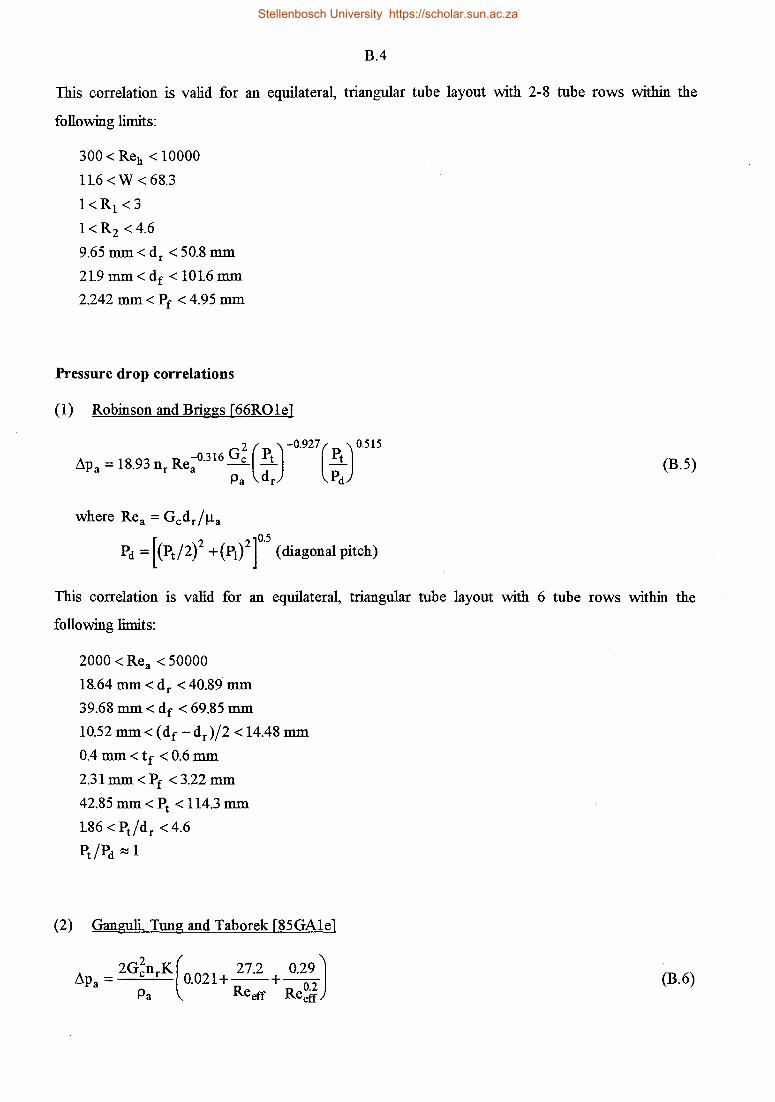
B.4

This correlation is valid for an equilateral, triangular tube layout with 2-8 tube rows within the

following limits:

300 <Reh < 10000

116 <W < 68.3

l<R1<3

l<R2 <4.6

9.65 mm< dr < 50.8 mm

219mm<dr <1016mm

2.242 mm< Pr < 4.95 mm

Pressure drop correlations

(1) Robinson and Briggs [66R01e]

L1pa = 18.93 nr Re;0.316 Ge Pt Pt 2 ( )-0.927( ) 0.515

Pa dr Pd (B.5)

This correlation is valid for an equilateral, triangular tube layout with 6 tube rows within the

following limits:

2000 < Rea < 50000

18.64 mm< dr < 40.89 mm

39.68 mm< dr < 69.85 mm

10.52 mm< (dr -dr)/2<14.48 mm

0.4 mm <tr < 0.6 mm

2.31mm<Pr<3.22 mm

42.85 mm< Pt < 114.3 mm

186 < Ptf dr < 4.6

Pt/Pd :.::J 1

(2) Ganguli Tung and Taborek [85GA1e]

(B.6)

B.5

where Reeff = ( Gcdr/µa)[ 0.5( dr - dr )/(Pr - tr) r1

K=l+ ( 2

)/ exp[-0.25(Pt-dr)/dr] l+ pt -dr dr

This correlation is valid for an equilatera~ triangular tube layout with more than 3 tube rows. The

correlation is based on the literature data of Webb [80WEle]. The following geometrical limit is

imposed:

2.5 < ( dr - dr )/[2(Pr - tr)]< 12.5

(3) Nir [91NI1e]

A 106 R -0.25 W0.45 K G2 I LlPa = · edr p nr c Pa

where Reh =Gcdh/µ 3 =4Gcdr/µ 3 W=4Redr/W

W = P[ 1[ 0.5n( df - d;) + ndrtft + ndr (Pr - tr)]

(dr -dr)(l-tr/Pr)+Pt -dr

_ (dr-dr)(l-tr/Pr)+Pt -dr R1--'-~~-'---~--''--~~

(dr-dr)(l-tr/Pr)

2{[025(P,/dr)' +(Pi/dr )2 ]°' -I+[( dr -d, )(1-trf Pr )]/dr} R1=~~~~~....,---~---,,--~~~~~---=-"~~~~-=--

Pt / dr - 1 + [ ( dr - dr )( 1- tr /Pr)]/ dr

KP = Row correction factor for pressure drop

KP= 2.08-0.83R2 , 1<R2 <1.3

KP = 1, R 2 > 1.3

(B.7)

This correlation is valid for an equilatera~ triangular tube layout with 2-8 tube rows within the

following limits:

400 < Reh < 30000

8.5 <W <57.4

9.65 mm< dr < 50.8 mm

19.35mm<dr <114.3mm

2.217mm<Pr <8.475mm

The correlations presented by Ganguli et al. [85GA1e] and Nir [91Nile] are based on original and

published experimental data, whereas those presented by Briggs, Young and Robinson [63BR1e,

B.6

66ROle] are based on their own experimental data. It is difficult to recommend a single correlation.

However, the Briggs and Young [63BRle] (heat transfer) and the Robinson and Briggs [66ROle]

(pressure drop) correlations are widely used. The correlations by Ganguli et al. [85GAle] and Nir

[91Nile] are included because they are based on a very wide range of data and therefore are

assumed to give more accurate heat transfer and pressure drop correlations.

The arrangement (staggered vs. inline) of the finned tubes in the heat exchanger as well as the tube

and fin geometry (tube pitch, fin pitch, fin height, fin thickness, number of tube rows) affect both the

heat transfer and pressure drop. The interested reader is referred to the following literature for a

detailed discussion on these topics [45JAle, 59WAle, 63BRle, 66ROle, 66VA1e, 74MI2e,

76ROle, 80WEle, 81Glle, 81SH3e, 85EC1e, 85GA1e, 88STle, 88ZUle, 89RA1e]. There exists a

substantial amount of test data in the published literature. However, careful examination of the data

and the method of experimentation is needed in each specific case to establish their usefulness in

design. The few correlations that are listed present a wide spectrum of data and have been applied in

the design of practical systems.

In the optimization process, one can vary the geometrical parameters of the finned tubes and the tube

layout in the ranges of applicability. However, the optimum design/layout is done according to

economic criteria and may not necessarily present those required for optimum performance. In any

industrial application the selection of finned tubes is dictated by the combination of the operating and

capital costs as well as a variety of technical constraints. For a finned tube module, the capital cost is

primarily related to the size and layout of the tube bundle, whereas the operating cost is primarily

related to the fan and/or the pumping power.

B.2 HEAT TRANSFER AND PRESSURE DROP CHARACTERISTICS PRESENTED IN

DIMENSIONAL FORM

A method for presenting the experimentally obtained performance data of industrial finned tubes is

evaluated by Kem [80KE1e] and modified by Kroger [86KRle]. The method presents the

performance characteristics of finned tube bundles in the form of dimensional heat transfer and

pressure drop parameters. This form of data presentation eliminates uncertainties inherent in the

evaluation of the airside heat transfer coefficient, fin efficiency, thermal contact resistance fouling

and other thermal resistances.

Finned tube performance correlations contain Nusselt and Reynolds numbers. Both these numbers

contain an equivalent or hydraulic diameter. Because of the relatively arbitrary nature of the

definition of this quantity for finned surfaces, different definitions are found in the literature. In


B.7

practice this often leads to confusion and makes any comparison of peifonnance characteristics of

different types of finned surface meaningless. The method of which a summarized derivation is

presented below, eliminates potential sources of error in well conducted experiments.

In general, the overall heat transfer coefficient can be expressed as

(B.8)

where the summation term represents all the thermal resistances other than the airside and waterside

values. The heat transfer rate can be expressed in terms of the overall heat transfer coefficient and

the logarithmic mean temperature difference as follows:

(B.9)

where Fr is the cross flow temperature correction factor [86H0Ie]. Substitute equation (B.9) into

(B.8) and find

(B.10)

Rearrange equation (B.10) and define the effective heat transfer coefficient, hae•based on the airside

surface area as follows

(B.11)

The value of haeAa can be determined experimentally.

According to Colburn [33C01e] the heat transfer coefficient under conditions of forced convection

through finned surfaces may be expressed in terms of dimensionless parameters as

(B.12)

In the absence of the equivalent diameter, equation (B.12) may be written as

(B.13)

where Ry = ma/ (Afr µa) (characteristic flow parameter)


B.8

The effective finned surface area and the heat exchanger frontal area play a major role in comparing

and optimizing heat exchangers. These geometric parameters may be introduced into equation

(B.13) such that

N ha~a R bNy ( h . . h c. ) Y = 0_33 = a Ny y c aractenst1c eat trans.ier parameter Afrka Pra

(B.14)

All the physical properties are evaluated at the arithmetic mean temperature.

The pressure drop across a finned tube heat exchanger during isothermal flow conditions may also be

expressed in dimensionless form based on the free stream conditions as

E - A I 2 - R b3 uiso - 0 Piso Pav a - a3 e (B.15)

If the equivalent diameter is not included in this equation it may be written as

EYiso = Pa~Piso/ µ; = aEy Re bEy = Euis0 Ry2 (characteristic pressure drop parameter) (B.16)

A corresponding pressure loss coefficient based on the total pressure difference across the heat

exchanger can be defined as

(B.17)

The performance correlations presented in equations (B.14) and (B.17) are determined

experimentally. These correlations enable one to compare different finned surfaces (of any

geometry) directly and can be used in optimization studies where fixed finned surfaces are

considered. The finned tube geometrical parameters are subsumed in the constants a and b.

It should however be stressed that to date no correlation exists that accurately predicts the

performance over a wide spectrum of finned tube geometries and operating conditions.

Discrepancies do exist in literature correlations [86KRle]. Therefore, the final design of a costly air

cooled heat exchanger system cannot be based on approximate correlations. In such cases specific

performance tests should be conducted on the finned tubes to be used.


C.l

APPENDIXC

FORCED DRAFT DIRECT AIR-COOLED CONDENSERS

C.1 INTRODUCTION

The performance prediction of air-cooled condensers are based on two sets of governing equations,

i.e. the draft equation and the heat transfer equations. The governing heat transfer and draft

equations will be derived in this appendix (also refer to [83Slle, 91COle]). The coupling of the air

cooled condenser to a turbo-generator unit, as found in power plants, is also discussed. The results

of a considerable amount of experimental and theoretical work are taken into account to model all

the physical phenomena of such a system The search for economically viable air-cooled condenser

operation requires the proper formulation and modeling of the system The variables and constraints

required to perform this task are defined and discussed.

C.2 DESCRIPTION OF THE DIRECT AIR-COOLED CONDENSER

In the direct condensing air-cooled heat exchanger (ACHE), also referred to as air-cooled

condensers (ACC), the process fluid (low pressure turbine exhaust steam in the case of power plants)

is channeled directly to the air-cooled heat exchanger bundles, as shown in figure C.1. The heat

exchanger bundles can consist of one or more rows of finned tubes. The steam pressure inside the

exhaust duct and the ACC is lower than atmospheric pressure. The turbine exhaust steam duct has a

large diameter and is required to be as short as possible to minimize pressure losses. In very large

ACHEs the finned tube bundles are usually sloped at some angle with the horizontal (A-frame

arrangement) in order to reduce the plot area. This arrangement is also frequently used in condensing

plants due to good condensate discharge. Horizontal finned tube arrangements are also found in

many industrial applications.

Steam enters the top of the air-cooled heat exchanger bundles (finned tubes) and condenses as it

flows downward with the steam and the condensate flowing in the same direction. In actual

inStallations, provisions are made for the removal of noncondensable gasses and air (dephlegmator)

and for the prevention of freezing during cold weather (airflow control) [77SCle, 77SU1e, 78LA1e,

80RUle, 81KOle, 83PAle, 83SHle, 85MOle, 85M02e, 870Sle]. The airflow across the heat

exchangers is created by means of axial flow fans, i.e. the steam is condensed by forced convection


C.2

of air flowing over the heat exchanger bundles. The condensate that collects in the condensate tank

is pumped back to the boiler feedwater circuit.

Steam turbine

Condensate pump

Condensate storage tank

Steam

Exhaust steam duct

Supply header

Heat exchanger bundles

Condensate header

Condensate

Figure C. l: Forced draft direct air-cooled condenser (A-frame arrangement).

C.3 HEAT TRANSFER AND PRESSURE DROP DURJNG CONDENSATION

The finned tube elements are the heart of any air-cooled condensing plant. The air-cooled heat

exchanger may consist of one or more rows of finned tubes, each row having a different fin pitch.

The transfer ofheat from the process fluid to the air is influenced by a number of variables:

( 1) The temperature difference between the process fluid and the air.

(2) The design and surface arrangement of the finned tube bundles.

(3) The velocity of the air flowing across the finned tubes.

( 4) The velocity and physical properties of the process fluid.

Consider the forced draft air-cooled condenser shown schematically m figure C.2. In this

configuration the heat exchanger bundles are arranged in the form of an A-frame to drain the

condensate effectively, reduce the steam duct lengths and minimize the required ground surface area.

A windwall is provided to reduce recirculation of the hot plume air.

The amount of heat transferred from the condensing process fluid to the air stream can be expressed

as

(C.1)


C.3

Sub cooling of the condensate is neglected in the above relation and it is assumed that all the steam

entering the finned tubes is condensed. The thermophysical properties of the air will be determined

at the mean temperature and atmospheric pressure at ground level.

181

Windwall

Heat exchanger

Condensate drain

Walbvay

Supports

Figure C.2: Air-cooled condenser unit

Support bridge and drive

Steam header

~h-\

s~~ ~~~~~~ ... ] .. C. ~~.

. ....

If the geometry of the finned tubes changes in consecutive rows and performance data is available for

the individual rows, the heat transfer equation may be written as

(C.2)

Furthermore, the effectiveness of the condenser bundle or each tube row can be expressed as

[86H01e]

e(i) = 1- exp [-(UA )(i) / { m 3 Cpam(i))]

With this expression the heat transfer rate becomes

n,

Qac = L ma cpam(i) ( Tvm(i) -Tai(i)) e(i) i=l

(C.3)

(C.4)


C.4

The product of the overall heat transfer coefficient and area for each tube row can be expressed as

(C.5)

where

o.333 ( I ) hae(i)Aa(i) = kam(i) Pram(i) Arr NY (i) ntb(i) ntb(max) (C.6)

and

(C.7)

for any finned tube geometry, and

(C.8)

for radially finned tubes. The frontal area of the heat exchanger bundle corresponds to the area

covered by the maximum number of tubes per row in a multiple tube arrangement. Ry is corrected

for this effect. Furthermore, Ny is based on heat exchanger bundle tests in which the maximum

number of finned tubes are installed in the bundle. In actual heat exchanger bundles it is not practical

to install half-tubes and a correction is made when determining the effective heat transfer coefficient.

The effectiveness of the circular finned surface is expressed in terms of the fin efficiency, i.e.

(C.9)

According to Schmidt [46SC1e], the fin efficiency for radial fins of uniform thickness can be

determined approximately from

tanh(bdr /2 )(i)

llf(i) = (bdr /2 )(i) (C.10)

For galvanized steel fins, the fin thickness can be expressed as tr = 2tg +ts and the thermal

conductivity of the fin can be expressed as kr = (2tgkg +tsks)/tr.

The performance characteristics of the finned tubes are discussed in Appendix B and correlations are

stated to determine the airside heat transfer coefficient and the characteristic heat transfer parameter.

C.5

The pressure losses in the turbine exhaust steam duct and at the inlet to the finned tubes are

expressed as

~p sd = 0.5 Pvi(l) V~i(l) { 1- CJ~ +Kc + Ksd) (C.11)

where crc is the tube inlet contraction area ratio and the contraction loss coefficient, Kc ~ 0.6 (sharp

inlet). Ksd is the loss coefficient for the steam duct system The mean saturation pressure of the

steam at the inlet of the finned tubes, p vi, is calculated by subtracting ~p sd (equation ( C.11)) from

the mean saturation steam pressure at the turbine outlet. The mean steam temperature at the inlet of

the finned tubes, Tvi> is obtained from equation (A.5). The inlet conditions (thermophysical

properties) of all the tube rows are thus assumed to be equal.

Due to pressure changes along the finned tube and in the direction of air flow, the condensation

process will not take place at a constant temperature. The mean static pressure in the finned tubes

can be determined from the correlations given by Groenewald and Kroger [94GR1e].

2 0.1582µviLt ( 2.75 1.75 ) 2 2

Pvm(i) = Pvi - 3 0.267al(i) Revi(i) +0.364a2(i) Revi(i) +- PviV vi(i) Pvide Revi(i) 3

(C.12)

The coefficients a1 and a2 are functions of the suction Reynolds number, Revn. For round tubes,

these coefficients are

-3 -6 2 al(i) =1.0046+1.719xl0 Revn(i)-9.7746x10 Revn(i)

2 a2(i) = 574.3115+24.2891Revn(i)+ 18515Revn(i) (C.13)

and the suction Reynolds number is expressed as

(C.14)

For non-round tubes (elliptical or flattened tubes or ducts) with a high aspect ratio, these coefficients

are

-3 -7 3 al(i) = l.0649+10411x10 Revn(i)-2.0llxlO Revn(i)

-2 3 a2(i) = 290.1479+59.3153Revn(i)+15995x 10 Revn(i)

and the suction Reynolds number is expressed as

Re . ~ Pviv vi(i)de Wt _ Re . . Wt vn(1) µ . 2L - v1(1) 2L

~ t t

(C.15)

(C.16)


C.6

It is assumed that condensation occurs at the mean steam temperature, Tvm(i)' corresponding to the

mean steam pressure inside the tubes (refer to equation (A.5)).

It should be noted that the pressure drop in the different tube rows is usually not identical, with the

result that backflow of steam will occur [78LA1e]. To avoid this and the corresponding

accumulation of noncondensables, a dephlegmator is usually installed after the condenser.

For non-round tubes (elliptical or flattened tubes or ducts) the correlation of Groenewald [93GR1e]

is employed to determine the mean condensation heat transfer coefficient, i.e.

[ ]

0.333

L k3

(")P2

(·)gcos(90° -Sb)if: (") hc(i) = 0.9245 t cm

1 cm 1 g

1 (C.17) µcm(i)ma1Cpam(i)(Tvm(i) -Tai(i))[ 1- exp{-(uc(i)HtLt )/(ma1Cpam(i) )} ]

By neglecting the thermal resistance of the condensate film, the approximate overall heat transfer

coefficient based on the condensation surface area can be expressed as

(C.18)

The air mass flow rate flowing on one side of the finned tube is

(C.19)

For round tubes, the mean condensation heat transfer coefficient for inclined tubes according to

Schulenburg [69SC1e] is used, i.e.

h _ 1197( . e )0.115 kcm(i) Pcm(i)µvm(i) R 0.325 ( )

0.5

c(i) - sm b evi(i) di Pvm(i)µcm(i)

(C.20)

This equation is valid within the following ranges: 5°.::::; eb.::::; 90° (angle of inclination with respect to

the vertical), 10950.::::; Revm = RevJ2.::::; 14150 and 6525N/ m2

.::::; Pvm ::5 8085N/m2.

Ac(i)' referred to in equation (C.5), is the inside tube area of tube row (i) exposed to the condensing

steam

The energy balance for the forced draft air-cooled condenser thus requires that the following

relationships be satisfied for each tube row:

(C.21)


C.7

C.4 DERIVATION OF THE DRAFf EQUATION FOR A FORCED DRAFf AIR

COOLED CONDENSER

The draft equation describes the relation between the various flow resistances encountered, the

atmospheric conditions, heat exchanger dimensions, the heat exchanger bundle performance

characteristics and the fan performance characteristics at a given flow rate. The draft equation is

derived similarly to the procedure described in Kroger [94KR2e]

Significant changes in the ambient air temperature occur near the ground level during any 24-hour

period [94KRle]. During the day, a temperature lapse rate of -0.00975 Kim, also known as the dry

adiabatic lapse rate (DALR), is observed in the region of the surface boundary layer (SBL). For this

analysis, the specified ambient air temperature at any elevation z, will be assumed to be given by the

equation

Taz = Tal - 0.00975 Z (C.22)

To derive the draft equation, consider the variation with elevation of the pressure in the atmosphere

external to the air-cooled condenser in a gravity field, i.e.

(C.23)

Substitute equations (C.22) and (Al), the perfect gas law, into equation (C.23) and integrate to find

the pressure difference between point 1 and a point at elevation z external to the air-cooled

condenser (refer to figure C.2)

[ ( ) 102.564g/R] [ ( )3.5] Pa1-Paz=Pa11- l-0.00975z/Tai ~Pal 1- l-0.00975z/Tal (C.24)

According to equation (C.22), the approximate air temperature before the fan can be expressed as

(C.25)

The approximate temperature at the inlet to the heat exchanger bundle can be derived from the first

law ofThermodynamics (conservation of energy) and can be expressed as [94KRle, 94KR2e]

(C.26)

where H5 ~ H6 is the mean heat exchanger height above the ground level.

Stagnant ambient air at 1 accelerates and flows across the heat exchanger supports at 2 before

reaching the fan at section 3, where upstream obstacles such as structural supports or a safety screen

may be located. After leaving the fan at 4 where further downstream obstacles may be located, the


C.8

flow experiences losses in the plenum before entering the heat exchanger bundle at 5 and exiting at 6.

Additional flow losses are encountered due to the inclined flow approaching and leaving the heat

exchanger bundles.

Taking into consideration all the flow losses, the pressure difference between sections 1 and 7 can be

expressed as [94KR2e]

Pal -Pa7 =Pa1[1-(l-0.00975H6/Ta1)3·5]+Kts(ma/A2)

2 /(2Pa2)

+Kup(ma/A3)2

/(2Pa3)-Pa3Pp/ma +Kdo(ma/A4)2

/(2Pa4)

+Kpl (ma/Apc)2

/(2Pa4)+Ket (ma/Arr)2

/(2Pa56)

+Pa6[1-{1-0.00975(H1-H6)/Tai}3·5] .

(C.27)

When evaluating the effective frontal area, Arr, obstructions like straps or stiffening beams located

up against the finned surface and thus impeding flow through it, must be taken into consideration. In

all the heat transfer and pressure drop calculations, the effective finned tube length, Lt , is used as a

result.

Fan performance characteristics incorporated in the Pa3 Pp /ma term are obtained from standard

installation tests. According to Venter [90VE1e], the total dynamic component after the fan is

dissipated in the plenum when the fan is operating in its application range. For this configuration,

Kpl = aeP and it follows that

(C.28)

where the fan static coefficient is defined as

(C.29)

Ape is the fan casing cross-sectional area and the fan static pressure, Lipps, is obtained from fan

performance tests conducted according to certain test codes [94KR.le, 94KR.2e].

If the ambient air far from the heat exchanger is dry and the temperature distnlmtion is according to

the DALR, the difference in pressure between 1and8 is according to equation (C.24)

Pai-Pas =Pal -Pa7 =(Pa1-Pa6)+(Pa6-Pa1)

:::! Pai[ 1-(1-0.00975H6/Ta1)35

]+pa6[ 1-{1- 0.00975(Hs - H6)/Ta1}3"5]

(C.30)


C.9

where the ambient air temperature at elevation 6 is assumed to be approximately equal to T31 .

Although the air temperature distribution near ground level generally deviates considerably from the

DALR, the error introduced by this assumption in equation (C.30) is small for large units.

Substitute equation (C.30) into equation (C.27) and find with equation (C.29) the draft equation for

the air-cooled condenser shown in figure C.2 (H7 = H 8)

Pa1[ {1-0.00975(H1 - H6)/Ta6 }3·5

-{l-0.00975(H1 - H6)/Tai}3·5]

= Kts(ma/A2)2

/(2Pa1)+Kup (ma/AFe)2

/(2Pa3)-KFs(ma/AFc)2

/(2Pa3)

+ Kdo (IDa/AFe)2

/(2Pa3)+ Ket (ma/Afr )2

/(2Pa56)

(C.31)

where it is assumed that Paz ::::i Pal, p34 ::::i p33 and Pa7 ::::i Pa6. Furthermore, the area on which the

upstream and downstream flow obstacles are based is defined as A Fe= A3 = A 4 =(A Fe -AFh),

where A Fe and A Fh are the fan casing and hub cross-sectional areas respectively.

The approximate air density at section 3 is

(C.32)

The density of the air immediately after the heat exchanger is

(C.33)

and the harmonic mean density through the heat exchanger is given by

(C.34)

In the above equations the thermophysical properties of dry air (Appendix A) are usually employed

since the influence of moisture is a negligible factor in determining the forced draft air-cooled heat

exchanger's draft.

The loss coefficient of the air-cooled condenser supports, Kts, is based on the drag coefficient of

these supports, i.e.

(C.35)

The effective pressure drop across the air-cooled condenser supports is given by

(C.36)


C.10

where Lts is the support length and dts is its effective diameter or width, and nts is the number of

supports, while A 2 is the corresponding free flow area into the air-cooled condenser. The

corresponding loss coefficient based on these conditions at section 2 is

(C.37)

The loss coefficients due to the flow obstacles at both the fan suction (upstream) and discharge

(downstream) sides are obtained from the bulk method proposed by Venter and Kroger [91VEle].

The bulk method [85VEle] is related to the total blockage area of the different flow distorting

components, as well as the distance between the fan rotor and the respective components. These

loss coefficients are obtained from figures C. 3 and C.4 (copied from [85VE 1 e ]).

The pressure loss across the heat exchanger bundles and the kinetic energy losses at the outlet

elevation (section 7) are derived by Van Aarde and Kroger [93V Ale] for an A-frame heat exchanger

array. For non-isothermal oblique flow through an A-frame heat exchanger bundle, the loss

coefficient is

Ket=Kh· +-2-(Pa5-Pa6)+( 1 _ 1l( 1 -l+ 2K~·5)( 2Pa6 )-+ eiso cr2 Pa5 +Pa6 sin Sm J sin Sm Pa5 +Pa6 O"fl

+K ( 2Pa5 ) d Pa5+Pa6

(C.38)

where a is the ratio of the minimum free flow area through the heat exchanger bundle to the free

stream flow (frontal) area and crfl is the ratio of the fin leading edge frontal area to the free stream

flow area.

The heat exchanger loss coefficient under normal non-isothermal flow conditions, including inlet-,

frictional-, and exit losses as well as acceleration effects (due to heating), is defined as (refer to

AppendixB)

K = a RybK + ~(Pa5 - Pa6) he K 2

a Pa5 +Pa6 (C.39)

for finned tube bundles with any finned tube geometry. For radially finned tubes the heat exchanger

loss coefficient under normal non-isothermal flow conditions can, in general, be expressed as

[86KRle]


C.11

Khe = -3z[Eu+(Pa5 -Pa6)] = -3z[L1Pa~am +(Pa5 -Pa6)] <J Pa5 + Pa6 <J Ge Pa5 + Pa6

(C.40)

The Euler number can be obtained from the pressure drop correlations discussed in Appendix B.

1.4 0.05

1.2 x =Distance from obstacle to front of fan blade-----1

§' 0.8 ~

0.6

0.4

0.2

0.0

0.00 0.05 0.10 0.15 0.20 0.25

Figure C.3: Loss coefficients for flow obstacles at the fan suction side (upstream).

.g

1.6 0.05

1.4 x =Distance from obstacle to rear of fan blade------..c-1

1.2 x/dFc = 0.05 - 0.2

1.0 0.1

~ 0.8

0.6

0.4

0.2

0.0

0.00 0.05 0.10

0.15

0.15 0.20 0.25

Figure C.4: Loss coefficients for flow obstacles at the fan discharge side (downstream).

C.12

The second term on the right hand side of equation (C.38) represents the loss due to acceleration

effects during non-isothermal operation. The third term represents the loss due to the oblique flow

at the inlet to the bundle. The entrance contraction loss coefficient, Kc, is according to Kays

[50KA1e]

11(1 )12

Kc=l- --1 J 0"21 O"c

(C.41)

where cr21 = {Pr - tr) /Pr is the ratio of the flow area between the fins to the free stream flow area at

the inlet to the finned tube bundles. The contraction coefficient, crc, for flow between parallel plates

is given by

2 3 4 CTc = 0.6144517+0.04566493cr21 -0.336651cr21 +0.4082743cr21 +2.672041cr21

-5.963169cr~1 +3.558944cr~1 (C.42)

For round and elliptical fins a value of Kc:::::: 0.05 is assumed.

When the finned tube bundles are arranged in the form of A-frames, the curvature of the downstream

flow patterns cause the actual mean flow incidence angle to differ from the heat exchanger bundle

semi-apex angle eb. An empirical correlation for the mean flow incidence angle is presented by

Kotze et al. [86K01e], i.e.

2 em= 0.00198b +0.91338b -3.1558 (C.43)

Kd is the downstream loss coefficient that consists of two components, namely the turning and

jetting losses in the V-region, Kdj' and the loss of kinetic energy into the atmosphere, K 0 • The

following empirical correlations for these losses are obtained from Van Aarde and Kroger [93VA1e]

28 2 3 2 . [ ]

0.4 0 5

x eb +(exp(2.36987+5.8601xl0- eb-3.3797x10- eb)) (C.44)

and


C.13

(C.45)

where Lw is the half-width of the walkway between the A-frames. Thus, Kd = Kdj + K0 . Both

equations (C.44) and (C.45) are valid within the following limits:

20° ::;eb::; 35°

0.5dsh/Lt 0 ::; ::; 0.17886 sin Sb + Lw /Lt

0::; Lw /Lt ::; 0.09033

0::; dsh /Lt ::; 0.303 for Lw = 0

Khe:::: 30 (uniform normal velocity distribution)

If performance correlations from oblique flow experiments are available, the pressure loss coefficient

for the heat exchanger bundle under non-isothermal flow conditions has the following form

(C.46)

Equation (C.31) is known as the draft equation for a forced draft air-cooled heat exchanger where

the heat exchanger bundles are arranged in the formation of A-frames. This equation can be

rewritten with all the loss coefficients based on the heat exchanger frontal area and the mean

harmonic air density through the heat exchanger bundle. Multiply equation (C.31) by

2Pa56(Afr/m3 )

2 to obtain

2Pa56(Afr/ma)2Pa1[ {l-0.00975(H1 -H6)/Ta6 }

3'5

-{l-0.00975(H1 - H6)/Ta1}3·5]

= Kts(Afr /A2)2(Pa56/Pa1)+ Kup(Afr/ AFe)\Pa56/Pa3)-KFs(Afr/ AFc)

2(Pa56/Pa3)

+ Kdo(Afr/AFe)2

(Pa56/Pa3)+ Ket

(C.47)

By means of equation (C.47) it is possible to compare the magnitude of the loss coefficients directly.


C.14

C.5 FAN PERFORMANCE CHARACTERISTICS

The choice of a suitable axial flow fan must be such that it will efficiently deliver a cooling air flow

rate that will guarantee the desired heat transfer rate. In ACHE systems, the design of the fan system

is as important as the heat exchanger. In order to achieve this, a series of resistances must be

overcome [94KR2e]. It is, however, possible to rearrange the draft equation and obtain the system

resistance curve as a function of the air mass flow rate. The point where the system resistance curve

meets the fan performance curve at the desired air mass flow rate, defines the fan operating point.

The performance characteristics of an axial flow fan are determined experimentally according to

certain fan performance test codes, e.g. the British Standards Institution BS848 [80BS1e]. Fans

should be tested according to the method most closely representing the actual performance

conditions. Fan test results are presented in the form of a performance curve as shown in figure C.5.

300

250

200

150 ~---+Fan diameter= 9.145 m---+---~______,_ __ .....,

100

50

0

0

Blade angle = 16 ----+Air density= 1.2 kg/nf

Speed= 125 rpm

200 300 400 500 600 700 3

Volume flow rate, VF, m Is

Figure C. 5: Performance of an axial flow fan.

The fan static efficiency can be defined as

800 900

220

210 ~

200 ~~ ~

170

160

(C.48)

In practice, it is preferred that the actual air volume flow rate, corresponding to the fan operating

point, is larger than the volume flow rate at the optimum fan static efficiency. A decrease in air


C.15

volume flow rate will thus result in an increase in fan static efficiency rather than a decrease in fan

static efficiency.

The total electrical power requirement of the fans can be calculated as follows:

(C.49)

Model tests may be conducted if it is impractical to conduct full scale tests. The model must be

geometrically similar to the actual fan in all the parts which affect the air flow and its dimensions

must not exceed those of the actual fan. The actual full size fan may be expected to show a slight

improvement in efficiency. However, no allowance is made for this effect [66VDle, 80BS1e]. The

model test results can be scaled, according to the fan laws [80BSle], to obtain the prototype

performance characteristics. The fan laws are as follows (for a fixed fan blade angle):

( 1) Volume flow rate

(C.50)

(2) Fan static pressure rise

(C.51)

(3) Power consumption

(C.52)

The tip clearance of the prototype fan which results in the same fan static efficiency as measured for

the model fan is presented by the VDI fan test code [66VDle] as

(

A )0.1( d )0.8 SF 0 PFm F

SFm = L\pF dFm (C.53)

According to this equation the tip clearance ratio Sf/ dF for the prototype fan is required to be

smaller than the corresponding ratio for the model to ensure similar operating conditions. In

practice, a small tolerance between the fan casing and the fan blade is difficult to guarantee due to

the material properties and construction methods of the blades and fan casing. As a result, typical

values for tip clearances of 0.5% to 1 % of the fan diameter are employed by the manufacturers.


C.16

Performance curves for large fans are generally obtained under ideal conditions. However, in actual

installations the efficiencies are always lower than those obtained under the ideal test conditions.

The reduction can be ascribed to a number of reasons, such as a high air approach velocity when the

fan is located too close to the ground level and distorted inlet flow conditions. In large cooling

plants covering a considerable area and including numerous fans, some of the fans may be subjected

to significant cross-flow which tends to distort inlet conditions to the fan, resulting in a

corresponding reduction in performance. Flow separation at the inlet to the fan can be avoided by

attaching a well designed inlet bell to the fan housing [85VEle]. The effect of the inlet losses is

correlated by Salta and Kroger [94SAle] for more than two fan rows as a volumetric effectiveness,

1.e.

Vp = 0.985-exp[- (1+45/n)H3] = ev VFid 6.35dF

(C.54)

where n = nFr for a freestanding fan platform and n = 2nFr for a non-freestanding fan platform This

correlation is applicable for Hb / d F = 0.19 and Wp / d F = 127, where Hb is the height of the

bellmouth fan inlet from the fan platform and Wp is the fan pitch. nFr is the number of fan rows

(number of fans per bay), n Fb is the number of fan bays and the total number of fans are

np = nFrnFb· VF /VFid correlates the effect of the inlet losses on the whole fan system and states

that nFma will be less than npma,id. When using this correlation, the layout of the fan platform

must be fixed beforehand.

The actual airside heat transfer rate can be obtained by multiplying the maximum ideal airside heat

transfer rate by the fan volumetric effectiveness, ev. Thus, equation ( C.21) changes to

(C.55)

The fan motor must be selected to handle the maximum load, which will occur during operation at

low ambient air temperatures (due to the higher air density). The fan motor must be oversized by

25-30% for fans that are not autovariable and 15% otherwise [83PAle]. In large mechanical draft

dry-cooling towers incorporating axial flow fans, it is essential that the required fan power be kept as

low as possible. Ambient air is a coolant which exhibits large temperature :fluctuations. Constant

speed fan drives may result in a much higher air mass flow rate than needed at low ambient air

temperatures, which can result in freezing (in the ACC) or throttling of the steam flow (in the turbine

exit) when coupled to a steam turbine. At high ambient air temperatures the constant speed drives

may result in an air mass flow rate that is inadequate to meet the cooling demands. Thus, it seems


C.17

that the fan energy costs can be minimized by harmonizing the fan operating conditions with the

external ambient air temperatures, and the turbine performance characteristics when applicable.

The variation of the air mass flow rate can be achieved by varying the fan blade angle during

operation, the fan motor speed during operation (refer to the fan laws) or by means of louvers

[77SCle, 81KOle, 81STle, 83PAle, 85MOle, 85M02e, 93ADle]. Automatically variable pitch

(fan blade angle) fans are limited in diameter (up to ± 6 m) and automatically variable speed drives

are expensive, although in some applications they may present a more cost effective proposition than

other methods of flow control. The most common means of flow control is to switch single-speed

electric motors on (full speed) or off: or to have two-speed electric motors that allow the fans to

operate at full speed, half speed or to be switched off. Fan speed is usually limited by noise

restrictions, available gear ratios, or the manufacturer's practice. To meet noise requirements, the

rule of thumb is to limit the fan tip speed to 60 mis [83SHle].

C.6 OPERATING POINT CALCULATION

The operating point (ability to reject heat) of the fixed geometry ACC is defined as the combination

of operating variables that will simultaneously satisfy the draft and heat transfer (energy) equations

for specified turbine exhaust and ambient air conditions. This point is obtained from the intersection

of the system resistance line and the fan performance curve.

Defmition of the operating variables, operating constraints and equations to be satisfied

For a specified air-cooled condenser system geometry, specified turbine outlet conditions (Ttv, Ptv)

and specified ambient air conditions (Tdb' Twb' Pa) the following variables, constraints and equations

(balances) can be defined for the simultaneous solution of the operating point conditions:

( 1) One tube row

The operating variables are: ma, Tao(l)> Tvi' mc(l)

These variables must satisfy the following feasibility inequality constraints (bounds):

ma ::?: mal +s1 (C.56)

-ma;?: -mau +s1 (C.57)

mc(l) ;?: S2 (C.58)

Tao(l) ::?: Tai(l) + S3 (C.59)


C.18

-Tao(l) 2 -Tvi + e3

- Tvi 2 - Ttv + e 4

The following equations must be satisfied by the operating variables:

Qa(l) = Qc(l)

Qa(l) = Qac(l)

Tvi = T(pvi)

~Psystem = ~PFs

(2) Two tube rows

The operating variables are: ma, Tao(l)> Tao(2)• Tvi• mc(l)• mc(2)


ma 2 mal +e1

-ma 2-mau +e1

mc(l) 2 ez

mc(2) 2 ez

Tao(l) 2 Tai(l) + e3

-Tao(l) 2 -Tao(2) + e3

-Tao(2) 2 -Tvi + e3

-Tvi 2-Ttv +e4


Qa(l) = Qc(l)

Qa(2) = Qc(2)

Qa(l) = Qac(l)

Qa(2) = Qac(2)

(C.60)

(C.61)

(C.62)

(C.63)

(C.64)

(C.65)

(C.66)

(C.67)

(C.68)

(C.69)

(C. 70)

(C.71)

(C. 72)

(C.73)

(C.74)

(C.75)

(C.76)

(C. 77)


C.19

(C.78)

L\psystem = L\pFs (C.79)

e i are small constants and are used to introduce the ~ sign in the feasibility inequalities. The bounds

on the operating variables are introduced to safeguard against the violation of the physical laws. The

upper and lower limits on the air mass flow rate can be obtained from the fan performance

characteristic curve.

C.7 POWER GENERATION

The turbo-generator characteristics of the direct condensing system, i.e. the heat to be rejected and

the power output of the turbo-generator, are expressed in terms of the turbine back pressure, Ptv, or

the corresponding saturated vapor temperature, Ttv. The performance characteristics of an example

of such a system is shown in figure C. 6. It is assumed that the power needed for the boiler

feedpumps and other auxiliaries, excluding the fan operating power, is already subtracted from the

generated power.

240 365

235

~ 230 ~n 225 .... n

& 220 = 0 215 ..... (!)

~ 210 0 ~

205

- -............ ~ r---... /

" v I'.. /

- " / -'./ -

/ ""' / ~

/ '\. ~ __ ......

360

355 ~ 350 ~

"'O (!)

345 ...... C'CI .e-

340 en en .....

"'O

335 ...... C'CI (!)

::r: 330

200 325

40 45 50 55 60 65 70 75 80 85 90 95

Turbine exhaust saturated steam temperature, Ttv, °C

Figure C.6: Performance characteristics of a turbo-generator.

Atmospheric conditions influence the performance of air-cooled condensers, resulting in a wide

fluctuation of turbine back pressure (and the corresponding saturated steam temperature). Changes

in the ambient temperature are the most important reason for this, although other environmental

effects such as wind, inversions, solar radiation, and rain all contribute to this behavior. The mean

hourly frequency of ambient temperatures over a peri.od of one year is normally supplied in tabulated


C.20

or graphical form An example of the frequency of the dry- and wetbulb temperatures 2m above the

ground level at a particular location is shown in figure C. 7. It should be noted that the air entering

the air-cooled condenser may deviate considerably from these measured values and more detailed

information on the actual ambient temperature distribution would be preferred for more sophisticated

designs [94.KRle].

800

~ 700 :::i Wetbulb Dry bulb s 600 ::s temperature § 500 ~

1-o

& 400 rJl

~ 300 0

...::= OJ~ 200

.§ 100 E-i

0

-5 0 5 10 15 20 25 30 35

Temperature, T, ° C

Figure C. 7: Frequency of ambient dry- and wet bulb air temperatures.

The operating point of the turbo-generator is determined by matching the operating point of the air

cooled condenser and the performance characteristics of the turbo-generator (Figure C.6) at a

specific ambient air temperature selected from Figure C.7. This calculation involves the selection of

turbine exhaust conditions such that the heat to be rejected by the turbo-generator, equals the heat

absorbed by the air (heat rejected by the air-cooled condenser), i.e.

~ ~

nF L:macpam(i)(Tao(i) -Tai(i))ev = nF L:mc(i)ifg(i) i=l i=l

n,

= nF L:maCpam(i)(Tvm(i) -Tai(i))e(i)ev i=l

= Qtg

(C.80)

At this point the power requirement of the fans as well as the generator power output are known.

Subtract the total power consumed by the fans from the generator power output to find the net

power output of the plant. The net power output is multiplied by the corresponding number of


C.21

operating hours to give the net energy output for this period. These calculations are repeated for

each of the ambient temperatures listed to obtain the total annual net energy output.

In the cases when very low ambient temperatures are experienced, it is possible that the air-cooled

condenser can dissipate more heat than the amount required by the turbo-generator characteristic at

its bottom limit. As the turbine back pressure decreases, more power can be generated due to the

more complete expansion of steam through the turbine. The ACC will tend to lower the turbine

exhaust pressure under these conditions, thus giving rise the a phenomenon called "choking"

(71HAle, 71HEle, 91SZ1e]. No further advantages are obtained by lowering the turbine back

pressure and turbine losses may become excessive due to high steam velocities. As performance of

the air-cooled condenser deteriorates with increasing ambient air temperatures, the turbine back

pressure increases, resulting in a decrease in power generation. The maximum allowable turbine

exhaust pressure is such that flow induced vibration of the turbine blades will not occur for lower

values (91SZle]. When reaching the upper limit of the characteristic curve, the turbine load must be

reduced. The variation of air mass flow rate, as discussed in section C.5, should be considered to

overcome these difficulties and to give optimum utilization of the fans (auxiliary power needed) and

the cooling demands to be met during annual operation (77SCle, 81KOle]. Air humidification can

also be used as a means to increase the cooling capacity during high ambient air temperatures

[83PAle, 94KRle].


For a fixed air-cooled condenser system geometry, a fixed turbo-generator characteristic curve and

an annual frequency of ambient temperatures (at a constant pa ), the following variables, constrnints

and equations (balances) can be defined for the simultaneous solution of the operating point

conditions during the annual operation:

( 1) One tube row

The operating variables are: ma, Tao(l)• Tvi' mc(l)' Ttv

These variables must satisfy the following constraints (bounds):

Equations (C.56), (C.57), (C.58), (C.59), (C.60), (C.61), as well as

Ttv ;::: Ttv1 +Es

-Ttv ;:::-Ttvu +Es

(C.81)

(C.82)


C.22

The upper and lower limits on the turbine exhaust steam temperature can be obtained from the

turbo-generator characteristic curve.


Equations (C.62), (C.63), (C.64), (C.65) as well as

(2) Two tube rows

The operating variables are: m3 , Tao(l)' Tao(2)' Tvi' mc(l)' mc(2)' Ttv


Equations (C.66), (C.67), (C.68), (C.69), (C.70), (C.71), (C.72), (C.73) as well as


Equations (C.74), (C.75), (C.76), (C.77), (C.78), (C.79) as well as

np( Qa(l) + Qa(2)) = Qtg

(C.83)

(C.84)

(C.85)

(C.86)

With the turbo-generator's operating point known, the net power output of the plant at that specific

condition is calculated as follows:

(C.87)

For each temperature data set (consisting of a drybulb air temperature, a wet bulb air temperature and

the annual duration of these temperatures), a new set of operating variables with bounds are defined

and used to determine the turbo-generator's operating point. The net annual energy output of the

plant is thus

n

Enet = L Pnet(i) 't (i) i=l

(C.88)

where n is the number of temperature frequency data sets and 'tis the duration of these temperatures.

When the ambient conditions are such that the air-cooled condenser can dissipate more heat than

required by the turbo-generator characteristic, fans are switched off to control the air mass flow rate

in order to achieve the desired cooling capacity.


C.23

C.8 OPERATING POINT OPTIMIZATION

Operating point optimization involves the process of finding the combination of operating and

geometrical variables that will minimize the total annual cost (capital and operating) of the ACC for

specified turbine exhaust conditions (Ttv,Ptv), specified ambient air conditions (Tdb' Twb,Pa) and

specified heat transfer rate QACC, while satisfying all the imposed constraints.

Optimization variables

Table C.1: Optimization variables ( ./ = applicable; JC= not applicable)

Number Variable Round tubes Finned tubes with circular with fixed fins 2eometry

1 ma ./ ./

2 Tao(l) ./ ./

3 Tao(2) ./ ./

4 Tvi ./ ./

5 mc(l) ./ ./

6 mc(2) ./ ./

7 Ttv ./ ./

8 H3 ./ ./

9 dF ./ ./

10 SF ./ ./

11 NF ./ ./

12 nb ./ ./

13 ntb(max) ./ ./

14 Lt ./ ./

15 eb ./ ./

16 do ./ JC

17 tt ./ JC

18 tr ./ JC

19 dr ./ JC

20 tr ./ JC

21 tg ./ JC

22 pf(l) ./ JC

23 pf(2) ./ JC

24 pt ./ JC

The optimization variables defined for the round tubes with circular fins use the airside performance

correlations specified in Appendix B.1, while the variables defined for finned tubes with any


C.24

geometry use the peiformance correlations defined in Appendix B.2. The optimization variables are

defined for finned tube bundles having one or two tube rows. The operating variables are also

considered as optimization variables because the ACC model is included as equality and inequality

constraints (balances and bounds) in the minimization problem formulation (integrated approach).

The operating variables (numbers 1-6) are, as a result, always present during optimization, whereas

the geometrical variables (numbers 8-24) can be kept constant or varied during the optimization

process.

Objective function

The objective function requires that the total annual cost be minimized. The construction of the

objective function from its various capital and operating cost components is discussed in Appendix

E. The total annual cost is

Ctotal = Coperating + Cmaintenance + CFCR ($/annum)

Constraints

( 1) One tube row

The following equality constraints must always be satisfied:

Equations (C.62), (C.63), (C.64), (C.65) as well as

n FQa(l) = QACC

The following inequality constraints must always be satisfied:

Equations (C.56), (C.57), (C.58), (C.59), (C.60), (C.61), as well as

-v vi(l) ~ -120 (The steam velocity at the tube inlet must be less than 120 mis.)

(2) Two tube rows


Equations (C.74), (C.75), (C.76), (C.77), (C.78), (C.79) as well as

nF( Qa(l) + Qa(2)) = QACC


Equations (C.66), (C.67), (C.68), (C.69), (C.70), (C.71), (C.72), (C.73) as well as

-v vi(l) ~ -120

(C.89)

(C.90)

(C.91)

(C.92)

(C.93)


C.25

-v vi(2) ~ -120 (C.94)

The following general inequality constraints (geometrical constraints) must be satisfied, depending

on whether or not the relevant optimization variables are varied during the optimization process:

The ratio of the fan unit's width and the fan unit's length to the fan diameter must be kept within

practical limits to assure a reasonable heat exchanger normal approach velocity (2 to 4 mis). The

ratio of the total heat exchanger frontal area to the fan casing area usually ranges from 1.8 to 2.6.

(C.95)

15dF -2Lt sin8b ~ 0 (C.96)

(C.97)

(C.98)

The fan blade angle must lie within the limits imposed by the fan performance characteristics.

(C.99)

(C.100)

The heat exchanger bundle width is limited by transport requirements.

(C.101)

The tip speed of the fan blade is usually limited to 60 mis to control noise.

(C.102)

The correlations of the downstream loss, Kd , are valid within the following limits:

(C.103)

(C.104)

(C.105)

(C.106)

(C.107)

For round tubes with circular fins, the following inequality constraints are imposed (refer to

Appendix B.1 ):


C.26

The finned tubes must be kept from touching.

Pt -dr ~ o (C.108)

The fin diameter must exceed the fin root diameter (extended airside surface area is required).

(C.109)

Due to structural considerations, the fin root thickness and the tube thickness must exceed their

lower limits.

(C.110)

(C.111)

For effective cleaning and where airside fouling is of significance, the fin pitch must exceed the

imposed lower limit.

Pr(l) - pfl ~ 0

Pr(2) - pfl ~ 0

The galvanizing thickness ~ust lie within practical limits.

tg -tgl ~ 0

tgu -tg ~ 0

The fin thickness is limited by the manufacturing processes.

tr -tfl ~ o

The fin pitch must exceed the fin thickness.

Pr(l) -tr~ o

Pr(2) -tr~ O

(C.112)

(C.113)

(C.114)

(C.115)

(C.116)

(C.117)

(C.118)

The application limits of the finned tube performance correlations, as discussed in Appendix B

(section B .1 ), are not used as constraints during the optimization of circular finned tubes.

The following assumptions and relations are used to obtain values for the geometrical parameters

linked to the optimization variables:

ntb(l) = ntb(max) for 1 tube row


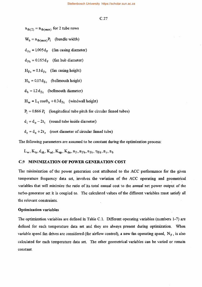
ntb(2) = ntb(max) for 2 tube rows

Wb = ntb(max)Pt (bundle width)

dFc = 1005dF (fan casing diameter)

dFh = 0.165dF (fan hub diameter)

HFc = O.ldFc (fan casing height)

Hb = 0.15dFc (bellmouthheight)

db= 12 dFc (bellmouth diameter)

Hw =Lt cos9b +0.3dFc (windwallheight)

C.27

P1 = 0.866 Pt (longitudinal tube pitch for circular finned tubes)

di = d0 - 2tt (round tube inside diameter)

dr = d0 + 2tr (root diameter of circular finned tube)

The following parameters are assumed to be constant during the optimization process:

C.9 MINl1\1IZATION OF POWER GENERATION COST

The minimization of the power generation cost attnlmted to the ACC performance for the given

temperature frequency data set, involves the variation of the ACC operating and geometrical

variables that will minimize the ratio of its total annual cost to the annual net power output of the

turbo-generator set it is coupled to. The calculated values of the different variables must satisfy all

the relevant constraints.


The optimization variables are defined in Table C. l. Different operating variables (numbers 1-7) are

defined for each temperature data set and they are always present during optimization. When

variable speed fan drives are considered (for airflow control), a new fan operating speed, NF, is also

calculated for each temperature data set. The other geometrical variables can be varied or remain

constant.


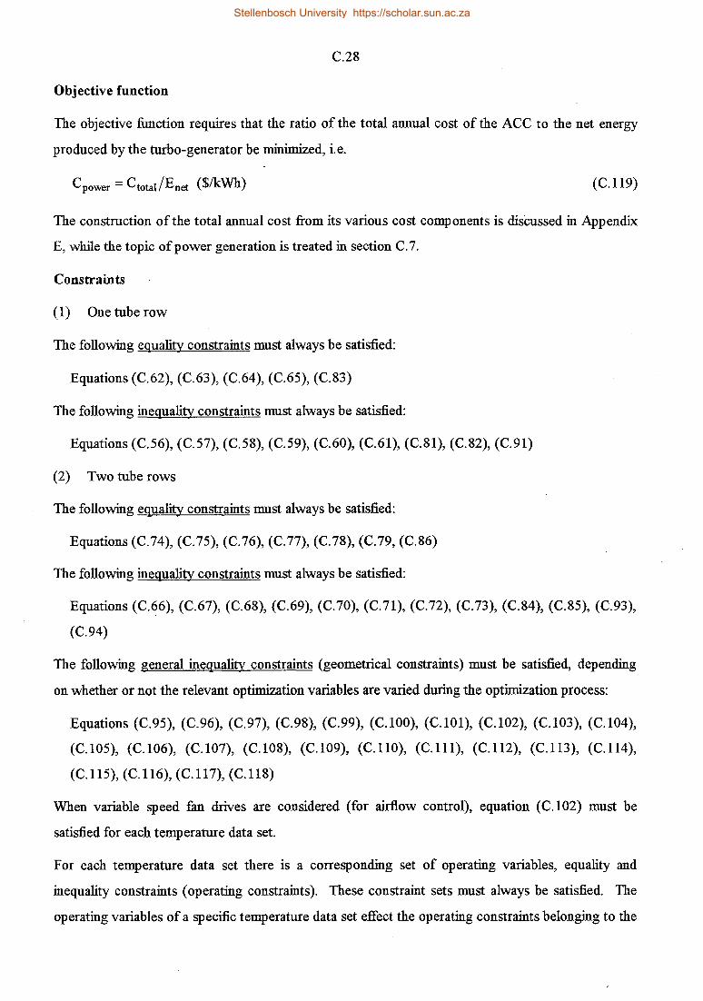
C.28

Objective function

The objective function requires that the ratio of the total annual cost of the ACC to the net energy

produced by the turbo-generator be minimized, i.e.

(C.119)

The construction of the total annual cost from its various cost components is discussed in Appendix

E, while the topic of power generation is treated in section C. 7.

Constraints

( 1) One tube row


Equations (C.62), (C.63), (C.64), (C.65), (C.83)


Equations (C.56), (C.57), (C.58), (C.59), (C.60), (C.61), (C.81), (C.82), (C.91)

(2) Two tube rows


Equations (C.74), (C.75), (C.76), (C.77), (C.78), (C.79, (C.86)


Equations (C.~6), (C.67), (C.68), (C.69), (C.70), (C.71), (C.72), (C.73), (C.84), (C.85), (C.93),

(C.94)



Equations (C.95), (C.96), (C.97), (C.98), (C.99), (C.100), (C.101), (C.102), (C.103), (C.104),

(C.105), (C.106), (C.107), (C.108), (C.109), (C.110), (C.111), (C.112), (C.113), (C.114),

(C.115), (C.116), (C.117), (C.118)

When variable speed fan drives are considered (for airflow control), equation (C.102) must be

satisfied for each temperature data set.

For each temperature data set there is a corresponding set of operating variables, equality and

inequality constraints (operating constraints). These constraint sets must always be satisfied. The

operating variables of a specific temperature data set effect the operating constraints belonging to the


C.29

same temperature data set only. Tue operating variables do not effect the geometrical constraints.

However, the geometrical variables effect all the operating constraints of the different temperature

data sets.


D.l

APPENDIXD

NATURAL DRAFT INDIRECT DRY-COOLING TOWERS

D.1 INTRODUCTION

The performance prediction of dry-cooling towers are based on two sets of governing equations, i.e.

the draft equation and the heat transfer equations. The governing heat transfer and draft equations

will be derived in this appendix. The coupling of the indirect dry-cooling tower to a turbo-generator

unit, as found in power plants, is also discussed. The results of a considerable amount of

experimental and theoretical work are taken into account to model all the physical phenomena of

such a system The search for economically viable dry-cooling tower operation requires the proper

formulation and modeling of the system The variables and constraints required to perform this task

are defined and discussed.

D.2 DESCRIPTION OF THE INDIRECT DRY-COOLING TOWER

Indirect dry-cooling systems make use, either of surface (conventional) condensers or spray Get)

condensers to condense the process fluid (steam). The secondary fluid (water) that is used to

condense the process fluid is cooled by the cooling tower. Only the indirect dry-cooling system

employing a surface condenser and water as the secondary cooling fluid will be considered in this

study. As shown in figure D. l, cold water flows through the tubes of the condenser and removes

heat from the steam passing over them This heated water is pumped through the finned tubes of the

heat exchanger bundles arranged in the natural draft cooling tower. This water is cooled by natural

convection of air flowing over the extended surface heat exchanger bundles. The density of the

heated air.inside the tower shell is less than that of the atmosphere outside the tower, with the result

that the pressure inside the tower is less than the external pressure at the same elevation. The

pressure differential causes air to flow through the tower at a rate which is dependent on the various

flow resistances encountered, the cooling tower dimensions and the heat exchanger characteristics.

D.3 BEAT TRANSFER AND PRESSURE DROP CALCULATION

The finned tube elements are the heart of any the indirect dry-cooling system The air-cooled heat

exchanger bundles may consist of one or more rows of finned tubes. Various heat exchanger bundle

arrangements do exist, i.e. the cooling deltas can, for example, be installed either horizontally,

conically or vertically at the tower's inlet section. For the purpose of this study the heat exchanger


D.2

bundles are located horizontally at the inlet section of the hyperbolic natural draft dry-cooling tower

shoYVIl schematically in figure D.2.

Process fluid (steam)

Surface condenser ---------------

Condensate

Steam turbine

Recooled fluid (water) \

\

."---- Circulating pump

Circulating pump

Natural draft cooling tower


\ r Airflow \"-./" '~

______ Heated fluid (water)

Figure D.1: Natural draft dry-cooling tower with surface condenser (indirect system).

14 ~1---,---~~~~~.--~~~-+-~--i

Tower support columns

Figure D.2: Natural draft dry-cooling tower with horizontal heat exchanger.

Tower shell


Airflow

The amount of heat transferred from the condenser cooling water to the air stream can be expressed

as


D.3

The thermophysical properties of the air and water will be determined at their respective mean

temperatures.

The product of the overall heat transfer coefficient and area can be expressed as

(D.2)

where

o.333 ( I ) haeA.a = kam Pram ArrNY nth( actual) ntb(max) (D.3)

and

(D.4)

for any finned tube geometry, and

(D.5)

for radially finned tubes. Ny is based on heat exchanger bundle tests in which the maximum number

of finned tubes are installed in the bundle. In the actual cooling tower bundle it is not practical to

install half-tubes at the bundle ends and a correction is made when determining the effective heat

transfer coefficient.

The effectiveness of the circular finned surface is expressed in terms of the fin efficiency, i.e.

(D.6)

According to Schmidt [46SCle], the fin efficiency for radial fins of uniform thickness can be .

determined approximately from

_ tanh(bdr <t>/2) llr - (bdr <t>/2)

(D.7)

For galvanized steel fins, the fin thickness can be expressed as tr= 2tg +t5 and the thermal

conductivity of the fin can be expressed as kr = {2tgkg +t5ks)/tr.

D.4

The performance characteristics of the finned tubes are discussed in Appendix B and correlations are

stated to determine the airside heat transfer coefficient and the characteristic heat transfer parameter.

The Reynolds number of the water flowing inside the heat exchanger tubes is

The corresponding average water velocity in the heat exchanger tubes is

mwnwp Vw=-----

Atsntbnbpw

The friction factor inside the tube for Sf/ de > 10-4 is, according to Haaland [83HA1 e]

[ { lll}]-2 f0w = 0.3086 log10 :~: +( s~~e).

The frictional pressure drop inside the tubes per unit length is

2 Llp = £ PwmVw

fw Dw 2d e

The total water pumping power is

(D.8)

(D.9)

(D.10)

(D.11)

(D.12)

where Lw is the total equivalent length, based on the heat exchanger tubing geometry, to make

provision for additional flow resistances (e.g. bends, headers, valves). The ratio Lw/(ntbnbLt) = ~ is always greater than one.

The waterside heat transfer coefficient is, according to Gnielinski [75GN1e]

h = kwm(f0w/8)(Rew- IOOO)Prwm[1 +(de/Lt)0"67

]

w de[1+12.7(f0w/8) 0·5 (Pr~7 -1)] (D.13)

and Aw is the total waterside surface area.

According to Roetzel [84R01e], the logarithmic mean temperature difference correction factor for

crossflow conditions can be expressed as


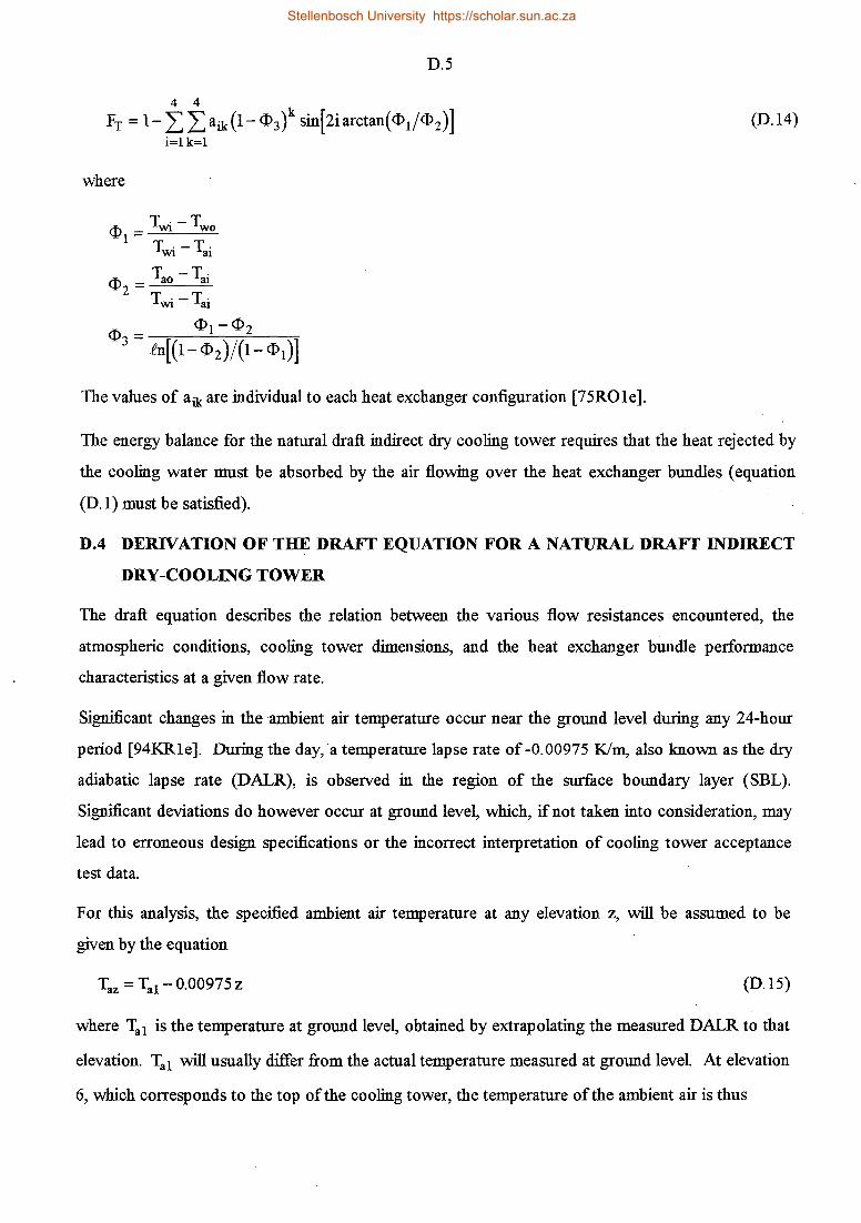
D.5

4 4

FT = 1-LL aik (1- 3t sin[2iarctan( i/ 2)]

i=l k=l

where

,n _ Twi - Two '*'l -

T · -T· WI a1

The values of aik are individual to each heat exchanger configuration [75R01e].

(D.14)

The energy balance for the natural draft indirect dry cooling tower requires that the heat rejected by

the cooling water must be absorbed by the air flowing over the heat exchanger bundles (equation

(D.1) must be satisfied).

D.4 DERIVATION OF THE DRAFT EQUATION FOR A NATURAL DRAFT INDIRECT

DRY-COOLING TOWER

The draft equation describes the relation between the various flow resistances encountered, the

atmospheric conditions, cooling tower dimensions, and the heat exchanger bundle performance

characteristics at a given flow rate.

Significant changes in the ambient air temperature occur near the ground level during any 24-hour

period [94KR1e]. During the day, a temperature lapse rate of-0.00975 Kim, also known as the dry

adiabatic lapse rate (DALR), is observed in the region of the surface boundary layer (SBL).

Significant deviations do however occur at ground level, which, if not taken into consideration, may

lead to erroneous design specifications or the incorrect interpretation of cooling tower acceptance

test data.

For this analysis, the specified ambient air temperature at any elevation z, will be assumed to be

given by the equation

Taz = Tal -0.00975 Z (D.15)

where Tai is the temperature at ground level, obtained by extrapolating the measured DALR to that

elevation. Tai will usually differ from the actual temperature measured at ground level At elevation

6, which corresponds to the top of the cooling tower, the temperature of the ambient air is thus

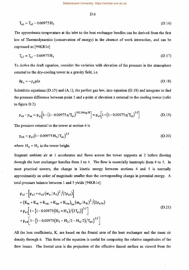
D.6

(D.16)

The approximate temperature at the inlet to the heat exchanger bundles can be derived from the first

law of Thermodynamics (conservation of energy) in the absence of work interaction, and can be

expressed as [94KRle]

(D.17)

To derive the draft equation, consider the variation with elevation of the pressure in the atmosphere

external to the dry-cooling tower in a gravity field, i.e.

dpa =-pagdz (D.18)

Substitute equations (D.15) and (A.1), the perfect gas law, into equation (D.18) and integrate to find

the pressure difference between point 1 and a point af elevation z external to the cooling tower (refer

to figure D.2)

[ ( )102.564g/R] [ ( )3.5] Pal-Paz =Pal 1- l-0.00975z/Tal ~Pal 1- l-0.00975z/Tal (D.19)

The pressure external to the tower at section 6 is

(D.20)

where H 6 = H5 is the tower height.

Stagnant ambient air at 1 accelerates and flows across the tower supports at 2 before flowing

through the heat exchanger bundles from 3 to 4. The flow is essentially isentropic from 4 to 5. In

most practical towers, the change in kinetic energy between sections 4 and 5 is normally

approximately an order of magnitude smaller than the corresponding change in potential energy. A

total pressure balance between 1 and 5 yields [94KRle]:

Pal -[Pa5 +ae5 (ma/ A5)2

/(2Pa5)]

= (Kts +Ket+ Kctc + Khe + Kcte)he (ma/Arr)2

/(2Pa34)

+Pai[ l-{l-0.00975(H3 + H4)/(2Ta1)}3"5]

+Pa4[ l-{l-0.00975(H5 -H3/2-H4/2)/Ta4 }3·5]

(D.21)

All the loss coefficients, K, are based on the frontal area of the heat exchanger and the mean air

density through it. Th.is form of the equation is useful for comparing the relative magnitudes of the

flow losses. The frontal area is the projection of the effective finned surface as viewed from the


D.7

upstream side. Stiffening beams, straps or other obstructions located up against the finned surface,

thereby impeding flow through the heat exchanger must be considered when evaluating the effective

frontal area, Afr. The last two terms on the right hand side of equation (D.21) take into

consideration static pressure differentials due to elevation between ground level and the mean heat

exchanger elevation and the latter between the ground level and the tower outlet respectively.

Du Preez and Kroger [94DU1e] studied the velocity and pressure distribution in the outlet plane of

hyperbolic natural draft cooling towers. They find that for 1/Frn s 3 , the velocity distribution is

almost uniform, i.e. ae5 ~ 1 for dry-cooling towers where the heat exchangers are located in the

cross-section near the base of the tower. The mean pressure at the outlet plane is found to be

slightly less than that of the ambient air at the same elevation, i.e.

(D.22)

For a hyperbolic tower with a cylindrical outlet the loss coefficient is given by

(D.23)

where Frn =(m3/As)2/[Pas(Pa6-Pas)gd5]. This equation is valid for 0.5sd5/d3 s0.85 and

5sKhe s 40.

The approximate temperature at the tower can be derived from the first law of thermodynamics

(conservation of energy) in the absence of work interaction, and can be expressed as [94KR1e]

(D.24)

From the perfect gas relation it thus follows for p35 ~ p36 , the density at the outlet of the tower is

(D.25)

The density of the ambient air at elevation 6 is

(D.26)

If dynamic effects are neglected, an approximate expression for p34 may similarly obtained.

Pa4 ~ Pa1[1-0.00975(H3 +H4)/(2T31))3-5

-(Kts +Ket +Kctc + Khe + Kcte)he (ma/Afr)2

/(2Pa34)

(D.27)

Substitute equations (D.20), (D.22) and (D.27) into equation (D.21) and find with ae5 = 1


D.8

Pai[ {l-0.00975(H3 + H4)/(2Ta1)}3·5 {l-0.00975(Hs -H3/2- H4/2)/Ta4 }3"5.

-(l-0.00975H5/Ta1)3·5]

= {Kts +Ket+ Kctc + Khe + Kcte)he (ma/Afr)2

/(2Pa34)

x [ l-0.00975(H5 - H 3/2- H4/2)/Ta4 ]3"5 +(1 + Kt0 )(m3/A5)

2 /(2p35)

(D.28)

This equation is known as the draft equation for a natural draft dry-cooling tower where the heat

exchangers are arranged horizontally in the base of the tower. Thus, the left hand side of the draft

equation, ~PLHS, must equal the right hand side of the equation, ~PRHS. If the heat exchangers are

arranged in the form of A-frames or V-arrays, Khe (non-isothermal) is replaced by Ket.

In determining the dry air density after the heat exchanger, the specified pressure at ground level can

be employed in the perfect gas relation, i.e.

(D.29)

The approximate air density at section 3 is

(D.30)

The harmonic mean density through the heat exchanger is given by

(D.31)

The loss coefficient of the tower supports, Kts, is based on the drag coefficient of these supports, i.e.

(D.32)

The effective pressure drop across the dry-cooling tower supports is given by

(D.33)

where Lts is the support length and dts is its effective diameter or width, and nts is the number of

supports. The corresponding loss coefficient based on these conditions at section 2 is

(D.34)

For substitution into equation (D.28), this loss coefficient is required to be based on conditions at the

heat exchanger, i.e.


D.9

(D.35)

It is assumed that the air density and the velocity distribution through the supports is uniform. Since

the distance between the tower supports is finite, the above approach tends to underestimate the

magnitude of the loss coefficient.

Due to separation at the lower edge of the tower shell and distorted inlet flow patterns, a cooling

tower loss coefficient Ket, based on the tower cross-sectional area at 3, can be defined to take these

effects into consideration. For dry-cooling towers where Khe;;::: 30 and 5 ~ d3/H3 ~ 10,

Geldenhuys and Kroger [86GEle] recommend the following expression

(D.36)

The cooling tower inlet loss coefficient based on conditions at the heat exchanger is

(D.37)

Depending on the heat exchanger bundle arrangement in the cooling tower base, only a portion of

the available area is effectively covered due to the rectangular shape of the bundles. The reduction in

effective flow area results in contraction, and subsequent expansion losses. The contraction losses

can be approximated by loss coefficients based on the effective reduced flow area Ae3 [50KAle]

(D.38)

The contraction coefficient, crc, is given by

2 3 4 cr c = 0.6144517 + 0.04566493cre3 -0.33665 lcre3 + 0.4082743cre3 + 2.67204lcre3

- 5.963169 cr~3 + 3.558944cr~3 (D.39)

The expansion losses can be approximated by

(D.40)

The effective area, Ae3 , corresponds to the frontal area of the heat exchanger bundles if they are

installed horizontally. In the case of an array of A-frames, Ae3 =Arr sineb and thus corresponds to

the projected frontal area of the bundles. Because of the essentially porous nature of the bundles, the

actual contraction loss coefficient will be less than the value given by the above equation.

Based on the conditions at the heat exchanger, the above expressions become


D.10

(D.41)

and

(D.42)

For non-isothermal oblique flow through an array of V-bundles, the following relation holds for the

loss coefficient [86KOle]:

K _ K . 2_(Pa3 -Pa4) ( 1 - l~ ( 1 et - he1so + 2 + a Pa3+Pa4 sin8m sin8m

+K ( . 2Pa3 ) d Pa3 +Pa4

l + 2K~·5) ( 2Pa4 ) Pa3 +Pa4

(D.43)

where a is the ratio of the minimum free flow area through the heat exchanger b.undle to the free

stream flow (frontal) area.

The heat exchanger loss coefficient under normal non-isothermal flow conditions, including inlet-,

frictional-, and exit losses as well as acceleration effects (due to heating), is defined as (refer to

AppendixB)

K =a RybK +2-(Pa3 -Pa4) he K 2

a Pa3 +Pa4 (D.44)

for finned tube bundles with any finned tube geometry. For radially finned tubes the heat exchanger

loss coefficient under normal non-isothermal flow conditions can, in general, be expressed as

[86KRle]

Khe =~[Eu+ (Pa3 - Pa4)] = -;-[L1Pa~am + (Pa3 - Pa4)] a l Pa3 +Pa4 a Ge Pa3 +Pa4

(D.45)

The Euler number can be obtained from the pressure drop correlations discussed in Appendix B.

The second term on the right hand side of equation (D.43) represents the loss due to acceleration

effects during non-isothermal operation. The third term represents the loss due to the oblique flow

at the inlet to the bundle. The entrance contraction loss coefficient, Kc, is according to Kays

[50KAle]

(D.46)


D.11

where cr21 = (Pf - tf) /Pf is the ratio of the flow area between the fins to the free stream flow area at

the inlet to the finned tube bundles. The contraction coefficient, crc, is given by equation (D.39),

with cr 21 replacing cr e3. For round and elliptical fins a value of Kc ~ 0.05 is assumed.

When the finned tube bundles are arranged in the form of A-frames, the curvature of the downstream

flow patterns cause the actual mean flow incidence angle to differ from the heat exchanger bundle

semi-apex angle eb. An empirical correlation for the mean flow incidence angle is presented by

Kotze et al. [86K01e], i.e.

2 em= 0.00198b +0.91338b -3.1558 (D.47)

Kd is the downstream loss coefficient that includes the jetting and kinetic energy losses, and can be

expressed in terms of the following relation [86KO 1 e]

Kd =exp ( 5.488405- 0.21312098b + 3.533265x10-3 9~ - 0.2901016x10-48~) (D.48)

If performance correlations from oblique flow experiments are available, the pressure loss coefficient

for the heat exchanger bundle under non-isothermal flow conditions has the following form

(D.49)

Natural draft cooling towers are prone to the inflow of cold air at the upper edge of the tower shell.

Significant performance degradation is observed under these conditions. According to Richter

[69Rlle], small disturbances may cause flow instabilities in cooling towers, resulting in cold air

inflow under the following conditions

1/Frn ~ 3.05 (D.50)

Equation (D.50) will be employed in the design of natural draft dry-cooling towers as a safeguard

against cold inflow.

In most of the hyperbolic cooling towers found in practice, the following typical relationships

between the tower dimensions can be observed:

0.05 ~ H 3/H5 ~ 0.15

0.64 ~ d3/(H5 -H3)~113 137 ~ d3/ds ~ 177

0.08 ~ H3/d3 ~ 0.16


D.12

D.5 OPERATING POINT CALCULATION

The operating point (ability to reject heat) of the fixed geometry dry-cooling tower is defined as the

combination of operating variables that will simultaneously satisfy the draft and heat transfer

(energy) equations for specified condenser outlet and ambient air conditions

Definition of the operating variables, operating constraints and equations to be satisfied

For a specified hyperbolic dry-cooling system geometry, specified condenser outlet conditions

(Twi) and specified ambient air conditions (Tdb' Twb' Pa) the following variables, constraints and

equations (balances) can be defined for the simultaneous solution of the operating point conditions:

The operating variables are: ma, T3 4, Two


(D.51)

(D.52)

(D.53)

(D.54)

(D.55)

(D.56)

ei are small constants and are used to introduce the :2:: sign in the feasibility inequalities. Equation

(D. 56) is introduced to prevent the logarithmic temperature difference of being undefined. The

bounds on the operating variables are introduced to safeguard against the violation of the physical

laws.


Qa = QLMID

Qa =Qw

LipLHS = LipRHS

D.6 POWER GENERATION

(D.57)

(D.58)

(D.59)

The turbo-generator-condenser characteristics of the indirect condensing system, i.e. the heat to be

rejected by the condenser and the power output of the turbo-generator, are expressed in terms of the


D.13

turbine back pressure, Ptv, or the corresponding vapor temperature, Ttv. The performance

characteristics of an example of such a system is shown in figure D.3. It is assumed that the power

needed for the auxiliaries, excluding the cooling water pumping power, is already subtracted from

the generated power.

The temperature of the heated water that leaves the surface condenser is not equal to the steam

temperature. The temperature difference that exists between the condensing steam and the water

leaving the condenser is known as the terminal temperature difference (TTD). Typical values for

TTD range from 2 ° C to 4 ° C . The relation between the heat rejection rate and the TTD can be

approximated as follows:

240

235

~ 230

~~ 225 ...... ~

8. 220 -a ~ 215

~ 210 ~

205

200

- - r---. ~

' / ""'

/

' / - ...... / -

'V' -

/ "'-/ ~ v "\

.-----40 45 50 55 60 65 70 75 80 85 90 95

Turbine exhaust saturated steam temperature, Ttv, °C

Figure D.3: Performance characteristics of a turbo-generator.

365

360

355 ~ 350 d

.-d' Cl

345 ...... ce .s-

340 (/] (/] .....

"O

335 ~ Cl

::I: 330

325

For a fixed condenser design the water mass flow rate , mw , the heat transfer area, A, and the

overall heat transfer coefficient, U, are constant. Thus,

Q = UA (Ttv -Two)-(Ttv -Twi)

Rn[(Ttv -Tw0 )/(Ttv -Twi)]

= mwcpwm(Twi -Two)

By rearranging equation (D.60), find

or

(D.60)


D.14

(D.61)

where c1 is a constant. Equation (D.61) can be simplified by using the equation for the water heat

transfer rate, i.e.

For the design point, find

For off-design conditions, find

From equations (D.63) and (D.64), find

TTD :::J TTD design Q/ Qdesign

(D.62)

(D.63)

(D.64)

(D.65)

With the aid of equation (D.65), the temperature of the water leaving the condenser (entering the

cooling tower) can be calculated.

Atmospheric conditions influence the performance of indirect dry-cooling tower, resulting in a wide

fluctuation of turbine back pressure (and the corresponding steam temperature). Changes in the

ambient temperature are the most important reason for this, although other environmental effects

such as wind, inversions and humidity must also be considered. The mean hourly frequency of

ambient temperatures over a period of one year is normally supplied in tabulated or graphical form

An example of the frequency of the dry- and wet bulb temperatures 2m above the ground level at a

particular location is shown in figure D.4. It should be noted that the air entering the dry-cooling

tower may deviate considerably from these measured values and more detailed information on the

actual ambient temperature distribution would be preferred for more sophisticated designs

[94KRle].

The operating point of the turbo-generator-condenser is determined by matching the operating point

of the indirect dry-cooling tower and the performance characteristics of the turbo-generator

condenser (Figure D.3) at a specific ambient air temperature selected from Figure D.4. This

calculation involves the selection of turbine exhaust conditions such that the heat to be rejected by


~

D.15

the turbo-generator-condenser, equals the heat absorbed by the air (heat rejected by the dry-cooling

tower), i.e.

(D.66)

At this point the power requirement of the cooling water pumps as well as the generator power

output are known. Subtract the total power consumed by the pump from the generator power

output to find the net power output of the plant. Tue net power output is multiplied by the

corresponding number of operating hours to give the net energy output for this period. These

calculations are repeated for each of the ambient temperatures listed to obtain the total annual net

energy output.

800

ce 700 ~ Wetbulb Dry bulb

I 600 temperature temperature

500 .... &. 400 rJJ

~ 300 0

...:::= of 200

.§ ~ 100

0

-5 0 5 10 15 20 25 30 35

Temperature, T, ° C

Figure D.4: Frequency of ambient dry- and wetbulb air temperatures.

In the cases when very low ambient temperatures are experienced, it is possible that the dry-cooling

tower can dissipate more heat than the amount required by the turbo-generator characteristic at its

bottom limit. As the turbine back pressure decreases, more power can be generated due to the more

complete expansion of steam through the turbine. The dry-cooling tower will tend to lower the

turbine exhaust pressure under these conditions, thus giving rise the a phenomenon called "choking"

[71HA1e, 71HEle, 91SZ1e]. No further advantages are obtained by lowering the turbine back

pressure and turbine losses may become excessive due to high steam velocities. As performance of

the dry-cooling tower deteriorates with increasing ambient air temperatures, the turbine back

pressure increases, resulting in a decrease in power generation. The maximum allowable turbine

exhaust pressure is such that flow induced vibration of the turbine blades will not occur for lower


D.16

values [91SZle]. When reaching the upper limit of the characteristic curve, the turbine load must be

reduced. Air humidification can also be used as a means to increase the cooling capacity during high

ambient air temperatures [83PAle, 91C02e, 94KRle].

For better part load performance it is preferable to divide circulating pump capacity between two

50%-duty units. Sometimes three 50%-duty pumps are installed so as to have a stand-by unit in

emergencies; this solution makes it possible to bring in the third pump to assist the cooling effect

under conditions ofhigh ambient air temperatures [71HEle, 87TRle, 91SZle].


For a fixed hyperbolic dry-cooling tower system geometry, a fixed turbo-generator-condenser

characteristic curve and an annual :frequency of ambient temperatures (at a constant Pa), the

following variables, constraints and equations (balances) can be defined for the simultaneous solution

of the operating point conditions during the annual operation:

The operating variables are: ma, Ta4 , Tw0 , Ttv


Equations (D.51), (D.52), (D.53), (D.54), (D.55), (D.56), as well as

(D.67)

(D.68)

The upper and lower limits on the turbine exhaust steam temperature can be obtained from the

turbo-generator characteristic curve.


Equations (D.57), (D.58), (D.59), (D.66)

With the turbo-generator-condenser operating point known, the net power output of the plant at that

specific conditions is calculated as follows:

(D.69)

For each temperature data set (consisting of a drybulb air temperature, a wetbulb air temperature and

the annual duration of these temperatures), a new set of operating variables with bounds are defined

and used to determine the turbo-generator-condenser operating point. Tue net annual energy output

of the plant is thus


n

Enet = LPnet(i)'t(i) i=l

D.17

(D.70)

where n is the number of temperature frequency data sets and 'tis the duration of these temperatures.

D.7 OPERATING POINT OPTIMIZATION

Operating point optimization involves the process of finding the combination of operating and

geometrical variables that will minimize the total annual cost (capital and operating) of the dry-

cooling tower for specified operating conditions, specified ambient air conditions (Tdb' Twb' Pa) and

specified heat transfer rate Qct , while satisfying all the imposed constraints.

Four different cases of operating point optimization calculations are investigated:

( 1) Case 1: mw and Twi fixed

The mass flow rate and the temperature of the water that enters the dry-cooling tower are fixed at

some specified values, while ma, Ta4 , and Two are variable.

(2) Case 2: Twi fixed

The temperature of the water that enters the dry-cooling tower is fixed at a specified value, while

ma, Ta4, Two and mw are variable ..

(3) Case 3: Maintaining a constant waterside pressure drop (and pumping power) [89BU1e]

The replacement of ineffective finned tube bundles of an existing natural draft dry-cooling tower by

optimally dimensioned units is investigated in this optimization study. No changes are allowed to the

bundle base support, the water pipe layout, the water flow rate and the pressure drop through the

heat exchanger bundles (i.e. the pumping power remains unchanged). Only round tubes with circular

fins are considered in this investigation.

Equation (D.12) can be rewritten for round tubes as

(D.71)

Hence, if all the parameters on the right hand side of the above equation remain constant, so will P w .

For a constant total pressure drop in a tube, find

(D.72)


D.18

Assuming that mw, Lt, Pwm, and nb remain constant, find

or

(D.73)

The bundle base length must be kept constant, i.e.

wb sine b = constant (original value) (D.74)

and

nrP1 cos9b =constant (original value) (D.75)

The constants c1 and c2 are determined from the original specifications. The optimization is

performed by keeping the variables that describe the tower geometry, d3 , d5, H 3 and H 5 , as well as

variable. The number of water passes, nwp , can be varied in consideration with the number of tube

rows, to get a realistic heat exchanger bundle configuration.

(4) Case 4: Fixed condenser design ((UA) =constant) [89BU2e] con

When the dry-cooling tower is coupled to a condenser having a specified thermal conductance,

(UA)con, the following relations can be derived for the specified cooling rate:

or

(D.76)

where TTD = Ttv -Twi. Assume that both (UA)con and TTD are constant at their initial specified

values. mw, Twi and Two are variable. In order to achieve the specified cooling capacity, the water

mass flow rate must be calculated from:


D.19

(D.77)


The optimization variables are shown in table D. l.

Table D. l: Optimization variables ( ./ = applicable; X= not applicable)

Number Variable Round tubes Finned tubes with circular with fixed fins geometry

1 ma ,/ ,/

2 Ta4 ,/ ,/

3 Two ,/ ,/

4 mw ,/ ,/

5 T· ,/ ,/ WI

6 Ttv ,/ ,/

7 H3 ,/ ,/

8 H5 ,/ ,/

9 d3 ,/ ,/

10 ds ,/ ,/

11 ntb(max) ,/ - ,/

12 Lt ,/ ,/

13 eb ,/ ,/

14 do ,/ x

15 tt ,/ x

16 tr ,/ x

17 df ,/ x

18 tf ,/ x

19 tg ,/ x

20 pf ,/ x

21 pt ,/ x

The optimization variables defined for the round tubes with circular fins use the airside performance

correlations specified in Appendix B. l, while the variables defined for finned tubes with any

geometry use the performance correlations defined in Appendix B.2. The operating variables are

also considered as optimization variables because the dry-cooling tower model is included as equality

and inequality constraints (balances and bounds) in the minimization problem formulation (integrated

approach). The geometrical variables (numbers 7-21) can be kept constant or varied during the

optimization process.


D.20

Objective function

The objective function requires that the total annual cost be minimized. The construction of the

objective function from its various capital and operating cost components is discussed in Appendix

E. The total annual cost is

Ctotal = Coperating + Cmaintenance + CFCR ($/annum)

Constraints


Equations (D.57), (D.58), (D.59) as well as

Qa = Qct = Qw = QLMTD


Equations (D.51), (D.52), (D.53), (D.54), (D.55), (D.56)

(D.78)

(D.79)

To prevent cold inflow, equation (D.50) is also a prescribed constraint. The velocity of the water

flowing inside the tube can be specified as a fixed value and thus presented as an equality constraint,

i.e.

Vw =vwfix (D.80)

In order to prevent fouling caused by a low water velocity inside the tubes, a lower velocity limit can

also be specified and formulated by means of an inequality constant, i.e.

Vw:;?: Vwl

Considering case 2, the following limit is introduced:

Considering case 3; the following equality constraints are introduced:

Equations (D.73), (D.74), (D.75)

Considering case 4, the following limits are introduced:

Twi ;::: Twil + c 7

(D.81)

(D.82)

(D.83)

(D.84)




D.21

The relationship between the hyperbolic cooling tower dimensions are limited to the practical values

stated in section D.4.

H3/H5 ~ 0.05 (D.85)

-H3/H5 ~ -0.15 (D.86)

d3/(H5 -H3) ~ 0.64 (D.87)

-d3/(H5 - H3) ~ -1.13 (D.88)

d3/d5~1.37 (D.89)

-d3/d5 ~ -1.77 (D.90)

The heat exchanger bundle width is limited by transport requirements.

Wbu-Wb ~o (D.91)

The finned tube length is limited by structural, transport and construction requirements.

Ltu -L1 ~0 (D.92)

The bundle semi-apex angle cannot exceed 90° .

(D.93)

For round tubes with circular fins, the following inequality constraints are imposed (refer to

Appendix B. l):

The finned tubes must be kept from touching.

(D.94)

The fin diameter must exceed the fin root diameter (extended airside surface area is required).

(D.95)

Due to structural considerations, the fin root thickness and the tube thickness must exceed their

lower limits.

(D.96)

(D.97)


D.22

For effective cleaning and where airside fouling is of significance, the fin pitch must exceed the

imposed lower limit.

Pr -Pn;::: o

The galvanizing thickness must lie within practical limits.

tg -tgl;::: 0

tgu - tg;;::: 0

The fin thickness is limited by the manufacturing processes.

tr - tn;;::: o

The fin pitch must exceed the fin thickness.

Pr -tr;::: o

(D.98)

(D.99)

(D.100)

(D.101)

(D.102)

The application limits of the finned tube performance correlations, as discussed in Appendix B

(section B. l), are not used as constraints during the optimization of circular finned tubes.

The following assumptions and relations are used to obtain values for the geometrical parameters

linked to the optimization variables:

The number of finned tube bundles is obtained from

nb = actnd~/[4Lt(Wb sin8b +nrP1 coseb)]

where act is the fraction of the tower area covered by heat exchanger bundles.

nth = ntb(max)nr -nr/2 (total number of tubes per bundle)

Wb = ntb(max)Pt (bundle width)

P1 = 0.866 Pt (longitudinal tube pitch for circular finned tubes)

di = d0 - 2tt (round tube inside diameter)

dr = d0 +2tr (root diameter of circular finned tube)

The following parameters are assumed to be constant during the optimization process:


D.23

D.8 MINIMIZATION OF POWER GENERATION COST

The minimization of the power generation cost attributed to the dry-cooling tower performance for

the given temperature frequency data set, involves the variation of the dry-cooling tower operating

and geometrical variables that will minimize the ratio of its total annual cost to the annual net power

output of the turbo-generator-condenser set it is coupled to. The calculated values of the different

variables must satisfy all the relevant constraints.


The optimization variables are defined in Table D. l. Different operating variables (numbers 1,2,3

and 6) are defined for each temperature data set and they are always present during optimization.

The water mass flow rate remains constant and the cooling tower inlet water temperature, Twi, is

calculated from equations (D.62) and (D.65). The other geometrical variables can be varied or

remain constant.

Objective function

The objective function requires that the ratio of the total annual cost of the dry-cooling tower to the

net energy produced by the turbo-generator be minimized, i.e.

(D.103)

The construction of the total annual cost from its various cost components is discussed in Appendix

E, while the topic of power generation is treated in section D.6.

Constraints


Equations (D.57), (D.58), (D.59), (D.66)


Equations (D.50), (D.51), (D.52), (D.53), (D.54), (D.55), (D.56), (D.67), (D.68), (D.81)

The following general inequality constraints (geometrical constraints) must be sat_isfied, depending


Equations (D.85), (D.86), (D.87), (D.88), (D.89), (D.90), (D.91), (D.92), (D.93), (D.94), (D.95),

(D.96), (D.97), (D.98), (D.99), (D.100), (D.101), (D.102)

For each temperature data set there is a corresponding set of operating variables, equality and

inequality constraints (operating constraints). These constraint sets must always be satisfied. The


D.24

operating variables of a specific temperature data set effect the operating constraints belonging to the

same temperature data set only. The operating variables do not effect the geometrical constraints.

However, the geometrical variables effect all the operating constraints of the different temperature

data sets.


E.1

APPENDIXE

DRY-COOLING SYSTEM COST ESTIMATION

E.1 INTRODUCTION

In this appendix the cost components needed to define the objective functions are described. The

objective functions to be minimized are the annual cost of the dry-cooling system under prescribed

conditions or the annual cost of electricity production that is attributed to the dry-cooling system

when coupled to a turbo-generator unit. Capital and operating cost estimation methods, based on

the methods discussed in Chapter 4, are proposed for both forced draft and natural draft dry-cooling

systems.

E.2 COOLING SYSTEM CAPITAL COST ESTIMATION

Heat exchanger bundle cost

( 1) Tube cost per unit tube length, Ct

Ct = CtmMt + Ctu ($/m)

Mt is the tube mass per unit tube length (kg/m)

ctu is the tube added unit cost ($/m)

ctm is the tube material cost ($/kg)

(2) Cost of fins per unit tube length, Cf

Cf = CfmMf + CfuLfb ($/m)

cfu is the fin material added unit cost per unit tube length ($/m)

cfm is the fin material cost ($/kg)

Mf is the fin material mass per unit tube length (kg/m)

Lib is the length of fin strip per unit tube length (m/m)

(3) Surface coating cost per unit tube length, Csc

cscm is the surface coating material unit cost ($/kg)

(E.1)

(E.2)

(E.3)


E.2

Cscu is the smface coating added unit cost ($/m2)

Msc is the mass of the smface coating material per unit tube length (kg/m)

Aa is the air side smface area per unit tube length (m2 /m)

( 4) Total finned tube cost per unit tube length, Cft

Cft = (Ct +Cr +csc)wft ($/m)

W ft is the finned tube cost weighting factor

(5) Heat exchanger bundle header and frame cost, Ch

Ch= CftLtnth Wh ($/bundle)

wh is the header and frame cost weighting factor

(6) Bundle assembly cost, Cha

Cha = Chatllth ($/bundle)

Chat is the assembly cost per finned tube ($/finned tube)

(7) Total heat exchanger bundle cost, Che

Che= ( CftLtnth +Ch +Cha)whe ($/bundle)

Whe is the heat exchanger bundle cost weighting factor (installation)

Fan system capital cost

(E.4)

(E.5)

(E.6)

(E.7)

It is assumed that dFc ~ 1.005dF, dFh ~ 0.165dF, the height of the fan casing is 0. ldFc' the inlet

bell height is 0.15dFc and the inlet bell diameter is l.2dFc·

(1) Fan capital cost, CF

CF= CFuAF +CFf ($/fan)

CFu is the fan unit cost ($/m2

)

CFf is the fan fixed cost ($/fan)

AF is the fan sweep area ( m 2 )

(E.8)


E.3

(2) Fan casing and inlet bell cost, CFc

(E.9)

CFcb is the fan casing and inlet bell unit cost ($/m2

)

AF c is the fan casing circumference area ( m 2

)

A Fb is the inlet bell circumference area, approximated by a conical frustum ( m 2 )

2 2 AFc = 0.btdFc (m )

(3) Fan safety screen cost, CFs

CFs = CFsgAFs ($/fan) .(E.10)

CFss is the safety screen cost ($/m2

)

A Fs is the safety screen area ( m 2 )

( 4) Electric motor cost, Cem

(E.11)

cemf is the electric motor fixed cost ($/motor)

Cemu is the electric motor unit cost ($/kW)

Pe is the electric power input to the electric motor (kW)

A safety factor, sem' against electric motor undersizing is also introduced.

(5) Speed reducer cost, Csr

csr = (CF +Cem)wsr ($/speed reducer) (E.12)

wsr is the speed reducer cost weighting factor

(6) Electric wiring and switching cost, Cws

(E.13)

Wws is the wiring and switching cost weighting factor


E.4

(7) Total fan system cost, CFt

CFt = ( Cp + CFc +CFS+ cem + csr + Cws)wF ($/fan)

Wp is the fan system cost weighting factor

Forced draft cooling tower structure

( 1) Cost ofland, excavation, foundations and construction, Cc

Cc= ( C1 +CcuH3 +Cpp1)AFp1Wc ($)

C1 is the land, excavation and foundation cost ($/m2)

Ccu is the construction unit cost ($/m3)

CFpl is the fan platform cost ($/m2)

A Fpl is the fan platform area ( m 2 )

We is the construction cost weighting factor

Natural draft cooling tower shell (Hyperbolic reinforced concrete)

(E.14)

(E.15)

The cooling tower shell will be approximated by means of two conical frustums, one above and the

other below the throat. A constant shell thickness is assumed. The volume of the conical frustum

can be calculated as follows:

(E.16)

with H5 -Ht= 0.25(H5 -H3), Ht -H3 = 0.75(H5 -H3) and d5 =1.05dt. These relationships are

typical in most of the existing hyperbolic cooling towers found in practice. The volume of concrete

in the tower shell can be calculated with the aid of equation (E.16). It is further assumed that the

tower base angle, <Pb, is fixed at 70° (which is the minimum limit for construction [84AL1e]) and

that the tower support length can be expressed as Lts = H 3/sin(<!>h)

( 1) Cost ofland, excavation and foundation, C1

C1u is the land, excavation and foundation cost ($/m2)

Ab is the tower base area (m2)

(E.17)

Ab= 0.25rc(d3 +2H3/tan$b)2

(2) Cost of the tower shell, Cct

cct = cctc vts ($)

E.5

Cctc is the cost of the reinforced concrete used in the shell ($/m3

)

Vts is the volume of reinforced concrete in the tower shell ( m 3 )

(3) Cost of the heat exchanger bundle platform, ChepI

Chepl = Cp1uAhepI ($)

cplu is the platform unit cost ($/m2)

A hep! is the heat exchanger platform area ( m 2

)

(4) Cost of the tower supports, Cts

Cts = CtsuLtsdtsnts ($)

ctsu is the tower support unit cost ($/m3)

(5) Total construction cost, Cc

cc= ( C1 +Cct +ChepI +cts)wc ($)

Wc is the structural maintenance cost weighting factor

Steam/condensate distribution system costs (ACC)

( 1) Distribution system cost, C sd

csd = (Che+ CFt)wsd ($)

wsd is the steam/condensate distribution system cost weighting factor

Circulation system costs

Two 50%-duty pump units will be considered in this analysis.

(1) Pump capital cost, cpmnp

Cpump = 2( Cpf + CpuP w) ($)

(E.18)

(E.19)

(E.20)

(E.21)

(E.22)

(E.23)

(E.24)


E.6

cpf is the pump fixed cost ($/pump)

Cpu is the pump unit cost ($/kW)

P w is the required pumping power (kW)

(2) Electric motor cost, Cem

(E.25)

cemf is the electric motor fixed cost ($/motor)

Cemu is the electric motor unit cost ($/kW)

A safety factor, S6 m, against electric motor undersizing is also introduced.

(3) Electric wiring and switching cost, Cws

(E.26)

Wws is the wiring and switching cost weighting factor

( 4) Total pump system cost, Cpst

(E.27)

wps is the pump system cost weighting factor

(5) Piping and valves cost, Cpv

(E.28)

Wpv is the piping and valves cost weighting factor

E.3 COOLING SYSTEM OPERATION COST ESTIMATION

Fuel cost

The total annual fuel cost , C ft, can be expressed as

(E.29)

Tl plant is the overall plant efficiency

Pg is the gross power output of the turbo-generator (MW)

cfav, levelized unit cost of the fuel ($/MJ)


E.7

'tis the number of operating hours (h)

Fan operating cost

The annual operating cost of the fan, CFo, can be expressed as

Ceav levelized electricity cost ($/kWh)

Pe is the input power to the fans (kW)

't is the number of operating hours (h)

Pump operating cost

The annual operating cost of the pump, CP0 , can be expressed as

ceav levelized electricity cost ($/kWh)

Pe is the input power to the pumps (kW)

't is the number of operating hours (h)

Fixed charges

The cost of the fixed charges, CFcR,can be expressed as

CFCR = FCR ccapital

FCR is the levelized fixed charge rate

Ccapital is the total capital cost($)

Maintenance costs

(E.30)

(E.31)

(E.32)

The maintenance cost weighting factors are assumed to be levelized values over the operating

lifetime of the plant.

( 1) Heat exchanger bundle maintenance cost, Chem

chem= whemche ($/bundle) (E.33)

Whem is the heat exchanger bundle maintenance cost weighting factor


E.8

(2) Fan system maintenance cost, CFm

(E.34)

WFm is the fan system maintenance cost weighting factor

(3) Structural maintenance cost, Ccm

(E.35)

wcm is the structural maintenance cost weighting factor

( 4) Distribution system maintenance cost, Csdm

(E.36)

wsdm is the steam/condensate distribution system maintenance cost weighting factor

(5) Pump system maintenance cost, cpm

(E.37)

Wpm is the pump system maintenance cost weighting factor

( 6) Piping maintenance cost, Cpvm

(E.38)

W pvm is the piping and valves maintenance cost weighting factor

E.4 TOT AL COSTS

The total annual cost of the cooling system is:

Ctotal = Coperating + cmaintenance + CFcR ($/annum) (E.39)

The cost of power generation (attributed to the cooling system) is:

c = ctota1 ($/kWh) power E

net (E.40)

where Enet is the net annual power output.

Equations (E.39) and (E.40) present the required objective functions for the operating point

optimization andthe minimization of power generation cost respectively.


F.1

APPENDIXF

SOLUTION OF SYSTEMS OF NONLINEAR EQUATIONS BY USING A

CONSTRAINED NONLINEAR LEAST SQUARES APPROACH

F.1 INTRODUCTION

The solution methods for unconstrained optimization and the nonlinear equations problem

(simultaneous solution of n nonlinear equations in n unknowns) are closely related. Newton's

method is the basic method for solving both these types of problems [83DE1m, 89DE1m]. A

significant percentage of real-world unconstrained optimization problems in science and engineering

arise from fitting model :functions to data, i.e. nonlinear parameter estimation. Usually the number of

data points, m, is greater than the number of independent variables, n, and it is not possible to obtain

an exact solution. This gives rise to a special class of unconstrained optimization problems with a

special structure, the so-called nonlinear least squares (NLS) problems where the objective :function

is a sum of squares.

In this section we consider the special case of the NLS problem where m = n. Such problems can be

viewed as an attempt to obtain the simultaneous solution of n nonlinear equations in n unknowns. A

globally convergent solution technique (convergence to a local minimizer from a poor starting point)

for these problems will be explained. The problem is extended to include inequality constraints and

bounds on the variables. The implementation of the modified NLS problem is presented by stating

its algorithmic representation.

F.2 THE NONLINEAR LEAST SQUARES PROBLEM

If f(x) is the sum of squares of nonlinear :functions, the objective :function of the nonlinear least

squares problem is written as [74LA1m, 81Gllm, 83DElm, 87FLlm, 89DE1m]

m

f(x) = 0.5Lfi(x)2 = 0.5f(x)Tf(x) (F.1)

i=l

where xis an n-vector. fi(x) = 0, i = 1, ... ,m can be viewed as a system of mnonlinear equations.

When m > n, least squares solutions to over-determined systems of equations are computed by

minimizing expression (F.1 ).

The derivatives of the objective :function are given by


F.2

g(x) = J(x)f (x) (F.2)

and

m

G(x) = J(x)J(x)T + Lfi (x)V2fi (x) (F.3) i=l

where J(x) is the nxm Jacobian matrix, the columns of which are the first derivative vectors Vfi of

the components off. We observe that the Hessian of the NLS objective function consists of a

combination of first- and second-order information. Most solution methods assume that the second

term on the right hand side of equation (F.3) is small compared to the first term, and it is simply

omitted. The resulting problem is referred to as a small residual problem Large residual problems

do exist, but will not be considered in this analysis (refer to [81Gllm, 83DElm, 89DElm] for more

information). Note that the linear least squares and zero residual problem is a special case of the

above formulation.

A good approximation to the Hessian of the objective function, G(x), can be obtained by assuming

that the residual is small, i.e.

G(x) ~ J(x)J(x) T (F.4)

Special purpose NLS solution techniques make use of the special problem structure. For example,

equations (F.1), (F.2) and (F.4) can be used with Newton's basic method or with a quasi-Newton

method. Whereas a quasi-Newton method might take n iterations to estimate G(x) satisfactorily,

here the approximation is immediately available. The basic Newton method (equation (2.21))

becomes the Gauss-Newton method when (F.4) is used to approximate G(x(k)). The Gauss-

Newton direction, s(k), is based on the minimization of the following quadratic model at iteration

(k):

(F.5)

The k-th iteration of the basic Gauss-Newton method can thus be written as

(F.6)

Gauss-Newton methods perform better on zero and small residual problems that are not too

nonlinear than on large residual problems. Convergence of this method is slowed as the problem


F.3

nonlinearity or the relative residual size increases; if either of these is too large, the method may not

converge at all [83DElm]. The Gauss-Newton method is also not necessarily globally convergent.

The Gauss-Newton method's global convergence and performance characteristics can be improved

in two ways: using it with a line search or with a trust region strategy [83DElm, 87FLlm]. The

basic idea of both line search and trust region methods, is that they use the properties of the quickly

convergent local methods (e.g. Newton's method) when the estimated solution is close to a

minimizer, and when a solution estimate lies outside the convergence region of these methods, some

reliable approach is used that gets them closer to the region where the local methods will work.

The k-th iteration of the Gauss-Newton method that incorporates a line search is simply

Solve J( x(k) )J( x(k) f s(k) + J( x(k) )r( x(k)) = 0 for s(k)

Set x(k+l) = x(k) +a(k)s(k)

(F.7)

where the step length a(k) is chosen by a line search procedure (see Dennis and Schnabel [83DElm]

or Fletcher [87FL1m]). We will refer to equation (F.7) as the damped Gauss-Newton method.

The idea of a line search algorithm is simply to calculate an acceptable point x(k+l), given a descent

direction, s(k), and a positive step length a(k). High accuracy line searches are very expensive to_.

carry out and researchers have developed some conditions for low accuracy line searches while still

obtaining global convergence [83DElm, 87FLlm]. They have shown that line search methods can

be globally convergent if each step size satisfies two simple conditions:

(1) The average rate of decrease from r( x(k)) tor( x(k+l)) must be at least some prescribed

fraction of the initial rate of decrease in that direction; i.e. we pick an A e ( 0, 0.5) that satisfies

(F.8)

(2) The steps must not be too short, i.e. we pick a 13 e('A,l) that satisfies

( (k+l))T (k) > r.t ( (k))T (k) gx s -pgx s (F.9)

Typical line search algorithms set A= 10-4 and13 between 0.7 and 0.9 [83DElm, 89DElm]. These

two conditions, when incorporated into a line search algorithm, lead to a practical and globally


F.4

convergent method. In practice, equation (F.9) is generally not needed, because backtracking will

avoid small steps being taken.

The common procedure is to try and use a (k) = 1.0 as the first step, and when it fails, backtracking

is performed in a systematic way along the direction of search until an acceptable x(k) +a(k)s(k) is

found. The backtracking strategy as well as line search algorithms that employ the concepts above

are described in Dennis and Schnabel [83DElm] and Fletcher [87FLlm].

Since the damped Gauss-Newton method always takes descent steps that satisfy the line search

criteria, it is usually globally convergent on almost all NLS problems, including large residual and

very nonlinear problems. However, it may still be slowly convergent or fail on the problems that the

Gauss-Newton method had trouble with.

The other modification to the Gauss-Newton method is the use of globally convergent trust region

strategies by solving the system (refer to chapter 2, section 2.2)

(F.10)

This formulation was first suggested by Levenberg [44LElm] and Marquardt [63MAlm] and is

known as the Levenberg-Marquardt method. A. (k) is changed during the course of the iterations in

order for J(x(k))J(x(k))T +A.(k)I to remain positive definite. Many versions of this algorithm do

exist; some control the iterations using A.(k) directly, while others use the radius h(k) and choose

A.(k) to satisfy II s(k)ll ~ h(k) [83DElm]. The local convergence properties of the Levenberg-

Marquardt method are similar to those of the Gauss-Newton method. The Levenberg-Marquardt

method may still find difficulty in solving some large residual or very nonlinear problems. There are,

however, certain factors that make Levenberg-Marquardt methods preferable to damped Gauss

Newton methods on many problems, e.g. when the Gauss-Newton step is too long, the Levenberg

Marquardt step is close to being the steepest descent direction, and is often superior to the damped

Gauss-Newton step [83DElm, 89DElm].

When m = n in the above analysis, the NLS problem can also be interpreted as the simultaneous

solution of n nonlinear equations in n unknowns, i.e. fi ( x) = 0 , i = 1, ... , n . The minimum of the

well-determined NLS problem corresponds to the solution of the system of n nonlinear equations in

n unknowns. The gradient of the NLS objective function vanishes when f(x) is zero. The Newton-

Raphson method that is usually used to solve systems of nonlinear equations is equivalent to the


F.5

basic Gauss-Newton method [81Gllm, 83DE1m]. Global strategies for solving systems of nonlinear

equations are obtained from the global strategies of unconstrained optimization. Thus, the line

search or trust region strategies can be used to ensure global convergence of this solution technique.

F.3 SIMULTANEOUS SOLUTION OF A SYSTEM OF NONLINEAR EQUATIONS

We have shown that exploiting the special form of the NLS problem can lead to substantial

improvements over using standard solution methods for unconstrained minimization problems.

Furthermore, this method can also be used to solve systems of nonlinear equations due to its

efficiency. In this section a procedure based on the Levenberg-Marquardt method will be

implemented to solve the system of nonlinear equations subject to linear inequality constraints.

The problem to be solved is

Solve fj{x) = 0, j = 1, ... ,n


! > b· . -1 a 1 x_ 1 , 1- , ... ,m

(F.11)

where the constraints are feasibility inequalities, ie. lower and upper bounds on the variables as well

as linear relationships between the variables. These constraints are not expected to be satisfied as

equalities at the solution, but rather define the feasible region for the iterative solution method.

Problem (F.11) can also be interpreted as a minimization of a NLS problem where the minimum of

the objective :function is known to be equal to zero, i.e.

n ~ 2 T

Solve f(x) = 0.5:L//x) = 0.5f(x) f(x) = 0 j=l

subject to the constraints (F.12)

afx~bi, i=l, ... ,m

Holt and Fletcher [79H01m] describe an algorithm for constrained NLS problem with special

constraints for specific application in data fitting problems.

The Levenberg-Marquardt step is obtained by solving the system of equations stated in (F.10). A

quadratic :function of the following form presents a solution to this system of equations subject to the

constraints:

~ze 0.5s(k)T[J(x(k))J(x(k)r +A(k)I}(k) +(J(x<k))r(x(k))f s(k)


! (k) > b· - ! (k) . - 1 a1 s _ 1 a 1 x , I- , ... ,m

(F.13)

F.6

The NLS problem is thus rewritten as a quadratic programming ( QP) problem that can deal with the

imposed linear inequality constraints. This QP problem can be solved by means of any active set

method, although none of the constraints will be active at the solution. We use the dual active set

QP algorithm explained in Appendix G.

We shall form the approximation to the Hessian matrix of the objective :function,

J(x(k))J(x(k))T + A.(k)I, directly and not by means of QR factorizations, because the problems to be

considered are not large-dimensional (typically n ~ 10 ). QR factorizations can result in considerable

savings if calculations with several values of A.(k) are required and also introduce computational

stability (refer to [87FLlm]).

The Levenberg-Marquardt method uses the trust region strategy to obtain global convergence. The

parameter A.(k) is decreased by a constant factor if a suitable search direction s(k) is found which

satisfies the following condition [83DE lm]

I{ x(k+l)) =I{ x(k) + s(k)) ~ 1( x(k)) + 10-4 g( x(k)) T s(k) (F.14)

Otherwise A. (k) is increased by some factor and inner iterations are performed with this value.

Subsequent inner iterations with consequent further increases in A.(k) may follow until condition

(F.14) is satisfied. However, under certain conditions, A.(k) can become very large, resulting in slow

convergence or no convergence at all (steepest descent search direction). In these cases, we

introduce a line search procedure to find a new point x(k+l) = x(k) +a(k)s(k) that satisfies equation

(F.14). Previously, either the damped Gauss-Newton method or the Levenberg-Marquardt method

was used to overcome some of the difficulties in the basic Gauss-Newton method. Here, we use a

combination of both improvement schemes to obtain a reliable solution method for a system of

nonlinear equations subject to linear inequality constraints.

The line search procedure using a backtracking procedure, as implemented by Dennis and Schnabel

[83DE1m], is used. The line search fails if a point x(k+l) sufficiently distinct from x(k) cannot be

found. A user-supplied maximum step length is also imposed to ensure feasibility in the domain of

interest.

Due to the presence of constraints, the largest step size a (k) to retain feasibility during iteration k is

obtained from solving [87FL1m]


F.7

-(k)_ . ( . bi-afx(k) i"t=t_A(k)J a - mm mm T (k) , jl::

T (k) 0 3. S 3j S < I

(F.15)

If a(k) < 1 is obtained (move towards a constraint), then a new constraint becomes active and a (k)

is used as an upper limit for the step size in the line search. This procedure must be executed before

the line search is performed in order to retain constraint feasibility during the line search procedure.

An initial feasible point is required for the algorithm because of the feasibility inequalities (e.g.

physical laws) to be satisfied at each iteration. Such a point can be found by minimizing the distance

between the given point, x0 , and the nearest feasible point. This problem can be stated

mathematically as a QP problem, i.e.

Minimize 0.5llx-xoll2 = Minimize 0.5llsll

2 =0.5sTls

x s


a[(x0 +s);::=:bi, i=l, ... ,m

(F.16)

This problem can be solved, for example by the active set QP method explained in Appendix G. The

initial feasible point is then calculated as x(O) = x 0 +s.

F.4 ALGORITHM

The algorithm given below implements a modified NLS method for the solution of a system of

nonlinear equations where the variables are subjected to feasibility inequality constraints. The

algorithm is based on the Levenberg-Marquardt method with line search.

Step 0: Initialization

(i) Choose a starting point x0 .

(ii) Compute the constraints. at the given point, x0 (equation (F.16)).

(iii) Solve the QP problem (F.16) and find s that satisfies the imposed constraints (refer to

Appendix G). If the QP algorithm fails, the problem was not properly set up. Go to step 6.

Otherwise, determine the initial feasible starting point x(O) = x0 +s

(iv) Initialize the Levenberg-Marquardt parameter, A.(O) (typically 1.0).

Initialize the factors by which A.(k) will increase (typically 3.0) and decrease (typically 5.0).

Set the iteration counter k to 0

Specify a convergence tolerance, E

F.8

Step 1: Solve the system of nonlinear equations subject to the imposed feasibility constraints

(i) Evaluate the objective function r( x(k)) (equation (F.12)).

(ii) Calculate the Jacobian matrix, J( x(k)), the gradient vector, J( x(k) )r( x(k)), and the

approximate Hessian matrix J(x(k))J(x(k)( of the objective function (equations (F.2) and

(F.4) respectively). These first-order derivatives are calculated by means of the finite

difference derivative approximations outlined in Dennis and Schnabel [83DElm].

(iii) Set the iteration counter for the case when the objective function increases, k, to zero.

(lV. ) S th . t T (k) > b - T (k) . - 1 ( t" (F 13)) et up e constram s ai s _ i ai x , 1- , ... ,m equa ion . .

(v) Adjust the diagonal elements of the Hessian matrix, i.e. compute J( x(k) )J( x(k)) T + A.(k)I .

. (vi) Solve problem (F.13) to obtain the new search direction, s(k) (refer to Appendix G). If the

QP algorithm fails to find a solution, go to step 6.

(vii) Calculate the new point x(k+l) = x(k) + s(k) and the directional derivative g( x(k)) T s(k).

(viii) Evaluate the objective function r( x<k+l)) (equation (F.12)).

Step 2: Test if the objective function increases or decreases

(i) If 'f( x(k+l)) ~ 'f( x(k)) + 10-4 g( x(k)) T s(k), go to step 5.

(ii) If 'f( x(k+l)) > f ( x(k)) + 10-4 g( X(k)) T S(k), go to step 3.

film.]_: Increase A.(k), because the objective function has increased.

(i) If k ~ 4 or A.(k) ~ 50.0, go to step 4.

(ii) Set A.(k) = 3.0A.(k) and k = k + 1. If k ~ 3, set A.(k) = 15A.(k).

(iii) Go to step 1 (v).

Step 4: Line search procedure (refer to [83DElm] for details)

F.9

(i) Determine the maximum allowable step length, a (k), to remain feasible with regard to the

constraints (an inactive constraints become active). If none of the constraints become active,

the maximum allowable step length is set to a positive constant (typically 10.0).

(ii) Perform a line search and determine a (k) ~ a (k) such that the objective function decreases

(conditions (F.8) and (F.9) are satisfied). Set x(k+l) = x(k) +a(k)s(k). Go to step 5.

If the line search fails to find a point, x(k+l), sufficiently distinct from x(k) which satisfies

conditions (F.8) and (F.9), an error return occurs. Go to step 6.

filsm.2: Test for convergence

(i) Determine the maximum component of the objective function and the maximum relative

change in x(k):

I( (k+l) (k) )/// (k) I . _ Xj - Xj Xj , 1 - 1, ... , n

(ii) Set k = k + 1.

(iii) If the convergence tolerance is satisfied, i.e. fmax ~ E , a feasible solution to the system of

nonlinear equations has been found. Go to step 6.

(iv) If ~xmax > E and k = 0, set 1.,(k) = 1.,(k) /s.o and go to step 1 (ii).

If ~Xmax > E and k -:t: 0, keep A, (k) constant and go to step I (ii).

If ~xmax ~ E for 3 consecutive iterations, negligible changes in x(k) has occurred (very slow

convergence). Go to step 6.

Step 6: Return to caller program

(i) Stop, return to the caller program and indicate the reason for the return. The following cases

can occur:

(a) Successful completion of calculations.

(b) Modified nonlinear least squares algorithm failed to find a solution.

( c) Variables changed less than E for three consecutive iterations.

( d) Line search failed to locate new point sufficiently distinct from the original point.

( e) QP algorithm failed to find a solution (refer to Appendix G for explanation).


G.1

APPENDIXG

DUAL ACTIVE SET ALGORITHM FOR CONVEX QUADRATIC


G.1 INTRODUCTION

The quadratic programming (QP) problem involves the minimization of a quadratic objective

function subject to linear constraints. QP methods can be used as an optimizing technique on its own

and also play an important role in the solution of general nonlinear programming problems. In the

latter case a series of QP problems (with different constraint sets) may be posed to approximate the

actual problem behavior.

QP problems can contain linear equality and/or inequality constraints. The major difference between

QP problems subject to only equality constraints and those subject to some inequality constraints is

that the set of constraints active at the solution is unknown in the latter case. Therefore, QP

algorithms must include a procedure, termed an active set strategy, that determines the correct set of

active constraints at the solution. This is usually done by maintaining a working set that estimates

the final active set. QP problems containing some inequality constraints are solved as a sequence of

problems in which the constraints in the working set are treated as equalities.

The major difference among QP methods arise from the numerical procedures for solving the

associated linear equations and the strategies that control the changes in the working set. Three

methods for selecting the constraints for the working set can be identified, namely :

(1) primal active set methods allowing only feasible iterates (refer to chapter 2, section 2.2)

[81GII:m, 85GI2m, 87FL1m, 89Gllm];

(2) dual active set methods (for convex QP) where it is not required to satisfy primal feasibility

during each iteration [83G01m, 85GI2m, 87FL1m];

(3) primal-dual active set methods (for convex QP) which allows both primal and dual

infeasibilities [87FL1m].

In this appendix a dual active set method for convex QP problems that is based on the method

proposed by Goldfarb and Idnani [83G01m] will be developed. General QP problems containing

both equality and inequality constraints will be considered. This method will primarily be used as an


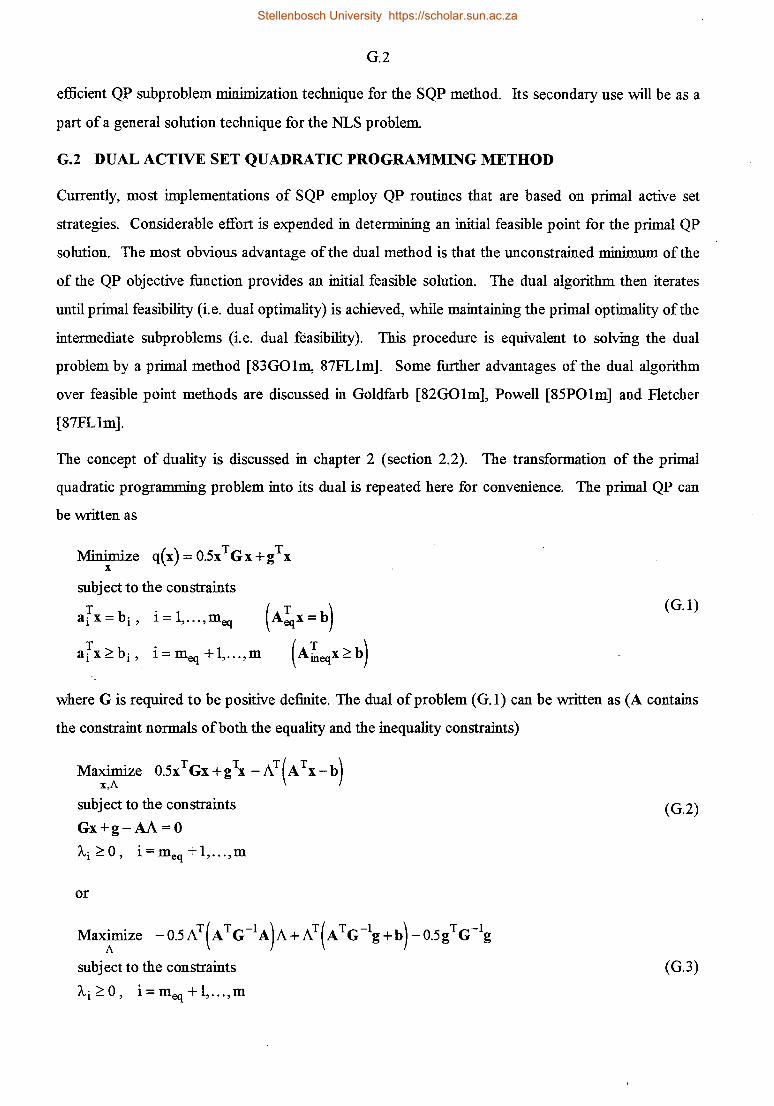
G.2

efficient QP subproblem minimization technique for the SQP method. Its secondary use will be as a

part of a general solution technique for the NLS problem

G.2 DUAL ACTIVE SET QUADRATIC PROGRAMMING METHOD

Currently, most implementations of SQP employ QP routines that are based on primal active set

strategies. Considerable effort is expended in determining an initial feasible point for the primal QP

solution. The most obvious advantage of the dual method is that the unconstrained minimum of the

of the QP objective function provides an initial feasible solution. The dual algorithm then iterates

until primal feasibility (i.e. dual optimality) is achieved, while maintaining the primal optimality of the

intermediate subproblems (i.e. dual feasibility). This procedure is equivalent to solving the dual

problem by a primal method [83GOlm, 87FL1m]. Some further advantages of the dual algorithm

over feasible point methods are discussed in Goldfarb [82G01m], Powell [85P01m] and Fletcher

[87FL1m].

The concept of duality is discussed in chapter 2 (section 2.2). The transformation of the primal

quadratic programming problem into its dual is repeated here for convenience. The primal QP can

be written as

subject to the constraints T

aix=bi, i=l, ... ,meq

T ai x ~bi, i = meq + 1, ... ,m

(G.l)

where G is required to be positive definite. The dual of problem (G.l) can be written as (A contains

the constraint normals of both the equality and the inequality constraints)

Maximize 0.5xTGx+gTx -AT(ATx-b) x,A


Gx+g-AA=O

Ai ~O, i=meq +l, ... ,m

or

Ma~ze -0.5AT( A TG-1A)A+ AT(A TG-1g+b)-o.5gTG-1g


A.i~O, i=meq+l, ... ,m

(G.2)

(G.3)


G.3

where the constraints are used to solve for x, i.e. x = G-1AA-G-1g and A.i, i = l, ... ,meq have no

sign restriction. Problem (G.3) has only simple constraints on the dual variables (Lagrange

multipliers). Tue Kuhn-Tucker condition for the primal problem state (refer to equation (2.8)):

(G.4)

Similarly, the Kuhn-Tucker conditions for the dual problem state:

uiA.i = 0, i = meq + 1, ... ,m (G.5)

where ui are the Lagrange multipliers of the dual problem Thus, the values of the Lagrange

multipliers of the dual problem, ui, correspond to the values (a'[ x - bi) , i = meq + 1, ... , m of the

primal problem (It should be noted, however, that this is not a formal proof) Tue following points

should be noted about the relationship between equations (G.4) and (G.5):

( 1) If ui = 0 , i = p and the corresponding element of A.i is greater than zero, it indicates that the

primal inequality constraint corresponding to the value of A.i is active. If ui = 0 , i = p and the

corresponding element of A.i is equal to zero (weakly active); it indicates that constraint p is

superfluous.

(2) If ui > 0, i = p, then the corresponding element of A.i is equal to zero which indicates that the

primal inequality constraint corresponding to the value of A.i is inactive.

In the dual active set method, x(k) is not primal feasible (some of the constraints are not satisfied),

but the Lagrange multipliers are dual feasible, i.e. A.i;::: 0, i = meq + 1,. .. ,m. Changes in the

working set are performed to maintain non-negative Lagrange multipliers while moving to satisfy the

violated constraints, i.e. obtain primal feasibility.

The dual active set strategy can be explained from a primal point of view as follows:

(1) Solve the unconstrained QP problem to obtain x(l). This provides an initial feasible solution

for the dual problem All the Lagrange multipliers are equal to zero. Set k = 1.

(2) Test the linear constraints for primal feasibility. If the current point x(k) satisfies all the

constraints, a feasible solution is found; terminate with x* = x(k). Otherwise, the most or any

violated constraint not in the current active set is added, i.e. A(k) is enlarged.


G.4

(3) Store the current values of the Lagrange multipliers of the inequality constraints,

~- = ~ (k) . + 1 s t k k + 1 11,1 11, 1 , 1 = meq , ... ,m. e = .

(4) Solve the QP to obtain new values for x(k) and Alk), i = l, ... ,m.

(5) Test the inequality constraints for dual feasibility, i.e. Alk) ~ 0, i = meq + 1, ... ,m. If the

Lagrange multipliers of the inequality constraints are dual feasible, go to step 2. Otherwise

one or more of the new Lagrange multipliers of the inequality constraints contained in the

current active set is negative (dual infeasibility). Thus, A (k) is not the correct active set. In

order to remain dual feasible, a search direction,

~ (k) - ~ (k) - . [{ } (k)] uAi - 11,i - /...i, 1 E meq + l, ••• ,m n A

and the largest possible step length, 0 ~ a (k) ~ 1, are determined such that the Lagrange

multipliers of the inequality constraints in the current active set satisfy dual feasibility, i.e.

- - (k) (k) (k) > . [{ } (k)] /...i - Ai +a o'Ai - 0 , 1 E meq + 1, ... , m n A

The inequality constraint corresponding to the first Lagrange multiplier that becomes zero is

dropped from the active set and A (k) is reduced (inequality constraint becomes inactive). Go

to step 4.

The largest step size a (k) to retain dual feasibility during iteration k is obtained from solving

. ( (~ ~ (k) . . 0- 'Ai . (k) a = IDlil IDlil (k) , i E ({meq + 1, .. ., m} n A ]

ot..<.k><o OA· 1 1

(G.6)

During the course of the QP solution the active set will change from one iteration to the next.

Therefore, as constraints are added to and deleted from the active set, various matrices need to be

updated, rather than recomputed.

G.3 SOLUTION OF THE EQUALITY CONSTRAINED QP PROBLEM

Equality constrained QP subproblems occur within many active set methods for general QP problems

as well as in SQP methods. A variety of methods are available for solving these problems, e.g.

[81Gllm, 87FLlm, 89Gllm]. The method that will subsequently be derived are based on the

procedures proposed by Gill et al. [84GI1m] and Betts [80BElm, 80BE2m].

G.5

Calculation of the search direction and the Lagrange multipliers

In this section a procedure is developed for solving the QP problem by means of an orthogonal

decomposition of the constraint matrix. We shall be concerned with the numerical solution of the

following QP problem:

subject to the equality constraints T A x=b

(G.7)

where AT is an m x n matrix with rank(A) = m, Gann x n positive definite symmetric matrix, g is

an n-vector, b is an m-vector and x is an n-vector and n ~ m

Let Q be an orthogonal n x n matrix (Qr Q = I), and

(G.8)

where T is an m x m reversed lower-triangular nonsingular matrix.

Let Q be partitioned as

Q=[Z : Y] (G.9)

where Z is an n x (n-m) and Y is an n x m matrix respectively. Substitute equation (G.9) into

equation (G.8) and find

(G.10)

hence

(G.11)

The equality constraints can be rewritten as

(G.12)

Define the n-vector p as

(G.13)


G.6

where pz is an (n-m)-vector and py is an m-vector. Substitute equation (G.13) into equation

(G.12) and find

(G.14)

Since T is nonsingular, the m-vector py can be solved by means of back substitution. Call the

solution py, i.e. py = T-1b.

Now, if

x = Qp = Zpz + Ypy (G.15)

then problem ( G. 7) can be written as an unconstrained problem, i.e.

q(x) = 0.5(Zpz + Ypy )T G(Zpz + Ypy )+gT(Zpz + Ypy)

T T ( T A T )T ~ T T A T A = 0.5pzZ GZpz + Z GYpy +Z g pz +0.5pyY GYpz +g Ypy (G.16)

q(x) is minimized when pz satisfies (gradient of equation (G.16) is set equal to zero)

The solution of problem (G.7) can be calculated from

i=Zpz +Ypy . (G.17)

The Lagrange multipliers A= (A.1) .. 2 , ... ,A.m) can be obtained as follows:

AA=Gi+g (G.18)

or

(G.19)

Now

[

zTGz

Y]= ...

YTGz

(G.20)


G.7

hence

(G.21)

and A is determined by back substitution.

The original constrained problem is replaced by a lower dimensional unconstrained problem in the

variables pz after choosing the variables py to satisfy the constraints. A unique solution to the

equality constrained QP problem will exist due the positive definite restriction placed on G.

Changes in the working set

Unless the correct active set is known a priori, the working set must be modified during execution of

an active set method by adding and deleting constraints. The corresponding matrix factorizations

will be updated accordingly, because computing them ab initio would be too expensive. Numerically

stable updating methods of a matrix when it is modified by adding or deleting a row are well known

[74Gllm]. In our updating procedures we make use of Givens rotations. Sequences of plane

rotations (Givens rotations) are used to introduce zeros into the appropriate positions of a vector or

matrix [74Gllm, 84Gllm]. Basic linear algebra manipulations are then used to perform the matrix

modifications (updates).

Before the changes in the working set are discussed, we define the following matrices and vectors

and assume that they are available:

(i) Matrices Q and T such that Q is an orthogonal n x n matrix, i.e. Qr Q = I, and T is an m x m

reversed lower-triangular nonsingular matrix. A TQ = [o ; T] and Q is partitioned as

Q = [z : Y] (Z is an n x (n-m) and Y is an n x m matrix).

(ii) Matrices U, Gyy and Gzy, where

(a) U is an (n-m) x (n-m) upper triangular matrix, UTU = Z TGZ

(b) Gyy is an m x mmatrix, Gyy = YrGY

(c) Gzy is an (n-m) x m, Gzy = zTGY

(ili) Vectorgq, w n x I vector ruch iliat gQ = Qrg = [ ::]g = [ ::: ] = [::].

The partitioning of gQ is such that gz is an (n-m)-vector and gy is an m-vector.


G.8

The following should also be noted:

(i) When m = 0, let Q = I, Z = I, gQ = g and Uthe Cholesky factor of G ( G = UTu). T, Y,

Gyy and Gzy are empty matrices.

(ii) The storage required for the following matrices are:

(a) Q (n x n)

Gzyl ... (n x n)

Gyy

GQ is symmetric so only its upper triangular part is stored (refer to equation (G.20)).

(c)T(mxm)

( 1) Adding a constraint

When a constraint is added to the working set, its index can simply be placed at the end of the list of

constraint indices of the working set. Therefore we assume that the new constraint is added at the

last row of AT.

Suppose Q, T ,U, Gyy, Gzy and gQ corresponding to the constrains A Tx = b are available and

that the constraint T am+lx = bm+l is added to the set of constraints. Furthermore,

Q, T, U, Gyy, Gzy and gQ correspond to AT= [ ~ T ] . am+l

(a) Updating Q and T:

T T Let w = am+lQ, then

where w~ and w~ represent the partitioning of the new row that is added. We see that a new

matrix Q can be obtained by applying a sequence of plane rotations (Givens rotations) on the right


G.9

of Q to transform w i to suitable form The sequence of rotations take linear combinations of the

elements of w i to reduce it to a multiple (say y) of a column of the identity matrix.

Let ij be an orthogonal matrix formed by the product of rotations in the planes (1,2), (2,3),

(3,4), ... , (n-m-1,n-m) such that the effect ofthe transformation can be expressed as

-T - [o : 0 T ] [ . -] - [o T ] A QQ = . T = 0 : T , where T = T . 0 : y Wy y Wy

Note, however, that Q has the form [·:· ·:-1 with Pan (n - m) x (n - m) matrix; hence the

rotations affect only the first (n-m) columns of Q so that the last m columns of Q are identical to

those ofQ. The first (n-m) columns of Q are linear combinations of the first (n-m) columns of Q.

Q can be expressed as

[

p :

Q=(Z : Y] ··· ··· 0 :

where ZP = [z y] and Y=(y

(b) Updating U, Gyy and Gzy:

The matrix QT GQ can be expressed as

-T -The matrix Q GQ can be expressed as

[

PT -T -Q GQ= ·~·

Y]=(Z y Y]=(Z

Y] (the last column of Z becomes the first column of Y ).


G.10

The matrix QT GQ must be repartitioned, because m increases by 1 and (n-m) decreases by 1.

Let UP=(U

- [~T Furthermore Gzy = U u ~r l ::

u should satisfy UTU = uTu = ijTj>Tj>ij where ji is an orthogonal matrix chosen to triangularize

U (upper triangular form). Uhas subdiagonal elements (introduced by the plane rotations applied to

Z) that must be eliminated. P is a product of rotations (Givens rotations) in the planes (1,2),

(2,3), ... , (m-l,m-1).

The following procedure must be performed to update GQ :

Gzy] ··· , then

Gyy

(11 .. ) C U~T~ d n ~T~ ompute v = u an -., = u u

v Gzy

(ill) Form [:] = 9 iih (Both Gyy and Gyy are symmetric matrices)

hzy Gyy

(iv) Form U =PU where P triangularizes U.


G.11

[

ZTGZ It can be shown that QT GQ = ...

YTGz

zTGY] · · · to illustrate that the repartitioning procedure

YTGY

is correct.

( c) Updating gQ :

[

pT - -T -T gQ = Q g = Q Qg = -~·

where gz is an (n-m-1) vector and gy is an (m+ 1) vector. Hence, compute PT gz and repartition.

( d) Linear dependent constraints

A linear dependent constraint can be expressed as a linear combination of all the other constraints in

the active set.

Suppose that the current equality constraints are A Tx = b. If the new constraint, a~+1x = bm+1'

that is added to the active set is linear dependent on the other constraints, then a m+l can be

expressed in terms of the other constraint normals as

m

am+1=L:Iiai=Ar, r=[r1 rz ... rmr· i=l

where r is the vector of coefficients expressing the linear dependence.

It is known that

hence


G.12

Let

Thus w z = 0 and r can be determined from solving the following system of equations:

T T r=wy.

( 2) Deleting a constraint

When a constraint is deleted from the working set, the row dimension of AT and the dimension of T

are decreased by one, while the column dimension of Z is increased by one.

Suppose Q, T , U, Gyy , Gzy and gQ corresponding to the constraints AT x = b are available and

that the constraint a[x =bi is deleted from the active set of constraints. Let the new set of active

-T constraints be A x = b .

(a) Updating Q and T:

A TQ = [o : s], where S is an (m-1) x m matrix such that rows 1 to (i-1) are in the reverse

triangular form and the remaining rows have one extra element above the reverse diagonal. In order

to reduce these columns of S to the desired triangular form of T , a sequence of plane rotations

(Givens rotations) are applied on the right of S.

Let Q be an orthogonal matrix formed by the product of rotations in the planes (m-i+ 1,m-i), ... ,

(2,1) such that SP= T, where T is in the reverse lower-triangular form.

[I : OJ

Note, however, that Q has the form · · · · · · · · · with P an m x m matrix; hence the rotations

0 : p

affect only the last m columns of Q so that the first m columns of Q = QQ are identical to those of

Q. Then


G.13

Q can be expressed as

Q =QQ=[Z l I : OJ Y] ·~· ·~· = [z YP]=[Z z Y]=[Z

where YP = [ z : Y] and Z = [ Z : z] (the first column of YP becomes the last column of Z ).

z is a linear combination of the relevant columns ofY.

(b) Updating U, Gyy and Gzy :

The matrix QT GQ can be expressed as

-T -The matrix Q GQ can be expressed as

QTGQ = r·~· ·~· ·O;J[~:~. ·'.· ~~1r·~· O : P Gzy : Gyy 0

The matrix QT GQ must be repartitioned, because m decreases by 1 and (n-m) increases by 1, and

U must be retriangularized.

Let

It then follows that

and U should satisfy


G.14

·:·] Suppose that the Cholesky factor can be defined as

then

Hence choose UT u = v and u Tu+ p2 = .S and solve for u and p. (If .S ~ u Tu, G cannot be positive

definite.)

The following procedure must be performed to update GQ :

Gzy] ·· · , then

Gyy

(i) [ GzyP ]

Compute ··· = PTGyyP

v Gzv

-T hyy

(ii) Solve UT u = v for u and calculate p = ~ .S - u Tu

(iii) Form the new Cholesk.y fuctor U = [·:· -:-]


G.15

[

zTGz

It can again be shown that QT GQ = ... YTGz

zTGY] · · · which indicates that the repartitioning

YTGY

procedure is correct.

( c) Updating gQ :

l I

- -T -T gQ = Q g = Q Qg = ·~·

where gz is an (n-m+ 1) vector and gy is an (m-1) vector. Hence, compute PTgy and repartition.

Computational algorithm

The computational algorithm to find the solution ( i, A ) of an equality constrained QP is explained

below.

Step O: Preliminaries

(i) When m = 0, let Q =I, Z =I, gQ = g and Uthe Cholesk:y factor of G, i.e. G = UTU. T, Y,

Gyy and Gzy are empty matrices. Go to step 3.

(ii) When a constraint is added to the active set, update Q, T , U , Gyy , Gzy and gQ .

(iii) When a constraint is deleted from the active set, update Q, T , U , Gyy , Gzy and gQ .

(iv) Test for linear dependence of the constraints in the active set. If the constraints are linearly

independent, go to step 2. Otherwise, calculate the coefficients, r, that express the linear

dependence. Go to step 9.


(i) Check for errors in the input dimensions. Go to step 9 if an error is encountered .

.film.1: Solve for py

(i) Solve Tpy = b for py.

(ii) If m = n, go to step 5.


G.16

Step 3: Compute Gzypy +gz

(i) Let g = Gzypy + gz.

Step 4: Solve for p z

(i) Solve (uru)pz = -g for pz.

(Note: When m = 0, solve Gx = -g for i . )

Step 5: Compute Ghi>z +Ghpy +gy

(i) If m = 0, go to step 7.

~: Solve for the Lagrange multipliers A

(i) T A

Solve T A = d for A

Step 7: Solve for i

(i) If it is not necessary to calculate i , go to step 8.

(ii) Calculate i = Qp = Zpz + Ypy

Step 8: Calculate the objective function q( i)

Step 9: Exit subroutine

(i) Stop.

G.4 DUAL ACTIVE SET ALGORITHM

The algorithm given below follows the dual approach described in the previous sections for convex

quadratic programming problems (refer to Goldfarb and ldnani [83GOlm] and Powell [83P02m,

85POlm]).


(i) Check for errors in the input dimensions (e.g. meq > n)

(ii) Find the reciprocals of the lengths of the constraint normals. Go to step 9 if a constraint is

infeasible due to a zero normal.


G.17

(iii) Store the original G-matrix and the g-vector.

(iv) Form the Cholesky decomposition of G. IfG is not positive definite, go to step 9.

(v) Find the unconstrained millimum of problem (G.1). Go to step 5.

Step 1: Solve the equality constrained QP problem (section G.3)

(i) Solve problem ( G. 7), the equality constrained QP problem.

(ii) If an error occurs in the input dimensions of the routine that solves the equality constrained QP

problem, go to 9.

(iii) If the constraints in the active set are linearly dependent, go to step 7.

(iv) If the calculation is successful, go to step 2.

Step 2: Test for dual feasibility

(i) If all the Lagrange multipliers of the inequality constraints contained in the current active

(working) set are greater than or equal to zero, dual feasibility is achieved. Go to step 5.

(ii) If one or more of the Lagrange multipliers contained in the current active set is negative, go to

step 3.

~: Determme the largest step size to retain dual feasibility (partial step)

(i) Perform a line search with the Lagrange multipliers of the inequality constraints contained in

the current active set and determme the first inequality constraint to become inactive (Lagrange

multiplier equals zero, refer to equation ( G. 6) ).

(ii) Calculate the new Lagrange multipliers with the partial step taken in the dual space.

Step 4: Drop the inactive inequality constraint from the active set

(i) Drop the inequality constraint which becomes inactive (Lagrange multiplier equals zero) from

the current active set (reduce the active set) .

. (ii) Store the values of the Lagrange multipliers of the inequality constraints in the reduced active

set.

(iii) Go to step 1.

Step 5: Test for primal feasibility

(i) If the number of constraints in the active set equals the total number of constraints, the current

solution is both feasible and optimal. Go to step 8.


G.18

(ii) Test all the inactive constraints for feasibility.

(iii) If no constraint violations occur, the current solution is both feasible and optimal. Go to step

8.

(iv) If one or more of the constraints is violated, a feasible solution has not yet be found. Store the

index of the most violated constraint and go to step 6.

Step 6: Add the violated constraint to the active set

(i) Add the violated constraint to the active set (enlarge the active set).

(ii) Set the Lagrange multiplier of this constraint equal to zero.

(iii) Store the values of the Lagrange multipliers of the inequality constraints in the enlarged active

set.

(iv) Go to step 1.

Step 7: Linear dependent active set

(i) If a violated equality constraint in the current active set is linear dependent on the other

constraints in the active set, the QP problem is infeasible. (An equality constraint, once added

to the active set, can never be dropped.) Go to step 9.

(ii) If the constraint violation and the coefficient expressing the linear dependence of the

constraints have similar signs (refer to (83GOlm], theorem 2). The QP problem is thus

infeasible. Go to step 9.

(iii) Drop the inequality constraint with the largest coefficient expressing the linear dependence

from the current active set i.e. reduce the active set (step in the dual space).

(iv) Store the values of the Lagrange multipliers of the inequality constraints in the reduced active

set.

(v) Go to step 1.

Step 8: Store the Lagrange multipliers

(i) Store the Lagrange multipliers of the active constraints. The inactive constraints have zero

Lagrange multipliers.

Step 9: Return to caller program

(i) Stop, return to the caller program and indicate the reason for the return. The following cases

can occur:


(a) Successful completion of calculations

(b) Error in input dimensions

( c) Inconsistent constraints

( d) Infeasible QP problem

( e) Matrix G is not positive definite

G.19

G.5 EXTENSIONS TO THE DUAL ACTIVE SET ALGORITHM

The dual algorithm described in the previous section is modified in several ways which result in

computational advantageous for application with the SQP method and as a general solution

technique. Gill et al. [85Gllm, 86Gllm] discuss the benefits (e.g. reduction in linear algebra

computations) of designing and implementing a specialized QP algorithm intended for use within

SQP methods. These developments are motivated by the special features of the QP subproblems

associated with the SQP methods. A specialized QP algorithm can also be used on general problems

with equal success. The modifications are:

(1) The x-values are only calculated when necessary. The Lagrange multipliers are used as the

decision variables in the dual active set algorithm and the x-values are only needed for testing

primal feasibility.

(2) Goldfarb and Idnani [83G01m] remarked that the active set at the optimal solution of the QP

subproblem in Powell's SQP method [82P02m] tends not to change very much from one

iteration to the next. This means that a good estimate of the active set of the QP subproblem

will often be available before the QP subproblem is solved. The major work within a general

QP algorithm is to identify the correct active set.

To take advantage of this, the dual algorithm is executed in two passes on every iteration of

the SQP algorithm. An active set, containing only the equality constraints are assumed for the

first iteration of the SQP method (initialization). In the first pass all the active constraints of

the previous iteration of the SQP method are considered when testing for primal feasibility.

The first violated (normalized violation), rather than the most violated constraint is added to

the current active set. In the second pass all the inactive constraints are tested for primal

feasibility and the dual algorithm is started from the optimal solution obtained in the first pass.

The most violated constraint (normalized violation) is added to the active set in the second

pass. The indices of the active constraints of the previous SQP iteration must thus be available

for its next iteration.


G.20

This procedure where the active set at the solution of each QP subproblem is used as a . prediction of the working set of the next, is referred to as the "warm start" procedure. Since

the active sets eventually do not change, the effect of the warm start procedure is that later QP

subproblems reach optimality in only one iteration. Using warm starts can greatly reduce the

QP problem solution time [78Gllm, 83GOlm, 85Blle, 85Gllm, 86Gllm].

(3) All the constraint equations are scaled to a magnitude of about unity by using some typical

values of problem parameters. With this approach it is easier to check for linear dependence of

the constraint gradients during the solution process. The QP subproblem is also solved in

terms of the dual variables. These schemes make the QP problems well scaled and numerically

stable. The normalized constraint violations, rather than the unscaled constraint violations, are

compared with each other in order to determine which constraint to add to the active set.

(4) The constraint updating formulae use stable and efficient updating procedures (also refer to

[94K.Ale]). Givens rotations are used to introduce zeros in the required positions of the

matrices to be updated when the active set changes from one iteration to the next. Powell

[85POlm] states that the Goldfarb and Idnani [83GOlm] implementation of the dual algorithm

can become unstable under certain conditions. Powell [83P02m, 85POlm] implemented this

dual QP algorithm for convex quadratic programming calculations.

Schmid and Biegler [94SC1e] discuss several modifications made to the dual algorithm of Goldfarb

and Idnani [83GOlm] when it is used with reduced Hessian SQP methods. These modifications

include, for example, a warm start option, the special treatment of the doubly-bounded constraints

(e.g. variable bounds) and the handling of infeasible QP problems.

The dual QP algorithm explained in this appendix and ZQPCVX [83P02m, 85POlm] will be used in

the computational procedures. The major difference between the two algorithms are the updating

methods used to account for the addition to and removal of constraints from the active set. Our

algorithm employs the methods proposed by Gill et al. [84Gllm], while ZQPCVX uses the methods

of Goldfarb and Idnani [83G0lm]. Furthermore, ZQPCVX will be treated as a "black box",

whereas our algorithm makes use of the special features of the QP subproblems associated with SQP

methods. It is expected that ZQPCVX will be faster than our algorithm due to the matrix updating

and transformation methods used. However, our implementation, using orthogonal transformations,

will be more stable. ZQPCVX does not employ any of the modifications to the dual QP algorithm as

discussed above.


H.1

APPENDIXH

SUCCESSIVE QUADRATIC PROGRAMMING ALGORITHM

H.1 INTRODUCTION

A variety of successive quadratic programming (SQP) methods have been developed and used for

solving nonlinear programming problems, e.g. [63Wllm, 72Bllm, 76HA1m, 78P01m, 85NOlm].

SQP methods usually require fewer function and gradient evaluations when compared to other

nonlinear programming methods. Various different numerical implementations of the SQP algorithm

can be found, e.g. [78P01m, 82P02m, 86Llle, 86SC1m]. The fundamental differences between

these algorithms and the numerical implementations based thereon, are the definition of the QP

subproblem to be solved at each iteration and the descent function used during the step size

calculation. The performances of these algorithms are mainly influenced by the implementation and

execution of the above-mentioned differences. In this section we will discuss the numerical

implementation of the SQP method as proposed by Powell [78P01m, 82P01m, 82P02m]. Both

implementations of Powell are used in this study: [78P01m] for the reduced Hessian or general.SQP

methods and [82P02m] for the general SQP method only.

H.2 ALGORITHM

Powell has written two FORTRAN subroutines VF02AD [78P01m] and VMCWD [82P01m,

82P02m] that implement the Wilson, Han and Powell SQP algorithm. VMCWD is basically an

extension of VF02AD to overcome the algorithmic disadvantages of cycling and the Maratos effect

[79CH1m, 82CH1m, 82PO Im]. The SQP algorithm can be outlined as follows:

The nonlinear programming (optimization) problem to be solved is formulated as [87FL1m]

Minimize f(x) = f(xi.x2, ... ,xn) x


ci (x) = 0, i = 1,. . .,meq

Ci (x) :2: 0, i = meq + 1,. . .,m

(H.1)

where x = ( x 1, x2, ... , xn) is a vector of variables, called the decision variables. It is assumed that

the bounds on the variables are incorporated into the inequality constraints. The Lagrange function

of the problem stated above has the form


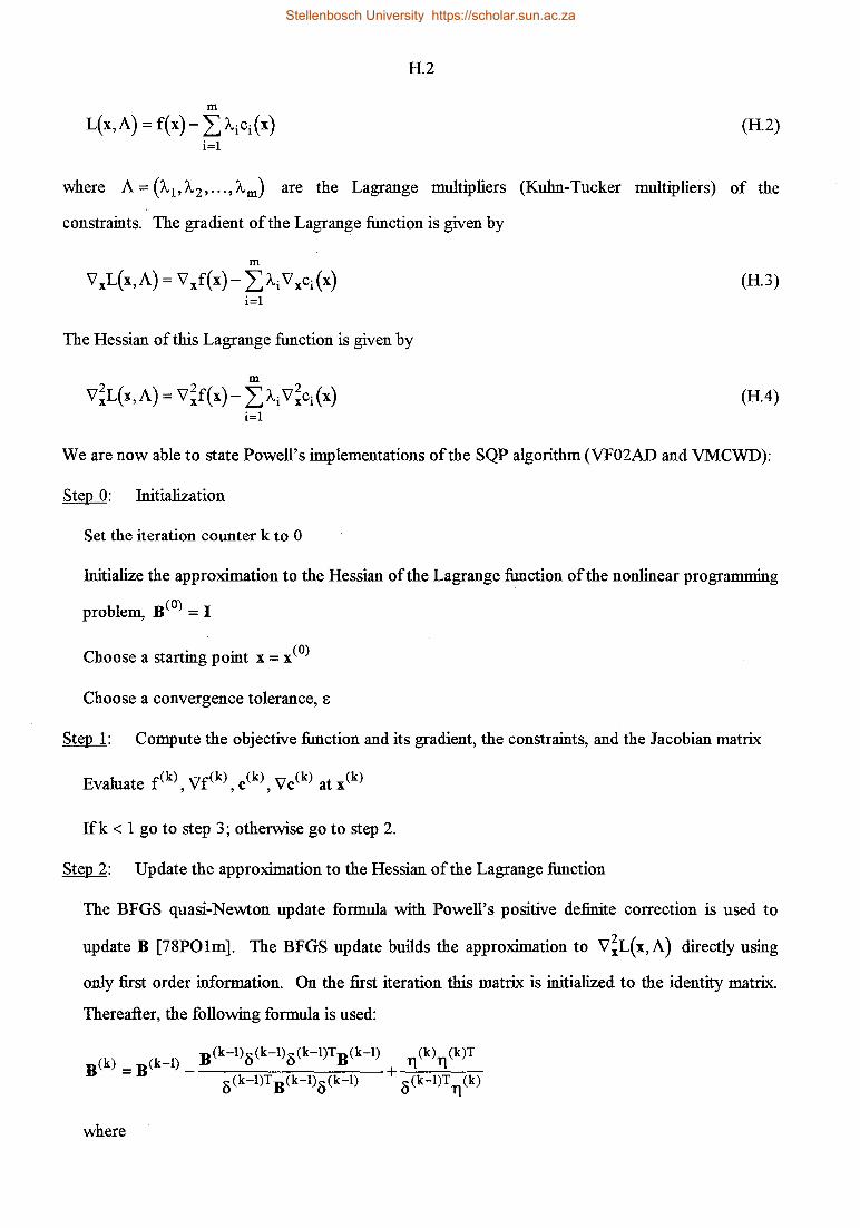
H.2

m

L(x,A) = f(x)- L A.ici (x) (H.2) i=l

where A= ("-i.A-2 , ... ,A.m) are the Lagrange multipliers (Kuhn-Tucker multipliers) of the

constraints. The gradient of the Lagrange function is given by

m

V xL(x,A) = V xf(x)- LA,i"V xci(x) (H.3) i=l

The Hessian of this Lagrange function is given by

m

V~L(x,A)=V~f(x)-L:A.i"V~ci(x) (H.4) i=l

We are now able to state Powell's implementations of the SQP algorithm (VF02AD and VMCWD):

~: Initialization


Initialize the approximation to the Hessian of the Lagrange function of the nonlinear programming

problem, B(O) = I

Choose a starting point x = x(O)

Choose a convergence tolerance, e

Step 1: Compute the objective function and its gradient, the constraints, and the Jacobian matrix

If k < 1 go to step 3; otherwise go to step 2.

Step 2: Update the approximation to the Hessian of the Lagrange function

The BFGS quasi-Newton update formula with Powell's positive definite correction is used to

update B [78P01m]. The BFGS update builds the approximation to V~L(x,A) directly using

only first order information. On the first iteration this matrix is initialized to the identity matrix.

Thereafter, the following formula is used:

B(k-l)dk-l)dk-l)TB(k-1) (k) (k)T B(k) = B(k-1) _ u u + rt rt

8 (k-l)T B(k-1)0(k-1) 0(k-l)T rt (k)

where

H.3

k = the iteration counter

8 (k-l) = x{k) -x(k-1) = a(k-l)s(k-1)

y(k) = v'xL{x(k) ,A(k-1))-v xL{x(k-1) ,A(k-1))

Tl(k) = Sy(k) +(1.0-S)B(k-1)8(k-l)

8=1.0 if ()(k-l)Ty(k) ~ 0_28(k-l)TB(k-l)()(k-l)

O g()(k-l)TB(k-1)0(k-l) e = . othef\.\.ise

8 (k-l)T B(k-1)0 (k-1) - 0 (k-l)Ty {k)

Step 3: Solve the QP subproblem and evaluate the Lagrange multipliers

Powell proposes the following QP subproblem to be solved at each iteration:

~ze Vf( x(k) f s(k) +0.5 s(k)TB(k)s(k)


ci(x(k))+vci(x(k))\<k) =O, i=l, ... ,meq

ci( x(k)) + Vci( x(k) f s(k) ~ 0, i = meq + 1, ... ,m

The solution of the QP subproblem gives the search direction at the current iteration, s(k), and

the Lagrange multipliers, A (k) . Powell's SQP implementations used a primal quadratic

programming package contained in the Harwell subroutine library.

Powell observed that the linearized constraints can be inconsistent, even if the nonlinear

constraints of the original problem are consistent and define a feasible region and a solution.

Powell has recommended the introduction of a dummy (feasibility) variable, ~' such that the QP

subproblem becomes:

Minimize Vf( x(k)) T s(k) + 0.5 s(k)TB(k)s(k) - a~ s,1;


~ci(x(k))+vci(x(k))Ts(k) =O, i=l, ... ,meq

~ici(x(k))+vci(x(k))Ts(k) ~O, i=meq +1, ... ,m

0.$~.$1

where a is set to a large positive number ( 106, for example). ~i = 1 for the inequality constraints

that are satisfied, and ~i = ~ othef\.\.ise. ~ is made as large as possible within the range 0 .$ ~ .$ 1

H.4

by setting the gradient of the objective function with respect to ~ to a large negative number. The

elements in the extra column and row of B for ~ are set to zero. If~ = 1, the original problem is

obtained. If no solution is found for the QP, ~ < 1 will allow additional freedom to find a search

direction to the modified problem Ifno solution can be found with~> 0, then the algorithm fails,

i.e. ~=O=>s(k) =0.

Step 4: Check for convergence

If the convergence criterion is satisfied, i.e. [ Iv r( x (k)) ', (k) I + ~Ai c, ( x (k)) ] ~ ' , set x* ~ x (k)

and A*= A(k). Go to step 6.

Step 5: Calculate the line search step length parameter

Perform a line search along the search direction, s(k), to determine the value of a(k) e[O,l] such

that the chosen merit function satisfies the following inequality:

where ~(k) is an approximation to ( 8'I') (~(k) ~'I'( x(k) + s(k), ~(k) )- 'I'( x(k), ~(k) )) . aa a.=0

In the line search a step length of one is tried initially, but it is reduced if the above inequality is

not satisfied.· A quadratic approximation of the merit function using two function values and its

slope at the current point is constructed. A suitable value of a (k) is obtained by means of

quadratic interpolation and its value is not reduced by more than 10% per line search. If five step

length reductions are insufficient, there is an error return from the subroutine. The line search

uses a L1 -exact penalty function as a merit function, i.e.

meq m

'I'(x,~)=f(x)+ L~ilci(x)I+ L~i\max[o,-ci(x)]\ i=l i=m.,q +l

where "-i are the constraint weighting factors which are functions of the Lagrange multipliers at

the solution of the QP. . On the first iteration, they are set equal to the absolute value of the

Lagrange or Kuhn-Tucker multipliers, i.e. ~i = l"-i I , i = 1, ... , m . After the first iteration,

H.5

The requirement of a decrease in the merit function at every iteration may sometimes inhibit the

superlinear rate of convergence of the SQP method. This phenomenon is also known as the

Maratos effect and causes slow convergence. Furthermore, the technique for adjusting the

constraint weighting factors during line search may give rise to cycling. Powell [82CHlm,

82POlm, 82P02m] implemented the watchdog technique in VMCWD to remedy these

disadvantages. Here the step size is chosen by reducing either the Lagrange function or the line

search objective function during the line search. This technique allows the line search objective

function to increase on some iterations. However, the line search objective function must be

reduced every t iterations (t :?:'.: 2); otherwise a restart is required from the previous point if no

reduction occurs.

The choice and adjustment of the constraint weighting factors, A. , are also done according to

different prescribed conditions in VMCWD: Before the first iteration all the values of A. are given

tiny positive values, in case the objective function is constant. If the search direction s(k) of an

iteration satisfies the condition

then no change is made to ~(k). Otherwise we require the inequality

~~fk)lci( x(k) )j +. f ~fk) max[o,- ci( x(k)) ]- ~~fk)lci( x(k)) +s(k)TV'ci( x(k) )I I=l I=nt,,q+l I=l .

-. f ~fk) ma~ o, - ci( x(k) )- s(k)T v ci( x(k))]:?::: 13Ck),s(k)T vf(x(k) )I l=nt,,q+l

to hold, where 13<k) is a positive constant. If the ~(k) that is set at the beginning of the iteration

satisfies this condition when 13<k) = 15, then ~(k) is not altered. Otherwise the following

procedure is used to obtain a value of ~(k) such that the above inequality holds for 13<k) = 2.0.

The increase in 13<k) ensures that at least one component of ~(k) is multiplied by a number that

exceeds 1. 3 3 3.

For i = 1, ... ,m we let A.i be the Lagrange multiplier of the i-th constraint at the solution of the QP

subproblem that determines s(k). For each i we leave ~i unchanged if increasing its value would

not increase the left hand side of the above inequality. Otherwise A.i is given the value

H.6

where the positive parameter v, which is independent of i, is determined by the condition that the

above inequality is satisfied as an equation when 13<k) = 2.0.

After a suitable choice of a(k), the next point, x(k+l), is calculated from

(k+l) (k) + (k) (k) x =x a s

Increment the iteration counter k, i.e. k = k + 1

Go to step 1 and repeat the calculations.

Step 6: Return to the caller program

Stop, return to the caller program and indicate the reason for the return. The following cases can

occur:

(a) Optimization completed successfully

(b) Maximum number of function calls reached

( c) Line search required 5 function calls

(d) Uphill search direction calculated

( e) Constraints seem to be inconsistent

(f) Not enough working space reserved

(g) QP algorithm failed to find a solution

Auxiliary subroutines

The user must provide a subroutine called CALCFG to define the objective and constraint functions

and their gradients for any vector of variables. The user can also provide his/her own QP subroutine

to solve the subproblems at each iteration. Powell's original SQP implementation uses a primal QP

method from the Harwell library.

H.3 MODIFICATIONS TO THE SQP ALGORITHM

Several modifications were made to Powell's SQP algorithm, VMCWD [82P02m], which will be

discussed below.

( 1) Quadratic programming routine

The solution of the QP subproblem is a major calculation in SQP methods and can affect the overall

efficiency of the SQP method. SQP methods require the solution of strictly convex QP subproblems

H.7

to determine the direction of search at each iteration. Powell [82P02m] noted that a more accurate,

efficient and reliable QP algorithm is desirable for solving the subproblems.

The most significant change to Powell's implementation is the change in the algorithm to solve the

QP subproblem The feasible point primal QP algorithm normally used with Powell's SQP

implementation is replaced by a dual QP algorithm for convex quadratic problems based on the

method of Goldfarb and Idnani [83GOlm] (refer to Appendix G). The dual QP subproblem has only

simple constraints on the dual variables (Lagrange multipliers). The active set seems not to change

very much from one iteration to the next iteration [83G0lm].

Gill et al. [85Gllm, 86Gllm] state that substantial gains m efficiency of the linear algebra

calculations can result from a suitably tailored QP algorithm for use with SQP methods. The dual

QP algorithm explained in Appendix G is extended and includes special features such as the warm

start procedure. Since the iterations of a QP method are essentially a search for the correct active

set, it is computationally highly desirable to exploit this information. Further discussions on

specialized QP algorithms for SQP methods can be found in Gill et al. [85Gllm, 86Gllm].

(2) Evaluation of derivatives

VMCWD requires that the gradients of the objective and constraint functions be calculated even

during line search iterations. Since this information is only required on the last line search point (the

new point), a modification was made so that the values of the objective function and the constraints

and their corresponding gradients can be calculated only when required.

(3) Modification of the objective function

. 6 The dual QP algorithm requires a strictly convex objective function. Therefore, the term -1 O ~

added to the objective function in Powell's original code is replaced by 0.5x106e-2.o x 106 ~ as

suggested by Goldfarb and Idnani [83GOlm]. The elements in the extra column and row of B for~

are set to zero, except for the last element in this column and row which becomes 106.

( 4) QP algorithm failed to find a solution

When the QP algorithm fails to find a solution, an error return from VMCWD occurs to enable the

user to modify some input parameters and restart the optimization process.


H8

( 5) Auxiliary subroutines

The user is responsible for the calculation of the objective and constraint functions, as well as their

gradients. Therefore, the problem structure should be exploited to perform these calculations as

efficiently as possible and the corresponding subroutine should be developed with this goal in mind.

The first-order derivatives that are needed by the SQP method are calculated by means of the finite

difference derivative approximations outlined in Dennis and Schnabel [83DE lm].

( 6) Large-scale nonlinear optimization problems

Although the SQP method performs very effectively on small to moderately sized problems, the

computational and storage ·requirement can become quite excessive for large sized problems. The

SQP method however, can be extended to solve large-scale problems by means of reduced Hessian

SQP decomposition methods. The structure and implementation ofVMCWD make it too difficult to

adjust and use with the reduced Hessian SQP decomposition methods. All the modifications to

VF02AD, e.g. the watchdog technique etc., were removed from VMCWD to obtain a representation

of Powell's original SQP implementation [78P01m]. The resulting subroutine is used as the basis

for the implementation of the reduced Hessian SQP decomposition methods. All the modifications

discussed above are also contained in this SQP algorithm Reduced Hessian SQP decomposition

methods are treated in detail in Appendix I.

Arora [86~e, 89AR1e] and Thanedar et al. [86THle] discuss a potential constraint strategy in

which only a subset of the original constraints is used to define the QP subproblem. This strategy is

motivated by the fact that only a subset of the total number of constraints is active at the optimum

Such a strategy only requires gradient computations of those constraints that play a role in deciding

the optimum solution. The number of constraints used to define the QP subproblem to be solved at

each iteration are drastically reduced when compared to the original problem These authors state

that certain large-scale engineering optimization problems cannot be solved without a potential

constraint strategy. This modification is not implemented in the current study, but may prove to be

worthwhile for large-scale engineering optimization problems containing very large numbers of

inequality constraints.

SQP methods usually require fewer function and gradient evaluations when compared to other

nonlinear programming solution techniques. They have desirable properties such as, for example

global convergence and only first order information is used in updating the Hessian of the Lagrange

function. However, SQP methods must be computationally properly implemented, to enable one to

fully exploit their advantages over other solution methods.


I. l

APPENDIX I

DECOMPOSITION OF LARGE-SCALE SUCCESSIVE QUADRATIC


1.1 INTRODUCTION

The successive quadratic programming (SQP) method has emerged as the preferred algorithm for

solving nonlinear programming (optimization) problems with a small to moderate number of

variables. It consistently requires fewer function evaluations per iteration than other solution

methods (e.g. reduced gradient methods). The basic step in the SQP algorithm is the formulation

and solution of a quadratic programming (QP) problem Aside from the effort required for function

and gradient evaluations, this is the most time consuming step for the algorithm This operation

requires the storage and updating of the Hessian matrix of the Lagrange function of the original

nonlinear programming problem at each iteration, which is of the order of the number of decision

variables. Therefore, when the size of the nonlinear programming problem becomes large,

considerable storage and computational overhead are required. To extend SQP to large systep:IS,

two approaches have emerged recently, i.e. either exploiting the natural problem structure or

decomposition techniques [80BEle, 82GAlm, 83LOle, 85N0lm, 88VAle, 89GUlm, 90LUle,

90VAle, 92Blle, 93SCle].

In the first approach, advantage has been taken of the quasi-Newton updates so that they are. stored

and evaluated in an efficient manner. The QP methods have also been tailored to take advantage of

the system sparsity. The second approach exploits the fact that while the optimization problem with

m active constraints and n variables can be very large, few degrees of freedom are generally present.

Thus, decomposition strategies can be applied to reduce the size (dimensionality) of the quadratic

subproblem This approach considers a much smaller QP problem with a reduced Hessian matrix in

the reduced space, where the number of variables is equal to the degrees of freedom of the problem,

n - m. The reduced Hessian is expected to be positive definite at the solution and can consequently

be approximated by positive definite Quasi-Newton formulae, such as BFGS [87FLlm].

This study will concentrate on decomposition strategies since they are better suited to general

purpose problems than the first approach. Powell's implementation of the SQP method [78POlm]


1.2

will be used as the basis for the implementation of the reduced Hessian SQP decomposition

strategies.

L2 DECOMPOSITION STRATEGIES FOR SQP

Several SQP decomposition algorithms have been proposed that reduce the size of the QP

subproblem by eliminating dependent variables and equality constraints. Berna et al. [80BE1e] and

Locke et al. [83L01e] proposed decomposition strategies that are modifications of Powell's SQP

algorithm [78P01m]. The decomposition of Berna et al. [SOBE le] is difficult to implement and still

requires a large amount of storage. The decomposition strategy of Locke et al. [83L01e]

overcomes these difficulties. The variables are partitioned into dependent and independent (decision)

variables. The equality constraints are used to "eliminate" the dependent variables and the QP

problem is solved in the decision variable space only. Thus the algorithm is similar to the generalized

reduced gradient algorithm [87FL1m], which also eliminates the dependent variables and the equality

constraints from the optimization problem Unlike this method, the algorithm proposed by Locke et

al. [83LOle] does not converge the constraints before eliminating them Rather, it "eliminates" the

constraints based on a linear approximation of the constraints, thus performing one Newton-Raphson

iteration towards converging the constraints. The decrease in the number of variables in the QP

subproblem results in substantial savings in the storage requirements for the approximate Hessian

matrix and in the computation time for updating the approximate Hessian matrix. This

decomposition strategy uses coordinate bases matrices. While this decomposition method is in itself

efficient, it frequently requires more iterations than the full SQP method and in some instances leads

to inconsistent convergence results [88VA1e, 93SC1e]. The algorithm of Locke et al. [83LOle] is

also very sensitive to variable partitioning.

Vasantharajan and Biegler [88VAle] proposed a decomposition strategy using orthogonal bases

representations to remedy this difficulty. Although the computational effort per iteration is higher in

this case, especially as the number of degrees of freedom increases, the resulting SQP performs

better. However, orthogonal projections are not always easy to adapt to the mathematical structure

of the model under consideration [93SCle]. Coordinate bases decomposition strategies are the best

suited to take advantage of the underlying mathematical structure of the model. Schmid and Biegler

[93SCle] improved the coordinate bases decomposition strategy of Locke et al. [83LOle] to

guarantee consistent convergence results and reduce its dependence on variable partitioning.


I.3

1.3 COORDINATE BASES DECOMPOSITION METHOD

The improved coorclinate bases decomposition algorithm will subsequently be explained (refer to

[88VA1e, 93SC1e]).

The nonlinear optimization problem to be solved can be formulated as

Minimize f(x, y) x,y


ci(x,y) = 0, i = l, ... ,meq

ci(x,y) ~ 0, i = meq + 1,. . .,m1

h(x,y) = 0

where

f objective function (e.g. cost function)

x (n-r)-component vector of independent variables (e.g. geometrical variables)

y r-component vector of dependent variables (e.g; operating variables)

ci general constraints (e.g. geometric constraints or feasibility inequalities)

h r-component vector of equality constraints (e.g. balance equations)

r number of equality constraints, h

meq number of general equality constraints

m1 total number of general constraints

n total number of variables

(I.1)

It is assumed that the problem is formulated in such a way that, for fixed x values, it is possible to

determine y (r-component vector) by solving the equality constraints, h(x, y) = 0, that describe the

physical model to be optimized. This procedure is known as the sequential or feasible path method.

However, we use the infeasible path integrated approach where x and y are adjusted simultaneously

and all the equations need only to be satisfied at the final solution. It is assumed that any bounds on

the variables are incorporated into the inequality constraints.

The Lagrange function of the problem stated above has the form

L(x,y, u, v) = f(x,y)- u Tc(x,y)-v Th(x,y) (I.2)


1.4

where v and u are the Lagrange multipliers (Kuhn-Tucker multipliers) of the equality and general

constraints respectively. SQP is motivated by a Newton method for the solution of the Kuhn-Tucker

optimality conditions. This can be shown to be equivalent to the solution of a sequence of QP

subproblems. At each major SQP iteration the values of (x,y) are fixed and the resulting QP

subproblem has the form:

Minimize Vf(x,y)T s +0.5 sTBs s


Ci ( X, y) + V' Ci ( X, y) TS = 0, i = 1, ... , Il1eq

ci(x,y)+Vci(x,y)Ts2::0, i=meq +l, ... ,mt

b( x, y) + Vb( x, y) Ts = 0

(1.3)

where s is the search direction and B is an approximation to the Hessian of the Lagrange function

(equation (1.2)). Convexity of problem (1.3) is guaranteed by calculating Busing the BFGS matrix

update formula with Powell damping [78P01m]. The Lagrange function ofthis QP subproblem is

L(s, ii, v) = Vf(x,y) Ts+ 0.5 sTBs-ii T[ c(x,y) + Vc(x,y)T s]

-vT[b(x,y)+ Vb(x,y)T s] (1.4)

where v and ii are the Lagrange multipliers of the equality and general constraints respectively.

These Lagrange multipliers approximate the values of v and u during the SQP iterations. At the

optimal solution the Lagrange multipliers of the subproblem, v and ii, are exactly equal to the

Lagrange multipliers of the original problem, v and u.

At each iteration, the following first-order Kuhn-Tucker optimality conditions for equation (1.3) (QP

subproblem) must be satisfied:

Vf(x,y) + B s- Vc(x,y)ii-Vb(x,y)v = O

ci(x,y)+Vci(x,y)Ts=O, ieA

Ui [Ci ( X, Y) + \i' Ci ( X, Y) TS] = 0 , i = IDeq + 1, ... , fit

~ > 0 . 1 ui _ , 1 = meq + , ... , mt

b(x,y) + Vb(x, y)T s = 0

(1.5)

where A is set of general constraints which are active at the current iteration (satisfied as equalities).

The active set consists of m general active constraints. Let c A present the vector of general active


1.5

constraints at each iteration. The above first order necessary conditions for the QP subproblem can

be presented in matrix form as follows:

(I.6)

where V c A and Vb are n x m and n x r matrices respectively. B is a dense n x n matrix that must be

updated, factored and stored at each iteration. As the size of the nonlinear programming problem in

equation (I. I) increases, the solution of the QP subproblem becomes increasingly expensive. The

performance of this method can be considerably improved through a suitable change of bases

representation [88VA1e, 93SC1e]. The new bases vectors are obtained by partitioning the search

space into two subspaces which are spanned by the columns of matrices Z and Y, respectively,

where Z is chosen so that its columns span the null space of Vb(x,y)T, i.e. Vb(x,y)T Z = 0 (where

Z is a nx(n-r) matrix and Y is a nxr matrix). It is assumed that the rank of Vb(x,y)T is r. Several

distinct choices of the bases matrices, Zand Y, can be made such that [Y z] is non-singular (spans

the entire search space). These choices include orthonormai orthogonal and coordinate bases

[93SC1e]. After the decomposition, the matrix to be updated is a projection of B onto a space

whose dimension is given by the number of degrees of freedom of the problem The actual project.ed

Hessian matrix is expected to be positive definite at the solution, which is sufficient to guarantee

optimality.

The variables are partitioned into the dependent variables, ye ~r, and the independent variables,

x e ~(n-r). The decomposition method that corresponds to the coordinate bases method is obtained

when the following choice is made for Z and Y (Z represents the influence of h(x,y) = 0 in the

reduced QP subproblem):

(I.7)

The search direction, s, can be expressed as the sum ofits components in the two subspaces, i.e.

s = Ysy +Zsz (I.8)

Let Q be a non-singular matrix of order (n + m + r) given by


I.6

[

Y z o ol Q= 0 0 I 0

0 O O I

(I.9)

Premultiplying equation (I.6) by QT and substituting for s (equation (I.8)) yields:

YTBY YTBz T -Y VcA -YT Vb Sy -YTVf

zTBY zTBZ T 0 Sz -zTVf -z VcA (I.10) T T =

-VcAY -VcAZ 0 0 u CA

-Vb TY 0 0 0 v h

The Lagrange multipliers of the equality constraints, v, can be obtained from the solution of (the

first row of equation (I.10)):

(I.11)

Exact values of these multipliers are only required at the solution of the nonlinear programming

problem As the algorithm converges, s ~ 0 and equation (I.11) can be simplified to

(I.12)

The second and third rows of equation (I.10 ), namely

z TBZsz +( z TBYsy + z Tvf)-z Tvc Aii = 0

T T cA + VcA Ysy + VcAZsz = 0

(I.13)

are the optimality conditions of the following reduced QP subproblem to be solved at each iteration:

Minimize (zTBYsy +zTvfr s2 +o.ssizTBZsz Sz


ci +Ve'[ (Zsz + Ysy) = 0,

ci + V cf (Zsz + Ysy) 2:: 0,

i = 1, ... ,meq

i = meq + 1, ... ,mt

where sy is obtained from the last row of equation (I.10):

( T )-1 Sy= - Vb y h

(I.14)

(I.15)

The search direction for the dependent variables satisfies the set of linearized equality constraints.

Problem (I.14) may be solved to obtain Sz and ii (Lagrange multipliers of the general constraints).


I.7

The Jacobian matrix of the equality constraints, h, can be written as

(I.16)

Due to the particular choice of Y, yT Vb is now simply equal to V yh. Any sparsity and structure

of the equations that describe the model is thus maintained and it is thus straightforward to tailor this

algorithm to take advantage of the particular structure of certain problems classes which can greatly

improve the performance of SQP. An additional benefit is that coordinate bases require less

computational effort per iteration than the other decomposition methods.

Equation (I.12) now simplifies to

(I.17)

and equation (I.15) simplifies to

( T)-1 Sy=- Vyh h (I.18)

The coordinate bases decomposition strategy is computationally the cheapest decomposition method

and allows us to exploit the particular structure of the model when calculating Sy [93SC1e]. This

method is therefore preferred for large-scale optimization problems.

The matrix Z T BY contained in the objective function (equation (I.14)) can become too large to

store or to compute when r becomes large. The term Z T BY Sy can usually be neglected in the

objective function when orthonormal or orthogonal bases are used [88VA1e, 93SC1e]. The original

algorithm proposed by Locke et al [83LOle] also did not include this term However, the

performance of the coordinate bases method using an objective function for the QP subproblem that

omits this term, depends to a large extent on the partitioning of the variables and can lead to

inconsistent performance of the algorithm [87Klle, 88VAle, 93SC1e].

Schmid and Biegler [93SCle] propose an improved coordinate bases SQP algorithm which

constructs an approximation of the term Z T BY Sy to enhance the performance of the original

algorithm Three different approaches are considered, i.e. the finite difference correction, the

Broyden update correction and the limited memory Broyden update correction. The finite difference

correction method yields the most consistent results, while the Broyden updates are computationally


1.8

cheaper. Schmid and Biegler [93SCle] propose an update criterion which allows the algorithm to

determine at which iteration it requires the finite difference correction or the Broyden update.

The finite difference correction method will be considered in this study. A first order approximation

of Z TBYsy is given by a Taylor series expansion about the current point x:

T T 2 ( ) Z BYsy ~z Y' L x,y,u,v Ysy

~ Z TVL(x,y +sy, u, v)-Z TVL(x,y, u, v)

where

VL(x, y, u, v) ~ VL(x, y, ii, v) = Vf(x,y)- Vc(x,y) ii- Y'h(x, y)v

Since Z lies in the null space of Vb T, equation (1.19) becomes

z TBYsy ~ z TY'f(x,y + sy )-z Tvf(x,y)-[z Tvc(x,y+sy )-z Tvc(x,y)]ii

-z Tvh(x,y +sy )v

(1.19)

(1.20)

(1.21)

This correction improves the convergence rate of the coordinate bases method. A disadvantage of

this correction method is the additional gradient evaluation to be performed at each iteration.

The Hessian matrix of the reduced QP subproblem, Z T BZ , can be approximated by means of the

. T BFGS quasi-Newton update formula as proposed by Powell [78POlm, 83L0le, 88VAle]. Z BZ

is of much smaller dimension than the original full Hessian matrix B. This matrix is initialized to the

identity matrix and updated at each iteration.

The BFGS quasi-Newton update formula with Powell's positive definite correction is used to update

zTBz [78POlm]. On the first iteration, (zTBzr0) =I. Thereafter,

( T )(k-l) (k 1) (k l)T( T )(k-l)

( T )(k) ( T )(k-1) Z BZ 8 - 8 - Z BZ Tt(k)Tt(k)T

Z BZ = Z BZ - +---::---::-:-=--::-.,.--8 (k-l)T ( z TBZ) (k-1) 8(k-l) 8(k-l)T11 (k)

(1.22)

where (k) is the iteration counter and


1.9

s::(k-1) - (k) (k-1) - (k-1) (k-1) u -x -x -a sz

y(k) =(zTBYsy+ZTVfrk) -(zTvcA)(k)ii(k-l)

( T T )(k-1) ( T )(k-1)

- z BYsy +z Vf + z VcAii

ll(k) =er<k) +(i.o-e)(zTBzrk-l)bck-1)

9=1.0 if b(k-l)Ty(k)~0.28(k-l)T(zTBz)(k-l)b(k-l)

0.8 b (k-l)T ( z T BZ) (k-1) b (k-1)

e = (k 1) otherwise b(k-l)T(zTBz) - b(k-1) _b(k-l)Ty(k)

The line search step length parameter, a(k), is selected from a(k) e[0,1] such that the chosen merit

function satisfies the following inequality [78P01m] (refer to Appendix H):

\Tl( Ck+1) Ck+I) -Ck) -(k)) < n1( (k) (k) -Ck) -(k)) +o 1 (k)r:1Jk) TX ,y ,U ,V -TX ,y ,U ,V .a tJ (1.23)

where (k) is the iteration counter,

(1.24)

The merit function has the form [78PO Im]

r lll,,q m1

'I'(x,y, ii, v) = r(x,y)+ L: vJlhj(x,y)j + L: uilci(x,y)I + L: uijmax[ o,- ci(x,y)]I (1.25) j=l i=l i=tn,,q + 1

where ii and v are the constraint weighting factors. On the first iteration, they are set equal to the

absolute value of the Lagrange or Kuhn-Tucker multipliers, i.e. v = jvj and ii= \ii\. After the first

iteration,

ii(k) = max{lu(k)I, 0.5(ii(k-l) +lu(k)I)}

v(k) = max{l"(k)I, o.5(v-<k-l) +lv(k)I)} (1.26)

I.10

where (k) is the iteration counter. A value of a (k) = 1 is tried initially and it is reduced in an ordered

manner if the inequality (equation (I. 23)) is not satisfied.

All the equality and inequality constraints are included in the merit function, equation (I.25), of the

nonlinear programming problem, because a suitable a (k) that scales the search direction in both x

and y (satisfy equation (I. 23)) must be found. A step in the direction of the solution is given such

that convergence of the model equations and the optimization problem will be reached

simultaneously.

L4 APPLICATION TO PRACTICAL PROBLEM

The problem formulation presented in equation (I.1) can be classified as the infeasible path integrated

approach, where the simulation (performance evaluation) model is included directly as a set of

equality constraints, h( x, y) = 0, in the problem formulation and the operating variables, y, are

considered as decision variables [93SC1e]. These model equations are then solved as part of the

optimization process. The operating variables, y, depend on the independent geometrical variables,

x. This formulation tends to disguise the variable dependence.

For the particular practical application under consideration (minimization of the power generation

cost), the vector of operating variables can be expanded as follows:

Y1

y = Y2 = [Yil) . . . Ylq) y}l) . . . y}q) . . . y~l) . . . y~q) r (I.27)

Yp

where q is the number of variables contained in each vector, y j, j = 1, ... , p and p x q = r . The

partitioning of the variables into dependent and independent variables is also fixed in this particular

practical application. The performance evaluation model's equality constraints can be expanded as

follows:

h --[h1 ]T -[ (1) (q) (1) (q) h(l) ... h(q)]T h2 . . . hp - h1 . . . h1 h2 . . . h2 . . . p p (I.28)

The structure of the performance evaluation model is such that h j, j = 1, ... , p , is a function of

( x, y j) only. This can be mathematically expressed as:

(I.29)


1.11

Equation (I. 1) can thus be reformulated as

Minimize f(x,Yi>Y2,· .. ,yp) x,y1,···,Yp


ci(x,y1'y2, ... ,yp) = 0, i = l, ... ,meq

ci(x,y1,y2 , ... ,yP);::::o, i=meq +l, ... ,mt

bj(x,yj) = 0, j = l, ... ,p

Equation (1.16) can now be rewritten as

Vb= [v ,h] = [v ,h1 Y'yh Y'yhl

Y' xhl

V' Y1h1

= V' Y2 h1

and

T y V'h = V' h = y

Y'xh2

V' Y1h2

V' Y2 h2

0

Y' xh2 ...

V' yh2 ...

Y'xhp

V' Y1hP

V' Y2hP

0

V,hP] V' yhp

=

Y' xhl

V' Ythl

0

0

0

0

Y' xh2

0

V' Y2h2

0

Furthermore, sy can be obtained by solving the following systems of equations

T 0 0 (1) h1 V' Y1hl Sy

0 T 0 (2) h2 V' Y2h2 Sy =

0 0 T V' YphP s~) hp

which decomposes into p smaller systems: V' YihfsV) =-hi , i = l, ... ,p.

Z can be determined by solving ( V' yh T) A= -V' xh T for A= -( V' yh T)-1v xh T, i.e.

(1.30)

(1.31)

(1.32)

(1.33)


I.12

0 0 A1 T Y'xhl

0 A1 T Y'xh2

= (I.34)

0 0 T Y'yphP AP

T Y'xhp

Thus,

(I.35)

The above problem simplifications are possible due to the specific structure of the original

engineering optimization problem The block diagonal structure in equations (I.33) and (I.34)

provide great computational advantages (e.g. solution techniques and storage requirements).

1.5 ALGORITHM

The SQP algorithm of Powell with its modifications ([78P01m], also refer to Appendix H), is used

as the basis for the implementation of the coordinate bases method. We are now able to state the

coordinate bases algorithm:



Initialize the projected Hessian ( Z T BZ) (O) = I

( T )(0)

Set Z BYsy =0

Choose a starting point x = x(O), y = y<0>

Choose a convergence tolerance, ~

Step 1: Compute the objective function, constraints, Jacobian matrices, coordinate bases matrices,

and the range space search direction

Increment the iteration counter k, i.e. k = k + 1

Evaluate f(k), Vf(k), h (k), Vb (k), c(k), V c(k) at ( x(k), y(k))

1.13

Set z(k) = [ I ] y(k) =[OJ A (k) ' I

Solve ( V yh(k)T) s~) = -h(k) for s~). The above two systems of equations can be solved

simultaneously by performing only one LU-decomposition of the augmented matrix

[ V' yh(k)T : -V xh(k)T : -h (k)].

Step 2: Evaluate the reduced gradients

Evaluate the reduced gradient: z(k)T Vf(k) = V xf(k) +A (k)T V yf(k)

Evaluate Vc(k)Ty(k): Vc(k)Ty(k) = V c(k)T y

Step 3: Evaluate the finite difference correction and update the approximate Hessian of the

Lagrange function

If k < 2 go to step 4.

Evaluate ( Z T BY sy) (k) by making use of equation (I.21 ).

Update ( Z TBZ) (k) by making use of equation (I.22).

Step 4: Solve the reduced QP subproblem and evaluate the Lagrange multipliers

Solve the reduced QP subproblem, equation (I.14), to obtain the null space component of the

search direction, s~k), and the Lagrange multipliers of the general constraints, ii(k):

Mi~tll'ize ((zTnv)(kJ s<,;J +zCkJTvrC•l) T s2'l +o.ss2'lT(zTnz)(kJ s2'l


c?) + Vc?)T (Zsz + Ysy )(k) = 0, i = 1, ... ,meq

c?) + Vc?)T (Zsz + Ysy yk) ~ 0, i = meq + l, ... ,mt

Calculate the search direction, s(k):

I.14

(k) _ ( )(k) ( )(k) -[ s~k) l s - Zsz + Ysy - (k) (k) (k) Sy +A Sz

Step 5: Calculate the line search step length parameter

Solve equation (I.17) to obtain the Lagrange multipliers of the equality constraints, v(k), i.e.

-" h(k)~(k) = -" f(k) +" (k)~(k) v y V v y v yC A U .

Perform a line search along the search direction, s(k), to determine the value of a(k) e[0,1]

which minimizes the merit function according to the procedure described in equations (I.23),

(I.24), (I.25), and (I.26). With a suitable choice of a(k), increment x<k) and y(k) as follows:

Step 6: Check for convergence

Otherwise, go to step 1 and repeat the calculations.

In problem (I.30) the variable partitioning is fixed and its effect on the performance of the original

coordinate bases algorithm 'is unknown. As a result, the algorithm stated above is implemented in

such a way that the term ( Z TBYsy tk) can be included or ignored during the computational

process. The inclusion of this term will improve the convergence rate of the algorithm, but increases

its computational overhead.

J. l

APPENDIXJ

SCALING AND POST-OPTIMALITY ANALYSIS

J.1 INTRODUCTION

Suitable scaling of variables and constraints can dramatically improve the efficiency and accuracy of

optimization methods. The scale of a problem is the measure of the relative importance of the

variables and constraints. In a properly scaled problem, equal weight will be assigned to each

variable or constraint and as such, the implicit definitions of ''large" and "small" are based on similar

grounds. The discussion of scaling in this section will be restricted to simple transformations of the

variables and constraints.

Post-optimality or sensitivity analysis is the study of the variation in the optimum solution as some of

the original problem parameters are changed. This analysis is helpful to estimate the effect of

parameter variation and changes in the constraint limits on the optimum solution without actually

solving the optimization problem again. The effects that changes of the constraint limits and some

problem parameters have on the optimum objective function will be discussed.

J.2 SCALING

In real world problems the dependent or independent variables may differ greatly in magnitude.

Scaling of the variables by means of variable transformation to convert them to similar magnitudes

may enhance the efficiency and the reliability of the numerical optimization procedures. A badly

scaled problem is essentially an ill-conditioned problem Badly scaled variables lead to ill

conditioned Hessian matrices, while badly scaled constraints give rise to near singular Jacobian

matrices.

If typical values of all the variables are known, the variables are usually scaled to the order of unity in

the region of interest, thus giving them equal "weight" during the optimization process. Variables

can be scaled by means of a linear transformation of the form x = Dy, where x are the original

variables, y are the transformed variables and Dis a constant diagonal matrix [81Gllm, 83DElm].

Unfortunately, this simple type of transformation has the disadvantages that some accuracy may be

lost during scaling and that the magnitude of the variables may vary significantly during optimization,

making the scaling harmful [81Gllm]. These disadvantages can be overcome if we know a realistic


J.2

range of values that a variable is likely to assume during optimization. Suppose that the variable xi

will always lie in the range ai :::; xi :::; bi. A new variable Yi can be defined as [81Gllm]

(J.1)

This transformation guarantees that - 1 :::; y i :::; 1 for all i, regardless of the value of xi in the interval

[ ai, bJ. Transformation (J.1) can be written in matrix form as

x =Dy+c (J.2)

where D is a diagonal matrix and c a vector. The values of the derivatives of the objective function

are also affected by this scaling method. Let gy and Gy denote the gradient vector and Hessian

matrix of the transformed problem's objective function respectively. The derivatives of the original

and transformed problems are then related by [81Gllm, 87FLlm]

gy = Dg and Gy = DGD (J.3)

Once the variables are transformed, the optimization can proceed in the scaled space. Once the

optimization is complete, the variables are unscaled to provide the final solution in terms of the

original variables.

The scaling of constraints has several effects on the computation of the solution and the

interpretation of the results. For example, the Lagrange multiplier estimates are dependent on the

condition number of the Jacobian matrix of the active constraints. Furthermore, scaling also plays a

vital role in the choice of constraints to be added to, or deleted from the current active set.

Constraints should thus have equal weight in the solution process.

Linear constraints can be defined, either in terms of scaled variables or in terms of the original

variables. When using scaled variables to define the constraints, it should be noted that the different

variables in the same constraint function should be scaled within the same limits, [ ai, bi]. When

using the original variables to define the constraint functions, the constraint functions can be divided

by suitable constants to scale them to the order of unity.

The objective function can also be scaled easily by choosing an appropriate constant with which it is

multiplied. As mentioned previously, scaling of the objective function and the constraints do not

alter the solution. The values of the Lagrange multipliers for constrained optimization will be

affected by these transformations. Consider the mathematical programming problem stated in

equation (2.1 ). The Lagrange function of problem (2.1) at the optimum point is


m

L(x*,A*)=f(x*)-Z:A.tci(x*) i=l

J.3

where A*= (A.1 *, A.2 *, ... , A.m* ) are the Lagrange multipliers, associated with the constraints.

(J.4)

When the objective function is multiplied by a constant, the Lagrange multipliers also get multiplied

by the same constant, i.e.

Replace f(x *) with a f(x *) (J.5)

:. A.i* = aA.f, i = l, ... ,m

where A.t is the optimum Lagrange multiplier of the scaled problem When a constraint is

multiplied by a constant, its Lagrange multiplier gets divided by the same constant, i.e.

Replace ci ( x *) with gi ci ( x *)

:. A.i*=A.i*/gi, i=l, ... ,m (J.6)

When both the objective and constraint functions are scaled, the values of the Lagrange multipliers of

the original unscaled problem can be obtained from

(J.7)

Jn practice, the objective function, constraints and their derivatives are usually calculated in the

unscaled space and the optimization calculations performed in the scaled space. The above practices

of variable and constraint scaling are used in the present study. Tue advantages, disadvantages and

the pitfalls involved in the scaling of the variables, objective and constraint functions are discussed in

detail in Gill et al. [81Gllm], Dennis and Schnabel [83DElm] and Luenberger [84LUlm].

J.3 POST-OPTIMALITY OR SENSITWITY ANALYSIS

Jn this section we consider methods of estimating the approximate effect that some changes in the

problem parameters and constraints have on the optimum solution.

(1) Tue effect of variations of constraint limits on the optimum objective function

Tue Lagrange multipliers at the optimum solution can be used to investigate the effect of changing

the constraint limits on the optimum objective function value. Th.us the multipliers can be used to

study the benefit of relaxing a constraint or the penalty of tightening it; relaxation enlarges the

feasible region (constraint set), while tightening contracts it. Consider the modified problem



Cj ( X) = bi , i = 1, ... , meq

ci ( x) :2: ei , i = meq + 1, ... , m

J.4

(J.8)

where bi and ei are small variations in the neighborhood of zero. The optimum solution of this

perturbed problem depends on the vectors band e, i.e. x = x*(b,e). The optimum objective :function

will also depend on these vectors. However, the explicit dependence in this case is not known. The

constraint variation sensitivity theorem states that [83Fllm, 84LUlm, 89ARle]

af(x*(o,o)) ab· = A.i* i = 1, ... ,meq

1

af(x *(o,o)) -'-------'-- = A.r i = meq + 1, ... , m

. aei

(J.9)

(J.10)

and thus provides a means of calculating changes in the optimum objective function as bi and ei are

changed. Using this theorem, one can estimate changes in the objective :function if one decides to

adjust the right-hand side of the constraints in the neighborhood of zero, i.e.

IDeq m

i'.1f*= L:A.i*bi + :LA.i*ei (J.11) i=l i=meq+l

The magnitude of the optimum Lagrange multipliers (corresponding to the original unscaled

problem) of the active constraints can also be compared with each other. The multipliers with the

relatively larger values will have the most significant effect on the optimum objective :function value

if the corresponding constraint parameters are changed.

For inequality constraint right hand side perturbations ( i'.1ei ), the sensitivity Si , i = 1, ... ,m for the

unscaled problem is

M* S· =A.·*~--

1 1 i'.1e· 1

(J.12)

A scale-invariant measure of the sensitivity, Si , i = 1, ... , m, for inequality constraint right hand

side perturbations ( i'.1ei ) can be defined as the relative change in the objective function divided by the

relative change in the constraint right hand side, i.e.


J.5

S· = S· _s_ = Af*/Aei 1 1

f * f * e· l (J.13)

For problems where both the objective :function and the constraints are scaled, scale-invariant

measure of the sensitivity is

S· = ~f*/Aei =I.* ~i· =_.!._/....·* giei = /....·* _s_ l f* - l f * l f* l f* ~ gi a

Hence, for i = 1, ... ,m

Af* ~ Ae· --=S·-1 f* 1

e· . l

M* ~Se· or ---= S·-1

f* 1 e· l

(J.14)

(J.15)

If Aei < 0 the feasible region will expand (relax constraints), resulting in a lower objective :function

value. If Aei > 0 the feasible region will contract (tighten constraints), resulting in a higher objective

:function value. Information about the sensitivity of the constraints is often very useful because

constraints may not be rigidly defined within the context of the problem to be optimized [81Gllm,

89ARle].

(2) The effect of variations of problem parameters on the optimum objective :function

Parameter sensitivity enables one to determine the relative importance of specifying certain

parameters in the problem statement. The theory regarding the sensitivity of the optimal solution

with respect to the variation of some problem parameters are discussed in detail by Fiacco [83Fllm].

Mathematically the sensitivity of the objective :function with respect to some parameter a, is obtained

by evaluating the partial derivative of the objective :function with respect to a. If the optimal

solution of the problem is known, and the minimum value of the objective :function as a :function of a

parameter a is denoted by f"(a), then it is shown by Fiacco (83Fllm] that

af*(a) 8L(x*,A *) = (J.16) aa aa

where L( x* ,A*) is the optimum Lagrange :function. Once the optimal solution is known, it is a

simple matter using equation (J.16) to calculate the sensitivity of the objective function with respect

to the specified parameter. The scale-invariant measure of sensitivity can be expressed as

S= Bf* .!!:_r:::J Af*/Aa = &*/Aa or &* =SAa aa f* f * a f * a f * a

(J.17)

J.6

We use equation (J.17) to calculate the scale-invariant measure of sensitivity when some problem

parameters are perturbed from their original values. Furthermore, we consider only positive

perturbations of a, i.e. L'.1a > 0. A positive value of§ corresponds to an increase in the optimum ~

value of the objective :function, while a negative value of S corresponds to a decrease in the

objective :function.


Kl

APPENDIXK

FORCED DRAFT DIRECT Am-COOLED CONDENSERS:


K.1 PROGRAM INPUT DATA

Table K 1: General input data

FAN INSTALLATION SPECIFICATIONS H3 Height of fan platform above ground level nfr Number of fan rows (No. of fans per bay) nfb Number of fan bays . . . . . free Freestanding fan platform (No=O, Yes=l) df Fan diameter dfc Fan casing diameter . . . dfh Fan hub diameter . . . . Kos Loss coeff. for flow obstacles (suction) Kod Loss coeff. for flow obst. (discharge) THETf: Fan blade angle ....... . RPM Fan operating speed . . . . . . . . . . ETAfd: Efficiency of fan drive system .... Lsw Half-width of walkway between A-frames Kts ACC installation support loss coefficient Hw Height of wind wall . . . . .

ACC OPERATING CHARACTERISTICS ·pal Tal Twb g Taal: Tao2: Ts Tacc: ma mcl mc2 dsh

Barometric pressure at ground level. Dry bulb air temperature at ground level Wet bulb air temperature at ground level Gravitational acceleration . . Air outlet temperature (row 1) . . Air outlet temperature (row 2) . . Saturated steam supply temperature Saturated steam temperature at ACC inlet Air mass flow rate . . . . . . Condensate mass flow rate (row 1) Condensate mass flow rate (row 2) Effective steam header diameter

Ksd Mean steam ducting loss coefficient FINNED TUBE BUNDLE SPECIFICATIONS nb No. of heat exchanger bundles above fan nr Number of tube rows (maximum 2) ntrl Number of tubes per row - row 1 ntr2 Number of tubes per row - row 2 (maximum) Lt Effective finned tube length Wb Width of heat exchanger bundle THETb: Bundle semi-apex angle ....

EXPERIMENTAL PERFORMANCE CHARACTERISTICS PC Correlation(normal flow=O,inclined flow=l) AKhe: Constant in Khe correlation BKhe: Exponent ANyl: Constant ANy2: Constant BNyl: Exponent BNy2: Exponent

in in in in in

Khe correlation Ny correlation - row 1 Ny correlation - row 2 Ny correlation - row 1 Ny correlation - row 2

30.000 5.0000 6.0000

O.OOOOOE+OO 9.1450 9.1700 1.4000

0.29693 0.39080 16.000 100.00 90.000

0.20000 1.5000 8.2700

84600. 15.600

O.OOOOOE+OO 9.8000 23.375 30.605 60.000 59.545 665.94 2.0396 1.8935 1. 2500

0.60000

2.0000 2.0000 152.00 153.00 10.000 11. 659 30.000

O.OOOOOE+OO O.OOOOOE+OO O.OOOOOE+OO 0.00000E+OO 0.00000E+OO O.OOOOOE+OO O.OOOOOE+OO

m

m

m m

m m

deg rpm

m

m m

N/m ... 2 c c

m/s ... 2 c c c c

kg/s kg/s kg/s

m

m

m deg


K2

FINNED TUBE DIMENSIONS: GENERAL tt tf tg Pfl Pf 2 Pt Pl

FINNED do

Tube thickness . . . . . Fin thickness (mean - core material) .. Thickness of galvanizing material (mean) Fin pitch - row 1 Fin pitch - row 2 Transversal tube pitch Longitudinal tube pitch TUBE DIMENSIONS: ROUND TUBES Tube outside diameter

tr Fin root thickness . . df Fin diameter . . . . .

FINNED TUBE DIMENSIONS: NON-ROUND TUBES Peri de Ht Wtn Ates Ati Afl Af2 Arl

Ar2 Vfl

Fin perimeter form (Ellip=l, Rect=2) Tube hydraulic diameter Inside height of tube Inside width of tube . . Tube cross-sectional area Tube inside perimeter length Surface area of one fin - row 1 Surface area of one fin - row 2 Surface area of exposed root - row 1 Surface area of exposed root - row 2 Material volume of one fin - row 1

Vf2 Material volume of one fin - row 2 SIGMfl: Fin leading edge fr. area/HE fr. area SIGM21: HE inlet contraction area ratio SIGM Minimum HE free flow area/HE fr. area

FINNED TUBE PROPERTIES RHOt: Density of tube material ... RHOf: RHOg: kt kf kg

Density of fin material Density of galvanizing material Thermal conductivity of tube material Thermal conductivity of fin material . Thermal conductivity of galv. material

COST FACTORS: GENERAL INFORMATION Ce ese Cf esf i NY FCR

Present electricity cost (self-generated) Electricity cost escalation rate Present fuel cost Fuel cost escalation rate Interest rate . . . . . . Capital repayment period (plant life) . Levelized fixed charge rate

Tau Running hours per annum FINNED TUBE BUNDLE COSTS

Cbl Cb2 Cb3 Cb4 Cb5 Cb6 Cb? Cb8

Tube material unit cost Tubing fixed cost Fin material unit cost . Finning fixed cost . . . Galvanizing material unit cost Surface coating fixed cost . . Finned tube cost weighting factor Bundle frame and header cost factor

Cb9 Tube assembly and end preparation cost CblO: Bundle cost weighting factor . Cbll: Bundle maintenance cost factor

FAN SYSTEM COSTS Cfl Fan fixed cost . . . . . Cf2 Fan unit cost . . . . . Cf3 Fan casing and inlet bell unit cost

1.5000 0.35000 0.00000E+OO

3.6300 2.5400 76.200 65. 991

38.100 1.1000 69.900

O.OOOOOE+OO O.OOOOOE+OO O.OOOOOE+OO O.OOOOOE+OO O.OOOOOE+OO O.OOOOOE+OO 0.00000E+OO 0.00000E+OO 0.00000E+OO 0.00000E+OO O.OOOOOE+OO O.OOOOOE+OO O.OOOOOE+OO 0.00000E+OO 0.00000E+OO

7850.0 2707.0

O.OOOOOE+OO 50.000 204.00

0.00000E+OO

5.0000 7.5000

0.25000E-02 8.5000 10.000 30.000 20.000 8760.0

0.80000 2.0000 4.0000

0.20000 0.00000E+OO 0.00000E+OO 1. 3000

0.20000 25.000 1.3000

O.lOOOOE-01

650.00 l10. 00 10.000

mm mm mm mm mm mm mm

mm mm mm

mm mm mm mm ... 2 mm mm ... 2 mm ... 2 mm ... 2 mm ... 2 mm ... 3 mm ... 3

kg/mA3 kg/mA3 kg/mA3 W/mC W/mC W/mC

c/kWh % $/MJ % % years % h

$/kg $/m $/kg $/m $/kg $/mA2

$/FT


Cf4 Fan safety screen unit cost Cf5 Electric motor fixed cost Cf6 Electric motor unit cost . .

K3

Cf7 Electric motor safety factor (undersizing) Cf8 Speed reducer cost multiplier . . . . . . Cf9 Electric wiring/switching cost multiplier CflO: Fan system cost weighting factor . Cfll: Fan system maintenance cost factor .

STRUCTURAL AND CONSTRUCTION COSTS Csl Land, excavation and foundation unit cost Cs2 Structural material/installation unit cost Cs3 Fan platform unit cost . . . . . . Cs4 Structural cost weighting factor . Cs5 Structural maintenance cost factor

STEAM/CONDENSATE DISTRIBUTION COSTS Cdl : Distribution system cost factor Cd2 : Distribution system maintenance cost fact.

FIN MATERIAL PROPERTIES RHOal: Density of aluminum RHOcu: Density of copper RHOst: Density of steel RHOzn: Density of zinc kal Thermal conductivity of aluminum kcu Thermal conductivity of copper kst Thermal conductivity of steel kzn Thermal conductivity of zinc

PARAMETERS FOR SUBROUTINE SOLVE H Step length for numerical differentiation ACCS : Stopping accuracy for SOLVE . . . . . . ITMAX: Maximum no. of iterations for SOLVE .. IPRNT: Controls intermediate printing of SOLVE

PARAMETERS FOR SUBROUTINE OPTIM IPRNT : Controls intermediate printing of OPTIM MAXFUN: Maximum no. of function evaluations ACCO : Stopping accuracy for OPTIM . . . . . . H : Step length for numerical differentiation

ALL FINNED TUBE TYPES: CONSTANT VALUES(=O.O) H3 Height of fans above ground level df Fan diameter THETf: Fan blade angle RPM Fan operating speed nb No. of heat exchanger bundles above fan ntr Number of tubes per row Lt Length of finned tubes THETb: Bundle semi-apex angle

ALL FINNED TUBE TYPES: LOWER VALUES H3 Height of fans above ground level df Fan diameter THETf: Fan blade angle . RPM Fan operating speed . nb No. of heat exchanger bundles above fan ntr Number of tubes per row Lt Length of finned tubes THETb: Bundle semi-apex angle

ALL FINNED TUBE TYPES: UPPER VALUES H3 Height of fans above ground level df Fan diameter THETf: Fan blade angle RPM Fan operating speed nb No. of heat exchanger bundles above fan

2.5000 400.00 120.00 1.2500

0.40000 0.10000 1.2500

0.30000E-Ol

15.000 17.500 75.000 1. 2500

0.50000E-03

0.35000 0.50000E-02

2707.0 8954.0 7850.0 7144. 0 204.00 386.00 50.000 116.00

0.lOOOOE-07 O.lOOOOE-06 50.000 1.0000

1. 0000 500.00

O.lOOOOE-06 O.lOOOOE-07

1.0000 1.0000 1.0000 1.0000

O.OOOOOE+OO 1.0000 1. 0000 1.0000

10.000 5.0000 10.000 30.000 2.0000 100.00 5.0000 20.000

60.000 12.000 30.000 150.00 10.000

$/mA2 $/EM $/kW

kg/m"3 kg/mA3 kg/mA3 kg/mA3 W/mC W/mC W/mC W/mC

m m

deg rpm

m

deg

m

m deg rpm


K4

ntr Number of tubes per row Lt Length of finned tubes THETb: Bundle semi-apex angle

ROUND TUBES: CONSTANT VALUES(=O.O) do tt tr df tf tg Pfl Pf 2

Tube outside diameter Tube thickness . . Fin root thickness Fin diameter . . . Fin thickness Thickness of galvanizing material Fin pitch (row 1) . . . Fin pitch (row 2)

Pt Transversal tube pitch ROUND TUBES: LOWER VALUES

do tt tr df. tf tg Pfl Pf 2

Tube outside diameter Tube thickness . . Fin root thickness Fin diameter . . . Fin thickness Thickness of galvanizing material Fin pitch (row 1) Fin pitch (row 2)

Pt Transversal tube pitch ROUND TUBES: UPPER VALUES

do tt tr df

Tube outside diameter Tube thickness . . Fin root thickness Fin diameter . . .

tf Fin thickness tg Thickness of galvanizing material Pfl Fin pitch (row 1) Pf2 Fin pitch (row 2) Pt Transversal tube pitch

OPTIMIZATION VARIABLES: GENERAL INFORMATION trL Lower bound for tr ttL Lower bound for tt tfL Lower bound for tf tgL Lower bound for tg tgU Upper bound for tg PfL Lower bound for Pf WbU Upper bound for Wb WFL Lower bound for fan unit width ratio WFU Upper bound for fan unit width ratio LFL Lower bound for fan unit length ratio LFU Upper bound for fan unit length ratio THbL Lower bound for bundle semi-apex angle THbU Upper bound for bundle semi-apex angle vbtU Upper bound for fan blade tip speed Qacc ACC specified heat transfer rate

CHOICE OF CORRELATIONS AND FORMULAE Finned tube type . . . . .. : 1. 0

1 Round tubes (extruded fins) 2 Non-round tubes

Round tube performance correlations 1 Ny vs. Ry and Khe vs. Ry 2 Briggs, Young, Robinson 3 Ganguli, Tung, Taborek 4 Nir

Non-round tube performance correlations 1 Ny vs. Ry and Khe vs. Ry

3.0

1. 0

250.00 20.000 35.000

1.0000 1.0000 1.0000 1. 0000 1.0000

O.OOOOOE+OO 1.0000 1.0000 1.0000

10.000 1.0000 1.0000 20.000

0.50000E-Ol 0.30000E-Ol 1.0000 1.0000 20.000

90.000 2.0000 2.0000 120.00 1. 0000

0.70000E-Ol 5.0000 5.0000 120.00

m deg

mm mm mm mm mm mm mm mm mm

mm mm mm mm mm mm mm .mm mm

1.0000 mm 1.2000 mm

0.50000E-Ol mm 0.30000E-04 mm 0.70000E-04 mm 1.7500 mm 15.000 m 1. 2000 1.3500 1.2000 1.3500 20.000 deg 35.000 deg 60.000 m/s 331.10 MW


Fin material 1 Aluminum 2 Copper 3 Steel 4 Galvanized fin (steel core)

Table K2: Fan performance characteristics

FAN PERFORMANCE CHARACTERISTICS

K5

1. 0

nbs Number of fan curves (maximum 5) .... RHOrf: Reference air density for characteristics

5.0000 1.2000 9.1450 125.00 1.0000

dfm Fan diameter for characteristics . . . . Nfm Fan rotational speed for characteristics SPD Speed drive: Constant=O, Variable=l

FAN PERFORMANCE CURVE No. 1 THETf: Fan blade angle .... 12.000

150.00 Vsmin: Minimum air volume flow rate Vsmax: Maximum air volume flow rate 770.00

FAN STATIC PRESSURE [N/mA2] vs. AIR VOLUME FLOW RATE [mA3/s] 316.06 CspfO: Constant coefficient

Cspfl: First degree coefficient Cspf2: Second degree coefficient Cspf3: Third degree coefficient Cspf4: Fourth degree coefficient

FAN SHAFT POWER [kW] vs. AIR VOLUME CpfO Constant coefficient Cpf l First degree coefficient Cpf2 Second degree coefficient Cpf3 Third degree coefficient Cpf4 Fourth degree coefficient

FAN PERFORMANCE CURVE No. 2 THETf: Fan blade angle .... Vsmin: Minimum air volume flow rate

-0.28085 0.33046E-03

-0.63900E-06 O.OOOOOE+OO

FLOW RATE [mA3/s] 135. 04

-0.25995E-02 0.33536E-03

-0. 49629E-06 0.00000E+OO

14.000 150.00

Vsmax: Maximum air volume flow rate 825.00 FAN STATIC PRESSURE [N/mA2] vs. AIR VOLUME FLOW RATE [mA3/s]

CspfO: Constant coefficient Cspfl: First degree coefficient Cspf2: Second degree coefficient Cspf3: Third degree coefficient Cspf4: Fourth degree coefficient

FAN SHAFT POWER [kW] vs. AIR VOLUME CpfO Constant coefficient Cpfl First degree coefficient Cpf2 Second degree coefficient Cpf3 Third degree coefficient Cpf4 Fourth degree coef~icient

FAN PERFORMANCE CURVE No. 3

310.99 -0.20930 0.27940E-03


FLOW RATE [mA3/s] 165.90

-0.64406E-01 0.45685E-03


THETf: Fan blade angle . . . . 16.000 Vsmin: Minimum air volume flow rate 150.00 Vsmax: Maximum air volume flow rate 870.00

FAN STATIC PRESSURE [N/mA2] vs. AIR VOLUME FLOW RATE [mA3/s] CspfO: Constant coefficient 320.05 Cspfl: First degree coefficient -0.29752 Cspf2: Second degree coefficient 0.63515E-03 Cspf3: Third degree coefficient -0.81400E-06 Cspf4: Fourth degree coefficient O.OOOOOE+OO


FAN SHAFT POWER [kW] vs. AIR VOLUME CpfO Constant coefficient Cpfl First degree coefficient Cpf2 Second degree coefficient Cpf3 Third degree coefficient Cpf4 Fourth degree coefficient

FAN PERFORMANCE CURVE No. 4 THETf: Fan blade angle ....

K6

FLOW RATE [mA3/s] 186.65

-0.59414E-01 0.47617E-03

-0.50831E-06 0.00000E+OO

18.000 Vsmin: Minimum air volume flow rate 150.00 Vsmax: Maximum air volume flow rate 940.00

FAN STATIC PRESSURE [N/mA2] VS. AIR VOLUME FLOW RATE [mA3/s] CspfO: Constant coefficient Cspfl: First degree coefficient Cspf2: Second degree coefficient Cspf3: Third degree coefficient Cspf4: Fourth degree coefficient

FAN SHAFT POWER [kW] vs. AIR VOLUME CpfO Constant coefficient Cpfl First degree coefficient Cpf2 Second degree coefficient Cpf3 Third degree coefficient Cpf 4 Fourth degree coefficient

FAN PERFORMANCE CURVE No. 5 THETf: Fan blade angle .... Vsmin: Minimum air volume flow Vsmax: Maximum air volume flow

rate rate

305.12 -0.87519E-01

0.14541E-03 -0.42190E-06

O.OOOOOE+OO FLOW RATE [mA3/s]

211. 03 -0.75730E-01

0.47561E-03 -0.45873E-06

O.OOOOOE+OO

20.000 150.00 980.00

FAN STATIC PRESSURE [N/mA2] vs. AIR VOLUME FLOW RATE [mA3/sl CspfO: Constant coefficient Cspfl: First degree coefficient Cspf2: Second degree coefficient Cspf3: Third degree coefficient Cspf4: Fourth degree coefficient

FAN SHAFT POWER [kW] vs. AIR VOLUME CpfO Constant coefficient Cpfl First degree coefficient Cpf2 Second degree coefficient Cpf3 Third degree coefficient Cpf4 Fourth degree coefficient

FAN SPEEDS FOR VARIABLE SPEED DRIVES

279.09 0.48486E-01

-0.25045E-04 -0.29590E-06

0.00000E+OO FLOW RATE [mA3/s]

248.36 -0.11954

0.52012E-03 -0 .42960E-06

O.OOOOOE+OO

No Speed [rpm] No Speed [rpm] 1 100.00 11 100.00 2 100.00 12 100.00 3 100.00 13 100.00 4 100.00 14 100.00 5 100.00 15 100.00 6 100.00 16 100.00 7 100.00 17 100.00 8 100.00 18 100.00 9 100.00 19 100.00

10 100.00 20 100.00 21 100.00 31 100.00 22 100.00 32 100.00 23 100.00 33 100.00 24 100.00 34 100.00 25 100.00 35 100.00 26 100.00 36 100.00 27 100.00 37 100.00 28 100.00 38 100.00 29 100.00 39 100.00 30 100.00 40 100.00

deg mA3/s mA3/s


K7

Table K3: Frequency of dry- and wetbulb temperatures

MEAN HOURLY FREQUENCY OF AMBIENT TEMPERATURES Number of data sets (maximum 40): 34 Tdb Dry bulb temperature at ground level [CJ Twb Wet bulb temperature at ground level [CJ h Annual duration of these temperatures [h/a] No Tdb [ Cl Twb [ Cl h [h/a]

1

2 3 4

5

6 7

8 9

10 11

12 13 14 15 16 17 18 19 20 21 22 23 24 25 26 27 28 29 30 31 32 33 34

-1.000 0.000 1. 000 2.000 3.000 4.000 5.000 6.000 7.000 8.000 9.000

10.000 11. 000 12.000 13. 000 14.000 15.000 16.000 17.000 18.000 19.000 20.000 21.000 22.000 23.000 24.000 25.000 26.000 27.000 28.000 29.000 30.000 31.000 32.000

0.000 0.000 0.000 0.000 0.900 1.900 2.900 3.800 4.600 5.400 6.300 7.100 7.800 8.600 9.400

10.200 10.900 11. 600 12.200 12.700 13.200 13.700 14.100 14.500 14.900 15.200 15.500 15.700 15.900 16.100 16.400 16.800 17 .400 18.000

4.000 10.000 26.000 43.000 59.000 82.000

112. 000 152.000 201.000 254.000 312.000 371.000 434.000 506.000 578.000 656.000 738.000 764.000 655.000 553.000 459.000 381.000 320.000 265.000 219.000 177.000 140.009 105.000

76.000 51.000 30.000 15.000

8.000 4.000

Table K4: Turbo-generator-condenser characteristic curves

TURBO-GENERATOR-CONDENSER PERFORMANCE CHARACTERISTICS Tsmin: Minimum saturated steam temperature . . . 42.000 C Tsmax: Maximum saturated steam temperature . . . 94.610 C

HEAT TO BE REJECTED [MW] vs. SATURATED STEAM TEMPERATURE (CJ CqO Constant coefficient 336.40 Cql First degree coefficient 0.18223 Cq2 Second degree coefficient -0.16010E-01 Cq3 Third degree coefficient 0.17753E-03 Cq4 Fourth degree coefficient O.OOOOOE+OO Cq5 Fifth degree coefficient O.OOOOOE+OO


K8

GENERATOR POWER OUTPUT [MW) vs. SATURATED STEAM TEMPERATURE [CJ cpo Constant coefficient Cpl First degree coefficient Cp2 Second degree coefficient Cp3 Third degree coefficient Cp4 Fourth degree coefficient Cp5 Fifth degree coefficient

K.2 PROGRAM OUTPUT

Operating point calculations

Table KS: Operating point output and cost data

COMPLETE OUTPUT DATA SET:

AIRSIDE DATA: Air temperature:

At inlet of fan, Tsa3 At inlet of heat exchangers, Tsa5 At outlet of heat exchangers, Tsa6 Mean temperature (Row 1), Tsam Mean temperature (Row 2), Tsam Humidity ratio, w 0.0000000 kg

225.83 -0.42994E-02

0.13317E-01 -0.16257E-03

0.00000E+OO O.OOOOOE+OO

15.308 c 15.432 c 37.302 c

21. 049 c 31.984 c

moisture/kg dry air

Air properties (evaluated at ground level air pressure) : At fan inlet temperature:

Density, RH0sa3 Specific heat, cpsa3

At HE inlet temperature: Density, RHOsa5

At HE outlet temperature: Density, RHOsa6

At mean bundle temperature: Harmonic mean density, RHOsa56 Viscosity , MUsa56

1. 021611 kg/m"'3 1006.601792 J/kgK

1. 021169 kg/m"'3

0.949234 kg/m"'3

0.983888 kg/m"'3 0.000018 kg/ms

Air properties (evaluated at ground level air pressure) : At mean HE temperature (Row 1) :

Density, RHOsam Viscosity, MUsam Specific heat, cpsam Thermal conductivity, ksam Prandtl number, PRAsam

At mean HE temperature (Row 2): Density, RHOsam Viscosity, MUsam Specific heat, cpsam Thermal conductivity, ksam Prandtl number, PRAsam

Air flow data: Air mass flow rate per fan, msa

1.001672 0.000018

1006.760748 0. 025771 0. 711030

0. 965776 0.000019

1007.148846 0.026618 0.707717

Air volume flow rate per fan, VsF Mean axial fan inlet velocity, vsnF HE normal approach velocity, vshen

kg/m"'3 kg/ms J/kgK W/mK

kg/m"'3 kg/ms J/kgK W/mK

540.821 kg/s 529.381 m"'3/s

8.016 m/s 2.271 m/s


Fan performance data: Fan blade angle, THETsF Fan operating speed, NsF

K9

Air volume flow rate per fan, VsF Fan static pressure, DpsFs Fan coefficient, KsF Fan power consumption, PsF Electrical power input, Pse Fan static efficiency, ETAsF Optimum fan static efficiency, ETAso Optimum air volume flow rate, VsFo

HEAT TRANSFER AND PRESSURE DROP CORRELATIONS: Correlation: Ganguli, Tung, Taborek Heat transfer (Row 1) :

Coefficient asHA Exponent bsHA Equivalent diameter, de Air side Reynolds number, Re Air side heat transfer coeff., hsa Fin efficiency, ETAsf Surface effectiveness, EPSisf Effective heat transfer coeff., hAsae

Pressure drop (Row 1) : Coefficient asEU Exponent bsEU Equivalent diameter, de Air Reynolds number, Re Euler number,Eu Pressure loss coefficient, Kshe

Heat transfer (Row 2): Coefficient asHA Exponent bsHA Equivalent diameter, de Air side Reynolds number, Re Air side heat transfer coeff., hsa Fin efficiency, ETAsf Surface effectiveness, EPSisf Effective heat transfer coeff., hAsae

Pressure drop (Row 2): Coefficient asEU Exponent bsEU Equivalent diameter, de Air Reynolds number, Re Euler number,Eu Pressure loss coefficient, Kshe

Total bundle loss coefficient, Kshet

EFFECTIVE OUTSIDE HEAT TRANSFER COEFFICIENTS: Row 1 Effective outside heat transfer coeff. based on the inside area, hsaeff Row 2 Effective outside heat transfer coeff. based on the inside area, hsaeff

16.000 deg 100.000 rpm 529.381 mA3/s

90.137 N/mA2 2.746

90.906 kW 101.007 kW

52.490 % 55.051 %

454.480 mA3/s

0.261050 -0.400000

40.3000 mm 11919.9 41.5858 W/mA2K

0.894320 0.902135

173376. W/K

0.486208 O.OOOOOOE+OO 40.3000 mm 11919.9

0.486208 5.37343

0.248362 -0.400000

40.3000 mm 11966. 9 40.8973 W/mA2K

0.895852 0. 901124 237458. W/K

0.539793 O.OOOOOOE+OO 40.3000 mm. 11966.9

0.539793 6.39047

23.9768

517.1992 W/mA2K

703.7329 W/mA2K

PRESSURE LOSS COEFFICIENTS (based on HE frontal area and mean air density) : Fan pressure rise coefficient, KsFs 32.970 ACHE support loss coefficient, Ksts 1.445


KIO

Obstacle loss coeff. (fan suction), Ksos Obstacle loss coeff. (fan discharge), Ksod HE inlet loss coefficient, Kshi

3.737 4.918 2.145

HE normal flow loss coefficient, Kshe HE outlet kinetic energy loss coeff., Kso HE outlet jetting loss coeff., Ksdj

11. 764 7.993 2.075

PRESSURE LOSS TERMS (based on HE frontal area and mean Fan pressure rise , dpsFs

air density) : 90.137 N/m ... 2

ACHE support pressure loss , dpsts 3.951 N/m ... 2 Obstacle press. loss (fan suction), dpsos Obstacle press. loss (fan discharge), dpsod= HE inlet press. loss, dpshi

10.216 N/m ... 2 13. 445 N/m ... 2

5.863 N/m ... 2 HE normal flow pressure loss, dpshe 32.161 N/m ... 2 HE outlet kinetic energy press. loss, dpso HE outlet jetting pressure loss, dpsdj

21.852 N/m ... 2 5.674 N/m ... 2

DRAFT EQUATION: Draft equation LHS Draft equation RHS

STEAMSIDE DATA:

3.025 N/m ... 2 3.025 N/m ... 2

Steam temperatures and pressures: Turbine outlet steam temp., Tss Turbine outlet steam pres., pss ACC inlet steam temp., Tsvi ACC inlet steam pres., psvi

60.000 c 19754.440 N/m ... 2

59.372 c 19185.831 N/m ... 2

ACC inlet temperature: 0.126715 0.000011

Steam properties at Density, RHOsvi Viscosity, MUsvi Specific heat, cpsvi Thermal conductivity,

kg/m ... 3 kg/ms J/kgK W/mK ks vi

1925.844202 0.020993

Water properties at mean steam temperature (Row 1) : Mean condensation temp., Tsvm 59.121807 Mean condensation pressure, psvm Density, RHOsw Viscosity, MUsw Specific heat, cpsw Thermal conductivity, ksw Latent heat of vaporization, isfg Prandtl number, PRAsw

18963. 649381 983.676422

0.000469 4183.534441

0.652337 2360765.792716

3.010293

Water properties at mean steam temperature (Row 2) : Mean condensation temp., Tsvm 59.143239 Mean condensation pressure, psvm 18982.615384 Density, RHOsw 983.665265 Viscosity, MUsw 0.000469 Specific heat, cpsw 4183.547882 Thermal conductivity, ksw 0.652358 Latent heat of vaporization, isfg 2360713.451617 Prandtl number, PRAsw 3.009211

Pressure and temperature drop parameters (Row 1): Steam inlet velocity, vs vi 64.414289 Steam inlet Reynolds number, Res vi 25634.918538 Normal flow Reynolds number, Resvn 22.725272 Constant al 1.038617 Constant a2 2082.472784

c N/m ... 2 kg/m ... 3 kg/ms J/kgK W/mK J/kg

c N/m ... 2 kg/m ... 3 kg/ms J/kgK W/mK J/kg

m/s


Kll

Pressure and temperature drop parameters Steam inlet velocity, vsvi Steam inlet Reynolds number, Resvi Normal flow Reynolds number, Resvn Constant al Constant a2

Condensation data (Row 1) : Condensation heat transfer coeff., hsc Condensate mass flow rate, msc

Condensation data (Row 2): Condensation heat transfer coeff., hsc Condensate mass flow rate, msc

Condensate mass flow rate per fan, msc

SYSTEM DATA: System data (Row 1):

Overall heat transfer coeff., UA Heat exchanger effectiveness, e Airside heat transfer rate, Qsa Steamside heat transfer rate, Qsw Heat transfer rate based on UA, Qsu

System data (Row 2) : Overall heat transfer coeff., UA Heat exchanger effectiveness, e Airside heat transfer rate, Qsa Steamside heat transfer rate, Qsw Heat transfer rate based on UA, Qsu

(Row 2): 60.606801

24140.781771 21.381995

1.036887 1940 .147696

7258.309 2.400981

7116. 270 2.273923

4.6749

161843.4 25. 71382 5668155. 5668155. 5668155.

216088.6 32.74778 5368081. 5368081. 5368081.

Heat transfer rate per fan, Q = 0.1103624E+08 W

TOTAL SYSTEM DATA: Number of fans in operation, nsF Air mass flow rate, msat Air volume flow rate, VsFt Fan power consumption, PsFt Electrical power input to fans, Pset Mass flow rate steam condensed, mswt Fan system effectiveness, esfs

30.00000 16224.64 15881.42 2727.176 3030.195 140.2471 92.66538

m/s

W/m ... 2K kg/s

W/m ... 2K kg/s

kg/s

W/K % w w w

W/K % w w w

kg/s m ... 3/s kW kW kg/s %

Heat transfer rate, Qst 0. 3310871E+09 w

HEAT EXCHANGER BUNDLE COST:

FAN

Cost of tubes, Cstm Cost of fins, Csfm Cost of galvanizing, Csgm Cost of finned tubes, Csft Cost of bundle frames/headers, Csbf Cost of bundle assembly, Csba Total HE bundle cost, Cshe

SYSTEM COST: Cost of fans, Csfanc Cost of fan casing/inlet bell, Csfc= Cost of fan safety screen, Csfsc Cost of electric motor, Cs em Cost of speed reducer, Cssr Cost of electric wiring, Csew Total fan system cost, Csfant

564213. 372 $ 2414586.86 $

O.OOOOOOOOOE+OO $ 3872440.30 $ 774488.060 $ 457500.000 $ 6635756.87 $

236256.056 $ 17671.8897 $ 7132. 67293 $ 466529.295 $ 281114 .140 $ 46652.9295 $ 1319196 .23 $


K12

STRUCTURAL, CONSTRUCTION AND DISTRIBUTION COSTS: Cost of land, structure, construction, Csc= 1888693.20 $ Cost of fan platform ,Csfp 262318.500 $ Total structural/construction cost, Cssc 2688764.63 $ Total steam/cond. distribution cost, Csdis= 2784233.58 $

OPERATING AND MAINTENANCE COSTS: Operating cost of fans, Csfo 2806057.52 $/a HE bundles maintenance cost, Cshem 66357.5687 $/a Fan system maintenance cost, Csfsm 39575.8869 $/a Structural maintenance cost, Cssm 1344.38231 $/a Distribution system maint. cost, Csdm= 13921.1679 $/a Fuel cost, Csfuel O.OOOOOOOOOE+OO $/a

TOTAL COSTS: Total power consumption cost Total maintenance cost Total fuel cost Total capital cost Total annual cost

Power generation calculations

Table K6: Power generation output and cost data

RESULTS OF NET ANNUAL POWER OUTPUT

2806057.52 $/a 121199.006 $/a

O.OOOOOOOOOE+OO $/a 13427951. 3 $ 5612846.78 $/a

No Tdb [Cl

Twb h Ts [Cl [h/a] [C]

ps [kPa]

Q

[MW] Pg

[MW] PF

[MW] Pn nsF

[MW] FOS

[rpm]

1 -1. 00 2 0.00 3 1. 00 4 2.00 5 3.00 6 4.00 7 5.00 8 6.00 9 7.00

10 8.00 11 9. 00 12 10.00 13 11. 00 14 12.00 15 13.00 16 14.00 17 15.00 18 16.00 19 17.00 20 18.00 21 19.00 22 20.00 23 21.00 24 22.00 25 23.00 26 24.00 27 25.00 28 26.00

0.00 0.00 0.00 0.00 0.90 1.90 2.90 3.80 4.60 5.40 6.30 7.10 7.80 8.60 9.40

10.20 10.90 11. 60 12.20 12.70 13.20 13. 70 14.10 14.50 14.90 15.20 15.50 15.70

4 44.42 10 45.18 26 45.96 43 46.77 59 47.60 82 48.45

112 49.32 152 50.22 201 51.13 254 52.06 312 53.00 371 53.96 434 54.94 506 55.93 578 56.93 656 57.95 738 58.98 764 60.02 655 61.08 553 62.15 459 63.22 381 64.31 320 65.41 265 66.53 219 67.65 177 68.79 140 69.94 105 71.10

9.26 328.46 9.62 328.33

10.01 328.19 10.42 328.06 10.87 327.95 11. 34 327. 84 11. 84 327. 74 12.38 327.66 12.94 327.59 13.54 327.54 14.18 327.52 14.85 327.51 15.56 327.53 16.32 327.57 17.11 327.64 17.95 327.74 18.84 327.88 19.78 328.05 20.77 328.26 21.81 328.50 22.91 328.79 24.07 329.12 25.29 329.51 26.59 329.94 27.95 330.42 29.39 330.96 30.91 331.56 32.51 332.23

237.67 237.83 237.98 238 .13 238.27 238.39 238.51 238.61 238.69 238.76 238.81 238.83 238.83 238.80 238.75 238.66 238.55 238.39 238.20 237.98 237.70 237.39 237.03 236.62 236.15 235.63 235.05 234.42

3.203 3.193 3.182 3 .171 3.159 3.147 3 .135 3.124 3 .112 3.101 3.089 3 .078 3.066 3.055 3.044 3.033 3.022 3. 011 3.000 2.989 2.979 2. 969 2.959 2.949 2.939 2. 929 2.919 2. 910

234.46 234.63 234.80 234. 96 235 .11 235.25 235.37 235.49 235.58 235.66 235.72 235.75 235.76 235.75 235. 71 235.63 235.53 235.38 235.20 234.99 234.73 234.42 234.07 233.67 233.21 232.70 232.14 231.51

30 100.00 30 100.00 30 100.00 30 100.00 30 100.00 30 100.00 30 100.00 30 100.00 30 100.00 30 100.00 30 100.00 30 100.00 30 100.00 30 100.00 30 100.00 30 100.00 30 100.00 30 100.00 30 100.00 30 100.00 30 100.00 30 100.00 30 100.00 30 100.00 30 100.00 30 100.00 30 100.00 30 100.00


29 27.00 30 28.00 31 29.00 32 30.00 33 31.00 34 32.00

15.90 16.10 16.40 16.80 17.40 18.00

76 51 30 15

8 4

72.27 73.45 74.65 75.87 77.09 78.34

Kl3

34.21 332.96 36.00 333.76 37.89 334.64 39.89 335.60 42.01 336.64 44.25 337.77

NET ANNUAL POWER OUTPUT= 2058.351 GWh ANNUAL HEAT DISSIPATED 2877.138 GWh

HEAT EXCHANGER BUNDLE COST: Cost of tubes, Cstm Cost of fins, Csfm Cost of galvanizing, Csgm Cost of finned tubes, Csft Cost of bundle frames/headers, Csbf Cost of bundle assembly, Csba Total HE bundle cost, Cshe

FAN SYSTEM COST: Cost of fans, Csfanc Cost of fan casing/inlet bell, Csfc= Cost of fan safety screen, Csfsc Cost of electric motor, Csem Cost of speed reducer, Cssr Cost of electric wiring, Csew Total fan system cost, Csfant

233. 71 232.94 232.09 231.16 230.16 229.06

2.901 2. 891 2.882 2.872 2.862 2.852

564213 .372 2414586.86

230.81 230.04 229.21 228.29 227.29 226.21

$ $

0.000000000E+OO $ 3872440.30 774488.060 457500.000 6635756.87

236256.056 17671. 88 97 7132. 67293 465100.503 280542.624 46510.0503 1316517.25

$ $ $ $ $ $ $

$ $ $ $

STRUCTURAL, CONSTRUCTION AND DISTRIBUTION COSTS:

30 100.00 30 100.00 30 100.00 30 100.00 30 100.00 30 100.00

Cost of land, structure, construction, Csc= 1888693.20 $ Cost of fan platform ,Csfp 262318.500 $ Total structural/construction cost, Cssc 2688764.63 $ Total steam/cond. distribution cost, Csdis= 2783295.94 $

OPERATING AND MAINTENANCE COSTS:

TOTAL

Operating cost of fans, Csfo HE bundles maintenance cost, Cshem Fan system maintenance cost, Csfsm Structural maintenance cost, Cssm Distribution system maint. cost, Csdm= Fuel cost, Csfuel

COSTS:

2797236.81 66357.5687 39495.5174 1344.38231 13916. 4797 106623684.

Total power consumption cost 2797236.81 $/a Total maintenance cost 121113. 948 Total fuel cost 106623684. Total capital cost 13424334.7 Total annual cost 112226902.

Operating point optimization

Table K 7: Optimization output and cost data

OPTIMIZATION OUTPUT DATA SET: FINNED TUBE TYPE: Round tubes (extruded fins) CORRELATION: Ganguli, Tung, Taborek OPERATING POINT OPTIMIZATION

$/a $/a $ $/a

$/a $/a $/a $/a $/a $/a


K14

VARIABLES FOR OPTIMIZATION: ma Taal Tao2 Tacc mwl mw2 H3 dfan THETF rpm Lt ntr THETB do tt tr df tf Pfl Pf2 Pt

FAN INSTALLATION H3 Height of fans above ground level= 35.3768 nf Total number of fans 30.0000 df Fan diameter 10 .1350 THETF: Fan blade angle 12.0000 rpm Fan operating speed 63.0471 Qacc: Specified heat transfer rate 0. 331100E+09 Q Calculated heat transfer rate 0. 331100E+09

FINNED TUBES do Tube outside diameter tt Tube thickness tr Fin root thickness df Fin diameter tf Fin thickness (core) Pfl: Fin pitch (row 1) Pf2: Fin pitch (row 2) Pt Transversal tube pitch Pl : Longitudinal tube pitch

HEAT EXCHANGER BUNDLE nr ntrl ntr2 nb Lt THETb: Wb

Number of tube rows Number of tubes per row (row 1) Number of tubes per row (row 2) Number of heat exchanger bundles Length of finned tubes Bundle semi-apex angle Width of heat exchanger bundle

HEAT EXCHANGER BUNDLE COST: Cost of tubes, Cstm Cost of fins, Csfm

37.9285 1.20000 1.00000 92.0346

0.222671 3.19237 1.75000 93.5534 81.0173

2.00000 129.000 130. 000 2.00000 10.6019 35.0000 12.1619

472766.073 2998530.58

$ $

Cost of galvanizing, Csgm Cost of finned tubes, Csft

O.OOOOOOOOOE+OO $

Cost of bundle frames/headers, Csbf Cost of bundle assembly, Csba Total HE bundle cost, Cshe

FAN SYSTEM COST: Cost of fans, Csfanc Cost of fan casing/inlet bell, Csfc= Cost of fan safety screen, Csfsc Cost of electric motor, Csem Cost of speed reducer, Cssr Cost of electric wiring, Csew Total fan system cost, Csfant

4512685.65 902537 .131 388500.000 7544839.62

285724.149 21803 .1915 8800.13607 147886.368 173444.207 14788.6368 815558.359

STRUCTURAL, CONSTRUCTION AND DISTRIBUTION COSTS:

$ $ $ $ $ $ $

$ $ $ $

m

m deg rpm w w

mm mm mm mm mm mm mm mm mm

m deg m

Cost of land, structure, construction, Csc= 2813720.04 $ Cost of fan platform ,Csfp 332804.076 $ Total structural/construction cost, Cssc 3933155.15 $ Total steam/cond. distribution cost, Csdis= 2926139.29 $

OPERATING AND MAINTENANCE COSTS: Operating cost of fans, Csfo HE bundles maintenance cost,· Cshem

838900.745 75448. 3962

$/a $/a


K15

Fan system maintenance cost, Csfsm Structural maintenance cost, Cssm Distribution system maint. cost, Csdm= Fuel cost, Csfuel

24466.7508 1966. 57758 14630. 6965

$/a $/a $/a $/a O.OOOOOOOOOE+OO

TOTAL COSTS: Total power consumption cost 838900.745 $/a Total maintenance cost 116512. 421 $/a Total fuel cost O.OOOOOOOOOE+OO $/a Total capital cost 15219692 .4 Total annual cost 3999351.65

Table KS: Post-optimality analysis

SCALE-INVARIANT MEASURE OF SENSITIVITY

GENERAL COST FACTORS Ce : Present electricity cost (self-generated) ere: Electricity cost escalation rate Cf : Present fuel cost erf: Fuel cost escalation rate i Interest rate FCR: Levelized fixed charge rate Tau: Running hours per annum

FINNED TUBE BUNDLE COST Cbl Cb2 Cb3 Cb4 Cb5 Cb6 Cb7 Cb8

Tube material unit cost Tubing fixed cost Fin material unit cost Finning fixed cost Galvanizing material unit cost Surface coating fixed cost Finned tube cost weighting factor Bundle frame and header cost factor

Cb9 Tube assembly and end preparation cost CblO: Bundle cost weighting factor Cbll: Bundle maintenance cost factor

FAN SYSTEM COSTS Cfl Fan fixed cost Cf2 Fan unit cost Cf3 Fan casing and inlet bell unit cost Cf4 Fan safety screen unit cost Cf5 Electric motor fixed cost Cf6 Electric motor unit cost Cf7 Electric motor safety factor Cf8 Speed reducer cost multiplier

$ $/a

0.209759 0.187191 0.000000E+OO O.OOOOOOE+OO

-0.880034E-01 0. 761108 0.209759

0.204677E-01 0.470766E-01 0.166896 0.261505 O.OOOOOOE+OO O.OOOOOOE+OO 0.495946 0.826576E-01 0.355802E-Ol 0.531526 0.188652E-01

Cf9 Electric wiring/switching cost multiplier CflO: Fan system cost weighting factor

0.257472E-02 0.351515E-01 0.205631E-02 0.829957E-03 0.169761E-02 0.192236E-01 0.192236E-01 0.163579E-01 0.139475E-02 0.615337E-Ol 0. 611768E-02 Cfll: Fan system maintenance cost factor

STRUCTURAL AND CONSTRUCTION COSTS Csl Cs2 Cs3 Cs4 Cs5

Land, excavation and foundation unit cost Structural material/installation unit cost Fan platform unit cost Structural cost weighting factor Structural maintenance cost factor

0.417113E-02 0.172155 0.208556E-Ol 0.197181 0.491714E-03


K16

STEAM/CONDENSATE DISTRIBUTION COSTS Cdl Distribution system cost factor 0.149989 Cd2 : Distribution system maintenance cost fact. 0.365826E-02

PRESCRIBED PARAMETERS Kos Kod ETAfd: Lsw Kts pal dsh Ksd Ts Tal

Loss coeff. for flow obstacles (suction) Loss coeff. for flow obst. (discharge) Efficiency of fan drive system Half-width of walkway between A-frames ACC installation support loss coefficient Barometric pressure at ground level Effective steam header diameter Mean steam ducting loss coefficient Saturated steam supply temperature Air temperature at ground level

GEOMETRIC CONSTRAINT VARIATION SENSITIVITY CONSTRAINTS: ROUND TUBES 1 (2*LT*SIN(THETB)/DFAN-WFL) 2 (WFU-2*LT*SIN(THETB)iDFAN) 3 (0.5*NB*WB/DFAN-LFL) 4 (LFU-0.5*NB*WB/DFAN) 5 (1. 0-WB/WBU) 6 (THETF-THETFMIN) 7 (THETFMAX-THETF) 8 (l.O-PI*DFAN*RPM/60/VBTU) 9 (0.09033-LSW/LT)

10 (THETB/THBL-1.0) 11 (1.0-THETB/THBU) 12 (0.17886-(DSH/LT)/(2*(DSIN(THETB)+LSW/LT))) 13 (PT/DF-1. 0) 14 (OF /DR-1. 0) 15 (TR/TRL-1.0) 16 (TT/TTL-1.0) 17 (PF(l)/PFL-1.0) 18 (PF (2) /PFL-1. 0) 19 (TF/TFL-1.0) 20 (PF(l)/TFIN-1.0) 21 (PF(2)/TFIN-l.O)

Minimization of power generation cost

Table K9: Optimization output and cost data

OPTIMIZATION OUTPUT DATA SET: FINNED TUBE TYPE: Round tubes (extruded fins) CORRELATION: Ganguli, Tung, Taborek

ANNUAL NET POWER OUTPUT OPTIMIZATION

VARIABLES FOR OPTIMIZATION:

0 .197513E-01 0.259953E-Ol

-0.228983 -0.529491E-02

0.943268E-02 -0.500096

0.184559E-02 0.574610E-02 -8.62346 7. 38966

0.661276E-Ol 0.000000E+OO 0.666161E-01 O.OOOOOOE+OO O.OOOOOOE+OO 0.301764E-Ol O.OOOOOOE+OO O.OOOOOOE+OO 0.000000E+OO 0.000000E+OO 0.269489E-Ol O.OOOOOOE+OO O.OOOOOOE+OO 0.000000E+OO 0.380751E-Ol 0.379985E-Ol O.OOOOOOE+OO 0.612912E-02 O.OOOOOOE+OO 0.000000E+OO O.OOOOOOE+OO

ma Taol Tao2 Tacc mwl mw2 Ts rpm H3 df an THETF Lt ntr THETB do tt tr df tf Pfl Pf2 Pt

FAN INSTALLATION H3 Height of fans above ground level= nf Total number of fans df Fan diameter

35.9088 30.0000 10.4918

m

m


K17

THETF: Fan blade angle 12.0000 deg

FINNED WBES

do Tube outside diameter 36.8049 mm tt Tube thickness 1.20000 mm tr Fin root thickness 1.00000 mm df Fin diameter 92. 3285 mm tf Fin thickness (core) 0.215643 mm Pfl: Fin pitch (row 1) 3.06108 mm Pf2: Fin pitch (row 2) 1.75000 mm Pt Transversal tube pitch 96 .1082 mm Pl : Longitudinal tube pitch 83.2297 mm

HEAT EXCHANGER BUNDLE nr Number of tube rows ntrl Number of tubes per row (row 1) ntr2 Number of tubes per row (row 2) nb Number of heat exchanger bundles

2.00000 130. 000 131.000 2.00000

Lt Length of finned tubes 10.9752 m THETb: Bundle semi-apex angle 35.0000 deg Wb Width of heat exchanger bundle 12.5902 m

HEAT EXCHANGER BUNDLE COST: Cost of tubes, Cstm 488620.069 $ Cost of fins, Csfm 3099237.82 $ Cost of galvanizing, Cs gm 0.000000000E+OO $ Cost of finned tubes, Cs ft 4664215.25 $ Cost of bundle frames/headers, Cs bf 932843.050 $ Cost of bundle assembly, Csba 391500.000 $ Total HE bundle cost, Cs he 7785125.79 $

FAN SYSTEM COST: Cost of fans, Csfanc 304802.242 $ Cost of fan casing/inlet bell, Csfc= 23365.6468 $ Cost of fan safety screen, Csf sc 9430.76941 $ Cost of electric motor, Cs em 107933.618 $ Cost Of speed reducer, Cssr 165094.344 $ Cost of electric wiring, Csew 10793.3618 $ Total fan system cost, Csfant 776774. 979 $

STRUCWRAL, CONSTRUCTION AND DISTRIBUTION COSTS: Cost of land, structure, construction, Csc= 3059628.50 $ Cost of fan platform ,Csfp 356653.405 $ Total structural/construction cost, Cssc 4270352.39 $ Total steam/cond. distribution cost, Csdis= 2996665.27 $

OPERATING AND MAINTENANCE COSTS: Operating cost of fans, Csfo 592250.607 $/a HE bundles maintenance cost, Cs hem 77851.2579 $/a Fan system maintenance cost, Csfsm 23303.2494 $/a Structural maintenance cost, Cssm 2135.17619 $/a Distribution system maint. cost, Csdm= 14983.3263 $/a Fuel cost, Cs fuel 106630383. $/a

TOTAL COSTS: Total power consumption cost 592250.607 $/a Total maintenance cost 118273.010 $/a Total fuel cost 106630383. $/a Total capital cost 15828918.4 $ Total annual cost 110506690. $/a


K18

NET ANNUAL POWER OUTPUT Net annual power output Annual heat dissipated Cost per kWh

2079. 41 GWh 2877.25 GWh

0.531434E-01 $/kWh

Table K 10: Power generation output


No Tdb [CJ

1 -1.00 2 0.00 3 1. 00 4 2.00 5 3.00 6 4.00 7 5.00 8 6.00 9 7.00

10 8.00 11 9.00 12 10.00 13 11. 00 14 12.00 15 13.00

16 14.00 17 15.00 18 16.00 19 17.00 20 18.00 21 19.00 22 20.00 23 21. 00 24 22.00 25 23.00 26 24.00 27 25.00 28 26.00 29 27.00 30 28.00 31 . 29.00 32 30.00 33 31.00 34 32.00

Twb h Ts ps Q Pg [MW] [CJ [h/a] [CJ [kPa] [MW)

0.00 0.00 0.00 0.00 0.90 1. 90 2.90 3.80 4.60 5.40 6.30 7.10 7.80 8.60 9.40

10.20 10.90 11. 60 12.20 12.70 13.20 13. 70 14.10 14.50 14.90 15.20 15.50 15.70 15.90 16.10 16.40 16.80 17.40 18.00

4

10 26 43 59 82

112 152 201 254 312 371 434 506 578 656 738 764 655 553 459 381 320 265 219 177 140 105

76 51 30 15

8 4

53.77 14.72 327.51 238.83 56.38 16.67 327.60 238.78 57.28 17.39 327.67 238.72 56.91 17.10 327.64 238.75 57.36 17.46 327.68 238.72 57.58 17.64 327.70 238.70 57.89 17.90 327.74 238.67 58.08 18.06 327.76 238.65 58.37 18.31 327.79 238.62 58.66 18.56 327.83 238.59 58.97 18.83 327.88 238.55 59.30 19.12 327.93 238.50 59.63 19.42 327.98 238.46 60.00 19.75 328.04 238.40 60.38 20.11 328.11 238.33 60.77 20.48 328.19 238.26 61.19 20.87 328.28 238.18 61.62 21.29 328.38 238.09 62.07 21.73 328.48 237.99 62.54 22.20 328.60 237.88 63.03 22.71 328.74 237.76 63.56 23.26 328.89 237.61 64.06 23.79 329.04 237.47 64.61 65.17 65.74 66.29 66.93 67.51 68.22 68. 71

69.88 70.34 70.02

24.39 329.22 25.02 329.42 25.66 329.63 26.31 329.84 27.07 330.11 27.77 330.36 28.67 330.69 29.28 330.92 30.83 331.53 31.46 331. 79 31. 02 331. 61

237.30 237 .11

236.91 236. 71

236.45 236.21 235.90 235.67 235.09 234.84 235.01

NET ANNUAL POWER OUTPUT = 2079.407 GWh ANNUAL HEAT DISSIPATED= 2877.253 GWh

PF [MW]

Pn nsF FOS [MW] [rpm]

0.254 238.57 30 36.07 0.210 238.57 30 36.27 0.212 238.51 30 36.40 0.244 238.51 30 38.15 0.258 238.46 30 38.88 0.279 238.42 30 39.94 0.300 238.37 30 40.91 0.325 238.33 30 42.09 0.350 238.27 30 43.15 0.376 238.21 30 44.24 0.404 238.14 30 45.35 0.433 238.07 30 46.46 0.465 237.99 30 47.60 0.497 237.90 30 48.73 0.531 237.80 30 49.86 0.567 237.70 30 51.02 0.605 237.58 30 52.18 0.644 237.45 30 53.34 0.685 237.31 30 54.51 0.729 237.15 30 55.69 0.773 236.98 30 56.85 0.817 236.79 30 57.98 0.868 236.60 30 59.23 0.917 0. 969 1.024 1.084 1.138 1.205 1.257 1.347 1.335 1.436 1. 698

236.38 236.14 235.89 235.62 235.32 235.01 234.64 234.32 233.75 233.40 233.31

30 30 30 30 30 30 30 30 30 30 30

60.40 61.57 62.78 64.06 65.17 66.50 67.51 69.16 69.02 70.81 74.97


K19

Table K 11: Post-optimality analysis


GENERAL COST FACTORS Ce : Present electricity cost (self-generated) 0.535940E-02 ere: Electricity cost escalation rate 0.478279E-02 Cf : Present fuel cost 0.964922 erf: Fuel cost escalation rate 1.01856 i Interest rate -0.466996 FCR: Levelized fixed charge rate 0.286479E-01

FINNED TUBE BUNDLE COST Cbl Tube material unit cost 0.749104E-03 Cb2 Tubing fixed cost 0.177735E-02 Cb3 Fin material unit cost 0.628484E-02 Cb4 Cb5 Cb6 Cb7 Cb8

Finning fixed cost Galvanizing material unit cost Surface coating fixed cost Finned tube cost weighting factor Bundle frame and header cost factor

Cb9 Tube assembly and end preparation cost CblO: Bundle cost weighting factor Cbll: Bundle maintenance cost factor

0.974015E-02 O.OOOOOOE+OO 0.000000E+OO 0.185515E-Ol 0.309190E-02 0.129762E-02 0 .198491E-Ol 0.704481E-03

FAN SYSTEM COSTS Cfl Fan fixed cost Cf2 Fan unit cost Cf3 Fan casing and inlet bell unit cost Cf4 Fan safety screen unit cost Cf5 Electric motor fixed cost Cf6 Electric motor unit cost Cf7 Electric motor safety factor Cf8 Speed reducer cost multiplier Cf9 Electric wiring/switching cost multiplier CflO: Fan system cost weighting factor Cfll: Fan system maintenance cost factor

STRUCTURAL AND CONSTRUCTION COSTS Csl Cs2 Cs3 Cs4 Cs5

Land, excavation and foundation unit cost Structural material/installation unit cost Fan platform unit cost Structural cost weighting factor Structural maintenance cost factor

STEAM/CONDENSATE DISTRIBUTION COSTS

0.931743E-04 0 .136334E-02 0. 797371E-04 0.321890E-04 0.614365E-04 0. 491158E-03 0. 491158E-03 0.563491E-03 0.368352E-04 0.212105E-02 0.210866E-03

0.161764E-03 0. 677734E-02 0.808870E-03 0.774800E-02 0.193201E-04

Cdl Distribution system cost factor 0.555909E-02 Cd2 : Distribution system maintenance cost fact. 0.135575E-03

PRESCRIBED PARAMETERS Kos Kod ETAfd: Lsw Kts pal dsh Ksd

Loss coeff. for flow obstacles (suction) Loss coeff. for flow obst. (discharge) Efficiency of fan drive system Half-width of walkway between A-frames ACC installation support loss coefficient Barometric pressure at ground level Effective steam header diameter Mean steam ducting loss coefficient

0. 759359E-03. 0.999419E-03

-0.854487E-02 -0.197914E-03

0.362630E-03 -0.192358E-01

0.676723E-04 0.208786E-03


K20

GEOMETRIC CONSTRAINT VARIATION SENSITIVITY CONSTRAINTS: ROUND TUBES 1 (2*LT*SIN(THETB)/DFAN-WFL) 2 (WFU-2*LT*SIN(THETB)/DFAN) 3 (0.5*NB*WB/DFAN-LFL) 4 (LFU-0.5*NB*WB/DFAN) 5 (1. 0-WB/WBU) 6 (THETF-THETFMIN) 7 (THETFMAX-THETF) 8 ( 0. 09033-LSW/LT) 9 (THETB/THBL-1.0)

10 (1.0-THETB/THBU) 11 (0.17886-(DSH/LT)/(2*(DSIN(THETB)+LSW/LT))) 12 (PT/DF-1. 0) 13 (DF/DR-1. 0) 14 (TR/TRL-1.0) 15 (TT/TTL-1.0) 16 (PF(l)/PFL-1.0) 17 (PF(2) /PFL-1.0) 18 (TF /TFL-1. 0) 19 (PF(l) /TFIN-1.0) 20 (PF(2)/TFIN-1.0)

0.247300E-02 O.OOOOOOE+OO 0.283731E-02 O.OOOOOOE+OO 0.000000E+OO 0 .109201E-02 O.OOOOOOE+OO 0.000000E+OO 0.000000E+OO 0.724287E-03 O.OOOOOOE+OO O.OOOOOOE+OO 0.000000E+OO 0 .140311E-02 0 .139961E-02 0.000000E+OO 0. 213565E-03 O.OOOOOOE+OO O.OOOOOOE+OO O.OOOOOOE+OO


L.1

APPENDIXL

NATURAL DRAFT INDIRECT DRY-COOLING TOWERS:


L.1 PROGRAM INPUT DATA

Table L.1: General input data

COOLING TOWER DIMENSIONS HS Tower overall height H3 Tower inlet height d5 Tower diameter at outlet d3 Tower diameter at inlet PHisb: Tower base angle CDts Tower support drag coefficient Lts Tower support length . dts Tower support diameter/width nts Number of tower supports tcts Tower shell thickness ALPH Fraction of tower area covered by bundles

COOLING TOWER OPERATING CHARACTERISTICS pal Barometric pressure at ground level ... Tal Dry bulb air temperature at ground level Twb Wet bulb air temperature at ground level g Gravitational acceleration Ta4 Air outlet temperature . Twi Water inlet temperature Two Water outlet temperature ma Air mass flow rate . . . maL Lower bound for air mass flow rate mau Upper bound for air mass flow rate mw Water mass flow rate . . . . . . mwL Lower bound for water mass flow rate mwU Upper bound for water mass flow rate

FINNED TUBE BUNDLE SPECIFICATIONS nb Number of heat exchanger bundles . ntb : Number of tubes per bundle . . . . nt/r: Number of tubes per row (maximum) nr Number of tube rows nwp Number of water passes . . . . Lt Length of finned tubes ~ . . . Wb Width of heat exchanger bundle THET: Bundle semi-apex angle .... Ke Total flow resistance length ratio

EXPERIMENTAL PERFORMANCE CHARACTERISTICS PC Correlation(normal flow=O,inclined AKhe: Constant in Khe correlation BKhe: Exponent in Khe correlation ANy : Constant in Ny correlation BNy : Exponent in Ny correlation

FINNED TUBE DIMENSIONS: GENERAL Tube thickness . . . . . .

flow=l)

tt tf tg

Fin thickness (mean - core material) Thickness of galvanizing material (mean)

120.00 m 13.670 m 58.000 m 82.958 m 70.000 deg 2.0000 14.547 m

0.50000 m 60.000

0.25000 m 0.52379

84600. N/m ... 2 15.600 c

O.OOOOOE+OO c 9.8000 m/s ... 2 45.475 c 61. 450 c 43. 097 c 11203. kg/s 5000.0 kg/s 20000. kg/s 4390.0 kg/s 2000.0 kg/s 7000.0 kg/s

142.00 154.00 39.000 4.0000 2.0000 15.000 m 2.2620 m 30.750 deg 2.0000

O.OOOOOE+OO O.OOOOOE+OO 0.00000E+OO O.OOOOOE+OO O.OOOOOE+OO

1.9000 mm 0.50000 mm O.OOOOOE+OO mm


L.2

Pf Fin pitch . . . . . . . Pt Transversal tube pitch . Pl Longitudinal tube pitch EPS Tube inside surface roughness

FINNED TUBE DIMENSIONS: ROUND TUBES do Tube outside diameter tr Fin root thickness . . df Fin diameter . . . . .

FINNED TUBE DIMENSIONS: NON-ROUND TUBES Peri Fin perimeter form (Ellip=l, Rect=2) de Tube hydraulic diameter . . . . . . Ates Tube cross-sectional area ..... Ati Tube inside surface area/unit length Afl Surface area of one fin . . . . . . Aal Surface area of one fin and exposed root Vfl Material volume of one fin . . . SIGMfl: Fin leading edge fr. area/HE fr. area SIGM21: HE inlet contraction area ratio SIGM Minimum HE free flow area/HE fr. area

FINNED TUBE PROPERTIES RHOt: Density of tube material ... RHOf: Density of fin material RHOg: kt kf kg

Density of galvanizing material Thermal conductivity of tube material Thermal conductivity of fin material . Thermal conductivity of galv. material

COST FACTORS: GENERAL INFORMATION Ce ese Cf esf i NY FCR Tau

FINNED Cbl Cb2 Cb3 Cb4 Cb5 Cb6 Cb7 Cb8

Present electricity cost (self-generated) Electricity cost escalation rate Present fuel cost Fuel cost escalation rate Interest rate . . . . . Capital repayment period Fixed charge rate Running hours per annum TUBE BUNDLE COSTS Tube material unit cost Tubing fixed cost Fin material unit cost . Finning fixed cost . . . Galvanizing material unit cost Surface coating fixed cost . . Finned tube cost weighting factor Bundle frame and header cost factor

Cb9 Tube assembly and end preparation cost CblO: Bundle cost weighting factor . Cbll: Bundle maintenance cost factor

CIRCULATION SYSTEM COSTS Cpl Pump fixed cost Cp2 Pump unit cost Cp3 Electric motor fixed cost Cp4 Electric motor unit cost . Cp5 Electric motor safety factor (undersizing) Cp6 Electric wiring/switching cost multiplier Cp7 Pump system cost multiplier . . . . Cp8 Pump system maintenance cost factor Cp9 Piping and valves cost factor CplO: Piping and valves maintenance cost factor

2.8000 mm 58.000 mm 50.220 mm

0.11500E-01 mm

25.400 mm 1.1000 mm 57.200 mm

0.00000E+OO 0.00000E+OO mm 0.00000E+OO mmA2 O.OOOOOE+OO mm O.OOOOOE+OO mmA2 O.OOOOOE+OO mmA2 O.OOOOOE+OO mmA3 0.00000E+OO O.OOOOOE+OO O.OOOOOE+OO

7850.0 kg/mA3 2707.0 kg/mA3

O.OOOOOE+OO kg/mA3 50.000 W/mC 204.00 W/mC

O.OOOOOE+OO W/mC

5.0000 c/kWh 7.5000 %'

0.25000E-02 $/MJ 8.5000 %' 10.000 %' 30.000 years 20.000 %' 8760.0 h

0.80000 $/kg 2.0000 $/m 4.0000 $/kg

0.20000 $/m 0.00000E+OO $/kg O.OOOOOE+OO $/mA2 1. 2000

0.20000 25.000 $/FT 1.2000

0.lOOOOE-01

2300.0 $/P 180.00 $/kW 400.00 $/EM 120.00 $/kW 1.2500

0.10000 1.2500

0.30000E-01 0.25000 0.50000E-02


L.3

COOLING TOWER CONSTRUCTION COSTS Csl Land, excavation and foundation unit cost Cs2 Cooling tower shell cost . Cs3 HE Bundle support platform cost Cs4 Cooling tower support cost . CsS Construction cost multiplier Cs6 Maintenance cost factor

FIN MATERIAL PROPERTIES RHOal: Density of aluminium RHOcu: Density of copper RHOst: Density of steel RHOzn: Density of zinc kal Thermal conductivity of aluminium kcu Thermal conductivity of copper kst Thermal conductivity of steel kzn Thermal conductivity of zinc

PARAMETERS FOR SUBROUTINE SOLVE H Step length for numerical differentiation ACCS : Stopping accuracy for SOLVE . . . . . . ITMAX: Maximum no. of iterations for SOLVE .. IPRNT: Controls intermediate printing of SOLVE

PARAMETERS FOR SUBROUTINE OPTIM IPRNT : Controls intermediate printing of OPTIM MAXFUN: Maximum no. of function evaluations ACCO : Stopping accuracy for OPTIM . . . . . . H : Step length for numerical differentiation

ALL FINNED TUBE TYPES: CONSTANT VALUES(=O.O) HS Tower overall height . . H3 Tower inlet height . . . dS Tower diameter at outlet d3 Tower diameter at inlet nt/r: Number of tubes per row Lt Length of finned tubes . THET: Bundle semi-apex angle .

ALL FINNED TUBE TYPES: LOWER VALUES HS H3 dS d3 nt/r: Lt

Tower overall height . . Tower inlet height . . . Tower diameter at outlet Tower diameter at inlet Number of tubes per row Length of finned tubes .

THET: Bundle semi-apex angle . ALL FINNED TUBE TYPES: UPPER VALUES

HS Tower overall height . . H3 Tower inlet height . . . dS Tower diameter at outlet d3 Tower diameter at inlet nt/r: Number of tubes per row Lt Length of finned tubes . THET: Bundle semi-apex angle .

ROUND TUBES: CONSTANT VALUES(=O.O) do Tube outside diameter tt Tube thickness . . tr Fin root thickness df Fin diameter . . . tf Fin thickness tg Thickness of galvanizing material Pf Fin pitch Pt Transversal tube pitch .

70.000 $/mA2 2SO.OO $/mA3 100.00 $/mA2 17S.OO $/mA3 l.2SOO

O.SOOOOE-03

2707.0 kg/mA3 89S4.0 kg/mA3 78SO.O kg/mA3 7144. 0 kg/mA3 204.00 W/mC 386.00 W/mC S0.000 W/mC 116. 00 W/mC

0.lOOOOE-07 0.lOOOOE-06 S0.000 1.0000

1.0000 2SO.OO

0.lOOOOE-06 O.lOOOOE-07

1.0000 1.0000 1.0000 1.0000 1.0000 1.0000 1.0000

80.000 m S.0000 m 40.000 m 4S.OOO m 10.000 S.0000 m 10.000 deg

200.00 m 2S.000 m 100.00 m lS0.00 m 100.00 20.000 m 80.000 deg

1. 0000 1.0000 1.0000 1.0000 1.0000

O.OOOOOE+OO 1.0000 1.0000


L.4

ROUND TUBES: LOWER VALUES do Tube outside diameter tt Tube thickness tr Fin root thickness df Fin diameter tf Fin thickness tg Thickness of galvanizing material Pf Fin pitch Pt Transversal tube pitch

ROUND WEES: UPPER VALUES do Tube outside diameter tt Tube thickness tr Fin root thickness df Fin diameter tf Fin thickness tg Thickness of galvanizing material Pf Fin pitch . Pt Transversal tube pitch

OPTIMIZATION: GENERAL INFORMATION trL Lower bound for tr ttL Lower bound for tt tfL Lower bound for tf tgL Lower bound for tg tgU Upper bound for tg PfL Lower bound for Pf LtU Upper bound for Lt WbU Upper bound for Wb HirL Lower bound for H3/H5-ratio HirU Upper bound for H3/H5-ratio DirL Lower bound for d3/(H5-H3)-ratio DirU Upper bound for d3/(H5-H3)-ratio DrL Lower bound for d3/d5-ratio Dru Upper bound for d3/d5-ratio THbU Upper bound for bundle semi-apex angle

OPTIMIZATION: GENERAL INFORMATION vwL vwfx Qct UAC TTDc Tsu TsL

Lower bound for vw . . . . . . . . Fix vw at this value, O otherwise Tower heat transfer rate . . . . . Condenser thermal conductance Cond. terminal temperature difference Upper steam temperature limit Lower steam temperature limit

CHOICE OF CORRELATIONS AND FORMULAE Finned tube type . . . . . .

1 Round tubes (round fins) 2 Non-round tubes

Round tubes performance correlations 1 Ny vs. Ry and Khe vs. Ry 2 Briggs, Young, Robinson 3 Ganguli, Tung, Taborek 4 Nir

Non-round tubes performance 1 Ny vs. Ry and Khe vs. Ry

Fin material 1 Aluminium 2 Copper 3 Steel

correlations . .

4 Galvanized fin (steel core)

10.000 1.0000 1.0000 20.000

0.50000E-01 0.30000E-Ol 1.0000 20.000

80.000 2.0000 2.0000 100.00 1.0000

0.70000E-Ol 5.0000 120.00

1. 0000~ 1. 2000

0.50000E-Ol 0.20000E-Ol 0.10000

2.0000 25.000 3.0000

0.50000E-Ol 0.15000 0.64000

1.1300 1.3700 1. 7700 60.000

mm mm mm mm mm mm mm mm


mm mm mm mm mm mm m m

deg

1. 0000 m/s O.OOOOOE+OO m/s

331.10 MW 0.38480E+08 W/K 2.5000 c 90.000 c 30.000 c

1. 0

2.0

1. 0

1. 0


Optimization model (Operating point) 1 Constant water pressure drop 2 Constant condenser design 3 Fixed mw and Twi 4 Fixed Twi

L.5

Table L.2: Frequency of dry- and wetbulb temperatures

MEAN HOURLY FREQUENCY OF AMBIENT TEMPERATURES Number of data sets (maximum 40): 34 Tdb Dry bulb temperature at ground level [CJ Twb Wet bulb temperature at ground level [CJ

3.0

h Annual duration of these temperatures [h/a] No Tdb [ CJ Twb [ CJ h [h/a]

1 -1.000 0.000 4.000 2 0.000 0.000 10.000 3 1.000 0.000 26.000 4

5 6 7

8 9

10 11 12 13 14 15 16 17 18 19 20 21 22 23 24 25 26 27 28 29 30 31 32 33 34

2.000 3.000 4.000 5.000 6.000 7.000 8.000 9.000

10.000 11. 000 12.000 13. 000 14.000 15.000 16.000 17.000 18.000 19.000 20.000 21.000 22.000 23.000 24.000 25.000 26.000 27.000 28.000 29.000 30.000 31.000 32.000

0.000 0.900 1.900 2.900 3.800 4.600 5.400 6.300 7.100 7.800 8.600 9.400

10.200 10.900 11.600 12.200 12.700 13.200 13. 700 14.100 14. 500 14.900 15.200 15.500 15.700 15.900 16.100 16 .400 16.800 17.400 18.000

43.000 59.000 82.000

112. 000 152.000 201.000 254.000 312.000 371. 000 434.000 506.000 578.000 656.000 738.000 764.000 655.000 553.000 459.000 381.000 320.000 265.000 219.000 177.000 140.000 105.000

76.000 51.000 30.000 15.000 8.000 4.000

Table L.3: Turbo-generator-condenser characteristic cmves

TURBO-GENERATOR-CONDENSER PERFORMANCE CHARACTERISTICS Tsmin: Minimum saturated steam temperature . . 42.000 C Tsmax: Maximum saturated steam temperature . . 94.610 C Qdes Heat to be rejected at the design point 327.63 MW TTDd : Design point terminal temp. difference 2. 5.000 K


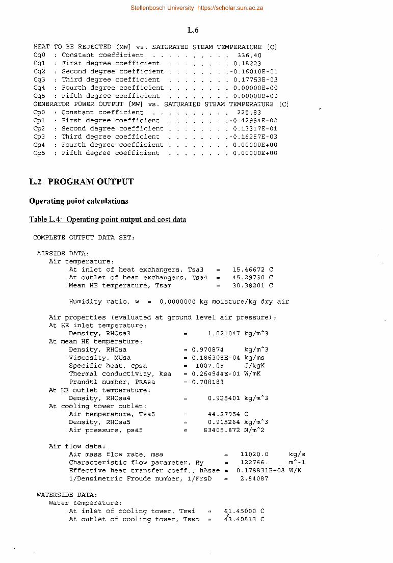
L.6

HEAT TO BE REJECTED [MW] vs. SATURATED STEAM TEMPERATURE [CJ CqO Constant coefficient 336.40 Cql First degree coefficient . 0.18223 Cq2 Second degree coefficient .-0.16010E-01 Cq3 Third degree coefficient 0.17753E-03 Cq4 Fourth degree coefficient . O.OOOOOE+OO Cq5 Fifth degree coefficient . O.OOOOOE+OO GENERATOR POWER OUTPUT [MW] vs. SATURATED STEAM TEMPERATURE [CJ CpO Constant coefficient 225.83 Cpl First degree coefficient .-0.42994E-02 Cp2 Second degree coefficient . 0.13317E-Ol Cp3 Third degree coefficient .-0.16257E-03 Cp4 Fourth degree coefficient O.OOOOOE+OO Cp5 Fifth degree coefficient . O.OOOOOE+OO

L.2 PROGRAM OUTPUT

Operating point calculations

Table L.4: Operating point output and cost data

COMPLETE OUTPUT DATA SET:

AIRSIDE DATA: Air temperature:

At inlet of heat exchangers, Tsa3 At outlet of heat exchangers, Tsa4 Mean HE temperature, Tsam

15.46672 c 45.29730 c 30.38201 c

Humidity ratio, w 0.0000000 kg moisture/kg dry air

Air properties (evaluated at ground level air pressure) : At HE inlet temperature:

Density, RHOsa3 1.021047 kg/mA3 At mean HE temperature:

Density, RHOsa Viscosity, MUsa Specific heat, cpsa Thermal conductivity, ksa Prandtl number, PRAsa

At HE outlet temperature: Density, RHOsa4

At cooling tower outlet: Air temperature, Tsa5 Density, RHOsa5 Air pressure, psa5

Air flow data:

0.970874 kg/mA3 0.186308E-04 kg/ms 1007.09 J/kgK

0.264944E-01 W/mK =·0.708183

0.925401 kg/mA3

44.27954 c 0.915264 kg/mA3

83405.872 N/mA2

11020.0 122766.

kg/s mA-1

Air mass flow rate, msa Characteristic flow parameter, Ry Effective heat transfer coeff., hAsae l/Densimetric Froude number, l/FrsD

0.178831E+08 W/K 2.84087

WATERSIDE DATA: Water temperature:

At inlet of cooling tower, Tswi At outlet of cooling tower, Tswo

61. 45000 c ii

43.40813 c


L.7

Mean CT temperature, Tswm 52.42907 c

Water properties at mean CT temperature: At mean CT temperature: '

Density, RHOsw 987.010 Viscosity, MUsw 0.522417E-03

kg/mA3 kg/ms J/kgK W/mK

Specific heat, cpsw Thermal conductivity, ksw Prandtl number, PRAsw

Water flow data: Water mass flow rate, msw Water mass velocity, Gsw

4179.89 0.645492

3.38292

Water velocity inside tubes, vw Bundle tube Reynolds number, Resw Tube friction factor, fsw Pressure drop per unit length, dpsw Total water pumping power, Psw Waterside heat transf coeff., hsw

SYSTEM DATA: Overall heat transfer coeff., UA Log. mean temperature diff., LMTD Cross-flow correction factor, Fst Airside heat transfer rate, Qsa Waterside heat transfer rate, Qsw Heat transfer rate based on LMTD, Qsu

DRAFT EQUATION: Draft equation LHS Draft equation RHS

97.785 97.785

HEAT EXCHANGER GEOMETRIC DETAILS: Total tube length, Lstt Total waterside surface area, Aswt Total fin surface area, Asft Total air side surface area, Asat Total frontal bundle area, Asfr Min. HE flow area/frontal area, SIGM

HEAT TRANSFER AND PRESSURE DROP CORRELATIONS: Correlation: Briggs, Young, Robinson Heat transfer:

Coefficient asHA Exponent bsHA Equivalent diameter, de Air side Reynolds number, Re Air side heat transfer coeff., hsa Fin efficiency, ETAsf Surface effectiveness, EPSisf

Pressure drop: Coefficient asEU Exponent bsEU Equivalent diameter, de Air Reynolds number, Re Euler number,Eu Total bundle loss coefficient, Kshet

4390.00 kg/s 1095.69 kg/smA2 l. llOll m/s 45302.8

0. 227298E-Ol 639.979 N/mA3 2ll503. w 6969.06 W/mA2K

0.160346E+08 W/K 21.5ll4

0.959809 0.331063E+09 0.331063E+09 0.331063E+09

328020. 22258.9 472428. 495791. 4818.06

0.433005

0.109788 0.681000 27.6000 7825.19 40 .4130

0.917840 0.921711

9.51000 -0.316000

27.6000 7825.19 2.23819 30.7376

mm

mm

c

w w w

PRESSURE LOSS COEFFICIENTS (based on HE frontal area and mean air density): Tower support loss coefficient, Ksts = .42625


L.8

Tower inlet loss coefficient, Ksct Contraction loss coefficient, Kscon HE inlet loss coefficient, Kshi HE normal flow loss coefficient, Kshe HE downstream loss coefficient, Ksd Expansion loss coefficient, Ksexp Tower outlet loss coefficient, Kso

1. 7289 1. 2131 1.9442 24.399 4.3944 1.1887 1.3972

PRESSURE LOSS TERMS (based on HE frontal area Tower support pressure loss, dpsts Tower inlet pressure loss, dpsct Tower contraction press. loss, dpscon HE inlet pressure loss, dpshi

and mean air density) :

HE normal flow pressure loss, dpshe HE downstream pressure loss, dpsd Tower expansion pressure loss, dpsexp Tower outlet pressure loss, dpso

1.1484 4.6579 3.2683 5.2380 65.736 11. 839 3.2026 3.7643

N/m"2 N/m"2 N/m"2 N/m"2 N/m"2 N/m"2 N/m"2 N/m"2

HEAT EXCHANGER BUNDLE COST: Cost of tubes, Cstm 944995. 725 $ Cost of fins, Csfm 3607200.59 $ Cost of galvanizing, Cs gm 0.000000000E+OO $ Cost of finned tubes, Cs ft 5462635.58 $ Cost of bundle frames/headers, Cs bf 1092527.12 $ Cost of bundle assembly, Csba 546700.000 $ Total HE bundle cost, Cs he 8522235.23 $

CIRCULATION SYSTEM COST: Cost of pumps, Cspc Cost of electric motors, Csem Cost of electric wiring, Csew Total pumping system cost, Cspt Cost of piping and valves, Cspv

80741.1488 32525.4787 3252.54787 145648. 969 2130558. 81

$ $ $ $ $

COOLING TOWER STRUCTURAL AND CONSTRUCTION COSTS: Cost of land, excavation, foundation, Csle= Cost of cooling tower shell, Cscts Cost of HE bundle platform, Cspl Cost of cooling tower supports, Csts Total structural, construction cost, Cssc

474572. 960 1382704. 24 540513. 354 38186.6891 3044971. 56

$ $ $ $ $


TOTAL

Operating cost of pumps, Cspo HE bundles maintenance cost, Cshem Pump system maintenance cost, Cspsm Piping and valves maint. cost, Cspvm Cooling tower struct. maint. cost, Cssm Fuel cost, Csfuel

COSTS: Total operating cost 195858.702 Total maintenance cost 101767.101

195858.702 $/a 85222.3523 $/a 4369.46907 $/a 10652.7940 $/a 1522.48578 $/a

0.000000000E+OO $/a

$/a $/a

Total fuel cost O.OOOOOOOOOE+OO $/a Total capital cost 13843414. 6 $ Total annual cost 3066308.72 $/a


L.9

Power generation calculations

Table L.5: Power generation output and cost data


No Tdb [CJ

1 -1.00 2 0.00 3 1. 00 4 2.00 5 3.00 6 4.00 7 5.00 8 6.00 9 7.00

10 8.00 11 9. 00 12 10.00 13 11. 00 14 12.00 15 13.00 16 14.00 17 15.00 18 16.00 19 17.00 20 18.00 21 19.00 22 20.00 23 21. 00 24 22.00 25 23.00 26 24.00 27 25.00 28 26.00 29 27.00 30 28.00 31 29.00 32 30.00 33 31. 00 34 32.00

Twb [C]

0.00 0.00 0.00 0.00 0.90 1. 90 2.90 3.80 4.60 5.40 6.30 7.10 7.80 8.60 9.40

10.20 10.90 11. 60 12.20 12.70 13.20 13. 70 14.10 14.50 14.90 15.20 15.50 15.70 15.90 16.10 16.40 16.80 17.40 18.00

h Twi [h/a] (C]

4 43.36 10 44.41 26 45.46 43 46.52 59 47.58 82 48.64

112 49.70 152 50.77 201 51.84 254 52.91 312 53.99 371 55.07 434 56.16 506 57.25 578 58.35 656 59.45 738 60.55 764 61.67 655 62.78 553 63.91 459 65.04 381 66.17 320 67.32 265 68.47 219 69.63 177 70.79 140 71. 97 105 73.15

76 74.35 51 75.55 30 76.76 15 77.98

8 79.22 4 80.47

Two [C]

25.47 26.52 27.58 28.64 29. 71 30.77 31. 84 32.90 33.98 35.05 36.12 37.20 38.28 39.37 40.45 41.54 42.64 43.73 44.83 45.93 47.04 48.15 49.27 50.38 51.51 52.63 53.76 54.90 56.04 57.19 58.34 59.50 60.67 61. 84

Ts [CJ

45.87 46. 91 47. 96 49.02 50.08 51.14 52.20 53.26 54.34 55.41 56.49 57.57 58.66 59.75 60.85 61. 95 63.06 64.18 65.30 66.43 67.56 68.70 69.85 71. 00 72.17 73.34 74.52 75.71 76. 91 78.12 79.35 80.58 81. 82 83.08

NET ANNUAL POWER OUTPUT = 2074.337 GWh ANNUAL HEAT DISSIPATED 2886.389 GWh


Q

(MW]

328.21 328.04 327.90 327.77 327.67 327.59 327.54 327.51 327.51 327.54 327.61 327.70 327.83 328.00 328.21 328.45 328.75 329.08 329.46 329.90 330.38 330.92 331. 52 332.17 332.90 333.68 334.54 335.47 336.48 337.57 338.75 340.01 341. 38 342.84

Pg [MW]

237. 96 238.15 238.32 238.47 238.59 238.69 238.77 238.82 238.83 238.82 238.78 238.70 238.59 238.44 238.25 238.02 237.75 237.43 237.07 236.66 236.19 235.67 235.10 234.47 233. 77 233.01 232.19 231.29 230.31 229.26 228.12 226.89 225.58 224.16

944995. 725 3607200.59

Pp [MW]

0.221 0.221 0.220 0.219 0.219 0.218 0.217 0.217 0.216 0.215 0.215 0 .214 0.214 0 .213 0.213 0.212 0.212 0.211 0 .211 0 .211 0.210 0.210 0.209 0.209 0.209 0.208 0.208 0.208 0.207 0.207 0.207 0.207 0.206 0.206

$ $


O.OOOOOOOOOE+Od $


CIRCULATION SYSTEM COST: Cost of pumps, Cspc Cost of electric motors, Csem

5462635.58 1092527.12 546700.000 8522235.23

78781.4240 31708.9267

$ $

$ $ $ $

Pn [MW]

237.74 237.93 238.10 238.25 238.38 238.48 238.55 238.60 238.62 238.61 238.56 238.49 238.37 238.22 238.04 237.81 237.54 237.22 236.86 236.45 235.98 235.47 234.89 234.26 233.56 232.80 231. 98 23.1. 08 230.10 229.05 227. 91 226.69 225.37 223. 96


L.10

Cost of electric wiring, Csew Total pumping system cost, Cspt Cost of piping and valves, Cspv

3170.89267 142076.554 2130558.81

COOLING TOWER STRUCTURAL AND CONSTRUCTION COSTS:

$ $ $

Cost of land, excavation, foundation, Csle= Cost of cooling tower shell, Cscts Cost of HE bundle platform, Cspl Cost of cooling tower supports, Csts Total structural, construction cost, Cssc

474572. 960 1382704. 24 540513. 354 38186.6891 3044971.56


TOTAL


COSTS:

196280. 725 85222.3523 4262 .29662 10652.7940 1522.48578 106637256.

Total operating cost 196280. 725 $/a Total maintenance cost 101659. 929 $/a Total fuel cost 106637256. $/a Total capital cost 13839842. 2 $ Total annual cost 109703165. $/a

Operating point optimization

Table L.6: Optimization output and cost data

OPTIMIZATION OUTPUT DATA SET:

FINNED TUBE TYPE: Round tubes (round fins) CORRELATION: Briggs, Young, Robinson

OPERATING POINT OPTIMIZATION: Fixed mw and Twi

VARIABLES FOR OPTIMIZATION: ma Ta4 Two H5 H3 d5 d3 Lt nt/r THET do tt tr df tf Pf Pt

COOLING TOWER H5 Tower overall height 127.857 H3 Tower inlet height 17.7755 d5 Tower diameter at outlet 67.3921 d3 Tower diameter at inlet 92. 3271 Lts Tower support length 18.9163 nts Number of tower supports 60.0000 Qct Specified heat transfer rate 0. 331100E+09 Q Calculated heat transfer rate 0.331100E+09 1/FrsD: 1/Densimetric Froude number 2.30787

FINNED TUBES do Tube outside diameter 27.2636 mm tt Tube thickness 1.20000 mm tr Fin root thickness 1.00000 mm df Fin diameter 86.2928 mm tf Fin thickness (core) 0.206700 mm Pf Fin pitch 2.22286 mm

m m m m m

w w

$ $ $ $ $

$/a $/a $/a $/a $/a $/a


Pt Pl

Transversal tube pitch Longitudinal tube pitch

L.11

100.000 86.6000

HEAT EXCHANGER BUNDLE nt/r: Number of tubes per row ntb Number of tubes per bundle nb Number of heat exchanger bundles nr Number of tube rows nwp Number of water passes Lt Length of finned tubes THET: Bundle semi-apex angle Wb Width of heat exchanger bundle vw Water velocity inside tubes


mm mm

30.0000 118.000 138.203 4.00000 2.00000 9.15604 m 60.0000 deg 3.00000 m 1.12345 m/s

390769.862 2156819.00

Cost of galvanizing, Cs gm 0.000000000E+OO Cost of finned tubes, Cs ft Cost of bundle frames/headers, Cost of bundle assembly, Csba Total HE bundle cost, Cs he


Cs bf 3057106. 63 611421. 329 407699.886 4891473 .42.

44495.3310 17423.0546 1742.30546 79575.8638 1222868.35

$ $ $ $ $


$ $ $ $ $ $ $

Cost of land, excavation, foundation, Csle= 609213.602 $ Cost of cooling tower shell, Cscts 1629478.63 $ Cost of HE bundle platform, Cspl 669497.010 $ Cost of cooling tower supports, Csts 49655.3150 $ Total structural, construction cost, Cssc 3697305.69 $


TOTAL


COSTS: Total operating cost 102623.192 Total maintenance cost 59265.0047

102623.192 $/a 48914.7342 $/a 2387.27591 $/a 6114.34177 $/a 1848.65285 $/a

0.000000000E+OO $/a

$/a $/a

Total fuel cost O.OOOOOOOOOE+OO $/a Total capital cost 9891223. 33 $ Total annual cost 2140132. 86 $/a


L.12

Table L.7: Post-optimality analysis


GENERAL COST FACTORS Ce : Present electricity cost (self-generated) ere: Electricity cost escalation rate Cf : Present fuel cost erf: Fuel cost escalation rate i Interest rate FCR: Levelized fixed charge rate Tau: Running hours per annum

FINNED TUBE BUNDLE COST Cbl Cb2 Cb3 Cb4 Cb5 Cb6 Cb7 Cb8

Tube material unit cost Tubing fixed cost Fin material unit cost Finning fixed cost Galvanizing material unit cost Surface coating fixed cost Finned tube cost weighting factor Bundle frame and header cost factor

0.479518E-01 0.427927E-Ol O.OOOOOOE+OO O.OOOOOOE+OO

-0.201179E-01 0.924356 0.479518E-Ol

0.194353E-01 0.629938E-01 0.194427 0.260533 O.OOOOOOE+OO 0.000000E+OO 0.537389 0.895648E-01

Cb9 Tube assembly and end preparation cpst 0.597224E-01 CblO: Bundle cost weighting factor 0.597111 Cbll: Bundle maintenance cost factor 0.228559E-01

CIRCULATION SYSTEM COSTS Cpl Cp2 Cp3 Cp4 Cp5 Cp6 Cp7 Cp8 Cp9 CplO:

Pump fixed cost Pump unit cost Electric motor fixed cost Electric motor unit cost Electric motor safety factor (undersizing) Electric wiring/switching cost multiplier Pump system cost multiplier Pump system maintenance cost factor Piping and valves cost factor Piping and valves maintenance cost factor

COOLING TOWER CONSTRUCTION COSTS Csl Cs2 Cs3 Cs4 Cs5 Cs6

Land, excavation and foundation unit cost Cooling tower shell cost HE Bundle support platform cost Cooling tower support cost Construction cost multiplier Maintenance cost factor

PRESCRIBED PARAMETERS

0.617972E-03 0.535945E-02 0.118237E-03 0.245643E-02 0.245643E-02 0.234087E-03 0.855203E-02 0 .111549E-02 0.117137 0.285700E-02

0.713433E-01 0.190824 0.784030E-Ol 0.581501E-02 0.346385 0.863804E-03

dts : Tower support diameter/width 0.140626E-01 ALPH: Fraction of tower area covered by bundles -0.182248 pal Barometric pressure at ground level -0.414740 Twi Water inlet temperature -9.45551 mw Water mass flow rate -0.192260 Ke Total flow resistance length ratio 0.557677E-Ol Tal Air temperature at ground level 8.37099

GEOMETRIC CONSTRAINT VARIATION SENSITIVITY CONSTRAINTS: ROUND TUBES 1 (HIRU-H3/H5) 2 (H3/H5-HIRL)

0.000000E+OO O.OOOOOOE+OO


L.13

3 (DIRU-D3/(HS-H3)) 4 (D3/(HS-H3)-DIRL) s (DRU-D3/DS) 6 (D3/DS-DRL) 7 (DF/DR-1. 0) 8 (TT/TTL-1.0) 9 (TR/TRL-1.0)

10 (PT/DF-1. 0) 11 (TF/TFL-1.0) 12 (PF /PFL-1. O) 13 (1. 0-WB/WBU) 14 ( 1. 0-LT/LTU) lS (1. 0-THTE/THBU)

Minimization of power generation cost

Table L.8: Optimization output and cost data

OPTIMIZATION OUTPUT DATA SET: FINNED TUBE TYPE: Round tubes (round fins) CORRELATION: Briggs, Young, Robinson

ANNUAL NET POWER OUTPUT OPTIMIZATION

VARIABLES FOR OPTIMIZATION:

O.OOOOOOE+OO O.OOOOOOE+OO O.OOOOOOE+OO 0.288041E-02 0.000000E+OO 0.S3S09SE-Ol 0.461663E:.Ol 0.000000E+OO 0.000000E+OO O.OOOOOOE+OO 0.1S9110E-Ol O.OOOOOOE+OO 0.230760E-Ol

ma Ta4 Two Ts HS H3 dS d3 Lt nt/r THET do tt tr df tf Pf Pt

COOLING TOWER HS Tower overall height H3 Tower inlet height dS Tower diameter at outlet d3 Lts nts

Tower diameter at inlet Tower support length Number of tower supports

FINNED TUBES do tt tr df tf Pf Pt Pl

Tube outside diameter Tube thickness Fin root thickness Fin diameter Fin thickness (core) Fin pitch Transversal tube pitch Longitudinal tube pitch

HEAT EXCHANGER BUNDLE nt/r: Number of tubes per row ntb Number of tubes per bundle

27.2S87 1.20000 1.00000 86.62S6

0.20S304 2.22441 96. 7742 83.806S

nb Number of heat exchanger bundles nr Number of tube rows nwp Lt THET: Wb

Number of water passes Length of finned tubes Bundle semi-apex angle Width of heat exchanger bundle


136. 398 18.8443 70.7988 97.63S6 20.0S37 60.0000


31.0000 122.000 148.991 4.00000 2.00000 9.Sl700 60.0000 3.00000

4S2703.627 2498644.72

m m m m m

m

deg m

$ $


L.14


O.OOOOOOOOOE+OO $



3541618.02 708323.605 454422.277 5645236.68

39007.2483 15136. 3535 .1513. 63 535 69571.5464 1411309.17

$ $ $ $ $


$ $ $ $

Cost of land, excavation, foundation, Csle= 681699.380 $ Cost of cooling tower shell, Cscts 1833304.29 $ Cost of HE bundle platform, Cspl 748697.217 $ Cost of cooling tower supports, Csts 52641.0144 $ Total structural, construction cost, Cssc 4145427.38 $


TOTAL


COSTS:

88506.1374 56452.3668 2087.14639 7056.54585 2072. 71369 106623742.

Total operating cost 88506.1374 $/a Total maintenance cost Total fuel cost Total capital cost Total annual cost

NET ANNUAL POWER OUTPUT Net annual power output Annual heat dissipated Cost per kWh

Table L.9: Power generation output

67668.7727 $/a 106623742. $/a 11271544. 8 $ 109034226. $/a

2083.90 GWh 2877.21 GWh

0.523222E-01 $/kWh


No Tdb Twb h Twi Two Ts Q Pg Pp [C] [C] [h/al [CJ (C] [Cl [MW] (MW] [MW]

1 -1. 00 0.00 4 40.50 22.58 43.01 328.75 237.35 0.100 2 0.00 0.00 10 41.49 23.57 43.99 328.55 237.57 0.100 3 1. 00 0.00 26 42.47 24.57 44.98 328.36 237.78 0.099 4 2.00 0.00 43 43.46 25.57 45.97 328.19 237.98 0.099 5 3.00 0.90 59 44.46 26.57 46. 96 328.04 238.16 0.099 6 4.00 1. 90 82 45.46 27.57 47. 96 327.90 238.32 0.098 7 5.00 2.90 112 46.45 28.58 48. 96 327.78 238.46 0.098 8 6.00 3.80 152 47.46 29.58 49.96 327.68 238.58 0.098 9 7.00 4.60 201 48.46 30.59 50. 96 327.60 238.68 0.098

10 8.00 5.40 254 49.47 31. 61 51.97 327.55 238.76 0.097 11 9.00 6.30 312 50.48 32.62 52.98 327.52 238.81 0.097

$/a $/a $/a $/a $/a $/a

Pn [MW]

237.25 237.47 237.69 237.88 238.06 238.22 238.36 238.48 238.58 238.66 238. 71


12 10.00 13 11.00 14 12.00 15 13.00 16 14.00 17 15.00 18 16.00 19 17.00 20 18.00 21 19.00 22 20.00 23 21. 00 24 22.00 25 23.00 26 24.00 27 25.00 28 26.00 29 27.00 30 31 32 33 34

28.00 29.00 30.00 31.00 32.00

7.10 7.80 8.60 9.40

10.20 10.90 11. 60 12.20 12.70 13 .20 13.70 14.10 14.50 14.90 15.20 15.50 15.70 15.90 16.10 16.40 16.80 17.40 18.00

371 434 506 578 656 738 764 655 553 459 381 320 265 219

51.50 52.52 53.54 54.57 55.60 56.63 57.67 58.72 59.77 60.82 61. 88 62.94 64.01 65.09

177 66.17 140 67.26 105 68.35

76 69.45 51 70.56 30 71.68 15 72.80

8 73.93 4 75.07

33.64 34.65 35.68 36.70 37.73 38.76 39.79 40.82 41. 86 42.90 43.94 44.99 46.04 47.09 48.15 49.21 50.27 51. 34 52.41 53.48 54.56 55.65 56.74

L.15

54.00 55.01 56.04 57.07 58.10 59 .13 60.18 61.22 62.27 63.33 64.39 65.46 66.53 67.61 68.70 69.79 70.89 71. 99 73 .11 74.23 75.36 76.50 77.65

NET ANNUAL POWER OUTPUT = 2083.902 GWh ANNUAL HEAT DISSIPATED= 2877.214 GWh

Table L.10: Post-optimality analysis


GENERAL COST FACTORS

327.51 327.53 327.58 327.65 327.76 327.90 328.08 328.29 328.53 328.82 329.15 329.52 329.94 330.40 330.92 331.48 332.10 332.78 333.52 334.32 335.19 336.12 337 .13

238.83 238.83 238.80 238.74 238.65 238.53 238.37 238.18 237.95 237.68 237.37 237.01 236.61 236.17 235.68 235 .13 234.53 233.88 233.17 232.40

0.097 0.096 0. 096 0. 096 0. 096 0.096 0.095 0.095 0.095 0.095 0.094 0.094 0.094 0.094 0.094 0.094 0.093 0.093 0 .. 093 0.093

231. 56 0. 093 230.66 0.093 229.68 0.093

Ce : Present electricity cost (self-generated) 0.811736E-03 ere: Electricity cost escalation rate 0.724399E-03 Cf : Present fuel cost 0.977892 erf: Fuel cost escalation rate 1.03225 i Interest rate -0.471335 FCR: Levelized fixed charge rate 0.206753E-Ol

FINNED Cbl Cb2 Cb3 Cb4 Cb5 Cb6 Cb7 Cb8 Cb9 CblO:

TUBE BUNDLE COST Tube material unit cost Tubing fixed cost Fin material unit cost Finning fixed cost Galvanizing material unit cost Surface coating fixed cost Finned tube cost weighting factor Bundle frame and header cost factor Tube ,assembly and end preparation cost Bundle cost weighting factor

Cbll: Bundle maintenance cost factor

0.441881E-03 0.143249E-02 0.442586E-02 0. 591942E-02 0.000000E+OO 0.000000E+OO 0.122196E-01 0.203662E-02 0 .130658E-02 0.135262E-01 0.517760E-03

CIRCULATION SYSTEM COSTS Cpl Cp2 Cp3 Cp4 Cp5

Pump fixed cost Pump unit cost Electric motor fixed cost

0 .121373E-04 0.907324E-04 0.232560E-05

Electric motor unit cost 0.415892E-04 Electric motor safety factor (undersizing) 0.415892E-04

238.73 238.73 238.70 238.64 238.55 238.43 238.27 238.08 237.85 237.58 237.27 236. 92 236.52 236.08 235.58 235.04 234.44 233.79 233.08 232.30 231.47 230.56 229.59


L.16

Cp6 Cp7 Cp8 Cp9 CplO:

Electric wiring/switching cost multiplier Pump system cost multiplier Pump system maintenance cost factor Piping and valves cost factor Piping and valves maintenance cost factor

COOLING TOWER CONSTRUCTION COSTS Csl Cs2 Cs3 Cs4 Cs5 Cs6

Land, excavation and foundation unit cost Cooling tower shell cost HE Bundle support platform cost Cooling tower support cost Construction cost multiplier Maintenance cost factor

PRESCRIBED PARAMETERS dts : Tower support diameter/width ALPH: Fraction of tower area covered by bundles pal Barometric pressure at ground level Ke Total flow resistance length ratio mw Water mass flow rate Qdes: Design point heat rejection TTD : Design point terminal temp. difference

GEOMETRIC CONSTRAINT VARIATION SENSITIVITY CONSTRAINTS: ROUND TUBES 1 (HIRU-H3/H5) 2 (H3/H5-HIRL) 3 (DIRU-D3/(H5-H3)) 4 (D3/(H5-H3)-DIRL) 5 (DRU-D3/D5) 6 (D3/D5-DRL) 7 (DF /DR-1. 0) 8 (TT/TTL-1.0) 9 (TR/TRL-1.0)

10 (PT/DF-1. 0) 11 ( TF /TFL- 1 . 0 ) 12 (PF/PFL-1.0) 13 (1. 0-WB/WBU) 14 ( 1 . 0 - LT /LTU) 15 (1.0-THTE/THBU)

0.398917E-05 0.146767E-03 0 .191480E-04 0.265348E-02 0.647264E-04

0.156695E-02 0.421402E-02 0 .172096E-02 0.120999E-03 0. 762291E-02 0.190122E-04

0.289878E-03 -0.401616E-02 -0. 912144E-02

0.134576E-02 -0.609977E-02 -0.185092E-02

0.185088E-02

O.OOOOOOE+OO O.OOOOOOE+OO O.OOOOOOE+OO O.OOOOOOE+OO O.OOOOOOE+OO 0.000000E+OO O.OOOOOOE+OO 0.121021E-02 0.104727E-02 0.000000E+OO O.OOOOOOE+OO O.OOOOOOE+OO 0.236809E-03 O.OOOOOOE+OO 0.350549E-03


PERFORMANCE OPTIMIZATION OF ENGINEERING ... - CORE

Documents

Transcript of PERFORMANCE OPTIMIZATION OF ENGINEERING ... - CORE