978-1-4799-7938-7/14/$31.00 ©2014 IEEE 145

ACO for Continuous Function Optimization: APerformance Analysis

Varun Kumar Ojha∗, Ajith Abraham∗,Vaclav Snasel∗∗IT4Innovations, VSB Technical University of Ostrava, Ostrava, Czech Republic

varun.kumar.ojha@vsb.cz, ajith.abraham@ieee.org, vaclav.snasel@vsb.cz

Abstract—The performance of the meta-heuristic algorithmsoften depends on their parameter settings. Appropriate tuningof the underlying parameters can drastically improve the perfor-mance of a meta-heuristic. The Ant Colony Optimization (ACO),a population based meta-heuristic algorithm inspired by theforaging behavior of the ants, is no different. Fundamentally, theACO depends on the construction of new solutions, variable byvariable basis using Gaussian sampling of the selected variablesfrom an archive of solutions. A comprehensive performanceanalysis of the underlying parameters such as: selection strategy,distance measure metric and pheromone evaporation rate ofthe ACO suggests that the Roulette Wheel Selection strategyenhances the performance of the ACO due to its ability toprovide non-uniformity and adequate diversity in the selection ofa solution. On the other hand, the Squared Euclidean distance-measure metric offers better performance than other distance-measure metrics. It is observed from the analysis that the ACO issensitive towards the evaporation rate. Experimental analysis be-tween classical ACO and other meta-heuristic suggested that theperformance of the well-tuned ACO surpasses its counterparts.

Index Terms—Metaheuristic; Ant colony optimization; Con-tinuous optimization; Performance analysis;

I. INTRODUCTION

Ant Colony Optimization (ACO) was initially proposedfor the solving discrete optimization problems. Later, it wasextended for solving the continuous optimization problems. Inthe present research work, we have examined the strength andweakness of the classical ACO algorithm over the continu-ous function optimization problems. The performance of theclassical ACO fundamentally depends on the mechanism ofthe construction of new solutions, variable by variable basis,where an n dimensional continuous optimization problem hasn variables. Therefore, the key to success of the ACO liesin its construction of new solutions. In order to construct anew variable of a new solution, a variable from the availablesolution archive is selected for Gaussian sampling. Hence,n newly obtained variables, construct a new solution. Theother crucial parameters that influence the performance of theACO are, distance measure metric and pheromone evaporationrate. The distance-measure metric is used for computing theaverage distance between ith variable of the selected solutionand the ith variables of all the other solutions in the availablesolutions archive. In order to establish goodness of the tunedACO, its performance was compared to the popular meta-heuristic algorithm such as: Particle Swarm Optimization andDifferential Evolution Algorithms.

The rest of the paper is organized as follows: In Section

II, we explore the details of the classical ACO used forthe optimization of continuous functions. A comprehensiveperformance analysis based on the underlying parameters ofthe ACO is provided in Section III followed by discussionsand conclusion in Section IV.

II. CONTINUOUS ANT COLONY OPTIMIZATION (ACO)

The foraging behavior of the ants inspired the formationof a computational optimization technique, popularly knownas Ant Colony Optimization. Deneubourg, Aron and Goss [1]illustrated that while searching for food source, initially theants randomly explore the area around their nest (colony) andthey secretes a chemical substance known as pheromone thatthey use for the communication among them. The quantityof pheromone secretion may depend on the quantity of thefood source found by the ants. On a successful search, theants return to their nest with the food sample. The pheromonetrail left by the returning ants, guide the other ants to reachto the food source. Deneubourg Aron and Goss in theirpopular double bridge experiment, have demonstrated that theants always prefer to use the shortest path among the pathsavailable between a nest and a food source.

Dorigo and Gambardella [2], [3] in the early 90s proposedthe Ant Colony Optimization (ACO) algorithm inspired by theforaging behavior of the ants. Initially, the ACO was limitedonly to the discrete optimization problems [2], [4], [5], butlater, it was extended to the continuous optimization problems[6]. Blum and Socha [7], [8] proposed the continuous versionof ACO for the training of neural network (NN). Basically, theclassical ACO algorithm has three phases: Pheromone rep-resentation, Ant based solution construction and Pheromoneupdate.

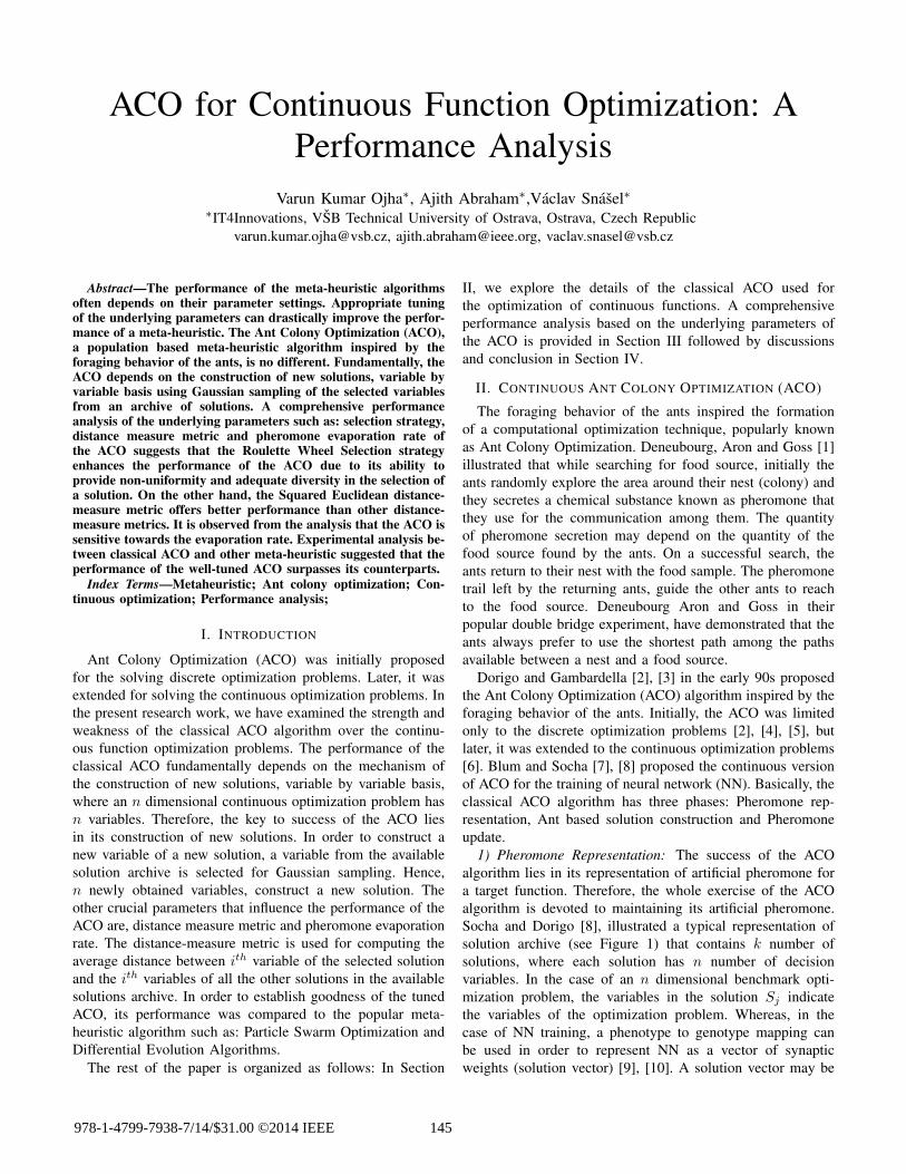
1) Pheromone Representation: The success of the ACOalgorithm lies in its representation of artificial pheromone fora target function. Therefore, the whole exercise of the ACOalgorithm is devoted to maintaining its artificial pheromone.Socha and Dorigo [8], illustrated a typical representation ofsolution archive (see Figure 1) that contains k number ofsolutions, where each solution has n number of decisionvariables. In the case of an n dimensional benchmark opti-mization problem, the variables in the solution Sj indicatethe variables of the optimization problem. Whereas, in thecase of NN training, a phenotype to genotype mapping canbe used in order to represent NN as a vector of synapticweights (solution vector) [9], [10]. A solution vector may be

146 2014 International Conference on Intelligent Systems Design and Applications (ISDA)

S1 s11 s21 . . . si1 . . . sn1 f(s1) ω1

S2 s12 s22 . . . si2 . . . sn2 f(s2) ω2

......

. . ....

. . ....

......

Sj s1j s2j . . . sij . . . snj f(sj) ωj

......

. . ....

. . ....

......

Sk s1k s2k . . . sik . . . snk f(sk) ωk

g1 g2 gi gn

Fig. 1. A typical Solution Archive/Pheromone Table. In a sorted solutionarchive for a minimization problem, the function-value associated with thesolutions are f(s1) � f(s2) � . . . � f(sk). Therefore, the weightassociated with the solutions are ω1 � ω2 � . . . � ωk . The weightindicates that the best solution should have the highest weight. For theconstruction of new solution n Gaussian are sampled using a selected µ fromthe archive.

initialized using random values chosen from a search spacedefined as S ∈ [min,max], where min and max indicateslower and upper bound respectively. For the construction ofnew solutions, in the case of the discrete version of the ACO,a discrete probability mass function (pdf ) is used. Whereas, inthe case of the continuous version of the ACO, a continuouspdf is derived from the pheromone table is used.

2) Ant Based Solutions Construction: The variable byvariable construction of the new solution is as follows. First,a solution is chosen from the set of solutions archive based onits probability of selection. The probability of selection of thesolution’s in an archive is assigned using (1) or (2), where theprobability of the jth solution computed according to (1) and(2) are based on the fitness value of the solution and the rankof the solution respectively. Therefore, for the construction ofthe ith (i ∈ [1, n]) variable of lth (index into new solution set,i.e., l ∈ [1,m]) solution, the jth (j ∈ [1, k]) solution from thesolution archive is chosen based on its probability of selectionaccording to (1) or (2) expressed as:

pj =f(sj)k∑

r=1f(sr)

, (1)

pj =ωj

k∑r=1

ωr

, (2)

where ωj is weight associated to the solution j computed as:

ωj =1

qk√

2πe

−(rank(j)−1)2

2q2k2 , (3)

where q is a parameter of the algorithm and the mean ofthe Gaussian function is set to one, so that the best solutioncan acquire the maximum weight. Since in (1), the smallestfunction-value gets the lowest probability, a further processingis required in order to assign the highest probability to thesmallest function-value. In the case of the optimization prob-lems, function-value computation is straightforward. Whereas,in the case of the NN training, the fitness of the solution isassigned using the Root Mean Square Error (RMSE) inducedon NN for a given input training pattern (a given training

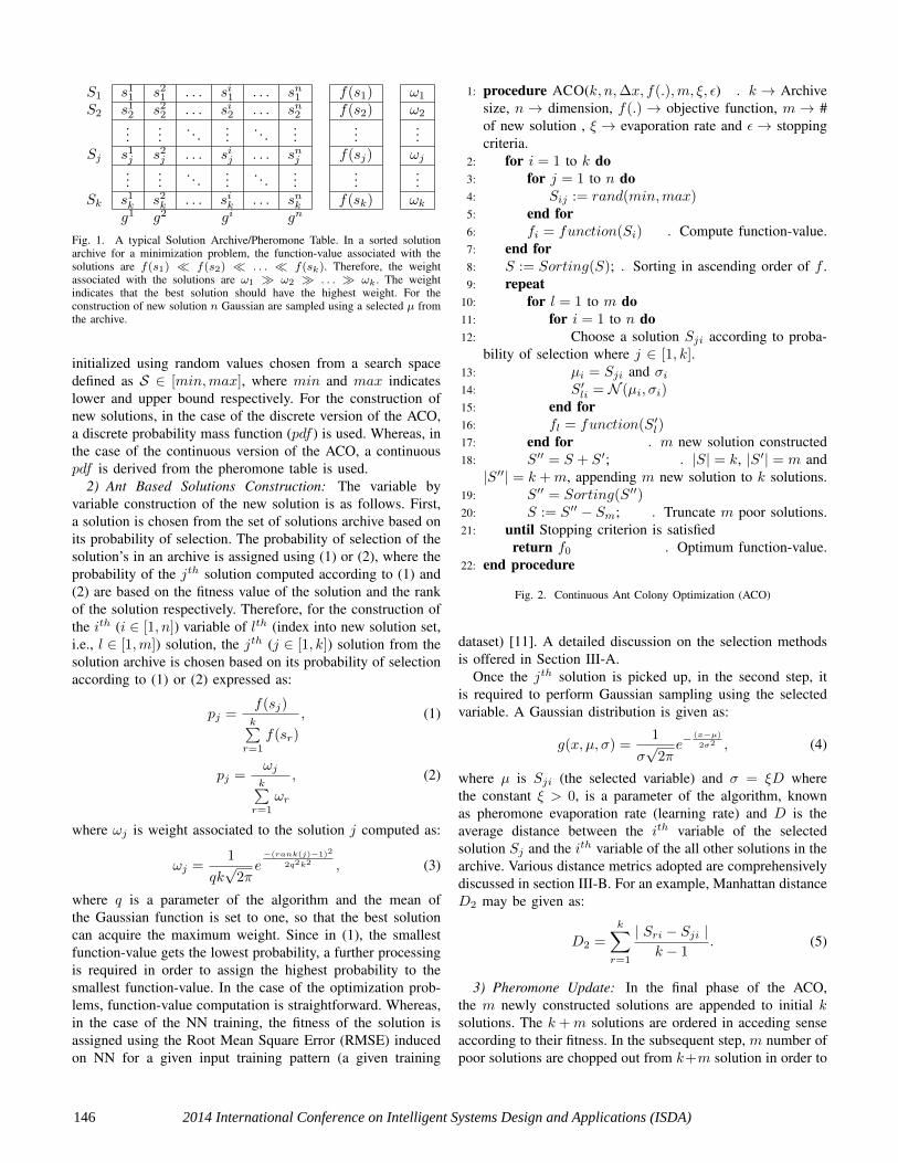
1: procedure ACO(k, n,∆x, f(.),m, ξ, ε) . k → Archivesize, n → dimension, f(.) → objective function, m → #of new solution , ξ → evaporation rate and ε→ stoppingcriteria.

2: for i = 1 to k do3: for j = 1 to n do4: Sij := rand(min,max)5: end for6: fi = function(Si) . Compute function-value.7: end for8: S := Sorting(S); . Sorting in ascending order of f .9: repeat

10: for l = 1 to m do11: for i = 1 to n do12: Choose a solution Sji according to proba-

bility of selection where j ∈ [1, k].13: µi = Sji and σi14: S′li = N (µi, σi)15: end for16: fl = function(S′l)17: end for . m new solution constructed18: S′′ = S + S′; . |S| = k, |S′| = m and|S′′| = k +m, appending m new solution to k solutions.

19: S′′ = Sorting(S′′)20: S := S′′ − Sm; . Truncate m poor solutions.21: until Stopping criterion is satisfied

return f0 . Optimum function-value.22: end procedure

Fig. 2. Continuous Ant Colony Optimization (ACO)

dataset) [11]. A detailed discussion on the selection methodsis offered in Section III-A.

Once the jth solution is picked up, in the second step, itis required to perform Gaussian sampling using the selectedvariable. A Gaussian distribution is given as:

g(x, µ, σ) =1

σ√

2πe−

(x−µ)2σ2 , (4)

where µ is Sji (the selected variable) and σ = ξD wherethe constant ξ > 0, is a parameter of the algorithm, knownas pheromone evaporation rate (learning rate) and D is theaverage distance between the ith variable of the selectedsolution Sj and the ith variable of the all other solutions in thearchive. Various distance metrics adopted are comprehensivelydiscussed in section III-B. For an example, Manhattan distanceD2 may be given as:

D2 =

k∑r=1

| Sri − Sji |k − 1

. (5)

3) Pheromone Update: In the final phase of the ACO,the m newly constructed solutions are appended to initial ksolutions. The k +m solutions are ordered in acceding senseaccording to their fitness. In the subsequent step, m number ofpoor solutions are chopped out from k+m solution in order to

1472014 International Conference on Intelligent Systems Design and Applications (ISDA)

maintain solution archive size to k. The complete discussionabout the ACO is summed up in the algorithm given in Figure2.

III. PERFORMANCE EVALUATION

The classical ACO algorithm mentioned in Figure 2 wasimplemented using Java programming language and the per-formance was analyzed by tuning the underlying parameterssuch as (i) Selection strategies (ii) Distance metric and (iii)pheromone evaporation rate. We tested the ACO over thebenchmark functions given in Table I in order to obtain animproved set of parameters or in other words, a well-tunedACO (ACO*). The benchmark functions used are as follows:

−a exp

−b√√√√1

d

d∑i=1

x2i

−exp(1

d

d∑i=1

cos(cxi)

)+a+exp(1), (6)

d∑i=1

x2i , (7)

d∑i=1

ix2i , (8)

d−1∑i=1

[100(xi+1 − x2i )2 + (xi − 1)2], (9)

10d+

d∑i=1

[x2i − 10 cos(2πxi)], (10)

d∑i=1

x2i4000

−d∏

i=1

cos

(xi√i

)+ 1, (11)

d∑i=1

x2i +

(d∑

i=1

0.5ixi

)2

+

(d∑

i=1

0.5ixi

)2

, (12)

(x1 − 1)2d∑

i=1

i(2x2i − xi − 1)2, (13)

and √√√√ 1

n

n∑i=1

e2i , (14)

where in (14) ei = (yi − yi) is the difference between thetarget value yi and predicted value yi of a training dataset.

A. Selection Strategies

To analyze how the selection strategies influence the perfor-mance of the ACO, we used several strategies: Roulette WheelSelection (RWS), Stochastic Universal Sampling (SUS) andBernoulli Heterogeneous Selection (BHS), where each of theseavailable strategies was allowed to use both the mentionedprobability assignment methods (1) (hereafter called FitVal)and (2) (hereafter called Weight). Therefore, six differentstrategies RWS (FitVal), RWS (Weight), SUS (FitVal), SUS(Weight), BHS (FitVal) and BHS (Weight) were used.

TABLE ITHE BENCHMARK OPTIMIZATION FUNCTIONS CONSIDERED

Function Expression Dim. Range f(x∗)F1 Ackley as per (6) d -15,30 0.0F2 Sphere as per (7) d -50,100 0.0F3 Sum Square as per (8) d -10,10 0.0F4 Dixon & Price as per (13) d -10,10 0.0F5 Rosenbrook as per (9) d -5,10 0.0F6 Rastring as per (10) d -5.12,5.12 0.0F7 Griewank as per (11) d -600,600 0.0F8 Zakarov as per (12) d -10,10 0.0F9 abolone(RMSE) as per (14) 90 -1.5,1.5 0.0F10 baseball(RMSE) 170 0.0

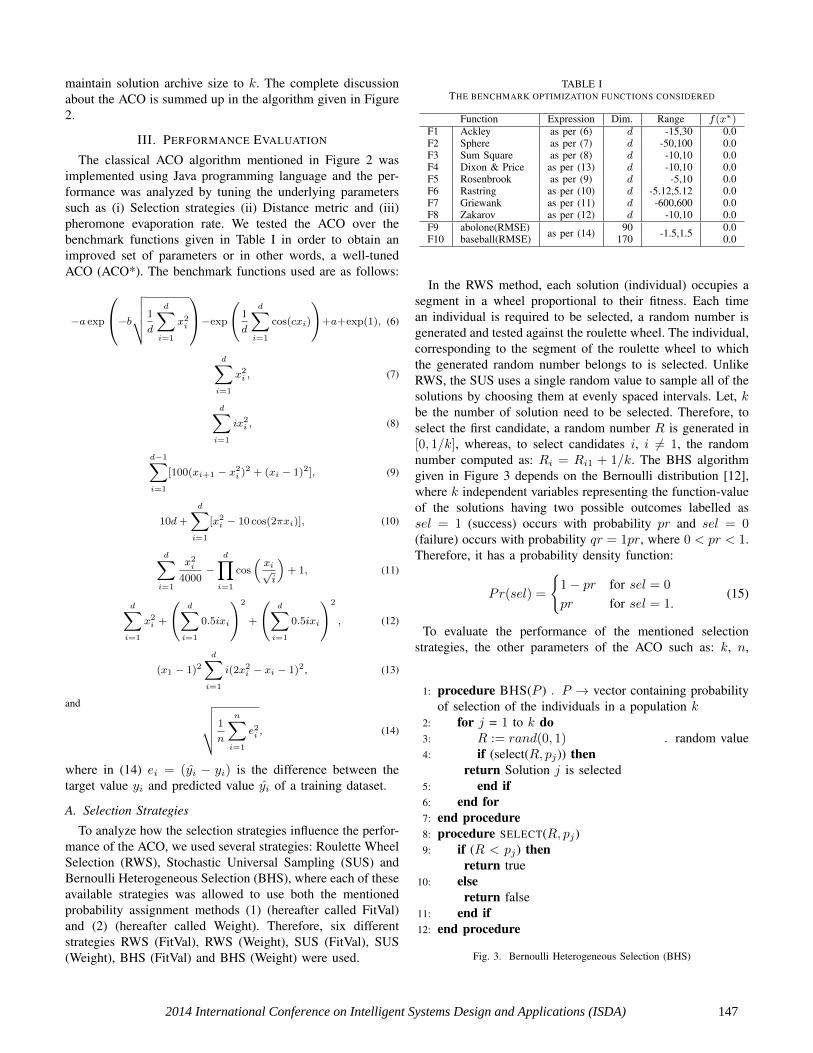
In the RWS method, each solution (individual) occupies asegment in a wheel proportional to their fitness. Each timean individual is required to be selected, a random number isgenerated and tested against the roulette wheel. The individual,corresponding to the segment of the roulette wheel to whichthe generated random number belongs to is selected. UnlikeRWS, the SUS uses a single random value to sample all of thesolutions by choosing them at evenly spaced intervals. Let, kbe the number of solution need to be selected. Therefore, toselect the first candidate, a random number R is generated in[0, 1/k], whereas, to select candidates i, i 6= 1, the randomnumber computed as: Ri = Ri1 + 1/k. The BHS algorithmgiven in Figure 3 depends on the Bernoulli distribution [12],where k independent variables representing the function-valueof the solutions having two possible outcomes labelled assel = 1 (success) occurs with probability pr and sel = 0(failure) occurs with probability qr = 1pr, where 0 < pr < 1.Therefore, it has a probability density function:

Pr(sel) =

{1− pr for sel = 0

pr for sel = 1.(15)

To evaluate the performance of the mentioned selectionstrategies, the other parameters of the ACO such as: k, n,

1: procedure BHS(P ) . P → vector containing probabilityof selection of the individuals in a population k

2: for j = 1 to k do3: R := rand(0, 1) . random value4: if (select(R, pj)) then

return Solution j is selected5: end if6: end for7: end procedure8: procedure SELECT(R, pj)9: if (R < pj) then

return true10: else

return false11: end if12: end procedure

Fig. 3. Bernoulli Heterogeneous Selection (BHS)

148 2014 International Conference on Intelligent Systems Design and Applications (ISDA)

TABLE IIPERFORMANCE EVALUATION OF SELECTION STRATEGIES

Selection probabilityassignment

Selection Method

RWS SUS BHS Rank 1Function’s fitnessvalue - (1)

28.202 101.252 34.931 41.725

Weight computed ac-cording to rank - (2)

35.105 95.216 36.503

m, ξ, ε and D were set to ten, thirty, ten, zero point five,one thousand iterations and D2 (Manhattan) respectively. Theexperimental results of the various selection strategies areprovided in Table II, where the values appear are the mean ofthe values of the functions F1 to F10 listed in Table I, whereeach of the function-value Fi is computed over an average oftwenty trials.

Examining Table II, it may be observed that the strategiesRWS significantly outperformed its counterparts with the bestresult obtained using the probability of selection computedaccording to (1). The performance of the BHS strategy wascompetitive to the RWS with the result comparable to the RWSwhereas, the performance of the SUS was the worst amongthe all mentioned selection methods. However, it is interestingto note that unlike the RWS and the BHS, the performance ofthe SUS over probability of selection computed according to(2) was better than that of the computed according to (1).

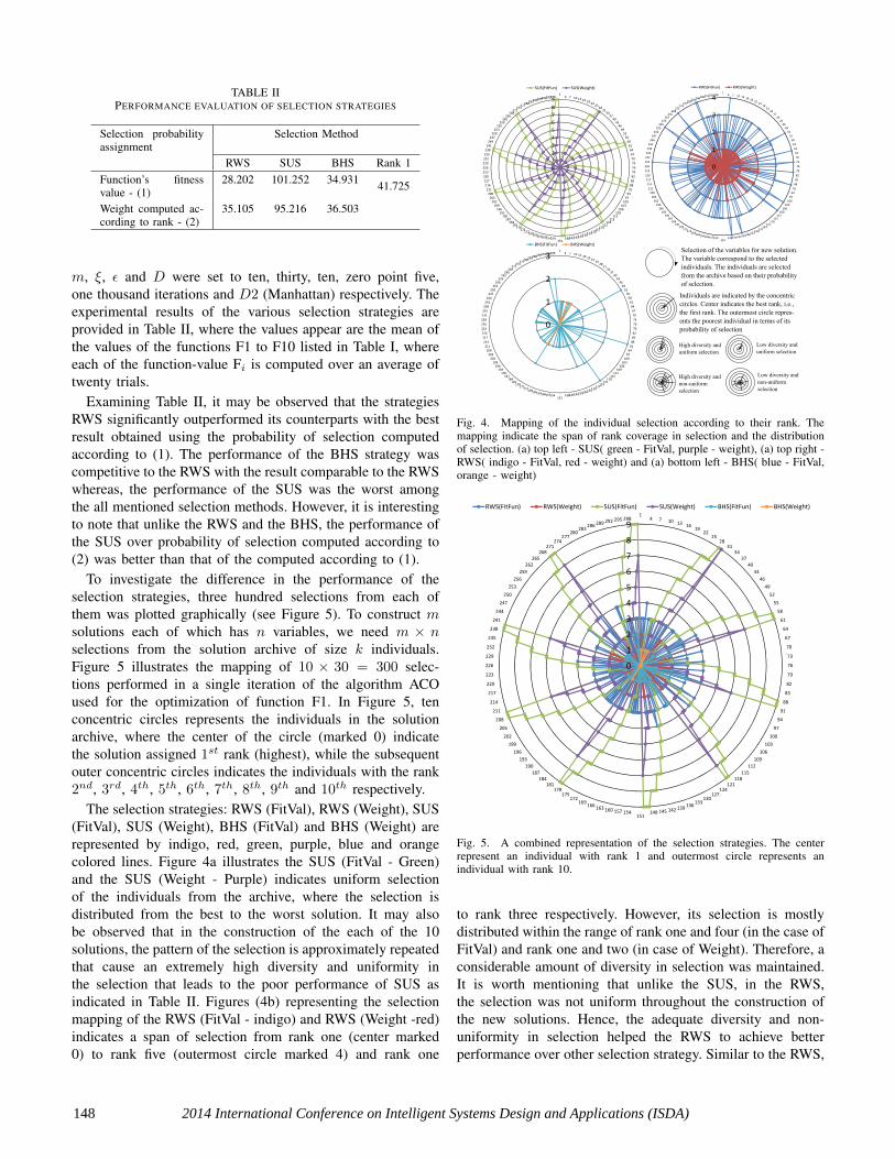
To investigate the difference in the performance of theselection strategies, three hundred selections from each ofthem was plotted graphically (see Figure 5). To construct msolutions each of which has n variables, we need m × nselections from the solution archive of size k individuals.Figure 5 illustrates the mapping of 10 × 30 = 300 selec-tions performed in a single iteration of the algorithm ACOused for the optimization of function F1. In Figure 5, tenconcentric circles represents the individuals in the solutionarchive, where the center of the circle (marked 0) indicatethe solution assigned 1st rank (highest), while the subsequentouter concentric circles indicates the individuals with the rank2nd, 3rd, 4th, 5th, 6th, 7th, 8th, 9th and 10th respectively.

The selection strategies: RWS (FitVal), RWS (Weight), SUS(FitVal), SUS (Weight), BHS (FitVal) and BHS (Weight) arerepresented by indigo, red, green, purple, blue and orangecolored lines. Figure 4a illustrates the SUS (FitVal - Green)and the SUS (Weight - Purple) indicates uniform selectionof the individuals from the archive, where the selection isdistributed from the best to the worst solution. It may alsobe observed that in the construction of the each of the 10solutions, the pattern of the selection is approximately repeatedthat cause an extremely high diversity and uniformity inthe selection that leads to the poor performance of SUS asindicated in Table II. Figures (4b) representing the selectionmapping of the RWS (FitVal - indigo) and RWS (Weight -red)indicates a span of selection from rank one (center marked0) to rank five (outermost circle marked 4) and rank one

0

1

2

3

4

5

6

7

8

91

4 7 10 13 16 1922

2528

313437404346495255586164

67

70

73

76

79

82

85

889194

97100

103106

109112

115118

121124

127130

133136139142145148151

154157160163166169172

175178

181184

187190

193196

199202

205208211214

217

220

223

226

229

232

235

238241244247250253256259262265268271

274277

280283286

289292295298

SUS(FitFun) SUS(Weight)

0

1

2

3

41

4 7 10 13 16 1922

2528

3134

3740434649

52

55

58

61

64

67

70

73

76

79

82

85

88

91

94

97

100103

106109

112115

118121

124127

130133136139142145148

151154157160163166169

172175

178181

184187

190193

196199

202

205

208

211

214

217

220

223

226

229

232

235

238

241

244

247

250

253256259262

265268

271274

277280

283286289292

295298

RWS(FitFun) RWS(Weight)

0

1

2

31

4 7 10 13 16 1922

2528

3134374043464952555861

64

67

70

73

76

79

82

85

88

9194

97100

103106

109112

115118

121124

127130

133136139142145148151

154157160163166169172

175178

181184

187190

193196

199202

205208211

214

217

220

223

226

229

232

235

238

241244247250253256259262265268

271274

277280

283286289292295

298

BHS(FitFun) BHS(Weight)

SelectionLofLtheLvariablesLforLnewLsolution.LTheLvariableLcorrespondLtoLtheLselectedLindividuals.LTheLindividualsLareLselectedLfromLtheLarchiveLbasedLonLtheirLprobabilityofLselection.

IndividualsLareLindicatedLbyLtheLconcentricLcircles.LCenterLindicatesLtheLbestLrank,Li.e.,LtheLfirstLrank.LTheLoutermostLcircleLrepres-entsLtheLpoorestLindividualLinLtermsLofLitsLprobabilityLofLselection

HighLdiversityLandLuniformLselection

LowLdiversityLandLuniformLselection

HighLdiversityLandLnon-uniformselection

LowLdiversityLandLnon-uniformLselection

Fig. 4. Mapping of the individual selection according to their rank. Themapping indicate the span of rank coverage in selection and the distributionof selection. (a) top left - SUS( green - FitVal, purple - weight), (a) top right -RWS( indigo - FitVal, red - weight) and (a) bottom left - BHS( blue - FitVal,orange - weight)

0

1

2

3

4

5

6

7

8

91

4 7 10 13 1619

2225

2831

3437

40

43

46

49

52

55

58

61

64

67

70

73

76

79

82

85

88

91

94

97

100

103

106

109

112

115118

121124

127130

133136

139142145148151

154157160163166

169172

175178

181184

187

190

193

196

199

202

205

208

211

214

217

220

223

226

229

232

235

238

241

244

247

250

253

256

259

262265

268271

274277

280283

286 289292 295 298

RWS(FitFun) RWS(Weight) SUS(FitFun) SUS(Weight) BHS(FitFun) BHS(Weight)

Fig. 5. A combined representation of the selection strategies. The centerrepresent an individual with rank 1 and outermost circle represents anindividual with rank 10.

to rank three respectively. However, its selection is mostlydistributed within the range of rank one and four (in the case ofFitVal) and rank one and two (in case of Weight). Therefore, aconsiderable amount of diversity in selection was maintained.It is worth mentioning that unlike the SUS, in the RWS,the selection was not uniform throughout the construction ofthe new solutions. Hence, the adequate diversity and non-uniformity in selection helped the RWS to achieve betterperformance over other selection strategy. Similar to the RWS,

1492014 International Conference on Intelligent Systems Design and Applications (ISDA)

TABLE IIIPERFORMANCE OF DIFFERENT DISTANCE MEASURE METRICS

# Distance Measure Metric Mean Fun. ValueExpression Metric Name

D1

(∑|xi − yi|r)1/r

Minkowsky (r = 0.5) 28.792D2 Manhattan (r = 1) 33.203D3 Euclidean (r = 2) 44.578D4 Minkowsky (r = 3) 45.211D5 Minkowsky (r = 4) 51.909D6 Minkowsky (r = 5) 53.702D7

∑(xi − yi)2 Squared Euclidean 14.308

D8 max |xi − yi| Chebychev 93.642

D9

∑|xi−yi|∑xi+yi

Bray Curtis 98.983

D10∑ |xi−yi||xi|+|yi|

Canberra 103.742

the BHS selection illustrated in Figures 4 (c) offered non-uniformity in the selection of individuals, but on the contrary,to the RWS, its coverage of the selection mostly concentratedto the fittest individuals that lead to a weaker performancethan that of the RWS due to the poor diversity in selection.

From Figures 4 (a), (b) and (c) and 5, it may be observedthat probability assignment based on Weight indicated inpurple (see Figure 4a), red (see Figure 4b) and orange (seeFigure 4c) behaves similar to the probability assignment basedon function-value, but it tends to prefer selection towards thebest ranks. Hence, probability assignment based on Weightleads to the poor performance in comparison to the probabilityassignment based on function-value exceptional being the caseof SUS due to the reason being less diversity in the selection.

B. Distance Measure Metric

After the selection of the parameter µ, the ith variable ofthe jth solution (selected solution), for Gaussian sampling,another crucial operation in ACO algorithm is the computationof the parameter σ which is the average distance betweenselected solution and the rest of the other solution in thearchive.

Such distance was computed using the distance metric D(D ∈ [1, 10]) mentioned in Table III. In general, to computedistances between two points (x1, x2, . . ., xn) and (y1, y2,. . ., yn), the Minkowski distance of order r can be used,where usually, the Euclidean distance metric a special caseof the Minkowski distance metric with r = 2 can be used.Experimental results based on the parameter setting k = 10,n = 20, m = 10, ξ = 0.5 and ε = 1000 iterations wasconducted over all the distance metric provided in Table III. Itmay be noted that for the experimentation purpose the RWSselection with probability of selection based on function-valuewas used. Table III, reveals that the Squared Euclidean (D6)performed better than all the other distance metrics. However,it may also be noted that the performance of ACO decreasesover the increasing order of r of the Minkowski metric.

C. Evaporation Rate

Pheromone evaporation rate ξ is treated as a learning rate.The performance evaluation of ACO based on the evaporation

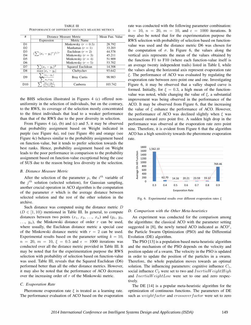
rate was conducted with the following parameter combination:k = 10, n = 20, m = 10, and ε = 1000 iterations. Itmay also be noted that for the experimentation purpose theRWS selection with probability of selection based on function-value was used and the distance metric D6 was chosen forthe computation of σ. In Figure 6, the values along thevertical axis represents the mean of the values obtained bythe functions F1 to F10 (where each function-value itself isan average twenty independent trails) listed in Table I, whilethe values along the horizontal axis represent evaporation rateξ. The performance of ACO was evaluated by regulating theevaporation rate between zero point one and one. InvestigatingFigure 6, it may be observed that a valley shaped curve isformed. Initially, for ξ = 0.3, a high mean of the function-value was noted, while changing the value of ξ, a substantialimprovement was being observed in the performance of theACO. It may be observed from Figure 6, that the increasingthe value of ξ enhance the performance of ACO. However,the performance of ACO was declined slightly when ξ wasincreased onward zero point five. A sudden high drop in theperformance was observed at the evaporation rate zero pointnine. Therefore, it is evident from Figure 6 that the algorithmACO has a high sensitivity towards the pheromone evaporationrate.

1,562.10

62.70 14.16 20.21 23.59 33.12

769.46

0

200

400

600

800

1000

1200

1400

1600

1800

0.3 0.4 0.5 0.6 0.7 0.8 0.9

Ave

rage

On

All

Fun

ctio

n

Evoporation Rate

Fig. 6. Experimental results over different evaporation rates ξ

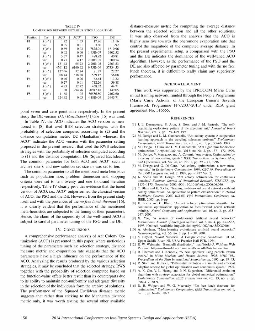
D. Comparison with the Other Meta-heuristics

An experiment was conducted for the comparison amongthe algorithms: the classical ACO with the parameter settingsuggested in [8], the newly turned ACO indicated as ACO∗,the Particle Swarm Optimization (PSO) and the DifferentialEvolution (DE) algorithm.

The PSO [13] is a population based meta-heuristic algorithmand the mechanism of the PSO depends on the velocity andposition update of a swarm. The velocity in the PSO is updatedin order to update the position of the particles in a swarm.Therefore, the whole population moves towards an optimalsolution. The influencing parameters: cognitive influence C1,social influence C2 were set to two and InertiaWeightHighand InertiaWeightLow were set to one and zero respec-tively.

The DE [14] is a popular meta-heuristic algorithm for theoptimization of continuous functions. The parameters of DEsuch as weightfactor and crossoverfactor were set to zero

150 2014 International Conference on Intelligent Systems Design and Applications (ISDA)

TABLE IVCOMPARISON BETWEEN METAHEURISTICS ALGORITHMS

Funtion Test ACO ACO∗ PSO DEF1 f(x∗) 1.72 1.63 17.86 11.16

var 0.05 0.01 3.80 13.92F2 f(x∗) 0.69 0.02 7875.01 1610.96

var 0.02 0.00 1.45E+07 3402.52F3 f(x∗) 5.57 0.47 488.92 40.81

var 0.73 4.17 2.00E+05 200.54F4 f(x∗) 131.42 65.23 2.20E+05 2763.53

var 4501.12 6160.92 9.35E+09 37334.53F5 f(x∗) 127.56 32.24 81.27 22.27

var 308.44 618.88 569.12 56.08F6 f(x∗) 0.46 0.06 62.64 13.22

var 0.27 0.01 712.26 39.88F7 f(x∗) 4.93 12.72 458.32 44.71

var 1.60 294.76 20947.18 149.05F8 f(x∗) 11.68 1.05 36556.80 2162.60

var 324.92 0.03 4.18E+09 13945.71

point seven and zero point nine respectively. In the presentstudy the DE version DE/Randtobest/1/bin [15] was used.

In Table IV, the ACO indicates the ACO version as men-tioned in [8] that used BHS selection strategies with theprobability of selection computed according to (2) and thedistance computation metric D2 (Manhattan) whereas, theACO∗ indicates the ACO version with the parameter settingproposed in the present research that used the RWS selectionstrategies with the probability of selection computed accordingto (1) and the distance computation D6 (Squared Euclidean).The common parameter for both ACO and ACO∗ such asarchive size k and new solution set size m was set to ten.

The common parameter to all the mentioned meta-heuristicssuch as population size, problem dimension and stoppingcriteria were set to ten, twenty and one thousand iterationrespectively. Table IV clearly provides evidence that the tunedversion of ACO, i.e., ACO∗ outperformed the classical versionof ACO, the PSO and the DE. However, from the present studyitself and with the presences of the no free lunch theorem [16],it is clearly evident that the performance of the mentionedmeta-heuristics are subjected to the tuning of their parameters.Hence, the claim of the superiority of the well-tuned ACO issubject to careful parameter tuning of the PSO and the DE.

IV. CONCLUSIONS

A comprehensive performance analysis of Ant Colony Op-timization (ACO) is presented in this paper, where meticuloustuning of the parameters such as: selection strategy, distancemeasure metric and evaporation rate suggests that the ACOparameters have a high influence on the performance of theACO. Analyzing the results produced by the various selectionstrategies, it may be concluded that the selected strategy, RWStogether with the probability of selection computed based onthe function-value offers better result than its counterparts dueto its ability to maintain non-uniformity and adequate diversityin the selection of the individuals form the archive of solutions.The performance of the Squared Euclidean distance metricsuggests that rather than sticking to the Manhattan distancemetric only, it was worth testing the several other available

distance-measure metric for computing the average distancebetween the selected solution and all the other solutions.It was also observed from the analysis that the ACO ishighly sensitive towards the pheromone evaporation rate thatcontrol the magnitude of the computed average distance. Inthe present experimental setup, a comparison with the PSOand the DE indicates the dominance of the well-tuned ACOalgorithm. However, as the performance of the PSO and theDE are also affected by parameter tuning and with the no freelunch theorem, it is difficult to really claim any superiorityperformance.

ACKNOWLEDGMENT

This work was supported by the IPROCOM Marie Curieinitial training network, funded through the People Programme(Marie Curie Actions) of the European Union’s SeventhFramework Programme FP7/2007-2013/ under REA grantagreement No. 316555.

REFERENCES

[1] J. L. Deneubourg, S. Aron, S. Goss, and J. M. Pasteels, “The self-organizing exploratory pattern of the argentine ant,” Journal of InsectBehavior, vol. 3, pp. 159–169, 1990.

[2] M. Dorigo and L. M. Gambardella, “Ant colony system: A cooperativelearning approach to the traveling salesman problem,” EvolutionaryComputation, IEEE Transactions on, vol. 1, no. 1, pp. 53–66, 1997.

[3] M. Dorigo, D. Caro, and L. M. Gambardella, “Ant algorithms for discreteoptimization,” Artificial Life, vol. Vol 5, no. No. 2, pp. 137 – 172, 1999.

[4] M. Dorigo, V. Maniezzo, and A. Colorni, “Ant system: Optimization bya colony of cooperating agents,” IEEE Transactions on Systems, Man,and Cybernetics, vol. Vol 26, no. No. 1, pp. 29 – 41, 1996.

[5] M. Dorigo and G. Di Caro, “Ant colony optimization: a new meta-heuristic,” in Evolutionary Computation, 1999. CEC 99. Proceedings ofthe 1999 Congress on, vol. 2, 1999, pp. –1477 Vol. 2.

[6] K. Socha and M. Dorigo, “Ant colony optimization for continuousdomains,” European Journal of Operational Research, ElSEVIER, pp.1155–1173, November 2006, dOI : 10.1016/j.ejor.2006.06.046.

[7] C. Blum and K. Socha, “Training feed-forward neural networks with antcolony optimization: An application to pattern classification,” in HybridIntelligent Systems, 2005. HIS’05. Fifth International Conference on.IEEE, 2005, pp. 6–pp.

[8] K. Socha and C. Blum, “An ant colony optimization algorithm forcontinuous optimization: application to feed-forward neural networktraining,” Neural Computing and Applications, vol. 16, no. 3, pp. 235–247, 2007.

[9] X. Yao, “A review of evolutionary artificial neural networks,”International Journal of Intelligent Systems, vol. 8, no. 4, pp. 539–567,1993. [Online]. Available: http://dx.doi.org/10.1002/int.4550080406

[10] A. Abraham, “Meta learning evolutionary artificial neural networks,”Neurocomputing, vol. 56, no. 0, pp. 1 – 38, 2004.

[11] S. Haykin, Neural Networks: A Comprehensive Foundation, 1st ed.Upper Saddle River, NJ, USA: Prentice Hall PTR, 1994.

[12] E. W. Weisstein, “Bernoulli distribution,” mathWorld–A Wolfram WebResource http://mathworld.wolfram.com/BernoulliDistribution.html.

[13] R. Eberhart and J. Kennedy, “A new optimizer using particle swarmtheory,” in Micro Machine and Human Science, 1995. MHS ’95.,Proceedings of the Sixth International Symposium on, 1995, pp. 39–43.

[14] R. Storn and K. Price, “Differential evolution - a simple and efficientadaptive scheme for global optimization over continuous spaces,” 1995.

[15] A. K. Qin, V. L. Huang, and P. N. Suganthan, “Differential evolutionalgorithm with strategy adaptation for global numerical optimization,”Evolutionary Computation, IEEE Transactions on, vol. 13, no. 2, pp.398–417, 2009.

[16] D. H. Wolpert and W. G. Macready, “No free lunch theorems foroptimization,” Evolutionary Computation, IEEE Transactions on, vol. 1,no. 1, pp. 67–82, 1997.