Performance analysis of spatial filtering of RF interference in radio astronomy

896 IEEE TRANSACTIONS ON SIGNAL PROCESSING, VOL. 53, NO. 3, MARCH 2005

Performance Analysis of Spatial Filtering of RFInterference in Radio Astronomy

Sebastiaan van der Tol and Alle-Jan van der Veen, Fellow, IEEE

Abstract—Radio astronomical observations are increasinglycontaminated by man-made RF interference (RFI). If these signalsare continuously present, then they cannot be removed by theusual techniques of detection and blanking. We have previouslyproposed a spatial filtering technique, where the impact of theinterferer is projected out from the estimated covariance data. As-suming that the spatial signature of the interferer is time-varying,several such estimates can be combined to recover the missingdimensions. In this paper, we give a detailed performance analysisof this algorithm. It is shown that the spatial filter introduces asmall increase in variance of the estimates (because of the loss ininformation) and that the algorithm is unbiased in case the truespatial signatures of the interferers are known but that there maybe a bias in case the signatures are estimated from the same data.Some of the bias may be removed, and moreover, the bias only af-fects the auto-correlations, whereas the astronomical informationis mostly in the cross-correlations.

Index Terms—Algorithm performance, eigenvalues, interferencecancellation, radio astronomy, RF interference, spatial filtering.

I. INTRODUCTION

RADIO astronomical observations are increasingly con-taminated by man-made RF interference. In bands below

2 GHz, we find TV and radio signals, mobile communication(GSM), radar, satellite communication (Iridium), and local-ization beacons (GPS, Glonass), etc. Although some bandsare specifically reserved for astronomy, the stopband filtersof some communication systems are not always adequate.Moreover, scientifically relevant observations are not limitedto these bands. Hence, there is a growing need for interferencecancellation techniques.

The output of a radio telescope is usually in the form of corre-lations: the auto-correlation (power) of a single telescope dish,split into frequency bins and integrated over periods of 10–30seconds or more, and/or the cross-correlations of several dishes.The astronomer uses several hours of such correlation obser-vations to synthesize images and to create frequency-domainspectra at specific sky locations (in particular for the study ofspectral emission and absorption lines). Most interference can-cellation today is done at the post-correlation level by rejecting

Manuscript received August 18, 2003; revised April 2, 2004. This work wassupported in part by the NOEMI project under Contract STW DEL77-476 andby VICI-SPCOM under Contract STW DTC.5893. Parts of this paper were pub-lished in [1]. The associate editor coordinating the review of this manuscript andapproving it for publication was Dr. Constantinos B. Papadias.

The authors are with the Department of Electrical Engineering, Delft Uni-versity of Technology, 2628 CD Delft, The Netherlands (e-mail: [email protected]; [email protected]).

Digital Object Identifier 10.1109/TSP.2004.842177

suspect correlation products or by specialized imaging algo-rithms, but these techniques have their limits and interferencerejection at shorter time scales is needed.

Depending on the interference and the type of instrument,several kinds of radio frequency interference (RFI) mitigationtechniques are applicable. Overviews can be found in [2] and[3], e.g., intermittent interference such as radar pulses can bedetected using short-term Fourier transforms and the contam-inated time-frequency cells omitted during long-term integra-tion [2]. However, many communication signals are continuousin time. For a single-dish telescope, there are not many otheroptions1 than to consider an extension by a reference antennathat picks up only the interference, so that adaptive cancellationtechniques based on output power minimization can be imple-mented [5]–[7].

With an array of telescope dishes (an interferometer), spa-tial filtering techniques are applicable as well. The desired in-strument outputs in this case are correlation matrices, in-tegrated to, e.g., 10 s (in practice, this can range from a fractionof a second up to several minutes, and only the nonredundantentries are computed and retained). Based on short-term corre-lation matrices (integration to e.g., 10 ms) and narrow subbandprocessing, the array signature vector of an interferer can beestimated and subsequently projected out. The resulting long-term averages of these matrices are mostly interference-free, buta correction is needed to take into account that some dimen-sions were underrepresented. This algorithm was introduced in[8]—we describe it in more detail in Section II.

The goal of the present paper is to give a detailed performanceanalysis of this algorithm. It has to be demonstrated that the in-formation the astronomer is looking for is unaffected by the spa-tial filter—a delicate affair because this information is at least15 dB below the noise level and typically much more.

In Section III, we derive the bias and standard deviation of thefinal covariance estimate. We then analyze the effect of the inter-ferer stationarity on the performance of the filter (Section IV).The bias is studied in more detail in Section V, and the theo-retical performance equations are verified with simulations. Wealso show that much of the bias can be corrected. Conclusionsare in Section VI.

Notation: An overbar denotes complex conjugate, super-script denotes matrix transpose, and denotes complex con-jugate transpose. vec denotes the stacking of the columns of amatrix in a vector, the Kronecker product, the column-wiseKronecker product (Khatri–Rao product), and the entrywisemultiplication of two matrices of equal size. is the identity

1An exception is a technique based on higher order statistics [4].

1053-587X/$20.00 © 2005 IEEE

VAN DER TOL AND VAN DER VEEN: PERFORMANCE ANALYSIS OF SPATIAL FILTERING OF RF INTERFERENCE IN RADIO ASTRONOMY 897

matrix, and is a vector with all ones. The covariance of an es-timated matrix is defined as

cov vec vec

where .

II. DATA MODEL AND ALGORITHM SUMMARY

A. Received Data Model

Assume we have a telescope array with elements. We con-sider the signals received at the antennas in asufficiently narrow subband. For the interference-free case, thearray output vector is modeled in complex baseband formas

where is the vector of telescopesignals at time , is the received sky signal possibly due tomany astronomical sources, assumed on the time scale of 10 sto be a stationary Gaussian vector with covariance matrix(the astronomical “visibilities”), and is the noisevector with independent identically distributed Gaussian entriesand covariance matrix (this implies accurate calibration).The astronomer is interested in the nonredundant off-diagonalentries of .

If an interferer is present the output vector is modeled as

where is the interferer signal with spatial signature vector, which is assumed stationary only over short time intervals.

Without loss of generality, we can absorb the unknown ampli-tude of into and, thus, set the power of to 1.

We make the following additional assumptions on this model:

A1) The noise variance is known from calibration, e.g.,from observations of nearby uncontamined frequen-cies.

A2) , so that . This is reason-able as even the strongest sky sources are about 15 dBunder the noise floor. This condition will be made moreprecise in (6).

A3) The processing bandwidth is sufficiently narrow,meaning that the maximal propagation delay of asignal across the telescope array is small compared tothe inverse bandwidth so that this delay can be repre-sented by a phase shift of the signal. For a maximalbaseline , the condition on the maximal bandwidthis , where is the speed of light,e.g., for a maximal baseline of 3000 m,32 kHz. Without this assumption, it does not makesense to define an interferer signature vector . Ifthe assumption is not satisfied, as for many existingtelescopes, a form of subband processing has to beimplemented.

A4) The interferer signature is stationary over shortprocessing times (say 10 ms).

A5) is varying over periods longer than the short-termintegration time. Note that even interferers fixed onearth will appear to move as the earth rotates and thetelescopes track in the opposite direction. This effectis worked out in Section IV-B.

This was the model considered in [8]. The model is easilyextended to multiple narrowband interfering sources, in whichcase, we obtain

where has columns corresponding to interferers,and is a vector with entries.

B. Covariance Model

Suppose that we have obtained observations, where is the sampling period. We assume that

is stationary at least over intervals of , and constructshort-term covariance estimates

where is the number of samples per short-term average. Theinterference filtering algorithm in this paper is based on ap-plying operations to each to remove the interference, fol-lowed by further averaging over resulting matrices to obtaina long-term average.

Considering the as deterministic, the ex-pected value of each is denoted by . According to theassumptions, has model

(1)

where is the interference-free covariance matrix,and is assumed to be known from calibration. The objectiveis to estimate the interference-free covariance .

C. Spatial Filtering Using Projections

In [8], a spatial filtering algorithm based on projections wasintroduced. In summary, it is as follows.

Momentarily suppose that an orthogonal basis of thesubspace spanned by interferer spatial signatures span isknown. We can then form a spatial projection matrix

(2)

which is such that . When this spatial filter is appliedto the data covariance matrix, all the energy due to the interfererwill be nulled. Indeed, let

then


When we subsequently average the modified covariance ma-trices , we obtain a long-term estimate

(3)

is an estimate of , but it is biased due to the projection.To correct for this, we first write the two-sided multiplicationas a single-sided multiplication employing the matrix identityvec vec . This gives

vec vec (4)

where

If the interference was completely removed, then

vec vec vec (5)

where

In view of this, we can apply a correction to to obtainthe corrected estimate

unvec vec

If the interference was completely projected out, then is anunbiased estimate of the covariance matrix without interference.This was the algorithm introduced in [8].

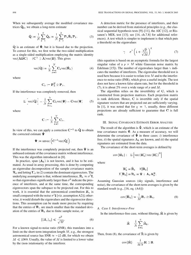
In practice, span is not known, and it has to be esti-mated. As usual in array processing, this is done by computingan eigenvalue decomposition of the sample covariance matrix

and letting in (2) contain the dominant eigenvectors. Theunderlying assumption is that, without interference, ,so that eigenvalues significantly larger than indicate the pres-ence of interferers, and at the same time, the correspondingeigenvectors span the subspace to be projected out. For this towork, it is essential that the astronomical contribution issmall compared with the noise [viz. assumption A2)]; other-wise, it would disturb the eigenvalues and the eigenvector direc-tions. This assumption can be made more precise by requiringthat the entries of are much smaller than the standard devi-ation of the entries of due to finite sample noise, or

(6)

For a known signal-to-noise ratio (SNR), this translates into alimit on the short-term integration length , e.g., the strongestastronomical source has SNR dB, for which we obtain

. Usually, the value of is limited to a lower valueby the (non-)stationarity of the interferer.

A detection metric for the presence of interferers, and theirnumber can be derived from statistical principles (e.g., the clas-sical sequential hypothesis tests [9]–[11], the AIC [12], or Ris-sanen’s MDL test [13]; see [14, ch.7.8] for additional refer-ences). A test which is simpler to implement is that which putsa threshold on the eigenvalues

(7)

(this equation is based on an asymptotic formula for the largestsingular value of a white Gaussian noise matrix byEdelman [15]). The number of eigenvalues larger than indi-cates the number of interferers. The eigenvalue threshold test isused here because it is easier to relate it to and to the interfer-ence-to-noise ratio (INR), which gives a useful insight. The testdoes not have a known false-alarm rate, but for the threshold in(7), it is about 2% over a wide range of and .

The algorithm relies on the invertibility of , which isconstructed from projection matrices. Each projection matrixis rank deficient. Hence, is invertible only if the spatialsignature vectors that are projected out are sufficiently varying.In [1], it was noted that for , usually, three differentprojections are already sufficient to guarantee that is fullrank.

III. SIGNAL COVARIANCE ESTIMATE ERROR ANALYSIS

The result of the algorithm is , which is an estimate of thetrue covariance matrix . As a measure of accuracy, we willdetermine the covariance of in three cases: i) interferencefree, ii) the spatial signatures are known, and iii) the spatialsignatures are estimated from the data.

The covariance of the short-term averages is defined by

cov vec vec

where

Assuming Gaussian sources (sky signals, interference andnoise), the covariance of the short-term averages is given by thestandard result (e.g., [16, eq. (A4)])

cov (8)

A. Case I: Interference-Free

In the interference-free case, without filtering, is given by

Then, from (8), the covariance of is given by

cov


where . Because

cov (9)

Hence, all entries of are disturbed by uncorrelated noise withvariance . This interference-free result gives a refer-ence performance for the estimation of .

B. Case II: Interference With Known Spatial Signatures

Suppose the subspace spanned by the spatial signaturesof the interferers is deterministic and perfectly known. In thatcase, the interference will be completely removed, and the al-gorithms are unbiased by design. According to the algorithm inSection II-C, the estimate of is given by

vec vec vec vec

(10)

where , , and is theprojection onto the orthogonal complement of . (Note thatand are Hermitian.) Thus, the covariance of the long-termestimate is

cov cov

where

cov vec vec (11)

and . The estimation errors and areuncorrelated for , and ;hence

cov vec vec

Multiplication by projects out the contribution of the inter-ferers so that

cov

Thus

cov cov (12)

Compared to (9), this indicates that determines the relativeperformance of the spatial filtering algorithm of Section II-C.

In turn, depends on the variability of , which are thespatial signatures of the interferer. If is sufficiently varyingand the number of antennas is sufficiently large, then for large

, , and the performance is similar as in the interference-free case [see also (16) later in the paper]. In practice, a moderate

is sufficient. Even for stationary located interferers, willchange because of earth rotation. A more detailed discussion onthe conditioning of in that case is found in Section IV-B.

C. Case III: Interference With Unknown DeterministicSpatial Signatures

In practice, the spatial signatures are unknown, and theircolumn span will be estimated from eigendecompositions of the

. Because of the estimation error, the projection is not per-fect, and there will be a residual that might affect the perfor-mance. In previous work [1], we have presented a first-orderperturbation analysis, which said that the performance is thesame as in (12): It is in first order unchanged, even if the pro-jections are estimated. Obviously, this cannot be entirely true.A more detailed second-order analysis presented in this subsec-tion reveals that, with projections estimated from an eigenvaluedecomposition, a bias is introduced on the main diagonal of ,which in certain cases can be significant compared with the stan-dard deviation. We also show that for reasonably large , thecovariance of the estimate is as derived before in (12), i.e., notaffected by the interference subspace estimation.

In this section, we assume for simplicity that the noise powerhas been normalized to . The main results of the second-order perturbation analysis are summarized in the following the-orem, and proofs are in the Appendices.

Theorem 1: Let be a Taylor seriesexpansion of . Assume that . Let be the th eigen-value of (sorted in descending order) and the number ofdimensions that are projected out in the th interval. Assumethat the largest eigenvalues are distinct. Then

vec

vec (13)

The bias on is given by . If the eigenvalues of arestationary (independent of ), the bias is

(14)

For sufficiently large

cov vec vec

Proof: See Appendix B.


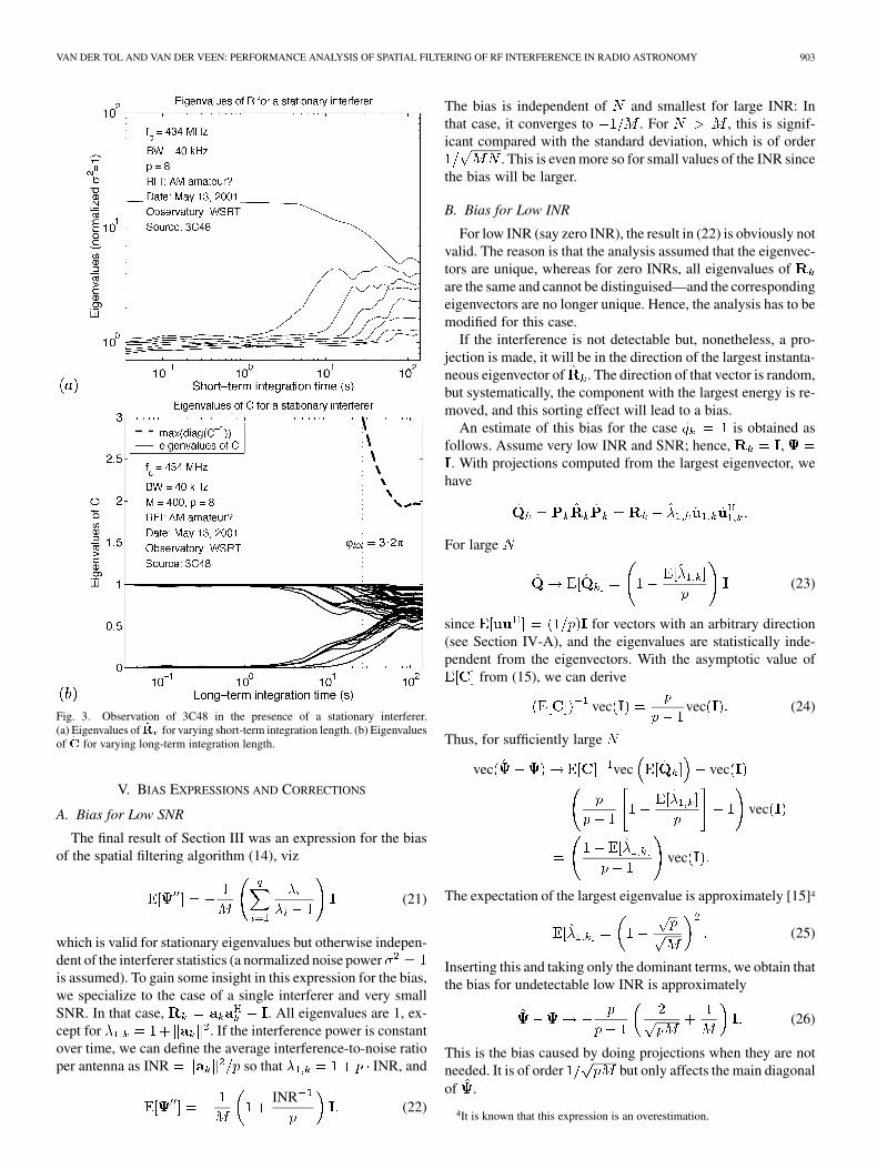
Clearly, (13) and (14) indicate that there is a bias term. Underthe assumption that the eigenvalues are stationary and the skysignal powers are much below the noise power, (14) also showsthat only the diagonal entries of are biased, even if the inter-ferer is not uniformly distributed over space (in fact, even ifis almost stationary). This is acceptable for most astronomy ap-plications (e.g., imaging, spectral analysis). The bias is studiedin more detail in Section V.

The variance of the estimates is the same as we obtained be-fore in (12). The effect of the projections is described entirelyby . The properties of are analyzed in the next section.

IV. EXPECTED VALUE OF

From the covariance expression (12), it is seen that de-termines the penalty on the estimation performance due to spa-tial filtering. The main diagonal of contains the factors bywhich the variance of is multiplied compared with the inter-ference-free case. only depends on the projected directions,i.e., on the collection of , the spatial signatures of the inter-ferer over time. We consider a single interferer and two extremecases: I) the are independent random vectors, with normallydistributed entries, and II) the are the spatial signatures of aninterferer fixed to earth.

A. Case I: Interferer With Normally Distributed SpatialSignatures

If a ground-based interferer without direct line-of-sight ismoving, then due to fast fading effects, it is reasonable to modelthe corresponding spatial signature vectorsas a collection of i.i.d. random vectors with directions uni-formly distributed over the -dimensional unit sphere.2 Fromthis model, we can determine . For , convergesto ; hence, converges to .

Thus, assuming and i.i.d. for different , let

Then, is uniformly distributed over the unit sphere. Note that

To evaluate this expression, we need to establish the second-and fourth-order moments of . Denote by the -th entryof . Due to symmetry, is zero, except when .Let ; then, has a beta distribution with parameters

[17, p. 487] for which

var

2In other cases, this model may represent a workable simplification whichallows for a meaningful analysis.

It follows that

and subsequently

All other cases of are 0 due to symmetry. In sum-mary

vec vec

vec vec (15)

The inverse is given by

vec vec (16)

For large , converges to . The variance of theentries of is determined by the main diagonal of . Inparticular

var

var (17)

e.g., with antennas, the variance of the diagonal entriesof is multiplied by approximately 1.29, and the variance ofthe off-diagonal entries is multiplied by 1.31, or an increase ofabout 1.1 dB. Alternatively, we can say that if one dimensionis always projected out, then 31% more samples are needed tocompensate for the loss of information.

B. Case II: Stationary Interferers

For to be invertible, the spatial signatures need to besufficiently variable. For stationary interferers (not moving, nomultipath), the only source of variability is the geometric delaycompensation. This is a delay placed between each telescopeand the correlator to correct for the different path lengths of theastronomical signal to each of the telescopes: After the correc-tion, signals arriving from the look direction will arrive in-phaseand will be processed coherently. The geometric delay de-pends on the locations of the telescopes and the direction of theobserved field in the sky. Due to the daily rotation of the earth,the stars are moving along the sky, and hence, the geometricdelay is time varying.


For practical reasons, the compensating delay is usuallyinserted only after frequency downconversion. In this case,the downconversion of an RF signal with carrier frequency

and delay introduces a phase shift . For coherentprocessing of the sky signals, it is therefore necessary to applyan additional time-varying phase correction to each telescopesignal after downconversion, which is called fringe stopping[18], [19]. This correction will make interferers fixed on earthappear to have a telescope-dependent time-varying phase-shift.

For a uniform linear East–West array of telescopes, the ge-ometrical delay is , where isthe longest baseline length in wavelengths, is the declinationof the sky source ( for a source at the celestial pole),and is the “hour angle” (azimuth) of the source( rad/s is the earth rotation speed basedon a siderial day) [19]. For time scales of a few seconds, the re-quired phase correction can be approximated by a linear-phaseprogression , where is called the “fringe fre-quency” [19]

The effect of the time-varying fringe correction on the spatialsignature of an interferer can thus be modeled as

...

(18)

where is the spatial signature vector of the inter-ferer without fringe correction.

For a stationary interferer and sufficiently large , de-pends mostly on the number of antennas and the total fringerotation over the longest baseline and over the complete in-tegration period of duration

(19)

Simulations [see Fig. 1(a) and (b)] show how the asymp-totic value of diag depends on and . InFig. 1(a), the initial interferer signature vector is

. It is seen that a reasonably good performance isalready obtained once the total fringe rotation is larger thanabout two cycles (other simulations indicated that this result isindependent of the number of samples per fringe cycle). Theasymptotic values actually correspond to the same levels aspredicted in (16) for the uniformly distributed case. In Fig. 1(b),

is selected randomly, and confidence intervals fordiag are shown for telescopes.

This condition on can be translated into a division of thesky in an “observable” and an “unobservable” area (sky loca-tions that cause insufficient fringe rotations to tolerate the pro-jection of stationary interferers). Let be an angle such that

. In view of (19), a condition for sufficientfringe rotation corresponds to a certain minimum value of .Translating this to values for and , it can be shown that thiscorresponds geometrically to a band from the East horizon overthe celestial pole to the West horizon, as is shown in Fig. 1(c),

Fig. 1. (a) max(diag(C )) as function of fringe rotation � . (b) Con-fidence intervals for a random initial signature vector (p = 8). (c) Unobservablearea of the sky due to a fixed interferer.

which depicts the sky as seen above the observatory in a coor-dinate system relative to the observatory; the vertical directioncorresponds to zenith, and the latitude of the observatory wasassumed to be 52 . The black ring is the unobservable area.

Let be the smallest value of that is acceptable. Thewidth of the unobservable band is given by

(20)


Fig. 2. Observation of 3C48 in the presence of an interfering signal from aGPS satellite. (a) Eigenvalues of ^R for varying short-term integration length.(b) Eigenvalues ofC for varying long-term integration length.

e.g., if rad, s, cm (correspondingto an observation frequency of about 1 GHz), and m,then the width of this band is 16 .

C. Experimental Results

The preceding results can be illustrated further using twomeasurement sets taken at the Westerbork Sythesis Radio Tele-scope (WSRT) in The Netherlands. The measurements consistof correlation products of telescopes with a maximalbaseline of m, split into subbands of 40 kHz andsubsequently short-term integrated over samples, thuscorresponding to a short term integration time of ms.We will consider only a single subband channel. The observedsource was 3C48 at declination . The data was offlinecalibrated to have noise power .

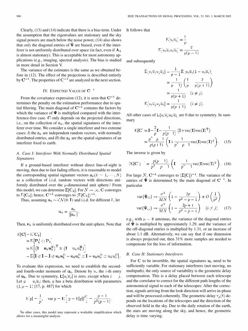
The first data set was measured at MHz and con-tained interference from a GPS satellite. Fig. 2 shows the re-sults. In Fig. 2(a), the eigenvalues of the short-term data covari-

ance matrix are shown for increasing levels of integration. For an integration length shorter than 0.5 s, the eigen-

values indicate a single interferer plus white noise. After 0.5 s,the interfer starts to occupy more than one spatial dimensionbecause its motion changes the direction of the instantaneousspatial signature vector .

Since this clearly shows that the spatial signature is constantover the short-term integration interval of 10 ms, we subse-quently do our spatial filtering at that level and vary the long-term integration length. The question now is whether the re-sulting is invertible. Fig. 2(b) shows the eigenvalues offor various levels of long-term integration (the short-term inte-gration length is fixed at 10 ms). For integration lengths shorterthan 0.5 s, has eigenvalues that are close to zero. After 0.5s, these eigenvalues start to grow, and after about 3 s, is wellconditioned. At the same time, the value of diagdrops to about 1.5.

The GPS satellite is in the far field and moves at a constantspeed. Its spatial signatures can also be modeled by (18), i.e.,by a linear phase progression, although the “fringe frequency”now does not correspond to the earth rotation. Indeed, wehave verified that the data satisfies this model well and haveestimated the corresponding frequency. The dotted vertical lineshows where the condition is met, and it is seenthat it coincides with the integration length above which iswell conditioned.

The second data set, shown in Fig. 3, was measured atMHz and contained interference from a stationary inter-

ferer, possibly an AM amateur broadcast. The stationarity of thesource and the lower observing frequency result in a low fringefrequency. In this case as well, increasing the long-term inte-gration period causes the smallest eigenvalues of to rise and

diag to drop but at a later time than in the previouscase.

In this case, it is seen that at (dotted ver-tical line), diag has not dropped, as low as in theprevious case. The reason is that one antenna was receivingmost of the energy, and such an imbalance was not consideredin the analysis of the previous section.3 Still, at s,

diag has dropped to 2.8 and to 2.1 at s.Integration times of this length are not uncommon for the an-tenna configuration used for this experiment. Indeed, in radioastronomy, a condition that is used to estimate the longest per-missible integration time is [19]

where is the antenna diameter (here 25 m) and the longestbaseline length (here 1296 m); as before,

rad/s. As a result, s. For sand MHz, (20) gives an unobservable band withwidth 10 .

3Moreover, this measurement was done 2 hr after the fringe frequency reachedits maximum value so that better results can still be achieved.


Fig. 3. Observation of 3C48 in the presence of a stationary interferer.(a) Eigenvalues of ^R for varying short-term integration length. (b) Eigenvaluesof ^C for varying long-term integration length.

V. BIAS EXPRESSIONS AND CORRECTIONS

A. Bias for Low SNR

The final result of Section III was an expression for the biasof the spatial filtering algorithm (14), viz

(21)

which is valid for stationary eigenvalues but otherwise indepen-dent of the interferer statistics (a normalized noise poweris assumed). To gain some insight in this expression for the bias,we specialize to the case of a single interferer and very smallSNR. In that case, . All eigenvalues are 1, ex-cept for . If the interference power is constantover time, we can define the average interference-to-noise ratioper antenna as INR so that INR, and

INR(22)

The bias is independent of and smallest for large INR: Inthat case, it converges to . For , this is signif-icant compared with the standard deviation, which is of order

. This is even more so for small values of the INR sincethe bias will be larger.

B. Bias for Low INR

For low INR (say zero INR), the result in (22) is obviously notvalid. The reason is that the analysis assumed that the eigenvec-tors are unique, whereas for zero INRs, all eigenvalues ofare the same and cannot be distinguised—and the correspondingeigenvectors are no longer unique. Hence, the analysis has to bemodified for this case.

If the interference is not detectable but, nonetheless, a pro-jection is made, it will be in the direction of the largest instanta-neous eigenvector of . The direction of that vector is random,but systematically, the component with the largest energy is re-moved, and this sorting effect will lead to a bias.

An estimate of this bias for the case is obtained asfollows. Assume very low INR and SNR; hence, ,. With projections computed from the largest eigenvector, we

have

For large

(23)

since for vectors with an arbitrary direction(see Section IV-A), and the eigenvalues are statistically inde-pendent from the eigenvectors. With the asymptotic value of

from (15), we can derive

vec vec (24)

Thus, for sufficiently large

vec vec vec

vec

vec

The expectation of the largest eigenvalue is approximately [15]4

(25)

Inserting this and taking only the dominant terms, we obtain thatthe bias for undetectable low INR is approximately

(26)

This is the bias caused by doing projections when they are notneeded. It is of order but only affects the main diagonalof .

4It is known that this expression is an overestimation.


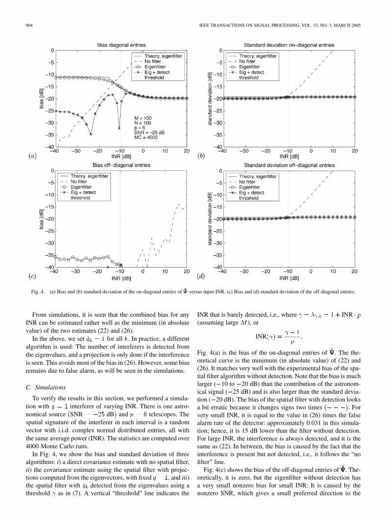
Fig. 4. (a) Bias and (b) standard deviation of the on-diagonal entries of ^ versus input INR. (c) Bias and (d) standard deviation of the off-diagonal entries.

From simulations, it is seen that the combined bias for anyINR can be estimated rather well as the minimum (in absolutevalue) of the two estimates (22) and (26).

In the above, we set for all . In practice, a differentalgorithm is used: The number of interferers is detected fromthe eigenvalues, and a projection is only done if the interferenceis seen. This avoids most of the bias in (26). However, some biasremains due to false alarm, as will be seen in the simulations.

C. Simulations

To verify the results in this section, we performed a simula-tion with interferer of varying INR. There is one astro-nomical source SNR dB and telescopes. Thespatial signature of the interferer in each interval is a randomvector with i.i.d. complex normal distributed entries, all withthe same average power (INR). The statistics are computed over4000 Monte Carlo runs.

In Fig. 4, we show the bias and standard deviation of threealgorithms: i) a direct covariance estimate with no spatial filter,ii) the covariance estimate using the spatial filter with projec-tions computed from the eigenvectors, with fixed , and iii)the spatial filter with detected from the eigenvalues using athreshold as in (7). A vertical “threshold” line indicates the

INR that is barely detected, i.e., where INR(assuming large ), or

INR

Fig. 4(a) is the bias of the on-diagonal entries of . The the-oretical curve is the minimum (in absolute value) of (22) and(26). It matches very well with the experimental bias of the spa-tial filter algorithm without detection. Note that the bias is muchlarger ( 10 to 20 dB) than the contribution of the astronom-ical signal ( 25 dB) and is also larger than the standard devia-tion ( 20 dB). The bias of the spatial filter with detection looksa bit erratic because it changes signs two times . Forvery small INR, it is equal to the value in (26) times the falsealarm rate of the detector: approximately 0.031 in this simula-tion; hence, it is 15 dB lower than the filter without detection.For large INR, the interference is always detected, and it is thesame as (22). In between, the bias is caused by the fact that theinterference is present but not detected, i.e., it follows the “nofilter” line.

Fig. 4(c) shows the bias of the off-diagonal entries of . The-oretically, it is zero, but the eigenfilter without detection hasa very small nonzero bias for small INR: It is caused by thenonzero SNR, which gives a small preferred direction to the


Fig. 5. (a) Bias. (b) Standard deviation of the on-diagonal entries of ^ versusinput INR after bias correction.

eigenvectors. Thus, the spatial filter tends to remove a smallfraction of the astronomical signal. The filter with detection didnot show a bias because it would be 15 dB lower.

In all cases, the variance of the covariance estimate is as pre-dicted (17).

D. Bias Removal

Since the preceding expressions give quite an accurate ideaabout the bias, it is natural to try to remove the bias using them.A complication is that the bias is dependent on the INR, onthe detected number of interferers in each interval, and on thethreshold and the corresponding false alarm rates (these are alsodependent on the number of interferers). We have derived someexperimental techniques that were able to reduce the bias tobelow 35 dB for low INRs or INRs above the threshold [see(35) and (36) in Appendix C] . These results are not completelygeneral and depend on knowledge of the false alarm rates of thedetectors for various numbers of interferers.

Fig. 5 shows the results after this bias correction. Comparedto Fig. 4(a), it is seen that most of the bias is removed, except ina region around the detection limit: Interference below this limitis not removed; hence, the bias line follows that of the unfilteredcurve, but above the limit, the interference is quickly filteredout completely. Hence, the remaining bias directly corresponds

to the remaining (averaged) interference. Whether the bias isabove the standard deviation (hence visible) depends on ; thebias is independent of , but the standard deviation scales as

. Hence, for long integration lengths, there is always anINR window where the interference remains and will be visibleafter integration.

The bias is only present on the main diagonal of . For manyastronomical applications, this is acceptable, e.g., astronomicalimaging does not use the auto-correlations. For spectral line ob-servations, there is usually a single source of interest in the co-variance data, for which the power can be recovered from theoff-diagonal entries using factor analysis techniques (a form ofself-calibration); see, e.g., [20]. Thus, we expect that the bias onthe auto correlations will not be a major impediment, even if itis not removed.

VI. CONCLUSIONS

Spatial filtering can give a significant reduction in unwantedinterference. Its effectiveness depends on the strength of the in-terferer: Stronger interference is more easily detected and canbe better estimated and removed. The quality (covariance) ofthe resulting estimate is given by (12) and is almost as good asthe unperturbed estimate in case the projection direction is suf-ficiently nonstationary. There is a small increase in variance dueto the loss of information in the dimensions that were projectedout.

Assuming the noise power is normalized to , a detec-tion threshold can be defined as

INR

where is the number of antennas and the short-term in-tegration length. Interference with INR above this threshold isusually detected and filtered out. Below the threshold, the INR isusually too weak to be seen and will not be filtered out, leadingto a bias on the diagonal entries of the covariance estimate. Themost difficult interference has INR at this threshold.

In addition, for higher INR, spatial filtering can give somebias in the on-diagonal entries of the covariance estimate. Thisis because the projection directions and sample covariance ma-trices are estimated from the same data. Some of the bias canbe removed, but there are two remaining effects that are hard tocompensate for:

• In case of very weak/no interference, the false-alarmrate of the detector (a few percent) will lead to projec-tions in random directions.

• Interference just below the detection threshold will notbe reliably detected and will remain present in the co-variance estimate. For randomly oriented interference,the effect will only be visible on the main diagonal ofthe final covariance estimate.

The use of reference antennas can improve the detection of weakinterference and the estimation of its projection vectors, canhandle interference with stationary projection directions, andis expected to generate smaller bias. Hence, this is an impor-tant direction for further research. Algorithms for this have beenstudied in [21], [22], and in our recent work.


APPENDIX APRELIMINARY RESULTS

In the proof of Theorem 1 in Appendix B, we use a few re-sults on eigenvalue perturbation theory. They are listed in thissection. The results are known—see, e.g., [16], [23]–[26]—butoften derived and written in indexed form (i.e., in terms of indi-vidual matrix entries). We will write them in an integrated formusing Kronecker products.

To set some notation, let be the true covariance matrixfor the th interval and be the corresponding finite sampleestimate. All our estimates, eigenvalues, eigenvectors etc., arefunctions of and can be written in terms of the truefunction value and a Taylor series expansion on the error

, or , where ,etc. We will only consider the first-order perturbation andsecond-order perturbation .

Let be an eigenvalue decomposition of ,where is unitary, and is diagonal with entries sorted indescending order,5 and define

Lemma 2: For the unique eigenvectors (i.e., those corre-sponding to distinct eigenvalues)

Proof: See, e.g., [24] and [25, eq. (C.2)].Lemma 3: For Gaussian sources

vec vec

vec vec

Proof: For the first line, see, e.g., [16, eq. (A4)]. Thesecond line is derived from the first as follows: Let denotethe th column of an identity matrix; then, a specific entry of

is

vec vec

Apply the expectation operator and use the first line to obtain

vec vec

5The phase ambiguity on the columns of U is resolved in some defaultmanner; see [27].

The following result is a direct result of the preceding twolemmas and appears, e.g., in [16] and [25] where it is writtenusing summations.

Lemma 4: For the unique eigenvectors of the covariance ma-trix of Gaussian sources

Proof: Using Lemma 2

vec vec

Using Lemma 3

If , then , else .

APPENDIX BPROOF OF THEOREM 1

In this section, for simplicity of notation, we assume that thenoise power has been scaled to unity .

We derive the perturbation on in the case that interferersare present in the th period. More precisely, the algorithm com-putes eigendecompositions and applies theprojection , where is the set of domi-nant eigenvectors (spanning the “signal subspace”). Then, withsecond-order accuracy

Let be the Taylor series expansionof ; then, we can identify

.

Subsequently


Define ; then, we can identify

.

Similarly

Note that has some entries on the main diagonal that arealways positive. Since these do not average to 0, does notscale with .

Continuing, we have

vec vec vec

vec vecvec vec

vec

vec vecvec

As with , in addition, does not scale with becausecertain entries of are always positive. Subsequently, we ob-tain

vec

vec

vec

vec vec

vec vec vec

vec vec vec

vec

(27)

By expansion of , it can be shown that

(28)

To work out vec , we first show that vecvec vec . Indeed

vec vec

and

so that

vec vec

Since , andlikewise for the third term, only the first term remains.

It follows that

vec vec vec

Inserting in (27) and using (28) gives

vec vec

vec vec

Since vec vec , the first two terms cancel, and weremain, in first order, with

vec vec (29)

The second-order perturbation on is evaluated as

vec vec vec vec

vec

vec

vec vec


If is large, then the second and third terms can be neglected,and we obtain

vec vec vec

vec vec

vec

vec vec (30)

Each of the two terms inside the summation is . Using(the “sky” contribution is

ignored, and the “noise” eigenvalues are 1), the first term isworked out as

vec

vec

vec

vec

vec

vec

The expected value of this term is worked out as (the tedious butstraightforward derivation uses Lemmas 2–4)

vec vec (31)

The second term in (30) is worked out as

vec vec

vec

Using a similar derivation as before, this is worked out as

vec vec

Altogether, we obtain

vec vec

which is the result stated in the theorem. If the eigenvalues arestationary (independent of ), this can be further simplified as

(32)

since, by definition of

vec vec

vec

vec

is with expected value 0, and iswith nonzero expected value. Thus

The bias is given by . The covariance of the estimate ofis given by

cov vec vec

In the evaluation of cov , for large , we can ignore , andthe covariance is equal to the case where the are known:

cov vec vec

(note that we scaled ). This performance depends onlyon the total number of samples. A more detailed analysis showsthat this result is even valid for small (the covariance willbe larger by terms of , which can be ignored for

).

APPENDIX CBIAS REMOVAL EQUATIONS

We try to remove the bias by adding correction terms to .The complication here is that, even if we know quite preciselythe bias as function of INR, in practice, the INR is unknown.Hence, we need to make corrections that are independent ofthe INR. The idea is to use the eigenvalues to correct thecorresponding rather than the final .

For higher INRs, we can set, based on (13)

(33)


The added term will increase by a term

and the premultiplication by will give the desired result.Here, is the number of interferers in interval or the numberof detected interferers in case of eigenvalue filtering with detec-tion. This correction removes most of the bias for higher INRs.

For very low INRs, we need a different correction. In thatcase, we can set

(34)

Using (23), we obtain . Pre-multiplication of vec by [cf. (24)] gives the requiredresult: .

For growing INRs, this term would grow linearly and be toolarge. Hence, even if we always project out one dimension, acorrect bias removal still requires detection of the presence ofinterference. If it is detected, we correct using (33); else (34).

A further refinement is needed to take into account the falsealarm rate. For very low INR, there are cases where the biaswas removed according to (33) instead of (34). The followingcorrection algorithms take this into account as well.

Bias Removal, Spatial Filtering of One Dimension

Consider the spatial filtering algorithm, where always,dimension is projected out (independent of the actual INR). Tocorrect for the bias, assume that a detector is available, which,in the th interval, detects and has false-alarm rate . Set

if

if (35)

then this removes the bias for low and high INR up to secondorder terms. Indeed, for high INR, the interference is alwaysdetected, and the correction is as in (33). For low INR, we have

in number of cases and in numberof cases. The expected value of is then

since for arbitrary 1-D projections. Thisgives us back the situation in (34). For , we can take theexpression in (25).

Bias Removal, Spatial Filtering With Detection

Consider the spatial filtering algorithm where the number ofinterferers is first detected and the corresponding eigen-vectors projected out. Only if an interferer is detected, a cor-rection using (33) is needed. If the interference is not detected,then no correction is needed, except to correct for the bias dueto false alarm.

Let be the false alarm rate of detecting inter-ferers when there are only , and let be the projectionmatrix that projects out the first eigenvectors. Without furthermotivation, we mention the following algorithm:

if

if

(36)

The algorithm tries to take into account that for interfererand high INR (hence always detected), it might happen that asecond eigenvalue is larger than the threshold ( , with prob-ability ).

REFERENCES

[1] S. van der Tol, A. J. van der Veen, and A. J. Boonstra, “Mitigation ofcontinuous interference in radio astronomy using spatial filtering,” inProc. URSI General Assembly, Maastricht, The Netherlands, Aug. 2002.

[2] A. Leshem, A.-J. van der Veen, and A.-J. Boonstra, “Multichannel in-terference mitigation techniques in radio astronomy,” Astrophys. J. Sup-plement Series, vol. 131, pp. 355–373, Nov. 2000.

[3] P. A. Fridman and W. A. Baan, “RFI mitigation methods in radio as-tronomy,” Astron. Astrophys., vol. 378, pp. 327–344, 2001.

[4] P. A. Fridman, “RFI excision using a higher order statistics analysis ofthe power spectrum,” Astron. Astrophys., vol. 368, pp. 369–376, 2001.

[5] C. Barnbaum and R. F. Bradley, “A new approach to interference ex-cision in radio astronomy: real time adaptive filtering,” Astron. J., vol.115, pp. 2598–2614, 1998.

[6] S. W. Ellingson, J. D. Bunton, and J. F. Bell, “Removal of the GLONASSC/A signal from OH spectral line observations using a parametric mod-eling technique,” Astrophys. J. Supplement, vol. 135, no. 1, pp. 87–93,2001.

[7] L. Li and B. D. Jeffs, “Analysis of adaptive array algorithm performancefor satellite interference cancellation in radio astronomy,” in Proc. URSIGeneral Assembly, Aug. 2002.

[8] J. Raza, A. J. Boonstra, and A. J. van der Veen, “Spatial filtering of RFinterference in radio astronomy,” IEEE Signal Process. Lett., vol. 9, no.2, pp. 64–67, Feb. 2002.

[9] M. S. Bartlett, “Tests of significance in factor analysis,” British J. Psych.(Statist. Sect.), vol. 3, pp. 77–85, 1950.

[10] , “A note on the multiplying factors for various� approximations,”J. R. Statist. Soc., ser. B, vol. 16, pp. 296–298, 1954.

[11] T. W. Anderson, “Asymptotic theory for principal component analysis,”Ann. Math. Stat., vol. 34, pp. 122–148, 1963.

[12] H. Akaike, “Information theory and an extension of the Maximum Like-lihood principle,” in Proc. 2nd Int. Symp. Inf. Theory, 1973, pp. 267–281.

[13] M. Wax and I. Ziskind, “Detection of the number of coherent signals bythe MDL principle,” IEEE Trans. Acoust., Speech, Signal Process., vol.37, no. 7, pp. 1190–1196, Aug. 1989.

[14] H. L. van Trees, Optimum Array Processing (Part IV of Detection,Estimation, and Modulation Theory). New York: Wiley-Interscience,2002.


[15] A. Edelman, “The distribution and moments of the smallest eigenvalueof a random matrix of Wishart type,” Lin. Alg. Appl., vol. 159, pp. 55–80,1991.

[16] M. Kaveh and A. J. Barabell, “The statistical performance of theMUSIC and the minimum-norm algorithms in resolving plane wavesin noise,” IEEE Trans. Acoust., Speech, Signal Process., vol. ASSP-34,pp. 331–341, Apr. 1986 [Corrections in ASSP-34 (6) 1986].

[17] K. V. Mardia, J. T. Kent, and J. M. Bibby, Multivariate Analysis. NewYork: Academic, 1979.

[18] R. A. Perley, F. Schwab, and A. H. Bridle, Eds., Synthesis Imagingin Radio Astronomy (A Collection of Lectures From the Third NRAOSynthesis Imaging Summer School). San Francisco, CA: AstronomicalSoc. Pacific, 1989, vol. 6.

[19] A. R. Thompson, J. M. Moran, and G. W. Swenson, Interferometry andSynthesis in Radioastronomy, Second ed. New York: Wiley, 2001.

[20] A. J. Boonstra and A. J. van der Veen, “Gain calibration methods forradio telescope arrays,” IEEE Trans. Signal Process., vol. 51, pp. 25–38,Jan. 2003.

[21] B. D. Jeffs, K. Warnick, and L. Li, “Improved interference cancellationin synthesis array radio astronomy using auxiliary antennas,” in Proc.IEEE ICASSP, Hong Kong, Apr. 2003.

[22] B. D. Jeffs, L. Li, and K. Warnick, “Auxiliary antenna assisted interfer-ence cancellation for radio astronomy arrays,” IEEE Trans. Signal Pro-cessing, vol. 53, pp. 439–451, Feb. 2005.

[23] J. H. Wilkinson, The Algebraic Eigenvalue Problem. Oxford, U.K.:Clarendon, 1965.

[24] T. W. Anderson, An Introduction to Multivariate Analysis. New York:Wiley, 1984.

[25] B. Ottersten, M. Viberg, and T. Kailath, “Analysis of subspace fittingand ML techniques for parameter estimation from sensor array data,”IEEE Trans. Signal Process., vol. 40, pp. 590–600, Mar. 1992.

[26] N. Yuen and B. Friedlander, “Asymptotic performance analysis ofESPRIT, higher-order ESPRIT, and virtual ESPRIT algorithms,” IEEETrans. Signal Process., vol. 44, pp. 2537–2550, Oct. 1996.

[27] B. Friedlander and A. J. Weiss, “On the second-order statistics of theeigenvectors of sample covariance matrices,” IEEE Trans. Signal Pro-cessing, vol. 46, pp. 3136–3139, Nov. 1998.

Sebastiaan van der Tol was born in The Nether-lands in 1977. He received the M.Sc. degree inelectrical engineering from Delft University ofTechnology, Delft, The Netherlands, in 2004, where,since January 2004, he has been a research assistantand has been pursuing the Ph.D. degree in electricalengineering.

His current research interests include array signalprocessing and interference mitigation techniques forlarge phased-array radio telescopes.

Alle-Jan van der Veen (S’87–M’94–SM’02–F’05)was born in The Netherlands in 1966. He graduated(cum laude) from Department of Electrical Engi-neering, Delft University of Technology, Delft, TheNetherlands, in 1988, from which he received thePh.D. degree (cum laude) in 1993.

Throughout 1994, he was a postdoctoral scholarat Stanford University, Stanford, CA. At present, heis a Full Professor in the Signal Processing Groupof DIMES, Delft University of Technology. Hisresearch interests are in the general area of system

theory applied to signal processing and, in particular, to algebraic methods forarray signal processing.

Dr. van der Veen received the 1994 and the 1997 IEEE SPS Young Authorpaper award and was an Associate Editor for IEEE TRANSACTIONS ON SIGNAL

PROCESSING from 1998 to 2001. He was chairman of the IEEE SPS SPCOMTechnical Committee from 2002 to 2004 is and Editor-in-Chief of the IEEESIGNAL PROCESSING LETTERS.

Performance analysis of spatial filtering of RF interference in radio astronomy

Documents

Transcript of Performance analysis of spatial filtering of RF interference in radio astronomy