2008 8th IEEE-RAS International Conference on Humanoid RobotsDecember 1 -.; 3, 2008 / Daejeon, Korea

Pattern Generation for Bipedal Walkingon Slopes and Stairs

Weiwei Huang, Chee-Meng Chew, Yu Zheng, Geok-Soon Hong

Department of Mechanical EngineeringNational University of Singapore, Singapore

{huangweiwei, mpeccm, mpezy, mpehgs }@nus.edu.sg,

TP1-13

Abstract-Uneven terrain walking is one of the key challengesin bipedal walking. In this paper, we propose a motion patterngenerator for slope walking in 3D dynamics using preview controlof zero moment point (ZMP). In this method, the future ZMPlocations are selected with respect to known slope gradient. Thetrajectory of the Center of Mass (CoM) of the robot is generatedby using the preview controller to maintain the ZMP at thedesired location. Two models of slope walking, namely upslopeand downslope, are investigated. Continuous walking on slopeswith different gradients is also studied to enable the robots towalk on uneven terrains. Since staircase walking is similar toslope walking, the slope walking trajectory generator can alsobe applied to the staircase walking. Simulation results show thatthe robot can walk on many types of slopes and stairs by usingthe proposed pattern generator.

I. INTRODUCTION

Humanoid robots have received much attention recently.Many advanced robots such as ASIMO, HRP, and HUBOhave shown us robust walking behaviors in human environ­ment. Since uneven terrain is common in human environment,uneven terrain walking is one of the important tasks in bipedalrobot research. This motivates us to achieve dynamic walkingon the slope and staircase.

To achieve slope walking, Chew et al. proposed an intuitiveapproach [1]. Kajita et al.[2] developed a simple controlmethod based on Linear Inverted Pendulum Mode to control abipedal walking on ground and rough terrain. Other interestingwork on slope walking can be found in [3][4][5][6]. Inaddition, inspired by biological experiment, Taga et al. [7] in­vestigated the use of CPG to control the walking of a simulatedhumanoid on slope terrain. However, those algorithms are allbased on 2D experiment. None of them have been extendedto 3D environment in which the dynamics is much morecomplex.

To investigate the stability of human walking,Vukobratovic[8] proposed a concept called Zero MomentPoint (ZMP). Although the ZMP algorithm and its variantshave been used to realize stable walking for many bipedalrobots, they are somewhat complex and computationallyintensive since the full dynamics of the robot is considered.Kajita et al.[9] proposed a cart-table model to simplify theZMP calculation. He introduce a controller named previewcontroller, which uses foot placement information as an inputto generate a walking gait. By utilizing the future foot placeinformation, the gait generator produces a robust walking

978-1-4244-2822-9/08/$25.00 ©2008 IEEE

trajectory for the robot walking on the flat terrain. Park andYoum[lO] further improved the model by taking into accountthe effect of horizontal angular momentum. Although themodel shows a good performance on the flat terrain walking,it was not extended to slope and staircase walking. To do this,Kajita et al. [9] introduced another constraint to decouple thefrontal and sagittal motion and achieved spiral stair walking.However, the detail of this method was not disclosed.

In this paper, we present a new method for slope walkingbased on cart-table model and preview controller. When CoMmoves parallel with the slope, the frontal and sagittal motioncan be decoupled. Here, no additional constraint is required.Assume that the slope gradient is known, the model couldgenerate the walking trajectories based on the gradient anddesired step length. In the real environment, the slope gradientmay not be constant. Thus, we also analyze the case that therobot walks continuously on slopes with different gradients.Using simulation, we have shown that the robot can walk fromflat ground to slope with different gradients and then walkdown to flat ground successfully. The detail of the proposedmethod is presented in Section III. The simulation results areincluded in Section IV.

II. CART-TABLE MODEL WITH PREVIEW CONTROLLER[9]

A. Cart-table model in 2D

By combining the ZMP approach and the inverted pendulumbased approach, Kajita et al.[9] introduced the cart-table modelto simplify the ZMP based control. Fig. 1 shows an exampleof cart-table model in 2D plane. The robot is assumed to be apoint mass. When the robot moves forward, the height of thecenter of mass (CoM) is assumed to be constant.

CoM iS

H

x

Fig. 1. An example of cart-table model[9]

205

Authorized licensed use limited to: National University of Singapore. Downloaded on June 4, 2009 at 11:36 from IEEE Xplore. Restrictions apply.

(8)

(7)

(9)

(10)

(11 )

mzH + m(xz - zx)a

-mxH + m(xz - zx)b

.I~_...1..- """X

y == ax + bz + H

Tx + mgz

Tz - mgx

.. HZZMP == z - z-

g.. H

XZMP==X-X-g

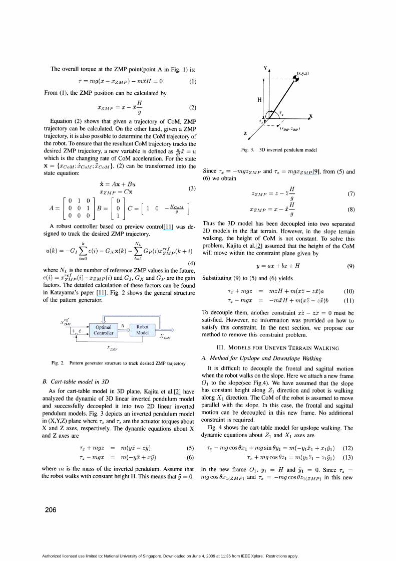
Thus the 3D model has been decoupled into two separated2D models in the flat terrain. However, in the slope terrainwalking, the height of CoM is not constant. To solve thisproblem, Kajita et al.[2] assumed that the height of the CoMwill move within the constraint plane given by

Substituting (9) to (5) and (6) yields

Since Tx == -mgzZMP and Tz == mgxzMP[9], from (5) and(6) we obtain

Fig. 3. 3D inverted pendulum model

y

z

(3)

_HCoM

9

x== Ax+ BuXZMP == ex

A=[~ ~ ~]B=[~]C=[l 0

A robust controller based on preview control[11] was de­signed to track the desired ZMP trajectory.

The overall torque at the ZMP point(point A in Fig. 1) is:

T == mg(x - XZMP) - mxH == 0 (1)

From (1), the ZMP position can be calculated by

.. HXZMP == x - x- (2)

g

Equation (2) shows that given a trajectory of CoM, ZMPtrajectory can be calculated. On the other hand, given a ZMPtrajectory, it is also possible to determine the CoM trajectory ofthe robot. To ensure that the resultant CoM trajectory tracks thedesired ZMP trajectory, a new variable is defined as ~x == uwhich is the changing rate of CoM acceleration. For the statex == {XCoNI; :rCoM; XCoNI}, (2) can be transformed into thestate equation:

k N L

u(k) == -Gf L e(i) - Gxx(k) - L Gp(i)x;eltp(k + i)i=O i=l

(4)where NL is the number of reference ZMP values in the future,e(i) == x;eltp(i) -xzMP(i) and Gf , Gx and Gp are the gainfactors. The detailed calculation of these factors can be foundin Katayama's paper [11]. Fig. 2 shows the general structureof the pattern generator.

X ZMP

Fig. 2. Pattern generator structure to track desired ZMP trajectory

B. Cart-table model in 3D

As for cart-table model in 3D plane, Kajita et al.[2] haveanalyzed the dynamic of 3D linear inverted pendulum modeland successfully decoupled it into two 2D linear invertedpendulum models. Fig. 3 depicts an inverted pendulum modelin (X,Y,Z) plane where Tx and Tz are the actuator torques aboutX and Z axes, respectively. The dynamic equations about Xand Z axes are

To decouple them, another constraint xz - zx == 0 must besatisfied. However, no information was provided on how tosatisfy this constraint. In the next section, we propose ourmethod to remove this constraint problem.

III. MODELS FOR UNEVEN TERRAIN WALKING

A. Method for Upslope and Downslope Walking

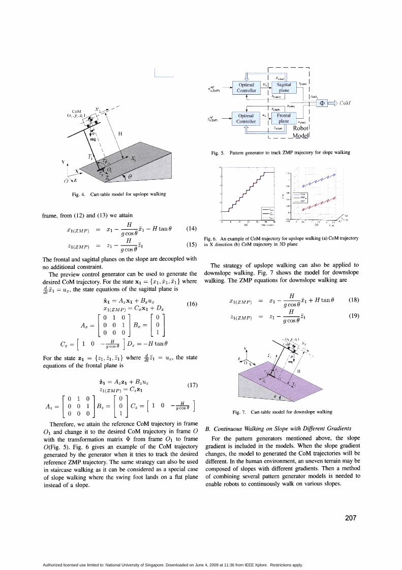
It is difficult to decouple the frontal and sagittal motionwhen the robot walks on the slope. Here we attach a new frame0 1 to the slope(see Fig.4). We have assumed that the slopehas constant height along Zl direction and robot is walkingalong Xl direction. The CoM of the robot is assumed to moveparallel with the slope. In this case, the frontal and sagittalmotion can be decoupled in this new frame. No additionalconstraint is required.

Fig. 4 shows the cart-table model for upslope walking. Thedynamic equations about Zl and Xl axes are

where m is the mass of the inverted pendulum. Assume thatthe robot walks with constant height H. This means that ii == O.

Tx +mgz

Tz - mgx

m(yz - zii)

m(-yx + xii)

(5)

(6)

Tz - mg cos f)xl + mg sin f)Yl == m( -YlXl + XliiI) (12)

Tx + m.g cos (}Zl == m(Ylzl - zliil) (13)

In the new frame 0 1, Yl == H and iiI == O. Since T z ==mgcosf)xl(ZMP) and Tx == -mgcosf)zl(ZMP) in this new

206

Authorized licensed use limited to: National University of Singapore. Downloaded on June 4, 2009 at 11:36 from IEEE Xplore. Restrictions apply.

(18)

(19)

CoAl

-0.2_:-r-~""""';----r-:---r--~

-0.5 0 0.5 1 1.5 2 2.5

(b) X(m)

~ 0.4

H.. H ()Xl - --()Xl + tan

gcosH ..

Zl- --Zl9 cos ()

Fig. 7. Cart-table model for downslope walking

Pattern generator to track ZMP trajectory for slope walking

Zl(ZMP)

Xl(ZMP)

1.50l.--~-1~0-----15~2~0~~

(a)

Fig. 5.

B. Continuous Walking on Slope with Different Gradients

For the pattern generators mentioned above, the slopegradient is included in the models. When the slope gradientchanges, the model to generated the CoM trajectories will bedifferent. In the human environment, an uneven terrain may becomposed of slopes with different gradients. Then a methodof combining several pattern generator models is needed toenable robots to continuously walk on various slopes.

Fig. 6. An example of CoM trajectory for upslope walking (a) CoM trajectoryin X direction (b) CoM trajectory in 3D plane

The strategy of upslope walking can also be applied todownslope walking. Fig. 7 shows the model for downslopewalking. The ZMP equations for downslope walking are

(17)

(16)

(15)

(14)

Zl(ZlvIP)

Xl(ZMP)

Fig. 4. Cart-table model for upslope walking

Zl == Azzl + BzuzZl(ZMP) == Czz l

Az = [~ ~ ~] E z = [ ~ ] Cz = [1 0

Therefore, we attain the reference CoM trajectory in frame0 1 and change it to the desired CoM trajectory in frame 0with the transformation matrix <I> from frame 0 1 to frameO(Fig. 5). Fig. 6 gives an example of the CoM trajectorygenerated by the generator when it tries to track the desiredreference ZMP trajectory. The same strategy can also be usedin staircase walking as it can be considered as a special caseof slope walking where the swing foot lands on a flat planeinstead of a slope.

Xl == AxXl + BxuxXl(ZMP) == CxXl + D x

Ax = [~ ~ ~] Ex = [ ~ ]

Cx = [1 0 -gc1[,slJ ]Dx =-Htan8

For the state Zl == {Zl' Zl, Zl} where i Zl == u z , the stateequations of the frontal plane is

frame, from (12) and (13) we attain

H.. H ()Xl - --Xl - tan

9 cos ()H ..

Zl- --ZlgcosO

The frontal and sagittal planes on the slope are decoupled withno additional constraint.

The preview control generator can be used to generate thedesired CoM trajectory. For the state Xl == {Xl, Xl, Xl} wherefftXl == u x , the state equations of the sagittal plane is

207

Authorized licensed use limited to: National University of Singapore. Downloaded on June 4, 2009 at 11:36 from IEEE Xplore. Restrictions apply.

(25)

When the robot walks from one slope gradient to anothergradient, the model to generate the CoM trajectories will shiftfrom one model to another model. This may cause the walkingtrajectories discontinuous. To make this shift successful, thetrajectories should be smooth and continuous when the modelshifts. Fig. 8 shows an example of a robot walking from a flatterrain to a slope.

Fig. 8. Walking from flat terrain to slope

ZMP equation at point C in frame Olis x zmp == Xl - Xl Jil.

Since C is the origin of frame 0 1, X zrnp == O. 9

.. Yl 9SCOSOYIXl == Xl - == - (24)

9 2Hl

Here, Xl and Yl can be computed by (20) and (21). Therefore,to make the robot stable when it walks from flat terrain toslope, the last imaginary step length of flat terrain walkingshould satisfy

8 == _ 2Hl X l

YlCOSO

To keep the trajectory continuous, the constant height of thenew model H 2 should be equal to Yl.

The same idea can also be applied to the case of differenttypes of slopes. Fig. 9 shows an example of CoM trajectorygenerator by pattern generator of four models when the robotstarts from a flat terrain, walks through 10° and 20° slopessuccessively, and finally arrives at another flat terrain.

In Fig. 8, point C is the desired ZMP location after the foottouches the slope. A new frame 0 1 is attached to point C forthe slope walking. The coordinate transformation of a pointbetween the two frames is given by

4X(m)(b)

:[1N 0,8

_XCoM

-, - _XZMP

_XZVlP

-1L-..-,,----o.-----'---'-----'-----'------lo 10 20 30 40 50 60 70

(a) Time seconds

:[X 2

Fig. 9. An example of CoM trajectory for 100 and 20 0 slope walking

IV. SIMULATION EXPERIMENTS

A. Setup of Simulation Experiments

The simulation software used here is Webots, which allowsusers to conduct realistic physical and dynamical simulationof robots in the 3D virtual environment. The simulated robotis about 175cm high and weighs 75 kg. It has 42 DoFs (7 oneach leg, 6 on each arm, 6 on each hand, 2 on the waist and2 on the neck).The mass distribution of the robot is listed inTable 1. A schematic diagram of the robot is shown in Fig.10. To measure the real ZMP location during the walking,four force sensors are placed on each foot of the robot. Usingthe force sensors can avoid the requirement on knowing theaccurate model of the robot and is an effective way to measurethe actual ZMP location[12].

B. Slope and Stair Walking

To test the effectiveness of our controller, we conductfour simulations(upslope walking, downslope walking, stairwalking and transition walking from 10° to 20° slopes). Theactual ZMP location is measured and compared with thereference ZMP trajectories.

Fig. 11 shows the CoM trajectory for the upslope walkinggenerated by (16) and (17). In the flat terrain walking, the

(20)

(21)

(22)

(23)

(X - Xc) cos 0 + (y - Yc) sin 0

-(x - xc) sinO + (y - Yc) cosO

Z - Zc

Yl

Xl

where {xc, Yc, zc} is the position of point C, namely the originof frame Ot, in frame O.

However, point C cannot be used as the future ZMPreference for flat terrain model as it is on the slope. Here,we create an imaginary reference ZMP location B on theflat terrain. The CoM will move forward according to theimaginary reference ZMP B, while the foot is actually placedat point C. The location of B is designed to ensure that theZMP location will shift to point C when the foot touches theslope.

The step distance between A and B is S. If the swing footcould move to point B, the position of the CoM{X, Y, x} is:x == x B - ~; Y == HI; z == 0 when the foot touches B. Then,the ZMP location would shift to B once the foot touches B.According to (2), the acceleration of CoM at that momentshould be

x == !L(x - XB) == _ g8HI 2Hl

However, the foot is actually at point C on the slope. In thiscase, the CoM position is still taken to be the one obtained withrespect to the imaginary location B in the flat terrain model.The CoM position{Xl, Y!' Zl} in frame 0 1 can be calculatedby (20)-(22). In frame 0 1 , Xl == xcosO + ysinO == xcosO. Ifthe ZMP location in frame 0 1 could be at point C, the robotwill be stable when shifting from one model to another. The

208

Authorized licensed use limited to: National University of Singapore. Downloaded on June 4, 2009 at 11:36 from IEEE Xplore. Restrictions apply.

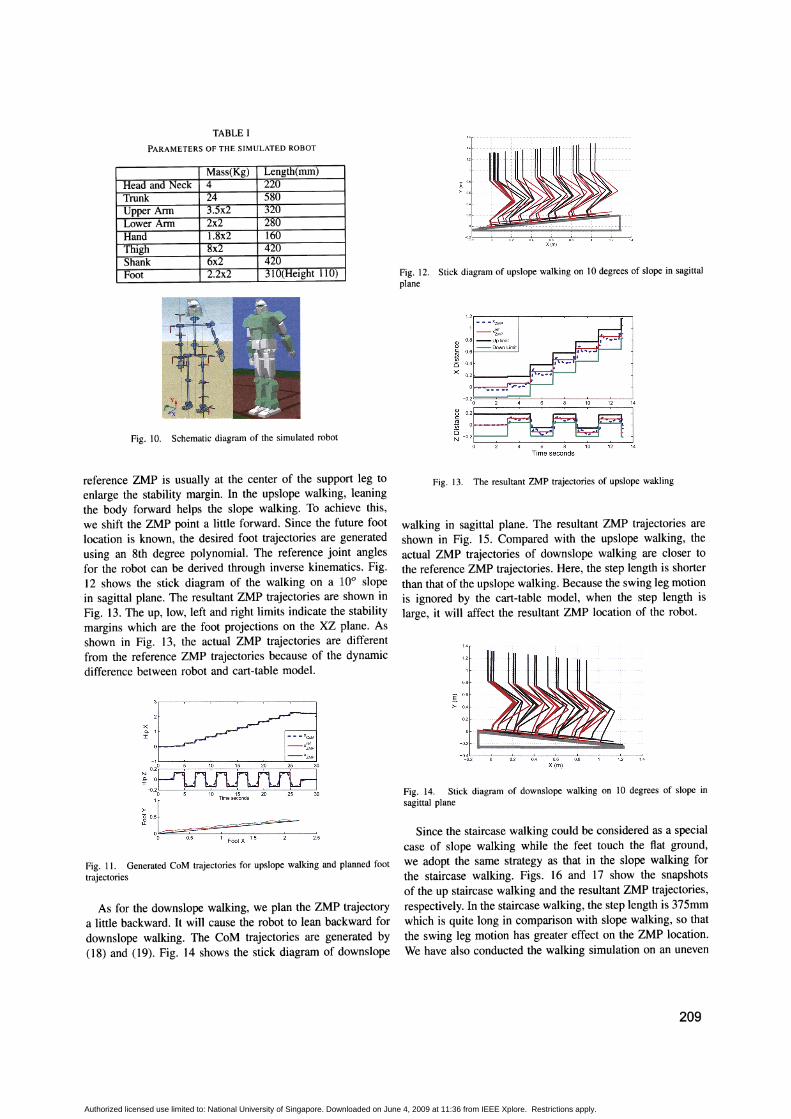
TABLE I

PARAMETERS OF THE SIMULATED ROBOT

Mass(Kg) Length(mm)Head and Neck 4 220Trunk 24 580Upper Arm 3.5x2 320Lower Arm 2x2 280Hand 1.8x2 160Thigh 8x2 420Shank 6x2 420Foot 2.2x2 310(Height 110)

--.0.8.§.>- 06

X(m)

Fig. 12. Stick diagram of upslope walking on 10 degrees of slope in sagittalplane

Fig. 10. Schematic diagram of the simulated robot

- - -'7MP1_~~p

g 0.8 =~~;~~imit~ 0.6

(5 0.4

X

-0.2~=~=~..J...------1._---'--_....L...-----.Jo 2 4 6 8 10 12 14

!O:~jN -0.2 ~

o 2 4 6 8 10 12 14

Time seconds

Fig. 11. Generated CoM trajectories for upslope walking and planned foottrajectories

As for the downslope walking, we plan the ZMP trajectorya little backward. It will cause the robot to lean backward fordownslope walking. The CoM trajectories are generated by(18) and (19). Fig. 14 shows the stick diagram of downslope

~: --_XCoM

o -~~P

-'7MP-1

iO:~-0.2

o 5 10 15 20 25 30Time seconds

io:[~~~=0:: - J -= ::---'--

Fig. 13. The resultant ZMP trajectories of upslope wakling

Fig. 14. Stick diagram of downslope walking on 10 degrees of slope insagittal plane

walking in sagittal plane. The resultant ZMP trajectories areshown in Fig. 15. Compared with the upslope walking, theactual ZMP trajectories of downslope walking are closer tothe reference ZMP trajectories. Here, the step length is shorterthan that of the upslope walking. Because the swing leg motionis ignored by the cart-table model, when the step length islarge, it will affect the resultant ZMP location of the robot.

Since the staircase walking could be considered as a specialcase of slope walking while the feet touch the flat ground,we adopt the same strategy as that in the slope walking forthe staircase walking. Figs. 16 and 17 show the snapshotsof the up staircase walking and the resultant ZMP trajectories,respectively. In the staircase walking, the step length is 375mmwhich is quite long in comparison with slope walking, so thatthe swing leg motion has greater effect on the ZMP location.We have also conducted the walking simulation on an uneven

2.5o 0.5 1 FootX 1.5 2

reference ZMP is usually at the center of the support leg toenlarge the stability margin. In the upslope walking, leaningthe body forward helps the slope walking. To achieve this,we shift the ZMP point a little forward. Since the future footlocation is known, the desired foot trajectories are generatedusing an 8th degree polynomial. The reference joint anglesfor the robot can be derived through inverse kinematics. Fig.12 shows the stick diagram of the walking on a 10° slopein sagittal plane. The resultant ZMP trajectories are shown inFig. 13. The up, low, left and right limits indicate the stabilitymargins which are the foot projections on the XZ plane. Asshown in Fig. 13, the actual ZMP trajectories are differentfrom the reference ZMP trajectories because of the dynamicdifference between robot and cart-table model.

209

Authorized licensed use limited to: National University of Singapore. Downloaded on June 4, 2009 at 11:36 from IEEE Xplore. Restrictions apply.

1.2,---------r,----,----,,----,r-------,---,- - _XZMP

1_X;~p

0.8-Uplimit-Down limit

0.6

-0.2 t=:===_.....L-..'------''------':-------'_--lo 2 4 6 8 10 12 14

j-::~N 0 2 4 6 8 10 12 14

Time seconds

Fig. 15. The resultant ZMP trajectories of downslope walding Fig. 18. Snapshots of continuously walking on 100 and 200 slopes

2.5.....----.,......-----.------.-------.------,--,

Fig. 17. The resultant ZMP trajectories of up stair walking

Fig. 16. Stick diagram of stair walking in sagittal plane (stair height=65mmand stair length=375mm)

trajectories generated by the proposed pattern generator. Inthe simulation, the slope gradient is assumed to be known.In the real implementation, we may design some methods todetect the slope gradient, such as using a distance sensor toapproximate the slope gradient, then using the force torquesensor on the foot to make the foot level with the slope, thusknowing the exact slope gradient.

REFERENCES

[1] C.-M. Chew, J. Pratt, and G. Pratt, "Blind walking of a planar bipedalrobot on sloped terrain," in Proceedings of the 1999 IEEE InternationalConference on Robotics and Automation, Detroit, Michigan, May 1999,pp. 381-386.

[2] S. Kajita, O. Matsumoto, and M. Saigo, "Real-time 3d walking patterngeneration for a biped robot with telescopic legs," in Proceedings ofthe 2001 IEEE International Conference on Robotics and Automation,Seoul, Korea, May 200 1, pp. 2299-2306.

[3] T. Erez and W. D. Smart, "Bipedal walking on rough terrain usingmanifold control," in Proceedings of the 2007 IEEE/RSJ InternationalConference on Intelligent Robots and Systems, San Diego, CA, 2007,pp. 1539-1544.

[4] J. K. Hodgins and M. H. Raibert, "Adjusting step length for rough terrainlocomotion," IEEE TRANSACTIONS ON ROBOTICS AND AUTOMA­TION, vol. 7, no. 3, pp. 289-298, 1991.

[5] M. Ogino, H. Toyama, and M. Asada, "Stabilizing biped walking onrough terrain based on the compliance control," in Proceedings of the2007 IEEE/RSJ International Conference on Intelligent Robots andSystems, San Diego, CA, 2007, pp. 4047-4052.

[6] L. Yang, C.-M. Chew, T. Zielinska, and A.-N. Poo, "A uniform biped gaitgenerator with offline optimization and online adjustable parameters,"Robotica, vol. 25, p. 549C565, 2007.

[7] G. Taga, Y. Yamaguchi, and H. Shimizu, "Self-organized control ofbipedal locomotion by neural oscillators in unpredicatable environment,"Biological Cybernetics, vol. 65, pp. 147-159, 1991.

[8] M. Vukobratovic, A. A. Frank, and D. Juricic, "On the stability of bipedlocomotion," Biomedical Engineering, IEEE Transactions on, vol. BME­17, no. 1, pp. 25-36, 1970.

[9] S. Kajita, F. Kanehiro, K. Kaneko, K. Fujiwara, K. Harada, K. Yokoi,and H. Hirukawa, "Biped walking pattern generation by using previewcontrol of zero-moment point," in Proceedings of the 2003 IEEEInternational Conference on Robotics and Automation, Taipei, Taiwan,2003, pp. 1620-1626.

[10] 1. Park and Y. Youm, "General zmp preview control for bipedal walking,"in Proceedings of the 2007 IEEE International Conference on Roboticsand Automation, Roma, Italy, 2007, pp. 2682-2687.

[11] T. Katayama, T. Ohki, T. Tnoue, and T. Kato, "Design of an optimalcontroller for a discrete-time system subject to previewable demand,"International Journal of Control, vol. 41, no. 3, pp. 677-699, 1985.

[12] T. Ishida and Y. Kuroki, "Development of sensor system of a small bipedentertainment robot," in Proceedings of the 2004 IEEE InternationalConference on Robotics and Automation, New Orleans, LA, May 2004,pp. 648-653.

terrain composed of different types of slopes. The robot canwalk from a flat terrain, pass through 10° and 20° slopes, andreach another flat terrain. The snapshots of continuous walkingbetween the 10° and 20° slopes are shown in Fig. 18.

- - _xZMP

2 _x~e~p

~ 1.5 -Up limitC - Down limiteniiii5X 0.5

-0.5l----'----'----'------L.------'----L-~

o 2 4 6 8 10 12 14

i ~; ~., ~ Io -0.1 '\

N -0.2 ' • • •

o 2 4 6 8 10 12 14

Time seconds

v. CONCLUSION AND FUTURE WORK

We proposed an intuitive method for slope and staircasewalking based on cart-table model. No additional constraintis needed to decouple the frontal and sagittal motions. Threekinds of slope walking are studied: upslope walking, downs­lope walking and continuous walking on slope with differentgradients. Dynamic simulation results show that the robot canwalk on many kinds of uneven terrains by using the CoM

210

Authorized licensed use limited to: National University of Singapore. Downloaded on June 4, 2009 at 11:36 from IEEE Xplore. Restrictions apply.