
Parlar Scientific Pu - Fresenius Environmental Bulletin
166
FEB – Fresenius Environmental Bulletin founded jointly by F. Korte and F. Coulston Production by PSP – Parlar Scientific Publications, Angerstr. 12, 85354 Freising, Germany in cooperation with Lehrstuhl für Chemisch-Technische Analyse und Lebensmitteltechnologie, Technische Universität München, 85350 Freising - Weihenstephan, Germany Copyright © by PSP – Parlar Scientific Publications, Angerstr. 12, 85354 Freising, Germany. All rights are reserved, especially the right to translate into foreign language. No part of the journal may be reproduced in any form- through photocopying, microfilming or other processes- or converted to a machine language, especially for data processing equipment- without the written permission of the publisher. The rights of reproduction by lecture, radio and television transmission, magnetic sound recording or similar means are also reserved. Printed in GERMANY – ISSN 1018-4619
-
Upload
khangminh22 -
Category
Documents
-
view
3 -
download
0
Transcript of Parlar Scientific Pu - Fresenius Environmental Bulletin

FEB – Fresenius Environmental Bulletin founded jointly by F. Korte and F. Coulston
Production by PSP – Parlar Scientific Publications, Angerstr. 12, 85354 Freising, Germany in cooperation with Lehrstuhl für Chemisch-Technische Analyse und Lebensmitteltechnologie,
Technische Universität München, 85350 Freising - Weihenstephan, Germany
Copyright © by PSP – Parlar Scientific Publications, Angerstr. 12, 85354 Freising, Germany. All rights are reserved, especially the right to translate into foreign language. No part of the journal
may be reproduced in any form- through photocopying, microfilming or other processes- or converted to a machine language, especially for data processing equipment- without the written permission of the publisher. The rights of reproduction by lecture, radio and television transmission, magnetic sound
recording or similar means are also reserved.
Printed in GERMANY – ISSN 1018-4619

© by PSP Volume 24 – No 7. 2015 Fresenius Environmental Bulletin
0
FEB - EDITORIAL BOARD
Chief Editor:
Prof. Dr. H. Parlar Institut für Lebensmitteltechnologie und Analytische Chemie TU München - 85350 Freising-Weihenstephan, Germany e-mail: [email protected]
Co-Editors:
Environmental Analytical Chemistry:
Dr. D. Kotzias Via Germania 29 21027 Barza (Va) ITALY Environmental Proteomic and Biology:
Prof. Dr. A. Görg Fachgebiet Proteomik TU München - 85350 Freising-Weihenstephan, Germany Prof. Dr. A. Piccolo Università di Napoli “Frederico II”, Dipto. Di Scienze Chimico-Agrarie Via Università 100, 80055 Portici (Napoli), Italy Prof. Dr. G. Schüürmann UFZ-Umweltforschungszentrum, Sektion Chemische Ökotoxikologie Leipzig-Halle GmbH, Permoserstr.15, 04318 Leipzig, Germany Environmental Chemistry:
Prof. Dr. M. Bahadir Institut für Ökologische Chemie und Abfallanalytik TU Braunschweig Hagenring 30, 38106 Braunschweig, Germany
Prof. Dr. M. Spiteller Institut für Umweltforschung Universität Dortmund Otto-Hahn-Str. 6, 44221 Dortmund, Germany
Prof. Dr. Ivan Holoubek RECETOX_TOCOEN Kamenice 126/3, 62500 Brno, Czech Republic Environmental Management:
Dr. H. Schlesing Secretary General, EARTO, Rue de Luxembourg,3, 1000 Brussels, Belgium Prof. Dr. F. Vosniakos T.E.I. of Thessaloniki, Applied Physics Lab. P.O. Box 14561, 54101 Thessaloniki, Greece Dr. K.I. Nikolaou Organization of the Master Plan & Environmental Protection of Thessaloniki (OMPEPT) 54636 Thessaloniki, Greece
Environmental Toxicology: Prof. Dr. H. Greim Senatskomm. d. DFG z. Prüfung gesundheitsschädl. Arbeitsstoffe TU München, 85350 Freising-Weihenstephan, Germany
Prof. Dr. A. Kettrup Institut für Lebensmitteltechnologie und Analytische Chemie TU München - 85350 Freising-Weihenstephan, Germany
FEB - ADVISORY BOARD
Environmental Analytical Chemistry:
K. Ballschmitter, D - K. Bester, D - K. Fischer, D - R. Kallenborn, N D.C.G. Muir, CAN - R. Niessner, D - W. Vetter, D – R. Spaccini, I Environmental Proteomic and Biology:
D. Adelung, D - G.I. Kvesitadze, GEOR A. Reichlmayr-Lais, D - C. Steinberg, D Environmental Chemistry:
J.P. Lay, D - J. Burhenne, D - S. Nitz, D - R. Kreuzig, D D. L. Swackhammer, U.S.A. - R. Zepp, U.S.A. – T. Alpay, TR V. Librando; I Environmental Management:
L.O. Ruzo, U.S.A - U. Schlottmann, D Environmental Toxicology:
K.-W. Schramm, D - H. Frank, D - D. Schulz-Jander, U.S.A. - H.U. Wolf, D – M. McLachlan, S
Managing Editor:
Dr. G. Leupold
Editorial Chief-Officer:
Selma Parlar PSP- Parlar Scientific Publications Angerstr.12, 85354 Freising, Germany e-mail: [email protected] - www.psp-parlar.de
Marketing Chief Manager:
Max-Josef Kirchmaier MASELL-Agency for Marketing & Communication, Public-Rela-tions Angerstr.12, 85354 Freising, Germany e-mail: [email protected] - www.masell.com
Abstracted/ indexed in: Biology & Environmental Sciences, BIOSIS, C.A.B. International, Cambridge Scientific Abstracts, Chemical Abstracts, Current Awareness, Current Contents/ Agricul-ture, CSA Civil Engineering Abstracts, CSA Mechanical & Trans-portation Engineering, IBIDS database, Information Ventures, NISC, Research Alert, Science Citation Index Expanded (SCI Expanded), SciSearch, Selected Water Resources Abstracts

© by PSP Volume 24 – No 7. 2015 Fresenius Environmental Bulletin
2262
CONTENTS
ORIGINAL PAPERS
SPATIAL VARIATIONS OF NPP IN DIFFERENT 2264 ALTITUDES AT A MEDITERRANEAN WATERSHED Cenk Donmez, Suha Berberoglu and Ahmet Cilek ESTIMATION OF OCCUPATIONAL RISK IN HERBICIDE APPLICATION 2275 Ali Musa Bozdogan, Nigar Yarpuz-Bozdogan, Ibrahim Tobi and Bahadir Sayinci
SYNTHESIS AND CHARACTERIZATION OF ZnS NANO- 2280 CRYSTALS AND ITS PHOTOCATALYTIC ACTIVITY ON ANTIBIOTICS Yuting Wu, Liang Ni, Xinlin Liu, Mingjun Zhou, Zhi Zhu, Ziyang Lu, Changchang Ma and Pengwei Huo
EVALUATION OF PARTICLE SIZE AND INITIAL CONCENTRATION 2289 OF TOTAL SOLIDS ON BIOHYDROGEN PRODUCTION FROM FOOD WASTE Iván Moreno-Andrade and Germán Buitrón
APPLICATION OF CELLULOSE ACETATE MEMBRANES FOR 2296 REMOVAL OF TOXIC METAL IONS FROM AQUEOUS SOLUTION Nadjib Benosmane, Baya Boutemeur, Maamar Hamdi and Safouane M. Hamdi
IN VITRO ANTIOXIDANT POTENTIAL OF para-ALKOXYPHENYLCARBAMIC ACID ESTERS 2310 CONTAINING 4-(4-FLUORO-/3-TRIFLUOROMETHYLPHENYL)PIPERAZIN-1-YL MOIETY Ivan Malík, Jan Muselík, Lukáš Stanzel, Jozef Csöllei and Matej Maruniak
AN ASSESSMENT OF RUNOFF AND SEDIMENT IN SOME 2319 IRRIGATION DISTRICTS IN A SEMI-ARID REGION OF TURKEY Ali Fuat Tari, Öner Çetin, Ramazan Yolcu and Vyacheslav Bogdanets
TEMPORAL AND SPATIAL CHARACTERISTICS OF PHOSPHORUSFRACTIONS 2325 UNDER LONG-TERM WASTEWATER IRRIGATION IN TONGLIAO CITY, CHINA Yintao Lu, Fang Liu, Hong Yao and Kelin Hu
INACTIVATION OF Monopylephorus limosus BY CHLORAMINE, CHLORINE 2334 DIOXIDE, AND HYDROGEN DIOXIDE: EFFECTIVENESS AND SAFETY Kun Yao, Yao Yang, Lihong Zhao, Baiyang Chen and Xiaoshan Zhu
ADSORPTION OF LEAD METAL FROM AQUEOUS SOLUTIONS 2341 USING ACTIVATED CARBON DERIVED FROM SCRAP TIRES Ali R. Rahmani, Ghorban Asgari, Fateme Barjasteh Askari and Ameneh Eskandari Torbaghan
PREPARATION, CHARACTERIZATION OF Fe ION EXCHANGE MODIFIED TITANATE 2348 NANOTUBES AND PHOTOCATALYTIC ACTIVITY FOR OXYTETRACYCLINE Changyu Lu, Weisheng Guan, Yuexin Peng, Li Yang, Tuan K. A. Hoang and Xiao Dong Wang

© by PSP Volume 24 – No 7. 2015 Fresenius Environmental Bulletin
2263
ADSORPTION CHARACTERISTICS OF PHOSPHORUS ONTO SOILS 2354 FROM DIFFERENT LAND USE TYPES IN DANJIANGKOU RESERVOIR AREA Meng Xu, Liang Zhang, Yun Du, Chao Du and Yan-Hua Zhuang
ASSESSMENT OF LIMITING FACTORS FOR POTENTIAL 2362 ENERGY PRODUCTION IN WASTE TO ENERGY PROJECTS Orhan Sevimoğlu
APPLICATIONS OF FACTOR ANALYSIS AND GEOGRAPHICAL INFORMATION 2374 SYSTEMS FOR PRECISION AGRICULTURE OVER ALLUVIAL LANDS Kadir Ersin Temizel, Hakan Arslan and Mustafa Sağlam
PHOTOSYNTHETIC ACTIVITY OF Microcystis IN FISH GUTS AND ITS 2384 IMPLICATION FOR FEASIBILITY OF BLOOM CONTROL BY FILTER-FEEDING FISHES Zhicong Wang, Zhongjie Li, Yiyong Zhou and Dunhai Li
CELLULAR LOCALIZATION OF COPPER AND ITS 2394 TOXICITY ON ROOT TIPS OF HORDEUM VULGARE Junran Wang, Qiuyue Shi, Jinhua Zou, Ze Jiang, Jiayue Wang, Hangfeng Wu, Wusheng Jiang and Donghua Liu
EVALUATION OF STABILITY AND MATURITY PARAMETERS 2406 IN WASTEWATER SLUDGE COMPOSTING WITH DIFFERENT AERATION STRATEGIES AND A MIXTURE OF GREEN PLANT WASTES AS BULKING AGENT Amir Hossein Nafez, Mahnaz Nikaeen, Bijan Bina, Akbar Hassanzadeh and Sharareh Moghim
ADSORPTION OF CARMINE ON ETHYLENEDIAMINE 2415 MODIFIED PEANUT HUSK FROM AQUEOUS SOLUTION Yinghua Song, Xi Zhang, Mei Ye, Hui Xu and Jianmin Ren
INDEX 2421
© by PSP Volume 24 – No 7. 2015 Fresenius Environmental Bulletin
2264
SPATIAL VARIATIONS OF NPP IN DIFFERENT
ALTITUDES AT A MEDITERRANEAN WATERSHED
Cenk Donmez1,*, Suha Berberoglu1, and Ahmet Cilek1
1 University of Cukurova, Department of Landscape Architecture, 01330 Adana, Turkey.
ABSTRACT
The aim of study was to estimate the current net pri-mary productivity (NPP) of Goksu River Basin (forest, grasslands, bare soil, agriculture) located at the Eastern Mediterranean coast of Turkey using remote sensing and a biogeochemical model. Four elevation zones between 0 to 2500 m were defined and spatial patterns of NPP in those elevation zones were assessed to understand the impacts of topographyon local spatial patterns of productivity. The model results are incoorporated with available topographic information in watershed level. The Carnegie-Ames-Stan-ford approach (CASA) model approach was used to esti-mate annual and monthly NPP. This model uses a light-use efficiency (LUE) factor, which is the efficiency of conver-sion of light energy into dry materials by plant, together with remotely sensed, climate (to express the effects of air temperature and water stress), soil and biotic data and ground measurements. Thus, a comprehensive spatial and temporal data set including temperature, precipitation, so-lar radiation, soil texture, percent tree cover, land cover type, and normalized difference vegetation index (NDVI) were used in modelling process. Percent tree cover was predicted using multi-temporal LANDSAT images by ag-gregating tree cover estimates made from high resolution Geo-EYE imagery in a regression tree algorithm. The re-sults indicated several interesting trends between NPP and regional climate gradients. NPP was correlated strongly with solar radiation and precipitation during the growing season suggesting that water limitation as important varia-ble controlling regional patterns of productivity.
KEYWORDS: Remote sensing, NPP, spatial modelling, Mediterra-nean, NASA-CASA Model.
1. INTRODUCTION
The atmospheric concentrations of the carbon have been recently increasing and its widely believed as one of
* Corresponding author
the most important driver for global warming. Addressing to the climate change, the carbon balance is a critical issue that comprises both scientific and political importance. Thus, the quantification of carbon is a major research need to derive management scenarios in respect to the effects of climate change at different scales.
The quantification of terrestrial carbon depends on the net photosynthetic accumulation of carbon by plants. Ac-cumulation of carbon by plants, also known as Net Primary Productivity (NPP) provides the energy that drives most biotic processes on Earth [1]. NPP is a function of standing biomass, an important component of the carbon cycle and a key indicator of ecosystem performance. NPP contributes to biological properties of Earth’s terrestrial surface by pro-ducing organic matter which can be consumed by living organisms [2]. Accounting for the potential of atmospheric CO2 in terrestrial ecosystems depends on understanding of seasonal climate controls on NPP fluxes. Thus, the terres-trial carbon sinks can further be accounted at local and re-gional scales.
Surface temperature, precipitation, and solar radiation have been realised as the strongest controllers of annual terrestrial NPP and its seasonal changes at different scales [1, 3, 4]. Hence, integrating of these climate forcing varia-bles into the improved techniques is essential to predict the annual and seasonal NPP fluxes.
Addressing the strong relationship between climate variables and topography is known as an important factor for vegetation diversity at the Mediterranean where moun-tain formations are often the dominant factor for the vege-tation pattern [5, 6]. However, the impact of topography on vegetation dynamics is rather poorly understood at water-shed level, due to its complexity of the mountainous sys-tems.
Recently, remote sensing and modelling processes as improved techniques provide a better understanding and quantification of the carbon sources and sinks in different land uses and land covers at different altitudes. Particu-larly, the ecosystem models based on satellite sensor data have significant importance to capture variability in eco-system processes when ground-based measurements of lo-cal fluxes are not adequate.
© by PSP Volume 24 – No 7. 2015 Fresenius Environmental Bulletin
2265
In previous studies, three groups of models have been used to estimate NPP for large areas in last decades: (i) based on satellite sensor data; such as, the Carnegie, Ames, Stanford Approach (CASA) ([7, 8]; (ii) simulating carbon flux using a prescribed vegetation structure such as, the Bi-ome BioGeochemical Cycle (BIOME-BGC) model [9]; (iii) simulating both vegetation structure and carbon flux such as, the Dynamic Global Phytogeography (DOLY) model [10].
The aim of this paper was to estimate the current NPP in the Mediterranean using LANDSAT TM/ETM images with a 30 m resolution and CASA model. Seasonal NPP fluxes in respect to different land cover types were derived using land cover data, climate variables, soils and ground truth. Spatial variations of NPP in four elevation zones ranging between 0 to 2500 m were examined to investigate influence of topography on forest land cover. This study enabled us to define the spatial composition of the NPP where the ground measurements are limited. It is also im-portant to expose the variability of NPP at different alti-tudesto investigate the potential effects of diverse topogra-phy on local NPP in a Mediterranean watershed.
2. MATERIALS AND METHODS
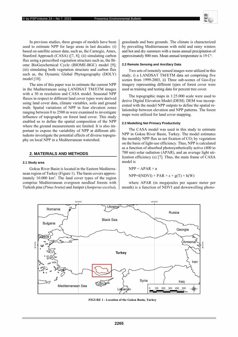
2.1 Study area
Goksu River Basin is located in the Eastern Mediterra-nean region of Turkey (Figure 1). The basin covers approx-imately 10.000 km2. The land cover types of the region comprise Mediterranean evergreen needleaf forests with Turkish pine (Pinus brutia) and Juniper (Juniperus excelsa),
grasslands and bare grounds. The climate is characterized by prevailing Mediterranean with mild and rainy winters and hot and dry summers with a mean annual precipitation of approximately 800 mm. Mean annual temperature is 19 Co.
2.2 Remote Sensing and Ancillary Data
Two sets of remotely sensed images were utilized in this study; i) a LANDSAT TM/ETM data set comprising five scenes from 1999-2003, ii) Three sub-scenes of Geo-Eye imagery representing different types of forest cover were used as training and testing data for percent tree cover.
The topographic maps in 1:25.000 scale were used to derive Digital Elevation Model (DEM). DEM was incoop-erated with the model NPP outputs to define the spatial re-lationship between elevation and NPP patterns. The forest maps were utilized for land cover mapping.
2.3 Modelling Net Primary Productivity
The CASA model was used in this study to estimate NPP in Goksu River Basin, Turkey. The model estimates the monthly NPP flux as net fixation of CO2 by vegetation on the basis of light-use efficiency. Thus, NPP is calculated as a function of absorbed photosynthetically active (400 to 700 nm) solar radiation (APAR), and an average light uti-lization efficiency (ε) [7]. Thus, the main frame of CASA model is
NPP = APAR × ε
NPP=f(NDVI) × PAR × ε × g(T) × h(W)
where APAR (in megajoules per square meter per month) is a function of NDVI and downwelling photo-
FIGURE 1 - Location of the Goksu Basin, Turkey
© by PSP Volume 24 – No 7. 2015 Fresenius Environmental Bulletin
2266
synthetically active solar radiation (PAR) and ε (in grams of C per megajoule) is a function of the maximum achiev-able light utilization efficiency ε adjusted by functions that account for effects of temperature g(T) and water h(W) stress. Whereas previous versions of the CASA model [4,8] used a normalized difference vegetation index (NDVI) to estimate FPAR, the current model version instead relies upon canopy radiative transfer algorithms [11], which are designed to generate improved FPAR products as inputs to carbon flux calculations. The model was utilized to predict annual regional fluxes in terrestrial net primary production at variable degrees of C, depending on the yearly condi-tions, with terrestrial net production. Several diverse da-tasets were used in this research. Calculation of annual ter-restrial NPP is based on the concept of light-use efficiency, modified by temperature, rainfall values and solar radiation scalars. In addition, percentage of tree cover, land cover map of the region, soil texture and NDVI (normalized dif-ference vegetation index) will be used to constitute this model.
2.4 Climate Data
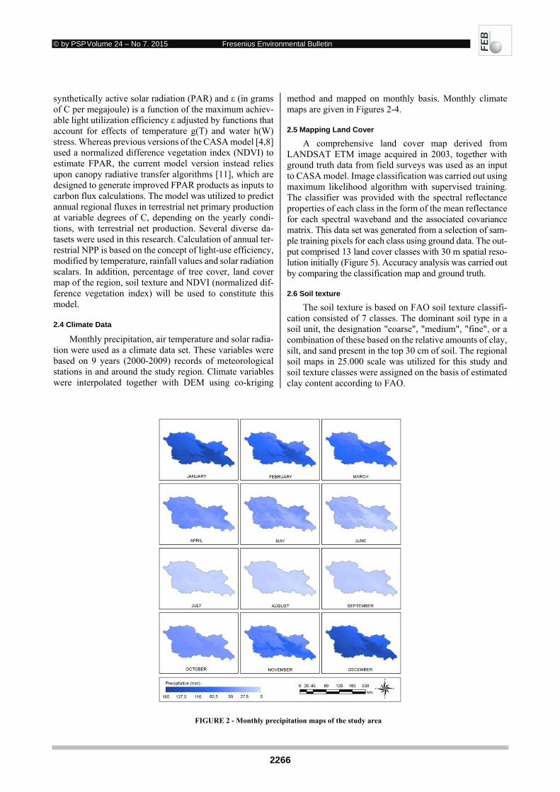
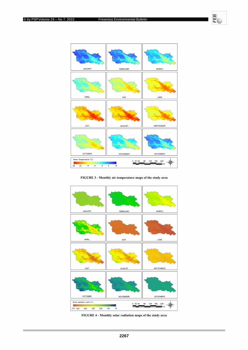
Monthly precipitation, air temperature and solar radia-tion were used as a climate data set. These variables were based on 9 years (2000-2009) records of meteorological stations in and around the study region. Climate variables were interpolated together with DEM using co-kriging
method and mapped on monthly basis. Monthly climate maps are given in Figures 2-4.
2.5 Mapping Land Cover
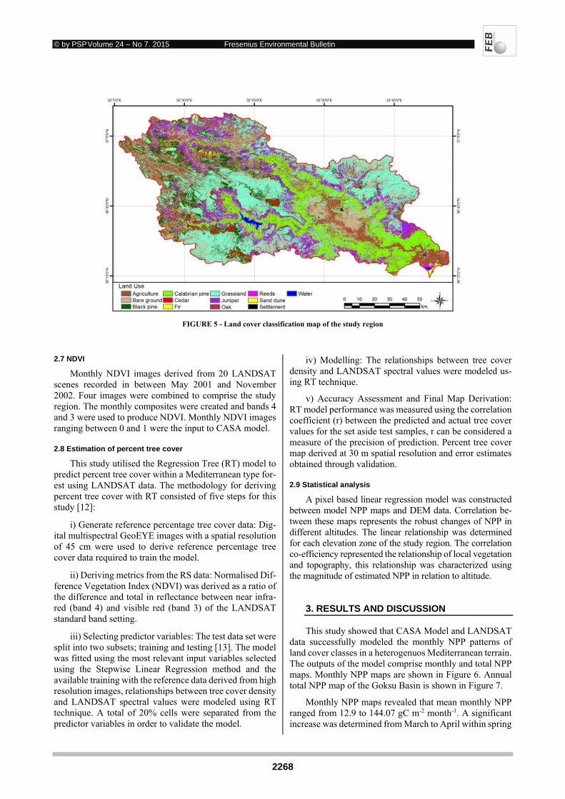
A comprehensive land cover map derived from LANDSAT ETM image acquired in 2003, together with ground truth data from field surveys was used as an input to CASA model. Image classification was carried out using maximum likelihood algorithm with supervised training. The classifier was provided with the spectral reflectance properties of each class in the form of the mean reflectance for each spectral waveband and the associated covariance matrix. This data set was generated from a selection of sam-ple training pixels for each class using ground data. The out-put comprised 13 land cover classes with 30 m spatial reso-lution initially (Figure 5). Accuracy analysis was carried out by comparing the classification map and ground truth.
2.6 Soil texture
The soil texture is based on FAO soil texture classifi-cation consisted of 7 classes. The dominant soil type in a soil unit, the designation "coarse", "medium", "fine", or a combination of these based on the relative amounts of clay, silt, and sand present in the top 30 cm of soil. The regional soil maps in 25.000 scale was utilized for this study and soil texture classes were assigned on the basis of estimated clay content according to FAO.
FIGURE 2 - Monthly precipitation maps of the study area
© by PSP Volume 24 – No 7. 2015 Fresenius Environmental Bulletin
2267
FIGURE 3 - Monthly air temperature maps of the study area
FIGURE 4 - Monthly solar radiation maps of the study area
© by PSP Volume 24 – No 7. 2015 Fresenius Environmental Bulletin
2268
FIGURE 5 - Land cover classification map of the study region
2.7 NDVI
Monthly NDVI images derived from 20 LANDSAT scenes recorded in between May 2001 and November 2002. Four images were combined to comprise the study region. The monthly composites were created and bands 4 and 3 were used to produce NDVI. Monthly NDVI images ranging between 0 and 1 were the input to CASA model.
2.8 Estimation of percent tree cover
This study utilised the Regression Tree (RT) model to predict percent tree cover within a Mediterranean type for-est using LANDSAT data. The methodology for deriving percent tree cover with RT consisted of five steps for this study [12]:
i) Generate reference percentage tree cover data: Dig-ital multispectral GeoEYE images with a spatial resolution of 45 cm were used to derive reference percentage tree cover data required to train the model.
ii) Deriving metrics from the RS data: Normalised Dif-ference Vegetation Index (NDVI) was derived as a ratio of the difference and total in reflectance between near infra-red (band 4) and visible red (band 3) of the LANDSAT standard band setting.
iii) Selecting predictor variables: The test data set were split into two subsets; training and testing [13]. The model was fitted using the most relevant input variables selected using the Stepwise Linear Regression method and the available training with the reference data derived from high resolution images, relationships between tree cover density and LANDSAT spectral values were modeled using RT technique. A total of 20% cells were separated from the predictor variables in order to validate the model.
iv) Modelling: The relationships between tree cover density and LANDSAT spectral values were modeled us-ing RT technique.
v) Accuracy Assessment and Final Map Derivation: RT model performance was measured using the correlation coefficient (r) between the predicted and actual tree cover values for the set aside test samples, r can be considered a measure of the precision of prediction. Percent tree cover map derived at 30 m spatial resolution and error estimates obtained through validation.
2.9 Statistical analysis
A pixel based linear regression model was constructed between model NPP maps and DEM data. Correlation be-tween these maps represents the robust changes of NPP in different altitudes. The linear relationship was determined for each elevation zone of the study region. The correlation co-efficiency represented the relationship of local vegetation and topography, this relationship was characterized using the magnitude of estimated NPP in relation to altitude.
3. RESULTS AND DISCUSSION
This study showed that CASA Model and LANDSAT data successfully modeled the monthly NPP patterns of land cover classes in a heterogenuos Mediterranean terrain. The outputs of the model comprise monthly and total NPP maps. Monthly NPP maps are shown in Figure 6. Annual total NPP map of the Goksu Basin is shown in Figure 7.
Monthly NPP maps revealed that mean monthly NPP ranged from 12.9 to 144.07 gC m-2 month-1. A significant increase was determined from March to April within spring

© by PSP Volume 24 – No 7. 2015 Fresenius Environmental Bulletin
2269
FIGURE 6 - Monthly NPP maps of Goksu Basin
FIGURE 7 - Annual total NPP map of the Goksu Basin Mean annual NPP was estimated as 388 g C m-2 yr-1 for the study area.

© by PSP Volume 24 – No 7. 2015 Fresenius Environmental Bulletin
2270
FIGURE 8 - Monthly NPP results from the CASA model; a) Needleaf Evergreen Forests (NLEF), b) Broadleaf Deciduous Forests (BDF), c) grasslands, d) bare soils, e) agriculture
season in the entire basin. Slight changes in NPP were ob-served from April to June until a dramatic decrease occured in July.
Monthly NPP changes for each land cover class of Goksu Basin were estimated with CASA model. The NPP of major land cover classes were aggregated and total an-nual NPP was estimated (Table 1). Monthly NPP results derived for the CASA model is shown in Figure 8.
TABLE 1 - Annual net primary productivity (NPP) of major land co-vers and land uses of Goksu
Land Cover/Land Use Classes Mean NPP (gC m2 yr-1)
NLEF 742.98
BDF 740.80
Grasslands 668.92
Bare soil 563.40
Agriculture 660.98
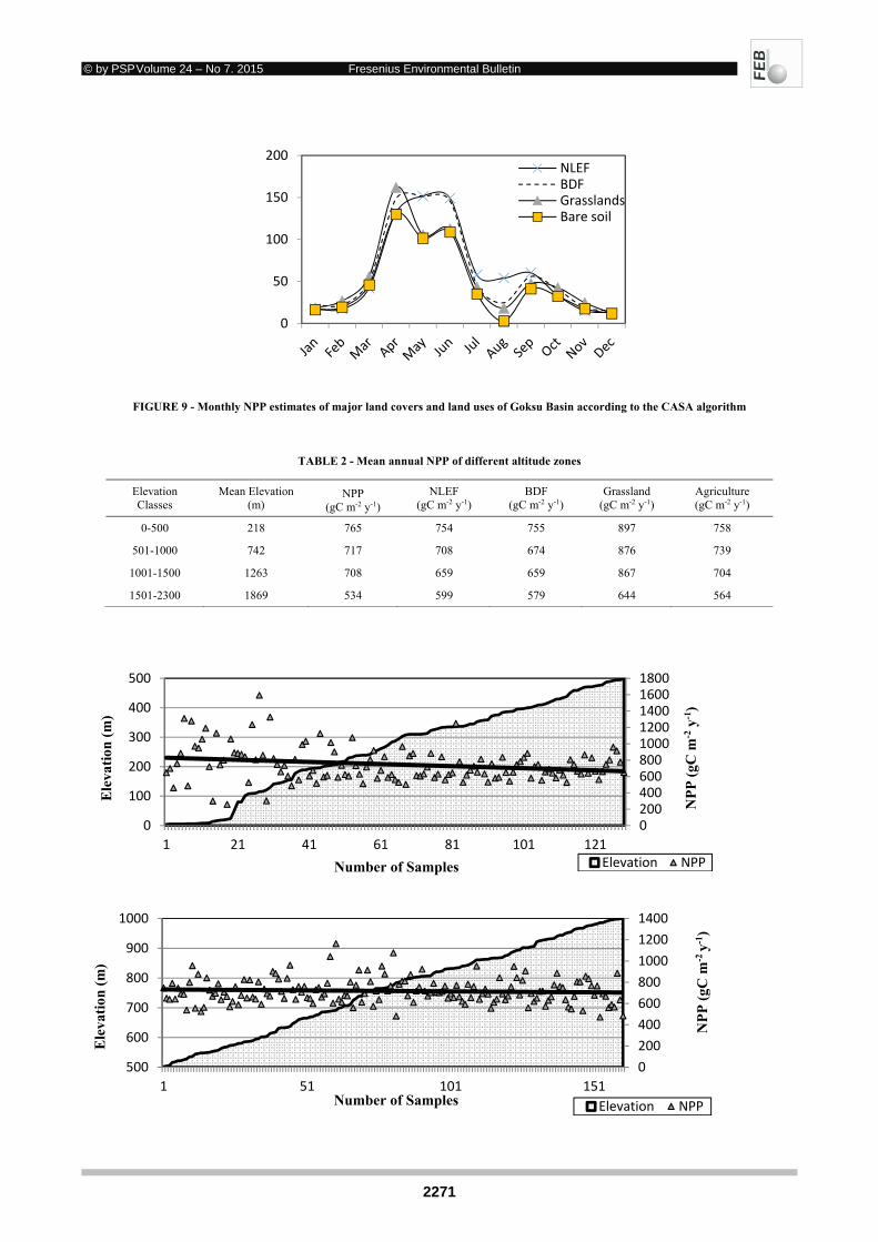
Monthly NPP estimates of major land covers and land uses of Goksu Basin according to the CASA algorithm is shown in Figure 9. Annual NPP of major land covers and land uses of Goksu are also shown in Table 2.
The forest stands of Goksu Basin were combined to two formation classes as NLEF and BDF. The forest NPP estima-tion using CASA model was based on those two classes that comprise the main forest types of Goksu Basin. NLEF com-prised Juniperus excelsa, Pinus nigra, Pinus brutia, Cedrus libani and Abies cilicica. BDF comprised only Quercus sp.,.
The relationship between NPP and elevation were eval-uated according to four general altitude zones (Figure 10). These zones were defined considering the transition bound-aries of forest in the region. Each elevation zone represents the NPP variation in respect to its spatial distribution.
Total annual NPP of different land cover classes was also estimated by incooperating the model results, land cover and DEM data (Table 2).
0
50
100
150
200
0
50
100
150
200
0
50
100
150
200
0
50
100
150
200
0
50
100
150
200
NP
P (
gC
m2
y-1)
N
PP
(g
C m
2y-
1)
a) b)
c) d)
e)
© by PSP Volume 24 – No 7. 2015 Fresenius Environmental Bulletin
2271
FIGURE 9 - Monthly NPP estimates of major land covers and land uses of Goksu Basin according to the CASA algorithm
TABLE 2 - Mean annual NPP of different altitude zones
Elevation Classes
Mean Elevation (m)
NPP (gC m-2 y-1)
NLEF (gC m-2 y-1)
BDF (gC m-2 y-1)
Grassland (gC m-2 y-1)
Agriculture (gC m-2 y-1)
0-500 218 765 754 755 897 758
501-1000 742 717 708 674 876 739
1001-1500 1263 708 659 659 867 704
1501-2300 1869 534 599 579 644 564
0
50
100
150
200NLEFBDFGrasslandsBare soil
020040060080010001200140016001800
0
100
200
300
400
500
1 21 41 61 81 101 121Elevation NPP
0
200
400
600
800
1000
1200
1400
500
600
700
800
900
1000
1 51 101 151
Elevation NPP
Ele
vati
on (
m)
Number of Samples
Ele
vati
on (
m)
Number of Samples
NP
P (
gC m
-2 y
-1)
NP
P (
gC m
-2 y
-1)
© by PSP Volume 24 – No 7. 2015 Fresenius Environmental Bulletin
2272
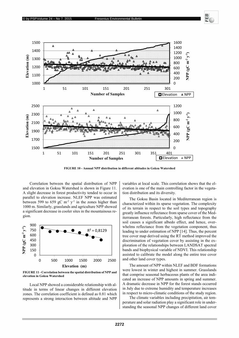
FIGURE 10 - Annual NPP distribution in different altitudes in Goksu Watershed
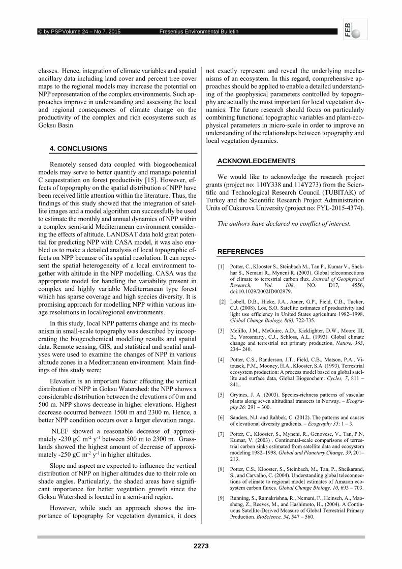
Correlation between the spatial distribution of NPP and elevation in Goksu Watershed is shown in Figure 11. A slight decrease in forest productivity tended to occur in parallel to elevation increase. NLEF NPP was estimated between 599 to 659 gC m-2 y-1 in the zones higher than 1000 m. Similarly, grasslands and agriculture NPP showed a significant decrease in cooler sites in the mountainous re-gion.
FIGURE 11 - Correlation between the spatial distribution of NPP and elevation in Goksu Watershed
Local NPP showed a considerable relationship with al-
titude in terms of linear changes in different elevation zones. The correlation coefficient is defined as 0.81 which represents a strong interaction between altitude and NPP
variables at local scale. This correlation shows that the el-evation is one of the main controlling factor in the vegeta-tion distribution and its diversity.
The Goksu Basin located in Mediterranean region is characterized within its sparse vegetation. The complexity of its terrain in respect to the soil types and topography greatly influence reflectance from sparse cover of the Med-iterranean forests. Particularly, high reflectance from the soil causes a significant albedo effect, and hence, over-whelms reflectance from the vegetation component, thus leading to under estimation of NPP [14]. Thus, the percent tree cover map derived using the RT method improved the discrimination of vegetation cover by assisting in the ex-ploration of the relationships between LANDSAT spectral bands and biophysical variable of NDVI. This relationship assisted to calibrate the model along the entire tree cover and other land cover types.
The amount of NPP within NLEF and BDF formations were lowest in winter and highest in summer. Grasslands that comprise seasonal herbaceous plants of the area indi-cated an increase of NPP amounts in spring and summer. A dramatic decrease in NPP for the forest stands occurred in July due to extreme humidity and temperature increases in respect to micro-climatic conditions of the study region.
The climate variables including precipitation, air tem-perature and solar radiation play a significant role in under-standing the seasonal NPP changes of different land cover
0
200
400
600
800
1000
1200
1400
1600
1000
1100
1200
1300
1400
1500
1 51 101 151 201 251 301
Elevation NPP
0
200
400
600
800
1000
1200
1500
1700
1900
2100
2300
2500
1 51 101 151 201 251 301 351 401Elevation NPP
R² = 0,8129
0150300450600750900
0 500 1000 1500 2000 2500
NP
P (
gC m
-2 y
-1)
Ele
vati
on (
m)
Number of Samples
NP
P (
gC m
-2 y
-1)
Number of Samples
Elevation (m)
Ele
vati
on (
m)
NP
P (
gC m
-2 y
-1)
© by PSP Volume 24 – No 7. 2015 Fresenius Environmental Bulletin
2273
classes. Hence, integration of climate variables and spatial ancillary data including land cover and percent tree cover maps to the regional models may increase the potential on NPP representation of the complex environments. Such ap-proaches improve in understanding and assessing the local and regional consequences of climate change on the productivity of the complex and rich ecosystems such as Goksu Basin.
4. CONCLUSIONS
Remotely sensed data coupled with biogeochemical models may serve to better quantify and manage potential C sequestration on forest productivity [15]. However, ef-fects of topography on the spatial distribution of NPP have been received little attention within the literature. Thus, the findings of this study showed that the integration of satel-lite images and a model algorithm can successfully be used to estimate the monthly and annual dynamics of NPP within a complex semi-arid Mediterranean environment consider-ing the effects of altitude. LANDSAT data hold great poten-tial for predicting NPP with CASA model, it was also ena-bled us to make a detailed analysis of local topographic ef-fects on NPP because of its spatial resolution. It can repre-sent the spatial heterogeneity of a local environment to-gether with altitude in the NPP modelling. CASA was the appropriate model for handling the variability present in complex and highly variable Mediterranean type forest which has sparse coverage and high species diversity. It is promising approach for modelling NPP within various im-age resolutions in local/regional environments.
In this study, local NPP patterns change and its mech-anism in small-scale topography was described by incoop-erating the biogeochemical modelling results and spatial data. Remote sensing, GIS, and statistical and spatial anal-yses were used to examine the changes of NPP in various altitude zones in a Mediterranean environment. Main find-ings of this study were;
Elevation is an important factor effecting the vertical distribution of NPP in Goksu Watershed: the NPP shows a considerable distribution between the elevations of 0 m and 500 m. NPP shows decrease in higher elevations. Highest decrease occurred between 1500 m and 2300 m. Hence, a better NPP condition occurs over a larger elevation range.
NLEF showed a reasonable decrease of approxi-mately -230 gC m-2 y-1 between 500 m to 2300 m. Grass-lands showed the highest amount of decrease of approxi-mately -250 gC m-2 y-1 in higher altitudes.
Slope and aspect are expected to influence the vertical distribution of NPP on higher altitudes due to their role on shade angles. Particularly, the shaded areas have signifi-cant importance for better vegetation growth since the Goksu Watershed is located in a semi-arid region.
However, while such an approach shows the im-portance of topography for vegetation dynamics, it does
not exactly represent and reveal the underlying mecha-nisms of an ecosystem. In this regard, comprehensive ap-proaches should be applied to enable a detailed understand-ing of the geophysical parameters controlled by topogra-phy are actually the most important for local vegetation dy-namics. The future research should focus on particularly combining functional topographic variables and plant-eco-physical parameters in micro-scale in order to improve an understanding of the relationships between topography and local vegetation dynamics.
ACKNOWLEDGEMENTS
We would like to acknowledge the research project grants (project no: 110Y338 and 114Y273) from the Scien-tific and Technological Research Council (TUBITAK) of Turkey and the Scientific Research Project Administration Units of Cukurova University (project no: FYL-2015-4374).
The authors have declared no conflict of interest.
REFERENCES
[1] Potter, C., Klooster S., Steinbach M., Tan P., Kumar V., Shek-har S., Nemani R., Myneni R. (2003). Global teleconnections of climate to terrestrial carbon flux. Journal of Geophysical Research, Vol. 108, NO. D17, 4556, doi:10.1029/2002JD002979.
[2] Lobell, D.B., Hicke, J.A., Asner, G.P., Field, C.B., Tucker, C.J. (2008). Los, S.O. Satellite estimates of productivity and light use efficiency in United States agriculture 1982–1998. Global Change Biology, 8(8), 722-735.
[3] Melillo, J.M., McGuire, A.D., Kicklighter, D.W., Moore III, B., Vorosmarty, C.J., Schloss, A.L. (1993). Global climate change and terrestrial net primary production, Nature, 363, 234– 240.
[4] Potter, C.S., Randerson, J.T., Field, C.B., Matson, P.A., Vi-tousek, P.M., Mooney, H.A., Klooster, S.A. (1993). Terrestrial ecosystem production: A process model based on global satel-lite and surface data, Global Biogeochem. Cycles, 7, 811 – 841,.
[5] Grytnes, J. A. (2003). Species-richness patterns of vascular plants along seven altitudinal transects in Norway. – Ecogra-phy 26: 291 – 300.
[6] Sanders, N.J. and Rahbek, C. (2012). The patterns and causes of elevational diversity gradients. – Ecography 35: 1 – 3.
[7] Potter, C., Klooster, S., Myneni, R., Genovese, V., Tan, P.N, Kumar, V. (2003) . Continental-scale comparisons of terres-trial carbon sinks estimated from satellite data and ecosystem modeling 1982–1998. Global and Planetary Change, 39, 201–213.
[8] Potter, C.S., Klooster, S., Steinbach, M., Tan, P., Sheikarand, S., and Carvalho, C. (2004). Understanding global teleconnec-tions of climate to regional model estimates of Amazon eco-system carbon fluxes. Global Change Biology, 10, 693 – 703.
[9] Running, S., Ramakrishna, R., Nemani, F., Heinsch, A., Mao-sheng, Z., Reeves, M., and Hashimoto, H., (2004). A Contin-uous Satellite-Derived Measure of Global Terrestrial Primary Production. BioScience, 54, 547 – 560.
© by PSP Volume 24 – No 7. 2015 Fresenius Environmental Bulletin
2274
[10] Woodward, F.I., Smith, T.M., and Emanuel, W.R. (1995). A global land primary productivity and phytogeography model. Global Biogeochemical Cycles, 9, 471 490.
[11] Knyazikhin, Y., Martonchik, J.V., Myneni, R.B., Diner, D.J., Running S.W. (1998). Synergistic algorithm for estimating vegetation canopy leaf area index and fraction of absorbed photosynthetically active radiation from MODIS and MISR data. Journal of Geophysical Research 103: 32257– 32276.
[12] Donmez, C., Berberoglu, S., and Curran, P.J. (2011). Model-ling the current and future spatial distribution of Net Primary Production in a Mediterranean watershed. International Jour-nal of Applied Earth Observation and Geoinformation, Vol-ume 13: Issue 3, pp.336.-345.
[13] Rokhmatuloh, Nitto, D., Al-Bilbisi, H. Tateishi. R. (2005). Percent Tree Cover Estimation Using Regression Tree Method: a case study of Africa with very-high resolution QuickBird images as training data, Geoscience and Remote Sensing Symposium IEEE 2005 International, IGARSS 05. Vol. 3, pp 2157-2160.
[14] Berberoglu, S., Evrendilek, F., Ozkan C., Donmez C. (2007). Modeling Forest Productivity Using Envisat MERIS Data. Sensors, 7, 2115-2127.
[15] Meydan, S.M., Evrendilek, F., Berberoglu, S., Donmez, C. (2010). Modeling above-ground litterfall in eastern Mediterra-nean conifer forests using fractional tree cover, and remotely sensed and ground data, Applied Vegetation Science, 1–26.
Received: November 10, 2014 Revised: March 31, 2015 Accepted: April 28, 2015
CORRESPONDING AUTHOR
Cenk Donmez University of Cukurova Department of Landscape Architecture 01330 Adana TURKEY E-mail: [email protected]
FEB/ Vol 24/ No 7/ 2015 – pages 2264 - 2274
© by PSP Volume 24 – No 7. 2015 Fresenius Environmental Bulletin
2275
ESTIMATION OF OCCUPATIONAL
RISK IN HERBICIDE APPLICATION
Ali Musa Bozdogan1*, Nigar Yarpuz-Bozdogan2, Ibrahim Tobi3 and Bahadir Sayinci4
1Cukurova University, Agriculture Faculty, Agricultural Machinery and Technologies Engineering Dept., 01330 Adana/Turkey 2Cukurova University, Vocational School of Technical Sciences, 01350 Adana/Turkey
3Harran University, Agriculture Faculty, Agricultural Machinery Dept., Sanliurfa/Turkey 4Ataturk University, Agriculture Faculty, Agricultural Machinery Dept., Erzurum/Turkey
ABSTRACT
The aim of this study was to estimate the occupational risk for operators and workers in herbicide application in Sanliurfa, Turkey. In this study, 2,4-D, clodinafop-propar-gyl, dicamba, diclofop-methyl, fenoxaprop-p-ethyl, foram-sulfuron, iodosulfuron-methyl-sodium, nicosulfuron, pinox-aden, tribenuron-methyl, and tritosulfuron were used for determining the occupational risk. In this study, it was ob-tained that the highest risk was assessed in diclofop-methyl as 1.913 Exceedence Factor (EF) value. The lowest risk was found in nicosulfuron due to its 0.230 EF value. In the re-sult of this study, it was determined that herbicide has risk for occupational health. These risks can be minimized by using equipment such as personnel protective equipment, increasing awareness of pesticide side effects on operator and worker and advanced proper application technique and equipment, etc.
KEYWORDS: Weed control, Pesticide application, Human health, Environment, Cereal.
1. INTRODUCTION
Pesticides are defined as chemical formulations that are used for improving quality and quantity of agricultural crops by farmers. These are mainly classified as insecti-cide, herbicide, and fungicide. Herbicides are used to con-trol weed in agricultural land. World pesticide active ingre-dients (a.i.) amount used exceeded 2 million tonnes in 2007. In this value, herbicide a.i. was 951 584 tonnes [1]. In EU-15, herbicide a.i. consumption was 70 874 tonnes in 2010 [2]. In Turkey, 6 056 tonnes herbicide (a.i.) was used in agriculture in 2010 [2]. In Turkey, cereals are approxi-mately cultivated in an area of 16 million ha [3]. In San-liurfa, in 2013, herbicides were applied in 260 000 ha in cereal cultivation [4]. In cereal cultivation areas, 11 a.i. were used for weed control in 2013, in Sanliurfa. These a.i. were 2,4-D, clodinafop-propargyl, dicamba, diclofop-me-
* Corresponding author
thyl, fenoxaprop-p-ethyl, foramsulfuron, iodosulfuron me-thyl sodium, nicosulfuron, pinoxaden, tribenuron methyl, and tritosulfuron. These a.i. consumption were 10 000 kg for 2,4-D, 1 125 kg for tribenuron-methyl, 3 408 kg for di-clofop-methyl, 360 kg for fenoxaprop-p-ethyl, 2 016 kg for clodinafop-propargyl, 243 kg for pinoxaden, 1 250 kg for nicosulfuron, 625 kg for tritosulfuron, 125 kg for dicamba, 225 kg for foramsulfuron, and 7.5 kg for iodosulfuron me-thyl sodium [3]. In Sanliurfa, total herbicide a.i. consump-tion in cereal cultivation was 19 400 kg.
Pesticides used in agriculture have potential negative effects on human health and environment. It was indicated that the average cost of the health treatment of the poisoned worker was calculated as USD 787.97 in Brazil [5]. Pesti-cide exposure on human and environment can be mini-mized by selecting the type of tractors such as closed and open cabin, and suitable pesticide application technology such as proper anti-drift nozzles, air-assisted nozzles, pes-ticide application methods, etc. [6-14]. Yet, these are not enough to protect the worker and operator, some additional precautions such as personnel protection equipment (PPE) should be taken for occupational risk during pesticide ap-plication. Operators are persons who attend to mix, load and apply pesticide in application [9, 15, 16]. Workers are persons who are occupied with thinning, pruning, and har-vesting etc. of the agricultural crop [9, 15-17].
In Turkey, generally, farmers apply overdose pesticide than the recommended dose by manufacturer and do not take care of personnel protection during pesticide applica-tions [18-20]. Demircan and Yılmaz (2005) indicated that, in apple production, farmers applied pesticides 186% more than the recommended dose in Isparta province, Turkey [18]. Application rate effects the pesticide exposure on hu-man and environment. Application rate plays a role in the occupational pesticide exposure [19]. Yalap Tuna (2011) determined that farmers were eating and drinking during pesticide applications. Researcher indicated that the ratio of health problems after the applying process was 25% amoung the farmers [20].
The aim of this study was to estimate the occupational risk in herbicide applications in cereal fields, Sanliurfa, Turkey.

© by PSP Volume 24 – No 7. 2015 Fresenius Environmental Bulletin
2276
2,4‐D
C8H6Cl2O3
Clodinafop‐propargyl
C17H13ClFNO4
Dicamba
C8H6Cl2O3
Diclofop‐methyl
C16H14Cl2O4
Fenoxaprop‐p‐ethyl
C18H16ClNO5
Foramsulfuron
C17H20N6O7S
Iodosulfuron‐methyl‐sodium
C14H13IN5NaO6S
Nicosulfuron
C15H18N6O6S
Pinoxaden
C23H32N2O4
Tribenuron‐methyl
C15H17N5O6S
Tritosulfuron
C13H9F6N5O4S
FIGURE 1 - Chemical formula of a.i. [21]
2. MATERIAL AND METHODS
In this study, 11 herbicide a.i., named as 2,4-D, clodinafop-propargyl, dicamba, diclofop-methyl, fenoxa-prop-p-ethyl, foramsulfuron, iodosulfuron-methyl-sodium, nicosulfuron, pinoxaden, tribenuron-methyl, and tritosul-furon were used in cereal fields in Sanliurfa (Figure 1).
In this study, risk indices (RI) of occupational health for each a.i. were estimated via Equations 1, 2, and 3.
The RI for operator was determined via Equation 1 [15, 16, 22, 23].
AOEL
ARRIoperator
292.0
(1)
AR: Application rate (kg a.i. ha-1); AOEL: Acceptable operator exposure level (mg kg-1 body weight day-1).
The RI for worker was assessed with Equation 2 and 3 [15-17, 22, 23].
AOEL
AbDERI DE
wor
ker
(2)
PTTFLAI
ARDE 01.0
(3)
DE: Dermal Exposure of worker (mg day-1), AbDE: Factor of dermal absorption (default:0.1). LAI: Leaf Area
Index (m2; default: field crops: 1), TF: Transfer factor (cm2 person-1 h-1; default: field crops: 5000), T: The duration of re-entry (h; default: 8), and P: Factor for Personal Protec-tive Equipment (PPE) (default: no PPE: 1).
Exceedence factor (EF) was determined by Equation 4 [22, 24].
DTRANSFORMEDTRANSFORME
DTRANSFORMEDTRANSFORME
LLUL
LLXEF (4)
RI+, LL+ and UL+ was calculated by dividing, respec-tively the risk index values RI, LL and UL by UL. RI+, LL+ and UL+ values were transformed with Equation 5 [22, 24].
XX dtransforme
11log (5)
with
X = RI+, LL+ and UL+.
If the EF value for each a.i. is equal or lower than 0, it is regulate to 0 and indicates a low risk. EF value equal or higher than 1 is regulated to 1, and it means a high risk. An intermediate risk is found for the values between 0 and 1 [22, 24]. In this study, EF values of the operator and worker were summed for the determination of the total risk on oc-cupational health. Therefore, total EF for the occupational risk was between 0 and 2 according to POCER (The Pesti-cide Occupational and Environmental Risk) indicator [22].

© by PSP Volume 24 – No 7. 2015 Fresenius Environmental Bulletin
2277
3. RESULTS AND DISCUSSION
EF values for worker and operator were calculated by Eq. 1-4. These values are shown in Figure 2 presenting each a.i. with the applied doses in herbicide application.
In the present study, 2,4-D, diclofop-methyl, and fenoxa-prop-p-ethyl have total risk on operator. As seen in Figure 2, diclofop-methyl has the highest hazard for operator with the EF value of 0.913. 2,4-D (EF 0.112) and fenoxaprop-p-ethyl (EF 0.057) have intermediate risk. According to Fig-ure 2, all a.i. have risk for the worker in herbicide applica-tion for cereal cultivation. EF value was calculated as 1.000 for 2,4-D, diclofop-methyl, and fenoxaprop-p-ethyl. It means that they have the highest hazard for worker. Others a.i. have intermediate risk because of the EF values be-tween 0.000 and 1.000.
In the present study, worker hazard in pesticide application was found higher than operator hazard. As shown in Figure 2, the total risk was determined as 86.69% for worker and 13.31% for operator. Similar results, 85.11% for worker and 14.89% for operator were founded in fungicide appli-
cation for wheat [24]. Yarpuz-Bozdogan [25] found it as 80.07% for worker and 19.93 % for operator in herbicide application. Ribeiro et al. [26] notified that workers enter into greenhouse for pruning, sorting, thinning, picking etc. after pesticide application. Therefore, pesticide exposure on worker is higher than operator’s.
Table 1 represents the percentage of total risk value for the occupational risk in herbicide application.
As shown in Table 1, the theoretical total EF value was 2 because of the maximum 1.000 EF values of operator and worker. The theoretical total EF value of each a.i. is 2.000 for occupational risk. The highest total occupational risk was in diclofop-methyl due to its 1.913 EF value (Table 1). Total occupational risk value for diclofop-methyl was cal-culated as 1.000 for worker and 0.913 for operator.
Total EF value for operator was 1.082 for 2,4-D, diclo-fop-methyl, and fenoxaprop-p-ethyl a.i. If the operator had 1.000 EF value for each a.i., the theoretical total EF value for all a.i. would be 11.000. For this reason, in this study, percentage risk for operator was calculated as 9.84% of the total theoretical EF value. On the contrary, clodinafop-pro-
FIGURE 2 - EF values of the operator and worker
TABLE 1 - The applied dose, total EF value, and percentage of total risk
Active ingredient (a.i.) name Applied dose (kg a.i. ha-1)
Total EF value Percentage of total risk (%)
2,4-D 0.80000 1.112 55.60 Clodinafop-propargyl 0.48000 0.958 47.90 Dicamba 0.01000 0.631 31.55 Diclofop-methyl 0.56800 1.913 95.65 Fenoxaprop-p-ethyl 0.06000 1.057 52.85 Foramsulfuron 0.04000 0.672 33.60 Iodosulfuron-methyl-sodium 0.00375 0.275 13.75 Nicosulfuron 0.05000 0.230 11.50 Pinoxaden 0.04050 0.674 33.70 Tribenuron methyl 0.00750 0.363 18.15 Tritosulfuron 0.05000 0.246 12.30
© by PSP Volume 24 – No 7. 2015 Fresenius Environmental Bulletin
2278
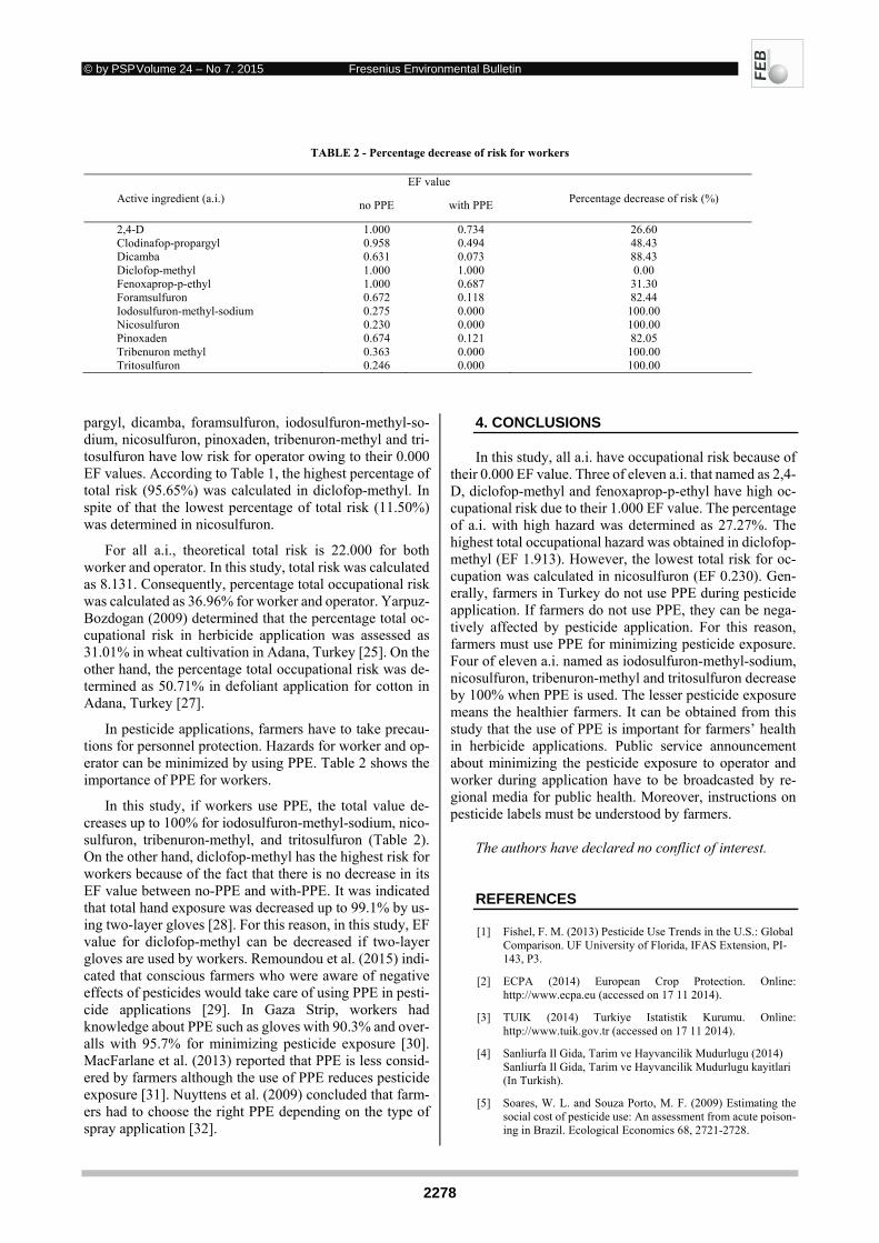
TABLE 2 - Percentage decrease of risk for workers
Active ingredient (a.i.)
EF value
Percentage decrease of risk (%) no PPE with PPE
2,4-D 1.000 0.734 26.60 Clodinafop-propargyl 0.958 0.494 48.43 Dicamba 0.631 0.073 88.43 Diclofop-methyl 1.000 1.000 0.00 Fenoxaprop-p-ethyl 1.000 0.687 31.30 Foramsulfuron 0.672 0.118 82.44 Iodosulfuron-methyl-sodium 0.275 0.000 100.00 Nicosulfuron 0.230 0.000 100.00 Pinoxaden 0.674 0.121 82.05 Tribenuron methyl 0.363 0.000 100.00 Tritosulfuron 0.246 0.000 100.00
pargyl, dicamba, foramsulfuron, iodosulfuron-methyl-so-dium, nicosulfuron, pinoxaden, tribenuron-methyl and tri-tosulfuron have low risk for operator owing to their 0.000 EF values. According to Table 1, the highest percentage of total risk (95.65%) was calculated in diclofop-methyl. In spite of that the lowest percentage of total risk (11.50%) was determined in nicosulfuron.
For all a.i., theoretical total risk is 22.000 for both worker and operator. In this study, total risk was calculated as 8.131. Consequently, percentage total occupational risk was calculated as 36.96% for worker and operator. Yarpuz-Bozdogan (2009) determined that the percentage total oc-cupational risk in herbicide application was assessed as 31.01% in wheat cultivation in Adana, Turkey [25]. On the other hand, the percentage total occupational risk was de-termined as 50.71% in defoliant application for cotton in Adana, Turkey [27].
In pesticide applications, farmers have to take precau-tions for personnel protection. Hazards for worker and op-erator can be minimized by using PPE. Table 2 shows the importance of PPE for workers.
In this study, if workers use PPE, the total value de-creases up to 100% for iodosulfuron-methyl-sodium, nico-sulfuron, tribenuron-methyl, and tritosulfuron (Table 2). On the other hand, diclofop-methyl has the highest risk for workers because of the fact that there is no decrease in its EF value between no-PPE and with-PPE. It was indicated that total hand exposure was decreased up to 99.1% by us-ing two-layer gloves [28]. For this reason, in this study, EF value for diclofop-methyl can be decreased if two-layer gloves are used by workers. Remoundou et al. (2015) indi-cated that conscious farmers who were aware of negative effects of pesticides would take care of using PPE in pesti-cide applications [29]. In Gaza Strip, workers had knowledge about PPE such as gloves with 90.3% and over-alls with 95.7% for minimizing pesticide exposure [30]. MacFarlane et al. (2013) reported that PPE is less consid-ered by farmers although the use of PPE reduces pesticide exposure [31]. Nuyttens et al. (2009) concluded that farm-ers had to choose the right PPE depending on the type of spray application [32].
4. CONCLUSIONS
In this study, all a.i. have occupational risk because of their 0.000 EF value. Three of eleven a.i. that named as 2,4-D, diclofop-methyl and fenoxaprop-p-ethyl have high oc-cupational risk due to their 1.000 EF value. The percentage of a.i. with high hazard was determined as 27.27%. The highest total occupational hazard was obtained in diclofop-methyl (EF 1.913). However, the lowest total risk for oc-cupation was calculated in nicosulfuron (EF 0.230). Gen-erally, farmers in Turkey do not use PPE during pesticide application. If farmers do not use PPE, they can be nega-tively affected by pesticide application. For this reason, farmers must use PPE for minimizing pesticide exposure. Four of eleven a.i. named as iodosulfuron-methyl-sodium, nicosulfuron, tribenuron-methyl and tritosulfuron decrease by 100% when PPE is used. The lesser pesticide exposure means the healthier farmers. It can be obtained from this study that the use of PPE is important for farmers’ health in herbicide applications. Public service announcement about minimizing the pesticide exposure to operator and worker during application have to be broadcasted by re-gional media for public health. Moreover, instructions on pesticide labels must be understood by farmers.
The authors have declared no conflict of interest. REFERENCES
[1] Fishel, F. M. (2013) Pesticide Use Trends in the U.S.: Global Comparison. UF University of Florida, IFAS Extension, PI-143, P3.
[2] ECPA (2014) European Crop Protection. Online: http://www.ecpa.eu (accessed on 17 11 2014).
[3] TUIK (2014) Turkiye Istatistik Kurumu. Online: http://www.tuik.gov.tr (accessed on 17 11 2014).
[4] Sanliurfa Il Gida, Tarim ve Hayvancilik Mudurlugu (2014) Sanliurfa Il Gida, Tarim ve Hayvancilik Mudurlugu kayitlari (In Turkish).
[5] Soares, W. L. and Souza Porto, M. F. (2009) Estimating the social cost of pesticide use: An assessment from acute poison-ing in Brazil. Ecological Economics 68, 2721-2728.
© by PSP Volume 24 – No 7. 2015 Fresenius Environmental Bulletin
2279
[6] Vercruysse, F., Drieghe, S., Steurbut, W. and Dejonckheere, W. (1999) Exposure assessment of professional pesticide users during treatment of potato fields. Pestic Sci 55, 467-473.
[7] Ucar, T. and Hall, F.R. (2001) Windbreaks as a pesticide drift mitigation strategy: a review. Pest Management Science 57, 663-675.
[8] Colosio, C., Fustinoni, S., Birindelli, S., Bonomi, I., De Pas-chale, G., Mammone, T., Tiramani, M., Vercelli, F., Visentin, S. and Maroni, M. (2002) Ethylenethiourea in urine as an in-dicator of exposure to mancozeb in vineyard workers. Toxi-cology Letters, 134, 133-140.
[9] Matthews, G.A. (2006) Pesticides: Health , Safety and the En-vironment. Blackwell Publishing, Oxford, UK, 235 p.
[10] Bozdogan, A.M. and Yarpuz-Bozdogan, N. (2008) Determi-nation of dermal bystander exposure of malathion for differ-ent application techniques. Fresenius Environmental Bulletin, 12a, 2103-2108.
[11] Bozdogan, A.M. and Yarpuz-Bozdogan, N. (2008) Assessment of buffer zones to ditches of dicofol for different applied doses and replication numbers in pesticide applications in Adana province, Turkey. Fresenius Environmental Bulletin, 3, 275-281.
[12] Yarpuz-Bozdogan, N. and Bozdogan, A. M. (2009) Compari-son of field and model percentage drift using different types of hydraulic nozzles in pesticide applications. Int. J. Environ. Sci. Tech. 2, 191-196.
[13] Yarpuz-Bozdogan, N. and Bozdogan, A.M. (2009) Assess-ment of different types of nozzles on dermal bystander expo-sure in pesticide applications. International Journal of Food, Agriculture & Environment 7, 678-682.
[14] Yarpuz-Bozdogan, N. (2011) Drift of Pesticide. Editor David Pimentel Encyclopedia of Pest Management, Taylor and Fran-cis, pp:1-4.
[15] Garreyn,F.; Vagenende,B. and Steurbaut,W. (2003) “Occupa-tional” Indicators - Operator, Worker and Bystander. Harmo-nised Environmental Indicators for Pesticide Risk, HAIR. 6th Framework Programme. SSPE-CT-2003-501997, 173 p.
[16] Claeys, S.; Vagenende, B.; De Smet, B.; Lelieur, L. and Steurbaut, W. (2005) The POCER indicator: a decision tool for non-agricultural pesticide use. Pest Management Science 61, 779–786.
[17] De Schamphelerie, M.; Spanoghe, P.; Brusselman, E. and Sonck, S. (2007) Risk assessment of pesticide spray drift dam-age in Belgium. Crop Protection 26, 602-611.
[18] Demircan, V. and Yılmaz, H. (2005) The Analysis of Pesticide Use in Apple Production in Isparta Province in terms of Econ-omy and Environmental Sensitivity Perspective. Ecoloji 14, 57: 15-25.
[19] Baldi, I., Lebailly, P., Bouver, G., Rondeau, V., Kientz-Bou-chart, V., Canal-Raffin, M. and Garrigou, A. (2014) Levels and determinants of pesticide exposure in re-entry workers in vineyards: Results of the PESTEXPO study. Environmental Research 132, 360-369.
[20] Yalap Tuna, R. (2011) Knowledge, attitude and practice of farmers about pesticides storage conditions, safe using man-ners. PhD Thesis, Erciyes University, Graduate School of Health Sciences, Department of Public Health. (In Turkish)
[21] Chemicalbook.com. (2014) Online: http://www.chemical-book.com. (accessed on 20/11/2014).
[22] Vercruysse,F. and Steurbaut,W. (2002) POCER, the pesticide occupational and environmental risk indicator. Crop Protec-tion 21, 307-315.
[23] Vergucht, S.; De Voghel, S.; Misson, C.; Vrancken, C.; Callebaut, K.; Steurbaut, W.; Pussemier, L.; Marot, J.; Maraite, H. and Vanhaecke, P. (2006) Health and environmen-tal effects of pesticide and type 18 biocides (HEEPEBI). Available online: http://www.crphyto.be/pdf/heepebi.pdf (ac-cessed on 11 11 2013).
[24] Bozdogan A.M. (2014) Assessment Of Total Risk On Non-Target Organisms In Fungicide Application For Agricultural Sustainability. Sustainability 6, 1046-1058.
[25] Yarpuz Bozdoğan N. (2009) Assessing the Environment and Human Health Risk of Herbicide Application in Wheat Culti-vation. International Journal of Food, Agriculture & Environ-ment 7, 775-781.
[26] Ribeiro, M. G., Colasso, C. G., Monteiro, P. P., Filho, W. R. P. and Yonamine, M. (2012) Occupational safety and health prac-tices among flower greenhouses workers from Alto Tiete region (Brazil). Science of the Total Environment 416, 121-126.
[27] Bozdogan, A.M. and Yarpuz-Bozdogan, N. (2009) Determi-nation of total risk of defoliant application in cotton on human health and environment. Journal of Food, Agriculture & Envi-ronment 1, 229-234.
[28] Gao, B.B.; Tao, C.J.; Ye, J.M.; Ning, J.; Mei, X.D.; Jiang, Z.F.; Chen, S. and She, D.M. (2014) Measurement of opera-tor exposure to chlorpyrifos. Pest. Manag. Sci. 70, 636-641.
[29] Remoundou, K., Brennan, M., Sacchettini, G., Panzone, L., Butler-Ellis, M. C., Capri, E., Charistou, A., Chaideftou, E., Gerritsen-Ebben, M. G., Machera, K., Spanoghe, P., Glass, R., March,s, A., Doanngoc, K., Hart, A. and Frewer, L. J. (2015) Perceptions of pesticide exposure risks by operators, workers, residents and bystanders in Greece, Italy and the UK. Science of the Total Environment 505, 1082-1092.
[30] Yassin, M.M.; Abu Mourad, T. A. and Safi, J.M. (2002) Knowledge, Attitude, Practice, and Toxicity Symptomps As-sociated with Pesticide Use Among Farm Workers in the Gaza Strip. Occup Environ Med 59, 387-394.
[31] MacFarlane E., Carey, R., Keegel, T., El-Zaemay, S. and Fritschi, L., (2013) Dermal exposure associated with occupa-tional end use of pesticides and the role of protective measures. Safety and Health at Work 4, 136-141.
[32] Nuyttens, D., Braekman, P., Windey, S. and Sonck, B., (2009) Potential dermal pesticide exposure affected by greenhouse spray application technique. Pest Manag Sci 63, 781-790.
Received: December 10, 2014 Revised: February 24, 2015 Accepted: March 06, 2015 CORRESPONDING AUTHOR
Assoc. Prof. Dr. Ali Musa BOZDOGAN Cukurova University Agriculture Faculty, Agricultural Machinery and Technologies Engineering Dept. 01330 Adana TURKEY Phone: +90 322 338 6408 Fax: +90 322 338 7165 E-mail: [email protected]
FEB/ Vol 24/ No 7/ 2015 – pages 2275 – 2279
© by PSP Volume 24 – No 7. 2015 Fresenius Environmental Bulletin
2280
SYNTHESIS AND CHARACTERIZATION OF ZnS NANOCRYSTALS
AND ITS PHOTOCATALYTIC ACTIVITY ON ANTIBIOTICS
Yuting Wu1, Liang Ni1,*, Xinlin Liu2, Mingjun Zhou1, Zhi Zhu1, Ziyang Lu3, Changchang Ma3 and Pengwei Huo1
1School of Chemistry & Chemical Engineering, Jiangsu University, Zhenjiang 212013, PR China 2School of Energy & Power Engineering, Jiangsu University, Zhenjiang 212013, PR China
3School of the Environment & Safety Engineering, Jiangsu University, Zhenjiang 212013, PR China
ABSTRACT
ZnS nanocrystals were synthesized via hydrothermal process and characterized by X-ray diffraction (XRD), Transmission electron microscope (TEM), Ultraviolet–vis-ible spectroscopy (UV-vis) and Fourier transform infrared spectrometer (FT-IR). The results indicated that the ob-tained ZnS nanocrystals are cubic sphalerite with little par-tical size and good dispersity. Under UV light irradiation and controlling the experimental conditions, the photocata-lytic activity of ZnS nanocrystals was evaluated by degra-dation of tetracycline (TC). Various factors have been com-pared through a series of experiments, and the optimal reac-tion condition has been found out. Additionally, the photo-catalytic activity of recycled ZnS decreased with the in-creasing runs of recycling. Finally, the photocatalytic reac-tion mechanism of ZnS nanocrystals was proposed and the photocatalytic degradation pathway of TC was analysed. Overall, the ZnS photocatalysis was found to be a promis-ing process for removing TC from wastewater.
KEYWORDS: ZnS nanocrystals; synthesis and characterization; tetracycline; photocatalytic degradation
1. INTRODUCTION
Semiconductor nanocrystals are usually composed of group II–VI or III–V elements, also termed as quantum dots (QDs) [1]. Because they often consist of a little number of atoms, their particle size is very small (less than 100 nm in three dimensions, an average of about 2~10nm). The characteristic optical properties of nanocrystals include in-tense fluorescence, broad excitation, narrow emission and resistance to photobleaching [2]. In the past several dec-ades, nanocrystals have received substantial attention due to their outstanding optical properties and biological appli-cations [3]. More recently, there have been intense con-cerns on CdE (E = S, Se, Te) nanocrystals [4-9]. How-
* Corresponding author
ever, these types of nanocrystals are made from heavy metal ions (e.g., Cd(2+)), which may result in potential bio-logical and environmental toxicity, and this drawback seri-ously hampers their practical applications [10]. ZnS nano-crystals are one of the most important II–VI semiconductor materials which attracted tremendous attention because of their outstanding properties: wide band gap energy [11], low level of harm, stability, moderate price and easily ac-cessibility. Moreover, its quantum size effect also shows many specific photoelectric properties [12, 13].
Techniques for preparing ZnS nanocrystals are various, such as precipitation method [14], electrodeposition method [15], ultrasonic-assisted method [16], microwave-assisted method [17] and hydrothermal method [18]. Among these methods, hydrothermal method has the advantages of sim-ple operation, high production purity, and obtained materi-als possess small crystal size, narrow size distribution, good crystallinity and high photoluminescence intensity [12, 18, 19]. Recently, more and more different nanocrys-tals have been prepared via hydrothermal method [20-24].
Antibiotics, also known as antibacterials, are types of medications that are used for treating infections caused by bacteria [25]. However, not only the extensive use of anti-biotics has led to worldwide environmental pollution, but also the development of multi-resistant bacterial strains can no longer be treated by the presently known drugs [26]. Tet-racycline (TC), in virtue of its moderate price, represents a major proportion of the antibiotics in use currently [27], par-ticularly in the field of medicines, aquaculture and veteri-nary medicines [28]. Recently, due to its poor absorption by organisms, a significant amount of TC has been detected in natural environment, causing growing concerns about its potential impact to the ecosystem [29].
In the present work, ZnS nanocrystals were prepared via hydrothermal synthesis method and characterized by X-ray diffraction (XRD), Transmission electron micro-scope (TEM), Ultraviolet–visible spectroscopy (UV-vis) and Fourier transform infrared spectrometer (FT-IR). The photodegradative effect of TC under UV light irradiation was investigated by using ZnS as the photocatalyst, and the effects of solution pH, TC concentration and ZnS dosage
© by PSP Volume 24 – No 7. 2015 Fresenius Environmental Bulletin
2281
were evaluated to determine the optimal reaction condi-tion. After that, the activity of the recycled catalyst was as-sessed. And finally, the photocatalytic reaction mechanism of ZnS nanocrystals was proposed and the photodegrada-tive process of TC was analysed.
In summary, we have found a much more simple and low-cost process to synthesize ZnS nanocrystals. More im-portantly, the as-prepared ZnS exhibited higher photodeg-radative rate to TC, and showed promising prospect for the treatment of TC in future industrial application.
2. MATERIALS AND METHODS
2.1 Materials
The materials used included Zn(CH3COO)2·2H2O and Na2S·9H2O. They were purchased from Sinopharm Chem-ical Rengent Co. Ltd. Tetracycline, oxytetracycline hydro-chloride, ciprofloxacin and danofloxacin mesylate were obtained from Shanghai Shunbo Biological Engineering Co. Ltd.. All chemicals were used as received without any further purification and doubly deionized water was used throughout the experiments.
2.2 Preparation of ZnS nanocatalysts
Weighed 2.6341g Zn(CH3COO)2•2H2O (0.012mol) and 2.8800g Na2S•9H2O (0.012mol) were added separately to 40 mL deionized water in the beakers. These two solutions were mixed and stirred for 30min with continuous nitrogen bubbling at room temperature. Then, the mixtures were transferred to a 100 mL Teflon-lined stainless steel auto-clave, followed by putting them in an electroheat blasting baking oven with 150 °C for 10 h. After that, the products were cooled to ambient temperature naturally, and the solu-tions were centrifuged at 1000 rpm for 3 min to harvest ZnS precipitate. Then the precipitates were washed with deion-ized water and ethanol several times and dried in a vacuum evaporator at 60 ◦C for 48 h to obtain ZnS nanocrystals.
2.3 ZnS structural Characterization
The XRD pattern was obtained by a MO3XHF22 X-ray diffractometer (MAC Science, Japan) equipped with Ni-fil-trated Cu Kα radiation (40 kV, 30 mA). The 2θ scanning an-gle range was 10–80◦ at a scanning rate of 10◦ min−1. The morphology and size of ZnS photocatalyst was studied by TEM (JEOL IEM-200CX) microscope. UV–vis absorption spectrum was obtained by dry-pressed disk samples using Specord 2450 spectrometer (Shimazu, Japan), and adopted BaSO4 was used as the reflectance sample. Fourier trans-form infrared (FT-IR) spectrum was recorded by a Nicolet Nexus 470 FT-IR (America thermo-electricity Company) with 2 cm−1 resolution in the range of 500–4000 cm−1, pellet was prepared by mixing nanoparticles with KBr powder.
2.4 Antibiotics photodegradative experiment
150 mL antibiotics solution was injected to quartz re-actor (total volume of 200 mL) by a 100mL syringe. The
pH adjusted by NaOH was determined by a microprocessor pH meter (Leichi Instruments, Shanghai, China), and pho-todegradative experiments were carried out in a GHX-2 photochemical reactor with a 500 W ultraviolet lamp. To determine the initial absorbency, all samples were stirred for 30 min in dark to ensure the adsorption equilibrium. Then the ultraviolet lamp was turned on, and we main-tained the reactive temperature below 298 K by a flow of cooling water. The whole photodegradative process con-tinued for 1 h and was conducted in 10 min interval. After that, all samples were centrifuged at 1000 rpm for 3 min and their supernatant’s UV–vis adsorption spectrum was recorded by an UV–vis spectrophotometer. The adsorption detections were performed at 356nm (tetracycline), 356nm (oxytetracycline hydrochloride), 275nm (ciprofloxacin) and 190nm (danofloxacin mesylate). The degradation rate was expressed as DR=(A0-A)/A0, where A0 and A are the absorbance of antibiotics before and after photodegrada-tive reaction.
3. RESULTS AND DISCUSSION
3.1 ZnS structural characterization
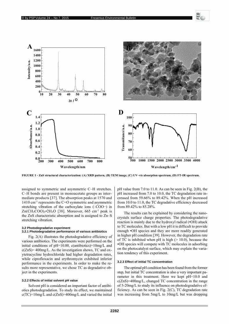
X-ray powder diffraction pattern of the synthesized ZnS nanocrystals is illustrated in Fig.1 (A). All peaks can be well indexed to the cubic sphalerite phase of ZnS (JCPDS No. 05-0566) [30-32]. There are three characteristic diffraction peaks at 2θ = 28.59°, 47.78°, and 56.74°, corresponding to the (111), (220) and (311) crystal plane of pure ZnS, re-spectively.
To further characterize ZnS nanostructures, TEM anal-ysis was carried out. The typical TEM image of ZnS nano-crystals is shown in Fig. 1(B) and the inset figure repre-sents its corresponding particle size distribution. Fig. 1(B) exhibits that the obtained ZnS was approximately spherical and homogeneous. Some of the particles were agglomer-ates. From the particle size distribution statistics, it can be seen that ZnS size distribution was in the range of about 2.5–32.5 nm, and their mean diameter was 14.55 nm with a standard deviation of 5.37.
UV–vis absorption spectrum is presented in Fig. 1(C). It is similar to the image described in previous articles [33, 34]. It is obvious that the absorption spectrum was very broad and featureless in the whole region. The band gap of materials can be estimated via the formula: Eg = 1240/λ, which Eg represents band gap energy and λ is the wave-length of the absorption edge [35]. As the spectrum shows, the absorption edge wavelength of pure ZnS nanoparticles was about 380 nm, corresponding to a bandgap of 3.26 eV.
At last, ZnS FT-IR spectrum is presented in Fig. 1(D). As can be seen from the Fig. 1(D), peaks at 3420 and 1090 cm-1 are corresponding to the O-H bond vibrations adsorbed of -OH groups, which belong to the adsorbent H2O on the ZnS surface [36]. This phenomenon indicates that Zn2+ ions have strong bonding effect with H2O molecular on ZnS sur-face. The weak peaks located at 2900 and 2970 cm−1 are
© by PSP Volume 24 – No 7. 2015 Fresenius Environmental Bulletin
2282
10 20 30 40 50 60 70 800
200
400
600
800
1000
1200
1400
1600
Inte
nsi
ty/a
.u.
2/ O
A
200 300 400 500 600 700 8000.0
0.2
0.4
0.6
0.8
1.0
1.2
1.4
Ab
sorb
ance
/a.u
.
Wavelength/nm
C
500 1000 1500 2000 2500 3000 3500 400050
60
70
80
90
100
Tra
nsm
itan
ce/a
.u.
Wavelength/cm-1
D
FIGURE 1 - ZnS structural characterization: (A) XRD pattern, (B) TEM image, (C) UV–vis absorption spectrum, (D) FT-IR spectrum.
assigned to symmetric and asymmetric C–H stretches. C–H bonds are present in monoacetate groups as inter-mediate products [37]. The absorption peaks at 1570 and 1410 cm-1 represents the C=O symmetric and asymmetric stretching vibration of the carboxylate ions (–COO−) in Zn(CH3COO)2•2H2O [38]. Moreover, 665 cm-1 peak is the ZnS characteristic absorption and is assigned to Zn–S stretching vibration.
3.2 Photodegradative experiment 3.2.1 Photodegradative performance of various antibiotics
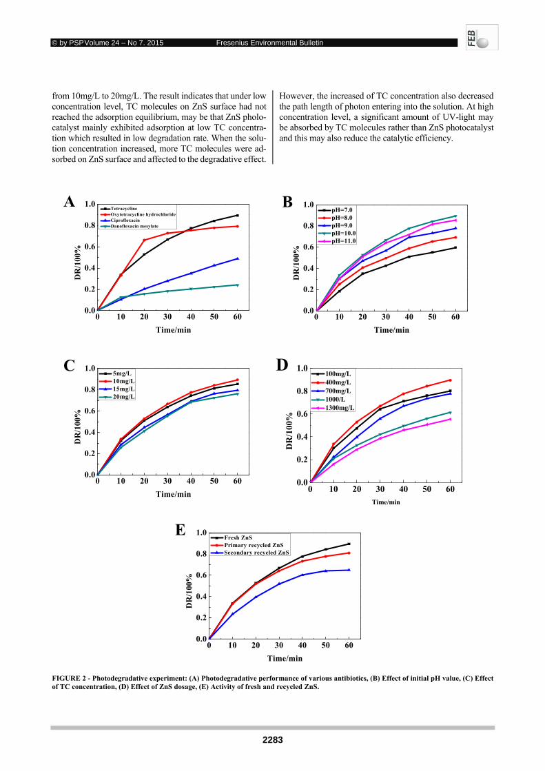
Fig. 2(A) illustrates the photodegradative efficiency of various antibiotics. The experiments were performed on the initial conditions of pH=10.00, c(antibiotics)=10mg/L and c(ZnS)= 400mg/L. As the investigation shows, TC and ox-ytetracycline hydrochloride had higher degradation rates, while ciprofloxacin and erythromycin exhibited inferior performance in the experiments. In order to make the re-sults more representative, we chose TC as degradative ob-ject in the experiments.
3.2.2 Effects of initial solvent pH value
Solvent pH is considered an important factor of antibi-otics photodegradation. To study its effect, we maintained c(TC)=10mg/L and c(ZnS)=400mg/L and varied the initial
pH value from 7.0 to 11.0. As can be seen in Fig. 2(B), the pH increased from 7.0 to 10.0, the TC degradation rate in-creased from 59.66% to 89.42%. When the pH increased from 10.0 to 11.0, the TC degradative efficiency decreased from 89.42% to 85.28%.
The results can be explained by considering the nano-crystals surface charge properties. The photodegradative reaction is mainly due to the hydroxyl radical (•OH) attack to TC molecules. But with a low pH it is difficult to provide enough •OH species and they are more readily generated in higher pH condition [39]. However, the degradation rate of TC is inhibited when pH is high (> 10.0), because the •OH species will compete with TC molecules in adsorbing on the photocatalyst surface, which may explain the varia-tion tendency of this experiment.
3.2.3 Effect of initial TC concentration
The optimal pH condition has been found from the former step, but initial TC concentration is also a very important pa- rameter in this treatment. Here we kept pH=10.0 and c(ZnS)=400mg/L, changed TC concentration in the range of 5-20mg/L to study its influence on photodegradative ef-ficiency. As can be seen in Fig. 2(C), TC degradation rate was increasing from 5mg/L to 10mg/L but was dropping
© by PSP Volume 24 – No 7. 2015 Fresenius Environmental Bulletin
2283
from 10mg/L to 20mg/L. The result indicates that under low concentration level, TC molecules on ZnS surface had not reached the adsorption equilibrium, may be that ZnS pholo-catalyst mainly exhibited adsorption at low TC concentra-tion which resulted in low degradation rate. When the solu-tion concentration increased, more TC molecules were ad-sorbed on ZnS surface and affected to the degradative effect.
However, the increased of TC concentration also decreased the path length of photon entering into the solution. At high concentration level, a significant amount of UV-light may be absorbed by TC molecules rather than ZnS photocatalyst and this may also reduce the catalytic efficiency.
0 10 20 30 40 50 600.0
0.2
0.4
0.6
0.8
1.0
DR
/100
%
Time/min
Tetracycline Oxytetracycline hydrochloride Ciprofloxacin Danofloxacin mesylate
A
0 10 20 30 40 50 600.0
0.2
0.4
0.6
0.8
1.0
DR
/100
%
Time/min
pH=7.0 pH=8.0 pH=9.0 pH=10.0 pH=11.0
B
0 10 20 30 40 50 600.0
0.2
0.4
0.6
0.8
1.0
DR
/100
%
Time/min
5mg/L 10mg/L 15mg/L 20mg/L
C
0 10 20 30 40 50 600.0
0.2
0.4
0.6
0.8
1.0
DR
/100
%
Time/min
100mg/L 400mg/L 700mg/L 1000/L 1300mg/L
D
0 10 20 30 40 50 600.0
0.2
0.4
0.6
0.8
1.0
DR
/100
%
Time/min
Fresh ZnS Primary recycled ZnS Secondary recycled ZnS
E
FIGURE 2 - Photodegradative experiment: (A) Photodegradative performance of various antibiotics, (B) Effect of initial pH value, (C) Effect of TC concentration, (D) Effect of ZnS dosage, (E) Activity of fresh and recycled ZnS.
© by PSP Volume 24 – No 7. 2015 Fresenius Environmental Bulletin
2284
3.2.4 Effect of ZnS pholocatalyst dosage
For economic removal of TC effluent from wastewater, it is necessary to find out the optimal amount of photocata-lyst. In this section, we first ensured the initial pH=10.0, and ZnS dosage was varied from 100 to 1300mg/L in the 10mg/L TC solution. As presented in Fig. 2(D), with in-creased ZnS amont from 100 to 400mg/L, TC degradation rate improved from 80.24% to 89.42%. However, while ZnS amount exceeded 400mg/L, TC degradation rate dropped from 89.42% to 55.25%. As can be seen from the result, at low ZnS concentration, the number of available adsorption and catalytic sites increased with increasing ZnS dosage. After optimal level, high turbidity of solution system and penetration of UV light decreased thereby enhanced scat-tering effect and lowed the photodegradation rate.
3.2.5 Activity of recycled ZnS
In practice, in order to reduce the cost of treatment and maintaining the continuity of production, people must assess the stability of photocatalyst. In the present study, we pre-served the reaction conditions of pH = 10.00, c(TC)=10mg/L and c(ZnS)= 400mg/L, repeated the exper-iment and recycled the ZnS. As the results of Fig. 2(E) sug-gested, photocatalytic activity of primary recycled ZnS has decreased to a certain extent. Furthermore, the efficiency of secondary recycled ZnS was unsatisfactory. The deacti-vation of photocatalyst is caused by the degraded substance and other impurities has been adsorbed on ZnS surface and also affected to its adsorption properties.
3.3. Photodegradation mechanisms analysis
3.3.1 Photocatalytic reaction mechanism of ZnS nanocrystals
ZnS nanocrystals were irradiated by the light whose photon energy was larger or equal to its bandgap energy, the electrons in valence band can be excited into conduc-tion band, leading to the formation of positively charged photogenerated holes(h+) in valence band, and negatively charged photogenerated electron (e-) in conduction band:
ZnS+hv→ZnS (e-,h+) (1)
At this moment, photogenerated holes and electrons have two evolve possibilities. In one case, the absorbed light energy will release as heat or photons and emitting fluorescence, all these situations can not use the absorbed light energy. In another case, the strong oxidizing photo-generated holes will react with H2O moleculars to generate hydroxyl radicals(•OH), and the strong reducing photogen-erated electrons will react with dissolved oxygen to pro-duce oxyradicals(•O2
−). Eventually, the oxyradicals will also translate into hydroxyl radicals. These reactions will separate photogenerated holes and electrons and transfer absorbed light energy into chemical energy. The possible reactions are listed as follows:
h+ + H2O→•OH + H+ (2)
h+ +OH−→•OH (3)
e−+O2→•O2− (4)
•O2−+H+→HO2• (5)
2HO2•→O2+H2O2 (6)
© by PSP Volume 24 – No 7. 2015 Fresenius Environmental Bulletin
2285
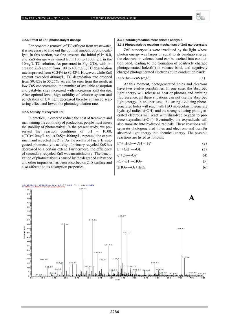
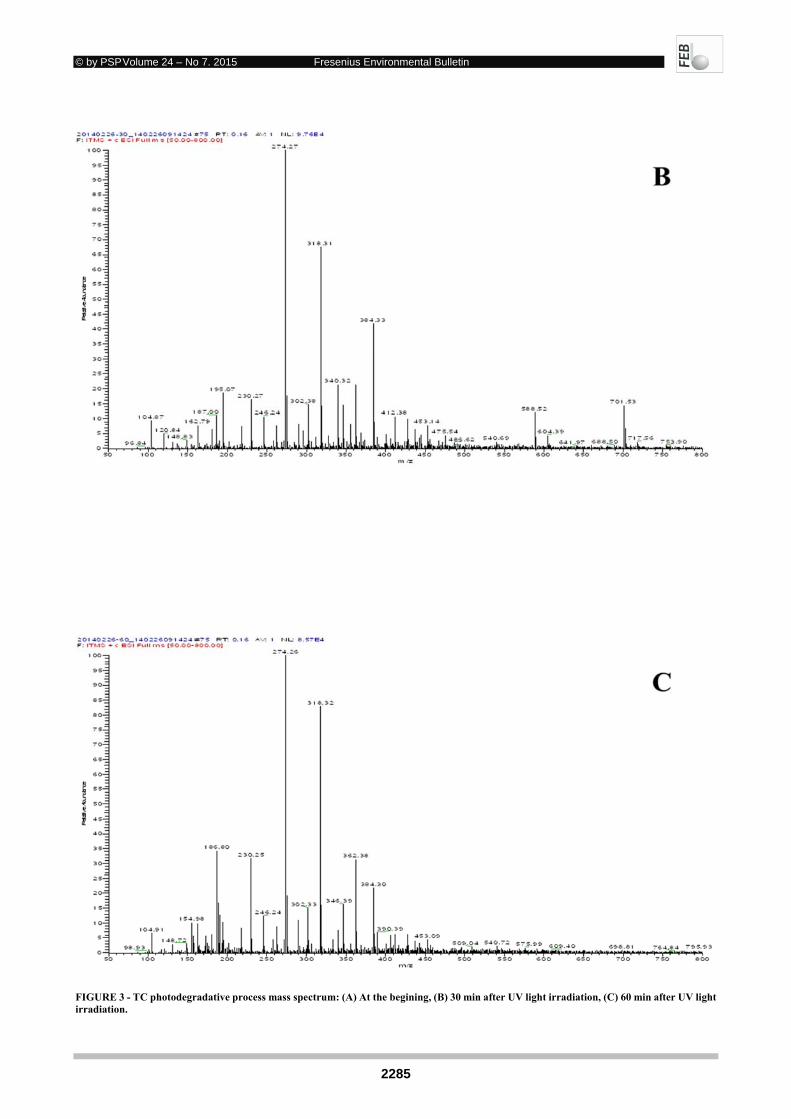
FIGURE 3 - TC photodegradative process mass spectrum: (A) At the begining, (B) 30 min after UV light irradiation, (C) 60 min after UV light irradiation.

© by PSP Volume 24 – No 7. 2015 Fresenius Environmental Bulletin
2286
OH OH
OH
NH2
OH
N(CH3)2
OH
O O
HO CH3
·OH
OH
+ NH2
OH
OH
N(CH3)2
·OH
OH
NH2
OH
OH
N(CH3)2
+
OH
NH2
OH
N(CH3)2
OH OHOH
O
+
-C2H5OH
OH
OH
OH
OH OH OH
OH
HO CH3
NH2
OH
OH
N(CH3)2
NH2
N(CH3)2
·OH-CH3OH
NH2
NHCH3
·OH-CH3OH
NH2
NH2
·OH-CH3OH
-H2O
O
O
OH OH
·OH-C2H5OH
-H2O
OH
·OH
OH
·OH
OH
-C2H5OH
m/z=445.37
m/z=120.84 m/z=318.31 m/z=162.79 m/z=274.27
m/z=162.79
m/z=120.84
m/z=96.84
m/z=96.84 m/z=148.83
m/z=246.24
m/z=186.80
m/z=162.79
m/z=130.92
m/z=112.17
m/z=98.93
FIGURE 4 - Photodegradative pathway of TC

© by PSP Volume 24 – No 7. 2015 Fresenius Environmental Bulletin
2287
H2O2+•O2−→•OH + OH−+ O2 (7)
•O2− +H2O + H+→ H2O2 +OH− (8)
H2O2+e−→•OH+ OH− (9) 3.3.2 Photodegradative process of TC
In order to ensure the TC degradative pathways, the in-termediates and final products were determined by mass spectrometry, the results taken at the beginning, 30 and 60 min after UV light irradiation are shown in Fig. 3(A)~(C). Through the analysis, in the early stage of photodegradative process, by the attacked of hydroxyl radicals, carbon–carbon single bonds at A and C ring of TC were first broken, then the m/z=274.27 and m/z=162.79 or m/z=318.31 and m/z= 120.84 substance were formed. With the increased of deg-radation time, these intermediates were further splintering into small fragments. Eventually, TC was degraded thor-oughly and the remains were H2O, methanol, ethanol, phe-nol, amine and some other small molecules. This process is presented Fig.4.
4. CONCLUSIONS
In this research, ZnS nanocrystals was prepared by hy-drothermal method. The obtained ZnS was cubic sphalerite phase crystal, and its shape was approximately spherical. Then the optimal photodegradative conditions was dis-cussed, while pH = 10.00, c(TC)=10mg/L and c(ZnS)= 400mg/L, ZnS nanocrystals exhibited highest photocata-lytic activity, nearly 90% of TC was removed within 60 min. According to the photocatalyst recycled experiment, the photocatalytic activity of recycled ZnS was obviously declined. At last, the photocatalytic reaction mechanism of ZnS nanocrystals for TC was discussed, the degradative process of TC was analysed and its pathways were pro-posed. By the attacked of hydroxyl radicals, TC was de-composed to H2O, methanol, ethanol, phenol, amine and some other small molecules. Generally, this research im-plied a promising application of photodegrading TC in wastewater treatment.
ACKNOWLEDGMENTS
We gratefully acknowledge the financial support of the National Natural Science Foundation of China (No. 21207053, 21407064), the Natural Science Founda-tion of Jiangsu Province (BK20131259, BK20130489, BK20140532).
The authors have declared no conflict of interest.
REFERENCES
[1] Saran, A.D. and Bellare, J.R. (2010) Green engineering for large-scale synthesis of water-soluble and bio-taggable CdSe and CdSe–CdS quantum dots from microemulsion by double-capping. Colloids and Surfaces A: Physicochemical and Engi-neering Aspects 369, 165–175.
[2] Weilnau, J.N., Black, S.E., Chehata, V.J., Schmidt, M.P., Holt, K.L., Carl, L.M., Straka, C.J., Marsh, A.L., Patton, W.A. and Lappas, C.M. (2013) ZnS nanocrystal cytotoxicity is influenced by capping agent chemical structure and duration of time in sus-pension. Journal of Applied Toxicology 33, 227–237.
[3] Yin, N.Q., Liu, L., Lei, J.M., Liu, Y.S., Gong, M.G., Wu, Y.Z., Zhu, L.X. and Xu X.L. (2012) Preparation and characteriza-tion of nontoxic magnetic-luminescent nanoprobe. Chinese Physics B 21, 116101.
[4] Akshya, S., Hariharan, P.S., Vinod Kumar, V. and Anthony S.P. (2015) Surface functionalized fluorescent CdS QDs: Se-lective fluorescence switching and quenching by Cu2+ and Hg2+ at wide pH range. Spectrochimica Acta Part A: Molecu-lar and Biomolecular Spectroscopy 135, 335–341.
[5] Maji, S.K., Dutta, A.K., Dutta, S., Srivastava, D.N., Paul P., Mondal, A. and Adhikary, B. (2012) Single-source precursor approach for the preparation of CdS nanoparticles and their photocatalytic and intrinsic peroxidase like activity. Applied Catalysis B: Environmental 126, 265-274.
[6] Kaur, G. and Tripathi S.K. (2015) Investigation of trypsin–CdSe quantum dot interactions via spectroscopic methods and effects on enzymatic activity. Spectrochimica Acta Part A: Molecular and Biomolecular Spectroscopy 134, 173–183.
[7] Ullah, K., Jo, S.B. and Ye, S. (2015) Degradation of Organic Dyes by CdSe Decorated Graphene Nanocomposite in Dark Ambiance. Fullerenes, Nanotubesa and Carbon Nanostruc-tures 23, 437-448.
[8] Song, H.L., Yang, M., Fan, X.X. and Wang, H.Y. (2014) Turn-on electrochemiluminescence sensing of Cd2+ based on CdTe quantum dots. Spectrochimica Acta Part A: Molecular and Bi-omolecular Spectroscopy 133, 130–133.
[9] Mobedi, N., Marandi, M. and Zare Bidaki, H. (2014) Effect of hydrazine hydrate on the luminescence properties of MPA capped CdTe nanocrystals in hot injection method. Journal of Luminescence156, 235–239.
[10] Chen, N., He, Y., Su, Y.Y., Li, X.M., Huang, Q., Wang, H.F., Zhang, X.Z., Tai, R.Z. and Fan, C.H. (2012) The cytotoxicity of cadmium-based quantum dots. Biomaterials 33, 1238-1244.
[11] Pal, S., Sharma, R., Goswami, B. and Sarkar, P. (2009) Theo-retical prediction of ring structures for ZnS quantum dots. Chemical Physics Letters 467, 365–368.
[12] Liu, C.X., Ji, Y.Y. and Tan T.W. (2013) One-pot hydrothermal synthesis of water-dispersible ZnS quantum dots modified with mercaptoacetic acid. Journal of Alloys and Compounds 570, 23–27.
[13] Shahid, R., Toprak M.S. and Muhammed, M. (2012) Micro-wave-assisted low temperature synthesis of wurtzite ZnS quantum dots. Journal of Solid State Chemistry 187, 130–133.
[14] Kho, R., Torres-Mart´ınez, C.L. and Mehra, R.K. (2000) A Simple Colloidal Synthesis for Gram-Quantity Production of Water-Soluble ZnS Nanocrystal Powders. Journal of Colloid and Interface Science 227, 561–566.
[15] Monika, Kumar, R. and Chauhan, R. P. (2015) Preparation and field emission study of low-dimensional ZnS arrays and tu-bules. Journal of Experimental Nanoscience 10, 126-134.

© by PSP Volume 24 – No 7. 2015 Fresenius Environmental Bulletin
2288
[16] Behboudnia, M., Habibi-Yangjeh, A. and Jafari-Tarzanag, Y. (2008) Preparation and characterization of monodispersed nanocrystalline ZnS in water-rich [EMIM]EtSO4 ionic liquid using ultrasonic irradiation. Journal of Crystal Growth 310, 4544-4548.
[17] La Porta, F.A., Ferrer, M.M., Santana, Y.V.B., Raubach, C.W., Longo, V.M., Sambrano, J.R., Longo, E., Andrés, J., Li, M. and Varela, J.A. (2013) Synthesis of wurtzite ZnS nanopar-ticles using the microwave assisted solvothermal method. Journal of Alloys and Compounds 556, 153–159.
[18] Nirmala Jothi, N.S., Joshi, A.G., Jerald Vijay, R., Muthuvina-yagam, A. and Sagayaraj, P. (2013) Investigation on one-pot hy-drothermal synthesis, structural and optical properties of ZnS quantum dots. Materials Chemistry and Physics 138, 186-191.
[19] Liu, L.Q., Li, Y.F., Zhan, L., Liu, Y. and Huang, C.Z. (2011) One-step synthesis of fluorescent hydroxyls-coated carbon dots with hydrothermal reaction and its application to optical sensing of metal ions. Science China Chemistry 54, 1342-1347.
[20] Hernández-Adame.L., Méndez-Blas, A., Ruiz-García, J., Vega-Acosta, J.R., Medellín-Rodríguez, F.J. and Palestino, G. (2014) Synthesis, characterization, and photoluminescence properties of Gd:Tb oxysulfide colloidal particles. Chemical Engineering Journal 258, 136–145.
[21] Cao, C.Y., Luo, Z.Y., Guo, S.L., Cao, R.P., Noh, H.M., Jeong, J.H. and Xie, A. (2014) Synthesis, optical properties, and en-ergy transfer of Ce3+/Tb3+ co-doped MyGdFx (M = Li, Na, K). Spectrochimica Acta Part A: Molecular and Biomolecular Spectroscopy 133, 457–462.
[22] Xu, C.J., Wang, Y.J., Chen, H.Y., Nie, D. and Liu Y.Q. (2014) Hydrothermal synthesis of silver crystals via a sodium chlo-ride assisted route. Materials Letters 136, 175–178.
[23] Sakoda, K. and Hirano, M. (2014) Formation of complete solid solutions, Zn(AlxGa1-x)2O4 spinel nanocrystals via hydrother-mal route. Ceramics International 40, 15841–15848.
[24] Zhu, X.H., Zuo, X.X., Hu, R.P., Xiao, X., Liang, Y. and Nan J.M. (2014) Hydrothermal synthesis of two photoluminescent nitrogen-doped graphene quantum dots emitted green and khaki luminescence. Materials Chemistry and Physics 147, 963-967.
[25] Karpecki, P., Paterno, M.R. and Comstock, T.L. (2010) Limi-tations of current antibiotics for the treatment of bacterial con-junctivitis.Optometry and Vision Science 87, 908-919.
[26] Zhu, X.D., Wang, Y.J., Sun, R.J. and Zhou, D.M. (2013) Pho-tocatalytic degradation of tetracycline in aqueous solution by nanosized TiO2 .Chemosphere 92, 925–932.
[27] Maroga Mboula, V., Héquet, V., Gru, Y., Colin, R. and An-drès, Y. (2012) Assessment of the efficiency of photocatalysis on tetracycline biodegradation. Journal of Hazardous Materi-als 209– 210, 355– 364.
[28] Niu, J.F., Ding, S.Y., Zhang, L.W., Zhao, J.B. and Feng, C.H. (2013) Visible-light-mediated Sr-Bi2O3 photocatalysis of tet-racycline: Kinetics, mechanisms and toxicity assessment. Chemosphere 93, 1–8.
[29] Fatiha, F.S., Florence, F., Isabelle, S., Hamid, A.A., Hayet, D and Abdeltif, A. (2013) Tetracycline degradation and mineral-ization by the coupling of an electro-Fenton pretreatment and a biological process. Journal of Chemical Technology and Bi-otechnology 88, 1380-1386.
[30] Huang, Q.S., Dong, D.Q., Xu, J.P., Zhang, X.S., Zhang, H.M. and Li, L. (2010) White Emitting ZnS Nanocrystals: Synthesis and Spectrum Characterization. Chinese Physics Letters 27, 057306.
[31] Wang, L.P. and Hong, G.Y. (2000) A new preparation of zinc sulfide nanoparticles by solid-state method at low temperature. Materials Research Bulletin 35, 695–701.
[32] Wang, L., Tao, X.T., Yang, J.X., Ren, Y., Liu, Z. and Jiang, M.H. (2006) Preparation and characterization of the ZnS nan-ospheres with narrow size distribution. Optical Materials 28, 1080–1083.
[33] Shi, Y.H., Chen, J. and Shen, P.W. (2007) ZnS micro-spheres and flowers: Chemically controlled synthesis and template use in fabricating MS(shell)/ZnS(core) and MS(M = Pb, Cu) hol-low microspheres. Journal of Alloys and Compounds 441, 337–343.
[34] Maryam, S.A. and Masoud, S.N. (2014) Synthesis and charac-terization of wurtzite ZnS nanoplates through simple sol-vothermal method with a novel approach. Journal of Industrial and Engineering Chemistry 20, 3179–3185.
[35] Xing, W.N., Ni, L., Huo, P.W., Lu, Z.Y., Liu, X.L., Luo, Y.Y. and Yan, Y.S. (2012) Preparation high photocatalytic activity of CdS/halloysite nanotubes (HNTs) nanocomposites with hy-drothermal method. Applied Surface Science 259, 698– 704.
[36] Maged, E.K. and Hany, E.S. (2009) Fluorescence modulation and photodegradation characteristics of safranin O dye in the presence of ZnS nanoparticles. Journal of Photochemistry and Photobiology A: Chemistry 205, 151–155.
[37] Perez, R.C., Sandoval, O.J. , Mann, J.M. , Galvan, A.M. and Delgado, G.T. (1999) Influence of annealing temperature on the formation and characteristics of sol-gel prepared ZnO films. Journal of Vacuum Science and Technology A: Vac-uum, Surfaces and Films17, 1811–1816.
[38] Zhao, J.J., Zhao, L. and Wang, X.P. (2008) Preparation and characterization of ZnO/ZnS hybrid photocatalysts via micro-wave-hydrothermal method. Frontiers of Environmental Sci-ence & Engineering in China 2, 415–420.
[39] Chow, K.L., Man, Y.B., Zheng, J.S., Liang, Y., Tam, F.Y. and Wong, M.H. (2012) Characterizing the optimal operation of photocatalytic degradation of BDE-209 by nano-sized TiO2.Journal of Environmental Sciences 24(9), 1670–1678.
Received: August 31, 2014 Revised: January 12, 2015 Accepted: February 13, 2015 CORRESPONDING AUTHOR
Liang Ni School of Chemistry & Chemical Engineering Jiangsu University Zhenjiang 212013 P.R. CHINA Phone: +86 511 8878 2621 Fax: +86 511 8879 1800 E-mail: [email protected], [email protected]
FEB/ Vol 24/ No 7/ 2015 – pages 2280 - 2288
© by PSP Volume 24 – No 7. 2015 Fresenius Environmental Bulletin
2289
EVALUATION OF PARTICLE SIZE AND
INITIAL CONCENTRATION OF TOTAL SOLIDS ON
BIOHYDROGEN PRODUCTION FROM FOOD WASTE
Iván Moreno-Andrade* and Germán Buitrón
Laboratory for Research on Advanced Processes for Water Treatment, Unidad Académica Juriquilla, Instituto de Ingeniería, Universidad Nacional Autónoma de México, Blvd. Juriquilla 3001, 76230 Querétaro, México.
ABSTRACT
The influence of different parameters including parti-cle size and initial total solids on the biohydrogen produc-tion from food waste was studied. The results demonstrated that the initial particle size and the concentration of initial total solids (TS0) have a positive effect on hydrogen (H2) production. Results showed that if no pH adjustment (buffer) or particle size selection is applied, the maximal volumetric hydrogen production (2.2 LH2 kg-1 of the initial total solids added) was obtained at 90 gTS0 L-1. However, the maximal total solids and chemical oxygen demand re-moval percentages were obtained at 10 gTS0 L-1. For parti-cles larger than 2 mm, the H2 production increases as the TS0 increase. In the case of particle sizes between 0.5 and 2.0 mm, and smaller than 0.5 mm, the higher H2 production was reached at 50 gTS0 L-1 and 15 gTS0 L-1, respectively. Larger particles size required more time to produce the same amount of hydrogen. The maximum hydrogen pro-duction rate per initial total solids was obtained with the smallest particle size by applying 15 gTS0 L-1. The princi-pal volatile fatty acids generated were acetic and butyric acids. The values of acetic acid were similar when TS0 ap-plied between 5 to 20 g L-1 for each different particle size. Higher concentration of TS0 than 30 g L-1 results in a fast increase of acetic acid production.
KEYWORDS: biohydrogen; initial total solids; organic solid waste; particle size; restaurant waste.
1. INTRODUCTION
The application of the hydrolytic-acidogenic stage of the anaerobic digestion process is an appropriate alterna-tive to produce hydrogen (H2) and to obtain an effluent rich in volatile fatty acids, (VFA), mainly acetic, propionic and butyric acid, lactate and solvents (acetone and ethanol).
* Corresponding author
The H2 production yields are closely related to the fermen-tation pathway and end-products [1,2]. The main biochem-ical reactions for H2 production are related to the organic matter transformation into acetate and butyrate. When ace-tic acid is the end-product of the reaction, a theoretical maximum of 4 moles of hydrogen per mole of glucose can be produced (Eq. 1):
22326126 4222 HCOCOOHCHOHOHC (1)
and when butyrate is the end-product, a theoretical maximum of 2 moles of hydrogen per mole of glucose is produced (Eq. 2):
222236126 22 HCOCOOHCHCHCHOHC (2)
If propionic acid is produced during the dark fermen-tation, there exist a consumption of H2 (Eq. 3), thus, reduc-ing the H2 yields.
OHCOOHCHCHHOHC 22326126 222 (3)
From the above reactions, it is clear that if the process is mainly oriented to acetic and butyric acid production pathway, the H2 production can be maximized. H2 produc-tion can be achieved in a cost-effective way by using a wide variety of non-expensive residues such as the organic solid waste (OSW) as substrate [2-4].
Different initial parameters affect the hydrogen pro-duction including the feedstock source, initial pH and ini-tial total solid concentration [5-7]. In the case of methane, it has been reported that particle size influences the produc-tion rate and yield [8-10]. Izumi et al. [8] showed that as re-sult of a pre-treatment (particle size from 0.84 to 0.39 mm), the total chemical oxygen demand (COD) was increased, improving the methane yield by 28%. However, it was ob-served that an excessive reduction of the particle size of the substrate resulted in VFA accumulation, decreasing the me-thane production. The reduction of the particle size gener-ates an increase of the surface area available to the micro-organisms and thus favouring the methanogenic process [9]. For the case of hydrogen production, only few reports have been published about the effect of particle size. For

© by PSP Volume 24 – No 7. 2015 Fresenius Environmental Bulletin
2290
the municipal solid waste, it has been proposed that the de-crease of the particle size can lead to the increase of hydro-gen production. Yuan et al. [10] used different particles sizes (1, 5 and 10 mm) of a wheat stalk for hydrogen pro-duction, observing differences at constant total solids value. They found that the cumulative production of hydro-gen, acetate and butyrate decrease as the particle size in-crease. Chen et al. [11], applied different particle size (from <0.297 mm to >10 mm) of rice straw, obtaining a peak of hydrogen production at the smaller particle size.
On the other hand, it has been demonstrated that the initial total solids (TS0) concentration affects the hydrogen production [8]. High TS0 content can result in problems with mass transfer between the substrate and microorgan-isms, which negatively affects the production of hydrogen. In addition, the initial concentration of substrate (either solid or liquid) may result in inhibition of H2-producing bacteria. The TS0 values applied by several authors varied from 1.3 to 120 g L-1 [6,13,14], obtaining different yields of hydrogen production. For this reason, it is necessary to determine the effect of the particle size and different initial total solids on the biohydrogen production for the feed-stocks used.
The objective of this paper was to evaluate the influ-ence of particle size and initial total solids concentration on biohydrogen production for food waste from a cafeteria us-ing hydrolytic-acidogenic microorganisms in batch reac-tors operated at mesophilic conditions.
2. MATERIALS AND METHODS
Two sets of experiments were done. Set 1) Effect of TS0 when no pH adjustment nor particle size selection is applied in the test, and Set 2) Effect of particle size and TS0
on the hydrogen production.
2.1 Food Waste Feedstock
The organic fraction of solid waste (fermentable mat-ter from food waste) was obtained from a university cafe-teria (Universidad Nacional Autónoma de México, Ju-riquilla-campus at Querétaro). Sampling was performed during 15 days and refrigerated at 4 °C for preservation. In each collection, bones and inert material (paper and plastic) were discarded; only the fermentable matter was pre-served. The sampling of cafeteria waste showed the follow-ing fractions: residues from fruits and vegetables 69.5 ±16.1 %; protein residues (meat and egg) 13.9 ± 7.3 %; flour derived residues (including bread) 13.2 ± 8.0 % and others 3.34 ± 16.0 %. The collected raw waste was crushed in a blender, mixed and homogenized. The feedstock (after blender) showed the following characteristics: moisture 82%, 206 g TS L-1; total COD 140 g L-1 and alkalinity of 17.6 gCaCO3 L-1. For the experiments of Set 2), three dif-ferent particles size were selected: a) particles larger than 2 mm (named PS1), b) particles between 0.5 and 2 mm (PS2) and c) particles smaller than 0.5 mm (PS3). The se-
lected particle sizes resulted after a mechanical pre-treat-ment using a wet macerated grinder. The typical particle size distribution using this pre-treatment has been reported to be around 2 mm (35%) with a substantial percentage of particles smaller than 0.3 mm (33%) [15]. Finally, the se-lected waste was freeze at -20 °C and preserved it until the experiments.
2.2 Hydrogen production test
Hydrogen production was evaluated in serum bottles of 120 mL according to Ramos et al. [6]. Anaerobic granular sludge from an upflow anaerobic sludge blanket reactor treating brewery wastewater was used as inoculum (43.9 gTS L-1 wet basis). A thermal pre-treatment was carried out at 100°C for 24 h to inhibit the bioactivity of methanogens and to select the hydrogen-producing microorganisms. After the thermal treatment, the material was broken up into a mor-tar, sieved with a # 20 mesh (850 µm) and stored in a sealed glass container at room temperature (24 ± 0.1 °C) until use, according to [16]. The powder obtained was used as inocu-lum in each experiment in an initial concentration of 16 g of TS L-1. Boiled deoxygenated water was added to fill a total volume of 80 mL, leaving a headspace of 40 mL. Oxygen was removed by nitrogen purging to assure an anaerobic en-vironment. Incubation was at constant temperature of 36°C, and the content was mixed using an orbital shaking at 130 rpm. The TS0 concentration was varied from 5 to 120 gTS0 L-1 in the experiments of set 1) and 2). In Set 1) the pH was not adjusted, while in Set 2), the pH were adjusted and main-tained at 5.5 using a citrate buffer (sodium citrate and citric acid 1M) [6]. All the experiments were run in triplicate. An-alytical analysis as TS and COD were determined according to the Standard Methods [17].
2.3 Biogas and fermentation products analysis
The production of the biogas was followed using a pressure transducer as described by Shelton and Tiedje [18]. The pressure was monitored in regular intervals. Dur-ing each pressure measurement, the bottle was allowed to reach the atmospheric pressure, avoiding to work with sys-tems under pressure that are prone to gas leaks or inhibition of hydrogen producers microorganisms. Biogas amount was estimated from the pressure using the ideal gas law. Endogenous biogas production was evaluated by tests with no substrate addition for the inoculum and subtracted in the biogas calculations. The hydrogen percentage in the biogas was determined using gas chromatography (Agilent 6890 / TCD, column Supelco-Carboxen 1010 Plot). VFA (acetic, propionic, butyric and iso-butyric acids) and solvents (eth-anol and acetone) were determined by gas and liquid chro-matography, respectively according to Ramos et al. [6]. A kinetic analysis of cumulative hydrogen production from different particle size and initial TS was done with the ex-perimental data obtained. Each condition represents the av-erage of three experiments for hydrogen production during reaction time. The modified Gompertz equation (Eq.4) was used to fit the kinetics of biohydrogen production as de-scribed by Buitron and Carvajal [16].
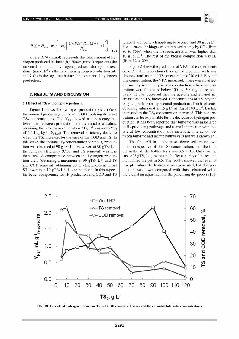
© by PSP Volume 24 – No 7. 2015 Fresenius Environmental Bulletin
2291
1
)(*71828.2expexp*)(
max
maxmax H
tRHtH
(4)
where, H(t) (mmol) represents the total amount of hy-drogen produced in time t (h); Hmax (mmol) represents the maximal amount of hydrogen produced during the test; Rmax (mmol h-1) is the maximum hydrogen production rate and λ (h) is the lag time before the exponential hydrogen production.
3. RESULTS AND DISCUSSION
3.1 Effect of TS0 without pH adjustment
Figure 1 shows the hydrogen production yield (YH2), the removal percentage of TS and COD applying different TS0 concentrations. The YH2 showed a dependency be-tween the hydrogen production and the initial total solids, obtaining the maximum value when 90 g L-1 was used (YH2 of 2.2 LH2 kg-1 TSadded). The removal efficiency decrease when the TS0 increase, for the case of the COD and TS. In this sense, the optimal TS0 concentration for the H2 produc-tion was obtained at 90 gTS0 L-1. However, at 90 gTS0 L-1, the removal efficiency (COD and TS removal) was less than 10%. A compromise between the hydrogen produc-tion yield (obtaining a maximum at 90 gTS0 L-1) and TS and COD removal (obtaining better efficiencies at initial ST lower than 10 gTS0 L-1) has to be found. In this aspect, the better compromise for H2 production and COD and TS
removal will be reach applying between 5 and 30 gTS0 L-1. For all cases, the biogas was composed mainly by CO2 (from 80 to 85%) when the TS0 concentration was higher than 10 gTS0 L-1. The rest of the biogas composition was H2
(from 12 to 20%).
Figure 2 shows the production of VFA in the experiments done. A stable production of acetic and propionic acids was observed until an initial TS concentration of 70 g L-1. Beyond this concentration, the VFA increased. There was no effect on iso-butyric and butyric acids production, where concen-trations were fluctuated below 100 and 300 mg L-1, respec-tively. It was observed that the acetone and ethanol in-creased as the TS0 increased. Concentrations of TS0 beyond 90 g L-1 produce an exponential production of both solvents, obtaining values of 4.8, 1.5 g L-1 at TS0 of 100 g L-1. Lactate increased as the TS0 concentration increased. This concen-tration can be responsible for the decrease of hydrogen pro-duction. It has been reported that butyrate was associated to H2-producing pathways and a small interaction with lac-tate at low concentration, this metabolic interaction be-tween butyrate and lactate pathways is not well known [7].
The final pH in all the cases decreased around two units, irrespective of the TS0 concentration, i.e., the final pH in the all the bottles tests was 3.5 ± 0.3. Only for the case of 5 gTS0 L-1, the natural buffer capacity of the system maintained the pH in 5.5. The results showed that even at low pH values the hydrogen was generated, but this pro-duction was lower compared with those obtained when there exist an adjustment in the pH during the process [6].
FIGURE 1 - Yield of hydrogen production, TS and COD removal efficiency at different initial total solids concentrations.
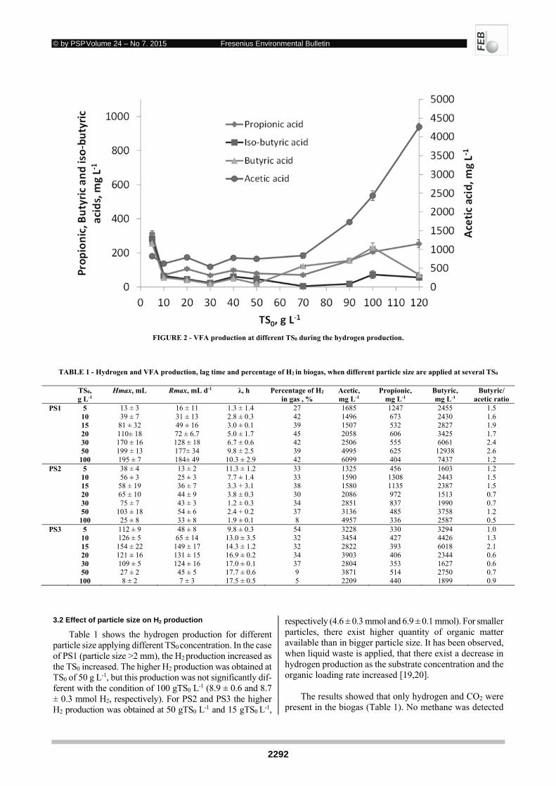
© by PSP Volume 24 – No 7. 2015 Fresenius Environmental Bulletin
2292
FIGURE 2 - VFA production at different TS0 during the hydrogen production.
TABLE 1 - Hydrogen and VFA production, lag time and percentage of H2 in biogas, when different particle size are applied at several TS0
TS0, g L-1
Hmax, mL Rmax, mL d-1 λ, h Percentage of H2 in gas , %
Acetic, mg L-1
Propionic, mg L-1
Butyric, mg L-1
Butyric/ acetic ratio
PS1 5 13 ± 3 16 ± 11 1.3 ± 1.4 27 1685 1247 2455 1.5 10 39 ± 7 31 ± 13 2.8 ± 0.3 42 1496 673 2430 1.6 15 81 ± 32 49 ± 16 3.0 ± 0.1 39 1507 532 2827 1.9 20 110± 18 72 ± 6.7 5.0 ± 1.7 45 2058 606 3425 1.7 30 170 ± 16 128 ± 18 6.7 ± 0.6 42 2506 555 6061 2.4 50 199 ± 13 177± 34 9.8 ± 2.5 39 4995 625 12938 2.6 100 195 ± 7 184± 49 10.3 ± 2.9 42 6099 404 7437 1.2
PS2 5 38 ± 4 13 ± 2 11.3 ± 1.2 33 1325 456 1603 1.2 10 56 ± 3 25 ± 3 7.7 ± 1.4 33 1590 1308 2443 1.5 15 58 ± 19 36 ± 7 3.3 + 3.1 38 1580 1135 2387 1.5 20 65 ± 10 44 ± 9 3.8 ± 0.3 30 2086 972 1513 0.7 30 75 ± 7 43 ± 3 1.2 ± 0.3 34 2851 837 1990 0.7 50 103 ± 18 54 ± 6 2.4 + 0.2 37 3136 485 3758 1.2 100 25 ± 8 33 ± 8 1.9 ± 0.1 8 4957 336 2587 0.5
PS3 5 112 ± 9 48 ± 8 9.8 ± 0.3 54 3228 330 3294 1.0 10 126 ± 5 65 ± 14 13.0 ± 3.5 32 3454 427 4426 1.3 15 154 ± 22 149 ± 17 14.3 ± 1.2 32 2822 393 6018 2.1 20 121 ± 16 131 ± 15 16.9 ± 0.2 34 3903 406 2344 0.6 30 109 ± 5 124 ± 16 17.0 ± 0.1 37 2804 353 1627 0.6 50 27 ± 2 45 ± 5 17.7 ± 0.6 9 3871 514 2750 0.7 100 8 ± 2 7 ± 3 17.5 ± 0.5 5 2209 440 1899 0.9
3.2 Effect of particle size on H2 production
Table 1 shows the hydrogen production for different particle size applying different TS0 concentration. In the case of PS1 (particle size >2 mm), the H2 production increased as the TS0 increased. The higher H2 production was obtained at TS0 of 50 g L-1, but this production was not significantly dif-ferent with the condition of 100 gTS0 L-1 (8.9 ± 0.6 and 8.7 ± 0.3 mmol H2, respectively). For PS2 and PS3 the higher H2 production was obtained at 50 gTS0 L-1 and 15 gTS0 L-1,
respectively (4.6 ± 0.3 mmol and 6.9 ± 0.1 mmol). For smaller particles, there exist higher quantity of organic matter available than in bigger particle size. It has been observed, when liquid waste is applied, that there exist a decrease in hydrogen production as the substrate concentration and the organic loading rate increased [19,20].
The results showed that only hydrogen and CO2 were
present in the biogas (Table 1). No methane was detected

© by PSP Volume 24 – No 7. 2015 Fresenius Environmental Bulletin
2293
in any sample. The concentration of H2 varied from 5 to 54%. The higher values for hydrogen percentage in biogas were obtained when the TS0 were 50 gTS0 L-1 or lower. In the case of PS1 the percentage of H2 was maintained stable with percentage from 27 to 45% with an average value of 41.5 ± 2.3% in an initial ST from 10 to 100 g L-1. For PS2, the percentage was stable in 34.2 ± 2.9% except for the value of 100 gTS0 L-1 where the percentage was 8%. In PS3, the hydrogen content in the biogas decreased from 54 to 5% as the TS0 increase. The percentages of H2 agree with the results obtained by Gomez et al. [21] and Zhu et al. [2] using food residues obtaining 25 to 45% of H2 in biogas. They also applied pH adjustment in order to avoid the in-hibition of the process and carried out at mesophilic tem-perature (34-35°C).
Figure 3 show the production of H2 obtained after 48 h
of reaction. For low concentrations of TS0 (5-15 g L-1) there is an increase of H2 production in condition PS3 (6 mmol). However, higher values than 30 g L-1 produced a decrease in H2 production. Larger particles size required more time to produce the same amount of hydrogen. When the con-centration of TS0 is between 5 to 20 g L-1, the best option is to apply a particle size smaller than 0.5 mm because the production rate is higher per TS0 added. In the case of 15 gTS0 L-1 the hydrogen production per TS were 0.068 ± 0.008, 0.078 ± 0.008 and 0.192 ± 0.009 mmol of H2 g-1TS d-1 for PS1, PS2 and PS3 respectively. Those hydrogen pro-ductions can be related to the different rate of solubility of organic matter and the influence of particle size. The small
particle size increased the solubility rate, increasing the ac-cessibility of the organic matter to the microorganisms- In this sense, it was suggested that pre-treatment methods, ap-plied to organic solid waste, make more accessible com-plex carbohydrates resulting in an increase of biohydrogen production [7]. However, as the particle size decreased, an inhibitory effect was detected beyond 15 and 50 gTS0 L-1 for PS2 and PS3, respectively. In the case of higher TS0 concentrations (> 50 gTS0 L-1) it is recommended to use larger particle size.
In a practical operation of a continuous bioreactor, it can
be more suitable to work at concentrations below 30 gTS0 L-1 because higher values show a substrate thickness and make difficulties in the agitation and draw of the reactor. In ad-dition, higher levels of ST0 produce high VFA (Table 1) concentrations that can inhibit the microorganism's activity [21]. The principal VFA generated were acetic and butyric acids in all the cases, in agreement with other studies ap-plying organic solid waste [6,22,23]. The VFAs are inter-mediate products of H2 production, and a high concentra-tion of them causes inhibition to the microorganisms [23,24]. The results demonstrated that when the TS0 in-crease, the VFA production increases as well. The values of acetic acid were similar when the TS0 concentration ap-plied was between 5 and 20 gTS0 L-1 for each different par-ticle size. Higher concentration than 30 gTS0 L-1 results in a faster increase in the acetic acid production. Some studies showed that the butyric/acetic ratio (B/A) decrease as the hydrogen production increase [22,25]. Low values of B/A
FIGURE 3 - Effect of different particle size and TS0 on the hydrogen production after 48 h.
© by PSP Volume 24 – No 7. 2015 Fresenius Environmental Bulletin
2294
(lower than 0.8) can be obtained when pure substrates as sucrose or glucose are applied [12,26]. However, for the case of organic solid waste, the values for B/A between 1.0 to 5.0 has been reported [22,25]. In our study, the values varied between 0.5 to 2.6.
Beyond the acetic and butyric acids as the main meta-
bolic products, other sub-products can be obtained during the dark fermentation of food waste, e.g. lactate. The lac-tate can be produced due to the presence of microorgan-isms as lactic acid bacteria (LAB) in the food waste [27-30]. It was demonstrated that other groups of microorgan-isms, including Bacteroidales strains, can produce lactate as well as acetate, succinate, formate or propionate which are generated from the carbohydrates present in the food waste [27]. However, it has been reported that the effect of LAB on H2 production depends on pH and temperature [3]. The inhibition effect on hydrogen-producing bacteria can be prevented by keeping the pH at over 5.0 [29], as the con-ditions that we maintain in our study.
Due to the use of a buffer, the average final pH values
were higher than 5.0 for all the particle size and TS0 tested (5.3 ± 0.26, 5.4 ± 0.10, 5.13 ± 0.60 for PS1, PS2 and PS3, respectively), showing that the buffer capacity was enough to avoid inhibition of the microorganism’s activity. Only the case PS3 with TS0 of 100 gTS0 L-1 the final pH was 4, in this case, the high VFA production decrease the pH and produce a decrease on hydrogen production [24].
4. CONCLUSIONS
The results demonstrated that there is an effect of the initial particle size and the concentration of initial total sol-ids on the hydrogen production. When no pH adjustment is applied, it was observed that the maximal hydrogen pro-duction (2.2 LH2 kg-1 TSadded) was obtained at 90 gTS0 L-1, but the high TS and COD removal were obtained at 10 gTS0 L-1. The H2 production increases as the TS0 increase when particles larger than 2 mm were used. For particle sizes between 0.5 and 2.0 mm, and smaller than 0.5 mm, the higher H2 production was reached at 50 gTS0 L-1 and 15 gTS0 L-1, respectively. Larger particles size required more time to produce the same amount of hydrogen. The maxi-mal hydrogen production rate was obtained with a smaller particle size applying initial 15 gTS0 L-1. The principal vol-atile fatty acids generated were acetic and butyric. The val-ues of acetic acid were similar when initial TS applied were between 5 to 20 gTS0 L-1 for each different particle size. Higher concentration of TS0 than 30 gTS0 L-1 results in a fast increase in the acetic acid production.
ACKNOWLEDGMENTS
The authors gratefully acknowledge the financial sup-port of PAPIIT (DGAPA-UNAM) project IN103315 and
Marie Curie Research Fellowship Programme PIRSES-GA-2011-295170. Carlos Ramos, César Figueroa and Mónica Rangel are acknowledged for their participation in test experiments. Jaime Pérez Trevilla and Gloria Moreno Rodríguez are acknowledged for their technical assistance.
The authors have declared no conflict of interest. REFERENCES
[1] Edwards, P.P., Kuznetsov, V.L., & David, W.I.F. and Bran-don, N.P. (2008) Hydrogen and fuel cells: towards a sustaina-ble energy future. Energy Policy, 36, 4356-4362.
[2] Zhu, H., Parker, W., Conidi, D., Basnar, R. and Seto, P. (2011) Eliminating methanogenic activity in hydrogen reactor to im-prove biogas production in a two-stage anaerobic digestion process co-digesting municipal food waste and sewage sludge. Bioresourse Technology, 102, 7086-7092.
[3] Chu, C-F., Li, Y-Y., Xu, K-Q., Ebie, Y., Inamori, Y. and Kong, H-N. (2008) A pH- and temperature-phased two-stage process for hydrogen and methane production from food waste. Interna-tional Journal of Hydrogen Energy, 33, 4739-4746.
[4] Mohan, S.V., Mohanakrishna, G., Goud, R.K. and Sarma, P.N. (2009) Acidogenic fermentation of vegetable based market waste to harness biohydrogen with simultaneous stabilization. Bioresource Technology, 100, 3061-3068.
[5] Fang, H.H.P., & Liu, H. (2002) Effect of pH on hydrogen pro-duction from glucose by a mixed culture. Bioresource Tech-nology, 82, 87-93.
[6] Ramos, C., Buitrón, G., Moreno-Andrade, I. and Chamy, R. (2012) Effect of the initial total solids concentration and initial pH on the bio-hydrogen production from cafeteria food waste. International Journal of Hydrogen Energy, 37, 13288-13295.
[7] Guo, X.M., Trably, E., Latrille, E., Carrere, H. and Steyer, J-P. (2013) Predictive and explicative models of fermentative hydrogen production from solid organic waste: Role of butyr-ate and lactate pathways. International Journal of Hydrogen Energy, 39, 7476-7485.
[8] Izumi, K., Okishio, Y-K., Nagao, N., Niwa, C., Yamamoto, S. and Toda, T. (2010) Effects of particle size on anaerobic di-gestion of food waste. International Biodeterioration and Bio-degradation, 64, 601-608.
[9] Mshandete, A., Bjornsson, L., Kivaisi, A.K., Rubindamayugi, M.S.T. and Mattiasson, B. (2006) Effect of particle size on bi-ogas yield from sisal fiber waste. Renewable Energy, 31, 2385-2392.
[10] Yuan, X., Shi, X., Zhang, P., Wei, Y., Guo, R. and Wang L. (2011) Anaerobic biohydrogen production from wheat stalk by mixed microflora: Kinetic model and particle size influence. Bioresource Technology, 102, 9007-9012.
[11] Chen, C-C., Chuang, Y-S., Lin, C-Y., Lay, C-H. and Sen, B. (2012) Thermophilic dark fermentation of untreated rice straw using mixed cultures for hydrogen production. International Journal of Hydrogen Energy, 37, 15540-15546.
[12] Maintinguer, S.I., Fernandes, B.S., Duarte, I.C.S., Saavedra, N.K., Adorno, M.A.T. and Varesche, M.B. (2008) Fermenta-tive hydrogen production by microbial consortium. Interna-tional Journal of Hydrogen Energy, 33, 4309-4317.
[13] Fountoulakis, M.S. and Manios, T. (2009) Enhanced methane and hydrogen production from municipal solid waste and agro-industrial by-products con-digested with crude glycerol. Bioresource Technology, 100, 3043-3047.
© by PSP Volume 24 – No 7. 2015 Fresenius Environmental Bulletin
2295
[14] Ma, J., Ke, S. and Chen, Y. (2008) Mesophilic biohydrogen production from food waste. Proceedings of the 2nd Interna-tional Conference on Bioinformatics and Biomedical Engi-neering, Shanghai, 16-18 May, 2841-2844.
[15] Zhang, Y. and Banks, C.J. (2013) Impact of different particle size distributions on anaerobic digestion of the organic frac-tion of municipal solid waste. Waste Management, 33, 297-307.
[16] Buitrón, G. and Carvajal, C. (2010) Biohydrogen production from Tequila vinasses in an anaerobic sequencing batch reac-tor: effect of initial substrate concentration, temperature and hydraulic retention time. Bioresourse Technology. 101, 9071-9077.
[17] APHA. (2005). Standard Methods for the Examination of Wa-ter and Wastewater. 21th ed., APHA/AWWA/WEF, Port city press. Baltimore, Maryland.
[18] Shelton, D. and Tiedje, J. (1984) General method for deter-mining anaerobic biodegradation potential. Applied and Envi-ronmental Microbiology, 47, 850-857.
[19] De Amorim, E.L.C., Sader, L.T. and Silva, E.L. (2012) Effect of substrate concentration on dark fermentation hydrogen pro-duction using an anaerobic fluidized bed reactor. Applied Bi-ochemistry and Biotechnology, 166, 1248-1263.
[20] Shen, L., Bagley, D.M. and Lis, S.N. (2009) Effect of organic loading rate on fermentative hydrogen production from con-tinuous stirred tank and membrane bioreactors. International Journal of Hydrogen Energy, 34, 3689-3696.
[21] Gomez, X., Moran, A., Cuetos, M.J. and Sánchez, M.E. (2006) The production of hydrogen by dark fermentation of municipal solid waste and slaughterhouse waste: a two phase process. Journal of Power Sources, 157, 727-732.
[22] Zhu, H., Stadnyk, A., Bèland, M. and Seto, P. (2008) Co-pro-duction of hydrogen and methane from potato waste using a two-stage anaerobic digestion process. Bioresource Technol-ogy, 99, 5078-5084.
[23] Dong, L., Zhenhong, Y., Yongming, S., Xiaoying, K. and Yu, Z. (2009) Hydrogen production characteristics of the organic fraction of municipal solid wastes by anaerobic mixed culture fermentation. International Journal of Hydrogen Energy, 34, 812-820.
[24] Lay, J-J., Fan, K-S., Chan, J-I. and Ku, C-H. (2003) Influence of chemical nature of organic wastes on their conversion to hydrogen by heat-shock digested sludge. International Journal of Hydrogen Energy, 28, 1361-1367.
[25] Shin, H-S., Youn, J-H. and Kim, S.H. (2004) Hydrogen pro-duction from food waste in anaerobic mesophilic and thermo-philic acidogenesis. International Journal of Hydrogen En-ergy, 29, 1355-1363.
[26] Wang, J. and Wan, W. (2008) Effect of temperature on fer-mentative hydrogen production by mixed cultures. Interna-tional Journal of Hydrogen Energy, 33, 5392-5397.
[27] Shin, H-S., Youn, J-H. and Kim, S-H. (2004) Hydrogen pro-duction from food waste in anaerobic mesophilic and thermo-philic acidogenesis. International Journal of Hydrogen En-ergy, 29, 1355-1363.
[28] Kim, S-H., Han, S-K. and Shin H-S. (2004) Feasibility of bio-hydrogen production by anaerobic co-digestion of food waste and sewage sludge. International Journal of Hydrogen Energy, 29, 1607-1616.
[29] Noike, T., Ko, I.B., Yokoyama S., Kohno, Y. and Li Y.Y. (2005). Continuous hydrogen production from organic waste. Water Science and Technology, 52, 145-151.
Received: September 02, 2014 Revised: November 10, 2014 Accepted: December 18, 2014 CORRESPONDING AUTHOR
Iván Moreno-Andrade Laboratory for Research on Advanced Processes for Water Treatment Unidad Académica Juriquilla Instituto de Ingeniería Universidad Nacional Autónoma de México Blvd. Juriquilla 3001 76230 Querétaro MÉXICO Phone: + 52 (442) 1926171 Fax: + 52 (442) 1926185 E-mail: [email protected]
FEB/ Vol 24/ No 7/ 2015 – pages 2289 - 2295

© by PSP Volume 24 – No 7. 2015 Fresenius Environmental Bulletin
2296
APPLICATION OF CELLULOSE ACETATE MEMBRANES FOR
REMOVAL OF TOXIC METAL IONS FROM AQUEOUS SOLUTION
Nadjib Benosmane1,2,*, Baya Boutemeur2,*, Maamar Hamdi2 and Safouane M. Hamdi3
1Departement of Chemistry, Faculty of Sciences, University M’Hamed Bougara de Boumerdes (UMBB), Avenue de l’indépendance 35000, Boumerdes, Algérie.
2Laboratoire de Chimie Organique Appliquée. Faculty of Chemistry, USTHB BP 32 El-Alia 16111, Alger, Algérie. 3Clinical Biochemistry Department, CHU Toulouse, University of Toulouse, UPS, Toulouse, France.
ABSTRACT
In this study, we investigated the transport of heavy metals ions through a polymer inclusion membrane (PIM) containing cellulose acetate (CA) as support, calix[4]resor-cinarenes (RC) as carriers, 2-nitrophenyloctanoate (NPOT) and 2-nitrophenyloctylether (NPOE) as plasticizers. The effects of several transport conditions including, pH, PIM thickness, plasticizers amount and carriers concentration were studied. The optimal transport conditions for Pb(II), Cu(II) and Zn(II) were found to be 10.8 mM of carriers, 0.13 mL/g of CA for NPOE, a pH of 5.1 and 1.5 for feeding and receiving phases respectively. Our experiments revealed a facilitated counter-transport mechanism for ions transfer and showed that such PIMs can be reused for five consec-utive cycles without appreciable deterioration. We charac-terized PIMs structure by several techniques and deter-mined their water content and porosity. Applying these op-timized transport conditions to remove metal ions from municipal wastewater samples, we found an overall re-moval efficiency of 87%, 86%, 75%, 72%, and 71% for Pb(II), Ni(II), Cd(II), Cu(II) and Zn(II) respectively. Of in-terest, the residual concentrations of these heavy metal ions were below the permissible limits according to the Alge-rian standards for wastewaters quality.
KEYWORDS: Polymer inclusion membranes, Calix[4]resorcina-renes, Metals ions, Separation, Municipal wastewater.
1. INTRODUCTION
Lead, copper and zinc are heavy metals of concern for their role in environmental pollution, as have toxic effects in humans via inhalation, oral ingestion and/or skin con-tact. The presence of these metals in the human body may induce elevated blood pressure, anaemia, and gastrointes-tinal, cardiovascular, nervous and memory diseases [1].
* Corresponding author
Currently, due to anthropogenic activities where lead is the raw material (i.e. fuel refining and use, metallurgy, pig-menting, etc.), its removal from wastewater is a problem of great significance [2]. Due to concern for the environment and the possibility of using a very low amount of the ex-tractant, liquid membrane-based separation methods are considered viable alternatives to currently employed sol-vent extraction methods [3-6].
Polymer inclusion membranes (PIMs) are thin, flexi-ble, and stable films, formed by casting a solution contain-ing an extractant (carrier), a plasticiser, and a base polymer (cellulose triacetate, CTA or poly(vinyl chloride), PVC) [7-15]. Selectivity, stability, and efficient transport of metal ions are the properties that make PIMs valuable tech-nologies for the removal of toxic ions from liquid effluents. Over the last 30 years, PIMs have been widely used in the production of chemical sensors with applications in the po-tentiometric determination of many cations and anions [16]. Moreover, since the use of flammable solvents has been eliminated from the composition of PIMs [16], many studies have presented additional applications of these membranes as solid sorbents in separation and extraction processes, with obvious implications for green chemistry-controlled technology.
Cellulose acetate can be characterised by its extensive linearity, good flexibility, excellent durability, biodegrada-bility, non-toxicity, low cost, and displays good solubility in organic solvents [17-23]. On the other hand, it has some disadvantages such as poor mechanical strength, low oxi-dation, as well as thermal and chemical resistance [24-28]. Cellulose acetate membranes have been used in many ap-plications of particular interest are reverse osmosis sys-tems, and as a neutral matrix for the incorporation of dif-ferent polymers (e.g., conducting polymers), inorganic ions (e.g., lanthanides), and organic (e.g., pharmaceutical) compounds [14, 17, 18, 23, 29, 30].
The calixarenes are a major class of supramolecular hosts of phenolic units. One of the important properties of calixarene is its ability to recognise cationic and anionic species, as well as neutral molecules. These receptors have the possibility to form interesting complexes both with metal

© by PSP Volume 24 – No 7. 2015 Fresenius Environmental Bulletin
2297
cations and biological compounds by exhibiting extracta-bility and selectivity. Many studies have been published dedicated to calixarenes, particularly in the molecular in-clusion of biological substrates, such as amines and amino acids [31-33]. Various applications of calixarenes also re-fer to purification, chromatography, catalysis, enzyme mimics, ion selective electrodes, phase transfer, transport across membranes, ion channels, and self-assembling mon-olayers [1, 34-41]. The aim of this work is to investigate the efficiency of metal ions removal from synthetic aque-ous wastewater solutions and municipal wastewater by a PIM technology. The influence of the PIM carrier concen-tration, plasticizer amount, PIM thickness, pH, and phase composition were investigated for estimate their impact both on transport fluxes of the optimal membrane.
2. MATERIALS AND METHODS
2.1 Municipal wastewater collection
The triplicate samples of municipal wastewater was col-lected from a wastewater stream flowing over nearby location of city of El Harrach (latitude deg. North 36.710455, longitude deg. East 3.12295), 11 km east of Algiers, Algeria. Col-lected wastewater was brought immediately to laboratory. Sample was collected just before the starting of experimen-tation in order to avoid alternation in the wastewater char-acteristics mainly due to open storage of sample. Before
treatment, the samples were filtered through Millipore fil-ter paper (0.45 µm) and kept in Teflon® bottles, at 4 °C, in the dark. The general characteristics of the municipal waste-water are presented in Table 1 Concentrations of Pb(II) and Cd(II) are high enough to be considered as a serious environ-mental problem. Therefore, they were chosen for our study.
2.2 Chemicals
The structures and abbreviations of the carriers used in the present study are shown in Fig. 1. The carrier, (C-butyl)calix[4]resorcinarene, abbreviated as RC4, (C-oc-tyl)calix[4]resorcinarene, abbreviated as RC8, and 2-ni-trophenyloctanoate (NPOT) were synthesised in our la-boratory [36,42]. Final products were purified by recrys-tallisation and identified by FT-IR, 1H NMR, and ele-mental analysis.
Lead (II) chloride, copper (II) chloride, zinc (II) chlo-
ride, resorcinol, aldehydes, ethanol, hydrochloric acid, po-tassium hydroxide, dichloromethane, cellulose acetate (CA, molecular weight Mw = 50.000, with an acetyl content of 39.7%, and refractive index =1.475), and 2-nitrophenyl-oc-tylether (NPOE) were analytical grade reagents purchased from Fluka. Aqueous phases were prepared by dissolving the different reagents in deionised water. The pH adjust-ment was done by addition of dilute hydrochloric acid or potassium hydroxide to prepare the desired pH solution.
A B
RC4: R = C4H9
RC8: R = C8H17
FIGURE 1 - Molecular structures of calix[4]resorcinarenes. A Chemical formula and abbreviation of calix[4]resorcinarenes used as carriers. B Cartoon representation of RC8 showing the characteristic and truncated cone shape with eight hydroxyl groups on the wide rim and four hydrophobic tails on the narrow rim.
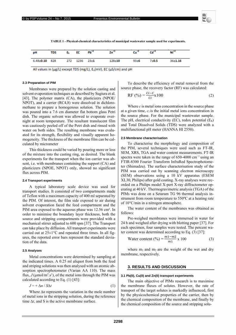
© by PSP Volume 24 – No 7. 2015 Fresenius Environmental Bulletin
2298
TABLE 1 - Physical-chemical characteristics of municipal wastewater sample used for experiments.
2.3 Preparation of PIM
Membranes were prepared by the solution casting and solvent evaporation techniques as described by Sugiura et al. [43]. The polymer matrix (CA), the plasticizers (NPOE/ NPOT), and a carrier (RC4,8) were dissolved in dichloro-methane to prepare a homogenous solution. The solution was poured into a 7.6 cm diameter flat bottom glass Petri dish. The organic solvent was allowed to evaporate over-night at room temperature. The resultant translucent film was cautiously peeled off of the Petri dish and rinsed with water on both sides. The resulting membrane was evalu-ated for its strength, flexibility and visually apparent ho-mogeneity. The thickness of the membrane film can be cal-culated by micrometer
This thickness could be varied by pouring more or less of the mixture into the casting ring, as desired. The blank experiments for the transport when the ion carrier was ab-sent, i.e. with membranes containing the support (CA) and plasticizers (NPOE, NPOT) only, showed no significant flux across PIM.
2.4 Transport experiments
A typical laboratory scale device was used for transport studies. It consisted of two compartments made of Teflon with a maximum capacity of 400 ml separated by the PIM. Of interest, the film side exposed to air during solvent evaporation faced the feed compartment and the PIM area exposed to the aqueous phase was 12.56 cm². In order to minimise the boundary layer thickness, both the source and stripping compartments were provided with a mechanical stirrer adjusted to 600 rpm [37]. The Transport can take place by diffusion. All transport experiments were carried out at 25±1°C and repeated three times. In all fig-ures, the reported error bars represent the standard devia-tion of the data.
2.5 Analyses
Metal concentrations were determined by sampling at the indicated times. A 0.25 ml aliquot from both the feed and striping solutions was then analysed with an atomic ab-sorption spectrophotometer (Varian AA 110). The mass flux, J (µmol/m2.s1), of the metal ions through the PIM was calculated according to Eq. (1) [43]:
J = + n / St (1)
Where n represents the variation in the mole number of metal ions in the stripping solution, during the reference time t, and S is the active membrane surface.
To describe the efficiency of metal removal from the source phase, the recovery factor (RF) was calculated:
RF (%) = x100 (2)
Where c is metal ions concentration in the source phase
at a given time, ci is the initial metal ions concentration in the source phase. For the municipal wastewater sample. The pH, electrical conductivity (EC), redox potential (Eh) and Total Dissolved Solids (TDS) were analyzed with a multifunctional pH meter (HANNA HI 2550).
2.5 Membrane characterisation
To characterise the morphology and composition of the PIM, several techniques were used such as FT-IR, SEM, XRS, TGA and water content measurements. FT-IR spectra were taken in the range of 650-4000 cm−1 using an FTIR-8300 Fourier Transform InfraRed Spectrophotome-ter (Shimadzu). The surface characterisation study of the PIM was carried out by scanning electron microscopy (SEM) observations using a 10 kV apparatus (ESEM XL30, Philips) after gold coating. X-ray analyses were rec-orded on a Philips model X-pert X-ray diffractometer op-erating at 40 kV. Thermogravimetric analysis (TGA) of the PIMs was done on a Setaram TG 96 thermal analysis in-strument from room temperature to 550ºC at a heating rate of 10°C/min in a nitrogen atmosphere.
The water content of the membranes was obtained as follows:
Pre-weighed membranes were immersed in water for 24 h and weighed after drying with blotting paper [37]. For each specimen, four samples were tested. The percent wa-ter content was determined according to Eq. (3) [37]:
Water content (%) = x 100 (3)
where m1 and m2 are the weight of the wet and dry
membrane, respectively. 3. RESULTS AND DISCUSSION
3.1 Pb(II), Cu(II) and Zn(II) transport experiments
The main objective of PIMs research is to maximise the membrane fluxes of solutes. However, the rate of transport of the target solutes is markedly influenced, first by the physicochemical properties of the carrier, then by the chemical composition of the membrane, and finally by the chemical composition of the source and stripping solu-

© by PSP Volume 24 – No 7. 2015 Fresenius Environmental Bulletin
2299
0,04 0,06 0,08 0,10 0,12 0,14 0,16 0,18
0
1
2
3
Flu
x (
mo
l.m-2.s
-1)
Amount of NPOE (ml)
Pb(II) Cu(II) Zn(II)
tions [44, 46]. Therefore, we investigated the impact of these three parameters on the facilitated transport properties of our PIM system toward Pb(II), Cu(II) and Zn(II). The choice of metals ions was driven by the fact that calix[4]resorcina-renes are known to form complexes with Cu(II) and Zn(II) [47] and thus mediate the transport of Cu(II) complexes through liquid chloroform membranes [48].
As seen in Table 2, the initial flow of PIM in this study is lower than the initial flux in the previous study [36]. Probably due to the difference in the nature of the support (CTA/CA), the transport of metals is mainly by diffusion, and therefore the transport rates are lower. Furthermore we observed that transport efficiency of PIM in this study is higher than that of unplasticized PIM in previous study [37]. The obtained data prove that the PIM with any addi-tionally plasticizers is not only considerably cheaper but it has enhanced metal ions transport compared with other un-plasticized PIMs [37].
3.2 Amount of plasticizer
To understand the influence of the amount of plasti-cizer on transport flux, membranes were prepared with var-iable amounts of NPOE at a constant concentration of car-rier the (RC4) and CA in the PIM. Fig. 2 shows the effect of the amount of NPOE on the transport flux of metals ions. The flux was increased by increasing the amount of NPOE until a value of 0.13 mL, further addition caused a decrease in the transport flux. This decrease was attributed to the in-crease in the thickness and viscosity of the membrane re-sulting in lower mass transfer [49-51]. Thus, the amount of NPOE was selected as 0.13 mL (4.13M) for further exper-iments. The results (Fig. 2) show that the choice of the ap-propriate composition of the various components of PIM must be based not only on the interactions between the dif-ferent components, but also their effect on the extraction and transport of the species of interest.
TABLE 2 - Comparison of PIM containing RC8 for Pb(II) transport (feed phase: 1×10⁻² M Pb(II), pH of feed phase 5.1, receiving phase: HCl at pH 1.5).
Support material Plasticizer Carrier Flux (μmol/m2.s1) of Pb(II) Ref
Cellulose Tri Acetate (CTA) NPOE RC8 5.03 [36]
Cellulose Tri Acetate (CTA) NPOT RC8 1.43 [36]
Cellulose Acetate (CA) Without RC8 0.13 [37]
Cellulose Acetate (CA) NPOE RC8 4.78 This study
Cellulose Acetate (CA) NPOT RC8 0.98 This study
FIGURE 2 - Change of transport flux with the amount of NPOE. Transport conditions: Source phase (synthetic aqueous solution of PbCl2, CuCl2 and ZnCl2, 10-3M pH: 5.1) and stripping phase (deionized water, pH=1.5) were stirred at 600 rpm, membrane area of 12.56 cm2 with 10.8 mM of carrier (RC4) and [0.05-0.17] ml of NPOE, time of transport : 3 days, T =25°C.

© by PSP Volume 24 – No 7. 2015 Fresenius Environmental Bulletin
2300
FIGURE 3 - Pb(II), Cu(II) and Zn(II) mass fluxes through PIMs. Transport conditions : Source phase (synthetic aqueous solution of PbCl2, CuCl2 and ZnCl2, 10-3M pH: 5.1) and stripping phase (deionized water, pH=1.5) were stirred at 600 rpm, membrane area of 12.56 cm2 with 10.8 mM of carrier and 0.13 ml of (NPOE/NPOT), time of transport : 5 days, T = 25°C.
3.3 Influence of carrier structure on cation flux
First, we wondered whether modifying the calix[4]re-sorcinarene structure (particularly the length of the alkyl moieties, Fig. 1) would have an effect on the rate of metals ions transport through the PIM. The collected data are de-picted in Fig 3. Thus, our initial hypothesis that calix[4]re-sorcinarene is able to mediate cation transfer through a CA matrix was confirmed. RC8 appeared to be the most effi-cient carrier for Cu(II) with a three-fold increase in flux, followed by RC4. Rates of Zn(II) transport were below those of Cu(II), but the pattern of carrier efficiencies was roughly the same (RC8 > RC4). We can infer from these results that metals ions fluxes depend on the alkyl chain length of calix [4] resorcinarene. The influence of the length of the alkyl chain on the transport of metal ions has already been demonstrated for diazadibenzocrown ethers [16]. These results imply that the efficiency of the macro-cyclic carrier based on an optimal combination of polar rings and hydrophobic tails.
3.4 PIM thickness
In order to assess the influence of membrane thickness on metals ions transport through the membrane, transport exper-iments were carried out using membranes of the same chemi-cal composition, but with different thicknesses, i.e. 22, 28, 33, 39 and 48 µm. As seen in Fig. 4, the metals ions flux decreased by increasing the thickness of the membrane. This was ex-plained by the appropriate formulation of Fick’s first law of diffusion illustrated in earlier studies [52,53]:
J= D0
(4) Neglecting the aqueous diffusion layer, ∆x=d (d: mem-
brane thickness) and ∆C≅Ci(Ci is the initial source phase concentration). Eq. (5) can be simplified to:
(5)

© by PSP Volume 24 – No 7. 2015 Fresenius Environmental Bulletin
2301
20 25 30 35 40 45 500
1
2
3
4
5
Flu
x (m
ol.m
-2.s
-1)
Thickness of membranes
Pb(II) Cu(II) Zn(II)
On the other hand, decrease with increasing the thick-ness of the membrane may be due to possible interactions between the plasticizer and carrier. This can be explained in terms of the diffusion of complex through the mem-brane. Since the rate of mass transport is determined by diffusion through the membrane from the source solution to the stripping solution, the rate of mass transport de-creases logically with an increase in film thickness.
The maximum membrane transport was observed
when the membrane thickness was 22 µm, as can be seen in Fig. 4. However, a negligible value was found with a membrane thickness of 48 µm. Therefore, the membrane thickness of 28 µm was used in our study.
3.5 Influence of the aqueous phases composition
The facilitated transport of divalent metal ions through membrane systems containing acidic organic compounds such as calix[4]resorcinarenes is generally ensured by a counter-transport of protons. The carrier exchanges one metal ion at the source solution-membrane interface releas-ing two protons. The complex formed between the carrier and the metal diffuse through the membrane and one metal ion is released at the membrane-stripping phase interface by substitution of two protons. It is clear that the pH differ-ence between source and striping aqueous solutions may play the role of driving force for the transfer of metal from the source to the stripping aqueous solution [9].
In order to improve the dissociation of the complexe in the striping phase, the variation of the extracted metals ions M(II) amount was studied as a function of the pH of the striping phase solution, ranging from 1.5 to 3.5 by varying the concentration of HNO3 (Fig. 5). A pH gradient between the source and stripping phases is the driving force for the transport of metals ions through the membrane phase. So, an acidic solution was needed for the stripping of Metals ions from the PIM.
The pH of the source phase has been fixed at 5.1, tak-ing into account the maximum efficiency of experimental biphasic extraction obtained in this pH range, from the re-sults shown in Fig.5, when a larger difference in pH be-tween the source and stripping phases is applied, the initial flux of lead (II) increases from 1.33 (at pH 3.5) to 4.68 µmol.m-2.s-1 (at pH 1.5). A lower pH in the stripping phase afforded the quantitative stripping of metals ions from the membrane phase. These observations are reasonable be-cause, according to the proton-driven mechanism dis-cussed earlier, the hydrogen ion concentration in the strip phase is the only factor that influences the transport process [36,37]. One can suggest that the increase of the pH differ-ence between the feed and the strip phases enhances the release of the metal ions in the stripping phase by a facili-tated protonation of carrier with two protons as expected in Eq (6):
M2+ + RC4,8 M(RC4,8)Org + 2 H+ (6)
3.6 Effect of the carrier concentration on initial metals ions flux
Fig. 6 displays the variation of the entrance flux of metals ions in the PIMs as a function of the carrier concen-tration RC4 (the concentration is referred to the carrier con-tent in the plasticizer NPOE). When the RC4 concentration increases from 1.35 mM to 10.8 mM, the initial flux in-creases by a factor Two. At lower carrier quantity the in-terface between the donor phase and the membrane is not saturated by carrier. A further increase in the carrier con-centration up to about 10.8 mM resulted in only a slight increase in the flux. At higher RC4 concentration the or-ganic membrane becomes saturated in M(RC4)Org complex and initial flux remains constant, the main reason of the enhancement of the flux is the increase of the kinetic of metal-carrier association at the source membrane interface as the concentration of the metal ions is also increased, this plateau may be due to high viscosity in the membrane
FIGURE 4 - Influence of membrane thickness on the transport of metal ions. Transport conditions: Source phase (synthetic aqueous solution of metal ions PbCl2, CuCl2 and ZnCl2, 10-3M pH: 5.1) and stripping phase (deionized water, pH=1.5) were stirred at 600 rpm, membrane area of 12.56 cm2 with 10.8 mM of carrier (RC8) and 0.13 ml of NPOE, time of transport : 5 days, T = 25°C.
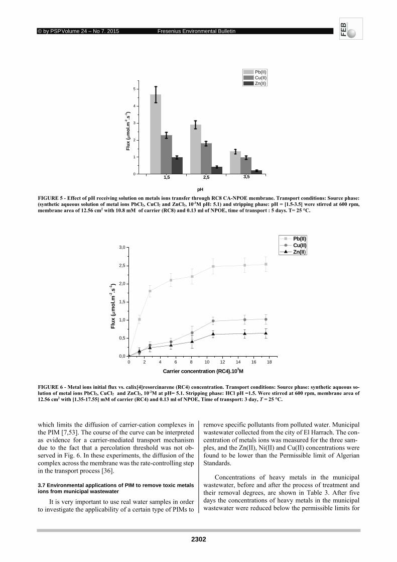
© by PSP Volume 24 – No 7. 2015 Fresenius Environmental Bulletin
2302
0
1
2
3
4
5
Flu
x (m
ol.m
-2.s
-1)
pH
Pb(II) Cu(II) Zn(II)
1,5 2,5 3,5
0 2 4 6 8 10 12 14 16 180,0
0,5
1,0
1,5
2,0
2,5
3,0
Flu
x (
mo
l.m-2.s
-1)
Carrier concentration (RC4).103M
Pb(II) Cu(II) Zn(II)
FIGURE 5 - Effect of pH receiving solution on metals ions transfer through RC8 CA-NPOE membrane. Transport conditions: Source phase: (synthetic aqueous solution of metal ions PbCl2, CuCl2 and ZnCl2, 10-3M pH: 5.1) and stripping phase: pH = [1.5-3.5] were stirred at 600 rpm, membrane area of 12.56 cm2 with 10.8 mM of carrier (RC8) and 0.13 ml of NPOE, time of transport : 5 days. T= 25 °C.
FIGURE 6 - Metal ions initial flux vs. calix[4]resorcinarene (RC4) concentration. Transport conditions: Source phase: synthetic aqueous so-lution of metal ions PbCl2, CuCl2 and ZnCl2, 10-2M at pH= 5.1. Stripping phase: HCl pH =1.5. Were stirred at 600 rpm, membrane area of 12.56 cm2 with [1.35-17.55] mM of carrier (RC4) and 0.13 ml of NPOE, Time of transport: 3 day, T = 25 °C.
which limits the diffusion of carrier-cation complexes in the PIM [7,53]. The course of the curve can be interpreted as evidence for a carrier-mediated transport mechanism due to the fact that a percolation threshold was not ob-served in Fig. 6. In these experiments, the diffusion of the complex across the membrane was the rate-controlling step in the transport process [36]. 3.7 Environmental applications of PIM to remove toxic metals ions from municipal wastewater
It is very important to use real water samples in order to investigate the applicability of a certain type of PIMs to
remove specific pollutants from polluted water. Municipal wastewater collected from the city of El Harrach. The con-centration of metals ions was measured for the three sam- ples, and the Zn(II), Ni(II) and Cu(II) concentrations were found to be lower than the Permissible limit of Algerian Standards.
Concentrations of heavy metals in the municipal
wastewater, before and after the process of treatment and their removal degrees, are shown in Table 3. After five days the concentrations of heavy metals in the municipal wastewater were reduced below the permissible limits for
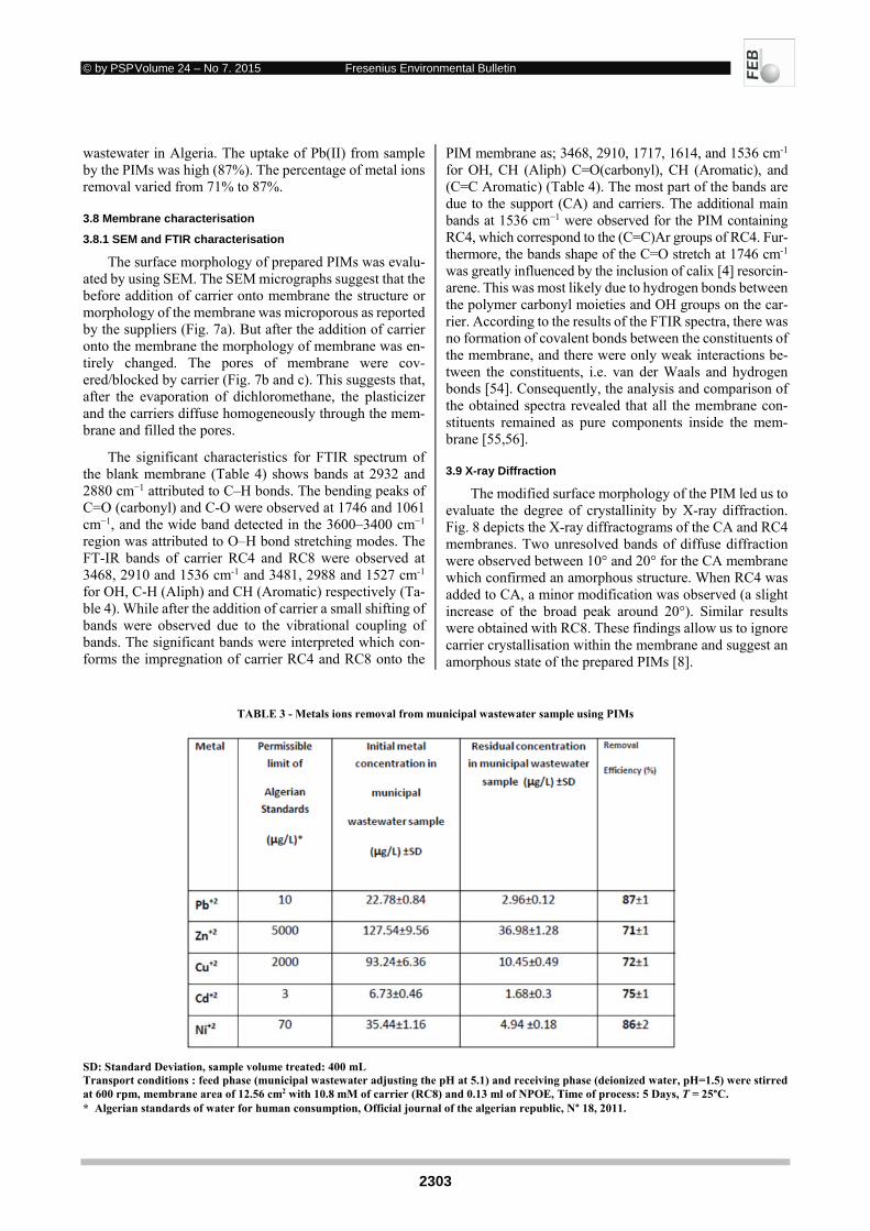
© by PSP Volume 24 – No 7. 2015 Fresenius Environmental Bulletin
2303
wastewater in Algeria. The uptake of Pb(II) from sample by the PIMs was high (87%). The percentage of metal ions removal varied from 71% to 87%.
3.8 Membrane characterisation
3.8.1 SEM and FTIR characterisation
The surface morphology of prepared PIMs was evalu-ated by using SEM. The SEM micrographs suggest that the before addition of carrier onto membrane the structure or morphology of the membrane was microporous as reported by the suppliers (Fig. 7a). But after the addition of carrier onto the membrane the morphology of membrane was en-tirely changed. The pores of membrane were cov-ered/blocked by carrier (Fig. 7b and c). This suggests that, after the evaporation of dichloromethane, the plasticizer and the carriers diffuse homogeneously through the mem-brane and filled the pores.
The significant characteristics for FTIR spectrum of the blank membrane (Table 4) shows bands at 2932 and 2880 cm−1 attributed to C–H bonds. The bending peaks of C=O (carbonyl) and C-O were observed at 1746 and 1061 cm−1, and the wide band detected in the 3600–3400 cm−1 region was attributed to O–H bond stretching modes. The FT-IR bands of carrier RC4 and RC8 were observed at 3468, 2910 and 1536 cm-1 and 3481, 2988 and 1527 cm-1 for OH, C-H (Aliph) and CH (Aromatic) respectively (Ta-ble 4). While after the addition of carrier a small shifting of bands were observed due to the vibrational coupling of bands. The significant bands were interpreted which con-forms the impregnation of carrier RC4 and RC8 onto the
PIM membrane as; 3468, 2910, 1717, 1614, and 1536 cm-1 for OH, CH (Aliph) C=O(carbonyl), CH (Aromatic), and (C=C Aromatic) (Table 4). The most part of the bands are due to the support (CA) and carriers. The additional main bands at 1536 cm−1 were observed for the PIM containing RC4, which correspond to the (C=C)Ar groups of RC4. Fur-thermore, the bands shape of the C=O stretch at 1746 cm-1 was greatly influenced by the inclusion of calix [4] resorcin-arene. This was most likely due to hydrogen bonds between the polymer carbonyl moieties and OH groups on the car-rier. According to the results of the FTIR spectra, there was no formation of covalent bonds between the constituents of the membrane, and there were only weak interactions be-tween the constituents, i.e. van der Waals and hydrogen bonds [54]. Consequently, the analysis and comparison of the obtained spectra revealed that all the membrane con-stituents remained as pure components inside the mem-brane [55,56].
3.9 X-ray Diffraction
The modified surface morphology of the PIM led us to evaluate the degree of crystallinity by X-ray diffraction. Fig. 8 depicts the X-ray diffractograms of the CA and RC4 membranes. Two unresolved bands of diffuse diffraction were observed between 10° and 20° for the CA membrane which confirmed an amorphous structure. When RC4 was added to CA, a minor modification was observed (a slight increase of the broad peak around 20°). Similar results were obtained with RC8. These findings allow us to ignore carrier crystallisation within the membrane and suggest an amorphous state of the prepared PIMs [8].
TABLE 3 - Metals ions removal from municipal wastewater sample using PIMs
SD: Standard Deviation, sample volume treated: 400 mL Transport conditions : feed phase (municipal wastewater adjusting the pH at 5.1) and receiving phase (deionized water, pH=1.5) were stirred at 600 rpm, membrane area of 12.56 cm2 with 10.8 mM of carrier (RC8) and 0.13 ml of NPOE, Time of process: 5 Days, T = 25°C. * Algerian standards of water for human consumption, Official journal of the algerian republic, N° 18, 2011.

© by PSP Volume 24 – No 7. 2015 Fresenius Environmental Bulletin
2304
(a) (b)
(c)
FIGURE 7 - Surface view of membranes. (a) CA ; (b) CA-RC4-NPOE ; (c) CA-RC8-NPOE.
TABLE 4 - FTIR characterization: absorption peak values and the corresponding moieties in CA membrane and PIMs.
Membrane Peak value (cm-1) Corresponding moietiesCA 3400-3600 O-H
2932 C-H ( CH3) 2880 C-H ( CH2) 1746 C=O 1253 C-O 1194 asym( C-O-C )
CA-NPOE Same bands and C-N
1372 1497 1554
C=C (NPOE) NO2 (NPOE)
CA-NPOT Same bands and C-N
1370 1495 1531
C=C (NPOT) NO2 (NPOT)
CA-NPOE-RC4 same bands and 1527
(C=C)Ar (RC4)
CA-NPOT-RC4 same bands and 1536
(C=C)Ar (RC4)

© by PSP Volume 24 – No 7. 2015 Fresenius Environmental Bulletin
2305
3.10 Thermal analysis (TGA) of PIMs
Fig. 9 shows the TGA curves of the CA, CA-NPOE and CA-NPOT membranes at a heating rate of 10 °C/min in N2. The thermal degradation of the CA membrane con-sisted of a series of degradation reactions, such as dehydra-tion at 100°C.
In order to investigate the heat resistance of CA+plas-
ticizer+carriers membranes, and then we then used thermo-gravimetric analyses (TGA) to link specific temperature and mass changes to the degradation of a specific com-pound. It should be noted that normally according to the results of the FTIR: there are not new covalent bands be-tween the carrier and polymer, thus in the membrane there
exist two aggregates: polymer CA and aggregates of the carrier solubilised in plasticizer, in theory the thermogram of the system (support-carrier+plastifiant) gives two losses of mass. This weight loss was mainly due to the evapora-tion of bonding water on the CA membrane. Thermal py-rolysis of cellulose acetate skeleton was found at ≈330°C.
In the case of the NPOE-CA membrane, weight loss
started at around 206°C, which was due in part to the NPOE, since the boiling temperature of NPOE is 198°C. At around 370°C, CA polymer degradation started. The PIM containing NPOT-CA showed a first weight loss at 215°C which was due in part to the NPOT, since the boil-ing temperature of NPOT is 200°C. In this case, CA poly-mer degradation started at 357°C [36].
FIGURE 8 - X ray diffractogramms of RC(4,8), CA membrane alone and PIMs.

© by PSP Volume 24 – No 7. 2015 Fresenius Environmental Bulletin
2306
FIGURE 9 - Thermogrammes of CA membrane alone, CA-NPOE membrane and CA-NPOT membrane
TABLE 5 - Chemical and physical characteristics of PIMs
Membrane Quantity (g) of carrier Weight (mg/cm2) Thickness (μm) Water content (%)
CA 0 4.30 18.83 37.37 CA-NPOE 0 5.36 23.60 13.98 CA-NPOT 0 5.29 20.43 10.86 CA-NPOE-RC4 0.015 5.81 25.17 11.90 CA-NPOT-RC4 0.015 5.67 21.40 09.56 CA-NPOE-RC8 0.013 5.73 28.91 10.78 CA-NPOT-RC8 0.013 5.43 23.43 09.10
FIGURE 10 - Fluxes in consecutive transport experiments performed on the PIM with RC8 and (NPOE/NPOT). Transport conditions: Source phase (synthetic aqueous solution of PbCl2: 10-3M, pH: 5.1) and stripping phase (deionized water, pH=1.5) were stirred at 600 rpm, membrane area of 12.56 cm2 with 10.8 mM of carrier (RC8) and 0.13 ml of (NPOE/NPOT), T = 25 °C.
3.11 Water content
Water content is used to investigate the hydrophilicity of the material surface, as shown in Table 5. When the ali-phatic chain length of calix[4]resorcinarene was increased in the PIM at a constant carrier concentration, a continuous decrease in the water content of the PIM was observed.
This phenomenon can be attributed to the enhanced hydro-phobic character of the PIM surface. A possible explana-tion of these results is the adsorption and/or inclusion pro-cess of the carrier molecules at the interface between air and the surface of the membrane. As the hydrophobic part of the molecular skeleton is oriented toward the air inter-
© by PSP Volume 24 – No 7. 2015 Fresenius Environmental Bulletin
2307
face, it is also possible that a hydrophobic PIM could re-pulse water molecules inside the membrane matrix. This means that embedding calix[4]resorcinarene with long ali-phatic chains into the CA matrix could create a membrane with greater hydrophobic content [37].
3.12 Stability of the PIM
The stability of the PIM was evaluated under the same conditions where the feed and strip phases were renewed every 24 h without changing the membrane. During the transport of Pb(II) ions through the PIM carried out for 24 h (first cycle), no decrease in transport efficiency was ob-served. However, when further transport experiments were carried out using the same membrane, it was observed that the PIM was stable during the first five cycles (Fig. 10). From the sixth cycle on, a remarkable decrease was ob-served, particularly after seven cycles, by approximately 20%, as shown in Fig. 10. The decrease in the stability of the membrane may have been caused by the partitioning of the carrier between the membrane and the aqueous solution [55]. Moreover, the stability of the PIM was influenced by the properties of plasticiser used in the PIM [36,57].
4. CONCLUSIONS
Homogeneous, transparent, and mechanically stable PIMs with CA as base polymer, NPOE/NPOT as plasti-ciser and calix[4]resorcinarene as carrier were prepared, and tested for their ability to extract Pb(II), Zn(II) and Cu(II) from their acidic aqueous solution. The optimal transport conditions were obtained at pH 5.1 in the feed phase and pH 1.5 in the receiving phase. The experiments demonstrated that the mechanism of metal ions transport by the PIM system occurred by facilitated counter-transport mechanism. Also, the optimal content of PIM was found to be 0.13 ml of plasticiser (NPOE) per 1.0 g of CA with 10.8 mM of calix[4]resorcinarene. The membrane has been reused for five consecutive cycles without apprecia-ble deterioration in performance, which showed the good stability. This work provides an opportunity to explore the efficiency of a PIMs system (with CA as base polymer, NPOE/NPOT as plasticiser and calix[4]resorcinarene as carrier) in treatment of municipal wastewater. Although, results clearly indicates the efficacy of PIMs system in wastewater treatment but further detailed studies are still required to answer few key issues of this system.
The authors have declared no conflict of interest. REFERENCES
[1] Sgarlata, C. Arena, G. Longo, E. Zhang, D. Yang, Y. R.A. and Bartsch, R.A. (2008) Heavy metal separation with pol-ymer inclusion membranes. J. Memb. Sci, 323,444-451.
[2] Salazar-Alvarez, G. Bautista-Flores, A.N. de San Miguel, E.R. Muhammed, M. and Gyves, J. (2005) Transport char-acterisation of a PIM system used for the extraction of Pb(II) using D2EHPA as carrier, J. Memb. Sci, 250, 247-257.
[3] Alguacil, F. J. Coedo, A. G. Dorado, M. T. and Padilla, I. (2001) Phosphine oxide mediate transport: modeling of mass transfer in supported liquid membrane transport of gold (III) using Cyanex923, Chem. Eng. Sci, 56,3115-3122.
[4] Boyadzhiev, L. Lazarova, Z. and Noble, R.D. Stern (Eds.), S.A., (1995) Membrane Separations Technology: Principles and Applications, Elsevier Science B.V,. pp. 28-300.
[5] Kocherginsky, N.M. Yang, Q. and Seelam, L. (2007) Recent advances in supported liquid membrane technology, Sep. Pur. Tech, 53, 171-177.
[6] Mohapatra, P.K., and Manchanda, V.K. (2003) Liquid mem-brane based separations of actinides and fission products, Ind. J. Chem., 42(A): 2925-2939.
[7] Bhattacharyya, A., Mohapatra, P.K., Hassan, P.A. and Manchanda, V.K. (2011) Studies on the selective Am3+ transport, irradiation stability and surface morphology of polymer inclusion membranes containing Cyanex-301 as carrier extractant, J. Hazard. Mat., 192: 116-123.
[8] Cherif, A.Y., Arous, O., Amara, M., Omeiri, S., Kerdjoudj, H., and Trari, M. (2012) Synthesis of modified polymer inclusion membranes for photo-electrodeposition of cadmium using po-larized electrodes, J. Hazard. Mat., 227-228: 386-393.
[9] Gherasim, Cristina-Veronica I. , Bourceanu, G., Olariu, R.I. and Arsene, C. (2011) A novel polymer inclusion membrane applied in chromium (VI) separation from aqueous solutions, J. Hazard. Mat., 197:244-253.
[10] Lamb, J. D,; West, J. N., Shaha, D. P. and Johnson, J. C. (2010) An evaluation of polymer inclusion membrane per-formance in facilitated transport with sequential membrane reconstitution, J. Memb. Sci., 365:256-259.
[11] Panja, S., Mohapatra, P.K., Tripathi, S.C. and Manchanda, V.K. (2011) Facilitated transport of uranium(VI) across sup-ported liquid membranes containing T2EHDGA as the car-rier extractant. J. Hazard. Mat., 188: 281-287.
[12] St John, A. M., Cattrall, R. W. and Kolev, S. D. (2012) Transport and separation of uranium(VI) by a polymer inclu-sion membrane based on di-(2-ethylhexyl) phosphoric acid. J. Memb. Sci., 409- 410:242-250.
[13] Raut, D.R., Kandwal, P., Rebello, G. and Mohapatra, P.K. (2012) Evaluation of polymer inclusion membranes contain-ing calix[4]-bis-2,3-naptho-crown-6 for Cs recovery from acidic feeds: Transport behavior, morphology and modeling studies. J. Memb. Sci., 407-408: 17-26.
[14] Radzyminska-Lenarcik, E. and Ulewicz, M. (2012) Selec-tive Transport of Cu(II) across a Polymer Inclusion Mem-brane with 1-Alkylimidazole from Nitrate Solutions, Sep. Sci. Tech., 47: 1113–1118.
[15] Zawierucha, I., Kozlowski, C. and Malina, G. (2013) Re-moval of toxic metal ions from landfill leachate by comple-mentary sorption and transport across polymer inclusion membranes. Waste Management., 33 :2129-2136.
[16] Nghiem, L.D., Mornane, P., Potter, I.D., Perera, J.M. and Cattrall, R.W.; Kolev, S.D. (2006) Extraction and transport of metal ions and small organic compounds using polymer inclusion membranes (PIMs ). J. Memb. Sci., 281:7-41.
[17] Crowley, M.M., Schroeder, B., Fredersdorf, A., Obara, S., Tal-arico, M., Kucera, S. and McGinity, J.W. (2004) Physico-chemical properties and mechanism of drug release from ethyl cellulose matrix tablets prepared by direct compression and hot-melt extrusion. Int. J. Pharm., 269:509-522.
© by PSP Volume 24 – No 7. 2015 Fresenius Environmental Bulletin
2308
[18] Heinze, T. and Liebert, T. (2004) Chemical characteristics of cellulose acetate. Macromolecule Symposium., 208:167-237.
[19] Klemn, D., Philipp, B., Heinze, T., Heinze, U. and Wagenknecht, W. (1998) Comprehensive Cellulose Chemis-try, vol. 1, Wiley-VCH, Weinheim.
[20] Klemm, D., Heublein, B., Fink, H. and Bohn, A. (2005) Cellulose: fascinating biopolymer and sustainable raw mate-rial, Angew. Chimie International Edition., 44: 3358-3393.
[21] Kosan, B., Michels, C. and Meister, F. (2005) Contribution to forming and analytical investigation of solution of cellu-lose and cellulose derivatives: a research and development topic of the TITK eV. Macromol. Symp., 223 :1-12.
[22] Li, X.G., Kresse, I., Xu, Z.K. and Springer, J. (2001) Effect of temperature and pressure on gas transport in ethyl cellu-lose membranes. Polymer., 42: 6801-6810.
[23] Zugenmaier, P. (2004) Characteristics of cellulose acetates: characterization and physical properties of cellulose ace-tates. Macromol. Symp., 208:81-166.
[24] Kutowy, O. and Sourirajan, S. (1975) Cellulose acetate ul-trafiltration membranes. J. Appl. Polym. Sci., 19 :1449-1460.
[25] Sivakumar, M., Malaisamy, R., Sajitha, C.J. , Mohan, D., Mohan, V. and Rangarajan, R. (1999) Ultrafiltration appli-cation of cellulose acetate–polyurethane blend membranes. Eur. Polym. J., 35 1647-1651.
[26] Sivakumar, M., Malaisamy, R., Sajitha, C.J., Mohan, D., Mohan, V. and Rangarajan, R. (2000) Preparation and per-formance of cellulose acetate–polyurethane blend membrane and their applications—II. J. Memb. Sci., 169: 215-228.
[27] Sivakumar, D.R.M. and Rangarajan, R. (2006) Studies on cel-lulose acetate–polysulfone ultrafiltration membranes. II. Effect of additive concentration. J. Memb. Sci., 268:208-219.
[28] Zavastin, I.D., Cretescu, M., Bezdadea, M., Bourceanu, M., Dr agana, G., Lisa, I., Mangalagiuc, V. and Savi, J. (2010) Preparation characterization and applicability of cellulose acetate–polyurethane blend membrane in separation tech-niques. Colloids Surfaces A: Physicochemical and Engineer-ing Aspect., 370: 120-128.
[29] Regel-Rosocka, M., Nowak, L. and Wisniewski, M. (2012) Removal of zinc(II) and iron ions from chloride solutions with phosphonium ionic liquids. Sep. Puri. Tech., 97: 158–163
[30] Valente, A.J.M., Polishchuk, A.Y., Burrows, H.D. and Lobo, V.M.M. (2005) Permeation of water as a tool for char-acterizing the effect of solvent, film thickness and water sol-ubility in cellulose acetate membranes. Eur. Polym.J., 41: 275-281.
[31] Buschmann, H.J., Cleve, E., Jansen, K., Wego, A. and Schollmeyer, E. (2001) The determination of complex sta-bilities between different cyclodextrins and dibenzo-l8-crown-6, cucurbit[6]uril, decamethylcucurbit[S]uril, cucur-bit-[5]uriluril, p-tert-butylcalix[4]arene and p-tertbutyl-calix[6]arene in aqueous solutions using a spectrophotomet-ric method. Mat. Sci. Eng C., 14: 35-39.
[32] Danil de Namor, F., Cleverley, R.M. and Zapata-Ormachea, M.L. (1998) Thermodynamics of calixarene chemistry,. Chem. Rev., 98:2495-2525.
[33] Ikeda, A. and Shinkai, S. (1997) Novel cavity design using calix[n]arene skeletons: Toward molecular recognition and metal binding. Chem. Rev., 97 1713-1734.
[34] Antipin, I., Stoikov, I.I., Pinkhassik, E.M., Fitseva, N.A., Stibor, I. and Konovalov, A.I. (1997) Calix[4]arene based a-aminophosphonates: Novel carriers for zwitterionic amino acids transport. Tetra. Lett., 33:5865-5868.
[35] Arnaud-Neu, F. and Schwing-Weill, M.J. (1997) Ca-lixarenes, new selective molecular receptors. Synthetic Met-als. 90:157-164.
[36] Benosmane, N., Hamdi, S.M., Hamdi, M. and Boutemeur, B. (2009) Selective transport of metal ions across polymer inclusion membranes (PIMs) containing calix[4]arenes. Sep. Pur. Tech., 65: 211- 219.
[37] Benosmane, N., Guedioura, B., Hamdi, S.M. , Hamdi, M. and Boutemeur, B. (2010) Preparation, characterization and thermal studies of polymer inclusion cellulose acetate mem-brane with calix[4]resorcinarenes as carriers. Mat. Sci. Eng C., 30 :860-867.
[38] Chang, S.K., Hwang, H.S., Son, H. , Youk, J. and Kang, Y.S. (1991) Selective transport of amino acid esters through a chloroform liquid membrane by a calix[6]arene-based ester carrier. J. Chem. Soc. Chem. Comm., 217-218.
[39] Chrisstoffels, L.A.J., Struijk, W., Jong, F. and Reinhoudt, D.N. (1996) Carrier mediated transport through supported liquid membranes; determination of transport parameters from a single transport experiment. J. Chem. Soc, Perkin Transactions., 1(2):1617-1622.
[40] Chung, T.D., Kang, S.K., Kim, J., Kim, H.S. and Kim, H. (1997) Interaction between various alkylammonium ions and quinone-derivatized calix[4]arenes in aprotic media. J. Elec.anal. Chem., 43871-78.
[41] Ulewicz, M., Lesinska, U., Bochenska, M. and Walkowiak, W. (2007) Facilitated transport of Zn(II), Cd(II) and Pb(II) ions through polymer inclusion membranes with calix[4]-crown-6 derivatives. Sep. Pur Tech., 54: 299-305.
[42] Hedidi, M., Hamdi, S. M., Mazari, T., Boutemeur, B., Rabia, C., Chemat, F. and Hamdi, M. (2006) Microwave-assisted syn-thesis of calix[4]resorcinarenes. Tetrahedron., 62 :5652-5655.
[43] Sugiura, M., Kikkawa, M. and Urita, S. (1987) Effect of plas-ticizer on carrier-mediated transport of zinc ions through cel-lulose triacetate membranes.Sep. Sci. Tech., 22: 2263-2268.
[44] Harrick, N.J. (1971) Determination of refractive index and film thickness from interference frings. Applied optics., 10 :2344-2349.
[45] Zhang, P., Yang, L.C., Li, L., Qu, Q.T., Wu, Y.P. and Shimizu, M. (2010) Effects of preparation conditions on po-rous polymer membranes by microwave assisted efferves-cent disintegrable reaction and their electrochemical proper-ties. J. Memb. Sci., 362: 113-118.
[46] Fedorenko, S.V. and Mustafina, A.R. (2001) Calix[4]resorcin-arene and alkylaminomethylated calix[4]resorcinarene-medi-ated transport of some metal complexes through chloroform bulky liquid membrane. Mat. Sci. Eng C., 18: 271-274.
[47] Sugiura, M. (1992) Effect of polyoxyethylene n-alkyl ethers on carrier mediated transport of lanthanide ions through cel-lulose triacetate membranes. Sep. Sci. Tech., 27: 269-276.
[48] De San Miguel, E.R., Aguilar, J.C. and De Gyves, J. (2008) Structural effects on metal ion migration across polymer in-clusion membranes: Dependence of transport profiles on na-ture of active plasticizer. J. Memb. Sci., 307 :105-116.
[49] Arous, O., Kerdjoudj, H. and Seta, P. (2004) Comparison of carrier-facilitated silver (i) and copper(ii) ions transport mech-anisms in a supported liquid membrane and in a plasticized cellulose triacetate membrane. J. Memb. Sci., 241 :177-185.
[50] Gherrou, A., Kerdjoudj, H., Molnari, R. and Seta, P. (2005) Preparation and characterization of polymeric plasticized membranes (PPM) embedding a crown ether carrier applica-tion to copper ions transport. Mat. Sci. Eng C., 25(4) :436-443.
© by PSP Volume 24 – No 7. 2015 Fresenius Environmental Bulletin
2309
[51] Pośpiech,B. (2012) Separation of Silver(I) and Copper(II) from Aqueous Solutions by Transport through Polymer In-clusion Membranes with Cyanex 471X. Sep. Sci. Tech., 47: 1413-1419.
[52] Konczyk, J., Kozlowski, C. and Walkowiak, W. (2010) Re-moval of chromium(III) from acidic aqueous solution by pol-ymer inclusion membranes with D2EHPA and Aliquat 336. Desalin., 263:211-216.
[53] Mohapatra, P.K., Pathak, P.N., Kelkar, A. and Manchanda, V.K. (2004) Novel polymer inclusion membrane containing a macrocyclic ionophore for selective removal of strontium from nuclear waste solution. N. J. Chem., 28 :1004-1009.
[54] Kebiche-Senhadji, O., Mansouri, L., Tingry, S., Seta, P. and Benamor, M. (2008) Facilitated Cd(II) transport across CTA polymer inclusion membrane using anion (Aliquat336) and cation (DE2HPA) metal carriers. J. Memb. Sci., 310:438-445.
[55] Bayou, N., Arous, O., Amara, M. and Kerdjoudj, H. (2010) Elaboration and characterization of a plasticized cellulose triacetate membrane containing trioctylphosphine oxyde (TOPO): application to the transport of uranium and molyb-denum ions. Comp. Rend. Chim., 13 :1370-1376.
[56] Kebiche-Senhadji, O., Tingry, S., Seta, P. and Benamor, M. (2010) Selective extraction of Cr(VI) over metallic species by polymer inclusion membrane (PIM) using anion (Aliquat 336) as carrier. Desalin., 258: 59-65.
[57] Scindia, Y.M., Pandey, A.K. and Reddy, A.V.R. (2005) Cou-pled-diffusion transport of Cr(VI) across anion-exchange membranes prepared by physical and chemical immobiliza-tion methods. J. Memb. Sci., 249:143-152.
Received: September 08, 2014 Revised: February 02, 2015 Accepted: February 19, 2015 CORRESPONDING AUTHORS
Nadjib Benosmane Departement of Chemistry Faculty of Sciences University M’Hame Bougara de Boumerdes (UMBB), Avenue de l’indépendance 35000, Boumerdes ALGERIA and Laboratoire de Chimie Organique Appliquée Faculty of Chemistry USTHB BP 32 El-Alia 16111 Alger ALGERIA E-mail: [email protected] Baya Boutemeur Laboratoire de Chimie Organique Appliquée Faculty of Chemistry USTHB BP 32 El-Alia 16111, Alger ALGERIA E-mail: [email protected]
FEB/ Vol 24/ No 7/ 2015 – pages 2296 - 2309
© by PSP Volume 24 – No 7. 2015 Fresenius Environmental Bulletin
2310
IN VITRO ANTIOXIDANT POTENTIAL OF para-ALKOXY-
PHENYLCARBAMIC ACID ESTERS CONTAINING 4-(4-FLUORO-
/3-TRIFLUOROMETHYLPHENYL)PIPERAZIN-1-YL MOIETY
Ivan Malík1,*, Jan Muselík2, Lukáš Stanzel1, Jozef Csöllei3 and Matej Maruniak1
1Department of Pharmaceutical Chemistry, Faculty of Pharmacy, Comenius University, Bratislava, Slovak Republic 2Department of Pharmaceutics, Faculty of Pharmacy, University of Veterinary and Pharmaceutical Sciences, Brno, Czech Republic
3Department of Chemical Drugs, Faculty of Pharmacy, University of Veterinary and Pharmaceutical Sciences, Brno, Czech Republic
ABSTRACT
Antioxidant properties of certain β-adrenoceptor block-ing agents (β-ABAs) may provide their significant benefit in the therapy of cardiovascular diseases. Considering men-tioned, the potential of original β-ABAs, para-alkoxy-phenylcarbamic acid esters 6i–6l and 8f–8i with incorpo-rated 4-(4-fluoro- or 3-trifluoromethylphenyl)piperazin-1--yl fragment, to reduce stable 2,2-diphenyl-1-picrylhydra-zyl radical (DPPH•) applying UV/VIS spectrophotometry and to scavenge peroxynitrite ions (ONOO–) using HPLC method, has been in vitro investigated. It has been observed that para-position of attached alkoxy group has appeared to be most suitable for antioxidative efficiency. The in-crease in lipophilicity in homological series 6i–6l and 8f–8i could be regarded as important but it has been questiona-ble whether principal factor in terms of capabilities of these esters being effective reductants of DPPH• and the ONOO– scavengers as well. From entire evaluated set, para-meth-oxy substituted molecule 6i has been able to reduce refer-ence DPPH• most markedly. The in vitro experiments have also revealed the most pronounced ONOO– scavenging po-tential of para-propoxy substituted compound 8h.
KEYWORDS: β-adrenoceptor antagonists, antioxidant efficiency, positional isomerism
1. INTRODUCTION
In clinical practice, β-adrenoceptor blocking agents (β--ABAs) have shown several beneficial cardiovascular con-tributions to patients with hypertension, angina pectoris or myocardial infarction [1]. It has been reported that part of carvedilol´s effects, a lipophilic third-generation non-se-lective vasodilating β-ABA [2], might be related to the re-duction of myocardial oxygen demand and cardiac workout as a result of β-adrenoceptor blockade. In addition, notable
* Corresponding author
antioxidant properties of concerned compound and the im-pacts on cardiac remodeling could be also responsible for its final beneficial outcome [3]. The potency of carvedilol to in-hibit reactive oxygen-derived free radicals might also be rel-evant in heart failure therapy [4-6].
As shown in Figure 1, chemical structure of carvedilol consists of some fundamental parts: (i) lipophilic carbazole moiety (the substituent R) which is responsible for antioxi-dant properties, (ii) etheric oxygen directly connected to 2-hydroxypropane-1,3-diyl chain which is essential for the β-blockade and (iii) basic fragment (guaiacoxyethylamino group) which primarily invokes blocking ability on α-adre-noceptors resulting in moderate vasodilator properties of considered molecule [7, 8].
During past two decades, in vitro and in vivo antioxidant potency of various third-generation non-selective β-blockers with both β1- and β2-adrenoceptor as well as α1-adrenergic receptor blocking activities have been investigated [9, 10]. These compounds (Figure 1), namely ferulidilol which was derived from ferulic acid and isoeugenodilol which was de-rived from isoeugenol, isoform of eugenol, have contained lipophilic vanilloid base. The modification of lipophilic and salt forming compartments and isosteric replacement of po-lar etheric bridge by carbamoyloxy moiety has led to the class of presently investigated para-alkoxyphenylcarbamic acid derivatives 6i–8i (Table 1).
Concerning legislative complexity which has been con-nected with preparation and realization of pharmacological experiments focused on the ability of inspected derivatives to influence the functions of cardiovascular system, it has been possible to investigate relatively narrow group of the compounds. Preliminary pharmacological evaluation has in-dicated the ability of some molecules from the set 6 to pro-tect heart against extrasystoles, fibrillations and heart failure exceeding the effect of propaphenone [11]. Following phar-macological screening of the compound 6j [12], it has been suggested that an incorporation of carbamoyloxy group has not significantly influenced its β-adrenolytic activity com-pared to original aryloxyaminopropanols. Moreover, its ability to in vitro inhibit contractibility of aortal strips and

© by PSP Volume 24 – No 7. 2015 Fresenius Environmental Bulletin
2311
to decrease a blood pressure in normotensive and hyperten-sive rats has enabled to consider 6j as a proper representa-tive of potential antihypertensives [12]. Fundamental prop-erty of β-ABAs to antagonize the influence of β-sympatho-mimetics has been in vitro evaluated for the compound 6j [12] and 6k [11], respectively. The experiments have been based on the molecules´ characteristics to specifically block positively chronotropic effect of isoprenaline. The estimated value of pA2 for 6j was 7.9 and for 6k was 9.2 which indicated their notable anti-isoprenaline (β-adrenolytic) efficiency [11, 12].
Outlined backgrounds have motivated current research to explore whether any of above mentioned compounds 6i–8i could be also antioxidants under in vitro conditions.
2. MATERIAL AND METHODS
2.1 Synthesis and physicochemical parameters determination of the compounds under the study
Preparation of currently evaluated compounds 6i–6l and 8f–8i (Table 1), chemically 1-[3-(4-alkoxyphenylcar-bamoyloxy)-2-hydroxypropyl]-4-(4-fluoro-/3-trifluoro-methylphenyl)piperazinium chlorides (where alkoxy= methoxy to butoxy group), their spectral characteristics and elemental analyses data have already been pub-lished [13, 14].
Determination of some physicochemical parameters of these molecules, i.e. solubility profile, dissociation con-stant pKa and lipophilicity descriptors (the log Pexps esti-mated by shake-flask method in the octan-1-ol/buffer me-dium with pH=7.3, the log k´s from RP-HPLC, the RMs from RP-TLC), with corresponding readouts can be found in research papers [13-16].
Other compounds, which have been used in carried in vitro experiments, were purchased: tyrosine (BDH Chemi-cals, United Kingdom), 3-nitrotyrosine (Sigma-Aldrich, Ger-many), carvedilol (Sigma-Aldrich, Germany) and Trolox, chemically (±)-6-hydroxy-2,5,7,8-tetramethylchromane--2-carboxylic acid (Fluka Chemie, Switzerland). All these chemicals were of an analytical grade.
2.2 2,2-Diphenyl-1-picrylhydrazyl (DPPH) Radical Reduction Assay
Free radical reduction ability of tested compounds was determined with the DPPH assay by following the proce-dure described in research articles of Malík et al. [17] and Masteiková et al. [18]. The solution (200 µL) of par-ticular compound dissolved in ethylene glycol monomethyl ether (c=0.1 mg·mL–1) was made up to 2.0 mL with meth-anolic solution of DPPH (c=0.1 mmol·L–1), one of a few sta-ble organic nitrogen radicals with strong visible absorption [19]. After 5 min, the absorbance value was measured at the wavelength of 517 nm using the UV/VIS spectrophotometer HP 8453 (Hewlett Packard, USA). Decrease in the absorb-ance of respected DPPH solution has indicated increase in DPPH radical (DPPH•) scavenging effect [19, 20].
Reduction of DPPH• was calculated relatively to the measured absorbance of control as means ± standard devi-ation (SD) of three parallel measurements according to the equation given below:
1001%
control
sample
A
ADPPH
where: %DPPH – the percentage of the DPPH reduc-tion; Asample – the absorbance at 517 nm; Acontrol – the ab-sorbance at 517 nm in control measurement.
TABLE 1 – The potential of evaluated compounds 6i–8i to reduce DPPH radicals (%DPPH) and to protect tyrosine from peroxynitrite mediated nitration (%INH).
Entry R1 R2 log Pexpa %DPPH %INH
6i OCH3 4´-F 3.42 7.7 ± 0.2 -8.5 ± 0.3 6j OC2H5 4´-F 3.28 5.3 ± 0.3 -10.4 ± 0.3 6k OC3H7 4´-F 3.12 7.1 ± 0.2 -11.7 ± 0.4 6l OC4H9 4´-F 3.54 7.2 ± 0.2 -10.0 ± 0.2
8f OCH3 3´-CF3 3.60 1.2 ± 0.2 2.4 ± 0.3
8g OC2H5 3´-CF3 3.71 0.9 ± 0.1 -0.1 ± 0.2 8h OC3H7 3´-CF3 3.92 1.0 ± 0.1 3.6 ± 0.2 8i OC4H9 3´-CF3 3.98 1.0 ± 0.1 -1.3 ± 0.3
Carvedilol – – – 15.4 ± 0.2 0.8± 0.5 Trolox – – – 94.7 ± 0.3 51.3 ± 0.2
a The log Pexp readouts of investigated compounds have been adopted from the article [15]
NNHN O
O
OH
.
R2
R1
H
Cl

© by PSP Volume 24 – No 7. 2015 Fresenius Environmental Bulletin
2312
FIGURE 1 – Chemical structure of some non-selective α-/β-adrenoceptor blocking agents which have shown antioxidant properties.
2.3 Peroxynitrite Scavenging Potential
2.3.1 Preparation of Solutions
Peroxynitrite solution was prepared by applying previ-ously published method [21]. Aliquots of H2O2 (c=0.6 mol·L–1) dissolved in HClO4 (c=0.5 mol·L–1) and NaNO2 (c=0.5 mol·L–1) in water (10 mL each) were pre-cooled to -2 °C and rapidly mixed. The reaction was quenched imme-diately by an addition of 5 mL cold NaOH (c=3.5 mol·L–1). Unreacted H2O2 was removed by a treatment with an excess of MnO2 and the solution was filtered. The concentration of ONOO ions was determined spectrophotometrically in al-kaline solution using 302=1670 L·mol1·cm1. The stock so-lutions were stored frozen at -80 °C for several months with-out noticeable decomposition.
The volume of 8 μL of prepared peroxynitrite solution (c=15 mmol·L–1) in NaOH (c=50 mmol·L–1) was drawn and rapidly mixed in the injector of HPLC autosampler with 42 μL of tyrosine solution (c=1.0 mmol·L–1) in 80 mmol·L–1 KH2PO4–Na2HPO4 buffer (pH=6.0) containing 0.25 mmol· L–1 of tested compound and ethylene glycol monomethyl ether (in a 1:1 ratio with water solution).
2.3.2 Peroxynitrite Scavenging Assay Using HPLC System
The reaction mixture was directly injected into the HPLC system HP 1100 with autosampler, quaternary pump and diode-array detector (Agilent Technologies, USA). The separation was carried out with Supelcosil ABZ + Plus col-umn (250 × 4.6 mm, 5 μm particle size; Supelco, USA),
column temperature was set to 25 °C, mobile phase con-sisted of 90 % HCOOH (c=40 mmol·L–1) and 10 % CH3CN (v/v) at a flow rate of 1 mL·min–1. Chromatograms were detected at the wavelength of 276 ± 20 nm against reference wavelength of 600 ± 100 nm.
The activity of inspected compounds (including refer-ence drugs) was calculated relative to the measured 3-ni-trotyrosine peak area of the control as means ± standard deviation (SD) of three parallel measurements according following equation:
1001%
control
sample
AUC
AUCINH
where: %INH – the percentage of inhibition of tyrosine nitration; AUCsample – the area under curve of 3-nitrotyro-sine peak; AUCcontrol – the area under curve of 3-nitrotyro-sine peak in control measurement.
The percentage of inhibition of tyrosine nitration was compared to that of the Trolox standard.
3. RESULTS AND DISCUSSION
In this study, both in vitro antioxidant tests, i.e. the DPPH radical reduction assay and the peroxynitrite scav-enging evaluation, were used to examine, compare and ex-plain (i) differences in the potency of para-alkoxyphenyl-
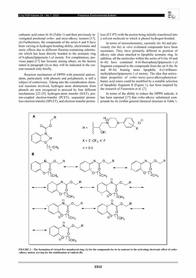
© by PSP Volume 24 – No 7. 2015 Fresenius Environmental Bulletin
2313
carbamic acid esters 6i–8i (Table 1) and their previously in-vestigated positional ortho- and meta-alkoxy isomers [17]. (ii) Furthermore, the compounds of the series 6 and 8 have been varying in hydrogen bonding ability, electrostatic and steric effects due to different fluorine-containing substitu-ent which has been directly bonded to the aromatic ring of 4-(phenyl)piperazin-1-yl moiety. For completeness, pre-vious paper [17] has focused, among others, on the factors stated in paragraph (ii) so they will be indicated in the cur-rent research only briefly.
Reaction mechanism of DPPH with potential antioxi-dants, particularly with phenols and polyphenols, is still a subject of controversy. Taking into the consideration chem-ical reactions involved, hydrogen atom abstractions from phenols are now recognized to proceed by four different mechanisms [22-25]: hydrogen-atom transfer (HAT), pro-ton-coupled electron-transfer (PCET), sequential proton-loss electron transfer (SPLET), and electron-transfer proton-
loss (ET-PT) with the proton being initially transferred into a solvent molecule to which is phenol hydrogen-bonded.
In terms of stereochemistry, currently (6i–8i) and pre-viously (6a–8e) in vitro evaluated compounds have been racemates. They have primarily differed in position of alkoxy side chain attached to lipophilic aromatic ring. In addition, all the molecules within the series of 6 (6a–6f and 6i–6l) have contained 4-(4-fluorophenyl)piperazin-1-yl fragment compared to the compounds from the set 8 (8a–8e and 8f–8i) bearing more lipophilic 4-(3-trifluoro-methylphenyl)piperazin-1-yl moiety. The idea that antiox-idant properties of ortho-/meta-/para-alkoxyphenylcar-bamic acid esters could be modified by a suitable selection of lipophilic fragment R (Figure 1), has been inspired by the research of Feuerstein et al. [7].
In terms of the ability to reduce the DPPH radicals, it has been reported [17] that ortho-alkoxy substituted com-pounds 6a–6c (within general chemical structure in Table 1,
FIGURE 2 – The formation of virtual five-membered ring (A) for the compounds 6a–6c in contrast to the activating electronic effect of ortho--alkoxy moiety serving for the stabilization of radical (B).
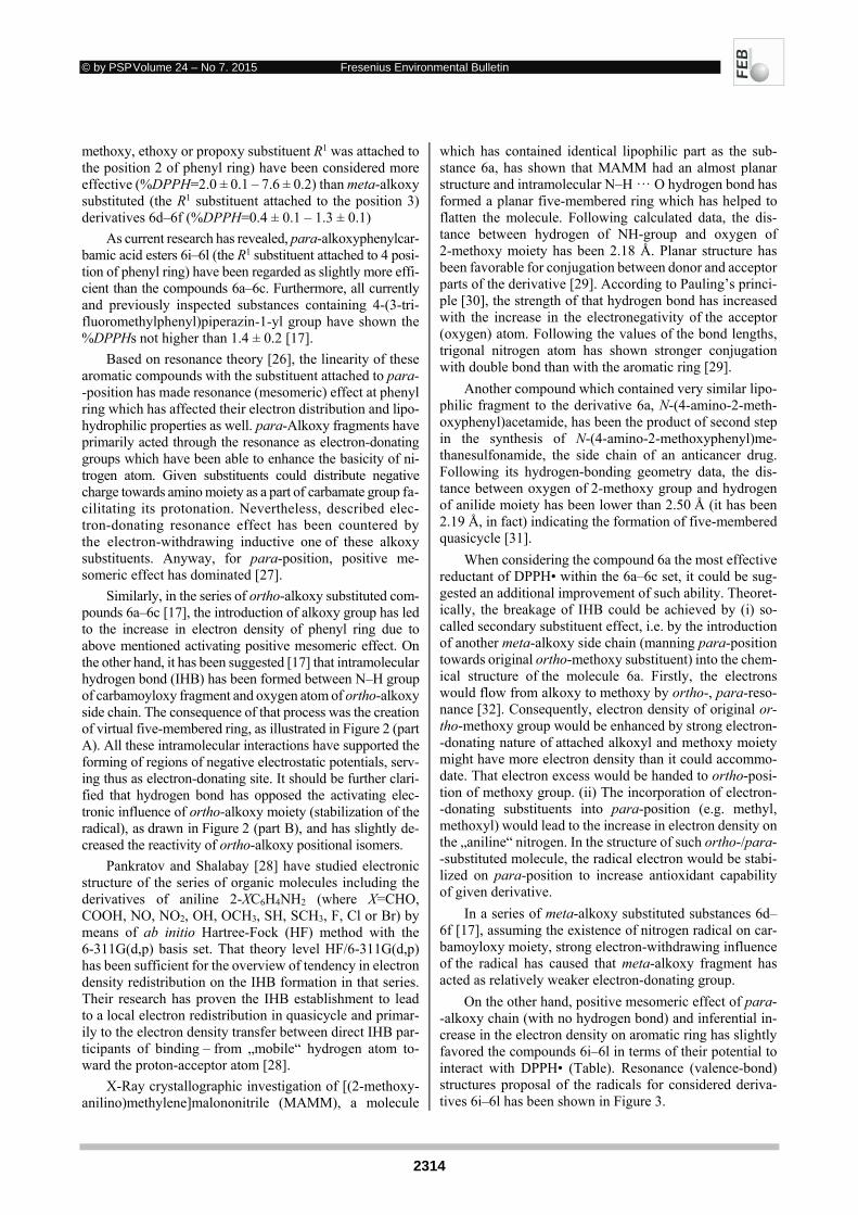
© by PSP Volume 24 – No 7. 2015 Fresenius Environmental Bulletin
2314
methoxy, ethoxy or propoxy substituent R1 was attached to the position 2 of phenyl ring) have been considered more effective (%DPPH=2.0 ± 0.1 – 7.6 ± 0.2) than meta-alkoxy substituted (the R1 substituent attached to the position 3) derivatives 6d–6f (%DPPH=0.4 ± 0.1 – 1.3 ± 0.1)
As current research has revealed, para-alkoxyphenylcar-bamic acid esters 6i–6l (the R1 substituent attached to 4 posi-tion of phenyl ring) have been regarded as slightly more effi-cient than the compounds 6a–6c. Furthermore, all currently and previously inspected substances containing 4-(3-tri-fluoromethylphenyl)piperazin-1-yl group have shown the %DPPHs not higher than 1.4 ± 0.2 [17].
Based on resonance theory [26], the linearity of these aromatic compounds with the substituent attached to para--position has made resonance (mesomeric) effect at phenyl ring which has affected their electron distribution and lipo-hydrophilic properties as well. para-Alkoxy fragments have primarily acted through the resonance as electron-donating groups which have been able to enhance the basicity of ni-trogen atom. Given substituents could distribute negative charge towards amino moiety as a part of carbamate group fa-cilitating its protonation. Nevertheless, described elec-tron-donating resonance effect has been countered by the electron-withdrawing inductive one of these alkoxy substituents. Anyway, for para-position, positive me-someric effect has dominated [27].
Similarly, in the series of ortho-alkoxy substituted com-pounds 6a–6c [17], the introduction of alkoxy group has led to the increase in electron density of phenyl ring due to above mentioned activating positive mesomeric effect. On the other hand, it has been suggested [17] that intramolecular hydrogen bond (IHB) has been formed between N–H group of carbamoyloxy fragment and oxygen atom of ortho-alkoxy side chain. The consequence of that process was the creation of virtual five-membered ring, as illustrated in Figure 2 (part A). All these intramolecular interactions have supported the forming of regions of negative electrostatic potentials, serv-ing thus as electron-donating site. It should be further clari-fied that hydrogen bond has opposed the activating elec-tronic influence of ortho-alkoxy moiety (stabilization of the radical), as drawn in Figure 2 (part B), and has slightly de-creased the reactivity of ortho-alkoxy positional isomers.
Pankratov and Shalabay [28] have studied electronic structure of the series of organic molecules including the derivatives of aniline 2-XC6H4NH2 (where X=CHO, COOH, NO, NO2, OH, OCH3, SH, SCH3, F, Cl or Br) by means of ab initio Hartree-Fock (HF) method with the 6-311G(d,p) basis set. That theory level HF/6-311G(d,p) has been sufficient for the overview of tendency in electron density redistribution on the IHB formation in that series. Their research has proven the IHB establishment to lead to a local electron redistribution in quasicycle and primar-ily to the electron density transfer between direct IHB par-ticipants of binding – from „mobile“ hydrogen atom to-ward the proton-acceptor atom [28].
X-Ray crystallographic investigation of [(2-methoxy-anilino)methylene]malononitrile (MAMM), a molecule
which has contained identical lipophilic part as the sub-stance 6a, has shown that MAMM had an almost planar structure and intramolecular N–H ··· O hydrogen bond has formed a planar five-membered ring which has helped to flatten the molecule. Following calculated data, the dis-tance between hydrogen of NH-group and oxygen of 2-methoxy moiety has been 2.18 Å. Planar structure has been favorable for conjugation between donor and acceptor parts of the derivative [29]. According to Pauling’s princi-ple [30], the strength of that hydrogen bond has increased with the increase in the electronegativity of the acceptor (oxygen) atom. Following the values of the bond lengths, trigonal nitrogen atom has shown stronger conjugation with double bond than with the aromatic ring [29].
Another compound which contained very similar lipo-philic fragment to the derivative 6a, N-(4-amino-2-meth-oxyphenyl)acetamide, has been the product of second step in the synthesis of N-(4-amino-2-methoxyphenyl)me-thanesulfonamide, the side chain of an anticancer drug. Following its hydrogen-bonding geometry data, the dis-tance between oxygen of 2-methoxy group and hydrogen of anilide moiety has been lower than 2.50 Å (it has been 2.19 Å, in fact) indicating the formation of five-membered quasicycle [31].
When considering the compound 6a the most effective reductant of DPPH• within the 6a–6c set, it could be sug-gested an additional improvement of such ability. Theoret-ically, the breakage of IHB could be achieved by (i) so-called secondary substituent effect, i.e. by the introduction of another meta-alkoxy side chain (manning para-position towards original ortho-methoxy substituent) into the chem-ical structure of the molecule 6a. Firstly, the electrons would flow from alkoxy to methoxy by ortho-, para-reso-nance [32]. Consequently, electron density of original or-tho-methoxy group would be enhanced by strong electron--donating nature of attached alkoxyl and methoxy moiety might have more electron density than it could accommo-date. That electron excess would be handed to ortho-posi-tion of methoxy group. (ii) The incorporation of electron- -donating substituents into para-position (e.g. methyl, methoxyl) would lead to the increase in electron density on the „aniline“ nitrogen. In the structure of such ortho-/para--substituted molecule, the radical electron would be stabi-lized on para-position to increase antioxidant capability of given derivative.
In a series of meta-alkoxy substituted substances 6d–6f [17], assuming the existence of nitrogen radical on car-bamoyloxy moiety, strong electron-withdrawing influence of the radical has caused that meta-alkoxy fragment has acted as relatively weaker electron-donating group.
On the other hand, positive mesomeric effect of para--alkoxy chain (with no hydrogen bond) and inferential in-crease in the electron density on aromatic ring has slightly favored the compounds 6i–6l in terms of their potential to interact with DPPH• (Table). Resonance (valence-bond) structures proposal of the radicals for considered deriva-tives 6i–6l has been shown in Figure 3.
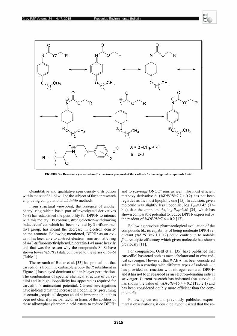
© by PSP Volume 24 – No 7. 2015 Fresenius Environmental Bulletin
2315
FIGURE 3 – Resonance (valence-bond) structures proposal of the radicals for investigated compounds 6i–6l.
Quantitative and qualitative spin density distribution within the set of 6i–6l will be the subject of further research employing computational ab initio methods.
From structural viewpoint, the presence of another phenyl ring within basic part of investigated derivatives 6i–8i has established the possibility for DPPH• to interact with this moiety. By contrast, strong electron-withdrawing inductive effect, which has been invoked by 3-trifluorome-thyl group, has meant the decrease in electron density on the aromate. Following mentioned, DPPH• as an oxi-dant has been able to abstract electron from aromatic ring of 4-(3-trifluoromethylphenyl)piperazin-1-yl more heavily and that was the reason why the compounds 8f–8i have shown lower %DPPH data compared to the series of 6i–6l (Table 1).
The research of Butler et al. [33] has pointed out that carvedilol´s lipophilic carbazole group (the R substituent in Figure 1) has played dominant role in bilayer perturbation. The combination of specific chemical structure of carve-dilol and its high lipophilicity has appeared as required for carvedilol´s antioxidant potential. Current investigations have indicated that the increase in lipophilicity (presuming its certain „requisite“ degree) could be important, but it has been not clear if principal factor in terms of the abilities of these alkoxyphenylcarbamic acid esters to reduce DPPH•
and to scavenge ONOO– ions as well. The most efficient methoxy derivative 6i (%DPPH=7.7 ± 0.2) has not been regarded as the most lipophilic one [15]. In addition, given molecule was slightly less lipophilic, log Pexp=3.42 (Ta-ble), than the compound 6a, log Pexp=3.61 [34], which has shown comparable potential to reduce DPPH• expressed by the readout of %DPPH=7.6 ± 0.2 [17].
Following previous pharmacological evaluation of the compounds 6k, its capability of being moderate DPPH re-ductant (%DPPH=7.1 ± 0.2) could contribute to notable β-adrenolytic efficiency which given molecule has shown previously [11].
For comparison, Oettl et al. [35] have published that carvedilol has acted both as metal chelator and in vitro rad-ical scavenger. However, that β-ABA has been considered selective in a reacting with different types of radicals – it has provided no reaction with nitrogen-centered DPPH• and it has not been regarded as an electron-donating radical scavenger. Current research has indicated that carvedilol has shown the value of %DPPH=15.4 ± 0.2 (Table 1) and has been considered doubly more efficient than the com-pound 6k.
Following current and previously published experi-mental observations, it could be hypothesized that the re-
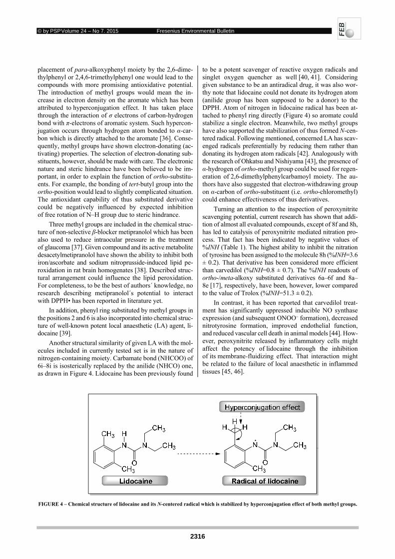
© by PSP Volume 24 – No 7. 2015 Fresenius Environmental Bulletin
2316
placement of para-alkoxyphenyl moiety by the 2,6-dime-thylphenyl or 2,4,6-trimethylphenyl one would lead to the compounds with more promising antioxidative potential. The introduction of methyl groups would mean the in-crease in electron density on the aromate which has been attributed to hyperconjugation effect. It has taken place through the interaction of σ electrons of carbon-hydrogen bond with π-electrons of aromatic system. Such hypercon-jugation occurs through hydrogen atom bonded to α-car-bon which is directly attached to the aromate [36]. Conse-quently, methyl groups have shown electron-donating (ac-tivating) properties. The selection of electron-donating sub-stituents, however, should be made with care. The electronic nature and steric hindrance have been believed to be im-portant, in order to explain the function of ortho-substitu-ents. For example, the bonding of tert-butyl group into the ortho-position would lead to slightly complicated situation. The antioxidant capability of thus substituted derivative could be negatively influenced by expected inhibition of free rotation of N–H group due to steric hindrance.
Three methyl groups are included in the chemical struc-ture of non-selective β-blocker metipranolol which has been also used to reduce intraocular pressure in the treatment of glaucoma [37]. Given compound and its active metabolite desacetylmetipranolol have shown the ability to inhibit both iron/ascorbate and sodium nitroprusside-induced lipid pe-roxidation in rat brain homogenates [38]. Described struc-tural arrangement could influence the lipid peroxidation. For completeness, to be the best of authors´ knowledge, no research describing metipranolol´s potential to interact with DPPH• has been reported in literature yet.
In addition, phenyl ring substituted by methyl groups in the positions 2 and 6 is also incorporated into chemical struc-ture of well-known potent local anaesthetic (LA) agent, li-docaine [39].
Another structural similarity of given LA with the mol-ecules included in currently tested set is in the nature of nitrogen-containing moiety. Carbamate bond (NHCOO) of 6i–8i is isosterically replaced by the anilide (NHCO) one, as drawn in Figure 4. Lidocaine has been previously found
to be a potent scavenger of reactive oxygen radicals and singlet oxygen quencher as well [40, 41]. Considering given substance to be an antiradical drug, it was also wor-thy note that lidocaine could not donate its hydrogen atom (anilide group has been supposed to be a donor) to the DPPH. Atom of nitrogen in lidocaine radical has been at-tached to phenyl ring directly (Figure 4) so aromate could stabilize a single electron. Meanwhile, two methyl groups have also supported the stabilization of thus formed N-cen-tered radical. Following mentioned, concerned LA has scav-enged radicals preferentially by reducing them rather than donating its hydrogen atom radicals [42]. Analogously with the research of Ohkatsu and Nishiyama [43], the presence of α-hydrogen of ortho-methyl group could be used for regen-eration of 2,6-dimethylphenylcarbamoyl moiety. The au-thors have also suggested that electron-withdrawing group on α-carbon of ortho-substituent (i.e. ortho-chloromethyl) could enhance effectiveness of thus derivatives.
Turning an attention to the inspection of peroxynitrite scavenging potential, current research has shown that addi-tion of almost all evaluated compounds, except of 8f and 8h, has led to catalysis of peroxynitrite mediated nitration pro-cess. That fact has been indicated by negative values of %INH (Table 1). The highest ability to inhibit the nitration of tyrosine has been assigned to the molecule 8h (%INH=3.6 ± 0.2). That derivative has been considered more efficient than carvedilol (%INH=0.8 ± 0.7). The %INH readouts of ortho-/meta-alkoxy substituted derivatives 6a–6f and 8a–8e [17], respectively, have been, however, lower compared to the value of Trolox (%INH=51.3 ± 0.2).
In contrast, it has been reported that carvedilol treat-ment has significantly uppressed inducible NO synthase expression (and subsequent ONOO– formation), decreased nitrotyrosine formation, improved endothelial function, and reduced vascular cell death in animal models [44]. How-ever, peroxynitrite released by inflammatory cells might affect the potency of lidocaine through the inhibition of its membrane-fluidizing effect. That interaction might be related to the failure of local anaesthetic in inflammed tissues [45, 46].
FIGURE 4 – Chemical structure of lidocaine and its N-centered radical which is stabilized by hyperconjugation effect of both methyl groups.

© by PSP Volume 24 – No 7. 2015 Fresenius Environmental Bulletin
2317
4. CONCLUSIONS
Major novel findings of current study has been that the potency of evaluated compounds 6i–8i has been closely connected with the position of alkoxy side chain at-tached to phenylcarbamoyloxy fragment. In regard to posi-tional isomerism and electronic effects, it seemed that para-alkoxy substitution as well as the selection of the sub-stituents with electron-donating and suitable steric proper-ties has contributed most positively to the reduction effect of investigated compounds towards DPPH•. It has been provided that bonding of short alkoxy group has been more favorable than the presence of prolonged side chain. These structural features have notably influenced such effective-ness together with balanced lipohydrophilic properties. Current experimental observations have also shown that the introduction of strongly electron-withdrawing substitu-ent, i.e. 3-trifluoromethyl group, to 4-(substituted phe-nyl)piperazin-1-yl has provided slightly better prospect to scavenge ONOO– ions than the incorporation of 4-fluoro substituent.
ACKNOWLEDGEMENTS
The authors thank the anonymous reviewers for their valuable comments and helpful revision suggestions.
The authors have declared no conflict of interest. REFERENCES
[1] Mak, I.T. and Weglicki, W.B. (2004) Potent antioxidant properties of 4-hydroxyl-propranolol. J. Pharmacol. Exp. Ther. 308, 85-90.
[2] Bristow, M.R., Larrabee, P., Minobe, W., Roden, R., Skerl, L., Klein, J., Handwerger, D., Port, J.D. and Müller-Beckmann, B. (1992) Receptor pharmacology of carvedilol in the human heart. J. Cardiovasc. Pharmacol. 19 (Suppl. 1), S68-S80.
[3] Yue, T.-L., Cheng, H.Y., Lysko, P.G., McKenna, P.J., Feuerstein, R., Gu, J.L., Lysko, K.A., Davies, L.L. and Feuerstein, G.Z. (1992) Carvedilol, a new vasodilator and beta adrenoreceptor antagonist, is an antioxidant and free radical scavenger. J. Pharmacol. Exp. Ther. 263, 92-98.
[4] Chin, B.S.P., Langford, N.J., Nuttall, S.L., Gibbs, Ch.R., Blann, A.D. and Lip, G.Y.H. (2003) Anti-oxidative properties of beta-blockers and angiotensin-converting enzyme inhibitors in congestive heart failure. Eur. J. Heart Fail. 5, 171-174.
[5] Gilbert, E.M., Abraham, W.T., Olsen, S., Hattler, B., White, M., Mealy, P., Larrabee, P. and Bristow, M.R. (1996) Comparative he-modynamic, left ventricular functional, and antiadrenergic effects of chronic treatment with metoprolol versus carvedilol in the fail-ing heart. Circulation 94, 2817-2825.
[6] Rouleau, J.L., Roecker, E.B., Tendera, M., Mohacsi, P., Krum, H., Katus, H.A., Fowler, M.B., Coats, A.J., Castaigne, A., Scherhag, A., Holcslaw, T.L. and Packer, M.; Carvedilol Prospective Ran-domized Cumulative Survival Study Group. (2004) Influence of pretreatment systolic blood pressure on the effect of carvedilol in patients with severe chronic heart failure: the Carvedilol Prospec-tive Randomized Cumulative Survival (COPERNICUS) study. J. Am. Coll. Cardiol. 43, 1423-1429.
[7] Feuerstein, G.Z., Bril, A. and Ruffolo, Jr., R.R. (1997) Protective effects of carvedilol in the myocardium. Am. J. Cardiol. 80, 41-45.
[8] Yoshikawa, T., Port, J.D., Asano, K., Chidiak, P., Bouvier, M., Dutcher, D., Roden, R.L., Minobe, W., Trammel, K.D. and Bris-tow, M.R. (1996) Cardiac adrenergic receptor effects of carvedilol. Eur. Heart J. 17 (Suppl. B), B8-B16.
[9] Huang, Y.-Ch., Yeh, J.-L., Wu, B.-N., Lo, Y.-Ch., Liang, J.-Ch., Lin, Y.-T., Sheu, S.-H. and Chen, I.-J. (1999) Ferulidilol: A vaso-dilatory and antioxidant adrenoceptor and calcium entry blocker, with ancillary β2-agonist activity. Drug Dev. Res. 47, 77-89.
[10] Yeh, J.-L., Yang, T.-H., Liang, J.-Ch., Huang, Y.-Ch., Lo, Y.-Ch., Wu, J.-R., Lin, Y.-T. and Chen, I.-J. (2000) Isoeugenodilol: A vas-orelaxant α/β-adrenoceptor blocker with antioxidant activity. Drug Dev. Res. 51, 29-42.
[11] Račanská, E., Tumová, I. and Foltánová, T. (2005) 2-, And 4-fluor-ophenylpiperazine derivatives of alkoxyphenylcarbamic acid and their potential antidysrhythmic effect. Farm. Obzor 74, 247-250.
[12] Racanska, E., Balaz, M. and Malik, I. (2007) Effect of a newly synthesized fluorophenylpiperazine derivative on basic cardiovas-cular functions. Biomed. Pap. 151 (Suppl. 1), 74-75.
[13] Malík, I., Sedlárová, E., Csöllei, J., Račanská, E., Čižmárik, J. and Kurfürst, P. (2004) Synthesis, physico-chemical properties and bi-ological activity of 1-(4-fluorophenyl)-4-[3-(2-, 3- and 4-alkyloxy- phenylcarbamoyloxy)-2-hydroxypropyl]piperazinium chlorides. Sci. Pharm. 72, 283-291.
[14] Malík, I., Sedlárová, E., Csöllei, J., Andriamainty, F., Kurfürst, P. and Vančo, J. (2006) Synthesis, spectral description, and lipo-philicity parameters determination of phenylcarbamic acid deriva-tives with integrated N-phenylpiperazine moiety in the structure. Chem. Pap. 60, 62-67.
[15] Malík, I., Sedlárová, E., Čižmárik, J., Andriamainty, F. and Csöl-lei, J. (2005) Study of physicochemical properties of 4-alkoxy-phenylcarbamic acid derivatives with various substituted N-phe-nylpiperazin-1-yl moiety in the basic part of the molecule. Farm. Obzor 74, 211-215.
[16] Sedlárová, E., Malík, I., Andriamainty, F., Kečkéšová, S. and Csöllei, J. (2007) Study of lipophilicity of phenylcarbamic acid de-rivatives with substituted N-phenylpiperazine moiety. Farm. Ob-zor 76, 86-90.
[17] Malík, I., Muselík, J., Sedlárová, E., Csöllei, J. and Stanzel, Ľ. (2014) In vitro antioxidant properties of basic ortho-/meta-alkox-yphenylcarbamic acids esters bearing 4-(4-fluoro-/3-trifluoro-methylphenyl)piperazin-1-yl fragment. Fresen. Environ. Bull. 23, 2361-2368.
[18] Masteiková, R., Muselík, J., Bernatonienė, J., Majienė, D., Savickas, A., Malinauskas, F., Bernatonienė, R., Pečiūra, R., Cha-lupová, Z. and Dvořáčková, K. (2008) Antioxidant activity of tinc-tures prepared from hawthorn fruits and motherwort herb. Čes. slov. Farm. 57, 35-38.
[19] Kaurinovic, B., Popovic, M., Vlaisavljevic, S., Zlinska, J. and Trivic, S. (2011) In vitro effect of Marrubium peregrinum L. (La-miaceae) leaves extracts. Fresen. Environ. Bull. 12, 3152-3157.
[20] Mosquera, O.M., Correa, Y.M., Buitrago, D.C. and Niño, J. (2007) Antioxidant activity of twenty five plants from Colombian biodi-versity. Mem. Inst. Oswaldo Cruz 102, 631-634.
[21] Vančo, J., Švajlenová, O., Račanská, E., Muselík, J. and Valen-tová, J. (2004) Antiradical activity of different copper(II) Schiff base complexes and their effect on alloxan-induced diabetes. J. Trace Elem. Med. Biol. 18, 155-161.
[22] Litwinienko, G. and Ingold, K.U. (2007) Solvent effects on the rates and mechanisms of reaction of phenols with free radicals. Acc. Chem. Res. 40, 222-230.
[23] Tishchenko, O., Truhlar, D.G., Ceulemans, A. and Nguyen, M.T. (2008) A unified perspective on the hydrogen atom transfer and proton-coupled electron transfer mechanisms in terms of topo-graphic features of the ground and excited potential energy sur-faces as exemplified by the reaction between phenol and radicals. J. Am. Chem. Soc. 130, 7000-7010.
© by PSP Volume 24 – No 7. 2015 Fresenius Environmental Bulletin
2318
[24] Litwinienko, G. and Ingold, K.U. (2005) Abnormal solvent effects on hydrogen atom abstraction. 3. Novel kinetics in sequential pro-ton loss electron transfer chemistry. J. Org. Chem. 70, 8982-8990.
[25] Galian, R.E., Litwinienko, G., Pérez-Prieto, J. and Ingold, K.U. (2007) Kinetic solvent effects on the reaction of an aromatic ke-tone π,π* triplet with phenol. Rate-retarding and rate-accelerating effects of hydrogen-bond acceptor solvents. J. Am. Chem. Soc. 129, 9280-9281.
[26] Carey, F.A. and Sundberg, R.J. (2007) Advanced Organic Chem-istry, Part A: Structure and Mechanisms. 5th Ed. Springer, New York, 1199 pp.
[27] Dewick, P.M. (2006) Essentials of Organic Chemistry: For Stu-dents of Pharmacy, Medicinal Chemistry and Biological Chemis-try. 2nd Ed. John Wiley and Sons, Chichester, 710 pp.
[28] Pankratov, A.N. and Shalabay, A.V. (2007) Electronic structure of planar-quasicycled organic molecules with intramolecular hydro-gen bond. J. Serb. Chem. Soc. 72, 265-273.
[29] Nesterov, V.N., Viltchinskaia, E.A. and Nesterova, S.V. (2003) [(2-Methoxyanilino)methylene]malononitrile. Acta Cryst. E59, o625-o627.
[30] Pauling, L. (1960) The Nature of the Chemical Bond. An Introduc-tion to Modern Structural Chemistry. 3rd Ed. Cornell University Press, Ithaca, New York, 664 pp.
[31] Robin, M., Galy, J.-P., Kenz, A. and Pierrot, M. (2002) N-(4-Amino-2-methoxyphenyl)acetamide. Acta Cryst. E58, o644-o645.
[32] Kajiyama, T. and Ohkatsu, Y. (2002) Effect of meta-substituents of phenolic antioxidants – proposal of secondary substituent effect. Polym. Degrad. Stabil. 75, 535-542.
[33] Butler, S., Wang, R., Wunder, S.L., Cheng, H.-W. and Randal, C.S. (2006) Perturbing effects of carvedilol on a model membrane system: Role of lipophilicity and chemical structure. Biophys. Chem. 119, 307-315.
[34] Malík, I., Sedlárová, E., Čižmárik, J., Andriamainty, F. and Csöl-lei, J. (2005) A study of physicochemical properties of 2-, 3-, 4-alkoxyphenylcarbamic acid derivatives with a substituted N-phenylpiperazine moiety in the basic part. Čes. slov. Farm. 54, 235-239.
[35] Oettl, K., Greilberger, J., Zangger, K., Haslinger, E., Reibnegger, G. and Jürgens, G. (2001) Radical-scavenging and iron-chelating properties of carvedilol, an antihypertensive drug with antioxida-tive activity. Biochem. Pharmacol. 62, 241-248.
[36] Pahari, A.K. and Chauhan, B.S. (2006) Engineering Chemistry. Laxmi Publications, New Delphi, 583 pp.
[37] Battershill, P.E. and Sorkin, E.M. (1988) Ocular metipranolol. Drugs 36, 601-615.
[38] Melena, J. and Osborne, N.N. (2003) Metipranolol attenuates lipid peroxidation in rat brain: A comparative study with other antiglau-coma drugs. Graefe´s Arch. Clin. Exp. Ophthalmol. 241, 827-833.
[39] Gordh, T., Gordh, T.E. and Lindqvist, K. (2010) Lidocaine: The origin of a modern local anesthetic. Anesthesiology 113, 1433-1437.
[40] Das, K.C. and Misra, H.P. (1992) Lidocaine: a hydroxyl radical scavenger and singlet oxygen quencher. Mol. Cell. Biochem. 115, 179-185.
[41] Lee, J.M., Suh, J.K., Jeong, J.S., Cho, S.Y. and Kim, D.W. (2010) Antioxidant effect of lidocaine and procaine on reactive oxygen species-induced endothelial dysfunction in the rabbit abdominal aorta. Korean J. Anesthesiol. 59, 104-110.
[42] Tang, Y.-Z., Liu, Z.-Q. and Wu, D. (2009) Lidocaine: An inhibitor in the free-radical-induced hemolysis of erythrocytes. J. Biochem. Mol. Toxicol. 23, 81-86.
[43] Ohkatsu, Y. and Nishiyama, T. (2001) Phenolic antioxidants-effect of ortho-substituents. Polym. Degrad. Stabil. 67, 313-318.
[44] Ma, X.-L., Gao, F., Nelson, A.H., Lopez, B.L., Christopher, T.A., Yue, T.-L. and Barone, F.C. (2001) Oxidative inactivation of nitric oxide and endothelial dysfunction in stroke-prone spontaneous hy-pertensive rats. J. Pharmacol. Exp. Ther. 298, 879-885.
[45] Ueno, T., Mizogami, M., Takakura, K. and Tsuchiya, H. (2008) Membrane effect of lidocaine is inhibited by interaction with per-oxynitrite. J. Anesth. 22, 96-99.
[46] Ueno, T., Mizogami, M., Takakura, K. and Tsuchiya, H. (2008) Peroxynitrite affects lidocaine by acting on membrane-constituing lipids. J. Anesth. 22, 475-478.
Received: September 27, 2014 Revised: January 22, 2015 Accepted: February 11, 2015 CORRESPONDING AUTHOR
Ivan Malík Department of Pharmaceutical Chemistry Faculty of Pharmacy Comenius University Odbojárov 10 Bratislava, 832 32 SLOVAK REPUBLIC Phone: (+421)-2-50117-226 Fax: (+421)-2-50117-100 E-mail: [email protected]
FEB/ Vol 24/ No 7/ 2015 – pages 2310 - 2318

© by PSP Volume 24 – No 7. 2015 Fresenius Environmental Bulletin
2319
AN ASSESSMENT OF RUNOFF AND SEDIMENT IN SOME
IRRIGATION DISTRICTS IN A SEMI-ARID REGION OF TURKEY
Ali Fuat Tari1, Öner Çetin2,*, Ramazan Yolcu3 and Vyacheslav Bogdanets4
1Harran University, Agricultural Faculty, Dept. of Agricultural Structures and Irrigation, Sanliurfa, Turkey 2Dicle University, Agricultural Faculty, Dept. of Agricultural Structures and Irrigation, Diyarbakir, Turkey
3Regional Directorate of State Hydraulic Works, Diyarbakır, Turkey 4National University of Life and Environmental Sciences of Ukraine, Kyiv, Ukraine
ABSTRACT
This study was carried out to assess runoff and mass sediment (soil losses) from 3 irrigation districts in the south-eastern Anatolia Region of Turkey in 2005 and 2006. The total irrigating area was 3582 ha, 10044 ha, and 4758 ha for Çinar-Göksu, Devegecidi, and Kralkızı Districts, respec-tively. The numbers of samples in the irrigation districts for measurement of runoff and sediment ranged from 2 to 9 depending on the exit of these districts. A volumetric cup was used for discharge of runoff based on time. To estimate sediment in the runoff, water samples were collected using a 1-liter bottle. The total soil loss was estimated using the amount of soil mass lost with runoff per second and per liter. Runoff and mass sediment losses from these irrigation districts ranged from 28.0–42.4% and 98.4–4503.6 tons for one irrigation season, respectively. The reasons for excess runoff and mass sediment might be attributed to excessive flooding of lands and inappropriate irrigation methods. These runoff and soil losses are not acceptable for sustain-able irrigation and environmental pollution, and these losses were affected by size of irrigation districts, land slopes, crop pattern, irrigation methods, amount of irriga-tion water applied, and climatic conditions.
KEY WORDS: irrigation, surface irrigation, runoff, sediment, erosion
1. INTRODUCTION
Irrigation is a basic and inevitable factor in increasing and securing the agricultural production in arid and semi-arid regions. Irrigation is, thus, essential to profitable crop production. Irrigation and drainage projects have very im-portant impacts on both agriculture and human life.
On the other hand, soil erosion is acknowledged as a major environmental problem, threatening sustainable live-lihoods around the world. Inappropriate land use and man-
* Corresponding author
agement is often viewed as the main cause of accelerated erosion rates. Soil erosion is, thus, one of the main envi-ronmental problems in irrigated areas.
There are four basic methods of applying irrigation water: surface (or flood), sprinkler, trickle, and subsurface. The choice of a specific irrigation method is usually based on crop type, land slope, soil texture, cost, and local cus-toms. Furrow irrigation, however, can be a major contrib-utor to soil loss. Furrow irrigation results in greater loss because furrow irrigation uses the soil as the transmission line and distributes the water along the irrigation furrow. More efficient irrigation water use not only saves money but can also reduce irrigation-induced erosion and reduce leaching potential. There are several ways of improving ir-rigation efficiency, including the use of pressurized irriga-tion systems such as drip, sprinkler, and gated pipe and surge irrigation [1].
Roughly 75 billion tons of fertile topsoil is lost world-wide from agricultural systems every year [2]. Erosion re-sults in the degradation of a soil’s productivity in a number of ways: it reduces the efficiency of plant nutrient use, dam-ages seedlings, decreases plants’ rooting depth, reduces the soil’s water-holding capacity, decreases its permeability, in-creases runoff, and reduces its infiltration rate.
Irrigation-induced erosion begins when water is first applied to the soil surface where the land slope is sufficient that the moving water has enough shear force energy to de-tach soil particles from the soil mass and transport them as suspended sediment or bed load. Some of the first irrigation was done in this way by wild flooding [3].
Most high-value crops are planted in rows, and to sur-face irrigate them, small ditches are made parallel to these crop rows; thus, furrow irrigation has become a common method.
In general, soil erosion is a three-step process. It begins with the detachment of soil particles, continues with the transport of those particles, and ends with the deposition of soil particles in a new location. Bare soils (soils that lack a cover of living or dead plant biomass) are highly susceptible to erosion, even on flat land. There are three main types of water- induced soil erosion: sheet, rill, and gull [2].
© by PSP Volume 24 – No 7. 2015 Fresenius Environmental Bulletin
2320
The topographical structure of Turkey is generally sloping, high land, and mountainous. In Turkey nearly 63% of the land has slopes steeper than 15% on average, even in the coastal areas. The percentage of the land with high slopes is very high and 48.0% of the soil is on a slope of 20%. High slopes are associated with soil erosion, which is one of the major problems in Turkey. About 73% of cul-tivated land and 68% of prime agricultural land are prone to erosion in Turkey. Areas with moderate or high rates of precipitation erosion, caused largely by water soil erosion, are the biggest problems for Turkey. In Turkey, 59% of land is exposed to severe and very severe soil erosion. In these lands soil fertility is decreased by about 50% and they cannot be used economically [4].
GAP, the Southeastern Anatolia Project, in Turkey is one of the world’s largest and most ambitious regional de-velopment projects, which includes a giant water resources development plan. It includes developing irrigation infra-structure to increase the income in the region through di-versified crop patterns including main field and horticul-tural crops and also secondary crops that require intensive farm workers, alleviating poverty to some extent. Totally, 1.82 million hectares of land will be irrigated by GAP [5]. Although there are many agronomical and economic bene-fits, such as this big-scale irrigation project, there will also be some negative impacts on the environment, such as ero-sion. Soil erosion is the main threat to the sustainability of agriculture in the Mediterranean region [6].
In this article, the impacts of soil erosion in irrigated lands in the GAP region, soil losses, and runoff from some irrigation districts are presented and discussed.
2. MATERIALs AND METHODS
2.1 Irrigation districts
This study was carried out in three irrigation districts in the southeastern Anatolia Region of Turkey, Diyarbakır. These were Çınar-Goksu, Devegeçidi, and P-II. The char-acteristics of irrigation districts are given below.
Çinar-Göksu reservoir and district: This reservoir
was constructed in 1997 and it has been operated only for irrigation. The total operation area for irrigation is 3582 hec-tares (ha). The total capacity of the reservoir is 56.5x10⁶ m3
and the active capacity (operation capacity) is 46.5x10⁶ m3. The capacity of the main conveying canal is 3,226 m3 sec-1. Irrigation methods used in the district were mainly surface irrigation methods and furrow irrigation.
Devegeçidi reservoir and district: The main water
resource for the reservoir is Devegecidi Creek. The water-shed of the dam is originated by the surrounding lands, which have altitudes between 580 and 730 m. The slope of the lands ranges from 0.5% to 10%. The irrigated areas are dominated by storage reservoirs (dams) supplying only the surface waters conveyed through large open channels.
Yearly average precipitation and evaporation are 475 mm and 897 mm, respectively. In summers, the rainfall ranges from 0.6 mm through 7.9 mm. In the irrigated areas, the soils have, in general, clay texture and flat lands. There are no significant drainage problems. Irrigation water quality is reasonable and the salinity level is 0.45 dS m-1.
Irrigation reservoir, Devegecidi Dam, and the irriga-tion scheme were built in 1971. The irrigation scheme was operated and managed by State Hydraulic Works (DSI), governmental sector, between 1971 and 1994. The govern-mental organizations have been mandated to transfer oper-ation and maintenance irrigation systems to the Water User Organizations (WUOs) of Devegecidi. The main canal flow is 9.3 m3 sec.-1 It has a gross command area of 10,044 ha. The average land holding in the irrigation district is 2.5 ha. Water to the scheme is delivered by means of the main con-veyed canal (9.3 m3 sec.-1, max capacity). The irrigation comprises 47 km of main canals, 13 km of secondary, and 126 km of tertiary canals [7].
Kralkızı dam and P-II irrigation district: This dam
was constructed for electricity production and irrigation in 1998. There are different components of this irrigation dis-trict, and P-II is one of these districts. The main irrigation resource of the P-II District is provided by means of pump-ing systems from the Kralkizi Dam and open canal systems are used to convey irrigation water into the irrigation dis-trict. The total irrigation area is about 4,758 ha. Most of the farmers use surface irrigation including furrow irrigation.
2.2 Runoff and mass sediment measurements
A volumetric cup was used for discharge of runoff based on time. The amount of irrigation water discharge, which was released to the main canals in the irrigation dis-tricts, was measured using an orifice system. To estimate sediment in the runoff, water was collected using a 1-liter bottle. The number of samples in the irrigation districts ranged from 2 to 9 depending on the exit of these irrigation districts, and all samples represented for each irrigation district.
The quantity of sediment transported from a small land area can be, thus, measured by trapping the water and sed-iment runoff in a catch pit, which is a tank constructed from plastic.
The runoff samples collected were put into an oven, thus water in the runoff samples was evaporated and resi-due in the samples was weighed; thus mass sediment was calculated for each different discharge of runoff.
The irrigation period and total runoff during the irriga-tion season were considered when measuring the total amount of sediment deposited in runoff water. Thus, the mass of sediment collected from the irrigated area repre-sented the covered area.
Runoff was calculated as discharge of water in exits of irrigation districts. The total soil loss (mass sediment) was estimated using the amount of soil mass lost with runoff
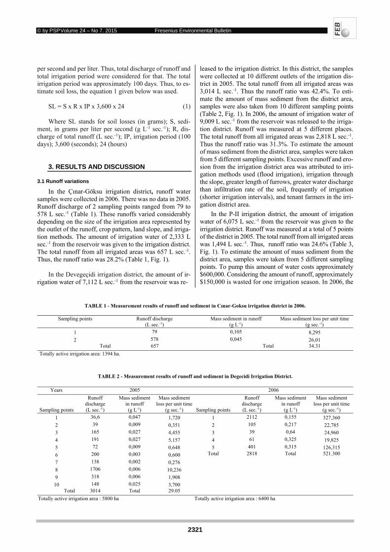
© by PSP Volume 24 – No 7. 2015 Fresenius Environmental Bulletin
2321
per second and per liter. Thus, total discharge of runoff and total irrigation period were considered for that. The total irrigation period was approximately 100 days. Thus, to es-timate soil loss, the equation 1 given below was used.
SL = S x R x IP x 3,600 x 24 (1) Where SL stands for soil losses (in grams); S, sedi-
ment, in grams per liter per second (g L-1 sec.-1); R, dis-charge of total runoff (L sec.-1); IP, irrigation period (100 days); 3,600 (seconds); 24 (hours)
3. RESULTS AND DISCUSSION
3.1 Runoff variations
In the Çınar-Göksu irrigation district, runoff water samples were collected in 2006. There was no data in 2005. Runoff discharge of 2 sampling points ranged from 79 to 578 L sec.-1 (Table 1). These runoffs varied considerably depending on the size of the irrigation area represented by the outlet of the runoff, crop pattern, land slope, and irriga-tion methods. The amount of irrigation water of 2,333 L sec.-1 from the reservoir was given to the irrigation district. The total runoff from all irrigated areas was 657 L sec.-1. Thus, the runoff ratio was 28.2% (Table 1, Fig. 1).
In the Devegeçidi irrigation district, the amount of ir-
rigation water of 7,112 L sec.-1 from the reservoir was re-
leased to the irrigation district. In this district, the samples were collected at 10 different outlets of the irrigation dis-trict in 2005. The total runoff from all irrigated areas was 3,014 L sec.-1. Thus the runoff ratio was 42.4%. To esti-mate the amount of mass sediment from the district area, samples were also taken from 10 different sampling points (Table 2, Fig. 1). In 2006, the amount of irrigation water of 9,009 L sec.-1 from the reservoir was released to the irriga-tion district. Runoff was measured at 5 different places. The total runoff from all irrigated areas was 2,818 L sec.-1. Thus the runoff ratio was 31.3%. To estimate the amount of mass sediment from the district area, samples were taken from 5 different sampling points. Excessive runoff and ero-sion from the irrigation district area was attributed to irri-gation methods used (flood irrigation), irrigation through the slope, greater length of furrows, greater water discharge than infiltration rate of the soil, frequently of irrigation (shorter irrigation intervals), and tenant farmers in the irri-gation district area.
In the P-II irrigation district, the amount of irrigation water of 6,075 L sec.-1 from the reservoir was given to the irrigation district. Runoff was measured at a total of 5 points of the district in 2005. The total runoff from all irrigated areas was 1,494 L sec.-1. Thus, runoff ratio was 24.6% (Table 3, Fig. 1). To estimate the amount of mass sediment from the district area, samples were taken from 5 different sampling points. To pump this amount of water costs approximately $600,000. Considering the amount of runoff, approximately $150,000 is wasted for one irrigation season. In 2006, the
TABLE 1 - Measurement results of runoff and sediment in Cınar-Goksu irrigation district in 2006.
Sampling points Runoff discharge (L sec.-1)
Mass sediment in runoff (g L-1)
Mass sediment loss per unit time (g sec.-1)
1 79 0,105 8,295
2 578 0,045 26,01 Total 657 Total 34.31
Totally active irrigation area: 1394 ha.
TABLE 2 - Measurement results of runoff and sediment in Degecidi Irrigation District.
Years 2005 2006
Sampling points
Runoff discharge (L sec.-1)
Mass sediment in runoff (g L-1)
Mass sediment loss per unit time
(g sec.-1) Sampling points
Runoff discharge (L sec.-1)
Mass sediment in runoff (g L-1)
Mass sediment loss per unit time
(g sec.-1)
1 36,6 0,047 1,720 1 2112 0,155 327,360
2 39 0,009 0,351 2 105 0,217 22,785
3 165 0,027 4,455 3 39 0,64 24,960
4 191 0,027 5,157 4 61 0,325 19,825
5 72 0,009 0,648 5 401 0,315 126,315
6 200 0,003 0,600 Total 2818 Total 521.300
7 138 0,002 0,276
8 1706 0,006 10,236
9 318 0,006 1,908
10 148 0,025 3,700
Total 3014 Total 29.05
Totally active irrigation area : 5800 ha Totally active irrigation area : 6400 ha

© by PSP Volume 24 – No 7. 2015 Fresenius Environmental Bulletin
2322
TABLE 3 - Measurement results of runoff and sediment in PII irrigation district.
Years 2005 2006
Sampling points
Runoff discharge (L sec.-1)
Mass sediment in runoff (g L-1)
Mass sediment lost per unit time
(g sec.-1) Sampling points
Runoff discharge (L sec.-1)
Mass sediment in runoff (g L-1)
Mass sediment lost per unit time
(g sec.-1)
1 90 0,016 1,440 1 239 0,384 91,776
2 207 0,014 2,898 2 55 0,59 32,450
3 587 0,008 4,696 3 141 0,748 105,468
4 27 0,001 0,027 4 88 0,632 55,616
5 583 0,004 2,332 5 231 0,163 37,653 Total 1494 Total 11.390 6 5 0,21 1,050
7 51 0,041 2,091 8 1.549 0,033 51,117 9 154 0,036 5,544 Total 2513 Total 382.770
Totally active irrigation area :5021 ha Totally active irrigation area : 4582 ha
FIGURE 1 – Runoff according to the studied years in the irrigation districts.
amount of irrigation water of 7,230 L sec.-1 from the reser-voir was given to the irrigation district. The total runoff from all irrigated areas was 2,513 L sec.-1. Thus the runoff ratio was 34.8%. (Table 3, Fig. 1). To estimate the amount of mass sediment from the district area, samples were taken from 9 different sampling points. To pump this amount of water costs approximately $650,000. Considering the amount of runoff, approximately $253,000 is wasted for one irrigation season depending on energy prices.
Runoff or tailwater (24.6–42.4%) in all irrigation dis-tricts was significantly higher. Schwankl et al. [8] calcu-lated the tailwater volume to be 15 to 25 % of the water applied to an irrigation set.
On the other hand, cotton-cultivated areas ranged from 50 to 98% in all irrigation districts [9]. Cotton is one of the crops that consume much more irrigation water compared to other field crops [10]. Cotton is irrigated almost entirely by surface irrigation. All these reasons might cause the use of more irrigation water in the irrigation districts.
When water reaches the lowest part, or end, of the field, “tailwater” runoff begins unless the water is shut off or the end of the field is blocked with berms to keep the water in the field. Allowing runoff is a common part of normal surface irrigation to ensure that sufficient water is applied at the lowest end of the field. With border irrigation, this often means that the water must be stopped before it advances to the end of the field, since water will continue to advance even after it is turned off. Water will not ad-vance far after a furrow irrigation system is shut off; crops at the end of the row may be under irrigated water if this technique is used with furrow irrigation [11].
3.2 Sediment measurements
To estimate the amount of mass sediment from the dis-trict area, samples were taken from 2 different sampling points in the Çınar-Göksu irrigation district. The irrigation period was approximately 100 days in this irrigation district. Considering this irrigation period, the total amount of soil
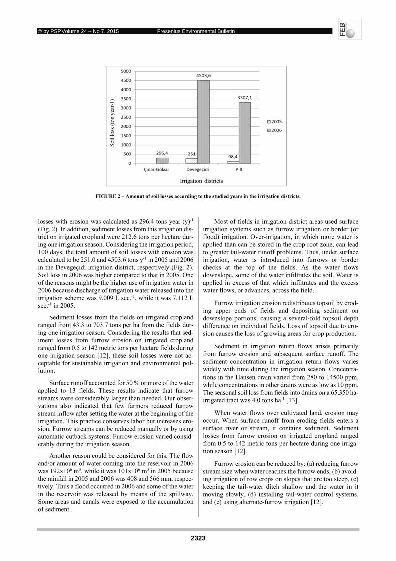
© by PSP Volume 24 – No 7. 2015 Fresenius Environmental Bulletin
2323
FIGURE 2 – Amount of soil losses according to the studied years in the irrigation districts.
losses with erosion was calculated as 296.4 tons year (y)-1 (Fig. 2). In addition, sediment losses from this irrigation dis-trict on irrigated cropland were 212.6 tons per hectare dur-ing one irrigation season. Considering the irrigation period, 100 days, the total amount of soil losses with erosion was calculated to be 251.0 and 4503.6 tons y-1 in 2005 and 2006 in the Devegeçidi irrigation district, respectively (Fig. 2). Soil loss in 2006 was higher compared to that in 2005. One of the reasons might be the higher use of irrigation water in 2006 because discharge of irrigation water released into the irrigation scheme was 9,009 L sec.-1, while it was 7,112 L sec.-1 in 2005.
Sediment losses from the fields on irrigated cropland ranged from 43.3 to 703.7 tons per ha from the fields dur-ing one irrigation season. Considering the results that sed-iment losses from furrow erosion on irrigated cropland ranged from 0.5 to 142 metric tons per hectare fields during one irrigation season [12], these soil losses were not ac-ceptable for sustainable irrigation and environmental pol-lution.
Surface runoff accounted for 50 % or more of the water applied to 13 fields. These results indicate that furrow streams were considerably larger than needed. Our obser-vations also indicated that few farmers reduced furrow stream inflow after setting the water at the beginning of the irrigation. This practice conserves labor but increases ero-sion. Furrow streams can be reduced manually or by using automatic cutback systems. Furrow erosion varied consid-erably during the irrigation season.
Another reason could be considered for this. The flow and/or amount of water coming into the reservoir in 2006 was 192x106 m3, while it was 101x106 m3 in 2005 because the rainfall in 2005 and 2006 was 408 and 566 mm, respec-tively. Thus a flood occurred in 2006 and some of the water in the reservoir was released by means of the spillway. Some areas and canals were exposed to the accumulation of sediment.
Most of fields in irrigation district areas used surface irrigation systems such as furrow irrigation or border (or flood) irrigation. Over-irrigation, in which more water is applied than can be stored in the crop root zone, can lead to greater tail-water runoff problems. Thus, under surface irrigation, water is introduced into furrows or border checks at the top of the fields. As the water flows downslope, some of the water infiltrates the soil. Water is applied in excess of that which infiltrates and the excess water flows, or advances, across the field.
Furrow irrigation erosion redistributes topsoil by erod-ing upper ends of fields and depositing sediment on downslope portions, causing a several-fold topsoil depth difference on individual fields. Loss of topsoil due to ero-sion causes the loss of growing areas for crop production.
Sediment in irrigation return flows arises primarily from furrow erosion and subsequent surface runoff. The sediment concentration in irrigation return flows varies widely with time during the irrigation season. Concentra-tions in the Hansen drain varied from 280 to 14500 ppm, while concentrations in other drains were as low as 10 ppm. The seasonal soil loss from fields into drains on a 65,350 ha-irrigated tract was 4.0 tons ha-1 [13].
When water flows over cultivated land, erosion may occur. When surface runoff from eroding fields enters a surface river or stream, it contains sediment. Sediment losses from furrow erosion on irrigated cropland ranged from 0.5 to 142 metric tons per hectare during one irriga-tion season [12].
Furrow erosion can be reduced by: (a) reducing furrow stream size when water reaches the furrow ends, (b) avoid-ing irrigation of row crops on slopes that are too steep, (c) keeping the tail-water ditch shallow and the water in it moving slowly, (d) installing tail-water control systems, and (e) using alternate-furrow irrigation [12].

© by PSP Volume 24 – No7. 2015 Fresenius Environmental Bulletin
2324
4. CONCLUSION
The most important problem in the irrigation districts is environmental damage by soil erosion and soil lost. Run-off and mass sediment losses from these irrigation districts ranged from 28–42.4 % and 98.4–4503.6 tons for one irri-gation season, respectively. These runoff and soil losses are not acceptable for sustainable irrigation and environmental pollution.
Sustainable irrigation is at risk due to excessive flood-ing of lands with inappropriate irrigation methods. Exces-sive irrigation and soil erosion occurred since the amount of irrigation water applied to the lands of the farmers was not measured. Some technically improper practices in-clude: inappropriate irrigation methods, sides of cultivation and furrow parallel to the land slope, longer furrow lengths, use of higher discharges than infiltration rate for the lands, and tenant irrigation instead of property owner irrigation in the irrigation schemes.
The goal of every irrigator should be to apply the right amount of water as uniformly as possible to meet the crop needs. To do this, irrigators need to take into account how much water is applied during irrigation and where the wa-ter goes. Factors affecting furrow erosion are the slope along the furrow, stream size, residue, surface roughness, and cropping sequence.
Tail-water return systems, in which tail-water runoff is collected in a pond and reused, are common in surface-ir-rigated row and field crops. However, they are not as com-mon in these irrigation districts areas. In addition, there is no reason the farmers should be used because farmers do not pay water prices based on the volumetric unit for the amount of irrigation water applied. In fact, a tail-water re-turn system collects the runoff water in a storage pond until it can be reused for irrigation on another section of the field or on other land being irrigated. Reusing the collected wa-ter maintains high irrigation efficiency and makes room in the pond for additional runoff.
The authors have declared no conflict of interest. REFERENCES
[1] Anonymous. (2013). Erosion control for irrigated land. ES-6. (Available: http://www.cals.ncsu.edu, accessed on: October 12, 2013)
[2] O’Geen, A.T. and Schwankl, L.J. (1986). Understanding soil erosion in irrigated agriculture. University of California, Divi-sion of Agriculture and Natural Resources. Publication 8196 CA, USA
[3] Carter, D.L. (1990). Soil erosion on irrigated lands. In: Stew-art, B.A. and Nielsen, D.R. (Eds.) Irrigation of Agricultural Crops. Agronomy Monograph No. 30, ASA-CSSA-SSSA, 677 South Segoe Road, Madison, WI 53711, 1143-1171.
[4] Haktanır, K., Karaca, A. and Omar, S.M. (2004). The pro-spects of the impact of desertification on Turkey, Lebanon, Syria and Iraq. In: Marquina, A. (Ed.) Environmental Chal-lenges in the Mediterranean 2000-2050. Kluwer Academic Publishers, Netherland, Chapter 9, 139-154
[5] GAP-BKİ (2014). What is GAP? (Available: http://www.gap.gov.tr, accessed on: September 14, 2014)
[6] Boulal, H., Gomez-Macpherson, H., Gomez, J.A. and Mateos, L. (2011). Effect of soil management and traffic on soil erosion in irrigated annual crops. Soil and Tillage Research 115-116, 62-79
[7] Üzen, N., Yolcu, R. and Cetin, Ö. (2013). Evaluation of De-vegecidi irrigation scheme on the irrigation management in Southeastern Anatolia Region of Turkey. AgroLife Scientific Journal 2 (1), 151-156
[8] Schwankl, L.J., Prichard, T.L. and Hanson, B.R. (2007). Tailwater return systems. University of California, Division of Agriculture and Natural Resources. Publication 8225 CA, USA
[9] DSI (2007). Reports on irrigation districts. X. Regional Direc-torate of State Hydraulic Works, Diyarbakir, Turkey (in Turk-ish).
[10] Çetin, Ö. and Bilgel, L. (2002) Effects of different irrigation methods on shedding and yield of cotton. Agricultural Water Management 54 (1), 1-15
[11] Schwankl, L.J., Prichard, T.L. and Hanson, B.R. (2007). Causes and management of runoff from surface irrigation in orchards. University of California, Division of Agriculture and Natural Resources. Publication 8214, CA, USA
[12] Berg, R.D. and Carter, D.L. (1980). Furrow erosion and sedi-ment losses on irrigated cropland. Journal of Soil and Water Conservation 35 (6), 267- 70
[13] Carter, D.L. (1976). Guidelines for sediment control in irriga-tion return flow. Journal of Environmental Quality 5 (2), 119-124.
Received: October 06, 2014 Revised: January 09, 2015 Accepted: February 20, 2015 CORRESPONDING AUTHOR
Öner Çetin
Dicle University Agricultural Faculty Dept. of Agricultural Structures and Irrigation Diyarbakir TURKEY Phone: +90 412 248 85 09 Fax: +90 412 248 81 53 E-mail: [email protected]
FEB/ Vol 24/ No 7/ 2015 – pages 2319 - 2324
© by PSP Volume 24 – No7. 2015 Fresenius Environmental Bulletin
2325
TEMPORAL AND SPATIAL CHARACTERISTICS
OF PHOSPHORUSFRACTIONS UNDER LONG-TERM
WASTEWATER IRRIGATION IN TONGLIAO CITY, CHINA
Yintao Lu1,2,*, Fang Liu1,2, Hong Yao1,2, and Kelin Hu3 1 School of Civil Engineering, Beijing Jiaotong University, Beijing 100044, China
2 Beijing Key Laboratory of Aqueous Typical Pollutants Control and Water Quality Safeguard, Beijing 10044, China 3College of Resources and Environmental Sciences, China Agricultural University, Beijing 100083, China
ABSTRACT
The irrigation reuse of municipal and industrial efflu-ents conserves freshwater resources and avoids direct nu-trient discharges to surface waters. The sustainability of ag-ricultural reuse programs, however, may be challenged by changes in phosphorus (P) availability. To understand the characteristics of P fractions, 130 soil samples were col-lected around an irrigation drain in May 2009, at the begin-ning of the growing season. In the study area, total phos-phorus (TP) varied from 302.32 to 716.30 mg/kg, residual P varied from18.21 to 126.08 mg/kg, and Olsen P varied from 0.71 to 90.04 mg/kg. The relative abundance detected for nearly every P fraction followed the order Ca-P>resid-ual P>NaOH-Po≈NaOH-Pi>KCl-P. Although NaOH-Pi and most of the Ca-P fractions contributed markedly to P avail-ability, NaOH-Po and Ca-P contributed more to residual P when different phosphate sources were added to the soil. However, the available P in the studied soils represented only 5.5% of the TP, which was inadequate for the growth and development of crops. The influence of wastewater ir-rigation differs significantly at different depths. Wastewater irrigation is favorable to the transformation of stable P (NaOH-Po and Ca-P) into available P (NaOH-Pi), and cancause an increase in residual P in the shallow layer (0-60 cm), as well as an increase in TP in the middle layer (60-110 cm). However, wastewater and groundwater irrigation is beneficial to the increase in soil P concentration in the deep layer (110-170 cm). These effects may depend on soil properties, water cycles and biological processes, among other factors.
KEYWORDS: Phosphorus transport,soil phosphorus, wastewater irrigation, groundwater irrigation
1. INTRODUCTION
Wastewater effluentsare increasingly being viewed as potential water supply sources [1]. The major reuse option
* Corresponding author
for reclaimed wastewaters is irrigation of agricultural, for-ested, and urban landscapes [2-5]. Effluent reuse allows eu-trophication-promoting nutrients to enhance plant growth and reduce water-quality effects. Phosphorus (P) is a plant nutrient present in treated sewage effluents, which rarely affects the daily operation ofmunicipal wastewater effluent irrigation systems [6].P is not typically considered as a lim-iting parameter for effluent irrigation because only a small amount of P is typically added to soil by irrigation with treated sewage effluents [7-9].
However, soluble P can be easily fixed in soils, result-ing in low P availability for plant utilization [10]. P frac-tionation studies considering fertilizer applications of sev-eral years or longer have been conducted to understand P availability in soil [11].Calcium-bound phosphorus (Ca-P) is the dominant inorganic form of P [12]. The availability of P fractions to plants depends on time-varying soil changes[13]. Despite an increase in the total soil P over the life of a system, most fields have inadequate plant-availa-ble P [14]. After 70 years of irrigating citrus crops with wastewater from Cairo and Alexandria (Egypt), the surface soil contained only 10-11 mg/kg Olsen P [15]. Unfortu-nately, few studies have considered the variation of P frac-tions in wastewater-irrigated areas.
In northern China, P-deficient soils are widespread. Although wastewater has beenwidely used as an important irrigation source in China, relevant studies evaluating the effects ofreclaimed wastewater irrigation on soil P are stilllacking. This study aimed to investigate the proportions and relationships of soil P fractions in wastewater-irrigated and groundwater-irrigated areas, and to study the transport and conversion of soil P with respect to spatial and vertical variationsin soil P fractions.
2. MATERIALS AND METHODS
2.1 Site description
The experimental area is located in the northeastern re-gion of China, downstream of the Xiliao river catchment (43°38′11″–43°45′50″ N; 122°19′50″–122°31′52″ E). The site lies in the semi–arid grassland area of the North Tem-
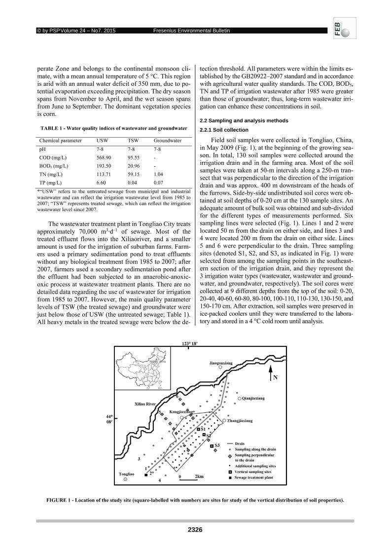
© by PSP Volume 24 – No7. 2015 Fresenius Environmental Bulletin
2326
perate Zone and belongs to the continental monsoon cli-mate, with a mean annual temperature of 5 °C. This region is arid with an annual water deficit of 350 mm, due to po-tential evaporation exceeding precipitation. The dry season spans from November to April, and the wet season spans from June to September. The dominant vegetation species is corn.
TABLE 1 - Water quality indices of wastewater and groundwater
Chemical parameter USW TSW Groundwater
pH 7-8 7-8 7-8
COD (mg/L) 568.90 95.55 -
BOD5 (mg/L) 193.50 20.96 -
TN (mg/L) 113.71 59.15 1.04
TP (mg/L) 6.60 0.04 0.07
*“USW” refers to the untreated sewage from municipal and industrial wastewater and can reflect the irrigation wastewater level from 1985 to 2007; “TSW” represents treated sewage, which can reflect the irrigation wastewater level since 2007.
The wastewater treatment plant in Tongliao City treats
approximately 70,000 m3·d–1 of sewage. Most of the treated effluent flows into the Xiliaoriver, and a smaller amount is used for the irrigation of suburban farms. Farm-ers used a primary sedimentation pond to treat effluents without any biological treatment from 1985 to 2007; after 2007, farmers used a secondary sedimentation pond after the effluent had been subjected to an anaerobic-anoxic-oxic process at wastewater treatment plants. There are no detailed data regarding the use of wastewater for irrigation from 1985 to 2007. However, the main quality parameter levels of TSW (the treated sewage) and groundwater were just below those of USW (the untreated sewage; Table 1). All heavy metals in the treated sewage were below the de-
tection threshold. All parameters were within the limits es-tablished by the GB20922–2007 standard and in accordance with agricultural water quality standards. The COD, BOD5, TN and TP of irrigation wastewater after 1985 were greater than those of groundwater; thus, long-term wastewater irri-gation can enhance these concentrations in soil.
2.2 Sampling and analysis methods
2.2.1 Soil collection
Field soil samples were collected in Tongliao, China, in May 2009 (Fig. 1), at the beginning of the growing sea-son. In total, 130 soil samples were collected around the irrigation drain and in the farming area. Most of the soil samples were taken at 50-m intervals along a 250-m tran-sect that was perpendicular to the direction of the irrigation drain and was approx. 400 m downstream of the heads of the furrows. Side-by-side undistributed soil cores were ob-tained at soil depths of 0-20 cm at the 130 sample sites. An adequate amount of bulk soil was obtained and sub-divided for the different types of measurements performed. Six sampling lines were selected (Fig. 1). Lines 1 and 2 were located 50 m from the drain on either side, and lines 3 and 4 were located 200 m from the drain on either side. Lines 5 and 6 were perpendicular to the drain. Three sampling sites (denoted S1, S2, and S3, as indicated in Fig. 1) were selected from among the sampling points in the southeast-ern section of the irrigation drain, and they represent the 3 irrigation water types (wastewater, wastewater and ground-water, and groundwater, respectively). The soil cores were collected at 9 different depths from the top of the soil: 0-20, 20-40, 40-60, 60-80, 80-100, 100-110, 110-130, 130-150, and 150-170 cm. After extraction, soil samples were preserved in ice-packed coolers until they were transferred to the labora-tory and stored in a 4 °C cold room until analysis.
FIGURE 1 - Location of the study site (square-labelled with numbers are sites for study of the vertical distribution of soil properties).
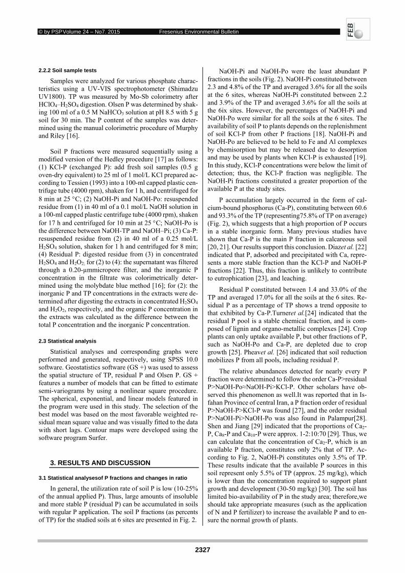
© by PSP Volume 24 – No7. 2015 Fresenius Environmental Bulletin
2327
2.2.2 Soil sample tests
Samples were analyzed for various phosphate charac-teristics using a UV-VIS spectrophotometer (Shimadzu UV1800). TP was measured by Mo-Sb colorimetry after HClO4–H2SO4 digestion. Olsen P was determined by shak-ing 100 ml of a 0.5 M NaHCO3 solution at pH 8.5 with 5 g soil for 30 min. The P content of the samples was deter-mined using the manual colorimetric procedure of Murphy and Riley [16].
Soil P fractions were measured sequentially using a
modified version of the Hedley procedure [17] as follows: (1) KCl-P (exchanged P): add fresh soil samples (0.5 g oven-dry equivalent) to 25 ml of 1 mol/L KCl prepared ac-cording to Tessien (1993) into a 100-ml capped plastic cen-trifuge tube (4000 rpm), shaken for 1 h, and centrifuged for 8 min at 25 C; (2) NaOH-Pi and NaOH-Po: resuspended residue from (1) in 40 ml of a 0.1 mol/L NaOH solution in a 100-ml capped plastic centrifuge tube (4000 rpm), shaken for 17 h and centrifuged for 10 min at 25 C; NaOH-Po is the difference between NaOH-TP and NaOH–Pi; (3) Ca-P: resuspended residue from (2) in 40 ml of a 0.25 mol/L H2SO4 solution, shaken for 1 h and centrifuged for 8 min; (4) Residual P: digested residue from (3) in concentrated H2SO4 and H2O2; for (2) to (4): the supernatant was filtered through a 0.20-µmmicropore filter, and the inorganic P concentration in the filtrate was colorimetrically deter-mined using the molybdate blue method [16]; for (2): the inorganic P and TP concentrations in the extracts were de-termined after digesting the extracts in concentrated H2SO4 and H2O2, respectively, and the organic P concentration in the extracts was calculated as the difference between the total P concentration and the inorganic P concentration.
2.3 Statistical analysis
Statistical analyses and corresponding graphs were performed and generated, respectively, using SPSS 10.0 software. Geostatistics software (GS +) was used to assess the spatial structure of TP, residual P and Olsen P. GS + features a number of models that can be fitted to estimate semi-variograms by using a nonlinear square procedure. The spherical, exponential, and linear models featured in the program were used in this study. The selection of the best model was based on the most favorable weighted re-sidual mean square value and was visually fitted to the data with short lags. Contour maps were developed using the software program Surfer.
3. RESULTS AND DISCUSSION
3.1 Statistical analysesof P fractions and changes in ratio
In general, the utilization rate of soil P is low (10-25% of the annual applied P). Thus, large amounts of insoluble and more stable P (residual P) can be accumulated in soils with regular P application. The soil P fractions (as percents of TP) for the studied soils at 6 sites are presented in Fig. 2.
NaOH-Pi and NaOH-Po were the least abundant P fractions in the soils (Fig. 2). NaOH-Pi constituted between 2.3 and 4.8% of the TP and averaged 3.6% for all the soils at the 6 sites, whereas NaOH-Pi constituted between 2.2 and 3.9% of the TP and averaged 3.6% for all the soils at the 6ix sites. However, the percentages of NaOH-Pi and NaOH-Po were similar for all the soils at the 6 sites. The availability of soil P to plants depends on the replenishment of soil KCl-P from other P fractions [18]. NaOH-Pi and NaOH-Po are believed to be held to Fe and Al complexes by chemisorption but may be released due to desorption and may be used by plants when KCl-P is exhausted [19]. In this study, KCl-P concentrations were below the limit of detection; thus, the KCl-P fraction was negligible. The NaOH-Pi fractions constituted a greater proportion of the available P at the study sites.
P accumulation largely occurred in the form of cal-cium-bound phosphorus (Ca-P), constituting between 60.6 and 93.3% of the TP (representing75.8% of TP on average) (Fig. 2), which suggests that a high proportion of P occurs in a stable inorganic form. Many previous studies have shown that Ca-P is the main P fraction in calcareous soil [20, 21]. Our results support this conclusion. Diazet al. [22] indicated that P, adsorbed and precipitated with Ca, repre-sents a more stable fraction than the KCl-P and NaOH-P fractions [22]. Thus, this fraction is unlikely to contribute to eutrophication [23], and leaching.
Residual P constituted between 1.4 and 33.0% of the TP and averaged 17.0% for all the soils at the 6 sites. Re-sidual P as a percentage of TP shows a trend opposite to that exhibited by Ca-P.Turneret al.[24] indicated that the residual P pool is a stable chemical fraction, and is com-posed of lignin and organo-metallic complexes [24]. Crop plants can only uptake available P, but other fractions of P, such as NaOH-Po and Ca-P, are depleted due to crop growth [25]. Pheavet al. [26] indicated that soil reduction mobilizes P from all pools, including residual P.
The relative abundances detected for nearly every P fraction were determined to follow the order Ca-P>residual P>NaOH-Po≈NaOH-Pi>KCl-P. Other scholars have ob-served this phenomenon as well.It was reported that in Is-fahan Province of central Iran, a P fraction order of residual P>NaOH-P>KCl-P was found [27], and the order residual P>NaOH-Pi>NaOH-Po was also found in Palampur[28]. Shen and Jiang [29] indicated that the proportions of Ca2-P, Ca8-P and Ca10-P were approx. 1-2:10:70 [29]. Thus, we can calculate that the concentration of Ca2-P, which is an available P fraction, constitutes only 2% that of TP. Ac-cording to Fig. 2, NaOH-Pi constitutes only 3.5% of TP. These results indicate that the available P sources in this soil represent only 5.5% of TP (approx. 25 mg/kg), which is lower than the concentration required to support plant growth and development (30-50 mg/kg) [30]. The soil has limited bio-availability of P in the study area; therefore,we should take appropriate measures (such as the application of N and P fertilizer) to increase the available P and to en-sure the normal growth of plants.

© by PSP Volume 24 – No7. 2015 Fresenius Environmental Bulletin
2328
FIGURE 2 -Soil P fractions as percentages of total P for the studied soils at six sites.
TABLE 2 - Pearson correlation coefficients of TP, Olsen P and P frac-tions
TP Olsen P
NaOH‐Pi
NaOH‐Po Ca‐P Residual P
TP 1.000 0.667** 0.774** ‐0.486** 0.956*** 0.573**
Olsen P 1.000 0.571** ‐0.569** 0.653** 0.365*
NaOH‐Pi 1.000 ‐0.115NS 0.775** 0.312NS
NaOH‐Po 1.000 ‐0.465** ‐0.359*
Ca‐P 1.000 0.347*
Residual P 1.000n=39. NS: not significant at the P≤0.05 level. *P=0.05; **P=0.01; ***P=0.001
The Ca-P fraction and TP were significantly (P<0.001)
positively correlated, with a Pearson correlation coefficient of 0.956; these results emphasize that Ca-P is the main fraction contributing to TP. At a calcareous soil site, simi-lar results were reported [31]. The NaOH-Pi and Ca-P frac-tions and Olsen P were positively correlated (P<0.01); these 2 fractions were correlated with P removal by plants
(Table 2). The NaOH-Pi and Ca-P fractions contributed markedly to P availability when different phosphate sources were added to the soil, confirming the findings re-ported in [13]. In all treatments, the organic P fraction (NaOH-Po) and Olsen P correlated negatively (P<0.01). Organic P not only constituted a low percentage of TP but was also not an available P source in these soils.
Residual P and 2 P fractions (NaOH-Po and Ca-P) were correlated (P<0.05); this finding suggests that NaOH-Po and Ca-P contribute more to residual P. Conversely, the NaOH-Pi fraction did not correlate significantly with resid-ual P (P≥0.05), which suggests that the NaOH-Pi fraction cannot be converted to residual P and can be used by plants. In addition, Olsen P was positively correlated with residual P (P<0.05), which demonstrates that Olsen P and residual P can be converted into one another.
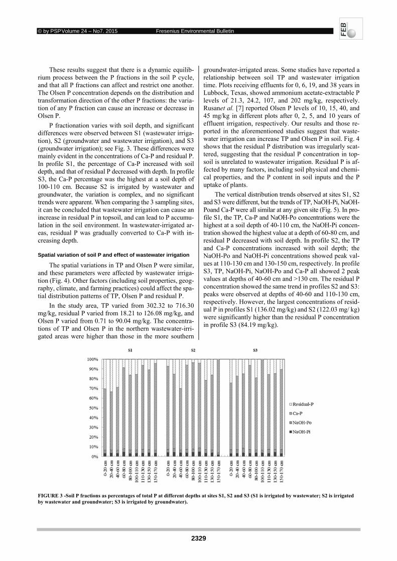
© by PSP Volume 24 – No7. 2015 Fresenius Environmental Bulletin
2329
These results suggest that there is a dynamic equilib-rium process between the P fractions in the soil P cycle, and that all P fractions can affect and restrict one another. The Olsen P concentration depends on the distribution and transformation direction of the other P fractions: the varia-tion of any P fraction can cause an increase or decrease in Olsen P.
P fractionation varies with soil depth, and significant differences were observed between S1 (wastewater irriga-tion), S2 (groundwater and wastewater irrigation), and S3 (groundwater irrigation); see Fig. 3. These differences were mainly evident in the concentrations of Ca-P and residual P. In profile S1, the percentage of Ca-P increased with soil depth, and that of residual P decreased with depth. In profile S3, the Ca-P percentage was the highest at a soil depth of 100-110 cm. Because S2 is irrigated by wastewater and groundwater, the variation is complex, and no significant trends were apparent. When comparing the 3 sampling sites, it can be concluded that wastewater irrigation can cause an increase in residual P in topsoil, and can lead to P accumu-lation in the soil environment. In wastewater-irrigated ar-eas, residual P was gradually converted to Ca-P with in-creasing depth.
Spatial variation of soil P and effect of wastewater irrigation
The spatial variations in TP and Olsen P were similar, and these parameters were affected by wastewater irriga-tion (Fig. 4). Other factors (including soil properties, geog-raphy, climate, and farming practices) could affect the spa-tial distribution patterns of TP, Olsen P and residual P.
In the study area, TP varied from 302.32 to 716.30 mg/kg, residual P varied from 18.21 to 126.08 mg/kg, and Olsen P varied from 0.71 to 90.04 mg/kg. The concentra-tions of TP and Olsen P in the northern wastewater-irri-gated areas were higher than those in the more southern
groundwater-irrigated areas. Some studies have reported a relationship between soil TP and wastewater irrigation time. Plots receiving effluents for 0, 6, 19, and 38 years in Lubbock, Texas, showed ammonium acetate-extractable P levels of 21.3, 24.2, 107, and 202 mg/kg, respectively. Rusanet al. [7] reported Olsen P levels of 10, 15, 40, and 45 mg/kg in different plots after 0, 2, 5, and 10 years of effluent irrigation, respectively. Our results and those re-ported in the aforementioned studies suggest that waste-water irrigation can increase TP and Olsen P in soil. Fig. 4 shows that the residual P distribution was irregularly scat-tered, suggesting that the residual P concentration in top-soil is unrelated to wastewater irrigation. Residual P is af-fected by many factors, including soil physical and chemi-cal properties, and the P content in soil inputs and the P uptake of plants.
The vertical distribution trends observed at sites S1, S2 and S3 were different, but the trends of TP, NaOH-Pi, NaOH-Poand Ca-P were all similar at any given site (Fig. 5). In pro-file S1, the TP, Ca-P and NaOH-Po concentrations were the highest at a soil depth of 40-110 cm, the NaOH-Pi concen-tration showed the highest value at a depth of 60-80 cm, and residual P decreased with soil depth. In profile S2, the TP and Ca-P concentrations increased with soil depth; the NaOH-Po and NaOH-Pi concentrations showed peak val-ues at 110-130 cm and 130-150 cm, respectively. In profile S3, TP, NaOH-Pi, NaOH-Po and Ca-P all showed 2 peak values at depths of 40-60 cm and >130 cm. The residual P concentration showed the same trend in profiles S2 and S3: peaks were observed at depths of 40-60 and 110-130 cm, respectively. However, the largest concentrations of resid-ual P in profiles S1 (136.02 mg/kg) and S2 (122.03 mg/ kg) were significantly higher than the residual P concentration in profile S3 (84.19 mg/kg).
FIGURE 3 -Soil P fractions as percentages of total P at different depths at sites S1, S2 and S3 (S1 is irrigated by wastewater; S2 is irrigated by wastewater and groundwater; S3 is irrigated by groundwater).
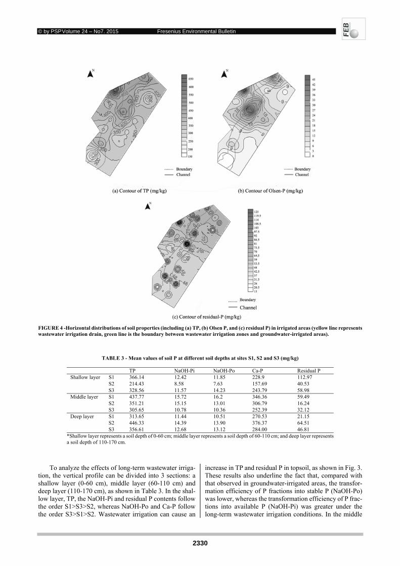
© by PSP Volume 24 – No7. 2015 Fresenius Environmental Bulletin
2330
FIGURE 4 -Horizontal distributions of soil properties (including (a) TP, (b) Olsen P, and (c) residual P) in irrigated areas (yellow line represents wastewater irrigation drain, green line is the boundary between wastewater irrigation zones and groundwater-irrigated areas).
TABLE 3 - Mean values of soil P at different soil depths at sites S1, S2 and S3 (mg/kg)
TP NaOH-Pi NaOH-Po Ca-P Residual P Shallow layer S1 366.14 12.42 11.85 228.9 112.97
S2 214.43 8.58 7.63 157.69 40.53 S3 328.56 11.57 14.23 243.79 58.98
Middle layer S1 437.77 15.72 16.2 346.36 59.49 S2 351.21 15.15 13.01 306.79 16.24 S3 305.65 10.78 10.36 252.39 32.12
Deep layer S1 313.65 11.44 10.51 270.53 21.15 S2 446.33 14.39 13.90 376.37 64.51 S3 356.61 12.68 13.12 284.00 46.81
*Shallow layer represents a soil depth of 0-60 cm; middle layer represents a soil depth of 60-110 cm; and deep layer represents a soil depth of 110-170 cm.
To analyze the effects of long-term wastewater irriga-tion, the vertical profile can be divided into 3 sections: a shallow layer (0-60 cm), middle layer (60-110 cm) and deep layer (110-170 cm), as shown in Table 3. In the shal-low layer, TP, the NaOH-Pi and residual P contents follow the order S1>S3>S2, whereas NaOH-Po and Ca-P follow the order S3>S1>S2. Wastewater irrigation can cause an
increase in TP and residual P in topsoil, as shown in Fig. 3. These results also underline the fact that, compared with that observed in groundwater-irrigated areas, the transfor-mation efficiency of P fractions into stable P (NaOH-Po) was lower, whereas the transformation efficiency of P frac-tions into available P (NaOH-Pi) was greater under the long-term wastewater irrigation conditions. In the middle
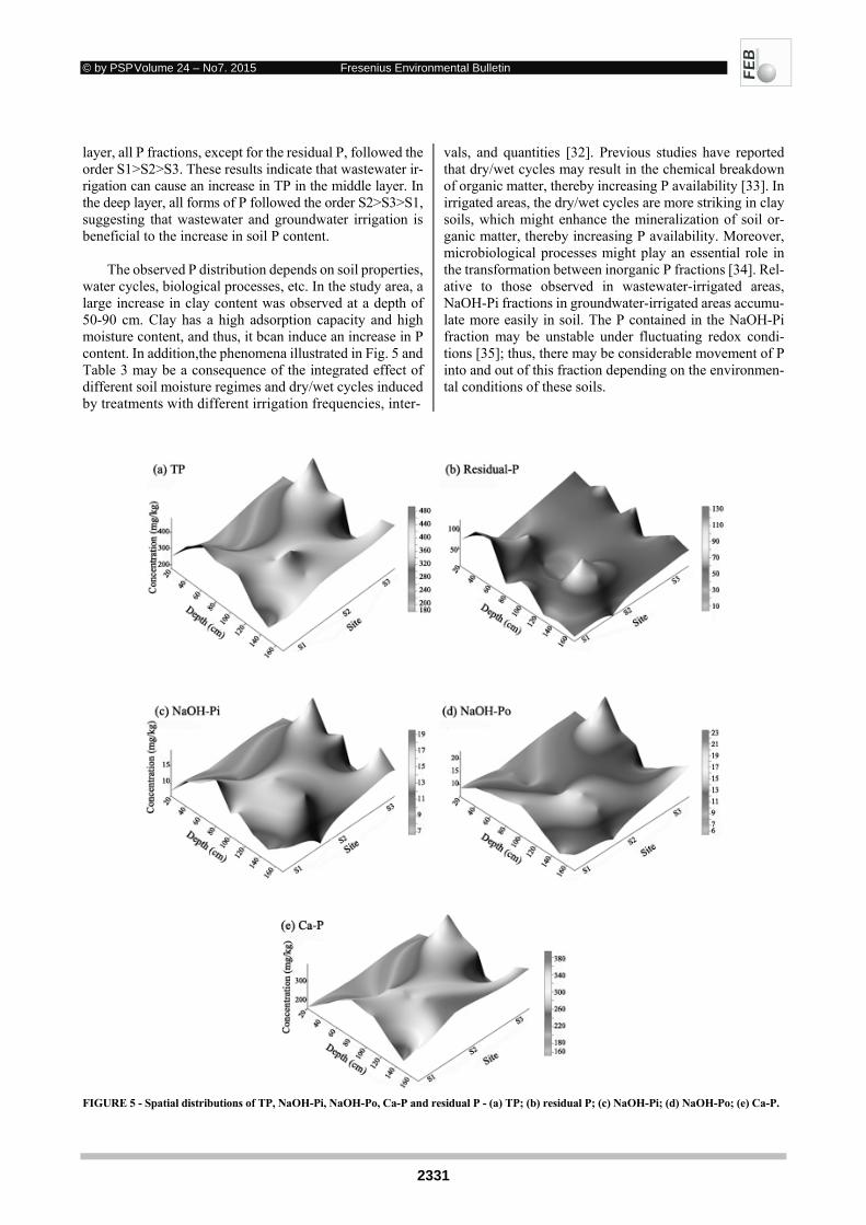
© by PSP Volume 24 – No7. 2015 Fresenius Environmental Bulletin
2331
layer, all P fractions, except for the residual P, followed the order S1>S2>S3. These results indicate that wastewater ir-rigation can cause an increase in TP in the middle layer. In the deep layer, all forms of P followed the order S2>S3>S1, suggesting that wastewater and groundwater irrigation is beneficial to the increase in soil P content.
The observed P distribution depends on soil properties,
water cycles, biological processes, etc. In the study area, a large increase in clay content was observed at a depth of 50-90 cm. Clay has a high adsorption capacity and high moisture content, and thus, it bcan induce an increase in P content. In addition,the phenomena illustrated in Fig. 5 and Table 3 may be a consequence of the integrated effect of different soil moisture regimes and dry/wet cycles induced by treatments with different irrigation frequencies, inter-
vals, and quantities [32]. Previous studies have reported that dry/wet cycles may result in the chemical breakdown of organic matter, thereby increasing P availability [33]. In irrigated areas, the dry/wet cycles are more striking in clay soils, which might enhance the mineralization of soil or-ganic matter, thereby increasing P availability. Moreover, microbiological processes might play an essential role in the transformation between inorganic P fractions [34]. Rel-ative to those observed in wastewater-irrigated areas, NaOH-Pi fractions in groundwater-irrigated areas accumu-late more easily in soil. The P contained in the NaOH-Pi fraction may be unstable under fluctuating redox condi-tions [35]; thus, there may be considerable movement of P into and out of this fraction depending on the environmen-tal conditions of these soils.
FIGURE 5 - Spatial distributions of TP, NaOH-Pi, NaOH-Po, Ca-P and residual P - (a) TP; (b) residual P; (c) NaOH-Pi; (d) NaOH-Po; (e) Ca-P.

© by PSP Volume 24 – No 7. 2015 Fresenius Environmental Bulletin
2332
4. CONCLUSIONS
There is a dynamic equilibrium process among all P fractions in the soil P system, and all P fractions can affect and restrict one another. The relative abundance detected for nearly every P fraction followed the order Ca-P>resid-ual P>NaOH-Po≈NaOH-Pi>KCl-P. NaOH-Pi and a part of the Ca-P fraction contributed markedly to P availability when different phosphate sources were added to soil. Wastewater irrigation has various effects on P. In the shal-low layer, the transformation efficiency of P fractions into stable P (NaOH-Po) was lower than that in the groundwa-ter-irrigated area, whereas the transformation efficiency of P fractions into available P (NaOH-Pi) was greater under long-term wastewater irrigation conditions. In the middle layer, wastewater irrigation can cause an increase in TP, and in the deep layer, wastewater and groundwater irriga-tion is beneficial to the down-transformation of P.These re-sults may depend on soil properties, water cycles, and bio-logical processes, among other factors.
ACKNOWLEDGEMENTS
This study was supported by the National Natural Sci-ence Foundation of China (No. 41103007) and the Appli-cation and Development Fund from the Ministry of Sci-ences and Technology of the Inner Mongolia Autonomous Region (No. 2009058). The authors are grateful to the State Key Laboratory of Environmental Aquatic Chemistry, the Research Center for Eco-Environmental Sciences, and the Chinese Academy of Sciences for their assistance in soil sampling and analysis. We also thank all supporters from the Tongliao Environmental Protection Agency and all re-viewers and editors for their valuable comments and sug-gestions during the review process.
The authors have declared no conflict of interest. REFERENCES
[1] O’Connor, G.A., Elliott, H.A.,and Bastian, R.K. (2008) De-graded water reuse: An overview. Journal of Environmental Quality 37, S157-S168.
[2] Hamilton, A., Stagnitti, F., Xiong, S.Z., Kreidl, S., Benke, K., and Maher, P. (2007) Wastewater irrigation: The state of play.Vadose Zone Journal6, 823-840.
[3] Egwu, G.N. andAgbenin, J.O. (2012) Lead enrichment, ad-sorption and speciation in urban garden soils under long-term wastewater irrigation in northern Nigeria.Environmental Earth Sciences 69, 1861-1870.
[4] Guo, G.X., Deng, H., Qiao, M., Yao, H.Y. and Zhu, Y.G. (2013) Effect of long-term wastewater irrigation on potential denitrification and denitrifying communities in soils at the wa-tershed scale. Environmental science & technology 47, 3105-3113.
[5] Blum, J., Melfi, A.J., Montes, C.R. and Gomes, T.M. (2013) Nitrogen and phosphorus leaching in a tropical Brazilian soil cropped with sugarcane and irrigated with treated sewage ef-fluent. Agricultural Water Management 117, 115-122.
[6] Angelakis, A.N.,Marecos, M.H.F., Do Monte,Bontoux, L. and Asano, T. (1999) The status of wastewater reuse practice in the Mediterranean basin: Need for guidelines.Water Research33, 2201–2217.
[7] Rusan, M.J.M., Hinnawi, S. and Rousan, L. (2007) Long term effect of wastewater irrigation of forage crops on soil and plant quality parameters. Desalination 215, 143-152.
[8] Jaiswal, D. and Elliott, H.A.(2011) Long-Term Phosphorus Fertility in Wastewater-Irrigated Cropland. Journal of Envi-ronment Qualit 40 (1), 214-223.
[9] Guo, H.A. andJaiswal, D.(2012) Phosphorus management for sustainable agricultural irrigation of reclaimed water. Journal of Environmental Engineering138, 367-374.
[10] Park, M., Singvilay, O., Shin, W., Kim, E., Chung, J. andSa, T.(2004) Effect of long-term compost and fertilizer applica-tion on soil phosphorus status under paddy cropping sys-tem.Communications in Soil Science and Plant Analysis 35 (11–12), 1635-1644.
[11] Scherer, H.W. and Sharma, S.P.(2002) Phosphorus fractions and phosphorus delivery potential of a luvisol derived from lo-ess amended with organic material. Biology and Fertility of Soils 35, 414-419.
[12] Shen, J., Li, R., Zhang, F., Fan, J., Tang, C. andRengel, Z. (2004) Crop yields, soil fertility, and phosphorus fractions in response to long-term fertilization under the rice monoculture system on a calcareous soil. Field Crops Research6, 225-238.
[13] Guo, F., Yost, R.S., Hue, N.V., Evensen, C.I. and Silva, J.A. (2000) Changes inphosphorus fractions in soils under inten-sive plant growth. Soil Science Society of America Journal 64, 1681–1689.
[14] Hu, C., Zhang, T.C., Kendrick, D., Huang, Y.H. andSuram-palli, R.(2006) Muskegon wastewater land treatment system: Fate and transport of phosphorus in soils and life expectancy of the system. Engineering in Life Science 6 (1), 17-25.
[15] Waly, T.M., Elnaim, E.M., Omran, M.S. and El Nashar, B.M.B.(1987) Effect of sewage water on chemical properties and heavy metals content of ElGabal El Asfar sandy soils. Bi-ological wastes 22 (4), 275-284.
[16] Murphy, J. and Riley, J.P. (1962) A modified single solution method for the determination of phosphate in natural waters. AnalyticaChimicaActa 27, 31-36.
[17] Huguenin-Elie, O., Kirk, G.J.D. andFrossard, E.(2003) Phos-phorus uptake by rice from soil that is flooded, drained or flooded then drained. European Journal of Soil Science 54(1), 77-90.
[18] Zhang, T.Q., MacKenzie, A.F., Liang, B.C. and Drury, C.F. (2004) Soil test phosphorus and phosphorus fractions with long-term phosphorus addition and depletion. Soil Science So-ciety of America Journal 68, 519-528.
[19] Babatunde, A.O. and Zhao, Y.Q. (2009) Forms, patterns and extractability of phosphorus retained in alum sludge used as substrate in laboratory-scale constructed wetland systems. Chemical Engineering Journal 152 (1), 8-13.
[20] Jalali, M. and SajadiTabar, S. (2011) Chemical fractionation of phosphorus in calcareous soils of Hamadan, western Iran under different land use. Journal of Plant Nutrition and Soil Science 174, 523-531.
© by PSP Volume 24 – No 7. 2015 Fresenius Environmental Bulletin
2333
[21] Yang, J.C., Wang, Z.G., Zhou, J., Jiang, H.M., Zhang, J.F., Pan, P., Han, Z., Lu, C., Li, L.L. and Ge, C.L. (2012) Inorganic phosphorus fractionation and its translocation dynamics in a low-P soil. Journal of Environmental Radioactivity 112, 64-69.
[22] Diaz, O.A., Daroub, S.H., Stuck, J.D., Clark, M.W., Lang, T.A. and Reddy, K.R. (2006) Sediment inventory and phos-phorus fractions for Water Conservation Area canals in the Ev-erglades. Soil Science Society of America Journal 70, 863-871.
[23] Wright, A.L. (2009) Soil phosphorus stocks and distribution in chemical fractions for long-term sugarcane, pasture, turfgrass, and forest systems in Florid. Nutrient Cycling in Agroecosys-tems 83, 223-231.
[24] Turner, B.L., Cade-Menun, B.J., Condron, L.M. and Newman, S. (2005) Extraction of soil organic phosphorus. Talanta 66, 294-306.
[25] Saleque, M.A. and Kirk, G.J.D. (1995) Root-induced solubili-zation of phosphate in the rhizosphere of lowland rice. New Phytologist 129, 325-336.
[26] Pheav, S., Bell, R.W., White, P.F. and Kirk, G.J.D. (2002) Phosphate sorption–desorption behaviour, and phosphorus re-lease characteristics of three contrasting lowland rice soils of Cambodia. Cambodian Journal of Agriculture 6, 39-54.
[27] Mohsen, J. and Narges, H.M. (2013) Soil phosphorus forms and their variations in selected paddy soils of Iran. Environ-mental Monitoring and Assessment 185, 8557-8565.
[28] Verma, S., Subehia, S.K. and Sharma, S.P. (2005) Phosphorus fractions in an acid soil continuously fertilized with mineral and organic fertilizers. Biology and Fertility of Soils 41, 295-300.
[29] Shen, R. and Jiang, B. (1992) Distribution and availability of various forms of inorganic-P in calcareous soils. ActaPedolog-icaSinica 29 (1), 81-86 (in Chinese)
[30] Chu, Q., Wang, X.X., Yang, Y., Chen, F.J., Zhang, F.S. and Feng, G. (2013) Mycorrhizal responsiveness of maize (Zea mays L.) genotypes as related to releasing date and available P content in soil. Mycorrhiza 23, 497-505.
[31] Li, B., Ma, Q. and Guo, B. (2008) Forms and bioavailability of phosphorus in sand samples from Wulanbuhe Desert. Jour-nal of Ecology and Rural Environment 24 (3), 86-88, 93(in Chinese).
[32] Wang, Y. and Zhang, Y. (2012) Soil inorganic phosphorus fractionation and availability under greenhouse subsurface ir-rigation. Communications in Soil Science and Plant Analysis 43, 519-532.
[33] Magid, J., Kjærgaard, C., Gorissen, A. and Kuikman, P.J. (1999) Drying and rewetting of a loamy sand soil did not in-crease the turnover of native organic matter, but retarded the decomposition of added 14C-labelled plant material. Soil Bi-ology and Biochemistry 31, 595-602.
[34] Nguyen, B.T. andMarschner, P.(2005) Effect of drying and re-wetting on phosphorus transformations in red brown soils with different soil organic matter content. Soil Biology and Bio-chemistry 37, 1573-1576.
[35] Moore, P.A. and Reddy, K.R. (1994) Role of Eh and pH on phosphorus geochemistry in sediments of Lake Okeechobee, Florida. Journal of Environmental Quality 23, 955-964.
Received: October 06, 2014 Accepted: January 08, 2015 CORRESPONDING AUTHOR
Yintao Lu School of Civil Engineering Beijing Jiaotong University Beijing 100044 P.R. CHINA Phone: +8613810048080 E-mail: [email protected]
FEB/ Vol 24/ No 7/ 2015 – pages 2325 - 2333
© by PSP Volume 24 – No 7. 2015 Fresenius Environmental Bulletin
2334
INACTIVATION OF Monopylephorus limosus
BY CHLORAMINE, CHLORINE DIOXIDE, AND
HYDROGEN DIOXIDE: EFFECTIVENESS AND SAFETY
Kun Yao1,2,3, Yao Yang3, Lihong Zhao2, Baiyang Chen4 and Xiaoshan Zhu2,*
1School of Environmental Science and Engineering, Guangdong University of Technology, Guangzhou 510006, China 2Shenzhen Public Platform for Screening and Application of Marine Microbial Resources,
Graduate School at Shenzhen, Tsinghua University, Shenzhen 518055, China 3College of Environmental Science and Engineering, Nankai University, Tianjin 300071, China
4Harbin Institute of Technology Shenzhen Graduate School, Shenzhen 518055, China
ABSTRACT
The occurrence of redworms in water supplies raises concerns among consumers regarding the safety of their drinking water. In this study, the inactivation effects of three disinfectants, chloramines, chlorine dioxide (ClO2), and hydrogen peroxide (H2O2), on the redworm (Mono-pylephorus limosus) in tap water were comparatively eval-uated. After inactivation, a Photobacterium phosphoreum acute toxicity experiment and a zebrafish embryonic devel-opment toxicity experiment were conducted to evaluate the safety of the disinfected water. The results show that chlo-ramines with 4 mg/L residual chlorine has relatively good effect in killing redworm, and the disinfected water main-tains low health risks; in contrast, the tap water is high toxic after killing redworm with even a low concentration (0.005%) of H2O2, suggesting that H2O2 is probably not a good disin-fectant for controlling redworm in water supply; ClO2 at 6- 8 mg/L level can inactive redworm effectively while the risk of disinfected water to human health remains low. Based on the overall results of disinfection effectiveness, side-effect chemical safety, and practicality, chloramines and ClO2 appear to be useful in reducing redworm risks in water supplies.
KEYWORDS: Redworm; inactivation; tap water; safety
1. INTRODUCTION
“Red worm” is a group of benthic organisms that in-clude various types of annelids (such as tubificids) and in-sects (such as chironomid larvae) [1]. Red worms are com-monly detected in water sources and secondary tanks. They can grow and distribute in water supply systems. They have
* Corresponding author
been found in the tap water of Shenzhen, Guangzhou, Wujiang, Tianjin, and Shanghai cities in China, and also oc-cur in Essex of Britain and Lowell, Tacoma and Colcord of the United States [1-10]. The presence of red worms in wa-ter supplies raises concerns among consumers regarding the safety of their drinking water. Thus, inactivation of red worms in the water system while pose minimal risk to con-sumers is desired. This paper investigates the killing effect of chloramine, chlorine dioxide, and hydrogen dioxide on redworm (Monopylephorus limosus) eggs, larvae, and adults found in the tap water of Tianjin, China. Because disinfection byproducts in drinking water may have certain toxic effects on the human body [2], the chemical safety of the disinfected water was evaluated using a Photobacte-rium phosphoreum acute toxicity test and a zebrafish em-bryonic development test. The purpose is to identify an ef-fective, safe, and economical disinfectant that can improve the quality of urban water supply and ensure its chemical safety.
2. MATERIALS AND METHODS
2.1 Experimental organisms
All the experiments using animals in this study were approved by the Animal Welfare and Ethics Committee of Tsinghua University (Shenzhen), China (No. 2012-XSZ-F66).
2.1.1 Red Worms
The red worms used in this experiment were M. limo-sus of phylum Annelida, class Oligochaeta, family Tubifi-cidae, and genus Monopylephorus. M. limosus were col-lected from the tap water of three consumers in Tianjin and cultivated in the environmental science laboratory of Nan-kai University [8, 9]. M. limosus eggs (Figures 1A) and non-hatching larvae (Figures 1B) were picked from the cul-ture dish using tweezers. Healthy eggs whose internal de-velopment could be observed were selected by microscopy
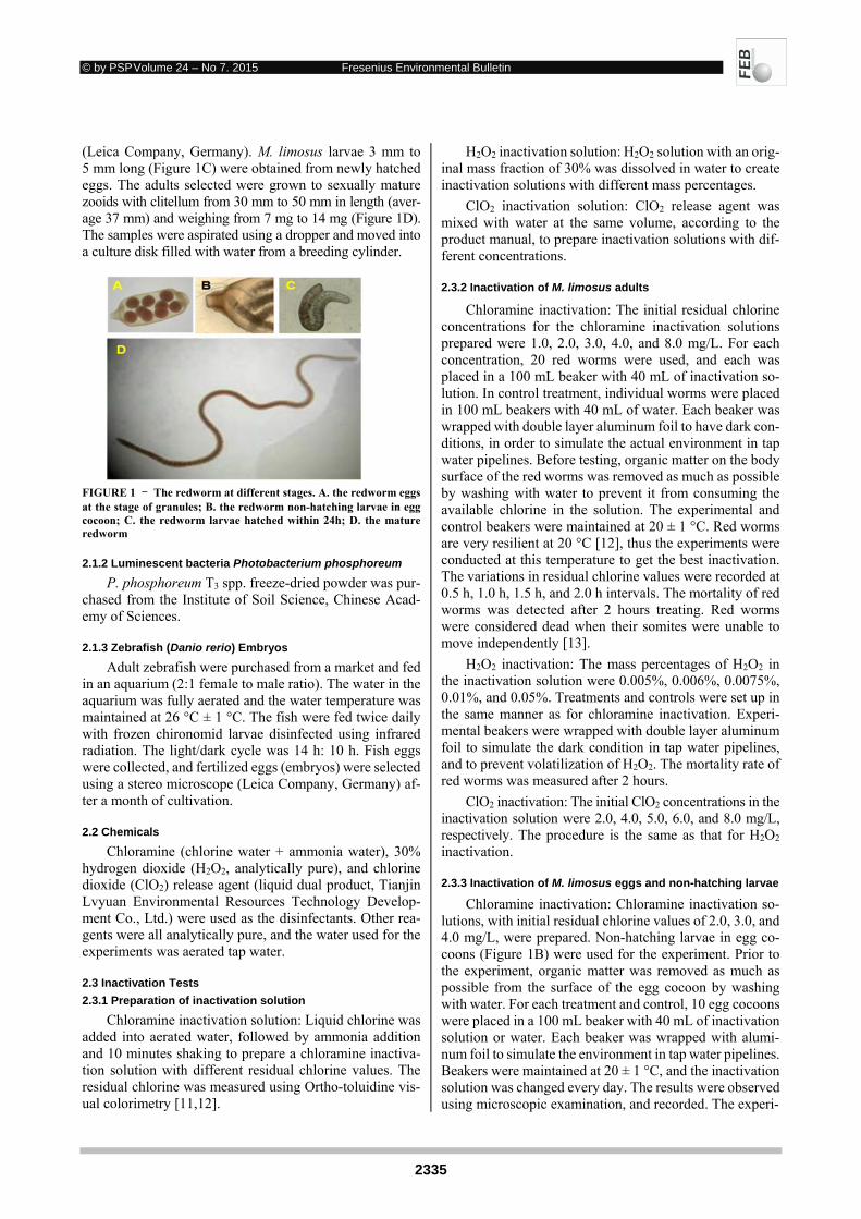
© by PSP Volume 24 – No 7. 2015 Fresenius Environmental Bulletin
2335
(Leica Company, Germany). M. limosus larvae 3 mm to 5 mm long (Figure 1C) were obtained from newly hatched eggs. The adults selected were grown to sexually mature zooids with clitellum from 30 mm to 50 mm in length (aver-age 37 mm) and weighing from 7 mg to 14 mg (Figure 1D). The samples were aspirated using a dropper and moved into a culture disk filled with water from a breeding cylinder.
FIGURE 1 - The redworm at different stages. A. the redworm eggs at the stage of granules; B. the redworm non-hatching larvae in egg cocoon; C. the redworm larvae hatched within 24h; D. the mature redworm
2.1.2 Luminescent bacteria Photobacterium phosphoreum
P. phosphoreum T3 spp. freeze-dried powder was pur-chased from the Institute of Soil Science, Chinese Acad-emy of Sciences.
2.1.3 Zebrafish (Danio rerio) Embryos
Adult zebrafish were purchased from a market and fed in an aquarium (2:1 female to male ratio). The water in the aquarium was fully aerated and the water temperature was maintained at 26 °C ± 1 °C. The fish were fed twice daily with frozen chironomid larvae disinfected using infrared radiation. The light/dark cycle was 14 h: 10 h. Fish eggs were collected, and fertilized eggs (embryos) were selected using a stereo microscope (Leica Company, Germany) af-ter a month of cultivation.
2.2 Chemicals
Chloramine (chlorine water + ammonia water), 30% hydrogen dioxide (H2O2, analytically pure), and chlorine dioxide (ClO2) release agent (liquid dual product, Tianjin Lvyuan Environmental Resources Technology Develop-ment Co., Ltd.) were used as the disinfectants. Other rea-gents were all analytically pure, and the water used for the experiments was aerated tap water.
2.3 Inactivation Tests
2.3.1 Preparation of inactivation solution
Chloramine inactivation solution: Liquid chlorine was added into aerated water, followed by ammonia addition and 10 minutes shaking to prepare a chloramine inactiva-tion solution with different residual chlorine values. The residual chlorine was measured using Ortho-toluidine vis-ual colorimetry [11,12].
H2O2 inactivation solution: H2O2 solution with an orig-inal mass fraction of 30% was dissolved in water to create inactivation solutions with different mass percentages.
ClO2 inactivation solution: ClO2 release agent was mixed with water at the same volume, according to the product manual, to prepare inactivation solutions with dif-ferent concentrations.
2.3.2 Inactivation of M. limosus adults
Chloramine inactivation: The initial residual chlorine concentrations for the chloramine inactivation solutions prepared were 1.0, 2.0, 3.0, 4.0, and 8.0 mg/L. For each concentration, 20 red worms were used, and each was placed in a 100 mL beaker with 40 mL of inactivation so-lution. In control treatment, individual worms were placed in 100 mL beakers with 40 mL of water. Each beaker was wrapped with double layer aluminum foil to have dark con-ditions, in order to simulate the actual environment in tap water pipelines. Before testing, organic matter on the body surface of the red worms was removed as much as possible by washing with water to prevent it from consuming the available chlorine in the solution. The experimental and control beakers were maintained at 20 ± 1 °C. Red worms are very resilient at 20 °C [12], thus the experiments were conducted at this temperature to get the best inactivation. The variations in residual chlorine values were recorded at 0.5 h, 1.0 h, 1.5 h, and 2.0 h intervals. The mortality of red worms was detected after 2 hours treating. Red worms were considered dead when their somites were unable to move independently [13].
H2O2 inactivation: The mass percentages of H2O2 in the inactivation solution were 0.005%, 0.006%, 0.0075%, 0.01%, and 0.05%. Treatments and controls were set up in the same manner as for chloramine inactivation. Experi-mental beakers were wrapped with double layer aluminum foil to simulate the dark condition in tap water pipelines, and to prevent volatilization of H2O2. The mortality rate of red worms was measured after 2 hours.
ClO2 inactivation: The initial ClO2 concentrations in the inactivation solution were 2.0, 4.0, 5.0, 6.0, and 8.0 mg/L, respectively. The procedure is the same as that for H2O2 inactivation.
2.3.3 Inactivation of M. limosus eggs and non-hatching larvae
Chloramine inactivation: Chloramine inactivation so-lutions, with initial residual chlorine values of 2.0, 3.0, and 4.0 mg/L, were prepared. Non-hatching larvae in egg co-coons (Figure 1B) were used for the experiment. Prior to the experiment, organic matter was removed as much as possible from the surface of the egg cocoon by washing with water. For each treatment and control, 10 egg cocoons were placed in a 100 mL beaker with 40 mL of inactivation solution or water. Each beaker was wrapped with alumi-num foil to simulate the environment in tap water pipelines. Beakers were maintained at 20 ± 1 °C, and the inactivation solution was changed every day. The results were observed using microscopic examination, and recorded. The experi-
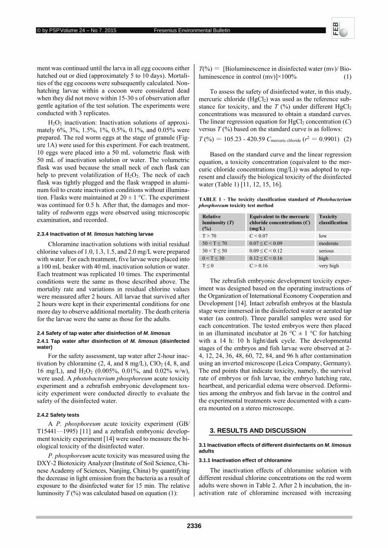
© by PSP Volume 24 – No 7. 2015 Fresenius Environmental Bulletin
2336
ment was continued until the larva in all egg cocoons either hatched out or died (approximately 5 to 10 days). Mortali-ties of the egg cocoons were subsequently calculated. Non-hatching larvae within a cocoon were considered dead when they did not move within 15-30 s of observation after gentle agitation of the test solution. The experiments were conducted with 3 replicates.
H2O2 inactivation: Inactivation solutions of approxi-mately 6%, 3%, 1.5%, 1%, 0.5%, 0.1%, and 0.05% were prepared. The red worm eggs at the stage of granule (Fig-ure 1A) were used for this experiment. For each treatment, 10 eggs were placed into a 50 mL volumetric flask with 50 mL of inactivation solution or water. The volumetric flask was used because the small neck of each flask can help to prevent volatilization of H2O2. The neck of each flask was tightly plugged and the flask wrapped in alumi-num foil to create inactivation conditions without illumina-tion. Flasks were maintained at 20 ± 1 °C. The experiment was continued for 0.5 h. After that, the damages and mor-tality of redworm eggs were observed using microscopic examination, and recorded.
2.3.4 Inactivation of M. limosus hatching larvae
Chloramine inactivation solutions with initial residual chlorine values of 1.0, 1.3, 1.5, and 2.0 mg/L were prepared with water. For each treatment, five larvae were placed into a 100 mL beaker with 40 mL inactivation solution or water. Each treatment was replicated 10 times. The experimental conditions were the same as those described above. The mortality rate and variations in residual chlorine values were measured after 2 hours. All larvae that survived after 2 hours were kept in their experimental conditions for one more day to observe additional mortality. The death criteria for the larvae were the same as those for the adults.
2.4 Safety of tap water after disinfection of M. limosus
2.4.1 Tap water after disinfection of M. limosus (disinfected water)
For the safety assessment, tap water after 2-hour inac-tivation by chloramine (2, 4, and 8 mg/L), ClO2 (4, 8, and 16 mg/L), and H2O2 (0.005%, 0.01%, and 0.02% w/w), were used. A photobacterium phosphoreum acute toxicity experiment and a zebrafish embryonic development tox-icity experiment were conducted directly to evaluate the safety of the disinfected water.
2.4.2 Safety tests
A P. phosphoreum acute toxicity experiment (GB/ T15441—1995) [11] and a zebrafish embryonic develop-ment toxicity experiment [14] were used to measure the bi-ological toxicity of the disinfected water.
P. phosphoreum acute toxicity was measured using the DXY-2 Biotoxicity Analyzer (Institute of Soil Science, Chi-nese Academy of Sciences, Nanjing, China) by quantifying the decrease in light emission from the bacteria as a result of exposure to the disinfected water for 15 min. The relative luminosity T (%) was calculated based on equation (1):
T(%) = [Bioluminescence in disinfected water (mv)/ Bio-luminescence in control (mv)]×100% (1)
To assess the safety of disinfected water, in this study,
mercuric chloride (HgCl2) was used as the reference sub-stance for toxicity, and the T (%) under different HgCl2 concentrations was measured to obtain a standard curves. The linear regression equation for HgCl2 concentration (C) versus T (%) based on the standard curve is as follows:
T (%) = 105.23 - 420.59 Cmercuric chloride (r2 = 0.9901) (2) Based on the standard curve and the linear regression
equation, a toxicity concentration (equivalent to the mer-curic chloride concentrations (mg/L)) was adopted to rep-resent and classify the biological toxicity of the disinfected water (Table 1) [11, 12, 15, 16].
TABLE 1 - The toxicity classification standard of Photobacterium phosphoreum toxicity test method
Relative luminosity (T) (%)
Equivalent to the mercuric chloride concentrations (C) (mg/L)
Toxicity classification
T > 70 C < 0.07 low
50 < T ≤ 70 0.07 ≤ C < 0.09 moderate
30 < T ≤ 50 0.09 ≤ C < 0.12 serious
0 < T ≤ 30 0.12 ≤ C < 0.16 high
T ≤ 0 C > 0.16 very high
The zebrafish embryonic development toxicity exper-
iment was designed based on the operating instructions of the Organization of International Economy Cooperation and Development [14]. Intact zebrafish embryos at the blastula stage were immersed in the disinfected water or aerated tap water (as control). Three parallel samples were used for each concentration. The tested embryos were then placed in an illuminated incubator at 26 °C ± 1 °C for hatching with a 14 h: 10 h light/dark cycle. The developmental stages of the embryos and fish larvae were observed at 2-4, 12, 24, 36, 48, 60, 72, 84, and 96 h after contamination using an inverted microscope (Leica Company, Germany). The end points that indicate toxicity, namely, the survival rate of embryos or fish larvae, the embryo hatching rate, heartbeat, and pericardial edema were observed. Deformi-ties among the embryos and fish larvae in the control and the experimental treatments were documented with a cam-era mounted on a stereo microscope.
3. RESULTS AND DISCUSSION
3.1 Inactivation effects of different disinfectants on M. limosus adults
3.1.1 Inactivation effect of chloramine
The inactivation effects of chloramine solution with different residual chlorine concentrations on the red worm adults were shown in Table 2. After 2 h incubation, the in-activation rate of chloramine increased with increasing
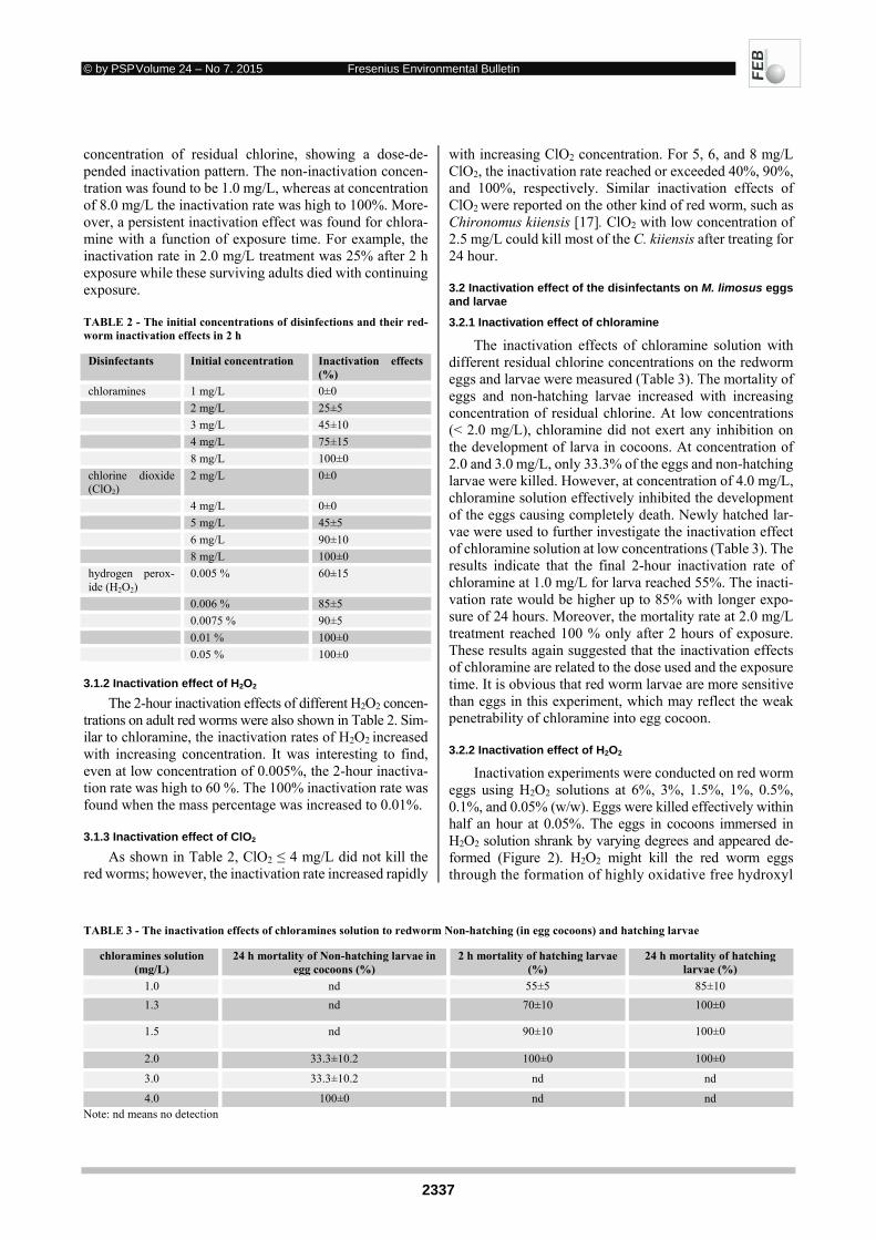
© by PSP Volume 24 – No 7. 2015 Fresenius Environmental Bulletin
2337
concentration of residual chlorine, showing a dose-de-pended inactivation pattern. The non-inactivation concen-tration was found to be 1.0 mg/L, whereas at concentration of 8.0 mg/L the inactivation rate was high to 100%. More-over, a persistent inactivation effect was found for chlora-mine with a function of exposure time. For example, the inactivation rate in 2.0 mg/L treatment was 25% after 2 h exposure while these surviving adults died with continuing exposure.
TABLE 2 - The initial concentrations of disinfections and their red-worm inactivation effects in 2 h
Disinfectants Initial concentration Inactivation effects (%)
chloramines 1 mg/L 0±0
2 mg/L 25±5
3 mg/L 45±10
4 mg/L 75±15
8 mg/L 100±0
chlorine dioxide (ClO2)
2 mg/L 0±0
4 mg/L 0±0
5 mg/L 45±5
6 mg/L 90±10
8 mg/L 100±0
hydrogen perox-ide (H2O2)
0.005 % 60±15
0.006 % 85±5
0.0075 % 90±5
0.01 % 100±0
0.05 % 100±0
3.1.2 Inactivation effect of H2O2
The 2-hour inactivation effects of different H2O2 concen-trations on adult red worms were also shown in Table 2. Sim-ilar to chloramine, the inactivation rates of H2O2 increased with increasing concentration. It was interesting to find, even at low concentration of 0.005%, the 2-hour inactiva-tion rate was high to 60 %. The 100% inactivation rate was found when the mass percentage was increased to 0.01%.
3.1.3 Inactivation effect of ClO2
As shown in Table 2, ClO2 ≤ 4 mg/L did not kill the red worms; however, the inactivation rate increased rapidly
with increasing ClO2 concentration. For 5, 6, and 8 mg/L ClO2, the inactivation rate reached or exceeded 40%, 90%, and 100%, respectively. Similar inactivation effects of ClO2 were reported on the other kind of red worm, such as Chironomus kiiensis [17]. ClO2 with low concentration of 2.5 mg/L could kill most of the C. kiiensis after treating for 24 hour.
3.2 Inactivation effect of the disinfectants on M. limosus eggs and larvae
3.2.1 Inactivation effect of chloramine
The inactivation effects of chloramine solution with different residual chlorine concentrations on the redworm eggs and larvae were measured (Table 3). The mortality of eggs and non-hatching larvae increased with increasing concentration of residual chlorine. At low concentrations (< 2.0 mg/L), chloramine did not exert any inhibition on the development of larva in cocoons. At concentration of 2.0 and 3.0 mg/L, only 33.3% of the eggs and non-hatching larvae were killed. However, at concentration of 4.0 mg/L, chloramine solution effectively inhibited the development of the eggs causing completely death. Newly hatched lar-vae were used to further investigate the inactivation effect of chloramine solution at low concentrations (Table 3). The results indicate that the final 2-hour inactivation rate of chloramine at 1.0 mg/L for larva reached 55%. The inacti-vation rate would be higher up to 85% with longer expo-sure of 24 hours. Moreover, the mortality rate at 2.0 mg/L treatment reached 100 % only after 2 hours of exposure. These results again suggested that the inactivation effects of chloramine are related to the dose used and the exposure time. It is obvious that red worm larvae are more sensitive than eggs in this experiment, which may reflect the weak penetrability of chloramine into egg cocoon.
3.2.2 Inactivation effect of H2O2
Inactivation experiments were conducted on red worm eggs using H2O2 solutions at 6%, 3%, 1.5%, 1%, 0.5%, 0.1%, and 0.05% (w/w). Eggs were killed effectively within half an hour at 0.05%. The eggs in cocoons immersed in H2O2 solution shrank by varying degrees and appeared de-formed (Figure 2). H2O2 might kill the red worm eggs through the formation of highly oxidative free hydroxyl
TABLE 3 - The inactivation effects of chloramines solution to redworm Non-hatching (in egg cocoons) and hatching larvae
chloramines solution (mg/L)
24 h mortality of Non-hatching larvae in egg cocoons (%)
2 h mortality of hatching larvae (%)
24 h mortality of hatching larvae (%)
1.0 nd 55±5 85±10
1.3 nd 70±10 100±0
1.5 nd 90±10 100±0
2.0 33.3±10.2 100±0 100±0
3.0 33.3±10.2 nd nd
4.0 100±0 nd nd Note: nd means no detection
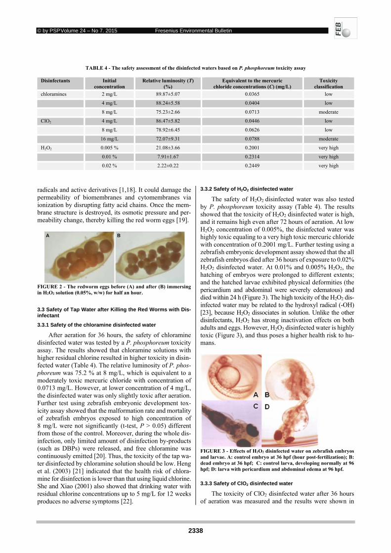
© by PSP Volume 24 – No 7. 2015 Fresenius Environmental Bulletin
2338
TABLE 4 - The safety assessment of the disinfected waters based on P. phosphoreum toxicity assay
Disinfectants Initial concentration
Relative luminosity (T) (%)
Equivalent to the mercuric chloride concentrations (C) (mg/L)
Toxicity classification
chloramines 2 mg/L 89.87±5.07 0.0365 low
4 mg/L 88.24±5.58 0.0404 low
8 mg/L 75.23±2.66 0.0713 moderate
ClO2 4 mg/L 86.47±5.82 0.0446 low
8 mg/L 78.92±6.45 0.0626 low
16 mg/L 72.07±9.31 0.0788 moderate
H2O2 0.005 % 21.08±3.66 0.2001 very high
0.01 % 7.91±1.67 0.2314 very high
0.02 % 2.22±0.22 0.2449 very high
radicals and active derivatives [1,18]. It could damage the permeability of biomembranes and cytomembranes via ionization by disrupting fatty acid chains. Once the mem-brane structure is destroyed, its osmotic pressure and per-meability change, thereby killing the red worm eggs [19].
FIGURE 2 - The redworm eggs before (A) and after (B) immersing in H2O2 solution (0.05%, w/w) for half an hour.
3.3 Safety of Tap Water after Killing the Red Worms with Dis-infectant
3.3.1 Safety of the chloramine disinfected water
After aeration for 36 hours, the safety of chloramine disinfected water was tested by a P. phosphoreum toxicity assay. The results showed that chloramine solutions with higher residual chlorine resulted in higher toxicity in disin-fected water (Table 4). The relative luminosity of P. phos-phoreum was 75.2 % at 8 mg/L, which is equivalent to a moderately toxic mercuric chloride with concentration of 0.0713 mg/L. However, at lower concentration of 4 mg/L, the disinfected water was only slightly toxic after aeration. Further test using zebrafish embryonic development tox-icity assay showed that the malformation rate and mortality of zebrafish embryos exposed to high concentration of 8 mg/L were not significantly (t-test, P > 0.05) different from those of the control. Moreover, during the whole dis-infection, only limited amount of disinfection by-products (such as DBPs) were released, and free chloramine was continuously emitted [20]. Thus, the toxicity of the tap wa-ter disinfected by chloramine solution should be low. Heng et al. (2003) [21] indicated that the health risk of chlora-mine for disinfection is lower than that using liquid chlorine. She and Xiao (2001) also showed that drinking water with residual chlorine concentrations up to 5 mg/L for 12 weeks produces no adverse symptoms [22].
3.3.2 Safety of H2O2 disinfected water
The safety of H2O2 disinfected water was also tested by P. phosphoreum toxicity assay (Table 4). The results showed that the toxicity of H2O2 disinfected water is high, and it remains high even after 72 hours of aeration. At low H2O2 concentration of 0.005%, the disinfected water was highly toxic equaling to a very high toxic mercuric chloride with concentration of 0.2001 mg/L. Further testing using a zebrafish embryonic development assay showed that the all zebrafish embryos died after 36 hours of exposure to 0.02% H2O2 disinfected water. At 0.01% and 0.005% H2O2, the hatching of embryos were prolonged to different extents; and the hatched larvae exhibited physical deformities (the pericardium and abdominal were severely edematous) and died within 24 h (Figure 3). The high toxicity of the H2O2 dis-infected water may be related to the hydroxyl radical (-OH) [23], because H2O2 dissociates in solution. Unlike the other disinfectants, H2O2 has strong inactivation effects on both adults and eggs. However, H2O2 disinfected water is highly toxic (Figure 3), and thus poses a higher health risk to hu-mans.
FIGURE 3 - Effects of H2O2 disinfected water on zebrafish embryos and larvae. A: control embryo at 36 hpf (hour post-fertilization); B: dead embryo at 36 hpf; C: control larva, developing normally at 96 hpf; D: larva with pericardium and abdominal edema at 96 hpf.
3.3.3 Safety of ClO2 disinfected water
The toxicity of ClO2 disinfected water after 36 hours of aeration was measured and the results were shown in
© by PSP Volume 24 – No 7. 2015 Fresenius Environmental Bulletin
2339
Table 4. The disinfected water from high concentration (8 mg/L) ClO2 treatment had low toxicity (Figure 3), equiv-alent to 0.0626 mg/L mercuric chloride. Further checking using a zebrafish teratogenicity test revealed that the 8 mg/L ClO2 disinfected water was not teratogenic to zebrafish, again suggesting that the toxicity of ClO2 disinfected water is low. Moreover, considering the toxicity of ClO2 could be minimized by aeration in the water plant and consumption in the pipe network. Therefore, although the concentration of 6 mg/L or 8 mg/L may be slightly high in the redworm inactivation, their disinfected water still remains low toxic. Nevertheless, during the actually redworm inactivation op-eration, the ClO2 dosage should be optimized to maximize water quality and inactivation effect while minimizing the health risks.
4. CONCLUSION
The inactivation effects of chloramine, ClO2 and H2O2 on M. limosus eggs, larvae, and adults were compared and the safeties of the resulting tap water were evaluated. The key finding are summarized as following: (1) 4 mg/L of chloramine has an excellent effect on killing M. limosus adults, eggs, and larvae with very low chemical toxicity identified for the resulting tap water. (2) Although H2O2
has a significant effect on killing both adults and eggs of redworms, the resulting water is too toxic thus may pose a relatively high risk to human health. (3) ClO2 at a range from 6 mg/L to 8 mg/L is very effective in killing M. limo-sus and poses low toxicity for the resulting water. These results suggested that chloramines and ClO2 but not H2O2
probably should be good disinfectants for controlling red-worm in tap water. The findings in this paper may be help-ful for water treatment plants to better control the redworm pollution in water distribution systems.
ACKNOWLEDGEMENTS
This project was supported by the National Natural Science Foundation of China (21107058, 41373089), the Shenzhen Key Laboratory for Coastal Ocean Dynamic and Environment (ZDSY20130402163735964), the Scientific Research Foundation for the Returned Overseas Chinese Scholars,State Education Ministry of China.
The authors have declared no conflict of interest.
REFERENCES
[1] Zhou, L., Zhang, J., Lei, P., Liang, M. (2003) The advances on the bloodworm control in water purification process. Water. Wastewater. Eng. 29, 25-28.
[2] Michael, K. (1997) New strategies for the control of the par-thenogenetic chironomid. J. Am. Mosq. Control. Assoc. 13, 189-192.
[3] Bay, E.C. (1993) Chironomid (Diptera: Chironomidae) larval occurrence and transport in a unicipal water system. J. Am. Mosq. Control. Assoc. 9, 275-284.
[4] Berg, M.B. (1995) Infestation of enclosed water supplies by Chironomids (Diptera: Chironomidae): Two case studies. Chi-ronomids from genes to ecosystems. Australia:CSIRO pub-lications, East Melbourne.
[5] Cui, F., Sun, X., Zhang, J., Xu, F., Liu, L. (2005) A review on preventions of chironomus larva pollution in water treatment system. Environ. Pollut. Control. 27, 235-238.
[6] Dong, J. (2002) Causes and preventive measures of blood-worm pollution in drinking water. Jiangsu. J. Prev. Med. 13, 47-48.
[7] Lu, J. (2001) Growth pattern and the control strategies of chi-ronomid (Tendipes gr. thammi) larvae in tap water. Chin. Wa-ter. Wastewater. 17, 53-54.
[8] Chen, X., Zhu, L., Wang, Q., Yang, Y., Zhao, W., He, W., Han, H., Zhang, X. (2005a) Pilot study on control of redworm in drinking water. Water. Wastewater Eng. 31, 7-10.
[9] Chen. X., Zhu, L., Wang, Q., Yang, Y., Zhao, W., He, W., Han, H., Zhang, X. (2005b) Pilot study on growth and repro-duction of Red Worm. Water. Wastewater. Eng. 31, 38-40.
[10] Eaton, K. (2013) Red worms found in drinking water supply for Oklahoma town. NBC News. http://www.nbcnews.com/news/other/red-worms-found-drinking-water-supply-oklahoma-town-f8C11028887.
[11] MEPPRC, Ministry of Environmental Protection of the Peo-ple’s Republic of China. (1995) GB/T-15441. Water quality—Determination of the acute toxicity—Luminescent bacteria test. http://kjs.mep.gov.cn/hjbhbz/bzwb/shjbh/sjcgfffbz/199508/t19950801_67352.htm
[12] SAPRC, Standardization Administration of the People’s Re-public of China. (2006) GB5750.11. Standard examination methods for drinking water – disnifectants parameters. http://www.moh.gov.cn/zwgkzt/pgw/201212/33655.shtml
[13] Song, ZH., Chen, TY. (1998) Toxicity of Tributyltin to Chi-ronomus Larvae. Environ. Sci. 19, 87-91.
[14] OECD. (1998) OECD212. Fish, short term toxicity test on em-bryo and sac-fry stages. OECD Guideline for Testing of Chemicals.
[15] Gu, Z., Xie, S., Wu, L., et al. (1983) The bio-toxicity determi-nation of contaminated water using photobioluminometer. En-viron. Sci. 4, 30-33.
[16] Qiao, H., Gu, Z. (1993) Use of luminescent bacteria test for quantitatively determining the toxicity of contaminated water. Environ. Her. (5), 11-13.
[17] He W. (2005) The control methods for Chironomus Kiiensis, and the molecular classification of Chironomus Species in mu-nicipal water supply system. Thesis for master degree. China Agricultural University, Beijing, China.
[18] Ye, J., Li, B. (2001) The killing experiments of Chironomid larvae as well as several associated issues. The 8th annual meet-ing of water supply committee, Water Industry Branch, China Civil Engineering Society. Chengdu, China.
[19] Ge, Y., Huan, P. (1999) Hydrogen peroxide disinfection and its application. Sh. J. Prev. Med. (11), 157-158.
[20] Zhang, X., Chen, C., He, W., et al. (2004) Control of disinfec-tion byproducts in safe-chlorine-disinfection process. China Water. Wastewater. 20, 13-16.
[21] Heng, Z., Li, C., Jiang, W., et al. (2003) Effect of chloramine disinfection on the formation of drinking water disinfection by-products and their muta-genicity. J. Environ. Heal. 20, 134-136.
© by PSP Volume 24 – No 7. 2015 Fresenius Environmental Bulletin
2340
[22] She, L., Xiao, G. (2001) The toxicological character of Cl2 and chlorine dioxide used in drinking water disinfection. Fujian. Chem. Industry. (1), 15-17.
[23] Liu, X., Tang, Y., Xu, S., et al. (2003) Study on treatment of pre-oxidation hanjiang river water with hydrogen peroxide in pilot plant. J. Hunan. Ur. Construc. Col. 12, 23-25.
Received: October 12, 2014 Revised: December 11, 2014 Accepted: January 08, 2015 CORRESPONDING AUTHOR
Xiaoshan Zhu Shenzhen Public Platform for Screening and Application of Marine Microbial Resources Graduate School at Shenzhen Tsinghua University Shenzhen 518055 P.R. CHINA Phone: +86-755-26036381 Fax: +86-755-26036381. E-mail: [email protected]
FEB/ Vol 24/ No 7/ 2015 – pages 2334 - 2340
© by PSP Volume 24 – No 7. 2015 Fresenius Environmental Bulletin
2341
ADSORPTION OF LEAD METAL FROM AQUEOUS SOLUTIONS
USING ACTIVATED CARBON DERIVED FROM SCRAP TIRES Ali Reza Rahmani1, Ghorban Asgari2, Fateme Barjasteh Askari3,* and Ameneh Eskandari Torbaghan4
1 Environmental Health Engineering Department, Faculty of Health and Research Center for Health Sciences, Hamadan University of Medical Sciences, Hamadan, Iran
2 Department of Environmental Health Engineering, Faculty of Health, Hamadan University of Medical Sciences, Hamadan, Iran
3 Department of Environmental Health Engineering, Torbat Heydariyeh University of Medical Sciences, Torbat Heydariyeh, Iran 4 Department of Environmental Health Engineering, Torbat Heydariyeh University of Medical Sciences, Torbat Heydariyeh, Iran
ABSTRACT
Heavy metals in water-bodies are one of the serious en-vironmental problems in many communities. In this study, the potential of activated carbon derived from scrap tires was investigated for adsorption of lead metal cations (Pb2+) from aqueous solutions. Activated carbon was prepared from scrap vehicle tires using a thermo-chemical activation method. Scanning electron microscopy (SEM), BET and BJH analyses were used to characterize the prepared acti-vated carbon. Batch adsorption experiments were carried out to determine the effects of initial concentration of the ions, pH, contact time and adsorbent dosage. Adsorption isotherms of the metal ions on the adsorbent were meas-ured and correlated with the Langmuir and Freundlich iso-therm models. The predominant component of prepared activated carbon is carbon (76.481%) with 185.046 m2/g surface area and an average pore diameter of 52 nm. The results showed that there was a decrease in removal of Pb2+ with increasing contact time, adsorbent dosage and pH. Ex-perimental adsorption data were best fitted by Freundlich model. In view of the findings, it can be claimed that the production of the activated carbon from scrap tires can pro-vide a green and cost-effective method for heavy metals removal.
KEYWORDS: Activated carbon, adsorption, scrap tire, thermo-chemical
1. INTRODUCTION
Industrialization has increased the environmental pol-lution through producing huge amounts of wastes. Heavy metals are classified as the most important environmental pollutants due to their high toxicity to humans and ecosys-tems. Some human activities, such as mining, extraction industries and metal melting, discharge wastewaters con-
* Corresponding author
taining large quantities of heavy metals like cadmium, lead and copper [1]. Lead is one of those heavy metals which is harmful to human health causing different signs, such as anemia, headache etc. [2]. Different techniques, such as chemical precipitation, coagulation and flocculation, are used to remove highly concentrated and heavy metal-con-taining wastewaters [1, 3]. However, most of them are not practical enough due to the low concentration of heavy metals; therefore, these methods should be used along with supplementary techniques [1].
Ion exchange and membrane filtration technologies can reduce heavy metal concentrations to acceptable levels of environmental regulations, but high costs and opera-tional problems are the drawbacks of these methods [3, 4]. During the recent decades, the use of activated carbon in water and wastewater treatment industries has been consid-ered [5, 6]. Activated carbon had successfully been able to remove a wide range of pollutants from the environment. It can also remove most heavy metals [5]. In general, find-ing economic ways of water and wastewater treatment have been a controversial issue among experts.
Activated carbon can be produced from raw materials having high amounts of carbon and small parts of inorganic matters [7]. The most prevailing ones in this case are wood, some plants, piceous coal, brown coal, lignin, coconut shell, fruit shells like nut shells, almond shells, rice husks etc. [8, 9].
Just in Iran, about 250000 tons of scrap tires are pro-duced annually (6.3 kg per capita per year) [10]. The meth-ods used to recycle scrap tires are not efficient enough [10]. Accumulated masses in the environment cause environ-mental problems and lead to an increase in flies and rodent numbers; on the other hand, illegally piled scrap tires can set fires [11]. The positive aspects of using scrap tires to make new products are cheapness and abundance. One of the products that can be obtained from the scrap tires is ac-tivated carbon. A fixed amount of carbon (about 25% of mass) and very low levels of volatile ash (>5%) of rubber are the advantages of the derived carbon [7, 11]. Pyro-oil and pyro-gas produced beside the pyrolysis of scrap tires
© by PSP Volume 24 – No 7. 2015 Fresenius Environmental Bulletin
2342
to produce activated carbon, can be used as a source of re-newable energy [7, 8].
Production of scrap tire-derived carbon could have commercial value in air quality and wastewater treatment industries, and can be used to store gas, to separate and treat various pollutants [12]. As a whole, economical prof-itability and eco-friendly properties are the two main ad-vantages of producing activated carbon from scrap tires [9].
In this study, the ability of prepared activated carbon in removal of Pb2+ as a heavy metal from aqueous solutions was investigated.
2. MATERIALS AND METHODS
This experiment involves three separate but sequential steps: activated carbon production, characterization of ac-tivated carbon, and adsorption experiments. Activated car-bon was produced by a thermo/chemical method through the pyrolysis process. Scrap tire samples were pyrolysed by a muffle furnace (model Exiton). All the experiments were carried out based on the standard methods mentioned in reference [13]. The unknown concentrations of Pb2+ so-lutions were measured by atomic absorption (Analyst 700, Perkin Elmer). NaOH or H2SO4 solution (1N) was used to adjust the pH during the experiments (pH-meter, model PP-50, Sartorius). All the chemicals used in this study were prepared from Merck and Aldrich companies. Distilled wa-ter was prepared by a Fater Electronic water distiller model 2104 (Tehran, Iran). For all batch experiments, glassware and bottles were washed and rinsed with HNO3 before use, and then by distilled water. A 301 Sigma centrifuge was used for sample separation.
2.1. Adsorbent preparation
Scrap tire samples were crushed into 0.2-0.3 cm pieces and put into KOH solution for 3 h to become activated (mass ratio for KOH to tire was 4:1). Next, the mixture was heated up to 110 °C in an oven for 24 h. Then, the tires were pyrolysed (oven temperature raised to 700 °C during 2 h). The pyrolysis products were washed with 250 ml HCl solution (0.5 N) at 85 °C for 30 min. In the next step, the products were washed with water until the pH of water and carbon mixture reached above 6.9. At last, the final product was dried at 110 °C for 24 h. The produced samples were sieved by standard ASTM sieves into 100 mesh (149 µm) particles and kept for the next usages.
2.2. Characterization of prepared activated carbon
A scanning electron microscope (SEM) of Majlesi University of Material Engineering (Kv 20.0, take off an-gle 25.0º and elapsed lifetime 10.0) was used to show the morphologic properties. Specific surface area, total pore volume and average pore size were measured by BET (Bar-ret, Brunner and Emerett) isotherm using Belsorp software (BEL, Japan, Inc.). The distribution size of the pores was determined by BJH (Barrett, Joyner Halenda) method.
2.3. Adsorption experiments
The adsorption tests were performed in a batch system, and the effective parameters on the adsorption process in-cluding the contact time (30-180 min), pH of solution (2, 4, 6 and 8), adsorbent dosage (0.1-0.6 g), and initial Pb2+ concentration (10-100 mg/L) were studied in different stages. The speed of stirring was 200 rpm, the tempera-ture was 25±1 °C, and the size of adsorbent particles was 100 mesh. The volume of test solutions was 50 ml and the adsorbent particles were separated after the Pb2+ removing process by centrifugation. The tests were performed by making the other variables constant. To study the isotherm model fitting, Langmuir and Freundlich models were used.
In order to determine pHZPC, the equilibrium technique in a batch system was applied [14]. The percent of removed Pb2+ by activated carbon was calculated from Eq. 1:
Removed Pb2+(%) = [(Ca-C)/Ca]×100 (1)
Where, Ca is the initial Pb2+ concentration before ad-dition of the adsorbent and C is Pb2+ concentration after adsorption, with produced activated carbon, and with Eq. 2, the carbon yield after pyrolysing was calculated.
Carbon yield% = Wac/Wti (2)
In the equation, Wti is the weight of used scrap tire for pyrolysing and Wac is final produced activated carbon.
3. RESULTS AND DISCUSSION
3.1. The structural characteristics of the prepared activated carbon
Based on the conducted analyses, carbon is the main element (76%) of the structure of the processed activated carbon (Table 1). The result of this section are consistent with the findings of other investigators. Teng et al. (2000) [7], Galvagno et al. (2002) [8] and Mahramanlioglu et al. (2006) [15] reported on carbon as the main compound of scrap tire-derived activated carbon. As shown in Table 1, the specific surface area of prepared activated carbon was determined 185 m2 g-1 (Table 1).
TABLE 1 - Characteristics of the prepared activated carbon
BET(m2gr-1) 185.046 BJH(m2gr-1) 146.4
Total pore volume (cm3 gr-1) 0.58 pHzpc 6.87
Particle size (µm) <149 Average pore size (nm) 52.461
Components (wt.%)
C 76.481 O 10.136 Al 7.29 K 6.093
In the preparation process, the production efficiency of
activated carbon from scrap tires was 32 and 36.5%. A SEM micrograph of the produced activated carbon is shown in Fig. 1. Based on the SEM micrograph, processed

© by PSP Volume 24 – No 7. 2015 Fresenius Environmental Bulletin
2343
activated carbon has a non-crystalline structure with a wide range of pore sizes. (Fig. 1).
FIGURE 1 - SEM micrograph of scrap tire derived carbon
3.2. The effect of pH on adsorption process
Adsorption experiments were conducted at different pH values while other parameters were constant. Experi-ments showed that metal removal efficiency increased with increasing pH (Fig. 2). Alkaline pH was found as the opti-mum pH. Meanwhile, the blank solution was used during the rest of the experiment. Regardless of the different val-ues of adsorption efficiencies, adsorption was observed at all pHs and metal ions were removed from the solution. The process can highly be used to remove heavy metals from effluents at different pH values (Fig. 2).
The pH value is one of the most effective parameters in adsorption process. Hydrogen ions compete with cations (adsorbate fraction) in adsorption process [16]. The pH can also affect adsorbent surface charge. According to other studies, the pH range for adsorption on different activated carbons is between 4 and 8 [16-18]; therefore, this range was determined for the experiments in this study. As can be seen from Fig. 2, the removal efficiency of lead cations under acidic conditions was lowest, particularly at pH 2.
FIGURE 2 - Effect of solution pH on Pb2+ adsorption: time=60 min., Pb2+=10 mg/L, activated carbon 0.1 g
The pHzpc is a parameter that affects the adsorption
efficiency, and it was determined to be 6.87 in this study.
At pH values above pHzpc, the carbon surface has more neg-ative charge and lead as a cation attracts more to the adorbent surface whereas at pHs below pHzpc, lead cation adsorption decreased. In the present study, the highest removal effi-ciency was obtained at pH 8. That is to say, in acidic condi-tions, H3O+ ions which compete with metal cations are ad-sorbed on active sites of the adsorbent. When saturating these sites, the adsorption of metal cations decreased [18]. Mehrasbi et al. (2008) [19] investigated the removal of heavy metals from an aqueous solution by adsorption on al-mond shells; their results show that the adsorption values de-creased when lowering pH value, and optimum pH was de-termined to be 5-6 [19]. In this study, almond shells were separately treated with acidic solution (0.4 mol/L HNO3) and basic solution (0.4 mol/L NaOH). Kannan and Rengasamy (2005) [17] studied the adsorption of nickel(II) ions on different carbons. In this study, it was reported that the increase in pH increased the removal percentage of Ni(II) ions which is in accordance with our results [17]. Meena et al. [12] investigated the efficiency of heavy metal removal by granular activated carbon; the results show that at pH 4, bivalence cations like mercury, manganese and cadmium have the highest removal efficiencies, and up to pH 7, Cd removal efficiency decreased. But for other 3 bivalence cat-ions (Pb, Ni, Zn), pH 8 was determined as the optimum pH [12]. The results of this research are consistent with those of the present study. Increase in adsorption efficiency at pHs >6 is due to the reaction of metal hydroxide species with the micropores of activated carbon. The differences in results of different pH values can be because of the various effects of pH on adsorbents used in the different studies [2, 19, 20]. Moreover, in the mentioned studies, the concentration of the metal cations are different from examined concentrations in this study (more or less than 10 ppm), and this can be another reason for these differences. At higher initial concentration, the decrease of adsorption rate resulted in equilibrium time reduction. Hossein Zadeh et al. (2010) [20] reported that the most efficient acidic dye removal on scrap tire-derived acti-vated carbon was observed in acidic conditions [20]. In gen-eral, according to the obtained results and also to parallel studies, it is concluded that in adsorption process, the pH plays a significant role in pollutants removal. That is to say, the effect of pH on adsorption differs with the types of both adsorbent and pollutant.
3.3. The effect of contact time on adsorption process
The effect of contact time on removal of Pb2+ by pro-duced activated carbon indicated that with increasing the contact time, the adsorption rate was increased (Fig. 3). The metal cations adsorption on activated carbon reached an equilibrium after 3 h, and after that, the amount of ad-sorption remained constant. These results show that the in-itial adsorption on scrap tire-derived activated carbon is a rapid process which is related to activated carbon structure (activated carbon pores are classified in the meso range). The blanks, which were used to show the effects of pH on removal efficiency in different contact times, removed the pollutants to some extent but it was negligible (Fig. 3).
0
20
40
60
80
100
2 4 6 8
pH
Ads
orpt
ion
eff
icie
ncy
%

© by PSP Volume 24 – No 7. 2015 Fresenius Environmental Bulletin
2344
FIGURE 3 - Effect of contact time on removal of Pb2+: activated car-bon 0.1 g, pH=8, Pb2+ =10 mg/L
Determining optimum contact time is required to use
an adsorbent for pollutant removal. Thus, the adsorption efficiency was investigated at different times (30, 45, 60, 90, 120 and 180 min). As can be seen in Fig. 3, for lead, the greatest amount of adsorption happened up to 30 min, and after that, amount increased slightly with a constant trend; this is also mentioned in the study carried out by Meena et al. (2010) [12]. The reason is that, at first, more adsorption sites are available and a higher driving force transferred the solute to the adsorption sites more easily. But after a while, the number of active sites occupied by adsorbate were diminished and, consequently, adsorption rates decreased [12]. This can be related to the tiny struc-ture of pores on the surface of adsorbents (Fig. 1). Since the adsorption is an equilibrium reaction, the adsorption of metal cations on the activated carbon continued to reach an equilibrium. If the active adsorption sites are more acces-sible to the soluble metal cations or other adsorbate com-ponents, less time will be required for the maximum ad-sorption, and otherwise, it will take more time [20]. Meena et al. (2010) [12] investigated the removal of heavy metals on granular activated carbon, the equilibrium time was ob-tained to be 48 h while it was determined to be 3 h in this study. In Hossein Zadeh et al. (2010) [20], adsorption of acidic dyes on activated carbon derived from scrap tire was studied, and the equilibrium time was measured to be 2 h; in the study of Kim et al. (2005) [21], the equilibrium time for Pb and Cu adsorption on brewery biomass was meas-ured to be 60 min which is inconsistent with our findings. Uzun et al. (2000) [16] found that the equilibrium time for adsorption of various metal cations on activated carbon was 130-150 min which was similar to the results of our study. The difference in our findings is a result of structural properties of the used adsorbents.
3.4. The effect of adsorbent dose on adsorption process
Lead adsorption was investigated by using different amounts of the produced activated carbon (0.1, 0.2, 0.3, 0.4, 0.5 and 0.6 g). As shown in Fig. 4, removal efficiency increased with increasing adsorbent dose. The Pb removal efficiency increased from 68.3 to 88.1% (Fig. 4).
Increasing the adsorbent dose (activated carbon) raised the lead metal cation removal efficiency. This rise is sig-
nificant and can be due to the either increase of adsorption activated sites or general increase in specific surface area of the adsorbent. These results are consistent with the find-ings of Meena et al. (2010) [12]. Conversely, in studies with herbal biomass or other living organisms as adsor-bents, the removal efficiency decreased with increasing ad-sorbent dose, and the results were not the same as in our study. This decrease can be because of a rise in bioadsor-bent concentration which prevents metal cations from ad-sorbing into the cells. In addition, as the amount of bio-sorbent increases, the density of cellular compounds in-creases, and leads to adsorption sites reduction [22], while for activated carbon it i not like that. Kim et al. (2005) [21] reported that the adsorption of Pb2+ and Cu2+ increased with increasing the bioadsorbent dose while for Cd this was quite opposite [21]. In Elaigwu et al. (2010) [23], the in-crease in activated carbon dose enhanced the Pb2+ removal efficiency.
FIGURE 4 - Effect of adsorbent dose on removal of Pb2+: time=180 min., Pb2+ =10 mg/L, pH=8
3.5. The effect of initial concentration of the metallic solution
Lead removal under various initial concentrations did not show a clear trend but the highest removal efficiency (%99.166) was observed in a 60 ppm Pb solution. (Fig. 5).
FIGURE 5 - Effect of initial concentration on removal of Pb2+: time=180 min., activated carbon 0.1 g, pH=8
The results showed that the adsorption capacity of the
sorbent increased by raising the initial concentration of metal ions, which may be due to an increase in metal ions driving force. Under concentrations higher than the opti-mum level, the adsorption sites get saturated which reduces
0
20
40
60
80
100
0 30 60 90 120 150 180
Contact time, min
Ads
orpt
ion
effi
cien
cy, %
Experimental samples
Blank samples
0
20
40
60
80
100
0.1 0.2 0.3 0.4 0.5 0.6
Adsorbent dose, gr
Ads
orpt
ion
effi
cien
cy, %
Experimental samples
Blank samples
0
20
40
60
80
100
10 20 40 60 80 100
Pb concentration, mg/L
.Ads
orpt
ion
effi
cien
cy, %
With activated carbon
Without activated carbon

© by PSP Volume 24 – No 7. 2015 Fresenius Environmental Bulletin
2345
more adsorption capacity and removal efficiency [12]. Meena et al. (2010) [12] results conform to our findings whereas in Kim et al. (2005) [21] experiments, the results were quite different.
3.6. Adsorption isotherms
Equilibrium studies were conducted in 100-ml conical flasks at 20 °C. Weighed amounts (0.6 g) of prepared acti-vated carbon were added into conical flasks containing 50 ml Pb2+ solution with 10-100 mg/L concentration. The samples were agitated with 100 rpm up to 24 h. Then, after centrifugation, the samples were withdrawn and the equi-librium concentration of Pb2+ was determined.
The equilibrium data were fitted onto 2 common iso-
therm models, Freundlich and Langmuir. The linear form of both isotherms are presented in Eqs. 3 and 4:
Freundlich isotherm (3)
qe = the equilibrium adsorbate concentration on adsor-bent (mg/g), and Ce = equilibrium concentration of adsorb-ate (mg/L).
n and k are 2 constants which describe the properties of adsorption process at particular temperature.
Langmuir isotherm (4) qm = maximum adsorption capacity (mg/g) (Fig. 6).
The results showed that the adsorption isotherms of Pb2+
on activated carbon were better fitted by the Freund-lich model (0.982<R2). The higher correlation coefficient indi-cates this (Table 2). Calculated parameters of Pb2+ metal ad-sorption for each model are summarized in Table 2.
3.7. Fitting the data with adsorption isotherms
Adsorption isotherms are adsorption characteristics and equilibrium data describing how pollutants react with adsorbents. They have a major role in optimizing adsorbent consumption. In this study, the obtained values from the experiments were investigated by Langmuir and Freund-lich isotherm models. The results showed that the adsorp-tion of the studied metal cations is best correlated by Freund-lich isotherm. This isotherm expresses adsorption process onto heterogenous surfaces [6]. Therefore, adsorp-tion activation energy is not equal for all adsorption sites which resulted in multilayer adsorption for solutes [5]. In
Langmuir isotherm, the maximum adsorption capacity (qm) for Pb2+ was 8.69 mg/g. The amounts of the 2 parameters n and k in Freundlich model show the energy consumption rate. The more 1/n is near zero, the more heterogenous su-faces will be [7]. The results of the isotherm section of our study are consistent with some studies but inconsistent with some others. For example, in the study of Seki et al. [24], Cd adsorption from aqueous solutions was best fitted by the Freundlich isotherm while Kim et al. [21] and Ozdemir et al. [25] found that heavy metal adsorption was more according to Langmuir isotherm.
Langmuir Freundlich
FIGURE 6 - Sorption isotherms with fitted models for Pb2+ metal sorption: pH=8, activated carbon=0.6 gr
TABLE 2 - Isotherm parameters for Pb2+ adsorption on the prepared activated carbon
qm (mg/g) N K R2 Isotherm model
- 1.876 2.259 0.982 Freundlich
8.695 - 3.197×10⁻² 0.960 Langmuir
y = 0,115x + 0,2789R² = 0,9607
0
0,4
0,8
1,2
1,6
2
0 5 10
Ce/qe
Ce
y = 0,533x + 0,3541R² = 0,9827
-0,2
0
0,2
0,4
0,6
0,8
1
-1 -0,5 0 0,5 1 1,5
Log qe
Log Ce
efe Cn
kq log1
loglog
mm q
Ce
Kqqe
Ce
1
© by PSP Volume 24 – No 7. 2015 Fresenius Environmental Bulletin
2346
4. CONCLUSION
The results showed that there was a decrease in re-moval of Pb2+ with increasing contact time, adsorbent dos-age and pH. The optimum pH was found to be 8 and the adsorption data were best fitted to Freundlich model.
Activated carbon has been used under different aspects of environmental issues to remove various pollutants but the production of commercial activated carbon is costly. Moreover, the management of solid wastes, especially non-biodegradable wastes such as scrap tires, is one of the most common and important environmental issues. Therefore, preparing activated carbon from scrap tires can be an eco-nomic solution to solve the accumulation problems of high volumes of used tires. On the other hand, there is a wide range of pollutants in industrial effluents which are dis-charged into the environment. The best way ever to remove these pollutants, in terms of low costs, simple design, ease of operation and insensitivity, is adsorption. Thus, with re-gard to environmental and economical features, the scrap tire derived activated carbon can be profitable although fur-ther research should be done.
ACKNOWLEDGMENT
This study was carried out with technical and financial support of the Vice Chancellor for Research and the Re-search Center for Health Sciences of Hamadan University of Medical Sciences. The authors of the manuscript do not have any relation with the commercial identities mentioned in the manuscript.
The authors have declared no conflict of interest. REFERENCES
[1] Lagoa R. and Rodrigues J.R. (2007). Evaluation of dry proto-nated calcium alginate beads for biosorption applications and studies of lead uptake. Applied Biochemistry and Biotechnol-ogy, 143(2), 115–28.
[2] Khalir W., Hanafiah M., So’ad S. and Ngah W. (2011). Ad-sorption behavior of Pb (II) onto xanthated rubber (Hevea brasiliensis) leaf powder. Polish Journal of Chemistry, 13(4), 84-88.
[3] Fu F. and Wang Q. (2011). Removal of heavy metal ions from wastewaters: A review. Journal of Environmental Manage-ment, 92(3), 407–418.
[4] Kurniawan T.A., Chan Y.S. G., Lo W-H and Babel S. (2006). Physico–chemical treatment techniques for wastewater laden with heavy metals. Chemical Engineering Journal, 118(1-2), 83-98.
[5] Amuda O.S., Giwa A.A. and Bello I.A. (2007). Removal of heavy metal from industrial wastewater using modified acti-vated coconut shell carbon. Biochemical Engineering Journal, 36, 174–181.
[6] Sciban M., Radetic B., Kevresan Z. and Klasnja M. (2007). Adsorption of heavy metals from electroplating wastewater by wood sawdust. Bioresource Technology, 98, 402-409.
[7] Teng H., Lin Y-C and Hsu L-Y (2000). Production of Acti-vated Carbons from Pyrolysis of Waste Tires Impregnated with Potassium Hydroxide. Air & Waste Management Asso-ciation, 50(11), 1940-6.
[8] Galvagno S., Casu S., Casabianca T., Calabrese A. and Cor-nacchia G. (2002). Pyrolysis process for the treatment of scrap tyres: preliminary experimental results, Waste Management, 22(8), 917-23.
[9] Ioannidou O. and Zabaniotou A. (2007). Agricultural residues as precursors for activated carbon production—A review, Re-newable and Sustainable Energy Reviews, 11(9), 1966-2005.
[10] Brady T.A., Rostam-Abadi M. & Rood M.J. (1996). Applica-tions for activated carbons from waste tires: Natural Gas Stor-age and Air Pollution Control, Journal of Separation and Puri-fication, 10(2), 97-102.
[11] Ko D.C.K., Mui E.L.K., Lau K.S.T. and McKay G. (2004). Pro-duction of activated carbons from waste tire - process design and economical analysis, Waste Management, 24(9), 875-88.
[12] Meena A.K., Chitra R., Kiran and Mishra G.K. (2010). Re-moval of heavy metal ions from aqueous solutions using chemically (Na2S) treated granular activated carbon as an ad-sorbent, Journal of Scientific & Industerial Research, 69(6), 449-53.
[13] Glesceria L.A., Greenberg E. and Eaton A.D. (1998). Stand-ards method for the Examination of Water and Wastewater. 20th edition.
[14] Hameed B.H., Tan I.A.W. and Ahmad A.L. (2008). Adsorp-tion isotherm, kinetic modeling and mechanism of 2,4,6-tri-chlorophenol on coconut husk-based activated carbon, Chem-ical Engineering Journal, 144, 235–244.
[15] Mahramanlioglu M., Bicer I.O., Misirli T., Caliskan E., Gül S. and Misirli C. (2006) The removal of anionic naphtalene de-rivatives by the adsorbents produced from used tires, Fresenius Environmental Bulletin, 15(9b), 1150-55.
[16] Uzun I. and Guzel F. (2000). Adsorption of some heavy metal ions from aqueous solution by activated carbon and compari-son of percent adsorption results of activated carbon with those of some other adsorbents, Turkish Journal of Chemistry 24, 291-7.
[17] Kannan N., Rengasamy G. (2005). Studies on the removal of nickel(II) ions by adsorption using various carbons - a com-parative study, Fresenius Environmental Bulletin, 14(6), 435-43.
[18] Taty-Costodes V.C., Fauduet H., Porte C. (2003). Removal of Cd(II) and Pb(II) ions, from aqueous solutions, by adsorption onto sawdust of Pinus sylvestris, Hazardous Materials, 105, 121-142.
[19] Mehrasbi M. R., Farahmandkia Z., Taghibeigloo B. and Taromi A. (2009). Adsorption of lead and cadmium from aqueous solution by using almond shells, Water, Air, and Soil Pollution, 199(1-4), 343-351.
[20] Hoseinzadeh E., Rahmani A.R., Asgari Gh., McKay G. and Dehghanian A.R. (2012). Adsorption of acid black 1 using ac-tivated carbon prepared from scrap tires: kinetic and equilib-rium studies, Journal of Scientific & Industrial Research, 71, 682-689.
[21] Kim T-Y., Park S-K., Cho S-Y., Kim H-B., Kang Y., Kim S-D., Kim S-J. (2005). Adsorption of heavy metals by brewery biomass, Korean Journal of Chemical Engingeering, 22(1), 91-8.

© by PSP Volume 24 – No 7. 2015 Fresenius Environmental Bulletin
2347
[22] Vasudevan P., Padmavathy V., Dhingra S.C. (2003). Kinetics of biosorption of cadmium on bakers yeast, Bioresource Tech-nology, 89(3), 281-287.
[23] Elaigwu S.E., Usman L.A., Awolola G.V., Adebayo G.B., Ajayi R.M.K. (2009). Adsorption of Pb(II) from aqueous so-lution by activated carbon prepared from cow dung, Advances in Natural and Applied Sciences, 3(3), 442-46.
[24] Seki K, Saito N, Aoyama M. (1997). Removal of heavy metal ions from solutions by coniferous barks. Wood Science Tech-nology. 31(6), 441-7.
[25] Özdemir M., Şahin Ö. and Güler E. (2004). Removal of Pb(II) ions from water by sunflower seed peel, Fresenius Environ-mental Bulletin, 13(6), 524-531.
Received: October 16, 2014 Revised: December 11, 2014 Accepted: March 04, 2015 CORRESPONDING AUTHOR
Fateme Barjasteh Askari Torbat Heydariyeh University of Medical Sciences Department of Environmental Health Engineering Torbat Heydariyeh IRAN E-mail: [email protected]
FEB/ Vol 24/ No 7/ 2015 – pages 2341 - 2347
© by PSP Volume 24 – No 7. 2015 Fresenius Environmental Bulletin
2348
PREPARATION, CHARACTERIZATION OF
Fe ION EXCHANGE MODIFIED TITANATE NANOTUBES
AND PHOTOCATALYTIC ACTIVITY FOR OXYTETRACYCLINE
Changyu Lu1,2, Weisheng Guan1,*, Yuexin Peng1, Li Yang1, Tuan K.A. Hoang2 and Xiao Dong Wang2,3
1School of Environmental Science and Engineering, Chang’an University, Xi’an, 710054, China 2Department of Chemical Engineering, Waterloo Institute for Nanotechnology, University of Waterloo, Waterloo Ontario N2L 3G1, Canada
3 State Key Laboratory of Coal Conversion, Institute of Coal Chemistry, Chinese Academy of Sciences, Taiyuan, 030001, China
ABSTRACT
To enhance the photo degradation efficiency for oxy-tetracycline (OTC), Fe-TiNTs were prepared via a simple and fast hydrothermal process using TiO2 powder as pre-cursors. A wide range of techniques, such as X-ray diffrac-tion (XRD), X-ray photoelectron spectroscopy (XPS), trans-mission electron microscopy (TEM), Brunauer-Emmett-Teller (BET) and Ultraviolet-visible spectroscopy (UV-vis) were applied to characterize as-obtained Fe-TiNTs. Moreover, we have studied the photocatalytic properties of the Fe-TiNTs in the degradation of OTC. The results of our investigation and analysis have shown that regularly uni-form nanotubes were fabricated by the hydrothermal treat-ment, and they had homogeneous tubular structures and open ends. UV-vis spectra of Fe-TiNTs demonstrated its absorption edge had remarkable red shift to the visible light region. Fe-TiNTs exhibited higher photocatalytic activities than that of TiNTs and TiO2 powder when they were eval-uated to degrade OTC under visible light irradiation.
KEYWORD: titanate nanotubes; photocatalysis; ion exchange; oxytetracycline.
1. INTRODUCTION
Antibiotics have become a special group of pharma-ceuticals used to control and treat infection diseases in hu-man and veterinary medicine [1]. The resulting environmen-tal contamination by the use of antibiotics in a wide range of human activities has been receiving special attention in re-cent years. Oxytetracycline (OTC) is a famous broad-spec-trum antibacterial agent widely used for treating bacterial in-fection [2]. And it has been found in a wide range of envi-ronmental samples including surface water, groundwater, wastewater and drinking water [3, 4]. Unfortunately, the conventional degradation processes are often constrained by
* Corresponding author
the low efficiency and high cost. Recently, the photocata-lytic oxidation has been established to be one of the most prospective technologies for environment remediation and provided a promising proposal for the transformation and degradation of OTC [5].
TiO2, due to its nature of chemical stability, environ-mental-friendliness, and high activity, has been widely used as a highly-efficient photo-catalyst [6, 7]. Titanate nanotubes (TiNTs) with a high specific surface area, ion-changeable potentiality, and photocatalytic ability have been considered for an extensive number of applications [8, 9]. Therefore, preparation of TiNTs by simple hydro-thermal method has caught the attention of the scientific community. Unfortunately, as is well known, TiO2, due to its wide band gap (Eg = 3.2 eV), can only respond to ultra-violet light (less than 387 nm), which means a low utiliza-tion rate of solar energy [10]. Meanwhile, the low photo efficiency of TiNTs caused by their wide band gap and quick recombination of electron-hole pairs limit the practi-cal use of TiNTs as an efficient photocatalyst [11]. Metal ion [12-15] modified TiNTs will definitely change their properties, however, as a result of the metal ion modifica-tion the structure of the nanotubes can be strongly influ-enced as well. Recently, many researchers have been re-ported for the intercalation of alkaline ions [16] and some transition-metal ions [17] between the layers in the multi-layered nanotubes by ion-exchange method. Some groups incorporated Fe, Ni into TiNTs via a simple hydrothermal procedure and investigated their electronic, optical, and magnetic properties [18, 19].
Herein, we for the first time report the photocatalytic degradation of OTC on Fe-TiNTs under visible-light. Fe-TiNTs photocatalyst is synthesised via a fast and conven-ient method under a simple and mild reaction condition. Furthermore, Fe-TiNTs was characterized by XRD, XPS, TEM, BET and UV-vis. Moreover, we have also studied the properties of photoabsorption and photocatalytic deg-radation of the as-prepared Fe-TiNTs. Then, our study is necessary and significant for Fe-TiNTs from the value of practical applications.
© by PSP Volume 24 – No 7. 2015 Fresenius Environmental Bulletin
2349
2. MATERIALS AND METHODS
All of the reagents were of analytical grade and were used without further purification and the water used was been deionized. TiNTs were successfully prepared via the hydrothermal synthesis as follow: Firstly, 1 g of TiO2 was added to 60 ml of 8 M NaOH solution, and the mixture was hydrothermally reacted at 150 °C for 15 h under stirring in a Teflon-lined stainless steel autoclave. The resulting white precipitate was washed with 3% HNO3 and finally with water again to obtain a neutral salt-free product. The nano-tubes were dried at 80 °C. We prepared the Fe-TiNTs in the same procedures as the TiO2 nanotubes except instead of washing with 3% HNO3 solution, without roasting at a high temperature, we washed the precipitate with 3% Fe(NO3)3 so-lution.
2.1 Characterization and measurements.
The products were characterised by X-ray diffraction measurements performed on an X-ray diffractometer (XRD, Bruker D8 Advance diffractometer) with Cu-Ka ra-diation in the range of 10-80° at a scanning rate of 7°min−1. The morphology of the products was observed by a trans-mission electron microscope (TEM, JEM-2100). The UV-vis diffused reflectance spectra of the samples were ob-tained from a UV-vis spectrophotometer (UV2550, Shi-madzu, Japan), BaSO4 was used as a reflectance standard. The investigation of the surface of the sample was by an X-ray photoelectron spectrometer (XPS, PHI-5300). The Brunauer-Emmett-Teller (BET) surface areas were deter-mined from nitrogen adsorption-desorption isotherms at 77 K (ASAP 2020, Micromeritics, America).
2.2 Photocatalytic degradation of antibiotic.
The photocatalytic properties of the powders were car-ried out at 298 K in our home-made instruments. The pho-tochemical reactor contains 0.1 g Fe-TiNTs and 100 mL of 20 mg/L OTC aqueous solution. To exclude the influence of physical adsorption, the reactor was kept into darkness for 30 min to reach the adsorption equilibrium. The photo-chemical reactor was irradiated with a 300 W xenon lamp which was located with a distance of 8 cm at one side of the containing solution. UV lights with wavelengths less than 420 nm were removed by a UV-cutoff filter. The sam-pling analysis was conducted in 15 min interval. The pho-tocatalytic degradation ratio (DR) was calculated by the following formula OTC absorption concentration was de-termined using the TU-1800 UV-vis spectrophotometer (Shanghai AoXi technology Instrument CO., Ltd.) by re-cording the variations of the absorption band maximum at λ = 267nm (OTC) .The degradation rate (DR) was calcu-lated by this formula (1):
DR = [(1–Ai/A0)] ×100%. (1)
Where A0 is the initial absorbency of the OTC antibi-otic waste water solution which reached absorbency bal-ance and Ai is the absorbency of reaction solution.
3. RESULTS AND DISCUSSION
To investigate the crystalline structures of composite photocatalysts, XRD studies of TiO2 power, TiNTs and Fe-TiNTs were conducted. Fig.1 exhibits the corresponding XRD patterns of as-obtained samples. As shown in Fig. 1, the diffraction peak of TiNTs and Fe-TiNTs both are at 2θ = 24.5°, 28.6°, 48.3° which can be confidently correspond to the (110), (130), (200) reflection of the H2Ti3O7. Other-wise, Fe-TiNTs has extra peak at 25.3°which is correspond to the (101) reflection. XRD results displayed that the TiO2 have been transformed to TiNTs completely and no anatase or rutile was found in the obtained nanotubes. However, we can’t find diffraction peak about Fe in the XRD results. XPS measurement was applied to measure the chemical state of the elements in Fe-TiNTs samples. As shown in Fig. 2, the Ti 2p3/2 peaks of the Fe-TiNTs appear at 458.53 eV [20]. The O 1s has a binding energy of 530.48 eV [21]. In addi-tion, the peaks of 709.57 eV and 711.55 eV [22, 23] are response to the Fe2p3/2 and indirectly indicates that the Fe exists in the sample.
The typical TEM images of TiNTs and Fe-TiNTs are presented in Fig. 2. Fig. 2(a) demonstrates the similar micro-structure of TiNTs with an outer tube diameter of 10 nm, inner diameter of 5 nm and a wall thickness of about 2-3 nm. The smooth nanotubes are hollow and the two terminals are opening. In Fig. 2(b), the surface of Fe-TiNTs is still smooth and the tube did not change much after Fe ion ex- change treatment which suggested the Fe did not accumu-late on the cover of the nanotube [24]. Photo-generated charge carries can be quickly transferred to the surface of nanotubes, because walls of these nanotubes are rather thin.
BET results, summarized in Table 1, the surface areas and bore diameter of Fe-TiNTs, TiNTs, and TiO2 powder were 174.02, 176.29 and 43.78 m2/g, 5.76, 5.82 and 3.76 Å, respectively. The surface area was significant increased after hydrothermal treatment, which was strongly related to the morphological change from nanoparticles to elongated nanostructures with hollow tubes. Moreover, the large spe-cific surface area of nanotubes also provides more effective reaction sites for photocatalysis [25].
To further understand Fe-TiNTs, we have studied the UV-vis diffused reflection spectra. As shown in the Fig. 3, the absorption cut-off wavelength for TiO2 is determined to be about 400 nm, which means TiO2 only absorb ultra-violet (UV) light and transmit visible light. The absorption spectrum of TiNTs presented in Fig. 3 shows the similar curve in UV light, but the adsorption is weaker than TiO2. This phenomena belongs to the blue shift in the UV-vis wavelength which be attributed to the reduce of the particle size after the synthesis of nanotube by hydrothermally re-acted [26]. In Fig. 3, the absorption edge of the Fe-TiNTs displays an obvious shift to the visible light region as com-pared to TiNTs. That may be attributed that Fe exchanged Ti and formed impurity levels near or above the valence band resulting in a decrease in band gap energy. Another reason underlying this phenomenon that Fe 3d electron en-
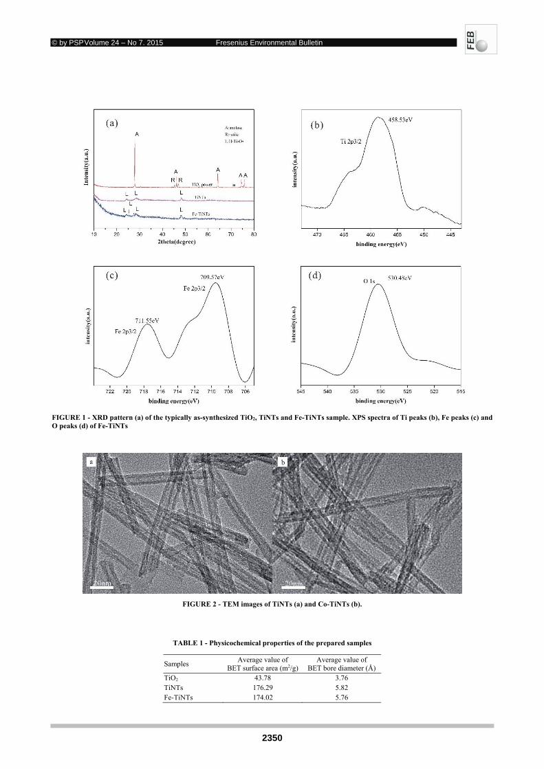
© by PSP Volume 24 – No 7. 2015 Fresenius Environmental Bulletin
2350
FIGURE 1 - XRD pattern (a) of the typically as-synthesized TiO2, TiNTs and Fe-TiNTs sample. XPS spectra of Ti peaks (b), Fe peaks (c) and O peaks (d) of Fe-TiNTs
FIGURE 2 - TEM images of TiNTs (a) and Co-TiNTs (b).
TABLE 1 - Physicochemical properties of the prepared samples
Samples Average value of
BET surface area (m2/g) Average value of
BET bore diameter (Å) TiO2 43.78 3.76 TiNTs 176.29 5.82 Fe-TiNTs 174.02 5.76
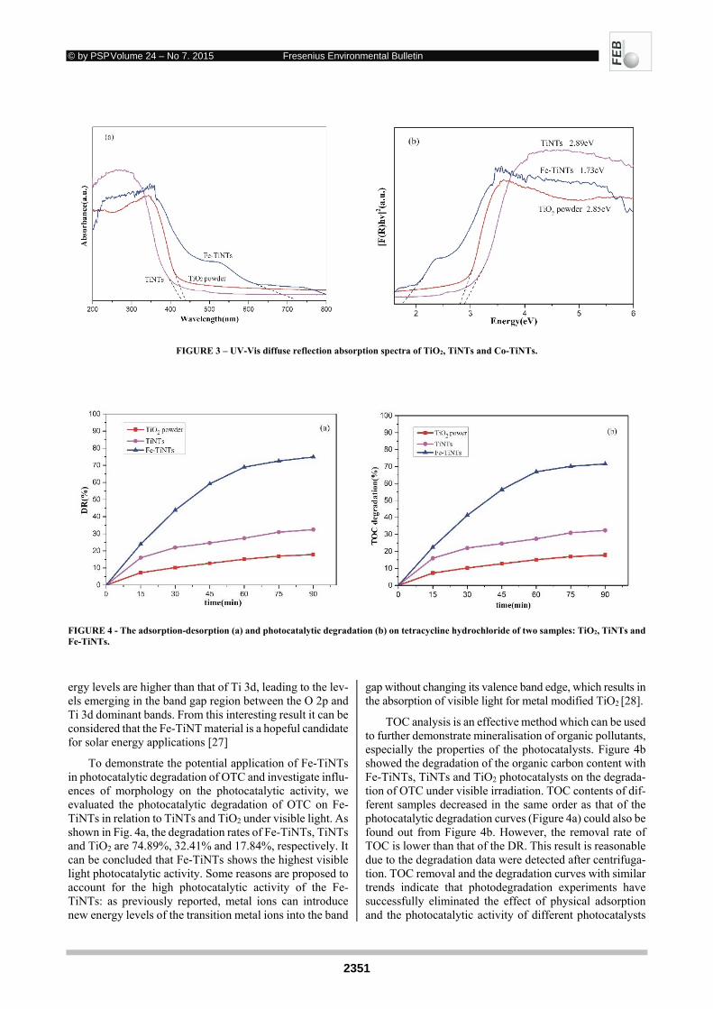
© by PSP Volume 24 – No 7. 2015 Fresenius Environmental Bulletin
2351
FIGURE 3 – UV-Vis diffuse reflection absorption spectra of TiO2, TiNTs and Co-TiNTs.
FIGURE 4 - The adsorption-desorption (a) and photocatalytic degradation (b) on tetracycline hydrochloride of two samples: TiO2, TiNTs and Fe-TiNTs.
ergy levels are higher than that of Ti 3d, leading to the lev-els emerging in the band gap region between the O 2p and Ti 3d dominant bands. From this interesting result it can be considered that the Fe-TiNT material is a hopeful candidate for solar energy applications [27]
To demonstrate the potential application of Fe-TiNTs in photocatalytic degradation of OTC and investigate influ-ences of morphology on the photocatalytic activity, we evaluated the photocatalytic degradation of OTC on Fe-TiNTs in relation to TiNTs and TiO2 under visible light. As shown in Fig. 4a, the degradation rates of Fe-TiNTs, TiNTs and TiO2 are 74.89%, 32.41% and 17.84%, respectively. It can be concluded that Fe-TiNTs shows the highest visible light photocatalytic activity. Some reasons are proposed to account for the high photocatalytic activity of the Fe-TiNTs: as previously reported, metal ions can introduce new energy levels of the transition metal ions into the band
gap without changing its valence band edge, which results in the absorption of visible light for metal modified TiO2 [28].
TOC analysis is an effective method which can be used to further demonstrate mineralisation of organic pollutants, especially the properties of the photocatalysts. Figure 4b showed the degradation of the organic carbon content with Fe-TiNTs, TiNTs and TiO2 photocatalysts on the degrada-tion of OTC under visible irradiation. TOC contents of dif-ferent samples decreased in the same order as that of the photocatalytic degradation curves (Figure 4a) could also be found out from Figure 4b. However, the removal rate of TOC is lower than that of the DR. This result is reasonable due to the degradation data were detected after centrifuga-tion. TOC removal and the degradation curves with similar trends indicate that photodegradation experiments have successfully eliminated the effect of physical adsorption and the photocatalytic activity of different photocatalysts
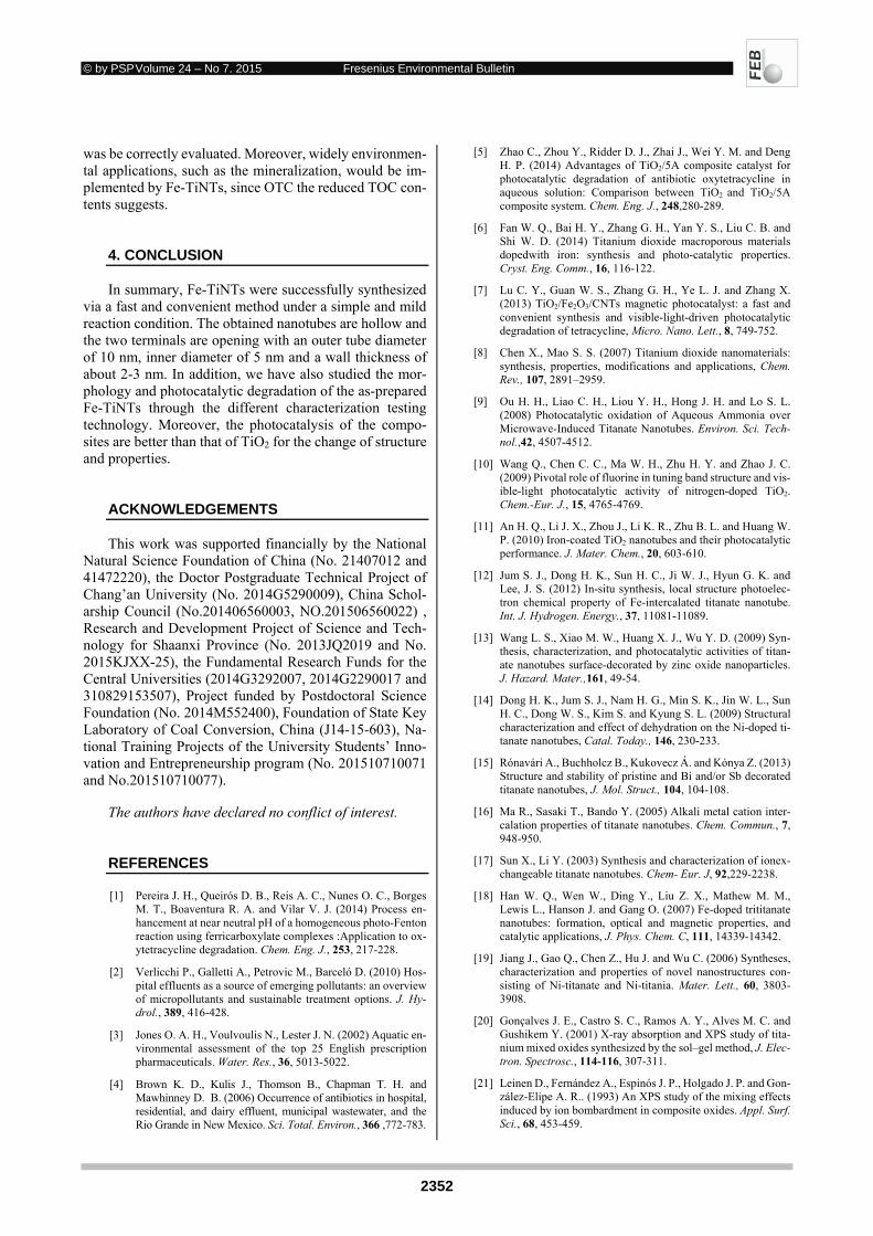
© by PSP Volume 24 – No 7. 2015 Fresenius Environmental Bulletin
2352
was be correctly evaluated. Moreover, widely environmen-tal applications, such as the mineralization, would be im-plemented by Fe-TiNTs, since OTC the reduced TOC con-tents suggests.
4. CONCLUSION
In summary, Fe-TiNTs were successfully synthesized via a fast and convenient method under a simple and mild reaction condition. The obtained nanotubes are hollow and the two terminals are opening with an outer tube diameter of 10 nm, inner diameter of 5 nm and a wall thickness of about 2-3 nm. In addition, we have also studied the mor-phology and photocatalytic degradation of the as-prepared Fe-TiNTs through the different characterization testing technology. Moreover, the photocatalysis of the compo-sites are better than that of TiO2 for the change of structure and properties.
ACKNOWLEDGEMENTS
This work was supported financially by the National Natural Science Foundation of China (No. 21407012 and 41472220), the Doctor Postgraduate Technical Project of Chang’an University (No. 2014G5290009), China Schol-arship Council (No.201406560003, NO.201506560022) , Research and Development Project of Science and Tech-nology for Shaanxi Province (No. 2013JQ2019 and No. 2015KJXX-25), the Fundamental Research Funds for the Central Universities (2014G3292007, 2014G2290017 and 310829153507), Project funded by Postdoctoral Science Foundation (No. 2014M552400), Foundation of State Key Laboratory of Coal Conversion, China (J14-15-603), Na-tional Training Projects of the University Students’ Inno-vation and Entrepreneurship program (No. 201510710071 and No.201510710077).
The authors have declared no conflict of interest. REFERENCES
[1] Pereira J. H., Queirós D. B., Reis A. C., Nunes O. C., Borges M. T., Boaventura R. A. and Vilar V. J. (2014) Process en-hancement at near neutral pH of a homogeneous photo-Fenton reaction using ferricarboxylate complexes :Application to ox-ytetracycline degradation. Chem. Eng. J., 253, 217-228.
[2] Verlicchi P., Galletti A., Petrovic M., Barceló D. (2010) Hos-pital effluents as a source of emerging pollutants: an overview of micropollutants and sustainable treatment options. J. Hy-drol., 389, 416-428.
[3] Jones O. A. H., Voulvoulis N., Lester J. N. (2002) Aquatic en-vironmental assessment of the top 25 English prescription pharmaceuticals. Water. Res., 36, 5013-5022.
[4] Brown K. D., Kulis J., Thomson B., Chapman T. H. and Mawhinney D. B. (2006) Occurrence of antibiotics in hospital, residential, and dairy effluent, municipal wastewater, and the Rio Grande in New Mexico. Sci. Total. Environ., 366 ,772-783.
[5] Zhao C., Zhou Y., Ridder D. J., Zhai J., Wei Y. M. and Deng H. P. (2014) Advantages of TiO2/5A composite catalyst for photocatalytic degradation of antibiotic oxytetracycline in aqueous solution: Comparison between TiO2 and TiO2/5A composite system. Chem. Eng. J., 248,280-289.
[6] Fan W. Q., Bai H. Y., Zhang G. H., Yan Y. S., Liu C. B. and Shi W. D. (2014) Titanium dioxide macroporous materials dopedwith iron: synthesis and photo-catalytic properties. Cryst. Eng. Comm., 16, 116-122.
[7] Lu C. Y., Guan W. S., Zhang G. H., Ye L. J. and Zhang X. (2013) TiO2/Fe2O3/CNTs magnetic photocatalyst: a fast and convenient synthesis and visible-light-driven photocatalytic degradation of tetracycline, Micro. Nano. Lett., 8, 749-752.
[8] Chen X., Mao S. S. (2007) Titanium dioxide nanomaterials: synthesis, properties, modifications and applications, Chem. Rev., 107, 2891–2959.
[9] Ou H. H., Liao C. H., Liou Y. H., Hong J. H. and Lo S. L. (2008) Photocatalytic oxidation of Aqueous Ammonia over Microwave-Induced Titanate Nanotubes. Environ. Sci. Tech-nol.,42, 4507-4512.
[10] Wang Q., Chen C. C., Ma W. H., Zhu H. Y. and Zhao J. C. (2009) Pivotal role of fluorine in tuning band structure and vis-ible-light photocatalytic activity of nitrogen-doped TiO2. Chem.-Eur. J., 15, 4765-4769.
[11] An H. Q., Li J. X., Zhou J., Li K. R., Zhu B. L. and Huang W. P. (2010) Iron-coated TiO2 nanotubes and their photocatalytic performance. J. Mater. Chem., 20, 603-610.
[12] Jum S. J., Dong H. K., Sun H. C., Ji W. J., Hyun G. K. and Lee, J. S. (2012) In-situ synthesis, local structure photoelec-tron chemical property of Fe-intercalated titanate nanotube. Int. J. Hydrogen. Energy., 37, 11081-11089.
[13] Wang L. S., Xiao M. W., Huang X. J., Wu Y. D. (2009) Syn-thesis, characterization, and photocatalytic activities of titan-ate nanotubes surface-decorated by zinc oxide nanoparticles. J. Hazard. Mater.,161, 49-54.
[14] Dong H. K., Jum S. J., Nam H. G., Min S. K., Jin W. L., Sun H. C., Dong W. S., Kim S. and Kyung S. L. (2009) Structural characterization and effect of dehydration on the Ni-doped ti-tanate nanotubes, Catal. Today., 146, 230-233.
[15] Rónavári A., Buchholcz B., Kukovecz Á. and Kónya Z. (2013) Structure and stability of pristine and Bi and/or Sb decorated titanate nanotubes, J. Mol. Struct., 104, 104-108.
[16] Ma R., Sasaki T., Bando Y. (2005) Alkali metal cation inter-calation properties of titanate nanotubes. Chem. Commun., 7, 948-950.
[17] Sun X., Li Y. (2003) Synthesis and characterization of ionex-changeable titanate nanotubes. Chem- Eur. J, 92,229-2238.
[18] Han W. Q., Wen W., Ding Y., Liu Z. X., Mathew M. M., Lewis L., Hanson J. and Gang O. (2007) Fe-doped trititanate nanotubes: formation, optical and magnetic properties, and catalytic applications, J. Phys. Chem. C, 111, 14339-14342.
[19] Jiang J., Gao Q., Chen Z., Hu J. and Wu C. (2006) Syntheses, characterization and properties of novel nanostructures con-sisting of Ni-titanate and Ni-titania. Mater. Lett., 60, 3803-3908.
[20] Gonçalves J. E., Castro S. C., Ramos A. Y., Alves M. C. and Gushikem Y. (2001) X-ray absorption and XPS study of tita-nium mixed oxides synthesized by the sol–gel method, J. Elec-tron. Spectrosc., 114-116, 307-311.
[21] Leinen D., Fernández A., Espinós J. P., Holgado J. P. and Gon-zález-Elipe A. R.. (1993) An XPS study of the mixing effects induced by ion bombardment in composite oxides. Appl. Surf. Sci., 68, 453-459.

© by PSP Volume 24 – No 7. 2015 Fresenius Environmental Bulletin
2353
[22] Bajnóczi É. G., Balázs N., Mogyorósi K., Srankó D. F., Pap Z., Ambrus Z., Canton S. E., Norén K., Kuzmann E., Vértes A., Homonnay Z., Oszkó A., Pálinkó I. and Sipos P. (2011) The influence of the local structure of Fe(III) on the photocata-lytic activity of doped TiO2 photocatalysts-An EXAFS, XPS and Mössbauer spectroscopic study. Appl. Catal. B-Environ., 103, 232-239.
[23] Sathe A., Peck M. A., Balasanthiran C., Langell M. A., Roux R. M. and Hoefelmeyer J. D. (2014) X-ray photoelectron spec-troscopy of transition metal ions attached to the surface of rod-shape anatase TiO2 nanocrystals, Inorg. Chim. Acta., in press, DOI: 10.1016/j.ica..08.011.
[24] Xiong L., Yang Y., Mai J. X., Sun W. L., Zhang C. Y., We D. P., Chen Q. and Ni J. R. (2010) Adsorption behavior of meth-ylene blue onto titanate nanotubes. Chem. Eng. J., 156, 313-320.
[25] Liang H. C., Li X. Z. (2009) Effects of structure of anodic TiO2 nanotube arrays on photocatalytic activity for the degradation of 2, 3-dichlorophenol in aqueous solution, J. Hazard. Mater, 162, 1415-1422.
[26] Yao B. D., Chan Y. F., Zhang X. Y. and Zhang W. F. (2003) Formation mechanism of TiO2 nanotubes. Appl. Phys. Lett., 82, 281-283.
[27] Ohsaki Y., Masaki N., Kitamura T., Wada Y., Okamoto T., Sekino T., Niihara K. and Yanagida S. (2005) Dye-sensitized TiO2 nanotube solar cellsfabrication and electronic characteri-zation. Phys. Chem. Chem. Phys., 7, 4157-4163.
[28] Litter M. I. (1999) Heterogeneous photocatalysis-Transition metal ions in photocatalytic systems, Appl. Catal. B-Environ., 23, 89-114.
Received: November 02, 2014 Revised: December 08, 2014 Accepted: January 22, 2015 CORRESPONDING AUTHOR
Weisheng Guan School of Environmental Science and Engineering Chang'an University Yanta Road 126 Xi'an, 710054 P. R. CHINA Phone: +86 02982334561 E-mail: [email protected]
FEB/ Vol 24/ No 7/ 2015 – pages 2348 - 2353
© by PSP Volume 24 – No 7. 2015 Fresenius Environmental Bulletin
2354
ADSORPTION CHARACTERISTICS OF
PHOSPHORUS ONTO SOILS FROM DIFFERENT
LAND USE TYPES IN DANJIANGKOU RESERVOIR AREA
Meng Xu1,2, Liang Zhang1,*, Yun Du1, Chao Du1,2, and Yan-Hua Zhuang1
1.Institute of Geodesy and Geophysics, Chinese Academy of Sciences, Wuhan 430077, China 2.University of Chinese Academy of Sciences, Beijing 100049, China
ABSTRACT
Characteristics of phosphorus adsorption onto soils have been studied in many researches to reveal the adsorp-tion capacities and to explore the mechanism of phospho-rus behavior in water-sediment interface. In this study, the land use types in Danjiangkou reservoir riparian area was investigated in April 2013 before the soon-coming impound-ment of Danjiangkou reservoir for the first time. The inves-tigation was implemented between 160m and 170m water-lines, and samples of soil in five different land uses (cropland, forest land, abandon cropland, grass land, orange orchard) were taken in the elevations of 160m, 165m and 170m. After the field work, the analysis of chemical com-ponents of the soil and the experiments of phosphorus ad-sorption capacity of these samples were conducted in labor-atory. The results showed that: (a) the traditional Langmuir and Freundlich equations can be well fitted to experiment data, the Qmax obtained ranged from 141.89~209.96 mg/kg with an average value of 191.61mg/kg; (b) The values of EPC0 ranged from 0.05~0.59 mg/L, which were higher than the liquid phosphate concentrations. This indicated these samples had a trend of releasing P as a source; (c) the adsorption capacity and isotherm parameters were influ-enced by sediment components, especially by the content of Fe and Al, while surface area and sample elevation showed no obvious effect in the present system.
KEYWORDS: water-level fluctuations; South-North Water Diver-sion Project; cropland; sediment; isotherm
1. INTRODUCTION
As an essential element for plants and crops, phospho-rus (P) is also one of the most important components of non-point source pollution. The worldwide application of phosphatic fertilizers brings great prosperity in agricultural
* Corresponding author
industry though, the excess P entering into water body may cause eutrophication among other environmental problems [1]. Agricultural runoff is considered to be the largest source of phosphate causing eutrophication because of the overuse of soluble phosphate as a fertilizer [2]. The sedi-ment-water interface such as riparian zone, lakeside zone or water-level-fluctuate zone are always considered to be buffer zones when receiving runoff containing P, since they act as both sinks and sources of P [3,4]. These buffer zones between the pollutant source areas and the receiving waters were considered to have potential use in improving water quality decades ago [5,6] and their effectiveness of removing P has been confirmed in many later researches [7]. The study of the buffer zones functioning has per-suaded researchers to explore the mechanism of P behavior in these sediment-water interfaces. As an important ap-proach to reveal the various biogeochemical processes oc-curring in sediment-water interfaces, the study of adsorp-tion of P has always been concerned. The primary re-searches of P adsorption during 1950s to 1960s focused on phosphatic fertilizers in lakes and sediments [8], later ex-periments confirmed that P was an important limiting fac-tor in eutrophication [9,10].
To study the adsorption characteristics of P, adsorption capacity was explored by many experiments as an essential point to predict long-term P availability [11-14]. To reveal the P adsorption behavior and response in nature, environ-mental parameters which may affect the adsorption were always concerned [15-17] and many of the researches fo-cused on the effect of land use types [18,19]. Moreover, there were researchers found the traditional adsorption models failed in some way to explain the mechanism, and then tried to provide new theories and models [20].
The Danjiangkou reservoir is an important drinking water source protection area and also part of the middle route for China’s South-to-North Water Diversion Project. The project has changed some of the land use types and the water-level-fluctuated zone in this area would be operated out-of-season due to the impoundment and future dis-charge. The consequent variations of water levels and the changing of hydrological regime in this area would make water quality protection a new challenge in the future. The

© by PSP Volume 24 – No 7. 2015 Fresenius Environmental Bulletin
2355
study of potential pollutant and assessment of future risks would be necessary and appreciated. To explore the P con-tent and retention in this special background, this study fo-cused on P adsorption in typical land uses of Danjiangou. Batch experiments of adsorption and analysis of soil com-ponents were conducted to: (a) investigate the P sorption isotherm of soils from different land uses and (b) explore the relationship between p adsorption and soil characters in this area.
2. MATERIALSAND METHODS
2.1 Study site
This study was conducted in Danjiangkou reservoir area(32°11'34''~32°52'40''N,109°23'7''~111°57'55''E) (Fig. 1). This area belongs to the subtropical monsoon of the north subtropical zone. The distribution of precipitation is declining from south to north, shaped by both the topog-raphy and the monsoon. The annual precipitation fluctu-ated from 500mm in low flow year to 1500mm in high flow
year. The average annual precipitation was 830mm and 70–80 % occurs between April and October. The mean an-nual temperature ranged from 12~16 ºC. According to the statistic data in 2010, the land area in Danjiangkou city was 3121km2 including 204.2km2 cultivated land and the forest cover was 39.9%; the water quality of Danjiangkou reser-voir held steady in class II national water quality standard [21]. The official website of south-to north water diversion announced the water transfer would be launched in late Oc-tober of 2014, right after the flood season. The protection of water quality in Danjiangkou reservoir is becoming well concerned as the water transfer project has changed both the hydrological and the environmental conditions.
2.2 Land use investigation method
The land use investigation of Danjiangkou reservoir was based on the USGS land use classification system. The image data used in this study was from HJ-1 with a spatial resolution of 30m. Geometric correction and atmospheric correction was conducted before classification. Supporting data also included DEM, slope and social references of
FIGURE 1 -Map of study site and sampling locations
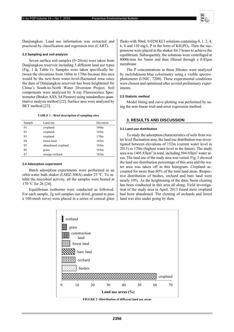
© by PSP Volume 24 – No 7. 2015 Fresenius Environmental Bulletin
2356
Danjiangkou. Land use information was extracted and practiced by classification and regression tree (CART).
2.3 Sampling and soil analysis
Seven surface soil samples (0~20cm) were taken from Danjiangkou reservoir including 5 different land use types (Fig. 1 & Table 1). Samples were taken specifically be-tween the elevations from 160m to 170m because this area would be the new-born water-level-fluctuated zone since the dam of Danjiangkou reservoir has been heightened for China’s South-to-North Water Diversion Project. Soil components were analyzed by X-ray Fluorescence Spec-trometer (Bruker AXS, S4 Pioneer) using standardless quan-titative analysis method [22]. Surface area were analyzed by BET method [23].
TABLE 1 - Brief description of sampling sites
Sample Land use Elevation
S1 cropland 160m
S2 cropland 165m
S3 cropland 170m
S4 forest land 165m
S5 abandoned cropland 165m
S6 grass 165m
S7 orange orchard 165m
2.4 Adsorption experiment
Batch adsorption experiments were performed in an orbit water bath shaker (LSHZ-300A) under 25 ºC. To in-hibit the microbial activity, all the samples were heated at 170 ºC for 2h [24].
Equilibrium isotherms were conducted as followed. For each sample, 2g soil samples (air-dried, ground to pass a 100-mesh sieve) were placed in a series of conical glass
flasks with 50mL 0.02M KCl solutions containing 0, 1, 2, 4, 6, 8 and 110 mg/L P in the form of KH2PO4. Then the sus-pensions were placed in the shaker for 3 hours to achieve the equilibrium. Subsequently, the solutions were centrifuged at 8000r/min for 5mins and then filtered through a 0.45μm membrane.
The P concentrations in these filtrates were analyzed by molybdenum blue colorimetry using a visible spectro-photometer (UNIC, 7200). These experimental conditions were chosen and optimized after several preliminary exper-iments.
2.5 Statistic method
Model fitting and curve plotting was performed by us-ing the non-linear trial-and-error regression method.
3. RESULTS AND DISCUSSION
3.1 Land use distribution
To study the adsorption characteristics of soils from wa-ter level fluctuation area, the land use distribution was inves-tigated between elevations of 152m (current water level in 2013) to 170m (highest water level in the future). The study area was 1405.83km2 in total, including 504.03km2 water ar-eas. The land use of the study area was varied. Fig. 2 showed the land use distribution percentage of this area and the wa-ter area was taken off in this histogram. Cropland ac-counted for more than 60% of the total land areas. Respec-tive distribution of bushes, orchard and bare land were nearly 10%. As the heightening of the dam, basin clearing has been conducted in this area all along. Field investiga-tion of the study area in April, 2013 found most cropland had been abandoned. The clearing of orchards and forest land was also under going by then.
FIGURE 2 -Distribution of different land use areas
cropland
bushes
orchard
bare land
forest land
construction land
grass
wetland
0 10 20 30 40 50 60 70
Land use areas (%)
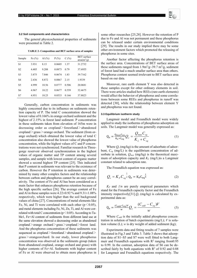
© by PSP Volume 24 – No 7. 2015 Fresenius Environmental Bulletin
2357
3.2 Soil components and characteristics
The general physicochemical properties of sediments were presented in Table 2.
TABLE 2- Composition and BET surface area of samples
Sample Fe (%) Al (%) P (%) C (%) BET surface area(m2/g)
S1 3.931 8.15 0.0605 1.37 31.2732
S2 4.405 9.288 0.0873 0.79 37.6955
S3 3.875 7.846 0.0674 1.83 39.7162
S4 2.436 8.872 0.0867 2.15 1.9339
S5 4.999 10.56 0.0777 0.506 20.0681
S6 4.967 10.22 0.0677 0.559 32.4675
S7 4.951 10.25 0.0533 0.166 37.8823
Generally, carbon concentration in sediments was
highly concerned due to its influence on sediments reten-tion capacity of P. The total C concentration showed the lowest value of 0.166% in orange orchard sediment and the highest of 2.15% in forest land sediment. P concentration in these sediments taken from elevation of 165m were in decreasing order as cropland>forestland>abandoned cropland>grass>orange orchard. The sediment (from or-ange orchard) which obtained the lowest value of total C concentration also showed the lowest value of phosphorus concentration, while the highest values of C and P concen-trations were not synchronized. Familiar research in Three-gorge reservoir observed synchronization in the highest values of organic matter and TP content among several samples, and sample with lowest content of organic matter showed a second highest TP content [25]. This indicated that P content in sediments was relevant to the existence of carbon. However the P retention in sediments was deter-mined by many other complex factors and the relationship between carbon and phosphorus cannot be an easy correl-ativity. The content of Fe and Al has been considered as a main factor that enhances phosphorus retention because of the high specific surface [26]. The average content of Fe and Al in these samples were 4.22±0.92 % and 9.31±1.08% respectively, which were higher than the soil background values of china [27]. Concentrations of metal elements like Fe, Ni, and Ti were correlated with each other (p<0.05), and metal elements including Fe, Ni, Zn, Ti, and Al were cor-related with total C concentration (p<0.05). According to Ta-ble1, Fe+Al content of sediments from different land use at the same elevation showed a decreasing order as abandoned cropland>orange orchard>grass>cropland>forest land. And the phosphorus concentration of these sediments was sequenced as cropland>forestland>abandoned cropland>
grass>orangeorchard. In our study, lower phosphorus concentration was observed in the sediments group (taken from abandoned cropland, orange orchard and grass) with higher contents of Fe+Al. Sediments with higher content of Fe or Al were observed to obtain more phosphorus in
some other researches [25,28]. However the retention of P due to Fe and Al was not permanent and these phosphorus can be released under certain environmental conditions [29]. The results in our study implied there may be some other environment factors which promoted the releasing of phosphorus in some sites.
Another factor affecting the phosphorus retention is the surface area. Concentrations of BET surface areas of these sediments ranged from 1.9m2/g~39.7 m2/g, sediment of forest land had a much smaller surface area than others. Phosphorus content seemed irrelevant to BET surface area based on our data.
Moreover, rare earth element Y was also detected in these samples except for other ordinary elements in soil. There were articles studied how REEs (rare earth elements) would affect the behavior of phosphorus and some correla-tions between some REEs and phosphorus in runoff was detected [30], while the relationship between element Y and phosphorus was not found.
3.3 Equilibrium isotherm study
Langmuir model and Freundlich model were widely applied to study the isotherms of phosphorus adsorption on soils. The Langmuir model was generally expressed as:
QeqL
eqe CK
CQQ
max
(1)
Where Qe (mg/kg) is the amount of adsorbate of adsor-bent, Ceq (mg/L) is the equilibrium concentration of ad-sorbate in solution, Qmax (mg/kg) is the theoretical maxi-mum of adsorption capacity and KL (mg/L)is a Langmuir constant related to adsorption rate.
The Freundlich equation was expressed as:
neqFe CKQ1
Q K C (2)
KF and 1/n are purely empirical parameters which stand for the Freundlich capacity factor and the Freundlich intensity respectively[31].Qe (mg/kg) is calculated by ex-perimental data as:
Q‐
w
VCCQ eqadd
e
)( (3)
Where Cadd is the initially added phosphorus concen-tration in solution of batch experiments (mg/L); V is solu-tion volume (L); w is dry weight of added sediment (kg);
Experiments data and fitting results of 7 samples were illustrated in Fig.3 and Table 3. Table 3 shows that adsorp-tion data of S1~S5 and S7 were well fitted to both Lang-muir and Freundlich equations with R2 ranging from0.95 to 0.99. In the contrast, adsorption data of S6 can be de-scribed fairly by both equations with R2 of 0.92 and 0.88 for Langmuir and Freundlich equations respectively. The

© by PSP Volume 24 – No 7. 2015 Fresenius Environmental Bulletin
2358
Langmuir equation gave a Qmax of these samples ranged from 141.89 to 211.33mg/kg.
TABLE 3 - Summary of the fitting results of the traditional Langmuir and Freundlich equations
Langmuir equation Freundlich equation
Sample Qmax
(mg/kg) KL R2 1/n KF R2
S1 206.97 1.26 0.98 0.51 83.28 0.95
S2 209.96 1.02 0.98 0.49 94.56 0.99
S3 156.76 2.21 0.99 0.52 48.31 0.99
S4 141.89 7.03 0.99 0.69 18.97 0.97
S5 211.33 0.99 0.99 0.49 95.89 0.98
S6 208.12 1.02 0.92 0.49 92.67 0.88
S7 206.24 0.29 0.98 0.38 145.79 0.98
However, the study of exchangeable P on natural sed-iments indicated that native adsorbed exchangeable phos-phorous (NAP) of sediment also takes part in the process of adsorption [32] and should be taking into the isotherms.
Taking NAP into account, the modified Langmuir ad-
sorption equation could be written as [29]: (4)
Where NAP stands for the amount of total native ex-
changeable phosphorus (mg/kg) In the case of 0addC ,0eqeq CC , the Eq. (4) can be described as:
(5) Substituted NAP in equation (4) by equation (5) to ob-
tain the modified Langmuir isotherm equation [29]:
(6) Zero-equilibrium P concentration, which is usually
known as EPC0 refers that there is no net adsorption or re-lease and phosphorus on sediments and in water phase is in
dynamic equilibrium. When addeq CC , EPC0 can be
obtained by equation (6) as:
(7) The partitioning coefficients (KP) can be calculated by:
(8)
Based on the theory of modified isotherm and taking NAP into account, the modified Freundlich equation [32] can be described as:
(9) (10) (11) (12)
With the experiment data, modified Langmuir and Freundlich equations can be applied to describe the rela-tionship between concentration of adsorbate and the amount of adsorption using non-linear trial-and-error re-gression method [33].
The intersection of y-axes and the regression curves refers to NAP value and the x-intercept of the model indi-cates EPC0 value. These two parameters are highlighted because they play important roles in the retention and re-lease of phosphorus in sediment-water interface. NAP stands for native adsorbed exchangeable phosphorous, and EPC0 indicates the critical point of adsorption and desorp-tion. When actual phosphorus concentration in water were higher than EPC0, the sediment would absorb phosphorus from water, otherwise the phosphorus obtained in sedi-ments would release.
Table 4 shows that for sample S2 to S5, adsorption data were well fitted to both adsorption equations, with all the R2 value over 0.95. Although the R2 of both Langmuir and
TABLE 4- Summary of the fitting results of the modified Langmuir and Freundlich equations
Modified Langmuir Modified Freundlich
Fitting results
Sample Qmax KL R2 1/n KF R2
S1 337.22 0.84 0.84 0.019 3048.56 0.94
S2 215.02 0.82 0.98 0.483 91.89 0.98
S3 157.71 1.98 0.99 0.628 37.27 0.98
S4 130.26 5.16 0.99 0.885 11.80 0.95
S5 216.86 0.78 0.98 0.459 97.53 0.98
S6 501.40 0.13 0.91 0.003 18410.87 0.96
S7 277.26 0.29 0.89 0.002 18410.87 0.96
Calculated parameters
NAP EPC0 KP NAP EPC0 KP
S1 109.91 0.41 0.27 2997.59 0.42 7.16
S2 12.81 0.05 0.25 22.13 0.05 0.42
S3 5.35 0.07 0.08 7.14 0.07 0.10
S4 9.27 0.40 0.02 7.38 0.59 0.01
S5 14.52 0.06 0.26 26.11 0.06 0.46
S6 328.79 0.26 1.28 18339.58 0.27 67.54
S7 50.66 0.06 0.79 18289.98 0.06 285.89

© by PSP Volume 24 – No 7. 2015 Fresenius Environmental Bulletin
2359
Freundlich equations were over 0.9 when data of S1, S6 and S7 were fitted, the inapplicability in these 3 cases was obvious due to the unreasonably high NAP. The mod-ified Freundlich equation may lack some scientific founda-tion and appear unsuitable in our cases.
The results of EPC0 ranged from 0.05~0.59 mg/L, S4 from forest land showed the highest EPC0 and S2 from cropland obtained the lowest EPC0. The values of EPC0 by modified Langmuir model and modified Freundlich model were nearly the same, while the NAP values showed some abnormal values. The abnormal NAP values might indicate the inapplicability of modified Freundlich model when de-scribing adsorption on complex natural sediments such as soils.
3.4 Effect of land uses and soil characters
S1 to S7 present different phosphorus adsorption iso-therms in Fig.3. The Qmax obtained from Langmuir equa-tion ranged from 141.89~209.96 mg/kg with an average value of 191.61mg/kg. According to different land use, the order of adsorption capacity was abandoned cropland>
cropland>grass>orange orchard>forest land. In the case of cropland, the adsorption capacity of samples taken at 160m and 165m were nearly the same, while the sample at 170m showed an obvious decrease in Qmax. S1, S2, S5 and
S6 shared a similar Langmuir isotherm with a maxQ about
209mg/kg, while the adsorption capacity of S3 and S4 were relatively lower. Cluster analysis based on sample compo-nents data showed that S2, S5 and S6 can be classified to one group, while S1, S3 and S4 were classified to the other
group. This result indicates the varied adsorption capacity of samples is relevant to soil components. Resemblance of components contributes to similarity in adsorption capacity and isotherms.
Although the surface area was usually considered to be responsible for adsorption capacity of absorbent [21,34], the data of BET surface area showed no correlations with the parameters of adsorption. However, the soil sample S4 with the lowest adsorption capacity also has a much smaller BET surface area than other samples. BET surface area may not influence phosphorus adsorption in an obvi-ous way though, significant decrease in surface area would affect the adsorption capacity.
The adsorption capacity can be related to many factors especially when complicate adsorbent such as soil in-volved. The metal content was considered to be the main factor that determines soil adsorption capacity, because the iron/aluminum hydroxides in soil has high specific surface [26]. Table 5 illustrates the correlations between adsorp-tion parameters and Fe, Al contents in this study.
The parameters obtained from both equations were generally correlated with Fe content in soil, indicating Fe content to be an important factor of phosphorus adsorption in this case. The contribution of Al content to phosphorus adsorption was present in affecting NAP value. Samples with more Al resulted in a higher NAP. Generally, samples with higher content of Fe and Al can adsorb more phospho-rus from natural environment to obtain a higher NAP, and the adsorption capacity of soil will increase with content of Fe and Al as well.
FIGURE 3 -Adsorption isotherms fitted by traditional Langmuir isotherm
0
50
100
150
200
0 2 4 6 8 10
P a
dso
rbed
(m
g/k
g)
Equilibrium P Concentration (mg/L)
S1S2S3S4S5
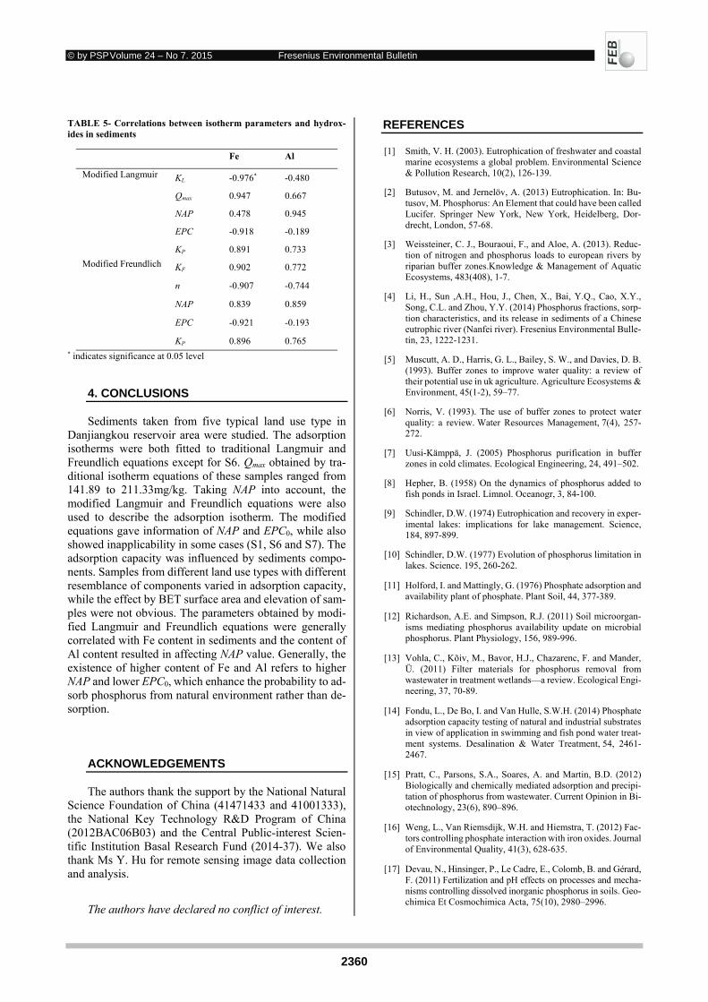
© by PSP Volume 24 – No 7. 2015 Fresenius Environmental Bulletin
2360
TABLE 5- Correlations between isotherm parameters and hydrox-ides in sediments
Fe Al
Modified Langmuir KL -0.976* -0.480
Qmax 0.947 0.667
NAP 0.478 0.945
EPC -0.918 -0.189
KP 0.891 0.733
Modified Freundlich KF 0.902 0.772
n -0.907 -0.744
NAP 0.839 0.859
EPC -0.921 -0.193
KP 0.896 0.765 * indicates significance at 0.05 level
4. CONCLUSIONS
Sediments taken from five typical land use type in Danjiangkou reservoir area were studied. The adsorption isotherms were both fitted to traditional Langmuir and Freundlich equations except for S6. Qmax obtained by tra-ditional isotherm equations of these samples ranged from 141.89 to 211.33mg/kg. Taking NAP into account, the modified Langmuir and Freundlich equations were also used to describe the adsorption isotherm. The modified equations gave information of NAP and EPC0, while also showed inapplicability in some cases (S1, S6 and S7). The adsorption capacity was influenced by sediments compo-nents. Samples from different land use types with different resemblance of components varied in adsorption capacity, while the effect by BET surface area and elevation of sam-ples were not obvious. The parameters obtained by modi-fied Langmuir and Freundlich equations were generally correlated with Fe content in sediments and the content of Al content resulted in affecting NAP value. Generally, the existence of higher content of Fe and Al refers to higher NAP and lower EPC0, which enhance the probability to ad-sorb phosphorus from natural environment rather than de-sorption.
ACKNOWLEDGEMENTS
The authors thank the support by the National Natural Science Foundation of China (41471433 and 41001333), the National Key Technology R&D Program of China (2012BAC06B03) and the Central Public-interest Scien-tific Institution Basal Research Fund (2014-37). We also thank Ms Y. Hu for remote sensing image data collection and analysis.
The authors have declared no conflict of interest.
REFERENCES
[1] Smith, V. H. (2003). Eutrophication of freshwater and coastal marine ecosystems a global problem. Environmental Science & Pollution Research, 10(2), 126-139.
[2] Butusov, M. and Jernelöv, A. (2013) Eutrophication. In: Bu-tusov, M. Phosphorus: An Element that could have been called Lucifer. Springer New York, New York, Heidelberg, Dor-drecht, London, 57-68.
[3] Weissteiner, C. J., Bouraoui, F., and Aloe, A. (2013). Reduc-tion of nitrogen and phosphorus loads to european rivers by riparian buffer zones.Knowledge & Management of Aquatic Ecosystems, 483(408), 1-7.
[4] Li, H., Sun ,A.H., Hou, J., Chen, X., Bai, Y.Q., Cao, X.Y., Song, C.L. and Zhou, Y.Y. (2014) Phosphorus fractions, sorp-tion characteristics, and its release in sediments of a Chinese eutrophic river (Nanfei river). Fresenius Environmental Bulle-tin, 23, 1222-1231.
[5] Muscutt, A. D., Harris, G. L., Bailey, S. W., and Davies, D. B. (1993). Buffer zones to improve water quality: a review of their potential use in uk agriculture. Agriculture Ecosystems & Environment, 45(1-2), 59–77.
[6] Norris, V. (1993). The use of buffer zones to protect water quality: a review. Water Resources Management, 7(4), 257-272.
[7] Uusi-Kämppä, J. (2005) Phosphorus purification in buffer zones in cold climates. Ecological Engineering, 24, 491–502.
[8] Hepher, B. (1958) On the dynamics of phosphorus added to fish ponds in Israel. Limnol. Oceanogr, 3, 84-100.
[9] Schindler, D.W. (1974) Eutrophication and recovery in exper-imental lakes: implications for lake management. Science, 184, 897-899.
[10] Schindler, D.W. (1977) Evolution of phosphorus limitation in lakes. Science. 195, 260-262.
[11] Holford, I. and Mattingly, G. (1976) Phosphate adsorption and availability plant of phosphate. Plant Soil, 44, 377-389.
[12] Richardson, A.E. and Simpson, R.J. (2011) Soil microorgan-isms mediating phosphorus availability update on microbial phosphorus. Plant Physiology, 156, 989-996.
[13] Vohla, C., Kõiv, M., Bavor, H.J., Chazarenc, F. and Mander, Ü. (2011) Filter materials for phosphorus removal from wastewater in treatment wetlands—a review. Ecological Engi-neering, 37, 70-89.
[14] Fondu, L., De Bo, I. and Van Hulle, S.W.H. (2014) Phosphate adsorption capacity testing of natural and industrial substrates in view of application in swimming and fish pond water treat-ment systems. Desalination & Water Treatment, 54, 2461-2467.
[15] Pratt, C., Parsons, S.A., Soares, A. and Martin, B.D. (2012) Biologically and chemically mediated adsorption and precipi-tation of phosphorus from wastewater. Current Opinion in Bi-otechnology, 23(6), 890–896.
[16] Weng, L., Van Riemsdijk, W.H. and Hiemstra, T. (2012) Fac-tors controlling phosphate interaction with iron oxides. Journal of Environmental Quality, 41(3), 628-635.
[17] Devau, N., Hinsinger, P., Le Cadre, E., Colomb, B. and Gérard, F. (2011) Fertilization and pH effects on processes and mecha-nisms controlling dissolved inorganic phosphorus in soils. Geo-chimica Et Cosmochimica Acta, 75(10), 2980–2996.

© by PSP Volume 24 – No 7. 2015 Fresenius Environmental Bulletin
2361
[18] Majumdar, B., Venkatesh, M. and Saha, R. (2013) Long term effect of land use systems on phosphorus adsorption behaviour under acidic alfisol of Meghalaya, India. Agrochimica, 55(4), 233-247.
[19] Alt, F., Oelmann, Y., Herold, N., Schrumpf, M. and Wilcke, W. (2011) Phosphorus partitioning in grassland and forest soils of Germany as related to land-use type, management in-tensity, and land use-related pH. Journal of Plant Nutrition & Soil Science, 174(2), 195–209.
[20] McGechan, M. and Lewis, D. (2002) Sorption of phosphorus by soil, part 1: Principles, equations and models. Biosystems engineering, 82, 1-24.
[21] Li, D. (2011) National economic statistic information of Dan-jiangkou city, 2010. In: Luo, T.Y. National economic statistic information of Danjiangkou city. Statistics Bureau of Dan-jiangkou city, Danjiangkou city, 16-18.
[22] Arai, T. (2007) Quantitative Analysis. In: Beckhoff, B., Kan-ngieber, B., Langhoff, N., Wedell, R., Wolff, H.H. Handbook of practical X-ray fluorescence analysis. Springer, Berlin, Hei-delberg, 36-39.
[23] Brunauer, S., Emmett, P.H. and Teller, E. (1938) Adsorption of gases in multimolecular layers. J. Am. Chem. Soc, 60, 309-319.
[24] Labeda, D., Balkwill, D. and Casida Jr, L. (1975) Soil sterili-zation effects on in situ indigenous microbial cells in soil. Ca-nadian Journal of Microbiology, 21(3), 263-269.
[25] Wang, Y., Shen, Z., Niu, J. and Liu, R. (2009) Adsorption of phosphorus on sediments from the Three-Gorges Reservoir (China) and the relation with sediment compositions. Journal of Hazardous Materials,162(1), 92-8.
[26] Brinkman, A.G. (1993) A double-layer model for ion adsorp-tion onto metal oxides, applied to experimental data and to nat-ural sediments of Lake Veluwe, The Netherlands. Hydrobio-logia, 253, 31-45.
[27] Zhang, N.M. and Wang, S.Q. (2005) Capacity and speciation of phosphorus in soils. In: Chen, H. Environmental Soil Sci-ence. Science Press, Beijing, 164-170.
[28] Lai, D.Y.F. and Lam, K.C. (2009) Phosphorus sorption by sed-iments in a subtropical constructed wetland receiving storm-water runoff. Ecological Engineering, 35(5), 735-743.
[29] Zhou, A., Tang, H. and Wang, D. (2005) Phosphorus adsorp-tion on natural sediments: Modeling and effects of pH and sed-iment composition. Water Research, 39(7), 1245-1254.
[30] Wang, L., Liang, T., Kleinman, P.J.A. and Cao, H. (2011) An experimental study on using rare earth elements to trace phos-phorous losses from nonpoint sources. Chemosphere, 85(6), 1075-1079.
[31] Achife, E. C., and Ibemesi, J. A. (1989). Applicability of the freundlich and Langmuir adsorption isotherms in the bleach-ing of rubber and melon seed oils. Journal of Oil & Fat Indus-tries, 66(2), 247-252.
[32] Aminot, A. and Andrieux, F. (1996) Concept and determination of exchangeable phosphate in aquatic sediments. Water Re-search, 30(11), 2805-2811.
[33] Zhang, L., Hong, S., He, J., Gan, F. and Ho, Y.S. (2011) Ad-sorption characteristic studies of phosphorus onto laterite. De-salination & Water Treatment, 25(1), 98-105.
[34] Xiang, Q., Xie, H. Q., Henderson, H., Kay, A. F., Fontes, M. P. F., and Weed, S. B. (1996). Phosphate adsorption by clays from brazilian oxisols: relationships with specific surface area and mineralogy.Geoderma, 72(1-2), 37–51.
Received: November 03, 2014 Revised: December 11, 2014 Accepted: December 18, 2014 CORRESPONDING AUTHOR
Liang Zhang Institute of Geodesy and Geophysics Chinese Academy of Sciences Wuhan, Hubei Province P.R. CHINA Phone: +86 27 68881362 Fax: +86 27 68881362 E-mail: [email protected]
FEB/ Vol 24/ No 7/ 2015 – pages 2354 - 2361
© by PSP Volume 24 – No 7. 2015 Fresenius Environmental Bulletin
2362
ASSESSMENT OF LIMITING FACTORS FOR POTENTIAL
ENERGY PRODUCTION IN WASTE TO ENERGY PROJECTS
Orhan Sevimoğlu
Istanbul Metropolitan Municipality, Şehzadebaşı Caddesi, 34134 Fatih / Istanbul /Turkey
ABSTRACT
The popularity of landfill gas to energy projects in-creased worldwide as well as in Turkey in the last two dec-ades due to the importance of renewable energy sources and the green house gas emission control in environmental protection. Many Waste-to-Energy (WTE) projects focus on methods that employ landfill gas (LFG) from landfills to produce electric power. Most of the projects refer to gas prognosis models such as USEPA-LandGEM, GasSim, EPER, and IPCC to determine the installation power ca-pacity. However, problems related to landfill, power gen-eration and energy delivery have limiting factors for land-fill gas and energy production. In this study, the limiting parameters with their assessments are discussed for Odayeri and Kömürcüoda Sanitary Landfills, Istanbul, Turkey. To overcome these issues, several improvements were done such as top surface cover application to both landfill sites, buffer gas tank installation to minimize the fluctuation of LFG quality and reduction of leachate water level via pumping. Accordingly, an increase in the recov-ery of LFG has been accomplished. The recovery LFG rate to theoretical extractable LFG rate ratios reached to 75 % and 60% in 2012 for Odayeri and Kömürcüoda landfills, respectively.
KEYWORDS: waste-to-energy, landfill gas, limitations, energy, recovery
1. INTRODUCTION
Municipal solid waste (MSW) is generally disposed in a sanitary landfill site due to environmental concerns and public health [1]. Stored MSW produces LFG including methane, carbon dioxide, and trace gases under anaerobic conditions. Energy recovery utilizing LFG has been ac-cepted as a widely used application for several decades around the world [2, 3] as well as in Turkey [4, 5]. The first power plant utilizing LFG in Turkey was built in Bursa province at Demirtas landfill in 1997. Since then electricity production from renewable energy sources in Turkey has enormously increased due to updates and new regulations
in the energy market [6]. There are 76 sanitary landfill sites that are used by 1010 municipalities with 16 operating WTE plants which are forecasted to grow in number in re-spect to the new subventions given by the government. These projects are mostly designed based on generally ac-cepted rules and regulations of especially United States (US) and European techniques. The goals of WTE projects from an environmental regulations standpoint are the re-duction of greenhouse gas emissions to the atmosphere from landfills [7] and the climate change impact [8], all the while utilizing methane of LFG in energy production [9,10]. In order to evaluate the acceptability of these pro-jects, a detailed gas prognosis is needed to check the feasi-bility for an accurate investment [11]. Provided that the prognosis of LFG recovery is done incorrectly, the conse-quence will be failure in terms of cost-benefit analysis of the project [12]. One of the methods for a high-quality as-sessment is performing a pump trial on the landfill site [13] to get an actual LFG flow rate from the landfill site. An-other assessment method can be surface emission measure-ment [14, 15] by which an analogy can be made to flow rate to evaluate the real potential. On the other hand, math-ematical models are mostly used for the evaluation of the-oretical LFG potential. The LandGEM (USEPA), GasSim, EPER, IPCC LFG estimation models are widely used in many applications of LFG emission. The models require waste character and empirical parameters to calculate LFG emission. However, the potential of actual gas production depends on many factors, especially landfill site conditions such as the level of anaerobic activity, solid waste contents, rainfall, surface covering. Besides, the recovery of LFG de-pends on the design quality of the extraction system and the performance of the operation as well as management of the collection system. In many applications, the theoretical landfill gas potential is calculated by the accepted models, and then WTE projects are designed based on the estima-tion of LFG recovery for each year of the project life. The considered recovery rate of LFG is in the wide range of 90% to 10%. In many cases, the extracted landfill gas vol-ume was lower than the estimated recovery LFG volume which is misleading for inventors [16].
There are several reasons for low extraction rates of landfill gas such as poor sanitary landfill site management, failure to comply with waste storage techniques, lack of ac-curate characterization of waste and absence of complete
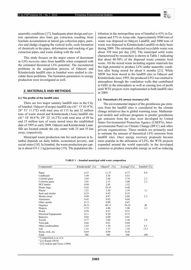
© by PSP Volume 24 – No 7. 2015 Fresenius Environmental Bulletin
2363
anaerobic conditions [17]. Inadequate plant design and sys-tem operations also limit gas extraction resulting from leachate accumulation in lateral gas collection pipes, parti-cles and sludge clogging the vertical wells, scale formation of chemicals in the pipes, deformation and cracking of gas extraction pipes, and waste sliding with the well.
This study focuses on the major causes of decrement in LFG recovery rates from landfills when compared with the estimated theoretical LFG potential. The encountered problems in the acquisition process of Odayeri and Kömürcüoda landfill sites in Istanbul were studied to elu-cidate these problems. The limitation parameters in energy production were investigated as well.
2. MATERIALS AND METHODS
2.1 The profile of the landfill sites
There are two major sanitary landfill sites in the City of Istanbul: Odayeri (Europe) landfill site (41° 13' 02.9"N; 28° 51' 11.3"E) with total area of 115 ha and 32 million tons of waste stored and Kömürcüoda (Asia) landfill site (41° 10' 30.6"N; 29° 22' 16.2"E) with total area of 89 ha and 15 million tons of waste stored since the established date of 1995 to early 2009. Odayeri and Kömürcüoda Land-fills are located outside the city center with 25 and 55 km away, respectively.
Municipal waste production rate for each person in Is-tanbul depends on daily habits, economical poverty, and social status [18]. In Istanbul, the waste production per cap-ita is about 0.9-1.1 kg/person/day [19]. The population dis-
tribution in the metropolitan area of Istanbul is 63% in Eu-ropean and 37% in Asian side. Approximately 9500 tons of waste was disposed in Odayeri Landfill, and 5000 tons of waste was disposed in Kömürcüoda Landfill on daily basis during 2009. The estimated collected recyclable waste was about 350 tons per day [20]. The municipal solid waste characterized by researchers is shown in Table 1 indicating that about 48-50% of the disposed waste contains food waste. All the stored waste including organic materials has the high potential to produce LFG under anaerobic condi-tion after being stored for about 6 months [21]. While MSW has been stored in the landfill sites in Odayeri and Kömürcüoda since 1995, the produced LFG was emitted to atmosphere through the ventilation wells that contributed to GHG in the atmosphere as well as causing loss of profit until WTE projects were implemented in both landfill sites in 2009.
2.2. Theoretical LFG versus recovery LFG
The environmental impact of the greenhouse gas emis-sion from the landfill sites is considered by the climate change initiatives due to global warming issue. Mathemat-ical models and software programs to predict greenhouse gas emission from the sites were developed by United States Environmental Protection Agency (USEPA), Inter-governmental Panel on Climate Change (IPCC) and other private organizations. These models are primarily used to estimate the amount of theoretical LFG emission from landfill sites. Once energy recovery proposals became more popular in the utilization of LFG, the WTE projects expanded around the world especially in the developed countries to produce renewable energy as well as reducing
TABLE 1 - Istanbul municipal solid waste composition
Componentsa Kömürcüodab (%) Odayerib (%) Averageb (%) Istanbulc (%) Paper 6.27 11.27 8.77 8.4 Cardboard 3.49 5.56 4.53 Colorful glass 2.05 3.44 2.74 2.3 Colorless glass 3.01 3.15 3.08 2.3 PET bottles 0.99 2.05 1.52 Plastic bags 8.42 10.55 9.48 Plastic 3.21 3.56 3.39 11 Sack and similar 0.25 0.45 0.35 Metals (iron) 0.89 0.87 0.88 2.3 Aluminum 0.45 0.92 0.68 Other metals 0.13 0.00 0.07 Organics 56.31 44.13 50.22 48 Diapers 3.72 4.08 3.90 3.2 Wood 0.50 0.53 0.51 Electrical Equipments 0.11 0.20 0.15 Batteries 0.02 0.00 0.01 Textile 4.77 5.80 5.28 2.9 Tetra-pak 0.66 0.61 0.64 Other combustibles 2.62 1.58 2.10 6.3 Ash 1.51 1.17 1.34 13.2 Stone, rock, etc. 0.64 0.09 0.36 Total 100 100 100 100 a Composition is as w/w b [21] Kanat (2010) c [32] Arikan and Toroz (1999)
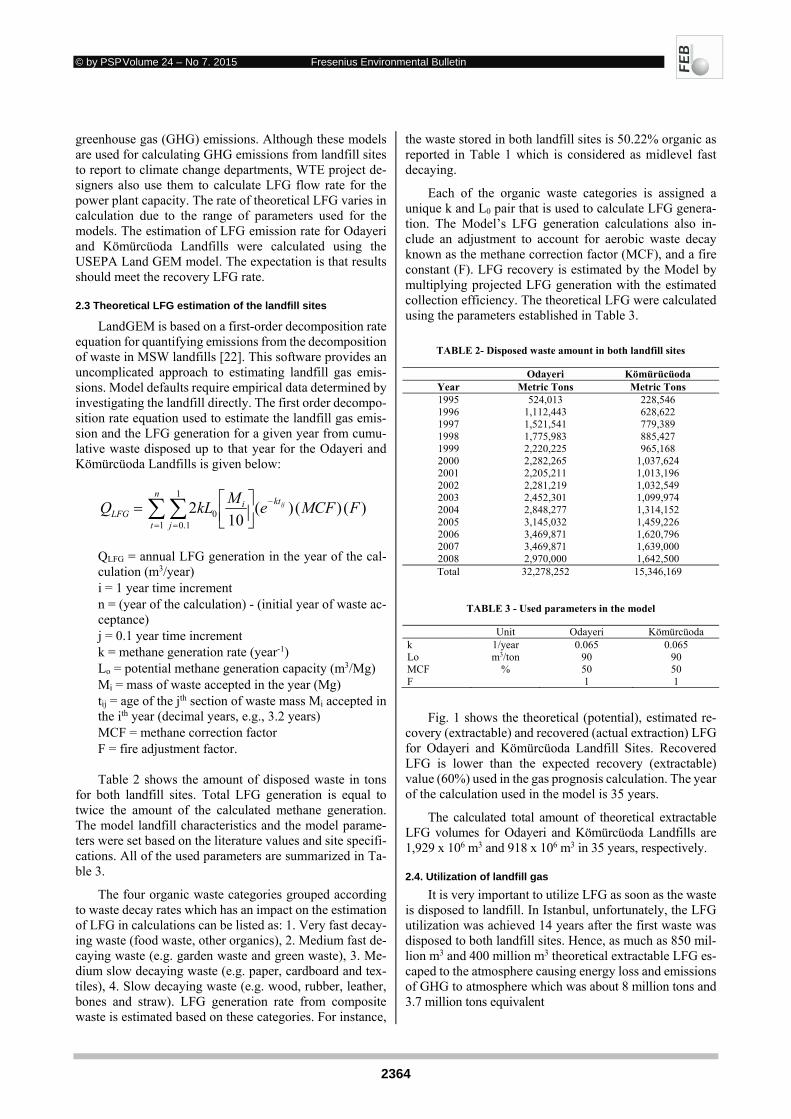
© by PSP Volume 24 – No 7. 2015 Fresenius Environmental Bulletin
2364
greenhouse gas (GHG) emissions. Although these models are used for calculating GHG emissions from landfill sites to report to climate change departments, WTE project de-signers also use them to calculate LFG flow rate for the power plant capacity. The rate of theoretical LFG varies in calculation due to the range of parameters used for the models. The estimation of LFG emission rate for Odayeri and Kömürcüoda Landfills were calculated using the USEPA Land GEM model. The expectation is that results should meet the recovery LFG rate.
2.3 Theoretical LFG estimation of the landfill sites
LandGEM is based on a first-order decomposition rate equation for quantifying emissions from the decomposition of waste in MSW landfills [22]. This software provides an uncomplicated approach to estimating landfill gas emis-sions. Model defaults require empirical data determined by investigating the landfill directly. The first order decompo-sition rate equation used to estimate the landfill gas emis-sion and the LFG generation for a given year from cumu-lative waste disposed up to that year for the Odayeri and Kömürcüoda Landfills is given below:
)()()(10
21
1
1.00 FMCFe
MkLQ ijkti
n
t jLFG
QLFG = annual LFG generation in the year of the cal-culation (m3/year) i = 1 year time increment n = (year of the calculation) - (initial year of waste ac-ceptance) j = 0.1 year time increment k = methane generation rate (year-1) Lo = potential methane generation capacity (m3/Mg) Mi = mass of waste accepted in the year (Mg) tij = age of the jth section of waste mass Mi accepted in the ith year (decimal years, e.g., 3.2 years) MCF = methane correction factor F = fire adjustment factor. Table 2 shows the amount of disposed waste in tons
for both landfill sites. Total LFG generation is equal to twice the amount of the calculated methane generation. The model landfill characteristics and the model parame-ters were set based on the literature values and site specifi-cations. All of the used parameters are summarized in Ta-ble 3.
The four organic waste categories grouped according to waste decay rates which has an impact on the estimation of LFG in calculations can be listed as: 1. Very fast decay-ing waste (food waste, other organics), 2. Medium fast de-caying waste (e.g. garden waste and green waste), 3. Me-dium slow decaying waste (e.g. paper, cardboard and tex-tiles), 4. Slow decaying waste (e.g. wood, rubber, leather, bones and straw). LFG generation rate from composite waste is estimated based on these categories. For instance,
the waste stored in both landfill sites is 50.22% organic as reported in Table 1 which is considered as midlevel fast decaying.
Each of the organic waste categories is assigned a unique k and L0 pair that is used to calculate LFG genera-tion. The Model’s LFG generation calculations also in-clude an adjustment to account for aerobic waste decay known as the methane correction factor (MCF), and a fire constant (F). LFG recovery is estimated by the Model by multiplying projected LFG generation with the estimated collection efficiency. The theoretical LFG were calculated using the parameters established in Table 3.
TABLE 2- Disposed waste amount in both landfill sites
Odayeri Kömürücüoda Year Metric Tons Metric Tons 1995 524,013 228,546 1996 1,112,443 628,622 1997 1,521,541 779,389 1998 1,775,983 885,427 1999 2,220,225 965,168 2000 2,282,265 1,037,624 2001 2,205,211 1,013,196 2002 2,281,219 1,032,549 2003 2,452,301 1,099,974 2004 2,848,277 1,314,152 2005 3,145,032 1,459,226 2006 3,469,871 1,620,796 2007 3,469,871 1,639,000 2008 2,970,000 1,642,500 Total 32,278,252 15,346,169
TABLE 3 - Used parameters in the model
Unit Odayeri Kömürcüoda k 1/year 0.065 0.065 Lo m3/ton 90 90 MCF % 50 50 F 1 1
Fig. 1 shows the theoretical (potential), estimated re-
covery (extractable) and recovered (actual extraction) LFG for Odayeri and Kömürcüoda Landfill Sites. Recovered LFG is lower than the expected recovery (extractable) value (60%) used in the gas prognosis calculation. The year of the calculation used in the model is 35 years.
The calculated total amount of theoretical extractable LFG volumes for Odayeri and Kömürcüoda Landfills are 1,929 x 106 m3 and 918 x 106 m3 in 35 years, respectively.
2.4. Utilization of landfill gas
It is very important to utilize LFG as soon as the waste is disposed to landfill. In Istanbul, unfortunately, the LFG utilization was achieved 14 years after the first waste was disposed to both landfill sites. Hence, as much as 850 mil-lion m3 and 400 million m3 theoretical extractable LFG es-caped to the atmosphere causing energy loss and emissions of GHG to atmosphere which was about 8 million tons and 3.7 million tons equivalent
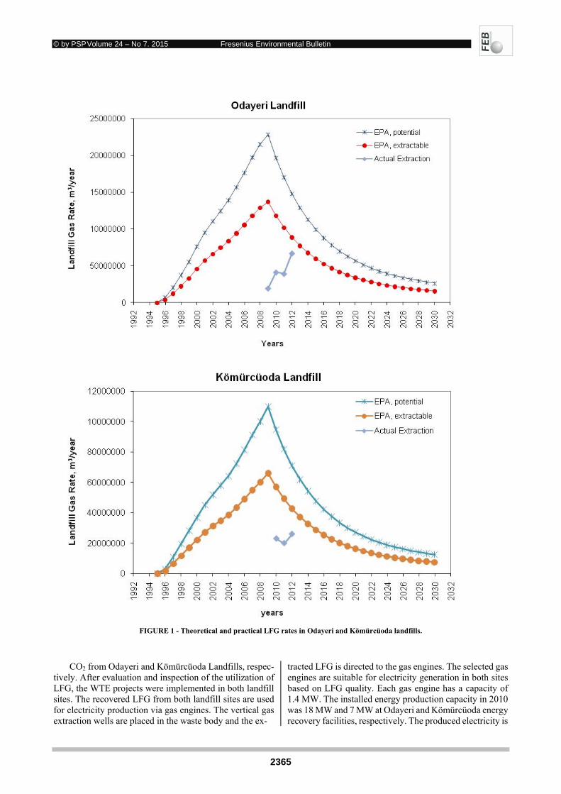
© by PSP Volume 24 – No 7. 2015 Fresenius Environmental Bulletin
2365
FIGURE 1 - Theoretical and practical LFG rates in Odayeri and Kömürcüoda landfills.
CO2 from Odayeri and Kömürcüoda Landfills, respec-tively. After evaluation and inspection of the utilization of LFG, the WTE projects were implemented in both landfill sites. The recovered LFG from both landfill sites are used for electricity production via gas engines. The vertical gas extraction wells are placed in the waste body and the ex-
tracted LFG is directed to the gas engines. The selected gas engines are suitable for electricity generation in both sites based on LFG quality. Each gas engine has a capacity of 1.4 MW. The installed energy production capacity in 2010 was 18 MW and 7 MW at Odayeri and Kömürcüoda energy recovery facilities, respectively. The produced electricity is
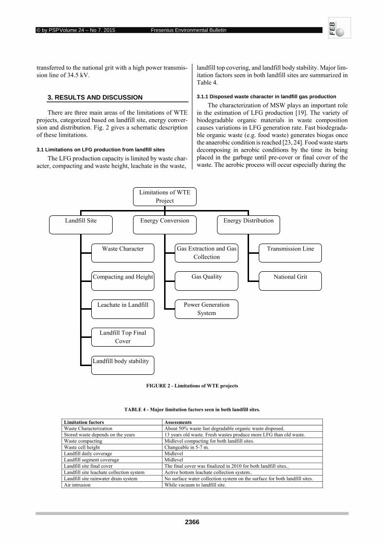
© by PSP Volume 24 – No 7. 2015 Fresenius Environmental Bulletin
2366
transferred to the national grit with a high power transmis-sion line of 34.5 kV.
3. RESULTS AND DISCUSSION
There are three main areas of the limitations of WTE projects, categorized based on landfill site, energy conver-sion and distribution. Fig. 2 gives a schematic description of these limitations.
3.1 Limitations on LFG production from landfill sites
The LFG production capacity is limited by waste char-acter, compacting and waste height, leachate in the waste,
landfill top covering, and landfill body stability. Major lim-itation factors seen in both landfill sites are summarized in Table 4.
3.1.1 Disposed waste character in landfill gas production
The characterization of MSW plays an important role in the estimation of LFG production [19]. The variety of biodegradable organic materials in waste composition causes variations in LFG generation rate. Fast biodegrada-ble organic waste (e.g. food waste) generates biogas once the anaerobic condition is reached [23, 24]. Food waste starts decomposing in aerobic conditions by the time its being placed in the garbage until pre-cover or final cover of the waste. The aerobic process will occur especially during the
Limitations of WTE Project
Energy Conversion Energy Distribution
Gas Extraction and Gas Collection
Gas Quality
Power Generation System
Landfill Site
Waste Character
Compacting and Height
Leachate in Landfill
Landfill Top Final Cover
Transmission Line
National Grit
Landfill body stability
FIGURE 2 - Limitations of WTE projects
TABLE 4 - Major limitation factors seen in both landfill sites.
Limitation factors Assessments Waste Characterization About 50% waste fast degradable organic waste disposed. Stored waste depends on the years 13 years old waste. Fresh wastes produce more LFG than old waste. Waste compacting Midlevel compacting for both landfill sites. Waste cell height Changeable in 5-7 m. Landfill daily coverage Midlevel Landfill segment coverage Midlevel Landfill site final cover The final cover was finalized in 2010 for both landfill sites.. Landfill site leachate collection system Active bottom leachate collection system.. Landfill site rainwater drain system No surface water collection system on the surface for both landfill sites. Air intrusion While vacuum to landfill site.
© by PSP Volume 24 – No 7. 2015 Fresenius Environmental Bulletin
2367
disposal process due to light compaction and delayed soil covering, downwards into a depth of two meters or even more [25]. 90 % of the degradable carbon will be destroyed during one year in aerobic landfills [26]. A first order model can be used to calculate the degradation of the or-ganic matter, eg. in the first 3 months nearly 50 % will be degraded [27, 28]. Therefore, it is very important to con-sider decomposed organic waste in aerobic conditions for the right prognosis and to estimate the influence of daily covering. Early waste decomposing in aerobic conditions causes potential LFG loss as well. To avoid immediate de-composition the organic matter needs to be collected regu-larly from the daily top soil cover.
3.1.2 Compacting and height of disposed waste.
Compacting of solid waste is an important factor in bi-ogas generation. Fewer voids in the waste volume increase the LFG production [29]. Compactors were used in both landfill sites, however, high quality compaction could not be achieved due to field problems (rainfall, compactor fail-ure) and high waste load in a short period of time. Another significant factor is covering the waste with soil as soon as possible. When the waste remains open to atmosphere in the landfill site for a long time the biodegradable organic waste degrades aerobically that causes a loss in LFG pro-duction capacity. There is a high waste load in Odayeri and Kömürcüoda landfills; consequently, considerably less daily coverage over the waste. The old waste is usually covered by fresh waste daily. Once the lot is filled with waste, the top is covered with soil.
The height of the waste in the landfill is another im-portant limitation parameter in the utilization of LFG. The gas extraction wells can be drilled up to 40 meters. The height of the waste has reached up to 90 meters in both landfills, thus it is not feasible to extract LFG below the extraction wells.
3.1.3. Leachate in landfill
The moisture in the waste encourages bacterial growth and transports nutrients and bacteria to all areas within a landfill [30]. The moisture content of 40% or higher, based on wet weight of waste promotes maximum gas produc-tion, especially in a capped landfill [31]. The disposed waste in both Odayeri and Kömürcüoda landfill sites con-tains about 50%-70% water [19, 32, 33]. Once the waste is
stored in the landfill site, leachate production rate begins to increase. In addition, if rain water penetrates into the non-covered landfill site, it increases the leachate flow rate as well. Unfortunately, both of the landfill sites top surface final covers were finalized in 2010. The average leacheate flow rate at Odayeri and Kömürcüoda landfill sites were about 2100 m³/day and 1000 m³/day, respectively in 2008. The organic matters dissolve during rainwater infiltration through the waste and leave the waste with leachate which causes a decrease in the LFG generation potential due to the lower organic content of the waste [34]. The leachate accumulation in the waste body observed in both landfill sites is over 40 meters high, attributable to a 13 year period of rainfall on the open landfill site. The high waste height causes high pressure on the bottom layer causing it to be more compact.
The LFG collection wells are the most important part of a WTE plant. High leachate level in the waste body and high waste body height have a potential on limiting the for-mation of LFG as well as extraction [35], which in fact were observed in Odayeri and Kömürcüoda landfill sites. Once the LFG extraction wells were placed in the waste body, leachate increased by capillary effect by causing it to fill the holes in the perforated wells. The remaining water free perforated wells available for gas extraction during the vacuum application in Odayeri and Kömürcüoda landfill sites are 16% and 40% percent, respectively. Hence, high vacuum should be applied to the wells to extract LFG from the mass of waste. In order to decrease level of leachate in the wells, it is discharged by the help of a pump, which increased the amount of water free perforated wells used in gas extraction. This additional step brought increased workload for the maintenance of the wells as well as con-struction and operating costs, in both landfill sites. Table 5 represents the values of the wells. In order to decrease leachate in the wells, the submerge pumps were placed in all the gas extraction wells. The height of the available wa-ter free perforated wells increased from 16% to about 30 % in Odayeri and from 40% to about 45% Kömürcüoda, re-spectively.
3.1.4. Top cover impermeability
Top cover is an important aspect of gas extraction perfor-mance needed for blocking air intrusion into waste body [36]. Anaerobic reactions should be sustained during gas extrac-
TABLE 5 - The values of wells
Odayeri Kömürcüoda
Average Well depth (m) 35 23,2
Average perforated well height (m) 29,4 18,8
Average water depth height (m) 24,7 10,7
Total pipe length in the wells (m) 4685,5 2760
Total perforated pipe length (m) 3933,5 2403
Total free slotted pipe length (m) 626,4 1423
Closed perforated pipe length with leachate (m) 84% 40%
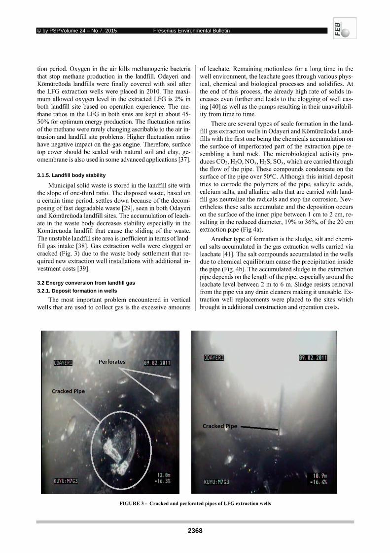
© by PSP Volume 24 – No 7. 2015 Fresenius Environmental Bulletin
2368
tion period. Oxygen in the air kills methanogenic bacteria that stop methane production in the landfill. Odayeri and Kömürcüoda landfills were finally covered with soil after the LFG extraction wells were placed in 2010. The maxi-mum allowed oxygen level in the extracted LFG is 2% in both landfill site based on operation experience. The me-thane ratios in the LFG in both sites are kept in about 45-50% for optimum energy production. The fluctuation ratios of the methane were rarely changing ascribable to the air in-trusion and landfill site problems. Higher fluctuation ratios have negative impact on the gas engine. Therefore, surface top cover should be sealed with natural soil and clay, ge-omembrane is also used in some advanced applications [37].
3.1.5. Landfill body stability
Municipal solid waste is stored in the landfill site with the slope of one-third ratio. The disposed waste, based on a certain time period, settles down because of the decom-posing of fast degradable waste [29], seen in both Odayeri and Kömürcüoda landfill sites. The accumulation of leach-ate in the waste body decreases stability especially in the Kömürcüoda landfill that cause the sliding of the waste. The unstable landfill site area is inefficient in terms of land-fill gas intake [38]. Gas extraction wells were clogged or cracked (Fig. 3) due to the waste body settlement that re-quired new extraction well installations with additional in-vestment costs [39].
3.2 Energy conversion from landfill gas
3.2.1. Deposit formation in wells
The most important problem encountered in vertical wells that are used to collect gas is the excessive amounts
of leachate. Remaining motionless for a long time in the well environment, the leachate goes through various phys-ical, chemical and biological processes and solidifies. At the end of this process, the already high rate of solids in-creases even further and leads to the clogging of well cas-ing [40] as well as the pumps resulting in their unavailabil-ity from time to time.
There are several types of scale formation in the land-fill gas extraction wells in Odayeri and Kömürcüoda Land-fills with the first one being the chemicals accumulation on the surface of imperforated part of the extraction pipe re-sembling a hard rock. The microbiological activity pro-duces CO2, H2O, NOx, H2S, SOx, which are carried through the flow of the pipe. These compounds condensate on the surface of the pipe over 50oC. Although this initial deposit tries to corrode the polymers of the pipe, salicylic acids, calcium salts, and alkaline salts that are carried with land-fill gas neutralize the radicals and stop the corrosion. Nev-ertheless these salts accumulate and the deposition occurs on the surface of the inner pipe between 1 cm to 2 cm, re-sulting in the reduced diameter, 19% to 36%, of the 20 cm extraction pipe (Fig 4a).
Another type of formation is the sludge, silt and chemi-cal salts accumulated in the gas extraction wells carried via leachate [41]. The salt compounds accumulated in the wells due to chemical equilibrium cause the precipitation inside the pipe (Fig. 4b). The accumulated sludge in the extraction pipe depends on the length of the pipe; especially around the leachate level between 2 m to 6 m. Sludge resists removal from the pipe via any drain cleaners making it unusable. Ex-traction well replacements were placed to the sites which brought in additional construction and operation costs.
FIGURE 3 - Cracked and perforated pipes of LFG extraction wells
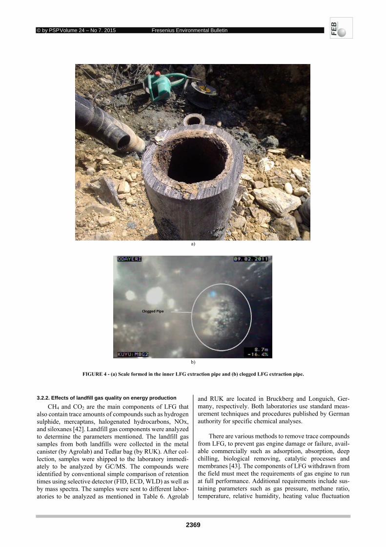
© by PSP Volume 24 – No 7. 2015 Fresenius Environmental Bulletin
2369
a)
b)
FIGURE 4 - (a) Scale formed in the inner LFG extraction pipe and (b) clogged LFG extraction pipe.
3.2.2. Effects of landfill gas quality on energy production
CH4 and CO2 are the main components of LFG that also contain trace amounts of compounds such as hydrogen sulphide, mercaptans, halogenated hydrocarbons, NOx, and siloxanes [42]. Landfill gas components were analyzed to determine the parameters mentioned. The landfill gas samples from both landfills were collected in the metal canister (by Agrolab) and Tedlar bag (by RUK). After col-lection, samples were shipped to the laboratory immedi-ately to be analyzed by GC/MS. The compounds were identified by conventional simple comparison of retention times using selective detector (FID, ECD, WLD) as well as by mass spectra. The samples were sent to different labor-atories to be analyzed as mentioned in Table 6. Agrolab
and RUK are located in Bruckberg and Longuich, Ger-many, respectively. Both laboratories use standard meas-urement techniques and procedures published by German authority for specific chemical analyses.
There are various methods to remove trace compounds from LFG, to prevent gas engine damage or failure, avail-able commercially such as adsorption, absorption, deep chilling, biological removing, catalytic processes and membranes [43]. The components of LFG withdrawn from the field must meet the requirements of gas engine to run at full performance. Additional requirements include sus-taining parameters such as gas pressure, methane ratio, temperature, relative humidity, heating value fluctuation
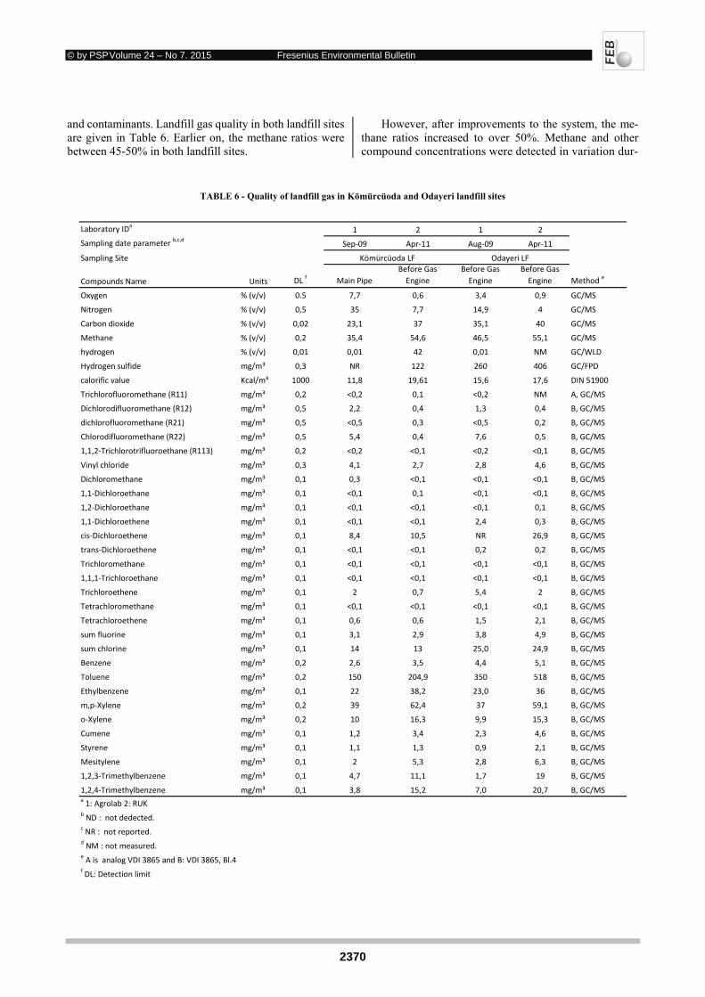
© by PSP Volume 24 – No 7. 2015 Fresenius Environmental Bulletin
2370
and contaminants. Landfill gas quality in both landfill sites are given in Table 6. Earlier on, the methane ratios were between 45-50% in both landfill sites.
However, after improvements to the system, the me-thane ratios increased to over 50%. Methane and other compound concentrations were detected in variation dur-
TABLE 6 - Quality of landfill gas in Kömürcüoda and Odayeri landfill sites
Laboratory IDa
1 2 1 2
Sampling date parameter b,c,d
Sep‐09 Apr‐11 Aug‐09 Apr‐11
Sampling Site
Compounds Name Units DL f
Main Pipe
Before Gas
Engine
Before Gas
Engine
Before Gas
Engine Method e
Oxygen % (v/v) 0.5 7,7 0,6 3,4 0,9 GC/MS
Nitrogen % (v/v) 0,5 35 7,7 14,9 4 GC/MS
Carbon dioxide % (v/v) 0,02 23,1 37 35,1 40 GC/MS
Methane % (v/v) 0,2 35,4 54,6 46,5 55,1 GC/MS
hydrogen % (v/v) 0,01 0,01 42 0,01 NM GC/WLD
Hydrogen sulfide mg/m³ 0,3 NR 122 260 406 GC/FPD
calorific value Kcal/m³ 1000 11,8 19,61 15,6 17,6 DIN 51900
Trichlorofluoromethane (R11) mg/m³ 0,2 <0,2 0,1 <0,2 NM A, GC/MS
Dichlorodifluoromethane (R12) mg/m³ 0,5 2,2 0,4 1,3 0,4 B, GC/MS
dichlorofluoromethane (R21) mg/m³ 0,5 <0,5 0,3 <0,5 0,2 B, GC/MS
Chlorodifluoromethane (R22) mg/m³ 0,5 5,4 0,4 7,6 0,5 B, GC/MS
1,1,2‐Trichlorotrifluoroethane (R113) mg/m³ 0,2 <0,2 <0,1 <0,2 <0,1 B, GC/MS
Vinyl chloride mg/m³ 0,3 4,1 2,7 2,8 4,6 B, GC/MS
Dichloromethane mg/m³ 0,1 0,3 <0,1 <0,1 <0,1 B, GC/MS
1,1‐Dichloroethane mg/m³ 0,1 <0,1 0,1 <0,1 <0,1 B, GC/MS
1,2‐Dichloroethane mg/m³ 0,1 <0,1 <0,1 <0,1 0,1 B, GC/MS
1,1‐Dichloroethene mg/m³ 0,1 <0,1 <0,1 2,4 0,3 B, GC/MS
cis‐Dichloroethene mg/m³ 0,1 8,4 10,5 NR 26,9 B, GC/MS
trans‐Dichloroethene mg/m³ 0,1 <0,1 <0,1 0,2 0,2 B, GC/MS
Trichloromethane mg/m³ 0,1 <0,1 <0,1 <0,1 <0,1 B, GC/MS
1,1,1‐Trichloroethane mg/m³ 0,1 <0,1 <0,1 <0,1 <0,1 B, GC/MS
Trichloroethene mg/m³ 0,1 2 0,7 5,4 2 B, GC/MS
Tetrachloromethane mg/m³ 0,1 <0,1 <0,1 <0,1 <0,1 B, GC/MS
Tetrachloroethene mg/m³ 0,1 0,6 0,6 1,5 2,1 B, GC/MS
sum fluorine mg/m³ 0,1 3,1 2,9 3,8 4,9 B, GC/MS
sum chlorine mg/m³ 0,1 14 13 25,0 24,9 B, GC/MS
Benzene mg/m³ 0,2 2,6 3,5 4,4 5,1 B, GC/MS
Toluene mg/m³ 0,2 150 204,9 350 518 B, GC/MS
Ethylbenzene mg/m³ 0,1 22 38,2 23,0 36 B, GC/MS
m,p‐Xylene mg/m³ 0,2 39 62,4 37 59,1 B, GC/MS
o‐Xylene mg/m³ 0,2 10 16,3 9,9 15,3 B, GC/MS
Cumene mg/m³ 0,1 1,2 3,4 2,3 4,6 B, GC/MS
Styrene mg/m³ 0,1 1,1 1,3 0,9 2,1 B, GC/MS
Mesitylene mg/m³ 0,1 2 5,3 2,8 6,3 B, GC/MS
1,2,3‐Trimethylbenzene mg/m³ 0,1 4,7 11,1 1,7 19 B, GC/MS
1,2,4‐Trimethylbenzene mg/m³ 0,1 3,8 15,2 7,0 20,7 B, GC/MSa 1: Agrolab 2: RUKb ND : not dedected.
c NR : not reported.d NM : not measured.
e A is analog VDI 3865 and B: VDI 3865, Bl.4f DL: Detection limit
Kömürcüoda LF Odayeri LF
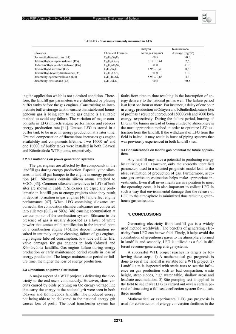
© by PSP Volume 24 – No 7. 2015 Fresenius Environmental Bulletin
2371
TABLE 7 - Siloxanes commonly measured in LFG
Odayeri Komurcuoda Siloxanes Chemical Formula Average (mg/m³) Average (mg/m³) Decamethyltetrasiloxan (L4) C10H30Si4O3 <0.5 <0.5 Dekamethylcyclopentasiloxan (D5) C10H30O5Si5 3.18 ± 0.61 2,6 Dodecamethylcyclohexasiloxan (D6) C12H36O6Si6 <1.0 <1.0 Hexamethyldisiloxane (L2) C6H18Si2O 1.95 ± 0,40 0,6 Hexamethyl-(cyclo)-trisiloxane (D3) C12H18O3Si3 <1.0 <1.0 Octamethylcyclotetrasiloxan (D4) C8H24O4Si4 5.93 ± 0,88 4,3 Octamethyl-trisiloxane (L3) C8H24Si3O2 <0.5 <0.5
ing the application which is not a desired condition. There-fore, the landfill gas parameters were stabilized by placing buffer tanks before the gas engines. Constructing an inter-mediate buffer storage tank to ensure that stable and homo-geneous gas is being sent to the gas engine is a suitable method to avoid any failure. The variation of major com-ponents in LFG impacts engine performance and reduces energy production rate [44]. Unused LFG is stored in a buffer tank to be used in energy production at a later time. Optimal compensation of fluctuations increases gas engine availability and components lifetime. Two 16000 m3 and one 16000 m3 buffer tanks were installed in both Odayeri and Kömürcüoda WTE plants, respectively.
3.2.3. Limitations on power generation systems
The gas engines are affected by the compounds in the landfill gas during energy production. Especially the silox-anes in landfill gas hamper to the engine in energy produc-tion [45]. Siloxanes contain silicon atoms attached to VOCs [43]. Common siloxane derivatives in LFG of both sites are shown in Table 7. Siloxanes are especially prob-lematic in landfill gas to energy projects since they result in deposit formation in gas engines [46] and effect engine performance [47]. When LFG containing siloxanes are burned in the combustion chamber, siloxanes are converted into silicates (SiO2 or SiO3) [48] causing accumulation at various points of the combustion system. Siloxane in the presence of gas is usually deposited as a layer of white powder that causes mild stratification in the internal parts of a combustion engine [46].The deposit formation re-sulted in untimely engine cleaning, failure of gas engines, high engine lube oil consumption, low lube oil filter life, valve damages for gas engines in both Odayeri and Kömürcüoda landfills. Gas engine failure during energy production or early maintenance period results in loss of energy production. The longer maintenance period or fail-ure time, the higher the loss of energy production.
3.3 Limitations on power distribution
A major aspect of a WTE project is delivering the elec-tricity to the end users continuously. However, short cir-cuits caused by birds perching on the energy voltage line that carry the energy to the national grit were seen in both Odayeri and Kömürcüoda landfills. The produced energy not being able to be delivered to the national energy grit causes loss of profit. The local transformer system has
faults from time to time resulting in the interruption of en-ergy delivery to the national grit as well. The failure period is at least one hour or more. For instance, a delay of one hour in energy production in Odayeri and Kömürcüoda cause loss of profit as a result of unproduced 18000 kwh and 7000 kwh energy, respectively. During the failure period, burning of LFG in the burner instead of being emitted to atmosphere is the most appropriate method in order to optimize LFG ex-traction from the landfill. If the withdrawal of LFG from the field is halted, it may result in burst of piping systems that was previously experienced in both landfill sites.
3.4 Considerations on landfill gas potential for future applica-tions
Any landfill may have a potential in producing energy by utilizing LFG. However, only the correctly identified parameters used in a selected prognosis model lead to the ideal estimation of production of gas. Furthermore, accu-rate gas emission estimation helps make appropriate in-vestments. Even if all investments are in a position to meet the operating costs, it is also important to collect LFG in such a way that environmental damage thru the release of LFG to the atmosphere is minimized thus reducing green-house gas emissions.
4. CONCLUSIONS
Generating electricity from landfill gas is a widely used method worldwide. The benefits of generating elec-tricity from LFG can be two fold. Firstly, it helps avoid the contribution of greenhouse gases to the atmosphere formed in landfills and secondly, LFG is utilized as a fuel in dif-ferent revenue-generating energy systems.
A successful WTE project reaches its targets by fol-lowing these steps: 1) A mathematical gas prognosis is done to see if the landfill is suitable for a WTE project. 2) Landfill site is inspected with static tests to see the influ-ence on gas production such as bad compaction, waste height, steep slopes, high water table, shallow areas and leachate accumulation. 3) Site pumping test is applied in the field to see if real LFG is carried out over a certain pe-riod of time using a full scale collection system for at least three months.
Mathematical or experimental LFG gas prognosis is used for construction of energy conversion facilities in the
© by PSP Volume 24 – No 7. 2015 Fresenius Environmental Bulletin
2372
feasibility phase. The installation capacity of a facility is determined by calculating recovered LFG, utilizing a re-covery constant. The recovered LFG rate is used for calcu-lating installation capacity of the energy conversion facil-ity. In many applications, field LFG extraction rate is usu-ally lower than the estimated recovery LFG rate. The ab-sence of accurate estimations in WTE projects prevents them from being income-generating projects. Even when the recovered LFG is estimated accurately, operational problems are often encountered such as engine damage and clogging of the wells. Problems related to landfill site, power generation and energy delivery are limiting factors for landfill gas and energy production. Some of these prob-lems occur naturally and they can be reduced by taking necessary measures.
LFG production and collection systems as well as en-ergy production and distribution systems of a WTE project should be checked regularly for it to continuously produce high-performance energy and be revenue-generating. As was the case in Odayeri and Kömürcüoda WTE applica-tions, parameters were established and collected regularly and analyzed for optimum energy production. The esti-mated amount of LFG to be recovered in both landfills was determined by taking 60% of the value of the prognosis model. The actual recovered LFG rates were below the es-timated prognosis values. The recovered LFG ratio for Odayeri in 2009, 2010, 2011, 2012 were 13%, 34%, 38% and 75 % respectively and for Kömürcüoda in 2010, 2011, 2012 were 40%, 40%, 60%, respectively. The recovery rates increased once the actual operating conditions im-proved after the first year.
ACKNOWLEDGMENTS
The author thanks Ortadogu Energy A.S. and ISTAC A.S. for their support during this study. Parties cannot be held responsible for the findings.
The authors have declared no conflict of interest. REFERENCES
[1] Pandey, P.C., Sharma, L.K. and Nathawat, M.S., (2012) Geo-spatial strategy for sustainable management of municipal solid waste for growing urban environment. Environmental Moni-toring and Assessment, 184,2419-2431.
[2] Chen, Z., Gong, H., Jiang, R., Jiang, Q. and Wu, W., (2010) Overview on LFG projects in China. Waste Management, 30, 1006-1010.
[3] Unnikrishnan, S. and Singh,A., (2010) Energy recovery in solid waste management through CDM in India and other countries. Resources, Conservation and Recycling, 54, 630-640.
[4] Demirbas, A., (2001) Energy balance, energy sources, energy policy, future developments and energy investments in Turkey. Energy Conversion and Management, 42, 1239–1258.
[5] Gokcol, C., Dursun, B., Alboyaci, B. and Sunan E., (2009) Im-portance of biomass energy as alternative to other sources in Turkey. Energy Policy, 37, 424-431.
[6] Dolgen, D., Sarptas, H., Alpaslan, N. and Kucukgul, O., (2005) Energy potential of municipal solid wastes. Energy Sources, 27, 1483-1492.
[7] Lombardi, L., Carnevale, E. and Corti, A., (2006) Greenhouse effect reduction and energy recovery from waste landfill. En-ergy, 31, 3208-3219.
[8] Chun, S.K. and Bae, Y.S. (2012) An impact analysis of landfill for waste disposal on climate change: Case study of Sudokwon landfill Site 2nd landfill in Korea. Korean Journal of Chemical Engineering, 29, 1549-1555.
[9] Papageorgiou, A., Barton, J.R. and Karagiannidis, A. (2009) As-sessment of the greenhouse effect impact of technologies used for energy recovery from municipal waste: A case for England. Journal of Environmental Management, 90, 2999-3012.
[10] Kumar, A. and Sharma, M.P. (2014) Estimation of GHG emis-sion and energy recovery potential from MSW landfill sites. Sustainable Energy Technologies and Assessments, 5, 50-61.
[11] White, A.L. and Zack, M. (1989) Avoided-cost pricing of elec-tricity from waste-to-energy plants the regulatory economics of a negative cost fuel, Energy Policy, 17, 370-381.
[12] Niskanen, A., Värri, H., Havukainen, J., Uusitalo, V. and Horttanainen, M. (2013) Enhancing landfill gas recovery. Journal of Cleaner Production, 55, 67-71.
[13] Gardner, N. and Probert, S.D. (1993) Forecasting landfill-gas yields. Applied Energy, 44, 131-163.
[14] Park, J.W. and Shin, H.C. (2001) Surface emission of landfill gas from solid waste landfill. Atmospheric Environment, 35, 3445-3451.
[15] Siegal, J.P. (1987) Testing large landfill sites before construc-tion of gas recovery facilities. Waste Management and Re-search, 5, 123-131.
[16] Rubio-Romero, J.C., Arjona-Jiménez, R. and López-Arquil-los, A. (2013) Profitability analysis of biogas recovery in Mu-nicipal Solid Waste landfills. Journal of Cleaner Production, 55, 84-91.
[17] Gardner, N., Manley, B.J.W. and Probert, S.D. (1990) Design considerations for landfill gas producing sites. Applied Energy, 37, 99-109.
[18] Maldonado, L. (2006) The economics of urban solid waste re-duction in educational institutions in Mexico: A 3-year experi-ence.Resources, Conservation and Recycling, 48, 41-55.
[19] Kanat, G. (2010) Municipal solid-waste management in Istan-bul. Waste Management, 30, 1737–1745.
[20] Yaman, C. (2011) Evaluation of the current condition of pack-aging wastes throughout Istanbul, Scientific Research and Es-says. 6, 3378-3388.
[21] Findikakis, A.N., Papelis, C., Halvadakis, C.P. and Leckie J.O. (1988) Modelling gas production in managed sanitary landfill. Waste Management and Research, 6, 115-123.
[22] Faour, A.A., Reinhart, D.R. and You, H. (2007) First-order ki-netic gas generation model parameters for wet landfills. Waste Management, 27, 946-953.
[23] Khalid, A., Arshad, M., Anjum, M., Mahmood, T. and Daw-son, L. (2011) The anaerobic digestion of solid organic waste. Waste Management, 31, 1737-1744.
[24] Faverial, J. and Sierra J. (2014) Home composting of house-hold biodegradable wastes under the tropical conditions of Guadeloupe (French Antilles). Journal of Cleaner Production, 83, 238-244.
© by PSP Volume 24 – No 7. 2015 Fresenius Environmental Bulletin
2373
[25] Lefebvre, X., Lanini S. and Houi, D. (2000) The role of aero-bic activity on refuse temperature rise, I. Landfill experimental study. Waste Management and Research, 18, 444-452.
[26] Francou, C., Linères, M., Derenne, S., Le Villio-Poitrenaud, M. and Houot, S. (2008) Influence of green waste, biowaste and paper–cardboard initial ratios on organic matter transfor-mations during composting. Bioresource Technology, 99, 8926-8934.
[27] De Gioannis, G., Muntoni, A., Cappai, G. and Milia, S. (2009) Landfill gas generation after mechanical biological treatment of municipal solid waste. Estimation of gas generation rate constants. Waste Management, 29, 1026-1034.
[28] Seng, B., Hirayama, K., Katayama-Hirayama, K., Ochiai, S. and Kaneko H. (2013) Scenario analysis of the benefit of mu-nicipal organic-waste composting over landfill, Cambodia. Journal of Environmental Management, 114, 216-224.
[29] Yesiller, N., Hanson, J.L., Cox, J.T. and Noce, D.E. (2014) De-termination of specific gravity of municipal solid waste. Waste Management, 34, 848-858.
[30] Sanphoti, N., Towprayoon, S., Chaiprasert, P. and Nopha-ratana, A. (2006) The effects of leachate recirculation with supplemental water addition on methane production and waste decomposition in a simulated tropical landfill. Journal of En-vironmental Management, 81, 27-35.
[31] Zhang, H., Yan, X., Cai, B., Zhang, Y., Liu, J. and Ao, H. (2015) The effects of aged refuse and sewage sludge on land-fill CH4 oxidation and N2O emissions: Roles of moisture con-tent and temperature. Ecological Engineering, 74, 345-350.
[32] Basturk, A. (1997) Design of solid waste plant and problems in Istanbul. In: Proceedings of the International Symposium on Environmental Problems of Istanbul and Solutions of Them. YTU Press, Istanbul, Turkey, 103–109.
[33] Arikan, O. and Toroz, I. (1999) Investigation on solid waste recycling in Istanbul. In: City Administration Human and En-vironment Problems 99 Symposium, Istanbul, Turkey, 263–272 (in Turkish).
[34] Benson, C.H., Barlaz, M.A., Lane, D.T. and Rawe, J.M. (2007) Practice review of five bioreactor/recirculation landfills. Waste Management, 27, 13-29.
[35] Jain, P., Ko, J.H., Kumar, D., Powell, J., Kim, H., Maldonado, L., Townsend, T. and Reinhart, D.R. (2014) Case study of landfill leachate recirculation using small-diameter vertical wells. Waste Management, 34, 2312-2320.
[36] Rajesh, S., Gourc, J.P. and Viswanadham, B.V.S. (2014) Eval-uation of gas permeability and mechanical behaviour of soil barriers of landfill cap covers through laboratory tests. Applied Clay Science, 97–98, 200-214.
[37] Simon, F.G. and Müller, W.W. (2004) Standard and alternative landfill capping design in Germany. Environmental Science & Policy, 7, 277-290.
[38] Elagroudy, S.A., Abdel-Razik, M.H., Warith, M.A. and Ghobrial, F.H. (2008) Waste settlement in bioreactor landfill models. Waste Management, 28, 2366-2374.
[39] Yi, F., Xu, Y., Tian, Y. and Jiang, F. (2014) The influence of landfill settlement on the efficiency of landfill gas collection. Advances in Science and Technology of Water Resources, 34, 30-33.
[40] Beaven, R.P., Hudson, A.P., Knox, K., Powrie, W. and Robin-son, J.P. (2013) Clogging of landfill tyre and aggregate drain-age layers by methanogenic leachate and implications for prac-tice. Waste Management, 33, 431-444.
[41] Van Gulck, J.F. and Rowe, R.K. (2004) Influence of landfill leachate suspended solids on clog (biorock) formation. Waste Management, 24, 723–738.
[42] Eklund, B., Anderson, E.P., Walker, B.L. and Burrows, D.B. (1998) Characterization of landfill gas composition at the fresh kills municipal solid-waste landfill. Environmental Science and Technology, 32, 2233–2237.
[43] Ajhar, M., Travesset, M., Yüce, S. and Melin, T. (2010) Silox-ane removal from landfill and digester gas – A technology overview. Bioresource Technology, 101, 2913–2923.
[44] Sevimoglu, O. and Tansel B. (2013) Composition and source identification of deposits forming in landfill gas (LFG) en-gines and effect of activated carbon treatment on deposit com-position. Journal of Environmental Management, 128, 300-305.
[45] Dewil, R., Appels, L. and Baeyens, J. (2006) Energy use of biogas hampered by the presence of siloxanes. Energy Con-version and Management, 47, 1711-1722.
[46] Sevimoglu O. and Tansel, B. (2013) Effect of persistent trace compounds in landfill gas on engine performance during en-ergy recovery: A case study. Waste Management, 33, 74-80.
[47] Appels, L., Baeyens, J. and Dewil, R. (2008) Siloxane removal from biosolids by peroxidation. Energy Conversion and Man-agement, 49, 2859-2864.
[48] Tansel, B. and Surita, S.C. (2014). Oxidation of siloxanes dur-ing biogas combustion and nanotoxicity of Si-based particles released to the atmosphere. Environmental Toxicology and Pharmacology, 37, 166-173.
Received: January 01, 2015 Revised: February 23, 2015 Accepted: March 11, 2015 CORRESPONDING AUTHOR
Orhan Sevimoğlu Istanbul Metropolitan Municipality Şehzadebaşı Caddesi 34134 Fatih / Istanbul TURKEY Phone: +90 (212) 455 33 00 E-mail: [email protected]
FEB/ Vol 24/ No 7/ 2015 – pages 2362 - 2373
© by PSP Volume 24 – No 7. 2015 Fresenius Environmental Bulletin
2374
APPLICATIONS OF FACTOR ANALYSIS AND
GEOGRAPHICAL INFORMATION SYSTEMS FOR
PRECISION AGRICULTURE OVER ALLUVIAL LANDS
Kadir Ersin Temizel1,*, Hakan Arslan1 and Mustafa Sağlam2
1Ondokuz Mayis University, Faculty of Agriculture, Department of Agricultural Structures and Irrigation, 55139 Samsun-Turkey 2Ondokuz Mayis University, Faculty of Agriculture, Department of Soil Science and Plant Nutrition, 55139 Samsun-Turkey
ABSTRACT
In this study, soil samples were taken from 32 different locations from two different soil depths (0-30 and 30-60 cm) and 16 physical and chemical soil properties were as-sessed through factor analysis (FA) and geographical in-formation systems (GIS). FA revealed 5 factors for the sur-face soil depth (0-30 cm) explaining 79.58% of total vari-ation in data set. These factors were entitled as factor 1 “soil water holding capacity”, factor 2 “microelement availability”, factor 3 “organic matter”, factor 4 “soil reac-tion” and factor 5 “soil salinity”. FA for the subsurface depth (30-60 cm) revealed 4 factors explaining 75.14% of total variation in data set. These factors were entitled as factor 1 “nutrient availability–soil reaction relationship”, factor 2 “soil water holding capacity”, factor 3 “organic matter” and factor 4 “soil salinity”. A total of nine spatial distribution maps were prepared for these factors by using the factor scores obtained from FA for both soil depths. Significant similarities were observed in both factor com-ponents and spatial distribution patterns of both soil depths. It was concluded that FA with various soil properties used as multiple variables might reveal significant hidden infor-mation about soil properties and yield highly valuable out-comes for the management and planning of precise agricul-tural practices.
KEYWORDS: Precision agriculture, factor analysis, geographical information systems, soil properties, alluvial lands
1. INTRODUCTION
Precision agriculture represents the approaches allow-ing the implementation of environment-friendly methods and techniques in agricultural production activities. Paral-lel to developments in global positioning systems (GPS),
* Corresponding author
farmers have started to be aware of the advantages brought by the implementations carried out in agriculture through considering the spatial differences. Knowledge about the factors exhibiting spatial and temporal variations plays a significant role for optimum profit, sustainability and envi-ronmental protection. Knowledge and technology-based precision agriculture are used to analyze and manage such factors and recently has a wide range of application in ag-ricultural practices [1]. Precise agricultural implementa-tions are basically composed of accurate analysis of present conditions and performance of implementations in accord-ance with the present needs. Precision agriculture inte-grates developing technologies into agricultural production and covers the practices aiming maximum gain and taking the environmental protection principles into consideration together with various low-cost inputs [2].
Multivariate statistic is a general term defining the sta-
tistical methods allowing the analysis of two or more fac-tors together [3]. In multivariate statistical analysis, there are multiple interrelated variables in a system. The appli-cations of multivariate analytical methods such as cluster analysis (CA), FA and principle component analysis (PCA) to environmental data have tremendously increased and yielded meaningful information. FA is a multivariate statistical technique used to get less and unrelated variables by using multiple interrelated variables. CA and PCA have been widely used in soil surveys [4-6]. FA and GIS have also together been used in several studies investigating soil characteristics [7, 8] Shan et al. [9] carried out a study to find out the heavy metal source of soils and used multivar-iate statistical techniques and GIS together. Soil samples were taken from 149 different points in that study and 11 different soil parameters were determined. Researchers de-termined anthropogenic factor as factor 1, lithogetic factor as factor 2 and prepared spatial distribution map of each factor.
The present study was conducted to present the bene-
fits and advantages brought by combined use of FA and GIS in planning and management of precision agriculture implementations.

© by PSP Volume 24 – No 7. 2015 Fresenius Environmental Bulletin
2375
2. MATERIALS AND METHOD
2.1 Study area and sampling
The study area is located within the Black Sea Coastal Region of the Samsun province (between 41º30’- 41º45’ latitude and 35º30’-36º15’ longitude) in the northern Tur-key (Figure 1). Soils are formed over alluvial deposits of Kizilirmak River at various elevations and classified as Typical Ustifluvents, Chromic Haplusterts and Vertic Hap-lustepts [10]. Bafra plain has a mild climate with annual average temperature of 14.4 °C and annual precipitation of 802.6 mm. The main rock of Bafra Plain and close sur-roundings are composed of Mesozoic Tertiary and quater-nary lands. Quaternary lands are composed of alluvial and terrace depots. The alluvium over the flood plains along the Kızılırmak crossing the plain in North-south direction and other streams are silty and gravelly and he gravels are mostly composed of volcanic rocks and lime stones. The soils of Bafra Plain may be broadly characterized as deep, alluvial delta and colluvial terrace-alluvial fans. These are young soils extremely variable, ranging from sandly loans to heavy clays. Particularly paddy and tomato, pepper, melon, watermelon and eggplant are grown in Bafra Plain. Over these lands, generally surface gravity irrigation meth-ods and randomly sprinkler and drip irrigation method are used in irrigations. Since Bafra Plain is close to sea, there is a drainage problem in some sections of the plain.
Global positioning (GPS) device was used to locate the soil sampling points. The distance between soil sampling points was 70 m. Disturbed soil samples were taken from 0-30 cm and 30-60 cm soil depths. Since horticultural crops are grown over the research site of the present study and rooting depths of most of these crops are within the initial 60 cm soil layer, soil samples were taken from these depths. Samples were air dried at laboratory and sieved through 2 mm sieve to make them ready for analyses. Soil texture was determined by Bouyoucos hydrometer method [11]; lime content was determined with Scheibler calcime-ter [12]; organic matter content was determined in accord-ance with Smith-Weldon method [13]; soil pH [14] and electrical conductivity [15] were determined in 1:2 soil-water mixture; Kjeldahl method was used to determine the total nitrogen [16]; available phosphorus was determined by Olsen method [17]; extractable potassium (Kext) was de-termined in accordance with Soil Survey Staff [18]; DTPA-extracted solution was used to determine available iron, copper, zinc and manganese in an atomic adsorption device [19]. The analyses on entire soil characteristics were per-formed in three replications and the data set was used through taking the arithmetical mean of these replications.
2.2 Principle component and spatial analysis methods
Soil samples were taken from 32 different locations and 16 different physical and chemical analyses were per-
FIGURE 1 - Location of Study Area and Distribution of Sampling Points

© by PSP Volume 24 – No 7. 2015 Fresenius Environmental Bulletin
2376
formed on these samples. Analyses results were assessed through FA and GIS. FA is a multivariate statistical tech-nique and uses multiple interrelated variables to derive un-related new variables. It includes dimension reduction and dependence elimination phases and brings together p num-ber of interrelated variables of a case and tries to find less unrelated new (common) variables [20]. While finding the number of principle components, the ones with an eigen value over 1 are selected. This method has been utilized in assessment of soil data in several studies [21, 22]. In FA, resultant factors are assessed as: f > 0.75 strong, 0.50< f <0.75 medium and 0.30 < f <0.50 weak [23]. In FA of the present study, varimax rotation was employed to reduce the number of factors through maximizing the variations of factor loads. Statistical analyses were performed by using SPSS 21 software.
For unsampled locations, kriging is considered as an optimal method of spatial prediction that provides a supe-rior liner unbiased estimator for spatially varying quantities [24]. Various researchers have used Geographic Infor-mation System (GIS) to investigate a wide range of soil and
water properties [25-26]. To explore the spatial distribution of FA results, ordinary kriging method was used with PC software ArcGIS 10.0.
3. RESULTS AND DISCUSSION
3.1 Definition of descriptive statistics
Descriptive statistics for surface (0-30 cm) and subsur-face (30-60 cm) soil depths are provided in Table 1 and assessment of soil characteristics with regard to threshold values of these parameters in plant production are provided in Table 2.
Considering the average values, soil texture of surface
and subsurface depths was classified as clay (Table 1). While field capacity (FC) of the surface depth varied be-tween 25.26-39.18%, permanent wilting points (PWP) var-ied between 11.85-22.60%. EC values of the surface depth varied between 0.23-0.51 dSm-1 and a salinity problem was not observed in surface depth considering the threshold
TABLE 1 - Descriptive statistics for soil samples of surface (0-30 cm ) and subsurface (30-60 cm) soil depths.
Soil properties Unit Min. Max Mean S.D. CV (%) Skewness Kurtosis TransformationSurface depth (0-30 cm)
Sand % 9.27 24.12 15.23 4.15 27.24 0.49 2.12 NormalClay % 33.88 58.10 48.73 6.51 13.36 -0.76 2.85 LognormalSilt % 27.98 43.95 36.04 3.53 9.78 -0.19 3.20 NormalFC % 25.26 39.18 32.55 3.37 10.34 -0.28 2.28 NormalPWP % 11.85 22.60 17.41 2.60 14.94 -0.34 2.62 NormalEC dS m-1 0.232 0.511 0.344 0.073 21.35 0.56 2.33 LognormalpH 7.44 8.12 7.91 0.16 2.00 -1.25 4.70 LognormalOM % 0.52 2.55 1.73 0.50 28.62 -0.59 2.84 LognormalCaCO3 % 3.88 8.54 6.53 1.20 18.37 -0.17 2.12 NormalNtotal % 0.03 0.13 0.09 0.02 28.62 -0.59 2.85 LognormalFeav mg kg-1 14.89 32.76 22.19 4.46 20.08 0.14 2.35 NormalCuav mg kg-1 3.77 6.50 4.79 0.64 13.34 0.49 3.03 NormalZnav mg kg-1 0.31 1.16 0.60 0.26 42.82 0.80 2.35 LognormalMnav mg kg-1 9.52 21.23 14.18 3.24 22.87 0.66 2.47 LognormalKext cmol(+) kg-1 0.37 1.09 0.71 0.14 19.88 -0.04 3.98 NormalPav mg kg-1 7.57 46.40 16.80 7.53 44.81 2.18 9.06 Lognormal
Subsurface depth (30-60 cm) Sand % 8.63 25.87 17.24 5.08 29.48 0.23 1.76 NormalClay % 31.32 55.78 44.58 6.36 14.26 -0.17 2.66 NormalSilt % 30.94 51.41 38.18 4.79 12.54 0.77 3.12 LognormalFC % 25.40 40.00 33.75 4.63 13.73 -0.21 1.91 NormalPWP % 11.97 23.60 18.47 2.93 15.88 -0.30 2.45 NormalEC dS m-1 0206 0.541 0.350 0.087 24.96 0.52 2.41 LognormalpH 7.57 8.18 7.97 0.12 1.51 -1.05 5.27 LognormalOM % 0.30 2.06 1.48 0.42 28.16 -0.98 3.35 LognormalCaCO3 % 4.66 8.93 6.93 1.10 15.93 -0.01 2.11 NormalNtotal % 0.02 0.10 0.07 0.02 28.16 -0.97 3.35 LognormalFeav mg kg-1 17.87 61.06 25.32 7.78 30.71 3.07 15.05 LognormalCuav mg kg-1 4.25 7.29 5.40 0.69 12.83 0.57 3.12 LognormalZnav mg kg-1 0.34 1.25 0.65 0.27 42.16 1.09 2.92 LognormalMnav mg kg-1 12.25 22.21 16.90 2.53 14.99 -0.01 2.36 NormalKext cmol(+) kg-1 0.34 1.19 0.70 0.16 23.03 0.36 4.51 NormalPav mg kg-1 6.25 47.88 15.90 7.64 48.02 2.55 11.09 LognormalFC: Field Capacity; PWP: Permanent Wilting Point; OM: Organic Matter; Ntotal: Total Nitrogen; Feav: Available Iron; Cuav: Available Copper; Znav: Available Zinc; Mnav: Available Manganese; Kext: Extractable Potassium; Pav: Available Phosphorus. S.D: Standart Deviation
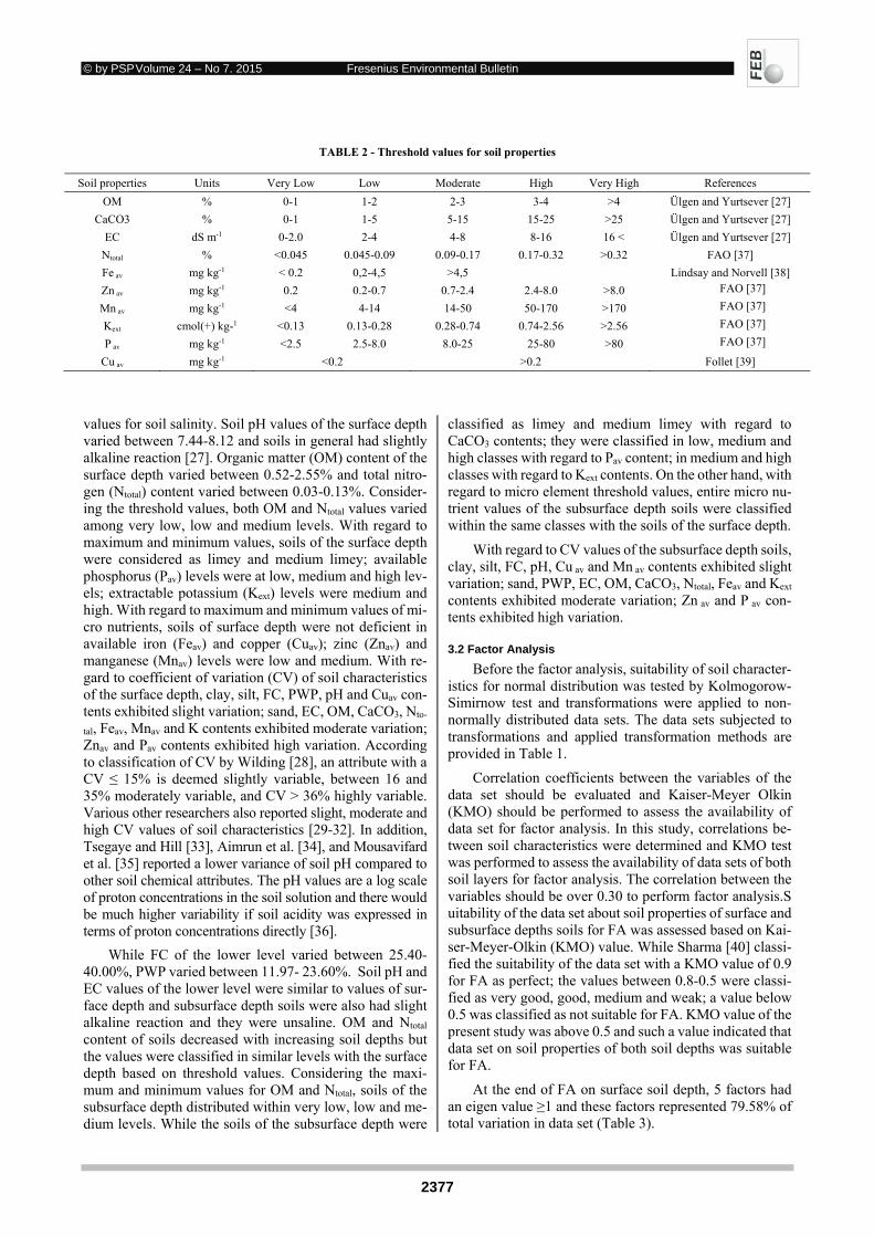
© by PSP Volume 24 – No 7. 2015 Fresenius Environmental Bulletin
2377
TABLE 2 - Threshold values for soil properties
Soil properties Units Very Low Low Moderate High Very High References
OM % 0-1 1-2 2-3 3-4 >4 Ülgen and Yurtsever [27]
CaCO3 % 0-1 1-5 5-15 15-25 >25 Ülgen and Yurtsever [27]
EC dS m-1 0-2.0 2-4 4-8 8-16 16 < Ülgen and Yurtsever [27]
Ntotal % <0.045 0.045-0.09 0.09-0.17 0.17-0.32 >0.32 FAO [37]
Fe av mg kg-1 < 0.2 0,2-4,5 >4,5 Lindsay and Norvell [38]
Zn av mg kg-1 0.2 0.2-0.7 0.7-2.4 2.4-8.0 >8.0 FAO [37]
Mn av mg kg-1 <4 4-14 14-50 50-170 >170 FAO [37]
Kext cmol(+) kg-1 <0.13 0.13-0.28 0.28-0.74 0.74-2.56 >2.56 FAO [37]
P av mg kg-1 <2.5 2.5-8.0 8.0-25 25-80 >80 FAO [37]
Cu av mg kg-1 <0.2 >0.2 Follet [39]
values for soil salinity. Soil pH values of the surface depth varied between 7.44-8.12 and soils in general had slightly alkaline reaction [27]. Organic matter (OM) content of the surface depth varied between 0.52-2.55% and total nitro-gen (Ntotal) content varied between 0.03-0.13%. Consider-ing the threshold values, both OM and Ntotal values varied among very low, low and medium levels. With regard to maximum and minimum values, soils of the surface depth were considered as limey and medium limey; available phosphorus (Pav) levels were at low, medium and high lev-els; extractable potassium (Kext) levels were medium and high. With regard to maximum and minimum values of mi-cro nutrients, soils of surface depth were not deficient in available iron (Feav) and copper (Cuav); zinc (Znav) and manganese (Mnav) levels were low and medium. With re-gard to coefficient of variation (CV) of soil characteristics of the surface depth, clay, silt, FC, PWP, pH and Cuav con-tents exhibited slight variation; sand, EC, OM, CaCO3, Nto-
tal, Feav, Mnav and K contents exhibited moderate variation; Znav and Pav contents exhibited high variation. According to classification of CV by Wilding [28], an attribute with a CV ≤ 15% is deemed slightly variable, between 16 and 35% moderately variable, and CV > 36% highly variable. Various other researchers also reported slight, moderate and high CV values of soil characteristics [29-32]. In addition, Tsegaye and Hill [33], Aimrun et al. [34], and Mousavifard et al. [35] reported a lower variance of soil pH compared to other soil chemical attributes. The pH values are a log scale of proton concentrations in the soil solution and there would be much higher variability if soil acidity was expressed in terms of proton concentrations directly [36].
While FC of the lower level varied between 25.40-40.00%, PWP varied between 11.97- 23.60%. Soil pH and EC values of the lower level were similar to values of sur-face depth and subsurface depth soils were also had slight alkaline reaction and they were unsaline. OM and Ntotal
content of soils decreased with increasing soil depths but the values were classified in similar levels with the surface depth based on threshold values. Considering the maxi-mum and minimum values for OM and Ntotal, soils of the subsurface depth distributed within very low, low and me-dium levels. While the soils of the subsurface depth were
classified as limey and medium limey with regard to CaCO3 contents; they were classified in low, medium and high classes with regard to Pav content; in medium and high classes with regard to Kext contents. On the other hand, with regard to micro element threshold values, entire micro nu-trient values of the subsurface depth soils were classified within the same classes with the soils of the surface depth.
With regard to CV values of the subsurface depth soils, clay, silt, FC, pH, Cu av and Mn av contents exhibited slight variation; sand, PWP, EC, OM, CaCO3, Ntotal, Feav and Kext contents exhibited moderate variation; Zn av and P av con-tents exhibited high variation.
3.2 Factor Analysis
Before the factor analysis, suitability of soil character-istics for normal distribution was tested by Kolmogorow-Simirnow test and transformations were applied to non-normally distributed data sets. The data sets subjected to transformations and applied transformation methods are provided in Table 1.
Correlation coefficients between the variables of the data set should be evaluated and Kaiser-Meyer Olkin (KMO) should be performed to assess the availability of data set for factor analysis. In this study, correlations be-tween soil characteristics were determined and KMO test was performed to assess the availability of data sets of both soil layers for factor analysis. The correlation between the variables should be over 0.30 to perform factor analysis.S uitability of the data set about soil properties of surface and subsurface depths soils for FA was assessed based on Kai-ser-Meyer-Olkin (KMO) value. While Sharma [40] classi-fied the suitability of the data set with a KMO value of 0.9 for FA as perfect; the values between 0.8-0.5 were classi-fied as very good, good, medium and weak; a value below 0.5 was classified as not suitable for FA. KMO value of the present study was above 0.5 and such a value indicated that data set on soil properties of both soil depths was suitable for FA.
At the end of FA on surface soil depth, 5 factors had an eigen value ≥1 and these factors represented 79.58% of total variation in data set (Table 3).

© by PSP Volume 24 – No 7. 2015 Fresenius Environmental Bulletin
2378
TABLE 3 - Rotated factor patterns of four factors after varimax rotation (0-30 cm)
Parameters PC1 PC 2 PC 3 PC 4 PC 5
Clay 0.888 0.044 0.238 -0.153 -0.165
PWP 0.879 0.042 0.042 0.240 0.033
FC 0.866 0.079 0.174 0.195 0.241
Sand -0.800 -0.074 -0.314 0.228 -0.223
Kext 0.724 0.325 0.259 -0.147 -0.267
Silt -0.700 0.007 -0.071 0.014 0.568
Feav 0.150 0.852 -0.068 0.042 0.209
Mnav -0.167 0.823 -0.059 0.010 -0.169
CaCO3 -0.168 -0.670 -0.181 0.304 -0.020
Znav -0.048 0.613 -0.062 -0.524 0.169
Cuav 0.327 0.573 0.276 0.016 0.081
OM 0.300 0.040 0.921 0.070 -0.083
Ntotal 0.315 0.062 0.916 0.077 -0.076
pH 0.088 -0.037 0.057 0.938 -0.095
Pav 0.278 0.420 -0.377 -0.479 -0.006
EC 0.058 0.116 -0.096 -0.149 0.917
Eigen value 5.468 3.183 1.532 1.349 1.20
Total variance (%) 34.176 19.896 9.574 8.433 7.503
Cumulative variance (%) 34.176 54.073 63.646 72.08 79.582
Bold and italic values indicate strong (> 0.75) and moderate (0.75 – 0.50) loadings, respectively
Factor 1 was able to explain 34.18% of total variation in data set. In this factor, clay, PWP and FC were strong positively represented, sand was strong negatively repre-sented, Kext and silt were respectively medium positively and negatively represented. Considering the soil properties assigned as variable in this factor, it was observed that gen-erally physical soil properties related to water holding in soil were assigned as the variables. Clay content with pos-itive impacts on water holding capacity had positive factor loading, but sand and silt contents with negative impacts on soil water holding capacity had negative factor loadings. Thus, considering the factor components and relationships among them, this factor was entitled as “soil water holding capacity”. The spatial distribution of the scores for factor 1 (soil water holding capacity) are shown in Figure 2. For each factor, higher values were indicated by darker colors and lower values were indicated by lighter colors.
Spatial distribution map of the factor indicated high water holding capacities of the soils over the southern, east-ern and south-eastern sections of the study area, on the other hand indicated low water holding capacities of the soils over the northern and north-westerns sections of the study area. Therefore during the precise agricultural prac-tices to be implemented over the study area, it was recom-mended for the areas with low water holding capacities that either more frequent irrigations should be applied or measures should be taken to improve water holding capac-ities of the soils through improving organic matter con-tents.
Factor 2 was able to explain 19.90% of the total varia-tion in data set. In this factor, Feav and Mnav were strong
positively represented; CaCO3 was medium negatively represented; Znav and Cuav were medium positively repre-sented. Considering the soil properties assigned as factor components, the factor was entitled as “microelement availability”. The negative relationship between microele-ments and CaCO3 contents indicated increasing microele-ment availability with decreasing CaCO3 contents. Feav, Cuav, Znav and Mnav are the essential micro nutrients for plant growth and development. [41] reported that availabil-ity of micro nutrients were especially sensitive against var-iations around the soils and indicated the soil properties like OM, pH, CaCO3, clay, silt and sand content as the sig-nificant factors effecting micro nutrient contents of the soils. The spatial distribution of the scores for factor 2 (mi-croelement availability) are shown in Figure 2. The spatial distribution map of the factor indicated heterogeneity in microelement availability over the study area. Microele-ment availability was found to be high over the southern sections of the study area and low over the western and northern sections of the study area. Therefore during the precise agricultural practices to be implemented over the study area, it was recommended for the areas with low mi-croelement availability levels that foliar micro nutrient treatments might improve the availability of microele-ments.
Factor 3 was composed of OM and Ntotal components and was able to explain 9.57% of total variation in data set. Thus, this factor was entitled as “organic matter”. Spatial distribution map of the factor indicated low OM levels over the south-western and north-western sections of the study area and high OM levels over the south-eastern and north-

© by PSP Volume 24 – No 7. 2015 Fresenius Environmental Bulletin
2379
FIGURE 2 - Spatial distribution maps of the factors (0-30cm)
eastern sections of the study area (Figure 3). Therefore dur-ing the precise agricultural practices to be implemented over the study area, it was recommended for the areas with low OM contents together with low water holding capaci-ties that plant production activities to improve OM contents might also improve water holding capacities.
Soil pH was assigned as the variable in factor 4 and it was able to explain 8.43% of total variation in data set. The factor can be defined as “soil reaction”. The spatial distri-bution map of factor 4 indicated high pH levels over the north, north-eastern and north-western sections of the study area and low pH levels over the south, south-western and south-eastern sections of the study area (Figure 3). When the spatial distribution map of factor 4 was assessed together with the spatial distribution map of factor 2 (mi-croelement availability), it was observed that maps re-vealed significant information about the relationships be-tween microelement availability and pH values. The north, north-eastern and north-western sections of the study area with high pH values had lower microelement availability levels and the southern sections with low pH values had increased microelement availability levels. Similar to find-ings of the present study, Chhabra et al. [42] reported de-creased Feav and Mnav levels with soil pH, increased Cuav
level with clay and OM content and increased Feav levels with sand content. The distribution map of factor 2 sup-ports the earlier recommendation of “foliar application of micro elements” to be made to improve the availability of microelements according to distribution map of factor 2.
Factor 5 including soil EC was able to explain 7.50% of total variation in data set. Considering the soil property assigned as variable, the factor was entitled as “soil salin-ity”. Spatial distribution map of the factor indicated low EC values over northern and north-eastern sections of the study area and high EC values over southern and south-western sections of the study area which may create a sa-linity risk over these sections. Maximum and minimum EC values of surface and subsurface soil depths did not indi-cate a salinity problem for the study area. However, inten-sive agricultural practices over the study area, seasonal changes in irrigation water quality, evaporation from soil surface and possible drainage problems because of inten-sive irrigations may eventually result in a salinity problem. Although currently a salinity problem does not exist over the study area, a leaching water requirement should be cal-culated and added to irrigation water to reduce the soil sa-linity during the implementation of precise agricultural practices.
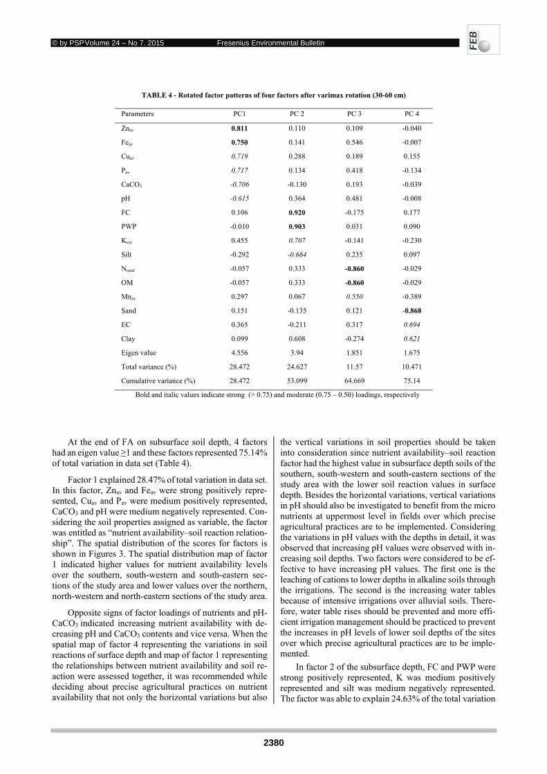
© by PSP Volume 24 – No 7. 2015 Fresenius Environmental Bulletin
2380
TABLE 4 - Rotated factor patterns of four factors after varimax rotation (30-60 cm)
Parameters PC1 PC 2 PC 3 PC 4
Znav 0.811 0.110 0.109 -0.040
Feav 0.750 0.141 0.546 -0.007
Cuav 0.719 0.288 0.189 0.155
Pav 0.717 0.134 0.418 -0.134
CaCO3 -0.706 -0.130 0.193 -0.039
pH -0.615 0.364 0.481 -0.008
FC 0.106 0.920 -0.175 0.177
PWP -0.010 0.903 0.031 0.090
Kext 0.455 0.707 -0.141 -0.230
Silt -0.292 -0.664 0.235 0.097
Ntotal -0.057 0.333 -0.860 -0.029
OM -0.057 0.333 -0.860 -0.029
Mnav 0.297 0.067 0.550 -0.389
Sand 0.151 -0.135 0.121 -0.868
EC 0.365 -0.211 0.317 0.694
Clay 0.099 0.608 -0.274 0.621
Eigen value 4.556 3.94 1.851 1.675
Total variance (%) 28.472 24.627 11.57 10.471
Cumulative variance (%) 28.472 53.099 64.669 75.14
Bold and italic values indicate strong (> 0.75) and moderate (0.75 – 0.50) loadings, respectively
At the end of FA on subsurface soil depth, 4 factors had an eigen value ≥1 and these factors represented 75.14% of total variation in data set (Table 4).
Factor 1 explained 28.47% of total variation in data set. In this factor, Znav and Feav were strong positively repre-sented, Cuav and Pav were medium positively represented, CaCO3 and pH were medium negatively represented. Con-sidering the soil properties assigned as variable, the factor was entitled as “nutrient availability–soil reaction relation-ship”. The spatial distribution of the scores for factors is shown in Figures 3. The spatial distribution map of factor 1 indicated higher values for nutrient availability levels over the southern, south-western and south-eastern sec-tions of the study area and lower values over the northern, north-western and north-eastern sections of the study area.
Opposite signs of factor loadings of nutrients and pH-CaCO3 indicated increasing nutrient availability with de-creasing pH and CaCO3 contents and vice versa. When the spatial map of factor 4 representing the variations in soil reactions of surface depth and map of factor 1 representing the relationships between nutrient availability and soil re-action were assessed together, it was recommended while deciding about precise agricultural practices on nutrient availability that not only the horizontal variations but also
the vertical variations in soil properties should be taken into consideration since nutrient availability–soil reaction factor had the highest value in subsurface depth soils of the southern, south-western and south-eastern sections of the study area with the lower soil reaction values in surface depth. Besides the horizontal variations, vertical variations in pH should also be investigated to benefit from the micro nutrients at uppermost level in fields over which precise agricultural practices are to be implemented. Considering the variations in pH values with the depths in detail, it was observed that increasing pH values were observed with in-creasing soil depths. Two factors were considered to be ef-fective to have increasing pH values. The first one is the leaching of cations to lower depths in alkaline soils through the irrigations. The second is the increasing water tables because of intensive irrigations over alluvial soils. There-fore, water table rises should be prevented and more effi-cient irrigation management should be practiced to prevent the increases in pH levels of lower soil depths of the sites over which precise agricultural practices are to be imple-mented.
In factor 2 of the subsurface depth, FC and PWP were strong positively represented, K was medium positively represented and silt was medium negatively represented. The factor was able to explain 24.63% of the total variation
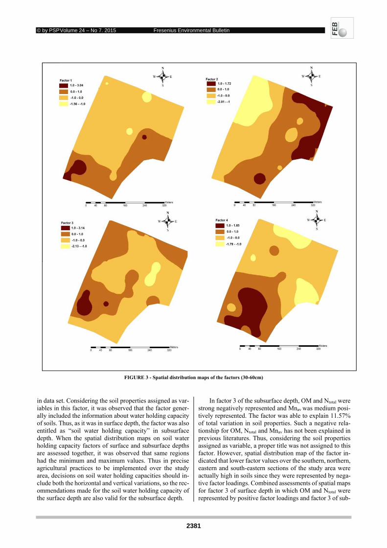
© by PSP Volume 24 – No 7. 2015 Fresenius Environmental Bulletin
2381
FIGURE 3 - Spatial distribution maps of the factors (30-60cm)
in data set. Considering the soil properties assigned as var-iables in this factor, it was observed that the factor gener-ally included the information about water holding capacity of soils. Thus, as it was in surface depth, the factor was also entitled as “soil water holding capacity” in subsurface depth. When the spatial distribution maps on soil water holding capacity factors of surface and subsurface depths are assessed together, it was observed that same regions had the minimum and maximum values. Thus in precise agricultural practices to be implemented over the study area, decisions on soil water holding capacities should in-clude both the horizontal and vertical variations, so the rec-ommendations made for the soil water holding capacity of the surface depth are also valid for the subsurface depth.
In factor 3 of the subsurface depth, OM and Ntotal were strong negatively represented and Mnav was medium posi-tively represented. The factor was able to explain 11.57% of total variation in soil properties. Such a negative rela-tionship for OM, Ntotal and Mnav has not been explained in previous literatures. Thus, considering the soil properties assigned as variable, a proper title was not assigned to this factor. However, spatial distribution map of the factor in-dicated that lower factor values over the southern, northern, eastern and south-eastern sections of the study area were actually high in soils since they were represented by nega-tive factor loadings. Combined assessments of spatial maps for factor 3 of surface depth in which OM and Ntotal were represented by positive factor loadings and factor 3 of sub-

© by PSP Volume 24 – No 7. 2015 Fresenius Environmental Bulletin
2382
surface depth in which OM and Ntotal were represented by negative factor loadings revealed that low and high OM and Ntotal values were observed in surface and subsurface depths of the similar sections of the study area. Although Mnav was assigned as a variable in factor 3 of the subsur-face depth, OM and Ntotal were determinants of the factor based on factor loadings of determinant factors. The factor which was not assigned with any titles initially may then be assessed as “organic matter” factor. Since the soil prop-erties assigned to factor 3 of both soil depths and their dis-tributions in spatial distribution maps were similar to each other, precision agricultural practices should take both hor-izontal and vertical variations in OM contents into consid-eration.
Factor 4 of the subsurface depth was able to explain 10.47% of total variation in soil properties. In this factor, sand was strong negatively represented; EC and clay were medium positively represented. Considering the soil prop-erties assigned as variables, the factor was entitled as “soil salinity” as it was in factor 5 of the surface depth. Such a title was also supported by similar high and low values at similar sections of the study area in both surface and sub-surface depths soils. It was recommended in precise agri-cultural practices that both horizontal and vertical varia-tions in soil salinity of both depths should be taken into consideration.
4. CONCLUSION
The present study was conducted over alluvial lands and 16 different physical and chemical soil properties of two soil depths were assessed through FA and GIS. FA re-vealed 5 factors for surface depth and 4 factors for subsur-face depth. These 5 factors of surface depth were able to explain 79.58% of total variation in date set and 4 factors of the subsurface depth were able to explain 75.14% of to-tal variation in data set.
While FA of surface depth revealed “soil water hold-
ing capacity” as the most significant factor, FA of subsur-face depth yielded “nutrient availability–soil reaction rela-tionship” as the most significant factor. There were signif-icant similarities in soil properties assigned as factor com-ponents of 5 factors of surface depth and 4 factors of sub-surface depth. There were also significant similarities be-tween spatial distribution patterns of the factors. Such sim-ilarities indicated that both horizontal and vertical varia-tions in soil properties should be taken into consideration.
It was concluded in this study that dimension reduc-
tioning FA might yield significant information revealing various hidden relationships among soil properties espe-cially of alluvial lands in which soil properties may exhibit significant variations in short distances. Spatial distribution patterns prepared by integrating factor scores of FA into GIS also revealed significant information about horizontal
and vertical variations in soil characteristics. It was proved in this study that combined use of FA and GIS might reveal successful outcomes for the implementation of precise ag-ricultural activities. Thus, these methods may also be used in larger-scale studies toward the planning of precise agri-cultural practices. Considering current international trends, it is evident that sustainable development is only possible through the performance of right implementations at right time in right places.
The authors have declared no conflict of interest. REFERENCES
[1]. Robert, P. C., R. H. Rust, and W. E. Larson. (1995) Proceedings of site-specific management for agricultural systems (second inter-national conference). American Society of Agronomy Inc., Crop Science Society of America, Inc., and Soil Science Society of America, Inc. (1995): xiii.
[2]. Güçdemir, İ., Türker, U., Karabulut, A. ve Arcak, Ç. (2004). Has-sas Tarım Teknolojilerinin Türkiye’deki Uygulamaları. Toprak Gübre ve Su Kaynakları Araştırma Enstitüsü. Ankara.
[3]. Shaw, P.J.A. (2003). Multivariate statistics for the environmental sciences. Hodder, Arnold, London. 233 pp.
[4]. Arslan, H., Günal, H., Güler, M., Cemek, B. and Acir, N. (2013). Assesment the Soil Properties Affecting Salinity and Sodicity of Bafra Plain using Multivariate Statistical Technigues. Carpathian Journal of Earth and Environmental Sciences, 8(1):81 – 90.
[5]. Sağlam, M. (2014). Evaluation of the physicochemical properties of alluvial and colluvial soils formed under ustic moisture regime using multivariate geostatistical techniques. Archives of Agron-omy and Soil Science, DOI: 10.1080/03650340.2014.978764.
[6]. Rahmanipour, F., Marzaioli, R., Bahrami, H.A., Fereidouni, Z. And Bandarabadi, S.R. (2014). Assessment of soil quality indices in agricultural lands of QazvinProvince, Iran, Ecological Indica-tors, 40, 19–26.
[7]. Akbarpour, A., Gholami, N., Azizi, H. and Torab, F.M. (2013). Cluster and R-mode factor analyses on soil geochemical data of Masjed-Daghi exploration area, northwestern Iran. Arabian Jour-nal of Geosciences, 6 (9), 3397-3408.
[8]. Zhang, C. (2006). Using multivariate analyses and GIS to identify pollutants and their spatial patterns in urban soils in Galway, Ire-land. Environmental Pollution, 142, 501-511.
[9]. Shan YS, Tysklind M, Hao FH, Ouyang W, Chen S.Y. and Lin, C.Y. (2013). Identification of sources of heavy metals in agricul-tural soils using multivariate analysis and GIS. J Soils Sediments, 13,720–729.
[10]. Dengiz, O. (2010). Determination and Modeling of Land Suitabil-ity Classes of Rice Cultivation Areas with GIS. Report of TOVAG 107 O 443.
[11]. Gee, G.W. and Bauder, J.W. (1986). Particle-size analysis. In: Klute A, editor. Methods of soil analysis. Part I: physical and min-eralogical analysis. Madison (WI): American Society of Agron-omy, Crop Science Society of America and Soil Science Society of America; p. 388–409.
[12]. Nelson, R.E. (1982). Carbonate and Gypsum. pp: 181-197. Editör: A.L. Page, R.H. Miller ve D.R. Keeney. Methods of Soil Analysis. Part 2: Chemical and Microbiological Properties. 2nd edition. American Society of Agronomy, Madison, USA.
[13]. Nelson, D.W. and L.E. Sommers. (1982). Total Carbon Organic Carbon, and Organic Matter. pp: 538-580. Editör: A.L. Page, R.H. Miller ve D.R. Keeney. Methods of Soil Analysis. Part 2: Chemi-cal and Microbiological Properties. 2nd edition. American Society of Agronomy, Madison, USA.

© by PSP Volume 24 – No 7. 2015 Fresenius Environmental Bulletin
2383
[14]. Hendershot, W.H, Laareae, H. and Duquette, M. (1993). Soil re-action and exchangeable acidity. In: Carter MR, editor. Soil sam-pling and methods of analysis. Boca Raton (FL): Lewis Publishers; p. 141–145.
[15]. Rhoades, J.D. (1986). Soluble Salts. In Page AL, editor. Methods of soil analysis. Part II. Chemical and microbiological properties. 2nd ed. Madison (WI): ASA and SSSA; p. 167–179.
[16]. Bremner, J.M. and Mulvaney, C.S. (1982). Nitrogen-total. In: Page AL, Miller RH, Keeney DR, editors. Methods of soil analysis. Part 2: chemical and microbiological properties. Madison (WI): Amer-ican Society of Agronomy, Inc.; p. 595–625.
[17]. Olsen, S.R., Cole, C.V., Watanable, F.S. and Dean, L.A. (1954). Estimation of available phosphorous in soils by extraction with so-dium bicarbonate. USDA Circular, No 939 Washington (DC): Government Printing Office; p. 1–19.
[18]. Soil Survey Staff. (1999). Soil taxonomy, a basic system of soil classification for making and interpreting soil surveys. 2nd ed. USDA Natural Resources Conservation Services. Agriculture Handbook Number 436. Washington (DC): Government Printing Office.
[19]. Anonymous (1990). FAO. Micronutrient. Assessment at the Coun-try Level: An International Study.FAO Soil Bulletin by Mikko Sil-lanpaa. Rome
[20]. Tatlıdil, H. (2002). Uygulamalı Çok Değişkenli İstatistiksel Ana-liz, Akademi Matbaası, Ankara, 167.
[21]. Lu, A.X., Wang, J.H., Qin, X.Y., Wang, K.Y., Han, P. and Zhang, S.Z. (2012). Multivariate and geostatistical analyses of the spatial distribution and origin of heavy metals in the agricultural soils in Shunyi, Beijing, China. Science of the Total Environment, 425, 66–74.
[22]. Sun, C.Y., Liu, J.S., Wang, Y., Sun, L.Q. and Yu, H.W. (2013). Multivariate and geostatistical analyses of the spatial distribution and sources of heavy metals in agricultural soil in Dehui, Northeast China. Chemosphere, 92,517–523.
[23]. Liu, C.W., Lin, K.H. and Kuo, Y.M. (2003). Application of factor analysis in the assessment of groundwater quality in a blackfoot disease area in Taiwan. The Science of the Total Environment, 313, 77–89
[24]. Goovaerts, P. (1999). Geostatistics in soil science: state of the art and perspectives. Geoderma 89(1–2):1–45.
[25]. Arslan, H., Güler, M. and Cemek, B. (2013). Spatial Estimation of The Risky Areas for Drainage and Salinity in Suluova Plain, Tur-key Using Geostatistical Methods. Fresenius Environmental Bul-letin, 22(10), 2916-2924.
[26]. Coşkun, G. H. and Güler, Y. (2014). Water quality determination of Büyükçekmece lake, Turkey by using remote sensing and GIS techniques. Fresenius Environmental Bulletin, 23(3),746-750.
[27]. Ülgen, N. and Yurtsever, N. (1974). Türkiye Gübre ve Gübreleme Rehberi. Toprak ve Gübre Araştırma Enstitüsü Teknik Yayın No:28, Ankara.
[28]. Wilding, L.P. (1985). Spatial variability: its documentation, ac-commodation andimplication to soil surveys. In: Nielsen, D.R., Bouma, J. (Eds.), Soil Spatial Vari-ability. Pudoc, Wageningen, Netherlands, pp. 166–194.
[29]. Erşahin, S. (1999). Aluviyal bir tarlada bazı fiziksel ve kimyasal toprak özelliklerinin uzaysal (Spatial) değişkenliğinin belirlen-mesi. Selçuk Üniversitesi Ziraat Fakültesi Dergisi, 13 (19), 34-41.
[30]. Mallants, D., Mohanty, B.P., Jacques, D. and Feyen, J. (1996). Spatial variability of hydraulic properties in a multi-layered soil profile. Soil Science, 161(3), 167-181.
[31]. Sağlam, M. (2008). Gökhöyük tarım işletmesinde yaygın toprak serilerinde bazı kalite göstergelerinin uzaysal değişkenliğinin jeoi-statistiksel yöntemlerle incelenmesi. Ankara Üniversitesi Fen Bilimleri Enstitüsü, Doktora Tezi, 160 s., Ankara.
[32]. Sağlam, M. (2013). Çok değişkenli istatistiksel yöntemler ile to-prak özelliklerinin gruplandırılması. Toprak Su Dergisi, 2(1): 7-14.
[33]. Tsegaye, T. and Hill, R.L. (1998). Intensıve tıllage effects on spatıal varıabılıty of soıl test, plant growth, and nutrient uptake measurements. Soil Sci. 163, 155–165.
[34]. Aimrun, W., Amin, M.S.M., Ahmad, D., Hanafi, M.M. and Chan, C.S. (2007). Spatial variability of bulk soil electrical conductivity in a Malaysian paddy field: key to soil management. Paddy Water Environ., 5,113–121.
[35]. Mousavifard, S.M., Momtaza, H., Sepehra, E., Davatgarb, N. and Sadaghiani, M.H.R. (2013). Determining and mapping some soil physico-chemical properties using geostatistical and GIS tech-niques in the Naqade region, Iran. Arch Agron Soil Sci. 59:1573–1589.
[36]. Sun, B., Zhou, S. and Zhao, Q. (2003). Evaluation of spatial and temporal changes of soil quality based on geostatistical analysis in the hill region of subtropical China. Geoderma. 115:85–99.
[37]. FAO. (1990). Micronutrient, Assessment at the Country Level: An International Study. FAO Soil Bulletin by Sillanpaa. Rome.
[38]. Lindsay, W.L. and Norvell, W.A. (1978). Development of a DTPA test for zinc, iron, manganese, and copper. Soil Sci. Soc. Am. J. 42:421-428.
[39]. Follet, R.H. (1969). Zn. Fe. Mn and Cu in Colorado Soils. PhD. Dissertation. Colo. State Univ.
[40]. Sharma, S. (1996). Applied Multivariate Techniques. John Wiley and Sons Inc., New York.
[41]. Nazif, W., Sajida, P. and Saleem, I. (2006). Status of micronutri-ents in soils of Districts Bhimber (Azad Jammu and Kashmir). Journal of Agricultural Biological Science, 1(2): 35 - 40.
[42]. Chhabra, G., Srivastava, P. C., Ghosh, D. and Agnihotri, A.K. (1996). Distribution of available micronutrient cations as related to soil properties in different soil zones of Gola-Kosi interbasin. Crop Research Hisar, 11(3): 296-303.
Received: January 16, 2015 Revised: February 16, 2015 Accepted: February 19, 2015 CORRESPONDING AUTHOR
Kadir Ersin Temizel Ondokuz Mayis University Faculty of Agriculture Department of Agricultural Structures and Irrigation 55139 Samsun TURKEY Phone: + 90 362 3121919-1276 Fax: + 90 362 4576034 E-mail: [email protected]
FEB/ Vol 24/ No 7/ 2015 – pages 2374 – 2383
© by PSP Volume 24 – No 7. 2015 Fresenius Environmental Bulletin
2384
PHOTOSYNTHETIC ACTIVITY OF Microcystis IN
FISH GUTS AND ITS IMPLICATION FOR FEASIBILITY
OF BLOOM CONTROL BY FILTER-FEEDING FISHES
Zhicong Wang, Zhongjie Li, Yiyong Zhou and Dunhai Li*
Key Laboratory of Algal Biology, Institute of Hydrobiology, Chinese Academy of Sciences, Wuhan 430072, P.R. China
ABSTRACT
In a background of increasingly frequent and intensive Microcystis blooms occurred in eutrophic lakes, many countries, particularly China, have used filter-feeding fish to control algal blooms according to non-traditional bio-manipulation theory. However, there is little information concerning the potential photosynthetic activity of cyano-bacteria in the guts of planktivorous fishes. To make a sci-entific assessment of this algal control technology, we evaluated the effects of digestion by two fish species, silver carp and bighead carp, on the growth potential of Micro-cystis blooms in terms of photosynthetic activity, meta-bolic activity, up-floating velocity, morphological size, and toxin production. The results showed that: 1) the potential photosynthetic activity of Microcystis dropped signifi-cantly in fish foreguts after ingestion, but gradually in-creased and recovered in the midgut and hindgut; 2) diges-tion by planktivorous fish could significantly decrease the colonial size and up-floating velocity of Microcystis; 3) se-lective digestion by bighead carp caused a sharp rise in cel-lular microcystin levels; and 4) Microcystis retained a high growth potential after digestion by filter-feeding fish. These results indicate that planktivorous fish could be used for controlling blooms due to the degree of digestion and long retention of Microcystis in fish guts, but the controlling ef-fect was limited because the potential photosynthesis ac-tivity of algae gradually recovered along the gut sections and the digested algae could grow normally after subse-quent release into lakes. In addition to being less effective at controlling algal blooms than silver carp, the digestion process in bighead carp might confer an advantage to toxic Microcystis species.
KEYWORDS: Microcystis bloom; filter-feeding fish; microcystin; photosynthetic activity.
* Corresponding author
1. INTRODUCTION
Eutrophication is an increasingly serious problem in freshwater ecosystems, and can be accompanied by fre-quent cyanobacterial blooms, which, particularly for spe-cies producing the toxin microcystin, may be extremely harmful to aquatic ecosystems and human health [1-3]. Several methods for bloom control are currently available and employ engineering [4, 5], physical [6, 7], chemical [8, 9] or biological methods [10]. Some researchers observed that water blooms were dissipated in lakes stocked with fil-ter-feeding fish, which led to the conclusion that grazing pressure by planktivorous fishes is a key factor in eliminat-ing water blooms from lakes [11]. Previous studies also suggested that cyanobacterial blooms consumed by plank-tivorous fish, could result in compositional changes of the phytoplankton community [12]. Also some researchers have reported the change of photosynthesis in Microcystis colo-nies after gut passage through crucian carp and koi carp [13]. But this research studied the algae outside the guts of fish. Furthermore, the fishes studied are not planktivorous fishes. Therefore, we think it is valuable and interesting to investigate the photosynthetic activity, growth potential, morphological changes and microcystin content of Micro-cystis in the guts of planktivorous fishes.
The silver carp (Hypophthalmichthys molitrix) and the bighead carp (Aristichthysnobilis) are the main species for freshwater fishery and aquaculture in China [14]. Aided by a filter-feeding organ comprised of gill rakers, a gill rak-ernetwork, palatal rugae and a gill raker tube [15], most bloom-forming cyanobacterial colonies can be consumed by silver carp and bighead carp. Algae sized 8-100 μm can be filter-fed by silver carp, while those sized 17-3,000μm can be consumed by bighead carp [16]. However, most co-lonial Microcystis cannot be completely digested by plank-tivorous fishes due to their cell wall composition that in-cludes cellulose and pectic substances. Therefore, the di-gestion of Microcystis colonies in the gut is sometimes re-ferred to be as “pseudo-digestion” because only the algal colony morphology is changed after digestion, and thus in-tact algal cells are excreted back to the lake water driven by continuous consumption and/or intestinal peristalsis.
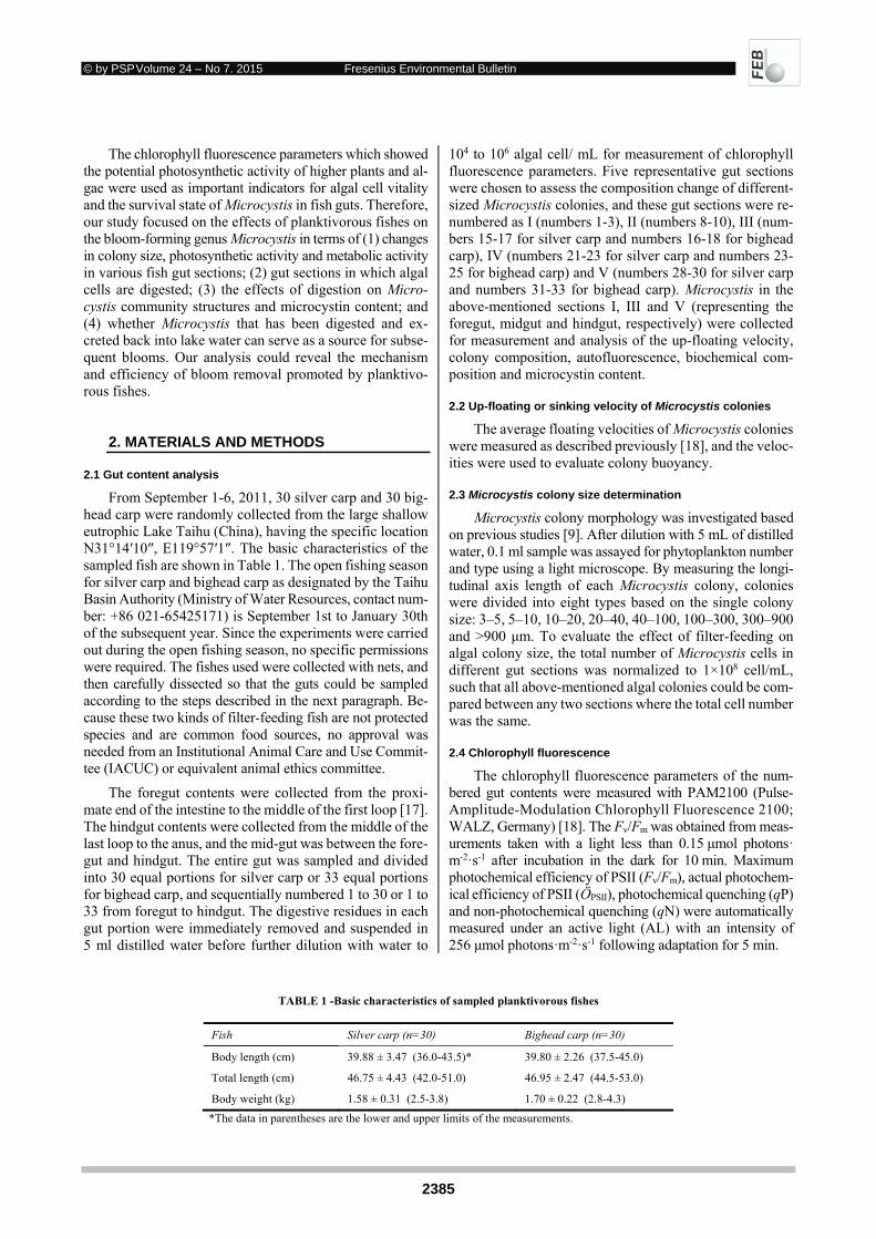
© by PSP Volume 24 – No 7. 2015 Fresenius Environmental Bulletin
2385
The chlorophyll fluorescence parameters which showed the potential photosynthetic activity of higher plants and al-gae were used as important indicators for algal cell vitality and the survival state of Microcystis in fish guts. Therefore, our study focused on the effects of planktivorous fishes on the bloom-forming genus Microcystis in terms of (1) changes in colony size, photosynthetic activity and metabolic activity in various fish gut sections; (2) gut sections in which algal cells are digested; (3) the effects of digestion on Micro-cystis community structures and microcystin content; and (4) whether Microcystis that has been digested and ex-creted back into lake water can serve as a source for subse-quent blooms. Our analysis could reveal the mechanism and efficiency of bloom removal promoted by planktivo-rous fishes.
2. MATERIALS AND METHODS
2.1 Gut content analysis
From September 1-6, 2011, 30 silver carp and 30 big-head carp were randomly collected from the large shallow eutrophic Lake Taihu (China), having the specific location N31°14′10″, E119°57′1″. The basic characteristics of the sampled fish are shown in Table 1. The open fishing season for silver carp and bighead carp as designated by the Taihu Basin Authority (Ministry of Water Resources, contact num-ber: +86 021-65425171) is September 1st to January 30th of the subsequent year. Since the experiments were carried out during the open fishing season, no specific permissions were required. The fishes used were collected with nets, and then carefully dissected so that the guts could be sampled according to the steps described in the next paragraph. Be-cause these two kinds of filter-feeding fish are not protected species and are common food sources, no approval was needed from an Institutional Animal Care and Use Commit-tee (IACUC) or equivalent animal ethics committee.
The foregut contents were collected from the proxi-mate end of the intestine to the middle of the first loop [17]. The hindgut contents were collected from the middle of the last loop to the anus, and the mid-gut was between the fore-gut and hindgut. The entire gut was sampled and divided into 30 equal portions for silver carp or 33 equal portions for bighead carp, and sequentially numbered 1 to 30 or 1 to 33 from foregut to hindgut. The digestive residues in each gut portion were immediately removed and suspended in 5 ml distilled water before further dilution with water to
104 to 106 algal cell/ mL for measurement of chlorophyll fluorescence parameters. Five representative gut sections were chosen to assess the composition change of different-sized Microcystis colonies, and these gut sections were re-numbered as I (numbers 1-3), II (numbers 8-10), III (num-bers 15-17 for silver carp and numbers 16-18 for bighead carp), IV (numbers 21-23 for silver carp and numbers 23-25 for bighead carp) and V (numbers 28-30 for silver carp and numbers 31-33 for bighead carp). Microcystis in the above-mentioned sections I, III and V (representing the foregut, midgut and hindgut, respectively) were collected for measurement and analysis of the up-floating velocity, colony composition, autofluorescence, biochemical com-position and microcystin content.
2.2 Up-floating or sinking velocity of Microcystis colonies
The average floating velocities of Microcystis colonies were measured as described previously [18], and the veloc-ities were used to evaluate colony buoyancy.
2.3 Microcystis colony size determination
Microcystis colony morphology was investigated based on previous studies [9]. After dilution with 5 mL of distilled water, 0.1 ml sample was assayed for phytoplankton number and type using a light microscope. By measuring the longi-tudinal axis length of each Microcystis colony, colonies were divided into eight types based on the single colony size: 3–5, 5–10, 10–20, 20–40, 40–100, 100–300, 300–900 and >900 μm. To evaluate the effect of filter-feeding on algal colony size, the total number of Microcystis cells in different gut sections was normalized to 1×10⁸ cell/mL, such that all above-mentioned algal colonies could be com-pared between any two sections where the total cell number was the same.
2.4 Chlorophyll fluorescence
The chlorophyll fluorescence parameters of the num-bered gut contents were measured with PAM2100 (Pulse-Amplitude-Modulation Chlorophyll Fluorescence 2100; WALZ, Germany) [18]. The Fv/Fm was obtained from meas-urements taken with a light less than 0.15 μmol photons· m-2·s-1 after incubation in the dark for 10 min. Maximum photochemical efficiency of PSII (Fv/Fm), actual photochem-ical efficiency of PSII (ÖPSII), photochemical quenching (qP) and non-photochemical quenching (qN) were automatically measured under an active light (AL) with an intensity of 256 μmol photons·m-2·s-1 following adaptation for 5 min.
TABLE 1 -Basic characteristics of sampled planktivorous fishes
Fish Silver carp (n=30) Bighead carp (n=30)
Body length (cm) 39.88 ± 3.47 (36.0-43.5)* 39.80 ± 2.26 (37.5-45.0)
Total length (cm) 46.75 ± 4.43 (42.0-51.0) 46.95 ± 2.47 (44.5-53.0)
Body weight (kg) 1.58 ± 0.31 (2.5-3.8) 1.70 ± 0.22 (2.8-4.3)
*The data in parentheses are the lower and upper limits of the measurements.
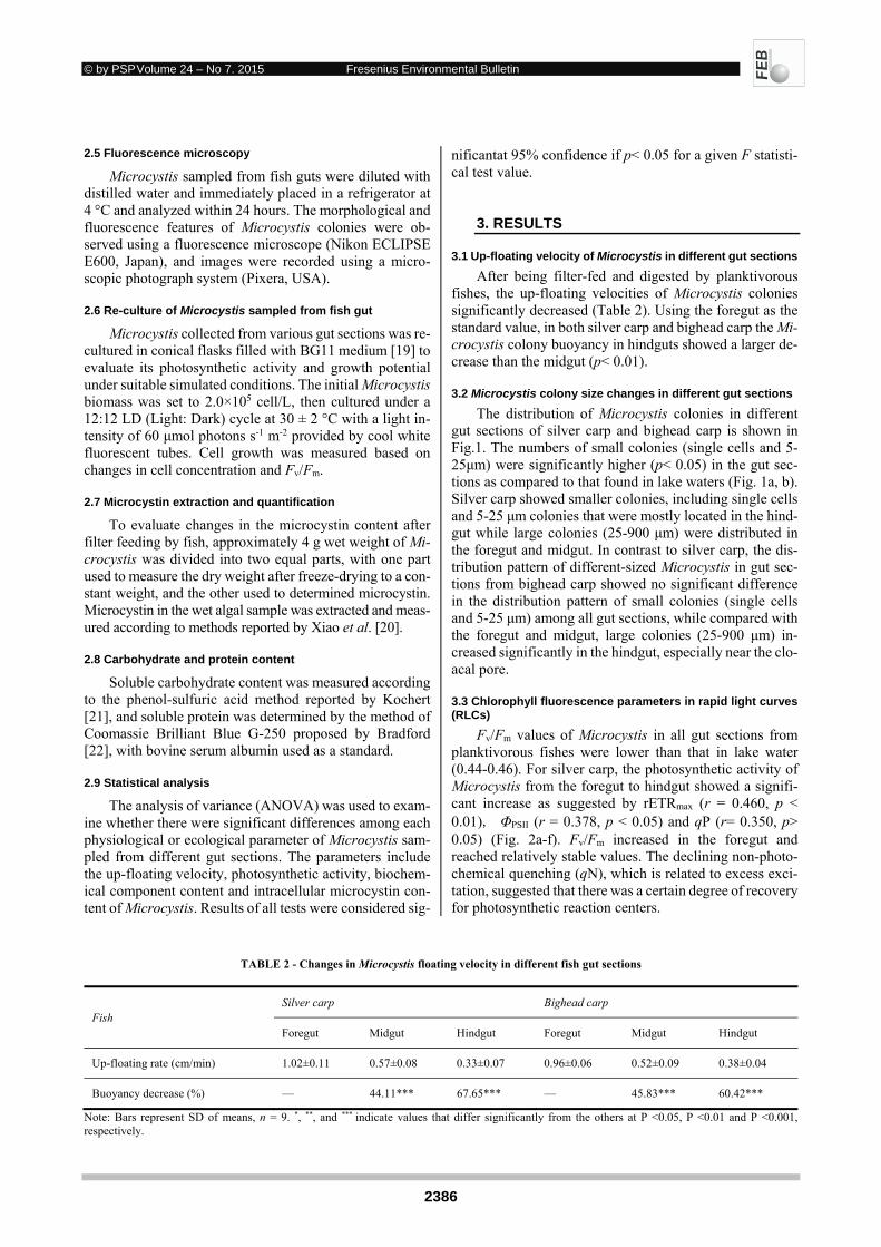
© by PSP Volume 24 – No 7. 2015 Fresenius Environmental Bulletin
2386
2.5 Fluorescence microscopy
Microcystis sampled from fish guts were diluted with distilled water and immediately placed in a refrigerator at 4 °C and analyzed within 24 hours. The morphological and fluorescence features of Microcystis colonies were ob-served using a fluorescence microscope (Nikon ECLIPSE E600, Japan), and images were recorded using a micro-scopic photograph system (Pixera, USA).
2.6 Re-culture of Microcystis sampled from fish gut
Microcystis collected from various gut sections was re-cultured in conical flasks filled with BG11 medium [19] to evaluate its photosynthetic activity and growth potential under suitable simulated conditions. The initial Microcystis biomass was set to 2.0×10⁵ cell/L, then cultured under a 12:12 LD (Light: Dark) cycle at 30 ± 2 °C with a light in-tensity of 60 μmol photons s-1 m-2 provided by cool white fluorescent tubes. Cell growth was measured based on changes in cell concentration and Fv/Fm.
2.7 Microcystin extraction and quantification
To evaluate changes in the microcystin content after filter feeding by fish, approximately 4 g wet weight of Mi-crocystis was divided into two equal parts, with one part used to measure the dry weight after freeze-drying to a con-stant weight, and the other used to determined microcystin. Microcystin in the wet algal sample was extracted and meas-ured according to methods reported by Xiao et al. [20].
2.8 Carbohydrate and protein content
Soluble carbohydrate content was measured according to the phenol-sulfuric acid method reported by Kochert [21], and soluble protein was determined by the method of Coomassie Brilliant Blue G-250 proposed by Bradford [22], with bovine serum albumin used as a standard.
2.9 Statistical analysis
The analysis of variance (ANOVA) was used to exam-ine whether there were significant differences among each physiological or ecological parameter of Microcystis sam-pled from different gut sections. The parameters include the up-floating velocity, photosynthetic activity, biochem-ical component content and intracellular microcystin con-tent of Microcystis. Results of all tests were considered sig-
nificantat 95% confidence if p< 0.05 for a given F statisti-cal test value.
3. RESULTS
3.1 Up-floating velocity of Microcystis in different gut sections
After being filter-fed and digested by planktivorous fishes, the up-floating velocities of Microcystis colonies significantly decreased (Table 2). Using the foregut as the standard value, in both silver carp and bighead carp the Mi-crocystis colony buoyancy in hindguts showed a larger de-crease than the midgut (p< 0.01).
3.2 Microcystis colony size changes in different gut sections
The distribution of Microcystis colonies in different gut sections of silver carp and bighead carp is shown in Fig.1. The numbers of small colonies (single cells and 5-25μm) were significantly higher (p< 0.05) in the gut sec-tions as compared to that found in lake waters (Fig. 1a, b). Silver carp showed smaller colonies, including single cells and 5-25 μm colonies that were mostly located in the hind-gut while large colonies (25-900 μm) were distributed in the foregut and midgut. In contrast to silver carp, the dis-tribution pattern of different-sized Microcystis in gut sec-tions from bighead carp showed no significant difference in the distribution pattern of small colonies (single cells and 5-25 μm) among all gut sections, while compared with the foregut and midgut, large colonies (25-900 μm) in-creased significantly in the hindgut, especially near the clo-acal pore.
3.3 Chlorophyll fluorescence parameters in rapid light curves (RLCs)
Fv/Fm values of Microcystis in all gut sections from planktivorous fishes were lower than that in lake water (0.44-0.46). For silver carp, the photosynthetic activity of Microcystis from the foregut to hindgut showed a signifi-cant increase as suggested by rETRmax (r = 0.460, p < 0.01), ΦPSII (r = 0.378, p < 0.05) and qP (r= 0.350, p> 0.05) (Fig. 2a-f). Fv/Fm increased in the foregut and reached relatively stable values. The declining non-photo-chemical quenching (qN), which is related to excess exci-tation, suggested that there was a certain degree of recovery for photosynthetic reaction centers.
TABLE 2 - Changes in Microcystis floating velocity in different fish gut sections
Fish Silver carp Bighead carp
Foregut Midgut Hindgut Foregut Midgut Hindgut
Up-floating rate (cm/min) 1.02±0.11 0.57±0.08 0.33±0.07 0.96±0.06 0.52±0.09 0.38±0.04
Buoyancy decrease (%) — 44.11*** 67.65*** — 45.83*** 60.42***
Note: Bars represent SD of means, n = 9. *, **, and *** indicate values that differ significantly from the others at P <0.05, P <0.01 and P <0.001, respectively.
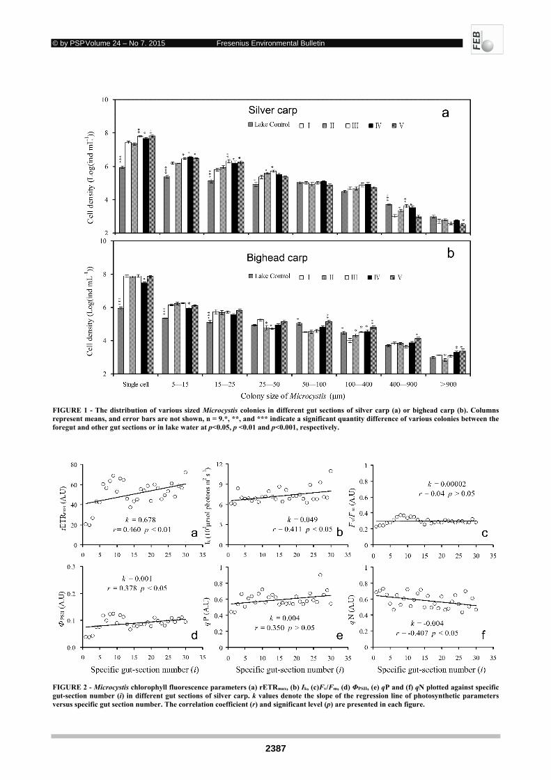
© by PSP Volume 24 – No 7. 2015 Fresenius Environmental Bulletin
2387
FIGURE 1 - The distribution of various sized Microcystis colonies in different gut sections of silver carp (a) or bighead carp (b). Columns represent means, and error bars are not shown, n = 9.*, **, and *** indicate a significant quantity difference of various colonies between the foregut and other gut sections or in lake water at p<0.05, p <0.01 and p<0.001, respectively.
FIGURE 2 - Microcystis chlorophyll fluorescence parameters (a) rETRmax, (b) Ik, (c)Fv/Fm, (d) ΦPSII, (e) qP and (f) qN plotted against specific gut-section number (i) in different gut sections of silver carp. k values denote the slope of the regression line of photosynthetic parameters versus specific gut section number. The correlation coefficient (r) and significant level (p) are presented in each figure.
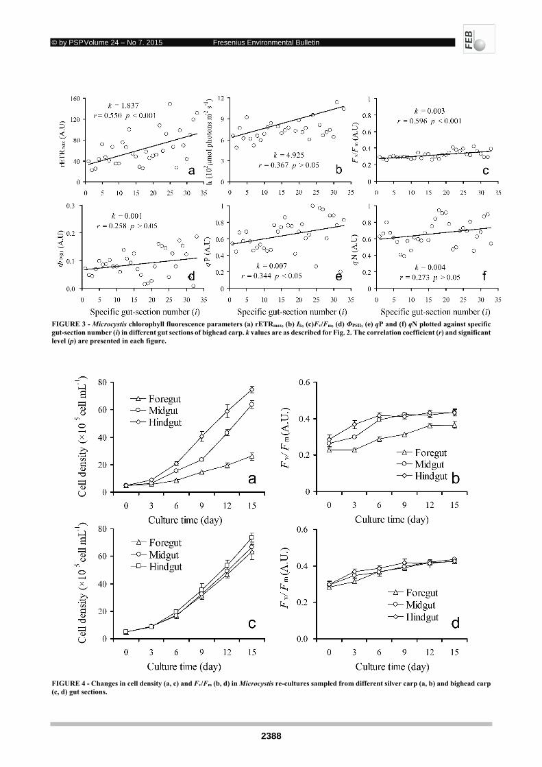
© by PSP Volume 24 – No 7. 2015 Fresenius Environmental Bulletin
2388
FIGURE 3 - Microcystis chlorophyll fluorescence parameters (a) rETRmax, (b) Ik, (c)Fv/Fm, (d) ΦPSII, (e) qP and (f) qN plotted against specific gut-section number (i) in different gut sections of bighead carp. k values are as described for Fig. 2. The correlation coefficient (r) and significant level (p) are presented in each figure.
FIGURE 4 - Changes in cell density (a, c) and Fv/Fm (b, d) in Microcystis re-cultures sampled from different silver carp (a, b) and bighead carp (c, d) gut sections.
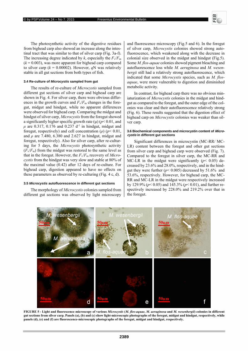
© by PSP Volume 24 – No 7. 2015 Fresenius Environmental Bulletin
2389
The photosynthetic activity of the digestive residues from bighead carp also showed an increase along the intes-tinal tract that was similar to that of silver carp (Fig. 3a-f). The increasing degree indicated by k, especially the Fv/Fm (k = 0.003), was more apparent for bighead carp compared to silver carp (k = 0.00002). However, qN was relatively stable in all gut sections from both types of fish.
3.4 Re-culture of Microcystis sampled from gut
The results of re-culture of Microcystis sampled from different gut sections of silver carp and bighead carp are shown in Fig. 4. For silver carp, there were obvious differ-ences in the growth curves and Fv/Fm changes in the fore-gut, midgut and hindgut, while no apparent differences were observed for bighead carp. Comparing the midgut and hindgut of silver carp, Microcystis from the foregut showed a significantly higher specific growth rate (μ) (p< 0.01, and μ are 0.317, 0.176 and 0.237 d-1 in hindgut, midgut and foregut, respectively) and cell concentration (ρ) (p< 0.01, and ρ are 7.480, 6.380 and 2.627 in hindgut, midgut and foregut, respectively). Also for silver carp, after re-cultur-ing for 5 days, the Microcystis photosynthetic activity (Fv/Fm) from the midgut was restored to the same level as that in the foregut. However, the Fv/Fm recovery of Micro-cystis from the hindgut was very slow and stable at 80% of the maximal value (0.42) after 12 days of re-culture. For bighead carp, digestion appeared to have no effects on these parameters as observed by re-culturing (Fig. 4 c, d).
3.5 Microcystis autofluorescence in different gut sections
The morphology of Microcystis colonies sampled from different gut sections was observed by light microscopy
and fluorescence microscopy (Fig.5 and 6). In the foregut of silver carp, Microcystis colonies showed strong auto-fluorescence, which weakened along with the decrease in colonial size observed in the midgut and hindgut (Fig.5). Some M. flos-aquae colonies showed pigment bleaching and autofluorescence loss while M. aeruginosa and M. wesen-bergii still had a relatively strong autofluorescence, which indicated that some Microcystis species, such as M. flos-aquae, were more vulnerable to digestion and diminished metabolic activity.
In contrast, for bighead carp there was no obvious min-iaturization of Microcystis colonies in the midgut and hind-gut as compared to the foregut, and the outer edge of the col-onies was clear and their autofluorescence relatively strong (Fig. 6). These results suggested that the digestion effect of bighead carp on Microcystis colonies was weaker than sil-ver carp.
3.6 Biochemical components and microcystin content of Micro-cystis in different gut sections
Significant differences in microcystin (MC-RR/ MC-LR) content between the foregut and other gut sections from silver carp and bighead carp were observed (Fig. 7). Compared to the foregut in silver carp, the MC-RR and MC-LR in the midgut were significantly (p< 0.05) de-creased by 23.6% and 28.0%, respectively, and in the hind-gut they were further (p< 0.005) decreased by 51.6% and 53.6%, respectively. However, for bighead carp, the MC-RR and MC-LR in the midgut were respectively increased by 129.9% (p< 0.05) and 145.3% (p< 0.01), and further re-spectively increased by 228.0% and 219.2% over that in the foregut.
FIGURE 5 - Light and fluorescence microscopy of various Microcystis (M. flos-aquae, M. aeruginosa and M. wesenbergii) colonies in different gut sections from silver carp. Panels (a), (b) and (c) show light-microscopic photographs of the foregut, midgut and hindgut, respectively, while panels (d), (e) and (f) are fluorescence-microscopic photographs of the foregut, midgut and hindgut, respectively.

© by PSP Volume 24 – No 7. 2015 Fresenius Environmental Bulletin
2390
FIGURE 6 - Light microscopy and fluorescence microscopy of various Microcystis (M. flos-aquae, M. aeruginosa and M. wesenbergii) colonies in different gut sections from bighead carp. Panels (a), (b) and (c) show light-microscopic photographs of the foregut, midgut and hindgut, respectively, while panels (d), (e) and (f) are fluorescence-microscopic photographs of the foregut, midgut and hindgut, respectively.
FIGURE 7 - Microcystin contents (a) and physiological components (b) of Microcystis in different gut sections. Bars represent SD of means, n = 9. *, **, *** indicate a significant difference between the foregut and midgut or between the foregut and hindgut at P <0.05, P <0.01 and P <0.001, respectively.
The algal biochemical composition is shown in Fig. 7b. In silver carp the hindgut showed a significant decrease (p< 0.05) in soluble protein and carbohydrate contents. For big-head carp, the carbohydrate contents in the midgut and the hindgut were significantly lower (p< 0.05) than that in the foregut, and protein content decreased, albeit to a non-sig-nificant level (p> 0.05).
4. DISCUSSION AND CONCLUSION
Because results from reports on the capacity of silver carp and bighead carp to control cyanobacteria blooms have been contradictory, we evaluated several morpholog-ical, ecological, and photosynthetic indictors to determine how these fish species affect Microcystis blooms (Table 3). Our results suggested that planktivorous filter-feeding fish do indeed have some effects on Microcystis colonies. The photosynthetic activities of algae in fish guts were lower
© by PSP Volume 24 – No 7. 2015 Fresenius Environmental Bulletin
2391
than those growing in lakes, which could have resulted from the decomposition and digestion related to gastroin-testinal microorganisms and digestive enzymes, respec-tively.
The quantity of small-sized Microcystis in the guts of planktivorous fish was significantly larger compared to that in lake water. The decreasing Microcystis colony size in the foregut can be mainly attributed to the filtering effect of the gill rakers [23] or grinding by the pharyngeal teeth [24], and the increase in small-sized colonies in the midgut and hindgut might be caused by the digestion process [25]. Potential photosynthetic activities of Microcystis colonies in silver carp gut were analyzed by chlorophyll fluores-cence [26], and the results showed that the digestion pro-cess had almost no effect on the activity of M. aeru-ginosaand M. wesenbergii while significantly decreasing the activity of M. flos-aquaeas indicated by the observed decrease in fluorescence intensity and bleached pigment. The reason why M. flos-aquae might be more prone to lose activity during the digestion process could be because there is a higher proportion of bound water as suggested by an apparently higher level of transparency in the gelatinous envelope of algal colonies as compared to other Micro-cystis species.
The nutrient composition of algal residues in different gut sections of planktivorous fishes was also analyzed. In silver carp the carbohydrate and soluble protein contents were significantly lower in the hindgut than those in the fore-gut, while there were no significant differences between the foregut and midgut of the bighead carp (Fig. 7b). This result suggested that some algal nutrients could be digested and ab-sorbed by planktivorous fishes, with digestion and absorp-tion mainly occurring in the hindgut section for silver carp, which might be attributed to decreased enzyme activity caused by the relatively low pH present in the silver carp foregut [33]. And this decline of enzyme activity along the guts might be the main reason for the slowest recovery of Microcystis growth in the foregut. However, for algae in var-ious gut sections of bighead carp, photosynthetic activities and nutrient contents of the Microcystis residues showed no significant changes. These digestion differences between sil-ver carp and bighead carp might be attributed to the gut length (the ratio of gut length and body length was 5.33 and 3.93 measured for silver carp and bighead carp, respectively, as reported by Ni & Jiang [23]) and differences in digestive enzymes between these two fishes [34]. In addition, these two fish species have different community structures of in-testinal microorganisms [35], which might also contribute to the above-mentioned digestion differences.
TABLE 3 – Comparison of the efficiency of using filter-feeding fish to control cyanobacterial bloom from the present study and previous studies
Fish species used for algal control
Algal species monitored
Lake name or number
Main monitoring indicators Algal control effect
Reference
Tilapia esculenta Bacillariophyta Cyanophyta Chlorophyta
Lake Victoria (Kenya, Africa)
Algal biomass in all fish gut sections Not effective for cyanobacteria
[27]
Silver carp Bighead carp
Cyanobacteria Chlorophyta Euglenophyta
17 lakes (China) Algal biomass in all fish gut sections Not effective for cyanobacteria
[23]
Silver carp Bighead carp
Microcystis (Cyanophyta) Euglena
Lake Donghu (China)
Algal biomass in all fish gut sections Effective [28]
Silver carp Bighead carp
Microcystis (Cyanophyta)
Lake Donghu (China)
Algal biomass in water column Not effective under high algal density
[25]
Silver carp Bighead carp
Microcystis (Cyanophyta)
Lake Donghu (China)
Algal species and biomass in water column
Significant efficiency
[11]
Silver carp Bighead carp Tilapia esculenta
Microcystis (Cyanophyta)
Man-made eutrophic lake (India)
Algal count and chlorophyll-a in the gut content or aquaria
Only effective for silver carp
[29]
Silver carp All species in phyto-plankton community
Villerest Reservoir (France)
Algal biomass Algal size Fish biomass
Not effective [30]
Silver carp All species in phyto-plankton community
Saidenbach Reser-voir (Germany)
Algal size Algal biomass
Effective in trophical lake with bloom
[31]
Silver carp Bighead carp
All species in phyto-plankton community
Enclosures in Yuqiao reservoir (China)
Algal species and biomass in enclo-sures
Effective for Mi-crocystis but not for total algal bio-mass
[32]
Silver carp Bighead carp
Microcystis (Cyanophyta)
Taihu Lake (China) Algal consumption in gut sections of fish
Only effective for silver carp
[12]
Silver carp Bighead carp
Microcystis (Cyanophyta)
Taihu Lake (China)
Algal colony buoyancy Algal colony size Algal photosynthesis Re-culture of Microcystis in gut Algal autofluorescence
Not significant effective
Present study
© by PSP Volume 24 – No 7. 2015 Fresenius Environmental Bulletin
2392
Chlorophyll fluorescence parameters are widely stud-ied and applied as indicators of photosynthetic activity [36]. The measurements here showed that Microcystis pho-tosynthesis gradually increased from the foregut to the hindgut in both kinds of planktivorous fish studied here, which would appear to contradict the conclusion that some algae lost metabolic activity in the hindgut of silver carp (Fig. 5c, f). This contradiction could have two explana-tions. On the one hand, chlorophyll fluorescence measure-ments are based on the average photosynthetic activity of single intact algal cells containing chlorophyll [18, 37], and the average photosynthesis increased due to some Micro-cystis species such as M. flos-aquae being bleached and in-activated after digestion, which results in complete loss of autofluorescence while other Microcystis species main-tained a high level of photosynthesis. On the other hand, photosynthetic activity might slightly increase due to the decreased digestive enzyme content in the hindgut that is related to the re-absorption process, which is consistent with previous research [33, 34, 38]. Therefore, some recov-ery of photosynthetic activity along the foregut to hindgut should be expected.
Microcystin contents in various gut sections were de-termined, and the results showed that the microcystin con-tent per gram dry weight decreased significantly in the midgut and hindgut of silver carp, but increased signifi-cantly in the midgut and hindgut of bighead carp after di-gestion, as compared with those in the foregut. However, some previous reports indicated that filter-feeding by planktivorous fish led to a decrease in the microcystin con-tent [17]. In our study, digestion in silver carp could result in decreased microcystin content due to a selective diges-tion of toxic Microcystis such as M. flos-aquae (Fig. 5c), which may relatively increase the proportion of non-toxic Microcystis and alter the ratio of toxic to non-toxic Micro-cystis. Our studies also showed an additional ecological risk, wherein stocking of bighead carp in blooming lakes could result in selective digestion of nontoxic Microcystis that may increase the number of toxic Microcystis in the water column.
In re-culture experiments we found that although the residual Microcystis in different gut sections was tempo-rarily inhibited by the digestive process, the photosynthetic activities of all cultures rapidly recovered and were main-tained at high final levels, which showed that these colo-nies would have the potential to form subsequent blooms. In comparing silver carp with bighead carp, we found that: (1) residual Microcystis in the midgut and foregut of big-head carp had higher recovery rates of algal physiological activity and growth; (2) the hindgut of bighead carp had higher up-floating velocity of Microcystis; and (3) the hindgut of bighead carp had higher numbers of large colo-nies. Taken together, these results suggest that Microcystis excreted by bighead carp would likely be more prone to form the next bloom than those by excreted by silver carp, and that the inhibitory effect of silver carp on subsequent blooms is more significant than that of bighead carp.
Although they had no significant removal effects on blooms, the filter-feeding of planktivorous fishes could postpone the occurrence of Microcystis blooms for two rea-sons: 1) algae cannot grow well in fish guts due to the lack of light and nutrients as well as exposure to digestive stress; and 2) the up-floating velocity of residual Microcystis de-creased, such that light becomes a limiting factor for ex-creted Microcystis colonies since they are suspended in the water column rather than floating on the water surface. Therefore, we conclude that, to a certain extent, the filter-feeding by planktivorous fishes, and in particular silver carp, could alter the morphology (i.e. decrease colony size), decrease the up-floating velocity, and inactivate pho-tosynthesis by Microcystis colonies. These changes could decrease the frequency and intensity of Microcystis blooms, which may explain the disappearance of blooms in eutrophic lakes such as Lake Donghu [11, 24] after stock-ing with some planktivorous fishes.
ACKNOWLEDGEMENTS
We thank Mr. Fangtian Cui for his assistance in exper-imental material collection. This study was jointly sup-ported by the National Science Foundation of China (41230748; 31300391), the State Key Laboratory of Fresh-water Ecology and Biotechnology (2011FBZ15), and the Major Science and Technology Program for Water Pollu-tion Control and Treatment (2012ZX07103-004-02).
The authors have declared no conflict of interest.
REFERENCES
[1] Rohrlack, T., Dittmann, E., Henning, M., Börner, T. and Kohl, J.G. (1999) Role of microcystins in poisoning and food ingestion inhi-bition of Daphnia galeata caused by the cyanobacterium Micro-cystis aeruginosa. Appl. Environ. Microb., 65, 737–739.
[2] Tyagi, M.M., Thakur, J.K., Singh, D.P., Kumar, A., Prasuna, E.G. and Kumar, A. (1999) Cyanobacterial toxins: the current status. J. Microbiol. Biotechn., 9, 9–21.
[3] Flemming, H.C. (2002) Biofouling in water systems—cases, causes and countermeasures. Appl. Microbiol. Biot., 59, 629–640.
[4] Ryding, S.O. (1982) Lake Trehomingen restoration project. Changes in water quality after sediment dredging. Hydrobiologia, 92, 549–558.
[5] Conklin, E., Co, D.E., Hauk, B., Hunter, C., Montgomery, A., Parscal, B. and Smith, C. (2008) Use of a mechanical device to control alien algal blooms on a coral reef in Kane'ohe Bay. Ha-wai'i. Abstracts 11th International Coral Reef Symposium, pp, 216.
[6] Hao, H. W., Wu, M. S., Chen, Y. F., Tang, J. W. and Wu, Q. Y. (2004) Cyanobacterial bloom control by ultrasonic irradiation at 20 kHz and 1.7 MHz.J. Environ. Sci. Heal. A, 36, 1435–1446.
[7] Jančula, D., Mikula, P., Maršálek, B., Rudolf, P. andPochylý, F. (2014) Selective method for cyanobacterial bloom removal: hy-draulic jet cavitation experience. Aquacult. Int., 22, 509-521
[8] He, R.X., Zheng, Y.J. and Gong, Z.Q. (2004) Preparation and Ap-plication of polyferricsulfate flocculants. Environ. Sci. Technol., 27, 146-149.

© by PSP Volume 24 – No 7. 2015 Fresenius Environmental Bulletin
2393
[9] Wang, Z.C., Li, D.H., Qin, H.J. and Li, Y.X. (2012) An integrated method for removal of harmful cyanobacterial blooms in eutrophic lakes. Environ. Pollut., 160, 34–41.
[10] Gross, E.M. (2003) Allelopathy of aquatic autotrophs. Crit. Rev. Plant Sci., 22, 313-339.
[11] Xie, P. (1996) Experimental studies on the role of planktivorous fishes in the elimination of Microcystis bloom from Donghu Lake using enclosure method. Chin. J. Oceanol. Limnol., 14, 193–204.
[12] Guo, L.G., Ke, Z.X., Xie, P. and Ni, L.Y. (2009) Food consump-tion by in situ pen-cultured planktivorous fishes and effects on an algal bloom in Lake Taihu, China. J. Freshwater Ecol., 24, 135–143.
[13] Zeng, Q.F., Gu, X.H., Wang Y.P., Mao, Z.G., Sun, M.B. and Gu, X.K. (2013) Growth and potential photosynthesis of Microcyst-iscolonies after gut passage through crucian carp (Carassiusau-ratus gibelio) and koi carp (Cryprinus carpiod). Afr. J. Agr. Res., 8(16), 1507-1512
[14] Liu, S.P., Chen, D.Q., Duan, X.B., Qiu,S.L. and Huang, M.G. (2004) Monitoring of the four famous Chinese carps resources in the middle and upper reaches of the Yangtze river. Res. Environ. Yangt. Bas., 18, 183-186 (In Chinese with English abstract).
[15] Liu, H.L., Cui, H., Li, L.P., Sun, C.M. and Zhu, W.H. (1992) A study on the bioloy of post-larval development of the filtering ap-paratus in bighead carp (Aristichthys nobilis). J. Dalian Fish. Univ., 7, 1–9 (In Chinese with English abstract).
[16] Cremer, M.C. and Smitherman, R.O. (1980) Food habits and growth of silver carp and bighead carp in cages and ponds. Aqua-culture, 20, 57–64.
[17] Ke, Z.X., Xie, P., Guo, L.G., Liu, Y.Q. and Yang, H. (2007) In situ study on the control of toxic Microcystis blooms using phytoplank-tivorous fish in the subtropical Lake Taihu of China: a large fish pen experiment. Aquaculture., 265, 127–138
[18] Wang, Z.C., Zuo, M., Wang, Y.C., Liu, Y.D. and Li, D.H. (2011) Dynamics of chlorophyll fluorescence and eco-morphological properties of Microcystis bloom in Meiliang Bay of Lake Taihu, China. Fresen. Environ. Bull., 20, 2295–2305.
[19] Rippka, R., Deruelles, J., Waterbury, J.B., Herdman, M. and Sta-nier, R.Y. (1979) Generic assignments, strain histories and proper-ties of pure cultures of cyanobacteria. J. Gen. Microbiol., 111, 1–61.
[20] Xiao, Y., Liu, Y.D., Wang, G.H., Hao, Z.J. and An, Y.J. (2010) Simulated microgravity alters growth and microcystin production in Microcystis aeruginosa (Cyanophyta). Toxicon, 56, 1–7.
[21] Kochert, G. (1978) Carbohydrate determination by phenol-sulfuric acid methods. In: Hellebust J A, Craigie J S, editors. Handbook of physiological methods: physiological and biochemical methods. London: Cambridge University Press, pp, 95–97
[22] Bradford, M. (1976) A rapid and sensitive method for the quanti-fication of microgram quantities of protein utilizing the principle of protein-dye binding. Anal. Biochem., 72, 248–254.
[23] Ni, D.S., Jiang and X. Z. (1954) Foodstuffs problem for silver carp (Hypophthalmichthys molitrix) and bighead carp (Aristichthys no-bilis). Acta Zool. Sin., 6, 59–71 (In Chinese with English abstract).
[24] Xie, P. and Liu, J.K. (2001) Practical success of biomanipulation using filter-feeding fish to control cyanobacteria blooms: a synthe-sis of decades of research and application in a subtropical hyper-eutrophic lake. The Scientific World, 1, 337–356.
[25] Chen, S.L., Liu, S.F., Hu, C.L. and Tian, L. (1990) On the diges-tion and utilization of Microcystis by fingerling of silver carp and bighead carp. Acta Hydrobiol. Sin., 14, 49-59 (In Chinese with English abstract).
[26] Zuo, M., Zhang, C.J., Chen, G.X., Shi, D.W., Zhang, C.Y., Lu, C.G. and Su, Z.Q. (2006) Effects of chilling temperature on chlo-roplast auto-fluorescenceand antioxidant system in rice seedlings. Acta Agr. Boreali-occidentalis Sin., 15, 20–26 (In Chinese with English abstract).
[27] Fish, G.R. (1951) Digestion in Tilapia esculenta. Nature, 167, 900 - 901
[28] Zhu, H. and Deng, W.J. (1983) Studies on the digestion of algae by fish. II. Microcystis aeruginosa and Euglena sp. digested and absorbed by silver carp and bighead. Trans. China Ichthyol. Soc., 3, 77-91
[29] Datta, S. and Jana, B.B. (1998) Control of bloom in a tropical lake: grazing efficiency of some herbivorous fishes. J. Fish Biol., 53, 12–24.
[30] Domaizon, I. andDevaux, J. (1999) Experimental study of the im-pacts of silver carp on plankton communities of eutrophic Villerest reservoir (France). Aquat. Ecol., 33, 193-204.
[31] Radke, R. andKahl, U. (2002) Effects of a filter-feeding fish [silver carp, Hypophthalmichthys molitrix (Val.)] on phyto-and zooplank-ton in a mesotrophic reservoir: results from an enclosure experi-ment. Freshwater Biol., 47: 2337-2344.
[32] Wang, S., Wang, Q.S., Zhang, L.B. and Wang, J.X. (2009) Large enclosures experimental study on algal control by silver carp and bighead. China Environ. Sci., 29, 1190~1195.
[33] Bitterlich, G. (1985) Digestive enzyme pattern of two stomachless filter feeders, silver carp, Hypophthalmichthys molitrix Val., and bighead carp, Aristichthys nobilis Rich. J. Fish Biol., 27, 103–112.
[34] Bi, Y., Sun, Z.W., Xiao, X.W. and Yin, H.B. (2011) Active com-parison of digestive enzymes in digestive tracts in common carp Cyprinus carpio, silver carp Hypophthalmichthys molitrix,grass carp Ctenopharyngodon idellus and bighead carp Aristichthysmo-bilis. Chin. J. Fish., 24, 17–20 (In Chinese with English abstract).
[35] Li, X.M., Yu, Y.H., Xie, S.Q., Yan, Q.Y., Chen, Y.H. and Dong, X.L. (2011) PCR-DGGE fingerprinting analysis on intestinal mi-crobial community of three indoor rearing fishes. Acta Hydrobiol. Sin., 35, 423–429 (In Chinese with English abstract).
[36] Wu, F.Z., Bao, W.K., Li, F.L. and Wu, N. (2008) Effects of water stress and nitrogen supply on leaf gas exchange and fluorescence parameters of Sophoradavidii seedlings. Photosynthetica, 46, 40–48.
[37] Wang, Z.C., Li, D.H., Li, G.W. and Liu, Y.D. (2010) Mechanism of photosynthetic response in Microcystis aeruginosa PCC7806 to low inorganic phosphorus. Harmful Algae, 9, 613–619.
[38] Haska, N. (1995) Alcohol production from sago starch granules by simultaneous hydrolyzation and fermentation using a raw starch digesting enzyme from Aspergillus sp. No. 47 and Saccharomyces cerevisiae No. 32. Acta Horticulturae, 389, 161–177.
Received: October 26, 2014 Revised: January 21, 2015 Accepted: March 06, 2015 CORRESPONDING AUTHOR
Dunhai Li Key Laboratory of Algal Biology Institute of Hydrobiology Chinese Academy of Sciences Wuhan 430072 P.R. CHINA E-mail: [email protected]
FEB/ Vol 24/ No 7/ 2015 – pages 2384 - 2393
© by PSP Volume 24 – No 7. 2015 Fresenius Environmental Bulletin
2394
CELLULAR LOCALIZATION OF COPPER AND ITS
TOXICITY ON ROOT TIPS OF HORDEUM VULGARE
Junran Wang, Qiuyue Shi, Jinhua Zou, Ze Jiang, Jiayue Wang, Hangfeng Wu, Wusheng Jiang and Donghua Liu*
Tianjin Key Laboratory of Animal and Plant Resistance, College of Life Sciences, Tianjin Normal University, Tianjin 300387, China
ABSTRACT
Copper (Cu) localization and cell damage in Hordeum vulgare root tips under Cu stress by means of electron mi-croscopy with energy dispersive X-ray spectrum analysis (EDXA), propidium iodide (PI), Carbol Fuchsin and silver staining and indirect immunofluorescent microscopy were investigated. The results indicated that the mitotic index (MI) in the root tips decreased significantly by increasing the concentration of Cu. Cu accumulated in the meristem and disturbed cell division, inducing C-mitosis, anaphase bridges (two types) and chromosome stickiness, which re-sulted in the inhibition of root growth. Cu had toxic effects on nucleoli in root tip cells. It could induce some particles containing argyrophilic proteins scattered in the nuclei and extruded from nucleoli into cytoplasm. Using indirect im-munofluorescent microscopy, we found that the two nucle-olar proteins, nucleolin and fibrillarin, were translocated from nucleolus to nucleoplasm and cytoplasm. Data from EDXA showed that the mature, elongation and meristem zones in the root tips could absorb Cu ions. The Cu level in meristem zone in the root tips was higher, suggesting that it could be considered as a primary target of Cu toxicity. There was a clear correlation between Cu content and cell damage in root tips of H. vulgare. The degree of cell dam-age increased with prolonged period of treatment.
KEYWORDS: Hordeum vulgare; copper (Cu); Cd-localization; nu-cleoprotein; cell division; cell damage
1. INTRODUCTION
Plants are very sensitive to Cu both the deficiency and the excess [1]. High Cu levels in soil can be phytotoxic, causing deleterious effects both morphologically and phys-iologically [2–5]. Root tip systems of various plants have been used for the assessment. This is because the root tips are often the first to be exposed to chemicals spread in na-ture in soil and water [6]. H. vulgare is well known as an excellent model plant and a useful biomarker for the detec-tion of heavy metal pollution in the laboratories [7].
* Corresponding author
The nucleolus is a nuclear structure, responsible for ri-bosome biogenesis and transcription [8]. It can be selec-tively stained by silver as it contains a set of acidic, non-histone proteins. It has been reported that nucleoproteins, detected by silver staining and described as “silver-stained particulate material”, is extruded into the cytoplasm in the root tip cells of plants exposed to Cu [9–10]. However, lim-ited information is available about the nature of these sil-ver-stained particles and the effects of Cu on nucleolus and nucleoproteins, especially what types of nucleoproteins are scattered in the nuclei or extruded into the cytoplasm under Cu stress.
Cu toxicity in plants has been known for a long time [2, 10–13]. The comprehensive evaluation of toxic effects of Cu on microlocalisation, and cell division, especially on nucleoli in the root tip cells of H. vulgare has not been re-ported before. The objective of this study was to try to pro-vide direct evidence of Cu toxic effects on H. vulgare root tips under Cu stress from Cu localization and cell damage (cell mitosis and nucleoli) aspects by means of electron mi-croscopy with EDXA, PI, Carbol Fuchsin and silver stain-ing and indirect immunofluorescent microscopy.
2. MATERIALS AND METHODS
2.1 Culture condition and copper treatment
Healthy seeds and equally-sized seeds of H. vulgare were collected and used for the present investigation. Be-fore starting the experiments, they were soaked in distilled water for 24 h, and then germinated in moistened gauze in the dark at 23 for 12 h. The seedlings were grown in plastic containers at 23 for 24 h, producing roots reach-ing about 0.6 cm length. Fifteen seedlings each treatment were selected and grew in a growth chamber under con-trolled climatic conditions: 15 h light / 9 h dark at 23-25 ºC diurnal cycle, 80% relative humidity. They were treated with the different concentrations of Cu solutions (1, 10 and 100 μM) for 24, 48 and 72 h. The test liquids were renewed regularly every 24 h. Cu was provided as copper sulfate (CuSO4 · 5H2O) manufactured by Sigma. Cu stock solu-tion was prepared in distilled water. The solutions were aerated by pump, which connected to the containers with pump lines. Control seedlings were grown in distilled wa-

© by PSP Volume 24 – No 7. 2015 Fresenius Environmental Bulletin
2395
ter alone. The length of roots were observed, measured and recorded at the end of each time interval (24 h). All treat-ments were done in three replicates.
2.2 Carbol Fuchsin-staining and silver-staining
Twenty root tips in each treatment group were cut every 24 h, respectively. They were fixed in 95% ethanol and acetic acid (3:2) for 1 h and hydrolyzed in 1 M hydro-chloric acid, 95% ethanol and 99.8% acetic acid (5:3:2) for 5 min at 60 °C. Then the tips were squashed in Carbol Fuchsin solution [14] for counting the cell mitosis and ob-serving the variation of chromosome. For the observation of changes in nucleolus, the root tips were squashed in 45% acetic acid and stained with silver nitrate after the slide was dry [9].
In order to obtain mitotic index (MI), approximately 3,000 cells (about 1,000 cells each slide) were observed each treatment group at the end of each time interval.
2.3 Propidium iodide staining
To visualize the damaged root tip cells of H. vulgare induced by Cu, the intact root tips from the seedlings ex-posed to 100 μM Cu for 1, 3, 6, 12, 24 and 48 h were stained with PI (PI, P4170; Sigma, Sigma-Aldrich, Buchs, Switzerland), according to Koyama et al. [15] as modified from Jones and Senft [16]. PI provides red fluorescence of nuclei in damaged cells, as PI has very low penetrability across intact membranes. The fluorescence density was calculated using “Analyse and Measure” function of the Image J software (NIH, Bethesda, MD, USA) to analyze distribution in the intact root tips of H. vulgare seedlings under Cu stress.
2.4 Sample preparation for scanning electron microscope
Elemental distribution and composition of experi-mental plants was determined from samples of freeze-dried root materials. Ten root samples of 1 cm length were cut from the root tips of H. vulgare exposed to 100 μM Cu for 48 h and rapidly frozen in liquid nitrogen and lyophilized. Cross-sections of the roots (about 1 mm) were coated by gold using the sputter/coater (EMITECH K550X, Quorum Group, England). The energy dispersive X-ray microana-lytical studies were carried out using scanning electron mi-croscopy (FEI Nova NANOSEM 230, Oregon, USA) pro-vided with EDXA (Genesis Apollo 10, EDAX, USA). EDAX spectra were collected by 20 KV and X-ray detector equipped with a super ultra thin window. The collection time of spectra was 30-40s. The Cu composition in the roots was showed by wt% (weight percent), which means that concentration percent on the basis of weight (or mass) of a particular element relative to the total elements weight (or mass).
2.5 Indirect immunofluorescent microscopy
For the visualization of nucleolin and fibrillarin, meri-stematic zones of root tips from control and seedlings of H. vulgare treated with Cu 100 μM 48 h were cut and fixed
with 4% (w/v) paraformaldehyde in phosphate-buffered saline (PBS, pH 7.0) for 1.5 h in darkness at room temper-ature and then they were washed with the same buffer. The methods are described in more detail [17].
2.6 Statistical analysis
Each treatment was replicated 3 times for statistical va-lidity. SPSS computer software was used for statistical analyses (SPSS Japan Inc., Shibuya, Tokyo, Japan) and SigmaPlot 8.0 software was used for mapping. Any differ-ences between treatments were determined using one-way analysis of variance (ANOVA) and t-test was used to de-termine the significance at P < 0.05.
3. RESULTS
3.1 Cellular localization of Cu
The evidence from EDXA revealed cellular localiza-tion of Cu in the root tips, as well as Wt% of Cu in locali-zation sites in H. vulgare exposed to 100 μM Cu for 48 h (Fig. 1). The levels of Cu on the surfaces of the different regions, mature zone, elongation and meristem zone, were 1.54, 3.79, and 1.80 Wt%, respectively (Fig. 1A–C), which exhibited that elongation zone was one of Cu main accu-mulation and poisoning sites. In transverse section of the mature zone, the Cu content in epidermal cells of the root tip was the lowest (1.2 Wt%) when compared with cortical cells (2.13 Wt%) and vascular cylinder cells in the center of roots (1.54 Wt%) (Fig. 1D–F). EDXA spectra revealed that Cu was found in all cortical cells after Cu stress. Dis-tribution of Cu in these cells was detected in both cyto-plasm and cell walls. The vascular tissues were also storage sites of Cu, where they were mainly located in the cell walls. Data from transverse section of the meristem zone (Fig. 2 A–D) showed a low Cu accumulation in the proto-derm cells (0.8 Wt%) and high contents in internal cell of meristem such as, ground meristem (5.41 Wt%) and pro-cambium (4.02 Wt%). From a transverse section point of view, the Cu level in meristem zone was high in compari-son with mature zone (Fig. 1D–F; Fig. 2A–D).
3.2 Effects of Cu on cell damage
To visualize damaged root tip cells induced by Cu, the root tip cells of H. vulgare exposed to 100 µM Cu for 0, 1, 3, 6, 12, 24 and 48 h were stained with PI. Red fluorescence is an indicator of cell damage, as PI enters cells. The toxic effects of Cu on cell damage in root tips of H. vulgare var-ied with the different treatment times (Fig. 3). Weak fluo-rescence was observed in control roots (Fig. 3A), suggest-ing there were some cell damages in root tips during the plant growth period, although the root tip cells without Cu treatment. The low level of fluorescence intensity was ob-served in the cells after 1 h Cu treatment, indicating that Cu could induce the cell damages as early as 1 h Cu exposure (Fig. 3B). The fluorescence intensity was more pronounced with prolonged exposure (Fig. 3B-G). Data from the fluo-rescence density analysis by Image J software could con-
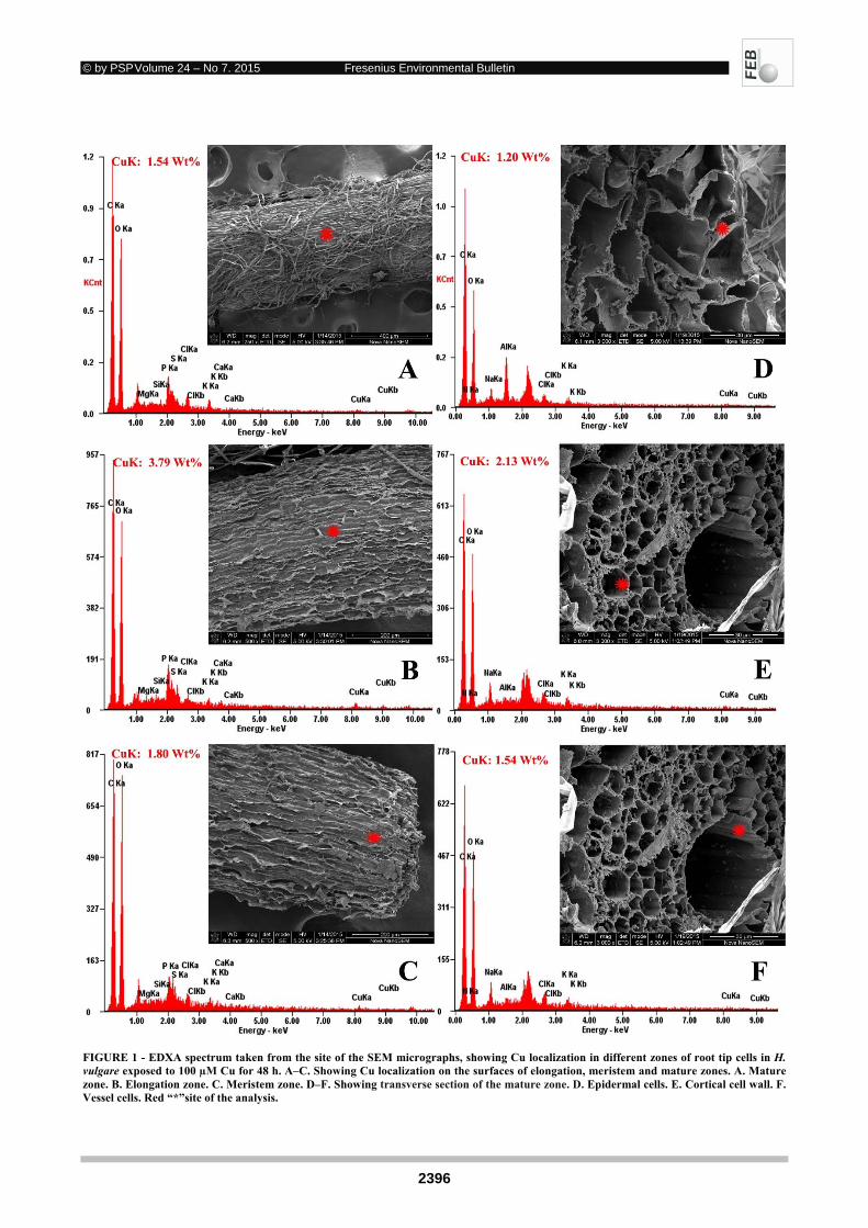
© by PSP Volume 24 – No 7. 2015 Fresenius Environmental Bulletin
2396
FIGURE 1 - EDXA spectrum taken from the site of the SEM micrographs, showing Cu localization in different zones of root tip cells in H. vulgare exposed to 100 µM Cu for 48 h. A–C. Showing Cu localization on the surfaces of elongation, meristem and mature zones. A. Mature zone. B. Elongation zone. C. Meristem zone. D–F. Showing transverse section of the mature zone. D. Epidermal cells. E. Cortical cell wall. F. Vessel cells. Red “*”site of the analysis.
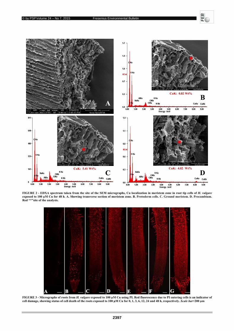
© by PSP Volume 24 – No 7. 2015 Fresenius Environmental Bulletin
2397
FIGURE 2 - EDXA spectrum taken from the site of the SEM micrographs, Cu localization in meristem zone in root tip cells of H. vulgare exposed to 100 µM Cu for 48 h. A. Showing transverse section of meristem zone. B. Protoderm cells. C. Ground meristem. D. Procambium. Red “*”site of the analysis.
FIGURE 3 - Micrographs of roots from H. vulgare exposed to 100 µM Cu using PI. Red fluorescence due to PI entering cells is an indicator of cell damage, showing status of cell death of the roots exposed to 100 μM Cu for 0, 1, 3, 6, 12, 24 and 48 h, respectively. Scale bar=200 µm
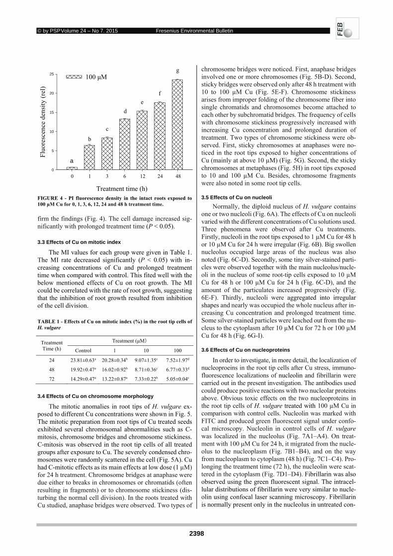
© by PSP Volume 24 – No 7. 2015 Fresenius Environmental Bulletin
2398
Treatment time (h)
Flu
ores
cenc
e de
nsit
y (r
el)
0
5
10
15
20
25100 μM
0 1 3 6 12 24 48
a
b
c
d
e
f
g
FIGURE 4 - PI fluorescence density in the intact roots exposed to 100 μM Cu for 0, 1, 3, 6, 12, 24 and 48 h treatment time. firm the findings (Fig. 4). The cell damage increased sig-nificantly with prolonged treatment time (P < 0.05).
3.3 Effects of Cu on mitotic index
The MI values for each group were given in Table 1. The MI rate decreased significantly (P < 0.05) with in-creasing concentrations of Cu and prolonged treatment time when compared with control. This fited well with the below mentioned effects of Cu on root growth. The MI could be correlated with the rate of root growth, suggesting that the inhibition of root growth resulted from inhibition of the cell division.
TABLE 1 - Effects of Cu on mitotic index (%) in the root tip cells of H. vulgare
Treatment Time (h)
)Treatment (μM
Control 1 10 100
24 23.81±0.63a 20.28±0.34b 9.07±1.35c 7.52±1.97d
48 19.92±0.47a 16.02±0.92b 8.71±0.36c 6.77±0.33d
72 14.29±0.47a 13.22±0.87a 7.33±0.22b 5.05±0.04c
3.4 Effects of Cu on chromosome morphology
The mitotic anomalies in root tips of H. vulgare ex-posed to different Cu concentrations were shown in Fig. 5. The mitotic preparation from root tips of Cu treated seeds exhibited several chromosomal abnormalities such as C-mitosis, chromosome bridges and chromosome stickiness. C-mitosis was observed in the root tip cells of all treated groups after exposure to Cu. The severely condensed chro-mosomes were randomly scattered in the cell (Fig. 5A). Cu had C-mitotic effects as its main effects at low dose (1 µM) for 24 h treatment. Chromosome bridges at anaphase were due either to breaks in chromosomes or chromatids (often resulting in fragments) or to chromosome stickiness (dis-turbing the normal cell division). In the roots treated with Cu studied, anaphase bridges were observed. Two types of
chromosome bridges were noticed. First, anaphase bridges involved one or more chromosomes (Fig. 5B-D). Second, sticky bridges were observed only after 48 h treatment with 10 to 100 µM Cu (Fig. 5E-F). Chromosome stickiness arises from improper folding of the chromosome fiber into single chromatids and chromosomes become attached to each other by subchromatid bridges. The frequency of cells with chromosome stickiness progressively increased with increasing Cu concentration and prolonged duration of treatment. Two types of chromosome stickiness were ob-served. First, sticky chromosomes at anaphases were no-ticed in the root tips exposed to higher concentrations of Cu (mainly at above 10 µM) (Fig. 5G). Second, the sticky chromosomes at metaphases (Fig. 5H) in root tips exposed to 10 and 100 µM Cu. Besides, chromosome fragments were also noted in some root tip cells.
3.5 Effects of Cu on nucleoli
Normally, the diploid nucleus of H. vulgare contains one or two nucleoli (Fig. 6A). The effects of Cu on nucleoli varied with the different concentrations of Cu solutions used. Three phenomena were observed after Cu treatments. Firstly, nucleoli in the root tips exposed to 1 µM Cu for 48 h or 10 µM Cu for 24 h were irregular (Fig. 6B). Big swollen nucleolus occupied large areas of the nucleus was also noted (Fig. 6C-D). Secondly, some tiny silver-stained parti-cles were observed together with the main nucleolus/nucle-oli in the nucleus of some root-tip cells exposed to 10 µM Cu for 48 h or 100 µM Cu for 24 h (Fig. 6C-D), and the amount of the particulates increased progressively (Fig. 6E-F). Thirdly, nucleoli were aggregated into irregular shapes and nearly was occupied the whole nucleus after in-creasing Cu concentration and prolonged treatment time. Some silver-stained particles were leached out from the nu-cleus to the cytoplasm after 10 µM Cu for 72 h or 100 µM Cu for 48 h (Fig. 6G-I).
3.6 Effects of Cu on nucleoproteins
In order to investigate, in more detail, the localization of nucleoproeins in the root tip cells after Cu stress, immuno-fluorescence localizations of nucleolin and fibrillarin were carried out in the present investigation. The antibodies used could produce positive reactions with two nucleolar proteins above. Obvious toxic effects on the two nucleoproteins in the root tip cells of H. vulgare treated with 100 µM Cu in comparison with control cells. Nucleolin was marked with FITC and produced green fluorescent signal under confo-cal microscopy. Nucleolin in control cells of H. vulgare was localized in the nucleolus (Fig. 7A1–A4). On treat-ment with 100 μM Cu for 24 h, it migrated from the nucle-olus to the nucleoplasm (Fig. 7B1–B4), and on the way from nucleoplasm to cytoplasm (48 h) (Fig. 7C1–C4). Pro-longing the treatment time (72 h), the nucleolin were scat-tered in the cytoplasm (Fig. 7D1–D4). Fibrillarin was also observed using the green fluorescent signal. The intracel-lular distributions of fibrillarin were very similar to nucle-olin using confocal laser scanning microscopy. Fibrillarin is normally present only in the nucleolus in untreated con-

© by PSP Volume 24 – No 7. 2015 Fresenius Environmental Bulletin
2399
FIGURE 5 - The effects of Cu on chromosomal morphology in root tip cells of H. vulgare. A. C-metaphase (1 μM Cu, 24 h). B–D. Chromosome bridges (10 μM Cu, 24 h). E–F. Sticky chromosome bridges (10 μM Cu, 24 and 48 h). G. Sticky chromosome at anaphase (10 μM Cu, 72 h). H. Sticky chromosome at metaphase (100 μM Cu, 48 h). Scale bar=10 μm.
FIGURE 6 - Effects of Cu on nucleoli in root tip cells of H. vulgare. A. Control cell. B. Showing irregular nucleoli. B. Showing swollen nucleolus occupied large areas of the nucleus. C–D. Showing big swollen nucleolus, which occupied large areas of the nucleus. E–F. Showing silver-stained particles together with the nucleolus scattered in the nucleus. G-I. Showing silver-stained materials extruded from the nucleus into the cytoplasm, the particulates aggregated into irregular shapes and nearly occupied the whole nucleus. Scale bar=10 μm.

© by PSP Volume 24 – No 7. 2015 Fresenius Environmental Bulletin
2400
FIGURE 7 - Simultaneous detection of nucleolin after incubation with primary anti-nucleolin antibody and secondary antibody conjugated with FITC (green), and of DNA after incubation with DAPI (blue) in the same single optical section using confocal microscopy. (A1,B1,C1,D1) Nucleolin detection; (A2,B2,C2,D2) DNA detection; (A3,B3,C3,D3) Merged image of “nucleolin detection” and “DNA detection”; (A4,B4,C4,D4) bright field image. (A1–A4) Nucleolin in nucleolus of control cells; (B1–B4) The migration of nucleolin from the nucleolus to the nucleoplasm in cells treated with 100 μM Cu for 24 h; (C1–C4) Nucleolin on the way from nucleoplasm to cytoplasm in the cytoplasm of cells treated with 100 μM Cu for 48 h. (D1–D4). Nucleolin scatted in the cytoplasm. Scale bar=10 μm. trol cells of H. vulgare (Fig. 8A1–A4). In comparison with control cells, it was transferred from nucleolus to nucleo-plasm (Fig. 8B1–B3). Fig. 8C1–C3 it was showed on the way from nucleoplasm to cytoplasm. Finally fibrillarin was scattered in the cytoplasm in some cells (Fig. 8D1–D3).
3.7 Effects of Cu on growth
Effects of Cu on root growth of H. vulgare varied with the different concentrations of Cu used (Fig. 9A). The root growth per day decreased with increasing Cu concentration and prolonged treatment time. Cu inhibited the root growth significantly (P < 0.05) at all concentrations (1 to 100 µM Cu) during the entire treatment (72 h) in comparison with
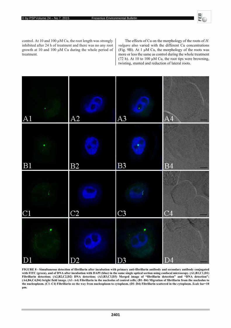
© by PSP Volume 24 – No 7. 2015 Fresenius Environmental Bulletin
2401
control. At 10 and 100 µM Cu, the root length was strongly inhibited after 24 h of treatment and there was no any root growth at 10 and 100 μM Cu during the whole period of treatment.
The effects of Cu on the morphology of the roots of H. vulgare also varied with the different Cu concentrations (Fig. 9B). At 1 μM Cu, the morphology of the roots was more or less the same as control during the whole treatment (72 h). At 10 to 100 μM Cu, the root tips were browning, twisting, stunted and reduction of lateral roots.
FIGURE 8 - Simultaneous detection of fibrillarin after incubation with primary anti-fibrillarin antibody and secondary antibody conjugated with FITC (green), and of DNA after incubation with DAPI (blue) in the same single optical section using confocal microscopy. (A1,B1,C1,D1) Fibrillarin detection; (A2,B2,C2,D2) DNA detection; (A3,B3,C3,D3) Merged image of “fibrillarin detection” and “DNA detection”; (A4,B4,C4,D4) bright field image. (A1–A4) Fibrillarin in the nucleolus of control cells; (B1–B4) Migration of fibrillarin from the nucleolus to the nucleoplasm. (C1–C4) Fibrillarin on the way from nucleoplasm to cytoplasm. (D1–D4) Fibrillarin scattered in the cytoplasm. Scale bar=10 μm.

© by PSP Volume 24 – No 7. 2015 Fresenius Environmental Bulletin
2402
FIGURE 9 - Effects of Cu on root and seedling growth of H. vulgare. A. Root length. B. Seedling growth. Vertical bars denote SE. Values with different letters differ significantly from each other (n = 10, P < 0.05).
4. DISCUSSION
Cu is an essential nutrient for plants and plays an irre-placeable role in the function of a large number of enzymes catalyzing oxidative reactions in a variety of metabolic pathways [18]. However, it can induce severe damage to plant growth and development when absorbed in large amounts [19]. The root is the most sensitive and accessible part of the plant to Cu stress. Inhibition of root growth is typical symptoms of Cu toxicity. Barley seeds grown in different concentrations of Cu showed a significant de-crease of root growth and mitotic index and higher number of chromosomal abnormalities. The MI, characterized by the total number of dividing cells in cell cycle, has been used as a parameter to assess the cytotoxicity of heavy met-als in monitoring environmental pollution [20]. In the pre-sent study, we determined that the MI in root tip of barley decreased significantly by increasing the concentration of Cu (see Table 1). The mitotic cells decreased in the root tips of H. vulgare, indicating that Cu was accumulated in the meristem where it disturbed cell division. Thus, it is clearly that the inhibition of the root growth resulted from inhibiting the cell division of root tips. This fits well with the above mentioned effects of Cu on root growth.
Chromosome aberrations have been used as a measure of reproductive success and as a method for the detection of possible genetic damage by environmental agents (such as herbicides, insecticides, fungicides and heavy metals in plant for many years [21]. Plant chromosomes are easy to analyze in terms of size, morphology and number, and re-spond to treatments with toxins at an early stage [22]. Chromosomal aberrations and proportion of mitotic phases can be accepted as indicators of genetic damage induced by stress conditions and the anaphase–telophase chromo-some aberration assay has been shown to be highly reliable in genotoxicity testing [23]. Several authors reported that the inhibition of root elongation caused by Cu may be due
to metal interference with cell division, including induce-ment of chromosomal aberrations and abnormal mitosis [24–26]. Chromosomal aberrations are changes in chromo-some structure resulting from a break or exchange of chro-mosomal material. Based on the results of the present in-vestigation, it is quite clear that Cu is capable of inducing such cytological abnormalities as c-mitosis, bridges, stick-iness, fragments, etc. The frequency of abnormalities in-creases, in most cases, as the concentration of the metal in-creases. The results from the present investigation are in agreement with the findings by Agarwal et al. [27], Jiang et al. [28] and Liu et al. [29], but with some differences. 1) Chromosome bridges exhibiting stickiness were observed in the treatment with 10 Cu µM for 48 h. 2) Anaphase con-figuration with chromosome bridges exhibiting disintegra-tion was found only after 72 h of treatment with 100 µM Cu. The chromosomal bridge aberrations and chromosome stickiness appeared in the root tips exposed to higher con-centration of Cu (100 µM) are lethal and probably lead to cell death. C-mitosis more often observed in low concen-tration of Cu, in which the chromosomes spread irregularly over the cell, may be due to disturbance of the spindle ap-paratus. This kind of chromosomal aberration reflects slight or moderate cytological toxicity.
The nucleolus is well known as the site of transcription of ribosomal genes and further transcript process [30], which also contains a set of acidic, nonhistone proteins that bind silver ions and are selectively visualized by silver methods. It is well known that silver impregnation is re-garded as a specific stain of the nucleolus. To better under-stand the nucleolar cycle and the nucleolar organization, the silver staining technique has been widely used in cyto-logical studies in both animals and plants. The results in this work showed that Cu could induce toxic effects on nu-cleoli, causing some particulate silver-stained material containing the argyrophilic proteins scattered in the nuclei and some particles extruded from the nucleus into the cy-
Time (h)
Roo
t le
ngt
h (
cm)
0
1
2
3
4
5
6Control1 ¦ÌM10 ¦Ì¦¬100 ¦ÌM
a
a
b
c d
a
b
c d
a
b
cd
0 24 48 72
a a a
A

© by PSP Volume 24 – No 7. 2015 Fresenius Environmental Bulletin
2403
toplasm. The results here are similar to those under Cu stress described by Liu et al. [31] for the effects Cu on the nucleolus of Allium cepa root tip cells, Jiang et al [25] for Cu on Helianthus annuus, Jiang et al. [28] for Cu on Zea mays and Liu et al. [29] for Cu on Allium sativum, but with a few differences. (1) There are not so many nucleolar par-ticles containing the argyrophilic proteins scattered in the nuclei and large amount of the materials extruded from the nucleus into the cytoplasm in the present study, when com-pared with the findings of Liu et al. [29, 31]. (2) Cu has weak toxic effect on nucleolus in root tip cells of H. annuus and Z. mays [25, 28], where the nucleolar material is only scattered in the nucleus, and not extruded from the nucleus into the cytoplasm when compared with the results here. Thus, the toxicity of Cu on the nucleoli varied with differ-ent species plants. The phenomenon Cu induced in the pre-sent investigation is in line with the previous findings, in-dicating that besides Cu some other metal ions can affect toxic effects on nucleolus in the same way, such as alumi-num (Al) [32], cadmium (Cd) [17] and lead (Pb) [20, 33]. Some reports indicated that the extrusion of nucleolar mate-rial containing argyrophilic proteins from the nucleus into the cytoplasm may be correlated with damage to the nuclear pore complex (NPC) proteins, causing the NPC to lose se-lectivity [34]. However, the mechanism needs to be studied further. Although there are some reports concerning Cu toxic effects on nucleolus in plant root tips, they hardly indicated what kinds of proteins involved in those reports.
The nucleolus has long been known playing important roles in the regulation of many fundamental cellular pro-cesses [35–36]. It is well known that the nucleolus contains several kinds of proteins. Nucleolin and fibrillarin are ma-jor nucleolar proteins conserved in all eukaryotic organ-isms [37]. They are multifunctional proteins involved in different cellular aspects like chromatin organization and stability, DNA and RNA metabolism, assembly of ribo-nucleoprotein complexes, cytokinesis, cell proliferation and stress response [37, 38]. Evidence obtained using in-direct immunofluorescent microscopy in the present in-vestigation revealed that the two nucleolar proteins, nu-cleolin and fibrillarin were localized in nucleoli in control groups. However, under Cu stress the two nucleolar pro-teins presented abnormal nucleoplasm and cytoplasmic location in the nucleoli of H. vulgare root tips, which con-firmed the observation with the silver impregnation stud-ies here. Recent investigations indicated that heavy met-als such as Cd and Pb could induce nucleolar proteins, nucleophosmin, nucleolin, and fibrillarin migrated from nucleolus to nucleoplasm and cytoplasm in root tip cells of Vicia faba [17] and Allium cepa [20]. Qin et al. [39, 40] and Zhang et al. [41] also reported that Al had the same toxic effects on nucleolus in root tip cells of V. faba and H. vulgare. These observations are in good agreement with the findings here, suggesting that nucleolus is a cen-ter to sense stress and can coordinate the stress response. Thus nucleolar morphology, composition and function will change upon stress [42].
EDXA following freezing of the plant sample has been employed systematically in biological sciences to localize ions in cellular compartments, to monitor ion distribution changes during physiological processes, to determine the behavior of toxic ions incorporated by cells, and thus can provide information on mechanisms of metal toxicity and tolerance [43–45]. EDXA was used to determine Cu local-ization in root tips of H. vulgare exposed to Cu in this study. The results here can be summarized as follows. 1) The three zones, mature, elongation and meristem zone can absorb Cu ions. 2) In mature zone, root hairs are found only in the region of maturation of the root, and they are out-growths at a tip of the plants roots. They have a large sur-face area, which makes absorbing both water and minerals more efficient using osmosis. Once Cu enters the roots, it easily penetrates the root through the cortical tissue and is translocated to the above-ground tissues. This can ex-plained why the level of Cu in mature zone is low when compared to meristem zone. 3) From a transverse section point of view, the Cu level in meristem zone is high in com-parison with mature zone (Fig. 1D–F; Fig. 2A–D), suggest-ing that root tip meristem of plants is a primary target of Cu accumulation and toxicity. Meristem cells are small and have thin walls without differentiation. These cells have not yet differentiated and have poor transport capacity up. Thus, excess Cu can easily induce damage of cell construc-tion. Evidence here shows Cu toxic effects on meristem cells under Cu stress, causing obviously toxic characteris-tics, such as low MI, chromosome aberrations, damage of nucleolus and production of large damaged cells. The re-sults also confirmed indirectly the previous results reported by Liu et al. [26] where they found that excess Cu could cause adverse effects on garlic meristem cells after 1 h treat-ment with Cu, increasing dictyosome vesicles in number, forming of cytoplasmic vesicles containing electron dense granules, altering mitochondrial shape, disrupting nuclear membranes ect. Due to Cu toxicity on meristem, the cell division was affected, leading to the mitotic cells decreased and interphase cells increased.
PI, an intercalating agent and a fluorescent molecule
with a small molecular mass of 668.4 Da that can be used to stain DNA, has been considered as a alternative agent to study cell membrane damage [46]. The amount of PI enter-ing into cells reflects the degree of cell membrane damage, and morphological changes in the cells may be related to damage to the integrity of the cell membrane [47]. Here, we can confirm that Cu has toxic effect on the cell mem-brane damage in the root tip cells of H. vulgare using PI staining. The cell damages were observed mainly in the meristem and elongation zone of root tip exposed to Cu for 1 h (Fig. 3). The data from PI staining here are in good agreement with the evidence obtained from EDXA in the roots of H. vulgare under Cu stress, indicating that there is a clear correlation between Cu content and cell damage in root tips of H. vulgare. At the cellular level, Cu toxic ef-fects at excess Cu concentrations is oxidative stress caused by the increased concentration of reactive oxygen species
© by PSP Volume 24 – No 7. 2015 Fresenius Environmental Bulletin
2404
(ROS), such as superoxide anion (O2.-), singlet oxygen (1O2), hydrogen peroxide (H2O2) and hydroxyl radical (OH-) [48]. ROS can damage all biomolecules where lipid peroxidation of the cell membranes is one of the most im-portant effects. Its selectivity is lower, due to damage to the cell membranes, leading to membrane breakage and leak-age of the cell contents [11, 49–50]. At higher level of malondialdehyde (MDA) in plants shows injury to func-tional membrane during Cu stress [50]. Data from the pre-sent investigation (unpublished) indicated that Cu could in-duce the increase of the MDA content in roots of H. vul-gare exposed to Cu when compared to control, indicating that Cu like other environmental stresses can generate the production of a powerful oxidation which in turn brings about lipid peroxidation [51].
5. CONCLUSION
Root tips of plants are the most sensitive organ to en-vironmental stresses. Excessive Cu has often caused poi-soning and environmental contamination. The findings of the present study confirm that Cu ions can be absorbed in mature, elongation and meristem zone in the root tips of H. vulgare under Cu stress. Root apical meristems play a key role in the immediate reaction to stress factors by activating signal cascades to the other plant organs. Due to high level of Cu in meristem zone, it can be considered as a primary target of Cu accumulation and toxicity, which disturbs cell division, induces chromosomal aberrations and abnormal mitosis, decreases MI and eventually results in inhibiting the root growth. Cu can also affect nucleolus and nucleolar proteins in the root tip cells, causing the two nucleopro-teins, nucleolin and fibrillarin, migrated from nucleolus to nucleoplasm and cytoplasm. There is a clear correlation be-tween Cu content and cell damage in root tips of H. vul-gare. H. vulgare is a good model plant, with many ad-vantages such as low cost, ease of storage and handling, excellent chromosome conditions, and ease of observing abnormal phenomena of chromosomes, nuclei, and nucle-oli affected during mitosis. The data obtained here give more detailed information on qualitatively and quantita-tively harmful effects at the microscopic level, which is very useful to understand the detoxification and tolerance mechanisms of Cu-induced toxicity.
ACKNOWLEDGMENTS
This project was supported by the National Natural Science Foundation of China. The authors wish to express their appreciation to the reviewers for this paper.
The authors have declared no conflict of interest.
REFERENCES
[1] Kukkola, E., Rautio, P. and Huttune, S. (2000). Stress indications in copper-and nickel-exposed Scots pine seedlings. Environ Exp Bot 43, 197–210.
[2] Meng, Q.M., Zou, J., Zou, J.H., Jiang, W.S. and Liu, D.H. (2007) Effect of Cu2+ concentration on growth, antioxidant enzyme activ-ity and malondialdehyde content in Garlic (Allium sativum L.). Acta Biol Cracov Bot 49, 95–101.
[3] Tanyolaç, D., Ekmekçi, Y. and Ûnalan, S. (2007) Changes in pho-tochemical and antioxidant emzyme activities in maize (Zea mays L.) leaves exposed to excess copper. Chemosphere 67, 89–98.
[4] Andrés-Colás, N., Perea-García, A., Puig, S. and Peňarrubia, L. (2010) Deregulated copper transport affects arabidopsis develop-ment especially in the absence of environmental cycles. Plant Physiol 153, 170–184.
[5] Sánchez-Pardo, B., Fernández-Pascual, M. and Zornoza, P. (2014) Copper microlocalisation and changes in leaf morphology, chloro-plast ultrastructure and antioxidative response in white lupin and soybean grown in copper excess. J Plant Res 127, 119–129.
[6] Fiskesjö, G. (1988) The Allium test – an alternative in environ-mental studies: the relative toxicity of metal ions. Mut Res 197, 243–260.
[7] Özkara, A., Akyil, D., Erdoğmus, S.F. and Konuk, M. (2011) Eval-uation of germination, root growth and cytological effects of wastewater of sugar factory (Afyonkarahisar) using Hordeum vul-gare bioassays. Environ Monit Assess 183, 517–524.
[8] Olson, M.O.J. and Dundr, M. (2005) The moving parts of the nu-cleolus. Histochem Cell Biol 123, 203–216.
[9] Liu, D.H. and Jiang, W.S. (1994) Effects of copper sulfate on the nucleolus of Allium cepa root tip cells. Hereditas 120, 87–90.
[10] Liu, D.H., Jiang, W.S., Meng, Q.M., Zou, J., Gu, J.G. and Zeng, M.A. (2009) Cytogenetical and ultrastructural effects of copper on root meristem cells of Allium sativum L. Biocell 33, 25–32.
[11] Yruela I (2005) Copper in plants. Braz J Plant Physiol 17, 145–156.
[12] Geremias, R., Fattorini, D., Fávere, V.T.D. and Pedrosa, R.C. (2010) Bioaccumulation and toxic effects of copper in common onion Allium cepa L. Chem Ecol 26, 19–26.
[13] Wei, Z.Q., Chen, Z.Y., Qin, R., Wang, Y.T. and Li, S.S. (2013) Cu2+ induced local toxicity and DNA damage, cell death in roots of Arabidopsis thaliana. Chin Bull Bot 48, 303–312.
[14] Li, M.X. (1982) Introducing a good stain used for nuclei and chro-mosome. Bull Biol 5, 53.
[15] Koyama, H., Toda, T., Yokota, S., Dawair, Z. and Hara, T. (1995) Effects of aluminum and pH on root growth and cell viability in Arabidopsis thaliana strain Landsberg in hydroponic culture. Plant Cell Physiol 36, 201–205.
[16] Jones, K.H. and Senft, J.A. (1985) An improved method to deter-mine cell viability by simultaneous staining with fluorescein diac-etate-propidium iodide. J Histochem Cytochem 33, 77–79.
[17] Qin, R., Jiang, W.S. and Liu, D.H. (2013) Cadmium can induce alterations in the cellular localization and expression of three major nucleolar proteins in root tip cells of Vicia faba L. Plant Soil 368, 365–373.
[18] Quartacci, M.F., Pinzino, C., Sgherri, C.L.M., Vecchia, F.D. and Navari-Izzo, F. (2000) Growth in excess copper induces changes in the lipid composition and fluidity of PSII-enriched membranes in wheat. Physiol Plantarum 108, 87–93.
[19] Shimizu, Y., Shimizu, T., Nara, M., Kikumoto, M., Kojima, H. and Morii, H. (2013) Effects of the KIF2C neck peptide on microtu-bules: Lateral disintegration of microtubules and structure for-mation. FEBS J 280, 1681–1692.
[20] Jiang, Z., Qin, R. Zhang, H.N., Zou, J.H. Shi, Q.Y. Wang, J.R. Jiang, W.S. and Liu, D.H. 2014. Determination of Pb genotoxic effects in Allium cepa root cells by fluorescent probe, microtubular immunofluorescence and comet assay. Plant Soil 383, 357–372.
© by PSP Volume 24 – No 7. 2015 Fresenius Environmental Bulletin
2405
[21] Grant, W.F. (1978) Chromosome aberrations in plants as a moni-toring system. Environ Health Perspect 1978, 27, 37–43.
[22] Qin, R., Jiao, Y.Q., Zhang, S.S., Jiang, W.S. and Liu, D.H. (2010) Effects of aluminum on nucleoli in root tip cells and selected phys-iological and biochemical characters in Allium cepa var. agrogarum L. BMC Plant Biol 10, 225.
[23] Mustafa, Y. and Arikan, E.S. (2008) Genotoxicity testing of quizalofop-P-ethyl herbicide using the Allium cepa anaphase–tel-ophase chromosome aberration assay. Caryologia 61, 45–52.
[24] Kahle, H. (1993) Response of roots of trees to heavy metals. Envi-ron Exp Bot 33, 99–119.
[25] Jiang, W.S., Liu, D.H. and Li, H.F. (2000) Effects of Cu2+ on root growth, cell division, and nucleolus of Helianthus annuus L. Sci Total Environ 256, 59–65.
[26] Liu, D.H., Jiang, W.S., Meng, Q.M., Zou, J., Gu, J.G. and Zeng, M.A. (2009) Cytogenetical and ultrastructural effects of copper on root meristem cells of Allium sativum L. Biocell 33, 25-32.
[27] Agarwal, K., Sharma, A. and Talukder, G. (1987) Copper toxicity in plant cellular systems. Nucleus 30, 131–158.
[28] Jiang, W., Liu, D. and Liu, X. (2001) Effects of copper on root growth, cell division, and nucleolus of Zea mays. Biol Plantarum 44, 105–109.
[29] Liu, D.H., Xue, P., Meng, Q.M., Zou, J., Gu, J.G., Jiang, W.S. 2009. Pb/Cu effects on the organization of microtubule cytoskele-ton in interphase and mitotic cells of Allium sativum L. Plant Cell Rep 28, 695-702.
[30] Shaw, P.J. and Jordan, E.G. (1995) The nucleolus. Annu Rev Cell Biol 11, 93–121.
[31] Liu, D., Jiang, W., Wang, W., Zhao, F., Lu, C. (1994) Effects of lead on root growth, cell division, and nucleolus of Allium cepa. Environ Pollut 86, 1–4.
[32] Liu, D.H. and Jiang, W.S. (1991) Effects of Al3+ on the nucleolus in root tip cells of Allium cepa. Hereditas 1991, 115, 213–219.
[33] Balcerzak, Ł., Glińska, S. and Godlewski, M. (2011) The reaction of Lupinus angustifolius L. root meristematic cell nucleoli to lead. Protoplasma 2011, 248, 353–361.
[34] Qin, R., Zhang, H.H., Li, S.S., Jiang, W.S. and Liu, D.H. (2014) Three major nucleolar proteins migrate from nucleolus to nucleo-plasm and cytoplasm in root tip cells of Vicia faba L. exposed to aluminum. Environ Sci Pollut Res 21, 10736–10743
[35] Boisvert, F.M., van Koningsbruggen, S., Navascués, J. and La-mond, A.I. (2007) The multifunctional nucleolus. Nat Rev Mol Cell Biol 8, 574–585.
[36] Sirri, V., Urcuqui-Inchima, S., Roussel, P. and Hernandez-Verdun, D. (2008) Nucleolus: the fascinating nuclear body: a review. His-tochem Cell Biol 129, 13–31.
[37] Durut, N. and Sáez-Vásquez, J. (2015) Nucleolin: Dual roles in rDNA chromatin transcription. Gene 556, 7–12.
[38] Sobol, M., Gonzalez-Camacho, F., Rodríguez-Vilariño, V., Kordyum, E., Medina, F.J. (2006) Subnucleolar location of fibril-larin and NopA64 in Lepidium sativum root meristematic cells is changed in altered gravity. Protoplasma 228, 209–219.
[39] Qin, R., Jiang, W.S. and Liu, D.H. (2013) Aluminum can induce alterations in the cellular localization and expressionof three major nucleolar proteins in root tip cells of Allium cepa var. agrogarum L., Chemosphere 90, 827–834.
[40] Qin, R., Zhang, H.N., Li, S.S., Jiang, W.S. and Liu, D.H. (2014) Three major nucleolar proteins migrate from nucleolus to nucleo-plasm and cytoplasm in root tip cells of Vicia faba L. exposed to aluminum. Environ Sci Pollut Res 21, 10736–10743.
[41] Zhang, H.N., Jiang, Z., Zhang, H.H., Zou, J.H., Shi, Q.Y., Wang, J.R., Jiang, W.S. and Liu, D.H. (2015) Aluminum can induce three nucleolar Proteins migrated from nucleolus to Cytoplasm in root tips of Hordeum vulgare L. Fresenius Enviro Bull 24(4), 1–8.
[42] Boulon, S., Westman, B.J., Hutten, S., Boisvert, F.M. and Lamond, A.I. (2010) The Nucleolus under Stress. Mol Cell 40, 216–227.
[43] Zierold, K. (1993) Rapid freezing techniques for biological elec-tron probe microanalysis. In: Sigee DC, Morgan AJ, Summer AT, Warley A (eds) X-ray Microanalysis in Biology: Experimental Techniques and Applications. Cambridge University Press, Cam-bridge, UK, pp. 110–116.
[44] Barceló, J. and Poschenrieder, C. (1999) Structural and ultrastruc-tural changes in heavy metal exposed plants. In: Prasad MNV, Hagemeyer J (eds) Heavy Metal Stress in Plants. Springer-Verlag, Berlin – Heidelberg, pp. 183–205.
[45] Rocchetta, I., Leonardi, P.I., Filho, A.G.M., Del Carmen Rίos De Molina, M. and Conforti, V. (2007) Ultrastructure and X-ray mi-croanalysis of Euglena gracilis (Euglenophyta) under chromium stress. Phycologia 46, 300–306.
[46] Liao, T.T., Jia, R.W., Shi, Y.L., Jia, J.W., Wang, L. and Chua, H. (2011) Propidium iodide staining method for testing the cytotoxi-city of 2,4,6-trichlorophenol and perfluorooctane sulfonate at low concentrations with Vero cells. J Environ Sci Health Part A 46, 1769–1775.
[47] Liao, T., Shi, Y., Jia, R. and Wang, L. (2010) Sensitivity of differ-ent cytotoxic responses of Vero cells exposed to organic chemical pollutants and their reliability in the bio-toxicity test of trace chem-ical pollutants. Biomed Environ Sci 23, 219–229.
[48] Apel, K. and Hirt, H. (2004) Reactiven oxygen species: Metabo-lism, oxidative Stress, and signal transduction. An Rev Plant Biol 55, 373–399.
[49] Opdenakker, K., Remans, T., Keunen, E., Vangronsveld, J. and Cuypers, A. (2012) Exposure of Arabidopsis thaliana to Cd or Cu excess leads to oxidative stress mediated alterations in MAP-Kinase transcript levels. Environ Exp Bot 83, 53– 61.
[50] Khan, A.L, and Lee, I.J. (2013) Endophytic Penicillium funicu-losum LHL06 secretes gibberellin that reprograms Glycine max L. growth during copper stress. BMC Plant Biology 13, 86.
[51] Hatata, M.M. and Abdel-Aal, E.A. (2008) Oxidative stress and an-tioxidant defense mechanisms in response to cadmium treatments. Amer-Eurasian J Agri Environ Sci 4, 655–669.
Received: March 25, 2015 Revised: May 08, 2015 Accepted: May 18, 2015 CORRESPONDING AUTHOR
Donghua Liu Tianjin Key Laboratory of Animal and Plant Re-sistance College of Life Sciences Tianjin Normal University Tianjin 300387 P.R. CHINA Phone: 0086-22-23766823 E-mail: [email protected]
FEB/ Vol 24/ No 7/ 2015 – pages 2394 - 2405
© by PSP Volume 24 – No 7. 2015 Fresenius Environmental Bulletin
2406
EVALUATION OF STABILITY AND
MATURITY PARAMETERS IN WASTEWATER SLUDGE
COMPOSTING WITH DIFFERENT AERATION STRATEGIES AND
A MIXTURE OF GREEN PLANT WASTES AS BULKING AGENT
Amir Hossein Nafez1,*, Mahnaz Nikaeen1, Bijan Bina2, Akbar Hassanzadeh3 and Sharareh Moghim4
1Department of Environmental Health Engineering, School of Public Health, Kermanshah University of Medical Sciences, Kermanshah, Iran 2Department of Environmental Health Engineering and Environment Research Center, School of Health, Isfahan University of Medical Sciences, Isfahan, Iran
3Department of Statistic and Epidemiology, School of Health, Isfahan University of Medical Sciences, Isfahan, Iran 4Department of Medical Microbiology and Virology, School of Medicine, Isfahan University of Medical Sciences, Isfahan, Iran
ABSTRACT
The aim of this study was to investigate the influence of bulking agent volumetric ratio on the stability and ma-turity parameters in composting process of anaerobically digested sludge (ADS) with different aeration strategies. Two main influencing factors including aeration method (aerated static pile and windrow process) and proportion of green plant wastes (GPW) and ADS (1:1, 2:1 and 3:1, GPW: ADS) were investigated through the evaluation of physico-chemical and biological parameters during the 83 days of composting. Heavy metals concentration, germination in-dex (GI), and microbiological indicators were also deter-mined in the final products. The results showed that wind-row method was superior to the aerated static piles, since the former enhances the composting process by favoring organic matter (OM) stabilization. Based on these results it appears that windrow method with 2:1 mixture of GPW: ADS was best for ADS composting due to the highest OM degradation ability and maximum GI in the final product.
KEYWORDS: Compost, Green plant wastes, Wastewater sludge, Static pile composting, Windrow composting
1. INTRODUCTION
Wastewater sludge (WS) is a by-product and insoluble residue remaining following wastewater treatment. Inap-propriate management of WS could lead to major public health and environmental concerns due to high amounts of pathogens and heavy metals [1-3]. With the increased pro-duction of WS, there is a great need to develop low cost
* Corresponding author
and high efficiency processes for recycling of this waste as an alternative to dumping and incineration [4]. WS is a good candidate for composting and subsequently for agri-cultural purposes since its pH is neutral to slightly alkaline and its organic matter (OM) can vary from 50% to 70% of the total solids content and rich in both phosphorus and ni-trogen [4-6]. Composting of WS is a biological process which converts OM to stabilized humic substances through mineralization with a significant reduction (40-50%) in vol-ume [4, 7]. In composting process pathogens can be killed by heat generated in the thermophilic phase [7]. Further-more, final product of composting process could act as a soil conditioner or fertilizer.
However, the high heavy metal content of WS com-post is a major limitation for land application of this end product. WS also has a compact structure because of its high moisture content even if a dewatering treatment is used [1-2, 5]. Many studies have verified that WS alone generates poor quality compost [1, 4, 8]. Due to the high moisture content and low C/N ratio of WS they need to be mixed with some materials as bulking agents which absorb the moisture and provide sufficient porosity and air permeabil-ity for composting of WS [4, 5, 9]. A long list of waste materials (e.g. municipal refuses, agricultural residues, an-imal manures and forest wastes) have been proposed as bulking agents in several studies [1, 2, 10, 11], but the most widely used materials are fibrous carbonaceous and ligno-cellulosic materials with low moisture content such as wood chips, straw and sawdust. These lignocellulosic materials have also the ability to uptake heavy metals and reduce heavy metals availability.
However, the type of bulking agent and the volume ra-tio of WS to bulking agent could strongly influence the property of composting process and mineralization [5]. For instance, Chazirakis et al. [12] investigated the effects of different mixture ratios of sewage sludge, organic fraction of municipal solid waste (OFMSW) and yard trimmings
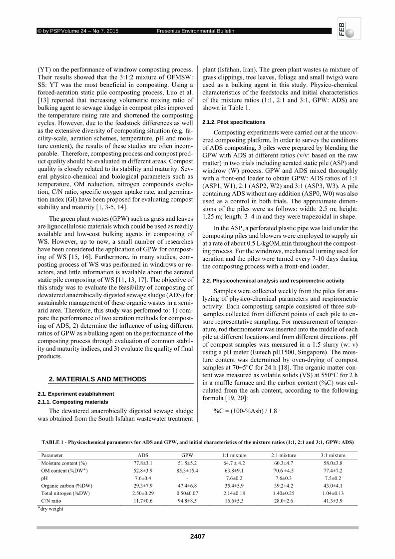
© by PSP Volume 24 – No 7. 2015 Fresenius Environmental Bulletin
2407
(YT) on the performance of windrow composting process. Their results showed that the 3:1:2 mixture of OFMSW: SS: YT was the most beneficial in composting. Using a forced-aeration static pile composting process, Luo et al. [13] reported that increasing volumetric mixing ratio of bulking agent to sewage sludge in compost piles improved the temperature rising rate and shortened the composting cycles. However, due to the feedstock differences as well as the extensive diversity of composting situation (e.g. fa-cility-scale, aeration schemes, temperature, pH and mois-ture content), the results of these studies are often incom-parable. Therefore, composting process and compost prod-uct quality should be evaluated in different areas. Compost quality is closely related to its stability and maturity. Sev-eral physico-chemical and biological parameters such as temperature, OM reduction, nitrogen compounds evolu-tion, C/N ratio, specific oxygen uptake rate, and germina-tion index (GI) have been proposed for evaluating compost stability and maturity [1, 3-5, 14].
The green plant wastes (GPW) such as grass and leaves are lignocellulosic materials which could be used as readily available and low-cost bulking agents in composting of WS. However, up to now, a small number of researches have been considered the application of GPW for compost-ing of WS [15, 16]. Furthermore, in many studies, com-posting process of WS was performed in windrows or re-actors, and little information is available about the aerated static pile composting of WS [11, 13, 17]. The objective of this study was to evaluate the feasibility of composting of dewatered anaerobically digested sewage sludge (ADS) for sustainable management of these organic wastes in a semi-arid area. Therefore, this study was performed to: 1) com-pare the performance of two aeration methods for compost-ing of ADS, 2) determine the influence of using different ratios of GPW as a bulking agent on the performance of the composting process through evaluation of common stabil-ity and maturity indices, and 3) evaluate the quality of final products.
2. MATERIALS AND METHODS
2.1. Experiment establishment
2.1.1. Composting materials
The dewatered anaerobically digested sewage sludge was obtained from the South Isfahan wastewater treatment
plant (Isfahan, Iran). The green plant wastes (a mixture of grass clippings, tree leaves, foliage and small twigs) were used as a bulking agent in this study. Physico-chemical characteristics of the feedstocks and initial characteristics of the mixture ratios (1:1, 2:1 and 3:1, GPW: ADS) are shown in Table 1.
2.1.2. Pilot specifications
Composting experiments were carried out at the uncov-ered composting platform. In order to survey the conditions of ADS composting, 3 piles were prepared by blending the GPW with ADS at different ratios (v/v: based on the raw matter) in two trials including aerated static pile (ASP) and windrow (W) process. GPW and ADS mixed thoroughly with a front-end loader to obtain GPW: ADS ratios of 1:1 (ASP1, W1), 2:1 (ASP2, W2) and 3:1 (ASP3, W3). A pile containing ADS without any addition (ASP0, W0) was also used as a control in both trials. The approximate dimen-sions of the piles were as follows: width: 2.5 m; height: 1.25 m; length: 3–4 m and they were trapezoidal in shape.
In the ASP, a perforated plastic pipe was laid under the composting piles and blowers were employed to supply air at a rate of about 0.5 L/kgOM.min throughout the compost-ing process. For the windrows, mechanical turning used for aeration and the piles were turned every 7-10 days during the composting process with a front-end loader.
2.2. Physicochemical analysis and respirometric activity
Samples were collected weekly from the piles for ana-lyzing of physico-chemical parameters and respirometric activity. Each composting sample consisted of three sub-samples collected from different points of each pile to en-sure representative sampling. For measurement of temper-ature, rod thermometer was inserted into the middle of each pile at different locations and from different directions. pH of compost samples was measured in a 1:5 slurry (w: v) using a pH meter (Eutech pH1500, Singapore). The mois-ture content was determined by oven-drying of compost samples at 70±5°C for 24 h [18]. The organic matter con-tent was measured as volatile solids (VS) at 550°C for 2 h in a muffle furnace and the carbon content (%C) was cal-culated from the ash content, according to the following formula [19, 20]:
%C = (100-%Ash) / 1.8
TABLE 1 - Physicochemical parameters for ADS and GPW, and initial characteristics of the mixture ratios (1:1, 2:1 and 3:1, GPW: ADS)
Parameter ADS GPW 1:1 mixture 2:1 mixture 3:1 mixture
Moisture content (%) 77.8±3.1 51.5±5.2 64.7 ± 4.2 60.3±4.7 58.0±3.8
OM content (%DW٭) 7.2±77.4 4.5± 70.6 9.1±63.8 15.4±85.3 3.9±52.8
pH 7.6±0.4 - 7.6±0.2 7.6±0.3 7.5±0.2
Organic carbon (%DW) 29.3±7.9 47.4±6.8 35.4±5.9 39.2±4.2 43.0±4.1
Total nitrogen (%DW) 2.50±0.29 0.50±0.07 2.14±0.18 1.40±0.25 1.04±0.13
C/N ratio 11.7±0.6 94.8±8.5 16.6±5.3 28.0±2.6 41.3±3.9
dry weight٭
© by PSP Volume 24 – No 7. 2015 Fresenius Environmental Bulletin
2408
Total Kjeldahl nitrogen (TKN), ammonium nitrogen ( -N) and nitrates nitrogen ( -N) contents were as-sayed as described by the US Department of Agriculture and US Composting Council (2001) [18], and their concen-trations determined by DR5000 Spectrophotometer (Hach Co. USA). Respirometric activity was determined by spe-cific oxygen uptake rate (SOUR) of the compost samples. The maximum rate of oxygen uptake was measured using a dissolved oxygen sensor (5740sc Galvanic Membrane, Hach Company, USA) in an aqueous suspension of 3-8 g compost (wet weight) in 500 ml distilled water, at 30°C. SOUR was determined from the slope of oxygen level de-crease according to the method described by Lasaridi and Stentiford (1998) [14].
2.3. Final compost quality assessment
To assess the final compost quality, analysis of micro-bial indicators, heavy metals content and cress seed germi-nation were performed on samples were taken from each pile at the end of the composting process (day 83). Micro-bial analyses including fecal coliforms and Salmonella were carried out according to Standard methods [21], and results expressed on a dry mass basis. In order to determine the available fraction of heavy metals including Cd, Cu, Pb, Cr, Ni, and Zn in final compost, the water-soluble fraction of heavy metals was digested and determined by flame atomic absorption spectrometry (Varian SpectrAA220FS, Australia). The seed germination bioassay was evaluated in the final samples according to the method of Tiquia et al. [22].
3. RESULTS AND DISCUSSION
3.1. Temperature evolution
Graphs in Fig. 1a and 1b show the temperature varia-tions of the composting piles as a function of the waste mixtures and aeration methods. Temperature follows a typ-ical temperature profile of organic waste composting for all mixtures [1, 23]. However, variation in mixing ratios caused different thermophilic temperatures. Throughout the experi-mental period, the ambient temperature ranged from 24 to 39°C. Initially the temperature of the compost mixtures was in the mesophilic phase and near to the ambient tem-perature. Temperature increased to 40–50°C in 2 weeks (start of the thermophilic phase), reached between 55 and 65°C in 4-5 weeks (except for ADS: GPW, 1:1) as a con-sequence of the vigorous biodegradation of the easily bio-degradable OM. As shown in Fig. 1a and 1b, after the start of composting, the temperatures increased in both trials; however, the rate of rise, as indicated by the gradient of the curves, was much faster in the windrow method than ASP. As have been reported, due to the lack of heat exchange in the static piles, a longer time is needed for OM stabilization in ASP process [1, 15].
As shown in Fig. 1a and 1b, higher temperatures (66 and 63°C) were achieved in the 2:1 and 3:1 mixtures in
windrow and static pile, respectively. This can be ex-plained by higher porosity and improved moisture of these piles as a consequence of the higher proportion of bulking agent [5]. The control piles, without bulking agent, did not show any significant variation in temperature. Moreover, the temperature of 1:1 piles not only increased slowly but also decreased rapidly which could be explained by an in-hibition effect on microorganism’s activity caused by high moisture content. Faster increase of the temperature and longer periods of thermophilic phase for the mixtures with higher ratios of GPW reflect the greater content of easily biodegradable C-fractions in 2:1 and 3:1 mixtures and also indicates high capability of GPW for preserving heat. These results confirm the hypothesis that the self-heating ability is directly associated to the feedstocks characteris-tics [4, 12]. The duration of thermophilic phase also de-pends on the chemical composition of feedstocks [4]. The temperature of 2:1 and 3:1 mixtures exceeded 55°C on day 13-19 and lasted for more than 15 days which be enough to ensure sanitization of composted materials [1].
Comparison of Fig. 1a and 1b shows that the tempera-
ture of the W piles not only increased faster, but also lasted longer time in comparison to the static piles. Therefore, as well as the feedstock composition, the aeration method also has a considerable effect on duration of thermophilic phase in the composting process. By days 47–54, the temperature in piles decreased gradually, reaching a second mesophilic phase and maturation process took place during the last stage of composting. At the end of process, after 83 days of composting, the temperature remained at 31°C in all of the mixtures.
3.2. Mineralization of OM
Reduction of OM is mainly caused by microbial activ-ity which significantly influences the composting process and quality of the final product [5, 24]. In both trials, the OM values decreased mainly in the initial stages of the composting process, which is related to the thermophilic phase and mineralization process. The decrease of OM content in ASP was 12.9%, 44.2%, and 59.2% for 1:1, 2:1, and 3:1 mixtures, respectively (Fig. 1c). While the OM content reduction for W mixtures was 18.2%, 65.3%, and 54.4% for the 1:1, 2:1, and 3:1 piles, respectively (Fig. 1d). The 1:1 mixtures showed a lower mineralization rate than the other piles. This can be explained by the greater activity of microorganisms in 2:1 and 3:1 piles, which used a large quantity of easily biodegradable compounds in these mix-tures. The remaining OM content at the end of the process was 55.6%, 39.4%, 31.6%, 52.2%, 24.5% and 30.3% for ASP1, ASP2, ASP3, W1, W2 and W3 mixtures, respec-tively, which indicated a good stability condition in 2:1 and 3:1 mixtures for both trials. Tognetti et al (2007) reported that OM content in the products of co-composting munici-pal organic waste with biosolids (at ratios of 1:1, 2:1, and 3:1 municipal organic waste /biosolids) ranged between 39% and 45%. The remained OM content in the final com-post of Rihani et al. [1] study also was higher than our com-
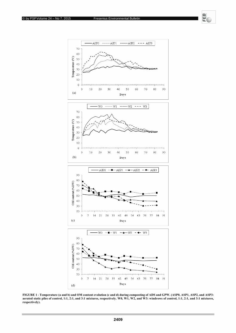
© by PSP Volume 24 – No 7. 2015 Fresenius Environmental Bulletin
2409
FIGURE 1 - Temperature (a and b) and OM content evolution (c and d) during composting of ADS and GPW. (ASP0, ASP1, ASP2, and ASP3: aerated static piles of control, 1:1, 2:1, and 3:1 mixtures, respectively. W0, W1, W2, and W3: windrows of control, 1:1, 2:1, and 3:1 mixtures, respectively).
(a)
(b)
(c)
(d)
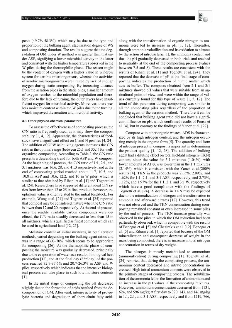
© by PSP Volume 24 – No 7. 2015 Fresenius Environmental Bulletin
2410
posts (49.7%-58.3%), which may be due to the type and proportion of the bulking agent, stabilization degree of WS and composting duration. The results suggest that the deg-radation of OM under W method was greater than that un-der ASP, signifying a lower microbial activity in the latter and consistent with the higher temperatures observed in the W piles during the thermophilic phase. The reason might be the content of oxygen with a higher value in windrow system for aerobic microorganisms, whereas the activities of aerobic microorganisms were limited by lack of enough oxygen during static composting. By increasing distance from the aeration pipes in the static piles, a smaller amount of oxygen reaches to the microbial population and there-fore due to the lack of turning, the outer layers have insuf-ficient oxygen for microbial activity. Moreover, there was less moisture content within the W piles due to the turning, which improved the aeration and microbial activity. 3.3. Other physico-chemical parameters
To assess the effectiveness of composting process, the C/N ratio is frequently used, as it may show the compost stability [1, 4, 12]. Apparently, the characteristics of feed-stock have a significant effect on C and N profiles [4, 24]. The addition of GPW as bulking agents increases the C/N ratio in the optimal range (between 25:1 and 35:1) for well-organized composting. According to Table 2, the C/N ratio presents a descending trend for both ASP and W compost. At the beginning of process, the C/N ratio of 1:1, 2:1, and 3:1 mixtures was 16.6, 28, and 41.3 respectively, and at the end of composting period reached about 11.7, 10.5, and 10.8 in ASP and 10.6, 12.2, and 10 in W piles, which is similar to that obtained by Rihani et al. [1] and Tognetti et al. [24]. Researchers have suggested different ideal C/N ra-tios from lower than 12 to 25 in final product; however, the optimum value is often related to the initial feedstock. For example, Wong et al. [24] and Tognetti et al. [25] reported that compost may be considered mature when the C/N ratio is lower than 17 and 20, respectively. At the end of process, once the readily available carbon compounds were de-clined, the C/N ratio steadily decreased to less than 15 in all mixtures, which is qualified as finest compost which can be used in agricultural land [12, 25].
Moisture content of initial mixtures, in both aeration methods, varied depending on the bulking agent ratios and was in a range of 60–70%, which seems to be appropriate for composting [26]. At the thermophilic phase of com-posting the moisture was gradually decreased, principally due to the evaporation of water as a result of biological heat production [12], and at the final day (83rd day) of the pro-cess reached 32.7-37.6% and 20.7-26.3% in ASP and W piles, respectively which indicates that no intensive biolog-ical process can take place in such low moisture contents [1].
In the initial stage of composting the pH decreased slightly due to the formation of acids resulted from the de-composition of OM. Afterward, intense activity of proteo-lytic bacteria and degradation of short chain fatty acids
along with the transformation of organic nitrogen to am-monia were led to increase in pH [1, 12]. Thereafter, through ammonia volatilization and its oxidation to nitrates by the action of nitrobacteria [1], the ammonia content and thus the pH gradually decreased in both trials and reached to neutrality at the end of the composting process (values between 7.5 and 8). These results are consistent with the results of Rihani et al. [1] and Tognetti et al. [24]. They reported that the decrease of pH at the final stage of com-posting indicates the production of humic matter which acts as buffer. The composts obtained from 2:1 and 3:1 mixtures showed pH values that were suitable from an ag-ricultural point of view, and were within the range of val-ues currently found for this type of waste [1, 5, 12]. The trend of this parameter during composting was similar in all the composting piles regardless of the proportion of bulking agent or the aeration method. Therefore it can be concluded that bulking agent ratio did not have a signifi-cant influence on pH, which confirmed results of Ponsa et al. [4], but in contrary to the findings of Yanez et al. [27].
Compare with other organic wastes, ADS is character-ized by its high nitrogen content, and the nitrogen occur-ring mostly in the organic form [5]. The quantity and form of nitrogen present in compost is important in determining the product quality [1, 12, 28]. The addition of bulking agent had a diluting effect on total kjeldahl nitrogen (TKN) content, since the value for 3:1 mixtures (1.04%), with lower amounts of ADS, was lower than in the 1:1 mixtures (2.14%), which is consistent with the Yanez et al.(2009) results [4]. TKN in the products was 2.65%, 2.09%, and 1.62% for 1:1, 2:1, and 3:1 ASP, respectively, and 2.73%, 1.12%, and 1.97% for the 1:1, 2:1, and 3:1 W, respectively which have a good compliance with the findings of Tognetti et al. [24]. A decrease in TKN may be expected due to the mineralization of nitrogen and transformation to ammonia and afterward nitrates [12]. However, this trend was not observed and the TKN concentration during com-posting remained constant or even increased in some piles by the end of process. The TKN increase generally was observed in the piles in which the OM reduction had been particularly observed, which is compatible with the results of Banegas et al. [5] and Chazirakis et al. [12]. Banegas et al. [5] and Rihani et al. [1] reported that because of the OM mineralization and consequent decrease of weight in the mass being composted, there is an increase in total nitrogen concentration in terms of dry weight.
The nitrogen is mostly metabolized to ammonium (ammonification) during composting [1]. Tognetti et al., [24] reported that during the composting process, the am-monium content decreased and nitrate concentration in-creased. High initial ammonium contents were observed in the primary stages of composting process. The solubiliza-tion of the ammonia led to the formation of ammonium and an increase in the pH values in the composting mixtures. However, ammonium concentration decreased from 1131, 624, and 596 mg/kg at first day to 320, 143, and 146 mg/kg in 1:1, 2:1, and 3:1 ASP, respectively and from 1219, 766,
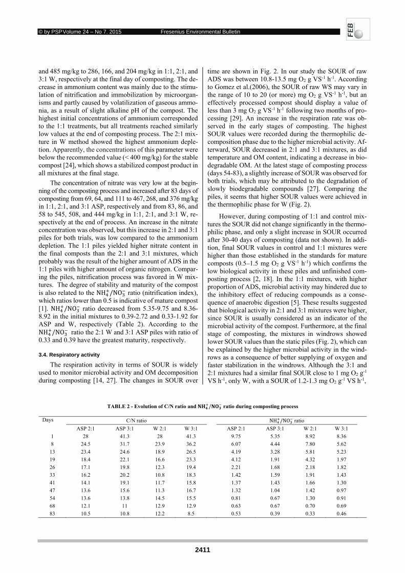
© by PSP Volume 24 – No 7. 2015 Fresenius Environmental Bulletin
2411
and 485 mg/kg to 286, 166, and 204 mg/kg in 1:1, 2:1, and 3:1 W, respectively at the final day of composting. The de-crease in ammonium content was mainly due to the stimu-lation of nitrification and immobilization by microorgan-isms and partly caused by volatilization of gaseous ammo-nia, as a result of slight alkaline pH of the compost. The highest initial concentrations of ammonium corresponded to the 1:1 treatments, but all treatments reached similarly low values at the end of composting process. The 2:1 mix-ture in W method showed the highest ammonium deple-tion. Apparently, the concentrations of this parameter were below the recommended value (< 400 mg/kg) for the stable compost [24], which shows a stabilized compost product in all mixtures at the final stage.
The concentration of nitrate was very low at the begin-ning of the composting process and increased after 83 days of composting from 69, 64, and 111 to 467, 268, and 376 mg/kg in 1:1, 2:1, and 3:1 ASP, respectively and from 83, 86, and 58 to 545, 508, and 444 mg/kg in 1:1, 2:1, and 3:1 W, re-spectively at the end of process. An increase in the nitrate concentration was observed, but this increase in 2:1 and 3:1 piles for both trials, was low compared to the ammonium depletion. The 1:1 piles yielded higher nitrate content in the final composts than the 2:1 and 3:1 mixtures, which probably was the result of the higher amount of ADS in the 1:1 piles with higher amount of organic nitrogen. Compar-ing the piles, nitrification process was favored in W mix-tures. The degree of stability and maturity of the compost is also related to the NH /NO ratio (nitrification index), which ratios lower than 0.5 is indicative of mature compost [1]. NH /NO ratio decreased from 5.35-9.75 and 8.36-8.92 in the initial mixtures to 0.39-2.72 and 0.33-1.92 for ASP and W, respectively (Table 2). According to the NH /NO ratio the 2:1 W and 3:1 ASP piles with ratio of 0.33 and 0.39 have the greatest maturity, respectively.
3.4. Respiratory activity
The respiration activity in terms of SOUR is widely used to monitor microbial activity and OM decomposition during composting [14, 27]. The changes in SOUR over
time are shown in Fig. 2. In our study the SOUR of raw ADS was between 10.8-13.5 mg O2 g VS-1 h-1. According to Gomez et al.(2006), the SOUR of raw WS may vary in the range of 10 to 20 (or more) mg O2 g VS-1 h-1, but an effectively processed compost should display a value of less than 3 mg O2 g VS-1 h-1 following two months of pro-cessing [29]. An increase in the respiration rate was ob-served in the early stages of composting. The highest SOUR values were recorded during the thermophilic de-composition phase due to the higher microbial activity. Af-terward, SOUR decreased in 2:1 and 3:1 mixtures, as did temperature and OM content, indicating a decrease in bio-degradable OM. At the latest stage of composting process (days 54-83), a slightly increase of SOUR was observed for both trials, which may be attributed to the degradation of slowly biodegradable compounds [27]. Comparing the piles, it seems that higher SOUR values were achieved in the thermophilic phase for W (Fig. 2).
However, during composting of 1:1 and control mix-tures the SOUR did not change significantly in the thermo-philic phase, and only a slight increase in SOUR occurred after 30-40 days of composting (data not shown). In addi-tion, final SOUR values in control and 1:1 mixtures were higher than those established in the standards for mature composts (0.5–1.5 mg O2 g VS-1 h-1) which confirms the low biological activity in these piles and unfinished com-posting process [2, 18]. In the 1:1 mixtures, with higher proportion of ADS, microbial activity may hindered due to the inhibitory effect of reducing compounds as a conse-quence of anaerobic digestion [5]. These results suggested that biological activity in 2:1 and 3:1 mixtures were higher, since SOUR is usually considered as an indicator of the microbial activity of the compost. Furthermore, at the final stage of composting, the mixtures in windrows showed lower SOUR values than the static piles (Fig. 2), which can be explained by the higher microbial activity in the wind-rows as a consequence of better supplying of oxygen and faster stabilization in the windrows. Although the 3:1 and 2:1 mixtures had a similar final SOUR close to 1 mg O2 g-1 VS h-1, only W, with a SOUR of 1.2-1.3 mg O2 g-1 VS h-1,
TABLE 2 - Evolution of C/N ratio and / ratio during composting process
Days C/N ratio NH /NO ratio
ASP 2:1 ASP 3:1 W 2:1 W 3:1 ASP 2:1 ASP 3:1 W 2:1 W 3:1
1 28 41.3 28 41.3 9.75 5.35 8.92 8.36
8 24.5 31.7 23.9 36.2 6.07 4.44 7.80 5.62
13 23.4 24.6 18.9 26.5 4.19 3.28 5.81 5.23
19 18.4 22.1 16.6 23.3 4.12 1.91 4.32 1.97
26 17.1 19.8 12.3 19.4 2.21 1.68 2.18 1.82
33 16.2 20.2 10.8 18.3 1.42 1.59 1.91 1.43
41 14.1 19.1 11.7 15.8 1.37 1.43 1.66 1.30
47 13.6 15.6 11.3 16.7 1.32 1.04 1.42 0.97
54 13.6 13.8 14.5 15.5 0.81 0.67 1.30 0.91
68 12.1 11 12.9 12.9 0.63 0.67 0.70 0.69
83 10.5 10.8 12.2 8.5 0.53 0.39 0.33 0.46
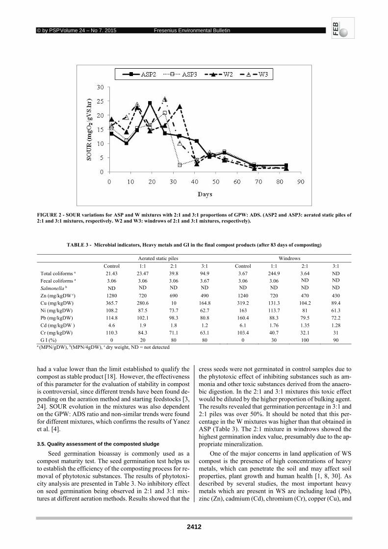
© by PSP Volume 24 – No 7. 2015 Fresenius Environmental Bulletin
2412
FIGURE 2 - SOUR variations for ASP and W mixtures with 2:1 and 3:1 proportions of GPW: ADS. (ASP2 and ASP3: aerated static piles of 2:1 and 3:1 mixtures, respectively. W2 and W3: windrows of 2:1 and 3:1 mixtures, respectively).
TABLE 3 - Microbial indicators, Heavy metals and GI in the final compost products (after 83 days of composting)
Aerated static piles Windrows
Control 1:1 2:1 3:1 Control 1:1 2:1 3:1
Total coliforms a 21.43 23.47 39.8 94.9 3.67 244.9 3.64 ND
Fecal coliforms a 3.06 3.06 3.06 3.67 3.06 3.06 ND ND
Salmonella b ND ND ND ND ND ND ND ND
Zn (mg/kgDW c) 1280 720 690 490 1240 720 470 430
Cu (mg/kgDW) 365.7 280.6 10 164.8 319.2 131.3 104.2 89.4
Ni (mg/kgDW) 108.2 87.5 73.7 62.7 163 113.7 81 61.3
Pb (mg/kgDW) 114.8 102.1 98.3 80.8 160.4 88.3 79.5 72.2
Cd (mg/kgDW ) 4.6 1.9 1.8 1.2 6.1 1.76 1.35 1.28
Cr (mg/kgDW) 110.3 84.3 71.1 63.1 103.4 40.7 32.1 31
G I (%) 0 20 80 80 0 30 100 90 a (MPN/gDW), b(MPN/4gDW), c dry weight, ND = not detected
had a value lower than the limit established to qualify the compost as stable product [18]. However, the effectiveness of this parameter for the evaluation of stability in compost is controversial, since different trends have been found de-pending on the aeration method and starting feedstocks [3, 24]. SOUR evolution in the mixtures was also dependent on the GPW: ADS ratio and non-similar trends were found for different mixtures, which confirms the results of Yanez et al. [4].
3.5. Quality assessment of the composted sludge
Seed germination bioassay is commonly used as a compost maturity test. The seed germination test helps us to establish the efficiency of the composting process for re-moval of phytotoxic substances. The results of phytotoxi-city analysis are presented in Table 3. No inhibitory effect on seed germination being observed in 2:1 and 3:1 mix-tures at different aeration methods. Results showed that the
cress seeds were not germinated in control samples due to the phytotoxic effect of inhibiting substances such as am-monia and other toxic substances derived from the anaero-bic digestion. In the 2:1 and 3:1 mixtures this toxic effect would be diluted by the higher proportion of bulking agent. The results revealed that germination percentage in 3:1 and 2:1 piles was over 50%. It should be noted that this per-centage in the W mixtures was higher than that obtained in ASP (Table 3). The 2:1 mixture in windrows showed the highest germination index value, presumably due to the ap-propriate mineralization.
One of the major concerns in land application of WS compost is the presence of high concentrations of heavy metals, which can penetrate the soil and may affect soil properties, plant growth and human health [1, 8, 30]. As described by several studies, the most important heavy metals which are present in WS are including lead (Pb), zinc (Zn), cadmium (Cd), chromium (Cr), copper (Cu), and

© by PSP Volume 24 – No 7. 2015 Fresenius Environmental Bulletin
2413
nickel (Ni) [1, 8]. Concentration of these heavy metals in the end-product of composting piles has been evaluated as shown in Table 3. Heavy metals concentration of compost products were found in levels lower than the international limits approved by USEPA (1995) [31], due to the fact that the main load of the treated wastewater was municipal sew-age. According to these limits, all composts could be clas-sified as type A compost. Some studies [8, 30] confirmed that the concentration of heavy metals in municipal WS compost is in the acceptable limits. Heavy metals are much less soluble at high pH levels of compost, making them less bioavailable in soil [8]. Other studies [1, 8] have demon-strated that the types of composting, raw materials, and bulking agents are major parameters could influence the metal concentration in composted materials. Smith [8] has reported that aerobic composting processes compared to other waste stabilization methods increase the complexa-tion of heavy metals in organic residuals and limiting their solubility and bioavailability in soil.
One of the problems posed by the direct use of WS in agriculture is the risk of plant and human contamination by pathogens [1, 5]. For compost sanitation, the EPA recom-mended a limit of 103 MPN g-1 (dry weight) for fecal coli-forms and 3 MPN 4g-1 (dry weight) for Salmonella [31]. The results of our study revealed that the density of these indicators in all the final composts was below the limits (Table 3). As shown in Table 3, the material in control pile was also sanitized, probably due to reduced moisture and solar disinfection. The results revealed that both compost-ing processes are quite efficient in the removal of indicator and pathogenic microorganisms. Even though efficient re-duction of pathogens was achieved in both systems, wind-row method, due to the higher temperatures with longer du-ration, is a more reliable method to achieve USEPA [31] class A compost requirements.
4. CONCLUSIONS
The present study showed that W method was superior to the ASP for ADS composting. Application of GPW, as a low cost bulking agent, in 2:1 and 3:1 ratios of GPW: ADS strongly enhanced the OM mineralization through moisture reduction, improved air distribution, and better microbial activity. A high degree of stability and maturity was achieved in 2:1 (GPW: ADS) W in terms of OM con-tent reduction, final SOUR value, NH /NO ratio, C/N ra-tio, and GI. The final compost product was also well sani-tized as a result of the high temperatures achieved.
ACKNOWLEDGEMENTS
This research was conducted with funding from the vice chancellery for research of Isfahan University of Med-ical Sciences (Research Project # 391442) as a part of PhD dissertation. The authors wish to acknowledge Mr. Ghoba-
dian, Mr. Rabierad, Mr. Amini, and Ms. Javadi, from Isfa-han Water and Wastewater Co., for technical support and Mr. Farrokhzadeh, Ms. Vahid Dastjerdy, and Ms. Hatam-zadeh for their assistance in supplying laboratory facilities of this research and valuable advice.
The authors have declared no conflict of interest. REFERENCES
[1] Rihani, M., Malamis, D., Bihaoui, B., Etahiri, S., Loizidou, M. and Assobhei, O. (2010) In-vessel treatment of urban primary sludge by aerobic composting. Bioresource Technol. 101: 5988-5995.
[2] Gea, T., Barrena, R., Artola, A. and Sanchez, A. (2007) Opti-mal bulking agent particle size and usage for heat retention and disinfection in domestic wastewater sludge composting. Waste Manage. 27: 1108-1116.
[3] Lasaridi, K., Stentiford, E. and Evans, T. (2000) Windrow composting of wastewater biosolids: process performance and product stability assessment. Water Sci. Technol. 42: 217-226.
[4] Yanez, R., Alonso, J.L. and Diaz, M.J. (2009) Influence of bulking agent on sewage sludge composting process. Biore-source Technol. 100: 5827-5833.
[5] Banegas, V., Moreno, J.L., Moreno, J.I., Garcia, C., Leon, G. and Hernandez, T. (2007) Composting anaerobic and aerobic sewage sludges using two proportions of sawdust. Waste Man-age. 27: 1317-1327.
[6] Singh, R. and Agrawal, M. (2008) Potential benefits and risks of land application of sewage sludge. Waste Manage. 28: 347-358.
[7] Zorpas, A.A., Kapetanios, E., Zorpas, G.A., Karlis, P., Vlys-sides, A., Haralambous, I. and Loizidou, M. (2000) Compost produced from organic fraction of municipal solid waste, pri-mary stabilized sewage sludge and natural zeolite. J. Hazard. Mater. 77: 149-159.
[8] Smith, S.R. (2009) A critical review of the bioavailability and impacts of heavy metals in municipal solid waste composts compared to sewage sludge. Environ. Int. 35: 142-156.
[9] Cukjati, N., Zupancic, G.D., Ros, M. and Grilc, V. (2012) Composting of anaerobic sludge: An economically feasible el-ement of a sustainable sewage sludge management. J. Environ. Manage. 106: 48-55.
[10] Miner, F.D., Koenig, R.T. and Miller, B.E. (2001) The influ-ence of bulking material type and volume on in-house com-posting in high-rise, caged layer facilities. Compost Sci. Util. 9: 50-59.
[11] Ruggieri, L., Artola, A., Gea, T. and Sanchez, A. (2008) Bio-degradation of animal fats in a co-composting process with wastewater sludge. Int. Biodeter. Biodegr. 62: 297-303.
[12] Chazirakis, P., Giannis, A., Gidarakos, E., Wang, J. and Steg-mann, R. (2011) Application of sludge, organic solid wastes and yard trimmings in aerobic compost piles. Global NEST J. 13: 405-411.
[13] Luo, W., Chen, T., Zheng, G., Gao, D., Zhang, Y. and Gao, W. (2008) Effect of moisture adjustments on vertical temperature distribution during forced-aeration static-pile composting of sewage sludge. Resour. Conserv. Recy. 52: 635-642.
[14] Lasaridi, K.E. and Stentiford, E.I. (1998) A simple respiro-metric technique for assessing compost stability. Water Res. 32: 3717-3723.
© by PSP Volume 24 – No 7. 2015 Fresenius Environmental Bulletin
2414
[15] Hafidi, M., Amir, S., Jouraiphy, A., Winterton, P., El Gharous, M., Merlina, G. and Revel, J.C. (2008) Fate of polycyclic aro-matic hydrocarbons during composting of activated sewage sludge with green waste. Bioresource Technol. 99: 8819-8823.
[16] Jouraiphy, A., Amir, S., El Gharous, M., Revel, J.C. and Hafidi, M. (2005) Chemical and spectroscopic analysis of organic mat-ter transformation during composting of sewage sludge and green plant waste. Int. Biodeter. Biodegr. 56: 101-108.
[17] Wang, K., Li, W., Guo, J., Zou, J., Li, Y. and Zhang, L. (2011) Spatial distribution of dynamics characteristic in the intermit-tent aeration static composting of sewage sludge. Bioresource Technol. 102: 5528-5532.
[18] Thompson, W., Leege, P., Millner, P. and Watson, M. (2001) Test Methods for the Examination of Composting and Compost. The United States Composting Council Research and Education Foundation The United States Department of Agriculture.
[19] Abdullah, N. and Chin N.L. (2010) Simplex-centroid mixture formulation for optimised composting of kitchen waste. Bio-resource Technol. 101: 8205-8210.
[20] Zeng, G., Yu, M., Chen, Y., Huang, D., Zhang, J., Huang, H., Jiang, R. and Yu, Z. (2010) Effects of inoculation with Phan-erochaete chrysosporium at various time points on enzyme ac-tivities during agricultural waste composting. Bioresource Technol. 101: 222-227.
[21] American Public Health Association (APHA). (2012) Stand-ard Methods for the Examination of Water and Wastewater, 22nd ed, Washington DC.
[22] Tiquia, S., Tam, N. and Hodgkiss, I. (1996) Effects of com-posting on phytotoxicity of spent pig-manure sawdust litter. Environ. Pollut. 93: 249-256.
[23] Lu, L.A., Kumar, M., Tsai, J.C. and Lin, J.G. (2008) High-rate composting of barley dregs with sewage sludge in a pilot scale bioreactor. Bioresource Technol. 99: 2210-2217.
[24] Tognetti, C., Mazzarino, M. and Laos, F. (2007) Cocompost-ing biosolids and municipal organic waste: effects of process management on stabilization and quality. Biol. Fert. Soils 43: 387-397.
[25] Wong, J., Mak, K., Chan, N., Lam, A., Fang, M., Zhou, L., Wu, Q.T. and Liao, X.D. (2001) Co-composting of soybean residues and leaves in Hong Kong. Bioresour. Technol. 76: 99-106.
[26] Malinska, K. and Zabochnicka-Swiatek M. (2013) Selection of bulking agents for composting of sewage sludge. Environ. Prot. Eng. 39: 91-103.
[27] Ponsa, S., Pagans, E. and Sanchez, A. (2009) Composting of dewatered wastewater sludge with various ratios of pruning waste used as a bulking agent and monitored by respirometer. Biosyst. Eng. 102: 433-443.
[28] De Guardia, A., Petiot, C., Rogeau, D. and Druilhe, C. (2008) Influence of aeration rate on nitrogen dynamics during com-posting. Waste manage. 28: 575-587.
[29] Gomez, R.B., Lima, F.V. and Ferrer, A.S. (2006) The use of respiration indices in the composting process: a review. Waste Manage. Res. 24: 37-47.
[30] Zorpas, A.A., Inglezakis, V.J. and Loizidou, M. (2008) Heavy metals fractionation before, during and after composting of sewage sludge with natural zeolite. Waste manage. 28: 2054-2060.
[31] USEPA (1995) guide to the biosolids risk assessment for the EPA Part 503 Rule EPA: B32-B-93-005. United States Envi-ronmental Protection Agency Office of Wastewater Manage-ment, Washington DC.
Received: October 30, 2014 Revised: December 29, 2014 Accepted: January 19, 2015 CORRESPONDING AUTHOR
Amir Hossein Nafez Department of Environmental Health Engineering School of Public Health Kermanshah University of Medical Sciences Kermanshah IRAN Phone: +98 833 826 4447 Fax: +98 833 826 3048 E-mail: [email protected]
FEB/ Vol 24/ No 7/ 2015 – pages 2406 – 2414

© by PSP Volume 24 – No 7. 2015 Fresenius Environmental Bulletin
2415
ADSORPTION OF CARMINE ON ETHYLENEDIAMINE
MODIFIED PEANUT HUSK FROM AQUEOUS SOLUTION
Yinghua Song*, Xi Zhang, Mei Ye, Hui Xu and Jianmin Ren
Department of Chemistry and Chemical Engineering; Chongqing Key Lab of Catalysis & Functional Organic Molecules, Chongqing Technology and Business University, Chongqing 400067, China
ABSTRACT
A new adsorbent was synthesized from peanut husk, an agricultural by-product, in which epichlorohydrin was used as a cross-linking agent and ethylenediamine as a modifica-tion agent. Factors affecting the adsorption behavior of this adsorbent for carmine in aqueous solution, namely, pH value, adsorption time, temperature and initial carmine concen-tration were evaluated through experiments in a batch sys-tem. It was concluded that the maximal adsorption capacity of this adsorbent for carmine was 95.2 mg / g at 303 K, which was improved 17.6 times as much as that of the un-modified peanut husk. The Langmuir isotherm model can provide a better description for the adsorption equilibrium when it was compared with the Freundlich equation under the conditions of the present study. In order to examine the controlling mechanisms of the process, kinetic equations of the mass transfer and chemical reaction, the Largergren first order model, the pseudo-second order model and the intra-particle diffusion model were used to correlate the experi-mental data. It was found that the intra-particle diffusion is the significant controlling step under the experimental con-ditions but it was not the unique one and it accompanied with chemical reactions. It showed that the peanut husk modified with ethylenediamine had good performance for removal of azo-dye and can be used as a highly efficient biomass adsorbent to treat dyes-containing wastewater.
KEYWORDS: peanut husk; ethylenediamine; modification; ad-sorption; carmine
1. INTRODUCTION
Synthetic dyes are widely used in various industries, such as paper, textiles, leather, plastics, printing and cos-metics. The discharged colored wastewater not only causes serious environmental issues, but also hazards human be-ings’ health due to their toxicity and carcinogenicity [1, 2]. Such effluent must be treated before discharged into the environment. But many synthetic dyes are difficult to be
* Corresponding author
degraded because of their complex aromatic species and xenobiotic properties. Among the most useful dyes, there is carmine that is used as an additive in pharmaceutical tab-lets and capsules, in confectionery items and etc. It has been shown that carmine may cause increasing risk of can-cer and many other diseases due to its carcinogenic and mutagenic characteristics.
There are many physical and chemical processes avail-able to remove dyes, such as advanced oxidation, com-bined chemical and biochemical process, adsorption mem-brane filtration, aerobic and anaerobic digestion. Nowa-days activated carbon works as adsorbent to remove dyes in most commercial systems because of its high adsorption ability. But the processing costs are still expensive. So peo-ple try to develop cheaper and effective adsorbents to re-move dyes and find an alternative method from different starting materials such as bagasse pith [3], rice husk [4], clay [5], sawdust [6], hen feather [7], polar leaf [8], papaya seed [9], and etc.
Peanut husk, an agricultural by-product available in large quantity in China, is often burned and discarded di-rectly, which produced waste gas and dust. Fortunately, a possible solution to utilize peanut husk as an adsorbent has been found to remove contaminants in waste water. Peanut husk was introduced directly as a low-cost adsorbent for the efficient removal of Sunset Yellow dye in aqueous so-lution [10]. However, raw peanut husk cannot be used as a good natural adsorbent due to two major limitations. Firstly, on its contact with water, there is a leaching of yel-lowish color into solutions; secondly, on its prolonged con-tact with water, peanut husk tends to scatter. Researchers have studied the removal of heavy metals [11], phenol [12] and dyes [13, 14] by partially carbonized peanut husk or by activated carbon from peanut husk. The purpose of this work was to produce a new adsorbent from peanut husk chemically modified with ethylenediamine and the adsorp-tion of carmine on it was investigated. The experiments were done in the same batch system to evaluate the adsorp-tion capacity of the adsorbent, and the adsorption of car-mine was studied on account of the initial carmine concen-tration, pH, adsorption time and temperature. The equilib-rium of adsorption was modeled with the Langmuir and the Freundlich isotherms. The kinetic parameters and intra-particle diffusion were also determined for this process.
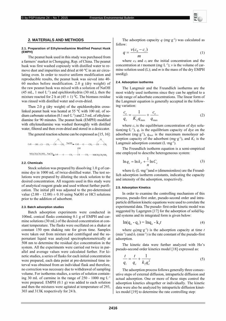
© by PSP Volume 24 – No 7. 2015 Fresenius Environmental Bulletin
2416
2. MATERIALS AND METHODS
2.1. Preparation of Ethylenediamine Modified Peanut Husk (EMPH)
The peanut husk used in this study was purchased from a farmers’ market in Chongqing, Rep. of China. The peanut husk was first washed copiously with distilled water to re-move dust and impurities and dried at 60 in an air circu-lating oven. In order to receive uniform modification and reproducible results, the peanut husk was sieved into 40- 60 meshes before modification. 2.0 g (dry weight) of the raw peanut husk was mixed with a solution of NaOH (45 mL, 1 mol·L-1) and epichlorohydrin (30 mL), then the mixture reacted for 2 h at (45 ± 1) . The biomass residue was rinsed with distilled water and oven-dried.
Then 2.0 g (dry weight) of the epichlorohydrin cross-linked peanut husk was heated at 55 with 100 mL of so-dium carbonate solution (0.1 mol·L-1) and 2.5 mL of ethylene-diamine for 90 minutes. The peanut husk (EMPH) modified with ethylenediamine was washed thoroughly with distilled water, filtered and then oven-dried and stored in a desiccator.
The general reaction scheme can be expressed as [15, 16]:
2.2. Chemicals
Stock solution was prepared by dissolving 1.0 g of car-mine dye in 1000 mL of twice-distilled water. The test so-lutions were prepared by diluting the stock solution to the desired concentration. All reagents used in this study were of analytical reagent grade and used without further purifi-cation. The initial pH was adjusted to the pre-determined value (2.00 - 12.00) ± 0.10 using NaOH or HCl solutions prior to the addition of adsorbent.
2.3. Batch adsorption studies
Batch adsorption experiments were conducted in 100mL conical flasks containing 0.1 g of EMPH and car-mine solutions (30 mL) of the desired concentration at con-stant temperature. The flasks were oscillated on a shaker at constant 150 rpm shaking rate for given time. Samples were taken out from mixture and centrifuged and the su-pernatant liquid was analyzed spectrophotometrically at 508 nm to determine the residual dye concentration in the system. All the experiments were carried out twice in par-allel and average values were calculated further. For ki-netic studies, a series of flasks for each initial concentration were prepared, each data point at pre-determined time in-terval was obtained from an individual flask and therefore, no correction was necessary due to withdrawal of sampling volume. For isotherms studies, a series of solution contain-ing 30 mL of carmine in the range of 250 - 1000 mg·L-1 were prepared. EMPH (0.1 g) was added to each solution and then the mixtures were agitated at temperature of 293, 303 and 313K respectively for 24 h.
The adsorption capacity q (mg·g-1) was calculated as follow:
m
ccvq t )( 0 (1)
where c0 and ct are the initial concentration and the concentration at t moment (mg·L-1); v is the volume of car-mine solution used (L); and m is the mass of the dry EMPH used(g).
2.4. Adsorption isotherms
The Langmuir and the Freundlich isotherms are the most widely used isotherms since they can be applied to a wide range of adsorbate concentrations. The linear form of the Langmuir equation is generally accepted in the follow-ing variation:
maxmax
1
q
c
qKq
c e
Le
e (2)
where ce is the equilibrium concentration of dye solu-tion(mg·L-1), qe is the equilibrium capacity of dye on the adsorbent (mg·g-1), qmax is the maximum monolayer ad-sorption capacity of the adsorbent (mg·g-1), and KL is the Langmuir adsorption constant (L·mg-1).
The Freundlich isotherm equation is a semi-empirical one employed to describe heterogeneous system:
eFe Cn
kq ln1
lnln (3)
where kF (L·mg-1)and n (dimensionless) are the Freund-lich adsorption isotherm constants, indicating the capacity and intensity of the adsorption, respectively.
2.5. Adsorption Kinetics
In order to examine the controlling mechanism of this process, pseudo-first order, pseudo-second order and intra-particle diffusion kinetic equations were used to correlate the experimental data. The pseudo- first order kinetic model was suggested by Lagergren [17] for the adsorption of solid/liq-uid systems and its integrated form is given below:
t1ete k - lnq= )q - ln(q (4)
where qt(mg·g-1) is the adsorption capacity at time t (min-1) and k1 (min-1) is the rate constant of the pseudo-first adsorption.
The kinetic data were further analyzed with Ho’s pseudo-second order kinetics model [18] expressed as:
22
1
eet qkq
t
q
t (5)
The adsorption process follows generally three consec-utive steps of external diffusion, intraparticle diffusion and actual adsorption. One or more of these steps control the adsorption kinetics altogether or individually. The kinetic data were also be analyzed by intraparticle diffusion kinet-ics model [19] to determine the rate controlling step:
Cell OH + Cl CH2 CH CH2
O
OCell
O
CH2CHCH2NaOH
NH2CH2CH2NH2 , NaCO3 CH2 CH CH2Cell O
OH
NHCH2CH2NH2

© by PSP Volume 24 – No 7. 2015 Fresenius Environmental Bulletin
2417
Ctkq pt 2/1 (6)
where kp (mg·min-1/2·g-1) is the intraparticle diffusion rate constant and C (mg·g-1) is a constant, k2 (g·mg-1·min-1) is the rate constant of the pseudo-second order adsorption.
For elucidation of the adsorption rate controlling mechanism, the Wünwald-Wagner intraparticle diffusion model was also proposed to give the intraparticle diffusion coefficient, D(cm2·s-1) [20]:
td
D
q
q
e
t2
2
2 303.2
4)
6lg()1lg(
(7)
where d (cm) is the mean particle diameter. 3. RESULTS AND DISCUSSION
3.1. Effect of initial pH of solution
The pH value of the solution was an important factor that must be considered in the adsorption process. The ini-tial pH of the working solutions was adjusted to between pH 2.0-12.0 by addition of diluting HCl or NaOH solution. The effect of pH on the adsorption of carmine was shown in Fig. 1.
As shown in Fig. 1, a sharp decrease in the adsorption capacity occurs as the pH of the initial solution was in-creased from 2.0 up to 4.0, beyond which the adsorption capacity remains almost constant. For the subsequent stud-ies, pH 2.0 was selected as an optimal pH value.
The higher adsorption capacity of carmine at low pH may be due to the enhanced protonation of -NH2 at the sur-face of the EMPH. It contributed to the preferential adsorp-tion of the negative dye ions to positive active sites and fa-cilitates the diffusion process in the working solution. As increasing pH, protonation reduces and electrostatic repul-sive force becomes dominant, which inhibits the diffusion and adsorption of carmine on EMPH.
FIGURE 1 - Effect of pH on the adsorption of carmine (T = 303K, c0
= 396.3 mg·L-1, contact time = 24 h, rpm = 150)
3.2. Effect of contact time
Removal of carmine by EMPH was performed with three different initial carmine concentrations at tempera-
ture 303K. According to the results (Fig. 2), the removal of carmine was faster in initial 150 minutes and then became slower and finally reached equilibrium at approximately 1200 minutes. During initial stages, a large number of va-cant sites were available on the surface of EMPH and the adsorption of carmine was very quick. Then the adsorption process became slower due to gradual occupancy of these sites. With increasing time, the occupation of the remain-ing vacant sites was more difficult due to increased repul-sive forces between dye molecules and bulk solution.
FIGURE 2 - Effect of contact time on the adsorption of carmine (T = 303K, pH = 2.0, rpm = 150)
Fig. 2 also shows that the equilibrium capacity of EMPH
increased from 71.48 to 86.15 mg·g-1 as increasing initial con-centration of carmine because the initial carmine concentra-tion provides an important driving force to overcome all mass transfer resistance. The increase of loading capacity of EMPH with increasing carmine concentration may also be derived from the higher interaction between carmine and EMPH.
3.3. Adsorption isotherm parameters
The experimental adsorption isotherms of EMPH at different temperatures are depicted in Fig.3. According to Fig.3, the adsorption of carmine onto EMPH was enhanced by increasing the temperature from 293 K to 313 K at dif-ferent initial dye concentration. The Langmuir and the Freundlich adsorption isotherms were used to evaluate the
adsorption equilibrium data. The Langmuir plot of ee qc /against ce yields straight lines (Fig.4). The isotherm con-stants and correlative coefficients were tabulated in Table 1. The correlative coefficient R2 values in Table 1 confirm that the adsorption equilibrium data fitted very well with the Langmuir model under the studied conditions. This in-dicates uniform adsorption and strong dye-adsorbent inter-actions over the surface of the adsorbent. The maximum monolayer capacity of EMPH is determined as 87.7, 95.2 and 101.0 mg·g-1 for 293, 303 and 313 K, respectively, which suggests an endothermic process. The values of Freundlich constant, kf, increased with increasing tempera-ture and showed easy uptake of carmine by EMPH. All n values were found to be greater than 1, which indicated a favorable adsorption condition during the process.
0 2 4 6 8 10 12 14
20
40
60
80
100
q e / m
g.g-1
pH
300 600 900 12000
20
40
60
80
100
t / min
q t / m
g.g-1
□ 563.3 mg·L-1 ■410.7 mg·L-1 ○254.1 mg·L-1
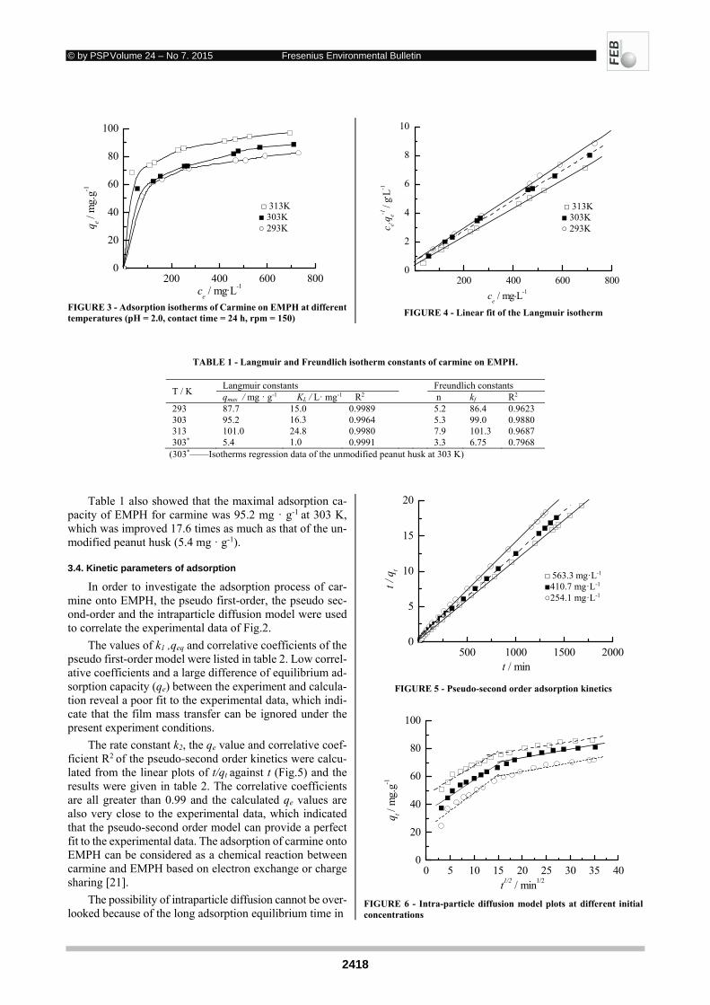
© by PSP Volume 24 – No 7. 2015 Fresenius Environmental Bulletin
2418
FIGURE 3 - Adsorption isotherms of Carmine on EMPH at different temperatures (pH = 2.0, contact time = 24 h, rpm = 150)
FIGURE 4 - Linear fit of the Langmuir isotherm
TABLE 1 - Langmuir and Freundlich isotherm constants of carmine on EMPH.
T / K Langmuir constants Freundlich constants qmax / mg · g-1 KL / L· mg-1 R2 n kf R2
293 87.7 15.0 0.9989 5.2 86.4 0.9623 303 95.2 16.3 0.9964 5.3 99.0 0.9880 313 101.0 24.8 0.9980 7.9 101.3 0.9687 303* 5.4 1.0 0.9991 3.3 6.75 0.7968
(303*——Isotherms regression data of the unmodified peanut husk at 303 K)
Table 1 also showed that the maximal adsorption ca-pacity of EMPH for carmine was 95.2 mg · g-1 at 303 K, which was improved 17.6 times as much as that of the un-modified peanut husk (5.4 mg · g-1).
3.4. Kinetic parameters of adsorption
In order to investigate the adsorption process of car-mine onto EMPH, the pseudo first-order, the pseudo sec-ond-order and the intraparticle diffusion model were used to correlate the experimental data of Fig.2.
The values of k1 ,qeq and correlative coefficients of the pseudo first-order model were listed in table 2. Low correl-ative coefficients and a large difference of equilibrium ad-sorption capacity (qe) between the experiment and calcula-tion reveal a poor fit to the experimental data, which indi-cate that the film mass transfer can be ignored under the present experiment conditions.
The rate constant k2, the qe value and correlative coef-ficient R2 of the pseudo-second order kinetics were calcu-lated from the linear plots of t/qt against t (Fig.5) and the results were given in table 2. The correlative coefficients are all greater than 0.99 and the calculated qe values are also very close to the experimental data, which indicated that the pseudo-second order model can provide a perfect fit to the experimental data. The adsorption of carmine onto EMPH can be considered as a chemical reaction between carmine and EMPH based on electron exchange or charge sharing [21].
The possibility of intraparticle diffusion cannot be over-looked because of the long adsorption equilibrium time in
FIGURE 5 - Pseudo-second order adsorption kinetics
FIGURE 6 - Intra-particle diffusion model plots at different initial concentrations
200 400 600 8000
20
40
60
80
100
.
q e / m
g.g-1
ce / mg L-1
200 400 600 8000
2
4
6
8
10
.
.
c e.qe-1
/ g
L-1
ce / mg L-1
500 1000 1500 20000
5
10
15
20
t / q
t
t / min
0 5 10 15 20 25 30 35 400
20
40
60
80
100
q t / m
g.g-1
t1/2 / min1/2
□ 313K ■ 303K ○ 293K
□ 313K ■ 303K ○ 293K
□ 563.3 mg·L-1 ■410.7 mg·L-1 ○254.1 mg·L-1
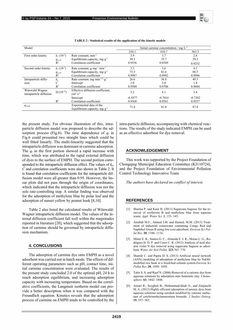
© by PSP Volume 24 – No 7. 2015 Fresenius Environmental Bulletin
2419
TABLE 2 - Statistical results of the application of the kinetic models
Model Initial carmine concentration / mg·L-1 254.1 410.7 563.3
First order kinetic k1 (10-3) Rate constant, min-1 3.9 3.7 2.8 qe,cal Equilibrium capacity, mg·g-1 39.3 35.7 29.3 R2 Correlation coefficient 0.9536 0.8589 0.9252
Second order kinetic k2 (10-3) Rate constant, g·mg-1·min-1 3.3 3.6 4.2 qe,cal Equilibrium capacity, mg·g-1 73.5 82.6 88.5 R2 Correlation coefficient 0.9987 0.9992 0.9996
Intraparticle diffu-sion
kp Rate constant, mg·min-1/2·g-1 26.6 36.8 49.3 C Intercept 2.0 2.0 1.8 R2 Correlation coefficient 0.9588 0.9706 0.9684
Wünwald-Wagner intraparticle diffusion
D (10-10) Effective diffusion coefficient, cm2·s-1
5.2 4.1 3.4
Intercept -0.5877 -0.7016 -0.7202 R2 Correlation coefficient 0.9568 0.9561 0.9557
qe,exp Experimental data of the Equilibrium capacity, mg·g-1
71.8 81.0 87.4
the present study. For obvious illustration of this, intra-particle diffusion model was proposed to describe the ad-sorption process (Fig.6). The time dependence of qt in Fig.6 could presented two straight lines which could be well fitted linearly. The multi-linearity suggested that the intraparticle diffusion was dominant in carmine adsorption. The qt in the first portion showed a rapid increase with time, which was attributed to the rapid external diffusion of dyes to the surface of EMPH. The second portion corre-sponded to the intraparticle diffusion effect. The values of kp, C and correlation coefficients were also shown in Table 2. It is found that correlation coefficients for the intraparticle dif-fusion model were all greater than 0.95. However, the lin-ear plots did not pass through the origin of coordinates, which indicated that the intraparticle diffusion was not the sole rate-controlling step. A similar finding was observed for the adsorption of methylene blue by polar leaf and the adsorption of sunset yellow by peanut husk [8,10].
Table 2 also listed the calculated results of Wünwald-Wagner intraparticle diffusion model. The values of the in-ternal diffusion coefficient fall well within the magnitudes reported in literature [20], which suggested that the adsorp-tion of carmine should be governed by intraparticle diffu-sion mechanism.
4. CONCLUSIONS
The adsorption of carmine dye onto EMPH as a novel adsorbent was carried out in batch mode. The effects of dif-ferent operating parameters such as pH, contact time, ini-tial carmine concentration were evaluated. The results of the present study concluded 2.0 of the optimal pH, 24 h to reach adsorption equilibrium, and increasing adsorption capacity with increasing temperature. Based on the correl-ative coefficients, the Langmuir isotherm model can pro-vide a better description when it was compared with the Freundlich equation. Kinetics reveals that the adsorption process of carmine on EMPH tends to be controlled by the
intra-particle diffusion, accompanying with chemical reac-tions. The results of the study indicated EMPH can be used as an effective adsorbent for dye removal.
ACKNOWLEDGEMENT
This work was supported by the Project Foundation of Chongqing Municipal Education Committee (KJ110724), and the Project Foundation of Environmental Pollution Control Technology Innovative Team.
The authors have declared no conflict of interest. REFERENCES
[1] Sharma P. and Kaur H. (2011) Sugarcane bagasse for the re-moval of erythrosin B and methylene blue from aqueous waste. Appl. Water Sci. 1, 135- 145.
[2] Attallah M.F., Ahmed I.M. and Hamed, M.M. (2013) Treat-ment of industrial wastewater containing Congo Red and Naphthol Green B using low-cost adsorbent. Environ Sci Pol-lut Res. 20, 1106- 1116.
[3] Mitter E. K., Santos G. C., Almeida E. J. R., Morao L. G., Ro-drigues H. D. P. and Corso C. R. (2012) Analysis of acid aliz-arin violet N dye removal using sugarcane bagasse as adsor-bent. Water Air Soil Pollut. 223,765- 770.
[4] Shamik C. and Papita D. S. (2013) Artificial neural network (ANN) modeling of adsorption of methylene blue by NaOH-modified rice husk in a fixed-bed column system.Environ Sci Pollut Res. 20, 1050- 1058.
[5] Tahir S. S. and Rauf N. (2006) Removal of a cationic dye from aqueous solutions by adsorption onto bentonite clay. Chemo-sphere. 63, 1842- 1848.
[6] Ansari R., Seyghali B., Mohammad-khah A., and Zanjanchi M. A. (2012) Highly efficient adsorption of anionic dyes from aqueous solutions using sawdust modified by cationic surfac-tant of cetyltrimethylammonium bromide. J Surfact Deterg. 15, 557- 565.
© by PSP Volume 24 – No 7. 2015 Fresenius Environmental Bulletin
2420
[7] Mittal A., Thakur V. and Gajbe V. (2013) Adsorptive removal of toxic azo dye Amido Black 10B by hen feather.Environ Sci Pollut Res. 20, 260- 269.
[8] Han X., Niu X. and Ma X. (2012) Adsorption characteristics of methylene blue on polar leaf in batch mode:Equilibrium,ki-netics and thermodynamics. Korean J Chem Eng. 29, 494- 502.
[9] Weber C. T., Foletto E.L. and Meili L. (2013) Removal of tan-nery dye from aqueous solution using papaya seed as an effi-cient natural biosorbent. Water Air Soil Pollut. 224, 1427-1437.
[10] Song Y., Liu Y., Chen S., Xu H. and Liao Y. (2014) Sunset yellow adsorption by peanut husk in batch mode. Fresenius Environmental Bulletin. 23, 1074- 1079.
[11] Ricordel S., Taha S., Cisse I. and Dorange G. (2004) Heavy metal removal by adsorption onto peanut husks carbon:char-acterization,kinetic study and modeling. SepPurif Technol. 24, 389- 401.
[12] Gonzo E.E. and Gonzo L.F. (2005) Kinetics of phenol removal from aqueous solution by adsorption onto peanut shell acid activated carbon. Adsorp Sci Technol. 23, 289- 302.
[13] Gong R., Ding Y., Li M., Yang C., Liu H. and Sun Y. (2005) Utilization of powdered peanut hull as biosorbent for removal of anionic dyes from aqueous solution. Dyes Pigments. 64, 187- 192.
[14] Ozer D., Dursun G. and Ozer A. (2007) Methylene blue ad-sorption from aqueous solution by dehydrated peanut hull. J Hazard Mater. 144, 171- 179.
[15] Li B., Li L. and Sun X. (2011) Preparation of Ethylenediamine modified peanutshell and its adsorption behavior for anionic dyes.J South—Central Univ for Nationalities (Nat. Sci. Edi-tion). 30, 20- 24. (in Chinese)
[16] Zou W., Li K., Gao S. and Bai H. (2013) Study on Congo Red adsorption with ethylenediamine modified sawdust. J Zheng-zhou Univ (Engineering Science). 34, 28- 31,36. (in Chinese)
[17] Lagergren S. (1898) About the theory of so-called adsorption of soluble substances. Kungl. Svenska Vetenskapsakademiens Handlingar. 24, 1- 39.
[18] Ho Y.S.and McKay G. (1999) Pseudo-second order model for sorption processes. Process Biochem, 34, 451- 465.
[19] Weber W.J. and Morriss J.C. (1963) Kinetics of adsorption on carbon from solution. J Sanit Eng Div. 89, 31- 60.
[20] Kalavathy M.H., Karthikeyan T., Rajgopal S. and Miranda L. R. (2005) Kinetic and isotherm studies of Cu(II) adsorption onto H3PO4-activated rubber wood sawdust. J Colloid and In-terface Science. 292, 354- 362.
[21] Wang G., Li L., Li Y. and Xue Q. (2010) Study on the prepa-ration of bamboo activated carbon and its phenol adsorption properties. J Chem Eng of Chinese Univ. 4, 700- 704. (in Chi-nese)
Received: October 24, 2014 Revised: December 15, 2014 Accepted: January 09, 2015 CORRESPONDING AUTHOR
Dr. Yinghua Song Department of Chemistry and Chemical Engineering College of Environmental and Biological Engineering Chongqing Technology and Business University Chongqing 400067 P.R. CHINA Phone: +86-023-62769785(office) Fax: +86-023-62769785 E-mail: [email protected]
FEB/ Vol 24/ No 7/ 2015 – pages 2415 – 2420

© by PSP Volume 24 – No 7. 2015 Fresenius Environmental Bulletin
2421
SUBJECT INDEX
A activated carbon 2341 adsorption 2341 adsorption 2415 alluvial lands 2374 antioxidant efficiency 2310
B β-adrenoceptor antagonists 2310 biohydrogen 2289
C Calix[4]resorcinarenes 2296 carmine 2415 Cd-localization 2394 cell damage 2394 cell division 2394 cereal 2275 compost 2406 copper (Cu) 2394 cropland 2354
E energy 2362 environment 2275 erosion 2319 ethylenediamine 2415
F factor analysis 2374 filter-feeding fish 2384
G geographical information systems 2374 green plant wastes 2406 groundwater irrigation 2325
H Hordeum vulgare 2394 human health 2275
I inactivation 2334 initial total solids 2289 ion exchange 2348 irrigation 2319 isotherm 2354
L landfill gas 2362 limitations 2362
M Mediterranean 2264
M metals ions 2296 microcystin 2384 Microcystis bloom 2384 modification 2415 municipal wastewater 2296
N NASA-CASA Model 2264 NPP 2264 nucleoprotein 2394
O organic solid waste 2289 oxytetracycline 2348
P particle size 2289 peanut husk 2415 pesticide application 2275 phosphorus transport 2325 photocatalysis 2348 photocatalytic degradation 2280 photosynthetic activity 2384 polymer inclusion membranes 2296 positional isomerism 2310 precision agriculture 2374
R recovery 2362 redworm 2334 remote sensing 2264 restaurant waste 2289 runoff 2319
S safety 2334 scrap tire 2341 sediment 2319 sediment 2354 separation 2296 soil phosphorus 2325 soil properties 2374 South-North Water Diversion Project 2354 spatial modelling 2264 static pile composting 2406 surface irrigation 2319 synthesis and characterization 2280
T tap water 2334 tetracycline 2280 thermo-chemical 2341 titanate nanotubes 2348
© by PSP Volume 24 – No 7. 2015 Fresenius Environmental Bulletin
2422
W waste-to-energy 2362 wastewater irrigation 2325 wastewater sludge 2406 water-level fluctuations 2354 weed control 2275 windrow composting 2406
Z ZnS nanocrystals 2280
AUTHOR INDEX
A Arslan, Hakan 2374 Asgari, Ghorban 2341 Askari, Fateme Barjasteh 2341
B Benosmane, Nadjib 2296 Berberoglu, Suha 2264 Bina, Bijan 2406 Bogdanets, Vyacheslav 2319 Boutemeur, Baya 2296 Bozdogan, Ali Musa 2275 Buitrón, Germán 2289
C Çetin, Öner 2319 Chen, Baiyang 2334 Cilek, Ahmet 2264 Csöllei, Jozef 2310
D Donmez, Cenk 2264 Du, Chao 2354 Du, Yun 2354
G Guan, Weisheng 2348
H Hamdi, Maamar 2296 Hamdi, Safouane M. 2296 Hassanzadeh, Akbar 2406 Hoang, Tuan K. A. 2348 Hu, Kelin 2325 Huo, Pengwei 2280
J Jiang, Wusheng 2394 Jiang, Ze 2394
L Li, Dunhai 2384 Li, Zhongjie 2384 Liu, Donghua 2394 Liu, Fang 2325 Liu, Xinlin 2280 Lu, Changyu 2348 Lu, Yintao 2325 Lu, Ziyang 2280
M Ma, Changchang 2280 Malík, Ivan 2310 Maruniak, Matej 2310
Moghim, Sharareh 2406
© by PSP Volume 24 – No 7. 2015 Fresenius Environmental Bulletin
2423
M Moreno-Andrade, Iván 2289 Muselík, Jan 2310
N Nafez, Amir Hossein 2406 Ni, Liang 2280 Nikaeen, Mahnaz 2406
P Peng, Yuexin 2348
R Rahmani, Ali R. 2341 Ren, Jianmin 2415
S Sağlam, Mustafa 2374
Sayinci, Bahadir 2275
Sevimoğlu, Orhan 2362 Shi, Qiuyue 2394 Song, Yinghua 2415 Stanzel, Lukáš 2310
T Tari, Ali Fuat 2319 Temizel, Kadir Ersin 2374 Tobi, Ibrahim 2275 Torbaghan, Ameneh Eskandari 2341
W
Wang, Jiayue 2394 Wang, Junran 2394 Wang, Xiao Dong 2348 Wang, Zhicong 2384 Wu, Hangfeng 2394 Wu, Yuting 2280
X Xu, Hui 2415 Xu, Meng 2354
Y Yang, Li 2348 Yang, Yao 2334 Yao, Hong 2325 Yao, Kun 2334 Yarpuz-Bozdogan, Nigar 2275 Ye, Mei 2415 Yolcu, Ramazan 2319
Z Zhang, Liang 2354 Zhang, Xi 2415
Z Zhao, Lihong 2334 Zhou, Mingjun 2280 Zhou, Yiyong 2384 Zhu, Xiaoshan 2334 Zhu, Zhi 2280 Zhuang, Yan-Hua 2354 Zou, Jinhua 2394