Applied Estimation of Mobile Environments by Kevin Pu ...
178
Applied Estimation of Mobile Environments by Kevin Pu Weekly A dissertation submitted in partial satisfaction of the requirements for the degree of Doctor of Philosophy in Engineering – Electrical Engineering and Computer Sciences in the Graduate Division of the University of California, Berkeley Committee in charge: Associate Professor Alexandre M. Bayen, Chair Professor Kristofer S. J. Pister Professor Costas J. Spanos Professor Steven D. Glaser Spring 2014
-
Upload
khangminh22 -
Category
Documents
-
view
3 -
download
0
Transcript of Applied Estimation of Mobile Environments by Kevin Pu ...
Applied Estimation of Mobile Environments
by
Kevin Pu Weekly
A dissertation submitted in partial satisfaction of the
requirements for the degree of
Doctor of Philosophy
in
Engineering – Electrical Engineering and Computer Sciences
in the
Graduate Division
of the
University of California, Berkeley
Committee in charge:
Associate Professor Alexandre M. Bayen, ChairProfessor Kristofer S. J. Pister
Professor Costas J. SpanosProfessor Steven D. Glaser
Spring 2014

Applied Estimation of Mobile Environments
Copyright 2014by
Kevin Pu Weekly
1
Abstract
Applied Estimation of Mobile Environments
by
Kevin Pu Weekly
Doctor of Philosophy in Engineering – Electrical Engineering and Computer Sciences
University of California, Berkeley
Associate Professor Alexandre M. Bayen, Chair
For many research problems, controlling and estimating the position of the mobile elementswithin an environment is desired. Realistic mobile environments are unstructured, but sharea set of common features, such as position, speed, and constraints on mobility. To estimatewithin these real-world environments requires careful selection of the best-suited estimationtools and software and hardware technologies. This dissertation discusses the design andimplementation of applied estimation infrastructures which overcome the challenges of real-world deployments.
Estimating the mobility of water within rivers and estuaries is a significant area of studyconsidering the need for fresh water all over the world. The Floating Sensor Network isdesigned to enable Lagrangian measurements, from devices called drifters, in these areaswhich was previously infeasible to collect. Two new types of drifters are developed: a low-cost Android smartphone based drifter and a motorized active drifter. The Android drifteris economical, allowing dense sensor deployments at low cost. Since drifter studies in riversare often beset by drifters becoming pushed onto the banks, the active drifter is able toavoid these obstacles by using a Hamilton-Jacobi safety control algorithm. Multiple fieldoperational tests validate that the active drifters successfully avoid becoming trapped indifficult terrain. Field tests also validate the operation of the estimation solution as a whole,measuring the water flow via drifters and producing flow fields of the river.
The mobile environment of occupants within an office building is also studied extensively.This dissertation introduces the environmental sensing platform for indoor occupant stud-ies. The platform includes a design of a battery-powered environmental sensor device andthe communication architecture needed to collect data into a central repository. The sensordevices themselves communicate via WiFi technology and have a rich suite of sensors, includ-ing passive infrared, temperature, humidity, light level and acceleration. Electrical currentconsumption measurements from the sensors show that they can operate for over 5 yearson a single battery. Discussed is how these sensors can be used for occupant tracking andoccupant estimation, either via the on-board instruments, or instruments which are addedto the devices via an expansion port.
2
A unified particle filter is proposed which can both estimate occupancy and track occu-pants within a building. This dissertation presents several prerequisite studies to motivatethis direction: Two studies are performed to understand how occupancy and occupant ac-tivity affects measurable variables: particulate matter and CO2. These variables are chosenas they are otherwise important for monitoring indoor air quality. Experimental studiesshow that there are indeed correlations between occupant activity and these variables. Fur-thermore, an estimator can be built which estimates the occupancy of a conference room,given CO2 measurements. Our third study accomplishes occupant tracking using a particlefiltering framework and signal strength measurements from a radio-based indoor positioningsystem. The implementation forms a basis from which to build the unified particle filter.

i
To Donna Lai Weekly:
my peer, teacher, student, friend, and life partner
towards our eternal study of the meaning of life.

ii
Contents
Contents ii
List of Figures iv
List of Tables vii
1 Introduction 11.1 Position of the research. . . . . . . . . . . . . . . . . . . . . . . . . . . . . . . . . . . . . . . . . . . . . . . . . . . . . . . . . . 11.2 Components of mobile environments . . . . . . . . . . . . . . . . . . . . . . . . . . . . . . . . . . . . . . . . . . . 21.3 Estimation problems and frameworks . . . . . . . . . . . . . . . . . . . . . . . . . . . . . . . . . . . . . . . . . . 31.4 Challenges of applied estimation . . . . . . . . . . . . . . . . . . . . . . . . . . . . . . . . . . . . . . . . . . . . . . . 41.5 Organization . . . . . . . . . . . . . . . . . . . . . . . . . . . . . . . . . . . . . . . . . . . . . . . . . . . . . . . . . . . . . . . . . . . . . 4
2 Mobile Floating Sensors 62.1 Introduction . . . . . . . . . . . . . . . . . . . . . . . . . . . . . . . . . . . . . . . . . . . . . . . . . . . . . . . . . . . . . . . . . . . . . . 62.2 Passive sensors using Android mobile phones. . . . . . . . . . . . . . . . . . . . . . . . . . . . . . . . . . 92.3 Actuated Generation 3 drifter design . . . . . . . . . . . . . . . . . . . . . . . . . . . . . . . . . . . . . . . . . . 172.4 Architecture for mobile floating sensor data collection and assimilation. . . . . 262.5 Conclusions. . . . . . . . . . . . . . . . . . . . . . . . . . . . . . . . . . . . . . . . . . . . . . . . . . . . . . . . . . . . . . . . . . . . . . . 30
3 Hamilton-Jacobi safety control for underactuated sensors 333.1 Introduction . . . . . . . . . . . . . . . . . . . . . . . . . . . . . . . . . . . . . . . . . . . . . . . . . . . . . . . . . . . . . . . . . . . . . . 333.2 Hamilton-Jacobi control methodology. . . . . . . . . . . . . . . . . . . . . . . . . . . . . . . . . . . . . . . . . . 353.3 Implementation and simulation . . . . . . . . . . . . . . . . . . . . . . . . . . . . . . . . . . . . . . . . . . . . . . . . . 383.4 Field operational tests . . . . . . . . . . . . . . . . . . . . . . . . . . . . . . . . . . . . . . . . . . . . . . . . . . . . . . . . . . . 443.5 Conclusions. . . . . . . . . . . . . . . . . . . . . . . . . . . . . . . . . . . . . . . . . . . . . . . . . . . . . . . . . . . . . . . . . . . . . . . 47
4 Indoor Environmental Sensors for Mobile Sensing 504.1 Introduction . . . . . . . . . . . . . . . . . . . . . . . . . . . . . . . . . . . . . . . . . . . . . . . . . . . . . . . . . . . . . . . . . . . . . . 504.2 System architecture. . . . . . . . . . . . . . . . . . . . . . . . . . . . . . . . . . . . . . . . . . . . . . . . . . . . . . . . . . . . . . 524.3 Recordstore data format . . . . . . . . . . . . . . . . . . . . . . . . . . . . . . . . . . . . . . . . . . . . . . . . . . . . . . . . 544.4 Communications protocol . . . . . . . . . . . . . . . . . . . . . . . . . . . . . . . . . . . . . . . . . . . . . . . . . . . . . . . 584.5 Environmental sensor devices . . . . . . . . . . . . . . . . . . . . . . . . . . . . . . . . . . . . . . . . . . . . . . . . . . . 65

iii
4.6 Evaluation . . . . . . . . . . . . . . . . . . . . . . . . . . . . . . . . . . . . . . . . . . . . . . . . . . . . . . . . . . . . . . . . . . . . . . . . 794.7 Conclusions and Future Work . . . . . . . . . . . . . . . . . . . . . . . . . . . . . . . . . . . . . . . . . . . . . . . . . . 84
5 Models of indoor occupancy 865.1 Introduction . . . . . . . . . . . . . . . . . . . . . . . . . . . . . . . . . . . . . . . . . . . . . . . . . . . . . . . . . . . . . . . . . . . . . . 865.2 Correlation of occupant activity to coarse particulate matter . . . . . . . . . . . . . . . . 875.3 Effect of occupant on room-level CO2 concentrations . . . . . . . . . . . . . . . . . . . . . . . . . 995.4 Conclusions. . . . . . . . . . . . . . . . . . . . . . . . . . . . . . . . . . . . . . . . . . . . . . . . . . . . . . . . . . . . . . . . . . . . . . . 118
6 Filtering Algorithms for Occupant Tracking 1206.1 Introduction . . . . . . . . . . . . . . . . . . . . . . . . . . . . . . . . . . . . . . . . . . . . . . . . . . . . . . . . . . . . . . . . . . . . . . 1206.2 Indoor positioning using SIR . . . . . . . . . . . . . . . . . . . . . . . . . . . . . . . . . . . . . . . . . . . . . . . . . . . 1226.3 System architecture. . . . . . . . . . . . . . . . . . . . . . . . . . . . . . . . . . . . . . . . . . . . . . . . . . . . . . . . . . . . . . 1306.4 Field operational test . . . . . . . . . . . . . . . . . . . . . . . . . . . . . . . . . . . . . . . . . . . . . . . . . . . . . . . . . . . . 1336.5 Future directions and extensions . . . . . . . . . . . . . . . . . . . . . . . . . . . . . . . . . . . . . . . . . . . . . . . 1426.6 Conclusions. . . . . . . . . . . . . . . . . . . . . . . . . . . . . . . . . . . . . . . . . . . . . . . . . . . . . . . . . . . . . . . . . . . . . . . 152
7 Conclusions and Future Work 1547.1 Contributions and status of the work . . . . . . . . . . . . . . . . . . . . . . . . . . . . . . . . . . . . . . . . . . 1547.2 Future applications . . . . . . . . . . . . . . . . . . . . . . . . . . . . . . . . . . . . . . . . . . . . . . . . . . . . . . . . . . . . . . 155
Bibliography 157

iv
List of Figures
2.1 Photo of drifter fleet prior to May 9, 2012 deployment . . . . . . . . . . . . . . . . . . . . . . . . . . . 82.2 Passive sensor COM and COB locations. . . . . . . . . . . . . . . . . . . . . . . . . . . . . . . . . . . . . . . . . . . 112.3 Android drifter assembly diagram . . . . . . . . . . . . . . . . . . . . . . . . . . . . . . . . . . . . . . . . . . . . . . . . . . 122.4 Android software UML diagram . . . . . . . . . . . . . . . . . . . . . . . . . . . . . . . . . . . . . . . . . . . . . . . . . . . . 142.5 CDF of the angle recorded by the Android drifter while upright . . . . . . . . . . . . . . . . 162.6 Android drifter usage photographs . . . . . . . . . . . . . . . . . . . . . . . . . . . . . . . . . . . . . . . . . . . . . . . . . 172.7 Photograph of active drifter and breakdown illustration . . . . . . . . . . . . . . . . . . . . . . . . . 202.8 Active drifter hardware components . . . . . . . . . . . . . . . . . . . . . . . . . . . . . . . . . . . . . . . . . . . . . . . 212.9 Python modules running during typical experiment . . . . . . . . . . . . . . . . . . . . . . . . . . . . . . 232.10 FSN communications architecture . . . . . . . . . . . . . . . . . . . . . . . . . . . . . . . . . . . . . . . . . . . . . . . . . . 272.11 Assimilation results from May 9, 2014 experiment . . . . . . . . . . . . . . . . . . . . . . . . . . . . . . . . 31
3.1 Controller implementation diagram . . . . . . . . . . . . . . . . . . . . . . . . . . . . . . . . . . . . . . . . . . . . . . . . 383.2 Constraint set definitions . . . . . . . . . . . . . . . . . . . . . . . . . . . . . . . . . . . . . . . . . . . . . . . . . . . . . . . . . . . 403.3 Time-to-reach results . . . . . . . . . . . . . . . . . . . . . . . . . . . . . . . . . . . . . . . . . . . . . . . . . . . . . . . . . . . . . . . . 403.4 Optimal bearing output . . . . . . . . . . . . . . . . . . . . . . . . . . . . . . . . . . . . . . . . . . . . . . . . . . . . . . . . . . . . . 413.5 Constraint sets for lane-splitting . . . . . . . . . . . . . . . . . . . . . . . . . . . . . . . . . . . . . . . . . . . . . . . . . . . 423.6 On-board hybrid automaton diagram . . . . . . . . . . . . . . . . . . . . . . . . . . . . . . . . . . . . . . . . . . . . . . 433.7 Simulated obstacle avoidance trajectories. . . . . . . . . . . . . . . . . . . . . . . . . . . . . . . . . . . . . . . . . . 453.8 Simulated lane splitting trajectories . . . . . . . . . . . . . . . . . . . . . . . . . . . . . . . . . . . . . . . . . . . . . . . . 453.9 Photographs of active drifters actuating . . . . . . . . . . . . . . . . . . . . . . . . . . . . . . . . . . . . . . . . . . . 463.10 Real obstacle avoidance trajectories . . . . . . . . . . . . . . . . . . . . . . . . . . . . . . . . . . . . . . . . . . . . . . . . 483.11 Real lane splitting trajectories . . . . . . . . . . . . . . . . . . . . . . . . . . . . . . . . . . . . . . . . . . . . . . . . . . . . . . 49
4.1 Environmental sensor network diagram . . . . . . . . . . . . . . . . . . . . . . . . . . . . . . . . . . . . . . . . . . . . 534.2 Screen capture of the website frontend. . . . . . . . . . . . . . . . . . . . . . . . . . . . . . . . . . . . . . . . . . . . . 554.3 Diagram of recordstore data structure . . . . . . . . . . . . . . . . . . . . . . . . . . . . . . . . . . . . . . . . . . . . . 574.4 Typical exchange between sensor and server . . . . . . . . . . . . . . . . . . . . . . . . . . . . . . . . . . . . . . 594.5 Environmental Sensor system diagram. . . . . . . . . . . . . . . . . . . . . . . . . . . . . . . . . . . . . . . . . . . . . 684.6 Pin configuration of expansion port . . . . . . . . . . . . . . . . . . . . . . . . . . . . . . . . . . . . . . . . . . . . . . . . 724.7 State machine diagram of firmware . . . . . . . . . . . . . . . . . . . . . . . . . . . . . . . . . . . . . . . . . . . . . . . . 734.8 Battery life contour plot . . . . . . . . . . . . . . . . . . . . . . . . . . . . . . . . . . . . . . . . . . . . . . . . . . . . . . . . . . . . 77
v
4.9 Breakdown of average current consumed . . . . . . . . . . . . . . . . . . . . . . . . . . . . . . . . . . . . . . . . . . 774.10 K-30 CO2 sensor photographs . . . . . . . . . . . . . . . . . . . . . . . . . . . . . . . . . . . . . . . . . . . . . . . . . . . . . . 794.11 Plot of noise added by CO2 sensor . . . . . . . . . . . . . . . . . . . . . . . . . . . . . . . . . . . . . . . . . . . . . . . . . 804.12 Door opening detector circuit schematic . . . . . . . . . . . . . . . . . . . . . . . . . . . . . . . . . . . . . . . . . . . 814.13 Current measurement circuit schematic . . . . . . . . . . . . . . . . . . . . . . . . . . . . . . . . . . . . . . . . . . . . 824.14 Current consumption trace while sampling . . . . . . . . . . . . . . . . . . . . . . . . . . . . . . . . . . . . . . . . 824.15 Current consumption trace while reporting. . . . . . . . . . . . . . . . . . . . . . . . . . . . . . . . . . . . . . . . 83
5.1 Particulate matter sensor and data . . . . . . . . . . . . . . . . . . . . . . . . . . . . . . . . . . . . . . . . . . . . . . . . 885.2 Diagram of low-cost PM sensor. . . . . . . . . . . . . . . . . . . . . . . . . . . . . . . . . . . . . . . . . . . . . . . . . . . . . 905.3 Photograph of corridor prior to PM experiments . . . . . . . . . . . . . . . . . . . . . . . . . . . . . . . . . 915.4 Physical configuration of PM sensors and visual landmarks. . . . . . . . . . . . . . . . . . . . . . 925.5 Implementation of experimental configuration . . . . . . . . . . . . . . . . . . . . . . . . . . . . . . . . . . . . 925.6 Example images from visual detection technique. . . . . . . . . . . . . . . . . . . . . . . . . . . . . . . . . . 935.7 Timeseries of PM data correlated with camera detection events . . . . . . . . . . . . . . . . . 945.8 Scatter plot of PM sensor output against OPC reference meter . . . . . . . . . . . . . . . . . 955.9 Scatter plot of PM sensor output against camera activity signal . . . . . . . . . . . . . . . . 975.10 Photograph of conference room studied. . . . . . . . . . . . . . . . . . . . . . . . . . . . . . . . . . . . . . . . . . . . 1015.11 The CO2 data-logging sensor used . . . . . . . . . . . . . . . . . . . . . . . . . . . . . . . . . . . . . . . . . . . . . . . . . 1025.12 CO2 concentrations during Experiment I . . . . . . . . . . . . . . . . . . . . . . . . . . . . . . . . . . . . . . . . . . 1035.13 Locations of CO2 sensors during Experiment I . . . . . . . . . . . . . . . . . . . . . . . . . . . . . . . . . . . . 1045.14 CO2 concentrations during Experiment II . . . . . . . . . . . . . . . . . . . . . . . . . . . . . . . . . . . . . . . . . 1055.15 Geometrical representation of CO2 model . . . . . . . . . . . . . . . . . . . . . . . . . . . . . . . . . . . . . . . . . 1085.16 Simulated concentration of CO2 at the air return . . . . . . . . . . . . . . . . . . . . . . . . . . . . . . . . . 1105.17 Input V to the model for Experiment I . . . . . . . . . . . . . . . . . . . . . . . . . . . . . . . . . . . . . . . . . . . . 1105.18 Simulated concentration of CO2 at the air return for Experiment II . . . . . . . . . . . . 1115.19 Input V to the model for Experiment II . . . . . . . . . . . . . . . . . . . . . . . . . . . . . . . . . . . . . . . . . . . 1115.20 Estimation results of room CO2 concentrations for Experiment I . . . . . . . . . . . . . . . 1135.21 Estimation results of generated CO2 for Experiment I . . . . . . . . . . . . . . . . . . . . . . . . . . . 1135.22 Estimation results of room CO2 concentrations for Experiment II . . . . . . . . . . . . . . 1145.23 Estimation results of generated CO2 for Experiment II . . . . . . . . . . . . . . . . . . . . . . . . . . 1145.24 Identification results for Experiment I . . . . . . . . . . . . . . . . . . . . . . . . . . . . . . . . . . . . . . . . . . . . . 1165.25 Identification results for Experiment II . . . . . . . . . . . . . . . . . . . . . . . . . . . . . . . . . . . . . . . . . . . . 117
6.1 Obstacle map of the indoor domain . . . . . . . . . . . . . . . . . . . . . . . . . . . . . . . . . . . . . . . . . . . . . . . . 1266.2 Illustration of state transition sampling approach. . . . . . . . . . . . . . . . . . . . . . . . . . . . . . . . . 1276.3 Example of learned probability distributions . . . . . . . . . . . . . . . . . . . . . . . . . . . . . . . . . . . . . . 1296.4 Active RFID tags and sensors . . . . . . . . . . . . . . . . . . . . . . . . . . . . . . . . . . . . . . . . . . . . . . . . . . . . . . 1306.5 Network diagram of RFID-based IPS . . . . . . . . . . . . . . . . . . . . . . . . . . . . . . . . . . . . . . . . . . . . . . 1316.6 Process of the IPS software flow. . . . . . . . . . . . . . . . . . . . . . . . . . . . . . . . . . . . . . . . . . . . . . . . . . . . 1326.7 Ground truth trajectory diagram. . . . . . . . . . . . . . . . . . . . . . . . . . . . . . . . . . . . . . . . . . . . . . . . . . . 1356.8 Intermediate steps of the SIR program . . . . . . . . . . . . . . . . . . . . . . . . . . . . . . . . . . . . . . . . . . . . 136
vi
6.9 Histogram of positioning error magnitudes . . . . . . . . . . . . . . . . . . . . . . . . . . . . . . . . . . . . . . . . 1376.10 Example estimated trajectory . . . . . . . . . . . . . . . . . . . . . . . . . . . . . . . . . . . . . . . . . . . . . . . . . . . . . . 1386.11 Plot of actual and estimated coordinates for VER experiment. . . . . . . . . . . . . . . . . . . 1396.12 Plot of actual and estimated coordinates for GT experiment . . . . . . . . . . . . . . . . . . . . 1406.13 Plot of resources used as a function of n . . . . . . . . . . . . . . . . . . . . . . . . . . . . . . . . . . . . . . . . . . . 1416.14 Plot of resources used as a function of C . . . . . . . . . . . . . . . . . . . . . . . . . . . . . . . . . . . . . . . . . . 1416.15 Plot of resources used as a function of δt . . . . . . . . . . . . . . . . . . . . . . . . . . . . . . . . . . . . . . . . . . 1426.16 Plot of execution time as a function of worker threads . . . . . . . . . . . . . . . . . . . . . . . . . . . 1436.17 Transition distribution strategies given occupant velocity . . . . . . . . . . . . . . . . . . . . . . . . 1446.18 Occupant-carried environmental sensor watch. . . . . . . . . . . . . . . . . . . . . . . . . . . . . . . . . . . . . 1476.19 Environmental features measured by the smart watch in different scenarios . . . . 1486.20 Cooling effect induced by walking . . . . . . . . . . . . . . . . . . . . . . . . . . . . . . . . . . . . . . . . . . . . . . . . . . 149

vii
List of Tables
2.1 Android drifter bill of materials . . . . . . . . . . . . . . . . . . . . . . . . . . . . . . . . . . . . . . . . . . . . . . . . . . . . 132.2 Generation 3 Drifter Platform Capabilities . . . . . . . . . . . . . . . . . . . . . . . . . . . . . . . . . . . . . . . 19
4.1 Iterations of Environmental Sensor. . . . . . . . . . . . . . . . . . . . . . . . . . . . . . . . . . . . . . . . . . . . . . . . . 654.2 Features of existing environmental sensors . . . . . . . . . . . . . . . . . . . . . . . . . . . . . . . . . . . . . . . . 674.3 Schedule of tasks executed . . . . . . . . . . . . . . . . . . . . . . . . . . . . . . . . . . . . . . . . . . . . . . . . . . . . . . . . . . 754.4 Power consumption worksheet . . . . . . . . . . . . . . . . . . . . . . . . . . . . . . . . . . . . . . . . . . . . . . . . . . . . . . 76
5.1 Sensor models tested . . . . . . . . . . . . . . . . . . . . . . . . . . . . . . . . . . . . . . . . . . . . . . . . . . . . . . . . . . . . . . . . 905.2 Pearson’s correlation coefficient for PM sensor outputs . . . . . . . . . . . . . . . . . . . . . . . . . . 955.3 MSE of calibrated PM sensor outputs against OPC reference meter . . . . . . . . . . . . 965.4 Parameters of the CO2 model for Experiment I . . . . . . . . . . . . . . . . . . . . . . . . . . . . . . . . . . . 1095.5 Parameters of the CO2 model for Experiment II . . . . . . . . . . . . . . . . . . . . . . . . . . . . . . . . . . 109
6.1 List of parameters tuned . . . . . . . . . . . . . . . . . . . . . . . . . . . . . . . . . . . . . . . . . . . . . . . . . . . . . . . . . . . . 134

viii
Acknowledgments
I find myself taking a step back to appreciate how fortunate I have been throughout mygraduate career, to have met so many brilliant, friendly, and encouraging people who haveguided my progress, tested my ideas, and developed my principles in conducting science andengineering.
Alex Bayen is the kind of advisor who brings his experience to the table, but feels more likea partner than a boss. I attribute so much of my success in navigating academia and researchto his candid advice. He finds the unique strengths in every one of his students and treats hisresearch group like a family. Although Alex’s students worked on two different projects: theFloating Sensor Network and the Connected Corridors project, everybody was quick to pickup a box of drifters to help the family. Therefore, I want to thank Andrew, Carlos, Chiheng,Christian, Jad, Jack, Jean-Baptiste, Jean-Bonoît, Jon, Leah, Mohammad, Nikos, Nolan,Olli-Pekka, Pierre-Henri, Qingfang, Samitha, Saurabh, and Timothy, for their contributionsto the success of the Floating Sensor Network, their guidance, and their friendship.
I met Kris Pister at the end of my first semester at Berkeley and immediately identifiedwith his down-to-earth attitude about engineering, stripping away politics and prejudices.Kris is also extremely sharp, and will immediately correct and/or extend the ideas of hisstudents. Kris holds weekly group meetings (home of the famous “burrito list”), where Ibrought my ideas to be truly tested by Kris and his students, and where my creative juiceswere invigorated. A special thanks to Ankur, Fabien, Travis, Mike, Thomas, and Xavi forkeeping me sharp as I grew in the EECS program.
I started working with Costas Spanos while he was chair of the EECS department andI was president of EEGSA. I was fortunate to work with him again, in a research capacity,as part of the SinBerBEST project. In both instances, Costas and I have worked togethertowards significant accomplishments. He has a keen sense of the big picture, and at the sametime, letting each student know how important their individual contributions are towardsaccomplishing it. I have enjoyed working with my teammates from both the Berkeley andSingapore side of the project, Chris, Han, Ioannis, Jimmy, Komang, Krish, Ming, Shayaan,Yuxun, and Zhaoyi. It has been very rewarding watching them grow and develop their ownscientific minds and careers.
I cannot list everybody in the Berkeley EECS department, but nonetheless, every studenthas done their part contributing towards the EECS culture which is decidedly laid-back andsupportive. Many students, faculty, and staff have helped me and others throughout theprogram as my friends and advisers. As EEGSA president, I want to thank Bobby, myco-president for taking on the challenge with me, and Matt and Gireeja for their guidance,as well as all of the officers.
I am eternally thankful to my loving family. My wife Donna, truly completes me andled me to discover myself, celebrating and sympathizing with me, supporting me every stepalong my journey (even when I decide to get married and graduate in the same month).Finally, I would not be the person I am without my mom, Sheila, dad, Roger, and sister,Sara’s, upbringing, their encouragement and guiding principles.
1
Chapter 1
Introduction
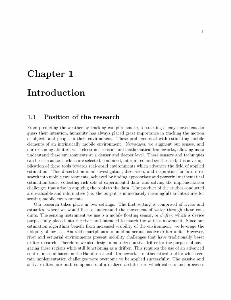
1.1 Position of the research
From predicting the weather by tracking campfire smoke, to tracking enemy movements toguess their intention, humanity has always placed great importance in tracking the motionof objects and people in their environment. These problems deal with estimating mobileelements of an intrinsically mobile environment. Nowadays, we augment our senses, andour reasoning abilities, with electronic sensors and mathematical frameworks, allowing us tounderstand these environments at a denser and deeper level. These sensors and techniquescan be seen as tools which are selected, combined, interpreted and synthesized; it is novel ap-plication of these tools towards real-world environments which advances the field of appliedestimation. This dissertation is an investigation, discussion, and inspiration for future re-search into mobile environments, achieved by finding appropriate and powerful mathematicalestimation tools, collecting rich sets of experimental data, and solving the implementationchallenges that arise in applying the tools to the data. The product of the studies conductedare realizable and informative (i.e. the output is immediately meaningful) architectures forsensing mobile environments.
Our research takes place in two settings. The first setting is comprised of rivers andestuaries, where we would like to understand the movement of water through these con-duits. The sensing instrument we use is a mobile floating sensor, or drifter, which is devicepurposefully placed into the river and intended to match the water’s movement. Since ourestimation algorithms benefit from increased visibility of the environment, we leverage theubiquity of low-cost Android smartphones to build numerous passive drifter units. However,river and estuarial environments present mobility challenges that have traditionally besetdrifter research. Therefore, we also design a motorized active drifter for the purpose of navi-gating these regions while still functioning as a drifter. This requires the use of an advancedcontrol method based on the Hamilton-Jacobi framework, a mathematical tool for which cer-tain implementation challenges were overcome to be applied successfully. The passive andactive drifters are both components of a realized architecture which collects and processes
CHAPTER 1. INTRODUCTION 2
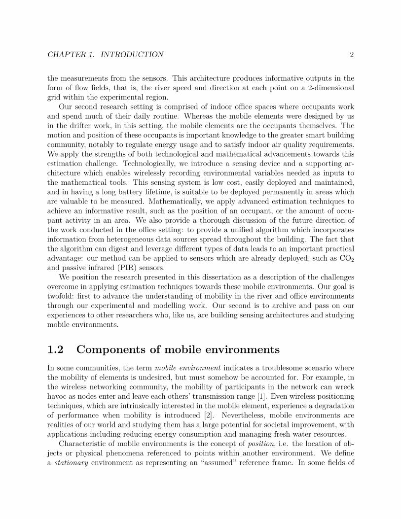
the measurements from the sensors. This architecture produces informative outputs in theform of flow fields, that is, the river speed and direction at each point on a 2-dimensionalgrid within the experimental region.
Our second research setting is comprised of indoor office spaces where occupants workand spend much of their daily routine. Whereas the mobile elements were designed by usin the drifter work, in this setting, the mobile elements are the occupants themselves. Themotion and position of these occupants is important knowledge to the greater smart buildingcommunity, notably to regulate energy usage and to satisfy indoor air quality requirements.We apply the strengths of both technological and mathematical advancements towards thisestimation challenge. Technologically, we introduce a sensing device and a supporting ar-chitecture which enables wirelessly recording environmental variables needed as inputs tothe mathematical tools. This sensing system is low cost, easily deployed and maintained,and in having a long battery lifetime, is suitable to be deployed permanently in areas whichare valuable to be measured. Mathematically, we apply advanced estimation techniques toachieve an informative result, such as the position of an occupant, or the amount of occu-pant activity in an area. We also provide a thorough discussion of the future direction ofthe work conducted in the office setting: to provide a unified algorithm which incorporatesinformation from heterogeneous data sources spread throughout the building. The fact thatthe algorithm can digest and leverage different types of data leads to an important practicaladvantage: our method can be applied to sensors which are already deployed, such as CO2
and passive infrared (PIR) sensors.We position the research presented in this dissertation as a description of the challenges
overcome in applying estimation techniques towards these mobile environments. Our goal istwofold: first to advance the understanding of mobility in the river and office environmentsthrough our experimental and modelling work. Our second is to archive and pass on ourexperiences to other researchers who, like us, are building sensing architectures and studyingmobile environments.
1.2 Components of mobile environments
In some communities, the term mobile environment indicates a troublesome scenario wherethe mobility of elements is undesired, but must somehow be accounted for. For example, inthe wireless networking community, the mobility of participants in the network can wreckhavoc as nodes enter and leave each others’ transmission range [1]. Even wireless positioningtechniques, which are intrinsically interested in the mobile element, experience a degradationof performance when mobility is introduced [2]. Nevertheless, mobile environments arerealities of our world and studying them has a large potential for societal improvement, withapplications including reducing energy consumption and managing fresh water resources.
Characteristic of mobile environments is the concept of position, i.e. the location of ob-jects or physical phenomena referenced to points within another environment. We definea stationary environment as representing an “assumed” reference frame. In some fields of
CHAPTER 1. INTRODUCTION 3
science, such as astronomy, the definition of the stationary environment is more ambiguoussince the earth can be seen as moving within the solar system or galaxy. For this disser-tation however, the stationary environment is assumed to be comprised of all objects andphenomena whose positions are fixed to the earth, such as buildings and terrain. The mobileelements are those which change their position (either intentionally or passively) over time,relative to the earth. Together, the stationary environment and the mobile elements withinthat environment comprise the mobile environment.
Since mobile elements change their position over time, there is also the concept of velocity,which is the first derivative of position with respect to time. As well, there is a concept ofacceleration, which is the second derivative of position with respect to time. Both velocityand acceleration are vector-valued quantities which can be decomposed into scalar parts.Velocity is commonly decomposed into speed and direction, and acceleration is commonlydecomposed into its 3-dimensional components X,Y, and Z (since acceleration sensors canmeasure these quantities).
In real mobile environments, there are constraints on the mobility of the mobile elements.There are two constraints commonly encountered: obstacles are positions which the mobileelement cannot occupy or cross, such as a solid wall. The other constraint is limited controlauthority: bounds on the amount a mobile element can change in its position, speed, orvelocity. In some cases, these constraints are problems that must be overcome, such as aswimming robot that is too weak to swim upstream. In other cases, we leverage the imposedconstraints to add information to the problem, such as a tracking problem where knowledgeof obstacles can indicate which positions do not need to be considered.
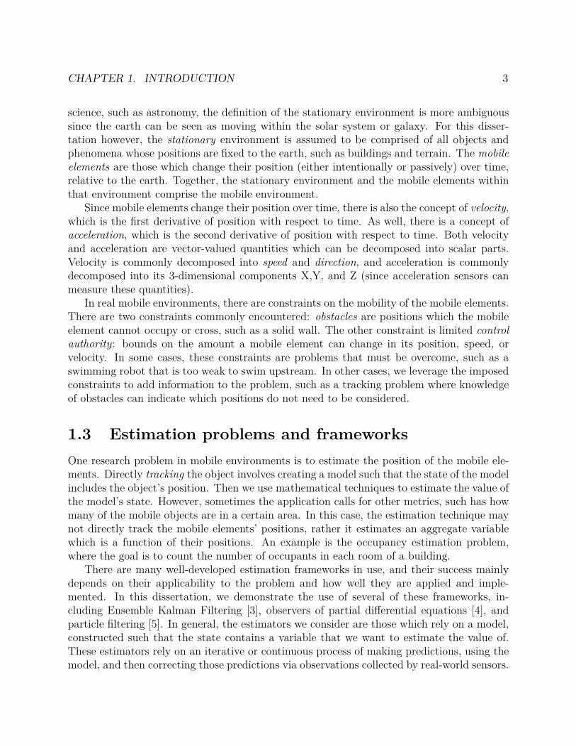
1.3 Estimation problems and frameworks
One research problem in mobile environments is to estimate the position of the mobile ele-ments. Directly tracking the object involves creating a model such that the state of the modelincludes the object’s position. Then we use mathematical techniques to estimate the value ofthe model’s state. However, sometimes the application calls for other metrics, such has howmany of the mobile objects are in a certain area. In this case, the estimation technique maynot directly track the mobile elements’ positions, rather it estimates an aggregate variablewhich is a function of their positions. An example is the occupancy estimation problem,where the goal is to count the number of occupants in each room of a building.
There are many well-developed estimation frameworks in use, and their success mainlydepends on their applicability to the problem and how well they are applied and imple-mented. In this dissertation, we demonstrate the use of several of these frameworks, in-cluding Ensemble Kalman Filtering [3], observers of partial differential equations [4], andparticle filtering [5]. In general, the estimators we consider are those which rely on a model,constructed such that the state contains a variable that we want to estimate the value of.These estimators rely on an iterative or continuous process of making predictions, using themodel, and then correcting those predictions via observations collected by real-world sensors.
CHAPTER 1. INTRODUCTION 4
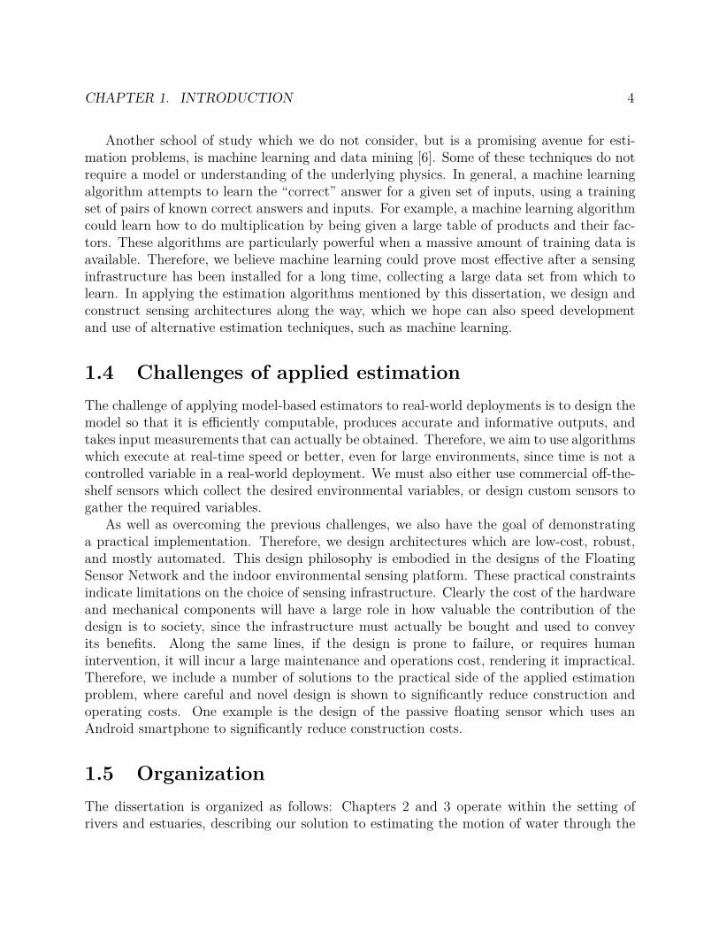
Another school of study which we do not consider, but is a promising avenue for esti-mation problems, is machine learning and data mining [6]. Some of these techniques do notrequire a model or understanding of the underlying physics. In general, a machine learningalgorithm attempts to learn the “correct” answer for a given set of inputs, using a trainingset of pairs of known correct answers and inputs. For example, a machine learning algorithmcould learn how to do multiplication by being given a large table of products and their fac-tors. These algorithms are particularly powerful when a massive amount of training data isavailable. Therefore, we believe machine learning could prove most effective after a sensinginfrastructure has been installed for a long time, collecting a large data set from which tolearn. In applying the estimation algorithms mentioned by this dissertation, we design andconstruct sensing architectures along the way, which we hope can also speed developmentand use of alternative estimation techniques, such as machine learning.
1.4 Challenges of applied estimation
The challenge of applying model-based estimators to real-world deployments is to design themodel so that it is efficiently computable, produces accurate and informative outputs, andtakes input measurements that can actually be obtained. Therefore, we aim to use algorithmswhich execute at real-time speed or better, even for large environments, since time is not acontrolled variable in a real-world deployment. We must also either use commercial off-the-shelf sensors which collect the desired environmental variables, or design custom sensors togather the required variables.
As well as overcoming the previous challenges, we also have the goal of demonstratinga practical implementation. Therefore, we design architectures which are low-cost, robust,and mostly automated. This design philosophy is embodied in the designs of the FloatingSensor Network and the indoor environmental sensing platform. These practical constraintsindicate limitations on the choice of sensing infrastructure. Clearly the cost of the hardwareand mechanical components will have a large role in how valuable the contribution of thedesign is to society, since the infrastructure must actually be bought and used to conveyits benefits. Along the same lines, if the design is prone to failure, or requires humanintervention, it will incur a large maintenance and operations cost, rendering it impractical.Therefore, we include a number of solutions to the practical side of the applied estimationproblem, where careful and novel design is shown to significantly reduce construction andoperating costs. One example is the design of the passive floating sensor which uses anAndroid smartphone to significantly reduce construction costs.
1.5 Organization
The dissertation is organized as follows: Chapters 2 and 3 operate within the setting ofrivers and estuaries, describing our solution to estimating the motion of water through the
CHAPTER 1. INTRODUCTION 5
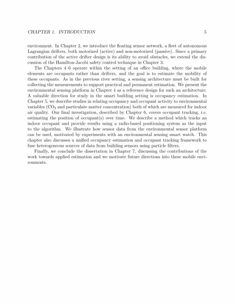
environment. In Chapter 2, we introduce the floating sensor network, a fleet of autonomousLagrangian drifters, both motorized (active) and non-motorized (passive). Since a primarycontribution of the active drifter design is its ability to avoid obstacles, we extend the dis-cussion of the Hamilton-Jacobi safety control technique in Chapter 3.
The Chapters 4–6 operate within the setting of an office building, where the mobileelements are occupants rather than drifters, and the goal is to estimate the mobility ofthese occupants. As in the previous river setting, a sensing architecture must be built forcollecting the measurements to support practical and permanent estimation. We present theenvironmental sensing platform in Chapter 4 as a reference design for such an architecture.A valuable direction for study in the smart building setting is occupancy estimation. InChapter 5, we describe studies in relating occupancy and occupant activity to environmentalvariables (CO2 and particulate matter concentration) both of which are measured for indoorair quality. Our final investigation, described by Chapter 6, covers occupant tracking, i.e.estimating the position of occupant(s) over time. We describe a method which tracks anindoor occupant and provide results using a radio-based positioning system as the inputto the algorithm. We illustrate how sensor data from the environmental sensor platformcan be used, motivated by experiments with an environmental sensing smart watch. Thischapter also discusses a unified occupancy estimation and occupant tracking framework tofuse heterogeneous sources of data from building sensors using particle filters.
Finally, we conclude the dissertation in Chapter 7, discussing the contributions of thework towards applied estimation and we motivate future directions into these mobile envi-ronments.

6
Chapter 2
Mobile Floating Sensors
2.1 Introduction
A complex mobile environment of high societal importance are the natural aqueducts ofour freshwater supplies, that is rivers, lakes, streams, and estuaries. Throughout history,the movement, storage, consumption and contamination of water resources have formed andtorn human communities together and apart. Freshwater is especially responsible for theflourishing of California’s population and rich agriculture. Natural and man-made systemsof channels, dams and aqueducts deliver and store the freshwater, supplying the agricultural,industrial, and consumer needs of the state. These are essential for the state’s survival, andare sometimes tested to its limits, such as the drought of early 2014, when the CaliforniaDepartment of Water Resources (DWR), for the first time ever, prepared to cut all waterdeliveries to the State Water Project’s (SWP) agricultural customers. During this time,many urban areas had to rely on their local groundwater storage for drinking water [7].
The Floating Sensor Network (FSN) project at the University of California Berkeley [8]hopes to improve the understanding of estuarial environments in California. We attempt toestimate the mobility of the environment by inventing novel sensor systems and algorithmswhich can tell us where water moves within the environment. Most of our studies haveoccurred in the Sacramento-San Joaquin River Delta region in which water is stored andtransported from melted snow in the Sierra mountains to the SWP and Central ValleyProject (CVP) which supplies over 23 million Californians. The delta also connects to theocean and freshwater outflow is required prevent saltwater from intruding into the delta andthreatening the local ecosystem, as well as contaminating the freshwater supply. Therefore,if too much water is drawn from the delta, allowing salt water to flow in from the ocean,it could have disastrous consequences for all of California. In some cases, water must bereleased from reservoirs for expressly this purpose [9]. Thus, understanding the way wateris moving and how it reacts to policy decisions will be extremely valuable in efficiently andsafely using this water system. We believe that the invention and demonstration of oursensor network is large step towards this understanding.
CHAPTER 2. MOBILE FLOATING SENSORS 7
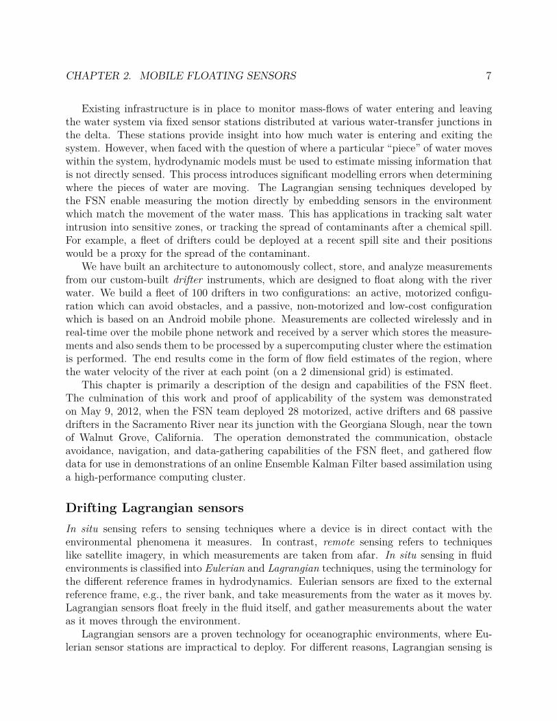
Existing infrastructure is in place to monitor mass-flows of water entering and leavingthe water system via fixed sensor stations distributed at various water-transfer junctions inthe delta. These stations provide insight into how much water is entering and exiting thesystem. However, when faced with the question of where a particular “piece” of water moveswithin the system, hydrodynamic models must be used to estimate missing information thatis not directly sensed. This process introduces significant modelling errors when determiningwhere the pieces of water are moving. The Lagrangian sensing techniques developed bythe FSN enable measuring the motion directly by embedding sensors in the environmentwhich match the movement of the water mass. This has applications in tracking salt waterintrusion into sensitive zones, or tracking the spread of contaminants after a chemical spill.For example, a fleet of drifters could be deployed at a recent spill site and their positionswould be a proxy for the spread of the contaminant.
We have built an architecture to autonomously collect, store, and analyze measurementsfrom our custom-built drifter instruments, which are designed to float along with the riverwater. We build a fleet of 100 drifters in two configurations: an active, motorized configu-ration which can avoid obstacles, and a passive, non-motorized and low-cost configurationwhich is based on an Android mobile phone. Measurements are collected wirelessly and inreal-time over the mobile phone network and received by a server which stores the measure-ments and also sends them to be processed by a supercomputing cluster where the estimationis performed. The end results come in the form of flow field estimates of the region, wherethe water velocity of the river at each point (on a 2 dimensional grid) is estimated.
This chapter is primarily a description of the design and capabilities of the FSN fleet.The culmination of this work and proof of applicability of the system was demonstratedon May 9, 2012, when the FSN team deployed 28 motorized, active drifters and 68 passivedrifters in the Sacramento River near its junction with the Georgiana Slough, near the townof Walnut Grove, California. The operation demonstrated the communication, obstacleavoidance, navigation, and data-gathering capabilities of the FSN fleet, and gathered flowdata for use in demonstrations of an online Ensemble Kalman Filter based assimilation usinga high-performance computing cluster.
Drifting Lagrangian sensors
In situ sensing refers to sensing techniques where a device is in direct contact with theenvironmental phenomena it measures. In contrast, remote sensing refers to techniqueslike satellite imagery, in which measurements are taken from afar. In situ sensing in fluidenvironments is classified into Eulerian and Lagrangian techniques, using the terminology forthe different reference frames in hydrodynamics. Eulerian sensors are fixed to the externalreference frame, e.g., the river bank, and take measurements from the water as it moves by.Lagrangian sensors float freely in the fluid itself, and gather measurements about the wateras it moves through the environment.
Lagrangian sensors are a proven technology for oceanographic environments, where Eu-lerian sensor stations are impractical to deploy. For different reasons, Lagrangian sensing is
CHAPTER 2. MOBILE FLOATING SENSORS 8
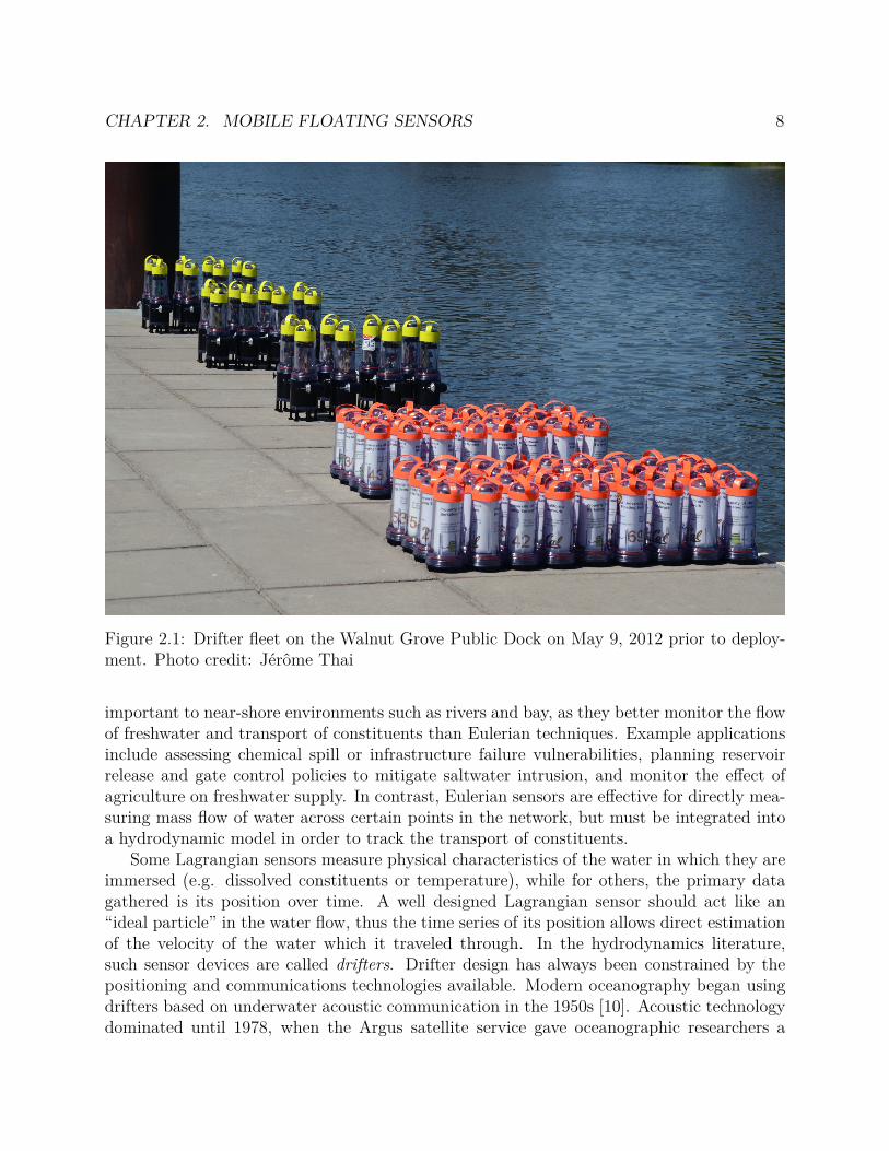
Figure 2.1: Drifter fleet on the Walnut Grove Public Dock on May 9, 2012 prior to deploy-ment. Photo credit: Jérôme Thai
important to near-shore environments such as rivers and bay, as they better monitor the flowof freshwater and transport of constituents than Eulerian techniques. Example applicationsinclude assessing chemical spill or infrastructure failure vulnerabilities, planning reservoirrelease and gate control policies to mitigate saltwater intrusion, and monitor the effect ofagriculture on freshwater supply. In contrast, Eulerian sensors are effective for directly mea-suring mass flow of water across certain points in the network, but must be integrated intoa hydrodynamic model in order to track the transport of constituents.
Some Lagrangian sensors measure physical characteristics of the water in which they areimmersed (e.g. dissolved constituents or temperature), while for others, the primary datagathered is its position over time. A well designed Lagrangian sensor should act like an“ideal particle” in the water flow, thus the time series of its position allows direct estimationof the velocity of the water which it traveled through. In the hydrodynamics literature,such sensor devices are called drifters. Drifter design has always been constrained by thepositioning and communications technologies available. Modern oceanography began usingdrifters based on underwater acoustic communication in the 1950s [10]. Acoustic technologydominated until 1978, when the Argus satellite service gave oceanographic researchers a
CHAPTER 2. MOBILE FLOATING SENSORS 9
global location and data uplink system [11]. Power, cost, and size constraints meant thatArgos-based drifters [12, 13, 14] were better suited to oceanography than inland environmentslike rivers and estuaries. In general, Lagrangian sensing has proven to be challenging in theseenvironments due to shallow areas and relatively narrow water passageways which can trapdrifters.
Global Positioning System (GPS) positioning and local radio frequency (RF) communica-tion have enabled inland drifter studies, by allowing smaller units which can traverse shallowand obstacle-rich areas in a river system. GPS-carrying river drifters have been the focusof development by the FSN project [15] and other groups [16, 17]. Studies in regions withwell-developed civilian infrastructure, like the continental United States, can take advantageof the mobile phone network for communications. The drifter design in this article is to ourknowledge the first design to use commercial mobile phones not only as the communicationsystem, but as the positioning and computation system as well.
2.2 Passive sensors using Android mobile phones
Motivation
Most of the drifters in our Floating Sensor fleet are our Android drifters [18], named asthey are based on the Android platform [19], whereas all of our previous drifter designsrelied heavily on custom, microcontroller-based designs. These custom designs requiredmany months of development and debugging hardware components, and often required thatfeatures be removed from the final product due to cost or time constraints. Thus, theproliferation of Android smartphones offered us a relatively low-cost package offering thefollowing features:
• All of the electronic functionalities required for a Lagrangian drifter– Positioning (viainternal GPS), long-range Internet communication (via the mobile connection), anduser interface (via the touch screen).
• A high-level programming interface (JAVA) and API for accessing the needed func-tionalities.
• Industry-tested hardware and software libraries, significantly improving reliability.
• High-volume pricing, due to the proliferation of smartphones in the consumer space.
In exchange for these features, the choice of the Android platform over a custom solutionhas the following drawbacks:
• Interfacing external sensors is difficult, requiring an unsupported and unreliable useof the Universal Serial Bus (USB) connection and a complex interfacing board. Thishas since been address by official support via the Android Accessory Development
CHAPTER 2. MOBILE FLOATING SENSORS 10
Kit (ADK), however, the solution is still more complex than interfacing sensors to amicrocontroller.
• The power usage is significantly increased due to a high-powered processor and in-creased processing needed to execute JAVA code as well as the rest of the miscella-neous operating system tasks and applications which are concurrently running. Thus,we need to add an external battery to achieve multi-day lifetimes (fortunately, a batterysatisfies a dual-purpose as a ballast weight).
• We have significantly less control of the processor due to running in user-space inan operating system. Our application could be delayed or even stopped from otherconcurrent processes running on the phone. The primary effect is increased latencyand lack of real-time assurances, which hinder using the phone for real-time controlpurposes (if the drifter were motorized), and possibly less reliability if our process wasunexpectedly terminated, although we have never encountered this happening.
Ultimately, we recognized that many of our drifter studies could benefit from high num-bers of floating sensors, which, due to cost, could not be met with custom hardware drifters.Thus, these Android drifters were designed to provide numerous sensors for studies in non-hostile environments, where obstacles posed less of a risk. Our smaller fleet of motorizeddrifters, using custom hardware, were used for those environments that proved too opera-tionally difficult for these Android drifters to be used in.
Physical form of the Android drifter
A real-time Lagrangian drifter has two basic intelligence requirements: it can sense its ownposition and it report it to a central location. Since these are both satisfied by consumerAndroid mobile phones, we design an enclosure to hold one of these phones. Similar to ourwork with the active sensors, we identified three considerations when designing the formfactor: First, as a Lagrangian flow sensor, it must suitably match the river’s local velocity.Secondly, the mass must be distributed such that the phone is oriented vertically (to ensurethe best GPS and communications reception). Finally, the phone should be nominally abovethe water line to ensure sufficient reception.
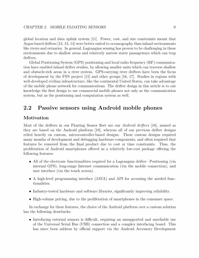
In the active drifter work, we found that a large, symmetric drag profile indicates goodLagrangian tracking performance, thus, the design is again a vertically oriented cylinderbased on a water filter housing. In addition to the weight of the battery, an additionalaluminum ballast weight was necessary to ensure a large separation between the centerof mass (COM), at approximately 94 mm from the base, and center of buoyancy (COB), atapproximately 126 mm from the base, while keeping the enclosure 90% submerged. Figure 2.2shows how the COM and COB are distributed in the design.
The hull is primarily an ultraviolet (UV) stabilized polyvinyl chloride (PVC) water filterhousing manufactured by Pentec. The bottom receiving cap of the water filter housing ismachined from Delrin, which is known for its durability and ease of machining by computer
CHAPTER 2. MOBILE FLOATING SENSORS 11
Figure 2.2: Sensor dimensions and COM and COB locations.
numeric controlled (CNC) equipment. Also, since it absorbs just 0.2% of its volume in water(24 hour submersion), it undergoes minimal changes in dimensional tolerances, which couldbe a source of leaks in other materials. The Delrin cap is given male threads which mate tothe water filter housing. A silicone O-ring forms a watertight seal between the water filterhousing and the Delrin cap and the two are tightened with two wrenches also manufacturedby Pentek. The Delrin cap has notches which receive the special wrench. Internally, theDelrin cap has an impression for the ballast weight to reside in. Additionally there is amachined PVC tube which holds the phone in the desired position. Slots are machinedinto the PVC tube to hold the phone as well as to not impede airflow to help ventilate thephone. The overall assembly cost and diagram of components is displayed in Table 2.1 andFigure 2.3.
Our choice of battery was primarily driven by the typical residence time of water in theSacramento-San Joaquin River Delta, approximately 48 hours. Thus we chose a batterywhich allowed 48 hours of continuous usage of the GPS, accelerometer, and Global System
CHAPTER 2. MOBILE FLOATING SENSORS 12
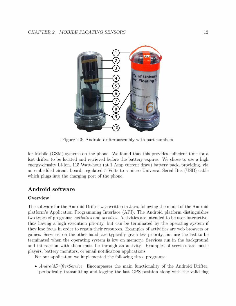
Figure 2.3: Android drifter assembly with part numbers.
for Mobile (GSM) systems on the phone. We found that this provides sufficient time for alost drifter to be located and retrieved before the battery expires. We chose to use a highenergy-density Li-Ion, 115 Watt-hour (at 1 Amp current draw) battery pack, providing, viaan embedded circuit board, regulated 5 Volts to a micro Universal Serial Bus (USB) cablewhich plugs into the charging port of the phone.
Android software
Overview
The software for the Android Drifter was written in Java, following the model of the Androidplatform’s Application Programming Interface (API). The Android platform distinguishestwo types of programs: activities and services. Activities are intended to be user-interactive,thus having a high execution priority, but can be terminated by the operating system ifthey lose focus in order to regain their resources. Examples of activities are web browsers orgames. Services, on the other hand, are typically given less priority, but are the last to beterminated when the operating system is low on memory. Services run in the backgroundand interaction with them must be through an activity. Examples of services are musicplayers, battery monitors, or email notification applications.
For our application we implemented the following three programs:
• AndroidDrifterService: Encompasses the main functionality of the Android Drifter,periodically transmitting and logging the last GPS position along with the valid flag

CHAPTER 2. MOBILE FLOATING SENSORS 13
# Item Price Quantity
1 Duct tape handle $1 1
2 Upper PVC hull $25 1
3 Motorola DEFY $175 1
4 Rubber bands $1 2
5 PVC phone holster $15 1
6 Foam disk $1 1
7 LiPo battery $250 1
8 If-found placard $1 1
9 Aluminum disk $10 1
10 Delrin base $50 1
Total $530 11
Table 2.1: Android drifter bill of materials
indicating if the unit is upright.
• AndroidDrifterActivity: Provides the user buttons to start and stop the service andstatus indicators to determine if data is being delivered properly.
• ConfigureActivity: Allows the user to configure the parameters (server address, port,update rate, etc.) of the service.
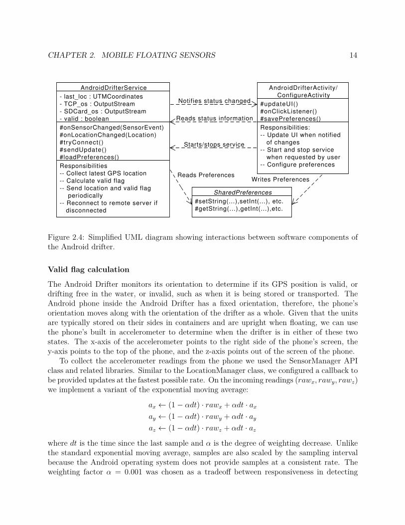
A simplified Unified Modeling Language (UML) diagram is provided in Figure 2.4. Inthe rest of this section, we describe the functionalities of the AndroidDrifterService in moredetail:
GPS location collection
To collect the GPS location of the device, we used the LocationManager API class andrelated libraries. We call the API by requesting location change updates to a custom callbackmethod and ask for minimum interval to receive updates. Thus, our callback method is calledabout every second with a new location object. The latitude and longitude coordinates areconverted to UTM coordinates and store temporarily into the last_loc variable.
CHAPTER 2. MOBILE FLOATING SENSORS 14
AndroidDrifterService
- last_loc : UTMCoordinates
- TCP_os : OutputStream
- SDCard_os : OutputStream
- valid : boolean
#onSensorChanged(SensorEvent)
#onLocationChanged(Location)
#tryConnect()
#sendUpdate()
#loadPreferences()
Responsibilities
-- Collect latest GPS location
-- Calculate valid flag
-- Send location and valid flag
periodically
-- Reconnect to remote server if
disconnected
AndroidDrifterActivity/
ConfigureActivity
#updateUI()
#onClickListener()
#savePreferences()
Responsibilities:
-- Update UI when notified
of changes
-- Start and stop service
when requested by user
-- Configure preferences
Notifies status changed
Reads status information
Starts/stops service
SharedPreferences
#setString(...),setInt(...), etc.
#getString(...),getInt(...),etc.
Writes PreferencesReads Preferences
Figure 2.4: Simplified UML diagram showing interactions between software components ofthe Android drifter.
Valid flag calculation
The Android Drifter monitors its orientation to determine if its GPS position is valid, ordrifting free in the water, or invalid, such as when it is being stored or transported. TheAndroid phone inside the Android Drifter has a fixed orientation, therefore, the phone’sorientation moves along with the orientation of the drifter as a whole. Given that the unitsare typically stored on their sides in containers and are upright when floating, we can usethe phone’s built in accelerometer to determine when the drifter is in either of these twostates. The x-axis of the accelerometer points to the right side of the phone’s screen, they-axis points to the top of the phone, and the z-axis points out of the screen of the phone.
To collect the accelerometer readings from the phone we used the SensorManager APIclass and related libraries. Similar to the LocationManager class, we configured a callback tobe provided updates at the fastest possible rate. On the incoming readings (rawx, rawy, rawz)we implement a variant of the exponential moving average:
ax ← (1− αdt) · rawx + αdt · ax
ay ← (1− αdt) · rawy + αdt · ay
az ← (1− αdt) · rawz + αdt · az
where dt is the time since the last sample and α is the degree of weighting decrease. Unlikethe standard exponential moving average, samples are also scaled by the sampling intervalbecause the Android operating system does not provide samples at a consistent rate. Theweighting factor α = 0.001 was chosen as a tradeoff between responsiveness in detecting
CHAPTER 2. MOBILE FLOATING SENSORS 15
placement in water and storage and effectiveness in filtering out bumps and shakes. We thencompute the valid flag representing these two states as:
valid←
1 if ay > |ax| and ay > |az|0 otherwise.
(2.1)
Therefore, if the phone’s longest dimension is aligned with the gravity vector and upright,valid becomes 1, whereas if the phone is on one of its other sides, valid is 0.
Without the filter, we find that there are many false-negatives, i.e. the drifter reportsvalid = 0 when it should report valid = 1. The errors are caused by noisy accelerometersignals which can be attributed to wave action buffeting the drifter as well as normal noisefrom the sensor. We ran a study to determine the effect of the filter described above on thefalse-negative rate. For this test, the drifter was moored floating upright for 14 hours whilelogging accelerometer samples. Sampling intervals during this study had a mean of 203 mSand a standard deviation of 17 mS. We then calculate the raw and filtered pitch angles φraw
and φ using the following formulae:
φraw = tan−1(
rawy√raw2
x+raw2z
)
φ = tan−1(
ay√a2
x+a2z
)
We evaluate the arctangent function tan−1(
y
x
)
using the two-argument function atan2(y, x)common to many computer languages in order to place the angle in the correct quadrant.
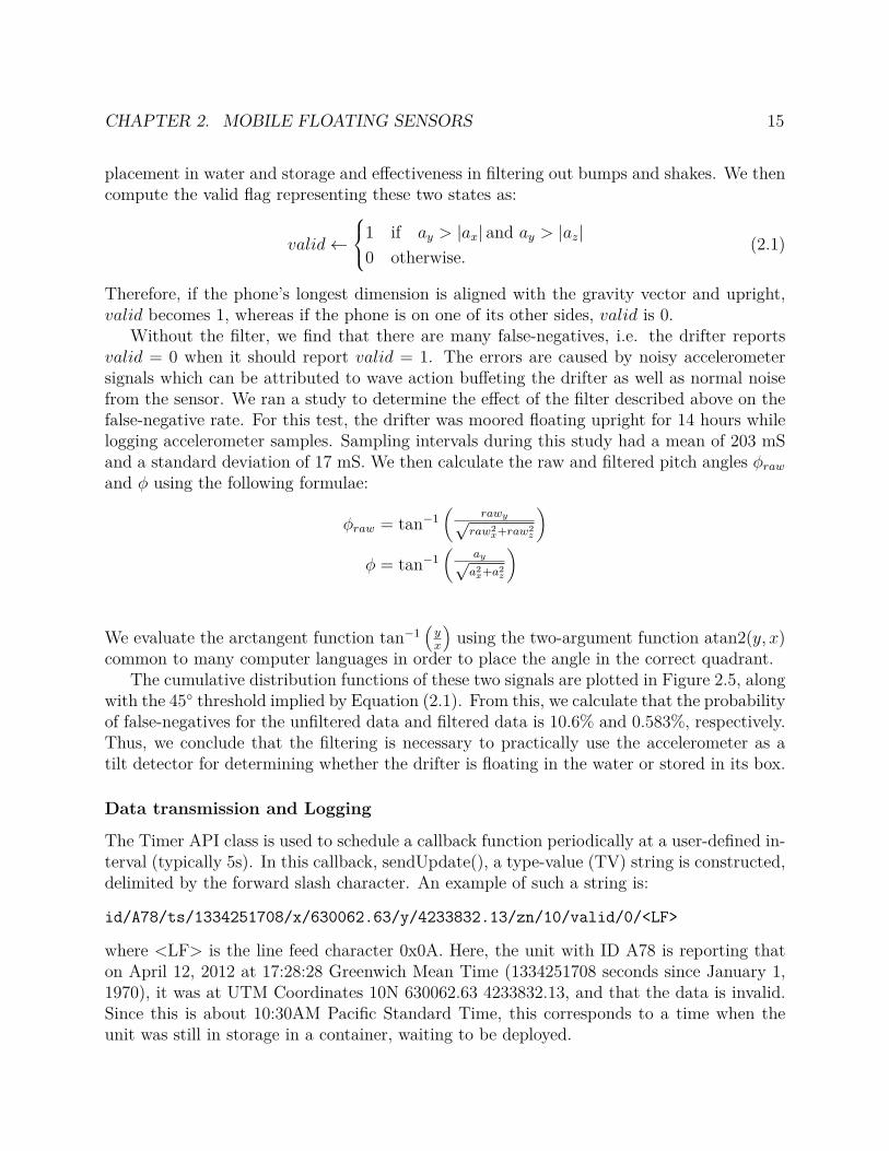
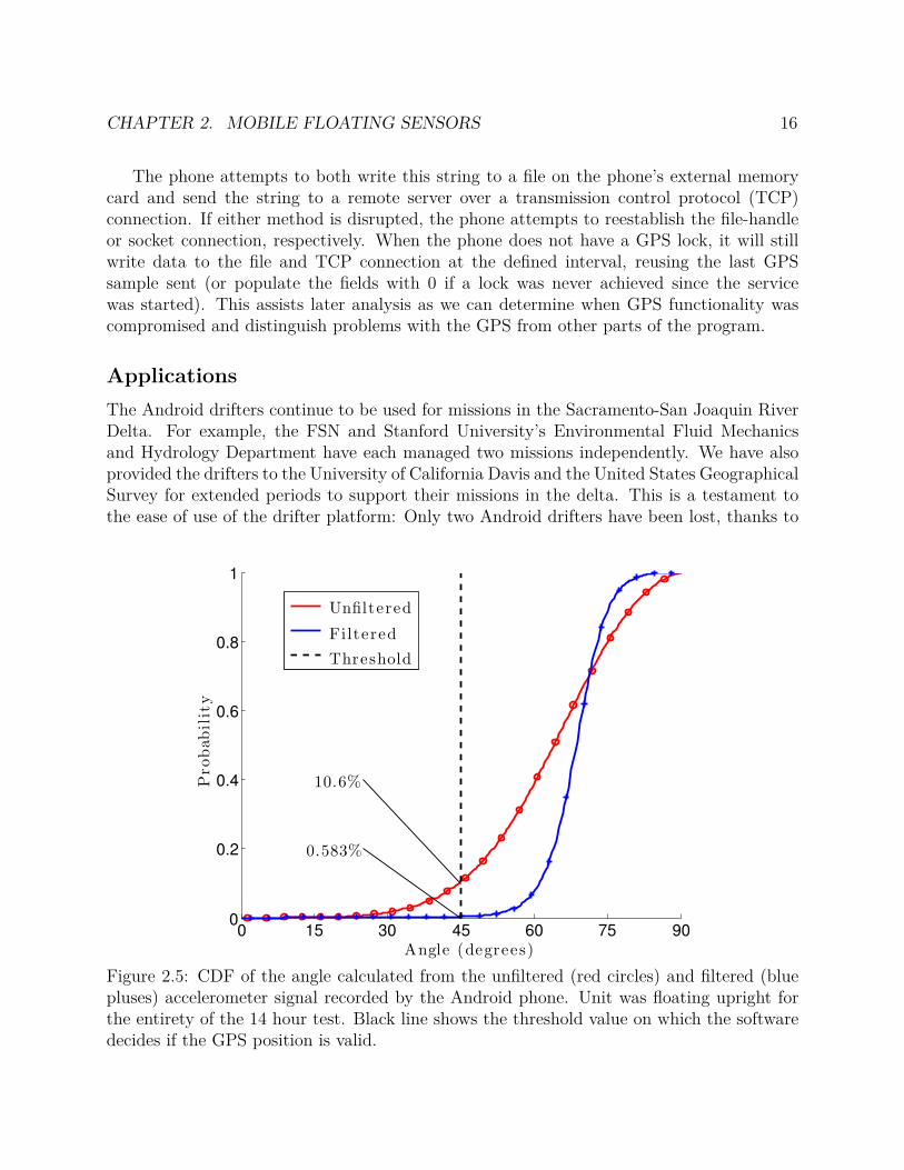
The cumulative distribution functions of these two signals are plotted in Figure 2.5, alongwith the 45 threshold implied by Equation (2.1). From this, we calculate that the probabilityof false-negatives for the unfiltered data and filtered data is 10.6% and 0.583%, respectively.Thus, we conclude that the filtering is necessary to practically use the accelerometer as atilt detector for determining whether the drifter is floating in the water or stored in its box.
Data transmission and Logging
The Timer API class is used to schedule a callback function periodically at a user-defined in-terval (typically 5s). In this callback, sendUpdate(), a type-value (TV) string is constructed,delimited by the forward slash character. An example of such a string is:
id/A78/ts/1334251708/x/630062.63/y/4233832.13/zn/10/valid/0/<LF>
where <LF> is the line feed character 0x0A. Here, the unit with ID A78 is reporting thaton April 12, 2012 at 17:28:28 Greenwich Mean Time (1334251708 seconds since January 1,1970), it was at UTM Coordinates 10N 630062.63 4233832.13, and that the data is invalid.Since this is about 10:30AM Pacific Standard Time, this corresponds to a time when theunit was still in storage in a container, waiting to be deployed.
CHAPTER 2. MOBILE FLOATING SENSORS 16
The phone attempts to both write this string to a file on the phone’s external memorycard and send the string to a remote server over a transmission control protocol (TCP)connection. If either method is disrupted, the phone attempts to reestablish the file-handleor socket connection, respectively. When the phone does not have a GPS lock, it will stillwrite data to the file and TCP connection at the defined interval, reusing the last GPSsample sent (or populate the fields with 0 if a lock was never achieved since the servicewas started). This assists later analysis as we can determine when GPS functionality wascompromised and distinguish problems with the GPS from other parts of the program.
Applications
The Android drifters continue to be used for missions in the Sacramento-San Joaquin RiverDelta. For example, the FSN and Stanford University’s Environmental Fluid Mechanicsand Hydrology Department have each managed two missions independently. We have alsoprovided the drifters to the University of California Davis and the United States GeographicalSurvey for extended periods to support their missions in the delta. This is a testament tothe ease of use of the drifter platform: Only two Android drifters have been lost, thanks to
0 15 30 45 60 75 900
0.2
0.4
0.6
0.8
1
10.6%
0.583%
Angle (degrees)
Pro
bab
ility
Unfiltered
Filtered
Threshold
Figure 2.5: CDF of the angle calculated from the unfiltered (red circles) and filtered (bluepluses) accelerometer signal recorded by the Android phone. Unit was floating upright forthe entirety of the 14 hour test. Black line shows the threshold value on which the softwaredecides if the GPS position is valid.
CHAPTER 2. MOBILE FLOATING SENSORS 17
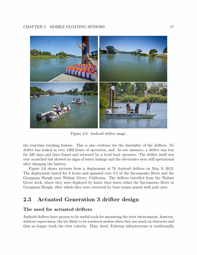
Figure 2.6: Android drifter usage.
the real-time tracking feature. This is also evidence for the durability of the drifters: Nodrifter has leaked in over 1300 hours of operation, and. In one instance, a drifter was lostfor 320 days and later found and returned by a local boat operator. The drifter itself wasvery scratched but showed no signs of water leakage and the electronics were still operationalafter charging the battery.
Figure 2.6 shows pictures from a deployment of 70 Android drifters on May 9, 2012.The deployment lasted for 8 hours and spanned over 3.5 of the Sacramento River and theGeorgiana Slough near Walnut Grove, California. The drifters travelled from the WalnutGrove dock, where they were deployed by hand, then down either the Sacramento River orGeorgiana Slough, after which they were retrieved by boat teams armed with pole nets.
2.3 Actuated Generation 3 drifter design
The need for actuated drifters
Android drifters have proven to be useful tools for measuring the river environment, however,without supervision, the are likely to be rendered useless when they are stuck on obstacles andthus no longer track the river velocity. Thus, fixed, Eulerian infrastructure is traditionally
CHAPTER 2. MOBILE FLOATING SENSORS 18
used in the river environment. However, the vision of the FSN is long term operation ofthe drifters, thus, some mechanism is needed to avoid obstacles such as debris or the rivershore. Thus, a motorized floating sensor is developed which has the ability to avoid thesehazards, while being low-cost and manufacturable. In fact, the FSN is the first to designand produce a fleet of 40 such motorized drifters and demonstrate their effectiveness in afield experiment.
Our design included the electrical and mechanical requirements for an advanced safetycontrol technique presented in Chapter 3. This safety control technique allows us to not onlyhave the motorized drifters avoid obstacles that threaten their operation, but also specify aparticular part of the river to proceed along. We demonstrated this ability near the riverjunction of the Sacramento river and the Georgiana Slough near Walnut Grove, CA [20].
Hardware
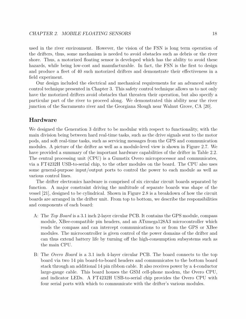
We designed the Generation 3 drifter to be modular with respect to functionality, with themain division being between hard real-time tasks, such as the drive signals sent to the motorpods, and soft real-time tasks, such as servicing messages from the GPS and communicationmodules. A picture of the drifter as well as a module-level view is shown in Figure 2.7. Wehave provided a summary of the important hardware capabilities of the drifter in Table 2.2.The central processing unit (CPU) is a Gumstix Overo microprocessor and communicates,via a FT4232H USB-to-serial chip, to the other modules on the board. The CPU also usessome general-purpose input/output ports to control the power to each module as well asvarious control lines.
The drifter electronics hardware is comprised of six circular circuit boards separated byfunction. A major constraint driving the multitude of separate boards was shape of thevessel [21], designed to be cylindrical. Shown in Figure 2.8 is a breakdown of how the circuitboards are arranged in the drifter unit. From top to bottom, we describe the responsibilitiesand components of each board:
A: The Top Board is a 3.1 inch 2-layer circular PCB. It contains the GPS module, compassmodule, XBee-compatible pin headers, and an ATxmega128A3 microcontroller whichreads the compass and can intercept communications to or from the GPS or XBeemodules. The microcontroller is given control of the power domains of the drifter andcan thus extend battery life by turning off the high-consumption subsystems such asthe main CPU.
B: The Overo Board is a 3.1 inch 4-layer circular PCB. The board connects to the topboard via two 14 pin board-to-board headers and communicates to the bottom boardstack through an additional 14 pin ribbon cable. It also receives power by a 4-conductorlarge-gauge cable. This board houses the GSM cell-phone modem, the Overo CPU,and indicator LEDs. A FT4232H USB-to-serial chip provides the Overo CPU withfour serial ports with which to communicate with the drifter’s various modules.
CHAPTER 2. MOBILE FLOATING SENSORS 19
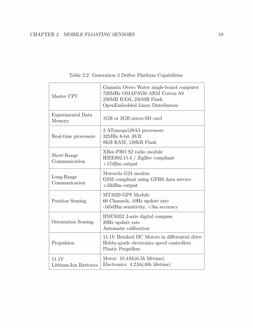
Table 2.2: Generation 3 Drifter Platform Capabilities
Master CPU
Gumstix Overo Water single-board computer720MHz OMAP3530 ARM Cortex-A8256MB RAM, 256MB FlashOpenEmbedded Linux Distribution
Experimental DataMemory
1GB or 2GB micro-SD card
Real-time processors2 ATxmega128A3 processors32MHz 8-bit AVR8KB RAM, 128KB Flash
Short-RangeCommunication
XBee-PRO S2 radio moduleIEEE802.15.4 / ZigBee compliant+17dBm output
Long-RangeCommunication
Motorola G24 modemGSM compliant using GPRS data service+33dBm output
Position SensingMT3329 GPS Module66 Channels, 10Hz update rate-165dBm sensitivity, <3m accuracy
Orientation SensingHMC6352 2-axis digital compass20Hz update rateAutomatic calibration
Propulsion11.1V Brushed DC Motors in differential driveHobby-grade electronics speed controllersPlastic Propellers
11.1VLithium-Ion Batteries
Motor: 10.4Ah(6.5h lifetime)Electronics: 4.2Ah(48h lifetime)
CHAPTER 2. MOBILE FLOATING SENSORS 20
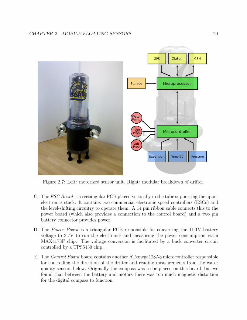
Figure 2.7: Left: motorized sensor unit. Right: modular breakdown of drifter.
C: The ESC Board is a rectangular PCB placed vertically in the tube supporting the upperelectronics stack. It contains two commercial electronic speed controllers (ESCs) andthe level-shifting circuitry to operate them. A 14 pin ribbon cable connects this to thepower board (which also provides a connection to the control board) and a two pinbattery connector provides power.
D: The Power Board is a triangular PCB responsible for converting the 11.1V batteryvoltage to 3.7V to run the electronics and measuring the power consumption via aMAX4173F chip. The voltage conversion is facilitated by a buck converter circuitcontrolled by a TPS5430 chip.
E: The Control Board board contains another ATxmega128A3 microcontroller responsiblefor controlling the direction of the drifter and reading measurements from the waterquality sensors below. Originally the compass was to be placed on this board, but wefound that between the battery and motors there was too much magnetic distortionfor the digital compass to function.
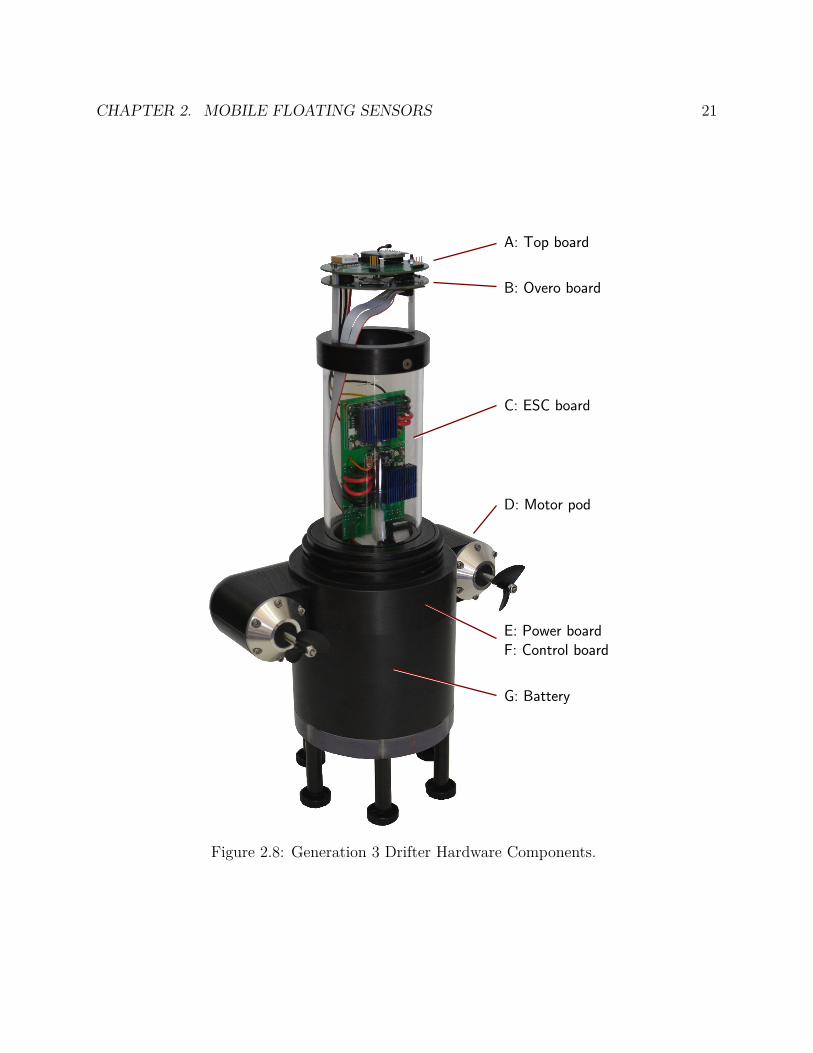
CHAPTER 2. MOBILE FLOATING SENSORS 21
A: Top board
B: Overo board
C: ESC board
D: Motor pod
E: Power boardF: Control board
G: Battery
Figure 2.8: Generation 3 Drifter Hardware Components.
CHAPTER 2. MOBILE FLOATING SENSORS 22
Software
With the power and flexibility of the Gumstix Overo running Linux, we designed our soft-ware to be primarily written in the Python language. This choice of language offered someimportant advantages over previous generations which were written in C. Most notably, sincePython is a scripting language, it does not require cross-compilation targeting the Overo.Thus, we were able to have rapid design cycles, as each code change required only upload-ing the new code to the drifter. Additionally, the scripts could be edited on the driftersthemselves.
An additional decision to aid in development and robustness was to separate the codeinto modules which would run in independent processes. The most immediate advantageof this strategy is that, if one module experiences errors and crashes, it can be restartedwithout affecting the rest of the system. We chose to use UNIX IPC sockets for inter-process communications (IPC) which enabled a straightforward implementation of a SILsimulator. To serialize and decode messages, we use Google Protocol Buffers[22].
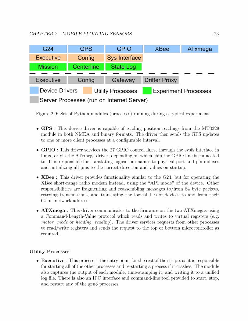
The modules are separated according to function, as shown in Figure 2.9 which lists theset of modules used in a typical experiment. Each module hosts a UNIX IPC server and acorresponding library of functions for other processes to call, making the appropriate UNIXIPC client connections and messages.
A feature of this modular design choice is that we can write virtual modules which emulatethe functionality of physical systems. For example, when testing the control algorithmpresented in this article, we wrote a virtual GPS module providing coordinates from thedynamics simulator described in Section 3.3. The dynamics simulator includes a simulatedheading-hold controller which exports a virtual motor interface and takes motor commandsvia this service.
The intent is that the same production code which runs on the actual drifter hardwarecan be connected to a simulated drifter. This enables running certain experiments withoutthe overhead of a field operation. Part of the motivation for future field tests is to tunesimulator parameters to produce the same trajectories as what we observe in the physicalworld.
An Internet server hosted at UC Berkeley runs a set of modules based on the samecodebase as the embedded Python modules running on the drifters. The Internet serverruns Ubuntu Linux, providing a similar environment for the code to be developed and runin. In the remainder of this section, we describe the various Python modules ( processes )running on the drifter and Internet server.
Device Drivers
• G24 : The G24 device is configured and operated with a set of AT serial commands.The corresponding device driver is a state machine responsible for creating a TCP/IPconnection to our remote Internet server and forwarding messages from other processes.
CHAPTER 2. MOBILE FLOATING SENSORS 23
Figure 2.9: Set of Python modules (processes) running during a typical experiment.
• GPS : This device driver is capable of reading position readings from the MT3329module in both NMEA and binary formats. The driver then sends the GPS updatesto one or more client processes at a configurable interval.
• GPIO : This driver services the 27 GPIO control lines, through the sysfs interface inlinux, or via the ATxmega driver, depending on which chip the GPIO line is connectedto. It is responsible for translating logical pin names to physical port and pin indexesand initializing all pins to the correct direction and values on startup.
• XBee : This driver provides functionality similar to the G24, but for operating theXBee short-range radio modem instead, using the “API mode” of the device. Otherresponsibilities are fragmenting and reassembling messages to/from 84 byte packets,retrying transmissions, and translating the logical IDs of devices to and from their64-bit network address.
• ATXmega : This driver communicates to the firmware on the two ATXmegas usinga Command-Length-Value protocol which reads and writes to virtual registers (e.g.motor_mode or heading_reading). The driver services requests from other processesto read/write registers and sends the request to the top or bottom microcontroller asrequired.
Utility Processes
• Executive : This process is the entry point for the rest of the scripts as it is responsiblefor starting all of the other processes and re-starting a process if it crashes. The modulealso captures the output of each module, time-stamping it, and writing it to a unifiedlog file. There is also an IPC interface and command-line tool provided to start, stop,and restart any of the gen3 processes.

CHAPTER 2. MOBILE FLOATING SENSORS 24
• Config : This process parses key-value pairs from a master configuration file which,in-turn, imports other subfiles. Key-value pairs are categorized by the modules theybelong to, although any module can access any other module’s configuration. An IPCserver allows other modules to retrieve their configuration values.
• Sys Interface : This process uses the XBee and G24 modules to implement a remotecontrol for field debugging. Commands can be sent over the Internet or over the ZigBeenetwork to the drifter to start and stop processes, read status, or drive the drifter’smotor.
Experiment Processes
• Mission : This process is responsible for the main experimental purpose of the drifters–to measure and report their position. The mission module supports reading the GPSposition and attempting to communicate over both G24 and XBee modules, dependingon the communications infrastructure in-place. It also supports configurable reportintervals.
• Centerline : This process implements the obstacle avoidance and path selection algo-rithm detailed in this article. Configuration options include choosing the thresholds forthe target and unsafe regions, choosing which policy files are used as well as automateswitching of policy files over the course of a 24-hour day to account for tidal cycles.
• State Log : This process periodically logs debugging and post-analysis data such asposition, number of satellites used, motor speed and desired bearing. The collectedvalues are stored in a sqlite3 database to be downloaded and analyzed at the end of amission.
Server Processes
• Executive and Config : These are the same modules as described above.
• Gateway : During normal operation, all drifters and other devices such as field laptopsconnect to the remote server via a TCP/IP server socket which this process opens.Additionally, other server processes such as the drifter proxy can connect. Each deviceor processes which connects to the gateway process provides an ID and a list of messagetypes to subscribe to. A device or process can then send (to one destination), publish(to all subscribers), or broadcast (to all clients) a message. All destination devices orprocesses are addressed by the IDs they provided.
• Drifter Proxy : This process is responsible for communicating drifter locations toa data assimilation server residing on the National Energy Research Scientific Com-puting Center (NERSC), which in turn integrates this into a large-scale model of the

CHAPTER 2. MOBILE FLOATING SENSORS 25
river system. Here, the line protocol is a stream of measurements separated by car-riage returns and each measurement is a list of key-value pairs, with fields such as id,timestamp, utm_x, utm_y.
Heading-hold Control
Control of the drifter’s propulsion facilities is divided into the high-level centerline moduleimplementing the algorithm described in Chapter 3, and low-level heading-hold control im-plemented on the lower ATXmega micro-controller. The goal of the heading-hold controlleris to drive the drifter forward along a bearing (angle relative to magnetic north). The con-troller generates pulse width modulated (PWM) signals for the ESCs which is ratiometricto the power delivered to the motors. The controller’s feedback comes from the HMC6352compass as tenths of degrees from magnetic north.
We chose to use a proportional-integral-derivative (PID) controller[23] to accomplish thecontrol task. Given a desired bearing, θdesired, from the centerline module, and θactual fromthe compass, the control law of the heading-hold controller can be expressed as:
θerror(t) = θactual(t)− θdesired(t)
udiff(t) = kdθerror(t) + kpθerror(t) + ki
∫ t
0θerror(τ)dτ
uleft(t) = umid + udiff(t)
uright(t) = umid − udiff(t)
where uleft and uright are the inputs to the PWM generator for the left and right motors andkd, kp, ki and umid are tuneable constants. The values for the PID constants were determinedexperimentally by setting a constant desired bearing and using classic PID tuning techniquesso that the drifter would travel in a straight line with minimal oscillations. We also ensuredthat, when giving the drifter a new bearing command, that the step response of the systemwas stable, a challenge particularly because of the nonlinearity at 0 = 360. In practice,we found that using the integral error term was only necessary and useful when θerror wassmall, so we set a configurable threshold on the error, outside of which, the integrator’sstate is set to zero. Without this modification, the step response of the system was usuallyunstable.
Simulator
A highly-parameterized and extensible SIL simulator was developed to assist in debuggingcode before it was deployed onto the drifters. SIL means that unmodified drifter code canbe run in a simulation environment, versus a separate behavioral model being constructed.The primary advantages are reducing code duplication and that the simulator can be usedto check for bugs in production code.
CHAPTER 2. MOBILE FLOATING SENSORS 26
A simulation definition file is given to the simulator, specifying one or more simulatormodules to be loaded and how to connect their interfaces. The difference between thesimulator modules and the drifters’ modules is that a single simulator module process canbe responsible for each unit in the entire fleet versus a drifter module process must bestarted for each unit in the fleet. The simulator acts as a sort of switchboard by connectingthe interfaces of both the simulator and drifter modules, according to the simulation file.
The simulator modules are Python objects having a number of exported and importedinterfaces, where exported interfaces are methods which can be called by other simulatormodules, and imported interfaces are those which must be set to another simulator module’sexported method. For example, the drifter_heading_hold_PID exports a motor_controlmethod returning the left and right motor inputs. This is connected to the drifter_dynamicsmodule’s imported interface also called motor_control. In addition to these code interfaces,the simulator modules additionally open UNIX sockets to accept connections from driftermodules being tested.
To verify an entire fleet, the simulator can simulate multiple units by dynamically gen-erating configuration files and running multiple copies of the modules under test. It ensuresthat there are no conflicts in UNIX socket names. We can configure groups of drifters andset specific parameters for those groups, for example, to configure a part of the fleet to godown a different fork of river.
This allows us to run a wide variety of studies including
• Obstacle avoidance and path selection studies with a fleet of motorized drifters, veri-fying they stay in the river and go down the correct path, respectively.
• Data delivery studies, exercising the mission code for errors and ensuring data is de-livered to the Internet server.
• Wireless networking experiments where we can simulation communication between theshort-range radios of the devices.
For example, figure 3.8 shows an example of a simulated fleet of drifters performing pathselection.
2.4 Architecture for mobile floating sensor data
collection and assimilation
Communications architecture
Figure 2.10 shows the communication links between various elements of the system. Datacollected by the active and passive drifters is communicated back to the database serverusing the General Packet Radio Service (GPRS) of GSM. The Android smartphone on boardeach passive sensor provides the necessary GPRS functionality. Our original design for the
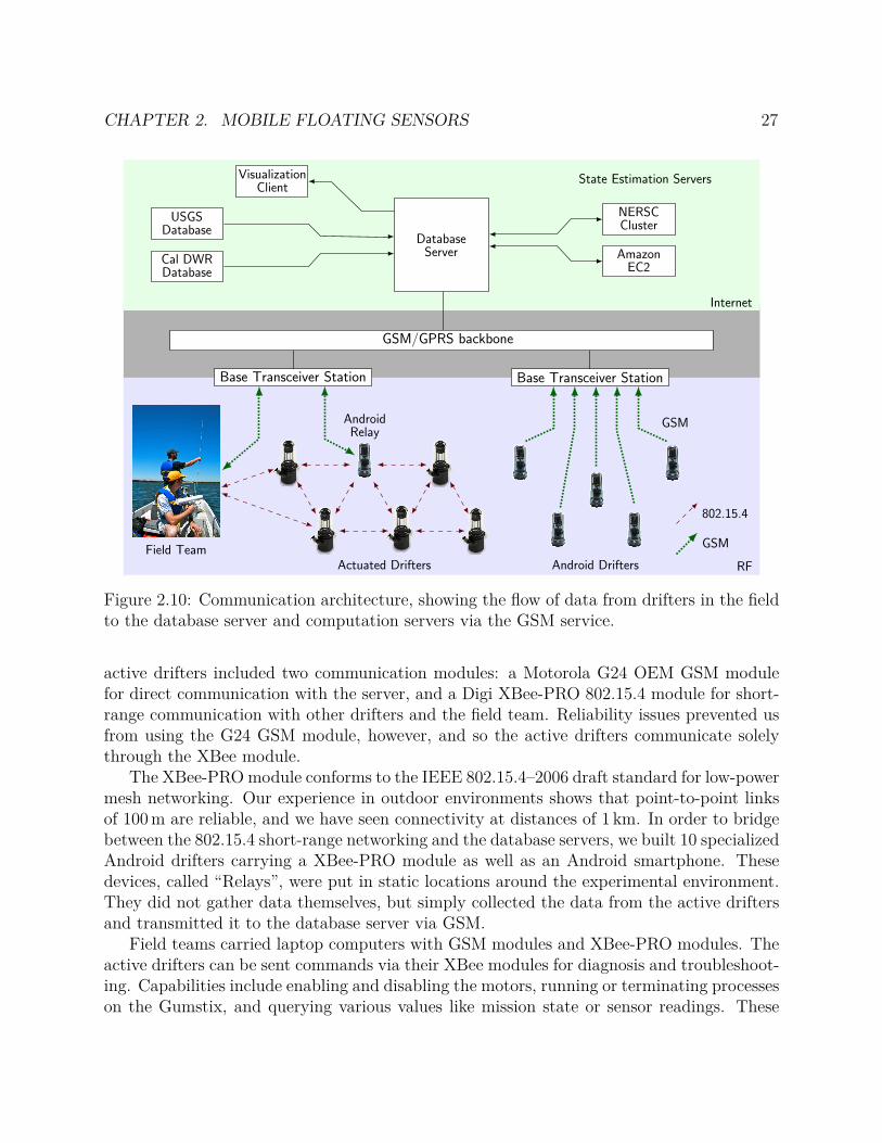
CHAPTER 2. MOBILE FLOATING SENSORS 27
RF
Internet
Actuated Drifters
GSM
802.15.4
GSMField TeamAndroid Drifters
AndroidRelay
GSM/GPRS backbone
Base Transceiver Station Base Transceiver Station
DatabaseServer
VisualizationClient
USGSDatabase
Cal DWRDatabase
State Estimation Servers
NERSCCluster
AmazonEC2
Figure 2.10: Communication architecture, showing the flow of data from drifters in the fieldto the database server and computation servers via the GSM service.
active drifters included two communication modules: a Motorola G24 OEM GSM modulefor direct communication with the server, and a Digi XBee-PRO 802.15.4 module for short-range communication with other drifters and the field team. Reliability issues prevented usfrom using the G24 GSM module, however, and so the active drifters communicate solelythrough the XBee module.
The XBee-PRO module conforms to the IEEE 802.15.4–2006 draft standard for low-powermesh networking. Our experience in outdoor environments shows that point-to-point linksof 100 m are reliable, and we have seen connectivity at distances of 1 km. In order to bridgebetween the 802.15.4 short-range networking and the database servers, we built 10 specializedAndroid drifters carrying a XBee-PRO module as well as an Android smartphone. Thesedevices, called “Relays”, were put in static locations around the experimental environment.They did not gather data themselves, but simply collected the data from the active driftersand transmitted it to the database server via GSM.
Field teams carried laptop computers with GSM modules and XBee-PRO modules. Theactive drifters can be sent commands via their XBee modules for diagnosis and troubleshoot-ing. Capabilities include enabling and disabling the motors, running or terminating processeson the Gumstix, and querying various values like mission state or sensor readings. These

CHAPTER 2. MOBILE FLOATING SENSORS 28
commands can be sent directly over the XBee link, or can be sent indirectly over GSMthrough the database server and the Android relays. This command capability is for devel-opment and debugging purposes. During the April 12 and May 9 experiments, no commandswere sent to the active drifters; they operated autonomously.
The database server acts as a central repository for gathered data and assimilation results.In addition to the Lagrangian data collected by the drifters, relevant data from USGS andCalifornia Department of Water Resources (DWR) sensor stations is collected and stored.The sensor data is sent to the computational cluster, which can be either a collection ofAmazon Elastic Computing Cloud (EC2) processors or the NSERC computational cluster.Results from the assimilation process are stored on the same database server, and queriedby the visualization application, which can be accessed on the Web by any browser.
Assembly and testing
The construction and debugging of this kind of autonomous system is made especially chal-lenging due to the quantity of units we built. In this section we describe our experience inbuilding the fleet, possibly offering ideas to others who wish to undertake a similar effort.We prototyped the drifters in several stages. The first drifter was built by hand assemblingthe electronics boards and drifter body. Subsequent drifters had the electronics and hullproduced by outside companies, although all of the pieces still needed to be attached to-gether. We created detailed documentation with pictures so that we could employ outsidehelp such as interns to assemble them. Our first batch of drifters was a quantity of 10,which we dubbed Generation 3.0. These electronics of the units had several problems, inparticular, they were expensive, used unreliable connectors, and were difficult to service.The second batch of 10 was dubbed Generation 3.1 and was redesigned to address theseproblems. Finally, we produced 20 more Generation 3.1 drifters, bring our total fleet size to40.
From our experience with the Generation 2 drifters, we made it a specific goal in designingGeneration 3 for them to be quick to set-up for experiments as well as update their software.Features of the drifters include a screw-top lid and battery connections that can be pulledout to be charged. A serial port is easily accessible which provides console access to theLinux computer. Since it proved time-consuming to update software or download logs fromeach drifter individually, a custom piece of software was written to automate the process byautonomously entering in console commands and interpreting the results. Combined witha 20-port serial cable and a bootloader program residing on the drifter, we can update thesoftware on all of the devices in less than an hour.
For keeping track of the fleet status, we found it invaluable to maintain a spreadsheet,shared amongst the group, listing drifter IDs and the status of their systems. Drifter IDs areassigned chronologically based on when they were built, from 0 to 39. We divide the fleetinto four groups: Drifters which are beyond repair, drifters which are not field ready butcould be repaired, drifters which perform sub-optimally, but can be deployed in the field, anddrifters which perform well. Tests to classify the drifters were carried out at a neighborhood
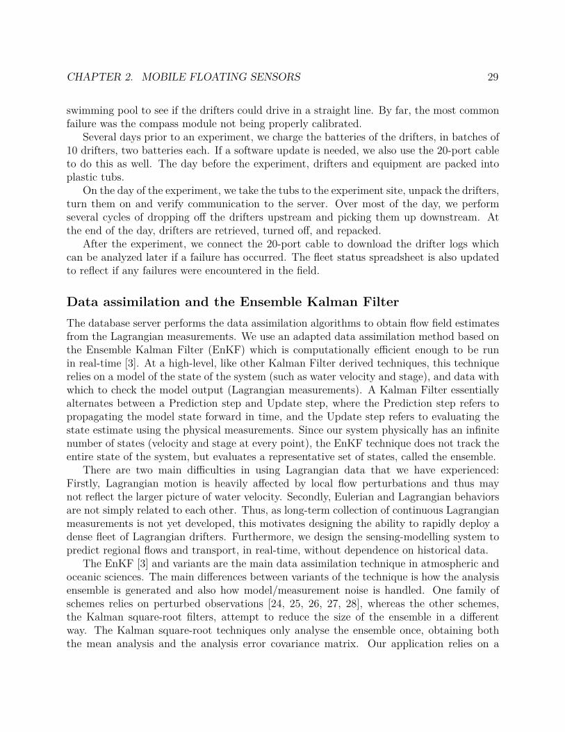
CHAPTER 2. MOBILE FLOATING SENSORS 29
swimming pool to see if the drifters could drive in a straight line. By far, the most commonfailure was the compass module not being properly calibrated.
Several days prior to an experiment, we charge the batteries of the drifters, in batches of10 drifters, two batteries each. If a software update is needed, we also use the 20-port cableto do this as well. The day before the experiment, drifters and equipment are packed intoplastic tubs.
On the day of the experiment, we take the tubs to the experiment site, unpack the drifters,turn them on and verify communication to the server. Over most of the day, we performseveral cycles of dropping off the drifters upstream and picking them up downstream. Atthe end of the day, drifters are retrieved, turned off, and repacked.
After the experiment, we connect the 20-port cable to download the drifter logs whichcan be analyzed later if a failure has occurred. The fleet status spreadsheet is also updatedto reflect if any failures were encountered in the field.
Data assimilation and the Ensemble Kalman Filter
The database server performs the data assimilation algorithms to obtain flow field estimatesfrom the Lagrangian measurements. We use an adapted data assimilation method based onthe Ensemble Kalman Filter (EnKF) which is computationally efficient enough to be runin real-time [3]. At a high-level, like other Kalman Filter derived techniques, this techniquerelies on a model of the state of the system (such as water velocity and stage), and data withwhich to check the model output (Lagrangian measurements). A Kalman Filter essentiallyalternates between a Prediction step and Update step, where the Prediction step refers topropagating the model state forward in time, and the Update step refers to evaluating thestate estimate using the physical measurements. Since our system physically has an infinitenumber of states (velocity and stage at every point), the EnKF technique does not track theentire state of the system, but evaluates a representative set of states, called the ensemble.
There are two main difficulties in using Lagrangian data that we have experienced:Firstly, Lagrangian motion is heavily affected by local flow perturbations and thus maynot reflect the larger picture of water velocity. Secondly, Eulerian and Lagrangian behaviorsare not simply related to each other. Thus, as long-term collection of continuous Lagrangianmeasurements is not yet developed, this motivates designing the ability to rapidly deploy adense fleet of Lagrangian drifters. Furthermore, we design the sensing-modelling system topredict regional flows and transport, in real-time, without dependence on historical data.
The EnKF [3] and variants are the main data assimilation technique in atmospheric andoceanic sciences. The main differences between variants of the technique is how the analysisensemble is generated and also how model/measurement noise is handled. One family ofschemes relies on perturbed observations [24, 25, 26, 27, 28], whereas the other schemes,the Kalman square-root filters, attempt to reduce the size of the ensemble in a differentway. The Kalman square-root techniques only analyse the ensemble once, obtaining boththe mean analysis and the analysis error covariance matrix. Our application relies on a

CHAPTER 2. MOBILE FLOATING SENSORS 30
system Bayesian approach [29, 30, 31] to recover from modelling errors. This approximatingapproach [32] approximates the modeling error with additive Gaussian noise processes.
We chose to use the REALM flow model developed by Lawrence Berkeley National Lab(LBNL). Every time step, new data is received from the drifters, and a shallow water modelgenerates a representative set of states by evolving the processed inputs. The EnKF routinethen compares the real data to gathered output estimates in order to give the best estimationof the flow.
For the May 9, 2012 experiment, 2 hours of field data was collected and run in the as-similation experiment (shown in Figure 2.11). A variety of ensemble members and inflationfactors were tested, as well as different data configurations and model setups. Since therewere no USGS Eulerian measurements available in the experimental domain, the data rec-onciliation method developed by [33] was used to get estimates of the discharge, and poseit to be the first guess of the data assimilation process. This data has also been used toverify an experimental model and estimation technique using hyberbolic partial differentialequations subject to periodic forcing [34].
2.5 Conclusions
The Floating Sensor Network (FSN) has enabled new types of experimental work in riversand estuaries via two novel drifter designs: First, the low-cost, manufacturable, and easy-to-use Android drifter enables economical and high-density collection of Lagrangian data inreal-time. We have shown that the capabilities provided by Android smartphones satisfymost of the features required by a surface drifter. The Android phone also enables real-timereporting and orientation detection by the GSM communications link and accelerometersensor, respectively.
The second technological contribution is the active motorized drifter which demonstratedthe feasibility of motorized Lagrangian sensors and proven that they can indeed avoid ob-stacles, thus significantly extending the particle lifetime of a Lagrangian sensor. We havedeveloped a high-level Hamilton-Jacobi Safety controller, described in the next chapter, aswell as the low-level heading-hold controller which successfully regulates the direction of themotorized drifter under actuation.
These two developments have implications for future drifter studies where previously im-practical areas of water systems can be monitored. Furthermore, the Lagrangian data whichis collected by the FSN has unique advantages over the traditional method of collecting fixedEulerian data, particularly when the mobility of the water is primarily important. In ourmany experiments carried out with the fleet of drifters, we have observed interesting phenom-ena such as jets (when fast moving water such as from a river, enters a stationary body, suchas a lake) and tidal inversions (when water enters a river system from the ocean). In thesecases, Lagrangian data is crucial to determining how the water is mixed and distributed, asthe drifters themselves will be proxies for the water mass.
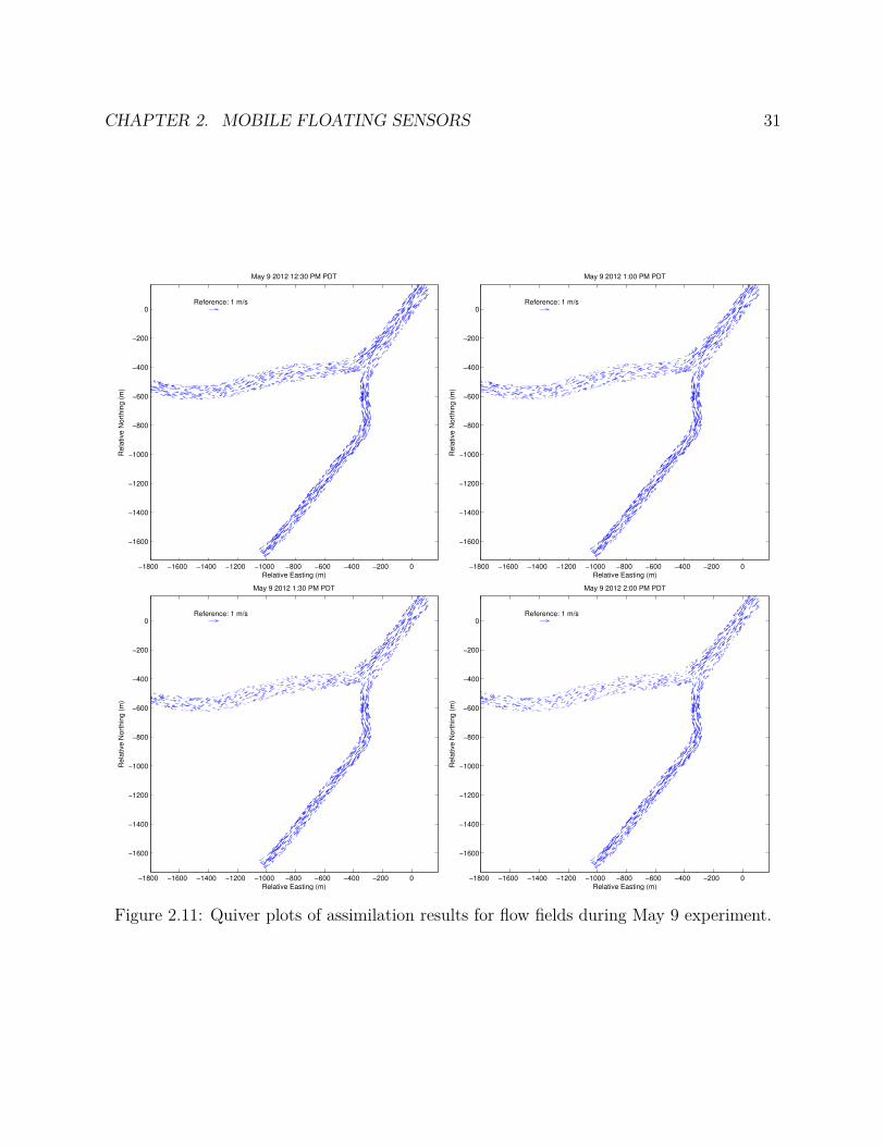
CHAPTER 2. MOBILE FLOATING SENSORS 31
−1800 −1600 −1400 −1200 −1000 −800 −600 −400 −200 0
−1600
−1400
−1200
−1000
−800
−600
−400
−200
0
Relative Easting (m)
Re
lative
No
rth
ing
(m
)
May 9 2012 12:30 PM PDT
Reference: 1 m/s
−1800 −1600 −1400 −1200 −1000 −800 −600 −400 −200 0
−1600
−1400
−1200
−1000
−800
−600
−400
−200
0
Relative Easting (m)
Re
lative
No
rth
ing
(m
)
May 9 2012 1:00 PM PDT
Reference: 1 m/s
−1800 −1600 −1400 −1200 −1000 −800 −600 −400 −200 0
−1600
−1400
−1200
−1000
−800
−600
−400
−200
0
Relative Easting (m)
Re
lative
No
rth
ing
(m
)
May 9 2012 1:30 PM PDT
Reference: 1 m/s
−1800 −1600 −1400 −1200 −1000 −800 −600 −400 −200 0
−1600
−1400
−1200
−1000
−800
−600
−400
−200
0
Relative Easting (m)
Re
lative
No
rth
ing
(m
)
May 9 2012 2:00 PM PDT
Reference: 1 m/s
Figure 2.11: Quiver plots of assimilation results for flow fields during May 9 experiment.

CHAPTER 2. MOBILE FLOATING SENSORS 32
As well, we hope that our successes within the FSN are not constrained to drifter studies,but find applications in mobile environments, such as monitoring airborne pollutants, or fluidflow in internal medicine. For instance, in the next chapter, we elaborate on the Hamilton-Jacobi Safety control method developed for the drifters which can be easily adapted to theaforementioned applications by changing the model.
33
Chapter 3
Hamilton-Jacobi safety control forunderactuated sensors
3.1 Introduction
As we have demonstrated in the previous chapter, the estimation of water mobility withinrivers and estuaries requires Lagrangian sensing. In this scenario, the drifter’s own mobilityis essentially the sensing technique. Therefore, when this mobility is impeded, such as byobstacles, it directly precludes the drifter from accomplishing its sensing task.
In Section 2.3, we described the Generation 3 drifter platform of the Floating SensorNetwork, which is designed to expand the operational capability of our river studies by ven-turing into obstacle-laden environments. We find that, in many of the river environments inthe Sacramento–San Joaquin delta, drifter studies using non-motorized sensors are infeasible.Even when continuously monitored using boat teams, the drifters become stuck on obsta-cles such as the river banks or vegetation. It is simply impossible to retrieve and re-deploythe drifters fast enough to keep them simultaneously unimpeded. Thus, we developed theGeneration 3 motorized drifters and a navigation technique to allow unattended studies inthese challenging environments.
In this chapter, we address the problem of obstacle avoidance and path selection in amobile environment by applying the solutions of Hamilton-Jacobi-Bellman-Isaacs (HJBI)equations. The obstacle avoidance task is the ability of the drifters to avoid becoming stuckon hazards. To comprehensively understand water conditions, it is also necessary for a drifterfleet to distribute itself among multiple paths throughout the water system, which we referto as the path selection task. Although we have developed this technique specifically forthe drifter application, these techniques could be applied to any other mobile environmentwhere we have some control over the mobile elements’ states, and these states must be heldwithin some constraints. Examples include Unmanned Aerial Vehicles (UAV), AutonomousUnderwater Vehicles (AUV), and nano-surgical implanted robots.
Controlling in the presence of obstacles is linked to path planning problems [35, 36],
CHAPTER 3. HAMILTON-JACOBI SAFETY CONTROL FOR UNDERACTUATED
SENSORS 34
which sometimes rely on the same theory as this article [37]. Two features of our problemdistinguish it from the traditional path-planning problem:
• The drifter is an underactuated system. That is, the unit is in the presence of a rivercurrent which is more powerful than the propulsion of the unit. Thus, a successfulalgorithm must account for the river current and act preemptively to avoid beingpushed into an obstacle.
• Our goal is not to reach a single target way-point, rather, the goal of the drifter is tonot run into obstacles.
Several approaches can be used to solve these types of problems. Viability-based ap-proaches compute regions of the state-space such as “all points guaranteed to be safe” [38,39]. Another approach is to use the level and sublevel sets of solutions to HJBI equations[40, 41, 42, 43, 44]. We chose to use the HJBI framework, which can be used to computethe same sets, in order to use an existing mathematical toolbox [45] to solve these equationsnumerically.
Generally, the HJBI method provides a way to evaluate the danger of areas in the river bythe time to reach obstacles, as opposed to the distance to reach obstacles. It incorporates thedynamics and movement of the drifter due to its own actuation, in addition to the movementthat the surrounding water current imparts on it. The HJBI method is a formulaic methodof calculating these areas from intuitive inputs. It applies to many parts of a river system:either large bodies of water, or small tributaries.
We show that the solution to a HJBI equation can be used to construct a minimum-time-to-reach (MTTR) function to a given target region. Two such MTTR functions, Vcenter andVshore, are used to determine the transitions of the on-off controller. With the properMTTR function, it is also possible to find the optimal control policy, i.e. the direction inwhich to travel in order to reach a target the quickest. It is well known that because theHJBI equation is derived by application of Dynamic Programming (DP) techniques [42],synthesizing these MTTR functions suffers the same curse of dimensionality as other DPmethods [46]. Fortunately, for low-dimensional systems, such as described in this article, theproblem is tractable.
The drifter unit’s measured velocity matches the local water velocity only while the drifteris not under actuation. Thus, we seek to maximize the amount of time the motors are turnedcompletely off. On-off control is therefore a natural choice, since it specifies using maximumactuation or none at all. It then remains to determine the on-state policy and thresholds ofthe on-off controller.
In this chapter, we extend upon the results of [20] and go more into depth describing thework, particularly with respect to simulation.
CHAPTER 3. HAMILTON-JACOBI SAFETY CONTROL FOR UNDERACTUATED
SENSORS 35
3.2 Hamilton-Jacobi control methodology
Model and problem statement
We model the system dynamics of a single drifter as a 2-dimensional single-integrator:
x = f(x, a, b) = w(x) + a(t) + b(t), (3.1)
‖a(t)‖2 ≤ a,
‖b(t)‖2 ≤ b,
where x ∈ R2 is a two-dimensional state vector representing the position of the drifter
in meters, a(t) is the control input, and b(t) is the disturbance input. Note the absence ofa yaw state variable, which is intentionally omitted to reduce the computational burden.We believe the term to be largely irrelevant for longer time scales as the vehicle is highlymaneuverable around its vertical axis, owing to the differential drive configuration.
An estimate of the river current, w(x), is given by a forward simulation of the regionwithout integration of drifter-collected data. Note that, although the purpose of the FSNproject, as a whole, is to provide more accurate estimates of the river currents using thedrifters, nevertheless, a less-accurate simulation can be used for the purposes of control. Asthe river current estimates improve by integrating the drifter-collected data, then the controlwill also benefit for future experiments by having a more accurately specified w(x).
We also define the following sets of functions and parameters, a and b:
A , a(·) : ‖a(t)‖2 ≤ a ∀t ,
B ,
b(·) : ‖b(t)‖2 ≤ b ∀t
,
and parametrize the trajectory of the system in terms of time, initial condition, and the a(·)and b(·) inputs,
x = x(t; x0, a(·), b(·)).
With these functions we will set up a differential game [47, 41] in which the inputs a(·)and b(·) work against each other to either satisfy or attempt to violate a safety condition,respectively. As we will see later, b(·) will always act in the opposite direction of a(·) withmagnitude b. Therefore, in this case running this differential game with input constraints(a, b) is equivalent to running a single-player game with input constraints (a− b, 0), althoughthis is not true for general differential games [47].
To set-up this game, we are given a set of undesirable positions, Tshore ⊂ R2 correspond-
ing to collisions with obstacles. Conversely, the complement of this set, S , T C
shore, givesthe positions for which the system is safe.
Our goal is to find a control input a(·) such that
∀t > 0, ∀x0 ∈ S, ∀b(·) ∈ B, x(t; x0, a(·), b(·)) ∈ S. (3.2)
CHAPTER 3. HAMILTON-JACOBI SAFETY CONTROL FOR UNDERACTUATED
SENSORS 36
Ideally, a(·) also minimizes the time of actuation,
tact =∫ ∞
0aon(t)dt,
aon(t) =
1 a(t) 6= 0
0 otherwise
however, the proposed algorithm does not necessarily produce an optimal a(·) in this respect.
Mathematical solutions
In this section we describe the meaning of a MTTR in the context of HJBI equations. Inthe next section, we describe several MTTR functions used in an algorithm to satisfy (3.2).We begin with a target set, T ⊂ R
n, giving a set of states we are trying to reach. Considerthe construction of a static cost function, V (x0):
V (x0) =
infa(·)∈A
supb(·)∈B
∫ t⋆
0l (x(t; x0, a(·), b(·)), a(·), b(·)) dt
, (3.3)
t⋆(x0, a(·), b(·)) = inf t : x(t; x0, a(·), b(·)) ∈ T , (3.4)
where l(·, ·, ·) (Rn,Rni) 7→ R is a Lagrangian cost functional associating a cost for the systemto be in a certain state and taking a certain action.
Thus, the interpretation of (3.4) is that it designates the first time the trajectory,
x(·; a(·), b(·)),
enters T .Suppose we take l(·, ·, ·) ≡ 1, representing a constant accrual of cost until the target set
is reached. Substituting into (3.3),
V (x0) = infa(·)∈A
supb(·)∈B
∫ t⋆
01 · dt
(3.5)
= infa(·)∈A
supb(·)∈B
t⋆(x0, a(·), b(·)),
or, more concisely
V (x0) = t⋆ (x0, a⋆(·), b⋆(·)) , (3.6)
a⋆(·) = arg infa(·)∈A
t⋆, (3.7)
b⋆(·) = arg supb(·)∈B
t⋆,

CHAPTER 3. HAMILTON-JACOBI SAFETY CONTROL FOR UNDERACTUATED
SENSORS 37
where a⋆(·) is called the optimal control for this particular cost function as it minimizes theaccrued cost, and b⋆(·) is the worst case disturbance.
In this case, (3.6) simply gives the minimum time to reach the target set T from x0, sowe call V a MTTR function for this system. Note that V (x0) = +∞ in the case in whichthe target set is not reachable from the initial condition x0.
We are interested in finding the optimal control, or disturbance, which satisfies (3.7) andachieves a minimum-time trajectory to, or from, T . Both can be computed explicitly as afunction of the gradient of the MTTR function by the following relations:
a⋆(x) = −a∇V (x)‖∇V (x)‖2
, b⋆(x) = b∇V (x)‖∇V (x)‖2
. (3.8)
In general, V is difficult to compute especially for systems such as (3.1) which have anarbitrary forcing term, w, and an arbitrary target set, T . We elect to extend the techniquefound in [45] for finding the MTTR function of a holonomic system: a time-dependent HJBIequation, for which there are known methods to solve [48], is constructed as follows:
0 = φt + min[
0, G(x,∇φ)]
, 0 < t < h, (3.9)
G(x, p) , max‖a‖2≤a
min‖b‖2≤b
pT · f(x, a, b)
.
φ(x, 0) =
−1 x ∈ T1 otherwise
, (3.10)
noting that, although φ is, by definition, discontinuous at t = 0, that by using the Lax-Friedrichs numerical method, this discontinuity is be dissipated and the solution is stable[49, 45].
As shown in [41], T can be reached in h time or less from the set of points
G(h) = x : φ(x, h) ≤ 0 .
The frontier of this set of points as it evolves through time is also the set of points fromwhich T can be reached in exactly h time. The set is related to V by
∂G(h) = x : φ(x, h) = 0 .
Consider a contour, x : V (x) = h of the MTTR function, describing a set of pointsreachable in exactly h time units. Comparing this contour with ∂G(h), we find that, for agiven x, V (x) is given by the first temporal zero crossing of φ(x, t). If such a zero crossingdoes not exist, this means the system cannot navigate from x to T , therefore, V (x) = +∞.This zero crossing can be calculated numerically as in [45].
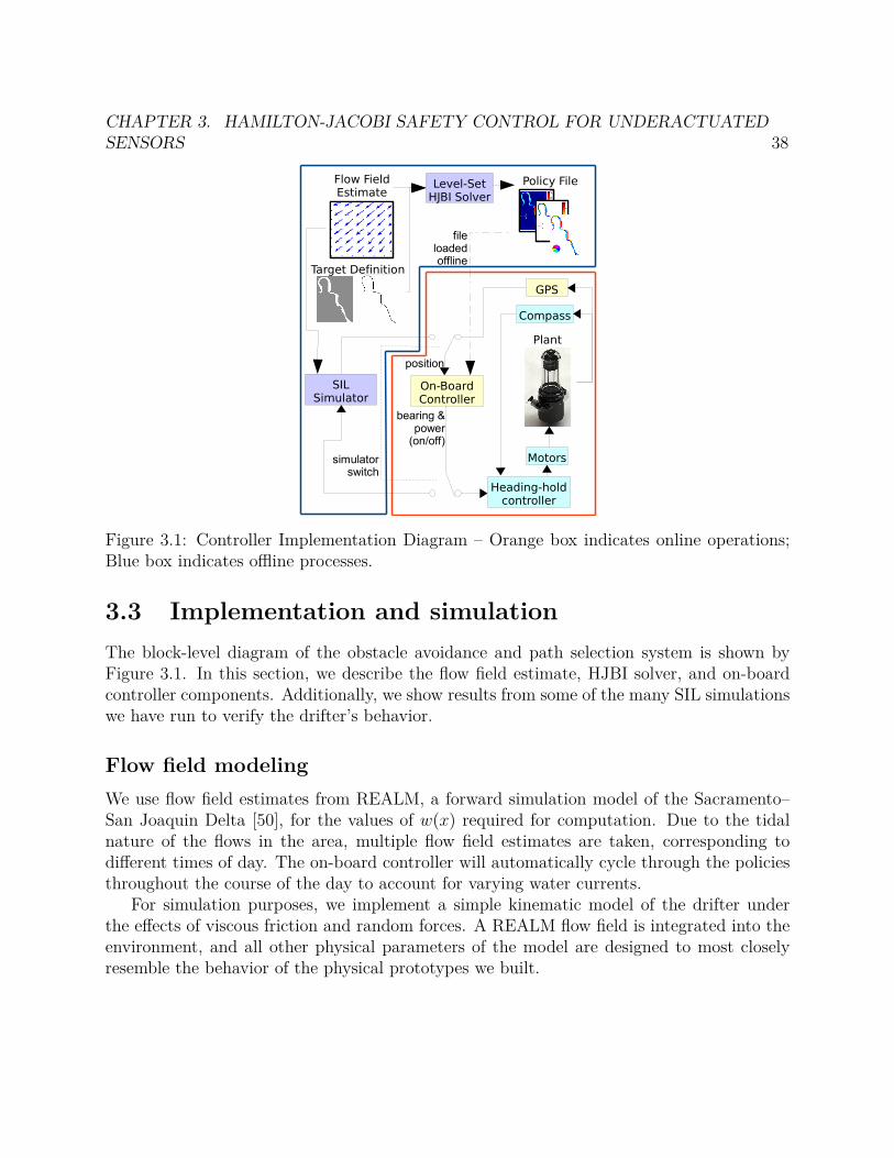
CHAPTER 3. HAMILTON-JACOBI SAFETY CONTROL FOR UNDERACTUATED
SENSORS 38
Level-SetHJBI Solver
Flow FieldEstimate
Target Definition
Policy File
On-BoardController
GPS
SILSimulator
Plant
Motors
Compass
Heading-holdcontroller
fileloadedoffline
bearing &power
(on/off)
simulatorswitch
position
Figure 3.1: Controller Implementation Diagram – Orange box indicates online operations;Blue box indicates offline processes.
3.3 Implementation and simulation
The block-level diagram of the obstacle avoidance and path selection system is shown byFigure 3.1. In this section, we describe the flow field estimate, HJBI solver, and on-boardcontroller components. Additionally, we show results from some of the many SIL simulationswe have run to verify the drifter’s behavior.
Flow field modeling
We use flow field estimates from REALM, a forward simulation model of the Sacramento–San Joaquin Delta [50], for the values of w(x) required for computation. Due to the tidalnature of the flows in the area, multiple flow field estimates are taken, corresponding todifferent times of day. The on-board controller will automatically cycle through the policiesthroughout the course of the day to account for varying water currents.
For simulation purposes, we implement a simple kinematic model of the drifter underthe effects of viscous friction and random forces. A REALM flow field is integrated into theenvironment, and all other physical parameters of the model are designed to most closelyresemble the behavior of the physical prototypes we built.
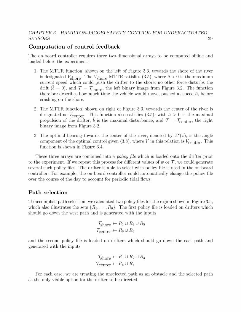
CHAPTER 3. HAMILTON-JACOBI SAFETY CONTROL FOR UNDERACTUATED
SENSORS 39
Computation of control feedback
The on-board controller requires three two-dimensional arrays to be computed offline andloaded before the experiment:
1. The MTTR function, shown on the left of Figure 3.3, towards the shore of the riveris designated Vshore. The Vshore MTTR satisfies (3.5), where a > 0 is the maximumcurrent speed which could push the drifter to the shore, no other force disturbs thedrift (b = 0), and T = Tshore, the left binary image from Figure 3.2. The functiontherefore describes how much time the vehicle would move, pushed at speed a, beforecrashing on the shore.
2. The MTTR function, shown on right of Figure 3.3, towards the center of the river isdesignated as Vcenter. This function also satisfies (3.5), with a > 0 is the maximalpropulsion of the drifter, b is the maximal disturbance, and T = Tcenter, the rightbinary image from Figure 3.2.
3. The optimal bearing towards the center of the river, denoted by ∠⋆(x), is the anglecomponent of the optimal control given (3.8), where V in this relation is Vcenter. Thisfunction is shown in Figure 3.4.
These three arrays are combined into a policy file which is loaded onto the drifter priorto the experiment. If we repeat this process for different values of w or T , we could generateseveral such policy files. The drifter is able to select with policy file is used in the on-boardcontroller. For example, the on-board controller could automatically change the policy fileover the course of the day to account for periodic tidal flows.
Path selection
To accomplish path selection, we calculated two policy files for the region shown in Figure 3.5,which also illustrates the sets R1, . . . , R6. The first policy file is loaded on drifters whichshould go down the west path and is generated with the inputs
Tshore ← R1 ∪R4 ∪R5
Tcenter ← R6 ∪R3
and the second policy file is loaded on drifters which should go down the east path andgenerated with the inputs
Tshore ← R1 ∪R2 ∪R3
Tcenter ← R6 ∪R5
For each case, we are treating the unselected path as an obstacle and the selected pathas the only viable option for the drifter to be directed.
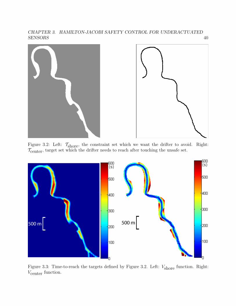
CHAPTER 3. HAMILTON-JACOBI SAFETY CONTROL FOR UNDERACTUATED
SENSORS 40
Figure 3.2: Left: Tshore, the constraint set which we want the drifter to avoid. Right:Tcenter, target set which the drifter needs to reach after touching the unsafe set.
Figure 3.3: Time-to-reach the targets defined by Figure 3.2. Left: Vshore function. Right:Vcenter function.

CHAPTER 3. HAMILTON-JACOBI SAFETY CONTROL FOR UNDERACTUATED
SENSORS 41
∠⋆ (by color)
Figure 3.4: The optimal bearing to center of the river, ∠⋆(x).
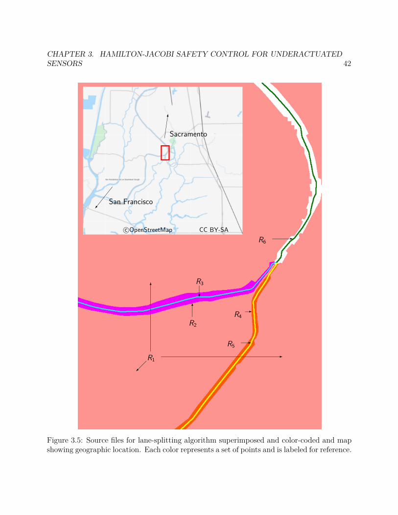
CHAPTER 3. HAMILTON-JACOBI SAFETY CONTROL FOR UNDERACTUATED
SENSORS 42
San Francisco
Sacramento
c©OpenStreetMap CC BY-SA
R1
R2
R3
R4
R5
R6
Figure 3.5: Source files for lane-splitting algorithm superimposed and color-coded and mapshowing geographic location. Each color represents a set of points and is labeled for reference.
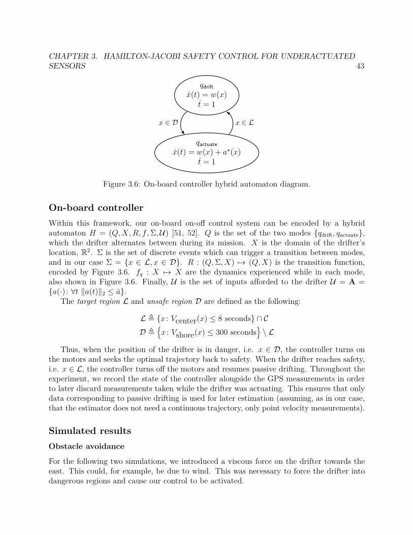
CHAPTER 3. HAMILTON-JACOBI SAFETY CONTROL FOR UNDERACTUATED
SENSORS 43
qdrift
x(t) = w(x)t = 1
qactuate
x(t) = w(x) + a⋆(x)t = 1
x ∈ D x ∈ L
Figure 3.6: On-board controller hybrid automaton diagram.
On-board controller
Within this framework, our on-board on-off control system can be encoded by a hybridautomaton H = (Q, X, R, f , Σ,U) [51, 52]. Q is the set of the two modes qdrift, qactuate,which the drifter alternates between during its mission. X is the domain of the drifter’slocation, R2. Σ is the set of discrete events which can trigger a transition between modes,and in our case Σ = x ∈ L, x ∈ D. R : (Q, Σ, X) 7→ (Q, X) is the transition function,encoded by Figure 3.6. fq : X 7→ X are the dynamics experienced while in each mode,also shown in Figure 3.6. Finally, U is the set of inputs afforded to the drifter U = A =a(·) : ∀t ‖a(t)‖2 ≤ a.
The target region L and unsafe region D are defined as the following:
L , x : Vcenter(x) ≤ 8 seconds ∩ CD ,
x : Vshore(x) ≤ 300 seconds
\ L
Thus, when the position of the drifter is in danger, i.e. x ∈ D, the controller turns onthe motors and seeks the optimal trajectory back to safety. When the drifter reaches safety,i.e. x ∈ L, the controller turns off the motors and resumes passive drifting. Throughout theexperiment, we record the state of the controller alongside the GPS measurements in orderto later discard measurements taken while the drifter was actuating. This ensures that onlydata corresponding to passive drifting is used for later estimation (assuming, as in our case,that the estimator does not need a continuous trajectory, only point velocity measurements).
Simulated results
Obstacle avoidance
For the following two simulations, we introduced a viscous force on the drifter towards theeast. This could, for example, be due to wind. This was necessary to force the drifter intodangerous regions and cause our control to be activated.
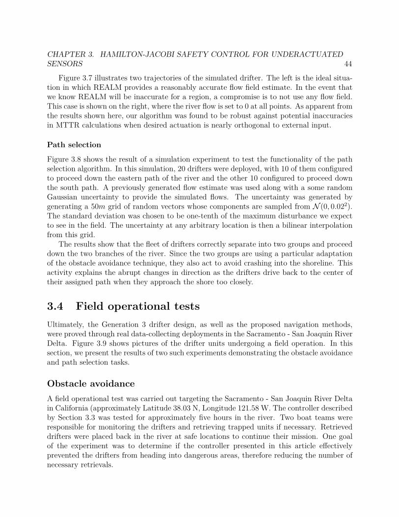
CHAPTER 3. HAMILTON-JACOBI SAFETY CONTROL FOR UNDERACTUATED
SENSORS 44
Figure 3.7 illustrates two trajectories of the simulated drifter. The left is the ideal situa-tion in which REALM provides a reasonably accurate flow field estimate. In the event thatwe know REALM will be inaccurate for a region, a compromise is to not use any flow field.This case is shown on the right, where the river flow is set to 0 at all points. As apparent fromthe results shown here, our algorithm was found to be robust against potential inaccuraciesin MTTR calculations when desired actuation is nearly orthogonal to external input.
Path selection
Figure 3.8 shows the result of a simulation experiment to test the functionality of the pathselection algorithm. In this simulation, 20 drifters were deployed, with 10 of them configuredto proceed down the eastern path of the river and the other 10 configured to proceed downthe south path. A previously generated flow estimate was used along with a some randomGaussian uncertainty to provide the simulated flows. The uncertainty was generated bygenerating a 50m grid of random vectors whose components are sampled from N (0, 0.022).The standard deviation was chosen to be one-tenth of the maximum disturbance we expectto see in the field. The uncertainty at any arbitrary location is then a bilinear interpolationfrom this grid.
The results show that the fleet of drifters correctly separate into two groups and proceeddown the two branches of the river. Since the two groups are using a particular adaptationof the obstacle avoidance technique, they also act to avoid crashing into the shoreline. Thisactivity explains the abrupt changes in direction as the drifters drive back to the center oftheir assigned path when they approach the shore too closely.
3.4 Field operational tests
Ultimately, the Generation 3 drifter design, as well as the proposed navigation methods,were proved through real data-collecting deployments in the Sacramento - San Joaquin RiverDelta. Figure 3.9 shows pictures of the drifter units undergoing a field operation. In thissection, we present the results of two such experiments demonstrating the obstacle avoidanceand path selection tasks.
Obstacle avoidance
A field operational test was carried out targeting the Sacramento - San Joaquin River Deltain California (approximately Latitude 38.03 N, Longitude 121.58 W. The controller describedby Section 3.3 was tested for approximately five hours in the river. Two boat teams wereresponsible for monitoring the drifters and retrieving trapped units if necessary. Retrieveddrifters were placed back in the river at safe locations to continue their mission. One goalof the experiment was to determine if the controller presented in this article effectivelyprevented the drifters from heading into dangerous areas, therefore reducing the number ofnecessary retrievals.
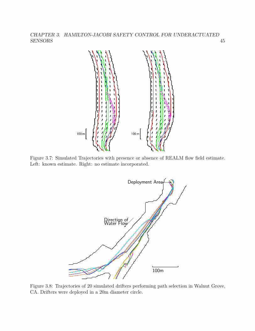
CHAPTER 3. HAMILTON-JACOBI SAFETY CONTROL FOR UNDERACTUATED
SENSORS 45
Figure 3.7: Simulated Trajectories with presence or absence of REALM flow field estimate.Left: known estimate. Right: no estimate incorporated.
Deployment Area
Direction ofWater Flow
100m
Figure 3.8: Trajectories of 20 simulated drifters performing path selection in Walnut Grove,CA. Drifters were deployed in a 20m diameter circle.
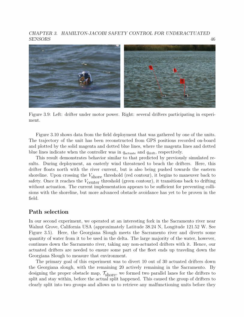
CHAPTER 3. HAMILTON-JACOBI SAFETY CONTROL FOR UNDERACTUATED
SENSORS 46
Figure 3.9: Left: drifter under motor power. Right: several drifters participating in experi-ment.
Figure 3.10 shows data from the field deployment that was gathered by one of the units.The trajectory of the unit has been reconstructed from GPS positions recorded on-boardand plotted by the solid magenta and dotted blue lines, where the magenta lines and dottedblue lines indicate when the controller was in qactuate and qdrift, respectively.
This result demonstrates behavior similar to that predicted by previously simulated re-sults. During deployment, an easterly wind threatened to beach the drifters. Here, thisdrifter floats north with the river current, but is also being pushed towards the easternshoreline. Upon crossing the Vshore threshold (red contour), it begins to maneuver back tosafety. Once it reaches the Vcenter threshold (green contour), it transitions back to driftingwithout actuation. The current implementation appears to be sufficient for preventing colli-sions with the shoreline, but more advanced obstacle avoidance has yet to be proven in thefield.
Path selection
In our second experiment, we operated at an interesting fork in the Sacramento river nearWalnut Grove, California USA (approximately Latitude 38.24 N, Longitude 121.52 W. SeeFigure 3.5). Here, the Georgiana Slough meets the Sacramento river and diverts somequantity of water from it to be used in the delta. The large majority of the water, however,continues down the Sacramento river, taking any non-actuated drifters with it. Hence, ouractuated drifters are needed to ensure some part of the fleet ends up traveling down theGeorgiana Slough to measure that environment.
The primary goal of this experiment was to divert 10 out of 30 actuated drifters downthe Georgiana slough, with the remaining 20 actively remaining in the Sacramento. Bydesigning the proper obstacle map, Tshore, we formed two parallel lanes for the drifters tosplit and stay within, before the actual split happened. This caused the group of drifters toclearly split into two groups and allows us to retrieve any malfunctioning units before they
CHAPTER 3. HAMILTON-JACOBI SAFETY CONTROL FOR UNDERACTUATED
SENSORS 47
are in danger. In practice, the algorithm does not require that these lanes are drawn, onlythat an obstacle be drawn across unselected paths.
Figure 3.11 is a plot of the trajectories of two drifters, one from each group. The datarepresents a GPS location taken every two seconds by each drifter and passed through a twoelement moving average filter to remove sensor noise from the GPS system. Note that, unlikeFigure 3.10, the drifters clearly enter the unsafe region, however, this does not indicate afailure to satisfy (3.2), since the drifter remained within C. The figure demonstrates thatthe drifters have successfully actuated in a manner placing them in the correct lane andsimultaneously avoiding obstacles.
3.5 Conclusions
The Floating Sensor Network has addressed the practical problem of mobile sensing inobstacle-laden rivers by building a fleet of motorized floating sensors. In this chapter, wedescribed a successful technique for controlling our autonomous floating sensor platforms sothat they avoid obstacles and the shoreline during a mission. We demonstrated, throughsimulation and field testing, the efficacy of the algorithm for the scenarios in which the unitmust actively avoid running against the bank of a river, and in which the unit must driveitself down a particular fork of the river.
At the conclusion of this study, we achieved our primary goal which was to preventobstacle collisions in the presence of a water current which was stronger than the controlauthority of the drifter itself. In fact, the primary reasons for failure of the drifters toavoid obstacles were hardware failure (e.g. a compass losing calibration or a motor failure),and unmodelled hindrances, such as seaweed. The amount of failures could be significantlyreduced by redesign of the hardware and more detailed mapping of the region prior to anexperiment. However, the results we have achieved clearly demonstrate that the technique isfeasible. The Hamilton-Jacobi safety control techniques prove to be a powerful and effectivetool in mobile environments where control authority is limited, as it can predict dangerouspositions and act accordingly and optimally.
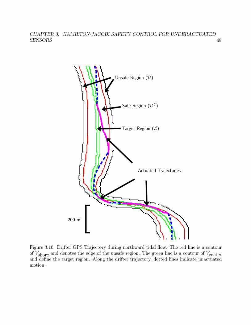
CHAPTER 3. HAMILTON-JACOBI SAFETY CONTROL FOR UNDERACTUATED
SENSORS 48
Unsafe Region (D)
Safe Region (DC)
Target Region (L)
Actuated Trajectories
200 m
Figure 3.10: Drifter GPS Trajectory during northward tidal flow. The red line is a contourof Vshore and denotes the edge of the unsafe region. The green line is a contour of Vcenterand define the target region. Along the drifter trajectory, dotted lines indicate unactuatedmotion.
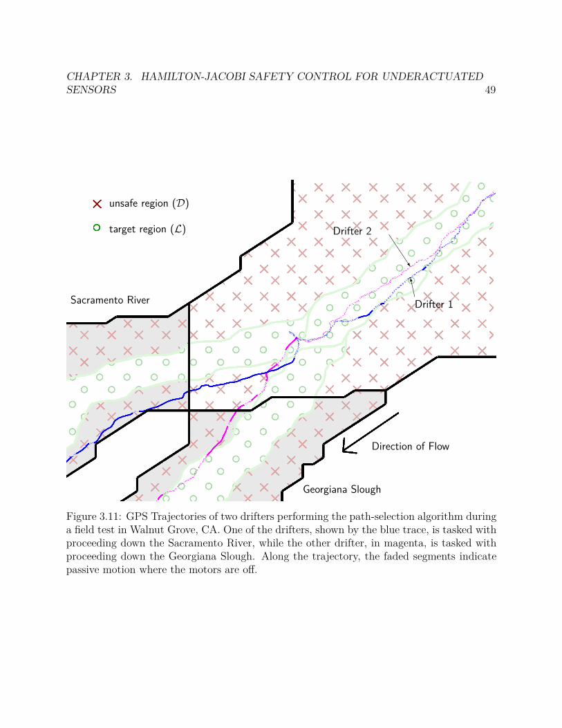
CHAPTER 3. HAMILTON-JACOBI SAFETY CONTROL FOR UNDERACTUATED
SENSORS 49
unsafe region (D)
target region (L)
Direction of Flow
Sacramento River
Georgiana Slough
Drifter 1
Drifter 2
Figure 3.11: GPS Trajectories of two drifters performing the path-selection algorithm duringa field test in Walnut Grove, CA. One of the drifters, shown by the blue trace, is tasked withproceeding down the Sacramento River, while the other drifter, in magenta, is tasked withproceeding down the Georgiana Slough. Along the trajectory, the faded segments indicatepassive motion where the motors are off.
50
Chapter 4
Indoor Environmental Sensors forMobile Sensing
4.1 Introduction
Mobile elements, particularly occupants, of indoor spaces play an important role in the op-eration of a building. The main purpose of an office building is to ensure the safety andcomfort of its occupants, and recently, the goal is to accomplish this while consuming theleast energy possible. Tailoring services such as Heating, Ventilation, and Air Condition-ing (HVAC), lighting, and electrical power, has the potential to save a significant amountof energy consumed. HVAC and lighting respectively comprise 48% and 22% of the totalenergy use of buildings in the USA [53]. To illustrate the impact of occupant-awareness incontrolling these services, occupant-aware control schemes have been shown to save between10-15% [54], 8.3-28.3% [55], or even 42% [56], depending on factors such as outdoor climateand control strategy. Having a more detailed view of occupancy, by knowing where specificoccupants are located, i.e. tracking, can enable control strategies on a person-by-person ba-sis, and opens the door to more energy savings as well as building services which are tailoredto specific occupants.
It is clear that, treated as individuals, or as a mass quantity, occupants are an importmobile element to be observed in a building. Therefore, we seek to answer how many occu-pants are in a space (i.e. occupancy estimation, Chapter 5) and where individual occupantsare located (i.e. occupant tracking, Chapter 6). In the next three chapters, we will discussthe technological and theoretical developments which answer these questions. The lattertwo chapters discuss the estimation frameworks and techniques. As in the river current es-timation problem, special tools were developed in order to sucessfully apply the estimationproblem to the real-world. In this chapter, we introduce one of these tools, an environmen-tal sensor platform which collects measurements needed for the occupancy estimation andtracking frameworks.
We have invented indoor sensors to support continuous and long-term estimation of
CHAPTER 4. INDOOR ENVIRONMENTAL SENSORS FOR MOBILE SENSING 51
occupancy and occupants. The sensor is a low-cost, battery-powered sensor which is smalland light enough to be unobtrusively installed in an office space. The sensor can optionallybe outfitted with CO2 or particulate matter sensors, which are inputs to the estimation ofoccupancy level (See Chapter 5). The sensor could also be a “tag” which is carried in anoccupant’s pocket, providing information about that occupant’s position. This informationcould be combined with other information via the sensor fusion capabilities of the particlefilter (See Chapter 6).
Paramount to the adoption of an indoor sensing platform is battery lifetime, as it iscostly to replace the batteries of a sensor, especially if the sensor is installed in a difficult toaccess location. For sensors which operate for less than a year, this cost can be unacceptableto a business and the platform will not be installed. We use a combination of strategies toreduce the power consumption of the battery-powered elements in our platform. First, weselect peripheral components with very low standby current consumption (e.g. < 10 µA)and relatively low active current consumption (e.g. < 250 mA). Second, the componentsare heavily duty-cycled, leaving them in their standby state for long periods of time. Forexample, the component with the greatest power consumption, the radio, is used for about5 seconds out of every hour. We also implement an efficient binary communications protocolwhich includes rudimentary data compression. Our stated goal is to achieve a battery lifetimeof over 5 years, however we achieve a theoretical lifetime of over 6 years, calculated fromcurrent measurements taken from the device.
Our estimation framework benefits greatly from having frequent and regular measure-ments of environmental variables. Therefore, we stress the importance of reliable and high-volume communications between the sensor and server. We chose a WiFi-compatible radiotransceiver which supports data rates over 200 times higher than IEEE 802.15.4 technology.Additionally, we chose the TCP/IP protocol stack to leverage its built-in retry mechanismfor reliability. However, this choice necessitates a radio which consumes much more activepower than traditional sensor nodes which use low-power IEEE 802.15.4 technology. Theenergy cost per bit can be reduced by storing a large amount of data and transmitting rela-tively infrequently (e.g. once per hour), thus, our sensor node sacrifices latency of receivingreal-time measurements.
Many sensor network implementations are custom-tailored to the application, howeverthere have been efforts to standardize architectures amongst the various efforts, such asthe ZigBee Alliance [57], WirelessHART which have sucessfully achieved multi-vendor andmulti-national interoperability between devices. We also recognize academic projects suchas OpenWSN [58] and TinyOS [59] which incorporate the latest advancements in protocoldesign. Our resulting sensor architecture is differentiated from these other implementationsprimarily by this use of WiFi versus IEEE 802.15.4 technology. Additionally, these architec-tures usually provide for the transport of bytes from the sensor to the server, but provideonly a small amount of guidance as far as what those bytes should signify (i.e. they donot specify the application layer). Therefore, we document the application protocol of oursensing architecture, which was designed to efficiently accomplish the sensing goal, while stillflexible enough to incorporate additional types of lightweight sensors and actuators.
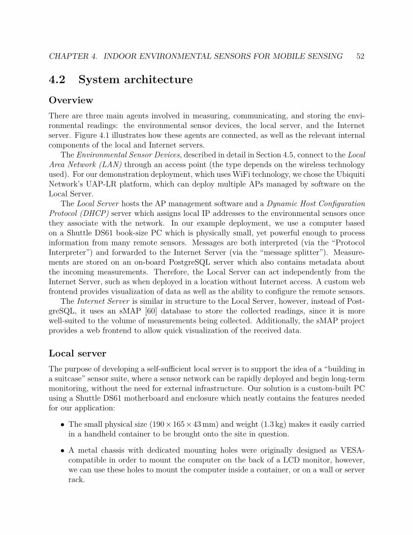
CHAPTER 4. INDOOR ENVIRONMENTAL SENSORS FOR MOBILE SENSING 52
4.2 System architecture
Overview
There are three main agents involved in measuring, communicating, and storing the envi-ronmental readings: the environmental sensor devices, the local server, and the Internetserver. Figure 4.1 illustrates how these agents are connected, as well as the relevant internalcomponents of the local and Internet servers.
The Environmental Sensor Devices, described in detail in Section 4.5, connect to the LocalArea Network (LAN) through an access point (the type depends on the wireless technologyused). For our demonstration deployment, which uses WiFi technology, we chose the UbiquitiNetwork’s UAP-LR platform, which can deploy multiple APs managed by software on theLocal Server.
The Local Server hosts the AP management software and a Dynamic Host ConfigurationProtocol (DHCP) server which assigns local IP addresses to the environmental sensors oncethey associate with the network. In our example deployment, we use a computer basedon a Shuttle DS61 book-size PC which is physically small, yet powerful enough to processinformation from many remote sensors. Messages are both interpreted (via the “ProtocolInterpreter”) and forwarded to the Internet Server (via the “message splitter”). Measure-ments are stored on an on-board PostgreSQL server which also contains metadata aboutthe incoming measurements. Therefore, the Local Server can act independently from theInternet Server, such as when deployed in a location without Internet access. A custom webfrontend provides visualization of data as well as the ability to configure the remote sensors.
The Internet Server is similar in structure to the Local Server, however, instead of Post-greSQL, it uses an sMAP [60] database to store the collected readings, since it is morewell-suited to the volume of measurements being collected. Additionally, the sMAP projectprovides a web frontend to allow quick visualization of the received data.
Local server
The purpose of developing a self-sufficient local server is to support the idea of a “building ina suitcase” sensor suite, where a sensor network can be rapidly deployed and begin long-termmonitoring, without the need for external infrastructure. Our solution is a custom-built PCusing a Shuttle DS61 motherboard and enclosure which neatly contains the features neededfor our application:
• The small physical size (190×165×43 mm) and weight (1.3 kg) makes it easily carriedin a handheld container to be brought onto the site in question.
• A metal chassis with dedicated mounting holes were originally designed as VESA-compatible in order to mount the computer on the back of a LCD monitor, however,we can use these holes to mount the computer inside a container, or on a wall or serverrack.
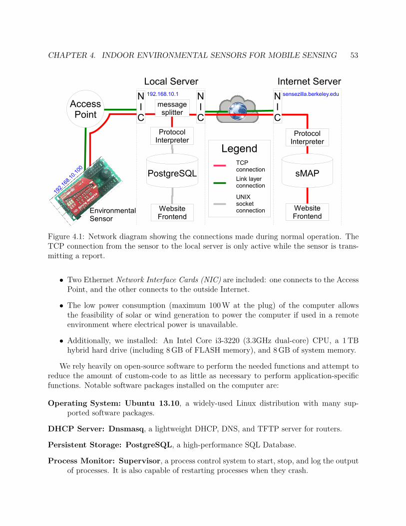
CHAPTER 4. INDOOR ENVIRONMENTAL SENSORS FOR MOBILE SENSING 53
Figure 4.1: Network diagram showing the connections made during normal operation. TheTCP connection from the sensor to the local server is only active while the sensor is trans-mitting a report.
• Two Ethernet Network Interface Cards (NIC) are included: one connects to the AccessPoint, and the other connects to the outside Internet.
• The low power consumption (maximum 100 W at the plug) of the computer allowsthe feasibility of solar or wind generation to power the computer if used in a remoteenvironment where electrical power is unavailable.
• Additionally, we installed: An Intel Core i3-3220 (3.3GHz dual-core) CPU, a 1 TBhybrid hard drive (including 8 GB of FLASH memory), and 8 GB of system memory.
We rely heavily on open-source software to perform the needed functions and attempt toreduce the amount of custom-code to as little as necessary to perform application-specificfunctions. Notable software packages installed on the computer are:
Operating System: Ubuntu 13.10, a widely-used Linux distribution with many sup-ported software packages.
DHCP Server: Dnsmasq, a lightweight DHCP, DNS, and TFTP server for routers.
Persistent Storage: PostgreSQL, a high-performance SQL Database.
Process Monitor: Supervisor, a process control system to start, stop, and log the outputof processes. It is also capable of restarting processes when they crash.
CHAPTER 4. INDOOR ENVIRONMENTAL SENSORS FOR MOBILE SENSING 54
Our custom code is written in Python and uses SQLAlchemy as a Object RelationalMapper (ORM) to map Python objects to rows in the PostgreSQL database. One piece ofcustom code, the “Protocol Interpreter” receives and interprets the messages from the sensordevices and inserts the decoded measurements into the database. It also uses the databaseto retrieve metadata about the devices, for example, which timeseries IDs are associatedwith a given WiFi MAC address.
Another piece of custom code, the “Website Frontend” is built on Flask, a light weightweb application framework. Figure 4.2 shows some screen captures of the web application.Client-side scripting (such as plotting and animating timeseries) is written in Javascriptand extensively uses the JQuery and Flot libraries. The frontend allows a person managingthe network to view, at a glance, the sensor devices associated with the network and when thelast report was received. There is also an interface to create configuration tuples consistingof Name, Fields-to-Report, Sample Interval, and Report Interval (See ConfigureSensor Command in Section 4.4). This is useful, for instance, to easily switch betweena “development” configuration (where nodes report in frequently at the cost of energy),and a “deployment” configuration (where nodes report in long intervals to reduce powerconsumption).
Internet Server
Like the Local Server, the Internet Server also runs an Ubuntu installation. However, theInternet Server is actually a virtual machine hosted by the Berkeley Information Servicesand Technology (IST) Cloud Computing services. This reduces the maintenance, setup effortand costs associated with provisioning a new server platform, as well as being more reliable,since generator-backed power and redundant storage is provided.
Unlike the Local Server, the measurement storage and website interface features areprovided by the sMAP [60] project. The database used by sMAP, ReadingDB [61], is adatabase designed to efficiently store large amounts of timeseries signals, unlike a databasesuch as PostgreSQL which is designed to store relational data. ReadingDB compresses andindexes the timeseries data which reduces the storage requirements, yet maintains quickinsertion and retrieval of the data and minimizes corruption by using write-ahead logging.
Our custom software manages receiving messages forwarded from one or more LocalServers, interpreting the messages, and inserting any parsed data into the sMAP database.We use a PostgreSQL database installed on the Internet Server to store necessary metadataabout the device, such as mapping WiFi MAC Addresses to sMAP stream identifiers.
4.3 Recordstore data format
Our sensor device relies on an inexpensive, low-cost, and low-power microcontroller withlimited computational resources. Since we must store sampled measurements to be later
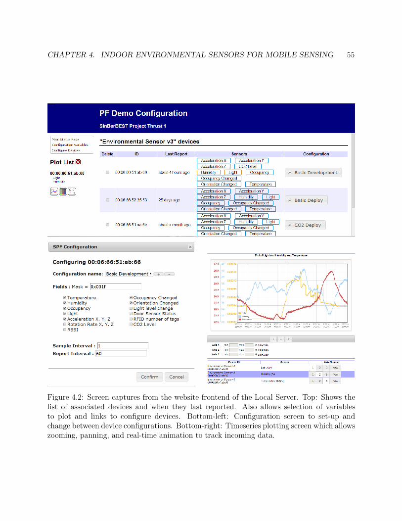
CHAPTER 4. INDOOR ENVIRONMENTAL SENSORS FOR MOBILE SENSING 55
Figure 4.2: Screen captures from the website frontend of the Local Server. Top: Shows thelist of associated devices and when they last reported. Also allows selection of variablesto plot and links to configure devices. Bottom-left: Configuration screen to set-up andchange between device configurations. Bottom-right: Timeseries plotting screen which allowszooming, panning, and real-time animation to track incoming data.
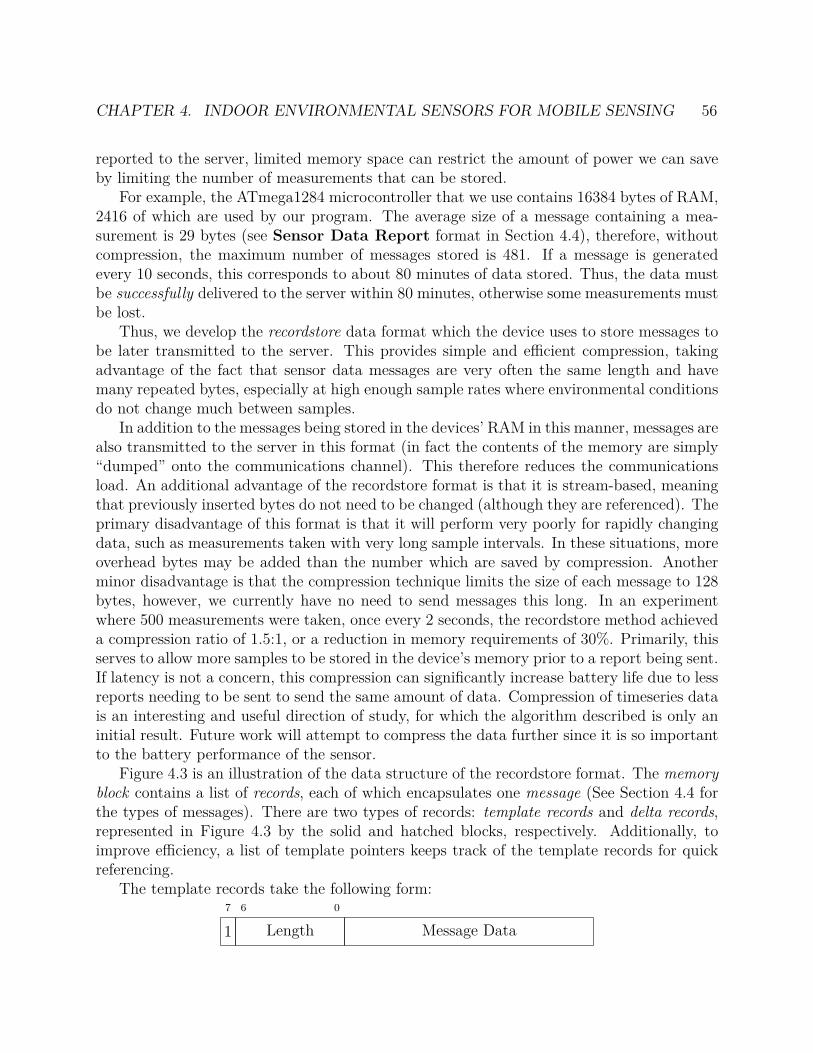
CHAPTER 4. INDOOR ENVIRONMENTAL SENSORS FOR MOBILE SENSING 56
reported to the server, limited memory space can restrict the amount of power we can saveby limiting the number of measurements that can be stored.
For example, the ATmega1284 microcontroller that we use contains 16384 bytes of RAM,2416 of which are used by our program. The average size of a message containing a mea-surement is 29 bytes (see Sensor Data Report format in Section 4.4), therefore, withoutcompression, the maximum number of messages stored is 481. If a message is generatedevery 10 seconds, this corresponds to about 80 minutes of data stored. Thus, the data mustbe successfully delivered to the server within 80 minutes, otherwise some measurements mustbe lost.
Thus, we develop the recordstore data format which the device uses to store messages tobe later transmitted to the server. This provides simple and efficient compression, takingadvantage of the fact that sensor data messages are very often the same length and havemany repeated bytes, especially at high enough sample rates where environmental conditionsdo not change much between samples.
In addition to the messages being stored in the devices’ RAM in this manner, messages arealso transmitted to the server in this format (in fact the contents of the memory are simply“dumped” onto the communications channel). This therefore reduces the communicationsload. An additional advantage of the recordstore format is that it is stream-based, meaningthat previously inserted bytes do not need to be changed (although they are referenced). Theprimary disadvantage of this format is that it will perform very poorly for rapidly changingdata, such as measurements taken with very long sample intervals. In these situations, moreoverhead bytes may be added than the number which are saved by compression. Anotherminor disadvantage is that the compression technique limits the size of each message to 128bytes, however, we currently have no need to send messages this long. In an experimentwhere 500 measurements were taken, once every 2 seconds, the recordstore method achieveda compression ratio of 1.5:1, or a reduction in memory requirements of 30%. Primarily, thisserves to allow more samples to be stored in the device’s memory prior to a report being sent.If latency is not a concern, this compression can significantly increase battery life due to lessreports needing to be sent to send the same amount of data. Compression of timeseries datais an interesting and useful direction of study, for which the algorithm described is only aninitial result. Future work will attempt to compress the data further since it is so importantto the battery performance of the sensor.
Figure 4.3 is an illustration of the data structure of the recordstore format. The memoryblock contains a list of records, each of which encapsulates one message (See Section 4.4 forthe types of messages). There are two types of records: template records and delta records,represented in Figure 4.3 by the solid and hatched blocks, respectively. Additionally, toimprove efficiency, a list of template pointers keeps track of the template records for quickreferencing.
The template records take the following form:7 6 0
1 Length Message Data

CHAPTER 4. INDOOR ENVIRONMENTAL SENSORS FOR MOBILE SENSING 57
Figure 4.3: Diagram of the recordstore data structure in a typical scenario. There are twosets of records in this scenario, designated by the yellow and blue blocks. The solid yellowand blue blocks are the templates for that type of record and the hatched blocks are deltarecords which refer to the respective templates.
where Length contains the length, in bytes, of the Message Data field, which contains anexact copy of the message to be encoded.
The delta records take the form:7 6 0
0 Length Changed Bytes Mask Changed Bytes List
where Length contains the length, in bytes, of the uncompressed message to be encoded.This field directly determines which template record that the delta record corresponds to,where the Length field matches between the two. The Changed Bytes Mask field is a(
8 · ⌈Length
8⌉)
-bit bitmask specifying which bytes are different between the message to beencoded, and the message in the corresponding template record. The following ChangedBytes List field then provides only the bytes of the message which were not the same as thetemplate. For example, Changed Bytes List = 0x11 means that only the first and fifthbytes were different between the template and the message to be encoded. Then, ChangedBytes List would contain two bytes: the first and fifth byte from the message to be encoded,in that order.
Encoding
Assume we are given a message, M , whose length in bytes is l, which must be inserted intothe recordstore. The encoding procedure is as follows:
1. Look through the template records pointed to by the template pointers list. If theLength field of any template, T , is equal to l, then do 1b, however, if there are nosuch templates do 1a.
CHAPTER 4. INDOOR ENVIRONMENTAL SENSORS FOR MOBILE SENSING 58
a) Create a new template record by prepending l as a 7-bit integer and the 1-bitvalue 1 to M . Insert this record at the end of the memory block and create a newentry in the template pointers list pointing to this new template record.
b) Create a new delta record starting with the 1-bit value 0 and l as a 7-bit unsignedinteger. Create the Changed Bytes Mask field with a length of ⌈ l
8⌉ bytes and
initialize all bits to 0, and also create Changed Bytes List as an empty list.From the first to the last byte, compare the template T with the message M . Ifthe byte at position p is different, then set the pth bit of the Changed BytesMask field to 1 and append the pth byte from M to the Changed Bytes List.After all bytes are compared, insert the record at the end of the memory block.
Decoding
Assume we are given a memory block of length L containing all of the records, in theorder they were inserted. Let bi represent the ith byte from the memory block, and letP : (lengths)→ (messages) be an initially-empty map. The goal is to generate a list, D, ofdecoded messages, which is initially empty. The decoding procedure, starting at i = 1, is asfollows:
1. If i ≥ L, then we are done. Otherwise, retrieve the length l from the 7 least significantbits of bi. Look at the MSB of bi, if it is 1, then do 1a, otherwise do 1b.
a) The record is a template record. The decoded message, M are the bytes bi+1
through bi+l. Insert M into D as a decoded message and set the map P (l)←M .Set i← i + 1 + l and continue with 1.
b) The record is a delta record. Retrieve the template message from the map andinitialize the decoded message to an exact copy: M ← P (l) (it is an error if nomapping yet exists). Retrieve the Changed Bytes Mask bitfield from the next⌈ l
8⌉ bytes, and create a list O = o1 . . . on of the bit-positions set to 1. Retrieve
the Changed Bytes List from the next n bytes. For each oj in O, set the ojthbyte of M to the jth byte of the Changed Bytes List. Insert M into D as adecoded message. Finally, Set i← i + 1 + ⌈ l
8⌉+ n and continue with 1.
4.4 Communications protocol
We developed a custom binary format for sensors to report their readings to the databaseserver. Our motivations are the following:
• The protocol should be simple enough to encode and decode on a microcontrollerwithout consuming very much power. Thus, we chose to use a binary protocol relyingon native C data types such as integers and IEEE 754 floating point numbers.

CHAPTER 4. INDOOR ENVIRONMENTAL SENSORS FOR MOBILE SENSING 59
Sensor Server
TCP SYN
TCP SYN-ACK
TCP ACK
Timesync message
Recordstore Data message, TCP ACK
Wait 500ms for host commands
Configure Sensor message (optional)
TCP ACK
TCP FIN
TCP ACK
TCP FIN
TCP ACK
Figure 4.4: Typical exchange between sensor and server during one report, showing packetsat the transport layer and above.
• We should also balance extensibility of the protocol to add new types of messages andsensor data without the protocol becoming overly complex. Our compromise was tohave fixed-length fields specifying the type of hardware, type of message, and types ofsensor data present in each message. The meaning of the field values must be knownacross all agents that wish to encode and decode the messages.
• To reduce power consumption, the protocol should reduce the number of packets thatneed to be sent and minimize the amount of time the radio needs to be active. Thus,our protocol incorporates “batching” many sensor samples into one compressed reportwhich is sent to the server infrequently. Section 4.3 describes the recordstore techniquedesigned to accomplish this.
With these considerations in mind, we develop a simple, yet easily extensible, protocolfor the environmental sensors. Our protocol is essentially a custom binary format relyingon the TCP/IP networking stack to deliver bytes from the sensor to the server and fromthe server to the sensor. Figure 4.4 illustrates a typical packet exchange between the sensordevices and the server (at the transport layer and above) for one sensor report interval.

CHAPTER 4. INDOOR ENVIRONMENTAL SENSORS FOR MOBILE SENSING 60
Lower-layer considerations
Our protocol relies on a layered communications model where lower layers ensure certainproperties about the connection. Our protocol requires that the lower layers guarantee areliable and error-free transmission of bytes between agents on the network, or, if this cannotbe guaranteed, to inform our application as such. Thus, we chose to build our protocol asan application atop a TCP/IP stack. The TCP/IP stack extensively uses acknowledgementpackets to validate the successful transmission of data, which is important to ensure thatour sensor data is not lost, since we can later re-send the data if a transmission failed. Inpractice, if the current link is reliable enough to establish a connection, then we assumethe link is also ready to transmit data, whereas if the link does not survive the initial TCPhandshake, we assume that the link is not reliable and save the data for later retransmission.While we have observed this assumption to be correct while developing the sensors, we haveyet to perform any extended tests to validate the assumption.
Thus, TCP is chosen for its built-in mechanisms to ensure data reliably reaches theserver, however, this comes with a major drawback. Since TCP relies on many separatecontrol packets to establish and tear-down a connection (at a minimum 7, See Figure 4.4),this requires that the radio to be active for the entire time. Thus, approximately one-third (See Figure 4.9) of the sensor’s battery life is expended by the radio alone, even ata very infrequent reporting rate. Future work will be to use the UDP protocol for whichpacket reliability is not enforced by the protocol. We can add a custom acknowledgmentmethod which requires less overhead than TCP. For example, the server could send a singleacknowledgement to the sensor upon receiving a data message, rather then setting up andtearing down an entire TCP connection.
Message framing and escaping
Since TCP is a stream-oriented protocol, it guarantees that bytes are delivered reliably andin order (otherwise delivering an error). However, TCP does not provide framing utilities todesignate discrete sets of bytes that should be treated as one message. We considered thefollowing options when faced with the task of framing messages in the TCP stream:
Connection-based framing
The first method is to constrain each TCP connection to only contain one message, therefore,simply initiating and terminating the TCP connection signals the start and end of a message.This is simple to implement, and requires no extra overhead (i.e. extra energy consumed)when only one message needs to be sent per reporting interval. However, the overhead isvery significant when needing to transmit more than one message since the TCP connectionmust be reconnected, and the radio must be awake during that time.
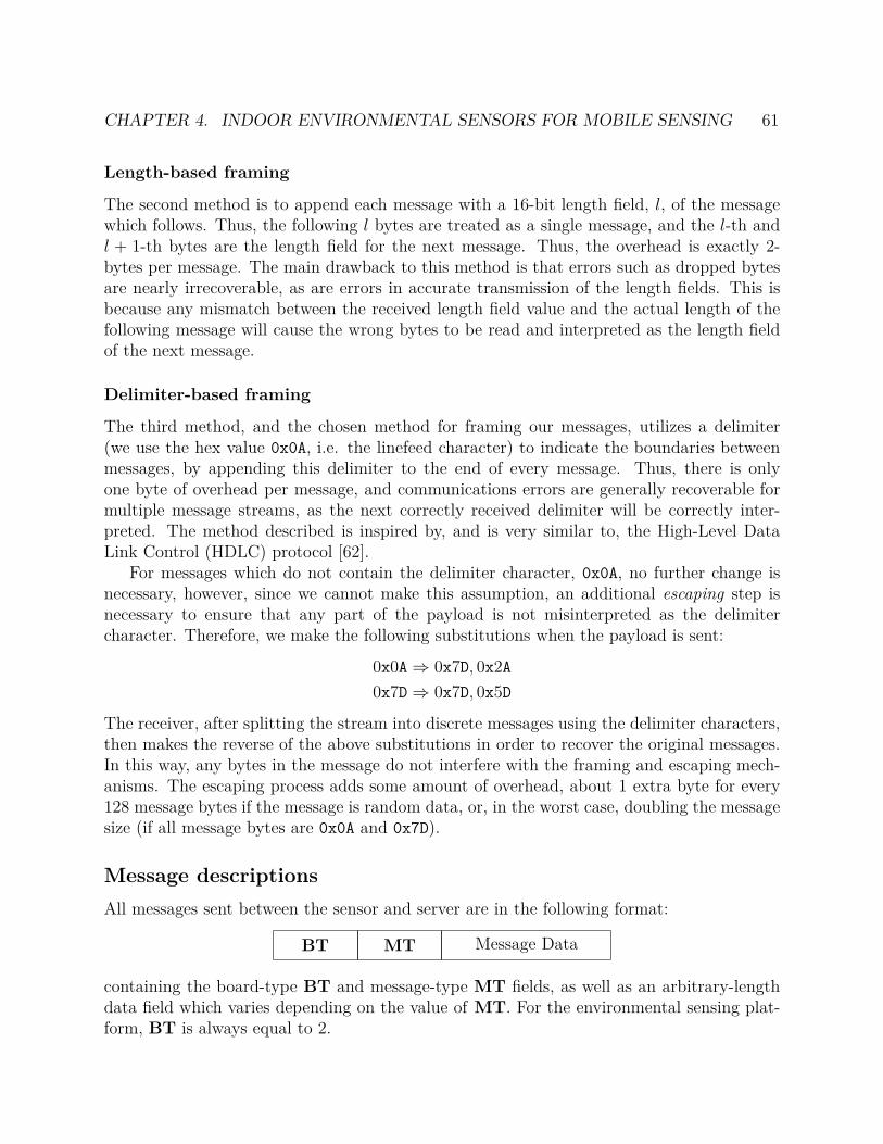
CHAPTER 4. INDOOR ENVIRONMENTAL SENSORS FOR MOBILE SENSING 61
Length-based framing
The second method is to append each message with a 16-bit length field, l, of the messagewhich follows. Thus, the following l bytes are treated as a single message, and the l-th andl + 1-th bytes are the length field for the next message. Thus, the overhead is exactly 2-bytes per message. The main drawback to this method is that errors such as dropped bytesare nearly irrecoverable, as are errors in accurate transmission of the length fields. This isbecause any mismatch between the received length field value and the actual length of thefollowing message will cause the wrong bytes to be read and interpreted as the length fieldof the next message.
Delimiter-based framing
The third method, and the chosen method for framing our messages, utilizes a delimiter(we use the hex value 0x0A, i.e. the linefeed character) to indicate the boundaries betweenmessages, by appending this delimiter to the end of every message. Thus, there is onlyone byte of overhead per message, and communications errors are generally recoverable formultiple message streams, as the next correctly received delimiter will be correctly inter-preted. The method described is inspired by, and is very similar to, the High-Level DataLink Control (HDLC) protocol [62].
For messages which do not contain the delimiter character, 0x0A, no further change isnecessary, however, since we cannot make this assumption, an additional escaping step isnecessary to ensure that any part of the payload is not misinterpreted as the delimitercharacter. Therefore, we make the following substitutions when the payload is sent:
0x0A⇒ 0x7D, 0x2A
0x7D⇒ 0x7D, 0x5D
The receiver, after splitting the stream into discrete messages using the delimiter characters,then makes the reverse of the above substitutions in order to recover the original messages.In this way, any bytes in the message do not interfere with the framing and escaping mech-anisms. The escaping process adds some amount of overhead, about 1 extra byte for every128 message bytes if the message is random data, or, in the worst case, doubling the messagesize (if all message bytes are 0x0A and 0x7D).
Message descriptions
All messages sent between the sensor and server are in the following format:
BT MT Message Data
containing the board-type BT and message-type MT fields, as well as an arbitrary-lengthdata field which varies depending on the value of MT. For the environmental sensing plat-form, BT is always equal to 2.
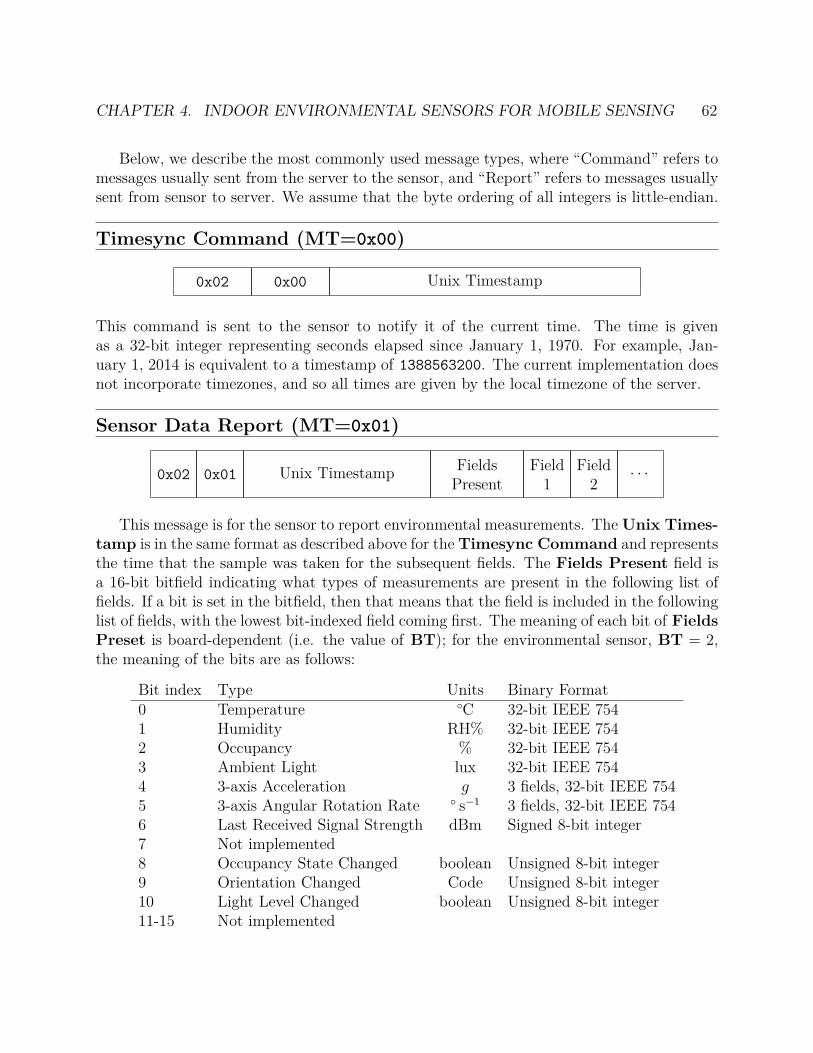
CHAPTER 4. INDOOR ENVIRONMENTAL SENSORS FOR MOBILE SENSING 62
Below, we describe the most commonly used message types, where “Command” refers tomessages usually sent from the server to the sensor, and “Report” refers to messages usuallysent from sensor to server. We assume that the byte ordering of all integers is little-endian.
Timesync Command (MT=0x00)
0x02 0x00 Unix Timestamp
This command is sent to the sensor to notify it of the current time. The time is givenas a 32-bit integer representing seconds elapsed since January 1, 1970. For example, Jan-uary 1, 2014 is equivalent to a timestamp of 1388563200. The current implementation doesnot incorporate timezones, and so all times are given by the local timezone of the server.
Sensor Data Report (MT=0x01)
0x02 0x01 Unix Timestamp FieldsPresent
Field1
Field2
· · ·
This message is for the sensor to report environmental measurements. The Unix Times-tamp is in the same format as described above for the Timesync Command and representsthe time that the sample was taken for the subsequent fields. The Fields Present field isa 16-bit bitfield indicating what types of measurements are present in the following list offields. If a bit is set in the bitfield, then that means that the field is included in the followinglist of fields, with the lowest bit-indexed field coming first. The meaning of each bit of FieldsPreset is board-dependent (i.e. the value of BT); for the environmental sensor, BT = 2,the meaning of the bits are as follows:
Bit index Type Units Binary Format0 Temperature C 32-bit IEEE 7541 Humidity RH% 32-bit IEEE 7542 Occupancy % 32-bit IEEE 7543 Ambient Light lux 32-bit IEEE 7544 3-axis Acceleration g 3 fields, 32-bit IEEE 7545 3-axis Angular Rotation Rate s−1 3 fields, 32-bit IEEE 7546 Last Received Signal Strength dBm Signed 8-bit integer7 Not implemented8 Occupancy State Changed boolean Unsigned 8-bit integer9 Orientation Changed Code Unsigned 8-bit integer10 Light Level Changed boolean Unsigned 8-bit integer11-15 Not implemented

CHAPTER 4. INDOOR ENVIRONMENTAL SENSORS FOR MOBILE SENSING 63
The Occupancy State Changed field is sent with value 1 whenever human activity isdetected (via the PIR sensor) after 10 seconds of inactivity, and sent with value 0 wheneverhuman activity is not detected for 10 seconds, after previously sending the value 1.
The Orientation Changed field is sent whenever the sensor device changes orientationso that any of its axis are aligned, or closely aligned with the gravity vector, and the othertwo axis are parallel to the ground. The following codes are defined:
Code Orientation Code Orientation0x02 X-axis pointed UP 0x01 X-axis pointed DOWN0x08 Y-axis pointed UP 0x04 Y-axis pointed DOWN0x20 Z-axis pointed UP 0x10 Z-axis pointed DOWN
The Light Level Changed field is sent with value 0 any time the ambient light is darkerthan a certain level (approximately the light level inside a closed desk drawer), and sent withvalue 1 whenever the ambient light is above that level. There is a small amount of hysteresisapplied to prevent chattering.
Typically, the sensor periodically samples the measurements and generates Sensor DataReport messages every Sample Interval seconds. However, the Occupancy StateChanged, Orientation Changed, and Light Level Changed fields are asynchronous,meaning that a Sensor Data Report message for these fields is generated exactly wheneverthe appropriate event occurs (to a resolution of 1 second). This allows us to capture eventswhich happen in between the sample intervals.
Configure Sensor Command (MT=0x02)
0x02 0x02VariablesPresent
Variable 1 Variable 2 Variable 3
This command is used to configure the sensor, mainly to allow remote configuration ofvariables that affect the battery lifetime of the device. This message is extensible to allowup to 8 configuration variables to be defined. The Variables Present bitfield is currentlyimplemented as:
bit 0 Fields-to-report variable present.
bit 1 Sample Interval variable present.
bit 2 Report Interval variable present.
bits 3–7 Not implemented.
If a bit is set in the bitfield, then the corresponding variable is present in the followingfields of the message, with the lowest bit-indexed variable coming first. For example, if
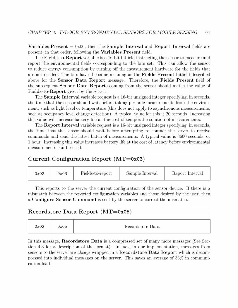
CHAPTER 4. INDOOR ENVIRONMENTAL SENSORS FOR MOBILE SENSING 64
Variables Present = 0x06, then the Sample Interval and Report Interval fields arepresent, in that order, following the Variables Present field.
The Fields-to-Report variable is a 16-bit bitfield instructing the sensor to measure andreport the environmental fields corresponding to the bits set. This can allow the sensorto reduce energy consumption by turning off the measurement hardware for the fields thatare not needed. The bits have the same meaning as the Fields Present bitfield describedabove for the Sensor Data Report message. Therefore, the Fields Present field ofthe subsequent Sensor Data Reports coming from the sensor should match the value ofFields-to-Report given by the server.
The Sample Interval variable request is a 16-bit unsigned integer specifying, in seconds,the time that the sensor should wait before taking periodic measurements from the environ-ment, such as light level or temperature (this does not apply to asynchronous measurements,such as occupancy level change detection). A typical value for this is 20 seconds. Increasingthis value will increase battery life at the cost of temporal resolution of measurements.
The Report Interval variable request is a 16-bit unsigned integer specifying, in seconds,the time that the sensor should wait before attempting to contact the server to receivecommands and send the latest batch of measurements. A typical value is 3600 seconds, or1 hour. Increasing this value increases battery life at the cost of latency before environmentalmeasurements can be used.
Current Configuration Report (MT=0x03)
0x02 0x03 Fields-to-report Sample Interval Report Interval
This reports to the server the current configuration of the sensor device. If there is amismatch between the reported configuration variables and those desired by the user, thena Configure Sensor Command is sent by the server to correct the mismatch.
Recordstore Data Report (MT=0x05)
0x02 0x05 Recordstore Data
In this message, Recordstore Data is a compressed set of many more messages (See Sec-tion 4.3 for a description of the format). In fact, in our implementation, messages fromsensors to the server are always wrapped in a Recordstore Data Report which is decom-pressed into individual messages on the server. This saves an average of 33% in communi-cation load.
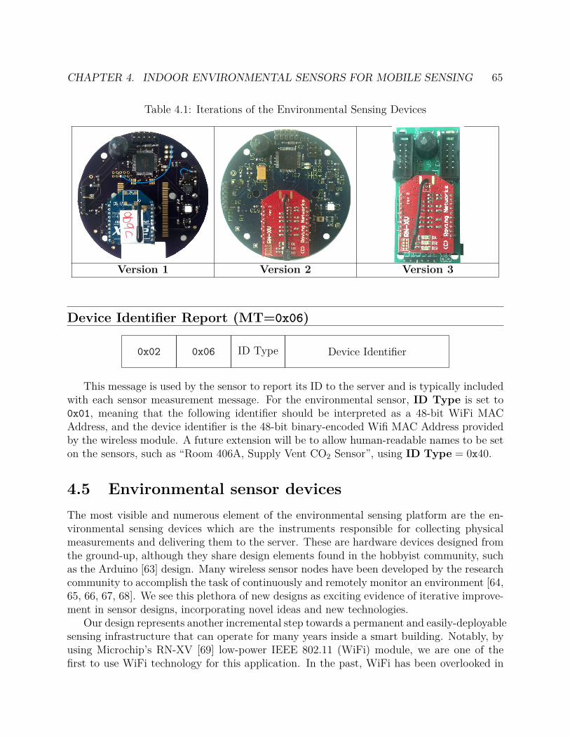
CHAPTER 4. INDOOR ENVIRONMENTAL SENSORS FOR MOBILE SENSING 65
Table 4.1: Iterations of the Environmental Sensing Devices
Version 1 Version 2 Version 3
Device Identifier Report (MT=0x06)
0x02 0x06 ID Type Device Identifier
This message is used by the sensor to report its ID to the server and is typically includedwith each sensor measurement message. For the environmental sensor, ID Type is set to0x01, meaning that the following identifier should be interpreted as a 48-bit WiFi MACAddress, and the device identifier is the 48-bit binary-encoded Wifi MAC Address providedby the wireless module. A future extension will be to allow human-readable names to be seton the sensors, such as “Room 406A, Supply Vent CO2 Sensor”, using ID Type = 0x40.
4.5 Environmental sensor devices
The most visible and numerous element of the environmental sensing platform are the en-vironmental sensing devices which are the instruments responsible for collecting physicalmeasurements and delivering them to the server. These are hardware devices designed fromthe ground-up, although they share design elements found in the hobbyist community, suchas the Arduino [63] design. Many wireless sensor nodes have been developed by the researchcommunity to accomplish the task of continuously and remotely monitor an environment [64,65, 66, 67, 68]. We see this plethora of new designs as exciting evidence of iterative improve-ment in sensor designs, incorporating novel ideas and new technologies.
Our design represents another incremental step towards a permanent and easily-deployablesensing infrastructure that can operate for many years inside a smart building. Notably, byusing Microchip’s RN-XV [69] low-power IEEE 802.11 (WiFi) module, we are one of thefirst to use WiFi technology for this application. In the past, WiFi has been overlooked in
CHAPTER 4. INDOOR ENVIRONMENTAL SENSORS FOR MOBILE SENSING 66
favor of other radio protocols, such as IEEE 802.15.4 and Bluetooth, due to WiFi’s highactive power consumption. However, as WiFi hardware becomes lower power (driven by thevenerable advancement of smartphones), WiFi is gaining attention as a contender to supplythe communication requirements of wireless sensor networks (WSN)[70].
Our hardware design has proceeded through several iterations to reach its current form(See Table 4.1). Since Version 1 was our first experience with the physical implementation ofthe design, it had several hardware errors that needed to be fixed. In Version 2, we correctedthese errors, allowing us to develop a codebase that would be compatible with Version 3,in which we added further expansion capabilities, reduced the physical size and significantlyreduced the cost of production (by using 2 routing layers instead of 4, and a rectangularoutline).
Commercial alternatives
Prior to designing a custom hardware solution, we first evaluated alternative commercialsolutions, some of which are listed in Table 4.2. Some platforms, such as the Digi XBeeSensors[71], are commercially packaged, produced and sold through major distributors, whichmakes it extremely quick and convenient to build a platform upon. However, none fulfilled allour requirements of variables sensed, battery life, or cost. Moreover, proprietary solutionsprevent us from extending the sensors to measure more variables, installing experimentalnetworking protocols, and are also vulnerable to becoming unsupported by the company.
There are also many WSN-centric development kits intended for research and develop-ment, perhaps the most referenced and studied being the Telos and TelosB platforms[66].These are somewhat unfinished products and require some development of software, hard-ware, and mechanics to fit the parameters of our deployment. They also rely on an exper-imental and changing code base, such as TinyOS, and requires a higher level of knowledgeto configure, as opposed to simple and user-friendly interfaces such as the X-CTU utility byDigi. However, with this cost comes the benefit of being able to keep up with improvingprotocols and a high amount of customization.
Finally, there are proof-of-concept and short-run products such as the Powercast WSN-1101[72] (and derivatives), which feature remarkable improvement in battery life and packagesize. Sensor nodes like these are usually developed by companies to demonstrate an under-lying technology innovation (in this case, wireless charging, low-power micro-controller, andenergy storage improvements). In many cases, the true product is an OEM module that issold to other companies to integrate into a commercially packaged product.
Hardware design
Designing the environmental sensor from the ground-up afforded us a great amount of flex-ibility in choosing state-of-the-art components available. As an overview, the block-leveldiagram of the Environmental Sensor node is shown in Figure 4.5.
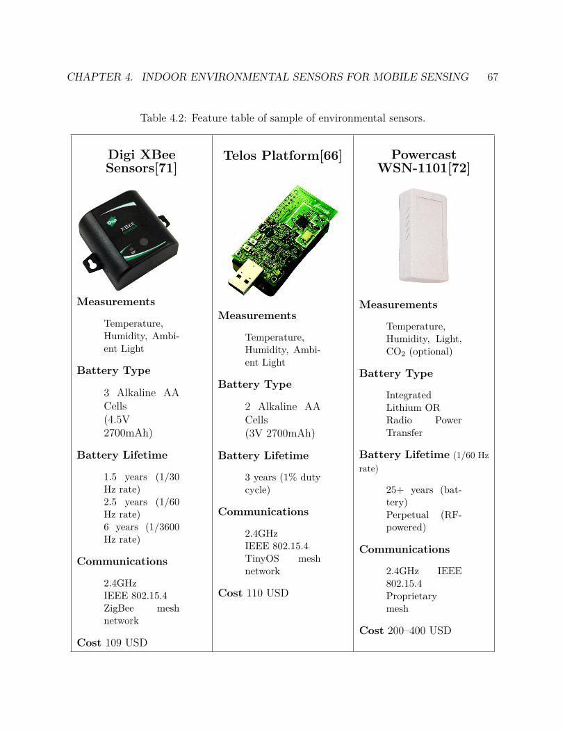
CHAPTER 4. INDOOR ENVIRONMENTAL SENSORS FOR MOBILE SENSING 67
Table 4.2: Feature table of sample of environmental sensors.
Digi XBeeSensors[71]
Measurements
Temperature,Humidity, Ambi-ent Light
Battery Type
3 Alkaline AACells(4.5V2700mAh)
Battery Lifetime
1.5 years (1/30Hz rate)2.5 years (1/60Hz rate)6 years (1/3600Hz rate)
Communications
2.4GHzIEEE 802.15.4ZigBee meshnetwork
Cost 109 USD
Telos Platform[66]
Measurements
Temperature,Humidity, Ambi-ent Light
Battery Type
2 Alkaline AACells(3V 2700mAh)
Battery Lifetime
3 years (1% dutycycle)
Communications
2.4GHzIEEE 802.15.4TinyOS meshnetwork
Cost 110 USD
PowercastWSN-1101[72]
Measurements
Temperature,Humidity, Light,CO2 (optional)
Battery Type
IntegratedLithium ORRadio PowerTransfer
Battery Lifetime (1/60 Hz
rate)
25+ years (bat-tery)Perpetual (RF-powered)
Communications
2.4GHz IEEE802.15.4Proprietarymesh
Cost 200–400 USD

CHAPTER 4. INDOOR ENVIRONMENTAL SENSORS FOR MOBILE SENSING 68
Figure 4.5: Environmental Sensor system diagram illustrating the major on-board instru-ments and expansion capabilities. Communications buses are indicted by solid-color paths.
Microcontroller
At the logical center of the design is Atmel’s ATmega1284 microcontroller. This particularchoice has a high amount of program memory (128KB) and RAM (16KB), which allows usto add in many code features without running out of space. However, most importantly,the microcontroller has the peripheral features required (I2C, SPI, and two UART ports),and the capability of low-power sleep while operating a timer from a 32.768KHz crystal.Even though there are many microcontroller families (e.g. TI’s MSP430, Microchip’s PIC)which satisfy our requirements, an additional reason for choosing the ATmega family is dueto its reliance on an open-source and free toolchain (GNU GCC) and extensive communitysupport through the Arduino community (e.g. the community provides driver code for manysensors).
Communications
A necessary component for a wireless sensor is the wireless transceiver. Initially, we did notseek to tie our design to a specific wireless module, therefore we included a universal 20-pinsocket, popularized by the ubiquitous XBee module. This is the connector footprint that isdefined by many of Digi’s OEM XBee modules. Due to the popularity of the XBee module,many other companies produce modules which adhere to the same connector footprint andsignal locations, therefore we allow ourselves to evaluate these alternative offerings withouta hardware redesign of the board.
Of these alternatives, we are particularly interested in integrating the OpenMote [73] sinceit incorporates the IEEE 802.15.4e stack via the OpenWSN project [58]. IEEE 802.15.4e usesTime Synchronized Channel Hopping (TSCH) to combat narrow-band challenges and achieve99.999% end-to-end reliability [74]. Therefore, when the OpenMote has reached maturity, it

CHAPTER 4. INDOOR ENVIRONMENTAL SENSORS FOR MOBILE SENSING 69
offers to address our reliability concerns while achieving much lower latency and power thanour WiFi selection.
Ultimately, we chose Microchip’s RN-XV[69] module which, in our experience, provedmore reliable than the XBee offering. Although the power consumption of this WiFi transceiveris up to 10 times greater than Bluetooth or IEEE 802.15.4 products, the high data rate (over200 times faster) allows us to transmit many measurements in one “burst”, thus limiting thetime that the radio must be turned on.
Power supply
In the standard configuration, the sensor is powered via a 3.7-volt Lithium-Thionyl ChlorideC-cell battery with a nominal battery life of 9Ah. This particular chemistry is intendedfor powering long-lifetime devices, having a low self-discharge of less than 1% per year.However, the capacity of the battery is significantly reduced when pulling more than 2 mAof continuous current or more than 400 mA of pulsed current (which could damage thebattery). The capacity of the battery is also reduced at lower current levels, such that ata 100 µA continuous current draw (roughly the average draw of the sensor), the effectivecapacity is roughly 8Ah. In our design, a 100 µF capacitor is used to lightly buffer thecurrent draw during the times that the radio is active.
The 3.7V battery voltage is dropped to the system voltage of 3.3V via a linear regulator.Therefore, instead of the battery, the system can also be supplied with another power sourceof up to 6V and as low as 3.5V. For proper operation, the external supply should be able tosupply current up to 250 mA (@12 dBm) or 140 mA (@0 dBm) during transmission, and, onaverage 200 µA.
Temperature and humidity sensing
Measuring Temperature and Humidity from the local environment is accomplished by Mea-surement Specialties’ HTU21D [75] instrument. This instrument is attached to the sharedI2C bus and can be queried to provide 12-bit and 14-bit digital readings of relative humidityand temperature, respectively. The stated accuracy of the humidity sensor is ±2%RH typicalover the 20%RH to 80%RH range, and up to ±3%RH outside of this range. The maximumerror tolerance is stated to be ±5%RH over the whole range. Although the instrument iscalibrated at the factory, the relative humidity reading must be temperature-compensated toachieve the stated accuracy. The coefficients and formula needed for this correction are spec-ified by the datasheet. The stated accuracy of the temperature sensor is typically ±0.3 Cand maximally ±0.4 C over the range of roughly 5 C to 60 C which well covers the expectedrange of temperatures encountered indoors.
Ambient light sensing
Ambient visible light is measured by AMS’ TSL2560 instrument [76]. This design of the ICincorporates two light-sensing photodiodes: one measures visible and IR light from 300 nm
CHAPTER 4. INDOOR ENVIRONMENTAL SENSORS FOR MOBILE SENSING 70
to 1100 nm, and the other measures IR light from 500 nm to 1100 nm. Therefore, the readingfrom the second (IR only) photodiode can be used to compensate for the light energy thatthe first (visible and IR) photodiode measures, but is not visible to the human eye. Anadditional feature of the instrument is its ability to change the integration time of the on-board analog-to-digital converter (ADC). This is typically changed to adapt to various lightconditions, such as a long integration time for dark environments, and short integration timefor outdoor environments. In our implementation, which is mostly to be deployed indoors,we have fixed the integration time to 101 ms. The light sensing instrument is attached to theshared I2C bus for configuring the instrument and reading the 16-bit values measurementsof the two photodiodes. The microcontroller uses the two measurements to calculate a luxreading, based on a relation described in the TSL2560 datasheet. We also used the interruptfeature of the instrument, which detects when the light level crosses above or below a pre-configured threshold. When enabled, this allows our sensor to timestamp events such aswhen the sensor is put inside a drawer or the lights are turned on and off.
A particular integration note about this instrument is that the responsivivity to lightis somewhat directional (120 beam-width at half-maximum). Therefore, the choice of en-closure and mounted configuration of the environmental sensor can dramatically affect theambient light readings. For practical studies, it would be prudent to ensure that all of thesensors are mounted in a similar way to properly measure the light levels in the indoorspace. Alternatively, we should study the changes in light intensity over time as opposed toemphasizing the absolute lux values of light.
Orientation sensing
Although capable of accurately measuring rapid acceleration, we include the LIS3DH Ac-celerometer by ST Microelectronics [77] primarily to measure the orientation of the device,with respect to gravity, and secondarily to measure high-acceleration “bumps”, such as foot-steps. Detecting orientation and bumps provides information in a mobile environment, suchas if the device is in the pocket of a mobile human occupant. The number of footsteps takenand whether the person is sitting or standing can be extremely valuable pieces of informationin an occupant tracking or occupancy estimation problem. In these situations, the accuracyof the instrument is not of large concern.
This instrument features low-power (6 µA at 50 Hz sample rate) continuous operation,which allows us to capture and timestamp events which occur in between periodic samples.For orientation purposes, the typical magnitude of acceleration we are measuring is 1 g, so thestated offset error of 40 mg represents about a 4% error. Additionally, there is some sensitivityto temperature which is stated as 0.01 %/C. The 3 16-bit values of acceleration are readfrom the device over the shared I2C bus. Additionally, we use the interrupt capabilities of thedevice to inform the processor when the orientation has changed (the x, y, or z measurementaxis is aligned with the gravity vector).
CHAPTER 4. INDOOR ENVIRONMENTAL SENSORS FOR MOBILE SENSING 71
Motion detection
We measure motion using Panasonic’s AMN41121 passive infrared (PIR) motion detectormodule [78]. This module utilizes a pyroelectric element to monitor small changes in infraredblack-body radiation emitted by humans (7-14 µm). There is a specialized lens which formsa pattern of discrete detection zones corresponding to one of four sensing regions of thepyroelectric element. Further circuitry within the device monitors changes in the infraredlight measured by the four regions to determine whether a detection event has occurred.Ultimately, the sensor will detect when an infrared-emitting body, such as a human movesacross the detection zones, but remain insensitive to overall temperature increases or de-creases within the field-of-view. In practice, we have found that the sensor is also insensitiveto an unmoving human, i.e. some movement across the detection zones is necessary to signala detection.
The field-of-view of the sensor is stated to be 100 along one axis and 82 along theother, and the detection range is at least 5 m from the sensor. Within this cone, there are64 discrete detection zones distributed somewhat uniformly. There are three other modelswithin the family line of sensors, each having different lenses and correspondingly differentfields-of-view and detection ranges. Since these other models are pin-compatible, we couldeasily switch out the AMN41121 for one of these alternative lens configurations, dependingon the end application. A drawback of the module is that it needs at least 7 seconds forthe circuit and sensor to stabilize before the detection is reliable. Therefore, we realisticallycannot duty-cycle the sensor to save power, however, since the static power consumption isonly 46 µA, we can leave the sensor powered and still achieve a long battery lifetimes.
The module interfaces to the microcontroller via a single output which connects theattached signal to Vdd (HIGH) when a detection occurs. An external pull-down resistorpulls the signal to GND (LOW) otherwise. Although the datasheet does not specify thetiming of the signal during a detection, we have found that, the signal will stay HIGH aslong as there is activity, but can sometimes intermittently go LOW, even while humans aremoving in front of the sensor. Therefore, we require some intelligent interpretation of thesignal, rather than simply assuming that a HIGH signal means humans are present and aLOW signal means humans are not present.
Our strategy is to report two calculated measurements: the first is the occupancy per-centage, which is the percentage of time (with a resolution of 1/256 seconds) that the signalwas HIGH over the last sample interval. The second is the occupancy state changed event,which sends a value of 1 if the signal goes HIGH after being LOW for 10 seconds, or sendsa value of 0 if the the signal is LOW for 10 seconds after previously sending a 1. We believethese measurements will be sufficient to determine whether the space in front of the sensoris occupied by one or more humans at any time.
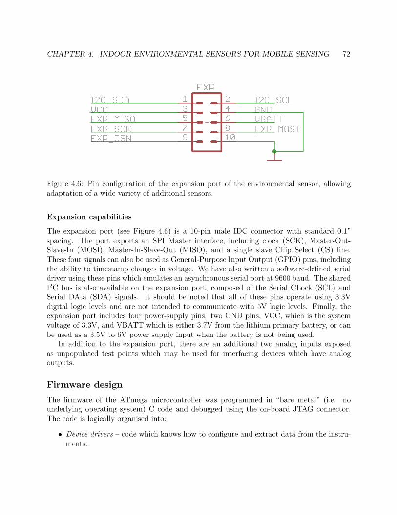
CHAPTER 4. INDOOR ENVIRONMENTAL SENSORS FOR MOBILE SENSING 72
Figure 4.6: Pin configuration of the expansion port of the environmental sensor, allowingadaptation of a wide variety of additional sensors.
Expansion capabilities
The expansion port (see Figure 4.6) is a 10-pin male IDC connector with standard 0.1”spacing. The port exports an SPI Master interface, including clock (SCK), Master-Out-Slave-In (MOSI), Master-In-Slave-Out (MISO), and a single slave Chip Select (CS) line.These four signals can also be used as General-Purpose Input Output (GPIO) pins, includingthe ability to timestamp changes in voltage. We have also written a software-defined serialdriver using these pins which emulates an asynchronous serial port at 9600 baud. The sharedI2C bus is also available on the expansion port, composed of the Serial CLock (SCL) andSerial DAta (SDA) signals. It should be noted that all of these pins operate using 3.3Vdigital logic levels and are not intended to communicate with 5V logic levels. Finally, theexpansion port includes four power-supply pins: two GND pins, VCC, which is the systemvoltage of 3.3V, and VBATT which is either 3.7V from the lithium primary battery, or canbe used as a 3.5V to 6V power supply input when the battery is not being used.
In addition to the expansion port, there are an additional two analog inputs exposedas unpopulated test points which may be used for interfacing devices which have analogoutputs.
Firmware design
The firmware of the ATmega microcontroller was programmed in “bare metal” (i.e. nounderlying operating system) C code and debugged using the on-board JTAG connector.The code is logically organised into:
• Device drivers – code which knows how to configure and extract data from the instru-ments.
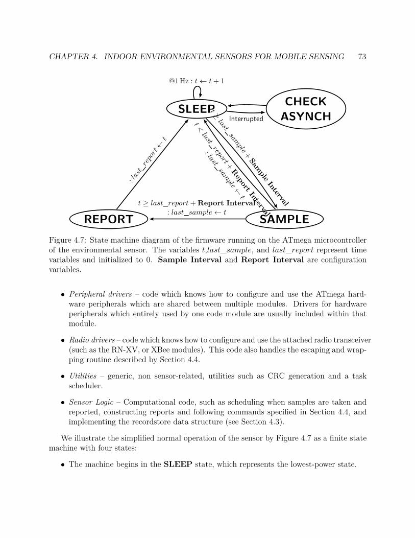
CHAPTER 4. INDOOR ENVIRONMENTAL SENSORS FOR MOBILE SENSING 73
SLEEPCHECK
ASYNCH
SAMPLEREPORT
Interrupted
@1 Hz : t← t + 1
t ≥last_
sample
+Sam
ple
Intervalt ≥ last_report + Report Interval
: last_sample← tt<
last_report+
Rep
ort
Interval
: last_sam
ple←t
: las
t_re
port←
t
Figure 4.7: State machine diagram of the firmware running on the ATmega microcontrollerof the environmental sensor. The variables t,last_sample, and last_report represent timevariables and initialized to 0. Sample Interval and Report Interval are configurationvariables.
• Peripheral drivers – code which knows how to configure and use the ATmega hard-ware peripherals which are shared between multiple modules. Drivers for hardwareperipherals which entirely used by one code module are usually included within thatmodule.
• Radio drivers – code which knows how to configure and use the attached radio transceiver(such as the RN-XV, or XBee modules). This code also handles the escaping and wrap-ping routine described by Section 4.4.
• Utilities – generic, non sensor-related, utilities such as CRC generation and a taskscheduler.
• Sensor Logic – Computational code, such as scheduling when samples are taken andreported, constructing reports and following commands specified in Section 4.4, andimplementing the recordstore data structure (see Section 4.3).
We illustrate the simplified normal operation of the sensor by Figure 4.7 as a finite statemachine with four states:
• The machine begins in the SLEEP state, which represents the lowest-power state.
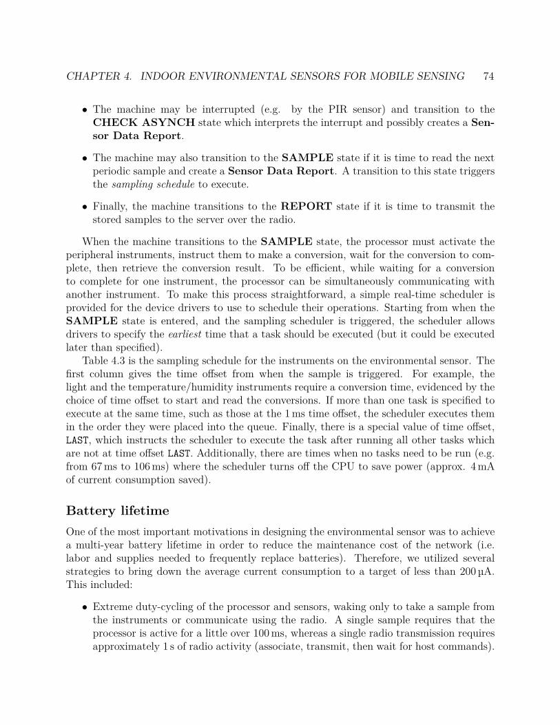
CHAPTER 4. INDOOR ENVIRONMENTAL SENSORS FOR MOBILE SENSING 74
• The machine may be interrupted (e.g. by the PIR sensor) and transition to theCHECK ASYNCH state which interprets the interrupt and possibly creates a Sen-sor Data Report.
• The machine may also transition to the SAMPLE state if it is time to read the nextperiodic sample and create a Sensor Data Report. A transition to this state triggersthe sampling schedule to execute.
• Finally, the machine transitions to the REPORT state if it is time to transmit thestored samples to the server over the radio.
When the machine transitions to the SAMPLE state, the processor must activate theperipheral instruments, instruct them to make a conversion, wait for the conversion to com-plete, then retrieve the conversion result. To be efficient, while waiting for a conversionto complete for one instrument, the processor can be simultaneously communicating withanother instrument. To make this process straightforward, a simple real-time scheduler isprovided for the device drivers to use to schedule their operations. Starting from when theSAMPLE state is entered, and the sampling scheduler is triggered, the scheduler allowsdrivers to specify the earliest time that a task should be executed (but it could be executedlater than specified).
Table 4.3 is the sampling schedule for the instruments on the environmental sensor. Thefirst column gives the time offset from when the sample is triggered. For example, thelight and the temperature/humidity instruments require a conversion time, evidenced by thechoice of time offset to start and read the conversions. If more than one task is specified toexecute at the same time, such as those at the 1 ms time offset, the scheduler executes themin the order they were placed into the queue. Finally, there is a special value of time offset,LAST, which instructs the scheduler to execute the task after running all other tasks whichare not at time offset LAST. Additionally, there are times when no tasks need to be run (e.g.from 67 ms to 106 ms) where the scheduler turns off the CPU to save power (approx. 4 mAof current consumption saved).
Battery lifetime
One of the most important motivations in designing the environmental sensor was to achievea multi-year battery lifetime in order to reduce the maintenance cost of the network (i.e.labor and supplies needed to frequently replace batteries). Therefore, we utilized severalstrategies to bring down the average current consumption to a target of less than 200 µA.This included:
• Extreme duty-cycling of the processor and sensors, waking only to take a sample fromthe instruments or communicate using the radio. A single sample requires that theprocessor is active for a little over 100 ms, whereas a single radio transmission requiresapproximately 1 s of radio activity (associate, transmit, then wait for host commands).

CHAPTER 4. INDOOR ENVIRONMENTAL SENSORS FOR MOBILE SENSING 75
Table 4.3: Standard schedule of tasks executed to take one sample
Time (ms) Component Description0 Reporting Start constructing new Sensor Data Report1 Temp/Humid Start humidity conversion1 PIR Calculate PIR occupancy percentage value and reset1 Light Wake light sensor to start conversion1 Accel. Read latest acceleration reading
17 Temp/Humid Read converted humidity & start temperature conversion67 Temp/Humid Read converted temperature
106 Light Read converted ambient light readingLAST∗ Reporting Store Sensor Data Report into recordstore memory
∗ Special signal to the scheduler to always run these tasks last.
Therefore, a sample taken every 10 s represents a sampling duty cycle of 1% and radiotransmission made every hour represents a communication duty cycle of 1.7%.
• Selection of components with low current requirements. Not only does this reducethe amount of energy consumed, it reduces the peak load needed to be supplied bythe linear regulator and battery. Typically, linear regulators with higher peak currentcapability also have a higher leakage current, and, additionally, high peak currentdraws can damage or reduce the effective capacity of the battery. The most importantcomponent, in this respect, is the choice of radio transceiver. For example, modulessuch as the XBee-PRO and XBee Series 6 (WiFi) are not used due to their high (over300 mA) peak consumption.
To determine the feasibility of having a multi-year battery life, we create a power con-sumption worksheet, shown in Table 4.4, listing the power requirements for each deviceduring their sleep and active modes, and the typical amount of time they are required to beactive to perform their functions.
Using the information in Table 4.4, we simulate and plot, in Figure 4.8 the batterylifetime of an environmental sensor node powered by a lithium battery (See “Power supply”in Section 4.5), over varying values of sample intervals (i.e. when a measurement is gatheredfrom the instruments) and report intervals (i.e. when a set of measurements are sent to theserver). We simulate current consumption from the light sensor, humidity and temperaturesensor, accelerometer, PIR sensor, microcontroller, and radio. We also simulate the reductionof battery capacity at low average current draw. We do not simulate leakage currents or thepower consumption of the 3.3V regulator, or atypical conditions which would cause devices tobe powered longer than expected, in particular, when communications problems may causethe radio to remain active for up to 5 seconds per report.
We believe that we can achieve a battery lifetime of over 5 years by using a 10 secondsample interval and 60 second reporting interval. In this configuration, the average current

CHAPTER 4. INDOOR ENVIRONMENTAL SENSORS FOR MOBILE SENSING 76
Tab
le4.
4:P
ower
cons
umpt
ion
wor
kshe
et
Dev
ice
Slee
ppo
wer
cons
umpt
ion
Aw
ake
pow
erco
nsum
ptio
nA
ctiv
eti
me
per
sam
ple
AT
meg
a128
40.
6µA
CP
Uon
:4.
5m
AC
PU
off:
0.5
mA
At
leas
t10
1m
s
RN
-XV
∗4
µAR
X:
40m
AT
X@
0dB
m:
135
mA
TX
@12
dBm
:24
0m
A
Ass
ocia
tion
:15
ms
Aut
hent
icat
ion:
50m
s–
250
ms
App
licat
ion:
500
ms
–5
s
AM
N41
121
No
slee
pm
ode
46µA
Alw
ays-
on
HT
U21
D20
nA45
0µA
Tem
pera
ture
:44
ms
Hum
idit
y:14
ms
TSL
2560
3.2
µA24
0µA
101
ms
LIS
3DH
∗∗
0.5
µA6
µA1
ms
∗N
otac
tive
for
ever
ydat
asa
mple
.T
ypic
ally
only
acti
veon
cep
erhou
r.∗
∗T
ypic
ally
alw
ays-
onto
do
asynch
ronou
sor
ienta
tion
chan
gedet
ecti
on.
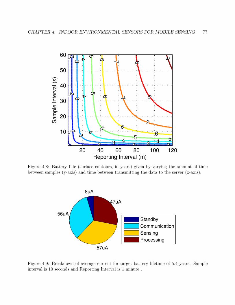
CHAPTER 4. INDOOR ENVIRONMENTAL SENSORS FOR MOBILE SENSING 77
1
11
222
22
2
33
33
3
444
44
55
5
55
6
66
6
7
77
8
8
9
Sa
mp
le I
nte
rva
l (s
)
Reporting Interval (m)20 40 60 80 100 120
10
20
30
40
50
60
Figure 4.8: Battery Life (surface contours, in years) given by varying the amount of timebetween samples (y-axis) and time between transmitting the data to the server (x-axis).
8uA
56uA
57uA
47uA
Standby
Communication
Sensing
Processing
Figure 4.9: Breakdown of average current for target battery lifetime of 5.4 years. Sampleinterval is 10 seconds and Reporting Interval is 1 minute .
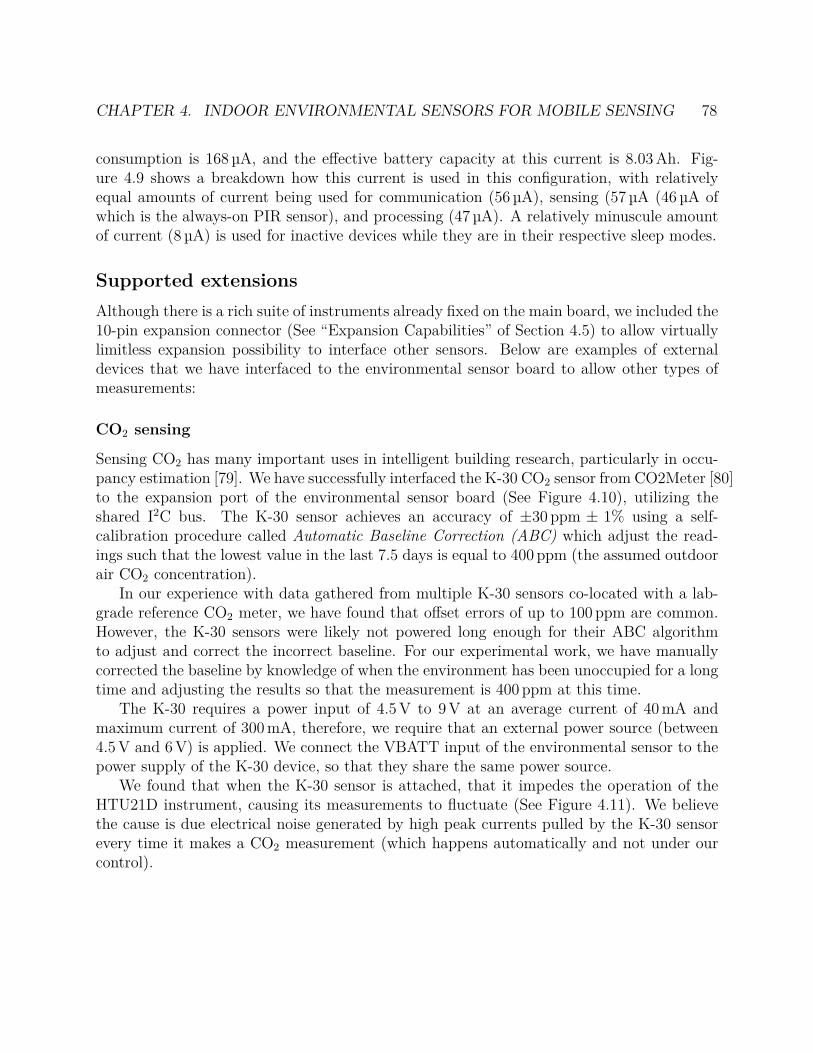
CHAPTER 4. INDOOR ENVIRONMENTAL SENSORS FOR MOBILE SENSING 78
consumption is 168 µA, and the effective battery capacity at this current is 8.03 Ah. Fig-ure 4.9 shows a breakdown how this current is used in this configuration, with relativelyequal amounts of current being used for communication (56 µA), sensing (57 µA (46 µA ofwhich is the always-on PIR sensor), and processing (47 µA). A relatively minuscule amountof current (8 µA) is used for inactive devices while they are in their respective sleep modes.
Supported extensions
Although there is a rich suite of instruments already fixed on the main board, we included the10-pin expansion connector (See “Expansion Capabilities” of Section 4.5) to allow virtuallylimitless expansion possibility to interface other sensors. Below are examples of externaldevices that we have interfaced to the environmental sensor board to allow other types ofmeasurements:
CO2 sensing
Sensing CO2 has many important uses in intelligent building research, particularly in occu-pancy estimation [79]. We have successfully interfaced the K-30 CO2 sensor from CO2Meter [80]to the expansion port of the environmental sensor board (See Figure 4.10), utilizing theshared I2C bus. The K-30 sensor achieves an accuracy of ±30 ppm ± 1% using a self-calibration procedure called Automatic Baseline Correction (ABC) which adjust the read-ings such that the lowest value in the last 7.5 days is equal to 400 ppm (the assumed outdoorair CO2 concentration).
In our experience with data gathered from multiple K-30 sensors co-located with a lab-grade reference CO2 meter, we have found that offset errors of up to 100 ppm are common.However, the K-30 sensors were likely not powered long enough for their ABC algorithmto adjust and correct the incorrect baseline. For our experimental work, we have manuallycorrected the baseline by knowledge of when the environment has been unoccupied for a longtime and adjusting the results so that the measurement is 400 ppm at this time.
The K-30 requires a power input of 4.5 V to 9 V at an average current of 40 mA andmaximum current of 300 mA, therefore, we require that an external power source (between4.5 V and 6 V) is applied. We connect the VBATT input of the environmental sensor to thepower supply of the K-30 device, so that they share the same power source.
We found that when the K-30 sensor is attached, that it impedes the operation of theHTU21D instrument, causing its measurements to fluctuate (See Figure 4.11). We believethe cause is due electrical noise generated by high peak currents pulled by the K-30 sensorevery time it makes a CO2 measurement (which happens automatically and not under ourcontrol).
CHAPTER 4. INDOOR ENVIRONMENTAL SENSORS FOR MOBILE SENSING 79
Figure 4.10: Left: The K-30 CO2 sensor from CO2Meter [80]. Right: Sensor attached tothe expansion port of a “Version 2” environmental sensor. This used the software-definedserial driver to read from the sensor, however support for the I2C interface has been addedin “Version 3” of the environmental sensor’s expansion connector.
Door opening detection
The door open detector expansion utilizes the GPIO capabilities of the expansion port byattaching a magnetic switch and pull-up resistor. A schematic of the simple circuit is shownby Figure 4.12. When the magnetic switch is closed by the magnet being close by, the signalgoes to 0V, whereas when the magnet is far, the magnetic switch is open and the signal ispulled to VCC by the pull-up resistor. The current consumption of the circuit is 10 µA, whenthe switch is closed, and the leakage current of the ATmega’s GPIO input driver (maximum1 µA), when the switch is open. The interrupt capabilities of the GPIO port allow us totimestamp exactly when the voltage level changes, to within one second.
To install the sensor, the magnetic switch is installed on either a door or its frame, andthe magnet is installed on the other side, such that when the door is closed, the magnet comeswithin 1 cm of the switch, and when the door is open, the magnet is far from the switch.Note that we could similarly install the switch and magnet combination on windows, draws,or cabinets which, given the context, could provide information about where occupants areand which objects in the office are being manipulated.
4.6 Evaluation
Given that a long battery life is one of the primary features of the platform described, itis necessary to validate that the platform actually consumes the theoretical amounts thatwe calculated from the data sheets. Therefore, we designed a circuit, shown in Figure 4.13
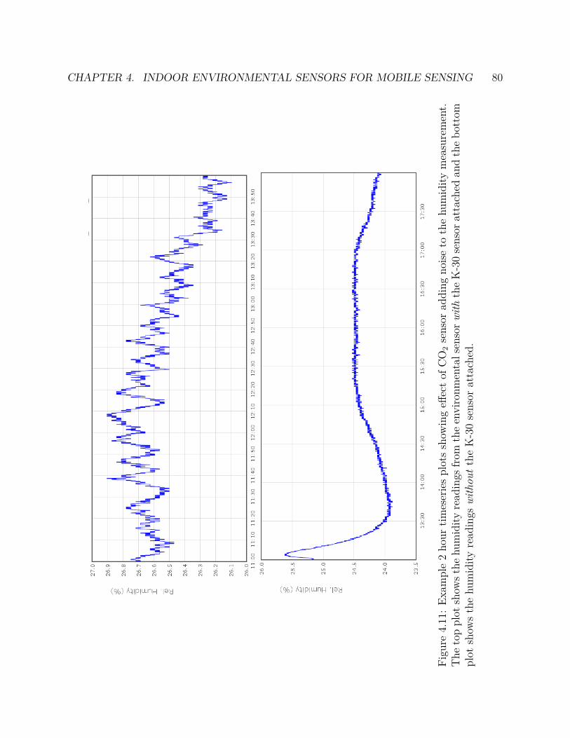
CHAPTER 4. INDOOR ENVIRONMENTAL SENSORS FOR MOBILE SENSING 80
Fig
ure
4.11
:E
xam
ple
2ho
urti
mes
erie
spl
ots
show
ing
effec
tof
CO
2se
nsor
addi
ngno
ise
toth
ehu
mid
ity
mea
sure
men
t.T
heto
ppl
otsh
ows
the
hum
idit
yre
adin
gsfr
omth
een
viro
nmen
tals
enso
rw
ith
the
K-3
0se
nsor
atta
ched
and
the
bott
ompl
otsh
ows
the
hum
idit
yre
adin
gsw
itho
ut
the
K-3
0se
nsor
atta
ched
.

CHAPTER 4. INDOOR ENVIRONMENTAL SENSORS FOR MOBILE SENSING 81
Figure 4.12: Schematic of door opening detection based on a magnetic switch attached toone of the GPIO pins of the expansion port.
to measure the current consumed by our prototype. An operational amplifier produces anregulated 3.75 V output voltage at up to 250 mA (i.e. (12 V− 3.75 V)÷ 33 Ω). The voltage,v, at the output of the amplifier is captured with an oscilloscope and we can calculate thesupply current, i, as
i =v − 3.75 V
33 Ω.
The standby current consumption was too low to precisely measure using the tools atour disposal (theoretically, the voltage difference across the 33 Ω resistor would be < 2 mVat 60 µA). Since we cannot reliably measure the standby current, for the following plots weplot the current differential, that is, the amount of extra current that doing a task consumesin addition to the standby current.
We measured the current consumption while the device took one environmental sampleand plotted the results in Figure 4.14. There are 5 spikes in current consumption, corre-sponding to the 5 times when the processor is active, according to the schedule in Table 4.3.We also calculated that the energy capacity drained from the battery for one sample is1.09 µAh. Note that this is much lower than expected by the numbers previously calculatedin Section 4.5, indicating that our previous estimates were conservative.
Figure 4.15 provides similar plots of the current consumption profile while the sensoris transmitting the collected measurements to the server. In this plot, the spikes represent
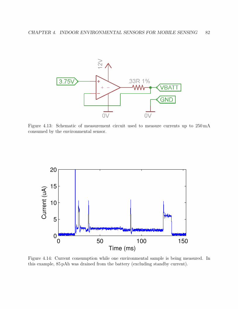
CHAPTER 4. INDOOR ENVIRONMENTAL SENSORS FOR MOBILE SENSING 82
Figure 4.13: Schematic of measurement circuit used to measure currents up to 250 mAconsumed by the environmental sensor.
0 50 100 1500
5
10
15
20
Time (ms)
Curr
ent (u
A)
Figure 4.14: Current consumption while one environmental sample is being measured. Inthis example, 85 pAh was drained from the battery (excluding standby current).

CHAPTER 4. INDOOR ENVIRONMENTAL SENSORS FOR MOBILE SENSING 83
0 1 2 3 4 5 6 70
50
100
150
Time (s)
Curr
ent
(mA
)
Figure 4.15: Current consumption during transmission of stored measurement data. In thisexample, 75 µAh was drained from the battery (excluding standby current).
times when the radio is transmitting and consuming up to 240 mA of current. The sensorconsumes around 50 mA of total current when the radio is active, but only listening (itselfconsuming 40 mA).
To estimate the battery lifetime, T , we assume a battery capacity, Cbatt = 8 Ah ( deratedfrom 9 Ah after 5 years of age ) and a standby power consumption of 60 µA. We also assumethe sensor is configured to take samples every 10 seconds and send a report (approx. 6.9kBeach) every hour. We assume that each sample and report consumes the amount of energyas measured above. Therefore, we have the relations:
nsamples =T
(10 s)Csamples = nsamples · (85 pAh)
nreports =T
(3600 s)Creports = nreports · (75 µAh)
Cstandby = T · (60 µA)
Cbatt = Csamples + Creports + Cstandby
Solving these equations gives a battery life of approximately 6.7 years, after taking 21 millionenvironmental samples and sending 59 thousand reports. Of the 8 Ah battery, approximately4.4 Ah (56%) is used for communication, 1.8 mAh (0.02%) for synchronous samples (not
CHAPTER 4. INDOOR ENVIRONMENTAL SENSORS FOR MOBILE SENSING 84
including consumption from the always-on PIR or accelerometer instruments), and 3.6 Ah(44%) used for standby consumption, including the PIR and Accelerometer instruments.
Clearly the battery lifetime could be extended by increasing the report interval. Addi-tionally, there does not appear to be a significant power penalty to increasing the samplerate of measuring light, humidity, and temperature. However, we are limited by the memoryspace of the device, as these samples must be stored until the next report is sent. Therefore,for future designs, increasing the amount of memory, perhaps via an externally connectedmemory chip, could prove fruitful in improving the battery lifetime. An alternative is toperform some computation on the sensor node to determine whether a sample is useful to beheld or discarded. For instance, if the sensor detects that a quantity is rapidly changing, itcould choose to store more of the samples, however, if the measurements are not significantlychanging, many of the high-rate samples could be discarded.
Secondarily, we could increase the battery lifetime by reducing the standby power con-sumption of the device, especially by turning off the PIR detector which consumes 46 µA.For instance, we could place two sensors with overlapping PIR detection regions and turnonly one PIR detector on at a time, or other sensors could be used to determine whether thePIR detector is needed. For instance, if a door-open detector senses that a door is closed toan empty room, then there is no reason for a PIR detector to be monitoring that room sincethere is no possibility of humans entering without opening the door.
4.7 Conclusions and Future Work
Ultimately, we achieve our objective of a 5+ year lifetime for the environmental sensor devicesand it is comforting to know that there is room for unaccounted factors. Therefore, theenvironmental sensing framework, as a whole, enables practical deployment of a permanentsensing architecture in the office space. The sensing devices themselves can operate for over5 years while consuming a lifetime average of 140 µA. Therefore, the costs of deploying andmaintaining such a network is significantly reduced in comparison to networks which requirewiring or frequent battery replacements.
Although we have achieved our power consumption targets using WiFi technology, werecognize that other standards-based technologies exist, such as IEEE 802.15.4e and Wire-lessHART, which offer high-reliability, low-latency, and low-power relative to WiFi technol-ogy. For example, the SmartMesh line of products from Linear Technology offers roughly thesame order of power consumption (less than 100 µA) for communications, but at a latency ofless than 10s and achieves 99% reliability (for 100 nodes) [81]. A future goal is to integrate theOpenMote [73] which implements an open-source implementation of IEEE 802.15.4e, Open-WSN [58]). Using the same standards-based protocols, OpenWSN theoretically achievessimilar performance to SmartMesh. The primary challenge in incorporating this technology,however, is that it is not well suited to mobile environments, since nodes must undergo alengthy and costly rejoining process if they frequently leave and enter the radio range of their
CHAPTER 4. INDOOR ENVIRONMENTAL SENSORS FOR MOBILE SENSING 85
neighbors [82]. To address this requires careful adjustment of the network parameters and anetwork topology that assists mobile nodes in staying associated within the mesh network.
From our observations of current, the WiFi module consumes most of its power in idlereceive mode, not during transmission of a packet. These times are spent either when theATmega microcontroller is communicating the data packet to the RN-XV module, or whenthe sensor is waiting for a command to be sent to it from the Local Server. Therefore, wecould significantly reduce power consumption with a faster data connection to the RN-XVand a protocol which does not rely on the module to wait for a possible command from theLocal Server. The first change would require selection of a WiFi module which supportsthe SPI communications bus, which can be much faster than an asynchronous connection.The second change could be accomplished by sending a flag with the TCP acknowledgementpacket, indicating whether the server has a command waiting for the sensor.
Another way to reduce the data throughput, and thus the communication and memoryrequirements, would be to process the data on the ATmega prior to storage. This processingstep would be highly dependent on the end application. For example, instead of recordingthe temperature every 10 seconds, we could record only when the temperature rises or fallsbelow some threshold. However, since we want to avoid constraining the sensors to oneapplication, and because WiFi affords a relatively high data bandwidth, we choose to sendthe measurements with very little processing.
Using the measurements collected from the on-board instruments, as well peripheralinstruments, such as CO2 and Particulate Matter sensors, we can gather information aboutthe occupancy of building spaces. For instance, in the following chapter, we will describe howmeasurements of CO2 concentrations inside of a conference room can be used to accuratelyestimate the occupancy of that room. We were able to accomplish this non-trivial feat bymodelling the CO2 concentrations within the room and building an estimator for the rateof CO2 production. To apply the estimation theory, it was necessary to develop the CO2
sensor platform shown in Figure 4.10.If the sensors are carried by occupants, this will provide information needed to track the
occupant using the particle filtering technique described by Chapter 6. We collect the signalstrength from an occupant-carried device and find the most likely position of the occupant bymapping these measurements to previously constructed statistical distributions. However,in addition to signal strength measurements, the framework can be adapted to accept anytype of measurement that is affected by the occupants’ positions. For instance, the particlefilter can glean information from light measurements, such as knowing that the occupant isnear or far from a sun-facing window. Further examples are discussed in Section 6.5.
As well as providing the inputs to our occupancy estimation and occupant trackingtechniques, the system also proves to provide valuable inputs to other smart building projects.The temperature, humidity, particulate matter, and CO2 readings are used to control andstudy the indoor air quality of the space, and the light-level readings are likewise used todetermine if an adequate and healthy amount of light is being provided. Since readings aretaken frequently and stored permanently, we enable future studies by collecting a rich andlong-running data set to be analyzed.
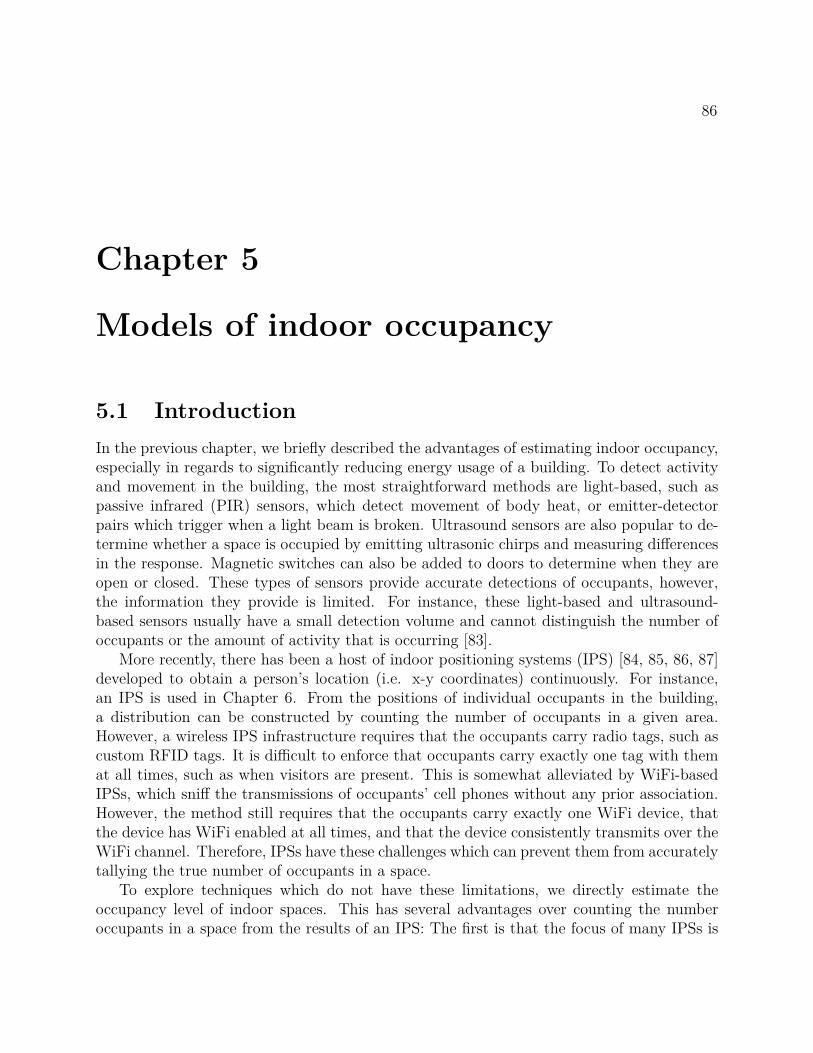
86
Chapter 5
Models of indoor occupancy
5.1 Introduction
In the previous chapter, we briefly described the advantages of estimating indoor occupancy,especially in regards to significantly reducing energy usage of a building. To detect activityand movement in the building, the most straightforward methods are light-based, such aspassive infrared (PIR) sensors, which detect movement of body heat, or emitter-detectorpairs which trigger when a light beam is broken. Ultrasound sensors are also popular to de-termine whether a space is occupied by emitting ultrasonic chirps and measuring differencesin the response. Magnetic switches can also be added to doors to determine when they areopen or closed. These types of sensors provide accurate detections of occupants, however,the information they provide is limited. For instance, these light-based and ultrasound-based sensors usually have a small detection volume and cannot distinguish the number ofoccupants or the amount of activity that is occurring [83].
More recently, there has been a host of indoor positioning systems (IPS) [84, 85, 86, 87]developed to obtain a person’s location (i.e. x-y coordinates) continuously. For instance,an IPS is used in Chapter 6. From the positions of individual occupants in the building,a distribution can be constructed by counting the number of occupants in a given area.However, a wireless IPS infrastructure requires that the occupants carry radio tags, such ascustom RFID tags. It is difficult to enforce that occupants carry exactly one tag with themat all times, such as when visitors are present. This is somewhat alleviated by WiFi-basedIPSs, which sniff the transmissions of occupants’ cell phones without any prior association.However, the method still requires that the occupants carry exactly one WiFi device, thatthe device has WiFi enabled at all times, and that the device consistently transmits over theWiFi channel. Therefore, IPSs have these challenges which can prevent them from accuratelytallying the true number of occupants in a space.
To explore techniques which do not have these limitations, we directly estimate theoccupancy level of indoor spaces. This has several advantages over counting the numberoccupants in a space from the results of an IPS: The first is that the focus of many IPSs is
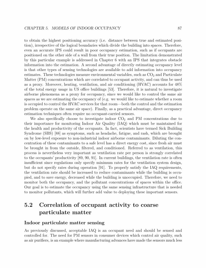
CHAPTER 5. MODELS OF INDOOR OCCUPANCY 87
to obtain the highest positioning accuracy (i.e. distance between true and estimated posi-tion), irrespective of the logical boundaries which divide the building into spaces. Therefore,even an accurate IPS could result in poor occupancy estimation, such as if occupants arepositioned on the other side of a wall from their true position. The limitation demonstratedby this particular example is addressed in Chapter 6 with an IPS that integrates obstacleinformation into the estimation. A second advantage of directly estimating occupancy levelis that other types of sensing technologies are available to add information into occupancyestimates. These technologies measure environmental variables, such as CO2 and ParticulateMatter (PM) concentrations which are correlated to occupant activity, and can thus be usedas a proxy. Moreover, heating, ventilation, and air conditioning (HVAC) accounts for 48%of the total energy usage in US office buildings [53]. Therefore, it is natural to investigateairborne phenomena as a proxy for occupancy, since we would like to control the same airspaces as we are estimating the occupancy of (e.g. we would like to estimate whether a roomis occupied to control the HVAC services for that room—both the control and the estimationproblem operate on the same air space). Finally, as a practical advantage, direct occupancyestimation techniques often require no occupant-carried sensors.
We also specifically choose to investigate indoor CO2 and PM concentrations due totheir importance for monitoring Indoor Air Quality (IAQ) which must be maintained forthe health and productivity of the occupants. In fact, scientists have termed Sick BuildingSyndrome (SBS) [88] as symptoms, such as headache, fatigue, and rash, which are broughton by low-level exposure to non-industrial indoor airborne contaminants. Diluting the con-centration of these contaminants to a safe level has a direct energy cost, since fresh air mustbe brought in from the outside, filtered, and conditioned. Referred to as ventilation, thisprocess is nevertheless very important as ventilation rate per person is strongly correlatedto the occupants’ productivity [89, 90, 91]. In current buildings, the ventilation rate is ofteninsufficient since regulations only specify minimum rates for the ventilation system design,but do not specify rates during operation [91]. To properly satisfy the IAQ requirements,the ventilation rate should be increased to reduce contaminants while the building is occu-pied, and to save energy, decreased while the building is unoccupied. Therefore, we need tomonitor both the occupancy, and the pollutant concentrations of spaces within the office.Our goal is to estimate the occupancy using the same sensing infrastructure that is neededto monitor pollutants, which will further add value to deploying these important sensors.
5.2 Correlation of occupant activity to coarse
particulate matter
Indoor particulate matter sensing
As previously discussed, acceptable IAQ is an occupant need and should be sensed andcontrolled for. The need for PM sensors in consumer devices which control air quality, suchas air purifiers, is an example where manufacturing advances have made the sensors much less
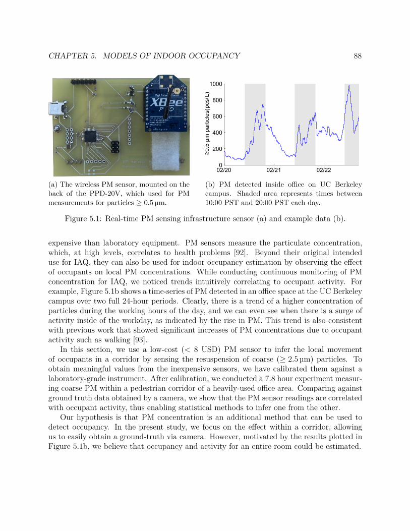
CHAPTER 5. MODELS OF INDOOR OCCUPANCY 88
(a) The wireless PM sensor, mounted on theback of the PPD-20V, which used for PMmeasurements for particles ≥ 0.5 µm.
02/20 02/21 02/220
200
400
600
800
1000
≥0
.5 µ
m p
art
icle
s (
L)
Co
nce
ntr
atio
n o
f pcs/
(b) PM detected inside office on UC Berkeleycampus. Shaded area represents times between10:00 PST and 20:00 PST each day.
Figure 5.1: Real-time PM sensing infrastructure sensor (a) and example data (b).
expensive than laboratory equipment. PM sensors measure the particulate concentration,which, at high levels, correlates to health problems [92]. Beyond their original intendeduse for IAQ, they can also be used for indoor occupancy estimation by observing the effectof occupants on local PM concentrations. While conducting continuous monitoring of PMconcentration for IAQ, we noticed trends intuitively correlating to occupant activity. Forexample, Figure 5.1b shows a time-series of PM detected in an office space at the UC Berkeleycampus over two full 24-hour periods. Clearly, there is a trend of a higher concentration ofparticles during the working hours of the day, and we can even see when there is a surge ofactivity inside of the workday, as indicated by the rise in PM. This trend is also consistentwith previous work that showed significant increases of PM concentrations due to occupantactivity such as walking [93].
In this section, we use a low-cost (< 8 USD) PM sensor to infer the local movementof occupants in a corridor by sensing the resuspension of coarse (≥ 2.5 µm) particles. Toobtain meaningful values from the inexpensive sensors, we have calibrated them against alaboratory-grade instrument. After calibration, we conducted a 7.8 hour experiment measur-ing coarse PM within a pedestrian corridor of a heavily-used office area. Comparing againstground truth data obtained by a camera, we show that the PM sensor readings are correlatedwith occupant activity, thus enabling statistical methods to infer one from the other.
Our hypothesis is that PM concentration is an additional method that can be used todetect occupancy. In the present study, we focus on the effect within a corridor, allowingus to easily obtain a ground-truth via camera. However, motivated by the results plotted inFigure 5.1b, we believe that occupancy and activity for an entire room could be estimated.
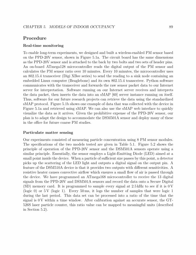
CHAPTER 5. MODELS OF INDOOR OCCUPANCY 89
Procedure
Real-time monitoring
To enable long-term experiments, we designed and built a wireless-enabled PM sensor basedon the PPD-20V sensor, shown in Figure 5.1a. The circuit board has the same dimensionsas the PPD-20V sensor and is attached to the back by two bolts and two sets of header pins.An on-board ATmega128 microcontroller reads the digital output of the PM sensor andcalculates the PM sensor ratio over 10 minutes. Every 10 minutes, the microcontroller usesan 802.15.4 transceiver (Digi XBee series) to send the reading to a sink node containing anembedded Linux computer (Beaglebone) and its own 802.15.4 transceiver. Python softwarecommunicates with the transceiver and forwards the raw sensor packet data to our Internetserver for interpretation. Software running on our Internet server receives and interpretsthe data packet, then inserts the data into an sMAP [60] server instance running on itself.Thus, software for our future research projects can retrieve the data using the standardizedsMAP protocol. Figure 5.1b shows one example of data that was collected with the device inFigure 5.1a and retrieved using sMAP. We can also use the sMAP web interface to quicklyvisualize the data as it arrives. Given the prohibitive expense of the PPD-20V sensor, ourplan is to adapt the design to accommodate the DSM501A sensor and deploy many of thesein the office for future coarse PM studies.
Particulate matter sensing
Our experiments consisted of measuring particle concentration using 8 PM sensor modules.The specifications of the two models tested are given in Table 5.1. Figure 5.2 shows theprinciple of operation of the PPD-20V sensor and the DSM501A sensors operate using asimilar principle. Essentially, the sensor employs a Light-Emitting Diode (LED) aimed at asmall point inside the device. When a particle of sufficient size passes by this point, a detectorpicks up the scattering of the LED light and outputs a digital signal on the output pin. Afeature of the DSM510A device is that it provides two outputs with different sensitivities. Aresistive heater causes convective airflow which ensures a small flow of air is passed throughthe device. We have programmed an ATmega168 microcontroller to receive the 13 digitalsignals from the PPD-20V and DSM501A sensors and record the data onto a Secure Digital(SD) memory card. It is programmed to sample every signal at 2.5 kHz to see if it is 0 V(logic 0) or 5 V (logic 1). Every 50 ms, it logs the number of samples that were logic 1during the last period. This data set can be processed into a ratio of the time that thesignal is 0 V within a time window. After calibration against an accurate sensor, the GT-526S laser particle counter, this ratio value can be mapped to meaningful units (describedin Section 5.2).
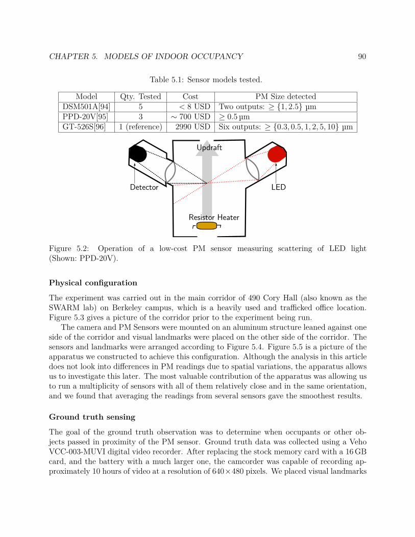
CHAPTER 5. MODELS OF INDOOR OCCUPANCY 90
Table 5.1: Sensor models tested.
Model Qty. Tested Cost PM Size detectedDSM501A[94] 5 < 8 USD Two outputs: ≥ 1, 2.5 µmPPD-20V[95] 3 ∼ 700 USD ≥ 0.5 µmGT-526S[96] 1 (reference) 2990 USD Six outputs: ≥ 0.3, 0.5, 1, 2, 5, 10 µm
Updraft
Resistor Heater
LEDDetector
Figure 5.2: Operation of a low-cost PM sensor measuring scattering of LED light(Shown: PPD-20V).
Physical configuration
The experiment was carried out in the main corridor of 490 Cory Hall (also known as theSWARM lab) on Berkeley campus, which is a heavily used and trafficked office location.Figure 5.3 gives a picture of the corridor prior to the experiment being run.
The camera and PM Sensors were mounted on an aluminum structure leaned against oneside of the corridor and visual landmarks were placed on the other side of the corridor. Thesensors and landmarks were arranged according to Figure 5.4. Figure 5.5 is a picture of theapparatus we constructed to achieve this configuration. Although the analysis in this articledoes not look into differences in PM readings due to spatial variations, the apparatus allowsus to investigate this later. The most valuable contribution of the apparatus was allowing usto run a multiplicity of sensors with all of them relatively close and in the same orientation,and we found that averaging the readings from several sensors gave the smoothest results.
Ground truth sensing
The goal of the ground truth observation was to determine when occupants or other ob-jects passed in proximity of the PM sensor. Ground truth data was collected using a VehoVCC-003-MUVI digital video recorder. After replacing the stock memory card with a 16 GBcard, and the battery with a much larger one, the camcorder was capable of recording ap-proximately 10 hours of video at a resolution of 640×480 pixels. We placed visual landmarks
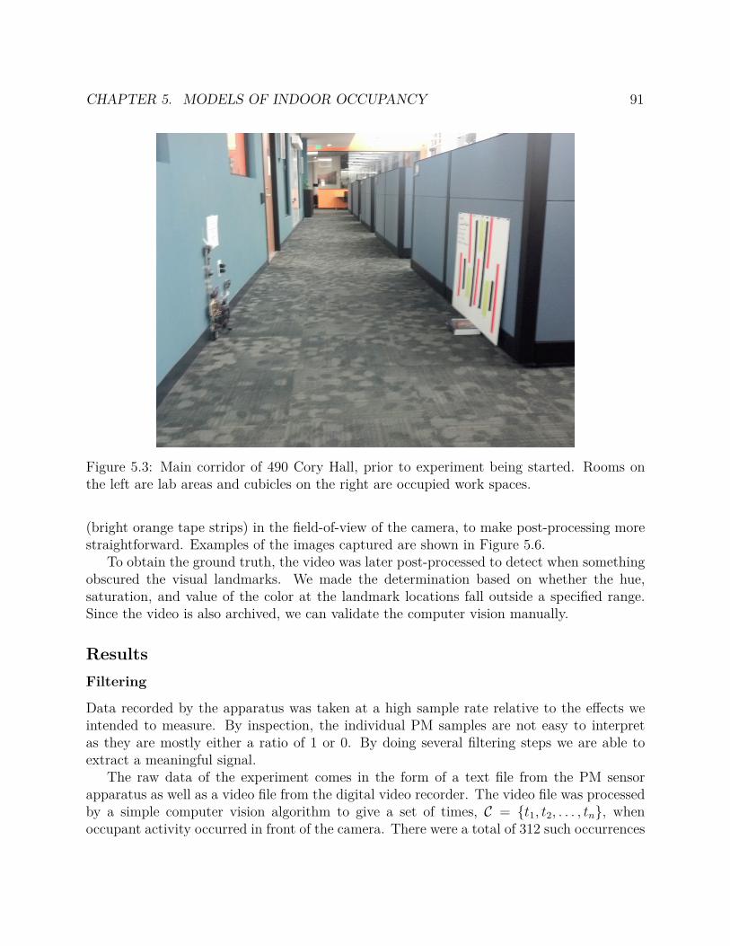
CHAPTER 5. MODELS OF INDOOR OCCUPANCY 91
Figure 5.3: Main corridor of 490 Cory Hall, prior to experiment being started. Rooms onthe left are lab areas and cubicles on the right are occupied work spaces.
(bright orange tape strips) in the field-of-view of the camera, to make post-processing morestraightforward. Examples of the images captured are shown in Figure 5.6.
To obtain the ground truth, the video was later post-processed to detect when somethingobscured the visual landmarks. We made the determination based on whether the hue,saturation, and value of the color at the landmark locations fall outside a specified range.Since the video is also archived, we can validate the computer vision manually.
Results
Filtering
Data recorded by the apparatus was taken at a high sample rate relative to the effects weintended to measure. By inspection, the individual PM samples are not easy to interpretas they are mostly either a ratio of 1 or 0. By doing several filtering steps we are able toextract a meaningful signal.
The raw data of the experiment comes in the form of a text file from the PM sensorapparatus as well as a video file from the digital video recorder. The video file was processedby a simple computer vision algorithm to give a set of times, C = t1, t2, . . . , tn, whenoccupant activity occurred in front of the camera. There were a total of 312 such occurrences
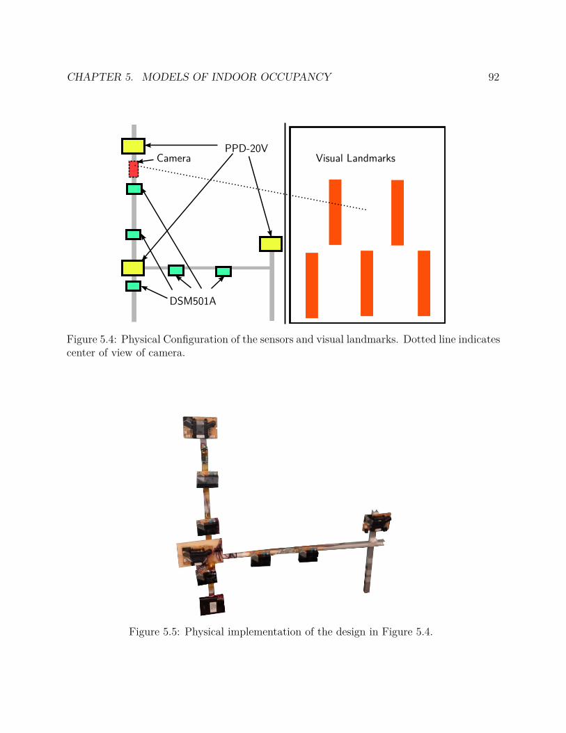
CHAPTER 5. MODELS OF INDOOR OCCUPANCY 92
PPD-20V
DSM501A
Camera Visual Landmarks
Figure 5.4: Physical Configuration of the sensors and visual landmarks. Dotted line indicatescenter of view of camera.
Figure 5.5: Physical implementation of the design in Figure 5.4.

CHAPTER 5. MODELS OF INDOOR OCCUPANCY 93
(a) Clear View (b) Obscured View
Figure 5.6: Example images showing detection of occupant in corridor from obscured visuallandmarks (orange strips).
during the experiment. We calculated a camera occurrence rate, xi, by the following:
xi =|t|t ∈ C ∧ t ≥ Ws(i− 0.5) ∧ t < Ws(i + 0.5)|
Ws
where Ws is the “sample period” and is set to 10 s for these results. Thus, xi is a discretesignal representing the number of camera occurrences per second, evaluated every 10 s.
The PM sensor signals, originally at a sample period of 50 ms, are down-sampled to asample period of Ws (10 s), by averaging every 200 readings.
We then passed each signal, both PM readings and camera occurrence rate, through asliding window average filter with a window size of 30 samples. Thus, the resulting samplesstill have a sample period of 10 s, but each sample represents the average of 300 s, or 5 min,worth of data.
Selection of variables
The text file provides timeseries of 13 variables, 2 per DSM501A sensor and 1 per PPM-20V sensor, so we sought to find which signals were relevant. We found that the coarseoutputs correlated most with camera occurrences, an effect which is also supported by [97],which found that occupancy is a large factor in supermicron particle concentration, but aninsignificant factor for finer particles. Intuitively, this is because larger particles are overcomeby gravity and settle faster than finer particles which are kept afloat by air currents. Sensorswhich are sensitive to smaller particles are actually less effective for inferring occupancysince their readings will ultimately be dominated by submicron particles (which have aconcentration almost 10 times as large as supermicron particles). To verify, we computedthe Pearson’s correlation coefficient between the camera data and PM readings, grouped
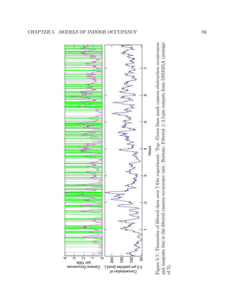
CHAPTER 5. MODELS OF INDOOR OCCUPANCY 94
01234
Camera Occurancesper 100s
12
34
56
75
0
10
0
15
0
20
0
Ho
urs
Concentration of
≥2 µm particles (pcs/L)
Fig
ure
5.7:
Tim
eser
ies
offil
tere
dda
taov
er7.
8hr
expe
rim
ent.
Top
:G
reen
lines
mar
kca
mer
aob
stru
ctio
noc
curr
ence
san
dm
agen
talin
eis
the
filte
red
cam
era
occu
rren
cera
te.
Bot
tom
:F
ilter
ed≥
2.5
µmou
tput
sfr
omD
SM50
1A(a
vera
geof
5).
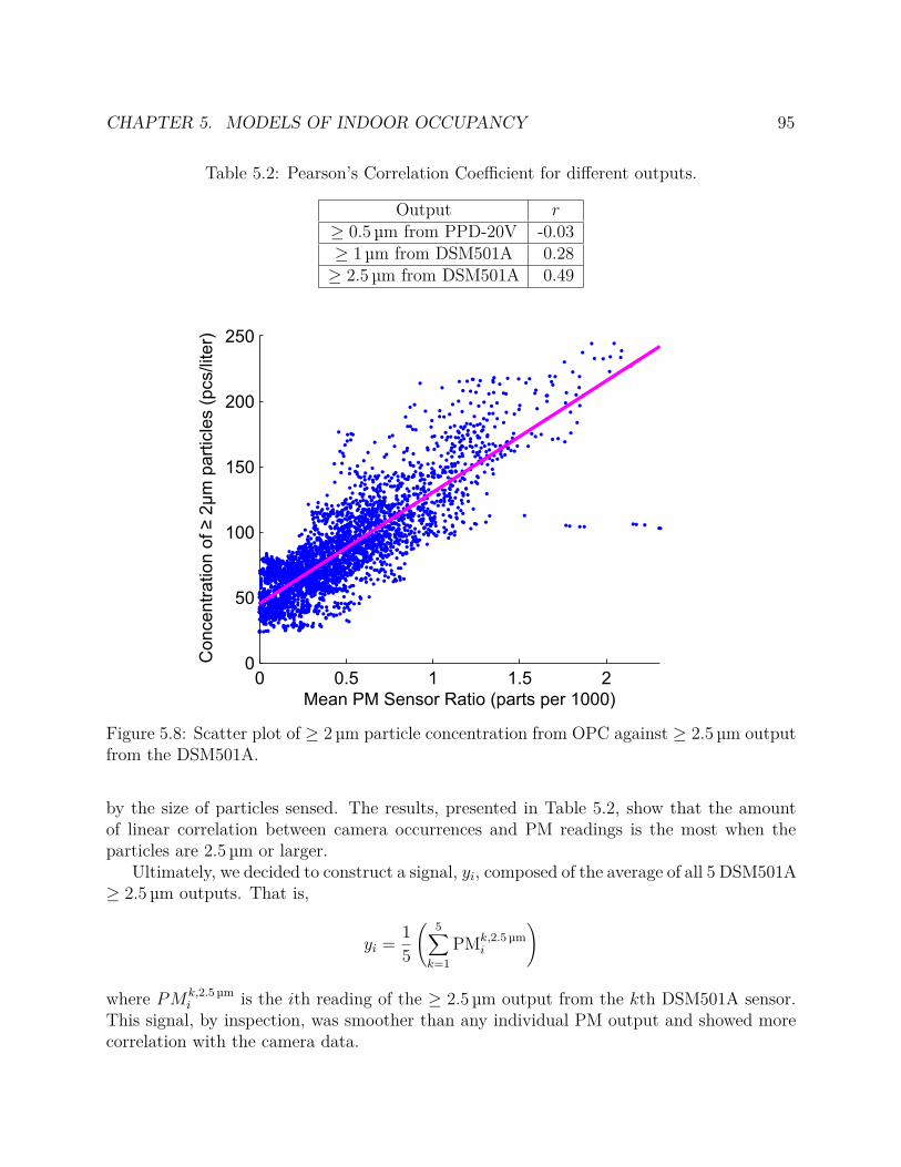
CHAPTER 5. MODELS OF INDOOR OCCUPANCY 95
Table 5.2: Pearson’s Correlation Coefficient for different outputs.
Output r≥ 0.5 µm from PPD-20V -0.03≥ 1 µm from DSM501A 0.28≥ 2.5 µm from DSM501A 0.49
0 0.5 1 1.5 20
50
100
150
200
250
Mean PM Sensor Ratio (parts per 1000)
Co
nce
ntr
atio
n o
f ≥
2µ
m p
art
icle
s (
pcs/lite
r)
Figure 5.8: Scatter plot of ≥ 2 µm particle concentration from OPC against ≥ 2.5 µm outputfrom the DSM501A.
by the size of particles sensed. The results, presented in Table 5.2, show that the amountof linear correlation between camera occurrences and PM readings is the most when theparticles are 2.5 µm or larger.
Ultimately, we decided to construct a signal, yi, composed of the average of all 5 DSM501A≥ 2.5 µm outputs. That is,
yi =15
(
5∑
k=1
PMk,2.5 µmi
)
where PMk,2.5 µmi is the ith reading of the ≥ 2.5 µm output from the kth DSM501A sensor.
This signal, by inspection, was smoother than any individual PM output and showed morecorrelation with the camera data.
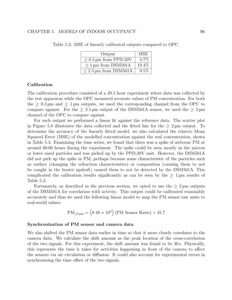
CHAPTER 5. MODELS OF INDOOR OCCUPANCY 96
Table 5.3: MSE of linearly calibrated outputs compared to OPC
Output MSE≥ 0.5 µm from PPD-20V 4.7%≥ 1 µm from DSM501A 19.4%≥ 2.5 µm from DSM501A 9.5%
Calibration
The calibration procedure consisted of a 29.5 hour experiment where data was collected bythe test apparatus while the OPC measured accurate values of PM concentration. For boththe ≥ 0.5 µm and ≥ 1 µm outputs, we used the corresponding channel from the OPC tocompare against. For the ≥ 2.5 µm output of the DSM501A sensor, we used the ≥ 2 µmchannel of the OPC to compare against.
For each output we performed a linear fit against the reference data. The scatter plotin Figure 5.8 illustrates the data collected and the fitted line for the ≥ 2 µm output. Todetermine the accuracy of the linearly fitted model, we also calculated the relative MeanSquared Error (MSE) of the modelled concentration against the real concentration, shownin Table 5.3. Examining the time series, we found that there was a spike of airborne PM ataround 00:00 hours during the experiment. The spike could be seen mostly in the micronor lower sized particles and was picked up by the PPD-20V unit. However, the DSM501Adid not pick up the spike in PM, perhaps because some characteristic of the particles suchas surface (changing the refraction characteristics) or composition (causing them to notbe caught in the heater updraft) caused them to not be detected by the DSM501A. Thiscomplicated the calibration results significantly as can be seen by the ≥ 1 µm results ofTable 5.3.
Fortunately, as described in the previous section, we opted to use the ≥ 2 µm outputsof the DSM501A for correlation with activity. This output could be calibrated reasonablyaccurately and thus we used the following linear model to map the PM sensor raw units toreal-world values:
PM≥2 µm =(
8.48× 10⁴)
(PM Sensor Ratio) + 45.7
Synchronization of PM sensor and camera data
We also shifted the PM sensor data earlier in time so that it more closely correlates to thecamera data. We calculate the shift amount as the peak location of the cross-correlationof the two signals. For this experiment, the shift amount was found to be 30 s. Physically,this represents the time it takes for activities happening in front of the camera to affectthe sensors via air circulation or diffusion. It could also account for experimental errors insynchronizing the time offset of the two signals.
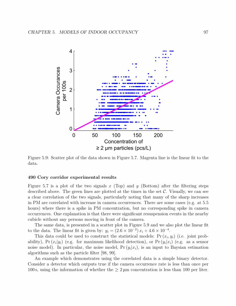
CHAPTER 5. MODELS OF INDOOR OCCUPANCY 97
0 50 100 150 200
0
1
2
3
4
Ca
me
ra O
ccu
ran
ce
sp
er
10
0s
Concentration of
≥ 2 µm particles (pcs/L)
Figure 5.9: Scatter plot of the data shown in Figure 5.7. Magenta line is the linear fit to thedata.
490 Cory corridor experimental results
Figure 5.7 is a plot of the two signals x (Top) and y (Bottom) after the filtering stepsdescribed above. The green lines are plotted at the times in the set C. Visually, we can seea clear correlation of the two signals, particularly noting that many of the sharp increasesin PM are correlated with increase in camera occurrences. There are some cases (e.g. at 5.5hours) where there is a spike in PM concentration, but no corresponding spike in cameraoccurrences. One explanation is that there were significant resuspension events in the nearbycubicle without any persons moving in front of the camera.
The same data, is presented in a scatter plot in Figure 5.9 and we also plot the linear fitto the data. The linear fit is given by: yi = (2.6× 10⁻²) xi + 4.6× 10⁻⁴.
This data could be used to construct the statistical models: Pr (xi, yi) (i.e. joint prob-ability), Pr (xi|yi) (e.g. for maximum likelihood detection), or Pr (yi|xi) (e.g. as a sensornoise model). In particular, the noise model, Pr (yi|xi), is an input to Baysian estimationalgorithms such as the particle filter [98, 99].
An example which demonstrates using the correlated data is a simple binary detector.Consider a detector which outputs true if the camera occurrence rate is less than once per100 s, using the information of whether the ≥ 2 µm concentration is less than 100 per liter.
CHAPTER 5. MODELS OF INDOOR OCCUPANCY 98
Used on this data set, the detector would be correct 66% of the time with a 42% falsepositive ratio and 28% false negative ratio. While this alone is far from ideal, it could becombined in a multiple agent decision framework containing other sensors such as passiveinfrared detectors.
Future work and connections
We have shown via experimentation that local occupant activity, measured visually by acamera, is correlated to the concentration of coarse particles, particularly those ≥ 2.5 µm.These types of particles can be easily sensed with low-cost PM sensors such as the DSM501A.Furthermore, if smoother data based on an average over numerous measurements is needed,more low-cost sensors could be added, while still being economical. We have also describedthe hardware developments which enable real-time reporting of PM sensor data to a centralserver using wireless technology. These hardware modules, while primarily intended for airquality monitoring, can also indicate occupant activity as we have shown by this article.We believe it will prove to be yet another piece of valuable information for estimating theoccupancy of smart buildings.
An important next step will be to investigate the causality of the variables we are mea-suring. Of particular concern is describing the hidden variable which is measured by boththe camera and PM sensor. That is, we have not determined whether how dependent thePM measurement is on the occupancy of the entire room versus the local occupancy directlyin front of the camera. An experiment which could disambiguate the two would be to alsoplace several PM sensors away from the test apparatus and measure the PM level of theentire room. For a permanent deployment, multiple sensors in the same room will be usefulfor estimating this background PM. We would then look at deviations of the local PM fromthe background level.
Further study into using coarse PM readings as a means of estimating occupancy directlyis motivated by these results which show that there is a correlation between the two variables.Our method would be to fuse the partial information provided by PM readings with theinformation gathered from other sources, such as CO2 concentration measurements. Thereis extensive literature[100] on information fusion techniques which can take redundant orcomplementary information and fuse them into a better estimate than either informationsource would provide on their own. For instance, in the next section, we discuss a methodwhich provides information about occupancy using CO2 measurements from the supply andreturn air vents of a conference room. In Section 6.5, a unified particle filter is introducedwhich can incorporate all sources of information into an occupant tracking and occupancyestimation framework.
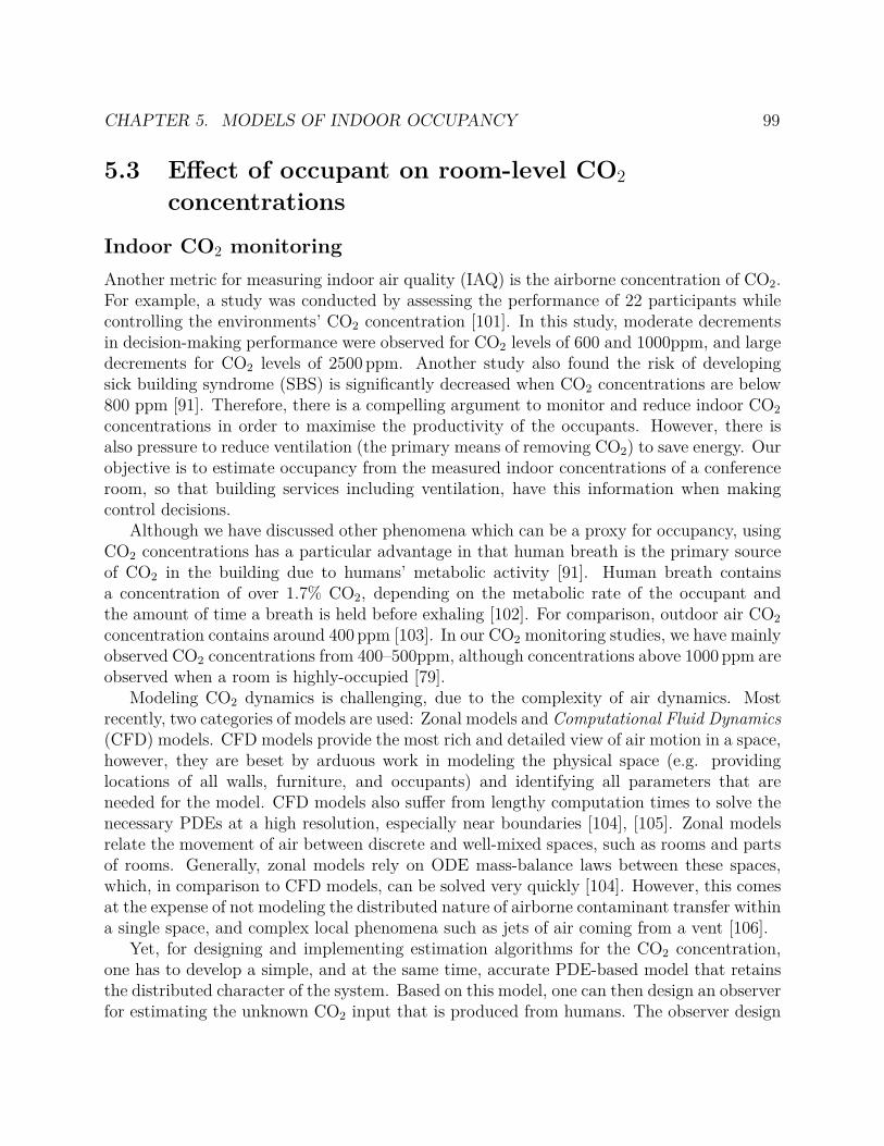
CHAPTER 5. MODELS OF INDOOR OCCUPANCY 99
5.3 Effect of occupant on room-level CO2
concentrations
Indoor CO2 monitoring
Another metric for measuring indoor air quality (IAQ) is the airborne concentration of CO2.For example, a study was conducted by assessing the performance of 22 participants whilecontrolling the environments’ CO2 concentration [101]. In this study, moderate decrementsin decision-making performance were observed for CO2 levels of 600 and 1000ppm, and largedecrements for CO2 levels of 2500 ppm. Another study also found the risk of developingsick building syndrome (SBS) is significantly decreased when CO2 concentrations are below800 ppm [91]. Therefore, there is a compelling argument to monitor and reduce indoor CO2
concentrations in order to maximise the productivity of the occupants. However, there isalso pressure to reduce ventilation (the primary means of removing CO2) to save energy. Ourobjective is to estimate occupancy from the measured indoor concentrations of a conferenceroom, so that building services including ventilation, have this information when makingcontrol decisions.
Although we have discussed other phenomena which can be a proxy for occupancy, usingCO2 concentrations has a particular advantage in that human breath is the primary sourceof CO2 in the building due to humans’ metabolic activity [91]. Human breath containsa concentration of over 1.7% CO2, depending on the metabolic rate of the occupant andthe amount of time a breath is held before exhaling [102]. For comparison, outdoor air CO2
concentration contains around 400 ppm [103]. In our CO2 monitoring studies, we have mainlyobserved CO2 concentrations from 400–500ppm, although concentrations above 1000 ppm areobserved when a room is highly-occupied [79].
Modeling CO2 dynamics is challenging, due to the complexity of air dynamics. Mostrecently, two categories of models are used: Zonal models and Computational Fluid Dynamics(CFD) models. CFD models provide the most rich and detailed view of air motion in a space,however, they are beset by arduous work in modeling the physical space (e.g. providinglocations of all walls, furniture, and occupants) and identifying all parameters that areneeded for the model. CFD models also suffer from lengthy computation times to solve thenecessary PDEs at a high resolution, especially near boundaries [104], [105]. Zonal modelsrelate the movement of air between discrete and well-mixed spaces, such as rooms and partsof rooms. Generally, zonal models rely on ODE mass-balance laws between these spaces,which, in comparison to CFD models, can be solved very quickly [104]. However, this comesat the expense of not modeling the distributed nature of airborne contaminant transfer withina single space, and complex local phenomena such as jets of air coming from a vent [106].
Yet, for designing and implementing estimation algorithms for the CO2 concentration,one has to develop a simple, and at the same time, accurate PDE-based model that retainsthe distributed character of the system. Based on this model, one can then design an observerfor estimating the unknown CO2 input that is produced from humans. The observer design

CHAPTER 5. MODELS OF INDOOR OCCUPANCY 100
has to be developed using the minimum number of sensors, in order to reduce cost andincrease reliability. It is also crucial to develop online identifiers for the parameters of themodel, since these parameters change with time due to their dependency on time-varyingquantities such as heat generation [107].
Tuning and verifying the applicability of the model requires experimental data to be col-lected. We conduct two experiments. In the first, a regulated amount of CO2 gas is releasedin the conference room for specific time periods while CO2 concentrations are measured ateight different locations in the room. We use the measurements of the CO2 concentrationin order to develop a model that reproduces the measured CO2 concentrations at the eightdifferent locations, given the known CO2 release. We also use the measurements from thisexperiment in order to identify in which sensing locations the measured CO2 concentrationsare more sensitive to an external CO2 source. In the second experiment, we monitor theevolution of the CO2 concentrations at three different locations in the room (the ventilationsystem’s input and output, and at a table located in the conference room) as two researchersenter and exit the room at recorded times. The purpose is to verify the model that wedevelop in the first experiment under a CO2 input that is generated by humans.
By conducting the two experiments, we aim to develop a data-driven model whose outputmatches the output of the actual system, when the same inputs are applied to both the modeland the system, which is simple enough for estimation and identification purposes. We donot attempt to modeling the exact physical phenomena govern the dynamics of the CO2.Yet, our model provides some insight on the actual spatially distributed dynamics of theCO2 concentration since it is a PDE model.
We model the dynamics of the CO2 concentration in the room using a convection PDEwith a source term which is the output of a first-order ODE system driven by an unknowninput which models the human’s emission rate of CO2. The source term represents the effectof the humans on the CO2 concentration in the room. In our experiments, we observe adelay in the response of the CO2 concentration in the room to changes in the human’s input.For this reason, the source term is a filtered version of the unknown input rather than theactual input. We assume that the unmeasured input from the humans has the form of apiecewise constant signal. This formulation is based on our experimental observation thathumans contribute to the rate of change of the CO2 concentration of the room with a filteredversion of step-like changes in the rate of CO2.
The value of the PDE at the one boundary of its spatial domain indicates the CO2
concentration inside the room at the location of the air supply. At this location, incomingair is entering the room, and hence, one can view the CO2 concentration of the fresh incomingair as an input to the system. The value of the PDE at the other boundary of its spatialdomain indicates the CO2 concentration at the air return of the ventilation system. The airat this point is mixed with CO2 that convects from the air supply towards the air return, andwith CO2 that is produced from humans. We consider the CO2 concentration at this pointas the output of our system. Any value of the PDE on an interior point of its spatial domainis an indicator of the concentration of CO2 at the ceiling in a (non-ratiometric) normalizeddistance along an axis from the supply to the return vent.
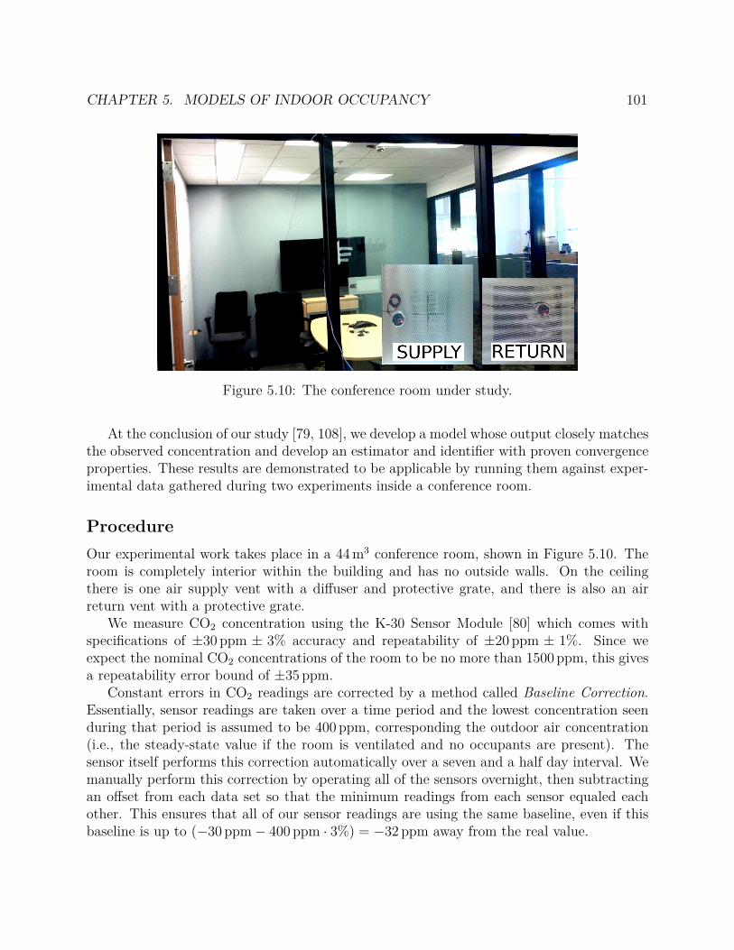
CHAPTER 5. MODELS OF INDOOR OCCUPANCY 101
Figure 5.10: The conference room under study.
At the conclusion of our study [79, 108], we develop a model whose output closely matchesthe observed concentration and develop an estimator and identifier with proven convergenceproperties. These results are demonstrated to be applicable by running them against exper-imental data gathered during two experiments inside a conference room.
Procedure
Our experimental work takes place in a 44 m3 conference room, shown in Figure 5.10. Theroom is completely interior within the building and has no outside walls. On the ceilingthere is one air supply vent with a diffuser and protective grate, and there is also an airreturn vent with a protective grate.
We measure CO2 concentration using the K-30 Sensor Module [80] which comes withspecifications of ±30 ppm ± 3% accuracy and repeatability of ±20 ppm ± 1%. Since weexpect the nominal CO2 concentrations of the room to be no more than 1500 ppm, this givesa repeatability error bound of ±35 ppm.
Constant errors in CO2 readings are corrected by a method called Baseline Correction.Essentially, sensor readings are taken over a time period and the lowest concentration seenduring that period is assumed to be 400 ppm, corresponding the outdoor air concentration(i.e., the steady-state value if the room is ventilated and no occupants are present). Thesensor itself performs this correction automatically over a seven and a half day interval. Wemanually perform this correction by operating all of the sensors overnight, then subtractingan offset from each data set so that the minimum readings from each sensor equaled eachother. This ensures that all of our sensor readings are using the same baseline, even if thisbaseline is up to (−30 ppm− 400 ppm · 3%) = −32 ppm away from the real value.
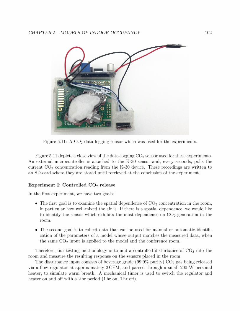
CHAPTER 5. MODELS OF INDOOR OCCUPANCY 102
Figure 5.11: A CO2 data-logging sensor which was used for the experiments.
Figure 5.11 depicts a close view of the data-logging CO2 sensor used for these experiments.An external microcontroller is attached to the K-30 sensor and, every seconds, polls thecurrent CO2 concentration reading from the K-30 device. These recordings are written toan SD-card where they are stored until retrieved at the conclusion of the experiment.
Experiment I: Controlled CO2 release
In the first experiment, we have two goals:
• The first goal is to examine the spatial dependence of CO2 concentration in the room,in particular how well-mixed the air is. If there is a spatial dependence, we would liketo identify the sensor which exhibits the most dependence on CO2 generation in theroom.
• The second goal is to collect data that can be used for manual or automatic identifi-cation of the parameters of a model whose output matches the measured data, whenthe same CO2 input is applied to the model and the conference room.
Therefore, our testing methodology is to add a controlled disturbance of CO2 into theroom and measure the resulting response on the sensors placed in the room.
The disturbance input consists of beverage grade (99.9% purity) CO2 gas being releasedvia a flow regulator at approximately 2 CFM, and passed through a small 200 W personalheater, to simulate warm breath. A mechanical timer is used to switch the regulator andheater on and off with a 2 hr period (1 hr on, 1 hr off).
CHAPTER 5. MODELS OF INDOOR OCCUPANCY 103
05
10
15
20
25
400
500
600
700
800
900
1000
Gla
ss S
hort
Wall
Whiteboard
Gla
ss L
ong W
all
Retu
rn - Table
Mid
dle
Ceili
ng
Supply
- Table
Supply
- C
eili
ng
Retu
rn - C
eili
ng
Tim
e(h
ours
)
CO2conc.(ppm)
Fig
ure
5.12
:C
O2
conc
entr
atio
nsdu
ring
Exp
erim
ent
I.Sh
owin
gm
easu
rem
ents
from
all
8lo
cati
ons
over
the
appr
oxi-
mat
ely
22ho
urex
peri
men
t.
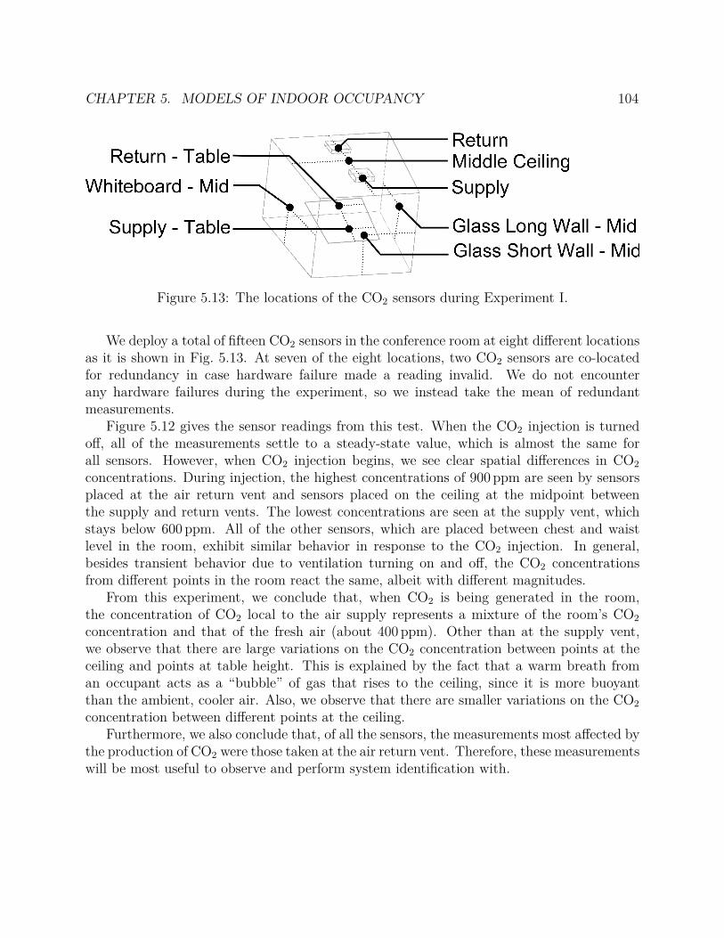
CHAPTER 5. MODELS OF INDOOR OCCUPANCY 104
Figure 5.13: The locations of the CO2 sensors during Experiment I.
We deploy a total of fifteen CO2 sensors in the conference room at eight different locationsas it is shown in Fig. 5.13. At seven of the eight locations, two CO2 sensors are co-locatedfor redundancy in case hardware failure made a reading invalid. We do not encounterany hardware failures during the experiment, so we instead take the mean of redundantmeasurements.
Figure 5.12 gives the sensor readings from this test. When the CO2 injection is turnedoff, all of the measurements settle to a steady-state value, which is almost the same forall sensors. However, when CO2 injection begins, we see clear spatial differences in CO2
concentrations. During injection, the highest concentrations of 900 ppm are seen by sensorsplaced at the air return vent and sensors placed on the ceiling at the midpoint betweenthe supply and return vents. The lowest concentrations are seen at the supply vent, whichstays below 600 ppm. All of the other sensors, which are placed between chest and waistlevel in the room, exhibit similar behavior in response to the CO2 injection. In general,besides transient behavior due to ventilation turning on and off, the CO2 concentrationsfrom different points in the room react the same, albeit with different magnitudes.
From this experiment, we conclude that, when CO2 is being generated in the room,the concentration of CO2 local to the air supply represents a mixture of the room’s CO2
concentration and that of the fresh air (about 400 ppm). Other than at the supply vent,we observe that there are large variations on the CO2 concentration between points at theceiling and points at table height. This is explained by the fact that a warm breath froman occupant acts as a “bubble” of gas that rises to the ceiling, since it is more buoyantthan the ambient, cooler air. Also, we observe that there are smaller variations on the CO2
concentration between different points at the ceiling.Furthermore, we also conclude that, of all the sensors, the measurements most affected by
the production of CO2 were those taken at the air return vent. Therefore, these measurementswill be most useful to observe and perform system identification with.
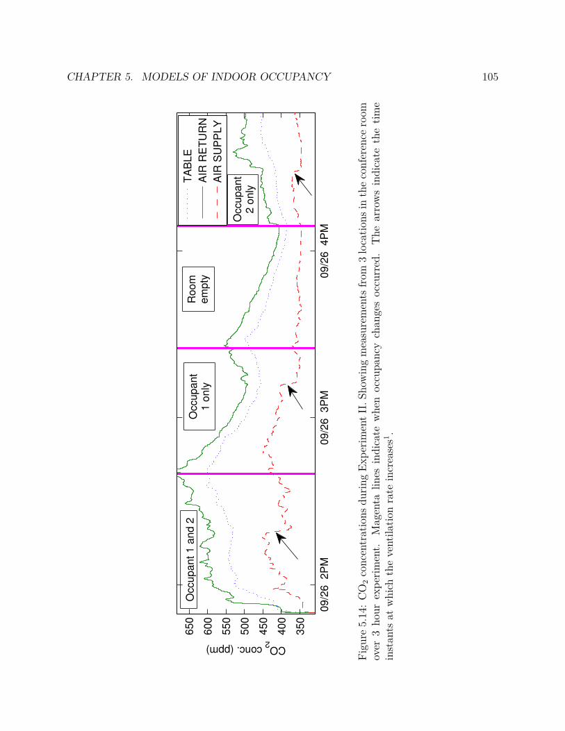
CHAPTER 5. MODELS OF INDOOR OCCUPANCY 105
09/2
6 2P
M09/2
6 3P
M09/2
6 4P
M
350
400
450
500
550
600
650
CO2 conc. (ppm)
T
AB
LE
AIR
RE
TU
RN
AIR
SU
PP
LY
Occupant
2 o
nly
Occupant 1 a
nd 2
Room
em
pty
Occupant
1 o
nly
Fig
ure
5.14
:C
O2
conc
entr
atio
nsdu
ring
Exp
erim
ent
II.S
how
ing
mea
sure
men
tsfr
om3
loca
tion
sin
the
conf
eren
cero
omov
er3
hour
expe
rim
ent.
Mag
enta
lines
indi
cate
whe
noc
cupa
ncy
chan
ges
occu
rred
.T
hear
row
sin
dica
teth
eti
me
inst
ants
atw
hich
the
vent
ilati
onra
tein
crea
ses1
.
CHAPTER 5. MODELS OF INDOOR OCCUPANCY 106
Experiment II: Release of CO2 from occupants
In the second experiment, the goal is to determine the effect of real occupancy on theconcentration of CO2 in the room. For this experiment, three CO2 sensors are deployed: oneeach at the air supply and return vents, and one on the conference table at the center of theroom. Our excitation procedure consists of adding or removing one of two participants ofthe experiment, and noting the time that the occupancy changes. Fig. 5.14 is a plot of thedata gathered from this experiment and when the occupancy transitions occur.
From this plot, we can see the general trend that CO2 concentration at the conferenceroom table and at the return vent increases when occupants arrive and decreases whenoccupants leave the room. We also conclude that the concentration at the air supply ventis much less dependent on occupancy. This can be attributed to the constant fresh airventilation that is provided by building services, so that fresh air concentration dominatesthe concentration in the area near the vent.
We can also see an interesting effect starting at the approximate times of 1:30PM, 2:20PMand 3:40PM, where the CO2 measurement at the air supply sharply drops and correspondsto a rise in CO2 in the other two measurements. We hypothesize this is due to the ventilationrate increasing. Near to the supply vent, a greater quantity of fresh air would mix with theair near the sensor, driving the concentration down. A higher air velocity in the room willalso impart more turbulent mixing of pockets of CO2 concentration within the room, pushingthem out of the air return and increasing the concentration at that point. The mixing ofthese pockets also causes an increase in the CO2 concentration near the table.
Modelling the CO2 dynamics
Model design
The model for the CO2 dynamics of the conference room are developed in [79]. Our modelconsists of a PDE and an ODE part. The ODE part is given by
X(t) = −aX(t) + V (t) (5.1)
V (t) = 0, (5.2)
where, X(t), in ppm, models the source term of occupant CO2 production on the relativeconcentration (in ppm) of the room in the local vicinity of the occupant (the evolution ofwhich is described later on by a PDE), and V (t) is a step-valued function, in ppm · s−1,representing the level of the occupant CO2 production rate within the vicinity of occupants.Parameter, 1
a, in units of 100s, represents a time constant specifying how fast changes in
occupancy affect the CO2 concentration in the room, in the local vicinity of the occupant.1We assume that the air ventilation rate increased at the marked points because an increased proportion
of fresh air (typically 400 ppm) would cause a drop in the supply CO2 concentration. The validity of thishypothesis could be verified by measuring the flow of incoming air at the supply with an anemometer.
CHAPTER 5. MODELS OF INDOOR OCCUPANCY 107
The ODE is coupled with a PDE that models the CO2 concentration in the room givenby
ut(x, t) = bux(x, t) + bXX(t) (5.3)
u(0, t) = Ue −∆U(t), (5.4)
with ∆U(t) = U(t) − Ue, where u(x, t), in ppm, is the concentration of CO2 in the roomat a time t ≥ 0 s and for 0 ≤ x ≤ 1, −b > 0, in 1
100s, represents the rate of air movement
in the room, and bX > 0, in 1104s
, specifies the rate of diffusion of CO2 from the localvicinity of the occupant to the room. The spatial variable x is unitless and represents anormalized distance along a horizontal axis that connects the air supply and air return. Theair supply and air return are located at x = 0 and x = 1 respectively. Therefore, u(0, t)is the CO2 concentration inside the room at the location of the air supply and u(1, t) isthe CO2 concentration inside the room at the location of the air return. The input U(t) isthe measured ppm concentration of the fresh incoming air. We do not simply specify theboundary condition at x = 0 as u(0, t) = U(t). The reason is that during our experimentswe observe that a sudden drop in the measured CO2 concentration at the air supply resultsin an increase of the CO2 concentration at the air return. Our explanation for this effectis that a drop in CO2 concentration at the supply from its equilibrium value correspondsto increased airflow at the vent, i.e. more fresh air gets mixed in the local vicinity. Theincreased airflow has the effect of pushing pockets of CO2 air out of the return vent. Oneway to capture this effect is to multiply the difference of the CO2 concentration from itsequilibrium value ∆U(t) = U(t)−Ue with minus one, where Ue, in ppm, is the steady stateinput CO2 concentration at the supply ventilation.
In Figure 5.15, we illustrate the geometrical representation of our model. The PDEportion of the model, u(x, t), represents convection of air from the air supply to the airreturn vent near the ceiling. Note the absence of a diffusive term, which we have omittedsince it plays a relatively minor role in dispersing indoor pollutants [107]. We choose tomodel the CO2 concentrations near the ceiling since this is where we see most effect fromoccupant-generated CO2 (see Section 5.3). This is explained by the fact that a warm breathfrom a occupant occupant acts as a “bubble” of gas that rises to the ceiling, since it ismore buoyant than the ambient, cooler air. Thus, the air coming from lower in the roomis modeled as a source term on the PDE across its entire length. The ODE portion of themodel is intended to model the fact that this bubble of air does not immediately rise to theceiling but only gradually.
Simulations
In Fig. 5.16 we show the concentration of CO2 at the air return and the air supply measuredby the CO2 sensors for our first experiment in which we periodically release CO2 every onehour. We also show the output u(1, t) of our model with parameters as shown in Table 5.42
2In this section we manually tune the parameters of model (5.1)–(5.4) in order to match the measuredCO2 concentration at the air return with u(1, t). In Section 5.3 we design identifiers for online identification
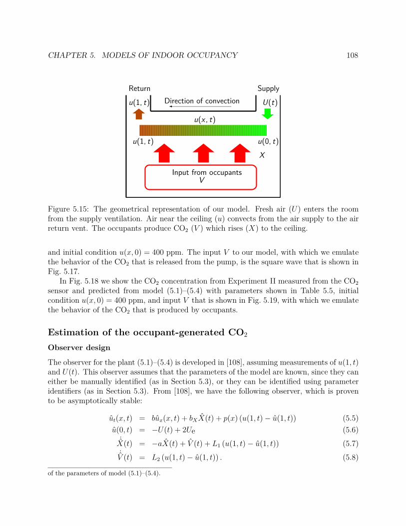
CHAPTER 5. MODELS OF INDOOR OCCUPANCY 108
Input from occupants
Direction of convection
SupplyReturn
V
u(x , t)
u(1, t) u(0, t)
X
u(1, t) U(t)
Figure 5.15: The geometrical representation of our model. Fresh air (U) enters the roomfrom the supply ventilation. Air near the ceiling (u) convects from the air supply to the airreturn vent. The occupants produce CO2 (V ) which rises (X) to the ceiling.
and initial condition u(x, 0) = 400 ppm. The input V to our model, with which we emulatethe behavior of the CO2 that is released from the pump, is the square wave that is shown inFig. 5.17.
In Fig. 5.18 we show the CO2 concentration from Experiment II measured from the CO2
sensor and predicted from model (5.1)–(5.4) with parameters shown in Table 5.5, initialcondition u(x, 0) = 400 ppm, and input V that is shown in Fig. 5.19, with which we emulatethe behavior of the CO2 that is produced by occupants.
Estimation of the occupant-generated CO2
Observer design
The observer for the plant (5.1)–(5.4) is developed in [108], assuming measurements of u(1, t)and U(t). This observer assumes that the parameters of the model are known, since they caneither be manually identified (as in Section 5.3), or they can be identified using parameteridentifiers (as in Section 5.3). From [108], we have the following observer, which is provento be asymptotically stable:
ut(x, t) = bux(x, t) + bXX(t) + p(x) (u(1, t)− u(1, t)) (5.5)
u(0, t) = −U(t) + 2Ue (5.6)˙
X(t) = −aX(t) + V (t) + L1 (u(1, t)− u(1, t)) (5.7)˙V (t) = L2 (u(1, t)− u(1, t)) . (5.8)
of the parameters of model (5.1)–(5.4).
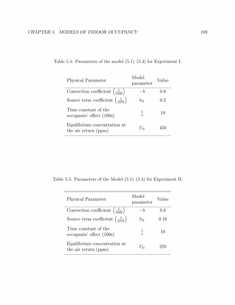
CHAPTER 5. MODELS OF INDOOR OCCUPANCY 109
Table 5.4: Parameters of the model (5.1)–(5.4) for Experiment I.
Physical ParameterModelparameter
Value
Convection coefficient(
1100s
)
−b 0.8
Source term coefficient(
1104s
)
bX 0.2
Time constant of theoccupants’ effect (100s)
1a
10
Equilibrium concentration atthe air return (ppm)
Ue 450
Table 5.5: Parameters of the Model (5.1)–(5.4) for Experiment II.
Physical ParameterModelparameter
Value
Convection coefficient(
1100s
)
−b 0.8
Source term coefficient(
1104s
)
bX 0.16
Time constant of theoccupants’ effect (100s)
1a
10
Equilibrium concentration atthe air return (ppm)
Ue 370
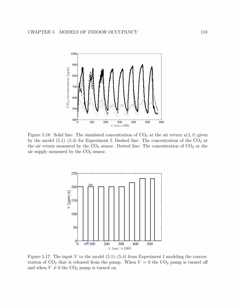
CHAPTER 5. MODELS OF INDOOR OCCUPANCY 110
0 100 200 300 400 500 600400
500
600
700
800
900
1000
t (sec×100)
CO
2co
ncentration(p
pm)
Figure 5.16: Solid line: The simulated concentration of CO2 at the air return u(1, t) givenby the model (5.1)–(5.4) for Experiment I. Dashed line: The concentration of the CO2 atthe air return measured by the CO2 sensor. Dotted line: The concentration of CO2 at theair supply measured by the CO2 sensor.
0 100 200 300 400 5000
50
100
150
200
250
t (sec ×100)
V(p
pm
/s)
on
off
Figure 5.17: The input V to the model (5.1)–(5.4) from Experiment I modeling the concen-tration of CO2 that is released from the pump. When V = 0 the CO2 pump is turned offand when V 6= 0 the CO2 pump is turned on.
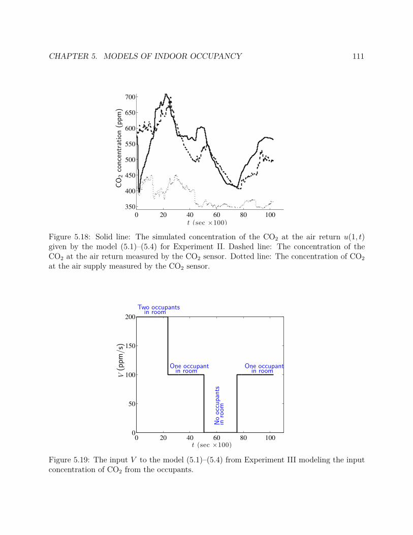
CHAPTER 5. MODELS OF INDOOR OCCUPANCY 111
0 20 40 60 80 100
350
400
450
500
550
600
650
700
t (sec ×100)
CO
2co
nce
ntr
atio
n(p
pm
)
Figure 5.18: Solid line: The simulated concentration of the CO2 at the air return u(1, t)given by the model (5.1)–(5.4) for Experiment II. Dashed line: The concentration of theCO2 at the air return measured by the CO2 sensor. Dotted line: The concentration of CO2
at the air supply measured by the CO2 sensor.
0 20 40 60 80 1000
50
100
150
200
V
t (sec ×100)
(ppm
/s)
Two occupantsin room
One occupantin room
No
occ
upan
tsin
room
One occupantin room
Figure 5.19: The input V to the model (5.1)–(5.4) from Experiment III modeling the inputconcentration of CO2 from the occupants.
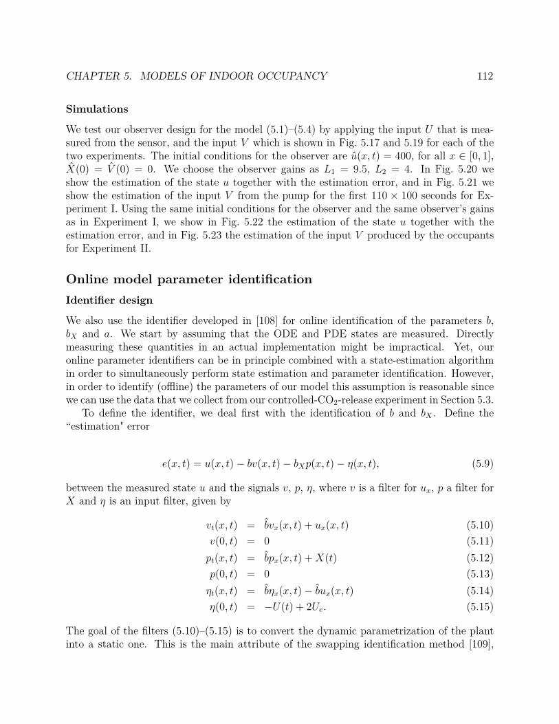
CHAPTER 5. MODELS OF INDOOR OCCUPANCY 112
Simulations
We test our observer design for the model (5.1)–(5.4) by applying the input U that is mea-sured from the sensor, and the input V which is shown in Fig. 5.17 and 5.19 for each of thetwo experiments. The initial conditions for the observer are u(x, t) = 400, for all x ∈ [0, 1],X(0) = V (0) = 0. We choose the observer gains as L1 = 9.5, L2 = 4. In Fig. 5.20 weshow the estimation of the state u together with the estimation error, and in Fig. 5.21 weshow the estimation of the input V from the pump for the first 110 × 100 seconds for Ex-periment I. Using the same initial conditions for the observer and the same observer’s gainsas in Experiment I, we show in Fig. 5.22 the estimation of the state u together with theestimation error, and in Fig. 5.23 the estimation of the input V produced by the occupantsfor Experiment II.
Online model parameter identification
Identifier design
We also use the identifier developed in [108] for online identification of the parameters b,bX and a. We start by assuming that the ODE and PDE states are measured. Directlymeasuring these quantities in an actual implementation might be impractical. Yet, ouronline parameter identifiers can be in principle combined with a state-estimation algorithmin order to simultaneously perform state estimation and parameter identification. However,in order to identify (offline) the parameters of our model this assumption is reasonable sincewe can use the data that we collect from our controlled-CO2-release experiment in Section 5.3.
To define the identifier, we deal first with the identification of b and bX . Define the“estimation" error
e(x, t) = u(x, t)− bv(x, t)− bXp(x, t)− η(x, t), (5.9)
between the measured state u and the signals v, p, η, where v is a filter for ux, p a filter forX and η is an input filter, given by
vt(x, t) = bvx(x, t) + ux(x, t) (5.10)
v(0, t) = 0 (5.11)
pt(x, t) = bpx(x, t) + X(t) (5.12)
p(0, t) = 0 (5.13)
ηt(x, t) = bηx(x, t)− bux(x, t) (5.14)
η(0, t) = −U(t) + 2Ue. (5.15)
The goal of the filters (5.10)–(5.15) is to convert the dynamic parametrization of the plantinto a static one. This is the main attribute of the swapping identification method [109],

CHAPTER 5. MODELS OF INDOOR OCCUPANCY 113E
stim
ated
CO
2co
nc.
(ppm
)
Est
imat
ion
erro
r(p
pm
)Figure 5.20: Left: The estimation of the CO2 concentration u(x, t) in the room for Experi-ment I. Right: The estimation error u(x, t) = u(x, t) − u(x, t) of the CO2 concentration inthe room for Experiment I (shown after 1× 100 sec for a better visualization).
0 20 40 60 80 100 1200
50
100
150
200
t (sec×100)
V (t)V (t)
Figure 5.21: The estimation V (blue line) of the pump input V (black line) in Fig. 5.17 forExperiment I.
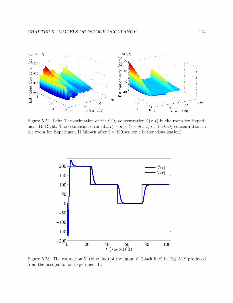
CHAPTER 5. MODELS OF INDOOR OCCUPANCY 114E
stim
ated
CO
2co
nc.
(ppm
)
Est
imat
ion
erro
r(p
pm
)Figure 5.22: Left: The estimation of the CO2 concentration u(x, t) in the room for Experi-ment II. Right: The estimation error u(x, t) = u(x, t)− u(x, t) of the CO2 concentration inthe room for Experiment II (shown after 3× 100 sec for a better visualization).
0 20 40 60 80 100−200
−150
−100
−50
0
50
100
150
200
t (sec×100)
V (t)
V (t)
Figure 5.23: The estimation V (blue line) of the input V (black line) in Fig. 5.19 producedfrom the occupants for Experiment II.
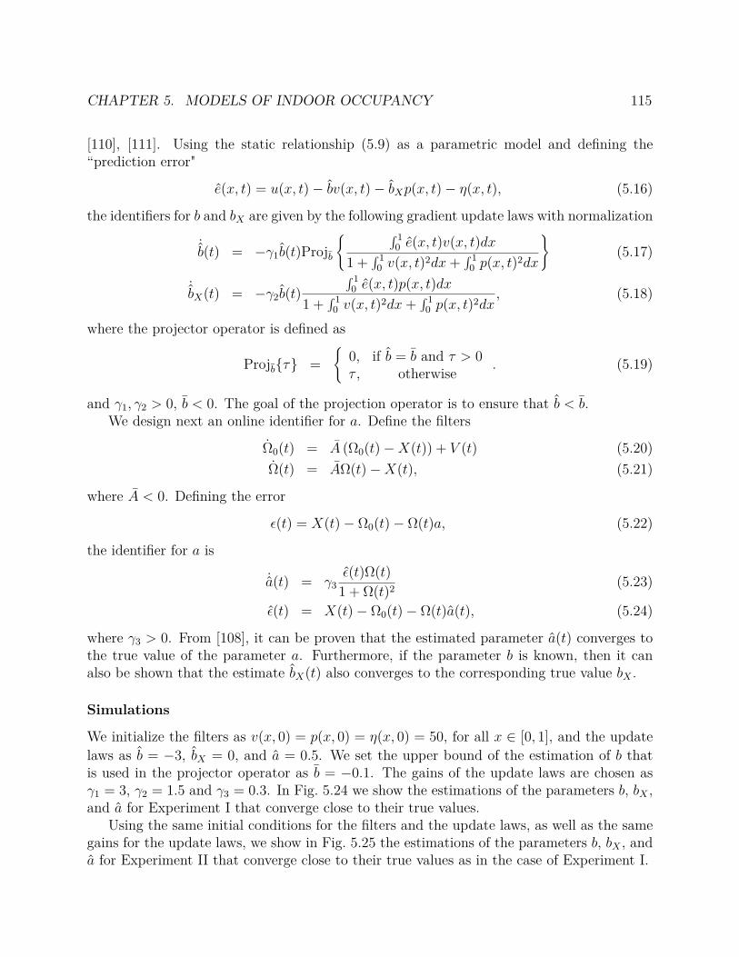
CHAPTER 5. MODELS OF INDOOR OCCUPANCY 115
[110], [111]. Using the static relationship (5.9) as a parametric model and defining the“prediction error"
e(x, t) = u(x, t)− bv(x, t)− bXp(x, t)− η(x, t), (5.16)
the identifiers for b and bX are given by the following gradient update laws with normalization
˙b(t) = −γ1b(t)Projb
∫ 1
0 e(x, t)v(x, t)dx
1 +∫ 1
0 v(x, t)2dx +∫ 1
0 p(x, t)2dx
(5.17)
˙bX(t) = −γ2b(t)
∫ 10 e(x, t)p(x, t)dx
1 +∫ 1
0 v(x, t)2dx +∫ 1
0 p(x, t)2dx, (5.18)
where the projector operator is defined as
Projbτ =
0, if b = b and τ > 0τ , otherwise
. (5.19)
and γ1, γ2 > 0, b < 0. The goal of the projection operator is to ensure that b < b.We design next an online identifier for a. Define the filters
Ω0(t) = A (Ω0(t)−X(t)) + V (t) (5.20)
Ω(t) = AΩ(t)−X(t), (5.21)
where A < 0. Defining the error
ǫ(t) = X(t)− Ω0(t)− Ω(t)a, (5.22)
the identifier for a is
˙a(t) = γ3ǫ(t)Ω(t)
1 + Ω(t)2(5.23)
ǫ(t) = X(t)− Ω0(t)− Ω(t)a(t), (5.24)
where γ3 > 0. From [108], it can be proven that the estimated parameter a(t) converges tothe true value of the parameter a. Furthermore, if the parameter b is known, then it canalso be shown that the estimate bX(t) also converges to the corresponding true value bX .
Simulations
We initialize the filters as v(x, 0) = p(x, 0) = η(x, 0) = 50, for all x ∈ [0, 1], and the updatelaws as b = −3, bX = 0, and a = 0.5. We set the upper bound of the estimation of b thatis used in the projector operator as b = −0.1. The gains of the update laws are chosen asγ1 = 3, γ2 = 1.5 and γ3 = 0.3. In Fig. 5.24 we show the estimations of the parameters b, bX ,and a for Experiment I that converge close to their true values.
Using the same initial conditions for the filters and the update laws, as well as the samegains for the update laws, we show in Fig. 5.25 the estimations of the parameters b, bX , anda for Experiment II that converge close to their true values as in the case of Experiment I.
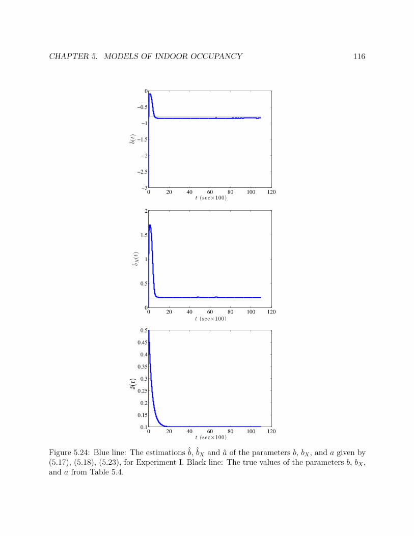
CHAPTER 5. MODELS OF INDOOR OCCUPANCY 116
0 20 40 60 80 100 120−3
−2.5
−2
−1.5
−1
−0.5
0
t (sec×100)
b(t)
0 20 40 60 80 100 1200
0.5
1
1.5
2
t (sec×100)
bX(t)
0 20 40 60 80 100 1200.1
0.15
0.2
0.25
0.3
0.35
0.4
0.45
0.5
t (sec×100)
α(t)
asdfa
sdfa
sdfa
sdf
a(t
)
Figure 5.24: Blue line: The estimations b, bX and a of the parameters b, bX , and a given by(5.17), (5.18), (5.23), for Experiment I. Black line: The true values of the parameters b, bX ,and a from Table 5.4.
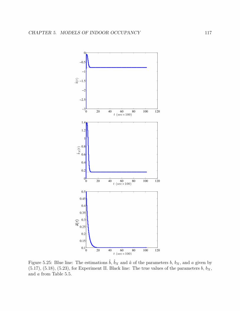
CHAPTER 5. MODELS OF INDOOR OCCUPANCY 117
0 20 40 60 80 100 120−3
−2.5
−2
−1.5
−1
−0.5
0
t (sec×100)
b(t)
0 20 40 60 80 100 1200
0.2
0.4
0.6
0.8
1
1.2
1.4
t (sec×100)
bX(t)
0 20 40 60 80 100 1200.1
0.15
0.2
0.25
0.3
0.35
0.4
0.45
0.5
t (sec×100)
α(t)
asdfa
sdfa
sdfa
sdf
a(t
)
Figure 5.25: Blue line: The estimations b, bX and a of the parameters b, bX , and a given by(5.17), (5.18), (5.23), for Experiment II. Black line: The true values of the parameters b, bX ,and a from Table 5.5.
CHAPTER 5. MODELS OF INDOOR OCCUPANCY 118
Conclusions of the CO2 study
Presently, we develop a PDE-ODE model that describes the dynamics of the CO2 concen-tration in a conference room, and validate that the model is suitable using data from twoground truth experiments. We design and validate an observer for the estimation of theunknown CO2 input that is generated by occupants, which acts as a intuitive proxy for thenumber of occupants breathing in the local air space. The estimator used in this studyalso has mathematical guarantees of convergence. To estimate unknown parameters of themodel, we design online parameter identifiers which can be proven to converge to the truevalues, and we show in our experimental work that the parameters are indeed identified.
A topic for future research is to combine the observer design with the update laws forthe estimation of the parameters of the model. In other words, to design an adaptiveobserver [109]. Yet, in contrast to the finite-dimensional case, in the case of PDE systemsthis is far from trivial due to the lack of systematic procedures for the construction ofstate-transformations that can transform the original system to a system having an observercanonical form [109], [111]. For this reason designing adaptive observers for PDE systems ispossible only in special cases [111]. As an alternative one could resort to finite-dimensionalapproximations as it is done, for example, in [112].
To address the end application of occupancy estimation, future work will address theproblem of estimation of the actual occupancy level using measurements of CO2. This is ahighly non trivial problem because occupants’ CO2 generation rates can vary widely betweendifferent persons depending on current activity, diet, and body size [105]. One possibilityto address this problem is to build a database of parameters which characterize the amountof CO2 generated by each individual, however, this would require a means of consistentlyidentifying occupants. A more robust direction that we are pursuing is to use sensor fusiontechniques to combine other sources of information, such as correlations to coarse PM (seeSection 5.2), into the estimation.
5.4 Conclusions
The primary purpose of office and residential buildings is always to provide comfortableresidence for their occupants to work and live. Heating, ventilation, air conditioning andlighting services are means of preparing the indoor environment for occupants, howeverprovisioning and operating these services incurs significant cost and energy demands. Tomitigate these costs, methods which estimate indoor occupancy can simply turn off lights andHVAC services when occupants are not present to consume them. Despite the simple controlstrategy, this can reduce consumption by up to 15% [54] when systems are heavily duty-cycled. However, perhaps more exciting is that once we can accurately estimate occupancyindoors, we can begin to improve models of occupancy in buildings. These models are usedto predict future occupancy, so that building services can plan ahead for energy-efficiency,and building designers can appropriately provision services to suit future occupant demands.
CHAPTER 5. MODELS OF INDOOR OCCUPANCY 119
The studies conducted in this chapter are the first steps in demonstrating that readingsfrom indoor air quality (IAQ) sensors, in this case CO2 and Particulate Matter (PM), canbe used to estimate local occupancy. The techniques we develop do not require occupant-carried tags or an indoor positioning infrastructure to function. This is an important resultsince the types of sensors used are already being deployed for IAQ purposes, meaning weare adding value to an existing value proposition. Our hope would be that this leads in adirection that encourages building owners to deploy more IAQ sensors, especially given thatSick Building Syndrome is becoming more of a concern.
Although we specifically illuminate the advantages of directly estimating occupancy, wealso note that the occupancy estimation problem is fundamentally coupled to the occupanttracking problem. In fact, we will demonstrate in the next chapter how occupancy informa-tion can be integrated into a positioning infrastructure. This is a new development in thefield of positioning, whereas traditionally, occupant tracking has been used as an input tosolving occupancy estimation only.
120
Chapter 6
Filtering Algorithms for OccupantTracking
6.1 Introduction
Within the office space mobile environment, a valuable direction of research is to directlyestimate the position of the occupants over time, i.e. occupant tracking. We have alreadydiscussed the benefits of occupancy estimation, which can calculated from accurate occu-pant tracking of all occupants. However, identifying and tracking individual occupants hasbenefits beyond occupancy estimation purposes. For instance, individual occupants couldhave different tolerances for indoor climates and lighting and building services could be ad-justed accordingly. Another popular use of occupant tracking is to provide location-basedservices, such as indoor navigation, advertising and assisting occupants in finding each otherindoors. There is also research interest in “social games” where occupants are incentivizedto save energy in their daily routine and tracking the position of the participants is essentialto enforcing the rules of the game. In this chapter, we construct a solution to the occupanttracking problem using particle filters. Via a field operational test, we validate that the par-ticle filter is a viable method for occupant tracking, and can be the basis of many possibleextensions. These extensions include connections to our work in occupancy estimation andon the development of the environmental sensing platform. Addressing the occupant track-ing and occupancy estimation problems simultaneously, a unified particle filter is proposedwhich shares information between the two problems and incorporates information gatheredfrom a variety of sensors.
Indoor Positioning Systems
The application area for Indoor Positioning Systems (IPS) is rapidly expanding as researchersdiscover location-aware services such as on-demand lighting or ventilation control. However,due to the unstructured nature of indoor environments, designing an IPS has many differ-ent challenges and requirements in comparison to outdoor and large-scale positioning sys-
CHAPTER 6. FILTERING ALGORITHMS FOR OCCUPANT TRACKING 121
tems [113]. The requirements of an IPS vary in cost, power usage, accuracy, reliability, andcomputational efficiency, depending on the application. This has led to many IPS conceptswhich fill particular niches. For example, a robot needs highly accurate positioning to avoidobstacles, whereas a location-aware service for occupants may only need to know which rooman occupant is in. For the former case, a highly accurate ultrasound system [114] might beused. However, in the latter case, power consumption is a greater concern than positioningaccuracy, where room-level accuracy might be sufficient.
Advances in low-power radios and improved wireless network protocols have enabledRadio Frequency Identification (RFID) as a practical solution to the occupant trackingproblem, with many approaches of how to use radio measurements for positioning [84]. Apopular avenue of research is to use existing WiFi infrastructure by measuring received signalstrength (RSS) to the building’s access points [85, 86]. However, some buildings do not havethe access point density needed for the IPS to function, and more must be installed. Also,WiFi devices inherently have higher power requirements than other technologies, but areconsidered practical since many occupants already carry and use these types of devices,such as smartphones. Alternatively, IEEE 802.15.4 is a low-cost and low-power wirelesssensor network technology which can be deployed for positioning and other low data-rateapplications [115, 116]. A device based on this technology can be installed in an employeeID badge, or in our case, a small fob that the occupant carries.
Statistical techniques for radio-based indoor positioning
In this chapter, we describe a method to filter RSS measurements using a sequential Monte-Carlo Bayesian estimation technique [99, 5], also known as a particle filter. We implement themost basic form of the algorithm, called Sampling Importance Resampling (SIR). Particlefiltering methods are especially applicable to unstructured environments due to their abil-ity to elegantly handle non-continuous systems and integrate heterogeneous measurements.They have been used successfully in robotics [117], and in IPS installations with a combina-tion of sensors such as RFID, inertial, infrared, and laser scanning [118, 119, 120]. A similarparticle filtering IPS implementation [121] to ours uses WiFi instead of RFID technologyand explores the same “histogram method” to model the RSS measurements. Their stateis modelled as the occupant being at one of 510 predefined calibration cells. The occupantmust travel along and adjacency graph between these cells. Our implementation also relieson an adjacency graph, but one which is parametrized and automatically computed from thefloorplan layout. We also directly model the state as continuous 2D coordinates, instead ofdiscrete locations.
Our IPS strictly uses RSS measurements, although we envision adding other types ofsensors to improve the tracking performance. This article is an account of how our IPS isbuilt up from the principles of particle filtering, including practical implementation detailsone might need if installing an RSS-based IPS system of their own. In particular, we pro-vide a unique method of incorporating the RSS sensor measurements in a way that reducesdependence on a physical transmission model by creating empirical estimates of sensor error
CHAPTER 6. FILTERING ALGORITHMS FOR OCCUPANT TRACKING 122
distributions. This leads our IPS implementation to achieve within a 5 m accuracy for 90%of estimates. We also provide a discussion of the computational requirements of our multi-threaded program, which achieves a real-time to execution time ratio of about 18000, leavingsignificant room for more complex models and tracking of several hundreds of occupants.
6.2 Indoor positioning using SIR
SIR estimation framework
In this section, we instantiate the SIR algorithm [5, 117] for our system. For this article,we denote xt as a three-dimensional random variable corresponding to time t. We use adiscrete-time algorithm with a time interval of δt, in seconds. The first two dimensions,xt,1:2, are the coordinates, in meters, of the occupant-carried RFID tag being positioned,and the last dimension, xt,3, represents an attenuation factor, in dBm, of the tag’s localenvironment. This third term attempts to correct for calibration errors or differences inradio propagation between different tags. To simplify notation when discussing the state ina general context, we use x1:2 to represent the coordinates of the tag and x3 to represent theattenuation factor. We define yt as the RSS observations measured at time t by the RFIDsystem. This observation vector has Nsensors dimensions and measured in units of dBm.
The goal of the algorithm is to estimate the belief distribution
Pr (xt|y1...t) , (6.1)
i.e. the probability at time t of state xt being the actual state of the system, given all ofthe past observations from t = 1. If we estimate the belief perfectly, then the maximumlikelihood estimate,
xt = argmaxx
Pr (x|y1...t) ,
is the ideal estimation of the tag’s position given all of the previous data.If we assume a hidden Markov Model, then the current observations only depend on the
current state, i.e.Pr (yt|x1...t, y1...t) = Pr (yt|xt) ,
and the next state depends only on the last state, i.e.
Pr (xt+1|x1...t) = Pr (xt+1|xt) .
Applying Bayes rule and the above assumptions gives
Pr(
xt
∣
∣
∣y1...(t−1)
)
= (6.2)∫
Pr (xt|xt−1) Pr(
xt−1
∣
∣
∣y1...(t−1)
)
dxt−1,
CHAPTER 6. FILTERING ALGORITHMS FOR OCCUPANT TRACKING 123
Pr (xt|y1...t) =Pr (yt|xt) Pr
(
xt
∣
∣
∣y1...(t−1)
)
Pr(
yt
∣
∣
∣y1...(t−1)
) (6.3)
= ηPr (yt|xt) Pr(
xt
∣
∣
∣y1...(t−1)
)
,
where η is a normalization constant and essentially accounted for by (6.4).Thus, (6.2) and (6.3), are a recursive solution to (6.1), and are termed the prediction and
update steps, respectively.For many problems, including the indoor positioning task, analytically evaluating (6.2)
and (6.3) is infeasible, therefore we turn to Monte-Carlo methods where samples are used toestimate the distribution.
We track the belief by a set of n particles, where the i-th particle consists of a state esti-mate, x(i), and importance factor, w(i). Although not strictly necessary, when the importancefactors are updated, they are renormalized so that
n∑
i=1
w(i) = 1. (6.4)
The prediction and update steps are adapted to propagate samples and are as follows:
Prediction
For each particle, samplex
(i)t ∼ Pr
(
x(i)t
∣
∣
∣x(i)t−1
)
,
so that the particles are now distributed as (6.2). The state transition distribution,
Pr(
x(i)t
∣
∣
∣x(i)t−1
)
,
represents the system dynamics and is described in Section 6.2.
Update
For each particle, evaluate the non-normalized importance weight
w(i)t = Pr
(
y(i)t
∣
∣
∣x(i)t
)
,
where the observation distribution, Pr(
y(i)t
∣
∣
∣x(i)t
)
, represents the sensor noise and is describedby Section 6.2. Then, the importance weights are normalized by
w(i)t =
n∑
j=1
w(j)t
−1
w(i)t .
We then take n samples,
x(i)t : i = 1, . . . , n
, from the discrete distribution defined over
x(i)t : i = 1, . . . , n
, where Pr(
x = x(i)t
)
= w(i)t .
CHAPTER 6. FILTERING ALGORITHMS FOR OCCUPANT TRACKING 124
After both steps are run, the particles are will be approximately distributed according tothe belief (6.1). Additionally, the pairs of x
(i)t and w
(i)t approximate the probability density
function (PDF) of the belief, i.e.
w(i)t ≈ Pr
(
x(i)t
∣
∣
∣y1...t
)
Two more implementation details remain. Since this is a recursive algorithm, an initialstate must be chosen for each of the particles
x(0)1 , . . . , x
(n)1
, from a given prior distributionf1(x). The initial states are sampled from uniform distributions since little is known aboutthe state of the system before any measurements arrive. For the coordinate states, x1:2,the uniform distribution is over the entire floor area of the office space, whereas for theattenuation factor, x3, we sample from U (−amax, amax), where amax is a model parameter.
The second implementation detail is the method used to select the actual estimate, xt,of the state from the set of particles. We chose the estimate via one of the following twomethods and evaluated both for their accuracy:
maximum likelihood particle (MLP)
xt = x(i)t ,
i = argmaxj
w(j)t .
nearest weighted mean particle (NWMP)
xt = x(i)t ,
i = argminj
‖x(j)t,1:2 −mt‖2,
mt =1n
n∑
k=1
w(k)t x
(k)t,1:2.
State Transition Distribution
During the update step, there is the need to sample from Pr(
x(i)t
∣
∣
∣x(i)t−1
)
. The state is com-prised of the x-y coordinate pair of the tag, xt,1:2, and the attenuation factor, xt,3, which aresampled from two separate models.
Tag Coordinates
The state transition distribution essentially adds knowledge about the system dynamics intothe estimation. For our problem, this means describing where a tracked occupant could
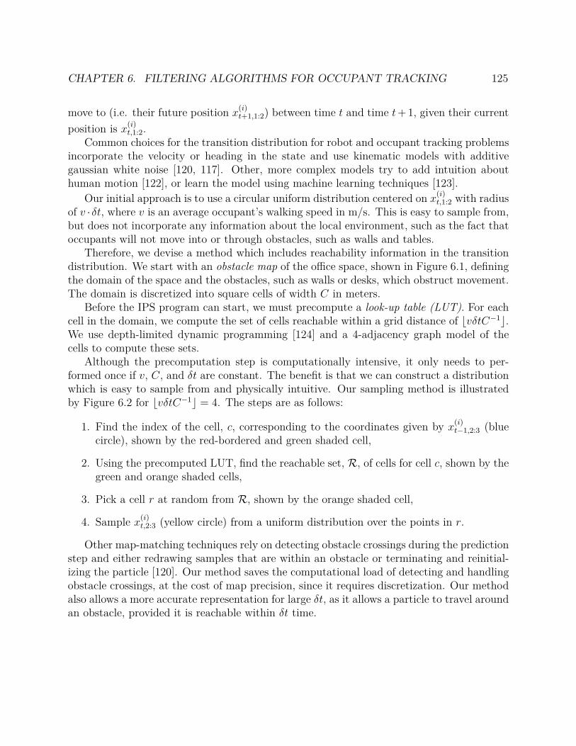
CHAPTER 6. FILTERING ALGORITHMS FOR OCCUPANT TRACKING 125
move to (i.e. their future position x(i)t+1,1:2) between time t and time t + 1, given their current
position is x(i)t,1:2.
Common choices for the transition distribution for robot and occupant tracking problemsincorporate the velocity or heading in the state and use kinematic models with additivegaussian white noise [120, 117]. Other, more complex models try to add intuition abouthuman motion [122], or learn the model using machine learning techniques [123].
Our initial approach is to use a circular uniform distribution centered on x(i)t,1:2 with radius
of v ·δt, where v is an average occupant’s walking speed in m/s. This is easy to sample from,but does not incorporate any information about the local environment, such as the fact thatoccupants will not move into or through obstacles, such as walls and tables.
Therefore, we devise a method which includes reachability information in the transitiondistribution. We start with an obstacle map of the office space, shown in Figure 6.1, definingthe domain of the space and the obstacles, such as walls or desks, which obstruct movement.The domain is discretized into square cells of width C in meters.
Before the IPS program can start, we must precompute a look-up table (LUT). For eachcell in the domain, we compute the set of cells reachable within a grid distance of ⌊vδtC−1⌋.We use depth-limited dynamic programming [124] and a 4-adjacency graph model of thecells to compute these sets.
Although the precomputation step is computationally intensive, it only needs to per-formed once if v, C, and δt are constant. The benefit is that we can construct a distributionwhich is easy to sample from and physically intuitive. Our sampling method is illustratedby Figure 6.2 for ⌊vδtC−1⌋ = 4. The steps are as follows:
1. Find the index of the cell, c, corresponding to the coordinates given by x(i)t−1,2:3 (blue
circle), shown by the red-bordered and green shaded cell,
2. Using the precomputed LUT, find the reachable set, R, of cells for cell c, shown by thegreen and orange shaded cells,
3. Pick a cell r at random from R, shown by the orange shaded cell,
4. Sample x(i)t,2:3 (yellow circle) from a uniform distribution over the points in r.
Other map-matching techniques rely on detecting obstacle crossings during the predictionstep and either redrawing samples that are within an obstacle or terminating and reinitial-izing the particle [120]. Our method saves the computational load of detecting and handlingobstacle crossings, at the cost of map precision, since it requires discretization. Our methodalso allows a more accurate representation for large δt, as it allows a particle to travel aroundan obstacle, provided it is reachable within δt time.
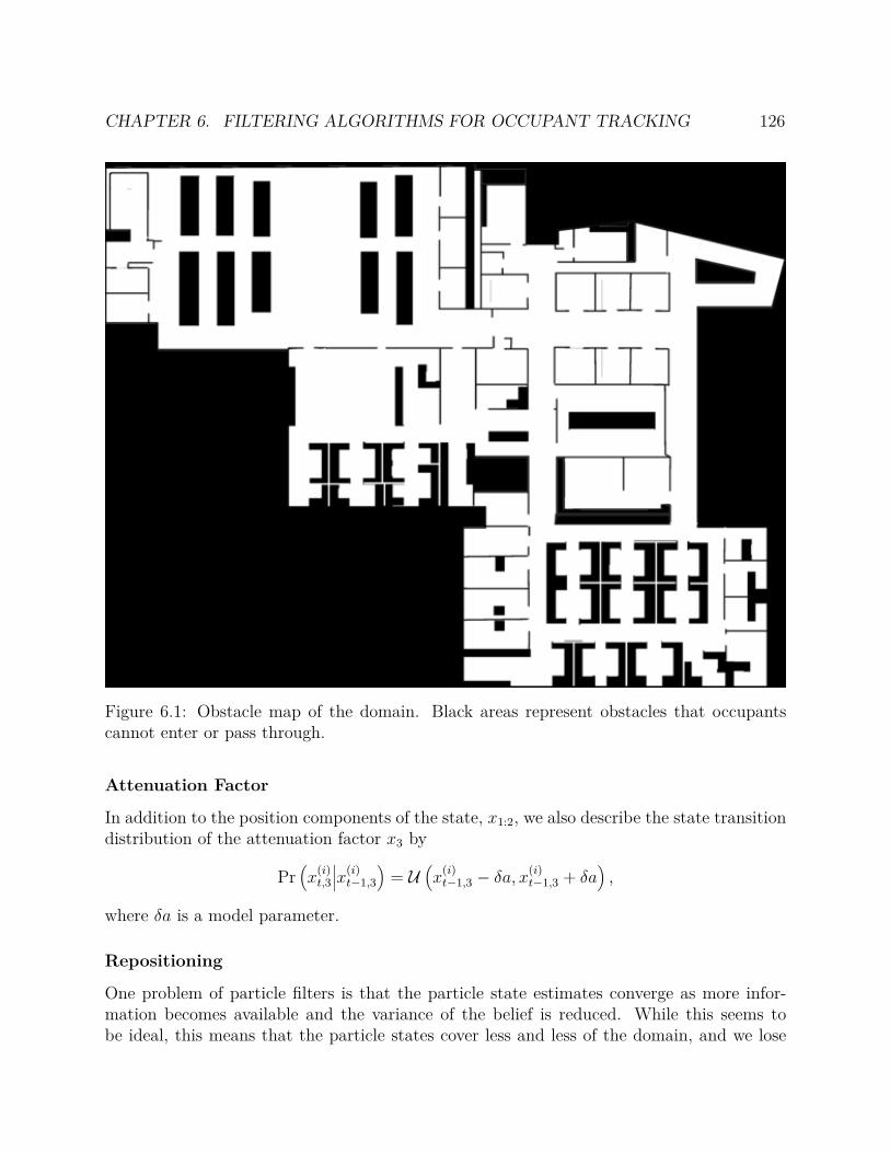
CHAPTER 6. FILTERING ALGORITHMS FOR OCCUPANT TRACKING 126
Figure 6.1: Obstacle map of the domain. Black areas represent obstacles that occupantscannot enter or pass through.
Attenuation Factor
In addition to the position components of the state, x1:2, we also describe the state transitiondistribution of the attenuation factor x3 by
Pr(
x(i)t,3
∣
∣
∣x(i)t−1,3
)
= U(
x(i)t−1,3 − δa, x
(i)t−1,3 + δa
)
,
where δa is a model parameter.
Repositioning
One problem of particle filters is that the particle state estimates converge as more infor-mation becomes available and the variance of the belief is reduced. While this seems tobe ideal, this means that the particle states cover less and less of the domain, and we lose
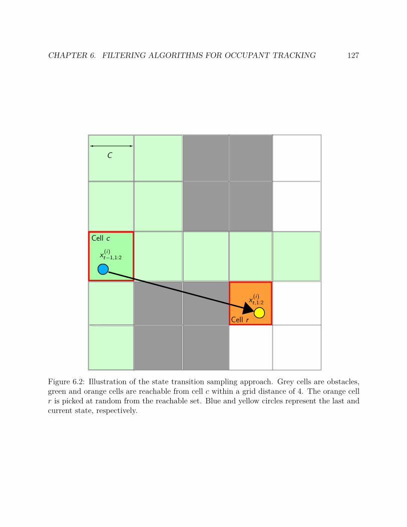
CHAPTER 6. FILTERING ALGORITHMS FOR OCCUPANT TRACKING 127
C
x(i)t−1,1:2
x(i)t,1:2
Cell c
Cell r
Figure 6.2: Illustration of the state transition sampling approach. Grey cells are obstacles,green and orange cells are reachable from cell c within a grid distance of 4. The orange cellr is picked at random from the reachable set. Blue and yellow circles represent the last andcurrent state, respectively.
CHAPTER 6. FILTERING ALGORITHMS FOR OCCUPANT TRACKING 128
information about that part of the distribution. Thus, we augment the sampling algorithmwith a repositioning step:
x(i)t ∼
f1(x) z < Γ
Pr(
x(i)t
∣
∣
∣x(i)t−1
)
otherwise
z ∼ U (0, 1)
where Γ ∈ [0, 1] is the repositioning ratio, and an algorithm parameter. A Γ > 0 ensuresthat some fraction of particles are artificially moved to “explore” parts of the domain thatmight have been missed.
Observation Distributions
It is well known that modelling propagation of radio signals in an unstructured indoorenvironment is highly complex [125] due to varied reflection and attenuation propertiesof materials in the space, as well as multi-path affects, which are especially present withnarrow-band and high-frequency channels. Therefore, there are a variety of models usedfor radio positioning systems such as ours. Some directly derive the model from physicalphenomena [86], and others are data-driven models where many measurements are taken atfixed points to create an RSS fingerprint [116, 87, 85].
Our method is a data-driven model, but motivated by the physical property that the RSSwill, in general, be lower as the sensor is farther from the transmitter. A broad descriptionof the method is that, for each sensor, r, we radially partition the domain into Nbins evenly-spaced bins. For each bin, b, there is a corresponding empirically-derived PDF, f r
b (·), of thesignal strength measurement if the sensor is inside the corresponding partition.
To derive the method, we start by assuming the sensor outputs are independent fromeach other, given the state. Thus, we can decompose the observation distribution by
Pr (y|x) =Nsensors∏
r=1
Pr (yr|x) ,
where yr is the RSS reading from the rth receiver. We model the individual sensor distribu-tions as
Pr (yr|x) =
f rb (yr) + x3 b ≤ Nbins
0 otherwise
b =⌊
Nbinsdmax
‖pr − x1:2‖2
⌋
+ 1,
where pr is the coordinates of the rth sensor and dmax is an algorithm parameter andrepresents the maximum distance between any sensor and a possible tag’s position.
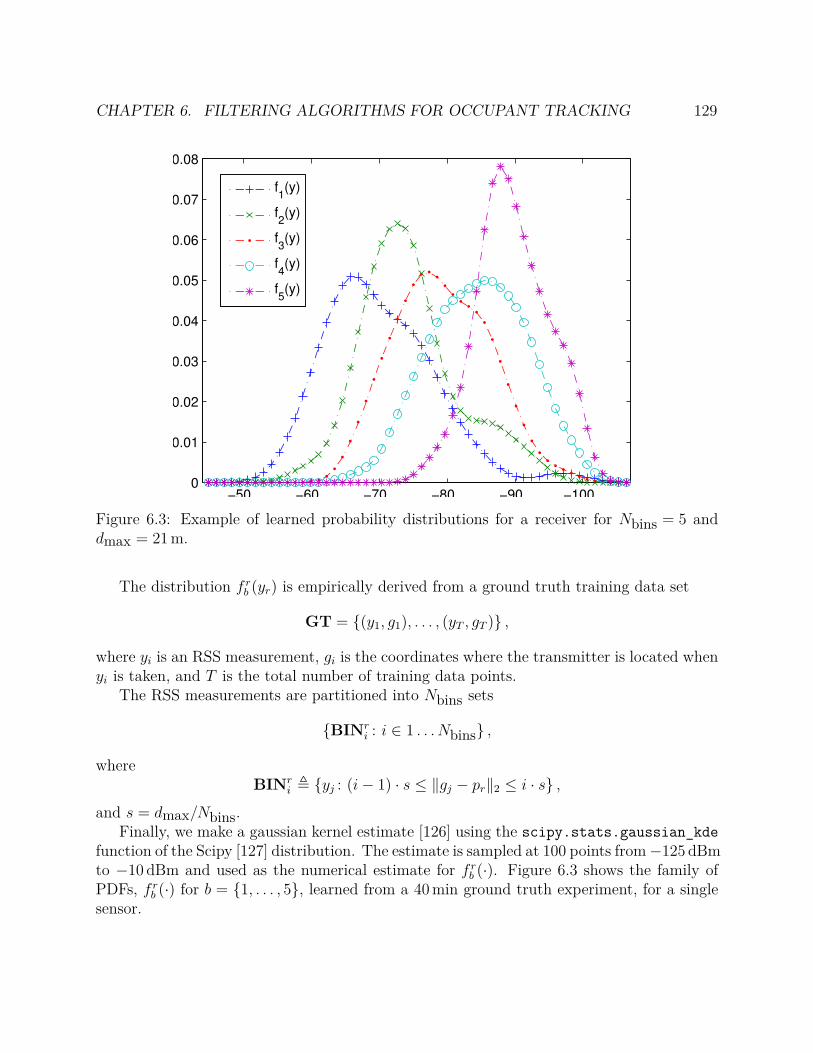
CHAPTER 6. FILTERING ALGORITHMS FOR OCCUPANT TRACKING 129
−100−90−80−70−60−500
0.01
0.02
0.03
0.04
0.05
0.06
0.07
0.08
f1(y)
f2(y)
f3(y)
f4(y)
f5(y)
Figure 6.3: Example of learned probability distributions for a receiver for Nbins = 5 anddmax = 21 m.
The distribution f rb (yr) is empirically derived from a ground truth training data set
GT = (y1, g1), . . . , (yT , gT ) ,
where yi is an RSS measurement, gi is the coordinates where the transmitter is located whenyi is taken, and T is the total number of training data points.
The RSS measurements are partitioned into Nbins sets
BINri : i ∈ 1 . . . Nbins ,
whereBINr
i , yj : (i− 1) · s ≤ ‖gj − pr‖2 ≤ i · s ,
and s = dmax/Nbins.Finally, we make a gaussian kernel estimate [126] using the scipy.stats.gaussian_kde
function of the Scipy [127] distribution. The estimate is sampled at 100 points from−125 dBmto −10 dBm and used as the numerical estimate for f r
b (·). Figure 6.3 shows the family ofPDFs, f r
b (·) for b = 1, . . . , 5, learned from a 40 min ground truth experiment, for a singlesensor.
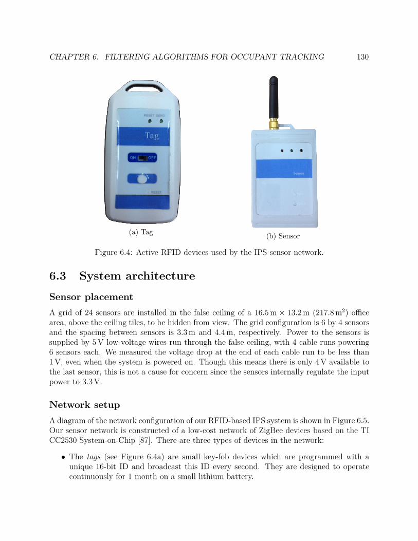
CHAPTER 6. FILTERING ALGORITHMS FOR OCCUPANT TRACKING 130
(a) Tag(b) Sensor
Figure 6.4: Active RFID devices used by the IPS sensor network.
6.3 System architecture
Sensor placement
A grid of 24 sensors are installed in the false ceiling of a 16.5 m × 13.2 m (217.8 m2) officearea, above the ceiling tiles, to be hidden from view. The grid configuration is 6 by 4 sensorsand the spacing between sensors is 3.3 m and 4.4 m, respectively. Power to the sensors issupplied by 5 V low-voltage wires run through the false ceiling, with 4 cable runs powering6 sensors each. We measured the voltage drop at the end of each cable run to be less than1 V, even when the system is powered on. Though this means there is only 4 V available tothe last sensor, this is not a cause for concern since the sensors internally regulate the inputpower to 3.3 V.
Network setup
A diagram of the network configuration of our RFID-based IPS system is shown in Figure 6.5.Our sensor network is constructed of a low-cost network of ZigBee devices based on the TICC2530 System-on-Chip [87]. There are three types of devices in the network:
• The tags (see Figure 6.4a) are small key-fob devices which are programmed with aunique 16-bit ID and broadcast this ID every second. They are designed to operatecontinuously for 1 month on a small lithium battery.
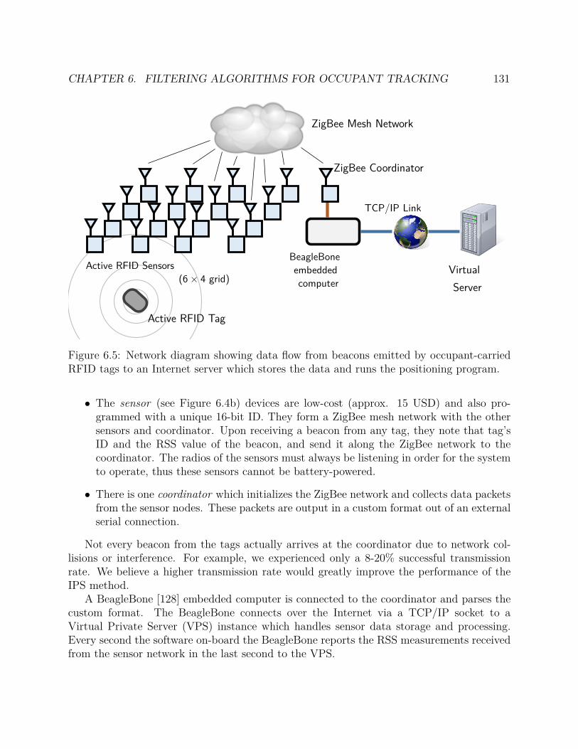
CHAPTER 6. FILTERING ALGORITHMS FOR OCCUPANT TRACKING 131
Active RFID Tag
Active RFID Sensors
(6 × 4 grid)
ZigBee Mesh Network
ZigBee Coordinator
BeagleBone
embedded
computer
TCP/IP Link
Virtual
Server
Figure 6.5: Network diagram showing data flow from beacons emitted by occupant-carriedRFID tags to an Internet server which stores the data and runs the positioning program.
• The sensor (see Figure 6.4b) devices are low-cost (approx. 15 USD) and also pro-grammed with a unique 16-bit ID. They form a ZigBee mesh network with the othersensors and coordinator. Upon receiving a beacon from any tag, they note that tag’sID and the RSS value of the beacon, and send it along the ZigBee network to thecoordinator. The radios of the sensors must always be listening in order for the systemto operate, thus these sensors cannot be battery-powered.
• There is one coordinator which initializes the ZigBee network and collects data packetsfrom the sensor nodes. These packets are output in a custom format out of an externalserial connection.
Not every beacon from the tags actually arrives at the coordinator due to network col-lisions or interference. For example, we experienced only a 8-20% successful transmissionrate. We believe a higher transmission rate would greatly improve the performance of theIPS method.
A BeagleBone [128] embedded computer is connected to the coordinator and parses thecustom format. The BeagleBone connects over the Internet via a TCP/IP socket to aVirtual Private Server (VPS) instance which handles sensor data storage and processing.Every second the software on-board the BeagleBone reports the RSS measurements receivedfrom the sensor network in the last second to the VPS.
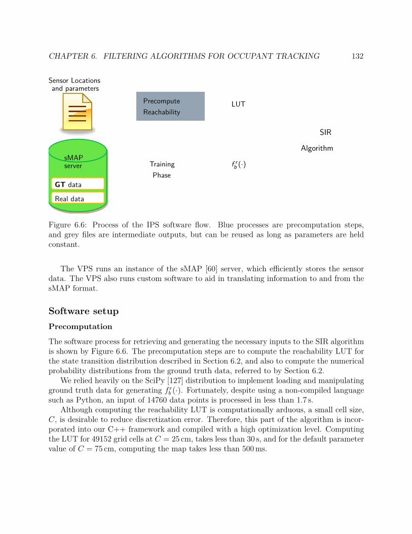
CHAPTER 6. FILTERING ALGORITHMS FOR OCCUPANT TRACKING 132
sMAPserver
GT data
Real data
Sensor Locationsand parameters
Precompute
ReachabilityLUT
Training
Phase
fr
b(·)
SIR
Algorithm
Figure 6.6: Process of the IPS software flow. Blue processes are precomputation steps,and grey files are intermediate outputs, but can be reused as long as parameters are heldconstant.
The VPS runs an instance of the sMAP [60] server, which efficiently stores the sensordata. The VPS also runs custom software to aid in translating information to and from thesMAP format.
Software setup
Precomputation
The software process for retrieving and generating the necessary inputs to the SIR algorithmis shown by Figure 6.6. The precomputation steps are to compute the reachability LUT forthe state transition distribution described in Section 6.2, and also to compute the numericalprobability distributions from the ground truth data, referred to by Section 6.2.
We relied heavily on the SciPy [127] distribution to implement loading and manipulatingground truth data for generating f r
b (·). Fortunately, despite using a non-compiled languagesuch as Python, an input of 14760 data points is processed in less than 1.7 s.
Although computing the reachability LUT is computationally arduous, a small cell size,C, is desirable to reduce discretization error. Therefore, this part of the algorithm is incor-porated into our C++ framework and compiled with a high optimization level. Computingthe LUT for 49152 grid cells at C = 25 cm, takes less than 30 s, and for the default parametervalue of C = 75 cm, computing the map takes less than 500 ms.
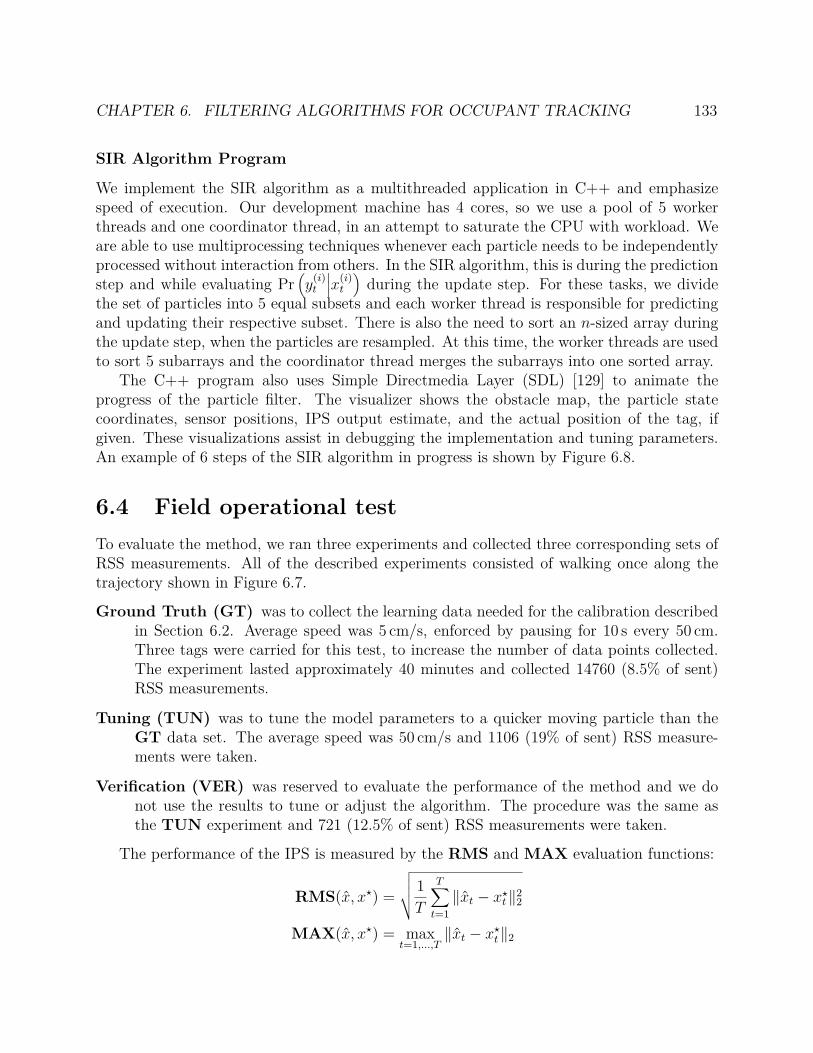
CHAPTER 6. FILTERING ALGORITHMS FOR OCCUPANT TRACKING 133
SIR Algorithm Program
We implement the SIR algorithm as a multithreaded application in C++ and emphasizespeed of execution. Our development machine has 4 cores, so we use a pool of 5 workerthreads and one coordinator thread, in an attempt to saturate the CPU with workload. Weare able to use multiprocessing techniques whenever each particle needs to be independentlyprocessed without interaction from others. In the SIR algorithm, this is during the predictionstep and while evaluating Pr
(
y(i)t
∣
∣
∣x(i)t
)
during the update step. For these tasks, we dividethe set of particles into 5 equal subsets and each worker thread is responsible for predictingand updating their respective subset. There is also the need to sort an n-sized array duringthe update step, when the particles are resampled. At this time, the worker threads are usedto sort 5 subarrays and the coordinator thread merges the subarrays into one sorted array.
The C++ program also uses Simple Directmedia Layer (SDL) [129] to animate theprogress of the particle filter. The visualizer shows the obstacle map, the particle statecoordinates, sensor positions, IPS output estimate, and the actual position of the tag, ifgiven. These visualizations assist in debugging the implementation and tuning parameters.An example of 6 steps of the SIR algorithm in progress is shown by Figure 6.8.
6.4 Field operational test
To evaluate the method, we ran three experiments and collected three corresponding sets ofRSS measurements. All of the described experiments consisted of walking once along thetrajectory shown in Figure 6.7.
Ground Truth (GT) was to collect the learning data needed for the calibration describedin Section 6.2. Average speed was 5 cm/s, enforced by pausing for 10 s every 50 cm.Three tags were carried for this test, to increase the number of data points collected.The experiment lasted approximately 40 minutes and collected 14760 (8.5% of sent)RSS measurements.
Tuning (TUN) was to tune the model parameters to a quicker moving particle than theGT data set. The average speed was 50 cm/s and 1106 (19% of sent) RSS measure-ments were taken.
Verification (VER) was reserved to evaluate the performance of the method and we donot use the results to tune or adjust the algorithm. The procedure was the same asthe TUN experiment and 721 (12.5% of sent) RSS measurements were taken.
The performance of the IPS is measured by the RMS and MAX evaluation functions:
RMS(x, x⋆) =
√
√
√
√
1T
T∑
t=1
‖xt − x⋆t‖2
2
MAX(x, x⋆) = maxt=1,...,T
‖xt − x⋆t‖2

CHAPTER 6. FILTERING ALGORITHMS FOR OCCUPANT TRACKING 134
Para
mete
rD
esc
rip
tio
nD
efa
ult
Eff
ect
of
Ad
just
ing
δtT
ime
inte
rval
5s
Bes
tpe
rfor
man
cebe
twee
n3
san
d9
s.
nN
umbe
rof
part
icle
s10
0P
erfo
rman
cede
grad
esbe
low
n=
60,
othe
rwis
em
argi
nal
impr
ovem
ent
wit
hm
ore
part
icle
s.
Sele
ctio
nM
etho
dM
etho
dto
sele
ctx
tfr
omth
ese
tof
part
icle
s.N
WM
PU
sing
ML
Pre
sult
sin
slig
htly
redu
ced
perf
orm
ance
.
ΓR
epos
itio
ning
rati
o0%
Slig
htly
wor
sepe
rfor
man
cefr
om0
<%
Γ≤
50%
,si
gnifi
cant
lyw
orse
whe
nΓ
>50
%.
am
axM
axim
umin
itia
lat
tenu
atio
n1.
5dB
mN
oeff
ect
onpe
rfor
man
ce.
δaM
axim
umch
ange
ofat
tenu
atio
n0.
75dB
mSl
ight
impr
ovem
ent
insi
de0.
25dB
man
d0.
75dB
m.
CR
each
abili
tyL
UT
cell
wid
th0.
75m
Sign
ifica
ntly
wor
sepe
rfor
man
cew
hen
C>
0.75
m.
vO
ccup
ant
mov
esp
eed
0.5
m/s
Sign
ifica
ntde
crea
sein
perf
orm
ance
asv
mov
esaw
ayfr
om0.
5m
/s.
Nbin
sN
umbe
rof
part
itio
nsfo
rth
eca
libra
tion
inSe
ctio
n6.
25
Sign
ifica
ntly
wor
sepe
rfor
man
cefo
rN
bin
s/∈3
,5.
Tab
le6.
1:L
ist
ofpa
ram
eter
stu
ned
and
thei
reff
ects
onth
eac
cura
cyof
the
IPS.
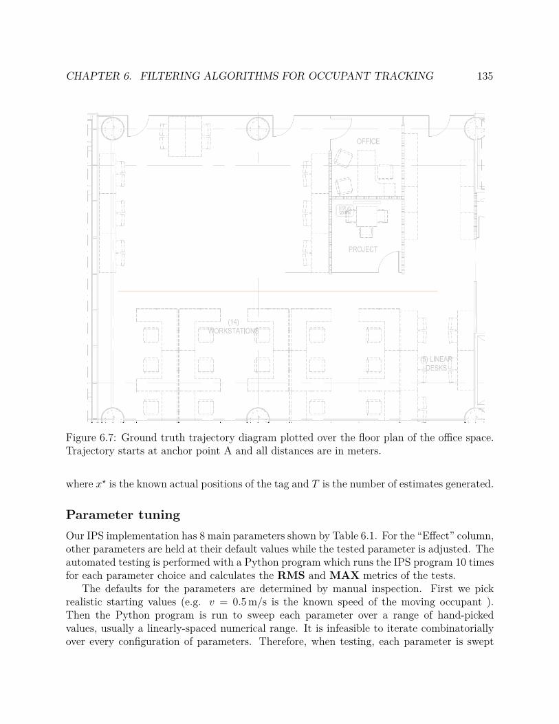
CHAPTER 6. FILTERING ALGORITHMS FOR OCCUPANT TRACKING 135
A B
H
Q R
Q
S
N M
F D
P O
T
C
L J
E
Q
8.5
3
5.5
3.5
3 2 2
5 5
6.5
5
2
2
7
5.5
3.5
5.5
Figure 6.7: Ground truth trajectory diagram plotted over the floor plan of the office space.Trajectory starts at anchor point A and all distances are in meters.
where x⋆ is the known actual positions of the tag and T is the number of estimates generated.
Parameter tuning
Our IPS implementation has 8 main parameters shown by Table 6.1. For the “Effect” column,other parameters are held at their default values while the tested parameter is adjusted. Theautomated testing is performed with a Python program which runs the IPS program 10 timesfor each parameter choice and calculates the RMS and MAX metrics of the tests.
The defaults for the parameters are determined by manual inspection. First we pickrealistic starting values (e.g. v = 0.5 m/s is the known speed of the moving occupant ).Then the Python program is run to sweep each parameter over a range of hand-pickedvalues, usually a linearly-spaced numerical range. It is infeasible to iterate combinatoriallyover every configuration of parameters. Therefore, when testing, each parameter is swept
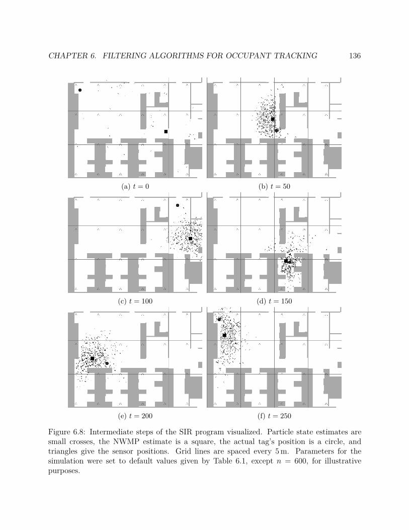
CHAPTER 6. FILTERING ALGORITHMS FOR OCCUPANT TRACKING 136
(a) t = 0 (b) t = 50
(c) t = 100 (d) t = 150
(e) t = 200 (f) t = 250
Figure 6.8: Intermediate steps of the SIR program visualized. Particle state estimates aresmall crosses, the NWMP estimate is a square, the actual tag’s position is a circle, andtriangles give the sensor positions. Grid lines are spaced every 5 m. Parameters for thesimulation were set to default values given by Table 6.1, except n = 600, for illustrativepurposes.
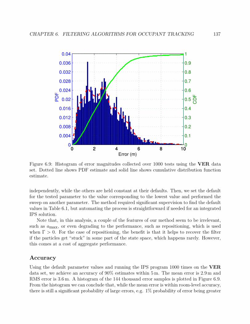
CHAPTER 6. FILTERING ALGORITHMS FOR OCCUPANT TRACKING 137
0 2 4 6 8 100
0.004
0.008
0.012
0.016
0.02
0.024
0.028
0.032
0.036
0.04P
DF
Error (m)0 2 4 6 8 10
0
0.1
0.2
0.3
0.4
0.5
0.6
0.7
0.8
0.9
1
CD
F
Figure 6.9: Histogram of error magnitudes collected over 1000 tests using the VER dataset. Dotted line shows PDF estimate and solid line shows cumulative distribution functionestimate.
independently, while the others are held constant at their defaults. Then, we set the defaultfor the tested parameter to the value corresponding to the lowest value and performed thesweep on another parameter. The method required significant supervision to find the defaultvalues in Table 6.1, but automating the process is straightforward if needed for an integratedIPS solution.
Note that, in this analysis, a couple of the features of our method seem to be irrelevant,such as amax, or even degrading to the performance, such as repositioning, which is usedwhen Γ > 0. For the case of repositioning, the benefit is that it helps to recover the filterif the particles get “stuck” in some part of the state space, which happens rarely. However,this comes at a cost of aggregate performance.
Accuracy
Using the default parameter values and running the IPS program 1000 times on the VERdata set, we achieve an accuracy of 90% estimates within 5 m. The mean error is 2.9 m andRMS error is 3.6 m. A histogram of the 144 thousand error samples is plotted in Figure 6.9.From the histogram we can conclude that, while the mean error is within room-level accuracy,there is still a significant probability of large errors, e.g. 1% probability of error being greater
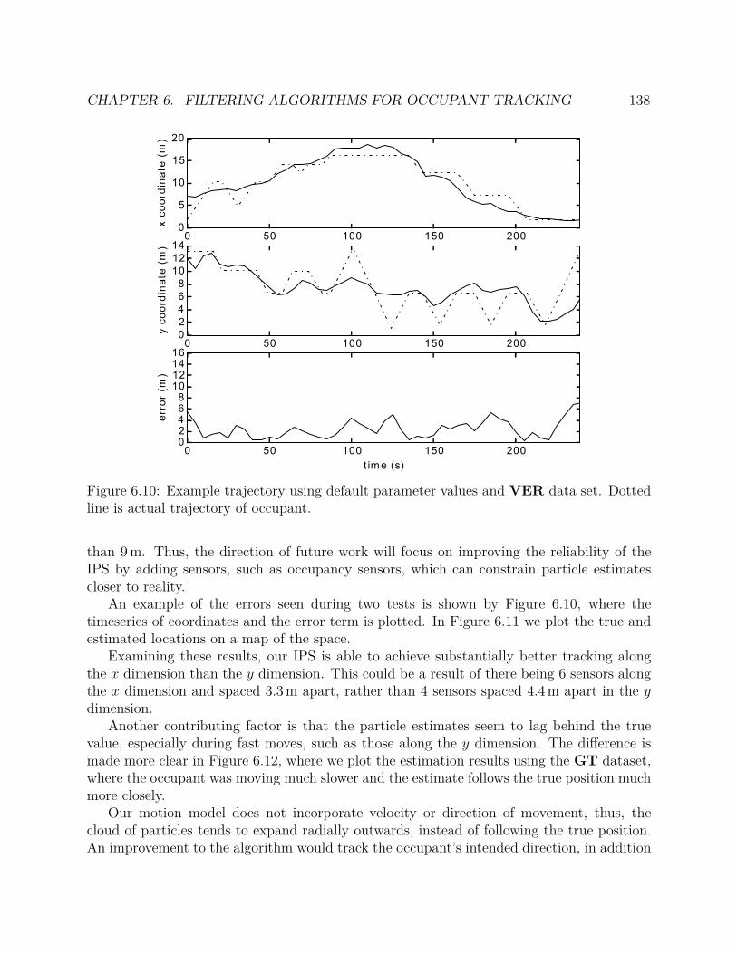
CHAPTER 6. FILTERING ALGORITHMS FOR OCCUPANT TRACKING 138
0 50 100 150 2000
5
10
15
20
x c
oo
rdin
ate
(m
)
0 50 100 150 2000
2
4
6
8
10
12
14
y c
oo
rdin
ate
(m
)
0 50 100 150 200
t im e (s)
02468
10121416
err
or
(m)
Figure 6.10: Example trajectory using default parameter values and VER data set. Dottedline is actual trajectory of occupant.
than 9 m. Thus, the direction of future work will focus on improving the reliability of theIPS by adding sensors, such as occupancy sensors, which can constrain particle estimatescloser to reality.
An example of the errors seen during two tests is shown by Figure 6.10, where thetimeseries of coordinates and the error term is plotted. In Figure 6.11 we plot the true andestimated locations on a map of the space.
Examining these results, our IPS is able to achieve substantially better tracking alongthe x dimension than the y dimension. This could be a result of there being 6 sensors alongthe x dimension and spaced 3.3 m apart, rather than 4 sensors spaced 4.4 m apart in the ydimension.
Another contributing factor is that the particle estimates seem to lag behind the truevalue, especially during fast moves, such as those along the y dimension. The difference ismade more clear in Figure 6.12, where we plot the estimation results using the GT dataset,where the occupant was moving much slower and the estimate follows the true position muchmore closely.
Our motion model does not incorporate velocity or direction of movement, thus, thecloud of particles tends to expand radially outwards, instead of following the true position.An improvement to the algorithm would track the occupant’s intended direction, in addition
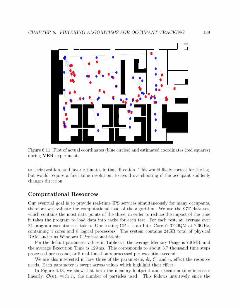
CHAPTER 6. FILTERING ALGORITHMS FOR OCCUPANT TRACKING 139
Figure 6.11: Plot of actual coordinates (blue circles) and estimated coordinates (red squares)during VER experiment.
to their position, and favor estimates in that direction. This would likely correct for the lag,but would require a finer time resolution, to avoid overshooting if the occupant suddenlychanges direction.
Computational Resources
Our eventual goal is to provide real-time IPS services simultaneously for many occupants,therefore we evaluate the computational load of the algorithm. We use the GT data set,which contains the most data points of the three, in order to reduce the impact of the timeit takes the program to load data into cache for each test. For each test, an average over24 program executions is taken. Our testing CPU is an Intel Core i7-3720QM at 2.6GHz,containing 4 cores and 8 logical processors. The system contains 24GB total of physicalRAM and runs Windows 7 Professional 64-bit.
For the default parameter values in Table 6.1, the average Memory Usage is 7.9 MB, andthe average Execution Time is 129 ms. This corresponds to about 3.7 thousand time stepsprocessed per second, or 5 real-time hours processed per execution second.
We are also interested in how three of the parameters, δt, C, and n, effect the resourceneeds. Each parameter is swept across values which highlight their effect.
In Figure 6.13, we show that both the memory footprint and execution time increaseslinearly, O(n), with n, the number of particles used. This follows intuitively since the
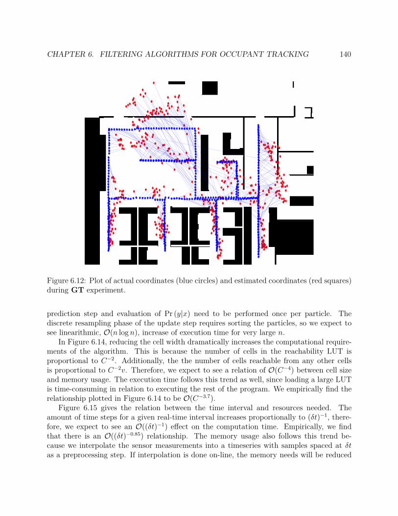
CHAPTER 6. FILTERING ALGORITHMS FOR OCCUPANT TRACKING 140
Figure 6.12: Plot of actual coordinates (blue circles) and estimated coordinates (red squares)during GT experiment.
prediction step and evaluation of Pr (y|x) need to be performed once per particle. Thediscrete resampling phase of the update step requires sorting the particles, so we expect tosee linearithmic, O(n log n), increase of execution time for very large n.
In Figure 6.14, reducing the cell width dramatically increases the computational require-ments of the algorithm. This is because the number of cells in the reachability LUT isproportional to C−2. Additionally, the the number of cells reachable from any other cellsis proportional to C−2v. Therefore, we expect to see a relation of O(C−4) between cell sizeand memory usage. The execution time follows this trend as well, since loading a large LUTis time-consuming in relation to executing the rest of the program. We empirically find therelationship plotted in Figure 6.14 to be O(C−3.7).
Figure 6.15 gives the relation between the time interval and resources needed. Theamount of time steps for a given real-time interval increases proportionally to (δt)−1, there-fore, we expect to see an O((δt)−1) effect on the computation time. Empirically, we findthat there is an O((δt)−0.85) relationship. The memory usage also follows this trend be-cause we interpolate the sensor measurements into a timeseries with samples spaced at δtas a preprocessing step. If interpolation is done on-line, the memory needs will be reduced
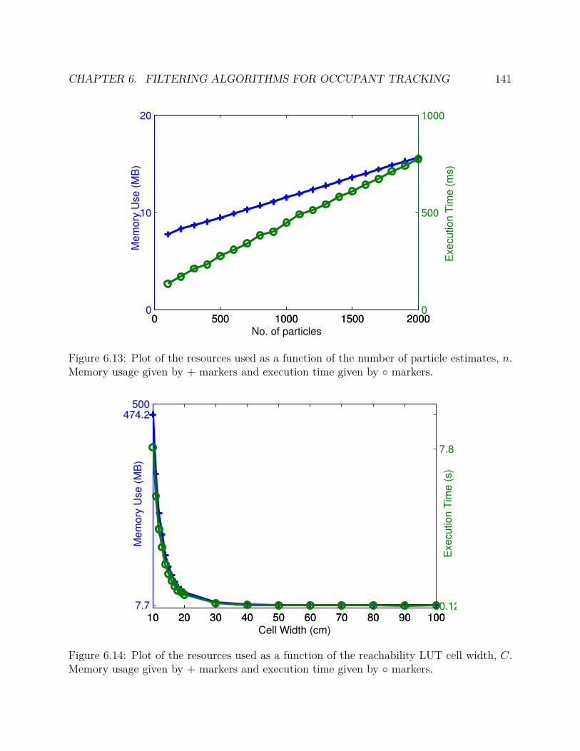
CHAPTER 6. FILTERING ALGORITHMS FOR OCCUPANT TRACKING 141
0 500 1000 1500 20000
10
20
Me
mo
ry U
se
(M
B)
No. of particles0 500 1000 1500 2000
0
500
1000
Exe
cu
tio
n T
ime
(m
s)
Figure 6.13: Plot of the resources used as a function of the number of particle estimates, n.Memory usage given by + markers and execution time given by markers.
10 20 30 40 50 60 70 80 90 1007.7
474.2500
Mem
ory
Use (
MB
)
Cell Width (cm)10 20 30 40 50 60 70 80 90 100
0.12
7.8E
xecution T
ime (
s)
Figure 6.14: Plot of the resources used as a function of the reachability LUT cell width, C.Memory usage given by + markers and execution time given by markers.

CHAPTER 6. FILTERING ALGORITHMS FOR OCCUPANT TRACKING 142
0 1 2 3 4 50
20
40
Me
mo
ry U
se
(M
B)
Time Interval (s)0 1 2 3 4 5
0
2
4
Exe
cu
tio
n T
ime
(s)
Figure 6.15: Plot of the resources used as a function of the time interval, δt. Memory usagegiven by + markers and execution time given by markers.
significantly.Finally, the benefit of multithreading is examined by changing the number of worker
threads used by the program to assist in the prediction and update steps. The resultsdisplayed in Figure 6.16, show that there is a significant benefit to execution time if threadsare used at all, and that 5 threads is the optimal value for this particular 4-core computer.Note that a number of threads greater than the number of cores is optimal since at timesthreads may be blocked waiting for memory accesses, and having an extra thread to occupythe CPU during this time can actually improve processor throughput. However, having toomany threads, and the associated overhead, can quickly degrade throughput.
The results achieved in this section lead us to believe our algorithm is well-suited forbroader deployment covering more area and occupants. There is also room for more complexmotion and sensor models to be incorporated and continue to achieve real-time performance.
6.5 Future directions and extensions
State augmentations
Motivation for augmenting the state
Currently, the state of the particle filter tracks the 2-dimensional position of the occupanton the office floor and also tracks the attenuation factor. A future direction is to alsoaugment the state to estimate additional information about the occupant. This will benefit
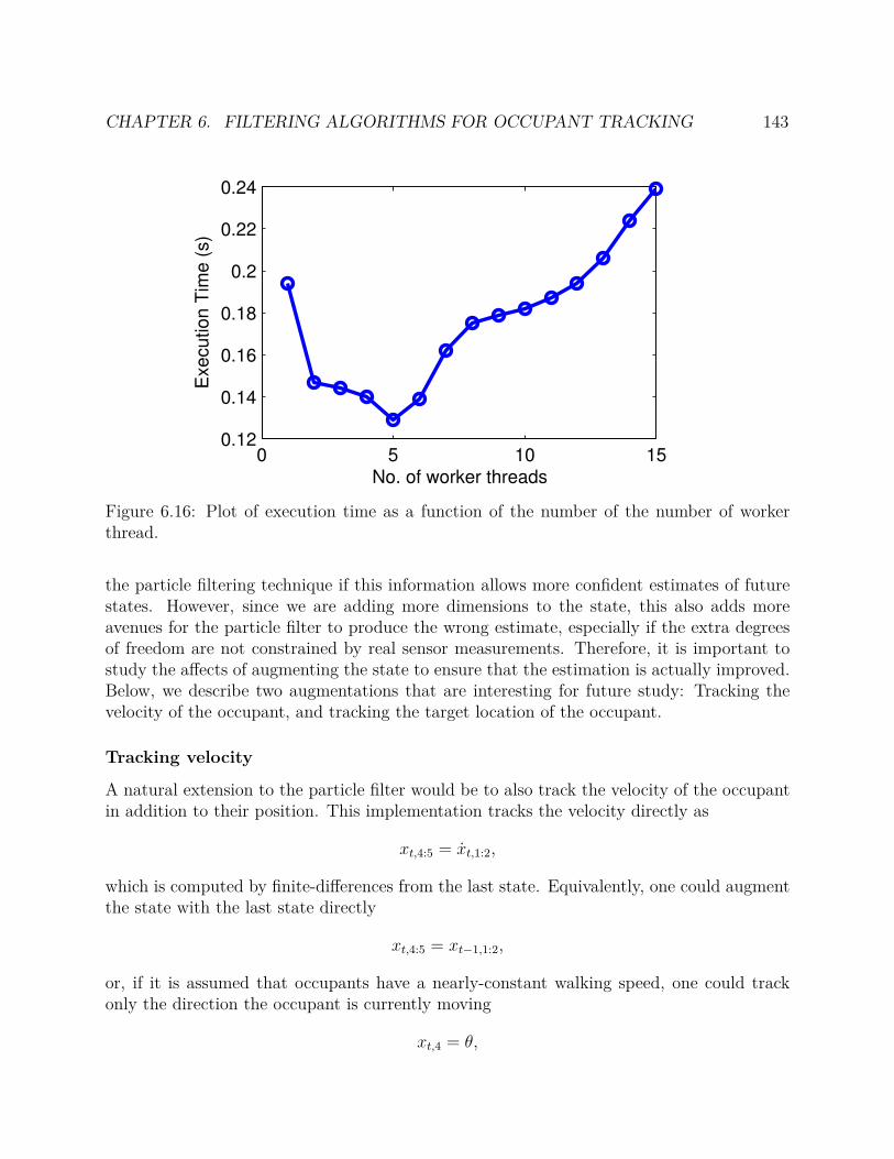
CHAPTER 6. FILTERING ALGORITHMS FOR OCCUPANT TRACKING 143
0 5 10 150.12
0.14
0.16
0.18
0.2
0.22
0.24E
xe
cu
tio
n T
ime
(s)
No. of worker threads
Figure 6.16: Plot of execution time as a function of the number of the number of workerthread.
the particle filtering technique if this information allows more confident estimates of futurestates. However, since we are adding more dimensions to the state, this also adds moreavenues for the particle filter to produce the wrong estimate, especially if the extra degreesof freedom are not constrained by real sensor measurements. Therefore, it is important tostudy the affects of augmenting the state to ensure that the estimation is actually improved.Below, we describe two augmentations that are interesting for future study: Tracking thevelocity of the occupant, and tracking the target location of the occupant.
Tracking velocity
A natural extension to the particle filter would be to also track the velocity of the occupantin addition to their position. This implementation tracks the velocity directly as
xt,4:5 = xt,1:2,
which is computed by finite-differences from the last state. Equivalently, one could augmentthe state with the last state directly
xt,4:5 = xt−1,1:2,
or, if it is assumed that occupants have a nearly-constant walking speed, one could trackonly the direction the occupant is currently moving
xt,4 = θ,
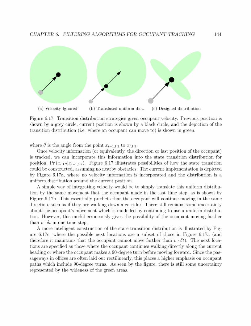
CHAPTER 6. FILTERING ALGORITHMS FOR OCCUPANT TRACKING 144
(a) Velocity Ignored (b) Translated uniform dist. (c) Designed distribution
Figure 6.17: Transition distribution strategies given occupant velocity. Previous position isshown by a grey circle, current position is shown by a black circle, and the depiction of thetransition distribution (i.e. where an occupant can move to) is shown in green.
where θ is the angle from the point xt−1,1:2 to xt,1:2.Once velocity information (or equivalently, the direction or last position of the occupant)
is tracked, we can incorporate this information into the state transition distribution forposition, Pr (xt,1:2|xt−1,1:2). Figure 6.17 illustrates possibilities of how the state transitioncould be constructed, assuming no nearby obstacles. The current implementation is depictedby Figure 6.17a, where no velocity information is incorporated and the distribution is auniform distribution around the current position.
A simple way of integrating velocity would be to simply translate this uniform distribu-tion by the same movement that the occupant made in the last time step, as is shown byFigure 6.17b. This essentially predicts that the occupant will continue moving in the samedirection, such as if they are walking down a corridor. There still remains some uncertaintyabout the occupant’s movement which is modelled by continuing to use a uniform distribu-tion. However, this model erroneously gives the possibility of the occupant moving fartherthan v · δt in one time step.
A more intelligent construction of the state transition distribution is illustrated by Fig-ure 6.17c, where the possible next locations are a subset of those in Figure 6.17a (andtherefore it maintains that the occupant cannot move farther than v · δt). The next loca-tions are specified as those where the occupant continues walking directly along the currentheading or where the occupant makes a 90-degree turn before moving forward. Since the pas-sageways in offices are often laid out rectilinearly, this places a higher emphasis on occupantpaths which include 90-degree turns. As seen by the figure, there is still some uncertaintyrepresented by the wideness of the green areas.

CHAPTER 6. FILTERING ALGORITHMS FOR OCCUPANT TRACKING 145
Tracking desired areas
We can also utilize the logical division of a building into spaces (such as rooms, desks, andcubicles) to add intuitive information into the tracking algorithm. A useful addition to thestate would be a prediction of the desired location that an occupant would want to go. Forexample, if we determine that an occupant is thirsty, then there is a higher probability thatthe occupant will follow a path leading to the water cooler. Although we do not yet havesensors to directly sense a occupant’s intention, information such as historical behavior, timeof day, and current direction provide clues.
A corollary of this augmentation is to gather and track knowledge about where an oc-cupant will not travel to, such as a janitor’s closet, or the opposite-gendered restroom.Depending on how many areas are removed from consideration, this can significantly reducethe size of the state space and consequently, possible errors in the estimation. In addition toremoving these specific areas from consideration, we can also remove any paths which leadonly to non-considered areas, since the occupant will not walk along these paths as well.
Information from fixed infrastructure
CO2 concentration
In Section 5.3, we describe a study carried out to model the effect of occupants on the CO2
concentration within a room and built an estimator and identifier for the model. GivenCO2 measurements at the supply and return vents in an enclosed room (such as a conferenceroom), we demonstrate a technique to estimate the rate of CO2 being generated by occupants.Since this value is heavily dependent on occupants, it would be appropriate to augment theobservation distribution accordingly. For instance, if we detect that very little CO2 is beinggenerated in a room, this indicates very low probability that any tracked occupants are insideof this room. A further improvement is to augment the state of positioning system to includethe metabolic rate of the tracked occupant, thus, the actual value of CO2 production maybe able to identify individual occupants inside a CO2-monitored room. The metabolic rateof the occupant is determined when the occupant is known to be the only occupant inside aCO2-monitored room (e.g. their own office with no visitors).
Coarse Particulate Matter
Like CO2, coarse particulate matter (PM) (i.e. airborne particles with diameter ≥ 2 µm) isa proxy to local occupancy (See Section 5.2), thus, we will be able to use similar methods asdiscussed for CO2. The main difference is that human occupants are the primary producersof CO2 in office buildings, whereas many factors can influence coarse PM concentrations.For instance, vacuuming frequency and floor type (e.g. carpet or tile) affects the amountof particles latent on the floor to be re-suspended. Therefore, given a detected spike incoarse PM from nearby occupant activity, there is still much uncertainty as to the number ofoccupants nearby, and very clean floors can result in especially weak and uncertain detection
CHAPTER 6. FILTERING ALGORITHMS FOR OCCUPANT TRACKING 146
events. Fortunately, the particle filter is well adapted to accept uncertain sensor data, aslong as the sensor noise is well modelled. In our implementation, coarse PM can play a roleindicating whether an occupant is at their desk, i.e. if the sensor is mounted at foot-levelnear their desk. The results from Section 5.2 show that a coarse PM sensor is useful asa rudimentary threshold sensor, detecting when occupants walk past it. These detectionscould indicate higher probabilities of trajectories which estimate that the occupant walkedpast the sensor.
Light-based detection
Passive Infrared (PIR) sensing is a popular technology used by security systems, since theyreliably detect human occupant movement within a specified cone of detection. The mainlimitation of PIR sensing for indoor positioning purposes is that the sensor cannot identifyoccupants, nor can it distinguish between one or multiple occupants. Therefore, PIR sensingalone cannot be easily used for positioning, but nonetheless is very valuable for narrowingdown the feasible state space. That is, if the PIR does not detect an occupant, then theparticle filter can remove any estimates falling within its cone of detection. Thus, a richnetwork of environmental sensor devices (See Chapter 4) carrying PIR devices allows theparticle filter to focus the particle estimates on only the occupied areas of the building.
Infrared light is also used for reliable threshold detectors. Often seen in businesses todetect customers entering and exiting the storefront, these sensors utilize a beam of lightfrom a laser or focused infrared diode and a corresponding light sensor. The beam of lightis directed across the detection area, such as a doorway, possibly reflected off of a mirror,and finally reaches the sensor. An occupant is detected when they pass through the beam,blocking it from reaching the sensor. Like the PM sensor, detection events provided by thissensor can indicate a higher probability of trajectories which include crossing the beam oflight.
Contact-based detection
Switches are simple, reliable, and low-power devices which can immediately detect statechanges of objects like doors, windows, and drawers. Using switches connected to the expan-sion port of environmental sensor devices (See Chapter 4), we can continuously monitor thestate of doors, which, when closed, represents an obstacle in the state-transition distribu-tion. Switches can also be mounted on windows and drawers to detect state changes whichprovide, with high-confidence, a small area (i.e. within arms-length) of possible locations ofan occupant.
Information from occupant-carried infrastructure
Wearable electronics, such as the Pebble [130] and eWatch [131], are becoming more ubiq-uitous and carrying more sensors, owing to advances in miniaturization and manufacturing.
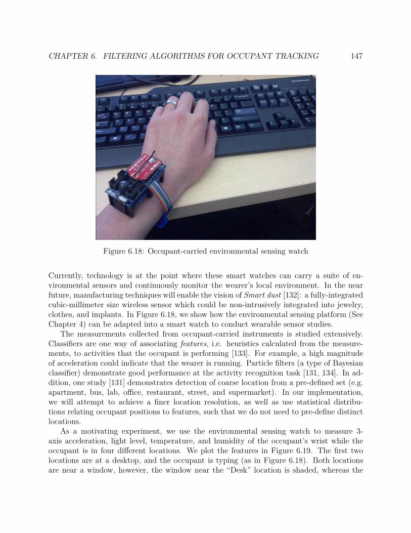
CHAPTER 6. FILTERING ALGORITHMS FOR OCCUPANT TRACKING 147
Figure 6.18: Occupant-carried environmental sensing watch
Currently, technology is at the point where these smart watches can carry a suite of en-vironmental sensors and continuously monitor the wearer’s local environment. In the nearfuture, manufacturing techniques will enable the vision of Smart dust [132]: a fully-integratedcubic-millimeter size wireless sensor which could be non-intrusively integrated into jewelry,clothes, and implants. In Figure 6.18, we show how the environmental sensing platform (SeeChapter 4) can be adapted into a smart watch to conduct wearable sensor studies.
The measurements collected from occupant-carried instruments is studied extensively.Classifiers are one way of associating features, i.e. heuristics calculated from the measure-ments, to activities that the occupant is performing [133]. For example, a high magnitudeof acceleration could indicate that the wearer is running. Particle filters (a type of Bayesianclassifier) demonstrate good performance at the activity recognition task [131, 134]. In ad-dition, one study [131] demonstrates detection of coarse location from a pre-defined set (e.g.apartment, bus, lab, office, restaurant, street, and supermarket). In our implementation,we will attempt to achieve a finer location resolution, as well as use statistical distribu-tions relating occupant positions to features, such that we do not need to pre-define distinctlocations.
As a motivating experiment, we use the environmental sensing watch to measure 3-axis acceleration, light level, temperature, and humidity of the occupant’s wrist while theoccupant is in four different locations. We plot the features in Figure 6.19. The first twolocations are at a desktop, and the occupant is typing (as in Figure 6.18). Both locationsare near a window, however, the window near the “Desk” location is shaded, whereas the
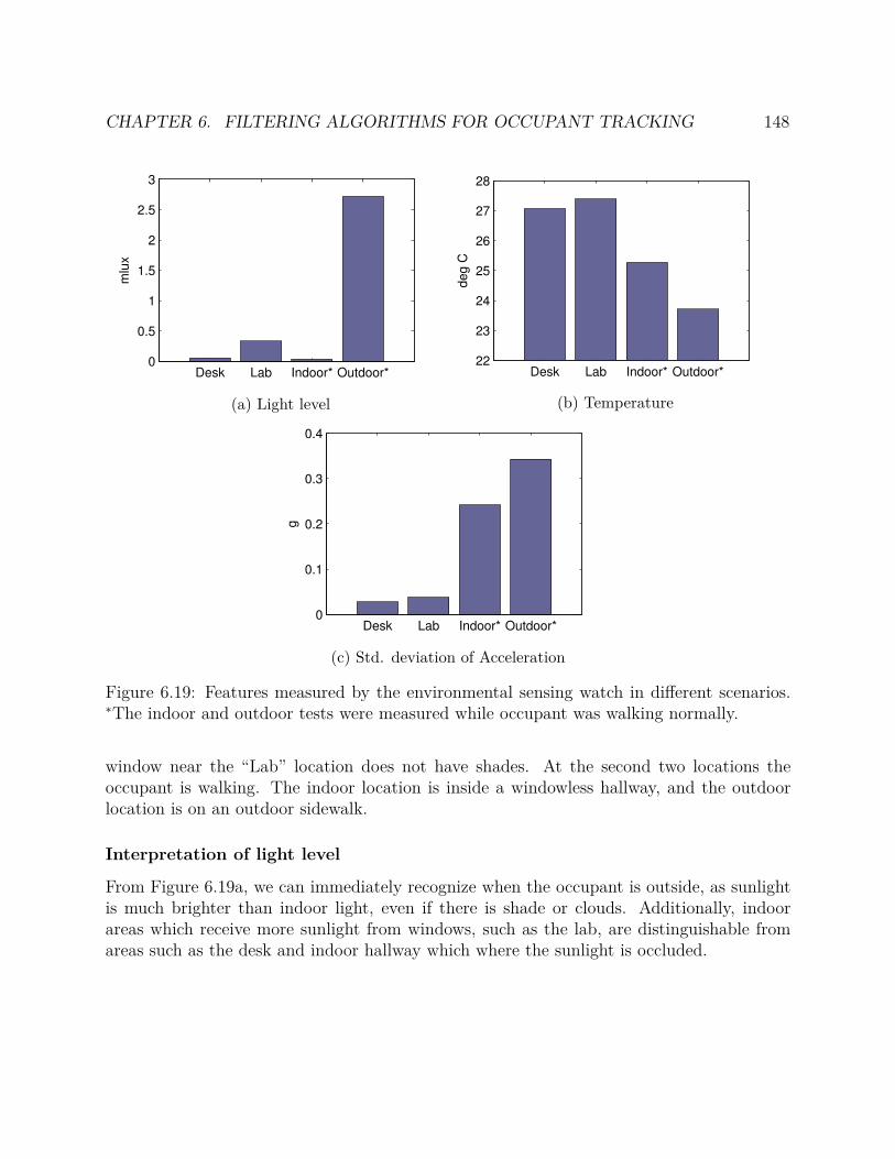
CHAPTER 6. FILTERING ALGORITHMS FOR OCCUPANT TRACKING 148
Desk Lab Indoor* Outdoor*0
0.5
1
1.5
2
2.5
3
mlu
x
(a) Light level
Desk Lab Indoor* Outdoor*22
23
24
25
26
27
28
deg C
(b) Temperature
Desk Lab Indoor* Outdoor*0
0.1
0.2
0.3
0.4
g
(c) Std. deviation of Acceleration
Figure 6.19: Features measured by the environmental sensing watch in different scenarios.∗The indoor and outdoor tests were measured while occupant was walking normally.
window near the “Lab” location does not have shades. At the second two locations theoccupant is walking. The indoor location is inside a windowless hallway, and the outdoorlocation is on an outdoor sidewalk.
Interpretation of light level
From Figure 6.19a, we can immediately recognize when the occupant is outside, as sunlightis much brighter than indoor light, even if there is shade or clouds. Additionally, indoorareas which receive more sunlight from windows, such as the lab, are distinguishable fromareas such as the desk and indoor hallway which where the sunlight is occluded.
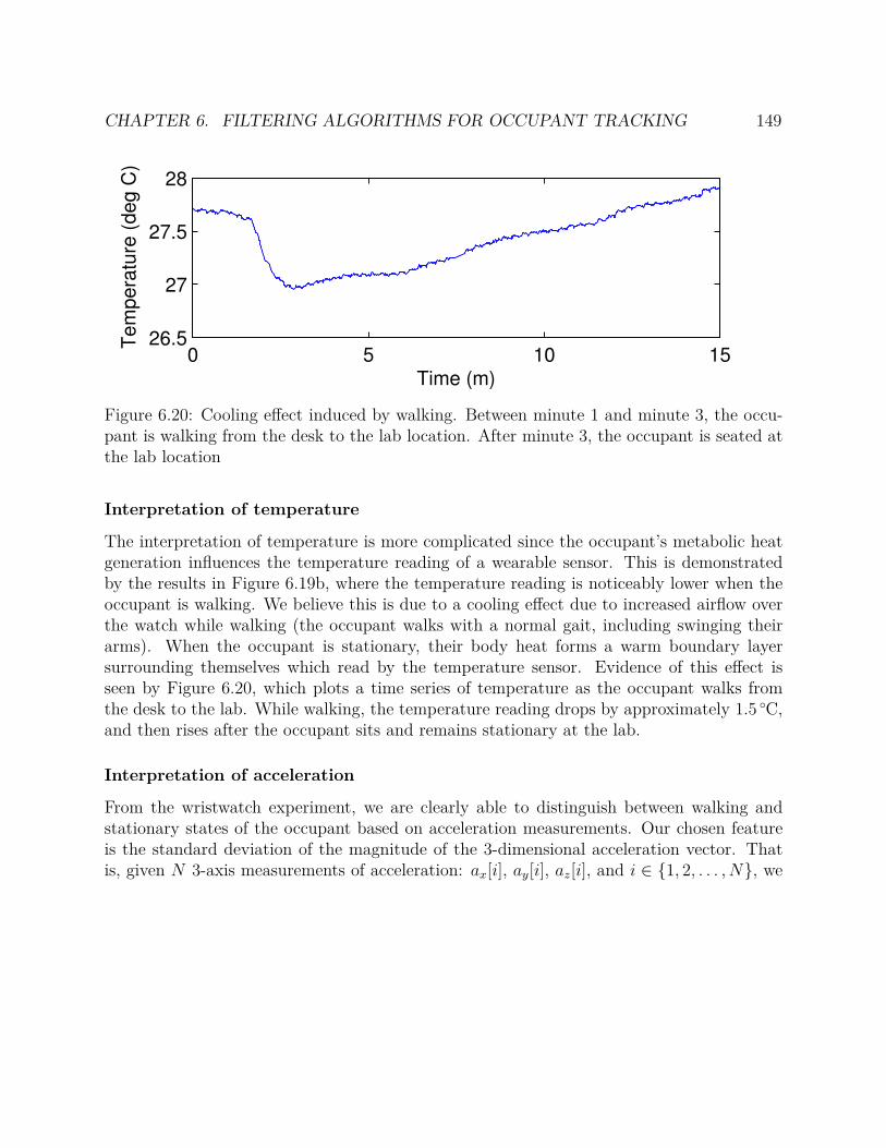
CHAPTER 6. FILTERING ALGORITHMS FOR OCCUPANT TRACKING 149
0 5 10 1526.5
27
27.5
28
Tem
pera
ture
(deg C
)
Time (m)
Figure 6.20: Cooling effect induced by walking. Between minute 1 and minute 3, the occu-pant is walking from the desk to the lab location. After minute 3, the occupant is seated atthe lab location
Interpretation of temperature
The interpretation of temperature is more complicated since the occupant’s metabolic heatgeneration influences the temperature reading of a wearable sensor. This is demonstratedby the results in Figure 6.19b, where the temperature reading is noticeably lower when theoccupant is walking. We believe this is due to a cooling effect due to increased airflow overthe watch while walking (the occupant walks with a normal gait, including swinging theirarms). When the occupant is stationary, their body heat forms a warm boundary layersurrounding themselves which read by the temperature sensor. Evidence of this effect isseen by Figure 6.20, which plots a time series of temperature as the occupant walks fromthe desk to the lab. While walking, the temperature reading drops by approximately 1.5 C,and then rises after the occupant sits and remains stationary at the lab.
Interpretation of acceleration
From the wristwatch experiment, we are clearly able to distinguish between walking andstationary states of the occupant based on acceleration measurements. Our chosen featureis the standard deviation of the magnitude of the 3-dimensional acceleration vector. Thatis, given N 3-axis measurements of acceleration: ax[i], ay[i], az[i], and i ∈ 1, 2, . . . , N, we
CHAPTER 6. FILTERING ALGORITHMS FOR OCCUPANT TRACKING 150
calculate
σ =
√
√
√
√
1N
N∑
i=1
(a[i]− µ)2,
µ =1N
N∑
i=1
a[i],
a[i] =√
(ax[i])2 + (ay[i])2 + (az[i])2.
We show the values of σ for the four tested locations in Figure 6.19c. As expected, in thelatter two locations, when the occupant is walking, the value of σ is significantly higher thanthe first two locations, when the occupant is stationary. This is likely due to the accelerationsensor measuring the swinging of the arms as the occupant walks. We believe that detectingwhether the occupant is stationary or moving will improve the practical performance of theparticle filter, especially in the office, where occupants frequently stop and start movingbetween places.
We have shown via a simple experiment that accelerometer measurements can provideinformation useful for positioning. In future studies with occupant-carried acceleration sen-sors, we will explore two additional manners in which the measurements can be used: bydetecting orientation and by detecting footsteps.
Orientation is relatively straightforward to obtain from filtered 3-axis acceleration mea-surements simply by finding the relative direction of the gravity vector. We believe thatorientation of occupant-carried devices can provide valuable information towards determin-ing the state of the occupant, given the context of the sensor placement. For instance, if sucha device is placed in a pocket, this can indicate whether an occupant is sitting or standing.For the positioning problem, detecting that an occupant is sitting indicates that the occu-pant is stationary, and probably located in a part of the office containing chairs. A sensormounted in a wristwatch similarly measures whether an occupant is doing desk work or theirhands are at their sides.
A popular and intuitive direction to integrate measurements from occupant-carried ac-celerometers is to detect footsteps which can provide information about immediate motionsthat the occupant is making [135, 136, 137]. For example, knowing the number of footstepsan occupant takes in a given time period constrains the distance they have moved in thatperiod given an estimate of the occupant’s stride length. It is also possible to distinguishbetween types of footsteps, such as walking, running and climbing stairs. This is powerfulif a map of the building is available, for instance, if an occupant is known to be climbingstairs, then only trajectories which include a stairway will be considered. In some cases, ifgyroscopes and accelerometers are mounted on both feet, an Extended Kalman Filter can beused to estimate the displacement of each foot between steps [138], further narrowing downpossible locations of the occupant.

CHAPTER 6. FILTERING ALGORITHMS FOR OCCUPANT TRACKING 151
Instead of being mounted on the feet and estimating positional displacements, our methodwould only attempt to detect footsteps by looking for spikes in the signal when the occupant’sfoot strikes the ground. Therefore, the accelerometer can be mounted anywhere on the bodyof the occupant as long as there is a fairly rigid physical connection to the foot. Ourhypothesis is that using accelerometer data from a smartphone carried in the occupant’spocket will be sufficient. If the occupant is carrying an environmental sensor (See Chapter 4),then the accelerometer readings from this sensor can be used as well. We would programeither the phone or environmental sensor to report the number of footsteps ft counted everysecond. To integrate into the particle filter, we would adjust the state transition distributionto account for an adaptive travel distance per time step, instead of statically limiting it tov ·δt (where v is the occupant’s walking speed and δt is the duration of one time step). Giventhe current number of footsteps per second ft, we can instead constrain the occupant’s traveldistance to ft · s · δt, where s is occupant’s stride length. Since the parameter s is difficultto identify, The most information will be gained when ft = 0, since this indicates that theoccupant is stationary (travel distance is equal to 0).
Coupling to occupancy estimation
As we demonstrate in Section 6.4, our implementation has the benefit of processing data at5 real-time hours per second and requiring only 7.9 MB. Therefore, it is feasible to builda composite particle filter which can track hundreds of occupants, in order to track everyoccupant in a building. At this point, we will then be able to calculate an estimate of occu-pancy for each space in the building by simply counting the number of tracked occupants ineach room. This is a typical application of IPSs, given the advantages of knowing occupancywithin a building (See Chapter 5).
This counting technique is a one-way transfer of information from the occupant trackingproblem to the occupancy estimation problem, however, our next direction will be to explorethe bi-directional sharing of information between the two problems. Our method is to usethe particle filter framework to create a joint estimator that tracks the occupancy of roomsalong with the position of occupants by augmenting the state. This allows us to addressthe relationship between the two problems directly in the same framework via the statetransition distribution. For example, we can add a rule which explicitly specifies that aroom’s occupancy level is equal to the sum of the tracked occupants within it. This ruleimplicitly defines a bi-directional dependency between the occupant tracking and occupancyestimation results, since the particle filter will essentially estimate both simultaneously toreach a feasible solution. The flow of information from the occupancy estimation problemto the occupant tracking problem is especially interesting since we have identified new andinformative models of indoor phenomena like CO2 and particulate matter.
In building this new framework, we foresee several complications that will require specialtreatment. For instance, it will be difficult to model visitors who are unknown and nottracked by the system, yet still affect the true occupancy of the space. We will need toallow some uncertainty in the coupling between the occupancy estimation and occupant
CHAPTER 6. FILTERING ALGORITHMS FOR OCCUPANT TRACKING 152
tracking problems. Another complication from building this composite estimator is that itwill create a very large and high-dimensional state space. Particle filters are some of thebest techniques for large state spaces, due to their scalability, however, there is still thepossibility of the particle estimates getting “lost” or “trapped” in parts of the state space.With limited sensing, it is also more difficult to distinguish improbable states and narrowdown an estimate when the state space is large. We hope to address these problems byproviding enough information through a multitude of sensing technologies and intuitionsabout occupant behavior. This information serves to narrow down the feasible areas of thestate space.
6.6 Conclusions
In this chapter, we have described an occupant-tracking system using particle filters thatachieves an average of room-level accuracy when deployed in a real office environment. More-over, by construction, our method does not position occupants inside inaccessible areas,which may lead to better estimates of the room that an occupant is inside. The particlefilter method is also dynamic, meaning that the estimation will improve over time as moreinformation is gathered. This results in slower-moving or stationary occupants resulting invery good predictions, such as in Figure 6.12.
If we assume all occupants are participating by carrying the RFID tag required by ourIPS, then our method is likely to be accurate enough to estimate occupancy of the spaces inthe office. However, we understand that this assumption is invalid in the case where thereare visitors, or when participants forget to carry the tag. A popular answer to this problemis to use WiFi-based technology that can sense any WiFi-enabled smartphone carried byoccupants since the occupants have other incentives to carry their phone with them. Thereare drawbacks to this as well, since occupants might not own a WiFi-enabled smartphone,or have the WiFi-disabled, or be carrying more than one WiFi-enabled device, such as alaptop. An additional drawback is that there is heterogeneity in the radio transmissioncharacteristics of WiFi devices due to differences in the antennas, transceivers, and the waythey are used. Therefore, relying on a characterization of signal strength can fail when thesedifferences are not accounted for.
Therefore, as we describe in Section 6.5, our vision is that a hybrid infrastructure can bebuilt which simultaneously estimates occupancy and tracks many or all occupants. The in-formation from both problems would be elegantly integrated together by the particle filteringframework, which sees the building’s occupancy and position of its occupants as componentsof a encompassing state variable. Although the state space will consequently be very large,particle filters are well suited to estimate within these spaces, due to the Monte-Carlo ap-proach. Particle filters also allow us to leverage the peculiarities of each type of sensor toguide the particle filter estimates. Our studies into CO2 and particulate matter concen-trations in Chapter 5 are examples of experiments we have conducted to understand howthese environmental variables are affected by occupants, and the results of these experiments

CHAPTER 6. FILTERING ALGORITHMS FOR OCCUPANT TRACKING 153
can produce the parameters and models needed to integrate the readings into the particlefiltering framework.
154
Chapter 7
Conclusions and Future Work
7.1 Contributions and status of the work
Applying estimation techniques towards real-world problems and using practical sensing in-frastructures has particular challenges when facing mobile environments. However, thesechallenges can be overcome when mathematical and technological tools are properly chosenand applied towards the estimation problem. In this dissertation, we have described sev-eral mathematical estimation tools which were successfully adapted and applied towards areal-world scenario: Ensemble Kalman Filtering was used to estimate river currents givenmeasurements from Lagrangian sensors. PDE estimators were used to estimate the amountof CO2 generated by humans in a conference room. Particle filters were used to estimatethe position of an occupant with radio signal strength readings. We have also described twosensing architectures which provide the measurement inputs necessary for the estimationtools: the Floating Sensor Network and the environmental sensing platform.
The contribution of the Floating Sensor Network is to enable more types of Lagrangianriver studies via the development of two novel drifter designs: the passive Android drifterand the active Generation 3 drifter. Due to the low manufacturing cost of the units (around$300), the Android drifter allows scientists to perform studies with a highly dense observationof the river state, and satisfy cost constraints. As well, the real-time remote reporting abilityallows scientists to find and retrieve the units much easier than if the drifters only loggedtheir measurements locally. The motorized Generation 3 drifter design is also easily mass-produced and has the unique ability to maneuver itself to avoid shorelines using an advancedHamilton-Jacobi safety control technique that we developed. This drifter gives scientists theability to conduct drifter studies in many parts of the river which cannot be otherwisesensed, due to factors such as wind, pushing passive drifters into the shorelines. Currently,we lend the Android drifter fleet to other environmental research groups within Stanford,the University of California Davis, and the US Geographical Survey.
We have also contributed an architecture for the sensing of mobile occupants in a build-ing. A sensor device was designed which uses WiFi for robust data delivery and is also
CHAPTER 7. CONCLUSIONS AND FUTURE WORK 155
low-power enough to last for over 5 years on a battery. At the same time, the sensor is ableto collect a rich set of environmental variables from its suite of on-board instruments, and isexpandable to take measurements from nearly any other instrument, such as a CO2 sensor.The device is also small enough to be carried by occupants or be deployed in size-constrainedlocations. The long battery life and compatibility with existing WiFi infrastructure resultin a low-cost of deployment and maintenance. The environmental sensing platform is un-der active development and deployment. Currently, we have produced 100 of the “Version3” environmental sensor devices for deployment at UC Berkeley’s Center for Research inEnergy Systems Transformation (CREST) laboratory and the Singapore Berkeley BuildingEfficiency and Sustainability in the Tropics (SinBerBEST) headquarters at the Campus forResearch Excellence and Technological Enterprise (CREATE) tower in Singapore. There areeventual plans for inserting the measurements into a cluster-computing distributed databasewith nodes in both Singapore and Berkeley. After this, the measurements will be availablealongside data from the buildings’ lighting, HVAC, and electrical systems.
7.2 Future applications
We envision many avenues of extension to the work described in this dissertation. Duringour development of the active drifters, we explored the idea of a depth-profiling drifter, whichused a buoyancy control system allowing it to dive underwater. This capability would notonly allow 3-dimensional drifter studies, but also allow the drifters to leverage underwatercurrents to carry them to a desired destination. We have have also prototyped Android-based active drifters which have the capabilities of the active Generation 3 drifter, but aresignificantly more economical due to using off-the-shelf Android smartphones.
Our experiences in developing the Hamilton-Jacobi safety control technique can be ap-plied to other mobile environments which have mobility constraints. We imagine that mete-orological sensing could be augmented with underactuated gliders, kites, and balloons whichhave limited control authority, but can navigate enough to ride global wind currents to theirdestination. Minimum time-to-reach functions, calculated as an intermediate step of thesafety control method, are also very powerful and can be used for other control algorithms.For instance, we have explored finding Zermelo-Voronoi partitions [139] for distributed con-trol of drifter fleets. These partitions can be generated by finding the intersections of mini-mum time-to-reach functions emanating from each drifter in the fleet.
There is also significant interest by other researchers into the progression of the environ-mental platform due to its suite of sensors supporting indoor climate and energy efficientcontrol studies. One project is to create a “building in a suitcase” which includes several ofthe sensor devices, an access point, and a gateway PC with a mobile Internet connection.With this, scientists or building contractors could rapidly deploy a functional environmentalsensor network to survey a building site.
Finally, we envision that the particle filtering framework will inspire future research inthis direction, as discussed in Section 6.5. An immediate goal is to extend the particle filter

CHAPTER 7. CONCLUSIONS AND FUTURE WORK 156
to perform occupancy estimation as well as occupant tracking. In the further future, weare especially excited about the flexibility in the types of measurements that the particlefilter can accept. This is because future smart buildings will undoubtedly be outfitted witha plethora of sensors, such as temperature, light, occupancy (passive infrared and ultra-sound), and plugload meters (i.e. devices which measure power consumption of appliances).Our tracking framework could theoretically be installed on such a smart building and pro-vide occupant tracking and occupancy estimation services without requiring any additionaldedicated infrastructure. Coupled with occupancy-aware control algorithms, this is clear ad-vantage for future smart buildings to save energy without incurring prohibitive installationcosts.
More generally, this dissertation exhibits solutions to real-world estimation challenges. Inmany cases, these solutions are not specific to the setting for which they were designed. Forinstance, the environmental sensing architecture was extended from, and shared significantportions of source code with, the Floating Sensor Network. Essentially we are building alibrary of algorithms and tools (both hardware and software) for future studies in mobileenvironments. Our goal is to give other researchers a head-start into their own experiments,either by adapting the techniques developed by us, or finding inspiration in the design choiceswe have made while designing their own platforms.

157
Bibliography
[1] P. Samar and S. B. Wicker. “On the behavior of communication links of a node in amulti-hop mobile environment”. In: 5th ACM international symposium on mobile adhoc networking and computing. ACM. 2004, pp. 145–156.
[2] P. Bergamo and G. Mazzini. “Localization in sensor networks with fading and mobil-ity”. In: 13th IEEE International Symposium on Personal, Indoor and Mobile RadioCommunications. Vol. 2. IEEE. 2002, pp. 750–754.
[3] G. Evensen. “Sequential data assimilation with a nonlinear quasi-geostrophic modelusing Monte Carlo methods to forecast error statistics”. In: Journal of GeophysicalResearch 99.C5 (1994), pp. 10143–10162. doi: 10.1029/94JC00572.
[4] M. Krstic and A. Smyshlyaev. Boundary control of PDEs: A course on backsteppingdesigns. Vol. 16. SIAM, 2008.
[5] N. J. Gordon, D. J. Salmond, and A. F. Smith. “Novel approach to nonlinear/non-Gaussian Bayesian state estimation”. In: IEE Proceedings F (Radar and Signal Pro-cessing). Vol. 140. 2. IET. 1993, pp. 107–113.
[6] I. H. Witten and E. Frank. Data Mining: Practical machine learning tools and tech-niques. Morgan Kaufmann, 2005.
[7] DWR Drops State Water Project Allocation to Zero, Seeks to Preserve RemainingSupplies. Jan. 31, 2014. url: http://www.water.ca.gov/news/newsreleases/
2014/013114pressrelease.pdf.
[8] Floating sensor network. 2010. url: http://float.berkeley.edu/.
[9] T. Conomos, R. Smith, and J. Gartner. “Environmental setting of San FranciscoBay”. In: Hydrobiologia 129.1 (1985), pp. 1–12.
[10] J. C. Swallow. “A neutral-buoyancy float for measuring deep currents”. In: Deep SeaResearch 3.1 (1955), pp. 74–81. doi: doi:10.1016/0146-6313(55)90037-X.
[11] D. D. Clark. “Overview of the Argos system”. In: OCEANS ’89. Proceedings. Vol. 3.Sept. 1989, pp. 934–939. doi: 10.1109/OCEANS.1989.586711.
[12] R. E. Davis. “Drifter observations of coastal surface currents during CODE: Themethod and descriptive view”. In: Journal of Geophysical Research 90.C3 (1985),pp. 4741–4755. doi: 10.1029/JC090iC03p04741.

BIBLIOGRAPHY 158
[13] D. S. Bitterman and D. V. Hansen. “The design of a low cost tropical drifter buoy”.In: Marine Data Systems International Symposium (MDS). 1986, pp. 575–581.
[14] P. P. Niiler, R. E. Davis, and H. J. White. “Water-following characteristics of a mixedlayer drifter”. In: Deep Sea Research Part A. Oceanographic Research Papers 34.11(1987), pp. 1867–1881. doi: 10.1016/0198-0149(87)90060-4.
[15] A. Tinka, M. Rafiee, and A. M. Bayen. “Floating sensor networks for river studies”.In: IEEE Systems Journal (2012). to appear; accepted Nov. 2011.
[16] J. C. Perez et al. “Development of a cheap, GPS-based, radio-tracked, surface drifterfor closed shallow-water bays”. In: IEEE/OES 7th Working Conference on CurrentMeasurement Technology. Mar. 2003, pp. 66–69. doi: 10.1109/CCM.2003.1194285.
[17] J. Austin and S. Atkinson. “The design and testing of small, low-cost GPS-trackedsurface drifters”. In: Estuaries 27.6 (Dec. 2004), pp. 1026–1029. doi: 10 . 1007 /
BF02803428.
[18] J. Beard et al. “Mobile phone based drifting lagrangian flow sensors”. In: IEEE 3rd In-ternational Conference on Networked Embedded Systems for Every Application (NE-SEA). IEEE. 2012, pp. 1–7.
[19] Android Developers. Google, Inc. 2014. url: http://developer.android.com/.
[20] K. Weekly et al. “Autonomous river navigation using the Hamilton-Jacobi frameworkfor underactuated vehicles”. In: IEEE Transactions on Robotics (2014). in review.
[21] C. Oroza et al. “Design of a network of robotic Lagrangian sensors for shallow waterenvironments with case studies for multiple applications”. In: Journal of MechanicalEngineering Science (2012). in review.
[22] Google. Protocol Buffers: Google’s Data Interchange Format. url: https : / /
developers.google.com/protocol-buffers/.
[23] K. Ang, G. Chong, and Y. Li. “PID control system analysis, design, and technology”.In: IEEE Transactions on Control Systems Technology 13.4 (2005), pp. 559–576.
[24] P. J. Van Leeuwen and G. Evensen. “Data assimilation and inverse methods in termsof a probabilistic formulation”. In: Monthly Weather Review 124.12 (1996), pp. 2898–2913.
[25] P. L. Houtekamer and H. L. Mitchell. “Data assimilation using an ensemble Kalmanfilter technique”. In: Monthly Weather Review 126.3 (1998), pp. 796–811. doi: 10.
1175/1520-0493(1998)126<0796:DAUAEK>2.0.CO;2.
[26] P. L. Houtekamer and H. L. Mitchell. “A sequential ensemble Kalman filter for at-mospheric data assimilation”. In: Monthly Weather Review 129.1 (2001), pp. 123–137.
[27] T. M. Hamill and C. Snyder. “A hybrid Ensemble Kalman Filter–3D variationalanalysis scheme.” In: Monthly Weather Review 128.8 (2000).
BIBLIOGRAPHY 159
[28] C. L. Keppenne and M. M. Rienecker. “Initial testing of a massively parallel ensem-ble Kalman filter with the Poseidon isopycnal ocean general circulation model.” In:Monthly Weather Review 130.12 (2002).
[29] J. P. Kaipio and E. Somersalo. Statistical and computational inverse problems.Vol. 160. Springer, 2005.
[30] J. M. Huttunen and J. P. Kaipio. “Approximation error analysis in nonlinear stateestimation with an application to state-space identification”. In: Inverse Problems23.5 (2007), p. 2141. doi: 10.1088/0266-5611/23/5/019.
[31] J. M. Huttunen and J. P. Kaipio. “Approximation errors in nonstationary inverseproblems”. In: Inverse Problems and Imaging 1.1 (2007), p. 77. doi: 10.3934/ipi.
2007.1.77.
[32] A. Nissinen, V. P. Kolehmainen, and J. P. Kaipio. “Compensation of modelling errorsdue to unknown domain boundary in electrical impedance tomography”. In: IEEETransactions on Medical Imaging 30.2 (2011), pp. 231–242. doi: 10.1109/TMI.2010.
2073716.
[33] Q. Wu, X. Litrico, and A. M. Bayen. “Data reconciliation of an open channel flownetwork using modal decompositions”. In: Advances in Water Resources 32.2 (2009),pp. 193–204. doi: 10.1016/j.advwatres.2008.10.009.
[34] Q. Wu et al. “Variational Lagrangian data assimilation in open channel networks”.In: Water Resources Research (2014). in review.
[35] J. Latombe. Robot motion planning. Springer Verlag, 1990.
[36] S. LaValle. Planning algorithms. Cambridge Univ Pr, 2006.
[37] S. Sundar and Z. Shiller. “Optimal obstacle avoidance based on the Hamilton-Jacobi-Bellman equation”. In: IEEE transactions on robotics and automation 13.2 (1997),pp. 305–310.
[38] A. Tinka et al. “Viability-based computation of spatially constrained minimum timetrajectories for an autonomous underwater vehicle: implementation and experiments”.In: American Control Conference. June 2009.
[39] P. Cardaliaguet, M. Quincampoix, and P. Saint-Pierre. “Set-valued numerical analysisfor optimal control and differential games”. In: Stochastic and Differential Games:Theory and Numerical Methods 4 (1999), pp. 177–247.
[40] A. Bayen et al. “A differential game formulation of alert levels in ETMS data forhigh altitude traffic”. In: Proceedings of the AIAA Guidance, Navigation, and ControlConference. Aug. 2003.
[41] I. Mitchell, A. Bayen, and C. Tomlin. “A time-dependent Hamilton-Jacobi formulationof reachable sets for continuous dynamic games”. In: IEEE Transactions on AutomaticControl 50.7 (2005), pp. 947–957.
BIBLIOGRAPHY 160
[42] M. Bardi and I. Capuzzo-Dolcetta. Optimal control and viscosity solutions ofHamilton-Jacobi-Bellman equations. Birkhauser Boston, 2008.
[43] J. Sethian. Level set methods and fast marching methods: evolving interfaces in com-putational geometry, fluid mechanics, computer vision, and materials science. 3. Cam-bridge University Press, 1999.
[44] S. Osher and R. Fedkiw. Level set methods and dynamic implicit surfaces. Vol. 153.Springer Verlag, 2003.
[45] I. Mitchell. “A toolbox of level set methods”. In: UBC Department of ComputerScience Technical Report 11 (2007).
[46] R. Bellman. “Dynamic Programming”. In: Princeton University Press (1957).
[47] R. Isaacs. Differential Games: A mathematical theory with applications to warfareand pursuit, control and optimization. 1965.
[48] S. Osher. “A level set formulation for the solution of the Dirichlet problem forHamilton–Jacobi equations”. In: SIAM Journal on Mathematical Analysis 24 (1993),p. 1145.
[49] J. W. Thomas. Numerical partial differential equations: finite difference methods.Vol. 1. Springer, 1995.
[50] E. Ateljevich et al. “CFD modeling in the San Francisco Bay and Delta”. In: 4thSIAM Conference on Mathematics for Industry. 2009.
[51] J. Lygeros, C. Tomlin, and S. Sastry. “Controllers for reachability specifications forhybrid systems”. In: Automatica-Oxford 35 (1999), pp. 349–370.
[52] C. Cassandras and S. Lafortune. Introduction to discrete event systems. Vol. 11.Kluwer academic publishers, 1999.
[53] L. Pérez-Lombard, J. Ortiz, and C. Pout. “A review on buildings energy consumptioninformation”. In: Energy and buildings 40.3 (2008), pp. 394–398.
[54] Y. Agarwal et al. “Occupancy-driven energy management for smart building automa-tion”. In: 2nd ACM Workshop on Embedded Sensing Systems for Energy-Efficiencyin Building. ACM. 2010, pp. 1–6.
[55] C. Chao and J. Hu. “Development of a dual-mode demand control ventilation strategyfor indoor air quality control and energy saving”. In: Building and Environment 39.4(2004), pp. 385–397.
[56] V. L. Erickson, M. Á. Carreira-Perpiñán, and A. E. Cerpa. “OBSERVE: Occupancy-based system for efficient reduction of HVAC energy”. In: 10th International Confer-ence on Information Processing in Sensor Networks (IPSN). IEEE. 2011, pp. 258–269.
[57] ZigBee Alliance. ZigBee specification. 2006.
BIBLIOGRAPHY 161
[58] T. Watteyne et al. “OpenWSN: a standards-based low-power wireless developmentenvironment”. In: Transactions on Emerging Telecommunications Technologies 23.5(2012), pp. 480–493.
[59] P. Levis et al. “TinyOS: An operating system for sensor networks”. In: Ambient in-telligence. Springer, 2005, pp. 115–148.
[60] S. Dawson-Haggerty et al. “sMAP: a simple measurement and actuation profile forphysical information”. In: 8th ACM Conference on Embedded Networked Sensor Sys-tems. ACM. 2010, pp. 197–210.
[61] ReadingDB. 2014. url: https://github.com/stevedh/readingdb.
[62] INCITS, ANSI. “ISO/IEC 13239”. In: Information technology–Telecommunicationsand information exchange between systems–High-level Data Link Control (HDLC)procedures (2002).
[63] Arduino. 2014. url: http://www.arduino.cc/ (visited on 02/16/2014).
[64] P. Dutta et al. “A building block approach to sensornet systems”. In: 6th ACM con-ference on Embedded network sensor systems. ACM. 2008, pp. 267–280.
[65] J. L. Hill and D. E. Culler. “Mica: A wireless platform for deeply embedded networks”.In: IEEE Micro 22.6 (2002), pp. 12–24.
[66] J. Polastre, R. Szewczyk, and D. Culler. “Telos: enabling ultra-low power wirelessresearch”. In: Information Processing in Sensor Networks, 2005. IPSN 2005. FourthInternational Symposium on. IEEE. 2005, pp. 364–369.
[67] H. Dubois-Ferrière et al. “TinyNode: a comprehensive platform for wireless sensornetwork applications”. In: 5th international conference on Information processing insensor networks. ACM. 2006, pp. 358–365.
[68] M. Ceriotti et al. “Monitoring heritage buildings with wireless sensor networks: theTorre Aquila deployment”. In: International Conference on Information Processingin Sensor Networks. IEEE Computer Society. 2009, pp. 277–288.
[69] Microchip Technology Inc. RNXV Datasheet. 2012. url: http://ww1.microchip.
com / downloads / en / DeviceDoc / rn - 171 - xv - ds - v1 . 04r . pdf (visited on10/29/2012).
[70] L. Li et al. “The applications of WiFi-based wireless sensor network in internet ofthings and smart grid”. In: 6th IEEE Conference on Industrial Electronics and Ap-plications (ICIEA). IEEE. 2011, pp. 789–793.
[71] Digi International Inc. XBee sensor. 2014. url: http://www.digi.com/pdf/ds_
xbeesensors.pdf (visited on 02/13/2014).
[72] Powercast Corporation. Lifetime power wireless sensor system. 2014. url: http :
/ / www . powercastco . com / PDF / wireless - sensor - system . pdf (visited on02/13/2014).
BIBLIOGRAPHY 162
[73] OpenMote: Open hardware for the Internet of Things. May 2012. url: http://www.
openmote.com/.
[74] L. Doherty, W. Lindsay, and J. Simon. “Channel-specific wireless sensor network pathdata”. In: Computer Communications and Networks, 2007. ICCCN 2007. Proceedingsof 16th International Conference on. IEEE. 2007, pp. 89–94.
[75] Measurement Specialties. Humidity and temperature Sensor - HTU21D. 2014. url:http : / / www . meas - spec . com / product / humidity / HTU21D . aspx (visited on02/17/2014).
[76] ams AG. TSL2560 ambient light sensor with SMBus Interface. 2014. url: http:
//www.ams.com/eng/Products/Light-Sensors/Light-to-Digital-Sensors/
TSL2560.
[77] STMicroelectronics. LIS3DH MEMS digital output motion sensor ultra low-power highperformance 3-axes "nano" accelerometer. 2014. url: http://www.st.com/web/en/
catalog/sense_power/FM89/SC444/PF250725#.
[78] Panasonic Corporation. AMN41121 | NaPiOn Series. 2014. url: http : / / www3 .
panasonic.biz/ac/e/search_num/index.jsp?c=detail&part_no=AMN41121.
[79] K. Weekly, N. Bekiaris-Liberis, and A. M. Bayen. “Modeling and estimation of thehumans’ effect on the CO2 dynamics inside a conference room”. Under review. 2014.
[80] CO2Meter, Inc. K-30 10,000ppm CO2 Sensor. 2014. url: http://www.co2meter.
com/products/k-30-co2-sensor-module.
[81] Linear Technology. Dust Networks SmartMesh Power and Performance Estimator.2014. url: http://www.linear.com/docs/42452.
[82] Linear Technology. SmartMesh IP Application Notes. 2014. url: http : / / www .
linear.com/docs/43189.
[83] B. T. Rosenblum. Collecting occupant presence data for use in energy management ofcommercial buildings. 2012. url: http://escholarship.org/uc/item/1pz2528w.
[84] H. Liu et al. “Survey of wireless indoor positioning techniques and systems”. In: IEEETransactions on Systems, Man, and Cybernetics, Part C: Applications and Reviews37.6 (2007), pp. 1067–1080.
[85] K. Kaemarungsi and P. Krishnamurthy. “Modeling of indoor positioning systemsbased on location fingerprinting”. In: 23rd Annual Joint Conference of the IEEEComputer and Communications Societies (INFOCOM). Vol. 2. IEEE. 2004, pp. 1012–1022.
[86] P. Bahl and V. N. Padmanabhan. “RADAR: An in-building RF-based user locationand tracking system”. In: 19th Joint Conference of the IEEE Computer and Commu-nications Societies. Vol. 2. IEEE. 2000, pp. 775–784.
BIBLIOGRAPHY 163
[87] H. Zou et al. “An RFID indoor positioning system by using weighted path loss andextreme learning machine”. In: 1st IEEE International Conference on Cyber-PhysicalSystems, Networks, and Applications (CPSNA). 2013, pp. 66–71. doi: 10 . 1109 /
CPSNA.2013.6614248.
[88] C. A. Redlich, J. Sparer, and M. R. Cullen. “Sick-building syndrome”. In: The Lancet349.9057 (1997), pp. 1013–1016.
[89] P. Wargocki et al. “The effects of outdoor air supply rate in an office on perceived airquality, sick building syndrome (SBS) symptoms and productivity”. In: Indoor Air10.4 (2000), pp. 222–236.
[90] D. Wyon. “The effects of indoor air quality on performance and productivity”. In:Indoor air 14.s7 (2004), pp. 92–101.
[91] O. Seppänen, W. Fisk, and M. Mendell. “Association of ventilation rates and CO2
concentrations with health and other responses in commercial and institutional build-ings”. In: Indoor air 9.4 (1999), pp. 226–252.
[92] A. Zanobetti and J. Schwartz. “The effect of fine and coarse particulate air pollutionon mortality: a national analysis”. In: Environmental Health Perspectives 117.6 (2009),p. 898.
[93] J. Qian and A. R. Ferro. “Resuspension of dust particles in a chamber and associatedenvironmental factors”. In: Aerosol Science and Technology 42.7 (2008), pp. 566–578.
[94] Dust sensor module P/N: DSM501 Specifications. 2013. url: http : / / www .
samyoungsnc.com/products/3-1%20Specification%20DSM501.pdf.
[95] PPD-20V (Particle Sensor Unit). 2013. url: http://www.shinyei.co.jp/stc/
optical/main_ppd20v_e.html.
[96] GT-526S Handheld Particle Counter. 2013. url: http : / / www . metone . com /
documents/GT-526S-Datasheet.pdf.
[97] J. Qian et al. “Size-resolved emission rates of airborne bacteria and fungi in an occu-pied classroom”. In: Indoor air (2012).
[98] D. Fox et al. “Bayesian techniques for location estimation”. In: Workshop on Location-Aware Computing. 2003, pp. 16–18.
[99] S. Maskell and N. Gordon. “A tutorial on particle filters for on-line nonlinear/non-Gaussian Bayesian tracking”. In: Target Tracking: Algorithms and Applications (Ref.No. 2001/174), IEEE. IET. 2001, pp. 2–1.
[100] E. F. Nakamura, A. A. Loureiro, and A. C. Frery. “Information fusion for wirelesssensor networks: methods, models, and classifications”. In: ACM Computing Surveys(CSUR) 39.3 (2007), p. 9.
[101] U. Satish et al. “Is CO2 an indoor pollutant? Direct effects of low-to-moderate CO2
concentrations on human decision-making performance”. In: Environmental healthperspectives 120.12 (2012), p. 1671.
BIBLIOGRAPHY 164
[102] M. J. Thorpe et al. “Cavity-enhanced optical frequency comb spectroscopy: applica-tion to human breath analysis”. In: Optics Express 16.4 (2008), pp. 2387–2397.
[103] E. S. R. Laboratory. Up-to-date weekly average CO2 at Mauna Loa. 2014. url: http:
//www.esrl.noaa.gov/gmd/ccgg/trends/weekly.html.
[104] A. C. Megri and F. Haghighat. “Zonal modeling for simulating indoor environmentof buildings: review, recent developments, and applications”. In: HVAC&R Research13.6 (2007), pp. 887–905.
[105] A. K. Persily. “Evaluating building IAQ and ventilation with indoor carbon dioxide”.In: ASHRAE Transactions 103 (1997), pp. 193–204.
[106] L Mora, A. Gadgil, and E Wurtz. “Comparing zonal and CFD model predictions ofisothermal indoor airflows to experimental data”. In: Indoor air 13.2 (2003), pp. 77–85.
[107] A. Baughman, A. Gadgil, and W. Nazaroff. “Mixing of a point source pollutant bynatural convection flow within a room”. In: Indoor air 4.2 (1994), pp. 114–122.
[108] K. Weekly, N. Bekiaris-Liberis, and A. M. Bayen. “Modeling and estimation of thehumans’ effect on the CO2 dynamics inside a conference room”. In: (Mar. 20, 2014).arXiv: 1403.5085.
[109] P. A. Ioannou and J. Sun. Robust adaptive control. Prentice-Hall, Inc., 1995.
[110] M. Krstic, I. Kanellakopoulos, P. V. Kokotovic, et al. Nonlinear and adaptive controldesign. Vol. 8. John Wiley & Sons New York, 1995.
[111] A. Smyshlyaev and M. Krstic. Adaptive control of parabolic PDEs. Princeton Univer-sity Press, 2010.
[112] S. Moura, M Krstic, and N. Chaturvedi. “Adaptive PDE observer for batterySOC/SOH estimation via an electrochemical model”. In: ASME Journal of DynamicSystems, Measurement, and Control 136 (2014).
[113] A. H. Sayed, A. Tarighat, and N. Khajehnouri. “Network-based wireless location:challenges faced in developing techniques for accurate wireless location information”.In: IEEE Signal Processing Magazine 22.4 (2005), pp. 24–40.
[114] N. B. Priyantha. “The cricket indoor location system”. PhD thesis. MassachusettsInstitute of Technology, 2005.
[115] S. Lanzisera, D. T. Lin, and K. S. Pister. “RF time of flight ranging for wirelesssensor network localization”. In: International Workshop on Intelligent Solutions inEmbedded Systems. IEEE. 2006, pp. 1–12.
[116] L. M. Ni et al. “LANDMARC: indoor location sensing using active RFID”. In: Wire-less networks 10.6 (2004), pp. 701–710.
[117] S. Thrun et al. “Robust Monte Carlo localization for mobile robots”. In: Artificialintelligence 128.1 (2001), pp. 99–141.
BIBLIOGRAPHY 165
[118] D. Schulz, D. Fox, and J. Hightower. “People tracking with anonymous and id-sensorsusing rao-blackwellised particle filters”. In: International Joint Conference on Artifi-cial Intelligence (IJCAI). 2003, pp. 921–928.
[119] F. Evennou and F. Marx. “Advanced integration of WiFi and inertial navigation sys-tems for indoor mobile positioning”. In: EURASIP journal on applied signal processing2006 (2006), pp. 164–164.
[120] S. Beauregard, Widyawan, and M. Klepal. “Indoor PDR performance enhancementusing minimal map information and particle filters”. In: IEEE/ION Position, Locationand Navigation Symposium (PLANS). IEEE. 2008, pp. 141–147.
[121] A. Haeberlen et al. “Practical robust localization over large-scale 802.11 wireless net-works”. In: 10th annual international conference on mobile computing and networking.ACM. 2004, pp. 70–84.
[122] A. Bruce and G. Gordon. “Better motion prediction for people-tracking”. In: IEEEinternational conference on robotics and automation (ICRA). 2004.
[123] M. Bennewitz, W. Burgard, and S. Thrun. “Using EM to learn motion behaviorsof persons with mobile robots”. In: Conference on Intelligent Robots and Systems(IROS). Lausanne, Switzerland, 2002.
[124] E. Dijkstra. “A note on two problems in connexion with graphs”. In: NumerischeMathematik 1.1 (1959), pp. 269–271.
[125] H. Hashemi. “The indoor radio propagation channel”. In: Proceedings of the IEEE81.7 (1993), pp. 943–968.
[126] D. Scott. Multivariate Density Estimation. Wiley, 1992.
[127] E. Jones, T. Oliphant, P. Peterson, et al. SciPy: Open source scientific tools forPython. http://www.scipy.org/. 2001–.
[128] BeagleBone. http://beagleboard.org/Products/BeagleBone. 2013.
[129] Simple DirectMedia Layer. http://www.libsdl.org/. 2013.
[130] Pebble Technology Corp. Pebble Smartwatch. 2014. url: https://getpebble.com/.
[131] U. Maurer et al. “Location and activity recognition using eWatch: A wearable sensorplatform”. In: Ambient Intelligence in Everyday Life. Springer, 2006, pp. 86–102.
[132] B. Warneke et al. “Smart dust: Communicating with a cubic-millimeter computer”.In: Computer 34.1 (2001), pp. 44–51.
[133] S. J. Preece et al. “Activity identification using body-mounted sensorsÂŮa review ofclassification techniques”. In: Physiological measurement 30.4 (2009), R1.
[134] N. Ravi et al. “Activity recognition from accelerometer data”. In: AAAI. Vol. 5. 2005,pp. 1541–1546.
BIBLIOGRAPHY 166
[135] H. Wang et al. “WLAN-based pedestrian tracking using particle filters and low-costMEMS sensors”. In: 4th Workshop on Positioning, Navigation and Communication,2007. WPNC’07. IEEE. 2007, pp. 1–7.
[136] D. Gusenbauer, C. Isert, and J Krosche. “Self-contained indoor positioning on off-the-shelf mobile devices”. In: International conference on indoor positioning and indoornavigation (IPIN). IEEE. 2010, pp. 1–9.
[137] J. Collin, O. Mezentsev, G. Lachapelle, et al. “Indoor positioning system using ac-celerometry and high accuracy heading sensors”. In: ION GPS/GNSS 2003 Confer-ence. 2003, pp. 9–12.
[138] B. Krach and P. Robertson. “Integration of foot-mounted inertial sensors into aBayesian location estimation framework”. In: 5th Workshop on Positioning, Navi-gation and Communication, 2008. WPNC 2008. IEEE. 2008, pp. 55–61.
[139] E. Bakolas and P. Tsiotras. “The Zermelo–Voronoi diagram: A dynamic partitionproblem”. In: Automatica 46.12 (2010), pp. 2059–2067.