Parameter Characterization of Low FrequencyPulsating Emissions from Space Vector PWM drives

Mathias Enohnyaket, Kalevi Hyyppa, and Jerker DelsingEISLAB

Lulea University of Technology

SE-97176 Lulea Sweden

Email: Mathias.Enohnyaket@ltu.se, Kalevi.Hyyppa@ltu.se,

Jerker.Delsing@ltu.se

Abstract—Power converters in hybrid electric drivesconstitute a major source of electromagnetic disturbances.Recent studies have established that the space vector PWMscheme commonly employed in drive systems, generateslow frequency pulsating (LFP) emissions, at a frequencyof 6f0, where f0 is the fundamental frequency the phasevoltages. The switching of voltage vectors generates com-mon mode current (icm) spikes due to the presence of straycapacitances and inductances. Across sector boundaries,the icm spikes superpose forming spikes of double ortipple amplitude which constitute the LFP emissions. Thesepulsating emissions could pose EMC issues, and function-ality issues like torque pulsations and speed fluctuationsthat could affect the reliability of the drive. This paperinvestigates the effects of drive speed, load, and converterslew rates, on the amplitude of the LFP emissions, usingtheoretical models.

Keywords: Low frequency pulsating emissions, EMI,

torque pulsations, common mode currents, time domain

measurements, drive system.

I. INTRODUCTION

The increasing demand for clean energy systems in ve-

hicles has propelled a rapid development of electric and

hybrid electric vehicles (HEV). Power converters play

a central role in hybrid electric drive systems and con-

stitute a major source of electromagnetic disturbances.

PWM switching of DC/AC converters generates common

mode current spikes (icm) due to the presence of stray ca-

pacitances. These spikes account for the emissions from

PWM drives at harmonics of the switching frequency

(fc) and harmonics of the fundamental frequency f0,

mostly reported in the literature [1]–[8].

Amongst the PWM schemes, the space vector scheme

is mostly preferred for its flexible speed control capa-

bilities [9]–[12]. However recent studies have reported

some issues related to the space vector scheme. In [8],

it was shown that the amplitude of current ripples at

switching frequency (fc) are influenced by the placement

of active vectors within each half carrier or PWM period.

Issues related to the crossing of sector boundaries in

the space vector hexagon has been reported [1], [13]–

[15]. In [14], the formation of common mode current

spikes due to sector boundary crossing was mentioned.

In [13], the generation of large torque pulsations due to

sector boundary crossing was reported. The generation of

low frequency pulsating (LFP) common mode emissions

during sector boundary crossing reported in [15], shall

be considered in this paper. The LFP emissions were

formed by the superposition of common mode current

spikes generated during the switching of voltage vectors.

In the space vector PWM scheme, a given reference

vector is obtained as a linear combination of the adjacent

voltage vectors (Vk, Vk+1), with duty cycles Dk and

Dk+1, respectively [9], [10]. The duty cycles determine

the time interval between the icm spikes. Closed to

sector boundaries, either Dk or Dk+1 tends to zero

causing a superposition of icm spikes to occur. These

pulsations enhance emissions at harmonics of switching

frequency (fc); create low frequency magnetic fields, and

when injected into electric motors could lead to torque

pulsations and speed fluctuations [13], [14], [16], [17].

This paper investigates the effects of drive speed, load,

and converter slew rates, on the amplitudes of the LFP

emissions, using theoretical models.

Section II presents some measurements from an HEV

showing LFP emissions. Section III presents the theoret-

ical modeling of LFP emissions using Gaussian pulses,

and models the effects of different drive parameters. Sec-

tion V rounds off with some discussions and conclusions.

II. MEASUREMENTS ON HEV

This section presents some measurements from an

HEV showing LFP emissions.

HVDC bus

HV batteryElectrical energy storage

Phase Cables

A

Electric machine

B

Fig. 1. Hybrid Drive System on which measurements were per-formed.

A. Measurement setup

Fig. 1 shows a schematic of the hybrid drive system on

which the measurements were performed. The electric

machine is a three phase synchronous machine. The

phase current was measured at location A, with a Tek-

tronix current probe (model TCP404XL), of bandwidth

dc to 2 MHz, and peak current 750 A DC. Common

mode currents were measured at location B, with a

Powertek Rogowski coil (model CWT 6B) of bandwidth

0.1 Hz to 16 MHz, with peak current rating of 1.2 kA,

and 8 kA/μs. The measurements were recorded on a

Tektronix digital oscilloscope (TDS7254), of bandwidth

2.5 GHz, and maximum sampling rate of 20 giga samples

per second.

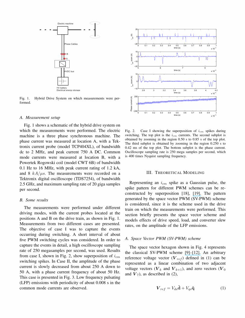
B. Some results

The measurements were performed under different

driving modes, with the current probes located at the

positions A and B on the drive train, as shown in Fig. 1.

Measurements from two different cases are presented.

The objective of case I was to capture the events

occurring during switching. A short interval of about

five PWM switching cycles was considered. In order to

capture the events in detail, a high oscilloscope sampling

rate of 250 megasamples per second, was used. Results

from case I, shown in Fig. 2, show superposition of icmswitching spikes. In Case II, the amplitude of the phase

current is slowly decreased from about 250 A down to

50 A, with a phase current frequency of about 50 Hz.

This case is presented in Fig. 3. Low frequency pulsating

(LFP) emissions with periodicity of about 0.008 s in the

common mode currents are observed.

0 0.1 0.2 0.3 0.4 0.5 0.6 0.7 0.8 0.9 1

x 10−3

−20

0

20

i cm (A

)

time (s)

5 6 7 8

x 10−4

−20

−10

0

10

i cm z

oom

(A)

time (s)

2.8 3 3.2 3.4 3.6 3.8 4 4.2

x 10−4

−10

0

10

i cm z

oom

(A)

time (s)

0 0.1 0.2 0.3 0.4 0.5 0.6 0.7 0.8 0.9 1

x 10−3

−200

0

200

Pha

se c

urre

nt (A

)

time (s)

Fig. 2. Case I showing the superposition of icm spikes duringswitching. The top plot is the icm currents. The second subplot isobtained by zooming in the region 0.50 s to 0.85 s of the top plot.The third subplot is obtained by zooming in the region 0.250 s to0.42 ms of the top plot. The bottom subplot is the phase current.Oscilloscope sampling rate is 250 mega samples per second, whichis 400 times Nyquist sampling frequency.

III. THEORETICAL MODELING

Representing an icm spike as a Gaussian pulse, the

spike pattern for different PWM schemes can be re-

constructed by superposition [18], [19]. The pattern

generated by the space vector PWM (SV-PWM) scheme

is considered, since it is the scheme used in the drive

train on which the measurements were performed. This

section briefly presents the space vector scheme and

models effects of drive speed, load, and converter slew

rates, on the amplitude of the LFP emissions.

A. Space Vector PWM (SV-PWM) scheme

The space vector hexagon shown in Fig. 4 represents

the classical SV-PWM scheme [9]–[12]. An arbitrary

reference voltage vector (V ref ) defined in (1) can be

represented as a linear combination of two adjacent

voltage vectors (V k and V k+1), and zero vectors (V 0

and V 7), as described in (2),

V ref = Vdsd + Vqsq (1)

0 0.05 0.1 0.15 0.2 0.25 0.3 0.35 0.4−20

0

20i cm

(A)

time (s)

0.006 0.008 0.01 0.012 0.014 0.016−20

0

20

i cm z

oom

(A)

time (s)

8 8.5 9 9.5 10 10.5 11

x 10−3

−20

0

20

i cm z

oom

(A)

time (s)

0 0.05 0.1 0.15 0.2 0.25 0.3 0.35 0.4−500

0

500

Pha

se c

urre

nt (A

)

time (s)

Fig. 3. Case II showing LFP emissions with periodicity 0.008 s.The second subplot is obtained by zooming in the region 0.005 s to0.016 s of the top plot. The third subplot is obtained by zooming inthe region 0.008 s to 0.011 s of the top plot. The bottom plot is thephase current. Oscilloscope sampling rate is 1.25 mega samples persecond, which is twice the Nyquist frequency.

Fig. 4. Space vector scheme showing voltage vectors V0, V1, ..., V7

and arbitrary reference voltage vector V ref . The binary numbers000, 001, ... represents the switch states.

V ref = DkV k + Dk+1V k+1 + [1− (Dk + Dk+1)]V 0,7

(2)

where Dk = Tk

Tsis the duty cycle, Tk is the time spent on

the V k voltage vector, Ts the PWM period, and Vd is the

dc source voltage. The voltage vectors V k are defined

as

V k =23

Vd exp jπ(k − 1)

3. (3)

For half a PWM period, Dk is constrained as

Dk + Dk+1 + D0,7 = 0.5, (4)

where D0,7 is the duty ratio for either V 0 or V 7 zero

voltage vectors. Considering that V 0,7 = 0, V ref is

simplified as

V ref = DkV k + Dk+1V k+1. (5)

Using (1) to (5), the switching times Tk and Tk+1

are obtained. The T ′ks determine when the converter

switches fire or voltage transitions occur. This, in turn,

determines the interval between the icm spikes.

B. Modeling of icm spikes

The spike rise time and amplitude are varied using

parameters A and C, as shown in Fig. 5. The time

of occurrence of the spike is varied by moving the

centre of the Gaussian pulse, and is equivalent to varying

parameter b in (6).

0 0.1 0.2 0.3 0.4 0.5 0.6 0.7 0.8 0.9 10

0.1

0.2

0.3

0.4

0.5

0.6

0.7

0.8

0.9

1

time [s]

CA

Fig. 5. Gaussian pulse of height A, width C and centered at timet = 0.5s. The center of the pulse corresponds to the parameter b in(6).

f(t) = A exp (−(t− b)2

2C2), (6)

Consider a Vref in the sector 1, where 0 < α < π3 .

In the symmetric SV-PWM scheme [11], a feasible PWM

switching cycle is the following:

{...000 → 100 → 110 → 111→ 111 → 110 → 100 → 000...},with switching times {D1

2 , D22 , D7

2 , D72 , D2

2 , D12 }, respec-

tively. The icm spike pattern generated by this switching

cycle is shown in Fig. 6.

35 35.1 35.2 35.3 35.4 35.5 35.6 35.7 35.8 35.9 36−1.5

−1

−0.5

0

0.5

1

1.5

switching period (Ts)

i cm (A

uni

ts)

Fig. 6. icm pattern for one PWM cycle, with V ref in sector 1. timeis expressed in terms of PWM switching periods, Ts = 0.0002s

0 5 10 15 20 25 30 35 40 45 50−3

−2

−1

0

1

2

3

number of switching periods(Ts)

i cm (A

uni

ts)

38.2 38.4 38.6 38.8 39 39.2 39.4 39.6 39.8 40

−1

−0.5

0

0.5

1

number of switching periods (Ts)

i cm (A

uni

ts)

Fig. 7. Simulation results showing LFP emissions of periodicity0.001 s. The results obtained using the following parameter settings:0 < Dk ≤ 0.2, Ts = 0.0002s, T0 = 50Ts. The lower subplotis obtained by zooming in the response when 38.1Ts ≤ time ≤40.0Ts. This corresponds to case I, presented in Fig. 2 showing thesuperposition of switching spikes.

C. Reconstruction of LFP emissions

An anticlockwise rotation of a constant amplitude

reference voltage Vref generates steady state sinusoidal

phase voltages. This is obtained by varying Dk and Dk+1

while respecting the constraints given in (4). Closed to

sector boundaries, either Dk or Dk+1 tends to zero.

These cause spike superpositions during sector boundary

crossings, forming double or tripple amplitude spikes

which constitute the LFP emissions. The six sector

boundaries give rise to six LFP pulses in one complete

0 200 400 600 800 1000 1200 1400 1600 1800 2000−3

−2

−1

0

1

2

3

number of switching periods(Ts)

i cm (A

uni

ts)

20 30 40 50 60 70 80−3

−2

−1

0

1

2

3

number of switching periods (Ts)

i cm (A

uni

ts)

Fig. 8. Simulation results showing LFP emissions of 40Ts =0.008s. The results obtained using the following parameter settings:0 < Dk ≤ 0.2, Ts = 0.0002s, T0 = 240Ts. This a reconstruction ofcase II, shown in Fig. 3. The lower subplot is obtained by zoomingin the response when 20Ts ≤ time ≤ 80Ts.

revolution.

T0 = 6 TLFP (7)

The period of the sinusoidal phase voltage T0, is thus

related to the period of the LFP emissions (TLFP ) as in

(7). Fig. 7 shows simulated LFP emissions of periodicity

0.001 s. The results were obtained using the following

parameter settings: 0 < Dk ≤ 0.2, Ts = 0.0002s,

T0 = 50Ts. Fig. 8 presents simulation results showing

LFP emissions of periodicity TLFP = 40Ts = 0.008s,

obtained using the following parameter settings: 0 <Dk ≤ 0.45, Ts = 0.0002s, T0 = 240Ts. This was a

reconstruction attempt of case II, shown in Fig. 3.

IV. PARAMETERS AFFECTING THE LFP EMISSIONS

In this section, the dependence of the amplitudes of the

LFP emissions on the voltage slew rates of the converter

switches, the drive speed, and load is investigated using

the theoretical models developed in section III.

A. Effects of Voltage slew rates on LFP emissions

Close to the boundary between the kth sector, and the

(k+1)th sector, Dk becomes comparable to the width of

the gaussian pulse (C), as described in (8). The rise time

tr is an estimate of the voltage slew rate, for a fixed dc

source voltage, and is approximately equal to the pulse

width (C) of the generated common mode current spike

[2]. In the boundary region, marked by θ in Fig. 9, Dk

can be represented as a fraction of the maximum duty

cycle Dkmax, as in (8) and (9), assuming that PWM

period Ts = 1. When Dk = C, the angular width of

the LFP emissions, θ = θc can expressed as a fraction

of the sector angle as in (10). Using (8) to (10), the

expression for θc in terms of tr and Dkmax given in

(11), is obtained. The width of the LFP emissions in

seconds is obtained as dLFP = θc/2π ∗ T0 and is given

in (12).

Vk

Vk+1

Vref

Dk

Dk+1

Fig. 9. Space vector hexagon showing the boundary region, whereDk ≤ C ∼ tr , denoted by θ

Dk ≤ C ∼ tr, DkTs = C (8)

Dk =Dkmax

x(9)

θc/2 =π

3/x (10)

θc/2 =π

3tr

Dkmax(11)

dLFP =16

1Dkmax

T0

Tstr (12)

dLFP ∝ tr (13)

The effects of slew rates is described by (13) when

Dkmax, T0, and Ts are held constant. Thus the larger the

rise time, the larger the width of the LFP emissions. This

is shown in Fig. 10 and Fig. 11, where C ∼ tr = 0.02sand C ∼ tr = 0.035s, respectively.

B. Effects of drive speed on LFP emissions

The drive speed is assumed proportional to the fun-

damental frequency of the phase voltages (1/T0). From

(11), when θc is fixed, dLFP is given by

dLFP =θc

2πT0. (14)

This is seen in the simulated prediction of LFP

emissions when T0 = 0.6s, shown in Fig. 10, with

dLFP ∼ 100Ts.

0 200 400 600 800 1000 1200 1400 1600 1800 2000−3

−2

−1

0

1

2

3

time [Ts]

I cm [A

uni

ts]

20 30 40 50 60 70 80−3

−2

−1

0

1

2

3

time [Ts]

I cm [A

uni

ts]

Fig. 10. Reconstruction of case II with C ∼ tr = 0.02s,dLFP ∼10Ts, TLFP = 40Ts = 0.008s and T0 = 240Ts. Parameter settings:0 < Dk ≤ 0.45, Ts = 0.0002s. The lower subplot is a zoom of theregion 20Ts < t < 80Ts.

0 200 400 600 800 1000 1200 1400 1600 1800 2000−3

−2

−1

0

1

2

3

time [Ts]

i cm [A

uni

ts]

20 30 40 50 60 70 80−3

−2

−1

0

1

2

3

time [Ts]

i cm [A

uni

ts]

Fig. 11. Reconstruction of case II with C ∼ tr = 0.035s, dLFP ∼20Ts, TLFP = 40Ts = 0.008s and T0 = 240Ts. Parameter settings:0 < Dk ≤ 0.45, Ts = 0.0002s.

C. Effects of load on LFP emissions

The load or torque output is assumed proportional to

the amplitude of the phase current. This is simulated by

varying the maximum duty cycle Dkmax in the interval

0 < Dkmax < 0.5. From (12) it is observed that dLFP

is proportional to Dkmax, when T0, tr and Ts are held

constant. This is an indication of light load instabilities.

This is shown in Fig. 13, when Dkmax = 0.05. It is

observed that the LFP pulses overlap in this case, unlike

in the previous cases where was set to 0.2 or 0.45.

V. DISCUSSIONS AND CONCLUSIONS

Drive systems employing the space vector PWM

scheme could emit Low Frequency Pulsating (LFP)

emissions at a frequency of 6f0, where f0 is the funda-

mental frequency of the phase voltages. The LFP emis-

0 0.2 0.4 0.6 0.8 1 1.2 1.4 1.6 1.8 2

x 104

−3

−2

−1

0

1

2

3

time [Ts]

I cm [A

uni

ts]

0 200 400 600 800 1000 1200−3

−2

−1

0

1

2

3

time [Ts]

I cm [A

uni

ts]

Fig. 12. Simulated prediction of LFP emissions with T0 =3000Ts = 0.6s and dLFP ∼ 100Ts. Parameter settings: 0 < Dk ≤0.45, Ts = 0.0002s. The lower subplot is a zoom of the region0 < t < 1200Ts

0 50 100 150 200 250 300 350 400−3

−2

−1

0

1

2

3

time [Ts]

I cm [A

uni

ts]

20 30 40 50 60 70 80−3

−2

−1

0

1

2

3

time [Ts]

I cm [A

uni

ts]

Fig. 13. Light load conditions, with a period of 0.005 s. Parametersettings: 0 < Dk ≤ 0.05, Ts = 0.0002s, T0 = 150Ts. The lowersubplot is a zoom of the region 20Ts < t < 80Ts.

sions is built up from double or tipple amplitude common

mode current spikes, formed from the superposition of

common mode spikes generated during sector boundary

crossings. Measurements from an HEV showing the

LFP emissions were presented. Using simple theoretical

models the effects of parameters like the voltage slew

rates, drive speed and drive load on the LFP emissions of

have been investigated. The coupling of these pulsations

to torque pulsations requires further investigations, how-

ever, relationships between current harmonics and torque

pulsations have been deveped in [16], [17]. Mitigation

approaches shall be investigated in a future work.

REFERENCES

[1] Q. Liu, “Modular approach for characterizing and modelingconducted EMI emissions in power converters,” Ph.D. disser-

tation, Virginia Polytechnic Institute and State University, VA,USA, 2005.

[2] C. Paul, Introduction to Electromagnetic Compatibility. JohnWiley and Sons, Inc., New York, 2006.

[3] T. Hubing, “Using component level measurements to determinesystem level radiated emissions,” in Proc. of the IEEE Int.symposium on EMC, Detroite MI, USA, 2008.

[4] Q. Liu, F. Wang, and D. Boroyevich, “Frequency-domain EMInoise emission characterization of switching power modules inconverter systems,” in Proc. of IEEE Applied Power ElectronicsConference and Exposition, 2005, pp. 787–79.

[5] R. Thomas, F. Li, and C. Garrett, “Prediction of radiatedEMI from high frequency power converters,” in Proc. of IEEinternational Conference on Power Electronics and VariableSpeed Drives, 2000, pp. 80–85.

[6] K. Mainali, R. Oruganti, K. Viswanathan, and N. Swee, “Ametric for evaluating the EMI spectra of power converters,”IEEE Trans. Power Electron., vol. 23, no. 4, pp. 2075–2081,2008.

[7] N. Mutoh, J. Nakashima, and M. Kanesaki, “Multilayer powerprinted structures suitable for controlling EMI noises generatedin power converters,” IEEE Trans. Power Electron., vol. 50,no. 6, pp. 1085–1094, 2003.

[8] D. G. Holmes, “The significance of zero space vector placementfor carrier-based pwm schemes,” IEEE Trans. Ind. Applicat.,vol. 32, no. 5, pp. 1122 – 1129, 1996.

[9] M. Ehsani, S. Gay, and A. Amadi, Modern Electric, HybridElectric, and Fuel Cell Vehicles. CRC Press, New York, 2005.

[10] G. Oritiand, A. L. Julian, and A. Lipo, “A new space vectormodulation strategy for common mode voltage reduction,” inProc. of the IEEE PESC’97, Saint Louis, MO, USA, 1997, pp.1541 – 1546.

[11] M. M. Bech, “Random pulse-width modulation techniquesfor power electronic converters,” Ph.D. dissertation, AalborgUniversity, Aaborg, Denmark, 2000.

[12] I. Husain, Electric and Hybrid Vehicles. CRC Press, New York,2003.

[13] K. Basu, J. Prasad, G. Narayanan, H. Krishnamurthy, andR. Ayyanar, “Reduction of torque ripple in induction motordrives using an advanced hybrid pwm technique,” IEEE Trans.Ind. Applicat., vol. 00, no. 99, pp. 1–1, 2009.

[14] M. Cirrincione, M. Pucci, G. Vitale, and G. Cirrincione, “A newdirect torque control strategy for the minimization of common-mode emissions,” IEEE Trans. Ind. Applicat., vol. 46, no. 2, pp.504 – 517, 2006.

[15] M. Enohnyaket, K. Hyyppa, and J. Delsing, “Generation of lowfrequency pulsating emissions from PWM power converters,”IEEE Power Electronics Society Newsletter, Submitted 2010.

[16] J. Song-Manguelle, S. Schroder, T. Geyer, G. Ekemb, andJ. Nyobe-Yome, “Prediction of mechanical shaft failures dueto pulsating torques of variable frequency drives,” in Proc. ofthe IEEE Energy Conversion Congress and Exposition, ECCE2009, San Jose, CA, USA, 2009, pp. 3469 – 3476.

[17] J. Song-Manguelle, J. Nyobe-Yome, and G. Ekemb, “Pulsatingtorques in pwm multi-megawatt drives for torsional analysis oflarge shafts,” IEEE Trans. Ind. Applicat., vol. 46, no. 1, pp. 130– 138, 2010.

[18] J. W. Strutt and B. Rayleigh, The Theory of Sound. DoverPublications Inc., New York, 1945.

[19] L. E. Kinsler, A. R. Frey, A. B. Coppens, and J. V. Sanders,Fundamentals of Acoustics. John Wiley and Sons, New York,1982.