HAL Id: tel-02102687https://tel.archives-ouvertes.fr/tel-02102687

Submitted on 17 Apr 2019

HAL is a multi-disciplinary open accessarchive for the deposit and dissemination of sci-entific research documents, whether they are pub-lished or not. The documents may come fromteaching and research institutions in France orabroad, or from public or private research centers.

L’archive ouverte pluridisciplinaire HAL, estdestinée au dépôt et à la diffusion de documentsscientifiques de niveau recherche, publiés ou non,émanant des établissements d’enseignement et derecherche français ou étrangers, des laboratoirespublics ou privés.

Parallelism and modular proof in differential dynamiclogic

Simon Lunel

To cite this version:Simon Lunel. Parallelism and modular proof in differential dynamic logic. Artificial Intelligence[cs.AI]. Université Rennes 1, 2019. English. �NNT : 2019REN1S005�. �tel-02102687�

THESE DE DOCTORAT DEL’UNIVERSITE DE RENNES 1

L’UNIVERSITE DE RENNES 1COMUE UNIVERSITE BRETAGNE LOIRE

Ecole Doctorale N°601Mathematiques et Sciences et Technologiesde l’Information et de la CommunicationSpécialité : Informatique

Par

Simon Lunel! Parallelism and modular proof in Differential Dynamic Logic "

Soutenance de la these prevue a Rennes, le 28 janvier 2019IRISA

Rapporteurs avant soutenance :

AIT AMEUR Yamine, Professeur, INPT-ENSEEIHT, Toulouse, France

ZHAN Naijun, Professeur, Chinese Academy of Science, Beijing, China

Composition du jury :

President : BLAZY Sandrine, Professeure, ISTIC, Universite de Rennes 1, Rennes, France

Examinateurs : AIT AMEUR Yamine, Professeur, HDR, INPT-ENSEEIHT, Toulouse, France

ZHAN Naijun, Professeur, Chinese Academy of Science, Beijing, China

GAO Sicun, Assistant Professor, University of California, San Diego, USA

BOYER Benoit, Chercheur, Mitsubishi Electric R&D Centre Europe, Rennes, France

Invite(s) : GHORBAL Khalil, Chercheur, CNRS, IRISA, Rennes, France

Dir. de these : TALPIN Jean-Pierre, H, Chercheur, HDR, INRIA, Rennes, France

Remerciements

Je tiens a remercier Sandrine BLAZY, Professeure de l’Universite de Rennes 1, d’avoir acceptede presider mon jury. Je remercie egalement Yamine AIT AMEUR, Directeur de Recherche al’INPT-ENSEEIHT, et Naijun Zhan, Professeur au Chinese Academy of Science, d’avoir bienvoulu rapporter cette these et pour leur relecture minutieuse. Khalil GHORBAL, Charge derecherche a l’INRIA, et Sicun GAO, Assistant Professor de l’Universite de San Diego, ontaccepte de faire partie de mon jury de these et je les en remercie.

Je tiens a remercier tout particulierement mon directeur de these, Jean-Pierre TALPIN,Directeur de recherche a l’INRIA, pour m’avoir guide tout au long de ces trois annees dedoctorat et sans qui je n’aurais pu accomplir ce travail. Ses retours ont toujours ete pertinentset ont abondamment nourri ma reflexion. Je remercie aussi Benoit BOYER, Ingenieur deRecherche a Mitsubishi Electric qui m’a encadre sur toute la duree de mes travaux et qui atoujours ete present pour repondre a mes nombreuses questions. Son enthousiasme m’a aidea continuer a de nombreuses reprises. Mes remerciements vont aussi a David MENTRE pourles nombreux echanges constructifs que l’on a eu dans les locaux de Mitsubishi Electric.

Je remercie aussi Denis COUSINEAU et Ocan SANKUR pour avoir ete membre de moncomite de suivi de these ainsi que pour leur nombreux conseils et encouragements lors de cesdiscussions.

Ce manuscrit n’aurait pas ete possible sans les nombreuses interactions et echanges quej’ai eu avec d’autres chercheurs, notamment Andre PLATZER, Stefan MITSCH, AndreasMULLER, Rajesh GUPTA, Shuling WANG. La liste n’est probablement pas exhaustive,et je tiens a m’excuser d’avance pour tout ceux que j’oublie. Je tiens aussi a remerciertous mes collegues de l’equipe TEA pour les echanges toujours interessants et pour un sou-tien bien necessaire parfois : Loic BESNARD, Thierry GAUTIER, Vania JOLOBOFF, HaiNam TRAN, Alexandre HONORAT, Jean-Joseph MARTY, Liangcong ZHANG et LucasFRANCESCHINO. Merci a Stephanie LEMAILE et Armelle MOZZICONACCI pour leurprecieuse aide dans les dedales administratifs de l’INRIA. Enfin, je remercie Mitsubishi Elec-tric et l’INRIA pour avoir respectivement finance et soutenu materiellement ma these.

Je tiens a remercier mes parents pour leur soutien durant ma these ainsi que pour touteleur implication les vingts-trois annees precedentes. Cette these n’aurait jamais vu le joursans eux. Je remercie aussi mes amis a qui j’ai donne des nouvelles de maniere erratique etqui ne m’en tiennent pas rigueur. Enfin, je remercie Lucie qui a reussi a me supporter durantces trois annees et m’a toujours soutenu.

2

Resume en francais

3

Les systemes cyber-physiques melangent des comportements physiques continus, tel lavitesse d’un vehicule, et des comportement discrets, tel que le regulateur de vitesse d’unvehicule. Ils sont desormais omnipresents dans notre societe. Un grand nombre de cessystemes sont dits critiques, i.e. une mauvaise conception entrainant un comportement nonprevu, un bug, peut mettre en danger des etres humains. Ainsi, un regulateur de vitesse quiautoriserait un vehicule a depasser les limitations de vitesse met en danger les passagers duvehicule.

Il est necessaire de developper des methodes pour garantir le bon fonctionnement de telssystemes. La methode la plus repandue est le test. On va tester de maniere approfondie siune voiture se comporte comme attendue ou si le programme reagit comme souhaite pour ungrand nombre de situations possibles. Mais si cette approche permet de mettre en evidencedes problemes, elle n’est pas en mesure de garantir l’absence de problemes. En effet, si onteste la voiture pendant un millier d’heures, il est possible qu’un probleme arrive uniquementa partir de la mille-et-unieme heure de fonctionnement. Une autre approche a ete developpeces dernieres decennies en informatique et qui permet de garantir l’absence problemes : lesmethodes formelles.

Les methodes formelles regroupent des procedes mathematiques pour garantir qu’un pro-gramme se comporte comme attendu, par exemple que le regulateur de vitesse n’autorise pasde depasser la vitesse maximale autorisee. Mais les procedes developpes l’ont principalementete pour des programmes, i.e. que l’on ne considere pas la partie continue du systeme commel’evolution de la vitesse, et on peuvent donc garantir le bon fonctionnement du systemephysique. Il est donc souhaitable de developper des methodes formelles specifiques pourgarantir le bon fonctionnement de systemes cyber-physiques.

Une telle tache rencontre neanmoins un probleme de taille qui est de reussir a conjuguerdeux formalismes de natures differentes. En effet, les systemes physiques sont representes pardes equations differentielles a valeur dans l’ensemble des nombre reels R. Les programmes sonteux modelises comme etant a valeur dans les entiers naturels N. Cela est particulierementproblematique pour la representation du temps. Quand un programme s’execute, on nes’interesse pas au temps qui peut s’ecouler entre deux instructions, la representation du tempsest discrete. Mais l’evolution d’un phenomene physique est continue : il n’y a pas de pause.

Andre Platzer a propose en 2007 un nouveau formalisme, la logique dynamique differentielle,reunissant ces deux aspects. Ce formalisme permet de modeliser formellement, i.e. avec unesemantique definie mathematiquement, des systemes exhibant a la fois des comportementscontinus et discrets, ainsi que leurs interactions possibles. De plus, Andre Platzer a defini unsysteme de preuve permettant de raisonner sur de tel systemes et donc de garantir leur bonfonctionnement. Il devient alors possible de modeliser formellement un regulateur de vitesseavec l’evolution reelle de la vitesse et de demontrer qu’il est impossible que le vehicule depasseles vitesses maximales autorisees, cela pour un intervalle de temps arbitrairement long et nonpour les mille premieres heures.

Malheureusement, la mise en œuvre de cette methode requiert une connaissance appro-fondie des systemes etudies ainsi que des mecanismes de preuves formelles associees. En effet,le systeme est represente dans sa globalite, en un bloc monolithique, et la complexite de lapreuve augmente en fonction de la taille du systeme. Ainsi, des systemes relativement simplesdu point de vue d’un ingenieur dans l’industrie necessitent un effort important de preuve quine peut etre supporte par un ordinateur. Il nous faut donc developper des methodes pourpasser a l’echelle et augmenter la complexite des systemes etudies.

La complexite d’un systeme cyber-physique revet deux aspects a notre connaissance. Le

4

premier aspect est la complexite que nous appelons mathematique. Il s’agit de la complexiteinherente a un phenomene physique, par exemple le deplacement d’un satellite ou l’on estoblige de prendre en compte la theorie de la relativite. Le deuxieme aspect est la complexiteque nous appelons structurelle. Elle provient de la repetition de composants elementaires,par exemple une usine de traitement des eaux ou plusieurs cuves sont connectees ensemble.Chaque cuve prise individuellement est simple a comprendre, modeliser, et de la, a prouverson bon fonctionnement. Mais il est difficile de considerer l’usine en entier car la repetitionrend la modelisation plus complexe ainsi que la preuve. Ces systemes sont tres courants dansles milieux industriels.

C’est ce dernier aspect que nous avons voulu traiter dans ce memoire. Notre problematiqueest comment modeliser efficacement des systemes cyber-physiques dont la complexite residedans une repetition de morceaux elementaires. Et une fois que l’on a obtenu une modelisation,comment garantir le bon fonctionnement de tels systemes.

L’approche classique ou l’on modelise le systeme d’un seul tenant et essaye ensuite demontrer son bon fonctionnement n’est pas applicable. La modelisation serait laborieuse etsujette a erreurs dues a la taille du modele. La preuve du modele resultant ne pourra pasetre prise completement en charge par un ordinateur car la puissance de calcul necessaireest beaucoup trop elevee. Un expert en demonstration de systeme cyber-physique sera doncnecessaire.

Notre approche consiste a modeliser le systeme de maniere compositionnelle. Plutot quede vouloir le modeliser d’un seul tenant, il faut le modeliser morceaux par morceaux, appelescomposants. Chaque composant correspond a une brique elementaire du systeme et il estdonc possible de le modeliser facilement. On obtient le systeme complet en assemblant lescomposants ensembles. Ainsi l’usine de traitement des eaux est obtenue en assemblant lescuves ensembles. L’interet de cette methode est qu’elle correspond a l’approche des ingenieursdans l’industrie : considerer des elements separes que l’on compose ensuite.

Mais cette approche seule ne resout pas le probleme de la preuve de bon fonctionnementdu systeme. Il faut aussi rendre la preuve compositionnelle. Pour cela, on associe a chaquecomposant des proprietes et on prouve qu’elles sont respectees. Cette preuve peut etre effectuepar un expert, mais aussi par un ordinateur si les composants sont de tailles raisonnables. Ilfaut ensuite nous assurer que lors de l’assemblage des composants, les proprietes continuenta etre respectees. Ainsi, la charge de la preuve est reportee sur les composants elementaires,l’assurance du respect des proprietes desirees est conservee lors des etapes de composition.On peut alors obtenir une preuve du bon fonctionnement de systemes industriels avec un coutde preuve reduit.

Notre contribution majeure est de proposer une telle approche compositionnelle a la foispour modeliser des systemes cyber-physiques, mais aussi pour prouver qu’ils respectent lesproprietes voulues. Ainsi, a chaque etape de la conception, on s’assure que les proprietessont conservees, si possible a l’aide d’un ordinateur. Le systeme resultant est correct parconstruction.

Plus precisement, nous avons defini formellement une notion de composant dans la logiquedynamique differentielle. Un composant est constituee d’une partie discrete, par exemple lecontroleur du niveau d’eau dans une cuve, et d’une partie continue –sous la forme d’uneequation differentielle–, par exemple l’evolution du niveau d’eau, le tout formant un systemecyber-physique. On ne fait pas d’hypotheses de priorite entre chaque partie, ce qui corresponda la realite de fonctionnement des systemes cyber-physiques. Le systeme est reactif, et peuts’executer pour une duree de temps arbitrairement longue. Il est possible pour un composant

5

d’etre uniquement discret, par exemple le controleur du niveau d’eau, ou uniquement continue,par exemple l’evolution du niveau d’eau. Cette definition est assez generique pour permettrede modeliser un vaste ensemble de systemes industriels.

Une fois la notion de composant definie, il nous faut un moyen pour les assembler. Ona defini un operateur de composition parallele. Il permet de modeliser deux composantss’executant simultanement – en parallele–, par exemple deux cuves d’eau. Le parallelismedes parties discretes est obtenue par entrelacement; n’importe quelle ordre d’execution estpossible. Le parallelisme des parties continues est obtenue en considerant le systeme composeede chaque equation differentielles. Le composant resultant est la reunion des deux parties,encore une fois sans hypothese de priorite.

Notre operateur de composition parallele est syntaxique et peut donc etre implementeepar un ordinateur. Ainsi, un ingenieur aurait a definir chaque composant formellement, puisle systeme resultant par composition serait generee par l’ordinateur, reduisant les risquesd’erreurs d’inattention.

Notre operateur possede deux importantes proprietes algebriques : la commutativite etl’associativite. La commutativite veut dire que l’ordre de composition n’est pas pertinent.Composer une cuve d’eau A en parallele avec une autre cuve d’eau B en parallele revientexactement a la meme chose que de composer la cuve B en parallele avec la cuve d’eau A.L’associativite veut dire que l’on peut construire notre systeme pas-a-pas. On n’est pas obligede composer tout les composants d’un coup. Ainsi la composition d’une cuve A avec une cuveB, puis le tout compose avec une troisieme cuve C est equivalent a la composition des cuves Bet C d’abord, puis compose ensuite avec A.

L’associativite est une propriete cle pour obtenir une approche vraiment modulaire. Destravaux precedents avaient deja propose une approche compositionnelle dans la logique dy-namique differentielle, mais leur operateur de composition parallele n’etait pas associatif.

On a donc une methode permettant de modeliser un systeme cyber-physique de manieremodulaire grace a une approche par composant. Mais ce n’est que la moitie du resultat desire.On veut aussi pouvoir faire les preuves de correction des systemes cyber-physique de manieremodulaire.

A chacun de nos composants, on associe ce que l’on appelle un contrat. Un contrat est unestructure formelle permettant de representer les hypotheses sous lesquelles un composant peuts’executer ainsi que les garanties apportees par le composant. On peut prouver ensuite enutilisant le systeme de preuves de la logique dynamique differentielle qu’un composant satisfaitson contrat associe, i.e. que sous les hypotheses enoncees, les garanties seront toujours verifieespour n’importe quelle execution du composant.

Nous avons demontre un theoreme qui nous assure que sous l’hypothese que chaque com-posant satisfait son contrat, la composition parallele de ces composants satisfait la conjonctiondes contrats. La conjonction de deux contrats est le contrat ou les hypotheses sont la conjonc-tion des hypotheses respectives et les garanties sont la conjonction des garanties respectives.Ainsi, on conserve la satisfaction des contrats a travers la composition permettant d’obtenir lapreuve de bon fonctionnement du systeme par construction. Cependant, plusieurs conditionssont requises pour que ce theoreme soit applicable.

La premiere condition est que les composants ne partagent pas de sorties communes. Celaveut dire que deux composants ne doivent pas agir sur les memes parties du systeme. Parexemple, deux controleurs pour des cuves differentes ne doivent pas controler la meme vanne.Il s’agit d’une bonne pratique de conception, deux composants agissant sur une meme sortieamene des conflits et peut produire des comportements inattendus.

6

La second condition est que les garanties d’un composant ne doivent pas faire referenceaux sorties d’un autre composant. Ainsi, les garanties d’un controleur d’une cuve ne doiventpas referer aux sorties d’un controleur d’une autre cuve. Il s’agit la aussi d’une bonne pratiquede conception. Les garanties d’un composant doivent faire reference a ses propres sorties, i.e.celles sur lesquelles il a une capacite d’action.

La derniere condition est que les garanties d’un composant ne doivent pas infirmer leshypotheses d’un autre composant. En effet, cela veut dire qu’un composant ne se comportepas de la maniere attendue par le second composant. Il y a donc un probleme de conception.

Ces trois conditions sont enoncees de maniere syntaxique et peuvent donc etre verifieespar un ordinateur. Ainsi, il est possible d’implementer completement cette methode pourconserver les contrats lors de la composition.

Pour resumer, nous avons propose une approche permettant de modeliser et verifier unsysteme de maniere modulaire. Nos definitions sont syntaxiques et l’approche peut donc etreimplemente afin d’automatiser notre approche.

Nous avons implemente un prototype dans le prouveur interactif de theoremes KeY-maera X. Cela permet de montrer la faisabilite d’une telle implementation. Nous avonsetudie deux systemes industriels afin de valider notre approche. Le premier est un regulateurde vitesse, le second une usine de traitements des eaux composee de plusieurs cuves d’eau enparallele. L’etude de ces deux exemples a permis de montrer la viabilite de notre approche,mais a aussi mis en relief les ameliorations possibles.

Un point particulierement important concerne la classe des systemes controles par or-dinateur. Il s’agit des systemes ou une grandeur physique, par exemple l’evolution duniveau d’eau d’une cuve, est regule par un programme, par exemple le controleur du niveaud’eau. Le programme surveille l’evolution continue a l’aide d’un capteur qui mesure la valeurperiodiquement. Le programme doit ensuite agir de maniere a ce que les proprietes desireessoit toujours respectees. Ainsi, pour la cuve d’eau, on veut que le niveau d’eau ne deborde ja-mais. La caracteristique cle de ces systemes est la relation periodique au temps. Le controleurdoit avoir une information suffisamment souvent pour pouvoir reguler le systeme.

On a montre comment on pouvait ameliorer notre approche precedente pour prendreen compte ces aspects temporels supplementaires. Lors de la definition d’un controleur,l’ingenieur doit preciser sa periode d’execution, i.e. l’intervalle maximum entre deux executionsdu controleur. Lors de la definition de la partie dynamique, il doit fournir sa controlabilite. Ils’agit de la duree maximum pendant laquelle le systeme dynamique peut evoluer sans inter-vention du controleur et encore satisfaire les proprietes voulues. On a modifie notre operateurde composition parallele et demontre que l’on conserve la satisfaction des contrats lors de lacomposition sous les memes conditions. On requiert en plus que la periode d’execution ducontroleur soit inferieure a la controlabilite du systeme dynamique. Il s’agit encore une foisd’une bonne pratique de conception, un systeme ne satisfaisant pas cette condition aurait peude chance de fonctionner.

On a ensuite generalise cette adaptation. On associe une periode d’execution lors de ladefinition d’un composant discret et une controlabilite lors de la definition d’un composantcontinu. On modifie aussi legerement notre operateur de composition parallele pour prendreen compte ces deux caracteristiques temporelles. Lors de la composition parallele de deuxsystemes discrets, la periode d’execution resultante est la somme des periodes d’execution.En effet, on suppose que l’execution se fait sur une seule unite de calcul et le parallelisme estobtenue par entrelacement. La controlabilite d’un composant continu resultant de la compo-sition parallele de deux composants continus est le minimum des controlabilites respectives.

7

Malgre ces ajouts, notre operateur de composition parallele reste commutatif et associatif.De la meme maniere que l’on a generalise la modelisation par composants a des systemes

avec des caracteristiques temporelles, on a generalise notre theoreme permettant de conserverla satisfaction des contrats lors de la composition. Etant donne la preuve de satisfaction descontrats respectifs, on peut exhiber la preuve de satisfaction de la conjonction des contrats.Les memes conditions que precedemment sont necessaires ainsi que la periode d’executionresultante doit toujours etre inferieure a la controlabilite resultante.

Finalement, on a adapte notre approche pour modeliser deux autres cas que l’on rencontrefrequemment dans les systemes industriels : les modes de fonctionnement et la causalitetemporelle. L’exemple recurrent des modes de fonctionnement est la presence d’un modenominal, ou le systeme fonctionne normalement, et d’un mode degrade, ou le systeme doitgarantir uniquement des proprietes vitales. Par exemple, dans le cas de nos cuves d’eauinterconnectes, le premier mode correspond au fonctionnement normal ou les niveaux d’eaune doivent pas deborder, mais aussi etre suffisamment eleves pour garantir un debit minimala la sortie de la cuve. Le mode degrade correspond a une urgence, par exemple un boutonpoussoir d’urgence enclenche, et toutes les vannes sont fermees. On veut juste alors garantirque les cuves ne debordent pas.

On modelise chaque mode comme etant un composant et on obtient le systeme compor-tant les deux modes de fonctionnement avec notre operateur de composition parallele. Maison ne peut pas conserver les contrats lors de la composition. En effet, nos deux composantsrepresentant chacun un mode ont des sorties communes, et les conditions de notre theoremede composition ne sont pas donc pas remplies. Mais ces deux modes ne s’executent pasvraiment en parallele, ils sont meme exclusifs; il n’est pas possible qu’ils se deroulent simul-tanement. On caracterise chaque mode avec une formule, et sous condition que les formulessont contradictoires, on peut conserver les contrats lors de la composition.

Nous avons aussi defini un operateur de composition causale. Il est souhaitable parfoisd’ordonnancer deux composants plutot que de les executer en parallele. Par exemple, un cap-teur doit toujours s’executer avant le programme utilisant les donnees du capteur pour regulerle systeme dynamique. Dans le cas contraire, le programme raisonnerait avec des donneesperimees et ne se comporterait pas comme attendu. Ce nouvel operateur de composition restecompatible avec l’operateur de composition parallele et est toujours associatif, necessaire pourla modularite de notre approche. Comme precedemment, nous avons demontre un theoremepermettant de conserver les contrats lors de la composition.

En conclusion, nous avons developpe une methodologie modulaire fondee sur la composi-tion pour modeliser formellement et verifier des systemes cyber-physiques. Nous avons illustrequ’elle peut etre implemente et modifie pour s’adapter a de nouveaux defis. Elle sert de basetheorique pour developper un outil sur la modelisation formelle et la preuve de systemescyber-physiques.

8

Introduction

9

Programs are used to govern numerous parts of our society: in the monitoring of railwaynetworks or money transfers for example. It is mandatory that they behave correctly. Whenwe order online goods, we want to be sure that no one can access our personal information.Power grids, water-plant and planes are all supervised by complex programs; a bug may leadto disastrous and potentially deadly consequences. Such systems are called safety-critical.

To avoid bugs, software engineers have developed numerous testing procedures, but theyare fundamentally limited. “The test of programs may be a very efficient way to show thepresence of bugs, but is desperately inadequate to prove their absence” (Djikstra, 1972). Atest can not ensure that every behavior of a program is correct since there is an infinity ofbehaviors, it only assesses that it works for the finite set of tested behaviors. Another approachis to use the so-called formal methods. Instead of testing if a program works correctly for somebehaviors, it advocates the use of mathematics to prove that the program behaves correctlyfor every possible execution. They are costly, being thus applied for critical programs only.

Numerous approaches and tools have been developed these past decades, and great suc-cesses have been achieved. The CompCert compiler is a compiler for a consequent subset ofthe C language formally verified using the theorem prover Coq. The Communication-BasedTrain Control (CBTC) program running the lane 14 of Parisian subway has been entirelydeveloped using the B method, an other formal verification technique. But they have beenobtained at the cost of great effort and intensive research, and their systematic replication inthe industry is still not feasible.

Most approaches to the problem of verification of program assumed it to be already writtenand try to prove that it behaves correctly. The conception of the program is usually achievedby an expert of the domain and the verification process by a proof engineer who is notfamiliar with the domain. The former conducts the development without thinking about theformal verification. The latter has to deconstruct the software in order to conduct the proof.It results in a huge amount of wasted time and resources, and possibly misunderstandings.The correct-by-construction approach advocates the idea that the design and the verificationshould not be separated, but rather conducted simultaneously. The verification providessignificant insights for the development of the software which is in return produced with itsverification as a goal. The B method follows this paradigm, which is believed to be the keypoint of its success.

In the case of the CBTC verification, only the program has been verified; the physicalquantities involved (e.g. the speed of the train) are not considered or idealized. Programsas the CBTC do not simply perform a computation, they exhibit frequent interactions withthe physical environment. The resulting behavior can not be fully understood without takingphysical evolution into consideration. Since such programs are often critical, e.g. auto-pilot ofplanes or monitors of water-plant treatment, it is highly desirable to develop specific formalmethods.

Systems where physical behavior, e.g. the speed of a train, is mixed with discrete behav-iors, e.g. the CBTC, are called cyber-physical systems (CPS) or hybrid systems. The firstbehavior assumes a continuous model of time when the second possesses a discrete model oftime. The difference of nature between theses two models render the formal design of hybridsystems very complex. Plus, many systems exhibit intangible interactions between discreteand continuous behavior. Reasoning about such systems demands tools capable to accom-modate the different abstractions level such as the system level, processor level, logic level,etc.

In 2007, the Differential Dynamic Logic is defined by Andre Platzer to model and verify

10

such systems. It provides a precise mathematical semantics and considers physical evolutionon the same level as programming constructs. It features a proof system to ensure thecorrectness of behaviors which has been used to prove numerous use-cases, some of themunverified previously. The proof system has been implemented in the interactive theoremprover KeYmaera X. This theorem prover is designed toward automation which is a keyfunctionality to make tractable proofs.

Despite this, most of the problems are still intractable in practice and a methodology totackle large problems is thus required. One of the most ancient method to address a difficultproblem is to divide it into smaller parts, as exposed by Descartes in his book Discours de lamethode. Each part is easier to understand for a human, but also easier for a computer totreat. Seeking methods to efficiently break down a system is thus highly desirable. Numerousworks have been produced for programs, but few have been done for cyber-physical systemsand in Differential Dynamic Logic.

My main contribution is the definition of a modular component-based framework in Differ-ential Dynamic Logic to model and prove correctness of Cyber-Physical Systems. It providestheoretical basis to represent parallel composition of Cyber-Physical systems and how toimplement a correct-by-design approach.

11

Contents

1 Adressed problem 151.1 Verification of Cyber-Physical Systems . . . . . . . . . . . . . . . . . . . . . . 16

1.1.1 Scalable verification of hybrid systems . . . . . . . . . . . . . . . . . . 161.1.2 Interest of hybrid systems . . . . . . . . . . . . . . . . . . . . . . . . . 161.1.3 Our approach: correct-by-design . . . . . . . . . . . . . . . . . . . . . 17

1.2 State of the art . . . . . . . . . . . . . . . . . . . . . . . . . . . . . . . . . . . 171.2.1 Formalisms for discrete systems . . . . . . . . . . . . . . . . . . . . . . 171.2.2 Addition of continuous features . . . . . . . . . . . . . . . . . . . . . . 181.2.3 Other approaches to verification of Cyber-Physical Systems . . . . . . 211.2.4 Existing tools . . . . . . . . . . . . . . . . . . . . . . . . . . . . . . . . 23

1.3 Contributions . . . . . . . . . . . . . . . . . . . . . . . . . . . . . . . . . . . . 25

2 Introduction to Differential Dynamic Logic 272.1 Modeling of Cyber-Physical Systems . . . . . . . . . . . . . . . . . . . . . . . 28

2.1.1 Discrete behaviors or programs . . . . . . . . . . . . . . . . . . . . . . 282.1.2 Ordinary Differential Equations . . . . . . . . . . . . . . . . . . . . . . 312.1.3 Blending discrete and continuous aspects . . . . . . . . . . . . . . . . 33

2.2 Expressing Properties in dL . . . . . . . . . . . . . . . . . . . . . . . . . . . . 332.2.1 First-order Real Arithmetic . . . . . . . . . . . . . . . . . . . . . . . . 342.2.2 A modal logic . . . . . . . . . . . . . . . . . . . . . . . . . . . . . . . . 35

2.3 Proving properties in dL . . . . . . . . . . . . . . . . . . . . . . . . . . . . . . 362.3.1 Generalities on sequent calculus . . . . . . . . . . . . . . . . . . . . . . 362.3.2 First Order Real Arithmetic . . . . . . . . . . . . . . . . . . . . . . . . 372.3.3 Structural rules . . . . . . . . . . . . . . . . . . . . . . . . . . . . . . . 412.3.4 Hybrid program rules . . . . . . . . . . . . . . . . . . . . . . . . . . . 42

2.4 Theoretical results . . . . . . . . . . . . . . . . . . . . . . . . . . . . . . . . . 51

3 A modular component-based approach in Differential Dynamic Logic 533.1 Definition of a component . . . . . . . . . . . . . . . . . . . . . . . . . . . . . 54

3.1.1 What is a component . . . . . . . . . . . . . . . . . . . . . . . . . . . 543.1.2 Definition in dL . . . . . . . . . . . . . . . . . . . . . . . . . . . . . . 58

3.2 Parallel composition operator . . . . . . . . . . . . . . . . . . . . . . . . . . . 613.2.1 Parallel composition of components . . . . . . . . . . . . . . . . . . . 613.2.2 Definition in dL . . . . . . . . . . . . . . . . . . . . . . . . . . . . . . 633.2.3 Comparison with the parallel composition of hybrid action systems . . 673.2.4 Relation to the meta-theory of Benveniste . . . . . . . . . . . . . . . . 69

12

3.3 Modular proof . . . . . . . . . . . . . . . . . . . . . . . . . . . . . . . . . . . 703.3.1 Necessary conditions . . . . . . . . . . . . . . . . . . . . . . . . . . . . 713.3.2 Technical result . . . . . . . . . . . . . . . . . . . . . . . . . . . . . . . 733.3.3 For two continuous components . . . . . . . . . . . . . . . . . . . . . . 743.3.4 For two discrete components . . . . . . . . . . . . . . . . . . . . . . . 823.3.5 For a discrete component and a continuous component . . . . . . . . . 853.3.6 For two general components . . . . . . . . . . . . . . . . . . . . . . . . 89

3.4 A prototype in KeYmaera X . . . . . . . . . . . . . . . . . . . . . . . . . . . 923.4.1 Presentation of Bellerophon . . . . . . . . . . . . . . . . . . . . . . . . 923.4.2 Implementation in KeYmaera X . . . . . . . . . . . . . . . . . . . . . 93

3.5 Study of a water-plant example . . . . . . . . . . . . . . . . . . . . . . . . . . 1003.5.1 Environment and initial conditions . . . . . . . . . . . . . . . . . . . . 1003.5.2 Water-level . . . . . . . . . . . . . . . . . . . . . . . . . . . . . . . . . 1023.5.3 Controller . . . . . . . . . . . . . . . . . . . . . . . . . . . . . . . . . . 1033.5.4 Water-tank . . . . . . . . . . . . . . . . . . . . . . . . . . . . . . . . . 1043.5.5 Water-Plant . . . . . . . . . . . . . . . . . . . . . . . . . . . . . . . . . 1073.5.6 Discussion . . . . . . . . . . . . . . . . . . . . . . . . . . . . . . . . . . 108

4 Extensions of our framework 1104.1 Computer-Controlled Systems . . . . . . . . . . . . . . . . . . . . . . . . . . . 111

4.1.1 Modeling Computer-Controlled Systems . . . . . . . . . . . . . . . . . 1114.1.2 Coverage of the standard encoding . . . . . . . . . . . . . . . . . . . . 1144.1.3 Modular proof of a Computer-Controlled System . . . . . . . . . . . . 116

4.2 Parallel composition in a timed framework . . . . . . . . . . . . . . . . . . . . 1184.2.1 Definition of a timed component . . . . . . . . . . . . . . . . . . . . . 1194.2.2 Timed parallel composition for discrete components . . . . . . . . . . 1214.2.3 Timed parallel composition of continuous components . . . . . . . . . 1244.2.4 Timed parallel composition of a discrete and a continuous component 1274.2.5 Timed parallel composition of two general components . . . . . . . . . 129

4.3 Handling of modes . . . . . . . . . . . . . . . . . . . . . . . . . . . . . . . . . 1334.3.1 Modular modeling . . . . . . . . . . . . . . . . . . . . . . . . . . . . . 1334.3.2 Modular proof . . . . . . . . . . . . . . . . . . . . . . . . . . . . . . . 135

4.4 A Causal Composition operator . . . . . . . . . . . . . . . . . . . . . . . . . . 1394.4.1 Modular Modelling . . . . . . . . . . . . . . . . . . . . . . . . . . . . . 1394.4.2 Algebraic properties . . . . . . . . . . . . . . . . . . . . . . . . . . . . 1414.4.3 Modular proof . . . . . . . . . . . . . . . . . . . . . . . . . . . . . . . 143

5 Future works 1465.1 Continuing from the results on parallel composition . . . . . . . . . . . . . . . 147

5.1.1 Extending the parallel continuous composition with complementary do-mains . . . . . . . . . . . . . . . . . . . . . . . . . . . . . . . . . . . . 147

5.1.2 Relaxing conditions of composition theorem . . . . . . . . . . . . . . . 1495.1.3 Addition of communication channels . . . . . . . . . . . . . . . . . . . 1505.1.4 Implementation . . . . . . . . . . . . . . . . . . . . . . . . . . . . . . . 153

5.2 Improving extensions of the parallel composition . . . . . . . . . . . . . . . . 1545.2.1 Timed parallel composition with several CPUs . . . . . . . . . . . . . 1545.2.2 Modes for continuous systems . . . . . . . . . . . . . . . . . . . . . . . 154

13

5.2.3 Causal composition for continuous components . . . . . . . . . . . . . 1555.3 Toward integration of refinement into component-based approach . . . . . . . 155

5.3.1 Refinement in dL . . . . . . . . . . . . . . . . . . . . . . . . . . . . . . 1555.3.2 Refinement and parallel composition . . . . . . . . . . . . . . . . . . . 156

14

Chapter 1

Adressed problem

15

Cyber-Physical systems (or hybrid systems) are pervasive in our society. Autonomousvehicles, water-plant or train control systems are examples of such systems. It is importantto have methods to faithfully model such systems and soundly reason on it. Furthermore,these methods should be scalable, i.e. applicable to industrial systems as a water-plant factory.

We present briefly the problem of the scalable verification of hybrid systems in Section 1.1.Verification of hybrid systems is an important subject and numerous solutions have beenproposed. We present in Section 1.2 such solutions. Lastly, we detail our contribution inSection 1.3; it consists of a modular component-based framework, to address the problem ofmodeling and proof of hybrid systems.

1.1 Verification of Cyber-Physical Systems

In Subsection 1.1.1, we give a detailed presentation of hybrid systems and of the verificationproblem. We identify the challenges specific to this problem. We justify in Subsection 1.1.2the interest of a formal treatment of hybrid systems and detail the need for proved systems.In Subsection 1.1.3, we detail briefly our approach.

1.1.1 Scalable verification of hybrid systems

Cyber-Physical Systems (CPS) (or hybrid systems) mix continuous behaviors with discretebehaviors. Continuous behaviors can be the speed of a vehicle or the water-level in a tank.Discrete behaviors can be computer programs as a tachymeter or a water-level controller. Itcan also be discontinuities between two continuous behaviors. In the bouncing ball example[105], the fall and the bounce of the ball are two different continuous evolution and thetransition is modeled by a discrete behavior.

The problem of verification of hybrid systems consists in the development of mathemat-ical methods to ensure the correct behavior of such systems. Numerous methods have beenproposed over the years for cyber systems, but much less for CPS. The reason is the com-plicated interaction between the continuous behaviors and discrete behaviors. They have adistinct model of time. Computers are assumed to function on a discrete basis. Between twooperations, there is a gap. But a plant evolves continuously; the speed of a car does not jolt.

Numerous solutions have been proposed to answer the challenge of modeling and verifica-tion of CPS. But they are still not applicable to industrial systems as a water-plant factorydue to an increasing complexity in the conception or/and the verification. There is a needfor methodologies to scale up.

1.1.2 Interest of hybrid systems

Hybrid systems are ubiquitous and are used daily by everyone without knowing it. Theyperform numerous tasks, most of them being critical. It is thus mandatory to ensure thatthey behave correctly, i.e. they meet their requirements. The most common methods to verifyit is the use of testing methods. But they are fundamentally limited since they can only showthe presence of bugs, not their absence. Formal methods ensure such absence and are thusdesirable for systems where the failure is not acceptable.

A massive amount of efforts have been put to the development of efficient verification toolsand of methodologies for computer systems, but few for cyber-physical systems due to thecomplicated relation between continuous and discrete behaviors. Efficient verification tools

16

reduce the proof effort to ensure that desired safety properties are satisfied. Methodologiesprovide designers with guidance to efficiently model and prove systems. There is a crucialneed for efficient tools and methodologies to scale formal verification for hybrid systems.

1.1.3 Our approach: correct-by-design

The current process to obtain reliable cyber-physical systems is to first design the system, thento verify if meets its specification. But, once a system is designed, it is very difficult to proveits correctness with respect to the specification. The processing of a proof is very differentfrom the design process and is often realized by a different person or team. Communicationissues add up in the case of different teams restraining more an efficient processing of theproof. It is thus highly desirable to have methods to carry the design phase simultaneouslywith the verification phase. It is the correct-by-design spirit.

Numerous formal methods have been developed to ensure correctness of a system, but afew of them are scalable, i.e. that can be applied to realistic systems used in the industryand not just on toy examples. The correct-by-design approach has been used for most of therealistic systems verified by formal methods, e.g. the lane 14 of the Parisian subway. But itis not enough to ensure scalability and the other proven approach is the component-basedapproach.

1.2 State of the art

The most popular approach to tackle the issue of modeling and verification of hybrid sys-tems has been the extension of existing formalisms with hybrid features, i.e. with differentialequations. We present such formalisms and their extensions in the two Subsections 1.2.1and 1.2.2. Yet, several formalisms are not adaptation of previous work. We present them inSubsection 1.2.3 s.

1.2.1 Formalisms for discrete systems

We present briefly formalisms primarily introduced to model and verify computer programsor discrete systems. They have been extended to hybrid systems.

Automata theory Automata theory denotes the approach where systems are modeled byautomata and the verification is performed by model-checking [68]. It is widely used to modelformal languages and plays a major role in the field of formal verification.

B/Event-B The B-method is a refinement-based approach to develop programs from anabstract specification [3]. It has been successfully used to develop the lane 14 of the Parisiansubway.

Event-B is an extension with a more flexible approach to refinement [70]. It is for examplepossible to introduce events during a refinement step.

Dynamic Logic Dynamic Logic is a deductive approach to the verification of infinite-statediscrete systems [108]. Its characteristics are to internalize the operational model of thesystem within logical formulas to the same level as the properties to be verified. A single

17

formula thus represents a system with its environment, assumptions, model and guaranteesof good behavior. It has been able to verify consequent Java programs [91].

Action Systems Action Systems are a formalism describing general reactive systems interms of atomic actions occurring during the execution of a system. The approach has beenapplied to parallel and distributed systems [13].

It allows to model terminating or infinitely repeating systems, e.g. embedded systems.Since most of hybrid systems are reactive systems, several extensions to continuous behaviorshave been proposed.

Communicating Sequential Processes Communicating Sequential Processes (CSP) is aformalism proposed by Hoare in 1978 [66] to describe concurrent aspects of programs. CSPallows to describe systems as independent component processes. It uses message-passingcommunication to model the interaction between processes. It is mainly used to model safety-critical systems.

Synchronous languages Synchronous languages have been developed to ensure the cor-rectness of safety-critical embedded systems [21,53,58]. They support functional concurrencyand synchronicity. They aim to remain simple in order to facilitate the adoption by softwareengineers. They are founded on a solid mathematical basis which makes it amenable forproofs of correctness and certification purposes. Several successes in the industry have beenobtained [19].

1.2.2 Addition of continuous features

This section presents formalisms obtained by the addition of continuous features. The originalformalisms are presented in Subsection 1.2.1. The approach consists of the adjunction ofdifferential equations as a new language construct.

Hybrid automata Hybrid automata is a formalism introduced in 1993 to model hybridsystems. It extends the notion of automata with differential equations [8,63]. It has been oneof the first formalisms for modeling systems with mixed discrete-continuous behavior and hasattracted a lot of attention during the last decades. Hybrid automata have allowed the studyof numerous sub-classes of hybrid systems and provided important theoretical results.

Once a system is modeled as a hybrid automaton, we verify properties by model-checking.The properties are usually expressed in the Real Arithmetic theory. For example, the model-checker Hytech can verify properties on linear hybrid automaton [65].

Given two hybrid automata, it is possible to compose them in parallel to obtain a newsystem. The resulting hybrid automaton is exponential in size, and thus intractable; it is thestate-space explosion problem.

I/O hybrid automata I/O hybrid automata is an extension of hybrid automata wherethe inputs and outputs are explicit [83]. It has been developed to tackle the composabilityissue and it allows to use the notions from contract theory. The verification of systems is alsoperformed by model-checking of desired properties.

18

Simulation-based verification Verification by simulation [40, 41, 54, 60, 90] considers fullset of time-bounded trajectories of a hybrid system evolving from an initial state. The ver-ification is carried on by means of finite sample of initial states and a sensitivity argument.It starts with a sufficiently dense sample of initial states on which numerical simulation isapplied to obtain the corresponding trajectories. The sensitivity argument is then used toover-approximate the “tube” of trajectories.

Verification of stochastic hybrid systems Stochastic behaviors are omnipresent in hy-brid systems due to the inherent uncertainty of environment or simplifications tackle thecomplexity of modeling and verification. Stochastic hybrid systems exhibit a tight interac-tion of discrete, continuous and stochastic behaviors.

Hybrid automata have been extended to model such systems. The verification is then donethrough reachability analysis [2,7,29,44,121,129] or simulation [84,133]. Theses works haveintroduced different notion of hybrid automata which differ on the randomness is introduced.

Another possibility is to introduce stochastic differential equations which generalize dif-ferential equations [2, 30, 69]. A compositional modeling framework have been proposed tohandle the modeling of complex stochastic hybrid systems by Andre Platzer in dL [100] andthe formalism HMODEST [57]. This last works extends the MODEST modeling languagewith differential equations. MODEST is high-level language inspired by process algebra andfeatures compositional modeling as a native feature.

Hybrid Event-B Hybrid Event-B intends to apply the approach by refinement, character-istic of the B method, to hybrid systems [4,16]. The development is carried as with Event-B,except that continuous behaviors can be specified.

Differential Dynamic Logic (dL) Differential Dynamic Logic (dL) is a hybrid extensionof the Dynamic Logic. It is a logic-based approach to the modeling and verification of hybridsystems [95]. The theory is implemented in the theorem prover KeYmaera X [85] whose corehas been formally verified in Coq and Isabelle [25].

Differential Dynamic Logic provides important theoretical results. It has proved thatdiscrete systems, continuous systems and hybrid systems are equivalent in a proof-theoreticviewpoint [101]. More precisely, there is a sound and complete axiomatization of hybridsystems relative to continuous dynamical systems, and conversely, there is a sound and com-plete axiomatization of hybrid systems relative to discrete dynamical systems. These resultsincrease the confidence in the ability of computers, intrinsically discrete, to handle the veri-fication of hybrid systems.

Hybrid systems are modeled by the so-called hybrid programs. The discrete fragment isa small and Turing-complete programming language. It corresponds to the modeling partof Dynamic Logic, which has been successfully used to verify several Java programs in thetheorem prover KeY [6].

The continuous fragment is comprised of Ordinary Differentials Equations (ODEs). Theinstructions of the programming language are at the same level as discrete instructions. Theycan thus be combined freely with them. The differential equations are required to have asolution, but it is not mandatory to exhibit it to verify properties.

Properties are expressed in First-Order logic of Real Arithmetic augmented with a modal-ity (r.s). Real Arithmetic allows to represent polynomials, but not trigonometric or exponen-

19

tial functions. First-Order Logic connects real arithmetic terms. The modality articulatesthe behavior of hybrid programs with the properties.

A proof system under the form of a sequent calculus has been defined. Key aspects ofsequent calculus are a syntactic deductive approach amenable to automation and an adapt-ability to extensions of logic. It features rules to handle First-Order logical connectives andstructural properties of proofs and rules to reason on hybrid programs. The former are com-mon to many other sequent calculus. The latter can be subdivided in two. One part isdevoted to discrete instructions, and corresponds to rules in Dynamic Logic. The second partregroups rules to reason on ODEs. Among these, the rule of Differential Invariant standsout by its importance. It allows to prove that an ODE satisfies a property without havingto provide the solution. It makes a parallel between the discrete iteration and an ODE. Thesequent calculus has been proved sound, i.e. that every derived formula is semantically true.

Several extensions of dL have been proposed. In [96] and [71], the authors proposed anextension of dL with the diamond – ♦ – and the box – l – constructs of standard temporallogic [107]. This conservative extension allows to express that a property ϕ is true alongall states of every trace of a hybrid program α – rαslϕ. Other extensions are QuantifiedDifferential Dynamic Logic used to model distributed hybrid systems [99], or an extensionfor hybrid games [109]. In [118], the authors introduce architectural abstractions for hybridprograms. They address the issues caused by the monolithic approach of dL, difficulty ofunderstanding and change, bu using component-based engineering.

The proof system has been first implemented in KeYmaera [105], which is an extension ofthe KeY theorem prover [17]. The theorem prover has been completely rewritten to becomeKeYmaera X [47]. The kernel asserting and checking the correctness of the proof has beenreduced to several thousands of lines of code and has been verified in Coq and Isabelle [25].KeYmaera X is aimed toward automation [85]. It uses back-end tools, Z3 [39] and Math-ematica [126], to respectively discard real arithmetic formula and reasoning on differentialequations.

In [88], the authors introduced a commutative (non-associative) composition operator indL. It allows to break down a system model into independent functional parts or components.Under a proof of the properties associated to these components as a contract, a theorem allowsto transfer properties to the global system. A more recent work of A. Muller and A. Platzer[89] is more closely related to our contribution. It extends previous work on component-based design in dL by presenting a way to handle retro-action along with a methodology toefficiently use it. It adds an important feature to earlier work [88] allowing to model a widerclass of systems, but it still lacks modularity for design and proof automation capabilities asthe composition is not associative.

Hybrid Action Systems Two different extensions of Action Systems have been intro-duced: Differential Action Systems and Continuous Action Systems.

Differential Action Systems are an extension of Action Systems with a new action: thedifferential action [114, 116]. It represents differential equation. The weakest preconditionreasoning associated for differential action is developed with it.

The approach taken by Continuous Action Systems [12] is to enhance the variable withtime-dependent attributes. They are seen as functions from R`, the time-domain, to con-tinuous or discrete value domains. It allows to model real-time systems without adding newactions and thus not having to redesign a proof theory behind it.

20

Hybrid Communicating Sequential Processes Hybrid Communicating Sequential Pro-cesses is an extension of the process algebra CSP proposed in 1994 by Jifeng He [32, 73]. Itintegrates real-time and continuous constructs such differential equations to model continuousevolution. As a process algebra, HCSP features to construct complex systems out of simplerones, notably using communication channels and a parallel composition operator which arenative. It has been used to model several industrial systems such as the Chinese Train ControlSystem [80] and a running aircraft [124].

In 2010, a Hoare-style calculus is introduced to reason about HCSP [56,80,123]. It makesan extensive use of the Duration Calculus [31] to record the execution history of HCSP process.The reasoning is a standard pre and post-conditions calculus. To reason about continuousevolution, the authors introduce differential invariant [104, 120]. They have extended theirapproach to take into account communication failures, or probability and stochastic behav-iors [93, 124]. The calculus have been implemented in the theorem prover Isabelle [92] usingboth a shallow and deep embedding [125]. They make use of the SledgeHammer tool to au-tomate consequent parts of the proof. They have used it to verify several industrial systemssuch as the Chinese Train Control System [80, 123] or the descent guidance control programof a lunar lander [130].

A framework to link HCSP models to Simulink diagrams have been proposed Zou etal. [132]. Simulink diagrams are prominent in the industry, and brings many benefits tovalidate systems by simulation, but they lack formal guarantees. Translating a Simulinkmodel into an HCSP model allows to obtain them. They have extended it to take intoaccount Stateflow diagrams [131].

Yan, Zhan et al. show how to discretize continuous HCSP to discrete HCSP. From thediscrete model, they generate executable code and prove that the generation does not alterthe meaning of the program [127, 131]. It leads to a toolcgain, MARS [33], within whichit is possible to model a hybrid system with Simulink, translate it into an HCSP process,generates invariant and verify them using the implementation into Isabelle, and finally obtainexecutable SystemC code [128].

Extensions of synchronous languages Zelus is an extension of Lustre with OrdinaryDifferential Equations [26]. It allows to model both continuous and discrete behaviors andstay compatible with synchronous programs.

1.2.3 Other approaches to verification of Cyber-Physical Systems

Other approaches have been proposed and are not the extension of a formalism with dif-ferential equation. They may be a new formalism as the δ-decidability. They may be alsoformalisms which have not been primarily intended for hybrid systems, but is expressiveenough to be applied to, e.g. TLA or Coq.

δ-decidability δ-decidability has been introduced by Sicun Gao, Jeremy Avigad and Ed-mond Clark in 2012 [49, 50]. It is a new decision procedure to decide the satisfiability offormulas of extensions of Real Arithmetic. Real Arithmetic is decidable, but extensions withtrigonometric or exponential functions are undecidable. This undecidability holds for a pre-cise and symbolic decision procedure. Most of the algorithms used for numerical computationare based on approximations and are precise only up to a certain error. The authors follow

21

this idea to define a relaxed notion of correctness up to some error δ, hence the name ofδ-decidability.

They define a procedure called the δ-decision problem. It either proves that the system issafe or states that it is unsafe under some perturbation which can be made arbitrarily small.It is implemented in the SMT solver dReal [51]. The procedure is fully automatic. It hasbeen adapted for several extensions of the theory and provides a way to encode ODEs [52].A system has to be modeled as one formula in the SMT solver dReal, and it is thus notcompositional.

Linear Temporal Logic (LTL) The Linear Temporal Logic (LTL) [107] is a modal logicdevised to reason about temporal properties of a program. It allows to state properties suchas “For every execution of the program, the property ϕ will hold” or “There is an executionof the program for which the property ϕ holds”. A generic use is to design a system underthe form of an automaton, and then to model-check a property expressed in LTL [34,35].

It is widely used to express properties of discrete fragment of hybrid systems. But it is notadapted to reason about complete hybrid systems which exhibit continuous behaviors sincethe properties of LTL are related to discrete executions of a program.

Temporal Logic of Actions (TLA and TLA+) Temporal Logic of Actions (TLA) is aformal specification language inspired by the Temporal Logic of A. Pnueli [107], and devisedby L. Lamport in 1990 [76]. The author intend to provide a mathematical setting to specifyconcurrent programs.

The extension TLA+ is designed to be more suitable for engineers by providing means torepresent large formulas and systems [77]. Both formalisms feature a proof system to performproofs. It has been used to specify hybrid systems in [110], and a general approach to theverification of hybrid systems is proposed in [76].

Modular proofs of hybrid systems in Coq In [111,112], the authors follow the idea ofmodular proof of hybrid systems in the foundational proof assistant Coq. They have beenable to verify the behavior of a drone.

Hybrid Algebras for hybrid systems Several attempts have been made toward the defi-nition of a process algebra for hybrid systems. Brinksma and Krilavicius propose an extensionof the classical processes algebra to hybrid processes [27,28], but their approach stays at thedesign level and does not provide any tool to prove properties. Peter Hofner presents algebraicapproaches for several formalisms such as hybrid automata, CTL or Neighborhood Logic [67].R. Alur et al. have presented a theory of modular design and refinement from hierarchicalstate machines implemented in Charon [9], where verification of large systems would amountto non-modularly explore the state-space of its composed elements.

Abstract interpretation Abstract interpretation tackles the problem of verification ofproperties on a complex system by abstracting it [37]. It aims to formalize the notion ofapproximation. The system is transferred into an abstract domain where it is easier to verifyproperties. The proof on the abstract domain transfers to the concrete domain. This approachhas obtained some great successes [38]. Several specific abstract domains have been proposedfor hybrid systems [10,59].

22

Contract-based design Contract-based design advocates the use of contracts to preciselydefine the inputs and outputs of a system. In the legal system, a contract formalizes thecommitment of a supplier, an employee or a product, for example the supply of ten tons ofsteel per day to a car company by a smelting plant, the selling of five cars per day or theguarantee that the product will work perfectly fine for three years. It formalizes also theassumptions under which the output is guaranteed, for example, there is enough iron oredelivered to the smelting plant, that the employee is provided with a computer and a salary,or again that the product is used properly.

Contracts in systems are pairs of formulas pA,Gq which state the assumptions A underwhich the system operates, and its outputs satisfy the guarantees G. A and G are formulasof a logic defined according to the type of system under consideration. It is known also aspre and post-conditions and is used in several proof tools as [43].

The meaning of a contract is intuitive to grasp and matches the current work-flow ofengineers. It is natural to use it with a component-based approach. We associate to everycomponent a contract representing the assumptions on its inputs and the guarantees on theoutputs.

It has attracted a lot of attention in the field of embedded systems and hybrid systemsbecause it is easily understandable by engineers and scalable. But a drawback is that itconsiders component as a black box, and just specifies the behaviors on inputs and outputs.To develop a system, we need to couple it with a modeling language to specify components,e.g. a Java program. To ensure that the properties defined in the contract are coherent andthat the component satisfies them, we need a proof system. It can be a theorem prover asCoq [22] or [92] or an SMT solver as [39] or [51].

Benveniste et al. defined in 2012 a meta-theory of contracts to provide a unified frameworkfor contract-based design [18]. It can be instantiated by different contract theories, e.g. A-Gcontracts or I{O contracts, and aims to ease the communication between separate teams ofengineers.

1.2.4 Existing tools

This section is devoted to tools that have been developed to model and verify hybrid sys-tems. There are general interactive theorem provers (Coq, Isabelle) or specific (KeYmaera,KeYmaera X). We present also model-checkers like HyTech, PHAVer or UPPAAL, and SMT-solvers like Z3 or dReal.

General theorem provers: Coq and Isabelle Coq and Isabelle [22, 36, 92] are genericinteractive proof assistants first released respectively in 1986 and 1989. Coq implements theCalculus of Inductive Functions. It is used for the formalization of mathematics and proof ofmathematical theorems, but also to model and verify software. It provides interactive proofmethods along with a tactic language. It has notably been used for the formalization of theproof of the four-color theorem [55] and the verification of a C compiler [79].

Isabelle is also an interactive theorem prover providing a meta-logic used to express math-ematical formulas in a formal language. It features several proof tools and has been used forthe proof of correctness of the seL4 microkernel [74].

KeYmaera KeYmaera is the first theorem prover to implement dL [105]. As the DifferentialDynamic Logic is an extension of Dynamic Logic, KeYmaera is an extension of the theorem

23

prover KeY which implements Dynamic Logic. It is coupled with Mathematica [126] andZ3 [39] to treat real arithmetic formulas.

It provides some automation, but is not designed toward this goal; most of the proofsrequire a manual effort. The kernel amounts to more than one hundred of thousand lines ofcodes and has not been verified. The proofs produced are not completely trustworthy.

KeYmaera has been completely redesigned into KeYmaera X.

KeYmaera X KeYmaera X is the successor of KeYmaera [47], but completely rewrittenwith clean foundations and automation in mind. It still uses Mathematica and Z3 as externalsolvers to discharge goals. The kernel numbers less than ten thousand lines of codes and hasbeen formally verified in Coq and Isabelle [25]. A tactic mechanism, Bellerophon, has beenadded, which allows proof programming [46].

dReal dReal is an SMT solver specialized in Real Arithmetic enriched with trigonometricfunctions or exponential functions [51]. It implements the mechanisms of δ-decidability. Ithas been used to verify hybrid systems that were outside of the scope of existing tools.

Z3 Z3 is a general SMT-solver developed by Microsoft [39]. It is used as a back-end tool inKeYmaera and KeYmaera X to discharge real arithmetic formulas.

HyTech HyTech is a symbolic model checker for hybrid systems [65]. The systems arerepresented under the form of hybrid automata and safety or liveness properties are model-checked against it. It has been used to verify multiple case studies such as the generic railroadcrossing [62, 64].

PHAVer PHAVer is another model checker for hybrid systems [45]. It uses the same corealgorithm as HyTech, but adds several features to treat systems that were outside the capa-bilities of HyTech. It has been used to verify the navigation benchmark [42] or the bouncingball system.

UPPAAL UPPAAL is a tool designed for the verification of real-time systems, but alsomodeling and simulation [78]. The systems are modeled as a network of timed automata. Ithas been used to verify multiple use-cases such as a collision-avoidance protocol [5, 72].

Conclusion The formalisms in Section 1.2.2 and 1.2.3 have all proposed methods to modelhybrid systems and means to verify some properties on them. Several ideas have been imple-mented and tested on various kinds of problems, allowing to evaluate their power. We havepresented different verification and modeling tools in Section 1.2.4.

To our understanding, there are two kinds of complexity that researchers have tried totackle, mathematical and systemic. The mathematical complexity is about the kind of systemsthat are considered. Some formalisms are restricted to the linear differential equations andother handle larger classes of ODEs. The properties may be expressed only in Real Arithmetic,or others use trigonometric or exponential functions. From this point of view, dL and theδ-decidability approach provide great advances.

The systemic complexity refers to systems that do not possess theoretical mathematicaldifficulties, but where the size, often through repetition of similar components, is the main

24

difficulty to handle. This problem is not restricted to hybrid systems and is encountered indiverse domains. For example, a factory is often a system with numerous captors, monitors,and actuators, each one being very simple to understand and handle, but the overall behavioris difficult to apprehend.

Two methods have emerged as an efficient way to tame systemic complexity: refinementand component-based approach. The former consists of starting with a simple system, easy tounderstand and verify. It is upgraded progressively, refined, until obtaining the desired system.Each upgrade is kept simple allowing to handle the growing complexity. This approachobtained successful results and the B method is its most famous representative. The lattertames the complexity by breaking a system into pieces, the so-called components, which aresimple enough to be handled separately. It is a popular approach in computer science orengineering.

1.3 Contributions

Modular component-based approach in Differential Dynamic Logic We have de-fined a modular component-based approach to model and prove correctness of cyber-physicalsystems in Differential Dynamic Logic (dL). The modeling and the proof are carried togetherfollowing correct-by-design principles.

We have defined a notion of component in dL which is able to model a wide variety ofhybrid systems. We have defined a parallel composition operator to build a system from itsparts and illustrated it with a cruise-controller example.

We have proved that the operator is commutative, which means that the order of com-position is not important, and associative, which means that we can compose in a modularway. It allows to model a system by considering each component separately rather than ina monolithic way. To our knowledge, it is the first syntactic parallel composition operator indL which is commutative and associative. Previous attempts do not yield associativity, andtherefore modularity.

We have associated to every component a contract which specifies its assumptions andguarantees. The user is required to prove that the components satisfies its contract using thesequent calculus of dL.

We have demonstrated a composition theorem which ensures that we retain contractsthrough parallel composition; if two components satisfy their respective contract, then thecomponent resulting from their parallel composition satisfies the conjunction of contracts. Itallows to carry the proof of correctness of components during the construction of the system,reducing the proof effort to smaller systems, more likely to be tractable. Instead of provingthe correctness of the complete system as in the monolithic approach, we have to prove thecorrectness of each part.

The proof that we retain contracts from composition is constructive; given the proof ofsatisfaction of respective contracts, we have showed how to obtain a proof of satisfaction of theconjunction of contracts. We have implemented this process as a prototype in KeYmaera X toshow the feasibility of an automation of our process. We have studied a water-plant use-caseto identify improvement points, leading us to new developments.

Extension of our modular component-based approach We have adapted our par-allel composition operator to modularly model Computer-Controlled Systems (CCS). They

25

are systems where a continuous part, the plant, is regulated by a program, the controller, andregroups most of industrial systems. A key aspect of such system is the timing aspect; thecontroller must executes sufficiently often to ensure a correct functioning. But our parallelcomposition operator does not provide insights on the timing aspects.

We have presented how to systematically take into account timing aspects: the controlperiod of the plant and the execution period of the controller. We have identified a frameworkto apply our parallel composition operator and demonstrated that we retain contracts throughcomposition, all illustrated with a water-tank example.

We have extended the timing approach to handle systems where several plant and monitorsare running in parallel. We keep track of the control period and execution period throughcomposition to ensure it does not result in flawed systems. We have demonstrated that westill retain contract and illustrated how it applies to the water-plant example.

We have identified a framework to soundly and modularly represent modes in a cyber-physical systems via an composition operator adapted from the parallel composition operator.As previously, we can associate contracts and retain them through composition.

We have defined a causal composition operator to model the ordering of two components,e.g. a sensor before a monitor. It is an adaptation of the parallel composition operator andis thus compatible with it. We have showed that it is associative, hence modular, and thatwe retain contracts through composition.

26

Chapter 2

Introduction to Differential

Dynamic Logic

27

Differential Dynamic Logic (dL) is an extension of the Dynamic Logic, DL, of V. Pratt[61,108] obtained by the addition of Ordinary Differential Equations (ODEs). DL is a modallogic developed to model and verify imperative programs, in particular Java programs [6].dL extends it in both aspects; it allows the modeling of ODEs and interactions with regularprograms, and it provides verification methods for hybrid systems.

dL has been proposed to model and verify hybrid systems. The dominant approach inthe previous decade was the modeling of a hybrid system as a hybrid automaton and themodel-checking of various properties. dL adopts a deductive approach to the problem ofverification. It is designed to be a general framework for hybrid systems.

Hybrid systems are represented by so-called hybrid programs which can be discrete orcontinuous. Every system that can be represented under the form of a hybrid automatoncan be represented by a hybrid program [95]. It allows the modeling of a wide variety ofuse-cases. We can model the speed of a car or its position relatively to a fixed point, essentialfor autonomous vehicles. We can also model the water-level of a tank in a water-treatmentplant along with their control systems. An important aspect is the possibility to representand reason on real time instead of a discretized version.

The properties are formulas of the First-Order Real Arithmetic augmented with the modal-ity r.s. It allows to reason on the executions of a hybrid program. For example, we can expressthat at every point of time, the speed of a car stays in a safe range.

The verification of properties is achieved by a specific sequent calculus. It has been demon-strated sound and is implemented in the theorem prover KeYmaera X [47]. It features specificrules to reason on instructions of the language.

We present in Section 2.1 how to model hybrid systems with the help of hybrid programs.We show in Section 2.2 how to associate properties to hybrid systems, notably safety andliveness properties. The Section 2.3 is devoted to the presentation of the sequent calculusand its rules to prove properties on hybrid programs. We present theoretical results on dL inSection 2.4.

2.1 Modeling of Cyber-Physical Systems

Hybrid systems exhibit both discrete and continuous behaviors. This duality is expressed indL by the modeling of ODEs and programs. We present in Subsection 2.1.1 how we model pro-grams and in Subsection 2.1.2 how we represent differential equations. The Subsection 2.1.3is devoted to examples of hybrid systems modeled in dL.

2.1.1 Discrete behaviors or programs

In this section, we define the syntax and the semantics of discrete programs. We illustratethe semantics with graphical examples and show how to implement the Fibonacci sequenceand a car-controller example.

Programs are usual computer programs. They are defined from a small language which isTuring-complete; every program written in C or Java can be expressed in dL. It is easier toreason on a small language, and the lack of usability can be overcome by definition of macros.This small language is the same as in Dynamic Logic (DL) [108] [61].

Definition 1 (Syntax of discrete programs).

α,β ::“ x :“ θ |?ϕ | α;β | α Y β | α˚

28

where ϕ is a formula (Def. 6) and θ is a real arithmetic term (Def. 5).

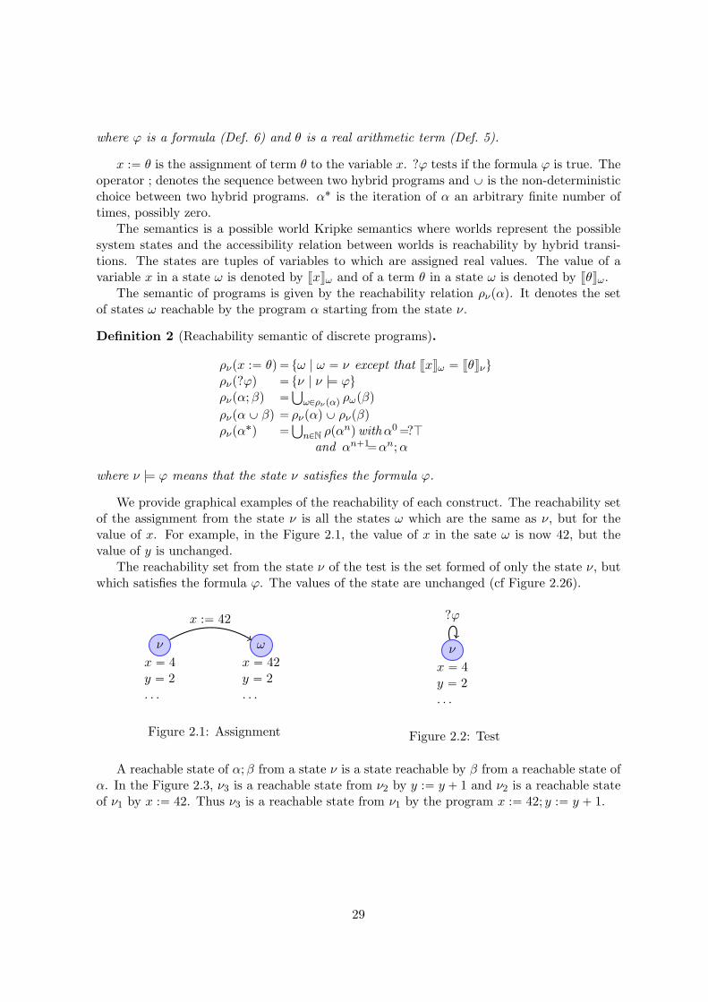
x :“ θ is the assignment of term θ to the variable x. ?ϕ tests if the formula ϕ is true. Theoperator ; denotes the sequence between two hybrid programs and Y is the non-deterministicchoice between two hybrid programs. α˚ is the iteration of α an arbitrary finite number oftimes, possibly zero.

The semantics is a possible world Kripke semantics where worlds represent the possiblesystem states and the accessibility relation between worlds is reachability by hybrid transi-tions. The states are tuples of variables to which are assigned real values. The value of avariable x in a state ω is denoted by vxwω and of a term θ in a state ω is denoted by vθwω.

The semantic of programs is given by the reachability relation ρνpαq. It denotes the setof states ω reachable by the program α starting from the state ν.

Definition 2 (Reachability semantic of discrete programs).

ρνpx :“ θq “ tω | ω “ ν except that vxwω “ vθwνuρνp?ϕq “ tν | ν |ù ϕuρνpα;βq “

Ť

ωPρνpαq ρωpβq

ρνpα Y βq “ ρνpαq Y ρνpβqρνpα˚q “

Ť

nPN ρpαnqwithα0 “?Jand αn`1“αn;α

where ν |ù ϕ means that the state ν satisfies the formula ϕ.

We provide graphical examples of the reachability of each construct. The reachability setof the assignment from the state ν is all the states ω which are the same as ν, but for thevalue of x. For example, in the Figure 2.1, the value of x in the sate ω is now 42, but thevalue of y is unchanged.

The reachability set from the state ν of the test is the set formed of only the state ν, butwhich satisfies the formula ϕ. The values of the state are unchanged (cf Figure 2.26).

ν

x “ 4y “ 2. . .

ω

x “ 42y “ 2. . .

x :“ 42

Figure 2.1: Assignment

ν

x “ 4y “ 2. . .

?ϕ

Figure 2.2: Test

A reachable state of α;β from a state ν is a state reachable by β from a reachable state ofα. In the Figure 2.3, ν3 is a reachable state from ν2 by y :“ y ` 1 and ν2 is a reachable stateof ν1 by x :“ 42. Thus ν3 is a reachable state from ν1 by the program x :“ 42; y :“ y ` 1.

29

ν1

x “ 4y “ 2. . .

ν2

x “ 42y “ 2. . .

ν3

x “ 42y “ 3. . .

x :“ 42 y :“ y ` 1

x :“ 42; y :“ y ` 1

Figure 2.3: Sequence

A reachable state from the state ν by α Y β is either a reachable state of α or of β. Inthe Figure 2.4, ω1 is a reachable state from ν by x :“ 42 and ω2 is a reachable state from ν

by y :“ y ` 1. Thus, ω1 and ω2 are reachable states of x :“ 42 Y y :“ y ` 1.

ν

x “ 4y “ 2. . .

ω1

x “ 42y “ 2. . .

ω2

x “ 4y “ 3. . .

x :“ 42 Y y :“ y ` 1

x :“ 42

y :“ y ` 1

Figure 2.4: Non-deterministic choice

A state ω is reachable from the state ν by α˚ if it is reachable by the program αn whichis n consecutive executions of α. For example, ν2 is reachable by y :“ y ` 1 and ν3 byy :“ y ` 1; y :“ y ` 1. They are both reachable states of py :“ y ` 1q˚.

v1

x “ 4y “ 2. . .

v2

x “ 4y “ 3. . .

v3

x “ 4y “ 4. . .

. . .

py :“ y ` 1q˚

y :“ y ` 1 y :“ y ` 1 y :“ y ` 1

Figure 2.5: Iteration

We can define the program that computes the Fibonacci sequence.

Example 1 (Fibonacci sequence).

Fibonacci fi pFn :“ Fn`1;Fn`1 :“ Fn`2;Fn`2 :“ Fn`1 ` Fnq˚

30

We assume that the formulas Fn “ 0, Fn`1 “ 1 and Fn`2 “ 1 hold at the initialization.

We can also encode a simple speed-controller for a car.

Example 2 (Controller for a car).

`

p?accel; a :“ Aq Y a :“ ´b˘

˚

If the condition accel is true, the car may accelerate by A, but it can always brake by ´b.

Encoding of usual programming structure We retrieve the while and if-then-else

structure with the following encoding. The interested reader can find more encoding in [61, p.167].

if ϕ then α else β ” p?ϕ;αq Y p?�ϕ;βqwhile ϕ do α ” p?ϕ;αq˚; ?�ϕ

2.1.2 Ordinary Differential Equations

In this section, we present the syntax and the semantic of Ordinary Differential Equations(ODEs) in dL. We illustrate it with several examples.

The modeling of physical phenomena is mostly made by the use of differential equationssince the foundational work of Leibniz and Newton. The idea is to consider any infinitesimalchange in an equation to represent continuous motion. In mathematics, the change is madewith respect to an arbitrary variable, but in physics, we are mostly interested by the changewith respect to time. We adopt the convention that the variation of a quantity, representedby x, over the time is denoted by 9x.

Definition 3 (Syntax of differential equation).

9X “ ΘX & H

where H is a formula of dL.

X is vector of variables px1, . . . , xnq and ΘX a vector pΘ1, . . . ,Θnq of terms of real arith-metic. The symbol & stands for a separator between the differential equation and theevolution domain H. It characterizes the domain in which it can evolve; if the formula H isnot true, then the evolution is not considered. For example, the evolution domain of time,represented by the variable t, is t ě 0 since it does not make sense to consider negative timeby convention.

We assume that every differential equation has a solution which is unique. We defineaccordingly the semantic using this solution. We define the reachability for a differentialequation with only one variable, but it is easily generalized for a vector of variables.

Definition 4 (Reachability semantics of differential equation).

ρνp 9x “ θx & Hq “ tfprq | there is a function f : r0, rs Ñ S such thatfptq |ù 9x “ θ and fptq |ù H for every t P r0, rsu

31

S is the set of states. fptq has to be understood as a solution of the differential equation.The reachable states are every point to which the dynamic system can evolve providing thatthe evolution domain still holds.

For example, in the Figure 2.6, ω is a reachable state where the value of x is fp2q, butthe value of y stays unchanged. Another reachable state is the one where the value of x isfp2.1q and the value of y is unchanged. The behavior of an ODE can be understood as anassignment iterated, except that the iteration step is infinitesimal.

ν

x “ fp1q “ 1y “ 2. . .

ω

x “ fp2q “ 4y “ 2. . .

9x “ 2t & t ě 0

t

x

v

w

‚

0

‚

r

fptq

Hx

Figure 2.6: Differential equation

We can model most of physical systems of interest. A limit is the modeling of dynamicsystems which do not admit solution, e.g. Partial Differential Equations (PDEs).

Example 3 (Passing of time).9t “ 1 & t ě 0

t represents the time, and it evolves linearly. We consider also the time to be alwayspositive by convention.

We are able to model more complex systems such as the speed of a car or the water-levelin a tank or in several tanks.

Example 4 (Speed of a car).9x “ v, 9v “ a & v ě 0

where x is the position of the car, v the velocity (speed) of the car and a the acceleration ofthe car.

It is a system of differential equations and we add in the evolution domain v ě 0 becausea speed is always considered positive.

Example 5 (Water-Tank).9wl “ fin ´ fout & wl ě 0

where wl is the water-level, fin is the inlet flow and fout is the outlet flow. We assume thatthe water-level is always positive, i.e. that it is not below the bottom of tank.

Example 6 (Water-Plant). We can represent the water-level of a network of connected water-tanks. For example, if the inlet flow of the second water-tank is the outlet flow of the firstwater-tank and similarly for the second and third water-tank.

32

$

&

%

wl1 “ fin1 ´ fout1wl2 “ fout1 ´ fout2 & wl1 ě 0 ^ wl2 ě 0 ^ wl3 ě 0wl1 “ fout2 ´ fout3

We can model continuous systems and discrete systems, but the very interest of hybridsystems is the interaction of the two. The next section is devoted to several examples of suchinteractions.

2.1.3 Blending discrete and continuous aspects

We present in this subsection several examples of standard hybrid systems. We present thebouncing-ball example where the discrete interaction is not provoked by humans, and the classof computer-controlled systems which are designed by humans. The bouncing-ball exampleis a popular and simple hybrid system where the discrete interaction does not come from acontroller.

Example 7 (Bouncing ball). It models the velocity v and height h of a falling ball. Thediscrete interaction comes from the bouncing on the floor. The ball falls until it touches thefloor (h “ 0), then it bounces back. The velocity of the bouncing back is function of the fallingvelocity moderated by a damping factor c accounting for loss of kinetic energy.

p 9h “ v, 9v “ ´g & h ě 0; ?h “ 0; v :“ ´cvq˚

g is the value of gravity. The differential equation evolves until the height h equals 0.Then, we can pass the test ?h “ 0 and we assign the value ´cv to the velocity which accountsfor the bouncing. The iteration constructs allows to consider an arbitrary large number ofsuch sequences.

Modeling Computer-Controlled System Computer-Controlled systems are frequentlyencountered and regroup systems where a continuous behavior, so-called plant, is monitoredby a controller, in this case a computer with sensors and actuators. The controller is triggeredby a timing condition. It executes at least every ∆ units of time.

Example 8 (Time triggered).

ppp?accel; a :“ Aq Y a :“ ´bq; tCtrl :“ t; (Control)

9x “ v, 9v “ a, 9t “ 1 & v ě 0 ^ t ě 0 ^ t ´ tCtrl ď ∆q˚ (Plant)

We are now able to model hybrid systems in dL, the next step is to express propertiesthat such systems should satisfy, for example that the water-level of the tank is within someinterval.

2.2 Expressing Properties in dL

First Order Real Arithmetic is a first-order logic with terms of Real Arithmetic. It allowsto represent polynomial terms, but not trigonometric or exponential terms. We present it inSubsection 2.2.1. Formulas in dL are First Order Real Arithmetic formulas augmented withthe modality r.s. rαsϕ means that the formula ϕ holds for every executions of the hybridprogram α. We detail it in Subsection 2.2.2.

33

2.2.1 First-order Real Arithmetic

We define the syntax of terms of Real Arithmetic and their semantic. We define also thesyntax of formulas of First-Order Real Arithmetic and their semantic. We present examples ofproperties that we can express and state the surprising result of Tarski about the decidabilityof the First Order Real Arithmetic.

Definition 5 (Terms of Real Arithmetic).

θ1, θ2 ::“ x | 0 | 1 | θ1 ` θ2 | θ1 ´ θ2 | θ1 ˆ θ2 | θ1 ˜ θ2

The variables x are valuated in R. We have the usual semantic for the operators `, ´, ˆ, ˜.It allows polynomials, e.g. x`x2 `x3, but does not allow more complex expressions like log-arithms, exponential or trigonometric functions. The valuation of a term θ at a state ν isdenoted by vθwν .

We define the formulas of Real Arithmetic by adding comparison operators between terms,ă,ď,“,ě,ą, and logical connectives.

Definition 6 (Formulas of First-Order Real Arithmetic).

ϕ,ψ ::“ θ1 „ θ2 | �ϕ | ϕ ^ ψ | ϕ _ ψ | ϕ Ñ ψ | @xϕ | Dxϕ | Kwhere „ P tă,ď,“,ě,ąu

We define the semantic only for the connectives „, K, ^, Ñ and @. The others can bededuced from it.

Definition 7 (Semantic of formulas). The satisfiability of formulas is provided for any stateν:

ν |ù θ1 „ θ2 ô vθ1wν „ vθ2wν , „ P tă,ď,“,ě,ąuν |ù ϕ ^ ψ ô ν |ù ϕ and ν |ù ψ

ν |ù ϕ Ñ ψ ô if ν |ù ϕ then ν |ù ψ

ν |ù @x ϕ ô @ω such that @z, z ‰ x ñ vzwω “ vzwν we have ω |ù ϕ

ν * K

We can express that a quantity x is within an interval x P r´42, 42s as ´42 ď x^ x ď 42.

Example 9 (Water-level property). We require that the water-level wl in the water-tankstays between 3 and 7 : wl ě 3 ^ wl ď 7. It means that there is always a sufficient outletflow, and that it does not overflow.

Tarski Algebra Surprisingly, contrary to the First-Order Natural Arithmetic, the First-Order Real Arithmetic is decidable, it is the so-called Tarski’s Miracle [122]. The reasoncomes from the sign conservation between two zeros of a polynomial in R, which is not thecase for the natural arithmetic.

Theorem (Tarski’s Miracle). The First-Order Real Arithmetic is decidable, with a complexitydoubly exponential in time.

Despite of the decidability result, it is still complex to prove formulas of Real Arithmetic.Much progress have been made these last decades with efficient SMT solvers like Z3 [39].

We want to ultimately prove that a system satisfies a property for all its executions, i.e.that it is an invariant. For example, we want that the water-level wl stays always between 3and 7. We need modality to express such statement.

34

2.2.2 A modal logic

We present in this section the syntax and the semantic of the modal operator r.s. It allowsto express safety properties of a system. We show how to encode the notion of contract. Wepresent also the modal operator x.y to express liveness properties.

Modal operator r.s We add to the definition of formula of the Real Arithmetic the modalityrαsϕ which means that “for every reachable state by α, the formula ϕ is true”.

Definition 8 (Formulas of dL).

ϕ,ψ ::“ rαsϕ | θ1 „ θ2 | �ϕ | ϕ ^ ψ | ϕ _ ψ | ϕ Ñ ψ | @xϕ | Dxϕ | Kwhere „ P tă,ď,“,ě,ąu

where α is a hybrid program (Def. 1 and Def. 3). We retrieve the Real Arithmetic formulasdefined in Def. 6.

The semantic is defined as follows.

Definition 9 (Semantic).

ν |ù rαsϕ ô @ω P ρνpαq, ω |ù ϕ

The modality r.s articulates the behavior of hybrid programs and formulas of Real Arith-metic.

Example 10. The formula r 9t “ 1, 9d “ e, 9e “ ´d & t ě 0sd2 ` e2 ď r2 means that theproperty d2 ` e2 ď r2 is always true for any execution of 9t “ 1, 9d “ e, 9e “ ´d.

Example 11 (Satisfaction of the water-level property). The formula rWater ´ tanks3 ď

wl ď 7 means that the water-tank system satisfies the water-level property.

Remark 1. In rαsϕ, the formula ϕ is required to hold only at the end state of the execution.For example, the formula rx :“ ´1;x :“ 42sx ě 0 is valid although x is negative in the middleof the execution. An extension of dL with temporal constructs has been proposed to take intoaccount the intermediary states [96]. However, most of systems of interest are modeled as aiterated hybrid program α‹. The semantic of the iteration implies that ϕ will be required tohold at every possible executions of α, including the initial state since it is allowed to havezero iteration.

Assume-Guarantee reasoning The Assume-Guarantee reasoning is widely used to ex-press properties under which a system works and the properties guaranteed. It consists inthe specification of formulas which hold for the inputs, the assumptions, and for the outputs,the guarantees. A contract is the 2-tuple of assumptions and guarantees.

Definition 10 (Contract in dL). Let α be a hybrid program, A the assumptions under whichα behaves and G the guarantees provided. A contract is represented by the formula

A Ñ rαsG

Example 12. We want to ensure that under the assumption that Fn “ 0^Fn`1 “ 1^Fn`2 “1, the Fibonacci program in the Example 1 satisfies the property Fn`2 “ Fn`1 ` Fn. It isrepresented by the formula

pFn “ 0 ^ Fn`1 “ 1 ^ Fn`2 “ 1q Ñ rFibonaccisFn`2 “ Fn`1 ` Fn

35

Liveness properties The modality r.s allows to express safety properties, i.e. true for everyexecution of the system under consideration. We may be interested by liveness properties,i.e. properties which have to hold for at least one execution of the system under consideration.The notion of liveness in dL differs from the one in LTL or CTL. In the former, it is “thereis one execution of the system for which the desired property holds”, but for the latter, itis that “for every execution of a system, there is a possible execution which leads to a statewhere the property is true”.

The liveness modality x.y is the dual of the safety modality.

Definition 11 (Syntax of x.y).xαyϕ fi �rαs�ϕ

From the semantics of r.s, we can deduce the semantics of x.y.

Definition 12 (Semantics of x.y).

ν |ù xαyϕ ô Dω P ρνpαq, ω |ù ϕ

Conclusion We have presented how to model hybrid systems in dL (Section 2.1) and thedefinition of formulas of dL (Section 2.2). We have also shown how to associate properties tohybrid programs. In order to verify that a hybrid program satisfies its properties, we needa proof system. The next section is devoted to the presentation of the rules of the sequentcalculus of dL.

2.3 Proving properties in dL

This section is devoted to the detailed presentation of the proof system of dL. We presentbriefly the general characteristics and definitions of sequent calculus in Subsection 2.3.1. InSubsection 2.3.2, we present proof rules to prove First-Order Real Arithmetic formulas. Wepresent structural rules in Subsection 2.3.3. Theses rules are used to clarify proofs. InSubsection 2.3.4, we present specific rules to reason on the execution of hybrid programs.

2.3.1 Generalities on sequent calculus

We present in this section generalities on sequent calculus along with the definition of a sequentand how to read proof rules. We also state the definition of soundness and completeness fora proof system.

A sequent calculus is a deductive proof calculus which relies on proof rules. It is widelyused to perform and represent proofs. Sequent calculus exhibits interesting aspects such asthe fact that it is a syntactic approach and thus amenable to automation. It is also easy toimplement proof strategies to augment its usability. Lastly, it is easily extendable to take intoaccount other theories. Several theorem provers use sequents to represent proof reasoning,for example Coq [36], B-method [3], KeY [6].

It is characterized by the use of sequents Γ $ ∆ where Γ (resp. ∆) is a finite set of formulasγ1, . . . , γn (resp. δ1, . . . , δm). The meaning is “the conjunction of formulas in Γ implies thedisjunction of formulas in ∆” and is thus equivalent to the formula

Ź

1ďiďn

γi ÑŽ

1ďjďm

δj .

36

Premise 1 . . . Premise nConclusion

Given a sequent, we can derive a proof tree by the use of proof rules. It is composed of nsequents above the bar, called premises, and one sequent under the bar, called the conclusion.The semantic is “If the premises are valid, the conclusion is valid”.

The set of proof rules is the sequent calculus. An important property is the soundness ofrules, i.e. that if the premises of a proof rule are valid, then the conclusion is valid.

Definition 13 (Soundness). A sequent calculus is sound if all its proof rules are sound.Equivalently, for any formula ϕ, if we have a derivation (denoted by $ ϕ), then the formulais valid (denoted by |ù ϕ).

It means that every formula proved with a sound sequent calculus is semantically valid.It links a syntactical and mechanical procedure with a semantic meaning. The converse isthe completeness property. Every valid formula can be proved within the sequent calculus.

Definition 14 (Completeness). A sequent calculus is complete if for any valid formula ϕ,i.e. |ù ϕ, we have a derivation, i.e. $ ϕ.

A sequent calculus for a logical theory which exhibits both properties implies that thetheory is decidable.

2.3.2 First Order Real Arithmetic

We present the rules to handle First-Order Real Arithmetic formulas. We define closing ruleswhich are leaves of a proof tree, then propositional rules which are for logical connectives �,Ñ, ^ and _. We present quantifier rules for quantified formulas.

Closing rules Closing rules are rules which do not have any premises. They are used toclose the proof tree, i.e. they are leaves. We present them in the Figure 2.7.

KΓ,K $ ∆

JΓ $ J,∆

axΓ,ϕ $ ϕ,∆

Real Arithmetic QEΓ $ θ1 „ θ2,∆

Figure 2.7: Closing rules

The axiom rule ax means that “If ϕ is known and we try to prove ϕ, then the proof isvalid”. The rule K is the ex falso quod libet reasoning; if we have false in the hypothesis, wecan derive every formula, and thus our current goal. The rule J is the inverse. We try toprove that the goal J is true, which is the case by definition.

The rule QE is slightly different. It is the rule to handle the validity of terms of realarithmetic. They are are premises, but we do not consider them because we assume thatthere is an external procedure to handle them. In KeYmaera X, it is achieved by Z3. Thename QE stands for Quantifier Elimination. A first-order theory admits quantifier elimination

37

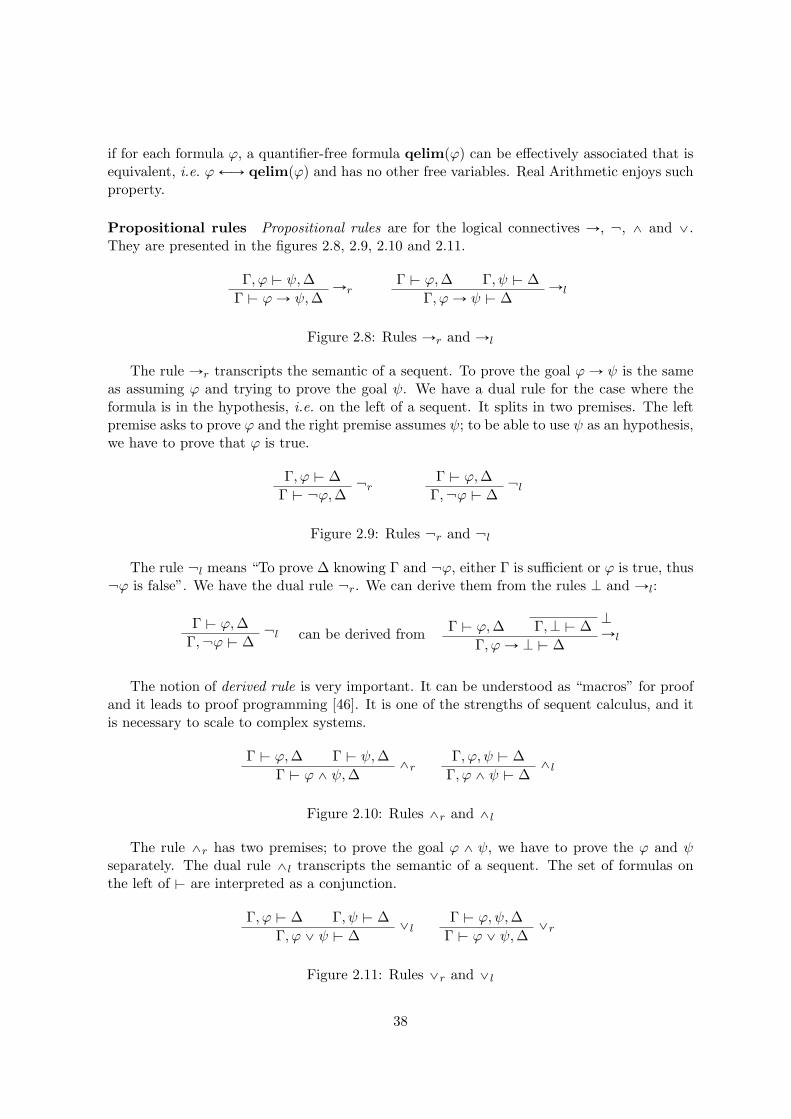
if for each formula ϕ, a quantifier-free formula qelimpϕq can be effectively associated that isequivalent, i.e. ϕ ÐÑ qelimpϕq and has no other free variables. Real Arithmetic enjoys suchproperty.

Propositional rules Propositional rules are for the logical connectives Ñ, �, ^ and _.They are presented in the figures 2.8, 2.9, 2.10 and 2.11.

Γ,ϕ $ ψ,∆ ÑrΓ $ ϕ Ñ ψ,∆

Γ $ ϕ,∆ Γ,ψ $ ∆ ÑlΓ,ϕ Ñ ψ $ ∆

Figure 2.8: Rules Ñr and Ñl

The rule Ñr transcripts the semantic of a sequent. To prove the goal ϕ Ñ ψ is the sameas assuming ϕ and trying to prove the goal ψ. We have a dual rule for the case where theformula is in the hypothesis, i.e. on the left of a sequent. It splits in two premises. The leftpremise asks to prove ϕ and the right premise assumes ψ; to be able to use ψ as an hypothesis,we have to prove that ϕ is true.

Γ,ϕ $ ∆�r

Γ $ �ϕ,∆

Γ $ ϕ,∆�l

Γ,�ϕ $ ∆

Figure 2.9: Rules �r and �l

The rule �l means “To prove ∆ knowing Γ and �ϕ, either Γ is sufficient or ϕ is true, thus�ϕ is false”. We have the dual rule �r. We can derive them from the rules K and Ñl:

Γ $ ϕ,∆�l

Γ,�ϕ $ ∆can be derived from

Γ $ ϕ,∆K

Γ,K $ ∆ ÑlΓ,ϕ Ñ K $ ∆

The notion of derived rule is very important. It can be understood as “macros” for proofand it leads to proof programming [46]. It is one of the strengths of sequent calculus, and itis necessary to scale to complex systems.

Γ $ ϕ,∆ Γ $ ψ,∆^r

Γ $ ϕ ^ ψ,∆

Γ,ϕ,ψ $ ∆^l

Γ,ϕ ^ ψ $ ∆

Figure 2.10: Rules ^r and ^l

The rule ^r has two premises; to prove the goal ϕ ^ ψ, we have to prove the ϕ and ψ

separately. The dual rule ^l transcripts the semantic of a sequent. The set of formulas onthe left of $ are interpreted as a conjunction.

Γ $ ϕ,ψ,∆_r

Γ $ ϕ _ ψ,∆

Γ,ϕ $ ∆ Γ,ψ $ ∆_l

Γ,ϕ _ ψ $ ∆

Figure 2.11: Rules _r and _l

38

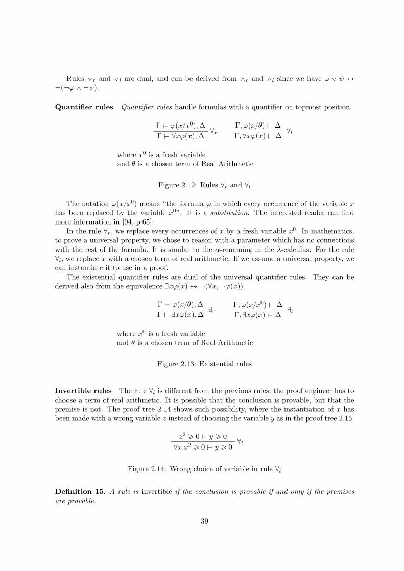
Rules _r and _l are dual, and can be derived from ^r and ^l since we have ϕ _ ψ Ø�p�ϕ ^ �ψq.

Quantifier rules Quantifier rules handle formulas with a quantifier on topmost position.

Γ $ ϕpx{x0q,∆@r

Γ $ @xϕpxq,∆

Γ,ϕpx{θq $ ∆@l

Γ,@xϕpxq $ ∆

where x0 is a fresh variableand θ is a chosen term of Real Arithmetic

Figure 2.12: Rules @r and @l

The notation ϕpx{x0q means “the formula ϕ in which every occurrence of the variable x

has been replaced by the variable x0”. It is a substitution. The interested reader can findmore information in [94, p.65].

In the rule @r, we replace every occurrences of x by a fresh variable x0. In mathematics,to prove a universal property, we chose to reason with a parameter which has no connectionswith the rest of the formula. It is similar to the α-renaming in the λ-calculus. For the rule@l, we replace x with a chosen term of real arithmetic. If we assume a universal property, wecan instantiate it to use in a proof.

The existential quantifier rules are dual of the universal quantifier rules. They can bederived also from the equivalence Dxϕpxq Ø �p@x,�ϕpxqq.

Γ $ ϕpx{θq,∆Dr

Γ $ Dxϕpxq,∆

Γ,ϕpx{x0q $ ∆Dl

Γ, Dxϕpxq $ ∆

where x0 is a fresh variableand θ is a chosen term of Real Arithmetic

Figure 2.13: Existential rules

Invertible rules The rule @l is different from the previous rules; the proof engineer has tochoose a term of real arithmetic. It is possible that the conclusion is provable, but that thepremise is not. The proof tree 2.14 shows such possibility, where the instantiation of x hasbeen made with a wrong variable z instead of choosing the variable y as in the proof tree 2.15.

z2 ě 0 $ y ě 0@l

@x.x2 ě 0 $ y ě 0

Figure 2.14: Wrong choice of variable in rule @l

Definition 15. A rule is invertible if the conclusion is provable if and only if the premisesare provable.

39

y2 ě 0 $ y ě 0@l

@x.x2 ě 0 $ y ě 0

Figure 2.15: Right choice of variable in rule @l

Invertible rules play an important role into the automation of proof. They can be appliedsafely since they do not change the provability of the considered formula, and a possibleheuristic is to favor their use. The propositional rules and the rule @r are invertible, but therule @l is not. The rules presented in the following subsection are not invertible.

Theorem (Soundness theorem). The rules presented in figures 2.7 to 2.13 are sound.

Proof. We detail the case of the rule ^r. The others can be found in [98, p. 97]. We reasonby induction on the structure of the formula. To prove that ^r is sound, we assume that eachpremise is valid. We prove then that the conclusion is valid.

Assume that |ù ϕ _ ∆ and |ù ψ _ ∆. We want to prove |ù pϕ ^ ψq _ ∆. We obtain it byapplication of the definition of the semantic of ^ (def. 7).

Conclusion The rules presented in figures 2.7 to 2.13 are sufficient to prove validity ofFirst-Order Real Arithmetic formulas. For example, we can prove the validity of the formula`

pp Ñ qq^pr Ñ sq^pp_rq˘

Ñ pq_sq (cf proof tree 2.16) or of the formula x “ 3 Ñ @x, x2 ě 0(cf proof tree 2.17).

axr Ñ s, p $ p, q, s

axr Ñ s, q $ q, s Ñl

p Ñ q, r Ñ s, p $ q, sSimilar to left branchp Ñ q, r Ñ s, r $ q, s

_lp Ñ q, r Ñ s, p _ r $ q, s

_rp Ñ q, r Ñ s, p _ r $ pq _ sq

^lp Ñ q, pr Ñ sq ^ pp _ rq $ pq _ sq

^lpp Ñ qq ^ pr Ñ sq ^ pp _ rq $ pq _ sq

Ñr$

`

pp Ñ qq ^ pr Ñ sq ^ pp _ rq˘

Ñ pq _ sq

Figure 2.16: Proof tree of the formula`

pp Ñ qq ^ pr Ñ sq ^ pp _ rq˘

Ñ pq _ sq

For the proof of`

pp Ñ qq ^ pr Ñ sq ^ pp_ rq˘

Ñ pq _ sq, we apply mechanically the proofrules and there is no need for a human intervention. This proof may be perform automatically.

Real Arithmetic QEx “ 3 $ x20 ě 0

@rx “ 3 $ @x.x2 ě 0 Ñr

$ x “ 3 Ñ @x.x2 ě 0

Figure 2.17: Proof tree of the formula x “ 3 Ñ @x.x2 ě 0

40

For the proof of x “ 3 Ñ @x.x2 ě 0, we apply the logical rule Ñr and @r to obtain aReal Arithmetic term x20 ě 0 to prove. It is a well-known result that the square of a value isalways positive. It is thus closed by the rule QE.

2.3.3 Structural rules

We present in this subsection structural rules weakening and cut. they do not change thepower of the proof system; a provable formula is still provable without theses rules. But theyare important to structure a proof, hence for the scalability of proof of complex systems. Wepresent how we can derive the modus ponens rule with the cut rule.

Weakening rules In the left branch of the proof tree 2.16, the formulas r Ñ s in thehypothesis and s in the goal are not used in the proof, and diminish the readability of aproof. We introduce the weakening rules to handle this problem.

Γ $ ∆Wr

Γ $ ϕ,∆

Γ $ ∆Wl

Γ,ϕ $ ∆

Figure 2.18: Rules Wr and Wl

The rule Wl allows to discard a formula in hypothesis. It is not invertible. The sequent inthe conclusion can be valid, but the resulting sequent in the premise may not be. Nevertheless,the rule is still sound since, if we are able to prove a goal with a set of hypothesis Γ, we areable to prove it with one additional hypothesis. The rule Wr is the dual.

Weakening rules are intended to improve readability, but are also precious allies in theconduction of proof in an interactive theorem prover. By discarding useless formulas, wenarrow the proof search and help the computer to automatically prove a goal.

Cut rule The Cut rule allows to introduce new formulas in a proof to strengthen hypotheses.It is the transcript of the use of lemmas in a standard mathematical proof.

Γ,ϕ $ ∆ Γ $ ϕ,∆Cut

Γ $ ∆

Figure 2.19: Cut rule

Examples Let us assume that we want to prove the validity of the formula x ě 0 Ñ x`y2 ě

0, and we already have a proof Π of the formula @x, x2 ě 0 (cf proof tree 2.17). We cut thisformula in the proof tree to achieve our proof tree 2.20.

It is a very important rule for the structuring of proofs. It allows to focus on one part ofthe problem. The rule Cut is also very useful to define derived rules.

The modus ponens rule By using the Cut rule, we can define a specific proof rule for theModus Ponens (MP) reasoning (cf Fig. 2.21).

If we know ϕ Ñ ψ and ϕ, then we can deduce ψ. The proof rule derives from the prooftree 2.22.

41

Real Arithmetic QEy2 ě 0, x ě 0 $ x ` y2 ě 0

@l@x.x2, x ě 0 $ x ` y2 ě 0

Π

$ @x.x2 ě 0Wl, Wr

x ě 0 $ @x.x2 ě 0, x ` y2 ě 0Cut

x ě 0 $ x ` y2 ě 0 Ñr$ x ě 0 Ñ x ` y2 ě 0

Figure 2.20: Proof tree of x ě 0 Ñ x ` y2 ě 0

Γ $ ϕ Ñ ψ,∆ Γ $ ϕ,∆MP

Γ $ ψ,∆

Figure 2.21: Modus Ponens rule.

axΓ,ϕ $ ϕ,ψ,∆

axΓ,ψ $ ψ,∆

Γ,ϕ Ñ ψ,ϕ $ ψ,∆

Γ $ ϕ Ñ ψ,∆Wl

Γ,ϕ $ ϕ Ñ ψ,∆Wr

Γ,ϕ $ ϕ Ñ ψ,ψ,∆Cut

Γ,ϕ $ ψ,∆

Γ $ ϕ,∆Wr

Γ $ ϕ,ψ,∆Cut

Γ $ ψ,∆

Figure 2.22: Proof tree for the derivation of the Modus Ponens rule

We have covered the proof rules for the standard logical connectives. The next step is toconsider proof rules to reason about hybrid programs.

2.3.4 Hybrid program rules

This subsection regroups the rules used to reason on runs of a hybrid program. We recallthat rαsϕ means that “the formula ϕ holds for every run of the hybrid program α”.

Assignment The assignment rule r:“s performs the change of value in the formula ϕ byreplacing every occurrence of x in ϕ by the term θ.

Γ $ ϕpθq,∆r:“s

Γ $ rx :“ θsϕpxq,∆

Figure 2.23: r:“s rule

We have to be careful with the phenomenon of capture of variables as in the β-reduction inλ-calculus. We need a bound variable renaming process similar to α-conversion. Intuitively,bound variables are variables that can change over the execution of a given system.

Bound variable renaming

Definition 16 (Bound variable). A variable x is bound if it is under the scope of a quantifier,e.g. @xϕpxq or Dxϕpxq, or if it is in the scope of a modality where x is the variable assigned,

42

e.g. x :“ θ, or the variable derived, e.g. 9x “ θ.

Bound variables of a hybrid program α are variables that depend of the execution of α.The renaming of bound variables is necessary to ensure soundness. For example, we have thetwo proof trees 2.24 and 2.25, one without taking care of renaming bound variables, the otherone with renaming. The first one is obviously unsound and does not match the semantic ofthe assignment.

x ą 0, z ą 0 $ z ` z ą z ` zr:“s

x ą 0, z ą 0 $ rz :“ z ` zsz ą zr:“s

x ą 0, z ą 0 $ rx :“ zsrz :“ z ` xsz ą x

Figure 2.24: No bound variable renaming

In Figure 2.24, the value of the variable z assigned to x is not the same as the variablez in the second modality. It leads to a proof stuck, and there is thus no means to prove aformula clearly valid.

Real Arithmetic QEx ą 0, z ą 0 $ z ` z ą z

r:“sx ą 0, z ą 0 $ ru :“ z ` zsu ą z

r:“sx ą 0, z ą 0 $ rx :“ zsru :“ z ` xsu ą x

Renaming z � ux ą 0, z ą 0 $ rx :“ zsrz :“ z ` xsz ą x

Figure 2.25: With bound variable renaming

In Figure 2.25, we rename the bound variable z in the second modality by a fresh variableu to avoid confusion. The renaming step will not be made explicit in the next sections, butis performed “on the fly”.

Test, sequence and non-deterministic choice The rule r?s is equivalent to try to proveψ under the assumption ϕ. It amounts to add ϕ as an hypothesis for the proof.

Γ $ ϕ Ñ ψ,∆r?s

Γ $ r?ϕsψ,∆

Figure 2.26: Rules for the test

The rule r; s dissociates the two programs α and β.

Γ $ rαsrβsϕ,∆r; s

Γ $ rα;βsϕ,∆

Figure 2.27: Rules for the sequence

43

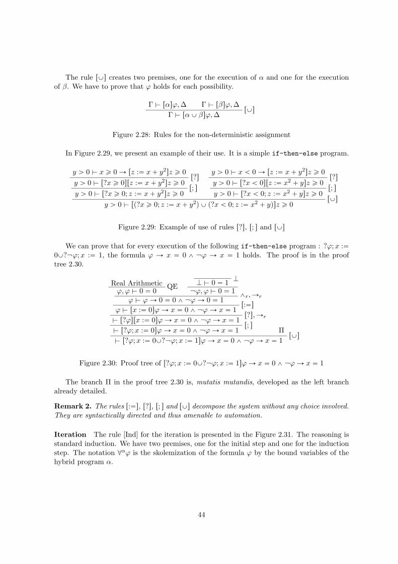
The rule rYs creates two premises, one for the execution of α and one for the executionof β. We have to prove that ϕ holds for each possibility.

Γ $ rαsϕ,∆ Γ $ rβsϕ,∆rYs

Γ $ rα Y βsϕ,∆

Figure 2.28: Rules for the non-deterministic assignment

In Figure 2.29, we present an example of their use. It is a simple if-then-else program.

y ą 0 $ x ě 0 Ñ rz :“ x ` y2sz ě 0r?s

y ą 0 $ r?x ě 0srz :“ x ` y2sz ě 0r; s

y ą 0 $ r?x ě 0; z :“ x ` y2sz ě 0

y ą 0 $ x ă 0 Ñ rz :“ x ` y2sz ě 0r?s

y ą 0 $ r?x ă 0srz :“ x2 ` ysz ě 0r; s

y ą 0 $ r?x ă 0; z :“ x2 ` ysz ě 0rYs

y ą 0 $ rp?x ě 0; z :“ x ` y2q Y p?x ă 0; z :“ x2 ` yqsz ě 0

Figure 2.29: Example of use of rules r?s, r; s and rYs

We can prove that for every execution of the following if-then-else program : ?ϕ;x :“0Y?�ϕ;x :“ 1, the formula ϕ Ñ x “ 0 ^ �ϕ Ñ x “ 1 holds. The proof is in the prooftree 2.30.

Real Arithmetic QEϕ,ϕ $ 0 “ 0

KK $ 0 “ 1

�ϕ,ϕ $ 0 “ 1^r,Ñr

ϕ $ ϕ Ñ 0 “ 0 ^ �ϕ Ñ 0 “ 1r:“s

ϕ $ rx :“ 0sϕ Ñ x “ 0 ^ �ϕ Ñ x “ 1r?s,Ñr

$ r?ϕsrx :“ 0sϕ Ñ x “ 0 ^ �ϕ Ñ x “ 1r; s

$ r?ϕ;x :“ 0sϕ Ñ x “ 0 ^ �ϕ Ñ x “ 1 ΠrYs

$ r?ϕ;x :“ 0Y?�ϕ;x :“ 1sϕ Ñ x “ 0 ^ �ϕ Ñ x “ 1

Figure 2.30: Proof tree of r?ϕ;x :“ 0Y?�ϕ;x :“ 1sϕ Ñ x “ 0 ^ �ϕ Ñ x “ 1

The branch Π in the proof tree 2.30 is, mutatis mutandis, developed as the left branchalready detailed.

Remark 2. The rules r:“s, r?s, r; s and rYs decompose the system without any choice involved.They are syntactically directed and thus amenable to automation.

Iteration The rule [Ind] for the iteration is presented in the Figure 2.31. The reasoning isstandard induction. We have two premises, one for the initial step and one for the inductionstep. The notation @αϕ is the skolemization of the formula ϕ by the bound variables of thehybrid program α.

44

Γ $ ϕ,∆ Γ $ @αpϕ Ñ rαsϕq,∆[Ind]

Γ $ rα˚sϕ,∆

Initial step Induction step

Figure 2.31: Rule [Ind]

To prove that a formula ϕ holds for every run of α‹, we have to prove that it holds forzero iteration, the initial step, and that if it holds an arbitrary number n of iterations, thenit holds for the next iteration, the induction step.

The skolemization of a formula ϕ by a set of variables tx1, . . . , xnu is the addition ofuniversal quantification over these variables in front of ϕ, i.e. @x1, . . .@xnϕ. It is a necessaryabstraction to ensure soundness. If we do not add it, we can prove obviously false formulasas for example x “ 1 Ñ rpx :“ x ´ 1q˚sx ě 0 (proof tree 2.32).

Real Arithmetic QEx “ 1 $ x ě 0

Real Arithmetic QEx “ 1 $ x ´ 1 ě 0

Wlx “ 1, x ě 0 $ x ´ 1 ě 0r:“s

x “ 1, x ě 0 $ rx :“ x ´ 1sx ě 0Ñr

x “ 1 $ x ě 0 Ñ rx :“ x ´ 1sx ě 0[Ind]

x “ 1 $ rpx :“ x ´ 1q˚sx ě 0Ñr

$ x “ 1 Ñ rpx :“ x ´ 1q˚sx ě 0

Figure 2.32: Incorrect proof without skolemisation

In the Figure 2.32, the problem comes from that we can use the formula x “ 1 to concludethe induction step, but it is the initial value of x.

Fibonacci We can prove that our implementation of Fibonacci (Example 1) satisfiesthe property Fn`2 “ Fn`1 ` Fn. We use the following notations:

• Fibonacci fi pbodyq˚

• where body fi Fn :“ Fn`1;Fn`1 :“ Fn`2;Fn`2 :“ Fn`1 ` Fn

• Init fi Fn “ 0, Fn`1 “ 1, Fn`2 “ 1

• ϕ fi Fn`2 “ Fn`1 ` Fn

Our goal is to exhibit a proof tree of the sequent Init $ rFibonaccisϕ.

Πinit

Init $ ϕ

ΠStep

Init $ @Fn, Fn`1, Fn`2pϕ Ñ rbodysϕq[Ind]

Init $ rpbodyq˚sϕ

Figure 2.33: Proof tree for Fibonacci

45

We apply the induction rule [Ind] and it results in two premises: ΠInit and ΠStep. Wehandle them separately in their respective branches 2.34 and 2.35.

Real Arithmetic QEFn “ 0, Fn`1 “ 1, Fn`2 “ 1 $ 1 “ 1 ` 0

Evaluation of Fn, Fn`1 and Fn`2Fn “ 0, Fn`1 “ 1, Fn`2 “ 1 $ Fn`2 “ Fn`1 ` Fn

Init $ ϕ

Figure 2.34: Branch ΠInit

For the initial step (branch Πinit), we verify that ϕ holds initially, i.e. if it is true afterzero execution of the system. We just have to replace the variables Fn, Fn`1 and Fn`2 in theright-hand side by their values in the left-hand side. We can conclude by trivial arithmetic.

ax$ F 0

n`2 ` F 0n`1 “ F 0

n`2 ` F 0n`1

r; s, r:“s$ rF 1

n`2 :“ F 0n`2 ` F 0

n`1sF 1n`2 “ F 0

n`2 ` F 0n`1

r; s, r:“s$ rF 1

n`1 :“ F 0n`2;F

1n`2 :“ F 1

n`1 ` F 0n`1sF 1

n`2 “ F 1n`1 ` F 0

n`1r:“s

$ rF 0n :“ F 0

n`1srF 1n`1 :“ F 0

n`2;F1n`2 :“ F 1

n`1 ` F 0nsϕ1

Wl, r; sϕ0 $ rF 0

n :“ F 0n`1;F

1n`1 :“ F 0

n`2;F1n`2 :“ F 1

n`1 ` F 0nsϕ1

Renamingϕ0 $ rF 0

n :“ F 0n`1;F

0n`1 :“ F 0

n`2;F0n`2 :“ F 0

n`1 ` F 0nsϕ0

Wl, ÑrInit $ ϕ0 Ñ rbody0sϕ0

@rInit $ @Fn, Fn`1, Fn`2pϕ Ñ rbodysϕq

Figure 2.35: Branch ΠStep

For the induction step (branch ΠStep), we apply the rule @r, and thus replace everyoccurrence of variables Fn, Fn`1 and Fn`2 by F 0

n , F0n`1 and F 0

n`2 which are assumed fresh.body0 (resp. ϕ0) is the program body (resp. formula ϕ) where this replacement has been made.We discard then the hypothesis Init which brings no information on the new variables andpass ϕ0 in hypothesis by the use of the rule Ñr. We rename the variables to avoid confusionfor the multiple applications of rule r:“s.

We deconstruct then the body with the rules r; s and r:“s until we obtain the formulaF 0n`2 ` F 0

n`1 “ F 0n`2 ` F 0

n`1. We conclude by the rule ax.

Generalization The rule [Gen] allows to replace the invariant ψ by another invariant ϕ ifwe prove that ϕ is stronger that ψ.

Γ $ rαsϕ,∆ Γ $ @αpϕ Ñ ψq,∆[Gen]

Γ $ rαsψ,∆

Figure 2.36: [Gen] rule

The skolemization in the right premise of the rule presented in Figure 2.36 is for soundnesspurposes as the rule in [Ind] (cf Fig. 2.31).

46

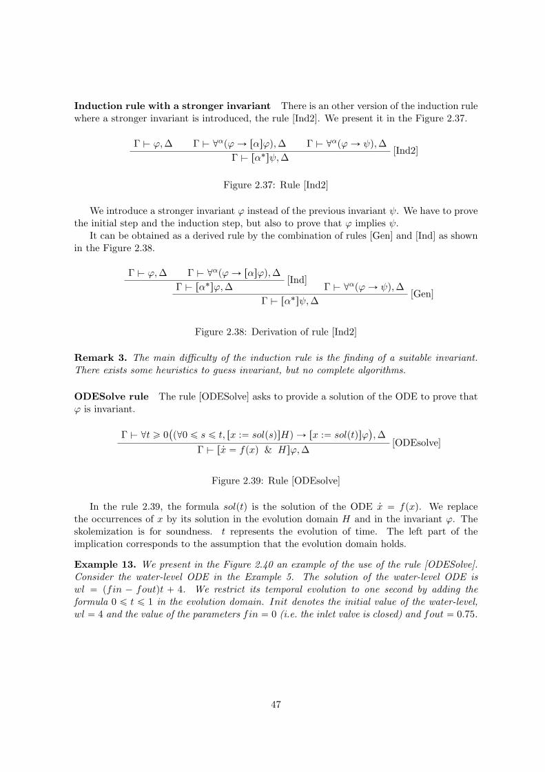
Induction rule with a stronger invariant There is an other version of the induction rulewhere a stronger invariant is introduced, the rule [Ind2]. We present it in the Figure 2.37.

Γ $ ϕ,∆ Γ $ @αpϕ Ñ rαsϕq,∆ Γ $ @αpϕ Ñ ψq,∆[Ind2]

Γ $ rα˚sψ,∆

Figure 2.37: Rule [Ind2]

We introduce a stronger invariant ϕ instead of the previous invariant ψ. We have to provethe initial step and the induction step, but also to prove that ϕ implies ψ.

It can be obtained as a derived rule by the combination of rules [Gen] and [Ind] as shownin the Figure 2.38.

Γ $ ϕ,∆ Γ $ @αpϕ Ñ rαsϕq,∆[Ind]

Γ $ rα˚sϕ,∆ Γ $ @αpϕ Ñ ψq,∆[Gen]

Γ $ rα˚sψ,∆

Figure 2.38: Derivation of rule [Ind2]

Remark 3. The main difficulty of the induction rule is the finding of a suitable invariant.There exists some heuristics to guess invariant, but no complete algorithms.

ODESolve rule The rule [ODESolve] asks to provide a solution of the ODE to prove thatϕ is invariant.

Γ $ @t ě 0`

p@0 ď s ď t, rx :“ solpsqsHq Ñ rx :“ solptqsϕ˘

,∆[ODEsolve]

Γ $ r 9x “ fpxq & Hsϕ,∆

Figure 2.39: Rule [ODEsolve]

In the rule 2.39, the formula solptq is the solution of the ODE 9x “ fpxq. We replacethe occurrences of x by its solution in the evolution domain H and in the invariant ϕ. Theskolemization is for soundness. t represents the evolution of time. The left part of theimplication corresponds to the assumption that the evolution domain holds.

Example 13. We present in the Figure 2.40 an example of the use of the rule [ODESolve].Consider the water-level ODE in the Example 5. The solution of the water-level ODE iswl “ pfin ´ foutqt ` 4. We restrict its temporal evolution to one second by adding theformula 0 ď t ď 1 in the evolution domain. Init denotes the initial value of the water-level,wl “ 4 and the value of the parameters fin “ 0 (i.e. the inlet valve is closed) and fout “ 0.75.

47

Real Arithmetic QEInit,@s 0 ď s ď 1 $ pfin ´ foutqt ` 4 ď 7

ÑrInit $ p@s 0 ď s ď 1q Ñ pfin ´ foutqt ` 4 ď 7

@rInit $ @t ě 0

`

p@s 0 ď s ď 1q Ñ pfin ´ foutqt ` 4 ď 7˘

r:“s, r:“sInit $ @t ě 0

`

p@srt :“ ss0 ď t ď 1q Ñ rwl :“ pfin ´ foutqt ` 4swl ď 7˘

[ODESolve]Init $ r 9wl “ fin ´ fout & 0 ď t ď 1swl ď 7

Figure 2.40: Example of use of the rule [ODESolve]

We apply the rule [ODESolve], then the assignment rule r:“s twice to replace the variablesby their solution. We deconstruct the formula @t ě 0

`

p@s 0 ď s ď 1q Ñ pfin´foutqt`4 ď 7˘

,and then discharge it to an external solver, e.g. Z3.

Structural differential rules The Differential Cut rule [DC] and the Differential Weak-ening rule [DW] are two structural rules for the evolution domain. They are analogous to therule Cut and the weakening rules Wl and Wr in Subsection 2.3.3.

The rule [DW] in Figure 2.41 means that the evolution domain is sufficiently strong toprove the guarantee without considering the behavior.

Γ $ @xpH Ñ ϕq,∆[DW]

Γ $ r 9x “ fpxq & Hsϕ,∆

Figure 2.41: Rule [DW]

We have an example of its use in the Figure 2.42.

Real Arithmetic QEInit $ @wl, t

`

p0 ď t ď 1 ^ wl ď 7 ^ 3 ď wlq Ñ 3 ď wl ď 7˘

[DW]Init $ r 9wl “ fin ´ fout, 9t “ 1 & 0 ď t ď 1 ^ wl ď 7 ^ 3 ď wls3 ď wl ď 7

Figure 2.42: Example of use of the rule [DW]

We need to have a strong evolution domain to apply the rule [DW]. But it is usually notthe case when we model a hybrid system. It is typically reinforced by multiple application ofthe rule [DC].

The rule [DC] in the Figure 2.43 introduces a new formula ψ in the evolution domain(right premise) provided we prove that the formula ψ is an invariant (left premise).

Γ $ r 9x “ fpxq & Hsψ,∆ Γ $ r 9x “ fpxq & H ^ ψsϕ,∆DC

Γ $ r 9x “ fpxq & Hsϕ,∆

Figure 2.43: Rule [DC]

48

As for the rule Cut (Figure 2.19), it is very useful for the structuration of proofs. Weillustrate it in the Figure 2.44.

Example 14 (Water-level example). In the water-level example (cf Ex. 5 and 13), we wantnow prove that the water-level does not overflow (wl ď 7) and that it stays above a limit(3 ď wl) in order to keep a sufficient pressure on the outlet valve. We want a proof of thesequent Init $ r 9wl “ fin ´ fout & 0 ď t ď 1s3 ď wl ď 7. With the help of the rule rDCs,we can consider each case separately.

In the Figure 2.44, we first apply the rule [DC] twice to isolate each case. Finally, weapply the rule [DW] since the evolution contain the formula 3 ď wl ď 7. The branch Π1 isalready considered in the Figure 2.40. Mutatis mutandis, the branch Π2 is closed by the samereasoning. The branch Π3 is trivially closed .

Π1

Init $ r 9wl “ fin ´ fout & 0 ď t ď 1swl ď 7[DC]

Init $ r 9wl “ fin ´ fout & 0 ď t ď 1s3 ď wl ď 7

Π2

Init $ r 9wl “ fin ´ fout & 0 ď t ď 1 ^ wl ď 7s3 ď wl[DC]

Init $ r 9wl “ fin ´ fout & 0 ď t ď 1 ^ wl ď 7s3 ď wl ď 7

Π3

Init $ @wl`

p0 ď t ď 1 ^ wl ď 7 ^ 3 ď wlq Ñ 3 ď wl ď 7˘

[DW]Init $ r 9wl “ fin ´ fout & 0 ď t ď 1 ^ wl ď 7 ^ 3 ď wls3 ď wl ď 7

Figure 2.44: Example of use of rule [DC]

Differential induction The differential induction rule [DI] is similar to the induction rule,but for differential equation. In the case of discrete iteration, we are interested in the changebetween one step, the induction step. The step in a differential equation is just infinitesimaland corresponds to the derivation of the equation. The rule is presented in the Figure 2.45.

Γ $ ϕ,∆ Γ $ @αpH Ñ ϕ1θ9x q,∆

[DI]Γ $ r 9x “ θ & Hsϕ,∆

Initial stepDifferential Induction step

where ϕ1θ9x means that we substitute every occurrence of 9x by θ

and ϕ1 is the derivation of ϕ as in def. 17 and 18

Figure 2.45: Differential induction rule

49

The left premise is the initial step. It demands that ϕ holds at the initial time. In the rightpremise, the differential induction step, we derive the formula ϕ according to Definitions 17and 18 which implement the idea of differential step. We replace then the occurrences of 9x

by θ.

Definition 17 (Derivation of terms).

prq1 “ 0 for r P Q

pxq1 “ 9x for variable x

pa ` bq1 “ paq1 ` pbq1

pa ´ bq1 “ paq1 ´ pbq1

pa ¨ bq1 “ paq1 ¨ b ` a ¨ pbq1

pa{bq1 “ paq1¨b´a¨pbq1

b2

They are the usual rules of the derivation calculus as taught in high school.

Example 15. If θ fi x2 ` y2, then θ1fi 2x 9x ` 2y 9y

We define also the derivation of formulas.

Definition 18 (Derivation of formulas).

pθ1 „ θ2q1 “ pθ1q1 „ pθ2q1 except if „ is ‰pF ^ Gq1 “ pF q1 ^ pGq1

pF _ Gq1 “ pF q1 ^ pGq1

p@xF q1 “ @xpF q1

pDxF q1 “ @xpF q1

The rule [DI] allows to reason on differential equations without having to provide a solu-tion.

Example 16. Let us consider the differential equations 9d “ e, 9e “ ´d which represent anobject moving along a circle of radius r in the plane with coordinates d and e. The solutioninvolves trigonometric functions, and therefore is very difficult to handle. We want to provethat d2 ` e2 “ r2 holds at any moment in the system. We apply the differential inductionrule and then the several rules of derivation until the obtaining of a First-Order formula ofthe Real Arithmetic.

Real Arithmetic QEd “ 0, e “ 1, r “ 1 $ d2 ` e2 “ r2

Real Arithmetic QE$ @d@e, p2de ´ 2de “ 0q

$ @d@e, p2de ` 2e ¨ ´d “ 0q

$ @d@e, p2dd1 ` 2ee1 “ 0qe ´dd1 e1

$ @d@e, pd2 ` e2 “ r2q1e ´dd1 e1

[DI]d “ 0, e “ 1, r “ 1 $ r 9d “ e, 9e “ ´dsd2 ` e2 “ r2

Figure 2.46: Proof tree of d “ 0, e “ 1, r “ 1 $ r 9d “ e, 9e “ ´dsd2 ` e2 “ r2

50

2.4 Theoretical results

We state the soundness of the sequent calculus and its incompleteness. We present its relativecompleteness with respect to its discrete and continuous fragment. We present several soundextensions of dL and give a brief presentation of the theorem prover KeYmaera X.

Soundness theorem The soundness theorem means that if we have a derivation of asequent, then the sequent is valid.

Theorem (Soundness theorem). If Γ $ ϕ _ ∆, then Γ |ù ϕ _ ∆.

Proof. We have already stated that the rules for the first-order real arithmetic formulas aresound. The interested reader can refer to [98, p.97] for a more detailed presentation of thesoundness of other rules.

This theorem is very important since it ensures that if we obtain a proof of a formula,then it is valid. The converse is not true. If a sequent is valid, there is not necessarily aderivation. As a consequence, the logic dL is incomplete.

Incompleteness theorem

Theorem (Incompleteness theorem). dL is incomplete, i.e. there exists a formula ϕ whichis valid, but for whose it is impossible to derive a proof tree.

Proof. We reduce this result to the halt problem. Since the discrete part of dL is Turing-complete, if we assume that it is complete, then the verification problem of programs iscomplete too. The halt problem is thus decidable which is absurd.

Although the sequent calculus is not complete, we have relative completeness with respectto the discrete or continuous fragment.

Relative completeness Relative completeness of a proof calculus with respect of an otherproof calculus means that if the first is complete, then the second too. The sequent calculusof dL is relatively complete with respect to both its discrete and continuous fragment [101].

Theorem (Relative completeness with respect to the discrete fragment). If we assume thediscrete fragment to be complete, then the sequent calculus of dL is complete.

Theorem (Relative completeness with respect to the continuous fragment). If we assumethe continuous fragment to be complete, then the sequent calculus of dL is complete.

These results show that reasoning on hybrid systems, purely discrete systems or purelycontinuous systems is equivalent from a proof-theoretical view.

Extensions Several extensions of dL have been proposed to address fundamental prob-lems. Each of these extensions has a sound sequent calculus and has been implemented inKeYmaera.

Differential temporal logic (dTL) is a conservative extension with temporal constructs. Itallows to reason about the temporal behavior during the execution of a hybrid system [96] [71].It provides means to express more complex liveness specification.

51

Quantified differential dynamic logic (QdL) is an extension to handle distributed hybridsystems [99]. Differential dynamic game logic (dDGL) integrates several game constructs ontop of dL allowing to analyze hybrid games [109]. Finally, Stochastic differential dynamic logic(SdL) is designed to handle stochastic hybrid systems [100]. Security and privacy concernsare addressed by introducing the notion of hybrid dynamic information flows. It allows toreason about leakage of informations both in cyber channels and physical channels.

KeYmaera and KeYmaera X dL has been first implemented in KeYmaera [105]. As dLis an extension of Dynamic logic, KeYmaera is an extension of the theorem prover Key whichimplements Dynamic logic [6].

It has been completely rewritten to form KeYmaera X [47] [85]. It features a small kernelwhich has been verified in Coq and Isabelle [25] and a graphical interface. There is also aproof programming language Bellerophon [46] which allows a user to define its own tactics.

52

Chapter 3

A modular component-based

approach in Differential Dynamic

Logic

53

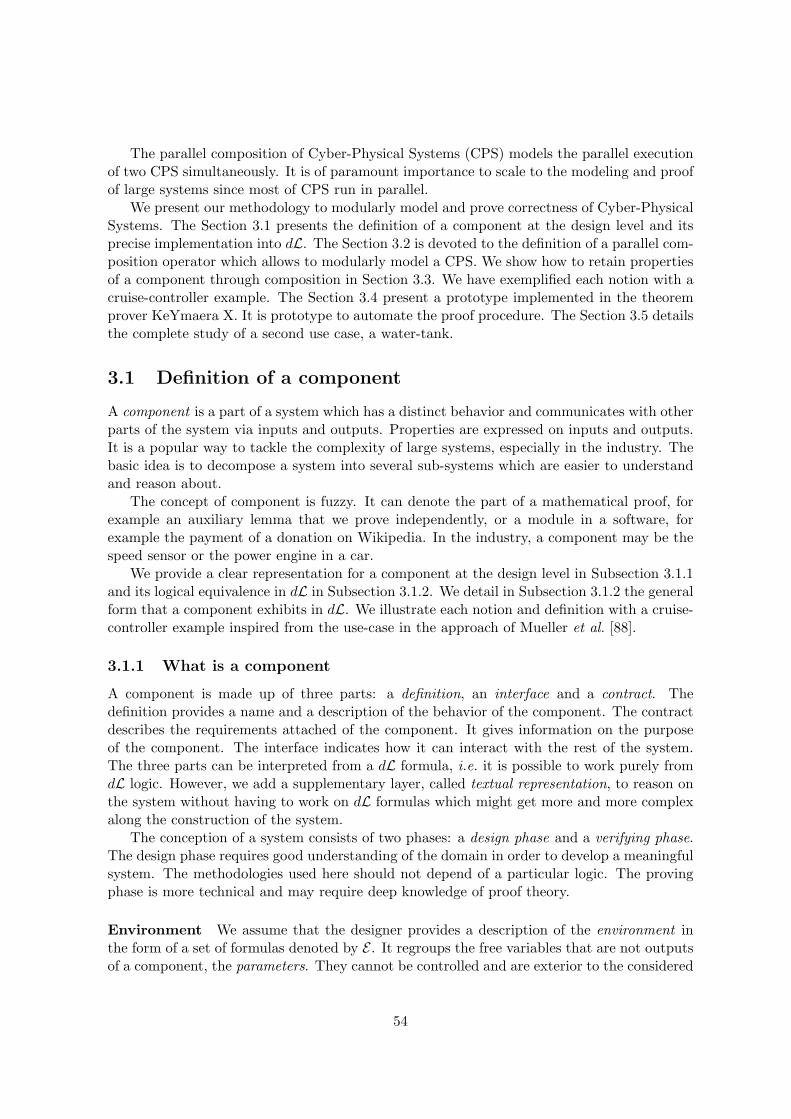
The parallel composition of Cyber-Physical Systems (CPS) models the parallel executionof two CPS simultaneously. It is of paramount importance to scale to the modeling and proofof large systems since most of CPS run in parallel.

We present our methodology to modularly model and prove correctness of Cyber-PhysicalSystems. The Section 3.1 presents the definition of a component at the design level and itsprecise implementation into dL. The Section 3.2 is devoted to the definition of a parallel com-position operator which allows to modularly model a CPS. We show how to retain propertiesof a component through composition in Section 3.3. We have exemplified each notion with acruise-controller example. The Section 3.4 present a prototype implemented in the theoremprover KeYmaera X. It is prototype to automate the proof procedure. The Section 3.5 detailsthe complete study of a second use case, a water-tank.

3.1 Definition of a component

A component is a part of a system which has a distinct behavior and communicates with otherparts of the system via inputs and outputs. Properties are expressed on inputs and outputs.It is a popular way to tackle the complexity of large systems, especially in the industry. Thebasic idea is to decompose a system into several sub-systems which are easier to understandand reason about.

The concept of component is fuzzy. It can denote the part of a mathematical proof, forexample an auxiliary lemma that we prove independently, or a module in a software, forexample the payment of a donation on Wikipedia. In the industry, a component may be thespeed sensor or the power engine in a car.

We provide a clear representation for a component at the design level in Subsection 3.1.1and its logical equivalence in dL in Subsection 3.1.2. We detail in Subsection 3.1.2 the generalform that a component exhibits in dL. We illustrate each notion and definition with a cruise-controller example inspired from the use-case in the approach of Mueller et al. [88].

3.1.1 What is a component

A component is made up of three parts: a definition, an interface and a contract. Thedefinition provides a name and a description of the behavior of the component. The contractdescribes the requirements attached of the component. It gives information on the purposeof the component. The interface indicates how it can interact with the rest of the system.The three parts can be interpreted from a dL formula, i.e. it is possible to work purely fromdL logic. However, we add a supplementary layer, called textual representation, to reason onthe system without having to work on dL formulas which might get more and more complexalong the construction of the system.

The conception of a system consists of two phases: a design phase and a verifying phase.The design phase requires good understanding of the domain in order to develop a meaningfulsystem. The methodologies used here should not depend of a particular logic. The provingphase is more technical and may require deep knowledge of proof theory.

Environment We assume that the designer provides a description of the environment inthe form of a set of formulas denoted by E . It regroups the free variables that are not outputsof a component, the parameters. They cannot be controlled and are exterior to the considered

54

system. For example, the gravity value g is a parameter in most of mechanical systems or thevalue of the speed limit S in our example. It is a value fixed by the government, a tachymetercannot change it freely. Parameters can be constant or in a range of value if we want torepresent uncertainty.

Time We assume that the time evolves continuously and linearly. It is represented by thereserved variable t and its evolution is modeled by the differential equation 9t “ 1.

Name and behavior A component is defined by a name and a behavior. The behavior isthe functional modeling of the component. It is represented as a hybrid program of dL1 anddefines the evolution of the component trough time. We adopt the convention of denoting ageneric component by a capital letter and the associated behavior with its equivalent in thegreek alphabet.

Example 17 (Name and behavior of the Tachymeter component). The Tachymeter is asoftware which senses the speed of the vehicle every ε seconds. It decides the speed that shouldbe attained by the vehicle after ε seconds and set up the acceleration given to the engine. Itsbehavior is defined by the hybrid program denoted Tach. We give a detailed presentation inExample 21.

Name: Tachymeter

Behavior:

Tach fi

`

?ttach ` ε ě t; sacm :“ seng; stach :“ ˚;?p0 ď stach ď S ^ ´δ ď stach ´ sacm ď δq;a :“ stach´sacm

ε; ttach :“ t

˘

˚

Figure 3.1: Tachymeter

Interface The interface of a component describes how it interacts with the world. Itspecifies the inputs and the outputs along with the properties associated to every component.

Example 18 (Interface of the Tachymeter). The component Tachymeter possess one inputand three outputs. The input seng represents the actual speed of the engine and the outputsacm the measured speed. stach is the target speed the vehicle should attain after ε seconds anda the acceleration to follow to reach the target speed.

1The syntax of hybrid programs can be found in Definitions 1 and 3

55

Name: Tachymeter

Inputs:

sengOutputs:

sacmstacha

Behavior:

Tach fi

`

?ttach ` ε ě t; sacm :“ seng; stach :“ ˚;?p0 ď stach ď S ^ ´δ ď stach ´ sacm ď δq;a :“ stach´sacm

ε; ttach :“ t

˘

˚

Figure 3.2: Tachymeter with inputs and outputs

Contract We associate properties to a component by using contracts. A contract is a pairof formulas pA,Gq, called the assumptions A and the guarantees G. Guarantees are propertieson the outputs of the component. Assumptions are properties that the inputs are presumedto satisfy.

We get inspiration from the meta-theory of contracts of Benveniste et al. [18]. The for-mulas are formulas of dL2.

Example 19 (Contract of the Tachymeter). We assume that the speed of the vehicle, seng,does not exceed the speed limit S. Under this assumption on the real speed, the tachymeterguarantees that the target speed does not exceed the speed limit. It also guarantees that themeasured speed is inferior to S and links the value of the acceleration to the measured and thetarget speed.

Name: Tachymeter

Inputs:

sengAssumptions:

0 ď seng ď S

Outputs:

a

stachsacmGuarantees:

0 ď sacm ď S ^ 0 ď stach ď S ^ a “ stach´sacmε

Behavior:

Tach fi

`

?ttach ` ε ě t; sacm :“ seng; stach :“ ˚;?p0 ď stach ď S ^ ´δ ď stach ´ sacm ď δq;a :“ stach´sacm

ε; ttach :“ t

˘

˚

Figure 3.3: Complete representation of the tachymeter

We can also define the component Engine representing the speed of the vehicle regulatedby the Tachymeter component.

2The syntax of formulas of dL can be found in Definition 8

56

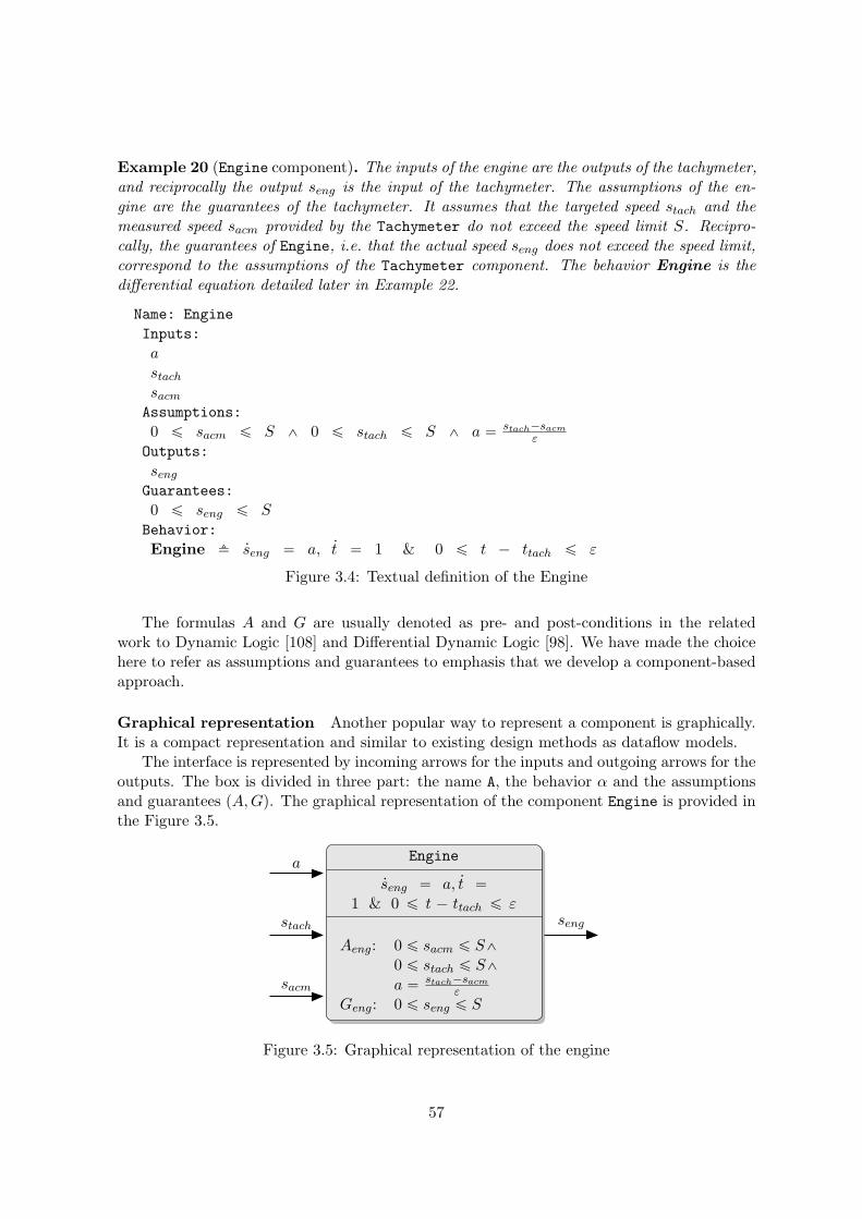
Example 20 (Engine component). The inputs of the engine are the outputs of the tachymeter,and reciprocally the output seng is the input of the tachymeter. The assumptions of the en-gine are the guarantees of the tachymeter. It assumes that the targeted speed stach and themeasured speed sacm provided by the Tachymeter do not exceed the speed limit S. Recipro-cally, the guarantees of Engine, i.e. that the actual speed seng does not exceed the speed limit,correspond to the assumptions of the Tachymeter component. The behavior Engine is thedifferential equation detailed later in Example 22.

Name: Engine

Inputs:

a

stachsacmAssumptions:

0 ď sacm ď S ^ 0 ď stach ď S ^ a “ stach´sacmε

Outputs:

sengGuarantees:

0 ď seng ď S

Behavior:

Engine fi 9seng “ a, 9t “ 1 & 0 ď t ´ ttach ď ε

Figure 3.4: Textual definition of the Engine

The formulas A and G are usually denoted as pre- and post-conditions in the relatedwork to Dynamic Logic [108] and Differential Dynamic Logic [98]. We have made the choicehere to refer as assumptions and guarantees to emphasis that we develop a component-basedapproach.

Graphical representation Another popular way to represent a component is graphically.It is a compact representation and similar to existing design methods as dataflow models.

The interface is represented by incoming arrows for the inputs and outgoing arrows for theoutputs. The box is divided in three part: the name A, the behavior α and the assumptionsand guarantees pA,Gq. The graphical representation of the component Engine is provided inthe Figure 3.5.

Engine

9seng “ a, 9t “1 & 0 ď t ´ ttach ď ε

Aeng: 0 ď sacm ď S^0 ď stach ď S^a “ stach´sacm

ε

Geng: 0 ď seng ď S

a

stach

sacm

seng

Figure 3.5: Graphical representation of the engine

57

Conclusion We have presented a concise representation of a component. It allow to reasonon CPS without requiring a deep knowledge of dL. It is very similar to the meta-theory ofcontract defined by Benveniste et al. [18]. We have instantiated with the logic dL in ourapproach, but one can imagine to mix it with other approaches.

3.1.2 Definition in dL

We show how to transcript our notion of component into a formula of dL. The behavioris already a hybrid program, but it should respect a particular form that we detail. Theinterface corresponds to bound and free variable of the behavior and the contract can benaturally expressed in dL as seen in Definition 10.

General form of a behavior in dL We define a general form that the behavior of acomponent should respect. To gain in clarity, we partition specifications α into their discreteand continuous parts discα and contα.

Definition 19 (General form of a behavior). The general form of a behavior α fi pcontα Ydiscαq˚ consists of its partition into a continuous part contα, of the form 9X “ θX & HX ,and the discrete part discα.

Notice that the discrete part of a system discα is itself defined by the union of discrete,functional, components.

Example 21 (Behavior of Tachymeter). We model the discrete controller of a cruise controlsystem that is responsible for delivering a targeted speed to the vehicle engine (e.g. a car).

Tach fi

`

?ttach ` ε ě t; sacm :“ seng; stach :“ ˚;?p0 ď stach ď S ^ ´δ ď stach ´ sacm ď δq;

a :“ stach´sacmε

; ttach :“ t˘

˚

The test ?ttach ` ε ě t ensure that no more that ε seconds have passed since the last executionmarked by ttach. We measure then the value of the speed seng by memorizing it in the variablesacm (sacm :“ seng. It chooses an arbitrary value for sctrl, the targeted speed, and checks ifit is in the desired range r0, Ss, where S is the speed limit. It additionally checks that thedifference between the speed measured by the tachymeter, stach, and the targeted speed, sctrl,is not too high, in order to ensure that the acceleration set is not too brutal and/or within thecapabilities of the engine.

Example 22 (Behavior of Engine). We model the continuous acceleration of the engine bya guarded derivative:

9seng “ a, 9t “ 1 & 0 ď t ´ ttach ď ε

The differential equation describes the evolution of speed by a function of the acceleration overtime.

We can model a large variety of hybrid systems as sensors, programs, plant.

58

Contract of a component in dL To soundly ensure that a component satisfies its contract,we use the proof theory of dL.

A component A in an environment E is translated in dL as a formula of the form pE ^Aq Ñ rαsG where E is the environment, A and G are the assumptions and guarantees andα the behavior of the component. For example, the component Tachymeter is translated aspE ^ Atachq Ñ rTachsGtach.

The interface is implicit. The inputs (resp. outputs) of a component correspond to thefree variables (resp. bound variables) of the behavior. We have A.inputs Ď FV pαq andA.outputs Ď BV pαq. This notion is translated in dL by the notion of bounds and freevariables. The bound variables of a hybrid program α are variables that can be changedduring the execution of α, i.e. a variable on which the hybrid program acts. It is assimilatedto outputs. The remaining variables are the free variables, i.e. all the variables that are notbound. The component cannot modify theses variables. We have to distinguish in thesevariables the parameters, which are part of the environment, and the inputs which are thevariables that can potentially be outputs of other components.

It is now possible to precisely define the satisfaction of a contract by a component.

Definition 20 (Satisfaction of a contract). A component A satisfies its contract pA,Gq if theformula pE ^ Aq Ñ rαsG is valid.

We add the environment E in the formula because it is needed to achieve the proof. Weprove the validity of the formula by using rules of the sequent calculus of dL [98].

We refer to the behavior of the tachymeter by Tach in the next sections. We have:

Tach fi

`

?ttach ` ε ě t; sacm :“ seng; stach :“ ˚;?p0 ď stach ď S ^ ´δ ď stach ´ sacm ď δq;

a :“ stach´sacmε

; ttach :“ t˘

˚

Example 23 (Satisfaction of the contract of the Tachymeter). To show that the Tachymetercomponent satisfies its contract, we prove the validity of the sequent:

E , ATach $ rTachsGTach

where:

Tach fi pBodyq˚

Body fi ?ttach ` ε ě t; sacm :“ seng; stach :“ ˚;?p0 ď stach ď S ^ ´δ ď stach ´ sacm ď δq;a :“ stach´sacm

ε; ttach :“ t

ATach fi 0 ď seng ď S

GTach fi 0 ď sacm ď S ^ 0 ď stach ď S ^ a “ stach´sacmε

E fi S ą 0 ^ ε ą 0 ^ stach “ seng ^ sacm “ seng ^ a “ 0

We distinguish the hybrid program Body in the loop from the behavior of the componentTach to clarify the proof. Body will occurs at multiple times. We use GTach as an invariantfor the application of the rule [Ind].

ΠInit

E , ATach $ GTach

ΠStep

E , ATach $ @sacm, stach, a, ttachpGTach Ñ rBodysGTachq[Ind]

E , ATach $ rpBodyq˚sGTach

59

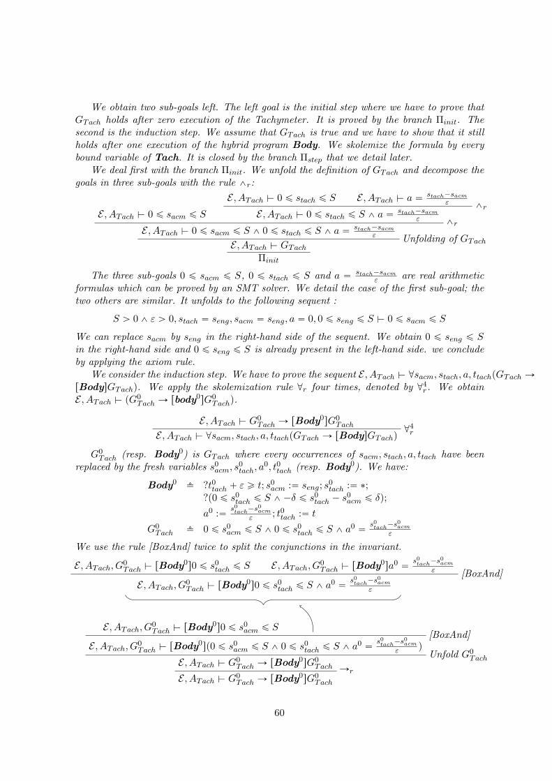
We obtain two sub-goals left. The left goal is the initial step where we have to prove thatGTach holds after zero execution of the Tachymeter. It is proved by the branch Πinit. Thesecond is the induction step. We assume that GTach is true and we have to show that it stillholds after one execution of the hybrid program Body. We skolemize the formula by everybound variable of Tach. It is closed by the branch Πstep that we detail later.

We deal first with the branch Πinit. We unfold the definition of GTach and decompose thegoals in three sub-goals with the rule ^r:

E , ATach $ 0 ď sacm ď S

E , ATach $ 0 ď stach ď S E , ATach $ a “ stach´sacmε ^r

E , ATach $ 0 ď stach ď S ^ a “ stach´sacmε ^r

E , ATach $ 0 ď sacm ď S ^ 0 ď stach ď S ^ a “ stach´sacmε Unfolding of GTach

E , ATach $ GTach

Πinit

The three sub-goals 0 ď sacm ď S, 0 ď stach ď S and a “ stach´sacmε

are real arithmeticformulas which can be proved by an SMT solver. We detail the case of the first sub-goal; thetwo others are similar. It unfolds to the following sequent :

S ą 0 ^ ε ą 0, stach “ seng, sacm “ seng, a “ 0, 0 ď seng ď S $ 0 ď sacm ď S

We can replace sacm by seng in the right-hand side of the sequent. We obtain 0 ď seng ď S

in the right-hand side and 0 ď seng ď S is already present in the left-hand side. we concludeby applying the axiom rule.

We consider the induction step. We have to prove the sequent E , ATach $ @sacm, stach, a, ttachpGTach ÑrBodysGTachq. We apply the skolemization rule @r four times, denoted by @4

r. We obtainE , ATach $ pG0

Tach Ñ rbody0sG0Tachq.

E , ATach $ G0Tach Ñ rBody0sG0

Tach @4rE , ATach $ @sacm, stach, a, ttachpGTach Ñ rBodysGTachq

G0Tach (resp. Body0) is GTach where every occurrences of sacm, stach, a, ttach have been

replaced by the fresh variables s0acm, s0tach, a0, t0tach (resp. Body0). We have:

Body0 fi ?t0tach ` ε ě t; s0acm :“ seng; s0tach :“ ˚;

?p0 ď s0tach ď S ^ ´δ ď s0tach ´ s0acm ď δq;

a0 :“s0tach

´s0acmε

; t0tach :“ t

G0Tach fi 0 ď s0acm ď S ^ 0 ď s0tach ď S ^ a0 “

s0tach

´s0acmε

We use the rule [BoxAnd] twice to split the conjunctions in the invariant.

E , ATach, G0Tach $ rBody0s0 ď s0acm ď S

[BoxAnd]E , ATach, G

0Tach $ rBody0sp0 ď s0acm ď S ^ 0 ď s0tach ď S ^ a0 “

s0tach

´s0acmε

qUnfold G0

TachE , ATach $ G0

Tach Ñ rBody0sG0Tach Ñr

E , ATach $ G0Tach Ñ rBody0sG0

Tach

E , ATach, G0Tach $ rBody0s0 ď s0tach ď S E , ATach, G

0Tach $ rBody0sa0 “

s0tach

´s0acmε [BoxAnd]

E , ATach, G0Tach $ rBody0s0 ď s0tach ď S ^ a0 “

s0tach

´s0acmε

60

We detail the proof of the sub-goal E , ATach, G0Tach $ rBody0s0 ď s0acm ď S in Figure 3.6.

The two other sub-goals are similar. The basic idea is to unfold Body, the resulting sequentis composed of Real Arithmetic formulas and is trivial to prove.

The corresponding .kyx file can be found in the annexes 5.3.2 for the Tachymeter and 5.3.2for the Engine.

Conclusion We have presented how to represent a component A with its interface, contractand behavior. We have defined the meaning of A satisfying its contract. We have explainedhow it is translated in the dL framework. It gives us a strong logical basis to soundly reasonon CPS. The next section is devoted to the presentation of the process of parallel compositionto modularly build a system.

3.2 Parallel composition operator

The composition of components is the core aspect of the component-based approach; it is themechanism that allow us to obtain a full system after having considered each of its componentsseparately. It specifies how we connect components and what the resulting behavior is.

The operator achieving it shall be the more general possible in order to handle a widevariety of systems. The result of the composition of two components, the composite, shallbe a component that we can composed later with another component. The operator mustbe modular, i.e. commutative and associative. If we compose two components A and B, thenanother one C, we shall obtain the same result as if we have composed first B and C together,and then A as illustrated in the Figure 3.7.

We present the parallel composition of components A and B in Subsection 3.2.1. TheSubsection 3.2.2 is devoted to the definition of the operator ˝ to compose behaviors in dL.We discuss the differences with the parallel composition of hybrid action systems in Subsec-tion 3.2.3.

3.2.1 Parallel composition of components

When composing two components, there is no need to specify the inputs, the assumptions,the outputs, the guarantees and the behavior of the resulting component; these characteristicsare automatically inherited from the composition. The inputs (resp. outputs) are the unionof respective inputs (resp. outputs). The assumptions (resp. guarantees) are the conjunctionof respective assumptions (resp. guarantees). The behavior is obtained by application of theoperator ˝, defined in Subsection 3.2.2.

Our model of communication for our parallel composition operator is based on variable-sharing and is thus very simple. An output can be the input of several components, and it isthus not possible to abstract matching inputs and outputs through composition. We outlinehow we can model communication channels in our paradigm in the Subsection 5.1.3 of futureworks.

Example 24 (Cruise-Control). The cruise-control system is obtained by parallel compositionof components Tachymeter and Engine. It is itself a component, named Cruise-Control

that may be composed later with other part of a vehicle, e.g. a power-train. The result of thecomposition is given in Figure 3.8.

A graphical representation is given in the Figure 3.9.

61

axE,0

ďs0 eng

ďS,G

0 Tach,t

0 tach

`ε

ět,0

ďx

ďS

^´δ

ďx

´s0 eng

ďδ

$0

ďs0 eng

ďS

Unfold

definitionof

ATach

E,A

Tach,G

0 Tach,t

0 tach

`ε

ět,0

ďx

ďS

^´δ

ďx

´s0 eng

ďδ

$0

ďs0 eng

ďS

r:“

sE,A

Tach,G

0 Tach,t

0 tach

`ε

ět,0

ďx

ďS

^´δ

ďx

´s0 eng

ďδ

$rt0 tach:“

ts0

ďs0 eng

ďS

r:“

sE,A

Tach,G

0 Tach,t

0 tach

`ε

ět,0

ďx

ďS

^´δ

ďx

´s0 eng

ďδ

$ra

0:“

x´s0 eng

εsrt0 ta

ch:“

ts0

ďs0 eng

ďS

r;s

E,A

Tach,G

0 Tach,t

0 tach

`ε

ět,0

ďx

ďS

^´δ

ďx

´s0 eng

ďδ

$ra

0:“

x´s0 eng

ε;t

0 tach:“

ts0

ďs0 eng

ďS

rÑrs

E,A

Tach,G

0 Tach,t

0 tach

`ε

ět

$p0

ďx

ďS

^´δ

ďx

´s0 eng

ďδq

Ñra

0:“

x´s0 eng

ε;t

0 tach:“

ts0

ďs0 eng

ďS

r?s

E,A

Tach,G

0 Tach,t

0 tach

`ε

ět

$r?

p0ď

xď

S^

´δ

ďx

´s0 eng

ďδqs

ra0:“

x´s0 eng

ε;t

0 tach:“

ts0

ďs0 eng

ďS

r;s

E,A

Tach,G

0 Tach,t

0 tach

`ε

ět

$r?

p0ď

xď

S^

´δ

ďx

´s0 eng

ďδq;a0:“

x´s0 eng

ε;t

0 tach:“

ts0

ďs0 eng

ďS

r@rs

E,A

Tach,G

0 Tach,t

0 tach

`ε

ět

$@x

pr?p0

ďx

ďS

^´δ

ďx

´s0 eng

ďδq;a0:“

x´s0 eng

ε;t

0 tach:“

ts0

ďs0 eng

ďS

qr;

sE,A

Tach,G

0 Tach,t

0 tach

`ε

ět

$rs

0 tach:“

˚sr?p0

ďs0 tach

ďS

^´δ

ďs0 tach

´s0 eng

ďδq;a0:“

s0 tach

´s0 eng

ε;t

0 tach:“

ts0

ďs0 eng

ďS

r;s

E,A

Tach,G

0 Tach,t

0 tach

`ε

ět

$rs

0 tach:“

˚;?

p0ď

s0 tach

ďS

^´δ

ďs0 tach

´s0 eng

ďδq;a0:“

s0 tach

´s0 eng

ε;t

0 tach:“

ts0

ďs0 eng

ďS

r:“

sE,A

Tach,G

0 Tach,t

0 tach

`ε

ět

$rs

0 acm

:“sengsrs0 tach:“

˚;?

p0ď

s0 tach

ďS

^´δ

ďs0 tach

´s0 acm

ďδq;a0:“

s0 tach

´s0 acm

ε;t

0 tach:“

ts0

ďs0 acm

ďS

r;s

E,A

Tach,G

0 Tach,t

0 tach

`ε

ět

$rs

0 acm

:“seng;s

0 tach:“

˚;?

p0ď

s0 tach

ďS

^´δ

ďs0 tach

´s0 acm

ďδq;a0:“

s0 tach

´s0 acm

ε;t

0 tach:“

ts0

ďs0 acm

ďS

Ñr

E,A

Tach,G

0 Tach

$t0 ta

ch

`ε

ět

Ñrs

0 acm

:“seng;s

0 tach:“

˚;?

p0ď

s0 tach

ďS

^´δ

ďs0 tach

´s0 acm

ďδq;a0:“

s0 tach

´s0 acm

ε;t

0 tach:“

ts0

ďs0 acm

ďS

r?s

E,A

Tach,G

0 Tach

$r?t0 ta

ch

`ε

ěts

rs0 acm

:“seng;s

0 tach:“

˚;?

p0ď

s0 tach

ďS

^´δ

ďs0 tach

´s0 acm

ďδq;a0:“

s0 tach

´s0 acm

ε;t

0 tach:“

ts0

ďs0 acm

ďS

r;s

E,A

Tach,G

0 Tach

$r?t0 ta

ch

`ε

ět;s0 acm

:“seng;s

0 tach:“

˚;?

p0ď

s0 tach

ďS

^´δ

ďs0 tach

´s0 acm

ďδq;a0:“

s0 tach

´s0 acm

ε;t

0 tach:“

ts0

ďs0 acm

ďS

E,A

Tach,G

0 Tach

$rB

ody0s0

ďs0 acm

ďS

Figure

3.6:Proof

thatthemeasuredspeedsacm

staysin

thepre-defined

range

afteron

eexecution

oftheTachymeter

62

`

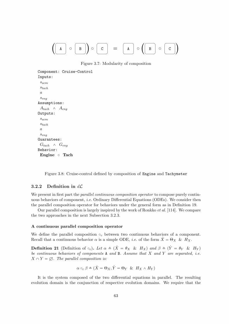
A ˝ B

˘

˝ C ” A ˝

`

B ˝ C

˘

Figure 3.7: Modularity of composition

Component: Cruise-Control

Inputs:

sacmstacha

sengAssumptions:

Atach ^ Aeng

Outputs:

sacmstacha

sengGuarantees:

Gtach ^ Geng

Behavior:

Engine ˝ Tach

Figure 3.8: Cruise-control defined by composition of Engine and Tachymeter

3.2.2 Definition in dL

We present in first part the parallel continuous composition operator to compose purely contin-uous behaviors of component, i.e. Ordinary Differential Equations (ODEs). We consider thenthe parallel composition operator for behaviors under the general form as in Definition 19.

Our parallel composition is largely inspired by the work of Ronkko et al. [114]. We comparethe two approaches in the next Subsection 3.2.3.

A continuous parallel composition operator

We define the parallel composition ˝c between two continuous behaviors of a component.Recall that a continuous behavior α is a simple ODE, i.e. of the form 9X “ ΘX & HX .

Definition 21 (Definition of ˝c). Let α fi p 9X “ θX & HXq and β fi p 9Y “ θY & HY qbe continuous behaviors of components A and B. Assume that X and Y are separated, i.e.X X Y “ H. The parallel composition is:

α ˝c β fi p 9X “ ΘX , 9Y “ ΘY & HX ^ HY q

It is the system composed of the two differential equations in parallel. The resultingevolution domain is the conjunction of respective evolution domains. We require that the

63

Engine

9seng “ a, 9t “1 & 0 ď t ´ ttach ď ε

Aeng: 0 ď sacm ď S^0 ď stach ď S^a “ stach´sacm

ε

Geng: 0 ď seng ď S

Tachymeter`

?ttach ` ε ě t; sacm :“ seng; stach :“ ˚;?p0 ď stach ď S ^ ´δ ď stach ´ sacm ď δq;

a :“ stach´sacmε

; ttach :“ t˘

˚

Atach: 0 ď seng ď S

Gtach: 0 ď sacm ď S^0 ď stach ď S^a “ stach´sacm

ε

senga, stach, sacm

Figure 3.9: Cruise-control system

derived variables are separated (X X Y “ H), i.e. that they do not describe the evolutionof the same system. It is a restriction that makes sense at the design level, but it is alsomandatory to lift the contracts through composition. But occurrences of variables in X

(resp. in Y ) can occur in ΘY (resp. in ΘX).To illustrate the operator, assume that we want to set a time limit to our vehicle engine

component.

Example 25 (Time limit to the engine vehicle). Assume that in the description of the engine,we did not make explicit the time and we do not have set a limit. We do not want to considerperpetual execution of Engine since the tachymeter controls it periodically. To obtain thebehavior of the component Engine in 22, we consider the time as a component with outputthe variable t, and the representation of the passing of time is achieved by introducing theODE 9t “ 1. We add the formula 0 ď t ´ ttach ď ε in the evolution domain of 9t “ 1, whereε is the desired limit. Here, we limit the time with the formula 0 ď t ´ ttach ď ε rather thant ď ε. It limits the time passed since the last execution of the Tachymeter component.

By composing this proposition with our example, we obtain the timed model:

p 9seng “ aq ˝c p 9t “ 1 & 0 ď t ´ ttach ď εq fi p 9seng “ a, 9t “ 1 & 0 ď t ´ ttach ď εq

We may also compose the speed with other physical parts of the vehicle like the temper-

64

ature of the engine or the fuel’s consumption.

Algebraic properties The parallel continuous composition operator ˝c is commutativeand associative. Commutativity means that we can compose two physical systems in anyorder. Associativity means that we can build a system step-by-step; we can compose twocomponents together, add a third component later, and we still obtain the same system asif we have compose all together in the first place. It allows to hierarchy the composition ofcomponents.

Proposition 1 (Commutativity of ˝c). Let α and β be continuous behaviors of componentsA and B.

α ˝c β “ β ˝c α

Proof. The idea is that the order of variables in an ODE is not important, we can re-arrangethem to show associativity.

Let α and β be continuous behaviors of components A and B, i.e. α fi 9X “ θX & HX

and β fi 9Y “ θY & HY .

p 9X “ θX & HXq ˝c p 9Y “ θY & HY q

fi 9X, 9Y “ θX , θY & pHX ^ HY q (definition of ˝c )

fi 9Y , 9X “ θY , θX & pHX ^ HY q (re-arrangement)

fi 9Y , 9X “ θY , θX & pHY ^ HXq (commutativity of ^ )

fi p 9Y “ θY & HY q ˝c p 9X “ θX & HXq (definition of ˝c )

Proposition 2 (Associativity of ˝c). Let α, β and γ be continuous behaviors of componentsA, B and C.

pα ˝c βq ˝c γ “ α ˝c pβ ˝c γq

Proof. As for the proof of commutativity, the order of variables in an ODE is not important;we can re-arrange them to show associativity.

Let α, β and γ be continuous behaviors of components A, B and C, i.e. α fi 9X “ θX & HX ,β fi 9Y “ θY & HY and γ fi 9Z “ θZ & HZ .

pα ˝c βq ˝c γ

fi p 9X, 9Y “ θX , θY & HX ^ HY q ˝c γ punfold definition of ˝cq

fi 9X, 9Y , 9Z “ θX , θY , θZ & HX ^ HY ^ HZ punfold definition of ˝cq

fi α ˝c p 9Y , 9Z “ θY , θZ & HY ^ HZq pfold definition of ˝cqfi α ˝c pβ ˝c γq pfold definition of ˝cq

We have presented the parallel composition operator for continuous behaviors of compo-nents. We have shown that it is associative and commutative, two mandatory conditions forthe modularity. We present in the next section the parallel composition operator for behaviorsof the general form.

65

A parallel composition operator

Recall that a behavior α is said of the general form if α fi pdiscα Ycontαq˚ (cf Definition 19.We define the parallel composition between such behaviors. The behavior is divided betweenits discrete part discα and continuous part contα. Due to their different nature, the com-position between discrete parts of components differs from the composition between theircontinuous part.

Definition 22 (Parallel composition between general behaviors). Let α and β be generalbehaviors of components A and B, i.e. α fi pdiscα Y contαq˚ and β fi pdiscβ Y contβq˚. Theparallel composition operator ˝ is defined by:

α ˝ β fi

`

discα Y discβ Y pcontα ˝c contβq˘

˚

where ˝c is defined in Definition 21.

The composition between the discrete parts is a non-deterministic choice, which amountsto an interleaving of every discrete parts. This full interleaving allows to model parallelcomposition of discrete parts of hybrid systems. The continuous part are composed with ˝c.the discrete and continuous dynamics are then composed with the non-deterministic choiceY. Two examples of executions are given in the Figure 3.10.

α β˝

discβ

contα

contβ discα discα

discβ

discα

contβcontα discα discβ

Figure 3.10: Possible executions of the parallel composition

We exemplify the parallel composition of behaviors with both discrete and continuous partby considering the composition of the Engine’s behavior with the Tachymeter’s behavior.

Example 26 (Behavior of the Cruise-control). The Cruise-control component is madeup of the Tachymeter and the Engine. It is itself a component that can be composed withother components like the fuel consumption monitor. Its behavior Cruise-control is obtainedby the composition of Engine and Tach.

Cruise-control fi Engine ˝ Tach fi´

`

?ttach ` ε ě t; sacm :“ seng; stach :“ ˚; ?p0 ď stach ď S ^ ´δ ď stach ´ sacm ď δq;

a :“ stach´sacmε

; ttach :“ t˘

Y`

9seng “ a, 9t “ 1 & 0 ď t ´ ttach ď ε˘

¯

˚

The tachymeter’s behavior senses the speed seng and decides of the targeted speed stach. It setthe acceleration a followed by the engine’s behavior. The test ttach ` ε ě t at the beginning ofTach ensures that there is at most ε seconds between two execution of the tachymeter. ttachrecords the last instant the controller have executed.

66

Algebraic properties As in the continuous case, the parallel composition operator ˝ iscommutative and associative.

Proposition 3 (Commutativity). Let α and β be behaviors of components A and B.

α ˝ β “ β ˝ α

Proof. The commutativity property results from the commutativity of the operator Y andthe commutativity of the operator ˝c. Let α and β be behaviors of components A and B, i.e.α fi pdiscα Y contαq˚ and β fi pdiscβ Y contβq˚. We have:

α ˝ β fi

`

discα Y discβ Y pcontα ˝c contβq˘

˚pUnfold definition of ˝q

fi

`

discβ Y discα Y pcontα ˝c contβq˘

˚pCommutativity of Yq

fi

`

discβ Y discα Y pcontβ ˝c contαq˘

˚pCommutativity of ˝cq

fi β ˝ α pFold definition of ˝q

Proposition 4 (Associativity). Let α, β and γ be behaviors of components A, B and C.

pα ˝ βq ˝ γ “ α ˝ pβ ˝ γq

Proof. The associativity property results from the associativity of the operator Y and theassociativity of the operator ˝c.

Let α, β and γ be behaviors of components A, B and C, i.e. α fi pdiscα Y contαq˚,β fi pdiscβ Y contβq˚ and γ fi pdiscγ Y contγq˚.

pα ˝ βq ˝ γ

fi

´

`

discα Y discβ Y pcontα ˝c contβq˘

˚¯

˝ γ pUnfold definition of ˝q

fi

´

pdiscα Y discβq Y discγ Y`

pcontα ˝c contβq ˝c contγ˘

¯

˚

pUnfold definition of ˝q

fi

´

discα Y pdiscβ Y discγq Y`

pcontα ˝c contβq ˝c contγ˘

¯

˚

pAssociativity of Yq

fi

´

discα Y pdiscβ Y discγq Y`

contα ˝c pcontβ ˝c contγq˘

¯

˚

pAssociativity of ˝cq

fi α ˝

´

`

discβ Y discγ Y pcontβ ˝c contγq˘

˚¯

pFold definition of ˝q

fi α ˝ pβ ˝ γq pFold definition of ˝q

Conclusion We have defined a parallel composition operator for Cyber-Physical Systems.It is syntactically defined, and thus amenable to automation. It enjoys two important al-gebraic properties: commutativity and associativity. The associativity property allows toconsider the construction of a system step-by-step.

3.2.3 Comparison with the parallel composition of hybrid action systems

We compare our parallel composition operator ˝ with the parallel composition for hybridsystems presented by Ronkko et al. [114]. We briefly present the hybrid action systems. Thesecond part is devoted to a detailed comparison of both approaches.

67

Hybrid action systems We first define what is a hybrid action system. It is used to modelreactive components, possibly non-terminating.

Definition 23 (Action system). An action system is an initialized block of the form:

A “ | r var X : TX :“ E;do A1} . . . }An od

s | : Z

var X : T declares the list of variables X of type T . The variables can be global orlocal. Global variables can be shared with other action systems. Z declares the importedglobal variables that are used in A1, . . . , An, but do not belong to X. The action X :“ E

initializes the variables X by expressions E. After the initialization, the actions A1, . . . , An

are repeatedly executed when it is possible. There is no fairness assumption and the choiceis non-deterministic.

Actions can be assignment X :“ E, sequence A;B, non-deterministic choice }, or a guardp Ñ A where p is a predicate and A an action.

Example 27 (Tachymeter). The tachymeter example presented in the Example 21 is repre-sented by the following action system:

T ACH “ | r var ttach : R, sacm : R, stach : R, a : Rsacm :“ seng, stach :“ seng, a :“ 0;do ttach ` ε ě t Ñ

`

sacm :“ seng; stach :“ ˚;p0 ď stach ď S ^ ´δ ď stach ´ sacm ď δq Ñpa :“ stach´sacm

ε; ttach :“ tq

˘

od

s | : seng, ε, t, S, δ

We first declare the variables ttach, sacm, stach, a since they are the bounds variables of thesystem and type them with R. Then we initialize them. The specification is very similar toour definition in Example 21. The two differences are that the test ?ttach `ε ě t; . . . is writtenttach ` ε ě t Ñ . . . and the iteration symbol ˚ is not explicit since the semantic of do . . .od isthe one of a while loop. Finally, we have to declare the variables seng, ε, t, S, δ as imported.

Definition 24 (Differential action). A differential action is of the form e : 9X “ F pXq wheree is a guard and 9X “ F pXq is a system of differential equations.

The notation in dL would be 9X “ F pXq & e.

Definition 25 (Hybrid action system). A hybrid action system is an initialized block of theform:

H “ | r var X : TX :“ I;alt D with DA

s | : Z

alt D with DA is equivalent to do gD Ñ D}�gD Ñ DA od. All the discrete actionsD must execute before the differential action may execute. Thus, discrete changes have apriority over continuous changes.

Time is assumed to pass linearly during a continuous evolution and do not evolves with adiscrete change. It is the same assumption as in dL.

68

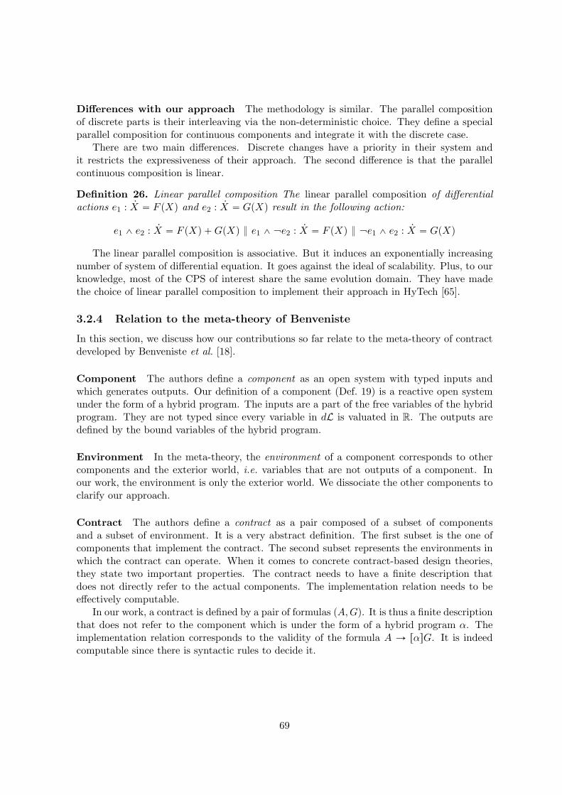
Differences with our approach The methodology is similar. The parallel compositionof discrete parts is their interleaving via the non-deterministic choice. They define a specialparallel composition for continuous components and integrate it with the discrete case.

There are two main differences. Discrete changes have a priority in their system andit restricts the expressiveness of their approach. The second difference is that the parallelcontinuous composition is linear.

Definition 26. Linear parallel composition The linear parallel composition of differentialactions e1 : 9X “ F pXq and e2 : 9X “ GpXq result in the following action:

e1 ^ e2 : 9X “ F pXq ` GpXq } e1 ^ �e2 : 9X “ F pXq } �e1 ^ e2 : 9X “ GpXq

The linear parallel composition is associative. But it induces an exponentially increasingnumber of system of differential equation. It goes against the ideal of scalability. Plus, to ourknowledge, most of the CPS of interest share the same evolution domain. They have madethe choice of linear parallel composition to implement their approach in HyTech [65].

3.2.4 Relation to the meta-theory of Benveniste

In this section, we discuss how our contributions so far relate to the meta-theory of contractdeveloped by Benveniste et al. [18].

Component The authors define a component as an open system with typed inputs andwhich generates outputs. Our definition of a component (Def. 19) is a reactive open systemunder the form of a hybrid program. The inputs are a part of the free variables of the hybridprogram. They are not typed since every variable in dL is valuated in R. The outputs aredefined by the bound variables of the hybrid program.

Environment In the meta-theory, the environment of a component corresponds to othercomponents and the exterior world, i.e. variables that are not outputs of a component. Inour work, the environment is only the exterior world. We dissociate the other components toclarify our approach.

Contract The authors define a contract as a pair composed of a subset of componentsand a subset of environment. It is a very abstract definition. The first subset is the one ofcomponents that implement the contract. The second subset represents the environments inwhich the contract can operate. When it comes to concrete contract-based design theories,they state two important properties. The contract needs to have a finite description thatdoes not directly refer to the actual components. The implementation relation needs to beeffectively computable.

In our work, a contract is defined by a pair of formulas pA,Gq. It is thus a finite descriptionthat does not refer to the component which is under the form of a hybrid program α. Theimplementation relation corresponds to the validity of the formula A Ñ rαsG. It is indeedcomputable since there is syntactic rules to decide it.

69

Composition of components The authors define a composition operator to support hor-izontal processes. It must satisfies two important algebraic properties: commutativity andassociativity. The operator we have defined in the Definition 22 exhibit theses two properties.

The authors define also a composability criterion. It must be a syntactic property on pairsof component that defines conditions under which the two components can interact. The twocomponents must not share common outputs. It is one of the condition presented in thenext section to be allowed to derive the satisfiability of the conjunction of contracts by thecomposition of components. They define also a compatibility criterion on contracts which isthat there exists an environment in which the two contracts properly interact. It correspondsto the conditions pbq and pcq of the theorem of the next section.

The authors have presented a meta-theory for contracts listing the right properties thata contract-based theory must exhibit. Our component-based approach in dL matches thestated characteristics. They present also two other contract operators: contract refinementand contract conjunction. We think that it is possible to extend our approach to instantiatetheses constructs.

Conclusion

After having presented the definition of a component in dL in Section 3.1, we have defineda parallel composition operator to build a system from its parts. The operator is associativeand commutative, which is mandatory to modularly design a system. It is also syntactical,making it amenable to automation.

We want to prove that the system resulting from the composition of component is correct.Proving correctness of each individual component is not enough. We have to be able totransfer the correctness of the component to the global system. In the next section, we stateand prove the theorem which allow to transfer the proof of correctness through composition.It provides a proof that the result of the composition of two components satisfies the contractpAα^Aβ , Gα^Gβq provided that each component satisfies their respective contracts pAα, Gαqand pGα, Gβq.

3.3 Modular proof

We want to transfer the proof of correctness of component through composition. More pre-cisely, let A and B be components with behaviors α and β and contracts pAα, Gαq and pAβ , Gβq.If A and B satisfy their respective contracts, then we want that the component AB resultingfrom the composition of A and B satisfies the contract pAα ^ Aβ , Gα ^ Gβq. In dL, it meansthat if we have a proof tree for the sequents E , Aα $ rαsGα and E , Aβ $ rβsGβ , then we wantto automatically derive a proof tree for the sequent E , Aα, Aβ $ rα ˝ βspGα ^ Gβq.

We present in Subsection 3.3.1 the necessary syntactic conditions to prove the desired the-orem. We prove a technical result in Subsection 3.3.2. We state and prove in Subsection 3.3.3the theorem for the parallel continuous composition operator ˝c. In Subsection 3.3.4, we con-sider the case where both components are discrete, then in Subsection 3.3.5, the case whereone component is discrete and the second one is continuous. Last, we consider the case whereboth components are general in Subsection 3.3.6.

70

3.3.1 Necessary conditions

There is three necessary conditions that components must respect to transfer the proof ofcorrectness through composition. They must not share the same outputs. The guaranteesof a component must not refer to the output of the other component. The assumptions of acomponent must be implied by the relevant guarantees of the other component.

No common outputs The outputs of each component must be dissociated. Otherwise, itmeans that two components A and B intervene on the same output, and thus have same thesame purpose.

In dL, it means that the bound variables of each behaviors are distinct, i.e. BV pαq XBV pβq “ H; the behaviors α and β cannot modify the same variable. Otherwise, the execu-tion of α ˝ β may make no sense and the sequent E , Aα, Aβ $ rα ˝ βspGα ^ Gβq may also beinvalid although E , Aα $ rαsGα and E , Aβ $ rβsGβ are valid.

Example 28 (Composition with same outputs). Let α “ px :“ 10q˚ and β “ px :“ 100q˚ betwo hybrid programs. We can easily prove rαspx ď 15q and rβspx ď 100q, but not rα ˝ βspx ď

15 ^ x ď 100q which is equivalent to rpx :“ 10 Y x :“ 100q˚spx ď 15 ^ x ď 100q. As soonas the last loop iteration assigns 100 to x, the left-handside px ď 15q of the formula does nothold anymore.

A

px :“ 10q˚

Aα: px ď 15qGα: px ď 15q

B

px :“ 100q˚

Aβ : x ď 100Gβ : x ď 100

x

x

✗

Figure 3.11: Unsafe composition with common outputs

This example provides us with a first necessary condition toward automated derivation ofproof trees.

Guarantees do not refer to exterior outputs The second condition requires that theguarantees of the component A do not refer to outputs of the component B, i.e. it does notdepend of the behavior of an other component. The converse is also true. It would be aberrantfor a tachymeter to refer to the fuel’s level of a vehicle.

71

In dL, it means that variables occurring in Gα (resp. Gβ) must not be bound in β (resp.α). The condition amounts to:

V arpGαq X BV pβq “ H and V arpGβq X BV pαq “ H

Example 29 (Guarantee dependent of another component). Let α “ px :“ 10q˚ and β “py :“ 100q˚ be two hybrid programs. Assume that Gβ refers to bound variables of α, e.g. ifGβ fi x ě 42. It is easy to prove that it is an invariant of β, i.e. x ě 42 $ rpy :“ 100q˚sx ě 42is valid. But it is not an invariant of the component α˝β; the sequent x ě 42 $ rpx :“ 10; y :“100q˚sx ě 42 is not valid. As soon as the last loop iteration assigns 10 to x, the formula x ě 42does not hold anymore.

It is graphically represented in the Figure 3.12. A correct guarantee would refer to theoutput y.

A

px :“ 10q˚

Aα: px ď 15qGα: px ď 15q

B

py :“ 100q˚

Aβ : x ě 42Gβ : x ě 42

x

y

✗

Figure 3.12: Unsafe composition with a guarantee referring to an exterior output

For the continuous case, we request also that the evolution domain of the discrete fragmentof a component does not refer to outputs of the other continuous fragment. We request thatV arpHXq X BV pcontβq and V arpHY q X BV pcontαq.

Assumptions are not falsified by exterior components A last condition is that theguarantees Gα of a component A must implies the assumptions Aβ of the component B thatrefers to outputs of A, and conversely. It means that the execution of A do not break theassumptions under which B operated.

In dL, it is translated by the condition that the sequents Aβ $ @αpGα Ñ Aβq andAα $ @βpGβ Ñ Aαq are valid.

Example 30 (Assumption not implied by other guarantee). Let α “ px :“ 10q˚ and β “py :“ xq˚ be two behaviors, Gα fi J, Aβ fi x “ 4 and Gβ fi y “ 4. The sequents $ rαsJ andx “ 4 $ rβsy ě 4 are valid. Yet, the sequent x “ 4 $ rpx :“ 10Y y :“ xq˚sy “ 4 is clearly notvalid. A first iteration assigns 10 to the variable x, then a second assigns x to y. We havethen y “ x “ 10 which contradicts y “ 4.

72

A

px :“ 10q˚

Aα:Gα: J

B

py :“ xq˚

Aβ : x “ 4Gβ : y “ 4

x y

✗

Figure 3.13: Guarantee does not imply the assumption

Conclusion We have presented three necessary conditions for the sound composition ofcomponents. They amount to good modeling practices and are mandatory to design a mean-ingful system.

We believe that theses conditions may be weakened if we develop a more complex model ofcommunications such as in Hybrid Communicating Sequential Processes [73]. HCSP processesuses outputs ch!e to send a message e along a channel ch and inputs ch?x to receive a messagealong the channels ch. Such channels are unique and thus to an output corresponds preciselyan input. It allows a more subtle management of inputs and outputs during the composition.We detail some preliminary results in the future works Section 5.1.3.

We present in the next section a technical result needed to achieve the proofs in Subsec-tion 3.3.3 and 3.3.6. They are related to the conditions we have presented.

3.3.2 Technical result

We state and demonstrate an useful technical result, the separation lemma, to achieve theproof of Theorems 1, 2, 3 and 4. It is to make use of the condition that the guarantee of acomponent must not refer to outputs of another component. We recall the definition of theskolemization of formulas, a notion needed in next subsections.

Definition 27 (Skolemization). We denote by @αϕ the skolemization of a formula with respectto the bound variables of its hybrid program α. (We will use the shorter notation ϕα whereunambiguous).

Example 31. Recall that BV pEngineq “ tsengu. The skolemization of Gtach by the behaviorEngine is G

engtach fi @seng, Gtach.

Separation lemma We need a lemma which state that if the guarantees Gα of a componentA do not refer to the outputs of the other component B, i.e. they are separated, then B doesnot affect Gα.

Lemma 1 (Separation). Let α be a behavior of a component and ϕ a formula such thatBV pαq X V arpϕq “ H. Then the skolemization ϕα is equivalent to ϕ, i.e. ϕα Ø ϕ.

Proof. We prove the lemma by induction on the structure of the formula ϕ.Let ϕ be an atomic formula, e.g. x ě θ. We have to prove that the equivalence @αx ě

θ ÐÑ x ě θ is valid. We recall that the bound variables of α are separated of the freevariables of ϕ. We first prove that @αx ě θ Ñ x ě θ.

73

axx ě θ $ x ě θ

@l@αx ě θ $ x ě θ

We apply the proof rule @l to eliminate the quantification in the left-hand side of the sequent.Since the quantification is over variables that are not present in the atomic formula x ě θ, itleaves it unchanged. We conclude using the axiom rule. We reason similarly for the secondimplication x ě θ Ñ @αx ě θ.

axx ě θ $ x ě θ

@rx ě θ $ @αx ě θ

We apply the proof rule @r, and since the quantification is over variables that are notpresent in the atomic formula x ě θ, it leaves the right-hand side unchanged. We concludeusing the axiom rule.

Let ϕ be the conjunction ϕ1 ^ ϕ2 and we assume that the formula ϕαi Ø ϕi (i “ 1, 2)

is valid under the assumption that BV pαq X V arpϕiq (i “ 1, 2) is empty. We have to provethat the formula @αpϕ1 ^ ϕ2q ÐÑ ϕ1 ^ ϕ2 is valid assuming that BV pαq X V arpϕ1 ^ ϕ2q.By definition of quantification, @αpϕ1 ^ ϕ2q is equivalent to p@αϕ1q ^ p@αϕ2q. By inductionhypothesis, ϕα

i Ø ϕi (i “ 1, 2), and thus p@αϕ1q ^ p@αϕ2q ÐÑ ϕ1 ^ ϕ2.Let ϕ be an universally quantified formula @x,ϕ0. Again, we assume that the formula

@αϕ0 ÐÑ ϕ0 is valid under the assumption that the intersection BV pαq X V arpϕ0q is empty.By definition, @α@xϕ0 is equivalent to @x@αϕ0. By applying the induction hypothesis, weobtain the formula @xϕ0.

3.3.3 For two continuous components

We first state the theorem for the composition of components at the textual representationlevel. We state and prove after the equivalent result with behaviors in dL 1.

Theorem. Let A and B be two components with continuous behaviors and respective contractspAα, Gαq and pAβ , Gβq. Assume that they both satisfy their contracts. Furthermore, assumethat

paq A.outputs X B.outputs “ H,

pb1q A.outputs is separated from Gβ and HY ,

pb2q B.outputs is separated from Gα and HX ,

pc1q Gα must implies the assumptions Aβ that refers to outputs of A,

pc2q Gβ must implies the assumptions Aα that refers to outputs of B.

Then the component AB resulting from the parallel composition of A and B satisfies the con-junction of contracts pAα ^ Aβ , Gα ^ Gβq.

The conditions paq, pbq and pcq are detailed in Subsection 3.3.1. The first assumption paqassumes components to have separate internal variables and requires them to define disjointoutput variables (i.e. unique definitions), which essentially amounts to good modeling prac-tice. The second assumption pb1q (resp. pb2q) requires the safety property Gα (resp. Gβ) toguard the behavior of the system α (resp. β), i.e. its outputs, and of course not βs (resp. α).

74

It hence seems natural to require its separation with Gβ (resp. Gα). The condition pc1q (resp.pc2q) requires the assumptions Aβ (resp. Aα) to be implied by the guarantees Gα (resp. Gβ).

Recall that the behavior α of a component A is the form α fi 9X “ θX & HX and thatthe behavior β of a component B is of the form β fi 9Y “ θY & HY .

Theorem 1. Let α and β be two continuous behaviors of components A and B with respectivecontracts pAα, Gαq and pAβ , Gβq. Assume that we have two proof trees of E , Aα $ rαsGα andE , Aβ $ rβsGβ respectively, where E is the environment. Furthermore, assume that

paq BV pαq X BV pβq “ H,

pb1q BV pαq X FV pGβq “ H and BV pαq X FV pHY q “ H,

pb2q BV pβq X FV pGαq “ H and BV pβq X FV pHXq “ H,

pc1q E , Aα $ @βpGβ Ñ Aαq,

pc2q E , Aβ $ @αpGα Ñ Aβq.

Then it exists a proof tree of E , Aα, Aβ $ rα ˝c βspGα ^ Gβq.

Proof. Let α and β be two continuous behaviors of components A and B, and assume thatwe have a proof tree Pα of E , Aα $ rαsGα and a proof tree Pβ of E , Aβ $ rβsGβ . We have

α fi 9X “ θX & HX and β fi 9Y “ θY & HY .The composition is still a continuous component and we want a proof tree of E , Aα, Aβ $

rα˝c βspGα ^Gβq by using the proofs Pα and Pβ . We inspect all the rules that can be appliedin Pα to prove the sequent E , Aα $ rαsGα (resp. for the proof tree Pβ of E , Aβ $ rβsGβ) andfor each particular association, we give a proof of E , Aα, Aβ $ rα ˝c βspGα ^ Gβq.

Inspection of proof rules We can apply the following rules to the sequent E , Aα $ rαsGα:differential invariant [DI], ODE solution [ODEsolve], differential weakening [DW], differentialcut [DC], Cut and generalization [Gen]. The rules cut, generalization and differential cutdo not decompose the ODE since we still have to prove rαsGα in one of the premises. Forexample, if we apply the rule Cut, we have the following proof tree:

E , Aα $ rαsGα,ϕ E , Aα,ϕ $ rαsGαCut

E , Aα $ rαsGα

We still have to prove the modality rαsGα in the right premise.This careful inspection shows that there are only three rules to consider: [DI], [ODEsolve]

and [DW]. We first consider the case where E , Aα $ rαsGα and E , Aβ $ rβsGβ are provedby the rule [DI]. For the rule [ODEsolve], we show how to construct a proof using [DI] ruleinstead. Last, we consider the case where one have been proved by rule [DI] and the otherby rule [DW] and the case where both sequents have been proved by rule [DW].

We consider four cases :

• [DI]-[DI] Where the two have been proved using the rule [DI]: we apply also the rule[DI] to the sequent representing the contract of the composite. It is divided in threesub-cases:

75

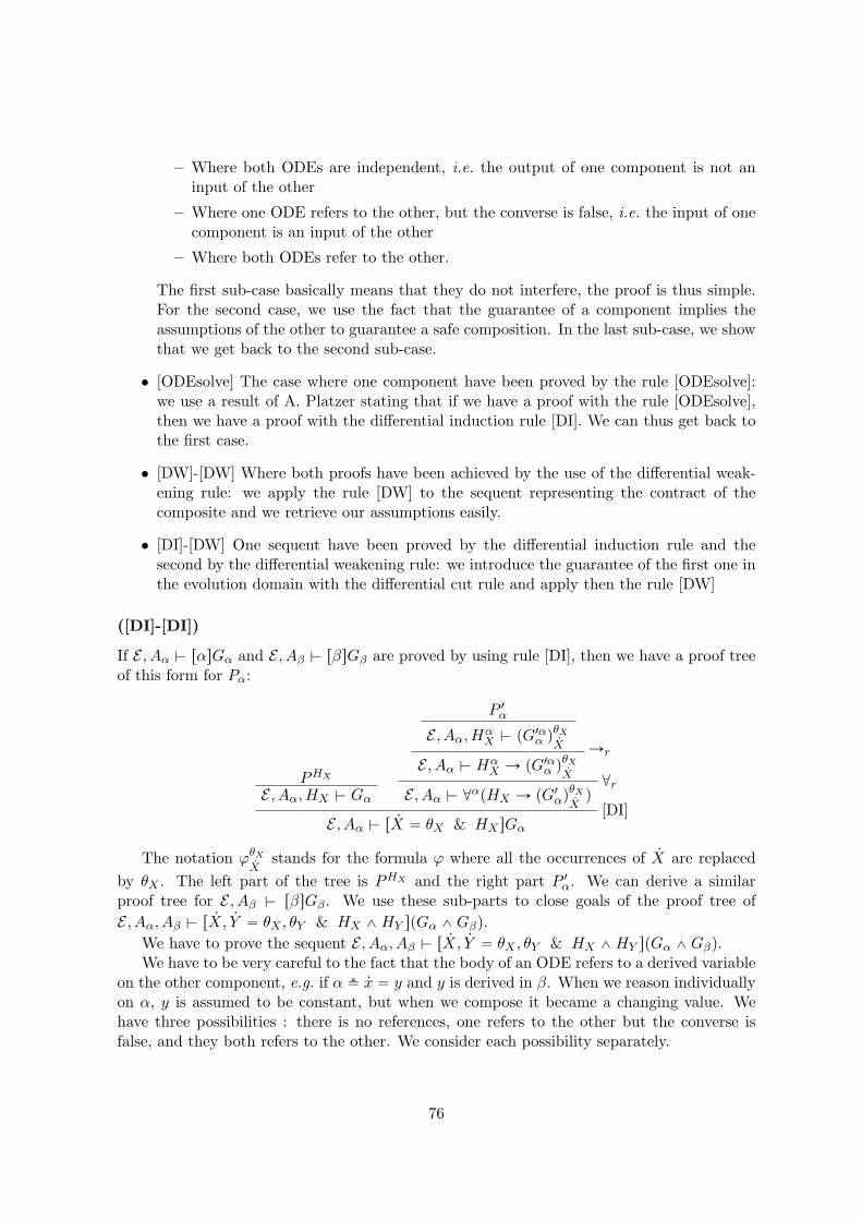
– Where both ODEs are independent, i.e. the output of one component is not aninput of the other

– Where one ODE refers to the other, but the converse is false, i.e. the input of onecomponent is an input of the other

– Where both ODEs refer to the other.

The first sub-case basically means that they do not interfere, the proof is thus simple.For the second case, we use the fact that the guarantee of a component implies theassumptions of the other to guarantee a safe composition. In the last sub-case, we showthat we get back to the second sub-case.

• [ODEsolve] The case where one component have been proved by the rule [ODEsolve]:we use a result of A. Platzer stating that if we have a proof with the rule [ODEsolve],then we have a proof with the differential induction rule [DI]. We can thus get back tothe first case.

• [DW]-[DW] Where both proofs have been achieved by the use of the differential weak-ening rule: we apply the rule [DW] to the sequent representing the contract of thecomposite and we retrieve our assumptions easily.

• [DI]-[DW] One sequent have been proved by the differential induction rule and thesecond by the differential weakening rule: we introduce the guarantee of the first one inthe evolution domain with the differential cut rule and apply then the rule [DW]

([DI]-[DI])

If E , Aα $ rαsGα and E , Aβ $ rβsGβ are proved by using rule [DI], then we have a proof treeof this form for Pα:

PHX

E , Aα, HX $ Gα

P 1α

E , Aα, HαX $ pG1α

α qθX9X Ñr

E , Aα $ HαX Ñ pG1α

α qθX9X @r

E , Aα $ @αpHX Ñ pG1αqθX

9Xq

[DI]E , Aα $ r 9X “ θX & HX sGα

The notation ϕθX9X

stands for the formula ϕ where all the occurrences of 9X are replaced

by θX . The left part of the tree is PHX and the right part P 1α. We can derive a similar

proof tree for E , Aβ $ rβsGβ . We use these sub-parts to close goals of the proof tree of

E , Aα, Aβ $ r 9X, 9Y “ θX , θY & HX ^ HY spGα ^ Gβq.

We have to prove the sequent E , Aα, Aβ $ r 9X, 9Y “ θX , θY & HX ^ HY spGα ^ Gβq.We have to be very careful to the fact that the body of an ODE refers to a derived variable

on the other component, e.g. if α fi 9x “ y and y is derived in β. When we reason individuallyon α, y is assumed to be constant, but when we compose it became a changing value. Wehave three possibilities : there is no references, one refers to the other but the converse isfalse, and they both refers to the other. We consider each possibility separately.

76

Systems are independent We consider the case where both systems are independent, e.g.α fi 9x “ 3t and β fi 9y “ 42. Thus we assume here that θX (resp. θY ) does not refer tooutputs of β (resp. αq, i.e. that FV pθXq X BV pβq “ H (resp. FV pθY q X BV pαq “ H).

We first apply the rule [DI] with Gα ^ Gβ as invariant.

E , Aα, Aβ , HX , HY $ Gα ^ Gβ E , Aα, Aβ $ @αβ`

pHX ^ HY q Ñ pG1α ^ G1

βqθX θY9X 9Y

˘

[DI]E , Aα, Aβ $ r 9X, 9Y “ θX , θY & HX ^ HY spGα ^ Gβq

The left premise correspond to the initial step. We apply the rule ^r to split the goaland end up with the sequent E , Aα, Aβ , HX , HY $ Gα and E , Aα, Aβ , HX , HY $ Gβ . Byassumption, we have the proof tree PHX and PHY to conclude.

PHX

E , Aα, Aβ , HX , HY $ Gα

PHY

E , Aα, Aβ , HX , HY $ Gβ ^rE , Aα, Aβ , HX , HY $ Gα ^ Gβ

The second premise is the differential induction step. We have to prove the sequentE , Aα, Aβ $ @αβ

`

pHX ^ HY q Ñ pG1α ^ G1

βqθX θY9X 9Y

˘

to finish our proof tree.

Thanks to the condition paq and pbq, the formula pG1α ^ G1

βqθX θY9X 9Y

is equivalent to the

formula pG1αqθX

9X^ pG1

βqθY9Y. Since the outputs of each component are dissociated and Gα does

not contain occurrences of bound variables of β, i.e. of Y , the substitution of 9Y by θY doesnot have any effect on Gα. Idem for Gβ .

We apply the rule @r to eliminate the universal quantification in the goal. By applyingthe separation lemma (Lemma 1) to the evolution domain HX ^ HY , the resulting sequent

is E , Aα, Aβ $ pHαX ^ H

βY q Ñ ppG1

αqθX9X

^ pG1βqθY

9Yqαβ where the superscript α (resp. β) in G1α

α

means that the bound variables of α (resp. β) occurring in G1α are replaced by fresh variables.

The conditions pb1q and pb2q allows to apply the separation lemma to pG1αqθX

9Xand pG1

βqθY9Y.

Thus, we have the sequent E , Aα, Aβ $ pHαX ^ H

βY q Ñ pppG1

αqθX θY9X 9Y

qα ^ ppG1βqθX θY

9X 9Yqβq.

E , Aα, Aβ $ pHαX ^ H

βY q Ñ pppG1

αqθX9X

qα ^ ppG1βqθX

9Xqβq

@rE , Aα, Aβ $ @αβ

`

pHX ^ HY q Ñ pG1α ^ G1

βqθX θY9X 9Y

˘

We apply successively the rules Ñr and ^l to pass the left-hand side of the implicationon the hypothesis.

E , Aα, Aβ , HαX , H

βY $ ppG1

αqθX9X

qα ^ ppG1βqθX

9Xqβ

^l

E , Aα, Aβ , HαX ^ H

βY $ ppG1

αqθX9X

qα ^ ppG1βqθX

9Xqβ

Ñr

E , Aα, Aβ $ pHαX ^ H

βY q Ñ pppG1

αqθX9X

qα ^ ppG1βqθX

9Xqβq

We split the conjunction. The left premise is closed by P 1α. the second premise is closed

by P 1β .

77

E , Aα, Aβ , HαβX , H

βY $ ppG1

αqθX9X

qαβ

P 1β

E , Aα, Aβ , HαβX , H

βY $ ppG1

βqθY9Y

qβ^r

E , Aα, Aβ , HαβX , H

βY $ ppG1

αqθX9X

qαβ ^ ppG1βqθY

9Yqβ

For the left goal, either θX does not refer initially to bound variables of β, and we canthus conclude by P 1

α. Either, occurrences of y have been replaced by fpzq and we can thusconclude by the proof tree p1

α0.

Application of rule [DI]

Initial step

PHX PHY

Differential induction step

Separation lemma (with conditions paq, pb1q and pb2q)

P 1α

P 1β

Figure 3.14: Summary of the proof for the case [DI]-[DI]

One system is dependent of the other We assume here that one system is dependent ofthe other, e.g. the speed equations 9v “ a, 9x “ v. Here the second part of the equation refers tothe derived variable in the first part. More formally, we assume that FV pθXq XBV pβq “ tyuand FV pθY q X BV pαq “ H. It is easy to generalize it to a set of variables.

If we conduct the proof as in the previous case, we will have trouble with the skolemizationstep. Indeed, y will be captured and it will not be possible to use Aα to retrieve the prooftree P 1

α.Before applying the differential induction rule [DI], we introduce Gβ in the evolution

domain thanks to the rule (Cut).

E , Aα, Aβ $ r 9X, 9Y “ θX , θY & HX ^ HY sGβ[DC]

E , Aα, Aβ $ r 9X, 9Y “ θX , θY & HX ^ HY spGα ^ Gβq

E , Aα, Aβ $ r 9X, 9Y “ θX , θY & HX ^ HY ^ GβspGα ^ Gβq

The left premise is closed exactly as for the case where the continuous systems are inde-pendent. By assumption, α will not interfere and the proof follows without trouble.

78

We introduce now the formula Aα in the evolution domain of the right premise. Theskolemization step will now include Aα and we will be able to retrieve the proof tree P 1

α.

E , Aα, Aβ $ r 9X, 9Y “ θX , θY & HX ^ HY ^ GβsAα[DC]

E , Aα, Aβ $ r 9X, 9Y “ θX , θY & HX ^ HY ^ GβspGα ^ Gβq

E , Aα, Aβ $ r 9X, 9Y “ θX , θY & HX ^ HY ^ Gβ ^ AαspGα ^ Gβq

The left premise is closed by an application of the proof rule [DW] and the use of thecondition pcq.

E , Aα, Aβ $ @αβ`

pHX ^ HY ^ Gβq Ñ Aα

˘

[DW]E , Aα, Aβ $ r 9X, 9Y “ θX , θY & HX ^ HY ^ GβsAα

For the right premise, we now apply the differential induction rule [DI] to the sequentE , Aα, Aβ $ r 9X, 9Y “ θX , θY & HX ^ HY ^ Gβ ^ AαspGα ^ Gβq.

E , Aα, Aβ $ pHX ^ HY ^ Gβ ^ Aαq Ñ pGα ^ Gβq[DI]

E , Aα, Aβ $ r 9X, 9Y “ θX , θY & HX ^ HY ^ Gβ ^ AαspGα ^ Gβq

E , Aα, Aβ $ @αβ`

pHX ^ HY ^ Gβ ^ Aαq Ñ pG1α ^ G1

βqθX θY9X 9Y

˘

We now apply the skolemization step as in the previous case and we can conclude.

Both systems are dependent of the other We consider now the case where both systemsare dependent of the other, e.g. 9x “ y, 9y “ x. Recall that we assume that our ODEs possessa solution fptq. Assume that fptq is such solution for the differential equation 9y “ x. Wecan then replace y in the differential equation 9x “ y by fptq. Notice that fptq may containoccurrences of x. We have now the following system 9x “ fptq, 9y “ x and we are in the secondsituation that have already been considered.

(rule [ODESolve])

We consider the case where E , Aα $ r 9X “ θX & HX sGα is proved by the use of the rule[ODEsolve], which means that we find an explicit solution w.r.t. time to the ODE and wereplace each occurrence of X in Gα by this solution. We show that, given a proof using therule [ODEsolve], we can derive a proof using the differential invariant rule [DI]. This leadsus back to the previous situation. We do the proof with only one variable, X. It is easy togeneralize it to a system of ODEs. Our reasoning is inspired from [98, p. 247]. By hypothesis,we have the following rule for [ODEsolve]

E , Aα $ @t ě 0p@0 ď t ď t, pHXqyptqX q Ñ pGαq

yptqX [ODEsolve]

E , Aα $ r 9X “ θX & HX sGα

79

yptq is the solution of the ODE 9X “ θX .Let us introduce a fresh variable t to stand for time in the ODE. It will be evaluated after

the rule [DI] by using the differential auxiliaries rule [DA].

E , Aα $ r 9X “ θX , 9t “ 1 & HX sGα[DA]

E , Aα $ r 9X “ θX & HX sGα

Also, the solution of the ODE shall contain an occurrence of the initial value. To rememberit, we use the auxiliary variable rule [IA].

E , Aα $ rX0 :“ Xsr 9X “ θX , 9t “ 1 & HX sGα[IA]

E , Aα $ r 9X “ θX , 9t “ 1 & HX sGα

The proof tree of E , Aα $ rαsGα using the rule [DI] is in the Figure 3.3.3. To introducethe solution as an invariant, we use the generalization rule [gen].

Π1

E , Aα, X0 “ ypt0q $ G0

α ÑrE , Aα $ X0 “ ypt0q Ñ G0

α @rE , Aα $ @X@t,X “ yptq Ñ Gα

axE , Aα, HX $ X “ yp0q

axE , Aα, HX $ θX “ θX (i)

E , Aα, HX $ pX “ yptqq1θX 1

9X 9t Ñr

E , Aα $ HX Ñ pX “ yptqq1θX 1

9X 9t @rE , Aα $ @X,HX Ñ pX “ yptqq1θX 1

9X 9t [DI]E , Aα $ r 9X “ θX , 9t “ 1 & HX sX “ yptq

[gen]E , Aα $ r 9X “ θX , 9t “ 1 & HX sGα

By hypothesis, we assume a proof P of $ ϕypt0qX . Here, t0 is the fresh variable introduced

by the rule @r, idem for X0 and ϕ0. On the branch Π1, we apply exactly the same logicalrules that the ones applied in P . For the logical connectives, there is no problem since thestructure is similar. We need to pay a little more attention to the case of arithmetic overreals. Indeed, suppose we have proved ypt0q ď θX in P . Then, we will have to prove X0 ď θ

in the proof of G0α. Fortunately, we also know that X0 “ yptq by hypothesis. Hence the

conclusion by applying basic arithmetic.For the left premise of rule [DI], we must remember that it is here to prove the initial

condition: the property at time t “ 0, i.e. to ensure that the initials conditions prove the(inductive) safety property. But the value of X is exactly yp0q, so we can conclude with theaxiom rule. For the right premise, we just perform the substitution and the step (i) is justifiedby the same reasoning as for [DI].

80

([DW]-[DW])

We still need to prove the differential weakening case. The proofs are of the following form:

Pα

E , Aα, HαX $ Gα

α ÑrE , Aα $ Hα

X Ñ Gαα

@rE , Aα $ @αpHX Ñ Gαq

[DW]E , Aα $ r 9X “ θX & HX sGα

Once E , Aα $ rαsGα and E , Aβ $ rβsGβ are both proved by the mean of differentialweakening, then the proof of the composition is the following:

Pα

E , Aα, Aβ , HαX , H

βY $ Gα

α

P β

E , Aα, Aβ , HαX , H

βY $ G

ββ ^r

E , Aα, Aβ $ pHαX ^ H

βY q Ñ pGα

α ^ Gββq

@rE , Aα, Aβ $ @αβ

`

pHX ^ HY q Ñ pGα ^ Gβq˘

[DW]E , Aα, Aβ $ rα ˝c βspGα ^ Gβq

It is a very simple case, where the evolution domains are sufficient to prove the safetyproperties. We first apply the differential weakening rule [DW]. Then the quantification rule

which results in the sequent E , Aα, Aβ $ pHαX ^ H

βY q Ñ pGα

α ^ Gββq thanks to the separation

lemma and conditions paq, pb1q and pb2q. We split then the conjunction and ends up with

premises E , Aα, Aβ , HαX , H

βY $ Gα

α and E , Aα, Aβ , HαX , H

βY $ G

ββ . They are closed by the proof

tree Pα and P β .

([DI]-[DW])

Assume that E , Aα $ rαsGα have been proved by the use of rule [DI] and E , Aβ $ rβsGβ byrule [DW]. The idea is to add Gα into the evolution domain of α ˝c β using the differentialcut rule [DC].

E , Aα, Aβ $ r 9X, 9Y “ θX , θY & HX ^ HY sGα[DC]

E , Aα, Aβ $ r 9X, 9Y “ θX , θY & HX ^ HY spGα ^ Gβq

E , Aα, Aβ $ r 9X, 9Y “ θX , θY & HX ^ HY ^ GαspGα ^ Gβq

The left premise requires to prove that Gα is an invariant of α ˝c β. We can follow themethodology for the case where both components have been proved by differential inductionwith J as invariant of Gβ . The right premise requires to prove that Gα ^ Gβ is an invariantof α ˝c β. We apply the differential weakening rule [DW].

E , Aα, Aβ $ @αβ`

pHX ^ HY ^ Gαq Ñ pGα ^ Gβq˘

[DW]E , Aα, Aβ $ r 9X, 9Y “ θX , θY & HX ^ HY ^ GαspGα ^ Gβq

81

We apply the skolemization step with the rule @r and, thanks to the separation lemma(cf Lemma 1) with conditions paq, pb1q and pb2q, we obtain the sequent E , Aα, Aβ $ pHα

X ^

HβY ^ Gα

αq Ñ pGαα ^ G

ββq.

E , Aα, Aβ $ pHαX ^ H

βY ^ Gα

αq Ñ pGαα ^ G

ββq

@rE , Aα, Aβ $ @αβ

`

pHX ^ HY ^ Gαq Ñ pGα ^ Gβq˘

We apply successively the rules Ñr, ^l and ^r.

axE , Aα, Aβ , H

αX , H

βY , G

αα $ Gα

α

P β

E , Aα, Aβ , HαX , H

βY , G

αα $ G

ββ ^r

E , Aα, Aβ , HαX , H

βY , G

αα $ Gα

α ^ Gββ ^l

E , Aα, Aβ , HαX , H

βY ^ Gα

α $ Gαα ^ G

ββ ^l

E , Aα, Aβ , HαX ^ H

βY ^ Gα

α $ Gαα ^ G

ββ Ñr

E , Aα, Aβ $ pHαX ^ H

βY ^ Gα

αq Ñ pGαα ^ G

ββq

The left branch is closed by the rule ax. The right sequent is closed by P β as in the caseof [DW]-[DW].

When we compose two components with continuous behaviors, the Theorem 1 ensuresthat the resulting component satisfies the conjunction of contracts. We have a similar resultfor the composition of purely discrete components in Subsection 3.3.4.

3.3.4 For two discrete components

As in the previous subsection, we have a theorem ensuring that we retain contracts throughparallel composition of purely discrete components. The conditions are similar to the Theo-rem 1.

Theorem. Let A and B be two discrete components with respective contracts pAα, Gαq andpAβ , Gβq. Assume that they both satisfy their contracts. Furthermore, assume that

paq A.outputs X B.outputs “ H,

pb1q A.outputs is separated from Gβ

pb2q B.outputs is separated from Gα,

pc1q Gα must implies the assumptions Aβ that refer to outputs of A

pc2q Gβ must implies the assumptions Aα that refer to outputs of B.

Then the component AB resulting from the parallel composition of A and B satisfies the con-junction of contracts pAα ^ Aβ , Gα ^ Gβq.

We have the equivalent theorem with the behaviors in dL.

82

Theorem 2. Let α and β be two discrete behaviors of components A and B with respectivecontracts pAα, Gαq and pAβ , Gβq. Assume that we have two proof trees of E , Aα $ rαsGα andE , Aβ $ rβsGβ respectively, where E is the environment. Furthermore, assume that

paq BV pαq X BV pβq “ H,

pb1q BV pαq X FV pGβq “ H,

pb2q BV pβq X FV pGαq “ H,

pc1q E , Aα $ @βpGβ Ñ Aαq,

pc2q E , Aβ $ @αpGα Ñ Aβq.

Then it exists a proof tree of E , Aα, Aβ $ rα ˝ βspGα ^ Gβq.

The conditions are similar to the Theorem 1, except for conditions pb1q and pb2q wherewe do not refer to the evolution domain as it is non-existent since we are working with purelydiscrete components.

Proof. Assume α fi rpdiscαq˚s and β fi rpdiscβq˚s are two behaviors of component A and B

respecting the conditions above. The composition α ˝ β is given by the behavior pdiscα Ydiscβq˚. Given the proof of contracts E , Aα $ rαsGα and E , Aβ $ rβsGβ , we want to provethe sequent E , Aα, Aβ $ rα ˝ βspGα ^ Gβq.

An application of the rule [Ind] have been necessary to prove the sequent E , Aα $rpdiscαq˚sGα. It results in two premises : the initial step and the induction step. We assumethat we have a proof tree Pinitα such that the premise corresponding to the initial step isclosed by Pinitα . For the second premise, we apply the proof rule @r to skolemize boundvariables of α. We recall that the superscript α on a formula or a hybrid program means thatwe have replaced every occurrences of bound variables of α by fresh variables. The remaininggoal E , Aα, G

αα $ rdiscααsGα

α is closed by the proof tree Pindα .

Pinitα

E , Aα $ Gα

Pindα

E , Aα, Gαα $ rdiscααsGα

α ÑrE , Aα $ Gα

α Ñ rdiscααsGαα @r

E , Aα $ @αpGα Ñ rdiscαsGαq[Ind]

E , Aα $ rpdiscαq˚sGα

We apply a similar reasoning to the proof of the sequent β fi rpdiscβq˚s. We have thusthe proof tree Pinitβ and Pindβ .

To prove the sequent E , Aα, Aβ $ rpdiscα Y discβq˚spGα ^ Gβq, we apply the rule [Ind].

E , Aα, Aβ $ Gα ^ Gβ E , Aα, Aβ $ @αβ`

pGα ^ Gβq Ñ rdiscα Y discβspGα ^ Gβq˘

[Ind]E , Aα, Aβ $ rpdiscα Y discβq˚spGα ^ Gβq

The left premise corresponds to the initial step. We have to prove that both guaranteeshold after zero executions. We split the goal with the rule ^r and obtain two premises thatcorrespond to the initial step of each individual proof. They are closed by using the prooftrees Pinitα and Pinitβ .

83

Pinitα

E , Aα, Aβ $ Gα

Pinitβ

E , Aα, Aβ $ Gβ ^rE , Aα, Aβ $ Gα ^ Gβ

The right premise corresponds to the induction step. We first apply the skolemization stepwith the rule @r to the sequent E , Aα, Aβ $ @αβ

`

pGα ^ Gβq Ñ rdiscα Y discβspGα ^ Gβq˘

.

E , Aα, Aβ $ pGαβα ^ G

αββ q Ñ rdiscαβα Y discαββ spGαβ

α ^ Gαββ q

E , Aα, Aβ $ @αβ`

pGα ^ Gβq Ñ rdiscα Y discβspGα ^ Gβq˘

We can apply the separation lemma (cf Lemma 1) since the bound variables are dissociated(condition paq) and the variables of Gα (resp. Gβ) are different from the bound variables of β

(resp. α) (conditions pb1q and pb2q). Thus, the sequent E , Aα, Aβ $ pGαβα ^G

αββ q Ñ rdiscαβα Y

discαββ spGαβα ^ G

αββ q is equivalent to E , Aα, Aβ $ pGα

α ^ Gββq Ñ rdiscαβα Y discαββ spGα

α ^ Gββq.

We apply the rule Ñr to this sequent followed by the rule ^l to pass in the hypothesispGα

α ^ Gββq.

E , Aα, Aβ , Gαα, G

ββ $ rdiscαβα Y discαββ spGα

α ^ Gββq

^l

E , Aα, Aβ , Gαα ^ G

ββ $ rdiscαβα Y discαββ spGα

α ^ Gββq

Ñr

E , Aα, Aβ $ pGαα ^ G

ββq Ñ rdiscαβα Y discαββ spGα

α ^ Gββq

The next step is to split discαβα Y discαββ with the non-deterministic rule rYs to considerseparately their action. We obtain two premises which are similar to handle. We consideronly the case of the left premise, i.e. the sequent E , Aα, Aβ , G

αα, G

ββ $ rdiscαβα spGα

α ^Gββq, the

second one is closed by the same reasoning.

E , Aα, Aβ , Gαα, G

ββ $ rdiscαβα spGα

α ^ Gββq E , Aα, Aβ , G

αα, G

ββ $ rdiscαββ spGα

α ^ Gββq

rYsE , Aα, Aβ , G

αα, G

ββ $ rdiscαβα Y discαββ spGα

α ^ Gββq

We have to prove the sequent E , Aα, Aβ , Gαα, G

ββ $ rdiscαβα spGα

α ^ Gββq. We split the

guarantees by using the rule [BoxAnd] since they are of different nature. Gαα is a guarantee

of the component A and we have already a proof by assumption. Gββ is a guarantee of the

component B, but it is not affected by the execution of α thanks to the conditions paq andpbq.

E , Aα, Aβ , Gαα, G

ββ $ rdiscαβα sGα

α E , Aα, Aβ , Gαα, G

ββ $ rdiscαβα sGβ

β[BoxAnd]

E , Aα, Aβ , Gαα, G

ββ $ rdiscαβα spGα

α ^ Gββq

We have a proof tree Pindα of E , Aα, Gαα $ rdiscααsGα

α and we want to close the left premise

: E , Aα, Aβ , Gαα, G

ββ $ rdiscαβα sGα

α. Here discαα differs from discαβα by the variables of β thatare captured by the skolemization. We can not make use of the assumption Aα to concludesince it may refer to bound variables of β.

The condition pcq states that the sequent Aα $ Gββ Ñ A

βα is valid. We introduce the

formula Gββ Ñ A

βα with the cut rule (Cut).

84

E , Aα, Aβ , Gαα, G

ββ , G

ββ Ñ A

βα $ rdiscαβα sGα

α E , Aα, Aβ , Gαα, G

ββ $ rdiscαβα sGα

α, Gββ Ñ A

βα

(Cut)E , Aα, Aβ , G

αα, G

ββ $ rdiscαβα sGα

α

The right premise is closed by the assumption that we have a proof of Gββ Ñ A

βα. For the

left premise, we can deduce the formula Aβα in the hypothesis thanks to an application of the

rule Ñl. The left premise is closed by the rule ax.

axE , Aα, Aβ , G

αα, G

ββ $ G

ββ , rdiscαβα sGα

α E , Aα, Aβ , Gαα, G

ββ , A

βα $ rdiscαβα sGα

αÑl

E , Aα, Aβ , Gαα, G

ββ , G

ββ Ñ A

βα $ rdiscαβα sGα

α

We are left with the right sequent E , Aα, Aβ , Gαα, G

ββ , G

ββ Ñ A

βα, A

βα $ rdiscαβα sGα

α, and byassumption we have a proof Pα of it.

To prove the remaining sequent E , Aα, Aβ , Gαα, G

ββ $ rdiscαβα sGβ

β , we symbolically execute

discαβα . Since Gββ does not contain any bound variables of α (and thus of discαβα ), it is not

affected. We conclude then by the rule ax.

axE , Aα, Aβ , G

αα, G

ββ $ G

ββ

Symbolic executionE , Aα, Aβ , G

αα, G

ββ $ rdiscαβα sGβ

β

We have a summary of the structure of the proof tree in the Figure 3.15.

3.3.5 For a discrete component and a continuous component

We consider the case where one discrete component A is composed with a continuous com-ponent B. We mix here reasoning for discrete and continuous composition, and thus have tobe very careful for the composition. As for the two previous section, we state the theoremfor the components expressed with the textual representation and the equivalent results withbehaviors.

Theorem. Let A be a discrete component and B be a continuous component with respectivecontracts pAα, Gαq and pAβ , Gβq. Assume that they both satisfy their contracts. Furthermore,assume that

paq A.outputs X B.outputs “ H,

pb1q A.outputs is separated from Gβ

pb2q B.outputs is separated from Gα,

pc1q Gα must implies the assumptions Aβ that refer to outputs of A

pc2q Gβ must implies the assumptions Aα that refer to outputs of B.

Then the component AB resulting from the parallel composition of A and B satisfies the con-junction of contracts pAα ^ Aβ , Gα ^ Gβq.

85

Application of rule [Ind]

Initial step

PInitα PInitβ

Induction step

Separation lemma (with conditions paq, pb1q and pb2q)

Application of rule rYs

[BoxAnd]

Condition pcq

PIndα

ax

[BoxAnd]

Condition pcq

PIndα

ax

Figure 3.15: Summary of the proof for the discrete case

We have the equivalent theorem for behaviors of components. Recall that the behavior βof a component B is of the form β fi 9Y “ θY & HY .

Theorem 3. Let α be the discrete behaviors of a component A and β be the continuousbehavior of a component B with respective contracts pAα, Gαq and pAβ , Gβq. Assume that wehave two proof trees of E , Aα $ rαsGα and E , Aβ $ rpβq˚sGβ respectively, where E is theenvironment. Furthermore, assume that

paq BV pαq X BV pβq “ H,

pb1q BV pαq X FV pGβq “ H and BV pαq X FV pHY q “ H,

pb2q BV pβq X FV pGαq “ H,

pc1q E , Aα $ @βpGβ Ñ Aαq,

pc2q E , Aβ $ @αpGα Ñ Aβq.

Then it exists a proof tree of E , Aα, Aβ $ rα ˝ βspGα ^ Gβq.

86

We also require that the bound variables of the discrete behavior do not occur in theevolution domain HY of β. It is similar to the condition pb1q of the Theorem 1.

There is a major point to consider in this theorem. Instead of assuming having a proofof the sequent E , Aβ $ rβsGα, we assume having a proof of E , Aβ $ rpβq˚sGα. Indeed, whenwe compose, the differential equation is now under an iteration. Thus, it may not accessto assumptions due to supplementary skolemization. We provide a counter-example to showthat without this assumption, the theorem does not hold.

Example 32 (Counter-example). Assume that the behavior of our continuous component is9x “ y & x “ y. Its contract is pJ, x ď 10q and the initial value of x is 0. It is simple toobtain a proof of the sequent x “ 0 $ r 9x “ y & x “ ysx ď 10. Indeed, we have that 9x “ 0,and thus x does not evolve. Since it is initialized at 0, we have that x ď 10.

Let compose it with a behavior discα of a discrete component and with contract pJ,Jq.The behavior resulting from the composition is pdiscα Y 9x “ y & x “ yq˚. We want to provethe following sequent:

x “ 0 $ rpdiscα Y 9x “ y & x “ yq˚sx ď 10

We start by applying the induction rule [Ind] and obtain two sub-goals, one for the initialstep, the other for the induction step.

x “ 0 $ x ď 10 x “ 0 $ @x, px ď 10 Ñ rdiscα Y 9x “ y & x “ ysx ď 10q[Ind]

x “ 0 $ rpdiscα Y 9x “ y & x “ yq˚sx ď 10

Consider the induction step. We apply the rule @r and replace the variable x by the freshvariable x0. We then split the behavior between discα and 9x “ y & x “ y by using the rulerYs.

x “ 0 $ x0 ď 10 Ñ rdiscαsx0 ď 10 x “ 0 $ x0 ď 10 Ñ r 9x0 “ y & x0 “ ysx0 ď 10rYs

x “ 0, x0 ď 10 $ rdiscα Y 9x0 “ y & x0 “ ysx0 ď 10Ñr

x “ 0 $ x0 ď 10 Ñ rdiscα Y 9x0 “ y & x0 “ ysx0 ď 10@r

x “ 0 $ @x, px ď 10 Ñ rdiscα Y 9x “ y & x “ ysx ď 10q

The sequent x “ 0 $ x0 ď 10 Ñ r 9x0 “ y & x0 “ ysx0 ď 10 is clearly not valid. Forexample, if x0 “ 1 at the initialization, then we have x0 ď 10, y “ 1, and thus 9x0 “ 1. As x0is evolving linearly, we have that the formula x0 ď 10 will not hold at some point.

Proof. The behavior α is of the form pdiscαq˚ since it is a purely discrete component. Weassume to have a proof tree of the sequent E , Aα $ rpdiscαq˚sGα. It is the same assumptionas in the proof of Theorem 2.

Πinitα

E , Aα $ Gα

Πindα

E , Aα, Gαα $ rdiscααsGα

α ÑrE , Aα $ Gα

α Ñ rdiscααsGαα @r

E , Aα $ @αpGα Ñ rdiscαsGαq[Ind]

E , Aα $ rpdiscαq˚sGα

87

The behavior β of the continuous component B is of the form 9Y “ θY & HY . We assumeto have a proof tree of the sequent E , Aβ $ rp 9Y “ θY & HY q˚sGβ . It has the following shape.

Πinitβ

E , Aβ $ Gβ

Πstepβ

E , Aβ , Gββ $ rp 9Y “ θY qβ & H

βY sGβ

β Ñr

E , Aβ $ Gββ Ñ rp 9Y “ θY qβ & H

βY sGβ

β@r

E , Aβ $ @βpGβ Ñ r 9Y “ θY & HY sGβq[Ind]

E , Aβ $ rp 9Y “ θY & HY q˚sGβ

We first apply the induction rule and then the skolemization step (rule @r). Notice thatoccurrences of bound variables of β inHY are replaced by fresh variables, which is the meaningof the notation H

βY .

Recall that the parallel composition of α and β results in the behavior`

discα Y p 9Y “

θY & HY q˘

˚. We provide a proof tree for the sequent E , Aα, Aβ $ r

`

discα Y p 9Y “ θY &

HY q˘

˚spGα ^ Gβq.

We first apply the induction rule [Ind] with pGα ^ Gβq as invariant.

E , Aα, Aβ $ Gα ^ Gβ E , Aα, Aβ $ @αβ`

pGα ^ Gβq Ñ rdiscα Y p 9Y “ θY & HY qspGα ^ Gβq˘

E , Aα, Aβ $ r`

discα Y p 9Y “ θY & HY q˘

˚spGα ^ Gβq

We obtain two sub-goals, one corresponding for the initial step and one for the inductionstep. The first sub-goal is handled as in the proof of the previous Theorem 2. We split theformula Gα ^ Gβ using the rule ^ and then use the proof tree Πinitα and Πinitβ to conclude.

We consider the second sub-goal E , Aα, Aβ $ @αβ`

pGα ^ Gβq Ñ rdiscα Y p 9Y “ θY &HY qspGα ^Gβq

˘

. We apply the rule @r to replace all occurrences of bound variables of α and

β in the formula pGα ^ Gβq Ñ rdiscα Y p 9Y “ θY & HY qspGα ^ Gβq. We denote by Gαβα the

effect of this replacement on the formula Gα.The step piq is the application of the separation Lemma 1. Indeed, from conditions pb1q

and pb2q, we deduce that Gαβα is equivalent to Gα

α. It justifies the fact that we obtain the

sequent E , Aα, Aβ $ pGαα ^ G

ββq Ñ rdiscαβα Y

`

p 9Y “ θY qαβ & HβY

˘

spGαα ^ G

ββq. We apply

successively the rules Ñr and ^l to pass the formula pGαα ^ G

ββq into the hypothesis.

E , Aα, Aβ , Gαα, G

ββ $ rdiscαβα Y

`

p 9Y “ θY qαβ & HβY

˘

spGαα ^ G

ββq

^l

E , Aα, Aβ , Gαα ^ G

ββ $ rdiscαβα Y

`

p 9Y “ θY qαβ & HβY

˘

spGαα ^ G

ββq

E , Aα, Aβ $ pGαα ^ G

ββq Ñ rdiscαβα Y

`

p 9Y “ θY qαβ & HβY

˘

spGαα ^ G

ββq

piqE , Aα, Aβ $ pGαβ

α ^ Gαββ q Ñ rdiscαβα Y

`

p 9Y “ θY qαβ & HβY

˘

spGαβα ^ G

αββ q

@rE , Aα, Aβ $ @αβ

`

pGα ^ Gβq Ñ rdiscαβα Y`

p 9Y “ θY qαβ & HβY

˘

spGα ^ Gβq˘

Our next step is to split the hybrid program discαβα Y`

p 9Y “ θY qαβ & HβY

˘

in two withthe non-deterministic choice rule rYs. We have two cases to consider: the execution of thediscrete part and the execution of the continuous part.

88

E , Aα, Aβ , Gαα, G

ββ $ rdiscαβα spGα

α ^ Gββq E , Aα, Aβ , G

αα, G

ββ $ rp 9Y “ θY qαβ & H

βY spGα

α ^ Gββq

rYsE , Aα, Aβ , G

αα, G

ββ $ rdiscαβα Y

`

p 9Y “ θY qαβ & HβY

˘

spGαα ^ G

ββq

The left sub-goal, E , Aα, Aβ , Gαα, G

ββ $ rdiscαβα spGα

α ^ Gββq, is handled as in the proof of

the Theorem 2. We detail the proof tree for the right sub-goal, E , Aα, Aβ , Gαα, G

ββ $ rp 9Y “

θY qαβ & HβY spGα

α ^ Gββq.

We first split the formula Gαα ^ G

ββ under the modality with the rule [BoxAnd]. We then

carefully consider the two sub-goals.

E , Aα, Aβ , Gαα, G

ββ $ rp 9Y “ θY qαβ & H

βY sGα

α E , Aα, Aβ , Gαα, G

ββ $ rp 9Y “ θY qαβ & H

βY sGβ

β[BoxAnd]

E , Aα, Aβ , Gαα, G

ββ $ rp 9Y “ θY qαβ & H

βY spGα

α ^ Gββq

For the first sub-goal, E , Aα, Aβ , Gαα, G

ββ $ rp 9Y “ θY qαβ & H

βY sGα

α, remember that Gα

does not contain any occurrences of bound variables of 9Y “ θY & HY . Thus the evolution ofthe differential equation does not affect Gα

α. We symbolically execute it to obtain the sequentwhich is closed by the axiom rule.

axE , Aα, Aβ , G

αα, G

ββ $ Gα

αSymbolic execution

E , Aα, Aβ , Gαα, G

ββ $ rp 9Y “ θY qαβ & H

βY sGα

α

It remains to prove the sequent E , Aα, Aβ , Gαα, G

ββ $ rp 9Y “ θY qαβ & H

βY sGβ

β . Using the

condition pc2q, we obtain Aββ in the hypothesis. We conclude with the branch Πstepβ .

3.3.6 For two general components

We have shown in Subsection 3.3.3 how to retain contracts in the case of the parallel composi-tion of two continuous components. We have proved a similar theorem in Subsection 3.3.4 forthe case of the parallel composition of two purely discrete components. In Subsection 3.3.5,we have proved how to retain contracts when we compose discrete component with continuouscomponent. We state the main theorem which reunite the previous results for the case of theparallel composition of general components, i.e. with both discrete and continuous aspects.

Theorem. Let A and B be two components with behaviors of the general form and respectivecontracts pAα, Gαq and pAβ , Gβq. Assume that they both satisfy their contracts. Furthermore,assume that

paq A.outputs X B.outputs “ H,

pb1q A.outputs is separated from Gβ

pb2q B.outputs is separated from Gα,

pc1q Gα must implies the assumptions Aβ that refers to outputs of A

pc2q Gβ must implies the assumptions Aα that refers to outputs of B.

89

Then the component AB resulting from the parallel composition of A and B satisfies the con-junction of contracts pAα ^ Aβ , Gα ^ Gβq.

Recall that the behavior α of a general component is of the form pdiscα Ycontαq˚, wherecontα is a differential equation with evolution domain HX .

Theorem 4. Let α and β be two behaviors of general form of components A and B withrespective contracts pAα, Gαq and pAβ , Gβq. Assume that we have two proof trees of E , Aα $rαsGα and E , Aβ $ rβsGβ respectively, where E is the environment. Furthermore, assumethat

paq BV pαq X BV pβq “ H,

pb1q BV pαq X FV pGβq “ H and BV pαq X FV pHY q “ H,

pb2q BV pβq X FV pGαq “ H and BV pβq X FV pHXq “ H,

pc1q Aα $ @βpGβ Ñ Aαq,

pc2q Aβ $ @αpGα Ñ Aβq.

Then it exists a proof tree of E , Aα, Aβ $ rα ˝ βspGα ^ Gβq.

The proof uses the same mechanism as in the proofs of Theorems 1, 2 and 3.

Proof. Recall that the behavior α of component A is of the form pdiscα Y contαq˚. Asin previous theorems, we assume to have a proof tree of the sequent E , Aα $ rpdiscα Ycontαq˚sGα. It is of the following form:

Πinitα

E , Aα $ Gα

Πinddiscα

E , Aα, Gαα $ rdiscααsGα

α

Πindcontα

E , Aα, Gαα $ rcontααsGα

α rYsE , Aα, G

αα $ rdiscαα Y contααsGα

α ÑrE , Aα $ Gα

α Ñ rdiscαα Y contααsGαα @r

E , Aα $ @αpGα Ñ rdiscα Y contαsGα[Ind]

E , Aα $ rpdiscα Y contαq˚sGα

We have the same for the proof of the sequent E , Aβ $ rpdiscβ Y contβq˚sGβ Recall thatthe behavior of the resulting component is α ˝ β fi

`

discα Y discβ Y pcontα ˝c contβq˘

˚.

We apply the induction rule [Ind]. We obtain two sub-goals: the initial step piq and theinduction step piiq. The first step piq is handled exactly as for the discrete case or for thecontinuous case with rule [DI].

For the last sequent E , Aα, Aβ $ @αβ`

pGα ^Gβq Ñ rpdiscα YdiscβqYcontαβspGα ^Gβq˘

,we first apply the skolemization rule, and then the non-deterministic choice rule rYs (cfFigure 3.17).

As shown in the Figure 3.17, we have two premises to consider. The left premise E , Aα, Aβ , Gαβα ^

Gαββ $ rdiscαβα Ydiscαββ spGαβ

α ^Gαββ q is exactly similar to the induction step of the case where

both components are discrete and is closed using Πinddiscαand Πinddiscβ

. The right premise

E , Aα, Aβ , pGαβα ^ G

αββ q $ rcontαβαβspGαβ

α ^ Gαββ q is closed by applying the Theorem 1 and

using the proof trees Πindcontαand Πindcontβ

.

90

piq

E , Aα, Aβ $ Gα ^ Gβ

piiq

E , Aα, Aβ $ @αβ`

pGα ^ Gβq Ñ rpdiscα Y discβq Y pcontα ˝c contβqspGα ^ Gβq˘

[Ind]E , Aα, Aβ $ rpdiscα Y discβ Y contα ˝c contβq˚spGα ^ Gβq

Figure 3.16: Application of the rule [Ind] for the general case

rYsE , Aα, Aβ , G

αβα ^ G

αββ $ rpdiscαβα Y discαββ q Y contαβαβspGαβ

α ^ Gαββ q

Ñr

E , Aα, Aβ $ pGαβα ^ G

αββ q Ñ rpdiscαβα Y discαββ q Y contαβαβspGαβ

α ^ Gαββ q

@rE , Aα, Aβ $ @αβ

`

pGα ^ Gβq Ñ rpdiscα Y discβq Y contαβspGα ^ Gβq˘

E , Aα, Aβ , Gαβα ^ G

αββ $ rdiscαβα Y discαββ spGαβ

α ^ Gαββ q

E , Aα, Aβ , Gαβα ^ G

αββ $ rcontαβαβspGαβ

α ^ Gαββ q

Figure 3.17: Induction step

The proof follows the distinction between the discrete part and the continuous one. Wenow consider the proof of the Cruise-Control component.

Example 33 (Contract of the cruise-control). The Tachymeter and Engine componentsrespect the conditions of the Theorem 4:

• The outputs are separated. We have BV pEngineq “ tsengu and BV pTachq “ tsacm, stach, au,thus BV pEngineq X BV pTachq “ H.

• The guarantees do not refers to exterior outputs. We have V arpGengq “ tsengu andV arpGtachq “ tsacm, stach, au. It is easy to check that BV pEngineq X V arpGtachq “ Hand BV pTachq X V arpGengq “ H.

• The guarantees imply the assumptions. We have Aeng fi Gtach and Atach fi Geng. It isthus trivial to verify Aeng $ @tachpGtach Ñ Aengq and Atach $ @engpGtach Ñ Aengq.

Thus, by application of the Theorem 4, the following sequent is valid:

E , Acruise $ rCruise-controlsGcruise

91

where Acruise fi Aeng ^ Atach and Gcruise fi Geng ^ Gtach. The Cruise-Control satisfies itscontract, and we have obtained this proof automatically.

We have exhibited in this section a methodology to lift the contracts of individual compo-nents through composition. If components A and B satisfies their respective contracts pAα, Gαqand pAβ , Gβq, then the compound component AB resulting from the parallel composition sat-isfies the contract pAα ^ Aβ , Gα ^ Gβq.

The next section is devoted to the presentation of the implementation of a prototype inKeYmaera X. We have successfully passed the cruise-controller example.

3.4 A prototype in KeYmaera X

We have implemented a prototype using the tactic language Bellerophon in KeYmaera X todemonstrate the feasibility of our approach. We present the tactic language Bellerophon inSubsection 3.4.1 and exemplify with the Fibonacci Example 1. We present the structure ofour prototype in Subsection 3.4.2. The cruise-controller have been verified using this example.

3.4.1 Presentation of Bellerophon

Bellerophon is a tactic language for the proof of hybrid systems and a library implementedin KeYmaera X. It is both a stand-alone language and a Domain-Specific Language in theScala programming language [46, 47].

It has been developed to provide decision procedures and heuristics for the theorem provingof hybrid systems in KeYmaera X. It aims to ease proof automation.

It uses built-in tactics that can be combined through several tactic combinators. Built-in tactics directly manipulate the KeYmaera X core to transform formulas in a validity-preserving manner. They correspond either to specific rules of the sequent calculus, e.g. thetactic andR which corresponds to the rule ^r, or correspond to heuristics, e.g. the tactic propcorresponds to the repeated application of propositional rules until they are not applicable.

Definition 28 (Tactic combinators).

e1, e2 ::“ τ | epvq | e1&e2 | e1|e2 | e˚ |?peq |ă pe1, e2, . . . , enq | abbrvP pxq “ ϕ in e

τ is a built-in tactic. epvq applies a tactic e to a list of positions or formulas. e1&e2 is thesequential composition of two tactics; it applies the tactic e2 on the output of e1. e1|e2 appliese2 if e1 fails. e˚ repeatedly applies the tactic e as long as it is applicable. ?peq applies e if itdoes not result in a error. ă pe1, e2, . . . , enq is used when there is n subgoals; it applies e1 tothe first subgoal, e2 to the second subgoal, etc. abbrvP pxq “ ϕ in e replaces all occurrencesof ϕ with P pxq in the current subgoal, and then applies e. After e, remaining occurrences ofP pxq are uniformly substituted back to ϕ.

Example 34 (Fibonacci example). Remember that the hybrid program representing the Fi-bonacci sequence is Fibonacci fi pFn :“ Fn`1;Fn`1 :“ Fn`2;Fn`2 :“ Fn`1 ` Fnq˚ (cf Defi-nition 1) and we want to prove the following formula pFn “ 0 ^ Fn`1 “ 1 ^ Fn`2 “ 1q ÑrFibonaccisFn`2 “ Fn`1 ` Fn (cf proof tree 2.33).

We can find the .kyx file of the Fibonacci example in the annex 5.3.2. It is proved inKeYmaera X by the following tactic:

92

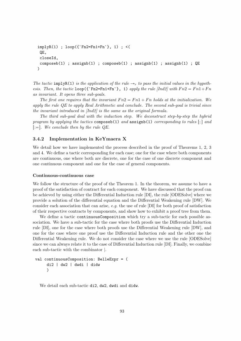
implyR(1) ; loop({`Fn2=Fn1+Fn`}, 1) ; <(

QE,

closeId,

composeb(1) ; assignb(1) ; composeb(1) ; assignb(1) ; assignb(1) ; QE

)

The tactic implyR(1) is the application of the rule Ñr to pass the initial values in the hypoth-esis. Then, the tactic loop({`Fn2=Fn1+Fn`}, 1) apply the rule [Ind2] with Fn2 “ Fn1`Fn

as invariant. It opens three sub-goals.The first one requires that the invariant Fn2 “ Fn1 ` Fn holds at the initialization. We

apply the rule QE to apply Real Arithmetic and conclude. The second sub-goal is trivial sincethe invariant introduced in [Ind2] is the same as the original formula.

The third sub-goal deal with the induction step. We deconstruct step-by-step the hybridprogram by applying the tactics composeb(1) and assignb(1) corresponding to rules r; s andr:“s. We conclude then by the rule QE.

3.4.2 Implementation in KeYmaera X

We detail how we have implemented the process described in the proof of Theorems 1, 2, 3and 4. We define a tactic corresponding for each case; one for the case where both componentsare continuous, one where both are discrete, one for the case of one discrete component andone continuous component and one for the case of general components.

Continuous-continuous case

We follow the structure of the proof of the Theorem 1. In the theorem, we assume to have aproof of the satisfaction of contract for each component. We have discussed that the proof canbe achieved by using either the Differential Induction rule [DI], the rule [ODESolve] where weprovide a solution of the differential equation and the Differential Weakening rule [DW]. Weconsider each association that can arise, e.g. the use of rule [DI] for both proof of satisfactionof their respective contracts by components, and show how to exhibit a proof tree from them.

We define a tactic continuousComposition which try a sub-tactic for each possible as-sociation. We have a sub-tactic for the case where both proofs use the Differential Inductionrule [DI], one for the case where both proofs use the Differential Weakening rule [DW], andone for the case where one proof use the Differential Induction rule and the other one theDifferential Weakening rule. We do not consider the case where we use the rule [ODESolve]since we can always relate it to the case of Differential Induction rule [DI]. Finally, we combineeach sub-tactic with the combinator |.

val continuousComposition: BelleExpr = (

di2 | dw2 | dwdi | didw

)

We detail each sub-tactic di2, dw2, dwdi and didw.

93

DI-DI We consider the case where both cases have been proved with the differential in-duction rule [DI]. We require the user to provide the tactic used to proved the initial step(tactic baseStep1) and the differential induction step (tactic diffInductionStep1). Theycorrespond to the proof trees PHX and P 1

α in the proof of Theorem 1. We have the same forthe second component (baseStep2 and diffInductionStep2).

/* Base case of the first tactic */

val baseStep1: BelleExpr = (

/* To fill by the user */

...

)

/* Differential induction step of the first tactic */

val diffInductionStep1: BelleExpr = (

/* To fill by the user */

...

)

We follow the procedure presented in the proof of the Theorem 1. We apply the DifferentialInduction rule [DI] (tactic dI('diffInd)(1)) and consider the initial step and the differentialinduction step. We split the goal corresponding to the initial step with the rule ^r (tacticandR('R)) and use our two assumptions baseStep1 and baseStep2 to conclude. In theinduction step, the sequent is of the form E , Aα, Aβ $ r 9X :“ θX ; 9Y :“ θY sG1

α ^ G1β . We

perform all the assignments with the tactic chase('R) and split the resulting goal in two.We use then our assumptions diffInductionStep1 and diffInductionStep2.

val di2: BelleExpr = (

print("Try DI2 tactic") & implyR(1) & dI('diffInd)(1) <(

print("Base step") & andR('R) <(

baseStep1,

baseStep2

),

print("Differential Induction step") & chase('R) & andR('R) <(

diffInductionStep1,

diffInductionStep2

)

)

)

The Differential Induction rule in KeYmaera X is implemented by the tactic dI withseveral degrees of automation. We have chosen to consider only the case corresponding to theversion of the rule we have presented in the Chapter 2, the other cases are for future works.

DW-DW We consider the case where the proof of satisfaction of contracts of both compo-nents have been achieved with the Differential Weakening rule [DW]. We follow the structureof the proof of the Theorem 1. First, we require the user to provide the tactics tacticDW1and tacticDW2 used to achieve each respective proof.

94

val tacticDW1: BelleExpr = (

/* To fill by the user */

...

)

val tacticDW2: BelleExpr = (

/* To fill by the user */

...

)

We apply the tactic dW('R) corresponding to the Differential Weakening rule [DW]. Weuse the tactics tacticDW1 and tacticDW2 to close the proof.

val dw2: BelleExpr = (

print("Try DW2 tactic") & implyR(1) & dW('R)

& implyR(1) & andR(1) <(

tacticDW1,

tacticDW2

)

)

DI-DW We consider the case where the proof of satisfaction of contract of the firstcomponent has been achieved with the Differential Induction rule [DI] and the one for thesecond component has been achieved with the Differential Weakening rule [DW]. We requirethe user to provide the tactic used to proved the initial step (tactic baseStep1) and thedifferential induction step (tactic diffInductionStep1). We require also that she providesthe guarantee invariant1 of the first contract and the tactic tacticDW2 used to achieve thesecond proof.

/* Base case of the first tactic */

val baseStep1: BelleExpr = (

/* To fill by the user */

...

)

/* Differential induction step of the first tactic */

val diffInductionStep1: BelleExpr = (

/* To fill by the user */

...

)

95

val invariant1: Formula =

/* To fill by the user */

...

val tacticDW2: BelleExpr = (

/* To fill by the user */

...

)

We follow the structure of the proof of the Theorem 1. We first add the guarantee ofthe first component into the evolution domain using the Differential Cut rule [DC] (tacticdC(invariant1)(1)). It results in two sub-goals. We close the first sub-goal by applyingthe Differential Weakening rule [DW] (tactic dW('R)) and split the current goal in two parts.The first part is trivial to handle since it requires to prove the formula Gα (equivalent toinvariant1) under the assumption Gα, hence the use of the tactic master(). The secondpart is closed by using our assumptions baseStep1 and diffInductionStep1.

val didw: BelleExpr = (

print("Try DIDW tactic") & implyR(1) & dC(invariant1)(1) <(

dW('R) & implyR('R) & andR(1) <(

master(),

tacticDW2

),

dI('diffInd)(1) <(

print("Base step") & baseStep1,

print("Differential Induction step") & chase('R) & diffInductionStep1,

)

)

)

We define also a symmetrical tactic dwdi for the inverse case.

Conclusion We have presented how to implement several of the possible associations con-sidered in the proof of the Theorem 1. The implementation is not complete and does notcover every possibility in KeYmaera X, but it shows the feasibility of such implementation.

Discrete-discrete case

We present the tactic corresponding to the case where both components are purely discrete.The behavior α of the first component is assumed to be purely discrete and is of the formα fi pdiscαq˚. Given the contract pAα, Gαq, its satisfaction is obtained by the proof of thesequent E , Aα $ rpdiscαq˚sGα. The proof tree is obtained by the use of Induction rule [Ind]and is closed by the branches ΠInitα and ΠStepα . We require to the user to provide the tacticscorresponding to these two steps. We also require to have the guarantee Gα.

96

/* Base case of the first tactic */

val baseStep1: BelleExpr = (

/* To fill by the user */

...

)

/* Induction step of the second tactic */

val inductionStep1: BelleExpr = (

/* To fill by the user */

...

)

val invariant1: Formula =

/* To fill by the user */

...

We have similar tactics (baseStep2, inductionStep2 and invariant2) for the othercomponent. The tactic to obtain the proof of satisfaction of the conjunction of contracts bythe composition of components is given in the tactic discDiscCase.

val discDiscCase: BelleExpr = (

print("Try Discrete-Discrete tactic") & implyR(1)

& loop(And(invariant1, invariant2))('R) <(

print("Base step") & andR('R) <(

baseStep1,

baseStep2

),

print("Use step") & master(),

print("Induction step") & inductionStepTactic

)

)

In a .kyx file, the sequent is of the form $ A Ñ rαsG. We apply the rule Ñr (tacticimplyR(1) to pass the left-hand side of the implication on the hypothesis. We then applythe induction rule [Ind] with the conjunction of guarantees. It yields three steps: the initialstep, the use step and the induction step. For the first one, we split the goal in two with therule ^r (tactic andR('R)) and then use our assumptions (tactics baseStep1 and baseStep2).The second one corresponds to the case where we want to strengthen the invariant, but wedo not need it here, hence the use of the tactic master() to close this trivial goal. For thethird one, we apply the induction tactic detailed below.

97

val inductionStepTactic: BelleExpr = (

choiceb(1) & andR('R) <(

boxAnd(1) & andR('R) <(

inductionStep1,

V(1) & master()

),

boxAnd(1) & andR('R) <(

V(1) & master(),

inductionStep2

)

)

)

We follow the structure in the proof of Theorem 2. Recall that the sequent we wantto prove is of the form E , Aα, Aβ , Gα, Gβ $ rdiscα Y discβspGα ^ Gβq. We first apply thenon-deterministic choice rule rYs (tactic choiceb(1)) and split the resulting goal in two withthe rule ^r (tactic andR('R)). We obtain two branches which are similar. In the first one,we split the formula under the modality with the rBoxAnds rule (tactic boxAnd(1)) and therule ^r. It yields two cases; one where we have to prove that Gα holds after one execution ofdiscα and one where we have to prove that Gβ holds after one execution of discα. We useour assumption inductionStep1 for the first case. For the second, we apply the symbolicexecution (tactic V(1)) and then apply the tactic master().

Discrete-continuous case

The exact same tactic can be applied for the composition of a discrete component with acontinuous component. Indeed, given a continuous component with behavior β and contractpAβ , Gβq, we require to have a proof of the sequent E , Aβ $ rβ˚sGβ instead of a proof of thesequent E , Aβ $ rβsGβ . The tactic inductionStep1 corresponds to the branch Πindβ . Thetactic related to the continuous nature are present in the induction step.

General case

We present the tactic corresponding to the case where both components are general, i.e. withdiscrete and continuous evolution. We follow the structure of the proof of the Theorem 4. Aspreviously, we require the user to provide the tactics baseStep1, discInductionStep1 andcontInductionStep1 which corresponds to the proof trees Πinitα , Πinddiscα

and Πindcontα. We

have the corresponding tactics baseStep2, discInductionStep2 and contInductionStep2

for the second component.

/* Base case of the first tactic */

val baseStep1: BelleExpr = (

/* To fill by the user */

...

)

98

/* Discrete induction step of the first tactic */

val discInductionStep1: BelleExpr = (

/* To fill by the user */

...

)

/* Continuous induction step of the first tactic */

val contInductionStep1: BelleExpr = (

/* To fill by the user */

...

)

We also require the user to provide the guarantees invariant1 and invariant2 for eachcontract. We apply the induction rule (tactic loop) with the conjunction of guarantees(And(invariant1, invariant2)) as invariant. We consider the three resulting sub-goals.The first two are handled exactly as in the case of composition of discrete components.For the third sub-goal corresponding to the induction step, we use the non-deterministicchoice rule rYs (tactic choiceb) to separate the discrete part from the continuous part.We apply the tactic inductionStepTactic for the discrete part. It is exactly the sameas in the case of purely discrete components. For the continuous part, we use the tacticcontinuousComposition.

val generalCase: BelleExpr = (

print("Try General tactic") & implyR(1) & loop(And(invariant1, invariant2))('R) <(

print("Base step") & andR('R) <(

baseStep1,

baseStep2

),

print("Use step") & master(),

print("Induction step") & choiceb(1) & andR('R) <(

inductionStepTactic,

continuousComposition

)

)

)

Conclusion

We have presented the implementation of a prototype for our parallel composition operator.It follows the structure of the proofs of Theorems 1, 2, 3 and 4 and shows the feasibility of animplementation. Yet, it not a complete and usable implementation. We have to take care of allvariations of rules in KeYmaera X. There is also other problems due to the implementation ofa theoretical process into an actual implementation, e.g. there is a difference between formulasGα ^ Gβ ^ Gγ and pGα ^ Gβq ^ Gγ although they are theoretically equivalent. We leave tofuture works such complete implementation.

99

3.5 Study of a water-plant example

We present a water-plant example. It is a use-case with four components to exemplify asso-ciativity. It is composed of two water-tanks with their respective controllers.

The water-tank example in Figure 3.18 is a simple example of a cyber-physical system.The water-level wl1 inside the tank can go down or up depending if the inlet valve fin isopen or not. There is a hole at the bottom of the tank which provokes an assumed constantoutlet flow fout1. The inlet valve is commanded by a monitor, which is a standard computerprogram. It decides the opening according to the value of the measured water-level wlm1 bythe sensor which repeatedly senses the value of the water-level. The controller is made of themonitor, the sensor and the actuator. It is a time-triggered example.

Flow out(fout)

Water-level

Flow in(fin) Monitor

wlmax = 7

wlmin = 3

(wl)

Sensor(wlm)

Figure 3.18: Schema of water-Tank

A second version is possible where the actuation is on the outlet flow fout1 and the inletflow fin is assumed to be constant. When connecting theses two version together, we obtaina simple water-plant as in Figure 3.19.

We detail in Subsection 3.5.1 the environment under which the water-plant operates andthe initial conditions. The Subsections 3.5.2 and 3.5.3 are devoted respectively to the presenta-tion of the water-level and of the controller component. We compose them in Subsection 3.5.4to obtain the water-tank example. In Subsection 3.5.5, we present the water-plant obtainedby the composition of two water-tanks. The last Subsection 3.5.6 discuss some limitationsand the solutions that we provide in the Chapter 4.

3.5.1 Environment and initial conditions

We present the environment under which the water-plant should operate. It refers to globalvariables that are not modified by any components, e.g. the maximum water-level allowed.

100

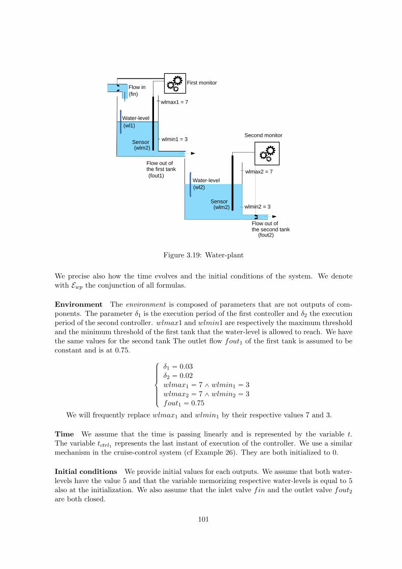
Flow out of the first tank

(fout1)

Water-level

Flow in

(fin)

First monitor

wlmax1 = 7

wlmin1 = 3

(wl1)

Sensor(wlm2)

Water-level

Second monitor

wlmax2 = 7

(wl2)

wlmin2 = 3

Flow out of the second tank

(fout2)

Sensor(wlm2)

Figure 3.19: Water-plant

We precise also how the time evolves and the initial conditions of the system. We denotewith Ewp the conjunction of all formulas.

Environment The environment is composed of parameters that are not outputs of com-ponents. The parameter δ1 is the execution period of the first controller and δ2 the executionperiod of the second controller. wlmax1 and wlmin1 are respectively the maximum thresholdand the minimum threshold of the first tank that the water-level is allowed to reach. We havethe same values for the second tank The outlet flow fout1 of the first tank is assumed to beconstant and is at 0.75.

$

’

’

’

’

&

’

’

’

’

%

δ1 “ 0.03δ2 “ 0.02wlmax1 “ 7 ^ wlmin1 “ 3wlmax2 “ 7 ^ wlmin2 “ 3fout1 “ 0.75

We will frequently replace wlmax1 and wlmin1 by their respective values 7 and 3.

Time We assume that the time is passing linearly and is represented by the variable t.The variable tctrl1 represents the last instant of execution of the controller. We use a similarmechanism in the cruise-control system (cf Example 26). They are both initialized to 0.

Initial conditions We provide initial values for each outputs. We assume that both water-levels have the value 5 and that the variable memorizing respective water-levels is equal to 5also at the initialization. We also assume that the inlet valve fin and the outlet valve fout2are both closed.

101

$

’

’

’

’

’

’

&

’

’

’

’

’

’

%

wl1 “ 5wl2 “ 5wlm1 “ 5wlm2 “ 5fin “ 0fout2 “ 0

The formula Ewp is thus the following conjunction:

δ1 “ 0.03 ^ δ2 “ 0.02 ^ wlmax1 “ wlmax2 “ 7 ^ wlmin1 “ wlmin2 “ 3 ^ fout1 “ 0.75^t “ tctrl1 “ tctrl2 “ 0 ^ wl1 “ wl2 “ 5 ^ wlm1 “ wlm2 “ 5 ^ fin “ fout2 “ 0

3.5.2 Water-level

The Water-level1 component is the continuous evolution of the water-level of the first tank.It depends of the inlet and outlet flow.

I/O and contract The Water-level1 component is defined in the Figure 3.20. The inputsare the value of the measured water-level (wlm1) by the controller and the inlet flow (fin).The assumptions Awl1 correspond to the guarantees Gctrl1 provided by the controller. Thereis only one output: the water-level wl1. The guarantee Gwl1 ensures that the water-levelstays within the defined range r3, 7s. We add the solution of the differential equation as aguarantee. It is necessary to specify the relation between the measured water-level and thereal water-level because we are in a time-triggered version. It requires a deep knowledge ofthe timing behavior of the system. The behavior is denoted by Wl1 and is detailed in theDefinition 29.

Name: Water-level1

Inputs:

fin // inlet flow

wlm1 // measured water-level

Assumptions:

Gctrl1

Outputs:

wl1 // water-level

Guarantees:

3 ď wl1 ď 7wl1 “ pfin ´ fout1qpt ´ tctrl1q ` wlm1

Behavior:

Wl1

Figure 3.20: Water-level component

We can notice that the solution of the differential equation introduced as a guarantee ofthe Water-level1 component refers to fin and wlm1 which are outputs of the controller (cfFigure 3.18). It is not an issue with respect to the Theorem 4 since we show that the solutionis also a guarantee of the controller.

102

Behavior of Water-level1 The behavior of the Water-level1 component is a differentialequation. It is defined as the difference between the inlet flow fin and the outlet flow fout1.

Definition 29 (Water-level behavior). The behavior Wl1 of the water-level of the first tankis defined by the following differential equation:

9wl1 “ fin ´ fout1, 9t “ 1 & pwl1 ě 0 ^ t ě 0 ^ 0 ď t ´ tctrl1 ď δ1q

The evolution of the component is the difference between the inlet flow fin and the outletflow fout1. We add in the evolution domain the formula 0 ď t ´ tctrl1 ď δ1 which restrictsthe evolution of the water-level to a duration of δ1 seconds. We use a similar mechanism inthe cruise-controller example (cf Example 26).

Implementation We have implemented the component as a model in KeYmaera X. Thecorresponding .kyx file is in the annex 5.3.2. The proof that the component Water-level1satisfies its contract is achieved with the proof tactic master in KeYmaera X. The Figure 3.21sum it up with the green tick meaning that we have a proof of the satisfaction of the contract.

Water-level1

Wl1

Awl1 : Gctrl1

Gwl1 : 3 ď wl1 ď 7wl1 “ pfin ´ fout1qpt ´ tctrl1q ` wlm1

�

fin

wlm1

wl1

Figure 3.21: Graphical representation of the Water-level1 component

3.5.3 Controller

The Controller1 component regulates the water-level of the first tank. It repeatedly mea-sures the value of the water-level at most every δ1 units of time. It decides accordingly tothis measured value to close or open the inlet valve. If the inlet valve is open, the water-levelrises, otherwise it goes down.

I/O and contract The component is detailed in the Figure 3.22. The only input is thewater-level wl1. The assumption Actrl1 correspond to the guarantee of the water-level. Itrequires that the water-level stays in the predefined range r3, 7s and that the solution of thedifferential equation is respected. The outputs are the measured water-level (wlm1) and theinlet flow (fin). The guarantees Gctrl1 state that wlm1 is within the range r3, 7s. They alsostate that if the measured water-level is below 3.5 (wlm1 ď 3.5), then the inlet valve is opened(fin “ 1). Conversely, if the measured water-level is above 6.5 (wlm1 ě 3.5), then the inletvalve is closed (fin “ 0). If the water-level is between these two values (3.5 ď wlm1 ď 6.5),the inlet valve can be either closed or opened (fin “ 1 _ fin “ 0). Finally, we add thesolution of the differential equation as a guarantee. It is indeed a guarantee since after theexecution of the controller, we have t “ tctrl1 (thus t ´ tctrl1 “ 0) and wl1 “ wlm1.

103

Name: Controller

Inputs:

wl1 // measured water-level

Assumptions:

Gwl1

Outputs:

fin // flow in

wlm1 // measured water-level

Guarantees:

3 ď wlm1 ď 73.5 ě wlm1 Ñ fin “ 1wlm1 ě 6.5 Ñ fin “ 0p3.5 ď wlm1 ď 6.5q Ñ pfin “ 0 _ fin “ 1qwl1 “ pfin ´ fout1qpt ´ tctrl1q ` wlm1

Behavior:

WlCtrl1

Figure 3.22: Controller component

Behavior of Controller The behaviorWlCtrl1 of the Controller1 component is definedin the Definition 30.

Definition 30 (Controller behavior). The behavior WlCtrl1 of the water-level controller ofthe first tank is defined by the following hybrid program:

`

?t ď tctrl1 ` δ1;wlm1 :“ wl1; p?wlm1 ě 6.5; fin :“ 0q Y p?wlm1 ď 3.5; fin :“ 1q; tctrl1 :“ t˘˚

It is made up of three parts : a temporal part, a sensing and the decision part. Thetemporal part is the test ?t ď tctrl1 ` δ1 and the assignment tctrl1 :“ t. The test ensuresthat the component executes at most every δ1 seconds. The assignment remembers the lastexecution. The sensing is implemented by wlm1 :“ wl1 where the value of the water-level wl1is assigned to the variable wlm1. The decision part is a standard if-then-else encoding.

Implementation We have implemented the component as a model in KeYmaera X. Thecorresponding .kyx file is in the annex 5.3.2. The proof that the component Controller1

satisfies its contract is achieved with the proof tactic master in KeYmaera X. The Figure 3.23sum it up with the green tick meaning that we have a proof of the satisfaction of the contract.

3.5.4 Water-tank

The Water-tank1 component is obtained by the parallel composition of the Water-level1

component and the Controller1 component.

Parallel composition of the controller with the Water-level The inputs (resp. out-puts) of the Water-tank1 component are the union of the inputs (resp. outputs) of theWater-level1 component and the Controller1 component. The assumptions Awt1 (resp.

104

Controller1

WlCtrl1

Actrl1 : Gwl1

Gctrl1 : wlm1 ď 3.5 Ñ fin “ 16.5 ď wlm1 Ñ fin “ 0p3.5 ě wlm1 ě 6.5qÑ pfin “ 0 _ fin “ 1q3 ď wlm1 ď 7wl1 “ pfin ´ fout1qpt ´ tctrl1q ` wlm1�

wl1

fin

wlm1

Figure 3.23: Graphical representation of the Controller1 component

guarantees Gwt1) of the Water-tank1 are the conjunction of Awl1 and Actrl1 (resp. Gwl1 andGctrl1). The behavior is detailed in Definition 31.

A summary of the parallel composition is given in the Figure 3.24. Notice that fornow, we have a proof of satisfaction of their contract by the components Water-level1

and Controller1. We do not still have a proof that the component Water-tank1 satisfies itscontract.

Behavior of Water-tank The behavior WT1 of the Water-tank component is presentedin the Definition 31.

Definition 31 (Water-tank behavior). The behavior WT1 of the first tank results from theparallel composition of Wl1 and WlCtrl1.

ˆ`

?t ď tctrl1 ` δ1;wlm1 :“ wl1; p?wlm1 ě 6.5; fin :“ 0q Y p?wlm1 ď 3.5; fin :“ 1q; tctrl1 :“ t˘

Y`

9wl1 “ fin ´ fout1, 9t “ 1 & pwl1 ě 0 ^ t ě 0 ^ δ1 ě t ´ tctrl1 ě 0 ^ t ě tctrl1q˘

˙˚

The addition of temporal constraints makes sense once we have composed the components.The variable tctrl1 remembers the instant of the last execution of the controller. It is thenequal to t. The water-level evolves along the time, and the difference between t and tctrl1grows until it reaches δ1. Then we know that the controller has to execute.

Application of the composition theorem The conditions of the Theorem 4 are re-spected. The outputs of both components are separated. The guarantees Gwl1 of theWater-level1 do not refer to the outputs of the Controller1 and the inverse is also true.The guarantee wl1 “ pfin´ fout1qpt´ tctrl1q `wlm1 contains occurrences of outputs of bothcomponents, but we have proved that it is a guarantee of both component. It is thus nota problem to the application of the theorem. The guarantees Gwl1 implies the assumptionsActrl1 trivially since they correspond, and the inverse is true. We have thus automatically theproof of satisfaction of the conjunction of contracts by the resulting component thanks to theapplication of the theorem.

We have sum up in the Figure 3.25 the Water-tank1 component. We have now a proofof satisfaction of its contract thanks to the application of the Theorem 4.

105

Water-level1

Wl1

Awl1 : Gctrl1

Gwl1 : 3 ď wl1 ď 7wl1 “ pfin ´ fout1qpt ´ tctrl1q ` wlm1

Controller1

WlCtrl1

Actrl1 : Gwl1

Gctrl1 : wlm1 ď 3.5 Ñ fin “ 16.5 ď wlm1 Ñ fin “ 0p3.5 ě wlm1 ě 6.5qÑ pfin “ 0 _ fin “ 1q3 ď wlm1 ď 7wl1 “ pfin ´ fout1qpt ´ tctrl1q ` wlm1

wl1fin, wlm1

�

�

Figure 3.24: Parallel composition of Water-level1 with the Controller1

Water-tank1

Wl1 ˝ WlCtrl1

Awt1 : Awl1 ^ Actrl1

Gwt1 : Gwl1 ^ Gctrl1 �

wl1

wlm1

fin

wl1

wlm1

fin

Figure 3.25: Graphical representation of the Water-tank1 component

Implementation in KeYmaera X We have implemented in KeYmaera X the componentresulting from the composition 5.3.2. At the end of the file, in commentary, there is thetactic used to achieve the proof. We have followed strictly our procedure detailed in the proofof the Theorem 4. It requires a minimal supplementary proof effort from the proof of eachcomponent. It may be automated.

The water-tank file shows us that even a simple example quickly grows in size. Ourapproach requires that the engineer only consider the basic component, here the water-leveland the controller, which are much simpler to understand and prove.

106

3.5.5 Water-Plant

We compose two water-tanks with our parallel composition operator. It follows an intuitivedesign in the sense that we first compose the Water-level1 component with the Controller1component to obtain a first tank Water-tank1, then compose it with a second water-tankobtained by similar mean.

Water-level1 Controller1

Water-tank1

b b Water-level2 Controller2

Water-tank2

b

Second water-tank The second water-tank is a lot similar to the first one, but it is theoutlet valve that can be closed or open by the controller, the inlet flow is assumed to be con-stant. A detailed .kyx file are given for the second water-level 5.3.2, the second controller 5.3.2and the second water-tank resulting from their composition 5.3.2.

We have summed up in the Figure 3.26.

Water-tank2

Wl2 ˝ WlCtrl2

Awt2 : Awl2 ^ Actrl2

Gwt2 : Gwl2 ^ Gctrl2 �

wl2

wlm2

fout2

wl2

wlm2

fout2

Figure 3.26: Graphical representation of the Water-tank2 component

Parallel composition The inputs (resp. outputs) of the Water-plant component arethe union of the inputs (resp. outputs) of the first Water-tank component and the secondWater-tank component. The assumptions Awp (resp. guarantees Gwp) of the Water-plant

are the conjunction of Awt1 and Awt2 (resp. Gwt1 and Gwt2). The behavior WP of theWater-plant component is presented in the Definition 32.

Definition 32 (Water-plant behavior). The behavior WP of the water-plant results from theparallel composition of WT1 and WT2, where WT1 results from the parallel composition ofWl1 and WlCtrl1 and WT2 results from the parallel composition of Wl2 and WlCtrl2.

WP fi WT11 ˝ WT2

fi pWl1 ˝ WlCtrl1q ˝ pWl2 ˝ WlCtrl2q

107

fi

¨

˚

˚

˚

˚

˚

˚

˚

˚

˚

˚

˝

´

`

?t ď tctrl1 ` δ1;wlm1 :“ wl1;

p?wlm1 ě 6.5; fin :“ 0q Y p?wlm1 ď 3.5; fin :“ 1q; tctrl1 :“ t˘

Y`

?t ď tctrl2 ` δ2;wlm2 :“ wl2;p?wlm2 ě 6.5; fout2 :“ 1q Y p?wlm2 ď 3.5; fout2 :“ 0q; tctrl2 :“ t

˘

Y`

9wl1 “ fin ´ fout1, 9wl2 “ fout1 ´ fout2, 9t “ 1& pwl1 ě 0 ^ t ě 0 ^ δ1 ě t ´ tctrl1 ě 0 ^ t ě tctrl1

^wl2 ě 0 ^ δ2 ě t ´ tctrl2 ě 0 ^ t ě tctrl2q˘

¯

˚

˛

‹

‹

‹

‹

‹

‹

‹

‹

‹

‹

‚

˚

In particular, we have an example of the parallel composition of two continuous compo-nents with the water-levels composed in parallel.

Application of the theorem The conditions of the Theorem 4 are respected. The outputsof both components are separated. The guarantees Gwt1 of the Water-tank1 do not referto the outputs of the Water-tank2 and the inverse is also true. The sequent Ewp, Awt2 $@wt1pGwt1 Ñ Awt2q is valid since the outputs of the first water-tank are separated from thevariables in Awt2 . The inverse is also true. We have thus automatically the proof of satisfactionof the conjunction of contracts by the resulting component thanks to the application of thetheorem. It is summed up in the Figure 3.27.

Water-plant

WT1 ˝ WT2

Awp: Awt1 ^ Awt2

Gwp: Gwt1 ^ Gwt2 �

wl1, wl2

wlm1, wlm2

fin, fout2

wl1, wl2

wlm1, wlm2

fin, fout2

Figure 3.27: Graphical representation of the Water-plant component

Implementation in KeYmaera X We have implemented in KeYmaera X the componentresulting from the composition 5.3.2. At the end of the file, in commentary, there is thetactic used to achieve the proof. We have followed strictly our procedure detailed in the proofof the Theorem 4. It requires a minimal supplementary proof effort from the proof of eachcomponent. It may be automated.

3.5.6 Discussion

Monolithic approach VS Modular approach The source files 5.3.2 show that the designof even a simple water-plant may result in a model quite complex to model. The proof isalso difficult to automate. New improvements in KeYmaera X can drastically improve thereadability and help to scale, but the same problem will arise for system more complex.

We strongly think that our component-based approach allows to handle both design andproof complexity of systems made up of simple and repetitive parts.

Improvement points Our two examples, the cruise-control and the water-tank shares thesame structure : a continuous evolution (the plant) is monitored by a discrete controller. It

108

is a frequent design in Cyber-physical Systems and is referred to as Computer-ControlledSystems. It includes most of the industrial systems.

In both examples, we have to add a machinery to ensure that the controller executesperiodically. This addition is not a function problem, but an architecture problem and thedesigner should have tools to automate it. It is the subject of Section 4.1.

When we compose several CCS together as in our water-plant Example 32, the controllermight be executed on the same computation unit and therefore their execution period maybe modified by the parallel execution. We answer to this problem in Section 4.2.

A common design in critical system is the addition of an emergency mode to the nominalmode. The natural way to express it in our framework is to compose in parallel the emergencymode with the nominal mode. But we have to be careful since they have the same outputs.We present a solution in Section 4.3.

When designing such system, one may want to define a causal relation between compo-nents. We propose in Section 4.4 the definition of a causal composition operator compatiblewith the previously defined framework.

109

Chapter 4

Extensions of our framework

110

We have presented a parallel composition operator in Chapter 3. The water-plant examplein Section 3.5 shows that our approach still requires that the engineer have to reason on non-functional problems to achieve its design and proof. We present in this chapter adaptations ofthe parallel composition operator to remediate to the problems identified in Subsection 3.5.6.

In Sections 4.1 and 4.2, we show how to adapt the results of the previous Chapter 3 tosystematically model Computer-Controlled Systems (CCS) in a modular approach. The ideais to analyse the control period of the plant, i.e. the period of time it can evolve withoutintervention of the controller, and the reactivity of the controller, i.e. the execution periodof the controller. We retain the associativity property and the ability to retain contractsthrough composition. To clearly separate the design part of a system and its representationin dL, we continue to use the textual representation of components.

In Section 4.3, we show how to express modes in a systematic and modular way by adaptingthe parallel composition operator ˝.

An usual decomposition of a controller is Sensor -> Program -> Actuator. But thethree components are not in parallel, but in sequence. In Section 4.4, we define a causalcomposition operator by adapting our parallel composition operator to enforce an order. Itfeatures associativity, essential for modularity, and a theorem allowing to transfer automat-ically guarantees of each component to the resulting compound component under relaxedconditions.

4.1 Computer-Controlled Systems

We present a component-based approach to model and verify Computer-Controlled Systems(CCS). We aim to simplify the reasoning on such systems and provide methodological insightsfor designers and proof engineers.

We adapt our previous work by taking into account the period of execution of the con-troller. We describe the integration and show that it cover the standard encoding of CCSin dL. We adapt the composition Theorem 4 to show that we retain contracts throughcomposition of components. We exemplify it with the water-tank example.

4.1.1 Modeling Computer-Controlled Systems

We present how we model Computer-Controlled System. A CCS is classically composed ofa controller and a plant as in Figure 4.1. The former regulates the behavior of the latterthrough an actuation. For example, the controller in the water-tank example regulates thewater-level by opening or closing a faucet.

Plant

Controller

Figure 4.1: Structure of a CCS

The key trait of CCS is the periodic execution of the controller to regulates the controller.

111

We associate a periodic value ∆Ctrl (resp. ∆P lant) to the controller (resp. the plant). For thecontrol part, it is the execution period, i.e. the maximal allowed time between two executionsof the controller. For the plant, it is the duration in which it can freely evolve and still satisfiesthe safety property, the control period. We add timing constraints to model this requirement.

We use the water-tank example of Section 3.5, except that we distinguish the executionperiod from the control period. These two notions were conflated in our previous example.

Time. We assume that the passing of time is accessible for every component through thedifferential equation 9t “ 1 & t ě 0. The variable t represents the time passing linearly andis a global read-only variable. It is initialized to 0.

Controller. We assume that a designer provides the functional behavior of a controller asa discrete program Ctrl and the associated period ∆Ctrl. The functional behavior representsone execution of the controller. We add timing constraints to model the periodic executionof the controller.

The controller acts every ∆Ctrl units of time. To ensure this periodic execution, we usea fresh variable tctrl. It works as a time-stamp saying that Ctrl has executed. We add atthe end the assignment tctrl :“ t, which signals that the controller has executed. We add theguard ?t ď tctrl `∆Ctrl before the controller Ctrl, which requires that at most ∆Ctrl units oftime have passed since the last execution. It results in the following canonical structure forthe controller, which is referred later as the behavior of the controller.

Definition 33 (Controller). The canonical structure of a controller is given by the hybridprogram:

Ctrl fi p?t ď tctrl ` ∆Ctrl;Ctrl; tctrl :“ tq˚

This definition allows Zeno behaviors, i.e. repetitive executions of the controller withouthaving the continuous systems to evolve. It is a problem when we want to implement a realcontroller, but we are here interested into the verification of safety properties. Having a moregeneral modeling is thus not a problem. We could forbid this Zeno behavior by adding thetest tctrl ă t in the guard. Another possibility is to replace the test t ď tctrl ` ∆Ctrl with thetest t “ tctrl ` ∆Ctrl. It assumed here that the controller executes every ∆Ctrl units of timewhich is unrealistic if we want to obtain a real implementation later.

For example, consider the controller for the water-level of a tank in a water-plant. If thelevel reaches a maximum (resp. minimum) threshold, here 6.5 (resp. 3.5), then we close theinlet faucet fin (resp. we open the inlet faucet).

Example 35 (Water-level controller). The functional behavior is :

BodyWlCtrl fi wlm :“ wl;`

p?wlm ě 6.5; fin :“ 0q Y p?wlm ď 3.5; fin :“ 1q˘

It describes how the component operates, but does not refer to structural constraints like theexecution period. The period ∆wlCtrl of the controller is 0.05 sec. We augment the functionalbehavior BodyWlCtrl with the period to obtain the behavior WlCtrl:

¨

˝

?t ď tctrl ` 0.05;wlm :“ wl; p?wlm ě 6.5; fin :“ 0q Y p?wlm ď 3.5; fin :“ 1q;tctrl :“ t

˛

‚

˚

At most every 0.05 seconds, the water-level controller samples the current water-level anddecides accordingly to open or close the inlet valve.

112

Retro-action It is possible to take account of the retro-action. Instead of using the lastsensing in the modeling, we use the previous one, i.e. the sensing performed ∆Ctrl units oftime before. We use a temporary variable to memorize it. It accurately models the fact thatthe actuation of controller at a time t0 is in function of the sensing at t0 ´ ∆Ctrl.

Example 36 (Water-tank controller with retro-action). The behavior of the water-tank con-troller with retro-action is:

¨

˚

˚

˝

?t ď tctrl ` ∆Ctrl;prewlm :“ wlm;wlm :“ wl;p?prewlm ě 6.5; fin :“ 0q Y p?prewlm ď 3.5; fin :“ 1q;tctrl :“ t

˛

‹

‹

‚

˚

In the example, the level of water of the tank is assigned to the variable wlm, then to thevariable prewlm. wlm is here to stock the value for one more iteration of the controller andsimulates a retro-action.

Plant. We assume that a designer provides the functional behavior of the plant as a differ-ential equation ODE & H and the control period ∆P lant. We implement it by adding theformula t ď ∆P lant in the evolution domain.

Definition 34 (Plant). The canonical structure of a plant is:

Plant fi ODE, 9t “ 1 & H ^ t ď ∆P lant

The addition of the formula t ď ∆P lant adequately models that we consider an evolutionof the system in the duration of the control period.

The value of the control period∆P lantis obtained by external methods and is not computedby our methodology. In practice, it is mostly obtained from the knowledge of engineers of thefield with some tolerance.

The evolution of the water-level is the difference between the inlet flow fin and the outletflow fout. The water-level is assumed to always be positive.

Example 37 (Water-level). The functional behavior of the water-level is the following dif-ferential equation:

9wl “ fin ´ fout & wl ě 0

The control period ∆wl of the water-level is 0.2 sec. The behavior Wl of the water-levelcomponent is thus given by:

9wl “ fin ´ fout, 9t “ 1 & wl ě 0 ^ t ď 0.2

Our proposed modeling is sufficient to reason on the system. Indeed, when we composethe plant with the controller, we iterate the interaction. Thus, considering only the evolutionon the duration ∆P lant amounts to consider one step of the loop Plant-Controller.

Full system The full system is obtained by applying our parallel composition operator onthe plant and the controller with a slight difference.

113

Definition 35 (Computer-Controlled System). The canonical structure of the behavior of aComputer-Control System is:

CCS fi

`

pPlant, 9t “ 1 & H ^ 0 ď t ´ tctrl ď ∆Ctrlq

Yp?t ď tctrl ` ∆Ctrl;Ctrl; tctrl :“ tq˘

˚

The controller and the plant interact by the use of the variable tctrl. At the beginning ofone loop iteration, we have t “ tctrl and thus t´ tctrl “ 0. The difference t´ tctrl grows alongthe evolution of time until the point t ´ tctrl “ ∆Ctrl. Then, the controller has to act, but itcan act before.

The difference with the parallel composition operator in Definition 22 is that we replacethe formula t ě ∆P lant by the formula 0 ď t ´ tctrl ď ∆Ctrl. We detail in the proof of theTheorem 6 why this replacement is safe.

For our system to fit the desired modeling, we must have ∆Ctrl ď ∆P lant, i.e. that thereactivity of the controller is shorter to the control period of the plant. Otherwise, there maybe runs of the whole system where the controller can not execute and the system is stuck. Yet,we do not forbid such composition, but we will not be able to retain the contracts throughcomposition.

Example 38 (Water-tank). We compose the water-level with the water-level controller toobtain the water-tank system. The behavior Water-tank resulting from the composition ofthe water-level and the water-level controller is:ˆ

p 9wl “ fin ´ fout & wl ě 0 ^ 0 ď t ´ tctrl ď 0.05qY p?t ď tctrl ` 0.05;wlm :“ wl; p?wlm ě 6.5; fin :“ 0q Y p?wlm ď 3.5; fin :“ 1q; tctrl :“ tq

˙˚

The composition is safe because the period of the controller (∆WlCtrl “ 0.05) is inferior tothe control period of the plant (∆wl “ 0.2).

We retain the general structure of component in Chapter 3 which is essential to obtainmodularity. Yet, one may ask if we accurately capture all CCS systems. We show in the nextsubsection that we capture all systems that are encoded by the standard encoding of CCSthat we repeatedly found in the literature in dL. It gives us confidence that our proposedapproach captures such systems.

4.1.2 Coverage of the standard encoding

We first define what we call the standard encoding of Computer-Controlled Systems in dL.It is a recurrent structure in the literature. We then show that our modeling proposition canmodel every system that can be modeled with the standard encoding.

Definition 36 (Standard encoding). The standard encoding of a CCS is:

pCtrl; tctrl “ t; Plant, 9t “ 1 & H ^ 0 ď t ´ tctrl ď ∆Ctrlq˚

The alternation of the controller and the plant is obtained by the use of the sequenceoperator ; . Notice that a similar encoding is used to represent the cyclic relation to time. Wehave a notification variable tctrl that is reset to t after the execution of the controller. Thismodeling is simple, yet very efficient in a monolithic approach. But we think that it is notthe appropriate approach if we want to use a component-based approach.

114

Remember that ρpαq, where α is an hybrid program, is the set of reachable states of α (cfDefinitions 2 and 4). We show that the set of reachable states of the standard encoding ofCCS is included in the set of reachable states of our encoding. It means that a system thatcan be modeled with the standard encoding can also modeled with our approach.

Theorem 5 (Coverage of the standard encoding). Every system that can be modeled with thestandard encoding may be modeled with our encoding, i.e.

ρ`

pCtrl; tctrl “ t; Plant, 9t “ 1 & H ^ 0 ď t ´ tctrl ď ∆Ctrlq˚˘

Ď ρ`

ppPlant, 9t “ 1 & H ^ 0 ď t ´ tctrl ď ∆Ctrlq Y p?t ď tctrl ` ∆;Ctrl; tctrl :“ tqq˚˘

Proof. We prove the equivalence by unfolding the semantic definition of our proposed encodingand show that one of the subset of reachable states of our encoding matches exactly the setof reachable states of the standard encoding. First, we add the test ?t ď tctrl `∆Ctrl in frontof the standard encoding. It does not change the reachability, but is here to simplify theidentification to our encoding. We have the following equality.

ρ`

pCtrl; tctrl “ t; Plant, 9t “ 1 & H ^ 0 ď t ´ tctrl ď ∆Ctrlq˚˘

“ ρ`

p?t ď tctrl ` ∆Ctrl;Ctrl; tctrl “ t; Plant, 9t “ 1 & H ^ 0 ď t ´ tctrl ď ∆Ctrlq˚˘

The right-hand side is trivially included in the left-hand side since we just add information,and thus potentially reduces the set of worlds. For the other inclusion, if it is not true, thenthere is a world w in ρ

`

pCtrl; tctrl “ t; Plant, 9t “ 1 & H ^ 0 ď t´ tctrl ď ∆Ctrlq˚˘

such thatw ­|ù t ď tctrl `∆Ctrl, but it contradicts the assumption that the continuous behaviors evolvein a world where t ď tctrl ` ∆Ctrl is true. We have thus the other inclusion.

We have to prove:

ρ`

p?t ď tctrl ` ∆Ctrl;Ctrl; tctrl “ t; Plant, 9t “ 1 & H ^ 0 ď t ´ tctrl ď ∆Ctrlq˚˘

Ď ρ`

ppPlant, 9t “ 1 & H ^ 0 ď t ´ tctrl ď ∆Ctrlq Y p?t ď tctrl ` ∆;Ctrl; tctrl :“ tqq˚˘

We adopt the following abbreviations:

P “ Plant, 9t “ 1 & H ^ 0 ď t ´ tctrl ď ∆Ctrl

C “?t ď tctrl ` ∆Ctrl;Ctrl; tctrl :“ t

Thus, the standard encoding corresponds to pC;P q˚ and our encoding corresponds to pC YP q˚. We unfold the semantic definition of the iteration. We obtain the following equality:

ρ`

pC Y P q˚˘

“Ť

nPN ρ`

pC Y P qn˘

We have thus ρ`

pC Y P q2˘

Ď ρ`

pC Y P q˚˘

.We unfold ρ

`

pC Y P q2˘

:

ρ`

pC Y P q2˘

“ ρ`

pC Y P q; pC Y P q˘

“ ρpC;Cq Y ρpC;P q Y ρpP ;Cq Y ρpP ;P q

Thus the left-hand side is included in the right-hand side.

115

4.1.3 Modular proof of a Computer-Controlled System

The Subsection 4.1.1 have presented how to modularly model a CCS. We want now to beable to still retain contracts through composition. This subsection presents an adaptationof the Theorem 4 to transfer the respective contract of the plant and the controller throughcomposition.

Environment. We assume that the designer provides a description of the environment,which is denoted by E . It contains all the variables that are not outputs of a component.They cannot be controlled and are exterior to the considered system. A classical example inhybrid systems is the gravity value g. The environment also regroups the initial values of thesystem.

Example 39 (Water-tank environment). In the water-tank, the environment Ewt is the outletflow fout which is equal to 0 or 1. There is also the control period ∆Ctrl of the plant which is0.2 sec and the period ∆Ctrl of the controller which is 0.05. The initial value of the water-levelwl and the measured water-level wlm are 5. The inlet valve fin is closed at the initialization.

Ewt fi fout “ 0.75 ^ ∆wlCtrl “ 0.05 ^ ∆wl “ 0.2 ^ wl “ wlm “ 5 ^ fin “ 0

Controller We assume that the designer provides the assumptions ACtrl and guaranteesGCtrl on the controller. Following the restriction of the Theorem 4, guarantees must notrefer to outputs of the plant. Remember that the controller is said to satisfy its contract(Definition 20) if the following formula is valid:

pE ^ ACtrlq Ñ rCtrlsGCtrl

We prove the validity by using the sequent calculus of dL, implemented in KeYmaera X.

Example 40 (Contract of the water-level controller). From the Example 3.22, the contractof the water-level controller is:

$

’

’

’

’

&

’

’

’

’

%

AwlCtrl : Gwl

GwlCtrl : wlm ď 3.5 Ñ fin “ 16.5 ď wlm Ñ fin “ 0p3.5 ě wlm ě 6.5q Ñ pfin “ 0 _ fin “ 1qwl “ pfin ´ foutqpt ´ tctrlq ` wlm

We have already a proof of the sequent:

Ewt, AwlCtrl $ rWlCtrlsGwlCtrl

Plant Similarly to the controller, we assume that the designer provides assumptions AP lant

and guarantees GP lant on the plant. Again, the guarantees of the plant must not refer to theoutputs of the controller. The plant satisfies its contract if the following formula is valid:

pE ^ AP lantq Ñ rPlantsGP lant

We prove the validity by using the sequent calculus of dL, implemented in KeYmaera X.

116

Example 41 (Contract of the water-level). From the Example 3.20, the contract of thewater-level is:

$

&

%

Awl : GwlCtrl

Gwl : 3 ď wl ď 7wl “ pfin ´ foutqpt ´ tctrlq ` wlm

We have already a proof of the sequent:

Ewt, Awl $ rWlsGwl

Full system The contract for the full system is the conjunction of the assumptions and ofthe guarantees. As in Section 3.3, we want that the system CCS as defined in Definition 35satisfies the conjunction of contracts pACtrl^AP lant, GCtrl^GP lantq. We adapt the Theorem 4by adding the condition that the execution period must be shorter than the control period,i.e. ∆Ctrl ď ∆plant, to retain contracts.

Theorem 6 (Safe composition of a Plant and a Controller). Let Plant and Ctrl be twobehaviors as defined previously with respective contracts pAP lant, GP lantq and pACtrl, GCtrlq.Assume that we have two proof trees of E , AP lant $ rPlantsGP lant and E , ACtrl $ rCtrlsGCtrl

respectively, where E is the environment. Furthermore, assume that

paq BV pPlantq X BV pCtrlq “ H,

pb1q BV pPlantq X FV pGCtrlq “ H,

pb2q BV pCtrlq X FV pGP lantq “ H and BV pCtrlq X FV pHq,

pc1q AP lant $ @CtrlpGCtrl Ñ AP lantq,

pc2q ACtrl $ @P lantpGP lant Ñ ACtrlq,

pdq ∆Ctrl ď ∆plant.

Then it exists a proof tree of E , AP lant, ACtrl $ rCCSspGP lant ^ GCtrlq.

The first assumption paq assumes components to have separate internal variables andrequires them to define disjoint output variables (i.e. unique definitions), which essentiallyamounts to good modeling practice. The second assumption pb1q (resp. pb2q) requires thesafety property GCtrl (resp. GP lant) to guard the behavior of the system α (resp. β), i.e. itsoutputs, and of course not βs (resp. α). It hence seems natural to require its separation withGP lant (resp. GCtrl). The condition pc1q (resp. pc2q) requires the assumptions Aβ (resp. Aα)to be implied by the guarantees GCtrl (resp. GP lant).

Proof. We re-use the result of the Theorem 4. In order to do so, we have to justify our slightchange where we replace the formula t ď ∆P lant with the formula 0 ď t´ tCtrl ď ∆Ctrl in theDefinition 35.

First, the condition pdq tells us that ∆Ctrl ď ∆P lant. Thus, if the sequent E , AP lant $rPlant, 9t “ 1 & H ^ t ď ∆P lantsGP lant is valid, we have that the sequent E , AP lant $rPlant, 9t “ 1 & H ^ t ď ∆CtrlsGP lant is valid too. It shorten the amount of time that theplant is allowed to evolve. So if we have proved that it satisfies the guarantees for a definedamount of time, we have trivially that it satisfies guarantees for a smaller amount of time.

117

We can then safely replace the formula t ď ∆Ctrl by 0 ď t´ tctrl ď ∆Ctrl in the evolutiondomain since it represents the same amount of time. It is now possible to apply the Theorem 4to conclude.

Example 42 (Contract of the water-tank). From the Example 3.25, the contract of thewater-tank resulting from the composition of the water-level and the controller is:

"

Awt : Awl ^ AwlCtrl

Gwt : Gwl ^ GwlCtrl

The conditions of the Theorem 6 are satisfied. The conditions paq to pc2q are already con-sidered in the previous section. Plus, we have that ∆wlCtrl ď ∆wl We have a proof of thefollowing sequent:

E , Awt $ rWater-tanksGwt

Conclusion

We have presented how we can adapt our parallel composition operator to modularly modeland prove a Computer-Controlled System and reason on a non-functional property like theexecution period and the control period. But the presentation in this section is only fortwo elements, and we want to extend this approach with to a plant where several systemsPlant-Controller are composed in parallel. The next section is devoted to the presentation ofparallel composition with a systematic integration of timed constraints.

4.2 Parallel composition in a timed framework

We want to extend the integration of temporal considerations for every component in a timedframework. Reasoning on temporal executions of CPS is an important step during the designof such systems and this extension aims to ease its development.

When we execute two programs in parallel on one CPU, their execution periods, that weidentify to Worst Case Execution Time (WCET), is augmented. The computation resourcesmay be preempted by the other program and the first program has to wait. More precisely,the resulting execution period is the sum of respective WCET. We have also to take intoconsideration if the composition with the continuous part is still valid, i.e. that the resultingexecution period is still inferior to the control period of the plant.

The parallel composition operator in Definition 22 is too general to handle this kind ofreasoning. We present in the next section its adaptation by extending the idea of Section 4.1and exemplify it with the water-plant example. We retain the algebraic properties, commuta-tivity and associativity, as well as the theorem guaranteeing that the conjunction of contractsis preserved through composition.

In Subsection 4.2.1, we defined how we integrate systematically the notion of executionperiods and control period to obtain a so-called timed component. The Subsection 4.2.2 detailsthe parallel composition between discrete timed components and we show that we retainassociativity and the composition theorem. The Subsection 4.2.3 is similar, but for continuoustimed component. The Subsection 4.2.4 show how we associate a discrete component and acontinuous component, where each of them may result from previous compositions. It is ageneralization of Section 4.1. Finally, the Subsection 4.2.5 show how to aggregate all theprevious definitions to obtain a parallel composition of timed general components.

118

4.2.1 Definition of a timed component

In this subsection, we present the definition of a component with the timed information andhow it is translated in dL. The designer should only provide the textual representation andthe translation in the dL framework is handled automatically.

We associate to every atomic component a duration which is assumed to be provided bythe designer. For the discrete case, it is called the execution period and is understood as thetime the component takes to execute. We may assimilate it to WCET. In the continuouscase, it is the control period of the continuous system, i.e. the duration during which thecontinuous component can evolves freely without an intervention of a controller. We extendthe definition by adding tests and assignment in a similar manner that in Section 4.1.1. Tokeep the structure of components and the associated properties, we add tests and assignmentto discrete atomic sub-component along with the execution period provided by the designer.The execution period of a compound component is obtained through composition of atomiccomponents.

Textual representation For a discrete component, ∆α represents the execution period ofthe component. We just add this information to our previously defined textual representationin Subsection 3.1.1. For example, for the first water-level controller, we add that the executionperiod ∆WlCtrl1 is 0.03 seconds.

Example 43 (Textual representation of water-level controller). From the Example 3.22, thewater-level controller of the first tank is defined by:

Component: Controller1

Period:

∆WlCtrl1 “ 0.03Inputs:

wl1Assumptions:

Gwl1

Outputs:

fin

wlm1

Guarantees:

3 ď wlm1 ď 73.5 ě wlm1 Ñ fin “ 1wlm1 ě 6.5 Ñ fin “ 0p3.5 ď wlm1 ď 6.5q Ñ pfin “ 0 _ fin “ 1qwl1 “ pfin ´ fout1qpt ´ tctrl1q ` wlm1

Functional behavior:

BodyWlCtrl1 fi wlm1 :“ wl1; p?wlm1 ě 6.5; fin :“ 0q Y p?wlm1 ď 3.5; fin :“ 1q

We have the same for the water-level controller WlCtrl2 of the second tank for which theexecution ∆WlCtrl2 is 0.02.

For a continuous component, εα represents the control period of the component. As forthe discrete case, we add this information in the textual representation. For example, for thewater-level component of the first tank, we have εWl1 “ 0.2.

119

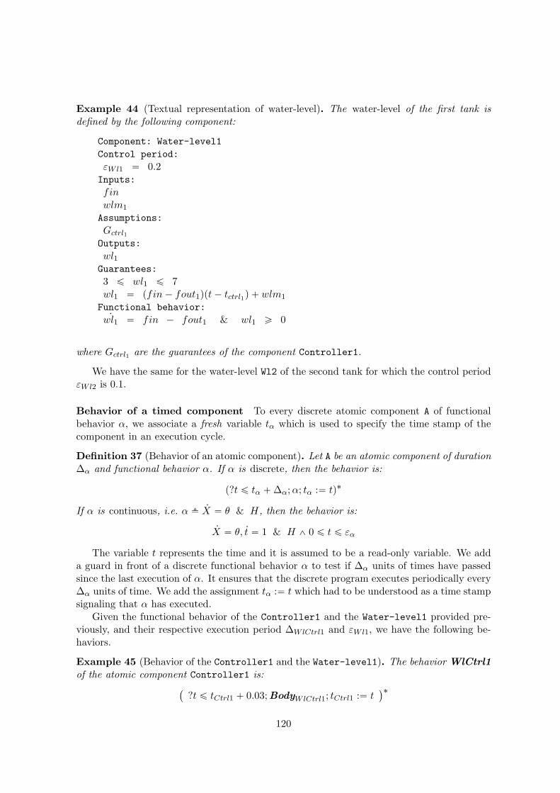
Example 44 (Textual representation of water-level). The water-level of the first tank isdefined by the following component:

Component: Water-level1

Control period:

εWl1 “ 0.2Inputs:

fin

wlm1

Assumptions:

Gctrl1

Outputs:

wl1Guarantees:

3 ď wl1 ď 7wl1 “ pfin ´ fout1qpt ´ tctrl1q ` wlm1

Functional behavior:9wl1 “ fin ´ fout1 & wl1 ě 0

where Gctrl1 are the guarantees of the component Controller1.

We have the same for the water-level Wl2 of the second tank for which the control periodεWl2 is 0.1.

Behavior of a timed component To every discrete atomic component A of functionalbehavior α, we associate a fresh variable tα which is used to specify the time stamp of thecomponent in an execution cycle.

Definition 37 (Behavior of an atomic component). Let A be an atomic component of duration∆α and functional behavior α. If α is discrete, then the behavior is:

p?t ď tα ` ∆α;α; tα :“ tq˚

If α is continuous, i.e. α fi 9X “ θ & H, then the behavior is:

9X “ θ, 9t “ 1 & H ^ 0 ď t ď εα

The variable t represents the time and it is assumed to be a read-only variable. We adda guard in front of a discrete functional behavior α to test if ∆α units of times have passedsince the last execution of α. It ensures that the discrete program executes periodically every∆α units of time. We add the assignment tα :“ t which had to be understood as a time stampsignaling that α has executed.

Given the functional behavior of the Controller1 and the Water-level1 provided pre-viously, and their respective execution period ∆WlCtrl1 and εWl1, we have the following be-haviors.

Example 45 (Behavior of the Controller1 and the Water-level1). The behavior WlCtrl1

of the atomic component Controller1 is:`

?t ď tCtrl1 ` 0.03;BodyWlCtrl1; tCtrl1 :“ t˘˚

120

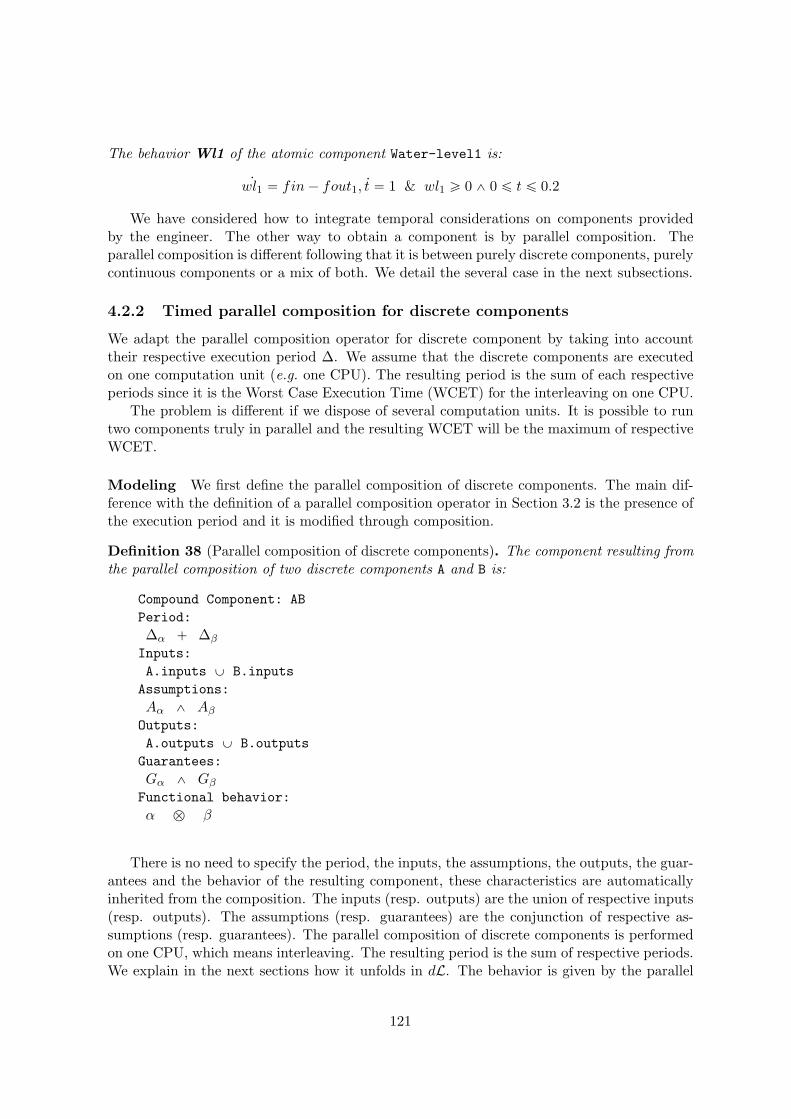
The behavior Wl1 of the atomic component Water-level1 is:

9wl1 “ fin ´ fout1, 9t “ 1 & wl1 ě 0 ^ 0 ď t ď 0.2

We have considered how to integrate temporal considerations on components providedby the engineer. The other way to obtain a component is by parallel composition. Theparallel composition is different following that it is between purely discrete components, purelycontinuous components or a mix of both. We detail the several case in the next subsections.

4.2.2 Timed parallel composition for discrete components

We adapt the parallel composition operator for discrete component by taking into accounttheir respective execution period ∆. We assume that the discrete components are executedon one computation unit (e.g. one CPU). The resulting period is the sum of each respectiveperiods since it is the Worst Case Execution Time (WCET) for the interleaving on one CPU.

The problem is different if we dispose of several computation units. It is possible to runtwo components truly in parallel and the resulting WCET will be the maximum of respectiveWCET.

Modeling We first define the parallel composition of discrete components. The main dif-ference with the definition of a parallel composition operator in Section 3.2 is the presence ofthe execution period and it is modified through composition.

Definition 38 (Parallel composition of discrete components). The component resulting fromthe parallel composition of two discrete components A and B is:

Compound Component: AB

Period:

∆α ` ∆β

Inputs:

A.inputs Y B.inputs

Assumptions:

Aα ^ Aβ

Outputs:

A.outputs Y B.outputs

Guarantees:

Gα ^ Gβ

Functional behavior:

α b β

There is no need to specify the period, the inputs, the assumptions, the outputs, the guar-antees and the behavior of the resulting component, these characteristics are automaticallyinherited from the composition. The inputs (resp. outputs) are the union of respective inputs(resp. outputs). The assumptions (resp. guarantees) are the conjunction of respective as-sumptions (resp. guarantees). The parallel composition of discrete components is performedon one CPU, which means interleaving. The resulting period is the sum of respective periods.We explain in the next sections how it unfolds in dL. The behavior is given by the parallel

121

composition operator b detailed below. We use a different symbol to mark that we are ina timed framework.

As in Definition 22, the timed parallel composition consists of the non-deterministic choicebetween each behaviors α and β. The parallelism occurs by the interleaving of traces. Theonly difference is that we replace the occurrences of ∆α (resp. ∆β) by ∆αβ . The executionperiod of each sub-components is now the execution period of the whole discrete system.

The notation α∆αβ

∆αrepresent the program α where every occurrences of ∆α is replaced

by ∆αβ . Recall that the general form of a discrete behavior α is given by pα1 Y . . . Y αnq˚,where αi are composed of functional behaviors of sub-components of α augmented with thetest ?t ď tαi

` ∆α and the assignment tαi:“ t.

Definition 39 (Parallel composition of discrete components). Let α and β be two behaviorsof discrete compound components A and B with respective periods ∆α and ∆β. The parallelcomposition α b β is given by:

´

α1

∆αβ

∆αY . . . Y αn

∆αβ

∆αY β1

∆αβ

∆βY . . . Y βm

∆αβ

∆β

¯

˚

where ∆αβ “ ∆α ` ∆β.

For example, we can compose the two water-level controller in parallel.

Example 46 (Composition of two water-level controllers). We want to compose Controller1and Controller2 on one CPU. The functional behavior of the first controller is BodyWlCtrl1

and is BodyWlCtrl2 for the second controller. The first controller has a period ∆WlCtrl1 of0.03 seconds, and the second has a period ∆WlCtrl2 of 0.02 seconds. The behavior resultingfrom the parallel composition of each respective behaviors is:

`

p?t ď tCtrl1 ` 0.05;BodyWlCtrl1; tCtrl1 :“ tq Y p?t ď tCtrl2 ` 0.05;BodyWlCtrl2; tCtrl2 :“ tq˘˚

Algebraic properties We retain the algebraic properties of the parallel composition op-erator ˝ (cf Propositions 3 and 4). The commutativity means that the order of compositionis not important. The associativity ensure that we can build a system step-by-step.

Proposition 5 (Commutativity and Associativity). Let α, β and γ be behaviors of discretecomponents A, B and C, and of respective periods ∆α, ∆β and ∆γ.

α b β “ β b α (Commutativity)pα b βq b γ “ α b pβ b γq (Associativity)

We retain the two algebraic properties because the sum operation is also commutative andassociative. In our definition, it is equivalent to update the period with ∆α `∆β or ∆β `∆α.

Proof. We first consider the case of commutativity. The behavior resulting from the parallel

composition of A with B is`

α1

∆αβ

∆αY . . .Yαn

∆αβ

∆αYβ1

∆αβ

∆βY . . .Yβm

∆αβ

∆β

˘

˚and the one resulting

from the parallel composition of A with B is`

β1∆αβ

∆βY . . . Y βm

∆αβ

∆βY α1

∆αβ

∆αY . . . Y αn

∆αβ

∆α

˘

˚.

We have the following equality:

∆αβ “ ∆α ` ∆β

“ ∆β ` ∆α

“ ∆βα

122

The behaviors are thus equivalent because of the commutativity of the non-deterministicchoice operator Y.

For the associativity, the key point is that the sum operation is associative, i.e. that:

p∆α ` ∆βq ` ∆γ “ ∆α ` p∆β ` ∆γq

The proof is then similar to the proof of associativity of the parallel composition operator ˝

in Proposition 4.

Composition theorem The contract for the timed parallel composition of components Aand B is the conjunction of respective assumptions and guarantees. As in Section 3.3, wewant that the component resulting from the parallel composition as in Definition 39 satisfiesthe conjunction of contracts pAα ^ Aβ , Gα ^ Gβq. We adapt the Theorem 4 by adding thecondition that the execution period of a component must not occurs in its functional behavior,nor its guarantees, to retain contracts.

Theorem 7. Let α and β be two behaviors of discrete components A and B with respectivecontracts pAα, Gαq and pAβ , Gβq and respective periods ∆α and ∆β. Assume that we have aproof tree of E , Aα $ rαsGα and E , Aβ $ rβsGβ. Then, under the conditions:

paq BV pαq X BV pβq “ H,

pb1q BV pαq X FV pGβq “ H,

pb2q BV pβq X FV pGαq “ H,

pc1q Aα $ @βpGβ Ñ Aαq,

pc2q Aβ $ @αpGα Ñ Aβq,

pdq The period ∆α (resp. ∆β) does not occur in the functional behavior of A or Gα (resp.functional behavior of B or Gβ).

We automatically obtain a proof tree of the sequent:

E , Aα, Aβ $ rα b βspGα ^ Gβq

The three first conditions are similar to the Theorem 4. The fourth condition forbidsthe occurrences of period ∆α in the functional behavior α or the guarantee Gα. It is notrestrictive on the design of hybrid systems since a component should not rely on its executionperiod or guarantee a property related to it. The period of execution of a program in a CPUis extremely difficult to plan and may vary because of others programs.

The proof of the theorem is similar to the Theorem 4 once we have dealt with the updateof the execution period induced by the parallel composition.

Proof. Recall that α and β are behaviors of discrete component and are thus of the formpα1 Y . . . Y αnq˚ and pβ1 Y . . . Y βmq˚. Without loss of generality, we can assume thatn “ m “ 1, the reasoning still works for an arbitrary n and m. α1 is of the form ?t ď

tα1` ∆α;Bodyα1

; tα1:“ t.

Substituting ∆α by ∆αβ does not break the guarantee Gα. More precisely, if the sequent

E , Aα $ rpα1q˚sGα is valid, then the sequent E , Aα $ rpα1

∆αβ

∆αq˚sGα is valid too.

123

The condition pdq ensures that ∆α does not occur in the functional behavior Bodyα1of

α1, i.e. it occurs only in the test ?t ď tα1` ∆α. Thus the substitution does not affect the

functional behavior α1, and the same proof rules used to prove the sequent E , Aα $ rpα1q˚sGα

can be used to prove the sequent E , Aα $ rpα1

∆αβ

∆αq˚sGα.

We have thus a proof of E , Aα $ rpα1

∆αβ

∆αq˚sGα and of E , Aβ $ rpβ1

∆αβ

∆βq˚sGβ . We apply

the Theorem 4 to conclude.

Example 47 (Proof of the composition of two controllers). We want to apply the Theorem 7to the timed parallel composition of two controllers as in the Example 46. The conditionspaq to pc2q are trivially satisfied since the two water-level controllers are independent. Thecondition pdq is also verified since neither the execution period ∆wlCtrl1 or ∆wlCtrl2 occurs inthe functional behaviors of both water-level controllers. Thus the component resulting fromthe parallel composition of Controller1 and Controller2 satisfies the contract pAWlCtrl1 ^AWlCtrl2, GWlCtrl1 ^ GWlCtrl2q.

Conclusion We have presented how we can compose discrete components and update theirexecution period during the parallel composition. We present next how we compose contin-uous components and still keep track of the control period, then how to compose continuousand discrete components.

4.2.3 Timed parallel composition of continuous components

When composing in parallel two continuous components, the control period of the resultingsystem is the minimum of respective control period. It is necessary to consider the minimumto retain safety guarantees. Indeed, if a property is guaranteed for some duration, it is alsoguaranteed for a shorter amount of time.

Modeling We present the textual representation of the parallel composition of two contin-uous components, then define the resulting behavior.

Definition 40 (Parallel composition of continuous components). The component resultingfrom the parallel composition of two continuous components A and B is:

Compound Component: AB

Control period:

minpεα, εβqInputs:

A.inputs Y B.inputs

Assumptions:

Aα ^ Aβ

Outputs:

A.outputs Y B.outputs

Guarantees:

Gα ^ Gβ

Functional behavior:

α b β

124

The resulting inputs (resp. outputs) is the union of respective inputs (resp. outputs) asfor the parallel composition of discrete components (cf Definition 38). Similarly, the resultingassumption (resp. guarantee) is the conjunction of assumptions (resp. guarantee). Thecontrol period εαβ is the minimum of respective control period εα and εβ . Recall that the

behavior α of a continuous component is differential equation: 9X “ θX , 9t “ 1 & HX ^ 0 ď

t ď εα.

Definition 41 (Parallel composition of continuous components). Let α and β be two behaviorsof continuous components A and B with control period εα and εβ. The parallel compositionα b β is:

9X “ θX , 9Y “ θY & HX ^ HZ ^ 0 ď t ď minpεα, εβq

For example, we have the parallel composition of the two water-level components. Theresulting control period is the minimum of respective control period, here 0.1 seconds.

Example 48 (Composition of the two water-level). We compose the components Water-level1and Water-level2. They have respective control period εwl1 “ 0.2 and εwl2 “ 0.1. The con-trol period of the resulting component is thus minp0.2, 0.15q “ 0.1 seconds. The resultingcontinuous component is:

9wl1 “ fin ´ fout1, 9wl2 “ fout1 ´ fout2, 9t “ 1 & wl1 ě 0 ^ wl2 ě 0 ^ 0 ď t ď 0.15

Algebraic properties As for the timed parallel composition of discrete components, weretain commutativity and associativity for the timed parallel composition of continuous com-ponent.

Proposition 6 (Commutativity and Associativity). Let α, β and γ be behaviors of continuouscomponents A, B and C, and of respective control period εα, εβ and εγ.

α b β “ β b α (Commutativity)pα b βq b γ “ α b pβ b γq (Associativity)

Proof. Recall that the behavior α of a continuous component is the differential equation:9X “ θX , 9t “ 1 & HX ^ 0 ď t ď εα. Idem for β of the form 9Y “ θY , 9t “ 1 & HY ^ 0 ď t ď εβ

and γ of the form 9Z “ θZ , 9t “ 1 & HZ ^ 0 ď t ď εγ .We first prove the commutativity property. The basic idea is that the operator minp., .q

is commutative and associative.We unfold the left-hand side and show it is equivalent to the right-hand side.

α b β fi 9X “ θX , 9Y “ θY & H ^ 0 ď t ď minpεα, εβq piq

fi 9Y “ θY , 9X “ θX & H ^ 0 ď t ď minpεα, εβq piiq

fi 9Y “ θY , 9X “ θX & H ^ 0 ď t ď minpεβ , εαq piiiqfi β b α

The step piq consists of the unfolding of the definition of the parallel composition operatorb for continuous behaviors. The second step piiq is the reordering of variables in the ODE.The step piiiq replace minpεα, εβq by minpεβ , εαq since they are equal. Finally, we fold thedefinition to obtain β b α.

125

For the associativity, we unfold the definition and use the associativity of the minp., .qoperator to show that pα b βq b γ “ α b pβ b γq.

pα b βq b γ

fi

`

9X “ θX , 9Y “ θY & H ^ ControlPeriodαβ˘

b γ pUnfoldingq

fi 9X “ θX , 9Y “ θY , 9Z “ θZ & H ^ ControlPeriodpαβqγ pUnfoldingq

fi 9X “ θX , 9Y “ θY , 9Z “ θZ & H ^ ControlPeriodαpβγq piq

fi α b`

9Y “ θY , 9Z “ θZ & H ^ ControlPeriodβγ˘

pFoldingqfi α b pβ b γq pFoldingq

The step piq use the equality minpminpεα, εβq, εγq “ minpεα,minpεβ , εγqq. We deducethat

ControlPeriodpαpβγq

“ 0 ď t ď minpminpεα, εβq, εγq“ 0 ď t ď minpεα,minpεβ , εγqq“ ControlPeriodαpβγq

Modular proof As for the timed parallel composition of discrete components, we retaincontracts through the timed parallel composition of continuous components.

Theorem 8. Let α and β be two behaviors of continuous components A and B with respectivecontracts pAα, Gαq and pAβ , Gβq. Assume that we have a proof tree of E , Aα $ rαsGα andE , Aβ $ rβsGβ. Then, under the conditions:

paq BV pαq X BV pβq “ H,

pb1q BV pαq X FV pGβq “ H and BV pαq X FV pHY q “ H

pb2q BV pβq X FV pGαq “ H and BV pβq X FV pHXq “ H,

pc1q Aα $ @βpGβ Ñ Aαq,

pc2q Aβ $ @αpGα Ñ Aβq.

We automatically obtain a proof tree of the sequent:

E , Aα, Aβ $ rα b βspGα ^ Gβq

We still have the restriction on separated outputs and that the guarantees of a componentmust not refer to the outputs of an other component. We also require that the guarantee ofa component does not break the assumption under which the second component operates.

Proof. α b β is the same as α1 ˝ β1 where α1fi 9X “ θX & HX ^ ControlPeriodαβ

and β1fi 9Y “ θY & HY ^ ControlPeriodαβ . ˝c is the parallel continuous composition in

Definition 21. If we have a proof of E , Aα $ rα1sGα and E , Aβ $ rβ1sGβ , we can conclude bythe Theorem 1.

We show that if we have a proof tree Πα of E , Aα $ rαsGα, then we have a proof tree ofE , Aα $ rα1sGα.

If minpεα, εβq “ εα, then α1 “ α and we have nothing to prove.

126

If minpεα, εβq “ εβ , we have α1fi 9X “ θX & HX ^ 0 ď t ď εβ . By assumption, we

have a proof of the sequent E , Aα $ r 9X “ θX & HX ^ 0 ď t ď εαsGα. Since εα ě εβ , α1

considers the evolution of the differential equation during a shorter amount of time, we canthen deduce the validity of the sequent E , Aα $ rα1sGα.

Example 49 (Composition of two water-level). We want to apply the Theorem 8 to the timedparallel composition of two water-level as in the Example 48. The conditions paq to pc2q aretrivially satisfied since the two water-level are independent. Thus the component resulting fromthe parallel composition of Water-level1 and Water-level2 satisfies the contract pAWl1 ^AWl2, GWl1 ^ GWl2q.

Conclusion We have presented how to integrate timing aspects in our component-basedapproach for purely discrete systems and purely continuous systems. But the main interestof hybrid systems is when the systems are hybrid, i.e. when there is an interaction betweencontinuous components and discrete components. It is also during this phase that a lot ofproblems can arise and that our approach help to solve.

4.2.4 Timed parallel composition of a discrete and a continuous component

In this section, we present the composition of a discrete and a continuous component. It isalmost the same as the presentation in Section 4.1, but a more general integration of thenotion of control period and execution periods to pass to the composition of different hybridsystems. We require that the control period of the continuous component is smaller to theexecution period of the discrete component to be able to retain contracts through composition.

Modeling We present the textual representation of the parallel composition of a discretecomponent with a continuous component, then define the resulting behavior in Definition 39.

Definition 42 (Parallel composition of a discrete and a continuous component). The com-ponent resulting from the parallel composition of a discrete component A and a continuouscomponent B is defined by:

Compound Component: AB

Control period:

εβPeriod:

∆α

Inputs:

A.inputs Y B.inputs

Assumptions:

Aα ^ Aβ

Outputs:

A.outputs Y B.outputs

Guarantees:

Gα ^ Gβ

Functional behavior:

α b β

127

The control period and the execution period do not change. The behavior of the resultingcomponent is defined using these two values. A discrete component may be the result of theparallel composition of several discrete sub-components and the behavior α of a component Ais of the following form: pα1 Y . . .Yαnq˚, where αi represent the behavior of sub-components.Each of them have a notification variable tαi

associated.

Definition 43 (Discrete-Continuous). Let α be the behavior of a discrete component A withexecution period ∆α and β be the behavior of a continuous component B with control periodεβ. The parallel composition α b β is:

`

α1 Y . . . Y αn Y 9X “ θ & H ^ ControlPeriodαβ˘˚

where ControlPeriodαβ “Ź

1ďiďn

0 ď t ´ tαiď ∆α.

The control period formula ControlPeriodαβ is the conjunction of control period formulasfor each sub-component behavior αi of α. It is necessary to retain the associativity as shownin the next Subsection 4.2.5. A simple example of the parallel composition of a discretecomponent and a continuous components is the water-tank as in the Example 38.

Example 50 (Water-tank). The component Water-tank1 is obtained by the composition ofcomponents Controller1 and Water-levell1. It is similar the behavior in Example 38.

Example 51 (Water-plant). In Example 46, we have composed the two water-level con-trollers. Let denote the resulting component by Controller12. In Example 48, we have com-posed the two water-level. Let denote the resulting component by Water-level12. By compos-ing Controller12 with Water-level12, we obtain the water-plant component Water-plant.The execution period ∆wp is the execution period of the parallel composition of both controllers,i.e. ∆wlCtrl1 ` ∆wlCtrl2 “ 0.03 ` 0.02 “ 0.05. The control period εwp is the control period ofthe parallel composition of the two water-level, i.e. minpεwl1, εwl2 “ minp0.2, 0.1q “ 0.1.

Modular proof As for the two previous case, we have a theorem ensuring that we retaincontracts through composition. It is in fact almost the same as Theorem 6. The difference isthat we explicitly distinguish the notion of control period and of execution period. Plus, we arenot restricted to a system with one controller and one plant, but possibly several controllersalready in parallel with several plants already in parallel as in Example 51.

Theorem 9. Let α and β be two behaviors of a discrete component A and a continuouscomponent B with respective contracts pAα, Gαq and pAβ , Gβq, control period εβ and executionperiod ∆α. Assume that we have a proof tree of E , Aα $ rαsGα and E , Aβ $ rβsGβ. Then,under the conditions:

paq BV pαq X BV pβq “ H,

pb1q BV pαq X FV pGβq “ H and BV pαq X FV pHβq,

pb2q BV pβq X FV pGαq “ H,

pc1q Aα $ @βpGβ Ñ Aαq,

128

pc2q Aβ $ @αpGα Ñ Aβq,

pdq εβ ě ∆α.

We automatically obtain a proof tree of the sequent:

E , Aα, Aβ $ rα b βspGα ^ Gβq

Proof. The proof is exactly the same as for Theorem 6.

Example 52 (Water-plant). The parallel composition of components Controller12 andWater-level12 satisfies the conditions paq to pc2q of the Theorem 9 as presented in Sub-section 3.5.5. Plus, we have seen in the Example 51 that the execution period ∆wp is0.05 and the control period εwp is 0.1. We have εwp ě ∆wp; the condition pdq is thus re-spected. By application of the Theorem 9, the component Water-plant satisfies the contractpAwlCtrl1 ^ AwlCtrl2 ^ Awl1 ^ Awl2, GwlCtrl1 ^ GwlCtrl2 ^ Gwl1 ^ Gwl2q.

4.2.5 Timed parallel composition of two general components

A general component can be discrete and continuous, e.g. a CCS. The behavior α of suchcomponent has the canonical form pdiscαYcontαq˚. If we want to add a discrete component,e.g. a program monitoring an other plant but which have to run on this CPU, in parallel,then we have to be careful that the new duration of execution of the resulting discrete sub-component does not exceed the control period of the plant.

Modeling We present the definition of timed parallel composition for general components.It aggregates the previous definitions.

Definition 44 (Parallel composition of two general components ). The component AB re-sulting from the parallel composition of a general component A and a general component B isdefined by:

Compound Component: AB

Control period:

minpεα, εβqPeriod:

∆α ` ∆β

Inputs:

A.inputs Y B.inputs

Assumptions:

Aα ^ Aβ

Outputs:

A.outputs Y B.outputs

Guarantees:

Gα ^ Gβ

Functional behavior:

α b β

129

The resulting control period is the minimum of respective control period as in Defini-tion 40. The resulting execution period is the sum of respective execution periods as inDefinition 39.

To define the parallel composition α b β of the behaviors α and β, we define the formulaControlPeriodαβ according to every possible association of α and β being discrete, continuousor general behaviors. Recall that the the canonical form of the discrete part of α (resp. β) ispα1 Y . . .αnq (resp. pβ1 Y . . .βnq).

Definition 45 (ControlPeriodαβ). Let α and β be behaviors of components A and B. Theirrespective execution periods are defined by ∆α and ∆β and their respective control period byεα and εβ. The formula ControlPeriodαβ is defined by:

$

’

’

’

’

’

’

’

’

’

’

’

’

&

’

’

’

’

’

’

’

’

’

’

’

’

%

0 ď t ď minpεα, εβq if α and β are continuousŹ

1ďjďm

0 ď t ´ tβjď ∆β if α is continuous and β is discrete

Ź

1ďiďn

0 ď t ´ tαiď ∆α if α is discrete and β is continuous

Ź

1ďjďm

p0 ď t ´ tβjď ∆α ` ∆βq ^ pControlPeriodαq

∆α`∆β

∆αif α is general and β is discrete

Ź

1ďiďn

p0 ď t ´ tαiď ∆α ` ∆βq ^ pControlPeriodβq

∆α`∆β

∆βif α is discrete and β is general

pControlPeriodαq∆α`∆β

∆α^ pControlPeriodβq

∆α`∆β

∆αif α and β are general

The first case where α and β are both continuous is presented in Subsection 4.2.3. Thesecond and third case, where one is discrete and the other continuous, is presented in Sub-section 4.2.2. The fourth and fifth case is the conjunction of the two following formulas,

Ź

1ďjďm

p0 ď t ´ tβjď ∆α ` ∆βq and pControlPeriodαq

∆α`∆β

∆α. The resulting execution period

is the sum of each respective period since both α and β exhibit discrete behaviors. The leftconjunct is obtained as in the second case, but with the updated value for the executionperiod. The right conjunct is the control period formula of α already obtained by parallelcomposition with also an updated value for the execution period. The control period formulain the last case, when both α and β are general, is just the conjunction of both control periodformulas with an update on the execution period.

Having defined the formula ControlPeriodαβ for every possible associations, we definethe parallel composition for general components.

Definition 46 (Parallel composition of general behaviors). Let α and β be behaviors ofgeneral components. Remember that they respect the canonical form α fi

`

discα Y p 9X “

ΘX & HX ^ ControlPeriodαq˘

˚and β fi

`

discβ Y p 9Y “ ΘY & HY ^ ControlPeriodβq˘

˚.

The parallel composition α b β is:

´

discα∆αβ

∆αY discβ

∆αβ

∆βY p 9X “ θX , 9Y “ θY & HX ^ HY ^ ControlPeriodαβq

¯

˚

Example 53 (Water-Plant). In Example 51, we obtain the water-plant example by firstcomposing the two controllers and the two water-level separately and then composing eachresulting component. Here, we assume that we have composed the water-level of the firsttank with its controller, the water-level of the second tank with its controller, resulting in twogeneral components representing the first tank and the second tank. We can now composethem to obtain the water-plant system.

130

The two ways to obtain the water-plant system are equivalent thanks to the commutativityand associativity properties that we retain.

Algebraic properties We retain the commutativity and associativity properties necessaryto a modular component-based approach.

Proposition 7 (Commutativity and associativity). Let α, β and γ be behaviors of generalcomponents A, B and C, of respective execution periods ∆α, ∆β and ∆γ, and of respectivecontrol period εα, εβ and εγ.

α b β “ β b α (Commutativity)pα b βq b γ “ α b pβ b γq (Associativity)

Proof. Recall that the behaviors α, β and γ are of the respective canonical form`

discαYp 9X “

ΘX & HX ^ ControlPeriodαq˘

˚,

`

discβ Y p 9Y “ ΘY & HY ^ ControlPeriodβq˘

˚and

`

discγ Y p 9Z “ ΘZ & HZ ^ ControlPeriodγq˘

˚.

The proof of commutativity is obtained by first unfolding the definition (step piq). We usethe commutativity of the Y operator to reorder the discrete parts (step piiq). We reorder thevariables in the differential equation and use the commutativity of the conjunction ^ to passfrom HX ^ HY to HY ^ HX (step piiiq). The fourth step pivq is justified by the equalitiesControlPeriodαβ “ ControlPeriodβα and ∆αβ “ ∆βα. We fold the definition to obtainβ b α (step pvq).

α b β

“`

pdiscαq∆αβ

∆αY pdiscβq

∆αβ

∆βY 9X “ θX , 9Y “ θY & HX ^ HY ^ ControlPeriodαβ

˘

˚piq

“`

pdiscβq∆αβ

∆βY pdiscαq

∆αβ

∆αY 9X “ θX , 9Y “ θY & HX ^ HY ^ ControlPeriodαβ

˘

˚piiq

“`

pdiscβq∆αβ

∆βY pdiscαq

∆αβ

∆αY 9Y “ θY , 9X “ θX & HY ^ HX ^ ControlPeriodαβ

˘

˚piiiq

“`

pdiscβq∆βα

∆βY pdiscαq

∆βα

∆αY 9Y “ θY , 9X “ θX & HY ^ HX ^ ControlPeriodβα

˘

˚pivq

“ β b α pvq

To prove the associativity property, we first unfold the definition of the parallel compo-sition (steps piq and piiq). We use the equalities ControlPeriodpαβqγ “ ControlPeriodαpβγq

and ∆pαβqγ “ ∆αpβγq in the step piiiq. We fold the definition in the steps pivq and pvq.

pα b βq b γ

“´

`

pdiscαq∆αβ

∆αY pdiscβq

∆αβ

∆β

Y 9X “ θX , 9Y “ θY & HX ^ HY ^ ControlPeriodαβ˘

˚¯

b γ piq

“`

pdiscαq∆pαβqγ

∆αY pdiscβq

∆pαβqγ

∆βY pdiscγq

∆pαβqγ

∆γ

Y 9X “ θX , 9Y “ θY , Z “ θZ & HX ^ HY ^ HZ ^ ControlPeriodpαβqγ

˘

˚piiq

“`

pdiscαq∆αpβγq

∆αY pdiscβq

∆αpβγq

∆βY pdiscγq

∆αpβγq

∆γ

Y 9X “ θX , 9Y “ θY , Z “ θZ & HX ^ HY ^ HZ ^ ControlPeriodαpβγq

˘

˚piiiq

“ α b

ˆ

`

pdiscβq∆βγ

∆βY pdiscγq

∆βγ

∆γ

Y 9Y “ θY , Z “ θZ & HY ^ HZ ^ ControlPeriodβγ˘

˚

˙

pivq

“ α b pβ b γq pvq

131

Modular proof We retain also the respective contracts through the timed parallel compo-sition.

Theorem 10. Let α and β be two behaviors of general components A and B with respectivecontracts pAα, Gαq and pAβ , Gβq, control period εα and εβ, and execution periods ∆α and ∆β.Assume that we have a proof tree of E , Aα $ rαsGα and E , Aβ $ rβsGβ. Then, under theconditions:

paq BV pαq X BV pβq “ H,

pb1q BV pαq X FV pGβq “ H,

pb2q BV pβq X FV pGαq “ H,

pc1q Aα $ @βpGβ Ñ Aαq,

pc2q Aβ $ @αpGα Ñ Aβq,

pdq The period ∆α (resp. ∆β) does not occur in the functional behavior of A or Gα (resp.functional behavior of A or Gβ),

peq minpεα, εβq ě ∆α ` ∆β.

We obtain automatically a proof tree of the sequent:

E , Aα, Aβ $ rα b βspGα ^ Gβq

The conditions are the aggregations of the conditions of Theorem 7 and Theorem 8. Theproof of this theorem is achieved by applying the three theorems of the previous subsections.

Proof. Remember that α and β are behaviors of general components. They respect thecanonical form, and thus we have α fi

`

discα Y p 9X “ ΘX & HX ^ ControlPeriodαq˘

˚

and β fi

`

discβ Y p 9Y “ ΘY & HY ^ ControlPeriodβq˘

˚. We want to prove the validity

of the sequent E , Aα, Aβ $ r`

pdiscαq∆αβ

∆αY pdiscβq

∆αβ

∆βY p 9X “ θX , 9Y “ θY & HX ^ HY ^

ControlPeriodαβq˘

˚spGα ^ Gβq.

The behavior resulting from the parallel composition is given by`

pdiscαq∆αβ

∆αYpdiscβq

∆αβ

∆βY

p 9X “ θX , 9Y “ θY & HX ^HY ^ControlPeriodαβq˘

˚and it can be expressed as the successive

composition of discrete parts on one side, the continuous part on the other side, and then thecomposition of both sides. More precisely, it is equivalent to

`

pdiscαq˚ b pdiscβq˚˘

b`

p 9X “ θX &HX^ControlPeriodαq b p 9Y “ θY &HY ^ControlPeriodβq˘

We successively apply the Theorems 7, 8 and 9 to conclude.

Example 54 (Water-plant). We already a proof that the water-tank1 component satisfies itscontract pAwt1, Gwt1q and that the water-tank2 component satisfies its contract pAwt2, Gwt2q.The conditions of the Theorem 10 are verified and we have that the resulting componentWater-plant satisfies the conjunction of contracts pAwt1 ^ Awt2, Gwt1 ^ Gwt2q.

132

Conclusion

In this section, we have presented how to extend our previous component-based approachto take into account the timing constraints inherent to the design of a Computer-ControlledSystem. We have proved that we retain the commutativity and associativity properties,essential to scale up to realistic systems. Finally, we state and prove theorems to retaincontracts through the parallel conditions. Theses results give us confidence in the ability ofour approach to be adapted to new challenges that will arise when confronted to realisticindustrial systems.

The next two sections present two adaptions of our parallel composition operator to handlemodes and causal composition. It features composition theorems with relaxed condition toretain contracts.

4.3 Handling of modes

Complex computer-controlled systems often exhibits several modes. For example, in a water-plant, there is the nominal mode where the treatment of water is working normally and thewater-level in tanks should be between a predefined range. And there is the error mode forwhen there is an anomaly, e.g. a worker push an emergency button, and we just want toensure that there is no overflow by closing all the inlet faucets. It allows to model systems ina degraded environment and still ensure some important safety properties.

The obvious approach will be to model each mode as a component behavior, and thenapply our parallel composition operator to obtain the global system. But by design, twodistinct modes have the same outputs and it is not possible to apply the Theorem 4 sincethe condition paq (the outputs must be separated) is not satisfied. The trick is that the twomodes do not execute simultaneously. They are exclusive; we cannot be in the two casesat the same time. We exploit this exclusion to slightly alter our definition of component inSubsection 3.1.1 similarly to our work in the previous Sections 4.1 and 4.2. We prove a similarresult to Theorem 4 while relaxing the condition of the disjoints outputs for this design.

Here, we present our approach only with discrete components. To our knowledge, thedefinition of modes is for discrete systems since it is a design choice performed by an engineer.The change of mode of a plant is enforced by the actuation of a controller.

4.3.1 Modular modeling

The designer provides an event E under the form of a formula which characterizes a mode,e.g. Error “ 0. Each event is added in the guard as for the time test in Section 4.2. Theevents can change from one to the other at every execution cycle.

We define a component A as in Subsection 3.1.1 to which we add a event Eα. From thisspecification, we derive a behavior as a hybrid program which models the desired working.

Component: A

Event:

Eα

Inputs:

A.inputs Y B.inputs

Assumptions:

133

Aα ^ Aβ

Outputs:

A.outputs Y B.outputs

Guarantees:

Gα ^ Gβ

Functional behavior:

α

We recall that α is the functional behavior of a discrete component and may result frommultiple previous compositions. It is thus of the form α fi α1Y. . .Yαn where αi are behaviorsof functional sub-components.

Definition 47 (Mode). Let α be the functional behavior of a discrete component A with eventEα. The canonical structure of a mode is given by the hybrid program:

´ Ť

1ďiďn

?Eα;αi

¯˚

We distribute the event formula Eα to every sub-components αi of the component α.We complicate the water-tank example by adding to the nominal mode, (cf Subsec-

tion 3.5.3), an emergency mode. The event formula is error “ 0 for the nominal modeand error “ 1 for the error mode. We introduce the variable error representing the pushingof an emergency button. It is assumed to be an external variable; we add in the environmentthe fact that error “ 1 _ error “ 0.

Example 55 (Error mode). The functional behavior of the error mode is fin :“ 0; fout :“ 0.We close both the inlet and outlet faucet and the system does not evolve anymore. It impliesthat the variable fout is no longer part of the environment, but an output of the componentError. The behavior is

p?error “ 1; fin :“ 0; fout :“ 0q˚

The composition of two modes is obtained by applying our parallel composition operator asin Definition 22.

Definition 48 (Mode composition). Let A and B be two discrete components with respectivebehavior α fi

`Ť

1ďiďn

?Eα;αi

˘

˚and β fi p

Ť

1ďjďm

?Eβ ;βj˘

˚, and respective events Eα and Eβ.

The behavior of the composition of A and B is defined as:

α ˝ β fi

`

ď

1ďiďn

?Eα;αi Yď

1ďjďm

?Eβ ;βj˘

˚

We use the parallel composition operator of Definition 22. We do not explicitly require thatthe events should be exclusive for the composition. We can model systems where two modescan overlap, but we will not be able to retain contracts through the parallel composition.

Example 56 (Composition of component Controller and component Error). From Def-inition 30, remember that the functional behavior of the water-level controller component,Controller, is:

wlm :“ wl; p?wlm ě 6.5; fin :“ 0q Y p?wlm ď 3.5; fin :“ 1q;

134

We drop the timing constraint for the sake of clarity, but they can be added without problem.By applying the Definition 48, the behavior of the resulting component is

ˆ

p?error “ 1; fin :“ 0; fout :“ 0qY

`

?error “ 0;wlm :“ wl; p?wlm ě 6.5; fin :“ 0q Y p?wlm ď 3.5; fin :“ 1q˘

˙˚

4.3.2 Modular proof

As in Section 3.3, we associate contracts to each component and prove that each componentsatisfies it. To obtain automatically the satisfaction of the conjunction of contracts by theglobal system, we have the following theorem.

Theorem 11. Let α and β be two behaviors of discrete components A and B with respectivecontracts pAα, Gαq and pAβ , Gβq, mode events Eα and Eβ. Assume that we have a proof treeof E , Aα $ rαsGα and E , Aβ $ rβsGβ. Then, under the conditions:

paq pEα ^ Eβq Ñ K,

pb1q FV pGαq X´

BV pβqz`

BV pαq X BV pβq˘

¯

“ H,

pb2q FV pGβq X´

BV pαqz`

BV pβq X BV pαq˘

¯

“ H,

pc1q Aα $ @βpGβ Ñ Aαq,

pc2q Aβ $ @αpGα Ñ Aβq.

We have a proof of:

E , Aα, Aβ $ rα b βspEα Ñ Gα ^ Eβ Ñ Gβq

We relax the condition that the outputs must be separated, i.e. that BV pαqXBV pβq “ H.To still guarantee the soundness of the composition, we add the requirement that the twoevents are exclusive, i.e. pEα ^ Eβq Ñ K. Since the we relax the condition on separatedoutputs, we have to be more careful for the statement of conditions pb1q and pb2q. Indeed,the guarantee Gα of a component may refer to a common output of both components, e.g.fin in our water-tank example. So, we forbid Gα to refer to outputs of B that are not also

outputs of A, hence the conditionFV pGαq X´

BV pβqz`

BV pαq X BV pβq˘

¯

“ H.

Proof. Let α and β be two behaviors. They respect the canonical form`

Ť

1ďiďn

?Eα;αi

˘

˚and

`Ť

1ďjďm

?Eβ ;βj˘

˚. To simplify the proof, we assume that n and m are reduced to 1, i.e.

α fi

`

?Eα;α1

˘

˚. The reasoning can be applied for arbitrary n and m.

We assume that we have a proof tree for the sequent E , Aα $ rp?Eα;α1q˚sGα. The prooftree is of the form

ΠInitα

E , Aα $ Gα

ΠStepα

E , Aα $ @αpGα Ñ r?Eα;α1sGαq[Ind]

E , Aα $ rp?Eα;α1q˚sGα

135

We apply the induction rule and obtain two goals, the initial step E , Aα $ Gα andthe induction step E , Aα $ @αβpGα Ñ r?Eα;α1sGαq. We assume that they are closedby the branches ΠInitα and ΠStepα . We have a similar proof tree for the sequent E , Aβ $rp?Eβ ;β1q˚sGβ with the branches ΠInitβ and ΠStepβ .

We want to derive a proof tree of the sequent E , Aα, Aβ $ r`

p?Eα;α1qYp?Eβ ;β1q˘

˚spEα Ñ

Gα ^ Eβ Ñ Gβq. We use the notation Gαβ fi Eα Ñ Gα ^ Eβ Ñ Gβ to shorten therepresentation of the guarantees. We first apply the induction rule.

E , Aα, Aβ $ Gαβ E , Aα, Aβ $ @αβ`

Gαβ Ñ rp?Eα;α1q Y p?Eβ ;β1qsGαβ

˘

[Ind]E , Aα, Aβ $ r

`

p?Eα;α1q Y p?Eβ ;β1q˘

˚sGαβ

We first consider the left premise which corresponds to the initial step. We unfold thenotation Gαβ and separate the conjunction to finally retrieve our assumptions ΠInitα andΠInitβ to close the proof tree.

ΠInitα

E , Aα, Aβ , Eα $ Gα ÑrE , Aα, Aβ $ Eα Ñ Gα

ΠInitβ

E , Aα, Aβ , Eβ $ Gβ ÑrE , Aα, Aβ $ Eβ Ñ Gβ ^r

E , Aα, Aβ $ Eα Ñ Gα ^ Eβ Ñ GβUnfold Gαβ

E , Aα, Aβ $ Gαβ

We now consider the second premise which corresponds to the induction step. We want toderive a proof tree for the sequent E , Aα, Aβ $ @αβ

`

Gαβ Ñ rp?Eα;α1q Y p?Eβ ;β1qsGαβ

˘

. Weapply the skolemization rule @r. As in the previous section, we denote with the superscript α

that a formula ϕ has seen all the occurrences of bound variables of α replaced by freshvariables. Thus Gαβ

α means that every occurrences of bound variables of both α and β in Gα

have been replaced by fresh variables.

E , Aα, Aβ $ pEαβα Ñ G

αβα ^ E

αββ Ñ G

αββ q Ñ rp?Eα;α1qαβ Y p?Eβ ;β1qαβspEαβ

α Ñ Gαβα ^ E

αββ Ñ G

αββ q

@rE , Aα, Aβ $ @αβ

`

pEα Ñ Gα ^ Eβ Ñ Gβq Ñ rp?Eα;α1q Y p?Eβ ;β1qspEα Ñ Gα ^ Eβ Ñ Gβq˘

Unfold GαβE , Aα, Aβ $ @αβ

`

Gαβ Ñ rp?Eα;α1q Y p?Eβ ;β1qsGαβ

˘

We can apply the separation lemma (cf Lemma 1), thanks to the condition pbq, to replace

Gαβα by Gα

α. The variables of Gα that may be captured by the quantification on boundvariables of β are already captured by the quantification on bound variables of β. Idemfor the replacement of Gαβ

β by Gββ . We apply the right implication rule Ñr to the sequent

E , Aα, Aβ $ pEαβα Ñ Gα

α ^ Eαββ Ñ G

ββq Ñ rp?Eα;α1qαβ Y p?Eβ ;β1qαβspEαβ

α Ñ Gαα ^ E

αββ Ñ

Gββq. We then split the program p?Eα;α1qαβ Y p?Eβ ;β1qαβ in two with the non-deterministic

choice rule rYs.

136

rYsE , Aα, Aβ , E

αβα Ñ Gα

α ^ Eαββ Ñ G

ββ $ rp?Eα;α1qαβ Y p?Eβ ;β1qαβspEαβ

α Ñ Gαα ^ E

αββ Ñ G

ββq

Ñr

E , Aα, Aβ $ pEαβα Ñ Gα

α ^ Eαββ Ñ G

ββq Ñ rp?Eα;α1qαβ Y p?Eβ ;β1qαβspEαβ

α Ñ Gαα ^ E

αββ Ñ G

ββq

E , Aα, Aβ , Eαβα Ñ Gα

α ^ Eαββ Ñ G

ββ Ñ G

αββ $ rp?Eα;α1qαβspEαβ

α Ñ Gαα ^ E

αββ Ñ G

ββq

E , Aα, Aβ , Eαβα Ñ Gα

α ^ Eαββ Ñ G

ββ $ rp?Eβ ;β1qαβspEαβ

α Ñ Gαα ^ E

αββ Ñ G

ββq

We have two cases to consider. We only consider the first one, the sequent E , Aα, Aβ , Eαβα Ñ

Gαα ^ E

αββ Ñ G

ββ $ rp?Eα;α1qαβspEαβ

α Ñ Gαα ^ E

αββ Ñ G

ββq; the second case is similar.

We split the invariant pEαβα Ñ Gα

α ^ Eαββ Ñ G

ββq with the rule [BoxAnd] and consider

separately each premise.

E , Aα, Aβ , Eαβα Ñ Gα

α, Eαββ Ñ G

ββ $ rp?Eα;α1qαβspEαβ

α Ñ Gααq

[BoxAnd]E , Aα, Aβ , E

αβα Ñ Gα

α, Eαββ Ñ G

ββ $ rp?Eα;α1qαβspEαβ

α Ñ Gαα ^ E

αββ Ñ G

ββq

E , Aα, Aβ , Eαβα Ñ Gα

α, Eαββ Ñ G

ββ $ rp?Eα;α1qαβspEαβ

β Ñ Gββq

We close the first premise E , Aα, Aβ , Eαβα Ñ Gα

α, Eαββ Ñ G

ββ $ rp?Eα;α1qαβspEαβ

α Ñ Gααq

with the branch ΠStepα . For the second premise, we make use of the assumption that theevents Eα and Eβ are exclusive.

First, notice that p?Eα;α1qαβ is equivalent to ?Eαβα ;ααβ

1. We apply the sequential compo-

sition rule r; s followed by the text rule r?s. We apply then the rule Ñr to pass the left-handside of the implication in the hypothesis.

E , Aα, Aβ , Eαβα Ñ Gα

α, Eαββ Ñ G

ββ , E

αβα $ rααβ

1spEαβ

β Ñ Gββq

Ñr

E , Aα, Aβ , Eαβα Ñ Gα

α, Eαββ Ñ G

ββ $ E

αβα Ñ rααβ

1spEαβ

β Ñ Gββq

r?sE , Aα, Aβ , E

αβα Ñ Gα

α, Eαββ Ñ G

ββ $ r?Eαβ

α srααβ1

spEαββ Ñ G

ββq

r; sE , Aα, Aβ , E

αβα Ñ Gα

α, Eαββ Ñ G

ββ $ r?Eαβ

α ;ααβ1

spEαββ Ñ G

ββq

We symbolically execute ααβ1

. Since Eβ does not refer to bound variables of α, the

symbolic execution of ααβ1

does not modify Eαββ . We have to derive a proof tree for the

sequent E , Aα, Aβ , Eαβα Ñ Gα

α, Eαββ Ñ G

ββ , E

αβα $ E

αββ Ñ pGβ

βqααβ1 .

We pass the event Eαββ in the left-hand side of the sequent with the rule Ñr and conclude

by ex falso quod libet (rule K). Indeed, we have that Eα and Eβ are exclusive, thus Eαβα and

Eαββ also.

137

KE , Aα, Aβ , E

αβα Ñ Gα

α, Eαββ Ñ G

ββ , E

αβα , E

αββ $ pGβ

βqααβ1

Ñr

E , Aα, Aβ , Eαβα Ñ Gα

α, Eαββ Ñ G

ββ , E

αβα $ E

αββ Ñ pGβ

βqααβ1

Example 57 (Contract for the error mode). The contract pAerr, Gerrq for the Error compo-nent is:

$

&

%

Aerr :Gerr : fin “ 0

fout “ 0

It is simple to verify that Error satisfies its contract. As we consider the two componentswithout a context, we can drop the assumption on the outputs of the water-level, we restrictthe contract of Controller as following:

$

’

’

&

’

’

%

Actrl :Gctrl : wlm ď 3.5 Ñ fin “ 1

6.5 ď wlm1 Ñ fin “ 0p3.5 ě wlm1 ě 6.5q Ñ pfin “ 0 _ fin “ 1q

Example 58 (Composition of Error and Controller components). The event error “ 0and error “ 1 are exclusive. Gerr does not refer to outputs of Controller other that fin

which is the common output. Also, Gctrl does not refer to outputs of Error other that fin.The condition pcq is also verified trivially.

Thus we have that the component ControllerError resulting from the composition ofController and Error satisfies the contract

`

Aerr ^ Actrl, perror “ 0 Ñ Actrlq ^ perror “1 Ñ Aerrq

˘

.

Conclusion

Compared to the previous theorem on parallel composition, we drop the assumptions thatthe outputs of the two components must be different, and still retain that the compoundcomponent satisfies the conjunction of respective guarantees.

We have presented how to handle two modes, but we think it is easy to generalize. Toretain the associativity of the parallel composition operator ˝, we must be careful that eachadded event is mutually exclusive with all the other existing events. We think that a similarmechanism can be extended to components of the general form with the event being incor-porated in the evolution of the continuous evolution. Yet, a mode is typically two possiblefunctioning flow of a system and is something decided by a human.

When we reason on modes, we do not want to loose the reasoning on temporal constraintsas presented in Section 4.2. We think it is possible to integrate both aspects, but it requiresextra carefulness to mix theses methods. For example, the notification variable tctrl must beshared with the component Error.

Fault-tolerance may also be handled using our mechanism of modes. The appearance ofa fault is modeled as one mode of functioning and the composition is carried accordingly.

138

4.4 A Causal Composition operator

When building a system from components, we may want to enforce a special ordering betweentwo components because they have a causal relation, for example the composition of a sensorand the associated monitor. The parallel composition operator is not fitted for that. In thissection, we present how we adapt it by adding ordering constraints to obtain a so-called acausal composition operator.

We work in the framework of timed parallel composition defined in Section 4.2. We makeadvantage of the notion of notification already introduced. Hence, one is able to freely combineour causal composition operator with the timed parallel composition operator. We exemplifythe causal composition by breaking the water-level controller into three components, a sensor,a monitor and an actuator. We want the sensor to run before the monitor since the monitorneeds value from the sensor to decide what to do. The actuator have to run after the monitorsince it needs the decision of the monitor to actuate on the system. Such decompositionhas the advantage that each component performs exactly one task, but our previous parallelcomposition operator was not fitted for that.

4.4.1 Modular Modelling

We define the causal composition operator for discrete components. To our knowledge, it isnot clear if an extension to continuous systems makes sense. Indeed, a design justificationfor the ordering of two continuous evolution is not obvious. But it may be interesting for thestructuring of the proof for a continuous evolution with different stages, e.g. the growth of abacterial population is first a lag phase, then exponential, followed by a stationary phase andthen a death phase as the resources rarefy.

Recall that the behavior α of a timed discrete component A and execution period ∆α is ofthe form

`

p?t ď tα1`∆α;α1; tα1

:“ tqY . . .Yp?t ď tαn `∆α;αn; tαn :“ tq˘

˚. αi are functional

behaviors of sub-components of A. The test ?t ď tαi` ∆α requires that at most ∆α units

of time have passed since the last execution of α. The assignment tαi:“ t remembers the

instant of the last execution of α.

Example 59 (Behavior of the water-level sensor). The functional behavior of the water-levelsensor component, denoted Sensor, is wlm :“ wl. Its execution period is 0.01 seconds andthe notification is the variable tsens. Thus, its behavior is:

p?t ď tsens ` 0.01;wlm :“ wl; tsens :“ tq˚

Example 60 (Behavior of the water-level monitor). The functional behavior of the water-levelmonitor component, denoted Monitor is the functional behavior of the controller componentas in Subsection 3.5.3, but without the sensing part. It is p?wlm1 ě 6.5; fin :“ 0qYp?wlm1 ď

3.5; fin :“ 1q where the inlet valve is open or closed according to the value send by the sensor.Its execution period is 0.02 seconds. Thus, the behavior of the water-level monitor is:

`

?t ď tctrl ` 0.02; p?wlm ě 6.5; fin :“ 0q Y p?wlm ď 3.5; fin :“ 1q; tctrl :“ t˘

˚

The execution period of a compound component obtained by the causal composition oftwo components A and B is the sum of respective execution periods.

Definition 49. The component resulting from the causal composition of two discrete compo-nents A and B is:

139

Compound Component: AB

Period:

∆α ` ∆β

Inputs:

A.inputs Y B.inputs

Assumptions:

Aα ^ Aβ

Outputs:

A.outputs Y B.outputs

Guarantees:

Gα ^ Gβ

Functional behavior:

α d β

We first present the definition for the case of two atomic discrete components to clearlyidentify the additions enforcing the ordering. We generalize it in the Definition 51. Weproceed as for the timed parallel composition with the update of the execution period, butwe also add ordering constraints in the test in front of the functional behavior.

Definition 50 (Causal composition of discrete atomic component). Let α and β be twofunctional behaviors of discrete atomic components A and B with respective periods ∆α and∆β. Their causal composition α d β is given by:

ˆ

p?tβ ă t ď tα ` ∆α ` ∆β ;α; tα :“ tqY p?t ď tβ ` ∆α ` ∆β ^ tβ ď tα;β; tβ :“ tq

˙˚

As for the timed parallel composition, we replace the occurrences of ∆α and ∆β by thesum ∆α ` ∆β . We add two supplementary formulas: tβ ă t in the guard of α and tβ ď tα inthe guard of β. The second formula constraint β to wait that α has executed, i.e. that thevalue of tα is greater meaning that it has executed more recently. It rules out traces where β

executes before α.The formula tβ ă t requires that a non-zero amount of time has passed since the last

execution of β before executing again α. We have to remember that we are in a context wherewe model systems that take real time. It is thus not too restrictive to add the assumptionthat a small lapse of time have passed since the last execution.

Example 61 (Sensor-Monitor). We causally compose the Sensor component with the Monitorcomponent. The resulting component SensorMonitor has the following behavior. The result-ing execution period is 0.01 ` 0.02 “ 0.03.

ˆ

p?t ď tsens ` 0.03;wlm :“ wl; tsens :“ tqY p?t ď tctrl ` 0.03; p?wlm ě 6.5; fin :“ 0q Y p?wlm ď 3.5; fin :“ 1q; tctrl :“ tq

˙˚

We generalize it for discrete general components. Remember that the canonical form of adiscrete behavior with execution period ∆α is α fi

`Ť

1ďiďn

p?t ď tαi` ∆α;αi; tαi

:“ tq˘

˚. The

αi are functional behaviors of discrete atomic sub-components.But the component may result from the causal composition of several of its sub-components.

We thus have to add the formula Lapseαiand Ordαi

accounting respectively for the forbidding

140

of a instant execution of the first component after the execution of the second component andfor the possible already existing ordering constraints. They may be equal to J. In our defi-nition with discrete atomic components, we have Lapseα fi tβ ă t, Lapseβ fi J, Ordα fi Jand Ordβ fi tβ ď tα.

Definition 51. (Discrete causal composition). Let α and β be two discrete behaviors ofcomponents A and B with execution periods ∆α and ∆β. They respect the canonical form`

Ť

1ďiďn

p?Lapseαi^ t ď tαi

` ∆α ^ Ordαi;αi; tαi

:“ tq˘

˚for the behavior α and we have

`Ť

1ďjďm

p?Lapseβj^ t ď tβj

` ∆β ^ Ordβj;βj ; tβj

:“ tq˘

˚for the behavior β.

The causal composition α d β is defined by:

¨

˚

˝

Ť

1ďiďn

`

?pŹ

1ďjďm

tβjă tq ^ Lapseαi

^ t ď tαi` ∆α ` ∆β ^ Ordαi

;αi; tαi:“ t

˘

YŤ

1ďjďm

`

?Lapseβj^ t ď tβj

` ∆α ` ∆β ^ Ordβj^ p

Ź

1ďiďn

tαiě tβj

q;βj ; tβj:“ t

˘

˛

‹

‚

˚

We add the constraint pŹ

1ďjďm

tβjă tq in front of each sub-behaviors αi of α. Since α

may result from previous parallel composition, and thus be made of several elements that areindependent, we have to forbid each of them to execute instantaneously after the executionof β. We also add the ordering constraint p

Ź

1ďiďn

tαiě tβj

q in front of each sub-behaviors βj

of β. Indeed, we have to constraint each of its sub-components to start before the end ofexecution of α.

4.4.2 Algebraic properties

We show in this subsection that we retain the associativity property, essential to achieve atruly modular component-based approach. We lose the property of commutativity, but it isexpected since we want to ensure a particular order between two components.

Proposition 8 (Non-commutativity and associativity). Let α, β and γ be behaviors of dis-crete components A, B and C, of respective execution periods ∆α, ∆β and ∆γ.

α d β ‰ β d α (Non-commutativity)pα d βq d γ “ α d pβ d γq (Associativity)

The associativity property ensures that the modularity is preserved with the addition ofthe causal composition operator.

Proof. Recall that the behavior α respects the following form

´

ď

1ďiďn

`

?Lapseαiβ ^ pt ď tαi` ∆αq

∆α`∆β

∆α^ Ordαi

;αi; tαi:“ t

˘

¯

˚

The behaviors β and γ respect a similar form.For the proof of non-commutativity, it is a negative result and we just have to exhibit

a counter-example to associativity. For that, we chose to reason with two discrete atomiccomponents to be in the case of Definition 50, simpler to handle. It means that n “ m “ 1and thus α is of the form p?t ď tα1

` ∆α;α1; tα1:“ tq˚ and β is p?t ď tβ1

` ∆β ;β1; tβ1:“ tq˚.

141

We show that there exists reachable states of α d β that are not reachable by β d α. Wehave:

α d β fi

`

p?tβ1ă t ď tα1

` ∆α ` ∆β ;α1; tα1:“ tq

Yp?t ď tβ1` ∆α ` ∆β ^ tβ1

ď tα1;β1; tβ1

:“ tq˘

˚

and on the other side:

β d α fi

`

p?tα1ă t ď tβ1

` ∆β ` ∆α;β1; tβ1:“ tq

Yp?t ď tα1` ∆β ` ∆α ^ tα1

ď tβ1;α1; tα1

:“ tq˘

˚

In the first case, a sole execution of α is possible, thus ρp?tβ ă t ď tα ` ∆α ` ∆β ;α; tα :“tq Ď ρpα d βq. But in the second case, a sole execution of α is not possible. We must haveβ executed before executing α, thus ρp?tβ ă t ď tα ` ∆α ` ∆β ;α; tα :“ tq Ę ρpβ d αq.

For the associativity property, we unfold the definition of each successive causal composi-tion. We denote the formula p

Ź

1ďjďm

tβjă tq ^ Lapseαi

by Lapseαiβ . In the similar manner,

we denote the formula Ordβj^ p

Ź

1ďiďn

tαiě tβj

q by Ordαβj.

We unfold twice the definition of d for pα d βq d γ.

pα d βq d γ

“

ˆ

´

Ť

1ďiďn

`

?Lapseαiβ ^ t ď tαi` ∆α ` ∆β ^ Ordαi

;αi; tαi:“ t

˘

YŤ

1ďjďm

`

?Lapseβj^ t ď tβj

` ∆α ` ∆β ^ Ordαβj;βj ; tβj

:“ t˘

¯

˚˙

d γ

“´

Ť

1ďiďn

`

?Lapseαiβ ^ Lapseαiγ ^ t ď tαi` p∆α ` ∆βq ` ∆γ ^ Ordαi

;αi; tαi:“ t

˘

YŤ

1ďjďm

`

?Lapseβjγ ^ t ď tβj` p∆α ` ∆βq ` ∆γ ^ Ordαβj

;βj ; tβj:“ t

˘

YŤ

1ďkďp

`

?Lapseγk ^ t ď tγk ` p∆α ` ∆βq ` ∆γ ^ Ordαγk ^ Ordβγk ; γk; tγk :“ t˘

¯

˚

We expand the definition for α d pβ d γq

α d pβ d γq

“ α d

ˆ

´

Ť

1ďjďm

`

?Lapseβjγ ^ t ď tβj` ∆β ` ∆γ ^ Ordβj

;βj ; tβj:“ t

˘

YŤ

1ďkďp

`

?Lapseγk ^ t ď tγk ` ∆β ` ∆γ ^ Ordβγk ; γk; tγk :“ t˘

¯

˚˙

“´

Ť

1ďiďn

`

?Lapseαiβ ^ Lapseαiβ ^ t ď tαi` ∆α ` p∆β ` ∆γq ^ Ordαi

;αi; tαi:“ t

˘

YŤ

1ďjďm

`

?Lapseβjγ ^ t ď tβj` ∆α ` p∆β ` ∆γq ^ Ordαβj

;βj ; tβj:“ t

˘

YŤ

1ďkďp

`

?Lapseγk ^ t ď tγk ` ∆α ` p∆β ` ∆γq ^ Ordαγk ^ Ordβγk ; γk; tγk :“ t˘

¯

˚

Since p∆α `∆βq `∆γ “ ∆α ` p∆β `∆γq, we conclude that pα d βq d γ “ α d pβ d γqbecause the unfolded definition are equivalent.

142

4.4.3 Modular proof

We present a version of the Theorem 4 where we relax the condition that the guarantee ofB must not refer to the outputs of A. The idea is to temporally characterize the execution ofthe component B (or of one of its sub-components). At this instant, we know that A has notexecuted, and we thus refers to outputs of A.

Recall that the behavior β of a discrete component B respects the following form`

Ť

1ďjďm

p?Lapseβj^

t ď tβj` ∆β ^ Ordβj

;βj ; tβj:“ tq

˘

˚. It is characterized by the formula

Ž

1ďjďm

tβj“ t, hence

the following theorem.

Theorem 12. Let α and β be two behaviors of discrete components A and B with respectivecontracts pAα, Gαq and pAβ , Gβq and respective execution periods ∆α and ∆β. Assume thatwe have a proof of E , Aα $ rαsGα and E , Aβ $ rβsGβ. Then, under the conditions:

paq BV pαq X BV pβq “ H,

pbq BV pβq X FV pGαq “ H,

pc1q Aα $ @βpGβ Ñ Aαq

pc2q Aβ $ @αpGα Ñ Aβq

We have a proof of:

E , Aα, Aβ $ rα d βs`

Gα ^ pł

1ďjďm

tβj“ tq Ñ Gβq

˘

Proof. For simplicity, we assume that the behaviors α and β are atomic. It is straightforwardto generalize. We recall that the behaviors α and β respect the following canonical formp?t ď tα1

` ∆α ` ∆β ;α1; tα1:“ tq˚ and p?t ď tβ1

` ∆α ` ∆β ;β1; tβ1:“ tq˚. Gβ is of the form

tβ1“ t Ñ ϕβ1

.By assumption, we have a proof tree of the sequents E , Aα $ rp?t ď tα1

`∆α`∆β ;α1; tα1:“

tq˚sGα and E , Aβ $ rp?t ď tβ1` ∆α ` ∆β ;β1; tβ1

:“ tq˚sptβ1“ t Ñ Gβq.

The proof tree of E , Aα $ rp?t ď tα1`∆α `∆β ;α1; tα1

:“ tq˚sGα is of the following form:

ΠInitα

E , Aα $ Gα

ΠStepα

E , Aα $ @αpGα Ñ r?t ď tα1` ∆α;β1; tα1

:“ tsGαq[Ind]

E , Aα $ rp?t ď tα1` ∆α;α1; tα1

:“ tq˚sGα

We have a similar proof tree for the sequent E , Aβ $ rp?t ď tβ1` ∆α ` ∆β ;β1; tβ1

:“tq˚sptβ1

“ t Ñ Gβq. Using the branches ΠInitα , ΠInitβ , ΠStepα and ΠStepβ , we derive a prooftree for the sequent E , Aα, Aβ $ rα1 d β1spGα ^ tβ1

“ t Ñ Gβq.We unfold the definition of α d β before applying the induction rule [Ind]. We adopt the

notation bodyα fi p?tβ1ă t ď tα1

`∆α `∆β ;α1; tα1:“ tq and bodyβ fi p?t ď tβ1

`∆α `∆β ^tβ1

ď tα1;β1; tβ1

:“ tq.

E , Aα, Aβ $ Gα ^ tβ1“ t Ñ Gβ E , Aα, Aβ $ @αβ

`

pGα ^ tβ1“ t Ñ Gβq Ñ rbodyα Y bodyβspGα ^ tβ1

“ t Ñ Gβq˘

[Ind]E , Aα, Aβ $ r

`

bodyα Y bodyβ˘

˚spGα ^ tβ1

“ t Ñ GβqUnfolding

E , Aα, Aβ $ rα d βspGα ^ tβ1“ t Ñ Gβq

143

The two premises correspond to the initial step and the induction step. We first considerthe case of the initial step. We split the conjunction using the rule ^r. We close each premisewith the branches ΠInitα and ΠInitβ .

ΠInitα

E , Aα, Aβ $ Gα

ΠInitβ

E , Aα, Aβ $ tβ1“ t Ñ Gβ ^r

E , Aα, Aβ $ Gα ^ tβ1“ t Ñ Gβ

It remains the induction step to consider. We first apply the rule @r to replace occurrencesof bound variables of α and β by fresh variables. We separate then the program by applyingthe non-deterministic choice rule rYs.

rYsE , Aα, Aβ , G

αβα ^ ptβ1

“ t Ñ Gβqαβ $ rbodyαβα Y bodyαββ spGαβ

α ^ ptβ1“ t Ñ Gβqαβq

Ñr

E , Aα, Aβ $ pGαβα ^ ptβ1

“ t Ñ Gβqαβq Ñ rbodyαβα Y bodyαββ spGαβ

α ^ ptβ1“ t Ñ Gβqαβq

@rE , Aα, Aβ $ @αβ

`

pGα ^ ptβ1“ t Ñ Gβqq Ñ rbodyα Y bodyβspGα ^ ptβ1

“ t Ñ Gβqq˘

E , Aα, Aβ , Gαβα ^ ptβ1

“ t Ñ Gβqαβ $ rbodyαβα spGαβα ^ ptβ1

“ t Ñ Gβqαβq

E , Aα, Aβ , Gαβα ^ ptβ1

“ t Ñ Gβqαβ $ rbodyαββ spGαβα ^ ptβ1

“ t Ñ Gβqαβq

We have two cases to consider, the case where there is one execution of α and the casewhere there is one execution of β. The second case is similar to the reasoning in Theorem 4.This reasoning can not be applied to the first case since Gβ may refer to bound variables ofα and thus be modified.

We first unfold the notation bodyα. We split the guarantee in the sequent E , Aα, Aβ , Gαβα ^

ptβ1“ t Ñ Gβqαβ $ rp?tβ1

ă t ď tα1`∆α`∆β ;α1; tα1

:“ tqαβspGαβα ^ptβ1

“ t Ñ Gβqαβq with

the rule [BoxAnd]. It yields two goals. Using the condition pbq, we have that Gαβα is equivalent

to Gαα. The goal E , Aα, Aβ , G

αα ^ ptβ1

“ t Ñ Gβqαβ $ rp?tβ1ă t ď tα1

` ∆α ` ∆β ;α1; tα1:“

144

tqαβsGαα is closed by the branch ΠStepα .

ΠStepα

E , Aα, Aβ , Gαα ^ ptβ1

“ t Ñ Gβqαβ $ rp?tβ1ă t ď tα1

` ∆α ` ∆β ;α1; tα1:“ tqαβsGα

α

E , Aα, Aβ , Gαβα ^ ptβ1

“ t Ñ Gβqαβ $ rp?tβ1ă t ď tα1

` ∆α ` ∆β ;α1; tα1:“ tqαβsGαβ

α[BoxAnd]

E , Aα, Aβ , Gαβα ^ ptβ1

“ t Ñ Gβqαβ $ rp?tβ1ă t ď tα1

` ∆α ` ∆β ;α1; tα1:“ tqαβspGαβ

α ^ ptβ1“ t Ñ Gβqαβq

UnfoldingE , Aα, Aβ , G

αβα ^ ptβ1

“ t Ñ Gβqαβ $ rbodyαβα spGαβα ^ ptβ1

“ t Ñ Gβqαβq

E , Aα, Aβ , Gαβα ^ G

αββ $ rp?tβ1

ă t ď tα1` ∆α ` ∆β ;α1; tα1

:“ tqαβsGαββ

It remains to derive a proof tree for the sequent E , Aα, Aβ , Gαβα ^ ptβ1

“ t Ñ Gβqαβ $rp?tβ1

ă t ď tα1` ∆α ` ∆β ;α1; tα1

:“ tqαβsptβ1“ t Ñ Gβqαβ . We first weaken the left side

of our sequent with the rule Wl because these formulas will not be needed. We symbolicallyexecute p?tβ1

ă t ď tα1`∆α `∆β ;α1; tα1

:“ tqαβ which yields in the hypothesis the formulastβ1

ň t and t ď tα1` ∆α ` ∆β .

We apply the rule Ñr and have two contradictory formulas in the left-side of the sequent.We can thus apply the ex falso quod libet (rule K) to conclude.

Ktβ1

ă t, t ď tα1` ∆α ` ∆β , tβ1

“ t $ Gβ Ñr

tβ1ă t, t ď tα1

` ∆α ` ∆β $ tβ1“ t Ñ G

αββ

Symbolic execution$ rp?tβ1

ă t ď tα1` ∆α ` ∆β ;α1; tα1

:“ tqαβsptβ1“ t Ñ Gβqαβ

WlE , Aα, Aβ , G

αβα ^ ptβ1

“ t Ñ Gβqαβ $ rp?tβ1ă t ď tα1

` ∆α ` ∆β ;α1; tα1:“ tqαβsptβ1

“ t Ñ Gβqαβ

Conclusion

We have presented how to order discrete components using notifications introduced in Sec-tion 4.2. For a causal composition of a component A with a component B, we relax thecondition stating that guarantees of a component B must not refer to outputs of a componentA.

145

Chapter 5

Future works

146

In this chapter, we present research directions following our work. There is two categoriesof directions; one where we extend the expressiveness of our framework to take into accountmore systems, and one where we validate our approach against use cases. For each directiondiscussed, it is yet unclear if the results hold or whether it will prove to be useful.

We organize them in three sections. Section 5.1 presents research ideas continuing the re-sults of Chapter 3. The Section 5.2 presents research ideas continuing the results of Chapter 4.The last Section 5.3 presents possible ideas on integrating refinement into component-basedapproach.

5.1 Continuing from the results on parallel composition

There are three main directions to investigate from the results of Chapter 3. Recall that wehave defined a parallel composition operator to modularly model cyber-physical systems anda composition theorem ensuring that the component resulting from a parallel composition oftwo components satisfies the conjunction of respective contracts, allowing a modular proof ofcorrectness of the system. We have also described a prototype to implement the process ofconstruction of a proof of satisfaction of respective contracts.

First, we may want to modify our continuous composition operator ˝c to take into accounta wider variety of models. We discuss possible ideas and difficulties that can be encountered.Secondly, we think that it is possible to relax the condition of Theorem 4 requiring that theguarantee of a component must not refer to outputs of an other component. Last, we discussimprovement points of the implementation of our prototype.

5.1.1 Extending the parallel continuous composition with complementary

domains

When composing in parallel two continuous components, we define the resulting behavior,a differential equation, on the conjunction of evolution domains. The main reason for thischoice is that we consider systems with distinct outputs. We also require that the evolutiondomain of a continuous behavior must not refer to outputs of other components. Theserequirements are crucial to ensure that the resulting component satisfies the conjunction ofcontracts. Given these conditions, two evolution domains should not interfere, making thechoice of considering the conjunction of evolution domains not too restrictive.

Given two continuous components, the parallel composition of their behaviors is definedto be the system of both differential equations on the conjunction of evolution domains.We recall the definition of parallel continuous composition. Let α fi 9X “ θX & HX andβ fi 9Y “ θY & HY be continuous behaviors of components A and B. The parallel compositionis:

α ˝c β fi 9X “ ΘX , 9Y “ ΘY & HX ^ HY

There exist systems that we would like to compose in parallel, but for which this operatoris not fitted. For example, consider two water-levels, one running during the duration r0, 5s,the other one running during the duration r3, 7s. We want to model the system during theduration r0, 7s. Yet, if we apply the parallel composition operator, we obtain the executiononly on the duration r3, 5s.

Example 62 (Two water-levels). Let 9wl1 “ fin1 ´ fout1, 9t “ 1 & 0 ď t ď 5 and 9wl2 “fin2 ´ fout2, 9t “ 1 & 3 ď t ď 7 be two behaviors.

147

Their parallel composition results in the following differential equation:

9wl1 “ fin1 ´ fout1, 9wl2 “ fin2 ´ fout2, 9t “ 1 & 0 ď t ď 5 ^ 3 ď t ď 7

which is equivalent to

9wl1 “ fin1 ´ fout1, 9wl2 “ fin2 ´ fout2, 9t “ 1 & 3 ď t ď 5

We lose the evolution of the first water-level on the duration r0, 3s and the evolution of thesecond water-level on the duration r5, 7s.

There is one global variable that is read by every component: the time. A restriction mayarise from time-related properties as in Example 62. In our work, we are mainly interested insystems that run for an arbitrary long period of time, and this kind of time-related propertiesis unlikely to arise. Yet, it may be interesting to investigate how to modularly model thiskind of systems.

Extension with complementary domains A possible adaptation is to consider the evo-lution on complementary domains as in the work of Ronkko et al. [114]. The continuousparallel composition of two differential equations 9X “ θX & HX and 9Y “ θY & HY wouldbe given by

`

p 9X “ θX , 9Y “ θY & HX ^ HY q Y p 9X “ θX & HX ^ HY q Y p 9Y “ θY & HX ^ HY q˘

˚

We have three differential equations separated with a non-deterministic choice. The no-tation HX means the complement of the domain defined by HX . We iterate the whole toallows to pass freely from a differential equation to another one during the execution. Theproposed definition still matches our general form of behavior.

Example 63 (Two water-levels on complementary domains). Applying it to the two water-level example results in the following model:

¨

˝

9wl1 “ fin1 ´ fout1, 9t “ 1 & 0 ď t ă 3

Y 9wl1 “ fin1 ´ fout1, 9wl2 “ fin2 ´ fout2, 9t “ 1 & 3 ď t ď 5

Y 9wl2 “ fin2 ´ fout2, 9t “ 1 & 5 ă t ď 7

˛

‚

˚

On the duration r0, 3q, we consider only the execution of the first water-level, and reciprocallywe consider only the execution of the second water-level in the duration p5, 7s. For the durationr3, 5s, we have both executions in parallel. We pass from one equation to the other with thepassing of time.

There are several points to investigate. First, we have chosen to not specify the evolutionof the differential equation 9X “ θX on the evolution domain HX . An other option, the linearcontinuous parallel composition in the work of Ronkko et al. [114], is to specify that 9X “ 0on the complementary domain HX . It means that we assume that the system does not evolvewhen it is not on its evolution domain.

Although the linear parallel composition is more restrictive, it also has more interestingproperties. According to Ronkko et al., it is associative when the case where the evolutionis not specified does not enjoy associativity. We think that this result may extend to the

148

definition presented in this subsection. Such property would have to be investigated to deter-mine whether this extension of the continuous parallel composition is useful to our modularcomponent-based approach.

A very important point of our approach is the guarantee that the component resulting fromthe parallel composition of two components satisfies the conjunction of respective contracts.It remains to investigate whether such result holds for both versions of the extension of theparallel continuous composition operator with complementary domains.

Lastly, we have to be cautious is that this extension of continuous parallel compositiondoes not build models with a combinatorial size, obliterating the scalability of such system.Considering complementary domains may lead to such problem ad it may be possible to haveto consider methods to tame it.

5.1.2 Relaxing conditions of composition theorem

One of the necessary conditions to retain contracts through parallel composition is that theguarantees of a component must not refer to the outputs of an other component. It is alsoa good design practice. Yet, we may want express a guarantee according to outputs of othercomponent. For example, the water-level controller has the guarantee wlm ď 3.5 Ñ fin “ 1which means that if the water-level measured wlm is below 3.5, we have to open the inletvalve (fin “ 1). Assume we split the controller in two sub-components, a sensor to measurethe value and a monitor deciding the course of action according to the value of the sensor.Then the guarantee wlm ď 3.5 Ñ fin “ 1 is the one of the monitor, but it refers to an outputof another component, the sensor.

But we think that it is possible to relax this condition. Assume that the guarantee Gα

of a component A is of the form p Ñ ϕα where p is a literal and ϕα is a formula. Insteadof requiring that there is no occurrences of outputs of another component B in p Ñ ϕα ,we forbid such occurrences only in ϕα. We can refer to outputs of B in p. The idea behindthis relaxation is that p is a “hidden hypothesis”. We require thus that p is implied by theguarantees of A.

Conjuncture 1. Let α and β be two behaviors of general form of components A and B withrespective contracts pAα, Gαq and pAβ , Gβq. Assume that Gα is of the form pα Ñ ϕα andGβ of the form pβ Ñ ϕβ. Assume that we have two proof trees of E , Aα $ rαsGα andE , Aβ $ rβsGβ respectively, where E is the environment. Furthermore, assume that

paq BV pαq X BV pβq “ H,

pb1q BV pαq X FV pϕβq “ H,

pb2q BV pβq X FV pϕαq “ H,

pc1q E , Aα $ @β`

Gβ Ñ pAα ^ pαq˘

,

pc2q E , Aβ $ @α`

Gα Ñ pAβ ^ pβq˘

.

Then it exists a proof tree of E , Aα, Aβ $ rα ˝c βspGα ^ Gβq.

149

Proof sketch We provide a proof sketch of the conjuncture. Recall that the behavior α isof the form pdiscα Y contαq˚ and β is of the form pdiscβ Y contβq. The parallel compositionα ˝ β results in the behavior

`

discα Y discβ Y pcontα ˝c contβq˘

˚.

The idea of the proof is to use the conjunction of guarantees Gα ^ Gβ as an invariant forthe induction rule. We separate discα, discβ and contα ˝c contβ with the non-deterministic

choice rule rYs. We have to prove the sequent E , Aα, Aβ , Gαβα , G

αββ $ rdiscαβα spGαβ

α ^ Gαββ q.

We have similar sequents for the branches corresponding to discβ and contα ˝c contβ . We

split the formula under the modality with the [BoxAnd] rule to distinct the cases of Gαβα and

Gαββ .

To prove the sequent E , Aα, Aβ , Gαβα , G

αββ $ rdiscαβα sGαβ

β , we use the separation lemma inthe proof of Theorem 4 and the fact that Gβ does not refer to bound variables of discα, andthus is not modified by the execution of discα. Here, since Gβ refers to bound variables ofdiscα, we cannot apply this mechanism immediately, we have to be more cautious.

We first unfold the formula Gαββ . The step piq is the application of the separation lemma

(cf Lemma 1 to the formula ϕαββ . We then symbolically execute discα which does not modify

ϕββ , but may modify p

αββ . To mark this possible change, we use the superscript discα . A

consequence is that pαββ and ppαββ qdiscα are possibly different formulas, and we can not use

them to conclude. Remember that we have the condition pc2q which allow us to obtain the

formula pβ from Gα, and thus pαββ from Gαβα . The conclusion is straightforward.

E , Aα, Aβ , Gαβα , p

αββ Ñ ϕ

ββ , ppαββ qdiscα $ ϕ

ββ Ñr

E , Aα, Aβ , Gαβα , p

αββ Ñ ϕ

ββ $ ppαββ qdiscα Ñ ϕ

ββ

Symbolic execution of discαE , Aα, Aβ , G

αβα , p

αββ Ñ ϕ

ββ $ rdiscαβα spαββ Ñ ϕ

ββ

piqE , Aα, Aβ , G

αβα , p

αββ Ñ ϕ

αββ $ rdiscαβα spαββ Ñ ϕ

αββ

Unfolding Gαββ

E , Aα, Aβ , Gαβα , G

αββ $ rdiscαβα sGαβ

β

The technical reason is that the literal p is in negative position. It is thus possible toextend it to the more general condition: “Occurrences of outputs of the component B canonly occurs into negative formulas”.

5.1.3 Addition of communication channels

Our model of communication is based on shared variables. It is a simplistic model and is notrealistic to tackle more complex systems. We present in this subsection how we can definecommunicating channels in a similar manner to the primitives of HCSP. We present how itcan be used to revisit our composition theorem 4. We also outline how it will be possible tointegrate communication delays.

Definition of communicating channels We follow the encoding proposed by Guelev etal. [56] to model inputs and outputs with several dedicated shared variables.

ch!e means that we send the value e along the channel ch and ch?x means that we assignthe value received on the channel ch to the variable x. A very naive way to encode this is bych!e fi ch :“ e and ch?x fi x :“ ch which is just variable sharing with one extra step. In such

150

setting, the sender does not care if the value has been received. It may send several timesa value (e.g. a sensor which repeatedly measure some physical variable sent to a controller)when the receiver only receive one of them (e.g. , the controller use one of two updates). Itis a very loose specification.

A less naive encoding is given by:

ch!e fi?rcv “ 1; ch :“ e; rcv :“ 0ch?x fi?rcv “ 0;x :“ ch; rcv :“ 1

where rcv is a dedicated variable accounting to know if the value has been received or not.With this encoding a sensor can not send a new value unless the controller has acknowledgedto have receive one.

Yet, it is not the way communications are modeled in HCSP. In Hybrid CommunicatingSequential Processes, a communication channel is blocking, i.e. that a process can not continueif the reception has not been acknowledged. For example, in the program ch!e;α, α can notexecute until e has been received by the other side of the channel. The proposed encoding isthe following one:

ch!e fi ch :“ e; ch! :“ J;await ch?; await �ch?; ch! :“ Kch?e fi ch? :“ J;await ch!;x :“ ch; ch? :“ K;await �ch!

where ch? and ch! are dedicated boolean variables. await ch? means that we wait for thevariable ch? to be true, i.e. that the receiver is ready. Then, we wait that the receiver signalsthat it has effectively received the value (�ch? is true). For the receiver, the encoding is amirror.

Alas, this encoding is not directly usable in dL. Indeed, it uses the fact that parallelismis a base feature of the formalism. If we directly use this definition, we would never receivethe acknowledgment sent by the receiver since we do not let a possibility to the receiver toexecutes. We need to adapt the encoding to comply with our notion of parallelism based onthe non-deterministic choice operator.

The idea is to separate the encoding of ch!e and ch?x of α by the non-deterministic choiceoperator Y to retrieve our framework. We have to add ordering constraints to ensure thatch!e executes before α. We make extensive use of guards in a similar manner to the encodingof Section 4.2. We proposed the following encoding:

ch!e fi p?ch? “ J ^ ch! “ K; ch :“ e; ch! :“ JqYp?pch? “ K ^ ch! “ Jq _ pch? “ J ^ ch! “ Jq; ch! :“ Kq

ch?x fi p?ch! “ J ^ ch? “ J;x :“ ch; ch? :“ KqYp?ppch? “ K ^ ch! “ Jq _ pch? “ K ^ ch! “ Kq ^ x “ ch; ch? :“ J

We also use two dedicated boolean variables ch! and ch? to perform the ordering con-straints. The two constructs in the right-hand side of the non-deterministic choice operatorY are here to account for the waiting periods await �ch? and await ch!. Using the non-deterministic choice operator allows time to flow between two executions.

We show how it interacts with other constructs. Let α and β be discrete programs. Wedefine ch!e;α and ch?x; β as following:

151

ch!e;α fi p?ch? “ J ^ ch! “ K; ch :“ e; ch! :“ JqYp?pch? “ K ^ ch! “ Jq _ pch? “ J ^ ch! “ Jq;α; ch! :“ Kq

ch?x;β fi p?ch! “ J ^ ch? “ J;x :“ ch; ch? :“ KqYp?ppch? “ K ^ ch! “ Jq _ pch? “ K ^ ch! “ Kqq ^ x “ ch;β; ch? :“ J

We do not use the sequence operator ; as it does not allow time to flow between com-munications. But the proposed encoding is equivalent in terms of reachability semantic.Remember that we assume our components to always be iterated an arbitrary number oftimes. Thus we compare the reachability set of pch!e;αq˚ and

`

p?ch? “ J ^ ch! “ K; ch :“

e; ch! :“ Jq Y p?ch? “ K ^ ch! “ J;α; ch! :“ Kq˘

˚.

Conjuncture 2.

ρ´

`

ch!e;α˘

˚¯

“ ρ´

`

p?ch? “ J^ch! “ K; ch :“ e; ch! :“ JqYp?ch? “ K^ch! “ J;α; ch! :“ Kq˘

˚¯

We can use the same idea to encode the other usual interactions such as non-deterministicchoice and iteration.

Revisiting the parallel composition Since we have an explicit notion of communicationchannels, we can assume that they are unique and more subtle during the composition for theresulting inputs and outputs. When composing two components with matching inputs andoutputs, we can hide it at the level of the component resulting from the parallel composition.The communication channel is internalized and communicates no more with the exterior. TheFigure 5.1 details the process.

A B

ch1!e1 ch1?x1‚ ‚

ch2?x2‚

ch3!e3‚

ch4?x4‚ ch5!e5

‚

A ˝ B

ch2?x2‚

ch4?x4‚

ch3!e3‚

ch5!e5‚

Figure 5.1: Parallel composition with communication channels

In the Figure 5.1, the channel ch1 is hidden by the composition. It helps the scalability ofour method since it allows to hide variables that are of no use during after the composition.Such process is not possible using our simple model of communications based on sharedvariables. Indeed, an output may be used by several components and hiding it during thecomposition may forbid associative composition and incremental design.

Communication delays Communication delays are a serious issue for the design of hy-brid systems in a compositional manner. The addition of new components may introduce

152

delays that were not expected and cause malfunction. We show how to add delays to ourcommunication channels using the work of Section 4.2.

Assume that the sending of a message takes ∆1 units of time and the acknowledgment∆2 units of time. We add two special notification variables tch! and tch? to remember thelast execution. We add the tests ?t ď tch! ` ∆1 and ?t ď tch? ` ∆2 in the guards and theassignment tch! :“ t and tch? :“ t as following:

ch!e fi p?ch? “ J ^ ch! “ K ^ t ď tch! ` ∆1; ch :“ e; ch! :“ J; tch! :“ tqYp?pch? “ K ^ ch! “ Jq _ pch? “ J ^ ch! “ Jq; ch! :“ Kq

ch?x � qp?ch! “ J ^ ch? “ J ^ t ď tch? ` ∆2;x :“ ch; ch? :“ K; tch? :“ tqYp?ppch? “ K ^ ch! “ Jq _ pch? “ K ^ ch! “ Kqq ^ x “ ch; ch? :“ J

We detail the case of ch!e;α where α (resp. β) is a discrete program and has an executionperiod of δα (resp. ∆β).

ch!e fi p?ch? “ J ^ ch! “ K ^ t ď tch! ` ∆1; ch :“ e; ch! :“ J; tch! :“ tqYp?ppch? “ K ^ ch! “ Jq _ pch? “ J ^ ch! “ Jqq ^ t ď tα ` ∆α;α; tα :“ t; ch! :“ Kq

ch?x fi p?ch! “ J ^ ch? “ J ^ t ď tch? ` ∆2;x :“ ch; ch? :“ K; tch? :“ tqYp?ppch? “ K ^ ch! “ Jq _ pch? “ K ^ ch! “ Kqq ^ x “ ch ^ t ď tβ ` ∆β ;β; tβ :“ t; ch? :“ J

Our composition operator can be modified accordingly to take into account communicationdelays.

Conclusion We have presented ideas on the integration of communications channels in ourframework, improving further the usability of our work. It allows the modeling of communi-cation delays. It may also served as a basis to take into account privacy and security concerns.Indeed, being able to model a communication channel allows the modeling of attackers.

5.1.4 Implementation

We have presented in Section 3.4 a prototype implementing the process of construction of aproof of satisfaction of the conjunction of contracts in KeYmaera X. It shows feasibility of anautomation of our approach, yet we are far from an usable tool. We discuss several directionsto improve our prototype.

First, we need to take into account all the subtleties of the implementation of dL inKeYmaeraX. This theorem prover is in active development, and it is difficult to keep track ofall introduced variations of proof rules.

A second is to implement the effect of the parallel composition operator. For now, eachcomponent are defined in the form of a .kyx file and the component resulting of the parallelcomposition is manually defined in a separate .kyx file. Since the parallel composition operatoris syntactically defined, there should not be theoretical issues to this work.

With the two previous steps achieved, it will allow to test the effectiveness of our approachagainst more use-cases. It will help to define by practice for which kind of systems ourapproach is really effective and compare it with the component-based approach of Mueller etal. [88] and the standard approach in KeYmaera X.

153

5.2 Improving extensions of the parallel composition

We discuss research directions coming from results of Chapter 4. In this chapter, we havedefined extensions of our parallel composition operator to take into accounts several categoryof systems. We have first defined a framework to take into account timing aspect inherent toComputer-Controlled Systems (CCS). We have also presented how to adapt the approach tomodel modes in a system and causality relations between discrete components.

First, we discuss in Subsection 5.2.1 how to handle timing aspects of CCS when thereis more than one computation unit. In Subsection 5.2.2, we investigate the extension tocontinuous component our approach to handle modes in Cyber-Physical Systems. Last, wediscuss also a possible extension of our causal composition operator to continuous componentin Subsection 5.2.3.

5.2.1 Timed parallel composition with several CPUs

We have presented in Section 4.2 how to take into account execution periods during parallelcomposition. We are in the context of Computer-Controlled Systems where discrete compo-nents are in fact programs. For that, we have assumed that we execute the programs on oneCPU, leading that the resulting execution period of two programs in parallel is the sum ofrespective execution periods. An interesting point to investigate is if we assume that eachprogram have its own CPU. Thus the resulting execution period from the parallel compositionwould be the maximum of each resulting periods.

Given this slight change in the definition of a timed parallel composition operator (cfDefinition 46), we should retain the commutativity and associativity properties. Also, weshould still be able to guarantee that the component resulting from this parallel compositionsatisfies the conjunction of respective contracts, i.e. a theorem similar to Theorem 10.

Yet, it seems a little unrealistic to assume that every program is executed on its own CPUand it may be too restrictive to assume that they all execute on one CPU. An interestingpoint to investigate would be how we can define a timed parallel composition operator whenwe have two CPUs, three CPUs, or a fixed number n of CPUs. More generally, how it ispossible to integrate results on WCET calculus in our framework.

5.2.2 Modes for continuous systems

We have defined modes only for discrete systems in Section 4.3. It is justified by the fact thatmodes are inherently human-made constructs, and thus it seems unnatural to define modeson continuous components. Yet, there may be systems outside our knowledge to which suchmodeling will be useful. It may also be useful as a proof artifact.

A possible modeling would be to add the events E in the evolution domain. To accountsfor the two possible modes, we would have to split our continuous system in two differentialequation and use the non-deterministic choice operator for consistency with our previousdefinition. It is somehow similar to the idea in Subsection 5.1.1.

Given two behaviors 9X “ θX & HX and 9Y “ θY & HY , and a mode event E, the modecomposition would result in the following behavior

`

p 9X “ θX & HX ^ Eq Y p 9Y “ θY & HY ^ �Eq˘

˚

154

It is unclear how it would interact with discrete components, and whether it is associative.Also, it is not clear whether the same reasoning as in Subsection 4.3.2 can be applied to retaincontracts through composition.

5.2.3 Causal composition for continuous components

As for the mode structure, we have defined the causal composition for discrete components.We think that an extension to continuous component is possible, but it is not clear if there isa need for it. However, it may be useful as a proof artifact.

Causal composition of two components means that one has to execute before the otherone. The obvious choice to model it is to use the sequence operator ; of dL. But, it does notfit our general form of a component’s behavior with the use of non-deterministic choice. Apossibility is to make profit of the control period notion to temporally separate them.

Definition 52 (Continuous causal composition). Let α fi 9X “ θX & HX ^ t ď ∆α be thebehavior of a component A with control period ∆α and β fi 9Y “ θY & HY ^ t ď ∆β bethe behavior of a component B with control period ∆β. The continuous causal composition ofthese behaviors would be:

`

p 9X “ θX & HX ^ t ď ∆αq Y p 9Y “ θY & HY ^ ∆α ď t ď ∆β ` ∆αq˘

˚

We first execute α, then β. It is similar to the idea of continuous composition presented inSubsection 5.1.1. Yet, there is several issues with this definition. First, it is incompatible withthe rest of the framework where the continuous part is only one differential equation. Thisseems more compatible if we have already extended the definition of the continuous parallelcomposition as discussed in Subsection 5.1.1. A second issue is how it would interact withthe discrete part. Two last issues are whether this composition is associative and whetherthe component resulting from this composition would satisfies the conjunction of contracts.

5.3 Toward integration of refinement into component-based

approach

5.3.1 Refinement in dL

In [86], the authors define a notion of refinement for hybrid programs. A hybrid program α

refines a hybrid program β if the set of reachable states of α is included in the set of reachablestates of β. Recall that we note ρpαq the set of reachable states of α.

Definition 53 (Refinement). A hybrid program α refines a hybrid program β, denoted byα Ď β, if

ρpαq Ď ρpβq

In [81], the authors integrate the notion of refinement as a first-class formula of the systemand provide an extension of the sequent calculus to syntactically reason on refinement. Theformula stating that α refines β is denoted by α ď β. Its semantic follows from the previousdefinition.

Definition 54 (Semantic α ď β).

ν |ù α ď β iff tω | pν,ωq P ρpαqu Ď tω | pν,ωq P ρpβqu

155

An important rule associated to this formula is the rule rďs. To prove that ϕ holds for allexecutions of α, it is sufficient to prove that ϕ holds for all executions of β and that α refinesβ.

Γ $ rβsϕ Γ $ α ď βrďs

Γ $ rαsϕ

The rule is correct. Indeed, if ϕ holds for every executions of β, and that executions of αare just a subset of executions of β, ϕ holds also for all executions of α.

The authors provide also rules to derive the validity of formula α ď β following thestructure of α and β. For example, we have the following rule.

Γ $ α1 ď α2 Γ $ rα1spβ1 ď β2qp; q

Γ $ pα1;β1q ď pα2;β2q

To show that α1;β1 refines α2;β2, we have to show that α1 refines α2 and, after all runsof α1, that β1 also refines β2.

5.3.2 Refinement and parallel composition

When designing an industrial system, it is common to update a component, e.g. a sensoris updated with a new model that samples twice faster. Yet, we do not want to redo allour design and proof only to u pdate one component. A very interesting feature would beto say that if the behavior of a component B refines the behavior of a component A, withsame contract and input/outputs, then we can replace A by B. We think that our parallelcomponent-based operator enjoys this property.

Conjuncture 3 (Update of a component). Let α, α1 and β be behaviors of component. Ifα1 ď α2, then :

pα1 b βq ď pα2 b βq

156

Conclusion

157

Our initial goal was how to modularly design and prove correctness of Cyber-PhysicalSystems (CPS)? Such systems feature physical evolution with discrete interactions. Suchsystems are pervasive, but their dual nature make them hard to model and verify. We aremore specifically interested into what we call structural complexity. It refers to systemswhere blocks are elementary and the complexity of the system arise from their repetitivecomposition. The challenge is to come up with a correct-by-design methodology usable byan engineer. For that, it must follow as much as possible the usual workflow of designer ofCyber-Physical Systems while integrating proof methods to ensure correctness of the system.

To tackle the structural complexity, we have developed a modular component-based ap-proach in the Differential Dynamic Logic (dL) presented in the Chapter 3. We have shownalso how to adapt it to several common design patterns in the Chapter 4.

More precisely, we have defined a notion of component at a high-level specification, theso-called textual representation, and at a low-level specification, the so-called behavior, as ahybrid program of dL. We have defined what it means for a component to satisfy its contractand exemplified it with a cruise-control example.

We have defined how to compose parallel components by mean of a parallel compositionoperator. We have shown that it is commutative, meaning that the order of compositionis not important, and associative, meaning that we can incrementally design a system. Wehence have a truly modular design method for CPS.

On top of that, we have stated and demonstrated a theorem that allows to construct con-tracts through composition. Given two components that satisfy their respective contracts, thecomponent resulting from the parallel composition satisfies the conjunction of contracts. Thetheorem operates under conditions that correspond to required properties for a meaningfulcomposition. It has also been exemplified with the cruise-control example.

To assess the feasibility of a possible implementation of our method, we have developeda small prototype using the tactic language defined in KeYmaera X. Although it is just aworking prototype, it comforts us to think that a full-fledged implementation is possible.

Finally, to explore the possibility of our methodology, we have studied a small water-plantexample where two water-tanks are linked together and they have their water-level controller.It shows that our methodology is general, and requires a lot of supplementary efforts from thedesigner to conceive Computer-Controlled Systems, a special class of Cyber-Physical Systemswidely used in industrial systems.

To remedy such facts, we have studied several adaptations of our parallel composition op-erator to take into account the timing constraints on executions of a system, the introductionof modes and the causal composition of two components.

For each adaptation, we have presented how to modularly model and prove correctnessof considered systems. We have be careful to retain the associativity property and that theadapted composition remains syntactic. We have also stated and demonstrated for each case atheorem ensuring that the component resulting from the composition satisfies the conjunctionof respective contracts.

We have presented a modular framework to model and prove correctness of Cyber-PhysicalSystems. We have showed it was adaptable if necessary. Yet, we have to validate it againstmore complex use cases to determine its effectiveness. For that, a complete implementationwill be necessary. Validation against use cases will also help to determine if there is a needfor more extensions of our framework or if the presented approach is sufficient.

158

Bibliography

[1] Proof measurement and estimation. https://ts.data61.csiro.au/projects/TS/

pme.pml.

[2] Alessandro Abate, Maria Prandini, John Lygeros, and Shankar Sastry. Probabilisticreachability and safety for controlled discrete time stochastic hybrid systems. Automat-ica, 44(11):2724–2734, 2008.

[3] Jean-Raymond Abrial. The B-book: assigning programs to meanings. Cambridge Uni-versity Press, 2005.

[4] Jean-Raymond Abrial, Wen Su, and Huibiao Zhu. Formalizing hybrid systems withevent-b. In International Conference on Abstract State Machines, Alloy, B, VDM, andZ, pages 178–193. Springer, 2012.

[5] Luca Aceto, Augusto Burgueno, and Kim G Larsen. Model checking via reachabilitytesting for timed automata. In International Conference on Tools and Algorithms forthe Construction and Analysis of Systems, pages 263–280. Springer, 1998.

[6] Wolfgang Ahrendt, Bernhard Beckert, Daniel Bruns, Richard Bubel, Christoph Glad-isch, Sarah Grebing, Reiner Hahnle, Martin Hentschel, Mihai Herda, Vladimir Kle-banov, et al. The key platform for verification and analysis of java programs. InWorking Conference on Verified Software: Theories, Tools, and Experiments, pages55–71. Springer, 2014.

[7] Eitan Altman and Vladimir Gaitsgory. Asymptotic optimization of a nonlinear hy-brid system governed by a markov decision process. SIAM Journal on Control andOptimization, 35(6):2070–2085, 1997.

[8] Rajeev Alur, Costas Courcoubetis, Thomas A Henzinger, and Pei-Hsin Ho. Hybrid au-tomata: An algorithmic approach to the specification and verification of hybrid systems.In Hybrid systems, pages 209–229. Springer, 1993.

[9] Rajeev Alur, Radu Grosu, Insup Lee, and Oleg Sokolsky. Compositional modelingand refinement for hierarchical hybrid systems. The Journal of Logic and AlgebraicProgramming, 68(1-2):105–128, 2006.

[10] Rajeev Alur, Thomas A Henzinger, Gerardo Lafferriere, and George J Pappas. Discreteabstractions of hybrid systems. Proceedings of the IEEE, 88(7):971–984, 2000.

[11] Karl J Astrom and Bjorn Wittenmark. Computer-controlled systems: theory and design.Courier Corporation, 2013.

159

[12] Ralph-Johan Back, Luigia Petre, and Ivan Porres. Continuous action systems as amodel for hybrid systems. Nord. J. Comput., 8(1):2–21, 2001.

[13] Ralph-Johan Back and Joakim Wright. Refinement calculus: a systematic introduction.Springer Science & Business Media, 1998.

[14] RJR Back and Joakim von Wright. Trace refinement of action systems. Springer, 1994.

[15] Jos CM Baeten. A brief history of process algebra. Theoretical Computer Science,335(2-3):131–146, 2005.

[16] Richard Banach, Michael Butler, Shengchao Qin, Nitika Verma, and Huibiao Zhu. Corehybrid event-b i: single hybrid event-b machines. Science of Computer Programming,105:92–123, 2015.

[17] Bernhard Beckert, Reiner Hahnle, and Peter H Schmitt. Verification of object-orientedsoftware: The KeY approach. Springer-Verlag, 2007.

[18] Albert Benveniste, Benoıt Caillaud, Dejan Nickovic, Roberto Passerone, Jean-BaptisteRaclet, Philipp Reinkemeier, Alberto Sangiovanni-Vincentelli, Werner Damm, ThomasHenzinger, and Kim Guldstrand Larsen. Contracts for system design. Technical report,2012.

[19] Albert Benveniste, Paul Caspi, Stephen A Edwards, Nicolas Halbwachs, Paul Le Guer-nic, and Robert De Simone. The synchronous languages 12 years later. Proceedings ofthe IEEE, 91(1):64–83, 2003.

[20] Albert Benveniste, Dejan Nickovic, and Thomas Henzinger. Compositional ContractAbstraction for System Design. Research report, INRIA, 2014.

[21] Gerard Berry and Georges Gonthier. The esterel synchronous programming language:Design, semantics, implementation. Science of computer programming, 19(2):87–152,1992.

[22] Yves Bertot and Pierre Casteran. Interactive theorem proving and program development:Coq’Art: the calculus of inductive constructions. Springer Science & Business Media,2013.

[23] Francois Bobot, Jean-Christophe Filliatre, Claude Marche, and Andrei Paskevich.Why3: Shepherd your herd of provers. In Boogie 2011: First International Workshopon Intermediate Verification Languages, pages 53–64, 2011.

[24] Brandon Bohrer and Andre Platzer. A hybrid, dynamic logic for hybrid-dynamic infor-mation flow. Technical report, Technical Report CMU-CS-18-105. School of ComputerScience, Carnegie Mellon . . . , 2018.

[25] Brandon Bohrer, Vincent Rahli, Ivana Vukotic, Marcus Volp, and Andre Platzer. For-mally verified differential dynamic logic. In Proceedings of the 6th ACM SIGPLANConference on Certified Programs and Proofs, pages 208–221. ACM, 2017.

[26] Timothy Bourke and Marc Pouzet. Zelus: A synchronous language with odes. InProceedings of the 16th international conference on Hybrid systems: computation andcontrol, pages 113–118. ACM, 2013.

160

[27] Ed Brinksma, Tomas Krilavicius, and Yaroslav S Usenko. Process algebraic approachto hybrid systems. IFAC Proceedings Volumes, 38(1):325–330, 2005.

[28] Hendrik Brinksma and Tomas Krilavicius. Behavioural hybrid process calculus. 2005.

[29] Manuela L Bujorianu. Extended stochastic hybrid systems and their reachability prob-lem. In International Workshop on Hybrid Systems: Computation and Control, pages234–249. Springer, 2004.

[30] Manuela L Bujorianu, John Lygeros, and Marius C Bujorianu. Bisimulation for generalstochastic hybrid systems. In International Workshop on Hybrid Systems: Computationand Control, pages 198–214. Springer, 2005.

[31] Zhou Chaochen, Charles Anthony Richard Hoare, and Anders P Ravn. A calculus ofdurations. Information processing letters, 40(5):269–276, 1991.

[32] Zhou Chaochen, Wang Ji, and Anders P Ravn. A formal description of hybrid systems.In International Hybrid Systems Workshop, pages 511–530. Springer, 1995.

[33] Mingshuai Chen, Xiao Han, Tao Tang, Shuling Wang, Mengfei Yang, Naijun Zhan,Hengjun Zhao, and Liang Zou. Mars: A toolchain for modelling, analysis and verifica-tion of hybrid systems. In Provably Correct Systems, pages 39–58. Springer, 2017.

[34] Edmund M Clarke, Orna Grumberg, and Kiyoharu Hamaguchi. Another look at ltlmodel checking. Formal Methods in System Design, 10(1):47–71, 1997.

[35] Edmund M Clarke, Orna Grumberg, and Doron Peled. Model checking. MIT press,1999.

[36] Thierry Coquand and Gerard Huet. The calculus of constructions. Information andcomputation, 76(2-3):95–120, 1988.

[37] Patrick Cousot and Radhia Cousot. Abstract interpretation: a unified lattice modelfor static analysis of programs by construction or approximation of fixpoints. In Pro-ceedings of the 4th ACM SIGACT-SIGPLAN symposium on Principles of programminglanguages, pages 238–252. ACM, 1977.

[38] Patrick Cousot, Radhia Cousot, Jerome Feret, Laurent Mauborgne, Antoine Mine,David Monniaux, and Xavier Rival. The astree analyzer. In European Symposiumon Programming, pages 21–30. Springer, 2005.

[39] Leonardo De Moura and Nikolaj Bjørner. Z3: An efficient smt solver. In Internationalconference on Tools and Algorithms for the Construction and Analysis of Systems, pages337–340. Springer, 2008.

[40] Alexandre Donze and Oded Maler. Systematic simulation using sensitivity analysis. InInternational Workshop on Hybrid Systems: Computation and Control, pages 174–189.Springer, 2007.

[41] Iulia Dragomir, Viorel Preoteasa, and Stavros Tripakis. Compositional semantics andanalysis of hierarchical block diagrams. In International Symposium on Model CheckingSoftware, pages 38–56. Springer, 2016.

161

[42] Ansgar Fehnker and Franjo Ivancic. Benchmarks for hybrid systems verification. InHybrid Systems: Computation and Control, pages 326–341. Springer, 2004.

[43] Jean-Christophe Filliatre and Andrei Paskevich. Why3—where programs meet provers.In European Symposium on Programming, pages 125–128. Springer, 2013.

[44] Martin Franzle, Ernst Moritz Hahn, Holger Hermanns, Nicolas Wolovick, and LijunZhang. Measurability and safety verification for stochastic hybrid systems. In Proceed-ings of the 14th international conference on Hybrid systems: computation and control,pages 43–52. ACM, 2011.

[45] Goran Frehse. Phaver: Algorithmic verification of hybrid systems past hytech. InInternational workshop on hybrid systems: computation and control, pages 258–273.Springer, 2005.

[46] Nathan Fulton, Stefan Mitsch, Brandon Bohrer, and Andre Platzer. Bellerophon: Tac-tical theorem proving for hybrid systems. In International Conference on InteractiveTheorem Proving, pages 207–224. Springer, 2017.

[47] Nathan Fulton, Stefan Mitsch, Jan-David Quesel, Marcus Volp, and Andre Platzer.Keymaerax: An axiomatic tactical theorem prover for hybrid systems. In InternationalConference on Automated Deduction, pages 527–538. Springer, 2015.

[48] Nathan Fulton and Andre Platzer. A logic of proofs for differential dynamic logic. 2016.

[49] Sicun Gao, Jeremy Avigad, and Edmund M Clarke. δ-complete decision procedures forsatisfiability over the reals. In International Joint Conference on Automated Reasoning,pages 286–300. Springer, 2012.

[50] Sicun Gao, Jeremy Avigad, and Edmund M Clarke. Delta-decidability over the reals.In Logic in Computer Science (LICS), 2012 27th Annual IEEE Symposium on, pages305–314. IEEE, 2012.

[51] Sicun Gao, Soonho Kong, and Edmund M Clarke. dreal: An smt solver for nonlineartheories over the reals. In International Conference on Automated Deduction, pages208–214. Springer, 2013.

[52] Sicun Gao, Soonho Kong, and Edmund M Clarke. Satisfiability modulo odes. In FormalMethods in Computer-Aided Design (FMCAD), 2013, pages 105–112. IEEE, 2013.

[53] Thierry Gautier, Paul Le Guernic, and Loic Besnard. Signal: A declarative languagefor synchronous programming of real-time systems. In Conference on Functional Pro-gramming Languages and Computer Architecture, pages 257–277. Springer, 1987.

[54] Antoine Girard and George J Pappas. Approximate bisimulation: A bridge betweencomputer science and control theory. European Journal of Control, 17(5-6):568–578,2011.

[55] Georges Gonthier. A computer-checked proof of the four colour theorem, 2005.

162

[56] Dimitar P Guelev, Shuling Wang, and Naijun Zhan. Compositional hoare-style reason-ing about hybrid csp in the duration calculus. In International Symposium on Depend-able Software Engineering: Theories, Tools, and Applications, pages 110–127. Springer,2017.

[57] Ernst Moritz Hahn, Arnd Hartmanns, Holger Hermanns, and Joost-Pieter Katoen. Acompositional modelling and analysis framework for stochastic hybrid systems. FormalMethods in System Design, 43(2):191–232, 2013.

[58] Nicholas Halbwachs, Paul Caspi, Pascal Raymond, and Daniel Pilaud. The synchronousdata flow programming language lustre. Proceedings of the IEEE, 79(9):1305–1320,1991.

[59] Nicolas Halbwachs, Yann-Eric Proy, and Pascal Raymond. Verification of linear hybridsystems by means of convex approximations. In International Static Analysis Sympo-sium, pages 223–237. Springer, 1994.

[60] Zhi Han and Bruce Krogh. Reachability analysis of large-scale affine systems usinglow-dimensional polytopes. Hybrid Systems: Computation and Control, pages 287–301,2006.

[61] David Harel, Dexter Kozen, and Jerzy Tiuryn. Dynamic logic. In Handbook of philo-sophical logic, pages 99–217. Springer, 2001.

[62] Constance L Heitmeyer, BG Labaw, and RD Jeffords. A benchmark for comparingdifferent approaches for specifying and verifying real-time systems. Technical report,NAVAL RESEARCH LAB WASHINGTON DC, 1993.

[63] Thomas A Henzinger. The theory of hybrid automata. In Verification of Digital andHybrid Systems, pages 265–292. Springer, 2000.

[64] Thomas A Henzinger, Pei-Hsin Ho, and HowardWong-Toi. Hytech: the next generation.In Real-Time Systems Symposium, 1995. Proceedings., 16th IEEE, pages 56–65. IEEE,1995.

[65] Thomas A Henzinger, Pei-Hsin Ho, and Howard Wong-Toi. Hytech: A model checkerfor hybrid systems. International Journal on Software Tools for Technology Transfer,1(1-2):110–122, 1997.

[66] Charles Antony Richard Hoare. Communicating sequential processes. Communicationsof the ACM, 21(8):666–677, 1978.

[67] Peter Hofner. Algebraic calculi for hybrid systems. BoD–Books on Demand, 2009.

[68] John E Hopcroft, Rajeev Motwani, and Jeffrey D Ullman. Introduction to automatatheory, languages, and computation. Acm Sigact News, 32(1):60–65, 2001.

[69] Jianghai Hu, John Lygeros, and Shankar Sastry. Towards a theory of stochastic hybridsystems. In International Workshop on Hybrid Systems: Computation and Control,pages 160–173. Springer, 2000.

[70] Abrial Jean-Raymond. Modelling in event-b. system and software engineering, 2008.

163

[71] Jean-Baptiste Jeannin and Andre Platzer. dtl 2: Differential temporal dynamic logicwith nested temporalities for hybrid systems. In International Joint Conference onAutomated Reasoning, pages 292–306. Springer, 2014.

[72] Henrik Ejersbo Jensen, Kim G Larsen, and Arne Skou. Modelling and analysis of acollision avoidance protocol using spin and uppaal. BRICS Report Series, 3(24), 1996.

[73] He Jifeng. From csp to hybrid systems. In A classical mind, pages 171–189. PrenticeHall International (UK) Ltd., 1994.

[74] Gerwin Klein, Kevin Elphinstone, Gernot Heiser, June Andronick, David Cock, PhilipDerrin, Dhammika Elkaduwe, Kai Engelhardt, Rafal Kolanski, Michael Norrish, et al.sel4: Formal verification of an os kernel. In Proceedings of the ACM SIGOPS 22ndsymposium on Operating systems principles, pages 207–220. ACM, 2009.

[75] Leslie Lamport. Hybrid systems in tla+. In Hybrid Systems, pages 77–102. Springer,1993.

[76] Leslie Lamport. The temporal logic of actions. ACM Transactions on ProgrammingLanguages and Systems (TOPLAS), 16(3):872–923, 1994.

[77] Leslie Lamport. Specifying systems: the TLA+ language and tools for hardware andsoftware engineers. Addison-Wesley Longman Publishing Co., Inc., 2002.

[78] Kim G Larsen, Paul Pettersson, and Wang Yi. Uppaal in a nutshell. Internationaljournal on software tools for technology transfer, 1(1-2):134–152, 1997.

[79] Xavier Leroy et al. The compcert verified compiler. Documentation and user’s manual.INRIA Paris-Rocquencourt, 2012.

[80] Jiang Liu, Jidong Lv, Zhao Quan, Naijun Zhan, Hengjun Zhao, Chaochen Zhou, andLiang Zou. A calculus for hybrid csp. In Asian Symposium on Programming Languagesand Systems, pages 1–15. Springer, 2010.

[81] Sarah M. Loos and Andre Platzer. Differential refinement logic. In LICS. ACM, 2016.

[82] Simon Lunel, Benoıt Boyer, and Jean-Pierre Talpin. Compositional proofs in differentialdynamic logic. In Axel Legay and Klaus Schneider, editors, ACSD, 2017.

[83] Nancy Lynch, Roberto Segala, and Frits Vaandrager. Hybrid i/o automata. Informationand computation, 185(1):105–157, 2003.

[84] Jose Meseguer and Raman Sharykin. Specification and analysis of distributed object-based stochastic hybrid systems. In International Workshop on Hybrid Systems: Com-putation and Control, pages 460–475. Springer, 2006.

[85] Stefan Mitsch and Andre Platzer. The keymaera x proof ide-concepts on usability inhybrid systems theorem proving. arXiv preprint arXiv:1701.08469, 2017.

[86] Stefan Mitsch, Jan-David Quesel, and Andre Platzer. Refactoring, refinement, andreasoning. In International Symposium on Formal Methods, pages 481–496. Springer,2014.

164

[87] Andreas Muller, Stefan Mitsch, and Andre Platzer. Verified traffic networks:component-based verification of cyber-physical flow systems. In 2015 IEEE 18th In-ternational Conference on Intelligent Transportation Systems, pages 757–764. IEEE,2015.

[88] Andreas Muller, Stefan Mitsch, Werner Retschitzegger, Wieland Schwinger, and AndrePlatzer. A component-based approach to hybrid systems safety verification. In ErikaAbraham and Marieke Huisman, editors, IFM, volume 9681 of LNCS, pages 441–456.Springer, 2016.

[89] Andreas Muller, Stefan Mitsch, Werner Retschitzegger, Wieland Schwinger, and AndrePlatzer. Change and delay contracts for hybrid system component verification. InInternational Conference on Fundamental Approaches to Software Engineering, pages134–151. Springer, 2017.

[90] Tarik Nahhal and Thao Dang. Test coverage for continuous and hybrid systems. InInternational Conference on Computer Aided Verification, pages 449–462. Springer,2007.

[91] Corina S Pasareanu and Willem Visser. Verification of java programs using symbolicexecution and invariant generation. In International SPIN Workshop on Model Checkingof Software, pages 164–181. Springer, 2004.

[92] Lawrence C Paulson. Isabelle: A generic theorem prover, volume 828. Springer Science& Business Media, 1994.

[93] Yu Peng, Shuling Wang, Naijun Zhan, and Lijun Zhang. Extending hybrid csp withprobability and stochasticity. In International Symposium on Dependable Software En-gineering: Theories, Tools, and Applications, pages 87–102. Springer, 2015.

[94] Andre Platzer. Cheat sheet of rules in keymaera. http://symbolaris.com/info/

KeYmaera-cheat.pdf.

[95] Andre Platzer. Differential dynamic logic for verifying parametric hybrid systems. InInternational Conference on Automated Reasoning with Analytic Tableaux and RelatedMethods, pages 216–232. Springer, 2007.

[96] Andre Platzer. A temporal dynamic logic for verifying hybrid system invariants. InInternational Symposium on Logical Foundations of Computer Science, pages 457–471.Springer, 2007.

[97] Andre Platzer. Differential dynamic logic for hybrid systems. J. Autom. Reas.,41(2):143–189, 2008.

[98] Andre Platzer. Logical Analysis of Hybrid Systems: Proving Theorems for ComplexDynamics. Springer, Heidelberg, 2010.

[99] Andre Platzer. Quantified differential dynamic logic for distributed hybrid systems. InInternational Workshop on Computer Science Logic, pages 469–483. Springer, 2010.

[100] Andre Platzer. Stochastic differential dynamic logic for stochastic hybrid programs. InInternational Conference on Automated Deduction, pages 446–460. Springer, 2011.

165

[101] Andre Platzer. The complete proof theory of hybrid systems. In LICS, pages 541–550.IEEE, 2012.

[102] Andre Platzer. Logics of dynamical systems. In LICS, pages 13–24. IEEE, 2012.

[103] Andre Platzer. A uniform substitution calculus for differential dynamic logic. In Inter-national Conference on Automated Deduction, pages 467–481. Springer, 2015.

[104] Andre Platzer and Edmund M Clarke. Computing differential invariants of hybridsystems as fixedpoints. In International Conference on Computer Aided Verification,pages 176–189. Springer, 2008.

[105] Andre Platzer and Jan-David Quesel. Keymaera: A hybrid theorem prover for hy-brid systems (system description). In International Joint Conference on AutomatedReasoning, pages 171–178. Springer, 2008.

[106] Andre Platzer and Jan-David Quesel. European Train Control System: A case studyin formal verification. In Karin Breitman and Ana Cavalcanti, editors, ICFEM, volume5885 of LNCS, pages 246–265. Springer, 2009.

[107] Amir Pnueli. The temporal logic of programs. In Foundations of Computer Science,1977., 18th Annual Symposium on, pages 46–57. IEEE, 1977.

[108] Vaughan R Pratt. Dynamic logic. Studies in Logic and the Foundations of Mathematics,104:251–261, 1982.

[109] Jan-David Quesel and Andre Platzer. Playing hybrid games with keymaera. In Inter-national Joint Conference on Automated Reasoning, pages 439–453. Springer, 2012.

[110] Anders P. Ravn, Hans Rischel, and Kirsten Mark Hansen. Specifying and verifying re-quirements of real-time systems. IEEE Transactions on Software Engineering, 19(1):41–55, 1993.

[111] Daniel Ricketts, Gregory Malecha, Mario M Alvarez, Vignesh Gowda, and Sorin Lerner.Towards verification of hybrid systems in a foundational proof assistant. In FormalMethods and Models for Codesign (MEMOCODE), 2015 ACM/IEEE InternationalConference on, pages 248–257. IEEE, 2015.

[112] Daniel Ricketts, Gregory Malecha, and Sorin Lerner. Modular deductive verification ofsampled-data systems. In Proceedings of the 13th International Conference on EmbeddedSoftware, page 17. ACM, 2016.

[113] Mauno Ronkko and Xuandong Li. Linear hybrid action systems. Nordic Journal ofComputing, 8(1):159–177, 2001.

[114] Mauno Ronkko and Anders P Ravn. Action systems with continuous behaviour. InInternational Hybrid Systems Workshop, pages 304–323. Springer, 1997.

[115] Mauno Ronkko, Anders P Ravn, and Kaisa Sere. Hybrid action systems. TheoreticalComputer Science, 290(1):937–973, 2003.

166

[116] Mauno Ronkko and Kaisa Sere. Refinement and continuous behaviour. In InternationalWorkshop on Hybrid Systems: Computation and Control, pages 223–237. Springer,1999.

[117] Ivan Ruchkin, Dionisio De Niz, Sagar Chaki, and David Garlan. Contract-based integra-tion of cyber-physical analyses. In Embedded Software (EMSOFT), 2014 InternationalConference on, pages 1–10. IEEE, 2014.

[118] Ivan Ruchkin, Bradley Schmerl, and David Garlan. Architectural abstractions for hybridprograms. In Proceedings of the 18th International ACM SIGSOFT Symposium onComponent-Based Software Engineering, pages 65–74. ACM, 2015.

[119] Alberto Sangiovanni-Vincentelli, Werner Damm, and Roberto Passerone. Taming dr.frankenstein: Contract-based design for cyber-physical systems. European journal ofcontrol, 18(3):217–238, 2012.

[120] Sriram Sankaranarayanan, Henny B Sipma, and Zohar Manna. Constructing invariantsfor hybrid systems. In International Workshop on Hybrid Systems: Computation andControl, pages 539–554. Springer, 2004.

[121] Jeremy Sproston. Decidable model checking of probabilistic hybrid automata. In Inter-national Symposium on Formal Techniques in Real-Time and Fault-Tolerant Systems,pages 31–45. Springer, 2000.

[122] Alfred Tarski. A decision method for elementary algebra and geometry. In Quantifierelimination and cylindrical algebraic decomposition, pages 24–84. Springer, 1951.

[123] Shuling Wang, Naijun Zhan, and Dimitar Guelev. An assume/guarantee based compo-sitional calculus for hybrid csp. In International Conference on Theory and Applicationsof Models of Computation, pages 72–83. Springer, 2012.

[124] Shuling Wang, Naijun Zhan, and Lijun Zhang. A compositional modelling and verifica-tion framework for stochastic hybrid systems. Formal Aspects of Computing, 29(4):751–775, 2017.

[125] Shuling Wang, Naijun Zhan, and Liang Zou. An improved hhl prover: an interactivetheorem prover for hybrid systems. In International Conference on Formal EngineeringMethods, pages 382–399. Springer, 2015.

[126] Stephen Wolfram. The mathematica. Cambridge university press Cambridge, 1999.

[127] Gaogao Yan, Li Jiao, Yangjia Li, Shuling Wang, and Naijun Zhan. Approximate bisimu-lation and discretization of hybrid csp. In International Symposium on Formal Methods,pages 702–720. Springer, 2016.

[128] Gaogao Yan, Li Jiao, Shuling Wang, and Naijun Zhan. Synthesizing systemc code fromdelay hybrid csp. In Asian Symposium on Programming Languages and Systems, pages21–41. Springer, 2017.

[129] Lijun Zhang, Zhikun She, Stefan Ratschan, Holger Hermanns, and Ernst Moritz Hahn.Safety verification for probabilistic hybrid systems. In International Conference onComputer Aided Verification, pages 196–211. Springer, 2010.

167

[130] Hengjun Zhao, Mengfei Yang, Naijun Zhan, Bin Gu, Liang Zou, and Yao Chen. Formalverification of a descent guidance control program of a lunar lander. In InternationalSymposium on Formal Methods, pages 733–748. Springer, 2014.

[131] Liang Zou, Naijun Zhan, Shuling Wang, and Martin Franzle. Formal verification ofsimulink/stateflow diagrams. In International Symposium on Automated Technologyfor Verification and Analysis, pages 464–481. Springer, 2015.

[132] Liang Zou, Naijun Zhan, Shuling Wang, Martin Franzle, and Shengchao Qin. Verifyingsimulink diagrams via a hybrid hoare logic prover. In Proceedings of the Eleventh ACMInternational Conference on Embedded Software, page 9. IEEE Press, 2013.

[133] Paolo Zuliani, Andre Platzer, and Edmund M Clarke. Bayesian statistical model check-ing with application to simulink/stateflow verification. In Proceedings of the 13th ACMinternational conference on Hybrid systems: computation and control, pages 243–252.ACM, 2010.

168

Models in KeYmaera X

Fibonnaci

/* .kyx file for the Fibonnaci function */

ProgramVariables.

R Fn.

R Fn1.

R Fn2.

End.

Problem.

Fn = 0 & Fn1 = 1 & Fn2 = 1 /* Initial value */

-> [{Fn := Fn1; Fn1 := Fn2; Fn2 := Fn1 + Fn;}*] /* Program*/

Fn2 = Fn1 + Fn /* Invariant */

End.

/* Proved by tactic :

implyR(1) ; loop({`Fn2=Fn1+Fn`}, 1) ; <(

QE,

closeId,

composeb(1) ; assignb(1) ; composeb(1) ; assignb(1) ; assignb(1) ; QE

)

*/

169

Cruise-control

Cruise-control: Engine

ProgramVariables.

R t. /* time */

R ttach. /* timestamp of the last execution of the tachymeter */

R a. /* acceleration set by the tachymeter */

R stach. /* speed choosen by the tachymeter */

R sacm. /* speed measured by the tachymeter */

R seng. /* speed of the engine */

R eps. /* maximum time between two executions of the tachymeter */

R S. /* maximum speed */

End.

Problem.

eps > 0 & S > 0 /* parameters value */

& t = ttach & sacm = seng /* initial values of t and seng */

& a = (stach - sacm) / eps /* assumption from the tachymeter */

& sacm >= 0 & S >= sacm /* assumption from the tachymeter */

& stach >= 0 & S >= stach /* assumption from the tachymeter */

-> [{seng' = a, t' = 1 /* behavior of the engine

& (eps >= t - ttach & t - ttach >= 0)} /* evolution domain */

] (seng >= 0 & S >= seng) /* guarantees of the engine */

End.

/* Proved by the following tactic

prop ; dC({`seng=a*(t-ttach)+sacm`}, 1) ; <(

master,

master

)

*/

170

Cruise-control: Tachymeter

ProgramVariables.

R t. /* time */

R ttach. /* timestamp of the last execution of the tachymeter */

R a. /* acceleration set by the tachymeter */

R stach. /* speed choosen by the tachymeter */

R sacm. /* speed measured by the tachymeter */

R seng. /* speed of the engine */

R eps. /* maximum time between two executions of the tachymeter */

R S. /* maximum speed */

R delta.

End.

Problem.

eps > 0 & S > 0 & delta > 0 /* parameters value */

& stach = 0 & sacm = 0 & a = 0 /* initial values of stach, sacm and a */

& seng >= 0 & S >= seng /* assumption from the engine */

-> [ {

/* behavior of the tachymeter */

? (ttach + eps >= t); sacm := seng; stach := *;

? (stach >= 0 & S >= stach

& stach - sacm >= - delta & delta >= stach - sacm);

a := ((stach - sacm) / eps); ttach := t;

}*

]

/* guarantees of the tachymeter */

(sacm >= 0 & S >= sacm

& stach >= 0 & S >= stach

& a = ((stach - sacm) / eps))

End.

/* Proved by the followign tactic :

prop ; loop({`sacm>=0&S>=sacm&stach>=0&S>=stach&a=(stach-sacm)/eps`}, 1) ; <(

master,

master,

prop ; master

)

*/

171

Water-plant

First water-level

ProgramVariables.

R wl1. /* water level of the first tank */

R wlm1. /* water level measured by the first controller */

R fin. /* inlet flow of the first tank */

R t. /* time */

R tctrl1. /* timestamp of the last execution of the first controller */

R delta1. /* execution period of the first controller */

R fout1. /* outlet flow of the first tank */

End.

Problem.

(fout1 = 0.75 & delta1 = 0.2) /* Environment */

/* Initial values */

& tctrl1 = t /* initial value of t and tctrl1 */

/* Assumptions from the first water-level controller */

/* value of fin according to the measured water-level */

& (((wlm1 >= 6.5 -> fin = 0) & (3.5 >= wlm1 -> fin = 1)

& ((wlm1 > 3.5 & 6.5 > wlm1) -> (fin = 0 | fin = 1)))

/* assumption that the measured water-level is in the range [3,7] */

& (wlm1 >= 3 & 7 >= wlm1)

/* solution of the differential equation */

& wl1=(fin-fout1)*(t-tctrl1)+wlm1)

->

[

/* Behavior of the water-level */

{wl1' = fin - fout1, t' = 1 /* differential equation */

& (t >= 0 & wl1 >= 0 & t - tctrl1 >= 0 & delta1 >= t - tctrl1)

/* evolution domain */

}

]

/* Guarantees */

((wl1 >= 3 & 7 >= wl1) /* the water-level stay in the desired range */

& wl1=(fin-fout1)*(t-tctrl1)+wlm1)

End.

/* Proved by the tactic master */

172

Second water-level

ProgramVariables.

R wl2. /* water level of the second tank */

R wlm2. /* water level measured by the second controller */

R fout1. /* inlet flow of the second tank */

R t. /* time */

R tctrl2. /* timestamp of the last execution of the second controller */

R delta2. /* execution period of the second controller */

R fout2. /* outlet flow of the second tank */

End.

Problem.

(fout1 = 0.75 & delta2 = 0.2) /* Environment */

/* Initial values */

& tctrl2 = t /* initial value of t and tctrl2 */

/* Assumptions from the second water-level controller */

/* value of fout2 according to the measured water-level */

& (((wlm2 >= 6.5 -> fout2 = 1) & (3.5 >= wlm2 -> fout2 = 0)

& ((wlm2 > 3.5 & 6.5 > wlm2) -> (fout2 = 0 | fout2 = 1)))

/* assumption that the measured water-level is within the range [3,7] */

& (wlm2 >= 3 & 7 >= wlm2)

/* solution of the differential equation */

& wl2=(fout1-fout2)*(t-tctrl2)+wlm2)

->

[

/* Behavior of the water-level */

{wl2' = fout1 - fout2, t' = 1 /* differential equation */

& (t >= 0 & wl2 >= 0 & t - tctrl2 >= 0 & delta2 >= t - tctrl2) /* evolution domain

}

]

/* Guarantees */

((wl2 >= 3 & 7 >= wl2) /* the water-level stay in the desired range */

& wl2=(fout1-fout2)*(t-tctrl2)+wlm2)

End.

/* Proved by tactic master*/

173

First water-level controller

ProgramVariables.

R wl1. /* water level of the first tank */

R wlm1. /* water level measured by the first controller */

R fin. /* inlet flow of the first tank */

R t. /* time */

R tctrl1. /* timestamp of the last execution of the first controller */

R delta1. /* execution period of the first controller */

R fout1. /* outlet flow of the first tank */

End.

Problem.

/* Environment */

delta1 = 0.2

/* Initial value */

& wlm1 >= 3 & 7 >= wlm1 /* initial assumption on the measured water-level */

/* initial assumption on the relation between the measured water-level and inlet flow */

& ((wlm1 >= 6.5 -> fin = 0) & (3.5 >= wlm1 -> fin = 1)

& ((wlm1 > 3.5 & 6.5 > wlm1) -> (fin = 0 | fin = 1)))

/* Assumption from the first water-level */

/* the first water-level is in the range [3,7] */

& wl1 >=3 & 7 >= wl1

/* solution of the differential equation */

& wl1=(fin-fout1)*(t-tctrl1)+wlm1

-> [

/* Behavior of the controller */

{

?tctrl1 + delta1 >= t;wlm1:=wl1;

{?wlm1>=6.5;fin:=0; ++ ?3.5>=wlm1;fin:=1;}

;tctrl1:=t;

}*

]

/* Guarantees of the controller */

/* behavior of the controller according to the value of the measured water-level */

((((wlm1 >= 6.5 -> fin = 0) & (3.5 >= wlm1 -> fin = 1)

& ((wlm1 > 3.5 & 6.5 > wlm1) -> (fin = 0 | fin = 1)))

/* measured water-level is in the range [3,7] */

& (wlm1 >= 3 & 7 >= wlm1))

/* solution of the differential equation */

& wl1=(fin-fout1)*(t-tctrl1)+wlm1)

End.

/* Proved by tactic master */

174

Second water-level controller

ProgramVariables.

R wl2. /* water level of the second tank */

R wlm2. /* water level measured by the second controller */

R fout1. /* inlet flow of the second tank */

R t. /* time */

R tctrl2. /* timestamp of the last execution of the second controller */

R delta2. /* execution period of the second controller */

R fout2. /* outlet flow of the second tank */

End.

Problem.

/* Environment */

delta2 = 0.2

/* Initial values */

& wlm2 >= 3 & 7 >= wlm2 /* initial assumption on the measured water-level */

/* initial assumption on the relation between the measured water-level and inlet flow

& ((wlm2 >= 6.5 -> fout2 = 1) & (3.5 >= wlm2 -> fout2 = 0)

& ((wlm2 > 3.5 & 6.5 > wlm2) -> (fout2 = 0 | fout2 = 1)))

/* Assumption from the second water-level */

/* the second water-level is in the range [3,7] */

& wl2 >=3 & 7 >= wl2

/* solution of the differential equation */

& wl2=(fout1-fout2)*(t-tctrl2)+wlm2

-> [

/* Behavior of the controller */

{

?tctrl2 + delta2 >= t;wlm2:=wl2;

{?wlm2>=6.5;fout2:=1; ++ ?3.5>=wlm2;fout2:=0;}

;tctrl2:=t;

}*

]

/* Guarantees of the controller */

/* behavior of the controller according to the value of the measured water-level */

((((wlm2 >= 6.5 -> fout2 = 1) & (3.5 >= wlm2 -> fout2 = 0)

& ((wlm2 > 3.5 & 6.5 > wlm2) -> (fout2 = 0 | fout2 = 1)))

/* measured water-level is in the range [3,7] */

& (wlm2 >= 3 & 7 >= wlm2))

/* solution of the differential equation */

& wl2=(fout1-fout2)*(t-tctrl2)+wlm2)

End.

/* Proved by tactic master */

175

First water-tank

ProgramVariables.

R wl1. /* water level of the first tank */

R wlm1. /* water level measured by the first controller */

R fin. /* inlet flow of the first tank */

R t. /* time */

R tctrl1. /* timestamp of the last execution of the first controller */

R delta1. /* execution period of the first controller */

R fout1. /* outlet flow of the first tank */

End.

Problem.

/* Environment */

(delta1 = 0.2 & fout1 = 0.75)

/* Assumptions of the plant */

/* value of fin according to the measured water-level */

& (((wlm1 >= 6.5 -> fin = 0) & (3.5 >= wlm1 -> fin = 1)

& ((wlm1 > 3.5 & 6.5 > wlm1) -> (fin = 0 | fin = 1)))

/* assumption that the measured water-level is in the range [3,7] */

& (wlm1 >= 3 & 7 >= wlm1)

/* Assumption of the controller */

/* the first water-level is in the range [3,7] */

& wl1 >=3 & 7 >= wl1

/* solution of the differential equation */

& wl1=(fin-fout1)*(t-tctrl1)+wlm1

-> [

/* Behavior obtained by parallel composition */

{

/* behavior of the first water-level controller */

{?tctrl1 + delta1 >= t;wlm1:=wl1;

{?wlm1>=6.5;fin:=0; ++ ?3.5>=wlm1;fin:=1;}

;tctrl1:=t;

}

/* behavior of the water-level */

++ {wl1' = fin - fout1, t' = 1

& (t >= 0 & wl1 >= 0 & t - tctrl1 >= 0 & delta1 >= t - tctrl1)

}

}*

]

/* Guarantees of the first controller */

/* behavior of the controller according to the value of the measured water-level */

((((wlm1 >= 6.5 -> fin = 0) & (3.5 >= wlm1 -> fin = 1)

& ((wlm1 > 3.5 & 6.5 > wlm1) -> (fin = 0 | fin = 1)))

/* measured water-level is in the range [3,7] */

& (wlm1 >= 3 & 7 >= wlm1))

/* Guarantees of the first water-level */

176

&((wl1 >= 3 & 7 >= wl1) /* the water-level stay in the desired range */

/* Solution of the differential equation */

& wl1=(fin-fout1)*(t-tctrl1)+wlm1)

End.

/* Proved by tactic

implyR(1) ; loop({`(((wlm1>=6.5->fin=0)&(3.5>=wlm1->fin=1)&(wlm1>3.5&6.5>wlm1->fin=0|fin=1))&wlm1>=3&7>=wlm1

master,

master,

choiceb(1) ; andL(-1) ; andL(-5) ; andR(1) ; <(

boxAnd(1) ; andR(1) ; <(

master,

boxAnd(1) ; andR(1) ; <(

GV(1) ; master,

master

)

),

boxAnd(1) ; andR(1) ; <(

GV(1) ; master,

master

)

)

)

*/

177

Second water-tank

ProgramVariables.

R wl2. /* water level of the second tank */

R wlm2. /* water level measured by the second controller */

R fout1. /* inlet flow of the second tank */

R t. /* time */

R tctrl2. /* timestamp of the last execution of the second controller */

R delta2. /* execution period of the second controller */

R fout2. /* outlet flow of the second tank */

End.

Problem.

/* Environment */

(delta2 = 0.2 & fout1 = 0.75)

/* Assumptions of the plant */

/* value of fout2 according to the second measured water-level */

& (((wlm2 >= 6.5 -> fout2 = 1) & (3.5 >= wlm2 -> fout2 = 0)

& ((wlm2 > 3.5 & 6.5 > wlm2) -> (fout2 = 0 | fout2 = 1)))

/* assumption that the measured water-level is in the range [3,7] */

& (wlm2 >= 3 & 7 >= wlm2))

/* Assumptions of the controller */

/* the second water-level is in the range [3,7] */

& (wl2 >=3 & 7 >= wl2)

/* solution of the differential equation */

& wl2=(fout1-fout2)*(t-tctrl2)+wlm2

-> [

/* Behavior obtained by parallel composition */

{

/* behavior of the second water-level controller */

{?tctrl2 + delta2 >= t;wlm2:=wl2;

{?wlm2>=6.5;fout2:=1; ++ ?3.5>=wlm2;fout2:=0;}

;tctrl2:=t;

}

/* behavior of the second water-level */

++ {wl2' = fout1 - fout2, t' = 1

& (t >= 0 & wl2 >= 0 & t - tctrl2 >= 0 & delta2 >= t - tctrl2)

}

}*

]

/* Guarantees of the controller */

/* behavior of the controller according to the value of the measured water-level */

((((wlm2 >= 6.5 -> fout2 = 1) & (3.5 >= wlm2 -> fout2 = 0)

& ((wlm2 > 3.5 & 6.5 > wlm2) -> (fout2 = 0 | fout2 = 1)))

/* measured water-level is in the range [3,7] */

& (wlm2 >= 3 & 7 >= wlm2))

/* Guarantees of the water-level */

178

& (wl2 >= 3 & 7 >= wl2)

/* Solution of the differential equation */

& wl2=(fout1-fout2)*(t-tctrl2)+wlm2)

End.

/*

Proved by tactic

implyR(1) ; loop({`(((wlm2>=6.5->fout2=1)&(3.5>=wlm2->fout2=0)&(wlm2>3.5&6.5>wlm2->fout2=0|fout2=1))&wlm2>=3&

master,

master,

andL(-1) ; andL(-5) ; choiceb(1) ; andR(1) ; <(

boxAnd(1) ; andR(1) ; <(

master,

boxAnd(1) ; andR(1) ; <(

GV(1) ; master,

master

)

),

boxAnd(1) ; andR(1) ; <(

GV(1) ; master,

master

)

)

)

*/

179

Water-plant

ProgramVariables.

R wl1. /* water level of the first tank */

R wlm1. /* water level measured by the first controller */

R fin. /* inlet flow of the first tank */

R t. /* time */

R tctrl1. /* timestamp of the last execution of the first controller */

R delta1. /* execution period of the first controller */

R fout1. /* outlet flow of the first tank */

R wl2. /* water level of the second tank */

R wlm2. /* water level measured by the second controller */

R tctrl2. /* timestamp of the last execution of the second controller */

R delta2. /* execution period of the second controller */

R fout2. /* outlet flow of the second tank */

End.

Problem.

/* Environment */

(delta1 = 0.2 & fout1 = 0.75 & delta2 = 0.2)

/* Assumptions of the first water-tank */

/* value of fin according to the measured water-level */

& (((wlm1 >= 6.5 -> fin = 0) & (3.5 >= wlm1 -> fin = 1)

& ((wlm1 > 3.5 & 6.5 > wlm1) -> (fin = 0 | fin = 1)))

/* assumption that the measured water-level is in the range [3,7] */

& (wlm1 >= 3 & 7 >= wlm1)

/* Assumption of the controller */

/* the first water-level is in the range [3,7] */

& wl1 >=3 & 7 >= wl1

/* solution of the differential equation */

& wl1=(fin-fout1)*(t-tctrl1)+wlm1

/* Assumptions of the second water-tank */

/* Assumptions of the plant */

/* value of fout2 according to the second measured water-level */

& (((wlm2 >= 6.5 -> fout2 = 1) & (3.5 >= wlm2 -> fout2 = 0)

& ((wlm2 > 3.5 & 6.5 > wlm2) -> (fout2 = 0 | fout2 = 1)))

/* assumption that the measured water-level is in the range [3,7] */

& (wlm2 >= 3 & 7 >= wlm2))

/* Assumptions of the controller */

/* the second water-level is in the range [3,7] */

& (wl2 >=3 & 7 >= wl2)

/* solution of the differential equation */

& wl2=(fout1-fout2)*(t-tctrl2)+wlm2

-> [

/* Behavior obtained by parallel composition */

{

/* behavior of the first water-level controller */

180

{?tctrl1 + delta1 >= t;wlm1:=wl1;

{?wlm1>=6.5;fin:=0; ++ ?3.5>=wlm1;fin:=1;}

;tctrl1:=t;

}

/* behavior of the second water-level controller */

++ {?tctrl2 + delta2 >= t;wlm2:=wl2;

{?wlm2>=6.5;fout2:=1; ++ ?3.5>=wlm2;fout2:=0;}

;tctrl2:=t;

}

/* parallel composition of two water-levels */

++ {wl1' = fin - fout1, wl2' = fout1 - fout2, t' = 1

& (t >= 0 & wl1 >= 0 & t - tctrl1 >= 0 & delta1 >= t - tctrl1

& wl2 >= 0 & t - tctrl2 >= 0 & delta2 >= t - tctrl2)

}

}*

]

/* Guarantees of the first controller */

/* behavior of the controller according to the value of the measured water-level */

(((((wlm1 >= 6.5 -> fin = 0) & (3.5 >= wlm1 -> fin = 1)

& ((wlm1 > 3.5 & 6.5 > wlm1) -> (fin = 0 | fin = 1)))

/* the measured water-level is in the range [3,7] */

& (wlm1 >= 3 & 7 >= wlm1))

/* Guarantees of the first water-level */

&((wl1 >= 3 & 7 >= wl1) /* the water-level stay in the desired range */

/* Solution of the differential equation */

& wl1=(fin-fout1)*(t-tctrl1)+wlm1))

/* Guarantees of the controller */

/* behavior of the controller according to the value of the measured water-level */

& ((((wlm2 >= 6.5 -> fout2 = 1) & (3.5 >= wlm2 -> fout2 = 0)

& ((wlm2 > 3.5 & 6.5 > wlm2) -> (fout2 = 0 | fout2 = 1)))

/* measured water-level is in the range [3,7] */

& (wlm2 >= 3 & 7 >= wlm2))

/* Guarantees of the water-level */

& (wl2 >= 3 & 7 >= wl2)

/* Solution of the differential equation */

& wl2=(fout1-fout2)*(t-tctrl2)+wlm2))

End.

/* Proved by tactic

implyR(1) ; loop({`((((wlm1>=6.5->fin=0)&(3.5>=wlm1->fin=1)&(wlm1>3.5&6.5>wlm1->fin=0|fin=1))&wlm1>=3&7>=wlm1

master,

closeId,

andL(-1) ; andL(-5) ; andL(-4) ; andL(-5) ; andL(-6) ; choiceb(1) ; andR(1) ; <(

boxAnd(1) ; andR(1) ; <(

boxAnd(1) ; andR(1) ; <(

master,

boxAnd(1) ; andR(1) ; <(

181

GV(1) ; master,

master

)

),

GV(1) ; master

),

choiceb(1) ; andR(1) ; <(

boxAnd(1) ; andR(1) ; <(

GV(1) ; master,

boxAnd(1) ; andR(1) ; <(

master,

boxAnd(1) ; andR(1) ; <(

GV(1) ; master,

master

)

)

),

boxAnd(1) ; andR(1) ; <(

boxAnd(1) ; andR(1) ; <(

GV(1) ; master,

master

),

boxAnd(1) ; andR(1) ; <(

GV(1) ; master,

master

)

)

)

)

)

*/

182