How much parallelism is there in irregular applications?

How Much Parallelism is There in Irregular Applications? ∗

Milind Kulkarni, Martin Burtscher,Rajasekhar Inkulu, Keshav Pingali

Institute for Computational Engineering and SciencesThe University of Texas at Austin

{milind, burtscher, rinkulu}@ices.utexas.edu,[email protected]

Calin CascavalIBM Research

[email protected]

AbstractIrregular programs are programs organized around pointer-baseddata structures such as trees and graphs. Recent investigationsby the Galois project have shown that many irregular programshave a generalized form of data-parallelism called amorphousdata-parallelism. However, in many programs, amorphous data-parallelism cannot be uncovered using static techniques, and itsexploitation requires runtime strategies such as optimistic parallelexecution. This raises a natural question: how much amorphousdata-parallelism actually exists in irregular programs?

In this paper, we describe the design and implementation of atool called ParaMeter that produces parallelism profiles for irreg-ular programs. Parallelism profiles are an abstract measure of theamount of amorphous data-parallelism at different points in the ex-ecution of an algorithm, independent of implementation-dependentdetails such as the number of cores, cache sizes, load-balancing,etc. ParaMeter can also generate constrained parallelism profilesfor a fixed number of cores. We show parallelism profiles for sevenirregular applications, and explain how these profiles provide in-sight into the behavior of these applications.

Categories and Subject Descriptors D.1.3 [Programming Tech-niques]: Concurrent Programming—Parallel Programming

General Terms Algorithms, Languages, Performance

Keywords Optimistic Parallelism, Profiling, Parallelism Profiles

1. IntroductionA theory is something nobody believes, except the personwho invented it. An experiment is something everybodybelieves, except the person who did it.

—Albert Einstein

Over the past twenty-five years, the parallel programming commu-nity has developed a deep understanding of the opportunities forexploiting parallelism in regular programs organized around densevectors and matrices, such as matrix factorizations and stencil com-putations. The bulk of the parallelism in these programs is data-

∗ This work is supported in part by NSF grants 0833162, 0719966,0702353, 0724966, 0739601, and 0615240, as well as grants from IBMand Intel Corportation.

Permission to make digital or hard copies of all or part of this work for personal orclassroom use is granted without fee provided that copies are not made or distributedfor profit or commercial advantage and that copies bear this notice and the full citationon the first page. To copy otherwise, to republish, to post on servers or to redistributeto lists, requires prior specific permission and/or a fee.PPoPP’09, February 14–18, 2009, Raleigh, North Carolina, USA.Copyright c© 2009 ACM 978-1-60558-397-6/09/02. . . $5.00.

parallelism, which arises when an operation is performed on dis-joint subsets of data elements of vectors and matrices. For example,in multiplying two N × N matrices using the standard algorithm,there are N3 multiplications that can be executed concurrentlyas well as N2 independent additions of N numbers each. Data-parallelism in regular programs is independent of the data valuesin the computations, so it usually manifests itself in FORTRAN-style DO-loops in which iteration independence can be staticallydetermined. Thanks to several decades of research, we now havepowerful tools based on integer linear programming for finding andexploiting data-parallelism in regular programs [16].

i1

i2

i3

i4

i5

Figure 1. Active elements and neighborhoods

In contrast, we understand relatively little about the patterns ofparallelism and locality in irregular programs, which are organizedaround pointer-based data structures such as trees and graphs. Re-cent case studies by the Galois project have shown that many irreg-ular programs have a generalized form of data-parallelism calledamorphous data-parallelism [20]. To understand this pattern of par-allelism, it is useful to consider Figure 1, which is an abstract rep-resentation of an irregular algorithm. Typically, these algorithmsare organized around a graph that has some number of nodes andedges; in some applications, the edges are undirected while in oth-ers, they are directed. At each point during the execution of anirregular algorithm, there are certain nodes or edges in the graphwhere computation might be performed. Performing a computa-tion may require reading or writing other nodes and edges in thegraph. The node or edge on which a computation is centered iscalled an active element. To keep the discussion simple, we assumefrom here on that active elements are nodes. Borrowing terminol-ogy from the literature on cellular automata, we refer to the set ofnodes and edges that are read or written in performing the compu-tation at an active node as the neighborhood of that active node.Figure 1 shows an undirected graph in which the filled nodes repre-sent active nodes, and shaded regions represent the neighborhoodsof those active nodes. Note that in general, the neighborhood of anactive node is distinct from the set of its neighbors in the graph.In some algorithms, such as Delaunay mesh refinement [5] andpreflow-push algorithm for maxflow computation [6], there is noa priori ordering on active nodes, and a sequential implementation

is free to choose any active node at each step of the computation. Inother algorithms, such as event-driven simulation [22] and agglom-erative clustering [25], the algorithm imposes an order on activeelements, which must be respected by the sequential implementa-tion. Both kinds of algorithms can be written using worklists tokeep track of active nodes.

We illustrate these notions using Delaunay mesh refinement [5].The input to this algorithm is a triangulation of a region in theplane such as the one in Figure 2(a). Some of the triangles in themesh may be badly shaped according to certain shape criteria (thesetriangles are colored black in Figure 2). If so, an iterative refinementprocedure, outlined in Figure 3, is used to eliminate them fromthe mesh. In each step, the refinement procedure (i) picks a badtriangle from the worklist, (ii) collects a number of triangles inthe neighborhood (called cavity) of that bad triangle (lines 6-7in Figure 4), shown as shaded regions in Figure 2, and (iii) re-triangulates the cavity (lines 8-9). If this re-triangulation createsnew badly-shaped triangles, they are added to the worklist (line 10in Figure 4). The shape of the final mesh depends on the order inwhich the bad triangles are processed, but it can be shown that everyprocessing order terminates and produces a mesh without badly-shaped triangles. To relate this algorithm to Figure 1, we note thatthe mesh is usually represented by a graph in which nodes representtriangles and edges represent triangle adjacencies. At any stage inthe computation, the active nodes are the nodes representing badlyshaped triangles and the neighborhoods are the cavities of thesetriangles. In this problem, active nodes are not ordered.

From this description, it is clear that bad triangles whose cavi-ties do not overlap can be processed in parallel. However, the par-allelism is very complex and cannot be exposed by compile-timeprogram analyses such as points-to or shape analysis [13, 24] be-cause the dependences between computations on different worklistitems depend on the input mesh and on the modifications made tothe mesh at runtime. To exploit this amorphous data-parallelism,it is necessary in general to use speculative or optimistic parallelexecution [20]: worklist items are processed concurrently by dif-ferent threads, but to ensure that the semantics of the sequentialprogram are respected, the runtime system detects dependence vio-lations between concurrent computations and rolls back conflictingcomputations as needed.

This paper addresses the following question: how much par-allelism is there in applications that exhibit amorphous data-parallelism? This information is useful for understanding the natureof amorphous data-parallelism, for making algorithmic choices fora given problem, for choosing scheduling policies for processingworklist items, etc. Speedup numbers on real machines do not ad-dress this question directly since speedups depend on many factorsincluding cache miss ratios, and communication and synchroniza-tion overheads. The amount of amorphous data-parallelism in ir-regular programs is usually dependent on the input data and variesin complex ways during the computation itself, as is the case forDelaunay mesh refinement, so analytical estimates are not possible.Therefore, we need a better approach to measure and express theparallelism of irregular programs.

This paper describes a tool called ParaMeter that uses instru-mented execution to generate parallelism profiles of irregular pro-grams. Intuitively, these profiles show how many (non-conflicting)worklist items can be executed concurrently at each step of the al-gorithm, assuming an idealized execution model in which (i) thereare an unbounded number of processors and (ii) each worklist itemtakes roughly the same amount of time to execute (this is true in allour applications). ParaMeter also provides an estimate of the lengthof the critical path through the program under these assumptions.ParaMeter can also use information from the unbounded-processorparallelism profile to provide an estimate of the parallelism profile

(a) Unrefined Mesh (b) Refined Mesh

Figure 2. Mesh refinement.

1: Mesh mesh = /* read in initial mesh */2: WorkList wl;3: wl.add(mesh.badTriangles());4: while (wl.size() != 0) {5: Triangle t = wl.get(); //get bad triangle6: if (t no longer in mesh) continue;7: Cavity c = new Cavity(t);8: c.expand();9: c.retriangulate();10: mesh.update(c);11: wl.add(c.badTriangles());12:}

Figure 3. Pseudocode of the mesh refinement algorithm.

if some fixed number of processors are used to execute the program.Although ParaMeter uses the Galois infrastructure [20], the paral-lelism profiles it produces are independent of the infrastructure, andprovide estimates of the amount of amorphous data-parallelism inthe algorithm.

The remainder of this paper is organized as follows. Section 2presents our notation for describing algorithms with amorphousdata-parallelism. This notation was introduced in our earlier workon the Galois system [20]. Section 3 discusses metrics for estimat-ing parallelism in programs. Section 4 describes how the ParaMetertool is implemented. Section 5 analyzes the output of ParaMeter forseven irregular programs. Section 6 presents related work. We con-clude in Section 7.

2. Program Notation and Execution Model forAmorphous Data-Parallelism

In this section, we briefly describe the programming notation andexecution model for amorphous data-parallelism that we will usethroughout this paper.

The programming model is a generic, sequential, object-orientedprogramming language such as Java augmented with two Galois setiterators:

• Unordered-set iterator: for each e in Set S do B(e)The loop body B(e) is executed for each element e of set S.Since set elements are not ordered, this construct asserts that ina serial execution of the loop, the iterations can be executed inany order. There may be dependences between the iterations,but any serial order of executing iterations is permitted. As aniteration executes, it may add elements to S.

• Ordered-set iterator: for each e in Poset S do B(e)This construct iterates over a partially-ordered set (Poset) S. Itis similar to the Set iterator above, except that any executionorder must respect the partial order imposed by the Poset S.

The use of Galois set iterators highlights opportunities in theprogram for exploiting amorphous data-parallelism. Figure 4 showspseudocode for Delaunay mesh refinement, written using the un-ordered Galois set iterator. The unordered-set iterator implements“don’t care non-determinism” [7] because it is free to iterate overthe set in any order, and it allows the runtime system to exploit thefact that the Delaunay mesh refinement algorithm allows bad trian-gles to be processed in any order. This freedom is absent from the

1: Mesh mesh = /* read in initial mesh */2: Worklist wl;3: wl.add(mesh.badTriangles());4: for each Triangle t in wl do {5: if (t no longer in mesh) continue;6: Cavity c = new Cavity(t);7: c.expand();8: c.retriangulate();9: mesh.update(c);10: wl.add(c.badTriangles());11:}

Figure 4. Delaunay mesh refinement using a set iterator.

Figure 5. The computation DAG of (a1 ∗ b1) + (a2 ∗ b2).

more conventional code in Figure 3, which constrains parallelismunnecessarily.

The execution model is the following. A master thread beginsexecuting the program. When this thread encounters a Galois set it-erator, it enlists the assistance of some number of worker threads toexecute iterations concurrently with itself. The assignment of iter-ations to threads is under the control of a scheduling policy imple-mented by the runtime system. All threads are synchronized usingbarrier synchronization at the end of the iterator. Iterators may con-tain nested iterators, and the current Galois execution model “flat-tens” inner iterators, always executing them sequentially. The run-time system also performs conflict detection and resolution [20].For ordered set iterators, the runtime system ensures that the itera-tions commit in the set order. We have used the Galois system to au-tomatically parallelize a number of complex irregular applicationsincluding Delaunay mesh generation, mesh refinement, agglomer-ative clustering, image segmentation using graph cuts, etc. [19] formulticore processors. Although the speedup numbers from theseexperiments are useful, we note that they do not provide insightinto how much parallelism there is to be exploited in irregular pro-grams.

3. Parallelism in ProgramsParallelism in a program can be measured at different levels ofgranularity, ranging from the instruction level [1, 26] to the level ofentire iterations or method invocations [2, 8]. For a given granular-ity level, parallelism is determined by generating a directed acyclicgraph (DAG) in which nodes represent computations at that gran-ularity level, and edges represent dependences between computa-tions. To simplify the discussion, the nodes in the DAG are oftenassumed to take the same amount of time to execute.

3.1 Instruction-level parallelismTo introduce the key ideas, we use the relatively simple context ofinstruction-level parallelism in regular programs. Figure 5 shows aninstruction-level DAG for the inner product of two vectors of lengthtwo. The maximum parallelism in this example is four. Moreover,because every path from a load to the addition contains threenodes, it will take three time units to perform this computation,assuming that each operation takes one time unit, even if there arean unbounded number of processors.

The longest path through the DAG is called the critical path (orthe span) of the DAG. The length of the critical path is a lowerbound on the execution time of the computation. If there are anunbounded number of processors and operations are scheduled as

Figure 6. Parallelism profiles for the dot-product code.

early as possible, the width of the DAG at any level reflects theinstantaneous parallelism, i.e., the amount of available parallelismat a specific step, and the average width determines the averageavailable parallelism.

The dataflow community has long used parallelism profiles [1]to visualize these kinds of execution metrics. The parallelism pro-file for a dataflow graph is a function pp(t), which is the number ofdataflow operators executed in each step t on an idealized dataflowmachine that has the following characteristics: (i) all dataflow oper-ators take unit time, (ii) any number of operations can be performedin a single step, (iii) communication is instantaneous, and (iv) eachoperator executes as early as possible. The parallelism profile there-fore represents a system-agnostic measure of how much parallelisman application has, independent of data locality, synchronizationand communication overheads, etc. It provides important informa-tion such as whether it is profitable to run an application in paralleland, if so, how many processors we might allocate to its execution.For example, the parallelism profile of the dot-product computa-tion in Figure 6(a) shows that it is useless to allocate more thanfour processors.

Parallelism profiles can also be generated for a fixed number ofprocessors, provided a scheduling policy for selecting operationsfor execution at each step is specified [1]. We refer to this asthe constrained parallelism profile. This information is useful tosee how changing the number of processors changes parallelismbehavior. Cilk, a language for writing task-parallel applications,uses a similar idea to estimate how much parallelism is availablein a task DAG and how that parallelism can be exploited by a givennumber of processors [2, 8]. In the case of the dot product, theconstrained parallelism profiles in Figure 6(b) and 6(c) reveal thatusing two or three CPUs results in the same runtime of four steps,but the utilization is better with two processors.

3.2 Amorphous data-parallelismIn this paper, we are interested in measuring the loop-level paral-lelism in the execution of Galois set iterators. At a high level, thiscan be accomplished by generating a computation DAG, similarto that of Figure 5, in which nodes represent iterations. However,it is important to realize that the behavior of irregular programsis vastly more complex than the behavior of the simple programshown in Figure 5 or even of dataflow programs. In these domains,the computation DAG for a program depends only on the input tothe program and is independent of the execution schedule for thosecomputations. Moreover, for many regular programs such as theBLAS kernels and most matrix factorization codes, the computa-tion DAG usually depends on the size of the input but not the inputvalues.

In contrast, the behavior of an amorphous data-parallel programis usually dependent not only on input values but also on the exe-cution schedule of the computations, even for an unbounded num-ber of processors. This is because an amorphous data-parallel pro-gram has a computation graph rather than a computation DAG:conflicting computations can be performed in any order, at leastfor unordered set iterators. Executing an amorphous data paral-lel program thus requires choosing an order to perform conflicting

Figure 7. Parallelism graph with multiple resulting schedules.

computations. Scheduling conflicting tasks is equivalent to turningthe computation graph into a computation DAG. However, differentschedules of execution can produce different DAGs that have differ-ent parallelism profiles. Figure 7 shows an example in the contextof Delaunay mesh refinement. If cavity B overlaps with cavities Aand C, we cannot execute all three computations in one step, andthe parallelism profile depends on scheduling choices even with anunbounded number of processors, as shown in Figures 7(b,c).

The previous example is relatively simple as the structure ofthe computation graph did not depend on scheduling decisions. Ingeneral, processing one piece of work may create new work orinvalidate existing pieces of work. If a bad triangle B is in the cavityof another bad triangle A, processing A first will eliminate triangleB from the mesh. However, if triangle B is processed first, it maycreate other bad triangles, and depending on the schedule, thesenewly created bad triangles may be processed before triangle A isprocessed. The key issue is that the number of nodes and edgesin the computation graph can change throughout the execution.Thus, there is no single “snapshot” of computation from whichparallelism can be determined.

To sum up, amorphous data parallelism introduces two wrinklesto the standard notion of using DAGs to compute parallelism. First,there is the problem of schedule dependence: different executionorders produce different parallelism profiles. Second, there is theproblem of evolving computation: the computation graph in anamorphous data parallel program changes dynamically.

3.3 Parallelism intensityWhile parallelism profiles show the absolute amount of availableparallelism, they do not reveal the full story. Consider two irregularprograms, one with a worklist containing 1000 elements and theother with a worklist of 100 elements. Further, suppose that initiallyboth programs have 100 elements that can be executed in parallel.From the perspective of available parallelism, both programs areidentical. However, there is clearly a qualitative difference in theparallelism available in the two programs: the first program haslittle parallelism compared to the amount of work, while the secondprogram is embarrassingly parallel.

What a parallelism profile does not capture is the amount ofparallelism relative to the total amount of work that needs to beperformed. We express this ratio using a metric called parallelismintensity. To compute this metric, we divide the amount of availableparallelism by the overall size of the worklist at every point in thecomputation. Parallelism intensity is useful for choosing schedul-ing policies; for example, if the parallelism intensity is high, workcan be picked at random from the worklist, but if the intensity islow, a random policy might result in frequent rollbacks because ofconflicts [18].

4. The ParaMeter ToolTo handle the complexities inherent in profiling parallelism in ir-regular programs, we have developed a tool called ParaMeter. Para-Meter can profile irregular programs with both ordered and un-ordered amorphous data-parallel loops. By using instrumentationand an execution harness, ParaMeter is able to generate parallelism

profiles for data parallel loops, measure parallelism intensity andmodel constrained parallelism.

As we outlined in the previous section, the highly dynamic andschedule-dependent nature of the computation DAGs of irregular,amorphous data-parallel programs makes it infeasible to generatea canonical parallelism profile for such applications. To tackle thisproblem, we first abandon the goal of an input-independent metric.Thus, the parallelism profiles ParaMeter generates for a programare input-dependent. In general, a profile may be valid for a classof inputs that behave similarly (for example, randomly generatedinput meshes for DMR), but will not be valid for all inputs.

Having accepted input dependence as a requirement for paral-lelism profiles, the second obstacle to generating parallelism pro-files is the schedule dependence of irregular programs. Recall thatin irregular programs, many edges in the computation graph maybe undirected. Scheduling is the act of choosing directions forthose edges, and different choices may lead to dramatically dif-ferent DAGs. Furthermore, executing a node in a DAG may lead tothe creation of additional DAG nodes. ParaMeter solves these prob-lems by adopting two policies: greedy scheduling and incrementalexecution. Greedy scheduling means that at each step of execution,ParaMeter will try to execute as many elements as possible. This isequivalent to finding a maximally independent set of nodes in thecomputation graph. Thus, given the computation graph in Figure7(a), ParaMeter would choose the schedule in Figure7(c) over theschedule shown in Figure 7(b).

To accommodate newly generated work, ParaMeter performsincremental execution. After performing greedy scheduling to de-termine which elements to execute in a computation step, Para-Meter fully executes them and adds any newly generated work tothe computation graph. Thus, the next step of computation will bescheduled taking work generated in the previous step into account.

Conceptually, ParaMeter generates parallelism profiles by sim-ulating the execution of a program on an infinite number of pro-cessors. Each computation step can be thought of as two phases:an inspection phase, which generates the computation graph fromthe current state of the worklist and identifies a maximal indepen-dent set of elements to execute, and an execution phase, which ex-ecutes that independent set and sets up the worklist for the nextstep. Because generating an explicit conflict graph at each step isoften computationally infeasible, the implementation of ParaMeterinstead interleaves the inspection and execution phases while im-plicitly building the conflict graph. This procedure is explained indetail for unordered loops in Section 4.1. Section 4.2 discusses thechanges required to profile ordered loops. We then discuss how wecan use ParaMeter to determine parallelism profiles and other mea-sures of parallel performance in Section 4.3.

4.1 Unordered loopsAn intuitive approach to finding a maximal independent set of tasksto execute in a computation step is to examine the worklist, builda computation graph and find a maximal independent set in thatcomputation graph. However, maintaining an explicit computationgraph can be very expensive; in many scenarios, the worklist mightcontain tens of thousands of nodes, each of which may conflictwith many other nodes. Representing such a graph can require largeamounts of memory, and re-building the graph at each step can becomputationally expensive1.

ParaMeter uses a different approach. The algorithm shown inFigure 8. At each step, ParaMeter chooses a worklist element eat random (line 6) and executes it speculatively (line 7). Para-Meter utilizes the machinery of the Galois system [20] to perform

1 Nevertheless, some parallel implementations of Delaunay mesh refine-ment use this approach [15].

1 Set<Element> wl ; / / w o r k l i s t o f e l e m e n t s2 wl = /∗ i n i t i a l i z e w o r k l i s t ∗ /3 whi le ( ! wl . empty ( ) ) {4 Set<Element> commitPool ;5 Set<Element> new wl ;6 f o r ( Element e : wl ) { / / random o r d e r7 i f ( s p e c P r o c e s s ( e ) ) { / / s p e c u l a t i v e l y e x e c u t e8 new wl . add ( newWork ( e ) ) ; / / add new work9 commitPool . add ( e ) ; / / s e t e t o commit

10 } e l s e {11 new wl . add ( e ) ; / / r e t r y e i n n e x t round12 a b o r t ( e ) ; / / r o l l back e13 }14 }15 f o r ( Element e : commitPool ) {16 commit ( e ) ; / / commit e x e c u t i o n17 }18 wl = new wl ; / / move t o n e x t round19 }

Figure 8. ParaMeter pseudocode for unordered loops.

speculative execution using commutativity conditions (see Section4.4 for further discussion of ParaMeter’s speculative execution). Ifspeculative execution succeeds, any new work generated by execut-ing e is added to a new worklist (line 8). However, the speculativeexecution of e is not immediately committed. Rather, it is deferreduntil later (line 9). If, on the other hand, speculative execution doesnot succeed, then ParaMeter takes this as an indication that e con-flicts with some previously processed worklist element (as specu-lative execution of earlier elements has not yet committed). Thus,e is assumed not to have executed in this computation step and isrolled back using the machinery of the Galois system (line 12). Itsexecution is deferred until the next step (line 11). Once the work-list is fully processed, all speculative execution is committed (lines15–17), and the next computation step begins, using the elementson the new worklist (line 18).

The algorithm adopted by ParaMeter ultimately executes a max-imally independent set of elements at each computation step, de-spite never explicitly computing a computation graph. To see whythis is the case, consider the standard sequential algorithm for find-ing a maximal independent set in a graph:

1. Choose a node at random from the graph.2. Remove the node and all its neighbors from the graph.3. Repeat steps 1 and 2 until the graph is empty.

The nodes chosen in step 1 represent a maximal independent set.Note the following regarding conflicts during speculative execu-tion: (i) if the speculative execution of two elements conflict, thenthe elements would have been neighbors in the computation graph;(ii) if the speculative execution of two elements do not conflict,then the elements would not neighbor each other in the conflictgraph. Thus, by choosing elements at random from the worklist,executing them speculatively, and discarding those elements thatconflict with previously executed elements, ParaMeter is emulatingthe algorithm for choosing a maximal independent set from a graphwithout explicitly building the computation graph.

Given this execution strategy, obtaining the parallelism profileis straightforward: the total number of elements committed at eachcomputation step represent the amount of available parallelism inthe profiled algorithm.

4.2 Ordered loopsIn one sense, handling ordered loops is easier than profiling un-ordered loops; there are no scheduling effects to worry about. How-ever, profiling ordered loops is more difficult than simply replacingthe random iteration in Figure 8 with an iterator that respects theloop ordering—the parallel execution model for ordered loops re-

1 Set<Element> wl ; / / o r d e r e d w o r k l i s t o f e l e m e n t s2 wl = /∗ i n i t i a l i z e w o r k l i s t ∗ /3 Map<Element , i n t e g e r > e x e c u t i o n H i s t o r y ;4 i n t round = 0 ;5 whi le ( ! wl . empty ( ) ) {6 f o r ( Element e : wl ) { / / i n p r i o r i t y o r d e r7 i f ( s p e c P r o c e s s ( e ) ) / / s p e c u l a t i v e l y e x e c u t e8 e x e c u t i o n H i s t o r y . p u t I f A b s e n t ( e , round ) ;9 e l s e

10 e x e c u t i o n H i s t o r y . remove ( e ) ;11 }12 f o r ( Element e : wl ) {13 a b o r t ( e ) ;14 }15 Set<Element> new wl ;16 f o r ( Element e : wl ) { / / i n p r i o r i t y o r d e r17 i f ( /∗ e . p r i o r i t y > e l e m e n t s i n new wl ∗ / ) {18 e x e c u t e ( e ) ; / / e x e c u t e non−s p e c u l a t i v e l y19 new wl . add ( newWork ( e ) ) ; / / add new work20 } e l s e {21 new wl . add ( e ) ; / / e l e m e n t w i l l be p r o c e s s e d l a t e r22 }23 }24 wl = new wl ; / / move t o n e x t round25 round ++;26 }

Figure 9. ParaMeter pseudocode for ordered loops.

quires that iterations appear to complete in order. Even if an ele-ment appears to be independent of all others in a given round, itcannot complete execution until it is the highest-priority element inthe system. This leads to the following situation: an element can beexecuted in a particular round, but until it becomes the highest pri-ority element in the system, it may be interfered with by higher pri-ority work generated in a later round. Consider an ordered worklistthat contains two elements, a and b, in that order. Further, supposethat a and b are independent, but executing a produces a new ele-ment c, which should execute before b and conflicts with b. Eventhough a and b appear to be independent, b will ultimately haveto wait until c executes before it can execute. However, if b and cdo not interfere, then b can safely execute in parallel with a (eventhough its execution will not “commit” until later).

The key difficulty in profiling an ordered loop is accounting forwhen an element executes. An element is not counted as executedwhen it first appears to be independent—as the previous exampleshows, the element’s execution may conflict with work generatedin later steps. Nor should an element be counted as executed whenit eventually commits, as the element may have actually executedearlier and the cost of committing is minimal. Instead, ParaMetercounts an element as executed in the earliest round where it (i)is independent, and (ii) remains independent of newly generatedwork until it can eventually commit. The algorithm ParaMeter usesto determine when to count an element’s execution is presented inFigure 9.

ParaMeter maintains a mapping from every element to the roundit executed in, called executionHistory. At each computa-tion step, ParaMeter speculatively executes every element in theworklist in order. If an element successfully executes, its exe-cution time is recorded in executionHistory if it does notalready appear in the map (line 8). Otherwise, the mapping inexecutionHistory is cleared (line 10). Next, all speculativeexecution is rolled back (line 13). Finally, ParaMeter “commits”the highest priority elements in the system by re-executing them(lines 16–23). Any newly created work will be executed in the nextround (line 19). Note that ParaMeter does not add newly createdwork to the worklist until the element that generates it commits,regardless of when the element first became independent. Becauselower priority work may conflict with this newly created work, it

cannot be executed in the current round and is deferred (line 21).This completes a single round of execution.

After all elements have been processed, ParaMeter assemblesthe parallelism profile by scanning executionHistory to seehow many elements were counted for each round.

4.3 MetricsThere are several parallelism metrics that ParaMeter can measure.Other than the parallelism profile, it also measures constrainedparallelism and the parallelism intensity.

Parallelism profile The parallelism profile can be approximatedby determining how many elements were executed in each round ofexecution. Since this data is maintained by ParaMeter, parallelismprofiles can be generated simply by iterating through the rounds ofexecution and recording how many elements are executed in eachround, as described in Section 4.

Parallelism intensity ParaMeter computes the parallelism inten-sity by dividing the amount of work executed in each round by thetotal amount of work available for execution at that time, i.e., thesize of the worklist. As we discussed in Section 3.3, parallelismintensity provides some insight as to the effectiveness of randomscheduling. Recall that the available parallelism is generated by ex-ecuting a maximally independent set of elements in each round.However, in a parallel implementation of an irregular program, itmay be infeasible to calculate an independent set of elements toexecute. Instead, elements will be chosen based on some heuris-tic. Parallelism intensity correlates with the likelihood that randomscheduling will actually choose independent iterations.

Constrained parallelism Constrained parallelism estimates thecritical path length of a program if it were to be run on a limitednumber of processors. This allows programmers to determine theincremental benefit of devoting additional processors to a problem.ParaMeter simulates the constrained parallelism by changing its be-havior while executing elements: if the number of elements that canbe executed in a round exceeds the number of simulated processors,all remaining elements are deferred to the next round.

Because it can be expensive to measure constrained parallelism,ParaMeter can also provide estimates of the constrained parallelismfrom the “unconstrained” parallelism profile. This estimate is basedon the following simplifying assumption: if the execution of an el-ement is deferred only because of processor constraints, it is as-sumed that it can still execute safely in subsequent rounds. Thisassumption drives ParaMeter’s estimate of constrained parallelism.Consider estimating the critical path length of a program when runon N processors. In each round, some number of elements areavailable to be executed in parallel. However, in a constrained set-ting, no more than N can actually execute in a given round; allother elements are considered “excess” elements, and their execu-tion must be deferred to a later round. ParaMeter examines eachround of execution and determines the total number of excess el-ements, p. ParaMeter then assumes these p elements can all beexecuted in parallel, taking e = dp/Ne rounds. The critical pathlength of the program when executed on N processors is thereforeestimated to be the number of rounds in the parallelism profile pluse.

4.4 DiscussionSpeculation Because ParaMeter’s speculative execution is builton top of the Galois system, the system precisely captures whichelements may be executed in parallel. ParaMeter uses commutativ-ity checks to provide an algorithmic notion of conflict, based on thesemantics of shared data structures, rather than the particular im-plementation of data structures. In fact, because ParaMeter is not

tuned for parallel execution, it uses more precise checks than thecommutativity checks of the Galois system, which are simplifiedfor efficiency reasons.

Actual speculative systems using techniques such as thread levelspeculation [17, 23], Transactional Memory [11, 14], or partitionlocking [19] may generate false conflicts and hide parallelism thatmay be available. Thus, ParaMeter should be viewed as characteriz-ing the parallelism in the algorithm rather than in a particular paral-lel implementation. However, the speculative execution frameworkused in ParaMeter can be replaced with other systems, allowingParaMeter to simulate the execution of parallel algorithms whenusing, e.g., transactional memory.

Scheduling ParaMeter’s greedy scheduling approach to profilingunordered loops is equivalent to simulating the execution of analgorithm on an infinite number of processors, with conflicts be-tween concurrently executed tasks settled randomly. Note that thisapproach does not mean that ParaMeter necessarily finds the maxi-mum amount of parallelism available in an algorithm; the schedul-ing heuristic finds a maximal set of independent iterations, not amaximum set. It is thus best to consider the amount of parallelismParaMeter finds in an algorithm as an informative bound that ap-proaches but does not necessarily reach the upper bound.

ParaMeter may produce a range of possible parallelism profileswhen using different seeds in the random scheduler. For many algo-rithms, such as Delaunay mesh refinement, the variance in the par-allelism profiles with different seeds is relatively small, as we seein Section 5.1. However, in some algorithms, different schedulingchoices can lead to vastly different amounts of parallelism. An ex-ample of such an algorithm is agglomerative clustering, presentedin Section 5.6.

Interestingly, there are algorithms for which ParaMeter’s ran-dom scheduling is required for completion. For example, some al-gorithms iterate over a set of active elements until some conver-gence criterion is reached. In these algorithms, active elements thatdo not help progress towards convergence are put back on the work-list, so their execution is effectively a no-op. If ParaMeter selectedindependent sets deterministically and every element in the inde-pendent set was a no-op, the algorithm would remain in the samestate after processing those elements. ParaMeter would choose ex-actly the same set of elements in subsequent rounds and the algo-rithm would never terminate. By introducing some randomness toits choice of independent sets, ParaMeter avoids this issue whenprofiling algorithms such as survey propagation (Section 5.5) andagglomerative clustering (Section 5.6).

5. Experimental ResultsWe evaluated ParaMeter on seven irregular applications exhibit-ing amorphous data-parallelism. Six of these applications use un-ordered set iterators: Delaunay mesh refinement, Delaunay trian-gulation, augmenting-paths maxflow, preflow-push maxflow, sur-vey propagation and agglomerative clustering. We also evaluate avariant of agglomerative clustering that uses an ordered set itera-tor. For each application, we present the parallelism profile gen-erated by ParaMeter and explain how the results correlate with thealgorithm’s characteristics. For three applications, Delaunay refine-ment, Delaunay triangulation and augmenting paths maxflow, wecompare ParaMeter’s estimate of constrained parallelism to an es-timate computed using the parallelism profile, cf. Section 4.3.

5.1 Delaunay mesh refinementDelaunay mesh refinement (DMR) is the running example in thispaper, and pseudocode for this algorithm was shown in Figure 3.The worklist is unordered and contains bad triangles from the mesh.As explained earlier, conflicts arise when the cavities of bad tri-

0 10 20 30 40 50 60Computation Step

0

2000

4000

6000

8000Av

aila

ble

Para

llelis

m

(a) Parallelism profile


0

20

40

60

80

100

% o

f Wor

klist

Exe

cute

d

(b) Parallelism intensity


0

2000

4000

6000

Avai

labl

e Pa

ralle

lism

(c) Parallelism profiles from multiple ParaMeter runs

Figure 10. Parallelism metrics for Delaunay mesh refinement.

angles overlap. For the experiments reported here, we used a ran-domly generated input mesh consisting of about 100,000 triangles,of which 47,000 are initially bad.

The parallelism profile for DMR is shown in Figure 10(a). Ini-tially, there are roughly 5,000 bad triangles that can be processedin parallel. The amount of parallelism increases as the computationprogresses, peaking at over 7,000 triangles at which point the avail-able parallelism drops slowly. The parallelism intensity increasessteadily as the computation progresses, as shown in Figure 10(b).

To explain the parallelism behavior of DMR, it is illustrativeto consider how the application behaves in the abstract. The meshcan be viewed as a graph, with each triangle representing a node inthe graph, and edges in the graph representing triangle adjacency.In this representation, processing a bad triangle is equivalent toremoving some small connected subgraph from the overall mesh(the cavity) and replacing it with a new subgraph containing morenodes (the re-triangulated cavity). Therefore, as the applicationprogresses, the graph becomes larger. However, the average sizeof a cavity remains the same, regardless of the overall size of themesh. Hence, as the graph becomes refined, the likelihood thattwo cavities overlap decreases. Therefore, the available parallelismincreases initially and then drops when the computation starts torun out of work, while the probability of conflicts decreases as thecomputation progresses.

Figure 10(c) shows the result of profiling DMR with Para-Meter five times with different seeds, overlaid on a single plot.The amount of parallelism found in each step is roughly the same;the peak parallelism varies between 7,216 and 7,306 independentiterations, and the critical path varies between 54 and 59 steps.The behavior of many applications is similarly independent of thescheduling choices. Other applications are more sensitive to thescheduling, as we will see in Section 5.6.

1: Mesh m = /* initialize with one triangle */2: Set points = /* randomly generate points */3: Worklist wl;4: wl.add(points);5: for each Point p in wl {6: Triangle t = m.surrounding(p);7: Triangle newSplit[3] = m.splitTriangle(t, p);8: Worklist wl2;9: wl2.add(edges(newSplit));10: for each Edge e in wl2 {11: if (!isDelaunay(e)) {12: Triangle newFlipped[2] = m.flipEdge(e);13: wl2.add(edges(newFlipped));14: }15: }16: }

Figure 11. Pseudocode for Delaunay triangulation.

0 20 40 60 80 100Computation Step

0

50

100

150

200

250

300

Avai

labl

e Pa

ralle

lism



0

20

40

60

80

100%

of W

orkli

st E

xecu

ted


Figure 12. Parallelism metrics for Delaunay triangulation.

5.2 Delaunay triangulationDelaunay triangulation (DT) is used to generate Delaunay meshessuch as those used as input to DMR. We utilize an unordered,amorphous data-parallel algorithm by Guibas et al. [10]. Figure11 shows the pseudocode. The input to DT is (i) a set of pointsin a plane and (ii) a large triangle in that plane that encompassesall those points. The output is the Delaunay triangulation of thosepoints. The worklist consists of the input points. The mesh is builtup incrementally. When a new point is inserted into the mesh,the triangle containing that point is split into three triangles, andthe region around those triangles is re-triangulated to restore theDelaunay property. Thus, two points conflict with one another iftheir insertion would modify the same parts of the mesh.

At the beginning of execution, there is very little parallelism be-cause all points attempt to split the same triangle and conflict withone another. This can be seen in the parallelism profile generatedby ParaMeter for an input of 10,000 random points, shown in Fig-ure 12(a). Initially, there is no parallelism (only one element canbe executed per round), but as execution progresses, the amount ofparallelism increases, and then decreases as the worklist is drained.

We notice that, in the abstract, DT, much like DMR, is a graphrefinement code. It is thus not surprising that the parallelism profileof DT has the same characteristic bell shape as that of DMR. Theparallelism intensity demonstrates the increase in parallelism thatwe expect of refinement codes, whereas the parallelism profilereflects a lack of work in later rounds.

1: worklist.add(SOURCE);2: worklist.add(SINK);3: for each Node n in worklist {

//n in SourceTree or SinkTree4: if (n.inSourceTree()) {5: for each Node a in n.neighbors() {6: if (a.inSourceTree())7: continue; //already found8: else if (a.inSinkTree()) {

//decrement capacity along path9: int cap = augment(n, a);10: flow.inc(cap); //update total flow

//put disconnected nodes onto worklist11: processOrphans();12: } else {13: worklist.add(a);14: a.setParent(n); //put a into SourceTree15: }16: }17: } else { //n must be in the SinkTree18: ... //similar to code for n in SourceTree19: }20:}

Figure 13. Pseudocode for augmenting paths algorithm.

0 5 10 15 20Computation Step

0

20000

40000

60000

80000

100000

Avai

labl

e Pa

ralle

lism



0

20

40

60

80

100

% o

f Wor

klist

Exe

cute

d


Figure 14. Parallelism metrics for augmenting paths maxflow.

5.3 Augmenting paths maxflowThe Boykov-Kolmogorov algorithm for image segmentation [3](AP) uses the idea of graph-cuts. This algorithm builds a graphin which there is a node for each pixel in the image and directededges between two nodes if the corresponding pixels are adjacentin the image. There is also a source node and a sink node, eachof which is connected to all the pixel nodes. In our experiments,the image is 512x512 pixels, so the bulk of the graph is a grid ofthat size. The algorithm assigns certain weights to nodes and edges.The main computation is a max-flow computation using the well-known principle of augmenting paths; pseudocode is provided inFigure 13. Search trees are built from both the source and the sink.When these trees connect, an augmenting path is found and the flowis augmented. Saturated edges are then dropped from the trees, andtree-building is resumed incrementally in the new graph.

The worklist consists of nodes on the frontiers of the searchtrees; initially, it contains only the source and sink nodes. Process-ing a node from the worklist involves a search operation and poten-tially an augment step. The search operation examines the neigh-bors of the node in the residual graph and attempts to grow the treeby finding a node that is not yet part of either the source tree orthe sink tree. An augment operation traverses an augmenting path

1: Worklist wl = /* Nodes with excess flow */2: for each Node u in wl {3: for each Edge e of Node u {

/* push flow from u along edge eupdate capacity of e and excess in uflow == amount of flow pushed */

4: double flow = Push(u, e);5: if (flow > 0)6: worklist.add(e.head);7: }8: Relabel(u); // raise u’s height if necessary9: if (u.excess > 0)

worklist.add(u);10: }

Figure 15. Pseudocode for preflow-push.

and updates values on nodes and edges along this path. Notice thatsearch and augment operations do not modify the structure of thegraph. Conflicts arise between two iterations if they perform over-lapping searches or augments.

Since there are a lot of short paths from the source to thesink, we would expect conflicts to be rare. This is borne out inFigure 14(b), which shows that the parallelism intensity is usuallyabove 50%. Given the high parallelism intensity, the general shapeof the parallelism profile, seen in Figure 14(a), is largely governedby the amount of work in the worklist. From the structure of thegraph, it is clear that the size of the worklist becomes large veryquickly (representing roughly half of the total amount of work doneby the program). After that, the amount of work and the parallelismdecrease steadily, as shown in Figure 14(a). It is likely that thebehavior of AP will be very different for graphs from a differentdomain.

5.4 Preflow-push maxflowPreflow-push (PP) is another algorithm for computing the maxi-mum flow in a graph [9]. Pseudocode for preflow push is shownin Figure 15. Nodes maintain a height, which represents a lowerbound on the node’s distance to the sink. Nodes also maintain ex-cess flow, which is the sum of all the flow entering that node. Theworklist contains the nodes in the graph. The algorithm consists ofpushing flow from a random node to a neighboring node of a lowerheight, and of raising the height of nodes so that they are higherthan neighboring nodes. Both the push and relabel operations tra-verse a node and its neighbors, potentially updating their values.

We use PP to solve the same types of image segmentationproblems that AP is used for and hence utilize the same inputgraphs. Because operations in PP touch only few nodes, we expectit to behave similarly to AP. Figure 16(b) shows that the program isable to maintain an intensity over 50% throughout execution, justas AP does. Thus, the parallelism profile, in Figure 16(a), chieflyreflects the amount of work available to be processed. We see thatthere is significant work to do until there are only a few nodes withexcess flow left in the graph.

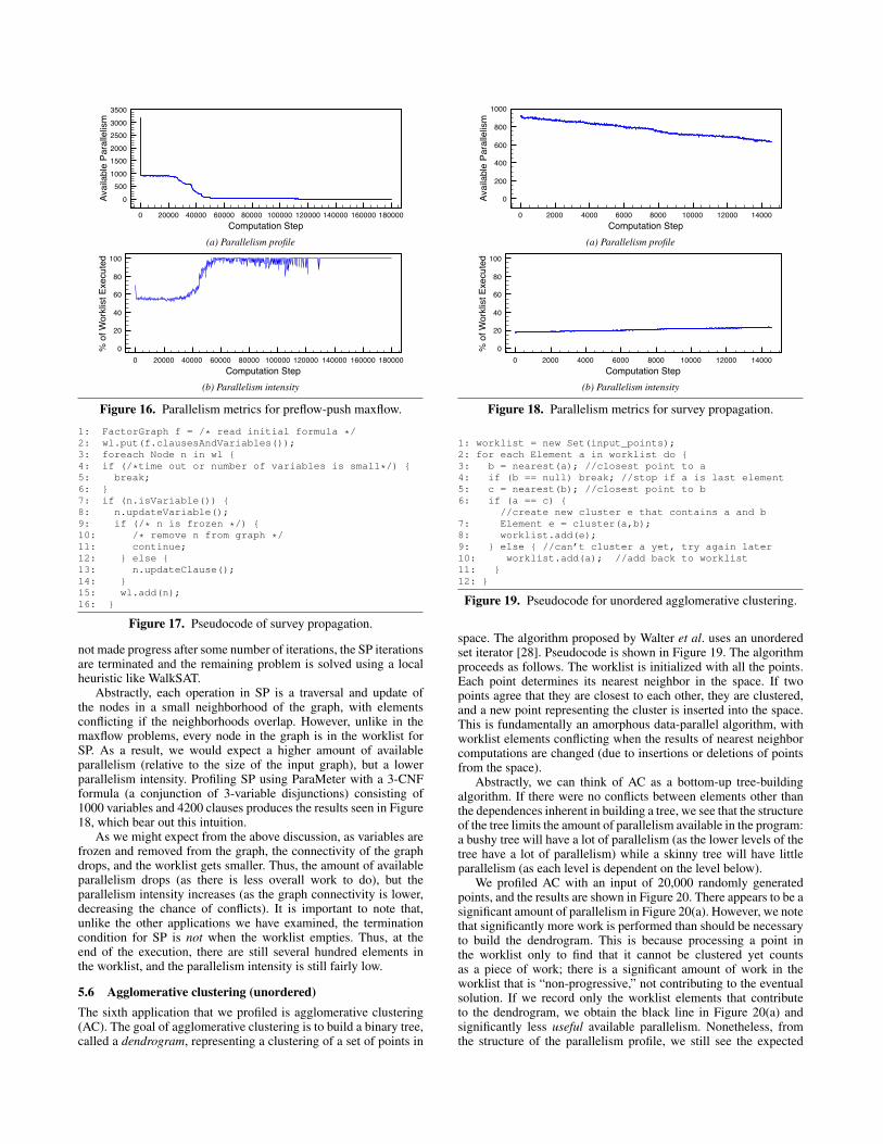
5.5 Survey propagationSurvey propagation (SP) for SAT is a heuristic solver based onBayesian inference [4]. Pseudocode is given in Figure 17. Theunderlying graph in SP is the factor graph for the Boolean formula,a bipartite graph in which one set of nodes represents the variablesin the formula, and the other set of nodes represents the clauses. Anedge links a variable to a clause if the variable or its negation is aliteral in that clause. The worklist for SP consists of all nodes (bothvariables and clauses) in the graph. To process a node, the algorithmupdates the value of the node based on the values of its neighbors.After a number of updates, the value for a variable may become“frozen” (i.e., set to true or false). At that point, the variable isremoved from the graph. The termination condition for SP is fairlycomplex – when the number of variables is small enough, or SP has

0 20000 40000 60000 80000 100000 120000 140000 160000 180000Computation Step

0500

100015002000250030003500

Avai

labl

e Pa

ralle

lism


0 20000 40000 60000 80000 100000 120000 140000 160000 180000Computation Step

0

20

40

60

80

100

% o

f Wor

klist

Exe

cute

d


Figure 16. Parallelism metrics for preflow-push maxflow.

1: FactorGraph f = /* read initial formula */2: wl.put(f.clausesAndVariables());3: foreach Node n in wl {4: if (/*time out or number of variables is small*/) {5: break;6: }7: if (n.isVariable()) {8: n.updateVariable();9: if (/* n is frozen */) {10: /* remove n from graph */11: continue;12: } else {13: n.updateClause();14: }15: wl.add(n);16: }

Figure 17. Pseudocode of survey propagation.

not made progress after some number of iterations, the SP iterationsare terminated and the remaining problem is solved using a localheuristic like WalkSAT.

Abstractly, each operation in SP is a traversal and update ofthe nodes in a small neighborhood of the graph, with elementsconflicting if the neighborhoods overlap. However, unlike in themaxflow problems, every node in the graph is in the worklist forSP. As a result, we would expect a higher amount of availableparallelism (relative to the size of the input graph), but a lowerparallelism intensity. Profiling SP using ParaMeter with a 3-CNFformula (a conjunction of 3-variable disjunctions) consisting of1000 variables and 4200 clauses produces the results seen in Figure18, which bear out this intuition.

As we might expect from the above discussion, as variables arefrozen and removed from the graph, the connectivity of the graphdrops, and the worklist gets smaller. Thus, the amount of availableparallelism drops (as there is less overall work to do), but theparallelism intensity increases (as the graph connectivity is lower,decreasing the chance of conflicts). It is important to note that,unlike the other applications we have examined, the terminationcondition for SP is not when the worklist empties. Thus, at theend of the execution, there are still several hundred elements inthe worklist, and the parallelism intensity is still fairly low.

5.6 Agglomerative clustering (unordered)The sixth application that we profiled is agglomerative clustering(AC). The goal of agglomerative clustering is to build a binary tree,called a dendrogram, representing a clustering of a set of points in

0 2000 4000 6000 8000 10000 12000 14000Computation Step

0

200

400

600

800

1000

Avai

labl

e Pa

ralle

lism


0 2000 4000 6000 8000 10000 12000 14000Computation Step

0

20

40

60

80

100

% o

f Wor

klist

Exe

cute

d


Figure 18. Parallelism metrics for survey propagation.

1: worklist = new Set(input_points);2: for each Element a in worklist do {3: b = nearest(a); //closest point to a4: if (b == null) break; //stop if a is last element5: c = nearest(b); //closest point to b6: if (a == c) {

//create new cluster e that contains a and b7: Element e = cluster(a,b);8: worklist.add(e);9: } else { //can’t cluster a yet, try again later10: worklist.add(a); //add back to worklist11: }12: }

Figure 19. Pseudocode for unordered agglomerative clustering.

space. The algorithm proposed by Walter et al. uses an unorderedset iterator [28]. Pseudocode is shown in Figure 19. The algorithmproceeds as follows. The worklist is initialized with all the points.Each point determines its nearest neighbor in the space. If twopoints agree that they are closest to each other, they are clustered,and a new point representing the cluster is inserted into the space.This is fundamentally an amorphous data-parallel algorithm, withworklist elements conflicting when the results of nearest neighborcomputations are changed (due to insertions or deletions of pointsfrom the space).

Abstractly, we can think of AC as a bottom-up tree-buildingalgorithm. If there were no conflicts between elements other thanthe dependences inherent in building a tree, we see that the structureof the tree limits the amount of parallelism available in the program:a bushy tree will have a lot of parallelism (as the lower levels of thetree have a lot of parallelism) while a skinny tree will have littleparallelism (as each level is dependent on the level below).

We profiled AC with an input of 20,000 randomly generatedpoints, and the results are shown in Figure 20. There appears to be asignificant amount of parallelism in Figure 20(a). However, we notethat significantly more work is performed than should be necessaryto build the dendrogram. This is because processing a point inthe worklist only to find that it cannot be clustered yet countsas a piece of work; there is a significant amount of work in theworklist that is “non-progressive,” not contributing to the eventualsolution. If we record only the worklist elements that contributeto the dendrogram, we obtain the black line in Figure 20(a) andsignificantly less useful available parallelism. Nonetheless, fromthe structure of the parallelism profile, we still see the expected


0

2000

4000

6000

8000

Avai

labl

e Pa

ralle

lism All Work

Useful Work

(a) Parallelism profile (random schedule)


0

1000

2000

3000

4000

5000

6000

Avai

labl

e Pa

ralle

lism

(b) Parallelism profile (oracle schedule)

Figure 20. Parallelism metrics for unordered agglomerative clus-tering.

behavior with a lot of parallelism at the beginning (when the lowerlevels of the tree are being constructed) and far less at the end.

Note, however, that executing non-progressive work may pre-vent other, useful work from being executed in a given round (dueto conflicts between worklist elements). We modified ParaMeter touse oracle scheduling rather than random scheduling. Thus, whenchoosing elements to execute in a given round, ParaMeter only con-siders elements that contribute to the solution. This approach gen-erated the profile shown in Figure 20(b). We see that the oraclescheduler exhibits much higher parallelism than random schedul-ing. We also note that the critical path length when using the oraclescheduler is an order of magnitude shorter than when using the ran-dom scheduler. This is a prime example of algorithms where par-ticular scheduling choices lead to dramatically different amounts ofparallelism. Interestingly, with oracle scheduling, we find that ACis able to achieve the maximum possible parallelism available in abottom-up tree building code.

5.7 Agglomerative clustering (ordered)There is an alternative, greedy algorithm for agglomerative clus-tering (GAC) that uses an ordered set iterator [25]. Pseudocode isshown in Figure 21. The worklist is initialized as follows: for eachpoint p, find the closest point n, and insert the potential cluster(p, n) into the worklist. The worklist is ordered by the size of thepotential clusters (i.e., the potential cluster whose points are closesttogether is at the top of the list). The algorithm proceeds by greedilyclustering the top potential cluster in the worklist. After clusteringthe two points, a new potential cluster is inserted containing thenewly created cluster and the point nearest to it. Interestingly, thisgreedy algorithm produces the same dendrogram as the unorderedalgorithm presented in the previous section.

When we profile GAC with ParaMeter on the same input as forAC, we obtain the parallelism profile shown in Figure 22. Notethat the first point in the profile is cut off and has a value of 5298.While there is a significant amount of parallelism in the first round,there is very little parallelism thereafter. This is due to the natureof the ordered execution strategy. In the first round, many of thepotential clusters representing the lowest level of the dendrogramcan be executed in parallel. However, recall that for ordered loopsParaMeter does not let a worklist element commit until it is thehighest priority element in the system—even if its execution isaccounted for in an earlier round—and new work is not added to

1: pq = new PriorityQueue();2: foreach p in input_points {pq.add(<p, nearest(p)>)}3: foreach Pair <p,n> in pq {4: if (p.isAlreadyClustered()) continue;5: if (n.isAlreadyClustered()) {6: pq.add(<p, nearest(p)>);7: continue;8: }9: Cluster c = new Cluster(p,n);10: dendrogram.add(c);11: Point m = nearest(c);12: if (m != ptAtInfinity) pq.add(<c,m>);13: }

Figure 21. Pseudocode for ordered agglomerative clustering.


0

200

400

600

800

1000

1200

Avai

labl

e Pa

ralle

lism

Figure 22. Parallelism profile for ordered agglomerative clustering

the worklist until the element that generates it commits. It takesseveral hundred steps for the elements recorded in the first roundto actually commit, and the new work generated by the executionof those elements happens much later than the first round. In otherwords, work generated by those initial elements becomes availablefor execution across hundreds of rounds, rather than immediately.Thus, the critical path length of the application is inflated, resultingin lower available parallelism in later rounds.

5.8 Constrained ParallelismBeyond generating parallelism profiles and calculating parallelismintensity, ParaMeter can also calculate constrained parallelism, asdescribed in Section 4.3. The goal of constrained parallelism isto estimate how the critical path of the execution changes if thenumber of processors available for execution is limited. Becauseit can be very expensive to calculate constrained parallelism for alarge number of constraints, we can also use the parallelism profile(i.e., the “unconstrained” parallelism) to estimate the length of thecritical path when there are resource constraints.

We used ParaMeter to calculate the constrained parallelism forthree of the applications we profiled: Delaunay mesh refinement,Delaunay triangulation, and augmenting paths maxflow. For eachapplication, we found the critical path length for a range of proces-sor counts. We also use the parallelism profiles to estimate the crit-ical path length using the technique described in Section 4.3. Theresults are presented in Figure 23. In all three cases, our estimatesof the critical path length closely track the critical path length mea-sured by ParaMeter. These results demonstrate that it is feasible touse simple, easy-to-calculate models, as well as a single piece ofprofiling data (the parallelism profile) to estimate the parallelism inirregular programs for arbitrary numbers of processors.

Constrained parallelism can inform the choice of platforms onwhich to run an application. We see that the constrained parallelismcurves all follow the same general shape: a quick increase in per-formance when the number of processors is relatively low, and de-creasing marginal benefits as the number of processors increases.The existence of a “knee” in the constrained parallelism curve isindicative of diminishing returns: beyond a certain point, there islittle reason to increase the number of processors devoted to a task.

200 400 600 800 1000 1200 1400 1600 1800 2000# of Simulated Processors

200

400

600

800

# of

Ste

psModeled StepsEstimated Steps

(a) Delaunay mesh refinement

20 40 60 80 100Number of Simulated Processors

0

200

400

600

800

# of

Ste

ps

Modeled StepsEstimated Steps

(b) Delaunay triangulation

0 2000 4000 6000 8000 10000Number of Simulated Processors

0

500

1000

1500

2000

# of

Ste

ps

Modeled StepsEstimated Steps

(c) Augmenting paths maxflow

Figure 23. Constrained parallelism: measured vs. estimated.

Application Unprofiled time Profiled timeDMR 18.0s 57.4sDT 4.2s 38.7sAP 0.36s 19.4sPP 24.5s 8m51.8sSP 3m54s 25m30.2sAC 2.36s 10m44.2sAC(O) N/A 3m0.1sGAC 1.48s 1m44.2s

Table 1. Running times of unprofiled and profiled applications.

5.9 ParaMeter PerformanceTable 1 shows the running time of each application when profiledwith ParaMeter, as well as the running time of the non-profiled code(note that there is no sequential oracle scheduler). Our test platformis a dual-core AMD Opteron system with each core running at 1.8GHz. ParaMeter and the test applications were written in Java andrun using the Sun HotSpot JVM, version 1.6.

ParaMeter is designed as an off-line profiling tool, and henceperformance is not the primary goal of its implementation. Never-theless, we see that the tool has reasonable performance for mostapplications. The overhead is largely governed by two factors. Thefirst is the cost of instrumentation. Thus, applications that requiremore instrumentation, such as augmenting paths and preflow push,suffer from higher overheads. Second, applications that have lowparallelism intensity have higher overhead, as ParaMeter must con-tinually inspect work that will ultimately not be executed. Unsur-prisingly, AC has a very high overhead as the non-progressive workmust be repeatedly executed by ParaMeter to no effect. Note thatthere is no equivalent sequential version of AC(O), as it requires anoracle scheduler.

6. Related WorkMuch of the related work on profiling parallel execution is dis-cussed in Section 3. Here, we highlight more recent work in thesame area.

Profiling for thread-level speculation In recent years, researchershave added profilers to compilers that target thread-level specula-tion systems [21, 29]. These profilers simulate the execution of aprogram on the target TLS system to determine how much paral-lelism can be exploited. While these approaches produce profileinformation akin to ParaMeter’s parallelism profiles, there are twokey differences.

The first difference recalls the distinction, discussed in Sec-tion 4.4, between profiling a particular parallelized program ver-sus characterizing an algorithm. The TLS profiling tools are notused to measure parallelism in an algorithm; rather, they are used tomeasure the effectiveness of TLS approaches on certain regions ofcode. In contrast, ParaMeter’s goal is to provide information aboutan algorithm, independent of the particular system used to paral-lelize that algorithm.

This difference of goals leads directly to the second distinctionbetween ParaMeter and TLS-based profilers: because ParaMeter isindependent of a parallelization system, it provides a more accu-rate view of the amount of parallelism in an algorithm. This is dueto two effects. First, because TLS systems must adhere to the se-quential ordering of the program; they are unable to find additionalparallelism by executing worklist elements in other orders. Second,existing TLS profilers use memory-based conflict detection, which,as we discuss in Section 4.4, may obscure available parallelism.

Profiling in functional languages For functional programs, Har-ris and Singh showed how profiling can be used to estimate avail-able parallelism [12]. ParaMeter instead targets imperative pro-grams that exhibit amorphous data-parallelism. This requires ad-ditional support for handling schedule dependence and conflicts inshared data structures.

Dependence density Von Praun et al. recently studied “depen-dence density” in programs using optimistic concurrency [27].While dependence density is a single number for a parallel sec-tion, it is essentially the inverse of the parallelism intensity. Thus,programs with a low dependence density can be easily executedby random schedulers, whereas those with higher dependence den-sities require more intelligent scheduling to exploit parallelism.However, von Praun et al. collect their data from an instrumented,sequential run of computation rather than staging computation asParaMeter does. This leads to an inefficient handling of newly gen-erated work: work generated at a later stage may conflict with workthat could have been safely executed earlier. Further, their notion ofdependence is tied to memory conflicts, which are more restrictivethan ParaMeter’s algorithmic conflicts, potentially resulting in anunderreporting of the amount of parallelism.

7. ConclusionsThis paper presents a tool called ParaMeter to determine how muchparallelism is latent in irregular programs that exhibit amorphousdata-parallelism. ParaMeter addresses some of the unique chal-lenges presented by such programs: dynamically generated workand schedule dependent execution. While ParaMeter measures par-allelism in amorphous data-parallel programs, its techniques can beextended to other models of parallelism in irregular programs. Forexample, thread-level speculation, which speculatively executes it-erations of for-loops, can be profiled in ParaMeter by viewing loopsas ordered worklists (with the order fixed by the for-loop).

The profiles generated by ParaMeter can be used to guide thedevelopment of parallel programs. Parallelism profiles produce a

“target” for parallelization: if an application’s parallelism profileindicates little or no parallelism, there may not be a need for paral-lelization. Similarly, it may not be necessary to continue optimizinga parallel implementation that approaches the speedups predictedby the parallelism profile. Parallelism profiles can further be used tocompare different implementations of the same algorithm. For ex-ample, we found that unordered agglomerative clustering exhibitsmore parallelism than the ordered counterpart.

Profiling parallelism intensity provides insight into the efficacyof random scheduling. High parallelism intensity makes it likelythat randomly chosen elements can be executed in parallel, whilelow intensity makes scheduling difficult, even if there is high avail-able parallelism. Finally, measuring constrained parallelism pro-vides an estimate of how performance will be affected by changingthe number of processors available to the program, which can beuseful in choosing the right platforms for an application.

References[1] Arvind, David Culler, and Gino Maa. Assessing the benefits of

fine-grain parallelism in dataflow programs. International Journal ofHigh-performance Computing Applications, 2(3), 1988.

[2] Robert D. Blumofe, Christopher F. Joerg, Bradley C. Kuszmaul,Charles E. Leiserson, Keith H. Randall, and Yuli Zhou. Cilk: Anefficient multithreaded runtime system. In Proceedings of the FifthACM SIGPLAN Symposium on Principles and Practice of ParallelProgramming (PPoPP), pages 207–216, Santa Barbara, California,July 1995.

[3] Yuri Boykov and Vladimir Kolmogorov. An experimental comparisonof min-cut/max-flow algorithms for energy minimization in vision.International Journal of Computer Vision (IJCV), 70(2):109–131,2006.

[4] A. Braunstein, M. Mezard, and R. Zecchina. Survey propagation:An algorithm for satisfiability. Random Structures and Algorithms,27:201–226, 2005.

[5] L. Paul Chew. Guaranteed-quality mesh generation for curvedsurfaces. In SCG ’93: Proceedings of the ninth annual symposium onComputational geometry, 1993.

[6] Thomas Cormen, Charles Leiserson, Ronald Rivest, and CliffordStein, editors. Introduction to Algorithms. MIT Press, 2001.

[7] Edsger Dijkstra. A Discipline of Programming. Prentice-Hall, 1976.[8] Matteo Frigo, Charles E. Leiserson, and Keith H. Randall. The

implementation of the Cilk-5 multithreaded language. In Proceedingsof the ACM SIGPLAN ’98 Conference on Programming LanguageDesign and Implementation, pages 212–223, Montreal, Quebec,Canada, June 1998. Proceedings published ACM SIGPLAN Notices,Vol. 33, No. 5, May, 1998.

[9] Andrew V. Goldberg and Robert E. Tarjan. A new approach to themaximum-flow problem. J. ACM, 35(4):921–940, 1988.

[10] Leonidas J. Guibas, Donald E. Knuth, and Micha Sharir. Random-ized incremental construction of delaunay and voronoi diagrams.Algorithmica, 7(1):381–413, December 1992.

[11] Tim Harris and Keir Fraser. Language support for lightweighttransactions. In OOPSLA ’03: Proceedings of the 18th annualACM SIGPLAN conference on Object-oriented programing, systems,languages, and applications, pages 388–402, New York, NY, USA,2003.

[12] Tim Harris and Satnam Singh. Feedback directed implicit parallelism.In ICFP ’07: Proceedings of the 12th ACM SIGPLAN internationalconference on Functional programming, pages 251–264, New York,NY, USA, 2007. ACM.

[13] L. Hendren and A. Nicolau. Parallelizing programs with recursivedata structures. IEEE Transactions on Parallel and DistributedSystems, 1(1):35–47, January 1990.

[14] Maurice Herlihy and J. Eliot B. Moss. Transactional memory: ar-chitectural support for lock-free data structures. In ISCA ’93: Pro-ceedings of the 20th annual international symposium on Computerarchitecture, 1993.

[15] Benoıt Hudson, Gary L. Miller, and Todd Phillips. Sparse paralleldelaunay mesh refinement. In SPAA ’07: Proceedings of thenineteenth annual ACM symposium on Parallel algorithms andarchitectures, pages 339–347, New York, NY, USA, 2007. ACMPress.

[16] Ken Kennedy and John Allen, editors. Optimizing compilersfor modren architectures:a dependence-based approach. MorganKaufmann, 2001.

[17] Venkata Krishnan and Josep Torrellas. A chip-multiprocessorarchitecture with speculative multithreading. IEEE Trans. Comput.,48(9):866–880, 1999.

[18] Milind Kulkarni, Patrick Carribault, Keshav Pingali, Ganesh Rama-narayanan, Bruce Walter, Kavita Bala, and L. Paul Chew. Schedulingstrategies for optimistic parallel execution of irregular programs. InSPAA’08: Proceedings of the ACM Symposium on Parallel Architec-tures and Algorithms, 2008.

[19] Milind Kulkarni, Keshav Pingali, Ganesh Ramanarayanan, BruceWalter, Kavita Bala, and L. Paul Chew. Optimistic parallelismbenefits from data partitioning. SIGARCH Comput. Archit. News,36(1):233–243, 2008.

[20] Milind Kulkarni, Keshav Pingali, Bruce Walter, Ganesh Rama-narayanan, Kavita Bala, and L. Paul Chew. Optimistic parallelismrequires abstractions. SIGPLAN Not. (Proceedings of PLDI 2007),42(6):211–222, 2007.

[21] Wei Liu, James Tuck, Luis Ceze, Wonsun Ahn, Karin Strauss, JoseRenau, and Josep Torrellas. Posh: a tls compiler that exploits programstructure. In PPoPP ’06: Proceedings of the eleventh ACM SIGPLANsymposium on Principles and practice of parallel programming,pages 158–167, New York, NY, USA, 2006. ACM.

[22] Jayadev Misra. Distributed discrete-event simulation. ACM Comput.Surv., 18(1):39–65, 1986.

[23] L. Rauchwerger, Y. Zhan, and J. Torrellas. Hardware for speculativerun-time parallelization in distributed shared-memory multiproces-sors. In HPCA ’98: Proceedings of the 4th International Symposiumon High-Performance Computer Architecture, 1998.

[24] M. Sagiv, T. Reps, and R. Wilhelm. Solving shape-analysis problemsin languages with destructive updating. ACM Transactions onProgramming Languages and Systems, 20(1):1–50, January 1998.

[25] Pang-Ning Tan, Michael Steinbach, and Vipin Kumar, editors.Introduction to Data Mining. Pearson Addison Wesley, 2005.

[26] K.B. Theobald, G.R. Gao, and L.J. Hendren. On the limits of programparallelism and its smoothability. In Proceedings of the 25th AnnualInternational Symposium on Microarchitecture (MICRO 25), pages10–19, Dec 1992.

[27] Christoph von Praun, Rajesh Bordawekar, and Calin Cascaval.Modeling optimistic concurrency using quantitative dependenceanalysis. In PPoPP ’08: Proceedings of the 13th ACM SIGPLANSymposium on Principles and practice of parallel programming,pages 185–196, New York, NY, USA, 2008. ACM.

[28] Bruce Walter, Kavita Bala, Milind Kulkarni, and Keshav Pingali.Fast agglomerative clustering for rendering. In IEEE Symposium onInteractive Ray Tracing (RT), 2008.

[29] Hongtao Zhong, Mojtaba Mehrara, Steve Lieberman, and ScottMahlke. Uncovering hidden loop level parallelism in sequentialapplications. IEEE 14th International Symposium on High Perfor-mance Computer Architecture, pages 290–301, Feb. 2008.

How much parallelism is there in irregular applications?

Documents

Transcript of How much parallelism is there in irregular applications?