O conte�udo do presente relat�orio �e de �unica responsabilidade dos autores.The contents of this report are the sole responsibility of the author(s).

Automatic reassembly of irregular fragmentsHelena Cristina da Gama Leit~ao and Jorge Stol�Relat�orio T�ecnico IC{98-06Abril de 1998

Automatic reassembly of irregular fragmentsHelena Cristina da Gama Leit~ao �and Jorge Stol� yAbstractThis report addresses following problem: given one or more unknown objects thathave been broken or torn into a large number of irregular fragments, �nd the pairs offragments that were adjacent in the original objects.Our approach is based on information extracted from fragment outlines that is usedto compute the mismatch between pairs of pieces of contour. For that, we use the tech-nique of dynamic programming. In order to asymptotically reduce the cost of matchingwe use multiple scale techniques: after �ltering and resampling the fragment outlines atseveral di�erent scales of detail, we look for initial matchings at the coarsest possiblescale. We then repeatedly select the most promising pairs, and re-match them at thenext �ner scale of detail. In the end, we are left with a small set of fragment pairs thatare most likely to be adjacent in the original object.

�Departamento de Computa�c~ao,Universidade Federal Fluminense, 24210-130 Niter�oi, RJyInstituto de Computa�c~ao, Universidade Estadual de Campinas, 13081-970 Campinas, SP.1

Automatic reassembly of irregular fragments 2

(this blank intentionally left on the page)

Automatic reassembly of irregular fragments 3Contents1 Introduction 51.1 Motivation : : : : : : : : : : : : : : : : : : : : : : : : : : : : : : : : : : : : 51.2 Related work : : : : : : : : : : : : : : : : : : : : : : : : : : : : : : : : : : : 52 Approach 62.1 The ideal model for fracture objects : : : : : : : : : : : : : : : : : : : : : : 62.2 The actual data : : : : : : : : : : : : : : : : : : : : : : : : : : : : : : : : : : 72.3 Geometric features of obtained contours : : : : : : : : : : : : : : : : : : : : 82.4 Reconstruction goal : : : : : : : : : : : : : : : : : : : : : : : : : : : : : : : 92.5 Identity of contours : : : : : : : : : : : : : : : : : : : : : : : : : : : : : : : : 92.6 Computational di�culties : : : : : : : : : : : : : : : : : : : : : : : : : : : : 102.7 Stages of processing : : : : : : : : : : : : : : : : : : : : : : : : : : : : : : : 103 Fragment image acquisition 103.1 The geometry of fracture lines : : : : : : : : : : : : : : : : : : : : : : : : : : 113.2 Minimum resolution : : : : : : : : : : : : : : : : : : : : : : : : : : : : : : : 124 Identi�cation and separation of fragments 125 Extration of contours 145.1 Contour extraction algorithm : : : : : : : : : : : : : : : : : : : : : : : : : : 145.2 Re-sampling : : : : : : : : : : : : : : : : : : : : : : : : : : : : : : : : : : : : 166 Filtering 166.1 Final sampling : : : : : : : : : : : : : : : : : : : : : : : : : : : : : : : : : : 187 Generic curve comparison 187.1 Basic concepts : : : : : : : : : : : : : : : : : : : : : : : : : : : : : : : : : : 187.1.1 Segments and candidates : : : : : : : : : : : : : : : : : : : : : : : : 187.1.2 True and recognizable candidates : : : : : : : : : : : : : : : : : : : : 187.1.3 Solutions and quality measures : : : : : : : : : : : : : : : : : : : : : 197.2 Evaluating a candidate : : : : : : : : : : : : : : : : : : : : : : : : : : : : : : 197.2.1 Segment reversal : : : : : : : : : : : : : : : : : : : : : : : : : : : : : 197.2.2 Sample matching : : : : : : : : : : : : : : : : : : : : : : : : : : : : : 208 Geometric invariants 218.1 Curvature sampling : : : : : : : : : : : : : : : : : : : : : : : : : : : : : : : 218.2 Curvature encoding : : : : : : : : : : : : : : : : : : : : : : : : : : : : : : : : 228.3 Quantization function : : : : : : : : : : : : : : : : : : : : : : : : : : : : : : 23

Automatic reassembly of irregular fragments 49 Multiples scales 249.1 Comparison cost : : : : : : : : : : : : : : : : : : : : : : : : : : : : : : : : : 249.2 The multiscale approach : : : : : : : : : : : : : : : : : : : : : : : : : : : : : 249.3 Analysis of the multiscale algorithm : : : : : : : : : : : : : : : : : : : : : : 259.4 Corner blurring : : : : : : : : : : : : : : : : : : : : : : : : : : : : : : : : : : 259.5 Maximum �ltering scale : : : : : : : : : : : : : : : : : : : : : : : : : : : : : 269.6 Multiscale fragment matching algorithm : : : : : : : : : : : : : : : : : : : : 269.7 Mapping candidates between scales : : : : : : : : : : : : : : : : : : : : : : : 279.8 Generation of initial candidates : : : : : : : : : : : : : : : : : : : : : : : : : 279.9 Merging overlapping candidates : : : : : : : : : : : : : : : : : : : : : : : : : 2810 Results and conclusions 2910.1 Test 1: paper fragments : : : : : : : : : : : : : : : : : : : : : : : : : : : : : 2910.2 Test 2: ceramic fragments : : : : : : : : : : : : : : : : : : : : : : : : : : : : 3210.3 Conclusions : : : : : : : : : : : : : : : : : : : : : : : : : : : : : : : : : : : : 35

Automatic reassembly of irregular fragments 51 IntroductionThe subject of this work is the computer-assisted reconstrution of unknown objects thathave been broken or torn into a large number of irregular fragments.We are concerned here with the �rst step in the reconstruction fragment-matching, whichis to identify pairs of fragments that were probably adjacent in the original object. Whenone is dealing with hundreds or thousands of fragments, these pairs may be impossible to�nd by hand. We develop here a set of mathematical techniques and algorithms that canbe used to locate such pairs. We also describe our implementation of those techniques, andthe results of preliminary experiments.After identifying a likely set of adjacent fragment pairs, we will have to face the problemof global reconstruction, where the goal is to reconstruct the topology and approximategeometry of the fracture network. We did not address this problem, because its di�cultyand practical relevance depend a lot on the correctness and completeness of the list ofadjacent pairs which are still being improved upon. Moreover, the global reconstructionstep requires human intervention, since it must take into account certain general informationthat cannot be easily quanti�ed|such as fragment texture and color, decoration, location,probable function, etc. Therefore, we felt that automating the global reconstruction problemwould be premature at this point.1.1 MotivationFragment assembly is a very real problem in archaeology, as this quote shows:'Pottery forms one of the most common and abundant types of artifactsfound at archaeological sites. As such, pottery provides important informationabout chronology, technology, trade, and art. Although most handbooks illus-trate whole or nearly complete vessels, the majority of ceramic remains fromany excavation consists of thousands of small, broken pieces which need to becleaned, sorted, counted, weighed, and analyzed. [13]'Besides pottery, the techniques we will describe could be applied to other kinds ofarchaeological materials, such as glass objects [16], chipped stone tools [13], clay tablets [14],mural paintings [11], ancient manuscripts [3], statues and bas-reliefs [14], building stones,and so on. Our techniques may be useful also in fragment reassembly problems from otherdisciplines, such as paleontology (fossils), surgery and forensics (shattered bone) and failureanalysis (debris).1.2 Related workAt present, the reconstruction of archaeological fragments is done largely by hand; com-puters are used, if at all, only in the classi�cation, indexing, and presentation of scannedimages of the fragments [3, 11, 29], which are indexed and retrieved based solely on textualdescriptions provided by the user. There is a modest technical literature about image en-hancing techniques specialized for archaeological materials [29, 11]. Only a few authors have

Automatic reassembly of irregular fragments 6considered the use of computer vision and pattern matching techniques to automaticallyextract indexing information from digital images of archaeological artifacts [28].The speci�c problem of identifying adjacent ceramic fragments by matching the shapesof their contours was recently considered by �U�coluk and Toroslu [28]. Their algorithmconsiders only a �xed scale of resolution, and therefore has large expected asymptotic cost(see section 2.6). No experiments are reported in the paper.The fragment reassembly problem is similar to that of automatic assembly of jigsawpuzzles, which has been addressed before mainly as a cute exercise in robotics and machinevision [8, 15, 7, 25]. In particular, H. Wolfson and G. C. Burdea developed a program thatcan �nd matching pieces in a standard puzzle game [7], and even control a robot arm toassemble the puzzle. However, the techniques used rely on special characteristics of puzzlegames (smooth borders and well-de�ned corners), which are not found in archaeologicalmaterials.More generally, the problem can be viewed as a special case of approximate contourmatching, an area with extensive bibliography [18, 22, 15, 17, 5, 24, 32, 1, 20, 26]. In par-ticular, there are many papers on machine vision that are concerned with object recognitionfrom outlines, mainly for industrial or military applications. Some of their results can beexpected to work also for irregular fragments. However, most of these works assume thatthe outlines are to be matched agaist a relatively small set of �xed templates, so that theirmain concern is to reduce the cost of comparing an outline against a template. In theapplication that interest us, however, the `templates' are the fragments outlines themselves,which may number in the thousands. We are thus interested mainly in techniques that canbe used to eliminate large sets of templates at relatively low cost.2 Approach2.1 The ideal model for fracture objectsOur approach is based on information extracted from fragment outlines. The idealizedmodel can be summarized as follows. We assume that the fragmented objects have a wellde�ned smooth surface. This surface is divided into two ou more parts, the ideal fragments,that are separated by ideal fracture lines, irregular curves with zero width. Two fragmentsare said to be adjacent if they share a fracture line. The fractures also split the originaloutline of the surface into one or more border lines.The fracture lines can be viewed as a graph G drawn over the object's surface, whichwe call the fracture network. See �gure 1(a). The point where three or more lines (fractureor boundary) meet is called an ideal corner. The boundary of an ideal fragment is an idealcontour; it is the concatenation of one or more fracture and border lines.

Automatic reassembly of irregular fragments 71

corners

2

34

fractureline

border line

ideal

(a)1

3

4 2

(b)Figure 1: Ideal fracture network (a) and the adjacency graph (b).We can assume that each fragment is a topological disk, that is, its contour is a singleloop. In the cases where this assumption does not hold (for example, when a handle orcylindrical vessel is broken at both ends), we can pretend that each closed loop in theboundary of the fragment is the contour of a separate fragment. The same holds for objectswith two smooth surfaces of similar characteristics (torn paper, ceramic pottery and tiles,etc.): we can view the two sides of each fragment as two separate fragments. The physicalconnection between these two contours only needs to be taken into account at the very laststage of the reconstruction (which does not concern us here).The topological dual of the fracture network (ignoring the border lines) is the fragmentadjacency graph G�. It has one vertex u� in each fragment u; for each fracture line e,separating two fragments u and v, there is an edge e� in G� connecting u� and v�, whichcrosses the boundary of u only once, at some point of e. Note that while G is both ageometrical and topological object, G� is topological object only.2.2 The actual dataThe fracture lines and ideal contours are mere abstractions, of course. What we obtainfrom the physical fragments are the observed contours; they di�er from the ideal contoursfor a number of reasons, such as barbs (common in torn paper), turned edges, or theloss of small portions of material. Because of these perturbations, the single fracture linethat separates two adjacent ideal fragments becomes two slightly di�erent sections of thecorresponding observed contours. This di�erence is where lies the main di�culty of thereassembly problem.

Automatic reassembly of irregular fragments 8contour recovered fragment

lost fragment

observed contour

ideal

Figure 2: Observed contours.A segment is a piece of contour. A pair of corresponding segments is a pair of maximalsegments, belonging to two observed contours, that correspond the same ideal fracture line.Figure 3: Corresponding segments.2.3 Geometric features of obtained contoursIn typical applications, we can expect that there are lost fragments. Therefore, there is anintrinsic ambiguity in this model: the loss of a small portion of the object along a fragmentboundary can be either attributed to noise (�gure 4(a)), or modeled as an ideal fragmentthat was not recovered (�gure 4(b)). Our algorithms will arbitrarily resolve this ambiguityone way or the other, depending on the size of the missing piece.(a) (b)Figure 4: Ambiguity of the fracture model.Another ambiguity of the model is that it is not possible to de�ne with precision thebeginning and end of corresponding segments. For one thing, we do not know the position of

Automatic reassembly of irregular fragments 9the ideal fracture corners; and, in any case, the presence of noise does not allow us to de�nea precise point-to-point correspondence between the observed and ideal contours. Again,our algorithms will arbitrarily de�ne the beginning and end of corresponding segments,based on the distance between the two contours.An important property of physical fracture lines is that each ideal corner is generallyincident to only three fracture lines, or one fracture line and two border lines. Moreover,two of these lines frequently make an angle close to 180�; that is, they are actually parts ofthe same physical fracture. Thus, the existence of the corner will be apparent only in two ofits three incident fragments. Moreover, physical fracture lines tend to display sharp bendseven where there are no ideal corners. For these reasons, we cannot expect to identify thecontour segments to be matched by looking for corners in the fragment outlines.2.4 Reconstruction goalWe formulate, the problem of fragment matching as follows: given a set F of observedcontours, determine as much information as possible about the ideal fracture graph G. Inparticular, try to determine all pairs of adjacent fragments, and the corresponding segmentsof their contours.2.5 Identity of contoursThe �rst question we must answer is whether the problem can be solved at all. Is it reallypossible to identify adjacent pairs in a large collection of fragments, only on the basis of the(noisy) observed contours? The answer is yes: by physical experiment, one can verify thatthe irregular nature of fracture lines allows pairs of adjacent fragments to be identi�ed, withhigh con�dence, by the congruence of their outlines at sub-millimeter scale. See �gure 5.

Figure 5: Correspondence of fragmentsOur strategy to solve the reconstrution problem exploits this observation. If two contoursegments are su�ciently long, and their shapes are su�ciently similar, we can discard thehipotesis that the similarity is due to mere coincidence. In section 3.2, we will analyze therelation between measurement accuracy, noise magnitude, and the probability of correctlyidentifying two corresponding segments of given length.

Automatic reassembly of irregular fragments 102.6 Computational di�cultiesFrom the computational viewpoint, the main di�culty of this problem is the large numberof segment pairs that we would need to consider.In order to identify adjacent fragments with adequate con�dence, we need to work withcontour segments comprising hundreds of independent sample points. Moreover, for eachpair of fragments, we would need to test all possible pairs of segments. As we will see insection 9.1, if we have N fragments, each fragment with L sample points, then exhaustivecomparison will require O(N2L4) operations. In typical instances of the problem, withthousands of fragments, this exhaustive search would be way too expensive.In order to asymptotically reduce this cost, we will use two complementary ideas. First,we decrease the number of sample points in each contour, by �ltering and resampling.Second, we reduce the number of segment pairs to be compared in detail, by usingmultiscaletechniques [2, 21]. In section 9, we show how these techniques allow us to reduce the costto O(N2 +ML2), where M is the number of adjacent fragment pairs.By using geometric hashing, as proposed by Kalvin and others [15], it would be possibleto reduce the term O(N2) to something closer to O(N log N). We did not implement thisoptimization yet.2.7 Stages of processingOur solution consists of the following stages:� Acquisition of fragment images;� Image segmentation and contour extraction;� Filtering of the contours at di�erent resolution scales;� Encoding of the contours as curvature strings;� Statistical analysis of the contours;� Identi�cation of similar segments at the coarsest scale;� Re�ning of candidate matchings at �ner scales;� Geometric alignment of similar segments;� Graphical presentation of results.In the following sections, we describe each stage in more detail.3 Fragment image acquisitionThe acquisition of fragment images can be done of many ways, depending of nature of theobjects. In the case of pieces of paper, for example, we can directly use a atbed scanner,as was done in �gure 6.

Automatic reassembly of irregular fragments 11

Figure 6: Pieces of paper.For other objects with a at surface, such as tiles and mural paintings,the direct useof a scanner may still be possible, although a photographic or TV camera may be moreadequate for bulky or delicate materials.In the case of pottery and stone fragments, where the contours to be matched are three-dimensional curves, it would be necessary to acquire two or more images of each fragment,from di�erents angles, and use techniques of stereoscopic vision to extract the contours. Inthis report, we consider only the case of at surfaces.3.1 The geometry of fracture linesFor the aplications we are interested in, fracture lines are self-similar to a certain extent;that is, a small portion of a contour, magni�ed, is statistically similar to the whole. See�gure 7. Indeed, fracture lines are a classical example of fractal curves [12]. It is preciselytheir randomness at many di�erent scales that makes our multi-scale approach possible.

(a) (b) (c)Figure 7: Fractality of fracture lines.The fractal model is apropriate for fractures in rigid and granulated materials, such asceramic, stone, and stucco. The fractal model can also be applied to certain types of agedpaper (which tend to crumble rather than tear).Fractures in glass or glazed ceramic objects tend to be smoother (technically, their fractaldimension is closer to 1); on the other hand, the observed contours are much sharper, andtherefore compared with greater precision.

Automatic reassembly of irregular fragments 123.2 Minimum resolutionThe resolution of scanned fragment images must be su�ciently �ne to capture the smallirregularities which are the key to the identi�cation of adjacent fragments.On a �rst aproximation, if we have N fragments, and we want to identify with highcon�dence the partner of a determined fragment, then we need to extract at least log2Nbits of information from the shared part of their contours. In the case of irregular fractures,we can assume that the shape of the scanned contour gives on the order of one bit ofinformation per linear pixel. Therefore, the resolution of the scanner should be at leastlog2N=L pixels per unit of length, where L is the length of the shared segment.For example, if we have N = 1000 fragments, and we want to identify pairs that share atleast one inch of their outline, we must obtain images with at least dlog2Ne = 10 pixels=inchresolution. In pratice, since image scanning is not the only source of error, we will need toscan the fragments at several times this resolution.It is important to observe that the resolution required increases only logarithmicallywith the number of fragments. In other words, it is theoretically possible to identify theadjacent fragments, with high con�dence, even in large instances of problem (with millionsof fragments), from contours acquired at ordinary scanner resolutions.4 Identi�cation and separation of fragmentsFor obvious practical reasons, one often scans two or more fragments at a time. Therefore,the �rst image processing problem we must solve is that of identifying and separating theindividual fragments in each image.In the algorithms of this section, we will use the following notation. The variablesnx and ny denote the horizontal and vertical dimensions of the scanned image, in pixels.R = [0:: nx � 1] � [0:: ny � 1] is the domain of the image. A generic pixel position p istherefore a pair (px; py) 2 R. The value (intensity) of the image at pixel p is v[p].To identify the fragments, we use a simple thresholding algorithm, that assumes thatthere is a unique grey level �sep such that pixels with color v[p] � �sep belong to thebackground and pixels with color v[p] > �sep belong to the fragment. This simple algorithmshould be adequate in the case of thin at fragments, since we can usually choose thebackground color at the time the images are scanned. We will assume, therefore, that thebackground has a uniform color �min < �sep.Once we have located a pixel v[p] > �sep, we use a straightforward propagation algorithm(a variant of the ood-�ll technique that is used in many graphic editors to paint region ofarbitrary contours) to identify all pixels q with v[q] > �sep that are conected to pixel p, inthe 4-neighborhood topology [23].We also extract a one-pixel wide safety \halo" around the fragment. These extra pixelsare essential for the precise positioning of the fragment contour, as will be explained insection 5. We assume here that the fragments are su�ciently separated from each otherand from the image border, so that these safety halos do not overlap, and surround theentire fragment.

Automatic reassembly of irregular fragments 13The output of this stage is a set of images, each containing a single fragment and itssafety halo, against a uniform background of color �min. See �gure 8.Figure 8: Examples of separated fragments.

Automatic reassembly of irregular fragments 145 Extration of contoursOnce we have a separate image for each fragment, we extract its raw contour, in the form ofa polygonal closed curve. As explained above, we assume that the fragments were scannedagainst a uniform background with known color �min. If each fragment has an approximatelyuniform color �max, like the fragments shown in 8, the contour can be extracted by a simplealgorithm that follows the level curve of an intermediate intensity �med, somewhere between�min and �max.In fact, it is important that the threshold �med be exactly (�min + �max)=2, in order toensure that the contours of adjacent fragments are congruent. This requirement can bededuced from the assumptions that the scanned images are linear blurrings of the ideal(in�nite-resolution) images, and that the original (unbroken) object had uniform color �maxon both sides of the fracture.Figure 9 shows the e�ect of varying the threshold �med on an image of two small con-gruent fragments. The background intensity �min is 10=255, and the fragment color �max is200=255.�med = 30=255 �med = 105=255 �med = 170=255Figure 9: Thresholding efects.Observe that the extracted contours are congruent only when �med is near the average of �minand �max. An incorrect choice of the threshold �med will change the curvature of convex andconcave parts in oposite directions, hampering the recognition of corresponding contours.5.1 Contour extraction algorithmTo extract the contour of a fragment, we �rst locate a pair of adjacent grid points, (a; b),with a inside the fragment (v[a] > �med), and b outside (v[b] � �med). We then follow thefragment boundary in counterclockwise sense while maintaining these conditions.More exactly, at each step the algorithm can be in one of the situations shown in�gure 10:

Automatic reassembly of irregular fragments 15a

b (a) ba(b)b

a(c)b a

(d)Figure 10: Possible situations during contour extraction.Suppose that a is directly above b, as at �gure 10(a). From this situation, the algorithmcan advance either a or b, or both, so as to keep a inside and b outside the fragment, asshown in �gures 11(a{c).b

a

(a)a

b(b) b

a(c)Figure 11: Alternative steps of algorithm for the situation of �gure 10(a).The handling of the other cases (�gures 10(b{d)) is analogous.We obtain from this process a sequence of pairs (ai; bi), where ai follows the contourfrom the inside (i.e. v[ai] > �med), and bi from the outside (i.e. v[bi] � �med). For greaterprecision, from each pair ai, bi we compute the (fractional) point pi on the edge (ai; bi)where the linearly interpolated grey level is exactly �med. (See �gure 12)

Automatic reassembly of irregular fragments 16

Figure 12: Extracted contours: external, interpolated and internal.The result of contour extraction is, therefore, a closed polygonal curve p0; p1; :: pn = p0.The sides of this polygonal have variable length between 0 and �p2 , where � is the distancebetween consecutive pixels.This simple contour extraction algorithm has its limitations. Even for at and thinfragments, such as the torn paper of �gure 6, the algorithm is frequently confused by barbs,turned edges, loose threads, etc.|like those that are visible on the right side of the fragmentin �gure 8(a).Another serious shortcoming of this algorithm is the fact that, in pratice, the foregroundcolor �max changes a lot from point to point; therefore, there is not a unique correct valuefor the thresholding �med. For such applications, one should use a more sophisticatedsegmentation algorithm that varies �max (and hence �med) from pixel to pixel, based on theimage values on the neighboring pixels.5.2 Re-samplingThe irregular spacing of the points pi in the intermediate contours is problematic for the�ltering stage. Therefore, before storing the extracted contour, we re-sample it with roughlyuniform steps, equal to approximately half the pixel spacing, using cubic interpolation [4].6 FilteringThe �ltering phase takes as input the observed contours, and outputs smoothed versions ofthem. See �gure 13. The �ltering serves two di�erent purposes. Firstly, it is used to remove

Automatic reassembly of irregular fragments 17non-signi�cant irregularities from the contours, caused by artifacts of the image acquisitionand contour extration processes, or by erosion of the material after fragmentation. For thispurpose, it is necessary to remove the highest-frequency components of the contour, becausethey are the ones more a�ected by these perturbations. Secondly, the �ltering is used toreduce the complexity of the contours, for the purpose of speeding up the identi�cation ofsimilar contour segments. This use will be further explained in section 9.

(a) Original curve. (b) Filtered to scale � = 64 pixels.Figure 13: Filtering a curve. (Grid spacing = 25 pixels apart.)Filtering time-based signals is a well developed �eld with extensive theory and e�ective,well understood procedures. Filtering a curve is harder since the natural parameter fordescribing the curve, its length, may shrink substantially and non-uniformily as the result of�ltering. To solve this problem, we developed an original technique which we call geometric�ltering, to be detailed in a separate report [10].The goal of �ltering is to remove all details smaller than a certain size �, the �lteringscale. See �gure 14.(a) � = 8 pixels (b) � = 16 pixels (c) � = 32 pixelsFigure 14: Filtering a curve at di�erent scales (and spacing = 25 pixels)

Automatic reassembly of irregular fragments 186.1 Final samplingAfter �ltering, each contour is resampled at uniform steps along the curve. The number nsof samples that we use is chosen based on the Nyquist criterion [6]. Namely, for a contourof length L that has been subjected to geometric Gaussian �ltering at scale �, we usens = �8L� �This formula is justi�ed by noting that Gaussian �ltering at scale � e�ectively removes allFourier components of the curve with wavelength smaller than �=4 [10].The corresponding step size is d = Lns = Ld8L� e � �8Since ns is usually in the hundreds range, the sampling step d is actually quite close to �=8,and therefore practically the same for all contours �ltered at the same scale �. Our contourmatching algorithms will take advantage of this fact.7 Generic curve comparison7.1 Basic concepts7.1.1 Segments and candidatesIn this section we will consider the problem of comparing the shape of two curves in a genericcontext. We will assume that each contour is represented by a circular sequence of samplesc0; c1; :: cn�1. Each sample can be a point of the contour, or any other local geometricproperty such as curvature or color. We assume also that the samples are uniformly spacedalong the contour, and that the sampling step d is approximately the same for all contours.We will need the following concepts:A step is a pair of consecutive samples ci, ci+1 on the same contour.A segment is a sequence of one or more consecutive samples of a contour, strictlyless than the complete contour. We denote by hc; i;mi the segment of contour c thatconsist of the samples ci; :: ci+m�1 (all sample indices are implicitly taken modulo thenumber of samples in the whole contour).A candidate is a pair of segments from two di�erent contours.7.1.2 True and recognizable candidatesA candidate is said to be true if its segments correspond to the same ideal fracture line, anddi�er only by image acquisition errors or loss of very small intervening pieces. Otherwisethe candidate is false.

Automatic reassembly of irregular fragments 19The concept of true candidate is not very useful for the purposes evaluating algorithms,because it is based on information that may not be present in the input data. If the materialloss and acquisition errors are large enough, the two segments of a true candidate may havecompletely di�erent shapes. Moreover, the true candidates include also pairs of segmentswhose ideal fracture lines are too small to allow unambiguous matching.Therefore, we are only interested in a true candidate if it is also recognizable; meaningthat it can be identi�ed by a careful and patient person, working only with the extractedcontours.7.1.3 Solutions and quality measuresIn general, a solution for the fragment reconstrution problem is a set of candidates. Ideally,the solution should be precisely the set R of recognizable candidates; but we cannot yetexpect the computer to perform as well as a human. In order to evaluate the quality of asolution S, we de�ne the following measures:Sensitivity: � = jS \ RjjRj .Signi�cance: = jS \ RjjSj .Informally, The sensitivity � measures the ability of the program to recognize truecandidates, while the signi�cance measures its capacity to reject false ones.7.2 Evaluating a candidateWe will try now to de�ne a quality measure for a single candidate, that is, a measure of howdi�erent the two segments are | in shape, or in some other derived characteristic, such ascurvature or color.Basically, the mismatch is can be de�ned as an integral of the distance between corre-sponding points along the two segments. The main di�culty here is to establish a likelycorrespondence between each point of one segment an the point on the other.7.2.1 Segment reversalWhen we extract the contour of a fragment, we always follow its boundary counterclockwise,as explained in section 5. Therefore, two segments that come from the same fracture linewill be traversed in opposite directions, as shown in �gure 15.

Automatic reassembly of irregular fragments 20

Figure 15: Matching segments are extracted in opposite directions.In the remaider of this section, we assume that one of the fragments to be comparedhas been reversed, to account for this fact.7.2.2 Sample matchingWe will de�ne a discrete matching of the two segments a0 : : : aR and b0 : : : bS as a sequenceof pairs (rj; sj), j 2 f0; :: m� 1g satisfying the following conditions:� rj 2 f0; :: R� 1g,� sj 2 f0; :: S � 1g,� rj � rj+1 � rj + 1,� sj � sj+1 � sj + 1,� (rj ; sj) 6= (rj+1; sj+1)Once established the matching r; s we compute the mismatch between the two segmentsby the formula: C(a0::R; b0::S) = d n�1Xi=0(kari ; bsik2 � �2) (1)where kari ; bsik is a measure of the di�erence between samples ari and bsi , and � is aparameter to be determined, the comparison threshold.The matching we use is the one that minimizes formula (1), among all discrete match-ings of the two segments. We �nd this matching using a standard dynamic programmingalgorithm [19] modi�ed to allow exible end conditions. More details are given in a separatetechnical report [9].Note that the mismatch C(: : :) is negative if the sample di�erence kari ; bsik2 is less thanthe threshold �2, in the squared-mean sense. If the candidate is su�ciently long, and � isthe maximum average displacement of observed samples away from the ideal fracture line,then negative and positive values of C indicate true and false candidates, respectively, withvery high con�dence [9].

Automatic reassembly of irregular fragments 218 Geometric invariantsSince each fragment was digitized with arbitrary orientation and position, it is not feasibleto �nd similar pairs by comparing directly the coordinates of sample points. In order toavoid the high cost of testing all possible rotations and translations when comparing twosegments, we must extract from them some kind of geometric invariant | some shapeinformation that will not change when the fragment is rotated or translated.The area, length, and moments of inertia are familiar examples of such geometric invari-ants. Unfortunately, these invariants are not useful for our problem, because they dependon the whole curve. The invariants that we need must be local, this is, they must dependonly on a small portion of the contour.The simplest local invariant is the curvature. This invariant has been widely employedin shape recognition work, as for example in the work of Wolfson[31], Rosin[24], Bousso�aneet al.[5], and Kalvin et al.[15].The curvature of a curve c at time t is given by the following expression:� = jc.(t) � c..(t)jjc.(t)j3 (2)where c.(t) is the �rst derivative, of the curve (the velocity vector), and c..(t) is the secondderivative (the acceleration vector).A disadvantage of the curvature is that it is very sensitive to noise [31]. Small changesin the shape of the contour may cause large changes in the curvature. For the same reason,the computation of c.(t) and c..(t) by numerical di�erentiation is very sensitive to samplingerror. We can reduce the severity these problems by working with the �ltered curve.Another possible problem of the curvature formula (2) is that the denominator can bezero, or too small. This problem does not happen in our case, because our �ltered contoursare parametrized by arc length, and therefore jc.(t)j = 1 for all t.Apart from computational issues, a disadvantage of using the curvature instead of po-sition is that curves with similar local curvature may have widely di�erent shapes. Moreprecisely, the mismatch of two segments, computed from their curvatures, does not pro-vide any guaranteed bound on the mismatch computed from their shapes. Nevertheless, inpratice we observe that the two measures are strongly correlated.8.1 Curvature samplingTo avoid aliasing artifacts in the sequence of curvature samples, the sampling frequencyneeds to obey the Nyquist principle as explained in section 5.2. This bound assumes thatthe curve has been �ltered with Gaussian �lter. The latter decays so fast at high frequenciesthat the �=4 cuto�, which we assumed in section 5.2, is still valid|in spite of the extrafactor (2�k)2 that appears in the Fourier transform of the second derivative.In fact, since our contour comparison algorithms consider only discrete matchings (whereeach sample of a curve is precisely aligned with a single sample of the other curve), we mustuse a higher sampling frequency, high enough so that the error caused by this limitationbe tolerable. More precisely, if the rate of change of the curvature jd�=dtj is limited by

Automatic reassembly of irregular fragments 22a constant �, and the time interval between two samples is �, then limiting the mismatchcomputation to discrete matchings is equivalent to perturbing the curvature by an amountno greater than ��=2. Therefore, if � is a signi�cant di�erence in curvature, we must use asampling step d � 2�=�.8.2 Curvature encodingThe curvature samples computed by formula 2 are real numbers. As we will see, thecontour comparison step accesses the curvature graphs of all contours in random order,which therefore have to be simultaneously stored in memory. In order to reduce storagerequirements, both in disk and in memory, we encode each curvature sample as a singlebyte.In the current implementation, we use an alphanumeric encoding, with upper case lettersfor positive curvature values (convex parts of the contour), lower case for negative values(concave parts), and `0' for zero curvature (straigth parts). (We chose this restricted-rangeencoding to simplify debugging. In the �nal implementation, we plan to switch to the fullsigned byte range [�127:: + 127]).The result of encoding each contour is a curvature string, a sequence of one or moresymbols from the alphabet z..a0A..Z, one symbol per sample 16.

TROLKKJEaBIKIEAEIKMPRSRQMCfaIMPRSSQLeklkgGNQRSQNHchkljEORTTFigure 16: A �ltered contour (top), its curvature graph (middle) and its encodedcurvature string.

Automatic reassembly of irregular fragments 238.3 Quantization functionThe curvature values are unbounded in principle, so the mapping to the �nite symbol setz..a0A..Zmust be non-linear. In fact, to maximize the information contents of the encodedvalues, the curvature values should be normalized so that that they have approximatelyuniform distribuition over the range f�26::+26g.For this purpose, we use the following function�(�) = 1� log 0@��� +s���� �2 + 11A (3)where � and � are two adjustable parameters. The encoded curvature string then consistsof the values of �(�) at each sampling point of the curve, rounded to the nearest integer,clipped to the range �26::+26, and encoded with the symbols z...a0A...Z.Formula (3) is similar to the �-law compression [27] that is often used in signal process-ing. The function � is approximately linear, with slope 1=�, for values of � near zero; andapproximately logarithmic in base � for large values of j�j. See �gure (17).

-10

-5

0

5

10

-0.2 -0.1 0 0.1 0.2

k

Figure 17: Graph of �(�) for � = 0:01 and � = 0:25.The reason for choosing this formula in particular is that it allows independent controlof the absolute quantization step for small curvature values (which is approximately �) andthe relative step for large values (which is approximately �).The quantization steps must be small enough to ensure that signi�cant di�erences ofcurvature are preserved in the encoded string. That is, the quantization error must besmall in comparison with other kinds of noise that a�ect the curvature graphs. Since mostcurvature values will fall in the range where � is approximately linear, the quantizationerror can be modeled as a perturbation uniformly distributed between ��=2 and +�=2, withexpected value zero and standard deviation approximately �=p12. Therefore, reasonablechoice for � is some fraction of the threshold � introduced in section 7.2.2.

Automatic reassembly of irregular fragments 24Once the value of � has been �xed, we �x the value of � so that the histogram of �(�)becomes as uniform as possible.Recall that, in the comparison of the segments, one of them must be ipped back-to-front, and the sign of its curvature values must complemented. Since the � function issymmetric around zero, complementing the sign of curvature sample corresponds in ourencoding to inverting the case of the corresponding letter.9 Multiples scales9.1 Comparison costSuppose we have a total of N observed contours with mean length C, and that the distancebetween two samples is d. The average number of samples per contour is then n = C=dSuppose also that we wish to detect all pairs of adjacent fragments where the shared fractureline has length Cmin or greater. In practice, we can assume that Cmin = �C for some constant� nor much smaller than 1. The minimum number of sampling steps in a candidate is thennmin = Cmin=d = �n.The cost of comparing two segments with nmin samples each, with the dynamic pro-gramming (DP) algorithm, is proportional (nmin)2. The number of candidates to compare,for two given contours of n samples each, is about n2=nmin = n=�. (There are n2 pairs ofsegments of length nmin in the two contours; however, pairs that have similar alignments anda sizeable overlap are in a sense redundant, and it would be possible to skip most of thoseredundant pairs, without compromising the algorithm's sensitivity.) Since we have N con-tours, that must be compared by pairs, the total cost would be (N2n2(n=�)) = (N2n3).Recall that we would like to solve problems with thousands of fragments, each onewith thousands of samples. Obviously, the cost of this simple-minded approach would beprohibitive.9.2 The multiscale approachTo reduce the cost of matching, we use a multiscale technique [30]. We begin by solvingthe problem for coarse versions of the contours, sampled with the largest possible step d,namely d0 � Cmin and nmin � 1. At this scale, each contour will have only 1=� = O(1)samples, so the exhaustive comparison can be done in time O(N2). Of course, the limitedinformation available will result in a huge number of possible candidates, on the order ofN2.That done, we solve again the problem at a �ner scale, with contours sampled with asmaller step d1 = d0=2; but now we compare only those candidates that looked promising inthe previous step. We repeat this process at �ner and �ner scales, with sampling steps drdecreasing in geometric progression. At the last stage, when we take into account all theinformation available in the contours, we should be left with a small set of candidates thathave good chances of being true.In order to avoid aliasing noise, which could lead us to incorrectly reject good candidatesat the coarsest scales, the contours we use at each stage must have been �ltered so as to

Automatic reassembly of irregular fragments 25satisfy the Nyquist criterion. Namely, the characteristic length ��r of the �lter must satisfy��r � 8dr.9.3 Analysis of the multiscale algorithmAs we observed above, the �rst (coarsest scale) stage takes time O(N2). At each successivestage, the average number of samples nr per segment doubles, and therefore the cost ofcomparing two candidates increases by a factor of four. On the other hand, two segmentsof each candidate are compared in greater detail, which means that false (unrecognizable)candidates will be progressively eliminated.If the elimination of false candidates happens su�ciently fast, the cost of all but the �rstfew stages will be O(Mn2r), where M is the number of recognizable candidates in the data.For the last (�nest scale) stage, the cost is O(Mn2), where M is the number of survivingcandidates. Since nr increases in geometric progression, the total cost of the latter stagesis proportional to that of the �nal stage. Therefore, the total cost should be O(N2+Mn2).9.4 Corner blurringWhen processing the coarse contours, we must take into account the fact that �lteringreduces the length of recognizable candidates.Figure 18 illustrates the problem: The ideal contours share the fracture segment AB =CD, but, as the corners get smoothed, the points A and B pull away from C and D, sothat the recognizable candidate gets reduced to the segments UV and XY .A B

C D

U

Y

V

X

A B

DCFigure 18: Blurring of fracture corners.Because of this phenomenon, the presence of a corner at some point of the raw contourprevents the algorithm from recognizing the congruence of a few samples of the �lteredcontour, in the neighborhood of that point.The number of a�ected samples depends on the matching threshold �, the �ltering scalelength ��, and the sharpness of the corner. In any case, the in uence of the corner decaysvery quickly with the distance x along the curve, roughly as exp(�(x=��)2). Therefore, thedistance at which the e�ect is less than �2 is approximately ���, where � depends on �and the corner's angle. It turns out that the dependence of � on � is logarithmic, so inpractice we can assume that � is constant. In the test example of �gure 6, we have veri�edempirically that � = 0:6 provides a conservative estimate of the corner e�ect for all scales.

Automatic reassembly of irregular fragments 269.5 Maximum �ltering scaleThe initial �ltering scale ��r that we should use is the largest one such that the desiredminimum shared fracture length Cmin, minus the amount 2���r of contour that is disturbedby corner blurring, is still greater than the sampling step dr = ��r=8; that is��r � Cmin1=8 + 2� (4)9.6 Multiscale fragment matching algorithmIn summary, the multiscale matching algorithm can be described as follows:Algorithm 1 Multiscale identi�cation of adjacent fragmentsInput:� the raw contours fc0; c1; :: cN�1g;� the initial scale length ��0;� the minimum length Cmin of the shared fracture line.Output:� A set fW0;W1; :: g of plausible candidates.1. r 0; d0 ��0=8;2. While dr + 2���r � Cmin2.1. Filter the contours c0; :: cN�1 at scale ��r, resulting in the �ltered contours�cr0; :: �crN�1;2.2. ��r+1 2��r; dr+1 2dr+1; r r + 1;3. r r � 1;4. Determine a set of initial candidates fW r0 ; :: g from the contours fc0r; :: cN�1rg.5. While r > 05.1. Map the candidates fW r0 ; :: g to the curves �c0r�1; :: cN�1r�1, resulting on can-didates nW r�10 ; ::o5.2. Combine overlapping candidates in nW r�10 ; ::o obtaining candidates n �W r�10 ; ::o.5.3. Re�ne the candidates n �W r�10 ; ::o using DP, obtaining candidates nW r�10 ; :: o.5.4. Remove from nW r�10 ; ::o the candidates with positive mismatch; keep only thebest kr candidates per curve, and the best mr candidates per curve pair.5.5. r r � 1;6. Return candidates �W 00 ; :: .The limits kr and mr are chosen so as to balance the processing cost and the loss oftrue candidates. Typical values we have used are kr =1 and mr = 2r.

Automatic reassembly of irregular fragments 279.7 Mapping candidates between scalesRecall that a candidate consists on two segments of di�erent contours. In order to mapa candidate found at some scale ��r to a di�erent scale ��s, we must take the time value�r corresponding to each endpoint of the two segments, in its respective contour cr, andcompute the corresponding time �s in the contour cs, which is the same fragment as cr�ltered to the new scale.To perform this computation, we use the reference times tri and tsi that were producedby the �ltering algorithm as a side e�ect of computing cr and cs. By de�nition, the pointscr(tri ) and cs(tsi ) are smoothed images of the same point pi of the original contour. Welocate �r among two consecutive times tri and tri+1, by binary search, and then compute �sby linear interpolation between tsi and tsi+1.The times tri and tsi are assumed to be dense enough in each curve for the interpolationerror to be negligible. In any case, the result �s does not have to be very accurate, since thebest matching for the mapped candidate will be recomputed from scratch in step 5.3, usingthe more detailed contours. As we discuss in a separate technical report [9], part of thetask of the matching algorithm is to recompute the initial and �nal points of each segment.This adjustment of the endpoints is necessary in any case, to account for the blurring offracture corners that happens at �ltering as discussed in section 9.4.Thus, after mapping a candidate from a coarse scale ��r to a �ner scale ��s � ��r, we mustextend it slightly in both directions, so that the candidate re�nement algorithm will have achance to �nd the additional samples near the corners that can be matched at scale ��s butnot at ��r. More precisely, after we map a candidate from a coarse scale ��r to a �ner scale��s, we need to extend the segments in each direction by a distance �(��r � ��s); that is, byd�(��r � ��s)=dse samples.9.8 Generation of initial candidatesIn order to start the multiscale process, we must solve the fragment matching problem atthe coarsest scale, where the smallest shared fracture line that we wish to �nd has beenreduced to nmin � 1 sampling steps. A naive solution would be to enumerate all segmentswith nmin steps, and apply the DP algorithm [9] to every pair of such segments. If weassume that the average length of the contours is at most Cmin=�, for some constant �,then the average number of samples n in the coarsest contour will be O(1=�). The cost ofthis solution would be �(N2=�2) = �(N2).The disadvantage of this solution is that any recognizable candidate c with more thannmin samples will be reported as many overlapping candidates of size nmin. Recoveringthe candidate c from all those little pieces is just as hard as solving the original fragmentmatching problem.We could solve this problem by enumerating all pairs of samples (ai; bj) on all pairsof contours (a; b), and running the bidirectional DP algorithm with (ai; bj) as center. Foreach center, the DP algorithm should be applied to two segments of a and b centered at aiand bj and extending halfway around each contour, in each direction. Then a recognizablecandidate c with n > nmin samples will be found approximately n times, but each of these

Automatic reassembly of irregular fragments 28occurrences will be complete; so we have only to eliminate any exact duplicates from theoutput list. Unfortunately, each run of the DP algorithm will cost �(1=�2), so the totalcost will be �(N2=�4). While 1=� is a constant, it is relatively large (typically 50 to 100),so this solution is unfeasible.Therefore, we adopt an intermediate heuristic, which assumes a 1 � 1 correspondencebetween the samples of the two matched segments (and therefore does not need the DPalgorithm), but still can �nd candidates longer than nmin. The method is described below:Recall that a contour is a circular string of samples a = a0; :: ana�1. Given two contoursa and b, consider the set of pairs (i; j), where i is an index into a and j is an index into b.These pairs can be viewed as a grid � with toroidal topology, with periods na and nb.A perfect matching between a segment of a and a segment of b is a sequence of consec-utive pairs (i; j) along some diagonal of this grid. Thus, we consider one diagonal of � ata time, and scan it looking for long sequences of index pairs (i; j) where all samples ai andbj are su�ciently close.Because of the toroidal topology, each diagonal is a circular string of index pairs, thatcan loop several times around the torus before returning to the starting pair. The numberof diagonals d of the toroidal grid is the largest common divisor of na and nb. The totalnumber of index pairs is nanb, so the length of each diagonal is = nanb=d, the leastcommon multiple of na and nb. We number the diagonals with indices f0:: d� 1g, and theelements in each diagonal with f0:: � 1g, in such a way that element r of diagonal numbert corresponds to the sample pair (ai; bj) where i = r and j = (t� r) mod nb.Each diagonal t is processed separately. For each element of the diagonal that corre-sponds to samples ai and bj , we compute the quadratic mismatch cr = kai; bjk2 � �2. Weset a boolean qr to true whenever the sum of the nmin consecutive mismatches ck startingwith cr is negative. Finally, we scan the vector q, looking for maximal substrings of trues;each of them is returned as an initial candidate.9.9 Merging overlapping candidatesSince the initial candidates found in step 4 are restricted to perfect matchings, the samerecognizable candidate c may still give rise to two or more partial candidates, in di�erentdiagonals, that together approximate the whole of c. Hopefully, as soon as these candidatesare mapped to the next scale (step 5.1) and re�ned with the DP algorithm (step 5.3), theywill converge to a set of overlapping pieces of c. See �gure 19(b). The goal of step 5.2 is todiscover and merge such overlapping partial candidates (�gure 19(c)).

Automatic reassembly of irregular fragments 29

(a) (b) (c)Figure 19: Merging of overlapping candidates. (a) Two initial candidates foundin step 4. (b) The same candidates after re�nement (step 5.3). (c) Mergedcandidates ( 5.2).10 Results and conclusionsWe now present preliminary results of our program, on two arti�cial but reasonably realistictest cases.10.1 Test 1: paper fragmentsThe input data for this test was the set of 20 paper fragments shown in �gure 20 below.

Figure 20: Input images for test 1.These fragments were obtained from a rectangular piece of paper, about 13.0 cm by8.0 cm, that was slightly charred to make it brittle, and then torn into pieces as shown in�gure 21.

Automatic reassembly of irregular fragments 30

Figure 21: Test 1 fragments, manually reassembledThe 20 fragments were directly digitized with a standard atbed scanner (UMAX modelUC630 maxcolor) at 300 dots per inch, resulting in the image of �gure 20. The averagelength L of the contours extracted from this image was 1200 pixels.The contours were �ltered and converted to coded curvature chains, as explained insection 8.2, with the following encoding parameters:�� (pixels) 4 8 16 32 64 128� 0.00800 0.00600 0.00240 0.00120 0.00040 0.00020� 0.1892 0.1892 0.1892 0.1892 0.1892 0.1892The multiscale matching algorithm was then applied to these coded contours, startingfrom scale ��5 = 128 pixels and ending at scale ��0 = 4 pixels. The target minimum segmentlength Cmin was 160 pixels (1.35 cm). The table below shows the values of the threshold�, the maximum allowable number of candidates per pair mr used, and the number ofcandidates obtained at each scale. �� �2 mr cands128 3.0 64 518364 4.0 32 74932 4.0 16 20816 5.0 8 628 5.5 4 304 9.0 2 27Figure 22 below shows the 27 surviving candidates (�ltered at scale � = 4:0 pixels).Each contour was rotated and translated so that the straight line segment connecting theendpoints of the matched segment was vertical and centered in the �gure. The matchedsegments are the thicker parts of each contour (barely visible at this scale).

Automatic reassembly of irregular fragments 31?10

13

?5

9

?0

8

?11

12

?0 5?

115

?1

7

?9

10

?8 14

?2

17?2

3

?3

4 79

?0

1 6

18

411

?4 6 9

11

?6

11 5

16?3

17

69

6

144

17 47

914

5

12

Figure 22: Candidates returned by the multiscale matching algorithm. The stars(?) identify true candidates.There were 24 recognizable candidates longer than 1:35 cm in the input data. Since 16of the 27 returned candidates are among this set, program achieved sensitivity � = 0:67 andsigni�cance = 0:59 in this test.

Automatic reassembly of irregular fragments 3210.2 Test 2: ceramic fragmentsThe input data for test 2 was the set of 112 ceramic fragments shown in �gure 23 below:

Figure 23: Input images for test 2.These fragments were obtained by shattering �ve rectangular unglazed ceramic tiles,about 25.0 cm by 6.0 cm by 5mm, as shown in �gure 24.

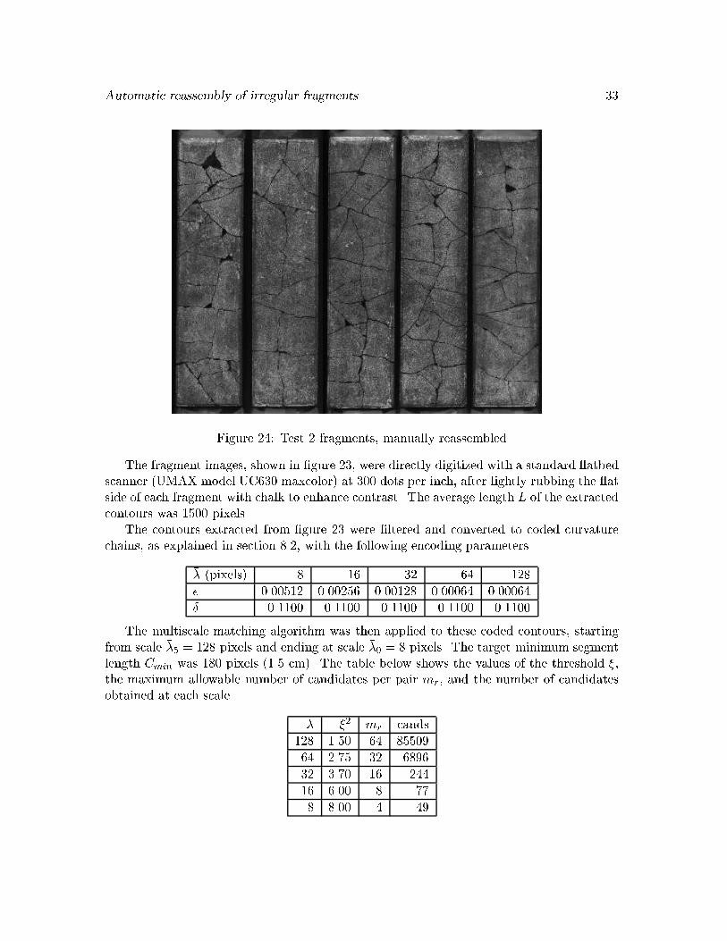
Automatic reassembly of irregular fragments 33

Figure 24: Test 2 fragments, manually reassembledThe fragment images, shown in �gure 23, were directly digitized with a standard atbedscanner (UMAX model UC630 maxcolor) at 300 dots per inch, after lightly rubbing the atside of each fragment with chalk to enhance contrast. The average length L of the extractedcontours was 1500 pixels.The contours extracted from �gure 23 were �ltered and converted to coded curvaturechains, as explained in section 8.2, with the following encoding parameters�� (pixels) 8 16 32 64 128� 0.00512 0.00256 0.00128 0.00064 0.00064� 0.1100 0.1100 0.1100 0.1100 0.1100The multiscale matching algorithm was then applied to these coded contours, startingfrom scale ��5 = 128 pixels and ending at scale ��0 = 8 pixels. The target minimum segmentlength Cmin was 180 pixels (1.5 cm). The table below shows the values of the threshold �,the maximum allowable number of candidates per pair mr, and the number of candidatesobtained at each scale. �� �2 mr cands128 1.50 64 8550964 2.75 32 689632 3.70 16 24416 6.00 8 778 8.00 4 49

Automatic reassembly of irregular fragments 34Figures 25 and 26 below show the 49 surviving candidates (�ltered at scale �� = 8:0pixels).?24

36

?20 37

?84

91 ?77 79

?67

96

?17

22

?20 40

?67 104

?25

40

?9

17?4 16

?2 13

?47 100

?14

21

?105 107?

3943

?76

91

?85

87

?81 82

?1

10?37 44

?82 99

?86

109

?81

102

?87

109

?18

36

?25

27

?89 106

?43

45

?74

78

147

?93

101

?3

5

?7 11

?26 46Figure 25: The best 35 candidates of the 49 returned by the multiscale matchingalgorithm. The stars (?) identify true candidates.

Automatic reassembly of irregular fragments 35?36

37

?7 8

?84

108

?93

100

?42

44

15

?18

27

?75

91

4 108

19

60

1

47

?67

8288

96

19 61

Figure 26: The next 14 of the 49 candidates returned by the multiscale matchingalgorithm. The stars (?) identify true candidates.There were 95 recognizable candidates longer than 1.5 cm in the input data. Since 42of the 49 returned candidates are among this set, the program achieved sensitivity � = 0:44and signi�cance = 0:86 on this test.10.3 ConclusionsThe experiments reported above, although modest size, have demonstrated the possibilitymechanically identifying adjacent fragments by matching their outlines. They also validatethe basic premise of the multiscale matching method, namely that the number of survivingcandidates decreases very quickly as they are re-tested with increasing resolutions.The computational cost of our multiscale matching program is still rather large (about2 hours for the 112 fragments of test 2). However, our implementation contains a numberof known ine�ciencies which can be removed with modest programming e�ort.

Automatic reassembly of irregular fragments 36References[1] N. Ayache and A. D. Faugeras. Hyper: A new approach for the recognition andpositioning of two-dimensional objects. Transactions on Pattern Analysis and MachineIntelligence, PAMI-8(1):44{54, 1986.[2] J. Babaud, A. Witkin, M. Baudin, and R. Duda. Uniquess of the Gaussian kernelfor scale-space �ltering. IEEE Transactions on Pattern Analysis and Machine Intelli-gence., 8(1):26{33, 1986.[3] Roger Bagnall. Advanced papyrological information system. File pa-pyrus/texts/APISgrant.html at http://scriptorium.lib.duke.edu/, 1994.[4] H. Bartels J. C. Beatty and B. A. Barsky. An Introduction to Splines for Use inComputer Graphics and Geometric Modeling. Morgan Kaufmann Publishers, 1987.[5] F. Bousso�ane and G. Bertrand. A new method for recognizing and locating objectsby searching longest paths. IEEE Transactions on Pattern Analysis and MachineIntelligence., 26(12):445{448, 1993.[6] Ronald N. Bracewell. The Fourier Transform and its Applications. McGraw-Hill, 1986.[7] Grigore C. Burdea and Haim J. Wolfson. Solving jigsaw puzzles by a robot. IEEETransactions on Robotics and Automation, 5(6):752{764, 1989.[8] Roland T. Chin and Charles R. Dyer. Model-based recognition in robot vision. ACMComputing Surveys, 18(1):67{108, 86.[9] Helena Cristina da Gama Leit~ao and Jorge Stol�. Comparing fracture lines. Technicalreport - in preparation, Institute of Computing(IC), University of Campinas, 1998.[10] Helena Cristina da Gama Leit~ao and Jorge Stol�. Geometric curve �ltering. Technicalreport - in preparation, Institute of Computing(IC), University of Campinas, 1998.[11] Alan D. Kalvin et al. Using visualization in the archaeological excavations of a pre-Incatemple in Peru. Report RC 20518, IBM T. J. Watson Research Center,, 1996.[12] K. Falconer. Fractal Geometry : Mathematical Foundations and Applications. JohnWiley & Sons, 1990.[13] K. T. Glowacki. Franchthi excavations: 17,000 years of Greek prehistory. Dept.of Classical Studies, Indiana University, Bloomington. http://www.indiana.edu/ ar-chaeol/franchthi/franchthi.html, 1990.[14] Multimedia Hochfeiler. Gli archivi di Ebla. http://www.sysin.it/ipertest/archi.htm,1997.[15] Alan Kalvin, Edith Schonberg, Jacob T. Schwartz, and Micha Sharir. Two-dimensional,model-based, boundary matching using footprints. The International Journal ofRobotics Research, 5(4):38{55, 1986.

Automatic reassembly of irregular fragments 37[16] Joan Keller. The glass from Sepphoris: A preliminary report.http://www.colby.edu/rel/Glass.html, 1995.[17] Raymond Legault and Ching Y. Suen. Optimal local weighted averaging methods incontour smoothing. IEEE Transactions on Pattern Analysis and Machine Intelligence.,19(8):801{817, 1997.[18] James W. McKee and J. K. Aggarwal. Computer recognition of partial views of curvedobjects. IEEE Transactions on Computers, c26(8):790{800, 1977.[19] Jo~ao Meidanis and Jo~ao Carlos Setubal. Introduction to Computational MolecularBiology. PWS, 1997.[20] Farzin Mokhtarian and Alan Mackworth. Scale-based description and recognition ofplanar curves and two-dimension shapes. IEEE Transactions on Pattern Analysis andMachine Intelligence., 8(1):34{43, 1986.[21] Farzin Mokhtarian and Alan K. Mackworth. A theory of multiscale, curvature-basedshape representation for planar curves. IEEE Transactions on Pattern Analysis andMachine Intelligence., 14(8):789{805, 1992.[22] Arthur R. Pope. Model based object recognition: A survey of recent research. TechnicalReport TR-94-04, Berkeley University, California, 1994.[23] Azriel Rosenfeld and Avinash C. Kac. Digital Picture Processing. Academic Press,1982.[24] Paul Rosin and Svetha Venkatesh. Extracting natural scales using the Fourier descrip-tion. Pattern Recogniton, 26(9):1383{1393, 1993.[25] B. Sandak, R. Nussinov, and Haim J. Wolfson. An automated computer vision androbotics based technique for 3-d exible biomolecular docking and matching. ComputerApplications in the Biosciences, 11(1):87, 95.[26] Behzad Shahraray and David J. Anderson. Optimal estimation of contour propertiesby cross-valided regularization. IEEE Transactions on Pattern Analysis and MachineIntelligence., 8(6):600{610, 1989.[27] Fred J. Taylor. Digital Filter Design Handbook (Eletrical Engineering and Eletronics18). Marcel Dekker, 1983.[28] G�okt�urk �U�coluk and I. Hakki Toroslu. Reconstruction of 3-d surface object from itspieces. In The Ninth Canadian Conference on Computational Geometry - Queen'sUniversity, Kingston, Ontario, CANADA, August 11-14, volume 1, 1997.[29] R. Vergnieux. Le fac-simil�e �electronique ou les restitutions virtuelles, - Xe CNRSTable Ronde de Informatique et �Egyptologie, Bordeaux. http://silicon.Montaigne.u-bordeaux.fr/8001/HTML/ONLINE/IE10/Robert.html, 1994.

Automatic reassembly of irregular fragments 38[30] Andrew P. Witkin. Scale-space �ltering. In Proc. IJCAI Eighth Proc. InternationalJoint Conference on Arti�cial Intelligence - Karlsruhe - Germany, pages 1019{1021,1983.[31] Haim J. Wolfson. On curve matching. IEEE Transactions on Pattern Analysis andMachine Intelligence., 12(5):483{488, 1990.[32] Daniel M. Wuescher and Kim L. Boyer. Robust contour decomposition using a constantcurvature criterion. IEEE Transactions on Pattern Analysis and Machine Intelligence.,13(1):41{51, 1991.