Flows associated with irregular R d —vector fields

J. Differential Equations 219 (2005) 183 – 201

www.elsevier.com/locate/jde

Flows associated with irregularRd—vector fields�

Fernanda Ciprianoa, Ana Bela Cruzeirob,∗aGrupo de Física-Matemática, Dep. de Matemática FCT-UNL, Av. Prof. Gama Pinto 2,

1649-003 Lisboa, PortugalbGrupo de Física-Matemática, Dep. de Matemática IST., Av. Rovisco Pais, 1049-001 Lisboa, Portugal

Received 9 August 2004; revised 4 February 2005

Available online 5 April 2005

Abstract

This work consists on the study of flows associated with non-smoothRd—vector fields,namely concerning existence and uniqueness for almost—every initial condition. It is alsoproved that the flows avoid some special compact sets.© 2005 Elsevier Inc. All rights reserved.

Keywords:Ordinary differential equations; Non-smooth vector fields

1. Introduction

We consider in this work ordinary differential equations onRd associated to non-smooth vector fields. Instead we assume that the vector fields together with their gradi-ent (in the distributions sense) and the exponential of the divergence satisfyLp(�)-typehypothesis. Here, the measure� denotes the standard Gaussian measure onRd .

Such problems have been studied, in particular, by Di Perna and Lyons[DiP-L].Because motivations come largely from Fluid Mechanics, the divergence (with respectto Lebesgue measure) of the vector field was first assumed to be zero, but the techniqueshave been subsequently generalized, for instance in [D]. These results rely on the

� This work was partially sponsored by the project Functional Integration and Applications(POCTI/MAT/55977/2004).

∗ Corresponding author. Fax: +351217954288.E-mail addresses:[email protected](F. Cipriano), [email protected](A.B. Cruzeiro).

0022-0396/$ - see front matter © 2005 Elsevier Inc. All rights reserved.doi:10.1016/j.jde.2005.02.015

http://www.elsevier.com/locate/jde

mailto:[email protected]

mailto:[email protected]

184 F. Cipriano, A.B. Cruzeiro / J. Differential Equations 219 (2005) 183–201

analysis of the associated (partial differential) transport equations,�u�t = B · ∇u, where

B is the vector field.On the other hand, the divergence accounts for the infinitesimal action of the flow

on the measure space, and therefore, under suitable integrability conditions, can beintegrated in order to obtain the density of the flow. These arguments were used in[C], in order to prove non-explosion of solutions of ordinary differential equations,almost - everywhere with respect to the initial conditions.

In this work, we use partly the techniques of DiPerna and Lions [DiP-L] based onthe study of the transport equations and partly the more probabilistic arguments basedon the study of the action of the flow on the Gaussian measure. We obtain existenceand uniqueness of solutions as well as an expression for their density (a.e.) continuityof the trajectories and the flow property.

Finally, in the last paragraph, we generalize for our flows the non-avoidance of setsproperty discussed in [A].

2. Notations and main results

Let � be the Gaussian measure onRd ,

d�(x) = (2�)−d2 e− 1

2 |x|2dx. (2.1)

We shall denote byW �,p(�) the Sobolev spaces with respect to the Gaussian measure�, namely

W �,p(�) ={� :

∫Rd

|�|p d� < +∞,∫

Rd|�k�|p d� < +∞ for |k|��

},

wherek = (k1, . . . , kd), |k| = k1 +· · ·+ kd , the partial derivatives�k� = �|k|��xk11 ···�xkdd

are

defined in the distribution sense and byW �,p(dx) the Sobolev spaces with respect tothe Lebesgue measuredx. Analogous notationsLp(�), Lp(dx) will be considered withrespect to integrability. We shall also consider

W�,ploc (�) =

{� :

∫K

|�|p d� < +∞,∫K

|�k�|p d� < +∞, |k|��,

∀ compactK ⊂ Rd}.

We represent by�� the divergence operator associated with the measure�. This operatorcorresponds to the adjoint of the gradient inL2(�). Given a vector fieldB on Rd , ��B

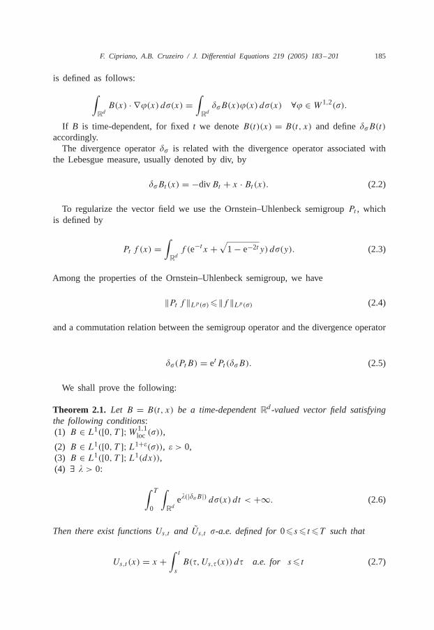
F. Cipriano, A.B. Cruzeiro / J. Differential Equations 219 (2005) 183–201 185

is defined as follows:

∫RdB(x) · ∇�(x) d�(x) =

∫Rd

��B(x)�(x) d�(x) ∀� ∈ W1,2(�).

If B is time-dependent, for fixedt we denoteB(t)(x) = B(t, x) and define��B(t)

accordingly.The divergence operator�� is related with the divergence operator associated with

the Lebesgue measure, usually denoted by div, by

��Bt(x) = −divBt + x · Bt(x). (2.2)

To regularize the vector field we use the Ornstein–Uhlenbeck semigroupPt , whichis defined by

Pt f (x) =∫

Rdf (e−t x +

√1 − e−2t y) d�(y). (2.3)

Among the properties of the Ornstein–Uhlenbeck semigroup, we have

‖Pt f ‖Lp(�)�‖f ‖Lp(�) (2.4)

and a commutation relation between the semigroup operator and the divergence operator

��(PtB) = etPt (��B). (2.5)

We shall prove the following:

Theorem 2.1. Let B = B(t, x) be a time-dependentRd -valued vector field satisfyingthe following conditions:(1) B ∈ L1([0, T ];W1,1

loc (�)),

(2) B ∈ L1([0, T ];L1+�(�)), � > 0,(3) B ∈ L1([0, T ];L1(dx)),(4) ∃ � > 0:

∫ T0

∫Rd

e�(|��B|) d�(x) dt < +∞. (2.6)

Then there exist functionsUs,t and Us,t �-a.e. defined for0�s� t�T such that

Us,t (x) = x +∫ ts

B(�, Us,�(x)) d� a.e. for s� t (2.7)


and

Us,t (x) = x −∫ ts

B(�, U�,t (x)) d� a.e. for s� t. (2.8)

The trajectoriest → Us,t defined on[s, T ] and t → Us,t defined on[0, t] are a.e.continuous.Moreover, if we denoteKs,t = d(Us,t )∗�/d� and Ks,t = d(Us,t )∗�/d�, we have

Ks,t = exp

(∫ ts

��Br(Ur,t ) dr

)(2.9)

and

Ks,t = exp

(−∫ ts

��Br(Us,r ) dr

). (2.10)

We also have the flow property, more precisely

Us,t = U�,t ◦ Us,� a.e., (2.11)

Us,t = Us,� ◦ U�,t a.e. (2.12)

for 0�s�� t�T . The flowUs,� is the inverse ofUs,t , in the sense that

Us,t ◦ Us,t (x) = Us,t ◦ Us,t (x) = x a.e. (2.13)

for 0�s� t�T . The flow satisfying these properties is(a.e.) unique.

The following result can also be established:

Theorem 2.2. Let B = B(t, x) be a time-dependentRd -valued vector field satisfyingthe following conditions:(1) B ∈ L1([0, T ];W1,1

loc (�));(2) ∃ � > 0:

∫ T0

∫Rd

e�(|��B|+|B|) d�(x) dt < +∞. (2.14)

Then there exist functionsUs,t and Us,t a.e. defined for0�s� t�T which satisfies allproperties of the Theorem2.1.


3. The existence of the flow (Theorem 2.1)

We first regularize the vector fieldB. Let � be a smooth positive function onRwith compact support and such that

∫R �(x) dx = 1. We consider�n(t) = n�(nt) and

B(n)(t, x) = (B(·, x) ∗ �n(·))(t). We define

Bn(t, x) = P 1n

B(n)(t, x). (3.1)

It follows from the properties of the semigroupPt that the vector fieldBn is smooth,therefore it defines a smooth local flow

Uns,t (x) = x +∫ ts

Bn(�, Uns,�(x)) d� ∀x ∈ Rd . (3.2)

We first consider the assumptions of Theorem2.1. Since

‖Bn‖L∞([0,T ]×Rd )�‖B‖L1([0,T ];L1(dx)), (3.3)

the flow is defined for allt ∈ [s, T ].For everys� t , the mapUns,t (·) is a diffeomorphism onRd and the inverseUns,t (·)

satisfies

Uns,t (x) = x −∫ ts

Bn(�, Un�,t (x)) d� ∀x ∈ Rd . (3.4)

The flow property

Uns,t (x) = Un�,t ◦ Uns,�(x), s�� t, (3.5)

Uns,t (x) = Uns,� ◦ Un�,t (x), s�� t (3.6)

holds for all x ∈ Rd .The measures(Uns,t )∗� and (Uns,t )∗� are absolutely continuous with respect to the

Gaussian measure� and the density functions, denoted byKns,t and Kns,t respectively,can be written as

Kns,t (x) = exp

(∫ ts

��Bnr (U

nr,t ) dr

)(3.7)

and

Kns,t (x) = exp

(−∫ ts

��Bnr (U

ns,r ) dr

). (3.8)


In order to prove the existence of the flow in Theorem2.1, we follow the method ofDiPerna and Lions [DiP-L]. We consider the forward and backward transport equationswhich correspond respectively to

�

�tu− B · ∇u = 0 (3.9)

with an initial condition and

�

�tu+ B · ∇u = 0 (3.10)

with a final condition.In fact it is enough to consider just one of these equations, since their solutions are

related by change of variables.Differentiating equality (3.5) with respect to the variables at � = s, we can verify

that U(s, x) = Uns,t (x) solves the vectorial backward transport equation (3.10), whereB is replaced byBn, with final conditionU(t, x) = Unt,t (x) = x.

We start with a result concerning the uniform estimation of theLp(�) norms of thedensity functions.

Lemma 3.1. Under the assumptions of Theorem1.1 and for t − s small enough thereexists a constant C which depends only on p and on the value of the integral in(2.6)such that‖Kns,t‖Lp(�)�C.

Proof. Using the expression (3.7) (cf. [C,U-Z]), we have

∫Rd

|Kns,t (x)|p d�(x)�et−sp�

q�

∫Rd

∫ ts

ep[(t−s)∨�]��Bnr (x) dr d�(x) (3.11)

with 0�s� t , � > 0, 1p

+ 1q

= 1. If � = �pe and t − s < �, we obtain

∫Rd

|Kns,t (x)|p d�(x)�c(�, p)∫

Rd

∫ T0

e�e |��B

nr (x)| dr d�(x). (3.12)

From properties (2.4) and (2.5) of the Ornstein–Uhlenbeck semigroup we have

∫Rd

e�e |��B

nr (x)| d�(x) =

∑k

�k

ekk!∫

Rd|��B

nr (x)|k d�(x)

�∑k

�k

k!∫

Rd|��B

(n)r (x)|k d�(x)

=∫

Rde�|��B

(n)r (x)| d�(x).


Since

∫ T0

∫Rd

e�|��B(n)r (x)| d�(x) dr�

∫ T0

∫Rd

e�|��Br(x)| d�(x) dr + T ,

the result follows. �

In the next two results we study the solutions of the transport equations, these solu-tions being considered in the distribution sense with respect to the Gaussian measure�. Analogous results were established in[DiP-L] in the context of the Lebesgue mea-sure. In particular, the first lemma enables us to approximate anyL1([0, T ];L∞(�))solution of the transport equation by smooth solutions of approximate equations, un-der the regularity assumptionL1([0, T ];W1,1

loc (�)) for the vector fieldB. We regularizethe solutionu of the transport equation, as in [DiP-L], by convolution with� where�(x) = 1

�N ( x� ), is C∞ with compact support and∫

Rd dx = 1.

Lemma 3.2. Let B ∈ L1([0, T ];W1,�loc (�)) and let u ∈ L∞([0, T ];Lploc(�)) be a solu-

tion in the distributions sense of Eq.(3.9).Then, the functionun defined byun = u∗ 1n

satisfies the following partial differential equation:

�

�tun(t, x) = B(t, x) · ∇un(t, x)+ rn(t, x), t > s,

un(s, x) = us(x) ∀ x ∈ Rd ,

(3.13)

where rn → 0 in L1([0, T ];Lloc(�)) with

1� + 1

p= 1

.

Proof. Since B ∈ L1([0, T ];W1,�loc (�)) and u ∈ L∞([0, T ];Lploc(�)), we haveB ∈

L1([0, T ];W1,�loc (dx)) and u ∈ L1([0, T ];Lploc(dx)) and we can apply the result of

DiPerna and Lions[DiP-L]. �

As a consequence of this result, for every function in C1(R) with bounded deriva-tive ′, (un) satisfies

�(un)

�t− B · ∇(un) = rn′(un). (3.14)

Taking the limit asn→ ∞ we obtain

�(u)

�t− B · ∇(u) = 0. (3.15)


Lemma 3.3. Let B satisfy assumptions(1), (2) and (4) of the Theorem2.1. For Tsmall enough, Eq. (3.9) with initial condition u0(s) has at most one solution inL∞([0, T ];L∞(�))).

Proof. Let u1 andu2 be bounded solutions in distributions sense of Eq. (3.9) with thesame initial conditionu0(s). We consideru = u1 − u2. Since the equation is linear,u is also a solution of (3.9) with initial conditionu(s) = 0. Let M > 0 and consider(�) = |�| ∧M. Approximating by functions inC1(R) we obtain

�(u)

�t= B · ∇(u). (3.16)

Let � be a positive smooth function defined onRd such that�(x) = 1, if |x|�1and �(x) = 0, if |x| > 2. For N > 1, we consider the functions�N(x) = �( x

N).

Multiplying the equation by�N and integrating with respect to the measure� weobtain

�

�t

∫Rd

(u)�N d� =∫

RdB(t) · ∇(u)�N d�

= −∫

Rd(u)��(B · �N) d�

= −∫

Rd(u)�N��B(t) d� + 1

N

∫Rd

(u)B · ∇� d�.

We have

1

N

∫Rd

(u)B · ∇� d�� CN

∫N� |x|�2N

|B| d�.

From the hypothesis (2) of Theorem2.1, this integral converges to zero asN → ∞.Taking the limit whenN → ∞ we obtain

�

�t

∫Rd

(u) d� = −∫

Rd(u)��B(t) d�. (3.17)

Let �k(t) be the subset ofRd where |��B(t)| < K.We have

�

�t

∫Rd

(u) d� �∫

�k(t)(u)|��B(t)| d� +

∫�ck(t)

(u)|��B(t)| d�

� K

∫Rd

(u) d� +∫

�ck(t)(u)|��B(t)| d�


that implies

∫Rd

(u) d��∫ ts

(K

∫Rd

(u) d�

)d� +

∫ Ts

∫�ck(�)

(u)|��B| d� d�.

Using Gronwall’s inequality, we deduce

∫Rd

(u)d��e(t−s)K(∫ Ts

∫�ck(�)

(u)|��B(�)| d� d�).

We have

�(�ck(t)) = �({x : |��B(t)| > K})= �({x : e�|��B(t)| > e�K})

� e−�K∫

Rde�|��B(t)| d�.

Using the assumption (2.6) we obtain

∫ Ts

�(�ck(�))�Ce−�K,

whereC is a constant.Therefore

∫ Ts

∫�ck(�)

(u)|��B(�)| d� d� �(∫ Ts

∫Rd

|��B(�)|2 d�d�)1

2(∫ Ts

�(�ck(�)) d�

)12

� Ce−�K2 .

If we considert − s small enough, the result follows taking the limit inK whenK → ∞. �

In the following, given a sequence�n of functions defined on some measurable space(X, ) with values in a Banach spaceM (endowed with the norm‖ · ‖), we say that�n converges to� in L0( ;M) if for all � > 0, {‖�n − �‖ > �} → 0.

Lemma 3.4. Let B satisfy the assumptions of the Theorem1.1. For s, t ∈ (0, T ) witht − s small enough, let us denote by dt the Lebesgue measure on the interval[s, t].


We have(a) The sequenceUns,r (·) converges inL0(�; Rd).(b) The sequenceUns,·(·) converges inL0(dt × �; Rd) (the limit will be denoted byUs,t ).

Proof. Let be a continuous and bounded function onR. Denote byUn(i)s,t the i-

component ofUns,t . The sequencesvin = (Un(i)s,t ) and win = 2(Un(i)s,t ) are bounded

sequences onL∞([0, T ] × [0, T ];L∞(Rd)), so there exists subsequences which con-verge inL∞((0, T )2 × Rd) - * to vi andwi , respectively. The functionsvi andwi arebounded solutions of the transport equation with initial conditions(xi) and2(xi), re-spectively. On the other hand, as written after Lemma3.2 the function(vi)2 also satisfiesthe transport equation with initial condition2(xi). From the uniqueness result,wi =(vi)2. Therefore, up to a subsequence,(vin)

2 converges to(vi)2 in L∞((0, T )2 × Rd) -* which implies vin → vi in L2((0, T )2 × Rd) (andL2([0, T ] × [0, T ];L2

loc(�))), con-

sequently we have convergence in measuredt×� (and�). Since(Un(i)s,t ) converges in

measure to some functionv, and with the above regularity is arbitrary,Un(i)s,· (·) shouldconverge in measuredt × � to some functionU(i)s,· (·) (andUn(i)s,t (·) should converge in

measure� to some functionU(i)s,t (·) and v(·, ·) = (U(i)s,· (·)). �

The measurable functionUs,t keeps the measure� quasi-invariant.

Lemma 3.5. Let Us,t be the function defined in above lemma withs, t ∈ (0, T ) andlet T be small enough. The measure(Us,t )∗� is absolutely continuous with respect tothe measure�, and the corresponding densityKs,t belongs inLp(�) for all p > 1.

Proof. SinceUns,t converges toUs,t in measure, for every functionf continuous withcompact support

∫Rdf (Uns,t ) d� →

∫Rdf (Us,t ) d�. (3.18)

On the other hand, by Lemma3.1, there exists a subsequenceKnks,t of Kns,t whichconverges weakly inLp(�) to some functionKs,t . Therefore

∫Rdf (U

nks,t ) d� =

∫Rdf (x)K

nks,t (x) d� (3.19)

converges to

∫Rdf (x)Ks,t (x) d� (3.20)

and the result follows. �


The next convergence result will be useful to pass to the limit the integral equationand to deduce some properties forUs,t (x) from the corresponding one forUns,t (x) (cf.[U-Z]).

Lemma 3.6.We consider the hypothesis of Theorem2.1. Let M be any Banach spaceand F any M-valued random variable. LetF1 be a Rd -valued random variable ands < t < T with t − s small enough. Then we have

(i) F (Uns,t (·))→ F(Us,t (·)) in L0(�;M)(ii ) F1(·, Uns,·(·))→ F1(·, Us,·(·)) in L0(dt × �; Rd),

where dt is the Lebesgue measure on[s, t].

Proof. We prove the first statement. The proof of the second one is similar.Let us suppose thatF ∈ L∞(�) and denote by‖ · ‖ the norm onM. From Lemma

3.4 Uns,t converges toUs,t in measure-�. If necessary, by taking a subsequence, we canconsider thatUns,t converges toUs,t �-a.e.

For all � > 0 there existsK� ⊂ Rd such that�(Kc� ) < � and F |K� is uniformlycontinuous. Fixeds, t,

∫Rd

‖F(Uns,t )− F(Us,t )‖ =∫

{Uns,t ,Us,t∈K�}‖F(Uns,t )− F(Us,t )‖

+∫

Rd−{Uns,t ,Us,t∈K�}‖F(Uns,t )− F(Us,t )‖ = I1(n)+ I2(n).

By continuity, given� > 0 there exists a constantc such that

I1(n) =∫

{Uns,t ,Us,t∈K�|Uns,t−Us,t |<c}‖F(Uns,t )− F(Us,t )‖

+∫

{Uns,t ,Us,t∈K�|Uns,t−Us,t |>c}‖F(Uns,t )− F(Us,t )‖

� � +(∫

Rd‖F(Uns,t )− F(Us,t )‖2

)12(�{|Uns,t − Us,t | > c})

12 ,

I2(n) =∫

{Uns,t∈K�,Us,t∈Kc� }‖F(Uns,t )− F(Us,t )‖

+∫

{Uns,t∈Kc� ,Us,t∈K�}‖F(Uns,t )− F(Us,t )‖


+∫

{Uns,t∈Kc� ,Us,t∈Kc� }‖F(Uns,t )− F(Us,t )‖ = I2,1(n)+ I2,2(n)+ I2,3(n),

I2,1(n) � C1

(∫Rd

‖F(Uns,t )− F(Us,t )‖2)1

2(�(Kc� ))

12 ,

whereC1 is a constant.The analysis ofI2,2(n), I2,3(n) are similar toI2,1(n). If F is not in L∞, we can

considerFa ∈ L∞, such that lima→0 Fa(x) = F(x), �- a.e-x. Then

�{‖F(Uns,t )− F(Us,t )‖ > c} � �{‖F(Uns,t )− Fa(Uns,t )‖ >

c

3

}

+ {‖Fa(Uns,t )− Fa(Us,t )‖ >

c

3

}

+ {‖Fa(Us,t )− F(Us,t )‖ > c

3

}.

Using the uniform integrability of the densities we obtain the result.�

Therefore, considering the limit in measure of the integral equation asn goes to∞,we obtain

Lemma 3.7. Under the assumptions of the Theorem2.1, the mapUs,t (x) satisfies theintegral equation

Us,t (x) = x +∫ ts

B(�, Us,�(x)) d� � − a.e. (3.21)

with 0�s < t and t − s small.

Proof. We have

∫Rd

∫ ts

|Bn(�, Uns,�(x))− B(�, Us,�(x))| ds d�(x)

�∫

Rd

∫ ts

|Bn(�, Uns,�(x))− B(�, Uns,�(x))| ds d�(x)

+∫

Rd

∫ ts

|B(�, Uns,�(x))− B(�, Us,�(x))| ds d�(x)

�∫ ts

∫Rd

|Bn(�, x)− B(�, x)|kns,� ds d�(x)

+∫st

∫Rd

|B(�, Uns,�(x))− B(�, Us,�(x))| ds d�(x).


By Lemma 3.1 and sinceBn converges toB in L1([0, T ];L1+�(�)) we deduce

∫ ts

∫Rd

|Bn(�, x)− B(�, x)|kns,� ds�C∫ T

0

(∫Rd

|Bn(�, x)− B(�, x)|1+�) 1

1+�d�.

Taking F1 = B in Lemma 3.6 we obtain

B(�, Uns,�(x))→ B(�, Us,�(x))

with respect to the measuredt×�. Therefore there exists a subsequence which convergesa.e.-dt × �. Moreover

∫[s,t]×Rd

|B(�, Uns,�(x))|p d�(x) dt (�) �(∫

[s,t]×Rd|B(�, x)|p2

d�(x) dt (�)

) 1p

×(∫

[s,t]×RdKqs,� d�(x) dt (�)

) 1q

with 1p

+ 1q

= 1 and 1< p, p2 < 1 + �. Therefore

supn

∫[s,t]×Rd

|B(�, Uns,�(x))|p d�(x) dt (�) <∞

andB(·, Uns,·(·)) is absolutely integrable with respect todt×�. Using the same notationfor the subsequence, we obtain

∫[s,t]×Rd

|B(�, Uns,�(x))− B(�, Us,�(x))| ds → 0

therefore

∫ ts

Bn(�, Uns,�)) ds →∫ ts

B(�, Us,�)) ds in L1(�). � (3.22)

Given T > 0, we need some result in order to define the flowUs,t on the wholeinterval [0, T ].

Lemma 3.8. Suppose0� t < ��T such that

∫ �

t

|Bn(r, Unt,r )− Bm(r, Umt,r )| dr → 0 in measure�. (3.23)


If 0�s < t where t − s is small, then

∫ �

s

|Bn(r, Unt,r )− Bm(r, Umt,r )| dr → 0 in measure�.

Proof.

∫ �

s

Bn(r, Uns,r ) dr =∫ ts

Bn(r, Uns,r ) dr +∫ �

t

Bn(r, Uns,r ) dr. (3.24)

Using the semigroup property for the regular flowUns,t , we have

∫ �

t

Bn(r, Uns,r ) dr =∫ �

t

Bn(r, Unt,r (Uns,t )) dr.

The convergence of the first term in the second member of (3.24) follows from (3.22).To prove the convergence of the second term, we consider the functionGn(x)(r) =�[s,�](r)Bn(r, Unt,r (x). By (3.23)Gn converges toG in L0(�;L1([t, �]; Rd)). If we nowapply Lemma 3.6 and use the uniform integrability of the densities we conclude thatGn ◦ Unt,r converges toG ◦ Ut,r in L0(�;L1([t, �]; Rd)) which is equivalent to write

∫ �

t

|Bn(r, Unt,r (Uns,t ))− B(r, Ut,r (Us,t ))| dr

converges to zero in measure�. �

Using Lemma3.8 a finite number of times, we obtain a subsequenceUnks,t such that

∫ Ts

|Bnk (r, Unks,r )− Bnl (r, Unls,r )| dr (3.25)

converges to zero in measure� as k, l → ∞.We can now complete the proof of Theorem2.1. We will omit the proof of the

existence ofUs,t and their properties because we just need to repeat the argumentsused forUs,t .

We remark that (3.25) implies

supr∈[s,T ]

|Unks,r − Unls,r | → 0 (3.26)

in measure�, soUs,t is �-a.e. defined for allt ∈ [s, T ], and is also continuous on theinterval [s, T ].


From Lemmas3.6–3.8 we conclude that for 0�s < t�T there existsUs,t , defined�-a.e. such that

Us,t (x) = x +∫ ts

B(�, Us,�(x)) d� for s� t�T . (3.27)

Now we prove thatUs,t verifies the flow property (2.11). By Lemma 3.8

Un�,t (Uns,�) = Uns,t → Us,t

in measure and

|Un�,t (Uns,�)− U�,t (Us,�)|� |Un�,t (Uns,�)− U�,t (Uns,�)| + |U�,t (U

ns,�)− U�,t (Us,�)|.

If we consider� − s small, from the uniform integrability of the density functions

|Un�,t (Uns,�)− U�,t (Uns,�)|

converges to zero in measure�. Applying Lemma3.6 with F1 = U�,t , we also have|U�,t (U

ns,�) − U�,t (Us,�)| → 0 in measure�. If � − s is not small there existsm ∈ N

and r small such that� = s +mr,

U�,t ◦ Us,� = U�,t ◦ (Us+r,� ◦ Us,s+r )= U�,t ◦ (Us+2r,� ◦ Us+r,s+2r ◦ Us,s+r )= . . .= U�,t ◦ (Us+(m−1)r,� ◦ Us+(m−2)r,s+(m−1)r ◦ · · · ◦ Us+r,s+2r ◦ Us,s+r )= (U�,t ◦ Us+(m−1)r,�) ◦ Us+(m−2)r,s+(m−1)r ◦ · · · ◦ Us+r,s+2r ◦ Us,s+r= Us+(m−1)r,t ◦ Us+(m−2)r,s+(m−1)r ◦ · · · ◦ Us+r,s+2r ◦ Us,s+r= . . .= (Us+2r,t ◦ Us+r,s+2r ) ◦ Us,s+r= Us+r,t ◦ Us,s+r= Us,t .

The laws of the random variablesUs,t are absolutely continuous with respect to�,the density functionsKs,t being given by the expressions

Ks,t = exp

(∫ ts

��Br(Ur,t ) dr

). (3.28)


In fact, from 3.6 it follows that there exists a subsequence of��Bnr (U

nr,t ) which con-

verges to��Br(Ur,t ) in L0(dt × �; Rd). Since��Bnr (U

nr,t ) is uniformly integrable we

have a subsequence which converges inL1(dt × �; Rd). Therefore there exists a sub-sequence of

∫ ts

��Bnr (U

nr,t ) dr which converges to

∫ ts

��Br(Ur,t ) dr in L0(�; Rd). Sincethe sequenceKns,t is uniformly integrable, we deduce thatKns,t converges toKs,t =exp(

∫ ts

��Br(Ur,t ) dr) in L1(�).The next paragraph completes the proof of the Theorem 2.1.

4. Uniqueness of the flow

To prove that the flow associated with the vector fieldB is unique, we follow thestrategy of DiPerna and Lions [DiP-L]. Letu0 be an arbitrary function inC∞(Rd)with compact support. Let us definev(s, x) = u0(Us,t (x)), s < t . We shall prove thatv(s, x) is solution in the distributions sense of Eq. (3.10) with final conditionu0(x).

Lemma 4.1. The functionv(s, x) is solution in distributions sense of the partial dif-ferential equation(3.10).

Proof. We consider

�h(s) =∫

Rd

1

h[v(s + h, x)− v(s, x)]�(x) d�(x)

=∫

Rd

1

h[u0(Us+h,t (x)− u0(Us,t (x)]�(x) d�(x)

for every � in C∞(Rd) with compact support.Using the flow property and knowing thatd(Us,t )∗� = Ks,t d� with Ks,t given by

(2.10) we have

�h(s) =∫

Rd

1

hu0(Us,t (x))[�(Us,s+h(x))Ks,s+h − �(x)] d�(x).

Since

�

�h[�(Us,s+h(x))Ks,s+h] = ∇�(Us,s+h(x))B(s + h,Us,s+h(x))Ks,s+h(x)

−�(Us,s+h(x))(��Bs+h)(Us,s+h(x))

×exp

(−∫ s+hs

(��Br)(Us,r (x)) dr

),


we have

�h(s) =∫

Rd

1

hu0(Us,t (x))

∫ h0

[∇�(Us,s+�(x))B(s + �, Us,s+�(x))Ks,s+�(x)

−�(Us,s+�(x))(��Bs+�)(Us,s+�(x))

× exp

(−∫ s+�

t


)]d� d�(x)

=∫ h

0

∫Rd

1

hu0(Us,t (x))[∇�(Us,s+�(x))B(s + �, Us,s+�(x))Ks,s+�(x)] d�(x) d�

−∫

Rdu0(Us,t (x))

1

h

∫ h0

[�(Us,s+�(x))(��Bs+�)(Us,s+�(x))

× exp

(−∫ s+�

s


)]d� d�(x).

The first integral converges to

∫Rd

∇�(x)u0(Us,t (x))B(s, x) d�(x)

when h goes to zero. The second integral converges to

∫Rd

�(x)u0(Us,t (x))(��Bs)(x) d�(x).

Using integration by parts, we obtain

�h(s)→ −∫

Rd�(x)v(s, x) · ∇B(s, x) d�(x) when h→ 0.

Using Lemma3.3 and the arbitrariness ofu0 the result follows. �

Remark (Concerning Theorem 1.2). (1) To prove Theorem 2.2, we begin with theregularization of the vector field made in (3.1). The assumptions of Theorem 2.2 implyall the assumptions of Theorem 2.1 except (3). This one was used just in (3.3) toassure the non-explosion ofUns,t on the interval[s, T ]. In the case of Theorem 2.2,the vector fieldBn satisfies the assumptions of Theorem 3.1 in [C], and that theoremassures that the flowUns,t is defined fors� t�T . Apart for the non-explosion all theresults of Theorem 2.2 are proved in the same way.


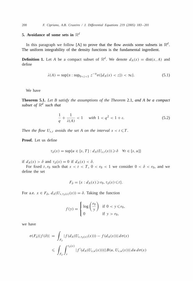
5. Avoidance of some sets inRd

In this paragraph we follow[A] to prove that the flow avoids some subsets inRd .The uniform integrability of the density functions is the fundamental ingredient.

Definition 1. Let A be a compact subset ofRd . We denotedA(x) = dist(x,A) anddefine

�(A) = sup{� : sup0<z<1 z−��({dA(x) < z}) <∞}. (5.1)

We have

Theorem 5.1. Let B satisfy the assumptions of the Theorem2.1, and A be a compactsubset ofRd such that

1

q+ 1

�(A)< 1 with 1< q2 < 1 + �. (5.2)

Then the flowUs,t avoids the set A on the intervals < t�T .

Proof. Let us define

��(x) = sup{u ∈ [s, T ] : dA(Us,t (x))�� ∀t ∈ [s, u]}

if dA(x) > � and ��(x) = 0 if dA(x) < �.For fixed t, r0 such thats < t < T , 0 < r0 < 1 we consider 0< � < r0, and we

define the set

F� = {x : dA(x)�r0, ��(x)� t}.

For a.e.x ∈ F�, dA(Us,��(x)(x)) = �. Taking the function

f (y) = log

(r0

y

)if 0 < y�r0,

0 if y > r0,

we have

�(F�)|f (�)| =∫F�

|f (dA(Us,��(x)(x)))− f (dA(x))| d�(x)

�∫F�

∫ ��(x)

s

|f ′(dA(Us,u(x)))||B(u,Us,u(x))| du d�(x)


�∫ ts

∫Rd

|f ′(dA(x))||B(u, x)|Ks,u(x) du d�(x)

=∫ ts

∫dA(x)� r0

1

dA(x)|B(u, x)|Ks,u(x) du d�(x)

�∫ Ts

(∫dA(x)� r0

(1

dA(x)

)pd�

) 1p(∫

Rd|B(u, x)|q2

d�(x)

) 1q2

× sups<u�T

‖Ks,u‖Lpq(�),

where 1q

+ 1p

= 1. Therefore

�(F�) �(

log( r0

�

))−1(∫dA(x)� r0

(1

dA(x)

)pd�

) 1p

×‖B(u, x)‖Lq

2(�) sups<u�T

‖Ks,u‖Lqp(�). (5.3)

Since�(A) defined in (5.1) satisfies (5.2),p��(A).Now, under the assumptions of the theorem,

(∫dA(x)� r0

(1

dA(x)

)pd�

) 1p

is finite. (cf. [A] for the proof of this property). Taking the limit in (5.3) as� → 0,we deduce that�(F�)→ 0, which implies that�(

⋂0<�<r0 F�) = 0. Sincet and r0 are

arbitrary this proves the theorem.�

References

[A] M. Aizenman, A sufficient condition for the avoidance of sets by measure preserving flows inRN , Duke Math. J. 45 (4) (1978) 809–812.

[C] A.B. Cruzeiro, Équation différentielles ordinaires: non-explosion et mesures quasi-invariantes, J.Funct. Anal. 54 (1983) 193–205.

[D] B. Desjardins, A few remarks on ordinary differential equations, Commun. Partial DifferentialEquations 21 (11&12) (1996) 1667–1703.

[DiP-L] R.J. DiPerna, P.L. Lions, Ordinary differential equations, transport theory and Sobolev spaces,Invent. Math. 98 (1989) 511–547.

[U-Z] A.S. Ustunel, M. Zakai, Transformation of measure on Wiener space, Springer Monographs inMathematics, Springer, Berlin, 2000.

https://www.researchgate.net/publication/236535755_A_few_remarks_on_ordinary_differential_equations?el=1_x_8&enrichId=rgreq-ad33eaf2ef4c6973a9ed21b04ea6be2b-XXX&enrichSource=Y292ZXJQYWdlOzI0MzAwNTY5NjtBUzo5OTc2MTY2NzQ0NDc0N0AxNDAwNzk2NDQ1MjE0

https://www.researchgate.net/publication/236535755_A_few_remarks_on_ordinary_differential_equations?el=1_x_8&enrichId=rgreq-ad33eaf2ef4c6973a9ed21b04ea6be2b-XXX&enrichSource=Y292ZXJQYWdlOzI0MzAwNTY5NjtBUzo5OTc2MTY2NzQ0NDc0N0AxNDAwNzk2NDQ1MjE0

Flows associated with irregular R d —vector fields

Documents

Transcript of Flows associated with irregular R d —vector fields