P

ROBUST CONTROL OF SYSTEMS WITH REAL PARAMETER

UNCERTAINTY AND UNMODELLED DYNAMICS

NASA Research Grant NAG- 1-1102

Prepared by:

Principal Investigator:Bor-Chin ChangDepartment of Mechanical Engineering and MechanicsDrexel UniversityPhiladelphia, PA 19104(215) 895-1790

and

Co-Principal Investigator:Robert Fischl

Department of Electrical EngineeringDrexel UniversityPhiladelphia, PA 19104(215) 895-2254

October 1991

"" ;/'_7

ABSTRACT

During this research period we have made significant progress in the four proposed

areas: (1) Design of robust controllers via H _' optimization, (2) Design of robust controllers

via mixed H2/H 0. optimization, (3) M-A Structure and robust stability analysis for

structured uncertainties, and (4) A study on controllability and observability of perturbed

plant.

It is well known now that the two-Riccati-equation solution to the Ho* control

problem can be used to characterize all possible stabilizing optimal or suboptimal H *°

controllers if the optimal H** norm or y, an upper bound of a suboptimal H o° norm, is

given. In this research, we discovered some useful properties of these Ho* Riccati

solutions. Among them, the most prominent one is that the spectral radius of the product of

these two Riccati solutions is a continuous, nonincreasing, convex function of y in the

domain of interest. Based on these properties, quadratically convergent algorithms are

developed to compute the optimal H** norm. We also set up a detailed procedure for

applying the Ho* theory to robust control systems design. The relationship between the H**

norm and robustness issues has been carefully reviewed and the guidelines to formulate Ho*

optimization problems including the construction of a state-space realization of the

generalized plant have been established. The controller formulas of Glover and Doyle are

slightly modified and used to construct an optimal controller without any numerical

difficulty.

The desire to design controllers with H *_ robustness but H 2 performance has

recently resulted in mixed H 2 and H °° control problem formulation. The mixed H2/H °°

problem have drawn attentions of many investigators. However, solution is only available

for special cases of this problem. We formulated a relatively realistic control problem with

H 2 performance index and H °° robustness constraint into a more general mixed H2/H °°

problem. No optimal solution yet is available for this more general mixed H2/H °*

problem. Although the optimal solution for this mixed H2/H °° control has not yet been

found, we proposed a design approach which can be used through proper choice of the

available design parameters to influence both robustness and performance.

For a large class of linear time-invariant systems with real parametric perturbations,

the coefficient vector of the characteristic polynomial is a multilinear function of the real

parameter vector. Based on this multilinear mapping relationship together with the recent

2

developmentsfor polytopic polynomialsand parameterdomainpartition technique,we

proposedan iterative algorithm for computingthe real structuredsingular value. The

algorithmrequiresneitherfrequencysearchnorRouth'sarraysymbolicmanipulationsand

allowsthedependencyamongtheelementsof theparametervector.Moreover,thenumber

of the independentparametersin theparametervectoris not limited to threeasis required

by manyexistingstructuredsingularvaluecomputationalgorithms.

For task 4, the work during this periodconcentratedon developingsoftwarefor

investigatingthecontrollability robustnessof lineartimeinvariantsystems.A preliminary

softwarepackage(describedin AppendixA) wasdevelopedfor measuringthesize,shape

and location of the recoveryregionof initial statesin finite time by boundedcontrol.

Although thevariousoptimizationalgorithms(neededto automaticallyobtainthevalueof

the indicators)work, theyneedto berefinedin orderto takecareof suchproblemsasill-

conditionedrecoveryregions.

3

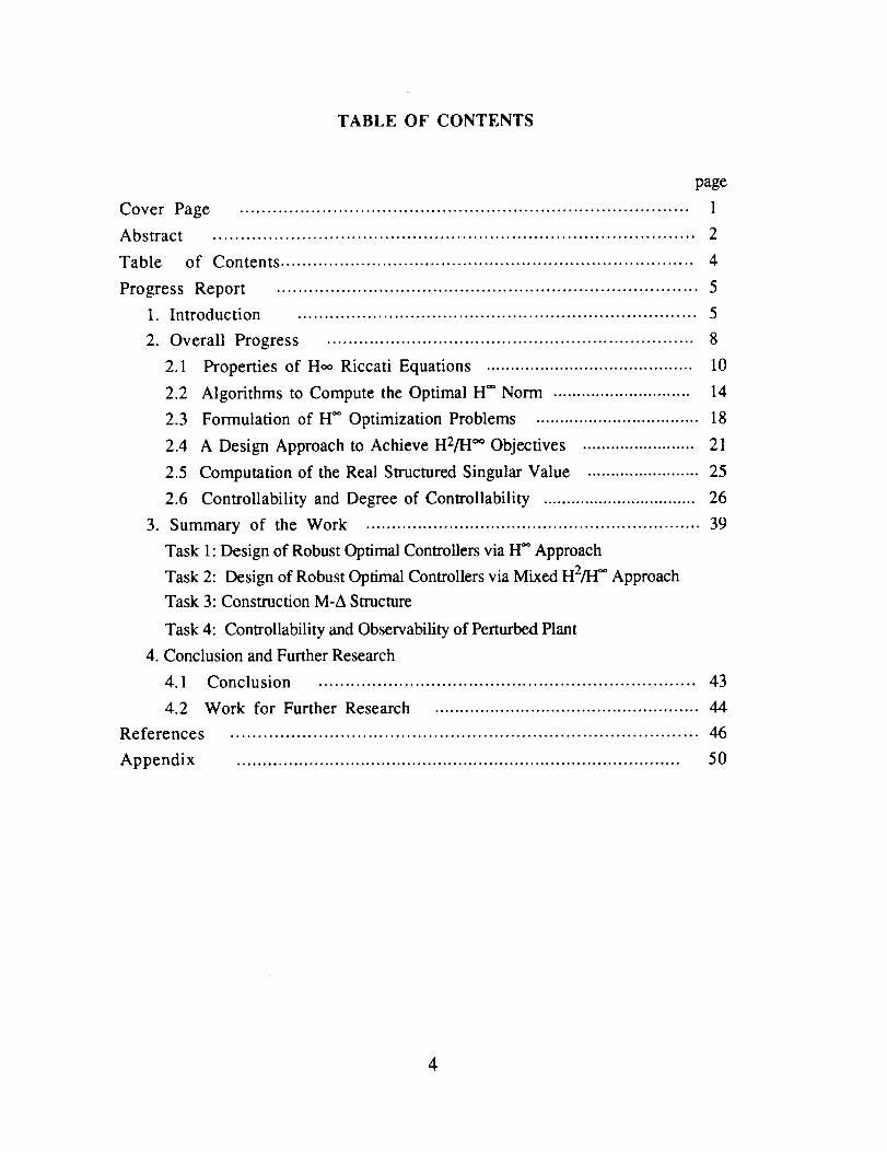
TABLE OF CONTENTS

page

Cover Page .................................................................................. 1

Abstract ....................................................................................... 2

Table of Contents ............................................................................. 4

Progress Report .............................................................................. 5

1. Introduction .......................................................................... 5

2. Overall Progress ..................................................................... 8

2.1 Properties of Hoo Riccati Equations .......................................... 10

2.2 Algorithms to Compute the Optimal H** Norm ............................. 14

2.3 Formulation of H '_ Optimization Problems .................................. 18

2.4 A Design Approach to Achieve H2/I-I °° Objectives ........................ 21

2.5 Computation of the Real Structured Singular Value ........................ 25

2.6 Controllability and Degree of Controllability ................................. 26

3. Summary of the Work ................................................................ 39

Task 1: Design of Robust Optimal Controllers via _ Approach

Task 2: Design of Robust Optimal Controllers via Mixed H2/I-_ Approach

Task 3: Construction M-A Structure

Task 4: Controllability and Observability of Perturbed Plant

4. Conclusion and Further Research

4.1 Conclusion ...................................................................... 43

4.2 Work for Further Research .................................................... 44

References ..................................................................................... 46

Appendix ...................................................................................... 50

4

PROGRESS REPORT

ROBUST CONTROL OF SYSTEMS WITH REAL PARAMETER

UNCERTAINTY AND UNMODELLED DYNAMICS

1. INTRODUCTION

This document is the second-period progress report on the NASA supported

research, "Robust Control of Systems with Real Parameter Uncertainty and Unmodelled

Dynamics", (No. NAG-1-1102). We are happy to report that in this research period we

have made significant progress in the following proposed research problems: (1) Design of

robust controllers via H °* optimization, (2) Design of robust controllers via mixed H2/H _0

optimization, (3) M-A Structure and robust stability analysis for structured uncertainties,

and (4) A study on controllability and observability of perturbed plant.

Doyle, Glover, Khargonekar, and Francis (abbr.: DGKF) [1], and Glover and

Doyle [2] presented a celebrating two-Riccati-equation type solution to a standard H**

control problem. The two-Riccati-equation method characterizes all possible stabilizing

suboptimal H** controllers whose order is not higher than that of the plant. The suboptimal

H** controller formulas in [1], [2] can be easily transformed into descriptor forms to

construct optimal H** controllers without numerical difficulties if the optimal H** norm is

given. The optimal H °* controllers, with very few exceptions, have direct feedthrough

terms and therefore infinite bandwidth. Hence, control engineers may prefer strictly proper

suboptimal Ho* controllers to the optimal ones. However, knowing the optimal H** norm is

important in determining which suboptimal controller to be chosen in practical design.

Recently, an efficient algorithm for computing the optimal H** norm was proposed

by Scherer [3]. Scherer considered the inverse (or pseudo inverse) of the DGKF H**

Riccati solutions, X**(T) and Y**(T), defined a new independent variable I.t = y-2, and

showed that these inverses are concave functions of _t in matrix sense on their domains of

definition. Based on this fact, a quadratically convergent Newton-like algorithm was

proposed to compute the optimal H" norm.

Pandey et. al.'s hybrid gradient-bisection method [4] and Chang et. al.'s double

secant and bisection method [5] were also proposed for the computation of the optimal H *_

norm. The significance of the conjecture that p[X**(y)Y**(y)], the spectral radius of

X**(T)Yo.(_'), is a convex function of T2 was mentioned in these two papers. Since there

was no proof for this conjecture, bisection was used in these two algorithms as supplement

5

to guarantee convergence.

In this research period, we discovered several important properties of the two

DGKF H _0 Riccati solutions, X,_(7) and Y_*(7). Among them, the most prominent one is

that p[X_,(7)Y_,(T)] is a continuous, nonincreasing, convex function of y on (13, oo), where

13is the infimum of Y such that the two DGKF H** Riccati solutions, Xo.(y) and Y**(7), exist

and are positive semidefinite. Based on this property, a quadratically convergent algorithm

can be easily developed to compute the optimal H *_ norm, i.e., the 70* such that

p[X0*(Yo,)Y_(70*)] = _, if a starting 7 is given inside the interval (]3, 70.), i.e., 7 > 13 and

p[X0*(y)Y0*(7)] > 7a.

A 7 inside the interval (13, y0*) most of the time can be easily found without the

knowledge of 13. However, the computation of 13 can be necessary if _ itself is the

optimum, which occurs when p[X0*(13)Y..(_)] < 132. Newton-Raphson's method can be

employed to compute _ and the convergence is quadratic.

H - control theory can handle the following two robustness issues: (1) Minimization

of the maximum error energy for all command/disturbance inputs with bounded energy,

and (2) Closed-loop stability under unstructured plant uncertainties with bounded H"

norm. Besides, H _ control theory is also indispensable in the structured singular value

treatment of structured plant uncertainties [6,7]. Detailed procedures to formulate these

robust control problems into I-_ optimization problems will be given in the report.

For most practical control systems, a particular performance index is usually of

considerable interest. At the same time there is also a desire to improve on the closed-loop

system robustness. However, it is well known that there exists a tradeoff between these

two design objective. Any improvement gained in one of the design goals is usually

accompanied by a loss in the other. The Linear Quadratic Gaussian (LQG) Theory has

been used successfully to design observer-based controllers with optimal performance for

plants with fixed (or fixed power spectrum) exogenous signals. It is well known however,

that the controllers derived using this approach possess poor robustness properties when

compared to the guaranteed stability margins provided by full-state feedback control.

Doyle and Stein [8, 9] devised a procedure, usually referred to in the literature as the Loop

Transfer Recovery (LTR), to asymptotically recover the full-state feedback loop by tuning

the LQG designed observer. The adjustment procedure is achieved by introducing a

fictitious noise to the nominal plant input. A new LQG observer based controller is then

derived. For the case of minimum-phase plants, the asymptotic recovery is achieved by

letting the intensity of the added fictitious noise approach infinity. The procedure however,

6

has limitations when applied to nonminimum phase plants.

In this research we concentrate on the recently developed H °° theory which evolved

from the sensitivity minimization problem formulated by Zames [10]. It was shown there

that many of the classical design objectives can be incorporated in the H °° design. For

instance, the modeling of plant uncertainties can easily be formulated in terms of normed

H _ plant neighborhoods. Another advantage of this relatively new theory can be revealed

in the flexibility it offers to the designer in the formulation of the problem. For example,

the well known design methodology of loop shaping can easily be achieved via the choice

of frequency dependent weights on input as well as output signals. Although no direct

relations between these two are known, with the new state-space solution to the general

H °° problem [1, 2, 11] the design approach as will be shown later reduces to simply

varying certain design parameters in order to achieve the design objectives.

The motivation to design controllers for desired H 2 performance with H °° robustness

constraints has recently resulted in mixed H 2 and H °° control problem formulation [11, 12,

13, 14]. Special cases of this problem have been studied there and a solution in the form of

coupled Riccati equations has been proposed. Although the optimal solution for this mixed

H2/H °° control has not yet been found, we proposed a design approach which can be used

through proper choice of the available design parameters to influence both robustness and

performance.

Stability robustness is an important issue in the analysis and design of control

systems. Currently, there are two major approaches to stability robustness analysis. One is

the structured-singular-value (SSV) [6,7] or the multivariable-stability-margin (MSM)

[ 15,16] approach and the other is the perturbed-characteristic-polynomials approach [ 17-

22]. Several significant progresses have been made in both approaches. In this research, an

iterative algorithm of computing the real SSV and the real MSM is developed based on the

existing results in both approaches.

For a large class of linear time-invariant systems with real parametric perturbations,

the coefficient vector of the characteristic polynomial is a multilinear function of the real

parameter vector. Based on this multilinear mapping together with the recent results by De

Gaston and Safonov [15], Sideris and Pena [16], Bartlett, Hollot, and Lin [18], and

Bouguerra, Chang, Yeh, and Banda [23], an algorithm for computing the real structured

singular value is proposed. The algorithm requires neither frequency search nor Routh's

array symbolic manipulations and allows the dependency among the elements of the

parameter vector. Moreover, the number of the independent parameters in the parameter

vector is not limited to three,as is requiredby manyexisting structuredsingular value

computationalgorithms.

The literature on controllability gives variousdegreeof controllability (DOC)measures,each basedon different point of view. That is either, in terms of the

controllability grammianor therecoveryregionof initial statesin finite time by boundedcontrol, or thevariationof thesystemandcontrolmatrices.The workduring this period

concentratedon: (i) trying to develop a relation betweenthe various DOC measures

encountered in the literature, and (ii) developing software for investigating the

controllability robustnessof lineartimeinvariantsystems.A preliminarysoftwarepackage(describedin AppendixA) wasdevelopedfor measuringthesize,shapeandlocationof the

recoveryregion. Although thevariousoptimizationalgorithms(neededto automatically

obtainthe valueof the indicators)work, theyneedto be refinedin order to takecareof

suchproblemsasill-conditionedrecoveryregions.

In section2 of this report, we will show the overall progressin this research

period.Thework performedandthestatusof theproposedtasksaresummarizedin section3. Section4 is theconclusion.Thework for futureresearchwill alsobebriefly described

in section4.

2. OVERALL PROGRESS

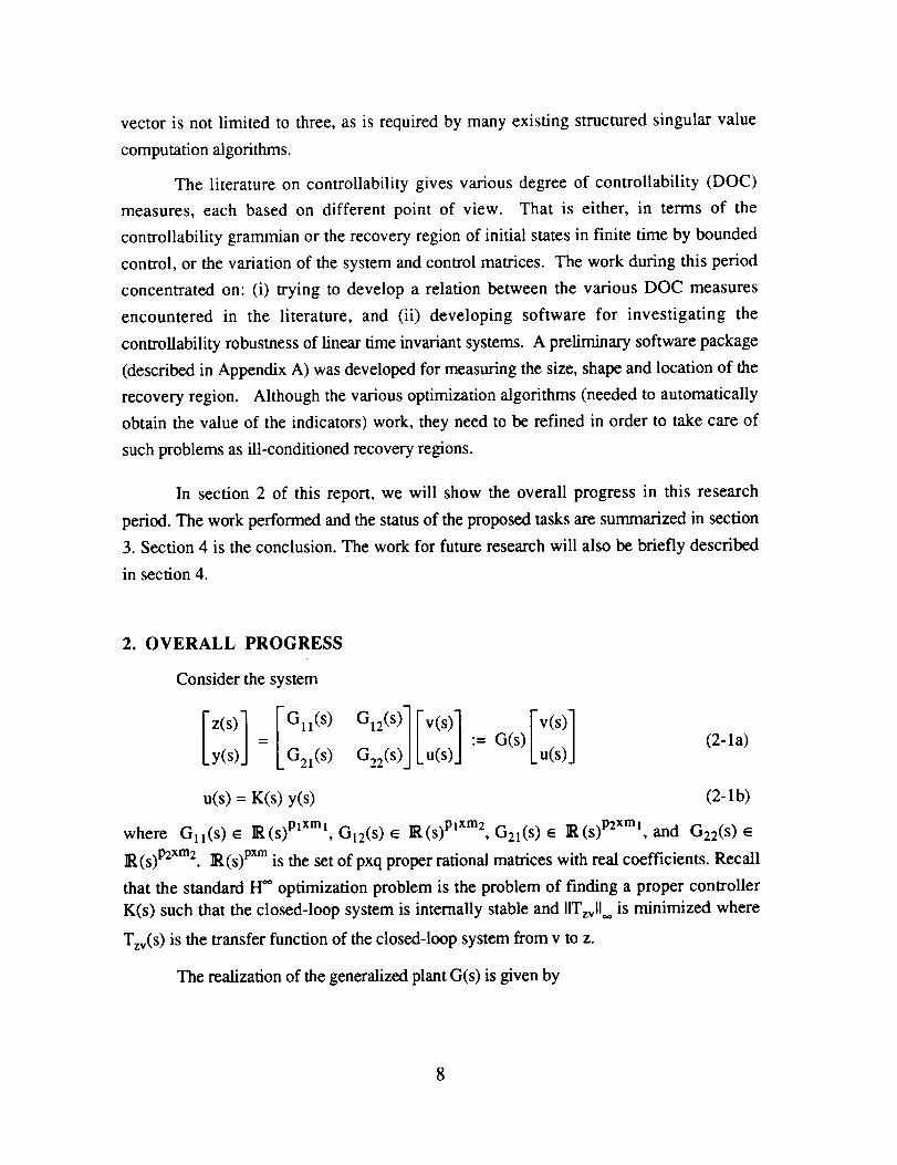
Consider the system

Iz(s)l IGll (s) GIE(S)I Iv(s)l Iv(s)l= := G(s) (2-1a)

Ly(s)J LG21 (s) G22(s)JLu(s)J ku(s)J

u(s) = K(s) y(s) (2-1 b)

where Gll(S) _ JR(s) plxml, GiE(S) e R(s) plxm2, GEl(S) _ R(s) pExml, and GE2(S)

_(s) pExmE, lR(s) pxm is the set of pxq proper rational matrices with real coefficients. Recall

that the standard H" optimization problem is the problem of finding a proper controller

K(s) such that the closed-loop system is internally stable and IITz,,ll** is minimized where

Tzv(S ) is the transfer function of the closed-loop system from v to z.

The realization of the generalized plant G(s) is given by

8

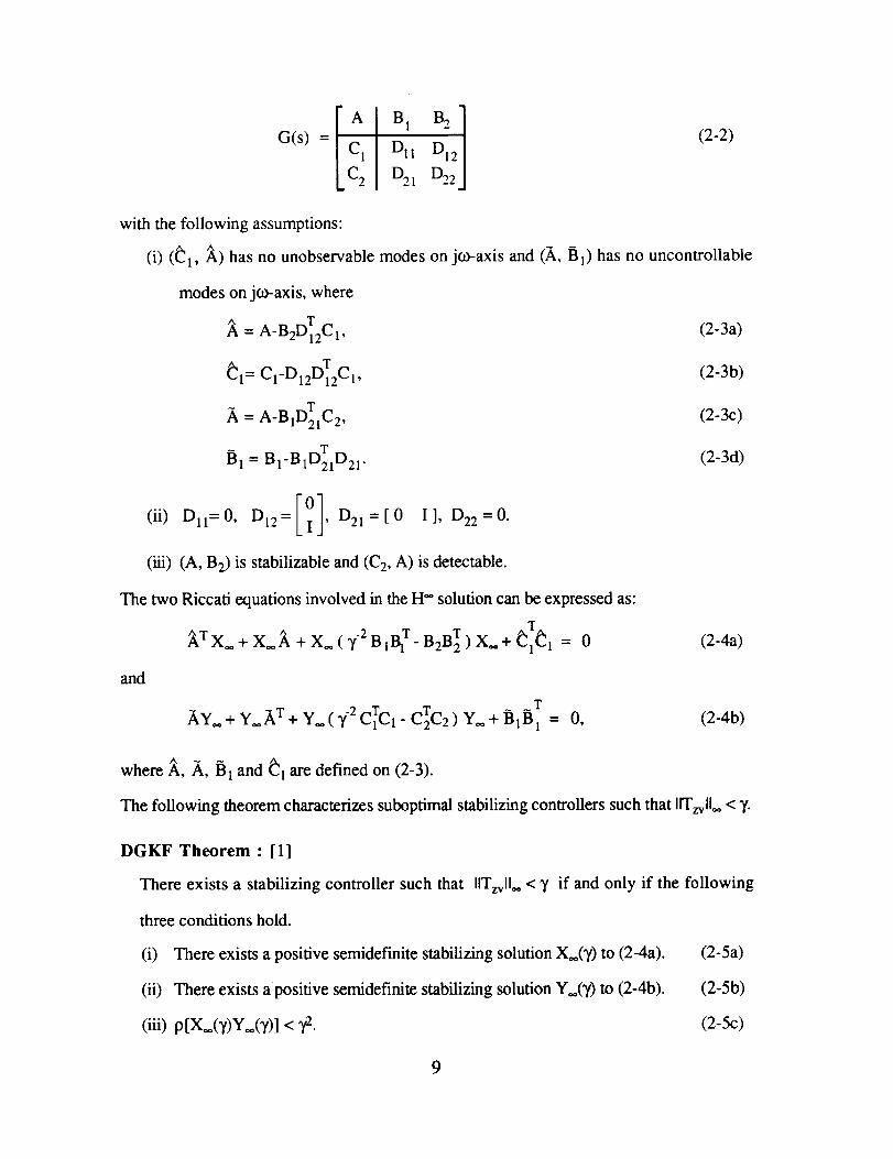
I A B 1 B2 ]G(s) = C1 D11 D12

C2 D21 D22 J

with the following assumptions:

(2-2)

(i) (_1, '_) has no unobservable modes on jco-axis and (_,, B1) has no uncontrollable

modes on jco-axis, where

,_ T (2-3a)= A-B2D12C l,

T (2-3b)_i = C1-DI2D12C1,

T (2-3C)= A-B1D:IC 2,

T

_31 = BI-B1D21D21. (2-3d)

(ii) DII=0, D12=[_], D21=[0 I], D22=0.

(iii) (A, B2) is stabilizable and (C a, A) is detectable.

The two Riccati equations involved in the H** solution can be expressed as:

,_T Xo. + Xoo_k + X** ( 7 -2 BIB1 T- B2 BT ) X** + (_(_1 = 0 (2-4a)

and

_y** + y**_T + y** ( y-2 cTcI_ cTc2 ) y. + B'BT = 0, (2-4b)

where _, _,, B1 and _l are defined on (2-3).

The following theorem characterizes suboptimal stabilizing controllers such that IITzvll. < y.

DGKF Theorem : [1]

There exists a stabilizing controller such that IITzvll, < y if and only if the following

three conditions hold.

(i) There exists a positive semidefinite stabilizing solution X.(y) to (2-4a). (2-5a)

(ii) There exists a positive semidefinite stabilizing solution Y,if) to (2-4b). (2-5b)

(iii) p[X**(7)Y**(y)] < 72. (2-5c)

9

Moreover, when these conditions hold, one such controller is

with

B k = -EL2, C k = F 2,

(2-6)

where

A k = A+[BI Fl]+B2][ F 2 EL2(C2+D21FI )'

E = (I- T2Y_Xo. )-1,

-2 TL1 =7 Y_,C1,

T _BTx_ TF 1 -B1X**, F2= = DI2C 1,

TL2 = -Y.C2 T B1D21"

The above theorem shows an easy state-space approach to construct a stabilizing

suboptimal controller such that IITzvll**< 7. The theorem can also be used to compute the

optimal H** norm and construct an optimal H'controller. The optimal IITz_IL. is the infimum

of Y such that the above three conditions hold. With very few exceptions, the optimum

occurs when p[X**(7)Y.(7)] = 72 which will render A k and E undefined. This numerical

difficulty can be easily resolved by transforming (2-6) into a descriptor form [1][25][26].

2.1 PROPERTIES OF H** RICCATI SOLUTIONS

First, we assume (Cp -A) is detectable. This assumption will be removed later in this

section. Suppose we have Riccati equation

_AT + A_ + (T2B1BT - B2B T) + 5tCTClSt=0,

then solution _(7) has following properties.

Theorem 2.1: _(y) is a well-defined function on (e. x, 4-0.), where

otx := inf {7: 7e R+ and 5_(7) exists}

Moreover, _(7) is analytic with

(2-7)

(2-8)

_(7) := d_(T_(T)) >--0 (2-9)

10

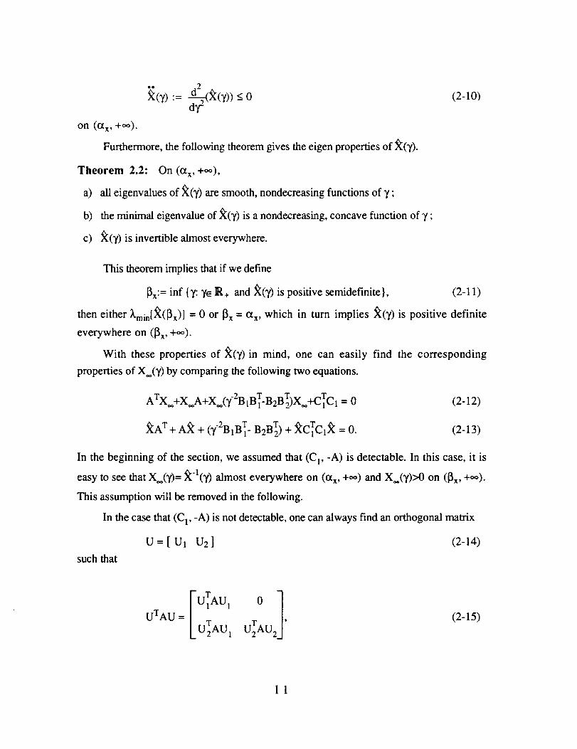
°° 2

R('t) := -<o

on (ct x, +oo).

Furthermore, the following theorem gives the eigen properties of _(y).

Theorem 2.2: On (c_x,+o_),

a) all eigenvalues of _(_') are smooth, nondecreasing functions of y ;

b) the minimal eigenvalue of _(y) is a nondecreasing, concave function of Y ;

c) _(y) is invertible almost everywhere.

(2-10)

This theorem implies that if we define

13x:= inf {'1(:ye IR+ and _(_,) is positive semidefinite}, (2-11)

then either _Lmin[_(_x) ] = 0 or [_x = _x, which in turn implies _(_,) is positive definite

everywhere on (13x, +oo).

With these properties of _(y) in mind, one can easily find the corresponding

properties of X(y) by comparing the following two equations.

T -2 T T TA X**+Xo.A+X**( 7 B1Bz-B2B2)X.+C1C1 = 0 (2-12)

_A T + A_ + O'-2B1B T- B2B T) + _CTCz_ = 0. (2-13)

In the beginning of the section, we assumed that (C z, -A) is detectable. In this case, it is

easy to see that X..(7)= _1(7 ) almost everywhere on (o_x, +oo) and X (y)>0 on ([3x, +oo).

This assumption will be removed in the following.

In the case that (C l, -A) is not detectable, one can always find an orthogonal matrix

U=[U_ U2] (2-14)

such that

uTAu= LU{AU, uTAu2

(2-15)

11

and

uTB=[uTB1 uTB2]= uTB1 uTB2J

(2-16)

C1U = [CIU 1 0] (2-17)

with (C1U1,-U:AU l) detectable [27]. Furthermore, the solution to (2-12) can be

expressed as

[ X("/)O0]uT (2-18)= U 0

with X(y)= _-l(y) almost everywhere on (a x, +_), where X(y) and _(y) are the stabilizing

solutions to (2-12) and (2-13) respectively with (A, B1, B2, C 1) replaced by (UTAU V

UIB 1, U B 2, C1U1). Therefore, no matter whether (C 1, -A) is detectable or not, it is

always true that X(y) exists almost everywhere on (a x, +_) and X,(y) > 0 on (_x, +¢¢).

Moreover, we have the following theorem which gives the properties of the first and

second derivatives of X(y).

Theorem 2.3: On (_x,+_),

•a) X.(y) := X**(y)) < 0, (2-19)

.o d 2

b) X**(y) := _-(X.(y)) ___0. (2-20)

Again, next theorem gives the eigen properties for X**(y).

Theorem 2.4: On ([3x,+*o),

a) all eigenvalues of X**(y) are smooth, nonincreasing functions of,/;

b) the maximal eigenvalue of X(y) is a nonincreasing, convex function of y.

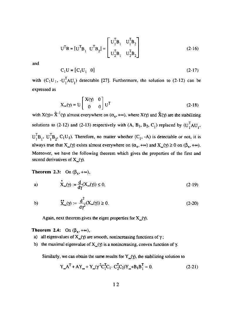
Similarly, we can obtain the same results for Y**(y), the stabilizing solution to

YA T+AY + Y (y-ZcTc1- T TC2C2)Y-+BIB 1 = 0. (2-21)

12

If (-A, B1)is stabilizable,thenY**(y)=_,-l(y)almosteverywhereon (Oty,+_) and

Y**(y)>0 on ([3y,+oo),where_'(y) is thestabilizingsolutionto

AT_ + _'A + (y-2cTcI-cTc2)+_'B1BT_' =0 (2-22)

and

O_y:= inf {y" y_ IR+ and Y**(y) exists} (2-23)

[_y := inf {y : _,_ 1R+ and Y**(y) is positive semidefinite }. (2-24)

If (-A, B1) is not stabilizable, then an orthogonal matrix V= [V1 V2] can be found such

that

V VTAV1

vTAv= L 0

V1AV2] ,vlj lV,c,v and CV C2VjL C2V 1 C2V2

with (-vTAv,. vTIB1) stabilizable. Furthermore, the stabilizing solution to (2.21) can be

expressed as

Y(y) 0]Y**(y) = V 0 0 VT' (2-25)

with Y(y)= _,-l(y) almost everywhere on (¢ty, _) and Y(y)> 0 on ([3y, +_). Again, Y(T)

and _(y) are the stabilizing solutions to (2-21) and (2-22) respectively with (A, B1, C1,

C2) replaced by (vTAvF VTB x, C1V1, CzV0. Note that all results presented above for

X**(y), X(y) and _(y) have their counterparts for Y**(y), Y(y) and _(y) respectively.

Before moving to the next theorem to investigate the properties of X**Y_, we define o_

and [3 as follows:

ot := max{or x, ¢ty} (2-26)

[_ := max{[3x, 13y}. (2-27)

With these definitions, we can see that X**Y**exists on (or, +_) almost everywhere.

Moreover, X**Y** has no negative eigenvalues on (13, +0-), since both X.. and Y** are

positive semidefinite on ([5, +_). Now, we are in the position to state our main result.

Theorem 2.5: On (13, +**),

a) all eigenvalues of X_Y** are smooth, nonincreasing functions of y;

b) 9(X**Y**) is a nonincreasing, convex function of y.

13

Furthermore,if wedefinep(y):=p(X=Y=)and13(y).- d(p(y))dy

of P(Y)canbeexpressedas

on (13,+_), the slope

[_(y)= vT(x"Y'_+X_*'_'_)w (2-28)vTw

where v and w are the left and the right eigenvectors of X**Y.. respectively corresponding

to its maximal eigenvalue. X_. and _'= can be obtained by solving the following Lyapunov

equations:

,_T_,,.+_**_, _2y-3X**B1BTx** = 0 (2-29)

and A'Y,,,,+'Y,_T -2"t'-3y..cTc 1Y. = 0, (2-30)

_, A+(y-2B T T y.cy2cTc_c2Tc2).= 1BI-B2B2)X andA=A+with

2.2 ALGORITHMS TO COMPUTE THE OPTIMAL H- NORM

According to DGKF theorem, we can see that finding the optimal H. norm,

denoted as y**, is equivalent to finding the infimum y such that all three conditions in (2-5)

hold. From the previous subsection, it is obvious that 7.._ [13, +'_). It is possible for 13to

be y., especially when 13and ot are identical, however, with very few exceptions, y._ (13,

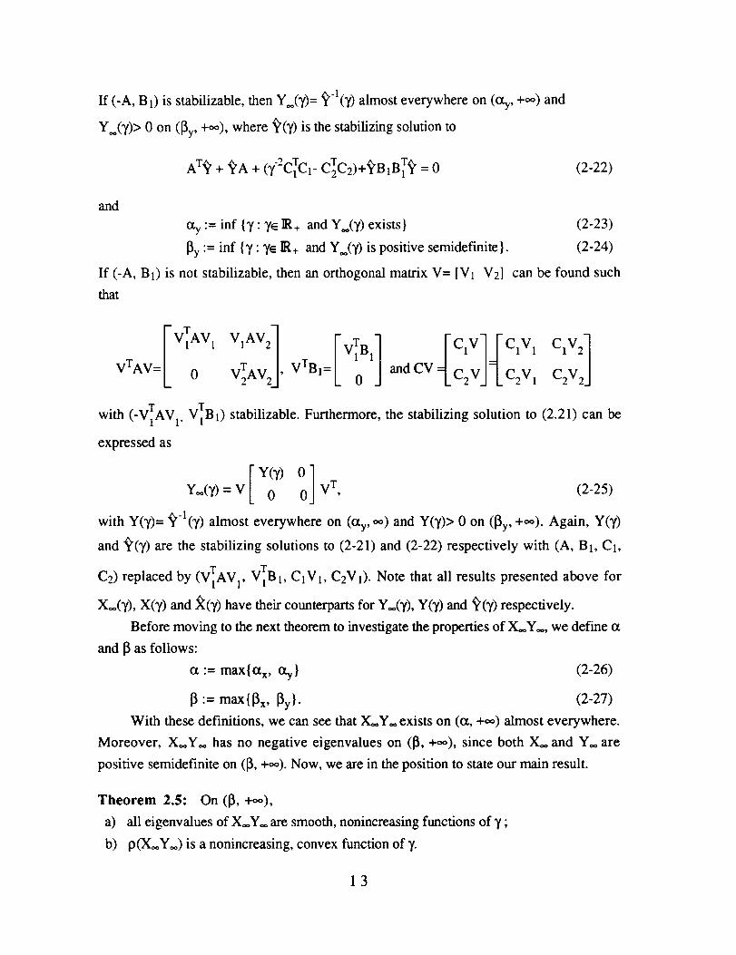
+_), which implies that y. is the solution to P(Y) = 72. The relations between o_, 13and y,

are shown in the figure below.

Both X,_ and Y** exist

Both X** > 0 and Y** >__0

0 Ot

All three conditions hold

14

The figure implies that the problem of finding the optimal y**is actually that of either

searching for the intersection point of p(y) with 72 inside (13, +o_) or computing the

boundary point 13. Since P(Y) is a convex function on ([3, +oo), then gradient searching

method can be employed.

Assume that we have a starting point Yn in the interval (13, y**), then the optimal y

can be obtained easily as follows. Refer to Fig. 2.2, draw the tangent line with slope [_(Yn)

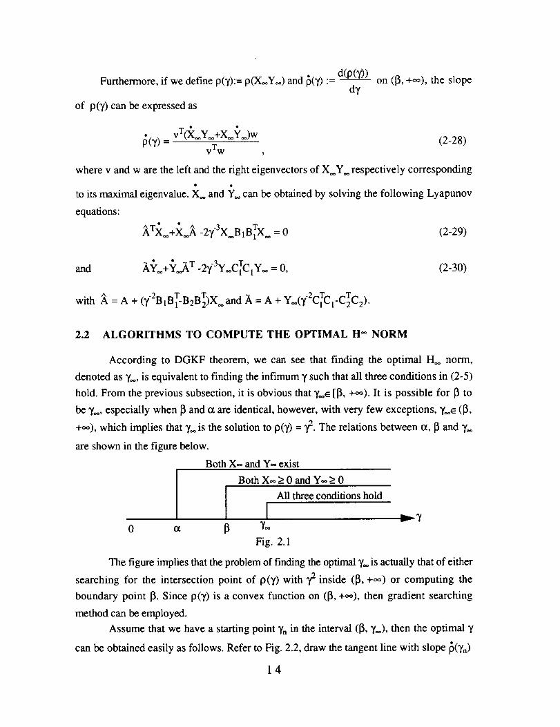
passingthroughthepoint (Tn,P(Yn))"Theabscissa,7n+1,of the intersectionof thetangent

line and thecurvey = 72, always lies between 7n and 70.. The search process is repeated

until the gap Y**- 7n+l is small enough.

Y,

P(L)

0 137n 7.+1

Fig. 2.2

Furthermore, we will see that the convergence rate is quadratic. Define en = 7_ - Yn and

en+l = 70* - Yn+l" It is straightforward to show that

"1_(7**) 2 (2-31)£nen+l --" 2 I [_(Y,,.) - 2_'0. I

which implies quadratic convergence. For convenience, the algorithm described will be

referred to as Q-step, since the quadratic convergence is guaranteed, provided there is a

starting point 7n_ (13,T**) to start with.

Based on the discussion above, following procedure is given to compute the

optimal H** norm.

Step 1. Initial point

Refer to Fig. 2.1, choose a relatively large initial Y1 such that 71_ [_, +oo). If

71_ ([3, y0*), then it can be used as the starting point for T**. Go to Q-step. If 71_ (7,.,

+,,o), which implies X**(y1) > 0 and Y**(Y1) > 0, then go to step 2.

Step 2. Starting point for Y**

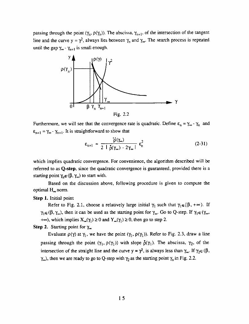
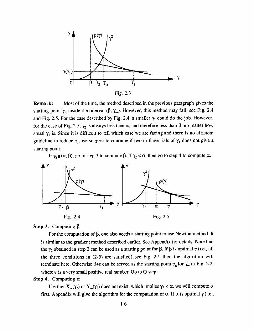
Evaluate 9(T) at 71, we have the point (T1, 9(71)). Refer to Fig. 2.3, draw a line

passing through the point (Tl, 9(71)) with slope [_(71). The abscissa, T2, of the

intersection of the straight line and the curve y = T2, is always less than T**. If 72¢ (13,

7..), then we are ready to go to Q-step with )'2 as the starting point "fnin Fig. 2.2.

15

P(71)

0

Fig. 2.3

Remark: Most of the time, the method described in the previous paragraph gives the

starting point 7n inside the interval (13, 7**). However, this method may fail, see Fig. 2.4

and Fig. 2.5. For the case described by Fig. 2.4, a smaller Y1 could do the job. However,

for the case of Fig. 2.5, 72 is always less than at, and therefore less than [5, no matter how

small 71 is. Since it is difficult to tell which case we are facing and there is no efficient

guideline to reduce Tl, we suggest to continue if two or three rials of YI does not give a

starting point.

If Y2_ (at, 13), go to step 3 to compute 13.If 72 < at, then go to step 4 to compute at.

Y

72 3 Yl

Y

72 C_ 71 v 7

Fig. 2.4 Fig. 2.5

Step 3. Computing 13

For the computation of 13,one also needs a starting point to use Newton method. It

is similar to the gradient method described earlier. See Appendix for details. Note that

the 72 obtained in step 2 can be used as a starting point for 13.If [3 is optimal 7 (i.e., all

the three conditions in (2-5) are satisfied), see Fig. 2.1, then the algorithm will

terminate here. Otherwise 13+e can be served as the starting point 7n for 70. in Fig. 2.2,

where e is a very small positive real number. Go to Q-step.

Step 4. Computing at

If either X0,(72 ) or Yoo(Y2) does not exist, which implies 72 < at, we will compute at

first. Appendix will give the algorithm for the computation of at. If at is optimal T (i.e.,

16

all the threeconditions in (2-5) aresatisfied),seeFig. 2.1,then the algorithm will

terminatehere.Otherwiseotcanbeusedeitherasastartingpoint for 13,whenot_:_;or

astartingpoint for y_,,whenot= _i.Goto step3andQ-steprespectively.

Q-step. Computingy_,

This stepwasdescribedin Fig. 2.2. We canseefrom theearlierdiscussion,oncewe havea startingpoint for y**,thequadraticconvergenceis guaranteed.Algorithm

terminates.

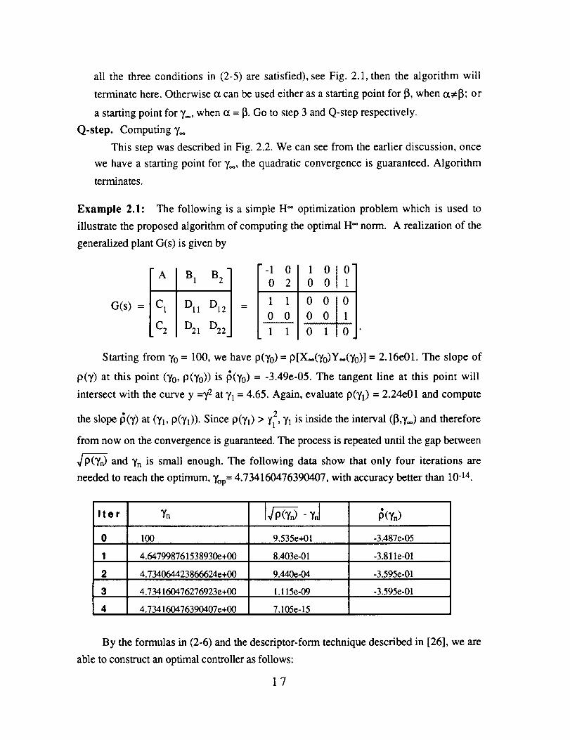
Example 2.1: The following is a simpleH** optimization problem which is used to

illustrate the proposed algorithm of computing the optimal H** norm. A realization of the

generalized plant G(s) is given by

G(s) =

A

C 1

C 2

B 1 B 2

Dll D12

D21 D22

"-1 0

0 2

1 1

0 0

1 1

1 0[00 0 1

o0 0

0 il0

Starting from Yo = 100, we have P(Yo) = P[X**(7o)Y**(Yo)] = 2.16e01. The slope of

P(Y) at this point (Yo, P(Yo)) is I_(Yo) = -3.49e-05. The tangent line at this point will

intersect with the curve y =72 at ]t 1 = 4.65. Again, evaluate P(Y1) = 2.24e01 and compute

the slope [_(y) at (Y1, P(Y1)). Since P(Y1) > _,2, Y1 is inside the interval (13,y..) and therefore

from now on the convergence is guaranteed. The process is repeated until the gap between

and Yn is small enough. The following data show that only four iterations are

needed to reach the optimum, Yop= 4.734160476390407, with accuracy better than 10 -14.

Iter

0

1

2

3

4

_(Y.)

100 9.535e+01 -3.487e-05

4.647998761538930e+00 8.403e-01 -3.81 le-01

4.734064423866624e+00 9.440e-04 -3.595e-01

4.734160476276923e+00 1.115e-09 -3.595e-01

4.734 160476390407e+00 7.105e- 15

By the formulas in (2-6) and the descriptor-form technique described in [26], we are

able to construct an optimal controller as follows:

17

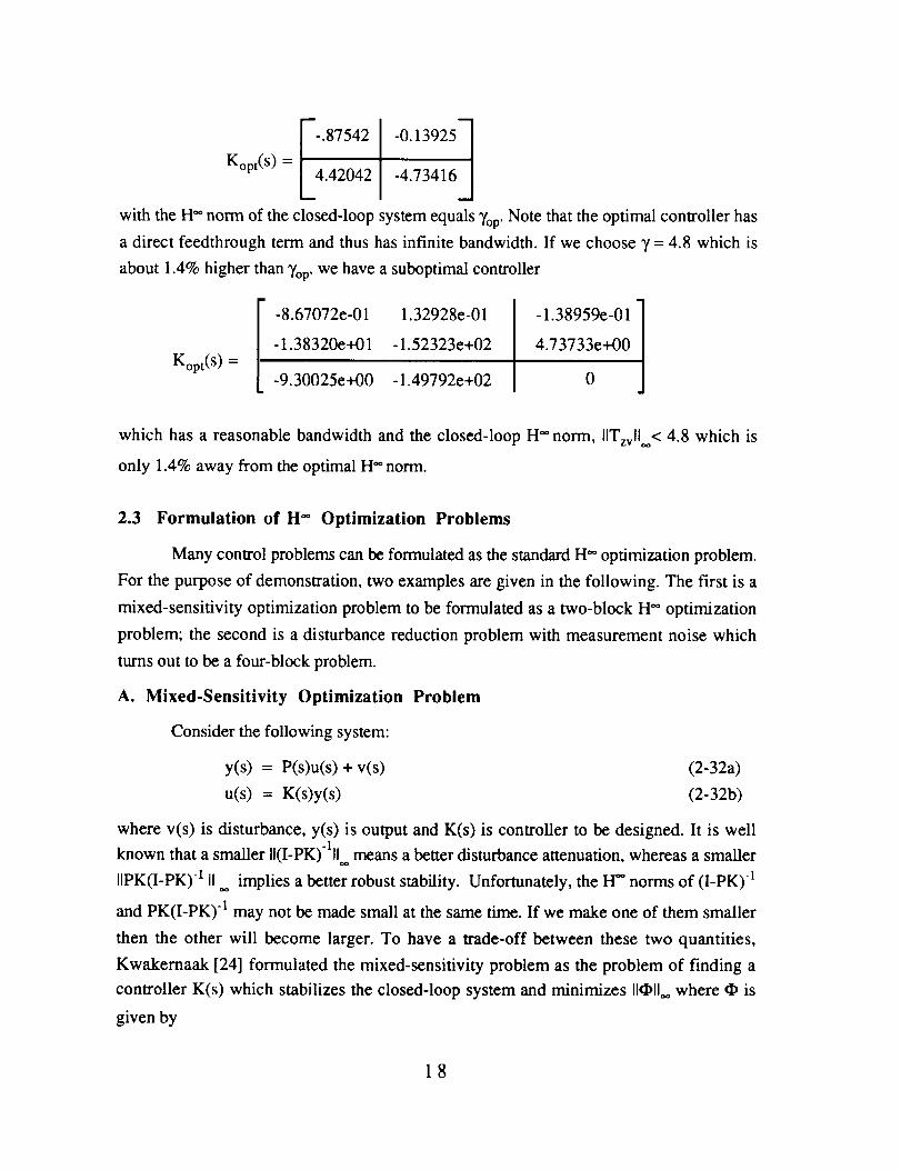
-.87542 -0.13925

K°pt(S)= 14.42042 -4.73416

with theH°*normof theclosed-loopsystemequals_'op.Notethattheoptimalcontrollerhasa direct feedthroughtermandthushasinfinite bandwidth.If we choose7 = 4.8 which is

about1.4%higherthan7op,wehaveasuboptimalcontroller

K°pt(S)= [

-8.67072e-01

-1.38320e+01

-9.30025e+00

1.32928e-01

-1.52323e+02

-1.49792e+02-1.38959e-01 1

4.73733e+00

0

which has a reasonable bandwidth and the closed-loop H °*norm, IITzvlloo< 4.8 which is

only 1.4% away from the optimal H** norm.

2.3 Formulation of H °* Optimization Problems

Many control problems can be formulated as the standard H _*optimization problem.

For the purpose of demonstration, two examples are given in the following. The first is a

mixed-sensitivity optimization problem to be formulated as a two-block H** optimization

problem; the second is a disturbance reduction problem with measurement noise which

turns out to be a four-block problem.

A. Mixed-Sensitivity Optimization Problem

Consider the following system:

y(s) = P(s)u(s) + v(s) (2-32a)

u(s) = K(s)y(s) (2-32b)

where v(s) is disturbance, y(s) is output and K(s) is controller to be designed. It is well

known that a smaller II(I-PK)dlI** means a better disturbance attenuation, whereas a smaller

IIPK(I-PK) q II ._ implies a better robust stability. Unfortunately, the I-I**norms of (I-PK) -l

and PK(I-PK) l may not be made small at the same time. If we make one of them smaller

then the other will become larger. To have a trade-off between these two quantities,

Kwakernaak [24] formulated the mixed-sensitivity problem as the problem of finding a

controller K(s) which stabilizes the closed-loop system and minimizes I1_11.. where @ is

given by

18

Wl(I-PK)-I 1= (2-33)

W2PK(I-PK) -1

W 1 and W 2 are weighting matrices chosen by the designer according to the concrete

situation. In other words, they depend on the characters of the disturbances and system

uncertainties. Usually, the disturbances occur most likely at low frequency, therefore

W1(s) is chosen to be a low-pass filter to emphasize the error energy at low frequency. The

plant uncertainty is also frequency-dependent; the higher the frequency is, the larger the

uncertainties become. Hence, W2(s ) is usually chosen to be a improper transfer function

(but W2P(s ) has to be a proper transfer function), which is analytic in closed right half

plane. In the following, we assume that Wl(S) is strictly proper, W2(s ) is a polynomial

such that W2P(s ) remains proper and both of them are analytic in closed right half plane.

The problem of finding a K(s) which stabilizes the closed-loop system and

minimizes I1_11.. can be rearranged into the standard H** optimization problem. Consider the

following system:

, .... vFlY I PJ u

(2-34a)

[zIT

that

u = K y (2-34b)

It is easy to show that the matrix _ defined by (2-33) is just the transfer function from v to

zzT IT of the closed-loop system (2-34). Comparing (2-34a) with (2-1 a), we can see

[wP]Gll = 0 ' G12 = WzP '

G21 = I, G22 = P.

If P, W2P, and W 1 have state-space realizations as follows

['1B] ['1"] [ 'lB"lP = W2P = W l =

Cp Dp ' Cw2 Dw2 ' Cwl Dwl.I

(2-35)

(2-36)

Then the generalized plant G(s) has a state space realization as shown in (2-2) with

19

= , B2=A = , Bl Bw1 BwlDrBwlCp Awl

C1= , Dll = , DI2 =Cw2 k 0 _l Dw2.J

C2=[Cp 0], D21 = I, D22 = Dp

Notethat because W 2 is a polynomial, the A-matrix of W2P is same as that of P.

B. Disturbance Reduction Problem

(2-37)

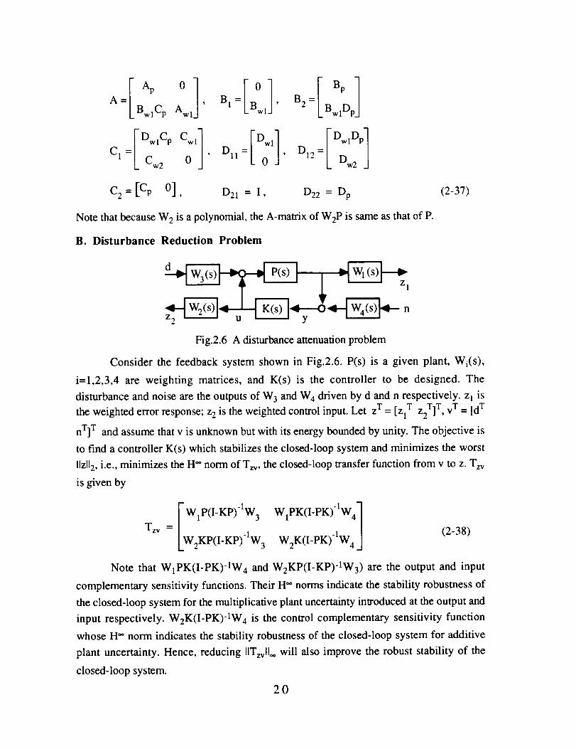
Fig.2.6 A disturbance attenuation problem

Consider the feedback system shown in Fig.2.6. P(s) is a given plant, Wi(s),

i=1,2,3,4 are weighting matrices, and K(s) is the controller to be designed. The

disturbance and noise are the outputs of W 3 and W 4 driven by d and n respectively, z I is

the weighted error response; z2 is the weighted control input. Let zT = [zlT z2T]T, v T = [d T

nT] T and assume that v is unknown but with its energy bounded by unity. The objective is

to find a controller K(s) which stabilizes the closed-loop system and minimizes the worst

Ilzll2, i.e., minimizes the H** norm of Tzv, the closed-loop transfer function from v to z. Tzv

is given by

Tzv = I W1P(I'KP)-tW3 WIPK(I-PK)Iw41

LW2KP(I_Kp)_Iw 3 W2K(I_PK).IW 4 j (2-38)

Note that WlPK(I-PK)-IW4 and W2KP(I-KP)-IW3) are the output and input

complementary sensitivity functions. Their H _' norms indicate the stability robustness of

the closed-loop system for the multiplicative plant uncertainty introduced at the output and

input respectively. W2K(I-PK)-IW4 is the control complementary sensitivity function

whose H _' norm indicates the stability robustness of the closed-loop system for additive

plant uncertainty. Hence, reducing IITzvll_ will also improve the robust stability of the

closed-loop system.

20

It is easy to verify that the generalized plant of the system can be expressed as:

"W 1PW 3 0

= 0 0

PW 3 W 4

(2-39)

That is,

I W1PW 0 ] I WIPGll = 0 0 ' G12 = W 2

G21 = [ PW3 W 4 ], G22 = P.

(2-40)

If P, W i, i=1,2,3,4 have state-space realizations as follows:

,p] [ il,i]p= W. =

Cp Dp ' _ Cwi Dwi

i=1,2,3,4 (2-41)

Then the generalized plant G(s) has a state space realization as shown in (2-2) with

Ap 0 0 BpCw3 0 "BpDw3 0 ] Bp

A= 3w1Cp Awl 0 B.1DpCw3 0 BI= BwIDpD 3 0 ] B2= BwlDp

0 0 Aw2 0 0 0 0 ] Bw 2

0 0 0 Aw3 0 Bw3 0 / 0

0 0 0 0 Aw_ , 0 Bwnl, 0

Cl = D12 =O 0 Cw2 0 , Dll= L 0 0 , LDw2J

C2 = [Cp 0 0 DpCw3 Cw4], D21 = [DpDw3 Dw4], D22 =Dp. (2-42)

Above {A,B,C,D } is the state-space representation for the generalized plant G(s).

2.4 A Design Approach to Achieve H2/H °° Objectives

The mixed H 2 and H** control problem in its most general form has not been solved

as of yet. However, taking advantage of the recent advances in H** theory, we believe

that it is possible to develop a simple design procedure that will address the performance-

21

robustness problem. In the following, we consider the disturbance attenuation problem

with control weighting as shown in Figure 2.6. The nominal plant is denoted by P(s)and

the energy bounded exogenous signals consist of plant input disturbances d and

measurement noise n. The weighted error response and the weighted control input consist

of zl and _, respectively.

Following the approach presented by Doyle et. al. in [1,2], this problem can easily

be transformed to the general H2/H °° configuration. The task is then to design a stabilizing

H °* controller K(s) such that the H °° norm of the transfer function matrix from the

exogenous input vector w T =[ d T n T ]T tO the output vector zT =[ Zl T z2T] T is minimized.

From Figure 2.6, this transfer function matrix is given by:

Tzw=[ W1P(I" Kp)-I W3 W1PK (I- P K)-I W4]W2 K P ( I - K P )-1 W3 W2 K ( I - P K )-1 W4J (2-43)

where Wi (s), i = 1..... 4 are weights to be chosen by the designer appropriate to the plant

and design objectives being considered. Usually, W3 is a low frequency filter indicating

that the disturbances introduced at the plant input are low frequency signals. The rest are

usually assumed to be high frequency filters to include measurement noise, unmodeled

dynamics, and any other plant uncertainties that may occur at high frequencies. Notice that

WI can be nonproper, hence providing the flexibility to consider frequency dependent

output responses. In this note however, we will only consider weights that lead to

controllers having the same order as that of the nominal plant.

The above disturbance rejection problem turns out to be a four-block problem and

its solution is described in [2]. It has been realized however, that suboptimal controller,

i.e. controllers satisfying IITzw Iloo < 2, for some positive _, greater than the optimal H °°-

norm of the closed-loop transfer matrix, are much easier to characterize than optimal ones.

It also turns out that the variable 2, can be used as a design parameter. This can easily be

verified when the general mixed HZ/H °* control problem is restricted to the case where the

H 2 closed-loop transfer matrix is the same as that of the H °° problem. In this case, the

suboptimal H °° controller approaches the H2/LQG controller as 2, approaches o,.

From the input/output relation described above, it can be seen that it is possible to

address the performance/robustness problem via the design weights. For instance, the

complementary sensitivity function which is a measure of the closed-loop robustness is

represented by the (1,2) block of the closed-loop transfer matrix above with the weights

W1 and W4 included. Thus by appropriately choosing these weights one can hope to gain

on performance without giving up too much robustness. As we will see later in the

22

example,thisprocedurewhenusedeffectivelyiscomparableto theLTR techniqueasfar asH2performanceandrobustnessareconcerned.

Example 2.2

ConsiderthefollowingtypicalLQGproblem:

1]x+[01u+[35]d4y=[2 1]x+n

with E(d) = E(n) = 0; E[d(t)d(_)] = E[n(t)n('_)]= _(t-'0. The following performance indexis of particular interest

J=ln-(xTQTQx+u2)dt where Q=4"(_[f_ 1]

In the H °° formulation, we construct the generalized plant

G s [AJBB21C1 Dll D12

C2 D21 D22

by considering the same nominal plant as in the LQG problem with the following weights:

W 1 (s) = 0_ 1 82 + 10 s + 4s + 2 and W2,3,4 (s) = (12,3,4 where the (1i's are real. The optimal

LQG performance index turns out to be equal to 493. Introducing a fictitious noise at the

plant input as described by the LTR technique improves the stability margins of the closed-

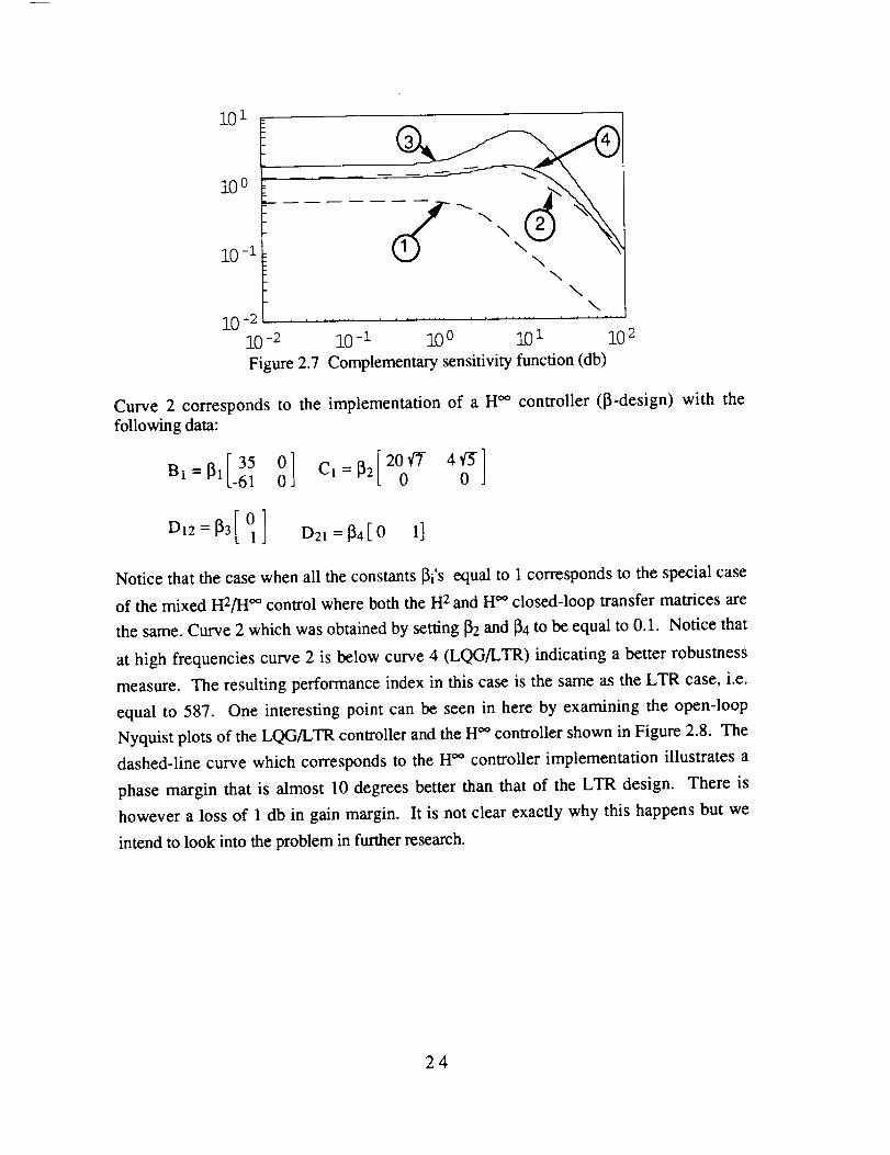
loop system, but at the expense of performance. The solid-line curve 3 in Figure 2.7

represents the singular values of the complementary sensitivity function with the LQG

controller implemented while curve 4 corresponds to the LTR design. The improvement in

robustness using the LTR technique results in a loss in performance as summarized in the

table below. The dashed line Curve 1 in Figure 2.7 corresponds to the implementation of

the ((1-design) H °_ controller with the constants (11 = (X2= (13 = 1 and (14--0.01. The

reason why (14 was varied was because it is directly related to the complementary

sensitivity function as indicated by the input-output relations above. The suboptimal H °°

controller was obtained for a value of ythat is 15% higher than the optimal H °_ norm.

23

1(31

i0 -z ki2 \ \

x\

i0 -2 \

10-2 10-1 10o 101 10 2

Figure 2.7 Complementary sensitivity function (db)

Curve 2 corresponds to the implementation of a H °° controller (13-design)

following data:

0]BI = _i -61 0 0

D12=_3[ 0] D21=134[0 1]

with the

Notice that the case when all the constants _li's equal to 1 corresponds to the special case

of the mixed H2/I-I °° control where both the H 2 and H o° closed-loop transfer matrices are

the same. Curve 2 which was obtained by setting [32 and [34 to be equal to 0.1. Notice that

at high frequencies curve 2 is below curve 4 (LQG/LTR) indicating a better robustness

measure. The resulting performance index in this case is the same as the LTR case, i.e.

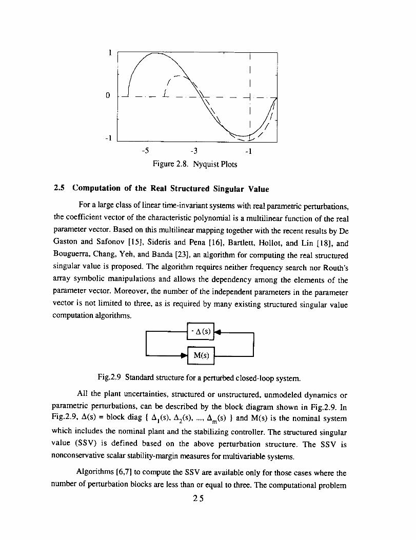
equal to 587. One interesting point can be seen in here by examining the open-loop

Nyquist plots of the LQG/LTR controller and the H °° controller shown in Figure 2.8. The

dashed-line curve which corresponds to the H °° controller implementation illustrates a

phase margin that is almost 10 degrees better than that of the LTR design. There is

however a loss of 1 db in gain margin. It is not clear exactly why this happens but we

intend to look into the problem in further research.

24

-1

-5 -3 -1

Figure 2.8. Nyquist Plots

2.5 Computation of the Real Structured Singular Value

For a large class of linear time-invariant systems with real parametric perturbations,

the coefficient vector of the characteristic polynomial is a multilinear function of the real

parameter vector. Based on this multilinear mapping together with the recent results by De

Gaston and Safonov [15], Sideris and Pena [16], Bartlett, Hollot, and Lin [18], and

Bouguerra, Chang, Yeh, and Banda [23], an algorithm for computing the real structured

singular value is proposed. The algorithm requires neither frequency search nor Routh's

array symbolic manipulations and allows the dependency among the elements of the

parameter vector. Moreover, the number of the independent parameters in the parameter

vector is not limited to three, as is required by many existing structured singular value

computation algorithms.

I

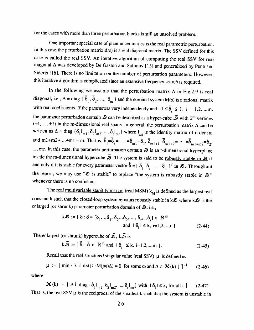
Fig.2.9 Standard structure for a perturbed closed-loop system.

All the plant uncertainties, structured or unstructured, unmedeled dynamics or

parametric perturbations, can be described by the block diagram shown in Fig.2.9. In

Fig.2.9, A(s) = block diag { Al(S), A2(s) ..... Am(S) } and M(s) is the nominal system

which includes the nominal plant and the stabilizing controller. The structured singular

value (SSV) is defined based on the above perturbation structure. The SSV is

nonconservative scalar stability-margin measures for multivariable systems.

Algorithms [6,7] to compute the SSV are available only for those cases where the

number of perturbation blocks are less than or equal to three. The computational problem

25

for the cases with more than three perturbation blocks is still an unsolved problem.

One important special case of plant uncertainties is the real parametric perturbation.

In this case the perturbation matrix A(s) is a real diagonal matrix. The SSV defined for this

case is called the real SSV. An iterative algorithm of computing the real SSV for real

diagonal A was developed by De Gaston and Safonov [ 15] and generalized by Pena and

Sideris [16]. There is no limitation on the number of perturbation parameters. However,

this iterative algorithm is complicated since an extensive frequency search is required.

In the following we assume that the perturbation matrix A in Fig.2.9 is real

diagonal, i.e., A = diag { 51 ,/52 ..... _m } and the nominal system M(s) is a rational matrix

with real coefficients. If the parameters vary independently and -1 _<5. < 1 i = 1,2 ..... m,t

the parameter perturbation domain ,/9 can be described as a hyper-cube ,_ with 2 m vertices

(+1 ..... +1) in the m-dimensional real space. In general, the perturbation matrix A can be

written as A = diag {/51lml ,/52Im2 ..... /srlmr } where Imi is the identity matrix of order mim

and ml+m2+ ...+mr = m. That is, fi1=82= ... =_m1=/51 , _ml+l=/srnl+2 = "'" =_ml+m2=/52 ,

.... etc. In this case, the parameter perturbation domain 29 is an r-dimensional hyperplane

inside the m-dimensional hypercube ,_. The system is said to be robustly stable in ,19 if

and only if it is stable for every parameter vector _ - [/51 52 "'" 8m ]T in 29. Throughout

the report, we may use ",19 is stable" to replace "the system is robustly stable in 29"

whenever there is no confusion.

The real multivariable stability mar_n (real MSM) k M is defined as the largest real

constant k such that the closed-loop system remains robustly stable in k29 where k29 is the

enlarged (or shrunk) parameter perturbation domain of 29, i.e.,

k29 := { /5" B = [/51.... /51'/52""/52 ..... _r .... /sr ] • _ m

and I/5.1<k,i=1,2 ..... r } (2-44)I

The enlarged (or shrunk) hypercube of ,_, k,_ is

k,_:={/5" /5• IRmand I/5.1<k,i=1,2 ..... m}. (2-45)1

Recall that the real structured singular value (real SSV) _ is defined as

l.t := [ rain { k I det [I+M(jco)A] = 0 for some co and A • X (k) } ] -1 (2-46)

where

X (k) = { A I diag {/51Iml,/52Im2 ..... /srlmr } with I/5i I < k, for all i } (2-47)

That is, the real SSV }.t is the reciprocal of the smallest k such that the system is unstable in

26

kdg. It is easyto seethattherelationbetweentherealSSV_ andtherealMSM kMis

I-t= 1/ k M (2-48)

As mentioned earlier, several significant results [ 17-22] have been obtained in the

perturbed-characteristic-polynomials approach. Probably the most famous are the

Kharitonov's theorems [17] which apply to the special case with a hyper-rectangular

perturbed region in the coefficient space. In this special case, the coefficients of the

characteristic polynomial vary independently and the robust stability of the system can be

easily determined by four bounding characteristic polynomials. Unfortunately, the

Kharitonov's theorems cannot be applied to our problem since the coefficient variations of

the characteristic polynomial are not independent.

Bartlett, Hollot, and Lin [18] developed an important theorem which is applicable to

the case when the coefficients of characteristic polynomial are linearly dependent. The

theorem is now well known as the Edge Theorem: For the set of characteristic polynomials

inside a polytope _ in the coefficient space, every polynomial in _ is stable if and only if

all the exposed edges of • are stable. This simplifies the stability checking tremendously

since checking the stability of exposed edges is much simpler than checking that of the full

_. The exposed-edge stability checking is done by sweeping t from 0 to 1 such that

t et i + (l-t) _J (2-49)

are all stable for all vertices O_i and _J of _.

Bialas [20] and Fu and Barmish [19] reduced the checking of the exposed-edge

sweep stability to a one-shot test. They showed that t o_i + (l-t) otj is stable for all t e

[0,1] if and only if the real eigenvalues of -H.H. -1 are all negative where oti and o_j arei .1

assumed to be stable and H i and Hj are the Hurwitz matrices for o_i and otj respectively.

Recently, a fast algorithm based on Chapellat and Bhattacharyya's Segment Lemma [22]

was proposed by Bouguerra, Chang, Yeh, and Banda [23] for checking the stability of the

exposed edges. The computation in the algorithm mainly depends on the number of vertices

instead of the edges and therefore reduces the computation burden due to the "combinatoric

explosion".

There are no such celebrated properties in the parameter space as those in the

coefficient space discovered by Kharitonov [17], Bartlett, Hollot, and Lin [18]. The

closed-loop system may be unstable inside ,_ although it is stable at all the edges of the

hypercube ,_. So far, there is no easy way of checking robust stability in the parameter

space.

27

For eachparametervector_ in theparameterperturbationdomain ,19,thereis acorrespondingcharacteristicpolynomial, i.e., a coefficient vector o_in the coefficient

space.Let 3(29) be theimageof ,19in thecoefficient space.Theclosed-loopsystemis

robustly stablein ,19if and only if everycharacteristicpolynomial in _(,19)is stable.Althoughseveralsignificantresultsfor robuststabilityhavebeenobtainedin thecoefficient

space,thereis noefficient way to checkrobuststability for _(dg)since _(dg) usually is

neithera Kharitonov'shyper-rectangle[17]norapolytopeconsideredby Bartlett,Hollot,andLin [18].

Def'methepolytope_(,19)astheconvexhull of the2mimagepointsin the (n+l)-

dimensionalcoefficientspacemappedfrom theverticesof ,_ wheren is the degreeof the

characteristicpolynomial.If themappingismultilinearthentheimageof theedgesof the

hypercube,1_will be the straight line segmentsconnectingthe correspondingmapped

vertices. The image of ,19,_(,19),is a subsetof J(,l_) and thereforeis a subsetof the

polytope_(,1_).Undertheconditionof themultilinearmapping,thestability of theedges

of _'(,1_)will guaranteetherobuststability in ,_. The multilinearmappingcanbeeasily

achievedby assumingthatthenominalsystemM(s) in Fig.2.9is arationalmatrixwith realcoefficients.

Now,wehaveaneasyway tocheckthesufficientconditionfor therobuststability

in ,19by using its correspondingpolytope_'(,_). The sufficient condition is still not

enoughto determinethe real MSM kM.Any k suchthat thepolytope • (k,l_) remains

stable,saykL, canbeservedasalower boundfor kM.However,theremayexist somek >

kL suchthatkd9 is stablealthoughthecorrespondingpolytope_(k,_) is unstable.

Any k whichcauseinstabilityof kd9or _(kdg)qualifiesasanupperboundfor kM.

To facilitatethedescriptionof therelationsbetweentheparameterspaceandthecoefficient

space,let theedges(vertices,resp.)of _(k,_) whicharemappedfrom theedges(vertices,

resp.)thatareparallelto anaxisof coordinatesof k,19becalledthecrucial edges (vertices.

and those which are not crucial be called noncrucial edges fvertices, resD.L The

noncrucial edges include two kinds of edges: supplemental edees and fictitious edges. The

supplemental edges are the image of the edges of k,_ which are not in kdg. The fictitious

edges are the edges of _(k,_) which are not mapped from the edges of k,_. The crucial

edges are all in _l(kdg). Thus, some k which causes instability at the crucial edges of

_(k,_), say k U, may be used as an upper bound for k M. If the lower and the upper bounds

coincide or are close enough, we have the real MSM k M and the real SSV la. The objective

28

of the iterativealgorithmto bepresentedin thepaperis to reducethegapof the lowerand

theupperbounds.When thegapis smallerthanthedesiredaccuracye, i.e., Iku - kLI _<_,

wehavetherealMSM kM=kLandtherealSSVla= I/kM.

2.6. CONTROLLABILITY AND DEGREE OF CONTROLLABILITY

The work performed in controllability has concentrated on discrete-time model

representation of linear systems, specifically the deterministic discrete-time system model

(sampled data system model) given by:

x(k+l) = (1)(k) x(k) + O(k) u(k) ; k = k O, ... (2-50)

where _x(k) is the system model state vector representation in R n at time k

u(k) is the system model control vector in R m at time k

• (k) is the (n-by-n) transition matrix of the system model from the state _x(k) to

x(k+l) with zero input applied to the system

O(k) is the (n-by-m) input matrix of the system model at time k

The degree of controllability measures the relation between the input u(k) and the state x(k)

[28]. Recall that the system is not completely controllable if there exists some direction in

state space which cannot be influenced by a control excitation. Further-more, some

directions are more easily influenced than others. Thus, the Degree of Controllability

(DOC) of a system must be some measure of the input-to-state gain along the direction in

which it is smallest, that is the smallest gain of the input-state map. This gain vanishes if

the system is uncontrollable. To define the DOe mathematically, consider the relevant

state and input sets for the deterministic linear discrete-time system of Eq.(2-50):

X := { x(k)_ R n , for 1%>0, ke [1%, 1%+1, 1%+2 ....... )} = set of the states

U := { u(k)_ R m , for 1%>0, ke [1%, 1%+1, 1%+2 ....... ) } = set of the inputs

X and U are normed linear spaces with norm II. lip of dimension n and m, respectively,

where x(k)e X and u(k)e U. In terms of these sets, the DOC is defined as:

Definition D.I (DOC): The degree of controllability, DOC(kN,k0) of a linear

discrete-time system of Eq.(2-50) over N steps in the interval [k0,kN], is the minimum gain

of the linear operator, G, at the initial state, 2io = x(k0), which describes the input-state

relation of (2-50), that is [28] :

29

IIAx(k) lip } (2-51)DOC(kN' k°)= _f IIu(k)lip

where G is the relation between the input space U and the state space X, namely:

O = {(Ax(k),u(k)) •Ax(k)e X, u(k)e U, (Ax_.(k),u(k))_(0,0)& (oooo)} (2-52)

Ax(k) = x(k) -x specified x_(k)isthe solutionto Eq.(2-50).

Note that if the norm p=2 then the input space U is 11*ll2-space and the DOC can be

considered as representing the degree of control accomplished when using an energy

bounded controller. Moreover, if the system is not controllable then DOC = 0.

To illustrate the mapping G of (2-52), we note that at k=k N, consider the solution of Eq.

(2-50) given by:

k-1

x(k) = _(k, ko) 21o+ Z Fc(k-l' i) ll(i) (2-53)

i -k 0

where Fc(k,i)= _(k,i)O(i), and @(k,i) is the transition matrix of the system from the state

at time i to the state at k with zero input. This solution can be rewritten as:

X(kN) = F(k,k0)x(k0) + Mc(kN,k0) U(kN,k0)

where Mc(k,k0) isan (n-by-mxk) controllabilitymatrix given by:

Mc(k,k0) = [O(k-l) IO(k,k-l)O(k-2) IO(k,k-3) O(k-3)I "-l_(k,l) O(k0)]

(2-54)

(2-55)

U(k,k0) is a vector in R mxk made up of a sequence of input vectors given by:

U(k,k0) = [ liT(k-l) I uT(k-2) IuT(k-3) I... I ttT(k0) ]T (2-56)

Thus the mapping G is the matrix Mc(kN,k0) of (2-55). This mapping is not 1:1, since Eq.

(2-54) represents n equations in mxk unknowns, U(kN,k0). This means that there are

many control sequences {u(0), u(1), u(2) ..... u(k-1)}that will return the system states to the

origin at k N. The usual approach to solving Eq(2-54) for U(kN,k0) is to obtain the mean

square solution (i.e, the pseudo inverse of Mc(kN,ko)), namely

U(kN,kO) =- McT(kN,k0) _T(k0,k N) [_(k0,k N ) Mc(kN,k0) McT(kN,k 0) cl)T(k0,k N) ]'Ix(k0)

Which can be written using thc controllability grammian Wc(k N, k0) as:

U(kN,k0) =_ McT(kN,k0 ) _T(k0,kN )[W¢(kN 'k0)]-I x(k0)

where Wc(kN,k0) isthe (n-by-n)controllabilitygrammian matrix given by:

(2-57)

30

Wc(kN,k 0) =F(k 0, k N) [Mc(kN,k0) McT(k N, k0)] FT(k0, k N ) (2-58)

or

kN-i

Wc(k N, ko)= Z(b(ko, i)O(i)oT(i)(I)T(ko, i)

i=k o

(2-59)

Note that if the matrix Wc(kN,k0) is singular then the system is uncontrollable. The only

way Wc(kN,k0) can be singular is if the matrix Mc(kN,k0) is not of maximal rank (i.e.,

rank{Mc(kN,k0)}< n). This c:m be shown by observing that each column vector of

Mc(kN,k0) represents a vector In the state space along which control is possible. For the

system to be controllable in the whole space R n, it must be controllable in n linearly

independent directions in the state space, or in terms of Eq.(2-54), the matrix Mc(kN,k0)

must contain n linearly independent column vectors which form a basis in R n (that is, the

range space of Mc(kN,k0) is equivalent to the state space, R n ).

Next consider the evaluation of the DOC of Def. D1. If the X_specified is the origin (i.e.,

x_sP ecified -----'0) then the Dx(k) = x(k) of Eq.(2-54) and the DOC of Eq.(2-51) can be

evaluated using Eq.(2-54). Specifically, if the norm in Eq.(2-51) is p=2, then the N step

degree of controllability at k 0 for the linear system of Eq.(2-50) is the square root of the

smallest eigenvalue of the controllability grammian Wc(kN, k0) [28], that is:

DOCI(kN, k0) = [ _'min (*_¢(kN, k0) )]I/2 (2-60)

where _-min( Wc(kN, k0)) is the smallest eigenvalue of the controllability grammian matrix

Fact Fl(Mtiller and Weber [29] ): The degree of controllability of Eq. (2-60) represents

the gain G of linear system of Eq.(2-50) under minimum energy , i.e., when

Ilu(k)ll 2 = minimum, where

m

Ilu(k)ll 2 = [ Z lui(k)l 2 ] 1/2i=l

Moreover, the direction in the X-space associated with kmin (dictated by the

eigenvector of We(k N, k0) ) is the worst controllable directions of the system of

Eq.(2-50), namely the influence of the control action is smallest as compare to the

other directions.

Remark: The DOC of Eq.(2-60) and Fact F1 give only part of the information provided

31

by thecontrollabilitygrammian,Wc(kN, ko) , about the controllability of system

of Eq.(2-50). For example, if We(k N, k0) is orthogonal, then according to Fact

F1 all direction in X-space are "worst controllable", so that one needs other

measures which give structural information about the mapping G in addition to

the DOC of (2-60).

A viable candidate which gives additional structural information about the mapping G is the

condition number of Wc(k N, k0) [30]. This measure gives another DOC:

Definition D2 (DOC based on Condition Number of Wc(kN, k0) [30]):

The degree of controllability of a deterministic linear discrete-time system,

Eq.(2-50), is given by the inverse of the condition number of the

controllability grammian matrix:

DOC2(kN,ko) =

11 IIWcN(kN,k0) I12

cond(WcN(kN,k0)) II WcN(kN,ko)ll2

where cond(A) is the condition number of matrix A

(2-61)

IIAII2m

cond(A) = IIA-1112 (2-62)

(Note that II A II2 is the largest eigenvalue, _-max, of A and IIA -1112 is the

smallest eigenvalue, _hnin, of A.)

Fact F2: DOC2(kN,ko) takes on values in 0 < DOC 2 < 1, where DOC 2 = 0 implies that

the system is uncontrollable while DOC 2 = 1 implies that all direction in the X-

space are equally controllable in terms of requiring the same control energy (since

the controllability grammian Wc(kN,k0) matrix is orthogonal).

Additional structural information about the mapping G can be obtained by considering the

Recovery Region, R(kN, k0) [31-36], which is the set all the initial states, x(k0), that

can be returned to the zero state in N steps by any bounded control, that is:

Definition D3 (Recovery Region in terms of finite-time bounded-control):

The N-step Recovery Region, R(N) at k0 of a discrete-time system is

defined as the set of initial states, 2_0, that can be returned to the origin in N

steps in the interval [k0, kr_ ] with a bounded control:

32

]_(N) = Ix_0:=x(k0),e R n I there exists a u(k)e U, k_ [k0,kN],

N steps }

where U := { u(k)_ R m , lui(k) I < 1 for i=1,2 ..... m }.

such that X(kN)=0 in

(2-63)

For the linear discrete-time system of Eq.(2-50), the recovery region, 1R(N), can be defined

as (using the solution of Eq.(2-54), when X(kN)=0):

R(N) = {x 0 e R n [ x-0 = -[¢(k,k0)l "1 Mc(kN,ko) U(kN,k0), Jui(k) I --- 1 V i} (2-64)

This ]_(N) is a polytope in the n-dimensional :X-space as shown in Figure A-1 for a 2nd

order system. Note that the equation describing the R(N)-region is characterized by many

constraints and only the binding ones are the relevant ones.

Since in general, it is impractical to monitor the DOC using the _(N)-region

characterization given in Eq.(2-64), we shall, instead, characterize it in terms "size",

"shape" and "location", specifically:

• The "size" is indicated by the volume of R(N)-region, Vol{R(N)}.

• The "location" is indicated by the "center" of the R(N)-region, denoted by 2_0c.

• The "shape" is indicated by the positive definite matrix Q which defines the largestimbedded ellipsoid.

All the above structural information about the R(N)-region can be obtained by solving the

following optimization problem:

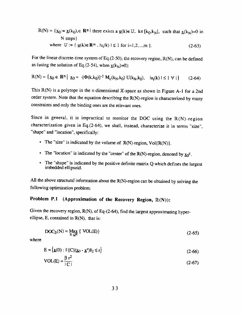
Problem P.1 (Approximation of the Recovery Region, _(N)):

Given the recovery region, R(N), of Eq-(2-64), find the largest approximating hyper-

ellipse, E, contained in R(N), that is:

where

DOC3(N) = EMa_ { VOL(E)}

E = {x(0)" II [C](_o - x¢)112< r}

VOL(E) = _r2ICI

(2-65)

(2-66)

(2-67)

33

/_n/213-

I_n2---_2)

R i s the recovery region, R(N)

C is an upper triangular matrix, whose diagonal elements Cii > O, for all i

_xc is the center of the recovery region

r is the radius of the hyperellipse

F(.) is the gamma function

(2-68)

Remark: (i). The DOC3 of Eq.(2-65) represents the approximate"size" of R(N).

(ii) The vector x c is the center of R(N).

(iii) The matrix C gives the shape of R(N), since Q = CTC is the positive definite

matrix defining the hyperellipse 1_.

An illustration of the solution of Problem P.1 is shown in Figure A.3 which show the

largest hyperellipse embedded in the R(N)-region for a 2nd order system.

Fact F3: The radius r of the hyperellipse Eof Eq. (2-66) gives an approximate value of

the gain G of linear system of Eq.(2-50). Moreover, the eigenvectors associated

with _,min of C-matrix gives the worst controllable directions of the system of

Eq.(2-50), namely the direction in which the influence the control action is

smallest as compare to the other directions.

A set of software was developed to solve the optimization problem of Problem P1. It is

described in Appendix A. This software investigates the robustness of linear time invariant

system, and determines the degree of controllability of the system under uncertainty d. The

function of the software is:

1. To solve the optimization problem Problem P1.

2. To graphically display the R.(N)-region in X-space of the LTI system.

3. To graphically display the regions of ft,-space of the LTI system.

4. To display the approximating hyperellipse to the R(N)-region in the X-space.

5. To display the approximate regions in the 5-space which are based on a

prescribed degree of controllability (DOC).

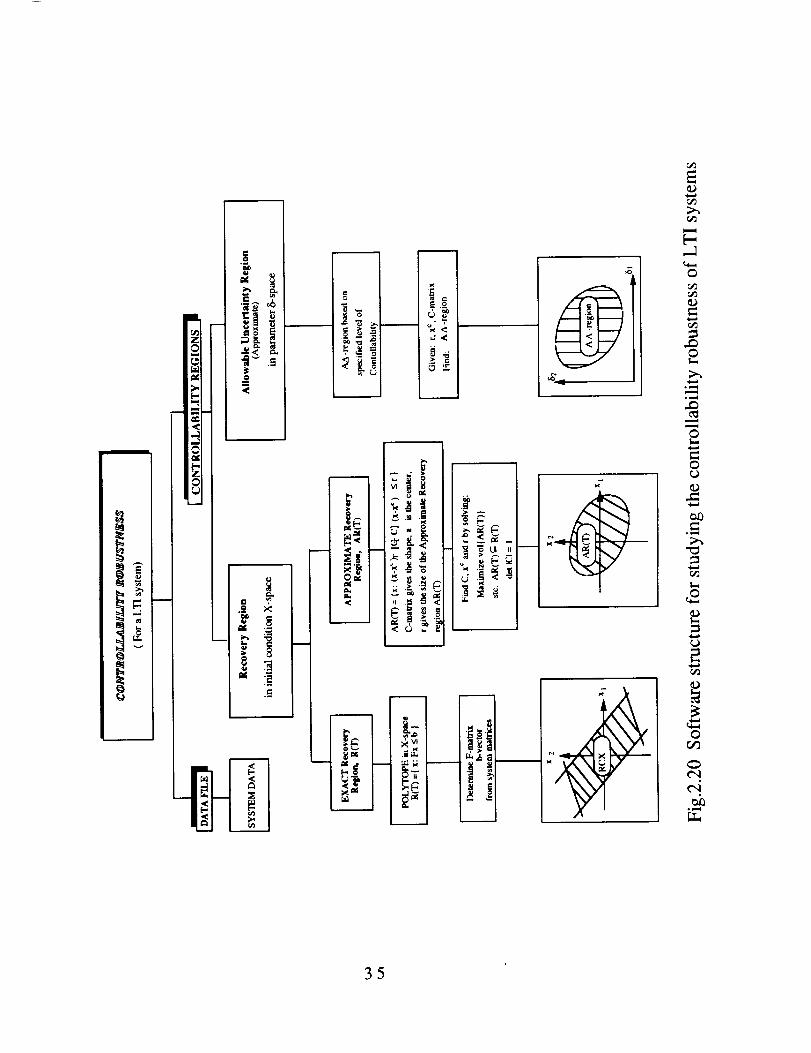
Figure 2.10 gives a structured diagram of this software and shows some of the specific

capabilities of the software. There are two main options of the controllability robustness

software One, investigates the recovery region while the other investigates the allowable

uncertainty region in the d-parameter space. Referring to Fig. 2.10, the branch denoted by

SYSDAT is the data file containing all the information about the LTIS and the parameter

34

m_

.o

I=o

I.<

i.2 x

'4" I

"" °I__'_

__ .:I

_ ._

"_t ,,

-_!._

[--

0

=

¢'4_g

35

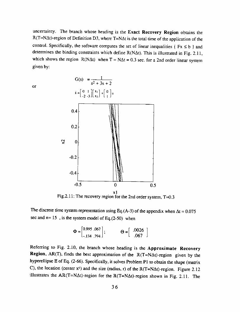
uncertainty. The branch whose heading is the Exact Recovery Region obtains the

R(T=NAt)-region of Definition D3, where T=NAt is the total time of the application of the

control. Specifically, the software computes the set of linear inequalities { Fx < b } and

determines the binding constraints which define R(NAt). This is illustrated in Fig. 2.11,

which shows the region _(NAt) when T = NAt = 0.3 sec. for a 2nd order linear system

given by:

or

G(s) - 1s 2 + 3s + 2

0.4

0.2

e,, 0

-0.2 I-O.4

-0.5 0 0.5

xl

Fig.2.11: The recovery region for the 2nd order system, T--0.3

The discrete time system representation using Eq.(A-3) of the appendix when At = 0.075

sec and n= 15 , is the system model of Eq.(2-50) when

o:r0995 o:E0026][-.134 .794 ' .067

Referring to Fig. 2.10, the branch whose heading is the Approximate Recovery

Region, AR(T), finds the best approximation of the R(T=NAt)-region given by the

hyperellipse E of Eq. (2-66). Specifically, it solves Problem P1 to obtain the shape (matrix

C), the location (center x c) and the size (radius, r) of the ]_(T=NAt)-region. Figure 2.12

illustrates the AR(T=NAt)-region for the _(T--NAt)-region shown in Fig. 2.11. The

36

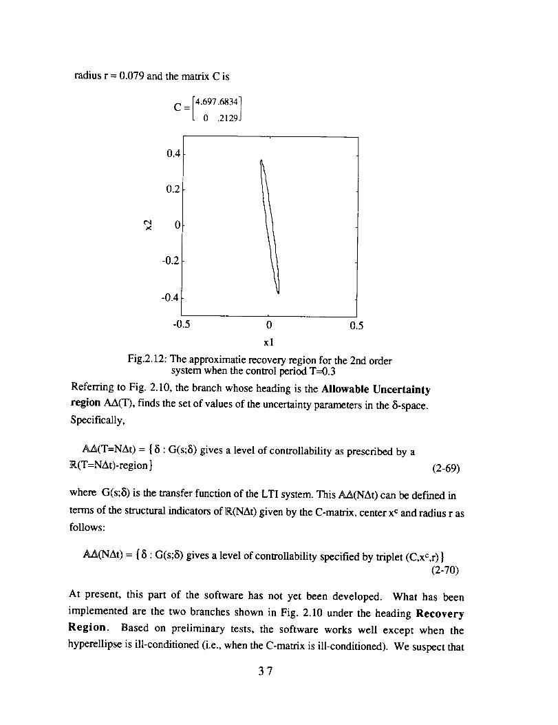
radiusr = 0.079andthematrixC is

C =[4.697.6834]L 0 .21293

0.4

0.2

0

-0.2

I

0 0.5

xl

Fig.2.12: The approximatie recovery region for the 2nd ordersystem when the control period T----0.3

Referring to Fig. 2.10, the branch whose heading is the Allowable Uncertainty

region AA(T), finds the set of values of the uncertainty parameters in the 8-space.

Specifically,

AA(T=NAt) = {8" G(s;8) gives a level of controllability as prescribed by a

R(T=NAt)-region } (2-69)

where G(s;8) is the transfer function of the LTI system. This A_(NAt) can be defined in

terms of the structural indicators of R(NAt) given by the C-matrix, center x c and radius r as

follows:

AA(NAt) = { 8" G(s;8) gives a level of controllability specified by triplet (C,xC,r) }

(2-70)

At present, this part of the software has not yet been developed. What has been

implemented are the two branches shown in Fig. 2.10 under the heading Recovery

Region. Based on preliminary tests, the software works well except when the

hyperellipse is ill-conditioned (i.e., when the C-matrix is ill-conditioned). We suspect that

37

this is dueto our choicesof theterminationconditionsin the(C,r) optimizationalgorithm

of Fig. A.3 andtheoveralloptimizationmethodof Fig.A.4 givenin AppendixA.

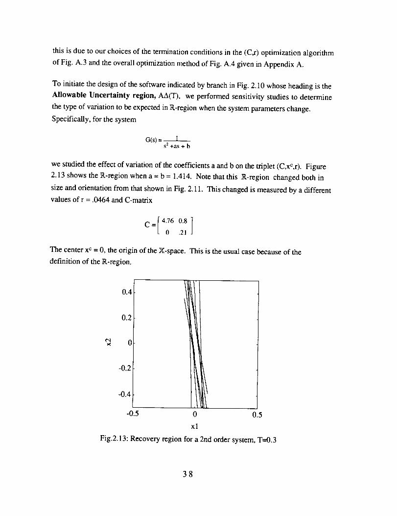
To initiate thedesignof thesoftwareindicatedbybranchin Fig. 2.10whoseheadingis theAllowable Uncertainty region, AA(T), weperformedsensitivitystudiesto determine

thetypeof variationto beexpectedinR-regionwhenthesystemparameterschange.

Specifically,for thesystem

G(s)= 1s 2 +a._ + b

we studied the effect of variation of the coefficients a and b on the triplet (C,xC,r). Figure

2.13 shows the k-region when a = b = 1.414. Note that this R-region changed both in

size and orientation from that shown in Fig. 2.11. This changed is measured by a different

values of r = .0464 and C-matrix

C=[4.76 0.8]o .21

The center x c = 0, the origin of the X-space. This is the usual case because of the

definition of the lK-region.

0.4

0.2

0

-0.2

0.5

xl

Fig.2.13: Recovery region for a 2nd order system, T---0.3

38

3. SUMMARY OF THE WORK

Task 1: Design of Robust Optimal Controllers via H" Approach

Task 1.1: Study of the aircraft flight guidance/control models and problems

provided by the Aircraft Guidance and Control Branch, NASA Langley

Research Center.

Status: In the process of obtaining appropriate practical aircraft flight

guidance/control models from AGCB scientists. Before the models arrive,

we use a hypothetical model with plant perturbations and uncertain

disturbances.

Accomplishment: A procedure to represent plant perturbations and uncertain

disturbances as H _ models is presented.

Task 1.2: Formulation of the aircraft flight guidance/control problems as a robust

H** optimization problem with unstructured and parametric uncertainties.

Status: Before the practical models arrive, a hypothetical model is used to

demonstrate how to formulate a robust H** optimization problem.

Accomplishment: A detailed procedure to formulate a robust H** optimization

problem is presented. See [Pub 1,2] for details.

Task 1.3: Computation of the H** norm of a given transfer function.

Status: 100% of the proposed work has been done. See [Pub 3] for details.

Accomplishment: The pole-zero diagram of G(s), the root locus concept, and

the jco-axis transmission zeros of _,2I-G'r(-s)G(s) are employed to quickly

locate a narrow frequency interval which brackets the supremum of

_[G(jto)]. Then Brent's method (an improved parabolic interpolation

search method) is employed to search for the supremum of _[G(j_)] over

the frequency interval.

Task 1.4: Solution of the robust H** optimization problem.

Status: 100% of the proposed work has been done. See [Pub 4,5,6] for details.

Accomplishment: Some useful properties of the two H** Riccati solutions have

been discovered. Among them, the most prominent one is that the spectral

radius of the product of these two Riccati solutions is a continuous,

nonincreasing, convex function of _/in the domain of interest. Based on

these properties, quadratically convergent algorithms are developed to

compute the optimal _ norm.

Task 1.5: Algorithm development for the computational problems arising in the

39

Task 1.6:

Status:

robust H °° optimization problem.

Status: 60% of the proposed work has been done. See [Pub 4-8] for details.

Accomplishment: The algorithm to compute the optimal H** norm and the

construction of an optimal or a suboptimal H °*controller are presented.

Computer simulation.

40% the proposed work has been done.

Accomplishment: The time-domain and frequency-domain behavior of the

closed-loop system for the hypothetical model has been tested.

Task 2: Design of Robust Optimal Controllers via Mixed H2/H _* Approach

Task 2.1: Formulation of the aircraft flight guidance/control problems provided by

the Aircraft Guidance and Control Branch, NASA Langley Research

Center as a mixed H2/H ** optimization problem with unstructured

uncertainties.

Status: In the process of obtaining appropriate practical aircraft flight

guidance/control models from AGCB scientists. Before the practical

models arrive, a hypothetical model is used to demonstrate how to

formulate an H**/I-I2 optimization problem.

Accomplishment: A procedure to formulate an H**/H 2 optimization problem is

presented. See [Pub 9-12] for details.

Task 2.2: Solution of the mixed H2/H **optimization problem.

Status: An important special case of the mixed H2/I-I **optimization problem has

been completely solved.

Accomplishment: In case that the H 2 and the H _' transfer functions are identical,

the mixed H2/H **problem can be solved by H** technique with 7 a free

parameter. Then 7 is used to trade off H** robustness against H 2

performance. See [Pub 9-12] for details.

Task 2.3: Plotting the HX/H **curve and using it for robust controller design.

Status: 80% of this study has been done.

Accomplishment: A graphical method to determine the best 7 for H** robustness

and H 2 performance is proposed. See [Pub 11,12] for details.

Task 2.4: Algorithm development for the computational problems arising in the he

mixed HX/H "* optimization problem.

Status: 40% of the proposed work has been done. See [Pub 11,12] for details.

40

Task 2.5:

Status:

Accomplishment: Algorithms to generate the H2/H ** curve and the construction

of an H2/H '' controller are presented.

Computer simulation.

40% the proposed work has been done.

Accomplishment: The time-domain and frequency-domain behavior of the

closed-loop system for the hypothetical model has been tested.

Task 3: Construction M-A Structure

Task 3.1: Construction of an M-A structure of a system with parametric

uncertainties for robust stability analysis.

Status: 100% of the proposed work has been done. See [Pub 16-17] for details.

Accomplishment: A systematic way of constructing an M-A structure of a

system with parametric uncertainties for robust stability analysis is

presented.

Task 3.2: Construction of an M-A structure of a system with parametric and

unmodelled uncertainties for robust stability analysis.

Status: 100% of the proposed work has been done. See [Pub 16-17] for details.

Accomplishment: A systematic way of constructing an M-A structure of a

system with parametric and unmodelled uncertainties for robust stability

analysis is presented.

3.3: Construction of an M-A structure of a system with parametric and

unmodelled uncertainties for robust stability and robust performance

analysis.

Status: 100% of the proposed work has been done. See [Pub 16-17] for details.

Accomplishment: A systematic way of constructing an M-A structure of a

system with parametric and unmodelled uncertainties for robust stability

and robust performance analysis is presented.

Verification of the minimality of an M-A structure of a system.

30% of the proposed work has been done. See [Pub 16-17] for details.

Accomplishment: We show that if the dimension of A is the least number of

assigned parameters such that the coefficients of the corresponding

characteristic polynomial are multilinear functions of the assigned

parameters, then the M-A structure is minimal.

Task

Task 3.4:

Status:

41

Task 3.5: Construction of a minimal M-A structure.

Status: 30% of the proposed work has been done. See [Pub 16-17] for details.

Accomplishment: For the case that the state-space realization is a linear function

of the uncertainties, a minimal M-A structure can be constructed in a

systematic way.

Task 4: Controllability and Observability of Perturbed Plant

Task 4.1: Controllability.

Status: 70% of the proposed work has been done.

Accomplishment: Developed (i) a software package for investigating the

controllability robustness of linear time invariant systems. This software

obtains the size, shape and location of the recovery region, and (ii)

relation between the various DOC measures encountered in the literature.

Task 4.2 Observability

Status: No work performed.

Task 4.3 Integration of Controllability and Observability Concepts intothe Overall Robust Controller design

Status: No work has been performed as yet.

Publications:

[Pub 1]

[Pub 2]

[Pub 3]

[Pub 4]

[Pub 5]

[Pub 6]

[Pub 7]

[Pub 8]

[Pub 9]

B. C. Chang, X. P. Li, S. S. Banda, and H. H. Yeh, "Robust Control

Systems Design by H_ Optimization Theory," Proceedings of the 1991 AIAAGuidance, Navigation, and Control Conference, Aug. 1991.X. P. Li, B. C. Chang, S. S. Banda, and H. H. Yeh, "Robust ControlSystems Design by H_* Optimization Theory," To appear in AIAA Journal ofGuidance, Control, and Dynamics.

B. C. Chang, X. P. Li, S. S. Banda and H. H. Yeh, "Computation of the H**Norm of a Transfer Function," Proceedings of the 1990 American Controlconference, pp. 2578-2582, San Diego, May, 1990.X.P. Li and B.C. Chang, "On Convexity of H** Riccati Solutions and ItsApplications," To appear in IEEE Transactions on Automatic Control.

X.P. Li and B.C. Chang, "On Convexity of H,,* Riccati Solutions," To appearin the Proceedings of IEEE Conference on Decision and Control, Dec. 1991.

X.P. Li and B.C. Chang, "Properties of H_ Riccati Equations," Proceedingsof the 1991 International Workshop on Robust Control, Sponsored by NSF,AFOSR, and Texas A & M, San Antonio, March, 1991.

B. C. Chang, X. P. Li, H. H. Yeh, and S. S. Banda, "Iterative Computation ofthe Optimal Hoo Norm By Using Two-Riccati-Equation Method, Proceedingsof IEEE Conference on Decision and Control, Dec. 1990.

B. C. Chang, X. P. Li, S. S. Banda, and H. H. Yeh, "Design of an HooOptimal Controller By Using DGKF's State-space Formulas", Proceedings ofIEEE Conference on Decision and Control, Dec. 1990.

H. H. Yeh, S. S. Banda, and B. C. Chang, "Necessary and Sufficient

42

[Pub 10]

[Pub 11]

[Pub 12]

[Pub 13]

[Pub 14]

[Pub15]

[Pub16]

[Pub 17]

Conditions for Mixed H 2 and H _0 Optimal Control," To appear in IEEETransactions on Automatic Control.

H. H. Yeh, S. S. Banda, and B. C. Chang, "Necessary and SufficientConditions for Mixed H2 and Hoo Optimal Control", Proceedings of IEEEConference on Decision and Control, Dec. 1990.

C. C. Belcastro, B. C. Chang, R. Zong, and R. Fischl, "Design of a

Suboptimal H _ Controller with H 2 and Bandwidth Constraints", Proceedingsof the 1991 American Control Conference, June 1991.

H. Bouguerra, B.C. Chang, H.H. Yeh, and S.S. Banda, "A Robust HooController Design with H2 Consideration," To appear in the Proceedings ofIEEE Conference on Decision and Control, Dec. 1991.

H. Bouguerra, B. C. Chang, H. H. Yeh, and S. S. Banda, "Fast StabilityChecking for the Convex Combination of Stable Polynomials," IEEETransactions on Automatic Control, Vol. 35, No. 5, pp. 586-588, May 1990.B. C. Chang, O. Ekdal, H. H. Yeh, and S. S. Banda, "Computation of theReal Structured Singular Value via Polytopic Polynomials," AIAA Journal ofGuidance, Control, and Dynamics, Vol. 14, No. 1, pp. 140-147, Jan. 1991.O. Ekdal and B. C. Chang, "Robust Stability Analysis of Real Structured

Uncertain Systems", Proceedings of the 1 lth IFAC (International Federation ofAutomatic Control) World Congress, Aug. 1990, Tallinn, USSR.C. C. Belcastro, B. C. Chang, and R. Fischl, "A Methodology for Formulatinga Minimal Uncertainty Model for Robust Control System Design and Analysis",Proceedings of the 3rd Annual Conference on Aerospace ComputationalControl, pp.355-369, December, 1989.C. C. Belcastro, B. C. Chang, and R. Fischl, "On the Formulation of aMinimal Uncertainty Model for Robust Control with Structured Uncertainty,"NASA Technical Paper 3094, Sept. 1991.

4. CONCLUSION AND WORK FOR FUTURE RESEARCH

4.1 Conclusion

In [Pub 4] we revealed several important eigen properties of the stabilizing

solutions of the two H** Riccati equations and their product. Among them, the most

prominent ones are: (1) p[X**(y)Y**(y)] is a nonincreasing, convex function of Y on (13,+"0).

(2) _,min[_('_/)] is a nondecreasing, concave function of y on (O_x,+O*). (3) _0') is invertible

almost everywhere on (Ctx,+**). Based on these properties, quadratically convergent

algorithms [Pub 5,6] were developed to compute the %., the optimal I-I**norm, such that

p[X**0',.)Y**(y**)] = 1,2 and to compute [3, the infimum of 1' such that the two H** Riccati

equations have positive semidefinite stabilizing solutions.

The formulation of the standard H** optimization problem, an easy way of

constructing a state-space realization of the generalized plant, an efficient algorithm for

computing the optimal H** norm, and a modified version of Glover and Doyle formulas for

constructing an optimal controller were addressed in the paper [Pub 2]. No numerical

43

difficulty will arisein constructinganH_ optimalcontrollerif we areallowed a proper

controller.In mostapplications,wemaylike to haveastrictlypropercontrollerwith limited

bandwidth.In thiscase,a trade-offbetweentheH**performanceandthebandwidthshould

bemadeby degradingthe H_ norm from its optimumin order to reducethe controllerbandwidth.

In [Pub 11], we found an easy way to trade off the H" robustnessand H2

performance for the case that H _ and H 2 transfer functions are the same. In general, these

two transfer functions may be different. In [Pub 12], we formulated a more realistic control

problem with H 2 performance index and H °_ stability robustness constraint into a mixed

H2/H _ problem. No optimal solution yet is available for this more general mixed H2]H °°

problem. Although the optimal solution for this mixed H2/H °° control has not yet been

found, we proposed a design approach which can be used through proper choice of the

available design parameters to influence both robustness and performance.

The theoretical work in controllability on developing a relation between the various

degree of controllability (DOC) measures encountered in the literature, indicates that there is

a relation and what is needed now to establish the specific relations. The simulation work

concentrated on developing software for investigating the controllability robustness of

linear time invariant systems. A preliminary software package (described in Appendix A)

was developed for measuring the size, shape and location of the recovery region. Initial

indications show that the various optimization algorithms (needed to automatically obtain

the value of the indicators) work, however they may need some refinements in order to take

care of such problems as obtaining DOCs for ill-conditioned recovery regions.

4.2 Work for Further Research

4.2.1 M-A Structure and Robust Stability Analysis for Structured

Uncertainties

M-A structure is a rearrangement of a perturbed system where M(s) is the nominal

system and A is a block diagonal matrix which consists of all the perturbations. M-A

structure is essential in the SSV(structured singular value) analysis and design techniques.

Although A is assumed stable, the M-A structure can handle a large class of uncertainties

which include unstable perturbation, i.e., the number of unstable poles of the perturbed

plant can be different from that of the nominal plant. It is always possible to pull out all

uncertain parts from a perturbed system and form an M-A structure. However, very little

about how to obtain this structure has been addressed in the literature. A systematic

44

procedurefor constructingM-A structureisproposed.

A minimal M-A structuremeansthat the dimensionof A (or M) of the M-A

structure is minimal. We can construct an M-A structure for a given perturbed system, but

the dimension of the structure may be unnecessarily large. A nonminimal structure will

cause unnecessary complexity in computation and therefore a minimal M-A structure is

essential in the computation of the SSV. So far, only some special cases of the minimal M-

A structure problems have been addressed [37,38]. A progress in the construction of a

minimal M-A structure will greatly simplify robust stability analysis for structured

uncertainties.

4.2.2 Design of Robust Flight Control Systems via H _ Optimization

In this research period, we developed a fast algorithm to compute the optimal H _

norm and to construct an optimal H_ controller without numerical difficulty. Next, we will

apply this design tool to flight control systems. We will use the H _ norm of the

complementary sensitivity function as a measure of robust stability and will formulate an

H_ optimization problem which minimizes the maximum error energy subject to a robust

stability constraint. The error reduction and the robust stability can be traded off by

choosing the weighting matrices in the cost function. Initially, a weighting matrix is chosen

and the corresponding H _ optimization problem is solved to obtain an optimal controller.

The weighting matrices are modified iteratively until the robust stability constraint is just

satisfied. The way the weighting matrices affect the trade-off is only partially understood.

In addition to the magnitude of the weighting matrix, the structure of the weighting matrix

is also an important factor in the trade-off. We will investigate how the weighting matrices

affect the trade-off. We will also develop an iterative updating procedure for the weighting

matrices by which a robust controller can be designed such that the closed-loop system is

robustly stable and the maximum of error energy is minimized.

4.2.3 Design of Robust Controllers via Mixed H2/H - Optimization

The optimal H°° controller which minimizes the H°° optimization problem usually

has wide bandwidth and leads to a poor H2 performance. In [ 13], we found that a little bit

sacrifice of the H a norm will greatly reduce the bandwidth of the controller and improve the

H2 performance tremendously. It is practical to formulate a robust control problem as a that

of minimizing an H 2 cost function subject to an H_ bound. The H 2 cost function is

equivalent to the well known LQG cost function and the H - bound can take care of robust

stability and robust error reduction.

45

In [39], we formulated a more realistic control problem with H 2 performance index

and H °° stability robustness constraint into a mixed H2/H °° problem. The H 2 and H-

transfer functions are different. No optimal solution yet is available for this more general

mixed H2/I-I °° problem. A research in finding an efficient approach for the mixed H2/I-t .0

optimization problem is proposed.

4.2.4 Controllability and Observability of Perturbed Plant

For task 4 in the next research period we will concentrate on: (i) Theoretical work

on developing a relation between the various DOC measures encountered in the literature,

and determine which of these is most suitable for characterizing the Allowable

Uncertainty region, AA(T), discussed in Section 2.6. (ii) Improving the algorithms

used in developing the Recover Region software shown in Fig. 2.10 Specifically, we will

take care of the ill-conditioning problem currently encountered when the recovery region is

very narrow. We will also design and develop the Allowable Uncertainty region,

AA(T), software indicated in Fig. 2.10. (iii) Perform robustness studies for a variation in

the system parameters (c i } and {bj } of the system function

ZbjsjG(s) -

cisi

REFERENCES

Ill J. Doyle, K. Glover, P. Khargonekar, and B. Francis, "State-space solutions to

standard H** and H 2 control problems," IEEE Trans. Automat. Contr., Vol. AC-34,

pp. 831-847, 1989.

[2] K. Glover and J. Doyle, "State-space formulae for all stabilizing controllers that

satisfy an H** norm bound and relations to risk sensitivity," Syst. Contr. Lett., Vol.

11, pp. 167-172, 1988.

[3] Carsten Scherer, "H**-control by state-feedback and fast algorithms for the

computation of optimal H,-norms," IEEE Trans. Automat. Contr., Vol. AC-35, pp.

1090-1099, 1990.

[4] P. Pandey, C. Kenny, A. Laub, and A. Packard, "Algorithms for computing the

optimal H**-norm," Proceedings of the 29th Conference on Decision and Control,

Dec. 1990.

[5] B.C. Chang, X. P. Li, S. S. Banda, and H. H. Yeh, "Iterative computation of the

optimal H** norm by two-Riccati-equtions method," Proceedings of the 29th

Conference on Decision and Control, Dec. 1990.

46

[10]

[11]

[12]

[6] J. Doyle, "Analysis of Feedback Systems with Structured Uncertainties," lEE

Proceedings, Vol. 129 Pt.D, No.6, 1982, pp. 242-250.

[7] J. Doyle, "Structured Uncertainty in Control System Design," Proceedings of the

24th Conference on Decision and Control, Dec. 1985.

[8] J.C. Doyle and G. Stein, "Robustness with observers," IEEE Trans. Aut. Cont.,

vol. AC-24, pp. 607-611, Apr. 1979.

[9] G. Stein and M. Athans, ' The LQGFLTR procedure for multivariable feedback

control design, ' IEEE Trans. Aut. Contr., Vol. AC-32, pp. 427-429, 1987.

G. Zames, "Feedback and Optimal sensitivity: Model reference transformations,

multiplicative seminorms, and approximate inverses, " IEEE Trans. Aut. Contr., vol.

AC-26. pp 301-320, 1981.

D. S. Bernstein and W. M. Haddad, " LQG Control with H °° Performance Bound,"

IEEE Trans. Aut. Cont., vol. AC-34, no. 3, March 1989.

K. Zhou, J.C. Doyle, K. Glover and B. Bodenheimer, "Mixed H 2 and H °° Control,

" Proc. of the 1990 American Control Conference, San Diego, CA pp. 2502-2507.

[13] M. Belcastro, B-C Chang, R. Zong and R. Fischl, " H °_ control with bandwidth and

H 2 constraints, " 1991 American Control Conference.

[14] D. Mustafa, "Relations between maximum-entropy/ H o° control and combined

H°°/LQG control, " Systems & Control Letters 12 (1989), pp. 193-203.

[15] R.E. De Gaston and M.G. Safonov, "Exact Calculation of the Multiloop Stability

Margin", IEEE Trans. A-C. AC-33, pp. 156-171, 1988.

[16] R.S.S. Pena and A. Sidefis, "A General Program to Compute the Multivariable

Stability Margin for Systems with Parametric Uncertainty", Proceedings of the 1988

American Control Conference.

[17] V. L. Kharitonov, "Asymptotic Stability of an Equilibrium Position of a Family of

Systems of Linear Differential Equations", Differential'nve Uraveniya. Vol. 14, No.

11, pp. 1483-1485, 1978.

[18] A.C. Bartlett, C.V. Hollot, and H. Lin, "Root Locations on an Entire Polytope of

Polynomials: It Suffices to Check the Edges", Proceedings of the 1987 American

Control Conference.

[19] M. Fu and B.R. Barmish, "Stability of Convex and Linear Combinations of

Polynomials and Matrices Arising in Robustness Problems", Proceedings of the

Conference on Information Sciences and Systems, John Hopkins University, 1987.

[20] S. Bialas, "A Necessary and Sufficient Condition for the Stability of Convex

Combinations of Stable Polynomials or Matrices", Bulletin of the Polish Academy of

Sciences, Technical Sciences, Vol. 33, No. 9-10, pp.473-480, 1985.

47

[31]

[32]

[33]

[21] K.H. Wei and Yedavalli, "Invariance of Strict Hurwitz Property for Uncertain

Polynomials with Dependent Coefficients", IEEE Trans. A-C. AC-_2, pp. 907-909,

1987.

[22] L.H. Keel, S.P. Bhattacharyya, and J.W. Howze, "Robust Control with Structured

Perturbations", IEEE Trans. A-C. AC-3_, pp. 68-78, 1988.

[23] H. Bouguerra, B-C Chang, H.H. Yeh, and S.S. Banda, "A Fast Algorithm for

Checking the Stability of Convex Combinations of Stable Polynomials", Proceedings

of the 28th IEEE Conference of Decision and Control, Dec. 1989.

[24] H. Kwakernaak, "Minimax Frequency Domain Performance and Robustness

Optimization of Linear Feedback Systems,"lEEE Transactions on automatic control,

Vol. AC-30, Oct. 1985, pp.994-1004.

[25] K. Glover, D.J.N. Limebeer, J.C. Doyle, E.M. Kasenally, and M.G. Safonov, "A

Characterization of All Solutions to the Four Block General Distance Problem,"

Preprint, 1989.

[26] B. C. Chang, X. P. Li, S. S. Banda, and H. H. Yeh, "Design of an H** optimal

controller by using DGKF's state-space formulas," Proceedings of the 29th

Conference on Decision and Control, Dec. 1990.

[27] I. Postlethwaite, D.-W. Gu, and S. D. O'Young, "Some computational results on

size reduction in H_, design", IEEE Trans. Automat. Contr., Vol. 33, pp. 177-185,

1988.

[28] Sevaston, G.E. and Longman, R.W.: " Gain measures of controllability and

observability," International Journal of Control, Vol. 41, No.4, p.865-893, 1985

[29] Muller, P.C. and Weber, H.I. : "Analysis and optimization of certain qualities of

controllability and observability for linear dynamic systems", Automatica, Vol.8,

p.237,1979

[30] Ham, F.M."Determination of the Degree of Observability in Linear Control

Systems", Ph.D. Diss., Ohio State University, 1980.

Viswanathan, C.N., Longman, R.W. and Likins, P.W. : "A degree of controllability

definition : Fundamental concepts and application of model system," Journal of

Guidance, Contr. and Dynamics, Vol. 7, p.222, Mar.-Apr., 1984

Longman, R.W. and Alfriend, K.T.," Energy Optimal Degree of Controllability and

Observability For Regulator and Manual Problems."Proc.. of the Sixteenth Annual

Conference On Information Sciences and Systems, Princeton, N.J., March, 1982.

Lindburg, R.E. and Longman, R.W.,"Optimization of Actuator Placement Via

Degree of Controllability Criteria Including Spillover Consideration," AIAA/AAS

Paper 82-1435, San Diego, California, 1982.

48

[34] Laskin, R.A., Longman,R.W., and Likins, P.W., "Actuator Placementin Modal

SystemsUsingFuelOptimalDegreeof ControllabilityConcepts."Proc.. of The 20_

Annual Allerton Conference on Communication. Control and Compofng, Monticello,

ILL, October, 1982.

[35] Schmitendorf, W.E., "An Exact Expression for Computing the Degree of

Controllability." Journal of Guidance. Control and Dynamics. Vol. 7, pp. 502-504,

July-August 1984.

[36] Sokolowski, S.J. and Fischl, R. : "An algorithm for computing the degree of

controllability of a discrete time, bounded input, regulator problem", Proceedings of

the 1986 ACC.

[37] C. C. Belcastro, B. C. Chang, and R. Fischl, "A Methodology for Formulating a

Minimal Uncertainty Model for Robust Control System Design and Analysis",

Proceedings of the 3rd Annual Conference on Aerospace Computational Control,

pp.355-369, December, 1989.

[38] C.C. Belcastro, B. C. Chang, and R. Fischl, "On the Formulation of a Minimal

Uncertainty Model for Robust Control with Structured Uncertainty," NASA

Technical Paper 3094, Sept. 1991.

[39] H. Bouguerra, B.C. Chang, H.H. Yeh, and S.S. Banda, "A Robust Hoo Controller

Design with H2 Consideration," To appear in the Proceedings of IEEE Conference

on Decision and Control, Dec. 1991.

49

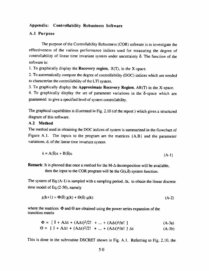
Appendix: Controllability Robustness Software

A.1 Purpose

The purpose of the Controllability Robustness (COR) software is to investigate the

effectiveness of the various performance indices used for measuring the degree of

controllability of linear time invariant system under uncertainty c5. The function of the

software is:

1. To graphically display the Recovery region, R(T), in the X-space.

2. To automatically compute the degree of controllability (DOC) indices which are needed

to characterize the controllability of the LTI system.

3. To graphically display the Approximate Recovery Region, AR(T) in the X-space.

4. To graphically display the set of parameter variations in the _i-space which are

guaranteed to give a specified level of system controllability.

The graphical capabilities is illustrated in Fig. 2.10 (of the report ) which gives a structured

diagram of this software.

A.2 Method

The method used in obtaining the DOC indices of system is summarized in the flowchart of

Figure A.1. The inputs to the program are the matrices {A,B} and the parameter

variations, d, of the linear time invariant system

= A(8)x + B(_i)u (A-l)

Remark: It is planned that once a method for the M-A decomposition will be available,

then the input to the COR program will be the G(s,8) system function.

The system of Eq.(A-1) is sampled with a sampling period, At, to obtain the linear discrete

time model of Eq.(2-50), namely

x(k+ 1) = _(8) x(k) + O(5) u(k) (A-2)

where the matrices _ and O are obtained using the power series expansion of thetransition matrix

= [I+AAt+(AAt)2/2! +...+(AAt)n/n! ]

O= [ I+AAt + (AAt)2/2[ +... +(AAt)n/n[ ] At

(A-3a)

(A-3b)

This is done in the subroutine DSCRET shown in Fig. A. 1. Referring to Fig. 2.10, the

50

programwhich computestheRecovery Region, R(T=NAt), implements the definition

of Eq.(2-64) and computes a set of linear inequalities { Fx < b} and then identifies those

constraints which are the binding constraints of R(NAt). This is implemented in subroutine

CONTRG shown in Fig. A. 1.

The Approximate Recovery Region, AR(T), software solves the optimization

Problem P1 to obtain the shape (matrix C), the location (center x c) and the size (radius, r)

of the g(T=NAt)-region and then uses this to define the largest embedded hyperellipse in

the _R(T=NAt)-region. The subroutine which executes the solution of Problem P1 is

labeled ELLIPSE in Fig. A.1. The approach to solving Problem P1 is based on the

realization that when the matrix C is given then Problem P1 is a Linear Problem (LP)

problem. This is exploited in our method as summarized in Fig. A.2. The first step is to

set up the linear constraints. Then, depending on if we want to obtain a new matrix C or

not we solve either an Linear Problem (LP) problem or a Non Linear Problem (NLP), that

is:

LP problem finds the optimum center, x c, and radius, r, for a given matrix C. The

LP problem solves a volume maximization problem in which the embedding hyperellipse E

shape is held constant but its size (i.e., volume of Eq.(2-66)) is maximized by increasing

the radius, r, and moving it around inside R (by moving the center, xc) while satisfying the

constraint E _ R.

NLP problem finds the matrix C and radius r for a given center xc. It solves the

same volume maximization problem of Eq.(2-66), when the center x c is fixed. The C-

matrix and r are optimized by a sequential unconstrained minimization (SUM) method. The

method minimizes an objective function _ which is a _ norm of a vector representing the

slack variable of the inequalities. The details of the updating method is shown in Fig. A.3.

The optimum is found by computing the gradient of "fk with respect to tij, the components

of the inverse of the C matrix (T=C-1). (The reason for using T instead of C in the

optimization is because the SUM method has better convergent properties.)

The method for optimizing all three sets of parameters, i.e. C-matrix, x c and r is

shown in Figure A.4. Note that it uses both the NL and the NLP algorithms to solve the

optimization problem stated in Problem P1. The subroutine implementing the optimization

algorithm shown in Fig. A.4 is called ELLIPSE.

51

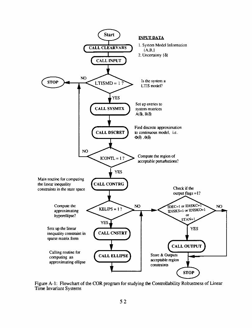
STOPNO

Start

CALL CLEARVARS

CALL _PUT

IIXg.UZ.I2A._

1. System Model Information{A.B,}

2.Uncertainty{8}

_,rrc_,,fr-, 1 Is the system a

_ LTIS model?YES

Set up entries to

] t LALLaltaMIA ! system matrices

[ _ Find discrete approximation[ [ CALL D_CRET _ tO continuous model, i.e.

_ acceptable perturbations?

Main routine for computing

the linear inequality

constraints in the state space Check if the

output flags = 1?

Compute the

approximating

hyperellipse?

Sets up the linear

inequality constraint in

sparse matrix form

Calling routine for

computing anapproximating ellipse

KELIPS = 1 ?

CALL

NO Or

IDISKS=I or IDISKO=Ior

NO

YES

CALL OUTPUT

Store & Outputs

acceptable regionconstraints

STOP

Figure A-l: Flowchart of the COR program for studying the Controllability Robustness of LinearTime Invariant Systems

52

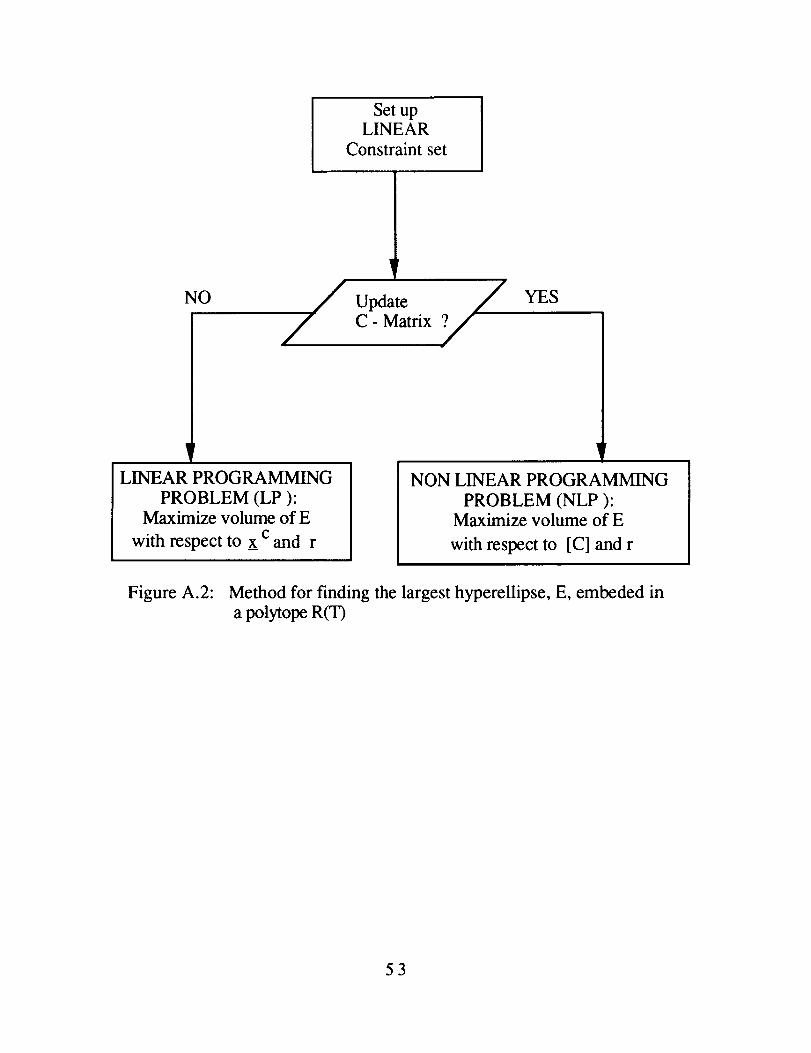
Set upLINEAR

Constraint set

NO

Update ?_ YESC- Matrix

LINEAR PROGRAMMING

PROBLEM (LP):Maximize volume of E

with respect to x c and r

NON LINEAR PROGRAMMING

PROBLEM (NLP):Maximize volume of E

with respect to [C] and r

Figure A.2: Method for finding the largest hyperellipse, E, embeded ina polytope R(T)

53

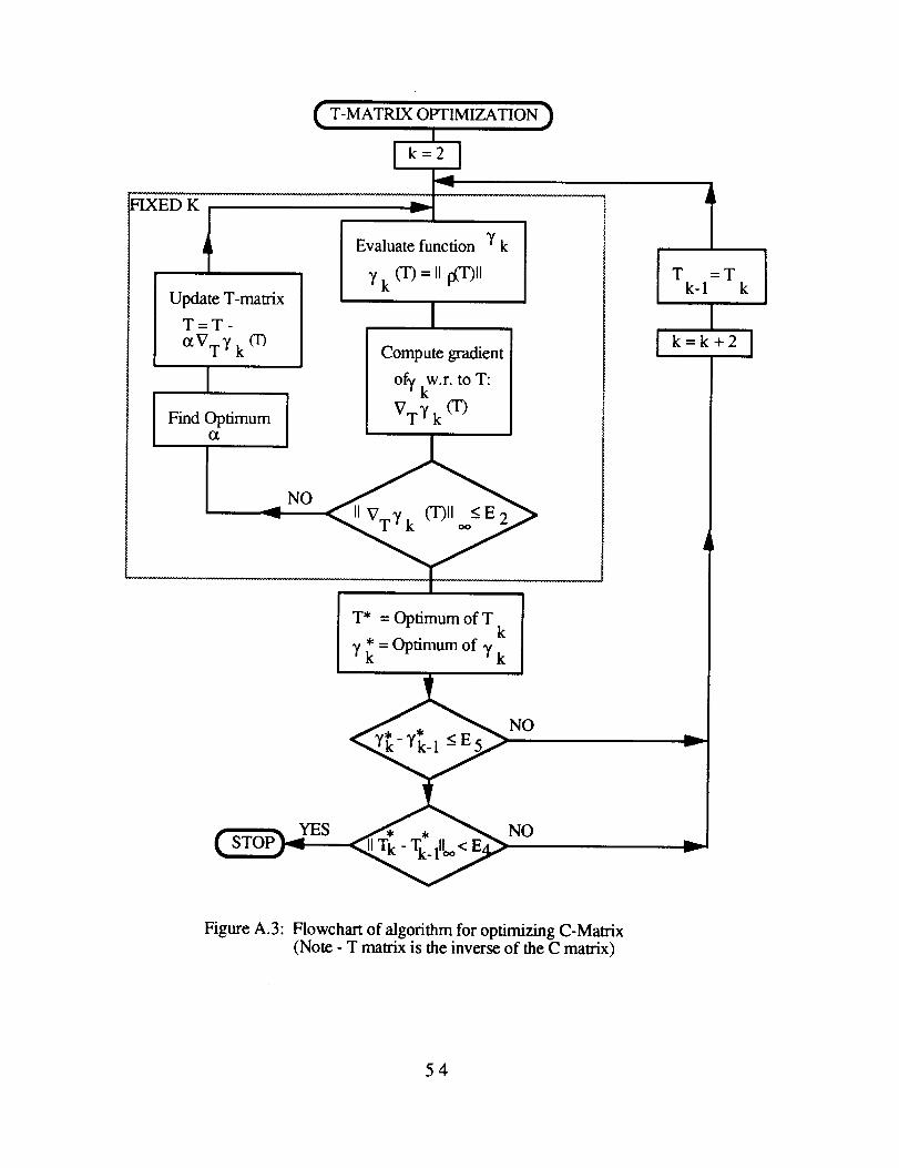
T-MATRIX OPTIMIZATI(

FIXED K

Update T-matrix

T=T -

°_VTY k 03

IFind Optimum

k=2

Evaluate function _/k

=, ga3,Yk

ICompute gradient

of T w.r. to T:k

VTYk (T)

NO

T* = Optimum of Tk

* = Optimum of7 k 7 k

T =T Ik-1 k

Ik=k+2

YES

NO

NO

h,..._

v

Figure A.3: Flowchart of algorithm for optimizing C-Matrix(Note - T matrix is the inverse of the C matrix)

54

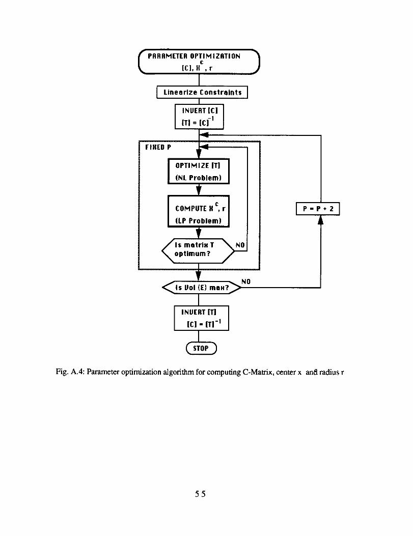
PARAMETER OPTIMIZATION )c

[C], X , r

II Linearize Constraints

I

I INVERT[C] I[TI = [CI-I

V_

OPTIMIZE IT] I(NL Problem)

cCOMPUTE X , r

(LP Problem)

V

FIXED P

1

Is matrix T

optimum?

_ itll

_Is Vol {E} max?_ NO

I

[C] = [TI -t

i P=P+2 i

Fig. A.4: Parameter optimization algorithm for computing C-Matrix, center x and radius r

55