Available online at www.sciencedirect.comCOMPUTER

Computer Speech and Language 24 (2010) 77–93

www.elsevier.com/locate/csl

SPEECH AND

LANGUAGE

A computational auditory scene analysis system for speechsegregation and robust speech recognition

Yang Shao a,*, Soundararajan Srinivasan b,1, Zhaozhang Jin a, DeLiang Wang a,c

a Department of Computer Science and Engineering, The Ohio State University, Columbus, OH 43210, USAb Biomedical Engineering Department, The Ohio State University, Columbus, OH 43210, USA

c Center for Cognitive Science, The Ohio State University, Columbus, OH 43210, USA

Received 5 July 2007; received in revised form 17 January 2008; accepted 3 March 2008Available online 28 March 2008

Abstract

A conventional automatic speech recognizer does not perform well in the presence of multiple sound sources, whilehuman listeners are able to segregate and recognize a signal of interest through auditory scene analysis. We present a com-putational auditory scene analysis system for separating and recognizing target speech in the presence of competing speechor noise. We estimate, in two stages, the ideal binary time–frequency (T–F) mask which retains the mixture in a local T–Funit if and only if the target is stronger than the interference within the unit. In the first stage, we use harmonicity to seg-regate the voiced portions of individual sources in each time frame based on multipitch tracking. Additionally, unvoicedportions are segmented based on an onset/offset analysis. In the second stage, speaker characteristics are used to group theT–F units across time frames. The resulting masks are used in an uncertainty decoding framework for automatic speechrecognition. We evaluate our system on a speech separation challenge and show that our system yields substantialimprovement over the baseline performance.� 2008 Elsevier Ltd. All rights reserved.

Keywords: Speech segregation; Computational Auditory Scene Analysis; Binary time–frequency mask; Robust speech recognition; Un-certainty decoding

1. Introduction

In everyday listening conditions, the acoustic input reaching our ears is often a mixture of multiple concur-rent sound sources. While human listeners are able to segregate and recognize a target signal under such con-ditions, robust automatic speech recognition remains a challenging problem (Huang et al., 2001). Automaticspeech recognition (ASR) systems are typically trained on clean speech and face the mismatch problem when

0885-2308/$ - see front matter � 2008 Elsevier Ltd. All rights reserved.doi:10.1016/j.csl.2008.03.004

* Corresponding author.E-mail addresses: shaoy@cse.ohio-state.edu (Y. Shao), srinivasan.36@osu.edu (S. Srinivasan), jinzh@cse.ohio-state.edu (Z. Jin),

dwang@cse.ohio-state.edu (D. Wang).1 Present address: Research and Technology Center, Robert Bosch LLC, Pittsburgh, PA 15212, USA.

78 Y. Shao et al. / Computer Speech and Language 24 (2010) 77–93

tested in the presence of interference. In this paper, we address the problem of recognizing speech from a targetspeaker in the presence of either another speech source or noise.

To mitigate the effect of interference on recognition, speech mixtures can be preprocessed by speech sepa-ration algorithms. Under monaural conditions, systems typically depend on modeling the various sources inthe mixture to achieve separation (Ephraim, 1992; Jang and Lee, 2003; Kristjansson et al., 2004; Roweis, 2005;Raj et al., 2005). An alternate approach to employing speech separation prior to recognition involves the jointdecoding of the speech mixture based on knowledge of all the sources present in the mixture (Varga andMoore, 1990; Gales and Young, 1996; Deoras and Hasegawa-Johnson, 2004). These model-based systems relyheavily on the use of a priori information of sound sources. Such approaches are fundamentally limited in theirability to handle novel interference (Allen, 2005). For example, systems that assume and model the presence ofmultiple speech sources only, do not lend themselves easily to handling speech in (non-speech) noiseconditions.

In contrast to the above model-based systems, we present a primarily feature-based computational auditoryscene analysis (CASA) system that makes weak assumptions about the various sound sources in the mixture. Itis believed that the human ability to function well in everyday acoustic environments is due to a process termedauditory scene analysis (ASA), which produces a perceptual representation of different sources in an acousticmixture (Bregman, 1990). In other words, listeners organize the mixture into streams that correspond to differ-ent sound sources in the mixture. According to Bregman (1990), organization in ASA takes place in two mainsteps: segmentation and grouping. Segmentation decomposes the auditory scene into groups of contiguoustime–frequency (T–F) units or segments, each of which mainly originates from a single sound source (Wangand Brown, 2006). A T–F unit denotes the signal at a particular time and frequency. Grouping involves com-bining the segments that are likely to arise from the same source together into a single stream (Bregman, 1990).Grouping itself is comprised of simultaneous and sequential organizations. Simultaneous organization involvesgrouping of segments across frequency, and sequential organization refers to grouping across time.

From an information processing perspective, the notion of an ideal binary T–F mask has been proposed asa major computational goal of CASA by Wang (2005). Such a mask can be constructed from the a priori

knowledge of target and interference; specifically a value of 1 in the mask indicates that the target is strongerthan the interference within the corresponding T–F unit and 0 indicates otherwise. The use of ideal binarymasks is motivated by the auditory masking phenomenon in which a weaker signal is masked by a strongerone within a critical band (Moore, 2003). Additionally, previous studies have shown that such masks can pro-vide robust recognition results (Cooke et al., 2001; Roman et al., 2003; Srinivasan et al., 2006; Srinivasan andWang, 2007). Hence, we propose a CASA system that estimates this mask to facilitate the recognition of targetspeech in the presence of interference. When multiple sources are of interest, the system can produce ideal bin-ary masks for each source by treating one source as target and the rest as interference.

In this paper, we present a two-stage monaural CASA system that follows the ASA account of auditoryorganization as shown in Fig. 1. The input to the system is a mixture of target and interference. The inputmixture is analyzed by an auditory filterbank in successive time frames. The system then generates segmentsbased on periodicity and a multi-scale onset and offset analysis, producing voiced and unvoiced segmentsrespectively (Hu and Wang, 2006). In the simultaneous grouping stage, the system estimates pitch tracks ofindividual sources in the mixture and employs periodicity similarity to group voiced segments into simulta-neous streams. A simultaneous stream comprises multiple segments that overlap in time. Subsequently, asequential grouping stage employs speaker characteristics to organize simultaneous streams and unvoiced seg-ments across time into whole streams corresponding to individual speaker utterances. Within this stage, wefirst sequentially group simultaneous streams corresponding to voiced speech and then unvoiced segments.Finally, the CASA system outputs an estimate of the ideal binary mask corresponding to an underlyingspeaker in the input mixture. Such a mask is then used in an uncertainty decoding approach to robust speechrecognition (Srinivasan and Wang, 2007). This approach reconstructs missing feature components as indicatedby the binary masks, and also incorporates reconstruction errors as uncertainties in the speech recognizer.Finally, in the case of multiple speech sources, a target selection process is employed for identifying the targetspeech.

The rest of the paper is organized as follows. Sections 2–5 provide a detailed presentation of the variouscomponents of our proposed system. The system is systematically evaluated on a speech separation challenge

Multipitch Tracking&

Voiced segmentation

Onset/offset BasedSegmentation

Au

dito

ryF

ront

-en

d UncertaintyDecoding

Speech Mixture

Segmentation c Grouping

TargetTranscript

SimultaneousStreams Binary Masks

Target Selection

Voiced SequentialGrouping

Unvoiced Grouping

SimultaneousGrouping

Recognition

Fig. 1. Schematic diagram of the proposed two-stage CASA system and its application to ASR. The auditory front-end decomposes inputsignal into a T–F representation called a cochleagram (see Section 2). In the segmentation stage, our system generates both voicedsegments and unvoiced segments. Then in the grouping stage, a simultaneous grouping process uses periodicity similarity to group voicedcomponents and produces simultaneous streams. Subsequently, a sequential grouping algorithm organizes these simultaneous streams andunvoiced segments across time. The resulting binary T–F masks are used by an uncertainty decoder and a target selection mechanism torecognize the target utterance.

Y. Shao et al. / Computer Speech and Language 24 (2010) 77–93 79

(SSC) task that involves the recognition of a target speech utterance in the presence of either a competingspeaker or speech-shaped noise (Cooke and Lee, 2006) The evaluation results are presented in Section 6.Finally, conclusions and future work are given in Section 7.

2. Auditory based front-end

Our system first models auditory filtering by decomposing an input signal into the time–frequency domainusing a bank of Gammatone filters. Gammatone filters are derived from psychophysical observations of theauditory periphery and this filterbank is a standard model of cochlear filtering (Patterson et al., 1992) Theimpulse response of a Gammatone filter centered at frequency f is:

gðf ; tÞ ¼ ta�1 e�2pbt cosð2pftÞ; t P 0:

0; else;

�ð1Þ

t refers to time; a ¼ 4 is the order of the filter; b is the rectangular bandwidth which increases with the centerfrequency f. We use a bank of 128 filters whose center frequency f ranges from 50 Hz to 8000 Hz. These centerfrequencies are equally distributed on the ERB scale (Moore, 2003) and the filters with higher center frequen-cies respond to wider frequency ranges.

Since the filter output retains original sampling frequency, we down-sample the 128 channel outputs to100 Hz along the time dimension, which includes low-pass filtering and decimation. This yields the corre-sponding frame rate of 100 Hz, which is used in many short-term speech feature extraction algorithms (Huanget al., 2001). The magnitudes of the down-sampled outputs are then loudness-compressed by a cubic rootoperation. The resulting responses compose a matrix, representing a T–F decomposition of the input. We callthis T–F representation a cochleagram (Wang and Brown, 2006), analogous to the widely used spectrogram.Note that unlike the linear frequency resolution of a spectrogram, a cochleagram provides a much higher fre-quency resolution at low frequencies than at high frequencies. We base our subsequent processing on this T–Frepresentation. Fig. 2 shows a cochleagram of a two-talker mixture. The signals from these two talkers aremixed at 0 dB signal-to-noise ratio (SNR).

We call a time frame of the above cochleagram a Gammatone feature (GF). Hence, a GF vector comprises128 frequency components. Note that the dimension of a GF vector is much larger than that of feature vectorsused in a typical speech recognition system. Additionally, because of overlap among neighboring filter chan-nels, the Gammatone features are largely correlated with each other. Here, we apply a discrete cosine trans-form (DCT) (Oppenheim et al., 1999) to a GF in order to reduce its dimensionality and de-correlate itscomponents. The resulting coefficients are called Gammatone frequency cepstral coefficients (GFCC) (Shao

Time (Sec)

Fre

quen

cy (

Hz)

0.2 0.4 0.6 0.8 1 1.2 1.4 1.650

363

1246

3255

8000

Fig. 2. Cochleagram of a two-talker mixture mixed at 0 dB signal-to-noise ratio. Darker color indicates stronger energy within thecorresponding time–frequency unit.

80 Y. Shao et al. / Computer Speech and Language 24 (2010) 77–93

et al., 2007). Rigorously speaking, the newly derived features are not cepstral coefficients because a cepstralanalysis requires a log operation between the first and the second frequency analysis for the purpose of decon-volution (Oppenheim et al., 1999). Here we regard these features as cepstral coefficients because of the func-tional similarities between the above transformation and that of a typical cepstral analysis.

In the previous study by Shao et al. (2007), the 23 lowest order GFCC coefficients are used as a featurevector due to computational considerations. After performing inverse DCT of GFCCs, we find that by includ-ing up to 30 coefficients almost all the GF information is captured while the GFCCs above the 30th are closeto 0 numerically (Shao, 2007). Hence, we use the 30-dimensional GFCCs as a feature vector in this paper.Fig. 3 illustrates a GFCC transformed GF and a cochleagram. The top plot shows a comparison of a GFframe at 1 s in Fig. 2 and the resynthesized GF from its 30 GFCCs. The bottom plot presents the resynthesizedcochleagram from Fig. 2 using 30 GFCCs. As can be seen from Fig. 3 the 30 lowest order GFCCs retain themajority information in a 128-dimensional GF. This is due to the ‘‘energy compaction” property of the DCT(Oppenheim et al., 1999). Besides the static feature, a dynamic feature that is composed of delta coefficients iscalculated to incorporate temporal information (Young et al., 2000). Specifically, a vector of delta coefficientszD at time frame m is calculated as,

zDðmÞ ¼XW

w¼1

wðzðmþ wÞ � zðm� wÞÞ=2XW

w¼1

w2: ð2Þ

Here, z refers to static GFCCs; w is a neighboring window index; W denotes the half-window length and it isset to 2.

3. Segmentation

With the T–F representation of a cochleagram, our goal here is to determine how the T–F units are segre-gated into streams so that the units in a stream correspond primarily to one source and the units that belong todifferent streams correspond to different sources. One could perform this separation by directly groupingindividual T–F units. However, a local unit is likely too small for robust global grouping. On the other hand,one could utilize local information to combine neighboring units into segments that allow for the use of moreglobal information such as spectral envelope that is missing from an individual T–F unit. The segment infor-

20 40 60 80 100 120

GF componentsM

agni

tute

Original GFGF from 30 GFCCs

Time (Sec)

Fre

quen

cy (

Hz)

0.2 0.4 0.6 0.8 1 1.2 1.4 1.650

363

1246

3255

8000

a

b

Fig. 3. Illustrations of energy compaction by GFCCs. Plot (a) shows a GF frame at time 1 s in Fig. 2. The original GF is plotted as thesolid line and the resynthesized GF by 30 GFCCs is plotted as the dashed line. Plot (b) presents the resynthesized cochleagram from Fig. 2using 30 GFCCs.

Y. Shao et al. / Computer Speech and Language 24 (2010) 77–93 81

mation provides a robust foundation for grouping and achieves better SNR improvement of segregated speechthan T–F unit information (Hu and Wang, 2004).

3.1. Voiced segmentation

To perform segmentation, an input mixture is first passed through the Gammatone filterbank in (1). Then,the response of each filter is transduced by the Meddis model of inner hair cells (Meddis, 1988), whose outputrepresents the firing rate of an auditory nerve fiber. We use hðc; nÞ to denote the hair cell output of filter chan-nel c at time step n. In each filter channel, the output is further divided into 20 ms time frames with a 10 msframe shift. To capture periodicity of the signal, we construct a correlogram, which is a periodicity represen-tation that consists of autocorrelations of filter responses across all the filter channels (Wang and Brown,2006). For a T–F unit of channel c in time frame m, its autocorrelation function of the hair cell response is

Aðc;m; sÞ ¼ 1

2T

X2T�1

n¼0

hðc;mT � nÞhðc;mT � n� sÞ: ð3Þ

Here, s refers to time lag, and the maximum lag corresponds to 50 Hz. T is the number of samples in the 10 mstime shift; a time window lasts 20 ms and contains 2T samples. Exact values of these three parameters can beeasily derived when input sampling frequency is known. hðc; nÞ is zero-padded at the beginning for the calcu-lation of the first frame of A. In addition, envelope correlogram is calculated by replacing the hair cell outputin (3) with envelope of the hair cell output, which is obtained using low-pass filtering (Hu and Wang, 2006).

82 Y. Shao et al. / Computer Speech and Language 24 (2010) 77–93

The periodic nature of voiced speech provides useful cues for segmentation by CASA systems. For exam-ple, a harmonic usually activates a number of adjacent auditory channels because the pass-bands of adjacentfilters have significant overlap, which leads to a high cross-channel correlation. For the same T–F unit, thecross-channel correlation is calculated as

Fig. 4.voiced

Cðc;mÞ ¼ 1

L

XL�1

s¼0

bAðc;m; sÞbAðcþ 1;m; sþ 1Þ: ð4Þ

bAðc;m; sÞ denotes normalized Aðc;m; sÞ with zero mean and unity variance. L refers to the aforementionedmaximum delay in sampling steps.

Additionally, the periodic signal usually lasts for some time, within which it has good temporal continuity.Hence, we perform segmentation of voiced portions by merging T–F units using cross-channel correlation andtemporal continuity (Hu and Wang, 2006). Specifically, neighboring T–F units in both time and frequency aremerged to form segments in the low frequency range (below 1 kHz) if the cross-channel correlation of the cor-responding correlogram responses is higher than the threshold of 0.985 (Hu and Wang, 2006). In the high-fre-quency range (above 1 kHz), where a Gammatone filter responds to multiple harmonics, we merge the T–Funits on the basis of cross-channel correlation of the envelope correlogram. The same threshold is used asin the low-frequency range. Fig. 4 illustrates voiced segments obtained from the signal in Fig. 2.

3.2. Unvoiced segmentation

In a speech utterance, unvoiced speech constitutes a smaller portion of overall energy than voiced speechbut it contains important phonetic information for speech recognition. Unvoiced speech lacks harmonic struc-ture, and as a result is more difficult to segment. Here we employ an onset/offset based segmentation methodproposed by Hu and Wang (2007). Onsets and offsets correspond to sudden intensity changes, reflectingboundaries of auditory events. They are usually derived from peaks and valleys of the time derivative ofthe intensity. However, these peaks and valley do not always correspond to real onsets and offsets. Hence,the intensity is typically smoothed over time to reduce noisy fluctuations. The intensity is also smoothed overfrequency to enhance the alignment of onsets and offsets. The degree of smoothing is called the scale. The lar-ger the scale is, the smoother the intensity becomes, and vice versa.

Time (Sec)

Fre

quen

cy (

Hz)

0.2 0.4 0.6 0.8 1 1.2 1.4 1.650

363

1246

3255

8000

Estimated voiced segments of the two-talker mixture in Fig. 2. White color shows the background. The dark regions represent thesegments.

Time (Sec)

Freq

uenc

y (H

z)

0.2 0.4 0.6 0.8 1 1.2 1.4 1.650

363

1246

3255

8000

Fig. 5. Extracted unvoiced segments of the two-talker mixture shown in Fig. 2. White color shows the background. Gray regions representunvoiced segments bounded by black lines.

Y. Shao et al. / Computer Speech and Language 24 (2010) 77–93 83

Specifically, this segmentation method has three steps: Smoothing, onset/offset detection, and multi-scaleintegration. An input mixture is first passed through the Gammatone filterbank. Then, the output from eachfilter channel is half-wave rectified, low-pass filtered and down-sampled to extract temporal envelope (Hu andWang, 2007). In the first processing stage, the system smoothes the temporal envelope by convolving it with aGaussian function. This function has zero mean and its standard deviation determines the smoothing scale(Weickert, 1997; Hu and Wang, 2007). In the second stage, the system detects onsets and offsets in each filterchannel and then merges simultaneous onsets and offsets from adjacent channels into onset and offset fronts,which are vertical contours connecting onset and offset candidates across frequency. Segments are formed bymatching individual onset and offset fronts. The smoothing operation may blur event onsets and offsets ofsmall T–F regions at a coarse scale, resulting in misses of some true onsets and offset. On the other hand,the detection process may be sensitive to insignificant intensity fluctuations within events at a small scale.Thus, a cochleagram may be under-segmented or over-segmented at a fixed scale. Hence, it is difficult to pro-duce satisfactory segmentation on a single scale. Therefore, a final set of segments are identified by integratingover four different scales (see Hu and Wang (2007) for details).

Since onsets and offsets correspond to sudden intensity increases and decreases which could be introducedby either voiced speech or unvoiced speech, segments obtained by the onset/offset analysis usually containboth speech types. Additionally, unlike natural conversations, the case of blind mixing of speakers in theSSC task leads to blurring and merging of onset–offset fronts. Thus, matching onset and offset fronts createssome segments that are not speaker homogeneous, i.e. the same segment contains T–F units from more thanone source. Here, we extract unvoiced segments from onset/offset segments by removing those portions thatare overlapped with the voiced segments. Specifically, if a T–F unit within an onset/offset segment is alsoincluded in a voiced segment, it is regarded as voiced speech and removed from the former. The remainingT–F units are regarded as unvoiced speech, and contiguous regions of such units are deemed unvoiced seg-ments. Fig. 5 illustrates unvoiced segments obtained from the signal in Fig. 2.

4. Grouping

Voiced and unvoiced segments generated at the segmentation stage are separated in both frequency andtime. The goal of the grouping process is to assign these segments into two streams, corresponding to two

84 Y. Shao et al. / Computer Speech and Language 24 (2010) 77–93

underlying sources in an input mixture. Since voiced speech exhibits consistent periodicity across frequencychannels at a particular time, we first group voiced segments across frequency, namely simultaneous grouping.Grouping outputs at this stage are simultaneous streams, each of which is composed of voiced segments thatshould be mainly produced by one source (speaker). We do not perform simultaneous grouping of unvoicedsegments because there is no reliable grouping cue for under multi-talker conditions. Since simultaneousstreams from the same speaker are still separated, they are further grouped across time to form speaker homo-geneous streams by a sequential grouping process. Unvoiced segments are then merged with speaker streamsto generate final outputs.

4.1. Simultaneous grouping

Since pitch is a useful cue for simultaneous grouping (Bregman, 1990; Wang and Brown, 1999), we employthe pitch-based speech segregation method of Hu and Wang (2006) for simultaneous grouping. Outputs of thismethod are pitch contours and their corresponding simultaneous streams.

For an input mixture, an initial estimate of pitch contours for up to two speakers is produced for the entiremixture based on the aforementioned correlogram. Then, T–F units are labeled according to their consistencyof periodicity with the pitch estimates. For each estimated pitch contour, we check the consistency of T–Funits within the corresponding time frames against the specific estimates and conduct unit labeling. Forlow-frequency channels where harmonics are resolved, if a unit shows a similar response at an estimated pitchperiod, the corresponding T–F unit is labeled consistent with the pitch estimate; it is labeled inconsistentotherwise. Specifically, for a T–F unit at channel c and frame m, the similarity is determined by comparinga correlogram ratio, Aðc;m; sSÞ=Aðc;m; sMÞ, with a predefined threshold (Hu and Wang, 2006). sS indicatesthe lag period corresponding to the pitch estimate and sM denotes the lag that gives the maximum value ofA over a plausible pitch range of 80–500 Hz. Since a high-frequency channel responds to multiple harmonics,its response is amplitude-modulated and the response envelope fluctuates at the pitch frequency (Wang, 2006).Thus, to determine whether a high-frequency T–F unit is pitch-consistent, the same similarity criterion isapplied on the envelope correlogram (Hu and Wang, 2006). Subsequently, a voiced segment is grouped intoa simultaneous stream if more than half of its units are labeled consistent with the pitch estimate. Since voicedsegmentation is conducted based on cross-channel correlation and pitch labeling is based on the periodicitycriterion, there are some T–F units labeled as pitch-consistent but have not been included in voiced segments.Thus, a simultaneous stream is further expanded by absorbing those units that are immediate neighbors to thestream and that are consistent with pitch estimate.

We regard a set of grouped voiced segments as a simultaneous stream, represented by a binary mask. If T–Funits of the stream are consistent with a pitch estimate, the corresponding units in the mask are labeled asforeground (target-dominant or 1) and others as background (interference-dominant or 0). Thus, simulta-neous streams are represented in the form of binary T–F masks. These masks correspond to individual streamsin the mixture (Hu and Wang, 2006). Note that for each estimated pitch contour, there is a correspondingsimultaneous stream. Fig. 6 shows a collection of such streams obtained from the signal in Fig. 2. The back-ground is shown in white, and the different gray regions represent different simultaneous streams. It is evidentthat some voiced segments have been dropped from Fig. 4. Some of these segments exhibit strong cross-chan-nel correlation and local periodicity, but they are actually not voiced speech and do not agree with any pitchestimates. Others exhibit distorted periodicity because of the mixing of two speakers and they are not consis-tent with either detected pitch estimate. As observed from the figure, compared with those voiced segments inFig. 4, simultaneous streams have grown bigger and absorbed more T–F units at high-frequency channels thanlow-frequency channels.

4.2. Sequential grouping

Simultaneous streams from the same speaker are still separated in time and interleaved with speech fromother speakers when multiple speakers are present. Thus, a CASA system requires a sequential grouping pro-cess to further organize simultaneous streams into streams that correspond to underlying speakers in an inputmixture. For this purpose, we adapt the sequential organization algorithm by Shao and Wang (2006). This

Time (Sec)

Fre

quen

cy (

Hz)

0.2 0.4 0.6 0.8 1 1.2 1.4 1.650

363

1246

3255

8000

Fig. 6. Simultaneous streams estimated from the two-talker mixture in Fig. 2. White color shows the background. Different gray-coloredregions indicate that the speech from the same speaker has been grouped across frequency but is still separated in time.

Y. Shao et al. / Computer Speech and Language 24 (2010) 77–93 85

algorithm performs sequential organization based on speaker characteristics, which are modeled as text-inde-pendent models in a typical speaker recognition system (Furui, 2001). The algorithm searches for the optimalstream assignment by maximizing a posterior probability of an assignment given simultaneous streams. As aby-product, it also detects underlying speakers from the input mixture. Specifically, for each possible pair ofspeakers, it searches for the best assignment using speaker identification (SID) scores of a stream belonging toa speaker model. Finally, the optimal stream assignment is chosen by the speaker pair that yields the highestaggregated SID score (Shao and Wang, 2006).

The goal of SID is to find the speaker model that maximizes the posterior probability for an observationsequence O given a set of K speakers K ¼ fk1; k2; . . . ; kKg (Furui, 2001) Assuming an input signal comprisestwo sources (two-talker) from the speaker set, we establish our computational goal of sequential grouping as,

g; kI; kII ¼ arg maxkI;kII2K;g2G

P ðkI; kII; gjSÞ ð5Þ

S ¼ fS1; S2; . . . ; Si; . . . ; SNg is the set of N simultaneous streams Si derived from preceding CASA processing. gis a stream labeling vector and its components take binary values of 0 or 1, referring to up to two speakerstreams. G is the assignment space. By combining g and a stream set S, we know how the individual streamsare assigned to two speaker streams. Note that g does not represent speaker identities but only denotes that thestreams marked with the same label are from the same speaker. Thus, our objective of sequential groupingmay be stated as finding a stream assignment g that maximizes the posterior probability. As a by-product,the underlying speaker identities are also detected.

The posterior probability in (5) can be rewritten as

P ðkI; kII; gjSÞ ¼PðkI; kII; g; SÞ

P ðSÞ ¼ P ðSjg; kI; kIIÞP ðgjkI; kIIÞP ðkI; kIIÞ

P ðSÞ ð6Þ

Since a two-talker mixture may be blindly mixed, the assignment is independent of specific models. Thus,P ðgjkI; kIIÞ becomes PðgÞ which may depend on the SNR level of a mixture because an extremely high orlow SNR might lead to a bias of either 0 or 1 in g. Without prior knowledge, we assume it to be uniformlydistributed.

Assuming independence of speaker models and applying the same assumption from speaker identificationstudies that prior probabilities of speaker models are the same, we insert Eq. (6) into (5) and remove the con-

86 Y. Shao et al. / Computer Speech and Language 24 (2010) 77–93

stant terms. The objective then becomes finding an assignment and two speakers that have the maximumprobability of assigned simultaneous streams given the corresponding speaker models as follows.

g; kI; kII ¼ arg maxkI;kII2K;g2G

P ðSjg; kI; kIIÞ ð7Þ

The conditional probability on the right-hand-side of the equation is essentially a joint SID score of assignedstreams.

Given a labeling g, we denote S0 as the subset of streams labeled 0, and S1 the subset labeled 1. Since S0 andS1 are complementary, the probability term in (7) can be written as follows,

P ðSjg; kI; kIIÞ ¼ P ðS0; S1jkI; kIIÞ ð8Þ

Here, the g term is dropped for simplification because the two subsets already incorporate the labelinginformation.

Assuming that any two streams, Si and Sj, are independent of each other given the models and that streamswith different labels are produced by different speakers, the conditional probability in (8) can be written as

P ðS0; S1jkI; kIIÞ ¼ PðS0jkI; kIIÞP ðS1jkI; kIIÞ ¼Y

Si2S0

P ðSijkIÞY

Sj2S1

PðSjjkIIÞ ð9Þ

Thus, the goal of sequential grouping leads to a search of the speaker and the label space for a specific label(grouping) and a pair of speakers that maximizes the joint probability of assigned streams given a speakerpair. This search requires evaluations of SID scores of a stream given a speaker model. However, as definedby a binary T–F mask, frequency components of a time frame within a stream are not all clean, which leads toa missing data problem for likelihood calculation (Cooke et al., 2001). Recently, we find that incorporatingGFCCs with uncertainty decoding (Srinivasan and Wang, 2007) yields substantially better SID performancethan state-of-the-art robust features and alternative missing-data methods (Shao et al., 2007). This approachenhances corrupted features by reconstructing missing T–F units from a speech prior model, and errors fromreconstruction are also incorporated in the likelihood of the enhanced features. Hence, we calculate the like-lihood score of a stream using this approach.

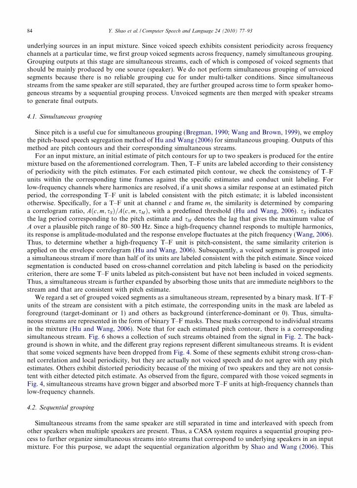
Studies such as Lovekin et al. (2001) and Shao and Wang (2006) have shown that voiced speech plays adominant role in sequential grouping and speaker recognition. Therefore, we first apply the above sequentialgrouping algorithm to organize simultaneous streams, which are mostly voiced speech. Outputs of the algo-rithm are two binary masks (streams) and corresponding speaker identities. Fig. 7a presents two estimatedspeaker streams in different gray colors after simultaneous streams are grouped.

Lovekin et al. (2001) have also shown that unvoiced speech contributes positively to speaker recognitionbut it is not as discriminative as voiced speech. Here, unvoiced segments are grouped with the two streamsusing the same sequential grouping algorithm. However, since likelihoods of unvoiced speech are not as dis-criminative, the grouping algorithm employs the already detected speaker pair associated with the organizedstreams instead of searching for it. In addition, we find that unvoiced segments are typically much smaller thansimultaneous streams, resulting in poor likelihood estimation by uncertainty decoding. Therefore, likelihoodsare calculated using a missing data method of marginalization (Cooke et al., 2001; Shao and Wang, 2006).Simply put, instead of reconstructing missing T–F units, this method ignores them in the likelihood calcula-tion. Fig. 7b presents two speaker streams after unvoiced segments are also grouped.

We find that the above processes do not capture all the speech segments. To further refine organizedstreams, we apply a watershed algorithm (Vincent and Soille, 1991) to the cochleagram of the mixture andextract segments that may have been missed by the preceding processes. Given an intensity map such as a coc-hleagram, the watershed technique identifies segment regions surrounding local minima, and it has beenwidely used for image segmentation. Additionally, watershed segments that contain less than eight T–F unitsare removed from further processing. Subsequently, a watershed segment is first absorbed by the two speakerstreams if it is largely (greater than or equal to two-thirds) overlapped with either of them, since a speaker’svoice tends to occupy contiguous time frames and activate neighboring filters due to large overlaps betweenneighboring Gammatone bandwidths. Then, if a segment has not been merged with either stream, i.e. theoverlapped region is less than two-thirds of its total area, those overlapped T–F units are removed from

Time (Sec)

Freq

uenc

y (H

z)

0.2 0.4 0.6 0.8 1 1.2 1.4 1.650

363

1246

3255

8000

Time (Sec)

Freq

uenc

y (H

z)

0.2 0.4 0.6 0.8 1 1.2 1.4 1.650

363

1246

3255

8000

a

b

Fig. 7. Estimated speaker streams. Plot (a) is obtained by sequential grouping of simultaneous streams. Plot (b) shows streams afterunvoiced segments are also grouped. White color shows the background. The two gray-colored regions represent two separated speakerstreams.

Y. Shao et al. / Computer Speech and Language 24 (2010) 77–93 87

the segment. Finally, watershed segments are sequentially grouped to the organized streams just like unvoicedsegments.

5. Uncertainty decoding

After processing a two-talker mixture by our CASA system, we have obtained two binary T–F masks. Howdo we use these masks for speech recognition? One solution is to use a missing data speech recognizer of Cookeet al. (2001). This recognizer treats noise-dominant T–F units as missing or unreliable and marginalizes them

88 Y. Shao et al. / Computer Speech and Language 24 (2010) 77–93

during recognition. However, this constrains the recognition to be performed in the T–F domain instead of thecepstral domain. Additionally, mask estimation errors degrade the recognition performance. Estimation ofthese errors would enable their use in an uncertainty decoder (Deng et al., 2005) for improved recognitionresults. Hence, we propose the use of our novel auditory cepstral feature, GFCC, in conjunction with the uncer-tainty decoder for speech recognition. Specifically, GFs are reconstructed from the estimated binary masks byutilizing the statistical information contained in a speech prior. At the same time reconstruction uncertaintiesare also estimated. These GFs and uncertainties are transformed into the GFCC domain as described in Section2. Finally the resulting GFCCs and the uncertainties are fed into an uncertainty decoder for recognition.

Given a binary T–F mask, a noisy spectral vector Y at a particular time frame is partitioned into reliableand unreliable constituents as Y r and Y u, where Y ¼ Y r [ Y u. The reliable features are the T–F units labeled 1(target-dominant) in the binary mask while the unreliable features are the ones labeled 0 (interference-domi-nant). Assuming that the reliable features Y r approximate well the true ones X r, a Bayesian decision is thenemployed to estimate the remaining features X u given the reliable ones and a prior speech model. As proposedby Raj et al. (2004) and Srinivasan and Wang (2007), we model the speech prior as a mixture of Gaussiandensities, widely known as Gaussian mixture model (GMM) (Huang et al., 2001).

pðX Þ ¼XM

k¼1

pðkÞpðX jkÞ; ð10Þ

where M ¼ 2048 is the number of Gaussians in the mixture, k indexes Gaussian component, pðkÞ refers tocomponent weight, and pðX jkÞ ¼ NðX ; lk;RkÞ. The binary mask is also used to partition the mean and covari-ance of each Gaussian into their reliable and unreliable parts as:

lk ¼lr;k

lu;k

" #; Rk ¼

Rrr;k Rru;k

Rur;k Ruu;k

� �: ð11Þ

Note that Rru;k and Rur;k denote the cross-covariance between the reliable and unreliable parts.We first estimate the unreliable features given the reliable ones as

EX ujX rðX uÞ ¼XM

k¼1

pðkjX rÞX u;k; ð12Þ

where pðkjX rÞ is the a posteriori probability of the k’th component given the reliable data and bX u;k is the ex-pected value of X u given the k’th Gaussian function. pðkjX rÞ is estimated using the Bayesian rule and the mar-ginal distribution pðX rjkÞ ¼ NðX r; lr;k;Rrr;kÞ (Srinivasan and Wang, 2007). The expected value in the unreliableT–F units corresponding to the k’th Gaussian is computed as

bX u;k ¼ lu;k þ Rur;kR

�1rr;kðX r � lr;kÞ: ð13Þ

Besides estimating unreliable T–F units, we are also interested in computing the uncertainty in our estimates.The variance associated with the reconstructed vector bX can also be computed in a similar fashion to the com-putation of the mean in (12) as:

bRbX ¼XM

k¼1

pðkjX rÞX rbX u;k

� �� lk

� ��

X rbX u;k

� �� lk

� �T

þ0 0

0 bRu;k

� �( ); ð14Þ

where

bRu;k ¼ Ruu;k � Rur;kR�1rr;kRru;k: ð15Þ

The observation density in each state of a hidden Markov model (HMM) based ASR system is usually mod-eled as a GMM. Therefore,

pðzjk; qÞ ¼ Nðz; lk;q;Rk;qÞ ð16Þ

is the likelihood of observing a speech frame z given state q and mixture component k; lk;q and Rk;q are themean and the variance of the Gaussian mixture component. When noisy speech is processed by unbiased

Y. Shao et al. / Computer Speech and Language 24 (2010) 77–93 89

speech enhancement algorithms, it is shown by Deng et al. (2005) that the observation likelihood should becomputed as

Z 1

�1pðzjk; qÞpðzjzÞdz ¼ Nðz; lk;q;Rk;q þ RzÞ: ð17Þ

It can be seen in (17) that the uncertainty decoder increases the variance of individual Gaussian components toaccount for feature reconstruction errors (Deng et al., 2005; Srinivasan and Wang, 2007). Here, the recon-structed GF feature bX and its uncertainty bRbX are transformed into the GFCC domain as z and bR z and thenused in the uncertainty decoder. bR z is the estimate of Rz in (17).

6. Experimental results

We evaluate our system using the SSC task (Cooke and Lee, 2006). This task aims to recognize speech froma target talker in the presence of another competing speaker (two-talker) or speech-shaped noise (SSN).

To build speaker models, we utilize the GFCC feature as described in Section 2. Each of the 34 speakermodels in the SSC task comprises a mixture of 64 Gaussians. The speech prior model is trained on GF featuresand is a mixture of 2048 Gaussian densities. This prior model and the binary masks are used in the cochlea-gram domain to reconstruct missing T–F units. The reconstructed GFs are then transformed into the GFCCdomain using the DCT. For recognition, we form the 60-dimensional feature vector of GFCC_D, whichincludes delta coefficients. GF uncertainties are transformed into the cepstral domain since DCT is a lineartransformation. Uncertainties of delta coefficients are also derived. Whole-word HMM-based speaker-inde-pendent ASR models are then trained on clean speech; each word model comprises 8 states and a 32-compo-nent Gaussian mixture with diagonal covariance in each state. The uncertainty decoder also uses diagonalcovariance for uncertainties. During the recognition process, given estimated uncertainties and clean ASRmodels, the uncertainty decoder calculates the likelihood of reconstructed GFCC_D features and transcribesthe speech.

Since our speech segregation does not rely on the content information in an utterance, the system does notknow which separated stream contains ‘‘white” in the two-talker task. In order to select the target, we employa normalized scoring method. We let our uncertainty decoder recognize both segregated streams using twodifferent grammars (TW and NW):

TW : $command white $preposition $letter $number $adverb

and

NW : $command $non-white $preposition $letter $number $adverb;

where $non-white only has three choices of colors except white. A normalized score is calculated for eachstream by subtracting the recognition likelihood score of NW from the one using grammar TW. The streamwith a larger score is chosen as the target, i.e., stream 1 ðs1Þ is chosen as the target when

P TWðs1Þ � P NWðs1Þ > P TWðs2Þ � P NWðs2Þ; ð18Þ

or stream 2 (s2) if otherwise. This selection metric is actually the same as evaluating the joint likelihood scoreof one stream containing the keyword ‘‘white” while the other containing $non-white. Eq. (18) is the same as,

P TWðs1Þ þ P NWðs2Þ > P NWðs1Þ þ P TWðs2Þ: ð19Þ

We first evaluate our proposed system on the two-talker task of SSC. On average, for a two-talker mixture oftwo-second long, the system produces transcription in 1–2 min on a Dell server with a dual Xeon 3.4 GHzprocessor and 4 GB memory. Speech segregation consumes approximately 90% of the total time and featurereconstruction and uncertainty decoding account for the rest. Evaluation results are summarized in Table 1.The performance is measured in terms of recognition accuracy of the relevant keywords at each TMR condi-tion (Cooke and Lee, 2006). We report the results for the different gender (DG), the same gender (SG) and thesame talker (ST) subcategories as well as the overall mean score (Avg.).

For comparison, we show the performance of our baseline system without segregation. The baseline systememploys the same speaker-independent ASR models as the proposed system but uses a conventional MFCC

Table 1Recognition accuracy (in %) of the baseline system and the stages of the proposed CASA system on the two-talker task

TMR(dB)/System DG SG ST Avg.

6 Baseline 66.00 65.92 66.52 66.17Voiced only 62.00 66.48 59.50 62.42Voiced + unvoiced 72.00 70.67 54.75 65.25Proposed overall 80.75 76.81 54.98 70.08

3 Baseline 51.25 49.44 51.58 50.83Voiced only 54.25 56.15 45.48 51.58Voiced + unvoiced 68.25 66.20 41.63 57.83Proposed overall 78.50 72.63 39.14 62.25

0 Baseline 36.00 34.64 32.58 34.33Voiced only 42.00 46.09 33.03 39.92Voiced + unvoiced 61.24 58.10 28.51 48.25Proposed overall 74.50 67.31 25.34 54.25

�3 Baseline 19.25 22.07 18.55 19.83Voiced only 36.00 32.96 23.98 23.67Voiced + unvoiced 52.25 46.92 20.18 39.08Proposed overall 63.50 53.07 20.59 44.58

�6 Baseline 9.50 10.34 9.50 9.75Voiced only 25.00 23.18 15.16 20.83Voiced + unvoiced 39.25 33.52 13.57 28.08Proposed overall 48.00 36.31 17.19 33.17

�9 Baseline 3.25 4.75 3.62 3.83Voiced only 17.75 16.20 11.99 15.17Voiced + unvoiced 30.00 24.02 11.76 21.50Proposed overall 32.00 22.34 11.99 21.75

DG, SG and ST refer to subconditions of ‘‘different gender”, ‘‘same gender” and ‘‘same talker” respectively. Avg. is the mean accuracy.

90 Y. Shao et al. / Computer Speech and Language 24 (2010) 77–93

feature instead of GFCC. This MFCC feature consists of 39 dimensions, including MFCCs, normalizedenergy, delta and acceleration coefficients (Huang et al., 2001). Speech recognition takes the grammar TWand is conducted using the HTK toolkit (Young et al., 2000). In addition, we include evaluation results fortwo intermediate stages of our system to illustrate the relative contributions of different stages. Specifically,we have evaluated speaker streams after sequential grouping of simultaneous streams. Since they are mainlyvoiced speech, their results are shown in the’Voiced only’ rows in the table. Results that evaluate speakerstreams after unvoiced segments are assigned (i.e. without watershed segments) are presented in the ‘Voice-d + unvoiced’ rows.

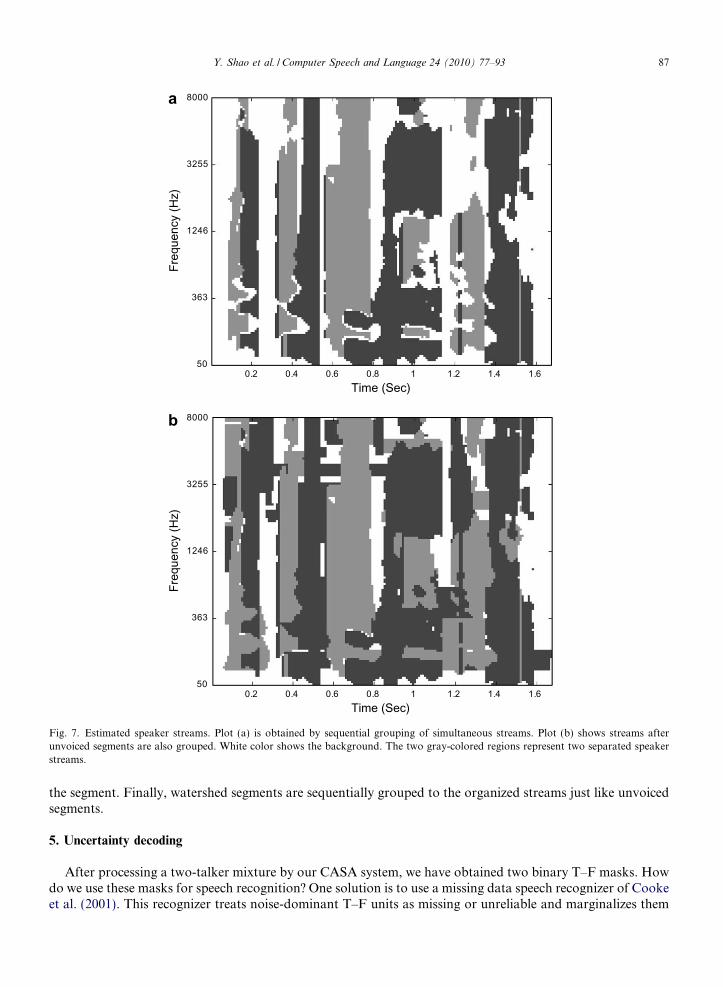
On average, the proposed system improves significantly over the baseline system in terms of average accu-racy across all TMR conditions. Except for the ST and 6 dB conditions, recognition accuracy is improved overthe baseline after simultaneous streams are organized by sequential grouping. The performance is furtherimproved after unvoiced segments and watershed segments are grouped. In general, large improvementsare observed in the DG and the SG conditions. However, the proposed system does not perform well inthe ST condition. This is primarily due to our use of speaker characteristics for sequential grouping. Note thatfor the ST condition, speaker characteristics are not distinctive for segregation. Fig. 8 compares the systemperformance with ðw=Þ and without ðw=oÞ the ST condition. Note that baseline performance is nearly the samein these two conditions. Our CASA system on average achieves a further absolute improvement of over 11%when the ST condition is excluded.

Since our sequential grouping algorithm also identifies the underlying speakers, we also present the evalu-ation results of SID performance in Table 2. Under most of the TMR conditions, we achieve an accuracy ofover 90% in recognizing the target speaker.

For the SSN task of SSC, since there is only one speaker in an input mixture and SSN is not voiced, we treatall the pitch contours and simultaneous streams as produced by the target speaker. Hence, we use a binary

–10 –8 –6 –4 –2 0 2 4 60

10

20

30

40

50

60

70

80

90

100

TMR (dB)

AS

R A

ccur

acy

(%)

Baseline w/ STProposed w/ STBaseline w/o STProposed w/o ST

Fig. 8. Average recognition accuracy on the two-talker task. The solid star line represents the baseline recognition results. The dashed plusline shows the baseline performance without the same talker (ST) data. The results of the proposed CASA system are given as the solidcircle line. Its accuracy without the ST condition is presented as the dashed square line.

Table 2Speaker identification (SID) accuracy (in %) on the two-talker task

TMR(dB) �9 �6 �3 0 3 6

Both SID 12.83 33.50 57.50 65.33 63.17 46.17Target SID 57.17 89.50 98.17 99.5 99.83 99.33

‘‘Both SID” shows the accuracies when both speakers in a mixture are identified correctly. ‘‘Target SID” presents the accuracies when thetarget speaker is identified as either of the SID outputs.

Table 3Speech recognition accuracy (in %) on the SSN task using the proposed CASA system

SNR(dB) �12 �6 0 6 Clean

Baseline system 13.00 12.50 16.22 29.50 93.94Proposed system 18.78 33.39 57.94 75.40 –

For comparison, the baseline performance is also shown.

Y. Shao et al. / Computer Speech and Language 24 (2010) 77–93 91

mask that aggregates all the simultaneous streams as the final output. In the two-talker task, GFCC_D fea-tures and associated uncertainties obtained from reconstructed GF features are fed to the uncertainty decoderfor recognition. Table 3 presents the performance of our system in terms of recognition accuracy in percent-age. Across all the SNR conditions, our CASA system shows a significant improvement over the baselinerecognizer.

7. Conclusions and discussions

In this paper, we have presented a CASA system capable of segregating and recognizing the contents of atarget utterance in the presence of another speech utterance or speech-shaped noise. The proposed CASA sys-tem is an end-to-end system that largely follows the ASA account of auditory organization and produces

92 Y. Shao et al. / Computer Speech and Language 24 (2010) 77–93

streams that correspond to different sound sources in a mixture. The contents of the target stream are thenrecognized using an uncertainty decoding framework. We have systematically evaluated our system on thespeech separation task and obtained significant improvement over the baseline performance across allTMR/SNR conditions. For example, at 0 dB TMR two-talker condition, the absolute improvement in wordaccuracy is about 20%. Additionally, the accuracy of identification of both speakers is 65.33%, and of the tar-get speaker is 99.5%.

The proposed system is primarily based on features such as periodicity and onset/offset. These propertiesare not specific to the target source to be segregated or even to speech sounds. In other words, the system doesnot use a priori knowledge of sound sources in the mixture, except in sequential grouping where the systemknows that there are two speakers in each mixture and utilizes text-independent speaker models to representspeaker characteristics. In addition, our system does not depend on the nature and the size of the target vocab-ulary, the recognition task or even the language of the speech sources in the mixture. A resulting advantage isthe generality of our system in terms of dealing with both speech and non-speech interferences. Furthermore,the ASA inspired architecture of the proposed system and adoption of the ideal binary mask as the compu-tational goal make the system readily scalable to handle multiple interference sources.

For the sequential grouping process to tackle multi-talker conditions, one could extend the model-basedalgorithm by replacing the speaker pair with a speaker triplet, a speaker quadruplet, etc., in (5). This will leadto a computational objective similar to (7) after applying the derivation in Section 4.2. This extension stillmakes an explicit assumption of the speaker number in a mixture. To remove this assumption, one could fur-ther extend the formulation by including another search that evaluates different speaker numbers. Such directextension, however, is not scalable to situations with a large number of speakers. Alternatively, one could viewa mixture as that of target speech and background, and construct the latter as a generic model Shao (2007).

Similar to the generality of our CASA segregation, the uncertainty decoding framework does not requireinterference conditions to be known a priori. Hence, it is used in conjunction with our CASA system for robustrecognition. Although the proposed uncertainty estimation approach provides promising results, otherapproaches for estimation of this uncertainty could also be explored. For example, it might be beneficial todirectly estimate the uncertainties corresponding to the static and the delta coefficients. This would enableus to exploit the differences in the a priori accuracies of these coefficients (Srinivasan and Wang, 2007).

Finally, Hu (2006) has shown that segmentation and simultaneous grouping achieve consistent SNRimprovement for various intrusion types, including non-stationary noise and music. Furthermore, Shao(2007) has demonstrated the effectiveness of the sequential grouping algorithm under speech, stationaryand non-stationary noise conditions. In addition, Srinivasan and Wang (2007) have also shown that the uncer-tainty decoder improves recognition accuracy in the presence of different noise types and for larger vocabu-laries. Therefore, our system is expected to generalize reasonably to other noise conditions that are notincluded in the SSC task.

Acknowledgements

This research was supported in part by an AFOSR Grant (FA9550-04-1-0117), an AFRL Grant (FA8750-04-1-0093) and an NSF Grant (IIS-0534707). We are grateful to Guoning Hu for discussion and much assis-tance. We acknowledge the SLATE Lab (E. Fosler-Lussier) for providing computing resources. A preliminaryversion of this work was presented in 2006 Interspeech.

References

Allen, J.B., 2005. Articulation and Intelligibility. Morgan & Claypool, San Rafael, CA.Bregman, A.S., 1990. Auditory Scene Analysis. The MIT Press, Cambridge, MA.Cooke, M., Lee, T., 2006. Speech separation and recognition competition. Available from: <http://www.dcs.shef.ac.uk/martin/

SpeechSeparationChallenge.htm>.Cooke, M., Green, P., Josifovski, L., Vizinho, A., 2001. Robust automatic speech recognition with missing and unreliable acoustic data.

Speech Commun. 34, 267–285.Deng, L., Droppo, J., Acero, A., 2005. Dynamic compensation of HMM variances using the feature enhancement uncertainty computed

from a parametric model of speech distortion. IEEE Trans. Speech Audio Process. 13, 412–421.

Y. Shao et al. / Computer Speech and Language 24 (2010) 77–93 93

Deoras, A.N., Hasegawa-Johnson, M., 2004. A factorial HMM approach to simultaneous recognition of isolated digits spoken bymultiple talkers on one audio channel. In: Proceedings of ICASSP’04, vol. 1. pp. 861–864.

Ephraim, Y., 1992. A Bayesian estimation approach for speech enhancement using hidden Markov models. IEEE Trans. Signal Process.40 (4), 725–735.

Furui, S., 2001. Digital Speech Processing, Synthesis, and Recognition. Marcel Dekker, New York.Gales, M.J.F., Young, S.J., 1996. Robust continuous speech recognition using parallel model combination. IEEE Trans. Speech Audio

Process. 4, 352–359.Hu, G., 2006. Monaural speech organization and segregation. Ph.D. Thesis, Biophysics Program, The Ohio State University.Hu, G., Wang, D.L., 2004. Monaural speech segregation based on pitch tracking and amplitude modulation. IEEE Trans. Neural

Networks 15, 1135–1150.Hu, G., Wang, D.L., 2006. An auditory scene analysis approach to monaural speech segregation. In: Hansler, E., Schmidt, G. (Eds.),

Topics in Acoustic Echo and Noise Control. Springer, Heidelberg, pp. 485–515.Hu, G., Wang, D.L., 2007. Auditory segmentation based on onset and offset analysis. IEEE Trans. Audio Speech Language Process. 15,

396–405.Huang, X., Acero, A., Hon, H., 2001. Spoken Language Processing. Prentice Hall PTR, Upper Saddle River, NJ.Jang, G., Lee, T., 2003. A probabilistic approach to single channel blind signal separation. In: Becker, S., Thrun, S., Obermayer, K. (Eds.),

Advances in Neural Information Processing Systems, vol. 15. MIT Press, Cambridge, MA, pp. 1173–1180.Kristjansson, T., Attias, H., Hershey, J., 2004. Single microphone source separation using high resolution signal reconstruction. In:

Proceedings of ICASSP’04, vol. 2. pp. 817–820.Lovekin, J.M., Yantorno, R.E., Krishnamachari, K.R., Benincasa, D.S., Wenndt, S.J., 2001. Developing usable speech criteria for speaker

identification technology. In: Proceedings of ICASSP’01, pp. 421–424.Meddis, R., 1988. Simulation of auditory neural transduction: further studies. The Journal of the Acoustical Society of America 83, 1056–

1063.Moore, B.C.J., 2003. An Introduction to the Psychology of Hearing, fifth ed. Academic Press, San Diego, CA.Oppenheim, A.V., Schafer, R.W., Buck, J.R., 1999. Discrete-time Signal Processing, second ed. Prentice-Hall, Inc., Upper Saddle River,

NJ.Patterson, R.D., Holdsworth, J., Allerhand, M., 1992. Auditory models as preprocessors for speech recognition. In: Schouten, M.E.H.

(Ed.), The Auditory Processing of Speech: From Sounds to Words. Mouton de Gruyter, Berlin, Germany, pp. 67–83 (Chapter 1).Raj, B., Seltzer, M.L., Stern, R.M., 2004. Reconstruction of missing features for robust speech recognition. Speech Commun. 43, 275–296.Raj, B., Singh, R., Smaragdis, P., 2005. Recognizing speech from simultaneous speakers. In: Proceedings of Interspeech’05, pp. 3317–3320.Roman, N., Wang, D.L., Brown, G.J., 2003. Speech segregation based on sound localization. J. Acoust. Soc. Am. 114, 2236–2252.Roweis, S.T., 2005. Automatic speech processing by inference in generative models. In: Divenyi, P. (Ed.), Speech Separation by Humans

and Machines. Kluwer Academic, Norwell, MA, pp. 97–134.Shao, Y., 2007. Sequential organization in computational auditory scene analysis. Ph.D. Thesis, Computer Science and Engineering, The

Ohio State University.Shao, Y., Wang, D.L., 2006. Model-based sequential organization in cochannel speech. IEEE Trans. Audio Speech Language Process. 14,

289–298.Shao, Y., Srinivasan, S., Wang, D.L., 2007. Incorporating auditory feature uncertainties in robust speaker identification. In: Proceedings

of ICASSP’07, vol. IV, pp. 277–280.Srinivasan, S., Wang, D.L., 2007. Transforming binary uncertainties for robust speech recognition. IEEE Trans. Audio, Speech Lang.

Process. 15 (7), 2130–2140.Srinivasan, S., Roman, N., Wang, D.L., 2006. Binary and ratio time–frequency masks for robust speech recognition. Speech Commun. 48,

1486–1501.Varga, A.P., Moore, R.K., 1990. Hidden Markov model decomposition of speech and noise. In: Proceedings of ICASSP’90, pp. 845–848.Vincent, L., Soille, P., 1991. Watersheds in digital spaces: an efficient algorithm based on immersion simulations. IEEE Trans. Pattern

Anal. Mach. Intell. 13 (6), 583–598.Wang, D.L., 2005. On ideal binary mask as the computational goal of auditory scene analysis. In: Divenyi, P. (Ed.), Speech Separation by

Humans and Machines. Norwell, MA, pp. 181–197.Wang, D.L., 2006. Feature-based speech segregation. In: Wang, D.L., Brown, G.J. (Eds.), Computational Auditory Scene Analysis:

Principles, Algorithms, and Applications. Wiley-IEEE Press, Hoboken, NJ, pp. 81–114.Wang, D.L., Brown, G.J., 1999. Separation of speech from interfering sounds based on oscillatory correlation. IEEE Trans. Neural

Networks 10 (3), 684–697.Wang, D.L., Brown, G.J. (Eds.), 2006. Computational Auditory Scene Analysis: Principles, Algorithms, and Applications. Wiley-IEEE

Press, Hoboken, NJ.Weickert, J., 1997. A review of nonlinear diffusion filtering. In: Romeny, B.H., Florack, L.J.K.a.M.V. (Eds.), Scale-space Theory in

Computer Vision. Springer, Berlin, pp. 3–28.Young, S., Kershaw, D., Odell, J., Valtchev, V., Woodland, P., 2000. The HTK Book (for HTK Version 3.0). Microsoft Corporation.