Clemson University College of Engineering and Science

Control and Robotics (CRB) Technical Report

Number: CU/CRB/2/28/06/#2 Title: Output Feedback Tracking Control of an Underactuated Quad-Rotor UAV Authors: DongBin Lee, Timothy Burg,

Bin Xian, and Darren Dawson

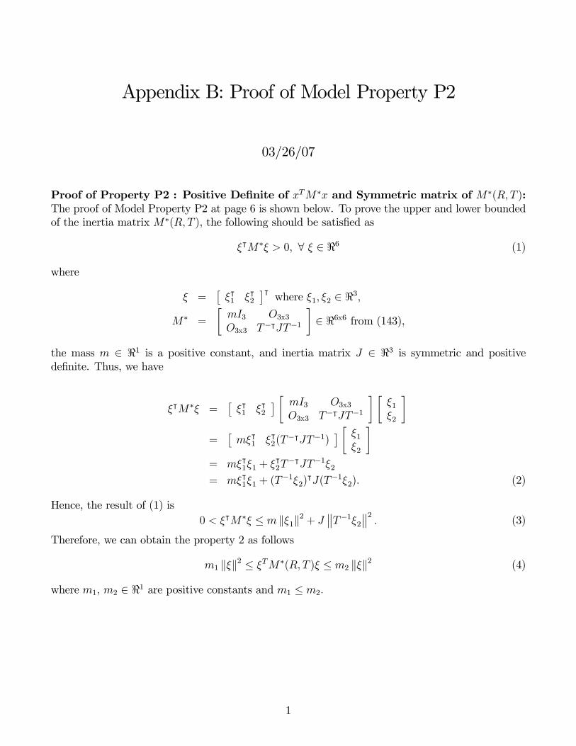
Appendix B: Proof of Model Property P2

03/26/07

Proof of Property P2 : Positive Definite of xTM∗x and Symmetric matrix of M∗(R,T ):The proof of Model Property P2 at page 6 is shown below. To prove the upper and lower boundedof the inertia matrix M∗(R, T ), the following should be satisfied as

ξ M∗ξ > 0, ∀ ξ ∈ 6 (1)

where

ξ = ξ1 ξ2 where ξ1, ξ2 ∈ 3,

M∗ =mI3 O3x3O3x3 T− JT−1

∈ 6x6 from (143),

the mass m ∈ 1 is a positive constant, and inertia matrix J ∈ 3 is symmetric and positivedefinite. Thus, we have

ξ M∗ξ = ξ1 ξ2mI3 O3x3O3x3 T− JT−1

ξ1ξ2

= mξ1 ξ2(T− JT−1)

ξ1ξ2

= mξ1ξ1 + ξ2T− JT−1ξ2

= mξ1ξ1 + (T−1ξ2) J(T

−1ξ2). (2)

Hence, the result of (1) is0 < ξ M∗ξ ≤ m ξ1

2 + J T−1ξ22. (3)

Therefore, we can obtain the property 2 as follows

m1 ξ 2 ≤ ξTM∗(R,T )ξ ≤ m2 ξ 2 (4)

where m1, m2 ∈ 1 are positive constants and m1 ≤ m2.

1

Output Feedback Tracking Controlof an Underactuated Quad-Rotor UAV∗

DongBin Lee1, Timothy Burg1, Bin Xian2, and Darren Dawson1

September 25, 2006 (Updated)

Abstract

This paper proposes a new controller for an underactuated quad-rotor family of small-scaleunmanned aerial vehicles (UAVs) using output feedback (OFB). Specifically, an observer isdesigned to estimate the velocities and an output feedback controller is designed for a nonlinearUAV system in which only position and angles are measurable. The design is performed via aLyapunov type analysis. A semi-global uniformly ultimate bounded (SGUUB) tracking resultis achieved. Simulation results are shown to demonstrate the proposed approach.Keywords: Output Feedback, Observer, Lyapunov, Nonlinear, Quad-rotor, UAV, Under-

actuated

1 Introduction

The potential for unmanned aerial vehicles (UAVs) in applications as diverse as fire fighting, emer-gency response, military and civilian surveillance, crop monitoring, and geographical registrationhas been well established. Many research groups have provided convincing demonstrations of theutility of UAVs in these applications. However, there is still a large chasm between the anticipated“tool of the future” and currently available systems. The commercial and military use of UAVs ispredicated on the ability of such vehicles to perform new, safer, or more cost effective tasks thantraditional manned aircraft. Until recently, this has been more of a question than a statement;however, recent advances in aerial vehicle construction, sensors, digital electronics, control designhave seen a rapid increase in UAV applications.Aerial vehicle construction should be considered as an important factor in UAV acceptance and

use. Materials such as carbon fiber can be used to reduce weight and improve robustness, bothcritical parameters in any aerial application. Improved manufacturing techniques are capable ofproducing small, complex, precise parts at a reasonable price and new battery technologies havemade electric hovering craft more feasible. One of the interesting small aerial vehicles that seems tohave benefited from these developments is the quad-rotor UAV depicted in Figure 1. The quad-rotorconsists of four independently driven rotating blades that can provide lift in the vertical direction.The vehicle moves in other directions by creating a mismatch between rotor speeds, and hence, thisconfiguration can produce torques about the roll, pitch, and yaw axes. The basic concept for thequad-rotor dates back to 1907; some notes on the history of the quad-rotor and related references

∗1Department of Electrical and Computer Engineering, Clemson University, Clemson, SC 29634-0915, email:tburg@clemson.edu, 2Controlled Semiconductor, FL 32819.

1

can be found in [1]. With this as a backdrop, the focus of the work presented here will be the smallquad-rotor family of aerial vehicles. The discussion will be limited to vehicles with less than 0.5kgpayload. This weight restriction means that certain technologies that may make sense for larger,more expensive aircraft may not apply to this class of aircraft.Position, velocity, and acceleration sensing issues will begin the discussion and will serve as par-

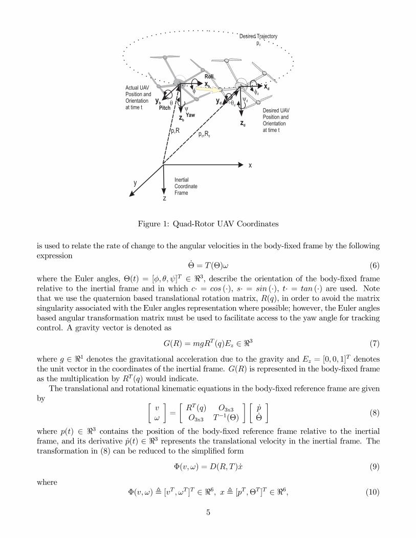
tial motivation for the choice of output feedback control design. From the schematic representationof a quad-rotor UAV shown in Figure 1, it can be seen that the arbitrarily positioned aircraft isfully located and oriented using three translational positions (x, y, and z) and three angles (roll -φ, pitch - θ, and yaw - ψ). Measurement of these six positions, the six first derivatives (velocity andangular velocity), and the six second derivatives (acceleration and angular acceleration) has provenchallenging. Measuring angular and translational quantities each present different challenges. Theangular velocity is perhaps the most accessible angular measurement. Angular velocity can besensed using a mechanical gyroscope. This approach has historically yielded good results and canbe scaled down in a cost effective manner. The major drawback is the moving mechanical partsmay add additional weight and reduce reliability. Piezoelectric gyros have provided an alternativethat does not have moving parts. More reliable gyroscopes such as the laser ring oscillator are notavailable for this application. Angular position may be more difficult to measure directly; however,devices such as magnetic compass, magnetometers, tilt sensors, optical horizon sensors may provideestimates of position for the roll or tilts axes, but typically have low bandwidth and poor accuracy.There are several technology options for building accelerometers to measure the angular accelerationincluding MEMs and piezoelectric devices.Translational position can be directly measured with global positioning system (GPS) based

systems. Enhancements, such as DGPS, are required to achieve improved accuracy. Direct sensingof the linear velocities is more difficult; an anemometer can be used to make indirect measurementsthat are not necessarily relative to a fixed inertial frame. An emerging alternative to the abovesensors is to use vision systems to measure positions or velocities. These camera systems may beground-based to monitor a UAV in a fixed area or may be vehicle based and used to estimate changesin scenery. Finally, it is often difficult to convert between data types with standard mathematicaloperations. For example, a backwards difference estimate of velocity from position information maylead to a noisy velocity signal, and integration of the velocity signal to obtain position informationcan rapidly accumulate error. If a trend were to be predicted based on review of literature, it wouldbe that angular and linear positions will be more easily attained as technology evolves. This view isdemonstrated in [2] where only a single GPS sensor is used to measure vehicle position and velocityfor a small plane. If this trend is true, then a controller that uses only position information is wellmotivated.The generally accepted end-goal that a vehicle would autonomously take-off, fly to a mission

site, perform a mission, return, and land creates a daunting challenge. One of the most fundamentalcomponents of this challenge is to ensure that the craft can move to or hold a desired position andorientation. Specifically, as shown in Figure 1, the aircraft must be able to move from a currentlocation to a new desired position (denoted by the triple xd, yd, zd) and achieve a new orientation(denoted by the angles φd, θd, ψd ). This low-level control objective, as it often called, is embeddedat the center of high-level control objectives such as path planning, target tracking, or coordinationwith other crafts. Design of the low-level control represents the point at which the peculiarities ofthe multi-bladed UAV system must be addressed; specifically, nonlinearities of the system dynamicsand the fundamental fact that the system is under-actuated. An under-actuated system is especiallychallenging to control since it has less control inputs than degrees of freedom, i.e. it has degrees offreedom that cannot be directly actuated. In order to achieve high overall performance, one must

2

address the low-level control problem. The quad-rotor UAV has six-degrees of freedom; the threetranslational directions and the three rotational angles; however, there are only four control inputs;the z-axis thrust and the three rotational torques. The quad-rotor UAV problem is sufficientlychallenging such that many researchers have proposed control solutions based on a variety techniquesthat accentuate and address different aspects of the control problem. Solving the underactuatedquad-rotor problem provides a choice of which degrees-of-freedom will be controlled. For example in[1], the authors use feedback linearization to explicitly control of the roll, pitch, and yaw angles andthe height. Translational positions are then implicitly controlled by specification of the trajectoriesfor the controlled axes. More typically, the translational control problem is directly addressed alongwith yaw angle control. For example in [4], the authors use a nested saturation algorithm. In [3], abackstepping approach to control the quad-rotor based on a model of the specific dynamics of theX4 flyer is used; this model is more complicated than that used in the other model-based designs asit includes additional terms such as gyroscopic effects of the rotating blades. In [5], the authors usea quaternion-based feedback control scheme for exponential attitude stabilization of a quad-rotoraircraft. The work given in [6], [7], and [8] are representative of vision based applications.In this paper, a tracking controller is designed for the nonlinear dynamic model of the quad-rotor

helicopter which uses only output feedback; that is, the controller operates using only position andattitude measurements. To appreciate the control design problem it is useful to consider the quad-rotor as a set of two coupled dynamic subsystems. The first subsystem contains the translationaldynamics of the craft and has a single input along the z-axis direction and the second subsystem con-tains the rotational dynamics of the craft and contains a torque input to each of the three rotationaldirections; thus, the translational subsystem is inherently underactuated. The systems are coupledvia the fact that the rotational velocities appear in the Coriolis force that acts on the translationalsubsystem — this coupling is critical as it provides the basis for the backstepping approach. Thechoice of control objectives can simplify or complicate the control design approach, for example,[Park] sought to control z-axis position and the three angles and thus the control inputs are alreadyacting at the point of interest and a PID control was directly applied (neglecting nonlinearities).The choice here to control the three linear translations and the yaw angle requires that some of thetorque inputs be “redirected” in order to achieve the translational tracking objectives. This workbuilds on previous backstepping approaches for injecting additional control action into the transla-tional dynamics of the quad-rotor but is greatly complicated by the co-design of a velocity observer.Velocity estimation is a well known problem in the robotics literature. In [9], de Queiroz et al. makea systematic presentation of the observed integrator backstepping technique to design an observerfor joint velocities in an n-link robot. In [9], it is shown that the observer and controller mustactually be designed concurrently via Lyapunov stability arguments in order to ensure a stabilityresult — a semi-global, exponential convergence of velocity estimation error and position trackingis shown for the rigid link robot. The reader is referred to this work to understand the observerand controller design and as a source of background for this technique. An additional reference forthe observer design is provided to [10] where this same observer design is used but a subtlety ofensuring that all signals in the implementable form of the observer are bounded. The payoff fromthis approach is the mathematical assertion of semi-global, uniformly ultimately bounded trackingwhile compensating for system nonlinearities, estimation error, and the perturbations that resultfrom the backstepping technique.The paper is organized as follows. In Section 2, a well known model of the quad-rotor vehicle

is presented. The assumptions and properties of this model are included. In Section 3, a velocityobserver for output feedback tracking control is designed to estimate the velocities and the OFBcontroller using this velocity estimate is derived. Stability analyses on observer, controller, and

3

composite system are considered mathematically in Section 4 followed by Theorem 1 and Remark1 which show the analysis result and the boundededness of all signals. Simulation results demon-strating the performance are presented in Section 5. Detailed developments and stability proofs aredeferred to Appendices followed by a conclusion.

2 System Modeling

2.1 Quad-Rotor Aerial Vehicle Model

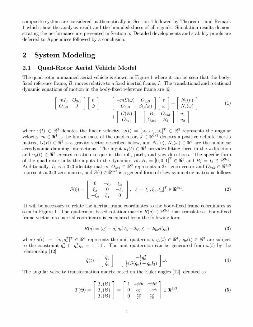
The quad-rotor unmanned aerial vehicle is shown in Figure 1 where it can be seen that the body-fixed reference frame, B, moves relative to a fixed inertial frame, I. The translational and rotationaldynamic equations of motion in the body-fixed reference frame are [6]

mI3 O3x3O3x3 J

vω

=−mS(ω) O3x3O3x3 S(Jω)

vω

+N1(v)N2(ω)

(1)

+G(R)O3x1

+B1 O3x3O3x1 B2

u1u2

where v(t) ∈ 3 denotes the linear velocity, ω(t) = [ωx,ωy,ωz]T ∈ 3 represents the angular

velocity, m ∈ 1 is the known mass of the quad-rotor, J ∈ 3x3 denotes a positive definite inertiamatrix, G(R) ∈ 3 is a gravity vector described below, and N1(v), N2(ω) ∈ 3 are the nonlinearaerodynamic damping interactions. The input u1(t) ∈ 1 provides lifting force in the z-directionand u2(t) ∈ 3 creates rotation torque in the roll, pitch, and yaw directions. The specific formof the quad-rotor links the inputs to the dynamics via B1 = [0, 0, 1]T ∈ 3 and B2 = I3 ∈ 3x3.Additionally, I3 is a 3x3 identity matrix, O3x1 ∈ 3 represents a 3x1 zero vector and O3x3 ∈ 3x3

represents a 3x3 zero matrix, and S(·) ∈ 3x3 is a general form of skew-symmetric matrix as follows

S(ξ) =

⎡⎣ 0 −ξ3 ξ2ξ3 0 −ξ1−ξ2 ξ1 0

⎤⎦ , ξ = [ξ1, ξ2, ξ3]T ∈ 3x1. (2)

It will be necessary to relate the inertial frame coordinates to the body-fixed frame coordinates asseen in Figure 1. The quaternion based rotation matrix R(q) ∈ 3x3 that translates a body-fixedframe vector into inertial coordinates is calculated from the following form

R(q) = (q2o − qTv qv)I3 + 2qvqTv − 2qoS(qv) (3)

where q(t) = [qo, qTv ]T ∈ 4 represents the unit quaternion, qo(t) ∈ 1, qv(t) ∈ 3 are subject

to the constraint q2o + qTv qv = 1 [11]. The unit quaternion can be generated from ω(t) by therelationship [12]

q(t) =qoqv

=−12qTv

12(S(qv) + qoI3)

ω. (4)

The angular velocity transformation matrix based on the Euler angles [12], denoted as

T (Θ) =

⎡⎣ Tx(Θ)Ty(Θ)Tz(Θ)

⎤⎦ =⎡⎣ 1 sφtθ cφtθ0 cφ −sφ0 sφ

cθcφcθ

⎤⎦ ∈ 3x3, (5)

4

InertialCoordinateFrame

Actual UAVPosition andOrientationat time t

Desired UAVPosition andOrientationat time tp,R

Pitch

Yaw

xb

zb

yb

Roll

Desired Trajectorypd

yd

zd

xd

x

y

z

p ,Rd d

�d�d

�d

��

�

Figure 1: Quad-Rotor UAV Coordinates

is used to relate the rate of change to the angular velocities in the body-fixed frame by the followingexpression

Θ = T (Θ)ω (6)

where the Euler angles, Θ(t) = [φ, θ,ψ]T ∈ 3, describe the orientation of the body-fixed framerelative to the inertial frame and in which c· = cos (·), s· = sin (·), t· = tan (·) are used. Notethat we use the quaternion based translational rotation matrix, R(q), in order to avoid the matrixsingularity associated with the Euler angles representation where possible; however, the Euler anglesbased angular transformation matrix must be used to facilitate access to the yaw angle for trackingcontrol. A gravity vector is denoted as

G(R) = mgRT (q)Ez ∈ 3 (7)

where g ∈ 1 denotes the gravitational acceleration due to the gravity and Ez = [0, 0, 1]T denotesthe unit vector in the coordinates of the inertial frame. G(R) is represented in the body-fixed frameas the multiplication by RT (q) would indicate.The translational and rotational kinematic equations in the body-fixed reference frame are given

byvω

=RT (q) O3x3O3x3 T−1(Θ)

p

Θ(8)

where p(t) ∈ 3 contains the position of the body-fixed reference frame relative to the inertialframe, and its derivative p(t) ∈ 3 represents the translational velocity in the inertial frame. Thetransformation in (8) can be reduced to the simplified form

Φ(v,ω) = D(R, T )x (9)

whereΦ(v,ω) [vT ,ωT ]T ∈ 6, x [pT ,ΘT ]T ∈ 6, (10)

5

and

D(R,T )RT (q) O3x3O3x3 T−1(Θ)

∈ 6x6. (11)

The dynamics in (1) can be compacted and transformed into the inertial frame as shown in AppendixA to yield the dynamic model

M∗(R,T )x = N∗(R,T, x)x+ h∗(R, T,.x) +G∗(R) +B∗(R,T )U (12)

where M∗(R,T ) ∈ 6x6 denotes the inertia matrix, N∗(R,T, x) ∈ 6x6 is a Centrifugal/Coriolisforce matrix, h∗(R, T,

.x) ∈ 6 is a hydrodynamic damping term, G∗(R) ∈ 6 is a gravity term, and

B∗(R, T ) ∈ 6x4 represents the input matrix. All are explicitly defined as (143) in Appendix A.

2.2 Model Properties and Assumptions

2.2.1 Model Properties

The dynamic system given in (12) satisfies the following properties.

P1: The inertia matrix M∗(R,T ) and Centrifugal/Coriolis matrix N∗(R, T, x) in (12) satisfy thefollowing skew-symmetric property [9]

ξTd

dt(M∗(R,T )) + 2N∗(R,T, x) ξ = 0, ∀ ξ ∈ 6,

which is proven in Appendix B.

P2: The inertia matrix M∗(R,T ) can be upper and lower bounded in the following form

m1 ξ 2 ≤ ξTM∗(R,T )ξ ≤ m2 ξ 2 , ∀ ξ ∈ 6

where m1, m2 ∈ 1 are positive constants.

The rotation matrix R(q) of (3) where R(q) = R(Θ) and the skew-symmetric matrix S(ω) of(2) satisfy the following properties [12].

P3: R = RS(ω), RT = −S(ω)RT

P4: RT = R−1, RTR = RRT = I3

P5: ST (ξ) = −S(ξ), S(ξ)δ = −S(δ)ξ, ∀ξ, δ ∈ 3

2.2.2 Model Assumptions

The following assumptions are made regarding specific components of the dynamic model. Notethat this assumptions can be shown true for specific models but not in general.

A1: With regard to angular transformation matrix, T (Θ) introduced in (5), we assume that θ = ±π

2or T−1(Θ) exists and T (Θ) i∞ is bounded (i.e., T (Θ) i∞ ≤ ε1 where ε1 ∈ 1 is a positiveconstant).

6

A2: The nonlinear damping term N1(v) ∈ 3, N2(ω) ∈ 3 introduced in (1) can be replaced by thelinearly parameterized form Y1(v)θ1 = N1(v), Y2(ω)θ2 = N2(ω) where Y1(v) ∈ 3xl, Y2(ω) ∈3xm are known regression matrices and θ1 ∈ l, θ2 ∈ m are known parameter vectors. Thedimension of l and m are related to the specific model for N1(v), N2(ω). Additionally, it isassumed that the first nonlinear parameterized term can be upper bounded as

Y1(v)θ1 ≤ ξc4 v , where ξc4 ∈ 1 is a positive constnat.

A3: The nonlinear term h∗(·) ∈ 6 in (12) can be linearly parameterized in terms of x(t) as follows

h∗(R,T, x) Y ∗(R, T )x (13)

in which Y ∗(R,T ) ∈ 6xp and Y ∗(R,T ) can be upper bounded in the following form

Y ∗(R, T ) ≤ ξc0, where ξc0 ∈ 1 is a positive constant. (14)

3 Output Feedback Tracking Control

The goal of the tracking controller is to force the aerial vehicle track a desired trajectory. Asdiscussed in the modeling section, the quad-rotor aerial vehicle is under-actuated, and hence, adecision must be made as to which degrees of freedom are to be controlled. First the choice wasmade to control the translational position, p(t) ∈ 3 in the inertial reference frame, along withyaw, ψ(t) ∈ 1 in the inertial reference frame. The translational position p(t) and the angularposition Θ(t) ∈ 3 are the only measurable states, other states such as the translational velocityv(t) ∈ 3 and the angular velocity ω(t) ∈ 3 are not measurable and cannot be included in thecontroller design. Here we assume that the desired trajectories and their up to third derivatives areall bounded; i.e., pd(t), pd(t), pd(t), and

...pd (t) ∈ L∞ and ψd(t), ψd(t), and ψd(t) ∈ L∞.

3.0.3 Full State Feedback (FSFB) Error Systems to Motivate the Structure of theOutput Feedback Control

In order to demonstrate the approach to designing an OFB controller the same approach is demon-strated for the less complicated FSFB. The position tracking error, denoted as ep(t) ∈ 3, expressedin the body-fixed frame is defined as the transformed difference between the inertial-frame basedposition and the inertial-frame based desired position, denoted as pd(t) ∈ 3, in the manner

ep RT (p− pd). (15)

The position tracking error rate, ep (t) ∈ 3, is obtained by taking the time derivative of (15),

ep = RT (p− pd) +RT p−RT pd, (16)

and after substituting for RT = −S(ω)RT from P3, and p(t) = Rv from (8), and using RTR = I3in P4 we have

ep = −S(ω)RT (p− pd) + v −RT pd. (17)

We now use the definition of ep(t) in (15) to collect terms in (17) and then the term 1mRT pd(t) is

added and subtracted to facilitate the introduction of the term ev(t) ∈ 3 as follows

ep = −S(ω)ep + 1

m(mv −RT pd) + 1

mRT pd −RT pd. (18)

7

From the equation in (18) the translational velocity tracking error, ev(t) ∈ 3, in the body-fixedframe is defined as

ev mv −RT pd (19)

where pd(t) ∈ 3 is the desired translational velocity. The final form of the open-loop positiontracking error dynamics in full state feedback system is obtained from (18), (19) as follows

ep = −S(ω)ep + 1

mev + (

1

m− 1)RT pd. (20)

After taking the time derivative of ev(t) in (19), then substituting for mv(t) from (1) and forRT (·) = −S(ω)RT from P3, we have

ev = −mS(ω)v + Y1(v)θ1 +G(R) +B1u1 + S(ω)RT pd −RT..pd (21)

where A2 was used to replace N1(v). After collecting the terms in (21) and applying the ev(t)definition in (19), we have the velocity error rate as

ev = −S(ω)ev +G(R) + Y1(v)θ1 −RT..pd +B1u1. (22)

The yaw angle tracking error, eψ(t) ∈ 1, is defined in the inertial coordinate system as

eψ ψ − ψd. (23)

The goal in the control development will be to ensure that eψ(t) and ep(t) are driven to small values;that is, to ensure the control objectives are met. The yaw angle rate error system is derived bytaking the time derivative of (23) as follows

eψ = ψ − ψd = Tz(Θ)ω − ωzd (24)

where the term Tz(Θ) ∈ 1x3 is the third row of T (Θ) from (5). Note that Tz(Θ)ω = ψ in (6) andωzd = ψd where ωzd(t) is the desired yaw angle rate in the body-fixed frame. In order to furtherdevelop the control design, the filtered position tracking error signal rp(t) ∈ 3 is defined in thefollowing manner [6]

rp ev + αep + δ (25)

where α ∈ 1 is a positive constant and δ = 0 0 δ3T ∈ 3 is a constant design vector in which

δ3 ∈ 1 is a scalar constant. The filtered position tracking error can be combined with the yawtracking error to create a composite tracking error r(t) ∈ 4 in the manner

r =rpeψ

. (26)

The filtered tracking error dynamics can be found by first differentiating (26) to yield

.r=

.rp.eψ

=

.ev +α

.ep

.eψ

. (27)

The filtered position tracking error rate, rp(t), are obtained by substituting (20) and (22) to yield

rp = −S(ω)(ev + αep + δ − δ) +α

mev + α(

1

m− 1)RT pd −RT

..pd +G(R) + Y1(v)θ1 +B1u1 (28)

8

where the term S(ω)δ has been added and subtracted to facilitate introduction of rp(t) ∈ 3 on theright-hand side as shown below

rp = −S(ω)rp + α

mev + α(

1

m− 1)RT pd −RT

..pd +G(R) + Y1(v)θ1 + [S(ω)δ +B1u1] . (29)

It is now a straightforward matter to substitute from (24) and (29) into (27) to yield the open-loopfiltered tracking error dynamics in the following form

r =−S(ω)rp + α

mev + α( 1

m− 1)RT pd −RT

..pd +G(R) + Y1(v)θ1

−ωzd +−S(δ)ω +B1u1

Tz(Θ)ω(30)

where S(ξ)δ = −S(δ)ξ in P5 was used to modify the S(ω)δ term. The last square bracketed term in(30) highlights the location where the control input will be eventually designed. The control input,u1(t) can be designed by introducing the auxiliary signal z(t) ∈ 3 in order to inject an auxiliarycontrol signal u1(t) into the translational dynamics from the rotational dynamics, ω(t) as

z = ω −Bzu1 (31)

where Bz = [I3, O3x1] ∈ 3x4 and the control input is defined by

u1 = 0 0 0 1 u1 (32)

Then we have

r =−S(ω)rp + α

mev + α( 1

m− 1)RT pd −RT

..pd +G(R) + Y1(v)θ1 +

1m(ep − ep)

−ωzd +Bµu1+Bµz0(33)

where the procedure is detailed in the Appendix C titled “Development and Derivative of Con-trol Signal u1(t)”, the term 1

mep(t) was added and subtracted in (30) to facilitate further control

development, and Bµ(·) ∈ 4x4 is defined as

Bµ =−S(δ) B1Tz(Θ) 0

. (34)

3.1 Observer Design

The next step in the control development is to address the problem that the velocity of the aerialvehicle, x(t) is not directly measurable. In the inertial coordinate system the vehicle velocity andvehicle angular velocity, x(t), cannot be obtained from sensor readings. The well known methodof circumventing this problem is to create an estimate of the unmeasurable states for use in thefeedback control law. The estimated linear and angular velocities v(t), ω(t) ∈ 3 are introducedusing (9) as

vω

=RT (q) O3x3O3x3 T−1(Θ)

.

p.

Θ. (35)

The equation (35) can be rewritten by introducing Φ(v, ω) = [vT , ωT ]T ∈ 6 and.

x (t) = [.

pT,.

ΘT

]T

to yieldΦ(v, ω) = D(R,T )

.

x . (36)

9

The goal of estimating velocity is achieved by using an observer similar to [9] as follows

.

x= y + k01x (37)

where the initial condition y(0) = −k01x(0), k01 ∈ 1 is a positive gain and x(t) = [pT , ΘT ] ∈ 6 isdefined as

x = x− x (38)

where x(t) = [pT , ΘT ]T ∈ 6 denotes a position estimate vector. The auxiliary signal y(t) ∈ 6

introduced in (37) is updated according to

y =M∗(R,T )−1 N∗(R,T, xo)xo + h∗(R, T, xo) +G∗(R) +B∗(R, T )U + k02x + k03x (39)

where k02, k03 ∈ 1 are positive constants and an auxiliary signal xo(t) ∈ 6 is defined as

xo =.

x −βx (40)

where β ∈ 1 is a positive constant. The equation (39) was obtained by substituting xo(t) for x(t)into the dynamic model in (12) and adding the x-terms to promote stability of the observer. Thebasic form of the internal observer signal y(t) ∈ 6 comes from substituting xo(t) into the modelingequation of (12); that is, the knowledge of the system dynamics and parameters are exploited toproduce the velocity estimate. In order to simplify the Lyapunov analysis, the following filteredobserver error signal is defined simlar to [10] as

s x− xo =.

x +βx ∈ 6 (41)

where (40) was used. This estimate must be faithful to the actual velocity signal in the sense thatthe velocity estimate,

.

x (t), will produce a small value for the velocity estimation error,.

x (t) ∈ 6,defined as

.

x=.x −

.

x (42)

where the estimated velocity errors can be represented by defining

Φ(v, ω) =vω

D(R,T ).

x= D(R,T )

.

p.

Θ(43)

and.

p= p−.

p and.

Θ= Θ−.

Θ . (44)

The motivation for the form of the observer and the proof that the observer will produce a properestimate in the observation error dynamics is developed below. Taking the time derivative of (37)yields

..

x= y + k01.

x . (45)

Multiplying (45) by M∗(R,T ), and then substituting from (39) for M∗(R,T )y(t) yields

M∗(R,T )..

x = N∗(R, T, xo)xo + h∗(R,T, xo) +G∗(R) +B∗(R,T )U (46)

+k02x+ k03M∗(R, T )x+ k01M∗(R, T )

.

x .

10

After subtracting (46) from (12), the dynamics of x(t) is as follows

M∗(R,T )..

x = N∗(R,T, x)x−N∗(R, T, xo)xo + h∗(R,T, x)− h∗(R,T, xo)−k02x− k03M∗(R, T )x− k01M∗(R,T )

.

x . (47)

On the other hand, taking time derivative of (41), and multiplying M∗(R,T ) yields

M∗(R, T )s =M∗(R,T )..

x +βM∗(R,T ).

x . (48)

Substituting (47) for M∗(R, T )..

x (t) and arranging the terms yields

M∗(R, T )s = N∗(R,T, x)x−N∗(R, T, xo)xo + h∗(R,T, x)− h∗(R,T, xo)−[k02 + k03M∗(R, T )]x+ [β − k01]M∗(R,T )

.

x . (49)

Introducing the new positive constants

k03 = k03β and k01 = β + k03 (50)

allows the last two terms in the right side of the (49) to be rewritten as

M∗(R, T )s = N∗(R,T, x)x−N∗(R, T, xo)xo + h∗(R,T, x)− h∗(R,T, xo)−k02x− k03M∗(R, T )s (51)

where (41) was used. The definition of s(t) in (41) is substituted as x(t) = s(t) + xo(t) into theoutside term of the first equation to the right side in (51) and then, we have

M∗(R,T )s = N∗(R, T, x)s+N∗(R,T, x)xo −N∗(R,T, xo)xo + h∗(R,T, x)− h∗(R,T, xo)−k02x− k03M∗(R,T )s. (52)

Substituting A3 yields

M∗(R,T )s = N∗(R,T, x)s+N∗(R,T, x)xo−N∗(R, T, xo)xo+Y ∗(R,T )s−k02x−k03M∗(R,T )s. (53)

The Centrifugal/Coriolis terms,N∗(R,T, x)xo−N∗(R, T, xo)xo are now utilized to writeN∗c (R,T, xo)s

developed in the Appendix F. Therefore, the velocity observer error dynamics yields

M∗(R,T )s = N∗(R,T, x)s+N∗c (R,T, xo)s+ Y

∗(R, T )s− k02x− k03M∗(R, T )s (54)

3.2 Output Feedback Control Formulation

Figure 2 shows the outline of the output feedback tracking system. We designed the observer toestimate the velocities v(t), ω(t) which are not measurable, producing

.

x (t) and then closed-loopcontroller using backstepping approach based on the Lyapunov stability which will enable to trackthe desired position and yaw angle is designed using the output feedback and estimated states basedon the error dynamics of the underactuated UAV system.

11

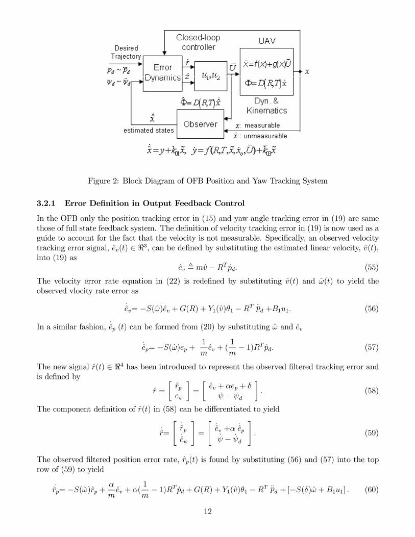
Figure 2: Block Diagram of OFB Position and Yaw Tracking System

3.2.1 Error Definition in Output Feedback Control

In the OFB only the position tracking error in (15) and yaw angle tracking error in (19) are samethose of full state feedback system. The definition of velocity tracking error in (19) is now used as aguide to account for the fact that the velocity is not measurable. Specifically, an observed velocitytracking error signal, ev(t) ∈ 3, can be defined by substituting the estimated linear velocity, v(t),into (19) as

ev mv −RT pd. (55)

The velocity error rate equation in (22) is redefined by substituting v(t) and ω(t) to yield theobserved vlocity rate error as

.

ev= −S(ω)ev +G(R) + Y1(v)θ1 −RT..pd +B1u1. (56)

In a similar fashion,.

ep (t) can be formed from (20) by substituting ω and ev

.

ep= −S(ω)ep + 1

mev + (

1

m− 1)RT pd. (57)

The new signal r(t) ∈ 4 has been introduced to represent the observed filtered tracking error andis defined by

r =rpeψ

=ev + αep + δ

ψ − ψd. (58)

The component definition of r(t) in (58) can be differentiated to yield

.

r=

.

rp.

eψ=

.

ev +α.

epψ − ψd

. (59)

The observed filtered position error rate,.

rp(t) is found by substituting (56) and (57) into the toprow of (59) to yield

.

rp= −S(ω)rp + α

mev + α(

1

m− 1)RT pd +G(R) + Y1(v)θ1 −RT

..pd + [−S(δ)ω +B1u1] . (60)

12

The rate of yaw error is found by substituting ω(t) into (24)

.

eψ=.

ψ −ωzd = Tz(Θ)ω − ωzd (61)

where ψd(t) = ωzd. The observed tracking error rate is obtained by substituting (60) and (61) as

.

r=S(ω)rp +

αmev + α( 1

m− 1)RT pd +G(R) + Y1(v)θ1 −RT

..pd

−ωzd +−S(δ)ω +B1u1

Tz(Θ)ω. (62)

The equation (62) can be derived by following the procedure which is shown the equations from(30) to (34) as

.

r=−S(ω)rp + α

mev + α( 1

m− 1)RT pd +G(R) + Y1(v)θ1 −RT

..pd

−ωzd +Bµu1 +Bµz0

(63)

where the auxiliary signal z(t) ∈ 3 is introduced in the same way in (31) by substituting ω(t) todenote

z = ω −Bzu1, (64)

and hence, the auxiliary estimation signal z(t) ∈ 3 can be defined using the (31) and (64) as

z = ω − ω = ω. (65)

3.3 Controller Formulation

3.3.1 Translational Input as a Lifting force

The filtered tracking error dynamics in (33) now presents the opportunity to design the auxiliarycontrol input u1(t). It can be seen from (33) that certain terms, those containing measurable signals,can be directly canceled by design of u1(t). Other unmeasurable terms, e.g., ev(t), rp(t), Y1(v)θ1,can be canceled to the best degree possible using an estimate of velocity. Additionally, a term ofthe form −r(t) ∈ 4 will be required to promote the convergence of r(t) to zero. With these threeobjectives in mind, the control u1(t) in (33) can be designed based on equation (63) as

u1 = B−1µ −krr + − α

mev − α( 1

m− 1)RT pd −G(R)− Y1(v)θ1 +RT pd − 1

mep

ωzd(66)

where kr =diag(kr1, kr1, kr1, kr2) ∈ 4x4 is a positive constant matrix. For stability analysis of thiscontrol, the observed filtered tracking error, denoted by r(t) ∈ 4, can be described by subtracting(58) from (26) as

r = r − r = rp − rp0

=rp0

(67)

where the observed filtered position tracking estimation error, rp(t) ∈ 3 is now defined as thedifference between rp(t) in (25) and rp(t) in (58) and can be shown to be

rp = rp − rp = mv. (68)

The difference between the actual velocity error, ev(t), and the estimated velocity error, ev(t) isdefined as

ev = ev − ev = m(v − v) = mv = rp (69)

13

where v(t) = v − v is the velocity tracking error. The equation (66) can be represented by substi-tuting −r(t) + r(t) for −r(t) and substituting −ev(t) + ev(t) for −ev(t) in the following form

u1 = B−1µ −krr + krr + − α

mev +

αmev − α( 1

m− 1)RT pd −G(R)− Y1(v)θ1 +RT pd − 1

mep

ωzd.

(70)Finally, the closed-loop filtered tracking error dynamics for r(t) is formed by substituting (70) into(33) to yield

.r= −krr + kr rp

0+−S(ω)rp − ep

m

0+

αmev + Y1θ10

+Bµz0

(71)

where (67), (69), and (31) were used, and Y1(·) ∈ 3xl is introduced as follows

Y1(v) = Y1(v)− Y1(v). (72)

3.3.2 Development of the Torque Input using a Backstepping Approach

Examining the meaning of the term z(t) introduced in (33) should help crystallize the exposition ofthe control design approach and motivate the next step. The definition of z(t) in (31) quantifies thecloseness of the control term u1(t) to the angular velocities ω(t), if z(t) is zero then ω(t) = u1(t).The implication is that the effect of rewriting the input term in (33) was to inject the signal u1(t)as a desired input to the rotational dynamics (a backstepping approach). The design now proceedsto ensure that the auxiliary signal z(t) in (31) is driven to a small value. Taking the time derivativeof z(t) in (31) and multiplying by the inertia matrix, J, yields

Jz = Jω − JBz.u1 . (73)

Substituting the second equation of (1) for Jω(t) into (73) produces

Jz = S(Jω)ω +N2(ω) +B2u2 − JBz.u1 (74)

where it can be viewed as backstepping -u1(t) through the integrator. It is now useful to groupterms in equation (74) and invoke A2 for the parameterization of N2(ω) as

Jz = S(Jω)ω + Y2(ω)θ2 − JBz.u1 +B2u2. (75)

The following assumption is made for (75):

A4: A linear parameterization has been assumed

Y3(p,R, v,ω)θ3 = S(Jω)ω + Y2(ω)θ2 − JBz.u1 (76)

where Y3(p,R, v,ω) ∈ 3xn and θ3 ∈ n (i.e., there are n known parameters in θ3 and n isdetermined by the specific models of (76), especially N1(v), N2(ω) and (79)).

Using the A4, (75) is rewritten as

Jz = Y3(p,R, v,ω)θ3 + B2u2. (77)

14

It should also be clear that ideally the control input u2(t) would be designed to stabilize the z(t)-dynamics and cancel Y3(p,R, v,ω)θ3, of course this can not be achieved directly because both ofthese objectives would require knowledge of unmeasurable quantities. The estimated velocities willprovide the best opportunity to achieve these goals; that is, in a similar way in (77), the estimatedvelocities v(t) and ω(t) are substituted into (76) to create the estimate Y3(p,R, v, ω) ∈ 3xn givenby

Y3(p,R, v, ω)θ3 = S(Jω)ω + Y2(ω)θ2 − JBz.u1 (78)

where Y2(ω), Y3(p,R, v, ω) are the estimated regression matrices. The time derivative of u1(t) canbe calculated using the error definition in (66) as follows

.u1

d

dt(B−1µ )U + (B

−1µ )

d

dtU (79)

where U(t) is from the parenthetical terms on the right equation (66) and the time derivative ofU(t) is defined as follows

d

dtU = −kr

.

r +− α

m

.

ev − ddt(Y1(v)θ1)− 1

m

.

ep

0

+S(ω) α

mRT pd − αRT pd −RT

..pd +mgR

TEz − α 1− 1mRT

..pd +R

T...pd

ωzd(80)

where (56), (57), (63), and G(R) = −S(ω)G(R) are utilized and the time derivative of Y1(v)θ1 areexplicitly calculated in Appendix E.The control input u2(t) ∈ 3 is now formulated from (77), making use of (78), in the following

formu2 = B

−12 −kzz − Y3(p,R, v, ω)θ3 − BTµ r (81)

where the first term is a linear feedback control, the last term is added to cancel a crossing termduring the Lyapunov stability analysis, and Bµ(·) ∈ 4x3 is formed from the first three columns ofBµ(·) in (34) and can be transposed as follows

BTµ = [−S(δ)T , Tz(Θ)T ]. (82)

After substituting (81) into (77), −z(t) + z(t) for z(t), and using ω(t) = z(t) in (65), we have

Jz = −kzz + kzω + Y3θ3 − BTµ r + BTµ r (83)

where (67) was used to create the last two terms, and the regression estimation error, Y3(·) ∈ 3xn,is defined as

Y3(v, ω) = Y3(p,R, v,ω)− Y3(p,R, v, ω). (84)

ST (ξ) = −S(ξ) in P5 can be invoked to rewrite the matrix BTµ (·) in (82) asBTµ = [S(δ), Tz(Θ)

T ], (85)

and hence, we have

BTµ r = [S(δ), Tz(Θ)T ]

mv0

= mS(δ)v. (86)

After substituting (86) into (83), we have the final form for the closed-loop system as shown below

Jz = −kzz + kzω + Y3θ3 − BTµ r +mS(δ)v. (87)

15

4 Stability Analysis

The combination of velocity observer error and closed-loop error systems given by (54), (71), and(87) yields the following stability result for the velocity observation and tracking error.

Theorem 1 The velocity observer of (37), (39), and the control law of (70), (81) ensure that thetracking error is semi-globally uniformly ultimately bounded (SGUUB) as shown below

η(t) ≤ λ4λ3

η(0) 2 exp(−2λ5λ4t) +

λ4ε20λ2λ3λ5

(1− exp(−2λ5λ4t)) (88)

whereη [eTp , r

T , zT , sT , xT ]T , (89)

and ε0, λ2, λ5 are positive constants and λ3, λ4 are positive constants given by the following form

λ3 min{1,m1, k02},λ4 max{1,m2, k02}, (90)

under the condition that

kr > 3, kz > 3, α >λ22m, k02 > 2ξc4β, (91)

k03 >1

m1

⎡⎣ξc0 + 2ξc4 + ξc1(ε2 + ε7) + 5ξc1ε8λ4λ3

η(0) 2 +λ4ε20

λ2λ3λ5

⎤⎦ (92)

where ξc0, ξc1, ξc4 and ε1 to ε8 are some positive constants. The details of subsequent stabilityanalysis is proved in Appendix D.

Remark 1 According to Theorem 1 and its subsequent composite stability analysis from (116) to(129), V (η(t)) is bounded. From (88), if the observer and controller gains in (92) are selected tosatisfy (121), it is straightforward to see that η(t) ∈ L∞. Hence, it ensures that the ep(t), r(t),z(t), s(t), and x(t) are bounded. We know that all desired position and yaw angle trajectories arebounded, and that R(q) and T (Θ) are bounded, thus D(R, T ) and G∗(R) ∈ L∞. We can now makea conclusion that p(t),ψ(t), v(t) ∈ L∞ owing to ep(t), ev(t), eθ(t), rp(t) ∈ L∞, based on the definitionof (15), (19), (23), (25). Due to the boundedness of v(t), we observe that p(t) in the first equation

of (8) is bounded..

x (t) is bounded in (41) because s(t), x(t) ∈ L∞, and this ensures that.

p (t),.

Θ (t)

∈ L∞ and we know.

p (t) is bounded from (42). We also know that v(t), ω(t) are bounded in (43),and hence, ev(t), rp(t), z(t) ∈ L∞ from (69), (68), (65), respectively. Also, the expression for theobserved velocity v(t) is bounded from the definition of v(t) in (164). Therefore, ev(t), rp(t) ∈ L∞,so we know the filtered position error r(t) is bounded in (58). Owing to v(t), v(t) are bounded, thenonlinearity of the aerodynamic damping term, N1(v), N1(v), Y1(v), Y1(v), Y1(·) are all bounded.Hence, we can state that u1(t) is bounded in (70), thus the translational control input u1(t) ∈ L∞in (32). Owing to the fact that u1(t) is bounded, ω(t) is bounded from (31). From (65), we knowthat ω(t) is bounded, and hence, z(t) ∈ L∞ from (64). Therefore, since v(t), ω(t) have been shownto be bounded, we know that the velocity output

.

x (t) is bounded from (36), thus the aerodynamicdamping, N2(ω), N2(ω), Y2(ω), Y2(ω), and Y2(·) are bounded. Hence, x(t), xo(t) are bounded from(42) and (40) because of

.

x (t) ∈ L∞. From the equations of (57), (56), (61) and (63), we can seethat

.

ep (t),.

ev (t),.

eθ (t), and.

r (t) are all bounded which can be used to show that.u1 (t) ∈ L∞ in

16

(79), thus Y3θ3 is bounded in (78), and consequently the torque input u2(t) is bounded from (81)using (64), (78), and (58). Thus

.

v (t),.

ω (t) ∈ L∞, in (12), dY1(v)dt∈ L∞ from (194), and y(t) is

bounded in (39). Therefore we can conclude that all signals remain bounded in the velocity observerand the closed-loop system.

4.1 Observer Stability Analysis

In order to analyze the results of the observer, a non-negative function V0(t) ∈ 1 is defined asfollows

V0 =1

2sTM∗(R,T )s+

1

2k02x

T x. (93)

The time derivative of V0(t) is

V0 =1

2sTd

dt(M∗(R, T )) s+ sTM∗(R,T )s+ k02xT

.

x . (94)

Substituting (54) into the second term of (94) and then arranging the equation yields

V0 =1

2sT

d

dt(M∗(R,T )) + 2N∗(R, T, x) s+ sTN∗

c (R, T, xo)s+ sTY ∗(R,T )s

−k03sTM∗(R,T )s− k02βxT x. (95)

P1 is used to show that the first term in (95) is zero because of its skew-symmetric property whichis validated in Appendix B, and hence, we have

V0 = −k03sTM∗(R,T )s− k02βxT x+ sTN∗c (R, T, xo)s+ s

TY ∗(R,T )s. (96)

The term N∗c (R, T, xo) is a Centrifugal/Coriolis force matrix which is derived from the difference

between N∗(R,T, x) in the modeling equation of (12) and N∗(R,T, xo) in the auxiliary signal y(t)in (39) of the observer design as shown in (218) in the Appendix F . Based on the structure ofN∗c (R,T, xo) and A1 the term N∗

c (R, T, xo) can be shown that

N∗c (R, T, xo) ≤ ξc1 xo where ξc1 ∈ 1 is a positive constant. (97)

According to P2, (14) in A3, and (97), (96) can be upper bounded as follows

V0 ≤ −k03m1 s2 − k02β x 2 + ξc1 xo · s 2 + ξc0 s

2 . (98)

From (40), xo(t) can be upper bounded as

xo ≤.

x + β x ; (99)

therefore, (99) can be used to upper bound (98) uniformly as follows

V0 ≤ −(k03m1 − ξc0) s2 − k02β x 2 + ξc1(

.

x + β x ) s 2 . (100)

17

4.2 Controller Stability Analysis

In order to prove the tracking result, a non-negative function V1(t) ∈ 1 is defined as follows

V1(t) =1

2eTp ep +

1

2rT r +

1

2zTJz. (101)

After taking the time derivative of (101), substituting from (20), (71), and (87), we have

V1 = eTp ep + rT r + zTJz

= eTp −S(ω)ep +1

m(rp − αep − δ) + (

1

m− 1)RT pd

+rT −krr + kr rp0

+−S(ω)rp − ep

m

0+

αv + Y1θ10

+Bµz0

+zT −kzz + kzω + Y3θ3 − BTµ r +mS(δ)v (102)

where ev(t) = rp(t) − αep − δ was used for ep(t). After collecting terms, deleting the zero terms,canceling the cross-terms, substituting rp(t) from (68), and using the relationship given by

Bµz0

=−S(δ)zTz(Θ)z

=−S(δ)Tz(Θ)

z = Bµz, (103)

the equation (102) becomes

V1 = −krrT r − kzzTz − α

meTp ep −

1

meTp δ + eTp (

1

m− 1)RT pd + krrTp (mv)

+rTp (αv + Y1θ1) + kzzT ω + zTmS(δ)v + zT Y3θ3. (104)

After upper bounding the first three terms in (104) and arranging, we have

V1 ≤ −kr r 2 − kz z 2 − α

mep

2 + eTp (1

m− 1)RT pd − 1

mδ (105)

+rTp (krm+ α)v + Y1θ1 + zT Y3θ3 + kzω +mS(δ)v .

The first bracket term in (105) can be upper bounded using the inequality

eTp (1

m− 1)RT pd − 1

mδ ≤ ep ε0 ≤ 1

2λ2 ep

2 +1

λ2ε20 . (106)

An upper bound for the second and third bracketed terms in (105) is now sought. The definitionof Φ(v, ω) in (43) is upper bounded as

Φ(v, ω) = D(R,T ).

x≤ D(R, T ).

x = d0.

x (107)

where d0 ∈ 1 is a positive constant. Hence

v ≤ d0.

x and ω ≤ d0.

x . (108)

Y1(v) and Y3(v, ω) are bounded utilizing (72) and A3 as follows

Y1θ1 ≤ ξc2.

x and Y3θ3 ≤ ξc3.

x (109)

18

where ξc2, ξc3, are positive constants. From the definition of s(t) in (41),.

x (t) can be upper boundedas

.

x ≤ s + β x (110).

x2

≤ 2 s 2 + 2β2 x 2 . (111)

Upper bounds for the last two bracket terms in (105) can be expressed in the following form by

utilizing (108) for v(t) and ω(t), (109) for Y1θ1 and Y3θ3 , (110) for.

x , and (111) for.

x2

toproduce

V1(t) ≤ −kr r 2 − kz z 2 − ( αm− λ22) ep

2 +1

2λ2ε20.

+3 r 2 + ξ2c2.

x2

+ α2.

x2

+ (krm)2

.

x2

(112)

+3 z 2 + ξ2c3.

x2

+ k2z.

x2

+m2 S(δ) 2.

x2

.

After rearranging (112), we have

V1 ≤ −(kr − 3) r 2 − (kz − 3) z 2 − ( αm− λ22) ep

2 + ξc4.

x2

+ε202λ2

(113)

whereξc4 = ξ2c2 + ξ2c3 + α2 + (krm)

2 + k2z +m2 S(δ) 2

i∞ .

After using (111), (113) becomes

V1 ≤ −(kr − 3) r 2 − (kz − 3) z 2 − ( αm− λ22) ep

2 + 2ξc4( s2 + β2 x 2) +

ε202λ2

. (114)

4.3 Composite Stability Analysis

The performance of the proposed controller and observer can now be examined by combining thenon-negative functions V0(t) in (93) and V1(t) in (101) as follows

V V0 + V1 =1

2eTp ep +

1

2rT r +

1

2zTJz +

1

2sTM∗(R, T )s+

1

2k02x

T x. (115)

The composite function V (t) now has theproperty

1

2λ3 η 2 ≤ V ≤ 1

2λ4 η 2 (116)

where (89) is used. After taking time derivative of (115), and utilizing the bounds on V0(t) andV1(t) from (100) and (114), we have

V ≤ −(kr − 3) r 2 − (kz − 3) z 2 − ( αm− λ22) ep

2 − (k03m1 − ξc0) s2

−k02β x 2 + ξc1.

x + β x s 2 + 2ξc4 s2 + 2ξc4β

2 x 2 +ε202λ2

. (117)

19

We can now upper bound V (t) of (117) as follows

V ≤ −(kr − 3) r 2 − (kz − 3) z 2 − ( αm− λ22) ep

2

− k03m1 − ξc0 − ξc1.

x − ξc1β x − 2ξc4 s 2

+(2ξc4β2 − k02β) x 2 +

ε202λ2

. (118)

.

x in (118) can be upper bounded by using (190) from Appendix D and substituting (110) into

(190) as follows.

x ≤ (2 + ε3) s + (2 + ε3)β x + ε4 z + (ε1 + ε5) r + (αε1 + ε6) ep + ε2 + ε7. (119)

After substituting (119) into (118) and arranging, we have

V ≤ −(kr − 3) r 2 − (kz − 3) z 2 − ( αm− λ22) ep

2 − [k03m1 − ξc0 − 2ξc4] s 2

−ξc1 ((2 + ε3) s + (3 + ε3)β x + ε4 z + (ε1 + ε5) r + (αε1 + ε6) ep + ε2 + ε7) s2

+(2ξc4β2 − k02β) x 2 +

ε202λ2

. (120)

Utilizing (89) for the second line in (120), V (t) yields

V ≤ −(kr − 3) r 2 − (kz − 3) z 2 − ( αm− λ22) ep

2

− [k03m1 − ξc0 − 2ξc4 − ξc1(ε2 + ε7)− 5ξc1ε8 η ] s 2

−(k02β − 2ξc4β2) x 2 +ε202λ2

. (121)

whereε8 = max{(2 + ε3), (3 + ε3)β, ε4, (ε1 + ε5), (αε1 + ε6)}, (122)

An upper bound can be written for (121) as

V ≤ −λ5 r 2 + z 2 + ep2 + s 2 + x 2 +

ε202λ2

≤ −λ5 η 2 +ε202λ2

(123)

where a positive constant scalar λ5 ∈ 1 is given by

λ5 = min (kr − 3), (kz − 3), ( αm − λ22), (k02β − 2ξc4β2),

[k03m1 − ξc0 − 2ξc4 − ξc1(ε2 + ε7 + 5ε8 η )]} . (124)

providedk03 >

1m1[ξc0 + 2ξc4 + ξc1(ε2 + ε7) + 5ξc1ε8 η ] , (125)

and the conditions for gains in (90) and (91) are met. A sufficient condition for (123) is found from(116) using

η 2 ≥ 2λ4V and η ≤ 2

λ3V (126)

20

to writeV ≤ −2λ5

λ4V +

ε202λ2, (127)

provided

k03 >1m1

ξc0 + 2ξc4 + ξc1(ε2 + ε7) + 5ξc1ε82λ3V (t) , (128)

which yields a new sufficient condition for (123). Solving the differential inequality in (127) yields

V ≤ V (0) exp(−2λ5λ4t) +

λ4ε204λ2λ5

1− exp(−2λ5λ4t) . (129)

Then we can writeV ≤ V (0) + λ4ε20

4λ2λ5, (130)

and from (116) we can writeV (0) ≤ λ4

2η(0) 2 ,

and combining these yieldsV ≤ λ4

2η(0) 2 +

λ4ε204λ2λ5

, (131)

which can be combined with (128) to produce the sufficient condition for given in Theorem 1 tosatisfy (123). Substituting (129) into (126) yields

η ≤ λ4λ3

η(0) 2 exp(−2λ5λ4t) +

λ4ε20λ2λ3λ5

(1− exp(−2λ5λ4t)). (132)

Therefore, the result of Theorem 1 can be obtained.

5 Simulation

The output feedback tracking control was simulated using a small quad-rotor unmanned aerialvehicle [13] as depicted in Figure 1. The inertial parameter of the simulation vehicle are borrowedfrom [14]

m = 0.9 [kg], J =

⎡⎣ 0.32 0 00 0.42 00 0 0.63

⎤⎦ [kg ·m2]

where g = 9.81[m/ sec2] is acceleration of gravity, and are assumed to be constant while followingthe trajectory. The desired position and yaw trajectory are given in the following form, respectively

pd(t) =

⎡⎣ pdxpdypdz

⎤⎦ =⎡⎣ Ax sin(wt)(1− e(−Bxt3))Ay cos(wt)(1− e(−Byt3))Az(1− e(−Bzt3))

⎤⎦ (m), (133)

[ψd] = cosin(2πTt) (rad) (134)

where Ax = Ay = 1, Az = 1, Bx = By = Bz = 5, T = 2.5, w = 2 · 2 πT,and co = 1. The initial

position and angle of the quad-rotor at the center of mass are selected as follows

p(0) = [0.1, 0.1, 0.1]T , Θ(0) = [0.1,−0.1, 0.1]T , x(0) = [0, 0,−0.1, 0, 0, 0]T

where all parameter estimates x(t) are initialized to zero except the position of z-direction (pz(0) =−0.1). The initial orientation and constant vector are chosen as follows

q(0) = [1, 0, 0, 0]T , δ = [0, 0, δ3]T , δ3 = −1.

21

The constant control parameters for observer and controller were iteratively chosen to be

k01 = 4, k02 = 4, k03 = 2, β = 2, k03 = 4,

kr1 = 5, kr2 = 1, kz = 45, α = 50,

which satisfies the condition of (92).Figure 3 shows the position tracking of the quad-rotor to the desired trajectory pd(t). The actual

quad-rotor trajectory represented by the solid line follows the desired trajectory represented by thedotted line which is commanded to go up 1[m] high and rotate around circular orbit of radius of 1[m]in the plane. Figure 4 shows position tracking at each axis corresponding to the motion in Figure3 and the last one shows yaw tracking result to the desired trajectory ψd(t). Figure 5 representsthe position errors about the each coordinates (x, y, z) and yaw angle errors. Figure 6 shows thecontrol inputs. The translational force input u1(t) is collectively steady when the UAV rotates atthe orbital trajectory. The torque commands u2(t) periodically changed when they rotate aroundthe circle. Figure 8 shows the estimated output of velocity observer.

6 Conclusion

The goal of designing and output feedback(OFB) controller for a quad-rotor UAV system has beendemonstrated mathematically and via a computer simulation. The mathematical result shows thata semi-global uniformly ultimate bounded (SGUUB) tracking result is achieved. The nonlinearitiesof the damping term were included in the system modeling and it was linearly parameterizedbecause the velocities or other factors are assumed to be unmeasurable. While the output feedbackcontrol design was predicated on a hypothetical sensing system that only produces angular andlinear positions, it does appear that low-cost GPS or a camera based units may provide justificationof this approach. It worth noting that the output feedback design has its advantage over the fullstate feedback where a full-state feedback controller could be considered a less complicated subsetof the current work. We believe this to be the first paper to present such a comprehensive result forquad-rotor tracking control based on only position measurements. Although the focus of this workis the quad-rotor class of aircraft, the results are directly applicable to other aerial vehicles such asthe co-axial helicopter and to unmanned underwater vehicles.

Acknowledgement This work is supported in part by a DOC Grant, an ARO Automotive CenterGrant, a DOE Contract, a Honda Corporation Grant and a DARPA Contract.

References

[1] A. Mokhtari and A. Benallegue, “Dynamic Feedback Controller of Euler Angles and WindParameters Estimation for a quad-rotor Unmanned Aerial Vehicle”, Proc. 2004 IEEE Interna-tional Conference on Robotics and Automation, Vol 3, May 2004, pp. 2359 - 2366.

[2] J. S. Jangy and C. J. Tomlin, “Longitudinal Stability Augmentation System ”Design for theDragonFly UAVUsing a Single GPS Receiver”, Proc. AIAA Guidance, Navigation, and ControlConference and Exhibit, Austin, Texas, August 2003.

[3] T. Hamel, R. Mahony, R. Lozano, and J. Ostrowski, “Dynamic Modelling and ConfigurationStabilization for An X4-Flyer”, Proc. IFAC World Congress, Barcelona, Spain, 2002.

22

[4] P. Castillo, A. Dzul, and R. Lozano, “Real-time Stabilization and Tracking of a Four-rotor MiniRotorcraft”, IEEE Transactions on Control Systems Technology, Volume 12, Issue 4, July 2004,pp. 510 - 516.

[5] A. Tayebi and S. McGilvray, “Attitude stabilization of a four-rotor aerial robot”, Proc. 43rdIEEE Conference on Decision and Control, Vol. 2, Dec. 2004, pp. 1216 - 1221.

[6] V. Chitrakaran, D. M. Dawson, J. Chen, and M. Feemster, “Vision Assisted Autonomous Land-ing of an Unmanned Aerial Vehicle”, Proc. 44th IEEE Conference on Decision and Control,Seville, Spain, Dec. 2005, pp. 1465-1470.

[7] D. Suter, T. Hamel, and R. Mahony, “Visual Servo Control Using Homography Estimation forthe Stabilization of an X4-Flyer”, Proc. 41st IEEE Conference on Decision and Control, LasVegas, NV, 2002, pp. 2872-2877.

[8] O. Shakernia, Y. Ma, T. J. Koo, and S. Sastry, “Landing an Unmanned Air Vehicle: VisionBased Motion Estimation and Nonlinear Control”, Asian Journal of Control, Vol. 1, No. 3, pp.128-145, 1999.

[9] M. Queiroz, D. Dawson, S. Nagarkatti, and F. Zang, Lyapunov-based Control of MechanicalSystems, Birkhauser, 2000.

[10] H. Berghuis and H. Nijmeijer, “A Passivity Approach to Controller-Observer Design for Ro-bots”, IEEE Transaction Robotics and Automation, Vol 9, No 6, Dec 1993, pp. 740 - 754.

[11] W. E. Dixon, A. Bethal, and D. M. Dawson, S. P. Nagarkatti, Nonlinear control of EngineeringSystems: A Lyapunov-based Approach, Birkhauser, 2003.

[12] T.I. Fossen, Marine Control Systems : Guidance, Navigation, and Control of Ships, Rigs andUndewater Vehicles, Marine Cybernetics, 2002.

[13] Dragonfly x-pro : http://www.rctoys.com/draganflyerxpro.php

[14] E.T. King, ”“Distributed Coordination and Control Experiments on a Multi-UAV Testbed”,Master Thesis in Aeronautics and Astronautics, MIT, Sep. 2004.

[15] M. Buschmann, J. Bange and P. Vörsmann, “A Miniature Unmanned Aerial Vehicle (Mini-UAV) for Meteorological Purposes”, Proc. 16th Symposium on Boundary Layers and Turbu-lence, Aug. 2004.

[16] DongBin Lee, Timothy Burg, Bin Xian, and Darren Dawson, “Output Feedback Track-ing Control of an Underactuated Quad-Rotor UAV”, CRB Technical Report, CU/CRB/,http://www.ece.clemson.edu/crb/publictn/tr.htm, 2006.

A Development of Dynamic Model in the Inertial frame

The dynamic equation of (1) describing the dynamics of the quad-rotor can be directly written inthe form

MΦ(v, ω) = C(R,T )D(R,T )x+ h(R, T, x) + G(R) + BU (135)

23

using the definition of Φ(v,ω) in (10) and the following substitutions

M =mI3 O3x3O3x3 J

∈ 6x6, C(R,T ) =−mS(ω) O3x3O3x3 S(Jω)

∈ 6x6,

G(R) =G(R)O3x1

∈ 6, h(R,T, x) =N1(v)N2(ω)

∈ 6, (136)

B =B1 O3x3O3x1 B2

∈ 6x4, U =u1u2

∈ 4 .

The time derivative of Φ(v,ω) in (10) can be related to x(t) by differentiating (9) and applying thedefinition

d

dt(D(R, T )) D(R,T, x) (137)

where

d

dt(D(R, T )) =

ddt(RT ) O3x3O3x3

ddt(T−1(Θ))

∈ 6x6,d

dt(RT ) = RT = −S(ω)RT and

d

dt(T−1(Θ)) =

∂

∂Θ(T−1(Θ))Θ ∈ 3x3 where

∂

∂Θ(T−1(Θ)) ∈ 3x3x3 is a tensor, (138)

to yield

Φ(v, ω) =d

dt(D(R, T )) x+D(R,T )x = D(R,T, x)x+D(R,T )x. (139)

Multiplying by M(·), substituting from (135) for MΦ(v, ω) and from (9) for Φ(v,ω), and arrangingterms yields

MD(R, T )x = C(R, T )D(R, T )x− MD(R,T, x)x+ h(R, T, x) + G(R) + BU . (140)

It can be shown that DT (R,T ) = R(q), O3x3;O3x3, T−T ∈ 6x6. After multiplying (140) by

DT = DT (R, T ), we have

DTMD(R,T )x = DT C(R,T )D(R, T )− MD(R, T, x) x+DT h(R,T, x) +DT G(R) +DT BU .(141)

Equation (141) is now written in the compact form

M∗(R,T )x = N∗(R,T, x)x+ h∗(R, T, x) +G∗(R) +B∗(R,T )U (142)

where the corresponding matrices were substituted as follows

M∗(R,T ) DT (R, T )MD(R,T ) = [mI3, O3x3;O3x3, T−T (Θ)JT−1(Θ)],

N∗(R,T, x) DT (R, T ) C(R, T )D(R,T )− MD(R,T, x) in (209)h∗(R,T, x) DT (R, T )h(R, T, x) = [RN1(v);T

−T (Θ)N2(ω)], (143)

G∗(R) DT (R, T )G(R) = [RG(R);O3x1],

B∗(R,T ) DT (R, T )B = [RB1, O3x3;O3x1, T−T (Θ)B2].

24

B Proof of Model Property P1

The validity of the skewed symmetric relationship in P1 is shown below. The definitions ofM∗(R, T )andN∗(R,T, x) from (143) in Appendix A are first applied to the matrix term of P1, that is

ξTd

dt(M∗(R,T )) + 2N∗(R, T, x) ξ = 0, ∀ ξ ∈ 6

to yield

ξT ddt(M∗(R, T )) + 2N∗(R,T, x) ξ = ξT d

dtDT (R,T )MD(R,T ) ξ (144)

+ξT 2DT (R, T ) C(R,T )D(R,T )− MD(R,T, x) ξ.

The definition of D(R, T, x) from (137) in Appendix A is now applied and terms collected to yield

ξTd

dt(M∗(R, T )) + 2N∗(R,T, x) ξ = ξT 2DT (R,T )C(R,T )D(R,T ) ξ (145)

+ξT DT (R, T, x)MD(R, T )−DTMD(R,T, x) ξ

where M(·) is a constant matrix and hence ddtM = 0 has been used. It is now useful to invoke the

symmetric property of M(·) to write

ξT DT (R, T, x)MD(R, T ) ξ − ξT DTMD(R,T, x) ξ = 0, (146)

which allows (145) to be written as

ξTd

dt(M∗(R,T )) + 2N∗(R, T, x) ξ = 2ξTDT (R,T )C(R, T )D(R, T )ξ. (147)

It is now possible to introduce a new vector ξ ∈ 6 defined as ξ = D(R, T )ξ in order to rewrite(147) as

ξTd

dt(M∗(R,T )) + 2N∗(R, T, x) ξ = 2ξ T C(R, T )ξ (148)

where it is clear that if C(R, T ) is skew symmetric then the right-hand side of (148) is zero. Thedefinition of C(R,T ) in (136) is substituted, and ξ partitioned into subvectors to write (148) as

ξ T C(R, T )ξ = ξ T1 ξ T2−mS(ω) O3x3O3x3 S(Jω)

ξ1ξ2

= −mξ T1 S(ω)ξ1 + ξ T2 S(Jω)ξ2 (149)

where it is clear that the skew symmetry property of S(ω) and S(Jω) can be invoked to write

2ξ T C(R, T )ξ = 0, (150)

and hence,

ξTd

dt(M∗(R, T )) + 2N∗(R,T, x) ξ = 0. (151)

25

C Development and Derivative of Control Signal u1(t)

The term of interest is first repeated from (30) and the definition of.r (t) in (27) is inserted as a

reminder to form

.r=

−S(ω)rp + αmev −RT

..pd +α(

1m− 1)RT pd +G(R)

−ωzd +N1(v)0

+−S(δ)ω +B1u1

Tz(Θ)ω.

(152)With B1 = [0, 0, 1]T , it can be seen that the control input u1(t) will only act on the z-axis trans-lational dynamics. A new control signal will be injected that creates control signals to all threetranslational axes; these injected control signals then become the tracking objectives for the rota-tional dynamics. The control term from (152) can be divided into two parts; Bµ(·) defined in (34)and µ(t) ∈ 4, and hence, becomes as follows

−S(δ)ω +B1u1Tz(Θ)ω

=−S(δ) B1Tz(Θ) 0

ωu1

= Bµµ. (153)

The term u1(t) = [uT

1 , u1] ∈ 4 with u1 (t) ∈ 3 can be added and subtracted to µ(t) of (153) asfollows

µ = +u1 − u1 + ωu1

= u1 +ωu1

− u1u1

= u1 +ω− u10

. (154)

The term z(t) can be defined to be a measure of the closeness of ω(t) to u1 (t) as

z = ω− u1,

which can then be written as

z = ω −Bzu1 where Bz =⎡⎣ 1 0 0 00 1 0 00 0 1 0

⎤⎦ . (155)

It is interesting to note that if z(t) is zero then the control signal u1(t) has been effectively injectedinto the open-loop filtered tracking error dynamics. The manipulation of µ(t) can be continuedfrom (154) using the definition of z(t) to yield

µ = u1 +z0

. (156)

After multiplying µ(t) of (156) by Bµ(·) of (153), we have

Bµµ = Bµu1 +Bµz0

, (157)

and thus−S(δ)ω +B1u1

Tz(Θ)ω= Bµu1 +Bµ

z0

. (158)

The derivative of.u1 (t) is obtained by taking time derivative of (66). It is perhaps more illustrative

to abbreviate (66) asu1 = B

−1µ U (159)

26

where B−1µ (·) is

B−1µ =

⎡⎢⎢⎣0 − 1

δ30 0

1δ3

0 0 0

− 1δ3

sφcφ 0 0 cθ

cφ

0 0 1 0

⎤⎥⎥⎦ , (160)

and hence, after differentiation, we have

.u1

d

dt(B−1µ )U + (B

−1µ )

d

dtU (161)

where is now clear that two derivatives are required. Term by term differentiation of B−1µ (·) yields

d

dt(B−1µ ) =

⎡⎢⎢⎢⎣0 0 0 00 0 0 0

− 1δ3

.

φc2φ 0 0 -cφsθ·

.

θ+sφcθ.

φc2φ

0 0 0 0

⎤⎥⎥⎥⎦ (162)

where Θ(t) is measurable and.

φ (t) = Tx(Θ)ω and.

θ (t) = Ty(Θ)ω are estimated from (35). Next,the time derivative of U(t) is rewritten from (80) as follows

d

dtU = −kr

.

r +− ddt(Y1(v)θ1)− α

m

.

ev − 1m

.

ep

0

+S(ω) α

mRT pd − αRT pd −RT

..pd +mgR

TEz + α 1− 1mRT

..pd +R

T...pd

ωzd

where (56), (57), and (63) are utilized. The term Y1(v)θ1 is a general representation of the nonlinearaerodynamic damping, and therefore, the time derivative cannot be written explicitly until a specificmodel has been assumed (such a model is assumed for use in the Simulation section and the resultingderivative d

dt(Y1(v)θ1) is calculated in Appendix E.3. Therefore,

.u1 (t) is obtained by substituting

(162) and (80) into (79).

D Details of Stability Analysis

Development of an upper bound.

x in (118) requires bounds for.

p (t) and.

Θ (t).

D.1 Upper Bound for.

p (t)

As a starting point for the bound on.

p (t), ev(t) in (19) is substituted into the definition of rp(t) in(25) and the result solved for v(t) to yield

v =1

m(rp − αep − δ +RT pd). (163)

We can now use (163) and v(t) = v − v to obtain

v = −v + 1

mrp − αep − δ +RT pd . (164)

27

Now.

p (t) can be expressed by using (35) and substituting from (164), as follows

.

p = Rv

= −Rv + 1

mR rp − αep − δ +RT pd , (165)

and then we utilize (35), (165), and.

p (t) = Rv to yield

.

p= − .

p +1

mR rp − αep − δ +RT pd . (166)

The triangle inequality can be utilized to create an upper bound for.

p (t) in (166) as follows

.

p ≤ .

p +R

mrp + α

R

mep +

R

mδ +RT pd , (167)

which can be further bounded as.

p ≤ .

p + ε1 rp + αε1 ep + ε2 (168)

where

ε11

msup∀θ

R i∞ , ε21

msup∀θ

R i∞ δ + sup∀θ

RTi∞ sup∀t

pd . (169)

D.2 Upper Bound for.

Θ (t)

To begin the development of a bound for.

Θ (t), ω(t) = ω − ω is solved for ω(t) producing

ω = ω − ω. (170)

After multiplying (170) by the transformation matrix T (Θ), we have

T (Θ)ω = T (Θ)ω − T (Θ)ω, (171)

which is equivalent to.

Θ= T (Θ)ω−.

Θ . (172)

The definition of z(t) in (31) is solved for ω(t) to yield

ω = z +Bzu1, (173)

and the control u1(t) in (66) is substituted into (173) to yield

ω = z +BzB−1µ −krr + kr mv

0

+− αm(rp − αep − δ) + αv − ep

m− α( 1

m− 1)RT pd +RT

..pd −G(R)− Y1(v)θ1

ωzd(174)

28

where rp(t) = mv was used for r(t), ev(t) was substituted from (25), and rp(t) was substituted from

(69). By substituting (174) into (172),.

Θ (t) can be expressed as follows

.

Θ = −.

Θ +Tz + TBzB−1µ −krr + kr mv

0

+− αm(rp − αep − δ) + αv − ep

m− α( 1

m− 1)RT pd +RT

..pd −G(R)− Y1(v)θ1

ωzd.(175)

In order to combine the two v(t) terms, the matrix BTz (·),

BTz =I3O1x3

∈ 4x3, (176)

and the equality RT.

p (t) = v(t) from (35) are used to formulate the equality

v0

= BTz v = BTz R

T.

p, (177)

which is then substituted into (175) to yield

.

Θ= −.

Θ +Tz + TBzB−1µ B

Tz (krm+ α)RT

.

p −TBzB−1µ krr

+TBzB−1µ

− αmrp − Y1(v)θ1 + ep

m(α2 − 1) + α

mδ − α( 1

m− 1)RT pd +RT

..pd −G(R)

ωzd.(178)

From the A2, the nonlinear aerodynamic damping term Y1(v)θ1 in (178) can be bounded by thefollowing expression

Y1(v)θ1 ≤ ξc4 v . (179)

It can be used to show v(t) = RT.

p which can be substituted into (164) to show that

v = −RT .

p +1

mrp − α

mep − 1

m(δ −RT pd). (180)

v(t) can now be upper bounded in the same manner as.

p in (167) as follows

v ≤ RT.

p +1

mrp +

α

mep +

1

mδ +RT pd . (181)

The definition of r(t) in (26) leads to the bound on rp(t) given by

rp ≤ r . (182)

The bound in (179) can now be upper bounded in the manner

Y1(v)θ1 ≤ ξc4 RT.

p +1

mrp +

α

mep +

1

mδ +RT pd , (183)

29

by using (181). An upper bound can now be developed for.

Θ (t) from (178) as follows

.

Θ ≤.

Θ + T · z + TBzB−1µ B

Tz (krm+ α)RT + TBzB

−1µ B

Tz · ξc4 RT

.

p

+ TBzB−1µ B

Tz (

α

m+ kr) + TBzB

−1µ B

Tz

ξc4m

r

+ TBzB−1µ B

Tz (

α2

m− 1

m) +

α

mξc4 TBzB

−1µ B

Tz ep (184)

+ TBzB−1µ B

Tz · α

mδ + α(

1

m− 1)RT pd +RT

..pd +G(R)

+ TBzB−1µ B3 · ωzd + TBzB

−1µ B

Tz · ξc4

mδ +RT pd

where the abbreviation T = T (Θ) and B3 = [0, 0, 0, 1]T for matrix dimension were used, and (182),(183) have been utilized. The following constants are introduced to simplify expression (184)

ε3 = ε4ε9 BzB−1µ B

Tz (krm+ α)

i∞ + ε4ε9 BzB−1µ B

Tz i∞ ξc4

ε4 = sup∀θ

T i∞ ,

ε5 = ε4 BzB−1µ B

Tz (

α

m+ kr)

i∞+

ξc4m

ε4 BzB−1µ B

Tz i∞

ε6 = ε4 BzB−1µ B

Tz (

α2

m− 1

m)i∞+

α

mξc4ε4 BzB

−1µ B

Tz i∞ (185)

ε7 = ε4 BzB−1µ B

Tz i∞

α

mδ + α

1

m− 1 ε9 sup

∀tpd + ε9 sup

∀t

..pd + G(R)

+ε4 BzB−1µ B3 i∞ sup

∀tωzd +

ξc4m

ε4 BzB−1µ B

Tz i∞ δ + ε9 sup

∀tpd

ε9 = sup∀θ

RTi∞ ,

thereby, creating the final bound for.

Θ (t) as follows

.

Θ ≤.

Θ + ε4 z + ε3.

p + ε5 r + ε6 ep + ε7. (186)

The definition of.

x (t) is formed from the right-hand terms in (35) and (36) and an upper boundapplied as follows

.

x =

.

p.

Θ≤

.

p +.

Θ . (187)

The bound in (168) for.

p (t) and the bound in (186) for.

Θ (t) can now be substituted into (187) tocreate an upper bound for

.

x (t) in the manner

.

x ≤ .

p + ε1 rp + αε1 ep + ε2

+.

Θ + ε4 z + ε3.

p + ε5 r + ε6 ep + ε7. (188)

30

Additionally, the terms.

p (t) and.

Θ (t) can be individually bounded as

.

p ≤ .

x ,.

Θ ≤ .

x . (189)

Now the substitution of the bounds from (189) and (182) into (188) yields.

x ≤ (2 + ε3).

x + ε4 z + (ε1 + ε5) r + (αε1 + ε6) ep + ε2 + ε7. (190)

E Simulation Notes

E.1 Desired Trajectory

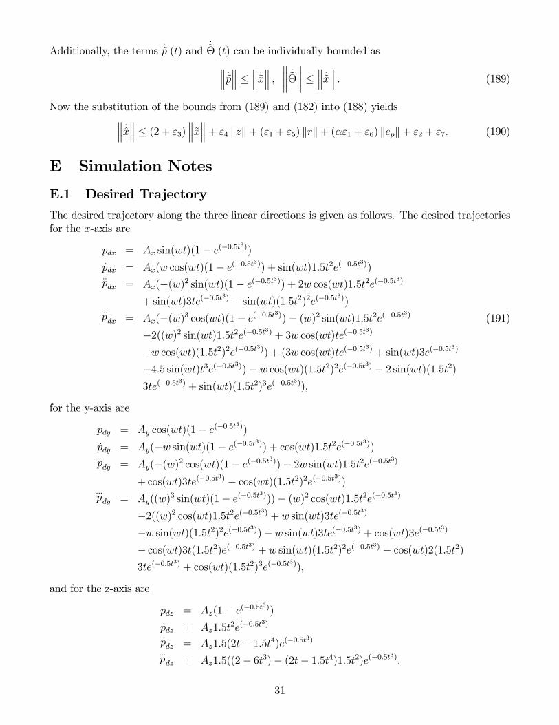
The desired trajectory along the three linear directions is given as follows. The desired trajectoriesfor the x -axis are

pdx = Ax sin(wt)(1− e(−0.5t3))pdx = Ax(w cos(wt)(1− e(−0.5t3)) + sin(wt)1.5t2e(−0.5t3))..pdx = Ax(−(w)2 sin(wt)(1− e(−0.5t3)) + 2w cos(wt)1.5t2e(−0.5t3)

+sin(wt)3te(−0.5t3) − sin(wt)(1.5t2)2e(−0.5t3))

...pdx = Ax(−(w)3 cos(wt)(1− e(−0.5t3))− (w)2 sin(wt)1.5t2e(−0.5t3) (191)

−2((w)2 sin(wt)1.5t2e(−0.5t3) + 3w cos(wt)te(−0.5t3)−w cos(wt)(1.5t2)2e(−0.5t3)) + (3w cos(wt)te(−0.5t3) + sin(wt)3e(−0.5t3)−4.5 sin(wt)t3e(−0.5t3))− w cos(wt)(1.5t2)2e(−0.5t3) − 2 sin(wt)(1.5t2)3te(−0.5t

3) + sin(wt)(1.5t2)3e(−0.5t3)),

for the y-axis are

pdy = Ay cos(wt)(1− e(−0.5t3))pdy = Ay(−w sin(wt)(1− e(−0.5t3)) + cos(wt)1.5t2e(−0.5t3))..pdy = Ay(−(w)2 cos(wt)(1− e(−0.5t3))− 2w sin(wt)1.5t2e(−0.5t3)

+cos(wt)3te(−0.5t3) − cos(wt)(1.5t2)2e(−0.5t3))

...pdy = Ay((w)

3 sin(wt)(1− e(−0.5t3)))− (w)2 cos(wt)1.5t2e(−0.5t3)−2((w)2 cos(wt)1.5t2e(−0.5t3) + w sin(wt)3te(−0.5t3)−w sin(wt)(1.5t2)2e(−0.5t3))− w sin(wt)3te(−0.5t3) + cos(wt)3e(−0.5t3)− cos(wt)3t(1.5t2)e(−0.5t3) + w sin(wt)(1.5t2)2e(−0.5t3) − cos(wt)2(1.5t2)3te(−0.5t

3) + cos(wt)(1.5t2)3e(−0.5t3)),

and for the z-axis are

pdz = Az(1− e(−0.5t3))pdz = Az1.5t

2e(−0.5t3)

..pdz = Az1.5(2t− 1.5t4)e(−0.5t3)...pdz = Az1.5((2− 6t3)− (2t− 1.5t4)1.5t2)e(−0.5t3).

31

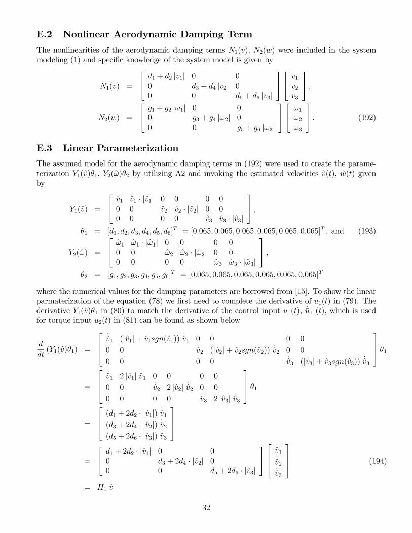
E.2 Nonlinear Aerodynamic Damping Term

The nonlinearities of the aerodynamic damping terms N1(v), N2(w) were included in the systemmodeling (1) and specific knowledge of the system model is given by

N1(v) =

⎡⎣ d1 + d2 |v1| 0 00 d3 + d4 |v2| 00 0 d5 + d6 |v3|

⎤⎦⎡⎣ v1v2v3

⎤⎦ ,N2(w) =

⎡⎣ g1 + g2 |ω1| 0 00 g3 + g4 |ω2| 00 0 g5 + g6 |ω3|

⎤⎦⎡⎣ ω1ω2ω3

⎤⎦ . (192)

E.3 Linear Parameterization

The assumed model for the aerodynamic damping terms in (192) were used to create the parame-terization Y1(v)θ1, Y2(ω)θ2 by utilizing A2 and invoking the estimated velocities v(t), w(t) givenby

Y1(v) =

⎡⎣ v1 v1 · |v1| 0 0 0 00 0 v2 v2 · |v2| 0 00 0 0 0 v3 v3 · |v3|

⎤⎦ ,θ1 = [d1, d2, d3, d4, d5, d6]

T = [0.065, 0.065, 0.065, 0.065, 0.065, 0.065]T , and (193)

Y2(ω) =

⎡⎣ ω1 ω1 · |ω1| 0 0 0 00 0 ω2 ω2 · |ω2| 0 00 0 0 0 ω3 ω3 · |ω3|

⎤⎦ ,θ2 = [g1, g2, g3, g4, g5, g6]

T = [0.065, 0.065, 0.065, 0.065, 0.065, 0.065]T

where the numerical values for the damping parameters are borrowed from [15]. To show the linearparmaterization of the equation (78) we first need to complete the derivative of u1(t) in (79). Thederivative Y1(v)θ1 in (80) to match the derivative of the control input u1(t),

.u1 (t), which is used

for torque input u2(t) in (81) can be found as shown below

d

dt(Y1(v)θ1) =

⎡⎢⎣.

v1 (|v1|+ v1sgn(v1)).

v1 0 0 0 0

0 0.

v2 (|v2|+ v2sgn(v2)).

v2 0 0

0 0 0 0.

v3 (|v3|+ v3sgn(v3)).

v3

⎤⎥⎦ θ1

=

⎡⎢⎣.

v1 2 |v1|.

v1 0 0 0 0

0 0.

v2 2 |v2|.

v2 0 0

0 0 0 0.

v3 2 |v3|.

v3

⎤⎥⎦ θ1

=

⎡⎢⎣ (d1 + 2d2 · |v1|).

v1

(d3 + 2d4 · |v2|).

v2

(d5 + 2d6 · |v3|).

v3

⎤⎥⎦=

⎡⎣ d1 + 2d2 · |v1| 0 00 d3 + 2d4 · |v2| 00 0 d5 + 2d6 · |v3|

⎤⎦⎡⎢⎣

.

v1.

v2.

v3

⎤⎥⎦ (194)

= H1.

v

32

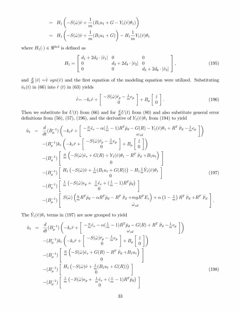
= H1 −S(ω)v + 1

m(B1u1 +G− Y1(v)θ1)

= H1 −S(ω)v + 1

m(B1u1 +G) −H1 1

mY1(v)θ1

where H1(·) ∈ 3x3 is defined as

H1 =

⎡⎣ d1 + 2d2 · |v1| 0 00 d3 + 2d4 · |v2| 00 0 d5 + 2d6 · |v3|

⎤⎦ , (195)

and ddt|v| =

.

v sgn(v) and the first equation of the modeling equation were utilized. Substituting

u1(t) in (66) into.

r (t) in (63) yields

.

r= −krr + −S(ω)rp − 1mep

0+Bµ

z0

. (196)

Then we substitute for U(t) from (66) and for ddtU(t) from (80) and also substitute general error

definitions from (56), (57), (196), and the derivative of Y1(v)θ1 from (194) to yield

.u1 =

d

dt(B−1µ ) −krr + − α

mev − α( 1

m− 1)RT pd −G(R)− Y1(v)θ1 +RT

..pd − 1

mep

ωzd

−(B−1µ )kr −krr + −S(ω)rp − 1mep

0+Bµ

z0

−(B−1µ )αm−S(ω)ev +G(R) + Y1(v)θ1 −RT

..pd +B1u1

0

−(B−1µ ) H1 −S(ω)v + 1m(B1u1 +G(R)) −H1 1m Y1(v)θ1

0(197)

−(B−1µ )1m−S(ω)ep + 1

mev + (

1m− 1)RT pd

0

−(B−1µ ) S(ω) αmRT pd − αRT pd −RT

..pd +mgR

TEz + α 1− 1mRT

..pd +R

T...pd

ωzd.

The Y1(v)θ1 terms in (197) are now grouped to yield

.u1 =

d

dt(B−1µ ) −krr + − α

mev − α( 1

m− 1)RT pd −G(R) +RT

..pd − 1

mep

ωzd

−(B−1µ )kr −krr + −S(ω)rp − 1mep

0+Bµ

z0

−(B−1µ )αm−S(ω)ev +G(R)−RT

..pd +B1u1

0

−(B−1µ ) H1 −S(ω)v + 1m(B1u1 +G(R))0

(198)

−(B−1µ )1m−S(ω)ep + 1

mev + (

1m− 1)RT pd

0

33

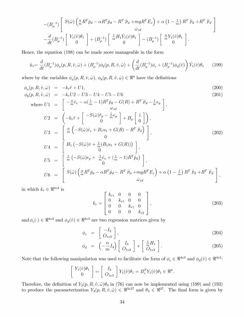
−(B−1µ ) S(ω) αmRT pd − αRT pd −RT

..pd +mgR

TEz + α 1− 1mRT

..pd +R

T...pd

ωzd

− ddt(B−1µ )

Y1(v)θ10

+ (B−1µ )1mH1Y1(v)θ10

− (B−1µ )αmY1(v)θ10

.

Hence, the equation (198) can be made more manageable in the form

.u1=

d

dt(B−1µ )φa(p,R, v, ω) + (B

−1µ )φb(p,R, v, ω) +

d

dt(B−1µ )φc + (B

−1µ )φd(v) Y1(v)θ1 (199)

where by the variables φa(p,R, v, ω), φb(p,R, v, ω) ∈ 4 have the definitions

φa(p,R, v, ω) = −krr + U1, (200)

φb(p,R, v, ω) = −krU2− U3− U4− U5− U6 (201)

where U1 =− αmev − α( 1

m− 1)RT pd −G(R) +RT

..pd − 1

mep

ωzd,

U2 = −krr + −S(ω)rp − 1mep

0+Bµ

z0

,

U3 =αm−S(ω)ev +B1u1 +G(R)−RT

..pd

0, (202)

U4 =H1 −S(ω)v + 1

m(B1u1 +G(R))0

,

U5 =1m−S(ω)ep + 1

mev + (

1m− 1)RT pd

0,

U6 =S(ω) α

mRT pd − αRT pd −RT

..pd +mgR

TEz + α 1− 1mRT

..pd +R

T...pd

ωzd,

in which kr ∈ 4x4 is

kr =

⎡⎢⎢⎣kr1 0 0 00 kr1 0 00 0 kr1 00 0 0 kr2

⎤⎥⎥⎦ , (203)

andφc(·) ∈ 4x3 and φd(v) ∈ 4x3 are two regression matrices given by

φc =−I3O1x3

, (204)

φd = − α

mI4

I3O1x3

+1mH1O1x3

. (205)

Note that the following manipulation was used to facilitate the form of φc ∈ 4x3 and φd(v) ∈ 4x3:

Y1(v)θ10

=I3O1x3

Y1(v)θ1 = BTz Y1(v)θ1 ∈ 4.

Therefore, the definition of Y3(p,R, v, ω)θ3 in (76) can now be implemented using (199) and (193)to produce the parameterization Y3(p,R, v, ω) ∈ 3x27 and θ3 ∈ 27. The final form is given by

34

Y3(p,R, v, ω) = [Y31, Y32, Y33, Y34, Y35, Y36] , with elements

Y31 =

⎡⎢⎢⎣φb2δ3

ω2ω3 −ω2ω3−ω1ω3 −φb1

δ3ω1ω3

ω1ω2 −ω1ω2 φa1δ3

.

(sφcφ) −

.

( cθcφ) φa4 +

φb1δ3tφ− cθ

cφφb4

⎤⎥⎥⎦ ,

Y32 =

⎡⎣ ω1 ω1 |ω1| 0 0 0 00 0 ω2 ω2 |ω2| 0 00 0 0 0 ω3 ω3 |ω3|

⎤⎦ ,

Y33 =

⎡⎢⎢⎣φd21δ3v1 0 0

0 −φd11δ3v1 0

0 0 − 1δ3

.

(sφcφ) +φd11tφ

δ3− φd41cθ

cφv1

⎤⎥⎥⎦ , (206)

Y34 =

⎡⎢⎢⎣φd21δ3v1 |v1| 0 0

0 −φd11δ3v1 |v1| 0

0 0 − 1δ3

.

(sφcφ) +φd11tφ

δ3− φd41cθ

cφv1 |v1|

⎤⎥⎥⎦ ,

Y35 =

⎡⎢⎣φd22δ3v2 0 0 φd22

δ3v2 |v2| 0 0

0 −φd12δ3v2 0 0 −φd12

δ3v2 |v2| 0

0 0 φd12tφδ3− φd42cθ

cφv2 0 0 φd12tφ

δ3− φd42cθ

cφv2 |v2|

⎤⎥⎦ ,

Y36 =

⎡⎢⎣φd23δ3v3 0 0 φd23

δ3v3 |v3| 0 0

0 −φd13δ3v3 0 0 −φd13

δ3v3 |v3| 0

0 0 φd13tφδ3− φd43cθ

cφv3 0 0 φd13tφ

δ3− φd43cθ

cφv3 |v3|

⎤⎥⎦ ,and by θ3 = [θ31, θ32, θ33, θ34]

T with elements given by

θ31 = J11 J22 J33 g1 g2 g3 g4 g5 g6 ,

θ32 = J11d1 J22d1 J33d1 J11d2 J22d2 J33d2 , (207)

θ33 = J11d3 J22d3 J33d3 J11d4 J22d4 J33d4 ,

θ34 = J11d5 J22d5 J33d5 J11d6 J22d6 J33d6 .

F Development of Centrifugal/Coriolis terms

Consider the Centrifugal/Coriolis force equations in (52), it can be rewritten as follows

N∗(R,T, x)xo −N∗(R,T, xo)xo = [N∗(R, T, x)−N∗(R,T, xo)] xo.

First we consider the first term, N∗(R,T, x), on the right-hand side of above equation

N∗(R, T, x) DT (R,T ) C(R,T )D(R,T )− MD(R, T, x) (208)

where

C(R, T )D(R, T )− MD(R, T, x)

35

=−mS(ω) O3x3O3x3 S(Jω)

RT O3x3O3x3 T−1(Θ)

− mI3 O3x3O3x3 J

ddt(RT ) O3x3O3x3

ddt(T−1(Θ))

=−mS(ω)RT O3x3

O3x3 S(Jω)T−1(Θ)− m d

dt(RT ) O3x3O3x3 J d

dt(T−1(Θ))

=−mS(ω)RT −m d

dt(RT ) O3x3

O3x3 S(Jω)T−1(Θ)− J ddt(T−1(Θ))

=O3x3 O3x3O3x3 S(Jω)T−1(Θ)− J d

dt(T−1(Θ))

.

Then, (208) becomes

N∗(R, T, x)R O3x3O3x3 T−T (Θ)

O3x3 O3x3O3x3 S(Jω)T−1(Θ)− J d

dt(T−1(Θ))

=O3x3 O3x3O3x3 T−T (Θ) S(Jω)T−1(Θ)− J d

dt(T−1(Θ))|Θ . (209)

In a same fashion, we can obtain

N∗(R, T, xo) =O3x3 O3x3O3x3 T−T (Θ) S(Jωo)T−1(Θ)− J d

dt(T−1(Θ))|Θ=Θo

. (210)

Then, the difference between (209) and (208) yields

N∗(R,T, x)−N∗(R, T, xo)

=O3x3 O3x3O3x3 T−T (Θ) S(Jω)T−1(Θ)− J d

dt(T−1(Θ)) − T−T (Θ) S(Jωo)T−1(Θ)− J d

dt(T−1(Θ))|Θ=Θo

=O3x3 O3x3O3x3 T−T (Θ) [S(Jω)T−1(Θ)− S(Jωo)T−1(Θ)] + T−T (Θ) −J d

dt(T−1(Θ)) + J d

dt(T−1(Θ))|Θ=Θo

.

(211)The first term in the last matrix in (211) yields

T−T (Θ) S(Jω)T−1(Θ)− S(Jωo)T−1(Θ)= T−T (Θ)S(Jω − Jωo)T−1(Θ)= T−T (Θ)S(JT−1(Θ)(Θ− Θo))T

−1(Θ)= T−T (Θ)S(JT−1(Θ)s Θ)T−1(Θ) (212)

where from the definition in (41) we can represent

s = x− xo = p− poΘ− Θo

s ps Θ

,

by defining ass p = p− po ∈ 3 and s Θ = Θ− Θo ∈ 3.

The second term in the last matrix in (211) yields using the (138)

T−T (Θ) −J ddt(T−1(Θ)) + J

d

dt(T−1(Θ))|Θ=Θo

36

= T−T (Θ) −J ∂

∂Θ(T−1(Θ))Θ+ J

∂

∂Θ(T−1(Θ))Θo

= −T−T (Θ)J ∂

∂Θ(T−1(Θ)) Θ− Θo

= −T−T (Θ)J ∂

∂Θ(T−1(Θ))s Θ (213)

whered

dt(T−1(Θ)) =

∂

∂Θ(T−1(Θ))Θ ∈ 3x3 (214)

∂

∂Θ(T−1(Θ)) ∈ 3x3x3 as a tensor. (215)

Thus, the matrix (211) yields

N∗(R,T, x)−N∗(R,T, xo)

=O3x3 O3x3

O3x3 T−T (Θ)S(JT−1(Θ)s Θ)T−1(Θ)− T−T (Θ)J ∂

∂Θ(T−1(Θ))s Θ

. (216)

Hence, the Centrifugal/Coriolis equations in (52) can be defined as

N∗(R, T, x)xo −N∗(R, T, xo)xo= (N∗(R, T, x)−N∗(R,T, xo)) xo

=O3x3 O3x3

O3x3 T−T (Θ)S(JT−1(Θ)s Θ)T−1(Θ)− T−T (Θ)J ∂

∂Θ(T−1(Θ))s Θ

xo

=O3x3 O3x3O3x3 T−T (Θ)S(JT−1(Θ)s Θ)T−1(Θ)− T−T (Θ)T (J,Θ, s Θ)

poΘo

=O3x1

T−T (Θ)S(JT−1(Θ)s Θ)T−1(Θ)Θo − T−T (Θ)T (J,Θ, s Θ)Θo

=O3x1

−T−T (Θ)S(T−1(Θ)Θo)JT−1(Θ)s Θ− T−T (Θ)Tc(J,Θ, Θo)s Θ

=O3x3 O3x3

O3x3 T−T (Θ) −S(T−1(Θ)Θo)JT−1(Θ)− Tc(J,Θ, Θo)

s ps Θ

= N∗c (R, T, xo)s (217)

where

N∗c (R,T, xo) =

O3x3 O3x3

O3x3 T−T (Θ) −S(T−1(Θ)Θo)JT−1(Θ)− Tc(J,Θ, Θo)

, (218)

and the followings are utilized

T (J,Θ, s Θ) = J∂

∂Θ(T−1(Θ))s Θ,

Tc(J,Θ, Θo)s Θ = T (J,Θ, s Θ)Θo.

G Figures

37

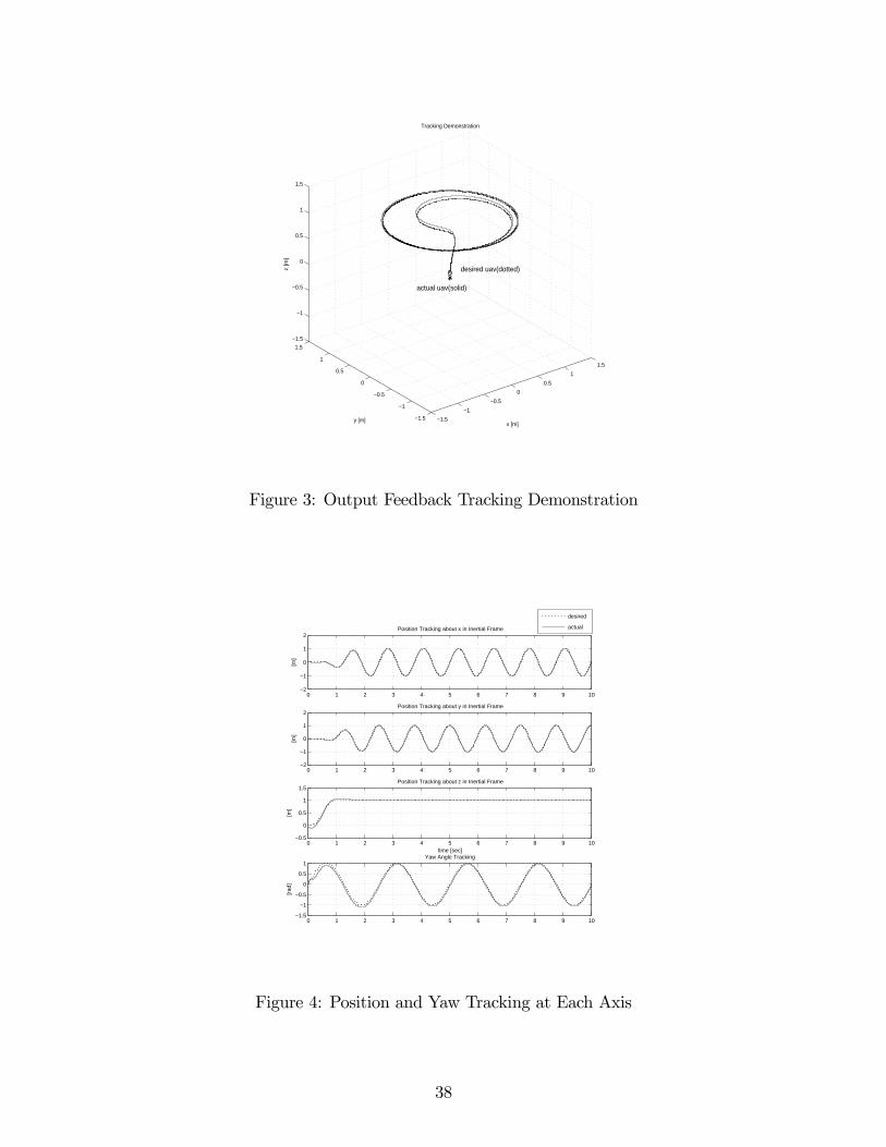
−1.5

−1

−0.5

0

0.5

1

1.5

−1.5

−1

−0.5

0

0.5

1

1.5

−1.5

−1

−0.5

0

0.5

1

1.5

x [m]

desired uav(dotted)

Tracking Demonstration

actual uav(solid)

y [m]

z [m

]

Figure 3: Output Feedback Tracking Demonstration

0 1 2 3 4 5 6 7 8 9 10−2

−1

0

1

2

[m]

Position Tracking about x in Inertial Frame

0 1 2 3 4 5 6 7 8 9 10−2

−1

0

1

2

[m]

Position Tracking about y in Inertial Frame

0 1 2 3 4 5 6 7 8 9 10−0.5

0

0.5

1

1.5

time [sec]

[m]

Position Tracking about z in Inertial Frame

desired

actual

0 1 2 3 4 5 6 7 8 9 10−1.5

−1

−0.5

0

0.5

1

[rad

]

Yaw Angle Tracking

Figure 4: Position and Yaw Tracking at Each Axis

38

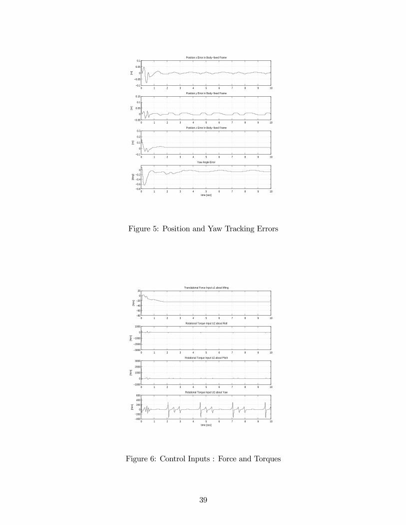
0 1 2 3 4 5 6 7 8 9 10−0.1

−0.05

0

0.05

0.1

[m]

Position x Error in Body−fixed Frame

0 1 2 3 4 5 6 7 8 9 10−0.05

0

0.05

0.1

0.15

[m]

Position y Error in Body−fixed Frame

0 1 2 3 4 5 6 7 8 9 10−0.1

0

0.1

0.2

0.3[m

]

Position z Error in Body−fixed Frame

0 1 2 3 4 5 6 7 8 9 10−0.8

−0.6

−0.4

−0.2

0

time [sec]

[deg]

Yaw Angle Error

Figure 5: Position and Yaw Tracking Errors

0 1 2 3 4 5 6 7 8 9 10−80

−60

−40

−20

0

20

[Nm

]

Translational Force Input u1 about lifting

0 1 2 3 4 5 6 7 8 9 10−3000

−2000

−1000

0

1000

[Nm

]

Rotational Torque Input U2 about Roll

0 1 2 3 4 5 6 7 8 9 10−1000

0

1000

2000

3000

[Nm

]

Rotational Torque Input U2 about Pitch

0 1 2 3 4 5 6 7 8 9 10−400

−200

0

200

400

600

time [sec]

[Nm

]

Rotational Torque Input U2 about Yaw

Figure 6: Control Inputs : Force and Torques

39

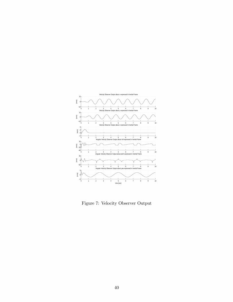
0 1 2 3 4 5 6 7 8 9 10−10

0

10

[m/s

]

Velocity Observer Output about x expressed in Inertial Frame

0 1 2 3 4 5 6 7 8 9 10−10

0

10

[m/s

]

Velocity Observer Output about y expressed in Inertial Frame

0 1 2 3 4 5 6 7 8 9 10−2

0

2

4

[m/s

]

Velocity Observer Output about z expressed in Inertial Frame

0 1 2 3 4 5 6 7 8 9 10−40

−20

0

20

[m/s

]

Angular Velocity Observer Output about roll expressed in Inertial Frame

0 1 2 3 4 5 6 7 8 9 10−50

0

50

[m/s

]

Angular Velocity Observer Output about pitch expressed in Inertial Frame

0 1 2 3 4 5 6 7 8 9 10−5

0

5

time [sec]

[m/s

]

Angular Velocity Observer Output about yaw expressed in Inertial Frame

Figure 7: Velocity Observer Output

40