Quad-Rotor UAV project

MS3 and MS4 report:

Controller Design and

Hardware/Software Implementation

Prepared for:

Professor Eric Klavins Charlie Matlack

Prepared By:

Justin Palm Andrew Nelson Andy Bradford

21 May 2010

2

Table of Contents

Introduction 2 Milestone 3 3 Controller Design Comparison 3 PID Control 3

Simulation Method 5 Simulation Results 6

Full state Feedback and LQR Pole Placement 8 LQR Simulation Results 10 Milestone 4 11 Project Update 11 Hardware Choices Software Choices Conclusion

Introduction This report will cover both materials that were required for milestone three as well as for milestone four. It is our intent to begin compiling our design procedures in a systematic way in an effort to better prepare ourselves for the final technical report. It is also the intent of this paper to make up for lost time due to unfortunate difficulties in modeling the quad-rotor dynamics and, subsequently, designing the control law for the system. We recently made much progress to this end and are presenting it here as an addendum to milestone four. The first half of this document will lead the reader through the controller design with detailed analysis of two types of controllers: PID, and LQR, and the limitations of the former. Results of simulations will be presented and discussed. The milestone-three segment concludes with a brief overview of the hardware/software planned implementation as a lead-in to milestone four. The last half of this paper is the scheduled milestone-four report. In this section, we will discuss the hardware and software choices used to power and control the quad rotor system. We will provide a project update and revised schedule specific to the last three weeks of the project and what maneuvers we plan to demonstrate at the completion of the project.

3

Milestone 3

Controller Design Comparison This section will discuss two approaches to designing a controller. The first is an attempt to use a simple PID approach while the second will use a Linear Quadratic Regulator (LQR). The limitations of the PID approach are immediately evident as one reads through the steps taken. PID Control

Figure 1: SIMULINK model for a step change in Z from a linearized system about a hovering position Figure 1 above shows the SIMULINK model built to model a step change in the Z position (altitude). The model has been linearized about a hovering position 1m above the ground. The input to the plant at that position is:

22 /

11

11

98.164 sradu

−

−

=

The value of 164.98 rad/s was derived ideally by simply assuming a static state, that is, the sum of all forces acting on the system in Z is equal to zero.

4

sradb

mg

bmg

FF ThrustGravity

/4921.8216

4 2

==

=

=

ω

ω

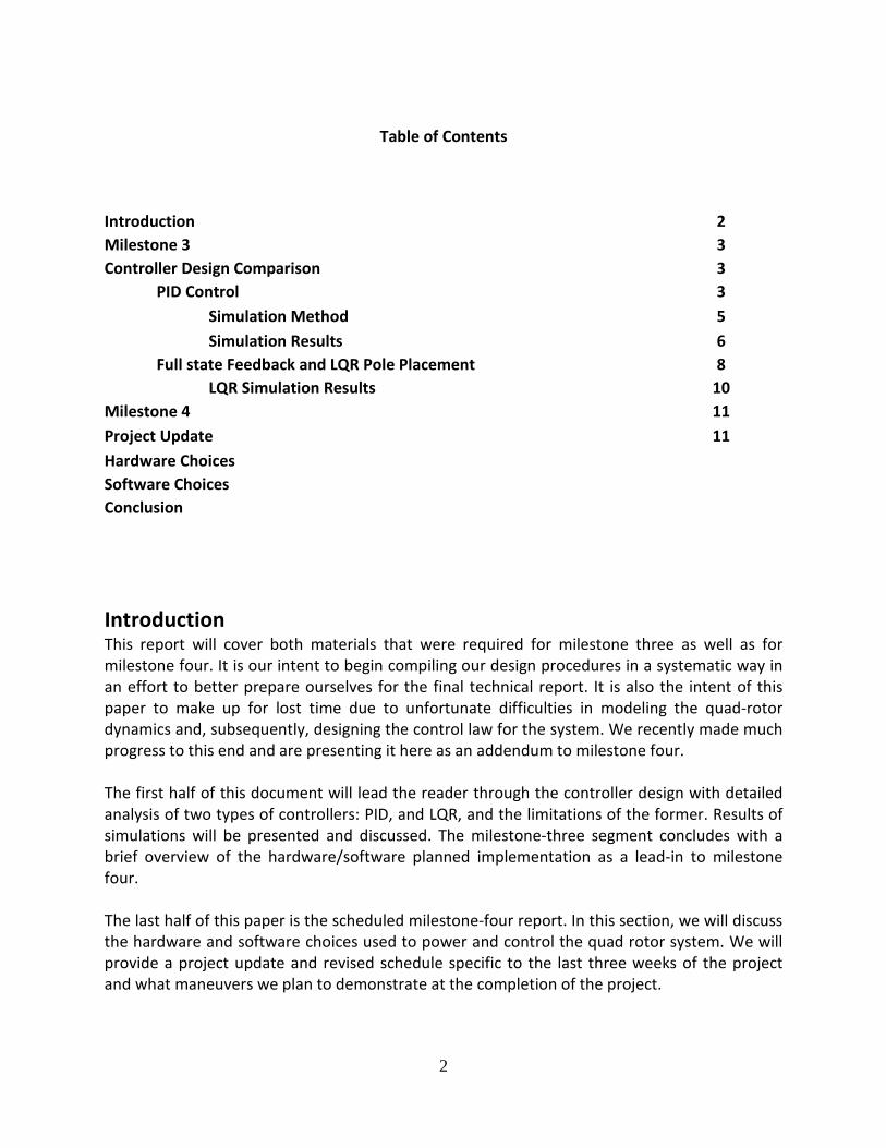
Substituting this value into the linearized input equation ωωωω ∆=∆= 98.16422 where ω∆ is the linearized input perturbation. The result of using this value in the linearized model is for no input, each rotor will be spinning at 12.845 rad/s. To verify that this is correct, the non linearized model is tested with a constant 164.94 (rad/s)2 applied at the input. The resulting plot is shown below.

Figure 2: Open loop test of non-Linearized plant with constant input of 164.984 (rad/s)2 One can see that the value being (164.98 [rad/s]2) used is fairly accurate as the altitude only drops by 6cm in 100 seconds without any feedback. Some clarification here is necessary: There is no floor on the simulation executed; that is, the quad rotor is being allowed to travel ‘through the ground’ just to demonstrate the correct linearized angular velocity was chosen. The plot of the linearized model is omitted here as it is simply zero throughout the 100 second simulation. Now that the base case has been determined, we can begin building up the controllers for each of the individual degrees of freedom we are interested in controlling. Again, we are focusing on only position and heading as these are the states that we can directly observe. It should be noted that in order to have control over translational and angular rates we would have to use

5

some form of estimator – a Luenburger Observer or Kalman filter for example. Given the time constraints we are focusing only on controlling those states we can directly observe. Simulation Method

Figure 3: Block: used to separate the error between the set point and actual position and heading. Figure 3 shows a set point block containing commanded positions (perturbations around linearized points) and actual position/heading being subtracted to give the error signals. These signals are then sent into separate PID controllers for each degree of freedom (here only X, Y, Z, and ψ). Each of the PID blocks are Identical in structure but will require separate gains to be specified. The structure of the PID blocks is shown in figure 4 below.

Figure 4: PID controller for Z position Control: P =3, I=0, D=8

6

Error between the commanded position and the actual position (both in inertial coordinates) is sent in to the PID controller shown in figure 3. The method used to determine the gains was that of trial and error with a Ziegler-Nichols type approach. First, the proportional gain was adjusted until a reasonable rise-time reached, and then damping (derivative gain) was added to stop any overshoot. It was found during simulation that no steady state error existed so integral gain is kept at zero. This is most likely due to the ideal nature of the model and simulation performed, but for now the gains shows are used. In a later section, noise will be added to the system and steady state error is predicted to exist. The output from the controller is sent into a vector that tells each of the motors to spin the same rate. This means that the error in the position is converted into angular velocities and sent into the plant. The step of converting the error to PWM signals that will ultimately drive the motors is left out of the simulation but will be addressed in the near future when we move from controller simulation to realization. Simulation Results (PID)

Figure 5: 2.5 meter step change in altitude Figure 5 shows a step change in altitude of 2.5 meters. The settling time is shown to be around 10 seconds with no overshoot and zero steady state error. This ideal model gives hope we will be able to achieve hover with the non linear system.

7

The next step is to test feedback for a heading change (i.e. PSI) In order to accomplish this, a gain block must be implemented that will increase or decrease the control signals based on which direction one wants to be oriented. The result of a 30 degree change in heading is shown below.

Figure 6: 30 degree step in psi. In order to maintain altitude, it was seen that the gains had to be increased to keep up with a sudden change in orientation. From this information, we now know that the degrees of freedom are not completely decoupled from our control input. Special care must be taken to ensure robustness to other commanded inputs such as X and Y. These simulations are yet unfinished but will be soon. The plot below shows the effect of a psi change after a Z command.

8

Figure 7: s Unit step change in Z followed by a 30 degree rotation about the Z axis. The change does affect the Z position but it recovers because of feedback As one can see from Figure 7, the control method currently being studied is not sufficient for our desired performance. The required mixing of signals is non-trivial and would ultimately require 12 independent PID loops – leading to 36 required gain calculations. While theoretically possible, this approach is impractical and quite difficult to calibrate. After exhausting our patience, we have changed the way the controller uses the error signals to that of Full-State feedback. Full-State Feedback and LQR pole placement Given our linearized plant, to achieve a desired control, we must add poles and/or zeros to the system’s forward path. By selecting the location of these poles carefully, we can achieve very tight tolerances to meet our specifications. The following diagram shows our system model with full-state feedback.

9

Figure 8: Full-state feedback system model The error between the commanded set point and the actual state of the system is sent into a proportional controller (denoted K*u). The gain block is an m x n matrix that will mix the error signals and convert them into angular velocities that are the inputs into the system. A quick analysis of the state matrix and input dimensions reveal the required size of the matrix K.

𝐾𝐾 ∗ [12 𝑥𝑥 1] = [4 𝑥𝑥 1] → 𝐾𝐾 𝑚𝑚𝑚𝑚𝑚𝑚𝑚𝑚 𝑏𝑏𝑏𝑏 [4 𝑥𝑥 12] The next step is to figure out what the necessary values in the K matrix must be to achieve the desired response. Enter LQR. The Linear Quadratic Regulator automatically calculates the gain matrix based on user defined control effort and state error by minimizing the cost function:

𝐽𝐽 = 𝑥𝑥′𝑄𝑄𝑥𝑥 + 𝑚𝑚′𝑅𝑅𝑚𝑚 𝑑𝑑𝑚𝑚

where x is the state vector and u = -Kx. By playing with Q and R we can achieve the desired results. Of course, we will not be doing this by hand; rather, Matlab conveniently has an LQR function that takes in the plant’s A and B matrices, and matrices Q and R and returns the gain matrix K. As a first attempt, we set the Q matrix to a 12x12 identity matrix and R to a 4x4 identity matrix scaled by 0.25. This essentially says that we don’t care how much control effort it takes to get there and we want it to get there fast. The results are discussed in the following section.

10

Simulation Results (LQR) The resulting simulation is shown in Figure 9 below. One can see an enormous difference in the controllability compared to the previous method of control (PID).

Figure 9: A one meter step changes in Z, X, Y, and 30 deg (π/6 rad) in psi. Each step is delayed in sequence to show the effect the step has on previous commands. The simulation includes a 5ms transport delay in the feedback to simulate a very bad latency with the Vicon system. We do not expect the delay to be so severe. It should be noted that Figure 9 shows all states. The lines going below the zero crossing are simply magnitudes in the negative direction. The Z step has a rise time of about 8 seconds and settles within 15 seconds. The X and Y responses are much faster – around 5 seconds each as there is less inertia to counter. At this point a discussion of assumptions made is in order. The model we are using is an ideal model. While we do have actuator saturations included in the simulation, there are no noise injections resulting in very nice simulations but will most likely not represent the true response of the system. Also, we are assuming we actually have the translational and rotational velocities in body coordinates. These states will need to be estimated. A recent test using derivatives of the inertial positions has yielded poor results and must be investigated further. The next section of the report discuses the hardware choices used to accomplish control of this system. There is a phenomenon when a rotor disc operates within approximately one diameter which results in an increased efficiency in a hover condition, called ground effect. This ground effect was not incorporated into our simulation such that the starting position of the quad rotor simulation occurs well above the region where this would occur.

11

Milestone 4

Project Update We have recently made good progress toward achieving our goal of autonomous hover. We have finally implemented the Vicon system as our feedback mechanism and run a test in the DSSL lab. This test resulted in less than satisfying results, but we have determined that the controller is trying to correct for error. This was determined by holding the quad rotor at a steady state and starting the system. As mentioned the rotors spin at near their saturation levels. One problem that may cause this is incorrectly estimating the full state of the system. Regarding scheduling, we have caught up and are back on schedule. Our plan of attack towards the beginning of this project was to get most of our hardware issues out of the way, giving us a time cushion to work on the controller aspect of the project, which turned out to be the majority of this project. This plan; however, backfired as it put us far behind the (recommended) schedule of milestones two and three. The big pay-off has arrived as we have already built the hardware portion of the project – effectively launching us ahead. The following is a schedule of what we hope to accomplish in the last three weeks of the quarter.

Figure 10: Current timeline for the last three weeks of the project

12

Week 11 marks the end of the project. At this point we hope to have achieved some of the initial goals specified in milestone one. Also during week 11 is a lab visit from our professor. It is our intention to demonstrate the following:

• open-loop joystick control for comparison purposes • closed-loop control.

o auto-hover capability o joystick control o unit step input in X, Y, Z, Ψ o possible 3D auto tracking

Hardware There are three pieces of electronics hardware used in the control setup, the Vicon vision system, a laptop running Simulink with the control loop and the electronics hardware on the quad rotor. Since the laptop is mostly software, discussion of that will be put off until the software section of this report. We will be discussing the other two components here. The entire hardware level feedback loop is shown in Figure 11.

Figure 11: Overview of Hardware level Feedback loop Vicon Vision System The Vicon vision system is comprised of 3 components. The Vicon cameras, the Vicon hardware processor, and the Vicon host computer. There are six Vicon cameras placed on the ceiling in the DSSL lab. Each camera is 2 megapixels and runs at 120fps. The system tracks an area that is about 8'x6'x5'. These cameras are infrared black and white cameras. By using special reflective balls on the subject, the Vicon cameras use IR LEDs to reflect off of the balls producing an image

13

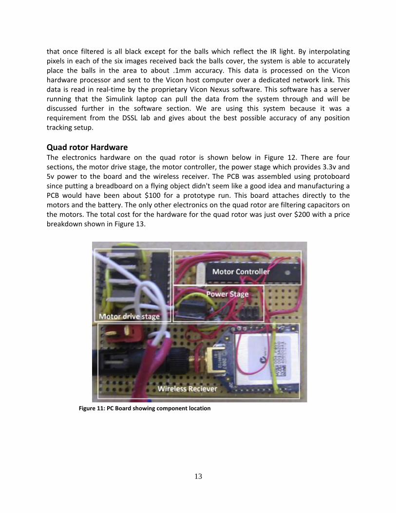
that once filtered is all black except for the balls which reflect the IR light. By interpolating pixels in each of the six images received back the balls cover, the system is able to accurately place the balls in the area to about .1mm accuracy. This data is processed on the Vicon hardware processor and sent to the Vicon host computer over a dedicated network link. This data is read in real-time by the proprietary Vicon Nexus software. This software has a server running that the Simulink laptop can pull the data from the system through and will be discussed further in the software section. We are using this system because it was a requirement from the DSSL lab and gives about the best possible accuracy of any position tracking setup. Quad rotor Hardware The electronics hardware on the quad rotor is shown below in Figure 12. There are four sections, the motor drive stage, the motor controller, the power stage which provides 3.3v and 5v power to the board and the wireless receiver. The PCB was assembled using protoboard since putting a breadboard on a flying object didn't seem like a good idea and manufacturing a PCB would have been about $100 for a prototype run. This board attaches directly to the motors and the battery. The only other electronics on the quad rotor are filtering capacitors on the motors. The total cost for the hardware for the quad rotor was just over $200 with a price breakdown shown in Figure 13.

Figure 11: PC Board showing component location

14

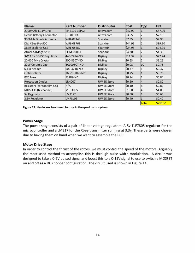
Name Part Number Distributor Cost Qty. Ext. 2100mAh 11.1v LiPo TP-2100-3SPL2 rctoys.com $47.99 1 $47.99 Deans Battery Connector DE-ULTRA rctoys.com $3.55 2 $7.10 900MHz Dipole Antenna WRL-09143 Sparkfun $7.95 1 $7.95 Digi XBee Pro 900 WRL-08768 Sparkfun $44.95 2 $89.90 XBee Explorer USB WRL-08687 Sparkfun $24.95 1 $24.95 Atmel ATMega328P COM-09061 Sparkfun $4.30 2 $4.30 3W 3.3v DC-DC Regulator 445-2474-ND Digikey $11.37 2 $22.74 20.000 MHz Crystal 300-8507-ND Digikey $0.63 2 $1.26 22pF Ceramic Cap BC1005CT-ND Digikey $0.08 10 $0.76 6-pin header 609-3218-ND Digikey $0.37 1 $0.37 Optioisolator 160-1370-5-ND Digikey $0.75 1 $0.75 PTC Fuse F3189-ND Digikey $0.84 1 $0.84 Protection Diodes 1N4007 UW EE Store $0.20 4 $0.80 Resistors (carbon film 5%) N/A UW EE Store $0.10 8 $0.80 MOSFETs (N-channel) MTP3055 UW EE Store $1.00 4 $4.00 5v Regulator LM317T UW EE Store $0.60 1 $0.60 3.3v Regulator LM78L05 UW EE Store $0.40 1 $0.40

Total $215.51

Figure 13: Hardware Purchased for use in the quad rotor system Power Stage The power stage consists of a pair of linear voltage regulators. A 5v TLE7805 regulator for the microcontroller and a LM317 for the Xbee transmitter running at 3.3v. These parts were chosen due to having them on hand when we went to assemble the PCB. Motor Drive Stage In order to control the thrust of the rotors, we must control the speed of the motors. Arguably the most used method to accomplish this is through pulse width modulation. A circuit was designed to take a 0-5V pulsed signal and boost this to a 0-11V signal to use to switch a MOSFET on and off as a DC chopper configuration. The circuit used is shown in Figure 14.

15

M1PWM0-5v

M2PWM0-5v

M3PWM0-5v M4

PWM0-5v

+11.1 V

+11.1 V

Figure 14: Motor Power Stage. The input is a 0-5V PWM signal and the output is speed control. Each motor is independently controllable. The components were chosen to handle the current draw requirements of the motors which are around 4 amps max and to provide isolation between the power stage and the micro controller. The MOSFETs (MTP3055) were selected for their performance, reliability, price and due to familiarity having used them on another EE related project. The MTP3055 are rated at 12A max current load, 0.15Ω on resistance, and are also ideal for switching applications. Next is the Opto-Isolator (LTV-847) which comes as a quad package perfectly suited for our four drive stages, 4µs rise-time which is 25 times our base frequency of 10 KHz and were very cheap at $0.75. Switching protection diodes are installed across the Motor to allow for freewheeling- current flow due to back EMF as the motors spin during the off cycle. 1 KΩ pull-up resistors are used to bias up the gate of the MOSFET in its linear region. Lastly is the Li-Polymer 3 Cell Battery which is rated at 2100mAhr, giving us an empirically determined flight endurance of approximately 40 minutes. However, we expect a typical flight on the order of 20 minutes. This battery gives us almost twice the capacity as the one that came with the original quad rotor. Motor Controller In order to control the motor, we decided on the Atmel ATMega328p microcontroller. This microcontroller was chosen due to having the PWM outputs we needed, the serial link to the Xbee we need, and already having familiarity with the microcontroller and owning the programmer. The motor controller is currently running off an external crystal at 20MHz. This was chosen so we could achieve a reasonable PWM speed of 10 KHz and allow a high serial data rate to the XBee of 115200 Kbps. Wireless Receiver

16

In order to communicate with the quad rotor we decided to go with a pair of 900MHz XBee radios. These radios offer two way communications with the quad rotor over a standard UART serial link. They provide 156 Kbps data rate and a line of sight range of 6 miles. These were chosen so the quad rotor could eventually be flown outside without having to worry about the signal fading out. The 900MHz radios were chosen due to having compact antennas while providing low link losses and not have issues with interference on the 2.4GHz band. While the current setup only sends 9600 bit/s, the high data rate was chosen due to its lower latency and having extra bandwidth for sending retries creating a more robust wireless link.

Software There are three major pieces of software being used in this project. There is the software on the quad rotor to control the motors, the software used to interface and pull data off of the Vicon system, and the Simulink model used to take data from the Vicon and input from the user to run the control loop and output the data over serial to the quad rotor. While the software on the quad rotor has been locked down for about 4 weeks, there have been issues with the Vicon setup prompting a look at possibly moving away from Simulink for feedback control. This section of the paper will first talk about the software on the quad rotor, then talk about the interface used for the Vicon camera system, and lastly, it will present the current Simulink setup. The section will then end with a few possible alternatives for feedback to Simulink and corresponding tradeoffs. Our plan for the weekend will be to decide on one to implement and move forward with. Quad rotor Microcontroller Software Since all of the feedback for the quad rotor is running on the control computer, the software on the quad rotor is very simple. The software was written in C and compiled for the ATMega328 using the gcc-avr toolchain. Each of the motors is attached to one of the PWM outputs on the ATMega328. These PWM outputs have 8-bits of resolution and run at about 10 KHz. The raw PWM values are calculated by Simulink and sent over the Xbee wireless link to the ATMega. In order to make sure the ATMega doesn't receive any bad PWM values, there is also a start and stop byte that it will check for and each value is sent twice to make sure it is what is really wanted. The ATMega waits in a loop for serial input looking for the start byte. Once it sees the start byte, it will read the next 8 bytes for the PWM values and check that the 9th byte sent is the stop byte. If it is it will then check to make sure the first four bytes of PWM values match the second four. If they do it will send these commands to the motor. Since the battery is running at 11.1v and the motors can only handle 9v, the ATMega will cap any PWM values sent from 0-180 instead of 0-255 with 0 representing a duty cycle of 0% and 255 representing a duty cycle of 100%.

Vicon Interface Since there were several questions today about the interface to the Vicon today, this section will describe in detail what the Vicon interface is and how it is possible to communicate with it. The six Vicon cameras capture in the infrared spectrum. By using IR LEDs, the cameras receive the reflections of the motion capture balls that are placed on the subject. The raw images are

17

each 2 megapixel in size and fed directly to a special Vicon hardware processor. This hardware processor is connected directly using a dedicated network to the Vicon host computer. The data being sent from the hardware processor to the host computer looks to be UDP, but since Vicon makes money selling specialized software packages to interface with the system, this protocol is not open. The Vicon host computer runs a program called Vicon Nexus. This software is what is used to capture data from the Vicon system. The software allows defining subjects to capture and labeling of the motion capture balls. This software is mostly designed to capture subjects and then use post processing on them. In order to do real time capture, there is a TCP/IP interface provided. This interface works in two modes. The first is frame-by-frame pulling and the second is continuous streaming. In frame-by-frame polling, the client requests a frame from the Vicon Nexus and it sends the most current frame. The second mode, Vicon Nexus will send the current frame as soon as it processes it. There is some documentation on how to write your own client for this system, but we are currently using a .dll file provided by Vicon for interfacing with Matlab. The .dll file works by calling a GetFrame() function which returns the current frame. There are several other functions to access the data in each frame. Also, there is a low latency mode for the library called SetPreFetchMode() that as far as I can tell puts the Vicon Nexus in continuous steaming mode. Further work will be done with Wireshark to confirm that this is the case. The only documentation we have on this setting is that it provides lower latency. There are several quirks and limitations to this interface that we are experiencing. The first is calling GetFrame() doesn't block when a new frame is not available so it just returns the current frame. This means that in order to get a new frame requires that we keep calling GetFrame() until the frame number is updated. We also suspect that we may be getting stale data from the .dll file may be stale at certain times. When we disconnect the connection, move the quad rotor, and start a new connection the first few frames we receive are from the previous position of the quad rotor. This may be a sign that all data we are receiving from the Vicon is stale. The biggest issue we have encountered is that there seems to be massive frame dropping in the data we are receiving. Creating a simple C program that requests GetFrame() in a loop and looks at the frame numbers shows that from a computer connected to the network, we have seen as high as 2000 out of the 2400 frames we have sent be lost. We suspect that this is an issue with the network, but it could also be an issue with the Vicon Nexus protocol. Since we already have to do repeated calls to GetFrame() to figure out even when a new frame comes in, this causes serious lag in the system and causes issues with the time steps in our derivatives. I have spent most of the past week trying to get this Vicon system working in a reasonable manor. Most of the issues are caused by lack of good documentation for these interfaces. Most of the clients for these systems use the motion capture in a post processing application so the real time interface is not well documented. For the .dll file we are using, we have a single .h file with vague one line comments describing what each function does and an example .m file. In order to link against this library with compiled code required manually creating a .lib file to link with since one wasn't provided. Very little information is even available on Google about these

18

systems. I suspect to get good performance out of the Vicon will require writing our own network client. Simulink Feedback Control The original plan was to implement our feedback loop entirely in the Real-time Workshop for Windows package for Simulink. The main advantage of using Simulink was that it allows for rapid prototyping, simulation, and deployment of the feedback loop in one package. With the difficulty of getting a working controller for a quad rotor, being able to easily change the feedback loop and have access to the large library of blocks was seen as the fastest way to get the system up and running. Due to needing to accurately set the feedback loop's speed to the Vicon's 120 Hz, we need to run the final version in Real-time Workshop. Getting our controller and serial output working under Real-time Workshop was fairly straightforward. There is a block in Simulink's library for serial output and the controller was just copied over from what we were running closed loop simulations on. Again issues came up due to the interface to the Vicon. While the .dll file interface works easily in Matlab, getting the interface into Simulink was quite difficult. It required writing a custom S-Function in C. We have had success getting this S-Function to work with Simulink and the Vicon in simulation mode, but getting it to build for Real-time Workshop looks require adding a lot more to the S-Function. In light of the issues with the Vicon and the Simulink interface, we are now looking at several possible replacement controller interfaces and will present them in the following section. Alternatives to Simulink Three alternatives to using Simulink are presented and discussed below. We will be looking at what it will take to implement the feedback controller with them in the next few days. Implement Feedback on ATMega328 One alternative to using Simulink would be to move the control to the ATMega328 itself. There are several downsides to this strategy. The first is the data types supported by the ATMega328. On most computers doubles use IEEE 754 64-bit floating point. For what we are doing, this is plenty. With avr-gcc, all floating point is limited to 32-bit floating point. With 32-bit floating point, the fractional component of the floating point number is only good for just over 7-bits of data. This could lead to some serious round off on our controller and cause instabilities. The second major issue is the chip does not provide any debug interface so troubleshooting issues would be difficult. Implement in Matlab While Simulink has problems with the Vicon interface, getting the interface into Matlab is relatively straightforward. This option would also allow for fairly fast prototyping of the controller so issues could be isolated and fixed very fast. Matlab also gives easy access to serial out and vector operations that are needed. In order to use Matlab we would have to figure out if it offers accurate timing to at least a millisecond for locking the data stream with the Vicon and having accurate timing for our derivatives. The main drawback could be issues with trying

19

to compile the script for speed. Since we need to run this near real-time, we will probably have to use the Matlab compiler mcc to convert it to machine code. This should be straightforward and perform well, but no one in the group has worked directly with mcc yet. Also, since we may have to end up running on the Vicon computer, the lack of most toolboxes offered by Matlab may end up being an issue. Implement in Python with NumPy This option seems like it could be promising. I have some experience working with Python and NumPy. This would allow us to have similar functionality to Matlab while offering a better purpose general programming language through Python. This would also allow us to easily make a GUI for controlling the quad rotor and have a real-time visual output, which is something I am not sure Matlab can do well without using Simulink. Since python already has well established libraries for serial interfaces and socket programming, it would also allow us to replace the Vicon's .dll file with something where we understand well how it works. The main drawback is that unlike Matlab, only one person in the group has experience with Python.

Conclusion We have presented our current design for both our controller and the hardware and software that run the system. Overall, we still feel we will be on track to get the quad rotor flying at the end of the quarter. The last major stumbling block has been the Vicon system which looks like it will make us rethink the use of Simulink for our feedback loop. With a few good alternative software replacements in mind, we should be able to choose one that will work for the project and still keep our goal of easily implementable in mind. The last step will be figuring how much the model differs from the real quad rotor and adjusting our controller to match the hardware. We still have high hopes for being able to finish in the three weeks remaining in the quarter.

20

Bibliography [1] B. Heemstra. (2010) Linear Quadratic Methods Applied to Quad rotor Control.

Unpublished Master's thesis. University of Washington. [2] C. Balas. (2007) Modeling and Linear Control of a Quad rotor. Master’s thesis. Cranfield

University.https://dspace.lib.cranfield.ac.uk/bitstream/1826/2417/1/Modelling%20and%20Linear%20Control%20of%20a%20Quadrotor.pdf

[3] S. Bouabdallah, A. Noth, and R. Siegwart, “PID vs LQ control techniques applied to an

indoor micro quadrotor”, 2004 IEEE/RSJ International Conference on Intelligent Robots and Systems, 2004.(IROS 2004). Proceedings, vol. 3, pp. 1-6. P. Castillo, A. Dzul, and R. Lozano, “Real-Time Stabilization and Tracking of a Four- Rotor Mini Rotorcraft”, IEEE Transactions on Control Systems Technology, Vol 12, No 4, July, 2004.

[4] McKerrow, P. (2004), "Modelling the Draganflyer four rotor helicopter", 2004 IEEE International Conference on Robotics and Automation, April 2004, New Orleans, pp. 3596.

[5] Observability. (2010, March 29). In Wikipedia, The Free Encyclopedia. Retrieved 00:26, April 24, 2010, fromhttp://en.wikipedia.org/w/index. php?title=Observability&oldid=352709914