UAV Photogrammetry under Poor Lighting Conditions ... - MDPI

sensors

Article

UAV Photogrammetry under Poor LightingConditions—Accuracy Considerations

Pawel Burdziakowski * and Katarzyna Bobkowska

��

Citation: Burdziakowski, P.;

Bobkowska, K. UAV Photogrammetry

under Poor Lighting Conditions—

Accuracy Considerations. Sensors

2021, 21, 3531. https://doi.org/

10.3390/s21103531

Academic Editors: José

Emilio Meroño de Larriva and

Francisco Javier Mesas Carrascosa

Received: 22 April 2021

Accepted: 17 May 2021

Published: 19 May 2021

Publisher’s Note: MDPI stays neutral

with regard to jurisdictional claims in

published maps and institutional affil-

iations.

Copyright: © 2021 by the authors.

Licensee MDPI, Basel, Switzerland.

This article is an open access article

distributed under the terms and

conditions of the Creative Commons

Attribution (CC BY) license (https://

creativecommons.org/licenses/by/

4.0/).

Department of Geodesy, Faculty of Civil and Environmental Engineering, Gdansk University of Technology,Narutowicza 11-12, 80-233 Gdansk, Poland; [email protected]* Correspondence: [email protected]

Abstract: The use of low-level photogrammetry is very broad, and studies in this field are conductedin many aspects. Most research and applications are based on image data acquired during theday, which seems natural and obvious. However, the authors of this paper draw attention to thepotential and possible use of UAV photogrammetry during the darker time of the day. The potentialof night-time images has not been yet widely recognized, since correct scenery lighting or lack ofscenery light sources is an obvious issue. The authors have developed typical day- and night-timephotogrammetric models. They have also presented an extensive analysis of the geometry, indicatedwhich process element had the greatest impact on degrading night-time photogrammetric product, aswell as which measurable factor directly correlated with image accuracy. The reduction in geometryduring night-time tests was greatly impacted by the non-uniform distribution of GCPs within thestudy area. The calibration of non-metric cameras is sensitive to poor lighting conditions, whichleads to the generation of a higher determination error for each intrinsic orientation and distortionparameter. As evidenced, uniformly illuminated photos can be used to construct a model with lowerreprojection error, and each tie point exhibits greater precision. Furthermore, they have evaluatedwhether commercial photogrammetric software enabled reaching acceptable image quality andwhether the digital camera type impacted interpretative quality. The research paper is concludedwith an extended discussion, conclusions, and recommendation on night-time studies.

Keywords: UAV; photogrammetry; night; model; light pollution

1. Introduction

Low-level air photogrammetry using unmanned aerial vehicles (UAVs) has attractedhuge interest from numerous fields over the last ten years. Photogrammetric products areused in various economic sectors, and thus intensively contribute to their growth. Thissituation primarily results from the development and widespread availability of UAVsequipped with good-quality non-metric cameras, the development of software base andeasy-to-use photogrammetric tools, as well as increased computing power of personalcomputers. Despite the already widespread use of the aforementioned techniques, there isstill a large number of issues associated with the processing of low-level photogrammetryproducts. This is mainly influenced by a relatively young age of this technology, thedynamic development of sensor design technology and modern computing methods. Itcan be stated without doubt that the complete potential of photogrammetry has not yetbeen fully discovered and unleashed, which is why scientists and engineers are constantlyworking on improving and developing the broadly understood UAV photogrammetry.

Works in the field of developing UAV measurement technologies are conductedconcurrently on many levels. Scientists quiet rightly focus on selected elements of the entirephotogrammetric product process, studying particular relationships, while suggesting newand more effective solutions. Research in the field of UAV photogrammetry can be dividedinto several mainstreams, with the main ones including:

Sensors 2021, 21, 3531. https://doi.org/10.3390/s21103531 https://www.mdpi.com/journal/sensors

https://www.mdpi.com/journal/sensors

https://www.mdpi.com

https://orcid.org/0000-0002-2869-5727

https://www.mdpi.com/article/10.3390/s21103531?type=check_update&version=1

https://doi.org/10.3390/s21103531

https://doi.org/10.3390/s21103531

https://creativecommons.org/

https://creativecommons.org/licenses/by/4.0/

https://creativecommons.org/licenses/by/4.0/

https://doi.org/10.3390/s21103531

https://www.mdpi.com/journal/sensors

Sensors 2021, 21, 3531 2 of 23

• Carrier system technology and techniques [1–4]: Works in this group focus on im-proving the navigation-wise aspects of flight execution, georeference accuracy, orsensor quality in order to achieve even better in-flight performance, flight time andstability [5–7], as well as the accuracy of navigation systems feeding their data tomeasuring modules [8,9].

• Optimization of photogrammetric product processes [10–13]: Scientists look at pro-cesses ongoing at each stage of image processing and suggest optimal recommenda-tions in terms of acquisition settings, image recording format [14], flight planning, orapplication of specific software settings [15].

• Evaluating the quality of results obtained using UAV photogrammetry [16,17]: Theseanalyses address the issues of errors obtained for photogrammetric images and prod-ucts, based on applied measuring technologies (from the acquisition moment, throughdata processing using specialized software).

• Focusing on the development of new tools improving the quality of low-level im-ages [18–20]: Studies in this group involve a thorough analysis of the procedure ofacquiring and processing UAV images and suggest new, mainly numerical, methodsfor eliminating identified issues [21–23]. As it turns out, photos taken from a dynam-ically moving UAV under various weather and UAV lighting conditions exhibit anumber of flaws. These flaws result directly from the acquisition method and impactphotogrammetric product quality.

• Showing new applications and possibilities for extracting information from spatialorthophotoimages based on photos taken in the visible light range [24–27] and bymulti-spectral cameras [28–30]: Unmanned aerial vehicles are able to reach placesinaccessible to traditional measurement techniques [31,32]. However, they carry anincomplete spectrum of sensors onboard, due to their restricted maximum take-offmass (MTOM). Therefore, scientists focus on methods that enable extracting significantinformation from this limited number of sensors and data, e.g., only from a singlecamera, but used at various time intervals [33] or a limited number of spectral channelsin cameras used on the UAV.

• Presenting new photogrammetric software and tools [34–36]: The increasing demandfor easy-to-use software obviously results in the supply of new products, both typi-cally commercial and non-commercial products. New technologies and methods aredeveloped in parallel.

• Using sensory data fusion [37–39]: The issue in this group is the appropriate har-monization of data obtained from a dynamically moving UAV and other stationarysensors. Very often, these data have a slightly different structure, density, or accu-racy, e.g., integration of point cloud data obtained during a photogrammetric flight,terrestrial laser scanning, and bathymetric data [40,41].

The above research, focusing strictly on specified certain narrow aspects of developinga photogrammetric product based on data acquired from an unmanned aerial vehicle,translate into further application studies, case studies, and new practical applications.Naturally, the most populated group of application studies are works addressing theissue of analysing the natural environment and urban areas. Popular application-relatedresearch subjects include analysing the wood stand in forestry [42–45], supporting preciseagriculture and analysing the crop stand [46–48], and geoengineering analyses for thepurposes of landform change and landslide analyses [49–52].

As evidenced above, the application of low-level photogrammetry is very broad,and studies in this field are conducted in many aspects. It should be noted that all theaforementioned research is based on image data acquired during the day, which seemsnatural and obvious. However, the authors of this paper draw attention to the potentialand possible use of UAV photogrammetry during the darker time of the day. Previously,the potential of night-time images has not been yet widely recognized, since correct scenerylighting or a lack of scenery light sources remain obvious issues [53].

Sensors 2021, 21, 3531 3 of 23

Studies dealing with night-time photogrammetry that point to the potential of suchphotos are still a niche topic [54]. A good example is the case of images inside religiousbuildings, obtained during the night and supported by artificial lighting. Such methodsare used in order to improve the geometric model quality of the studied buildings throughavoiding reflections and colour changes caused by sunlight penetrating into the interiorthrough colourful stained-glass windows [55]. Similar conclusions were drawn by theauthors of [56], who studied the issues associated of modelling building facades. Thedark time of the day favours background elimination and extracting light sources. Thisproperty was utilized by the authors of [57], who used light markers built from LEDs tomonitor the dynamic behaviour of wind turbines. This enabled to achieve a high contrastof reference light points on the night-time photos, which improved their location andidentification. Similar, too, was the case with analysing landslide dynamics [58]. Santiseet al. [59] focused on analysing the reliability of stereopairs taken at night, with variousexposure parameters, for the purposes of geostructural mapping of rock walls. Theseexamples show that terrestrial night-time photogrammetry has been functioning for years,albeit with a small and narrow scope of applications.

Night-time photogrammetry using UAVs has been developing for several years.The appearance of very sensitive digital camera sensors with low specific noise andsmall cameras working in the thermal infrared band made it quite easy to use them onUAVs [60,61]. So far, the main target of interest for UAV night-time photogrammetry hasbeen urban lighting analyses.

The problem of artificial lighting analysis may comprise of numerous aspects. Thefirst one is safety [62]. This topic covers analysing the intensity of lighting, which is impor-tant from the perspective of local safety, and enables optimizing lamppost arrangement,designing illumination direction, power, and angle, and thus selecting lighting fixtures. Aproperly illuminated spot on the road allows to see danger in time, is cost-efficient, anddoes not dazzle drivers [63–65]. On the other hand, artificial lighting also has a negativeimpact on humans and animals [66]. It has been an actor in the evolution of nature andhumans for a short time, and its presence, especially accidental, is defined as artificial lightpollution [67]. The issue associated with this phenomenon is increasingly noticed alreadyat society level [68]. Night-time spatial data will be an excellent tool for analysing lightpollution. Data from digital cameras mounted on UAVs and data from terrestrial laserscanning (TLS) for analysing street lighting is used for this purpose [69]. The authors of [70]showed that UAV data enable capturing urban lighting dynamics both in the spatial andtemporal domains. In this respect, the scientists utilized the relationship between observedquality and terrestrial observations recorded using a sky quality meter (SQM) light intensitytool. For the purposes of determining luminance, the authors of [71] present methods forcalibrating digital cameras fixed on UAVs and review several measuring scenarios.

UAVs equipped with digital cameras are becoming a tool that can play an impor-tant role in analysing artificial light pollution [72,73]. The possibility of obtaining high-resolution point clouds and orthophotoimages is an important aspect in this respect. Theaforementioned research did not involve an in-depth analysis of the photogrammetricprocess and the geometric accuracy of typical models based on night-time photos (withexisting street lighting). All analyses based on spatial data obtained through digital imag-ing should be supported with analysing point cloud geometric errors and evaluating thequality of developed orthomosaic. Night-time acquisition, as in the above cases, shouldnot be treated the same as day-time measurements. These studies assumed, a priori, thattypical photogrammetric software was equally good with developing photos taken in goodlighting and night-time photographs. The issues that impact night-time image quality canalso be scenery lighting discontinuity or too poor lighting at the scene, and increased levelsof noise and blur appearing on digital images obtained from UAVs.

As a result of the above considerations, the authors of this paper put forward athesis that a photogrammetric product based on night-time photos will exhibit lowergeometric accuracy and reduced interpretative quality. It seems that this thesis is rather

Sensors 2021, 21, 3531 4 of 23

obvious. However, after a deeper analysis of the photogrammetric imaging process,starting with data acquisition, through processing and to spatial analyses, it is impossibleto clearly state which of the elements of this process will have the greatest influence on thequality of a photogrammetric product. This leads to questions concerning which processelement had the greatest impact on degrading a night-time photogrammetric product,which measurable factor directly correlated with image accuracy, and whether commercialphotogrammetric software enabled reaching acceptable image quality and whether thedigital camera type impacted interpretative quality. Therefore, the authors of this study seta research objective of determining the impact of photogrammetric process elements onthe quality of a photogrammetric product, for the purposes of identifying artificial lightingat night.

2. Materials and Methods2.1. Research Plan

In order to verify the thesis and research assumptions of this paper, a test scheduleand computation process were developed. This process in graphic form, and the used tools,are shown in Figure 1. The test data were acquired using two commercial UAVs. The studyinvolved 4 research flights, two during the day, around noon, and two at night. Studydata were processed in popular photogrammetric software, and typical photogrammetricproducts were then subjected to comparative analysis. The study involved taking day-timephotos in automatic mode, and night-time ones manually. This enabled correctly exposingthe photos at night, without visible blur. The details of these operations are shown in thefurther section of this paper.

Sensors 2021, 21, x FOR PEER REVIEW 4 of 24

accuracy and reduced interpretative quality. It seems that this thesis is rather obvious. How-ever, after a deeper analysis of the photogrammetric imaging process, starting with data acquisition, through processing and to spatial analyses, it is impossible to clearly state which of the elements of this process will have the greatest influence on the quality of a photo-grammetric product. This leads to questions concerning which process element had the greatest impact on degrading a night-time photogrammetric product, which measurable factor directly correlated with image accuracy, and whether commercial photogrammetric software enabled reaching acceptable image quality and whether the digital camera type impacted interpretative quality. Therefore, the authors of this study set a research objective of determining the impact of photogrammetric process elements on the quality of a photo-grammetric product, for the purposes of identifying artificial lighting at night.

2. Materials and Methods 2.1. Research Plan

In order to verify the thesis and research assumptions of this paper, a test schedule and computation process were developed. This process in graphic form, and the used tools, are shown in Figure 1. The test data were acquired using two commercial UAVs. The study involved 4 research flights, two during the day, around noon, and two at night. Study data were processed in popular photogrammetric software, and typical photogram-metric products were then subjected to comparative analysis. The study involved taking day-time photos in automatic mode, and night-time ones manually. This enabled correctly exposing the photos at night, without visible blur. The details of these operations are shown in the further section of this paper.

Figure 1. Test and result processing diagram.

2.2. Data Acquisition Research flights were conducted using two UAV types: DJI Mavic Pro (MP1) and DJI

Mavic Pro 2 (MP2) (Shenzhen DJI Sciences and Technologies Ltd., China). Such an un-manned aerial vehicles are the representatives of commercial aerial systems, designed and intended primarily for recreational flying and for amateur movie-makers. The versatility and reliability of these devices was quickly appreciated by the photogrammetric commu-nity. Their popularity results mainly from their operational simplicity and the very intui-tive ground station software.

Both UAVs are equipped with an integrated digital camera with a CMOS (comple-mentary metal-oxide-semiconductor) sensor Table 1. An FC220 digital camera installed

Figure 1. Test and result processing diagram.

2.2. Data Acquisition

Research flights were conducted using two UAV types: DJI Mavic Pro (MP1) andDJI Mavic Pro 2 (MP2) (Shenzhen DJI Sciences and Technologies Ltd., Shenzhen, China).Such an unmanned aerial vehicles are the representatives of commercial aerial systems,designed and intended primarily for recreational flying and for amateur movie-makers. Theversatility and reliability of these devices was quickly appreciated by the photogrammetriccommunity. Their popularity results mainly from their operational simplicity and the veryintuitive ground station software.

Both UAVs are equipped with an integrated digital camera with a CMOS (comple-mentary metal-oxide-semiconductor) sensor Table 1. An FC220 digital camera installedonboard the MP1 is a compact device with a very small 1/2.3” (6.2 × 4.6 mm) sensor anda minor maximum ISO (1600) sensitivity. The more recent Hasselblad L1D-20c structure,

Sensors 2021, 21, 3531 5 of 23

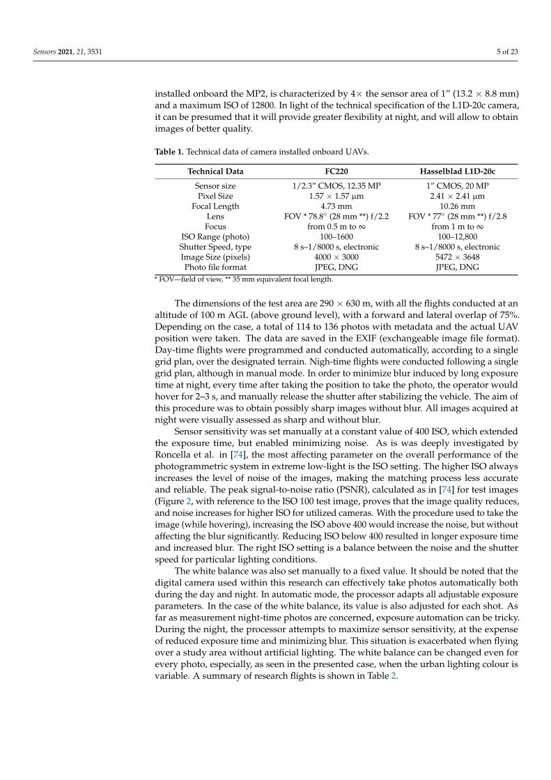
installed onboard the MP2, is characterized by 4× the sensor area of 1” (13.2 × 8.8 mm)and a maximum ISO of 12800. In light of the technical specification of the L1D-20c camera,it can be presumed that it will provide greater flexibility at night, and will allow to obtainimages of better quality.

Table 1. Technical data of camera installed onboard UAVs.

Technical Data FC220 Hasselblad L1D-20c

Sensor size 1/2.3” CMOS, 12.35 MP 1” CMOS, 20 MPPixel Size 1.57 × 1.57 µm 2.41 × 2.41 µm

Focal Length 4.73 mm 10.26 mmLens FOV * 78.8◦ (28 mm **) f/2.2 FOV * 77◦ (28 mm **) f/2.8Focus from 0.5 m to ∞ from 1 m to ∞

ISO Range (photo) 100–1600 100–12,800Shutter Speed, type 8 s–1/8000 s, electronic 8 s–1/8000 s, electronicImage Size (pixels) 4000 × 3000 5472 × 3648Photo file format JPEG, DNG JPEG, DNG

* FOV—field of view, ** 35 mm equivalent focal length.

The dimensions of the test area are 290 × 630 m, with all the flights conducted at analtitude of 100 m AGL (above ground level), with a forward and lateral overlap of 75%.Depending on the case, a total of 114 to 136 photos with metadata and the actual UAVposition were taken. The data are saved in the EXIF (exchangeable image file format).Day-time flights were programmed and conducted automatically, according to a singlegrid plan, over the designated terrain. Nigh-time flights were conducted following a singlegrid plan, although in manual mode. In order to minimize blur induced by long exposuretime at night, every time after taking the position to take the photo, the operator wouldhover for 2–3 s, and manually release the shutter after stabilizing the vehicle. The aim ofthis procedure was to obtain possibly sharp images without blur. All images acquired atnight were visually assessed as sharp and without blur.

Sensor sensitivity was set manually at a constant value of 400 ISO, which extendedthe exposure time, but enabled minimizing noise. As is was deeply investigated byRoncella et al. in [74], the most affecting parameter on the overall performance of thephotogrammetric system in extreme low-light is the ISO setting. The higher ISO alwaysincreases the level of noise of the images, making the matching process less accurateand reliable. The peak signal-to-noise ratio (PSNR), calculated as in [74] for test images(Figure 2, with reference to the ISO 100 test image, proves that the image quality reduces,and noise increases for higher ISO for utilized cameras. With the procedure used to take theimage (while hovering), increasing the ISO above 400 would increase the noise, but withoutaffecting the blur significantly. Reducing ISO below 400 resulted in longer exposure timeand increased blur. The right ISO setting is a balance between the noise and the shutterspeed for particular lighting conditions.

The white balance was also set manually to a fixed value. It should be noted that thedigital camera used within this research can effectively take photos automatically bothduring the day and night. In automatic mode, the processor adapts all adjustable exposureparameters. In the case of the white balance, its value is also adjusted for each shot. Asfar as measurement night-time photos are concerned, exposure automation can be tricky.During the night, the processor attempts to maximize sensor sensitivity, at the expenseof reduced exposure time and minimizing blur. This situation is exacerbated when flyingover a study area without artificial lighting. The white balance can be changed even forevery photo, especially, as seen in the presented case, when the urban lighting colour isvariable. A summary of research flights is shown in Table 2.

Sensors 2021, 21, 3531 6 of 23Sensors 2021, 21, x FOR PEER REVIEW 6 of 24

(a) (b)

Figure 2. The PSNR ratio calculated for (a) MP1 and (b) MP2 and diferent shuter speed.

The white balance was also set manually to a fixed value. It should be noted that the

digital camera used within this research can effectively take photos automatically both

during the day and night. In automatic mode, the processor adapts all adjustable exposure

parameters. In the case of the white balance, its value is also adjusted for each shot. As far

as measurement night-time photos are concerned, exposure automation can be tricky.

During the night, the processor attempts to maximize sensor sensitivity, at the expense of

reduced exposure time and minimizing blur. This situation is exacerbated when flying

over a study area without artificial lighting. The white balance can be changed even for

every photo, especially, as seen in the presented case, when the urban lighting colour is

variable. A summary of research flights is shown in Table 2.

Table 2. Research flight parameters.

Flight Symbol UAV Daytime Flight Plan Coverage Area

MP1-D DJI Mavic Pro day single grid auto 0.192 km²

MP2-D DJI Mavic Pro 2 day single grid auto 0.193 km²

MP1-N DJI Mavic Pro night single grid manual 0.114 km²

MP2-N DJI Mavic Pro 2 night single grid manual 0.147 km²

A photogrammetric network was developed that comprised of 23 ground control

points (GCPs), non-uniformly arranged throughout the study area, and their positions

were measured with the GNSS RTK accurate satellite positioning method. The non-

uniform distribution of points was forced directly by the lack of accessibility to the south-

eastern and central parts of the area. The south-eastern area is occupied by the closed part

of the container terminal, and the distribution of points in the central part, where the

viaduct passes, was unsafe due to the high car traffic. GCP position was determined

relative to the PL-2000 Polish state grid coordinate system and their altitude relative to

the PL-EVRF2007-NH quasigeoid. All control points were positioned in characteristic,

natural locations. These are mainly easyto identify in both day-time and night-time photos

of terrain fragments with variable structure, road lane boundaries, and manhole covers.

When locating control points, a priority rule that GCPs had to be located at spots

illuminated with streetlamp lighting was adopted (Figure 3a,b). Furthermore, for

analytical purposes, several points located within a convenient area were, however, not

illuminated with artificial lighting (Figure 3c,d).

Figure 2. The PSNR ratio calculated for (a) MP1 and (b) MP2 and diferent shuter speed.

Table 2. Research flight parameters.

Flight Symbol UAV Daytime Flight Plan Coverage Area

MP1-D DJI Mavic Pro day single grid auto 0.192 km2

MP2-D DJI Mavic Pro 2 day single grid auto 0.193 km2

MP1-N DJI Mavic Pro night single grid manual 0.114 km2

MP2-N DJI Mavic Pro 2 night single grid manual 0.147 km2

A photogrammetric network was developed that comprised of 23 ground controlpoints (GCPs), non-uniformly arranged throughout the study area, and their positions weremeasured with the GNSS RTK accurate satellite positioning method. The non-uniformdistribution of points was forced directly by the lack of accessibility to the south-easternand central parts of the area. The south-eastern area is occupied by the closed part of thecontainer terminal, and the distribution of points in the central part, where the viaductpasses, was unsafe due to the high car traffic. GCP position was determined relativeto the PL-2000 Polish state grid coordinate system and their altitude relative to the PL-EVRF2007-NH quasigeoid. All control points were positioned in characteristic, naturallocations. These are mainly easyto identify in both day-time and night-time photos ofterrain fragments with variable structure, road lane boundaries, and manhole covers. Whenlocating control points, a priority rule that GCPs had to be located at spots illuminatedwith streetlamp lighting was adopted (Figure 3a,b). Furthermore, for analytical purposes,several points located within a convenient area were, however, not illuminated withartificial lighting (Figure 3c,d).


(a) (b) (c) (d)

Figure 3. Day- and night-time control point image (a) MP1-D GCP No. 21, (b) MP1-N GCP No. 21, (c) MP1-D GCP No. 17, (d) MP1-N GCP No. 17.

2.3. Data Processing The flights enabled to obtain images that were used to generate a photogrammetric

product without any modifications. Standard products in the form of a point cloud, digital terrain model (DTM), and orthophotoimages in Figure 4 were developed in Agisoft Metashape v1.7.1 (Agisoft LLC, St. Petersburg, Russia).

(a) (b)

(c) (d)

Figure 4. Developed orthophotoimages (a) MP1-D, (b) MP2-D, (c) MP1-N, (d) MP2-N.

Figure 3. Day- and night-time control point image (a) MP1-D GCP No. 21, (b) MP1-N GCP No. 21, (c) MP1-D GCP No. 17,(d) MP1-N GCP No. 17.

Sensors 2021, 21, 3531 7 of 23

2.3. Data Processing

The flights enabled to obtain images that were used to generate a photogrammetricproduct without any modifications. Standard products in the form of a point cloud,digital terrain model (DTM), and orthophotoimages in Figure 4 were developed in AgisoftMetashape v1.7.1 (Agisoft LLC, St. Petersburg, Russia).


(a) (b) (c) (d)

Figure 3. Day- and night-time control point image (a) MP1-D GCP No. 21, (b) MP1-N GCP No. 21, (c) MP1-D GCP No. 17, (d) MP1-N GCP No. 17.

2.3. Data Processing The flights enabled to obtain images that were used to generate a photogrammetric

product without any modifications. Standard products in the form of a point cloud, digital terrain model (DTM), and orthophotoimages in Figure 4 were developed in Agisoft Metashape v1.7.1 (Agisoft LLC, St. Petersburg, Russia).

(a) (b)

(c) (d)



Products were developed smoothly. The processing for each data set followed thesame sequence, with the same settings. The operator tagged all visible GCPs both at nightand day. Some GCPs at night were not readily identifiable on the photos due to insufficientlighting. Table 3 shows a brief summary of the basic image processing parameters.

Table 3. Flight plan data—read from reports.

Flight Flying Altitude(Reported)

GroundResolution

Number ofPhotos

CameraStations

MP1-D 105 m 3.05 cm/px 129 129MP2-D 127 m 2.26 cm/px 126 126MP1-N 69.7 m 3.11 cm/px 136 136MP2-N 118 m 2.24 cm/px 114 114

Sensors 2021, 21, 3531 8 of 23

All of them contain a similar number of photos with the flight conducted at the samealtitude of 100 m AGL (above ground level). As said above, MP1-N flight altitude is signif-icantly underestimated, which is typical for photos of reduced quality, as demonstratedin [18]. Such an incorrect calculation is a symptom of errors that translate to the geometricquality of a product, which will be proven later in the paper.

Table 4 shows a summary of tie point data. As can be seen, day-time products have asimilar number of identified tie points, while night-time ones exhibit significantly fewer.

Table 4. Tie points and reprojection error data.

Flight TiePoints

Mean KeyPoint Size Projections Reprojection

ErrorMax Reprojection

Error

MP1-D 134.894 5.08186 px 450.874 0.952 px 20.844 pxMP2-D 141.035 3.26046 px 414.585 0.543 px 20.5249 pxMP1-N 46.870 8.41085 px 131.625 2.04 px 37.4667 pxMP2-N 57.392 9.15704 px 154.054 1.85 px 36.7523 px

Night-time data for the suggested analysis area enabled identifying approximately30–40% tie points of the ones identifiable during the day. In addition, the mean key pointsize in the case of night-time photos is from 165% to 312% higher than the respectiveday-time cases.

Tables 5 and 6 show the mean camera position error and root mean square error (RMSE)calculated for ground control point positions, respectively. The mean camera positionerror is the difference in the camera position, determined by an on-board navigation andpositioning system resulting from aerotriangulation. The values of errors in the horizontalplane (x,y) fall within the limits typical for GPS receivers used in commercial UAVs. Theabsolute vertical plane error (z) is significantly higher (from 13 to 45 m) and arises directlyfrom different altitude reference systems. Table 7 presents the root mean square error(RMSE) calculated for check points position.

Table 5. Average camera location error. X—Easting, Y—Northing, Z—Altitude.

Flight X Error (m) Y Error (m) Z Error (m) XY Error (m) Total Error (m)

MP1-D 2.60381 2.36838 44.9193 3.51981 45.057MP2-D 2.00514 2.68327 22.9008 3.34971 23.1445MP1-N 1.09268 3.65444 25.9414 3.8143 26.2203MP2-N 2.49058 1.48535 13.4276 2.89987 13.7372

Table 6. Control point root mean square error (RMSE). X—Easting, Y—Northing, Z—Altitude.

Flight GCPCount

X Error(cm)

Y Error(cm)

Z Error(cm)

XY Error(cm) Total (cm)

MP1-D 13 9.53984 11.439 2.57716 14.895 15.1163MP2-D 14 11.8025 15.6751 3.22474 19.6216 19.8848MP1-N 10 3.52971 2.80579 2.06805 4.50902 4.96066MP2-N 9 8.96118 8.146 0.531357 12.1103 12.122

Table 7. Check point root mean square error (RMSE). X—Easting, Y—Northing, Z—Altitude.

Flight CPs Count X Error(cm)

Y Error(cm)

Z Error(cm)

XY Error(cm) Total (cm)

MP1-D 3 8.48112 16.8594 15.6909 18.8725 24.5433MP2-D 3 21.8543 34.1211 25.9101 40.5199 48.0957MP1-N 3 2.36402 4.10461 2.97748 4.73671 5.5948MP2-N 3 2.03436 8.85104 5.07036 9.08182 10.4013

Sensors 2021, 21, 3531 9 of 23

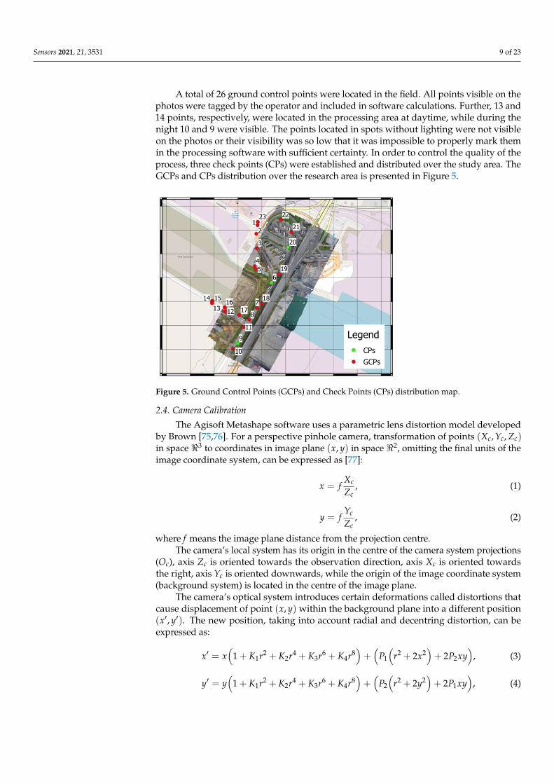
A total of 26 ground control points were located in the field. All points visible on thephotos were tagged by the operator and included in software calculations. Further, 13 and14 points, respectively, were located in the processing area at daytime, while during thenight 10 and 9 were visible. The points located in spots without lighting were not visibleon the photos or their visibility was so low that it was impossible to properly mark themin the processing software with sufficient certainty. In order to control the quality of theprocess, three check points (CPs) were established and distributed over the study area. TheGCPs and CPs distribution over the research area is presented in Figure 5.


Table 6. Control point root mean square error (RMSE). X—Easting, Y—Northing, Z—Altitude.

Flight GCP Count X Error (cm) Y Error (cm) Z Error (cm) XY Error (cm) Total (cm) MP1-D 13 9.53984 11.439 2.57716 14.895 15.1163 MP2-D 14 11.8025 15.6751 3.22474 19.6216 19.8848 MP1-N 10 3.52971 2.80579 2.06805 4.50902 4.96066 MP2-N 9 8.96118 8.146 0.531357 12.1103 12.122

A total of 26 ground control points were located in the field. All points visible on the photos were tagged by the operator and included in software calculations. Further, 13 and 14 points, respectively, were located in the processing area at daytime, while during the night 10 and 9 were visible. The points located in spots without lighting were not visible on the photos or their visibility was so low that it was impossible to properly mark them in the processing software with sufficient certainty. In order to control the quality of the process, three check points (CPs) were established and distributed over the study area. The GCPs and CPs distri-bution over the research area is presented in Figure 5.

Figure 5. Ground Control Points (GCPs) and Check Points (CPs) distribution map.

Table 7. Check point root mean square error (RMSE). X—Easting, Y—Northing, Z—Altitude.

Flight CPs Count X Error (cm) Y Error (cm) Z Error (cm) XY Error (cm) Total (cm) MP1-D 3 8.48112 16.8594 15.6909 18.8725 24.5433 MP2-D 3 21.8543 34.1211 25.9101 40.5199 48.0957 MP1-N 3 2.36402 4.10461 2.97748 4.73671 5.5948 MP2-N 3 2.03436 8.85104 5.07036 9.08182 10.4013

2.4. Camera Calibration The Agisoft Metashape software uses a parametric lens distortion model developed

by Brown [75,76]. For a perspective pinhole camera, transformation of points ( , , ) in space to coordinates in image plane ( , ) in space , omitting the final units of the image coordinate system, can be expressed as [77]: = , (1)

= , (2)

where f means the image plane distance from the projection centre.

Figure 5. Ground Control Points (GCPs) and Check Points (CPs) distribution map.

2.4. Camera Calibration

The Agisoft Metashape software uses a parametric lens distortion model developedby Brown [75,76]. For a perspective pinhole camera, transformation of points (Xc, Yc, Zc)in space <3 to coordinates in image plane (x, y) in space <2, omitting the final units of theimage coordinate system, can be expressed as [77]:

x = fXc

Zc, (1)

y = fYc

Zc, (2)

where f means the image plane distance from the projection centre.The camera’s local system has its origin in the centre of the camera system projections

(Oc), axis Zc is oriented towards the observation direction, axis Xc is oriented towardsthe right, axis Yc is oriented downwards, while the origin of the image coordinate system(background system) is located in the centre of the image plane.

The camera’s optical system introduces certain deformations called distortions thatcause displacement of point (x, y) within the background plane into a different position(x′, y′). The new position, taking into account radial and decentring distortion, can beexpressed as:

x′ = x(

1 + K1r2 + K2r4 + K3r6 + K4r8)+(

P1

(r2 + 2x2

)+ 2P2xy

), (3)

y′ = y(

1 + K1r2 + K2r4 + K3r6 + K4r8)+(

P2

(r2 + 2y2

)+ 2P1xy

), (4)

Sensors 2021, 21, 3531 10 of 23

where: K1, K2, K3, K4 are radial symmetric distortion coefficients, P1, P2 are decentringdistortion coefficients (including both radial asymmetric and tangential distortions), whiler is the radial radius, defined as:

r =√

x2 + y2. (5)

Because in the discussed case we are dealing with an image plane in the form ofCMOS sensors, it is necessary to convert (x′, y′) into image coordinates expressed in pixels.In the case of digital images, coordinates are usually given in accordance with the sensorindexation system adopted in the digital data processing software. Therefore, for thisimage, axis x is oriented to the right, axis y downwards, and the origin is located at thecentre of the pixel (1, 1). Coordinates for this system are expressed in pixels. Therefore,taking into account the image matrix size, the physical size of the image pixel, affinitynon-orthogonality, principal point offset, and the projected point coordinates in the imagecoordinate system, we can write:

u = 0.5w + cx + x′ f + x′B1 + y′B2, (6)

v = 0.5h + cy + y′ f , (7)

where: u, v is expressed in pixels (px), f denotes focal length (px), cx, cy principal pointoffset (px), B1, B2 affinity and non-orthogonality (skew) coefficients (px), w, h imagewidth and height, image resolution (px), and they are all defined as intrinsic orientationparameters (IOP).

Correct determination of IOPs (intrinsic orientation parameters) and distortion pa-rameters is very important in terms of photogrammetry. In the traditional approach, theseparameters are determined at a laboratory and are provided with a metric camera. UAVphotogrammetry usually uses small, non-metric cameras, where the intrinsic orientationand distortion parameters are unknown and unstable (not constant and can slightly changeunder the influence of external factors like temperature and vibrations). Due to the factthat the knowledge of current IOPs is required, the photogrammetric software used inthis study calibrates the camera in each case, based on measurement photos, and calcu-lates current IOPs for given the conditions and camera. Such a process ensures resultrepeatability. However, it functions correctly mainly in the case of photos taken undergood conditions, i.e., during the day, sharp, and well-illuminated. Table 8 shows IOPs anddistortion parameters determined by the software for each case.

Table 8. Camera internal orientation element value for each image.

Parameter

Flight

MP1-D MP2-D MP1-N MP2-N

Value Error Value Error Value Error Value Error

F 3127.860000 5.200000 5206.030000 10.000000 1532.460000 6.800000 4882.830000 12.000000Cx −28.166700 0.140000 −82.683800 0.490000 31.520100 0.210000 −75.996700 0.820000Cy 0.162081 0.120000 −6.182140 0.200000 −33.175400 0.180000 −28.009800 0.370000B1 −10.043200 0.076000 −22.277500 0.110000 0.457534 0.063000 - -B2 −6.308330 0.058000 −6.289880 0.088000 0.629884 0.057000 14.112600 0.170000K1 0.098579 0.000490 −0.029047 0.000170 0.047936 0.000510 −0.021496 0.000610K2 −0.585459 0.004500 0.026580 0.000780 −0.068125 0.001300 −0.002758 0.003500K3 1.420050 0.015000 −0.051838 0.001400 0.043968 0.001200 −0.011242 0.006000K4 −1.180670 0.017000 - - −0.009856 0.000370 - -P1 −0.000286 0.000010 −0.003291 0.000008 −0.000265 0.000021 −0.003015 0.000031P2 0.000362 0.000011 −0.001647 0.000009 −0.000030 0.000018 −0.001895 0.000023

Sensors 2021, 21, 3531 11 of 23

3. Results3.1. Geometry Analysis

The geometric quality of developed relief models was evaluated using the methodsdescribed in [78]. An M3C2 distance map (multiscale model to model cloud comparison)was developed for each point cloud. The M3C2 distance map computation process utilized3-D point precision estimates stored in scalar fields. Appropriate scalar fields were selectedfor both point clouds (referenced and tested) to describe measurement precision in X, Y,and Z (σX , σY, σZ). The results for the cases are shown in Figure 6.


Table 8. Camera internal orientation element value for each image.

Param-eter

Flight MP1-D MP2-D MP1-N MP2-N

Value Error Value Error Value Error Value Error F 3127.860000 5.200000 5206.030000 10.000000 1532.460000 6.800000 4882.830000 12.000000

Cx −28.166700 0.140000 −82.683800 0.490000 31.520100 0.210000 −75.996700 0.820000 Cy 0.162081 0.120000 −6.182140 0.200000 −33.175400 0.180000 −28.009800 0.370000 B1 −10.043200 0.076000 −22.277500 0.110000 0.457534 0.063000 - - B2 −6.308330 0.058000 −6.289880 0.088000 0.629884 0.057000 14.112600 0.170000 K1 0.098579 0.000490 −0.029047 0.000170 0.047936 0.000510 −0.021496 0.000610 K2 −0.585459 0.004500 0.026580 0.000780 −0.068125 0.001300 −0.002758 0.003500 K3 1.420050 0.015000 −0.051838 0.001400 0.043968 0.001200 −0.011242 0.006000 K4 −1.180670 0.017000 - - −0.009856 0.000370 - - P1 −0.000286 0.000010 −0.003291 0.000008 −0.000265 0.000021 −0.003015 0.000031 P2 0.000362 0.000011 −0.001647 0.000009 −0.000030 0.000018 −0.001895 0.000023

3. Results 3.1. Geometry Analysis

The geometric quality of developed relief models was evaluated using the methods described in [78]. An M3C2 distance map (multiscale model to model cloud comparison) was developed for each point cloud. The M3C2 distance map computation process utilized 3-D point precision estimates stored in scalar fields. Appropriate scalar fields were selected for both point clouds (referenced and tested) to describe measurement precision in X, Y, and Z ( , , ). The results for the cases are shown in Figure 6.

(a) (b)


(c) (d)

Figure 6. M3C2 Distances (a) MP1-D/ MP1-N, (b) MP2-D/ MP2-N, (c) MP1-D/ MP2-D, (d) MP1-N/ MP2-N.

The statistical distribution of M3C2 distances is close to normal, which means that a significant part of the observations is concentrated around the mean (Table 9). The mean (μ) for the comparison of night-time and day-time cases shows, both from MP1 and MP2, that the models are 0.4 to 1.6 m apart. Furthermore, standard deviation (σ) (above 4 m) indicates that there are significant differences between the models. A visual analysis Fig-ure 6 explicitly shows that the highest distance differences can be seen in the area of the flyover, which is a structure located much higher than the average elevation of the sur-rounding terrain in the case of the flight with UAV MP1 (Figure 6a). The same comparison of the night-time and day-time models for UAV MP1 does not exhibit such significant differences in this area (Figure 6b). It should be noted that M3C2 values are clearly higher in the area remote from GCP (south-eastern section of Figure 6a,b, values in yellow). It follows directly that, within the model development process, upon a significantly reduced tie point number, which is the case for night-time photos, aerotriangulation introduces a significant error. This is error is greater the farther the tie points are from identified GCPs. This phenomenon does not occur to such an extent for day-time cases (day MP1/day MP2) shown in Figure 6c. It is confirmed by the visual and parametric assessment of statistical data (Table 9).

Table 9. Mean distance value and standard deviation for M3C2.

M3C2 Case Mean (m) Std.Dev (m) MP1-D/N −0.39 4.14 MP2-D/N 1.63 4.59

D-MP1/MP2 0.11 2.52 N-MP1/MP2 −3.17 5.04

The D-MP1/MP2 case exhibits values μ = 0.11 m σ = 2.52 m, and a clear elevation of the deviation occurs only in the flyover area. The analysis of the night/night case clearly emphasizes the issue of reconstructing higher structures (flyover, building), which is par-ticularly based on correct aerotriangulation. The error of reconstructing objects located higher than the average terrain elevation, with rapidly increasing elevation is significant. This confirms that a reduction in the tie point number caused by low intensity has a great impact on reconstruction errors. It is clearly demonstrated in the area of the flyover high-way, where the software does not identify so many tie points.

Figure 6. M3C2 Distances (a) MP1-D/ MP1-N, (b) MP2-D/ MP2-N, (c) MP1-D/ MP2-D, (d) MP1-N/ MP2-N.

The statistical distribution of M3C2 distances is close to normal, which means thata significant part of the observations is concentrated around the mean (Table 9). Themean (µ) for the comparison of night-time and day-time cases shows, both from MP1and MP2, that the models are 0.4 to 1.6 m apart. Furthermore, standard deviation (σ)(above 4 m) indicates that there are significant differences between the models. A visualanalysis Figure 6 explicitly shows that the highest distance differences can be seen in thearea of the flyover, which is a structure located much higher than the average elevationof the surrounding terrain in the case of the flight with UAV MP1 (Figure 6a). The same

Sensors 2021, 21, 3531 12 of 23

comparison of the night-time and day-time models for UAV MP1 does not exhibit suchsignificant differences in this area (Figure 6b). It should be noted that M3C2 values areclearly higher in the area remote from GCP (south-eastern section of Figure 6a,b, values inyellow). It follows directly that, within the model development process, upon a significantlyreduced tie point number, which is the case for night-time photos, aerotriangulationintroduces a significant error. This is error is greater the farther the tie points are fromidentified GCPs. This phenomenon does not occur to such an extent for day-time cases(day MP1/day MP2) shown in Figure 6c. It is confirmed by the visual and parametricassessment of statistical data (Table 9).

Table 9. Mean distance value and standard deviation for M3C2.

M3C2 Case Mean (m) Std.Dev (m)

MP1-D/N −0.39 4.14MP2-D/N 1.63 4.59

D-MP1/MP2 0.11 2.52N-MP1/MP2 −3.17 5.04

The D-MP1/MP2 case exhibits values µ = 0.11 m σ = 2.52 m, and a clear elevationof the deviation occurs only in the flyover area. The analysis of the night/night caseclearly emphasizes the issue of reconstructing higher structures (flyover, building), whichis particularly based on correct aerotriangulation. The error of reconstructing objectslocated higher than the average terrain elevation, with rapidly increasing elevation issignificant. This confirms that a reduction in the tie point number caused by low intensityhas a great impact on reconstruction errors. It is clearly demonstrated in the area of theflyover highway, where the software does not identify so many tie points.

3.2. Autocalibration Process Analysis

Intrinsic orientation parameters (IOPs), including lens distortion parameters, havea significant impact on the geometry of a photogrammetric product. The automatic cali-bration process executed by Agisoft is based primarily on correctly identified tie points.Figure 7 shows a graphical comparison of the parameters, previously shown in Table 8.The graphical presentation of grouped results with corresponding error, for day/nightcases, shows a noticeable trend and relationships that translate to the above reducedimage quality.

Theoretically, and in line with previous experience [18,19,79], the calibration param-eters for a single camera should be the same or very similar. Typically, especially fornon-metric cameras, the recovered IOP are only valid for that particular project, and theycan be slightly different for another image block under different conditions. In the case ofnight-time calibration, which can be seen in Figure 7, IOPs are significantly different thanin the case of day-time calibration. This difference is particularly higher for cameras withlower quality and sensitivity (UAV MP1). The focal length (F) for MP1 changes its value by50% during the night, and only by 6% in the case of MP2. Tie point location (Cx, Cy) forMP1 was displaced by more than 60 pixels in the x-axis during the night. B coefficients fornight-time cases tend to strive to zero. We can also observe significant differences in termsof radial and tangential distortion for UAV MP1. Whereas the distortion parameters for theMP2 camera remain similar, they exhibit a higher error at night. The intrinsic orientationand distortion parameter determination error is significantly higher at night in all cases.

In order to achieve additional comparison of calibration parameters, their distributionwithin the image plane and a profile depend on the radial radius. Figures 8 and 9 showcorresponding visualisations for MP1 and MP2, respectively.

Sensors 2021, 21, 3531 13 of 23


3.2. Autocalibration Process Analysis Intrinsic orientation parameters (IOPs), including lens distortion parameters, have a

significant impact on the geometry of a photogrammetric product. The automatic calibra-tion process executed by Agisoft is based primarily on correctly identified tie points. Fig-ure 7 shows a graphical comparison of the parameters, previously shown in Table 8. The graphical presentation of grouped results with corresponding error, for day/night cases, shows a noticeable trend and relationships that translate to the above reduced image qual-ity.

(a) (b) (c)

(d) (e)

Figure 7. Graphical comparison of calibration parameters (a) F, (b) Cx and Cy, (c) B1 and B2, (d) K1-4, (e) P1 and P2.

Theoretically, and in line with previous experience [18,19,79], the calibration param-eters for a single camera should be the same or very similar. Typically, especially for non-metric cameras, the recovered IOP are only valid for that particular project, and they can be slightly different for another image block under different conditions. In the case of night-time calibration, which can be seen in Figure 7, IOPs are significantly different than in the case of day-time calibration. This difference is particularly higher for cameras with lower quality and sensitivity (UAV MP1). The focal length (F) for MP1 changes its value by 50% during the night, and only by 6% in the case of MP2. Tie point location ( , ) for MP1 was displaced by more than 60 pixels in the x-axis during the night. B coefficients for night-time cases tend to strive to zero. We can also observe significant differences in terms of radial and tangential distortion for UAV MP1. Whereas the distortion parameters for the MP2 camera remain similar, they exhibit a higher error at night. The intrinsic orienta-tion and distortion parameter determination error is significantly higher at night in all cases.

In order to achieve additional comparison of calibration parameters, their distribu-tion within the image plane and a profile depend on the radial radius. Figures 8 and 9 show corresponding visualisations for MP1 and MP2, respectively.

Figure 7. Graphical comparison of calibration parameters (a) F, (b) Cx and Cy, (c) B1 and B2, (d) K1-4, (e) P1 and P2.


(a) (b)

(c) (d)

Figure 8. Distortion visualisations and profiles for MP1 day (a,c) and night cases (b,d).

(a) (b)

(c) (d)

Figure 9. Distortion visualizations and profiles for MP2 day (a,c) and night cases (b,d).

As noted, the IOP and distortion determination error is significantly higher at night in each case. This means that these values are determined less precisely than during the day, which directly translates to reduced model development precision. In order to verify this


Sensors 2021, 21, 3531 14 of 23


(a) (b)

(c) (d)


(a) (b)

(c) (d)


As noted, the IOP and distortion determination error is significantly higher at night in each case. This means that these values are determined less precisely than during the day, which directly translates to reduced model development precision. In order to verify this


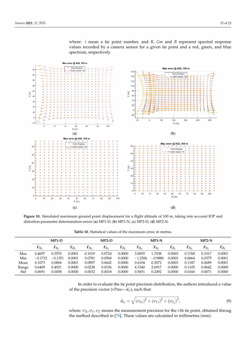
As noted, the IOP and distortion determination error is significantly higher at nightin each case. This means that these values are determined less precisely than during theday, which directly translates to reduced model development precision. In order to verifythis hypothesis, the authors conducted additional analyses and calculated the maximumpossible point ground displacement for a single air photo at an altitude of 100 m, takinginto account the value of intrinsic orientation and distortion parameters increased by themaximum error value reported by photogrammetric software. In other words, formulas(1) to (7) were used to convert u and v to the spatial position of the points (Xc, Yc, Zc) fora flight altitude of 100 m, considering IOPs and distortion parameters increased by themaximum error. The result of this operation is shown in Figure 10.

The statistical values of the maximum error in metres, for a flight altitude of 100 m,are shown in Table 10.

As shown in Table 10 the maximum displacement of ground points can occur in theMP1-N case and can even exceed 3 metres, with the mean displacement of approximately60 cm. This displacement, resulting from the occurrence of a maximum error, is onlyinformative, and according to Gaussian distribution, achieving such a situation in reallife is very unlikely. Nonetheless, the increased error analysis conducted during night-time calibration proves that methods functioning correctly during the day are not able toaccurately determine IOPs at night.

3.3. Relationships

Spatial relationships between point intensity, reprojection error and tie point deter-mination precision are shown in Figure 11. The intensity map was calculated for each tiepoint (Ii) according to the formula [80]:

Ii = 0.21 R + 0.72 G + 0.07 B, (8)

Sensors 2021, 21, 3531 15 of 23

where: i mean a tie point number, and R, Gm and B represent spectral responsevalues recorded by a camera sensor for a given tie point and a red, green, and bluespectrum, respectively.


hypothesis, the authors conducted additional analyses and calculated the maximum possi-ble point ground displacement for a single air photo at an altitude of 100 m, taking into account the value of intrinsic orientation and distortion parameters increased by the maxi-mum error value reported by photogrammetric software. In other words, formulas (1) to (7) were used to convert u and v to the spatial position of the points (X , Y , Z ) for a flight alti-tude of 100 m, considering IOPs and distortion parameters increased by the maximum error. The result of this operation is shown in Figure 10.

(a) (b)

(c) (d)

Figure 10. Simulated maximum ground point displacement for a flight altitude of 100 m, taking into account IOP and distortion parameter determination errors (a) MP1-D, (b) MP1-N, (c) MP2-D, (d) MP2-N.

The statistical values of the maximum error in metres, for a flight altitude of 100 m, are shown in Table 10.

Table 10. Statistical values of the maximum error, in metres.


Max 0.4697 0.3570 0.0001 0.1019 0.0724 0.0000 3.0835 1.7038 0.0003 0.1768 0.1017 0.0001 Min −0.1712 −0.1351 0.0001 0.0781 0.0568 0.0000 −1.2506 −0.9880 0.0003 0.0664 0.0375 0.0001

Mean 0.1073 0.0804 0.0001 0.0897 0.0642 0.0000 0.6104 0.3072 0.0003 0.1187 0.0689 0.0001 Range 0.6409 0.4921 0.0000 0.0238 0.0156 0.0000 4.3340 2.6917 0.0000 0.1105 0.0642 0.0000

Std 0.0691 0.0458 0.0000 0.0032 0.0018 0.0000 0.5651 0.2492 0.0000 0.0160 0.0071 0.0000

Figure 10. Simulated maximum ground point displacement for a flight altitude of 100 m, taking into account IOP anddistortion parameter determination errors (a) MP1-D, (b) MP1-N, (c) MP2-D, (d) MP2-N.

Table 10. Statistical values of the maximum error, in metres.


EXC EYC EZC EXC EYC EZC EXC EYC EZC EXC EYC EZC

Max 0.4697 0.3570 0.0001 0.1019 0.0724 0.0000 3.0835 1.7038 0.0003 0.1768 0.1017 0.0001Min −0.1712 −0.1351 0.0001 0.0781 0.0568 0.0000 −1.2506 −0.9880 0.0003 0.0664 0.0375 0.0001

Mean 0.1073 0.0804 0.0001 0.0897 0.0642 0.0000 0.6104 0.3072 0.0003 0.1187 0.0689 0.0001Range 0.6409 0.4921 0.0000 0.0238 0.0156 0.0000 4.3340 2.6917 0.0000 0.1105 0.0642 0.0000

Std 0.0691 0.0458 0.0000 0.0032 0.0018 0.0000 0.5651 0.2492 0.0000 0.0160 0.0071 0.0000

In order to evaluate the tie point precision distribution, the authors introduced a valueof the precision vector (vPrec—dσ), such that:

dσi =

√(σXi)

2 + (σYi)2 +

(σZi

)2, (9)

where: σX , σY, σZ means the measurement precision for the i-th tie point, obtained througthe method described in [78]. These values are calculated in millimetres (mm).

Sensors 2021, 21, 3531 16 of 23

Figure 12 shows the relationships of the dσi precision vector (vPrec) reprojection errorand intensity, calculated for each tie point. The blue line represents accurately obtainedvalues, while the red line averages them in order to visualise the trend and relationships.All data were sorted in ascending order of intensity.


As shown in Table 10 the maximum displacement of ground points can occur in the MP1-N case and can even exceed 3 metres, with the mean displacement of approximately 60 cm. This displacement, resulting from the occurrence of a maximum error, is only in-formative, and according to Gaussian distribution, achieving such a situation in real life is very unlikely. Nonetheless, the increased error analysis conducted during night-time calibration proves that methods functioning correctly during the day are not able to accu-rately determine IOPs at night.

3.3. Relationships Spatial relationships between point intensity, reprojection error and tie point deter-

mination precision are shown in Figure 11. The intensity map was calculated for each tie point ( ) according to the formula [80]: = 0.21 + 0.72 + 0.07 , (8)

where: i mean a tie point number, and R, Gm and B represent spectral response values recorded by a camera sensor for a given tie point and a red, green, and blue spectrum, respectively.

In order to evaluate the tie point precision distribution, the authors introduced a value of the precision vector (vPrec— ), such that: = + + , (9)

where: , , means the measurement precision for the i-th tie point, obtained throug the method described in [78]. These values are calculated in millimetres (mm).

(a) (b) (c)

(d) (e) (f)

Figure 11. Tie point quality measurements—night cases (a) MP1 intensity, (b) MP1 RE (c) MP1-vPrec (d) MP2 intensity, (e) MP2 RE (f) MP2-vPrec.

Figure 11. Tie point quality measurements—night cases (a) MP1 intensity, (b) MP1 RE (c) MP1-vPrec (d) MP2 intensity,(e) MP2 RE (f) MP2-vPrec.

The mean value for models based on day-time photos is 113 and 124 with a standarddeviation of 51 and 44, respectively (Table 11). The mean RE value for day-time modelsis 0.6656 px (sRE(MP1D) = 0.5253) and 0.3130 px (sRE(MP2D) = 0.3659), respectively. Themaximum RE value for day-time models does not exceed 21 pixels. The sRE analysis for day-time cases indicates that values are relatively constant for all points, which is also confirmedby the graph (Figure 12). The mean value for models based on night-time photos is 25 and32 with a standard deviation of 23 and 27, respectively. The mean RE value for night-timemodels is 1.3311 px (sRE(MP1N) = 1.407) and 1.168 px (sRE(MP2N) = 1.26), respectively, andthe maximum RE value is significantly higher at approximately 37 pixels. Conversely, fornight-time cases, sRE takes higher values, which proves high result variability. This can beeasily seen in the graphs (Figure 12), where the blue plot for RE and vPrec for night-timecases shows a high amplitude change.

Sensors 2021, 21, 3531 17 of 23


Figure 12 shows the relationships of the precision vector (vPrec) reprojection er-ror and intensity, calculated for each tie point. The blue line represents accurately obtained values, while the red line averages them in order to visualise the trend and relationships. All data were sorted in ascending order of intensity.

(a) (b)

(c) (d)

Figure 12. Correlations between accuracy parameters relative to point intensity (a) MP1 Day (MP1-D), (b) MP1 Night (MP1-N), (c) MP2-Day (MP2-D), (d) MP2-Night (MP2-N).

The mean value for models based on day-time photos is 113 and 124 with a standard deviation of 51 and 44, respectively (Table 11). The mean RE value for day-time models is 0.6656 px ( ( ) = 0.5253) and 0.3130 px ( ( ) = 0.3659), respectively. The max-imum RE value for day-time models does not exceed 21 pixels. The analysis for day-time cases indicates that values are relatively constant for all points, which is also con-firmed by the graph (Figure 12). The mean value for models based on night-time photos is 25 and 32 with a standard deviation of 23 and 27, respectively. The mean RE value for night-time models is 1.3311 px ( ( ) = 1.407) and 1.168 px ( ( ) = 1.26), re-spectively, and the maximum RE value is significantly higher at approximately 37 pixels. Conversely, for night-time cases, takes higher values, which proves high result vari-ability. This can be easily seen in the graphs (Figure 12), where the blue plot for RE and vPrec for night-time cases shows a high amplitude change.

Figure 12. Correlations between accuracy parameters relative to point intensity (a) MP1 Day (MP1-D), (b) MP1 Night(MP1-N), (c) MP2-Day (MP2-D), (d) MP2-Night (MP2-N).

Table 11. List of statistical data (m- mean, s-standard deviation).

Flight mI sI mRE (px) sRE (px) mvPrec (cm) svPrec (cm)

MP1-D 113.24 51.78 0.6656 0.5253 401.22 1458.20MP2-D 124.76 44.90 0.3130 0.3659 290.63 1686.36MP1-N 25.76 23.49 1.3311 1.4070 365.21 994.63MP2-N 32.839 27.02 1.1680 1.26 803.42 2471.73

An analysis of relationships between intensity, RE and vPrec shows a strong correlationbetween accuracy parameters in nigh-time photos, i.e., those, where the mean intensity isin the range from 25 to 35. On the other hand, the same relationships are not exhibited bymodels based on day-time photos. The results show that RE stabilizes towards the meanonly above an intensity of 30 and 50, respectively.

A decrease in the number of tie points following a decrease of intensity results directlyfrom the algorithm applied at the first stage of the photogrammetric stage, namely, featurematching. The software developer uses a modified version of the popular SIFT (scale-invariant feature transform) algorithm [81]. As shown by the studies in [82–87], the SIFTalgorithm is non-resistant to low intensity and low contrast. This leads to the generation of

Sensors 2021, 21, 3531 18 of 23

a certain number of false key points, which are later not found on subsequent photos, thusbecoming tie points.

The maximum total number of matches in MP1 night-time photos is 1080, including1018 valid and 62 invalid matches. Similarly, the maximum total number of matches forday-time photos is 3733, including 3493 valid and 240 invalid matches. A decrease in thenumber of matches by more than 70% greatly impacts image quality. This phenomenonwas demonstrated for a pair of identical photos in the same region in Figure 13. Thefigure shows a day-time example of a stereopair from 1238 total matches, and a night-timestereopair from 208 total matches.


An analysis of relationships between intensity, RE and vPrec shows a strong correla-tion between accuracy parameters in nigh-time photos, i.e., those, where the mean inten-sity is in the range from 25 to 35. On the other hand, the same relationships are not exhib-ited by models based on day-time photos. The results show that RE stabilizes towards the mean only above an intensity of 30 and 50, respectively.

Table 11. List of statistical data (m- mean, s-standard deviation).

Flight (px) (px) (cm) (cm) MP1-D 113.24 51.78 0.6656 0.5253 401.22 1458.20 MP2-D 124.76 44.90 0.3130 0.3659 290.63 1686.36 MP1-N 25.76 23.49 1.3311 1.4070 365.21 994.63 MP2-N 32.839 27.02 1.1680 1.26 803.42 2471.73

A decrease in the number of tie points following a decrease of intensity results di-rectly from the algorithm applied at the first stage of the photogrammetric stage, namely, feature matching. The software developer uses a modified version of the popular SIFT (scale-invariant feature transform) algorithm [81]. As shown by the studies in [82–87], the SIFT algorithm is non-resistant to low intensity and low contrast. This leads to the gener-ation of a certain number of false key points, which are later not found on subsequent photos, thus becoming tie points.

The maximum total number of matches in MP1 night-time photos is 1080, including 1018 valid and 62 invalid matches. Similarly, the maximum total number of matches for day-time photos is 3733, including 3493 valid and 240 invalid matches. A decrease in the number of matches by more than 70% greatly impacts image quality. This phenomenon was demonstrated for a pair of identical photos in the same region in Figure 13. The figure shows a day-time example of a stereopair from 1238 total matches, and a night-time ste-reopair from 208 total matches.

(a) (b)

Figure 13. Decrease in the number of matches for day- and night-time cases (a) 1238 total matches, (b) 208 total matches.

Figure 13. Decrease in the number of matches for day- and night-time cases (a) 1238 total matches,(b) 208 total matches.

4. Discussion

The results and analyses conducted within this study show the sensitivity of a pho-togrammetric process applied in modern software, relative to photos taken in extremelighting conditions. The issues analysed by the authors can be divided as per the divisionin [18], intro procedural, numerical and technical factors. Procedural factors that impactthe final quality of a photogrammetric product include GCP distribution and flight plan,whereas in terms of numerical factors, it is the issue of night-time calibration. Thirdly,presented technical factors included the difference between cameras on two different UAVs.

The reduction in geometry during night-time tests were greatly impacted by non-uniform distribution of GCPs within the study area. As was noted, wherever there wereno placed GCPs, the distance between the reference model and the night-time modelsignificantly increased. In the case of day-time photos, these differences are not as importantsince this phenomenon is compensated by high tie point density and their low meandiameter. As recommended by most photogrammetric software developers, 5–10 groundcontrol points should be arranged uniformly in such a case. This ensures acceptable productquality. The situation is quite the opposite at night, when the tie point density decreases byup to 70%, which results in the formation of aerotriangulation errors. A night-time studywill lead to the reprojection error increasing with growing distance from GCPs and with achange in object height. In the case in question, it was physically impossible to uniformlyarrange GCPs, due to safety (traffic on the flyover—expressway) and in the south-easternarea, which is a closed seaport section. The location of the research in such a challenging

Sensors 2021, 21, 3531 19 of 23

area was not a coincidence. The authors decided on this location because there is indeeda problem with light pollution in this area and there is a wide variety of urban lightingof different types. The location of the study is closest to the real problems that can beencountered during the measurements and can induce new and interesting challenges forscience. After all, it is not always physically possible to evenly distribute GCPs, whichduring the day does not induce significant problems, but as shown, at night can be a rathermore significant factor.

GCP arrangement at night should be properly planned. Objects intended to serveas natural or signalled points should be illuminated. This is a rather obvious statement.However, it requires a certain degree of planning when developing the photogrammetricmatrix and, more importantly, such a selection of control points so that they are sufficientlycontrasting. Low contrast of natural control points results in a significant reduction ofidentifiability at low lighting intensity. An active (glowing marker), new type of controlpoint might be a good solution in insufficiently illuminated spots, where it is impossible toplace or locate control points.

A developed and executed night-time flight plan covered manual flight execution,following a single grid. The UAV had to be stopped every time for 1–3 s, until hover wasstabilized, and the shutter released. The time required to stabilise the hover depends, ofcourse, on the inertia of the UAV itself and its flight dynamics. Such a procedure enablestaking a photo without clear blur and allows to optimally extend the exposure time, andreduce ISO sensitivity in order to avoid excessive matrix noise. It seems impossible totake sharp, unblurred photos without stopping in-flight, as is the case with a traditionalday-time flight. Commercially available software for planning and executing UAV flights(Pix4D Capture—Android version) does not offer a function of automatic breaking duringexposure, and furthermore, does not enable full control over exposure parameters. Thesame software offers the possibility to stop the UAV while taking picture only on iOS(mobile operating system created Apple Inc., Cupertino, CA, USA). Full control is possiblealso via UAV manufacturer’s dedicated software. However, it does not enable automaticflight plan execution.

Commercial aerial systems are equipped with built-in non-metric digital cameras, theintrinsic orientation and distortion parameters of which are not constant. Such camerasrequire frequent calibration, which is practically achieved every time, with each photogram-metric process. This process, as demonstrated, is sensitive to poor lighting conditions,which leads to the generation a higher determination error for each intrinsic orientation anddistortion parameter. Since it is these parameters that significantly influence the geometricquality of a product, their correct determination is extremely important. As indicated bystudies, a brighter camera of a generally better quality, used onboard Mavic 2 Pro, exhibitedclearly lower deviation of night-time calibration parameters, relative to the same settingsduring the day. This enables obtaining clearly more stable results.

As evidenced, uniformly illuminated photos can be used to construct a model withlower RE, and each tie point exhibits greater precision. The issue of decreasing precision atlow photo brightness results from the type of algorithm used to detect tie points, whichmeans that, potentially, improving this element within the software would improve thegeometric quality of the model generated based on night-time photos.

5. Conclusions

As shown in the introduction, a number of publications on night-time photogrammet-ric products did not analyse the issue of model geometry. These studies assumed, a priori,that geometry would be similar to that during the day, and focused on the application-related aspects of night-time models. As indicated in this research, popular photogram-metric software generates night-time models with acceptable geometry. However, theirabsolute quality is poor. It can be concluded that the geometry of night-time models cannotbe simply used for surveying or cartographic projects. This is greatly influenced by theimage processing itself and used algorithm.

Sensors 2021, 21, 3531 20 of 23

A more in-depth analysis of the photogrammetric process indicated that a decrease isexperienced on many levels, starting with procedural factors (data acquisition, photogram-metric flight), through numerical factors (calibration process and algorithms applied todetect key points), to technical factors (camera type and brightness). These factors blendand mutually impact image quality. It cannot be clearly stated which of the factors has thegreatest influence on the geometric quality of an image, although it seems obvious thata precise camera and a stable UAV flight will be the best combination. Therefore, it canbe concluded that technical factors will be the most decisive in terms of night-time imagequality. They will be followed by procedural factors. The very procedure of night-timephoto acquisition must ensure taking a sharp photo, namely a stable hover during theexposure time. Such a solution will ensure a sharp photo without blur. Another element ofthe procedure is uniform GCP distribution in an illuminated location. Distribution uni-formity has a significant impact on image geometry, especially with low tie point density.The last element is the numerical factor, which the user has little influence on in this case.Software does not allow to change applied algorithms or the calibration procedure, andone can guarantee conditions correct for the operation of these algorithms only throughgood practice. The biggest problem was noted in the terms of the calibration algorithm,with even a slight error increase resulting in significant geometric changes and groundpoint displacement, by up to several metres.

Author Contributions: Conceptualization, P.B. and K.B.; methodology, P.B.; software, P.B. and K.B.;validation, P.B. and K.B.; formal analysis, K.B.; investigation, P.B.; resources, P.B.; data curation,P.B.; writing—original draft preparation, P.B. and K.B.; writing—review and editing, K.B. and P.B.;visualization, P.B.; supervision, P.B.; project administration, K.B.; funding acquisition, K.B. All authorshave read and agreed to the published version of the manuscript.

Funding: Financial support of these studies from Gdansk University of Technology by the DEC-42/2020/IDUB/I.3.3 grant under the ARGENTUM—‘Excellence Initiative-Research University’ pro-gram is gratefully acknowledged.

Institutional Review Board Statement: Not applicable.

Informed Consent Statement: Not applicable.

Conflicts of Interest: The authors declare no conflict of interest.

References1. Goel, S. A Distributed Cooperative UAV Swarm Localization System: Development and Analysis. In Proceedings of the 30th

International Technical Meeting of The Satellite Division of the Institute of Navigation (ION GNSS), Portland, OR, USA, 25–29September 2017; pp. 2501–2518.

2. Goel, S.; Kealy, A.; Lohani, B. Development and Experimental Evaluation of a Low-Cost Cooperative UAV Localization NetworkPrototype. J. Sens. Actuator Netw. 2018, 7, 42. [CrossRef]

3. Zhang, X.; Lu, X.; Jia, S.; Li, X. A novel phase angle-encoded fruit fly optimization algorithm with mutation adaptation mechanismapplied to UAV path planning. Appl. Soft Comput. J. 2018, 70, 371–388. [CrossRef]

4. Kyristsis, S.; Antonopoulos, A.; Chanialakis, T.; Stefanakis, E.; Linardos, C.; Tripolitsiotis, A.; Partsinevelos, P. Towards Au-tonomous Modular UAV Missions: The Detection, Geo-Location and Landing Paradigm. Sensors 2016, 16, 1844. [CrossRef]

5. Oktay, T.; Kanat, Ö.Ö. A Review of Aerodynamic Active Flow Control. In Proceedings of the International Advanced TechnologiesSymposium, Elazig, Turkey, 19–22 October 2017.

6. Oktay, T.; Celik, H.; Turkmen, I. Maximizing autonomous performance of fixed-wing unmanned aerial vehicle to reduce motionblur in taken images. Proc. Inst. Mech. Eng. Part I J. Syst. Control. Eng. 2018, 232, 857–868. [CrossRef]

7. Oktay, T.; Coban, S. Simultaneous Longitudinal and Lateral Flight Control Systems Design for Both Passive and Active MorphingTUAVs. Elektron. Elektrotechnika 2017, 23, 15–20. [CrossRef]

8. Kedzierski, M.; Fryskowska, A.; Wierzbicki, D.; Nerc, P. Chosen Aspects of the Production of the Basic Map Using UAV Imagery.International Archives of the Photogrammetry, Remote Sensing and Spatial Information Sciences. ISPRS Arch. 2016, 2016, 873–877.

9. Kedzierski, M.; Fryskowska, A.; Wierzbicki, D.; Grochala, A.; Nerc, P. Detection of Gross Errors in the Elements of ExteriorOrientation of Low-Cost UAV Images. Baltic Geod. Congr. (BGC Geomat.) 2016, 95–100. [CrossRef]

10. Di Franco, C.; Buttazzo, G. Coverage Path Planning for UAVs Photogrammetry with Energy and Resolution Constraints. J. Intell.Robot. Syst. Theory Appl. 2016, 83, 445–462. [CrossRef]

http://doi.org/10.3390/jsan7040042

http://doi.org/10.1016/j.asoc.2018.05.030

http://doi.org/10.3390/s16111844

http://doi.org/10.1177/0959651818765027

http://doi.org/10.5755/j01.eie.23.5.19238

http://doi.org/10.1109/bgc.geomatics.2016.26

http://doi.org/10.1007/s10846-016-0348-x

Sensors 2021, 21, 3531 21 of 23

11. Ribeiro-Gomes, K.; Hernández-López, D.; Ortega, J.F.; Ballesteros, R.; Poblete, T.; Moreno, M.A. Uncooled Thermal CameraCalibration and Optimization of the Photogrammetry Process for UAV Applications in Agriculture. Sensors 2017, 17, 2173.[CrossRef] [PubMed]

12. Kromer, R.; Walton, G.; Gray, B.; Lato, M. Robert Group Development and Optimization of an Automated Fixed-Location TimeLapse Photogrammetric Rock Slope Monitoring System. Remote Sens. 2019, 11, 1890. [CrossRef]

13. Rau, J.-Y.; Jhan, J.-P.; Li, Y.-T. Development of a Large-Format UAS Imaging System with the Construction of a One SensorGeometry from a Multicamera Array. IEEE Trans. Geosci. Remote Sens. 2016, 54, 5925–5934. [CrossRef]

14. Alfio, V.S.; Costantino, D.; Pepe, M. Influence of Image TIFF Format and JPEG Compression Level in the Accuracy of the 3DModel and Quality of the Orthophoto in UAV Photogrammetry. J. Imaging 2020, 6, 30. [CrossRef]

15. Zhou, Y.; Daakir, M.; Rupnik, E.; Pierrot-Deseilligny, M. A two-step approach for the correction of rolling shutter distortion inUAV photogrammetry. ISPRS J. Photogramm. Remote Sens. 2020, 160, 51–66. [CrossRef]

16. Koutalakis, P.; Tzoraki, O.; Zaimes, G. UAVs for Hydrologic Scopes: Application of a Low-Cost UAV to Estimate Surface WaterVelocity by Using Three Different Image-Based Methods. Drones 2019, 3, 14. [CrossRef]

17. Zhou, Y.; Rupnik, E.; Meynard, C.; Thom, C.; Pierrot-Deseilligny, M. Simulation and analysis of photogrammetric uav imageblocks: Influence of camera calibration error. ISPRS Ann. Photogramm. Remote Sens. Spat. Inf. Sci. 2019, IV-2/W5, 195–200.[CrossRef]

18. Burdziakowski, P. A Novel Method for the Deblurring of Photogrammetric Images Using Conditional Generative AdversarialNetworks. Remote Sens. 2020, 12, 2586. [CrossRef]

19. Burdziakowski, P. Increasing the Geometrical and Interpretation Quality of Unmanned Aerial Vehicle Photogrammetry Productsusing Super-Resolution Algorithms. Remote Sens. 2020, 12, 810. [CrossRef]

20. Wierzbicki, D.; Kedzierski, M.; Fryskowska, A. Assesment of the influence of UAV image quality on the orthophoto production.In Proceedings of the International Archives of the Photogrammetry, Remote Sensing and Spatial Information Sciences, Toronto,ON, Canada, 30 August–2 September 2015. [CrossRef]

21. Wierzbicki, D.; Fryskowska, A.; Kedzierski, M.; Wojtkowska, M.; Delis, P. Method of radiometric quality assessment of NIRimages acquired with a custom sensor mounted on an unmanned aerial vehicle. J. Appl. Remote Sens. 2018, 12, 015008. [CrossRef]

22. Sekrecka, A.; Kedzierski, M.; Wierzbicki, D. Pre-Processing of Panchromatic Images to Improve Object Detection in PansharpenedImages. Sensors 2019, 19, 5146. [CrossRef]

23. Wierzbicki, D.; Kedzierski, M.; Sekrecka, A. A Method for Dehazing Images Obtained from Low Altitudes during High-PressureFronts. Remote Sens. 2019, 12, 25. [CrossRef]

24. Specht, C.; Lewicka, O.; Specht, M.; Dabrowski, P.; Burdziakowski, P. Methodology for Carrying out Measurements of theTombolo Geomorphic Landform Using Unmanned Aerial and Surface Vehicles near Sopot Pier, Poland. J. Mar. Sci. Eng.2020, 8, 384. [CrossRef]

25. Specht, M.; Specht, C.; Lewicka, O.; Makar, A.; Burdziakowski, P.; Dabrowski, P. Study on the Coastline Evolution in Sopot(2008–2018) Based on Landsat Satellite Imagery. J. Mar. Sci. Eng. 2020, 8, 464. [CrossRef]

26. Yan, G.; Li, L.; Coy, A.; Mu, X.; Chen, S.; Xie, D.; Zhang, W.; Shen, Q.; Zhou, H. Improving the estimation of fractional vegetationcover from UAV RGB imagery by colour unmixing. ISPRS J. Photogramm. Remote Sens. 2019, 158, 23–34. [CrossRef]

27. Wilkowski, W.; Lisowski, M.; Wyszynski, M.; Wierzbicki, D. The use of unmanned aerial vehicles (drones) to determine theshoreline of natural watercourses. J. Water Land Dev. 2017, 35, 259–264. [CrossRef]

28. Jhan, J.-P.; Rau, J.-Y.; Haala, N. Robust and adaptive band-to-band image transform of UAS miniature multi-lens multispectralcamera. ISPRS J. Photogramm. Remote Sens. 2018, 137, 47–60. [CrossRef]

29. Ampatzidis, Y.; Partel, V. UAV-Based High Throughput Phenotyping in Citrus Utilizing Multispectral Imaging and ArtificialIntelligence. Remote Sens. 2019, 11, 410. [CrossRef]

30. Bobkowska, K.; Inglot, A.; Przyborski, M.; Sieniakowski, J.; Tysiac, P. Low-Level Aerial Photogrammetry as a Source ofSupplementary Data for ALS Measurements. In Proceedings of the 10th International Conference “Environmental Engineering”,Vilnius, Lithuania, 27–28 April 2017.

31. Przyborski, M.; Szczechowski, B.; Szubiak, W. Photogrammetric Development of the Threshold Water at the Dam on the VistulaRiver in Wloclawek from Unmanned Aerial. In Proceedings of the SGEM2015, Albena, Bulgaria, 18–24 June 2015; pp. 18–24.

32. Kovanic, L.; Blistan, P.; Urban, R.; Štroner, M.; Blišt’anová, M.; Bartoš, K.; Pukanská, K. Analysis of the Suitability of High-Resolution DEM Obtained Using ALS and UAS (SfM) for the Identification of Changes and Monitoring the Development ofSelected Geohazards in the Alpine Environment—A Case Study in High Tatras, Slovakia. Remote Sens. 2020, 12, 3901. [CrossRef]

33. Hejmanowska, B.; Mikrut, S.; Strus, A.; Glowienka, E.; Michalowska, K. 4D Models in World Wide Web. Balt. Geod. Congr.2018, 1–6. [CrossRef]

34. Jeong, H.; Ahn, H.; Shin, D.; Ahn, Y.; Choi, C. A Comparative Assessment of the Photogrammetric Accuracy of Mapping UsingUAVs with Smart Devices. Photogramm. Eng. Remote Sens. 2019, 85, 889–897. [CrossRef]

35. Guimarães, N.; Pádua, L.; Adão, T.; Hruška, J.; Peres, E.; Sousa, J.J. VisWebDrone: A Web Application for UAV PhotogrammetryBased on Open-Source Software. ISPRS Int. J. Geo-Inf. 2020, 9, 679. [CrossRef]

36. Thevara, D.J.; Kumar, C.V. Application of photogrammetry to automated finishing operations. IOP Conf. Mater. Sci. Eng.2018, 402, 012025. [CrossRef]

http://doi.org/10.3390/s17102173

http://www.ncbi.nlm.nih.gov/pubmed/28946606

http://doi.org/10.3390/rs11161890

http://doi.org/10.1109/TGRS.2016.2575066

http://doi.org/10.3390/jimaging6050030

http://doi.org/10.1016/j.isprsjprs.2019.11.020

http://doi.org/10.3390/drones3010014

http://doi.org/10.5194/isprs-annals-IV-2-W5-195-2019

http://doi.org/10.3390/rs12162586

http://doi.org/10.3390/rs12050810

http://doi.org/10.5194/isprsarchives-XL-1-W4-1-2015

http://doi.org/10.1117/1.JRS.12.015008

http://doi.org/10.3390/s19235146

http://doi.org/10.3390/rs12010025

http://doi.org/10.3390/jmse8060384

http://doi.org/10.3390/jmse8060464


http://doi.org/10.1515/jwld-2017-0092


http://doi.org/10.3390/rs11040410

http://doi.org/10.3390/rs12233901

http://doi.org/10.1109/bgc-geomatics.2018.00007

http://doi.org/10.14358/PERS.85.12.889

http://doi.org/10.3390/ijgi9110679

http://doi.org/10.1088/1757-899X/402/1/012025

Sensors 2021, 21, 3531 22 of 23

37. Rossi, G.; Tanteri, L.; Tofani, V.; Vannocci, P.; Moretti, S.; Casagli, N. Multitemporal UAV surveys for landslide mapping andcharacterization. Landslides 2018, 15, 1045–1052. [CrossRef]

38. Bakuła, K.; Ostrowski, W.; Pilarska, M.; Szender, M.; Kurczynski, Z. Evaluation and Calibration of Fixed-Wing Multisensor UavMobile Mapping System: Improved Results. ISPRS-Int. Arch. Photogramm. Remote Sens. Spat. Inf. Sci. 2019, XLII-2/W13, 189–195.[CrossRef]

39. Mikrut, S.; Brzeczek, J. Studies on external geometry of a plane with photogrammetric methods and laser scanning. ISPRS-Int.Arch. Photogramm. Remote Sens. Spat. Inf. Sci. 2020, XLIII-B2-2, 459–464. [CrossRef]

40. Stateczny, A.; Wlodarczyk-Sielicka, M.; Gronska, D.; Motyl, W. Multibeam Echosounder and LiDAR in Process of 360-DegreeNumerical Map Production for Restricted Waters with HydroDron. Baltic Geod. Congr. 2018, 288–292. [CrossRef]

41. Stateczny, A.; Gronska, D.; Motyl, W. Hydrodron-New Step for Professional Hydrography for Restricted Waters. Balt. Geod.Congr. 2018, 226–230. [CrossRef]

42. Koc-San, D.; Selim, S.; Aslan, N.; San, B.T. Automatic citrus tree extraction from UAV images and digital surface models usingcircular Hough transform. Comput. Electron. Agric. 2018, 150, 289–301. [CrossRef]

43. Dash, J.P.; Watt, M.S.; Paul, T.S.H.; Morgenroth, J.; Pearse, G.D. Early Detection of Invasive Exotic Trees Using UAV and MannedAircraft Multispectral and LiDAR Data. Remote Sens. 2019, 11, 1812. [CrossRef]

44. Johansen, K.; Duan, Q.; Tu, Y.-H.; Searle, C.; Wu, D.; Phinn, S.; Robson, A.; McCabe, M.F. Mapping the condition of macadamiatree crops using multi-spectral UAV and WorldView-3 imagery. ISPRS J. Photogramm. Remote Sens. 2020, 165, 28–40. [CrossRef]

45. Torresan, C.; Berton, A.; Carotenuto, F.; Di Gennaro, S.F.; Gioli, B.; Matese, A.; Miglietta, F.; Vagnoli, C.; Zaldei, A.; Wallace, L.Forestry applications of UAVs in Europe: A review. Int. J. Remote Sens. 2017, 38, 2427–2447. [CrossRef]

46. Hobart, M.; Pflanz, M.; Weltzien, C.; Schirrmann, M. Growth Height Determination of Tree Walls for Precise Monitoring in AppleFruit Production Using UAV Photogrammetry. Remote Sens. 2020, 12, 1656. [CrossRef]

47. Sofonia, J.; Shendryk, Y.; Phinn, S.; Roelfsema, C.; Kendoul, F.; Skocaj, D. Monitoring sugarcane growth response to varying nitro-gen application rates: A comparison of UAV SLAM LiDAR and photogrammetry. Int. J. Appl. Earth Obs. Geoinf. 2019, 82, 101878.[CrossRef]

48. Batistoti, J.; Junior, J.M.; Ítavo, L.; Matsubara, E.; Gomes, E.; Oliveira, B.; Souza, M.; Siqueira, H.; Filho, G.S.; Akiyama, T.; et al.Estimating Pasture Biomass and Canopy Height in Brazilian Savanna Using UAV Photogrammetry. Remote Sens. 2019, 11, 2447.[CrossRef]

49. Barlow, J.; Gilham, J.; Cofrã, I.I. Kinematic analysis of sea cliff stability using UAV photogrammetry. Int. J. Remote Sens.2017, 38, 2464–2479. [CrossRef]

50. Gilham, J.; Barlow, J.; Moore, R. Detection and analysis of mass wasting events in chalk sea cliffs using UAV photogrammetry.Eng. Geol. 2019, 250, 101–112. [CrossRef]

51. Hugenholtz, C.H.; Whitehead, K.; Brown, O.W.; Barchyn, T.E.; Moorman, B.J.; LeClair, A.; Riddell, K.; Hamilton, T. Ge-omorphological mapping with a small unmanned aircraft system (sUAS): Feature detection and accuracy assessment of aphotogrammetrically-derived digital terrain model. Geomorphology 2013, 194, 16–24. [CrossRef]

52. Šašak, J.; Gallay, M.; Kanuk, J.; Hofierka, J.; Minár, J. Combined Use of Terrestrial Laser Scanning and UAV Photogrammetry inMapping Alpine Terrain. Remote Sens. 2019, 11, 2154. [CrossRef]

53. Partsinevelos, P.; Mertikas, S.; Agioutantis, Z.; Tsioukas, V.; Tripolitsiotis, A.; Zervos, P. Rockfall detection along road networksusing close range photogrammetry. In Proceedings of the Second International Conference on Remote Sensing and Geoinformationof the Environment (RSCy2014), Paphos, Cyprus, 7–10 April 2014.

54. Lessard, B. Shot in the Dark: Nocturnal Philosophy and Night Photography. In Critical Distance in Documentary Media; J.B. Metzler:Stuttgart, Germany, 2018; pp. 45–67.

55. Portalã, S.C.; Lerma, J.L.; Portalés, C.; Lerma, J.L.; Pérez, C. Photogrammetry and augmented reality for cultural heritageapplications. Photogramm. Rec. 2009, 24, 316–331. [CrossRef]

56. Teza, G.; Pesci, A.; Ninfo, A. Morphological Analysis for Architectural Applications: Comparison between Laser Scanning andStructure-from-Motion Photogrammetry. J. Surv. Eng. 2016, 142, 04016004. [CrossRef]

57. Ozbek, M.; Rixen, D.J.; Erne, O.; Sanow, G. Feasibility of monitoring large wind turbines using photogrammetry. Energy2010, 35, 4802–4811. [CrossRef]

58. Bulmer, M.H.; Farquhar, T.; Roshan, M. How to use fiducial-based photogrammetry to track large-scale outdoor motion. Exp.Tech. 2010, 34, 40–47. [CrossRef]

59. Santise, M.; Thoeni, K.; Roncella, R.; Diotri, F.; Giacomini, A. Analysis of Low-Light and Night-Time Stereo-Pair Images ForPhotogrammetric Reconstruction. ISPRS-Int. Arch. Photogramm. Remote Sens. Spat. Inf. Sci. 2018, XLII-2, 1015–1022. [CrossRef]

60. Sledz, A.; Unger, J.; Heipke, C. Thermal ir imaging: Image quality and orthophoto generation. ISPRS-Int. Arch. Photogramm.Remote Sens. Spat. Inf. Sci. 2018, XLII-1, 413–420. [CrossRef]

61. Li, F.; Yang, W.; Liu, X.; Sun, G.; Liu, J. Using high-resolution UAV-borne thermal infrared imagery to detect coal fires in Majiliangmine, Datong coalfield, Northern China. Remote Sens. Lett. 2018, 9, 71–80. [CrossRef]

62. Sun, C.; Xu, Y.; Ye, Z. Evaluating Road Lighting Effects on Traffic Safety around Critical Road Sites. In Proceedings of the CICTP2017; American Society of Civil Engineers (ASCE): Reston, VA, USA, 2018; pp. 4620–4630.

63. Budzynski, M.; Jamroz, K.; Mackun, T. Pedestrian Safety in Road Traffic in Poland. IOP Conf. Mater. Sci. Eng. 2017, 245, 42064.[CrossRef]

http://doi.org/10.1007/s10346-018-0978-0

http://doi.org/10.5194/isprs-archives-XLII-2-W13-189-2019

http://doi.org/10.5194/isprs-archives-XLIII-B2-2020-459-2020



http://doi.org/10.1016/j.compag.2018.05.001

http://doi.org/10.3390/rs11151812


http://doi.org/10.1080/01431161.2016.1252477

http://doi.org/10.3390/rs12101656

http://doi.org/10.1016/j.jag.2019.05.011

http://doi.org/10.3390/rs11202447

http://doi.org/10.1080/01431161.2016.1275061

http://doi.org/10.1016/j.enggeo.2019.01.013

http://doi.org/10.1016/j.geomorph.2013.03.023

http://doi.org/10.3390/rs11182154

http://doi.org/10.1111/j.1477-9730.2009.00549.x

http://doi.org/10.1061/(ASCE)SU.1943-5428.0000172

http://doi.org/10.1016/j.energy.2010.09.008

http://doi.org/10.1111/j.1747-1567.2008.00474.x

http://doi.org/10.5194/isprs-archives-XLII-2-1015-2018

http://doi.org/10.5194/isprs-archives-XLII-1-413-2018

http://doi.org/10.1080/2150704X.2017.1392632

http://doi.org/10.1088/1757-899X/245/4/042064

Sensors 2021, 21, 3531 23 of 23

64. Yannis, G.; Kondyli, A.; Mitzalis, N. Effect of lighting on frequency and severity of road accidents. Proc. Inst. Civ. Eng.-Transp.2013, 166, 271–281. [CrossRef]

65. Jamroz, K.; Budzynski, M.; Romanowska, A.; Zukowska, J.; Oskarbski, J.; Kustra, W. Experiences and Challenges in FatalityReduction on Polish Roads. Sustainability 2019, 11, 959. [CrossRef]

66. Zielinska-Dabkowska, K.M. Make lighting healthier. Nat. Cell Biol. 2018, 553, 274–276. [CrossRef] [PubMed]67. Chepesiuk, R. Missing the Dark: Health Effects of Light Pollution. Environ. Health Perspect. 2009, 117, 7–20. [CrossRef]68. Zielinska-Dabkowska, K.M.; Xavia, K.; Bobkowska, K. Assessment of Citizens’ Actions against Light Pollution with Guidelines

for Future Initiatives. Sustainability 2020, 12, 4997. [CrossRef]69. Vaaja, M.; Maksimainen, M.; Kurkela, M.; Virtanen, J.-P.; Rantanen, T.; Hyyppä, H. Approaches for mapping night-time road

environment lighting conditions. ISPRS Ann. Photogramm. Remote Sens. Spat. Inf. Sci. 2020, V-1-2020, 199–205. [CrossRef]70. Li, X.; Levin, N.; Xie, J.; Li, D. Monitoring hourly night-time light by an unmanned aerial vehicle and its implications to satellite

remote sensing. Remote Sens. Environ. 2020, 247, 111942. [CrossRef]71. Bouroussis, C.A.; Topalis, F.V. Assessment of outdoor lighting installations and their impact on light pollution using unmanned

aircraft systems-The concept of the drone-gonio-photometer. J. Quant. Spectrosc. Radiat. Transf. 2020, 253, 107155. [CrossRef]72. Guk, E.; Levin, N. Analyzing spatial variability in night-time lights using a high spatial resolution color Jilin-1 image-Jerusalem

as a case study. ISPRS J. Photogramm. Remote Sens. 2020, 163, 121–136. [CrossRef]73. Hänel, A.; Posch, T.; Ribas, S.J.; Aubé, M.; Duriscoe, D.; Jechow, A.; Kollath, Z.; Lolkema, D.E.; Moore, C.; Schmidt, N.; et al.

Measuring night sky brightness: Methods and challenges. J. Quant. Spectrosc. Radiat. Transf. 2018, 205, 278–290. [CrossRef]74. Roncella, R.; Bruno, N.; Diotri, F.; Thoeni, K.; Giacomini, A. Photogrammetric Digital Surface Model Reconstruction in Extreme

Low-Light Environments. Remote Sens. 2021, 13, 1261. [CrossRef]75. Fryer, J.G.; Brown, D.C. Lens Distortion for Close-Range Photogrammetry. Photogramm. Eng. Remote Sens. 1986, 52, 51–58.76. Brown, D. Decentering Distortion of Lenses. Photom. Eng. 1966, 32, 444–462.77. Hartley, R.; Zisserman, A. Multiple View Geometry in Computer Vision; Cambridge University Press: Cambridge, UK, 2004; ISBN

9780521540513. [CrossRef]78. James, M.R.; Robson, S.; Smith, M.W. 3-D uncertainty-based topographic change detection with structure-from-motion photogram-

metry: Precision maps for ground control and directly georeferenced surveys. Earth Surf. Process. Landf. 2017, 42, 1769–1788.[CrossRef]

79. Stateczny, A.; Kazimierski, W.; Burdziakowski, P.; Motyl, W.; Wisniewska, M. Shore Construction Detection by Automotive Radarfor the Needs of Autonomous Surface Vehicle Navigation. ISPRS Int. J. Geo-Inf. 2019, 8, 80. [CrossRef]

80. International Telecommunication Union Recommendation ITU-R BT.709-6(06/2015) Parameter Values for the HDTV Standardsfor Production and International Programme Exchange. Recommendation ITU-R BT.709-6 2002. Available online: https://www.itu.int/rec/R-REC-BT.709 (accessed on 19 May 2021).

81. Murtiyoso, A.; Grussenmeyer, P.; Börlin, N.; Vandermeerschen, J.; Freville, T. Open Source and Independent Methods for BundleAdjustment Assessment in Close-Range UAV Photogrammetry. Drones 2018, 2, 3. [CrossRef]

82. Alitappeh, R.J.; Saravi, K.J.; Mahmoudi, F. A New Illumination Invariant Feature Based on SIFT Descriptor in Color Space.Procedia Eng. 2012, 41, 305–311. [CrossRef]

83. Wang, H.; Jin, S.; Wei, X.; Zhang, C.; Hu, R. Performance Evaluation of SIFT under Low Light Contrast. In Proceedings of theMIPPR 2019: Pattern Recognition and Computer Vision, Wuhan, China, 2–3 November 2019; Liu, Z., Udupa, J.K., Sang, N., Wang,Y., Eds.; SPIE: Berlin, Germany, 2020; Volume 11430, p. 7.

84. Križaj, J.; Štruc, V.; Pavešic, N. Adaptation of SIFT Features for Face Recognition under Varying Illumination. In Proceedings ofthe The 33rd International Convention MIPRO, Opatija, Croatia, 24–28 May 2010; pp. 691–694.

85. El-Gayar, M.; Soliman, H.; Meky, N. A comparative study of image low level feature extraction algorithms. Egypt. Inform. J.2013, 14, 175–181. [CrossRef]

86. Karami, E.; Prasad, S.; Shehata, M. Image Matching Using SIFT, SURF, BRIEF and ORB: Performance Comparison for DistortedImages. arXiv 2017, arXiv:1710.02726.

87. Jia, Y.; Wang, K.; Hao, C. An Adaptive Contrast Threshold SIFT Algorithm Based on Local Extreme Point and Image Texture. InProceedings of the 2019 IEEE International Conference on Mechatronics and Automation (ICMA), Tianjin, China, 4–7 August2019; Institute of Electrical and Electronics Engineers (IEEE): Chem, Switzerland, 2019; pp. 219–223.

http://doi.org/10.1680/tran.11.00047

http://doi.org/10.3390/su11040959

http://doi.org/10.1038/d41586-018-00568-7

http://www.ncbi.nlm.nih.gov/pubmed/29345653

http://doi.org/10.1289/ehp.117-a20

http://doi.org/10.3390/su12124997

http://doi.org/10.5194/isprs-annals-V-1-2020-199-2020

http://doi.org/10.1016/j.rse.2020.111942

http://doi.org/10.1016/j.jqsrt.2020.107155


http://doi.org/10.1016/j.jqsrt.2017.09.008

http://doi.org/10.3390/rs13071261

http://doi.org/10.1017/CBO9780511811685

http://doi.org/10.1002/esp.4125

http://doi.org/10.3390/ijgi8020080

https://www.itu.int/rec/R-REC-BT.709

https://www.itu.int/rec/R-REC-BT.709

http://doi.org/10.3390/drones2010003

http://doi.org/10.1016/j.proeng.2012.07.177

http://doi.org/10.1016/j.eij.2013.06.003

UAV Photogrammetry under Poor Lighting Conditions ... - MDPI

Documents

Transcript of UAV Photogrammetry under Poor Lighting Conditions ... - MDPI