Optimizing the H.264/AVC Video EncoderApplication Structure for Reconfigurableand Application-Specific Platforms

Muhammad Shafique & Lars Bauer & Jörg Henkel

Received: 15 April 2008 /Accepted: 16 October 2008# 2008 Springer Science + Business Media, LLC. Manufactured in The United States

Abstract The H.264/AVC video coding standard featuresdiverse computational hot spots that need to be acceleratedto cope with the significantly increased complexity comparedto previous standards. In this paper, we propose an optimizedapplication structure (i.e. the arrangement of functionalcomponents of an application determining the data flowproperties) for the H.264 encoder which is suitable forapplication-specific and reconfigurable hardware platforms.Our proposed application structural optimization forthe computational reduction of the Motion CompensatedInterpolation is independent of the actual hardware platformthat is used for execution. For a MIPS processor we achievean average speedup of approximately 60× for MotionCompensated Interpolation. Our proposed application struc-ture reduces the overhead for Reconfigurable Platforms bydistributing the actual hardware requirements amongst the

functional blocks. This increases the amount of availablereconfigurable hardware per Special Instruction (within afunctional block) which leads to a 2.84× performanceimprovement of the complete encoder when compared to aBenchmark Application with standard optimizations. Weevaluate our application structure by means of four differenthardware platforms.

Keywords H.264 .MPEG-4 AVC .Motion compensation .

Motion estimation . Rate distortion . In-loop de-blockingfilter . ASIP. Reconfigurable platform . RISPP.

Special instructions . Hardware accelerators

1 Introduction and Motivation

The growing complexity of next generation mobile multi-media applications and the increasing demand for advancedservices stimulate the need for high-performance embeddedsystems. Typically, for real-time 30 fps (33 ms/frame) videocommunication at Quarter Common Intermediate Format(176×144) resolution, a video encoder has a 20 ms (60%)time budget. The remaining 40% of the time budget isgiven to video decoder, audio codec, and the multiplexer.Due to this tight timing constraint, a complex encoderrequires high performance using both application structureand hardware platform while keeping high video quality,low transmission bandwidths, and low storage capacity. Anapplication structure is defined as the organization offunctional/processing components of an application thatdetermine the properties of data flow.

H.264/MPEG-4 AVC [1] from the Joint Video Team(JVT) of the ITU-T VCEG and ISO/IEC MPEG is one ofthe latest video coding standards and aims to address theseconstraints. Various studies have shown that it provides a

J Sign Process SystDOI 10.1007/s11265-008-0304-5

This paper is an extended version of our ESTIMedia’07 paper. Wehave significantly extended (more than 50%) our ESTIMedia’07 paperby adding (a) detailed discussions of the proposed optimizations and adetailed diagram of the final optimized application structure, (b) a newsection presenting a comprehensive data flow diagram and datastructure formats with a memory-related discussion, (c) SpecialInstruction for De-blocking Filter, (d) extending the presented resultswith new figures and tables, (e) new section describing theoptimization steps to create the Benchmark Application, (f) A newsub-section with Functional Description of all Special Instructionswith constituting data paths, and (g) an extended overview of differenthardware platforms used for benchmarking.

M. Shafique (*) : L. Bauer : J. HenkelChair for Embedded Systems, University of Karlsruhe,Karlsruhe, Germanye-mail: shafique@informatik.uni-karlsruhe.de

L. Bauere-mail: lars.bauer@informatik.uni-karlsruhe.de

J. Henkele-mail: henkel@informatik.uni-karlsruhe.de

bit-rate reduction of 50% as compared to MPEG-2 with thesame subjective visual quality [5, 6] but at the cost ofadditional computational complexity (~10× relative toMPEG-4 simple profile encoding, ~2× for decoding [7]).The H.264 encoder uses a complex feature set to achievebetter compression and better subjective quality [6, 7]. Eachfunctional block of this complex feature set containsmultiple (computational) hot spots hence a complete mobilemultimedia application (e.g. H.324 video conferencingapplication) will result in many diverse hot spots (insteadof only a few). However, H.264/AVC is the biggestcomponent of the H.324 application and requires largeamount of computation, which makes it difficult to achievereal-time processing in software implementation.

The main design challenges faced by embedded systemdesigners for such mobile multimedia applications are:reducing chip area, increasing application performance,reducing power consumption, and shortening time-to-market. Traditional approaches e.g.Digital Signal Processors(DSPs), Application Specific Integrated Circuits (ASICs),Application-Specific Instruction Set Processors (ASIPs), andField Programmable Gate Arrays (FPGAs) do not necessar-ily meet all design challenges. Each of these has its ownadvantages and disadvantages, hence fails to offer acomprehensive solution to next generation complex mobileapplications’ requirements. DSPs offer high flexibility and alower design time but they may not satisfy the area, power,and performance challenges. On the other hand, ASICstarget specific applications where the area and performancecan be optimized specifically. However, the design processof ASICs is lengthy and is not an ideal approach consideringshort time-to-market. H.264 has a large set of toolsto support a variety of applications (e.g. low bit-ratevideo conferencing, recording, surveillance, HDTV, etc.). Ageneric ASIC for all tools is impractical and will be huge insize. On the other hand, multiple ASICs for differentapplications have a longer design time and thus an increasedNon-Recurring Engineering (NRE) cost. Moreover, whenconsidering multiple applications (video encoder is just oneapplication) running on one device, programmability isinevitable (e.g. to support task switching). ASIPs overcomethe shortcomings of DSPs and ASICs, with an application-specific instruction set that offers a high flexibility (thanASICs) in conjunction with a far better efficiency in terms ofperformance per power, performance per area (compared toGPP and DSPs). Tool suites and architectural IP forembedded customizable processors with different attributesare available from major vendors like Tensilica [13], CoWare[15], and ARC [16]. ASIPs provide dedicated hardware foreach hot spot hence resulting in a large area. Whilescrutinizing the behavior of H.264 video encoder, we havenoticed that these hot spots are not active at same time. Amore efficient approach to target such kind of applications

that are quite large and have a changing flow within a tighttiming constraint is a dynamically reconfigurable architecturewith customized hardware (see Section 7).

In a typical ASIP development flow, first the H.264reference software [2] is adapted to contain only therequired tools for the targeted profile (Baseline-Profile inour case) and basic optimizations for data structures areperformed. An optimized low-complexity Motion Estimatoris used instead of the exhaustive Full Search of thereference software. Then, this application is profiled tofind the computational hot spots. For each hot spot, SpecialInstructions (SIs) are designed and then integrated in theapplication. After all these enhancements, we take thisoptimized application as our Benchmark Application fordiscussion and comparison. Section 3 presents the details ofoptimizations steps to create the Benchmark Applicationand explains why comparing against reference software(instead of comparing with an optimized application) wouldresult in unrealistically high speedups. The functionalarrangement inside the Benchmark Application architectureis still not optimal and has several deficiencies. This papertargets these shortcomings and proposes architecturaloptimizations. Now we will motivate the need for theseoptimizations with the help of an analytical study.

Figure 1 shows the functional blocks (hot spots) of theBenchmark Application: Motion Compensation (MC),Motion Estimation (ME) using Sum of Absolute (Trans-formed) Differences (SA(T)D), Intra Prediction (IPRED),(Inverse) Discrete Cosine Transform ((I)DCT), (Inverse)Hadamard Transform ((I)HT), (Inverse) Quantization ((I)Q), Rate Distortion (RD), and Context Adaptive VariableLength Coding (CAVLC). These functional blocks operateat Macroblock-level (MB=16×16 pixel block) where anMB can be of type Intra (I-MB: uses IPRED for prediction)or Inter (P-MB: uses MC for prediction).

The H.264 encoder Benchmark Application interpolatesMBs before entering the MB Encoding Loop. We haveperformed a statistical study on different mobile videosequences with low-to-medium motion. Figure 2 shows theobservations for two representative video sequences. Wehave noticed that in each frame the number of MBs for

Figure 1 Arrangement of functional blocks inside the benchmarkapplication of the H.264 video encoder.

J Sign Process Syst

which an interpolation was actually required to process MCis much less than the number of MBs processed forinterpolation by the Benchmark Application. After analysis,we found that the significant gap between the processedand the actually required interpolations is due to thestationary background, i.e. the motion vector (whichdetermines the need for interpolations) is zero.

One of our contributions in this paper is to eradicate thisproblem by shifting the process of interpolation after theME computation. This enables us to determine and processonly the required interpolations, as it is explained inSection 4. It will save computational time for both GeneralPurpose Processor and other hardware platforms withapplication accelerators without affecting the visual quality.However, as a side effect, this approach increases thenumber of functional blocks inside the MB Encoding Loop.

Altogether, we evaluate our proposed application structureby mapping it to the following four different processor types:

& GPP: General Purpose Processor, e.g. MIPS/ARM& ASIP: Application-Specific Instruction Set Processor,

e.g. Xtensa from Tensilica [13]& Reconfigurable Platform: Run-time reconfigurable pro-

cessor with static reconfiguration decisions, e.g. Molen[52]

& Self-adaptive reconfigurable processor (e.g. RISPP: Ro-tating Instruction Set Processing Platform, see Section 7).

Note: These hardware platforms are not the focus of thiswork. The focus of the work is the application structuraloptimizations for H.264 video encoder. An applicationstructure running on a particular hardware platform iscompared with different application structures on the samehardware platform. To keep the comparison fair all the

application structures get the same set of Special Instructionsand data paths.

ASIPs may offer a dedicated hardware implementationfor each hot spot but this typically requires a large siliconfootprint. Still, the sequential execution pattern of theapplication execution may only utilize a certain portion ofthe additionally provided hardware accelerators at any time.The Reconfigurable Platforms overcome this problem byre-using the hardware in time-multiplex. In Fig. 1, first, thehardware is reconfigured for Interpolation and whilereconfiguring, the Special Instructions (SIs) for Interpolationare executed in software (i.e. similar to GPP). After thereconfiguration is finished, the Interpolation SIs execute inhardware. Once the Interpolation for the whole frame isdone, the hardware is reconfigured for the MB EncodingLoop and subsequently it is reconfigured for the in-loop De-blocking Filter (see Fig. 1). It is important to note that due toa high reconfiguration time, we cannot reconfigure inbetween the processing of a hot spot i.e. within processingof each MB. We noticed that there are several functionalblocks inside the MB Encoding Loop, and not all data pathsfor SIs of the MB Encoding Loop can be supported in theavailable reconfigurable hardware. The bigger number of datapaths required to expedite a computational hot spot corre-sponds to a high hardware pressure inside this hot spot (i.e. ahigh amount of hardware that has to be provided to expeditethe hot spot). A higher hardware pressure results in:

(a) more application-specific accelerators that might berequired (for performance) within a computational hotspot than actually fit into the reconfigurable hardware.Therefore, not hot spots might be expedited byhardware but have to be executed in software (similarto GPP) instead, and

MB Interpolations for QCIF (99 MBs) Video Sequences

0

20

40

60

80

100

0 10 20 30 40 50 60 70 80 90 100 110 120 130 140 150

Frame Number

Nu

mb

er o

f in

terp

ola

ted

MB

s Number of MBs that are interpolated in the Benchmark Application (video independent)

Number of actually required interpolated MBs in 'Trevor' video sequence

Number of actually required interpolated MBs in 'Claire' video sequence

Figure 2 Number of computed vs. required interpolated MBs for two standard test sequences for mobile devices.

J Sign Process Syst

(b) increased reconfiguration overhead, as the reconfigu-ration time depends on the amount of hardware thatneeds to be reconfigured.

Both points lead to performance degradations forReconfigurable Platforms, depending on the magnitude ofhardware pressure. This is a drawback for the class ofReconfigurable Platforms and therefore we propose afurther optimization in the application structure to counterthis drawback.

Our novel contributions in a nutshell:

& Application structural optimizations for reduced pro-cessing by offering an on-demand MB interpolation(Section 4).

& Application structural optimizations to reduce thehardware pressure inside the MB Encoding Loop bydecoupling the Motion Estimation and Rate Distortion(Section 5).

& Optimized data paths and the resulting Special Instructionfor the main computational hot spots of the H.264 encoderthat are implemented in hardware and used for bench-marking our optimized application structure (Section 6).

The rest of the paper is organized as follows: relatedwork is presented in Section 2. Section 3 gives details forcreating our Benchmark Application. We present ourapplication structural optimization for reduced interpolationin Section 4 along with the impact on memory and cacheaccesses. Section 5 sheds light on the application structuraloptimizations for reduced hardware pressure consideringMotion Estimation and Rate Distortion along with thediscussion on its impact on the application data flow inSection 5.1. We discuss the optimized data paths and theresulting Special Instructions for the main computationalhot spots of the H.264 encoder in Section 6. The details forSpecial Instruction and optimized data paths of De-blockingFilter are discussed in Section 6.1. The properties ofdifferent hardware platforms used for benchmarking areexplained in Section 7. The detailed discussion andevaluation of our proposed optimizations are presented inSection 8 with an in-sight of how we achieve the overallbenefit. We conclude our work in Section 9.

2 Related Work

In the following, we discuss three different types ofprominent related work for the H.264 video codec: (a)hardware/(re)configurable solutions, (b) dedicated hardwarefor a particular component, and (c) algorithmic optimizations.

A hardware design methodology for H.264/AVC videocoding system is described in [17]. In this methodology,five major functions are extracted and mapped onto a fourstage Macroblock (MB) pipelining structure. Reduction in

the internal memory size and bandwidth is also proposedusing a hybrid task-pipelining scheme. However, someencoding hot spots (e.g. MC, DCT, and Quantization) arenot considered for hardware mapping. An energy efficient,instruction cell based, dynamically reconfigurable fabriccombined with ANSI-C programmability, is presented in[18, 19]. This architecture claims to combine the flexibilityand programmability of DSP with the performance ofFPGA and the energy requirements of ASIC. In [20] theauthors have presented the XPP-S (Extreme ProcessingPlatform-Samsung), an architecture that is enhanced andcustomized to suit the needs of multimedia application. Itintroduces a run-time reconfigurable architecture PACT-XPP that replaces the concept of instruction sequencing byconfiguration sequencing [21, 22]. In [23, 24], and [25] theauthors have mapped an H.264 decoder onto the ADREScoarse-grained reconfigurable array. In [23] and [24]authors have targeted IDCT and in [25] MC optimizationsare proposed using loop coalescing, loop merging, and loopunrolling, etc. However, at the encoder side the scenario isdifferent from that in decoder, because the interpolation forLuma component is performed on frame-level. Althoughthe proposed optimizations in [25] expedite the overallinterpolation process, this approach does not avoid theexcessive computations for those MBs that lie on integer-pixel boundary.

A hardware co-processor for real time H.264 videoencoding is presented in [26]. It provides only ContextAdaptive Binary Arithmetic Coding (CABAC) and ME intwo different co-processors thus offers partial performanceimprovement. A major effort has been spent on individualblocks of the H.264 codec e.g. DCT ([33–35]) ME ([36–39]), and De-blocking Filter ([40–44]). Instead of targetingone specific component, we have implemented 12 hardwareaccelerators (see Section 3) for the major computational-intensive parts of the H.264 encoder and used them forevaluating our proposed application structure in the resultsection.

Different algorithmic optimizations are presented in [27–32] for the reduction of computational complexity. [27]introduces an early termination algorithm for variable blocksize ME in H.264 while giving a Peak Signal to NoiseRatio (PSNR: metric for video quality measurement) loss of0.13 dB (note: a loss of 0.5 dB in PSNR results in a visualquality degradation corresponding to 10% reduced bit-rate[9]) for Foreman video sequence along with an increase of4.6% in bit rate. Several algorithmic optimizations for theBaseline-Profile of H.264 are presented in [28]. Theseoptimizations include adaptive diamond pattern based ME,sub-pixel ME, heuristic Intra Prediction, loop unrolling,“early out” thresholds, and adaptive inverse transforms. Itgives a speedup of 4× at the cost of approximately 1 dB forCarphone CIF video sequence. A set of optimizations

J Sign Process Syst

related to transform and ME is given in [29]. Thisconstitutes avoiding transform and inverse transformcalculations depending upon the SAD value, calculationof Intra Prediction for four most probable modes, and fastME with early termination of skipped MBs. This approachgives a PSNR loss of 0.15 dB. [30] detects all-zerocoefficient blocks (i.e. all coefficients having value ‘zero’)before actual transform operation using SAD in an H.263encoder. However, incorrect detection results in loss ofvisual quality. [31] suggests all-zero and zero-motiondetection algorithms to reduce the computation of ME byjointly considering ME, DCT, and quantization. The valueof SAD is compared against different thresholds todetermine the stopping criterion. The computation reductioncomes at the cost of 0.1 dB loss in PSNR. Two methods toreduce computation in DCT, quantization, and ME in H.263are proposed in [32] that detect all-zero coefficients in MBswhile giving a 0.5 dB PSNR loss and 8% increase in bit-rate.It uses the DC coefficient of DCT as an indicator.

In short, these optimizations concentrate on processingreduction in ME and/or DCT at the cost of proportionalquality degradation (due to false early termination of theME process or false early detection of blocks with non-zeroquantized coefficient), but they did not consider othercomputational intensive parts. We instead reduce theprocessing load at functional level by avoiding advanceand extra processing and a reduced hardware pressure inthe MB Encoding Loop by decoupling processing blocks.In our test applications, we use an optimized low-complexity Motion Estimator to accentuate the optimizationeffect of other functional blocks. After ME load reduction,MC is the next bigger hot spot. Therefore, this paper ratherconsiders MC and hardware pressure.

Additionally, we have proposed an optimized data pathfor De-blocking Filter and now we will discuss somerelated work for this. [40] uses a 2×4×4 internal buffer and32×16 internal SRAM for buffering operation of De-blocking Filter with I/O bandwidth of 32-bits. All filteringoptions are calculated in parallel while the conditioncomputation is done in a control unit. The paper uses 1-Dreconfigurable FIR filter (8 pixels in and 8 pixels out) butdoes not target the optimizations of actual filter data path. Ittakes 232 cycles/MB. [41] introduces a five-stage pipelinedfilter using two local memories. This approach suffers withthe overhead of multiplexers to avoid pipeline hazards. Itcosts 20.9 K Gate Equivalents for 180 nm technology andrequires 214–246 cycles/MB. A fast De-blocking Filter ispresented in [42] that uses a data path, a control unit, anaddress generator, one 384×8 register file, two dual portinternal SRAMs to store partially filtered pixels, and twobuffers (input and output filtered pixels). The filter datapath is implemented as a two-stage pipeline. The firstpipeline stage includes one 12-bit adder and two shifters to

perform numerical calculations like multiplication andaddition. The second pipeline stage includes one 12-bitcomparator, several two’s complementers and multiplexersto determine conditional branch results. In worst case, thistechnique takes 6,144 clock cycles to filter one MB. Apipelined architecture for the De-blocking Filter is illustratedin [43] that incorporates a modified processing order forfiltering and simultaneously processes horizontal and verticalfiltering. The performance improvement majorly comes fromthe reordering pattern. For 180 nm synthesis this approachcosts 20.84 K Gate Equivalents and takes 192 (memory)+160 (processing) cycles. [44] maps the H.264 De-blockingFilter on the ADRES coarse-grained reconfigurable array([23, 24]). It achieves 1.15×and 3× speedup for overallfiltering and kernel processing respectively.

We are different from the above approaches because wetarget first the optimization of core filtering data paths inorder to reduce the total number of primitive operations inone filtering. In addition to this, we collapse all conditionsin one data path and calculate two generic conditions thatdecide the filtering output. We incorporate a parallelscheme for filtering one 4-pixel edge in eight cycles (seeSection 6) where each MB has 48 (32 Luma+16 Chroma)4-pixel edges. For high throughput, we use two 128-bitload/store units (as e.g. Tensilica [13] is offering for theircores [14]).

3 Optimization Steps to Create the BenchmarkApplication

The H.264/AVC reference software contains a large set oftools to support a variety of applications (video conferencingto HDTV) and uses complex data structures to facilitate allthese tools. For that reason, the reference software is not asuitable base for optimizations. We therefore spent atremendous effort to get a good starting point for ourproposed optimizations. A systematic procedure to convertthe reference C code of H.264 into a data flow model ispresented in [45] that can be used for different designenvironments for DSP systems. We have handled this issuein a different way i.e. from the perspective of ASIPs andReconfigurable Platforms. In order to achieve the Bench-mark Application, the H.264 reference software [2] ispassed through a series of optimization steps to improvethe performance of the application on the targetedhardware platforms. The details of these optimizations areas follows:

(a) First, we adapted the reference software to containonly Baseline-Profile tools (Fig. 3a) consideringmultimedia applications with Common IntermediateFormat (CIF=352×288) or Quarter CIF (QCIF=176×144) resolutions running on mobile devices. We

J Sign Process Syst

further truncated/curtailed the Baseline-Profile byexcluding Flexible Macroblock Ordering (FMO) andmultiple slice (i.e. complete video frame is one slice).

(b) Afterwards, we improved the data structure of thisapplication by replacing e.g. multi-dimensional arrayswith one-dimensional arrays to improve the memoryaccesses (Fig. 3b). We additionally improved the basicdata flow of the application and unrolled the innerloops to enhance the compiler optimization space andto reduce the amount of jumps.

(c) Enhanced Motion Estimation (ME) in H.264 comprisesvariable block size ME, sub-pixel ME up to quarterpixel accuracy, and multiple reference frames. As aresult, the ME process may consume up to 60% (onereference frame) and 80% (five reference frames) of thetotal encoding time [4]. Moreover, the referencesoftware uses a Full Search Motion Estimator that isnot practicable in real-world applications and is usedonly for quality comparison. Therefore, real-worldapplications necessitate a low-complexity Motion Esti-mator. We have used a low-complexity Motion Estima-tor called UMHexagonS [4] (also used in otherpublically available H.264 sources e.g. x264 [3]) toreduce the processing loads of ME process whilekeeping the visual quality closer to that of Full Search.Full Search requires on average 107811 SADs/framefor Carphone QCIF video sequence (256 kbps, 16Search Range and 16×16 Mode). On the contrary,

UMHexagonS requires only 4424 SADs/frame. Note:Special Instructions (SIs) are designed to support thisMotion Estimator in hardware (Section 6) and same SIsare used for all application structures to keep thecomparison fair. After optimizing the Motion Estimator,other functional blocks become prominent candidatesfor optimizations.

(d) Afterwards, this application is profiled to detect thecomputational hot spots. We have designed andimplemented several Special Instructions (composedof hardware accelerators as shown in Table 1) toexpedite these computational hot spots (Fig. 3c). Thisadapted and optimized application then serves as ourBenchmark Application for further proposed optimi-zations. We simulated it for a MIPS-based processor(GPP), an ASIP, a Reconfigurable Platform, andRISPP while offering the same SI implementations.

Note optimizations (a–c) are good for GPP, whileoptimizations (a–d) are good for all other hardwareplatforms i.e. ASIPs, Reconfigurable platforms, and RISPP.

Table 1 gives the description of implemented SIs ofH.264 video encoder that are used to demonstrate ouroptimized application structure. Section 6 presents thefunctional description of these Special Instructions alongwith the constituting data paths. All hardware platforms usethe same set of SIs to accentuate only the effect ofapplication structural optimizations.

Transform

// Horizontal transformfor (j=0; j < BLOCK_SIZE; j++){for (i=0; i < 2; i++){i1=3-i;m5[i]=img->m7[i][j]+img->m7[i1][j];m5[i1]=img->m7[i][j]-img->m7[i1][j];

}img->m7[0][j]=(m5[0]+m5[1]);img->m7[2][j]=(m5[0] -m5[1]);img->m7[1][j]=m5[3]*2+m5[2];img->m7[3][j]=m5[3]-m5[2]*2;

}// Vertical transformfor (i=0; i < BLOCK_SIZE; i++){for (j=0; j < 2; j++){j1=3-j;m5[j]=img->m7[i][j]+img->m7[i][j1];m5[j1]=img->m7[i][j]-img->m7[i][j1];

}img->m7[i][0]=(m5[0]+m5[1]);img->m7[i][2]=(m5[0] -m5[1]);img->m7[i][1]=m5[3]*2+m5[2];img->m7[i][3]=m5[3]-m5[2]*2;

}

Y20

Y30

+X00

X30

+

X10

X20

<< 1

<< 1

+

+

>> 1

>> 1

>> 1

>> 1

Y00

Y10

DCT HT

>> 1

>> 1

IDCT

Designing a hardware acceleratorfor the Discrete Cosine Transform

Figure 3 Steps to construct the benchmark application.

J Sign Process Syst

4 Application Structural Optimization for Interpolation

As motivated in Fig. 2, the H.264 encoder BenchmarkApplication performs the interpolation for all MBs,although it is only required for those with a certain motionvector value (given by the Motion Estimation ME).Additionally, even for those MBs that require an interpo-lation, only one of the 15 possible interpolation cases isactually required (indeed one interpolation case is neededper Block, potentially a sub-part of a MB), which shows theenormous saving potential. The last 2 bits of the motionvector hereby determine the required interpolation case.

Figure 4 shows the distribution of interpolation cases in139 frames of the Carphone sequence, which is the

standard videophone test sequence with the highest inter-polation computation load in our test-suite (see results inSection 8.2). Figure 4 demonstrates that in total 48.78% ofthe total MBs require one of these interpolation cases (C-1to C-15). The case C-16 is for those MBs where the last2 bits of the motion vector are zero (i.e. integer pixelresolution or stationary) such that no interpolation isrequired. The I-MBs (for Intra Prediction) actually do notrequire an interpolation either.

Figure 5 shows our optimizations to reduce the overheadof excessive interpolations in the Benchmark Application.After performing the Motion Estimation (ME) (lines 3–5),we obtain the motion vector, which allows us to performonly the required interpolation (line 7). The Sub-Pixel ME

49.2

2.03.74.03.73.32.61.82.31.75.44.94.03.32.13.32.6

0%

5%

10%

15%

20%

25%

30%

35%

40%

45%

50%

C-1

C-2

C-3

C-4

C-5

C-6

C-7

C-8

C-9

C-1

0

C-1

1

C-1

2

C-1

3

C-1

4

C-1

5

C-1

6

I MB

Distribution of the Interpolation Cases for 139 Frames of the Carphone Video Sequence

C-1: ½x, yC-2: x, ½yC-3: ½x, ½yC-4: ¼x, yC-5: ¾x, yC-6: x, ¼y

C-7: x, ¾yC-8: ¼x, ½yC-9: ¾x, ½yC-10: ½x, ¼yC-11: ½x, ¾yC-12: ¼x, ¼y

C-13: ¼x, ¾yC-14: ¾x, ¼yC-15: ¾x, ¾yC-16: x, y (no

interpolation required)

Figure 4 Distribution of interpolation cases.

Table 1 Implemented special instructions and data paths for the major functional components of H.264 video encoder.

Functional component Special instruction Description of special instructions Accelerating data paths

Motion estimation (ME) SAD Sum of absolute differences of a16×16 macroblock

SAD_16

SATD Sum of absolute transformed differencesof a 4×4 sub-block

QSub, Transform,Repack, SAV

Motion compensation (MC) MC_Hz_4 Motion compensated interpolation forhorizontal case for 4 pixels

PointFilter, BytePack, Clip3

Intra prediction (IPred) IPred_HDC 16×16 intra prediction for horizontal and DC PackLBytes, CollapseAddIPred_VDC 16×16 intra prediction for vertical and DC CollapseAdd

(Inverse) transform (I)DCT Residue calculation and (inverse) discretecosine transform for 4×4 sub-block

Transform, Repack, (QSub)

(I)HT_2×2 2×2 (inverse) Hadamard transform ofChroma DC coefficients

Transform

(I)HT_4×4 4×4 (inverse) Hadamard transform ofintra DC coefficients

Transform, Repack

Loop filter (LF) LF_BS4 4-pixel edge filtering for in-loop de-blockingfilter with boundary strength 4

Cond, LF_4

J Sign Process Syst

(line 5) might additionally require interpolations, but it isavoided in most of the cases (C-16) due to the stationarynature of these MBs. Our proposed application structuremaintains the flexibility for the designer to choose any low-complexity interpolation scheme for Sub-Pixel ME e.g.[39].

4.1 Memory-Related Discussion

Now we will discuss different memory related issues forcases of pre-computation and our on-demand interpolation.

(a) In case of on-demand interpolation scheme, weonly need storage for 256 pixels (1 MB), as weexactly compute one interpolation case per MB(even for sub-pixel ME we can use an array of 256interpolated pixels and then reuse it after calculationof each SATD). The same storage will be reused byother MBs as the interpolated values are no morerequired after reconstruction. Pre-computing all inter-polated pixels up to quarter-pixel resolution insteadneeds to store all interpolated values of one videoframe in a big memory of size 16×(size of one videoframe) bytes. For QCIF (176×144) and CIF (352×288) resolution this corresponds to a 1,584 (176×144×16/256) and 6,336 (352×288×16/256) timesbigger memory consumption, respectively, comparedto our on-demand interpolation.

(b) Pre-computing all interpolation cases results in non-contiguous memory accesses. The interpolated frameis stored in one big memory, i.e. interpolated pixels areplaced in between the integer pixel location. Due to

this reason, when a particular interpolation case iscalled for Motion Compensation, the access to thepixels corresponding to this interpolation case is in anon-contiguous fashion (i.e. one 32-bit load will onlygive one useful 8-bit pixel value). This will ultimatelylead to data cache misses as the data cache will soonbe filled with the interpolated frame i.e. includingthose values too that were not required. On the otherhand, our on-demand interpolation stores the interpo-lated pixels in an intermediate temporary storage usinga contiguous fashion i.e. four interpolated pixels of aparticular interpolation case are stored contiguously inone 32-bit register. This improves the overall memoryaccess behavior.

(c) Our on-demand computation improves the data flowas it directly forwards the interpolated result forresidual calculation (i.e. difference of current andprediction data) and then to DCT (as we will see inSection 5.1). Registers can be used to directly forwardinterpolated pixels. On the contrary, pre-computationrequires big memory storage after interpolation andloading for residual calculation.

(d) Pre-computation is beneficial in-terms of instructioncache as it processes a similar set of instructions in oneloop over all MBs. Conversely, on-demand interpola-tion is beneficial in-terms of data-cache which is morecritical for data intensive applications (e.g. videoencoder).

Our proposed optimization for on-demand interpolationis beneficial for all GPP, ASIPs, Reconfigurable Platforms,and RISPP.

1. // for simplicity of demonstration we are considering only 16x16 Mode, but the concept is orthogonal to all Modes.

2. FOR all MBs in frame DO // MB Encoding Loop

3. Perform ME for all reference frames and all Modes

4. a) Perform Integer ME

5. b) Perform Sub-Pixel ME6. FOR LUMA and CHROMA DO

7.

8. Perform DCT and Quantization for P-MB9. Perform IDCT and Inv. Quantization for P-MB10. Perform IPRED // I-MB11. Perform DCT, HT and Quantization for I-MB12. Perform IDCT, IHT and Inv. Quantization for I-MB13. RD: Decide for I- or P-MB Type and its Mode

14. END FOR15. Perform CAVLC // Both Luma and Chroma16. END FOR17. FOR all MBs in frame DO18. Perform Loop Filter// Both Luma and Chroma19. END FOR

Perform the required Interpolation for MC // P-MB

Figure 5 Optimized application structure of the H.264 encoder for on-demand interpolation.

J Sign Process Syst

5 Application Structural Optimization for Reducingthe Hardware Pressure

As motivated in Fig. 1, there is a high hardware pressure inthe MB Encoding Loop of the H.264 encoder BenchmarkApplication. Although the application structural optimizationpresented in Section 4 results in a significant reduction ofperformed interpolations, it further increases the hardwarepressure of the MB Encoding Loop, as the hardware for theMotion Compensated Interpolation is now shifted inside thisloop. A higher hardware pressure has a negative impactwhen the encoder application is executed on a Reconfig-urable Platform. This is due to the fact that the amount ofhardware required to expedite the MB Encoding Loop (i.e.the hardware pressure) is increased and not all data pathscan be accommodated in the available reconfigurablehardware. Moreover, it takes longer until the reconfigurationis completed and the hardware is ready to execute.Therefore, in order to reduce the hardware pressure wedecouple those functional blocks that may be processedindependent of rest of the encoding process. Decoupling ofthese functional blocks is performed with the surety that theencoding process does not deviate from the standardspecification and a standard compliant bitstream is generated.We decouple Motion Estimation and Rate Distortion as theyare non-normative and standard does not fix their imple-mentation. However, this decoupling of functional blocksaffects the data flow of application, as we will discuss later inSection 5.1.

Motion Estimation (ME) is the process of finding thedisplacement (motion vector) of an MB in the referenceframe. The accuracy of ME depends upon the searchtechnique of the Motion Estimator and the motioncharacteristics of the input sequence. As Motion Estimatordoes not depend upon the reconstructed path of encoder,ME can be processed independently on the whole frame.Therefore, we take it out of the MB Encoding Loop (asshown in Fig. 6) which will decouple the hardware for bothinteger and sub-pixel ME. Moreover, it is also worthy tonote that some accelerating data paths of SATD (i.e. QSub,Repack, Transform) are shared by (I)DCT, (I)HT_4×4, and(I)HT_2×2 Special Instructions (see Table 1). Therefore,after the Motion Estimation is completed for one frame andthe subsequent MB Encoding Loop is started, thesereusable data paths are already available which reducesthe reconfiguration overhead. As motion vectors are alreadystored in a full-frame based memory data structure, noadditional memory is required when ME is decoupled fromthe MB Encoding Loop. Decoupling ME will also improvethe instruction cache usage as same instructions are nowprocessed for long time in one loop. A much better data-arrangement (depending upon the search patterns) can beperformed to improve the data cache usage (i.e. reduced

number of misses) when processing ME on Image-level dueto the increased chances of availability of data in the cache.However, when ME executes inside the MB EncodingLoop these data-arrangement techniques may not help. Thisis because subsequent functional blocks (MC, DCT,CAVLC etc.) typically replace the data that might bebeneficial for the next execution of ME.,

Rate Distortion (RD) and Rate controller (RC) are thetools inside a video encoder that control the encodedquality and bit-rates. Eventually their task is to decide aboutthe Quantization Parameter (QP) for each MB and the typeof MB (Intra or Inter) to be encoded. Furthermore, theInter-/Intra-Mode decision is also attached with this as anadditional RD decision layer. The H.264 BenchmarkApplication computes both I- and P-MB encoding flowswith all possible Modes and then chooses the one with thebest trade-off between the required bits to encode the MBand the distortion (i.e. video quality) using a LagrangeScheme, according to an adjustable optimization goal.

We additionally take RD outside the MB Encoding Loop(see Fig. 6) to perform an early decision on MB type (I orP) and Mode (for I or P). This will further reduce thehardware pressure in the MB Encoding Loop and the totalprocessing load (either I or P computation instead of both).Shifting RD is less efficient in terms of bits/MB ascompared to the reference RD scheme as the latter checksall possible combinations to make a decision. However, RDoutside the MB Encoding Loop is capable to utilizeintelligent schemes to achieve a near-optimal solution e.g.Inter-Modes can be predicted using homogeneous regionsand edge map [46]. Rate Controllers are normally two-layered (Image-level and MB-level). The Image-level RCmonitors the bits per frame and selects a good starting QPvalue for the current frame hence provides a betterconvergence of the MB-level RC. The MB-level RC takesdecision on current and/or previous frame motion properties(SAD value and motion vectors) therefore can be integratedin the Motion Estimation loop. Furthermore, texture,brightness, and Human Visual System (HVS: whichprovides certain hints about psycho-visual behavior ofhumans) properties may be used to integrate the RD insidethe MB-level RC to make early Mode decisions. Theprocessing description of RD and RC are beyond the scopeof this paper but details can be found in [8, 10–12].

Our optimized application structure provides the flexi-bility for integration of any fast mode decision logic e.g.[46, 47]. Techniques like [46] detect the homogenousregions for mode decision, which can additionally be usedby MB-level RC as a decision parameter. Mode decision ofP-MB will be decided in ME loop while the mode of I-MBwill be decided in the actual Intra Prediction stage.Moreover, fast Intra Prediction schemes e.g. [48] can alsobe incorporated easily in our proposed architecture but the

J Sign Process Syst

edge map will be calculated at Image-level and can also beused by RC.

We need an additional memory to store the type (i.e. I-or P-MB) of all MBs in a current frame after the RCdecision which is equal to (Number of MBs in 1 Frame)×1 bit. In actual implementation, we have considered 99×8=792 bits (i.e. 99 bytes for QCIF) as we are using ‘char’ asthe smallest storage type, but still it is a negligible

overhead. Our optimized application structure with reducedhardware pressure provides a good arrangement of process-ing functions that facilitates an efficient data flow. Formultimedia applications, data format/structure and data floware very important as they greatly influence the resultingperformance. Therefore, now we will discuss the completedata flow inside the encoder along with the impact ofoptimizations of the application structures.

If (MB_Type = P_MB)

Motion Estimation (ME)Integer Pixel ME (uses SAD)

Sub-Pixel ME (uses SATD)- Up to Quarter-Pixel

Rate ControllerDecides about Image-Level Quantization Parameter

Decides about MB-Level Quantization Parameter

Rate DistortionMB-Type Decision (I or P)

Block-Mode Decision (for I or P)

Tranform and Quantization (DCT & Q)Residue Calculation

Luma : 16 DCT_4x4

Chroma : 8 DCT_4x4

Chroma : 2 HT_2x2

Quantize all Coefficients

Motion Compensation (MC)Luma: 1 out of 15 Interpolation Cases is executed on motion vectorChroma: Weighted Average

Intra Prediction (IPRED)For Luma

If (Block_Mode = 16x16) Then- Select 1 out of 4 Modes- Compute the Prediction

If (Block_Mode = 4x4) Then- Select 1 out of 9 Modes- Compute the Prediction

For ChromaBlock_Mode = 8x8

- Select 1 out of 4 Modes- Compute the Prediction

Hadamard Transform (HT)Luma : 1 HT_4x4

Quantize all Coefficients

Inverse Transform and Inverse Quantization (IDCT & IQ)

Inverse Quantize for all Coefficients

Chroma : 2 IHT_2x2

Chroma : 8 IDCT_4x4

Luma : 16 IDCT_4x4

Reconstruction

Inverse Hadamard Transform (IHT )Luma : 1 IHT_4x4

Inverse Quantize for all Coefficients

En

tro

py

Co

din

gE

nco

de

MB

Hea

der

wit

h E

xp-G

olo

mb

Co

din

g

En

cod

e Q

uan

itze

d C

oef

fici

ents

an

dM

oti

on

Ve

cto

rsw

ith

Co

nte

xt A

dap

tive

Var

iab

le L

eng

thC

od

ing

(C

AV

LC

)

Bit

stre

am G

ener

atio

n

In-LoopDe-Blocking Filter

BitstreamStorage

If (MB_Type = P_MB)

thenelse

then

else

ReferenceFrame

MemoryLoop Over MBs

Lo

op

Ove

r M

Bs

Lo

op

Ove

r M

Bs

Figure 6 Optimized application structure of the H.264 encoder with reduced hardware pressure.

J Sign Process Syst

5.1 Data Flow of the Optimized Application Structureof the H.264 Encoder with Reduced Hardware Pressure

Figure 7 shows the data flow diagram of our optimizedapplication structure with reduced hardware pressure. Theboxes show the process (i.e. the processing function of theencoder) and arrows represent the direction of the flow ofdata structure (i.e. text on these arrows). D2 and D2 are twodata stores that contain the data structures for current and

previous frames. E1 and E2 are two external entities tostore the coding configuration and encoded bitstream,respectively. The format of these data structures is shownin Fig. 8 along with a short description.

Motion Estimation (1.0, 1.1) takes Quantization Param-eter from Rate Controller (11.0), Luma components ofcurrent and previous frames (CurrY, PrevY) from two datastores D1 and D2 as input. It forwards the result i.e. MVandSAD arrays to the Rate-Distortion based Mode-Decision

Figure 7 Data flow diagram of the optimized H.264 encoder application structure with reduced hardware pressure.

J Sign Process Syst

process (1.2) that selects the type of an MB and its expectedcoding mode. If the selected type of MB is Intra then themode information (IMode) is forwarded to the IntraPrediction (2.1) block that computes the prediction usingcurrent frame (CurrYUV), otherwise PMode is forwarded tothe Motion Compensation (2.0) that computes the predictionusing previous frame (PrevYUV) and MV. The threetransform processes (3.0–3.2) calculate the residue fromusing Luma and Chroma prediction results (PredYUV) andcurrent frame data (CurrYUV) that is then transformed using4×4 DCT. In case of Intra Luma 16×16 the 16 DCcoefficients (TYDC Coeff.) are further transformed using4×4 Hadamard Transform (6.0) while in case of Chroma 4DC coefficients (TUVDC Coeff.) are passed to 2×2Hadamard Transform process (5.0). All the transformedcoefficients (TCoeff, HTUVDC Coeff, HTYDC Coeff) arethen quantized (4.0, 5.1, 6.1). The quantized result (QCoeff,QYDC Coeff, QUVDC Coeff) is forwarded to CAVLC (9.0)and to the backward path i.e. inverse quantization (6.3, 5.2,4.1), inverse transform (6.2, 5.3, 7.0–7.2), and reconstruc-tion (8.0). The reconstructed image is then processed with in-loop De-blocking Filter (10.0) while the output of CAVLC(i.e. bitstream) is stored in the Bitstream Storage (E1).Depending upon the achieved bit rate and coding configu-ration (E2) the Rate Controller (11.0) decides about theQuantization Parameter.

Optimizations of application structures change the dataflow i.e. the flow of data structures from one processingfunction to the other. As the looping mechanism is changed,the data flow is changed. On the one hand performing on-demand interpolation increases the probability of instructioncache miss (as discussed in Section 4.1). However, on theother hand it improves the data cache by offering a smooth

data flow between prediction calculation and transformprocess i.e. it improves the data flow as it directly forwardsthe interpolated result for residual calculation and then toDCT. After our proposed optimization, the size of datastructure for interpolation result is much smaller than beforeoptimization. The new PredYUV (Fig. 8) data structurerequires only 384 bytes [(256+128)×8-bits] for CIF videos,as the prediction result for only one MB is required to bestored. On the contrary, pre-computation requires a big datastructure (4×ImageSize i.e. 4×396×384 bytes) storageafter interpolation and loading for residual calculation.

For reduced hardware pressure optimization, the MotionEstimation process is decoupled from the main MBEncoding Loop. Since now Motion Estimation executes ina one big loop, the instruction cache behavior is improved.The rectangular region in Fig. 7 shows the surrounded datastructures whose flow is affected by this optimization ofreduced hardware pressure. Before optimizing for reducedhardware pressure, Motion Estimation was processed onMB-level, therefore MVand SAD arrays were passed to theMotion Compensation process in each loop iteration. Sincethe encoder uses MVs of the spatially neighboring MBs forMotion Estimation, the data structure provides the storagefor MVs of complete video frame (e.g. 396×32-bits for aCIF frame). After optimizing for reduced hardwarepressure, there is no change in the size of MV and SADdata structures. The MV and SAD arrays of the completevideo frame are forwarded just once to the MotionCompensation process.

Additionally now Rate-Distortion based Mode-Decisioncan be performed by analyzing the neighboring MVs andSADs. The type of MB and its prediction mode is stored atframe-level and is passed to the prediction processes.

Row 1 1 pixel = 8 Bytes

352x288

CurrYPrevY

Data Structures (all 1-D Arrays) for Encoding CIF YUV 4:2:0 Video Sequences[CIF: 288 Rows, each of 352 Pixels i.e. 396 MBs]

176x144

CurrU, V PrevU,V

x y x y x y

1 MB MV[x,y] 16-bit x 16

396x16x32-bit

MV, SAD(Curr, Prev)

396x32-bit

1 MB SAD 32-bit

396x8-bit

1 MB QP 8-bit

MBType,QP

396x8-bit

1 MBType 8-bit

PMode,IMode

396x8-bit

1 PMode 8-bit

396x8-bit

1 IMode 8-bit

(256+128)x16-bit

1 Coefficient is 16-bit

(I)TCoeff,(I)QCoeff

TYDC Coeff (I)HTYDC Coeff(I)QYDC Coeff 16x16-bit

Each 16-bit

TUVDC Coeff(I)HTUVDC Coeff (I)QUVDC Coeff 64-bit

CurrYUV,PrevYUV

Description of Data Structures

Luma and Chroma Components ofCurrent and Previous Frames

Pred YUVLuma and Chroma Components of

Prediction Data for 1 MB

(I)TCoeff,(I)QCoeff

TYDC Coeff (I)HTYDC Coeff (I)QYDC Coeff

TUVDC Coeff(I)HTUVDC Coeff (I)QUVDC Coeff

MBType

QP

Type of Macroblock (I or P)

PModeIMode

Mode of P-MB (e.g.16x16 or 8x8)Mode of I-MB (16x16 or 4x4)

Quantization Parameter

MV, SAD Motion Vector and SAD Arrays

(Inverse) Transformed Coefficients(Inverse) Quantized Coefficients

DCT Transformed DC Coefficients for Intra Luma 16x16, (Inverse) Hadamard

4x4 Transformed and (Inverse) Quantized

DCT Transformed DC Coefficients for Chroma, (Inverse) Hadamard 2x2

Transformed and (Inverse) Quantized

PredYUV

(256+128)x8-bit

1 Predictor = 8-bit

Figure 8 Description and organization of major data structures.

J Sign Process Syst

Without our proposed optimizations i.e. when processingMotion Estimation and Rate-Distortion at MB-level, modedecision algorithms cannot use the information of MVs andSADs of the spatially next MBs. On the contrary ourproposed optimized application structure facilitates muchintelligent Rate-Distortion schemes where modes can bepredicted using the motion properties of spatially next MBstoo. Summarizing: our proposed optimizations not onlysave the excessive computations using on-demand interpo-lation for Motion Compensation and relax the hardwarepressure in case of Reconfigurable Platforms by decouplingthe Motion Estimation and Rate-Distortion processes butalso improves the data flows and instruction cachebehavior.

6 Functional Description of Special Instructionsand Fast Data Paths

a. Motion estimation: sum of absolute differences andsum of absolute transformed differences [SA(T)D]

The ME process consists of two stages: Integer-Pixelsearch and Fractional-Pixel search. Integer-pixel ME usesSum of Absolute Differences (SAD) to calculate the blockdistortion for a Macroblock (MB=16×16-pixel block) inthe current video frame w.r.t. a MB in the reference frame atinteger pixel resolution. For one MB in the current frame(Ft), various SADs are computed using MBs from thereference frame (e.g. immediately previous Ft−1). Equation 1shows the SAD formula:

SAD ¼X15y¼0

X15x¼0

C x; yð Þ � R x; yð Þj j ð1Þ

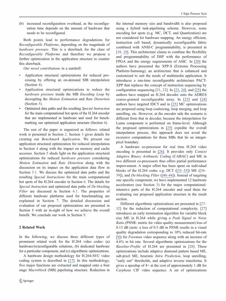
where C is the current MB and R is the reference MB. One16×16 SAD computation requires 256 subtractions, 256absolute operations, 255 additions along with loading of 256current and 256 reference MB pixels from memory. We havedesigned and implemented an SI that computes SAD of thecomplete MB. It constitutes two instances of the data pathSAD_16 (as shown in Fig. 9) that computes SAD of 4 pixelsof current MB w.r.t. 4 pixels of reference MB.

Once the best Integer-pixel Motion Vector (MV) isfound, the Sub-Pixel ME process refines the search tofractional pixel accuracy. At this stage, due to highcorrelation between surrounding candidate MVs, the accu-racy of minimum block distortion matters a lot. Therefore,H.264 proposes Sum of Absolute Transformed Differences(SATD) as the cost function to calculate the blockdistortion. It performs a 2-D Hadamard Transform on a4×4 array of difference values to give a closer representationto DCT that is performed later in the encoding process. Due

to this reason, SATD provides a better MV compared withthat calculated using SAD. However, because of highcomputational load, SATD is only used in Sub-Pixel MEand not in Integer-pixel ME. The SATD operation is definedas:

SATD ¼X4y¼0

X4x¼0

HT4�4 C x; yð Þ � R x; yð Þf gj j ð2Þ

where C is the current and R is the reference pixel value ofthe 4×4 sub-block, and HT4×4 is the 2-D 4×4 HadamardTransform on a matrix D (the differences between currentand reference pixel values) and it is defined as:

HT4�4 ¼1 1 1 11 1 �1 �11 �1 �1 11 �1 1 �1

2664

3775 D½ �

1 1 1 11 1 �1 �11 �1 �1 11 �1 1 �1

2664

3775

0BB@

1CCA,

2:

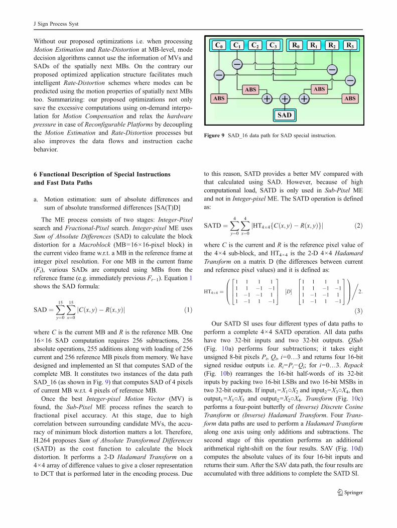
ð3ÞOur SATD SI uses four different types of data paths to

perform a complete 4×4 SATD operation. All data pathshave two 32-bit inputs and two 32-bit outputs. QSub(Fig. 10a) performs four subtractions; it takes eightunsigned 8-bit pixels Pi, Qi, i=0…3 and returns four 16-bitsigned residue outputs i.e. Ri=Pi−Qi; for i=0…3. Repack(Fig. 10b) rearranges the 16-bit half-words of its 32-bitinputs by packing two 16-bit LSBs and two 16-bit MSBs intwo 32-bit outputs. If input1=X1○X2 and input2=X3○X4, thenoutput1=X1○X3 and output2=X2○X4. Transform (Fig. 10c)performs a four-point butterfly of (Inverse) Discrete CosineTransform or (Inverse) Hadamard Transform. Four Trans-form data paths are used to perform a Hadamard Transformalong one axis using only additions and subtractions. Thesecond stage of this operation performs an additionalarithmetical right-shift on the four results. SAV (Fig. 10d)computes the absolute values of its four 16-bit inputs andreturns their sum. After the SAV data path, the four results areaccumulated with three additions to complete the SATD SI.

Figure 9 SAD_16 data path for SAD special instruction.

J Sign Process Syst

b. Motion compensation (MC_Hz_4)

Each MB in a video frame is predicted either by theneighboring MBs in the same frame i.e. Intra-Predicted (I-MB) or by an MB in the previous frame i.e. Inter-Predicted(P-MB). This prediction is subtracted from the currentblock to calculate the residue that is then transformed,quantized, and entropy coded. The decoder creates anidentical prediction and adds this to the decoded residual.Inter prediction uses block-based Motion Compensation.First, the samples at half-pixel location (i.e. betweeninteger-position samples) in the Luminance (Luma: Y)component of the reference frame are generated (Fig. 11:blue boxes for horizontal and green boxes for vertical)using a six tap Finite Impulse Response (FIR) filter withweights [1/32, −5/32, 20/32, 20/32, −5/32, 1/32]. Forexample, half-pixel sample ‘b’ (Fig. 11) is computed asb ¼ E � 5F þ 20Gþ 20H � 5I þ J þ 16ð Þ=32Þð . T h esamples at quarter-pixel positions are generated by BilinearInterpolation using two horizontally and/or verticallyadjacent half- or integer-position samples e.g. Gb ¼Gþ bþ 1ð Þ=2, where ‘Gb’ is the pixel at quarter-pixelposition between ‘G’ and ‘b’.

The MC_Hz_4 SI is used to compute the half-pixelinterpolated values. It takes two 32-bit input valuescontaining 8 pixels and applies a six-tap filter using SHIFTand ADD operations. In case of aligned memory access,BytePack aligns the data for the filtering operation. Thenthe PointFilter data path performs the actual six-tapfiltering operation. Afterwards Clip3 data path performsthe rounding and shift operation followed by a clippingbetween 0 and 255. Figure 12 shows the three constitutingdata paths for MC_Hz_4 SI.

c. Intra prediction: horizontal DC (IPred_HDC)and vertical DC (IPred_VDC)

In case of high motion scenes, the Motion Estimatornormally fails to provide a good match (i.e. MB withminimum block distortion) thus resulting in a high residueand for a given bit rate this deteriorates the encoded quality.In this case, Intra Prediction serves as an alternate byproviding a better prediction i.e. reduced amount ofresidues. Our two SIs Ipred_HDC and Ipred_VDC implementthree modes of Luma 16×16 i.e. Horizontal, Vertical, and

DC. Horizontal Prediction is given by p[−1, y], with x, y=0…15 and Vertical Prediction is given by p[x, −1], with x,y=0…15. DC Prediction is the average of top and leftneighboring pixels and is computed as follows:

& If all left and top neighboring samples are available,

then DC ¼ P15x'¼0

p x';�1½ � þ P15y'¼0

p �1; y'½ � þ 16

!>> 5.

& Otherwise, if any of the top neighboring samples are markedas not available and all of the left neighboring samples are

marked as available, then DC ¼ P15y'¼0

p �1; y'½ � þ 8

!>> 4.

& Otherwise, if any of the left neighboring samples are notavailable and all of the top neighboring samples are marked

as available, then DC ¼ P15x'¼0

p x';�1½ � þ 8

!>> 4.

& Otherwise, DC=(1≪(BitDepthY−1))=128, for 8-bit pixels.

IPred_HDC computes the Horizontal Prediction and thesum of left neighbors for DC Prediction. IPred_VDCcomputes the Vertical Prediction and the sum of topneighbors for DC Prediction. Figure 13 shows theCollapseAdd and PackLBytes data paths, which constituteboth of the Intra Prediction SIs.

P1P0 P3P2 Q1Q0 Q3Q2

R0 R1 R2 R3

QSub

X1

X2

Y

ABS

ABS+

X3

X4

ABS

ABS+

+

X1

X2

X3

X4

X1

X3

X2

Y4

SAV Repack

Y20

Y30

+X00

X30

+

–––

–

–

–

–

–

X10

X20

<< 1

<< 1

+

+

>> 1

>> 1

>> 1

>> 1

Y00

Y10

Transform

DCT HT

>> 1

>> 1

IDCT

a) b) c) d)

Figure 10 Data paths for SATD_4×4 special instruction.

Figure 11 Interpolation of Luma half-pixel positions.

J Sign Process Syst

d. (Inverse) discrete cosine transform ((I)DCT)

H.264 uses three different transforms depending on thedata to be coded. A 4×4 Hadamard Transform for the 16Luma DC Coefficients in I-MBs predicted in 16×16 mode, a2×2 Hadamard Transform for the 4 Chroma DC Coeffi-cients (in both I- and P-MBs) and a 4×4 Discrete Cosine

Transform that operates on 4×4 sub-blocks of residual dataafter Motion Compensation or Intra Prediction. The H.264DCT is an integer transform (all operations can be carried outusing integer arithmetic), therefore, it ensures zero mis-matches between encoder and decoder. Equation 4 shows thecore part of the 2-D DCT on a 4×4 sub-block X that can beimplemented using only additions and shifts:

DCT4�4 ¼ CXCT ¼1 1 1 12 1 �1 �21 �1 �1 11 �2 2 �1

2664

3775 X½ �

1 2 1 11 1 �1 �21 �1 �1 21 �2 1 �1

2664

3775

0BB@

1CCA: ð4Þ

The inverse transform is given by Eq. 5 and it isorthogonal to the forward transform i.e. T−1(T(X))=X:

IDCT4�4 ¼ CIY ′CTI ¼

1 1 1 1=21 1=2 �1 �11 �1=2 �1 11 �1 1 �1=2

2664

3775 Y ′½ �

1 1 1 11 1=2 �1=2 �11 �1 �1 1

1=2 �1 1 �1=2

2664

3775

0BB@

1CCA ð5Þ

where Y′=Y⊗Et given Et as the matrix of weighting factor.The DCT and IDCT SIs use QSub, Transform, and Repack(Fig. 10a–c) data paths to compute the 2-D (Inverse)Discrete Cosine Transform of 4×4 array.

e. (Inverse) Hadamard transform 4×4 ((I)HT_4×4)

If an MB is encoded as I-MB in 16×16 mode, each 4×4residual block is first transformed using Eq. 4. Then, the

Figure 12 Data paths for MC_Hz_4 special instruction.

Figure 13 Data paths for IPred_HDC and IPred_VDC special instructions.

J Sign Process Syst

DC coefficients 4×4 blocks are transformed using a 4×4Hadamard Transform (see Eq. 3). The inverse HadamardTransform is identical to the forward transform (Eq. 3). TheSIs for HT_4×4 and IHT_4×4 use Transform and Repack(Fig. 10b, c) data paths to compute the 2-D (Inverse)Hadamard Transform of 4×4 Intra Luma DC array.

f. (Inverse) Hadamard transform 2×2 ((I)HT_2×2)

Each 4×4 block in the Chroma components is trans-formed using Eq. 4. The DC coefficients of each 4×4 blockof Chroma coefficients are grouped in a 2×2 block (WDC)and are further transformed using a 2×2 HadamardTransform as shown in Eq. 6. Note: the forward andinverse transforms are identical:

HT2x2 ¼ 1 11 �1

� �WDC½ � 1 1

1 �1

� �� �� ð6Þ

The SIs for HT_2×2 and IHT_2×2 use one Transform(Fig. 10c) data path and computes the 2-D (Inverse)Hadamard Transform of 2×2 Chroma DC array.

g. Loop filter (LF_BS4)

The De-blocking Filter is applied after the reconstructionstage in the encoder to reduce blocking distortion bysmoothing the block edges. The filtered image is used formotion-compensated prediction of future frames. Thefollowing section describes the loop filter Special Instructionand the constituting data paths in detail along with ourproposed optimizations.

6.1 Fast Data Paths and Special Instruction for In-LoopDe-blocking Filter

The H.264 codec has an in-loop adaptive De-blockingFilter for removing the blocking artifacts at 4×4 sub-blockboundaries. Each boundary of a 4×4 sub-block is calledone 4-pixel edge onwards as shown in Fig. 14. Each MBhas 48 (32 for Luma and 16 for Chroma) 4-pixel edges. Thestandard specific details of the filtering operation can befound in [1]. Figure 15 shows the filtering conditions andfiltering equations for Boundary Strength=4 (as specified in[1]) where Pi and Qi (i=0, 1, 2, 3) are the pixel valuesacross the block horizontal or vertical boundary as shownin Fig. 16.

We have designed a Special Instruction (SI) for in-loopDe-blocking Filter (as shown in Fig. 17a) that targets theprocessing flow of Fig. 16. This SI filters one 4-pixel edge,

which corresponds to the filtering of four rows each with8 pixels. The LF_BS4 SI constitutes two types of datapaths: the first data path computes all the conditions(Fig. 17c) and the second data path performs the actualfiltering operation (Fig. 18). The LF_BS4 SI requires fourdata paths of each type to filter four rows of an edge.Threshold values α and β are packed with P (4-pixel groupon left side of the edge; see Fig. 16) and Q (4-pixel groupon right side of the edge) type pixels and passed as input tothe control data path. The UV and BS act as control signalsto determine the case of Luma-Chroma and BoundaryStrength respectively. The condition data path outputs two1-bit flags X1 (for filtering P-type i.e. Pi pixels) and X2 (forfiltering Q-type i.e. Qi pixels) that act as the control signalsof the filter data path. The two sets of pixels (P and Q type)are passed as input to this data path and appropriate filteredpixels are chosen depending upon the two control signals.

Figure 17b shows the processing schedule of theLF_BS4 SI. In first two cycles, two rows are loaded (Pand Q of one row are loaded in one LOAD command). Incycle 3, two control data paths are executed in parallelfollowed by two parallel filter data paths in the cycle 4 toget the filtered pixels for first and second row of the edge.In the mean time, next two loads are executed. In cycle 5and 6, the filtered pixels of first and second rows are storedwhile control and filter data paths are processed in parallelfor third and fourth rows. In cycle 7 and 8, the filteredpixels of third and fourth rows are stored. Now we willdiscuss the two proposed data paths.

We have collapsed all the if–else equation in onecondition data path that calculates two outputs to determinethe final filtered values for the pixel edge. In hardware, allthe conditions are processed in parallel and our hardwareimplementation is 130× faster than the software implementa-tion (i.e. running on GPP).

Figure 18 shows our optimized data path to compute thefiltered pixels for Luma and Chroma and selects theappropriate filtered values depending upon X1 and X2 flags.This new proposed data path needs fewer operations tofilter the pixels on block boundaries as compared to thestandard equations. The proposed data path exploitsthe redundancies in the operation sequence, re-arrangesthe operation pattern, and reuses the intermediate results asmuch as possible. Furthermore, this data path is not onlygood for hardware (ASIPs, Reconfigurable Platforms,RISPP) implementations, but also beneficial when imple-mented in software (GPP). In the standard equations, onlyone part is processed depending upon which condition ischosen at run time. For the software implementation of ourproposed data path, the else-part can be detached in order tosave the extra processing overhead. For the hardwareimplementation, we always process both paths in parallel.Note that the filtering data path is made more reusable

p3 p2 p1 p 0 q0 q1 q2 q3P Q

Figure 14 4-pixel edges in one macroblock.

J Sign Process Syst

using multiplexers. It is used to process two cases of Lumaand one case of Chroma filtering depending upon thefiltering conditions. The filtering of a four-pixel edge insoftware (i.e. running on GPP) takes 960 cycles for BoundaryStrength=4 case. Our proposed Special Instruction (Fig. 17a)using these two optimized data paths (Figs. 17c and18) requires only eight cycles (Fig. 17b) i.e. a speedup of120×.

We have implemented the presented data paths forcomputing the conditions (Fig. 17c) and the filteringoperations (Fig. 18) for a Virtex-II FPGA. The filteringoperation was implemented in two different versions. Thefirst one (original) was implemented as indicated by thepseudo-code in Fig. 16 and the second one (optimized) was

implemented in our optimized data path (Fig. 18). Theresults are shown in Table 2. The optimized loop filteroperation reduces the number of required slices to 67.8%(i.e. 1.47× reduction). At the same time, the critical pathincreases by 1.17× to 9.69 ns (103 MHz), which does notincrease the critical path for our hardware prototype (seeSection 7).

7 Properties of Hardware Platformsused for Benchmarking

We evaluate our proposed application structural optimiza-tions with diverse hardware platforms in the following

αβ β

ββ

β α

β α

Figure 16 Pixel samples across a 4×4 block horizontal or vertical boundary.

LUMA (32 4-pixel edges)

CHROMA (2*8=16 4-pixel edges)

4-pixel edge

4x4 sub-block

Block Edge (16-pixels)

A Block Edge spans the complete 16-pixel boundary in an MB

4-pixel edge is a part of the Block Edge considering

4x4 sub-blocks

Figure 15 The filtering process for boundary strength=4.

J Sign Process Syst

result section, i.e. GPP (General Purpose Processor), ASIP(Application-Specific Instruction set Processor), Reconfig-urable Platform, and RISPP (Rotating Instruction SetProcessing Platform). Although the focus of this paper ison our proposed application structural optimizations, wewill briefly describe the differences between ASIPs,Reconfigurable Platforms, and RISPP that are used ashardware platforms for benchmarking these optimizations.

The term ASIP comprises nowadays a far larger varietyof embedded processors allowing for customization invarious ways including (a) instruction set extensions, (b)parameterization and (c) inclusion/exclusion of predefinedblocks tailored to specific applications (like, for example,

an MPEG-4 decoder) [54]. A generic design flow of anembedded processor can be described as follows: (1) anapplication is analyzed/profiled, (2) an extensible instruc-tion set is defined, (3) extensible instruction set issynthesized together with the core instruction set, (4)retargetable tools for compilation, instruction set simulationetc. are (often automatically) created and applicationcharacteristics are analyzed, (5) the process might beiterated several times until design constraints comply.However, for large applications that feature many compu-tational hotspots and not just a few exposed ones, currentASIP concepts struggle. In fact, customization for manyhotspots bloats the initial small processor core to consider-

LO

AD

2 in

pu

tsL

OA

D2

inp

uts

ST

OR

E2

ou

tpu

tsS

TO

RE

2 o

utp

uts

Cyc

les

12

34

56

78

LO

AD

2 in

pu

tsL

OA

D2

inp

uts

ST

OR

E2

ou

tpu

tsS

TO

RE

2 o

utp

uts

- ABSp0

q0

-p0

p1

-q0

q1

ABS

ABS

<

α

β

β

β

<

<>> 1α +

2

<-p2

p0

-q2

q0

ABS

ABS <

<

UV

Ba

Bb

8

8

8

8

8

88

8

8

8

1

1

1

1X1

X21

BS

BS

c) Condition data path for Loop Filter

LF

_Co

nd

itio

nL

F_F

ilter

LE

GE

ND

:

a) LF_BS4 Special Instruction

OUTPUTINPUTBS = (Boundary_Strength==4)

b) OperationSchedule

32

32P1α

α

α

α

β

β

β

β

Q1

UV BS

11

1X1

1X2

32

32

P1

Q1

P1'

Q1'

32

32

32

32P2

Q2

UV BS

11

1X3

1X4

32

32

P2

Q2

P2'

Q2'

32

32

32

32P3

Q3

UV BS

11

1X5

1X6

32

32

P3

Q3

P3'

Q3'

32

32

32

32P4

Q4

UV BS

11

1X7

1X8

32

32

P4

Q4

P4'

Q4'

32

32

Figure 17 Special instruction with constituting optimized data path of filtering conditions for in-loop de-blocking filter and the processingschedule using condition and filtering operations.

Figure 18 Optimized data path of boundary strength=4 filtering operation for in-loop de-blocking filter with parallel processing of Luma andChroma paths.

J Sign Process Syst

ably larger sizes (factors of the original base processorcore). Moreover, to develop an ASIP, a design-spaceexploration is performed and the decisions (which SpecialInstructions (SIs), which level of parallelism, etc.) are fixedat design time.

Reconfigurable processors instead combine e.g. a pipelinewith reconfigurable parts. For instance, fine-grained reconfig-urable hardware (based on lookup tables i.e. similar to FPGAs)or coarse-grained reconfigurable hardware (e.g. arrays ofALUs) can be connected to a fixed processor as functionalunit or as co-processor [53]. This reconfigurable hardware canchange its functionality at run time, i.e. while the applicationis executing. Therefore, the SIs no longer need to be fixed atdesign time (like for ASIPs), but only the amount ofreconfigurable hardware is fixed. The SIs are fixed at compiletime and then reconfigured at run time. Fixing the SIs atcompile time has to consider constraints like their maximalsize (to fit into the reconfigurable hardware) and typicallyincludes the decisions when to reconfigure which part of thereconfigurable hardware. Determining the decision when tostart reconfiguring the hardware has to consider the ratherlong reconfiguration time (in the range of milliseconds,depending on the size of the SI).

Compared to typical ASIPs or Reconfigurable PlatformsRISPP is based on offering SIs in a modular manner. Themodular SIs are connected to the core pipeline in theexecute stage, i.e. the parameters are prepared in the decodestage and are then passed to the specific SI implementationin the execute stage. The interface to the core pipeline isidentical for ASIPs, Reconfigurable Platforms, and RISPP.The main difference is the way in which the SIs areimplemented. Instead of implementing full SIs indepen-dently, data paths are implemented as elementary re-usablereconfigurable units and then combined to build an SIimplementation. The resulting hierarchy of modular SIs (i.e.SIs, SI implementations, and data paths) is shown inFig. 17. Figure 17a shows the composition of the LoopFilter SI, while Fig. 17c shows one of its elementary datapaths. The schedule in Fig. 17b corresponds to one certainimplementation of this SI, for the case that two instances of

both required data paths are available and can be used inparallel. However, the same SI can also be implementedwith only one instance of each data path by executing thedata paths sequentially (note that parallelism is stillexploited within the implementation of a data path). Onthe one hand, this saves area but on the other hand, it costsperformance. Additionally, the Loop Filter SI can beimplemented without any data paths (executing it like aGPP) and it can be implemented if e.g. only the filteringdata paths (Fig. 18) is available in hardware (then theconditions are evaluated like on a GPP and then forwardedto the filtering data paths). These different implementationtrade-offs are available for all extensible processor plat-forms, i.e. ASIP, Reconfigurable Platform, and RISPP.ASIPs select a certain SI implementation at design time andReconfigurable Platforms select an implementation atcompile time. RISPP instead selects an implementation atrun time out of multiple compile-time prepared alternatives[49]. While performing this selection, RISPP considers thecurrent situation, e.g. the expected SI execution frequency(determined by an online monitoring [50]) to specificallyfulfill the dynamically changing requirements of theapplication.

To efficiently support different implementation alterna-tives of one SI, RISPP offers the data paths as elementaryreconfigurable units. This means that the configuration of asingle data path is loaded into one out of multiplereconfigurable regions. As soon as sufficient data pathsfor an SI implementation are available, the data paths areconnected (via busses, using a compile-time preparedconnection scheme) to implement this SI. As soon assufficient further data paths finished reconfiguration, theseconnections are changed to use the further data paths andthus to realize a faster SI implementation that exploits moreparallelism. Reconfiguring at the level of data paths notonly allows the concept of upgrading SI implementations atrun time but it furthermore allows sharing, i.e. onereconfigured data path can be used for the implementationsof different SIs. A run-time system manages the currentlyavailable SI implementation and controls the requiredconnections between the core pipeline and the data paths.This run-time system also controls in which sequence theSIs shall be upgraded. The feature to gradually upgrade SIimplementations diminishes the above-mentioned problemof rather long reconfiguration times, but it does notdiminish the conceptual problem of high hardware pressurelike presented in Section 5. Therefore, either morereconfigurable hardware has to be added or the hardwarepressure itself has to be distributed, e.g. by our optimizedapplication structure.

For evaluation purpose, we have implemented a RISPPprototype on an FPGA board (see Fig. 19). We haveimplemented the core pipeline and the reconfigurable

Table 2 Results for hardware implementation of individual datapaths.

Characteristics Data paths

Condition Loop filter(original)

Loop filter(optimized)

No. of slices 72 174 118No. of LUTs 138 306 204Gate equivalents 1,207 2,754 2,074Latency [ns] 6.49 8.25 9.69

J Sign Process Syst

regions on the FPGA and tightly coupled the reconfigurableparts (as functional units) with the execution stage of thepipeline. Our core pipeline is based on a MIPS processor thatwas extended for our requirements (e.g. four read ports in theregister file) and runs at 50 MHz. The processor is connectedto external SRAM for instruction and data memory of theapplication as well as to a fast external EEPROM for theconfiguration data. The realized peripheral connectionscomprise a touch-screen LCD that allows interaction withthe running application (not used while benchmarking).

8 Evaluation, Discussion and Results

8.1 Test Conditions and Fairness of Comparison

In the motivation (Section 1), we have introduced andanalyzed the problem of excessive Interpolation andhardware pressure. To solve this issue, we have proposeda set of application structural optimizations. At first, wehave created an optimized Benchmark Application of H.264video encoder [2] (Section 3) considering multimediaapplications with Common Intermediate Format (CIF=352×288) or Quarter CIF (QCIF=176×144) resolutionsrunning on mobile devices. The same Benchmark Applicationis used for all hardware platforms, i.e. GPP (General PurposeProcessor; in our case a MIPS), ASIP (Application-SpecificInstruction set Processor), Reconfigurable Platform, andRISPP). Detailed results are presented for the Carphone (atypical videophone sequence) under the test conditionsQuantization Parameter (QP)=30, Group of Pictures(GOP)=IPPP…, and Search Range=16. Before proceeding

to the discussion of results, we will present the fairness ofcomparison in this section.

This paper focuses on application structural optimiza-tions for H.264 video encoder. An application structurerunning on a particular hardware platform is compared withdifferent application structures on the same hardwareplatform. Therefore, the performance in terms of cycles isconsidered, as the test conditions with respect to theunderlying hardware platforms are always same fordifferent application structures. In order to study the effectof the proposed optimizations and to validate our concept,we have carried out this comparison on several hardwareplatforms keeping in mind that the different applicationstructures are only compared within one hardware platformat a time. We will now enumerate the similarities and testconditions that justify the fairness of comparison.

1. All the Application Structures use the same BenchmarkApplication as the starting point. Same set of optimizeddata paths and Special Instruction (SIs) is given to allapplication structures. Each data path takes one cyclefor execution.

2. All the application structures were given the samehardware resources, i.e. register file, number of read/write ports, memory accesses, etc. when executing on aparticular hardware platform.

3. Only the application structures running on the samehardware platforms are compared with each other i.e.Benchmark Application executing on ASIP is comparedwith Interpolation-Optimized Application and Hard-ware-Pressure-Optimized Application running onASIP.

Figure 19 FPGA-based RISPP prototyping platform.

J Sign Process Syst

8.2 Results and Discussion

Our proposed optimized filtering operation for the in-loopDe-blocking Filter (Fig. 18) needs (18+5)×48×#MBsadditions (CIF=399,168; QCIF=99,792 additions) whilethe standard equations need (30+6)×48×#MBs additions(CIF=684,288; QCIF=171,072 additions) for both Lumaand Chroma. It shows 41.67% operation reduction. Thestandard equations suffer performance degradation due tosix conditional jumps but our optimized implementationhas only two conditions. For a hardware implementation,this results in simple multiplexers. The optimized filteringoperation reduces the number of required slices to 67.8%(i.e. 1.47× reduction, see Table 2). At the same time thecritical path increases (by 1.17×) to 9.69 ns (103 MHz),which does not increase the critical path for our hardwareprototype that is running at 50 MHz (20 ns). In addition tothe filtering operation, the hardware implementation of ourcondition data path (Fig. 17c) is 130× faster than thecorresponding software implementation (i.e. running onGPP) as we process all conditions in parallel. The proposedcondition data path requires only 72 slices as the logic aftercomparing the absolute differences is done on bit-level (seeFig. 17c). Combining two instances of our both optimized

data paths to implement the proposed Special Instruction(Fig. 17a) takes only eight cycles (see Fig. 17b) to filter a4-pixel edge for the Boundary Strength=4 case. Performingthe same computation on the GPP requires 960 cycles,which corresponds to a 120× faster hardware execution.However, this speedup only considers the execution of ourproposed In-loop De-Blocking Filter, not the whole H.264encoder. Therefore, we subsequently concentrate on theexecution time of specific hot spots and the wholeapplication (showing the benefits of our proposed optimi-zations of the application structure). Eventually, we willpresent the detailed analysis of the SI execution patternwithin one frame to clarify and evaluate the conceptualdifferences of our both proposed application structures.

Figure 20 shows a comparison between the BenchmarkApplication and our on-demand interpolation processing(Section 4) running on GPP for four typical QCIF videosequences that cover most of the motion characteristics ofvideos for mobile devices. Carphone represents the videocall scenario in a moving car where the motion is due to thebody of the caller and the background from the side-window.Miss America is a typical head–shoulder movement se-quence and exhibits relatively low motion characteristics.Trevor is a relatively complex scene where several persons

Frame Number

Exe

cuti

on T

ime

[MC

ycle

s]

0

1

2

3

4

5

6

7

8

9

0 10 20 30 40 50 60 70 80 90 100 110 120 130

Quarter Pixel Half Pixel

Actual Occurances Benchmark Application

Half Pixel Line

a) Carphone Frame Number

Exe

cuti

on T

ime

[MC

ycle

s]

0

1

2

3

4

5

6

7

8

9

0 10 20 30 40 50 60 70 80 90 100 110 120 130

Quarter Pixel Half Pixel

Actual Occurances Benchmark Application

Half Pixel Line

b) Miss America

Frame Number

Exe

cuti

on T

ime

[MC

ycle

s]

0

1

2

3

4

5

6

7

8

9

0 10 20 30 40 50 60 70 80 90 100 110 120 130

Quarter Pixel Half Pixel

Actual Occurances Benchmark Application

Half Pixel Line

c) Trevor Frame Number

Exe

cuti

on T

ime

[MC

ycle

s]

0

1

2

3

4

5

6

7

8

9

0 10 20 30 40 50 60 70 80 90 100 110 120 130

Quarter Pixel Half Pixel

Actual Occurances Benchmark Application

Half Pixel Line

d) Table Tennis

Figure 20 Processing time of interpolation for the benchmark vs. our proposed application structure when running on GPP (MIPS).

J Sign Process Syst

are moving in one video sequence simulating severalmovements occurring in video conferencing. Table Tennisrepresents camera pan motion and the motion of gameobjects (persons and ball). In case of camera panning thebackground is not stationary, rather all the MBs ofbackground move with a same amount, i.e. motion vectorsare approximately equal for MBs of background.

The processing time of the interpolation in the Bench-mark Application is always 8.444 MCycles as it processesall cases. Using our optimized application structure fromSection 4, the interpolations for 1 QCIF frame requires atmaximum 2.417 (average 1.191), 1.244 (average 0.491),1.298 (average 0.893), and 2.441 (average 1.177) MCyclesfor Carphone, Miss America, Trevor, and Table Tennisrespectively. Analyzing the behavior of these four typicalvideo sequences we find that the maximum and averageprocessing time for interpolation is much smaller than that ofthe Benchmark Application (due to the stationary back-ground). Therefore, the application structural optimizationfor on-demand interpolation gives a huge saving in terms ofprocessing time (compared to the Benchmark Application) aswe will now evaluate with further video sequences (Table 3).

We have considered seven different QCIF video sequences[51] with different motion properties to simulate variousmobile video scenarios. In the Benchmark Application, theinterpolation of 139 frames takes 1,174 MCycles (139frames×8.444 MCycles; same for all video sequences).Table 3 shows the processing time and the speedup(compared to the Benchmark Application architecture) ofthe interpolation process in our optimized applicationstructure with on-demand interpolation on GPP. Our pre-sented approach to reduce the number of performedinterpolations is independent of any specific processorplatform as it conceptually reduces the amount of requiredcomputations, independent whether this computation is donein software (GPP) or in hardware (e.g. ASIP). It comes at thecost of increased hardware pressure.

While the above presented optimizations (i.e. optimizedfiltering operation and reduced interpolations) are beneficial

for a GPP as well, we will now focus on hardwareimplementations (especially on Reconfigurable Platforms).At design time, a particular amount of hardware is given toASIPs, Reconfigurable Platforms, and RISPP. The amountof hardware determines how many Special Instructions(SIs) can be expedited to exploit the inherent parallelismthus directly corresponding to the achieved performance. Incase of ASIPs, the data paths that can be accommodated inthis hardware are fixed, while for Reconfigurable Platformsand RISPP the data path are loaded at run time and only theamount of data path that can be present on the reconfig-urable hardware at the same time is fixed. Figure 21 showsthe execution times of the Benchmark Application (onwardscalled BApp), our Interpolation-Optimized Architecture (asexplained in Section 4; onwards called InOpt), and ourHardware-Pressure-Optimized Architecture (as explained inSection 5, onwards called HPOpt) running on a Reconfig-urable Platform. The x-axis in this plot shows to theamount of data paths that fit to the hardware at the sametime. The more reconfigurable hardware is available thefaster the execution becomes. The application executionwithout data paths i.e. always using the instruction set ofthe core-pipeline/base processor corresponds to a GPP. Asthe performance without data paths is much slower, we donot show it in the Fig. 21.

We will now shed light on the region between twoimportant points marked as Label A and Label B in Fig. 21where (contrary to the other regions) InOpt is notsignificantly faster than BApp. For one and two data paths,the Motion Compensation Special Instruction (i.e.MC_Hz4) executes in software for both BApp and InOpt.In this case, InOpt achieves its performance improvementdue to the reduced number of interpolations. HPOpt isfurther better than InOpt due to the reduced hardwarepressure, as we will see. At Label A, BApp has almost thesame processing time as of InOpt because in case of BApp,the MC_Hz4 SI (along with e.g. SAD and SATD) nowexecutes in hardware. However, for InOpt the MC_Hz4 SIstill executes in software. This is due to the high hardware

Table 3 Processing time and speedup of interpolation (half- and quarter-pixel) for 139 frames compared to the benchmark application(1,173.77 MCycles) for GPP.

Video sequence Half-pixel (MCycles) Quarter-pixel (MCycles) Total (MCycles) Speedup

Bridge_Close 0.02 3.46 3.48 333.33Carphone 18.23 147.37 165.60 7.09Claire 3.08 26.50 29.58 39.68Grandma 3.46 31.93 35.39 33.22Miss America 8.98 59.33 68.30 17.18Salesman 1.72 34.60 36.32 32.36Table_Tennis 18.98 144.69 163.67 7.17Trevor 8.89 115.27 124.16 9.45Average 7.92 70.39 78.31 59.96

J Sign Process Syst

pressure that is introduced by shifting the interpolationsinside the MB Encoding Loop (necessary to reduce thenumber of performed interpolations, see Section 4). Theavailable reconfigurable hardware has to be shared amongthe SIs of the MB Encoding Loop, as reconfiguring withinthe loop is not beneficial (due to the long reconfigurationtime as discussed in Section 7). As SAD and SATD aresignificantly more often executed than the MC_Hz4 SI, it ismore beneficial (concerning overall performance) to imple-ment SAD and SATD in hardware while executingMC_Hz4 in software. However, BApp can implementSAD and SATD as well as MC_Hz4 in hardware, as itexecutes them in different loops and reconfigurationbetween the loops is feasible. Due to this reason, the gainof reduced interpolations is cancelled out by the differenceof hardware and software executions of MC_Hz4. Thissituation exists between three (Label A) and five (Label B)available data paths. Afterwards, the main requirements(i.e. the execution of the most important SIs in hardware),of the MB Encoding Loop are fulfilled and the MC_Hz4 SIis executed in hardware for InOpt too.

HPOpt resolves the discussed problem of InOpt bydecoupling the SAD and SATD SIs from the MB EncodingLoop. The benefit of the reduced hardware pressurebecomes especially noticeable in the region between LabelA and Label B. When more reconfigurable hardware isavailable InOpt comes closer to HPOpt as the hardwareneeds of each SI are fulfilled. Due to high reconfigurationoverhead, after eight data paths the Reconfigurable Plat-form does not give significant benefits per additional datapath. However, the specific amount of data paths (wherefurther performance benefits are no longer significant)

highly depends on the application as well as the specificreconfiguration bandwidth.

Table 4 shows the maximum and average speedups(using one to 14 data paths; GPP does not use application-specific data paths therefore average=maximum) whenexecuting the H.264 video encoder with the BApp, InOpt,and HPOpt application structures for all four hardwareplatforms. It is worthy to note that all these applicationstructures use the same Special Instructions therefore thetable purely represents the improvement of applicationstructural optimizations. The table shows that HPOpt is upto 2.84× (average 2.36) and 1.94× (average 1.58×) fasterthan BApp for ASIP and Reconfigurable Platform respec-tively. For RISPP, HPOpt is at maximum 2.24× (average1.91×) and 1.82× (average 1.29×) faster than BApp andInOpt respectively. Note, higher speedup for ASIP does notnecessarily mean that ASIP is faster than ReconfigurablePlatform or RISPP. They have different ‘1×’ performance(i.e. execution time of BAPP on ASIP is different from thaton Reconfigurable Platform or RISPP) and we do notintend to compare them. Therefore, the speedup in Table 4only provides the comparison of different applicationstructures on a particular hardware platform.

We now analyze the detailed differences in the executionpatterns of InOpt (Fig. 5) vs. HPOpt (Fig. 6), on RISPPwith four, five, and six data paths when encoding one QCIFvideo frame of Carphone sequence to explain how we getthe performance benefit by reducing the hardware pressure.We show the number of executions of important SIs (y-axis) for timeframes of 100 KCycles time-slots (x-axis). Forclarity, we restrict to those SIs that show the difference ofthe application structures. InOpt runs the SIs for ME and

Encoding Time of 139 Frames from Carphone QCIF Video for Different Amount of Accelerating Hardware Resources

0

500

1,000

1,500

2,000

2,500

3,000

3,500

4,000

4,500

5,000

1 2 3 4 5 6 7 8 9 10 11 12 13 14Hardware Resources [#Data Paths]

Pro

cess

ing

Tim

e [M

Cyc

les]

Benchmark Application (BApp)

Encoder with Optimization of InterpolationComputations (InOpt)

Encoder with Additionally Reduced HardwarePressure (HPOpt)

Label A: Label B:

2X Speedup

Figure 21 Comparison of the benchmark application and our proposed optimized application structures for reconfigurable platforms.

J Sign Process Syst

Table 4 Maximum and average speedups of optimized vs. benchmark application architectures for different amount (i.e. one to 14) ofaccelerating hardware resources.

InOpt vs. BApp HPOpt vs. BApp HPOpt vs. InOpt

Maximum speedup Average speedup Maximum speedup Average speedup Maximum speedup Average speedup

GPP 1.38 1.46 1.06ASIP 2.34 2.01 2.84 2.36 1.30 1.17Reconf. 2.05 1.54 1.94 1.58 1.67 1.09RISPP 1.98 1.51 2.24 1.91 1.82 1.29

a)

6 D

ata

Pat

hs

0

500

1.000

1.500

2.000

2.500

3.000

3.500

4.000

0,0

0,5

1,0

1,5

2,0

2,5

3,0

3,5

DCT_4x4

MC_Hz4

SAD

Timeframe [MCycles]

Num

ber

of S

I E

xecu

tion

s

Execution of Loop Filter

Execution of Motion Estimation and Encoding Engine

SATD

LF_BS4

0

500

1.000

1.500

2.000

2.500

3.000

3.500

4.000

0,0

0,5

1,0

1,5

2,0

2,5

3,0

3,5

DCT_4x4

MC_Hz4

SAD

Timeframe [MCycles]

Num

ber

of S

I E

xecu

tion

s

Execution of Loop Filter

Execution of Motion Estimation

Execution of Encoding Engine

SATD

LF_BS4

b)

5 D

ata

Pat

hs

0

500

1.000

1.500

2.000

2.500

3.000

0,0

0,5

1,0

1,5

2,0

2,5

3,0

3,5

4,0

4,5

DCT_4x4

MC_Hz4

SAD

Timeframe [MCycles]

Num

ber

of S

I E

xecu

tion

s Execution of Loop Filter

Execution of Motion Estimation and Encoding Engine

SATD

LF_BS4

0

500

1.000

1.500

2.000

2.500

3.000

0,0

0,5

1,0

1,5

2,0

2,5

3,0

3,5

4,0

4,5

DCT_4x4

MC_Hz4

SAD

Timeframe [MCycles]

Num

ber

of S

I E

xecu

tion

s Execution of Loop Filter

Execution of Motion Estimation

Execution of Encoding Engine

SATD

LF_BS4

c)

4 D

ata

Pat

hs

0

200

400

600

800

1.000

1.200

1.400

1.600

0,0

0,5

1,0

1,5

2,0

2,5

3,0

3,5

4,0

4,5

5,0

5,5

6,0

6,5

7,0

7,5

8,0

8,5

DCT_4x4

MC_Hz4

SAD

Timeframe [MCycles]

Num

ber

of S

I E

xecu

tion

s

Execution of Loop Filter

Execution of Motion Estimation and Encoding Engine

SATD

LF_BS4

0

200

400

600

800

1.000

1.200

1.400

1.600

0,0

0,5

1,0

1,5

2,0

2,5

3,0

3,5

4,0

4,5

5,0

5,5

6,0

6,5

7,0

7,5

8,0

8,5

DCT_4x4

MC_Hz4

SAD

Timeframe [MCycles]

Num

ber

of S

I E

xecu

tion

s

Executionof LoopFilter

Execution of Motion Estimation

Execution of Encoding Engine

2,899

SATD

LF_BS4

Figure 22 Execution time profile of major functions (five SIs) in ourproposed application structures InOpt and HPOpt for 1 QCIF videoframe. Detailed utilization variations for four, five, and six availabledata paths, used by InOpt and HPOpt respectively for RISPP. Allfigures show the encoding of 1 video image. The x-axis shows the

timeframes of 100 KCycles, the y-axis denotes the number of SIexecutions. For a given number of data paths, the x-axis for InOpt andHPOpt was selected as the maximum number of timeframes that oneof the application structures required to encode one video image.

J Sign Process Syst

MB Encoding Loop (DCT, SATD, …) together in one bigloop over all MBs in a frame while HPOpt processes SIs ofME and MB Encoding Loop in two separate loops.

Figure 22a shows the detailed SI execution pattern forsix available (reconfigurable) data paths using InOpt andHPOpt for RISPP. As ME (Motion Estimation) and MC(Motion Compensation) are processed in the same loop forInOpt, the first five data paths are allocated to SAD andSATD to expedite ME which is the most compute-intensivepart of the video encoder. For InOpt, in the first100 KCycles SAD is executed (running in software). After100 KCycles (approximately one reconfiguration time,depending on which data path is loaded [49]), the firstaccelerating data path SAD_16 is loaded that will expeditethe SAD Special Instruction (SI). Additionally, SATDstarts execution, first in software and between 100 and500 KCycles the corresponding data paths are loadedsequentially, therefore the SATD execution upgradesgradually (as explained in Section 7). The amount ofSATD, DCT, and MC executions in the first 500 KCycleshows that not all accelerating data paths are loaded yet andtherefore RISPP is not yet executing SIs at full perfor-mance. As more data paths finish loading, the single SIexecutions become faster and thus more SIs are executedper timeframe. Table 5 shows the six selected data paths inthis case for the MB Encoding Loop. It is worthy to notethat five data paths are given to the ME SIs while the MCSI gets only one data path. The optimization target therebyis to reduce the execution time of the complete applicationand not only of one functional block. Additionally, the (I)DCT, (I)HT_2×2, and (I)HT_4×4 SIs are expedited due toreusable data paths (i.e. Repack, Transform, and QSub areshared between SATD and these SIs). Due to highhardware pressure not all SIs can be completely supportedin hardware therefore the MB Encoding Loop takes longerto finish its execution, i.e. 3.6 MCycles. Afterwards, thedata paths for in-loop De-blocking Filter are loaded. InOpt

requires 3.9 MCycles to process the encoding of one QCIFvideo frame.

In contradiction to the presented InOpt processing flow,HPOpt first processes the ME SIs and therefore all the datapaths are allocated to SAD (two data paths) and SATD(four data paths). It is noticeable in Fig. 22a that after all sixdata paths (2×SAD_16, Repack, Transform, QSub, SAV)are loaded, the total number of SI executions in the ME hotspot increases significantly as SAD and SATD are nowexecuted in a faster hardware implementation (exploitingmore parallelism). These faster hardware implementationswere not selected for InOpt, as then no data path wouldhave been left to accelerate MC. Therefore, MC would havebeen the bottleneck, leading to a reduced performance ofthis loop. After HPOpt finished the ME hot spot, the threedata paths 2×SAD_16 and SAVare replaced by PointFilter,Clip3, and BytePack to expedite the MC_Hz4 SI. The loopdecoupling in HPOpt allows offering more data paths perSI as less SIs are needed per timeframe (SAD nowadditionally gets another data path of SAD_16 whileMC_Hz4 additional gets Clip3 and BytePack). Therefore,all SIs can be offered in a better performance (exploitingmore parallelism) which results in more executions pertimeframe. Additionally, the number of DCT and MC_Hz4executions is reduced in HPOpt due to the early decisionbetween I- and P-MB types by Rate Distortion (RD). Inthe result, HPOpt requires 2.6 MCycles to process theencoding of one QCIF video frame and is finished muchearlier as compared to InOpt, showing the saving of1.3 MCycles.

Compared to the presented details for six data paths,Fig. 22b and c present the results for five and four datapaths respectively. It is noticeable in Fig. 22c that for fourdata paths InOpt requires 8.9 MCycles to process theencoding of one QCIF video frame which is significantlyslower when compared with the performance of six datapaths. This big difference comes due to the MB Encoding

Table 5 Data paths supported in hardware for InOpt and HPOpt for four, five, and six data paths.

No. ofdata paths

Data paths selected for acceleration

InOpt (data paths used in each hot spot) HPOpt (data paths used in each hot spot)

MB encoding loop In-loop de-blocking filter

Motion estimation MB encoding loop In-loop de-blocking filter

4 SAD_16, Repack,Transform, QSub

Cond, LF_4 SAD_16, Repack,Transform, QSub

Repack, Transform, QSub,PointFilter, Clip3

Cond, LF_4

5 SAD_16, Repack,Transform, QSub, SAV

Cond, LF_4 SAD_16, Repack,Transform, QSub, SAV

Repack, Transform, QSub,SAV, PointFilter, Clip3

Cond, LF_4

6 SAD_16, Repack, Transform,QSub, SAV, PointFilter

Cond, LF_4 2×SAD_16, Repack,Transform, QSub, SAV

Repack, Transform, QSub,PointFilter, Clip3, BytePack

Cond, LF_4

J Sign Process Syst

Loop that requires 8.6 MCycles to complete. Due to onlyfour available data paths, MC_Hz4 as well as SATD cannotbe supported in a fast hardware implementation (e.g. SAV ismissing for SATD, see Tables 1 and 5). HPOpt improvesthe performance (saving 1.6 MCycles compared to InOpt)but due to the absence of SAV the ME loop is still slow(requires 5.7 MCycles). However, for five data paths(Fig. 22b) SAV is available (see Table 5), therefore SATDexecutes in hardware but MC_Hz4 is still in software. AsSATD has a bigger contribution in the performance gainsand we target reducing the overall execution time of thewhole application, the data path for SATD is givenpreference on that of MC_Hz4. As a result the executionof InOpt for five data paths is faster than that of five datapaths (Fig. 22b) but still slower than that of six data paths.HPOpt here gets a bigger benefit as now it complete theME hot spot much earlier (1.8 MCycles) giving an overallsaving of 2 MCycles for one frame encoding. Summarizing,because of faster SI implementations (more data paths perSI) and reduced computations, HPOpt is finished muchearlier as compared to InOpt, showing the maximumspeedup of 1.82× for RISPP (compared to the BenchmarkApplication running on RISPP), as shown in Table 4.

9 Conclusion

We have presented optimizations for the H.264 encoderapplication structure for reduced processing and reducedhardware pressure along with several novel data paths andthe resulting Special Instruction for the main computationalhot spots of the H.264 encoder. For in-loop De-blockingFilter, the optimized filtering data path reduces the numberof required slices to 67.8% (i.e. 1.47× reduction, seeTable 2). The Special Instruction is 120× faster than theGeneral Purpose Processor Implementation. Our approachof reduced processing is good for all four hardwareplatforms (i.e. GPP, ASIP, Reconfigurable Platform, andRISPP), while the optimization of reduced hardwarepressure target the Reconfigurable Platform and RISPPspecifically. As compared to the optimized BenchmarkApplication, we achieve an average speedup of approxi-mately 60× for Motion Compensated Interpolation forMIPS. For RISPP, our optimized application structure forinterpolation achieves up to 1.98× improvement (seeTable 4) over the Benchmark Application architecture.The reduced hardware pressure improves the performanceof our optimized application architecture up to 2.24×compared to the Benchmark Application.

References

1. ITU-T Rec. H.264 and ISO/IEC 14496-10:2005 (E) (MPEG-4AVC) “Advanced video coding for generic audiovisual services”,2005.

2. ITU-T H.264 reference software version JM 13.2. Retrieved fromhttp://iphome.hhi.de/suehring/tml/index.htm.

3. X264—a free H.264/AVC encoder. Retrieved from http://www.videolan.org/developers/x264.html.

4. Chen, Z., Zhou, P., & He, Y. (2002). Fast integer pel andfractional pel motion estimation for JVT, JVT-F017, 6th JVTMeeting, Awaji, December.

5. Raja, G., & Mirza, M. J. (2004). Performance comparison ofadvanced video coding H.264 standard with baseline H.263and H.263+ standards. IEEE International Symposium onCommunications and Information Technology (ISCIT), 2, 743–746.

6. Wiegand, T., Sullivan, G. J., Bjntegaard, G., & Luthra, A. (2003).Overview of the H.264/AVC video coding standard. IEEETransactions on Circuits and Systems for Video Technology, 13(7), 560–576. doi:10.1109/TCSVT.2003.815165 (CSVT).

7. Ostermann, J., et al. (2004). Video coding with H.264/AVC: tools,performance, and complexity. IEEE Circuits and SystemsMagzine, 4(1), 7–28. doi:10.1109/MCAS.2004.1286980.

8. Wiegand, T., et al. (2003). Rate-constrained coder control andcomparison of video coding standards. IEEE Transactions onCircuits and Systems for Video Technology, 13(7), 688–703.doi:10.1109/TCSVT.2003.815168 (CSVT).

9. Bjontegaard, G. (2001). Calculation of average PSNR differencesbetween RD-curves. ITU-T SG16 Doc. VCEG-M33.

10. Ziauddin, S. M., ul-Haq, I., Nadeem, M., & Shafique, M. Methodsand systems for providing low cost robust operational control forvideo encoders, Pub. Date: Sept. 6, 2007; Patent Pub. No. US-2007-0206674-A1, Class: 375240050 (USPTO).

11. Yuan, W., Lin, S., Zhang, Y., Yuan, W., & Luo, H. (2006).Optimum bit allocation and rate control for H. 264/AVC. IEEETransactions on Circuits and Systems for Video Technology, 16(6),705–715. doi:10.1109/TCSVT.2006.875215 (CSVT).

12. Milani, S., et al. (2003). A rate control algorithm for theH.264 encoder. Baiona Workshop on Signal Processing inCommunications.

13. Xtensa, L.X.: 2 processor, Tensilica Inc. Retrieved from http://www.tensilica.com.

14. Xtensa, L.X.: 2 I/O Bandwidth. Retrieved from http://www.tensilica.com/products/io_bandwidth.htm.

15. CoWare Inc: LISATek. Retrieved from http://www.coware.com/.16. Arctangent processor. Retrieved from http://www.arc.com/config

urablecores/.17. Chen, T. C., Lian, C. J., & Chen, L. G. (2006). Hardware

architecture design of an H.264/AVC video codec, Asia and SouthPacific Conference on Design Automation (ASP-DAC), pp. 750–757.

18. Reconfigurable Instruction Cell Array, U.K. Patent ApplicationNumber 0508589.9.

19. Major, A., Yi, Y., Nousias, I., Milward, M., Khawam, S., &Arslan, T. (2006). H.264 Decoder implementation on a dynami-cally reconfigurable instruction cell based architecture. IEEEInternational SOC Conference, pp. 49–52.

20. Lee, W. H., & Kim, J. H. (2006). “H.264 Implementation withEmbedded Reconfigurable Architecture”, IEEE InternationalConference on Computer and Information Technology (CIT), pp.247–251.

J Sign Process Syst

21. The XPP team. (2002). The XPP White Paper, PACT Corporation,Release 2.1, pp. 1–4.

22. May, F. (2004). “PACT XPP virtual platform based on AXYSmaxSim 5.0”, PACT Corporation, Revision 0.3, pp. 12.

23. Berekovic, M., Kanstein, A., Desmet, D., Bartic, A., Mei, B., &Mignolet, J. (2005). Mapping of video compression algorithms onthe ADRES coarse-grain reconfigurable array. Workshop onMultimedia and Stream Processors, Barcelona, November 12.

24. Veredas, F. J., Scheppler, M., Moffat, W., & Mei, B. (2005).Custom implementation of the coarse-grained reconfigurableADRES Architecture for multimedia purposes. IEEE InternationalConference on Field Programmable Logic and Applications(FPL), pp. 106–111.

25. Mei, B., Veredas, F. J., & Masschelein, B. (2005). Mapping anH.264/AVC decoder onto the ADRES reconfigurable architecture.IEEE International Conference on Field Programmable Logic andApplications (FPL), pp. 622–625.

26. Martina, M., Masera, G., Fanucci, L., & Saponara, S. (2006).Hardware co-processors for real-time and high-quality H.264/avcvideo coding, 14th European Signal Processing Conference(EUSIPCO), pp. 200–204.

27. Yang, L., et al. (2005). An effective variable block-size earlytermination algorithm for H.264 video coding. IEEE Transactionson Circuits and Systems for Video Technology, 15(6), 784–788.doi:10.1109/TCSVT.2005.848306 (CSVT).

28. Lahti, J., et al. (2005). Algorithmic optimization of H.264/AVCencoder. IEEE International Symposium on Circuits and Systems(ISCAS), 4, 3463–3466.

29. Kant, S., Mithun, U., & Gupta, P. (2006). Real time H.264 videoencoder implementation on a programmable DSP processor forvideophone applications. International Conference on ConsumerElectronics (ICCE), pp. 93–94.

30. Zhou, X., Yu, Z. H., & Yu, S. Y. (1998). Method for detecting all-zero DCT coefficients ahead of discrete cosine transform andquantization. Electronics Letters, 34(19), 1839–1840. doi:10.1049/el:19981308.

31. Yang, J. F., Chang, S. H., & Chen, C. Y. (2002). Computationreduction for motion search in low rate video coders. IEEETransactions on Circuits and Systems for Video Technology, 12(10), 948–951. doi:10.1109/TCSVT.2002.804892 (CSVT).

32. Yu, A., Lee, R., & Flynn, M. (1997). Performance enhancement ofH.263 encoder based on zero coefficient prediction. ACMInternational Conference on Multimedia, pp. 21–29.

33. Suh, K. B., Park, S. M., & Cho, H. J. (2005). An efficienthardware architecture of intra prediction and TQ/IQIT module forH.264 encoder. ETRI Journal, 27(5), 511–524.

34. Agostini, L., et al. (2006). High throughput architecture for H.264/AVC forward transforms block. ACM Great Lakes symposium onVLSI (GLSVLSI), pp. 320–323.

35. Luczak, A., & Garstecki, P. (2005). A flexible architecture forimage reconstruction in H.264/AVC decoders (vol. 1). EuropeanConference Circuit Theory and Design, pp. I/217–I/220.

36. Deng, L., Gao, W., Hu, M. Z., & Ji, Z. Z. (2005). An efficienthardware implementation for motion estimation of AVC standard.IEEE Transactions on Consumer Electronics, 51(4), 1360–1366.doi:10.1109/TCE.2005.1561868.

37. Yap, S. Y., et al. (2005). A fast VLSI architecture for full-searchvariable block size motion estimation in MPEG-4 AVC/H.264. Asiaand South Pacific Conference on Design Automation (ASP-DAC),pp. 631–634.

38. Ou, C.-M., Le, C.-F., & Hwang, W.-J. (2005). An efficient VLSIarchitecture for H.264 variable block size motion estimation.IEEE Transactions on Consumer Electronics, 51(4), 1291–1299.doi:10.1109/TCE.2005.1561858.

39. Suh, J. W., & Jeong, J. (2004). Fast sub-pixel motion estimationtechniques having lower computational complexity. IEEE Trans-actions on Consumer Electronics, 50(3), 968–973. doi:10.1109/TCE.2004.1341708.

40. Min, K. Y., & Chong, J. W. (2007). A memory and performanceoptimized architecture of deblocking filter in H.264/AVC.International Conference on Multimedia and Ubiquitous Engi-neering (MUE), pp. 220–225.

41. Shih, S. Y., Chang, C. R., & Lin, Y. L. (2006). A near optimaldeblocking filter for H.264 advanced video coding. Asia andSouth Pacific Conference on Design Automation (ASP-DAC),pp. 170–175.

42. Parlak, M., & Hamzaoglu, I. (2006). An efficient hardwarearchitecture for H.264 adaptive deblocking filter algorithm. FirstNASA/ESA Conference on Adaptive Hardware and Systems(AHS), pp. 381–385.

43. Chen, C.-M., & Chen, C.-H. (2007). An efficient pipe-line architecture for deblocking filter in H.264/AVC. IEICETransactions on Information and Systems, E 90–D(1), 99–107.

44. Arbelo, C., Kanstein, A., Lopez, S., Lopez, J. F., Berekovic, M.,Sarmiento, R., et al. (2007). Mapping control-intensive videokernels onto a coarse-grain reconfigurable architecture: the H.264/AVC deblocking filter. Design, Automation, and Test in Europe(DATE), pp. 1–6.

45. Hwang, H., Oh, T., Jung, H., & Ha, S. (2006). Conversion ofreference C code to dataflow model H.264 encoder case study.Asia and South Pacific Conference on Design Automation (ASP-DAC), pp. 152–157.

46. Lim, K. P., Wu, S., Wu, D. J., Rahardja, S., Lin, X., Pan, F., et al.(2003). Fast Inter Mode Selection, JVT-I020, 9th JVT Meeting,San Diego, United States, September.

47. Hu, Y., Li, Q., Ma, S., & Kuo, C.-C.J. (2007). Fast H.264/AVCinter-mode decision with RDC optimization. International Con-ference on Intelligent Information Hiding and Multimedia SignalProcessing (IIH-MSP), pp. 511–516.

48. Pan, F., Lin, X., Rahardja, S., Lim, K. P., Li, Z. G., Feng, G.N.,Wu, D., & Wu, S. (2003). “Fast Mode Decision for IntraPrediction”, JVT-G013, 7th JVT Meeting, Pattaya, Thailand,March.

49. Bauer, L., Shafique, M., Kramer, S., & Henkel, J. (2007). RISPP:rotating instruction set processing platform, 44th Design Auto-mation Conference (DAC), pp. 791–796.

50. Bauer, L., Shafique, M., Teufel, D., & Henkel, J. (2007). A self-adaptive extensible embedded processor. International Conferenceon Self-Adaptive and Self-Organizing Systems (SASO), pp. 344–347.

51. Xiph.org Test Media. Retrieved from http://media.xiph.org/video/derf/.

52. Vassiliadis, S., et al. (2004). The MOLEN polymorphic processor.IEEE Transactions on Computers, 53(11), 1363–1375. doi:10.1109/TC.2004.104.

53. Vassiliadis, S., & Soudris, D. (2007). Fine- and coarse-grainreconfigurable computing. Berlin: Springer.

54. Henkel, J. (2003). Closing the SoC design gap. IEEE Computer,36(9), 119–121 (September).

J Sign Process Syst

Muhammad Shafique (S’07) received the M.Sc. degree in informationtechnology from the Pakistan Institute of Engineering and AppliedSciences in 2003. He is currently working toward the Ph.D. degree at theChair for Embedded Systems, University of Karlsruhe, Karlsruhe,Germany, under the supervision of Prof. Dr. Jörg Henkel. Prior tobeginning his doctoral work, he was a Senior Embedded SystemsEngineer with Streaming Networks, where he was involved in thedevelopment and optimization of H.264 Encoder on VLIW processors.His main research interests are extensible and reconfigurable processorsfor low-power mobile multimedia with a focus on dynamically varyingrun-time situations. He holds one U.S. patent. Mr. Shafique was therecipient of six Gold Medals and the Best Master Thesis Award.

Lars Bauer (S’05) received the M.Sc. degree in information technologyfrom the University of Karlsruhe, Karlsruhe, Germany, in 2004, where he

is currently working toward the Ph.D. degree at the Chair for EmbeddedSystems (CES) under Prof. Dr. Jörg Henkel. His main research interestsare extensible processors and reconfigurable computing systems with afocus on dynamically varying run-time situations and concepts that allowsystems to adapt to changing requirements.

Jörg Henkel (M’95-SM’01) is currently with Karlsruhe University(TH), Germany, where he is directing the Chair for EmbeddedSystems CES. Before, he was with NEC Laboratories in Princeton,NJ. His current research is focused on design and architectures forembedded systems with focus on low power and reliability. Dr.Henkel has organized various embedded systems and low powerACM/IEEE conferences/symposia as General Chair and ProgramChair and was a Guest Editor on these topics in various Journals likethe IEEE Computer Magazine. He is/has been a steering committeemember of major conferences in the embedded systems field like atICCAD and is also an editorial board member of various journals likethe IEEE TVLSI. He has given full/half-day tutorials at leadingconferences like DAC, ICCAD, DATE etc. In 2007 his co-edited book“Designing Embedded Processors - A low Power Perspective”appeared with Springer. Dr. Henkel is the Editor-in-Chief of theACM Transactions on Embedded Computing Systems (ACM TECS)and holds nine US patents.

J Sign Process Syst