i

Final Report

Optimized Development of Urban Transportation Networks 2.0

Paul Schonfeld

Maryland Transportation Institute 1173 Glen Martin Hall University of Maryland

College Park, Maryland, 20742 pschon@umd.edu

December 3, 2020

Prepared for the Urban Mobility & Equity Center, Morgan State University,

CBEIS 327, 1700 E. Cold Spring Lane, Baltimore, MD 21251

ii

ACKNOWLEDGMENT

The work presented in this report was partially funded by the University Transportation

Centers Program through the Urban Mobility & Equity Center led by Morgan State

University. The author is grateful to these organizations as well as to the many students and

other co-authors of the papers included in the Appendices of this report.

Disclaimer The contents of this report reflect the views of the authors, who are responsible for the facts

and the accuracy of the information presented herein. This document is disseminated under

the sponsorship of the U.S. Department of Transportation’s University Transportation

Centers Program, in the interest of information exchange. The U.S. Government assumes no

liability for the contents or use thereof.

©Morgan State University, 2020. Non-exclusive rights are retained by the U.S. DOT.

iii

1. Report No. 2. Government Accession No. 3. Recipient’s Catalog No.

4. Title and Subtitle Optimized Development of Urban

Transportation Networks

5. Report Date December 3, 2020

6. Performing Organization Code

7. Author(s) Paul Schonfeld

ORCID # https://orcid.org/0000-0001-9621-2355

8. Performing Organization Report No.

9. Performing Organization Name and Address

Maryland Transportation Institute, University of Maryland,

1173 Glenn Martin Hall, College Park, MD 20742

College Park, Maryland 20742

10. Work Unit No.

11. Contract or Grant No.

69A43551747123

12. Sponsoring Agency Name and Address

US Department of Transportation

Office of the Secretary-Research

UTC Program, RDT-30

1200 New Jersey Ave., SE

Washington, DC 20590

13. Type of Report and Period Covered

Final

14. Sponsoring Agency Code

15. Supplementary Notes

16. Abstract

This report presents as series of eight papers on methods for planning, designing, and

scheduling the implementation of improvements in urban transportation systems. Five of the

papers (1 – 4 and 6) focus on methods for evaluating, sequencing and scheduling interrelated

improvements in transportation networks while the others present methods for designing

flexible route services (5 – 7) and improving the reliability of rail transit networks (8). Due to

the complexity of the relevant functions for evaluating interrelated network improvements,

which cannot be optimized with classical calculus techniques, the proposed methods rely on

customized genetic algorithms for optimizing the selection, sequencing and scheduling of the

interrelated alternatives. Applications to urban transportation networks are presented in papers

for journals, which are included in appendices. The papers demonstrate the applicability of the

developed methods to urban road networks, intersections in urban road networks, urban rail

transit networks and flexible-route transportation systems.

17. Key Words : Urban transportation, Networks, Services,

Interrelated alternatives, System development, Scheduling 18. Distribution Statement

19. Security Classif. (of this

report) : Unclassified

20. Security Classif. (of this page)

Unclassified 21. No. of Pages

232

22. Price

iv

2

Table of Contents Page

Abstract ................................................................................................................ 3

Executive Summary ............................................................................................ 3

Appendix 1 - Selecting and Scheduling Interrelated Projects: Application in

Urban Road Network Investment .......................................................................... 7

Appendix 2 - Selecting and Scheduling Link and Intersection Improvements in

Urban Networks .................................................................................................. 25

Appendix 3 - Optimal Development of Rail Transit Networks over Multiple

Periods ................................................................................................................. 38

Appendix 4 - Selecting and Scheduling Interrelated Road Projects with

Uncertain Demand ............................................................................................... 67

Appendix 5 - Optimal Zone Sizes and Headways for Flexible-Route Bus

Services.............................................................................................................. 111

Appendix 6 - Optimized Two-directional Phased Development of a Rail Transit

Line .................................................................................................................... 139

Appendix 7 - Review of Length Approximations for Tours with Few Stops .. 175

Appendix 8 - The Value of Reserve Capacity Considering the Reliability and

Robustness of a Rail Transit Network .............................................................. 192

3

Abstract

This report presents as series of eight papers on methods for planning, designing, and

scheduling the implementation of improvements in urban transportation systems. Five of the

papers (1 – 4 and 6) focus on methods for evaluating, sequencing and scheduling interrelated

improvements in transportation networks while the others present methods for designing

flexible route services (5 – 7) and improving the reliability of rail transit networks (8). Due to

the complexity of the relevant functions for evaluating interrelated network improvements,

which cannot be optimized with classical calculus techniques, the proposed methods rely on

customized genetic algorithms for optimizing the selection, sequencing and scheduling of the

interrelated alternatives. Applications to urban transportation networks are presented in papers

for journals, which are included in appendices. The papers demonstrate the applicability of

the developed methods to urban road networks, intersections in urban road networks, urban

rail transit networks and flexible-route transportation systems.

Executive Summary

This project developed methods for planning, evaluating and scheduling improvements in

transportation networks in order to optimize the development of such networks in response to

evolving demand and societal objectives. The work was performed at the University of

Maryland, College Park, in the years 2017 to 2020, with funding from the Urban Mobility &

Equity Center led by Morgan State University, as well as from other sources. The work was

directed by Professor Paul Schonfeld from the University of Maryland’s Department of Civil

and Environmental Engineering. Important contributors included his students Elham Shayanfar,

Uros Jovanovic, Ya-Ting Peng, Joshua Levy, Fei Wu, and Jie Liu, as well as Professor Zi-Chun

Li from the Huazhong University of Science and Technology in Wuhan, China; Drs. Shuguang

Zhan, Qiyuan Peng and Yong Ying, from Southwest Jiaotong University in Chengdu, China;

and Dr. Myungseob (Edward) Kim from Western New England University.

This report includes an executive summary and eight appendices with papers prepared for

journals. The papers in Appendices 1– 5 have already been published in well-known journals

while those in Appendices 6 – 8 are still under review. The report presents newly developed

methods for planning, designing, and scheduling the implementation of improvements in urban

transportation systems. Five of the papers (1 – 4 and 6) focus on methods for evaluating,

sequencing and scheduling interrelated improvements in transportation networks while the

others present methods for designing flexible route services (5 – 7) and improving the reliability

of rail transit networks (8).

The problems of selecting and scheduling improvements in transportation networks are

greatly complicated by the pervasive interrelations among candidate alternatives. In

engineering economics and other fields, the alternatives are classified as (a) mutually

exclusive, (b) independent, and (c) interrelated. The alternatives are considered mutually

exclusive if only one alternative may be chosen, the others being necessarily rejected. They are

independent if the benefits and costs of each alternative do not depend on which other

alternatives are selected or when the other alternatives are implemented. If the benefits or costs

of alternatives depend on which others are selected and when all are implemented, the

4

alternatives are classified as interrelated. While generally accepted methods for analyzing

mutually exclusive and independent alternatives can be found in standard textbooks, no such

general methods are found for analyzing interrelated alternatives. Furthermore, even the

methods that have been designed for analyzing interrelated alternatives in some specific

applications have deficiencies in their abilities to deal with complex interrelations, dissimilar

types of alternatives, multiple uncertainties, scheduling decisions, realistic problem sizes and

other important factors.

The deficiencies of methods for analyzing interrelated alternatives constitute a major gap in

the state of the art in engineering economics, operations research, and related fields. This is

especially unfortunate since interrelated alternatives pervade the world. For example, in

transportation systems, which are the primary focus of our study, improvements to a network’s

various links and nodes are interrelated partly because such improvements redistribute flows in

networks. Each improved link may divert traffic from parallel links, shift congestion and

capacity bottlenecks to other links in-series, reduce the need for other improvements, and thus

affect the benefits obtainable from improving other network components. Hence the benefits of

various improvements may add up non-linearly. Some improvement projects may be

synergistic while others may be largely wasted or even counterproductive (e.g., according to

the Braess Paradox) when combined with other improvements.

Beyond interrelations due to non-linearly additive benefits (including some externalities),

alternatives may be interrelated through their costs (e.g., through economies of jointly

constructing several projects), their budget constraints and other financial relations, their

constructability or operability requirements, political or equity considerations, and in other

ways.

In addition, decisions regarding infrastructure maintenance or development are subject to

substantial uncertainties regarding future demand or usage, costs, finances, implementation

schedules, and future component performance (including capacity, delay, deterioration, and

failures). Methods have been developed for dealing with uncertainties in capacity expansion

and maintenance for infrastructure projects, but these are far from adequate in dealing with

realistic numbers of interrelated projects and their applicability is limited.

Appendices 1 – 4 and 6 of this report present five papers on the analysis of interrelated

alternatives for transportation networks. The first paper (in Appendix 1) by E. Shayanfar and

P. Schonfeld, entitled “Selecting and Scheduling Interrelated Projects: Application in Urban

Road Network Investment,” presents a metaheuristic method based on a genetic algorithm for

optimizing network development problem. The metaheuristic approach is needed because for

realistic problem sizes the objective function is very unsmooth and not solvable with either

classical methods of mathematical analysis or mathematical programming approaches. The

paper shows how a genetic algorithm can be formulated and applied to efficiently solve this

problem. In effect, the method consists of expressing all possible sequences for implementing

alternatives as genetic chromosomes, translating the sequences into exact development

schedules (in continuous time rather than discrete periods) by applying the binding constraints

(which, in this case, are the budget constraints) and using a relatively simple traffic assignment

algorithm to estimate traffic speeds and volumes throughout a multi-year analysis period for

any development schedule. The traffic speeds and volumes can then be used to estimate other

effectiveness measures, including travel times and user costs, throughout the analysis period.

5

Since heuristic methods do not guarantee that a global optimum is always found, the paper

shows how a statistical test can confirm the infinitesimal probability of finding significantly

better solutions than those found by the proposed heuristic method. Thus, it can be demonstrated

that any errors due to the proposed algorithm are negligible compared to unavoidable errors in

estimating inputs regarding the actual transportation system and its future demand

characteristics.

The paper in Appendix 2 by U. Jovanovic, E. Shayanfar and P. Schonfeld, titled “Selecting

and Scheduling Link and Intersection Improvements in Urban Networks,” shows how the

analysis, selection and scheduling of interrelated components in urban road networks can be

extended to include improvements at intersections, i.e., widening the intersections with

additional lanes through them. To accomplish this, the traffic assignment model had to be

adapted to analyze intersection flows and delays. This was accomplished by introducing into

the previously used Frank Wolfe assignment algorithm pseudo-links for each turning and

through movement at each intersection, e.g., 12 pseudo-links at each full four-leg intersection.

Delays on the pseudo-links were estimated with a model developed by Akcelik.

The paper in Appendix 3 by Y.T. Peng, Z.C. Li and P. Schonfeld, titled “Optimal

Development of Rail Transit Networks over Multiple Periods,” shows how the analysis,

selection and scheduling of interrelated network components can be extended to optimize the

phased development of a rail transit network. In this problem it is assumed that the locations of

rail lines and stations in the network are pre-determined. The remaining decisions are about

which links and stations should be added at what time, depending mainly on demand growth,

available external budgets and usable fare revenues from network segments that are already

operating.

The paper in Appendix 4 by E. Shayanfar and P. Schonfeld, titled “Selecting and Scheduling

Interrelated Road Projects with Uncertain Demand,” extends the paper in Appendix 1 by

considering multiple ways of determining road and lane widths, as well as optimizing the

network development based on multiple probabilistic demand growth rates rather than a single

estimated average growth rate. This approach avoids the “flaw of aver averages,” which can

distort decisions in damaging ways.

The paper in Appendix 5 by M. Kim, J. Levy and P. Schonfeld, titled “Optimal Zone Sizes

and Headways for Flexible-Route Bus Services,” shows how service zone sizes and frequencies

can be jointly optimized for flexible route bus services, depending on demand densities, unit

costs, speeds and distances from major trip generators of transfer terminals. The model

presented there applies directly to many-to-one demand patterns but can also be modularly

applied to many-to-many demand patterns, especially if transfers are made at major

transportation terminals.

The paper in Appendix 6 by F. Wu and P. Schonfeld, titled “Optimized Two-directional

Phased Development of a Rail Transit Line,” provides a model for determining which rail

transit links and stations should be added at what times over an extended analysis period. The

model optimizes net benefits by estimating user benefits from demand functions according to

which demand grows over time as well as with completion of additional rail transit stations.

This model may be extended later to consider entire rail transit networks and multi-modal public

transit systems.

6

The paper in Appendix 7 by Y. Choi and P. Schonfeld, titled “Review of Length

Approximations for Tours with Few Stops,” provides improved approximation models for

estimating multiple-stop (i.e. “travelling salesman”) tour distances for flexible-route public

transit services as well as for freight deliveries. Such approximations are critical in designing

flexible-route services, such as those analyzed in Appendix 5.

The paper in Appendix 8 by J. Liu, P. Schonfeld, S. Zhan, Q. Peng and Y. Yong, titled “The

Value of Reserve Capacity Considering the Reliability and Robustness of a Rail Transit

Network,” evaluates the value of reserve trains in an urban rail transit system from the

viewpoints of passengers and operators. The analysis considers the value of reserve capacity in

normal as well as disrupted operations. The number of reserve trains is optimized to maximize

their net value.

The methods developed and tested in this project are already usable for evaluating, selecting

and scheduling interrelated network improvement projects. Beyond the accomplishments of

this project, desirable improvements would include improved consideration of uncertainties

(e.g., in demand, costs, budgets and construction times) and extensions to multi-modal

transportation systems. Other methods developed in this project are applicable for planning

flexible-route passenger transportation and freight delivery systems, as well for evaluating and

optimizing the reserve capacity of urban rail transit systems. Although this project is completed

the researchers involved in it are continuing to pursue improvements to the methods presented

in this report.

7

Appendix 1 - Shayanfar, E. and Schonfeld, P. “Selecting and Scheduling

Interrelated Projects: Application in Urban Road Network Investment,”

International J. of Logistics Systems and Management, 29-4, 2018, pages 436-454.

Selecting and Scheduling Interrelated Projects:

Application in Urban Road Network Investment

Elham Shayanfar and Paul Schonfeld

ABSTRACT

Decisions about the selection of projects, alternatives, investments, operating policies and

their implementation schedules are major subjects in various fields including operations

research, financial analysis, business management, engineering economy and transportation

planning. In these various disciplines sufficiently good methods have been developed for

planning and prioritizing projects when interrelations among those projects are negligible.

However, methods for analyzing interrelated alternatives are still inadequate. We propose a

combinatorial method for evaluating and scheduling interrelated road network projects.

Specifically, this paper demonstrates how a traffic assignment model can be combined

effectively with a Genetic Algorithm (GA) in a multi-period analysis to select and schedule

road network projects while capturing interactions among those projects. The goal is to

determine which projects should be selected and when they should be funded in order to

minimize the present value of total system cost over a planning horizon, subject to budget

flow constraints.

KEYWORDS: Project selection and scheduling, Genetic Algorithm, GA, Project

interrelations, User equilibrium, Project evaluation, System optimization, Planning and

prioritizing projects, Minimizing system cost

8

1. INTRODUCTION Evaluating transportation infrastructure projects and determining which should be implemented at what time has been the subject of ongoing studies for decades. Commonly used evaluation practices aggregate linearly the project impacts in the objective function, which is then optimized. Such practices are often inadequate, especially for projects in transportation networks, since they disregard possible interrelations among projects due to non-linearly additive benefits, costs, budget constraints, constructability or operability requirements, and other possible factors. This paper deals with road expansion projects as an example of interrelated projects. However, the method proposed here for project selection and scheduling may be used to analyze interrelated alternatives in general cases if methods for evaluating objective functions are available.

In various disciplines sufficiently good methods have been developed for dealing with projects which are not interrelated. In general, alternatives are classified as (a) mutually exclusive, (b) independent and (c) interdependent or “interrelated”. The alternatives are considered mutually exclusive whenever implementing one project automatically excludes the others. Alternatives are independent if their benefits and costs do not depend on which other alternatives are selected or when the other alternatives are implemented. Otherwise, the alternatives are classified as interdependent. Although generally accepted methods for analyzing mutually exclusive and independent alternatives are available in the literature, no such general methods are found for analyzing interrelated alternatives. Even the methods that have been designed for analyzing interrelated alternatives in some specific applications have been incapable of dealing with enough interrelations and realistic problem features.

The problem of evaluating and selecting interdependent alternatives exists in various fields

including economics, operations research, business, management, transportation and portfolio

management. In portfolio management, interrelations between choices (stocks) were identified and modelled as early as the 1950s in pioneering work by Markowitz (1952). Since then more recent studies have addressed the problem of portfolio selection among interdependent projects (Cruz et al., 2014; Li et al., 2016). However, the literature review shows both insufficient studies on this problem and lack of comprehensive applicable methods for real world problems especially in the field of transportation.

This study demonstrates how a relatively simple method, namely a traffic assignment

algorithm, can be efficiently used to evaluate the objective function of an investment planning

optimization problem and thereby compute the relevant interrelations among many projects

that are implemented at various times. However, more complex methods for evaluating the

objective functions, such as microscopic simulations, can also be combined with the Genetic

Algorithm (GA) used here for optimizing the project selection and schedule. In recent years,

meta-heuristics have been widely used for finding optimal or near-optimal solutions. The

work presented in this paper is an extension of a previous study conducted by Shayanfar et al.

(2016). That study applied three meta-heuristic algorithms including a GA, Simulated

Annealing (SA) and, Tabu Search (TS) in seeking efficient and consistent solutions to the

selection and scheduling problem. Its main contribution was to compare three meta-heuristics

for this problem in terms of solution quality, computation time and consistency. The

comparative analysis was especially useful in determining which algorithm was preferable in

various circumstances. In summary, the results indicated that the GA yielded a better (lower

total cost) solution than the other two algorithms and yielded the most consistent solutions

(i.e. with the lowest coefficient of variation), indicating that different replications of the GA

yield almost similar final solutions after sufficient iterations.

Therefore, the current paper incorporates the GA used in Shayanfar et al. (2016) while

enhancing its assumptions and contributing to the literature in several ways. First, we

demonstrate how a traffic assignment model can be combined effectively with a GA for

planning and prioritizing purposes while capturing more interactions among projects, i.e.

beyond the previously considered pairwise interactions. Second, we modify the algorithms’

9

assumptions to account for the possibility that candidate projects may become economically

justified or unjustified after the implementation of previous projects. This may occur due to

project interrelations and the possibility that the cost savings from completing a project are

affected by earlier project implementations. Third, a multi-period analysis is incorporated in

this study to distinguish between peak and off-peak traffic flows. Fourth, the budget

constraint is reformulated to include possible internal funding from fuel taxes. Fifth, we

assume that the demand changes over time during the planning horizon (growing

exponentially in our example). Finally, we demonstrate this methodology on two example

networks and present a statistical test of the goodness of the heuristic results. Generally, the

methodology presented in this work should also be applicable to other prioritization problems

with interrelated alternatives, which abound in transportation and other activities.

2. LTERATURE REVIEW In engineering economics, a number of studies have developed methods to address the

problem of project scheduling. Beenhakker and Narayanan (1975) formulated the scheduling

problem as a simple integer program assuming projects are independent. The formulation

maximized the total net benefit of all projects subject to a budget constraint. Chiu and Park

(1998) proposed a capital budgeting model under uncertainty in which cash flow information

was considered as a special type of fuzzy number. To prioritize fuzzy projects based on the

present worth of each fuzzy project cash flow, a branch and bound procedure was suggested.

Koc et al. (2009) proposed a model that forms an optimal priority list of projects,

incorporating multiple scenarios for input parameters. For this purpose, a greedy heuristic

algorithm was developed to create the prioritize list. Our research indicates that in the field of

engineering economics and capital investment planning, the methods developed for selecting

and scheduling do not adequately deal with possible interrelations among alternatives.

One of the first works we could find that considered interdependent alternatives was

that of Markowitz (1952) on portfolio management. This study formulated a multi-objective

function minimizing the sum of purchase cost and risks. In this case, a “dependence matrix”

which captures two-way, three-way or n-way interrelations was introduced to model the

interdependence among a set of choices. This method and its variants can also be found in

more recent works. Dickinson et al. (2001) developed a model to optimize a portfolio of

development improvement projects for the Boing Company. The authors used a dependence

matrix to quantify the interdependencies among projects. Then a non-linear, integer program

model was developed to optimize the project selection. Sandhu (2006) introduced a

dependency structure matrix that captured the project logistic interdependencies. Durango-

Cohen and Sarutipand (2007) formulated a quadratic programming for optimizing

maintenance and repair (M&R) policies for transportation infrastructure systems. The

quadratic objective of their work included the pairwise economic dependencies capturing the

costs and benefits of improving adjacent facilities. Bhattacharyya et al. (2011) also considered

n-way interdependencies in the Research and Development (R&D) project portfolio selection

problem.

Two main issues arise from using a dependence matrix. First, as Disatnik and

Benninga (2007) argue, the estimation and manipulation of a dependence matrix becomes

computationally difficult as the project space grows. Second, the pairwise and n-way

dependencies do not completely represent the complex interrelations and fall short of the

desired relations among alternatives. Instead of a dependence matrix, complete system

models, such as queueing approximations (Jong and Schonfeld, 2001), equilibrium

10

assignment (Tao and Schonfeld, 2005), microsimulation (Wang and Schonfeld, 2008) and

neural networks (Bagloee and Tavana, 2012), are better suited for modeling interrelations.

This section reviews the current literature on evaluating and prioritizing interdependent

projects.

The SA algorithm developed by Bouleiman and Lecocq (2003) for the resource-

constrained project scheduling problem aimed to minimize the total project duration. To this

end, they replaced the conventional SA search scheme with a more novel design mindful of

the specificity of the solution space of project scheduling problems. Tao and Schonfeld (2005)

developed a GA to solve the Lagrangian problem, and optimized the selection of

interdependent projects under cost uncertainty. They employed a traffic assignment model to

evaluate the objective value of the Langragian problem and assess the project impacts.

Similarly, Wang and Schonfeld (2005) developed a GA to solve the problem of selecting and

scheduling interrelated lock improvements for a waterway network. They designed a

microscopic waterway simulation model (i.e. which traced every vehicle movement) to assess

the performance of the waterway system while evaluating the project interdependencies.

Dueñas-Osorio et al. (2007) incorporated the interdependence response among network

elements based on geographic proximity i.e. the response of one network given the state of

another network was monitored for various levels of coupling among them. They studied the

network response subject to external and internal disruptions such as attacks, lack of

maintenance and breakdown due to aging. Their work indicated that responses that are

destructive to networks are greater when interdependencies are considered after disruptions.

Tao and Schonfeld (2007) developed island model variants of GA’s for optimizing project

selection and scheduling, and used these models to solve a stochastic optimization problem.

Their work considered how uncertainties in travel times and construction costs affect total

system costs.

Szimba and Rothengatter (2012) developed a framework for integrating the

interdependence among infrastructure projects in classical benefit-cost analysis. They

addressed the complexity of a large-scale interdependence problem by introducing a heuristic

method to optimize the dynamic mixed integer program. In this approach, the number of

projects and their interrelations were reduced stepwise, resulting in a fewer interdependence

cases. They used two procedures to measure the magnitude of interdependencies. In the first,

projects were added to a minimum network configuration. In the second, projects were

deleted from a maximum network configuration. Bagloee and Tavana (2012) used the

Traveling Salesman Problem (TSP) to formulate the prioritization problem. They used a

Neural Network to consider the interdependence among projects, and developed a search

engine influenced by Ant Colony (AC) hybridized with GA to optimize the problem. Li et al.

(2013) developed a multi-commodity minimum cost network (MMCN) to evaluate the impact

of projects, i.e. to estimate the benefits of projects through a life-cycle-cost analysis. They

further proposed a hypergraph knapsack model to maximize these benefits for a set of

interdependent projects. Rebiasz et al. (2014) developed a hybrid method which combined

stochastic simulation with arithmetic on interactive fuzzy numbers and nonlinear

programming. The goal was to solve the problem of capital budgeting, accounting for both

stochastic and economic interdependency between projects.

Chen et al. (2015) reformulated the mixed network design problem (MNDP) to

identify optimal capacity expansions of existing links and new link additions. Their model

was designed to minimize the network cost in terms of the average travel time affected by the

expansion of existing links and the addition of new candidate links. In this case a surrogate-

based optimization framework was proposed to solve the MNDP. Bagloee and Asadi (2015)

developed a hybrid heuristic method to optimize the prioritization problem while considering

demand uncertainties. They formulated the objective function as the reduction in users’ travel

11

time and, introduced a policy based on “gradient maximization” to find solutions. Tofighi and

Naderi (2015) developed a mixed integer linear program to formulate the selection and

scheduling of projects maximizing total expected benefits. They also proposed an ant colony

algorithm to optimize the objective function. This paper defined the interdependencies among

projects with a simple dependence matrix, which is insufficient in capturing the full

interrelations among projects in transportation networks and various other complex systems.

3. PROBLEM FORMULATION Roadway improvement projects are usually interrelated since delays at one link are affected by operations at other links, both upstream and downstream. Conceptually, if the capacity increases in one link of a network, congestion and average travel times tend to increase in other links that are “in series” with it and decrease in its “parallel” links. Therefore, the total cost saved from multiple projects is not a linear summation of savings from individual links. Additionally, the interrelation among links is reflected in our budget constraint since the budget is partly supplied by internal taxes, which may change after each project implementation, thus complicating this problem.

The objective function for problems such as prioritizing interrelated projects has a

surface that is “noisy” (i.e. containing numerous local optima) and non-convex. Moreover, as

the number of candidate projects increases, the problem’s solution may soon exceed the

capabilities of conventional mathematical optimization methods. Consequently, heuristic

methods have become the preferred approach for solving such problems. In this study a GA is

very useful in effectively finding near-optimal solutions for such a large solution space and

noisy objective function. Our objective function is the net present value of total cost including

both (i) total road user and (ii) total supplier cost subject to budget constraints. The goal is to

specify which links should be selected for expansions in what order, and when they should be

started and completed over the horizon period T.

Therefore, the formulated objective function minimizes the present value of total user

and supplier cost, over a specified planning horizon, subject to a budget flow constraint over

that entire horizon. In this context, the user cost is the total delay for users in the system

multiplied by their value of time. The supplier cost is the present value of implementation

costs for all projects. An additional improvement over some previous studies is the inclusion

of project costs in the objective function. This is necessary since not all selected projects are

guaranteed to fit in the budget and be implemented within the analysis period. In fact, some

projects may be discarded from the sequence as they may become unjustified sometime

during the analysis. Therefore, different solutions (i.e. different sequence of projects) may

entail different project costs which should be considered in the objective function. The

objective function Z to be minimized is the present value of total cost:

𝑚𝑖𝑛 𝑍 = ∑{𝑣

(1 + 𝑟)𝑗∑𝑤𝑖𝑗

𝑛𝑙

𝑖=1

}

𝑇

𝑗=1

+∑𝑐𝑖𝑥𝑖(𝑡)

(1 + 𝑟)𝑡

𝑛𝑝

𝑖=1

(1)

{𝑥𝑖(𝑡) = 0 𝑖𝑓 𝑡 < 𝑡𝑖

𝑥𝑖(𝑡) = 1 𝑖𝑓 𝑡 > 𝑡𝑖

In this formulation 𝑡𝑖 is the time when project i is completed and ready for use while 𝑥𝑖(𝑡) is a

binary variable specifying whether project i is finished by time t. In the objective function,

𝑤𝑖𝑗 denotes the travel time over link i in year j, and 𝑐𝑖 is the present value of the cost of

project i. 𝑛𝑝, 𝑛𝑙, 𝑣 are the number of projects implemented, total number of links and value of

time, respectively, while r is the interest rate.

12

In this problem an internal budget source is considered for funding future projects.

Specifically, throughout the analysis period, fuel taxes collected from users are added to an

external budget in determining the overall investment budget. This assumption is realistic, as

fuel taxes and toll collections contribute substantially to highway improvement budgets. The

internal budget is estimated as:

𝑏(𝑡𝑖)𝑖𝑛𝑡𝑒𝑟𝑛𝑎𝑙 = 𝑉𝑀𝑇(𝑡𝑖−1) ∗ 𝑓𝑟 ∗ 𝑓𝑐 ∗ 𝑓𝑡

where 𝑓𝑟, 𝑓𝑐, 𝑓𝑡 denote fuel consumption rate (gal/veicle.mile), fuel cost ($/gal), and gas tax rate

(percentage of tax collected from dollar spent on gas) respectively. This formulation shows that

fuel taxes collected in period 𝑡𝑖−1 contribute to the budget available in period 𝑡𝑖. 𝑉𝑀𝑇(𝑡𝑖−1) presents the vehicle miles travelled during the time project 𝑖 − 1 is completed. Jong and

Schonfeld (2001) formulated the selection and sequencing problem by defining the decision

variables as the completion time of projects. In this formulation the budget constraint is defined

as follows:

∑𝑐𝑖𝑥𝑖(𝑡) ≤ ∫ 𝑏(𝑡)𝑑𝑡, 0 ≤ 𝑡 ≤ 𝑇𝑡

0

𝑛𝑝

𝑖=1

(3)

More specifically, under a limited budget, which is continuously distributed over time,

it is efficient to fund and complete projects one at a time, because the system gains immediate

benefits as soon as each additional project is completed and ready for use. The budget

constraint is almost invariably binding because, in actual cases, there are always some

justifiable projects waiting for funding. In fact, funding multiple projects concurrently

increases their completion time, meaning that their benefits are postponed. Therefore,

considering budget limitations, it is preferable to avoid funding overlaps, and fully fund

projects before starting to fund the next ones, and finish each project one at a time. It should

be noted that construction times of projects may overlap even if their budget accumulation

periods do not, if constrained budget flows can be shifted over time (e.g. through lending).

Thus, the optimized schedule of each project is uniquely and easily determined from the

optimized sequence by considering the budget flow.

To date, similar studies have assumed that the set of candidate projects remains

unchanged throughout the analysis period, thus disregarding that due to interrelations,

previous project implementations alter the benefits from completing succeeding projects,

possibly making them economically unjustifiable. It is also possible that initially unjustifiable

projects (i.e. with higher costs than benefits) may become economically desirable, e.g. after

bottlenecks in networks are cleared. Accordingly, in this paper, the undesirable projects (i.e.

whose benefits < costs) are temporarily removed from the list of candidate projects, with the

possibility of reentering the sequence after their benefits exceed their costs. In other words,

the set of candidate projects is constantly updated, and acceptableprojects may replaced

unacceptable ones at different stages of analysis.

4. EVALUATION MODEL This paper applies the convex combination algorithm of Frank-Wolf (1956) as an evaluation

model to assess the effects of each expansion project on the network. The Frank–Wolfe

algorithm is an iterative first-order optimization algorithm for constrained convex

optimization widely used for solving traffic assignment problems. In each iteration, the

13

Frank–Wolfe algorithm considers a linear approximation of the objective function, and moves

slightly towards a minimizer of this linear function. The algorithm starts with an initial flow

x. Subsequently, each iteration performs a direction search by solving a linear approximation

of the objective function which determines the step size and moves in that direction. Finally,

the algorithm terminates when it satisfies a convergence criterion based on the similarity of

successive solutions. In this case, the traffic assignment algorithm provides a relatively simple

model for evaluating solutions (i.e. computing the objective function value), and estimating

link travel times, speeds, volumes, and hence user costs.

5. OPTIMIZATION MODEL In general, simulation methods are reserved for complex problems which are not solvable

analytically. However, it may be computationally expensive to insert simulation modules

directly into optimization loops. Hence, various approximation methods have been substituted

for simulation (Dai and Schonfeld, 1998, Wei and Schonfeld, 1994). By now meta-heuristics,

especially population-based ones such as GA’s, along with faster computers, can solve

complex optimization problems with unsmooth objective functions, even when simulation is

used to evaluate the objective function (Balamurugan, 2006; Haq and Kennan, 2006; Wang

and Schonfeld, 2005). In this paper a GA is used to find the optimal or near-optimal solution

to the selection and scheduling problem. To test this approach, a Frank-Wolfe traffic

assignment algorithm is used to compute the objective function. This algorithm can be

replaced later with a detailed simulation model.

A GA (Genetic Algorithm) is a metaheuristic method that imitates the biological

evolution and is based on the natural selection process (Michalewicz and Janikow, 1991). At

first, GAs create a set of possible solutions which form the “initial population”. This process

mostly creates the initial population randomly. A string of encoded genes called a

“chromosome” specifies each individual in the population. In this algorithm some individual

solutions with the best “fitness” value (i.e. objective function value) are chosen to reproduce

new offspring. This is usually a probabilistic process in which the individuals with better

fitness values have a higher probability of being selected for creating the next generation.

Then a series of mutation and crossover operators mate the selected solutions and change their

attributes to maintain the population’s diversity, and create the new generation (Golberg,

1989). In this study, each individual is defined as a string of numbers each corresponding to a

specific project to be implemented (FIGURE 2). In addition to random order solutions, a

greedy-order solution, a bottleneck-order solution form the initial population. In this context,

the greedy-order solutions represent the sequence of projects ordered by their benefit-cost

ratio, disregarding their interrelations. In bottleneck-order solutions, projects are ranked based

on their link volume-capacity ratios, which measure their congestion severity. This assumes

that more congested links should have higher priority for improvement.

The fitness function is equal to the value of the objective function which, as stated

earlier, is computed through the traffic assignment model. In maximization problems, the

selection probability corresponds to the value of the objective function. In minimization

problems the selection probability correlates inversely with the objective function value. To

avoid prematurity properties, a ranking method proposed by Michalewicz (1995) is used. In

this method the population is ordered from best to worst. Then, based the exponential ranking

value, the selection probability of each chromosome is assigned, assuming the lowest fitness

value is one (Michalewicz, 1995). Letting q be the selective pressure∈ [0,1], the selection

probability is defined as follows:

14

𝑃𝑖 = 𝑐 ∗ 𝑞(1 − 𝑞)

𝑖−1, 𝑐 = 1/[1 − (1 − 𝑞)𝑃𝑜𝑝𝑆𝑖𝑧𝑒] (4)

Next, a roulette wheel approach is used to choose appropriate parents based on their

selection probabilities (Michalewicz, 1995). This process is conducted by spinning the

roulette wheel once for each individual in the population. Each time a random number r [0,1]

is generated, the 𝑖𝑡ℎ chromosome is selected so that 𝑤𝑖−1 < 𝑟 ≤ 𝑤𝑖 , where 𝑤𝑖 is the

cumulative probability for each chromosome. Then the crossover and mutation operators are

applied to reproduce offspring and create the new population. Common methods of mutation

and crossover are fairly inefficient for sequencing problems since they construct many

infeasible solutions with repetitive project numbers within one sequence. To avoid producing

such solutions, some other genetic operators are employed to solve the project sequencing

problem. These operators, adapted from Wang (2001), include Partial Mapped Crossover

(PMX), Position Based Crossover (PBX), Order Crossover (OX), Order Based Crossover

(OBX), Edge Recombination Crossover (ERX), Insertion Mutation (IM), Inversion Mutation

(VM) and Reciprocal Exchange Mutation (EM).

6. ANALYSIS FRAMEWORK The framework of the general proposed method for selecting, sequencing and scheduling interrelated road projects is presented in Figure 1. The proposed combination of traffic assignment and metaheuristic algorithms may be used to evaluate any sequence of projects and find a near-optimal solution to the project selection and scheduling problem.

The pseudo algorithm provided in this section explains step-by-step how this problem is

tackled. First, the traffic assignment algorithm known as Frank-Wolfe, which is also used in

this study to evaluate the system at various stages, is described. This user equilibrium model

distributes flow in the network in a way that no individual user can reduce its trip cost by

switching routes. The second part describes the optimization algorithm. It also explains how

the user equilibrium algorithm is used within the GA to evaluate the objective function i.e.

fitness value of the population. In this case, each chromosome presents a string of numbers

which is the sequence of projects. The fitness value i.e. the objective function for each

chromosome is estimated by re-running the user equilibrium model at relatively short

intervals during the analysis period, and thereby estimate the effects of additional projects on

traffic volumes and speeds throughout the system.. This in fact captures the interrelation

among projects. Equation 1 yields the present value of total cost which is also the fitness

value for the chromosome. Accordingly, new generations are created and evaluated until the

GA’s termination condition is met.

Evaluation Model – User Equilibrium (Frank-Wolfe) Given a current travel time for link a, 𝑡𝑎

𝑛−1 the nth iteration of the convex combination algorithm is summarized as follows:

1. Initialization: all or nothing assignment assuming 𝑡𝑎𝑛−1 which yields 𝑥𝑎

𝑛.

2. Updating travel time: use a BPR function 𝑡𝑎𝑛 = 𝑡𝑎(𝑥𝑎

𝑛) = 𝑡0(1 + 0.15 (𝑣

𝑐)4).

3. Direction finding: - Find shortest paths using Dijkstra Algorithm based on 𝑡𝑎

𝑛 - All or nothing assignment considering 𝑡𝑎

𝑛 which yields auxiliary flow 𝑦𝑎𝑛.

4. Line search: find 𝛼 that solves 𝑚𝑖𝑛∑ ∫ 𝑡𝑎(𝜔)𝑑𝜔𝑥𝑎𝑛+𝛼(𝑦𝑎

𝑛−𝑥𝑎𝑛)

0𝑎 .

5. Move: set 𝑥𝑎𝑛+1 = 𝑥𝑎

𝑛 + 𝛼𝑛(𝑦𝑎𝑛- 𝑥𝑎

𝑛), ∀𝛼. 6. Convergence test: If a convergence criterion met, stop. Otherwise set n=n+1 and go to step 1.

15

Optimization Model – Genetic Algorithm

1. t ← 0 2. Initial population: Set initial population [P(t)]. 3. Evaluate population:

- For each chromosome (sequence of projects), run User Equilibrium after each project (gene) is implemented.

- Obtain travel time 𝑤𝑖𝑗, volume, VMT.

- Compute the fitness value through eq.1. 4. While not termination, do

- Select parents [P𝑝(𝑡)]

- Reproduce offspring by crossover operators [P𝑐(𝑡)]← [P𝑝(𝑡)]

- Mutate [P𝑐(𝑡)] - Create next generation [P(t+1)] - t ← t+1

End.

5. Obtain optimized sequence of projects.

7. CASE STUDY In the literature, simple examples of related problems have been published, e.g. by Tao and Schonfeld (2006). A more complex example, namely the Sioux Falls network (LeBlank et al., 1975) is used as a case study here. Sioux Falls is the largest city in the U.S. state of South Dakota. Its simplified network with 24 nodes and 76 links, shown in Figure 3, is used here for testing purposes. It is assumed for this example that the demand grows exponentially over the planning horizon:

𝑑𝑖𝑗𝑡 = 𝑑𝑖𝑗

0 ∗ (1 + 𝑟)𝑡 (5)

where 𝑑𝑖𝑗𝑡 is the demand between origin 𝑖 and destination 𝑗, 𝑑𝑖𝑗

0 is the base demand for the 𝑖𝑗 origin

and destination (O/D) pair at time 0, and 𝑟 is the growth rate per period. After running the traffic assignment model, the critical lanes with high volume-capacity ratios

are selected as an initial set of candidate projects. Our model allows volume-capacity ratios above 1.0 since we use a BPR function for estimating link performances. Since the demand matrix is symmetric for O/D pairs, each link expansion improvement is assumed to be implemented in both directions between the two connected nodes, i.e. each project is defined as expanding two links between a pair of connected nodes. This assumption is also justified economically because it saves costs in using mobilized construction equipment and other resources. To find appropriate initial solutions, the traffic assignment model is run for all improvement scenarios. The first column in Table 1 shows the sequence of projects ranked by their benefit-cost ratio in descending order. In this context, the benefit is the present value of travel time savings, and the cost is the present value of implementation cost (greedy order solution). The third column displays the sequence of projects based on their congestion severity, where links with lower service levels have higher priorities (bottleneck order solution).

TABLE 1 Greedy Order and Bottleneck Order Solutions

Greedy Order

Solution

Project Benefit

(dollar)

Bottleneck V/C

Ratio

16

(Link #) Order Solution

(Link #)

11 $217,300,346 11 2.17

36 $193,368,891 36 1.89

3 $189,404,178 34 1.79

12 $161,423,613 14 1.62

9 $117,425,401 9 1.59

15 $91,362,677 27 1.48

2 $87,751,583 35 1.42

25 $71,863,522 12 1.41

21 $70,811,860 15 1.36

4 $69,331,975 21 1.35

27 $68,775,533 3 1.35

37 $61,764,580 13 1.32

16 $61,099,054 30 1.31

22 $60,702,083 37 1.22

13 $60,135,953 22 1.21

14 $59,110,008 4 1.11

35 $44,182,898 2 1.11

30 $36,073,907 16 1.09

34 $5,242,573 25 1.04

After identifying an initial set of candidates, all projects are further investigated through a

benefit-cost analysis to identify and rank the initial economically beneficial projects. It is

assumed that each improvement project adds one lane, which is equivalent to 700

vehicles/hour additional capacity to each link, and the equivalent annual cost of each lane

expansion is assumed to be 4,000,000 $/lane-mile (Zhang et al., 2013). The main cost saving

of link expansion projects is the reduced travel time for all the users. These travel time

reductions can be computed through the traffic assignment model by comparing the total

system travel time before and after project implementation. Next, the previously described

GA is used to find near-optimal solutions for the sequence and schedule of selected projects.

When optimizing, we seek a sequence of projects which can be implemented within the

planning horizon (30 years). Therefore, every project with a scheduled completion time

beyond the planning horizon is eliminated from the sequence.

8. RESULTS As discussed previously, a traffic assignment model is used to evaluate the candidate projects over the planning horizon and a GA is used to find near-optimal solutions. This section analyzes the GA results and compares the basic scenario without improvement projects to the scenarios with implemented projects.

TABLE 2 Optimal Sequence and Schedule

Optimal Sequence Completion Time

(year)

17

11 1.8

34 5.9

36 8.8

9 10.8

14 14.8

3 16.2

35 20.7

27 22.7

37 25.0

12 28.0

NPV of Total

Cost×106($) 8535.93

In this analysis the average GA running time per iteration is 300 sec and the entire analysis takes about 8 hours to run.

Table 2 presents the optimal sequence and the corresponding schedule of projects along with the objective value. The first column presents the link identifiers as ordered in the optimized solution. As stated earlier, each link expansion improvement is assumed to be implemented in both directions between the two connected nodes. Accordingly, the optimized schedule is directly determined by the sequence of selected projects, assuming it is efficient to fund and finish one project at a time, and gain its benefits as soon as it is completed. Thus, as explained in section 2, successive projects in the sequence are completed when the available cumulative budget equals the cumulative project cost. Figure 5 shows the accumulated total delay costs for three scenarios: (i) no project implementation, (ii) project implementation based on greedy solution, and (iii) optimized project schedule. These results indicate that at the end of 30 years, the improvement projects can save up to 21% of the total delay costs compared to no project implementation and 10.5% compared to the greedy order solution.

In addition to Sioux Falls network which is fairly small, this method is also applied to the much larger Anaheim network, which is displayed in Figure 5. It has 416 nodes (of which 38 are origin/destination centroids), 914 links, and 1406 O-D pairs. All the network-related information is extracted from (Bar-Gera, 2011). In this case, we tested the algorithm for 20, 40, 80 and 100 candidate projects. Table 3 compares CPU times for the Anaheim and Sioux Falls networks. It can be seen that a larger network significantly increases the CPU time. The results also indicate that the network size affects the CPU time much more than the number of projects. In this case, where number of links in the Anaheim network is 12 times higher, the CPU time per generation becomes almost 115 times higher. This occurs because the traffic assignment algorithm has to evaluate the entire network regardless of the number of projects. Also, the number of generations for comparable precision is likely to increase with network size. In conclusion, this method is applicable to fairly large networks with numerous projects, but computational improvements would be desirable for analyzing very large networks.

Table 3 CPU Time per Generation (Sec)

Sioux Falls Number of projects 5 10 15 20

CPU time 51.65 91.26 149.25 161.53

18

Anaheim Number of projects 20 40 80 100

CPU time 10,472 12,764 16,897 18,533

9. ALGORITHM TESTING

To evaluate the results emerging from this algorithm, an exhaustive enumeration is carried out

for the Sioux Falls network. Since the enumeration of the original problem with 20 candidate

projects (i.e. 20! possible solutions) is lengthy and requires extensive computation time, this

test is done for smaller problems with fewer projects. In this case, we consider four problems

with 4, 5, 6 or 7 projects to be ranked. Each case is solved both by the GA and by a complete

enumeration which evaluates each possible combination of projects and renders the exact

solution. The results presented in TABLE 4 indicate that the GA yields the exact solution

from enumeration in all four cases.

Table 4 Complete Enumeration Test

Complete enumeration GA solution

Number of

projects Solution space

Total system

cost * 106 Optimal

sequence Total system

cost * 106 Optimal

sequence

4 4!=24 90980 3,2,1,4 90980 3,2,1,4

5 5!=120 94248 3,2,5,4,1 94248 3,2,5,4,1

6 6!=720 98009 3,2,5,4,1,6 98009 3,2,5,4,1,6

7 7!=5040 99301 3,2,5,4,1,6,7 99301 3,2,5,4,1,6,7

In general, it is impractical to fully guarantee that the results of heuristic algorithms are

globally optimal, and it is somewhat difficult to assess the goodness of solutions obtained by the evolutionary methods. In this study, a statistical experiment is conducted to examine the effectiveness of the algorithm. For this purpose, first a sample of randomly generated independent solutions is created. The next step is to fit an appropriate distribution to the fitness values. The final step is to calculate the cumulative probability of the solution found by the algorithm based on the fitted distribution. It is desirable to obtain a very low probability to demonstrate the goodness of the solution. Accordingly, a random sample of 50,000 solutions is created, for which the objective function minimum is 8709.19×106 and maximum is 15769.69×106. After exploring different distributions, the Lognormal (mu= 9660, sigma= 0.0248) distribution is found to yield the best fit. Figure 6 shows the fitted distribution and the data derived from random sampling. It is evident that the minimum value in the distribution of 50,000 random solutions is higher (costlier) than the optimal solution presented in TABLE 2. In other words, the solution found by the algorithm excels all the random solutions in the distribution.

The cumulative probability of the best solution found by the GA according to the Lognormal

distribution is 𝑝 = 𝐹(𝑥| μ, σ) = 𝐹(8535.93 × 106| 9660, 0.0248) = 3.597 × 10−5 which can be derived from the following equation:

19

` 𝑝 = 𝐹(𝑥| μ, σ) =1

𝜎√2𝜋∫

𝑒−(ln(𝑡)−𝜇)2

2𝜎2

𝑡

𝑥

0

𝑑𝑡 (6)

This result implies that the best solution obtained by the algorithm dominates 99.999% of the

random solutions in the distribution. Therefore, the solution found by the GA, although not

guaranteed to be globally optimal, is very good compared to other possible alternatives in the

solution space and the deviation from global optimality is likely to be very small compared to

uncertainties and errors in the problem’s inputs.

10. CONCLUSIONS The capacity expansion of links in road networks is a typical example of interrelated

alternatives for which the selection and sequencing of projects becomes a challenging

optimization problem with a “noisy” objective function surface. Common methods for

evaluating and prioritizing such problems are often incapable of capturing the interactions

among projects, and are mostly limited to pair-wise or at best n-wise interactions. The main

contribution of this study is to demonstrate how a traffic assignment model can be combined

effectively with a GA in a multi-period analysis for planning and prioritizing purposes while

capturing interactions among projects. We also design the algorithm to account for the

possibility that candidate projects may become economically justified or unjustified after the

implementation of previous projects. Another contribution is to reformulate the budget

constraint to include possible internal funding from fuel taxes. Also, we assume that the

demand changes during the planning horizon (growing exponentially in our example).

Finally, we demonstrate this methodology by conducting a case study and present a statistical

test of the goodness of the heuristic results.

In this study, a GA approach is employed here to optimize the selection and

scheduling of link expansion projects. The study uses a simple traffic assignment model to

evaluate the objective function and combines it with the GA to optimize the solution.

Although road expansion projects are the focus of this study, the proposed methodology

should be applicable to general cases involving more complex systems. More specifically,

GAs can optimize very intractable objective functions without requiring restrictive

assumptions about their structures. This allows analysts to effectively combine an appropriate

evaluation tool (e.g. microscopic simulation, simulation approximates, queuing or neural

networks, depending on the problem) with the GA, and to solve the planning and scheduling

problem for a variety of interrelated alternatives.

Future research may focus on developing general frameworks for solving the problem

of planning and prioritizing interrelated alternatives in a wide range of applications. Although

many components of such a general method exist, they could benefit from further

improvements. Accordingly, the work presented in this paper may be extended by

incorporating more complex evaluation models (e.g. micro simulation) to capture saturation

effects in networks. Future work may also account for uncertainties of important variables,

and consider other possibilities, such as multiple alternatives per location, facility changes

over time at the same location, and traffic delays during construction. Computational

improvements in the algorithm would be desirable, e.g. by distributing GA’s operators

20

among multiple computer processors. It may also be interesting to optimize particular projects

endogenously instead of selecting them from among pre-specified projects.

11. ACKNOWLEDGEMENTS

The authors are grateful for the comments provided by two reviewers. This work was partly

funded by the U.S. Department of Transportation through the National Transportation Center

at the University of Maryland.

12. REFERENCES

1. Bagloee, S. A., and Tavana, M. (2012) An Efficient Hybrid Heuristic Method for Prioritising

Large Transportation Projects with Interdependent Activities. International Journal of

Logistics Systems and Management, Vol.11, No. 1, pp.114-142.

2. Bagloee, S. A., and Asadi, M. (2015). Prioritizing road extension projects with interdependent

benefits under time constraint. Transportation Research Part A: Policy and Practice, 75,

pp.196-216.

3. Balamurugan, K., Selladurai, V., and Ilamathi, B. (2006). Solving unequal area facility layout

problems using genetic algorithm. International Journal of Logistics Systems and

Management, 2(3), 281-301.

4. Beenhakker, H. L., and Narayanan, V. (1975). Algorithms for scheduling projects with limited

resources. The Engineering Economist, 21(2), pp.119-140.

5. Bhattacharyya, R., Kumar, P., and Kar, S. (2011) Fuzzy R&D Portfolio Selection of

Interdependent Projects. Computers & Mathematics with Applications, Vol. 62, No. 10, pp.

3857-3870.

6. Bouleimen, K., and Lecocq, H. (2003) A New Efficient Simulated Annealing Algorithm for

the Resource-Constrained Project Scheduling Problem and Its Multiple Mode

Version. European Journal of Operational Research, Vol. 149, No. 2, pp. 268-281.

7. Chen, X., Zhu, Z., He, X., and Zhang, L. (2015) Surrogate-based Optimization for Solving

Mixed Integer Network Design Problem. Transportation Research Record: Journal of the

Transportation Research Board, No. 15-4556.

8. Chiu, C. Y., and Park, C. S. (1998). Capital budgeting decisions with fuzzy projects. The

Engineering Economist, 43(2), pp. 125-150.

9. Dai, D.M., and Schonfeld, P. (1998) Metamodels for Estimating Delays through Series of

Waterway Queues. Transportation Research Part B: Methodological, Vol. 32, No.1, 1998, pp.

1-19.

10. Dickinson, M. W., Thornton, A. C., and Graves, S. (2001). Technology portfolio

management: optimizing interdependent projects over multiple time periods. Engineering

Management, IEEE Transactions on, 48(4), pp.518-527.

11. Disatnik, D. J., and Benninga, S. (2007) Shrinking the Covariance Matrix. The Journal of

Portfolio Management, Vol. 33, No. 4, pp. 55-63.

12. Dueñas-Osorio, L., Craig, J. I., Goodno, B. J., and Bostrom, A. (2007) Interdependent

Response of Networked Systems. Journal of Infrastructure Systems, Vol.13, No. 3, pp. 185-

194.

13. Durango-Cohen, P. L., and Sarutipand, P. (2007) Capturing Interdependencies and

Heterogeneity in the Management of Multifacility Transportation Infrastructure

Systems. Journal of Infrastructure Systems, Vol.13, No. 2, pp. 115-123.

14. Cruz, L., Fernandez, E., Gomez, C., Rivera, G., & Perez, F. (2014). Many-objective portfolio

optimization of interdependent projects with ‘a priori’incorporation of decision-maker

preferences. Appl. Math, 8(4), 1517-1531.

21

15. Frank, M., and Wolfe, P. (1956) An Algorithm for Quadratic Programming. Naval Research

Logistics Quarterly, Vol. 3, No. 1, pp. 95-110.

16. Golberg, D. E. (1989) Genetic algorithms in Search, Optimizaion, and Machine

Learning. Addion Wesley.

17. Haq, A. N., and Kannan, G. (2006). Two-echelon distribution-inventory supply chain model

for the bread industry using genetic algorithm. International Journal of Logistics Systems and

Management, 2(2), 177-193.

18. Jong, J. C., and Schonfeld, P. (2001) Genetic Algorithm for Selecting and Scheduling

Interdependent Projects. Journal of Waterway, Port, Coastal, and Ocean

Engineering, Vol.127, No. 1, pp. 45-52.

19. Koc, A., Morton, D. P., Popova, E., Hess, S. M., Kee, E., and Richards, D. (2009). Prioritizing

project selection. The Engineering Economist, 54(4), pp.267-297.

20. LeBlanc, L. J., Morlok, E. K., and Pierskalla, W. P. (1975) An Efficient Approach to Solving

the Road Network Equilibrium Traffic Assignment Problem. Transportation Research, Vol.9,

No. 5, pp. 309-318.

21. Li, Z., Roshandeh, A. M., Zhou, B., and Lee, S. H. (2013) Optimal Decision Making of

Interdependent Tollway Capital Investments Incorporating Risk and Uncertainty. Journal of

Transportation Engineering, Vol. 139, No.7, pp. 686-696.

22. Li, X., Fang, S. C., Guo, X., Deng, Z., and Qi, J. (2016). An extended model for project

portfolio selection with project divisibility and interdependency. Journal of Systems Science

and Systems Engineering, 25(1), 119-138.

23. Markowitz, H. (1952) Portfolio Selection. The Journal of Finance, Vol.7, No.1, , pp. 77-91.

24. Michalewicz, Z., and Janikow, C. Z. (1991) Genetic Algorithms for Numerical

Optimization. Statistics and Computing, Vol. 1, No. 2, pp. 75-91.

25. Michalewicz, Z. (1995) Genetic algorithms + data Structure = evolution programs. Springer.

26. Rebiasz, B., Gaweł, B., and Skalna, I. (2014). Capital budgeting of interdependent projects

with fuzziness and randomness. Information systems architecture and technology, Wrocław,

Oficyna Wydawnicza Politechniki Wrocławskiej, 125-135.

27. Sandhu, M. (2006). Project logistics with the dependency structure matrix approach–an

analysis of a power plant delivery. International Journal of Logistics Systems and

Management, 2(4), 387-403.

28. Shayanfar, E., Abianeh, A. S., Schonfeld, P., and Zhang, L. (2016) Prioritizing Interrelated

Road Projects Using Meta-Heuristics. Journal of Infrastructure Systems, 04016004.

29. Szimba, E., and Rothengatter, W. (2012) Spending Scarce Funds More Efficiently—Including

the Pattern of Interdependence in Cost-Benefit Analysis. Journal of Infrastructure

Systems, Vol.18, No. 4, pp. 242-251.

30. Tao, X., and Schonfeld, P. (2005) Lagrangian Relaxation Heuristic for Selecting

Interdependent Transportation Projects Under Cost Uncertainty. Transportation Research

Record: Journal of the Transportation Research Board, No. 1931, pp. 74-80.

31. Tao, X., & Schonfeld, P. (2006). Selection and scheduling of interdependent transportation

projects with island models. Transportation Research Record: Journal of the Transportation

Research Board, (1981), 133-141.

32. Tao, X., and Schonfeld, P. (2007) Island Models for a Stochastic Problem of Transportation

Project Selection and Scheduling. Transportation Research Record: Journal of the

Transportation Research Board, No. 2039, pp.16-23.

33. Tofighian, A. A., and Naderi, B. (2015). Modeling and solving the project selection and

scheduling. Computers & Industrial Engineering, 83, 30-38.

34. Wang, S. L., and Schonfeld, P. (2008) Scheduling of Waterway Projects with Complex

Interrelations. Transportation Research Record: Journal of the Transportation Research

Board, No. 2062, pp. 59-65.

35. Wang, S. L., and Schonfeld, P. (2005) Scheduling Interdependent Waterway Projects through

Simulation and Genetic Optimization. Journal of Waterway, Port, Coastal, and Ocean

Engineering, Vol.131, No. 3, pp. 89-97.

22

36. Wei, C.H., and Schonfeld, P. (1994) Multi-period Network Improvement Model.

Transportation Research Record: Journal of the Transportation Research Board, No. 1443,

pp. 110-118.

37. Wang, S. L. (2001) Simulation and Optimization of Interdependent Waterway Improvement

Projects. PhD dissertation, Univ. of Maryland, College Park, MD.

38. Zhang, L., Ji, M., and Ferrari, N. (2013) Comprehensive Highway Corridor Planning with Sustainability Indicators (Final Report), Maryland State Highway Administration.

FIGURE 1 Framework of Optimization Process.

FIGURE 2 Example of a Feasible Solution.

23

FIGURE 3 Sioux Falls Network.

FIGURE 4 Accumulated Total Delay Cost with and without projects.

0

2E+09

4E+09

6E+09

8E+09

1E+10

1.2E+10

0.0 10.0 20.0 30.0

To

tal

Co

st (

$)

Year

without projects

Projects ranked bygreedy order solution

Projects ranked byoptimal solution

24

Figure 5 Anaheim Network.

FIGURE 6 Fitted Lognormal Distribution.

25

Appendix 2 - U. Jovanovic, E. Shayanfar and P. Schonfeld. “Selecting and

Scheduling Link and Intersection Improvements in Urban Networks” Transportation

Research Record, v2672, Dec. 2018, pp 1-11.

Selecting and Scheduling Link and Intersection Improvements

in Urban Networks

U. Jovanovic, E. Shayanfar and P. Schonfeld

Abstract

Deciding which projects, alternatives or investments to implement is a complex and important problem

not only in transportation engineering, but in management, operations research and economics. Projects

are interrelated if their benefits or costs depend on which other projects are implemented. Furthermore,

in the network development problem analyzed here, the timing of projects also affects the benefits and

costs of other projects. This paper presents a method for optimizing the selection and scheduling of

interrelated improvements in road networks that explicitly considers intersections. The Frank Wolfe

algorithm, which is modified here to consider intersections, is used for evaluating network

improvements as well as for traffic assignment. Intersections are modelled with pseudo-links whose

delays are estimated with Akcelik’s generalized model. The objective is to minimize the present value

of total costs (including user time) by determining which projects should be selected and when they

should be completed. A genetic algorithm is used for optimizing the sequence and schedule of projects.

For decades transportation engineers have been dealing with the problem of evaluating, selecting and

scheduling infrastructure projects. Considered alternatives can be classified as follows:

● Mutually exclusive: Only one alternative may be selected;

● Independent: The benefits and costs of alternatives

are independent of which alternatives are selected or when those are implemented;

● Interdependent (interrelated).

Interrelated alternatives pervade transportation net- works since improvements alter the flows, and hence

bene- fits, on other network components. This paper aims to show how a traffic assignment model can

be used to evaluate the objective function of an investment planning optimization problem for an urban

road network, especially by showing how intersections can be included in the traffic assignment. A

method is presented for evaluating, selecting and scheduling interdependent improvement alternatives

in urban road networks, which extends Shayanfar et al. (1) by considering intersection improvements in

addition to link widening alternatives. It is shown how a traffic assignment model can be effectively

26

modified to consider intersection flows and delays by introducing pseudo-links. Adding pseudo-links

for each of three movements (left, through and right) at each approach of a four-leg intersection, creates

a total of 12 pseudo-links per intersection. Moreover, a traffic assignment model is shown to be

effectively combined with a genetic algorithm for planning and prioritizing purposes while considering

interrelations among candidate projects. The background section reviews some prior studies on

intersection delay, selection and scheduling of project alternatives, and traffic assignment. The next two

sections present the evaluation model and the genetic algorithm used for optimizing the project selection

and schedule. A case study is presented on the Sioux Falls network and the results obtained with the

modified traffic assignment model and genetic algorithm in optimizing the network development

schedule. Conclusions and suggestions for extensions are presented in the last section.

Background

Intersections are crucial components in urban road net- works since they affect traffic capacity and delay

at least as much as road links. Typically, four-leg intersections allow up to 12 legal vehicular movements

and 4 legal pedestrian crossing movements. Traffic signals assign right-of-way, and can significantly

reduce the number of conflicts, thus regulating the traffic flow. One of the many disadvantages of traffic

signals is the possibility of excessive delay which can congest the network, which, in turn, increases

cost, pollution and driver anxiety. Early studies on delays at signalized intersections include Wardrop

(2), who assumed that vehicles enter intersections with uniform arrivals, and Webster (3) who studied

delays for vehicles at pretimed signals and optimized their settings.

Delay relates to the amount of excess travel time, fuel consumption, and the frustration and discomfort

of drivers. Delay can also be used to compare the performance of an intersection under different demand,

control and operating conditions. For intersections, delay can be calculated simply, as the difference in

the departure time and the arrival time of a vehicle. Estimation of overflow delay is one of the major

difficulties in developing delay models at signalized intersections. The difficulty is obtaining a simple

and easily computable formula for overflow delay and has forced researchers and analysts to search for

approximations and boundary values. Numerous intersection delay models have been developed,

including Webster’s (3), Highway Capacity Manual (HCM) (4), Australian (variation of the Akcelik

delay model (5, 6), and Canadian (7). The delay model used here is Akcelik’s, because it gives delay

values close to the HCM formula for v/c \ 1.0, but with fewer assumptions about parameters. It is

expressed in Equations 1 and 2 as

where

d = average overall delay (sec/veh),

C = cycle time (sec),

l = fraction of the cycle which is effectively green for

the phase under consideration,

27

x = v/c ratio,

T = flow period (h),

c = link capacity (veh/h),

m, n, a, b = calibration parameters, whose values are available for different delay models (e.g.,

Australian, Canadian, TRANSYT (8), and HCM) in Akcelik’s paper (5), and

s*g = capacity per cycle (veh/cycle).

Parameters n, m, a and b according to Akcelik’s papers (5, 6) have the following values respectively: 0,

8, 0.5, and 0. Therefore, the two equations above become

The overall delay dI at an intersection can be calculated as

where dA is delay on approach A, and vA is volume on approach A. Heidemann (9) and Olszewski (10)

used probability distribution function to estimate delay at signalized intersections.In their models, the

probability distributions of delay were obtained from the probabilities of queue lengths.

Among many approaches used to tackle the problem of project selection and scheduling are integer

programming, used by Weingartner (11) and by Cochran et al. (12), and dynamic programming, used

by Weingartner (11) and by Nemhauser and Ulman (13). One notable study on interrelated projects is

Weingartner’s (11) which presents, among other problems, interdependent projects with budget

constraints.

Mehrez et al. (14) use a multi-attribute function to specify the decision maker’s preference with a zero-

one budget model to solve the problem of selection of interrelated multi-objective long-range projects.

The authors define a set of n indivisible projects contributing to m tangible and intangible attributes with

L limited resources available for T periods. In addition, they use a utility function with m attributes and

regard each project as a collection of subprojects, each one contributing to one of the attributes affected

by the projects.

Evaluation Model

Traffic assignment can be formulated as the problem of finding the equilibrium flow pattern over a given

transportation network, if its graph representation, the associated link performance function and an

origin–destination (O-D) matrix is known. Assignment of traffic flows on network links is a result of

equalizing transportation demand (O-D matrix) and transportation supply (link and node capacity,

management actions). A reasonable assumption is that all travelers try to minimize their own travel time

between their own origins and destinations. Other assumptions are that travel times increase with link

flows, and all individuals behave identically. User equilibrium (stable condition) is achieved when no

traveler can improve their travel time by changing route. Notable publications that dealt with traffic

28

assignment include Florian (15), Sheffi (16), and Boyce and Ran (17, 18). However, none of these

consider intersection characteristics and performance.

This paper applies the convex combination algorithm developed by Frank and Wolfe (19) to evaluate

link and intersection expansion projects upon their implementation in the network. The Frank-Wolfe

(FW) algorithm is an iterative algorithm used for solving a user equilibrium traffic assignment which is

a nonlinear programming problem with convex objective function and linear constraints. Given ta0 a

(initial travel time for link a), the convex combination algorithm is as follows:

Problem Statement

The problem considered here is NP hard (20) with a nonconvex objective function. The problem grows

rapidly as the number of candidate projects increases, and can be classified as a combinatorial

optimization problem. This type of problem involves finding values for discrete variables in such a way

that the optimal solution is found with respect to the objective function. Many practical problems can

be classified as combinatorial optimization problems such as the shortest path algorithm. Other

examples are the optimal assignment of employees to tasks to be performed and the traveling salesman

problem. Dorigo et al. (21) formulated a combinatorial optimization problem U as a triple (S, f, O),

where S is the set of candidate solutions (sequence of projects), f is the objective function (present value

of total costs) which assigns an objective function value f (s) to each candidate solution s 2 S, and O is

the set of constraints (budget constraint in our case). The solutions belonging to the set ~S S of candidate

solutions that satisfy the constraints O are called feasible solutions. The goal, according to Dorigo et al.

(21), is to find a globally optimal feasible solution s* (optimal sequence of projects).

In this study, the present value of total cost during the analysis period is the objective function, subject

to a budget constraint. The total cost consists of: (i) supplier cost, defined as the present value of all

project costs, and (ii) user cost, defined as the delay multiplied by the value of time. Accordingly, the

objective function can be formulated as

29

where

wij = waiting time on link i in year j,

ci = present value of the cost of link project i,

npl = number of link projects (link improvements),

nl = total number of links,

nI = total number of intersections,

npI = number of intersection improvement projects,

Ci = present value of the cost of intersection project i,

v = value of time, and

r = interest rate.

The cost of intersection project i can be written as

where

Cci =capital cost of improvement of intersection i ($/ft2),

Cpi = cost of pavement maintenance of intersection I ($/ft2),

AIi = area of the land needed to improve intersection I (ft2),

Ai = overall area of the intersection i (ft2)

The objective function is bound by the following cumulative budget constraint (22) as

where ti is the time when project i is finished, and xi(t) is a binary variable specifying whether project i

is finished by time t. Since in most realistic problems the cumulative budget constraint is binding, that

is there is never enough funding for all the available projects that are worth implementing, the optimized

project sequence represented by the set of all tis uniquely determines the schedule of projects (1, 22).

Optimization Method

30

A genetic algorithm (GA) is a search technique inspired by biologic natural selection and evolution:

‘‘survival of the fittest’’. Traditional techniques evaluate only one potential solution at a time when

searching for the optimal solution, while a GA searches by concurrently examining a population of

solutions. First, the GA generates many different solutions and computes their fitness value (which in

most cases is the objective function value). Then, solutions are ranked based on their fitness value.

Solutions with better fitness values are saved, while others are discarded. Some saved solutions are

chosen as parents, and genetic operators, such as mutation and recombination operators, are applied on

them to create a new generation of solutions. This process is repeated, until the specified number of

generations is achieved or until the fitness function stops improving significantly. The GA includes the

following steps (23):

1. Code the problem and determine the values of the parameters.

2. Form an initial population which contains n strings, where n depends on the type of problem

examined. Evaluate the fitness function of every string.

3. Assuming the probability of choice is proportional to values of fitness function, choose n potential

parents.

4. Randomly choose two or more parents and apply operators such as recombination and mutation

operators to create offspring until a new population of n offspring is created.

5. Evaluate the fitness function for the new population for every offspring.

6. If the stopping criterion is reached, terminate the algorithm, and report the optimized solution (one

with the best fitness value). Otherwise, return to step 3.

In this study, the initial population of the GA is generated randomly and solutions are represented by

integer digits showing the sequence of the projects being implemented. Each individual in a population

is defined as a string of numbers, each corresponding to a specific project in a sequence. The fitness

function is the value of the objective function and is computed through the traffic assignment model.

31

Figure 1. Graphical representation of the Sioux Falls network.

Case Study

The Sioux Falls network adopted from LeBlanc et al. (24) is used here as a case study. This network

differs from the real network since it mainly includes the city’s major arterials. It has been used in many

previous studies. Figure 1 depicts the Sioux Falls network with 24 nodes and 76 links.

After running the traffic assignment model on the Sioux Falls network, links and intersections (nodes)

that have critical volume-capacity (v-c) ratios are identified as an initial set of project improvements.

The BPR function (19) used as a link performance function allows v-c ratios to exceed 1.0, which helps

us identify the most congested links.

The project alternatives considered are link widenings (which are assumed to be applied symmetrically

in both directions between the two connecting nodes because the O-D table is symmetric), and vertical,

horizontal, or vertical and horizontal, improvements of intersections. Improvements are carried through

the entire intersection for consistency with the number of lanes on the intersection’s legs; there are two

types of improvements that are considered in this paper: (i) N-S widening of the intersection between

the North–South approaches, (ii) E-W widening of the intersection between East–West approaches. It

is assumed that some projects should be bundled because it saves costs due to the joint use of resources

and construction equipment. The assumption to bundle some projects is justified economically because

it saves costs due to the joint use of resources and construction equipment.

In this example, it is assumed that the demand grows exponentially over the planning horizon as

32

where dt ij is the demand between origin i and destination j, d0 ij is the base demand for the ij origin

and destination (O-D) pair at time 0, and g is the growth rate per period. Some numerical values of the

input parameters and their units are displayed in Table 1.

Nodes 8, 11 and 16 represent two-phased intersections in the Sioux Falls network. Intersections were

modeled by adding one pseudo-link for each movement between link pairs, for example, for intersection

8, link 47 there are three pseudo-links (47002, 47004, 47006) for three movements (left-turn (002 part),

through movement (004), and right-turn (006), respectively). Overall, for the three intersections (8, 11

and 16), 36 pseudo-links are added to the network. Table 2 shows the pseudo-links for intersections,

their capacity, free flow travel time (t0), and which pseudo-link belongs to which intersection. The

capacity of each pseudo-link was set as the minimum value of the capacities of the two real links it

connects.

Table 3 shows the initial volumes for each of the O-D pairs. It is evident that there are no trips originating

and ending at nodes 8, 11, 16, because we consider them as intersections in the Sioux Falls network. In

Table 4, the values of delay on intersection pseudo-links, the volumes on each pseudo-link, and pseudo

v-c ratio are presented.

Figure 2 shows how the values of delay increase as the pseudo v-c ratio increases, for the three pseudo-

links 36004, 16002, and 52002. These pseudo-links were chosen because of their large increases in

delays as volume increases. The delay on each of the pseudo-links varies slightly, as can be seen in

Figure 2.

Figure 3 shows overall intersection delay for the three intersections as function of the percentage of

increase of the original O-D volumes, in 10% increments ranging from 10% to 140% of the original O-

D table. In it the intersection delay usually increases as the percentage of volume increases, with

intersections 8 and 16 having the greatest increases in delay. Due to traffic re-assignment, the delay

increase is not monotonic at individual intersections.

Intersections 8 and 16 are considered for improvement based on their delay values. The links to be

improved were chosen because of their high v-c ratios (above 0.6). Table 5 summarizes the list of

projects. Intersections with the highest delay values and links with the highest v-c ratio are selected for

improvement. Table 6 shows the bottleneck sequence and schedule of projects (ordered based on the

33

projects’ v-c ratios), greedy sequence and schedule (ordered based on their benefit-cost (b-c) ratio), and

the GA-optimized sequence and schedule of projects. In this case, benefit is defined as the monetary

value of total travel time savings from implementing one project, and cost is simply the implementation

cost of each project. The present values of total costs after each project implementation are also shown

in Table 6. These results indicate that the GA yields a better solution, that is, with lower total cost

compared to sequences based on b-c and v-c ratios. This occurs because the GA process accounts for

project interrelations, unlike common practices such as b-c ratio and congestion level rankings.

Figure 4 shows the performance of the GA; the optimized solution is reached after 22 generations. The

stopping criterion for the GA was set at 10 successive similar solutions (shown in Figure 4) but, for

more confidence in the results, we let it run further for 200 generations, which yielded the same solution.

The CPU time for entire analysis is 3300 seconds. Table 7 demonstrates the sensitivity of the optimized

sequence, schedule, and the objective function value (total cost) to changes in demand.

Demand is changed by the same percentage for each cell in the O-D matrix. Table 7 also presents the

sensitivity of results to changes in the available budget. The variation in budget is specified as different

percentages of the original value, which was set to $1.5 million/year. It should be noted that unsteady

budget flows do not increase the model’s complexity or computation time.

34

35

Conclusion

The improvement of intersections and links in a network is just one example of interrelated alternatives

for which the selections and scheduling of projects becomes a challenging optimization problem. This

paper modifies the FW traffic assignment model to consider intersection flows and delays. This is done

by introducing pseudolinks to the network and applying Akcelik’s delay model. The modified model is

then incorporated within a GA loop to optimize the selection and scheduling problem. Common

prioritizing practices which are rankings based on b-c ratio and congestion level do not produce the

optimal sequence of projects because they disregard the interrelations among projects, unlike the GA

used here. This methodology can be applied more generally to other more complex cases. GAs can

optimize very intractable objective functions without requiring restrictive assumptions about their

structures which allows them to be efficiently combined with other evaluation tools, to solve selecting

and scheduling problems.

36

Future research may focus on extending the model by incorporating more detailed evaluation methods

(such as simulation models) to capture dynamic effects in congested networks that are missed by the

FW algorithm. Future model versions may also consider more elaborate intersection configurations,

control policies and cyclical variations in daily and weekly traffic. Gas could be solved considerably

faster by distributing the evaluation of population members among multiple processors. Moreover,

individual improvements (resurfacing, widening) could be grouped to form a project, bus traffic could

be traced along with passenger vehicles in the traffic assignment method, and different cost rates could

be assumed for different types of improvements implemented.

Acknowledgments

The authors are grateful for the support received from the National University Transportation Center at

the University of Maryland, which partly funded this work, and from TRB reviewers who provided

valuable suggestions and comments.

References

1. Shayanfar, E., A. S. Abianeh, P. Schonfeld, and L. Zhang. Prioritizing Interrelated Road Projects

Using Metaheuristics. Journal of Infrastructure Systems, Vol. 22, No. 2, 2016, p. 04016004.

2. Wardrop, J. G. Road Paper. Some Theoretical Aspects of Road Traffic Research. Proceedings of the

Institution of Civil Engineers, Vol. 1, No. 3, 1952, pp. 325–362. 3. Webster, F. V. Traffic Signal

Settings. Road Research Technical Paper No. 39. Road Research Laboratory, London, 1958.

4. Highway Capacity Manual. TRB, National Research Council, Washington, D.C., 2000.

5. Akcelik, R. The Highway Capacity Manual Delay Formula for Signalized Intersections. ITE Journal,

Vol. 58, No. 3, 1988, pp. 23–27.

6. Akcelik, R. Appendix: A Note on the Generalized Delay Model. Compendium of Technical Papers,

60th Annual Meeting of Institute of Transportation Engineers, Orlando, Fla., 1990, pp. 29–32.

7. Teply, S. Quality of Service in the New Canadian Signal Capacity Guide. Proc., International

Symposium on Highway Capacity and Level of Service, A. A. Balkema, Rotterdam, 1991, pp. 377–386.

8. Vincent, R.A., Mitchell, A.I., Roberston, D.I. User Guide to TRANSYT Version 8. Transportation

and Road Research Laboratory (TRRL), Workingham, Berkshire United Kingom, 1980.

9. Heidemann, D. Queue Length and Delay Distributions at Traffic Signals. Transportation Research

Part B: Methodological, Vol. 28, No. 5, 1994, pp. 377–389. https://doi.org/ 10.1016/0191-2615(94)

90036-1

37

10. Olszewski, P. S. Modeling Probability Distribution of Delay at Signalized Intersections. Journal of

Advanced Transportation, Vol. 28, No. 3, 1994, pp. 253–274.

https://onlinelibrary.wiley.com/doi/abs/10.1002/atr.5670280306

11. Weingartner, H. M. Capital Budgeting of Interrelated Projects: Survey and Synthesis. Management

Science, Vol. 12,No. 7, 1966, pp. 485–516. https://doi.org/10.1287/mnsc.12.7.485

12. Cochran, M. A., E. B. Pyle, L. C. Greene, H. A. Clymer, and A. D. Bender. Investment Model for

R&D Project Evaluation and Selection. IEEE Transactions on Engineering Management, Vol. EM-18,

No. 3, 1971, pp. 89–100. https://dx.doi.org/10.1109/TEM.1971.6447136

13. Nemhauser, G. L., and Z. Ullmann. Discrete Dynamic Programming and Capital Allocation.

Management

18. Ran, B., and D. Boyce. Modelling Dynamic Transportation Networks: An Intelligent ransportation

System Oriented Approach. Springer-Verlag, Berlin, Heidelberg, 1996.

19. Frank, M., and P. Wolfe. An Algorithm for Quadratic Programming. Naval Research Logistics

(NRL), Vol. 3, No. 1–2, 1956, pp. 95–110. http://dx.doi.org/10.1002/nav .3800030109

20. Van Leeuwen, J. Handbook of Theoretical Computer Science (Vol. A): Algorithms and Complexity.

The MIT Press/Elsevier, Cambridge MA/Amsterdam, The Netherlands, 1991.

21. Dorigo, M., and T. Sttzle Ant Colony Optimization. The MIT Press, Cambridge, Mass., 2004.

22. Jong, J. C., and P. Schonfeld. Genetic Algorithm for Selecting and Scheduling Interdependent

Projects. Journal of Waterway, Port, Coastal, and Ocean Engineering, Vol. 127, No. 1, 2001, pp. 45–52.

23. Teodorovic, D. Transportation Networks. University of Belgrade, Faculty of Transport and Traffic

Engineering, Belgrade, 2007.

24. LeBlanc, L. J., E. K. Morlok, and W. P. Pierskalla. An Efficient Approach to Solving the Road

Network Equilibrium Traffic Assignment Problem. Transportation Research, Vol. 9, No. 5, 1975, pp.

309–318. https://doi.org/10.1016/0041-1647(75)90030-1

38

Appendix 3 - Peng, Y., Li, Z. and Schonfeld P. “Optimal Development of Rail

Transit Networks over Multiple Periods,” Transp. Research Part A: Policy and Practice,

v121, March 2019, pp 235-250.

Optimizing development plan of rail transit projects

over multiple time periods

Ya-Ting Penga,b, Zhi-Chun Lia, Paul Schonfeldb

aSchool of Management, Huazhong University of Science and Technology, Wuhan 430074, China

bDepartment of Civil and Environmental Engineering, University of Maryland, 1173 Glenn Martin Hall,

College Park, MD 20742, USA

Abstract

This paper addresses the development of interrelated rail transit projects in urban rail transit networks

over multiple time periods. It extends the traditional network design problems by explicitly

considering the time horizon and interrelations among projects in rail transit networks. The proposed

model determines which projects in a rail transit network should be selected and completed at what

times (i.e., project selection, sequence and completion time), while jointly optimizing the evolving

headways of rail transit lines, in order to minimize the present value of the total cost. In addition to the

financial budget provided by relevant agencies (e.g., governments), we consider fare revenues

generated from the operations of previous completed projects as an internal source of funding for later

projects. A Genetic Algorithm (GA) is adapted to solve this model and tested on the transit network

development of Wuhan city in China. Sensitivity analysis is conducted to explore the effects on the

development plan of some important factors, such as travel demand and annual financial budget.

Findings are reported on the efficiency of the adapted GA approach as well as on the impacts of travel

demand and budgets.

Keywords: Rail transit network; development plan; correlated projects; financial budget constraint.

39

1. Introduction

The past decade has witnessed rapid growth in rail transit investments in China. According to the

latest report by the Chinese Urban Rail Transit Association (CURTA, 2017), by the end of 2017, 165

rail transit lines with a total length of 5033 kilometers were operating in 34 cities in mainland China.

Currently, 5636 km of rail transit lines are under construction, and 7305 km of rail lines were

approved but not yet built. These rail transit projects require huge investment costs. For example, the

capital cost of Wuhan Metro Line 2 was about RMB600 million per kilometer (RMB is the Chinese

currency “Renminbi”. US$1 approximates RMB6.51 as of January 1, 2018). However, the

government funds available for investment in rail transit projects are limited. The investment or

improvement of the rail transit lines is thus usually a multi-stage process.

As an example, Fig. 1 shows the gradual development process of the rail transit projects in Wuhan (a

city located in Central China) in the past dozen years. It can be seen that Wuhan’s rail transit network

gradually expands from one line in 2005 to seven lines in 2017. The corresponding total rail line

length grows from 34.57 km to 237 km. During the development process, the order and time of the

project implementations can significantly affect user cost and the investment efficiency in terms of

total cost. This raises an important question addressed here: how should we design an appropriate

development plan for rail transit projects within financial constraints over a planning horizon such that

the discounted total cost in the urban system is minimized?

In the literature, transportation infrastructure investment issues have attracted widespread interest due

to their practical importance. Table 1 summarizes some principal contributions to the related

problems, in terms of the type of infrastructure, consideration of time horizon, and consideration of

interrelations among projects. It can be seen from Table 1 that the existing studies mainly focused on

the general road network design problems with a discrete approach (see e.g., Wang et al., 2013; Zhang

et al., 2014; Wang et al., 2015), a continuous approach (see e.g., Li et al., 2012; Yin et al., 2014; Liu

and Wang, 2015), or in a hybrid way (see e.g., Luathep et al., 2011). These models usually aimed to

add new links or expand the capacities of the old ones in the network. Certainly, this is also an

important part of urban rail transit network development. However, the urban rail transit network

development problem is more complex than the general road network development problems due to

the design and operating characteristics of rail transit lines. In this regard, Gao et al. (2004) developed

a bi-level model to examine the interaction between the supply side and the demand side in a transit

network design problem. Farahani et al. (2013) provided a comprehensive review of urban

transportation network design problems.

However, most of these were static models focused on stationary states, which cannot address the

dynamic or progressive improvements of the rail transit system. It is well known that as the urban

economy and population grows, together with the development for the transit network, the demand for

the rail transit service may significantly increase. This increase can affect the rail services such as their

headways, operating costs and fare revenues. Hence, the development decisions for the rail transit

network should change, which in turn affect the system’s travel demand. Thus, the demand for rail

transit service, the operational condition and the network development decisions in one period are

significantly affected by the decisions made in the previous periods, and therefore, vary over the entire

time horizon. Consequently, it is important to incorporate the time dimension in the rail transit

40

network development problem such that interactions between the supply and demand over different

time periods can be taken into account.

So far, researchers have made considerable efforts to consider the time horizon in transport network

design problems. For example, Cheng and Schonfeld (2015) optimized the extension of single rail line

outward from a city center over time. Shayanfar et al. (2016) proposed an optimization framework for

selecting and scheduling interrelated projects in a road network. Sun et al. (2017) explored the

selection of public transit modes by costs and benefits analysis and considered essential factors in a

long-term planning process, such as economies of scale in rail extensions and future cost discounting.

More recently, Sun et al. (2018) extended the work of Cheng and Schonfeld (2015) by developing a

bi-level model to determine how many stations along a rail line should be completed in different time

periods, while considering demand elasticity. It should be noted that the previous relevant studies only

considered single rail line, expanded outward from a city center. No comparable studies have been

found for the more general rail transit network development problem.

In this paper, we extend the related studies to consider the gradual development process of urban rail

transit networks, while accounting for correlations among projects in the rail transit network over

different time periods. Here, a project means to invest in one segment or link in a rail transit network.

Correlations among projects occur when the benefits and costs of projects in the rail transit network

depend on whether and when other projects are completed. When a project is implemented, both the

user costs of the newly built segments and those of the completed segments change since the number

of OD pairs connected by rail lines and thus the demand for rail services increases. Growing travel

demand can decrease the train headways and thus the user costs of completed segments along the rail

lines. However, the operating costs increase due to the rail transit network expansion and decreasing

train headways. Consequently, the total cost change (or project benefit) due to project development is

not a simply linear summation of cost changes from individual segments, but a consideration of the

operating cost increases and the user cost savings from all segments in the network. The correlations

among projects significantly affect the investment decision and the development plan. Thus, it is

important to account for the correlations among projects in the transit network and their effects on the

system’s total cost.

In light of the above discussion, this paper proposes a model for optimizing transit network

development process over time by considering time-varying demand, financial constraints, and

interrelations among projects over time and space. There are two main contributions in this paper.

First, a novel model is proposed to determine the development process of rail projects in a rail transit

network with limited financial budget over a planning horizon. In the proposed model, the present

value of the total cost is minimized by optimizing the project selection, sequence and implementation

schedule. The effects of the newly completed projects on transit systems and the present value of the

total cost are explicitly explored by incorporating the correlations among projects over time and space.

In addition, the growth of the travel demand over time is effectively captured by a time-varying travel

demand function. The budget constraint includes possible internal funding, such as from the fare

revenue generated from the operation of the transit rail lines. In other words, in addition to externally

provided budgets, the fare revenue collected from the previous years is used as an internal source of

funding to finance the successive projects. Second, some important factors that affect the development

plan of the public transit projects and the present value of the total system cost are identified. Results

reveal that both the initial travel demand and annual financial budget can significantly affect the

41

development plan for a rail transit network. The proposed model can serve as a useful tool to guide the

development process of urban transit networks.

The remainder of this paper is organized as follows. The next section describes some basic

assumptions and the components of the models, including user cost and supplier cost. Section 3

presents the model for optimizing the development plan by determining which projects will be

selected, when these projects are completed, and the train headways in each period on the rail lines in

the network. A genetic algorithm (GA) for solving the proposed model is presented in Section 4. Next,

numerical examples are provided to illustrate the applications of the proposed model in Section 5.

Finally, Section 6 provides conclusions and recommendations for further studies.

2. Components of the model

2.1. Assumptions

To facilitate the presentation of essential ideas without loss of generality, some basic

assumptions are made as follows.

A1. The layouts of rail transit lines and station locations are assumed to be exogenously given, as

assumed in Cheng and Schonfeld (2015) and Sun et al. (2018). In fact, determining the layouts of rail

transit lines and station locations in an urban rail transit network is a major task of transit system

planning. In this paper, we focus on the future development plan for this pre-given transit network,

that is, determining which projects should be selected and when these projects should be invested over

a planning horizon.

A2. It is assumed that the sequenced projects can be invested once the financial budget is available.

We aim to explore the transit network development by considering financial feasibility over time.

Moreover, the system operations such as rail line length and train headways change if new projects are

completed. These assumptions have been adopted in various previous studies (see e.g., Wang and

Schonfeld, 2008; Shayanfar et al., 2016).

A3. Travel demand is assumed to be at a stationary state within each development period but varies

among periods. Here, period refers to the development state of a transit network. Specifically, when a

project is completed (i.e., the development state of the network changes), the current period ends and

the next period begins. Therefore, the duration of periods depends on the interval between the

completion of two successive projects, which is determined by the development plan and may vary

over different periods. It is assumed that travel demand in different periods increases due to

demographic trends, economic growth and network development. It is also assumed that the travel

demand between OD pairs which are already connected by rail lines increases at a higher rate than that

between unconnected OD pairs. In this paper, an exponential form of travel demand function is

adopted (as in e.g., Shayanfar et al., 2016; Cheng and Schonfeld, 2015; Sun et al., 2018).

42

A4. The present value of the total cost in the urban system is assumed to be the sum of the discounted

total cost over all development periods (see e.g., Shayanfar et al., 2016). In each period, the total cost

includes user cost and supplier cost. The supplier cost refers to the cost for providing transit service,

which includes the capital investment, network maintenance, and vehicle operating cost.

A5. It is assumed that until origin-destination pairs are connected by rail lines, their demands are

served by other modes (e.g. autos or buses), at a cost proportional to travel distance.

A6. In this model at most one rail route exists between any OD pair. In fact, except in central parts of

cities with very large rail networks, most rail trips have no alternative rail paths. This typical situation

can be seen in many cities, such as Atlanta.

2.2. User cost

Consider an urban rail transit network ( , )G N A , where N is the set of nodes (transit stations or stops)

and A is the set of transit line segments in the network. Let W be the set of origin-destination (OD)

pairs in the network, L be the set of transit lines and T be the set of development periods. The binary

decision variable can be defined as

( )1, if segment already exists in period , , ,

0, otherwise.

t

a

a t a A t Ty

(1)

It should be noted that in the rail transit network, segment a may include several stations. This is

consistent with actual practice because it can yield economies of scale and save costs in using

mobilized resources such as construction equipment.

Let ( )

1

t

ac and ( )

2

t

ac be the user cost on segment a by rail and by other modes in period t, respectively.

The travel cost by rail consists of waiting cost and in-vehicle time cost. Note that the access cost that

be omitted because we assume that the station locations are predetermined (see Assumption 1). Thus,

we have

( )( )

1 1 2 , , , ,2

tt a al l

a

d hc a A l L t T

V

(2)

where 1 and 2 are the values of in-vehicle time and waiting time, respectively. al is a 0-1

indicator, which equals 1 when segment a is a section of rail line l, and 0 otherwise. ad is the length

of segment a, V is the average speed of trains, and ( )t

lh is the average train headway of rail line l

where segment a is located in period t. According to Assumption 5, the user cost on segment a by

other modes, ( )

2

t

ac , can be expressed as

( )

2 0 , , ,t

a ac c d a A t T (3)

43

where 0c is the cost per km of travelling by other modes, which is assumed to be a constant. It can be

seen from Assumption 5 that, before segment a is implemented or connected to rail lines, persons

passing through it have to choose other travel modes. Let ( )t

ac be the user cost on segment a, which

can be expressed as

( ) ( ) ( ) ( ) ( )

1 2= 1 , , ,t t t t t

a a a a ac y c y c a A t T (4)

where ( )t

ay is the decision variable, defined in Eq. (1), indicating whether segment a is

completed in period t.

The daily traffic volume on segment a in period t, ( )t

aQ , can be expressed as

( ) ( ) ( ) , , , ,t t t

a w wa

w W

Q q a A w W t T

(5)

where ( )t

wq is the daily travel demand between OD pair w in period t. ( )t

wa is an indicator, which equals

1 when segment a is on the route between OD pair w in period t, and 0 otherwise. Note that there is at

most one rail route connecting OD pair w (see Assumption 6). Therefore, the route index is omitted

here. We assume the travel demand increases over time due to demographic and economic growth and

network development. According to Assumption 3, the exponential form of travel demand function

can be expressed as

( ) (0)

1 21 (1 ) , , ,t t wx x xt

w w wq q g g t T w W

(6)

where (0)

wq is the daily travel demand between OD pair w in period 0, 1g is the base growth rate per

year due to demographic and economic growth and 2g is the additional annual growth rate when OD

pair w is connected (see Assumption 3). w is a 0-1 indicator, which equals 1 when OD pair w is

connected, and 0 otherwise. tx is the starting time of period t, and wx is the first time to complete the

connection for OD pair w. Let ( )t

uC be the annual user travel cost in period t. Thus, we obtain

( ) ( ) ( ) , , ,t t t

u a a

a A

C Q c a A t T

(7)

where is the average number of days of travel per traveler per year, which is used to transform

the daily basis cost to the yearly one. ( )t

aQ is the daily traffic volume on segment a in period t

and ( )t

ac is the user cost on segment a.

2.3. Supplier cost

According to Assumption 4, the cost of providing the rail transit service in each period includes the

capital investment cost of the new project, the maintenance cost of existing rail lines in this period,

and the vehicle operating cost in this period. Let ( )t

c be the capital investment cost in period t, ( )t

m

44

be the annual maintenance cost in period t, and ( )t

o be the annual vehicle operating cost in period t.

The capital investment cost ( )t

c in period t, such as land acquisition, design, and construction costs,

can be expressed as

( ) ( 1) ( ) , ,t t t

c a a a

a A

y y t T

(8)

where a is the capital investment cost for segment a. Note that the capital investment cost only

occurs at the time when segment a is developed (i.e., the end of this period and the beginning of the

next period). Here, the term ( 1) ( )t t

a ay y indicates whether or not segment a is selected at the end of

period t. It equals 1 when segment a is implemented in period t, and 0 otherwise.

The maintenance cost ( )t

m per year in period t, is directly proportional to the total length of the

existing transit lines in period t, which can be expressed as

( ) ( ) ,t t

m a a

a A

y d

(9)

where is maintenance cost of transit lines per kilometer per year.

The annual vehicle operating cost is the sum of the vehicle operating cost of each transit line.

Specifically, the annual vehicle operating cost of a transit line is its fleet size multiplied by annual

operating cost per train. To obtain the fleet size, the transit round trip time should be derived first. Let ( )t

lR be the round trip time of line l in period t and ( )t

lF be the fleet size of transit line l in period t.

Thus,

( ) ( )2 , , ,t t

l a a al

a A

R d y V l L t T

(10)

( ) ( ) ( ) , , ,t t t

l l lF R h l L t T (11)

where al is a 0-1 indicator determining whether or not segment a is a section of rail line l, defined in

Eq. (2). ( )t

a a al

a A

d y

is the length of line l completed in period t, which may change due to the

network development. Let be the operating cost per train per year. Therefore, the total yearly

vehicle operating cost of the system in period t ( )t

o can be expressed as

( ) ( ) , .t t

o l

l L

F t T

(12)

The rail line’s headway varies with its travel demand. Consequently, the headways are steady in each

development period, but vary among periods, like the changes in travel demand (see Assumption 3).

Therefore, we have to re-optimize the headways in each period, i.e. after every decision made. The

optimal headway for rail line l in period t ( )t

lh , can be determined by minimizing the total cost of the

system in this period. Specifically, the system’s total cost in period t is defined as the sum of the user

45

cost and the supplier cost in this period. Let ( )t be the total cost of the system in period t. According

to Eqs. (4)-(12), it can be expressed as

( ) ( ) ( ) ( ) ( ) ( ) ( ) ( ) ( ) ( 1) ( )

1 21 , ,t t t t t t t t t t t

t a a a a a a a l l a a a

a A a A l L a A

Q y c y c y d R h y y t T

(13)

1 , ,t t tx x t T (14)

where t is the duration of period t, which is determined by the difference between the start time +1tx

of period t+1 and the start time tx of period t. In square brackets in the right hand side of Eq. (13) the

first term represents the annual user cost in period t, the second term is the annual maintenance cost in

period t, and the third term is the annual operating cost in period t. Setting

( )

( )0

t

t

lh

, we can

analytically obtain the optimal headway of transit line l in period t as

( )( )

( ) ( )

2

2, , ,

tt l

l t t

a a al

a A

Rh l L t T

y Q

(15)

where is the operating cost per train per year and 2 is the value of waiting time. ( ) ( )t t

a a al

a A

y Q

is traffic volume of line l in period t. Eq. (15) implies that the optimal headway of transit line l in

period t, ( )t

lh , decreases to accommodate the increased demand of this line over time.

3. Model formulation

As previously stated, the goal is to minimize the present value of the total cost by determining which

projects should be developed and when these projects should be completed. The discounted total cost

is the sum of the discounted total cost in each period. According to Eqs. (4)-(13), the model can be

formulated as follows.

( )

( ) ( ) ( ) ( ) ( ) ( 1) ( )

( )

,

min ,1+ 1+

t t ta t

t t t t t t t

t a a a a l l a a ata A a A l L a A

x xy x t T t T

Q c y d R h y y

r r

(16)

s.t.

( ) ( ) ( 1) , , , , =0,1,2,..., 1,t t t

i j az z y i j N a A t T (17)

( ) ( ) , , , ,t t

i az y t T a A i N (18)

( ) ( ) , , , ,t t

j az y t T a A j N (19)

( 1) ( ) , , =0,1,2,..., 1,t t

n nz z n N t T (20)

( 1) ( ) , , =0,1,2,..., 1,t t

a ay y a A t T (21)

46

( ) ( )

( ), , , ,t t veh

a a al ta A l

Ky Q a A t T l L

h

(22)

( ) ( ) ( ) , 0,1,2,..., ,t t t

cB t T (23)

( )

0 1= , 1,2,3,..., ,t

t tB B x x t T (24)

where r is the discount rate. The denominator (1+r) in Eq. (16) is used to convert the cost of future

investment to today’s cost. ( )t

ay and tx are the decision variables defined in Eqs. (1) and (6),

respectively. Eq. (16) is the objective function that minimizes the present value of the system’s total

cost. ( ) ( ) , 1, 2,...,t t

nz n N z is the vector of 0-1 variables indicating whether a node is completed

in period t. i and j denote the indices for the two end nodes of segment a. Constraint (17) expresses the

segment connectivity in the network, which implies that the segments to be built should have at least

one end node already completed (i.e., the newly built segments must connect to the segments that have

been already completed). This constraint ensures that the network’s rail lines are extended by

connecting to the existing lines. However, there is an exception. Initially, when none of nodes or

segments in the network are yet completed, i.e., no existing lines need to be connected, any projects

may be considered for immediate implementation without subject to Constraint (17). Constraints (18)-

(19) mean that if segment a is completed, its two end nodes are also completed. Constraints (20) and

(21) are realistic constraints ensuring that after nodes and segments are completed, they always remain

in service in later periods. is the peak-hour factor, i.e., the ratio of peak-hour demand to the daily

demand, which is used to convert the passenger volume from a daily basis to an hourly basis. vehK is

the capacity of vehicles (i.e., the maximum number of passengers allowed in a vehicle, both seated and

standing). Constraint (22) is the line capacity constraint, which guarantees that the rail service supply

satisfies the associated (peak-hour) passenger demand. ( )tB is the budget flow in period t and 0B is

the annual budget level provided by relevant agencies (e.g., governments). Constraint (23) is a

reformulated budget constraint which considers an internal funding source, such as the rail fare

revenue collected from the rail service operations. The left-hand side of Constraint (23) denotes the

total available funding at the end of period t and the right-hand side denotes the capital investment cost

needed. The reformulated budget constraint reflects interrelations among projects in the transit

network since the capital used for development is partly supplied by fare revenue collected from the

rail operations, which may change with the network development. ( )t denotes the fare revenue

collected from the rail operations in period t, which can be expressed as

( ) ( ) ( )t t t

t a a a

a A

y Q fd

， (25)

where t is the duration time of period t, defined in Eq. (14). The fare on segment a is the fare per km

f multiplied by its length ad .

It should be noted that if the budget is limited throughout the planning horizon, i.e., never sufficient

for all beneficial projects, a project sequence uniquely determines a project schedule. The available

funds should always be used whenever they suffice to complete a project (see Assumption 2). Hence,

after the sequence of projects is determined, the completion time of these projects can be obtained by

checking budget constraint. Accordingly, only those projects whose implementation times are within

the planning horizon are selected. Here, the projects that are completed at the time beyond the

47

planning horizon are implicitly rejected. Thus, the development plan is optimized by first optimizing

the sequence of projects, and then determining the completion time of each project.

4. Solution algorithm

The above total cost minimization model (16)-(24) is a constrained integer programming problem,

which is non-linear and non-convex, making it difficult to find its globally optimal solution. A GA

approach is presented in this section due to its suitability for very “noisy” objective functions. GA’s

are inspired by phenomena in evolutionary biology. In a GA, a solution of the problem is called an

individual. It is represented as a sequence of variables called a chromosome or gene string. A group

including multiple individuals is defined as population. The essence of GA is population evolution

through selection, crossover and mutation. Generally, a GA starts from initializing a set of individuals,

i.e., a population, and then selecting the better individuals to reproduce offspring by applying genetic

operators such as crossover and mutation operators. As a result, the most adapted individuals survive

and thus the population can converge toward an optimized solution.

The GA in this paper is developed from basic GAs but differs from them in many ways. First, an

efficient genetic encoding scheme is adopted to deal with the constraints. Since the proposed model

has the network connectivity constraint (see Eq. (17)), traditional representation schemes such as the

sequence of projects may generate too many infeasible solutions. A general remedy for this problem is

to add penalty terms to fitness functions or use repair operators to transform infeasible solutions into

feasible ones. However, these methods cannot handle the connectivity constraint efficiently and

degrade the search efficiency in terms of speed and accuracy. Therefore, a novel genetic encoding

scheme is needed. Second, solutions capturing the characteristics of the network and projects are

incorporated into the initial population to accelerate the convergence of the GA. For example,

solutions that represent the sequence of projects ordered by their demand level and investment cost are

included in the initial population. Intuitively, development of projects with higher travel demand and

lower investment cost can contribute more to the system cost saving and thus those projects have

higher priority for development. As a result, such solutions may make better use of existing

information, which help accelerate the convergence of the GA. Third, some mechanisms are designed

to avoid GA prematurity. In the selection process, a ranking method is used to help the GA escape

from local optima. In addition, the catastrophe mechanism is introduced when the optima remain

unchanged for a certain number of generations (e.g., 50 generations). These mechanisms are capable

of enhancing the accuracy and stability of the GA.

4.1. Genetic encoding and decoding

The process of encoding a chromosome into a string is called genetic encoding and the process of

decoding a chromosome into a feasible solution to the problem is called decoding. In this paper, each

individual has one chromosome, which is encoded by a string of numbers representing the selection

priority of a specific project to be completed. Let 1 2, ,..., JE e e e be a chromosome represented by

a string of genes, where J is the number of possible projects to be selected. , 1, 2,..., ,ie i J is the ith

gene on chromosome E, and its value indicates the selection priority of the ith project. The selection

priority for each project is randomly generated within 1, J exclusively. Thus, to initialize a

48

chromosome (i.e., an individual) is to generate J random numbers within 1, J . An example of a

chromosome is shown in Fig. 2.

The main idea of decoding is to choose the one with the highest selection priority value from the

candidate set as the successive project to be implemented. In this paper, a connectivity information

matrix Mark[i][n] is constructed to store whether node n is at the end of segment i (i.e., project i),

where 1,2,..., ,i J and 1, 2,..., .n N N is the number of nodes in the transit network. Besides, a

vector I is used to indicate whether a node is completed. A procedure to generate a feasible solution to

the problem from a chromosome is displayed as follows.

Step 1. Initialize the candidate set by including all the feasible projects.

Step 2. Choose the project with the highest selection priority value from candidate set.

Step 3. Update vector I by checking constraints (18)-(19).

Step 4. Update the candidate set by deleting the projects that have been already completed and making

changes by checking Mark and Constraint (17).

Step 5. Check whether the candidate set is empty. If so, stop and output the sequence of projects to be

completed. If not, repeat steps 2-4.

It should be noted that since the values of selection priority for projects are distinct, each chromosome

can uniquely determine a feasible sequence of projects. As discussed in the last paragraph in Section 3,

a feasible sequence of projects can eventually determine a development plan. Therefore, each

chromosome can be uniquely decoded into a feasible solution to the problem. With this genetic

encoding scheme, all feasible solutions can be represented by changing the sequence of project

priorities.

To further illustrate the process of decoding, we consider a transit network in Fig. 3 and decode the

chromosome in Fig. 2 into a feasible solution to this network development problem. At the beginning,

initialize the candidate set as (1, 2, 3, 4, 5, 6). Then, choose project 1 from the candidate set as the first

project to be implemented due to its highest selection priority, so that the nodes (1, 3) are completed.

According to Constraint (17), only projects that connect to segments that have been already completed

can be included in the candidate set. Thus, we update the candidate set as (2, 3, 4). Choose project 4 as

the successive project because we have 4 (the selection priority of project 4)>3(the selection priority

of project 2)>2(the selection priority of project 3). Repeat those steps until the candidate set becomes

empty, so that we can obtain a unique feasible sequence of projects as (1, 4, 6, 2, 3, 5).

4.2. Calculating the fitness value

Before calculating the fitness value of an individual, we have to translate a chromosome (e.g., E= (6,

3, 2, 4, 1, 5) in Fig. 2) into a feasible sequence of projects (e.g., (1, 4, 6, 2, 3, 5)). In this paper, the

fitness function is equal to the value of the objective function as shown in Eq. (16). Therefore, the

49

fitness value of an individual is the discounted total cost of a project sequence. Let be the planning

horizon. The steps are displayed as follows.

Step 0. Initialization. Let t be the counter of periods and set t = 0.

Step 1. Calculate the travel demand for OD pairs in period t ( )t

q by Eq. (6). Then, determine the daily

traffic volume on segments ( )t

Q by Eq. (5), headway of transit lines ( )t

h by Eq. (15) and Constraint

(22), annual user cost ( )t

uC by Eq. (7) and annual supplier cost by Eqs. (8)-(12), respectively.

Step 2. Calculate the implementation time of the next project ( 1)tx

by checking budget constraint in

Eq. (23). If ( 1)tx , let

( 1)tx .

Step 3. Obtain the duration time of period t t by Eq. (14). Then, calculate the discounted total cost in

period t ( )t by Eq. (13) and the cumulative discounted total cost by Eq. (16).

Step 4. If ( 1)tx holds, set t=t+1 and go to step 1. Otherwise, stop.

4.3. Selection

Parents are chosen from the population according to a probability which correlates inversely with the

fitness value of individuals. To avoid prematurity of the GA, a ranking method proposed by

Michalewicz (1996) is adopted. In this method, we first order the individuals in the population from

best to worst according to their fitness values, i.e., the individual with the lowest fitness value is the

best and is ranked first. Then, we calculate the selection probability of each individual based the

exponential ranking value by assuming the lowest fitness value is one. Let 0p be the selective

pressure, which is a positive value between 0 and 1, i.e., 0 (0,1)p , and ip be the selection

probability of the individual ranked at i. Then, ip can be expressed as

1

0 0 0(1 ) 1 (1 ) ,i M

ip p p p (26)

where M is the population size. Next, a roulette wheel approach is used to choose appropriate parents

based on their selection probabilities. This process is conducted by spinning the roulette wheel once

for each individual in the population. Each time a random number (0,1)b is generated, the i_th

individual will be selected if 1i ib , where i is the cumulative probability for each individual.

4.4. Operators

It should be noted that common methods of mutation and crossover are fairly inefficient for our

problem since they construct many infeasible solutions with repetitive numbers within one

chromosome. To avoid producing such solutions and improve the efficiency, we adopt Partial

Matched Crossover (PMX) as the crossover operator and Reciprocal Exchange Mutation (REM) as the

mutation operator. These operators are explained by Wang (2001), and thus omitted here.

50

In general, GA has a strong local search ability, but may get trapped in local optima, which is also

known as prematurity. Therefore, the catastrophe mechanism is introduced (Gu et al., 2009). The main

idea of this mechanism is to discard the current optima so that the population may produce better

solution. The specific approach in this paper is to regenerate the initial population randomly when the

optima stay unchanged over a specified number of generations.

5. Numerical study

In this section, numerical examples are used to illustrate the applications of the proposed model and

the contributions of this paper. We consider the urban rail transit network represented in Fig. 3

composed of 3 transit rail lines, 7 nodes (represented by circles) and 6 segments between them. To

complete the development of this network, 6 candidate projects are considered. Specifically, each

project includes the development of one segment and the two end nodes of this segment (if they are

not yet completed). The input data for segments such as length, investment costs and associated rail

line are displayed in Table 2. Table 3 shows the daily travel demand between OD pairs. In the

following analyses, unless specifically stated otherwise, the input parameters and their baseline values

used in the model are the same as those shown in Table 4. We set the planning horizon as 10 years, the

annual capital budget as $250 million and the genetic parameters as follows: population size, pop_size

= 10; maximum generation, max_gen = 100; crossover probability, 0.8cP ; mutation probability,

0.5mP ; the number of implementing catastrophe mechanism, 1cn . The proposed solution

algorithm is coded in MATLAB and run on a ThinkPad Carbon X1 computer with an Intel(R)

Core(TM) i5 CPU (2.4 GHz) and 8 GB of RAM. This numerical experiment takes about 0.8 seconds

of CPU time.

5.1 Example 1

5.1.1 Optimized solution for rail transit development plan

Table 5 displays the optimized development plan of rail projects and the system performance. It can be

seen in Table 5 that 3 projects are selected over a planning horizon of 10 years, i.e., projects 4, 6, and

3, and they are completed sequentially at years 6.00, 8.61 and 9.47, respectively. Over time, the

headways of rail lines decrease, but the demand for rail service and discounted cumulative total cost

saving increase. Specifically, the headway of Line 1 decreases by 0.13 min from 1.54 min in period 1

to 1.41 min in period 3, and the headway of Line 3 decreases by 0.05 min from 2.91 min in period 2 to

2.86 min in period 3. However, the daily demand for rail service increases by 624.2 thousand from

585.60 thousand riders in period 1 to 1209.80 thousand riders in period 3, and the discounted

cumulative total cost saving increases by $8.04 billion from $7.21 billion to $15.25 billion. This

occurs because the development of the rail transit network increases the connectivity of OD pairs and

hence the demand for rail service, thereby decreasing headways (see Eq. (15)). Thus, the user costs

and total costs are reduced and the total cost saving increases.

Fig. 4 shows the changes of the state of the rail transit network over time with the development plan.

The bold segments represent those which are already in service in a period. It should be noted that the

initial state (from year 0 to 6.00) in which no segments are completed is displayed in Fig. 3. Fig. 4a

51

shows the state of the network in the first period, i.e., from year 6.00 to 8.61. In this period, segment 4

is completed and in service. In period 2 from year 8.61 to 9.47, segment 6 is implemented and

connected to segment 4. Both segments 4 and 6 provide rail services, as shown in Fig. 4b. Fig. 4c

indicates that segment 3 is completed at the beginning of the third period and in service from year 9.47

to 10. It can be seen from Fig. 4 that throughout the planning horizon, the rail transit network

progressively expands to 3 rail lines with a total length of 41 km (i.e., sum of the length of segments 4,

6 and 3).

Fig. 5 shows the changes of discounted cumulative total cost with and without the rail transit

investment. It can be seen in Fig. 5 that the total cost curve with investment is under that without

investment after year 6.00. This means that the rail transit investment efficiently decreases the total

cost of system. It should be noted that in year 6.00, the discounted cumulative total cost with

investment is slightly above that without investment due to the capital investment cost of segment 4.

Fig. 5 also shows that over the planning horizon, the network development decreases the total cost

from $117.53 billion to $102.28 billion.

In order to verify the solution obtained by the proposed GA, we conduct a complete enumeration for

the urban transit network shown in Fig. 3. The comparsions of the results are displayed in Table 6.

Clearly, the solution obtained by the GA in this paper is consistent with that obtained by complete

enumeration. In addition, to test the convergence and stability of the proposed GA, the program is run

by 10 times. The results show that each run of the program converges to the same solution. This

demonstrates that the proposed GA has good stability. Therefore, we can conclude that the proposed

GA is capable of finding a very good and stable solution at acceptable computation cost (i.e., 0.8

seconds vs. 15 seconds).

5.1.2 Sensitivity analysis

To explore the effects of the initial travel demand on the optimized development plan and system

performance, we conduct numerical experiments by scaling the basic value of (0)

wq in Eq. (5) by 0.5

down and 1.5 up. Table 7 shows that as the travel demand increases, the number of implemented

projects and the total cost saving increases. Specifically, as the initial travel demand increases from (0)0.5 wq to

(0)1.5 wq , the number of projects selected increases from 2 to 4 and the total cost saving

increases from $6.22 billion to $28.62 billion. This is because higher fare revenue can be collected

from the operation of completed projects with higher demand, which increases the available budget for

network development. Thus, both the number of implemented projects and the total cost saving

increase.

Table 8 shows the changes of the optimized development plan with the annual budget level 0B in Eq.

(24). It can be noted in Table 8 that the annual budget level has a significant effect on the optimized

development plan and system performance in terms of the number of projects selected, the time of

implementation and the total cost saving. Specifically, as the annual budget level increases from

00.8 B to 01.2 B , the number of projects selected increases by 3 from 1 to 4, the first investment

time decreases by 4 years from year 9.00 to year 5.00 and the total cost saving increases by $22 billion

52

from $0.95 billion to $22.95 billion. This implies that a higher budget level can accelerate the

development process and save more costs.

5.2 Example 2

To further illustrate the applications of the proposed model and test the performance of the GA on a

more complex problem, we apply the proposed model to the rail transit network development of

Wuhan city in China. As shown in Fig. 6a, there are 3 rail lines represented by three colors: blue for

Line 1, purple for Line 2 and green for Line 4. A rail transit network with 14 nodes (represented by

circles) and 13 segments between them is considered, as shown in Fig. 6b. Similarly, we consider the

development of one segment and its two end nodes (if they are not yet completed) as a candidate

project. The input data for segments and OD pairs are displayed in Tables 9 and 10, respectively. The

base values of the input parameter are shown in Table 4. We set the planning horizon as 15 years and

the annual budget flow as $1 billion. The genetic parameters are: population size, pop_size = 50;

maximum generation, max_gen = 500; crossover probability, 0.8cP ; mutation probability,

0.2mP ; the number of implementing catastrophe mechanism, 20cn ; and run 10 times. This

numerical experiment requires an average CPU time of about 13 min. Using the proposed GA, we can

obtain the same solution for all runs, which shows that the proposed GA maintains its stability on a

more complex problem.

The optimized development plan and headways of rail lines are displayed in Table 11. It can be seen

that 11 projects are developed over a planning horizon of 15 years with a total cost of $99.28 billion.

Specifically, projects 3, 6, 8, 10, 4, 2, 5, 9, 11, 7 and 1 are completed in sequence at years 0.29, 1.60,

3.63, 4.67, 6.45, 7.98, 10.17, 11.40, 12.06, 12.76, 13.86, respectively. This result is roughly consistent

with the realistic development of the urban rail transit network in Wuhan between 2000 and 2014, as

shown in Fig. 1.

Since the enumeration of this problem with 13 candidate projects (i.e. 13! possible solutions) requires

extensive computation time, and no existing method can guarantee a globally optimal solution, it is

difficult to verify the solution obtained by the proposed GA. In this paper, a statistical method is

adopted to evaluate the solution (as in Jong and Schonfeld, 2003 or Shayanfar et al., 2016). The main

steps are as follows. First, a large sample of solutions is randomly generated. These solutions should

be representative and independent of each other to ensure the generality of the sample. Then, the

fitness values of the solutions in the sample are calculated. Next, a distribution is fitted to the fitness

values and checked with Chi-Square or K-S tests. It should be noted that the fitted distribution should

approximate the actual distribution of fitness values for all possible solutions in the search space due to

the representativeness and randomness of the sample. Finally, the cumulative probability of the

solution in the distribution can be calculated. This cumulative probability represents the probability

that is the other solutions in the distribution smaller than the obtained solution. Therefore, the lower

the probability, the better the solution.

In this paper, a sample size of 100,000 independent solutions is randomly generated, for which the

minimum of the fitness values is 99.88×109 and the maximum is 131.21×109. Note that the best

solution found by the proposed GA is 99.28×109 which is better than any of the 100,000 randomly

generated solutions, as shown in Fig. 7. The distribution of the fitness values for the solutions in the

53

sample is supposed to cover the fitness values for all possible solutions in the search space. Actually, it

does not. This means that better solutions (i.e., having lower fitness values) are extremely rare for this

example and are unlikely to be included in a randomly generated sample. The best fitting distribution

among those searched is the generalized extreme value distribution, i.e., GEV(9112.5 114 0 ,

5.27436 , 0.145511 ), as is shown in Fig. 7. Its probability density function can be

expressed as

1 ( )1( ) ( ) xf x x e

, where

1

( )

1 , if 0,( )

, if 0.x

x

x

e

(27)

The cumulative probability of the best solution found by the proposed GA (i.e., 99.28×109 in Table

11) can be calculated by integrating ( )f x from 0 to 99.28×109. The result is 2.0552×10-4, which

means that the solution obtained by the proposed GA dominates 99.98% of the solutions in the

distribution, as well as 100% of the 100,000 randomly generated solutions. That is to say, the best

solution found, although not guaranteed to be globally optimal, is still remarkably good when

compared with other possible solutions in the search space. This suggests that the accuracy of the

proposed development scheduling method is limited far more by the accuracy of input data than by the

optimization capability of the GA.

6. Conclusions and further studies

To address the dynamic development problem of urban rail transit networks with limited budgets, this

paper proposes a novel model to optimize the development plan of rail transit projects over a planning

horizon. The proposed model determines which projects should be implemented and when to complete

these projects together with train headways by minimizing the present value of the total cost. The

time-varying demand and the interrelation among projects are explicitly considered. Specifically, the

model captures how the travel demand for rail service, the headway of rail lines and the network

development decision change over time. In this dynamic decision making process, the budget

constraint is reformulated to include possible internal funding, such as the fare revenue generated from

the operation of the transit rail lines. The reformulated budget constraint reflects interrelations among

projects in the transit network since the capital used for development is partly supplied by fare revenue

collected from the rail operation. A GA approach is designed to solve the problem, and the properties

of the solution found by the proposed GA are verified.

Results show that (i) the GA approach developed here is capable of finding a quite good and stable

solution at acceptable computaion cost. (ii) The development of the rail transit network can

significantly increase the demand for rail service and reduce the total cost. (iii) Higher travel demand

can encourage more intensive network development and increase the total cost saving. This helps

explain why many large cities in China such as Beijing and Shanghai are investing heavily in transit

development. (iv) A higher budget level can accelerate the development process over the planning

horizon and reduce total costs. The proposed model can serve as a useful tool for making development

plan of transit networks from an economic viability and cost-effectiveness perspective.

54

Although this paper provides a new venue for addressing the transit network development problem,

some further extensions seem worth pursuing:

1. Travel demand is assumed to be attracted to rail service when OD pairs are connected by rail lines,

but is not affected by the transit service characteristics. However, travelers are usually sensitive to

the travel cost and thus the transit service level (Li et al., 2012a; Peng et al., 2017). Therefore, it

seems desirable to extend the proposed model to capture the responses of passengers to the quality

of the rail transit line service.

2. In this paper, the proposed model is deterministic because the demand and supply sides are assumed

to be deterministic. However, in reality there are various random factors (e.g., inflation and

economic changes) which affect the investment of rail lines and the operations of rail services. It is

thus especially important for the authority to consider the investment and operational risks of rail

transit projects in the development issue of urban rail transit networks, which is left for our future

study.

3. This paper focuses mainly on rail mode, and neglects the competition and substitution effects

between private auto and transit modes. It seems desirable to extend the proposed models to consider

different modes and analyze the transit network development in a multi-modal transportation system

(Li et al., 2012b; Ma and Lo, 2013).

4. Urban spatial structure in terms of households’ residential location choices and housing market has

a direct effect on travel demand pattern (Li et al., 2012c; Li and Peng, 2016; Wang and Lo, 2016;

Ng and Lo, 2017), and thus on the rail transit service and the network development process.

Therefore, it seems worthwhile to extend the proposed model to explore the effects of urban spatial

structure on transit network development.

Acknowledgments

The work described in this paper was jointly supported by grants from the National Natural Science

Foundation of China (71525003), the Major Program of National Social Science Foundation of China

(13&ZD175), and Huazhong University of Science and Technology (5001300001). The work

conducted at the University of Maryland was partly funded by the University Center for Mobility and

Equity Led by Morgan State University

References

Cheng, W.C., Schonfeld, P, 2015. A method for optimizing the phased development of rail transit

lines. Urban Rail Transit, 1(4), 227-237.

CURTA (Chinese Urban Rail Transit Association), 2017. Annual Urban Rail Transit Statistics and

Analysis Report in 2016. <http://www.camet.org.cn/index.php?m=content&c=index

&a=show&catid=18&id=1047>.

55

Farahani, R.Z., Miandoabchi, E., Szeto, W.Y., Rashidi, H., 2013. A review of urban transportation

network design problems. European Journal of Operational Research, 229(2), 281-302.

Jong, J.C., Schonfeld, P., 2003. An evolutionary model for simultaneously optimizing three-

dimensional highway alignments. Transportation Research Part B, 37(2), 107-128.

Gao, Z., Sun, H., Shan, L.L., 2004. A continuous equilibrium network design model and algorithm for

transit systems. Transportation Research Part B, 38(3), 235-250.

Gu, J., Gu, X., Gu, M., 2009. A novel parallel quantum genetic algorithm for stochastic job shop

scheduling. Journal of Mathematical Analysis and Applications, 355(1), 63-81.

Li, C., Yang, H., Zhu, D., Meng, Q., 2012. A global optimization method for continuous network

design problems. Transportation Research Part B, 46(9), 1144-1158.

Li, Z.C., Lam, W.H., Wong, S.C., Sumalee, A., 2012a. Design of a rail transit line for profit

maximization in a linear transportation corridor. Transportation Research Part E, 48(1), 50-70.

Li, Z.C., Lam, W.H.K., Wong, S.C., 2012b. Modeling intermodal equilibrium for bimodal

transportation system design problems in a linear monocentric city. Transportation Research Part

B, 46 (1), 30- 49.

Li, Z.C., Lam, W.H., Wong, S.C., Choi, K., 2012c. Modeling the effects of integrated rail and property

development on the design of rail line services in a linear monocentric city. Transportation

Research Part B, 46(6), 710-728.

Li, Z.C., Peng, Y.T., 2016. Modeling the effects of vehicle emission taxes on residential location

choices of different-income households. Transportation Research Part D, 48, 248-266.

Liu, H., Wang, D.Z., 2015. Global optimization method for network design problem with stochastic

user equilibrium. Transportation Research Part B, 72, 20-39.

Luathep, P., Sumalee, A., Lam, W.H., Li, Z.C., Lo, H.K., 2011. Global optimization method for mixed

transportation network design problem: a mixed-integer linear programming approach.

Transportation Research Part B, 45(5), 808-827.

Ma, X., Lo, H.K., 2013. On joint railway and housing development strategy. Transportation Research

Part B, 57, 451- 467.

Michalewicz, Z., 1996. Evolution strategies and other methods. In Genetic algorithms+ data

structures= evolution programs (pp. 159-177). Springer, Berlin, Heidelberg.

Ng, K.F., Lo, H.K., 2017. On joint railway and housing development: Housing-led versus railway-led

schemes. Transportation Research Part B, 106, 464-488.

Peng, Y.T., Li, Z.C., Choi, K., 2017. Transit-oriented development in an urban rail transportation

corridor. Transportation Research Part B, 103, 269-290.

Shayanfar, E., Abianeh, A.S., Schonfeld, P., Zhang, L., 2016. Prioritizing interrelated road projects

using metaheuristics. Journal of Infrastructure Systems, 22(2), 04016004.

Sun, Y., Guo, Q., Schonfeld, P., Li, Z., 2017. Evolution of public transit modes in a commuter

corridor. Transportation Research Part C, 75, 84-102.

Sun, Y., Schonfeld, P., Guo, Q., 2018. Optimal extension of rail transit lines. International Journal of

Sustainable Transportation. https://doi.org/10.1080/15568318.2018.1436730.

56

Wang, D.Z., Liu, H., Szeto, W.Y., 2015. A novel discrete network design problem formulation and its

global optimization solution algorithm. Transportation Research Part E, 79, 213-230.

Wang, D.Z., Lo, H.K., 2016. Financial sustainability of rail transit service: The effect of urban

development pattern. Transport Policy, 48, 23-33.

Wang, S., Meng, Q., Yang, H., 2013. Global optimization methods for the discrete network design

problem. Transportation Research Part B, 50, 42-60.

Wang, S.L., 2001. Simulation and optimization of interdependent waterway improvement projects

(Doctoral dissertation, University of Maryland, College Park).

Wang, S.L., Schonfeld, P., 2008. Scheduling of waterway projects with complex interrelations.

Transportation Research Record, 2062, 59-65.

Yin, Y., Li, Z.C., Lam, W.H., Choi, K., 2014. Sustainable toll pricing and capacity investment in a

congested road network: a goal programming approach. Journal of Transportation Engineering,

140(12), 04014062.

Zhang, L., Yang, H., Wu, D., Wang, D., 2014. Solving a discrete multimodal transportation network

design problem. Transportation Research Part C, 49, 73-86.

57

Table 1 Contributions to transportation infrastructure investment models.

Citation Type of

infrastructure

Considering time

horizon or not

Considering interrelation

among projects or not

Wang et al. (2013) Road network × ×

Li et al. (2012) Road network × ×

Luathep et al. (2011) Road network × ×

Gao et al. (2004) Transit network × ×

Sun et al. (2018) Rail line √ ×

Shayanfar et al. (2016) Road network √ √

This paper Transit network √ √

Note: “√” means that the associated item is considered, whereas “×” means that the associated item is not considered.

Table 2 Input data for segments.

Segment

No.

Segment length

(km)

Segment investment costs (million

$)

Associated rail line

1 12 1250 2

2 10 1050 1

3 8 850 2

4 15 1500 1

5 9 950 1

6 18 1800 3

Table 3 Daily travel demands between OD pairs (thousands person trips).

Nodes No.

(O/D) 1 2 3 4 5 6 7

1 0 10 30 11 12 24 25

2 10 0 35 10 27 20 12

3 30 35 0 30 40 25 20

4 11 10 30 0 30 10 15

5 12 27 40 30 0 35 20

6 24 20 25 10 35 0 15

7 25 12 20 15 20 15 0

58

Table 4 Input parameters for numerical examples.

Symbol Definition Baseline value

1 Value of in-vehicle time ($/h) 15

2 Value of waiting time ($/h) 30

V Average speed of trains (km/h) 40

f Marginal fare by transit ($/km) 0.2

1g Base growth rate of travel demand (year) 0.02

2g Annual growth rate caused by network development (year) 0.03

Average number of days of travel per traveler per year 250

Marginal maintenance cost of transit lines (million $/km/year) 5

Annual operating cost per train (million $/year) 3

r Discount rate 0.05

Peak-hour factor 0.1

vehK

Capacity of vehicles (passengers/vehicle) 1500

0p

Selective pressure 0.2

Table 5 Optimized development plan for rail transit network and resulting system performance.

Period

No.

Segment

developed

Completion

time (year)

Train headways of

line 1, 2 and 3 (min)

Daily demand

for rail service

(thousand

person trips)

Discounted

cumulative total

cost saving

(billion $/year) 1h 2h 3h

1 4 6.00 1.54 - - 585.60 7.21

2 6 8.61 1.44 - 2.91 930.27 11.71

3 3 9.47 1.41 2.12 2.86 1209.80 15.25

Notes: (1) The completion time of projects is also the starting or ending time of periods. (2) The discounted

cumulative total cost saving is calculated by the discounted cumulative total cost without investment minus

the that with investment.

59

Table 6 Comparisons of results obtained by GA and complete enumeration.

GA

(computation time: 0.8 seconds)

Complete enumeration

(computation time: 15 seconds)

Period

No.

Segment

developed

Completion time

(year)

Period

No.

Segment

developed

Completion time

(year)

1 4 6.00 1 4 6.00

2 6 8.61 2 6 8.61

3 3 9.47 3 3 9.47

Table 7 Effects of travel demand on the optimized development plan and system performance.

0.5×base value Base value 1.5×base value

Number of developed

projects 2 3 4

Developed projects

(completion time, year)

4 (6.00) 4 (6.00) 4 (6.00)

3 (7.81) 6 (8.61) 6 (7.98)

3 (9.47) 2 (8.76)

3 (9.30)

Total cost saving (billion $) 6.22 15.25 28.62

Table 8 Effects of annual budget on the optimized development plan and system performance.

0.8×base value Base value 1.2×base value

Number of developed

projects 1 3 4

Developed projects

(completion time)

6 (9.00) 4 (6.00) 4 (5.00)

6 (8.61) 6 (7.46)

3 (9.47) 2 (8.49)

3 (9.20)

Total cost saving (billion $) 0.95 15.25 22.95

60

Table 9 Input data for segments of Wuhan rail transit network.

Segment

No.

Segment length

(km)

Segment investment costs (million

$)

Associated rail line

1 8.4 2280 1

2 9.8 2325 1

3 3.9 292.5 1

4 10.3 2475 2

5 20.0 3600 2

6 9.2 1380 1

7 6.6 1387.5 1

8 8.0 2400 2

9 12.5 2250 4

10 9.1 1350 2

11 4.6 1275 4

12 10.9 2500 4

13 5.5 990 4

(Sources: http://www.whrt.gov.cn/ and Baidu Map)

61

Table 10 Initial daily travel demands between OD pairs of Wuhan rail transit network (thousand

person trips).

Nodes No.

(O/D) 1 2 3 4 5 6 7 8 9 10 11 12 13 14

1 0 3.2 2.4 6 2.4 3.2 6 3.2 2 1.6 1.6 0.8 0.4 0.4

2 3.2 0 8 10 3.2 4 9.6 3.2 3.2 2.4 2.4 1.6 0.8 0.4

3 2.4 8 0 16 8 8 20 10 4 3.2 3.2 2.4 1.6 0.8

4 6 10 16 0 6.4 10 16 12 8 4.8 4.8 2.4 1.6 1.2

5 2.4 3.2 8 6.4 0 9.6 4.8 4 6.4 4.8 4.8 2.4 1.6 0.8

6 3.2 4 8 10 9.6 0 2.4 2.4 3.2 3.2 3.2 1.6 1.2 0.8

7 6 9.6 20 16 4.8 2.4 0 1.6 3.2 2.4 16 1.6 1.2 0.8

8 3.2 3.2 10 12 4 2.4 1.6 0 2.4 1.6 1.6 1.2 0.8 0.8

9 2 3.2 4 8 6.4 3.2 3.2 2.4 0 4 32 2.4 2.4 1.6

10 1.6 2.4 3.2 4.8 4.8 3.2 2.4 1.6 4 0 8.8 4.8 3.2 2.4

11 1.6 2.4 3.2 4.8 4.8 3.2 16 1.6 32 8.8 0 6.4 1.6 1.2

12 0.8 1.6 2.4 2.4 2.4 1.6 1.6 1.2 2.4 4.8 6.4 0 0.8 0.4

13 0.4 0.8 1.6 1.6 1.6 1.2 1.2 0.8 2.4 3.2 1.6 0.8 0 2.4

14 0.4 0.4 0.8 1.2 0.8 0.8 0.8 0.8 1.6 2.4 1.2 0.4 2.4 0

62

Table 11 Optimized network development plan and headways of rail lines in Wuhan.

Period

No.

Segment

developed

Completion

time (year)

Train headways of

line 1, 2 and 4 (min)

Daily demand

for rail service

(thousand

person trips)

Discounted

cumulative total

cost

(billion $/year) 1h 2h 3h

1 3 0.29 1.38 - - 292.89 19.04

2 6 1.60 1.59 - - 564.44 38.78

3 8 3.63 1.51 2.09 - 862.10 47.77

4 10 4.67 1.46 1.94 - 1079.08 60.89

5 4 6.45 1.38 1.28 - 1353.40 70.51

6 2 7.98 1.04 1.22 - 1608.85 82.04

7 5 10.17 0.96 0.97 - 1869.98 87.57

8 9 11.40 0.91 0.92 3.90 2080.53 90.22

9 11 12.06 0.89 0.90 3.07 2277.75 92.85

10 7 12.76 0.78 0.87 3.03 2460.48 96.71

11 1 13.86 0.69 0.83 2.96 2672.02 99.28

63

Fig.1. Development process of rail transit network in Wuhan, China

(Sources: http://www.whrt.gov.cn/ and https://en.wikipedia.org/wiki/Wuhan_Metro).

Fig. 2. Example of a chromosome.

64

Fig. 3. Example of an urban rail transit network.

(a) t=1(year 6.00- 8.61) (b) t=2 (year 8.61- 9.47) (c) t=3 (year 9.47- 10)

Fig. 4. Evolution of the state of the rail transit network

2 3 5 7

1

4

6

Line 1

Line 2

Line 31

42 5

3

6

2 3 5 7

1

4

6

Line 1

Line 2

Line 31

42 5

3

6

2 3 5 7

1

4

6

Line 1

Line 2

Line 31

42 5

3

6

2 3 5 7

1

4

6

Line 1

Line 2

Line 31

42 5

3

6

65

Fig. 5. Changes of discounted cumulative total cost with and without the rail investment.

(a)

71.75

93.90

99.54

102.28

70.63

101.11

111.24

117.53

70.00

75.00

80.00

85.00

90.00

95.00

100.00

105.00

110.00

115.00

120.00

6.00 8.61 9.47 10

Dis

cou

nte

d c

um

ula

tiv

e to

tal

cost

(b

illi

on

$)

Invest time (year)

With investment

Without investment

66

(b)

Fig. 6. Map of Wuhan subway lines (blue for Line 1, purple for Line 2 and green for Line 4): (a) urban

rail transit network of Wuhan, China; (b) candidate rail transit projects.

Fig. 7. Fitted generalized extreme value distribution of the fitness values of the sample.

67

Appendix 4 - Shayanfar, E. and Schonfeld, P. “Selecting and Scheduling Interrelated

Road Projects with Uncertain Demand,” Transportmetrica A: Transport Science, 15-2, June

2019, pp 1712-1733.

Selecting and Scheduling Interrelated Road Projects with Uncertain Demand

Elham Shayanfara* and Paul Schonfeldb

a,bDepartment of Civil and Environmental Engineering, University of Maryland, College Park, Maryland, USA *corresponding author:

E-mail: eshayan@umd.edu; pschon@umd.edu

Abstract

In transportation systems, the existence of interrelations among components and uncertainties in

various elements such as future demand usually complicates the capital budgeting process. This

paper proposes a method for evaluating, selecting and scheduling interrelated road projects in an

urban network under demand uncertainties. The objective is to optimally determine the

selection, sequence and schedule of capacity improvement projects while minimizing the present

value of total system cost, including travel time, vehicle operating and safety costs, subject to a

cumulative budget flow constraint. The scheduling problem is formulated as a non-linear integer

optimization problem within a genetic algorithm that minimizes the present value of the system

cost over a planning horizon. The proposed model also includes a design feature which

determines the type of improvement at each location. This study constitutes a useful framework

for state planners and regional decision makers for the project prioritization process.

Keywords: Project selection and scheduling, Genetic Algorithm, Project interrelations, Project

prioritization, System optimization, Demand uncertainty

68

1 Introduction

The problem of selecting transportation projects under budget constraints is a resource allocation

problem which has been studied for decades. In early studies, the project selection problem was

formulated as a simple linear and binary optimization problem (Lorie and Savage, 1955). In this case,

some benefits and costs associated with each candidate project are considered, and the objective

function is formulated as a linear summation of benefits subject to the expenditure of projects bounded

by a budget. This problem is well known as the knapsack problem, which is proved to be NP-hard

(Crowder et al., 1983) and can be solved using branch-and-bound methods or dynamic programming

(Martello and Toth, 1990). Although this formulation can be effectively solved by mathematical

modeling and can optimize the selection, it assumes that projects are completely “independent”, and

lacks any timing component, presuming that projects are implemented at about the same time.

In the real world, especially in transportation networks, the benefits and costs of projects are quite

“interrelated”. In other words, the benefits and costs of each individual project depend on whether and

when some other projects are implemented. This is the case for most transportation networks since

changes in network components shift the locations of bottlenecks in the network and redistribute flows.

Therefore, the total benefit from multiple projects is not a linear summation of the impacts from individual

projects. Conventional sequencing and scheduling methods often set prioritization policies based on

congestion level (i.e. volume/capacity ratio) or benefit cost ratio. Such methods, even after adjusting for

the relative costs of links, do not produce the best solution as they do not consider the interrelations among

network links. In an interrelated road network, changes in one link redistribute flows on others and capacity

enhancements on some links may cause congestion elsewhere in the network. Therefore, in sequencing a

group of improvement projects, it is essential to consider the relevant interrelations among all projects.

Another issue that complicates the project selection and scheduling is uncertainty, which can cause

additional challenges in optimizing network investment decisions. Improving transportation

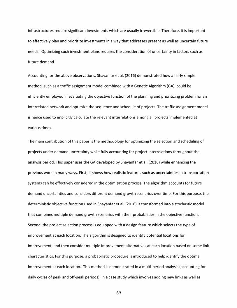
69

infrastructures require significant investments which are usually irreversible. Therefore, it is important

to effectively plan and prioritize investments in a way that addresses present as well as uncertain future

needs. Optimizing such investment plans requires the consideration of uncertainty in factors such as

future demand.

Accounting for the above observations, Shayanfar et al. (2016) demonstrated how a fairly simple

method, such as a traffic assignment model combined with a Genetic Algorithm (GA), could be

efficiently employed in evaluating the objective function of the planning and prioritizing problem for an

interrelated network and optimize the sequence and schedule of projects. The traffic assignment model

is hence used to implicitly calculate the relevant interrelations among all projects implemented at

various times.

The main contribution of this paper is the methodology for optimizing the selection and scheduling of

projects under demand uncertainty while fully accounting for project interrelations throughout the

analysis period. This paper uses the GA developed by Shayanfar et al. (2016) while enhancing the

previous work in many ways. First, it shows how realistic features such as uncertainties in transportation

systems can be effectively considered in the optimization process. The algorithm accounts for future

demand uncertainties and considers different demand growth scenarios over time. For this purpose, the

deterministic objective function used in Shayanfar et al. (2016) is transformed into a stochastic model

that combines multiple demand growth scenarios with their probabilities in the objective function.

Second, the project selection process is equipped with a design feature which selects the type of

improvement at each location. The algorithm is designed to identify potential locations for

improvement, and then consider multiple improvement alternatives at each location based on some link

characteristics. For this purpose, a probabilistic procedure is introduced to help identify the optimal

improvement at each location. This method is demonstrated in a multi-period analysis (accounting for

daily cycles of peak and off-peak periods), in a case study which involves adding new links as well as

70

expanding the capacities of existing links in a network. Third, the model is further developed to account

for vehicle operation and safety costs. For this purpose, appropriate models are incorporated and added

to the objective function to estimate the cost of fuel, tire, maintenance and repair and the cost of

crashes in the system. Finally, since in meta-heuristics, such as GA, global optimal solution is not

guaranteed, a statistical test is employed to test the optimality of the GA solution by estimating the

probability of arriving at a better solution. In effect, it is shown that the probability of finding a better

solution is negligible, thus demonstrating the soundness of the GA solution.

2 Literature Review

One of the early studies dealing with project interdependencies belongs to Nemhauser and Ullman

(1969). They proposed the following quadratic objective function:

𝑓(𝑥1, 𝑥2, … , 𝑥𝑛) = ∑𝑏𝑖𝑥𝑖

𝑛

𝑖=1

+∑ ∑ 𝑑𝑖𝑗𝑥𝑖𝑥𝑗

𝑛

𝑗=𝑖+1

𝑛−1

𝑖=1

(1)

In this formulation 𝑑𝑖𝑗 represents the interaction coefficient between projects i and j, having a positive

value when projects are complementary and a negative value when they are competing. This is a binary,

non-linear and non-separable knapsack problem which incorporates project interrelations. In the

literature, a collection of all 𝑑𝑖𝑗s (dependencies among pairs of projects) is called “dependence matrix”.

Compared to the linear objective function, the quadratic objective function and the dependence matrix

enhance the flexibility of the project selection problem by incorporating project interrelations. This

method which has numerus applications in recent literature such as Cruz et al., 2014, Rebiasz et al.,

2014, and Li et al., 2016 has considerable shortfalls. First, the pairwise dependencies (𝑑𝑖𝑗) do not fully

71

represent the complex interrelations and miss some relations among alternatives since the actual

interrelations may extend beyond two-way interactions to third, fourth and even higher degrees.

Second, the interrelations may be difficult to quantify even for pairwise interactions (i.e. estimate 𝑑𝑖𝑗

parameter for all pairs of projects), and the number of interactions requiring estimation explodes if we

go beyond pairwise relations. Third, the interrelation coefficients (𝑑𝑖𝑗) do not stay constant over time as

traffic flows change, especially after network modifications projects are implemented. Thus, such

methods ignore the timing aspect of project implementation and do not optimize the schedule of

projects. The benefits associated with particular projects may be highly related to the times when they

are implemented. Therefore, evaluating projects without considering their timing may yield misleading

results.

Instead, complete system models which can model all possible interactions among projects at various

network development stages, are more desirable. Some examples include equilibrium traffic assignment

(Shayanfar et al., 2016), simulation (Wang and Schonfeld, 2008), and artificial neural networks.

However, the objective function for problems such as prioritizing interrelated projects using complete

system models becomes non-convex and has a “noisy” surface (i.e. containing multiple local optima).

Therefore, mathematical programming such as gradient-based search, integer programming and

dynamic programming are incapable of solving such problems. As a result, heuristics and meta-

heuristics, especially population-based methods such as GA, have become more popular for solving

problems without analytical objective functions. These methods can quite easily and efficiently

distribute the evaluation of population members and probabilistic replications among multiple

processors to improve the speed of the optimization process, as in Yang et al (2015). Also, objectives

evaluated from computer simulations, which are mostly analytically intractable (i.e., discontinuous and

non-differentiable) (Koziel et al. 2011), can be easily inserted into the heuristic optimization loop.

72

In general, project prioritization is an important problem in transportation policy as projects require

significant investments which are usually irreversible. Therefore, many studies in recent literature address

the problem of project prioritization under uncertainty. Szeto and Lo (2005) addressed the problem of

planning road network projects under uncertainty through sensitivity analysis. Although sensitivity

analysis is a simple method to identify the variables which affect the output of the model, it fails to

consider the interrelation between underlying variables. A stochastic optimization formulation which

explicitly considers the uncertainty of variables based on probability distributions is a more effective way

to deal with uncertainty in the planning problem. Jian and Szeto (2015) proposed a network design

framework that considers health impacts. They used a Frank-Wolfe algorithm to evaluate the land-use

transportation problem, and a bee colony algorithm to optimize the network design. Huang et al. (2018)

use the artificial bee colony algorithm in a bi-level program to solve the network design in a multi-modal

transit system. Kumar and Mishra (2018) propose a bi-level model to select capacity improvement

projects and an optimization framework to determine the optimal sequence of projects in a network.

This paper addresses the problem of project prioritization but, in addition to project rank, it considers the

timing of project implementation and demand uncertainties, while focusing on the treatment of

interrelations among projects in a network setting.

3 Methodology

3.1 Problem Formulation

The analysis in this paper focuses on the cost of travel time, vehicle operating, and safety costs.

Therefore, the objective function is formulated to reflect the present value of total cost over planning

horizon T. In this problem, the decision variable is defined as the completion time of each project. Let

𝑥𝑖(𝑡) be a binary variable that shows if project i is finished by time t:

73

{𝑥𝑖(𝑡) = 0 𝑖𝑓 𝑡 < 𝑡𝑖

𝑥𝑖(𝑡) = 1 𝑖𝑓 𝑡 > 𝑡𝑖

The problem is then formulated as:

𝑚𝑖𝑛 𝑍 = ∑{

1

(1 + 𝑟)𝑗(∑𝑤𝑖𝑗 ∗ 𝑣𝑡

𝑛𝑙

𝑖=1

+∑{𝐶𝑣𝑜𝑝(𝑖𝑗)

𝑛𝑙

𝑖=1

∗ 𝑉𝑀𝑇𝑖𝑗} +∑{

𝑛𝑙

𝑖=1

𝑁𝑐𝑟(𝑖𝑗) ∗ 𝐶𝐶𝑟}}𝑇

𝑗=1

+∑𝑐𝑖𝑥𝑖(𝑡)

(1 + 𝑟)𝑡

𝑛𝑝

𝑖=1

(2)

𝑤𝑖𝑗 = travel time over link i in year j

𝑣𝑡 = value of time ($/hr)

𝑛𝑙 = total number of links

𝑉𝑀𝑇𝑖𝑗= vehicle kilometers traveled over link i in year j

𝐶𝑣𝑜𝑝(𝑖𝑗)= vehicle operating cost over link i in year j ($/veh.km)

𝑐𝑖 = cost of project i

𝑁𝑐𝑟(𝑗)= predicted number of crashes over link i in year j

𝐶𝑐𝑟= crash cost for one predicted crash

𝑛𝑝= number of projects

r= interest rate

74

t= completion time point

The above formulation minimizes the sum of total user and supplier cost subject to a budget flow

constraint, over a specified planning horizon. In this setting, the user cost consists of the total travel

time for users in the system multiplied by their value of time, vehicle operating cost, and number of

crashes multiplied by the cost of each crash. Note that project interrelations are not explicitly included

in the objective function. As mentioned previously, the proposed method considers not only pairwise or

slightly higher degrees of interrelation among alternatives, but all possible interactions among all

alternatives throughout an entire network and throughout the multi-year analysis period. The complete

interrelations are captured by applying a full network model for a set of improvement projects, with

each project implemented at a different optimized time. The interrelations, which cannot be explicitly

expressed in the objective function, are essentially captured among all network elements at one period

and among alternatives across multiple periods. This is done by applying a complete network model

such as traffic assignment before and after each project implementation. This is done by applying a

complete network model such as traffic assignment before and after each project implementation.

Recent improvements to this method (such as in dealing with demand uncertainties, multiple

improvements per location and inclusion of vehicle operating and safety costs) are demonstrated in this

paper with a fairly simple and fast network evaluation model, namely the well-known Frank-Wolfe

(1956) traffic assignment model. However, this approach for optimizing the prioritizing and scheduling

of interrelated projects is also applicable with more detailed network analysis models. For example, it

has been combined with microscopic simulation models (Wang and Schonfeld, 2005) and the cell

transmission model (Shayanfar, 2017).

Let 𝑡𝑖 be the time at which project i is completed, and T be the planning horizon (20 years). Then, the set

of 𝑡𝑖s will decide the final project sequence and schedule (Jong and Schonfeld, 2001). Jong and

Schonfeld (2001) apply a budget constraint which at any time t (0 ≤ t ≤ 𝑇), limits project expenditures

75

by the cumulative budget which is funded from “external” sources. In addition to their constraint, this

paper considers an “internal” budget source for funding future projects. Within the analysis period, the

“internal” fuel taxes collected from users in previous periods are added to an external budget to

determine the available funding for future projects. Other revenues collected from users can also easily

be added to the internal budget formulation. The external budget is assumed to “flow” uniformly over

time in this analysis, but non-uniform budget flows can also be easily specified. The following equation

specifies how the internal budget is calculated:

𝑏(𝑡𝑖)𝑖𝑛𝑡𝑒𝑟𝑛𝑎𝑙 = 𝑉𝑀𝑇(𝑡𝑖−1) ∗ 𝑓𝑟 ∗ 𝑓𝑐 ∗ 𝑓𝑡 (3)

In the above formulation 𝑓𝑟, 𝑓𝑐, 𝑓𝑡 represent fuel consumption rate (gal/vehicle*kilometer), fuel cost

($/gal), and gas tax rate respectively. This formulation suggests that the fuel taxes collected from period

𝑡𝑖−1 contribute to the available funding in period 𝑡𝑖. Specifically, 𝑉𝑀𝑇(𝑡𝑖−1) presents the vehicle

kilometers travelled during the period in which project 𝑖 − 1 is completed.

Assuming that 𝑛𝑝 is the number of candidate projects, for 0 ≤ 𝑡 ≤ 𝑇 the budget flow constraint is thus

formulated as:

∑𝑐𝑖𝑥𝑖(𝑡) ≤ ∫ (𝑏(𝑡)𝑒𝑥𝑡𝑒𝑟𝑛𝑎𝑙 + 𝑏(𝑡)𝑖𝑛𝑡𝑒𝑟𝑛𝑎𝑙) 𝑑𝑡 𝑡

0

𝑛𝑝

𝑖=1

(4)

The left-hand side of the above formulation displays the total cost expended by time t, which should not

exceed the cumulative budget available at that time. It is assumed here that projects should be funded

sequentially rather than concurrently, with each successive project completed as soon as the cumulative

76

budget permits, so the cost savings from each completed project should start flowing as soon as

possible. This, in turn, assumes that the cumulative budget constraint is binding, i.e. insufficient for all

the available projects whose benefits exceed their costs. This situation generally prevails for

transportation projects throughout the world.

Notably, since the cumulative budget constraint is expected to be binding, the optimal completion time

for all projects is uniquely determined for all projects in a given sequence. Thus, the optimized schedule

(in continuous time rather than discrete time periods) is uniquely determined by the optimized

sequence in conjunction with the cumulative budget. For any sequence, projects which are not funded

within the specified analysis period (e.g. 20 years in this paper’s numerical example), are effectively

rejected. Construction periods that exceed the budget accumulation period of the respective project,

and hence overlap with construction periods for other projects, can be considered without changing this

formulation by assuming virtual borrowing. However, some modifications to the above formulation

would be needed if resources other than budgets (e.g. construction equipment) were critical or if

additional budget constraints (e.g. by region or type of projects) were applicable.

As mentioned before, the objective function is not always convex and differentiable, which renders

gradient-based research methods, integer and linear programming ineffective. On the other hand, as

the number of alternatives grows, mathematical optimization models may no longer be feasible. As a

result, heuristic methods are now more common for solving such problems. A GA is very useful for

effectively optimizing the objective function over large solution spaces with unsmooth objective

functions. The GA is employed to solve the optimization model jointly with a network flow model which

is used to evaluate the objective function. More specifically, the GA optimizes the selection, sequence

and schedule of projects while the traffic assignment model estimates variables such as travel time,

speed and volume for evaluating the benefits and costs of projects. Figure 5 displays the general

framework proposed for selecting, sequencing and scheduling interrelated road projects. Detailed

77

explanation on the GA algorithm is provided later in section 5 and an illustrative example is provided in

section 6.

3.2 Safety Cost Model

According to Highway Safety Manual (HSM, 2010), crash prediction models for two-lane and multi-lane

roadway segments should include two analytical components: (i) safety performance functions (SPFs)

also called baseline models, and (ii) crash modification factors (CMFs). There are also calibration factors

that adjust the predictions to a specific geographical area. Here, we present two separate safety

performance functions for two-lane and multi-lane roadway segments. The general crash prediction

model for roadway segments is shown in Equation 5. Equations 6 and 7 present the safety performance

functions for two-lane and multi-lane roadway segments.

𝑁𝑐𝑟 = 𝐶𝑟 ∗ 𝑁𝑐𝑟−𝑠𝑝𝑓 ∗ (𝐶𝑀𝐹1 ∗ …∗ 𝐶𝑀𝐹12) (5)

𝑁𝑐𝑟2−𝑠𝑝𝑓 = AADT ∗ L ∗ 365 ∗ 10−6 ∗ 𝑒−0.312 (6)

𝑁𝑐𝑟𝑚−𝑠𝑝𝑓 = exp [−9.653 + 1.176 ∗ ln(𝐴𝐴𝐷𝑇) + ln(𝐿)] (7)

where:

𝑁𝑐𝑟= predicted number of crashes for a roadway segment per year

𝑁𝑐𝑟2−𝑠𝑝𝑓= nominal or baseline predicted number of crashes per year for two-lane roadways

𝑁𝑐𝑟𝑚−𝑠𝑝𝑓= nominal or baseline predicted number of crashes per year for multi-lane roadways

𝐶𝑟 = calibration factor for roadway segments in a particular geographical area.

𝐶𝑀𝐹𝑛 = crash modification factor.

78

AADT = average annual daily traffic (veh/day) on roadway segment;

L = length of roadway segment (mi).

In this study, the only changing condition among improvement types is lane width. Therefore, the

algorithm estimates CMF1 for lane width from the following equation:

𝐶𝑀𝐹1 = (𝐶𝑀𝐹𝑟𝑎 − 1) ∗ 𝑃𝑟𝑎 + 1 (8)

where:

𝐶𝑀𝐹1 = crash modification factor of lane width on total crashes.

𝐶𝑀𝐹𝑟𝑎 = crash modification factor for related crashes (run-off-the-road, head-on, and sideswipe)

calculated from Table 1.

𝑃𝑟𝑎 = proportion of total crashes to related crashes (with 0.574 as the default value).

From Table 7-4 HSM (2010) (Societal Crash Costs by Severity) and Table 10-3 HSM (2010) (Default

Distribution for Crash Severity Level), it is assumed that 32.1% of total crashes are “fatal and injury” (FI)

and 67.9% are “property damage only” (PDO). Therefore, cost for one predicted crash (𝐶𝑜𝑠𝑡𝐶𝑟) would be

calculated as: 0.321*172,438 ($/FI crash) + 0.679*8,066 ($/PDO crash) = $60,830 / Crash. All costs are

adjusted to 2015 dollars using an inflation factor from the latest Consumer Price Index (CPI) provided by

the Bureau of Labor Statistics.

79

3.3 Vehicle Operating Cost Model

The cost of operating a vehicle on a given section is a function of costs for fuel, tires, and

maintenance and repair. These costs are estimated as functions of average speed. Fuel

consumption rate, tire wear rate, and maintenance and repair rate are formulated, respectively, in

Equations 9 to 11 (HERS-ST technical report, 2005):

𝑅𝑓𝑐 = 88.556 − 5.414 ∗ 𝑆̅ + 1.7375 ∗ G + 0.136 ∗ 𝑆̅

2 + 0.18052 ∗

𝐺2 + 0.122166 ∗ 𝑆̅ ∗ G

(9)

𝑅𝑡𝑤 = 0.229 + 10.85 ∗ 10

−6 ∗ 𝑆̅3 − 0.0403 ∗ ln(1.6 ∗ 𝑆̅) + 0.122166 ∗ 𝑆̅ ∗ G

(10)

𝑅𝑚𝑟 = 48.4 + 0.02219 ∗ 𝑆̅2 + 0.0932 ∗ 𝑆̅ ∗ G (11)

where

𝑅𝑓𝑐 = fuel consumption rate (gallons/1000 kilometer)

𝑅𝑡𝑤 = tire wear rate (% worn/1000 kilometer)

𝑅𝑚𝑟 = maintenance and repair rate (% avg. cost/1000 kilometer)

𝑆̅ = average speed (kilometer /hour)

G = grade (%)

The operating cost per vehicle- kilometer (𝐶𝑣𝑜𝑝) is estimated as the sum of the above cost

components representing costs for fuel, tires, and maintenance and repair. The overall equation

for combining these components is:

80

𝐶𝑣𝑜𝑝 = (𝑅𝑓𝑐 × 𝐶𝑓 + 0.01 × 𝑅𝑡𝑤 × 𝐶𝑡 + 0.01 × 𝑅𝑚𝑟 × 𝐶𝑚𝑟) ∗ 0.001 (12)

where

𝐶𝑣𝑜𝑝= operating cost ($/veh.km)

𝐶𝑓 = unit cost of fuel ($/gallon)

𝐶𝑡 = unit cost of tire ($/tire)

𝐶𝑚𝑟= unit cost of maintenance and repair

𝐶𝑓, 𝐶𝑡, 𝐶𝑚𝑟 are, respectively, 2.1 ($/gallon), 105.8 ($/tire) and 151.1 ($/1000 mi). Prices are adjusted to

2015 dollars with the latest Consumer Price Index (CPI) given by the U.S. Bureau of Labor Statistics.

3.4 Design of Improvement Alternatives

The algorithm presented in this paper has the capability to consider multiple improvements over time at

the same location. These improvements include widening existing narrow lanes (from 3m to 3.6m),

adding one or multiple narrow lanes (3m wide) and adding one or multiple wide lanes (3.6m wide). The

alternatives considered for each link depend on the existing link characteristics, and are symmetric, i.e.

the same for both directions of a link. According to the Highway Capacity Manual (HCM, 2010), lane

widths under 3.6m reduce travel speed, and thus also reduce operational capacity. In this case, it is

assumed that the narrow and wide lanes are, respectively, 3m and 3.6m wide. According to HCM (2010),

widening lanes from 3m to 3.6m would increase the capacity by 15%. The following list shows the set of

improvement alternatives at each location:

81

A. If the existing link has narrow lanes:

1. Widen the existing lanes.

2. Add one narrow lane.

3. Widen existing lanes and add one wide lane.

B. If the existing link has wide lanes:

1. Add enough width for two narrow lanes. (In this case n wide lanes are transformed to n+1

narrow lanes.)

2. Add one wide lane.

C. If the there are no existing lanes (new development):

1. Add one narrow lane.

2. Add one wide lane.

3. Add two wide lanes.

4. Add three wide lanes. (This option considers the possibility of a major capacity addition

in the network)

For each case A, B and C the potential improvements are listed in increasing order of project costs. In this

case the algorithm first evaluates the characteristics of each location in terms of existing narrow/wide

lanes, and whether new lanes can be added. (In some locations new lanes cannot be added due to land

availability constraints.) Then, based on the current condition, the above set of improvements are

considered at each location. There are two problems to be resolved here. First, which links (locations)

should be selected for improvement and in what sequence and when should those links be improved?

Second, at each location, which improvement type should be selected and implemented? The first

problem is solvable by using the combination of the GA and the traffic assignment model. This method

will be explained further in section 5.

82

One way to address the second problem is to compute the benefit-cost ratio of each alternative and select

the best one at each location. This myopic search is quite prevalent in current practices. However, it

disregards the interrelation among projects. A simple benefit-cost ratio in this case cannot capture the

impact of selected projects on future project implementations. In other words, due to interrelations among

network links, the alternative with lower benefit-cost ratio may be more beneficial if considered in the

long run (over the entire analysis period) and in conjunction with other alternatives (e.g. in a series of

links that remove all bottlenecks rather than just shifting them). Therefore, it seems preferable to consider

all possible improvements at each location over the entire analysis period and allow the algorithm to

evaluate them over the planning horizon. This means that the GA will both optimize the selection and

sequence of projects among links in the network as well as optimize the selection of improvement types at

each location, all within one optimization process. This will result in more search steps and increased

computation time. To tackle this issue and guide the search process, we assign selection probabilities to

each alternative based on project costs which means that under each case the less costly alternatives have

a higher probability of being selected. This is reasonable since in practice it is more desirable to start with

less costly improvements, and later move to more expensive ones. Therefore, the selection probability of

improvements at each location is inversely proportional to their relative costs. If M improvements are

considered at one location, the probability of selecting each improvement Pr(m) is:

Pr(𝑚) =

1𝐶𝑜𝑠𝑡(𝑚)⁄

∑ (1 𝐶𝑜𝑠𝑡(𝑖)⁄ )𝑀𝑖=1

(13)

3.5 Stochastic Model

In long-term planning, decision makers are usually faced with the problem of uncertain information.

One of the most significant sources of uncertainties in transportation systems is future demand,

particularly for newly launched projects. This problem requires the network analysis to be robust to

83

changes in future demand. Thus, demand uncertainties should be explicitly considered when selecting

and scheduling projects. In this study, the demand is assumed to grow exponentially over time given the

following equation:

𝑑𝑖𝑗𝑡 = 𝑑𝑖𝑗

0 ∗ (1 + 𝑔)𝑡 (14)

where 𝑑𝑖𝑗𝑡 is the demand from origin 𝑖 to destination 𝑗, 𝑑𝑖𝑗

0 is the base-year demand for the 𝑖𝑗

origin and destination (O/D) pair, and 𝑔 is the growth rate per year. If we consider S plausible demand

scenarios (different values for the growth rate 𝑔) then the stochastic formulation can be re-written as:

𝑚𝑖𝑛𝑍 = ∑𝑃𝑠

{

∑{

1

(1 + 𝑟)𝑗(∑𝑤𝑖𝑗𝑠 ∗ 𝑣𝑡

𝑛𝑙

𝑖=1

+∑{𝐶𝑣𝑜𝑝𝑠(𝑖𝑗)

𝑛𝑙

𝑖=1

∗ 𝑉𝑀𝑇𝑖𝑗𝑠} +∑{

𝑛𝑙

𝑖=1

𝑁𝑐𝑟𝑠(𝑖𝑗) ∗ 𝐶𝐶𝑟}}

𝑇

𝑗=1

+∑𝑐𝑖𝑥𝑖(𝑡)

(1 + 𝑟)𝑡

𝑛𝑝

𝑖=1 }

𝑆

𝑠=1

(15)

In the above formulation S represents the set of scenarios, 𝑃𝑠 denotes the probability of each scenario s,

and the other parameters are the same as specified for Equation 2. Here, we consider three plausible

demand scenarios: (i) low demand growth, (ii) med (medium) demand growth, and (iii) high demand

growth. Under the three demand growth scenarios we assume the growth rate per year to be: 𝑔 =

0.005, 0.01, 0.02 for the low, med and high scenarios, respectively. The above formulation can be

adapted to consider more scenarios regarding demand uncertainties, as demonstrated in Sun and

Schonfeld (2015). While this study considers one source of uncertainty, future extensions of this model

84

may consider multiple uncertainties as it can reduce the probability of increasing the overall uncertainty

in the analysis.

4 Evaluation Model

Basic traffic assignment models are suitable methods for estimating the traffic-related attributes of

unsaturated networks with steady flows. These attributes consist of link travel time, flow, speed and

volume-capacity ratio. This information is useful for estimating the cost savings due to capacity

improvements and therefore supports an appropriate evaluation method for selection, sequencing and

scheduling of projects. Cost savings mainly pertain to the travel time reduction for users and can be

obtained by running the traffic assignment model at various times during the multi-year analysis period

to compute speeds, travel times, and vehicle miles travelled (VMT). Hence, the objective function (eq.15)

can be computed. The Frank-Wolfe algorithm (Frank and Wolfe 1956), a user equilibrium traffic

assignment method, is used here not just for traffic assignment but also to evaluate improvement projects

before and after their implementation in the network. This algorithm is explained in detail in Shayanfar et

al. (2016). Frank-Wolfe is a relatively simple and fast algorithm which is suitable for testing metaheuristics

such as GA. However, more advanced traffic assignment models and more detailed evaluation models

such as a micro-simulation, artificial neural network, or cell transmission model (CTM) may be more

desired and can replace the Frank-Wolfe algorithm.

5 Optimization Model

This study employs a Genetic Algorithm (GA) developed by Shayanfar et al. (2016) to optimize the

sequence and schedule of improvement alternatives. The GA is selected for this paper based on the

results from Shayanfar et al. (2016) which suggested that, compared to other two heuristic algorithms

(Simulated Annealing and Tabu Search), the GA yields a better (lower total cost) and more consistent

85

solution. Better consistency is indicated when multiple replications of the genetic search yield almost

similar final solutions after enough iterations. In general, population-based meta-heuristics such as GA,

are particularly suitable for solving large problems without analytical objective functions because they

can be easily and efficiently distributed among multiple processors. Also, objectives evaluated from

computer simulations, which are usually analytically intractable (i.e., discontinuous and non-

differentiable) (Koziel et al. 2011), can easily be embedded into the heuristic optimization loop.

Figure 2 illustrates the optimization process. Each population is comprised of I sequences, and each

sequence i is a string of J numbers which represents the location of the candidate project. As stated

earlier, at any specific location, several improvement projects or expansion alternatives with specified

capacities are considered. To incorporate project multiplicity, the chromosomes (sequences) should be

refined to represent specific alternatives at each location. Figure 3 shows an example of one sequence

with specific project locations. The shaded cells are locations where multiple alternatives may be

considered e.g. location 3 has three candidate alternatives (3-1, 3-2, 3-3). At each location the algorithm

selects a specific alternative based on the probabilistic approach specified in section 6 (Equation 13).

After identifying specific alternatives at each location, the algorithm begins to evaluate all sequences in

the current population. In Figure 2, for each sequence i, the algorithm selects projects 1 to j one-by-one,

schedules them as soon as the cumulative budget can fund those projects and runs the traffic

assignment after each project is implemented. In this sense, each project implementation requires a

specific change in the network e.g. widening lanes, adding one or two lanes to existing links, or adding

new links. At each step, the traffic assignment yields the travel time, VMT, speed, and number of

crashes which are inserted in the objective function to calculate the “fitness value”. Next, the budget

constraint, uniquely decides the 𝑡𝑗 (completion time) of project j. That is, project j is completed as soon

as the available budget equalizes the cost of project. This process is performed for all projects in the

sequence until the completion time exceeds the planning horizon T. Then the algorithm moves to the

86

next sequence until all sequences in the population are evaluated. At this step, the best sequences i.e.

the ones with lowest fitness values, are given higher probabilities to be selected as parents and produce

offspring. Through several crossover and mutation operators which are extensively described in

Shayanfar et al. (2016), the selected parents produce the next generation. The algorithm begins to

evaluate the new generation and continues to do so until the termination criterion is met. In this case,

the algorithm stops if the optimal sequence does not change after 40 generations.

6 Numerical Example

In this paper, the Sioux Falls network originally introduced by LeBlanc et al. (1975), is selected as a case

study for the proposed model. Note that this is just a test network and the heuristic method in this

paper was previously tested on a much larger network (Anaheim network with 416 nodes and 914 links)

in Shayanfar and Schonfeld (2017). The Sioux Falls network inputs (Shayanfar and Schonfeld, 2015)

contain trip table, link capacity, length, number of lanes and free flow travel times. Figure 4 presents the

example Sioux Falls network used as a case study. The dashed lines indicate potential locations for new

developments which have three potential alternatives as described in section 3.4 (case C). The links

surrounded by dashed circles indicate cases A and B from section 3.4 with multiple alternatives at each

location while the other links only have one potential improvement.

In this example, the narrow and wide lanes have a capacity of 1000 and 1150 vehicles/hour, respectively

(HCM, 2010), and the equivalent annual cost of constructing roads is assumed to be 247,500 $/km per

foot of road width (Zhang et al., 2013). Therefore, the cost of widening a lane, adding one narrow lane,

and one wide lane are 495,000 ($/km), 2,475,000 ($/km) and 2,970,000 ($/km), respectively. Table 2

provides a list of potential improvements for all links.

87

In order to incorporate demand uncertainty, we consider three plausible demand scenarios: (i) low

demand growth, (ii) med (medium) demand growth, and (iii) high demand growth. Under the three

demand growth scenarios we assume the following growth rate per year: 𝑔 = 0.005, 0.01, 0.02 for the

low, med and high scenarios, respectively (in Equation 15: S = {low, med, high}).

The first step is to find links with the highest volume-capacity ratios to identify the first list of candidate

projects. This is done by applying the traffic assignment model with the given O/D demand matrix which

is symmetric for all O/D pairs. It is assumed that the improvement projects, whether expanded or newly

added links, are implemented in both directions between two nodes. In this problem, the potential new

links (shown by dashed lines in Figure 4) are existing links in the original network which are treated as

potential new links in this study. Initially, the algorithm considers zero capacity for these links and later

examines whether and when they should be added to the network. A multi-period analysis is

incorporated in this model to account for cyclical demand fluctuations during each day. While only peak

and off-peak periods are presently considered, the number of periods per day can be easily increased.

After determining the initial set of candidates, the algorithm considers multiple improvement projects at

each location based on Table 2. Then, a benefit-cost analysis is applied to all projects to identify the

economically beneficial projects and order them based on their benefit-cost ratio. Thus, we can obtain

two initial solutions, one based on volume-capacity ratio (bottleneck order solution) and the other

based on benefit-cost ratio (greedy-order solution). These two set of initial solutions are later used as

part of the initial population in the GA.

The analysis begins by running the traffic assignment model to assess the travel times and traffic

volumes before and after improvement projects. Then the GA is used to find the near-optimal solution

for selecting and scheduling projects. At this stage, the algorithm selects one improvement from a set of

multiple improvement alternatives at each location following the procedure explained in section 6 and

88

the probabilistic Equation 13. Ultimately, the GA yields the optimized project selection at each location,

the order of their implementation, and the schedule of completing each one. In this study, we assume a

20-year planning horizon. That is, projects with scheduled completion time after the planning horizon

are eliminated from the sequence. Table 3 presents the results from the stochastic model which yields

the optimal selection of projects, their order and implementation schedule. The results also indicate the

optimal improvement type for each link which is obtained from the GA search.

Table 4 provides detailed costs yielded by the genetic search, bottleneck-order, and greedy-order

solutions. These results are shown in terms of the Present Value (PV) of total costs that include user

travel time, vehicle operating, crash, and total cost. The results indicate lower costs for the GA solution

(i.e. 9.03% less than the bottleneck-order and 8.06% less than the greedy-order solution). This

demonstrates that the greedy-order and bottle-neck order are far from the optimal sequence of

projects when project interrelations are considered.

Figure 9 displays the accumulated cost over time in terms of travel time, vehicle operating and safety

costs. Most of the user cost pertains to travel time, with much lower amounts for vehicle operation and

safety costs.

Figure 10 illustrates the evolution of the GA process. It indicates how the objective function converges

to the optimized value. The optimization process is completed after the genetic search has stopped

improving for 40 generations. It is observed that approximately between generations 60 to 100 the

result does not change which is why the algorithm stops at the 100th generation.

Figure 11 presents the computation time for different numbers of projects. These numbers

indicate how the computation time grows as the number of projects increases. As the number of

projects grows, the number of cells in each chromosome, and the number of chromosomes in each

population increase. Also, the number of generations needed to reach convergence increases simply

89

because more combinations of projects must be evaluated. Hence the computation time increases

considerably as the number of projects grows.

A simpler and easier alternative to the stochastic program is to insert the average demand scenario into

the deterministic formulation, which is less complicated and can thus be solved in less time. Figure 12

displays the average demand growth compared to the three scenarios. We can see that the average

demand is close to the medium growth rate and roughly between the low and high growth rate

scenarios. Using the average demand growth rate, we can solve a deterministic version of the selection

and sequencing problem whose objective is defined in Equation 15. However, with this approach the

results are subject to the flaw of averages (Savage and Markowitz, 2009), and hence less reliable, as

shown in De Neufville and Scholtes (2011).

To compare the deterministic with the stochastic formulation, the model is applied using the average

demand growth rate with the deterministic formulation (Equation 2). Figure 13 shows the PV of total

cost in the average scenario compared to other demand scenarios. We can see that the total cost in the

average scenario is close to the medium and low scenarios, and quite distant from the high scenario. In

other words, if decisions are made only based on the average scenario, the results will underestimate

the high cost of the high demand scenario. In fact, the results indicate that the total cost under the

average demand growth scenario (solving the deterministic program) is 7.5% above that using the

proposed stochastic program. This shows that solving the stochastic model yields a better solution with

a lower objective function i.e. yields a solution with a lower cost. Furthermore, the difference between

the objective function value (PV of total cost) of the deterministic and stochastic program, which is

called the Value of Stochastic Solution (VSS), is $669 million. This value shows the advantage of using the

stochastic model rather than using the expected value and solving the deterministic model. Failure to

consider the full probability distribution instead of the average scenario is also called the “flaw of

averages” (Savage and Markowitz, 2009).

90

7 Algorithm Testing

One major limitation of meta-heuristics is that global optimality is almost never guaranteed, and it is

challenging to assess whether evolutionary methods yield the global optimal solution. To evaluate the

accuracy of the genetic search, (Shayanfar and Schonfeld, 2017) conducted an exhaustive enumeration

and compared the GA results with enumeration results. The results indicated that the GA found the

same exact solution obtained through complete enumeration. For large problems where complete a

enumeration test would require excessive computation time, the quality of meta-heuristic results can be

verified with a statistical test (Jon and Schonfeld, 2003) which estimates the probability that better

solutions exist.

For this test, a random sample consisting of 100,000 solutions is created. After testing different

distribution functions, the Lognormal (mu=22.997, sigma= 0.0238) distribution is found to best fit the

sample. From Figure 10, it is evident that the GA solution (8917 ×106 from Table 3) is located at the far-

left tail of the diagram meaning that the GA solution has a lower objective function than the entire

sample. This means that the solution obtained by the genetic search has a lower cost than any of the

100,000 random solutions in the distribution. Accordingly, the cumulative probability of the optimized

solution (8917 ×106 from Table 3) can be calculated based on the fitted distribution: 𝑝 = 𝐹(𝑥| μ, σ) =

𝐹(8917 × 106|22.997, 0.0238) = 1.568 × 10−4 .

This result indicates that the probability of finding a solution better than the GA solution is extremely

small, i.e. 2.834 × 10−5 . In other words, the GA solution is better than 99.999% of the random

solutions in the fitted distribution (as well as 100% of the actual randomly generated sample).

Therefore, the GA optimized solution, is overwhelmingly better that other possible alternatives in the

solution space and the likelihood that significantly better solutions exist is negligible. Moreover, errors

91

from imperfect optimization (i.e. deviations from mathematically global optimality) are likely to be

greatly dominated by uncertainties in the input parameters.

8 Conclusions

This study proposes a general framework for selecting and scheduling interrelated alternatives while

dealing with demand uncertainties. The proposed methodology is intended to apply to any system with

interrelated alternatives as GAs can be effectively combined with an appropriate evaluation tool such as

microsimulation, simulation approximates, queuing or neural networks, to optimize the planning and

scheduling problem in a variety of applications. With a well-developed evaluation model, users can use

the proposed framework to evaluate and prioritize projects in any interrelated network.

The study introduces a stochastic program that analyzes the problem of selecting and scheduling

interrelated alternatives with consideration of uncertainties in demand forecasts and offers a significant

improvement on previous models by adding an improvement design component at each location where

multiple improvement alternatives based on current link characteristics are considered. Moreover, the

model is further developed to account for vehicle operation and safety costs.

It is observed that the genetic search yields a better solution than the naïve greedy and bottleneck

solutions when interrelations exist among alternatives. In this case, the total cost of the genetic solution

is 9.03% below the bottleneck-order and 8.06% below the greedy-order solution. Furthermore, it is

concluded that the stochastic model greatly improves upon the total cost of the deterministic solution

(which considers the average scenario rather than explicitly deal with uncertainty) due to the flaw of

averages. Specifically, the total cost of the stochastic solution is 7.5% below that for the average

scenario, and the difference between the two solutions is $669 million (VSS). Finally, although the

genetic solution is not guaranteed to be globally optimal, the statistical test demonstrates the goodness

92

of the result compared to a sample of the solution space. It is highly probable that the input errors and

uncertainties in many factors dominate errors due to imperfect GA solutions.

The work in this paper can be enhanced by replacing the Frank-Wolfe Algorithm with more advanced

traffic assignment models. In addition, for system evaluation purposes the traffic assignment algorithm

used here may be replaced with more detailed evaluation models such as micro simulations and cell

transmission models which can model queues and saturation effects in networks. Future work may also

include intersection characteristics at nodes, and effects of travel time variability. It is also worthwhile to

consider multiple uncertainties and explore other source of uncertainties such as project costs, available

budget and construction time.

Acknowledgements

The authors gratefully acknowledge funding received for this work from the U.S. Department of

Transportation through the National Transportation Center at the University of Maryland and the Urban

Mobility and Equity Center led by Morgan State University.

References

1 Crowder, H. P., E. L. Johnson, and M. W. Padberg. 1983. “Solving Large-Scale Zero-One Linear

Programming Problems.” Operations Research 31: 803–834.

2 Cruz, L., E. Fernandez, C. Gomez, G. Rivera, and F. Perez. 2014 “Many-objective Portfolio

Optimization of Interdependent Projects with ‘a priori’ Incorporation of Decision-maker

Preferences.” Applied Mathematics & Information Sciences 8(4): 1517-1531.

3 De Neufville, R., S. Scholtes. 2011. “ Flexibility in Engineering Design.” MIT Press.

93

4 Disatnik, D. J., and S. Benninga. 2007. “Shrinking the Covariance Matrix.” The Journal of Portfolio

Management 33(4): 55-63.

5 Frank, M., and P. Wolfe. 1956. “An Algorithm for Quadratic Programming.” Naval Research

Logistics Quarterly 3(1): 95-110.

6 Highway Capacity Manual. 2010. Washington, D.C., Transportation Research Board.

7 Highway Safety Manual. 2010. AASHTO, Washington, D.C.

8 HERS (Highway Economic Requirements System- State) Version. 2005. Technical report, U.S.

Department of Transportation, Federal Highway Administration.

9 Huang, D., Z. Liu, X. Fu and P.T. Blythe. 2018. “Multimodal Transit Network Design in a Hub-and-

spoke Network Framework.” Transportmetrica A: Transport Science: 1-30.

10 Jiang, Y. and W.Y. Szeto. 2015. “Time-dependent Transportation Network Design that Considers

Health Cost.” Transportmetrica A: Transport Science 11(1): 74-101.

11 Jong, J. C., and P. Schonfeld. 2001. “Genetic Algorithm for Selecting and Scheduling Interdependent

Projects.” Journal of Waterway, Port, Coastal, and Ocean Engineering 127(1): 45-52.

12 Jong, J. C. and P. Schonfeld. 2003. “An Evolutionary Model for Simultaneously Optimizing Three-

dimensional Highway Alignments.” Transportation Research Part B: Methodological 37(2): 107-

128.

13 Koziel, S., and X. S Yang. 2011. “Computational Optimization, Methods and Algorithms.” Springer

356: 33-59.

14 Kumar, A. , and S. Mishra. 2018. "A Simplified Framework for Sequencing of Transportation Projects

Considering User Costs and Benefits." Transportmetrica A: Transport Science 14(4): 346-371.

15 LeBlanc, L. J., E. K. Morlok, and W. P. Pierskalla. 1975. “An Efficient Approach to Solving the

Road Network Equilibrium Traffic Assignment Problem.” Transportation Research 9(5): 309-318.

94

16 Li, X., S. C. Fang, X. Guo, Z. Deng, and J. Qi. 2016. “An Extended Model for Project Portfolio

Selection with Project Divisibility and Interdependency” Journal of Systems Science and Systems

Engineering 25(1): 119-138.

17 Lorie, J. H., and L. J. Savage. 1955. “Three Problems in Rationing Capital.” Journal of Business: 679–

694.

18 Martello, S., and P. Toth. 1990. “Knapsack Problems: Algorithms and Computer Implementations.”

John Wiley and Sons, Chichester, England: 189–220.

19 Michalewicz, Z. 1995. “Genetic algorithms + data Structure = evolution programs.” Springer.

20 Nemhauser, G. L., and Z. Ullman. 1969. “Discrete Dynamic Programming and Capital Allocation.”

Management Science 15(9): 494–505.

21 Rebiasz, B., B. Gaweł, and I. Skalna. 2014. “Capital budgeting of interdependent projects with

fuzziness and randomness.” Information Systems Architecture and Technology: 125-135.

22 Savage, S. L., and H. M. Markowitz. 2009. “The Flaw of Averages: Why We Underestimate Risk in the

Face of Uncertainty.” John Wiley & Sons.

23 Shayanfar, E. and P. Schonfeld. 2015. Characteristics of the Sioux Falls Test Network, TSC Report

2015-04, University of Maryland, College Park.

24 Shayanfar, E., and P. Schonfeld. 2017. “Selecting and Scheduling Interrelated Projects: Application

in Urban Road Network Investment.” The International Journal of Logistics Systems and

Management 29(4): 436–454.

25 Shayanfar, E., A. S. Abianeh, P. Schonfeld, and L. Zhang. 2016. “Prioritizing Interrelated Road

Projects Using Meta-Heuristics.” Journal of Infrastructure Systems 22(2), 04016004.

26 Sun, Y. and P. Schonfeld. 2015. “Stochastic Capacity Expansion Models for Airport Facilities.”

Transportation Research Part B 80: 1-18.

27 Szeto, W. Y., and H. K. Lo. 2005. "Strategies for Road Network Design Over Time: Robustness

Under Uncertainty." Transportmetrica 1(1): 47-63.

95

28 Wang, S. L., and P. Schonfeld. 2008. “Scheduling of Waterway Projects with Complex

Interrelations.” Transportation Research Record: Journal of the Transportation Research Board

2062: 59-65.

29 Wang, S. L., and P. Schonfeld. 2005. “Scheduling Interdependent Waterway Projects through

Simulation and Genetic Optimization.” Journal of Waterway, Port, Coastal, and Ocean Engineering

131(3): 89-97.

30 Yang, N., S. Wang, and P. Schonfeld. 2015. “Simulation-Based Scheduling of Waterway Projects

using a Parallel Genetic Algorithm.” Transportation Systems and Engineering: Concepts,

Methodologies, Tools, and Applications: 334-347.

31 Zhang, L., M. Ji, and N. Ferrari. 2013. “Comprehensive Highway Corridor Planning with Sustainability

Indicators.” Final Report for Project MD-13-SP109B4Q, Maryland State Highway Administration.

96

Table 1 Values of CMF1 for Lane Width on Roadway Segments (HSM, Table 10-8)

Lane width(ft) ADT<400 (veh/day) ADT =400 to 2000 (veh/day) ADT>2000

(veh/day)

9 1.05 1.05+0.000281*(ADT-400) 1.50

10 1.02 1.02+0.000175*(ADT-400) 1.30

11 1.01 1.01+0.000025*(ADT-400) 1.05

12 1.00 1.00 1.00

97

Table 2 Improvement Alternatives for Different Links

Case Link Number Possible improvements

A 3, 11, 25 -Widen the existing lanes.

-Add one narrow lane in each direction.

-Widen existing lanes and add one wide lane.

B 8, 21, 36 - Add enough width for two narrow lanes.

- Add one wide lane in each direction.

C 9, 16, 24, 32, 35 - Add one narrow lane in each direction.

- Add one wide lane in each direction.

- Add two wide lanes.

- Add three wide lanes.

D All other links -Add one narrow lane in each direction.

98

Table 3 GA Optimal Sequence and Schedule

Project

Rank

Project #

(Link#)

Improvement Type

(on both directions)

Completion

Time (year)

1 25 Widen existing lanes 0.19

2 34 Add one narrow lane 1.13

3 36 Add one wide lane 4.60

4 14 Add one narrow lane 5.03

5 22 Add one narrow lane 7.17

6 16 Add a new link with a narrow lane 9.32

7 11 Widen existing lanes 9.94

8 15 Add one narrow lane 11.61

9 30 Add one narrow lane 13.35

10 3 Widen existing lanes 13.99

11 37 Add one narrow lane 15.90

12 2 Add one narrow lane 19.24

PV of Total Cost 8917 ×106($)

99

Table 4 GA, Bottleneck-order and Greedy-order Solution Results

User Travel Time Cost

($)

Vehicle Operating

Cost ($) Crash Cost ($) Total Cost ($)

Cost Improvement

by GA (%)

GA solution

25 34 36 14 22 16 11 15 30 3 37 2

7,505,448,440 890,475,922 489,829,910 8,917,684,007 -

Bottleneck order

11 36 34 14 15 3 30 37 22 2 16 25

8,265,225,305 970,186,444 533,935,197 9,803,467,182 9.03%

Greedy-order

11 36 3 15 2 25 37 16 22 14 30 34

8,194,600,060 950,522,818 521,753,124 9,700,467,112 8.06%

100

Figure 5 Framework of the Optimization Process

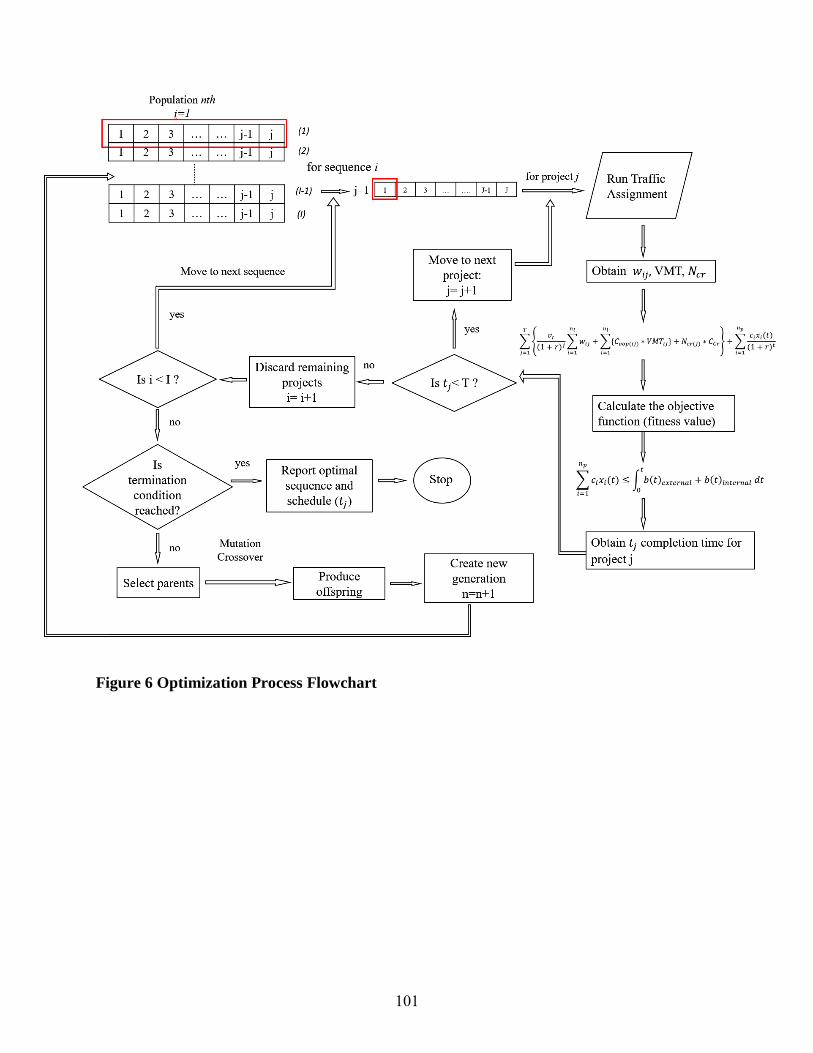
101

Figure 6 Optimization Process Flowchart

102

Figure 7 Process to Select Alternatives at Each Location

103

Figure 8 Sioux Falls Network

104

Figure 9 PV of Travel Time, Vehicle Operating and Safety Costs Over Time

0

1000

2000

3000

4000

5000

6000

7000

8000

9000

10000

0 1.4 4.7 6.2 8.6 10.8 13.4 14.9 17.3 19.2

PV

of

Tota

l Co

st (

$M

illio

ns)

Years

Travel time cost

Vehicle operating cost

Crash cost

105

Figure 10 GA Evolution Process

8.9E+09

8.95E+09

9E+09

9.05E+09

9.1E+09

9.15E+09

9.2E+09

0 20 40 60 80 100 120

Ob

ject

ive

Val

ue

(To

tal C

ost

) ($

)

Generation

106

Figure 11 Computation Time for Different Number of Projects

0

100

200

300

400

500

600

5 6 7 8 9 10 11 12 13 14 15 16 17 18 19 20 21

Co

mp

uta

tio

n t

ime

(min

)

Number of projects

107

Figure 12 Demand in the Average Scenario V.S. Demand in Each Scenario (low, med, high)

30

35

40

45

50

55

0 5 10 15 20 25

Dem

and

(1

00

0 p

er h

ou

r)

Analysis Period (year)

low demand growth

med demand growth

high demand growth

avg demand growth

108

Figure 13 PV of Total Cost in the Average Scenario V.S. Each Scenario (low, med, high)

0

2,000

4,000

6,000

8,000

10,000

12,000

14,000

16,000

18,000

0 5 10 15 20

PV

of

Tota

l Co

st (

Mill

ion

$)

Planning Period (year)

avg demand growth

low demand growth

medium demand growth

high demand growth

109

Figure 14 Fitted Lognormal Distribution

110

Figure List:

Figure 1 Framework of the Optimization Process

Figure 2 Optimization Process Flowchart

Figure 3 Process to Select Alternatives at Each Location

Figure 4 Sioux Falls Network

Figure 5 PV of Travel Time, Vehicle Operating and Safety Costs Over Time.

Figure 6 GA Evolution Process

Figure 7 Computation Time for Different Number of Projects

Figure 8 Demand in the Average Scenario V.S. Demand in Each Scenario (low, med, high)

Figure 9 PV of Total Cost in the Average Scenario V.S. Each Scenario (low, med, high)

Figure 10 Fitted Lognormal Distribution

111

Appendix 5 - Kim, M., Levy, J. and Schonfeld, P. “Optimal Zone Sizes and

Headways for Flexible-Route Bus Services,” Transp. Research Part B: Methodological,

v130, Dec 2019, 67-81.

Optimal Zone Sizes and Headways for Flexible-Route Bus Services

Myungseob (Edward) Kim1, Joshua Levy2, and Paul Schonfeld3

Abstract

Flexible-route bus systems serving passengers at their doorsteps may be preferable to fixed-route bus

systems in areas with low demand densities or whose roads cannot accommodate relatively large fixed-

route buses. Flexible-route systems may also be preferable for elderly or handicapped riders for whom

accessing the pre-determined stops on fixed routes is difficult. Since bus systems with flexible demand-

responsive routes retain the economic and environmental advantages of public transportation, it is

important to analyze them and optimize their characteristics to match their operating environments.

This study shows how the total cost can be minimized for a flexible-route bus system with a many-to-

one demand pattern by jointly optimizing its headway and service zone size. Numerical results

demonstrate the model’s applicability and indicate how such flexible-route systems should be adapted

to demand characteristics and planning constraints.

Introduction

Since public transit systems can transport many passengers efficiently, they have an important role in

urban areas. Hence, many researchers have sought to improve the costs and service quality of transit

systems. Bus transit operations may be classified as fixed-route or flexible-route services. Fixed-route

bus services have predetermined routes, stops and schedules, and they are very widely used in densely

populated urban areas since their average cost for serving high demand densities is relatively low (Kim

and Schonfeld, 2012 & 2013). When the demand densities or roadway geometric characteristics are

unsuitable for fixed-route bus operations, flexible-route services, which can operate on-demand without

predetermined stop locations, may offer a practical alternative. When the demand density is relatively

1 The corresponding author, Assistant Professor, Dept. of Civil and Environmental Engineering, Western New England

University, Springfield, MA 01119, myungseob.kim@wne.edu

2 Civil Engineer, Lorenzi, Dodds, & Gunnill, Inc. Walforf, MD 20601,joshlevy2012@gmail.com

3 Professor, Dept. of Civil and Environmental Engineering, University of Maryland, College Park, MD 20742, pschon@umd.deu

112

low, flexible-route service may have lower average system cost than conventional fixed-route bus

services. In an early study, Wilson and Hendrickson (1980) reviewed models for predicting the

performance of flexible transportation services such as taxi and dial-a-ride. Their review covered

methodological approaches such as simulation, empirical, deterministic queuing and stochastic

processes. With rapid developments of information technology and computation capabilities in recent

years, various studies (such as Luo and Schonfeld, 2007; Markovic et al, 2015) explored micro-level

transit service modeling by solving dial-a-ride problems or vehicle routing problems for public transit

systems.

Figure 15 Configuration of Flexible-route Bus Service Module

However, we observe that the relations among optimal zone sizes, headways and relevant exogenous

factors for flexible-route services have not been sufficiently explored, especially in considering how zone

sizes may be optimized based on the local demand densities. This paper presents a planning model for

optimizing a flexible-route bus operation serving many-to-one and one-to-many demand patterns, as

sketched in Figure 1. The rest of the paper includes a literature review for flexible transportation

operations, problem formulations, numerical studies and a concluding summary.

Literature Review

Flexible-route bus services, including demand-responsive dial-a-ride services, are widely considered to

improve the service quality for disabled passengers by providing door-to-door services or to reduce the

cost of public transit systems for regions with low demand densities. In this section, we present the

studies that are closely related to flexible-route bus operations. General reviews of fixed route bus

transit operations and network design may be found in Ceder and Wilson (1986) and in Ibarra-Rojas et al

(2015). An extensive overview of dial-a-ride problems, including recent developments, is provided in

Molenbruch et al (2017).

113

Nourbakhsh and Ouyang (2012) analyze the costs of flexible bus routes and their competitiveness versus

fixed bus routes and taxis. The optimal network layout, service area, and bus headway are used to

minimize total system cost. It is noted that in low to moderate demand areas, flexible bus route systems

have the lowest system cost among flexible-route bus, fixed-route bus and taxi services. Daganzo and

Ouyang (2019) present analytic models for door-to-door transit services, including non-shared taxi and

demand-responsive transportation as special variants of the model. Several objectives are considered in

the paper as follows: Firstly, the case of non-shared taxi is analyzed to emphasize the level of service

quality. Secondly, dial-a-ride services are analyzed for minimizing resources. Thirdly, the case of shared

taxi is analyzed for maximizing the number of served passenger trips. The model formulations assume a

uniform and steady many-to-many demand pattern. The deterministic analysis framework provides

approximated closed form solutions for the travel time and fleet size thresholds among dial-a-ride,

ridesharing, and non-shared taxi services.

Amirgholy and Gonzales (2016) employ an analytic model to approximate the operation cost of demand-

responsive transit (DRT) operations with time-dependent demand patterns. The cost of demand-

responsive transit services is estimated using the fleet size, the vehicle miles traveled, and the vehicle

hours traveled. The study also formulates the total cost that users experience as a result of the

operating decisions. This study analyzes the dynamic equilibrium that is associated with oversaturated

conditions in which the demand rate exceeds the operating capacity of the DRT system. A dynamic

pricing policy is considered that improves the efficiency of the DRT system by shifting the demand to a

different time of the day and avoiding the underutilization of capacity during off-peak times. Bakas et al

(2016) formulate a dial-a-ride problem with the assumption that customer pickups and drop-offs are

allowed only at pre-defined bus stops. With this assumption, the benefit of demand responsive

transportation services in low demand areas is compared to fixed-route bus operations.

Adebisi (1980) develops a model for estimating the travel time for fully- and partially flexible bus routes.

His model incorporates randomness in the number of passengers and their locations on grid networks.

Pei et al (2019) explore flexible bus operation by allowing turn-backs for dispatched vehicles as well as

skipping some bus stops. By adjusting the length of the service route with demand-responsive turn-

backs, the travel time for all passengers, including the onboard and waiting time, is minimized. This

study finds that a flexible bus operation performs well when demand density is low to medium. Qui et al

(2015) explore a flag-stop bus operation policy in which bus services do not provide complete curb-to-

curb services, but still offer some flexibility to transit riders. By comparing this operation policy to fixed-

and flexible-route bus operations, the flag-stop policy is found to be advantageous in low-demand

regions, such as suburban and rural areas. Zheng et al (2018) use two analytical models for comparing

services with limited route deviation versus more flexible point deviation. Stiglic et al (2015) analyze a

flexible dial-a-ride system in which passengers are picked up at their origin and dropped off at their

destinations, or passengers come to the designated points to be picked up or dropped off. Although a

possible inconvenience for such systems is that passengers have to arrive at the meeting point before

their vehicle arrives, the proposed model substantially improves the system performance. Gomes et al

114

(2015) develop a simulation-based optimization model for demand-responsive transportation

scheduling. Yu et al (2015) incorporate a dynamic vehicle routing algorithm into an agent-based traffic

simulation and compare demand responsive transportation services with conventional bus operations.

They note that demand-responsive service increases mobility by decreasing the travel time perceived by

passengers. Several case studies are found on implementing flexible transportation services (Horn, 2002;

Fernandez et al, 2008).

Pan et al (2015) propose a mathematical model for designing the service area and routing plan for a

flexible bus feeder system that is connected to a rail transit line. By assuming the fleet size and demand

as inputs, this model approximates the service area and routing schedule without assuming a grid street

geometry and uniform demand distributions. It is assumed that the passengers within the zone report to

the designated pickup or drop points, also called gates Thus, the tour within each zone is not modeled;

instead, a gravity-based heuristic approach for optimizing vehicle routes among gates is proposed. As an

extension from Pan et al (2015), Lu et al (2016) present a model for deviated fixed-route transit

operations. Their main purpose is to assign random requests to the nearest possible routes by allowing

route deviations based on the travelling salesman problem. Bus travel time is minimized with a genetic

algorithm. Saeed and Kurauch (2015) formulate mixed-integer problems to analyze a dial-a-ride (DAR)

system for rural areas. A branch-and-cut algorithm-based solution is proposed to minimize the operating

costs as well as user’s travel times for the DAR system. They note that flexible-route DAR operation is

suitable for low demand density and wide spatial coverage in complex road networks. Their DAR results

show decreased waiting times for rural area users.

The relative advantages of fixed-route, flexible-route and variable-type bus services are analyzed by

Chang & Schonfeld (1991) and by Kim and Schonfeld (2012). Kim and Schonfeld (2012) find that at low

demand densities, flexible-route services have lower average cost per passenger than conventional

fixed-route bus operations. Kim and Schonfeld (2013) integrate fixed and flexible bus services using a

genetic algorithm and analytic optimization while determining the type of service based on demand

density. Chen and Nie (2017) analyze hybrid systems with fixed and flexible services using simulation.

They use flexible services to increase accessibility to fixed-route bus systems. Häll et al (2018) propose a

simulation-based analysis for integrated bus operations combining a fixed-route service and demand-

responsive service. They find that for the integrated bus operations, the number of transfers as well as

the pricing policy for demand-responsive service strongly affect the performance of such integrated

transit services.

Chang and Schonfeld (1993) develop a model for jointly optimizing the dimensions for served zones and

headways, but only for fixed-route services whose characteristics and resulting model formulations

differ considerably from those for flexible-route services. They assume that zone shapes are rectangular

and find that zone lengths, zone widths and headways should increase with distance from a major

terminal. Some related studies such as Chang and Schonfeld (1991), Kim and Schonfeld (2013, 2014, and

2015) assume that each served zone is rectangular, while larger service regions are divided into multiple

zones, based on the demand levels. It should be noted that the zone size is a very important factor (and

not only for rectangular zones) in planning efficient flexible route services. Broome et al (2007)

115

completed a study showing the public’s positive perception of flexible bus route systems. Designed for

elderly persons who cannot travel to and from fixed bus stops, these flexible bus systems saw ridership

double over the course of the study. Satisfaction was also significantly increased and the flexible bus

system began to attract younger users.

From the literature review we note the importance of flexible-route bus operation for serving low

demand regions or handicapped passengers. However, the main interests in those studies are new

solution algorithms or heuristics for dial-a-ride or demand responsive transportation services. It is clear

that the relations among optimal zone sizes, headways and relevant exogenous factors have not been

sufficiently explored for flexible-route services. This paper contributes to the literature mathematical

relations for optimally matching headways and service zone sizes to exogenous local characteristics such

as demand density, distance from major terminals, unit costs and travel speeds, in order to minimize

average costs per passenger, including the supplier and user costs. The model presented in this paper

can help guide the design of relatively simple flexible-route bus services, especially where the demand

density is relatively low or where street geometry cannot accommodate the relatively large buses used

for fixed-route bus services.

Flexible-route Service Formulation

Each flexible-route module considered in this study includes one bus route that connects a local service

zone to a major terminal, through an express segment, as shown in Figure 1. The route’s headway and

the area of the local service zone are jointly optimized as functions of demand density, distance from

the major terminal, applicable unit costs, bus speeds, and other relevant exogenous parameters. The

major terminal may be a Central Business District (CBD), another major trip attractor, or a transfer

terminal along a rail transit route. The route within each module primarily serves a Many-to-One (M-to-

1) or One–to-Many (1-to-M) demand pattern. However, with multiple modules optimized for urban

regions around the major terminal(s), their converging routes would enable Many-to-Many (M-to-M)

demand patterns to be served, as briefly discussed below. This paper focuses on the optimization of

single modules while a future study is expected to optimize the development of multi-module flexible

route systems that cover substantial urban and suburban areas.

For each module, trip origins and destinations are assumed to be randomly and uniformly distributed

over the local zone and over time. An example of this type of bus system could be a suburban

neighborhood outside a large city. Passengers residing in that neighborhood or “service zone” take the

bus to or from a train station, a downtown terminal or an airport, as shown in Figure 1. Neighborhoods

may be divided into smaller subsections, depending on the results of the joint optimization of the

116

decision variables that are analyzed here. Figure 1 shows a zone with a rectangular shape, but the

analysis is also applicable to other zone shapes as long as the zones are fairly compact and fairly convex.

We noted that the flexible-route service model presented in this paper and illustrated in Figure 1 can

constitute a modular building block in designing larger and more comprehensive systems, which serve

M-to-M demand patterns. As an example, the region in Figure 2 can be subdivided into multiple zones,

roughly in accordance to the guidelines developed in this paper on jointly optimizing zone areas and

headways as functions of demand densities and distances from the central terminal (or central business

district). Then the M-to-M demand patterns can be served with transfers at the central terminal,

possibly with coordinated headways to minimize transfer delays, while minimizing system-wide costs.

Figure 16 Potential Extension to Multi-zone Flexible-route System

The formulated total cost for flexible bus services is the sum of supplier (operator) cost, user in-vehicle

cost, and user waiting cost. Since flexible-route services are assumed to provide door-to-door service,

they have no access time or cost. The relevant notation is defined in Table 1. In order to provide a

relatively simple and widely applicable model for planning and preliminary system design, the following

simplifying assumptions are made:

1. Stein (1978)’s formula is assumed to provide an acceptable approximation of the shortest tour

distance within a zone, with a constant k = 1.15 according to Daganzo (1984) for rectilinear

movements within the zone.

2. The service zone is fairly compact and fairly convex.

3. Destinations and origins are fairly uniformly distributed over time and space within the service

zone.

4. The number of stopping points in a zone for each vehicle tour exceeds five.

5. Dwell times and stopping times within the service zone are included in the average speed.

117

6. The average wait time is approximately half of the service headway.

7. Passenger pickups and drop-offs are intermingled within each tour.

Table 3 Notation and Baseline Values for Inputs

Symbol Variable Units Base Value Range for

Sensitivity

Analysis

A Zone Size (Area) Square Miles - -

a Parameter for bus operating

cost

$ / bus hour 30 -

b Parameter for bus operating

cost

$ / seat hour 0.3 -

CA Average Total Cost $ / passenger - -

CT Total Cost $ / hour - -

CS Supplier Cost $ / hour - -

CV In-vehicle Cost $ / hour - -

CW Waiting Cost $ per hour - -

c Unit Bus Operating Cost

(=a+b*S)

$ / bus hour - -

DC Tour Length within Zone Miles - -

h Headway Hours - -

J Line Haul Distance Miles 10 6-15

l Load factor Dimensionless 1.0 -

N Fleet Size Buses - -

∅ Stein’s Constant Dimensionless 1.15 -

Q Demand Density

Trips / square mile*hour

10 5-50

q Hourly demand Trips / hour - -

R Round Trip Time Hours - -

S Bus Capacity Seats / bus 45 10-50

u Number of Passengers per

Stop

Number of passengers 1 -

VX Line Haul Speed Miles / hour 30 15-60

VL Average Local Speed Miles / hour - 10 – 40

vv Value of in-vehicle time $ / passenger hour 12 6-20

vw Value of waiting time $ / passenger hour 15 6-20

w waiting time Hours - -

118

y Ratio of local speed to

express speed

Dimensionless 0.9 0.5-1.0

The operator’s service cost CS is formulated as the product of the required fleet size N and the unit

operating cost c:

𝐶𝑆 = 𝑁 × 𝑐 (1)

The required fleet size is the vehicle round trip time divided by headway:

𝑁 =𝑅

ℎ (2)

The round trip time R is the sum of 2-directional trip time for the line haul (i.e., express) segment and

trip time in the local zone. Stein’s approximation for tour length within the zone Dc is expressed as:

𝐷𝑐 = ∅ √𝑛𝐴 (3)

The approximation in Eq. (3) is very useful in this study for optimizing the headway and zone size for

flexible bus routes.

The number of stops during the tour n is expressed as a function of demand density Q, zone size,

A, headway h, and the number of passengers (boarding or alighting) per stop u:

𝑛 =𝑄𝐴ℎ

𝑢 (4)

As the actual hourly demand per zone q (in passenger trips/hour) is product of the demand density

Q and the zone size A, the demand q is expressed as:

𝑞 = 𝑄𝐴 (5)

Then, the tour length Dc is:

𝐷𝑐 = ∅√𝑞𝐴ℎ

𝑢 (6)

119

The line haul distance J, the express speed VX, and local speed VL are used to compute the vehicle

round trip time R:

𝑅 =2𝐽

𝑉𝑋+

𝐷𝑐

𝑉𝐿 (7)

We assume the local speed is a fraction of the express speed VX. We denote the ratio of local speed

VL, to express speed VX, as y. Then:

𝑉𝐿 = 𝑦 𝑉𝑋 (8)

The service cost, 𝐶𝑆 is then formulated as:

𝐶𝑆 =2𝐽𝑐

ℎ𝑉𝑋+

∅𝑐

𝑦 𝑉𝑋√𝑞𝐴

𝑢ℎ (9)

The in-vehicle cost CV is the product of the value of passenger’s in-vehicle time 𝑣𝑣, the demand q,

and passenger’s trip time, which is assumed to be half of the vehicle round trip time R:

𝐶𝑉 = 𝑣𝑣𝑞 𝑅

2 (10)

Eq. (10) can be re-written as:

𝐶𝑉 =𝑣𝑣𝑞𝐽

𝑉𝑥+

∅𝑣𝑣

2𝑦 𝑉𝑥√𝑞3ℎ𝐴

𝑢 (11)

Since we are formulating a planning-level model, we approximate the average wait time as half of

the headway h. This assumption is widely applied in urban transit services, in which the headways

are relatively short. It should also be noted that for flexible-route bus services much of the waiting

may be inside the users’ homes or workplaces rather than at remote bus stops. The resulting waiting

cost for passenger CW is product of the value of waiting time 𝑣𝑤, the demand q, and the average

waiting time h/2:

𝐶𝑊 = 𝑣𝑤𝑞ℎ

2 (12)

The total cost for the flexible service is the sum of operating cost, in-vehicle cost and waiting cost:

𝐶𝑇 = 𝐶𝑆 + 𝐶𝑉 + 𝐶𝑊 (13)

120

Eq. (13) is detailed as:

𝐶𝑇 =2𝐽𝑐

ℎ𝑉𝑋+

∅𝑐

𝑦 𝑉𝑋√𝑞𝐴

𝑢ℎ+𝑣𝑣𝑞𝐽

𝑉𝑥+

∅𝑣𝑣

2𝑦 𝑉𝑥√𝑞3ℎ𝐴

𝑢+ 𝑣𝑤𝑞

ℎ

2 (14)

The average cost per passenger CA can be found by dividing the total cost function in Eq. (14) by

the passenger flow q:

𝐶𝐴 =𝐶𝑇

𝑄𝐴=

𝐶𝑇

𝑞 (15)

Thus, the average cost for the service is:

𝐶𝐴 =2𝐽𝑐

ℎ𝑉𝑋

1

𝑄𝐴+

∅𝑐

𝑦 𝑉𝑋𝑄𝐴√𝑄𝐴⋅𝐴

𝑢ℎ+

1

𝑄𝐴

𝑣𝑣𝑄𝐴⋅𝐽

𝑉𝑥+

∅𝑣𝑣

2𝑦𝑉𝑋

1

𝑄𝐴√(𝑄𝐴)3ℎ𝐴

𝑢+𝑣𝑤𝑄𝐴ℎ

2𝑄𝐴 (16)

Eq. (16) is rewritten as:

𝐶𝐴 =2𝐽𝑐

𝑉𝑋𝑄𝐴ℎ+

∅𝑐

𝑦 𝑉𝑋√

1

𝑄ℎ𝑢+

𝑣𝑣𝐽

𝑉𝑋+

∅𝑣𝑣𝐴

2𝑦𝑉𝑋√𝑄ℎ

𝑢+𝑣𝑤ℎ

2 (17)

In Eq. (17), the average cost per passenger is a function of two decision variables, namely the zone

size A and the headway h.

The first order derivative of the average cost with respect to the zone size A, shown in Eq. (18), is

set equal to zero:

𝜕𝐶𝐴

𝜕𝐴= −

2𝐽𝑐

𝑉𝑋𝑄ℎ𝐴2 +

∅𝑣𝑣√𝑄ℎ

2𝑦𝑉𝑋√𝑢= 0 (18)

The necessary condition for the global optimality of the zone size A is that Eq. (19) should have a

positive value. Since Eq. (19) is always positive, we confirm that the optimal value of the zone

size A yields the global minimum in Eq. (17).

𝜕2𝐶𝐴

𝜕𝐶𝐴2 =

4𝐽𝑐

𝑉𝑋𝑄ℎ𝐴3> 0 (19)

The first order derivative of the average cost with respect to the headway h is:

𝜕𝐶𝐴

𝜕ℎ= −

2𝐽𝑐

𝑉𝑋𝑄𝐴ℎ2 −

∅𝑐

2𝑦𝑉𝑋√𝑄𝑢ℎ3+

∅𝑣𝑣𝐴√𝑄

4𝑦𝑉𝑋√𝑢ℎ+𝑣𝑤

2= 0 (20)

121

Similarly, the second-order derivative for the headway, which should be positive, is shown in Eq. (21).

𝜕2𝐶𝐴

𝜕ℎ2=

4𝐽𝑐

𝑉𝑋𝑄𝐴ℎ3 +

3∅𝑐

4𝑦𝑉𝑋√𝑄𝑢ℎ5−

∅𝑣𝑣𝐴√𝑄

8𝑦𝑉𝑋√𝑢ℎ3 (21)

We seek the solution by solving Eq. (18) and Eq. (20) simultaneously. From Eq. (18), we obtain

the following relation:

1

𝐴2√ℎ3=

∅𝑣𝑣√𝑄3

4𝑦𝐽𝑐√𝑢 (22)

By denoting t to substitute for the right hand side of Eq. (22), we find a simplified relation between

the headway and zone size, as shown in Eq. (23):

𝐴 = 1

√𝑡 √ℎ34 (23)

Eq. (23) is inserted in Eq. (20), and Eq. (20) is re-written as:

𝜕𝐶𝐴

𝜕ℎ= −

2𝐽𝑐√𝑡

𝑉𝑋𝑄 √ℎ54 −

∅𝑐

2𝑦𝑉𝑋√𝑄𝑢 √ℎ64 +

∅𝑣𝑣𝐴√𝑄

4𝑦𝑉𝑋√𝑢𝑡 √ℎ54 +

𝑣𝑤

2= 0 (24)

By using X to substitute for√ℎ4

, Eq. (25) is obtained:

𝑣𝑤

2𝑋6 + {

∅𝑣𝑣√𝑄

4𝑦𝑉𝑋√𝑢𝑡−2𝐽𝑐√𝑡

𝑉𝑋𝑄}𝑋 −

∅𝑐

2𝑦𝑉𝑋√𝑄𝑢= 0 (25)

Eq. (25) is re-arranged, and denoted as Y:

𝑌 =𝑣𝑤

2𝑋6 − {

∅𝑣𝑣√𝑄

4𝑦𝑉𝑋√𝑢𝑡} 𝑋 −

∅𝑐

2𝑦𝑉𝑋√𝑄𝑢 (26)

To investigate the convexity of Eq. (26), we find the partial derivative of Y with respect to X as

follows:

𝜕𝑌

𝜕𝑋= 3𝑣𝑤𝑋

5 − {∅𝑣𝑣√𝑄

4𝑦𝑉𝑋√𝑢𝑡} (27)

122

By setting Eq. (27) to zero, we find only one root, as shown in Eq. (28):

𝑋 = {∅𝑣𝑣√𝑄

12𝑣𝑤𝑦𝑉𝑋√𝑢𝑡}1/5

(28)

Since we find only one root, shown in Eq. (28), for which Eq. (27) equals zero, and since the

coefficient of the X6 term in Eq. (26), which is 𝑣𝑤/2, is positive, we confirm that the function in

Eq. (26) is convex. We apply Newton’s Method to find the optimal headway as h* = X4. The

pseudo-algorithm is shown as follows (Press et. al., 2007):

Step 1: Pick the initial value (x1) of X, which must be greater than zero.

Step 2: Evaluate Eq. (26), f(x1) at this point (x1)

Step 3: Assuming f(x1) was not the root of the equation, compute the following equation to determine

the next evaluation point, x2.

𝑥2 = 𝑥1 −𝑓(𝑥1)

𝑓′(𝑥1)

Step 4: Evaluate Eq. (26) at x2, and obtain f(x2).

Step 5: Repeat this iterative process until the root is determined or the tolerance criterion is satisfied.

𝑥𝑛+1 = 𝑥𝑛 −𝑓(𝑥𝑛)

𝑓′(𝑥𝑛)

In Eq. (19), the optimal zone size A*, yields the global minimum of the objective function. We

must also ensure that the optimal headway h* yields the globally optimal solution by investigating

the previously derived Eq. (21).

To ensure the optimal headway yields the global minimum, Eq. (21) should be positive. To achieve

the closed-form equation of headway boundary that yields the global solution, we note that either

of the following two conditions should be positive:

4𝐽𝑐

𝑉𝑋𝑄𝐴ℎ3 −

∅𝑣𝑣𝐴√𝑄

8𝑦𝑉𝑋√𝑢ℎ3> 0 (29)

or

3∅𝑐

4𝑦𝑉𝑋√𝑄𝑢ℎ5−

∅𝑣𝑣𝐴√𝑄

8𝑦𝑉𝑋√𝑢ℎ3> 0 (30)

123

Eq. (29) is rearranged in Eq. (31), and Eq. (30) is rearranged in Eq. (32):

ℎ < √ 1

𝐴4{32𝑦𝐽𝑐√𝑢

∅𝑣𝑣√𝑄3}23

(31)

or

ℎ <6𝑐

𝑣𝑣𝑄𝐴 (32)

Since both Eqs. (31) and (32) provide closed-form conditions, they can provide insights for decision

makers regarding headway planning. The visual representation of the global solution boundary will be

discussed in the numerical analysis section.

When the maximum allowable headway policy is considered (ℎ =𝑆𝑙

𝑄𝐴), the complexity of the problem is

reduced to analytically optimizing a single variable, which is the zone size A. The optimal zone size A* is

found in closed-form, as shown in Eq. (33):

𝐴∗ = √(

𝑣𝑤𝑆𝑙

2𝑄

{∅𝑐

2𝑦𝑉𝑋√𝑢𝑆𝑙+

∅𝑣𝑣√𝑆𝑙

4𝑦𝑉𝑋√𝑢}

⁄ )

23

(33)

The global optimality condition of the zone size A is presented in Eq. (34):

𝐴 <√{𝑣𝑤𝑆𝑙}

2

𝑄2 {∅𝑐

4𝑦𝑉𝑋√𝑢𝑆𝑙+

∅𝑣𝑣√𝑆𝑙

8𝑦𝑉𝑋√𝑢}2⁄

3 (34)

The details of the derivations of A, and the necessary condition for its global optimality are summarized

in Appendix A.

Numerical Analysis

124

Numerical cases are used to explore the relations between the decision variables, which are the

headway h and the zone size A, for the problem illustrated in Figure 1. This section explores how various

input parameters affect the design of flexible-route bus services. We present a baseline case and an

elasticity analysis for the sensitivity of solutions to service design parameters. The baseline values of the

parameter for the formulations and numerical cases are provided in Table 1.

Visual Representation of Convexity in the Objective Function

We seek to verify the global optimality of the solutions. By solving Eq. (27) using the baseline

values from Table 1, the minimum of X is obtained as 0.4426. As shown in Figure 3, the value of

Eq. (26) decreases until X is 0.4426, and then Eq. (26) increases beyond X values of 0.4426.

Therefore, we graphically confirm that Eq. (26) is a convex function with only one root (i.e., 0.692)

as discussed for Eq. (28). In Figure 3, we also note that the root of X, at which Eq. (26) equals

zero, is 0.692. Thus, the optimal headway h* (=0.229 hours) is found from X4 (=0.6924). From the

optimal headway* (i.e., 0.229 hours), we find the optimal zone size A* using Eq. (23), as 5.72 sq.

miles.

Figure 17 Convexity of Eq. (26)

Either Eq. (31) or Eq. (32) must be satisfied to guarantee the global optimality of the solution. As shown

in Figure 4, we note that the headway condition specified in Eq. (32) always satisfies the condition

specified in Eq. (31). Thus, we take Eq. (31) as the criterion which guarantees the globally optimal

solution for the headway. With baseline values, the optimal headway h* is 0.229 hours, and we obtain

125

the upper limit (i.e., condition) of the headway from Eq. (31) as 0.917 hours. Therefore, we find the

global solution.

Figure 18 Headway Limits Constrained by Eqs. (31) and (32)

Joint Optimization vs. Maximum Allowable Headway Solutions

For the baseline case, the optimal zone size A* is found as 5.72 sq. miles and the optimal headway h* is

found as 0.23 hours. As shown in Table 2, the average cost per person trip includes an operating cost of

3.44 $/person trip, an in-vehicle time of 6.21 $/person trip, and a waiting time cost of 1.72 $/person

trip, resulting a total cost for flexible service of 11.37 $/person trip. The operating cost, in-vehicle cost

and waiting cost components of the average system cost are about 30 %, 55% and 15%, respectively.

Figure 3 shows that the cost function is convex, and its optimal zone size and headway are the global

solution.

126

Figure 19 Average Cost Plot for Baseline Case

When the maximum headway policy is applied, a closed-form solution is achievable, which offers

insights regarding the relations among decision variables and input parameters. With the closed-form

solution shown in Eq. (33), the optimal solution for the zone size A* is analytically found as 10.48 sq.

miles. Using Eq. (34), the necessary condition (i.e., the maximum zone size A) is obtained as 26.4 sq.

miles, and the optimal zone size (10.48 sq. miles) satisfies the condition. Thus, we confirm that the

solution with the maximum allowable headway policy finds the global minimum solution. The maximum

allowable headway h* is obtained as 0.43 hours, using the relation ℎ = Sl/QA.

Table 2 provides comparisons between the two solution approaches, namely the joint optimal solution

and maximum allowable headway solution. The optimal zone size A* based on the maximum allowable

headway is 83% larger than that for the joint optimal solution. The maximum allowable headway h* is

almost double that of the joint optimal solution. For this base case, the maximum allowable headway

can reduce the operator cost compared to the joint optimal solution while the in-vehicle and waiting

costs exceed those in the joint optimal solution. The average cost per person trip is 26% higher for the

maximum allowable headway than for the joint optimal solution.

Table 4 Cost Comparison between the Maximum Allowable Headway and Joint Optimal Solution for

Zone Size and Headway

Zone Size,

A

(sq. miles)

Headway,

h

(hrs)

Operator

Cost

($/person)

In-vehicle

Cost

($/person)

Waiting

Cost

($/person)

Average

Cost

($/person)

127

Maximum Allowable

Headway Solution (1) 10.48 0.43 1.54 9.55 3.22 14.31

Joint Optimal Solution (2) 5.72 0.23 3.44 6.21 1.72 11.37

Cost Difference,

{(1)-(2)}/(2) 83.2% 87.8% -55.2% 53.7% 87.5% 25.9%

Sensitivity Analysis

Demand Density

Table 3 shows the sensitivity of costs to the demand density Q. In it the in-vehicle cost is the highest

among the cost components and is approximately double the operating cost, while the waiting cost is

the lowest cost component. Table 3 shows that as Q increases, the optimal zone size and headway

decrease. The resulting A* decreases from 8.42 to 2.31 sq. miles, and it shows greater variations

(between 47.3% increase and -59.6% decrease) than the headway variations (between 19% increase and

-33% decrease) over the range of demand changes. For instance, when the hourly demand density

increases from 5 to 10 person trips/sq. miles, A* decreases from 8.42 to 5.72 sq. miles, while the

demand density increase from 45 to 50 person trips/sq. miles reduces the zone size from 2.45 to 2.31

sq. miles. When the demand density increases from 10 to 50 persons/sq.mile, the average cost per

person decreases by 20% from 11.37 to 9.09 $/person.

Table 5 Joint Optimal Solution for Demand Variations

Demand Density (persons/sq.mile) 5 10 15 20 25 30 35 40 45 50

Zone Size (sq.

miles)

Joint Optimal

Solution 8.42 5.72 4.56 3.88 3.42 3.08 2.83 2.62 2.45 2.31

% Change 47.3 0.0 -20.3 -32.2 -40.3 -46.1 -50.6 -54.2 -57.1 -59.6

Headway

(hours)

Joint Optimal

Solution 0.27 0.23 0.21 0.19 0.18 0.17 0.17 0.16 0.16 0.15

% Change 19.4 0.0% -9.7 -16.0 -20.5 -24.0 -26.8 -29.2 -31.2 -33.0

Average

Operating Cost

($/hr)

Joint Optimal

Solution 4.10 3.44 3.10 2.89 2.73 2.61 2.51 2.43 2.36 2.30

% Change 19.4 0.0 -9.7 -16.0 -20.5 -24.0 -26.8 -29.2 -31.2 -33.0

Average In-

vehicle Cost

($/hr)

Joint Optimal

Solution 6.52 6.21 6.05 5.94 5.86 5.80 5.75 5.71 5.67 5.64

128

% Change 4.9 0.0 -2.6 -4.3 -5.6 -6.6 -7.5 -8.2 -8.8 -9.3

Average

Waiting Cost

($/hr)

Joint Optimal

Solution 2.05 1.72 1.55 1.44 1.37 1.31 1.26 1.22 1.18 1.15

% Change 19.4 0.0 -9.7 -16.0 -20.5 -24.0 -26.8 -29.2 -31.2 -33.0

Total Cost

(Average Cost

in

$ per person)

Joint Optimal

Solution 12.67 11.37 10.71 10.27 9.96 9.72 9.52 9.36 9.21 9.09

% Change 11.5 0.0 -5.8 -9.6 -12.4 -14.5 -16.3 -17.7 -18.9 -20.0

We also explore the effects of demand densities on headways while the zone size is not optimizable, as

presented in Table 4. We hold the zone size at A=5.72 sq. miles, as a fixed input parameter, and explore

the relations between the demand density and headway. When Q increases from 10 (in the baseline

conditions) to 50, we find that h* decreases from 0.23 hours to 0.07 hours, thus resulting in more

frequent bus service, while the total cost per trip decreases by 14.7%. When Q increases from 10 to 50

while fixing the zone size, the in-vehicle cost increase by 8.8% and the operating cost decreases by 30%.

As h* decreases from 0.23 to 0.07 hours, the waiting cost decreases significantly by 68.9%.

Table 6 Effects of Demand Density with Zone Size on Hold

Demand Density (persons/sq.mile) 5 10 15 20 25 30 35 40 45 50

Zone Size (sq.

miles)

Zone Size on

Hold (Input) 5.72 5.72 5.72 5.72 5.72 5.72 5.72 5.72 5.72 5.72

Headway

(hours)

Zone Size on

Hold (Input) 0.35 0.23 0.18 0.14 0.12 0.11 0.09 0.09 0.08 0.07

% Change 52.9 0.0 -23.5 -37.4 -46.7 -53.5 -58.7 -62.8 -66.1 -68.9

Average

Operating Cost

($/hr)

Zone Size on

Hold (Input) 4.29 3.44 3.07 2.86 2.72 2.62 2.55 2.49 2.44 2.40

% Change 25.0 0.0 -10.6 -16.8 -20.8 -23.7 -25.8 -27.5 -28.9 -30.0

Average In-

vehicle Cost

($/hr)

Zone Size on

Hold (Input) 5.93 6.21 6.37 6.48 6.55 6.61 6.66 6.70 6.73 6.76

% Change -4.5 0.0 2.5 4.2 5.5 6.4 7.2 7.8 8.4 8.8

Average

Waiting Cost

($/hr)

Zone Size on

Hold (Input) 2.63 1.72 1.31 1.08 0.92 0.80 0.71 0.64 0.58 0.53

% Change 52.9 0.0 -23.5 -37.4 -46.7 -53.5 -58.7 -62.8 -66.1 -68.9

Total Cost

(Average Cost

in

$ per person)

Zone Size on

Hold (Input) 12.86 11.37 10.76 10.41 10.19 10.03 9.92 9.83 9.76 9.70

% Change 13.1 0.0 -5.4 -8.4 -10.4 -11.7 -12.7 -13.5 -14.2 -14.7

129

Vehicle Capacity

The vehicle size S is a critical design parameter for planning and scheduling public transportation

operations. When S increases from 10 to 15 seats/bus, the optimal zone size A* increases by 6.3% while

the optimal headway h* increases by 5%. As expected, when the vehicle capacity increases, the optimal

zone size A* and optimal headway h* both increase to cover a larger area for each bus tour while

decreasing service frequency.

Table 7 Effects of Vehicle Capacity on Costs

Vehicle

Capacity (# of

seats)

Optimal Zone

Size (sq.

miles)

Optimal

Headway

(hrs)

Average

Operating

Cost ($/hr)

Average In-

vehicle Cost

($/hr)

Average

Waiting Cost

($/hr)

Total Cost

(Average

Cost in

$ per person)

10 5.23 0.19 3.22 5.85 1.43 10.50

15 5.56 0.20 3.06 6.03 1.53 10.62

20 5.59 0.21 3.12 6.06 1.56 10.75

25 5.62 0.21 3.19 6.09 1.59 10.88

30 5.65 0.22 3.25 6.12 1.63 11.00

35 5.67 0.22 3.31 6.15 1.66 11.13

40 5.70 0.23 3.38 6.18 1.69 11.25

45 5.72 0.23 3.44 6.21 1.72 11.37

50 5.74 0.23 3.50 6.24 1.75 11.49

55 5.77 0.24 3.55 6.27 1.78 11.60

Figures 6 and 7 each show a sharp turning point for optimal zone size and headway. These changes are

based on the vehicle capacity constraints (i.e., h ≤𝑆𝑙

𝑄𝐴). When the vehicle capacity is small (e.g.,

between 10 and 15 seats/bus), the vehicle capacity constraint is bounded so that the optimal zone size

increase sharply. When the capacity constraint is not binding (e.g., vehicle capacity larger than 15

seats/bus), the optimal zone size A* increases less rapidly.

130

Figure 20 Optimal Zone Size versus Vehicle Capacity

Figure 21 Optimal Headway versus Vehicle Capacity

Figure 7 shows how the optimal headway h* varies with given vehicle capacity S. We note that the

headway increases rapidly with vehicle capacities between 5 and 15 seats/bus. When vehicles have

sufficient capacity (i.e., above 15 seats/bus) to satisfy the demand, the increase in optimal headway

ranges between 0.08% and 0.09% as vehicle capacity increases by one seat. Table 6 summarizes the

resulting effects of vehicle capacity.

131

Table 8 Effects of Vehicle Capacity on Optimal Zone Size and Headway

Vehicle

Capacity (# of

seats)

Optimal Zone

Size (sq.mile)

% Increase of

Optimal Zone

Size per Unit

of Vehicle

Capacity (+1

seat/veh)

% Increase of

Optimal Zone

Size From

Baseline

Result

Optimal

Headway

(hrs)

% Increase of

Optimal Zone

Size per Unit

of Vehicle

Capacity (+1

seat/veh)

% Change of

Optimal

Headway

From

Baseline

Result

10 5.23 - -8.50 0.191 - -19.92

15 5.56 6.52 -2.79 0.204 0.26 -12.38

20 5.59 0.59 -2.28 0.208 0.09 -10.01

25 5.62 0.56 -1.79 0.213 0.09 -7.78

30 5.65 0.54 -1.31 0.217 0.08 -5.67

35 5.67 0.52 -0.86 0.221 0.08 -3.68

40 5.70 0.50 -0.42 0.225 0.08 -1.79

45 5.72 0.48 0.00 0.229 0.08 0.00

50 5.74 0.47 0.41 0.233 0.08 1.70

55 5.77 0.45 0.80 0.237 0.08 3.33

Elasticity Analysis of Input Parameters

Table 7 shows the elasticity of the optimized zone size A* and headway h* with respect to 10% increases

in various design parameters. For example, when demand density Q increases by 10%, A* decreases by

5.20%, implying a -0.52 elasticity of A* to Q. Similarly, a 10% increase in Q, reduces h* by 2.31%, implying

the elasticity of h* to Q is -0.23. In this case, the average cost per person-trip decreases from 11.368 to

11.260 $.

The sensitivities of A* and h* to other input parameters are also shown in Table 7. Increases in the

parameters a and b for the unit operating cost both increase A* and h*. The elasticities of A* and h* to

vehicle capacity are 0.04 and 0.16, respectively. An increase in the line haul distance increases the round

trip time. Thus, the supplier cost and in-vehicle cost are increased, which increase A* and h*.

132

Table 7 shows that, with respect to the value of the in-vehicle time, the elasticity of A* is negative while

the elasticity of h* is positive. As expected, the optimal vehicle round trip time decreases when the

passengers’ value of in-vehicle time increases. With respect to the value of waiting time vw and the

vehicle operating speed VX, the elasticities of A* are positive and the elasticities of h* are negative.

Table 9 Elasticities of Optimal Zone Size and Headway with Respect to Various Design Parameters

Q a B S J vv vw Vx y

Baseline Input Values 10.0 30.0 0.30 45.0 10.0 12.0 15.0 30.0 0.90

Baseline Case

A* 5.72

h* 0.23

TC* 11.37

Elasticity Results

+10%

change

of x

11.00 33.00 0.33 49.50 11.00 13.20 16.50 33.00 0.99

A* 5.42 5.77 5.74 5.74 5.90 5.36 6.03 6.03 6.22

elasticity

of A*

w.r.t.

+10%

change

of x

-0.52 0.08 0.04 0.04 0.31 -0.63 0.55 0.55 0.87

h* 0.22 0.24 0.23 0.23 0.23 0.23 0.21 0.21 0.22

elasticity

of h*

w.r.t.

+10%

change

of x

-0.23 0.35 0.16 0.16 0.24 0.24 -0.68 -0.68 -0.47

TC* 11.26 11.60 11.47 11.47 11.98 11.98 11.53 10.49 11.05

Conclusions

In this paper a model for optimizing the headway and zone size is formulated for a flexible-bus service. It

minimizes the average cost per passenger trip, which is the sum of the operator cost, in-vehicle cost,

and waiting cost, while considering a vehicle capacity constraint. An analytic relation is obtained

between optimal headway and optimal zone size, and the minimum cost is found by solving a sixth order

polynomial function using Newton’s method. We also analyze the case in which the zone size is

unchangeable as a policy constraint. For it, we treat the headway as the only decision variable, and

compare the results with the joint optimal solutions. We also consider the flexible-route bus service

based on the maximum allowable headway policy. Since its headway is determined based on the zone

133

size A, the average cost formulation, as shown in Eq. (A4), is reduced to a problem with one decision

variable, namely A. The maximum allowable headway approach provides a closed-form solution, and

thus useful insights into the relations among decision variables and input parameters.

The optimized relations presented here for zone sizes and headways may be used to design multi-zone

systems that serve many-to-many demand patterns (as sketched in Figure 2), as well as simpler single-

zone systems (as sketched in Figure 1). For the baseline case analysis, the cost percentages for vehicle

operation, in-vehicle time and waiting time are 30%, 55% and 16%, respectively. When demand density

increases from 10 to 50 persons/sq.mile, we find that the share of in-vehicle cost increases to 62%. The

numerical analyses confirm that, in general, the cost of in-vehicle time exceeds operating and waiting

cost components. Sensitivity analyses also explore how changes in design parameters affect the

operating decisions as well as costs. Thus, the obtained relations and results from numerical analysis can

be used as planning guidelines in designing flexible-bus route systems. A useful extension of this work

would explore how flexible-route modules which are separately optimized in this paper can be

integrated to serve larger regions with many-to-many demand patterns. Such analysis might consider

additional transfer stations away from the central one (e.g. at some zone boundaries) and possible

coordination of headways for different modules to reduce passenger wait times at transfer stations.

Acknowledgements

The authors thank four reviewers and the editor for providing comments that greatly helped in

improving the paper. They also thank the University Mobility and Equity Center led by Morgan State

University which partially funded this study.

References

1. Adebisi, O., 1980. A theoretical travel-time model for flexible buses. Transportation Research Part

B: Methodological, 14B, 319-330.

2. Amirgholy, M. and Gonzales, E. J. 2016. Demand responsive transit systems with time-dependent

demand: User equilibrium, system optimum, and management strategy. Transportation Research

Part B: Methodology. 92, 234-252.

3. Bakas, I., Drakoulis, R., Floudas, N. Lytrivis, P. and Amditis, A. 2016. A flexible transportation

service for the optimization of a fixed-route public transport network. Transportation Research

Procedia. 14, 1689-1698.

4. Broome, K., Worrall, L., Fleming, J., Boldy, D., 2012. Evaluation of flexible route bus transport for

older people. Transport Policy, 21, 85-91.

134

5. Ceder. A. and Wilson, N.H.M., 1986. Bus Network Design. Transportation Research Part B:

Methodological, 20B, 331-344.

6. Chang, S.K., Schonfeld, P., 1991. Optimization Models for Comparing Conventional and

Subscription Bus Feeder Services. Transportation Science, 25(4), 281-298.

7. Chang, S.K., Schonfeld, P., 1993. Optimal Dimensions of Bus Service Zones. Journal of

Transportation Engineering, 119(4), 567-585.

8. Chen, P. W. and Nie, Y. M., 2017. Analysis of an idealized system of demand adaptive paired-line

hybrid transit. Transportation Research Part B: Methodological, 102, 38-54.

9. Daganzo, C. and Ouyang, Y. 2019. A general model of demand-responsive transportation services:

from taxis to ridesharing to dial-a-ride. Transportation Research Part B: Methodological. 126, 213-

224.

10. Daganzo, C., 1984. The Length of Tours in Zones of Different Shapes. Transportation Research Part

B: Methodological, 18(2), 135-145.

11. Fernandez, J. E., de Cea Ch, Joanquin, and Malbran, R. H., 2008. Demand responsive public transport

system design: Methodology and application. Transportation Research Part A: Policy and Practice,

42, 951-972.

12. Gomes, R., Pinho de Sousa, J., Galvão Dias, T. 2015. Sustainable demand responsive transportation

system in a context of austerity: the case of a Portuguese city. Research in Transportation Economics.

51, 94-103.

13. Häll. C. H., Lundgren, J. T. and Värbrand, P. 2008. Evaluation of an integrated public transport

system: a simulation approach, 2008, Archives of Transport, 20, 29-46.

14. Horn. M. E. T., 2002. Multi-modal and demand-responsive passenger transport systems: a modeling

framework with embedded control systems. Transportation Research Part A: Policy and Practice,

36, 167-188.

15. Ibarra-Rojas, O. J., Delgado, F., Giesen, R., and Munoz, J. C., 2015. Planning, operation, and control

of bus transport systems: a literature review. Transportation Research Part B: Methodological, 2015,

38-75.

16. Kim, M., Schonfeld, P., 2012. Conventional, Flexible and Variable-type Bus Services. Journal of

Transportation Engineering, ASCE, 138(3), 263-273.

17. Kim, M., Schonfeld, P., 2013. Integrating Bus Services with Mixed Fleets. Transportation Research

Part B, Vol. 55B, 227-244.

18. Kim, M., Schonfeld, P., 2014. Integration of Conventional and Flexible Bus Services with Timed

Transfers. Transportation Research Part B: Methodological, 68B-2, 76-97.

19. Lu, X., Yu, J., Yang, X., Pan, S. and Zou, N. 2016. Flexible feeder transit route design to enhance

service accessibility in urban area. Journal of Advanced Transportation. 50, 507-521.

20. Lu, X., Yu, L., Yang, X., Pan, S., Zou, N., 2016. Flexible feeder transit route design to enhance

service accessibility in urban area. Journal of Advanced Transportation, 50, 507-521.

21. Luo, Y. and Schonfeld, P., 2007. A Rejected-Reinsertion Algorithm for the Static Dial-A-Ride

Problem. Transportation Research Part B: Methodological, 41B-7, 736-755.

22. Markovic, N., Nair, R., Schonfeld, P., Miller-Hooks, E. and Mohebbi, M., 2015. Optimizing Dial-a-

Ride Services in Maryland: Benefits of Computerized Routing and Scheduling. Transportation

Research Part C: Emerging Technologies, 55, 156-165.

23. Molenbruch, Y., Braekers, K. and Caris, A. 2017. Topology and literature review for dial-a-ride

problems. Annals of Operations Research. 259, 295-325.

135

24. Nourbakhsh, S., Ouyang, Y., 2012. A structured flexible transit system for low demand areas.

Transportation Research, 46 (1), 204-216

25. Pan S, Yu J, Yang XF, Liu Y, Zou N. 2015. Design a flexible feeder transit system serving irregular

shaped and gated communities: service area determination and feeder route planning. ASCE Journal

of Urban Planning and Development. 141(3): 04014028.

26. Pan, S., Yu, J., Yang, X., Liu, Y., Zou, N., 2015. Designing a flexible feeder transit system servicing

irregularly shaped and gated communities: determining service area and feeder route planning.

Journal of Urban Planning and Development, 141(3), 04014028.

27. Pei, M., Lin, P. and Ou, J. 2019. Real-time optimal scheduling model for transit system with flexible

bus line length. Transportation Research Record: Journal of the Transportation Research Board.

2673(4). 800-810.

28. Press, W. H., Teukolsky, S. A., Vetterling, W. T., and Flannery, B. P., 2007. Numerical recipes: the

art of scientific computing, 3rd edition, Cambridge University Press.

29. Qui, F. Shen, J. Zhang X. and An C. 2015. Demi-flexible operating policies to promote the

performance of public transit in low-demand areas. Transportation Research Part A: Policy and

Practice. 80, 215-230.

30. Saeed, K. and Kurauchi, F. 2015. Enhancing the service quality of transit systems in rural areas by

flexible transport services. Transportation Research Procedia. 10. 514-523.

31. Stein, D. M., 1978. An asymptotic probabilistic analysis of a routing problem. Mathematics of

Operations Research, 3(2), 89–101.

32. Stiglic, M., Agatz, N., Savelsbergh, M., and Gradisar, M., 2015. The benefits of meeting points in

ride-sharing systems. Transportation Research Part B: Methodological, 82, 36-53.

33. Wilson, N.H.M. and Hendrickson, C., 1980. Performance models of flexibly routed transportation

services. Transportation Research Part B: Methodological, 14B, 67-78.

34. Yu, Y., Machemehi, R. B. and Xie, C. 2015. Demand-responsive transit circulator service network

design. Transportation Research Part E: Logistics and Transportation Review. 76, 60-175.

35. Zheng, Y., Li, W., and Qui, F., 2018. A methodology for choosing between route deviation and point

deviation policies for flexible transit services. Journal of Advanced Transportation, Volume 2018,

Article ID 6292410, 12 pages.

Appendix A – Optimal Solution with Maximum Allowable Headway

The average cost in Eq. (17) is presented in Eq. (A1):

𝐶𝐴 =2𝐽𝑐

𝑉𝑋𝑄𝐴ℎ+

∅𝑐

𝑦 𝑉𝑋√

1

𝑄ℎ𝑢+

𝑣𝑣𝐽

𝑉𝑋+

∅𝑣𝑣𝐴

2𝑦𝑉𝑋√𝑄ℎ

𝑢+𝑣𝑤ℎ

2 (A1)

The maximum allowable headway hmax depends on the vehicle capacity S, the load factor l, the

demand density Q, and the zone size A:

ℎ𝑚𝑎𝑥 =𝑆𝑙

𝑄𝐴 (A2)

136

By substituting h in Eq. (A1) the maximum allowable headway hmax from Eq. (A2), we obtain the

average cost CA as

𝐶𝐴 =2𝐽𝑐𝑄𝐴

𝑉𝑋𝑄𝐴𝑆𝑙+

∅𝑐

𝑦 𝑉𝑋√

𝑄𝐴

𝑄𝑢𝑆𝑙+

𝑣𝑣𝐽

𝑉𝑋+

∅𝑣𝑣𝐴

2𝑦𝑉𝑋√𝑄𝑆𝑙

𝑢𝑄𝐴+𝑣𝑤𝑆𝑙

2𝑄𝐴 (A3)

Eq. (A3) is simplified as

𝐶𝐴 =2𝐽𝑐

𝑉𝑋𝑆𝑙+

∅𝑐

𝑦 𝑉𝑋√

𝐴

𝑢𝑆𝑙+

𝑣𝑣𝐽

𝑉𝑋+

∅𝑣𝑣

2𝑦𝑉𝑋√𝐴𝑆𝑙

𝑢+𝑣𝑤𝑆𝑙

2𝑄𝐴 (A4)

The optimal zone size A* is found by taking the derivative of the average cost CA, with respect to A, as

follows:

𝜕𝐶𝐴

𝜕𝐴=

∅𝑐

2𝑦𝑉𝑋√

1

𝑢𝑆𝑙𝐴+

∅𝑣𝑣

4𝑦𝑉𝑋√𝑆𝑙

𝑢𝐴−

𝑣𝑤𝑆𝑙

2𝑄𝐴2= 0 (A5)

By substituting t for √A:

∅𝑐

2𝑦𝑉𝑋√

1

𝑢𝑆𝑙

1

𝑡+

∅𝑣𝑣

4𝑦𝑉𝑋√𝑆𝑙

𝑢

1

𝑡−

𝑣𝑤𝑆𝑙

2𝑄𝑡4= 0 (A6)

We multiply Eq. (A6) by t4:

∅𝑐

2𝑦𝑉𝑋√

1

𝑢𝑆𝑙𝑡3 +

∅𝑣𝑣

4𝑦𝑉𝑋√𝑆𝑙

𝑢𝑡3 −

𝑣𝑤𝑆𝑙

2𝑄= 0 (A7)

Eq. (A7) is rewritten as:

𝑡3 {∅𝑐

2𝑦𝑉𝑋√𝑢𝑆𝑙+

∅𝑣𝑣√𝑆𝑙

4𝑦𝑉𝑋√𝑢} =

𝑣𝑤𝑆𝑙

2𝑄 (A8)

From Eq. (A8), the value of t is found as

137

𝑡 = √

𝑣𝑤𝑆𝑙

2𝑄

{∅𝑐

2𝑦𝑉𝑋√𝑢𝑆𝑙+

∅𝑣𝑣√𝑆𝑙

4𝑦𝑉𝑋√𝑢}

⁄3

(A9)

The optimal value of the zone size A* is then found as

𝐴∗ = √(

𝑣𝑤𝑆𝑙

2𝑄

{∅𝑐

2𝑦𝑉𝑋√𝑢𝑆𝑙+

∅𝑣𝑣√𝑆𝑙

4𝑦𝑉𝑋√𝑢}

⁄ )

23

(33, A10)

After the optimal value of the zone size A* is obtained from Eq. (A10), the maximum allowable headway

is obtained using Eq. (A2).

The global optimality of the solution for the zone area, A should be verified. The second derivative of the

average cost CA with respect to the zone size A is expressed as follows, and Eq. (A11) should be positive

to guarantee the globally minimal solution.

𝜕2𝐶𝐴

𝜕𝐴2= −

∅𝑐

4𝑦𝑉𝑋

1

√𝑢𝑆𝑙

1

√𝐴3−

∅𝑣𝑣

8𝑦𝑉𝑋

√𝑆𝑙

√𝑢

1

√𝐴3+𝑣𝑤𝑆𝑙

𝑄𝐴3> 0 (A11)

As we substitute √𝐴3 with P, Eq. (A11) becomes:

−∅𝑐

4𝑦𝑉𝑋

1

√𝑢𝑆𝑙

1

𝑃−

∅𝑣𝑣

8𝑦𝑉𝑋

√𝑆𝑙

√𝑢

1

𝑃+𝑣𝑤𝑆𝑙

𝑄𝑃2> 0 (A12)

By multiplying 𝑃2 in Eq. (A12),

𝑃 {∅𝑐

4𝑦𝑉𝑋√𝑢𝑆𝑙+

∅𝑣𝑣√𝑆𝑙

8𝑦𝑉𝑋√𝑢} <

𝑣𝑤𝑆𝑙

𝑄 (A13)

As we substitute √𝐴3 for Pin Eq. (A13):

138

√𝐴3 <{𝑣𝑤𝑆𝑙

𝑄}

{∅𝑐

4𝑦𝑉𝑋√𝑢𝑆𝑙+

∅𝑣𝑣√𝑆𝑙

8𝑦𝑉𝑋√𝑢}

⁄ (A14)

From Eq. (A14), we find the condition of the zone size A for global optimality:

𝐴 <√{𝑣𝑤𝑆𝑙}

2

𝑄2 {∅𝑐

4𝑦𝑉𝑋√𝑢𝑆𝑙+

∅𝑣𝑣√𝑆𝑙

8𝑦𝑉𝑋√𝑢}2⁄

3 (34, A15)

139

Appendix 6 - Wu, F. and Schonfeld, P. “Optimized Two-directional Phased

Development of a Rail Transit Line,” submitted to Transp. Research Part B:

Methodological, May 2020.

Optimizing the Two-directional Phased Development of a Rail Transit Line

Fei Wu and Paul Schonfeld

ABSTRACT:

A model is developed for optimizing the phased development of a pre-designed rail transit line. The investment plan and extension phases of the line are optimized over continuous time and under budget constraints to maximize net present value (NPV) over an analysis period. This model determines the maximal allowable train headway while considering demand elasticity. This model is formulated for a two-directional extension problem. A genetic algorithm with customized operators is developed for optimizing the sequence and grouping of link and station completions. The model is demonstrated with a numerical case. The sensitivity of results to several important input parameters is analyzed. Results show that the potential demand and in-vehicle time value greatly influence the optimized NPV, while the unit construction cost and potential demand are most influential on the optimized extension plan.

Keywords: Rail transit, Optimization, Phased development, Demand elasticity, Investment planning

1. Introduction

1.1 Background

In many metropolitan areas worldwide rail rapid transit systems play an important role in serving busy commuting corridors and relieving traffic congestion. Such rail transit systems can significantly reduce road congestion, help alleviate traffic-induced air pollution, and reduce travel times for transit users as well as others. Hence, the construction of rail transit systems is widely supported by decision makers in major cities.

Although many passengers may benefit from new links and stations, their construction as well as their regular operation and maintenance impose substantial costs on the operating agencies. Since fares should be affordable for most users, these costs make it difficult for rail transit projects to be profitable. Therefore, it is challenging to design affordable development plans, which are constrained by available

140

budgets. An operator’s available funds, including external subsidy and some fraction of revenues, may be needed to pay for operating and maintenance costs, as well as invest in new construction. As new stations and links are completed, new OD pairs become available for rail transit users and the numbers of passengers traveling through different sections of the rail transit network are affected in an interrelated process. Revenue, users’ total benefit, users’ total costs, and supplier’s costs increase as a rail transit network is extended. Moreover, while the value of satisfying travel demand favors earlier extensions, budget constraints and the discounting of costs and benefits through the time value of money favor delaying extensions (Sun et al., 2018). Given the above considerations, it is desirable to optimize a phased development plan. This plan determines which links and stations should be completed at what times in order to maximize the system’s discounted net benefit, i.e. its net present value (NPV).

1.2 Literature Review

The design and optimization of rail transit systems has been studied by numerous researchers. Most previous studies focus on the following aspects:

1) Timetabling. Wong et al. (2008) optimize trains' running times, dwell times, turnaround times and headways. Barrena et al. (2014) optimize single line timetabling under dynamic passenger demand. Hassannayebi et al. (2014) optimize a timetable to deal with uncertainty of travel time, demand, and dwell time. In these works, the users’ waiting time is minimized. However, for oversaturated passenger flows, Niu and Zhou (2013) optimize timetables with a binary integer programming model that minimizes the numbers of waiting passengers and weighted left-over passengers. Shang et al. (2018) optimize skip-stop scheduling with a passenger equity improvement model.

2) Coordination with other systems. To minimize total system cost in coordinated rail and bus transit systems with location-varying demand, Wirasinghe et al. (1977) optimize station spacings, feeder-bus zone boundaries, and train headways in a network with radial rail lines, while Chien and Schonfeld (1998) optimize rail length, rail station spacings, bus headway, bus stop and route spacings for a single rail route with feeder bus routes in an urban corridor. Gallo et al. (2011) optimize train frequency to minimize operator's cost, users' cost and external cost, considering the bus system as a feeding and competing system, and the private car system as a competing system.

3) Alignment and network design. These studies involve designing a network or a single line from scratch, or extending existing lines. For alignment design, Samanta and Jha (2011) optimize station locations for a given corridor using three different objective functions, while Lai and Schonfeld (2016) jointly optimize rail transit alignments and station locations under various realistic constraints. Both of those studies evaluate candidate solutions using data from geographic information systems (GIS’s). Guan et al. (2006) jointly minimize total line length with given candidate lines and minimize total travel time and total number of passenger transfers with optimized passenger line assignment. Li et al. (2012) develop two models using flat and distance-based pricing to maximize profit with optimized rail line length, station number and locations, train headway, and fare. Saidi et al. (2016) propose a long-term planning method for ring-radial rail transit networks with three steps: exactly optimizing the number of radial lines with minimized total cost, predicting passengers' route choice with a ring line in the network, and identifying optimality and feasibility of the ring line. Canca et al. (2017) formulate a profit-maximizing model for designing rail transit lines based on given demand points, and solve the problem with an adaptive neighborhood search metaheuristic algorithm.

141

The problem of phased development of a rail transit system is related to network design problems, but has some distinguishing features. It focuses on the timing of improvements for a pre-designed system. Completion times of various system components are decision variables. The objective function value is evaluated and discounted over an analysis period that includes multiple extension steps, while travel demand grows over time and may be affected by the system’s evolving characteristics.

Currently, the phased development problem is still largely unexplored for rail transit lines and even less explored for networks. Only a few studies on this problem have been published. Cheng and Schonfeld (2015) propose the first known model, where the system’s NPV is maximized in the analyzed period. Budget constraints, economies of scale (i.e. reducing construction costs by completing multiple links together), and a fixed growth rate of demand are considered. A simulated annealing method is used to optimize the extension plan, and the sensitivity of results to budget constraints and interest rates is examined. Sun et al. (2018) improve upon that model by proposing a bi-level program. Fare, headway and train capacity are jointly optimized in the lower-level problem using analytic methods. The extension plan is optimized with dynamic programming in the upper-level problem, where the system’s NPV is maximized. An elastic demand function is proposed to incorporate the effects of waiting time, access time and in-vehicle time. They find that a multi-phase plan may be preferable to a single-phase one even without budget constraints since rail segments to outer suburbs may by unwarranted until demand increases sufficiently. Peng et al. (2019) analyze a network with interrelated projects, and capture larger demand growth rates after new station completions. Their travel demand function is time-varying. They use a genetic algorithm to minimize the present value (PV) of total costs. The sensitivity of the results to initial travel demand and annual budget level is examined.

Models proposed by Cheng and Schonfeld (2015) and Sun et al. (2018) specifically for solving the phased development problem are formulated with the analysis period segmented into smaller time steps. Then, the number of possible values of completion times of links and stations is limited, which is somewhat unrealistic and may miss desirable solutions. A model that treats time as being continuous is desirable, so that in the optimized extension plan links can be completed at any time during the analysis period. Peng et al. (2019) formulate the problem with continuous time in the analysis period, but the stations and links to be completed in groups are pre-determined. The extension plan would be more flexible if any feasible sequence for completing links and stations and links could be applied.

It should be noted that the problem of selecting scheduling extensions in rail transit systems, which is studied here, is fairly closely related to system development problems for other kinds of transportation infrastructure. Thus, system development problems have been studied for general transportation infrastructure (Szimba and Rothengatter 2012), road networks (Szeto and Lo 2005, Tao and Schonfeld 2007, Bagloee and Asadi 2015, Jovanovic et al. 2018, Kumar and Mishra 2018, Shayanfar and Schonfeld 2019), airports (Sun and Schonfeld 2015) and inland waterways (Jong and Schonfeld 2001, Wang and Schonfeld 2005 and 2012, Yang et al. 2015 ).

1.3 Scope of Study

This paper presents a novel model for optimizing the phased development of a rail transit line. The model is based on a two-directional extension problem. Since time is continuously formulated, the model formulation is significantly different from most models proposed in previous studies. In this model, the only group of decision variables is the completion times of new stations and links. Demand elasticity is

142

considered by using a linear demand function that specifies effects of fare, waiting time (train headway) and in-vehicle time on actual demand. Demand growth rates, economies of completing multiple stations and links together, and funding constraints are also incorporated in the model. The objective is to maximize the overall system NPV (i.e., the discounted value of total consumer surplus plus total supplier revenue minus total supplier cost). A Genetic Algorithm (GA) is developed with customized operators. Constraints on sequence and grouping of station completion are considered in operator settings.

It should be noted that while a heuristic algorithm such as a GA is needed to solve this relatively complex problem, solutions found by GA’s are not guaranteed to be globally optimal. The terms “optimization” and “optimized” are used here to denote, respectively, a heuristic process that searches for the best possible solution and the result of that search, even if that result is not a guaranteed global optimum.

In this paper, the problem formulation is presented in Section 2. The solution method with the customized GA is presented in Section 3. A numerical case with its base scenario, the optimized extension plans, effects of selected parameters, and sensitivity analysis, are presented in Section 4. Conclusions and possible future improvements are presented in Section 5.

2. Problem Formulation

2.1 Problem settings

A planned single rail transit line (as shown in Figure 1) connects a central business district (CBD) with outer districts. It can be extended in two directions from its existing state. When completed the line will have 𝑚 (𝑚 ≥ 4) stations, among which 𝑛𝑒 (𝑛𝑒 ≥ 2) stations are existing, while 𝑛1 (𝑛1 ≥ 1) stations at one end of the existing line (denoted as End 1) and 𝑛2 (𝑛2 ≥ 1) stations at the other end (denoted as End 2) may be completed in the following 𝑇 years. Link 𝑖 is defined as the link between stations 𝑖 − 1 and 𝑖, and has a length 𝑑𝑖.

Figure 1 Planned rail transit line with two-directional extensions

In the problem with two-directional extensions, 𝑡𝑘 denotes the planned completion time of the 𝑘th group of planned stations (which can be one or several) and corresponding links. The number of potential extension steps 𝑘𝑚𝑎𝑥 as well as the stations and links to be completed in each extension step 𝑘 are given by a chromosome from the upper level genetic algorithm (GA). Each chromosome has two rows of

143

integers that represent groups of stations (and corresponding links) to be completed in a certain sequence in the next 𝑇 years. The customized GA and its chromosomes are presented in detail in Section 3.

Each chromosome in the GA assigns temporary terminal station codes 𝐸1𝑘 (for End 1) and 𝐸2

𝑘 (for End

2) after finishing the 𝑘th potential extension step. For all 1 ≤ 𝑘 ≤ 𝑘𝑚𝑎𝑥, either 𝐸1𝑘 < 𝐸1

𝑘−1 and 𝐸2𝑘 =

𝐸2𝑘−1, or 𝐸1

𝑘 = 𝐸1𝑘−1 and 𝐸2

𝑘 > 𝐸2𝑘−1. That is, for each extension step, the line can be extended in only

one direction. Before the first potential extension step is completed, the codes of temporary terminal

stations are given by 𝐸10 = 𝑛1 + 1 and 𝐸2

0 = 𝑛1 + 𝑛𝑒. After the last potential extension step is completed,

𝐸1𝑘𝑚𝑎𝑥 = 1 and 𝐸2

𝑘𝑚𝑎𝑥 = 𝑚.

The values of 𝑡𝑘 range continuously from 0 to 𝑇 in years. 𝑡𝑘 is numerically found for each potential step that can be realized within 𝑇 years, using the formulation for the problem (to be shown below). If 𝑡𝑘 ≠ 𝑇

and 𝐸1𝑘 < 𝐸1

𝑘−1 (or 𝐸2𝑘 > 𝐸2

𝑘−1), then stations with codes from 𝐸1𝑘 to 𝐸1

𝑘−1 − 1 (or from 𝐸2𝑘−1 + 1 to 𝐸2

𝑘) will be completed 𝑡𝑘 years from the start of the analysis period, and their corresponding links will be completed simultaneously. In the numerical search, if the 𝑘′th potential extension step cannot be completed within the analysis period (𝑡𝑘′ > 𝑇), then for Period 𝑘 such that 𝑘′ ≤ 𝑘 ≤ 𝑘𝑚𝑎𝑥, let 𝑡𝑘= 𝑇, and the stations and links that should be completed in the 𝑘′th and later potential extension steps will not be completed within 𝑇 years. For all 𝑘 = 1, 2, … , 𝑘𝑚𝑎𝑥 − 1, 0 < 𝑡𝑘 ≤ 𝑡𝑘+1 ≤ 𝑇 is ensured.

The time period between 𝑡𝑘 and 𝑡𝑘+1 (or 𝑇) is defined as “Period 𝑘”, whose duration is denoted as 𝑇𝑘 . Then, 𝑇𝑘 = 𝑡𝑘+1 − 𝑡𝑘 (1 ≤ 𝑘 ≤ 𝑘𝑚𝑎𝑥 − 1), and 𝑇𝑘𝑚𝑎𝑥 = 𝑇 − 𝑡𝑘𝑚𝑎𝑥. For the period before 𝑡1, “Period 0”

is defined with duration 𝑇0 = 𝑡1. If 𝑡𝑘 = 𝑇, Period 𝑘 has zero duration and is not realized within the analysis period which is limited to 𝑇 years.

The following simplifying assumptions are used in developing the model:

1. When extending the line, its continuity is always ensured. Also, considering past instances as well as the high costs of simultaneously altering two ends of a rail transit line , this line can be extended in only one direction at each step. These rules are used as constraints for generating feasible chromosomes in the GA.

2. Each potential extension step will be completed as soon as the available budget becomes sufficient for this extension within the analysis period.

3. The potential demand for each OD pair increases exponentially at an annual rate 𝑔. (

4. At most one transfer between rail transit and its alternative modes is allowed for potential rail transit passengers.

5. The cost of access time is neglected.

6. The average waiting time per transit trip is half the train headway.

7. The demand function for each OD pair is linear with respect to travel time and fare.

8. The maximum headway that satisfies the demand is used as the operating headway in each period.

9. The fleet size satisfies the peak demand at the end of each period and no new vehicles are added into the system within each period.

10. The fleet size can be non-integer.

11. Construction costs are incurred at the time of completion of new stations and links.

144

2.2 Notation

The notation and baseline values for used variables are shown in Table 1.

Table 10 Notation and baseline values for variables

Symbol Description Units Baseline

Value

𝑏𝑖𝑗 Maximal acceptable impedance (total travel cost) for a passenger from Station 𝑖 to 𝑗

$

𝑐𝑒𝑛𝑑 Cost related to terminal facilities for reversing train direction $ 1.5×108

𝑐𝑖𝑛 Initial cost of a train $/train 1.2×107

𝑐𝑚 Avg. hourly maintenance cost per unit length of the rail transit line

$/mile/hr 500

𝑐𝑜 Avg. hourly operation cost per train in operation $/train/hr 5000

𝑐𝑠𝑡 Construction cost of a new station $ 6×107

𝑐𝑙𝑛 Construction cost per unit length of rail transit line $/mile 1.4×108

𝐶𝑖𝑗𝑘 Impedance per passenger from Station 𝑖 to 𝑗 during Period 𝑘 $

𝑑𝑖 Length of Link 𝑖 miles

𝐸1/2𝑘 Temporary terminal station code for End 1/2 after finishing

the 𝑘th potential extension step

𝑓 Fixed rail transit fare $ 2.75

𝐹0 Initial available budget for construction $ 1×108

𝐹 Yearly external budget for construction $/yr 5×107

𝑔 Constant annual exponential growth rate of potential demand %/yr 3%

ℎ𝑘 Train headway during Period 𝑘 hours

ℎ𝑚𝑎𝑥𝑘 Maximum allowable train headway during Period 𝑘 hours

𝐻 Number of operation hours per year hrs/year 6000

𝑘𝑚𝑎𝑥 Number of potential extension steps

𝐾 Capacity of each train psgrs 1280

𝑚 Number of all planned stations in the transit line

145

𝑛 Number of existing stations in the rail transit line

𝑁𝑘 Number of trains on the rail transit line during Period 𝑘

𝑃𝑐𝑜𝑘 Present value (PV) of construction cost incurred at the start of

Period 𝑘 $

𝑃𝐶𝑆𝑘 PV of consumer surplus incurred during Period 𝑘 $

𝑃𝑓𝑘 PV of fare revenues during Period 𝑘 $

𝑃𝑚𝑘 PV of track maintenance cost incurred during Period 𝑘 $

𝑃𝑁𝐵 Net PV of social benefit = NPV $

𝑃𝑜𝑘 PV of operation cost to be incurred during Period 𝑘 $

𝑃𝑆𝐶 Total PV of supplier costs $

𝑞𝑖𝑗𝑘 Actual hourly passenger flow from Station 𝑖 to 𝑗 in Period 𝑘 psgrs/hr

𝑞𝑚𝑎𝑥𝑘 Largest hourly passenger flow over the operating line at end of

Period 𝑘 psgrs/hr

𝑄𝑖𝑗 Potential hourly passenger flow from Station 𝑖 to 𝑗 psgrs/hr

𝑟 Constant annual interest rate %/yr 7%

𝑅𝑘 Round-trip time on the rail transit line during Period 𝑘 hours

𝑆𝑘 Approx. avg. hourly consumer surplus during Period 𝑘 $/hour

𝑡𝑑 Average dwell time at a station hours 0.01

𝑡𝑑𝑡 Time needed for reversing direction at each terminal station hours 0.03

𝑡𝑣,𝑖𝑗𝑘 In-vehicle travel time from Station 𝑖 to 𝑗 during Period 𝑘 hours

𝑡𝑘 The time when 𝑘th group of planned stations and corresponding links are to be completed

years

𝑡𝑤𝑘 A passenger’s avg. waiting time for a train during Period 𝑘 hours

𝑇 Duration of the analysis period years

𝑇𝑘 Duration of Period 𝑘 years

𝑢𝑣 A passengers’ avg. value of in-vehicle time $/hour 18

𝑢𝑤 A passengers’ avg. value of waiting time $/hour 18

𝑉𝑜𝑡 Avg. speed of alternatives to rail transit mph 16

𝑉𝑡𝑟 Avg. cruising speed of a train (excluding stops) mph 40

𝛾𝑘 Binary variable indicating whether construction costs are incurred at start of Period 𝑘

146

𝛿𝑘 Binary variable indicating whether terminal facility costs are incurred at start of Period 𝑘

𝜂 Peak hour factor 1.25

𝜌 Fraction of fare revenues to be used for new construction 25%

2.3 Determining impedance, actual demand and consumer surplus

In the equations presented below, unless otherwise stated, let 1 ≤ 𝑖 ≤ 𝑚, 1 ≤ 𝑗 ≤ 𝑚, and 0 ≤ 𝑘 ≤𝑘𝑚𝑎𝑥. 𝑖, 𝑗, and 𝑘 are integers.

It is assumed here that the initial potential demand (i.e. the largest possible number of rail transit passenger trips, theoretically occurring at zero travel time and fare) for each OD pair (at the station level and for this line only) is externally given. The initial potential hourly passenger flow from Station 𝑖 to 𝑗 is denoted as 𝑄𝑖𝑗. If 𝑖 = 𝑗, let 𝑄𝑖𝑗 = 0.

In the two-directional extension problem, Period 𝑘 has its temporary terminal station codes 𝐸1𝑘 and 𝐸2

𝑘.

In Period 𝑘, the passengers’ travel impedance 𝐶𝑖𝑗𝑘 and actual rail transit ridership 𝑞𝑖𝑗

𝑘 of any OD pair (from

Station 𝑖 to 𝑗) depend on the rail connection status between Station 𝑖 and 𝑗. According to assumption 4, in a period, if the operating segment of the rail transit line partially covers the interval between origin and destination stations but none of the OD stations are in operation, passengers of this OD pair do not use rail transit.

The impedance 𝐶𝑖𝑗𝑘 equals the rail transit fare 𝑓 plus the user’s time costs, which include waiting cost

and in-vehicle cost. Then for passengers who use rail transit in Period 𝑘, the impedance is given by (for 𝑖 < 𝑗):

𝐶𝑖𝑗𝑘 = 𝑓 + 𝑢𝑣𝑡𝑣,𝑖𝑗

𝑘 + 𝑢𝑤𝑡𝑤𝑘 , ∀𝑖 < 𝑗 ∧ [

(𝐸1𝑘 ≤ 𝑖 ≤ 𝐸2

𝑘 − 1 ∧ 𝑗 ≥ 𝐸1𝑘 + 1)

∨ (𝑖 ≤ 𝐸1𝑘 − 1 ∧ 𝐸1

𝑘 + 1 ≤ 𝑗 ≤ 𝐸2𝑘)]

(1)

where 𝑢𝑣 is the average value of in-vehicle time, 𝑢𝑤 is the average value of waiting time, 𝑡𝑣,𝑖𝑗𝑘 is the in-

vehicle time for a passenger from Station 𝑖 to 𝑗 during Period 𝑘, and 𝑡𝑤𝑘 is the average waiting time per

transit trip during Period 𝑘.

For passengers who do not use rail transit in Period 𝑘, the impedance is given by (for 𝑖 < 𝑗):

𝐶𝑖𝑗𝑘 = 𝑏𝑖𝑗, ∀𝐸2

𝑘 ≤ 𝑖 < 𝑗, ∀𝑖 < 𝑗 ≤ 𝐸1𝑘 , ∀𝑖 ≤ 𝐸1

𝑘 − 1 ∧ 𝑗 ≥ 𝐸2𝑘 + 1 (2)

where 𝑏𝑖𝑗 is the pre-determined maximal acceptable impedance for passengers from Station 𝑖 to 𝑗

When determining values of travel impedance 𝐶𝑖𝑗𝑘 in equation (1), for 𝑖 < 𝑗 we have:

𝑡𝑣,𝑖𝑗𝑘 =

∑ 𝑑𝑙𝑗

𝑙=𝐸1𝑘+1

𝑉𝑡𝑟+∑ 𝑑𝑙𝐸1𝑘

𝑙=𝑖+1

𝑉𝑜𝑡+ (𝑗 − 𝐸1

𝑘)𝑡𝑑, ∀ 𝑖 < 𝐸1𝑘 < 𝑗

(3a)

147

𝑡𝑣,𝑖𝑗𝑘 =

∑ 𝑑𝑙𝐸2𝑘

𝑙=𝑖+1

𝑉𝑡𝑟+∑ 𝑑𝑙𝑗

𝑙=𝐸2𝑘+1

𝑉𝑜𝑡+ (𝐸2

𝑘 − 𝑖)𝑡𝑑 , ∀ 𝑖 < 𝐸2𝑘 < 𝑗

(3b)

𝑡𝑣,𝑖𝑗𝑘 =

∑ 𝑑𝑙𝑗𝑙=𝑖+1

𝑉𝑡𝑟+ (𝑗 − 𝑖)𝑡𝑑 , ∀ 𝐸1

𝑘 ≤ 𝑖 < 𝑗 ≤ 𝐸2𝑘

(3c)

𝑡𝑤𝑘 =

ℎ𝑘

2

(4)

where 𝑉𝑡𝑟 is the average running speed of a train, 𝑉𝑜𝑡 is the average speed of alternatives to rail transit,

𝑡𝑑 is the average dwell time at a station, and ℎ𝑘 is the train headway during Period 𝑘. Waiting time for alternatives to rail transit is not specifically considered because 𝑉𝑜𝑡 has taken it into account. 𝑉𝑡𝑟, 𝑉𝑜𝑡, and 𝑡𝑑 are assumed to be constant over time.

During each period, the in-vehicle time is assumed to be symmetric for each OD pair:

𝑡𝑣,𝑖𝑗𝑘 = 𝑡𝑣,𝑗𝑖

𝑘 , ∀𝑖 ≠ 𝑗 (5)

which makes the impedance symmetric for each OD pair:

𝐶𝑖𝑗𝑘 = 𝐶𝑗𝑖

𝑘 , ∀𝑖 ≠ 𝑗 (6)

According to assumption 7, there is an underlying linear demand function for determining the actual ridership of each OD pair, as shown in Figure 2. The actual hourly passenger flow from Station 𝑖 to 𝑗 at

Period 𝑘 is denoted as 𝑞𝑖𝑗𝑘 . Its approximate average value during this period is given by:

𝑞𝑖𝑗𝑘 = 𝑄𝑖𝑗(1 + 𝑔)

𝑡𝑘+𝑡𝑘+12

𝑏𝑖𝑗 − 𝐶𝑖𝑗𝑘

𝑏𝑖𝑗

(7)

The hourly ridership at the midpoint of this period is used as the approximate average. Using assumption

3, the initial hourly potential demand 𝑄𝑖𝑗 is multiplied by the factor (1 + 𝑔)𝑡𝑘+𝑡𝑘+1

2 to obtain the hourly

potential demand at this midpoint. If the impedance 𝐶𝑖𝑗𝑘 exceeds the maximal acceptable impedance 𝑏𝑖𝑗,

the actual ridership for the corresponding OD pair becomes zero.

With this demand function the approximate average hourly consumer surplus (CS) during Period 𝑘 can

be calculated. This value is denoted as 𝑆𝑘 and expressed as:

𝑆𝑘 =∑∑𝑞𝑖𝑗𝑘𝑏𝑖𝑗 − 𝐶𝑖𝑗

𝑘

2𝑗≠𝑖𝑖

= (1 + 𝑔)𝑡𝑘+𝑡𝑘+1

2 ∑∑𝑄𝑖𝑗(𝑏𝑖𝑗 − 𝐶𝑖𝑗

𝑘)2

2𝑏𝑖𝑗𝑗≠𝑖𝑖

(8)

where the hourly CS value at the midpoint of the period is used as the approximate average.

148

Figure 2 Linear demand curve and related parameters & amounts

2.4 Determining train headway

A set of OD pairs is defined whose corresponding passengers will use rail transit in Period 𝑘. This set is denoted as Ω𝑘, given by:

Ω𝑘 = {(𝑖, 𝑗)|𝑖 < 𝑗 ∧ [(𝐸1

𝑘 ≤ 𝑖 ≤ 𝐸2𝑘 − 1 ∧ 𝑗 ≥ 𝐸1

𝑘 + 1)

∨ (𝑖 ≤ 𝐸1𝑘 − 1 ∧ 𝐸1

𝑘 + 1 ≤ 𝑗 ≤ 𝐸2𝑘)]}

∪ {(𝑖, 𝑗)|𝑗 < 𝑖 ∧ [(𝐸1

𝑘 ≤ 𝑗 ≤ 𝐸2𝑘 − 1 ∧ 𝑖 ≥ 𝐸1

𝑘 + 1)

∨ (𝑗 ≤ 𝐸1𝑘 − 1 ∧ 𝐸1

𝑘 + 1 ≤ 𝑖 ≤ 𝐸2𝑘)]}

To determine the maximum allowable train headway in Period 𝑘, the capacity of each identical train (denoted as 𝐾) and the peak hour factor 𝜂 are considered. If the higher one-directional hourly passenger

flow through Link 𝑖 at the end of Period 𝑘 is denoted as 𝑞𝑖𝑘, then:

𝑞𝑖𝑘 = max{𝑞𝑖,𝑢𝑝

𝑘 , 𝑞𝑖,𝑑𝑛𝑘 } , ∀𝐸1

𝑘 + 1 ≤ 𝑖 ≤ 𝐸2𝑘 (9)

where 𝑞𝑖,𝑢𝑝𝑘 is the actual hourly “upbound” passenger flow in the direction from Station 1 to 𝑚 through

Link 𝑖 at the end of Period 𝑘, and 𝑞𝑖,𝑑𝑛𝑘 is the corresponding “downbound” flow in the direction from

Station 𝑚 to 1. Letting 𝑡𝑘𝑚𝑎𝑥+1 = 𝑇, 𝑞𝑖,𝑢𝑝𝑘 and 𝑞𝑖,𝑑𝑛

𝑘 are given by:

𝑞𝑖,𝑢𝑝𝑘 = (1 + 𝑔)𝑡𝑘+1 ∑ 𝑄𝑙𝑗

𝑏𝑙𝑗 − 𝐶𝑙𝑗𝑘

𝑏𝑙𝑗𝑙<𝑖≤𝑗,(𝑙,𝑗)∈Ω𝑘

, ∀𝐸1𝑘 + 1 ≤ 𝑖 ≤ 𝐸2

𝑘

(10a)

149

𝑞𝑖,𝑑𝑛𝑘 = (1 + 𝑔)𝑡𝑘+1 ∑ 𝑄𝑗𝑙

𝑏𝑗𝑙 − 𝐶𝑗𝑙𝑘

𝑏𝑗𝑙𝑙<𝑖≤𝑗,(𝑗,𝑙)∈Ω𝑘

, ∀𝐸1𝑘 + 1 ≤ 𝑖 ≤ 𝐸2

𝑘

(10b)

If the highest hourly passenger flow over the operating line at the end of Period 𝑘 is denoted as 𝑞𝑚𝑎𝑥𝑘 ,

then:

𝑞𝑚𝑎𝑥𝑘 = max {𝑞

𝐸1𝑘+1𝑘 , 𝑞

𝐸1𝑘+2𝑘 , … , 𝑞

𝐸2𝑘𝑘 } (11)

According to assumption 9, the maximum allowable headway ℎ𝑚𝑎𝑥𝑘 is determined by the peak hourly

passenger flow at the end of Period 𝑘:

ℎ𝑚𝑎𝑥𝑘 =

𝐾

𝜂𝑞𝑚𝑎𝑥𝑘

(12)

Since the impedance 𝐶𝑙𝑗𝑘 increases linearly as the headway ℎ𝑘 increases, and actual passenger flows

𝑞𝑖,𝑢𝑝𝑘 , 𝑞𝑖,𝑑𝑛

𝑘 decrease linearly as 𝐶𝑙𝑗𝑘 increases, 𝑞𝑖,𝑢𝑝

𝑘 , 𝑞𝑖,𝑑𝑛𝑘 decrease linearly as ℎ𝑘 increases. Then, to

determine the value of ℎ𝑚𝑎𝑥𝑘 , a quadratic equation must be solved. For each 𝑞𝑖,𝑢𝑝

𝑘 (𝐸1𝑘 + 1 ≤ 𝑖 ≤ 𝐸2

𝑘) the

following equation is used:

ℎ𝑖,𝑢𝑝𝑘 𝜂𝑞𝑖,𝑢𝑝

𝑘 = 𝐾 (12a)

It is expanded stepwise:

ℎ𝑖,𝑢𝑝𝑘 𝜂(1 + 𝑔)𝑡𝑘+1 ∑ 𝑄𝑙𝑗

𝑏𝑙𝑗 − 𝐶𝑙𝑗𝑘

𝑏𝑙𝑗𝑙<𝑖≤𝑗,(𝑙,𝑗)∈Ω𝑘

− 𝐾 = 0

(12b)

ℎ𝑖,𝑢𝑝𝑘 𝜂(1 + 𝑔)𝑡𝑘+1 ∑ 𝑄𝑙𝑗

𝑏𝑙𝑗 − 𝑓 − 𝑢𝑣𝑡𝑣,𝑙𝑗𝑘 − 𝑢𝑤𝑡𝑤

𝑘

𝑏𝑙𝑗𝑙<𝑖≤𝑗,(𝑙,𝑗)∈Ω𝑘

− 𝐾 = 0

(12c)

ℎ𝑖,𝑢𝑝𝑘 𝜂(1 + 𝑔)𝑡𝑘+1 [ ∑ 𝑄𝑙𝑗

𝑏𝑙𝑗 − 𝑓 − 𝑢𝑣𝑡𝑣,𝑙𝑗𝑘

𝑏𝑙𝑗𝑙<𝑖≤𝑗,(𝑙,𝑗)∈Ω𝑘

− ∑ 𝑄𝑙𝑗𝑢𝑤ℎ𝑖,𝑢𝑝

𝑘

2𝑏𝑙𝑗𝑙<𝑖≤𝑗,(𝑙,𝑗)∈Ω𝑘

]

−𝐾 = 0

(12d)

𝑢𝑤𝜂(1 + 𝑔)𝑡𝑘+1

2∑

𝑄𝑙𝑗

𝑏𝑙𝑗𝑙<𝑖≤𝑗,(𝑙,𝑗)∈Ω𝑘

ℎ𝑖,𝑢𝑝𝑘 2

− 𝜂(1 + 𝑔)𝑡𝑘+1 ∑ 𝑄𝑙𝑗𝑏𝑙𝑗 − 𝑓 − 𝑢𝑣𝑡𝑣,𝑙𝑗

𝑘

𝑏𝑙𝑗𝑙<𝑖≤𝑗,(𝑙,𝑗)∈Ω𝑘

ℎ𝑖,𝑢𝑝𝑘

+ 𝐾 = 0

(12e)

For simplicity, coefficients in the quadratic equation (12e) are denoted:

𝛼𝑖1𝑘 =

𝑢𝑤𝜂(1 + 𝑔)𝑡𝑘+1

2∑

𝑄𝑙𝑗

𝑏𝑙𝑗𝑙<𝑖≤𝑗,(𝑙,𝑗)∈Ω𝑘

(13a)

𝛽𝑖1𝑘 = −𝜂(1 + 𝑔)𝑡𝑘+1 ∑ 𝑄𝑙𝑗

𝑏𝑙𝑗 − 𝑓 − 𝑢𝑣𝑡𝑣,𝑙𝑗𝑘

𝑏𝑙𝑗𝑙<𝑖≤𝑗,(𝑙,𝑗)∈Ω𝑘

(13b)

150

The quadratic equation (12e) with unknown variable ℎ𝑖,𝑢𝑝𝑘 has two positive real roots when:

𝛽𝑖1𝑘 2 − 4𝐾𝛼𝑖1

𝑘 ≥ 0 (14a)

The smaller root is chosen because a longer headway that reduces ridership is undesirable:

ℎ𝑖,𝑢𝑝𝑘 =

−𝛽𝑖1𝑘 −√𝛽𝑖1

𝑘 2 − 4𝐾𝛼𝑖1𝑘

2𝛼𝑖1𝑘

(15a)

Since 𝑞𝑖,𝑢𝑝𝑘 decreases linearly as ℎ𝑖,𝑢𝑝

𝑘 increases, the value of ℎ𝑖,𝑢𝑝𝑘 𝜂𝑞𝑖,𝑢𝑝

𝑘 (the peak number of loaded

“upbound” passengers in a train through Link 𝑖 at the end of Period 𝑘) reaches the maximum when ℎ𝑖,𝑢𝑝𝑘 =

−𝛽𝑖1𝑘 /(2𝛼𝑖1

𝑘 ). If (14a) is not satisfied, then the quadratic equation (12e) has no real roots, which means

that 𝐾 > (ℎ𝑖,𝑢𝑝𝑘 𝜂𝑞𝑖,𝑢𝑝

𝑘 )𝑚𝑎𝑥, and the highest possible number of passengers in a train traveling “upbound”

on Link 𝑖 in Period 𝑘 is below the train capacity. To maximize the utilization of train capacity. the headway

for such “upbound” flow 𝑞𝑖,𝑢𝑝𝑘 is given by:

ℎ𝑖,𝑢𝑝𝑘 = −

𝛽𝑖1𝑘

2𝛼𝑖1𝑘

(15b)

Similarly, for each “downbound” flow 𝑞𝑖,𝑑𝑛𝑘 (𝐸1

𝑘 + 1 ≤ 𝑖 ≤ 𝐸2𝑘) the equation ℎ𝑖,𝑑𝑛

𝑘 𝜂𝑞𝑖,𝑑𝑛𝑘 = 𝐾 is used.

After expansion, coefficients in the resulting quadratic equation are denoted:

𝛼𝑖2𝑘 =

𝑢𝑤𝜂(1 + 𝑔)𝑡𝑘+1

2∑

𝑄𝑙𝑗

𝑏𝑙𝑗𝑙<𝑖≤𝑗,(𝑗,𝑙)∈Ω𝑘

(13c)

𝛽𝑖2𝑘 = −𝜂(1 + 𝑔)𝑡𝑘+1 ∑ 𝑄𝑙𝑗

𝑏𝑙𝑗 − 𝑓 − 𝑢𝑣𝑡𝑣,𝑙𝑗𝑘

𝑏𝑙𝑗𝑙<𝑖≤𝑗,(𝑗,𝑙)∈Ω𝑘

(13d)

Then when

𝛽𝑖2𝑘 2 − 4𝐾𝛼𝑖2

𝑘 ≥ 0 (14b)

the equation for headway becomes:

ℎ𝑖,𝑑𝑛𝑘 =

−𝛽𝑖2𝑘 −√𝛽𝑖2

𝑘 2 − 4𝐾𝛼𝑖2𝑘

2𝛼𝑖2𝑘

(15c)

If (14b) is not satisfied:

ℎ𝑖,𝑑𝑛𝑘 = −

𝛽𝑖2𝑘

2𝛼𝑖2𝑘

(15d)

Then the maximum allowable headway ℎ𝑚𝑎𝑥𝑘 in each period can be determined. Under assumption 8,

ℎ𝑚𝑎𝑥𝑘 is used as the operating train headway ℎ𝑘 in Period 𝑘:

ℎ𝑖𝑘 = min{ℎ𝑖,𝑢𝑝

𝑘 , ℎ𝑖,𝑑𝑛𝑘 }, ∀𝐸1

𝑘 + 1 ≤ 𝑖 ≤ 𝐸2𝑘 (16)

151

ℎ𝑘 = ℎ𝑚𝑎𝑥𝑘 = min{ℎ

𝐸1𝑘+1𝑘 , ℎ

𝐸1𝑘+2𝑘 , … , ℎ

𝐸2𝑘𝑘 } (17)

With temporary terminal stations 𝐸1𝑘 to 𝐸2

𝑘 in operation, the round-trip time of a train during Period 𝑘 is:

𝑅𝑘 = 2[∑ 𝑑𝑖𝐸2𝑘

𝑖=𝐸1𝑘+1

𝑉𝑡𝑟+ (𝐸2

𝑘 − 𝐸1𝑘 + 1)𝑡𝑑 + 𝑡𝑑𝑡]

(18)

where 𝑡𝑑𝑡 is the required time for a train to reverse direction at each terminal station.

The required number of trains (fleet size) for the rail transit line during Period 𝑘 is:

𝑁𝑘 = 𝑅𝑘/ℎ𝑘 (19)

Under assumption 10, the fleet size 𝑁𝑘 can be non-integer. In a more rigorous analysis, 𝑁𝑘 should be limited to integers, thus limiting possible values of headway ℎ𝑘 with given 𝑅𝑘.

2.5 Objective function and constraints

The objective of this model is to maximize net present value (NPV), i.e. the discounted net benefit. It is achieved by optimizing completion times of planned stations and links, so that the resulting overall NPV over the analysis period is maximized.

First, the components of the objective function (OF) are explained.

There are 𝐻 operating hours per year, and Period 𝑘 lasts for 𝑇𝑘 years. When calculating the present value (PV) of consumer surplus, a constant interest rate 𝑟 is used here. Then the PV of consumer surplus in Period 𝑘 is:

𝑃𝐶𝑆𝑘 =

𝑆𝑘𝐻𝑇𝑘

(1 + 𝑟)𝑡𝑘+𝑡𝑘+1

2

= 𝐻𝑇𝑘(1 + 𝑔

1 + 𝑟)𝑡𝑘+𝑡𝑘+1

2 ∑∑𝑄𝑖𝑗(𝑏𝑖𝑗 − 𝐶𝑖𝑗

𝑘)2

2𝑏𝑖𝑗𝑗≠𝑖𝑖

(20)

An approximation used here is that when discounting total consumer surplus in Period 𝑘, the original sum is concentrated at the midpoint of the period (as shown in Figure 3).

152

Figure 3 Approximation of total PV of consumer surplus during period k

Using Figures 2 and 3, the approximate PV of fares to be collected from passengers in Period 𝑘 can be determined similarly:

𝑃𝑓𝑘 =

𝑓𝐻𝑇𝑘

(1 + 𝑟)𝑡𝑘+𝑡𝑘+1

2

∑∑𝑞𝑖𝑗𝑘

𝑗≠𝑖𝑖

= 𝑓𝐻𝑇𝑘(1 + 𝑔

1 + 𝑟)𝑡𝑘+𝑡𝑘+1

2 ∑∑𝑄𝑖𝑗𝑏𝑖𝑗 − 𝐶𝑖𝑗

𝑘

𝑏𝑖𝑗𝑗≠𝑖𝑖

(21)

Then the PV of various supplier cost components can be determined. The approximate PV of total vehicle operation cost during Period 𝑘 is:

𝑃𝑜𝑘 =

𝑐𝑜𝑁𝑘𝐻𝑇𝑘

(1 + 𝑟)𝑡𝑘+𝑡𝑘+1

2

(22)

where 𝑐𝑜 is the average hourly operation cost of each train.

The approximate PV of total track maintenance cost during Period 𝑘 is:

𝑃𝑚𝑘 =

𝑐𝑚𝐻𝑇𝑘 ∑ 𝑑𝑖𝐸2𝑘

𝑖=𝐸1𝑘+1

(1 + 𝑟)𝑡𝑘+𝑡𝑘+1

2

(23)

where 𝑐𝑚 is the average hourly maintenance cost per unit length of the rail transit line.

It should be noted that all the above approximations that involve (1 + 𝑟)𝑡𝑘+𝑡𝑘+1

2 or (1 + 𝑔)𝑡𝑘+𝑡𝑘+1

2 are acceptable when the interest rate 𝑟 and the demand growth rate 𝑔 are small and (1 + 𝑟) is close to (1 +𝑔). Integration methods that yield more accurate PV’s may be considered in future versions of the model.

Using assumption 11, the PV of construction costs of new stations and links at the start of Period 𝑘 is:

153

𝑃𝑐𝑜𝑘 =

{

𝑐𝑠𝑡(𝐸1

𝑘−1 − 𝐸1𝑘) + 𝑐𝑙𝑛∑ 𝑑𝑖

𝐸1𝑘−1

𝑖=𝐸1𝑘+1

+ 𝑐𝑒𝑛𝑑

(1 + 𝑟)𝑡𝑘𝛾𝑘 , 𝑖𝑓 𝐸1

𝑘 < 𝐸1𝑘−1

𝑐𝑠𝑡(𝐸2𝑘 − 𝐸2

𝑘−1) + 𝑐𝑙𝑛∑ 𝑑𝑖𝐸2𝑘

𝑖=𝐸2𝑘−1+1

+ 𝑐𝑒𝑛𝑑

(1 + 𝑟)𝑡𝑘𝛾𝑘 , 𝑖𝑓 𝐸2

𝑘−1 < 𝐸2𝑘

,

∀1 ≤ 𝑘 ≤ 𝑘𝑚𝑎𝑥

(25)

where 𝑐𝑠𝑡 is the average construction cost of a new station, 𝑐𝑙𝑛 is the average construction cost per unit length of the transit line, and 𝑐𝑒𝑛𝑑 is the cost of removing old terminal facilities and setting new ones when the line is extended. Terminal facilities include tracks for turning back trains, and are used at both

ends of the transit line. The binary variable 𝛾𝑘 equals 0 when the completion time of the 𝑘th step 𝑡𝑘 = 𝑇, and equals 1 when 𝑡𝑘 < 𝑇. This indicates that if Period 𝑘 is not realized within the analysis period (i.e., has a duration of zero) for some extension plan, the construction costs are not incurred in this period.

In the evaluation of each chromosome (extension plan) in GA, using assumption 2, the completion time 𝑡𝑘 of each potential extension step is numerically determined using the binding budget constraint:

𝐹0 + 𝐹𝑡𝑘+1 + 𝜌∑𝑃𝑓𝑖(1 + 𝑟)

𝑡𝑖+𝑡𝑖+12

𝑘

𝑖=0

−∑𝑃𝑐𝑜𝑖+1(1 + 𝑟)𝑡𝑖+1

𝑘

𝑖=0

= 0,

∀0 ≤ 𝑘 ≤ 𝑘𝑚𝑎𝑥 − 1

(26)

where 𝐹0 is the initial available budget for construction, 𝐹 is the yearly external budget, and 𝜌 is the fraction of transit fare revenues that contribute to total available budget. In this constraint, sources of construction budget include a specified external budget and a fraction of fares collected from passengers. With assumption 2, upon completion of each group of stations and links, the available budget for construction reaches zero. With 𝑘 = 0 in equation (26) the completion time of the first extension step 𝑡1 is found first, given 𝑡0 = 0. Then, with 𝑘 = 1, the second completion time 𝑡2 is found given the first completion time 𝑡1. With 𝑘 = 2, 𝑡3 is found given 𝑡2, and so forth. As long as the most recently determined completion time is within the analysis period (𝑡𝑘 < 𝑇), this search continues until the completion time of the last potential extension step 𝑡𝑘𝑚𝑎𝑥 is found. Once some completion time is found to be larger than

the duration of analysis period (𝑡𝑘′ > 𝑇), we stop the search and let 𝑡𝑘= 𝑇 for 𝑘′ ≤ 𝑘 ≤ 𝑘𝑚𝑎𝑥 for unrealizable potential extension steps. Upon finding each realizable completion time (𝑡𝑘 < 𝑇), the various

present value items (𝑃𝐶𝑆𝑘−1, 𝑃𝑓

𝑘−1, 𝑃𝑜𝑘−1, and 𝑃𝑚

𝑘−1) that compose the system NPV in Period (𝑘 − 1) are

computed. The PV of construction cost at the beginning of Period 𝑘 (𝑃𝑐𝑜𝑘 ) is also computed. If the final

completion time is within the analysis period (𝑡𝑘𝑚𝑎𝑥 < 𝑇), non-zero PV items in the period after the last

potential extension step (𝑃𝐶𝑆𝑘𝑚𝑎𝑥, 𝑃𝑓

𝑘𝑚𝑎𝑥, 𝑃𝑜𝑘𝑚𝑎𝑥, and 𝑃𝑚

𝑘𝑚𝑎𝑥) are computed. When some unrealizable

completion time 𝑡𝑘′ > 𝑇 is found for the 𝑘′th extension step, let Period (𝑘′ − 1) terminate at the end of

the analysis period without next line extension (that is, let 𝑡𝑘′ = 𝑇, 𝑇𝑘′−1 = 𝑇 − 𝑡𝑘′−1, and 𝑃𝑐𝑜𝑘′ = 0). Non-

zero PV items in Period (𝑘′ − 1) (𝑃𝐶𝑆𝑘′−1, 𝑃𝑓

𝑘′−1, 𝑃𝑜𝑘′−1, and 𝑃𝑚

𝑘′−1) are computed. Since potential periods

later than Period (𝑘′ − 1) cannot be realized, let 𝑃𝐶𝑆𝑘−1 = 𝑃𝑓

𝑘−1 = 𝑃𝑜𝑘−1 = 𝑃𝑚

𝑘−1 = 𝑃𝑐𝑜𝑘 = 0 for all 𝑘′ + 1 ≤

𝑘 ≤ 𝑘𝑚𝑎𝑥, and let 𝑃𝐶𝑆𝑘𝑚𝑎𝑥 = 𝑃𝑓

𝑘𝑚𝑎𝑥 = 𝑃𝑜𝑘𝑚𝑎𝑥 = 𝑃𝑚

𝑘𝑚𝑎𝑥 = 0. The overall NPV over the analysis period is

given by:

154

𝑃𝑁𝐵 = ∑ (𝑃𝐶𝑆𝑘 + 𝑃𝑓

𝑘 − 𝑃𝑜𝑘 − 𝑃𝑚

𝑘)

𝑘𝑚𝑎𝑥

𝑘=0

− ∑ 𝑃𝑐𝑜𝑘

𝑘𝑚𝑎𝑥

𝑘=1

(27)

In this problem, the objective is to find the optimal extension plan of the rail transit line which maximizes 𝑃𝑁𝐵 for a given analysis period. This optimization search is done by the customized GA method presented in Section 3.

3. Optimization Method

A customized genetic algorithm (GA) is proposed here for optimizing a two-directional extension plan. The whole GA module with the mathematical model is coded in Python (Version 3.7.3) and run on Spyder IDE. The flowchart of this customized GA is shown in Figure 4.

At first, an initial population (Generation 0) is generated. Individuals in this generation are first evaluated for their fitness values, which are the NPV of each candidate solution. A small fraction of individuals with best (largest) fitness values are reserved for the next generation. Then some individuals are selected as “parents” based on their fitness values, and “children” are generated using the crossover operator and the mutation operator. The next generation is generated when the total number of individuals (reserved best individuals and newly generated “children”) reaches pop_size. For each generation thereafter, GA operators (evaluation, selection, crossover, mutation) are applied to individuals so that its next generation is created. This iteration continues until the best fitness value in a generation remains unimproved for a certain number (denoted as max_stall) of generations or the maximal iteration count (denoted as max_iter) is reached.

155

Figure 4 Flowchart of customized GA

3.1 Initialization of Population

The genetic algorithm starts with an initial population with a certain number (denoted as pop_size, usually an even number between 20 and 50) of individuals. Each individual is represented by a chromosome with two rows of integers. When a single rail transit line has 𝑛1 planned stations at one end and 𝑛2 planned stations at the other, each row has (𝑛1 + 𝑛2) locations with integers. Integers in Row 1 represent the sequence of planned stations to be completed in the future, while the binary ones in Row 2 indicate groups of stations to be completed. In Row 2, each integer is either 1 or 0. If the integer at a certain location of Row 2 is 1, it indicates that the station represented by the integer at the same location of Row 1 will be completed together with that represented by the integer at the preceding location. Figure 5 shows an example of a chromosome, given 𝑛1 = 𝑛2 = 3 and 𝑛𝑒 = 4 existing stations. This example indicates an extension plan where Stations 2 and 3 will be completed together first, then Stations 8 to 10 will be completed together, and finally Station 1 will be completed.

156

Figure 5 Example of a Chromosome

To randomly generate an individual, 𝑛1 locations randomly selected out of (𝑛1 + 𝑛2) locations are assigned integer 1, and the remaining 𝑛2 locations are assigned integer 2. Then, for each location (except the first) in Row 1 that shares an integer with the preceding location, we randomly assign either 0 or 1 (with equal probability) to this location in Row 2. Other locations in Row 2 are assigned 0. According to assumption 1, completion of multiple stations can be grouped in one extension step only when they are at the same end of the rail transit line. Finally, from left to right, replace 𝑛1 integers 1 in Row 1 with 𝑛1, 𝑛1 − 1, …, 1, and replace 𝑛2 integers 2 in Row 1 with 𝑚 − 𝑛2 + 1, 𝑚− 𝑛2 + 2, …, 𝑚. These steps generate an individual (chromosome) that represents a possible extension plan. These steps are looped for pop_size times to initialize the population of Generation 0.

3.2 Fitness Value Evaluation

After each generation is created, the GA evaluates the fitness values of its individuals The fitness value of each individual is equivalent to the NPV incurred within the analysis period under the extension plan that individual represents.

The evaluation of each individual takes the following steps. First, each chromosome is decoded into an extension plan with multiple potential periods, each having temporary terminal stations (with station

codes 𝐸1𝑘 and 𝐸2

𝑘) at both sides. The number of potential periods equals the number of integer 0’s in Row 2 (which equals the number of potential extension steps 𝑘𝑚𝑎𝑥) plus 1. Figure 6 shows an example, given 𝑛1 = 𝑛2 = 5 and 4 existing stations. The chromosome below indicates an extension with 6 potential

periods (𝑘𝑚𝑎𝑥 = 5). Temporary terminal station codes in Period 0 are 𝐸10 = 6 and 𝐸2

0 = 9, which are terminals of the line without any extension. After the first extension, in Period 1 the temporary terminal

station at one end is updated to Station 4 (𝐸11 = 4), while the other terminal remains Station 9 (𝐸2

1 = 9). In each period after each extension step, only one of two temporary terminal stations is changed, as is highlighted in Figure 6.

157

Figure 6 Decoding a Chromosome into Potential Periods and Temporary Terminals

In the second step, the completion times (𝑡𝑘, 1 ≤ 𝑘 ≤ 𝑘𝑚𝑎𝑥) are determined for each planned step in an extension plan. The available budget stays non-negative during the whole analysis period and reaches zero at each completion time. Using the “fsolve” function in the Python package of “scipy.optimize”, the first completion time 𝑡1 is numerically found such that the available budget (as shown in equation (26)) reaches zero upon the completion. Given 𝑡1, Period 0 starts at time 0 and ends at time 𝑡1, and has a duration of 𝑇0 = 𝑡1. Then, for each 𝑡𝑘 given (1 ≤ 𝑘 ≤ 𝑘𝑚𝑎𝑥 − 1), the (𝑘 + 1)th completion time 𝑡𝑘+1 is numerically found such that the available budget reaches zero upon this completion. If 𝑡𝑘𝑚𝑎𝑥 ≤ 𝑇, then

all completion times are within the analysis period. In this case, Period 𝑘 (1 ≤ 𝑘 ≤ 𝑘𝑚𝑎𝑥 − 1) has a duration of 𝑇𝑘 = 𝑡𝑘+1 − 𝑡𝑘, and Period 𝑘𝑚𝑎𝑥, which starts at time 𝑡𝑘𝑚𝑎𝑥 and ends at time 𝑇, has a duration

of 𝑇𝑘𝑚𝑎𝑥 = 𝑇 − 𝑡𝑘𝑚𝑎𝑥. Note that the periods in an extension plan are treated as “potential” because the

last periods may not be realized within the analysis period. During the numerical search, if there exists some 𝑡𝑘′ > 𝑇 (1 ≤ 𝑘′ ≤ 𝑘𝑚𝑎𝑥), then let 𝑡𝑘 = 𝑇 for 𝑘′ ≤ 𝑘 ≤ 𝑘𝑚𝑎𝑥, and end the search. In this case the last period to be realized within the analysis period is Period (𝑘′ − 1), which starts at time 𝑡𝑘′−1 (we set 𝑡0 = 0) and ends at time 𝑇. It is given that 𝑇𝑘′−1 = 𝑇 − 𝑡𝑘′−1. If 𝑘′ ≥ 2, then for all 0 ≤ 𝑘 < 𝑘′ − 1, it is given that 𝑇𝑘 = 𝑡𝑘+1 − 𝑡𝑘.

The third step is to compute the components of NPV (including present values of consumer surplus, fare revenues, and supplier’s costs) incurred during each of the realized periods within the analysis period using the model presented in Chapter 2, and aggregate to obtain the NPV incurred during the whole analysis period for the extension plan. Note that the construction cost is not counted in the last realized period. The NPV of this extension plan is used as the fitness value of its corresponding individual (chromosome).

3.3 Selection of “Parents”

After evaluating all individuals in a generation, “parent” individuals are selected for generating “children” in the next generation. Before selection, the fitness values of individuals in this generation are sorted in descending order, and directly succeed a certain number (denoted as best_chroms, usually an even number smaller than half of pop_size) of individuals with highest fitness values to the next generation. Then, the number of “children” needed in the next generation equals to pop_size minus best_chroms. The same number of “parents” is selected in the current generation. Each individual may be selected multiple times and some “parent” individuals may be duplicate.

To mimic the natural selection process, individuals with higher fitness values should be given higher probabilities of being selected as “parents”. For this optimization problem, the selection probabilities are

158

based on the fitness rankings of individuals. With this method, the selective pressure (in other words, the dominance of individuals with higher fitness value over those with lower fitness value in terms of selection probabilities) stays constant over successive generations and is not affected by absolute differences of fitness values (Whitley, 1989). If the selection probability is directly based on fitness values rather than the ranking, then as iterations proceed, the absolute gaps of fitness values among individuals tend to shrink, which reduces selective pressure and increases chance of staleness and prematurity.

The ranking-based selection probabilities are determined as follows. The individual with the highest fitness value has the ranking value of 1. Let 𝑖 be the ranking value (an integer between 1 and pop_size) of an individual in the current generation. The selection probability of this individual is given by:

𝑝𝑖 =𝛼(1 − 𝛼)𝑖−1

1 − (1 − 𝛼)𝑝𝑜𝑝_𝑠𝑖𝑧𝑒

where 0 < 𝛼 < 1. A greater 𝛼 poses greater selective pressure. The value of 𝛼 should be carefully determined. If 𝛼 is too large, there is excessive selective pressure that leads to extremely low selection probability of individuals with lower fitness values and limits the GA’s search breadth. If 𝛼 is too small, the pace of solution improvement is retarded. With a proper value of 𝛼, while better individuals are more likely to be chosen and generate potentially better offspring, worse individuals still have a non-negligible chance to pass on their potentially beneficial components to the next generation.

In each selection operation, two different “parent” individuals are selected from the current generation with their corresponding probabilities. After potential crossover and mutation, they produce two “children” for the next generation. These two “parents” are replaced into the population for the next selection. The operation loop of selection-crossover-mutation is executed (pop_size - best_chroms)/2 times until the number of individuals in the next generation reaches pop_size.

3.4 Crossover operator

Each pair of selected “parent” individuals (chromosomes) in the current generation is processed by the crossover operator. The crossover operator deals with two “parents” at a time and produces two “children”. The probability that crossover between two “parents” actually occurs is given by a parameter p_c. Before the crossover operation, a number uniformly distributed between 0 and 1 is randomly generated. Crossover will actually occur only if this number is smaller than p_c. Otherwise, no crossover occurs and the “children” are identical to their “parents” before possible mutation.

The whole process of crossover is illustrated in the example shown in Figure 7 (where 𝑛1 = 𝑛2 = 5 and there are 4 existing stations coded 6 to 9).

159

Figure 7 Process of PMX crossover and repairing infeasible results

The first crossover step is to swap segments in two chromosomes. In a chromosome with a length of (𝑛1 + 𝑛2) integers in each row, two different locations are randomly chosen in (𝑛1 + 𝑛2 + 1) possible locations (including two ends). For each of two chromosomes to be operated, the segment between these two locations is swapped with that segment in the other chromosome, as shown in (a1) and (a2) of Figure 7. This may create infeasible chromosomes with duplicate station codes in Row 1. In that case the Partial Mapped Crossover (PMX) method, proposed by Goldberg and Lingle (1985), is applied to fix the error. The mapping process is shown in the example in (a2) of Figure 7. In this example, station codes 5, 4, and 14 are duplicate in Chromosome 1, and station codes 11, 12, and 2 are duplicate in Chromosome 2. As shown by solid arrows, the mapping relation is set up by examining station codes at locations within the swapped sections. For duplicate station code 5 in Chromosome 1, the station code at the same location in Chromosome 2 is 11, which is not found in the swapped section in Chromosome 1. Thus, station code 5 is mapped to 11. For duplicate station code 4 in Chromosome 1, the station code at the same location in Chromosome 2 is 3, which is found in the swapped section in Chromosome 1. For the code 3 in Chromosome 1, the station code at the same location in Chromosome 2 is 2, which is not found in the swapped section in Chromosome 1. Thus, station code 4 is mapped to 2. Similarly, station code 14 is mapped to 12. After the mapping relation is determined, the mapping station codes are found outside the swapped segments, as shown by dashed arrows in (a2). Then these station codes are swapped together with the indicators at the same locations in Row 2, between two chromosomes. The result is shown in (a3), without any duplicate station codes in Row 1 in each chromosome.

160

After these operations, the resulting chromosomes may still be infeasible. These chromosomes should be fixed further to get rid of infeasible completion sequences and infeasible grouping of completion.

First, completion sequences are repaired. In the example in (b1) of Figure 7, station codes that belong to the same end of the line are highlighted with the same color. Then, station codes that belong to the same end are rearranged so that the order of station completion becomes feasible for this end (for example, the order {11, 10, 13, 14, 12} in Row 1 of Chromosome 1 is rearranged to {10, 11, 12, 13, 14}) , while the set of locations these station codes occupy in this chromosome is not changed. The indicator values in Row 2 move together with their corresponding station codes in Row 1. The resulting chromosomes are shown in (b2) of Figure 7.

Next, the grouping of completions (links and stations to be completed at each extension step) is repaired. The 1’s in the indicators in Row 2 of each chromosome are checked. If the corresponding station code and that station code at the previous location do not belong to the same end of the line, this indicator 1 is infeasible because it is assumed that multiple links and stations to be completed in one extension step must belong to the same end. Each infeasible indicator 1 in Row 2 is moved together with its corresponding station code in Row 1 to a destination location such that this station code, together with that station code at the previous location of this destination location, belong to the same end of the line, as shown in (b2). The resulting chromosomes in (b3) are the final products of the crossover of two “parents”, if crossover occurs.

3.5 Mutation operator

“Children” individuals may experience mutation before they are finally passed on to the next generation. The probability that mutation of a “child” actually occurs is given by a parameter p_m. Before the mutation operation, a number uniformly distributed between 0 and 1 is randomly generated. Mutation will actually occur only if this number is smaller than p_m. All possible mutation cases are illustrated in examples (where 𝑛1 = 𝑛2 = 5 and there are 4 existing stations coded 6 to 9) in Figure 8.

In a mutation operation, a location (except the first location) is randomly selected in a chromosome. Depending on whether the station code at the chosen location shares one end of the line with codes at neighboring locations, there will be three types of possible operations:

1) If the chosen station code shares one end of the rail transit line with the previous code and the next code, then the chosen indicator in Row 2 is changed from 0 to 1 (or from 1 to 0), as is highlighted in (a1) in Figure 8. If the last location is chosen, then the indicator is changed if the chosen station code shares one end with the previous code, as shown in (a2). This operation type yields the final result of mutation.

2) If the chosen station code does not share one end of the line with the previous code, then the chosen station code and indicator are moved to a randomly chosen new location such that the station completion sequence that the chromosome represents is still feasible after this move. As illustrated in (b1) and (b2) of Figure 8, possible moves are shown by dashed arrows while the actual move is shown by the solid arrow.

3) If the last location is not chosen, and the chosen station code shares one end of the line with the previous code but not the next one, as shown in (c), then a random number uniformly distributed between 0 and 1 is generated. If it is smaller than 0.5, then the chosen indicator in Row

161

Figure 8 Types of operations in the mutation operator

2 is changed from 0 to 1 (or from 1 to 0). The operation type in 1) is used, and the final result of mutation is obtained. If it is larger than 0.5, then the chosen elements are moved to a new feasible location. The operation type in 2) is used.

162

The operation type in 2) may produce chromosomes that represent infeasible groups of stations to be completed. These chromosomes are repaired using the method shown in Figure 9. First, the infeasible indicator 1’s that group stations in different ends into one completion step are counted and located. Then, the indicator 0’s that can be changed into 1’s without producing infeasible completion groups are counted and located. If the number of changeable 0’s (denoted here as 𝑎) exceeds that of infeasible 1’s (denoted here as 𝑏), then 𝑏 randomly chosen changeable 0’s out of 𝑎 are changed into 1’s, and all 𝑏 infeasible 1’s are changed into 0’s. If 𝑎 ≤ 𝑏, all changeable 0’s are changed into 1’s and all infeasible 1’s are changed into 0’s. After this correction the final result of mutation is obtained.

Figure 9 Repairing infeasible results of mutation

4. Numerical Results

4.1 Solving the problem in a base scenario

A numerical case is synthesized to demonstrate the model for this two-directional extension problem and its solution method, with 𝑚=20 stations and 19 links in a rail transit line similar to that shown in Figure 1. 𝑛𝑒=4 stations (Stations 9 to 12) and 3 links (Links 10 to 12) in the CBD are currently in operation. 𝑛1=8 stations at End 1 (with codes 1 to 8), 𝑛2=8 stations at End 2 (with codes 13 to 20) and their corresponding links may be completed in the upcoming analysis period of 𝑇=30 years. Link lengths and potential demand values in the base scenario are listed in Table 2. The synthetic potential demand matrix assumes that the existing segment (with 4 stations and 3 links) of the rail transit line is located in the city’s CBD, and the planned segments extend to suburban residential areas. Commuting between the CBD and residential areas is assumed to be the dominant trip purpose, and stations closer to the CBD have higher rates of trip production and attraction. For most stations (especially those in the CBD), the potential demands of rail transit trips to nearby stations tend to be lower than those to farther stations, because for shorter trips using rail transit tends to save less travel costs (fare plus time) over walking and cycling, especially given the waiting time for trains. Values of 𝑏𝑖𝑗 are given by:

𝑏𝑖𝑗 = 4 + 1.75 ∑ 𝑑𝑙

𝑗

𝑙=𝑖+1

, ∀𝑖 < 𝑗

𝑏𝑖𝑗 = 𝑏𝑗𝑖, ∀𝑗 < 𝑖

163

𝑏𝑖𝑗 = 4, ∀𝑖 = 𝑗

Other parameters in the base scenario use the values as listed in Table 1.

Table 2 Link lengths and potential demand values in the base scenario

𝑗 1 2 3 4 5 6 7 8 9 10 11 12 13 14 15 16 17 18 19 20 𝑑𝑗 2.0 2.0 1.5 1.2 1.1 1.0 0.8 1.0 0.8 0.8 1.0 1.0 1.1 1.2 1.2 1.4 1.0 1.6 1.8 𝑄1𝑗 0 50 60 120 100 150 200 305 335 440 470 360 305 255 200 135 110 70 90 55 𝑄2𝑗 50 0 45 90 70 140 190 270 370 490 465 365 350 295 225 180 135 85 80 65 𝑄3𝑗 60 45 0 90 90 160 225 305 375 575 505 375 335 280 240 160 145 95 95 90 𝑄4𝑗 120 90 90 0 75 110 185 240 350 490 480 340 280 255 185 145 105 75 130 110 𝑄5𝑗 100 70 90 75 0 95 185 315 400 585 490 405 295 280 210 150 140 105 110 120 𝑄6𝑗 150 140 160 110 95 0 145 245 370 495 510 375 280 270 210 185 145 125 145 135 𝑄7𝑗 200 190 225 185 185 145 0 185 335 450 510 400 310 270 230 210 150 175 175 185 𝑄8𝑗 305 270 305 240 315 245 185 0 280 425 415 310 305 305 265 230 240 225 250 270 𝑄9𝑗 335 370 375 350 400 370 335 280 0 335 370 295 280 335 350 315 360 330 350 335 𝑄10,𝑗 440 490 575 490 585 495 450 425 335 0 305 280 290 310 385 390 455 450 510 495 𝑄11,𝑗 470 465 505 480 490 510 510 415 370 305 0 265 310 350 360 430 440 505 560 520 𝑄12,𝑗 360 365 375 340 405 375 400 310 295 280 265 0 250 265 345 370 400 410 530 410 𝑄13,𝑗 305 350 335 280 295 280 310 305 280 290 310 250 0 210 270 265 280 350 375 360 𝑄14,𝑗 255 295 280 255 280 270 270 305 335 310 350 265 210 0 230 210 250 215 250 250 𝑄15,𝑗 200 225 240 185 210 210 230 265 350 385 360 345 270 230 0 175 195 150 130 120 𝑄16,𝑗 135 180 160 145 150 185 210 230 315 390 430 370 265 210 175 0 130 95 80 85 𝑄17,𝑗 110 135 145 105 140 145 150 240 360 455 440 400 280 250 195 130 0 70 70 55 𝑄18,𝑗 70 85 95 75 105 125 175 225 330 450 505 410 350 215 150 95 70 0 50 75 𝑄19,𝑗 90 80 95 130 110 145 175 250 350 510 560 530 375 250 130 80 70 50 0 65 𝑄20,𝑗 55 65 90 110 120 135 185 270 335 495 520 410 360 250 120 85 55 75 65 0

The GA optimization model coded in Python 3.7.3 is run on a personal laptop with an Intel® Core™ i7-8750H CPU @ 2.20GHz. For this numerical case, GA parameters are set as shown in Table 3.

Table 3 GA parameters used for the base scenario

Parameter Value Parameter Value

pop_size 40 best_chroms 4

max_iter 1000 max_stall 30

p_c 0.8 p_m 0.5

𝛼 0.06

164

The model is run 10 times on the base scenario. The average computation time per run is 712.49 seconds, and the average iteration count is 48. Each iteration takes 14.84 seconds on average. With the max_stall of 30, the average iteration count needed for GA to attain the optimized chromosome is 18, which requires 720 evaluations of fitness values (NPV) of chromosomes. With different initial populations, 6 of 10 runs return the same optimized chromosome with the best (largest) fitness value in these 10 runs. The best chromosome is shown as:

13 8 7 14 15 6 5 16 17 4 3 18 19 2 1 20

0 0 1 0 1 0 1 0 1 0 1 0 1 0 1 0

which represents an extension plan with 9 potential extension steps. This plan can be denoted as the following array, where station codes inside each pair of round brackets are to be completed together, and extension steps are shown chronologically from left to right, separated by commas.

[(13), (8 7), (14 15), (6 5), (16 17), (4 3), (18 19), (2 1), (20)]

With the binding constraint on available budget, all these extension steps can be realized within the analysis period. Results show the following completion times:

𝑡1 𝑡2 𝑡3 𝑡4 𝑡5 𝑡6 𝑡7 𝑡8 𝑡9

2.873 6.881 10.021 12.297 14.455 16.371 18.055 20.084 21.140

This means that, extension steps 1 to 9 should be completed in years 2.873, 6.881, 10.021, 12.297, 14.455, 16.371, 18.055, 20.084, and 21.140 into the analysis period, respectively. Periods 0 to 9 should last 2.873, 4.008, 3.140, 2.276, 2.158, 1.916, 1.684, 2.029, 1.056, and 8.860 years, respectively. For this optimized extension plan, 𝑃𝑁𝐵 = $15.781 × 10

9, which means the overall NPV over 30 years is $15.781 billion.

4.2 Effects of terminal cost

Next, the effect of terminal cost (𝑐𝑒𝑛𝑑) on the model and the optimized extension plan is examined. The original value of 𝑐𝑒𝑛𝑑 is halved to 7.5×107 first, and then doubled to 3.0×108, with other parameters unchanged. In each modified scenario the model is run 10 times.

When 𝑐𝑒𝑛𝑑=7.5×107, the average computation time per run is 850.40 seconds, and the average iteration count is 40.1. Each iteration takes 21.21 seconds on average. All 10 runs return the same optimized chromosome that represents the following extension plan:

[(13), (8), (14), (15), (7 6), (16), (5), (17), (4), (3), (18), (19), (2), (20), (1)]

The GA converges, i.e. attains the optimized chromosome in fewer iterations, because most chromosomes in the initial population have much more 0’s than 1’s in Row 2, and attaining the optimized chromosome with 15 0’s and only one 1 in Row 2 requires fewer mutations than attaining that with 9 0’s and 7 1’s in Row 2. Average calculation time per iteration increases, because as iterations proceed, chromosomes with more 0’s in Row 2 are favored. Since these chromosomes represent more extension steps, more completion times need to be numerically determined.

All 15 extension steps can be realized within the analysis period at the following completion times:

𝑡1 𝑡2 𝑡3 𝑡4 𝑡5 𝑡6 𝑡7 𝑡8 𝑡9 𝑡10 𝑡11 𝑡12 𝑡13 𝑡14 𝑡15

2.022 4.256 6.124 7.754 9.825 10.999 12.030 13.129 14.071 15.084 15.851 16.813 17.877 18.826 19.809

165

For this optimized extension plan, the overall NPV over 30 years (𝑃𝑁𝐵) is $17.067 billion.

When 𝑐𝑒𝑛𝑑=3.0×108, the average computation time per run is 698.50 seconds, and the average iteration count is 61.5. Each iteration takes 11.36 seconds on average. 9 out of 10 runs return the same optimized chromosome that represents the following extension plan:

[(13 14), (8 7 6), (15 16 17), (5 4 3), (18 19 20), (2 1)]

Compared to the case where 𝑐𝑒𝑛𝑑=1.5×108, the GA terminates after more generations due to more mutations needed for attaining the optimized chromosome with 6 0’s and 9 1’s in Row 2. Average computation time per iteration, however, becomes shorter than when 𝑐𝑒𝑛𝑑=1.5×108. As iterations proceed, chromosomes with more 1’s in Row 2 are favored. Since these chromosomes represent fewer extension steps, fewer completion times need to be numerically determined.

All 6 extension steps can be realized within the analysis period at the following completion times:

𝑡1 𝑡2 𝑡3 𝑡4 𝑡5 𝑡6

6.359 11.437 15.336 18.325 21.045 23.225

For this optimized extension plan, the overall NPV over 30 years (𝑃𝑁𝐵) is $14.265 billion.

The optimized extension steps with different terminal cost values are shown in Figure 10. It explicitly reveals that higher costs of terminal facilities lead to fewer extension steps and more stations to be completed together in each step. A higher 𝑐𝑒𝑛𝑑 increases the economic advantage of completing multiple neighboring stations in a single step, while completion of the rail transit line is delayed. For almost any given operating length, the optimized extension plan with higher 𝑐𝑒𝑛𝑑 achieves this length later. The delayed coverage of the operating segment on OD pairs reduces total consumer surplus and total fare revenues over the analysis period, resulting in a lower NPV for an extension plan with a higher 𝑐𝑒𝑛𝑑.

Figure 10 Optimized extension steps under different values of 𝑐𝑒𝑛𝑑

0

5

10

15

20

25

0 5 10 15 20 25 30

Op

erat

ing L

ength

of

Rai

l(m

iles

)

Time (years from the starting point)

$7.5×10⁷

$15×10⁷

$30×10⁷

166

To check the quality of optimized solutions obtained from the GA with customized operators, a statistical test is used, as in Jong and Schonfeld (2003). At first, a probability distribution function that fits the distribution of fitness values is sought. For the numerical case where 𝑛1 = 𝑛2 = 8, the total number of all possible permutations of chromosome is given by:

2 × [∑(7

𝑖) ∙ (

7

𝑖) ∙ 214−2𝑖

7

𝑖=0

+∑(7

𝑖) ∙ (

7

𝑖 + 1) ∙ 213−2𝑖

6

𝑖=0

] = 3,968,310

For each numerical case in 4.2 with different values of 𝑐𝑒𝑛𝑑, 50,000 different chromosomes are randomly sampled from the full set of all 3,968,310 possible permutations and are evaluated. The distribution of fitness values (𝑃𝑁𝐵) regarding these sampled chromosomes in cases with 𝑐𝑒𝑛𝑑 value of 7.5×107, 1.5×108, and 3.0×108, are shown in histograms (a), (b), and (c) in Figure 11, respectively.

It appears that no commonly known distribution can generalize the sample distribution of 𝑃𝑁𝐵 under three scenarios with different 𝑐𝑒𝑛𝑑. Hence, statistical tests using probability distribution fitting are not appropriate for these cases. However, the best (highest) fitness value among sampled chromosomes in each case with a 𝑐𝑒𝑛𝑑 value of 7.5×107, 1.5×108, and 3.0×108 is 17.058×109, 15.759×109, and 14.235×109, respectively. Each one is lower than the fitness value of the optimized chromosome obtained through GA for the same 𝑐𝑒𝑛𝑑 value.

(a) (b)

(c)

Figure 22 Distribution of fitness values of sampled chromosomes with different 𝑐𝑒𝑛𝑑

In each case, since the 50,000 chromosomes are randomly selected from all 3,968,310 unique chromosomes, the probability that at least one chromosome from the 0.01% of chromosomes with the

best fitness value is selected is: 1 − ∏3968310−396−𝑖+1

3968310−𝑖+150000𝑖=1 = 0.9934. This means, given that the best

fitness value among 50,000 randomly selected chromosomes is lower than that of the GA-optimized chromosome, we can claim with over 99% confidence that the fitness value of the GA-optimized chromosome dominates 99.99% of all possible chromosomes. This demonstrates the effectiveness of the proposed GA framework and operators customized for this problem. Heuristic methods such as GA’s

167

cannot guarantee the global optimality of the solution, and the globally maximal fitness value is unknown (unless we exhaustively evaluate all possible chromosomes, which is expected to take more than a week), but a 99.99% dominance in fitness value is acceptable for optimizing an extension plan in this problem. Moreover, in practice the uncertainties in input parameters (e.g., 𝑢𝑣, 𝑢𝑙𝑛, 𝐹, 𝑔, 𝑄𝑖𝑗) outweigh the

uncertainty in optimality of solutions under given input parameters.

4.3 Effects of analysis period duration

In numerical cases shown above with analysis period length of T=30 years, all potential extension steps can be realized within 30 years, with binding constraint of available budget. If a shorter analysis period is used, some later potential extension steps could not be completed within T years, and the optimized extension plans could be affected.

For each of 𝑐𝑒𝑛𝑑 values 7.5×107, 1.5×108, and 3.0×108, shorter analysis period durations of T=25 and T=20 are applied. Other parameters are unchanged. For each numerical case, the GA model is run multiple times until the optimized extension plan (chromosome) with the best fitness value among optimized plans in all finished runs is obtained at least three times. max_stall is adjusted to 50. The optimized results are shown in Table 4.

Table 4 Optimized extension plans under different values of 𝐜𝐞𝐧𝐝 and 𝐓

𝑐𝑒𝑛𝑑/$ T/year Optimized plan (only showing steps that can be completed within T years)

7.5×107

30 [(13), (8), (14), (15), (7 6), (16), (5), (17), (4), (3), (18), (19), (2), (20), (1)]

25 [(13), (8), (14), (15), (7 6), (16), (5), (17), (4), (3), (18 19), (2 1), (20)]

20 [(13), (8), (14), (15), (7), (6), (16), (5), (17), (4), (3), (18), (19), (2), (20)]*

1.5×108

30 [(13), (8 7), (14 15), (6 5), (16 17), (4 3), (18 19), (2 1), (20)]

25 [(13), (8 7), (14 15), (6 5), (16 17), (4 3), (18 19 20), (2 1)]

20 [(13 14), (8 7), (15 16), (6 5), (17), (4), (18 19)]*

3.0×108

30 [(13 14), (8 7 6), (15 16 17), (5 4 3), (18 19 20), (2 1)]

25 [(13 14), (8 7 6), (15 16), (5 4), (17 18), (3), (19), (20)]*

20 [(13 14), (8 7 6), (15 16 17)]*

Given that 𝑐𝑒𝑛𝑑 equals to 7.5×107 (1.5×108), if T is reduced from 30 to 25, all potential extension steps can still be completed and the first 10 (6) steps in optimized extension plans are identical in terms of sequence and station grouping, but several later steps are combined, with more stations to be completed in each step (as is underlined in Table 4). When T=20, or 𝑐𝑒𝑛𝑑=3.0×108 and T=25, the last potential steps in optimized extension plans cannot be completed, and only the steps that can be completed within T years are shown in Table 4 with a star mark (*).For each 𝑐𝑒𝑛𝑑, later extension steps under a shorter T tend to be smaller than those later steps containing same stations under a longer T. Also note that given that

168

T=20, as 𝑐𝑒𝑛𝑑 increases, the number of extension steps as well as stations that can be completed within the analysis period decreases sharply.

It can be learned from above that, if all potential steps in the optimized extension plan can be completed within the analysis period, a shorter analysis period T could decrease the fraction of completion of optimized extension plans and affect station grouping in steps, with late steps likely to be smaller. On the other hand, a longer T yields more and smaller extension steps, with most steps unchanged. One possible explanation is as follows. If 𝑐𝑒𝑛𝑑 is not too large, when a late extension step with multiple stations is decomposed into smaller steps without changing any other steps, inner stations in the original extension step are completed earlier, while the completion of outermost stations in this original step as well as stations in succeeding steps may be delayed. Typically, the completion advance of each inner station is greater than the completion delay of each outer and succeeding station. Given the same T, earlier completion of stations provides longer time in operation during the analysis period and therefore increases PV of consumer surplus (𝑃𝐶𝑆) and fare revenues (𝑃𝑓) from related OD pairs, while delayed

completion of stations has opposite effects on 𝑃𝐶𝑆 and 𝑃𝑓. More extension steps also lead to higher PV of

terminal cost. If all potential steps can be completed within the analysis period T regardless of grouping of completion and a shorter analysis period makes T closer to the final completion time (𝑡𝑘𝑚𝑎𝑥), negative

effects of decomposing steps on NPV are more likely to outweigh positive ones. The negative effects include decreased 𝑃𝐶𝑆 and 𝑃𝑓 due to delayed completion, shortened operation duration of some stations,

and increased PV of terminal cost. The positive effects include increased 𝑃𝐶𝑆 and 𝑃𝑓 due to advanced

completion and lengthened operation duration of inner stations.

It should be noted that with a smaller T, the proposed GA method is more susceptible to prematurity. A shorter analysis period means that more extension steps cannot be realized within T years, and more different chromosomes will have the same fitness value (NPV). Thus the optimization search becomes more likely to be trapped in local optima.

4.4 Analysis of sensitivity to selected parameters

For sensitivity analysis, five parameters that are likely to have major impacts on NPV or completion time are analyzed: 𝑐𝑙𝑛 (unit construction cost of rail line), 𝐹 (yearly external budget), 𝑄𝑖𝑗 (potential hourly

ridership), 𝑢𝑣 (value of in-vehicle time), and 𝜌 (fraction of fare revenues to be used for construction). The sensitivity of the optimized solution to these parameters is examined. For each of these parameters, its value is slightly changed from its base scenario value (within ±20%), while other parameters stay unchanged (except that 𝑐𝑠𝑡, the construction cost of a station, changes proportionally with 𝑐𝑙𝑛). The model is run to obtain the optimized solution. In each of the modified scenarios, the optimized extension plan is fully completed.

The optimized extension plans with changes of various parameters are shown in Table 5. Table 6 lists all changes of parameters in modified scenarios, the corresponding optimized NPVs and their change rates from the base scenario, the corresponding final completion time 𝑡𝑘𝑚𝑎𝑥 under optimized plans and their

change rates from the base scenario, and the proportional change (elasticity, calculated from the ratio of percentage changes) of NPV and 𝑡𝑘𝑚𝑎𝑥 in response to the change of each parameter.

For each parameter the elasticity calculation uses the two scenarios closest to the base value. For example, with all other parameters unchanged, a decrease of 𝑐𝑙𝑛 by 10% from its base value leads to a

169

3.07% increase of NPV, while an increase of 𝑐𝑙𝑛 by 10% from its base value leads to a 2.88% decrease of NPV. The elasticity of NPV to 𝑐𝑙𝑛 is [-2.88%-3.07%]/[10%-(-10%)] = -0.297.

Table 5 Changes of parameters in modified scenarios and corresponding changes of

optimized extension plans

Para-meter

Value Change Rate

Optimized Extension Plan

𝑐𝑙𝑛

1.12×108 -20% [(13), (8 7), (14 15), (6 5), (16 17), (4 3), (18), (19), (2), (20), (1)]

1.26×108 -10% [(13), (8 7), (14 15), (6 5), (16 17), (4 3), (18 19), (2), (20), (1)]

1.54×108 10% [(13 14), (8 7), (15 16), (6 5), (17), (4 3), (18 19), (2 1), (20)]

1.68×108 20% [(13 14), (8 7), (15 16), (6 5), (17), (4 3), (18 19), (2 1), (20)]

F

4.0×107 -20% [(13 14), (8 7), (15 16), (6 5), (17), (4 3), (18 19), (2 1), (20)]

4.5×107 -10% [(13 14), (8 7), (15 16), (6 5), (17), (4 3), (18 19), (2 1), (20)]

5.5×107 10% [(13), (8 7), (14 15), (6 5), (16 17), (4 3), (18 19), (2), (20), (1)]

6.0×107 20% [(13), (8 7), (14 15), (6 5), (16 17), (4 3), (18 19), (2), (20), (1)]

Q

0.8 Q -20% [(13 14), (8 7), (15 16), (6 5), (17), (4 3), (18 19), (2 1), (20)]

0.9 Q -10% [(13), (8 7), (14 15), (6 5), (16 17), (4 3), (18 19), (2 1), (20)]

1.1 Q 10% [(13 14), (8 7), (15 16), (6 5), (17), (4 3), (18 19), (2), (20), (1)]

1.2 Q 20% [(13 14), (8 7), (15 16), (6 5), (17), (4), (3), (18), (19), (2), (20), (1)]

𝑢𝑣

14.4 -20% [(13 14), (8 7), (15 16), (6 5), (17), (4), (3), (18), (19), (2), (20), (1)]

16.2 -10% [(13 14), (8 7), (15 16), (6 5), (17), (4 3), (18), (19), (2), (20), (1)]

19.8 10% [(13 14), (8 7), (15 16), (6 5), (17), (4 3), (18 19), (2 1), (20)]

21.6 20% [(13 14), (8 7), (15 16), (6 5), (17), (4 3), (18 19), (2 1), (20)]

𝜌

20% -20% [(13 14), (8 7), (15 16), (6 5), (17), (4 3), (18 19), (2 1), (20)]

22.5% -10% [(13 14), (8 7), (15 16), (6 5), (17), (4 3), (18 19), (2 1), (20)]

27.5% 10% [(13), (8 7), (14 15), (6 5), (16 17), (4 3), (18 19), (2 1), (20)]

30% 20% [(13), (8 7), (14 15), (6 5), (16 17), (4 3), (18 19), (2 1), (20)]

Table 6 Changes of parameters in modified scenarios and corresponding changes of

170

NPV and final completion time

Para-meter

Value Change Rate

NPV

(×$109)

Change Rate

Elasticity of NPV

𝑡𝑘𝑚𝑎𝑥

Value

Change Rate

Elasticity of 𝑡𝑘𝑚𝑎𝑥

𝑐𝑙𝑛

1.12×108 -20% 16.758 6.19%

-0.297

19.344 -8.50%

0.492 1.26×108 -10% 16.265 3.07% 20.244 -4.24%

1.54×108 10% 15.326 -2.88% 22.325 5.61%

1.68×108 20% 14.896 -5.61% 23.467 11.01%

F

4.0×107 -20% 15.420 -2.29%

0.117

21.945 3.81%

-0.110 4.5×107 -10% 15.598 -1.16% 21.538 1.88%

5.5×107 10% 15.966 1.17% 21.074 -0.31%

6.0×107 20% 16.137 2.26% 20.697 -2.10%

Q

0.8 Q -20% 11.009 -30.24%

1.654

24.356 15.21%

-0.626 0.9 Q -10% 13.363 -15.32% 22.634 7.07%

1.1 Q 10% 18.582 17.75% 19.987 -5.45%

1.2 Q 20% 21.266 34.76% 19.378 -8.34%

𝑢𝑣

14.4 -20% 22.553 42.91%

-1.986

19.861 -6.05%

0.425 16.2 -10% 19.244 21.94% 20.523 -2.92%

19.8 10% 12.976 -17.78% 22.318 5.57%

21.6 20% 10.525 -33.31% 23.527 11.29%

𝜌

20% -20% 15.297 -3.07%

0.141

23.873 12.93%

-0.569 22.5% -10% 15.554 -1.44% 22.410 6.01%

27.5% 10% 15.999 1.38% 20.006 -5.36%

30% 20% 16.184 2.55% 19.001 -10.12%

Recall that the optimized extension plan in the base scenario is denoted as:

[(13), (8 7), (14 15), (6 5), (16 17), (4 3), (18 19), (2 1), (20)]

It can be learned from the results that the optimized NPV is fairly sensitive to 𝑄𝑖𝑗 (potential hourly

ridership) and 𝑢𝑣 (value of in-vehicle time). An increase of 𝑄𝑖𝑗 or a decrease of 𝑢𝑣 by a small percentage

leads to an increase in NPV by a greater percentage. It should also be noted that the change of optimized extension plans is highly correlated with the change of the optimized NPV. The optimized extension plans

171

denoted as [(13 14), (8 7), (15 16), (6 5), (17), (4 3), (18 19), (2 1), (20)] all correspond to decreased NPV. While slight increases of NPV caused by decrease of 𝑐𝑙𝑛 (unit construction cost of rail line), increase of 𝐹 (yearly external budget), or increase of 𝜌 (fraction of fare revenues to be used for construction) correspond to slight changes in extension plans (with a few stations regrouped), significant increases of NPV (caused by increase of 𝑄𝑖𝑗 or decrease of 𝑢𝑣) correspond to greater changes in extension plans (with

more stations regrouped and more extension steps). Here is the explanation: Both the increase of 𝑄𝑖𝑗 and

decrease of 𝑢𝑣 increase actual hourly ridership for all OD pairs served by the operating segment. By completing some neighboring stations in multiple steps instead of one, some stations can be completed earlier, and the increase of PV of total consumer surplus and fare revenues incurred over T years could overcome the increase of PV of terminal cost.

The final completion time 𝑡𝑘𝑚𝑎𝑥 is moderately sensitive to 𝑄𝑖𝑗, 𝜌, 𝑐𝑙𝑛 (along with 𝑐𝑠𝑡), and

𝑢𝑣. 𝑡𝑘𝑚𝑎𝑥 is much less sensitive to 𝐹, because in this numerical case, the future ridership as well as the

reservation rate of revenue is relatively high, making internal funding (i.e., fares collected from passengers) dominant over the external funding. Note that while 𝑡𝑘𝑚𝑎𝑥 is similarly sensitive to 𝑄𝑖𝑗 and 𝜌,

the changes of optimized extension plans in response to 𝑄𝑖𝑗 and 𝜌 do not appear to be similar, which

implies that changes of optimized extension plans are more correlated to those of optimized NPVs than to those of optimized 𝑡𝑘𝑚𝑎𝑥.

5. Conclusions

A novel optimization model is developed for solving the phased development problem of a rail transit line with two extending directions. Demand elasticity is considered, and the closed form of the maximal allowable headway is derived. Time is treated as being continuous rather than subdivided into discrete periods. The objective is to maximize system NPV over the analysis period, while line continuity and the available budget at the start of each period serve as constraints. The economies of completing multiple links together and the option of not completing some links within the analysis period are captured in the model. The model is coded in Python 3.7.3, and customized operators of GA are developed for solution search in the two-directional extension problem. Under the assumption of a binding available budget constraint, an optimized extension plan is obtained with the customized GA for the base scenario of the two-directional extension problem. With other parameters unchanged, when the analysis period is lengthened, the completion of outermost planned links within the analysis period becomes justified, and when the construction cost of terminal facilities is increased, the optimized extension plan increasingly favors simultaneous completion of multiple links in one step. Sensitivities of the maximized NPV and the optimized completion sequence and grouping of planned stations to five selected parameters are examined. Sensitivity analysis reveals that decision makers should be especially careful in determining the potential future demands, the value of users’ in-vehicle time, and the unit construction cost of the rail transit line before making extension plans.

The model presented here may be improved in several ways in the future:

1) Due to the difficulty in formulating the closed form of the optimal train headway that maximizes total net social benefit in each period, the headway used in each period is assumed to be the maximal allowable headway. Some numerical method may be developed to optimize headways in each period. Fares, train capacity, and train speed may also be optimizable in more complex versions of this model.

172

2) Some additional demand features, such as faster growth due to new station completion, effect of access time, and nonlinear demand functions, may be developed.

3) Land use development induced by rail line extensions may be considered. 4) The computations of total PV of consumer surplus and supplier’s revenue, operation cost and

maintenance cost include approximations, which may be replaced with a more precise integration method.

5) Integer fleet sizes may be imposed. 6) Cyclical operations (e.g. peak and off-peak) may be considered. 7) Uncertainties regarding demand, budget and construction costs may be considered. 8) This model could be further extended beyond single rail lines to solve phased development

problems for rail transit networks and connecting bus routes.

Acknowledgements

The authors thank the University Mobility and Equity Center led by Morgan State University which partially funded this study.

References

Bagloee, S.A., Asadi, M., 2015. Prioritizing road extension projects with interdependent benefits under time constraint. Transportation Research Part A: Policy and Practice 75, 196-216.

Barrena, E., Canca, D., Coelho, L.C., Laporte, G., 2014. Single-line rail rapid transit timetabling under dynamic passenger demand. Transportation Research Part B: Methodological 70, 134-150.

Canca, D., De-Los-Santos, A., Laporte, G., Mesa, J.A., 2017. An adaptive neighborhood search metaheuristic for the integrated railway rapid transit network design and line planning problem. Computers & Operations Research 78, 1-14.

Cheng, W.C., Schonfeld, P., 2015. A method for optimizing the phased development of rail transit lines. Urban Rail Transit 1(4), 227-237.

Chien, S., Schonfeld, P., 1998. Joint optimization of a rail transit line and its feeder bus system. Journal of advanced transportation 32(3), 253-284.

Gallo, M., Montella, B., D’Acierno, L., 2011. The transit network design problem with elastic demand and internalisation of external costs: an application to rail frequency optimisation. Transportation Research Part C: Emerging Technologies 19(6), 1276-1305.

Guan, J.F., Yang, H., Wirasinghe, S.C., 2006. Simultaneous optimization of transit line configuration and passenger line assignment. Transportation Research Part B: Methodological 40(10), 885-902.

Hassannayebi, E., Sajedinejad, A., Mardani, S., 2014. Urban rail transit planning using a two-stage simulation-based optimization approach. Simulation Modelling Practice and Theory 49, 151-166.Jong,

173

J.C., Schonfeld, P., 2001. Genetic algorithm for selecting and scheduling interdependent projects. Journal of Waterway, Port, Coastal, and Ocean Engineering 127(1), 45-52.

Jong, J.C., Schonfeld, P. 2003. An Evolutionary Model for Simultaneously Optimizing Three-dimensional Highway Alignments, Transportation Research Part B: Methodological 37B(2), 107-128.

Jovanovic, U., Shayanfar, E., Schonfeld, P., 2018. Selecting and scheduling link and intersection improvements in urban networks. Transportation Research Record 2672, 1-11.

Kumar, A., Mishra, S., 2018. A simplified framework for sequencing of transportation projects considering user costs and benefits. Transportmetrica A: Transport Science 14(4), 346-371.

Lai, X., Schonfeld, P., 2016. Concurrent optimization of rail transit alignments and station locations. Urban Rail Transit 2(1), 1-15.

Li, Z.C., Lam, W.H., Wong, S.C., Sumalee, A., 2012. Design of a rail transit line for profit maximization in a linear transportation corridor. Transportation Research Part E: Logistics and Transportation Review 48(1), 50-70.

Niu, H., Zhou, X., 2013. Optimizing urban rail timetable under time-dependent demand and oversaturated conditions. Transportation Research Part C: Emerging Technologies 36, 212-230.

Peng, Y.T., Li, Z.C., Schonfeld, P., 2019. Development of rail transit network over multiple time periods. Transportation Research Part A: Policy and Practice 121, 235-250.

Saidi, S., Wirasinghe, S.C., Kattan, L., 2016. Long-term planning for ring-radial urban rail transit networks. Transportation Research Part B: Methodological 86, 128-146.

Samanta, S., Jha, M.K., 2011. Modeling a rail transit alignment considering different objectives. Transportation Research Part A: Policy and Practice 45(1), 31-45.

Shang, P., Li, R., Liu, Z., Yang, L., Wang, Y., 2018. Equity-oriented skip-stopping schedule optimization in an oversaturated urban rail transit network. Transportation Research Part C: Emerging Technologies 89, 321-343.

Storn, R., Price, K., 1997. Differential evolution–a simple and efficient heuristic for global optimization over continuous spaces. Journal of Global Optimization 11(4), 341-359.

Sun, Y., Schonfeld, P., 2015. Stochastic capacity expansion models for airport facilities. Transportation Research Part B: Methodological 80, 1-18.

Szeto, W.Y., Lo, H.K., 2005. Strategies for road network design over time: robustness under uncertainty. Transportmetrica 1(1), 47-63.

Szimba, E., Rothengatter, W., 2012. Spending scarce funds more efficiently -- including the pattern of interdependence in cost-benefit analysis. Journal of Infrastructure Systems December 18(4), 242-251.

Tao, X., Schonfeld, P., 2007. Island models for a stochastic problem of transportation project selection and scheduling. Transportation Research Record 2039, 16-23.

Sun, Y., Schonfeld, P., Guo, Q., 2018. Optimal extension of rail transit lines. International Journal of Sustainable Transportation 12(10), 753-769.

174

Wang, S., Schonfeld, P., 2005. Scheduling interdependent waterway projects through simulation and genetic optimization. Journal of Waterway, Port, Coastal and Ocean Engineering, ASCE 131(3), 89-97.

Wang, S., Schonfeld, P., 2012. Simulation-based scheduling of mutually exclusive projects with precedence and regional budget constraints. Transportation Research Record 2273, 1-9.

Whitley, L.D., 1989. The GENITOR algorithm and selection pressure: why rank-based allocation of reproductive trials is best. Icga 89, 116-123.

Wirasinghe, S.C., Hurdle, V.F., Newell, G.F., 1977. Optimal parameters for a coordinated rail and bus transit system. Transportation Science 11(4), 359-374.

Wong, R.C., Yuen, T.W., Fung, K.W., Leung, J.M., 2008. Optimizing timetable synchronization for rail mass transit. Transportation Science 42(1), 57-69.

Yang, N., Wang, S., Schonfeld, P., 2015. Simulation-based optimization of waterway projects using a parallel genetic algorithm. International Journal of Operations Research and Information Systems 6(1), 49-63.

175

Appendix 7 - Choi, Y and Schonfeld, P. “Review of Length Approximations for

Tours with Few Stops,” submitted for the Annual Meeting of the Transportation

Research Board, July 30, 2020.

Review of Length Approximations for Tours with Few Stops

Youngmin Choi1; Paul M. Schonfeld, Ph.D.2

1Graduate Research Assistant

Department of Civil and Environmental Engineering, 1173 Glenn Martin Hall, University of

Maryland, College Park, MD 20742, USA

Email: cym@umd.edu

2Professor

Department of Civil and Environmental Engineering, 1173 Glenn Martin Hall, University of

Maryland, College Park, MD 20742, USA (corresponding author),

E-mail: pschon@umd.edu

Submitted for presentation at the Transportation Research Board 100th Annual Meeting

ABSTRACT

The shortest tour distance for visiting all points exactly once and returning to the origin is

computed by solving the well-known Traveling Salesman Problem (TSP). Due to the large

computational effort for optimizing TSP tours, researchers have developed approximations that

relate the average length of TSP tours to the number of points n visited per tour. The existing

approximations are used in transportation system planning and evaluation for estimating the

distance for vehicles with a large capacity (e.g., delivery trucks) where n is relatively large.

However, the approximations are derived from large instances are underestimating the TSP tour

lengths for some recent delivery alternatives. The estimates of the approximation formula increase

at a decreasing rate (i.e., with √𝑛) as n increases. A comprehensive review is presented here of

existing studies in approximating the TSP tour lengths for low n values, which have become

important for some recently favored delivery alternatives (e.g., deliveries by bikes, drones, and

robots).

Keywords: Distance approximation, Tour length approximation, Travelling salesman problem

176

INTRODUCTION

The shortest tour distance for visiting all n points exactly once and returning to the origin is

computed by solving the well-known Traveling Salesman Problem (TSP) [5]. This problem

belongs to the class of NP-hard problems in which finding the optimal path requires computation

time that increases exponentially with the number of points n [6]. Due to this large computational

effort, researchers have developed approximations for the relation between the average length of

TSP tours and n values. Since the distance approximation models are capable of analyzing complex

transportation systems reasonably well, the approximations have been used in various

transportation planning and system design applications, such as for transit systems, facility

location and fleet sizing.

Figure 1 Some Examples of Delivery Tours to a Few Points

Adapted from Choi ………… [3]

An approximation provides flexibility to operators and researchers who seek to reduce costs or

improve system efficiency in large-scale problems. However, the approximation models tend to

underestimate the average tour length if n, i.e. the number of points served, is relatively small;

their approximated tour lengths asymptotically approach a specific value when n approaches

infinity. For practical applications, it is more useful to estimate average tour lengths with relatively

small n values, which reflect paratransit (e.g., carpool, dial-a-ride, and airport shuttle) [1, 2] or

package delivery services by vehicles with limited carrying capacities, such as autonomous ground

robotic vehicles, unmanned aerial vehicles, or environmentally friendly vehicles (e.g., bike

deliveries) in Figure 1 [3]. Even for vehicles with a large capacity (i.e., trucks), Holguín-Veras and

Patil [4] showed that more than 50% of truck routes had less than six stops, while 95% of the truck

routes had less than 20 stops in Denver, Colorado. Although these types of vehicles may not handle

economically many shipments per tour, new businesses adopting new technologies have grown

due to their advantages, which include speed, responsiveness, or freshness for some items.

Therefore, the tour length for these transportation alternatives may not be reliably approximated.

The approximations for small numbers of n points will show promise in analyzing new type of

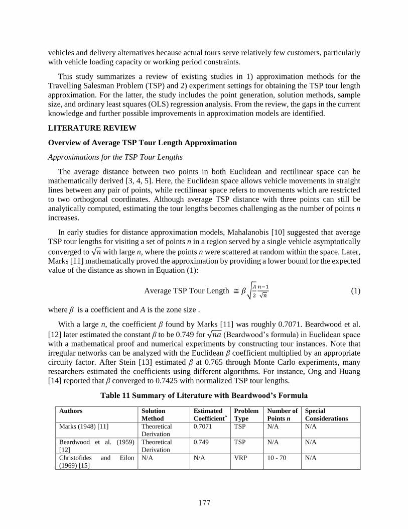
177

vehicles and delivery alternatives because actual tours serve relatively few customers, particularly

with vehicle loading capacity or working period constraints.

This study summarizes a review of existing studies in 1) approximation methods for the

Travelling Salesman Problem (TSP) and 2) experiment settings for obtaining the TSP tour length

approximation. For the latter, the study includes the point generation, solution methods, sample

size, and ordinary least squares (OLS) regression analysis. From the review, the gaps in the current

knowledge and further possible improvements in approximation models are identified.

LITERATURE REVIEW

Overview of Average TSP Tour Length Approximation

Approximations for the TSP Tour Lengths

The average distance between two points in both Euclidean and rectilinear space can be

mathematically derived [3, 4, 5]. Here, the Euclidean space allows vehicle movements in straight

lines between any pair of points, while rectilinear space refers to movements which are restricted

to two orthogonal coordinates. Although average TSP distance with three points can still be

analytically computed, estimating the tour lengths becomes challenging as the number of points n

increases.

In early studies for distance approximation models, Mahalanobis [10] suggested that average

TSP tour lengths for visiting a set of points n in a region served by a single vehicle asymptotically

converged to √𝑛 with large n, where the points n were scattered at random within the space. Later,

Marks [11] mathematically proved the approximation by providing a lower bound for the expected

value of the distance as shown in Equation (1):

Average TSP Tour Length ≅ 𝛽√𝐴

2

𝑛−1

√𝑛 (1)

where β is a coefficient and A is the zone size .

With a large n, the coefficient β found by Marks [11] was roughly 0.7071. Beardwood et al.

[12] later estimated the constant β to be 0.749 for √𝑛𝑎 (Beardwood’s formula) in Euclidean space

with a mathematical proof and numerical experiments by constructing tour instances. Note that

irregular networks can be analyzed with the Euclidean β coefficient multiplied by an appropriate

circuity factor. After Stein [13] estimated β at 0.765 through Monte Carlo experiments, many

researchers estimated the coefficients using different algorithms. For instance, Ong and Huang

[14] reported that β converged to 0.7425 with normalized TSP tour lengths.

Table 11 Summary of Literature with Beardwood’s Formula

Authors Solution

Method

Estimated

Coefficient*

Problem

Type

Number of

Points n

Special

Considerations

Marks (1948) [11] Theoretical

Derivation

0.7071 TSP N/A N/A

Beardwood et al. (1959)

[12]

Theoretical

Derivation

0.749 TSP N/A N/A

Christofides and Eilon

(1969) [15]

N/A N/A VRP 10 - 70 N/A

178

* the estimates β in the Euclidean space were listed

** Salesman’s origin (e.g., a depot) was positioned at a fixed location

*** The studies considered other decision variables or other terms from Beardwood’s

formula, such as the spatial distribution and variance of points

**** Clarke and Wright, Fisher and Jaikumar, and Gillet and Miller algorithm

Fiechter [19] found the constant β at 0.7298 for large values of n ranging from 500 to 100,000.

Lee and Choi [20] showed β to be 0.721, while Percus and Martin [22] estimated β to be 0.7120 ±

0.0002 in Euclidean space. Johnson et al. [23] generated large sets of points with n up to 100,000

and found the constant β to be 0.7124 within the 95% confidence intervals of ± 0.0002. Note that

the multiplier β is correlated with the value of n [32]. Applegate et al. [5] estimated the coefficient

β by running a regression on the optimized TSP solution instances for randomly generated n

ranging from 100 to 2000. Lei et al. [30] used a similar approach to Applegate et al. [5] where n

ranged between 20 and 90. With the two studies combined, the estimated β asymptotically

Stein (1977) [13] Partition

Heuristic

0.765 TSP N/A N/A

Daganzo (1984) [16] Theoretical

Derivation

0.9

TSP N/A Shape of a Space

Ong and Huang (1989) [14] 3-optimal

Heuristic

0.7425 TSP 5 – N/A N/A

Brunetti et al. (1991) [17] Cavity Method 0.7251 TSP 50 - 800 N/A

Chien (1992) [18] Exact Solution

0.88** TSP 5 - 30 Shape of a Space

Fiechter (1994) [19] Parallel Tabu

Search

0.7298 TSP 500 –

100,000

N/A

Lee and Choi (1994) [20] Multicanonical

Annealing

0.7239 ~

0.8075

TSP 50 - 40,000 N/A

Kwon et al. (1995) [21] Exact Solution -** TSP 10 - 80 Shape of a Space

Percus and Martin (1996)

[22]

Chained local

optimization

0.7120

± 0.0002

TSP 12 - 100 N/A

Johnson et al. (1996) [23] Iterated Lin-

Kernighan

0.7124

± 0.0002

TSP 100 –

100,000

N/A

Finch (2003) [24] N/A 0.62499 ~

0.91996

TSP N/A N/A

Hindle and Worthington

(2004) [25]

Cheapest

Insertion

-*** TSP 5 - 50 Point Distribution

Robusté et al. (2004) [26] Three Heuristic

Algorithms****

-*** TSP,

VRP

15 - 139 Shape of a Space

Figliozzi (2008) [27] Monte Carlo

Simulation

-*** VRP N/A Point Distribution,

and Depot location

Applegate et al. (2011) [5] Cutting-plane

method

0.7764689

~ 0.7241373

TSP 100 –

2,500

N/A

Cavdar and Sokol (2015)

[28]

Exact Solution

-*** TSP N/A Point Distribution,

Shape of a Space

Mei (2015) [29] Cutting-plane

method

-*** TSP,

VRP

N/A Point Distribution

Lei et al. (2016) [30] The Concorde

TSP Solver

0.8584265

~ 0.7773827

TSP 20 - 90 N/A

Nicola et al. (2019) [31] Pilot Method -*** TSP,

VRP

25 – 1,000 Time Window,

Demands

179

approached an interval ranging from 0.7256264 to 0.8584265 and had a downward trend as n

increased, as shown in Table 1. More rigorous bounds were found between 0.62499 and 0.91996

in other studies [20, 29].

Approximations for TSP Variants and VRP Tour Lengths

For the TSP variants and Vehicle Routing Problem (VRP), many researchers have attempted to

estimate the coefficient β through both analytical and experimental studies, for different

operational settings such as considered vehicle capacity, zone shape, geometry, or point

distributions. The major difference between the TSP and VRP is whether the problem considers

vehicle loading capacities, time constraints, or time windows [34]. Therefore, the TSP solution

would have a single route served by one vehicle, while the VRP has multiple routes possibly served

by multiple vehicles. Therefore, the number of vehicles should be known a priori for VRP

problems. Alternatively, the single TSP route can be split into several equal tours with an

optimistic assumption that a penalty in terms of extra travel distance does not exist [7].

Christofides and Eilon [15] first incorporated a vehicle capacity per tour in the formula and

suggested approximations to the VRP tour length based on the shape and area of a region. Daganzo

[16] proposed an intuitive approximation for a generic irregular district; a space was divided into

multiple subareas containing clusters of points. A vehicle route was developed to serve each

cluster. In this setting, he estimated β at 0.9 for Euclidean and 1.15 for rectilinear space. Although

β for the Euclidean might overpredict the tour distance, it suited spaces with typical shapes.

Chien [18] derived the constant β at 0.88 through empirical simulations and multiple

regressions. The paper considered 16 different shapes varying in the 1) elongation and 2) angle of

a space. Rectangular areas with different length-to-width ratios from 1 to 8 were proposed in Figure

2 (a). Sectorial-shaped areas were developed with eight central angles from 45° to 360° as

illustrated in Figure 2 (b). The starting point (i.e., a depot) was positioned at the lower left side of

the district. From generated TSP instances, the best-fitted coefficients for Beardwood’s formula

were derived though OLS regression.

(a) Elongation for Rectangular Areas

180

(b) Angle of Sectorial-shaped Areas

Figure 2 Shape of Areas Developed by Chien [18]

Aside from the widely used form of Beardwood, later studies included various terms in the

models, such as a length-to-width ratio or area of the smallest rectangle that covered all points.

Kwon et al. [21] carried out both simulations and OLS regressions to test the previous variations

(i.e., Beardwood et al. [12], Daganzo [16], and Chien [18]). That research team also compared

results from the regression with a neural network (NN) model in estimating the TSP tour length;

the latter model provided slightly better approximations than the former. However, the NN model

was difficult to interpret geometrically due to its characteristic as a so-called “a black box”, where

the model would not give any insights. Hindle and Worthington [25] approximated the average

TSP tour length through simulations and regressions as shown in Equation (2).

Average TSP distance = a × n + 𝑏 × ln(𝑛) + 𝑐 (2)

where a, b, and c are constants in a 100 x 100 unit square. a = 3.63, b = 85.78, and c = 62.67. Two

models were proposed based on demand patterns, namely uniformly random and probabilistic

point distribution. The probabilistic demands were designed to simulate point distributions and

settlement patterns.

Special Considerations in Tour Length Approximations

Later studies for TSP approximations, considered zone shape, geometry, or point distributions. An

extended version of Daganzo’s approximation [16] that considered circular and elliptical spaces

was proposed by Robusté et al. [26]. Figliozzi [27] proposed VRP tour length approximations

using six different spatial distributions. His models also considered time windows, demands, and

depot location. The study showed that time windows negatively affected the accuracy of the

models; the time windows increased travel distance not only because the number of routes was

increased but also because the distance between points per route was increased. Cavdar and Sokol

[28] developed approximations where the point distribution was not uniform and random. The

approximation models consisted of a few variables (e.g., the standard deviations of coordinates

and of distances between the point and center in a region). The models were tested with different

spatial distributions, including uniform and triangular distribution. In addition, the models also

performed well for various shapes of a space, such as triangular or polygon district. Mei [29]

incorporated spatial distributions in approximating the tour lengths. The average nearest neighbor

181

index was introduced for measuring the dispersion of points; the index utilized the distance

between centroid and each point. As the point distribution changed from dense (e.g., clustered) to

dispersed, the estimates for β increased linearly. Nicola et al. [31] proposed approximations based

on regression models by adding more variables, such as time windows, vehicle capacities, and

demands. The proposed model was compared with the previous models from Cavdar and Sokol

[28] and from Hindle and Worthington [25].

Guidelines for Using Distance Approximations

Larson and Odoni [7] pointed out that all these expressions could provide a good approximation

if 1) one of the measurements (e.g., width) of space was not much greater than the other

measurement (e.g., length) of a region, and 2) no obstructions or boundaries existed in the region.

Such conditions for a tour’s operating zone were generally called “fairly compact and fairly

convex.” For a rigorous definition for the rule of thumb, numerous measures for both compactness

and convexity had been proposed in the literature. Compactness measures were borrowed from

geometric concepts, such as perimeters, areas, centroids, and vertices [35]. Some measures are as

follows; 1) length-width ratio: the ratio between the length and width of the minimum bounding

rectangle. 2) convex hull: the ratio of the area between the space and minimum bounding convex

hull (i.e., the smallest convex polygon containing all the given points). 3) Polsby-Popper: the ratio

of the area of the space to the squared perimeter of the space. Similarly, convexity measures have

been based on the area or boundary of a space [36]. A boundary-based convexity measure is

computed as the ratio of the perimeter of a space and that of convex hull. An area-based convexity

measure computes the normalized average visible area of a space, divided by the area of the space

[33, 34]. The latter method is slightly more challenging to compute.

Experimental Approach

Experiment Procedures: Point Generations, Heuristics, and Sample Size

Figure 3 Overall Process for Estimating Beardwood's Coefficient β

182

Except for the theoretical derivations of Beardwood’s coefficients in Table 1, this section shed

light on the derivation of the estimates β from experiments. The experimental method is illustrated

in Figure 3. First, points (i.e., nodes or visited sites) are generated uniformly and randomly in a

unit space whose area is one.. For the point generation, most studies focus on a random and uniform

distribution, while the shape of space is limited to a unit square. Random numbers provided in

recent simulation programs are generated with the congruential algorithm, which has been widely

used in programming to mimic randomness [39]. By generating two random numbers uniformly

distributed in the interval (0,1), the numbers are regarded as a x- and y-coordinate of a point in the

space; each point in the x-y plane with both x and y between 0 and 1 is equally likely to be selected.

Second, a solution method is chosen to compute optimized TSP tour lengths. For every TSP run,

the visited points are regenerated after the TSP solution is obtained. From Table 1, no clear

preference or explanation is apparent from researchers in choosing the solution method.

Furthermore, no consensus exists on the “best” heuristic algorithm for solving the TSP instances,

as shown in Table 2; ranks imply the lowest TSP solution, while percentage differences show the

ratio between the best solution and the solution obtained by the selected heuristic method. This is

done mainly because the results sensitively vary with some parameter values of heuristic methods

and computation time.

In Adewole et al. [40], a simulated annealing (SA) procedure for the optimized TSP tour lengths

ranging from n of 10 to 60 performed better than a genetic algorithm (GA). The GA provided a

good solution if the time was sufficient meaning that a large population size was provided. In

contrast, Damghanijazi and Mazidi [41] showed that the GA performed the best in searching for

the TSP solution for 10- and 59-points, individually; the SA and hill climbing method were the

worst. More comparisons for the performance of heuristic had been carried out by Gupta [42],

Ansari et al. [6], Abdulkarim and Alshammari [43], and Gupta [44]. For a study conducted by

Antosiewicz et al. [45], six well-known metaheuristic algorithms were compared for n values

ranging from 20 to 80. The key idea was to find the best solution method when the computation

time was restricted (e.g., 100 seconds). The authors presented several criteria for performance

(e.g., accuracy, computation time, and standard deviation); however, none of the algorithms

outperformed the others for all the suggested criteria. Third, repeated iterations on a given n are

produced. After the predefined iterations for each n are reached (e.g., 1,000 runs per n values), the

TSP tour lengths for each n value are averaged. Then, the repeated runs move next for n+1. Finally,

the averaged TSP tour length is fitted with OLS regression.

183

Table 12 Comparison of Heuristic Algorithms

* SA: Simulated Annealing, TS: Tabu Search, GA: Genetic Algorithm, MA: Memetic Algorithm,

BCO: Bee Colony Optimization, ACO: Ant Colony Optimization, FA: Firefly, CS: Cuckoo Search,

HC: Hill Climbing, PSO: Particle Swarm Optimization, NN: Nearest Neighbor, GH: Greedy

Heuristic, HS: Harmony Search, and FA: Firefly

The recommended sample size (i.e., the number of intervals in the 3rd column of Table 2) for

running a regression should exceed 23 according to Green [46]. Green compiled a comprehensive

guide for choosing the minimum sample size as a function of the number of independent variables

and effect size (e.g., a correlation between two variables); the effect size referred to standardized

measures of the size of the mean difference, which generally used in multiple regression analysis.

Many metrics could be used for deriving the effect size, such as Cohen’s d (t distribution) or ω (χ2

distribution). If the effect size was small, a large number of observations were needed. Sample

SA TS GA MA BCO ACO FA CS HC PSO NN GH HS

Rank 1 2

% difference 0.0 1.7

Rank 1 2 7 6 8 3 3 3

% difference 0.0 0.0 -5.6 -5.7 -5.2 -5.7 -5.7 -5.7

Rank 5 1 2 4 3

% difference N/A N/A N/A N/A N/A

Rank 1 2

% difference 0.0 24.9

Rank 1 2

% difference 0.0 5.7

Rank 7 8 3 6 5 4 2 1

% difference -19.4 -19.4 -2.2 -7.3 -4.4 -2.2 -2.2 0.0

Rank 1 2

% difference 0.0 50.2

Rank 1 2 3

% difference 0.0 32.8 8.4

Rank 1 2

% difference 0.0 39.0

Rank 1 2

% difference 0.0 4.4

Rank 1 2

% difference 0.0 11.9

Rank 3 1 2

% difference 18.5 0.0 11.2

Rank 6 8 3 4 7 5 2 1

% difference 111.6 159.4 0.1 0.4 128.4 10.3 0.1 0.0

Rank 3 5 3 7 6 8 2 1

% difference 0.5 0.8 0.5 3.8 2.3 7.4 0.5 0.0

Rank 1 2

% difference 0.0 25.4

Rank 1 2

% difference 0.0 3.3

Rank 1 2

% difference 0.0 20.3

Rank 1 2

% difference 0.0 32.9

Rank 1 2

% difference 0.0 23.4

Rank 3 1 2

% difference 35.0 0.0 21.6

Rank 7 8 4 6 5 2 3 1

% difference 197.6 215.5 4.0 6.9 4.5 0.0 1.6 0.0

Rank 5 1 2 4 3

% difference N/A N/A N/A N/A N/A

Rank 1 N/A 2

% difference 0.0 N/A 24.0

Rank 3 1 2

% difference 50.4 0.0 39.2

Rank 2 3 1

% difference 9.3 14.4 0.0

Rank 3 1 2

% difference 45.7 0.0 36.8100

Gupta et al

(2020)N/A N/A N/A

100Abdulkarim and

Alshammari N/A N/A N/A

75Gupta et al

(2020)N/A N/A N/A

N/A N/A

60Adewole et al

(2012)N/A

N/A

51 Gupta (2013) N/A

59Damghanjiza

(2017)N/A N/A

50Ansari et al.

(2015)N/A N/A

50Gupta et al

(2020)N/A N/A

42Ansari et al.

(2015)N/A N/A

50Adewole et al

(2012)N/A N/A

30Ansari et al.

(2015)N/A N/A

40Adewole et al

(2012)N/A N/A

29 Gupta (2013) N/A

30 Gupta (2013) N/A

25Gupta et al

(2020)N/A N/A N/A

25Adewole et al

(2012)N/A N/A

25Ansari et al.

(2015)N/A N/A

N/A

20Ansari et al.

(2015)N/A N/A

20Adewole et al

(2012)N/A N/A

20Abdulkarim and

Alshammari

Elongated

SpaceN/A N/A

15Ansari et al.

(2015)N/A N/A

16 Gupta (2013) N/A

N/A

15Adewole et al

(2012)N/A N/A

10 Gupta (2013) N/A

10Damghanjiza

(2017)

Not a random

point generationN/A N/A N/A

# of

PointsCategory Authors Note

Solution Method

10Adewole et al

(2012)N/A N/A

184

sizes ranged from 23 (large effect size), 53 (medium effect size) and 400 (small effect size).

Alternatively, the number of iterations should be greater or equal to 50 plus 8 multiplied by the

number of estimates (e.g., one n for this case). This guideline for calculating the instance size is

simple and easy to use for a parsimonious model.

Literature with Experimental Approaches

Table 3 summarizes the experiment settings for distance approximations from the literature. Ong

and Huang [14] used 25 iterations for each n value starting from n = 5. In their experiments, the

sample variable of the optimized TSP tour length was shown to fluctuate, as shown in Figure 4.

Table 13 Summary of Studies with Experiments for TSP/VRP Tour Approximation

Authors Number of

points n

Number of

intervals

Increment

for n

Iterations

per n*

Shape of

space

Problem

type

Ong and Huang (1989)

[14]

5 – N/A N/A Irregular 25 Square TSP

Brunitti et al. (1991) [17] 50 – 800 5 2x** 500 –

20,000

Square TSP

Fiechter (1994) [19] 500 – 100,000 8 Irregular 10 – 30 Square TSP

Lee and Choi (1994) [20] 50 – 40,000 14 Irregular 4 – 1,300 Square TSP

Kwon et al. (1995) [21] 10 – 80 8 10 10 Irregular TSP

Percus and Martin (1996)

[22]

12 – 100 8 Irregular 5 – 20 Square TSP

Johnson et al. (1996) [23] 100 – 100,000 7 √10x** 2 – 2,098 Square TSP

Hindle and Worthington

(2004) [25]

5 – 50 46 1 500 Square TSP

Applegate et al. (2011)

[5]

100 – 2,500 13 Partially

Irregular

10,000 Square TSP

Lei et al. (2016) [30] 20 – 90 8 10 100 Square TSP

Nicola et al. (2019) [31] 25 – 1,000 N/A N/A 130 – 400 Square VRP

* Iterations here imply random configurations of point distribution for each n (e.g., Point

generation in Figure 3)

** x implies ‘a factor of’

185

Figure 4 Sample Variance of Optimized TSP Tour Lengths by Ong and Huang [14]

Brunetti et al. [17] found TSP solutions for their selected n values, which were 50, 100, 200,

400, and 800. For each n, iterations ranged from 500 to 20,000. Lee and Choi [20] conducted

different iterations for the selected 14 interval of n values, where the values ranged from 50 to

40,000. As few as four iterations were used for large n values (i.e., n = 40,000), while 1,300

iterations were conducted for small n values (i.e., n = 50).

Using the eight intervals of n, Fiechter [19] ran 10 to 30 iterations for each n. Since Kwon et

al. [21] separated training and testing sets for the optimized TSP tour lengths, the number of

instances was smaller than in other studies. For Johnson et al. [23], n ranged from 100 to 100,000

points, increasing by factors of √10. The exact TSP tour lengths were obtained for n values

between 100 and 316. Then, the number of iterations decreased as n increased. Percus and Martin

[22] derived the TSP instances for the eight n values between 12 and 100; iterations were

conducted between 5 and 12 runs. Unlike other researchers, Hindle and Worthington [25]

conducted the iterations using continuous intervals n.

Applegate et al. [5] ran 10,000 iterations for generating the TSP instances visiting each n values.

In their experiments, an increment of 100 was chosen for n between 100 and 1,000. Beyond n =

1000, the increment of 500 was selected between 1,500 and 2,500 for n values. In Lei et al. [30]

experiments were conducted with 100 iterations for each n ranging from 20 to 90. The number of

iterations for large n increased in Nicola et al. [31]. Since half of the TSP instances were used for

test sets, the unused instances were excluded in Table 3. In brief, the number of iterations per n

was arbitrary. Some researchers suggested descriptive statistics (e.g., mean or standard deviation)

and normality test for the obtained TSP instances [1, 13, 19]. From this, one can better understand

the central tendency and variability of the generated TSP instances. In addition, the instances with

small n values can be compared with those for large n values.

SUMMARY

Most reviewed studies focused on the derivation of asymptotic coefficients for the TSP tour

length; the estimated coefficients were based on a relatively large number of points visited per

186

tour, at least five or more visited points in the 5th column of Table 1 [14, 21]. However, without

using the approximations estimated with appropriate n values, the approximated distances would

be underestimated. First, this is attributed to a downward trend of the square root form √𝑛, As

more the optimized TSP instances from large n values are used for fitting a regression, smaller

coefficients would be estimated. Second, a larger increment in intervals (observable in the 4th

column of Table 3) results in a smaller value of the coefficient β. Since the smaller intervals

produce a larger deviation in the instances (i.e., samples), the estimated β would decrease. In other

words, regression results with the omitted intervals (i.e., missing samples) of n underestimate the

coefficients due to small mean and large deviation in deriving β. Such a small mean is attributed

to the fact that the TSP tour length increases non-linearly (i.e., with √𝑛) as n increases. Except for

Hindle and Worthington [25], researchers have used a discrete interval of n as an independent

variable for regression.

In experimental approaches for Beardwood’s coefficients, the number of iterations for

obtaining the optimal TSP tour length significantly varied in the existing studies, as shown in the

5th column of Table 2. Kwon et al. [21], Applegate et al. [5], and Lei et al. [30] used the same runs

across all n values, while others did not present any criteria for the number of iterations (e.g., less

iterations for large n, and vice versa). Therefore, consistent runs would help in providing

descriptive statistics of each n (e.g., mean, median, standard deviation, skewness or kurtosis); the

dataset of the optimum tour lengths can be investigated further, such as by using sample variance

provided in Ong and Huang [14] in Figure 4. In addition, the estimates for β change not only with

the value of n but also with other factors (e.g., the point distribution or shape of space).

Lastly, the VRP and distribution-free approximations may be less flexible than the TSP models

due to the required variables that were often unavailable or known a priori, such as the number of

vehicles, length-to-width ratio, predetermined number of routes, or standard deviations of a point

distribution in space.

Therefore, the approximations providing the estimates for few points would open new research

avenues for analyzing and planning such systems (e.g., paratransit and deliveries by drones or

robots).

POSSIBLE EXTENTIONS

Some potential extensions beyond the existing literature are suggested below.

1. Distance metrics: two types of distance measures can be considered, namely Euclidean and

rectilinear. In Euclidean space, movement directions are unrestricted and, hence, the

shortest air distances apply. In rectilinear space where movements are restricted to two

orthogonal coordinates, as in rectangular grid street networks, travel distances are longer.

For irregular networks distances can be approximated by multiplying Euclidean distances

with appropriately computed circuity factors.

2. Shape of service area: although an exact shape of service area varies with roadway

geometry, the basic shape categories to be considered are square and circular. The

elongations of area can be further investigated by changes in length-to-width ratio.

3. Distribution of points: the effects of concentrations of points n toward a particular direction

(e.g., non-uniform distribution of the points) or in certain clustering patterns may be

explored.

4. Approximations for tour distances with time windows may be developed.

187

5. Approximations for tours by vehicles with limited capacity, which may constrain the

sequence of pickups and drop-offs, may be developed.

AUTHOR CONTRIBUTION STATEMENT

The authors confirm contributions to the paper as follows: study conception and design: Y. Choi,

P. Schonfeld; analysis and interpretation of results: Y. Choi, P. Schonfeld; data collection: Y. Choi;

draft manuscript preparation; Y. Choi, P. Schonfeld. All authors reviewed the results and approved

the final version of the manuscript.

ACKNOWLEDGEMENT

The authors thank the University Mobility and Equity Center led by Morgan State University which

partially funded this study.

188

REFERENCES

[1] Chang, S.K. and Schonfeld, P. Optimization Models for Comparing Conventional and

Subscription Bus Feeder Services. Transportation. Science, Volume. 25. No. 4, Nov. pp. 281-298.

1991. https://doi.org/10.1287/trsc.25.4.281

[2] Kim, M. and Schonfeld, P. Integration of Conventional and Flexible Bus Services with Timed

Transfers. Transportation. Research Part B: Methodological, 68B-2, pp. 76-97. 2014.

https://doi.org/10.1016/j.trb.2014.05.017

[3] Choi, Y., Schonfeld, P., Lee. Y., and Shin, H. Innovative Methods for Delivering Fresh Food

to Underserved Populations. Journal of Transportation Engineering, Part A: Systems. 2020.

https://dot.org.10.1061/JTEPBS.0000464

[4] Holguín-Veras, J., and G. R. Patil. Observed Trip Chain Behavior of Commercial Vehicles. In

Transportation Research Record: Journal of the Transportation Research Board, No. 1906, pp. 74–

80. 2005. https://doi.org/10.1177/0361198105190600109

[5] Applegate, D., Bixby, R., Chvatal, V., and Cook, W. The Traveling Salesman Problem: A

Computational Study. Princeton University Press. 2006.

[6] Ansari, S., Basdere, M., Li, X., Ouyang, Y., and Smilowitz, K. Advancements in Continuous

Approximation Models for Logistics and Transportation Systems: 1996–2016. Transportation

Research Part B, 107. 2018. https://doi.org/10.1016/j.trb.2017.09.019

[7] Larson, R., and Odoni, A. Urban Operation Research. Dynamic Ideas. 1981.

[8] Phillip, J. The Probability Distribution of the Distance Between Two Random Points in a Box.

KTH mathematics, Royal Institute of Technology, 2007.

[9] Burgstaller, B and Pillichshammer, F. The Average Distance Between Two Points. Bulletin of

the Australian Mathematical Society, Volume. 80, no. 3, pp. 353–359, 2009.

https://doi.org/10.1017/S0004972712000354

[10] Mahalanobis, P. A Sample Survey of the Acreage under Jute in Bengal. The Indian Journal

of Statistics, Volume. 4, no. 4, pp. 511-530, 1940. https://www.jstor.org/stable/40383954

Accessed Jul. 26. 2020.

[11] Marks, E. A Lower Bound for the Expected Travel Among m Random Points. The Annals

of Mathematical Statistics, Volume. 19, no. 3, pp. 419-422, 1948.

https://www.jstor.org/stable/2235651 Accessed Jul. 26. 2020.

[12] Beardwood, J., Halton, J., and Hammersley, J. The Shortest Path through Many Points.

Mathematical Proceedings of the Cambridge Philosophical Society, vol 55, pp. 299–327, 1959.

[13] Stein, D. M. An Asymptotic Probabilistic Analysis of a Routing Problem. Mathematics of

Operations Research. Vol 3. No. 2. pp. 89–101. 1978. https://www.jstor.org/stable/3689335

Accessed Jul. 26. 2020.

[14] Ong, H. L., H. C. Huang. Asymptotic Expected Performance of Some TSP Heuristics: An

Empirical Evaluation. European Journal of Operational Research 43, 231–238. 1989.

https://doi.org/10.1016/0377-2217(89)90217-8

189

[15] Christofides, N., & Eilon, S. (1969a). Expected Distances in Distribution Problems. OR,

20(4), 437–443. http://doi.org/10.2307/3008762

[16] Daganzo, C. The Length of Tour in Zones of Different Shapes. Transportation Research Part

B: Methodology, Volume. 18B, no. 2, pp. 135–145, 1984. https://doi.org/10.1016/0191-2615(84)90027-4

[17] Brunetti, R., Krauth, W., Mézard, M., and Parisi, G. Extensive Numerical Simulations of

Weighted Matchings: Total Length and Distribution of Links in the Optimal Solution. Europhysics

Letters, Volume. 14, No. 4. 1991. https://doi.org/10.1209/0295-5075/14/4/002

[18] Chien, T. W. Operational Estimators for the Length of a Traveling Salesman Tour. Computers

& Operations Research, 19(6), 469–478. 1992. https://doi.org/10.1016/0305-0548(92)90002-M

[19] Fiechter, C., A Parallel Tabu Search Algorithm for Large Traveling Salesman Problems.

Discrete Applied Mathematics. 51, 243-267. 1994. https://doi.org/10.1016/0166-218X(92)00033-I

[20] Lee J., Choi M.Y. Optimization by Multicanonical Annealing and the Traveling-Salesman

Problem. Computer Simulation Studies in Condensed-Matter Physics VII. Volume. 78. pp. 193-

198. Springer, 1994.

[21] Kwon, O., Golden, B., and Wasil, E. Estimating the Length of the Optimal TSP Tour: An

Empirical Study Using Regression and Neural Networks. Computers & Operations Research,

22(10), pp. 1039–1046. 1995. https://doi.org/10.1016/0305-0548(94)00093-N

[22] Percus, A., and Martin, O. Finite size and dimensional dependence in the Euclidean traveling

salesman problem, Physical. Review. Letter. 76. 1996. 1188–1191.

https://doi.org/10.1103/PhysRevLett.76.1188

[23] Johnson, D., McGeoch, L., and Rothberg, E. Asymptotic Experimental Analysis for the Held-

Karp Traveling Salesman Bound. Proceedings of the 7th Annual ACM-SIAM Symposium on

Discrete Algorithms. 1996, 341-350

[24] Finch, S. Mathematical Constants. Cambridge University Press, Cambridge. 2003.

[25] Hindle A, Worthington D. Models to Estimate Average Route Lengths in Different

Geographical Environments, Journal of the Operational Research Society, 2004.

https://doi.org/10.1057/palgrave.jors.2601751

[26] Robusté, F., Estrada, M., and López-Pita, A. Formulas for Estimating Average Distance

Traveled in Vehicle Routing Problems in Elliptic Zones. Transportation Research Record: Journal

of the Transportation Research Board, No. 1873, pp. 64–69. 2004. https://doi.org/10.3141/1873-08

[27] Figliozzi, M, Planning Approximations to the Average Length of Vehicle Routing Problems

with Varying Customer Demands and Routing Constraints, Transportation Research Record:

Journal of the Transportation Research Board, No. 2089, pp. 1–8. 2008.

https://doi.org/%2010.3141/2089-01

190

[28] Cavdar, B., and Sokol, J. A Distribution-free TSP Tour Length Estimation Model for Random

Graphs, Volume. 243, no. 2, pp. 588-598, 2015. https://doi.org/10.1016/j.ejor.2014.12.020

[29] Mei, X. Approximating the Length of Vehicle Routing Problem Solutions Using

Complementary Spatial Information. George Mason University. 2005.

http://mars.gmu.edu/handle/1920/9623 Accessed Jul. 26. 2020.

[30] Lei, H., Laporte, G., Liu, Y., and Zhang, T. Dynamic Design of Sales Territories. Computers

& Operations Research Volume 56, pp. 84-92. 2015. http://dx.doi.org/10.1016/j.cor.2014.11.008

[31] Nicola, D., Vetschera, R., and Dragomir, A. Total Distance Approximations for routing

solutions, Computers and Operations Research 102. pp. 67–74. 2019.

https://doi.org/10.1016/j.cor.2018.10.008

[32] Franceschetti, A., Jabali, O. & Laporte, G. Continuous Approximation Models in Freight

Distribution Management. TOP 25, pp. 413–433. 2017. https://doi.org/10.1007/s11750-017-0456-1

[33] Arlotto, A., and Steele, M. Beardwood–Halton–Hammersley Theorem for Stationary Ergodic

Sequences: a Counterexample. The Annals of Applied Probability. Volume. 26, No. 4, pp. 2141–

2168. 2016. https://doi.org/10.1214/15-AAP1142

[34] Kumar, S., and Panneerselvam, R. A Survey on the Vehicle Routing Problem and Its Variants.

Intelligent Information Management, Volume. 4. No. 3. pp. 66-74. 2012.

http://dx.doi.org/10.4236/iim.2012.43010

[35] Kaufman, A., King, G., Komisarchik, M. How to Measure Legislative District Compactness

If You Only Know it When You See it. American Journal of Political Science. 2017

[36] Zunic, J., and Rosin, P. A New Convexity Measure for Polygons, IEEE Transactions on

Pattern Analysis and Machine Intelligence. Volume. 26, No. 7, 2004.

[37] Stern, H. Polygonal Entropy: A Convexity Measure. Pattern Recognition Letters, Volume.

10, pp. 229-235, 1989. https://doi.org/10.1016/0167-8655(89)90093-7

[38] Rote, G., The Degree of Convexity, EuroCG 2013, Braunschweig, Germany, 2013.

[39] Moler, C. Numerical Computing with MATLAB. Society for Industrial and Applied

Mathematics. 2008.

[40] Adewole. A., Otubamowo, K., Egunjobi, T. A Comparative Study of Simulated Annealing

and Genetic Algorithm for Solving the Travelling Salesman Problem. International Journal of

Applied Information Systems. Volume. 4. No.4, 2012.

[41] Damghanijazi, E., and Mazidi, A. Meta-Heuristic Approaches for Solving Travelling

Salesman Problem, International Journal of Advanced Research in Computer Science, Volume. 8

No. 5. 2017.

[42] Gupta, D. Solving TSP Using Various Meta-Heuristic Algorithms, International Journal of

Recent Contributions from Engineering, Science & IT. Vol 1, No 2. 2013.

191

[43] Abdulkarim, H., and Alshammari, I. Comparison of Algorithms for Solving Traveling

Salesman Problem, International Journal of Engineering and Advanced Technology, Volume. 4.

Issue. 6, 2015

[44] Gupta, S., Rana, A., and Kansal, V. Comparison of Heuristic Techniques: A case of TSP. 10th

International Conference on Cloud Computing, Data Science & Engineering. 2020.

https://doi.org/10.1109/Confluence47617.2020.9058211

[45] Antosiewicz, M., Koloch, G., and Kamiński, B. Choice of Best Possible Metaheuristic

Algorithm for the Travelling Salesman Problem with Limited Computational Time: Quality,

Uncertainty and Speed. Journal of Theoretical and Applied Computer Science Volume. 7, No. 1,

pp. 46-55. 2013

[46] Green, S.. How Many Subjects Does It Take To Do A Regression Analysis. Multivariate

Behavioral Research, Volume. 26, pp. 499–510. 1991.

https://doi.org/10.1207/s15327906mbr2603_7

192

Appendix 8 - Liu, J., Schonfeld, P., Zhan, S., Peng, Q. and Yong, Y. “The Value of

Reserve Capacity Considering the Reliability and Robustness of a Rail Transit

Network,” submitted to Reliability Eng. & System Safety, Oct. 2020

The value of reserve capacity considering the reliability and

robustness of a rail transit network

Jie Liua,b; Paul M. Schonfeldb*; Shuguang Zhana; Qiyuan Penga; Yong Yina*

a School of Transportation and Logistics, Southwest Jiaotong University, National United Engineering

Laboratory of Integrated and Intelligent Transportation, National Engineering Laboratory of Integrated

Transportation Big Data Application Technology, Chengdu 610031, Sichuan, China.

b Department of Civil and Environmental Engineering, University of Maryland, College Park, MD 20742,

USA

* Corresponding author: Paul M. Schonfeld, E-mail addresses: pschon@umd.edu; Yong Yin, E-mail

addresses: yinyong@swjtu.edu.cn

Abstract

A model is proposed for estimating the value of reserve capacity in a rail transit network (RTN),

which consists of (1) the reduction in the passengers’ total generalized travel cost (GTC) in

normal operations, (2) the value of reliability enhancement in normal operations, and (3) the

value of robustness enhancement due to reserve capacity when disturbances occur. The

passengers’ GTC equals the fare and monetary value of passengers’ perceived travel time (PTT),

which considers the seat availability, crowding in trains as well as transfer times. The perceived

buffer time (PBT), which is the difference between the 95th and the average PTT, represents the

extra PTT needed for arriving at the destination station reliably. The value of reliability

enhancement is the monetary value of decreased PBT with and without reserve capacity when

the RTN operates normally. The value of robustness enhancement is the difference in the

193

passengers’ total GTC with and without reserve capacity when disturbances occur. The net value

of the reserve capacity equals its value minus its cost. A model for optimizing reserve capacity to

maximize net value is developed and solved with a Quantum Genetic Algorithm (QGA). A case

study of Chengdu’s RTN shows that the proposed model and method are practical and effective

for estimating the value of reserve capacity and optimizing it. This can guide policy makers and

operators in quantifying the value of reliability and robustness when expanding an RTN’s

capacity.

Keywords: Rail transit network; Reserve capacity; Net value; Network reliability; Network

robustness;

1. Introduction

Due to their advantages of environmental protection, large capacity and high speed, rail

transit networks (RTNs) have expanded rapidly in cities (Litman, 2015). With rapid urban

development, passengers expect high-quality service in rail transit (Beirão and Cabral, 2007).

However, disturbances often occur in rail transit for various reasons, such as technical and

mechanical failures, man-made damages or natural disasters. Those disturbances cause

passengers to experience reduced travel comfort, increased travel time, travel cost and travel

time uncertainty, and thus decrease the passenger service quality.

The robustness of an RTN is the network’s ability to withstand disturbances without a

significant reduction in system performance (Cats and Jenelius, 2015). A network is robust when

it reacts well to disturbances (De-Los-Santos et al. 2012), and it is reliable when it can transport

passengers to their destination within a certain time (Bell and Cassir, 2000). The reliability and

robustness of an RTN are important manifestations of transportation performance and service

quality, which play significant roles in transportation planning and policymaking. Therefore,

investments in an RTN should aim at improving the reliability and robustness of the

transportation networks, rather than just reducing the passengers’ travel time and cost (Mackie et

al. 2014). Investment analyses should evaluate and quantify the value of reliability and

robustness enhancement according to the U.S. Department of Homeland Security (U.S. DHS.,

2010) and related studies (Jeekel, 2010 and Cats, 2016).

194

Reserve capacity is an investment in an RTN network, which not only increases the

possibility of transporting passengers to their destination reliably when the network operates

normally, but also enhance the network’s ability to withstand disturbances. Thus, the reserve

capacity of an RTN can improve its reliability and robustness (Jeekel, 2010, Cats, 2016, Cats and

Jenelius, 2015). However, the value of reliability and robustness enhancement due to reserve

capacity has not been both evaluated when measuring the value of reserve capacity on an RTN.

It reduces the accuracy and reasonableness of decisions to provide reserve capacity for an RTN

network. Therefore, this paper considers the values of RTN reliability and robustness in

estimating the reserve capacity value for an RTN. Then, a model for maximizing the net value of

reserve capacity for an RTN is proposed here for the first time and solved with a Quantum

Genetic Algorithm (QGA). The proposed model and QGA can be applied practically in

determining the reserve capacity that maximizes the net value.

The remainder of this paper is organized as follows: the research on the travel time

reliability and robustness of transportation networks is reviewed in section 2. The methodology

in section 3 presents (a) the framework for evaluating the value and net value of reserve capacity,

(b) the models for measuring the value and net value of reserve capacity and (c) the model for

maximizing the net value of reserve capacity. The application of QGA to solve the net value

maximization model is presented in section 4. The proposed model and method are applied to

Chengdu’s RTN in section 5. Finally, the conclusions of the study are discussed in section 6.

2. Literature review

2.1 The travel time reliability of transportation networks

Many studies analyzed the reliability of a transportation network based on travel time

reliability (Carrion and Levinson, 2012). Various proposed metrics that measure the travel time

reliability on transportation networks are shown in Table 1. The buffer time index was widely

used for measuring travel time reliability, since it not only measured the travel time reliability,

but also guided passengers to allow additional travel time for reliably reaching their destinations.

For example, the travel time reliability on the London Underground was evaluated with the

buffer time index according to the passengers’ trip time obtained from Automatic Fare

195

Collection data (Uniman et al. 2010). The buffer time index for London bus routes was evaluated

using Automatic Vehicle Location data (Ehrlich, 2010). The design criteria for the travel time

reliability metric from the passengers’ perspective was proposed by Wood (2015) and she noted

that the buffer time index satisfies the criteria for measuring travel time reliability.

Table 1 Indicators for measuring the travel time reliability of transportation networks

Indicators Description

Coefficient of variation

(Pu, 2011) The ratio of the standard deviation to the mean.

Skewness of travel time

(Van Lint, et al. 2008)

The ratio of the difference between 90th percentile

trip time and 50th percentile trip time to the difference

between 50th percentile trip time and 10th percentile trip

time.

90th or 95th percentile trip

time (Lomax and Margiotta, 2003)

90th or 95th percentile trip time used as the reliable

travel time

Buffer time (Furth and

Muller, 2006)

The difference between the average travel time and

95th percentile travel time.

Buffer time index (Furth

and Muller, 2006)

The buffer time as a percentage of the average travel

time.

On-time arrival (Lo, et al.

2006)

The probability that a trip arrives within the travel

time budget.

Travel time unreliability

(Lomax and Margiotta, 2003) The fraction of late arriving trips

Total travel time budget

(Lo, et al. 2006)

The minimum travel time threshold that satisfies a

certain reliability requirement is given by decision-makers at

a certain confidence level.

Mean-excess total travel

time (Xu, et al. 2014)

The conditional expectation of travel times exceeding

the corresponding total travel time budget at a given

confidence level.

Although many researchers were attracted to work on measuring travel time reliability, only

a small part of them measured the value of travel time reliability. The value of time reliability

was evaluated with different methods, such as experimental design, theoretical analysis and

travel time estimation (Carrion and Levinson, 2012). Different models were proposed to measure

the value of time reliability. For example, Nam et al. (2005) expressed the value of reliability on

a road network in terms of standard deviation and maximum delay. Hensher et al. (2011)

measured the value of expected travel time savings with Multinomial and Nested Logit models.

The results showed that the value of expected travel time savings considering time reliability was

much higher than that without considering reliability. Some analytical models for measuring the

196

value of time and value of time reliability were constructed based on the utility maximization

principle (Börjesson et al. 2012 & Uchida, 2014). Although measuring the value of travel time

reliability on a transportation network has received increasing attention, most studies focused on

the value of road network reliability. A few studies have measured the value of travel time

reliability on an RTN. In recent years, researchers have started to consider passengers’ trip

details (the crowding in vehicles, seat availability as well as transfer times) when estimating the

travel time reliability and its value. These details were reflected in the passengers’ perceived

travel time (PTT) which was used by Jenelius (2018) to measure the transportation network

reliability.

2.2 The robustness of transportation networks

Many studies on the robustness of transportation networks focused on constructing

indicators for measuring topological characteristics of networks and analyzing the effects of

physical links degradation on network connectivity. The indicators included the number of cyclic

paths in the network (Derrible and Kennedy, 2010), the mean of the reciprocal of the shortest

distances among all nodes and the proportion of connected nodes in the largest connected

subgraph before and after the network was damaged (Yang et al. 2015). Researchers investigated

the impact of random interruptions and intentional attacks on the robustness of urban rail transit

networks (Derrible and Kennedy, 2010 & Zhang et al. 2011), public transportation networks

(Rodriguez-Nunez and Garcia-Palomares, 2014) and an air transportation network (Lordan et al.

2014). The results showed, unsurprisingly, that intentional attacks had a greater negative impact

on transportation networks than random interruptions. The critical links or nodes in the network

were identified according to the network performance reduction due to the failure of links or

nodes (Lordan and Albareda-Sambola 2019 & Barker, et al. 2013).

The robustness indicators proposed based on topologies of networks could be applied to a

wide range of transportation networks. However, these indicators could not measure the service

quality changes in transportation networks, such as congestion of the network, passengers’

transfer times and travel comfort. Therefore, traffic demand and transportation supply were

considered in studying the robustness of a transportation network (Mattsson and Jenelius, 2015).

Nagurney and Qiang (2007) analyzed the robustness of a road network when the capacities of

197

links decrease by utilizing Bureau of Public Road link travel cost functions and a network

efficiency measure. Muriel-Villegas et al. (2016) considered traffic flows and capacity when

deriving the vulnerability and connectivity reliability of inter-urban transportation systems under

network disruptions. Sullivan et al. (2010) identified the critical links of a road network with

link-based capacity-disruption values and quantified the network robustness of a road network.

They found that the relations among network robustness, the capacity-disruption level and

network connectivity were non-linear. Faturechi et al. (2014) proposed a stochastic integer model

to assess and maximize the resilience of an airport’s runway and taxiway network under different

potential damage scenarios, which aimed at quickly restoring post-event takeoff and landing

capacities.

The studies on measuring the robustness of transportation networks were much more than

measuring its value. Cats (2016) estimated the robustness value of public transportation

development plan based on the passengers’ travel time loss. The result showed that neglecting

the robustness value resulted in the underestimation of the benefits of plans. Jenelius and Cats

(2015) assessed the value of new links for the robustness of a rail-based public transportation

network in Stockholm, Sweden in terms of passenger welfare under disruptions. Cats and

Jenelius (2015) also estimated the value of reserve capacity for alternative links on the public

transportation network in Stockholm, which aimed at mitigating the impact of disruptions. They

used the hypothesized traffic disturbances rather than actual disturbances data to measure the

value of network robustness enhancement. Finally, they suggested that the costs of providing

reserve capacity and constructing new links, which are not estimated in their study, should be

considered when measuring the value of network robustness.

2.3 Literature review summary

Many valuable studies have been done on measuring the reliability and robustness of

transportation networks. While some models and methods have been proposed separately for

estimating the value of the reliability and robustness of road networks, only a few articles have

measured the value of reliability or robustness for RTNs. Although some studies (U.S. DHS.,

2010; Jeekel, 2010; Cats, 2016) suggest that estimating the value of an investment should

consider the value of reliability and robustness enhancement, no studies are found that estimate

198

the value of reserve capacity which is an investment in an RTN while considering the values of

both network reliability and network robustness. In addition, no model has been found for

maximizing the net value of reserve capacity while considering the value of network reliability

and network robustness.

3 Methodology

3.1 Framework for estimating the value and net value of reserve capacity

The value of reserve capacity on an RTN considering the values of reliability and

robustness is estimated from both the passengers’ perspective and the operator’s perspective.

Passengers pay attention to the reliability of the RTN, travel time, travel comfort and fare

when the RTN operates normally. The travel time, travel comfort (crowding in the vehicle and

seat availability) and fare can be comprehensively measured by the passengers’ generalized

travel cost (GTC), which equals fare and the monetary value of the perceived travel time (PTT).

A trip’s PTT is the sum of the weighted time components and increased PTT due to transfers. In

Jenelius (2018), the travel reliability is measured with perceived buffer time (PBT) which equals

the 95th percentile PTT minus the average PTT, since it represents the extra PTT needed for

arriving at the destination station with 95% on-time arrival probability.

Operators are mainly concerned with the robustness of an RTN when disturbances occur and

with the cost of providing reserve capacity. The RTN’s robustness is its ability to withstand

disturbances without a significant reduction in system performance. The system performance

here is measured by the passengers’ total GTC and an RTN’s robustness is measured by the

difference in system performance with and without disturbances.

Reserve capacity reduces the passengers’ GTC and PBT (i.e., improves travel time

reliability) when the network operates normally. Reserve capacity also enhances the RTN’s

ability to withstand disturbances (i.e., enhances robustness) when disturbances occur. Therefore,

the value of reserve capacity consists of three parts: (1) reduction in passengers’ total GTC

compared with no reserve capacity when the RTN operates normally; (2) the value of reliability

enhancement, which is the decrease in the monetary cost of PBT compared with no reserve

199

capacity when the RTN operates normally; (3) the value of robustness enhancement, which is the

reduction in passengers’ total GTC compared with no reserve capacity when disturbances occur

(Cats and Jenelius, 2015). The cost of providing reserve capacity consists of the maintenance

cost, depreciation fee, electricity cost and labor cost. The net value of reserve capacity is the

value of reserve capacity minus its cost. The value and net value of reserve capacity are

estimated in four steps, as shown in Fig.1:

Step 1: The data are prepared for the estimation.

Step 2: The passengers’ GTC and PTT are estimated by applying a stochastic user

equilibrium model (Liu et al. 2009) to assign passenger OD trips on the RTN.

Step 3: The value of reserve capacity is converted into monetary terms from the passengers’

and operator’s perspectives.

Step 4: The net value of reserve capacity is estimated.

200

Train cancelation

Waiting time In-vehicle time Fare

Step 1: prepare data

for estimation

History data

OD tripsAFC dataHeadways of lines Walking time for access, egress & transfer Capacities and seats of trains

Operation data

Crowding in trains

Fare

GTC and PTT

Components of trip Weights of trip components Value of time parameter

Net value

Value of robustness enhancement

Value of reliability enhancement

Net value = +Cost of providing reserve capacity

Known data

Reserve capacity on linesDecision variable

Disturbances Reserve capacity

Stochastic user equilibrium assignment

Calculate unknown data

Step 2: estimate

passengers GTC and PTT

Step 3: estimate value

Step 4: estimate net

value

Value measurement

Value of reduction in passengers total GTC

+

Seat availability

¯

Value Value of time parameter×

Value of reliability enhancement during normal operations

Passengers perspective

Decreased PBT PBT without reserve capacity = PBT with reserve capacity

Decreased PBT

Reduction in passengers total GTC during normal operations

Total GTC without reserve capacity = Total GTC with reserve capacity Value

¯

¯

Value of robustness enhancement when disturbances occur

GTC without reserve capacity GTC with reserve capacity Value =

Cost of providing reserve capacity

Maintenance costCost = +

Operators perspective

+Depreciation fee Electricity cost Labor cost+

¯

=

Train delays

Fig. 1 The framework for estimating the value and net value of reserve capacity.

3.2 Assumptions and notations

Some basic assumptions are made for estimating the value and net value of reserve

capacity:

A1. The direct impacts of disturbances in an RTN can be examined in train operations, i.e.

in train cancellations and delays. The train delays may cause subsequent train cancellations. To

201

reduce the number of disturbance scenarios, train delays are converted into train cancellations.

The quotient of the delay time divided by headway of the line on which it occurs is rounded to

estimate the number of canceled trains due to a train delay.

A2. Due to the disturbances, some passengers may not able to board any train. Those

passengers may transfer to other transportation modes (bus and taxi) or abandon their trips to

avoid long waits for trains. Their GTC is assumed to be the maximum GTC of passengers who

can travel on the RTN.

A3. New passengers attracted by reserve capacity are not considered. Thus, the passenger

OD trips distribution with and without the reserve capacity remains the same.

A4. The probabilities of disturbances occurring on each line are independent.

The notations used in the model formulation are listed in Table 2.

Table 2 Notation used in the model formulation.

Set Definition

𝐸 Set of links.

𝑁 Set of stations.

𝐿 Set of rail transit lines

𝑌 Set of disturbances during the analysis period.

𝑍 Set of trains running on the RTN during the analysis period.

𝑍𝑦 Set of canceled trains due to disturbance 𝑦 during the analysis period.

𝑃𝑜𝑑 Set of travel paths from station 𝑜 to station 𝑑.

Element Definition

𝑖 Rail transit line 𝑖, 𝑖 ∈ 𝐿.

𝑜 and 𝑑 Origin station 𝑜 and destination station 𝑑, 𝑜, 𝑑 ∈ 𝑁.

𝑦 Disturbance 𝑦, 𝑦 ∈ 𝑌.

𝑘 Path 𝑘 from station 𝑜 to station 𝑑, 𝑘 ∈ 𝑃𝑜𝑑 .

Parameters Definition

𝛽1, 𝛽2, 𝛽3 and

𝛽4

Value of time weights for waiting time, walking time, in-vehicle time and

transfer times, respectively.

𝛼 Value of time parameter (¥/hour).

202

𝜇1,𝑖, 𝜇2,𝑖, 𝜇3,𝑖

𝜇4,𝑖 and 𝜇5,𝑖

Maintenance cost per vehicle-hour, maintenance cost per vehicle-kilometer,

depreciation fee per vehicle-hour, electricity cost per vehicle-kilometer and labor

cost per vehicle-hour, respectively, for trains on line 𝑖 (¥).

Variables Definition

𝑏 Total number of lines on an RTN.

𝐵𝛿𝑖,𝑥 Net value of reserve capacity 𝛿𝑖,𝑥 during the analysis period (¥).

𝐵𝑘𝑜𝑑 PBT from station 𝑜 to station 𝑑 on path 𝑘 (hours).

𝐵𝑘𝑜𝑑(0,0) and

𝐵𝑘𝑜𝑑(0, 𝛿𝑖,𝑥)

PBTs from station 𝑜 to station 𝑑 on path 𝑘 without and with reserve capacity

𝛿𝑖,𝑥, respectively, during normal operations (hours).

𝐶𝛿𝑖,𝑥 Cost of providing reserve capacity 𝛿𝑖,𝑥 during the analysis period (¥).

𝐶∗ A specified cost (¥).

𝐶𝑛,𝑘𝑜𝑑 (0,0) and

𝐶𝑛,𝑘𝑜𝑑 (0, 𝛿𝑖,𝑥)

GTC for passenger 𝑛 from station 𝑜 to station 𝑑 on path 𝑘 without and with

reserve capacity 𝛿𝑖,𝑥, respectively, when the RTN operates normally (¥).

𝐶𝑛,𝑘𝑜𝑑 (𝑦, 0) and

𝐶𝑛,𝑘𝑜𝑑 (𝑦, 𝛿𝑖,𝑥)

GTC for passenger 𝑛 from station 𝑜 to station 𝑑 on path 𝑘 without and with

reserve capacity 𝛿𝑖,𝑥, respectively, when the disturbance y occurs (¥).

𝐶𝑛,𝑘𝑜𝑑 GTC for passenger 𝑛 traveling from station 𝑜 to station 𝑑 on path 𝑘 (¥).

𝑓𝑛,𝑘𝑜𝑑 Passenger 𝑛’s fare from station 𝑜 to station 𝑑 on path 𝑘 (¥).

ℎ𝑖 Minimum safe headway of line 𝑖 (hour).

𝑙𝜏,𝑖 A train’s running distance on line 𝑖 during 𝜏 hours (kilometers).

𝑚𝑘trans Passenger 𝑛’s transfer times on path 𝑘.

𝑛𝑖 Number of cars per train on line 𝑖.

𝑇𝑛,𝑘𝑜𝑑 PTT for passenger 𝑛 from station 𝑜 to station 𝑑 on path 𝑘 (hours).

𝑇𝑘,95𝑜𝑑 and 𝑇𝑘,∗

𝑜𝑑 95th percentile PTT and the mean of PTT, respectively, from station 𝑜 to station

𝑑 on path 𝑘 (hours).

𝑡𝑛,𝑘wait, 𝑡𝑛,𝑘

walk and

𝑡𝑛,𝑘in

Passenger 𝑛’s waiting time, walking time and in-vehicle time on path 𝑘 (hours).

𝑉GTC(0, 𝛿𝑖,𝑥) Value of reserve capacity 𝛿𝑖,𝑥 to reduce passengers’ total GTC during the

analysis period when the RTN operates normally (¥).

𝑉rel(0, 𝛿𝑖,𝑥) Value of reserve capacity 𝛿𝑖,𝑥 for reliability enhancement during the analysis

period when the RTN operates normally (¥).

203

𝑉rob(𝑦, 𝛿𝑖,𝑥) Value of reserve capacity 𝛿𝑖,𝑥 for robustness enhancement during the analysis

period when the disturbance 𝑦 occurs (¥).

𝑉(0, 𝛿𝑖,𝑥) and

𝑉(𝑌, 𝛿𝑖,𝑥)

Value of reserve capacity 𝛿𝑖,𝑥 during the analysis period when the RTN operates

normally and disturbances occur, respectively (¥).

𝑉𝛿𝑖,𝑥 Value of reserve capacity 𝛿𝑖,𝑥 during the analysis period (¥).

𝑣𝑜𝑑 Passenger trips from station 𝑜 to station 𝑑 during the analysis period (trips per

hour).

𝑣𝑘𝑜𝑑

Passenger trips from station 𝑜 to station 𝑑 on path 𝑘 during the analysis period

(trips per hour).

𝑧𝑖 Actual train frequency on line 𝑖 during the analysis period.

𝛿𝑖,𝑥 Providing 𝑥 reserve trains on line 𝑖 during the analysis period.

𝜏 Duration of the analysis period (hours).

𝜌 Probability that the RTN operates normally (%).

Decision

variables Definition

𝑎𝑖 A binary variable. If line 𝑖 is chosen to provide reserve capacity, then 𝑎𝑖 = 1,

otherwise 𝑎𝑖 = 0.

𝑥 The number of reserve trains on line 𝑖, which is a natural number.

3.3 RTN, disturbances and reserve capacity

An RTN is represented here as a directed and weighted graph 𝐺 = (𝑁, 𝐸). 𝑁 and 𝐸

represent the station collection and link collection, respectively, on the RTN. The set of rail

transit lines on the RTN is represented 𝐿. The set of trains running on the RTN is represented as

𝑍 during the analysis period.

Disturbances that cause train cancellations and train delays are considered in estimating the

value of reserve capacity. A set of disturbances during the analysis period in the RTN is

represented as 𝑌. 𝑍𝑦, 𝑍𝑦 ⊆ 𝑍 is the set of canceled trains due to disturbance 𝑦, 𝑦 ∈ 𝑌 during the

analysis period.

204

The reserve capacity on an RTN network is realized by providing reserve trains on lines.

The reserve capacity for line 𝑖, 𝑖 ∈ 𝐿 is represented by 𝛿𝑖,𝑥, which means 𝑥 reserve trains are

provided on line 𝑖 during the analysis period.

3.4 GTC and PBT estimation

Passengers’ trip time is separated into walking time (access, egress and transfer walking

time), waiting time (waiting time at the origin and transfer stations) and in-vehicle time. Each

time component has its own value and weights (Todd 2008). Studies show that the time

components are perceived differently by passengers, e.g. waiting time has a much higher

perceived value compared with in-vehicle time when the vehicle is not crowded. The crowding

in vehicles, seat availability and transfer times affect passengers’ PTT (Bruzelius, 1981). The

passengers’ PTT on a path is the sum of the weighted time components and increased PTT due to

transfers in the trip. The PTT for passenger 𝑛 from station 𝑜 to station 𝑑 on path 𝑘 represented as

𝑇𝑛,𝑘𝑜𝑑 is computed with Eq. (1):

𝑇𝑛,𝑘𝑜𝑑 = 𝛽1 ∙ 𝑡𝑛,𝑘

wait + 𝛽2 ∙ 𝑡𝑛,𝑘walk + 𝛽3 ∙ 𝑡𝑛,𝑘

in + 𝛽4 ∙ 𝑚𝑘trans (1)

where 𝑡𝑛,𝑘wait, 𝑡𝑛,𝑘

walk, 𝑡𝑛,𝑘in and 𝑚𝑘

trans are passenger 𝑛’s waiting time, walking time, in-vehicle time

and transfer times on path 𝑘. 𝛽1, 𝛽2, 𝛽3 and 𝛽4 are weights for waiting time, walking time, in-

vehicle time and transfer times, respectively. The values of the weights for trip time components

are introduced in section 5.1. 𝛽3 is special, since it is related to seat availability and crowding in

trains. The load factor, which is the ratio of passenger trips to the number of seats on a train, is

used to indicate the crowding in the train. The values of 𝛽3 at different load factors when sitting

or standing are shown in Table 7.

The passengers’ GTC is the sum of the fare and the monetary value of passenger’s PTT,

which is estimated with Eq. (2):

𝐶𝑛,𝑘𝑜𝑑 = 𝑓𝑛,𝑘

𝑜𝑑 + 𝛼 ∙ 𝑇𝑛,𝑘𝑜𝑑 (2)

where 𝐶𝑛,𝑘𝑜𝑑 and 𝑓𝑛,𝑘

𝑜𝑑 are passenger 𝑛’s GTC and fare for traveling from station 𝑜 to station 𝑑 on

path 𝑘. 𝛼 is the value of time parameter related to the passengers’ income (Litman, 2008) that

converts the passenger’s PTT into money.

The PBT is the difference between the 95th and the average PTT:

205

𝐵𝑘𝑜𝑑 = 𝑇𝑘,95

𝑜𝑑 − 𝑇𝑘,∗𝑜𝑑 (3)

where 𝐵𝑘𝑜𝑑, 𝑇𝑘,95

𝑜𝑑 and 𝑇𝑘,∗𝑜𝑑 are the PBT, 95th percentile PTT and average of PTT, respectively,

from station 𝑜 to station 𝑑 on path 𝑘.

3.5 The value and net value of reserve capacity

3.5.1 The value of reserve capacity from the passengers’ perspective

(1) Reducing the passengers’ total GTC during normal network operations

Reserve capacity reduces the passengers’ total GTC when the network operates normally.

The reduction in passengers’ total GTC is estimated with Eq. (4):

𝑉GTC(0, 𝛿𝑖,𝑥) = ∑ ∑ ∑ ∑ 𝐶𝑛,𝑘𝑜𝑑 (0,0) − 𝐶𝑛,𝑘

𝑜𝑑(0, 𝛿𝑖,𝑥)𝑛∈𝑣𝑘𝑜𝑑𝑘∈𝑃𝑜𝑑𝑑∈𝑁,𝑜≠𝑑𝑜∈𝑁 (4)

where 𝑉GTC(0, 𝛿𝑖,𝑥) is the reduction in passengers’ total GTC with reserve capacity 𝛿𝑖,𝑥 during

the analysis period when the RTN operates normally. 𝑃𝑜𝑑 is the set of travel paths from station 𝑜

to station 𝑑. 𝐶𝑛,𝑘𝑜𝑑 (0,0) and 𝐶𝑛,𝑘

𝑜𝑑(0, 𝛿𝑖,𝑥) are estimated with Eqs.1 and 2, which are passenger 𝑛’s

GTC from station 𝑜 to station 𝑑 on path 𝑘 without and with reserve capacity, respectively, when

the RTN operates normally.

(2) Enhancing the RTN reliability during normal network operations

The value of reliability enhancement is the monetary value converted from decreased PBT

when the RTN operates normally, which is estimated with Eq. (5):

𝑉rel(0, 𝛿𝑖,𝑥) = ∑ ∑ ∑ 𝑣𝑘𝑜𝑑 ∙ (𝐵𝑘

𝑜𝑑(0,0) − 𝐵𝑘𝑜𝑑(0, 𝛿𝑖,𝑥)) ∙ 𝛼𝑘∈𝑃𝑜𝑑𝑑∈𝑁,𝑜≠𝑑𝑜∈𝑁 (5)

where 𝑉rel(0, 𝛿𝑖,𝑥) is the value of reserve capacity 𝛿𝑖,𝑥 for reliability enhancement during the

analysis period when the RTN operates normally. 𝐵𝑘𝑜𝑑(0,0) and 𝐵𝑘

𝑜𝑑(0, 𝛿𝑖,𝑥) are estimated with

Eqs.1 and 3, which are PBTs from station 𝑜 to station 𝑑 on path 𝑘 without and with reserve

capacity 𝛿𝑖,𝑥𝑗

, respectively, when the RTN operates normally. 𝑣𝑘𝑜𝑑 is the passenger trips from

station 𝑜 to station 𝑑 on path 𝑘 during the analysis period.

206

3.5.2 The value and cost of providing reserve capacity from the operator’s perspective

(1) Enhancing the robustness of the RTN when disturbances occur

The value of robustness enhancement is the passengers’ total GTC with reserve capacity minus

the passengers’ total GTC without reserve capacity when disturbances occur, which is estimated

with Eq. (6):

𝑉rob(𝑦, 𝛿𝑖,𝑥) = ∑ ∑ ∑ ∑ 𝐶𝑛,𝑘𝑜𝑑 (𝑦, 0) − 𝐶𝑛,𝑘

𝑜𝑑(𝑦, 𝛿𝑖,𝑥)𝑛∈𝑣𝑘𝑜𝑑𝑘∈𝑃𝑜𝑑𝑑∈𝑁,𝑜≠𝑑𝑜∈𝑁 (6)

where 𝑉rob(𝑦, 𝛿𝑖,𝑥) is the value of reserve capacity 𝛿𝑖,𝑥 for enhancing the RTN’s robustness

during the analysis period when the disturbance 𝑦 occurs. 𝐶𝑛,𝑘𝑜𝑑 (𝑦, 0) and 𝐶𝑛,𝑘

𝑜𝑑(𝑦, 𝛿𝑖,𝑥) are

estimated with Eqs.1 and 2, which are passenger 𝑛’s GTC from station 𝑜 to station 𝑑 on path 𝑘

without and with reserve capacity, respectively, when the disturbance 𝑦 occurs.

(2) The cost of providing reserve capacity

The cost of providing reserve capacity includes the maintenance cost for reserve trains,

reserve trains depreciation, electricity cost for reserve trains operation and labor cost for

operating reserve trains, which is thus expressed as Eq. (7):

𝐶𝛿𝑖,𝑥 = 𝑥 ∙ 𝑛𝑖 ∙ [𝜇1,𝑖 ∙ 𝜏 + 𝜇2,𝑖 ∙ 𝑙𝜏,𝑖 + 𝜇3,𝑖 ∙ 𝜏 + 𝜇4,𝑖 ∙ 𝑙𝜏,𝑖 + 𝜇5,𝑖 ∙ 𝜏] (7)

where 𝐶𝛿𝑖,𝑥 is the cost of proving reserve capacity 𝛿𝑖,𝑥 during the analysis period. 𝑛𝑖 is the

number of cars per train on line 𝑖. 𝜏 denotes the analysis period duration in hours. 𝜇1,𝑖 and 𝜇2,𝑖

are maintenance cost per vehicle-hour and maintenance cost per vehicle-kilometer, respectively,

for trains on line 𝑖. 𝜇3,𝑖 𝜇4,𝑖 and 𝜇5,𝑖 are depreciation fee per vehicle-hour, electricity cost per

vehicle-kilometer and labor cost per vehicle-hour, respectively, for trains on line 𝑖. 𝑙𝜏,𝑖 is a train’s

running distance on line 𝑖 during the analysis period.

3.5.3 The value and net value of reserve capacity

207

The value of reserve capacity is estimated with Eq. (8) when an RTN operates normally and

with Eq. (9) when disturbances occur. The value of reserve capacity considering probabilities of

normal operation and disturbances occurrence is estimated with Eq (10).

𝑉(0, 𝛿𝑖,𝑥) = 𝑉GTC(0, 𝛿𝑖,𝑥) + 𝑉rel(0, 𝛿𝑖,𝑥) (8)

𝑉(𝑌, 𝛿𝑖,𝑥) = ∑ 𝑉𝑟𝑜𝑏(𝑦, 𝛿𝑖,𝑥)𝑦∈𝑌 (9)

𝑉𝛿𝑖,𝑥 = 𝑉(0, 𝛿𝑖,𝑥) ∙ 𝜌 + 𝑉(𝑌, 𝛿𝑖,𝑥) ∙ (1 − 𝜌) (10)

where 𝑉(0, 𝛿𝑖,𝑥) and 𝑉(𝑌, 𝛿𝑖,𝑥) are the value of reserve capacity 𝛿𝑖,𝑥 during the analysis period

when the RTN operates normally and disturbances occur, respectively. 𝜌 is the probability that

the RTN operates normally. 𝑉𝛿𝑖,𝑥 is the value of reserve capacity 𝛿𝑖,𝑥 during the analysis period.

The net value of reserve capacity 𝛿𝑖,𝑥 equals the value minus the cost of providing reserve

capacity, which is estimated with Eq. (11):

𝐵𝛿𝑖,𝑥 = 𝑉𝛿𝑖,𝑥 − 𝐶𝛿𝑖,𝑥 (11)

where 𝐵𝛿𝑖,𝑥 is the net value of reserve capacity 𝛿𝑖,𝑥 during the analysis period.

3.6 Maximizing the net value of reserve capacity for the RTN

To obtain optimal reserve capacity for the RTN, a model that maximizes the net value of

reserve capacity is developed and shown in relations (12) to (17).

maximize ∑ ∑ 𝑎𝑖 ∙ 𝐵𝛿𝑖,𝑥𝑖∈𝐿𝑖∈𝑀 (12)

subject to:

𝑎𝑖 ∈ {0,1} (13)

0 ≤ 𝑎𝑖 ≤ 𝑏 (14)

𝑥 = 𝑎𝑖 ∙ 𝑥, 𝑥 ∈ ℕ (15)

0 ≤ 𝑥 ≤ (1

ℎ𝑖− 𝑧𝑖) ∙ 𝜏, 𝑥 ∈ ℕ (16)

208

∑ 𝑎𝑖 ∙ 𝐶𝛿𝑖,𝑥𝑖∈𝑙 ≤ 𝐶∗ (17)

where 𝑎𝑖 is a binary decision variable. If line 𝑖 is chosen to provide reserve capacity, then 𝑎𝑖 =

1; otherwise 𝑎𝑖 = 0. Constraint (14) limits that the lines chosen to provide reserve capacity is

between 0 and the total number of lines 𝑏. 𝑥 is a decision variable which means the number of

reserve trains on the line 𝑖 during the analysis period. Constraint (15) specifies that if line 𝑖 is

chosen to have reserve capacity, then x reserve trains will be provided for it. Otherwise, the

number of reserve trains on the line 𝑖 is 0. Constraint (16) specifies that the number of reserve

trains on line 𝑖 during the analysis period is limited by the maximum safe frequency and actual

train frequency on line 𝑖. ℎ𝑖 and 𝑧𝑖 are the minimum safe headway and actual frequency on line 𝑖,

respectively, during the analysis period. 𝜏 is the analysis period duration in hours. Constraint (17)

specifies that the cost of providing reserve capacity cannot exceed a specified 𝐶∗.

4 Solution Procedure

Passenger trips are assigned on the RTN to determine passenger flows on links, load factors

on links, and passengers’ route choices. Then, passengers’ GTC and PBT are estimated to

estimate the value and net value of reserve capacity. The model developed to maximize the net

value of reserve capacity in section 3 is a Nonlinear Integer Programming model, which is

difficult to solve. The Quantum genetic algorithm (QGA) is used here to solve the optimization

model due to its fast convergence, as well as its global and local search capabilities, which are

stronger than a standard genetic algorithm’s (SGA). QGA improves the convergence speed and

search capability by adopting the coding mechanism of a Quantum probability vector and the

crossover operator from SGA, as well as an update strategy from quantum computation (Lee et

al. 2011).

4.1 Net value estimation for reserve capacity

Passenger trips are assigned to the RTN with a stochastic user equilibrium assignment

model during the analysis period, which is solved by the method of successive weighted

averages (Liu et al. 2009).

209

4.1.1 The method of successive weighted averages

The steps of applying the method of successive weighted averages to solve the stochastic

user equilibrium assignment model are as follows:

Step 1: Set the iteration’s number ℎ = 1, the algorithm variable 𝛾0 = 1, the algorithm

parameter 𝑑 ≥ 0, and the stop iteration criterion 휀. The travel paths sets between OD pairs are

determined using Yen's algorithm. The GTCs of paths in travel path sets are computed without

considering passenger flow.

Step 2: Assign passenger OD trips to the URT network with the Logit model according to

the GTCs of travel paths to compute passenger flow on each link, which is represented

as 𝑓𝑒ℎ, ∀𝑒 ∈ 𝐸.

Step 3: Compute the GTCs of travel paths according to the passenger flow on links

𝑓𝑒ℎ, ∀𝑒 ∈ 𝐸. The passenger trips are assigned to the RTN again with the Logit model according

to the GTCs of travel paths. The passenger flows on each link 𝑧𝑒ℎ, ∀𝑒 ∈ 𝐸 is re-computed.

Step 4: Let ℎ = ℎ + 1, 𝜏ℎ = ℎ𝑑 and 𝜃ℎ = 𝛾ℎ−1 + 𝜏ℎ. Passenger flow on each link is

updated with the Eq. (18):

𝑓𝑒ℎ+1 = 𝑓𝑒

ℎ + 𝜃ℎ ∙ ( 𝑧𝑒ℎ − 𝑓𝑒

ℎ) (18)

Step 5: Convergence judgment. If √( 𝑓𝑒

ℎ+1 − 𝑓𝑒ℎ)2

∑ 𝑓𝑒ℎ

𝑒∈𝐸

⁄≤ 휀, then stop iteration and

𝑓𝑒ℎ+1 is passenger flow after passenger trip assignment; otherwise, go to step 3.

4.1.2 Passengers’ GTC and PBT estimation

After traffic assignment, the passengers’ GTC is estimated with Eqs. 1 and 2. To compute

passengers’ PBT on a path, enough passengers’ PTTs on the path are generated by applying a

Monte Carlo simulation (Mooney, 1997 & Johansson et al. 2013). The passengers’ PBT from

station 𝑜 to station 𝑑 on path 𝑘, 𝑘 ∈ 𝑃𝑜𝑑 which represents as 𝐵𝑘𝑜𝑑 is estimated as:

Step 1: Initialize.

210

Initialize the iteration number 𝑛=0;

Set the maximum iteration step 𝐻;

Step 2: Generate passengers’ PTT on path 𝑘 during 𝑛 iteration.

Let 𝑛 = 𝑛+1.

Step 2.1: generate a weighted waiting time for passenger 𝑛.

The waiting time is a uniformly distributed random variable ranging from 0 to the headways

of lines (Dixit et al. 2019). Therefore, the waiting time for passenger 𝑛 traveling on path 𝑘 is

generated according to the headway of the waiting lines on path 𝑘. A weighted waiting time for

passenger 𝑛 traveling on the path 𝑘 is 𝛽1 ∙ 𝑡𝑛,𝑘𝑤𝑎𝑖𝑡 .

Step 2.2: generate a weighted walking time for passenger 𝑛.

Generate a random walking speed between 53.33 m/min and 90.50 m/min (TranSafety,

1997). A generated walking time for passenger 𝑛 traveling on path 𝑘 is the quotient of the

walking distance on the path 𝑘 and the generated walking speed. The weighted walking time for

passenger 𝑛 traveling on the path 𝑘 is 𝛽2 ∙ 𝑡𝑛,𝑘𝑤𝑎𝑙𝑘.

Step 2.3: compute the weighted in-vehicle time for passenger 𝑛.

The in-vehicle time on a path is assumed to be fixed, since it fluctuates very slightly (Sun and

Xu, 2012 & Kusakabe et al. 2010). The weight of in-vehicle time 𝛽3 is related to load factors on

links. The load factors on links are determined after passenger trips assignment. Then, the values

of 𝛽3 on links are determined. Therefore, the weighted in-vehicle time for passenger 𝑛 travel on

path 𝑘 is the sum of weighted in-vehicle time on links belonging to path 𝑘.

Step 2.4: compute the increased PTT for passenger 𝑛.

The increased PTT due to transfer for passenger 𝑛 is computed with 𝛽4 ∙ 𝑚𝑘𝑡𝑟𝑎𝑛𝑠 according

to transfer times on path 𝑘.

Step 2.5: estimate the PTT for passenger 𝑛.

211

The PTT for passenger 𝑛 traveling on path 𝑘 is the sum of weighted trip components,

increased PTT due to transfer, which is estimated with Eq. (1).

Step 3: Determine whether the iteration is terminated.

If 𝑛 ≤ 𝐻, return to step 2; otherwise, go to step 4.

Step 4: Estimate PBT from station 𝑜 to station 𝑑 on path 𝑘.

The passengers’ PTT is obtained according to steps 1 to 4. The PBT on path 𝑘 that is

represented as 𝐵𝑘𝑜𝑑 is estimated with Eq. (3).

4.1.3 Net value estimation

Passengers’ total GTC on an RTN is estimated with and without reserve capacity when the

network operates normally after passenger trips are assigned to the network. Thus the value of

the reduction in passengers’ total GTC is estimated. The passengers’ PBTs on paths between OD

pairs are estimated with and without reserve capacity when the network operates normally

according to Monte Carlo simulation introduced in 4.1.2, Thus the value of RTN reliability

enhancement is estimated with Eq. (4). The value of reserve capacity during normal operations is

estimated with Eq. (8).

The trains on the network during the analysis period are canceled corresponding to a

disturbance. Then, passengers’ GTC is estimated with and without reserve capacity when a

disturbance occurs. The value of RTN robustness enhancement when a disturbance occurs is

estimated with Eq. (6). The value of reserve capacity considering different disturbances is

estimated with Eq. (9).

The value of reserve capacity is estimated with Eq. (10) when the network operates

normally or disturbances occur. The cost of providing reserve capacity is estimated with Eq. (7).

Then, the net value of reserve capacity is estimated with Eq. (11).

212

4.2 QGA application for maximizing the net value of reserve capacity

The QGA computation flowchart is shown in Fig. 2.

Measure individuals in the population

Calculating individual fitness in the population:

(1) compute the net benefit of each individual；(2) evaluation fitness of each individual and record the

best individual；

generation

maximum generationpopulation

Initialize:

If Output the best solution

Update population with quantum rotation gate.

𝑡 = 0 𝑀

𝑄(𝑡)

𝑡 ≤ 𝑀

𝑡 = 𝑡 + 1

Yes

No

Fig. 2 QGA computation flowchart.

The detailed steps for using the QGA to maximizes the net value of reserve capacity are as

follows:

Step 1: Initialize.

Initialize the number of generation 𝑡 = 0;

Set the maximum generation 𝑀;

Construct 𝑛 quantum chromosomes as the initialization population 𝑄(𝑡) =

{𝑞1𝑡 , 𝑞2

𝑡 , 𝑞3𝑡 , … , 𝑞𝑛

𝑡 }. The length of the chromosome corresponding to reserve trains on a line is

determined according to 2𝑚𝑖 − 1 ≥ 𝑛𝑖∗. 𝑚𝑖 is the length of the chromosome corresponding to

213

reserve trains on line 𝑖. 𝑛𝑖∗ is the maximum reserve trains that can run on line 𝑖, which equals the

maximum safe frequency minus the actual frequency on line 𝑖. The length of the quantum

chromosome for the reserve capacity of all lines equals ∑ 𝑚𝑖𝑖∈𝐿 .

A pair of complex numbers are used to define a quantum bit. A quantum chromosome with

length 𝑚 is described in Eq. (18) during 𝑡 evolving generation.

𝑞𝑘𝑡 = [

𝛼1,𝑡𝛽1,𝑡

|𝛼2,𝑡𝛽2,𝑡

| |𝛼3,𝑡𝛽3,𝑡

|…… |𝛼𝑓,𝑡𝛽𝑓,𝑡

|…… |𝛼𝑚,𝑡𝛽𝑚,𝑡

|] , 𝑘 = 1,2,3,… , 𝑛 (19)

In Eq. (19), |𝛼𝑓,𝑡|2+ |𝛽𝑓,𝑡|

2= 1, 𝑓 = 1,2,3, … ,𝑚. Assuming that the reserve capacity on

line 1 corresponds to the first three quantum bits and the first three quantum bits have the

probability amplitudes described in Eq. (20), then the numbers of reserve trains on line 1 are

shown as Eq. (21) based on Eq. (20).

[𝛼1,𝑡𝛽1,𝑡

|𝛼2,𝑡𝛽2,𝑡

| |𝛼3,𝑡𝛽3,𝑡

|] = [

1

√21

√2

|

√3

21

2

| |

1

2

√3

2

|] (20)

Eq. (21) shows |0 0 0⟩, |0 1 0⟩, …, |1 1 1⟩, which indicates that reserve trains on line 1 are 0

to 7. The probabilities of providing 0 to 7 reserve trains on line 1 are 3

32, 9

32, 1

32, 3

32, 3

32, 9

32, 1

32, and

3

32, respectively.

√3

4√2|0 0 0⟩ +

3

4√2|0 0 1⟩ +

1

4√2|0 1 0⟩ +

√3

4√2|0 1 1⟩ +

√3

4√2|1 0 0⟩ +

3

4√2|1 0 1⟩+

1

4√2|1 1 0⟩+

√3

4√2|1 1 1⟩ (21)

Step 2: Measure individuals in the population.

A common solution set 𝑅(𝑡) = {𝑎1𝑡 , 𝑎2

𝑡 , 𝑎3𝑡 , … , 𝑎𝑘

𝑡 , … , 𝑎𝑛𝑡 } is generated based on the state of

𝑄(𝑡) = {𝑞1𝑡 , 𝑞2

𝑡 , 𝑞3𝑡 , … , 𝑞𝑘

𝑡 , … , 𝑞𝑛𝑡 }. 𝑎𝑘

𝑡 = {𝑥1,𝑡, 𝑥2,𝑡, 𝑥3,𝑡, … , 𝑥𝑓,𝑡, … , 𝑥𝑚,𝑡}, 𝑘 = 1,2,3, … , 𝑛 is a series

of 0 or 1. The value of 𝑥𝑓,𝑡, 𝑓 = 1,2,3, … ,𝑚 in a quantum chromosome 𝑎𝑘𝑡 is determined based

on the norm squared value of 𝛼𝑓,𝑡 or 𝛽𝑓,𝑡 in 𝑞𝑘𝑡 . Based on 𝛼𝑓,𝑡, the value of 𝑥𝑓,𝑡 is determined as

follows: generate a random number between 0 and 1. If the random number exceeds the norm

squared value of qubit amplitude |𝛼𝑓,𝑡|2, then 𝑥𝑓,𝑡 = 1; otherwise, 𝑥𝑓,𝑡 = 0.

214

Step 3: Compute individual fitness in the population.

Step 3.1: Compute the net value of each individual.

The reserve trains on each line can be determined based on each individual 𝑎𝑘𝑡 =

{𝑥1,𝑡, 𝑥2,𝑡, 𝑥3,𝑡, … , 𝑥𝑓,𝑡, … , 𝑥𝑚,𝑡}, 𝑘 = 1,2,3, … , 𝑛, 𝑎𝑘𝑡 ∈ 𝑅(𝑡). e.g., assume the maximum reserve

trains on line 1 is 7, thus the chromosome length for line 1’ reserve capacity is 3. The serve trains

on line 1 is 22 ∙ 𝑥3,𝑡 + 21 ∙ 𝑥2,𝑡 + 2

0 ∙ 𝑥1,𝑡 for the individual 𝑎𝑘𝑡 . Similarly, the reserve trains on

other lines in the RTN can be determined with the individual 𝑎𝑘𝑡 . Then, the net value for the

individual 𝑎𝑘𝑡 is estimated by applying the methods used in part 4.1

Step 3.2: Evaluate fitness of each individual and record the best individual.

The fitness of each individual is evaluated according to their net values. A higher net value

indicates a higher fitness. The net value for the best individual with the highest fitness is

recorded as 𝑎𝑘𝑏𝑒𝑠𝑡 = {𝑥1,𝑡

𝑏𝑒𝑠𝑡, 𝑥2,𝑡𝑏𝑒𝑠𝑡, 𝑥3,𝑡

𝑏𝑒𝑠𝑡, … , 𝑥𝑓,𝑡𝑏𝑒𝑠𝑡, … , 𝑥𝑚,𝑡

𝑏𝑒𝑠𝑡}.

Step 3.3: Stop judgment.

If 𝑡 ≤ 𝑀, then go step 4, otherwise, stop the algorithm.

Step 4: Update population 𝑸(𝒕) with quantum rotation gate.

Step 4.1: Quantum rotation gate application.

The quantum rotation gate is adopted for changing the bit on chromosomes to achieve

population evolution, which is beneficial to search the optimal solution. The direction of the

quantum rotation and value of the quantum rotation angle are determined with Table 3. 𝑥𝑓,𝑡, 𝑓 =

1,2, … ,𝑚 is the bits on the chromosome 𝑎𝑘𝑡 , 𝑘 = 1,2, … , 𝑛. 𝑥𝑓,𝑡

𝑏𝑒𝑠𝑡, 𝑓 = 1,2, … ,𝑚 is the bits on the

best chromosome 𝑎𝑘𝑏𝑒𝑠𝑡. 𝑠(𝛼𝑓 , 𝛽𝑓) and ∆𝜃𝑡 are the direction and value of the quantum rotation

angle, respectively, which are determined with Table 3. 𝑓(𝑎𝑘𝑡 ) and 𝑓(𝑎𝑘

𝑏𝑒𝑠𝑡) are the fitness of the

individual 𝑎𝑘𝑡 and fitness of 𝑎𝑘

𝑏𝑒𝑠𝑡, respectively. During the adjustment process, if the individual

𝑎𝑘𝑡 ’s fitness 𝑓(𝑎𝑘

𝑡 ) exceeds the best individual’s fitness 𝑓(𝑎𝑘𝑏𝑒𝑠𝑡), then adjust the quantum bits on

𝑞𝑘𝑡 that corresponds to 𝑎𝑘

𝑡 to evolve 𝑠(𝛼𝑓 , 𝛽𝑓) in a direction conducive to the appearance of 𝑎𝑘𝑡 .

215

Otherwise, adjust the quantum bits on 𝑞𝑘𝑡 to evolve 𝑠(𝛼𝑓 , 𝛽𝑓) in a direction conducive to the

appearance of 𝑎𝑘𝑏𝑒𝑠𝑡.

Step 4.2: update generation and return to step 2.

Update generation 𝑡 = 𝑡 + 1 and return to step 2.

Table 3 The direction of the quantum rotation and value of quantum rotation angle.

𝑥𝑓,𝑡 𝑥𝑓,𝑡𝑏𝑒𝑠𝑡 𝑓(𝑎𝑘

𝑡 ) > 𝑓(𝑎𝑘𝑏𝑒𝑠𝑡) ∆𝜃𝑡

𝑠(𝛼𝑓 , 𝛽𝑓)

𝛼𝑓 ∙ 𝛽𝑓 > 0 𝛼𝑓 ∙ 𝛽𝑓 < 0 𝛼𝑓 = 0 𝛽𝑓 = 0

0 0 False 0 0 0 0 0

0 0 True 0 0 0 0 0

0 1 False 0.01𝜋 +1 -1 0 ±1

0 1 True 0.01𝜋 -1 +1 ±1 0

1 0 False 0.01𝜋 -1 +1 ±1 0

1 0 True 0.01𝜋 +1 -1 0 ±1

1 1 False 0 0 0 0 0

1 1 True 0 0 0 0 0

5 Case studies

5. 1 RTN in Chengdu

Chengdu is the capital of the Chinese province of Sichuan. It is one of the three most

populous cities in southwestern China. With its rapid development, Chengdu’s RTN has

improved quickly. There were 174 stations, six metro lines (lines 1 to 6), three suburban railway

lines (lines 7 to 9) and three intercity high-speed rail lines (lines 10 to 12) in Chengdu in May

2019. The 174 stations are numbered 1 to 174. The terminal stations and transfer stations with

their numbers as well as the lines with terminal stations numbers are shown in Fig. 3. The six

metro lines carry more than 50% of public transportation trips in the central area of Chengdu (the

area within the green box). The three suburban railway lines and three intercity high-speed rail

lines serve public transportation in the suburban area of Chengdu, as well as between Chengdu

and other small cities.

216

157

159 164

161

170

117

171

56

172

174

128

Station

Metro lines

Suburban railway lines

Intercity high-speed rail lines

156

117

13

3

36

569050

647

10

784

8011544

107 102

67

101

1

Line 1 (1-35)

35

Line 4 (128-102)

66

Line 5 (3-3)

3

Fig. 3 The RTN network in Chengdu in May 2019.

Chengdu’s RTN serves 355,868 passenger trips per hour during morning peak periods. To

measure the value of reserve capacity for Chengdu’s RTN network during morning peak periods

from 7:30 am to 9:30 am, the attributes of lines (as shown in Table 4), transfer walking distances

at transfer stations, train running time on links during morning peak periods are obtained from

Chengdu’s rail transit operators and a survey. To limit the length of this paper, we only list the

transfer walking distances at some randomly selected transfer stations and train running time on

some randomly selected links in Tables 5 and 6, respectively, during morning peak periods.

Table 4 The attributes of lines in Chengdu’s RTN during morning peak periods.

Lines

Actual

headway

(seconds)

Minimum safe

headway

(seconds)

Actual

frequency

Train capacity

(trips per train)

Seats on per train

1 120 90 30 1460 348

2 164 120 22 1460 348

3 180 120 20 1460 348

217

4 180 120 20 1460 348

5 240 120 15 1460 348

6 360 180 10 1460 348

7 360 180 10 680 250

8 600 450 6 680 250

9 600 450 6 680 250

10 600 450 6 1280 610

11 450 360 8 1280 610

12 450 360 8 1280 610

Table 5 Transfer walking distances at some transfer stations.

Station Transfer

direction Walking distance (m)

Transfer

direction Walking distance (m)

3 line 1 to line 5 174 line 5 to line 1 153

3 line 7 to line 1 232 line 1 to line 7 203

107 line 4 to line 5 247 line 5 to line 4 153

117 line 4 to line 9 211 line 9 to line 4 196

13 line 10 to line 1 196 line 1 to line 10 102

Table 6 Train running times on some links.

Link

(station-station)

Time (min) Link

(station-station)

Time (min)

Downstream Upstream Downstream Upstream

1-2 1.87 1.88 6-7 1.35 1.33

218

2-3 2.08 2.07 7-8 1.15 1.20

3-4 1.47 1.47 8-9 1.15 1.17

4-5 1.57 1.58 9-10 1.32 1.32

5-6 1.22 1.25 10-11 1.27 1.28

The above data are applied in a stochastic user equilibrium model to estimate passengers’

GTC and PBT during morning peak periods in Chengdu’s RTN. The time weights for trip

components in Eq. (1) are 𝛽1 = 1.75, 𝛽2 = 1.75 and 𝛽4 = 8.35, according to Cats and Jenelius

(2016). 𝛽3 is related to load factors and the seat availability on links (Wardman and Whelan

2011), which is shown in Table 7. The World Bank economist Kenneth Gwilliam recommended

that a value for personal travel time should be 30% of household income per hour (Litman 2009).

Chengdu’s average household income of 134,187 ¥/per year, which is computed with data from

“Chengdu Statistical Yearbook-2018”. Thus, the value of time parameter 𝛼 is computed to be

13.79 ¥/hour. The charging standards for metro lines, suburban railway lines and intercity high-

speed rail lines are different. The fare between an OD pair in Chengdu’s metro system is

computed based on the shortest distances between that OD pair. The relation of fare to the

shortest distance between an OD pair in Chengdu’s metro system is shown in Table 8. The fare

on suburban railway lines and intercity high-speed rail lines are 0.46 ¥/km and 0.31 ¥/km,

respectively.

Table 7 Weight of in-vehicle travel time for sitting or standing passengers.

Load factor (%) Sitting Standing

0-75 0.86 ----

75-100 0.95 ----

100-125 1.05 1.62

125-150 1.16 1.79

150-175 1.27 1.99

175-200 1.40 2.20

>200 1.55 2.44

219

Table 8 Fare corresponding to the shortest distance in Chengdu’s metro system.

Distance (km) (0,4] (4,8] (8,12] (12,18] (18,24] (24,32] (32,40] (40,50] >50

Fare (¥) 2 3 4 5 6 7 8 9 10

The parameters used to estimate the cost of providing reserve capacity in Eq. (9) are obtained

from Yang et al. (2017), and listed in Table 9. The speeds of trains on Metro lines, Suburban

railway lines and High-speed rail lines are 60 km/h, 160km/h and 250km/h, respectively. The

costs of providing reserve capacity for lines during morning peak periods are estimated with Eq.

(9) according to the parameters listed in Table 9 and the train speeds.

Table 9 parameters used to estimate the cost of providing reserve capacity.

Lines Mode 𝑛𝑖𝑗

(vpt)

𝜇1,𝑖

(¥/pvh)

𝜇2,𝑖

(¥/pvk)

𝜇3,𝑖

(¥/pvh)

𝜇4,𝑖

(¥/pvk)

𝜇5,𝑖

(¥/pvh)

1 to 6 Metro 6 50.50 7.69 42.47 2.03 56.25

7 to 9 Suburban railway 4 46.80 8.09 365.75 3.07 56.25

10 to 12 High-speed rail 8 46.80 8.09 355.75 3.07 56.25

Note: vpt= vehicles per train; pvh=per vehicle-hour; pvk=per vehicle-kilometer.

5.2 Historical disturbances data on lines and disturbances simulations

5.2.1 Historical disturbances data

The historical disturbances data on each line in Chengdu’s RTN from January 12th, 2018 to

April 7th, 2019 (a statistical total of 7560 hours.) are obtained from rail transit operators and

shown in Table 10. The probability of a disturbance on a line is the ratio of the statistical hours

with a disturbance to the total statistical hours on that line. The average canceled trains per

disturbance on a line equals the number of canceled trains divided by the number of disturbances

on that line. The normal operation probability of each line equals 1 minus the probability of a

disturbance on that line. The probability of Chengdu’s RTN normal operation is 86.71% during

morning peak period, which equals the product of the normal operation probability of each line

during morning peak period.

220

Table 10 Historical disturbances data for Chengdu’s rail transit lines.

Lines Disturbances Canceled

trains

Probability of a disturbance

per morning peak period

Average canceled trains per

disturbance (rounded)

1 207 660 1.96% 3

2 153 496 2.03% 3

3 157 445 1.85% 3

4 146 359 1.54% 2

5 131 327 1.51% 3

6 90 170 1.41% 2

7 44 67 0.87% 2

8 23 29 0.71% 1

9 21 26 0.64% 1

10 17 23 0.54% 1

11 30 39 0.57% 1

12 27 35 0.53% 1

5.2.2 Disturbance simulations

The disturbances cause train cancelations, which lead to increased headways, capacity

reductions and seats reductions on lines. The disturbance simulation on a line during morning

peak period is illustrated with line 1.

Before simulating disturbances: Table 4 shows that actual hourly frequency, the headway,

the capacity and the seats/hour on line 1 are 30 trains per hour, 120 seconds, 30×1460 passenger

trips and 30×348 seats/hour, respectively, when the RTN operates normally.

When simulating disturbances: the average canceled trains per disturbance are 3, as

shown in Table 10. Thus, the actual hourly frequency, the capacity and the seats/hour on line 1

221

decrease to 27 trains per hour, 27×1460 passenger trips and 27×348 seats/hour, respectively.

The headway on line 1 increases to 133.33 seconds.

The disturbances on multiple lines are not simulated when estimating the value and net

value of reserve capacity. The reason is that the probability of disturbances occurring on multiple

lines simultaneously is very low in Chengdu’s RTN. For example, the probability of

simultaneous disturbances on lines 1 and 2 is 1.96%×2.03% during morning peak periods.

5.3 Passengers’ GTC without reserve capacity

5.3.1 Normal network operations

Passenger trips are assigned to Chengdu’s RTN during morning peak periods when the

network operates normally. The average travel time per trip and average PTT per trip during

morning peak period is estimated after traffic assignment, as shown in Fig. 4. (a). The fraction of

GTC per trip is shown in Fig. 4. (b). The average travel time per trip and the average PTT per

trip are 36.69 minutes and 61.70 minutes, respectively. Fig. 4 (a) shows that the perceived in-

vehicle time is 1.32 times of in-vehicle time per trip and the increased PTT is 8.69 minutes per

trip due to transfer times. The average GTC per trip is 21.40 ¥ during morning peak periods. Fig.

4 (b) indicates that the perceived in-vehicle time and fare are large components in average GTC

per trip.

The PBT between OD pairs is estimated with the method proposed in section 4.1.2. The

PBT per trip and monetary value of PBT per trip are estimated to be 8.37 minutes and 1.92 ¥,

respectively, during morning peak period.

In-vehicle

(36%)

Waiting

(11%)

Transfer times

(9%)

Fare

(32%)

(a) The components of the average travel time per

trip and average PTT per trip(b) The fraction of average GTC per trip.

In-vehicle Walking Waiting Transfer times

Walking

(12%)0

10

20

30

40

Travel time

Perceived travel time

min

222

Fig. 4 Average travel time, average PTT, and fraction of GTC per trip.

5.3.2 Disturbed operations

The disturbance on each line in Chengdu’s RTN is simulated. Fig. 5 shows the percentage

increase in passengers’ total GTC due to the disturbances on a single line during morning peak

periods in Chengdu’s RTN.

1 2 3 4 5 6 7 8 9 10 11 120

2

4

6

8

Line

Per

cen

tage

incr

eas

e(%

)

Fig. 5 Percentage increase in passengers’ total GTC due to the disturbances on lines

Fig. 5 shows that the percentage increase in total GTC varies greatly when disturbances

occur on a different line during morning peak periods. It shows that the disturbances on lines 1

and 2 during morning peak hours increase total GTC higher than disturbances on another line.

The reason is that the passenger flows on lines 1 and 2 during morning peak hours is high. The

total GTC is 15,231,150 ¥ when the network operates normally. The increase in total GTC is

1,040,288 ¥ and 793,543 ¥, respectively, when disturbances occur on lines 1 and 2. To avoid a

high increase in GTC, the operators should avoid the disturbances occur on lines 1 and 2.

5.4 Maximizing the net value of reserve capacity for Chengdu’s RTN

The net value of reserve capacity for Chengdu’s RTN is maximized using QGA and GA,

respectively. The QGA and GA are performed on a personal computer (PC) with a 2.80 GHz i7-

7700HQ central processing unit, eight cores and 8GB RAM. The PC runs Windows 10

223

Enterprise and has a 64-bit operating system. MATLAB R2017a is used for obtaining the

solution.

The reserve trains on lines are limited by the maximum safe frequency which is the inverse

of the minimum safe headway on lines shown in Table 4. The optimized solution can be obtained

by using the QGA and GA under different cost constraints. The model for maximizing the net

value of reserve capacity is solved by QGA and GA in two cases. In case 1, the net value is

maximized without a cost constraint (i.e., 𝐶∗ = ∞ ¥). In case 2, the cost constraint is binding at

𝐶∗ = 150,000 ¥.

The maximum net values of reserve capacity in cases 1 and 2 are estimated with QGA and

SGA. The optimized net value curves over successive SGA generations for cases 1 and 2 are

shown in Fig. 6 (a) and (b), respectively. Fig. 6 shows that the final solutions for cases 1 and 2

can be obtained using QGA and SGA within 100 generations. QGA converges in fewer

generations to the same solutions as SGA. The QGA and SGA computation times for obtaining

the final solutions for case 1 are 237.32 minutes and 381.23 minutes, respectively. The QGA and

SGA computation times for obtaining the final solutions for case 2 are 311.57 minutes and

479.41 minutes, respectively. Thus, QGA computes faster than SGA and the minimum number

of generations is smaller for QGA than SGA when their computation results converge.

0 50 100 1501

1.2

1.4

1.6

1.8

210

5

Net

ben

efi

t

Generation

6741

QGA

SGA

(a) without cost constraint

0 50 100 1500.6

0.8

1

1.2

1.4

1.6

1.810

5

53 85

Generation

(b) cost constraint

Net

ben

efi

t

𝐶∗ = ∞ 𝐶∗ = 150,000

QGA

SGA

Fig. 6 The net value curve over successive generations.

224

The final solutions obtained with QGA for cases 1 and 2 are shown in Table 11. The reserve

trains do not exceed the maximum allowable reserve trains that can run on lines. The cost of

providing reserve capacity in case 2 is 149,224 ¥, which is less than the constraint limit 𝐶∗ =

150,000 ¥.

Table 11 Final solutions obtained with QGA for cases 1 and 2.

lines

maximum allowabke reserve

trains

Case 1 Case 2

reserve trains on lines reserve trains on lines

1 10 6 5

2 8 6 3

3 10 4 2

4 10 2 2

5 15 3 3

6 10 1 0

7 10 1 1

8 2 0 0

9 2 0 0

10 2 1 0

11 2 0 0

12 2 0 0

The values and net values of reserve capacity that correspond to the final solutions for cases

1 and 2 are shown in Fig. 7. Fig. 7 (a) shows the reductions in the passengers’ total GTC

compared with no reserve capacity are 423,152 ¥ and 295,974 ¥, respectively, in cases 1 and 2

during normal operations. Fig. 7 (b) demonstrates that the reliability enhancement values for

reserve capacity in cases 1 and 2 are 47,759 ¥ and 27,023 ¥, respectively, when Chengdu’s RTN

operates normally. Fig. 7 (c) shows that the robustness enhancement values for reserve capacity

225

in cases 1 and 2 are 457,208 ¥ and 326,963 ¥, respectively, when disturbances occur on

Chengdu’s RTN. The probabilities of normal operation and disturbances occurring in Chengdu’s

RTN are 86.71% and 13.29%, respectively, during morning peak period. The values of reserve

capacity in cases 1 and 2 are estimated to be 469,090 ¥ and 332,538 ¥ with Eq. (10),

respectively, which are shown in Fig. 7(d). Fig. 7(d) shows that the costs of providing reserve

capacity in cases 1 and 2 are 277,774 ¥ and 149,868 ¥, respectively. The net values for reserve

capacity are 191,316 ¥ and 173,656 ¥ in cases 1 and 2, respectively, as shown in Fig. 7 (d).

Moneta

ry/¥

Case 1 Case 2No reserve

capacity

6.5

7

7.5

810

6

(a) Reduction in passengers total GTC

5

5.5

6

6.5

7

7.510

5

Monetary of GBT

Value

Case 1 Case 2No reserve

capacity

(b) value of reliability enhancement

6.5

7

7.5

8

8.510

6

Case 1 Case 2No reserve

capacity

(c) value of robustness enhancement

0

1

2

3

4

510

5

Value

Cost

Net benefit

Case 1 Case 2

(d) Net benefit

Moneta

ry/¥

Moneta

ry/¥

Moneta

ry/¥

Total GTC

Value

Total GTC

Value

Fig. 7 The value and net values of reserve capacity for cases 1 and 2.

Table 12 shows the net values of reserved capacity with and without consideration of

reliability and robustness values. It shows that the fractions of underestimated net value without

consideration of reliability and robustness values are 24.01% and 16.77%, respectively, for cases

226

1 and 2. The reserve capacity which corresponds to the maximum net value obtainable by

considering reliability and robustness values.

Table 12 Net values of reserved capacity with and without considering

reliability and robustness values.

Case Net value without consideration

(¥)

Net value with consideration

(¥)

Underestimated net value

(¥)

1 145,378 191,316 45,938

2 136,709 164,378 27,669

6. Conclusions

The reliability and robustness of rail transit networks are important factors that should be

considered by transportation operators and planners when developing networks and allocating

capacity. A model for estimating the value of reserve capacity in an RTN which considers the

values of reliability and robustness is proposed here for estimating the value of reserve capacity

comprehensively. In addition, the optimal reserve capacity model that equals the value of reserve

capacity minus the cost of providing reserve capacity is proposed here to maximize the net value

on an RTN. This model overcomes an important gap in previous studies, namely that values of

network reliability and network robustness are neglected when measuring and optimizing the

value of reserve capacity.

The QGA and SGA are applied to solve the proposed model, which shows that the QGA can

obtain the solution more quickly and effectively than SGA. The numerical results demonstrate

that the proposed model and QGA can be applied practically and yielded the solution for

applying the reserve capacity effectively. The net value of reserve capacity is maximized by

applying the optimized reserve capacity. The net values with and without considering the value

of reliability and robustness are compared. This indicates that the optimal reserve capacity

corresponding to maximum net value can be obtained only by considering the reliability and

robustness values.

227

The potential application of the model can be extended to reserve capacity allocation on bus

networks and to capacity adjustment for demand fluctuation in rail transit and bus networks.

Although the proposed model and method are only applied for measuring the value and net value

of reserve capacity and obtaining the optimal reserve capacity on Chengdu’s RTN during

morning peak periods, they also can be used for the RTN’s in other cities during peak or off-peak

periods. The demand is assumed here to be inelastic when estimating the value of reserve

capacity. The value of potential passenger attraction attributable of reserve capacity should be

considered in further studies. In addition, a more effective and faster algorithm than QGA should

be sought for solving the model which maximizes the net value of reserve capacity.

Acknowledgments

The authors thank the Chengdu’s rail transit manager for providing relevant data. We also

acknowledge the support of National Key R & D Program of China (2017YFB1200700), the

National Natural Science Foundation of China (NSFC) (No.71701174), and the University

Mobility and Equity Center led by Morgan State University. The first author is supported by

China Scholarship Council (No.201907000071).

References

Barker, K., Ramirez-Marquez, J. E., Rocco, C. M., 2013. Resilience-based network component

importance measures. Reliab. Eng. Syst. Saf. 117, 89-97.

Beirão, G., Cabral, J.S., 2007. Understanding attitudes towards public transport and private car:

A qualitative study. Transp. Policy 14(6), 478-489.

Bell, M., Cassir, C., 2000. Reliability of Transport Networks. Research Studies Press Limited,

Baldock.

Börjesson, B., Eliasson, J., Franklin, J.P., 2012. Valuations of travel time variability in

scheduling versus mean–variance models. Transp. Res. Part B 46(7), 855–873.

228

Bruzelius, N.A., 1981. Microeconomic theory and generalised cost. Transportation 10(3), 233-

245.

Carrion, C., Levinson, D., 2012. Value of travel time reliability: A review of current

evidence. Transp. Res. Part A 46(4), 720-741.

Cats, O., 2016. The robustness value of public transport development plans. J. Transp. Geogr.

51, 236-246.

Cats, O., Jenelius, E., 2015. Planning for the unexpected: the value of reserve capacity for public

transport network robustness. Transp. Res. Part A 81, 47-61.

Cats, O., Koppenol, G. J., Warnier, M., 2017. Robustness assessment of link capacity reduction

for complex networks: Application for public transport systems. Reliab. Eng. Syst. Saf. 167,

544-553.

Chengdu Bureau of Statistics. Chengdu Statistical Yearbook. China Statistics Press, Beijing,

2018.

De-Los-Santos, A., Laporte, G., Mesa, J.A., Perea, F., 2012. Evaluating passenger robustness in

a rail transit network. Transp. Res. Part C 20, 34–46.

Derrible, S., and C. Kennedy., 2010. The complexity and robustness of metro networks.

Physica A 389 (17): 3678–3691.

Dixit, M., Brands, T., van Oort, N., Cats, O., Hoogendoorn, S., 2019. Passenger Travel Time

Reliability for Multimodal Public Transport Journeys. Transp. Res. Record 2673(2), 149-

160.

Ehrlich, J. E., 2010. Applications of Automatic Vehicle Location Systems towards Improving

Service Reliability and Operations Planning in London. Master’s thesis, Massachusetts

Institute of Technology.

Faturechi, R., Levenberg, E., Miller-Hooks, E., 2014. Evaluating and optimizing resilience of

airport pavement networks. Comput. Oper. Res. 43, 335-348.

Furth, P. G., Muller, T. H. J., 2006. Service Reliability and Hidden Waiting Time: Insights from

Automatic Vehicle Location Data. Transp. Res. Record 1955(1), 79-87.

229

Hensher, D.A., Greene, W.H., Li, Z., 2011. Embedding risk attitude and decision weights in non-

linear logit to accommodate time variability in the value of expected travel time savings.

Transp. Res. Part B 45(7), 954–972.

Higatani, A., Kitazawa, T., Tanabe, J., Suga, Y., Sekhar, R., Asakura, Y., 2009. Empirical

analysis of travel time reliability measures in Hanshin expressway network. J. Intell.

Transport. Syst. 13(1), 28-38.

Jeekel, J.F., 2010. Improving reliability on surface transport networks, OECD Publishing, Paris.

Jenelius, E., 2018. Public transport experienced service reliability: Integrating travel time and

travel conditions. Transp. Res. Part A 117, 275-291.

Jenelius, E., Cats, O., 2015. The value of new public transport links for network robustness and

redundancy. Transportmetrica A 11(9), 819-835.

Johansson, J., Hassel, H., Zio, E., 2013. Reliability and vulnerability analyses of critical

infrastructures: Comparing two approaches in the context of power systems. Reliab. Eng.

Syst. Saf. 120, 27-38.

Kusakabe, T., Iryo, T., Asakura, Y., 2010. Estimation method for railway passengers’ train

choice behavior with smart card transaction data. Transportation, 37(5), 731-749.

Lee, J.C., Lin, W.M., Liao, G.C., Tsao, T.P., 2011. Quantum genetic algorithm for dynamic

economic dispatch with valve-point effects and including wind power system. Int. J. Electr.

Power Energy Syst. 33(2), 189-197.

Litman, T., 2008. Valuing transit service quality improvements. J. Publ. Transp., 11(2): 43-63.

Litman, T., 2009. Transportation Cost and Benefit Analysis–Techniques, Estimates and

Implications, Second Edition. Victoria Transport Policy Institute, <http://www.vtpi.org/tca>

(accessed 15.04.11).

Litman, T., 2015. Impacts of rail transit on the performance of a transportation system. Transp.

Res. Record. 1930(1), 23-29.

230

Liu, H. X., He, X., He, B., 2009. Method of successive weighted averages (MSWA) and self-

regulated averaging schemes for solving stochastic user equilibrium problem. Netw. Spat.

Econ. 9(4): 485.

Lo, H. K., Luo, X. W., Siu, B. W., 2006. Degradable Transport Network: Travel Time Budget of

Travelers with Heterogeneous Risk Aversion. Transp. Res. Part B 40(9), 792-806.

Lo, H.K., Luo, X.W., Siu, B.W., 2006. Degradable transport network: travel time budget of

travelers with heterogeneous risk aversion. Transp. Res. Part B 40(9), 792-806.

Lomax, T., Margiotta, R., 2003. Selecting Travel Reliability Measures. Texas Transportation

Institute, Cambridge Systematics, Inc.

Lomax, T., Margiotta, R., 2003. Selecting Travel Time Reliability Measures. Texas

Transportation Institute, Texas.

Lordan, O., Albareda-Sambola, M., 2019. Exact calculation of network robustness. Reliab. Eng.

Syst. Saf. 183, 276-280.

Lordan, O., Sallan, J. M., Simo, P., Gonzalez-Prieto, D., 2014. Robustness of the air transport

network. Transp. Res. Part E 68, 155-163.

Mackie, P., Worsley, T., Eliasson, J., 2014. Transport appraisal revisited. Res. Transp. Econ. 47,

3-18.

Mattsson, L.G., Jenelius, E., 2015. Vulnerability and resilience of transport systems-A discussion

of recent research. Transp. Res. Part A 81, 16-34.

Mooney, C.Z., 1997. Monte Carlo simulation. Thousand Oaks, CA: Sage Publications.

Muriel-Villegas, J. E., Alvarez-Uribe, K. C., Patiño-Rodríguez, C. E., Villegas, J. G., 2016.

Analysis of transportation networks subject to natural hazards–Insights from a Colombian

case. Reliab. Eng. Syst. Saf. 152, 151-165.

Nagurney, A., Qiang, Q., 2007. Robustness of transportation networks subject to degradable

links. EPL (Europhysics Letters) 80(6), 68001.

Nam, D., Park, D., Khamkongkhun, A., 2005. Estimation of value of travel time reliability. J.

Adv. Transp. 39(1), 39-61.

231

Pu, W., 2011. Analytic relationships between travel time reliability measures. Transp. Res.

Record 2254(1), 122-130.

Pu, X., 2011. Analytic Relationships between Travel Time Reliability Measures. Transp. Res.

Record 2254(1), 122-130.

Rodriguez-Nunez, E., Garcia-Palomares, J.C., 2014. Measuring the vulnerability of public

transport networks. J. Transp. Geogr. 35, 50-63.

Sullivan, J.L., Novak, D.C., Aultman-Hall, L., Scott, D.M., 2010. Identifying critical road

segments and measuring system-wide robustness in transportation networks with isolating

links: A link-based capacity-reduction approach. Transp. Res. Part A 44(5), 323-336.

Sun, Y., Xu, R., 2012. Rail transit travel time reliability and estimation of passenger route choice

behavior: Analysis using automatic fare collection data. Transp. Res. Record 2275(1), 58-

67.

Taylor, M., 2009. Reliability and cost-benefit analysis in Australia and New Zealand. In:

International Meeting on Value of Travel Time Reliability and Cost-Benefit Analysis,

Vancouver, British Columbia, Canada.

Todd. L., 2008. Valuing transit service quality improvements. J. Publ. Transp. 11(2), 43-63.

TranSafety, I., 1997. Study compares older and younger pedestrian walking speeds. Road Eng.

J..

U.S. DHS., 2010. Transportation Systems Sector-Specific Plan, An Annex to the National

Infrastructure Protection Plan. Washington, DC: Department of Homeland Security.

Uchida, K., 2014. Estimating the value of travel time and of travel time reliability in road

networks. Transp. Res. Part B 66, 129-147.

Uniman, D. L., Attanucci, J., Mishalani, R. G., Wilson, N. H. M., 2010. Service Reliability

Measurement Using Automated Fare Card Data: Application to the London Underground.

Transp. Res. Record 2143(1), 92-99.

232

Van Lint, J. W. C., Van Zuylen, H. J., Tu, H., 2008. Travel Time Unreliability on Freeways:

Why Measures Based on Variance Tell only Half the Story. Transp. Res. Part A 42(1): 258-

277.

Van Lint, J.W.C., Van Zuylen, H.J., Tu, H., 2008. Travel time unreliability on freeways: Why

measures based on variance tell only half the story. Transp. Res. Part A 42(1), 258-277.

Wardman, M., Whelan, G., 2011. Twenty years of rail crowding valuation studies: Evidence

from lessons from British experience. Transp. Rev. 31(3), 379-398.

Wood, D. A., 2015. A Framework for Measuring Passenger-experienced Transit Reliability

Using Automated Data. Master’s thesis, Massachusetts Institute of Technology.

Xu, X., Chen, A., Cheng, L., Lo, H. K., 2014. Modeling Distribution Tail in Network

Performance Assessment: A Mean-excess Total Travel Time Risk Measure and Analytical

Estimation Method. Transp. Res. Part B 66: 32-49.

Yang, Y., Cheng, J., Zheng, Y., Chen, L., 2017. Research on urban rail transit operation cost

calculation. Journal of Shijiazhuang Tiedao University (Natural Science Edition) 30(3), 93-

97.

Yang, Y., Liu, Y., Zhou, M., Li, F., Sun, C., 2015. Robustness assessment of urban rail transit

based on complex network theory: A case study of the Beijing Subway. Saf. Sci. 79, 149-

162.

Zhang, J., Xu, X., Hong, L., Wang, S., Fei, Q., 2011. Networked analysis of the Shanghai

subway network, in China. Phys. A 390, 4562-4570.