Optimization of Slow Sand Filtration Design by ... - KIT
155
Optimization of Slow Sand Filtration Design by Understanding the Influence of Operating Variables on the Suspended Solids Removal zur Erlangung des akademischen Grades eines DOKTOR-INGENIEURS von der Fakultät für Bauingenieur-, Geo- und Umweltwissenschaften des Karlsruher Instituts für Technologie (KIT) genehmigte DISSERTATION von Agustina Kiky Anggraini, S.T., M.Eng. aus Yogyakarta, Indonesien Tag der mündlichen Prüfung: 18.04.2018 Hauptreferent: Prof. Dr.-Ing. Dr.h.c. mult. Franz Nestmann Korreferent: PD. Dr.rer.nat. Ulf Mohrlok Karlsruhe 2018
-
Upload
khangminh22 -
Category
Documents
-
view
0 -
download
0
Transcript of Optimization of Slow Sand Filtration Design by ... - KIT

Optimization of Slow Sand Filtration Design
by Understanding the Influence of Operating
Variables on the Suspended Solids Removal
zur Erlangung des akademischen Grades eines
DOKTOR-INGENIEURS
von der Fakultät für
Bauingenieur-, Geo- und Umweltwissenschaften
des Karlsruher Instituts für Technologie (KIT)
genehmigte
DISSERTATION
von
Agustina Kiky Anggraini, S.T., M.Eng.
aus Yogyakarta, Indonesien
Tag der mündlichen
Prüfung: 18.04.2018
Hauptreferent: Prof. Dr.-Ing. Dr.h.c. mult. Franz Nestmann
Korreferent: PD. Dr.rer.nat. Ulf Mohrlok
Karlsruhe 2018

This document is licensed under a Creative Commons
Attribution-ShareAlike 4.0 International License (CC BY-SA 4.0):
https://creativecommons.org/licenses/by-sa/4.0/deed.en

iii
Acknowledgements
I would like to thank Prof. Franz Nestmann, for taking over the supervision of this work
and PD. Ulf Mohrlok for all the valuable discussion and suggestions from the experimental
phase to the writing part.
I would like to especially acknowledge and express my gratitude to Dr. Stephan Fuchs for
his priceless support in every step of this work.
I gratefully acknowledge the Ministry of Research, Technology, and Higher Education of
Indonesia for granting me the DGHE scholarship so that I can pursue my Ph.D. Also, thanks
to FISKA for giving me the travel grant so that I could attend some conferences.
I would like to gratefully thank Adriana Silva for all of her support from the beginning of
this work. Thank you for being not only a friend but also a sister to me. A big thank goes
also to Carlos Grandas for all the discussions and inspired progress.
Special thanks to Ramona Wander for a great teamwork at the end of our Ph.D phase. I am
so grateful that we made it together and surely, I will miss our chatting time.
Thanks to Tobias Morck for his brilliant ideas and many other friendly supports.
Thanks to all of my colleagues, including the laboratory and workshop staff, for a great
time at the institute, especially Rebecca for the ideas during the experimental phase, Mike
for all of your help, Adrian and Karo for running together with me before I submitted my
dissertation, and Maria for a great teamwork during the project.
Thanks to my dear friends, Miriam, Claudia and Jie for always be there during my
adaptation period.
A very big thank for their support, my dear Indonesian friends, Ari, Susan, Syanti, Rinda
and Angga.
My best friend, Endy Triyannanto, for all the support during my downs, for all the
absurdity, for the laugh during the Germany-South Korea period, for everything, I am so
grateful.
Thank you to all of my family, especially to my dearest cousins for their endless support.
Finally, to the best mother in the world, Mimi Santosa, the best sister in the world, Natalia
Anggraini, my dearest late father, Daniel Santosa, words can t describe how thankful ) am.


v
Zusammenfassung
Im Jahr 2015 bezogen weltweit etwa 663 Millionen Menschen ihr Trinkwasser aus
unzureichend geschützten Quellen. Gleichzeitig haben es sich die Vereinten Nationen zum
Ziel gesetzt, bis 2030 das universelle Recht auf sichere und bezahlbare
Trinkwasserversorgung für jeden Menschen zu gewährleisten. Dieses Ziel kann durch die
Installation von Technologien zur Wasserbehandlung erreicht werden, welche die
Wasserqualität verbessern. Unter Berücksichtigung der für Entwicklungsländer
relevanten Kriterien könnte Langsamsandfiltration eine geeignete
Behandlungstechnologie zur Verbesserung der Wasserqualität sein.
Verschiedene Autoren geben Empfehlungen zum Bau wirksamer Langsamsandfilter. Als
entscheidende Parameter für die Ausführung der Filter wurden die Korngrößenverteilung
des Filtersandes sowie die hydraulische Belastungsrate identifiziert. Entsprechend der
gängigen Empfehlungen sollte das Filtermedium feinkörnig (d10 0.15-0.35 mm/Cu < 3) und
die Belastungsrate niedrig genug (0.04 – 0.40 m/h) sein, um einen hohen Reinigungsgrad
zu erreichen. Dabei ist zu berücksichtigen, dass auch bei diesen Konfigurationen kein
bakterien- und virenfreies Filtrat garantiert werden kann. Ein weiterer
Behandlungsschritt zu Desinfektion wird immer benötigt, um die übrigen
Mikroorganismen zu entfernen und das Filtrat als Trinkwasser nutzbar zu machen. Bei
niedrigen Belastungsraten wird allerdings eine große Filterfläche benötigt. Aufgrund
dieser Einschränkung sank die Beliebtheit von Langsamsandfiltern Anfang des 20.
Jahrhunderts. Deshalb wird eine Optimierung der empfohlenen Auslegungskriterien von
Langsamsandfiltern benötigt, wodurch diese Einschränkung aufgehoben werden kann. Es
mangelt derzeit weiterhin an einer Beschreibung des grundlegenden
Entfernungsmechanismus durch Langsamsandfiltration, was die breitere Anwendung
dieser Technologie weiter einschränkt.
Das Hauptziel dieser Arbeit ist die Optimierung der empfohlenen Entwurfskriterien von
Langsamsandfiltern als Wasseraufbereitungstechnologie. Im Mittelpunkt stand der
Korngrößenverteilung des Filtermediums, ausgedrückt als effektive Größe d10 und
Ungleichförmigkeitsgrad Cu, sowie der hydraulischen Belastungsrate auf die
Reinigungsleistung von Schwebstoffen. Der hier verfolgte Ansatz liegt in der unabhängigen
Betrachtung aller Kenngrößen, die auf den Wirkungsgrad des Filters Einfluss nehmen. Die
experimentelle Arbeit wurde in zwei Phasen unterteilt. In der ersten Phase lag der Fokus
auf der Identifikation der operativen Kenngrößen, die einen Einfluss auf die
Partikelentfernung haben. Dazu wurden 18 Filtersäulen mit verschiedenen
Filterkonfigurationen gebaut. In der zweiten Phase lag der Fokus auf dem Einfluss der
Parameter auf die Eindringtiefe der Feststoffe in den Filter. Dabei wurde auch der Einfluss
einer Schutzschicht auf die Filterlaufzeit evaluiert. Insgesamt wurden in der zweiten Phase
13 Filtersäulen getestet.

Zusammenfassung
vi
Die Ergebnisse zeigen, dass die bisherigen Empfehlungen der Parameter eher konservativ
ausgelegt sind. Bei der Verwendung von gröberem Filtersand (d10 0.90 mm und Cu 2.5)
wird immer noch eine durchschnittliche Ablauftrübung von unter 1 NTU erreicht. Es
konnte weiterhin gezeigt werden, dass der Betrieb der Filter bei höheren Belastungsraten
von 0.80 m/h nicht zu einer höheren Trübung im Ablauf führt. Basierend auf diesen
Ergebnissen wurden neue Empfehlungen für Entwurfskriterien festgelegt, bei denen die
Spanne der verwendbaren Korngrößenverteilungen und der hydraulischen
Belastungsrate vergrößert wurde. Diese umfasst eine d10 von 0,25 – 0,50 mm und Cu von
2.5 – 7 mit einer hydraulischen Belastungsrate von 0,20 – 0,60 m/h. Höhere hydraulische
Belastungsraten von 0,60 – 0,80 m/h können für feinen Filtersand mit d10 von 0,25 mm
und Cu < 3 angewendet werden. Gröberer Filtersand (d10 0,50 – 0,90 mm/Cu < 3) kann als
Alternative bei einer hydraulischen Belastungsrate 0,40 m/h verwendet werden. Die
Aufbringung einer Schutzschicht aus Kies verlangsamte die Abnahme der Filterkapazität
durch die Siebwirkung um bis zu 70 %.
Weitere Empfehlungen wurden für einen Langsamsandfilter in Gunungkidul auf Java,
Indonesien getroffen. Wegen der dortigen niedrigen Belastungsraten von 4 m/d und
begrenztem Platzangebot konnte eine bereits existierende Pilotanlage nicht den Bedarf
von fünf Dörfern mit insgesamt etwa 2800 Einwohnern decken. Unter den hier
vorgestellten Richtlinien könnte mit gröberem Filtermaterial die Belastungsrate bei
gleicher Reinigungsleistung verdoppelt werden, ohne die Betriebskosten oder die
beanspruchte Fläche zu erhöhen. Dies ist ein Beleg dafür, dass Langsamsandfiltration ein
großes Potential hat, die Trinkwasserversorgung speziell in Entwicklungsländern zu
verbessern.
Schlagworte: Langsamsandfiltration, Entfernungsmechanismus, Trinkwasseraufbereitung,
Filterkapazität, hydraulische Belastungsrate

vii
Abstract
In 2015, 663 million of people who mostly live in the developing countries were still
consuming unimproved water sources. On the other hand, United Nations set-up a target
that by 2030, a universal and equitable access for safe and affordable drinking water for
everyone must be achieved. This target can be achieved by implementing a water
treatment technology to improve water quality for the community. By considering the
terms safe , affordable and developing countries , slow sand filtration can be the suitable
treatment technology to improve water quality.
In order to construct an effective slow sand filter, some recommendations on the design
criteria have been proposed by several authors. Two critical parameters for the design
criteria are the grain size distribution and the hydraulic loading rate. According to the
recommendation, the filter media should be fine i.e. d10 0.15-0.35 mm/Cu < 3 and the rate
should be low enough i.e. 0.04 – 0.40 m/h to ensure its removal efficiency. In fact, even
though the slow sand filter is constructed using fine media and operated under low
hydraulic loading rate, it cannot be guaranteed that the filtrate is bacteria and viruses free.
A further step of treatments such as disinfection is always needed to remove the
microorganisms left after filtration so that the water can be used for drinking water
purposes. As a consequence of these low loading rates, a large filter area is needed. Due to
this limitation, in the early 20th century, slow sand filter became less attractive. Therefore,
an optimization on the recommended design criteria of slow sand filtration is required to
overcome this limit. Unfortunately, a comprehensive description on the fundamental
removal mechanism of slow sand filtration is still missing inhibiting the optimization and
wider application of this technology.
The main purpose of this work is to optimize the design recommendation of slow sand
filtration as a technology to improve the water quality. In order to achieve this purpose, a
specific objective is defined i.e. to understand the influence of the grain size distribution of
filter media represented by effective size d10 and uniformity coefficient Cu and the
hydraulic loading rate on the removal mechanisms of suspended solids. The approach to
reach this objective is by investigating each operating variable independently so that its
influence on the filter performance can be compared equally. The main experimental work
was divided into two phases. In the Phase I, the focus was to identify the influence of
operating variables on the suspended solids removal. A total of 18 filter columns with
different filter configuration were constructed for the investigation in Phase I. The focus in
Phase II was to find out the influence of the operating variables on the solids penetration
in filter depth including the evaluation on the method to prolong the filter run time by
applying protection layer. For the Phase II, a total of 13 filter columns were tested.
The results of this study showed that the recommended values of operating variables are
rather conservative. By using coarse media represented by d10 of 0.90 mm and Cu of 2.5, an

Abstract
viii
average outlet turbidity of less than 1 NTU could still be obtained. In regard to the
hydraulic loading rate, it was also found that operating the filter at high rate up to 0.80
m/h did not deteriorate the filter efficiency significantly. Hence, based on these results, a
new recommendation of the design criteria, where the usable range of the grain size
distributions of the filter media and hydraulic loading rate is expanded, has been
proposed. The new range proposed for filter media is d10 0.25 – 0.50 mm/Cu 2.5 – 7 with
the hydraulic loading rate of 0.20 – 0.60 m/h. Higher hydraulic loading rate of 0.60 – 0.80
m/h can be applied for fine sand with d10 of around 0.25 mm and Cu < 3. Coarser sand (d10
0.50 – 0.90 mm/Cu <3) can also be alternatives with the hydraulic loading rate of 0.40
m/h. Based on the evaluation of the method to prolong the filter run time, it was found
that applying gravel as a protection layer could be a promising method to decelerate the
decrease of filter capacity by up to 70 % by acting as strainer.
A recommendation was also given for the slow sand filter constructed in Gunungkidul in
Java Island, Indonesia. Due to low loading rate of 4 m/d and limited space, an existing pilot
plant was not able to comply with the water demand of five sub-villages (around 2,800
inhabitants). Following the new design recommendations proposed in this study, the
hydraulic loading rate of the system could be doubled by using coarser filter material,
while maintaining the operating costs, filter area and high suspended solids removal
capacity. This shows that slow sand filtration has a great potential to improve drinking
water security especially in developing countries.
Keywords: slow sand filtration, water treatment, suspended solids removal mechanism,
design optimization, drinking water quality, hydraulic loading rate, filter media

ix
Table of Contents
Acknowledgements ............................................................................................................................. iii
Zusammenfassung ................................................................................................................................ v
Abstract .................................................................................................................................................. vii
Table of Contents ................................................................................................................................. ix
List of Figures ........................................................................................................................................ xi
List of Tables ......................................................................................................................................... xv
List of Abbreviations ...................................................................................................................... xvii
1 Introduction ...................................................................................................................................... 1
2 Scientific Background .................................................................................................................... 5
2.1 Suspended Solids ................................................................................................................................... 5
2.2 Basic Design and Component of Slow Sand Filter.................................................................... 8
2.3 Hydraulics of Filtration .................................................................................................................... 13
2.4 Head Loss and Clogging Phenomena .......................................................................................... 19
2.5 Removal Mechanisms ....................................................................................................................... 23
2.5.1 Transport Mechanisms ........................................................................................................ 24
2.5.2 Attachment Mechanisms ..................................................................................................... 29
2.6 Settling Velocity of Suspended Solids and Stokes Law ...................................................... 31
2.7 Operating Variables Influencing Filter Performance........................................................... 31
2.7.1 Grain Size Distribution ......................................................................................................... 32
2.7.2 Hydraulic Loading Rate ....................................................................................................... 33
2.7.3 Sand Bed Depth ....................................................................................................................... 35
2.7.4 Supernatant Layer ................................................................................................................. 36
3 Research Questions and Objectives ....................................................................................... 39
4 Materials and Methods ............................................................................................................... 41
4.1 Overview of Experimental Setup ................................................................................................. 41
4.2 Pre-Experiment Phase ...................................................................................................................... 46
4.2.1 Filter Media and Determination of Specific Gravity ................................................ 46
4.2.2 Method of Filter Column Construction ......................................................................... 49
4.2.3 Selection of Surrogate Material and Turbidity Correlation .................................. 50
4.2.4 Selection of Suitable Supernatant Level ....................................................................... 53
4.2.5 Setup of Filter Columns with Variation in d10 ............................................................. 55
4.2.6 Setup of Filter Columns with Variation in Cu .............................................................. 56
4.2.7 Influence of Protection Layer on Suspended Solids Removal ............................. 57
4.3 Phase I ..................................................................................................................................................... 58
4.3.1 Large Scale Filter Columns with Variation in d10 ...................................................... 58
4.3.2 Large Scale Filter Columns with Variation in Cu ........................................................ 60

Table of Contents
x
4.3.3 Large Scale Filter Columns with Variation in Cu Operated Under High
Hydraulic Loading Rate ........................................................................................................ 61
4.4 Phase II .................................................................................................................................................... 62
4.4.1 Small Scale Filter Columns with Variation d10 ............................................................ 62
4.4.2 Small Scale Filter Columns with Variation in Cu ........................................................ 63
4.4.3 Small Scale Filter Columns with Variation in Hydraulic Loading Rates .......... 63
4.4.4 Evaluation on the Use of Protection Layer to Prolong Filter Run Time ........... 64
5 Results and Interpretation ....................................................................................................... 65
5.1 Filter Performance in the Pre-Experiment Phase ................................................................. 65
5.1.1 Comparison of Fine and Coarse Media .......................................................................... 65
5.1.2 Comparison of Narrow and Wide Graded Media ...................................................... 67
5.1.3 Effect of Protection Layer on Turbidity Removal ..................................................... 70
5.2 Influence of the Grain Size Distribution on Suspended Solids Removal ...................... 71
5.2.1 Variation in d10 ......................................................................................................................... 71
5.2.2 Variation in Cu .......................................................................................................................... 76
5.3 Influence of High Hydraulic Loading Rate on Suspended Solids Removal ................. 81
5.4 Influence of the Grain Size Distribution on Solids Penetration in Filter Bed ............. 87
5.4.1 Variation in d10 ......................................................................................................................... 87
5.4.2 Variation in Cu .......................................................................................................................... 92
5.5 Influence of Hydraulic Loading Rates on Solids Penetration in Filter Bed ................. 94
5.6 Increasing Filter Run Time by Applying Protection Layer ................................................ 98
6 Discussion ..................................................................................................................................... 103
6.1 Optimization of Slow Sand Filtration Design ....................................................................... 103
6.2 Case Study – Slow Sand Filter in Gunungkidul, Java Indonesia .................................... 110
7 Conclusion ..................................................................................................................................... 117
Appendix ............................................................................................................................................. 119
References .......................................................................................................................................... 127
xi
List of Figures
Figure 1. Proportion of population using improved drinking water source (Information
Evidence and Research (IER) WHO, 2015) .................................................................. 1
Figure 2. Scanning electron photomicrograph showing bacteria embedded in a particle. Bar: μm. LeChevallier et al., 1981) ............................................................................. 5
Figure 3. Basic components of slow sand filtration (Huisman and Wood, 1974)....................... 8
Figure 4. Slow sand filter scheme with inlet controlled system (Visscher, 1990) .................. 10
Figure 5. Slow sand filter scheme with outlet controlled system (Visscher, 1990) ................ 11
Figure 6. Weight and volume of a soil sample (left) and weight and volume of solid, water
and air constitutent (right) (Bardet, 1997) .............................................................. 16
Figure 7. A scheme of (a) constant head test and (b) falling head test (Budhu, 2015) ......... 19
Figure 8. Correlation of average initial head loss and bed depth after Naghavi and Malone
(1986)....................................................................................................................................... 20
Figure 9. Retention sites of suspended solids: (a). surface; (b). crevice; (c). constriction;
and (d). cavern (Herzig et al., 1970) ............................................................................ 24
Figure 10. Basic transport mechanisms in sand filtration (Yao et al., 1971; Bradford et al.,
2002; Binnie and Kimber, 2013) ................................................................................... 25
Figure 11. Filtration mechanisms: filter cake formation (left); straining (middle); and
physical-chemical filtration right McDowell‐Boyer et al., 1986) ............... 26
Figure 12. Straining in a triangular constriction (Herzig et al., 1970) ......................................... 28
Figure 13. Comparison of grain size distributions with different d10 but similar in Cu of 2.546
Figure 14. Comparison of grain size distributions with similar d10 of 0.26 mm but different
Cu ................................................................................................................................................. 47
Figure 15. Short circuiting in the filter column ...................................................................................... 50
Figure 16. Artificial raw water created from a mixture of natural soil and tap water under
varied concentration. The most transparent water has the lowest
concentration of suspended solids and turbidity value. ..................................... 51
Figure 17. Relationship between turbidity and suspended solids concentration for natural
soil, silica powder, silica gel and rock powder ........................................................ 52
Figure 18. Grain size distribution of natural soil and silica powder ............................................. 53
Figure 19. Scheme of filter columns operated under constant and decreasing head (not
drawn to scale) ...................................................................................................................... 54
Figure 20. Development of hydraulic loading rate in the filter columns operated under
constant and decreasing supernatant layer ............................................................. 55
Figure 21. Phase I - Construction of filter columns in Set 1 .............................................................. 58
Figure 22. Phase I - Sketch of large filter column (not drawn to scale) ........................................ 60

List of Figures
xii
Figure 23. Phase II - Sketch of small filter column without protection layer (not drawn to
scale).......................................................................................................................................... 62
Figure 24. Pre-Experiment Phase - Outlet turbidity of filter d10 0.075 mm and filter d10 0.50
mm ............................................................................................................................................. 66
Figure 25. Pre-Experiment Phase - Development of relative hydraulic conductivity in filter
d10 0.075 mm and filter d10 0.50 mm ............................................................................ 66
Figure 26. Pre-Experiment Phase - Development of normalized head loss at 0.20 m/h in
filter d10 0.075 mm and filter d10 0.50 mm ................................................................. 67
Figure 27. Pre-Experiment Phase - Outlet turbidity of filter Cu 2.5 and filter Cu 5 ................... 68
Figure 28. Pre-Experiment Phase - Development of relative hydraulic conductivity in filter
Cu 2.5 and filter Cu 5 ............................................................................................................. 69
Figure 29. Pre-Experiment Phase - Development of normalized head loss at 0.20 m/h in
filter Cu 2.5 and filter Cu 5.................................................................................................. 69
Figure 30. Pre-Experiment Phase - Outlet turbidity of WOPL-Filter (without protection
layer) and WPL-Filter (with protection layer) ........................................................ 70
Figure 31. Phase I - Outlet turbidity of filter columns in the test of varied d10 ......................... 72
Figure 32. Phase I - Visualization of water quality in the inlet (a) and outlet (b) that was
captured during the particle size distribution measurement ........................... 73
Figure 33. Phase I - Comparison of size distribution of solids in the outlet of filter columns
in the test of varied d10 ....................................................................................................... 74
Figure 34. Phase I - Development of relative hydraulic conductivity of Set 1 in the test of
varied d10 ................................................................................................................................. 75
Figure 35. Phase I - Development of normalized head loss at 0.20 m/h of Set 1 in the test of
varied d10 ................................................................................................................................. 76
Figure 36. Phase I - Outlet turbidity of filter columns in the test of varied Cu ........................... 78
Figure 37. Phase I - Outlet TSS of filter columns in the test of varied Cu ...................................... 79
Figure 38. Phase I - Development of average relative hydraulic conductivity of filter
columns in the test of varied Cu ...................................................................................... 80
Figure 39. Phase I - Development of average normalized head loss at 0.20 m/h of filter
columns the test of varied Cu ........................................................................................... 81
Figure 40. Phase I - Outlet turbidity of filter columns in test of high hydraulic loading rate
(0.60±0.15 m/h) ................................................................................................................... 83
Figure 41. Phase I - Outlet TSS of filter columns in the test of high hydraulic loading rate
(0.60±0.15 m/h) ................................................................................................................... 84
Figure 42. Phase I - Development of average relative hydraulic conductivity of filter
columns in the test of high hydraulic loading rate (0.60±0.15 m/h) ............. 85
Figure 43. Phase I - Development of average normalized head loss at 0.20 m/h of filter
columns in the test of high hydraulic loading rate (0.60±0.15 m/h) ............. 86

List of Figures
xiii
Figure 44. Phase I - Development of average relative hydraulic conductivity of filter
columns from the clean filter bed until the termination of the operation at
0.60±0.15 m/h ...................................................................................................................... 86
Figure 45. Phase II – Outlet turbidity of filter columns in the test of varied d10 ....................... 88
Figure 46. Phase II – Outlet TSS of filter columns in the test of varied d10 ................................. 88
Figure 47. Phase II - Development of relative hydraulic conductivity of filter columns in the
test of varied d10 ................................................................................................................... 89
Figure 48. Phase II - Development of normalized head loss at 0.20 m/h of filter columns on
the test of varied d10 ........................................................................................................... 90
Figure 49. Phase II - Solids penetration in filter columns in the test of varied d10 .................. 90
Figure 50. Phase II - Microscopic visualization of top layer i.e. first 1 cm (a) vs lower layer
i.e. 10 cm below surface (b) from filter column with d10 of 0.26 mm ............ 91
Figure 51. Phase II - Outlet turbidity of filter columns in the test of varied Cu ......................... 92
Figure 52. Phase II - Outlet TSS of filter columns in the test of varied Cu .................................... 93
Figure 53. Phase II - Development of relative hydraulic conductivity of filter columns in the
test of varied Cu ..................................................................................................................... 93
Figure 54. Phase II - Solids penetration in filter columns in the test of varied Cu ................... 94
Figure 55. Phase II - Outlet turbidity of filter columns operated under different hydraulic
loading rate ............................................................................................................................ 95
Figure 56. Phase II - Outlet TSS of filter columns operated under different hydraulic
loading rate ............................................................................................................................ 96
Figure 57. Phase II - Development of relative hydraulic conductivity of filter columns
operated under different hydraulic loading rate ................................................... 96
Figure 58. Phase II - Development of normalized head loss at 0.20 m/h of filter columns
operated under different hydraulic loading rate ................................................... 97
Figure 59. Phase II - Solids penetration in filter columns operated under different
hydraulic loading rate........................................................................................................ 98
Figure 60. Phase II - Outlet turbidity of filter columns without and with protection layer. 99
Figure 61. Phase II - Outlet TSS of filter columns without and with protection layer ........... 99
Figure 62. Phase II - Development of hydraulic conductivity filter columns without and
with protection layer ....................................................................................................... 100
Figure 63. Phase II - Development of normalized head loss at 0.20 m/h filter columns
without and with protection layer ............................................................................. 100
Figure 64. Phase II - Solids penetration in the filter columns without and with protection
layer ........................................................................................................................................ 101
Figure 65. Layout of the slow sand filter in Kaligoro (drawn not to scale: IWRM-Indonesia
(2015)) ................................................................................................................................... 112
Figure 66. Construction works in Kaligoro (Fuchs et al., 2015) ................................................... 112
Figure 67. Inlet and outlet turbidity of slow sand filter in Kaligoro after Nugraha (2016)113

List of Figures
xiv
Figure 68. Current condition of slow sand filter in Kaligoro (Doc.: Marjianto, 2017) ......... 114
Figure 69. Outlet position of current filter plant in Kaligoro ......................................................... 116
Figure 70. Sketch of current (a) and recommended (b) outlet position of slow sand filter in
Kaligoro (not drawn to scale) ....................................................................................... 116

xv
List of Tables
Table 1. Comparison of slow sand filtration design criteria according to different authors . 9
Table 2. Removal efficiencies of slow sand filtration........................................................................... 13
Table 3. Overview of constructed filter columns for each test ........................................................ 42
Table 4. Composition of sand fraction of filter media ......................................................................... 48
Table 5. Specific gravity test on quartz sand ........................................................................................... 49
Table 6. Turbidity correlation according to the type of suspended solids ................................. 51
Table 7. Settling velocity (20 °C) of natural soil and silica powder according to d10, d50 and
d90 of particles ....................................................................................................................... 53
Table 8. Pre-Experiment Phase - Characteristics of filter columns with fine and coarse
media ........................................................................................................................................ 65
Table 9. Pre-Experiment Phase - Characteristics of filter columns with varied Cu ................. 68
Table 10. Pre-Experiment Phase - Characteristics of filter column with and without
protection layer .................................................................................................................... 70
Table 11. Phase I - Characteristics of filter columns in the test of varied d10 ............................ 71
Table 12. Phase I - Average turbidity removal of filter columns in the test of varied d10 ..... 73
Table 13. Phase I - Results of One Way ANOVA test at significance level of 0.05 in the test of
varied d10 ................................................................................................................................. 73
Table 14. Phase I - Characteristics of filter columns in the test of varied Cu .............................. 76
Table 15. Phase I - Average turbidity and TSS removal in the test of varied Cu ....................... 77
Table 16. Phase I - Results of ANOVA test at significance level of 0.05 in the test of varied Cu80
Table 17. Phase I - Average turbidity and TSS removal of filter columns operated under
low (0.20±0.05 m/h) and high (0.60±0.15 m/h) hydraulic loading rate ..... 82
Table 18. Phase II - Characteristics of filter column in the test of varied d10 ............................. 87
Table 19. Phase II - Percentage of suspended solids mass retained at the first 1 cm of filter
bed in the test of varied d10.............................................................................................. 91
Table 20. Phase II - Characteristics of filter columns in the test of varied Cu ............................ 92
Table 21. Phase II - Characteristics of filter columns in the test of influence of hydraulic
loading rate ............................................................................................................................ 95
Table 22. Phase II - Characteristics of filter columns to test the method of filter run time
prolongation .......................................................................................................................... 99
Table 23. Selection criteria between finer and coarser media* ..................................................... 105
Table 24. Selection criteria between narrow and wide graded media* ..................................... 107
Table 25. Comparison of the past and new recommendation values of the design criteria of
slow sand filtration ........................................................................................................... 109
Table 26. Proposed design criteria for slow sand filter plant in Kaligoro (Fuchs et al., 2015)111

List of Tables
xvi
Table 27. Comparison of previous and current proposed design criteria for slow sand filter
Kaligoro ................................................................................................................................. 115

xvii
List of Abbreviations
ANOVA Analysis of Varian
BOD Biochemical Oxygen Demand
EPA Environmental Protection Agency
IWRM Integrated Water Resources Management
NG narrow graded sand
NTU Nephelometric Turbidity Unit
PDAM Perusahaan Daerah Air Minum (local water company in Indonesia)
PL protection layer
TSS Total Suspended Solid
UNICEF United Nations Children s Fund
WG wide graded sand
WHO World Health Organization
WOPL without protection layer
WPL with protection layer


1
1 Introduction
The demand of water supply is directly proportional with the increase in global
population. At the same time, water quality degradation causes the decrease in the amount
of freshwater available for consumption (Peters and Meybeck, 2000). In 2015, it was
reported that 663 million people worldwide were consuming unimproved water sources
or surface water (United Nations, 2016). According to Unicef and WHO (2015), most of
these people are living in sub-Saharan Africa and Asia (see Figure 1). Meanwhile, United
Nations set-up several targets in the Agenda 2030 for Sustainable Development which one
of them is by 0 0, achieve universal and equitable access to safe and affordable drinking water for all (Assembly, 2015). In order to achieve the target, a suitable water treatment
technology to improve the water quality must be implemented in these regions.
Figure 1. Proportion of population using improved drinking water source (Information Evidence
and Research (IER) WHO, 2015)
Considering that most of the people are living in developing regions, treatment
technologies to improve the water source must fulfill these criteria as follows (Duke et al.,
2006; Baker and Duke, 2006; Ray and Jain, 2011; Guchi, 2015):
a. simple to install, operate and maintain to comply with the local resources,
b. low capital, operation and maintenance cost considering the affordability and
sustainability, and
c. effective to improve the water quality.

1 Introduction
2
The water treatment concept which can meet those requirements is slow sand filtration
(Baker and Duke, 2006; Silva, 2010; Ray and Jain, 2011; Fuchs et al., 2015). Cleary (2005)
stated that slow sand filtration is a suitable technology for small community. This
statement confirmed that slow sand filtration is the best alternative for developing
countries by considering that in the developing countries, many people still live in rural
area which was divided into small community. Clark et al. (2012) stated that slow sand
filter is a favorable technology for the developing countries because it barely uses
chemicals, is simple to operate and maintain and is inexpensive.
Fuchs et al. (2015) conducted a study on the selection and installation of drinking water
treatment in Indonesia, one of developing countries in Asia. In the study, Fuchs et al.
compared four water treatment technologies: rapid sand filter, slow sand filter,
diatomaceous earth filtration and membrane filtration. According to the evaluation which
was based on the capability to meet regulatory requirements, capability to provide
treatment technology with low cost and level of operation and maintenance, slow sand
filter was found to be the most suitable technology for this region.
Slow sand filter may be considered as the oldest water treatment technology. The first
documented slow sand filter was reported in 1804 when John Gibb constructed an
experimental sand filter and implemented it successfully at his bleachery in Paisley,
Scotland (Guchi, 2015). In 1829, this technology was adopted for a public water supply by
James Simpson at the Chelsea Water Company in London for the first time (Barrett et al.,
1991). Since then, the use of slow sand filter for public purpose became well developed.
According to Huisman and Wood (1974), Haig et al. (2011) and Gottinger et al. (2011),
slow sand filter can provide settlement, straining, filtration, removal and inactivation of
microorganisms, chemical change and even –under certain circumstances– storage in a
single unit. However, the slow sand filtration alone will not be able to produce water
which is free from bacteria and viruses (Bellamy et al., 1985a; Bellamy et al., 1985b;
Collins et al., 1991; Galvis, 1999). Therefore, further treatment such as disinfection is
always needed.
In order to ensure its performance, it was recommended to use a fine media and the filter
is designed to be operated at a very low hydraulic loading rate (Huisman and Wood,
1974). By following this recommendation without interrupting the supply, a large area is
needed. Due to this limitation, in the early 20th century, slow sand filter became less
attractive and the rapid filter became a greater interest (Haig et al., 2011; Graham and
Collins, 2014; Yamamura, 2014). In addition, the land in developing countries recently
becomes a scarce resource due to the various land use interests (Görgen et al., 2009). In
order to overcome this limitation, the optimization on the design of slow sand filtration is
required. However, the existence of some open questions in the current knowledge of slow
sand filtration may restrict the optimization process. In 2014, Graham and Collins listed
the open questions in the knowledge of slow sand filtration as follows:
a. a thorough, quantitative description of the principal process mechanisms;
1 Introduction
3
b. correlation between the inlet water quality and the nature of the slow sand filtration
dirty layer (Schmutzdecke);
c. elimination of natural and synthetic organic substances;
d. estimating the filter run time;
e. mechanisms of increasing filtration rates and filter run time; and
f. improvement on cleaning technologies.
This research focusses on the understanding the influence of operating variables on the
filter performance, especially on the suspended solids removal, so that the optimization of
the slow sand filtration design can be achieved. It is expected that the findings of this
research can be adapted for the slow sand filter implementation especially in the
developing countries. As an example, slow sand filter installed in Gunungkidul, in Java
Island, Indonesia will be taken as a case study. Moreover, it is also expected that the
results of this study may support further studies on the improvement of cleaning
technologies.

5
2 Scientific Background
Review of previous literatures presented in this chapter is started from the topic of
suspended solids. It is because the particular focus in this research was the suspended
solids removal. Afterwards, description about slow sand filtration as one of the
technologies to improve water quality and its elements is presented herein.
2.1 Suspended Solids
Suspended solids in water can be ranged from inert to highly biologically active particles,
such as clay, silt, sewage solids, organic and biological sludge in water (EPA Ireland, 2001;
Hudson, 2010). These solid materials which may be found within the water are
aesthetically undesirable and to some extent may endanger human health (Hudson, 2010).
The presence of suspended solids may alter the physical, chemical and biological
properties of waterbody as a source of raw water for drinking purpose (Bilotta and
Brazier, 2008). According to EPA Ireland (2001), suspended solids may contain of algal
growth which can lead into eutrophic condition. Suspended solids may indicate the
discharge from sandpits, quarries or mines and sewage. Deposition of suspended solids
may be formed also on rivers of lakes bed. Moreover, EPA Ireland mentioned that
suspended solids may intervene the aquatic plant life due to the reduction of light
penetration in surface water body and affect fish life.
Figure 2. Scanning electron photomicrograph showing bacteria embedded in a particle. Bar: μm. (LeChevallier et al., 1981)
High levels of suspended solids also affect the disinfection process because the particles
may protect the pathogen organisms (see Figure 2) and carry nutrients to encourage the

2 Scientific Background
6
bacteria growth (LeChevallier et al., 1981; DeZuane, 1997; WHO, 2017). Hence, the
suspended solids levels in water must be as low as possible before the disinfection process
is introduced. Considering the effect both in water body and during the disinfection
process, suspended solids is deemed to be one of the significant pollutants in water body.
Concentration of suspended solids is expressed by a parameter so called Total Suspended
Solids (TSS) which is a measure of dry particle mass (mg) in certain water volume (L)
(Reynolds et al., 2002; Bilotta and Brazier, 2008; Binnie and Kimber, 2013).
The degree of alteration in the water body properties due to the presence of suspended
solids depends not only on some factors such as concentration, exposure period, chemical
composition and particle size distribution but also the variation between organisms and
environments (Bilotta and Brazier, 2008). Therefore, determination of water quality
guidelines for TSS is complicated. According to the Guidelines for Drinking Water Quality,
WHO does not establish the threshold value for TSS in raw water specifically (WHO, 2017).
However, a threshold value is proposed by the European Communities Regulations for
Quality of Surface Water Intended for the Abstraction of Drinking Water in 1989.
According to the regulation, it is mandatory for raw water which is classified as category
A1 to have a TSS value less than 50 mg/L (EPA Ireland, 2001). Raw water in category A1
has a high quality therefore requires only simple treatment (Erturk et al., 2010).
Value of TSS can be determined by gravimetric method. This method consists of filtering
certain volume of water through a filter paper, followed by drying the filter paper at 105
°C for two hours. The difference between the mass of dry filter paper before and after
filtration is considered as mass of the suspended solids. The calculated TSS is the ratio
between mass of the suspended solids and the volume of filtered water (EPA Ireland,
2001; Langenbach, 2010). Gravimetric analysis, however, has some disadvantages such as
time demanding and its sensitivity (Al-Yaseri et al., 2012). Hence, many researchers such
as Grayson et al. (1996), Packman et al. (1999), Holliday et al. (2003) and Hannouche et al.
(2011) correlated the TSS and turbidity because to measure the latter is easier and
cheaper.
According to Binnie and Kimber (2013), turbidity is not directly related to the TSS
concentration although the presence of suspended matter reduces the water clarity. It is
because the correlation between TSS and turbidity depends on some factors such as the
size, density, shape and type of the existing particles (Rügner et al., 2013). Therefore
depending on the particle types, turbidity can be a potential surrogate measurement to
determine the TSS concentration (Packman et al., 1999; Holliday et al., 2003; Daphne et al.,
2011; Hannouche et al., 2011; Al-Yaseri et al., 2012; Rügner et al., 2013).
Turbidity is defined as a measure of water clarity which is influenced by the existence of
suspended materials (EPA Ireland, 2001; Al-Yaseri et al., 2012). Turbidity has been
deemed not only as a physical parameter due to its influence to the aesthetic appearance
and psychological objections by the consumer, but also as a microbiological parameter
(DeZuane, 1997). Turbidity may not be associated directly to the pathogenic organisms

2.1 Suspended Solids
7
within the water but there is a strong connection between high turbidity level and high
microorganisms content (Lee and Lin, 2007; Al-Yaseri et al., 2012).
In order to determine the turbidity, formazine, a polymer formed from hydrazine and
formaldehyde, is accepted as the primary standard for turbidity measurement because
with this substance a repeatable accuracy of ± 1 % can be achieved (Hudson, 2010).
Turbidity value is determined by a turbidimeter. This device beams a light through the
sample and measures the amount of light absorbed and scattered by the solids at 90° (Safe
Drinking Water Committee and National Research Council, 1977; Hudson, 2010; Binnie
and Kimber, 2013). High turbidity values exhibit high concentration of suspended solids
(Daphne et al., 2011). However, amount of light scattered is not only influenced by the
solid concentration but also by the scattering angle, solids size and shape, as well as
refractive index of solids (Safe Drinking Water Committee and National Research Council,
1977; Hudson, 2010).
Although turbidity measurement cannot provide detailed information regarding the
suspended solids such as their size number and mass or type of solids, the values indeed
indicate whether or not other specific measurement shall be conducted such as for the
determination of coliform or heavy metal. The turbidity values can also suggest the
amount of chlorine required for the disinfection process (Safe Drinking Water Committee
and National Research Council, 1977; LeChevallier et al., 1981).
According to LeChevallier et al. (1981), the accepted turbidity level in drinking water has
been standardized by the National Interim Primary Drinking Water Regulations that is
promulgated on 24 December 1975 in accordance with the Safe Drinking Water Act. The
recommended turbidity value is 1 NTU. It is allowed to have a turbidity value up to 5 NTU
as far as it does not inhibit the disinfection process, avoid the maintenance of effective
disinfectant, or hinder the microbiological determination (LeChevallier et al., 1981). As
one of the most important parameters, the turbidity values shall be monitored on a daily
basis in every step of the drinking water treatment from the raw water to the distribution
system (LeChevallier et al., 1981; Tyagi et al., 2009; Daphne et al., 2011; WHO, 2017).
World Health Organization also proposed a standard value for the turbidity, which is
similar to the National Interim Primary Drinking Water Regulations and the Safe Drinking
Water Act. According to WHO (2017), turbidity should be reduced to less than 1 NTU to
ensure an effective disinfection process. At the worst scenario when it is difficult to reach
the proposed value, the turbidity level shall be maintained below 5 NTU. However, in
order to compensate this high turbidity level, a higher chlorine doses or a longer contact
time shall be given during the disinfection process to ensure the water quality. Hudson
(2010) mentioned that turbidity value of 0.1 NTU at the outlet of treatment technology for
drinking water will have low risk to human health. However the limits are that at the
customer taps, turbidity values shall be set at 4 NTU while at the treatment plant it shall
be 1 NTU.
2 Scientific Background
8
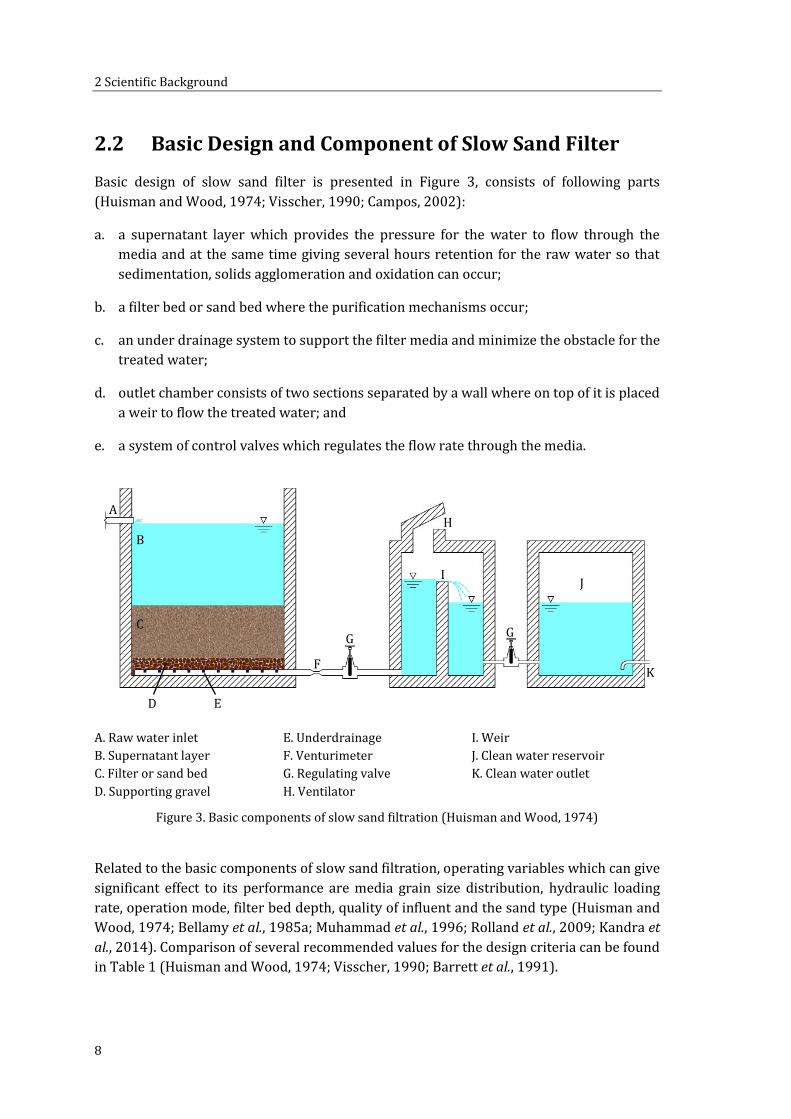
2.2 Basic Design and Component of Slow Sand Filter
Basic design of slow sand filter is presented in Figure 3, consists of following parts
(Huisman and Wood, 1974; Visscher, 1990; Campos, 2002):
a. a supernatant layer which provides the pressure for the water to flow through the
media and at the same time giving several hours retention for the raw water so that
sedimentation, solids agglomeration and oxidation can occur;
b. a filter bed or sand bed where the purification mechanisms occur;
c. an under drainage system to support the filter media and minimize the obstacle for the
treated water;
d. outlet chamber consists of two sections separated by a wall where on top of it is placed
a weir to flow the treated water; and
e. a system of control valves which regulates the flow rate through the media.
A. Raw water inlet E. Underdrainage I. Weir
B. Supernatant layer F. Venturimeter J. Clean water reservoir
C. Filter or sand bed G. Regulating valve K. Clean water outlet
D. Supporting gravel H. Ventilator
Figure 3. Basic components of slow sand filtration (Huisman and Wood, 1974)
Related to the basic components of slow sand filtration, operating variables which can give
significant effect to its performance are media grain size distribution, hydraulic loading
rate, operation mode, filter bed depth, quality of influent and the sand type (Huisman and
Wood, 1974; Bellamy et al., 1985a; Muhammad et al., 1996; Rolland et al., 2009; Kandra et
al., 2014). Comparison of several recommended values for the design criteria can be found
in Table 1 (Huisman and Wood, 1974; Visscher, 1990; Barrett et al., 1991).
A
B
C
D
F
G
E
H
I
G
J
K
2.2 Basic Design and Component of Slow Sand Filter
9
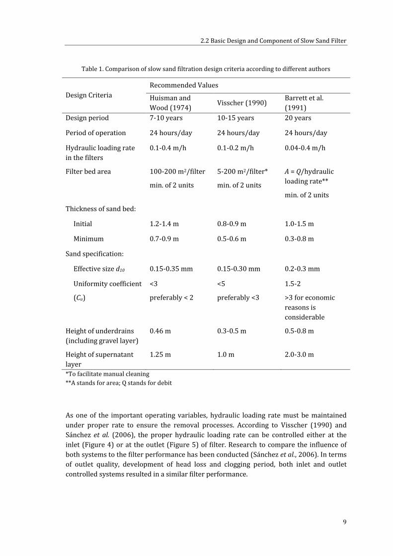
Table 1. Comparison of slow sand filtration design criteria according to different authors
Design Criteria
Recommended Values
Huisman and
Wood (1974) Visscher (1990)
Barrett et al.
(1991)
Design period 7-10 years 10-15 years 20 years
Period of operation 24 hours/day 24 hours/day 24 hours/day
Hydraulic loading rate
in the filters
0.1-0.4 m/h 0.1-0.2 m/h 0.04-0.4 m/h
Filter bed area 100-200 m2/filter
min. of 2 units
5-200 m2/filter*
min. of 2 units
A = Q/hydraulic
loading rate**
min. of 2 units
Thickness of sand bed:
Initial 1.2-1.4 m 0.8-0.9 m 1.0-1.5 m
Minimum 0.7-0.9 m 0.5-0.6 m 0.3-0.8 m
Sand specification:
Effective size d10 0.15-0.35 mm 0.15-0.30 mm 0.2-0.3 mm
Uniformity coefficient
(Cu)
<3
preferably < 2
<5
preferably <3
1.5-2
>3 for economic
reasons is
considerable
Height of underdrains
(including gravel layer)
0.46 m 0.3-0.5 m 0.5-0.8 m
Height of supernatant
layer
1.25 m 1.0 m 2.0-3.0 m
*To facilitate manual cleaning
**A stands for area; Q stands for debit
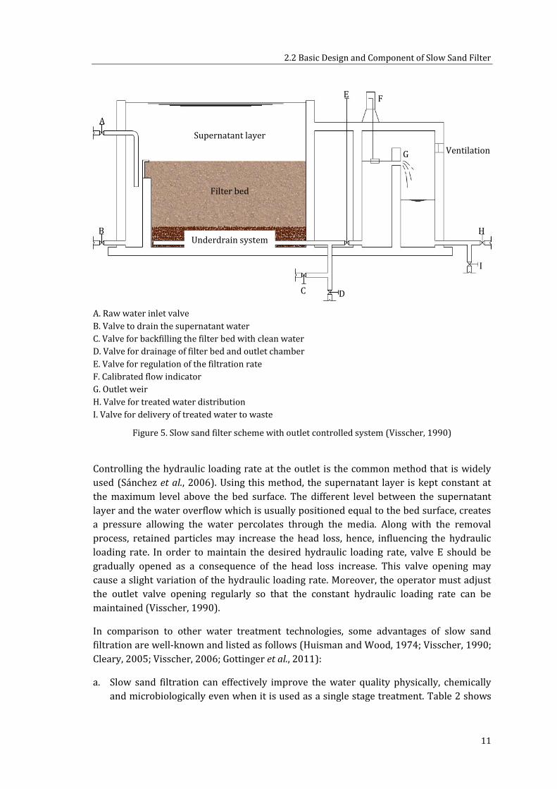
As one of the important operating variables, hydraulic loading rate must be maintained
under proper rate to ensure the removal processes. According to Visscher (1990) and
Sánchez et al. (2006), the proper hydraulic loading rate can be controlled either at the
inlet (Figure 4) or at the outlet (Figure 5) of filter. Research to compare the influence of
both systems to the filter performance has been conducted (Sánchez et al., 2006). In terms
of outlet quality, development of head loss and clogging period, both inlet and outlet
controlled systems resulted in a similar filter performance.

2 Scientific Background
10
A. Raw water inlet valve for regulation of hydraulic loading rate
B. Valve for drainage of supernatant water
C. Inlet weir
D. Calibrated flow indicator
E. Valve for backfilling the filter bed with clean water
F. Valve for drainage of filter bed and outlet chamber
G. Valve for treated water distribution
H. Valve for delivery of treated water to waste
Figure 4. Slow sand filter scheme with inlet controlled system (Visscher, 1990)
In a slow sand filter with inlet controlled system, hydraulic loading rate is regulated by the
raw water inlet valve (Visscher, 1990). This raw water inlet valve allows the water to flow
in a constant rate to the filter unit leads into a constant hydraulic loading rate. Inside the
system, a flow indicator is installed to measure the flow continuously (Visscher, 1990).
At the beginning of the operation, the supernatant layer is shallow therefore the retention
time of raw water to be in this layer is shorter. Supernatant layer will gradually increase to
compensate the head loss due to the development of Schmutzdecke at the filter bed surface
(Sánchez et al., 2006). When the supernatant level reaches the maximum, cleaning is
needed. The advantage of the inlet control system is that it simplifies the filter operation.
The rise of supernatant layer as a result of an increase of the head loss is directly visible
(Visscher, 1990).
Supernatant layer
Filter bed
Underdrain system
Ventilation
A
B
C
D
E F
G
H
2.2 Basic Design and Component of Slow Sand Filter
11
A. Raw water inlet valve
B. Valve to drain the supernatant water
C. Valve for backfilling the filter bed with clean water
D. Valve for drainage of filter bed and outlet chamber
E. Valve for regulation of the filtration rate
F. Calibrated flow indicator
G. Outlet weir
H. Valve for treated water distribution
I. Valve for delivery of treated water to waste
Figure 5. Slow sand filter scheme with outlet controlled system (Visscher, 1990)
Controlling the hydraulic loading rate at the outlet is the common method that is widely
used (Sánchez et al., 2006). Using this method, the supernatant layer is kept constant at
the maximum level above the bed surface. The different level between the supernatant
layer and the water overflow which is usually positioned equal to the bed surface, creates
a pressure allowing the water percolates through the media. Along with the removal
process, retained particles may increase the head loss, hence, influencing the hydraulic
loading rate. In order to maintain the desired hydraulic loading rate, valve E should be
gradually opened as a consequence of the head loss increase. This valve opening may
cause a slight variation of the hydraulic loading rate. Moreover, the operator must adjust
the outlet valve opening regularly so that the constant hydraulic loading rate can be
maintained (Visscher, 1990).
In comparison to other water treatment technologies, some advantages of slow sand
filtration are well-known and listed as follows (Huisman and Wood, 1974; Visscher, 1990;
Cleary, 2005; Visscher, 2006; Gottinger et al., 2011):
a. Slow sand filtration can effectively improve the water quality physically, chemically
and microbiologically even when it is used as a single stage treatment. Table 2 shows
Supernatant layer
Filter bed
Underdrain system
A
B
C D
E F
G
H
I
Ventilation
2 Scientific Background
12
the examples of removal efficiencies of slow sand filtration based on the results of
some previous studies by Slezak and Sims (1984), Bellamy et al. (1985a), Bellamy et al.
(1985b), Visscher (1990), Collins et al. (1991), Galvis (1999), Logsdon et al. (2002)
and Kaya and Takeuchi (2014). However, from these results it can be inferred that the
slow sand filtration cannot directly produce drinkable water without further step of
treatment because this technology alone cannot achieve 100 % of bacteria and viruses
removal.
b. Slow sand filter is an uncomplicated technology in respect to the construction,
operation and maintenance therefore the cost can be maintained low.
c. During the operation of slow sand filter, chemicals are not required.
d. Low energy is required because the filter operates exploiting only the gravity flow.
e. Slow sand filtration systems produce less dangerous waste compared to other
methods because the sludge resulted during filter scraping is handled in a dry state
and this material can be used as fertilizer.
f. Cleaning process requires only a little amount of water, thus conservation of water can
be managed.
In spite of its advantages, the disadvantages of slow sand filter is also reported, as
presented below (Huisman and Wood, 1974; Visscher, 1990; Logsdon et al., 2002;
Gottinger et al., 2011):
a. Due to its low velocity, a large area is needed to encounter the demand.
b. Slow sand filter may not be suitable for cold climates because the filter operation at
very low temperature influences the filter performance adversely. Therefore, an
additional expensive system against freezing should be installed.
c. Slow sand filtration is vulnerable to high turbidity as it accelerates the clogging period.
d. In some countries where the construction methods are mechanized, for instance in the
Netherlands, initial cost of slow sand filter may be higher than rapid filter.
e. The growth of certain types of algae may require a more frequent cleaning due to the
premature clogging.

2.3 Hydraulics of Filtration
13
Table 2. Removal efficiencies of slow sand filtration
Parameter Effluent or removal
efficiency
Reference(s)
Turbidity < 1 NTU* Slezak and Sims (1984); Visscher
(1990); Collins et al. (1991);
Galvis (1999)
Color 30-100 %
25-40 %
Visscher (1990)
Galvis (1999)
Total coliforms 96-99.9 %
98.9 %
Bellamy et al. (1985a)
Bellamy et al. (1985b)
Fecal coliforms 95-97 %
98 %
1-3 log units
Bellamy et al. (1985a)
Bellamy et al. (1985b)
Collins et al. (1991)
Enteric viruses 2-4 log units
99-99.99 %
Collins et al. (1991)
Galvis (1999)
Giardia cysts >99.9 %
2-4 log units
99-99.99 %
Bellamy et al. (1985a); Bellamy et
al. (1985b)
Collins et al. (1991)
Galvis (1999)
Cryptosporidium oocysts >99 % Galvis (1999)
Standard plate count
bacteria
>99 %
87-91 %
Bellamy et al. (1985a)
Bellamy et al. (1985b)
Organic matter 60-75 % Visscher (1990)
Biodegradable dissolved
organic carbon
<50 % Collins et al. (1991)
Iron and manganese Largely removed
30-90 %
>99.9 %
Visscher (1990)
Galvis (1999)
Kaya and Takeuchi (2014)
Heavy metals 30-95 % Visscher (1990)
Trihalomethane precursors <25 % Collins et al. (1991)
*Nephelometric Turbidity Unit
2.3 Hydraulics of Filtration
In the theory of granular filtration, discussion about hydraulics is started by determining
the flow types. Fluid flow may be classified as laminar, turbulent and transitional (Webber,
1965; Bardet, 1997). Webber stated that laminar flow occurs when the velocity is low and

2 Scientific Background
14
constant in such a way that the particles move parallel to the flow path. Adversely, the
particle velocity during turbulent flow is high and fluctuated causing the particles motion
is not in line with the flow path. Bardet define transitional as a type of flow between the
lamina and turbulent flows. The simplest method to characterize the fluid type is by using
the Reynolds number (Re). Following is the formula to calculate the Re (Binnie and
Kimber, 2013):
= ∙ ∙� (1)
where ρ is the density of water, v is hydraulic loading rate, D is the particle diameter and η
is the dynamic viscosity of fluid which in this research is water. According to Welty (2008),
when the Re is below 2300, the flow is classified as laminar. A flow is transitional when
2300 < Re < 3000 and turbulent flow occurs if the Re is above 3000.
Low hydraulic loading rate in slow sand filtration leads into very small Re thus the flow
regime is categorized as laminar flow (Campos et al., 2006). Jabur et al. (2005) described
that in slow sand filtration, Re < 2. Therefore, Darcy s Law which stating that hydraulic loading rate is proportional to the difference of pressure can be applied in this system
(Ives, 1987). An assumption in the application of Darcy s law is that the flow is steady, laminar, no change in viscosity (inviscid) and volume (incompressible) (Budhu, 2015). This equation from Darcy s law can describe the flow in porous media. According to the experiments done by Darcy, flow velocity v is influenced by the hydraulic conductivity k
and hydraulic gradient i (Bardet, 1997):
= ∙ � (2)
Filtration velocity v or hydraulic loading rate can be determined by dividing the
volumetric flowrate Q by the specimen cross-sectional area A (see Equation 3) (Sherard et
al., 1984). The value of Q can be obtained by dividing the volume and time t of water
collected. The A depends on the diameter of column D.
= � � � � � � = � = ⁄∙ ⁄ (3)
Hydraulic gradient i is the ratio of different head drop Δh and the bed depth L (Bardet,
1997):
� = ∆ℎ� (4)
Hydraulic conductivity is one of parameters generally used to characterize transport
phenomena in porous media (Koponen et al., 1997). Hydraulic conductivity describes how
ease the water flow through the media. There are many factors influencing hydraulic
2.3 Hydraulics of Filtration
15
conductivity in sand filtration such as size and shape of grains, homogeneity, size and
arrangement of voids which are represented by void ratio and porosity, layering and
fissuring, degree of saturation, fluid properties i.e. viscosity and temperature, fissuring,
compression or stress level and particles loading (Bardet, 1997; Deb and Shukla, 2012;
Budhu, 2015; Le Coustumer et al., 2012).
Coarse grains tend to have a higher hydraulic conductivity compared to the finer grains.
Fine fraction presence in the soil may significantly reduce the hydraulic conductivity
(Budhu, 2015). As a provisional basis for this fine fraction, effective size d10 (mm) is used.
The term d10 represents the grain size which is 10 % finer by weight. The d10 is used as one
of the parameters because Hazen (1905) found out that fine fraction represented by d10
mainly determines the characteristic of the sand. Budhu (2015) also mentioned that this
portion will result relatively the same effect as irregular particles. According to the d10
value, the sand is classified as fine or coarse. Low d10 value represents finer grains and vice
versa. Empirical relationship between the d10 and hydraulic conductivity kH (cm/s) is shown by (azen s formula as follows (Bardet, 1997; Budhu, 2015):
� = � ∙ (5)
where CH is the Hazen constant which ranges between 0.4 and 1.4. This constant reflects
the different type of soil. For fine and uniform sand, CH is typically 1.0. Another method to
determine the CH by considering the porosity n is presented by Naeej et al. (2017) as
follows:
� =
× × − × [ + − . ] (6)
In this study, the gravitational acceleration g is assumed to be 9.81 m/s2 and the kinematic
viscosity is 1×10⁻⁶ m2/s. (azen s formula is usually used to estimate the hydraulic conductivity value for coarse soils (Budhu, 2015). Calculation of empirical hydraulic conductivity based on (azen s formula was done using Equation 5 if the following
requirements are fulfilled: 0.1 mm d10 3 mm and Cu < 5.
Estimation of hydraulic conductivity of filter media which did not meet the requirements for (azen s formula was determined using the Beyer s formula. The formula from Beyer as
shown is Equation 7 is more suitable for finer grain size distribution (0.06 mm d10 0.6
mm and Cu < 20) (Vienken and Dietrich, 2011; Naeej et al., 2017):
= ∙ (7)
The constant after Beyer CB is also influenced by the gravitational acceleration g, kinematic
viscosity and the homogeneity of the sand which is represented by uniformity coefficient
Cu. Uniformity coefficient Cu, which characterizes the homogeneity of the sand, is the ratio
of d60 to d10 (Bardet, 1997). The d60 represents the grain size which is 60 % finer by weight.
The constant CB can be calculated using following formula (Naeej et al., 2017):

2 Scientific Background
16
=
× × − × (8)
Large voids are not directly related to high porosity which will result into higher hydraulic
conductivity. Figure 6 illustrates a sample of soil with total volume V and weight W. This
soil sample consists of solid, water and air. When each constituent is grouped, the solid
has a weight Ws and volume Vs. The weight and the volume of water are represented by Ww
and Vw respectively. The air is weightless with a volume of Va. Total volume of voids Vv is
composed by Vw and Va.
Figure 6. Weight and volume of a soil sample (left) and weight and volume of solid, water and air
constitutent (right) (Bardet, 1997)
Void ratio e is the ratio of total voids volume to the solid volume (see Equation 9). In a
sand bed with heterogeneous grain size, void ratio is reduced thus hydraulic conductivity
is lower (Mbonimpa et al., 2002).
= (9)
Porosity describes the total pores exist within the filter bed. Porosity n is the ratio of total
voids volume to the total volume as shown in Equation10 (Bardet, 1997):
= (10)
When the value of Vv and Vs are difficult to be measured, the void ratio e can be determined
based on the specific gravity Gs of the sand, water unit weight γw and dry unit weight γd.
Equation 11 shows the relation among e, Gs, γw and γd (Bardet, 1997). Specific gravity Gs is
a unit less expression which describes the ratio between unit masses of soil and water
(Bardet, 1997). Determination of Gs can be done by laboratory test and the method is
described in Section 4.2.1. In this study, the γw is assumed to be 9.81 kN/m3. The γd is
Weight Volume Weight Volume
Air
Water
Solid
W V
Ww Vw
Ws Vs
Va
Vv

2.3 Hydraulics of Filtration
17
obtained by dividing the dry sample weight by the volume of sample. The dry sample
weight in Newton is a product of dry sample mass in grams multiplied by the gravitational
acceleration.
= ∙ ��� − (11)
Porosity n can be determined from the value of e with following equation (Bardet, 1997):
= + (12)
According to Koponen et al. (1997), the interconnected pores are crucial because those
contribute to the flow in porous media. How the voids connect one another determines
greatly the hydraulic conductivity.
By considering the correlation of hydraulic conductivity and porosity, velocity through the
void spaces or seepage velocity vs can be calculated using a formula as follows (Budhu,
2015):
= ∙ � (13)
Based on the value of porosity, an empirical hydraulic conductivity is determined using
the Kozeny-Carman s formula as follows (Naeej et al., 2017):
� =
× 8. × − × − × (14)
Hydraulic conductivity is high in loose state soil layers leading to a very high seepage
velocity. In loose state soil layers, the existence of fissures may also increase the hydraulic
conductivity degree (Budhu, 2015).
Degree of saturation influences significantly the water flow in porous media. If the voids of
soil sample are filled completely with water, fully saturated condition is achieved. Degree
of saturation Sr (%) is calculated by comparing the water volume Vw and total voids
volume Vv (Bardet, 1997):
= × (15)
The possibility of fully saturated condition is very low due to the presence of entrapped air
within the soil sample. Consequently, the entrapped air reduce the hydraulic conductivity
due to the capillary action or soil suction (Budhu, 2015).

2 Scientific Background
18
Viscosity is a temperature dependent parameter. When the temperature increases, the
viscosity of fluid decreases (Cho et al., 1999). In a low viscosity, it is easier for the fluid to
pass through the sand bed thus the hydraulic conductivity is higher (Budhu, 2015).
Compression of the soil bed reduces the hydraulic conductivity due to the higher stress
level. There are two processes of compression i.e. compaction and consolidation.
Compaction decreases the total volume of voids, thus, it reduces the sand bed capability to
convey the water (Bardet, 1997; Hatt et al., 2008). Consolidation occurs through a gradual
flow of water independently of the clogging effects on the surface of filter bed (Hatt et al.,
2008).
In the filtration process, impurities or suspended solids are removed from the raw water.
These impurities are mostly deposited at the surface of filter bed. Due to the very fine size
of the retained solid, the hydraulic conductivity is significantly decreased (Le Coustumer
et al., 2012).
The hydraulic conductivity can be measured in–situ using a permeameter. In the
laboratory scale, hydraulic conductivity can be determined either by constant head or
falling head test (Figure 7).
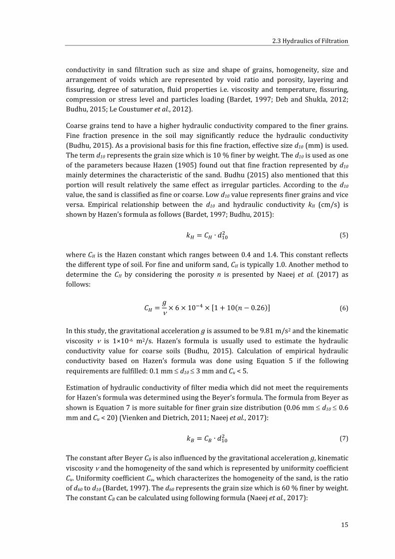
Constant head test is usually used to determine the hydraulic conductivity of coarse-
grained soils such as clean sand and gravels k ≥ -3) (Bardet, 1997). In this type of test,
water is flowing through a bed of soil under a constant head as shown in Figure 7a.
Hydraulic conductivity in vertical direction k can be determined by (Budhu, 2015):
= ∙ �� ∙ ∆ℎ (16)
where Q is the volumetric flowrate (see Equation 3), L is the thickness of soil bed, A is the
cross-sectional area and Δh is the head difference of inlet and outlet.
The water flow in the less permeable soils such as fine sand (k 10-3 cm/s) is too slow,
that the constant head test requires unreasonable measurement time. Therefore,
for this type of soil, hydraulic conductivity is determined by falling head test. In the
falling head test, water flows through a bed of soil with decreasing level as illustrated in
Figure 7b. Hydraulic conductivity k is calculated using the following formula (Bardet,
1997; Budhu, 2015):
= � ∙ �� ∙ − (ℎℎ ) (17)
2.4 Head Loss and Clogging Phenomena
19
(a) (b)
Figure 7. A scheme of (a) constant head test and (b) falling head test (Budhu, 2015)
2.4 Head Loss and Clogging Phenomena
Head loss, in this study, is a phenomenon in slow sand filtration where the downward raw
water flow is resisted by the existence of sand bed (Huisman and Wood, 1974).
Accumulation of impurities on the surface of filter bed is also responsible for the
progressive increase of head loss during filter operation (Graham and Collins, 2014). This
phenomenon can be describe as the difference between the head of the water above and
below the sand bed and it represents the frictional resistance of the sand layer (Hazen,
1905).
According to Holdich (2002), head loss is the inverse of hydraulic conductivity. High head
loss is related to the high fluid viscosity μ and low hydraulic conductivity as formulated in
the following:
� = � ∙ � � � � � � (18)
Outlet Outlet
L L
Δh Δh
dh Mariotte bottle
Cross sectional a
Cross sectional A

2 Scientific Background
20
Huisman and Wood (1974) proposed a simple method to calculate the head loss H which
is associated with hydraulic loading rate (Naghavi and Malone, 1986) within a sand bed
thickness of h as follows:
= � � � � � � ∙ ℎ (19)
At the beginning of the filter operation, the head loss is dominantly dependent on the grain
size distribution of media, bed depth and hydraulic loading rate (Naghavi and Malone,
1986; Zhu et al., 1996; Mandloi et al., 2004). Figure 8 shows how high initial head loss can
be associated with lower median grain size diameter and greater thickness of bed depth.
Figure 8. Correlation of average initial head loss and bed depth after Naghavi and Malone (1986)
Head loss gradually increases due to the deposition of sediment from the raw water and
mostly occurs at the top layer of sand bed (Hazen, 1905; Farooq and Al-Yousef, 1993;
Holdich, 2002; Aronino et al., 2009).
Hydraulic gradient or gradient of total head (Bardet, 1997) can be used as an indicator of
development head loss (Darby et al., 1992). Head loss development in filter bed is
determined by media grain size, bed depth, hydraulic conductivity, media shape, bed
porosity, hydraulic loading rate, water viscosity and density, concentration and size of
suspended solids in water, volume of treated water and the ratio of filter diameter to
media effective size(Yao et al., 1971; Lang et al., 1993; Boller and Kavanaugh, 1995;
Trussell and Chang, 1999; Holdich, 2002; Puig-Bargués et al., 2005; Mesquita et al., 2012).
Due to the limited literatures in slow sand filtration about head loss development,
references cited herein are predominantly from the research in deep bed filtration.

2.4 Head Loss and Clogging Phenomena
21
Head loss is always dependent on the hydraulic conductivity of filter bed. Hydraulic
conductivity has an inverse relationship with the head loss. Under a constant flow, lower
hydraulic conductivity leads into the increase of head loss (Mays and Hunt, 2005). One of
factors which affect the hydraulic conductivity and head loss is media shape (Bardet,
1997). According to Bardet, especially related to the coefficient values of grain shape and
the empirical hydraulic conductivity, the more irregular the media shape, the lower the
hydraulic conductivity is. This means that the more rounded media shape will result in a
lower head loss. However, Sperry and Peirce (1995) concluded that media size is more
significant for predicting the hydraulic conductivity rather than media shape. This
conclusion is confirmed by Trussell and Chang (1999) which stated that media shape has
much less influence on the head loss compared to the impact of porosity and media size.
Bed porosity is inversely proportional to the head loss as the higher bed porosity, the
lower the head loss is (Trussell and Chang, 1999). Deposition of suspended solids in filter
bed reduces the overall porosity (Tobiason and Vigneswaran, 1994). The decrease in
porosity increases the tortuosity of flow in filter bed and consequently, head loss (Boller
and Kavanaugh, 1995). Related to media size, O Melia and Ali (1978) stated that its impact
on the head loss development is less significant compared to the effect of suspended solids
concentration and size. Based on the study of O Melia and Ali, raw water with low
concentration of suspended solids results in slow increase of head loss. This result was
verified by Vigneswaran and Song (1986). Adin and Elimelech (1989) disproved the result
of O Melia and Ali, particularly on the impact of media size. According to their study, Adin
and Elimelech found that rate of head loss increase is strongly dependent on the media
size. Finer media produce much higher head loss increase due to the surface removal of
suspended solids, rather than the coarser media. Another study by Boller and Kavanaugh
(1995) also contradicts to O Melia and Ali in regard to media size. However, Boller and
Kavanaugh showed contrary results to Adin and Elimelech. In their study, head loss
increase in coarser media size is larger than in finer media size. Size of suspended solids
affects the head loss development in an inverse way. Suspended solids with larger size do
not produce enormous head loss, meanwhile the submicron solids do O Melia and Ali, 1978). This result was confirmed by Tobiason and Vigneswaran (1994) and Boller and
Kavanaugh where smaller solids result in higher head loss per unit mass deposited.
Hydraulic loading rate has an essential impact on the head loss development. Adin and
Elimelech (1989) observed that rapid head loss increase occurs in a filter bed operated
higher hydraulic loading rate. On the contrary, Veerapaneni and Wiesner (1997) found out
that lower hydraulic loading rate generates steep increases in head loss. It is because
deposits of suspended solid occupy more pore spaces in filter bed under low hydraulic
loading rate. Therefore, the drag loss for the water to flow is higher and consequently the
head loss is higher. Disproving the both studies of Adin and Elimelech (1989) and
Veerapaneni and Wiesner (1997), effect of hydraulic loading rate was found to be
insignificant on the head loss development by Boller and Kavanaugh (1995).
Progressive increase of head loss can be associated and used to predict the clogging rate
(Puig-Bargués et al., 2005). Based on its definition, clogging is a condition when the

2 Scientific Background
22
hydraulic conductivity decreases and water cannot percolate easily through the sand bed
due to sediment accumulation and deposition in the filter from the total period of
operation (Rodgers et al., 2004; Kandra et al., 2014; Mercado, Jean Margaret R et al., 2015).
Clogging is a result of physical, biological and chemical processes (Pérez Paricio, 2001).
The terms physical process refers to the attachments or detachment of suspended solids
into the sand grains McDowell‐Boyer et al., 1986). Biological process involves the
accumulation and growth of microorganisms in porous media (Vandevivere et al., 1995).
Chemical clogging seldom occurs unless there is a chemical interaction between the
dissolved salt in the water and the porous media (Rice, 1974).
Clogging that occurs in sand filtration is regarded as a surface phenomenon (Rodgers et al.,
2004; Leverenz et al., 2009; Le Coustumer et al., 2012). This surface phenomenon involves
the decline of pore space caused by suspended solids and bacterial growths on the
captured or dissolved solids, and reopening of pore space caused by bacterial
decomposition and the reduction of bacterial growths during the resting period (Leverenz
et al., 2009).
In slow sand filtration, at the beginning of the filter run, the sand characteristics such as its
size influenced the clogging layer development (Elisson, 2002). Fine sand tends to clog
faster than the coarser. However, once the clogging layer is formed, development of the
clogging layer does not depend on the sand bed characteristics anymore (Kropf et al.,
1977). Clogging is a serious problem which influence the filter performance (Kandra et al.,
2010). In the worst case, clogging may provoke a breakthrough in the filter bed (Hazen,
1905; Vries, 1972; Kandra et al., 2010).
In practical use, high initial head loss may not be beneficial. It is because the time to reach
the terminal head loss or clogging period is shorter. In order to ensure a consistently well
performance, a filter shall be designed and operated in a manner where the time to reach
the terminal head loss is considerably shorter than the time to reach the breakthrough.
According to Hazen (1905), breakthrough occurs when the pressure for the water to flow
becomes very high that the filter cake will no longer able to resist it. The filter cake will be
broken allowing the water to flow with a huge increase of the loading rates. As a
consequence, the breakthrough causes the decreased removal efficiency (Hazen, 1905).
From this point of view, head loss is not only a very significant parameter but also a
dominant design constraint (Boller and Kavanaugh, 1995).
Maintenance of filter when terminal head loss or clogging is reached normally involves
scraping of top layers to remove the clogging layer. Other method that can be done to put
the slow sand filter back into service is by filter cake harrowing (Collins et al., 1991;
Österdahl, 2015). Filter harrowing is done by draining the supernatant water into only
around 30 cm above the sand surface. Then the top 30 cm sand medium is raked –either
manually or using a machine– so that the colloidal debris is loosened and caught by the
moving water stream. The dirty water is not discharged through the filter bed but at the
surface. This harrowing is believed to be a better method because it requires less time and

2.5 Removal Mechanisms
23
labor compared to the normal scraping. Moreover, the filter can be put back into service
faster without compromising the removal efficiency (Collins et al., 1991).
2.5 Removal Mechanisms
Fundamental purpose of filtration is to remove the impurities from the water by passing it
through sand bed. Removal mechanisms and inactivation of microorganisms are mostly
related to a thin layer so called Schmutzdecke or dirty layer at the surface of filter bed (Weber-Shirk and Dick, 1997). Schmutzdecke, together with low hydraulic loading rate and
fine sand size, encourages the filter to achieve high efficiency of treatment (Campos et al.,
2002).
For more than a century, the role of Schmutzdecke in the removal mechanisms had been
argued due to its various definitions. Hazen (1905) expressed the Schmutzdecke as a
sediment layer resulted from coarser particles in the water that are restrained on the
surface of sand bed. This layer will then become another filter that is much finer than the
sand. Huisman and Wood (1974), Ellis (1987) and Binnie and Kimber (2013) had similar
definition on Schmutzdecke stating that it is a thin slimy mat or a biologically active mat
formed on the surface of sand bed composed of humus, sand, algae, plankton, diatoms,
protozoa, metazoan, rotifiers and bacteria. Cleasby et al. (1984) and Bellamy et al. (1985b)
stated that Schmutzdecke consists of inert deposits and living organisms that develops on
the surface of sand bed. Weber-Shirk and Dick summarized those various definitions of
Schmutzdecke as follows:
a. particle deposition which forms a layer on the surface of filter bed,
b. a surface skin formed by biological growth, and
c. a biologically active zone within the filter bed.
At the beginning of the filter operation,the Schmutzdecke is formed due to the physical
process (Campos, 2002; Ellis et al., 2009). This physical removal is regarded as the
principal removal mechanisms in slow sand filtration (Campos, 2002). Thus, in order to
understand the removal mechanisms in slow sand filtration, the focus in this study was on
the suspended solids removal. Considering this focus of research, the most suitable
definition of Schmutzdecke is the layer of solids deposition on the surface of filter bed. Another term that is more suitable to specify this solids deposition is filter cake (Weber-
Shirk and Dick, 1997). From this point on, the term of filter cake will be used herein.
Generally, removal mechanisms of suspended solids by filtration consist of two sequential
steps: transport and attachment processes Elimelech and O Melia, a . These
mechanisms that is responsible for suspended solids removal in slow sand filtration are
influenced by many variables such as the retention site, retention forces, particle size, type
of flow and transport or capture mechanisms (Herzig et al., 1970; Yao et al., 1971; (uisman and Wood, ; McDowell‐Boyer et al., 1986).

2 Scientific Background
24
2.5.1 Transport Mechanisms
Particles are brought into contact to the potential retention site where it can be remained
or transported by the stream during the flow through the sand bed (Herzig et al., 1970).
There are four possible locations where the suspended solids may be collected as
illustrated in Figure 9:
a. surface, where suspended solid may have contact with and retained on;
b. crevice, where suspended solids are wedged in between two convex surfaces of two
grains;
c. constriction, where suspended solid is retained among grains because its size is bigger
than the pore size; and
d. cavern, where the suspended solids are remained in such a sheltered pocket formed
by several sand grains.
(a) (b) (c) (d)
Figure 9. Retention sites of suspended solids: (a). surface; (b). crevice; (c). constriction; and (d).
cavern (Herzig et al., 1970)
Transport mechanisms are categorized into six types: sedimentation, interception, inertia,
diffusion or Brownian motion, hydrodynamic effects and mass attraction or van der Waals
force (Herzig et al., 1970; Yao et al., 1971; Huisman and Wood, 1974). By considering a
single grain of filter media as a collector, Yao et al. illustrated the transport mechanisms as
seen in Figure 10. Darby and Lawler (1990) mentioned that particle size distribution
determines the dominant transport mechanism whether it is sedimentation or
interception or Brownian motion. The first two types of transport mechanisms occur
when the suspended solids are >1 μm (Yao et al., ; O Melia and Ali, . Meanwhile,
Brownian motion will play more important role for the particles having the size of < 1 µm
(Keller and Auset, 2007). In this study, in order to study more about the head loss
development and ripening period in the slow sand filtration, particle size distribution also

2.5 Removal Mechanisms
25
needs to be considered since it is impossible to rely only on the measurement of turbidity
or TSS (Darby and Lawler, 1990).
Sedimentation occurs when the density of solids is higher than the water density. In this
case, the velocity of the particle is no longer the same as the water due to the gravitational
force (Herzig et al., 1970; Yao et al., 1971; Ives, 1987). Hence, the particles are precipitated
onto the collector. Temperature is also influencing sedimentation efficiency since it affects
the viscosity of water. The higher the temperature is, the lower the viscosity allowing a
faster settlement of particle (Ives, 1987).
Another factor affecting sedimentation efficiency is the ratio between the surface loading
rate and the settling velocity of suspended particles. If the settling velocity is equal to or
greater than the surface loading, removal by sedimentation can occur (Huisman and
Wood, 1974). Settling velocity will be discussed particularly in the Section 2.6.
Interception is due to the flow of suspended particles which follow the trajectory and at
some points come into contact with the collector (Yao et al., 1971). According to Keller and
Auset (2007), interception is not only a function of hydraulic loading rate but also of
diameter ratio between suspended solids and the sand grain as well as porosity.
Probability of interception will decrease if the hydraulic loading rate is high.
Figure 10. Basic transport mechanisms in sand filtration (Yao et al., 1971; Bradford et al., 2002;
Binnie and Kimber, 2013)
Particle path Flow direction
Streamline
Hydrodynamic action
Collector
A
B
C
A Sedimentation
B Interception
C Brownian
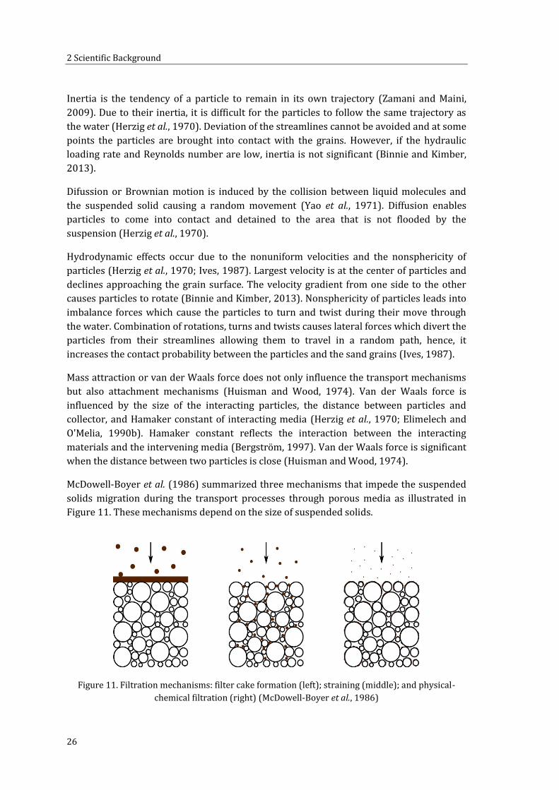
2 Scientific Background
26
Inertia is the tendency of a particle to remain in its own trajectory (Zamani and Maini,
2009). Due to their inertia, it is difficult for the particles to follow the same trajectory as
the water (Herzig et al., 1970). Deviation of the streamlines cannot be avoided and at some
points the particles are brought into contact with the grains. However, if the hydraulic
loading rate and Reynolds number are low, inertia is not significant (Binnie and Kimber,
2013).
Difussion or Brownian motion is induced by the collision between liquid molecules and
the suspended solid causing a random movement (Yao et al., 1971). Diffusion enables
particles to come into contact and detained to the area that is not flooded by the
suspension (Herzig et al., 1970).
Hydrodynamic effects occur due to the nonuniform velocities and the nonsphericity of
particles (Herzig et al., 1970; Ives, 1987). Largest velocity is at the center of particles and
declines approaching the grain surface. The velocity gradient from one side to the other
causes particles to rotate (Binnie and Kimber, 2013). Nonsphericity of particles leads into
imbalance forces which cause the particles to turn and twist during their move through
the water. Combination of rotations, turns and twists causes lateral forces which divert the
particles from their streamlines allowing them to travel in a random path, hence, it
increases the contact probability between the particles and the sand grains (Ives, 1987).
Mass attraction or van der Waals force does not only influence the transport mechanisms
but also attachment mechanisms (Huisman and Wood, 1974). Van der Waals force is
influenced by the size of the interacting particles, the distance between particles and
collector, and Hamaker constant of interacting media (Herzig et al., 1970; Elimelech and
O'Melia, 1990b). Hamaker constant reflects the interaction between the interacting
materials and the intervening media (Bergström, 1997). Van der Waals force is significant
when the distance between two particles is close (Huisman and Wood, 1974). McDowell‐Boyer et al. (1986) summarized three mechanisms that impede the suspended
solids migration during the transport processes through porous media as illustrated in
Figure 11. These mechanisms depend on the size of suspended solids.
Figure 11. Filtration mechanisms: filter cake formation (left); straining (middle); and physical-
chemical filtration (right) McDowell‐Boyer et al., 1986)

2.5 Removal Mechanisms
27
When the particles are larger than the pore size, their penetration into the sand bed is
limited. They are often remained at the surface of sand bed forming a filter cake or surface
mat McDowell‐Boyer et al., 1986). Types of particles contained in the filter cake influence
greatly its properties such as hydraulic conductivity, porosity, compressibility and the
capacity to restrain other particles (Weber-Shirk and Dick, 1997). This particle deposition
at the surface leads to a significant decrease of the hydraulic conductivity of the filter.
Straining occurs in constriction when the particles are small enough to penetrate the
porous media but too large to pass through the interstices between grains in the sand bed.
It mostly takes place at the surface of the filter which contributes to the formation of filter
cake since it restricts openings of the sand bed pores (Huisman and Wood, 1974; McDowell‐Boyer et al., 1986). Straining is the only one mechanism that is known from the
beginning of slow sand filtration establishment. Before the existence of pathogenic
bacteria was known, slow sand filtration is only deemed as a strainer for turbidity and
suspended solids (Hazen, 1905; Huisman and Wood, 1974). In that period, it was believed
that the filter performance depends on the fineness of the strainer which is sand (Hazen,
1905).
Independent of the hydraulic loading rate, straining that is also not influenced by
electrostatic interactions. Straining is influenced greatly by the system geometry and the
grain shape (Tufenkji et al., 2004). Prediction on the straining potential within porous
media based on the system geometry is influenced by the solid or particle diameter (dp)
and the grain mean diameter (dm) (Herzig et al., ; McDowell‐Boyer et al., 1986).
Sakthivadivel (1969), as cited by McDowell‐Boyer et al. , recommended some values of dm/dp to determine the straining potential. Particle penetration to media will not
be possible when dm/dp < 10. In such condition, a filter cake will be formed. For 10 < dm/dp
< 20, deposition of particles is expected to occupy > 30% of pore volume and hydraulic
conductivity is reduced by a factor of 7-15. Deposition of smaller particles which occupy
pore volume is predicted to be only 2-5% if dm/dp > 20. If the ratios of grain diameter and
particle diameter are ranging from dm/dp < 10 to dm/dp > 20, the constriction is blocked by
larger particles. These larger particles act as strainers for smaller particles. In this case, an
effective particle removal by a combination of surface and straining filtration can be
achieved McDowell‐Boyer et al., 1986). Sherard et al. (1984) conducted an experiment in
geotechnical filter materials using fine and coarse media. Sherard et al. (1984) found out
that there was no penetration of finer sand into the coarser if dc,15/df,85 < 9. The term dc,15
represents the coarse grain size corresponds to 15 % finer by weight and df,85 represents
the fine grain size corresponds to 85 % finer by weight.
Herzig et al. (1970) proposed a threshold value for dp/dm by considering a triangular
constriction composed by three tangent spherical grains (see Figure 12). If the value of
dp/dm is higher than this threshold, the particles cannot penetrate through the
constriction. The threshold values vary depending on the amount of the particle at the
constriction site. The limit values of dp/dm are 0.154, 0.10 and 0.082 for one, three and four
particles respectively. When the constriction is clogged due to the subsequent blockage of

2 Scientific Background
28
particles in each crevice, removal of microorganisms by straining is possible. Dullemont et
al. (2006) proved that by the existence of Schmutzdecke, E.coli removal was 2 log10 higher
due to the straining mechanisms.
���� i it = .
���� i it = . ���� i it = . 8
Figure 12. Straining in a triangular constriction (Herzig et al., 1970)
Another relevant variable contributing to the straining potential is media grain shape.
Variation of grain shapes leads to the increase of pore size distribution (Tufenkji et al.,
2004). Crucial aspect of straining by irregular shape of grains is the existence of very small
pore throats which allow capture and storage of broader range of particle sizes including
colloids (Barton and Buchberger, 2007).
The size of colloids in suspension is much smaller compared to the media grain size.
Removal by straining may occur in such condition, but this removal is not significant.
Percentage of mass retention by straining is higher for the larger colloid or for the smaller
grain (Bradford et al., 2003). For colloid straining, Bradford et al. proposed a value of
0.002 for dp/dm. However, Xu et al. (2006) found out that the straining rates will increase
above the dp/dm of 0.008.
Due to its size, colloids removal is dominated by physical-chemical mechanism or
attachment through a collision with the collector (Bradford et al., 2002; Xu et al., 2006) and securing colloids to the collector s surface (Ives, 1987). McDowell‐Boyer et al. (1986)
proposed a threshold value for colloid removal based on the geometry of the colloid and
sand grain. Ratio of media grain size and colloid or dm/dp should be > 1000 in order to
enable the attachment of colloid.
When characterizing the transport phenomena in porous media, there is a variable to
consider. This variable is specific surface area of sand As which can be related to hydraulic
conductivity (Koponen et al., 1997; Carrier III, 2003). This parameter can have an
influence to the removal mechanisms (Langenbach, 2010). Specific surface area of sand is
the total interstitial surface area of the voids and pores per unit bulk volume (Bear, 1988).
The As is influenced by the specific diameter of sand grains ds and porosity. It has the unit
of m2/m3 and can be approximated by the following formula (Bear, 1988; Langenbach,
2010):
dp
dm/2
dp
dm/2
dp
dm/2

2.5 Removal Mechanisms
29
� = − (20)
Value of ds in mm depends on the d10 and Cu given by (Huisman and Wood, 1974):
= + (21)
Total sand surface area AT where the water has passed within the inner column diameter
D and bed depth L can be calculated by (Langenbach, 2010):
�� = � ∙ � (22)
2.5.2 Attachment Mechanisms
The purpose of filtration is to separate the solids from the suspension. Therefore,
suspended solids which have made contact with grains need to be attached to the
collectors. Suspended solids can be detained at constriction due to the axial pressure of
the water which holds on the particles opposing the opening of pores. Friction forces the
particles to stop and remain in a crevice. Attachment process of particles to the grains is
influenced by not only various chemical-colloidal interactions but also the existence of
supporting forces or interactions between particles and grain surface (Elimelech and
O'Melia, 1990b). The dominant supporting forces are van der Waals forces and electrical
forces (Zamani and Maini, 2009). Van der Waals forces are always attractive while
electrical forces can be either attractive or repulsive depending on the physicochemical
conditions of the suspension. Derjaguin and Landau (1941) stated that these forces are a
function of the distance between the two masses. Thus, the attachment process depends
significantly on the distance between the particles and the sand grain surface (Herzig et
al., 1970; Huisman and Wood, 1974). If the distance is high, the total energy of interaction
is very small that it can be neglected (Hamaker, 1937). According to Zamani and Maini,
these supporting forces will be significant if the distance between the two masses is below
100 nm.
Electrostatic forces or interactions which are dominant in the attachment mechanism
occurs not only due to the short distance between a particle and a sand grain but also due
to the opposite electrical charges (uisman and Wood, ; McDowell‐Boyer et al.,
1986). Opposite electrical charges of a particle and a grain may lead into attraction force,
in contrary repulsion force is originated from interaction between two particles having the
same charge. Electrostatic character of particles is also affected by the chemistry of fluid
(Elimelech and O'Melia, 1990b; Redman et al., 1997). In this study, quartz sand was
selected as filter media. According to Huisman and Wood (1974) quartz sand has a
negative charge. The selected surrogate material which was quartz powder certainly has
the same charge as the filter media. Therefore, this type of attachment mechanisms is not

2 Scientific Background
30
significant during the filtration process except the grain sand took some positively charged
particles presence in tap water and this double layer lead into the attraction of quartz
powder. Moreover, related to Bradford et al. (2002), since the size of Millisil is larger than
the size of colloid, it can be predicted that the dominant removal mechanisms are by
sedimentation and interception.
Out of the van der Waals and electrostatic forces, there are some forces involved in the
mechanism of attachment. Those forces are steric forces adherence, hydration (structural)
forces and hydrophobic forces (Huisman and Wood, 1974; Elimelech and O'Melia, 1990b;
Bradford et al., 2002; Binnie and Kimber, 2013). Interaction of two surfaces due to steric
forces takes place when polymers are adsorbed onto the interfaces of interacting particles
and surfaces (Elimelech and O'Melia, 1990b).
Adhesion occur due to the formation of slimy material (zoogloea) during the ripening
period by the bacteria and other microorganisms that are deposited on the filter surface
(Huisman and Wood, 1974). This zoogloea produces a sticky gelatinous film which allows
some particles from the raw water to adhere when they are brought into contact through
one of the transport processes.
According to Liang et al. (2007) hydration forces refer to solvation forces when the solvent
is water. Hydration forces start to occur when the distance of two particles is closer than a
few nanometers. Geometric constrain and attractive interaction between the particle and
liquid molecules generate the solvation forces. These forces are influenced by the chemical
and physical properties of the particles and the medium.
Hydrophobic forces occur when two hydrophobic particles are attracted each other and
some water molecules are trapped in narrow space between them. A hydrophobic particle
does not have any hydrogen-bonding sites. In contrary, water molecules tend to form
hydrogen-bonding clusters. In the case of trapped water molecules, formation of
hydrogen-bonding clusters are restricted by the hydrophobic particles. Hence water
molecules will migrate to the bulk water where the formation of hydrogen-bonding
clusters is not restricted. As a consequence, an attractive force between the two
hydrophobic particles rises allowing the two particles to attach one another (Liang et al.,
2007).
Other factors controlling the kinetics of particles attachment are the hydraulic loading rate
and the fixation to the grain surface (Bradford et al., 2002). The efficiency of collector also
has an influence to the particles attachment. This efficiency is independent of the particle
size but it is affected by diffusion, interception and gravitational sedimentation (Elimelech and O Melia, a; Logan et al., 1995).

2.6 Settling Velocity of Suspended Solids and Stokes Law
31
2.6 Settling Velocity of Suspended Solids and Stokes’ Law
Characteristics of suspended solids influence the removal mechanism in the system,
especially by sedimentation. Efficiency of sedimentation is affected by settling velocity of
the particles. Camenen (2007) and Binnie and Kimber (2013) listed several parameters
which influence the settling velocity such as shape, roundness, size and density of
particles. When only gravitational force is participated, , a particle having greater density
than water will be sedimented (Binnie and Kimber, 2013). At the beginning of the
settlement, gravitational force accelerates the process before then its velocity becomes
gradually constant due to the resistance of water. This settling velocity vs is given by
(Rubey, 1933; Binnie and Kimber, 2013):
= [ ∙ ∙ − ∙∙ ∙ ] . (23)
where g is acceleration due to gravity; ρ1 is the density of particle; ρ is the density of
water; D is the particle diameter; CD is the drag coefficient.
Drag coefficient CD is influenced by the Re where it will be increased along with the
decrease of Re (Camenen, 2007). In laminar flow, CD is influenced by the Re where it will
be increased along with the decrease of Re. The relation between CD and Re is formulated
as follows (Johnson et al., 1996):
= (24)
By replacing the Re in Equation 24 with the one from Equation 1 followed by combining
the Equation 23 and 24, the settling velocity in laminar flow known as Stokes law can be determined as follows (Rubey, 1933; Binnie and Kimber, 2013):
= 8 ∙ ∙ −� ∙ (25)
Removal by sedimentation occurs if settling velocity is equal or greater than the surface
loading rate or in this case is hydraulic loading rate (Huisman und Wood 1974).
2.7 Operating Variables Influencing Filter Performance
The fundamental purpose of designing a slow sand filtration is to have a filter which can
maintain not only the high quality of treated water but also the operation period.
2 Scientific Background
32
Performance of slow sand filtration depends on the operating variables. These operating
variables are the matters of choice although some recommended values for them have
been established (see Table 1). In the following sections, influence of each operating
variables, i.e. grain size distribution, hydraulic loading rate, filter bed depth and
supernatant layer, on the filter performance are presented.
2.7.1 Grain Size Distribution
Sand as the filter media is the critical part of slow sand filtration. Huisman and Wood
(1974) and Rolland et al. (2009) agree that grain size distribution of media is one of the
most important operating variables which ensure the effluent quality. The grain size
distribution is represented by effective size d10 and uniformity coefficient Cu (Crites and
Tchnobanoglous, 1998) (see also Section 2.3). In the water filtration studies, d10 is a basis
to determine the diameter of filter column. The wall effect can be neglected as far as the
ratio of the diameter of filter column to the d10 is higher than 50 (Lang et al., 1993).
The d10 and Cu are very essential because both influence the internal characteristics of the
filter media such as its porosity and hydraulic conductivity (Clark et al., 2012). These
characteristics affect the filter performance, particularly to the impurities penetration to a
depth where the surface scraping is not sufficient to clean the filter (Huisman and Wood,
1974; Ellis and Aydin, 1995).
According to the recommendation values of grain size distribution on the design criteria of
slow sand filtration, fine media is preferably chosen but it does not necessarily need to be
uniform. Huisman and Wood (1974) collected the data around Europe and found out that
mostly the slow sand filters were designed with the d10 of 0.15-0.35 mm and Cu of below 3.
Small value of d10 will ensure the good effluent quality (Visscher, 1990) and such degree of
Cu is needed to provide regular pore sizes and sufficient porosity (Huisman and Wood,
1974).
In 1996, van der Hoek, J. P. et al. investigated the influence of grain size in the filter
performance. They compared two media with d10 of 0.19 mm and 0.25 mm. The result
showed that the smaller grain size produced a slightly better efficiency although the filter
run time is shorter. The research conducted by Rolland et al. (2009) revealed similar
conclusion as van der Hoek, J. P. et al.. Rolland et al. investigated the grain size effect to the
hydraulic and biological behaviors. The fine sand with d10 of 0.33 mm and Cu of 2.57 and
coarse sand with d10 of 0.8 and Cu of 3 were compared. Biological behaviors linked to the
treatment efficiency showed that fine grain performed significantly better than the coarse
sand.
Interesting results were reported by Bellamy et al. (1985a). They investigated the
influences of some operating variables on the slow sand filtration performance. One of the
operating variables tested was the grain size distribution. It was found out that filter
performance raises along with the decrease in d10. This observation was in agreement with
the result of van der Hoek, J. P. et al.. However, the removal of standard plate count

2.7 Operating Variables Influencing Filter Performance
33
bacteria reached 99.70 % for a filter with d10 of 0.62 mm while for finer media with d10 of
0.29 mm achieved 99.90 %. The filter with coarse sand was also able to reach high
removal efficiency of Giardia cysts and total coliform bacteria. From this result, it was
concluded that the argument from Huisman and Wood, Visscher and Barrett et al. (see
Table 4) to use fine sand cannot be considered as a general rule.
In addition to the conclusion of Bellamy et al. (1985a) on d10, Muhammad et al. (1996)
figured out that coarser sand up to 0.45 mm with Cu of 2 could provide satisfactory
removal level of fecal coliform and total coliform. In regard to the turbidity, Muhammad et
al. observed a removal efficiency of higher than 96 % for filters with d10 of 0.20 mm and
0.45 mm. Confirming this result, Langenbach (2010) did not detect significant impact from
the variation of d10 in the range of 0.25–0.8 mm with Cu of 1.6 on the total suspended solids
removal.
Related to the filter run time, Muhammad et al. (1996) and Elisson (2002) had the same
results where the sand with lower d10 will have shorter filter run time compared to the
coarser sand. It is because a slow sand filter with excessive fine grains lacks adequate pore
sizes.
Focusing on the influence of Cu, Di Bernardo and Escobar Rivera (1996) variated the Cu
from 2.2 to 4.3. In terms of the percent removal of apparent colour, turbidity, total iron
and manganese, faecal coliform and heterotropic bacteria colonies, it was found that
higher Cu provides better effluent quality. Moreover, the filter run time will be longer
although the particles may penetrate deeper in the filter with higher Cu. Confirming the
result of Di Bernardo and Escobar Rivera particularly on the filter run time, Zipf et al.
(2016) found out that lower Cu leads into shorter filtration career. However, a clear
comparison could not be achieved because the two media had a different characteristic.
One media had a d10 of 0.49 mm and a Cu of 2 while another media had a d10 of 0.17 and a
Cu of 5.
On the contrary to the results of Di Bernardo and Escobar Rivera and Zipf et al.,
Langenbach (2010) stated that higher Cu will lead into a shorter filter run time. It is
because higher Cu causes a lower porosity of the filter bed. In ungraded sand, grain sizes
are widely varied and the finer ones may fill in the interspaces between coarser grains
(Elisson, 2002). Therefore, the filter will be easier to clog with a higher Cu.
2.7.2 Hydraulic Loading Rate
Preference on the hydraulic loading rate that will be applied in the filter operation greatly
affects the surface area of slow sand filter required (Hazen, 1905). Equation 3 shows that
hydraulic loading rate is inversely proportional to the surface area of filter. This means in
order to fulfill the demand, if the filter is operated under a high hydraulic loading rate, a
filter with smaller surface area is sufficient. However, high hydraulic loading rate does not
only lead to a rapid clogging thus requires more often scraping, but also to a deeper
penetration of particulate impurities (Hazen, 1905; Huisman and Wood, 1974). Values for

2 Scientific Background
34
hydraulic loading rate recommended by Huisman and Wood (1974), Visscher (1990) and
Barrett et al. (1991) are in the range of 0.04-0.40 m/h (see Table 1). These low hydraulic
loading rates are recommended to ensure satisfactorily effluent quality.
Di Bernardo and Escobar Rivera (1996) confirmed that slow sand filter performed better
under low hydraulic loading rate. In their study, investigation on the influence of three
hydraulic loading rates i.e. 0.10 m/h, 0.20 m/h and 0.25 m/h on the turbidity removal was
conducted. It was proved that higher hydraulic loading rate does not only produce a worse
effluent quality in terms of turbidity but also a shorter filter run time.
The conclusion of Di Bernardo and Escobar Rivera (1996) on the removal efficiency and
filter run time was approved by Tyagi et al. (2009). During their research, Tyagi et al.
(2009) observed the development of head loss from a filter operated under three different
hydraulic loading rates i.e. 0.14 m/h, 0.19 m/h and 0.26 m/h. The results showed that a
rapid head loss development occurred in the filter with the hydraulic loading rate of 0.26
m/h. This rapid rate of head loss increase caused shortest filter run time. Under the
hydraulic loading rate of 0.26 m/h, the percentage of suspended solids and BOD removal
of the filter was the lowest.
Influence of the hydraulic loading rate on the slow sand filtration performance was also
investigated by Bellamy et al. (1985b) particularly in term of effluent quality. Using three
identical filter columns packed with d10 of 0.28 mm and Cu of 1.46, they compared three
different hydraulic loading rates of 0.04 m/h, 0.12 m/h and 0.40 m/h. Percent removal of
Giardia cysts, bacteria, turbidity and particles. was used to determine the effect of different
hydraulic loading rate. Findings showed that slow sand filtration performance declined
with the increase of hydraulic loading rate. Nevertheless, at the rate of 0.4 m/h removal of
Giardia cysts and coliform bacteria were still above 99%.
The results from Bellamy et al. (1985b) were strengthened by the findings of Muhammad
et al. (1996). By testing three hydraulic loading rates of 0.10 m/h, 0.20 m/h and 0.30 m/h,
Muhammad et al. (1996) found out that the bacteriological quality in the outlet does not
decline significantly with the increase of hydraulic loading rate. The percent removal of
turbidity and color declined considerably with increase of hydraulic loading rate but the
effluent quality was still good. From this study, it can be concluded that a hydraulic loading
rate which is higher than the conventional value of 0.10 m/h (Ellis and Wood, 1985), can
be employed when the raw water quality is good, although the high hydraulic loading rate
may cause frequent scraping. Cleasby (1991) as cited by Logsdon et al. (2002)
recommended a good quality raw water for slow sand filtration as follows:
a. The turbidity is low (< 5 NTU).
b. Iron concentration is < 0.3 mg/L.
c. Manganese concentration is < 0.05 mg/L.
d. Algae bloom is very low and chlorophyll a is < 0.05 μg/L.

2.7 Operating Variables Influencing Filter Performance
35
Langenbach (2010) rejected the conclusion of Muhammad et al. (1996) especially on the
physical removal. Langenbach (2010) reported that hydraulic loading rate did not show a
significant impact on the TSS removal. In the investigation, Langenbach (2010) employed
six filter columns. These columns were filled up with sand which had varied d10 from 0.23
mm to 0.82 mm and Cu ranged from 1.36 to 4.91. The test was divided into three phases. In
phase I, hydraulic loading rate was set under 0.05 m/h then 0.10 m/h and 0.20 m/h for
phase II and phase III respectively. Percent removal of TSS ranged from 70-84% and did
not influence by the different hydraulic loading rates. The reason for this was because the
mechanism on TSS removal is mechanical straining which takes place mostly in the filter
cake. This means after the ripening period, grain size distribution and hydraulic loading
rate do not play significant role anymore.
During the filter operation, avoiding frequent rate changing is the most suitable way to
enhance the slow sand filtration performance (Logsdon et al., 2002). In the case of
declining rate, Visscher (1990) stated that it may cause significant fluctuation in the
thickness of supernatant layer which later leads into larger filter area or higher filter box
requirements to be able producing the same amount of output as in the constant rate.
2.7.3 Sand Bed Depth
Collins et al. (1991) reported that slow sand filtration performance is a function of the
maturation degree and the depth of sand bed as filter media. According to the Section
2.7.2, a high hydraulic loading rate may decline the performance of slow sand filtration.
This decline can be diminished by increasing the thickness of sand bed. Determination of
filter bed thickness is influenced by the removal mechanisms within the media and the
consideration of re-sanding. Higher sand bed depth allows scraping and cleaning during
maintenance process therefore delaying the re-sanding (Clark et al., 2012).
Visscher (1990) suggests a minimum depth of 500-600 mm and a minimum of 600 mm
should be taken if slow sand filtration is a single treatment. According to Huisman and
Wood (1974), thickness of sand bed in slow sand filtration must be at least 700 mm due to
the purification zones. Bacteria purification occurs usually in the top 300-400 mm of sand
bed and below this layer lies the mineral oxidation zone with the thickness of 400-500
mm. Deposition of suspended solids and colloidal matter mostly happens at the surface of
sand bed which can be removed by scraping off 10-20 mm of the top layer (Huisman and
Wood, 1974; Weber-Shirk and Dick, 1997).
Datta and Chaudhuri (1991) found out that the inactivation of bacteria mostly occurs at
the top layer of the bed between 100-250 mm from the total of 1000 mm depth. Ellis and
Aydin (1995) investigated the removal of solids and particulate organic carbon through
the be depth of 1200 mm. They observed that solids content and particulate organic
carbon decreased rapidly to a depth of 300 mm. Both studies by Datta and Chaudhuri
(1991) and Ellis and Aydin (1995) confirmed that the purification mechanisms take place
mostly at the top of sand layer, ranging from one tenth to one fourth of the total bed depth.

2 Scientific Background
36
Bellamy et al. (1985a) observed that by increasing the bed depth, the percentage of
remaining coliforms decreases. However, by lowering the bed depth up to 480 mm does
not seriously impair the filtration performance where 95% of coliform removals could still
be achieved. Muhammad et al. (1996) approved the conclusion of Bellamy et al. by
investigating the influence of sand thickness of 400 mm and 730 mm on the effectiveness
of the filter. The result showed that the thickness of sand bed is not the key parameter for
bacteria removal. Related to the turbidity and color removal, filter column with thicker
bed depth performed slightly better. Overall, a sand bed with 400 mm can still provide a
good quality of effluent.
Nancy et al. (2014) confirmed the results of Bellamy et al. (1985a), Datta and Chaudhuri
(1991), Ellis and Aydin (1995) and Muhammad et al. (1996) by testing three various bed
depth of 500 mm, 700mm and 1000 mm respectively. Nancy et al. (2014) observed that
turbidity and TSS value in the effluent decreased with the increase of bed depth. Efficiency
of bacteria removal, however, did not significantly affected by the decrease of bed depth.
Those facts prove that recommended design criteria for bed thickness are rather for the
purpose of prolonging the re-sanding period than ensuring the filter performance.
Filter bed depth may alter due to the compaction process during the filter operation
(Kandra et al., 2014). By the compaction, porosity of the sand bed is smaller thus the
hydraulic conductivity decreases. Process of compaction in sand bed means reducing the
air fraction or available void and modifying the grains arrangement (Bardet, 1997).
Modification of initial and final hydraulic conductivity can be related to compaction where
it contributes to the reduction of filter capacity to transport water (Hatt et al., 2008).
2.7.4 Supernatant Layer
Purification mechanism in both inlet and outlet controlled systems is started from the
supernatant layer where sedimentation may take place (van Dijk and Oomen, 1978;
Sánchez et al., 2006). Supernatant layer above the filter media has two major function,
which are (Huisman and Wood, 1974; van Dijk and Oomen, 1978; Visscher, 1990):
a. providing a detention period for the raw water, during which some purification
mechanisms occur such as sedimentation, particle agglomeration and oxidation;
b. providing the head pressure for the water to flow through the sand bed.
Level of supernatant layer is influenced by the control system (see Figure 4 and Figure 5)
of the hydraulic loading rate. By using inlet controlled system, level of supernatant layer is
higher along with the increase of head loss. Meanwhile, in the outlet controlled system,
supernatant layer can be kept at constant level.
According to the studies of van Dijk and Oomen (1978) and Abudi (2011), level of
supernatant layer has some influences to the slow sand filtration performance. van Dijk
and Oomen (1978) stated that to maintain constant water height under the normal
operation condition is preferable. Under constant supernatant layer, the risk of disturbing
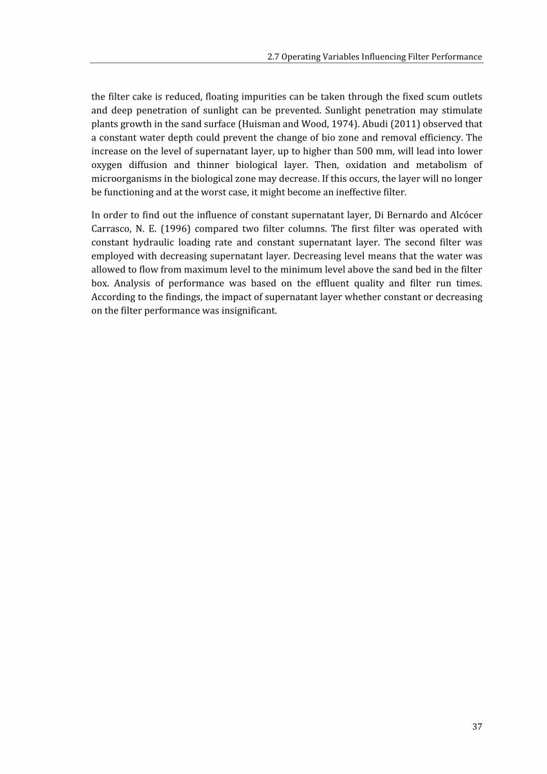
2.7 Operating Variables Influencing Filter Performance
37
the filter cake is reduced, floating impurities can be taken through the fixed scum outlets
and deep penetration of sunlight can be prevented. Sunlight penetration may stimulate
plants growth in the sand surface (Huisman and Wood, 1974). Abudi (2011) observed that
a constant water depth could prevent the change of bio zone and removal efficiency. The
increase on the level of supernatant layer, up to higher than 500 mm, will lead into lower
oxygen diffusion and thinner biological layer. Then, oxidation and metabolism of
microorganisms in the biological zone may decrease. If this occurs, the layer will no longer
be functioning and at the worst case, it might become an ineffective filter.
In order to find out the influence of constant supernatant layer, Di Bernardo and Alcócer
Carrasco, N. E. (1996) compared two filter columns. The first filter was operated with
constant hydraulic loading rate and constant supernatant layer. The second filter was
employed with decreasing supernatant layer. Decreasing level means that the water was
allowed to flow from maximum level to the minimum level above the sand bed in the filter
box. Analysis of performance was based on the effluent quality and filter run times.
According to the findings, the impact of supernatant layer whether constant or decreasing
on the filter performance was insignificant.


39
3 Research Questions and
Objectives
Previous findings in the influence of operating variables presented in Section 2.7 may
imply that the recommended design criteria are rather conservative. Applying the
recommended values does not necessarily ensure an excellent slow sand filtration
performance. As a matter of choice, the decision on the design of slow sand filtration
cannot be dependent on the recommended values (see Table 1) only. Unfortunately, most
of the previous tests were conducted with different filter configurations. As an example
the study of Zipf et al. (2016) who compared fine and coarse media with different values of
Cu. This setting may complicate the conclusion of which operating variables of the design
criteria dominate the effect to the slow sand filtration performance. Moreover, the
influence of every operating variable on the removal mechanism is still rare to be found in
the literature. Optimization and wider application of slow sand filtration technology may
be restricted due to the existence of this gap. Therefore, the main purpose of this study
was to optimize the design recommendation of slow sand filtration by understanding the
influence of each operating variable independently on the suspended solids removal
mechanisms. There were two reasons behind the selection of suspended solids removal as
a focus. The first was because suspended solid is a significant pollutant in the water and it
may affect the disinfection process (see Section 2.1). The second was because its physical
removal is a fundamental mechanism in slow sand filtration (see Section 2.5). Along with
the main purpose, an attention was also given to the method of increasing filter run time
and hydraulic loading rate.
In order to achieve the main purpose of this research, some specific objectives along with
the research questions were defined as follows:
1. to identify the effect of operating variables, specifically d10, Cu and high hydraulic
loading rate on the removal efficiency.
How is the influence of each operating variable on the removal efficiency of suspended
solids?
Is grain size distribution represented by d10 and Cu the dominant factor which influences
the removal efficiency?
Does coarse sand produce a low filtrate quality?
Does high hydraulic loading rate deteriorate the removal efficiency significantly?

3 Research Questions and Objectives
40
2. to find out the influence of d10, Cu, hydraulic loading rate and bed depth on the solids
penetration and dominant removal mechanisms within the filter bed.
How is the influence of each operating variable on the solids penetration in filter bed?
How does each operating variable influence the dominant removal mechanism?
How does suspended solids deposition influence the clogging period?
3. to identify the clogging period by observing the development of hydraulic conductivity
and head loss.
How is the influence of each operating variable on the progressive head loss?
4. to evaluate the method for prolonging the filter run time by adding protection layer.
Is the method of Mälzer and Gimbel (2006) on the addition of protection layer a suitable
approach to prolong the filter run time?
5. to investigate the method for increasing the hydraulic loading rate.
Are the recommended values of hydraulic loading rate plausible to be followed?
The approach to achieve the objectives was by investigating the influence of each
operating variable systematically. A systematic scientific investigation allows the
operating variables to be investigated independently. The experimental approach used in
this study is still limited in the literature making it as a great challenge in the study.

4.1 Overview of Experimental Setup
41
4 Materials and Methods
4.1 Overview of Experimental Setup
Due to the limited literature on the experimental approach, many parts of the
experimental set-up were not standardized. Therefore, the experimental works were
divided into three major phases i.e. pre-experiment, Phase I and Phase II.
Pre-experiment phase was conducted to set up the materials and procedure. Grain size
distribution of media, characteristic of media in regard to specific gravity, methods of filter
construction, potential surrogate material and suitable operation mode related to the
supernatant layer were determined in this phase. A part of the tests especially on the
setup of varied grain size distribution represented by d10 and Cu provided several results
which served as a presumptive basis of the filter performance in Phase I and Phase II. The
trial of the experimental setup was very important because methods of filter run,
hydraulic conductivity measurement, sampling and evaluation of filter performance for
Phase I and Phase II were tested here. In addition, the influence of protection layer was
also figured out.
Phase I focused on the investigation of the influence of operating variables on the
suspended solids removal. The operating variables that were tested consisted of d10 and Cu
of media and high hydraulic loading rate. Filter columns were constructed from Plexiglass
with the diameter of 125 mm and height of 1200 mm. A set of filter columns for the test of
each operating variable was replicated two to three times in order to obtain the reliable
data. In Phase I, the removal mechanisms of slow sand filtration remained into a black box
because the evaluation of filter performance was only based on its ability to remove the
suspended solids. Two important parameters used in the evaluation of filer performance
were turbidity and TSS. Development of hydraulic conductivity and head loss was also
observed to monitor the clogging period.
In Phase II, the focus was divided into two essential parts. The first part was similar to the
focus of Phase I, investigating the performance of filter especially on solids removal. The
second part was on the determination of solids penetration in the filter bed to identify the
removal mechanism. Observation on the penetration of solids is important because it also
relates to the filter maintenance. Deeper solids penetration may lead to the failure of
surface scraping. If the solids penetrate too deep in the filter bed, the risk of changing the
whole filter media was higher.
There were three independent variables tested in Phase II, i.e. d10, Cu and hydraulic loading
rate. During the tests in this phase, filter columns with diameter of 60 mm were used.
Analysis on the solids penetration was conducted adapting the method of Ellis and Aydin
(1995). At the beginning, every 10 mm of filter bed was scraped carefully using a small

4 Materials and Methods
42
long scoop. Each sand sample was placed in an Erlenmeyer flask. Then each sand sample
was diluted by adding 100 mL of distilled water. Every diluted sample was shaken for 40
minutes using a flask shaker operated at 100 rpm. Afterwards, the diluted sample was
rested for 5 minutes allowing the sand to settle down. The supernatant containing the
suspended solids was decanted for the turbidity measurement. By investigating the solids
penetration in the bed depth, influence of operating variables i.e. grain size distribution,
hydraulic loading rate and bed depth on the dominant removal mechanisms (see Figure
11) could be identified. Investigation on the adequacy of adding protection layer to
prolong the filter run time was also conducted within the Phase II. Based on the analysis of
solids penetration, the function of gravel layer above the sand bed could be verified.
In the entire experimental phases, a total of 10 filter columns were built for the pre-
experiment phase. The tests in Phase I and Phase II involved in total 18 and 13 filter
columns respectively. Table 3 presents the list of each test with the amount and diameter
of filter columns.
Table 3. Overview of constructed filter columns for each test
Test
Grain Size
Distribution of
Filter Media Porosity
n
Empirical Hydraulic Conductivity
(m/s)
d10
(mm) Cu Beyer kB Hazen kH
Kozeny-
Carman
kKC
Pre-experiment
Supernatant Layer:
Constant-Filter 1 0.26 2.5 0.33 9.16×10⁻⁴ 6.76×10⁻⁴ 2.14×10⁻⁴
Constant-Filter 2 0.26 2.5 0.33 9.16×10⁻⁴ 6.76×10⁻⁴ 2.14×10⁻⁴
Decreasing-Filter 1 0.26 2.5 0.33 9.16×10⁻⁴ 6.76×10⁻⁴ 2.14×10⁻⁴
Decreasing-Filter 2 0.26 2.5 0.33 9.16×10⁻⁴ 6.76×10⁻⁴ 2.14×10⁻⁴
Setup of d10:
Filter 1 0.075 2.5 0.38 7.62×10⁻⁵ - 2.83×10⁻⁵
Filter 2 0.50 2.5 0.35 3.39×10⁻³ 2.80×10⁻³ 9.59×10⁻⁴
Setup of Cu:
Filter 1 0.15 2.5 - 3.05×10⁻⁴ - -
Filter 2 0.15 5 - 2.65×10⁻⁴ - -

4.1 Overview of Experimental Setup
43
Table 3. (continued)
Test
Grain Size
Distribution of Filter
Media Porosity
n
Empirical Hydraulic Conductivity
(m/s)
d10 (mm) Cu Beyer kB Hazen kH
Kozeny-
Carman
kKC
Pre-experiment
Protection Layer:
WOPL Filter 0.20 1.74 - 5.79×10⁻⁴ - -
WPL Filter 0.20 1.74 - 5.79×10⁻⁴ - -
Phase I
Solids Removal in
Varied d10:
Set 1
Filter 1 0.075 2.5 0.42 7.62×10⁻⁵ - 3.86×10⁻⁵
Filter 2 0.15 2.5 0.41 3.05×10⁻⁴ 2.38×10⁻⁴ 7.85×10⁻⁵
Filter 3 0.26 2.5 0.36 9.16×10⁻⁴ 7.90×10⁻⁴ 2.81×10⁻⁴
Filter 4 0.40 2.5 0.35 2.17×10⁻³ 1.62×10⁻³ 5.14×10⁻⁴
Filter 5 0.50 2.5 0.34 3.39×10⁻³ 2.62×10⁻³ 8.56×10⁻⁴
Set 2
Filter 1 0.15 2.5 0.34 3.05×10⁻⁴ 3.26×10⁻⁴ 1.42×10⁻⁴
Filter 2 0.26 2.5 0.33 9.16×10⁻⁴ 6.71×10⁻⁴ 2.11×10⁻⁴
Filter 3 0.40 2.5 0.33 2.17×10⁻³ 1.75×10⁻³ 5.88×10⁻⁴
Filter 4 0.50 2.5 0.32 3.39×10⁻³ 2.37×10⁻³ 7.52×10⁻⁴
Solids Removal in
Varied Cu:
Set A
Filter 1 0.26 2.5 0.32 9.16×10⁻⁴ 6.30×10⁻⁴ 1.90×10⁻⁴
Filter 2 0.26 3 0.32 8.84×10⁻⁴ 6.30×10⁻⁴ 1.90×10⁻⁴
Filter 3 0.26 5 0.32 7.96×10⁻⁴ 6.19×10⁻⁴ 1.91×10⁻⁴
4 Materials and Methods
44
Table 3. (continued)
Test
Grain Size
Distribution of Filter
Media Porosity
n
Empirical Hydraulic Conductivity
(m/s)
d10 (mm) Cu Beyer kB Hazen kH
Kozeny-
Carman
kKC
Phase I
Set B
Filter 1 0.26 2.5 0.32 9.16×10⁻⁴ 6.30×10⁻⁴ 1.90×10⁻⁴
Filter 2 0.26 3 0.32 8.84×10⁻⁴ 6.30×10⁻⁴ 1.90×10⁻⁴
Filter 3 0.26 5 0.31 7.96×10⁻⁴ 5.81×10⁻⁴ 1.86×10⁻⁴
Set C
Filter 1 0.26 2.5 0.32 9.16×10⁻⁴ 6.30×10⁻⁴ 1.91×10⁻⁴
Filter 2 0.26 3 0.32 8.84×10⁻⁴ 6.21×10⁻⁴ 1.68×10⁻⁴
Filter 3 0.26 5 0.29 7.96×10⁻⁴ 5.31×10⁻⁴ 1.47×10⁻⁴
Solids Removal in
High Hydraulic
Loading Rate*:
Set A
Filter 1 0.26 2.5 0.32 9.16×10⁻⁴ 6.30×10⁻⁴ 1.90×10⁻⁴
Filter 2 0.26 3 0.32 8.84×10⁻⁴ 6.30×10⁻⁴ 1.90×10⁻⁴
Filter 3 0.26 5 0.32 7.96×10⁻⁴ 6.19×10⁻⁴ 1.91×10⁻⁴
Set B
Filter 1 0.26 2.5 0.32 9.16×10⁻⁴ 6.30×10⁻⁴ 1.90×10⁻⁴
Filter 2 0.26 3 0.32 8.84×10⁻⁴ 6.30×10⁻⁴ 1.90×10⁻⁴
Filter 3 0.26 5 0.31 7.96×10⁻⁴ 5.81×10⁻⁴ 1.86×10⁻⁴
Set C
Filter 1 0.26 2.5 0.32 9.16×10⁻⁴ 6.30×10⁻⁴ 1.91×10⁻⁴
Filter 2 0.26 3 0.32 8.84×10⁻⁴ 6.21×10⁻⁴ 1.68×10⁻⁴
Filter 3 0.26 5 0.29 7.96×10⁻⁴ 5.31×10⁻⁴ 1.47×10⁻⁴

4.1 Overview of Experimental Setup
45
Table 3. (continued)
Test
Grain Size
Distribution of Filter
Media Porosity
n
Empirical Hydraulic Conductivity
(m/s)
d10 (mm) Cu Beyer kB Hazen kH
Kozeny-
Carman
kKC
Phase II
Solids Removal
and Penetration in
Varied d10:
Filter 1 0.075 2.5 0.33 7.62×10⁻⁵ - 1.84×10⁻⁵
Filter 2 0.26 2.5 0.35 9.16×10⁻⁴ 7.49×10⁻⁴ 2.55×10⁻⁴
Filter 3 0.50 2.5 0.34 3.39×10⁻³ 2.58×10⁻³ 8.34×10⁻⁴
Filter 4 0.70 2.5 0.36 - 5.73×10⁻³ 2.04×10⁻³
Filter 5 0.90 2.5 0.35 - 9.05×10⁻³ 3.10×10⁻³
Solids Removal
and Penetration in
Varied Cu:
Filter 1 0.26 2.5 0.37 9.16×10⁻⁴ 8.30×10⁻⁴ 3.07×10⁻⁴
Filter 2 0.26 3 0.33 8.84×10⁻⁴ 6.76×10⁻⁴ 2.14×10⁻⁴
Filter 3 0.26 7 0.31 7.38×10⁻⁴ 6.09×10⁻⁴ 1.81×10⁻⁴
Solids Removal
and Penetration in
Varied Hydraulic
Loading Rate*:
Filter 1-0.08 m/h 0.26 2.5 0.33 9.16×10⁻⁴ 6.72×10⁻⁴ 2.12×10⁻⁴
Filter 2-0.20 m/h 0.26 2.5 0.37 9.16×10⁻⁴ 8.30×10⁻⁴ 3.07×10⁻⁴
Filter 3-0.80 m/h 0.26 2.5 0.34 9.16×10⁻⁴ 7.33×10⁻⁴ 2.45×10⁻⁴
Increasing the
Filter Run Time:
Filter 1-WOPL 0.26 2.5 0.37 9.16×10⁻⁴ 8.30×10⁻⁴ 3.07×10⁻⁴
Filter 2-WPL 0.26 2.5 0.34 9.16×10⁻⁴ 7.18×10⁻⁴ 2.37×10⁻⁴
*The test used the same filter columns as in the test of solids removal in varied Cu **One filter column is from the test of solids removal and penetration in varied Cu
4 Materials and Methods
46
4.2 Pre-Experiment Phase
4.2.1 Filter Media and Determination of Specific Gravity
Quartz sand was the only type of sands tested in the entire experimental phases. The
quartz sand was supplied by two companies from Germany, Gebrüder Willersinn GmbH in
Ludwigshafen and Friedrich Quarzsandwerke in Rheinhafen. The first supplier also
provided the gravels that were used for the supporting and protection layer. The gravel
was washed and dried in the laboratory and sieved with two sieve openings. The objective
of sieving was to separate the gravel size into coarse (>6.3 mm) and fine (2-6.3 mm)
fractions. By using the separate gravel size, construction of supporting layer could be
stratified where the coarse gravel was placed under the finer one. This grading allowed
the supporting layer to be more stable to hold up the sand bed. The fine gravel was also
used as a protection layer, which was installed above the sand bed, for several filter
columns.
Fulfilling the requirement of systematic investigation, grain size distribution represented
by d10 and Cu has to be determined so that at the end the configurations of filter columns
can be compared equally. As an example, when the purpose of the test was to identify the
influence of the media size on the slow sand filtration performance, then the grain size
distributions of media was varied in d10 while the Cu was maintained the same (see Figure
13). On the contrary, if the focus was to investigate the influence of the range of media size
on the slow sand filtration performance, then the grain size distributions of media was
varied in Cu while the d10 was maintained the same (see Figure 14). From the grain size
distribution graph, the y-axis shows the percentage of finer grain size by weight and the x-
axis shows the grain size.
Figure 13. Comparison of grain size distributions with different d10 but similar in Cu of 2.5

4.2 Pre-Experiment Phase
47
Figure 14. Comparison of grain size distributions with similar d10 of 0.26 mm but different Cu
A calculation involving the size of sieve openings has been made so that the desired grain
size distribution can be obtained. Since both suppliers were not able to provide the sand
with desired grain size distribution as presented in Table 4, they had to be prepared in the
laboratory. At the beginning, sand from the supplier should be separated based on the
grain size using a sieving machine. Sieving was conducted under the dry method using a
stack of sieves with seven to eight different size openings: 3 mm, 2 mm, 1 mm, 0.5 mm,
0.25 mm, 0.125 mm, 0.063 mm and 0 cm. After that, the sand was remixed based on the
grain composition in Table 4. The mixing was done manually using a bucket and a scoop
due to the small amount of mass per mixture. A sample of around 250 g of sand was then
taken from the new mixture for a sieving analysis. This sieving analysis was to ensure that
the sand is well-mixed.
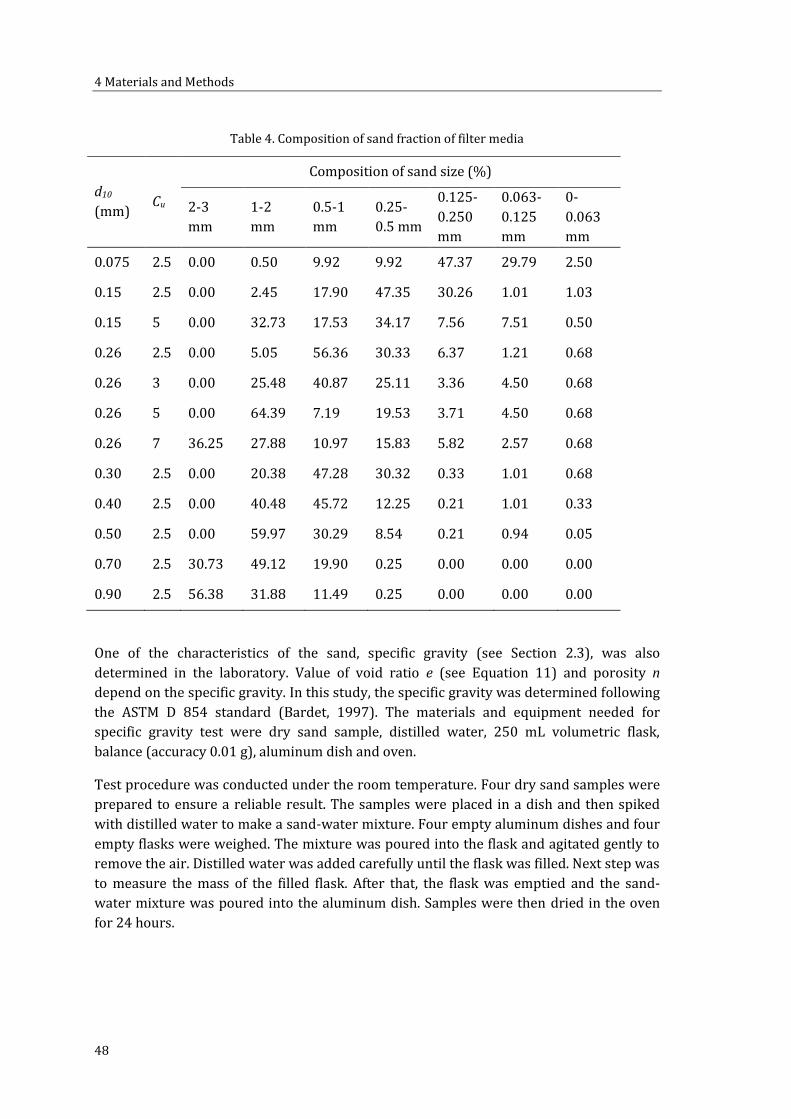
4 Materials and Methods
48
Table 4. Composition of sand fraction of filter media
d10
(mm) Cu
Composition of sand size (%)
2-3
mm
1-2
mm
0.5-1
mm
0.25-
0.5 mm
0.125-
0.250
mm
0.063-
0.125
mm
0-
0.063
mm
0.075 2.5 0.00 0.50 9.92 9.92 47.37 29.79 2.50
0.15 2.5 0.00 2.45 17.90 47.35 30.26 1.01 1.03
0.15 5 0.00 32.73 17.53 34.17 7.56 7.51 0.50
0.26 2.5 0.00 5.05 56.36 30.33 6.37 1.21 0.68
0.26 3 0.00 25.48 40.87 25.11 3.36 4.50 0.68
0.26 5 0.00 64.39 7.19 19.53 3.71 4.50 0.68
0.26 7 36.25 27.88 10.97 15.83 5.82 2.57 0.68
0.30 2.5 0.00 20.38 47.28 30.32 0.33 1.01 0.68
0.40 2.5 0.00 40.48 45.72 12.25 0.21 1.01 0.33
0.50 2.5 0.00 59.97 30.29 8.54 0.21 0.94 0.05
0.70 2.5 30.73 49.12 19.90 0.25 0.00 0.00 0.00
0.90 2.5 56.38 31.88 11.49 0.25 0.00 0.00 0.00
One of the characteristics of the sand, specific gravity (see Section 2.3), was also
determined in the laboratory. Value of void ratio e (see Equation 11) and porosity n
depend on the specific gravity. In this study, the specific gravity was determined following
the ASTM D 854 standard (Bardet, 1997). The materials and equipment needed for
specific gravity test were dry sand sample, distilled water, 250 mL volumetric flask,
balance (accuracy 0.01 g), aluminum dish and oven.
Test procedure was conducted under the room temperature. Four dry sand samples were
prepared to ensure a reliable result. The samples were placed in a dish and then spiked
with distilled water to make a sand-water mixture. Four empty aluminum dishes and four
empty flasks were weighed. The mixture was poured into the flask and agitated gently to
remove the air. Distilled water was added carefully until the flask was filled. Next step was
to measure the mass of the filled flask. After that, the flask was emptied and the sand-
water mixture was poured into the aluminum dish. Samples were then dried in the oven
for 24 hours.

4.2 Pre-Experiment Phase
49
Mass of dried sand then weighed and the specific gravity was calculated using Equation 26
as follows:
= + � − � (26)
where Gs is the specific gravity, Ws the mass of dry sand, Wfw the mass of flask filled with
distilled water only and Wfs the mass of flask filled with sand-water mixture.
Characteristics each variable in the tests and the specific gravity are presented in Table 5.
Table 5. Specific gravity test on quartz sand
Description Sample 1 Sample 2 Sample 3 Sample 4
Mass of flask (g) 100.32 94.14 98.06 88.85
Mass of aluminium dish (g) 5.96 5.98 5.55 5.56
Mass of flask and water(g) 349.75 343.53 347.38 338.10
Mass of flask, sand and water (g) 424.21 423.85 409.37 399.94
Mass of sand and aluminium dish (g) 125.74 136.05 105.36 105.46
Mass of dried sand (g) 119.78 130.07 99.81 99.90
Specific gravity Gs 2.64 2.61 2.64 2.62
Average specific gravity Gs 2.63
4.2.2 Method of Filter Column Construction
Construction of filter columns in the pre-experiment phase and Phase I was using free
falling method while in Phase II, water pluviation method was used. In the free falling
method, the dry sand was poured gradually and carefully into an empty column with the
help of a funnel. During the sand pouring, the funnel was rotated horizontally allowing the
sand to be distributed evenly in the entire filter area. After the sand was loaded into the
column up to the desired height, the water was introduced slowly in the up-flow direction
to avoid short circuiting as seen in Figure 15. Another reason for the up-flow direction was
to reduce the air bubbles that were trapped within the filter bed. In the free falling
process, compaction of sand was only due to the gravitational force. One disadvantage of
this method was the formation of fine grain layers because of the rapid settlement of
coarser grains. At the top of the sand surface, there was also this fine grain layer. The
existence of this layer might lead into faster clogging period because mostly removal in
slow sand filtration occurs at the top of sand bed.

4 Materials and Methods
50
The difference between the water pluviation method and the free falling method laid only
on the introduction of water. Prior to the sand loading, water was filled into the column
carefully under the up-flow direction until certain height. The water level should not be
too high to avoid the overflow due to the sand loading. After that, the process was the
same as in the free falling method where the sand was gradually loaded to the filter. The
loading was done carefully with a funnel to minimize the development of air bubbles when
the sand entering the water layer. Settlement of sand was also because of gravity but the
velocity is slower than from the free falling method due to the existence of water inside
the column, however, similar disadvantage on the formation of fine grain layers was still
found. An advantage of this method was that the sand grains were arranged inside the
water medium therefore, the interspaces between grains were filled with water. As a
consequence, the air bubble development could be reduced.
Figure 15. Short circuiting in the filter column
4.2.3 Selection of Surrogate Material and Turbidity Correlation
In order to maintain a constant quality of influent, artificial raw water created from a
mixture of solid material and tap water was used. In this study, the turbidity is used as the
controlled parameter to describe the quality of artificial raw water. For this purpose, the
turbidity should change linearly as a function of suspended solid concentration. At the
beginning, four materials i.e. natural soil (Heilerde), silica powder (Millisil W12), silica gel
and rock powder were evaluated in order to select the most suitable surrogate material to
represent suspended solids in the artificial raw water.

4.2 Pre-Experiment Phase
51
Prior to the creation of suspension, natural soil, silica powder, silica gel and rock powder
were sieved using 63 μm sieve. Each type of solids was then mixed with tap water under
varied concentration. Mixing process was done using a magnetic stirrer for 15 minutes as
seen in Figure 16. After that, the suspension was decanted and the turbidity was measured
using the Hach Lange 2100Q Portable Turbidimeter. Allowance for the turbidity
measurement was set for ± 10%. In order to investigate the correlation between the
turbidity and the suspended solids concentration, four different concentrations were
tested (Table 6).
Figure 16. Artificial raw water created from a mixture of natural soil and tap water under varied
concentration. The most transparent water has the lowest concentration of suspended solids and
turbidity value.
Table 6. Turbidity correlation according to the type of suspended solids
Suspended solid
concentration
(mg/L)
Turbidity by
natural soil
(NTU)
Turbidity by
silica
powder
(NTU)
Turbidity by
silica gel
(NTU)
Turbidity by
rock powder
(NTU)
50 4.16 21.40 1.61 23.06
250 32.09 121.33 2.45 104.64
500 67.00 252.00 3.50 222.86
1000 153.33 581.00 3.15 956.30
The values of measured turbidity are plotted in Figure 17. According to the regression
analysis, relationship between suspended solids concentration and turbidity for natural

4 Materials and Methods
52
soil and silica powder was strongly linear. However, the analysis for silica gel and rock
powder showed that the relationship between suspended solids and turbidity was not
linear. Concentration of silica gel in the liquid did not affect the turbidity values.
Meanwhile for rock powder, exponential regression fit more properly than linear
regression. Based on this result, silica gel and rock powder were omitted as potential
surrogate material in the raw water.
Figure 17. Relationship between turbidity and suspended solids concentration for natural soil, silica
powder, silica gel and rock powder
At the beginning, natural soil was chosen as the surrogate material solely because the
standard error of natural soil in the regression analysis was lower than the silica powder.
However, after some tests in the pre-experiment phase and the test of influence of the d10
in Phase I, it was observed that the settling velocity of natural soil was quite fast. Then the
settling velocity of the natural soil and the second potential surrogate material, silica
powder, was compared. The approach was by determining the grain size distribution of
both materials followed by the calculation of the settling velocity using Equation 25.
Measurement of particle size was conducted using EyeTech Particle Size and Shape
Analyzer.
Output from the particle size measurement indicated that silica powder has a larger fine
fraction than the natural soil (see Figure 17). Larger content of fine fraction in the silica
powder causes lower settling velocity of particle compared to the natural soil. Comparison
of settling velocity for both materials based on the value of d10, d50 and d90 is shown in
Table 7. Based on the settling velocity of natural soil which was higher than the applied
hydraulic loading rate (see Section 2.7.2), sedimentation was the only mechanism that
worked for the complete removal (see Section 2.6). Therefore, for the rest of the tests in
Phase I and Phase II, silica powder was used as surrogate material to create the artificial
raw water.

4.2 Pre-Experiment Phase
53
Figure 18. Grain size distribution of natural soil and silica powder
Table 7. Settling velocity (20 °C) of natural soil and silica powder according to d10, d50 and d90 of
particles
Parameter
Ø μm Settling Velocity
(m/h)
Natural
soil
Silica
powder
Natural
soil
Silica
powder
d10 16.11 9.18 0.84 0.27
d50 34.85 26.08 3.93 2.20
d90 54.33 51.58 9.55 8.61
4.2.4 Selection of Suitable Supernatant Level
Focus on this test was to select the suitable supernatant level for the filter operation
during the experimental phases. Influence of constant and decreasing supernatant levels
on the slow sand filtration performance was investigated. The investigation was
performed with distilled water as the inlet in order to minimize the effect of particle
addition on the alteration of the hydraulic loading rates. For the test, four filter columns
were constructed with the same grain size distribution of media, d10 of 0.26 mm and Cu of
2.5. All filter columns consisted of 30 mm supporting layer, 200 mm filter bed and 20 mm
protection layer. Two columns were operated under constant head i.e. Constant-Filter 1
and Constant-Filter 2. The other two columns were operated under decreasing head i.e.
Decreasing-Filter 1 and Decreasing-Filter 2.

4 Materials and Methods
54
Columns with constant head mode were operated with a constant Δh (Figure 19a). In
order to maintain the constant supernatant level, the principal of communicating vessel
was adopted. In the decreasing head mode, the supernatant level was allowed to drop
from the maximum level to the minimum level (Figure 19b). Once the supernatant reached
the minimum level, the operation was stopped and restarted after the supernatant was in
the maximum level.
(a) (b)
Figure 19. Scheme of filter columns operated under constant and decreasing head (not drawn to
scale)
Evaluation on the filter behavior under constant and decreasing supernatant levels was
based on the development of hydraulic loading rate. In the filter columns operated under
constant supernatant layer, the trend of hydraulic loading rate was constant as illustrated
in Figure 20. Meanwhile, in the decreasing mode, average hydraulic loading rates were
likely to decline from the initial value. Considering that there was no addition of
suspended solids to the filter bed which might lead into clogging, the behavior of filter
columns with decreasing supernatant level was quite distinctive. According to the
previous literatures, this decrease in hydraulic conductivity might be as a result of
compaction in the filter bed during the operation which altered its capacity to transport
water (Bardet, 1997; Hatt et al., 2008). This changing of the capacity might occur not only
due to the frequent openings and closings of the valve but also inconsistent hydraulic
loading rate.
min level
max level
Δh
Inlet
Outlet
Supernatant layer
Protection layer
Supporting layer
Sand layer
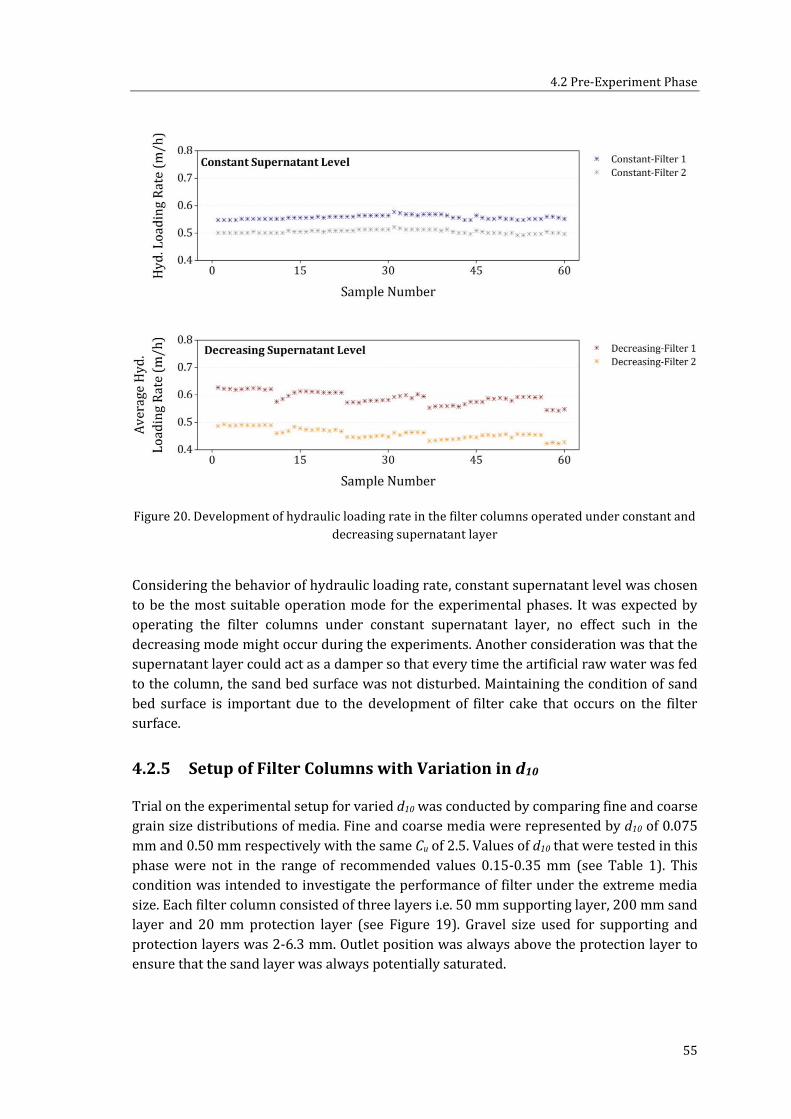
4.2 Pre-Experiment Phase
55
Figure 20. Development of hydraulic loading rate in the filter columns operated under constant and
decreasing supernatant layer
Considering the behavior of hydraulic loading rate, constant supernatant level was chosen
to be the most suitable operation mode for the experimental phases. It was expected by
operating the filter columns under constant supernatant layer, no effect such in the
decreasing mode might occur during the experiments. Another consideration was that the
supernatant layer could act as a damper so that every time the artificial raw water was fed
to the column, the sand bed surface was not disturbed. Maintaining the condition of sand
bed surface is important due to the development of filter cake that occurs on the filter
surface.
4.2.5 Setup of Filter Columns with Variation in d10
Trial on the experimental setup for varied d10 was conducted by comparing fine and coarse
grain size distributions of media. Fine and coarse media were represented by d10 of 0.075
mm and 0.50 mm respectively with the same Cu of 2.5. Values of d10 that were tested in this
phase were not in the range of recommended values 0.15-0.35 mm (see Table 1). This
condition was intended to investigate the performance of filter under the extreme media
size. Each filter column consisted of three layers i.e. 50 mm supporting layer, 200 mm sand
layer and 20 mm protection layer (see Figure 19). Gravel size used for supporting and
protection layers was 2-6.3 mm. Outlet position was always above the protection layer to
ensure that the sand layer was always potentially saturated.
4 Materials and Methods
56
After the filter columns were constructed, its characteristics related to the values of
porosity, specific surface area and initial hydraulic conductivity was determined. In the
whole tests of this study, the hydraulic conductivity measurement was always conducted
with the constant head method. The main reason was because the flow of water through
the filter media was too rapid to be measured with falling head test. In order to identify
the clogging pattern, hydraulic conductivity measurements were carried out for at least
two times i.e. initial one when the filter bed was still clean and final one when the filter has
been loaded with solids which come from the raw water. The design of filter column did
not allow the hydraulic conductivity measurement for the filter bed only because the
water flowed through the whole layers including the protection and supporting layer.
However, the hydraulic conductivity is significantly influenced by the finest grain within
the system. Therefore, it was assumed that the presence of protection and supporting
layer had an insignificant effect to the degree of hydraulic conductivity of filter column.
Based on the value of initial hydraulic conductivity, the initial hydraulic loading rate could
be set-up by adjusting the Δh. Initial hydraulic loading rate for both columns in this test
was set at 0.18±0.05 m/h.
Artificial raw water was created by mixing the natural soil and tap water under the
concentration of 1000 mg/L or 250±25 NTU. Intermittent mode was selected as the
method of filter operation for the whole experimental phases. The basic reason was
because with the intermittent mode, the amount of water filtered and the mass of solids
could be controlled easier which was very important for conducting the systematic
investigation. During the filter operation, a volume of 300 mL was fed to the column for
each filter run. Performance of filer columns was evaluated based not only on the
comparison of inlet and outlet water turbidity but also on the filter behavior in regard to
the development of hydraulic conductivity and head loss. In order to observe the clogging
potential, hydraulic conductivity was measured after every three feedings. For the head
loss, the values of each column would be comparable by converting them into normalized
head loss at certain hydraulic loading rate. In this study, the normalized head loss was
calculated using the formula from Sugimoto (2014) at the hydraulic loading rate of 0.20
m/h (see Equation 27).
� � � � � = � � ℎ × � � � � ℎ (27)
4.2.6 Setup of Filter Columns with Variation in Cu
Experimental setup for varied Cu was also conducted in this pre-experiment phase. Two
filter columns i.e. Cu 2.5 and Cu 5 were constructed for this test. Both filter columns had the

4.2 Pre-Experiment Phase
57
same d10 of 0.15 mm. Configuration of filter columns was as follows: 30 mm of supporting
layer; 250 mm of sand layer; and 20 mm of protection layer. Initial hydraulic conductivity
test was conducted to set-up the hydraulic loading rate of 0.2±0.05 m/h. Natural soil was
used as a surrogate material to create the artificial raw water with a concentration of 1000
mg/L with turbidity of 250±25 NTU. The feeding rate for each filter column was 500
mL/day. Evaluation of filter performance was based on the turbidity removal and
development of relative hydraulic conductivity and normalized head loss at 0.20 m/h. The
calculation of the relative hydraulic conductivity Δk was done by adopting the method of
Schwarz (2004) as follow:
∆ = � (28)
where k(m) is the hydraulic conductivity at solids mass m (m/s) and k(0) is the initial
hydraulic conductivity (m/s).
4.2.7 Influence of Protection Layer on Suspended Solids Removal
The influence of the protection layer on the filter performance on turbidity removal was
studied by constructing two filter columns i.e. WOPL1-Filter and WPL2-Filter. Filter media
that was used for this test was directly taken from the package provided by the supplier
without any modification. The grain size distribution of the sand was represented by d10 of
0.20 mm and Cu of 1.74. Both filter columns consisted of 30 mm supporting layer and 300
mm sand layer. One filter was added with 20 mm protection layer.
Initial hydraulic conductivity was determined after the filter column construction and a
hydraulic loading rate of 0.6±0.15 m/h was set. Silica powder was used as the surrogate
material to create the artificial raw water (220 mg/L and 100±10 NTU). In every feeding,
2000 mL of artificial raw water was filtered. At the end of filter operation, final hydraulic
conductivity was also measured so that the effect of solids addition to the filter capacity
could be observed. The outlet turbidity from both filter columns was also evaluated by
conducting One Way Analysis of Varian (ANOVA) test to find out whether the performance
of both filter was equal. The ANOVA test basically uses the variance of the sample means
to indicate whether they are difference or not (Schumacker and Tomek, 2013). The sample
means are homogeneous if they are similar. On the other hand, if the differences are quite
large then the sample means are heterogeneous. In this study the ANOA test was
performed by using the data analysis from Microsoft Excel. At the end of the calculation,
the results will show the p-value. This p-value will be compared with the significance
factor α. If the p-value is higher than the α then it can be concluded that the sample means
are not significantly different.
1 WOPL = without protection layer 2 WPL = with protection layer

4 Materials and Methods
58
4.3 Phase I
4.3.1 Large Scale Filter Columns with Variation in d10
The experimental setup of this first test in Phase I consisted of two similar sets, i.e. Set 1
and Set 2, of filter columns. Set 1 consisted of five filter columns with five different grain
size distributions which varied in d10 i.e. d10 0.075 mm, d10 0.15 mm, d10 0.26 mm, d10 0.40
mm and d10 0.50 mm (see Figure 21). Set 2 consisted of four filter columns with the same
grain size distributions as in Set 1 but without the d10 0.075 mm. Three values of d10
represented the recommended values (see Table 1) while d10 of 0.075 mm and 0.50 mm
represented the extreme fine and coarse media respectively. The heterogeneity of sand
fraction was represented by Cu of 2.5.
Figure 21. Phase I - Construction of filter columns in Set 1
The principal procedures tested in Section 4.2.5 such as the operation mode, sampling and
methods of parameters measurement were adopted for this investigation. Operating
variables such as bed depth and hydraulic loading rate of both sets were maintained equal.
Configuration of each filter column consisted of 100 mm stratified gravel as supporting
layer (see Section 4.2.1), 500 mm sand layer and 200 mm protection layer (see Figure 22).
The characteristic of each filter column was identified from the values of void ratio and
porosity, specific surface area and hydraulic conductivity. The hydraulic loading rate was
set at 0.20±0.05 m/h.
4.3 Phase I
59
Filter columns were fed up with artificial raw water created from a mixture of natural soil
and tap water. Concentration of the artificial raw water was 380 mg/L and the turbidity
was 100±10 NTU. In every filter run, a volume of 3000 mL was fed to the column. Both
sets of filter columns were under operation for 6 weeks. At the beginning of each week,
7000 mL of artificial raw water were added to the column in order to create the
supernatant layer (Δh). At the end of the week, the hydraulic conductivity was measured
to observe its development. After the measurement of hydraulic conductivity, the water
was allowed to drop until 2 cm above the protection layer to ensure that the sand bed was
potentially saturated. Filtrate samples were taken two times per filter run followed by the
measurement of turbidity and particle size. One Way ANOVA test was carried out to
evaluate the difference of outlet turbidity from each filter column. Another parameter
used to evaluate the filter performance was the development of relative hydraulic
conductivity and normalized head loss at 0.2 m/h.

4 Materials and Methods
60
Figure 22. Phase I - Sketch of large filter column (not drawn to scale)
4.3.2 Large Scale Filter Columns with Variation in Cu
Three similar sets of filter columns i.e. Set A, Set B and Set C, were constructed for this
investigation. Every set consisted of three filter columns with different grain size
distribution which varied in the Cu. The filter columns with narrow grain size distribution
were represented by Cu 2.5 and Cu 3 while the filter column with wide grain size
distribution was represented by Cu 5. The Cu of 2.5 and 3 were tested to validate the
Outlet
SP 1
SP 2
SP 3
SP 4
SP 5
SP 6
Protection
Layer
Sand
Layer
Supporting
Layer
Δh

4.3 Phase I
61
recommended values (see Table 1) while the Cu of 5 was used to investigate how a wide
grain size distribution affects the filter performance. Other operating variables such as d10
(0.26 mm), bed depth, operation mode and hydraulic loading rate were controlled to be
equal for all filter columns. Configuration of the filter columns was exactly the same to the
previous experiment on d10 (see Section 4.3.1, Figure 22). After the filter column
construction, physical properties of filter represented by void ratio, porosity and hydraulic
conductivity were determined. Hydraulic loading rate was set up at 0.2±0.02 m/h for each
filter column.
Artificial raw water in this test was created by mixing tap water and silica powder.
Concentration of suspended solids in the inlet was 220 mg/L and the turbidity was
100±10 NTU. At the beginning of every week, head drop for each column was created
using 2500 mL of artificial raw water. Then, for the next five days each filter column was
fed with a volume of 2500 mL every day. All filter columns were operated intermittently
with constant supernatant layer during seven weeks. Measurement of hydraulic
conductivity was conducted by the end of every week. After the hydraulic conductivity
measurement, the supernatant layer was allowed to drop until zero pressure.
Assessment of the slow sand filtration performance was based on some parameters such
as, turbidity, TSS and particle size. Determination of TSS was done by the gravimetric
method as described in Section 2.1. As the focus of this research experiment was to find
out the influence of Cu on the slow sand filtration performance, the capability of each filter
on removing the turbidity and TSS was compared and analyzed using the ANOVA test. The statistical analyses were conducted at % level of confidence α = . . Development of relative hydraulic conductivity and normalized head loss at 0.20 m/h were also observed
during the study.
4.3.3 Large Scale Filter Columns with Variation in Cu Operated Under
High Hydraulic Loading Rate
In this test, three sets of filter columns i.e. Set A, Set B and Set C from the previous test on
varied Cu were used. Hence, the grain size distribution of filter media was the same but the
initial hydraulic conductivity was different from the previous test. It is because certain
mass of solids was already deposited in the filter bed and affecting the filter capacity. The
test was conducted for eight weeks long. The filter columns were operated using the same
procedure as in the previous test described in Section 4.3.2 except the total volume of
artificial raw water loaded to create the supernatant layer at the beginning of each week
and the hydraulic loading rate (0.6±0.15 m/h). Parameters measured during the test were
turbidity, TSS and particle size. Development of turbidity at the outlet, relative hydraulic
conductivity and head loss was also evaluated. Gradual change in the relative hydraulic
conductivity during the filter run under 0.2±0.05 m/h and 0.6±0.15 m/h is also presented
in the result.
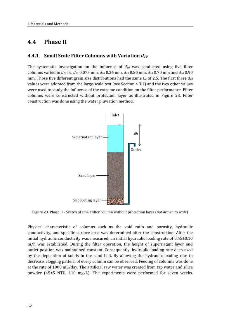
4 Materials and Methods
62
4.4 Phase II
4.4.1 Small Scale Filter Columns with Variation d10
The systematic investigation on the influence of d10 was conducted using five filter
columns varied in d10 i.e. d10 0.075 mm, d10 0.26 mm, d10 0.50 mm, d10 0.70 mm and d10 0.90
mm. Those five different grain size distributions had the same Cu of 2.5. The first three d10
values were adopted from the large-scale test (see Section 4.3.1) and the two other values
were used to study the influence of the extreme condition on the filter performance. Filter
columns were constructed without protection layer as illustrated in Figure 23. Filter
construction was done using the water pluviation method.
Figure 23. Phase II - Sketch of small filter column without protection layer (not drawn to scale)
Physical characteristic of columns such as the void ratio and porosity, hydraulic
conductivity, and specific surface area was determined after the construction. After the
initial hydraulic conductivity was measured, an initial hydraulic loading rate of 0.45±0.10
m/h was established. During the filter operation, the height of supernatant layer and
outlet position was maintained constant. Consequently, hydraulic loading rate decreased
by the deposition of solids in the sand bed. By allowing the hydraulic loading rate to
decrease, clogging pattern of every column can be observed. Feeding of columns was done
at the rate of 1000 mL/day. The artificial raw water was created from tap water and silica
powder (45±5 NTU, 110 mg/L). The experiments were performed for seven weeks.
Supporting layer
Outlet
Inlet
Supernatant layer
Sand layer
Δh
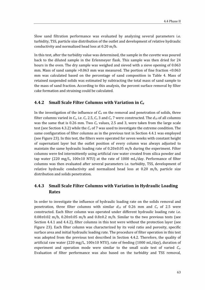
4.4 Phase II
63
Slow sand filtration performance was evaluated by analyzing several parameters i.e.
turbidity, TSS, particle size distribution of the outlet and development of relative hydraulic
conductivity and normalized head loss at 0.20 m/h.
In this test, after the turbidity value was determined, the sample in the cuvette was poured
back to the diluted sample in the Erlenmeyer flask. This sample was then dried for 24
hours in the oven. The dry sample was weighed and sieved with a sieve opening of 0.063
mm. Mass of sand sample >0.063 mm was measured. The portion of fine fraction <0.063
mm was calculated based on the percentage of sand composition in Table 4. Mass of
retained suspended solids was estimated by subtracting the total mass of sand sample to
the mass of sand fraction. According to this analysis, the percent surface removal by filter
cake formation and straining could be calculated.
4.4.2 Small Scale Filter Columns with Variation in Cu
In the investigation of the influence of Cu on the removal and penetration of solids, three
filter columns varied in Cu, i.e. Cu 2.5, Cu 3 and Cu 7 were constructed. The d10 of all columns
was the same that is 0.26 mm. Two Cu values, 2.5 and 3, were taken from the large scale
test (see Section 4.3.2) while the Cu of 7 was used to investigate the extreme condition. The
same configuration of filter columns as in the previous test in Section 4.4.1 was employed
(see Figure 23). In this test, the filters were operated for seven weeks with constant height
of supernatant layer but the outlet position of every column was always adjusted to
maintain the same hydraulic loading rate of 0.20±0.05 m/h during the experiment. Filter
columns were fed intermittently using artificial raw water created from silica powder and
tap water (220 mg/L, 100±10 NTU) at the rate of 1000 mL/day. Performance of filter
columns was then evaluated after several parameters i.e. turbidity, TSS, development of
relative hydraulic conductivity and normalized head loss at 0.20 m/h, particle size
distribution and solids penetration.
4.4.3 Small Scale Filter Columns with Variation in Hydraulic Loading
Rates
In order to investigate the influence of hydraulic loading rate on the solids removal and
penetration, three filter columns with similar d10 of 0.26 mm and Cu of 2.5 were
constructed. Each filter column was operated under different hydraulic loading rate i.e.
0.08±0.02 m/h, 0.20±0.05 m/h and 0.8±0.2 m/h. Similar to the two previous tests (see
Section 4.4.1 and 4.4.2), filter columns in this test were without the protection layer (see
Figure 23). Each filter column was characterized by its void ratio and porosity, specific
surface area and initial hydraulic loading rate. The procedure of filter operation in this test
was adopted from the previous test described in Section 4.4.2. Therefore, the quality of
artificial raw water (220 mg/L, 100±10 NTU), rate of feeding (1000 mL/day), duration of
experiment and operation mode were similar to the small scale test of varied Cu.
Evaluation of filter performance was also based on the turbidity and TSS removal,

4 Materials and Methods
64
development of relative hydraulic conductivity and normalized head loss at 0.20 m/h and
the solids penetration in the sand bed.
4.4.4 Evaluation on the Use of Protection Layer to Prolong Filter Run
Time
In 2006, Mälzer and Gimbel had done a study in regard to the effect of protection layer to
increase the filter run time. A similar experiment was conducted in this study by
employing gravel as protection layer. The study was completed with the analysis on the
solids penetration. The objective was to identify how the solids penetrated in the
protection layer, so that the role of gravel as protection layer to increase the filter run time
could be validated. In order to accommodate this objective, a new filter column with d10 of
0.26 mm and Cu of 2.5 was constructed with the configuration as follows: 30 mm
supporting layer, 200 mm sand layer and 20 mm protection layer. The approach in this
test was to compare the performance of this new constructed filter column and filter
column with d10 0.26 mm and Cu 2.5 from the previous test, which was constructed
without protection layer (see Section 4.4.1). Each filter column was operated under the
constant supernatant level with the adjustment of the outlet position to control the
hydraulic loading rate at 0.20±0.05 m/h. The filter columns were operated intermittently
and fed with artificial raw water (220 mg/L, 100±10 NTU) at the rate of 1000 mL/day for
seven weeks. The performance of slow sand filtration was evaluated based on the
turbidity and TSS removal, particle size distribution, development of relative hydraulic
conductivity and normalized head loss at 0.20 m/h and the solids penetration.

65
5 Results and Interpretation
5.1 Filter Performance in the Pre-Experiment Phase
5.1.1 Comparison of Fine and Coarse Media
Characteristic of filter columns with d10 0.075 mm and d10 0.50 mm that were tested in the
pre-experiment phase is presented in Table 8. From the values of initial hydraulic
conductivity, it can be inferred that the water flowed easier in the filter column with
coarse media. Equal hydraulic loading rate and the different values of initial hydraulic
conductivity led to the variation in the initial head differences (Δh). For the turbidity
removal, filter d10 0.075 mm and filter d10 0.50 mm achieved high efficiencies, i.e. 99.91 %
and 99.89 % respectively, independently from the d10. According to the outlet quality, filter
d10 0.075 mm and filter d10 0.50 mm were able to reduce the turbidity from 250±25 NTU to
below 1 NTU as presented in Figure 24. The values that can be read from the boxplot are
the following:
a. 1st percentile value shown by the lower horizontal line of the whisker,
b. 25th percentile value shown by the bottom part of the box,
c. mean value shown by the little box,
d. median value shown by the horizontal line in the box,
e. 75th percentile value shown by the upper part of the box,
f. 99th percentile value shown by the upper horizontal line of the whisker, and
g. outlier value shown by the small cross.
Table 8. Pre-Experiment Phase - Characteristics of filter columns with fine and coarse media
Parameters d10 0.075 mm d10 0.50 mm
Initial Hydraulic Conductivity k(0) (m/s) 2.96×10⁻⁵ 4.90×10⁻⁴
Initial Hydraulic Loading Rate (m/h) 0.17 0.16
Initial Δh (cm) 29 1.5

5 Results and Interpretation
66
Figure 24. Pre-Experiment Phase - Outlet turbidity of filter d10 0.075 mm and filter d10 0.50 mm
Development of hydraulic conductivity and normalized head loss demonstrated the effect
of suspended solids load to the filter behavior. Figure 25 shows a slight decrease of
hydraulic conductivity in filter d10 0.075 mm and filter d10 0.50 mm. Initial hydraulic
conductivity for filter d10 0.075 mm and filter d10 0.50 mm decreased only for 7 % and 2 %
respectively at the end of filter operation. A very low decrease indicated that an addition
of 6300 mg solids in the filter bed was insignificant for the hydraulic conductivity of both
filter columns. However, a presumptive basis that filter d10 0.075 mm would experience
faster clogging period could be made by considering two reasons i.e. the lower initial
hydraulic conductivity and the decrease of hydraulic conductivity after 6300 mg solids
load which was around three times higher than filter d10 0.50 mm.
Figure 25. Pre-Experiment Phase - Development of relative hydraulic conductivity in filter d10 0.075
mm and filter d10 0.50 mm

5.1 Filter Performance in the Pre-Experiment Phase
67
The decrease of hydraulic conductivity caused an increase in the head loss. In Figure 26,
the gradual increase of normalized head loss at 0.20 m/h due to the suspended solids load
was plotted. According to the graph, it could be inferred that the head loss was
significantly affected by the solids that retained in the filter bed. In regard to the clogging
pattern, interpreting the gradual increase of normalized head loss at 0.20 m/h during the
filter operation could be a promising approach. According to the findings either on the
decrease of hydraulic conductivity or increase of normalized head loss, the degree was
always greater for filter d10 0.075 mm rather than filter d10 0.50 mm.
Figure 26. Pre-Experiment Phase - Development of normalized head loss at 0.20 m/h in filter d10
0.075 mm and filter d10 0.50 mm
5.1.2 Comparison of Narrow and Wide Graded Media
Trial on the experimental setup for filter columns with varied Cu was done by constructing
two filter columns which had the characteristics presented in Table 9. Both filter Cu 2.5
and filter Cu 5 performed well in reducing the turbidity from 250±25 NTU to below 2 NTU
(Figure 27). Filter Cu 2.5 reached averagely a slightly higher turbidity removal (99.64 %)
than filter Cu 5 (99.47 %). This result was contradictory from previous studies by Di
Bernardo and Escobar Rivera (1996) and Zipf et al. (2016) (see Section 2.7.1). However, it
is worth noting again that in the study of Zipf et al., the filter with highest Cu had the
smallest d10. Consequently, it was difficult to evaluate whether the higher removal
turbidity was caused by the higher Cu or lower d10. The approach in this study was more
promising because the d10 was the same for all filter columns therefore the influence of
various Cu could be investigated independently.

5 Results and Interpretation
68
Table 9. Pre-Experiment Phase - Characteristics of filter columns with varied Cu
Parameters Cu 2.5 Cu 5
Initial Hydraulic Conductivity k(0) (m/s) 2.61×10⁻⁴ 1.39×10⁻⁴
Initial Hydraulic Loading Rate (m/h) 0.23 0.21
Initial Δh (cm) 6.5 12
Figure 27. Pre-Experiment Phase - Outlet turbidity of filter Cu 2.5 and filter Cu 5
Filter column with narrow graded media had a higher value of initial hydraulic
conductivity. However, at the end of filter operation, the hydraulic conductivity of filter Cu
2.5 was lower than filter Cu 5. After 8000 mg solids load, the initial hydraulic conductivity
of filter Cu 2.5 decreased up to 67 % while for filter Cu 5 was only 25 %. Figure 28 shows
that the solids load affected the changes of hydraulic conductivity significantly. The
relative hydraulic conductivity in filter Cu 2.5 was significantly greater than in filter Cu 5.
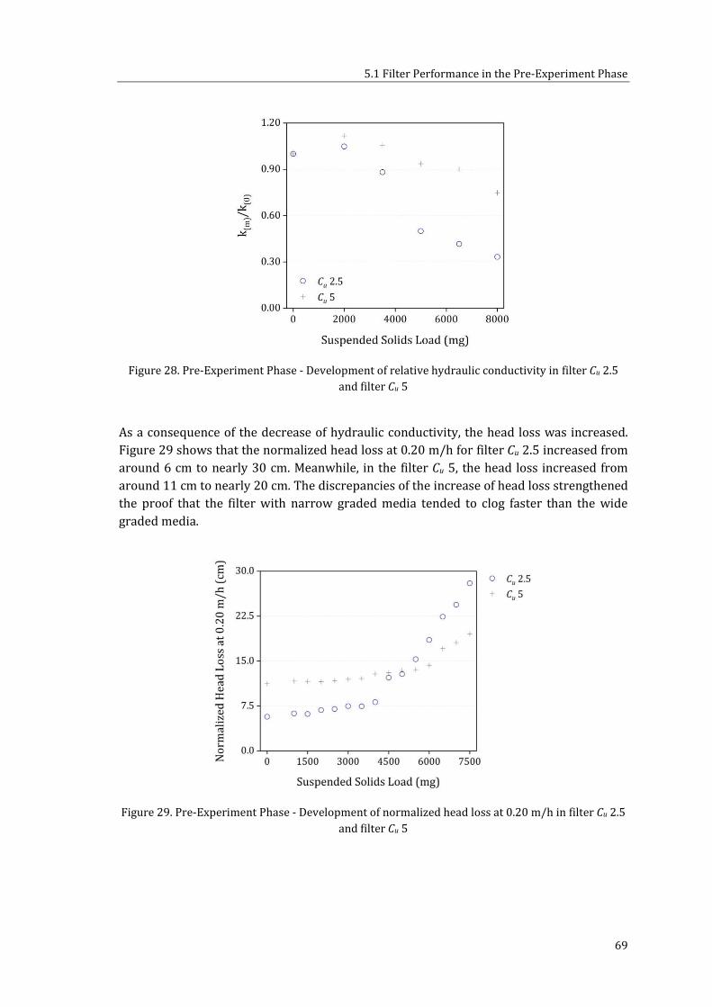
5.1 Filter Performance in the Pre-Experiment Phase
69
Figure 28. Pre-Experiment Phase - Development of relative hydraulic conductivity in filter Cu 2.5
and filter Cu 5
As a consequence of the decrease of hydraulic conductivity, the head loss was increased.
Figure 29 shows that the normalized head loss at 0.20 m/h for filter Cu 2.5 increased from
around 6 cm to nearly 30 cm. Meanwhile, in the filter Cu 5, the head loss increased from
around 11 cm to nearly 20 cm. The discrepancies of the increase of head loss strengthened
the proof that the filter with narrow graded media tended to clog faster than the wide
graded media.
Figure 29. Pre-Experiment Phase - Development of normalized head loss at 0.20 m/h in filter Cu 2.5
and filter Cu 5

5 Results and Interpretation
70
5.1.3 Effect of Protection Layer on Turbidity Removal
One of methods to maintain the sand bed surface undisturbed is by adding protection
layer at the surface of filter bed which may serve as a damper for the water flow. However,
the original design of slow sand filter does not have a protection layer. In this phase, an
experiment in regard to the effect of protection layer, which was constructed from gravel
(2–6.3 mm), on the turbidity removal was conducted. The characteristics of WOPL-Filter
and WPL-Filter which were tested are listed in Table 10. Based on the measurement, the
initial hydraulic conductivity of WOPL-Filter was slightly higher than WPL-Filter. It was
because the protection layer also restricted the water flow through the porous media.
Table 10. Pre-Experiment Phase - Characteristics of filter column with and without protection layer
Parameters WOPL-Filter WPL-Filter
Initial Hydraulic Conductivity k(0) (m/s) 5.40×10⁻⁴ 4.63×10⁻⁴
Initial Hydraulic Loading Rate (m/h) 0.60 0.60
Both filter columns achieved high percentage of turbidity removal i.e. 99.72 % for WOPL-
Filter and 99.70 % for WPL-Filter (Figure 30). Outlet turbidity for both columns was
reduced from 100±10 NTU to below 0.5 NTU independently from the protection layer.
According to the ANOVA test ( 0.05), outlet turbidity from both filter columns was not
significantly different with the p-value of 0.39511. Since the influence of protection layer
on filter performance was deemed to be insignificant, all filter columns in Phase I was
constructed with protection layer.
Figure 30. Pre-Experiment Phase - Outlet turbidity of WOPL-Filter (without protection layer) and
WPL-Filter (with protection layer)

5.2 Influence of the Grain Size Distribution on Suspended Solids Removal
71
In Phase II, filter columns were constructed mostly without protection layer. It is because
the focus of Phase II was to identify the removal mechanism by analyzing the solids
penetration and the presence of protection layer may affect the solids deposition in the
surface of filter bed.
5.2 Influence of the Grain Size Distribution on
Suspended Solids Removal
5.2.1 Variation in d10
The objective of this experiment was to evaluate the influence of varied d10 on the
suspended solids removal. Characteristics of filter columns in Set 1 and Set 2 are
summarized in Table 11. During the filter construction, the compaction of filter media was
only by gravity. Therefore, the mass of sand which was loaded into the filter column was
varied although the bed depth was equal for all filter columns. As a result, porosity values
of filter columns were not similar one another.
Table 11. Phase I - Characteristics of filter columns in the test of varied d10
Parameters d10 0.075 mm d10 0.15 mm d10 0.26 mm d10 0.40 mm d10 0.50 mm
Initial Hyd.
Cond. k(0)
(m/s)
Set 1 9.25×10⁻⁵ 2.61×10⁻⁴ 4.36×10⁻⁴ 4.98×10⁻⁴ 8.27×10⁻⁴
Set 2 6.76×10⁻⁵ 1.64×10⁻⁴ 4.72×10⁻⁴ 4.93×10⁻⁴
Initial Hyd.
Load. Rate
(m/h)
Set 1 0.20 0.19 0.18 0.19 0.20
Set 2 0.18 0.21 0.19 0.19
Initial Δh (cm)
Set 1 40 14 11.5 9 5
Set 2 40 18 9.5 7.5
Values of initial hydraulic conductivity of filter columns in Set 1 and Set 2 were greatly
influenced by the fine fraction. As expected, hydraulic conductivity of filter column with
d10 of 0.075 mm was the lowest among others because it had a high content of fine
fraction. On the contrary, in the filter columns with d10 of 0.50 mm, the content of fine

5 Results and Interpretation
72
fraction was the lowest among others. As a result, the values of initial hydraulic
conductivity of both filter columns Coarse-2 were the highest in both sets. Effect of
uncontrollable arrangement of voids and grains on the initial hydraulic conductivity could
be observed clearly in this phase. From all of the filter columns that were constructed with
the same grain size distribution, the same values of initial hydraulic conductivity were
never being observed. This fact proved that it was impractical to construct identical filter
columns even though both columns were constructed using the same filter media.
Figure 31. Phase I - Outlet turbidity of filter columns in the test of varied d10
After six weeks of intermittent operation, both sets performed satisfactorily by reducing
the inlet turbidity of 100±10 NTU to an average outlet turbidity of below 2 NTU
independently from the d10 (see Figure 31). Both Set 1 and Set 2 could achieve an average
turbidity removal of above 98.90 % (see Table 12). In order to identify the variation
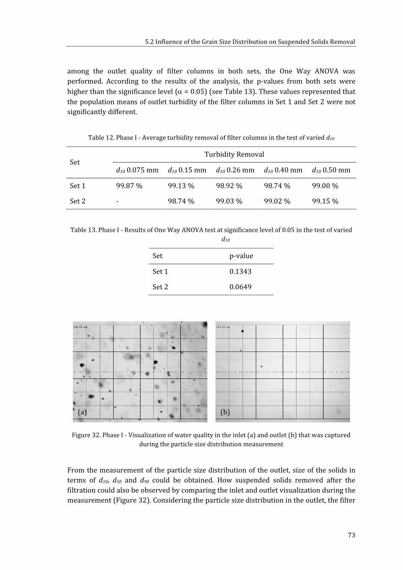
5.2 Influence of the Grain Size Distribution on Suspended Solids Removal
73
among the outlet quality of filter columns in both sets, the One Way ANOVA was
performed. According to the results of the analysis, the p-values from both sets were
higher than the significance level ( = 0.05) (see Table 13). These values represented that
the population means of outlet turbidity of the filter columns in Set 1 and Set 2 were not
significantly different.
Table 12. Phase I - Average turbidity removal of filter columns in the test of varied d10
Set Turbidity Removal
d10 0.075 mm d10 0.15 mm d10 0.26 mm d10 0.40 mm d10 0.50 mm
Set 1 99.87 % 99.13 % 98.92 % 98.74 % 99.00 %
Set 2 - 98.74 % 99.03 % 99.02 % 99.15 %
Table 13. Phase I - Results of One Way ANOVA test at significance level of 0.05 in the test of varied
d10
Set p-value
Set 1 0.1343
Set 2 0.0649
Figure 32. Phase I - Visualization of water quality in the inlet (a) and outlet (b) that was captured
during the particle size distribution measurement
From the measurement of the particle size distribution of the outlet, size of the solids in
terms of d10, d50 and d90 could be obtained. How suspended solids removed after the
filtration could also be observed by comparing the inlet and outlet visualization during the
measurement (Figure 32). Considering the particle size distribution in the outlet, the filter
(a) (b)

5 Results and Interpretation
74
column that was able to retain smaller size of solids could be determined. As presented in
Figure 33, filter columns with finer media represented by d10 of 0.075 mm and 0.15 mm
performed better on restraining smaller solids compared to other filter columns. Three
other columns could wash bigger size of solids out. In these filter columns, it would be
easier for the smaller size of solids to pass through the filter bed. However, those values
are still higher than the size of bacteria and viruses that might exist in raw water. In this
experiment bacteria and viruses were not taken into account.
Figure 33. Phase I - Comparison of size distribution of solids in the outlet of filter columns in the
test of varied d10
The development of relative hydraulic conductivity (see Figure 34) and normalized head
loss at 0.20 m/h (see Figure 35) was evaluated by taking Set 1 as a representative. Initial
hydraulic conductivity of filter columns d10 0.075 mm, d10 0.15 mm, d10 0.26 mm, d10 0.40
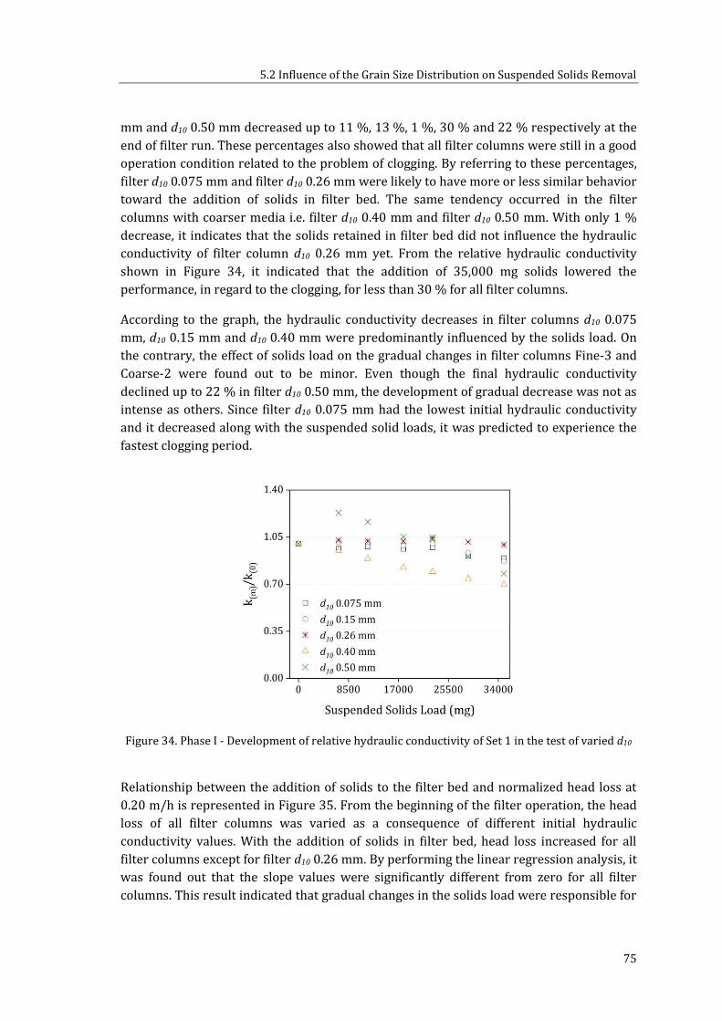
5.2 Influence of the Grain Size Distribution on Suspended Solids Removal
75
mm and d10 0.50 mm decreased up to 11 %, 13 %, 1 %, 30 % and 22 % respectively at the
end of filter run. These percentages also showed that all filter columns were still in a good
operation condition related to the problem of clogging. By referring to these percentages,
filter d10 0.075 mm and filter d10 0.26 mm were likely to have more or less similar behavior
toward the addition of solids in filter bed. The same tendency occurred in the filter
columns with coarser media i.e. filter d10 0.40 mm and filter d10 0.50 mm. With only 1 %
decrease, it indicates that the solids retained in filter bed did not influence the hydraulic
conductivity of filter column d10 0.26 mm yet. From the relative hydraulic conductivity
shown in Figure 34, it indicated that the addition of 35,000 mg solids lowered the
performance, in regard to the clogging, for less than 30 % for all filter columns.
According to the graph, the hydraulic conductivity decreases in filter columns d10 0.075
mm, d10 0.15 mm and d10 0.40 mm were predominantly influenced by the solids load. On
the contrary, the effect of solids load on the gradual changes in filter columns Fine-3 and
Coarse-2 were found out to be minor. Even though the final hydraulic conductivity
declined up to 22 % in filter d10 0.50 mm, the development of gradual decrease was not as
intense as others. Since filter d10 0.075 mm had the lowest initial hydraulic conductivity
and it decreased along with the suspended solid loads, it was predicted to experience the
fastest clogging period.
Figure 34. Phase I - Development of relative hydraulic conductivity of Set 1 in the test of varied d10
Relationship between the addition of solids to the filter bed and normalized head loss at
0.20 m/h is represented in Figure 35. From the beginning of the filter operation, the head
loss of all filter columns was varied as a consequence of different initial hydraulic
conductivity values. With the addition of solids in filter bed, head loss increased for all
filter columns except for filter d10 0.26 mm. By performing the linear regression analysis, it
was found out that the slope values were significantly different from zero for all filter
columns. This result indicated that gradual changes in the solids load were responsible for

5 Results and Interpretation
76
the development of head loss. Compared to other filter columns, filter d10 0.26 mm was the
most stable filter in regard to the alteration of hydraulic conductivity toward the addition
of solids. It indicates that filter d10 0.26 mm would have the longest filter run among
others. By taking the behavior of filter d10 0.26 mm into consideration, the d10 of 0.26 mm
was taken as the effective size of filter columns in the test of varied Cu in Phase I.
Figure 35. Phase I - Development of normalized head loss at 0.20 m/h of Set 1 in the test of varied
d10
5.2.2 Variation in Cu
Table 14. Phase I - Characteristics of filter columns in the test of varied Cu
Parameters Cu 2.5 Cu 3 Cu 5
Initial Hyd. Cond. k(0) (m/s)
Set A 3.72×10⁻⁴ 2.21×10⁻⁴ 2.78×10⁻⁴
Set B 3.55×10⁻⁴ 2.61×10⁻⁴ 6.01×10⁻⁴
Set C 4.00×10⁻⁴ 2.00×10⁻⁴ 4.72×10⁻⁴
Initial Hyd. Loading Rate (m/h)
Set A 0.22 0.21 0.23
Set B 0.21 0.21 0.22
Set C 0.20 0.21 0.21
Initial Δh (cm)
Set A 9.6 16.2 12.8
Set B 10.0 13.5 6.2
Set C 8.3 17.6 7.8

5.2 Influence of the Grain Size Distribution on Suspended Solids Removal
77
Characteristics of filter columns from Set A, Set B and Set C were presented in Table 14. It
was expected that the initial hydraulic conductivity of filter columns with wide graded
sand would be lower because the pores might be filled up with the finer grains. However,
based on the measurement, initial hydraulic conductivity of filter column with wide
graded sand were higher than the values of filter column with narrow graded.
The results from this test on the turbidity and TSS removal did not confirm the results
from the previous test in varied Cu in the Pre-Experiment Phase. The filter column with
higher Cu in the Phase I could achieve turbidity and TSS removal as high as filter columns
with the lower Cu. From the inlet quality of 100±10 NTU and 220 mg/L, outlet turbidity
and TSS was found to be in average less than 2 NTU (see Figure 36) and 3 mg/L (see
Figure 37) respectively for every column in all sets. All filter columns in Set A, Set B and
Set C achieved a percentage of turbidity removal around 99.00 % (see Table 15).
Table 15. Phase I - Average turbidity and TSS removal in the test of varied Cu
Set Turbidity Removal TSS Removal
Cu 2.5 Cu 3 Cu 5 Cu 2.5 Cu 3 Cu 5
Set A 98.97 % 98.95 % 98.92 % 98.63 % 98.57 % 98.09 %
Set B 99.06 % 99.20 % 99.17 % 98.78 % 99.00 % 98.66 %
Set C 99.13 % 99.25 % 99.21 % 98.81 % 98.97 % 99.02 %

5 Results and Interpretation
78
Figure 36. Phase I - Outlet turbidity of filter columns in the test of varied Cu
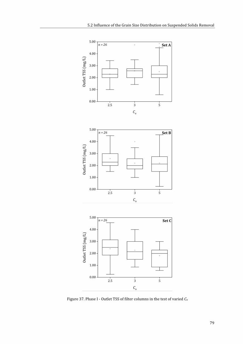
5.2 Influence of the Grain Size Distribution on Suspended Solids Removal
79
Figure 37. Phase I - Outlet TSS of filter columns in the test of varied Cu

5 Results and Interpretation
80
In order to analyze whether there was a significant difference among filter columns in
regard to the removal efficiency, ANOVA test was performed. It was found out that the
mean values of outlet turbidity and TSS of all filter were not significantly different (Table
16) since the p-values were higher than the significance level of 0.05 in every set. These
findings indicated that Cu did not influence significantly the turbidity and TSS removal.
Table 16. Phase I - Results of ANOVA test at significance level of 0.05 in the test of varied Cu
Set p-value
Turbidity TSS
Set A 0.9570 0.2145
Set B 0.3772 0.1431
Set C 0.4498 0.4783
Deposition of solids in the filter bed increased the resistance of the water to pass through
hence altered the hydraulic conductivity. The more solids were retained, the lower the
hydraulic conductivity should be. Figure 38 presents the changes in the average relative
hydraulic conductivity from the three grain size distributions. All filter columns except
filter Cu 3 in all set experienced the gradual decrease on hydraulic conductivity. After
approximately 22,500 mg solids retained in filter bed, the initial hydraulic conductivity of
filter Cu 2.5 and filter Cu 5 decreased up to 7 % and 18 % from the initial values
respectively. At the end of filter run the hydraulic conductivity increased up to 19 % from
the initial value in filter Cu 3. This increase might be caused by the released of the trapped
air bubbles, the changing of the voids arrangement and on the pores connection.
Figure 38. Phase I - Development of average relative hydraulic conductivity of filter columns in the
test of varied Cu

5.3 Influence of High Hydraulic Loading Rate on Suspended Solids Removal
81
With the addition of solids in the sand bed, average normalized head loss at 0.20 m/h
increased for filter columns Cu 2.5 and Cu 5 and decreased for filter columns Cu 3 (see
Figure 39). The increase of normalized head loss at 0.20 m/h for filter Cu 2.5 and filter Cu 5
was around 50 % and 31 % respectively. According to these findings, especially on the
alteration of hydraulic conductivity and normalized head loss, it could be inferred that that
filter columns with Cu of 2.5 tended to clog faster compared to other filter configurations.
This finding confirmed the result of the previous test the pre-experiment phase (see
Section 5.1.2) i.e. filter run time would be longer for a filter column with higher Cu. Since
the capacity of all filter columns was still high (see Figure 38), they were continued to be
operated to study the influence of high hydraulic loading rate on suspended solids
removal.
Figure 39. Phase I - Development of average normalized head loss at 0.20 m/h of filter columns the
test of varied Cu
5.3 Influence of High Hydraulic Loading Rate on
Suspended Solids Removal
When the filter operation under high hydraulic loading rate was started, approximately
22,500 mg of solids were already deposited in the filter bed. The existence of these solids
influenced the behavior of filter columns not only in regard to their hydraulics but also in
regard to the removal efficiencies. Table 17 presents the comparison of average filter
efficiencies under low (0.20±0.05 m/h) and high (0.60±0.15 m/h) hydraulic loading rates.
Turbidity and TSS removals of filter columns operated under high hydraulic loading rate
were surprisingly higher than when they were operated under low rate. For both types of
hydraulic loading rate, the filter columns were fed with the same inlet water quality i.e.
100±10 NTU and 220 mg/L. Under high rate, all filter columns were able to reduce the
turbidity to below 0.50 NTU averagely (see Figure 40). This value was around 75 % lower
than the average outlet turbidity of filter columns when they were operated under low

5 Results and Interpretation
82
hydraulic loading rate (see Figure 36). Based on the turbidity removal, filter columns NG-1
achieved the highest efficiency averagely. Meanwhile, filter columns NG-2 performed
slightly lower than the others.
Table 17. Phase I - Average turbidity and TSS removal of filter columns operated under low
(0.20±0.05 m/h) and high (0.60±0.15 m/h) hydraulic loading rate
Filter Columns Turbidity Removal TSS Removal
Low Rate High Rate Low Rate High Rate
Cu 2.5 99.05 % 99.70 % 98.88 % 99.22 %
Cu 3 99.13 % 99.58 % 98.94 % 99.25 %
Cu 5 99.10 % 99.66 % 99.02 % 99.22 %
The percentage of TSS removal was averagely in the same range for all filter columns.
Average outlet TSS dropped to below 2 mg/L after the filter columns were operated under
high hydraulic loading rate (see Figure 41). This value was around 33 % lower than the
average outlet concentration from the previous test (see Figure 37).
The measurement of size distribution of solids found in the outlet confirmed the previous
results that filter columns with Cu of 2.5 were more capable on retaining fine solids than
other columns (see Error! Reference source not found. and Appendix 4). From almost
all sets, the average size of solids found in the outlet of filter columns Cu 2.5 was finer than
of filter Cu 3 and filter Cu 5. It was also found out that the solids in the outlet of filter
columns operated under high hydraulic loading rate were finer than under low hydraulic
loading rate.

5.3 Influence of High Hydraulic Loading Rate on Suspended Solids Removal
83
Figure 40. Phase I - Outlet turbidity of filter columns in test of high hydraulic loading rate
(0.60±0.15 m/h)

5 Results and Interpretation
84
Figure 41. Phase I - Outlet TSS of filter columns in the test of high hydraulic loading rate (0.60±0.15
m/h)

5.3 Influence of High Hydraulic Loading Rate on Suspended Solids Removal
85
Changes in the hydraulic conductivity of filter columns toward the addition of solids were
observed during the operation (see Figure 42). During the filter operation under low rate,
an anomaly occurred in the filter columns Cu 3. In all sets, the hydraulic conductivity of
filter Cu 3 increased while the other filter columns decreased with the addition of solids. In
the filter operation under high hydraulic loading rate, average hydraulic conductivity
decreased up to 44 % and 21 % for filter Cu 2.5 and filter Cu 5. Meanwhile, in filter Cu 3, an
increase of 3 % on the hydraulic conductivity was found.
Figure 42. Phase I - Development of average relative hydraulic conductivity of filter columns in the
test of high hydraulic loading rate (0.60±0.15 m/h)
Compensating the decrease on the hydraulic conductivity, the head loss in the filter bed
was gradually increased except for filter columns Cu 3 (see Figure 43). Following the
pattern of hydraulic conductivity, suspended solids load affected the development of head
loss predominantly in the filter columns Cu 2.5 and Cu 5. After the filter operation was
terminated, the average value of the final head loss increased around 57 % and 23 % from
the initial values for filter columns Cu 2.5 and Cu 5 respectively. Meanwhile, the effect of
suspended solids load in the filter columns Cu 3 was minor. The average increase of final
head loss in filter columns Cu 3 was only 2 % from the initial values. As expected, the
increase of head loss in filter with Cu of 2.5 was higher compared to the other
configurations.

5 Results and Interpretation
86
Figure 43. Phase I - Development of average normalized head loss at 0.20 m/h of filter columns in
the test of high hydraulic loading rate (0.60±0.15 m/h)
Figure 44 presents the behavior of filter columns toward the total solids load from the
beginning of filter operation until the termination under high hydraulic loading rate.
Hydraulic conductivity of filter Cu 2.5 dropped up to 48 % from the initial value. It
indicated that after a load of around 62,500 mg solids the filter capacity declined to almost
50 % from its actual capacity. The same decreasing trend occurred in filter Cu 5 which
experienced a decrease of 36 %. Filter Cu 3 behaved differently due to the increase of
hydraulic conductivity up to 22 % from its initial. By considering both the development of
relative hydraulic conductivity and normalized head loss at 0.20 m/h, it could be inferred
that the filter columns with Cu of 2.5 tended to clog faster than the others.
Figure 44. Phase I - Development of average relative hydraulic conductivity of filter columns from
the clean filter bed until the termination of the operation at 0.60±0.15 m/h
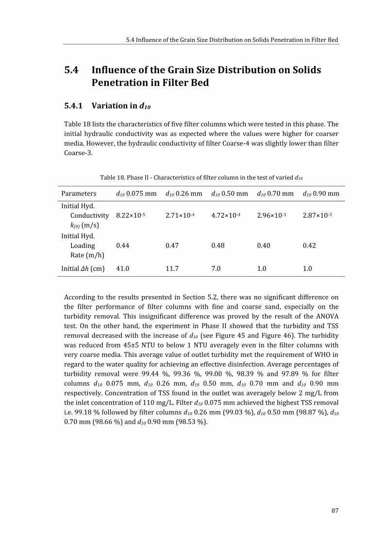
5.4 Influence of the Grain Size Distribution on Solids Penetration in Filter Bed
87
5.4 Influence of the Grain Size Distribution on Solids
Penetration in Filter Bed
5.4.1 Variation in d10
Table 18 lists the characteristics of five filter columns which were tested in this phase. The
initial hydraulic conductivity was as expected where the values were higher for coarser
media. However, the hydraulic conductivity of filter Coarse-4 was slightly lower than filter
Coarse-3.
Table 18. Phase II - Characteristics of filter column in the test of varied d10
Parameters d10 0.075 mm d10 0.26 mm d10 0.50 mm d10 0.70 mm d10 0.90 mm
Initial Hyd.
Conductivity
k(0) (m/s)
8.22×10⁻⁵ 2.71×10⁻⁴ 4.72×10⁻⁴ 2.96×10⁻³ 2.87×10⁻³
Initial Hyd.
Loading
Rate (m/h)
0.44 0.47 0.48 0.40 0.42
Initial Δh (cm) 41.0 11.7 7.0 1.0 1.0
According to the results presented in Section 5.2, there was no significant difference on
the filter performance of filter columns with fine and coarse sand, especially on the
turbidity removal. This insignificant difference was proved by the result of the ANOVA
test. On the other hand, the experiment in Phase II showed that the turbidity and TSS
removal decreased with the increase of d10 (see Figure 45 and Figure 46). The turbidity
was reduced from 45±5 NTU to below 1 NTU averagely even in the filter columns with
very coarse media. This average value of outlet turbidity met the requirement of WHO in
regard to the water quality for achieving an effective disinfection. Average percentages of
turbidity removal were 99.44 %, 99.36 %, 99.00 %, 98.39 % and 97.89 % for filter
columns d10 0.075 mm, d10 0.26 mm, d10 0.50 mm, d10 0.70 mm and d10 0.90 mm
respectively. Concentration of TSS found in the outlet was averagely below 2 mg/L from
the inlet concentration of 110 mg/L. Filter d10 0.075 mm achieved the highest TSS removal
i.e. 99.18 % followed by filter columns d10 0.26 mm (99.03 %), d10 0.50 mm (98.87 %), d10
0.70 mm (98.66 %) and d10 0.90 mm (98.53 %).

5 Results and Interpretation
88
Figure 45. Phase II – Outlet turbidity of filter columns in the test of varied d10
Figure 46. Phase II – Outlet TSS of filter columns in the test of varied d10
Although the five filter columns achieved high efficiencies, the difference of average outlet
turbidity and TSS between fine and coarse media was quite significant. Average outlet
turbidity of filter column d10 0.075 mm was 0.24 NTU which was nearly four times lower
than the average outlet turbidity of filter d10 0.90 mm (0.95 NTU). In the case of TSS, the
average outlet concentration of filter column d10 0.075 mm was 0.85 mg/L. Meanwhile, the
filter column d10 0.90 mm had the average outlet concentration of 1.61 mg/L which was
nearly two times the outlet of filter d10 0.075 mm. Based on this result, the argument of
using finer sand to ensure high slow sand filtration performance was confirmed. However,
it is worth noting that the coarser d10 tested in this study was nearly three times greater
than the upper limit of the recommended values (see Table 1).

5.4 Influence of the Grain Size Distribution on Solids Penetration in Filter Bed
89
During the filter operation, the hydraulic conductivity of filter columns was altered with
the deposition of solids in filter bed (see Figure 47). The changes in filter capacity could be
used to predict the clogging pattern of filter columns. Filter d10 0.075 mm contained the
finest media and the initial hydraulic conductivity was the lowest among others. At the
end of the filter operation, filter d10 0.075 mm experienced the highest decrease of
hydraulic conductivity i.e. 54 % followed by filter d10 0.26 mm with a decrease of 51 %.
Figure 47. Phase II - Development of relative hydraulic conductivity of filter columns in the test of
varied d10
Clogging period can be predicted from the development of relative hydraulic conductivity
and the increase of normalized head loss at 0.20 m/h (Figure 48). The changes of filter
capacity on filter d10 0.70 mm and filter d10 0.090 mm were not as predominant as in the
filter with finer media. Filter d10 0.70 mm and filter d10 0.90 mm behaved differently from
others toward the solids load. While the hydraulic conductivity of filter d10 0.075 mm, filter
d10 0.26 mm and filter d10 0.50 mm decreased with the solids load, filter columns d10 0.70
mm and d10 0.90 mm slightly increased up to around 4 % and 5 %.
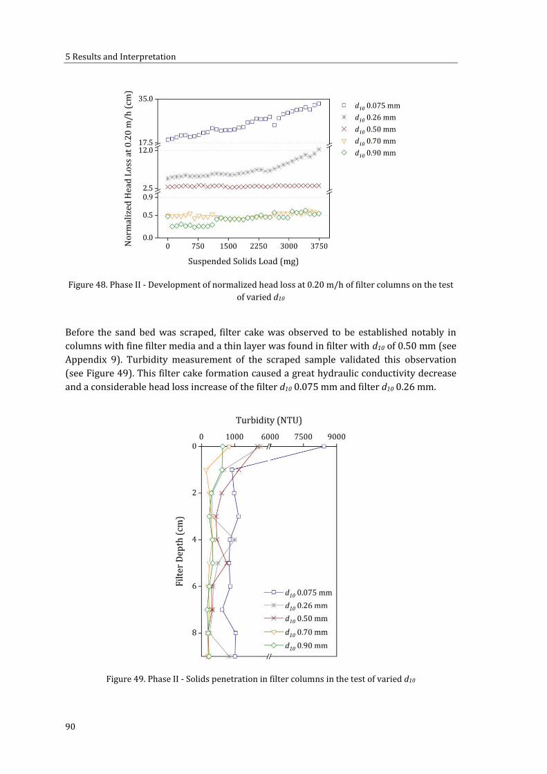
5 Results and Interpretation
90
Figure 48. Phase II - Development of normalized head loss at 0.20 m/h of filter columns on the test
of varied d10
Before the sand bed was scraped, filter cake was observed to be established notably in
columns with fine filter media and a thin layer was found in filter with d10 of 0.50 mm (see
Appendix 9). Turbidity measurement of the scraped sample validated this observation
(see Figure 49). This filter cake formation caused a great hydraulic conductivity decrease
and a considerable head loss increase of the filter d10 0.075 mm and filter d10 0.26 mm.
Figure 49. Phase II - Solids penetration in filter columns in the test of varied d10

5.4 Influence of the Grain Size Distribution on Solids Penetration in Filter Bed
91
Turbidity values of the first 1 cm sand layer were decreased with the increase of d10. From
the filter d10 0.075 mm and filter d10 0.26 mm, the turbidity values dropped considerably
on the second 1 cm sand layer. Meanwhile, in the filter d10 0.50 mm the turbidity value
decreased gradually and became more or less stable below 3 cm sand layer. In the two
coarse filter columns, the turbidity value did not decrease significantly from the first 1 cm
sand layer to lower depth indicating a deeper penetration of solids. In this test, the coarse
filter media did not contain any clay and silt fraction.
Microscopic visualization of sand sample (see Figure 50) shows that suspended solids
indicated by dark cloud among the grains are abundant in the top layer compared to the
lower layer. Suspended solids mass was estimated based on the total mass of sand sample
from the first 1 cm layer as a representative. Mass of suspended solids from filter columns
d10 0.075 mm, d10 0.50 mm and d10 0.70 mm are presented in Table 19. For fine media
formation of filter cake was the dominant mechanism on suspended solids removal
represented by high percentage removal at the first 1 cm of filter bed. Meanwhile, deeper
straining tends to be the dominant removal mechanism in the coarser media.
Figure 50. Phase II - Microscopic visualization of top layer i.e. first 1 cm (a) vs lower layer i.e. 10 cm
below surface (b) from filter column with d10 of 0.26 mm
Table 19. Phase II - Percentage of suspended solids mass retained at the first 1 cm of filter bed in
the test of varied d10
Filter Columns Mass Retained (mg) % Removal at Surface
of Filter Bed
d10 0.075 mm 3,498 90.87
d10 0.50 mm 1,865 48.43
d10 0.70 mm 1,240 16.10
(a) (b)

5 Results and Interpretation
92
5.4.2 Variation in Cu
According to the characteristics of filter columns (see Table 20), filter Cu 7 had the highest
hydraulic conductivity value confirming the previous result in Section 5.2.2. This can be
explained due to the composition of sand size (see Table 4) within the filter column. Filter
Cu 7 consisted of higher coarse fraction compared to the others.
Table 20. Phase II - Characteristics of filter columns in the test of varied Cu
Parameters Cu 2.5 Cu 3 Cu 7
Initial Hydraulic Conductivity k(0) (m/s) 2.73×10⁻⁴ 3.27×10⁻⁴ 3.71×10⁻⁴
Initial Hydraulic Loading Rate (m/h) 0.20 0.20 0.22
Initial Δh (cm) 4.8 4.1 3.8
Removal of turbidity in this test was satisfactory for all filter columns. Filter Cu 2.5,
achieved the highest percentage removal 99.68% followed by filter Cu 3 with 99.52% and
filter Cu 7 with 99.45% (Figure 51). This result confirmed the turbidity removal of filter
columns in the Pre-Experiment Phase (see Section 5.1.2). Average outlet turbidity for all
filter columns was <0.60 NTU. Related to TSS removal, filter Cu 2.5 was also found out to
perform slightly better compared to the other two columns. Removal percentage of filter
Cu 2.5 was 99.66% while filter Cu 3 and filter Cu 7 were 99.58% and 99.51% respectively
(Figure 52).
Figure 51. Phase II - Outlet turbidity of filter columns in the test of varied Cu

5.4 Influence of the Grain Size Distribution on Solids Penetration in Filter Bed
93
Figure 52. Phase II - Outlet TSS of filter columns in the test of varied Cu
Gradual decrease on hydraulic conductivity with suspended solids load was observed on
the whole filter columns. According to the development of the relative hydraulic
conductivity (see Figure 53), the behavior of filter Cu 3 and filter Cu 7 was similar toward
the addition of solids in the sand bed where both filter columns declined rapidly until the
load of 3,000 mg solids. After that, the decrease was slightly until the filter operation was
terminated. Filter Cu 2.5 experienced a gradual decrease of hydraulic conductivity. At the
end of the filter operation, the hydraulic conductivity decreased more or less in the same
rate i.e. 89 % for filter Cu 2.5 and filter Cu 7 and 88 % for filter Cu 3. By considering the
trend of the declination, filter Cu 2.5 tended to clog faster than the other two columns. This
result confirmed the finding of Pre-Experiment Phase (see Section 5.1.2) and Phase I (see
Section 5.4.2) where the media with lower Cu tended to experience faster clogging period.
Figure 53. Phase II - Development of relative hydraulic conductivity of filter columns in the test of
varied Cu

5 Results and Interpretation
94
Based on the analysis of solids penetration (Figure 54), turbidity of first 1 cm sand sample
was very high followed by a sudden decrease for lower depth. High turbidity values found
in the whole filter columns indicated that the dominant removal mechanism was the
formation of filter cake. The presence of filter cake on the filter bed was responsible for
the significant decrease of hydraulic conductivity in all filter columns.
Figure 54. Phase II - Solids penetration in filter columns in the test of varied Cu
5.5 Influence of Hydraulic Loading Rates on Solids
Penetration in Filter Bed
Uncontrolled grains and voids arrangement in the filter bed resulted in the different
values of porosity and void ratio which at the end affected the initial hydraulic
conductivity (see Table 21). Filter 0.08 m/h, as estimated, had the lowest initial hydraulic
conductivity compared to others. As a consequence, the Δh of filter 0.08 m/h was higher
than filter 0.20 m/h although the first filter was operated under a hydraulic loading rate
that was more than a half lower than the second filter.

5.5 Influence of Hydraulic Loading Rates on Solids Penetration in Filter Bed
95
Table 21. Phase II - Characteristics of filter columns in the test of influence of hydraulic loading rate
Parameters 0.08 m/h 0.20 m/h 0.80 m/h
Initial Hydraulic Conductivity k(0) (m/s) 9.03×10⁻⁵ 2.73×10⁻⁴ 2.55×10⁻⁴
Initial Hydraulic Loading Rate (m/h) 0.08 0.20 0.76
Initial Δh (cm) 6.0 4.8 19.1
As expected, the percentage of turbidity removal was higher with the lower hydraulic
loading rate. Highest average removal was achieved by filter 0.08 m/h with 99.72%
followed by filter 0.20 m/h with 99.68% and filter 0.80 m/h with 99.19% (see Figure 55).
Average outlet turbidity of High-1 was almost three times higher than from Low-1.
However, the average outlet turbidity for all filter columns was still below 1 NTU.
Figure 55. Phase II - Outlet turbidity of filter columns operated under different hydraulic loading
rate
Related to the TSS removal, the same pattern was applied. The lower the hydraulic loading
rate, the higher the percent removal is (see Figure 56). By operating the filter under
0.08±0.02 m/h and 0.20±0.05 m/h, average TSS removal reached 99.66%. Concentration
of TSS in the outlet for filter 0.08 m/h and filter 0.20 m/h was below1 mg/L while for filter
0.80 m/h was above1 mg/L. The filter column operated under 0.8±0.2 m/h achieved
99.33% TSS removal.

5 Results and Interpretation
96
Figure 56. Phase II - Outlet TSS of filter columns operated under different hydraulic loading rate
At the end of the filter operation, hydraulic conductivity declined significantly for filter
columns 0.08 m/h (92 %) and 0.20 m/h (89 %). In filter column 0.80 m/h, decrease of
hydraulic conductivity was only 43 %. The hydraulic conductivity of filter column 0.08
m/h decreased considerably until the load of 4,500 mg solids and then slightly until the
termination of filter operation (see Figure 57). As a consequence of the prevailing
decrease of filter 0.08 m/h, the normalized head loss at 0.20 m/h increased considerably
(see Figure 58). In the filter column 0.20 m/h, the hydraulic conductivity decreased
gradually with the solids load. Filter 0.80 m/h behaved differently as the hydraulic
conductivity decrease was linear with the solids load.
Figure 57. Phase II - Development of relative hydraulic conductivity of filter columns operated
under different hydraulic loading rate

5.5 Influence of Hydraulic Loading Rates on Solids Penetration in Filter Bed
97
Figure 58. Phase II - Development of normalized head loss at 0.20 m/h of filter columns operated
under different hydraulic loading rate
The different behavior of filter columns towards the solids load could be described by
considering the solids penetration. According to the turbidity measurement from the sand
sample, filter 0.08 m/h had the highest value on the first 1 cm scraping (see Figure 59).
This high value was followed by a sudden decrease to <1000 NTU. Having lower turbidity
value from the first 1 cm of sand sample, filter 0.20 m/h also experienced a sudden
decrease in the lower bed depth. Those values indicated that most of the suspended solids
retained at the top of filter bed causing significant decrease on hydraulic conductivity and
increase in head loss. Meanwhile in filter 0.80 m/h, it was found out that the solids
penetrated deeper within the filter columns by considering the turbidity values of first and
second 1 cm of sand samples. Therefore, the decrease of hydraulic conductivity and
increase of normalized head loss were not as high as in the filter columns with lower
hydraulic loading rates. Deeper straining in filter 0.80 m/h was found to be higher
compared to the filter 0.08 m/h and filter 0.20 m/h. If the feeding of filter column was
extended, at certain point the decrease pattern of hydraulic conductivity of filter 0.80 m/h
might be as the same as the pattern of filter columns 0.08 m/h and 0.20 m/h which likely
to be exponential.

5 Results and Interpretation
98
Figure 59. Phase II - Solids penetration in filter columns operated under different hydraulic loading
rate
5.6 Increasing Filter Run Time by Applying Protection
Layer
According to Mälzer and Gimbel (2006), protection layer applied in the filter columns may
inhibit the clogging period and prolonging the filter run time. Two filter columns with the
characteristics listed in Table 22 were tested in this phase to evaluate this method of
Mälzer and Gimbel (2006). The initial hydraulic conductivity of filter column with
protection layer was expected to be lower than without protection layer. However, based
on the measurement, filter column WPL had a slightly higher hydraulic conductivity than
filter WOPL.
Average turbidity removal of both filter columns was similar i.e. 99.68 % and 99.67 % for
filter columns WOPL and WPL respectively (see Figure 60). The average values of outlet
turbidity were 0.34 NTU for filter column without protection layer and 0.35 NTU for filter
column with protection layer. Related to the average removal of TSS (see Figure 61), filter
column WOPL (99.66 %) had slightly higher removal efficiency than filter column WPL
(99.55 %).

5.6 Increasing Filter Run Time by Applying Protection Layer
99
Table 22. Phase II - Characteristics of filter columns to test the method of filter run time
prolongation
Parameters WOPL WPL
Initial Hydraulic Conductivity k(0) (m/s) 2.73×10⁻⁴ 3.17×10⁻⁴
Initial Hydraulic Loading Rate (m/h) 0.20 0.20
Initial Δh (cm) 4.8 4.7
Figure 60. Phase II - Outlet turbidity of filter columns without and with protection layer
Figure 61. Phase II - Outlet TSS of filter columns without and with protection layer

5 Results and Interpretation
100
Hydraulic conductivity decreased significantly for filter column without protection layer
with the addition of solids in filter bed (see Figure 62). Decrease of hydraulic conductivity
in filter WOPL was up to 89 % while in filter WPL, the decrease was only 26 %. This
phenomenon led to the significant changes of the normalized head loss at 0.20 m/h in the
filter column without protection layer (see Figure 63). These discrepancies on the
developments of the relative hydraulic conductivity and normalized head loss at 0.20 m/h
were because the gravel layer acted as the first strainer for the suspended solids. Filter
cake was formed on the surface of sand bed in WOPL. Meanwhile, in filter column WPL, it
was observed that some solids were retained in the gravel layer as could be identified
from the solid penetration in Figure 64.
Figure 62. Phase II - Development of hydraulic conductivity filter columns without and with
protection layer
Figure 63. Phase II - Development of normalized head loss at 0.20 m/h filter columns without and
with protection layer

5.6 Increasing Filter Run Time by Applying Protection Layer
101
In the solids penetration graph, the first value for WPL was obtained from the scraping of
protection layer. The high turbidity value showed that some solids were retained in the
protection layer. The scraping of first 1 cm of sand layer from filter WPL resulted in the
significantly lower turbidity value than from filter WOPL. Since some solids were retained
in the protection layer, the formation of filter cake might be retarded and the clogging
could be decelerated.
Figure 64. Phase II - Solids penetration in the filter columns without and with protection layer


103
6 Discussion
6.1 Optimization of Slow Sand Filtration Design
Generally, the results of this study not only showed the effectiveness of slow sand filter on
removing the suspended solids but also proved that the ranges of the current
recommended values of design criteria were too narrow. These narrow ranges contribute
to the limitation on the optimization and wider utilization of the technology. In this study,
the influence of each operating variable on the suspended solids removal, solids
penetration and clogging period was investigated systematically so that the main purpose
i.e. optimization on the design recommendation could be achieved.
In Phase I, it was found out that the d10 of filter media can be raised up to 0.50 mm without
deteriorating the removal efficiency of suspended solids. According to the ANOVA test, the
outlet turbidity values of the filter columns with d10 of 0.50 mm were not significantly
different from the outlet turbidity of filter columns with finer media. Previously, Jenkins et
al. (2011) also reported that the effect of grain size distribution (i.e. d10 0.17 mm/Cu 2.4
and d10 0.52 mm/Cu 2.1) on the turbidity removal by intermittent slow sand filtration was
insignificant. Prior to Jenkins et al., Langenbach (2010) also found the same result at the
two newest studies (see Section 2.7.1). These findings strengthened the indication that the
recommended values of d10 i.e. 0.15 – 0.35 mm is rather conservative. By using coarser
media represented by d10 0.50 mm, it is not only that the high removal efficiency can be
obtained but also the capital cost to procure the sand can be reduced.
Since the d10 range tested in Phase I (0.075 – 0.50 mm) could not give the answer yet to
how the d10 influences the suspended solids removal, coarser sand represented by d10 of
0.70 mm and 0.90 mm were tested in Phase II. Three other d10 values tested in Phase II
were taken from the values in previous experiment i.e. d10 of 0.075 mm which represented
extreme fine media, d10 of 0.26 mm which represented the recommended value and d10
0.50 mm which represented the coarsest media in Phase I.
The results from Phase II confirmed that the coarser the filter media the lower the
removal efficiency of suspended solids. However, the range of tested d10 values so that the
confirmation could be proved was very broad i.e. 0.075 – 0.90 mm. The highest d10 value
tested was almost three times higher than the upper limit of the recommended d10 value
which is 0.35 mm. The average values of outlet turbidity of filter columns with coarser
media represented by d10 of 0.50 mm, 0.70 mm and 0.90 mm were reaching more than one
and a half, two and a half and three times the average of filter columns with recommended
d10 of 0.26 respectively. However, the average turbidity values for all filter columns with
coarser media tested in Phase II were still below 1 NTU. According to WHO, after the
treatment with slow sand filtration, outlet turbidity should never exceed 5 NTU to achieve
an effective disinfection process (WHO, 2017). Hence, average outlet quality from both
finer and coarser media investigated in this study met the requirement of WHO.
6 Discussion
104
From the perspective of suspended solids removal, employing coarser media did not lower
the filtrate quality. However, in regard to the removal mechanism, coarse media
contributed significantly to the deeper penetration of solids. According to the
investigation, the coarser the media the deeper the penetration of solids is. In the filter
columns with finer media, the pores size was too small for the solids to pass through.
Therefore, the solids were retained on the surface of filter bed forming a layer so called
filter cake. In this layer, which was actually an accumulation of very fine particles, the
pores size was very small inhibiting the other solids to pass through. Therefore, the filter
cake became a secondary filter layer. Formation of filter cake in the filter column with d10
of 0.075 mm occurred because most of the solids retained on the surface of filter bed, i.e.
91 % of total solids mass. On the contrary, formation of filter cake did not occur yet in
filter column with d10 of 0.70 mm because the solids retained at the first 1 cm of sand layer
were only around 16 % of total solids load and deeper straining became the dominant
removal mechanism.
As the consequence of the type of removal mechanisms, the decrease of filter capacity was
also different between the fine and coarse media. By the formation of filter cake, the
characteristics of the filter were no longer affected by the grain size distribution of the
media. The hydraulic conductivity of filter bed was determined by this layer. Therefore, in
the filter columns with fine media i.e. Fine-1.1 and Fine-3.1 the hydraulic conductivity
decreased significantly at the end of filter run. These hydraulic conductivity decreased
caused the increase of head loss in filter columns with fine media. On the other hand, the
hydraulic conductivity in coarse media tended to be more stable toward the addition of
solids. Deeper straining allowed the solids to penetrate deeper in the filter bed and spread
among the grains. As a result, the changes of head loss in filter columns with coarser media
were insignificant. These results showed that the filter columns with finer media tended to
experience faster clogging than the coarser media due to the faster formation of filter cake.
For the application in the real plant, a recommendation for the range of d10 values, which is
divided into finer and coarser media, is allowed to be proposed based on the results of the
study. A broader range of d10 values is introduced together with the risks that may occur
due to the selection of the d10. Table 23 summarizes the selection criteria between finer
and coarser media.

6.1 Optimization of Slow Sand Filtration Design
105
Table 23. Selection criteria between finer and coarser media*
Criteria Finer Media
(d10 0.25 – 0.50 mm)
Coarser Media
(d10 0.50 – 0.90 mm)
Average outlet turbidity < 1 NTU < 1 NTU, but higher than the
finer media
Initial cost** Higher Lower
Dominant removal
mechanism
Filter cake formation Deeper straining
Filter run time Shorter Longer
Maintenance Surface scraping or wet
harrowing
Deeper scraping or
replacement of the entire
bed depth
Maintenance cost Lower Higher
*Based on the investigation under narrow graded media (Cu = 2.5) **The cost to procure the sand
Investigation on the influence of different grain size distribution which varied in Cu was
also conducted in two phases. In Phase I, it was found out that the removal efficiency of
filter columns with narrow graded media, represented by Cu of 2.5 and 3, and wide graded
media, represented by Cu of 5, was not significantly different. This finding where the filter
columns with Cu of 5 produced high removal efficiency confirmed the previous results of
Slezak and Sims (1984) and Di Bernardo and Escobar Rivera (1996).
Similar to the finding in the investigation of varied d10, the range of recommended values
for Cu by previous authors (Huisman and Wood (1974), Visscher (1990) and Barrett et al.
(1991)) was also too limited. Therefore in Phase II, the range was extended and fine filter
media with the Cu of 2.5, 3 and 7 were tested. The first two values of Cu represented the
recommended values while Cu of 7 represented the extreme value. Based on the turbidity
removal in Phase II, it was found out that filter column with Cu of 7 produced average
outlet turbidity that around 42 % higher than the filter column with Cu of 2.5. However,
the outlet turbidity values for all filter columns were lower than 1 NTU which indicated
that the filtrate quality met the WHO turbidity standard. Related to the dominant removal
mechanism, the statement from Huisman and Wood (1974) where the solids penetration
might be deeper in the filter with higher Cu was not confirmed in this study. Formation of
filter cake was observed in all filter columns independently from the Cu. This result
indicated that the formation of filter cake was significantly influenced by the d10 and not by
Cu.
In regard to the hydraulic conductivity, theoretically, the filter with higher Cu was expected
to have lower initial hydraulic conductivity due to the reason that the finer fraction may

6 Discussion
106
occupy the larger pores and block the flow path (see Error! Reference source not
found.). From this reason, it was also expected that the filter column with higher Cu would
experience faster clogging period (Elisson, 2002; Langenbach, 2010). However, both
predictions did not occur in this experiment. According to the measurement especially in
Phase II, the values of initial hydraulic conductivity of the filter with wide graded media
were higher than with narrow graded media. This discrepancy was as a result of the
approach in the empirical values determination. The empirical calculation was mostly
based on the grain size distribution of media neglecting the effect of the arrangement of
grains and voids, the presence of air bubbles within the sand bed and the connections
between void. With the addition of solids that retained in filter bed, the initial hydraulic
conductivity of filter columns altered. Normally, the solids deposition, especially on the
surface of filter bed forming filter cake, caused the decrease of hydraulic conductivity. This
filter cake is a layer formed by the collection of very fine particles, therefore this layer
inhibits the water flow. However, there was also a possibility where the hydraulic
conductivity increased with the addition of solids especially when the filter cake is not yet
formed. Increase of hydraulic conductivity in filter column could be caused by the
alteration of grains and void arrangement and the release of entrapped air from the pores
during the filter operation.
According to the observation in Phase II, the hydraulic conductivity of all filter columns
decreased exponentially. The R2 values of all models were very high ensuring the
prediction of the influence of the solids addition on the relative hydraulic conductivity. A
prediction on the relative hydraulic conductivity by taking a solids load value of 10,000 mg
was done using the regression formula. It was found out that the relative hydraulic
conductivity would be around 0.03, 0.10 and 0.13 for filter columns with Cu of 2.5, 3 and 7
respectively. Capacity of filter column with Cu 2.5 would only be 3 % of its initial after a
load of 10,000 mg solids. Meanwhile, filter columns with higher Cu could still have around
10 % of its initial. This prediction indicated that the wider the grain size distribution of
media, the longer the filter run would be. The results from this study approved the
conclusion of Di Bernardo and Escobar Rivera (1996) who found out that lower Cu led to
shorter filter run time. Based on the results in the investigation on the influence of Cu on
the filter performance, a list of selection criteria is proposed in this study (see Table 24).

6.1 Optimization of Slow Sand Filtration Design
107
Table 24. Selection criteria between narrow and wide graded media*
Criteria Narrow Graded Media
(Cu < 3)
Wide Graded Media
(Cu 5 - 7)
Average outlet turbidity < 1 NTU < 1 NTU, but higher than the
narrow graded media
Initial cost** Higher Lower
Dominant removal
mechanism
Filter cake formation Filter cake formation
Filter run time Shorter Longer
Maintenance Surface scraping or wet
harrowing
Surface scraping or wet
harrowing
Maintenance cost Low Low
*Based on the investigation under fine media (d10 = 0.26 mm) **The cost to procure the sand
Actually, d10 and Cu are inseparable as both are the components which represent the grain
size distribution of sand. Taking this into consideration, it is worth to discuss the overall
results if the investigation on varied d10 and Cu. As it was mentioned in the previous
section (see Section 2.7.1), d10 and Cu influence the hydraulic conductivity of filter media.
By considering the results of the measurement (see Table 18 and Table 20), it could be
inferred that the d10 influenced more the hydraulic conductivity than the Cu. As an
example, filter column with d10 0.075 mm/Cu 2.5 had an initial hydraulic conductivity
which was two orders of magnitude lower than the filter column with d10 0.70 mm/Cu 2.5.
On the other hand, the initial hydraulic conductivity value of filter column with Cu 3/d10
0.26 mm was similar to the value of filter column with Cu 7/d10 0.26 mm. These results
indicated that Cu did not influence the hydraulic conductivity values as significant as d10.
Related to the removal mechanism, it could also be inferred that d10 had more significant
influence than Cu at the beginning of filter operation. The lower the d10 was, the faster the
filter cake was formed. In the filter columns with coarser media, formation of filter cake
took longer time. Appendix 9 shows how the solids cover the entire area of filter column
with finer media. Meanwhile, in the filter columns with coarser media, the filter cake layer
was not yet formed evenly on the entire bed surface. The faster the filter cake formation
was, the faster the filter operation had to be terminated due to the significant decrease of
hydraulic conductivity and increase of head loss. By considering that filter cake was
formed in filter columns NG-1.1, NG-2.1 and WG-2 independently from the Cu, it could be
inferred that the Cu did not influence the dominant removal mechanism as significant as
the d10. However, the influence of d10 was only significant at the beginning of filter
operation. Once the filter cake is formed, the removal efficiency and the changes in the
filter capacity are dependent on this layer which acts as the secondary filter.
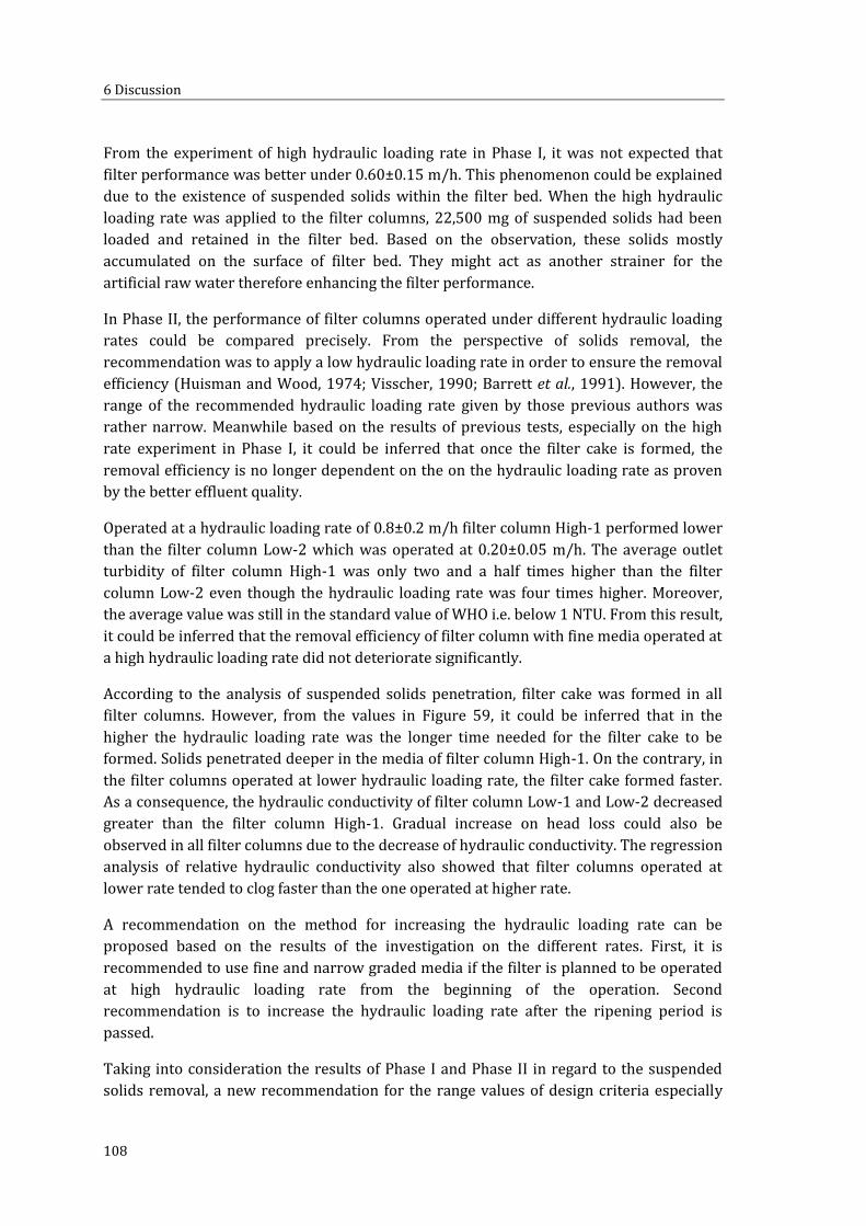
6 Discussion
108
From the experiment of high hydraulic loading rate in Phase I, it was not expected that
filter performance was better under 0.60±0.15 m/h. This phenomenon could be explained
due to the existence of suspended solids within the filter bed. When the high hydraulic
loading rate was applied to the filter columns, 22,500 mg of suspended solids had been
loaded and retained in the filter bed. Based on the observation, these solids mostly
accumulated on the surface of filter bed. They might act as another strainer for the
artificial raw water therefore enhancing the filter performance.
In Phase II, the performance of filter columns operated under different hydraulic loading
rates could be compared precisely. From the perspective of solids removal, the
recommendation was to apply a low hydraulic loading rate in order to ensure the removal
efficiency (Huisman and Wood, 1974; Visscher, 1990; Barrett et al., 1991). However, the
range of the recommended hydraulic loading rate given by those previous authors was
rather narrow. Meanwhile based on the results of previous tests, especially on the high
rate experiment in Phase I, it could be inferred that once the filter cake is formed, the
removal efficiency is no longer dependent on the on the hydraulic loading rate as proven
by the better effluent quality.
Operated at a hydraulic loading rate of 0.8±0.2 m/h filter column High-1 performed lower
than the filter column Low-2 which was operated at 0.20±0.05 m/h. The average outlet
turbidity of filter column High-1 was only two and a half times higher than the filter
column Low-2 even though the hydraulic loading rate was four times higher. Moreover,
the average value was still in the standard value of WHO i.e. below 1 NTU. From this result,
it could be inferred that the removal efficiency of filter column with fine media operated at
a high hydraulic loading rate did not deteriorate significantly.
According to the analysis of suspended solids penetration, filter cake was formed in all
filter columns. However, from the values in Figure 59, it could be inferred that in the
higher the hydraulic loading rate was the longer time needed for the filter cake to be
formed. Solids penetrated deeper in the media of filter column High-1. On the contrary, in
the filter columns operated at lower hydraulic loading rate, the filter cake formed faster.
As a consequence, the hydraulic conductivity of filter column Low-1 and Low-2 decreased
greater than the filter column High-1. Gradual increase on head loss could also be
observed in all filter columns due to the decrease of hydraulic conductivity. The regression
analysis of relative hydraulic conductivity also showed that filter columns operated at
lower rate tended to clog faster than the one operated at higher rate.
A recommendation on the method for increasing the hydraulic loading rate can be
proposed based on the results of the investigation on the different rates. First, it is
recommended to use fine and narrow graded media if the filter is planned to be operated
at high hydraulic loading rate from the beginning of the operation. Second
recommendation is to increase the hydraulic loading rate after the ripening period is
passed.
Taking into consideration the results of Phase I and Phase II in regard to the suspended
solids removal, a new recommendation for the range values of design criteria especially

6.1 Optimization of Slow Sand Filtration Design
109
for d10, Cu and hydraulic loading rate is proposed and listed in Table 25. By applying higher
hydraulic loading rate, the filter area can be reduced significantly. Hydraulic loading rate
of 0.60 m/h is preferably than 0.80 m/h based on two considerations. The first is that the
filter column operated under 0.60 m/h performed better in regard to the turbidity
removal. The second consideration is related to the solids penetration in the filter bed.
Hydraulic loading rate of 0.80 m/h contributes to the deeper penetration of solids in filter
bed which will lead into either higher possibility of breakthrough or higher cost during the
filter maintenance.
It is not recommended to use coarse sand with high Cu because in such configuration the
arrangement of grains and pores is heterogeneously distributed. Therefore, it will be
difficult to control an even hydraulic loading rate. Moreover, the stability of the filter bed
may be very poor because the risk of washout of finer media is high. It is also worth to
noting that this new recommendation is addressed for the purpose of water quality
improvement before disinfection process.
Table 25. Comparison of the past and new recommendation values of the design criteria of slow
sand filtration
Design Criteria
Recommended Values
1. Huisman and Wood
(1974)
2. Visscher (1990)
3. Barrett et al. (1991)
Anggraini (2017)
Hydraulic loading rate in the
filters
1. 0.1-0.4 m/h
2. 0.1-0.2 m/h
3. 0.04-0.4 m/h
0.20-0.60 m/h*;
> 0.60 m/h up to 0.80 m/h
can be alternatives for fine
media e.g. d10 ±0.25 mm/Cu
< 3
Sand specification:
Effective size d10 1. 0.15 – 0.35 mm
2. 0.15 – 0.30 mm
3. 0.20 – 0.30 mm
0.25 – 0.50 mm;
0.50 – 0.90 mm can be
alternatives as long as the
filter will be operated at
0.40 m/h
Uniformity coefficient
(Cu)
1. < 3, preferably < 2
2. < 5, preferably < 3
3. 1.5 – 2, > 3 for economic
reasons is considerable
2.5 – 7 for d10 < 0.50 mm;
< 3 is preferable for d10 >
0.50 mm
As part of the research, the method of prolonging the filter run by applying protection
layer (Mälzer and Gimbel, 2006) was evaluated. In this study, the development of head
loss and the observation on the solids penetration proved that adding gravel as a

6 Discussion
110
protection layer for the filter bed was an effective method to prolong the filter run time. In
regard to the removal of suspended solids, performance of both filter columns, with and
without protection layer, was satisfactorily. The average values of outlet turbidity from
both filter columns met the requirement of WHO. This result confirmed the previous test
in the Pre-Experiment Phase which figured out that the removal efficiency of filter
columns with and without protection layer was similar.
After the filter operation was terminated, it was found out the hydraulic conductivity of
filter column with protection layer was decreased insignificantly compared to the filter
column without protection layer. The decrease of hydraulic conductivity in the filter
column without protection layer was around three times greater than the decrease in the
filter column with protection layer. In the filter column without protection layer, the solids
were retained directly on the surface of filter bed. The constriction size of sand bed was
certainly lower than of gravel layer. Hence, as proven by the observation in the solids
penetration (see Figure 64), the formation of the secondary filter layer in the filter column
without protection layer was faster than in the filter column with protection layer.
Behavior of filter column toward the addition of solids could also be observed from the
development of head loss. The gradual increase of normalized head loss at 0.20 m/h in the
filter column without protection layer was found out to be significant. It indicated that the
filter column without protection layer tended to clog faster than the filter column with
protection layer. The difference of the final and the initial normalized head loss at 0.20
m/h in the filter column without protection layer was around 28 cm. In the contrary, the
increase of normalized head loss at 0.20 m/h in the filter column with protection layer
was only around 2 cm.
Those results above indicated that the presence of protection layer may inhibit the
occurrence of clogging. Therefore, the recommendation of Mälzer and Gimbel (2006) to
add the protection layer so that the filter run time can be prolonged is an appropriate
method.
6.2 Case Study – Slow Sand Filter in Gunungkidul, Java
Indonesia
The district of Gunungkidul is one of the poorest regions in Java Island, Indonesia which
suffers from severe water scarcity especially during the dry season (April – October). Due
to its karst topography, the water percolates rapidly to the underground forming
subsurface rivers. In general, local population may derive their water supply from wells,
surface water, rainwater harvesting and piped water from the public utility PDAM
(Nestmann et al., 2009). However, there are some limitations from these water sources i.e.
most wells and surface water run dry during the dry season, the cost to construct the
rainwater storage tanks is not easily affordable for most of the local population and the
level of service of the pipe water is very poor (Fuchs et al., 2015).

6.2 Case Study – Slow Sand Filter in Gunungkidul, Java Indonesia
111
By considering those conditions, an Integrated Water Resources Management Indonesia
Project (IWRM Indonesia) was established in Gunungkidul. Within the framework of the
project, an additional water intake was developed by constructing an underground dam
with an integrated micro-hydro power plant to pump out the water from Bribin cave to a
reservoir built in Kaligoro. This reservoir supplies the water for 3.5 % of the total
population which are served in the water supply system (Fuchs et al., 2015). In regard to
the quality, the water does not meet the requirements of any regulatory standard of
drinking water (Silva, 2010; Anggraini, 2011). Hence, a water treatment is needed to
improve the water quality. As part of the project, a pilot plant of slow sand filter was
installed in Kaligoro to improve the water quality by removing suspended solids.
Based on Fuchs et al. (2015), the pilot plant was designed to treat an amount of 195 m3 per
day which can be used to serve five sub-villages (around 2,800 inhabitants). By
considering the recommended values of design criteria (Table 1), Fuchs et al. determined
the hydraulic loading rate for the plant was m/d ≈ . m/h . )n order to encompass these criteria, the total filter bed are of 50 m2 was needed. This filter area was divided into
two filter beds with 25 m2 each. To maintain the continuous supply during the clogging
and maintenance period, four additional filter beds were needed. In total, six filter beds
with an area of 25 m2 each were proposed. Table 26 presents the proposed design criteria
for the plant in Kaligoro. However, the local authorities agreed to construct only half of the
proposed plant due to the budget procurement. Therefore, the amount of sub-villages that
should be supplied was also reduced by around the half. Figure 65 shows the layout of the
filter unit.
Table 26. Proposed design criteria for slow sand filter plant in Kaligoro (Fuchs et al., 2015)
Design Criteria Value
Filter bed area 25 m2 per unit
Total 6 filter units
Hydraulic loading rate 4 m/d (≈ . m/h
Height of filter bed
Initial 0.8 m
Minimum 0.5 m
Specification of sand Lava sand
Effective size d10 0.25 mm
Uniformity coefficient Cu 3.06
Height of underdrain including gravel layer 0.25 m
Height of supernatant level 1 m
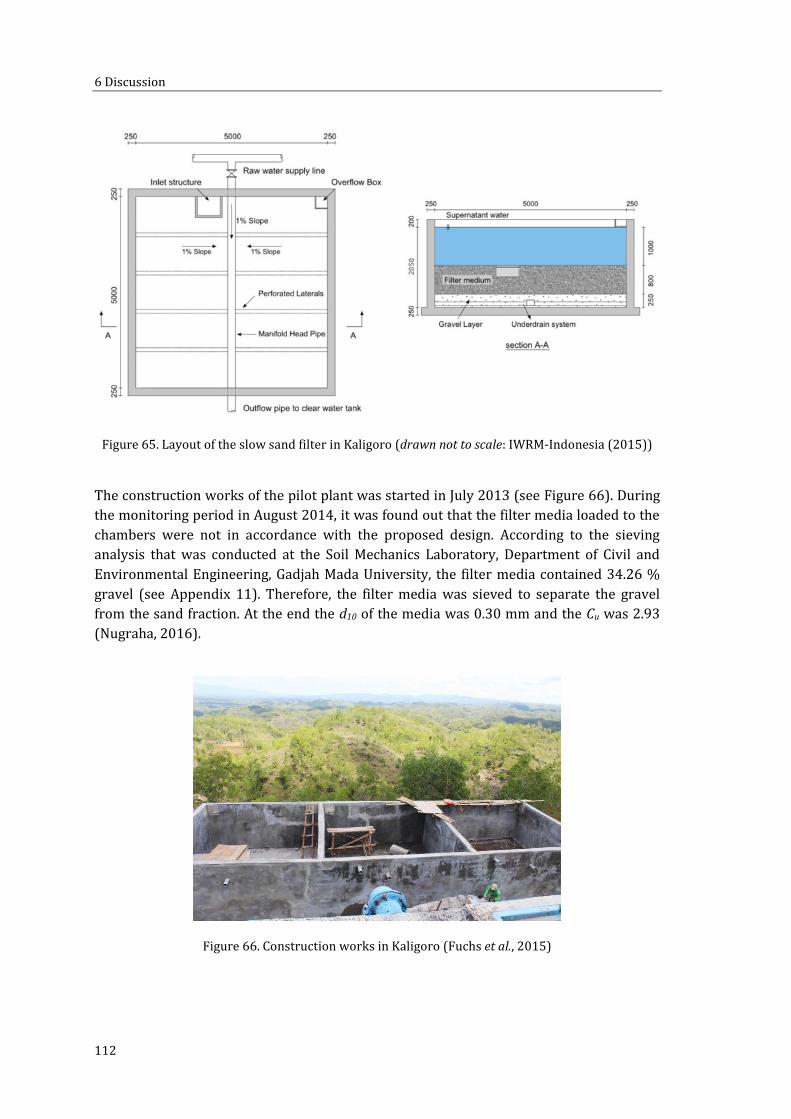
6 Discussion
112
Figure 65. Layout of the slow sand filter in Kaligoro (drawn not to scale: IWRM-Indonesia (2015))
The construction works of the pilot plant was started in July 2013 (see Figure 66). During
the monitoring period in August 2014, it was found out that the filter media loaded to the
chambers were not in accordance with the proposed design. According to the sieving
analysis that was conducted at the Soil Mechanics Laboratory, Department of Civil and
Environmental Engineering, Gadjah Mada University, the filter media contained 34.26 %
gravel (see Appendix 11). Therefore, the filter media was sieved to separate the gravel
from the sand fraction. At the end the d10 of the media was 0.30 mm and the Cu was 2.93
(Nugraha, 2016).
Figure 66. Construction works in Kaligoro (Fuchs et al., 2015)
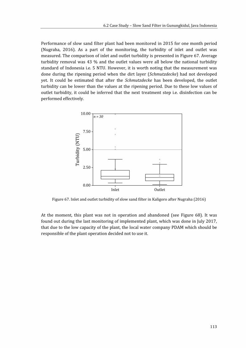
6.2 Case Study – Slow Sand Filter in Gunungkidul, Java Indonesia
113
Performance of slow sand filter plant had been monitored in 2015 for one month period
(Nugraha, 2016). As a part of the monitoring, the turbidity of inlet and outlet was
measured. The comparison of inlet and outlet turbidity is presented in Figure 67. Average
turbidity removal was 43 % and the outlet values were all below the national turbidity
standard of Indonesia i.e. 5 NTU. However, it is worth noting that the measurement was
done during the ripening period when the dirt layer (Schmutzdecke) had not developed
yet. It could be estimated that after the Schmutzdecke has been developed, the outlet
turbidity can be lower than the values at the ripening period. Due to these low values of
outlet turbidity, it could be inferred that the next treatment step i.e. disinfection can be
performed effectively.
Figure 67. Inlet and outlet turbidity of slow sand filter in Kaligoro after Nugraha (2016)
At the moment, this plant was not in operation and abandoned (see Figure 68). It was
found out during the last monitoring of implemented plant, which was done in July 2017,
that due to the low capacity of the plant, the local water company PDAM which should be
responsible of the plant operation decided not to use it.

6 Discussion
114
Figure 68. Current condition of slow sand filter in Kaligoro (Doc.: Marjianto, 2017)
With regard to its function and performance on improving the water quality, it is worth to
put this plant into operation. However, due to the current condition of the plant and the
issue regarding the plant capacity, some improvements on the constructed plant have to
be made. Based on the results of this research, the following are some recommendations in
regard to the filter media, the hydraulic loading rate and the construction that can be
proposed (see also Table 27):
1. Filter Media
According to Figure 68, some plants grow in the chambers of the plant. The risk that
some parts of the plants are decomposed in situ is very high. These decaying materials
may deteriorate the filtrate quality. Therefore, it is recommended to replace the entire
filter media in the three chambers. In regard to the sand specification, the d10 does not
necessarily to be very fine and the Cu does not necessarily to be as narrow as the
previous recommended values by Huisman and Wood (1974), Visscher (1990) and
Barrett et al. (1991). In order to ensure the filter performance and by considering the
peak turbidity during the rainy season, a d10 of 0.25 - 0.50 mm and Cu of 3-7 can be
selected. The d10 values of 0.70 mm and 0.90 mm were not recommended because the
solids may penetrate very deep into the filter bed and led to higher maintenance cost
because surface scraping will not be sufficient. By having a coarser and ungraded
media the capital cost may be reduced because further sieving process does not need
to be done. Lava sand can still be chosen because this material is abundant locally.
2. Hydraulic Loading Rate
Based on the results of the study, higher hydraulic loading rate may reduce the
removal efficiency. However, it was also found that a hydraulic loading rate of 0.8±0.2
m/h could still reach an average outlet turbidity of below 1 NTU. In the case of slow
sand filter Kaligoro, the low capacity can be increased by raising the hydraulic loading

6.2 Case Study – Slow Sand Filter in Gunungkidul, Java Indonesia
115
rate so that the five sub-villages can be supplied with improved water. In order to
achieve this purpose, the hydraulic loading rate only needs to be increased two times of the original proposal i.e. m/d ≈ . m/h . Since the higher hydraulic loading rate
(0.8±0.2 m/h) was capable to achieve high removal efficiency, it can be ensured that
higher performance can be obtained by operating the filter at lower hydraulic loading
rate (0.40 m/h).
Table 27. Comparison of previous and current proposed design criteria for slow sand filter Kaligoro
Design Criteria Previous Value Current Value
Filter bed area 25 m2 per unit 25 m2 per unit
Total 6 filter units Total 3 filter units
Hydraulic loading rate 4 m/d ≈ 0.20 m/h 8 m/d ≈ 0.40 m/h
Height of filter bed
Initial 0.8 m 0.8 m
Minimum 0.5 m 0.5 m
Specification of sand Lava sand Lava sand
Effective size d10 0.25 mm 0.25 – 0.50 mm
Uniformity coefficient Cu 3.06 2.5 - 7
Height of underdrain including
gravel layer 0.25 m 0.25 m
Height of supernatant level 1 m 1 m
3. Construction of Filter Plant – Outlet Position
The outlet position of current plant is located at the bottom of the chamber (see Figure
69). The outlet pipe is directly connected to the clean water storage tank which is
placed next to the filter and below the base of the filter chambers. In this position, the
Δh is too high and leads to the difficulty of controlling the water flow at the desired
rate. To ensure the filter is operated at the desired rate and to have a better control of
the rate, it is recommended to reduce the Δh. The approach is to adjust the point
where the water comes in to the storage tank up to the level around the surface of
sand bed. Therefore, the storage tank has to be put at least 1,000 mm higher than the
current level (see Figure 70).

6 Discussion
116
Figure 69. Outlet position of current filter plant in Kaligoro
Figure 70. Sketch of current (a) and recommended (b) outlet position of slow sand filter in Kaligoro
(not drawn to scale)
Outlet
Pipe
Storage
Tank
(a)
(b)
Δh
Δh

117
7 Conclusion
Based on the results of this research, some conclusions can be drawn as follows:
1. The current range values that were recommended in the design criteria of slow sand
filter was rather conservative. As a consequence of this limited range, the optimization
and the improvement of the technology were also limited. It was proved that coarser
filter media represented by d10 0.90 mm/Cu 2.5, which was almost three times greater
than the upper limit of the current recommended values, could produce low value of
outlet turbidity i.e. below 1 NTU averagely. Under this average value, the disinfection
process could be performed effectively. It was also found that for the filter with fine
media, the hydraulic loading rate could be increased up to 0.80 m/h which was two
times the upper limit of the current recommended values. By operating the filter at
0.80 m/h, the average outlet turbidity was also found to be below 1 NTU. As a result of
a higher hydraulic loading rate is that the area needed for the construction of slow
sand filter could be reduced significantly. Therefore, the design criteria can be
optimized by considering these results (see Table 27). Nevertheless, this new
recommendation on the range values of the slow sand filtration design criteria have to
be tested for the biological removal and further in a larger scale to provide a more
comprehensive findings.
2. In this study, it was figured out that the operating variables did not significantly
influence the removal efficiency. However, the operating variables, especially the d10 of
the grain size distribution, influence significantly the period needed for the dirt layer
to be formed. It was found out that the finer the media, the faster the formation of dirt
layer on the surface of filter bed is. The faster the formation of the dirt layer is, the
faster the filter will experience clogging period. This clogging period can be identified
by the significant decrease of hydraulic conductivity and increase of head loss. As an
example, by comparing the d10 of 0.26 mm/Cu 2.5 and d10 0.50 mm/Cu 2.5, it was
identified that the clogging in the finer filter column would occur for two and a half
time faster than the coarser filter column.
3. A method to enhance the hydraulic loading rate can be proposed by taking into
consideration the formation of dirt layer. It was found out that after the dirt layer is
formed, hydraulic loading rate was no longer affecting the filter performance. In this
case it has been proved in this study that once the dirt layer has been formed, the
hydraulic loading rate can be enhanced up to three times without deteriorating the
filter performance.
4. Applying protection layer in the filter can be a promising method to increase the filter
run time. It was proved that by adding gravel as a protection layer, the decrease of
filter capacity of the filter could be 70 % lower than the decrease of filter without any
protection layer.

List of Abbreviations
118
5. The implementation of a technology, especially in the developing countries, should
consider many aspects such as the socio-economic condition, human resource, local
policy etc. Another important factor is to develop the sense of belonging of the
technology among the local people so that the technology can last in a long term. This
sense of belonging can be grown by implementing an appropriate technology.
Implementation of too advanced technology in rural areas in developing countries may
be redoubtable for some local people in which they do not want to deal with it. Slow
sand filter can be a promising technology which is appropriate for the people living in
developing countries especially in rural areas. Its simplicity in the construction,
operation and maintenance process does not require the skilled personal. Further,
education on the personnel in charge so that they can have an advanced skill will also
support the successful implementation of the technology.

119
Appendix
Appendix 1. Grain size distribution of filter media for systematic investigation

Appendix
120
Appendix 2. Specific surface area of filter columns in all tests
Specific surface area does not have any influence on the suspended solids removal but it
will have a big influence on the bacteria removal as has been studied by Orb (2012)
Phase Filter Columns Specific Surface Area As (m2/m3)
Phase I
Set 1 Set 2
Fine-1 25,987
Fine-2 14,699 13,224
Fine-3 8,243 8,628
Coarse-1 5,583 5,467
Coarse-2 4,423 4,535
Set A Set B Set C
NG-1 8,759 8,760 8,758
NG-2 8,050 8,050 8,077
WG-1 6,587 6,680 6,799
Phase II
Fine-1.1 29,960
Fine-3.1 8,376
Coarse-2.1 4,441
Coarse-3 3,060
Coarse-4 2,413
NG-1.1 8,115
NG-2.1 7,913
WG-2 5,892
Low-1 8,623
Low-2 8,115
High-1 8,428
NG-1.1PL 8,474

Appendix
121
Appendix 3. Solids size distribution in the outlet of filter columns in Phase I-varied Cu

Appendix
122
Appendix 4. Solids size distribution in the outlet of filter columns in Phase I-high hydraulic
loading rate (0.60±0.15 m/h)

Appendix
123
Appendix 5. Filter columns in Phase II
Appendix 6. Process of sand samples shaking during the analysis of solids penetration in
Phase II
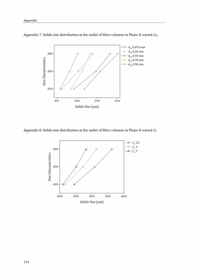
Appendix
124
Appendix 7. Solids size distribution at the outlet of filter columns in Phase II-varied d10
Appendix 8. Solids size distribution at the outlet of filter columns in Phase II-varied Cu

Appendix
125
Appendix 9. Formation of filter cake in Phase II - test of varied d10
Appendix 10. Development of normalized head loss at 0.20 m/h in the Phase II-varied Cu
d10 0.50 mm d10 0.90 mm
d10 0.26 mm

Appendix
126
Appendix 11. Grain size analysis of filter media of slow sand filter Kaligoro before sand-
gravel separation

127
References
Abudi, Z. , The effect of sand filter characteristics on removal efficiency of organic matter from grey water , Al-Qadisiya Journal for engineering sciences, Vol. 4 No. 2, pp.
143–155. Adin, A. and Elimelech, M. , Particle filtration for wastewater irrigation , Journal of
irrigation and drainage engineering, Vol. 115 No. 3, pp. 474–487.
Al-Yaseri, I., Morgan, S. and Retzlaff, W. , Using turbidity to determine total suspended solids in storm-water runoff from green roofs , Journal of Environmental
Engineering, Vol. 139 No. 6, pp. 822–828. Anggraini, A.K. , Suitable local media and operation mode of slow sand filtration for water treatment in Gunungkidul. Case study in Gua Seropan , Master thesis, Gadjah Mada University, Yogyakarta, Indonesia, 2011.
Aronino, R., Dlugy, C., Arkhangelsky, E., Shandalov, S., Oron, G., Brenner, A. and Gitis, V. , Removal of viruses from surface water and secondary effluents by sand filtration , Water research, Vol. 43 No. 1, pp. 87–96.
Assembly, U.G. (Ed.) (2015), Transforming our world: the 2030 Agenda for Sustainable
Development. Baker, D.L. and Duke, W.F. , )ntermittent slow sand filters for household use–A field study in (aiti , in Gimbel, R., Graham, N. and Collins, M.R. Eds. , Recent progress
in slow sand and alternative biofiltration processes, IWA Publishing, p. 278.
Bardet, J.-P. (1997), Experimental soil mechanics, Prentice Hall, New Jersey.
Barrett, J.M., Bryck, J., Collins, M.R., Janonis, B.A. and Logsdon, G.S. (1991), Manual of design
for slow sand filtration, The Foundation; American Water Works Association, Denver,
CO.
Barton, J.M.H. and Buchberger, S.G. , Effect of media grain shape on particle straining during filtration , Journal of Environmental Engineering, Vol. 133 No. 2, pp.
211–219.
Bear, J. (1988), Dynamics of fluids in porous media, Dover books on physics and chemistry,
Dover, New York, N.Y. Bellamy, W.D., (endricks, D.W. and Logsdon, G.S. a , Slow sand filtration: influences of selected process variables , Journal-American Water Works Association, Vol. 77
No. 12, pp. 62–66.
Bellamy, W.D., Silverman, G.P., Hendricks, D.W. and Logsdon, G.S. b , Removing giardia cysts with slow sand filtration , Journal-American Water Works Association,
Vol. 77 No. 2, pp. 52–60.
References
128
Bergström, L. , (amaker constants of inorganic materials , Advances in Colloid and
Interface Science, Vol. 70, pp. 125–169. Bilotta, G.S. and Brazier, R.E. , Understanding the influence of suspended solids on water quality and aquatic biota , Water research, Vol. 42 No. 12, pp. 2849–2861.
Binnie, C. and Kimber, M. (2013), Basic water treatment, 5th ed., ICE, London. Boller, M.A. and Kavanaugh, M.C. , Particle characteristics and headloss increase in granular media filtration , Water research, Vol. 29 No. 4, pp. 1139–1149.
Bradford, S.A., Simunek, J., Bettahar, M., van Genuchten, Martinus Th and Yates, S.R. , Modeling colloid attachment, straining, and exclusion in saturated porous media , Environmental science & technology, Vol. 37 No. 10, pp. 2242–2250. Bradford, S.A., Yates, S.R., Bettahar, M. and Simunek, J. , Physical factors affecting the transport and fate of colloids in saturated porous media , Water Resources
Research, Vol. 38 No. 12.
Budhu, M. (2015), Soil mechanics fundamentals, John Wiley & Sons. Camenen, B. , Simple and general formula for the settling velocity of particles , Journal of Hydraulic Engineering, Vol. 133 No. 2, pp. 229–233. Campos, L.C. , Modelling and simulation of the biological and physical processes of slow sand filtration , University of London, . Campos, L.C., Smith, S.R. and Graham, N.J.D. , Deterministic-based model of slow sand filtration. ): Model development , Journal of Environmental Engineering, Vol. 132
No. 8, pp. 872–886.
Campos, L.C., Su, M.F., Graham, N.J. and Smith, SR , Biomass development in slow sand filters , Water research, Vol. 36 No. 18, pp. 4543–4551. Carrier ))), W.D. , Goodbye, hazen; hello, kozeny-carman , Journal of geotechnical
and geoenvironmental engineering, Vol. 129 No. 11, pp. 1054–1056. Cho, W.J., Lee, J.O. and Chun, K.S. , The temperature effects on hydraulic conductivity of compacted bentonite , Applied clay science, Vol. 14 No. 1, pp. 47–58.
Clark, P.A., Pinedo, C.A., Fadus, M. and Capuzzi, S. , Slow-sand water filter: Design, implementation, accessibility and sustainability in developing countries , Medical
science monitor: international medical journal of experimental and clinical research,
Vol. 18 No. 7, RA105.
Cleary, S.A. ( , Sustainable drinking water treatment for small communities using multistage slow sand filtration , University of Waterloo, . Cleasby, J.L. (Ed.) (1991), Source water quality and pretreatment options for slow sand
filters, ASCE.
Cleasby, J.L., Hilmoe, D.J. and Dimitracopoulos, C.J. , Slow sand and direct in-line filtration of a surface water , Journal (American Water Works Association), pp. 44–55.
References
129
Collins, M.R., Eighmy, T.T. and Malley Jr, James P , Evaluating modifications to slow sand filters , Journal-American Water Works Association, Vol. 83 No. 9, pp. 62–70.
Crites, R. and Tchnobanoglous, G. (1998), Small and decentralized wastewater management
systems, McGraw-Hill, Boston.
Daphne, L.H.X., Utomo, H.D. and Kenneth, L.Z.H. (2011), Correlation between turbidity and total suspended solids in Singapore rivers , Journal of Water Sustainability, Vol. 1
No. 3, pp. 313–322. Darby, J.L., Attanasio, R.E. and Lawler, D.F. , Filtration of heterodisperse suspensions: Modeling of particle removal and head loss , Water research, Vol. 26
No. 6, pp. 711–726. Darby, J.L. and Lawler, D.F. , Ripening in depth filtration: Effect of particle size on removal and head loss , Environmental science & technology, Vol. 24 No. 7, pp. 1069–1079. Datta, A.K. and Chaudhuri, M. , Microbial purification in slow sand filter , Environmental Toxicology and Water Quality, Vol. 6 No. 2, pp. 239–247. Deb, S.K. and Shukla, M.K. , Variability of hydraulic conductivity due to multiple factors , American Journal of Environmental Sciences, Vol. 8 No. 5, p. 489. Derjaguin, B.V. and Landau, L. , Theory of the stability of strongly charged lyophobic sols and of the adhesion of strongly charged particles in solutions of electrolytes , Acta physicochim. URSS, Vol. 14 No. 6, pp. 633–662.
DeZuane, J. (1997), Handbook of drinking water quality, John Wiley & Sons. Di Bernardo, L. and Alcócer Carrasco, N. E. , Variable versus constant supernatant water layer in slow sand filtration , in Graham, Nigel Jonathon Douglas and Collins,
M.R. (Eds.), Advances in slow sand and alternative biological filtration, John Wiley &
Sons, Chichester [etc.], pp. 245–253. Di Bernardo, L. and Escobar Rivera, A. , )nfluence of sand uniformity coefficient on slow sand filtration performance , in Graham, Nigel Jonathon Douglas and Collins, M.R. (Eds.), Advances in slow sand and alternative biological filtration, John Wiley & Sons,
Chichester [etc.], pp. 179–188.
Duke, W.F., Nordin, R.N., Baker, D. and Mazumder, A. , The use and performance of BioSand filters in the Artibonite Valley of (aiti: a field study of households , Rural
Remote Health, Vol. 6 No. 3, p. 570.
Dullemont, Y.J., Schijven, J.F., Hijnen, W.A., Colin, M., Magic-Knezev, A. and Oorthuizen, W.A. , Removal of microorganisms by slow sand filtration , in Gimbel, R., Graham, N. and Collins, M.R. (Eds.), Recent progress in slow sand and alternative biofiltration
processes, IWA Publishing, pp. 12–20. Elimelech, M. and O Melia, C.R. a , Effect of particle size on collision efficiency in the deposition of Brownian particles with electrostatic energy barriers , langmuir, Vol. 6
No. 6, pp. 1153–1163.

References
130
Elimelech, M. and O'Melia, C. b , Kinetics of deposition of colloidal particles in porous media , Environmental science & technology, Vol. 24 No. 10, pp. 1528–1536. Elisson, J. , Rule Development Committee )ssue Research Report Draft , Sand/Media Specifications. Washington State Department of Health. USA. Ellis, J.B., Revitt, D.M., Vollertsen, J. and Blackwood, D.J. , Sewer exfiltration and the colmation layer , Water Science and Technology, Vol. 59 No. 11, pp. 2273–2280. Ellis, K.V. , Slow sand filtration as a technique for the tertiary treatment of municipal sewages , Water research, Vol. 21 No. 4, pp. 403–410. Ellis, K.V. and Aydin, M.E. , Penetration of solids and biological activity into slow sand filters , Water research, Vol. 29 No. 5, pp. 1333–1341.
Ellis, K.V. and Wood, W.E. (19 , Slow sand filtration , Critical Reviews in Environmental
Science and Technology, Vol. 15 No. 4, pp. 315–354.
EPA Ireland (2001), Parameters of water quality: Interpretation and standards.
Erturk, A., Gurel, M., Ekdal, A., Tavsan, C., Ugurluoglu, A., Seker, D.Z., Tanik, A. and Ozturk, I. , Water quality assessment and meta model development in Melen watershed–Turkey , Journal of environmental management, Vol. 91 No. 7, pp. 1526–1545.
Farooq, S. and Al-Yousef, A.K. , Slow sand filtration of secondary effluent , Journal
of Environmental Engineering, Vol. 119 No. 4, pp. 615–630. Fuchs, S., Silva, A., Anggraini, A.K. and Mahdariza, F. , Planning and installation of a drinking water treatment in Gunungkidul, Java, )ndonesia , Water Science and
Technology: Water Supply, Vol. 15 No. 1, pp. 42–49. Galvis, G. , Development and evaluation of multistage filtration plants: an innovative, robust and efficient water treatment technology , University of Surrey, 1999.
Görgen, M., Rudloff, B., Simons, J., Üllenberg, A., Väth, S. and Wimmer, L. (2009), Foreign
direct investment (FDI) in land in developing countries, GTZ. Gottinger, A.M., McMartin, D.W., Price, D. and (anson, B. , The effectiveness of slow sand filters to treat Canadian rural prairie water , Canadian Journal of Civil
Engineering, Vol. 38 No. 4, pp. 455–463. Graham, N. and Collins, M.R. , Slow sand filtration: recent research and application perspectives , in Nakamoto, N., Graham, Nigel J. D, Collins, M.R. and Gimbel, R. Eds. , Progress in slow sand and alternative biofiltration processes: Further developments and
applications ; [contributions presented at the 5th International Slow Sand and
Alternative Biological Filtration Conference, held in Nagoya, Japan in June 2014], IWA
Publ, London, pp. 3–16.
Grayson, R.B., Finlayson, B.L., Gippel, C.J. and Hart, B.T. , The potential of field turbidity measurements for the computation of total phosphorus and suspended solids loads , Journal of environmental management, Vol. 47 No. 3, pp. 257–267.

References
131
Guchi, E. , Review on slow sand filtration in removing microbial contamination and particles from drinking water , American Journal of Food and Nutrition, Vol. 3 No. 2, pp.
47–55. (aig, S.J., Collins, G., Davies, R.L., Dorea, C.C. and Quince, C. , Biological aspects of slow sand filtration: past, present and future , Water Science and Technology: Water
Supply, Vol. 11 No. 4, pp. 468–472. (amaker, (.C. , The London—van der Waals attraction between spherical particles , physica, Vol. 4 No. 10, pp. 1058–1072.
Hannouche, A., Chebbo, G., Ruban, G., Tassin, B., Lemaire, B.J. and Joannis, C. (2011), Relationship between turbidity and total suspended solids concentration within a combined sewer system , Water Science and Technology, Vol. 64 No. 12, pp. 2445–2452.
Hatt, B.E., Fletcher, T.D. and Deletic, A. , (ydraulic and pollutant removal performance of fine media stormwater filtration systems , Environmental science &
technology, Vol. 42 No. 7, pp. 2535–2541.
Hazen, A. (1905), The filtration of public water-supplies, J. Wiley.
Herzig, J.P., Leclerc, D.M. and Le Goff, P. , Flow of suspensions through porous media. Application to deep filtration , Industrial and Engineering Chemistry, Vol. 62
No. 5, pp. 8–35.
Holdich, R.G. (2002), Fundamentals of particle technology, Midland Information
Technology and Publ, Shepshed. (olliday, C.P., Rasmussen, T.C. and Miller, W.P. , Establishing the relationship between turbidity and total suspended sediment concentration , in (atcher, K.J. Ed. , Proceedings of the 2003 Georgia water resources conference, Athens, Georgia, April 23-
24, 2003, Georgia Institute of Technology. (udson, A. , Turbidity and Suspended Solids in Drinking Water , Measurement and
Control, Vol. 43 No. 1, pp. 22–23.
Huisman, L. and Wood, W.E. (1974), Slow sand filtration, World Health Organization
Geneva.
Information Evidence and Research (IER) WHO (2015), Proportion of population using
improved drinking water sources (%) 2015, WHO. )ves, K.J. , Filtration of clay suspensions through sand , Clay Miner, Vol. 22, pp. 49–61.
IWRM-)ndonesia , )WRM-Indonesia Fact Sheet. Adaptede slow sand filter with
intermittent operation as first step for the multi-barrier water treatment concept , available at: http://www.iwrm-indonesien.de/downloads/SSF.pdf (accessed 16
November 2017).

References
132
Jabur, (.S., Martensson, J. and Ollos, G. , Some notes on hydraulics and a mathematical description of slow sand filtration , Vatten, Vol. 61 No. 3, p. 193. Jenkins, M.W., Tiwari, S.K. and Darby, J. , Bacterial, viral and turbidity removal by intermittent slow sand filtration for household use in developing countries: Experimental investigation and modeling , Water research, Vol. 45 No. 18, pp. 6227–6239. Johnson, C.P., Li, X. and Logan, B.E. , Settling velocities of fractal aggregates , Environmental science & technology, Vol. 30 No. 6, pp. 1911–1918. Kandra, (.S., Deletic, A. and McCarthy, D. , Assessment of impact of filter design variables on clogging in stormwater filters , Water resources management, Vol. 28
No. 7, pp. 1873–1885.
Kandra, H.S., McCarthy, D., Deletic, A. and Fletcher, T.D. (Eds.) (2010), Assessment of
clogging phenomena in granular filter media used for stormwater treatment, Citeseer. Kaya, (. and Takeuchi, J. , The iron and manganese removal process: )ts microbial habitats and functions , in Nakamoto, N., Graham, N.J.D., Collins, M.R. and Gimbel, R. (Eds.), Progress in slow sand and alternative biofiltration processes: Further
developments and applications ; [contributions presented at the 5th International Slow
Sand and Alternative Biological Filtration Conference, held in Nagoya, Japan in June
2014], IWA Publ, London, pp. 161–165.
Keller, A.A. and Auset, M. (2007 , A review of visualization techniques of biocolloid transport processes at the pore scale under saturated and unsaturated conditions , Advances in Water Resources, Vol. 30 No. 6, pp. 1392–1407. Koponen, A., Kataja, M. and Timonen, J. , Permeability and effective porosity of porous media , Physical Review E, Vol. 56 No. 3, p. 3319. Kropf, F.W., Laak, R. and (ealey, K.A. , Equilibrium operation of subsurface absorption systems , Journal (Water Pollution Control Federation), pp. 2007–2016.
Lang, J.S., Giron, J.J., (ansen, A.T., Trussell, R.R. and (odges, W.E. , )nvestigating filter performance as a function of the ratio of filter size to media size , Journal-
American Water Works Association, Vol. 85 No. 10, pp. 122–130.
Langenbach, K. (2010), Slow sand filtration of secondary effluent for wastewater reuse:
evaluation of performance and modeling of bacteria removal, Herbert Hieronymus
Druck & Verlag, München.
Le Coustumer, S., Fletcher, T.D., Deletic, A., Barraud, S. and Poelsma, P. (2012), The influence of design parameters on clogging of stormwater biofilters: a large-scale column study , Water research, Vol. 46 No. 20, pp. 6743–6752. LeChevallier, M.W., Evans, T.M. and Seidler, R.J. , Effect of turbidity on chlorination efficiency and bacterial persistence in drinking water , Applied and environmental
microbiology, Vol. 42 No. 1, pp. 159–167.
References
133
Lee, C.C. and Lin, S.D. (2007), Handbook of environmental engineering calculations, McGraw
Hill.
Leverenz, H.L., Tchobanoglous, G. and Darby, J.L. , Clogging in intermittently dosed sand filters used for wastewater treatment , Water research, Vol. 43 No. 3, pp. 695–705. Liang, Y., (ilal, N., Langston, P. and Starov, V. , )nteraction forces between colloidal particles in liquid: Theory and experiment , Advances in Colloid and Interface Science,
Vol. 134, pp. 151–166. Logan, B.E., Jewett, D.G., Arnold, R.G., Bouwer, E.J. and O'Melia, C. , Clarification of clean-bed filtration models , Journal of Environmental Engineering, Vol. 121 No. 12, pp.
869–873. Logsdon, G.S., Kohne, R., Abel, S. and LaBonde, S. , Slow sand filtration for small water systems , Journal of Environmental Engineering and Science, Vol. 1 No. 5, pp.
339–348. Mälzer, (.J. and Gimbel, R. , Extension of slow sand filter running times by protection layers , in Gimbel, R., Graham, N. and Collins, M.R. Eds. , Recent progress in
slow sand and alternative biofiltration processes, IWA Publishing, pp. 251–259.
Mandloi, M., Chaudhari, S. and Folkard, G.K. , Evaluation of natural coagulants for direct filtration , Environmental technology, Vol. 25 No. 4, pp. 481–489. Mays, D.C. and (unt, J.R. , (ydrodynamic aspects of particle clogging in porous media , Environmental science & technology, Vol. 39 No. 2, pp. 577–584. Mbonimpa, M., Aubertin, M., Chapuis, R.P. and Bussière, B. , Practical pedotransfer functions for estimating the saturated hydraulic conductivity , Geotechnical and
Geological Engineering, Vol. 20 No. 3, pp. 235–259.
McDowell‐Boyer, L.M., (unt, J.R. and Sitar, N. , Particle transport through porous media , Water Resources Research, Vol. 22 No. 13, pp. 1901–1921.
Mercado, Jean Margaret R, Maniquiz-Redillas, M.C. and Kim, L.-(. , Laboratory study on the clogging potential of a hybrid best management practice , Desalination
and Water Treatment, Vol. 53 No. 11, pp. 3126–3133. Mesquita, M., Testezlaf, R. and Ramirez, J.C. , The effect of media bed characteristics and internal auxiliary elements on sand filter head loss , Agricultural Water
Management, Vol. 115, pp. 178–185. Muhammad, N., Ellis, K., Parr, J. and Smith, M.D. , Optimization of slow sand filtration , WEDC, Loughborough University, Leicestershire LE 11 3 TU (UK), pp. 283–285.
Naeej, M., Naeej, M.R., Salehi, J. and Rahimi, R. , (ydraulic conductivity prediction based on grain-size distribution using M model tree , Geomechanics and
Geoengineering, Vol. 12 No. 2, pp. 107–114.
References
134
Naghavi, B. and Malone, R.F. , Algae removal by fine sand/silt filtration , Water
research, Vol. 20 No. 3, pp. 377–383. Nancy, A.B., Josephine, M. and Lizzy, M.A. , Slow sand filtration of secondary sewage effluent: effect of sand bed depth on filter performance , International Journal
of Innovative Research in Science, Engineering and Technology (IJIRSET), Vol. 3 No. 8. Nestmann, F., Oberle, P., )khwan, M., Lux, T. and Scholz, U. , Bewirtschaftung unterirdischer Fließgewässer in Karstgebieten-Pilotstudie auf Java, )ndonesien. , WasserWirtschaft, pp. 7–8. Nugraha, M.P.(. , Kajian kualitas air sungai bawah tanah pada daerah imbuhan dan daerah pengolahan air Goa Bribin, Kabupaten Gunungkidul, Daerah Istimewa
Yogyakarta. Studi kasus pengujian kekeruhan, bakteri E. Coli dan Total Coliform pada
instalasi pengolahan air saringan pasir lambat - Integrated Water Resources Management Project , Bachelor thesis, Universitas Pembangunan Nasional "Veteran", Yogyakarta, Indonesia, 2016. O Melia, C.R. and Ali, W. , The role of retained particles in deep bed filtration , Prog.
Wat. Tech.–1978.–10.–P, pp. 167–182.
Orb, R.K. (2012), Rückhalt hygienerelevanter Bakterien in mischwasserbeschickten
Retentionsbodenfiltern - Konstruktive Hinweise, Schriftenreihe SWW, Vol. 142, Verl.
Siedlungswasserwirtschaft, Karlsruhe. Österdahl, M. , Slow sand filtration as a water treatment method. An inventorying study of slow sand filters purification rates in rural areas in Colombia , Bachelor Thesis, Karlstad Universitet, Karlstad, 2015.
Packman, J., Comings, K. and Booth, D. , Using turbidity to determine total suspended solids in urbanizing streams in the Puget Lowlands , available at: https://digital.lib.washington.edu/researchworks/bitstream/handle/1773/16333/tss
turb.pdf?sequence=1&isAllowed=y (accessed 28 March 2017).
Pérez Paricio, A. (2001), Integrated modelling of clogging processes in artificial
groundwater recharge, Universitat Politècnica de Catalunya. Peters, N.E. and Meybeck, M. , Water quality degradation effects on freshwater availability: impacts of human activities , Water International, Vol. 25 No. 2, pp. 185–193.
Puig-Bargués, J., Barragán, J. and de Cartagena, F Ramírez , Development of equations for calculating the head loss in effluent filtration in microirrigation systems
using dimensional analysis , Biosystems Engineering, Vol. 92 No. 3, pp. 383–390.
Ray, C. and Jain, R. (2011), Drinking water treatment: focusing on appropriate technology
and sustainability, Springer Science & Business Media.
Redman, J.A., Grant, S.B., Olson, T.M., (ardy, M.E. and Estes, M.K. , Filtration of recombinant Norwalk virus particles and bacteriophage MS2 in quartz sand:

References
135
)mportance of electrostatic interactions , Environmental science & technology, Vol. 31
No. 12, pp. 3378–3383.
Reynolds, J.P., Jeris, J.S. and Theodore, L. (2002), Handbook of chemical and environmental
engineering calculations, Wiley-Interscience, New York, N.Y. Rice, R.C. , Soil clogging during infiltration of secondary effluent , Journal (Water
Pollution Control Federation), pp. 708–716. Rodgers, M., Mulqueen, J. and (ealy, M.G. , Surface clogging in an intermittent stratified sand filter , Soil Science Society of America Journal, Vol. 68 No. 6, pp. 1827–1832. Rolland, L., Molle, P., Liénard, A., Bouteldja, F. and Grasmick, A. , )nfluence of the physical and mechanical characteristics of sands on the hydraulic and biological behaviors of sand filters , Desalination, Vol. 248 No. 1-3, pp. 998–1007.
Rubey, W.W. , Settling velocity of gravel, sand, and silt particles , American Journal
of Science, No. 148, pp. 325–338. R“gner, (., Schwientek, M., Beckingham, B., Kuch, B. and Grathwohl, P. , Turbidity as a proxy for total suspended solids (TSS) and particle facilitated pollutant transport in catchments , Environmental earth sciences, Vol. 69 No. 2, pp. 373–380.
Safe Drinking Water Committee and National Research Council (1977), Drinking water and
health, National Academy of Sciences, Washington, D.C.
Sakthivadivel, R. (1969), Clogging of a granular porous medium by sediment, Hydraulic
Engineering Laboratory, College of Engineering, University of California. Sánchez, L.D., Sánchez, A., Galvis, G., Latorre, J. and Visscher, J.T. , Multi-Stage Filtration , Thematic overview paper, Vol. 15.
Schumacker, R.E. and Tomek, S. (2013), Understanding statistics using R, Springer, New
York NY.
Schwarz, M. (2004), Mikrobielle Kolmation von abwasserdurchsickerten Bodenkörpern:
Nucleinsäuren zum Nachweis von Biomasse und Bioaktivität, Schriftenreihe des ISWW
Karlsruhe / Institut für Siedlungswasserwirtschaft, Universität Karlsruhe, Bd. 116,
ISWW, Bibliothek, Abt. Schriftenreihe, Karlsruhe. Sherard, J.L., Dunnigan, L.P. and Talbot, J.R. , Basic properties of sand and gravel filters , Journal of Geotechnical Engineering, Vol. 110 No. 6, pp. 684–700. Silva, A. , A suitable filtration process for a centralized water treatment in Gunung Kidul-Indonesia and influence of selected process variables on treatment performance , Master Thesis, )nstitute for Water and River Basin Management, Department of Aquatic Environmental Engineering, Karlsruhe Institute of Technology,
Karlsruhe, 2010. Slezak, L.A. and Sims, R.C. , The application and effectiveness of slow sand filtration in the United States , Journal American Water Works Association, Vol. 76.

References
136
Sperry, J.M. and Peirce, J.J. , A model for estimating the hydraulic conductivity of granular material based on grain shape, grain size, and porosity , Groundwater, Vol. 33
No. 6, pp. 892–898. Sugimoto, T. , Schmutzdecke development and treated water quality , in Nakamoto, N., Graham, N.J.D., Collins, M.R. and Gimbel, R. (Eds.), Progress in slow sand
and alternative biofiltration processes: Further developments and applications ;
[contributions presented at the 5th International Slow Sand and Alternative Biological
Filtration Conference, held in Nagoya, Japan in June 2014], IWA Publ, London, pp. 121–129.
Tobiason, J.E. and Vigneswaran, B. (1994), Evaluation of a modified model for deep bed filtration , Water research, Vol. 28 No. 2, pp. 335–342. Trussell, R.R. and Chang, M. , Review of flow through porous media as applied to head loss in water filters , Journal of Environmental Engineering, Vol. 125 No. 11, pp.
998–1006. Tufenkji, N., Miller, G.F., Ryan, J.N., (arvey, R.W. and Elimelech, M. , Transport of Cryptosporidium oocysts in porous media: Role of straining and physicochemical filtration , Environmental science & technology, Vol. 38 No. 22, pp. 5932–5938. Tyagi, V.K., Khan, A.A., Kazmi, A.A., Mehrotra, ). and Chopra, A.K. , Slow sand filtration of UASB reactor effluent: A promising post treatment technique , Desalination, Vol. 249 No. 2, pp. 571–576.
Unicef and WHO (2015), Progress on sanitation and drinking water: 2015 Update and MDG
assessment, WHO Press, Geneva. United Nations , Resolution E/ / : progress towards the sustainable development goals , available at: https://unstats.un.org/sdgs/files/report/2016/secretary-general-sdg-report-2016--
EN.pdf (accessed 24 February 2017). van der (oek, J. P., Bonné, P. A. C., Kors, L.J. and Te Welscher, R. A. G. , Slow sand filtration: effect of grain size and filtration rate on operation and performance , in Graham, Nigel Jonathon Douglas and Collins, M.R. (Eds.), Advances in slow sand and
alternative biological filtration, John Wiley & Sons, Chichester [etc.], pp. 201–210. van Dijk, J.C. and Oomen, J. , Slow sand filtration for community wwater supply in developing countries. A design and construction manual . Vandevivere, P., Baveye, P., Lozada, D.S. and DeLeo, P. , Microbial clogging of saturated soils and aquifer materials: Evaluation of mathematical models , Water
Resources Research, Vol. 31 No. 9, pp. 2173–2180. Veerapaneni, S. and Wiesner, M.R. , Deposit morphology and head loss development in porous media , Environmental science & technology, Vol. 31 No. 10, pp.
2738–2744.

References
137
Vienken, T. and Dietrich, P. , Field evaluation of methods for determining hydraulic conductivity from grain size data , Journal of Hydrology, Vol. 400 No. 1, pp. 58–71. Vigneswaran, S. and Song, C.J. , Mathematical modelling of the entire cycle of deep bed filtration , Water, Air, and Soil Pollution, Vol. 29 No. 2, pp. 155–164. Visscher, J.T. , Slow sand filtration: design, operation and maintenance , Journal
American Water Works Association, pp. 67–71. Visscher, J.T. , Facilitating Community Water Supply Treatment , From technology
transfer to multi-stakeholder learning, Delft, The Netherlands, IRC International Water
and Sanitation Centre. Vries, J. de , Soil filtration of wastewater effluent and the mechanism of pore clogging , Journal (Water Pollution Control Federation), pp. 565–573.
Webber, N.B. (1965), Fluid mechanics for civil engineers, Spon's Civil Engineering Series, E.
& F. N. Spon Ltd., London.
Weber-Shirk, M.L. and Dick, R.). , Physical-chemical mechanisms in slow sand filters , American Water Works Association. Journal, Vol. 89 No. 1, p. 87.
Welty, J.R. (2008), Fundamentals of momentum, heat, and mass transfer, 5th ed., Wiley;
John Wiley [distributor], Hoboken, N.J., Chichester.
WHO (2017), Guidelines for drinking-water quality, 4th ed., incorporating the first
addendum, Brazil. Xu, S., Gao, B. and Saiers, J.E. , Straining of colloidal particles in saturated porous media , Water Resources Research, Vol. 42 No. 12. Yamamura, S. , Overview on the current condition of slow sand filtration and its challenges in Japan , in Nakamoto, N., Graham, N.J.D., Collins, M.R. and Gimbel, R. (Eds.), Progress in slow sand and alternative biofiltration processes: Further
developments and applications ; [contributions presented at the 5th International Slow
Sand and Alternative Biological Filtration Conference, held in Nagoya, Japan in June
2014], IWA Publ, London, pp. 25–33.
Yao, K.-M., (abibian, M.T. and O'Melia, C.R. , Water and waste water filtration: concepts and applications , Environ. Sci. Technol., Vol. 5 No. 11, pp. 1105–1112. Zamani, A. and Maini, B. , Flow of dispersed particles through porous media—deep bed filtration , Journal of Petroleum Science and Engineering, Vol. 69 No. 1, pp. 71–88.
Zhu, H., Smith, D.W., Zhou, H. and Stanley, S.J. (1996), )mproving removal of turbidity causing materials by using polymers as a filter aid , Water research, Vol. 30 No. 1, pp.
103–114. Zipf, M.S., Pinheiro, ).G. and Conegero, M.G. , Simplified greywater treatment systems: Slow filters of sand and slate waste followed by granular activated carbon , Journal of environmental management, Vol. 176, pp. 119–127.