OPTIMAL REQUIREMENTS

OF A DATA ACQUISITION SYSTEM

FOR A QUADRUPOLAR PROBE

EMPLOYED IN ELECTRICAL SPECTROSCOPY

A. Settimi*, A. Zirizzotti, J. A. Baskaradas, C. Bianchi

INGV (Istituto Nazionale di Geofisica e Vulcanologia) –

via di Vigna Murata 605, I-00143 Rome, Italy

*Corresponding author: Dr. Alessandro Settimi

Istituto Nazionale di Geofisica e Vulcanologia (INGV)

Via di Vigna Murata 605

I-00143 Rome, Italy

Tel: +39-0651860719

Fax: +39-0651860397

Email: alessandro.settimi@ingv.it

1

Abstract

This paper discusses the development and engineering of electrical spectroscopy for

simultaneous and non invasive measurement of electrical resistivity and dielectric permittivity. A

suitable quadrupolar probe is able to perform measurements on a subsurface with inaccuracies

below a fixed limit (10%) in a bandwidth of low (LF) frequency (100kHz). The quadrupole probe

should be connected to an appropriate analogical digital converter (ADC) which samples in phase

and quadrature (IQ) or in uniform mode. If the quadrupole is characterized by a galvanic contact

with the surface, the inaccuracies in the measurement of resistivity and permittivity, due to the IQ or

uniform sampling ADC, are analytically expressed. A large number of numerical simulations

proves that the performances of the probe depend on the selected sampler and that the IQ is better

compared to the uniform mode under the same operating conditions, i.e. bit resolution and medium.

Keywords:

05.04. Instrumentation and techniques of general interest

04.02.04. Magnetic and electrical methods

05.05. Mathematical geophysics

05.01.01. Data processing

04.02. Exploration geophysics

2

1. Introduction.

Analogical to Digital Converter (ADC)(Razavi, 1995). Typically, an ADC is an electronic

device that converts an input analogical voltage (or current) to a digital number.

A sampler has several sources of errors. Quantization error and (assuming the sampling is intended

to be linear) non-linearity is intrinsic to any analog-to-digital conversion. There is also a so-called

aperture error which is due to clock jitter and is revealed when digitizing a time-variant signal (not a

constant value). The accuracy is mainly limited by quantization error. However, a faithful

reproduction is only possible if the sampling rate is higher than twice the highest frequency of the

signal. This is essentially what is embodied in the Shannon-Nyquist sampling theorem.

There are currently a huge number of papers published in scientific literature, and the

multifaceted nature of each one makes it difficult to present a complete overview of the ADC

models available today. Technological progress, which is rapidly accelerating, makes this task even

harder. Clearly, models of advanced digitizers must match the latest technological characteristics.

Different users of sampler models are interested in different modelling details, and so numerous

models are proposed in scientific literature: some of them describe specific error sources (Polge et

al., 1975); others are devised to connect conversion techniques and corresponding errors (Arpaia et

al., 1999)(Arpaia et al., 2003); others again are devoted to measuring the effect of each error source

in order to compensate it (Björsell and Händel, 2008). Finally, many papers (Kuffel et al.,

1991)(Zhang and Ovaska, 1998) suggest general guidelines for different models.

Electrical spectroscopy. Electrical resistivity and dielectric permittivity are two independent

physical properties which characterize the behavior of bodies when these are excited by an

electromagnetic field. The measurements of these properties provides crucial information regarding

practical uses of bodies (for example, materials that conduct electricity) and for countless other

purposes.

3

Some papers (Grard, 1990a,b)(Grard and Tabbagh, 1991)(Tabbagh et al., 1993)(Vannaroni et

al. 2004)(Del Vento and Vannaroni, 2005) have proved that electrical resistivity and dielectric

permittivity can be obtained by measuring complex impedance, using a system with four electrodes,

but without requiring resistive contact between the electrodes and the investigated body. In this

case, the current is made to circulate in the body by electric coupling, supplying the electrodes with

an alternating electrical signal of low (LF) or middle (MF) frequency. In this type of investigation

the range of optimal frequencies for electrical resistivity values of the more common materials is

between ≈10kHz and ≈1MHz. Once complex impedance has been acquired, the distributions of

resistivity and permittivity in the investigated body are estimated using well-known algorithms of

inversion techniques.

Applying the same principle, but limited to the acquisition only of resistivity, there are various

commercial instruments used in geology for investigating the first 2-5 meters underground both for

the exploration of environmental areas and archaeological investigation (Samouëlian et al., 2005).

As regards the direct determination of the dielectric permittivity in subsoil, omitting geo-radar

which provides an estimate by complex measurement procedures on radar-gram processing

(Declerk, 1995)(Sbartaï et al., 2006), the only technical instrument currently used is the so-called

time-domain reflectometer (TDR), which utilizes two electrodes inserted deep in the ground in

order to acquire this parameter for further analysis (Mojid et al., 2003)(Mojid and Cho, 2004).

1.1. Topic and structure of the paper.

This paper presents a discussion of theoretical modelling and moves towards a practical

implementation of a quadrupolar probe which acquires complex impedance in the field, filling the

technological gap noted above.

A quadrupolar probe allows measurement of electrical resistivity and dielectric permittivity using

alternating current at LF (30kHz<f<300kHz) or MF (300kHz<f<3MHz) frequencies. By increasing

4

the distance between the electrodes, it is possible to investigate the electrical properties of sub-

surface structures to greater depth. In appropriate arrangements, measurements can be carried out

with the electrodes slightly raised above the surface, enabling completely non-destructive analysis,

although with greater error. The probe can perform immediate measurements on materials with high

resistivity and permittivity, without subsequent stages of data analysis.

The authors' paper (Settimi et al., 2010) proposed a theoretical modelling of the simultaneous and

non invasive measurement of electrical resistivity and dielectric permittivity, using a quadrupole

probe on a subjacent medium. A mathematical-physical model was applied on propagation of errors

in the measurement of resistivity and permittivity based on the sensitivity functions tool (Murray-

Smith, 1987). The findings were also compared to the results of the classical method of analysis in

the frequency domain, which is useful for determining the behaviour of zero and pole frequencies in

the linear time invariant (LTI) circuit of the quadrupole. The authors underlined that average values

of electrical resistivity and dielectric permittivity may be used to estimate the complex impedance

over various terrains (Edwards, 1998) and concretes (Polder et al., 2000)(Laurents, 2005),

especially when they are characterized by low levels of water saturation or content (Knight and Nur,

1987) and analyzed within a frequency bandwidth ranging only from LF to MF frequencies

(Myounghak et al., 2007)(Al-Qadi et al., 1995). In order to meet the design specifications which

ensure satisfactory performances of the probe (inaccuracy no more than 10%), the forecasts

provided by the sensitivity functions approach are less stringent than those foreseen by the transfer

functions method (in terms of both a larger band of frequency f and a wider measurable range of

resistivity ρ or permittivity εr) [see references therein (Settimi et al, 2010)] .

This paper discusses the development and engineering of electrical spectroscopy for simultaneous

and non invasive measurement of electrical resistivity and dielectric permittivity. A suitable

quadrupolar probe is able to perform measurements on a subsurface with inaccuracies below a fixed

limit (10%) in a bandwidth of LF (100kHz). The quadrupole probe should be connected to an

appropriate analogical digital converter (ADC) which samples in phase and quadrature (IQ)

5

(Jankovic and Öhman, 2001) or in uniform mode. If the quadrupole is characterized by a galvanic

contact with the surface, the inaccuracies in the measurement of the resistivity and permittivity, due

to the IQ or uniform sampling ADC, are analytically expressed. A large number of numerical

simulations proves that the performances of the probe depend on the selected sampler and that the

IQ is better compared to the uniform mode under the same operating conditions, i.e. bit resolution

and medium. Assuming that the electric current injected in materials and so the voltage measured

by probe are quasi-monochromatic signals, i.e. with a very narrow frequency band, an IQ down-

sampling process can be employed (Oppenheim et al., 1999). Besides the quantization error of IQ

ADC, which can be assumed small both in amplitude and phase, as decreasing exponentially with

the bit resolution, the electric signals are affected by two additional noises. The amplitude term

noise, due to external environment, is modeled by the signal to noise ratio which can be reduced

performing averages over a thousand of repeated measurements. The phase term noise, due to a

phase-splitter detector, which, even if increasing linearly with the frequency, can be minimized by

digital electronics providing a rise time of few nanoseconds. Instead, in order to analyze the

complex impedance measured by the quadrupole in Fourier domain, an uniform ADC, which is

characterized by a sensible phase inaccuracy depending on frequency, must be connected to a Fast

Fourier Transform (FFT) processor, that is especially affected by a round-off amplitude noise linked

to both the FFT register length and samples number (Oppenheim et al., 1999). If the register length

is equal to 32 bits, then the round-off noise is entirely negligible, else, once bits are reduced to 16, a

technique of compensation must occur. In fact, oversampling can be employed within a short time

window, reaching a compromise between the needs of limiting the phase inaccuracy due to ADC

and not raising too much the number of averaged FFT values sufficient to bound the round-off.

The paper is organized as follows. Section 2 defines the data acquisition system. In sec. 3, the

theoretical modeling is provided for both IQ (3.1) and uniform (3.2) samplers. In sec. 4, assuming

quasi-monochromatic signals, an IQ down-sampling process is employed. Besides quantization

error of IQ ADC, the electric signals are affected by two additional noises: the amplitude term

6

noise, due to external environment; and the phase term noise, due to phase-splitter detector. In sec.

5, in order to analyze the complex impedance measured by the quadrupolar probe in Fourier

domain, the uniform sampling ADC is connected to a FFT processor being affected by a round-off

noise. In sec. 6, the design of the characteristic geometrical dimensions of the probe is analyzed.

Sec. 7 proposes a conclusive discussion. Finally, an Appendix presents an outline of the somewhat

lengthy calculations.

2. Data acquisition system.

In order to design a quadrupole probe [fig. 1.a] which measures the electrical conductivity σ

and the dielectric permittivity εr of a subjacent medium with inaccuracies below a prefixed limit

(10%) in a band of low frequencies (B=100kHz), the probe can be connected to an appropriate

analogical digital converter (ADC) which performs a uniform or in phase and quadrature (IQ)

sampling (Razavi, 1995)(Jankovic and Öhman, 2001), with bit resolution not exceeding 12, thereby

rendering the system of measurement (voltage scale of 4V) almost insensitive to the electric noise of

the external environment (≈1mV).

IQ can be implemented using a technique that is easier to realize than in the uniform mode, because

the voltage signal of the probe is in the frequency band of B=100kHz and IQ sampled with a rate of

only fS=4B=400kHz, while, for example, low resolution uniform samplers are specified for rates of

5-200MHz.

With the aim of investigating the physics of the measuring system, the inaccuracies in the

transfer impedance measured by the quadrupolar probe [fig. 1.b], due to uniform or IQ sampling

ADCs [fig. 2], are provided.

7

If, in the stage downstream of the quadrupole , the electrical voltage V is amplified VV=AV·V and the

intensity of current I is transformed by a trans-resistance amplifier VI=AR·I, the signals having been

processed by the sampler, then:

the inaccuracy Δ|Z|/|Z| for the modulus of the transfer impedance results from the negligible

contributes ΔAV/AV and ΔAR/AR, respectively for the voltage and trans-resistance amplifiers, and the

predominant one Δ|VV|/|VV| for the modulus of the voltage, due to the sampling,

2 2V VV R

V R V V

Z V VA AZ A A V V

Δ Δ ΔΔ Δ= + + ≅ , (2.1)

the inaccuracies for the modulus of the voltage and the current intensity being equal, Δ|VV|/|VV|=

Δ|VI|/|VI|;

instead, the inaccuracy ΔΦZ/ΦZ for the initial phase of the transfer impedance coincides with the

one ΔφV/φV for the phase of the voltage, due to the sampler,

VZ

Z V

ϕϕ

ΔΔΦ=

Φ, (2.2)

the initial phase of the current being null, φI=0.

3. Theoretical modeling.

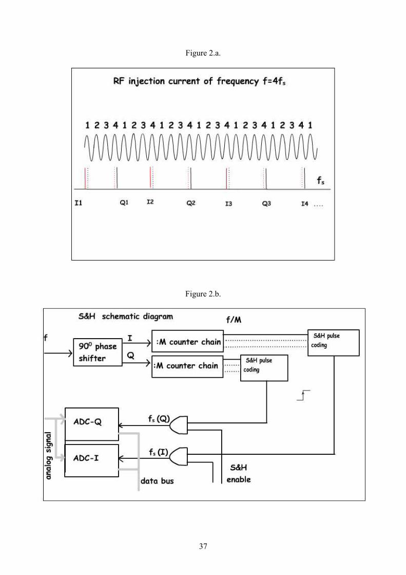
As concerns an IQ mode (Jankovic and Öhman, 2001), in which a quartz oscillates with a

high figure of merit Q=104-106, the inaccuracy Δ|Z|/|Z|IQ(n,φV) depends strongly on bit resolution n,

decreasing as the exponential function 2-n of n, and weakly on the initial phase of voltage φV, such

that [figs. 3.a, a.bis]

max

min max

1 2(1 ) ,2 41 2[1 tan (1 cos 2 )]1 22 (1 ) ,2

V Vn

V VnIQ

V V Vn

Z QZ Q

Q

π πϕ ϕπ ϕ ϕ

π ϕ ϕ π ϕ

⎧ + = =⎪Δ ⎪+ + = ⎨⎪ − = = −⎪⎩

, (3.1)

Δ|Z|/|Z|IQ(n,φV) being

8

lim

1lim2V V

nIQ

ZZϕ ϕ→

Δ= (3.2)

in the limit value

lim ( )4 2VQarctg πϕπ

= ≈ . (3.3)

Instead, as concerns uniform sampling (Razavi, 1995), the inaccuracy Δ|Z|/|Z|U(n) for |Z| depends

only on the bit resolution n, decreasing as the exponential function 2-n of n [fig. 4.a],

12n

U

ZZ

Δ= . (3.4)

Consequently, for all ADCs, with bit resolution n:

if the probe performs measurements on a medium, then the inaccuracy Δεr/εr(f) in the measurement

of dielectric permittivity εr is characterized by a minimum limit Δεr/εr|min(εr,n), interpretable as the

“physical bound” imposed on the inaccuracies of the problem, which depends on both εr and the bit

resolution n, being directly proportional to the factor (1+1/εr), while decreasing as the exponential

function 2-n of n [fig. 5.a];

if the probe, with characteristic geometrical dimension L, performs measurements on a medium,

with conductivity σ and permittivity εr, working within the cut-off frequency

fT=fT(σ,εr)=σ/(2πε0(εr+1)) (Settimi et al., 2010), then the absolute error E|Z|(L,σ,n) in the

measurement of the modulus for the transfer impedance |Z|N(L,σ) depends on σ, L and the bit

resolution n, the error being inversely proportional to both σ and L, while decreasing as the

exponential function 2-n of n [fig. 5.b] [In fact, ZN(f,L,σ,εr) is fully characterized by the high

frequency pole fT=fT(σ,εr), which cancels its denominator: the transfer impedance acts as a low-

middle frequency band-pass filter with cut-off fT=fT(σ,εr), in other words the frequency equalizing

Joule and displacement current. As discussed below, average values of σ may be used over the band

ranging from LF to MF, therefore |Z|N(L,σ) is not function of frequency below fT (Settimi et al.,

2010)].

9

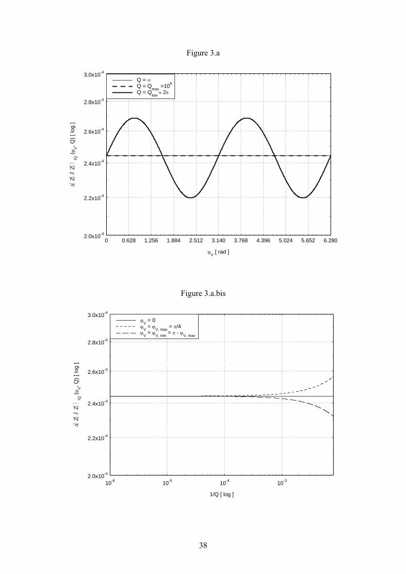
As concerns IQ mode, with a quartz of high merit figure Q, the inaccuracy ΔΦZ/ΦZ|IQ(n,φV) depends

both on the bit resolution n, decreasing as the exponential function 2-n of n, and on the voltage phase

φV, such that [fig. 3.b]

max

min

1 , 0sin(2 )1 2(1 tan ) 22 2 0 ,

V VnVZVn

Z VIQV V

Qϕ ϕϕ π ϕ

ϕ ϕ ϕ π

⎧ = =ΔΦ ⎪+ = ⎨Φ ⎪ = =⎩

, (3.5)

ΔΦZ/ΦZ|IQ(n,φV) being very low in φV =π/2, due to the high Q [fig. 3.b.bis],

2/ 2

1 1lim2V

Zn

Z IQQϕ π −→

ΔΦ=

Φ. (3.6)

Instead, as concerns uniform sampling, the inaccuracy ΔΦZ/ΦZ|U(f,fS) for ΦZ depends on both the

working frequency f of the probe and the rate sampling fS of the ADC, the inaccuracy being directly

proportional to the frequency ratio f/fS [fig. 4.b],

2Z

Z SU

ff

ΔΦ=

Φ. (3.7)

As a consequence, only for uniform sampling ADCs, the inaccuracy ΔΦZ/ΦZ (f,fS) for the phase ΦZ

must be optimized in the upper frequency fup, so when the probe performs measurements at the limit

of its band B, i.e. fup=B.

Still with the aim of investigating the physics of the measuring system, when the quadrupolar

probe exhibits a galvanic contact with the subjacent medium of electrical conductivity σ and

dielectric permittivity εr, i.e. h=0, and works in frequencies f lower than the cut-off frequency

fT=fT(σ,εr) (Grard and Tabbagh, 1991),

1T

ωω

Ω = ≤ , (3.8)

the inaccuracies Δσ/σ in the measurements of the conductivity σ and Δεr/εr for the permittivity εr are

analytically expressed [figs. 6, 9, 11][tabs. 1-3], achievable connecting uniform or IQ samplers,

10

which ensure the inaccuracies Δ|Z|/|Z| for the modulus |Z| and ΔΦZ /ΦZ for the phase ΦZ of the

transfer impedance (Settimi et al., 2010),

22(1 )( )Z

Z

ZZ

σσ

Δ ΔΦΔ≅ + Ω +

Φ, (3.9)

22

1 12(1 )(1 )( )r Z

r r Z

ZZ

εε ε

ΔΔ ΔΦ≅ + Ω + +

Ω Φ. (3.10)

Only if the quadrupole probe is in galvanic contact with the subjacent medium, i.e. h=0, then our

mathematical-physical model predicts that the inaccuracies Δσ/σ for σ and Δεr/εr for εr are invariant

in the linear (Wenner’s) or square configuration and independent of the characteristic geometrical

dimension of the quadrupole, i.e. electrode-electrode distance L (Settimi et al., 2010). If the

quadrupole, besides grazing the medium, measures σ and εr working in a frequency f much lower

than the cut-off frequency fT=fT(σ,εr), then the inaccuracy Δσ/σ=F(Δ|Z|/|Z|,ΔΦZ/ΦZ) is a linear

combination of the inaccuracies, Δ|Z|/|Z| and ΔΦZ/ΦZ, for the transfer impedance, while the

inaccuracy Δεr/εr=F(Δ|Z|/|Z|) can be approximated as a linear function only of the inaccuracy

Δ|Z|/|Z|; in other words, if f<<fT, then ΔΦZ/ΦZ is contributing in Δσ/σ but not in Δεr/εr.

As mentioned above, even if, according to Debye polarization mechanisms (Debye, 1929) or Cole-

Cole diagrams (Auty and Cole, 1952), the complex permittivity of various materials in the

frequency band from VLF to VHF exhibits several intensive relaxation effects and a non-trivial

dependence on the water saturation (Chelidze and Gueguen, 1999)(Chelidze et al., 1999), anyway

average values of electrical resistivity and dielectric permittivity may be used to estimate the

complex impedance over various terrains and concretes, especially when they are characterized by

low levels of water content and analyzed within a frequency bandwidth ranging only from LF to

MF.

11

3.1. For in phase and quadrature (IQ) sampling.

As concerns IQ sampling ADCs (merit figure Q)(Jankovic and Öhman, 2001), the inaccuracy

Δεr/εr(f,n) in the measurement of permittivity εr is characterized by an optimal working frequency

fopt,IQ(fT), close to the cut-off frequency for the modulus of the transfer impedance fT =fT(σ,εr), i.e.

,2(1 )opt IQ T Tf f f

Qπ

+ ≈ , (3.11)

which is tuned in a minimum value of inaccuracy Δεr/εr|min,IQ(εr,n), depending both on εr and the

specifications of the sampler, in particular only its bit resolution n. The inaccuracy is directly

proportional to the factor (1+1/εr), while decreasing as the exponential function 2-(n-3) of n, such that

[fig. 5.a]

3min,

1 1(1 ) (1 )2

rn

r rIQQ

ε πε ε −

Δ+ + . (3.12)

Consequently, if the frequency f of the probe is much lower than the cut-off frequency fT(σ,εr) for

the transfer impedance, then the inaccuracy Δσ/σ(n) for σ is a constant, and the inaccuracy Δεr/εr(f,n)

for εr shows a downward trend in frequency, as (fT/f)2, such that both the inaccuracies decrease as

exponential functions of n, the first inaccuracy as 1/2n-2 while the second one as 1/2n-1, i.e. [fig. 6]

[tab. 1]

2

1 (1 ) ,2

TnIQ

for f fQ

σ πσ −

Δ+ << , (3.13)

2

1

1 1 2(1 ) (1 ) ,2

r TTn

r rIQ

f for f fQ f

ε πε ε −

⎛ ⎞Δ+ + <<⎜ ⎟

⎝ ⎠. (3.14)

Even if the frequency f is much higher than fT(σ,εr), it could be proven that the inaccuracies

Δσ/σ(f,n) and Δεr/εr(f,n) do not deviate too much from an upward trend in frequency as a parabolic

line (f/fT)2, with a high gradient for the σ measurement and a low gradient for the εr measurement,

12

still decreasing as exponential functions of n, the first inaccuracy as 1/2n-2 while the second one as

1/2n-1, i.e. [fig. 6][tab. 1]

2

2

1 (1 ) ,2

TnIQ T

f for f fQ f

σ πσ −

⎛ ⎞Δ+ >>⎜ ⎟

⎝ ⎠, (3.15)

2

1

1 1(1 ) ,2

rTn

r r TIQ

f for f ff

εε ε −

⎛ ⎞Δ+ >>⎜ ⎟

⎝ ⎠. (3.16)

Only if f is lower than fT, then the measurements could be optimized for εr and σ, and might require

that the inaccuracy Δεr/εr(n,f) for εr is below the prefixed limit Δεr/εr|fixed (10%) within the frequency

band B=100kHz, choosing a minimum bit resolution nmin,IQ(fT,εr,), which depends on both fT and εr

and increases as the logarithmic function log2 of both the ratios fT/B and 1/εr, i.e.

min, 2 2 211 log 2log log (1 )r T

IQr rfixed

fnB

εε ε

Δ≈ − + + + . (3.17)

Referring to the IQ sampling ADCs, the inaccuracies Δσ/σ in the measurement of the electrical

conductivity σ and Δεr/εr for the dielectric permittivity εr were estimated for the worst case, when

the inaccuracies Δ|Z|/|Z|IQ(n,φV) in the measurement of the modulus and ΔΦZ/ΦZ|IQ(n,φV) for the

phase of the transfer impedance respectively assume the mean and the maximum values, i.e.

Δ|Z|/|Z|IQ = ΔΦZ/ΦZ|IQ = 1/2n.

To conclude, for the IQ mode, the optimal and minimum values of the working frequency of the

quadrupolar probe interact in a competitive way. The more the quadrupole analyzes a subjacent

medium characterized by a low electrical conductivity, with the aim of shifting the optimal

frequency into a low band, the more the low conductivity has the self-defeating effect of shifting the

minimum value of frequency into a higher band. In fact, the probe could work around a low optimal

frequency, achievable in measurements of transfer impedance with a low cut-off frequency, typical

of materials characterized by low conductivity. Instead, the more the minimum value of the working

frequency is shifted into a lower band, the more the minimum bit resolution for the sampler has to

be increased; if the medium was selected, then increasing the inaccuracy for the measurement of the

13

dielectric permittivity, or, if the inaccuracy was fixed, shifting the cut-off frequency into a high

band, i.e. selecting a medium with high conductivity. Finally, while the authors' analysis shows that

the quadrupole could work at a low optimal frequency, if the transfer impedance is characterized by

a low cut-off frequency, in any case and in accordance with the more traditional results of recent

scientific publications referenced (Grard, 1990, a-b)(Grard and Tabbagh, 1991)(Tabbagh et al.,

1993)(Vannaroni et al. 2004)(Del Vento and Vannaroni, 2005), the probe could perform

measurements in an appropriate band of higher frequencies, centered around the cut-off frequency,

where the inaccuracy for the measurements of conductivity and permittivity were below a prefixed

limit (10%).

3.2. For uniform sampling.

As concerns uniform sampling ADCs (Razavi, 1995), if the frequency f of the probe is lower

than the cut-off frequency fT for the modulus |Z|(f,L) of the transfer impedance, i.e. fT =fT(σ,εr),

then, the higher the bit resolution n, the more the optimal working frequency fopt,U(fT,fS,n), which

minimizes inaccuracy Δεr/εr(f,fS,n) in the measurement of the permittivity εr, approximately depends

on the cut-off frequency fT(σ,εr) and the specifications of the sampler, in particular the sampling rate

fS and n, increasing with both fT and fS, while decreasing as the exponential function 2-n/3 of n, such

that [fig. 7]

,3

12

opt U Sn

T T

f ff f

. (3.18)

Moreover, the higher the bit resolution n, the more the inaccuracy Δεr/εr(f,fS,n) for εr can not go

down beyond a minimum limit of inaccuracy Δεr/εr|min,U(εr,n), which approximately depends on

both εr and n, being directly proportional to the factor (1+1/εr), while decreasing as the exponential

function 2-(n-1) of n, similarly to IQ sampling. The minimum value of inaccuracy Δεr/εr|min,U(εr,n) in

14

uniform mode is higher than the minimum inaccuracy Δεr/εr|min,IQ(εr,n) corresponding to the IQ

mode, i.e. [figs. 5.a, 6] [tab. 1]

2,1

,min, min,

1 1 1(1 ) [1 ( ) ] ,2 4

r r T ropt U Tn

r r r opt U rU IQ

f f ff

ε ε εε ε ε ε−

Δ Δ Δ≥ + + >> << . (3.19)

Finally, the minimum value of frequency fU,min(fT,n), which allows an inaccuracy Δεr/εr(f,fS,n) below

a prefixed limit Δεr/εr|fixed (10%), depends both on fT(σ,εr) and n, being directly proportional to fT,

while decreasing as an exponential function of n, such that [fig. 8]

min, ,

min,

1

TU opt U

r r fixed

r r U

ff fε ε

ε ε

<Δ

−Δ

. (3.20)

To conclude, also in the uniform mode, the optimal frequency and the band of frequency of

the quadrupolar probe interact in a competitive way. In fact, an ADC with a high bit resolution is

characterized by a low sampling rate, for which, having selected the subjacent medium to be

analyzed, the higher the resolution of the sampler used, with the aim of shifting the optimal

frequency of the quadrupolar probe into a low band, the more the low sampling rate has the self-

defeating effect of narrowing its frequency band. Moreover, a material with low electrical

conductivity is usually characterized by low dielectric permittivity. Having designed the ADC, the

more the quadrupole measures a transfer impedance limited by a low cut-off frequency, the more it

can work at a low optimal frequency, even if centered in a narrow band. Finally, having selected the

medium to be analyzed and designed the sampler, the more the frequency band of the probe is

widened, the more the inaccuracy of the measurements is increased.

15

4. Noisy IQ Down-Sampling.

In signal processing, down-sampling (or "sub-sampling") is the process of reducing the

sampling rate of a signal. This is usually done to reduce the data rate or the size of the data

(Oppenheim et al., 1999)(Andren and Fakatselis, 1995).

The down-sampling factor, commonly denoted by M, is usually an integer or a rational fraction

greater than unity. If the quadrupolar probe injects electric current into materials at a RF frequency

f, then the ADC samples at a rate fs fixed by:

Sff

M= , (4.1)

being M preferably, but not necessary, a power of 2 to facilitate the digital circuitry

( 2 , mM m= ∈ ).

Since down-sampling reduces the sampling rate, one must be careful to make sure the Shannon-

Nyquist sampling theorem criterion is maintained. If the sampling theorem is not satisfied then the

resulting digital signal will have aliasing. To ensure that the sampling theorem is satisfied, a low-

pass filter is used as an anti-aliasing filter to reduce the bandwidth of the signal before the signal is

down-sampled; the overall process (low-pass filter, then down-sample) is called decimation. Note

that the anti-aliasing filter must be a low-pass filter in down-sampling. This is different from

sampling a continuous signal, where either a low-pass filter or a band-pass filter may be used.

A practical scheme to select the sampling rate is to launch two time sequences as in fig. 2.a..

Now there is a problem due to timing. If the quadrupole would work at a fixed frequency f, then the

proper relationship between the rate fs and the down-sampling factor M could be easily found.

Instead, if the probe is performing a sort of electrical spectroscopy, then an enable signal for the

sampling and holding circuit (S&H) must be generated. The time frame should be such that the

sequences n·M·T for the sample I and n·M·T+T/4 for the sample Q could be obtained, corresponding

to the period T of the maximum working frequency. So the rate fs would be ensured as a M factor

16

sub-multiple of frequency f. A possible conceptual scheme of this implementation is shown in fig.

2.b.

Besides the quantization error of IQ ADC, which can be assumed small both in amplitude and

phase, as decreasing exponentially with the bit resolution n, the electric signals are affected by two

additional noises. The amplitude term noise, due to external environment, is modelled by the signal

to noise ratio SNR = 30dB which can be reduced performing averages over one thousand of

repeated measurements (A = 103). The phase term noise, due to a phase-splitter detector, which,

even if increasing linearly with the frequency f, can be minimized by digital electronics providing a

rise time of few nanoseconds (τ = 1ns). In analytical terms:

1 1 1 22n

IQ Enviroment

Z Z ZZ Z Z SNRA A

Δ Δ Δ= + = + , (4.2)

12

Z Z Zn

Z Z ZIQ Phase Shifter

fτ−

ΔΦ ΔΦ ΔΦ= + = + ⋅

Φ Φ Φ. (4.3)

With respect to the ideal case involving only a quantization error, the additional noise both in

amplitude, due to external environment, and especially in phase, due to phase-shifter detector,

produce two effects: firstly, both the curves of inaccuracy Δεr/εr(f) and Δσ/σ(f) in measurement of

the dielectric permittivity εr and electric conductivity σ are shifted upwards, to values larger of

almost half a magnitude order, at most; and, secondly, the inaccuracy curve Δεr/εr(f) of permittivity

εr is narrowed, even of almost half a middle frequency (MF) decade. So, both the optimal value of

frequency fopt, which minimizes the inaccuracy Δεr/εr(f) of εr, and the maximum frequency fmax,

allowing an inaccuracy Δεr/εr(f) below the prefixed limit Δεr/εr|fixed (10%), are left shifted towards

lower frequencies, even of half a MF decade. Instead, the phase-splitter is affected by a noise

directly proportional to frequency, which is significant just from MFs; so, the minimum frequency

fmin, allowing Δεr/εr(f) below Δεr/εr|fixed (10%), remains almost invariant at LFs [fig. 9][tab. 2].

Therefore, the profit of employing the down-sampling method is obvious. This method

would allow to run a real electric spectroscopy because, theoretically, measurements could be

17

performed at any frequency. An advantage is that there are virtually no limitations due to the

sampling rate of ADCs and associated S&H circuitry [fig. 10][tab. 2].

5. Fast Fourier Transform (FFT) processor and round-off noise.

In mathematics, the Discrete Fourier Transform (DFT) is a specific kind of Fourier

transform, used in Fourier analysis. The DFT requires an input function that is discrete and whose

non-zero values have a limited (finite) duration. Such inputs are often created by sampling a

continuous function. Using the DFT implies that the finite segment that is analyzed is one period of

an infinitely extended periodic signal; if this is not actually true, a window function has to be used

to reduce the artefacts in the spectrum. In particular, the DFT is widely employed in signal

processing and related fields to analyze the frequencies contained in a sampled signal. A key

enabling factor for these applications is the fact that the DFT can be computed efficiently in practice

using a Fast Fourier Transform (FFT) algorithm.

It is important to understand the effects of finite register length in the computation. Specifically,

arithmetic round-off is analyzed by means of a linear-noise model obtained by inserting an additive

noise source at each point in the computation algorithm where round-off occurs. However, the

effects of round-off noise are very similar among the different classes of FFT algorithms

(Oppenheim et al., 1999).

Generally, a FFT processor which computes N samples, represented as nFFT+1 bit signed

fractions, is affected by a round-off noise which adds to the inaccuracy for transfer impedance, in

amplitude (Oppenheim et al., 1999)

12 FFTnRound off

Z NZ −

−

Δ= , (5.1)

and in phase (Dishan, 1995)(Ming and Kang, 1996),

18

12 FFT

Zn

Z Round off Nπ−

ΔΦ=

Φ. (5.2)

So, maximizing the register length to nFFT=32, the round-off noise is entirely negligible. Once that

nFFT<32, if the number of samples is increased N>>1, then the round-off noise due to FFT degrades

the accuracy of transfer impedance, so much more in amplitude (5.1) how much less in phase (5.2).

One can overcome this inconvenience by iterating the FFT processor for A cycles, as the best

estimate of one FFT value is the average of A FFT repeated values. The improvement is that the

inaccuracy for the averaged transfer impedance, in amplitude and phase, consists on the error of

quantization due to the uniform sampling ADC (3.4)-(3.7) and the round-off noise due to FFT (5.1)-

(5.2), the last term being decreased of A , i.e.:

1

1 1 12 2 FFTnn

U Round off

Z Z Z NZ Z ZA A −

−

Δ Δ Δ= + = + , (5.3)

1 1 122 FFT

Z Z Zn

Z Z Z SU Round off

ffA A Nπ−

ΔΦ ΔΦ ΔΦ= + = +

Φ Φ Φ. (5.4)

Once reduced the register length to nFFT≤16, only if the FFT processor performs the averages during

a number of cycles

2

212 FFTn n

N A N− −⎛ ⎞ << ≤⎜ ⎟⎝ ⎠

, (5.5)

then the round-off noise due to FFT can be neglected with respect to the quantization error due to

uniform ADC, in amplitude

1

1 1 12 2 2FFTnn n

U

Z ZZ Z−

Δ Δ≈ + = , (5.6)

and especially in phase

12 22 FFT

Z Zn

Z S Z SU

f ff N fπ

ΔΦ ΔΦ+ ≅ =

Φ Φ. (5.7)

19

So, the round-off noise due to FFT is compensated. The quantization error due to ADC decides the

accuracy for transfer impedance: it is constant in amplitude, once fixed the bit resolution n, and can

be limited in phase, by an oversampling technique fS>>f.

In the limit of the Shannon-Nyquist theorem, an electric signal with band of frequency B must

be sampled at the minimal rate fS = 2B, holding Nmin samples in a window of time T. Instead, in the

hypothesis of oversampling, the signal can be sampled holding the same number of samples Nmin

but in a shorter time window T/RO, due to an high ratio of sampling:

12

SO

fRB

= >> . (5.8)

This is equivalent to the operating condition in which, during the time window,

min

2NT

B= , (5.9)

the uniform over-sampling ADC hold a samples number

min minON R N N= ⋅ >> (5.10)

which is linked to the number of cycles iterated by the FFT processor:

2 2 2min 1OA N R N≅ = ⋅ >> . (5.11)

As comments on eqs. (5.9)-(5.11), a low number of samples Nmin, corresponding to the Shannon-

Nyquist limit, shortens the time window (5.9). An high oversampling ratio lowers the phase

inaccuracy although it raises the samples number hold by uniform ADC and especially the cycles

number iterated by FFT; however, even a minimal oversampling ratio RO,min limits the phase

inaccuracy with the advantage of not raising to much the samples number hold by ADC (5.10) and

especially the cycles number iterated by FFT (5.11).

The quadrupole (frequency band B) exhibits a galvanic contact with the subjacent non-

saturated medium (terrestrial soil or concrete with low permittivity εr = 4 and high resistivity σS ≈

3.334·10-4 S/m, σC ≈ 10-4 S/m). It is required that the inaccuracy Δεr/εr(f,fS,n) in the measurement of

εr is below a prefixed limit Δεr/εr|fixed (10-15%) within the band B (100kHz). As first result, if the

20

samples number satisfying the Shannon-Nyquist theorem is minimized, i.e. Nmin=2, then the time

window for sampling is shortened to T = Nmin/(2B) = 1/B ≈ 10μs. In order to analyze the complex

impedance measured by the probe in Fourier domain, an uniform ADC can be connected to a FFT

processor, being affected by a round-off amplitude noise. As conclusive result, a technique of

compensation must occur. The ADC must be specified by: a minimal bit resolution n≤12, thereby

rendering the system of measurement almost insensitive to the electric noise of the external

environment; and a minimal over-sampling rate fS, which limits the ratio RO=fS/(2B), so the actual

samples number N = RO·Nmin is up to one hundred (soil, fS = 10MHz, RO = 50, N ≈ 100)(concrete, fS

= 5MHz, RO = 25, N ≈ 50). Moreover, even if the FFT register length is equal to nFFT = 16, anyway

the minimal rate fS ensures a number of averaged FFT values A ≤ N2 even up to ten thousand,

necessary to bound the round-off noise (soil, A ≈ 104)(concrete, A ≈ 2.5·103) [fig. 11][tab. 3].

6. Characteristic geometrical dimensions of the quadrupolar probe.

In this section, we refer to Vannaroni’s paper (Vannaroni et al., 2004) which discusses the

dependence of TX current and RX voltage on the array and electrode dimensions. The dimensions

of the quadrupolar probe terminals are not critical in the definition of the system because they can

be considered point electrodes with respect to their separating distances. In this respect, the

separating distance to consider are either the square array side [fig. 12.a] or the spacing distance for

a Wenner configuration [fig. 12.b]. The only aspect that could be of importance for the practical

implementation of the system is the relationship between electrode dimensions and the magnitude

of the current injected into the ground. Current is a critical parameter of the mutual impedance

probe in that, in general, given the practical voltage levels applicable to the electrodes and the

capacitive coupling with the soil, the current levels are expected to be quite low, with a resulting

limit to the accuracy that can be achieved for the amplitude and phase measurements. Furthermore,

21

low currents imply a reduction of the voltage signal read across the RX terminals and more

stringent requirements for the reading amplifier.

In the Appendix it is proven that, having fixed the input resistance Rin of the amplifier stage

and selecting the minimum value of frequency fmin for the quadrupole [fig. 1], which allows an

inaccuracy in the measurement of the dielectric permittivity εr below a prefixed limit (10%), then

the radius r(Rin,fmin) of the electrodes can be designed, as it depends only on the resistance Rin and

the frequency fmin, the radius being an inversely proportional function to both Rin and fmin [fig.

13][tab. 4],

20 min

1(2 ) in

rR fπ ε

. (6.1)

Moreover, known the minimum bit resolution nmin for the uniform or IQ sampling ADC, which

allows an inaccuracy for permittivity εr below the limit 10%, the electrode-electrode distance

L(r,nmin) can also be defined, as it depends only on the radius r(Rin,fmin) and the bit resolution nmin,

the distance being directly proportional to r(Rin,fmin) and increasing as the exponential function 2nmin

of nmin [fig. 13][tab. 4],

min2nL r∝ ⋅ . (6.2)

Finally, the radius r(Rin,fmin) remains invariant whether the probe assumes the linear (Wenner’s) or

the square configuration, while, having also given the resolution nmin, then the distance LS(r,nmin) in

the square configuration must be smaller by a factor (2-21/2) compared to the corresponding distance

LW(r,nmin) in the Wenner configuration (Settimi et al., 2010)

min(2 2) (2 2) 2nS WL L r= − ⋅ = − ⋅ ⋅ . (6.3)

7. Conclusive discussion.

This paper has discussed the development and engineering of electrical spectroscopy for

simultaneous and non invasive measurement of electrical resistivity and dielectric permittivity. A

22

suitable quadrupolar probe is able to perform measurements on a subsurface with inaccuracies

below a fixed limit (10%) in a bandwidth of low (LF) frequency (100kHz). The quadrupole probe

should be connected to an appropriate analogical digital converter (ADC) which samples in phase

and quadrature (IQ) or in uniform mode. If the quadrupole is characterized by a galvanic contact

with the surface, the inaccuracies in the measurement of resistivity and permittivity, due to the IQ or

uniform sampling ADC, have been analytically expressed. A large number of numerical simulations

has proven that the performances of the probe depend on the selected sampler and that the IQ is

better compared to the uniform mode under the same operating conditions, i.e. bit resolution and

medium [fig. 6][tab. 1].

As regards the IQ mode, it is specified by an inaccuracy ΔΦZ/ΦZ(nIQ) for the phase of the transfer

impedance which depends only on the bit resolution nIQ, assuming small values [for example

ΔΦZ/ΦZ|max(12)=1/212≈2.4·10-4] over the entire frequency band B=100kHz of the quadrupole; in the

uniform mode, the corresponding inaccuracy ΔΦZ/ΦZ(f,fS) depends on the frequency f, only being

small for frequencies much lower than the sampling rate fS [i.e. 2f/fS≤ ΔΦZ/ΦZ|max(12)]. The

principal advantages are: firstly, the minimum value fmin(n) of the frequency, which allows an

inaccuracy for permittivity εr below 10%, is slightly lower when the probe is connected to an IQ

rather than a uniform ADC, other operating conditions being equal, i.e. the resolution and the

surface; and, secondly, the inaccuracy Δσ/σ for conductivity σ, calculated in fmin(n), is smaller using

IQ than with uniform sampling, being Δσ/σ|IQ<Δσ/σ|U of almost one order of magnitude, under the

same operating conditions, in particular the resolution. As a minor disadvantage, the optimal

frequency fopt, which minimizes the inaccuracy for εr, is generally higher using IQ than uniform

sampling, being fopt,IQ> fopt,U of almost one middle frequency (MF) decade, at most, under the same

operating conditions, in particular the surface [fig. 6].

Instead the uniform mode is specified by two degrees of freedom, the resolution of bit nU and the

rate of sampling fS, compared to the IQ mode, characterized by one degree of freedom, the bit

resolution nIQ. Consequently the quadrupolar probe could be connected to a uniform ADC with a

23

sampling rate fS sufficiently fast to reach, at a resolution (for example nU=8) lower than the IQ’s

(i.e. nIQ=12), the same prefixed limit (i.e. 10%) of inaccuracy in the measurement of the dielectric

permittivity εr, for various media, especially those with low electrical conductivities σ [tab.1].

Assuming that the electric current injected in materials and so the voltage measured by probe

are quasi-monochromatic signals, i.e. with a very narrow frequency band, an IQ down-sampling

process can be employed. Besides the quantization error of IQ ADC, which can be assumed small

both in amplitude and phase, as decreasing exponentially with the bit resolution, the electric signals

are affected by two additional noises. The amplitude term noise, due to external environment, is

modeled by the signal to noise ratio which can be reduced performing averages over a thousand of

repeated measurements. The phase term noise, due to a phase-splitter detector, which, even if

increasing linearly with the frequency, can be minimized by digital electronics providing a rise time

of few nanoseconds [figs. 9,10] [tab. 2].

Instead, in order to analyze the complex impedance measured by the quadrupole in Fourier domain,

an uniform ADC, which is characterized by a sensible phase inaccuracy depending on frequency,

must be connected to a Fast Fourier Transform (FFT) processor, that is especially affected by a

round-off amplitude noise linked to both the FFT register length and samples number. If the register

length is equal to 32 bits, then the round-off noise is entirely negligible, else, once bits are reduced

to 16, a technique of compensation must occur. In fact, oversampling can be employed within a

short time window, reaching a compromise between the needs of limiting the phase inaccuracy due

to ADC and not raising too much the number of averaged FFT values sufficient to bound the round-

off [fig. 11][tab. 3].

Since, in this paper, the conceptual and technical problem for designing the “heart” of the

instrument have already been addressed and resolved, a further paper will complete the technical

project, focusing on the following two aims.

First aim: the implementation of hardware which can handle numerous electrodes, arranged so as to

provide data which is related to various depths of investigation for a single measurement pass;

24

consequently, this hardware must be able to automatically switch transmitting and measurement

pairs.

Second aim: the implementation of acquisition configurations, by an appropriate choice of

transmission frequency, for the different applications in which this instrument can be profitably

used.

Appendix.

A series of two spherical capacitors with radius r and spacing distance L>>r is characterized

by the electrical capacitance

00

2 2 ,1 1 C r for L r

r L r

πε πε= >>−

−

, (A.1)

with ε0 the dielectric constant in vacuum.

A quadrupolar probe, with four spherical electrodes of radius r and separating distance L>>r, is

arranged in the Wenner’s configuration, with total length Ltot=3L, which is specified by the pairs of

transmitting electrodes T1 and T2 at the ends of quadrupole and the reading electrodes R1 and R2 in

the middle of probe. The quadrupolar probe is characterized by a capacitance almost invariant for

the pairs of electrodes T1,2 and R1,2,

1 2 1 2

0 0, , 0

2 2 2 ,1 1 1 13

T T R RC C C r for L r

r L r r L r

πε πε πε= = = >>− −

− −

. (A.2)

The charge Q of the electrodes being equal, the electrical voltage across the pair T1 and T2

approximates the voltage between R1 and R2,

1 2 1 2, ,T T R R

QV VC

Δ Δ . (A.3)

As regards the equivalent capacitance circuit which schematizes the transmission stage of

quadrupole [fig. 14.a], if the effect of the capacitance C, across the electrodes, is predominant

25

relative to the shunted capacitances CT1 and CT2, describing the electrical coupling between the

transmitting electrodes and the subjacent medium,

1 2T TC C C<< = , (A.4)

then, the probe, working in the frequency f, injects in the medium a minimum bound for the

modulus of the current |I|min,

1 2 1 2 1 2

20 , 0 ,min

2 2 (2 )T T T T T TI C V f r V rf Vω π πε π ε⋅ ⋅ Δ = ⋅ ⋅ Δ = Δ , (A.5)

|I|min increasing linearly with f.

Concerning the equivalent capacitance circuit which represents the reception stage of the

quadrupolar probe [fig. 14.b], the effect of the capacitance C, across the electrodes, is predominant

even relative to the shunted capacitances CR1 and CR2, describing the coupling between the reading

electrodes and the subjacent medium,

1 2R RC C C<< = . (A.6)

If the quadrupole, of electrode-electrode distance L, is immersed in vacuum, then it can be

characterized by the vacuum capacitance

0 04C Lπε= , (A.7)

and measures, in the frequency f, a minimum limit |Z|min for the transfer impedance in modulus,

2min0 0 0

1 1 12 4 2(2 )

ZC f L Lfω π πε π ε

= = =⋅ ⋅

, (A.8)

which gives rises to a minimum for the electrical voltage ΔVmin,R1,R2, flowing the current |I|min,

1 2 1 2 1 2

min 2, 0 , ,2min min

0

1 1(2 )2(2 ) 2R R T T T T

rV Z I rf V VLf L

π επ ε

Δ = ⋅ Δ = Δ . (A.9)

Notice that ΔVmin,R1,R2 is independent of f, as |I|min is directly and |Z|min inversely proportional to f.

As a first finding, the analogical digital converter (ADC), downstream of probe, must be specified

by a bit resolution n, such that:

1 2 1 2

1 2 1 2

min min, ,

1, ,

1 1 12 2 2

R R R Rn n

T T R R

V Vr rV L V L+

Δ Δ≈ = ⇒ ≈

Δ Δ. (A.10)

26

Instead, if the quadrupole exhibits a galvanic contact with a medium of electrical conductivity

σ and dielectric permittivity εr, working in a band lower than the cut-off frequency, i.e. fT

=fT(σ,εr)=1/2π·σ/ε0(εr+1), then it measures the transfer impedance in modulus

12

ZLπσ

= . (A.11)

As final findings, the voltage amplifier, downstream of the probe, must be specified by an input

resistance Rin larger than both the transfer impedance, i.e.

1 12 2

inin

R Z LL Rπσ πσ

> = ⇒ > , (A.12)

and the reactance associated to the capacitance C, which is characterized by a maximum value in

the minimum of frequency fmin, i.e.

2 2min min 0 0 min 0 min

1 1 1 12 2 (2 ) (2 )

inin

R rC f r rf R fω π πε π ε π ε

> = = ⇒ >⋅

. (A.13)

References.

Al-Qadi I. L., O. A. Hazim, W. Su and S. M. Riad (1995). Dielectric properties of Portland cement

concrete at low radio frequencies, J. Mater. Civil. Eng., 7, 192-198.

Andren C. and J. Fakatselis (1995). Digital IF Sub Sampling Using the HI5702, HSP45116 and

HSP43220, App. Note (Harris DSP and Data Acq.), No. AN9509.1 .

Arpaia P., P. Daponte and L. Michaeli (1999). Influence of the architecture on ADC error

modelling, IEEE T. Instrum. Meas, 48, 956-966.

Arpaia P., P. Daponte and S.Rapuano (2003). A state of the art on ADC modelling, Comput. Stand.

Int., 26, 31–42.

Auty R.P. and R.H.Cole (1952). Dielectric properties of ice and solid, J. Chem. Phys., 20, 1309-

1314.

27

Björsell N. and P. Händel (2008). Achievable ADC performance by post-correction utilizing

dynamic modeling of the integral nonlinearity, Eurasip J. Adv. Sig. Pr., 2008, ID 497187 (10 pp).

Chelidze T.L. and Y. Gueguen (1999). Electrical spectroscopy of porous rocks: a review-I,

Theoretical models, Geophys. J. Int., 137, 1-15.

Chelidze T.L. and Y. Gueguen, C. Ruffet (1999). Electrical spectroscopy of porous rocks: a review-

II, Experimental results and interpretation, Geophys. J. Int., 137, 16-34.

Debye P. (1929). Polar Molecules (Leipzig Press, Germany).

Declerk P. (1995). Bibliographic study of georadar principles, applications, advantages, and

inconvenience, NDT & E Int., 28, 390-442 (in French, English abstract).

Del Vento D. and G. Vannaroni (2005). Evaluation of a mutual impedance probe to search for water

ice in the Martian shallow subsoil, Rev. Sci. Instrum., 76, 084504 (1-8).

Dishan H. (1995). Phase Error in Fast Fourier Transform Analysis, Mech. Syst. Signal Pr., 9, 113-

118.

Edwards R. J. (1998). Typical Soil Characteristics of Various Terrains,

http://www.smeter.net/grounds/soil-electrical-resistance.php.

Grard R. (1990). A quadrupolar array for measuring the complex permittivity of the ground:

application to earth prospection and planetary exploration, Meas. Sci. Technol., 1, 295-301.

Grard R. (1990). A quadrupole system for measuring in situ the complex permittvity of materials:

application to penetrators and landers for planetary exploration, Meas. Sci. Technol., 1, 801-806.

Grard R. and A. Tabbagh (1991). A mobile four electrode array and its application to the electrical

survey of planetary grounds at shallow depth, J. Geophys. Res., 96, 4117-4123.

Jankovic D. and J. Öhman (2001). Extraction of in-phase and quadrature components by IF-

sampling, Department of Signals and Systems, Cahlmers University of Technology, Goteborg

(carried out at Ericson Microwave System AB).

Knight R. J. and A. Nur (1987). The dielectric constant of sandstone, 60 kHz to 4 MHz,

Geophysics, 52, 644-654.

28

Kuffel J., R. Malewsky and R. G. Van Heeswijk (1991). Modelling of the dynamic performance of

transient recorders used for high voltage impulse tests, IEEE T. Power Deliver., 6, 507-515.

Laurents S., J. P. Balayssac, J. Rhazi, G. Klysz and G. Arliguie (2005). Non-destructive evaluation

of concrete moisture by GPR: experimental study and direct modeling, Mater. Struct., 38, 827-832.

Ming X. and D. Kang (1996). Corrections for frequency, amplitude and phase in Fast Fourier

transform of harmonic signal, Mech. Syst. Signal Pr., 10, 211-221.

Mojid M. A., G. C. L. Wyseure and D. A. Rose (2003). Electrical conductivity problems associated

with time-domain reflectometry (TDR) measurement in geotechnical engineering, Geotech. Geo.

Eng., 21, 243-258.

Mojid M. A. and H. Cho (2004). Evaluation of the time-domain reflectometry (TDR)-measured

composite dielectric constant of root-mixed soils for estimating soil-water content and root density,

J. Hydrol., 295, 263–275.

Murray-Smith D. J. (1987). Investigations of methods for the direct assessment of parameter

sensitivity in linear closed-loop control systems, in Complex and distributed systems: analysis,

simulation and control, edited by Tzafestas S. G. and Borne P. (North-Holland, Amsterdam), pp.

323–328.

Myounghak O., K. Yongsung and P. Junboum (2007). Factors affecting the complex permittivity

spectrum of soil at a low frequency range of 1 kHz10 MHz, Environ. Geol., 51, 821-833.

Oppenheim A. V., R.W. Schafer and J. R. Buck (1999). Discrete-Time Signal Processing (Prentice

Hall International, Inc., New York - II Ed.).

Polder R., C. Andrade, B. Elsener, Ø. Vennesland, J. Gulikers, R. Weidert and M. Raupach (2000).

Test methods for on site measurements of resistivity of concretes, Mater. Struct., 33, 603-611.

Polge R. J., B. K. Bhagavan and L. Callas (1975). Evaluating analog-to-digital converters,

Simulation, 24, 81-86.

Razavi B. ( 1995). Principles of Data Conversion System Design (IEEE Press, New York).

29

Samouëlian A., I. Cousin, A. Tabbagh, A. Bruand and G. Richard (2005). Electrical resistivity

survey in soil science: a review, Soil Till,. Res., 83, 172-193.

Sbartaï Z. M., S. Laurens, J. P. Balayssac, G. Arliguie and G. Ballivy (2006). Ability of the direct

wave of radar ground-coupled antenna for NDT of concrete structures, NDT & E Int., 39, 400-407.

Settimi A., A. Zirizzotti, J. A. Baskaradas and C. Bianchi (April 2010). Inaccuracy assessment for

simultaneous measurements of resistivity and permittivity applying sensitivity and transfer function

approaches, Ann. Geophys. – Italy, 53, 2, 1-19; ibid., Earth-prints, http://hdl.handle.net/2122/5180

(2009); ibid., arXiv:0908.0641 [physics.geophysiscs] (2009).

Tabbagh A., A. Hesse and R. Grard (1993). Determination of electrical properties of the ground at

shallow depth with an electrostatic quadrupole: field trials on archaeological sites, Geophys.

Prospect., 41, 579-597.

Vannaroni G., E. Pettinelli, C. Ottonello, A. Cereti, G. Della Monica, D. Del Vento, A. M. Di

Lellis, R. Di Maio, R. Filippini, A. Galli, A. Menghini, R. Orosei, S. Orsini, S. Pagnan, F. Paolucci,

A. Pisani R., G. Schettini, M. Storini and G. Tacconi (2004). MUSES: multi-sensor soil

electromagnetic sounding, Planet. Space Sci., 52, 67–78.

Zhang J. Q. and S. J. Ovaska (1998). ADC characterization by an eigenvalues method,

Instrumentation and Measurement Technology Conference (IEEE), 2, 1198-1202.

30

Tables and captions.

Table 1.a

Soil (εr = 4,

ρ = 3000 Ω·m)

U Sampling ADC(12 bit,

10 MS/s)

U Sampling (12 bit, 60 MS/s)

(12 bit, 200 MS/s)

IQ Sampling (12 bit)

fopt 150.361 kHz 267.569 kHz 387.772 kHz ≈ 1.459 MHz fmin 92.198 kHz 98.042 kHz 95.055 kHz 94.228 kHz fmax 265.287 kHz 885.632 kHz ≈ 1.832 MHz ≈ 16.224 MHz

Table 1.b

Concrete (εr = 4,

ρ= 10000 Ω·m)

U Sampling ADC

(8 bit, 50 MS/s)

U Sampling

(8 bit, 100 MS/s)

(8 bit, 250 MS/s)

(8 bit, 2 GS/s)

fopt 241.41 kHz 289.103 kHz 364.485 kHz 607.522 kHz fmin 98.574 kHz 96.629 kHz 95.553 kHz 94.953 kHz fmax 591.657 kHz 815.1 kHz ≈ 1.079 MHz ≈ 1.443 MHz

Table 1.b.bis

Concrete (εr = 4,

ρ = 10000 Ω·m)

U Sampling ADC

(12 bit, 5 MS/s)

U Sampling (12 bit,

10 MS/s)

(12 bit, 60 MS/s)

(12 bit, 200 MS/s)

IQ Sampling(12 bit)

fopt 53.271 kHz 66.605 kHz 116.332 kHz 165.329 kHz 437.716 kHz fmin 35.085 kHz 30.646 kHz 28.517 kHz 28.273 kHz 28.268 kHz fmax 85.396 kHz 169.271 kHz 549.595 kHz ≈ 1.016 MHz ≈ 4.867 MHz

31

Table 2

fopt fS,opt IQ Down - Sampling(n = 12) f = M·fS (M = 8)

+ Electric Noise (SNR = 30 dB,

A = 103) +

Phase Shifter (τ = 1 ns)

+ Electric Noise (SNR = 30 dB,

A = 103) +

Phase Shifter (ΔΦZ/ΦZ = 0.2°)

fmin fS,min

fmax

fS,max

Soil (εr = 4, ρ = 3000 Ω·m)

1.459 MHz

182.381 kHz

775.286 kHz

96.911 kHz

733.816 kHz

91.727 kHz

94.228 kHz

11.779 kHz

105.952 kHz

13.244 kHz

110.857 kHz

13.857 kHz

16.224 MHz

2.028 MHz

5.659 MHz

707.414 kHz

7.968 MHz

995.938 kHz

Concrete (εr = 4, ρ = 10000 Ω·m)

437.716 MHz

54.714 kHz

304.818 kHz

38.102 kHz

220.145 kHz

27.518 kHz

28.268 kHz

3.534 kHz

31.756 kHz

3.969 kHz

33.257 kHz

4.157 kHz

4.867 MHz

608.413 kHz

2.699 MHz

337.416 kHz

2.39 MHz

298.781 kHz

32

Table 3.a

Soil (εr = 4,

ρ = 3000 Ω·m)

U Sampling ADC (n = 12,

fS = 10 MHz) +

FFT (nFFT = 16) T = Nmin/2B ≈ 10 μs

N = Nmin·(fS/2B) ≈ 100 (27 = 128) A ≤ N 2 ≈ 104

fopt, fmin, fmax (Δεr/εr, Δσ/σ ≤ 0.15)

156.256 kHz, 99.68 kHz, 261.559 kHz

Table 3.b

Concrete (εr = 4,

ρ = 10000 Ω·m)

U Sampling ADC (n = 8,

fS = 50 MHz) +

FFT (nFFT = 16)

U Sampling ADC (n = 12,

fS = 5 MHz) +

FFT (nFFT = 16) T = Nmin/2B ≈ 10 μs

N = Nmin·(fS/2B) ≈ 500 (29 = 512) ≈ 50 (26 = 64) A ≤ N 2 ≈ 2.5·105 ≈ 2.5·103

fopt, fmin, fmax

241.906 kHz, 99.007kHz, 591.411 kHz(Δεr/εr, Δσ/σ≤ 0.15)

55.344 kHz, 38.195kHz, 83.642 kHz(Δεr/εr, Δσ/σ ≤ 0.1)

33

Table 4.a

Soil (εr = 4, ρ = 3000 Ω·m)

Square configuration (Wenner’s) Linear configuration

L, LTOT = 3·L L ≈ 1 m LTOT ≈ 10 m Rin 72.8 MΩ 37.3 MΩ r 417.042 μm 813.959 μm

Table 4.b

Concrete (εr = 4, ρ = 10000 Ω·m)

Square configuration (Wenner’s) Linear configuration

L, LTOT = 3·L L ≈ 1 m LTOT ≈ 1 m Rin 242 MΩ 1.24 GΩ r 418.197 μm 81.616 μm

34

Tab. 1. Refer to the caption of fig. 6: a quadrupolar probe is connected to an uniform or IQ ADC

(bit resolution n). Optimal working frequency fopt, which minimizes the inaccuracy in the

measurement of permittivity Δεr/εr(f), minimum and maximum frequencies, fmin and fmax, which

limit the inaccuracies of permittivity and conductivity, Δεr/εr(f)≤0.1 and Δσ/σ(f)≤0.1, for

measurements performed on: soil, with n=12 (a); and concrete, with n=8 (b) or n=12 (b.bis).

Tab. 2. Refer to the captions of figs. 9 and 10. A quadrupole is connected to a noisy IQ ADC

(down-sampling factor M). Sampling frequencies, fS=f/M, relative to the optimal, minimum and

maximum working frequencies, i.e. fopt, fmin and fmax, for measurements performed on soil and

concrete.

Tab. 3. Refer to the caption of fig. 11. A probe is connected to an uniform ADC (Shannon-Nyquist

theorem: limit of samples number, Nmin = 2), in addition to a FFT processor with round-off noise

(T, time window; N, actual samples number; A, cycles number averaging FFT values). Optimal,

minimum and maximum working frequencies, fopt, fmin and fmax, for measurements performed on soil

(a) and concrete (b).

Tab. 4. Radius r of the probe electrodes and characteristic geometrical dimension of the quadrupole

in the square (side L) or Wenner’s (length LTOT=3L) configurations, employing an amplifier stage

with input resistance Rin, and that is connected to an IQ sampling ADC with bit resolution n=12, in

order to perform measurements on soil (a) or concrete (b).

35

Figures and captions.

Figure 1.a.

T1

R2T2

I

R1

Current Source

VVoltmeter

+

36

Figure 1.b.

37

Figure 2.a.

Figure 2.b.

38

Figure 3.a

Figure 3.a.bis

2.0x10-4

2.2x10-4

2.4x10-4

2.6x10-4

2.8x10-4

3.0x10-4

10-6 10-5 10-4 10-3

ϕV = 0ϕV = ϕV, max = π/4ϕV = ϕV, min = π - ϕV, max

1/Q [ log ]

ΔZ

/Z

IQ

(ϕV, Q

) [ lo

g ]

2.0x10-4

2.2x10-4

2.4x10-4

2.6x10-4

2.8x10-4

3.0x10-4

0 0.628 1.256 1.884 2.512 3.140 3.768 4.396 5.024 5.652 6.280

Q = ∞Q = Qmax =106

Q = Qlow ≈ 2π

ϕV [ rad ]

ΔZ

/Z

IQ (ϕ

V, Q) [

log

]

39

Figure 3.b

Figure 3.b.bis

0

0.5x10-4

1.0x10-4

1.5x10-4

2.0x10-4

2.5x10-4

0 0.628 1.256 1.884 2.512 3.140 3.768 4.396 5.024 5.652 6.280

Q = ∞Q = Qmax = 106

Q = Qlow ≈ 2π

ϕV [ rad ]

ΔΦ

Z/ΦZ (ϕ

V, Q)

10-10

10-8

10-6

10-4

10-6 10-5 10-4 10-3

1/Q [ log ]

ΔΦ

Z/ΦZ (ϕ

V =

π/2

,Q) [

log

]

40

Figure 4.a

Figure 4.b

10-4

10-3

10-2

10-1

100

105 106 107 108 109

fS [ Hz ] [ log ]

ΔΦZ/Φ

Z U (B

, fS) [

log

]

10-7

10-6

10-5

10-4

10-3

10-2

8 10 12 14 16 18 20 22 24

n

ΔZ

/Z

U (n

) [ lo

g ]

41

Figure 5.a

Figure 5.b

10-5

10-3

10-1

101

8 10 12 14 16 18 20 22 24

Soil, Uniform Sampling ADCConcrete, Uniform SamplingSoil, IQ Sampling ADCConcrete, IQ Sampling

n

EZ

(L0, σ

, n) [

Ohm

] [ l

og ]

10-7

10-5

10-3

10-1

8 10 12 14 16 18 20 22 24

Soil, Uniform Sampling ADCConcrete, Uniform SamplingSoil, IQ Sampling ADCConcrete, IQ Sampling

n

Δε r/ε

r min (ε

r, n) [

log

]

42

Figure 6.a

Figure 6.b

10-2

10-1

100

10-1 101 103 105 107

Δεr/εr (f, fS, n) , U Sampling ADC (8bit, 50MS/s)Δσ/σ (f, fS, n) , U Sampling (8bit, 50MS/s)Δεr/εr (f, fS, n) , (8bit, 100MS/s)Δσ/σ (f, fS, n) , (8bit, 100MS/s)Δεr/εr (f, fS, n) , (8bit, 250MS/s)Δσ/σ (f, fS, n) , (8bit, 250MS/s)Δεr/εr (f, fS, n) , (8bit, 2GS/s)Δσ/σ (f, fS, n) , (8bit, 2GS/s)

f [ Hz ] [ log ]

[ log

]

CONCRETE

10-3

10-2

10-1

100

10-1 101 103 105 107

Δεr/εr (f, fS, n) , U Sampling ADC (12bit, 10MS/s)Δσ/σ (f, fS, n) , U Sampling (12bit, 10MS/s)Δεr/εr (f, fS, n) , (12bit, 60MS/s)Δσ/σ (f, fS, n) , (12bit, 60MS/s)Δεr/εr (f, fS, n) , (12bit, 200MS/s)Δσ/σ (f, fS, n) , (12bit, 200MS/s)Δεr/εr (f, n) , IQ Sampling ADC (12bit)Δσ/σ (f, n) , IQ Sampling (12bit)

f [ Hz ] [ log ]

[ log

]

SOIL

43

Figure 6.b.bis

10-3

10-2

10-1

100

10-1 101 103 105 107

Δεr/εr (f, fS, n) , U Sampling ADC (12bit, 5MS/s)Δσ/σ (f, fS, n) , U Sampling (12bit, 5MS/s)Δεr/εr (f, fS, n) , (12bit, 10MS/s)Δσ/σ (f, fS, n) , (12bit, 10MS/s)Δεr/εr (f, fS, n) , (12bit, 60MS/s)Δσ/σ (f, fS, n) , (12bit, 60MS/s)Δεr/εr (f, fS, n) , (12bit, 200MS/s)Δσ/σ (f, fS, n) , (12bit, 200MS/s)Δεr/εr (f, n) , IQ Sampling ADC (12bit)Δσ/σ (f, n) , IQ Sampling (12bit)

f [ Hz ] [ log ]

[ log

]

CONCRETE

44

Figure 7.a

Figure 7.b

45

Figure 8

102

103

104

105

106

8 10 12 14 16 18 20 22 24

Soil, Uniform Sampling ADCConcrete, Uniform Sampling

n

f min (f

T, n) [

Hz

] [ lo

g ]

46

Figure 9.a

Figure 9.b

10-3

10-2

10-1

100

104 105 106 107 108

Δεr/εr, IQ (n = 12 bits)Δσ/σΔεr/εr, IQ (τ = 1 ns, SNR = 30 dB, A = 103)Δσ/σΔεr/εr , IQ (ΔΦZ/ΦZPhase Shifter = 0.2°, SNR = 30 dB, A = 103)Δσ/σ

f [ Hz ] [ log ]

[ log

]

CONCRETE

10-3

10-2

10-1

100

104 105 106 107 108

Δεr/εr , IQ (Quantization Error, n = 12 bits)Δσ/σΔεr/εr , IQ (Phase Shifter, τ = 1 ns, Electric Noise, SNR = 30 dB, A = 103)Δσ/σΔεr/εr , IQ (Phase Shifter, ΔΦZ/ΦZ = 0.2º, Electric Noise, SNR = 30 dB, A = 103)Δσ/σ

f [ Hz ] [ log ]

[ log

]

SOIL

47

Figure 10.a

Figure 10.b

104

105

106

0 10 20 30 40 50 60 70 80 90 100

Soil, IQ Down-Sampling, fopt = 1.459 MHz (Ideal)fopt = 755.286 kHz (Noisy, τ = 1 ns)fopt = 733.816 kHz (Noisy, ΔΦZ/ΦZPhase Shifter = 0.2°)

M

f S, o

pt =

f opt /

M [

log

]

SOIL

104

105

106

0 10 20 30 40 50 60 70 80 90 100

Concrete, IQ Down-Sampling, fopt = 437.716 kHz (Ideal)fopt = 304.818 kHz (Noisy, τ = 1 ns)fopt = 220.145 kHz (Noisy, ΔΦZ/ΦZPhase-Shifter = 0.2°)

M

f S, o

pt =

f opt /

M [

log

]

CONCRETE

48

Figure 11.a

Figure 11.b

10-3

10-2

10-1

100

10-1 101 103 105 107

Δεr/εr ( f, fS, n) , U Sampling ADC ( 12 bit, 10MHz )Δσ/σ (f, fS, n) , U ADCΔεr/εr (f, fS, n) , adding FFT processor ( 16 bit )Δσ/σ (f, fS, n) , adding FFT

f [ Hz ] [ log ]

[ log

]

SOIL

10-3

10-2

10-1

100

10-3 10-1 101 103 105 107

Δεr/εr (f, fS, n) , U Sampling ADC ( 8 bit, 50 MHz )Δσ/σ (f, fS, n) , U ADCΔεr/εr (f, fS, n) , adding FFT processor ( 16 bit )Δσ/σ (f, fS, n) , adding FFTΔεr/εr (f, fS, n) , U Sampling ADC ( 12 bit, 5 MHz )Δσ/σ (f, fS, n) , U ADCΔεr/εr (f, fS, n) , adding FFT processor ( 16 bit )Δσ/σ (f, fS, n) , adding FFT

f [ Hz ] [ log ]

[ log

]

CONCRETE

49

Figure 12.a

Figure 12.b

SUBSURFACE

Dielectric Permittivity:

Electrical Conductivity:

SQUARE CONFIGURATIONworking frequency: f

Height: h

Distance: L

T1

T2

R1

R2

σ εr

σ εr

SUBSURFACE

Dielectric Permittivity:

Electrical Conductivity:

WENNER'S CONFIGURATIONworking frequency: f

Height: h

Distance: L

R1

R2

T2

T1

50

Figure 13.a

Figure 13.b

10-5

10-4

10-3

10-2

10-1

100

105 106 107 108 109 1010

r (Rin) , (Wenner's) Linear configurationr (Rin) , Square configurationLTOT (Rin) , (Wenner's) Linear configurationL (Rin) , Square configuration

Rin [ Ohm ] [ log ]

[ m ]

[ log

]

CONCRETE

10-6

10-4

10-2

100

105 106 107 108 109 1010

r (Rin) , (Wenner's) Linear configurationr (Rin) , Square configurationLTOT (Rin) , (Wenner's) Linear configurationL (Rin) , Square configuration

Rin [ Ohm ] [ log ]

[ m

] [ l

og ]

SOIL

51

Figure 14.a

Figure 14.b

I

CT1,T2

Z

CT1 CT2

T2T1

V

CR1,R

Z

CR CR

RR +

52

Fig.1.a. Equivalent circuit of the quadrupolar probe.

Fig. 1.b. Block diagram of the measuring system, which is composed of: a series of four electrodes

laid on the material to be investigated; an analogical circuit for the detection of signals connected to

a high voltage sinusoidal generator; a digital acquisition system; and a personal computer. Starting

from the left, the four electrodes can be seen laid on the block of material to be analyzed. Two

electrodes are used to generate and measure the injected current (at a selected frequency), while the

other two electrodes are used to measure the potential difference. In this way, two voltages are

obtained: the first proportional to the current; the second proportional to the difference of potential.

These voltages are digitized through a digital analogical converter connected to a personal computer

for further processing. The real magnitudes hereby measured in the time domain are subsequently

transformed into complex magnitudes in the frequency domain. From the ratio of the complex

values, at the specific investigated frequency, it is possible to obtain the complex impedance. A

program with an algorithm of numerical inversion allows the electrical resistivity and dielectric

permittivity of the material to be obtained by measuring the transfer impedance; in this way, the

reliability of the measured data is immediately analyzed, proving very useful during a measurement

program.

Fig 2.a. Practical scheme of an in phase and quadrature (IQ) down-sampling process. Samples I and

Q can be enabled depending on whether the discrete time n is even or odd (n is a natural number).

The sample in phase I is picked up at time n·M·T and the sample in quadrature Q at time n·M·T +

T/4 (T is the signal period and M the down-sampling factor). Obviously one can also choose a

different values of M shown by the figure (M = 4).

Fig 2.b. Logical scheme of a sampling and holding circuit (S&H) employing two IQ ADCs. The

frequency f of input signal is forwarded to a 90° degree phase-shifter. Two chains of identical

53

programmable counters operate a division for the down-sampling factor M. The rate is precisely fS

= f/M.

Fig. 3. A quadrupolar probe, measuring an electrical voltage V of initial phase [0,2 ]Vϕ π∈ , is

connected to an IQ sampler of bit resolution n=12, in which a quartz oscillation is characterized by

a high figure of merit 4 6[10 ,10 ]Q ∈ . Plots for the inaccuracies Δ|Z|/|Z|IQ(φV,Q) and

ΔΦZ/ΦZ|IQ(φV,Q) in the measurement of the modulus and phase for the transfer impedance: (a, b,

semi-logarithmic) as functions of the phase φV, fixing the merit figure Q within the range [Qlow, ∞)

from the lower limit Qlow ≈ 2π, above which eq. (3.1) holds approximately; and (a.bis, b.bis, like-

Bode’s diagrams) as functions of 1/Q, fixing φV in the range [φV,min, φV,max] from the minimum φV,min

till the maximum φV,max of eq. (3.1) (a.bis) or in the limit φV,lim=π/2 of eq. (3.6) (b.bis).

Fig. 4. A class of uniform ADCs is specified by bit resolution n, ranging from 8 bit to 24 bit, and

rate sampling fS, in the frequency band [500 kHz, 2GHz]: (a) semi-logarithmic plot for the

inaccuracy Δ|Z|/|Z|U(n) in the measurement of the modulus for transfer impedance, as a function of

the resolution n; (b) Bode’s diagram for the inaccuracy ΔΦZ/ΦZ|U(B,fS) of the transfer impedance in

phase, plotted as a function of the rate fS, when the quadrupolar probe works in the upper frequency

at the limit of its band B=100kHz.

Fig. 5. A quadrupole of characteristic geometrical dimension L0=1m exhibits a galvanic contact on

a subsurface of dielectric permittivity around εr ≈ 4 and low electrical conductivity σ, like a non-

saturated terrestrial soil (σ ≈ 3.334·10-4 S/m) or concrete (σ ≈ 10-4 S/m). In the hypothesis that the

probe is connected to a sampler of bit resolution n, ranging from 8 bit to 24 bit: (a) semi-logarithmic

plot for the “physical bound” imposed on the inaccuracies, i.e. Δεr/εr|min(εr,n), as a function of the

resolution n; (b) semi-logarithmic plot for the absolute error E|Z|(L0,σ,n) for the transfer impedance

in modulus below its cut-off frequency, as a function of the resolution n.

54

Fig. 6. Refer to the operating conditions described in the caption of fig. 5 (for quadrupole and

subsurfaces). Bode’s diagrams for the inaccuracies Δεr/εr(f) and Δσ/σ(f) in the measurement of the

dielectric permittivity εr and the electrical conductivity σ, plotted as functions of the frequency f, for

non-saturated terrestrial soil (a) or concrete (b, c) analysis. The probe is connected to uniform or IQ

or samplers (in the worst case, when the internal quartz is oscillating at its lowest merit factor Q ≈

104), of bit resolution n=12 (a, c) or n=8 (b), which allow inaccuracies in the measurements below

a prefixed limit, 15% referring to (a, b) and 10% for (a, c), within the frequency band B=100kHz

[Tab. 1].

Fig. 7. Refer to the operating conditions described in the caption of fig. 4 (for uniform sampling

ADCs) and fig. 5 (for quadrupolar probe). Plots for the optimal working frequency fopt,U(n,fS), which

minimizes the inaccuracy in the measurement of dielectric permittivity, as a function of both the bit

resolution n and the sampling rate fS, for terrestrial soil (a) or concrete (b) analysis.

Fig. 8. Refer to the operating conditions described in the caption of fig. 5 (subsurface: non-saturated

terrestrial soil or concrete; sampling: uniform). Plot for the minimum value of frequency fU,min(n,fT),

which allows an inaccuracy in the measurement of the dielectric permittivity below a prefixed limit

(10%), as a function of the bit resolution n [the cut-off frequency of the transfer impedance fixed as

fT=fT(εr,σ) corresponding to the subsurface defined by the measurements (εr,σ)].

Fig. 9. Refer to the caption of fig. 6 [terrestrial soil (a) or concrete (b) analysis]. Here, the

quadrupole is connected to an IQ sampler of bit resolution n = 12 and it is affected by an additional

noise both in amplitude, due to the external environment (signal to noise ratio SNR = 30 dB,

averaged terms A =103), and in phase, due to a phase-splitter detector specified by (rise time, τ =

1ns) or (phase inaccuracy, ΔΦZ/ΦZ = 0.2°). The noisy probe allows inaccuracies Δεr/εr(f) and

55

Δσ/σ(f) in the measurement of permittivity εr and conductivity σ below a prefixed limit, 15%

referring to (a) and 10% for (b), within the frequency band B=100kHz [Tab. 2].

Fig. 10. Refer to the caption of fig. 9 [terrestrial soil (a) or concrete (b) analysis]. An ideal or noisy

quadrupole works at the optimal frequency fopt which minimizes the inaccuracy Δεr/εr(f) in

measurement of permittivity εr [see Tab. 2]. The IQ technique can be performed at a rate fS,opt(M) =

fopt/M inversely proportional to the down-sampling factor M.

Fig. 11. Refer to the caption of fig. 6 [terrestrial soil (a) or concrete (b) analysis]. Here, the

quadrupolar probe is connected to an uniform ADC of minimal bit resolution n≤12 and over-

sampling rate fS, (12 bit, 10 MHz)(a) and (8 bit, 50 MHz) or (12 bit, 5 MHz)(b), in addition to a FFT

processor of register length nFFT = 16 which allow inaccuracies Δεr/εr(f) and Δσ/σ(f) in the

measurement of permittivity εr and conductivity σ below a prefixed limit, 15% referring to (a) and

10% for (b), within the frequency band B=100kHz [Tab. 3].

Fig. 12. Quadrupolar probe in square (a) or linear (Wenner’s) (b) configuration.

Fig. 13. Refer to the operating conditions described in the caption of fig. 3 (for quadrupolar probe);

the quadrupole is connected to an IQ sampler of minimum bit resolution nmin=12, which allows

inaccuracies in the measurements below a prefixed limit (10%) within the band [fmin, B] from the

minimum value of frequency fmin to B=100kHz. Like-Bode’s diagrams of the radius r(Rin,fmin) for

probe electrodes and of the characteristic geometrical dimension LS(r,nmin) for square or of the

length LTOT(r,nmin)=3·LW(r,nmin) for (Wenner’s) linear configurations, plotted as functions of the

input resistance Rin for the amplifier stage [non saturated terrestrial soil (a) and concrete (b)][Tab.

4].

56

Fig. 14. Equivalent capacitance circuits of the quadrupolar probe which schematize the transmission

(a) and reception (b) stage.