Effective permittivity of porous media: a critical analysis of the complex refractive index model

$: Effective permittivity of porous media: a critical analysis of the complex refractive index model$
Geophysical Prospecting, 2008, 56, 715–727 doi: 10.1111/j.1365-2478.2008.00724.x

Effective permittivity of porous media: a critical analysisof the complex refractive index model

Alessandro Brovelli1 and Giorgio Cassiani2∗1Laboratoire de technologie ecologique, Institut des sciences et technologies de l’environnement, Ecole Polytechnique Federale de Lausanne,CH-1015 Lausanne, Switzerland, and 2Dipartimento di Geoscienze, Universita di Padova, Padova, Italy

Received October 2006, revision accepted April 2008

ABSTRACTThe availability of reliable constitutive models linking the bulk electric propertiesof porous media to their inner structure is a key requirement for useful quantita-tive applications of noninvasive methods. This study focuses on the use of dielectricmeasurements to monitor fluid saturation changes in porous materials. A numberof empirical, semi-empirical and theoretical relationships currently exists that linkthe bulk dielectric constant with volumetric water content. One such relationship,named complex refractive index model or Lichteneker-Rother model has been ex-tensively applied in recent years. Here we first analyse the characteristics of thisLichteneker-Rother model by means of theoretical considerations. This theoreticalanalysis indicates that the Lichteneker-Rother exponent is dependent upon the geo-metrical properties of the porous structure, as well as the permittivity contrast betweenthe different phases. Pore-scale modelling and experimental data further support thisresult. The parameter estimation robustness in presence of synthetic data error is alsoassessed. This demonstrates that Lichteneker-Rother parameters cannot, in general,be independently identified on the basis of bulk dielectric constant versus moisturecontent data.

INTRODUCTION

The development of reliable models for the prediction of ef-fective porous media permittivity is of great importance ingeophysics. In recent years, electromagnetic methods, such asground-penetrating radar (GPR), time-domain reflectometryand electrical resistivity tomography have been adopted for alarge number of applications, ranging from, for example, thestudy of contaminated soils, to hydrogeology and civil engi-neering (for reviews see Vereecken, Yaramanci and Kemna2002; Rubin and Hubbard 2005; Butler 2005; Vereeckenet al. 2005, 2006). The main advantage of such tools is thatthey allow fast, field-scale and noninvasive surveys. One of thelimitations however is the lack of general constitutive relation-ships that translate the measured data into useful subsurfaceinformation, such as moisture content, solute concentration

∗E-mail: [email protected]

and petrophysical and geotechnical properties of the porousmedium.

Most existing models are based on a simple geometryfor the porous medium, such as the assumption of grainswith a simple, well-defined shape (spherical, ellipsoidal,plate-like, etc.), while a number of other relationships in-volve some fitting parameters, which are not directly re-lated to the micro-geometrical properties of the medium(Gueguen and Palciauskas 1994; Chelidze and Gueguen 1999;Chelidze, Gueguen and Ruffet 1999; Martinez and Byrnes2001). With some approximation, three classes of models canbe identified: (i) effective medium or mean-field theories, (ii)mixing rules and (iii) empirical relationships.

Mean-field models are derived from Maxwell’s studies oneffective transport properties of composite media (Maxwell1891; Wagner 1924) and are based on the physical laws ofelectromagnetism. Nevertheless, the practical applicability ofsuch models is limited due to their oversimplification of the

C© 2008 European Association of Geoscientists & Engineers 715

716 A. Brovelli and G. Cassiani

pore structures. Maxwell’s approach was further developed,leading to different relationships that have been proved accu-rate under specific circumstances (Bergman 1978; Sen, Scalaand Cohen 1981; Sihvola and Kong 1988, 1989; Robinsonand Friedman 2001).

The second class of models introduced above is referred toas ‘mixing rules’. These models can be considered as weightedaverages of the permittivity of the constituents. A general for-mula is:

εαb =

n∑i=1

φiεαi (1)

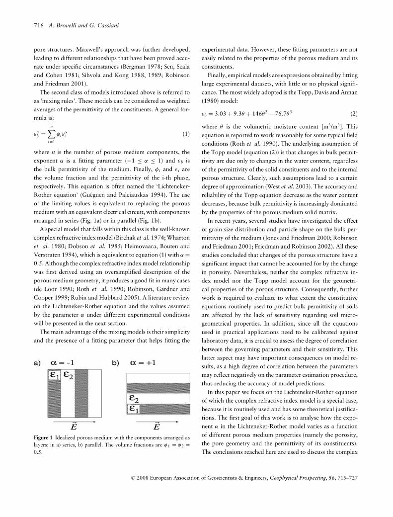
where n is the number of porous medium components, theexponent α is a fitting parameter (−1 ≤ α ≤ 1) and εb isthe bulk permittivity of the medium. Finally, φ i and ε i arethe volume fraction and the permittivity of the i-th phase,respectively. This equation is often named the ‘Lichteneker-Rother equation’ (Gueguen and Palciauskas 1994). The useof the limiting values is equivalent to replacing the porousmedium with an equivalent electrical circuit, with componentsarranged in series (Fig. 1a) or in parallel (Fig. 1b).

A special model that falls within this class is the well-knowncomplex refractive index model (Birchak et al. 1974; Whartonet al. 1980; Dobson et al. 1985; Heimovaara, Bouten andVerstraten 1994), which is equivalent to equation (1) with α =0.5. Although the complex refractive index model relationshipwas first derived using an oversimplified description of theporous medium geometry, it produces a good fit in many cases(de Loor 1990; Roth et al. 1990; Robinson, Gardner andCooper 1999; Rubin and Hubbard 2005). A literature reviewon the Lichteneker-Rother equation and the values assumedby the parameter α under different experimental conditionswill be presented in the next section.

The main advantage of the mixing models is their simplicityand the presence of a fitting parameter that helps fitting the

Figure 1 Idealized porous medium with the components arranged aslayers: in a) series, b) parallel. The volume fractions are φ1 = φ2 =0.5.

experimental data. However, these fitting parameters are noteasily related to the properties of the porous medium and itsconstituents.

Finally, empirical models are expressions obtained by fittinglarge experimental datasets, with little or no physical signifi-cance. The most widely adopted is the Topp, Davis and Annan(1980) model:

εb = 3.03 + 9.3θ + 146θ2 − 76.7θ3 (2)

where θ is the volumetric moisture content [m3/m3]. Thisequation is reported to work reasonably for some typical fieldconditions (Roth et al. 1990). The underlying assumption ofthe Topp model (equation (2)) is that changes in bulk permit-tivity are due only to changes in the water content, regardlessof the permittivity of the solid constituents and to the internalporous structure. Clearly, such assumptions lead to a certaindegree of approximation (West et al. 2003). The accuracy andreliability of the Topp equation decrease as the water contentdecreases, because bulk permittivity is increasingly dominatedby the properties of the porous medium solid matrix.

In recent years, several studies have investigated the effectof grain size distribution and particle shape on the bulk per-mittivity of the medium (Jones and Friedman 2000; Robinsonand Friedman 2001; Friedman and Robinson 2002). All thesestudies concluded that changes of the porous structure have asignificant impact that cannot be accounted for by the changein porosity. Nevertheless, neither the complex refractive in-dex model nor the Topp model account for the geometri-cal properties of the porous structure. Consequently, furtherwork is required to evaluate to what extent the constitutiveequations routinely used to predict bulk permittivity of soilsare affected by the lack of sensitivity regarding soil micro-geometrical properties. In addition, since all the equationsused in practical applications need to be calibrated againstlaboratory data, it is crucial to assess the degree of correlationbetween the governing parameters and their sensitivity. Thislatter aspect may have important consequences on model re-sults, as a high degree of correlation between the parametersmay reflect negatively on the parameter estimation procedure,thus reducing the accuracy of model predictions.

In this paper we focus on the Lichteneker-Rother equationof which the complex refractive index model is a special case,because it is routinely used and has some theoretical justifica-tions. The first goal of this work is to analyse how the expo-nent α in the Lichteneker-Rother model varies as a functionof different porous medium properties (namely the porosity,the pore geometry and the permittivity of its constituents).The conclusions reached here are used to discuss the complex

C© 2008 European Association of Geoscientists & Engineers, Geophysical Prospecting, 56, 715–727

Effective permittivity of porous media 717

refractive index model, which assumes a constant value for α.In the second part of the paper we investigate the robustnessof the Lichteneker-Rother relationship when the parameter α

and the permittivity of the solid matrix εs are estimated froma set of experimental data.

THE LICHTENEKER-ROTHER M ODEL

For a three-phase system, equation (1) can be written as:

εαb = (1 − φ)εα

s + θεαw + (φ − θ )εα

n (3)

where φ is the porosity, θ the volumetric moisture content, εb

is the effective (bulk) permittivity of the medium and εs, εw, εn

are the permittivities of the solid matrix, the aqueous phaseand an immiscible phase (such as air or an organic liquid),respectively.

As already noted, setting α = 0.5 reduces equation (3) tothe complex refractive index model. Some theoretical proofsof the validity of this latter constitutive relationship have beenproposed, which make use of the simplified assumption re-garding the distribution of the components within the porousmedium (Birchak et al. 1974; Zackri et al. 1998). For atwo-phase medium, assuming that the electromagnetic wavetraveltime through the porous medium is equal to the sum ofthe traveltimes through the separate phases, Birchak et al.(1974) recovered equation (3) with α = 0.5. This is equiva-lent to the well-known time-averaged model, frequently usedin seismics (Wyllie, Gregory and Gardner 1956). Under thesame assumptions, the Lichteneker-Rother model can be fur-ther extended to multi-phase porous media.

A self-consistent, effective medium approach was adoptedby Zackri et al. (1998) to demonstrate that the Lichteneker-Rother equation is physically plausible. Their model computesthe equivalent permittivity of a medium composed by a back-ground material, representing the solid matrix, filled with el-lipsoidal inclusion. The inclusions can have different volumesand shapes and the inclusion shapes follow a β-distribution.Following their analysis, Zackri et al. (1998) concluded thatthe exponent α is not a constant but varies with the shape ofthe inclusions and thus with the pore geometry.

Equation (3) has been widely applied in hydrogeophysicsto recover useful properties of the subsoil such as porosityand moisture content (e.g., Chan and Knight 1999; Binleyet al. 2001, 2002; Gloguen et al. 2001; West et al. 2003). Innearly all practical applications, water and nonaqueous phaseliquid permittivities are assumed to be known, while the actualvalue of matrix permittivity depends on the rock mineralogyand must be estimated, together with the value of α.

Several experimental studies are reported in the literature,which investigate (a) the value of α and (b) how α varies as afunction of soil type, mineralogy and fluid phases. For exam-ple, Roth et al. (1990) calibrated equation (3) on measure-ments performed in the time-domain reflectometry frequencyrange and on several soil types with a wide range of clay (2–20%) and organic carbon content. They found α = 0.46 ±0.007, which is close to the theoretical value of 0.5. Dobsonet al. (1985) modified the original equation introducing wa-ter bound to clay as a fourth phase. In this work, α wasfound to be 0.65 for soils ranging from sandy loam to siltyclay. Other authors have found α to vary in the range 0.25–0.8 both for three-phase systems (solid, water and air) andfour-phase systems (solid, water, air and nonaqueous phaseliquid) (Jacobsen and Schjonning 1995; Zackri et al. 1998;Persson and Berndtsson 2002). Moreover, Persson andBerndtsson (2002) and Ajo-Franklin, Geller and Harris (2004)measured the bulk permittivity of soil samples with variablewater, air and nonaqueous phase liquid content (the formerused sunflower seed oil as a nonaqueous phase liquid, whilethe latter used trichloroethylene) and observed a significantdependence of α on the nonaqueous phase liquid volumetriccontent. In summary, while previous experimental results aresomewhat contradictory they indicate that a constant value forα may not be appropriate. This conclusion seems to be fur-ther evident for unsaturated porous media. In the following,we will present some considerations on the physical meaningof α, examining in particular its dependence on the solid phasepermittivity and porosity.

Dependence of the Lichteneker-Rother exponentα on porous medium geometry

Theoretical considerations

For a two-phase, fully saturated porous medium (θ = φ),equation (3) reduces to:

εαb = (1 − φ) εα

s + φεαf (4)

where ε f is the permittivity of the saturating fluid phase. Di-viding both sides of equation (4) by εα

f gives:

(εb

ε f

)α

= (1 − φ)(

εs

ε f

)α

+ φ (5)

We can now evaluate the limit of equation (5) for εs/ε f →0,i.e., the permittivity of the saturating fluid is much larger than



the permittivity of the solid phase. This leads to:

limεs/ε f →0

(εb

ε f

)α

= φ ∀α > 0 (6)

which is equivalent to:(

εb

ε f

)εs/

ε f=0

= φ1α ∀α > 0 (7)

Equations (6) and (7) are valid for positive values of α only,because for α ≤ 0 the limit defined by equation (6) goes toinfinity. This restricts our analysis and thus conclusions to thecases where the exponent ‘a’ is strictly positive, i.e., does notapply in general for the Lichteneker-Rother equation. How-ever, this is only a minor limitation, since all the values of α wefound in the literature are positive. Moreover the same con-clusions apply to the complex refractive index model becauseα is set to 0.5.

The dielectric constant in the high-frequency limit, ε and thelow-frequency electrical conductivity σ are formally equiva-lent because of the analogy between the governing equations(Sen et al. 1981; Gueguen and Palciauskas 1994):

∇ · (ε∇V) = 0 (8)

∇ · (σ∇V) = 0 (9)

This implies that the computation of effective permittiv-ity and of effective electrical conductivity is mathematicallyequivalent (Sen et al. 1981; Gueguen and Palciauskas 1994).As a consequence, although physical processes controlling thedisplacement and the electrical fluxes are different, the sameconstitutive equations can be applied, given that the under-lying assumptions are honoured. In real systems, electricalconductivity and dielectric constant differ because (i) the con-trast in material permittivity is extremely small compared tothat of electrical conductivity, (ii) the lowest value for per-mittivity is 1 (i.e., the permittivity of the air phase), whileinsulating materials have an electrical conductivity that is inpractice negligible (e.g., quartz). Finally, (iii) in natural porousmedia electrical conductivity is often largely affected by theproperties of the water-solid interface (e.g., Brovelli et al.2005). The surface conductivity is mainly attributed to smallamounts of conductive materials (clays and oxides) dispersedin the porous medium and to surface charged sites. In thehigh-frequency limit ion displacement responsible for dielec-tric loss is not present and consequently the bulk dielectricconstant is poorly or non-sensitive to small fractions of claysand oxides.

Under the conditions of insulating porous matrix and neg-ligible surface conductivity (σ s = 0), the bulk electrical con-ductivity σ b of porous media can be computed using Archie’slaw (Archie 1942):

σb = σw

F= σw

φ−m(10)

where σ w is electrical conductivity of the pore-water, F isthe formation factor and m is Archie’s cementation exponentthat depends only on the micro-geometrical properties of theporous medium (e.g., grain shape, connectivity and tortuosityof the pore space) (Sen et al. 1981; Revil and Cathles 1999).Although Archie’s law (equation (10)) was originally devel-oped as a purely empirical equation, several studies showedthat it has rigorous theoretical justifications. Among these, Senet al. (1981) applied a differential self-consistent approach tocompute the bulk permittivity and electrical conductivity ofa simplified yet realistic porous geometry. One of the mainadvantages of the Sen et al. (1981) model is that the geomet-rical properties of the pore space and solid matrix are clearlydefined and the continuity of the fluid phase is ensured. TheSen et al. (1981) approach leads to a simple equation for thebulk conductivity of the system, equivalent to Archie’s lawwith a cementation exponent m = 2/3. Some later studies,based on a similar approach (e.g., Rubin and Hubbard 2005),demonstrated that the exponent varies as a function of thegrain geometry. Pride (1994) derived a constitutive equationequivalent to equation (10) using instead a volume averagingapproach. The Pride (1994) model was further extended (e.g.,by Revil and Glover 1998), giving additional insights intothe physical meaning of the formation factor and it extendedArchie’s equation to account for surface conductivity effects.

As discussed, due to the analogy between equations (8) and(9), under certain circumstances equation (10) can be adoptedfor permittivity. The principal limitation for applying Archie’slaw to compute the bulk dielectric constant is that the permit-tivity of the solid matrix must be negligible. As already noted,this is physically impossible, as the lowest possible permittiv-ity is that of air. Nevertheless, an equivalent condition is alarge contrast between the solid and the saturating fluid per-mittivities. When this condition is satisfied, it is possible tocombine equations (7) and (10), thus obtaining:

σb

σw

= φm =(

εb

ε f

)ε f >>εs

∀m > 0 (11)

Rearranging equation (11), it can be shown that, as the ratioεs/ε f → 0, α → m−1. According to equation (7), this resultholds only when both parameters α and m are positive. Whilethe exponent α could assume negative values, the cementation



factor is always positive. Thus, for a two-phase, fully satu-rated porous medium, the Lichteneker-Rother exponent canbe related to Archie’s cementation exponent when the expo-nent itself is larger than zero. As already pointed out, thiscondition is in practice always satisfied.

These results show that the exponent α depends only on theporous medium internal geometry when the solid permittivityis small compared to that of the fluid (equation (10)). Thissituation is in practice not realizable in natural porous media,because the solid matrix often has a permittivity between 5and 8 and the saturating fluid with a larger permittivity foundin natural conditions is water, εw = 80. Thus, α = m−1 pro-vides an upper limit for the value of the Lichteneker-Rotherexponent. Nevertheless, the above discussion implies that ingeneral α is not a constant (e.g., equal to 0.5, as in the com-plex refractive index model equation) but is a function of thestructural properties of the porous medium.

Dependence of the Lichteneker-Rother exponentα on porosity

Sen et al. (1981) published a dataset of bulk permittivityvalues for glass beads as a function of packing porosities. Ex-perimental observations with three saturating fluids are avail-able, including water (ε f = 79.8), methanol (ε f = 30) and air(ε f = 1).

We used these data to investigate the effect of porosity onthe exponent α for a two-phase porous system. The exponentvalues have been computed using the two-phase Lichteneker-Rother equation (equation (4)). Results are shown in Fig. 2and are relevant to water, methanol and air, respectively. Thedots represent the computed α values, while the solid line isthe best fit assuming a linear relationship between porosity φ

and α. We use the slope of such lines to investigate the cor-relation between the two parameters. For a saturating fluidwith a large permittivity (water) the slope of the fitted linesis close to zero and thus the correlation between φ and α isextremely weak. As the permittivity of the saturating fluiddecreases, the slope of the fitted line significantly increasestowards negative values, indicating a negative correlation be-tween the Lichteneker-Rother exponent α and porosity.

A possible explanation is that with a saturating fluid of highpermittivity, the asymptotic value at εs/ε f → 0 can be reachedwith small porosity. However, theoretical analysis indicatesthat the α value for the water-saturated porous medium isalways around 0.5 (Birchak et al. 1975).

Dependence of the Lichteneker-Rother exponent α on phasepermittivities

Pore-scale modelling

Here we address the possible dependence of α on the per-mittivity of both the solid matrix and the aqueous phase fora two-phase porous system. Brovelli et al. (2005) presenteda pore-scale modelling approach developed to compute thebulk electrical properties (conductivity and permittivity) ofporous media. The model solves numerically the electricalcontinuity equation within a digital representation of a porousmedium. Each digital sample is composed of a solid matrix,an aqueous phase and possibly an immiscible phase (air ornonaqueous phase liquid). Predicted values of both electricalconductivity and dielectric constant were compared againstdifferent experimental datasets, showing an excellent agree-ment. Further details on the approach and model validationcan be found in Dalla et al. (2004) and Brovelli et al. (2005).A major advantage of such a model is that the permittivityof each phase is defined at the microscopic scale and con-sequently the impact on the macroscale measurements canbe readily investigated for the full range of permittivitycontrasts.

Since both porosity and water content are known in the dig-ital porous medium, Archie’s cementation exponent is easilycomputed from equation (11), while α is recovered from equa-tion (4). This latter equation must be solved numerically. Thebisection method was adopted and the uniqueness of the solu-tion within the range of interest (−1:1) was verified. Positivevalues of α were always found.

The porous medium consists of a random packing of digitalspheres with a prescribed diameter distribution and poros-ity. The relevant information pertaining to the digital porousmedium used here is provided in Table 1. We conducted sev-eral numerical experiments using a fluid saturated digital sam-ple (i.e., only two phases are considered, the solid grains and afluid/gas). The phase permittivities were varied. For the solidphase the range we investigated was 1–10 while the permittiv-ity of the fluid phase was taken between 10 and 80. Thesesynthetic results are reported in Fig. 3 (solid symbols). Inthis figure the theoretical upper limit for α is also shown(dashed line). This latter value was computed from Archie’scementation factor m, as discussed above (equation (11)).Figure 3 clearly shows that the fitted exponent α is a func-tion of the phase permittivity. The simulated results confirmthe theoretical finding in section ‘Dependence of Liehteneker-Rother exponent α on porous medium geometry: Theoreticalconsiderations’. The computed values for the exponent



0 0.20

0.5

1Water, ε

f=79

α=0.04φ+0.47

Porosity φ

Exp

on

en

tα

0 0.20

0.5

1Methanol, ε

f=30

α φ+0.88

Porosity φ

Exp

on

en

tα

0 0.20

0.5

1Air, ε

f=1

α φ+1.01

Porosity φ

Exp

on

en

tα

Figure 2 Lichteneker-Rother exponent value as a function of porosity for glass beads (dots). The saturating fluids are water, methanol and air.Experimental data from Sen et al. (1981). The solid lines were fitted to identify a possible relationship between the exponent and the porosity.

Table 1 Geometrical and structural properties of the simulatedporous medium (based on Brovelli et al. 2005)

Property Value

Grain radius Rg 0.073 ± 0.025 mmDomain length L 3.987 mmPorosity φ 0.39Number of spheres 14501Specific surface area 16.95 mm−1

α approaches m−1 as the contrast between the two phasesincreases.

Comparison with experimental data

Robinson and Friedman (2003) reported extensive permittiv-ity measurements of fluid saturated porous materials. The aimof their study was to develop a method to independently esti-mate the permittivity of the solid matrix. We use their experi-mental data to evaluate how the Lichteneker-Rother exponentα varies as a function of the permittivity contrast. While theexperimental dataset consists of measurements made on five

0 5 10 15 200

0.1

0.2

0.3

0.4

0.5

0.6

0.7

0.8

εf/ε

s

α

Quartz data

Glass beads data

Simulated data

Theoretical limit, m=1.5

Figure 3 Effect of the permittivity contrast on the Lichteneker-Rotherexponent. Pore-scale modelling results from Brovelli et al. (2005) andexperimental data from Robinson and Friedman (2003).

different porous materials, in this work we only selected mea-surements performed on glass beads and silica sand, as theremaining materials (seashell fragments, tuff and hematite)are not representative of common geological materials. The



Table 2 Properties of the experimental porous material used (basedon Robinson and Friedman 2003)

Property Glass beads Silica sand

Grain radius Rg 0.5 mm 0.5 mmParticle density 2.49 g cm3 2.65 g cm3

Porosity φ 0.395 0.382Solid permittivity εs 7.6 4.7

relevant properties of the two selected porous media are re-ported in Table 2. Measurements of bulk permittivity wereperformed at 25 ◦C using five different fluids: air (ε f = 1),penetrating oil (ε f = 2.3), methylene chloride (ε f = 8.8),acetone (ε f = 20.8) and water (ε f = 78.6). Figure 3 showsthe results for glass beads and for silica sand (open symbols),together with the pore-scale modelling results. The theoreticalupper limit for α is also indicated. A constant value m = 1.5 isused in Fig. 3, because (i) the digital porous medium has a ce-mentation exponent of 1.56, (ii) the value of m for glass beadsis around 1.5 (Sen et al. 1981) and (iii) clean sands usuallyhave a cementation exponent close to this value (Rubin andHubbard 2005, Table 4.1).

The relations observed in simulated and experimental datahave an analogous shape. As expected, the values of α forthe water-saturated silica sands are slightly lower than thecorresponding values for glass beads. This is because the cor-responding cementation exponent m from the literature is ex-pected to be slightly larger.

Discussion

We conclude that, based on theoretical considerations, α can-not be assumed to be a constant because this parameter de-pends on both the micro-geometrical properties of the porousmedium and the ratio between the matrix and the pore spacepermittivity. Nevertheless, because water permittivity below1GHz is close to 80 and the dominant mineralogy of ‘geo-logical’ porous media is quartz, in most cases a value of α =0.5 seems to be appropriate for fully water-saturated porousmedia.

In addition, the experimental and simulated data reveal thata relationship possibly exists between α and the matrix permit-tivity. This is an important finding because typically the matrixpermittivity and the complex refractive index model exponentare estimated by performing a (joint) regression analysis onlaboratory permittivity data.

LICHTENEKER-ROTHER M ODELPARAMETER ESTIMATION

Following the results obtained above, in this section we focuson the Lichteneker-Rother model parameter estimation andthe relevant uncertainty. While some techniques have beendeveloped to estimate the permittivity of the porous mediumsolid phase, such as that presented in Robinson and Friedman(2003), in daily applications this value is jointly estimated to-gether with the Lichteneker-Rother exponent α. As the find-ings of section ‘The Lichteneker-Rother model’ clearly show,some degree of correlation exists between these two param-eters, here we develop and apply a procedure to rigorouslyquantify the degree of correlation. We also investigate if andto what extent the robustness and effectiveness of the regres-sion analysis is affected by the parameter correlation whendata are noisy. While the analysis conducted in the previoussection is limited to two-phase, fully saturated systems, wenow investigate the three-phase Lichteneker-Rother equation,thus taking into account the effect of water saturation.

Methodology

The robustness of the regression and the correlation betweenthe parameters is studied using the method described e.g., inCassiani et al. (1998) and Cassiani, Burbery and Giustiniani(2005). The method consists of the following steps (the super-scripts t and e stand for ‘true’ and ‘estimated’):1 The three-phase Lichteneker-Rother equation (equation(3)) is applied first as a forward model to create a syntheticdataset of bulk permittivity. The parameter pair (αt, εt

s) andthe porosity φ are arbitrarily chosen. The water saturationvaries in the range 0.1–1. Water permittivity is assumed equalto 80 and air permittivity is 1.2 The Gaussian random error is added to the bulk permittivitydataset. Different error levels are investigated from 0% (noerror) to 10% error.3 An estimated parameter set (αe, εe

s) is obtained via the least-square regression analysis by fitting the Lichteneker-Rothermodel to the synthetic, error affected dataset generated insteps 1 and 2. The Nelder-Mead simplex method (Lagariaset al. 1998) is used, as implemented in MATLAB.4 The sum-of-squared-errors function is mapped in the pa-rameter space.5 Following Draper and Smith (1998), under the assumptionof independent Gaussian errors in the data, an approximate



100(1−β)% confidence contour is computed as:

S(α, εs) = S(αe, εes )

{1 + 2

n − 2F (2,n − 2, 1 − β)

}(12)

where β is the confidence level, chosen arbitrarily as 0.05 forthis study. S is the sum-of- squares-error objective function,n is the number of observation points (number of data in thesynthetic dataset, i.e., number of different saturation values)and F(.) is the Fisher distribution function. Note that the joint(α, εs) confidence region computed by using equation (12) isexact in shape but only approximate in the confidence levelbecause the Lichteneker-Rother model is non-linear.

The bulk permittivity of a porous medium is strongly af-fected not only by matrix permittivity and the exponent α butalso by porosity and fluid permittivity (see previous section).While the latter can be assumed constant for water and air,the former has a relatively broad range of variability. As aresult the effect of porosity was also examined.

Indices for the sensitivity study

Following Cassiani et al. (2005), we computed a set of indicesto provide a brief and quantitative description of the results.

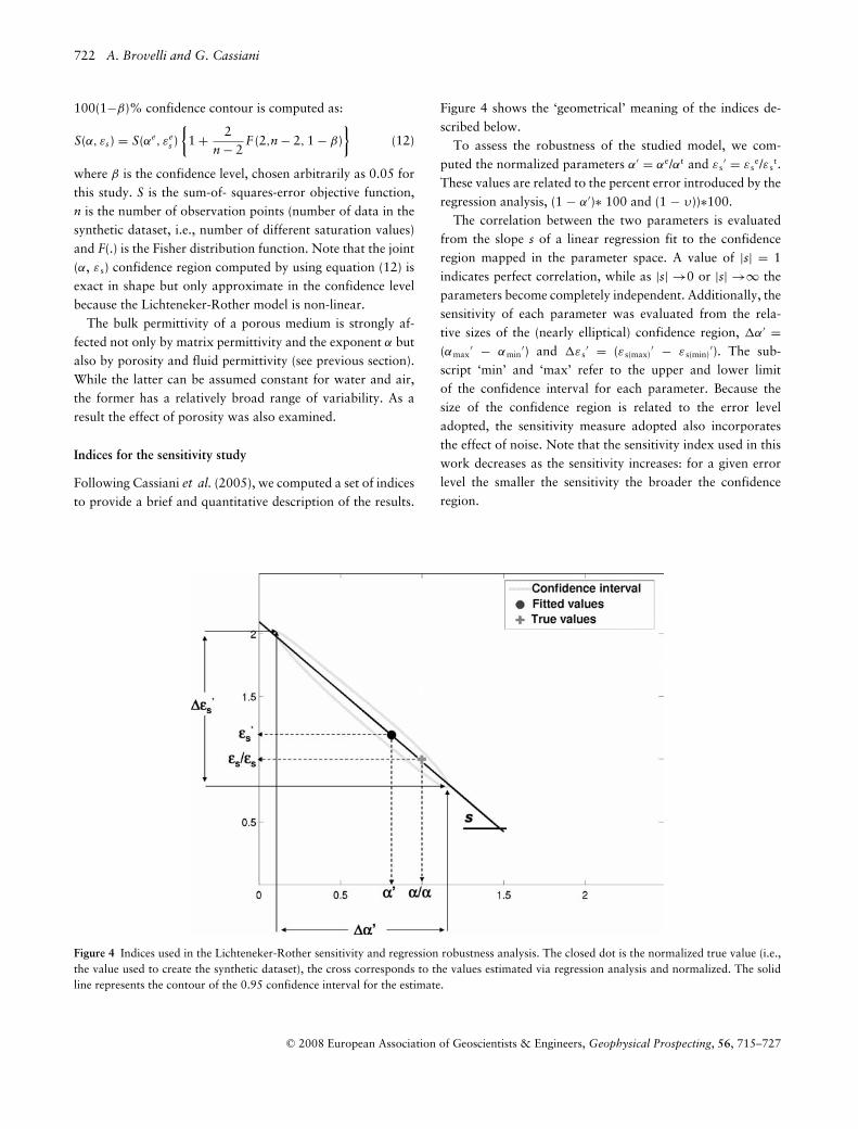
Figure 4 Indices used in the Lichteneker-Rother sensitivity and regression robustness analysis. The closed dot is the normalized true value (i.e.,the value used to create the synthetic dataset), the cross corresponds to the values estimated via regression analysis and normalized. The solidline represents the contour of the 0.95 confidence interval for the estimate.

Figure 4 shows the ‘geometrical’ meaning of the indices de-scribed below.

To assess the robustness of the studied model, we com-puted the normalized parameters α′ = αe/αt and εs

′ = εse/εs

t.These values are related to the percent error introduced by theregression analysis, (1 − α′)∗ 100 and (1 − υ))∗100.

The correlation between the two parameters is evaluatedfrom the slope s of a linear regression fit to the confidenceregion mapped in the parameter space. A value of |s| = 1indicates perfect correlation, while as |s| →0 or |s| →∞ theparameters become completely independent. Additionally, thesensitivity of each parameter was evaluated from the rela-tive sizes of the (nearly elliptical) confidence region, α′ =(αmax

′ − αmin′) and εs

′ = (εs(max)′ − εs(min)

′). The sub-script ‘min’ and ‘max’ refer to the upper and lower limitof the confidence interval for each parameter. Because thesize of the confidence region is related to the error leveladopted, the sensitivity measure adopted also incorporatesthe effect of noise. Note that the sensitivity index used in thiswork decreases as the sensitivity increases: for a given errorlevel the smaller the sensitivity the broader the confidenceregion.



Results

Figure 5 shows four examples of the sensitivity analysis results.Two porosities (0.35 and 0.25) and two values of matrixpermittivity (5.0 and 6.5) are investigated. These values wereselected as they are in the typical range for sands: clean sandshave a matrix permittivity of about 5.0, while the dielectricconstant of sands/sandstones with a moderate clay content isusually found in the range 6–6.5 (Gueguen and Palciauskas1994). In this first set of simulations, the Lichteneker-Rotherexponent α is kept constant and equal to 0.5 (i.e., the valuederived from theoretical considerations) and the random erroradded to the dataset is 5%.

The water saturation range for the forward model is 0.1–1,divided into 10 steps. As a result the water saturation / bulkpermittivity relationship consists of 11 values. The robustnessand accuracy of the regression may be influenced by the datadensity. The value we adopted is fully consistent with labora-tory measurement techniques.

Figure 5 demonstrates that a high degree of correlationexists between the matrix permittivity and the Lichteneker-Rother exponent α, as the 95% confidence levels are an elon-

0 1 20

0.5

1

1.5

2

No

rma

lize

dε s

εs=5.0, φ=0.35

0 1 20

0.5

1

1.5

2

εs=6.5, φ=0.35

0 1 20

0.5

1

1.5

2

Normalized α

No

rma

lize

dε s

εs=5.0, φ=0.25

0 1 20

0.5

1

1.5

2

Normalized α

εs=6.5, φ=0.25

0.95 confidence interval

True values

Estimated values

Figure 5 Lichteneker-Rother inverse problem robustness. Examples showing the shape and size of the confidence interval for different valuesof porosity and matrix permittivity.

gated region of nearly elliptical shape. Moreover, repeated nu-merical experiments indicate that even with a relatively smalldata error, the estimated values may fall outside the 95% con-fidence region (not shown in Fig. 5). Results for the error levelof 0% are not reported as the computed confidence level wasalways lower than 10−6. Results obtained using a larger error(10%) are also not reported as they show the same behaviouras the case with a 5% error but with larger values of theindices.

Following these considerations, we studied the indices (α′,εs′, s, α′, εs′) described in the previous paragraph for theporosity range φ = 0.1–0.4. This porosity range can be consid-ered representative of natural porous media. For each givencombination of porosity, matrix permittivity and exponentα, 50 different datasets of bulk permittivity versus volumet-ric moisture content have been generated by adding randomGaussian noise of the prescribed error level (e.g., 5%). Foreach dataset the estimated values (αe, εs

e), the confidence re-gion and the indices were calculated. Finally, the mean valueand the standard deviation of each index over the 50 rele-vant realizations were computed. The results are shown inFigs 6–10. Four different pairs of parameter values for (αr,



εsr) were adopted: (0.5, 5.0), (0.65, 6.5), (0.65, 5.0) and (0.5,

6.5). As discussed above, the matrix permittivity values se-lected were within the natural range for sand. The value of α

= 0.5 was also chosen as a ‘typical’ value for natural porousmedia, while α = 0.65 is the value computed in section ‘TheLichteneker-Rother model’ for the εs/ε f → 0 limit.

Figure 6 reports the mean error for the estimatedLichteneker-Rother exponent (left panel) and matrix per-mittivity (right panel). The mean error of both param-eters is constant and low for all four cases. The er-ror however is slightly larger for the matrix permittivitythan for the exponent. In Figure 7 we show the standard

0.1 0.15 0.2 0.25 0.3 0.35 0.4

0

0.05

0.1

Porosity

α’

α=0.5, εs=5.

α=0.65, εs=6.5

α=0.5, εs=6.5

α=0.65, εs=5.

0.1 0.15 0.2 0.25 0.3 0.35 0.4

0

0.05

0.1

Porosity

ε s’

Figure 6 Mean error between the true value and the parameters estimated by regression analysis. No correlation between the two indexes andthe porosity is observable for both the parameters.

0.1 0.15 0.2 0.25 0.3 0.35 0.40

0.05

0.1

0.15

0.2

0.25

Porosity

Sta

nd

ard

devia

tio

n,

α

0.1 0.15 0.2 0.25 0.3 0.35 0.40

0.05

0.1

0.15

0.2

0.25

Porosity

Sta

nd

ard

devia

tio

n,

ε s

α=0.5, εs=5.

α=0.65, εs=6.5

α=0.5, εs=6.5

α=0.65, εs=5.

Figure 7 Standard deviation of the error between the estimated and true values. The large values of standard deviation observed indicate thatthe estimated values can easily fall outside the 95% confidence region, thus resulting in a poor model calibration and non accurate parameterestimation.

deviation of the error. The standard deviation of α de-creases slightly over the porosity range but the level is dif-ferent for the four cases considered. The standard deviationof matrix permittivity steadily increases with porosity from0.05 to roughly 0.1 (Fig. 7). As previously pointed out inthe section ‘Indices for the sensitivity study’, the normalizedparameters used here (1 – mean value and standard devia-tion) are actually a percent error on the estimates. We canconclude that the mean error remains within the 5% error,which is the random error added to the synthetic datasetbut the error of a single estimate often falls outside thisvalue.



0.1 0.15 0.2 0.25 0.3 0.35 0.40

0.5

1

1.5

Porosity

Δα’

0.1 0.15 0.2 0.25 0.3 0.35 0.40

0.5

1

1.5

Porosity

Δεs’

α=0.5, εs=5.

α=0.65, εs=6.5

α=0.5, εs=6.5

α=0.65, εs=5.

Figure 8 Inverse problem robustness. Relative dimensions of the confidence contour. This parameter provides information on the relativesensitivity of each parameter, with larger values indicating a lower sensitivity.

The relative sensitivity of the two parameters is reported inFig. 8. The sensitivity of α remains relatively constant overthe porosity range. However, the four studied cases showa different behaviour and no clear dependence of sensitivityon ‘true’ model parameter values can be identified. On thecontrary, the relative sensitivity of εs steadily decreases asthe porosity increases and the studied parameter sets showsimilar behaviour (Fig. 8). Note that the parameter sensitivitiesreflect the behaviour observed in the standard deviation of thenormalized error. Figure 9 shows the parameter correlation

0.1 0.15 0.2 0.25 0.3 0.35 0.4

0

Porosity

co

rre

latio

n in

dex,

s

α=0.5, εs=5.

α=0.65, εs=6.5

α=0.5, εs=6.5

α=0.65, εs=5.

Figure 9 Investigation of the parameter correlation as a function ofporosity. A value of –1 indicates a complete inverse correlation ofthe two properties. All four parameter pairs show a high degree ofcorrelation, which may result in poor parameter estimation.

for the four cases. The correlation varies as a function ofporosity, matrix permittivity and exponent value. It can alsobe seen that all four cases have a porosity where the correlationis perfect (i.e., the correlation index |s| = 1).

DISCUSS ION AND C ONCLUSIONS

In this paper we analysed the characteristics of a classicalmixing model for the bulk permittivity of multiphase media– the Lichteneker-Rother model (often referred to as complexrefractive index model when the Lichteneker-Rother exponentα = 0.5). From this analysis some general conclusions couldbe drawn:1 The exponent α (for α > 0) is linked to Archie’s cementationexponent m and is consequently a function of the geometricalproperties of the porous medium. We also found that theexponent α depends on the ratio between the matrix and fluidphase permittivities, i.e., the relative permittivity of the fluidphase compared to that of the solid matrix (paragraph 2.2).2 The two key Lichteneker-Rother parameters (α, εs) are in-versely correlated. This results from the shape of the confi-dence interval, which is an elongated ellipsoid with the axisnot parallel to the (α, εs) axes.3 The parameter estimates are unbiased (correct on average)but due to large parameter correlation, the extent of the confi-dence region may be very large. As a result, the error affectinga single estimation may be substantial. This may have im-portant practical consequences on the accuracy of parameterestimation from field and laboratory measurements.



We conclude that the Lichteneker-Rother model is not en-tirely satisfactory either in terms of parameter meaning or asa purely empirical tool to represent laboratory data. Futureresearch will involve the development of an alternative con-stitutive model that should (a) be physically based and (b)involve only parameters that can be easily measured inde-pendently and not only fitted to the dielectric response of asample. The physical basis of such a model could rest uponthe Hashin and Shtrikman (1962) lower and upper boundsfor bulk permittivity.

ACKNOWLEDGEME N T S

This work was partly supported by the Consorzio Interuni-versitario CINECA and by the Italian Ministry of Education,University and Research (MIUR) FIRB grant RBAU01TAL5‘Spectral Induced Polarization for the identification of organicpollutants in the subsurface’ and the (MIUR) COFIN grant2005043992 ‘Study, definition and analysis of constitutivemodels linking the DC and induced polarization electrical re-sponse to the physical and chemical microstructure of mul-tiphase porous media’. The authors would like to acknowl-edge D.A. Robinson for providing some of the experimentaldatasets.

REFERENCES

Ajo-Franklin J.B., Geller J.T. and Harris J.M. 2004. The dielectricproperties of granular media saturated with DNAPL/water mix-tures. Geophysical Research Letters 31, L17501.

Ansoult M.L., De Baker W. and Declercq M. 1985. Statistical rela-tionship between apparent dielectric constant and water content inporous media. Soil Science Society of America Journal 49, 47–50.

Archie G.E. 1942. The electrical resistivity log as an aid in determin-ing some reservoir characteristics. Transactions American InstituteMining Metallurgical and Petroleum Engineers 146, 54–62.

Bergman D.J. 1978. The dielectric constant of a composite material. Aproblem in classical physics. Physics Reports (section C of PhysicsLetter) 43, 377–407.

Berryman J.G. 1992. Effective stress for transport properties of in-homogeneous porous rocks. Journal of Geophysical Research 97,17409–17424.

Binley A., Cassiani G., Middleton R. and Winship P. 2002. Vadosezone model parameterisation using cross-borehole radar and resis-tivity imaging. Journal of Hydrology 267, 147–159.

Binley A., Winship P., Middleton R., Pokar M. and West J. 2001.High resolution characterization of vadose zone dynamics usingcross-borehole radar. Water Resources Research 37, 2639–2652.

Birchak J.R., Gardner C.G., Hipp J.E. and Victor J.M. 1974. Highdielectric constant microwave probes for sensing soil moisture. Pro-ceedings of the IEEE 62, 93–98.

Brovelli A., Cassiani G., Dalla E., Bergamini F. and Pitea D. 2005.Electrical properties of partially saturated sandstones: Novel com-putational approach with hydrogeophysical applications. WaterResources Research 41, W08411. doi:10.1029/2004WR003628.

Butler D.K. 2005. Near-Surface Geophysics. Investigations in Geo-physics 13. SEG.

Cassiani G., Bohm G., Vesnaver A. and Nicolich R. 1998. A Geo-statistical framework for incorporating seismic tomography auxil-iary data into hydraulic conductivity. Journal of Hydrology 206,58–74.

Cassiani G., Burbery L.F. and Giustiniani M. 2005. A note on insitu estimates of sorption using push-pull tests. Water ResourcesResearch 41, W03005. doi:10.1029/2004WR003382.

Chan C.Y. and Knight R. 1999. Determining water content and ofsaturation from dielectric measurements in layered materials. WaterResources Research 35, 85–93.

Chelidze T.L. and Gueguen Y. 1999a. Electrical spectroscopy ofporous rocks: A review. I. Theoretical models. Geophysical JournalInternational 137, 1–15.

Chelidze T.L., Gueguen Y. and Ruffet C. 1999b. Electrical spec-troscopy of porous rocks: A review. II. Experimental results andinterpretation. Geophysical Journal International 137, 16–34.

Dalla E., Cassiani G., Brovelli A. and Pitea D. 2004. Electrical con-ductivity of unsaturated porous media: Pore-scale model and com-parison with laboratory data. Geophysical Research Letters 31,L05609. doi:10.1029/2003GL019170.

De Loor G.P. 1990. The dielectric properties of wet soils. BCRS Re-port No. 90-13 Proj. No. AO-2.1. The Netherlands Remote SensingBoard, Delft, The Netherlands.

Dobson M.C., Ulaby F.T., Hallikainen M.T. and El-Rayes M.A. 1985.Microwave dielectric behaviour of wet soils, II Dielectric mixingmodels. IEEE Transactions on Geoscience and Remote SensingGE-23, 35–46.

Draper N.R. and Smith H. 1998. Applied Regression Analysis, 3rdedn. John Wiley.

Friedman S.P. 1997. Statistical mixing model for the apparent dielec-tric constant of unsaturated porous media. Soil Science Society ofAmerica Journal 61, 742–745.

Friedman S.P. and Robinson D.A. 2002. Particle shape characteriza-tion using angle of repose measurements for predicting the effectivepermittivity and electrical conductivity of saturated media. WaterResources Research 38, 1236. doi:10.1029/2001WR000746.

Gloguen E., Chouteau M., Marcotte D. and Chapuis R. 2001. Es-timation of hydraulic conductivity of an unconfined aquifer usingcokriging of GPR and hydrostratigraphic data. Journal of AppliedGeophysics 47, 135–152.

Glover P.W.J., Hole M.J. and Pous J. 2000. A modified Archie’s lawfor two conducting phases. Earth and Planetary Science and Letters180, 369–383.

Gueguen Y. and Palciauskas V. 1994. Introduction to the Physics ofRocks. Princeton University Press.

Hashin Z. and Shtrikman S. 1962. A variational approach to the the-ory of the effective magnetic permeability of multiphase materials.Journal of Applied Physics 33, 3125–3131.

Heimovaara T.J., Bouten W. and Verstraten J.M. 1994. Frequencydomain analysis of time-domain reflectometry waveforms. 2. A



four component complex dielectric mixing model for soils. WaterResources Research 30, 201–209.

Jacobsen O.H. and Schjonning P. 1995. Comparison of time-domainreflectometry calibration function for soil water determination.Proceedings of the Symposium: Time-Domain Reflectometry Ap-plications in Soil Science, pp. 25–33.

Jones S.B. and Friedman S.P. 2000. Particle shape effects on the ef-fective permittivity of anisotropic or isotropic media consisting ofaligned or randomly oriented ellipsoidal particles. Water ResourcesResearch 36, 2821–2833.

Lagarias J.C., Reeds J.A., Wright M.H. and Wright P.E. 1998. Con-vergence properties of the Nelder-Mead Simplex Method in LowDimensions. SIAM Journal of Optimization 9, 112–147.

Martinez A. and Byrnes A.P. 2001. Modeling dielectric-constant val-ues of geologic materials: An aid to ground penetrating radar datacollection and interpretation. Current Research in Earth Sciences247.

Maxwell J.C. 1891. A Treatise on Eelectricity and Magnetism. DoverPublishing. Inc., New York

Persson M. and Berndtsson R. 2002. Measuring nonaqueous phaseliquid saturation in sil using time-domain reflectometry. Water Re-sources Research 38, 1064. doi:10.1029/2001WR000523.

Pride S. 1994. Governing equation for the coupled electromagneticsand acoustics of porous media. Physical Review B 50, 15678–15696.

Revil A. and Cathles III L.M. 1999. Permeability of shaly sands. WaterResources Research 35, 651–662.

Revil A. and Glover P.W.J. 1998. Nature of surface electrical conduc-tivity in natural sands, sandstones and clays. Geophysical ResearchLetters 25, 691–694.

Robinson D.A. and Friedman S.P. 2001. Effect of particle size distri-bution on the effective dielectric permittivity of saturated granularmedia. Water Resources Research 37, 33–40.

Robinson D.A. and Friedman S.P. 2003. A method for measuringthe solid particle permittivity or electrical conductivity of rocks,sediments and granular materials. Journal of Geophysical Research108, 2076. doi:10.1029/2001JB000691.

Robinson D.A., Gardner C.M.K. and Cooper J.D. 1999. Measure-ment of relative permittivity in sandy soils using TDR, capacitanceand theta probes: Comparison, including the effects of bulk soilelectrical conductivity. Journal of Hydrology 223, 198–211.

Roth K., Schulin R., Fluher H. and Attinger W. 1990. Calibration oftime-domain reflectometry for water content measurement using

a composite dielectric approach. Water Resources Research 26,2267–2273.

Rubin Y. and Hubbard S.S. 2005. Hydrogeophysics. Springer.Sen P.N., Scala C. and Cohen M.H. 1981. A self-similar model for

sedimentary rocks with application to the dielectric constant offused glass beads. Geophysics 46, 781–795.

Sihvola A. and Kong J.A. 1988. Effective permittivity of dielectricmixtures. IEEE Transactions on Geoscience and Remote Sensing26, 420–429.

Sihvola A. and Kong J.A. 1989. Correction to ‘Effective permittivity ofdielectric mixtures’. IEEE Transactions on Geoscience and RemoteSensing 21, 101–102.

Topp G., Davis J. and Annan A. 1980. Electromagnetic determinationof soil water content: Measurement in coaxial transmission lines.Water Resources Research 16, 574–582.

Vereecken H., Binley A.M., Cassiani G., Revil A. and Titov K. 2006.Applied Hydrogeophysics. Springer.

Vereecken H., Kemna A., Munch H.-M., Tillmann A. and VerweerdA. 2005. Aquifer characterization by geophysical methods. In:Encyclopedia of Hydrological Sciences (ed. M.G. Anderson), pp.2265–2283. John Wiley and Sons.

Vereecken H., Yaramanci U. and Kemna A. 2002. Noninvasive meth-ods in hydrology. Journal of Hydrology 267.

Wagner K.W. 1924. Erklarung der Dielectrishen Nachwirkungsvor-gange auf grund Maxwellscher vorstellungen. Archiv Electrotech-nik 2, 371–387.

West L.J., Handley K., Huang Y. and Pokar M. 2003. Radar fre-quency dielectric dispersion in sand and sandstone: Implicationsfor determination of moisture content and clay content. Water Re-sources Research 39, 1026. doi:10.1029/2001WR000923.

Wharton R.P., Hazen G.A., Rau R.N. and Best D.L. 1980. Electro-magnetic propagation logging: Advances in technique and interpre-tation. SPE paper, No. 9267.

Woodside W. and Messmer J.H. 1961. Thermal conductivity ofporous media. I. Unconsolidated sands. Journal of Applied Physics32, 1688–1699.

Wyllie M.R.J., Gregory A.R. and Gardner L.W. 1956. Elastic wavevelocities in heterogeneous and porous media. Geophysics 21, 41–70.

Zakri T., Laurent J.-P. and Vauclin M. 1998. Theoretical evi-dence for ‘Lichtenecker’s mixture formulae’ based on effectivemedium theory. Journal of Physics D: Applied Physics 31, 1589–1594.


Effective permittivity of porous media: a critical analysis of the complex refractive index model

Documents

Transcript of Effective permittivity of porous media: a critical analysis of the complex refractive index model