RL-TR-95-144 In-House Report June 1995

EFFECTIVE NON-LINEAR REFRACTIVE INDEX OF VARIOUS OPTICAL MATERIALS

John Malowicki ' I if "'

•' A '' '"11 100 '' ' *

APPROVED FOR PUBLIC RELEASE; D/STR/BUTION UNLIMITED.

Rome Laboratory Air Force Materiel Command

Griffiss Air Force Base, New York

1

)::':t. ■AT'? DS

This report has been reviewed by the Rome Laboratory Public Affairs Office (PA) and is releasable to the National Technical Information Service (NTIS). At NTIS it will be releasable to the general public, including foreign nations.

RL-TR-95-144 has been reviewed and is approved for publication.

APPROVED:

JAMES W. CUSACK, Chief Photonics Division Surveillance & Photonics Directorate

FOR THE COMMANDER:

DONALD W. HANSON Director of Surveillance & Photonics

If your address has changed or if you wish to be removed from the Rome Laboratory mailing list, or if the addressee is no longer employed by your organization, please notify RL ( OCPC ) Griffiss AFB NY 13441. This will assist us in maintaining a current mailing list.

Do not return copies of this report unless contractual obligations or notices on a specific document require that it be returned.

Form Approved OMB No. 0704-0188 REPORT DOCUMENTATION PAGE

Pubic reporting burden for this cctection of information is estimated to average 1 hour par response, hcijctng the time for reviewing instructions, searching existing data sources, gathering and martaining the data needed, and currjjtotiiy and reviewing thecctecfjon of Hormarjon Send comments regardrig this burden estimate or any other aspect of this cofection of information, inducing suggestions for reduchg this burden, to Washington Headquarters Services, Directorate for information Operations andReports, 121S Jefferson Davis Highway, Sute 1204, Arfrigton, VA 22202-4302, and to the Office of Management and Budget, Paperwork Reduction Project (07040188), Washngton, DC 2050a

1. AGENCY USE ONLY (Leave Blank) 2. REPORT DATE

June 1995

a REPORT TYPE AND DATES COVERED In-House Jan 94 - Mar 95

4. TITLE AND SUBTITLE EFFECTIVE NON-LINEAR REFRACTIVE INDEX OF VARIOUS OPTICAL MATERIALS

6. AUTHOR(S)

John Malowicki

5. FUNDING NUMBERS PR-4600 TA-PS WU-YS

7. PERFORMING ORGANIZATION NAME(S) AND ADDRESS(ES) Rome Laboratory (0CPC) 25 Electronic Parkway Griffiss AFB NY 13441-4515

a PERFORMING ORGANIZATION REPORT NUMBER

RL-TR-95-144

9. SPONSORING/MONITORING AGENCY NAME(S) AND ADDRESSES)

Rome Laboratory (0CPC) 25 Electronic Parkway Griffiss AFB NY 13441-4515

10. SPONSORING/MONITORING AGENCY REPORT NUMBER

11. SUPPLEMENTARY NOTES Rome Laboratory Project Engineer: John Malowicki/OCPC (315)330-3146

12a. DISTRIBUTION/AVAILABILITY STATEMENT

Approved for public release; distribution unlimited.

12b. DISTRIBUTION CODE

13. ABSTRACT(Madmum 200 words)

Photo-induced effective nonlinearity, n , of BS0 crystal is measured by using a Z-scan method which is based on the self-focusing/defocusing effect. The Z-scan technique is a simple yet accurate way to measure n„. An optical limiter utilizing photo-induced lensing is investigated and the influence of spatial self-phase modulation for strong CW illumination is presented.

14. SUBJECT TERMS

Z-scan, BS0, KNSBN,Effective Nonlinearity, n2 Spatial Self-phase Modulation, Optical Limiting

14 NUMBER OF PAGES 40

1a PRICE CODE

17. SECURITY CLASSIFICATION OF REPORT

UNCLASSIFIED

18. SECURITY CLASSIFICATION OF THIS PAGE UNCLASSIFIED

19. SECURITY CLASSIFICATION OF ABSTRACT UNCLASSIFIED

20. UMITATION OF ABSTRACT

UL NSN 7540-01 -280-5500 Standard Form 298 (Rev. 2-89)

Prescribed by ANSI Std Z39-18 298-102

Table of Contents Pg

• List of Figures iv

List of Tables

List of Symbols

Acknowledgment

I. Introduction

II. Z-Scan Theory

III. Z-Scan Experimental Results

IV. Optical Limiting

V. Optical Limiting Experimental Results

VI. Self Phase Modulation

VII. Self Phase Modulation Experimental Results

VIII. Conclusion

Bibliography

Appendix A - MacPhase Macro for Self Phase Modulation

Appendix B - Matlab Script for Self Phase Modulation

V

vi

vii

1

1

6

10

10

11

13

15

16

17

19

Appendix C - Matlab Script for Calculation of Z-Scan Curve 23

! ieesss Ida

ORA AB use lea

f©i?

DTTC 1 Uaannc JU3t.il

n ed G 11 OtU. .*— i

i

iii

BY t

Msir; r -*■■' i Avsi:

.but

.ab.i

ion/

lit? Cod«

bist i | A' i HP- M

.1 and/or

^1 --sm*

i

j

i

List of Figures Pg

1. Experimental setup for Z-scan measurement. 3

2. Calculated and measured Z-scan for KNSBN at 488nm 5

3. Position dispersion curves for a Z-scan of a thick sample. 6

4. Position dispersion for the BSO crystal for powers: 7 curve a, 0.1 mW; b, 1 mW; c, 5 mW and d, 10 mW.

5. Z-scan results for KNSBN showing the effects of polarization. 9

6. Behavior of BSO optical limiting for various aperture's linear 10 intensity transmittance: curves a, b, c and d are for s values of 0.2, 0.5, 0.66 and 0.8 respectively.

7. Optical limiting for KNSBN for 514nm, 488nm and 476nm 11 up to first dip.

8. Optical limiting for KNSBN for 514nm, 488nm and 476nm 11 at higher powers and simulation data.

9. Transverse intensity profiles of transmitted beam. 13 Curves a, b, c and d are for 5, 53, 66, 136, 156 mW respectively.

10. Results of calculations for the beam profile due to self phase modulation. 14

11. Far-field ring patterns for incident intensities: 14 150mW, 302mW, 378mW, and 514mW.

IV

List of Tables Pg

Results of KNSBN at 514.5nm, 488nm, and 476nm. 8

V

a

o

List of Symbols

a correction factor for geometrical and wave optics derived equations

a linear absorption coefficient

d distance between the focal plane in free space and the aperture plane

/ an empirical constant defined as / = 0.406(1 - s)

h thickness of the crystal

/ intensity at the Gaussian beam waist inside the sample

I(o(r) Gaussian illumination profile

k wave vector of the incident radiation

l effective optical thickness

A wavelength of the laser

n inherent index of the crystal

An light induced refractive index change

n2 effective non-linear refractive index

Pa power before limiting aperture

PT power transmitted by limiting aperture

AP _v difference between the peak and valley of the position dispersion curve

<J>(r) radially varying phase

AO0 on axis nonlinear phase shift

(p0 uniform retardation due to the n0 of the crystal

r radius of limiting aperture

s aperture transmittance

T normalized transmittance of the limiting aperture

CO radius of beam at limiting aperture

co radius of beam at focus

z distance between the focal plane in free space and the center of the sample

zdl diffraction length of focusing lens

z0 focal plane of the lens VI

Acknowledgments

The author would like to thank Dr. Song for his help and encouragement, Serey Thai for

his help in conducting this research, and Doug Norton for his help in writing macros in

MacPhase. Without their support this paper would not be possible.

Vll

1. Introduction

This paper will detail the research done on the non-linear refractive index of various optical materials, specifically, Bismuth Silicon Oxide (BSO), and a Ce-doped Ba2-

xSrxKi-yNayNb50i5 (KNSBN:Ce) crystal. The areas presented are the use of the Z-

scan technique to measure the non-linear refractive index of the crystals, use of the

samples as optical limiters, investigation into the self phase modulation inherent to the

samples, and experimental results for each of the areas. Recently, the self focusing in new

optical materials such as KNSBN:Ce and bacteriorhodopsin (BR) under low CW HeNe

illumination were reported^'2!. In this paper, the properties of the BSO and KNSBN:Ce

crystals were investigated using a high power Argon-Ion laser.

The major property of interest is that of the non-linear refractive index of the

crystals. Because of this nonlinear refractive index, a Gaussian beam propagating through

the crystals induces a lens-like refractive index profile. This refractive index change in

turn modifies the beam propagation. It is important to understand this lensing effect in

order to better use the material in optical system applications.

The Z-scan technique offers a non-complicated yet precise method of measuring

the effective non-linear refractive index coefficient of the samples. All that is needed is

the laser, a focusing lens, an aperture, and a power meter. This method is based on the

self-focusing or defocusing phenomena that occurs as the sample is translated through the

focus of the lens in the direction of propagation, or the Z direction.

After the measured and derived results are presented, the use of the samples as an

optical limiter is investigated. The optical configuration is the same except that the

crystal is stationary while the power is increased. An aperture is used in conjunction

with the self-focusing or defocusing effect of the crystal to limit the amount of power

transmitted down the optical path.

Finally the effect of self phase modulation on the samples is investigated. Self

phase modulation occurs along with self focusing/defocusing and has an important

influence on the optical limiting behavior of the crystals. A comparison between

experimental and measured data is also presented.

2. Z-Scan Theory

The Z-scan is a sensitive and convenient method for measuring the light induced

changes in the effective nonlinear refractive index and absorption coefficient of optical

1

materials!3^. The Z-scan is based on the transformation of the phase distortion

associated with the self-lensing into an amplitude distortions during the beam

propagation. The experimental arrangement is shown in Fig 1. A lens is used to focus the

illuminating laser as the crystal is translated along the optical path (the Z-scan). A

focusing lens is used to suppress the beam fanning effect of photorefractive materials,

which is proportional to the beam's lateral dimension, and to make the self focusing the

dominant effect. In particular, KNSBN has a strong fanning effect even under low

illumination intensities!5]. A limiting aperture is placed past the focus of the lens and a

detector is used to measure the output intensity. The aperture is set to let only half the

light intensity pass when no crystal is in the path. The aperture's intensity

transmittance, s, is defined as the ratio of output power to input laser beam power. The

crystal is placed directly behind the lens and translated through focus. The defocusing

(focusing) of the crystal will allow more (or less) of the light to pass the aperture by

creating a longer (or shorter) effective focal length of the lens and crystal system. The

beam diameter at the aperture is compressed or expanded with this changing effective

focal length. Measurements of the intensity at the detector with respect to crystal

position give the position dispersion curves which can be used to find the sign and

magnitude of the focusing. A pre-focal transmittance minimum (valley), followed by a

post-focal transmittance maximum (peak) indicates a positive lensing. Fig. 1 shows the

case of positive dispersion, with less then more light transmitted by the aperture as the

sample is translated through focus. It is believed that the focusing effect in KNSBN and BSO is due mainly to thermal

effects of the incident radiation on the index of refraction of the crystal^. The intensity dependence of the refractive index can be written as n = ntl+An = no + n2Ia where n0 is

the index of the crystal, An is the light induced index change, and n2 is the effective non-

linear refractive index. The magnitude of n2 can be determined from!3!

AAP, «, = £zL\ & 1 (1)

2 IrijVl-e"*

where AP,_V is the difference between the peak and valley of the position dispersion

curve, a is the linear absorption coefficient, h is the thickness of the sample, / is an

empirical constant defined as / = 0.406(1 - sf25 where s is the aperture linear transmittance, and Im is the intensity at the Gaussian beam waist inside the sample

2

calculated by I0)=2P/ K(02. Here P is the laser power and (O is the waist radius of the

illumination beam in the crystal.

Detector

Detector

Detector

200 mm Aperture

Fig. 1 Experimental setup for Z-scan measurement.

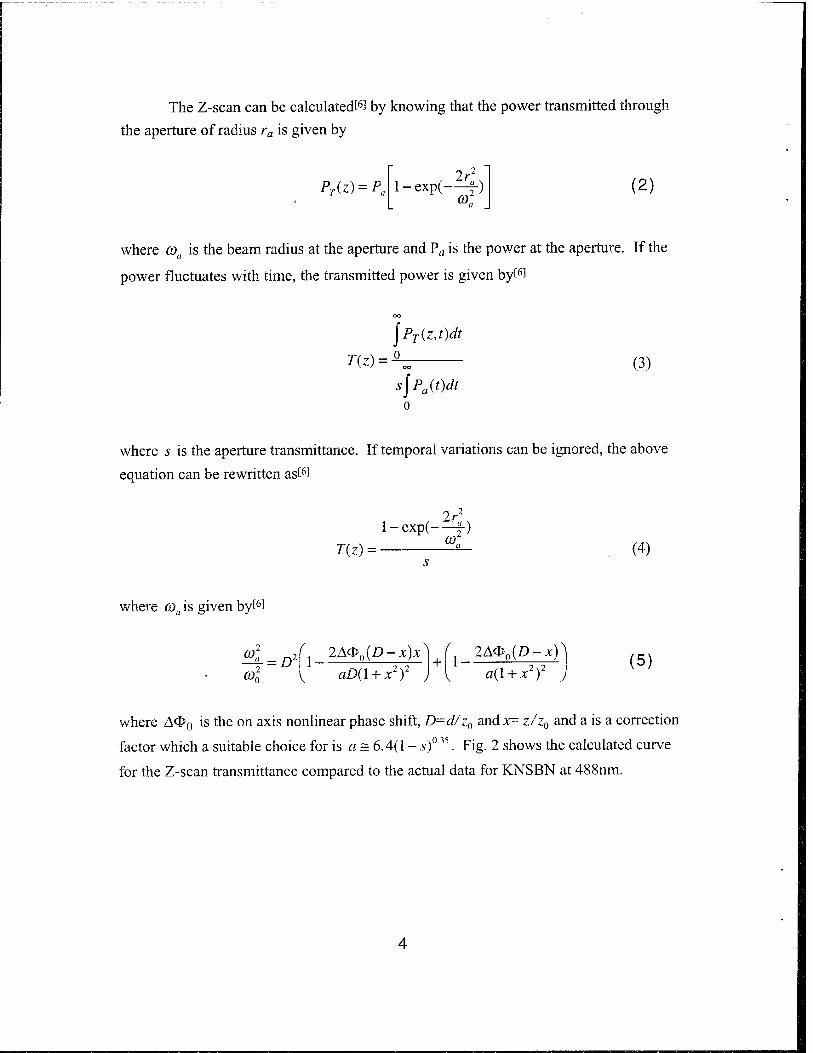
The Z-scan can be calculated^ by knowing that the power transmitted through

the aperture of radius ra is given by

PT(z) = Pa

2r2

l-exp( §-) (O,

(2)

where 0)u is the beam radius at the aperture and Pa is the power at the aperture. If the

power fluctuates with time, the transmitted power is given byf6l

jPT(z,t)dt

T(z) = ^

s\Pa{t)dt (3)

where 5 is the aperture transmittance. If temporal variations can be ignored, the above

equation can be rewritten as^

T(z) =

2rl

l-exp( f-) cot (4)

where (Oa is given by!6!

6),

(0, f = D' 1-

2A®0(D-x)x 2x2 aD{\ + xL)

+ 1- 2A®0{D-x)

a(l + x2)2 j (5)

where A<E>0 is the on axis nonlinear phase shift, D=d/z0 and x= z/z0 and a is a correction

factor which a suitable choice for is a = 6.4(1 - s)0,35. Fig. 2 shows the calculated curve

for the Z-scan transmittance compared to the actual data for KNSBN at 488nm.

2.5

0.5

-0.04

.I.A ;

f\ J ""^^^^

-0.02 0.02 0.04

Fig. 2 Z-scan for KNSBN at 488nm, a : calculated, b : measured.

The Z-scan theory presented here assumes the crystal can be treated as a thin

sample when its thickness is less than the diffraction length of the focusing lens. The diffraction length, zdl, is:

zdl -' TtCO

X (6)

Taking the data in the experiment using BSO, a> is 32|im, n is 2.6, and X is 514.5nm, the

value of zdl is approximately 14mm. The BSO crystal thickness is 4mm so it can indeed

be treated as a thin sample. When the length of the crystal is on the order of, or greater than zdl, the Z-scan in

Fig. 3 can be expected!3'6!. The peaks and valleys of the Z-scan trace have become more

pronounced and further separated. A conceptual understanding can be obtained if the flattened transmittance curve about z0 is considered first. When the thick sample is

centered at z0, the crystal will create large local phase distortions in the beam, but the

prefocal distortion will be balanced out by the postfocal distortion. It can be thought of as two lenses centered about z0 with the second lens canceling the effect of the first lens.

Therefore, the far field pattern will be relatively unchanged giving a flat transmission line.

As for the peak and valley, the maximum and minimum occur when the focus is at

the surfaces of the sample. Take the case of positive n2. When the focus is at the back

face of the sample, all of the lensing is acting to decrease the system focal length leading to

a minimum in the transmission curve. As the sample begins to move through focus, the

competing effects of the prefocal and postfocal phase distortions start to cancel each

other, leading to the flattened curve. The opposite happens after focus when the focal

point is at the front surface of the crystal and all the lensing tends to focus the beam,

allowing more light to pass the aperture leading to a maximum in transmittance. For the thin sample, the peak and valley are separated by approximately 1.7zdl.

For the thick sample, since the thickness is now on the order of, or greater than, the diffraction length zdh the thickness dominates and begins to push the peak and valley

apart. The peak and valley occur when the focus is at either the front or back surface.

The solid line in Fig. 3 is for the case of positive n2, and the dashed line is for negative n2.

Fig. 3 Position dispersion curves for a Z-scan of a thick sample.

3. Z-seam experimental results

Position dispersion curves for a sample of BSO are shown below in Fig. 4. These

position dispersion curves can be used to obtain a value of n2 for BSO. Each of the

curves correspond to a different input power level which is the reason for the different

amplitudes of the curves. Note that in Eq. 1, n2 is related to the difference in peak and

valley divided by the input intensity so that each position dispersion curve should yield similar values of n2 From these curves, the average n2 was found to be 1.47 x 10"6cm2AV.

This is comparable with the n2 = 1.9 x 10-6cm2/W reported in Ref. 7.

10 15 20

Fig. 4 Position dispersion for the BSO crystal for powers: curve a, 0.1 mW; b, 1 mW; c, 5 mW and d, 10 mW.

For the KNSBN:Fe crystal, position dispersion curves are presented in the Fig. 5.

The figures are for 514.5nm, 488nm, and 476nm. It is noted that the magnitude of the

curves varies with the polarization of the incident illumination. The polarizations were

parallel and perpendicular to the C-axis of the crystal. This can be explained by a

difference in the absorption coefficients of KNSBN for orthogonal polarizations!1]. The

absorption affects the change in the index of refraction leading to a larger or slightly

smaller position dispersion curves. In other words, the less absorption the crystal has,

the smaller the change in the index of refraction An, leading to a smaller variation in the

peak and valley of the position dispersion curve. For the opposite case of higher

absorption, the position dispersion curve would naturally exhibit a greater variation in the

peak to valley. Table 1 below gives the values of the absorption for the two polarizations

at the wavelengths used. The n2 for KNSBN is positive. Note that this is different from

KNbC>3 where the light induced lensing is negative^10'. Also a definite difference can be

seen in the absorption coefficients for the different polarizations.

A, (nm) 514.5 514.5 488 488 476 476

polarization 0 e 0 e 0 e

index 2.36 2.295 2.38 2.316 2.4 2.324

Power (mW) 22.3 22.7 22.3 23 22.3 | 23

%R 0.1638 0.1595 0.1667 0.1575 0.1696 0.1587

%T 0.09025 0.06875 0.062 0.048 0.05 0.037

a (cm"1) 4.0948 4.6832 4.8318 5.3876 5.2481 5.9024

CO (jim) 34 34 32 32 30 30

I (W/cm2) APp-v

1228.1 1250.1 1386.4 1429.9 1577.4 1626.9

1.15 1.45 1 1.45 1.2 1.6

Le •0.2127 0.193 0.1885 0.1731 0.1767 0.1606

n2 (cm2/W) 1.06xl0"7 1.31xl0"7 0.77xl0"7 1.08xl0"7 0.79xl0"7 1.03xl0"7

Table 1 Results of KNSBN at 514.5nm, 488nm, and 476nm.

8

Z-Scan 514 nm

1.5

0.5

I I 1 ' i i i i i i i i i i i i 1 1 1 1 1 1 1 1 1 1 1 1 1 1 1 1

- Parallel.. . Perpendicular «

- / X ̂

— —«

;X \ r

-

i i i i

\

i i i i

V iiti

/ 1 1 1 1 1 1 1 1 1 1 1 1 1 1 1 1

-40 -30 -20 -10 0 10 20 30 40

z (mm)

Z-Scan 488 nm

1.5

0.5

0 Itii

-40 -30 -20 -10 0 10 20

z (mm)

Z-Scan 476 nm

Fig. 5 Z-scan results for KNSBN showing the effects of polarization

9

4. Optical Limiting

An optical limiter is a device which produces an output power that is decreasingly

proportional to the input power when the input is beyond a certain threshold value. It

has many applications in laser damage protection. The self-focusing nature of KNSBN

and BSO can be used to limit the optical intensity transmitted through a system!2-6-8]. By

using a lens and an aperture as shown in Fig. 1, and placing the crystal in the valley of the

position dispersion curve, the intensity transmitted is not allowed to increase linearly but

is limited^. As the laser power is increased, the intensity measured before the aperture is

taken to be the input power and the intensity past the aperture is the output power. The

plot of output vs input power shows the nature of the crystal optical limiting. The

optical limiting experiment was repeated for various apertures; it was found that the value

of s around 0.5 produces the best optical limiting curve, i.e. the output is very flat. This

experimental data supports selection of s to be 0.5 in the Z-scan experiment. Fig. 6

shows various optical limiting curves for the BSO crystal.

For KNSBN, the limiting was measured at three Argon wavelengths, 514nm,

488nm, and 476nm. It can be seen in Figs. 7 and 8 that the optical limiting is strongly

wavelength dependent. This is most likely explained by an absorption wavelength

dependence. A characteristic dip in the transmitted intensity is evident at 30mw. This

oscillation can perhaps be best explained by self phase modulation of the incident beam.

5. Optical Limiting experimental results

4 6

Input Power in mW

Fig. 6 Behavior of BSO optical limiting for various aperture's linear intensity transmittance: curves a, b, c and d are for s values of 0.2, 0.5, 0.66 and 0.8 respectively.

0

0.6

0.5

0.4

0.3

0.2

0.1

0

i-

s

.T* B-

j»_L.

^sr

-o 514nm one period -e 488nm one period -a 476nm one period

^s: B :.:

0 5 10 15 20 25 30 35

Input (mW)

Fig. 7 Optical limiting for KNSBN for 514nm, 488nm and 476nm up to first dip.

1000

Fig. 8 Optical limiting for KNSBN for 514nm, 488nm and 476nm at higher powers and simulation data.

6. Self Phase Modulation

Self phase modulation (SPM) occurs in conjunction with self focusing. SPM is an

intensity dependent effect and is related to the non-linear coefficient n2. As the beam

propagates through the crystal, the intensity distribution of the beam affects the index of

the crystal which in turn affects the propagation of the beam. The change in the index of

refraction not only has a focusing effect on the beam but also causes a phase change in the

beam as well. The crystal will appear to have a different thickness corresponding to the

11

change in the index of refraction. In the context of self focusing, the Gaussian beam

profile of the incident radiation leads to a varying phase change across the beam profile

given by

W = ^H(r) (7)

where Ia(r) is the Gaussian illumination profile and lt is the effective optical thickness

defined as

(8) i-e'ae

a

where a is the effective absorption coefficient.

As the intensity increases to the point that the phase change exceeds 2K, the far-

field pattern begins to exhibit a concentric ring pattern. More rings become apparent as

the phase continues through multiple 2% phase shifts. The total number of rings N can be

estimated by a following relationship,

2% X

The far field projection of this complex intensity distribution can be calculated by

assuming the input intensity is Gaussian and by using the phase shift expressed in Eq. 7.

-The field amplitude at the exit surface of the crystal can be expressed ast1 '1

E(r) = [/»]"2 cxp{i[k,z + O(r) + <j)0]} (10)

where 4>(r) is the phase shift from Eq. 7 and (pQ is the uniform retardation due to the n0

of the crystal. Simply by taking the Fourier transform of the above equation, the far-field

radiation pattern can be obtained.

As the intensity of the irradiation increases, the phase change becomes stronger

which varies the interference pattern. When the pattern goes through a minimum at the

center of the beam, the effective transmittance of the system is lessened. The oscillatory

nature of the phase change with intensity explains the oscillations in the plots of the

output power.

12

A simulation of the above theory was done using MatLab and the results were

consistent with the observed experimental results. Appendix B contains the MatLab

code along with plots of the intensity profile and optical limiting curve. Fig. 8 shown

above, contains a comparison of the calculated and measured optical limiting curves for

the case of KNSBN at 514nm.

7. Self Phase Modulation Experimental Results

Fig. 9 shows line scan plots of the far-field intensity pattern resulting from the

self phase modulation of a BSO crystal. Note that the powers used in this figure are

much higher than that of the optical limiting curves in Fig. 6, which explains why no

oscillations in the optical limiting curves are apparent. Fig. 10 shows the predicted

intensity profiles resulting from self phase modulation.

600 800 1000

Fig. 9 Transverse intensity profiles of transmitted beam.

Curves a, b, c, d and e are for 5, 53, 66, 136, 156 mW respectively.

13

Fig. 10 Results of calculations for the beam profile due to self phase modulation.

The results in Fig. 11 were obtained with a Sony XC-75 black and white camera

and a Spiricon beam profiler which was used to transfer the pictures via GPIB to an

Apple Mac Ilex. The pictures clearly show the ring structure which results from the

phase distortion of the crystal. These results were from a BSO crystal.

Fig. 11 Far-field ring patterns for incident intensities: 150mW, 302mW, 378mW, and 514mW.

14

8. Conclusion

The experimental method for the measurement of the non-linear refractive index of

BSO and KNSBN has been presented along with the measured results. For BSO it was

found that n2 is on the order of 10~6 cm2/W. This result is consistent with previously

reported results based on the interferometric method. For KNSBN it was on the order of

10"7 cm2/W. The use of these materials as optical limiters has been investigated along

with the best configuration for their use. In the case of BSO, it was shown that its

performance as a limiter is at optimum when the aperture's linear transmission s is set to

0.5. Both crystals pointed out that for higher input power the self phase modulation

effect could not be ignored. The self-phase effect leads to a concentric ring pattern in the

far-field when the maximum phase distortion exceeds 27C. This ring pattern has a

profound effect on the optical limiting curve. Calculated optical limiting curves for self

phase modulation were in agreement with measured data.

15

References

1. Q.W. Song, C. Zhang, P. Talbot, H. Chen, and X. Liu, "Self-focusing in

KNSBN:Ce crystal under low power HeNe laser illumination," Opt. Mat., Vol. 2,

pp. 59-64, 1993.

2. Q. W. Song, C. Zhang, R. Gross, and R. Birge, "Optical limiting by chemically

enhanced bacteriorhodopsin films," Opt. Lett., Vol 18, No. 10, pp. 775-777, May

1993. 3. M. Sheik-Bahae, A. A. Said, T. H. Wei, D. J. Hagan, M. J. Soileau, and E. W. Van

Stryland, "Simple analysis and geometric optimization of a passive optical limiter

based on internal self-interaction," SPIE Vol. 1105 pp. 146-153, 1989

4. M. Sheik-Bahae, A. A. Said, T. H. Wei, D. J. Hagan, and E. W. Van

Stryland, "Sensitive measurement of optical nonlmearities using a single beam,"

IEEE J. Quantum Electronics, Vol. 26, No. 4, pp. 760-769, April 1990.

5. J. Rodriguez, A. Siahamakoun, G. Salamo, M. J. Miller, W. W. Clark III, G. L.

Wood, E. J. Sharp, and R. R. Neurgaonkar, "BSKNN as a self-pumped phase

conjugator," Applied Optics, Vol. 26, pp. 1732, 1987.

6. M. Sheik-Bahae, A. A. Said, T. H. Wei, D. J. Hagan, M. J. Soileau, and E. W. Van

Stryland, "Nonlinear refraction and optical limiting in thick media," Opt. Eng.,

Vol.30, No. 8, pp. 1228-1235, August 1991.

7. B. K. Bairamov, B. P. Zakharchenya, and Z. M. Khashkhozhev, "Self- focusing of argon laser radiation in Bii2SIO20 crystals," Sov. Physics-Solid State,

Vol 14, pp. 2357-2362, 1973.

8. P. P. Banerjee, R. M. Misra, and M. Maghraoui, "Theoretical and experimental

studies of propagation of beams through a finite sample of a cubically nonlinear

material," J. Opt. Soc. Am. B, Vol 8, No. 5, pp. 1072-1080, May 1991.

9. Q. W. Song, C. Zhang, P. Talbot, "Anisotropie light-induced scattering and

"position dispersion' in KNb03:Fe crystal," Opt. Comm, Vol. 98, pp. 269-273,

1993. 10. H. J. Zhang, J. H. Dia, P. Y. Wang, and L. A. Wu, "Self-focusing and self trapping

in new types of kerr media with large nonlinearities," Opt. Lett., Vol. 14, No. 13,

pp. 695, 1989. 11. S. D. Durbin, S. M. Arakelian, and Y. R. Shen, "Laser-induced diffraction rings

from a nematic-liquid-crystal film," Opt. Lett., Vol. 6, No. 9, pp. 411-413,

September 1981.

16

Appendix A

MacPhase Macro for Calculating Self Phase Modulation

macro SPM; var

begin

end;

boolean : ok; longint: i, maxNum; real: R, rPhase,sum; Str255 : gaussName, lineName;

DisposeUnClose; FFTSetting(TRUE,TRUE,TRUE); ok:=FrontData(gaussName,'data'); if(!ok)

beep; exit;

endif; maxNum:=50; lineName:='Line'; NewData(lineName,1,maxNum,0,false); MoveWindow(lineName,400,400,TRUE); for(i,1 ,maxNum)

R: = EvalNumber(i,*,1); rPhase: = EvalNumber(i,*,0.25); SimpleMath(gaussName,*,'None',R,'Amplitude'); SimpleMath(gaussName,VNone',rPhase,'Phase'); ok:=Exist('Farfield'); if(ok)

DisposeData('Farfield'); endif; FFT2D('Ampiltude','Phase',128,128,0.'Farfield'.'Farfield Phase'); SetROIOval('Farfield',59,59,72,72); lntegrate('Farfield',3,'asdf); GetRlndex(1,sum); PutDataNumber(lineName,1,i,sum); PlotData(lineName,'Line Plot'.TRUE); MoveWindow('Farfield',400,200,TRUE); PlotData('Farfield','Color Contour Plot'.TRUE); DisposeData('Ampiltude'); DisposeData('Phase'); DisposeData('Farfield Phase');

endfor;

17

Fig. 12 Gaussian Input Laser Beam

05 .Q CO _l

N

Title U.8

U.b \

U.b

U.4

U.2

1.0 6.8 12.6 18.4 24.2 30.0

X Label

Fig. 13 Optical Limiting Influenced by SPM ( normalized )

18

Appendix B

Matlab for SPM

% Plots the SPM farfield beam pattern and % finds the power in the central half clear clg,hold off load argonX.load argonY % loads actual data echo on count=0;

% previously determined from below

% absorption KNSBN in cmA-1 % wavelength

% thickness of crystal % from Table 1 % spot size of beam in crystal

thehalf =1253; x=(-64:.05:63); alpha=4.0948; Lambda=514.5e-9; d=0.05225*1e-2; n2=1.06e-7; aa=(6.8e-4)A2; phaseF=(2*pi*d*n2)/(l_ambda*aa) % as in Eq. 7

% Guassian profile sigma=1; f=sqrt(1/(2*pi*sigmaA2))*exp(-(x-4).A2/(2*sigmaA2));

norm=sum(sum(f)); f=f./norm; % make integrated area equal to one

% power in mW

plot(x.f) axis([-11 10 0 1e1]) run=1; for k = 1:15:300,

k; kk=k*1e-3 count=count+1; xx(count)=kk; phase=(phaseF*kk*f);phaser=max(max(phase))/pi U=((kk.*f).A0.5).*exp(i.*phase); UU=fftshift(fft(U));IUU=(UU.*conj(UU))/1; plot(x,IUU),hold on if run == 1, % Find the half power points

19

run u2=IUU; [y,themax]=max(u2); y2=y/2; if thehalf == 0,

for i=1:length(u2), if u2(i)>y2, u2(i)=0;

end; if i>length(u2)/2, u2(i)=0;

end; [yy,thehalf]=max(u2); % Find the half power points

end; % for max end; end; run=0; diff=abs(themax-thehalf)/1; % Find the power contained in the center b(count)=sum(IUU(themax-diff:themax+diff));

end; %pause hold off %plot(b') bb=b./max(b);

% plot calculated data with actual data plot((1e-3.*argonX),argonY), hold, plot(xx.bb), hold

20

C/3 C

C/3 C

5

4

3

1 -

0 ■10

5-

■10

Self Phase Modulation

//M\\\\\ (UK mj uuy,o

A. \ \

-5 0 5

Spatial Dimension

Self Phase Modulation

A

i / ■W-i

\i

-5 0 5

Spatial Dimension

10

10

21

U5 c

3 Q-,

■*—»

3 O

x 104 Effects of Self Phase Modulation on Optical Limiting

0 10 15 20

Input Intensity

25 30

% SPM in 2-D % July 28 1994 - Self Phase Modulation

% to offset gaussian from center

x=(-s:step:(s-step)); sigma=1; ax=0;ay=0; y=x'; X=ones(y)*x; Y=y*ones(x); R=sqrt((X-ax).A2+(Y-ay) A2) ; f=sqrt(1/(2*pi*sigmaA2))*exp(-(R).A2/(2*sigmaA2));

for i = 1:1, num=i;

G=num*f.*exp(i*num*f); B=fftshift(fft2(G))/(num*128)A2;

IG=(B.*conj(B)); s(i)=sum(sum(IG(61:69,61:69))); % assuming 1/2 power contour(IG) %plot(s)

%B=0;G=0;IG=0; end;

22

contour(IG) mesh(IG)

Matlab Function for calculation N2

h=.5;alpha=4.0948; lambda=476e-7; heff=(alpha/(1 -exp(-alpha*h))) wo=2.44*lambda*.2/.004; wo=30e-6;

f=.406*(1-.5)A.25; lc=2/(pi*woA2); k=2*pi/(lambda); l = (lc*.023)*1e-4 shift=(1.6)/f; n2=(shift/(k*l))*heff % as in Eq. 1

Appendix C

Matlab Function for calculation of Z-scan curve

% March 30 1994 hold off,clear step=.5;

load twox % data from Z-scan measurements used to find n2 below load twoy Power=.001; p=max(twoy);v=min(twoy); PV(1)=p-v; n2=NTwo(Power,p,v) alln(1)=n2;

% Curve fitting xi = .001.*(twox(1):step:-twox(1)); si=spline(twox,twoy,xi); c=polyfit(twox,twoy,7);

23

fjt=polyval(c,twox); %plot(twox,twoy,xi,si,twox,fit,xi,th);grid %plot(twox,twoy),grid,hold on

for i = 1:2, r= .00005+ i/2500 %+ i/3000 th=DPhaser(r+.002,(p-v),xi,1); % DPhaser subroutine listed below th2=DPhaser(r,(p-v),xi,0); plot((.001 .*twox),twoy,,g,,xi)th2,,r,,xi,th,,b,),hold on grid end,pause hold off

load threex % repeated for other data values load threey,Power=.0025; p=max(threey);v=min(threey); PV(2)=p-v; n2=NTwo(Power,p,v) alln(2)=n2; si=spline(threex,threey,xi);r=.000025 th=DPhaser(r+.002,(p-v)!xi,1);th2=DPhaser(r,(p-v),xi,0); plot((.001.*threex),threey,'g,,xi,th2,,r',xi,th>

lb') grid,pause hold off

load fourx % repeated for other data values load foury,Power=.005; p=max(foury);v=min(foury);%'Fours',p,v PV(3)=p-v; n2=NTwo(Power,p,v) alln(3)=n2; si=spline(fourx,foury,xi); th=DPhaser(r+.002,(p-v),xi,1);th2=DPhaser(r,(p-v),xi,0); plot((.001 .*fourx),foury,'g',xi,th2,'r',xi,th,'b') grid,pause hold off

load fivex % repeated for other data values load fivey,Power=.01; p=max(fivey);v=min(fivey);%'Five',p,v PV(4)=p-v;

24

n2=NTwo(Power,p,v) alln(4)=n2; si=spline(.001.*fivex,fivey,xi);r=.000015; th=DPhaser(r+.002,(p-v),xi,1);th2=DPhaser(r,(p-v),xi,0); th3=DPhaser(r,-(p-v),xi,0); plot((.001 .*fivex),fivey,,g,,xi,th2,,rl,xi,th,,r,

Ixi,th3,'r') averagen2=sum(alln)/4 % find average value of n2 from all

% inputted data plot(alln) AIW=74.8765; APV=sum(PV)/4;

h=.4;alpha=6; lambda=514e-9; heff=(alpha/(1-exp(-alpha*h))); wo=2.44*lambda*.2/.004;

f=.406*(1-.5)A.25;

k=2*pi/(lambda*1e2);

shift=(APV)/f; n2=(shift/(k*AIW))*heff;

Matlab Subroutine DPhaser

function[T]=DPhase(radius,pv,z,a) d=.44;wo=35e-6; % Input beam radius 1.22*514.5e-9*.2/0.0036 or .0015875 k=2*pi/(514e-9);S=.005; if a==0, a=6.4;%*(1-S)A(.35) else a=1; end zo=(k*woA2)/2;DD=d/zo; Delta=pv/(0.406*(1-.5)A(0.25)); % Change sign here for (de)focus x=(z)./zo; w=(woA2)*((DDA2)*(1-(2*Delta*(DD-x).*x)./(a*DD*(1+x.A2).A2)).A2 +(1 -(2*Delta*(DD-x))./(a*(1 +x.A2).A2)).A2); % as in Eq. 5

25

norm=(woA2)*((DDA2) +(1 -(2*Delta*DD)./a).A2);

%w=w./norm; % w is already squared % T=(1-exp(-2*(radiusA2)./(w)))/(.5); % as in Eq.4 TT=(1-exp(-2*(radiusA2)./(norm)))/(.5); T=T./mean(T); %hold off,plot(x,T),pause,subplot(211 ),plot(x,T),grid %subplot(212), plot(x,T),grid, pause, subplot(111)

26

Rome Laboratory

Customer Satisfaction Survey

RL-TR-

Please complete this survey, and mail to RL/IMPS, 26 Electronic Pky, Griffiss AFB NY 13441-4514. Your assessment and feedback regarding this technical report will allow Rome Laboratory to have a vehicle to continuously improve our methods of research, publication, and customer satisfaction. Your assistance is greatly appreciated. Thank You

Organization Name: (Optional)

Organization POC: (Optional)

Address:

1. On a scale of 1 to 5 how would you rate the technology developed under this research?

5-Extremely Useful 1-Not Useful/Wasteful

Rating

Please use the space below to comment on your rating. Please suggest improvements. Use the back of this sheet if necessary.

2. Do any specific areas of the report stand out as exceptional?

Yes No

If yes, please identify the area(s), and comment on what aspects make them "stand out."

3. Do any specific areas of the report stand out as inferior?

Yes No_

If yes, please identify the area(s) , and comment on what aspects make them "stand out»"

4. Please utilize the space below to comment on any other aspects of the report. Comments on both technical content and reporting format are desired.

MISSION

OF

ROME LABORATORY

Mission. The mission of Rome Laboratory is to advance the science and technologies of command, control, communications and intelligence and to transition them into systems to meet customer needs. To achieve this, Rome Lab:

a. Conducts vigorous research, development and test programs in all applicable technologies;

b. Transitions technology to current and future systems to improve operational capability, readiness, and supportability;

c. Provides a full range of technical support to Air Force Materiel Command product centers and other Air Force organizations;

d. Promotes transfer of technology to the private sector;

e. Maintains leading edge technological expertise in the areas of surveillance, communications, command and control, intelligence, reliability science, electro-magnetic technology, photonics, signal processing, and computational science.

The thrust areas of technical competence include: Surveillance, Communications, Command and Control, Intelligence, Signal Processing, Computer Science and Technology, Electromagnetic Technology, Photonics and Reliability Sciences.