sensors

Article

Differential Microstrip Sensor for Complex PermittivityCharacterization of Organic Fluid Mixtures

Amer Abbood al-Behadili 1, Iulia Andreea Mocanu 2,*, Teodor Mihai Petrescu 2 and Taha A. Elwi 3,4

Citation: al-Behadili, A.A.; Mocanu,

I.A.; Petrescu, T.M.; Elwi, T.A.

Differential Microstrip Sensor for

Complex Permittivity

Characterization of Organic Fluid

Mixtures. Sensors 2021, 21, 7865.

https://doi.org/10.3390/s21237865

Academic Editor: Yue Li

Received: 24 October 2021

Accepted: 22 November 2021

Published: 26 November 2021

Publisher’s Note: MDPI stays neutral

with regard to jurisdictional claims in

published maps and institutional affil-

iations.

Copyright: © 2021 by the authors.

Licensee MDPI, Basel, Switzerland.

This article is an open access article

distributed under the terms and

conditions of the Creative Commons

Attribution (CC BY) license (https://

creativecommons.org/licenses/by/

4.0/).

1 Department of Electrical Engineering, College of Engineering, Mustansiriyah University, Baghdad 00964, Iraq;amer_osman@uomustansiriyah.edu.iq

2 Department of Telecommunication, Telecommunications and Information Technology, Faculty of Electronics,University Politehnica of Bucharest, 060042 Bucharest, Romania; teodor.petrescu@upb.ro

3 Communication Engineering Department, Al-Ma’moon University College, Baghdad 1104, Iraq;taelwi82@gmail.com

4 Electrical and Computer Engineering Campus, New York Institute of Technology,Long Island City, NY 11568, USA

* Correspondence: iulia.mocanu@upb.ro

Abstract: A microstrip highly sensitive differential sensor for complex permittivity characterizationof urine samples was designed, fabricated and tested. The sensing area contains two pairs of open-stub resonators, and the working frequency of the unloaded sensor is 1.25 GHz. The sensor is easilyimplemented on an affordable substrate FR-4 Epoxy with a thickness of 1.6 mm. A Teflon beaker ismounted on the sensor without affecting the measurements. Numerically, liquid mixtures of waterand urine at different percentages were introduced to the proposed sensor to evaluate the frequencyvariation. The percentage of water content in the mixture varied from 0% (100% urine) to 100% (0%urine) with a step of 3.226%, thus giving 32 data groups of the simulated results. Experimentally,the mixtures of: 0% urine (100% water), 20% urine (80% water), 33% urine (66% water), 50% urine(50% water), 66% urine (33% water), and 100% urine (0% water) were considered for validation. Thecomplex permittivity of the considered samples was evaluated using a nonlinear least square curvefitting in MATLAB in order to realize a sensing sensitivity of about 3%.

Keywords: differential microstrip sensor; urine sensor; complex permittivity; open-stub resonator

1. Introduction

Resonating sensors are widely used in different applications such as: solid dielectriccharacterization [1–3], biomedical application [4,5], permittivity measurements for liquidmixtures [6–8], or even characterization of soil water content [9,10]. Generally, the mostused are planar sensors due to their low cost, low profile, easy fabrication, high precision,robustness, and compact size [11]. The sensing principle of such sensors is based ondetecting the change in the resonant frequency when placing a sample over the resonatingsurface [11].

The sample can be both a solid material and a liquid. Particular attention has beengiven to sensors for measuring the dielectric properties of microfluids. Usually, a mixtureof water and inorganic fluids is used to determine these properties and few papers addressthis aspect when it comes to organic fluids.

One of the important organic fluids of human biological liquids is urine [11]. Urine isa liquid waste of the body consisting of water, inorganic salts, and organic compounds [3].Urine color, which depends on the proportion between metabolites and water, can be usedto detect a person’s hydration state and early dehydration problems [12]. Thus, a urine colorchart was developed by Armstrong in 1994 for hydration assessment [13]. In particular,unconscious and elderly patients need their hydration state monitored. Water balance inthe human body is a key indicator for good functioning of different metabolic activities [14].

Sensors 2021, 21, 7865. https://doi.org/10.3390/s21237865 https://www.mdpi.com/journal/sensors

Sensors 2021, 21, 7865 2 of 20

In particular, the hydration state of a person is influencing blood pressure, heart rate, bodytemperature, etc. Thus, it is very important to have accurate measurements about thisstate. The hydration assessment techniques for the body involve urinary, hematologic,whole-body, and sensory measurements [15]. Determining the level of hydration whenanalyzing urine is one of the most efficient, easy, and least invasive methods, so sensorscapable of doing this have been investigated often.

Differential sensors are mostly used because they are robust against variations in ambi-ent factors [16–22]. Differential sensors are typically implemented by means of two sensingelements, e.g., two loaded transmission lines. The sensing principle practically relatesto symmetry. Under perfect symmetry, the structure exhibits a single transmission zerofrequency. When loading the sensor with samples on one side, the symmetry is interrupted,and two resonant frequencies appear [19]. One limitation of these frequency-splittingsensors may be caused by the possible coupling between resonant elements, which is un-avoidable when these elements are too close [22]. To avoid this phenomenon and to obtainthe advantages of differential sensors, in this paper a sensor consisting of two identicalparts is considered. One part is made of a Wilkinson power divider and two transmissionlines loaded with a pair of open-stub resonators each. The two sensing parts are placed farone from another not to have couplings between the elements. The sensing area is coveredby a Teflon beaker without affecting the sensitivity of the sensor. The beaker is used topour liquids in it and to make precise measurements.

2. Sensor’s Design2.1. Resonant Structures for the Sensor’s Design

In the literature there are two types of substrates for designing microfluidic substrate:rigid and flexible [23]. The flexible ones, such as Polydimethylsiloxane (PDMS), paper,and polyimide have the main advantage of being compatible with additive manufacturingtechniques, but some of the drawbacks referring to their usage are surface treatment,incompatibility with ink solutions (chemicals), and sensitivity to thermal sintering [23].On the other hand, the rigid substrates have the advantage of having constant dielectricproperties (εr and tan δ) even at different temperatures and frequencies, low-losses, and areaffordable [23]. This is the reason why, for our design a rigid substrate is chosen. The sensoris designed in microstrip technology on an affordable substrate, FR-4 Epoxy with relativepermittivity εr = 4.4, thickness h = 1.6 mm, and loss tangent tan δ = 0.02. For technologicalreasons, the width of the microstrip transmission lines must be greater than 0.5 mm. Theworking frequency of the sensor is then set to 1.245 GHz for fulfilling the technologicalrestrictions imposed.

To start, two microstrip lines are designed and analyzed through simulations: oneloaded with a λg/4 open stub resonator, as depicted in Figure 1a, and another one loadedwith a CSRR etched in the ground as depicted in Figure 1b. The guide wavelength, λg isthe one corresponding to the FR-4 Epoxy substrate at the operating frequency of 1.245 GHz.The length of the open stub resonator is ` = 53.45 mm. The width of the microstrip openresonator is w = 0.8 mm, while the width of the loaded transmission line is W = 3.083 mm,which corresponds to the characteristic impedance of 50 Ω for the access transmission lineat the operating frequency. The length of the access transmission line is set to 28.6 mm.

The CSRR loaded line is designed to work at the same resonant frequency as the openstub resonator, so the width of the loaded transmission line is W = 3.083 mm, the length isset to 28.6 mm, the width of the rings and the distance between them is d = g = c = 0.8 mm,and the radius of the exterior ring is set to r = 8.325 mm.

The equivalent circuits of the two resonating structures are depicted in Figure 2a,b. Forthe resonating structure in Figure 1a, the feeding line between ports 1 and 2 is modeled byan inductance, L and a capacitance C, while the open stub is modeled by an inductance Losand a capacitance Cos. For the resonating structure in Figure 1b, the feeding line betweenports 1 and 2 is modeled by the inductance L and the capacitance C, while the CSRR ismodeled by an inductance and capacitance Lc and Cc, respectively [24].

Sensors 2021, 21, 7865 3 of 20

Figure 1. Microstrip transmission line loaded with: (a) a λg/4 open stub resonator with physicaldimensions; (b) a CSRR etched in the ground with physical dimensions.

Figure 2. Equivalent circuit for the: (a) λg/4 open stub resonator; (b) CSRR etched in the ground.

The characteristic impedance of the transmission line between ports 1 and 2 isZ0 = 50 Ω and the substrate is FR-4 Epoxy, so the values for the inductance L = 8.9546 nHand, the capacitance C = 1.6798 pF are the same for both equivalent circuits. Consider-ing the geometrical dimensions of the two resonating structures and the same substrate,the values for the other lumped elements from the equivalent circuit are extracted [17]:Lc = 6.0958 nH, Cc = 2.085 pF, Cos = 1.69 pF, and Los = 9.528 nH.

In this case, the resonant frequency of the equivalent circuit in Figure 2a can bewritten as:

fos =1

2π√

LosCos= 1.248 GHz

for the equivalent circuit in Figure 2b:

fo =1

2π√

Lc(C + Cc)= 1.25 GHz

The resonant frequency obtained using the equivalent circuits is equal to the oneimposed by design.

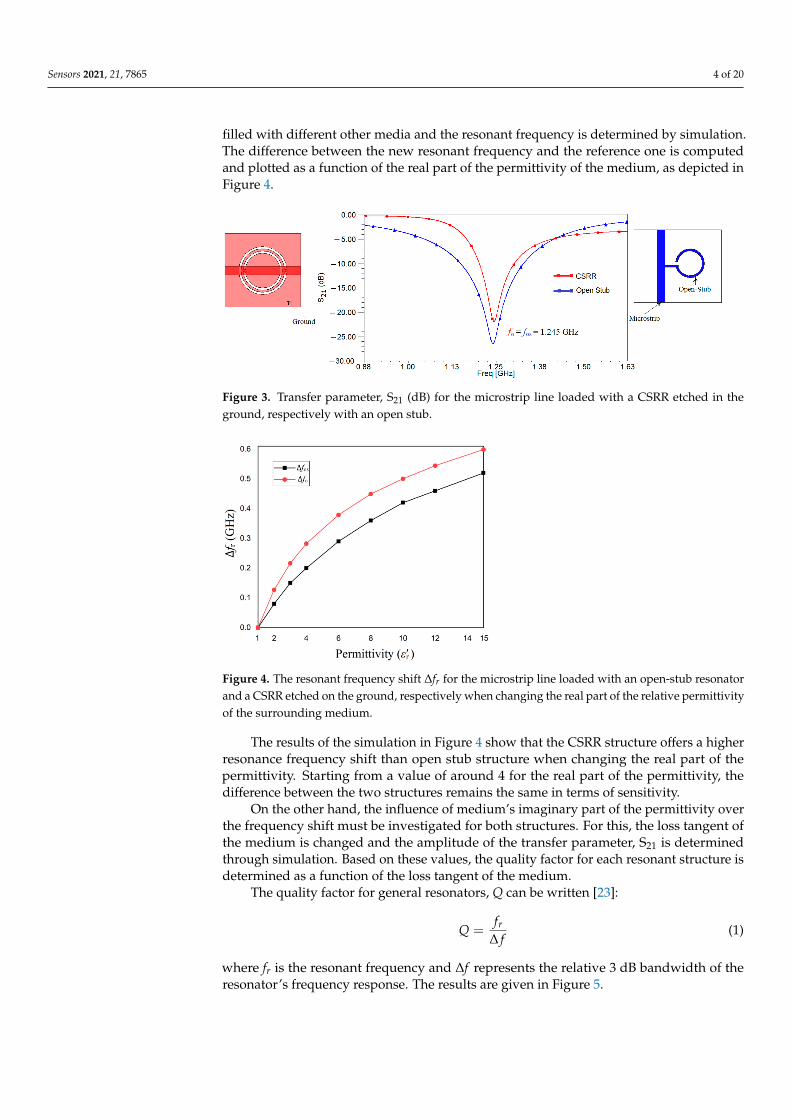
The next step in the design of the sensor is to compare the performances of thetwo resonant structures designed in Figure 1 and decide which one is best suited for ourapplication. Using the full-wave simulator High Frequency Structure Simulator (HFSS)both structures are analyzed. The results of the simulation for the transfer characteristicare depicted in Figure 3. The resonant frequency is the same for both resonant structures,proving that the designed is correct. Moreover, the resonant frequency is equal to the onesdetermined using the equivalent circuits from Figure 2.

Analyzing the results in Figure 3, it can be seen that the microstrip line loaded withan open stub has a value of 26 dB for parameter S21 rather than only 22 dB as in the case ofthe microstrip line loaded with a CSRR etched in the ground.

The sensitivity of the resonant structures is investigated by placing the two structuresin a box and modifying the medium’s characteristics inside the box. The resonant frequencyof each structure when the box is filled with vacuum is determined by simulation in HFSSand is considered the reference resonant frequency for each structure. Then, the box is

Sensors 2021, 21, 7865 4 of 20

filled with different other media and the resonant frequency is determined by simulation.The difference between the new resonant frequency and the reference one is computedand plotted as a function of the real part of the permittivity of the medium, as depicted inFigure 4.

Figure 3. Transfer parameter, S21 (dB) for the microstrip line loaded with a CSRR etched in theground, respectively with an open stub.

Figure 4. The resonant frequency shift ∆fr for the microstrip line loaded with an open-stub resonatorand a CSRR etched on the ground, respectively when changing the real part of the relative permittivityof the surrounding medium.

The results of the simulation in Figure 4 show that the CSRR structure offers a higherresonance frequency shift than open stub structure when changing the real part of thepermittivity. Starting from a value of around 4 for the real part of the permittivity, thedifference between the two structures remains the same in terms of sensitivity.

On the other hand, the influence of medium’s imaginary part of the permittivity overthe frequency shift must be investigated for both structures. For this, the loss tangent ofthe medium is changed and the amplitude of the transfer parameter, S21 is determinedthrough simulation. Based on these values, the quality factor for each resonant structure isdetermined as a function of the loss tangent of the medium.

The quality factor for general resonators, Q can be written [23]:

Q =fr

∆ f(1)

where fr is the resonant frequency and ∆f represents the relative 3 dB bandwidth of theresonator’s frequency response. The results are given in Figure 5.

Sensors 2021, 21, 7865 5 of 20

Figure 5. Quality factor for each resonant structure when changing the loss tangent of the mediuminside the box.

From Figure 5, one can notice that the quality factor of the CSRR structure decreasesdrastically with the increase of the medium’s loss tangent. This means, that the open stubstructure is better suited to applications which use samples with a large loss tangent, asurine, for example. This is the reason for which the sensor will be implemented using theopen-stub resonator.

2.2. Sensor’s Layout

After considering the best suited resonant structures for our application, the nextstep is to design the whole sensor. It will be a differential one, consisting of two identicalWilkinson power dividers and two pairs of microstrip transmission lines, each of themloaded with two open stub resonators as designed in the previous Section. Additionally, abeaker made of Teflon is perfectly attached to the surface of the two open stub resonatorsto avoid any measurement discrepancy because of the air gap effects between the beakerand the sensor. The beaker is filled with liquids that will be considered samples undertest (SUT).

The layout of the sensor is given in Figure 6.

Figure 6. The layout of the sensor, including an exploded view drawing of each layer.

As it can be seen in Figure 6, the power applied at one of the two ports is dividedequally by the Wilkinson power divider and then transmitted to the first pair of resonantstructures. As the sensor is symmetrically designed, once a sample is placed over one pairof resonant structures, it will affect the symmetry of the whole structure and this will beseen as a shift in the reference resonant frequency. Additionally, because of samples thatpossesses different electrical parameters, two resonant frequencies will appear, each givenby one pair of the resonant structures.

As described previously, the microstrip lines loaded with open-stub resonators are theones designed in Section 2.1, so the next step is to design the Wilkinson power divider. The

Sensors 2021, 21, 7865 6 of 20

substrate is the same, FR-4 Epoxy with a thickness of 1.6 mm and the central frequency is1.245 GHz. In this case, the electrical and physical dimensions for the Wilkinson powerdivider as well as the layout of the divider are given in Figure 7 and Table 1.

Figure 7. Wilkinson power divider: (a) perspective view; (b) top view.

Table 1. The electrical and physical parameters of the Wilkinson power divider.

Name of the Parameter Value of the Parameter

Reference impedance (Z0) 50 ΩCentral frequency (f ) 1.245 GHz

Resistance (R) 100 ΩWidth of the access transmission line (W) 3.083 mm

Width of the impedance inverter transmission line (w) 1.606 mmLength of the impedance inverter transmission lines (`) 75 mm

The frequency behavior of the Wilkinson power divider is simulated, and the resultsare given in Figure 8.

Figure 8. The scattering parameters of the Wilkinson power divider.

Figure 8 shows that the Wilkinson power divider works at the frequency of 1.245 GHzwith a return loss better than 30 dB, an isolation loss of 27 dB, and an insertion loss of3.25 dB, so it can be successfully used for the sensor’s design.

Next, a comparison between the sensor’s transmission characteristic and the one ofthe microstrip transmission line loaded with an open stub resonator is carried and theresults of the simulation are depicted in Figure 9. It can be seen that in the case of the sensor,a minimum of the transmission characteristic is obtained at a frequency very close to theimposed one which is now 1.25 GHz. Additionally, we can determine the quality factorscorresponding to each resonating structures as being equal to 34 and to 62.75, respectivelyusing Relation (1).

Sensors 2021, 21, 7865 7 of 20

Figure 9. The transmission coefficient for the two resonant structures: blue line for the microstriptransmission line loaded with open-stub resonator, red line for the sensor. The resonance frequenciesand the quality factors are also given.

Analyzing the results in Figure 9, it can be seen that by adding pairs of resonators, thequality factor increases by 84.56% than in the case of one resonator and the fact that thetransmission characteristic becomes sharper at the resonant frequency, providing a betteraccuracy to characterize the complex permittivity of the samples.

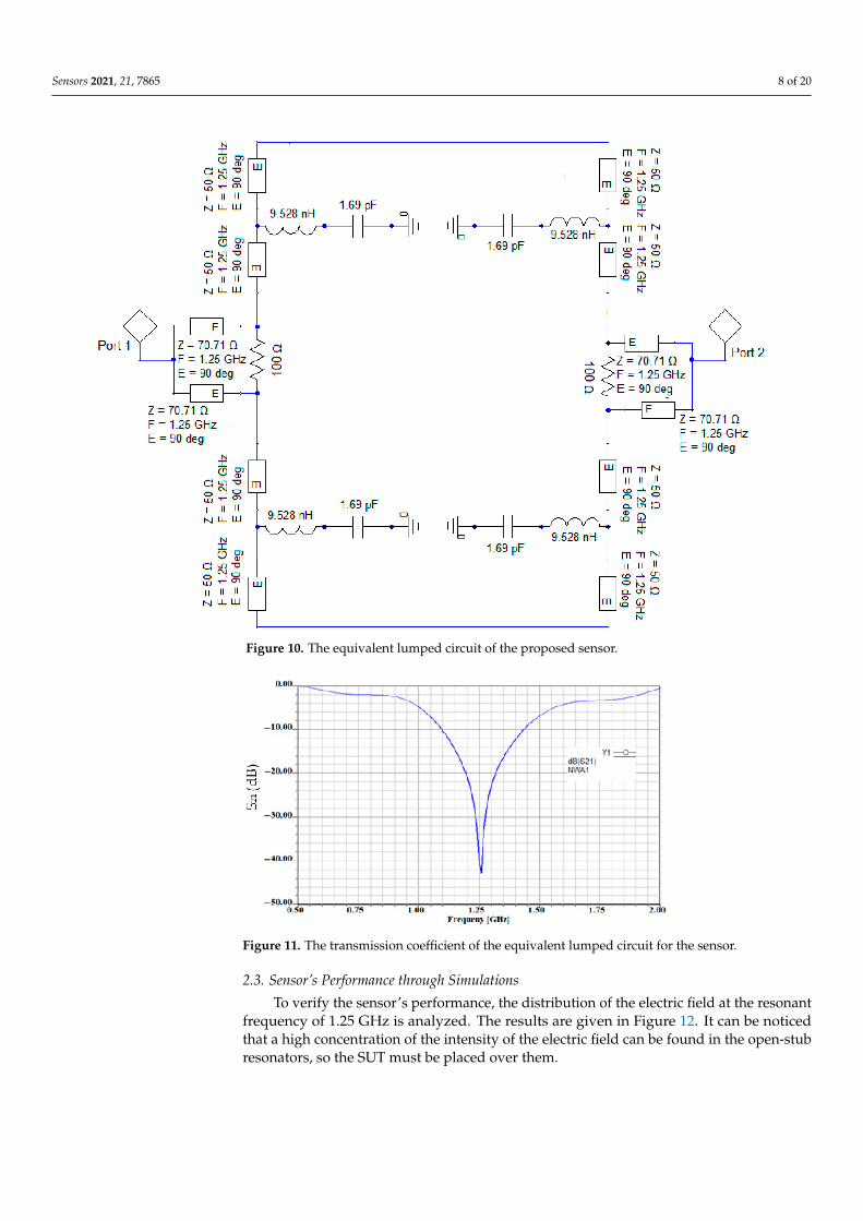
For a better understanding of the operational principal of the sensor, the equivalentcircuit model is depicted in Figure 10. The resonant structure is replaced by its equivalentlumped circuit from Figure 2a and the Wilkinson power divider is made of two identicaltransmission lines each having an electrical length E = 90 and a characteristic impedance70.71 Ω, isolated by a resistor of resistance R = 100 Ω. The value for the resistance of theresistor used to design the power divider is obtained by imposing that the two outputports of the Wilkinson divider are matched. The analysis of the three-port power divideris done using the even-odd excitation principle. Based on these two considerations, thevalue of the resistor placed in the Wilkinson power divider to isolate the output ports isdetermined, R = 2Z0 = 100 Ω. The transmission lines loading the resonant structure havethe characteristic impedance equal to 50 Ω and an overall electrical length of 360 in orderto not introduce additional phase shifts.

Practically, the power at port 1 is divided equally by the Wilkinson power dividerand each pair of resonating structure receives equal power. Due to the symmetry of thesensor, the same power arrives at the outputs of the second Wilkinson power divider andis summed at port 2. In fact, at port 1 we have connected the input of a Wilkinson powerdivider and at port 2, we have connected the output of an ideal Wilkinson power combiner.When adding liquid for test in the Teflon beaker placed above one of the sensing areas, thesymmetry is broken, and a second resonant frequency appears. This is used for measuringthe frequency shift and determine further on the electrical properties of the liquid sample.

The transfer characteristic of the equivalent circuit is obtained in Ansoft Designer bysimulation and is given in Figure 11.

Comparing the results in Figures 9 and 11, it can be noticed that for both circuitanalysis and electromagnetic simulation, the resonant frequency remains 1.25 GHz and theresponse in frequency of the transmission coefficient is identical. The losses consideredby the electromagnetic simulator can be seen in the value of parameter S21 which is only−38 dB compared to −41.3 dB.

Sensors 2021, 21, 7865 8 of 20

Figure 10. The equivalent lumped circuit of the proposed sensor.

Figure 11. The transmission coefficient of the equivalent lumped circuit for the sensor.

2.3. Sensor’s Performance through Simulations

To verify the sensor’s performance, the distribution of the electric field at the resonantfrequency of 1.25 GHz is analyzed. The results are given in Figure 12. It can be noticedthat a high concentration of the intensity of the electric field can be found in the open-stubresonators, so the SUT must be placed over them.

Sensors 2021, 21, 7865 9 of 20

Figure 12. Intensity of the electric field at the resonant frequency of 1.25 GHz.

Next, we investigate the best position of the sample over the resonant structures.Three cases are considered and the SUT is FR-4 epoxy with the same thickness. As areference for the frequency shift, ∆f, the resonant frequency of the sensor without a sampleis considered. The results of the simulation are given in Figure 13.

Figure 13. Simulated transmission characteristic, S21 of the proposed sensor for different positions ofthe sample: 1. no beaker, 2. longitudinal position of the beaker, 3. transversal position of the beaker,4. beaker positioned on the whole sensing area.

The reference for resonant frequency in the first case, when no SUT is mountedover the proposed sensor, is 1.25 GHz. The simulated frequency shifts for the second,third and fourth configurations depicted in Figure 13 are ∆f 2 = 40 MHz, ∆f 3 = 80 MHz,and ∆f 4 = 100 MHz, respectively. The values for the S21 parameters in the second, thirdand fourth case, measured at the resonant frequency are −31 dB, −33 dB, and −41 dB,respectively. We must remember that the sensor is differential, so the symmetry must bebroken when placing the SUT, so even if a better frequency shift is obtained for the fourthcase, the sensor is not a differential one anymore [23]. Thus, taking this into account andconsidering the performances of the sensor for both the frequency shift and the amplitudeof the S21 parameter at the resonant frequency, the third configuration offers the best results.

Next, we want to investigate the influence of the beaker over the performances ofthe sensor. Ideally, adding the beaker should have no influence over the performances,allowing the lines of electric field to go through the liquid and the sensing area. In additionto that, it should be able to keep the liquid distributed uniformly over the sensing area,increasing the sensing precision. For this reason, a Teflon beaker is chosen, as Teflon is a

Sensors 2021, 21, 7865 10 of 20

bio suitable material; is solid and soft enough to process for microfluidic devices; has verysmall losses (loss tangent of 0.001); and a small permittivity (εr = 2.1), which does not affectthe behavior of the sensor. In addition, we mounted a Teflon beaker instead of etching amicrofluidic channel made of PDMS because it requires less technological precision andto avoid any fabrication tolerance, but still maintained the sensing performances as isdemonstrated through simulations, as shown in Figure 11. The proposed Teflon beakerwidth is 13 mm, the length is 60 mm, the height is 1 mm, and the base thickness is 0.1 mm.These dimensions provide a volume of 0.78 mm3. If we consider the density of water997 kg/m3 and the one of urine from a healthy person between 1015–1022 kg/m3, thismeans that the liquid samples needed to make measurements have to be around 0.78 mL.On the other hand, urine is a biological liquid that is used for numerous tests, and it can beprovided in large quantities, not like sweat for example, so the capacity of the beaker is notan issue.

The Teflon beaker is located on the proposed sensor’s top surface, covering one pair ofopen stub resonators. To make sure that the beaker does not affect the sensor’s performance,a simulation of S21 parameter was carried in HFSS for two cases: the sensor with andwithout a beaker on top. The results of the simulation are given in Figure 14.

Figure 14. Transmission characteristic of the sensor without and with a beaker on top.

Analyzing the data in Figure 14, it can be observed that the influence of the beakeris minimal compared to the overall characteristic, due to the very small values for thedielectric constant and loss tangent for Teflon. The results in Figure 14 compared to the onesin [18] show the importance of the material used for beaker or the microfluidic channels.In [18] PDMS was used to create the channels and the results in Figure 15 [18] show adramatic decrease of the transmission coefficient S21 from almost −50 dB without channelsto −20 dB with channels. In our case, when using a Teflon beaker, the value of the S21parameter remains almost constant at a value of −35 dB, proving that Teflon is a goodchoice for this application. In these conditions, the sensor proposed in this study will havethe design as the one in Figure 15.

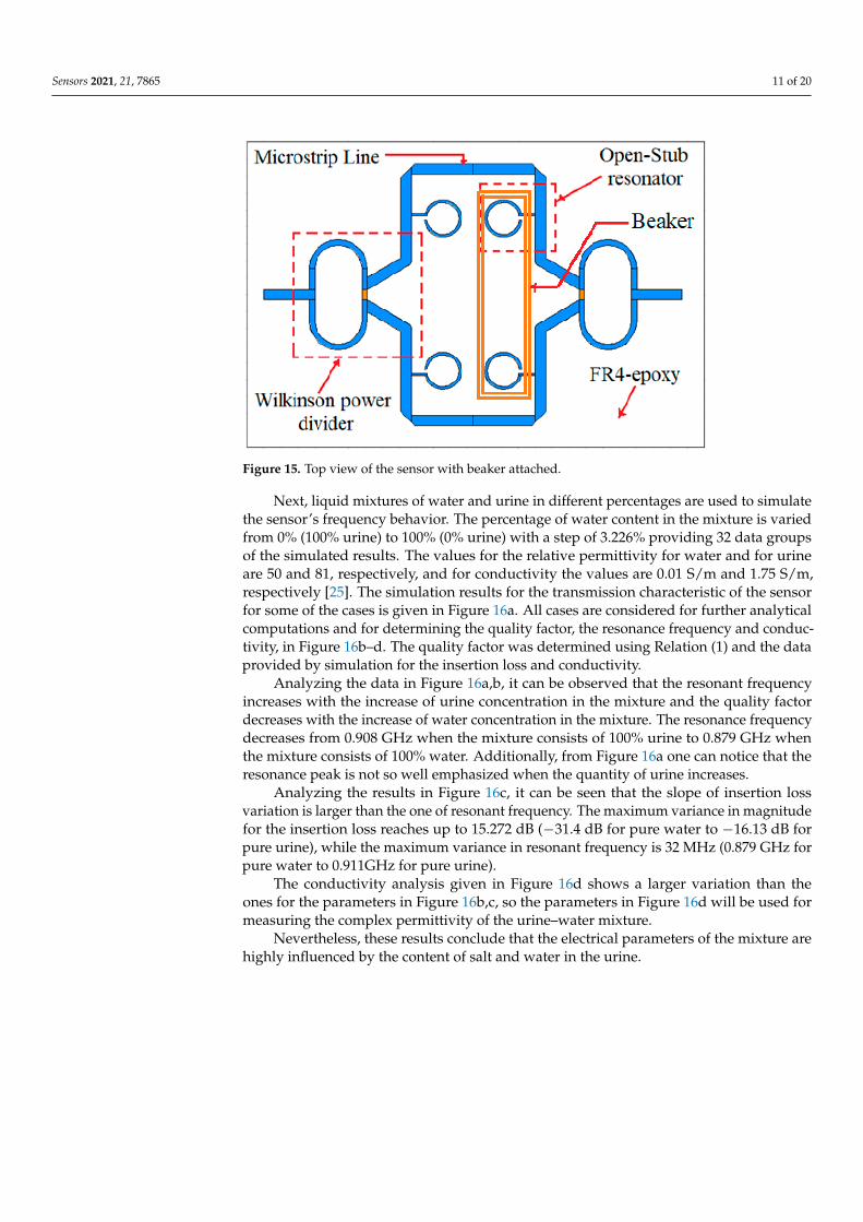
The sensor presented in Figure 15, is a differential sensor as it is made of two identicalsensing areas: one Wilkinson power divider/combiner and a pair of transmission linesloaded with two open-stub resonators. As the Teflon beaker has no influence on thefrequency response of the sensor, as proved in Figure 14, the sensing principle is similar toa differential sensor [23]: by loading the sensor with liquids under test (LUT) in the beaker,the symmetry is broken, and another resonant frequency appears. The reference will beconsidered the case when the sensor is loaded with pure water. This behavior will beproven by the results of both simulations and measurements for different organic mixturesin the next sections.

Sensors 2021, 21, 7865 11 of 20

Figure 15. Top view of the sensor with beaker attached.

Next, liquid mixtures of water and urine in different percentages are used to simulatethe sensor’s frequency behavior. The percentage of water content in the mixture is variedfrom 0% (100% urine) to 100% (0% urine) with a step of 3.226% providing 32 data groupsof the simulated results. The values for the relative permittivity for water and for urineare 50 and 81, respectively, and for conductivity the values are 0.01 S/m and 1.75 S/m,respectively [25]. The simulation results for the transmission characteristic of the sensorfor some of the cases is given in Figure 16a. All cases are considered for further analyticalcomputations and for determining the quality factor, the resonance frequency and conduc-tivity, in Figure 16b–d. The quality factor was determined using Relation (1) and the dataprovided by simulation for the insertion loss and conductivity.

Analyzing the data in Figure 16a,b, it can be observed that the resonant frequencyincreases with the increase of urine concentration in the mixture and the quality factordecreases with the increase of water concentration in the mixture. The resonance frequencydecreases from 0.908 GHz when the mixture consists of 100% urine to 0.879 GHz whenthe mixture consists of 100% water. Additionally, from Figure 16a one can notice that theresonance peak is not so well emphasized when the quantity of urine increases.

Analyzing the results in Figure 16c, it can be seen that the slope of insertion lossvariation is larger than the one of resonant frequency. The maximum variance in magnitudefor the insertion loss reaches up to 15.272 dB (−31.4 dB for pure water to −16.13 dB forpure urine), while the maximum variance in resonant frequency is 32 MHz (0.879 GHz forpure water to 0.911GHz for pure urine).

The conductivity analysis given in Figure 16d shows a larger variation than theones for the parameters in Figure 16b,c, so the parameters in Figure 16d will be used formeasuring the complex permittivity of the urine–water mixture.

Nevertheless, these results conclude that the electrical parameters of the mixture arehighly influenced by the content of salt and water in the urine.

Sensors 2021, 21, 7865 12 of 20

Figure 16. (a) Insertion loss for 10 ratios of water–urine mixture; (b) quality factor and resonancefrequency for 32 ratios of water–urine mixture; (c) insertion loss and resonance frequency for 32 ratiosof water–urine mixture; (d) conductivity and insertion loss for 32 ratios of water–urine mixture.

Sensors 2021, 21, 7865 13 of 20

3. Results

The sensor proposed in Figure 15 is now implemented and measured. The substrateused is FR-4 (relative permittivity εr = 4.4 and the dissipation factor, tan δ, is approximately0.02), with a thickness of 1.6 mm and cooper metallization electrodeposited on both sidesof the substrate, with a thickness of 18 µm.

The SMA (SubMiniature version A) connecters, which are classical semi-precisioncoaxial RF connectors used as interface for coaxial cables with screw-type coupling mech-anism are mounted on the structure using mechanical welding. The SMA has a 50 Ωcharacteristic impedance and is designed to work in the range 0–18 GHz, fully matchedwith the necessities of the current sensing structure. The beaker is made of Teflon andcarefully glued to the sensing area, making sure no air gap exists. The manufactured sensoris presented in Figure 17.

Figure 17. Photograph of the fabricated sensor for measuring different urine samples.

The measurement setup consists of the sensor connected to the Agilent E5071C,Agilent Technologies (Keysight Technologies), USA (9 kHz to 6.5 GHz) network analyzerthrough 50 Ω cables. Before starting the measurements, a short-open-load-through (SOLT)calibration was carried out using the Agilent calibration Kit. The number of sweep pointsis chosen 1601.

The resonant frequency measured for the empty sensor was 1.25 GHz as in simulations,verifying that the sensor has been implemented correctly.

A set of samples under test is selected and used for measurements. The pure urinesample (εr = 50, 1.75 S/m) is used only for obtaining calibration curves which are thenused to characterize the urine-water mixture samples. Practically, healthy male urineis combined with water in different ratios and six samples are obtained as explained inTable 2 and depicted in Figure 18.

For each measurement, the sensor is placed on a rough, stable surface and the SUT iscarefully placed to cover the whole sensing area, making sure no pellicular effect exists. Toreduce the effect of impurities and of humidity from previous tests, the beaker is washedthoroughly, then rinsed with water and dried by cotton brushes. Finally, the next urinesample is dropped in the beaker. Then, using the Agilent E5071C network analyzer, themagnitude of S21 parameter is measured. The measurements have been repeated fourtimes in the same environmental conditions. The results of the measurements are given inFigure 19.

Sensors 2021, 21, 7865 14 of 20

Table 2. Urine–water mixture samples.

Sample Water (%) Urine (%)

1 100 02 80 203 66 334 50 505 33 666 0 100

Figure 18. Different ratios urine-water mixtures used for measurements.

Figure 19. Measurement results for the samples presented in Figure 18, where the reference isrepresented by the unloaded sensor.

Analyzing the results in Figure 19, it can be seen that the differential behavior of thesensor, meaning when it is not loaded, only one resonant frequency appears and oncemixtures are added into the beaker, the symmetry is broken, and two resonant frequenciesappear. One advantage of using a Teflon beaker instead of microfluidic channels is that nosynchronization is required when filling the beaker.

The measurement results in Figure 19 show that the maximum value for the transmis-sion parameter, S21 is obtained at −26.93 dB for 100% water and starts to decrease onceurine is added to the mixture, reaching a minimum at −19.32 dB when the sample contains100% urine, so we can conclude that the sensor works properly.

The largest variance introduced by the insertion loss is 7.61 dB, this is about half of thedifference obtained by simulation due to using a water-free urine sample. As a result, themorning urine sample was calibrated to the new condition starting at 50% of the simulationof water content in mixture.

Sensors 2021, 21, 7865 15 of 20

The calibration of water content is derived as:

W′sam =Wsam + 100

2(2)

where W′sam represent calibrated water content and Wsam is water content ratio accordingto Table 2.

Calibrated ratios of water content in each sample corresponding to that in Table 2 aredepicted in both Figure 20 as well as Table 3.

Figure 20. The difference between water content ratios in Table 2 and that obtained using Equation (2).

Table 3. Urine-water mixture samples and their calibrated results.

Sample Water (%) Urine (%) Water (%) afterCalibration

Morning UrineCalibration (%)

1 100 0 100 02 80 20 90 103 66 33 83 174 50 50 75 255 33 66 67 336 0 100 50 50

Regarding the resonant frequency for all the samples, it is clear that frequency shiftsoccur, and the values are different depending on the quantity of urine that was been addedto the mixture. The data is synthesized in Table 3.

Further on, to obtain the values for the complex permittivity of the urine-watermixture, a nonlinear least square curve fitting in MATLAB is used to derive an equationdescribing the relation between variations of the resonance frequency and peak attenuationas a function of the complex permittivity variations [26,27]:[

∆f∆|S21|

]=

[m11 m12m21 m22

]·[

∆ε′sam∆ε′′sam

](3)

where the following notations have been used: ∆ε′sam = ε′sam – ε′ref, ∆ε′′sam = ε′′sam – ε′′ref,∆f sam = ∆f sam − ∆f ref, and ∆|S21| = ∆|S21|sam − ∆|S21|ref, with subscript “sam” for thesample and “ref” for the reference mixture. The values for |S21|sam and |S21|ref in thematrix are determined as f sam and f ref, respectively.

Sensors 2021, 21, 7865 16 of 20

However, in previous analyzing the measuring of the complex permittivity wasdecided relying on the insertion loss and conductivity parameters, hence the matrix inEquation (3) will be: [

∆σ∆|S21|

]=

[m11 m12m21 m22

]·[

∆ε′sam∆ε′′sam

](4)

where ∆σsam = ∆σsam − ∆σrefFrom data of Figure 16d, we have obtained the calibration curve for between conduc-

tivity and insertion loss, using linear regression. Such a curve is

[∆σ] = [0.0985]·[∆|S21|] (5)

For Equation (4), the relative resonant conductivity, ∆σ and relative magnitude ofparameter S21, ∆|S21| are computed and given in Table 4. The reference for both theconductivity and the transmission coefficient is the sample containing 100% water.

Table 4. Measurement results.

Sample S21 (dB) Quality Factor ∆σ (S/m) ∆|S21| (dB) ε′r ε′′r S (%)

1 −26.93 34 - -2 −23.39 23.181 0.348 3.54 75.6161 1.8058 2.533 −21.87 21.659 0.4986 5.06 72.9279 2.1292 2.714 −21.1 20.632 0.5744 5.83 69.3282 2.4418 2.845 −20.96 16.839 0.5882 5.97 69.3282 2.98054 2.8266 −19.32 14.1456 0.7498 7.61 66.4429 3.4337 2.89

The parameters m11, m12, m21, and m22 are related to the electrical characteristics of thefabricated sensor. According to Equation (4), a set of linear functions used for describingthe relationship of resonance characteristics of the sensor and the complex permittivity ofthe liquid sample under test can be accurately stated as follows [26]:[

∆σ∆|S21|

]=

[0.0507 0.03381.6464 −6.8621

]·[

∆ε′sam∆ε′′sam

](6)

By inverting the matrix in Equation (6), a mathematical model for determining thecomplex permittivity of unknown liquid sample is derived as:[

∆ε′sam∆ε′′sam

]=

[17.0041 0.08384.0797 −001256

]·[

∆σ∆|S21|

](7)

Using Equation (7) and the data (∆σ and ∆|S21|) of Table 4, we have obtained the realand imaginary part of the complex permittivity for the different mixtures of water in urine(Figure 21). Indeed, urine–water mixture is not a binary mixture such as ethanol–water,methanol–water, etc. Nevertheless, a good assent with the forecast presented by the Weinermodel that extracted relying on simulation results (the upper and lower limits of thatmodel are also specified in Figure 21) [27]. Evidence the validity of the proposed sensorto determine the reasonable complex permittivity of urine-water mixture. The computedvalues of real and imaginary parts are added to Table 4.

Sensors 2021, 21, 7865 17 of 20

Figure 21. Both the real (a) and the imaginary (b) parts of the permittivity in mixtures of urine/water.

For comparison objectives, the static Weiner model is also included. Next, we calculatethe sensitivity of the sensor. The sensitivity in resonance-based microfluidic dielectricsensors is defined as [26]:

S(%) =fεr − fre f

fre f ·(ε′r − 1)(8)

where fεr represents the resonant frequency of the urine–water mixture, fre f representsthe resonant frequency of the unloaded sensor and ε′r represents the real part of therelative permittivity.

Using Relation (8) and the data from the measurements, the sensitivity of the proposedsensor for organic fluids is determined. Based on different samples, different values for thesensitivity are obtained, as shown in Table 4.

The results from Table 4 show that the sensor can be used successfully to characterizeorganic liquid mixtures by their electrical properties. Additionally, the sensitivity hasgood results.

4. Discussion

In Table 5, the results for the sensitivity are compared to the ones in the literature.Note that there few investigations regarding measurements of mixtures between waterand organic liquids, such as urine. Still, the references in Table 5 refer to sensors measuringliquid mixtures with high relative permittivity.

Sensors 2021, 21, 7865 18 of 20

Table 5. Comparison between various resonance-based microwave microfluidic sensors.

Sensor Type of Fluid Central Frequency(GHz) ε′r Range S (%) References

Substrate integrated waveguide Isopropanol 3.6 4–76 0.15 [28]CSRR Ethanol 2.37 9–79 0.03 [29]

Shunt-connected series LC resonator Ethanol 2 30–80 0.44 [26]CSRR Ethanol 1.6 30–80 0.626 [19]

Open CSRR Methanol 0.9 35–80 1.8 [30]CSRR Urine 4 - - [31]

Dumbbell-Shaped Defect Ground Structures Isopropanol 1.05 75–80 1.02 [32]CSRR Ethanol 1.618 9–79 0.626 [18]RLC Glycerol 2.3 8.22–79.5 2.117 [33]

Open SRR Isopropanol 1.8 75–80 1.6 [34]Classic Glycerol/Ethanol 1.9 - 1.316 [35]

Open stub resonator Urine 1.25 66–74 2.53 Proposed

Interpreting the results obtained in comparison to other sensors, it can be observedthat the proposed sensor offers the best sensitivity. Nevertheless, it is used to electricallycharacterize samples containing organic liquids, such as urine. Urine is a complex com-pound made of inorganic and organic compounds. All of them influence the electricalpermittivity, so it is very important to have accurate sensors to determine these parameters.

When compared to other resonance-based microwave microfluidic sensors, it can beobserved that the relative permittivity is in a narrower range, from 66 to 74.

Additionally, the proposed sensor is not a microfluidic one but still has some advan-tages when compared to them. The main advantages refer to the fact that the technologicalprocess is much simplified as no microfluidic channels are required, just a Teflon beakerattached to the sensor, which does not influence the frequency behavior of the sensor.Additionally, the sensing area is in a better contact to the beaker due to its flat shaperather than microfluidic channels which have a cylindrical shape and thus, limiting theircontractability to the flat surface of the sensor. Nevertheless, no mechanical systems forpumping the liquid in the capillaries is required and no synchronization between fillingthe microfluidic channels with the LUT and reference liquid is needed. Another advantageis that it is implemented on an affordable substrate, such as FR-4. Urine can be provided inlarge quantities, while the capacity of the beaker is less than 1 mL.

In the literature, many studies refer to sensors used to characterize inorganic samplesrather than organic ones. The sensor in [31] is used to characterize the samples of urine onlyfrom the conductivity perspective and a color chart. No information about the complexpermittivity is given.

In [35] the urine samples are characterized by means of concentrations of electrolytes.The sensor proposed in this paper can detect electrolyte concentrations as small as 0.25 g/L,with maximum sensitivity of 0.033 (g/L) − 1. The sensor is validated by measuring theconcentration of three types of electrolytes, i.e., NaCl, KCl, and CaCl2 from urine. Again,the complex permittivity is not given.

Thus, the sensor proposed in this paper can be used successfully to detect with greatsensitivity the changes in the values of the complex permittivity of urine samples. This canbe used to determine metabolic changes and help diagnose different disorders.

5. Conclusions

A highly sensitive differential microstrip sensor for biomedical sensing applications isdesigned, fabricated, and tested. It consists of two identical parts, each of them made of aWilkinson power divider and a transmission line loaded with two open-stub resonators.The structure is easily fabricated on a single metal microstrip layer. The Teflon beaker isplaced on top of the microstrip surface instead of having a microfluid channel etched, thussimplifying the production process. The samples used for measurements were a mixturebetween water and urine with different percentages. The results were used to determine

Sensors 2021, 21, 7865 19 of 20

the complex permittivity of the liquid mixtures, including pure water and pure urine. Dueto starting with different mixture sample that are supplied in the simulation, the datarange of water content that was used in the simulation was recalibrated to match the samedata range of the measured samples. As the result, good assent between the measuredcomplex permittivity values and that forecasted by the Weiner model that extracted relyingon simulation results. The values for the complex permittivity show good agreementwith reference values. Additionally, the sensitivity of the sensor determined based onmeasurements is very good in comparison with similar works. The sensor can successfullybe used in medical applications that require investigating the electrical parameters of urinein different medical conditions.

Author Contributions: Conceptualization, A.A.a.-B. and I.A.M.; methodology, A.A.a.-B. and I.A.M.;software, A.A.a.-B., I.A.M. and T.A.E.; validation, A.A.a.-B., I.A.M. and T.M.P.; formal analysis,I.A.M. and T.A.E.; investigation, A.A.a.-B., I.A.M., T.M.P. and T.A.E.; resources, T.M.P.; data curation,T.A.E.; writing—original draft preparation, I.A.M. and A.A.a.-B.; writing—review and editing,T.M.P.; visualization, T.A.E. and I.A.M.; supervision, I.A.M.; project administration, I.A.M.; fundingacquisition, A.A.a.-B. and T.A.E. All authors have read and agreed to the published version ofthe manuscript.

Funding: This research received no external funding.

Conflicts of Interest: The authors declare no conflict of interest.

References1. Wang, C.; Ali, L.; Meng, F.-Y.; Adhikari, K.K.; Zhou, Z.L.; Wei, Y.C.; Zou, D.Q.; Yu, H. High-Accuracy Complex Permittivity

Characterization of Solid Materials Using Parallel Interdigital Capacitor- Based Planar Microwave Sensor. IEEE Sensors J. 2021, 21,6083–6093. [CrossRef]

2. Aquino, A.; Juan, C.G.; Potelon, B.; Quendo, C. Dielectric Permittivity Sensor Based on Planar Open-Loop Resonator. IEEESensors Lett. 2021, 5, 3500204. [CrossRef]

3. Oliveira, J.G.D.; Junior, J.G.D.; Pinto, E.N.M.G.; Neto, V.P.S.; D’Assunção, A.G. A New Planar Microwave Sensor for BuildingMaterials Complex Permittivity Characterization. Sensors 2020, 20, 6328. [CrossRef]

4. Mondal, D.; Tiwari, N.K.; Akhtar, M.J. Microwave Assisted Non-Invasive Microfluidic Biosensor for Monitoring GlucoseConcentration. In Proceedings of the 2018 IEEE Sensors, New Delhi, India, 28–31 October 2018; pp. 1–4. [CrossRef]

5. Hardinata, S.; Deshours, F.; Alquié, G.; Kokabi, H.; Koskas, F. Miniaturization of Microwave Biosensor for Non-invasiveMeasurements of Materials and Biological Tissues. IPTEK J. Proc. Ser. 2018, 1, 90–93. [CrossRef]

6. Liu, W.; Sun, H.; Xu, L. A Microwave Method for Dielectric Characterization Measurement of Small Liquids Using a Met-amaterial-Based Sensor. Sensors 2018, 18, 1438. [CrossRef]

7. Hao, H.; Wang, D.; Wang, Z.; Yin, B.; Ruan, W. Design of a High Sensitivity Microwave Sensor for Liquid Dielectric ConstantMeasurement. Sensors 2020, 20, 5598. [CrossRef]

8. Wei, Z.; Huang, J.; Li, J.; Xu, G.; Ju, Z.; Liu, X.; Ni, X. A High-Sensitivity Microfluidic Sensor Based on a Substrate IntegratedWaveguide Re-Entrant Cavity for Complex Permittivity Measurement of Liquids. Sensors 2018, 18, 4005. [CrossRef]

9. Liao, S.; Gao, B.; Tong, L.; Yang, X.; Li, Y.; Li, M. Measuring Complex Permittivity of Soils by Waveguide Transmission/ReflectionMethod. In Proceedings of the IGARSS 2019—2019 IEEE International Geoscience and Remote Sensing Symposium, Yokohama,Japan, 28 July–2 August 2019; pp. 7144–7147. [CrossRef]

10. Oliveira, J.G.D.; Pinto, E.N.M.G.; Neto, V.P.S.; D’Assunção, A.G. CSRR-Based Microwave Sensor for Dielectric MaterialsCharacterization Applied to Soil Water Content Determination. Sensors 2020, 20, 255. [CrossRef]

11. Becker, R. Non-invasive cancer detection using volatile biomarkers: Is urine superior to breath? Med. Hypotheses 2020, 143, 110060.[CrossRef]

12. Mentes, J.C.; Wakefield, B.; Culp, K. Use of a Urine Color Chart to Monitor Hydration Status in Nursing Home Residents. Biol.Res. Nurs. 2006, 7, 197–203. [CrossRef]

13. Armstrong, L.E.; Maresh, C.M.; Castellani, J.; Bergeron, M.F.; Kenefick, R.W.; Lagasse, K.E.; Riebe, D. Urinary Indices of HydrationStatus. Int. J. Sport Nutr. 1994, 4, 265–279. [CrossRef]

14. McKenzie, A.L.; Armstrong, L.E. Monitoring Body Water Balance in Pregnant and Nursing Women: The Validity of Urine Color.Ann. Nutr. Metab. 2017, 70, 18–22. [CrossRef] [PubMed]

15. Armstrong, L.E.; Ganio, M.S.; Klau, J.F.; Johnson, E.C.; Casa, D.J.; Maresh, C.M. Novel hydration assessment techniques employingthirst and a water intake challenge in healthy men. Appl. Physiol. Nutr. Metab. 2014, 39, 138–144. [CrossRef] [PubMed]

16. Ebrahimi, A.; Scott, J.; Ghorbani, K. Differential Sensors Using Microstrip Lines Loaded with Two Split-Ring Resonators. IEEESensors J. 2018, 18, 5786–5793. [CrossRef]

Sensors 2021, 21, 7865 20 of 20

17. Su, L.; Naqui, J.; Mata-Contreras, J.; Martin, F. Modeling and Applications of Metamaterial Transmission Lines Loaded with Pairsof Coupled Complementary Split-Ring Resonators (CSRRs). IEEE Antennas Wirel. Propag. Lett. 2016, 15, 154–157. [CrossRef]

18. Gan, H.-Y.; Zhao, W.-S.; Liu, Q.; Wang, D.-W.; Dong, L.; Wang, G.; Yin, W.-Y. Differential Microwave Microfluidic Sensor Based onMicrostrip Complementary Split-Ring Resonator (MCSRR) Structure. IEEE Sensors J. 2020, 20, 5876–5884. [CrossRef]

19. Velez, P.; Su, L.; Grenier, K.; Mata-Contreras, J.; Dubuc, D.; Martin, F. Microwave Microfluidic Sensor Based on a MicrostripSplitter/Combiner Configuration and Split Ring Resonators (SRRs) for Dielectric Characterization of Liquids. IEEE Sensors J.2017, 17, 6589–6598. [CrossRef]

20. Haq, T.; Ruan, C.; Ullah, S.; Fahad, A.K. Dual notch microwave sensors based on complementary metamaterial resonators. IEEEAccess 2019, 7, 153489–153498. [CrossRef]

21. Mayani, M.G.; Herraiz-Martinez, F.J.; Domingo, J.M.; Giannetti, R. Resonator-Based Microwave Metamaterial Sensors forInstrumentation: Survey, Classification, and Performance Comparison. IEEE Trans. Instrum. Meas. 2021, 70, 9503414. [CrossRef]

22. Su, L.; Mata-Contreras, J.; Vélez, P.; Martin, F. Splitter/Combiner Microstrip Sections Loaded with Pairs of Complementary SplitRing Resonators (CSRRs): Modeling and Optimization for Differential Sensing Applications. IEEE Trans. Microw. Theory Tech.2016, 64, 4362–4370. [CrossRef]

23. Salim, A.; Lim, S. Review of Recent Metamaterial Microfluidic Sensors. Sensors 2018, 18, 232. [CrossRef] [PubMed]24. Saadat-Safa, M.; Nayyeri, V.; Khanjarian, M.; Soleimani, M.; Ramahi, O.M. A CSRR-Based Sensor for Full Characterization of

Magneto-Dielectric Materials. IEEE Trans. Microw. Theory Tech. 2019, 67, 806–814. [CrossRef]25. Al-Fraihat, A.; Al-Mufti, A.W.; Hashim, U.; Adam, T. Potential of urine dielectric properties in classification of stages of breast

carcinomas. In Proceedings of the 2014 2nd International Conference on Electronic Design (ICED), Penang, Malaysia, 19–21August 2014; pp. 305–308.

26. Ebrahimi, A.; Scott, J.; Ghorbani, K. Ultrahigh-Sensitivity Microwave Sensor for Microfluidic Complex Permittivity Measurement.IEEE Trans. Microw. Theory Tech. 2019, 67, 4269–4277. [CrossRef]

27. Kaufman, A.; Donadille, J.-M. Principles of Dielectric Logging Theory; Elsevier: Amsterdam, The Netherlands, 2021; Chapter 6;pp. 222–224, ISBN 9780128222843.

28. Rocco, G.M.; Bozzi, M.; Schreurs, D.; Perregrini, L.; Marconi, S.; Alaimo, G.; Auricchio, F. 3-D Printed Microfluidic Sensor in SIWTechnology for Liquids’ Characterization. IEEE Trans. Microw. Theory Tech. 2020, 68, 1175–1184. [CrossRef]

29. Chuma, E.L.; Iano, Y.; Fontgalland, G.; Roger, L.L.B. Microwave Sensor for Liquid Dielectric Characterization Based on Metamate-rial Complementary Split Ring Resonator. IEEE Sensors J. 2018, 18, 9978–9983. [CrossRef]

30. Velez, P.; Grenier, K.; Mata-Contreras, J.; Dubuc, D.; Martin, F. Highly-Sensitive Microwave Sensors Based on Open Complemen-tary Split Ring Resonators (OCSRRs) for Dielectric Characterization and Solute Concentration Measurement in Liquids. IEEEAccess 2018, 6, 48324–48338. [CrossRef]

31. Li, C.-H.; Chen, K.-W.; Yang, C.-L.; Lin, C.-H.; Hsieh, K.-C. A urine testing chip based on the complementary split-ring resonatorand microfluidic channel. In Proceedings of the 2018 IEEE Micro Electro Mechanical Systems (MEMS), Belfast, UK, 21–25 January2018; pp. 1150–1153.

32. Vélez, P.; Muñoz-Enano, J.; Gil, M.; Mata-Contreras, J.; Martín, F. Differential Microfluidic Sensors Based on Dumbbell-ShapedDefect Ground Structures in Microstrip Technology: Analysis, Optimization, and Applications. Sensors 2019, 19, 3189. [CrossRef]

33. Ebrahimi, A.; Tovar-Lopez, F.J.; Scott, J.; Ghorbani, K. Differential microwave sensor for characterization of glycerol–watersolutions. Sens. Actuators B Chem. 2020, 321, 128561. [CrossRef]

34. Muñoz-Enano, J.; Vélez, P.; Gil, M.; Martín, F. Microfluidic reflective-mode differential sensor based on open split ring resonators(OSRRs). Int. J. Microw. Wirel. Technol. 2020, 12, 588–597. [CrossRef]

35. Wang, B.-X.; Zhao, W.-S.; Wang, D.-W.; Wu, W.-J.; Liu, Q.; Wang, G. Sensitivity optimization of differential microwave sensors formicrofluidic applications. Sens. Actuators A Phys. 2021, 330, 112866. [CrossRef]