One-dimensional modeling of flows and morphological ...
238
Université catholique de Louvain Ecole polytechnique de Louvain Institute of Mechanics, Materials and Civil Engineering One-dimensional modeling of flows and morphological changes in rivers: experimental and numerical approaches Thesis presented for the degree of Doctor in Engineering Sciences by Fabian Franzini March 2017 Members of the Jury: Prof. Sandra Soares-Frazão, Université catholique de Louvain, supervisor Prof. Vincent Guinot, Université Montpellier 2, co-advisor Dr. Catherine Swartenbroekx, Service Public Wallonie, co-advisor Prof. Yves Zech, Université catholique de Louvain Prof. Mustafa Altinakar, University of Mississippi Prof. Laurent Delannay, Université catholique de Louvain, president
-
Upload
khangminh22 -
Category
Documents
-
view
4 -
download
0
Transcript of One-dimensional modeling of flows and morphological ...

Université catholique de Louvain Ecole polytechnique de Louvain Institute of Mechanics, Materials and Civil Engineering
One-dimensional modeling of flows and morphological changes in rivers: experimental
and numerical approaches
Thesis presented for the degree of Doctor in Engineering Sciences by
Fabian Franzini
March 2017
Members of the Jury: Prof. Sandra Soares-Frazão, Université catholique de Louvain, supervisor Prof. Vincent Guinot, Université Montpellier 2, co-advisor Dr. Catherine Swartenbroekx, Service Public Wallonie, co-advisor Prof. Yves Zech, Université catholique de Louvain Prof. Mustafa Altinakar, University of Mississippi Prof. Laurent Delannay, Université catholique de Louvain, president


Contents
Remerciements .............................................................................................. 7
Introduction ................................................................................................... 9
Hydrodynamic Modeling.................................................... 37
I.1. Introduction .................................................................................. 38
I.2. Governing equations ..................................................................... 40
I.3. Numerical models ......................................................................... 42
I.3.1. Lateralized HLL .................................................................... 43
I.3.2. HLLS .................................................................................... 44
I.3.3. Augmented Roe’s solver with energy balance ...................... 46
I.4. Results ........................................................................................... 50
I.4.1. Water at rest .......................................................................... 50
I.4.2. Steady flows .......................................................................... 51
I.4.3. Transient flows ..................................................................... 60
I.4.4. Brembo River ........................................................................ 67
I.5. Discussion and conclusion ............................................................ 70
References ................................................................................................. 71
Modeling the flow around islands ..................................... 75
II.1. Introduction .................................................................................. 76
II.2. Governing equations and numerical scheme ................................ 79
II.2.1. One-dimensional Saint-Venant equations in conservative form .............................................................................................. 79
II.2.2. Finite-volume resolution of the equations ............................ 81
II.3. Internal boundary conditions ........................................................ 83
II.3.1. Subcritical junction ............................................................... 85
II.3.2. Subcritical bifurcation ........................................................... 87
II.3.3. Supercritical junction ............................................................ 89
II.3.4. Supercritical bifurcation ........................................................ 90
II.4. Results and discussion .................................................................. 93
II.4.1. Subcritical junction ............................................................... 95
II.4.2. Subcritical bifurcation ........................................................... 99
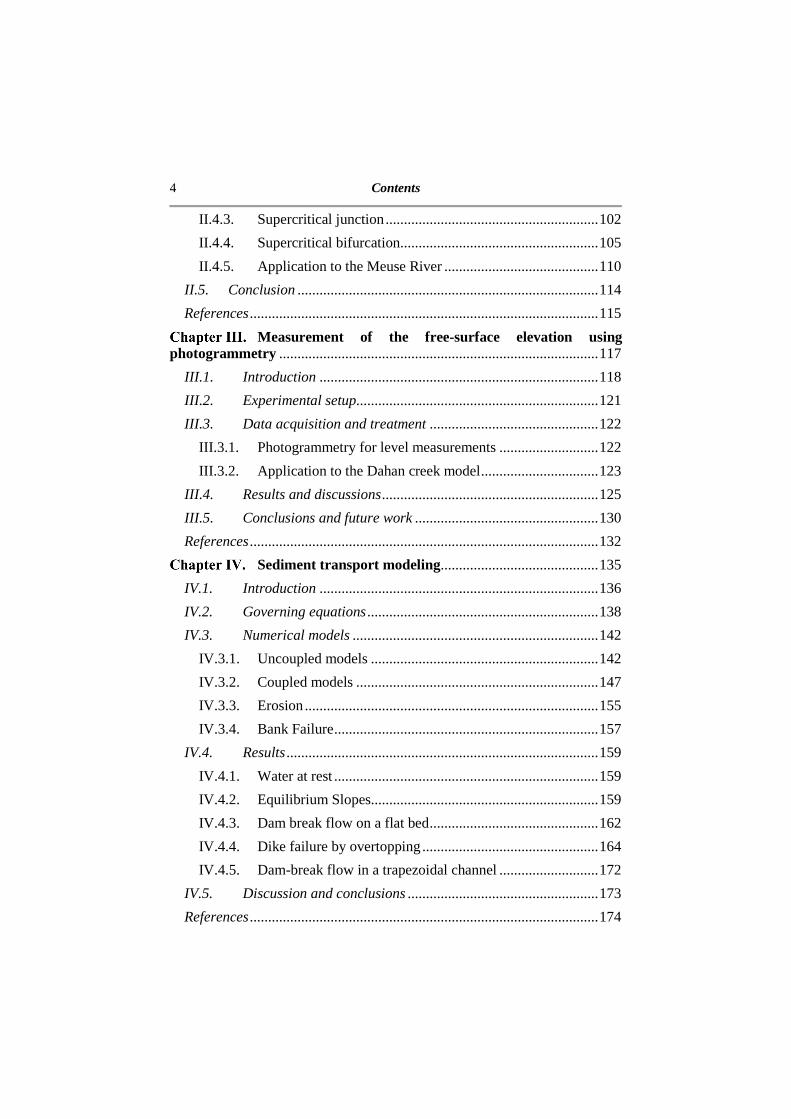
4 Contents
II.4.3. Supercritical junction .......................................................... 102
II.4.4. Supercritical bifurcation ...................................................... 105
II.4.5. Application to the Meuse River .......................................... 110
II.5. Conclusion .................................................................................. 114
References ............................................................................................... 115
Measurement of the free-surface elevation using photogrammetry ....................................................................................... 117
III.1. Introduction ............................................................................ 118
III.2. Experimental setup.................................................................. 121
III.3. Data acquisition and treatment .............................................. 122
III.3.1. Photogrammetry for level measurements ........................... 122
III.3.2. Application to the Dahan creek model ................................ 123
III.4. Results and discussions ........................................................... 125
III.5. Conclusions and future work .................................................. 130
References ............................................................................................... 132
Sediment transport modeling ........................................... 135
IV.1. Introduction ............................................................................ 136
IV.2. Governing equations ............................................................... 138
IV.3. Numerical models ................................................................... 142
IV.3.1. Uncoupled models .............................................................. 142
IV.3.2. Coupled models .................................................................. 147
IV.3.3. Erosion ................................................................................ 155
IV.3.4. Bank Failure ........................................................................ 157
IV.4. Results ..................................................................................... 159
IV.4.1. Water at rest ........................................................................ 159
IV.4.2. Equilibrium Slopes.............................................................. 159
IV.4.3. Dam break flow on a flat bed .............................................. 162
IV.4.4. Dike failure by overtopping ................................................ 164
IV.4.5. Dam-break flow in a trapezoidal channel ........................... 172
IV.5. Discussion and conclusions .................................................... 173
References ............................................................................................... 174
Contents 5
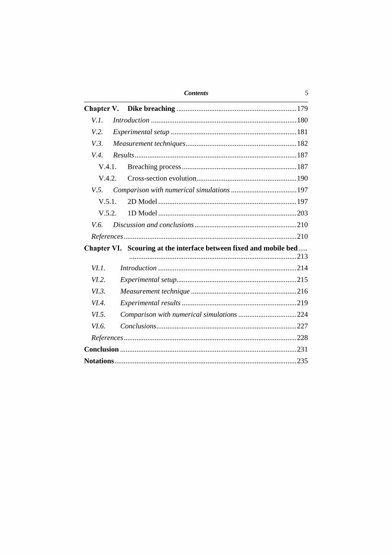
Dike breaching .................................................................. 179
V.1. Introduction ................................................................................ 180
V.2. Experimental setup ..................................................................... 181
V.3. Measurement techniques ............................................................. 182
V.4. Results ......................................................................................... 187
V.4.1. Breaching process ............................................................... 187
V.4.2. Cross-section evolution ....................................................... 190
V.5. Comparison with numerical simulations .................................... 197
V.5.1. 2D Model ............................................................................ 197
V.5.2. 1D Model ............................................................................ 203
V.6. Discussion and conclusions ........................................................ 210
References ............................................................................................... 210
Scouring at the interface between fixed and mobile bed ..... ............................................................................................ 213
VI.1. Introduction ............................................................................ 214
VI.2. Experimental setup.................................................................. 215
VI.3. Measurement technique .......................................................... 216
VI.4. Experimental results ............................................................... 219
VI.5. Comparison with numerical simulations ................................ 224
VI.6. Conclusions ............................................................................. 227
References ............................................................................................... 228
Conclusion ................................................................................................. 231
Notations .................................................................................................... 235


REMERCIEMENTS Je tiens à remercier tous ceux qui ont contribué à faire de cette thèse une expérience enrichissante. Merci à tous mes collègues du département hydraulique : Bastien Mathurin, Camille Raucent, Damien Christiaens, Damien Hoedenaeken, Ilaria Fent, Olivier Carlier, Pierre Rottenberg et Sylvie Van Emelen. Merci à Didier Bousmar, Benoit Spinewine, Catherine Swartenbroekx et Yves Zech pour leurs conseils et les échanges enrichissants tout au long de ma thèse. Merci à Pilar Garcia-Navarro, Javier Murillo, Carmelo Juez et toute l’équipe de l’Universidad de Zaragoza pour leur accueil et leur aide dans la compréhension des modèles numériques. Merci à Hervé Capart et toute l’équipe de la National Taiwan University pour leur accueil et leur partage de connaissances sur le travail expérimental. Et aussi, merci à tous les membres du pôle GC et du laboratoire pour leur bonne humeur et leur aide durant ma thèse. Ensuite, je voudrais remercier mon promoteur, le professeur Sandra Soares-Frazão de m’avoir permis de réaliser cette thèse. Merci pour son soutien, son aide précieuse lors de la rédaction d’articles et sa capacité à recadrer ma thèse. Merci également à tous les membres de mon jury pour leurs commentaires constructifs et l’intéressante discussion sur ma recherche lors de la défense privée. Enfin, je tiens surtout à remercier mes parents, ma sœur et mon beau-frère pour leurs encouragements durant ma thèse. Merci à Tania de m’avoir soutenu et motivé pendant les moments plus difficiles de ma thèse.


INTRODUCTION Floods are one of the most damaging natural disasters. The damage is caused by the fast moving water and, sometimes, by the large quantities of sediments transported. Modern history does not lack of evidence of their destructive nature. Moreover, every continent in the world can be subject to catastrophic consequences of floods. For instance, Hurricane Matthew hit Haiti in October 2016 and created huge damages, completely reshaping the course of multiple rivers. An example of this extreme reshaping can be observed comparing Figure A and Figure B. The two pictures were taken at the exact same location, two years apart. The small cabin was initially built several meters away of the riverbank. However, after Matthew, the cabin was almost destroyed by the widening of the Cavaillon River.
Figure A. Cavaillon River, Haiti, in 2014
Figure B. Cavaillon River, Haiti, in 2016, after the hurricane Matthew

10 Introduction
In August 2009, Typhoon Morakot created huge floods, landslides and debris flows in Taiwan, killing more than 600 people and reaching more than 3 billion US$ in damages (Lin et al. 2011). The failure of an iron ore-tailing dam in Brazil in 2015 killed at least 17 persons and released more than 60 million cubic meters of polluted water into the Doce River. In 2005, Hurricane Katrina created catastrophic flooding in New Orleans because of multiple levee failures. In 2013, heavy rains in Southwest China created large flooding in various regions with Sichuan being affected the most (Figure C). Recently, in February 2017, nearly 200 000 persons were evacuated when excessive erosion was observed in the spillway of the Oroville dam in USA (Figure D)
Figure C. Flood in Sichuan in July 2013
(http://www.nbcnews.com/news/photo/china-floods-trigger-landslide-bridge-collapse-dozens-remain-missing-v19392951)

Introduction 11
Figure D. Oroville dam (http://www.usatoday.com/story/news/nation-
now/2017/02/28/oroville-dam-spillway-damage/98528880/)

12 Introduction
One well documented, example is the flood of the Ha!Ha! River (Quebec, Canada) in July 1996 (Capart et al. 2007). The failure of a dike on the Ha!Ha! Lake released an important amount of water in the river, completely reshaping the valley (Figure E). This case will be the common thread throughout the complete thesis as it comprises different features that can be connected to modeling options and demonstrates clearly some of the challenges encountered when simulating the flood propagation and morphological changes in a real river.
Figure E. Ha!Ha! River after the flood of 1996 (Capart et al. 2007)

Introduction 13
Numerical modeling of floods induced by a dam or dike failure is important as it can help predicting and preventing the potential loss of life and property damage. During a natural disaster, time is a key parameter for saving lives. In order to be used for operational simulation in time of crisis, the numerical models need to be both reliable and computationally efficient. Several numerical models exist in the literature to simulate the river flow with sediment transport and morphodynamical changes. They can be classified in different categories considering the number of spatial dimensions, the equations used to represent the sediments in the water and the discretization scheme. By considering the number of spatial dimensions, three types of models can be identified to simulate the flow in a river:
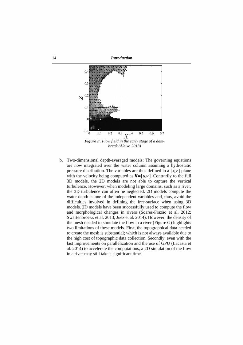
a. Three-dimensional models: These models are the most complete as the variables are defined in any [x,y,z] point and the three components of the velocities are taken into account VVVV=[u,v,w]. These models are particularly useful when studying the flow around hydraulic structures as the full velocities (in the three directions) model allows a better representation of the turbulence and pressure created around them. For instance, 3D models are needed to capture the formation of the horseshoe vortices when simulating the flow around a bridge pier. Vertical velocities need also to be considered when studying the early stages of a laboratory dam break, when the wall of water starts to fall down: Figure F shows the velocity field immediately after the gate removal for a dam break test case (Aleixo 2013). However, the number of components (elements, nodes or cells; depending on the discretization scheme, see below) needed to compute the flow in a river and the difficulties when treating moving boundaries (bed and water levels) makes 3D models impractical to model fast transient flows in river.
14 Introduction
Figure F. Flow field in the early stage of a dam-
break (Aleixo 2013)
b. Two-dimensional depth-averaged models: The governing equations
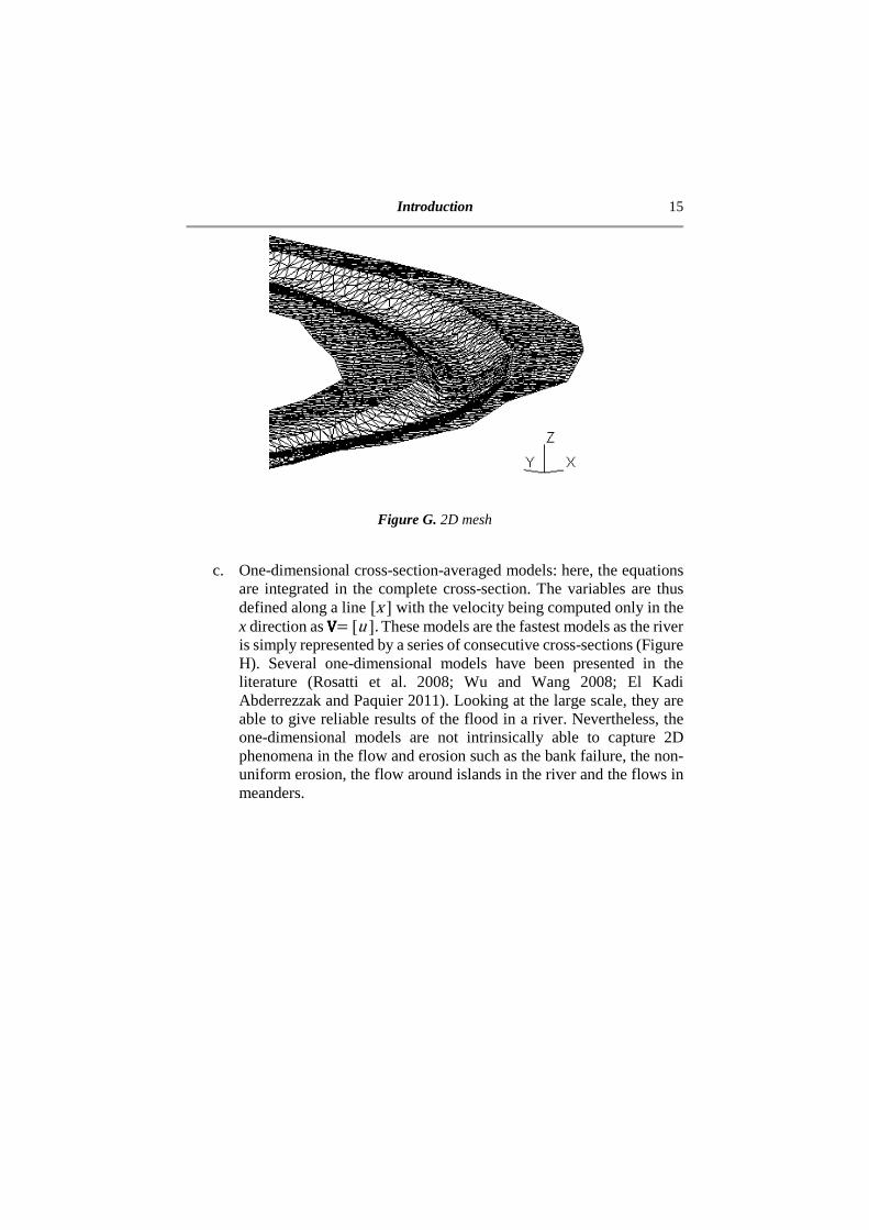
are now integrated over the water column assuming a hydrostatic pressure distribution. The variables are thus defined in a [x,y ] plane with the velocity being computed as VVVV=[u,v ]. Contrarily to the full 3D models, the 2D models are not able to capture the vertical turbulence. However, when modeling large domains, such as a river, the 3D turbulence can often be neglected. 2D models compute the water depth as one of the independent variables and, thus, avoid the difficulties involved in defining the free-surface when using 3D models. 2D models have been successfully used to compute the flow and morphological changes in rivers (Soares-Frazão et al. 2012; Swartenbroekx et al. 2013; Juez et al. 2014). However, the density of the mesh needed to simulate the flow in a river (Figure G) highlights two limitations of these models. First, the topographical data needed to create the mesh is substantial; which is not always available due to the high cost of topographic data collection. Secondly, even with the last improvements on parallelization and the use of GPU (Lacasta et al. 2014) to accelerate the computations, a 2D simulation of the flow in a river may still take a significant time.
Introduction 15
Figure G. 2D mesh
c. One-dimensional cross-section-averaged models: here, the equations
are integrated in the complete cross-section. The variables are thus defined along a line [x ] with the velocity being computed only in the x direction as VVVV= [u ]. These models are the fastest models as the river is simply represented by a series of consecutive cross-sections (Figure H). Several one-dimensional models have been presented in the literature (Rosatti et al. 2008; Wu and Wang 2008; El Kadi Abderrezzak and Paquier 2011). Looking at the large scale, they are able to give reliable results of the flood in a river. Nevertheless, the one-dimensional models are not intrinsically able to capture 2D phenomena in the flow and erosion such as the bank failure, the non-uniform erosion, the flow around islands in the river and the flows in meanders.
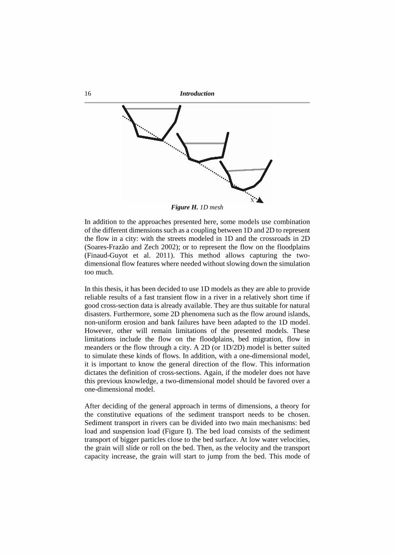
16 Introduction
Figure H. 1D mesh
In addition to the approaches presented here, some models use combination of the different dimensions such as a coupling between 1D and 2D to represent the flow in a city: with the streets modeled in 1D and the crossroads in 2D (Soares-Frazão and Zech 2002); or to represent the flow on the floodplains (Finaud-Guyot et al. 2011). This method allows capturing the two-dimensional flow features where needed without slowing down the simulation too much. In this thesis, it has been decided to use 1D models as they are able to provide reliable results of a fast transient flow in a river in a relatively short time if good cross-section data is already available. They are thus suitable for natural disasters. Furthermore, some 2D phenomena such as the flow around islands, non-uniform erosion and bank failures have been adapted to the 1D model. However, other will remain limitations of the presented models. These limitations include the flow on the floodplains, bed migration, flow in meanders or the flow through a city. A 2D (or 1D/2D) model is better suited to simulate these kinds of flows. In addition, with a one-dimensional model, it is important to know the general direction of the flow. This information dictates the definition of cross-sections. Again, if the modeler does not have this previous knowledge, a two-dimensional model should be favored over a one-dimensional model. After deciding of the general approach in terms of dimensions, a theory for the constitutive equations of the sediment transport needs to be chosen. Sediment transport in rivers can be divided into two main mechanisms: bed load and suspension load (Figure I). The bed load consists of the sediment transport of bigger particles close to the bed surface. At low water velocities, the grain will slide or roll on the bed. Then, as the velocity and the transport capacity increase, the grain will start to jump from the bed. This mode of

Introduction 17
transport is called saltation. Suspended load occurs in the complete water column and transports smaller particles than the bed load. This transport is mostly ruled by the turbulence in the flow.
Figure I. Sediment Transport
To model the sediment transport in rivers, different approaches are used in the literature:
a. Clear-water layer models. The impact of the sediments on the flow is neglected and thus the sediments are only computed considering their mass fluxes (Cunge and Perdreau 1973, Kassem and Chaudhry 1998, Goutière et al. 2008) as presented in Figure J. In this approach, two equations are written for the water flow mass and momentum conservation and one for the conservation of sediments. The main drawbacks of this approach are the non-consideration of the concentration of sediments on the flow and of the non-equilibrium transport (as the transport capacity is determined using empirical equations). Nevertheless, these models are best suited for transitioning from pure hydrodynamics models to models computing the sediment transport. In addition, if the majority of the transport is done by bed load, the concentration of sediments in the water column can indeed be neglected.
Figure J. Sediment transport modeling:
Clear-water layer
18 Introduction
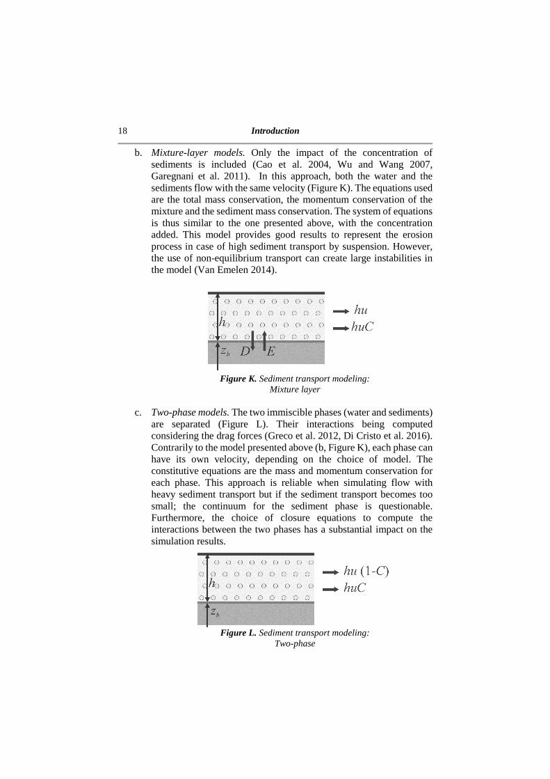
b. Mixture-layer models. Only the impact of the concentration of
sediments is included (Cao et al. 2004, Wu and Wang 2007, Garegnani et al. 2011). In this approach, both the water and the sediments flow with the same velocity (Figure K). The equations used are the total mass conservation, the momentum conservation of the mixture and the sediment mass conservation. The system of equations is thus similar to the one presented above, with the concentration added. This model provides good results to represent the erosion process in case of high sediment transport by suspension. However, the use of non-equilibrium transport can create large instabilities in the model (Van Emelen 2014).
Figure K. Sediment transport modeling:
Mixture layer
c. Two-phase models. The two immiscible phases (water and sediments) are separated (Figure L). Their interactions being computed considering the drag forces (Greco et al. 2012, Di Cristo et al. 2016). Contrarily to the model presented above (b, Figure K), each phase can have its own velocity, depending on the choice of model. The constitutive equations are the mass and momentum conservation for each phase. This approach is reliable when simulating flow with heavy sediment transport but if the sediment transport becomes too small; the continuum for the sediment phase is questionable. Furthermore, the choice of closure equations to compute the interactions between the two phases has a substantial impact on the simulation results.
Figure L. Sediment transport modeling:
Two-phase

Introduction 19
d. Two-layer models. The sediments are represented by a layer of
transport at the bottom of the channel with a layer of water flowing on top of it (Fraccarollo et al. 2003, Zech et al. 2008, Spinewine and Capart 2013), as presented in Figure M. This model thus completely separates bed load (bottom layer) and suspension load (top layer). Each layer can have its own velocity and concentration depending on the choice of model. The most complex models define the velocity and the concentration in the top layer as constant while a linear profile is imposed in the bottom layer with a constant concentration and a zero velocity in the bed. In this approach, the mass and momentum equations are written for each layer, with exchange possible. This model can give good results in 1D in rectangular channels. However, the definition of the bed transport layer becomes much more complex when studying arbitrary cross-sections.
Figure M. Sediment transport modeling:
Two-layer In this research, the first approach, corresponding to clear-water layer models (Figure J), will be used with a one-dimensional model. This approach has been favored here because these models are often more stable (Van Emelen 2014) and they require less calibration parameters. In addition, the thesis focuses on the transport of non-cohesive materials such as sand and these sediments are often transported by bedload, resulting in a negligible concentration in the water column. The equations are the shallow water equations, the conservation of water mass and momentum and the Exner equation, the conservation of sediment mass. Using a one-dimensional model adapted for rivers, the equations are area-averaged and written as:
∂A
∂t+ ∂Q
∂x=0 (i)

20 Introduction
∂Q
∂t+ ∂
∂xQ2
A+gI1 =gI2+AS0-Sf (ii)
∂Ab
∂t+ ∂
∂x Qs
1-0=0 (iii)
where Q is the discharge, A the wetter area, Ab is the area of the bed of sediments (Figure N), Qs the sediment transport and ε0 the bed porosity, S0 the bed slope and Sf the friction slope. The integral gI1 represents the hydrostatic pressure thrust while the integral gI2 represents the longitudinal component of the lateral pressure due to the longitudinal width changes. For the Exner (iii) equation, the assumption is made that the porosity is constant in both space and time.
Figure N. Definition of the area of sediments
If the sediments are not considered, as in the first part of the thesis, the equation used are the shallow water equations (the first two equations) only. The system of the three equations ((i) to (iii)) can be written as
∂U∂t
+∂F∂x
=S (iv)
with UUUU the conserved variables, FFFF the fluxes and S the source terms.
Introduction 21
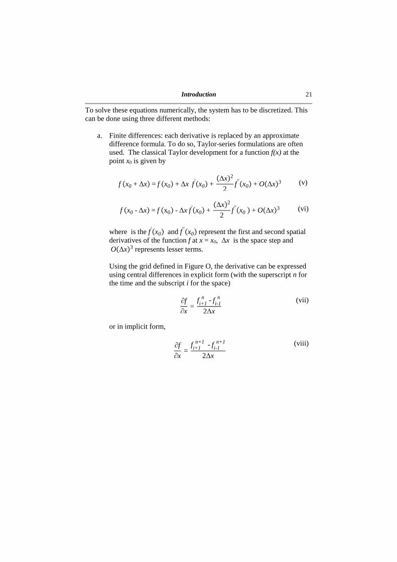
To solve these equations numerically, the system has to be discretized. This can be done using three different methods:
a. Finite differences: each derivative is replaced by an approximate difference formula. To do so, Taylor-series formulations are often used. The classical Taylor development for a function f(x) at the point x0 is given by fx0+∆x=fx0+∆xf'x0+ ∆x2
2f''x0+O∆x3 (v)
fx0-∆x=fx0-∆xf'x0+ ∆x22
f''x0+O∆x3 (vi)
where is the f'x0 and f''x0represent the first and second spatial derivatives of the function f at x = x0, ∆x is the space step and O∆x3 represents lesser terms. Using the grid defined in Figure O, the derivative can be expressed using central differences in explicit form (with the superscript n for the time and the subscript i for the space)
∂f
∂x= fi+1
n -fi-1n2∆x
(vii)
or in implicit form,
∂f
∂x= fi+1
n+1-fi-1n+1
2∆x
(viii)

22 Introduction
_ Figure O. Finite Difference grid
Several schemes have been presented in the literature to solve the shallow water equations. Here, two of the most common schemes will be briefly presented; one is the explicit MacCormack scheme and, and the other the implicit Preissmann scheme. The MacCormack scheme (MacCormack 1969; Chaudhry 2008) uses a two-step predictor-corrector method. First, the predictor (superscript p) uses a backward finite-difference on the spatial derivative, writing
∂U∂t
=Uip-Ui
n
∆t
(ix)
∂F∂x =Fi
n-Fi-1n
∆x
(x)
The predictor-step values of the conserved variables are computed as
Uip=Ui
n- ∆t
∆xFi
n-Fi-1n -Si
n∆t (xi)
Using the values of the conserved variables obtained with the predictor step, the fluxes and the source terms are computed. Then, the corrector (superscript c) step uses these values with a forward finite-difference on the spatial derivative, writing
∂U∂t
=Ui
c-Uin
∆t
(xii)

Introduction 23
∂F∂x =
Fi+1p -Fi
p
∆x
(xiii)
The corrector-step values of the variables are thus computed as
Uic=Ui
n- ∆t
∆xFi+1
p -Fip-Si
p∆t
(xiv)
Finally, the updated conserved variables for the time n+1 are given by the arithmetic average of the variables obtained by the predictor and the corrector steps as
Uin+1=Ui
c+Uip
2
(xv)
For the Preissmann scheme (Preissmann 1961; Wu 2008; Sart et al. 2010), a modified central difference is used to compute the derivatives. Using weight coefficient (ψ and θ), a function f and its spatial and time derivatives are written as f=θψfi+1
n+1+1-ψ fin+1+1-θψfi+1n +1-ψfin (xvi)
∂f
∂t=ψ fi+1
n+1-fi+1n
∆t+1-ψ fi
n+1-fin∆t
(xvii)
∂f
∂x=θ fi+1
n+1-fin+1
∆t+1-θfi+1
n -fin∆t
(xviii)
The weight coefficient ψ and θ must be chosen to achieve the best results. Considering the time weighting factor, two extremes can be highlighted: depending on whether is equal to zero or one, the scheme will be purely explicit or implicit, respectively. Usually, a value of 1/2 is set forψ while is between 0.6 and 0.7.
b. Finite volume approaches solve the integral form of the equations. In this method, the domain is divided into different control volumes, called cells. In each cell, the conserved variables are considered to have a constant value (for the first-order method). The updated values of the conserved variables are obtained by determining the fluxes at

24 Introduction
the interfaces between the cells (Figure P). This equation can be written as
Uin+1=Ui
n+ ∆t
∆xFi-1/2
* -Fi+1/2* +S∆t
(xix)
Figure P. Finite volumes scheme
The difficulty in the use of the finite volume method is the determination of the fluxes at the interfaces. The value of the conserved variable being known only in the cells, a Generalized Riemann Problem need to be solved across the cell interface (Figure Q). To solve this Riemann problem, several approaches are available in the literature (see Erduran et al. 2002 or Zoppou and Roberts 2003 for comparisons between numerical schemes). The most frequent models used are based on either the Roe scheme (Roe 1981; Murillo and García-Navarro 2014) or HLL scheme (Harten et al. 1983; Petaccia et al. 2013). These two approaches mostly differ in the computation of the waves celerities . While the first one computed the waves celerities by solving the approximate Riemann problem exactly, the second uses an approximate solution. For instance, for the pure hydrodynamic model, without integration of the source terms, the fluxes at the interface (F*) and the celerities are computed as
F/* = λ
+ Fi -λ- Fi+1-λ+λ
-Ui -Ui+1λ
+-λ- (xx)

Introduction 25
λHLL+ =max Qi
Ai
+!gAi
Bi
, Q
i+1
Ai+1
+!gAi+1
Bi+1
,0" (xxi)
λHLL- =min Qi
Ai
-!gAi
Bi
, Q
i+1
Ai+1
-!gAi+1
Bi+1
,0" (xxii)
λROE± =#Ai
Qi
Ai+#Ai+1
Qi+1
Ai+1 #Ai+#Ai+1 ±!g
2(Ai+1Bi+1
+Ai
Bi
) (xxiii)
Figure Q. Example of a Riemann problem for a
system of two equations
Equations (xxi) to (xxiii) clearly shows that the computation of the wave celerities is more complex for the Roe scheme than for the HLL scheme. Moreover, adding equations to the model (by including the sediment transport) increases this complexity gap between HLL and Roe models.
26 Introduction
Another important factor when solving the shallow water (with or without Exner) with a finite volume method is the inclusion of the source terms in the computation of the fluxes. This is important as it improves the stability and reliability of the schemes.
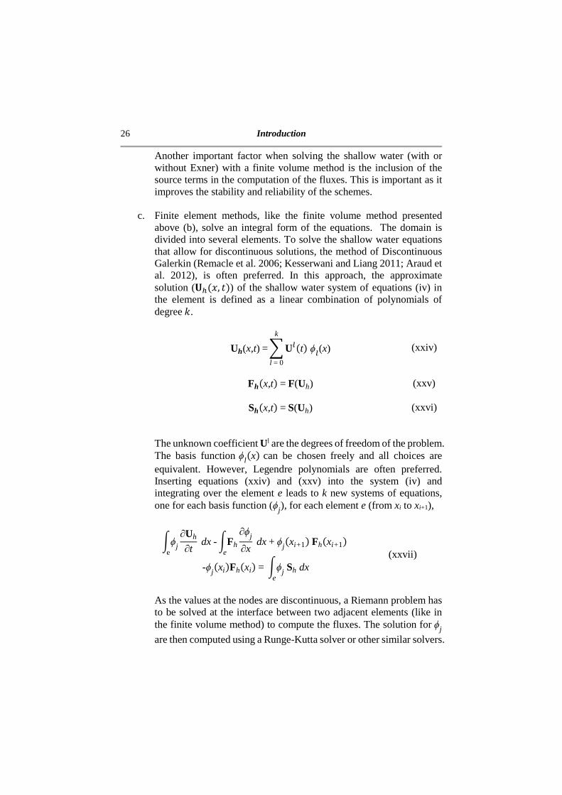
c. Finite element methods, like the finite volume method presented above (b), solve an integral form of the equations. The domain is divided into several elements. To solve the shallow water equations that allow for discontinuous solutions, the method of Discontinuous Galerkin (Remacle et al. 2006; Kesserwani and Liang 2011; Araud et al. 2012), is often preferred. In this approach, the approximate solution ($%&, ') of the shallow water system of equations (iv) in the element is defined as a linear combination of polynomials of degree(.
Uh(x,t)=)U*t ϕ*(x)
k
l=0 (xxiv)
Fhx,t=F(Uh) (xxv)
Shx,t=S(Uh) (xxvi)
The unknown coefficient Ul are the degrees of freedom of the problem. The basis function ϕl
x can be chosen freely and all choices are equivalent. However, Legendre polynomials are often preferred. Inserting equations (xxiv) and (xxv) into the system (iv) and integrating over the element e leads to k new systems of equations, one for each basis function (ϕj), for each element e (from xi to xi+1),
+ϕje
∂Uh
∂t dx-+Fh
e
∂ϕj
∂x dx+ϕj
xi+ 1Fhxi+ 1 -ϕjxiFhxi=+ϕj Sh dx
e
(xxvii)
As the values at the nodes are discontinuous, a Riemann problem has to be solved at the interface between two adjacent elements (like in the finite volume method) to compute the fluxes. The solution for ϕj
are then computed using a Runge-Kutta solver or other similar solvers.

Introduction 27
In the research presented here, the finite volumes are preferred as they have intrinsically better conservation and shock-capturing properties. Also, for fast transient flows like dam-break flows, high-order spatial accuracy, as can be achieved with high-order polynomial functions in each element, does not improve the results. More details on the comparison between Roe based and HLL based models and on the inclusion of the source terms in the models will be discussed in chapters I and IV. The present thesis aims at improving models for fast transient free-surface flows in rivers with intense sediment transport and significant morphological changes of the valley such as what happened during the Ha!Ha! dike failure. However, due to the important complexity of the Ha!Ha! flood, this event will not be simulated in this thesis. The thesis focuses mainly on the use and development of 1D models, with the aim of addressing the key problems encountered in real cases, that can be highlighted through the example of the Lake Ha!Ha! event. First, the hydrodynamic modeling of the flow in a river is investigated. Indeed, before modeling the sediment transport, it is important to ensure that the water levels and discharges are correctly predicted. Then, the impact of the sediment transport on the flow and on the morphology of the river is studied. Moreover, these one-dimensional models incorporate some 2D phenomena such as the presence of islands, the non-uniform erosion and the bank failure. In addition, several experiments have been realized to validate the models and highlight possible improvements. These experiments focused on new methods to capture the water level, on the failure of a non-cohesive dike by overtopping and on the transition between fixed and mobile bed in steep sloped channels. This thesis is divided into two main parts; each part being divided into three chapters. The first part focuses on hydrodynamic modeling of the flow in rivers while the second studies the impact of the sediment transport. The focus of each chapter is described below. As all chapters are written in a form suitable for submission to disciplinary conferences and journals, the choice was made not to present the complete review of the literature in an independent chapter. The corresponding literature reviews are included separately in each chapter.

28 Introduction
Chapter I – Efficiency and accuracy of Lateralized HLL, HLLS and Augmented Roe’s scheme with energy balance for river flows in irregular channels. (Published in Journal of Applied Mathematical Modeling) The first chapter of the thesis focuses on the modeling of the hydrodynamic part of the problem. Three types of models are presented. As presented before, all three models solve the shallow water equations using a finite volume model. Moreover, all three are developed to simulate the flow in arbitrary topographies using a one-dimensional approach. The difference lies in their different methods in computing the fluxes at the interfaces between the cells (celerities and source term inclusion). First the governing equations (the shallow water equations) and the three models are presented. Then, the models are compared using a variety of tests ranging from analytical solutions to real river flow simulations, and comprising both steady and unsteady flows.
Chapter II – Modeling the flow around islands in rivers using a one-dimensional approach (extended version of the article submitted to Simhydro 2017 conference) In the second chapter, one limit of one-dimensional modeling is addressed: the simulation of the flow around an island (Figure R). At the island, the channel is divided into two sub-channels. The bifurcation, before the island, and the junction, after the island, are modeled using inner boundary conditions. The domain is thus divided in four parts: the upstream channel, the two sub-channels around the island and the downstream channel. The equations used for the connections are the conservation of the discharge, the characteristics and the conservation of the water head. Four cases are considered: subcritical junction, subcritical bifurcation, supercritical junction and supercritical bifurcation. The one-dimensional model is compared to a full two-dimensional model for elementary numerical tests and shows good results in estimating the water level and the discharge partition.

Introduction 29
Figure R. Island on the Meuse River (credits Google Maps)
Chapter III – Measurement of the free-surface elevation in a steady flow in complex topography using photogrammetry (Published in the proceedings of Riverflow 2016) The third chapter presents a new measurement technique for experiments in pure hydrodynamics. In these tests, the use of photogrammetry to capture the evolution of the water level is analyzed. Photogrammetry uses stereoscopic pictures to reconstruct the 3D geometry of the captured object. This technique will allow capturing the water level evolution in the laboratory much more efficiently than the techniques used currently. Photogrammetry results could then be used to validate models and better study their limits. It has been used for a long time to capture non-moving object. However, capturing the evolution of the water level presents some difficulties such as the transparency of the water and the fact that the water is constantly moving, even in steady state. Solutions to these problems are proposed and tested for a steady state flow in an arbitrary topography. Finally, limitations of the current technique and potential improvements are presented.
Chapter IV– One-dimensional flow modeling with morphological evolution in arbitrary cross-sections (Submitted to International Journal for Numerical Methods in Fluids) The fourth chapter is the first chapter to consider sediment transport in the flow. In this chapter, four approaches are compared. All solve the shallow water and Exner equations but use different methods to compute the fluxes at
30 Introduction
the cell interfaces. Two approaches use an uncoupled model, solving the water before the sediment while the other two approaches solve all equations simultaneously. Each approach (uncoupled and coupled) then uses one of the two methods to compute the fluxes: HLL-based or Roe-based models. The sediment transport models can thus be considered as extensions of the hydrodynamic models presented in Chapter I. Special problems of non-uniform erosion and bank failure are also investigated. The models are then compared based on a variety of tests, both analytical and experimental. Finally, the strengths and weaknesses of the four approaches are highlighted.
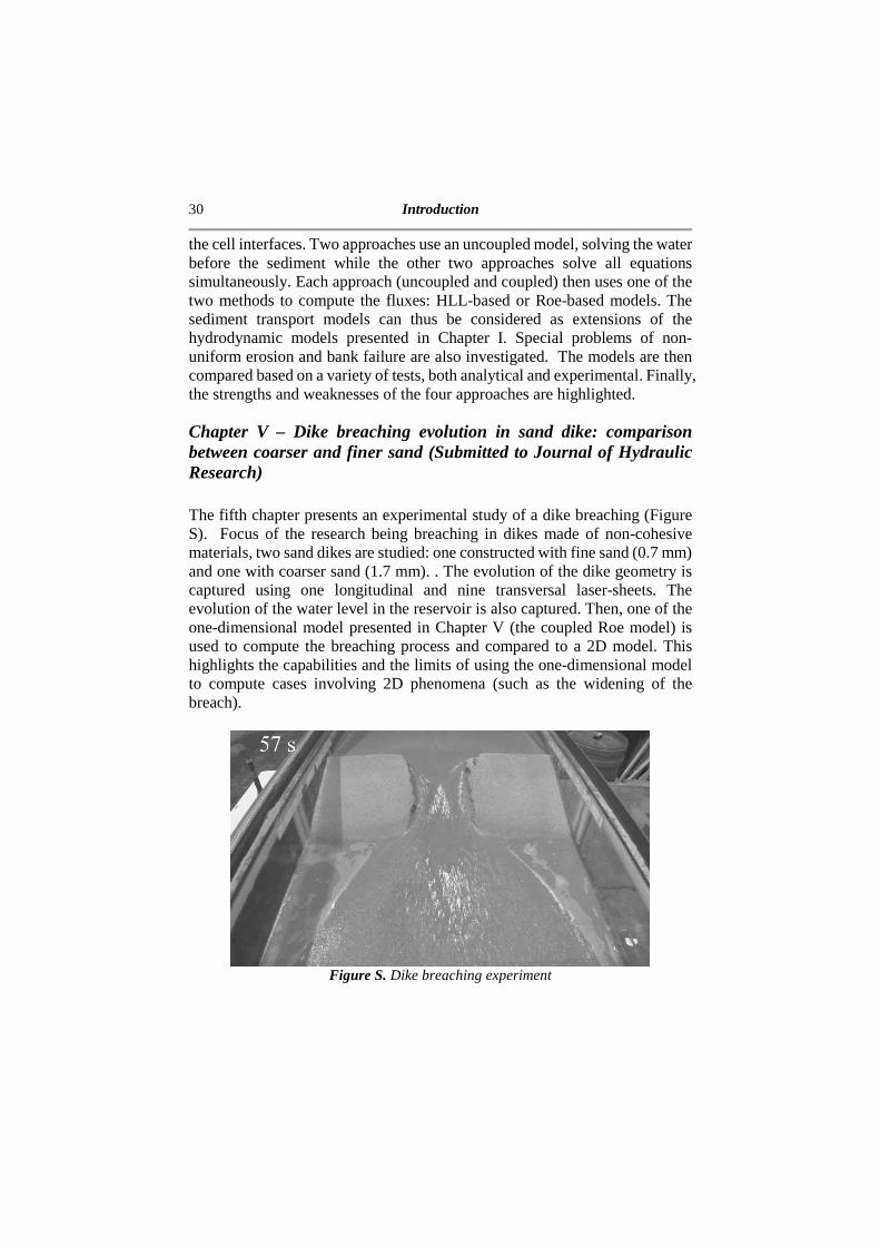
Chapter V – Dike breaching evolution in sand dike: comparison between coarser and finer sand (Submitted to Journal of Hydraulic Research) The fifth chapter presents an experimental study of a dike breaching (Figure S). Focus of the research being breaching in dikes made of non-cohesive materials, two sand dikes are studied: one constructed with fine sand (0.7 mm) and one with coarser sand (1.7 mm). . The evolution of the dike geometry is captured using one longitudinal and nine transversal laser-sheets. The evolution of the water level in the reservoir is also captured. Then, one of the one-dimensional model presented in Chapter V (the coupled Roe model) is used to compute the breaching process and compared to a 2D model. This highlights the capabilities and the limits of using the one-dimensional model to compute cases involving 2D phenomena (such as the widening of the breach).
Figure S. Dike breaching experiment
Introduction 31
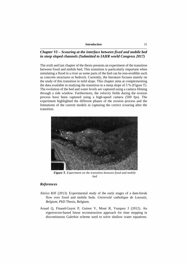
Chapter VI – Scouring at the interface between fixed and mobile bed in steep sloped channels (Submitted to IAHR world Congress 2017) The sixth and last chapter of the thesis presents an experiment of the transition between fixed and mobile bed. This transition is particularly important when simulating a flood in a river as some parts of the bed can be non-erodible such as concrete structures or bedrock. Currently, the literature focuses mainly on the study of this transition in mild slope. This chapter aims at complementing the data available in studying the transition in a steep slope of 5 % (Figure T). The evolution of the bed and water levels are captured using a camera filming through a side window. Furthermore, the velocity fields during the erosion process have been captured using a high-speed camera (500 fps). The experiment highlighted the different phases of the erosion process and the limitations of the current models in capturing the correct scouring after the transition.
Figure T. Experiment on the transition between fixed and mobile
bed
References Aleixo RJF (2013). Experimental study of the early stages of a dam-break
flow over fixed and mobile beds. Université catholique de Louvain, Belgium, PhD Thesis, Belgium.
Araud Q, Finaud-Guyot P, Guinot V, Mosé R, Vazquez J (2012). An eigenvector-based linear reconstruction approach for time stepping in discontinuous Galerkin scheme used to solve shallow water equations.

32 Introduction
International Journal for Numerical Methods in Fluids, 70 (12), 1590-1604.
Cao Z, Pender G, Wallis S, Carling PA (2004). Computational dam-break hydraulics over erodible sediment bed. Journal of Hydraulic Engineering, 130(7), 689–703.
Capart H, Spinewine B, Young DL, Zech Y, Brooks GR, Leclerc M, Secretan Y (2007). The 1996 Lake Ha! Ha! breakout flood, Quebec: Test data for geomorphic flood routing methods. Journal of Hydraulic Research, 45, 97–109.
Chaudhry MA (2008). Open-channel flow. Springer, Boston, USA.
Cunge JA, Perdreau N (1973). Mobile bed fluvial mathematical models. Houille Blanche, 28(7), 561–580.
Di Cristo C, Greco M, Iervolino M, Leopardi A, Vacca A (2016) Two-dimensional two-phase depth-integrated model for transients over mobile bed. Journal of Hydraulic Engineering, 142 (2).
El Kadi Abderrezzak K, Paquier A (2011). Applicability of sediment transport capacity formulas to dam-break flows over movable beds. Journal of Hydraulic Engineering, 137 (2), 209-221.
Erduran KS, Kutija V, Hewett JM (2002). Performance of finite-volume solutions to the shallow water equations with shock-capturing schemes. International Journal for Numerical Methods in Fluids, 40, 1237-1273.
Finaud-Guyot P, Delenne C, Guinot V (2011). Coupling of 1D and 2D models for river flow modelling. Houille Blanche, (3), 23-28.
Fraccarollo L, Capart H, Zech Y (2003). A Godunov method for the computation of erosional shallow water transient. Intl. J. Numer. Meth. Fluids, 41, 951–976.
Garegnani G, Rosatti G, Bonaventura L (2011). Free surface flows over mobile bed: mathematical analysis and numerical modeling of coupled and decoupled approaches. Commun. Appl. Indus. Math, 3(1), 1–22.
Goutière L, Soares-Frazão S, Savary C, Laraichi T, Zech Y (2008). One-dimensional model for transient flows involving bedload sediment transport and changes in flow regimes. Journal of Hydraulic Engineering, 134(6), 726–735.

Introduction 33
Greco M, Iervolino M, Vacca A, Leopardi A (2012). Two-phase modelling of
total sediment load in fast geomorphic transients. Proc. Int. Conf. on Fluvial Hydraul. - River Flow 2012, 1, 643–648.
Harten A, Lax PD, Van Leer B (1983). On upstream differencing and Godunov type schemes for hyperbolic conservation laws. SIAM review, 25, 35-61.
Juez C, Murillo J, García-Navarro P (2014). A 2D weakly-coupled and efficient numerical model for transient shallow flow and movable bed. Advances in Water Resources, 71, 93-109.
Kassem AA, Chaudry MH (1998). Comparison of coupled and semicoupled numerical models for alluvial channels. Journal of Hydraulic Engineering; 124(8), 794–802.
Kesserwani G, Liang Q (2011). A conservative high-order discontinuous Galerkin method for the shallow water equations with arbitrary topography. International Journal for Numerical Methods in Engineering, 86 (1), 47-69.
Lacasta A, Morales-Hernández M, Murillo J, García-Navarro P (2014). An optimized GPU implementation of a 2D free surface simulation model on unstructured meshes. Advances in Engineering Software, 78, 1-15.
Lin CW, Chang WS, Liu SH., Tsai TT, Lee SP, Tsang YC, Shieh CL, Tseng CM (2011). Landslides triggered by the 7 August 2009 Typhoon Morakot in southern Taiwan. Engineering Geology, 123 (1-2), 3-12.
MacCormack RW (1969). The Effect of Viscosity in Hypervelocity Impact Cratering, Amer. Inst. Aero. Astro. 69-354.
Murillo J, Garcìa-Navarro P (2014). Accurate numerical modeling of 1D flow in channels with arbitrary shape. Application of the energy balanced property. Journal of Computational Physics, 231, 222-248.
Petaccia G, Natale L, Savi F, Velickovic M, Zech Y, Soares-Frazão S (2013). Flood wave propagation in steep mountain rivers. Journal of Hydroinformatics, 15(1), 120-137.
Preismann A (1961). Propagation des intumescences dans les canaux et les rivières. 1 Congres de l’Association française de Calcul, Grenoble, France.
34 Introduction
Remacle JF, Soares-Frazão S, Li X, Shephard MS (2006). An adaptive
discretization of shallow-water equations based on discontinuous Galerkin methods. International Journal for Numerical Methods in Fluids, 52 (8), 903-923.
Roe P (1981). Approximate Riemann solvers, parameter vectors, and difference schemes. Journal of Computational Physics, 43, 357-372.
Rosatti G, Murillo J, Fraccarollo L (2008). Generalized Roe schemes for 1D two-phase, free-surface flows over a mobile bed. Journal of Computational Physics, 227 (24), 10058-10077.
Sart C, Baume JP, Malaterre PO, Guinot V (2010). Adaptation of Preissmann’s scheme for transcritical open channel flows. Journal of Hydraulic Research, 48 (4), 428-440.
Soares-Frazão S, Zech Y (2002). Dam break in channels with 90° bend. Journal of Hydraulic Engineering, 128, 956-968.
Soares-Frazão S, Canelas R, Cao Z, Cea L, Chaudhry HM, Die Moran A, El Kadi K, Ferreira R, Cadórniga IF, Gonzalez-Ramirez N, Greco M, Huang W, Imran J, Le Coz J, Marsooli R, Paquier A, Pender G, Pontillo M, Puertas J, Spinewine B, Swartenbroekx C, Tsubaki R, Villaret C, Wu W, Yue Z, Zech Y (2012). Dam-break flows over mobile beds: Experiments and benchmark tests for numerical models. Journal of Hydraulic Research, 50 (4), 364-375.
Spinewine B, Capart H (2013). Intense bed-load due to a sudden dam-break. Journal of Fluid Mechanic, 731, 579-614.
Swartenbroekx C, Zech Y, Soares-Frazão S (2013). Two-dimensional two-layer shallow water model for dam break flows with significant bed load transport. International Journal for Numerical Methods in Fluids, 73 (5), 477-508.
Van Emelen S (2014). Breaching processes of river dikes: effects on sediment transport and bed morphology. Université catholique de Louvain, Belgium, PhD Thesis, Belgium.
Wu W (2008). Computational River Dynamics. Taylor & Francis, London UK.
Wu W, Wang SSY (2007). One-Dimensional Modeling of Dam-Break Flow over Movable Beds. Journal of Hydraulic Engineering, 133(1), 48–58.

Introduction 35
Wu W, Wang SSY (2008). One-dimensional explicit finite-volume model for
sediment transport with transient flows over movable beds. Journal of Hydraulic Research, 46 (1), 87-98.
Zech Y, Soares-Frazão S, Spinewine B, Le Grelle N (2008). Dam-break induced sediment movement: Experimental approaches and numerical modelling. Journal of Hydraulic Research, 46(2), 176–190.
Zoppou C, Roberts S (2003). Explicit schemes for dam-break simulations. Journal of Hydraulic Engineering, 129(1), 11-34.


HYDRODYNAMIC MODELING
[Franzini F., and Soares-Frazão S. (2016) Efficiency and accuracy of Lateralized HLL, HLLS and Augmented Roe's scheme with energy balance for river flows in irregular channels. Applied Mathematical Modelling, 40(17–18), 7427-7446]
The first chapter presents three one-dimensional finite-volume models to compute the flow in rivers without sediment transport or morphological changes. A hydrodynamic model is important in the case of the Ha!Ha! River flood to compute the initial conditions when the erosion process was not substantial or some part, during the flood, where erosion was less important (Figure I-1). This chapter forms the basis of the thesis with other building upon it. Chapter II will use one of the models presented here and include the simulation of the flow around islands. Chapter III will illustrate the use of photogrammetry to obtain more data to validate the models. Chapter IV will extend the approaches presented here to morphological changes.
Figure I-1. Picture taken after the Ha!Ha! River flood (Capart et al.
2007): some part did not suffer too many morphological changes

38 Chapter I
Abstract This paper compares three different 1D numerical schemes used to simulate transient flows in rivers. All these schemes solve the shallow-water equations in cross-sections of arbitrary shape. Two are based on the HLL approach (namely Lateralized HLL and HLLS) and one on Roe's approach (Augmented Roe's solver with energy balance). The goal of the work presented hereafter is to highlight the capabilities and weaknesses of each scheme. Varied test cases are examined, including water at rest, steady flows, transient flows and a real river. Three conditions necessary to accurately simulate pure hydrodynamic flows are checked: (1) well-balancedness (also called C-property), (2) correct prediction of water level and (3) correct prediction of discharge across and within cells. The results revealed that the Lateralized HLL scheme is unable to provide accurate predictions for the discharge within the cells. However, if the focus is only on the water level, it gives good results and is quite robust, as the discharge at the interfaces is correctly predicted. The HLLS and the Augmented Roe's scheme with energy balance give better solutions. Nevertheless, these schemes also show limitations: incorrect discharge at shocks in the cells, a problem shared by many other schemes, and difficulties to reach a perfect steady state when the topography is highly irregular.
I.1. Introduction Even though floods are not the deadliest natural hazards, they affect large populations and generate heavy damages. Predicting them accurately is thus important. Numerical simulations of these flows present major challenges, including the strong influence of irregular topography on the computed results. Therefore, it is of paramount importance to calculate the topographical source terms accurately. Moreover, to study these flows, on the field, 1D models are often preferred. This is mainly due to two advantages of 1D models over 2D (or 3D) models. First, the data needed for a 1D model does not have to be as detailed. Thus, the data collection is less expensive. Then, 1D models tend to be faster and time is an important factor during a crisis. Nevertheless, it is important to note that 1D models are not able to the 2D and 3D behaviors of the flow and are therefore not suitable to simulate flows with strong 2D and 3D components. To simulate flows in hydraulics, solvers mostly use Godunov-type methods (Godunov 1959). The finite-volume methods that solve local Riemann
Hydrodynamic Modeling 39
problems (Roe 1981; Harten, Lax and Van Leer 1983; Toro 1997) provide accurate results in cases without source terms. However, when the geometry of the channel is more complex -- not being prismatic nor having a horizontal bed --, these simple methods fail, as they are not able to satisfy, for example, the C-property (Vásquez-Cendón 1999), i.e. keeping water at rest. To solve this problem, several models were presented in the literature (Bermudez and Vásquez-Cendón 1994; Nujic 1995; Bradford and Sanders 2002; Audusse et al. 2004; Burguete and García-Navarro 2004; Delenne and Guinot 2012; Murillo and García-Navarro 2012; Petaccia et al. 2013; Murillo and García-Navarro 2013; Murillo and García-Navarro 2014; Audusse et al. 2015) most of them treat the source terms by including them in the fluxes computation. However, not all have been developed for completely arbitrary topographies. Moreover, it is often difficult to compare these models as each author uses a different set of test cases. Finally, tests on real rivers are hardly ever presented. Among these finite-volume models, two families can be identified: (1) Roe-type schemes (Roe 1981), solving the approximate Riemann problem exactly, and (2) HLL-type schemes (Harten et al. 1983), solving the approximate problem in an approximate way, i.e. with approximate values for the wave celerities. One of the latest developments in Roe's scheme for arbitrary topography is the Augmented Roe's solver with energy balance (Murillo and García-Navarro 2014). This modification of the classical Roe's scheme adds a stationary wave to represent the source terms that are computed considering the energy conservation. A Lateralized HLL scheme for arbitrary sections was developed by Petaccia et al. (2013). This scheme uses Nujic variation (Nujic 1995) for the mass flux and, also, a distribution of the source terms on the momentum fluxes over each side of the interface according to the wave celerities (Fraccarollo et al. 2003; Goutière et al. 2008). Lastly, Murillo and García-Navarro (2012) developed a HLL based model which takes the source terms into account considering an intermediate state. This model, called HLLS, was developed only for rectangular and prismatic sections. The goal of this paper is, first to extend the HLLS to arbitrary topographies, then to compare its behavior with the Augmented Roe with energy balance and the Lateralized HLL schemes. Several test cases are selected to highlight the behaviors of each scheme. These tests -- always with source terms -- include steady and transient flows. Each time, cases with and without friction are investigated. To conclude the tests, the case of the Brembo River is studied (Petaccia et al. 2013). This river is interesting to model as it features strong topographical source terms. Two important variables of the flow are checked

40 Chapter I
for each case: the water level and the discharge, both being highly important in case of a flood. Evaluating accurately the former will allow a correct prediction of the flooded area. The latter is also important as the flow velocity can increase the damage during a flood, for example by inducing morphological changes. The paper is organized as follows: in sections I.2 and I.3, the 1D shallow water equations for arbitrary cross-sections and the different models are presented. Then, these models are compared to the panel of steady and transient tests in section 1.4. Finally, conclusions are drawn.
I.2. Governing equations This section presents one-dimensional shallow water equations. These governing equations, also called Saint-Venant equations, represent the conservation of the water mass and momentum. They consider a hydrostatic pressure and an incompressible fluid. For cross-sections of arbitrary shape, they read
∂A
∂t+
∂Q
∂x=0 (I.1)
∂Q
∂t+
∂
∂xQ2
A+gI1 =gI2+AS0-Sf (I.2)
Where Q is the discharge, A the area, g the gravity, S0 the bed slope defined by:
S0=- dzb
dx (I.3)
With zb the bed level –more precisely, the thalweg level. The integral gI1=g , h-ηb dηh
0 –with the water depth h and the width b – represents the
hydrostatic pressure thrust (see Figure I-2a) while the integral gI2=g, h-η ∂b
∂xdη
h
0 represents the longitudinal component of the lateral
pressure due to the longitudinal width variation. In these expressions, x is the longitudinal coordinate along the river thalweg and η is a local variable for the integration over the depth.

Hydrodynamic Modeling 41
Figure I-2. (a) Definition of the hydrostatic pressure. (b) Definition of the area for the Lateralized HLL model
It is possible to link those two integrals, which allows using a coupled formulation for the source terms, as first introduced by Cunge et al. (1980) and exploited by Capart et al. (2003) for finite-volume computations. Using Leibniz integral rule, the derivative of I1 could be written as:
g∂I1
∂x= gA
∂h
∂x+ gI2 (I.4)
Using the relation between the two integrals I1 and I2, it is possible to obtain different formulations for the topographical source terms. g (I2 +AS0)= g-∂I1
∂x-A∂h
∂x+AS0. (I.5)
g (I2 +A S0)= g-∂I1
∂x-A∂z
∂x. (I.6)

42 Chapter I
g (I2 +AS0)= g∂I1
∂x/z0 (I.7)
With z a suitable constant water level. The Manning formula models the friction term as
Sf =n2Q2P 4/3
A10/3 (I.8)
With the wetted perimeter P and the roughness coefficient n. The system of equations (I.1) and (I.2) will be hereafter written in vector form as
∂U∂t
+∂F∂x=S (I.9)
with U the vector of conserved variables (A,Q)T, F the vector of fluxes (Q,Q2/A+gI1)T and S the source terms (0,g[I2 +A(S0-Sf )])T. The source terms are often divided into topographical source terms Sg = (0,g(I2 +A S0))T and friction source terms Sτ=(0,-gASf )T, i.e. S = Sg + Sτ
I.3. Numerical models System (I.9) is discretized using a first-order finite-volume scheme
Uin+1=Ui
n+∆t
∆xFi-1/2
* -Fi+1/2* +S∆t (I.10)
The next sections describe how this equation is solved using the three different models (Lateralized HLL, HLLS and Augmented Roe's solver with energy balance).
Hydrodynamic Modeling 43
I.3.1. Lateralized HLL This model was developed for cross-sections of arbitrary shape (Petaccia et al. 2013). It consists of a modified HLL (Harten et al. 1983) with the topographical source terms introduced in the fluxes computation. Equation (I.10) thus becomes:
Uin+1=Ui
n+∆t
∆xFi-1/2
*R -Fi+1/2*L +Sτ ∆t (I.11)
The topographical source terms are distributed according to the waves celerities to the fluxes on each side of the interface (Bermudez and Vásquez-Cendón 1994; Fraccarollo et al. 2003), the difference between the flux on the right side and on the left side being F*R−F*L=Sg ∆x. As the topographical source in the mass flux is equal to zero, only the momentum is influenced: 4i+1/2
*L = λ+4i -λ-4i+1-λ+λ
-(Qi -Qi+1)
λ+-λ- +
λ-g∆I1|zλ
+ -λ- (I.12)
4i+1/2*R = λ+4i -λ-4i+1-λ+
λ-(Qi -Qi+1)
λ+ -λ- + λ+g ∆I1|zi+100000
λ+ -λ-
(I.13)
With 4 = Q 2/A + g I1 The topographical source terms are written considering the coupling between I1 and I2 (Soares-Frazão 2002; Capart et al. 2003) developed in (I.5) to (I.7) and ∆ represents the spatial difference between the cell i+1 and i. To introduce the impact of the topographical source terms in the mass flux, the mass flux is also modified using the Nujic variation (Nujic 1995): the idea is to consider the water level instead of the water depth. This approach is extended to arbitrary topographies by considering the wetted area corresponding to an averaged water level 6 (Petaccia et al. 2013) (see Figure I-2b):
Qi+1/2* = λi+1/2
+ Qi -λi+1/2- Qi+1-λi+1/2
- λi+1/2+ (Ai -Ai,z-Ai+1+Ai+1,z)
λi+1/2+ -λi+1/2
- (I.14)
The waves celerities are written, as defined by Davis (1988) as:
44 Chapter I
λi+1/2
+ =max(ui +ci , ui+1+ci+1 , 0) (I.15)
λi+1/2- =min (ui -ci , ui+1-ci+1 , 0) (I.16)
With the velocity ui = Qi /Ai and celerity ci =#g Ai /Bi The friction source term is accounted for by a two-step method: first, the problem is solved without friction to obtain an intermediate solution; then, the friction term is calculated to obtain the final solution:
Uin+1=Ui
n+1/2+∆t Sτin+1/2 (I.17)
I.3.2. HLLS This model is another variation of the HLL model (Harten et al. 1983). It was developed for rectangular sections (Murillo and García-Navarro 2012) and is, here, extended to cross-sections of arbitrary shape. A stationary wave is added to represent the impact of the source terms in the fluxes determination. Here, both source terms (topographical and friction) are introduced in the flux computation, and Eq. (I.10) thus becomes:
Uin+1 = Ui
n + ∆t
∆xFi-1/2
*R - Fi+1/2*L (I.18)
This modification, considering a stationary wave, impacts both fluxes
Fi+1/2*L = λ+ Fi -λ- Fi+1-λ+
λ-Ui -Ui+1+λ-(S ∆x-λ+T)
λ+ -λ-
(I.19)
Fi+1/2*R = λ+ Fi-λ- Fi+1-λ+
λ-Ui -Ui+1+λ+(S ∆x-λ-T)
λ+ -λ-
(I.20)
The source terms are written as: S ∆x= 7 0
-gA8∆z+g∆I1-g A8 Sf8∆x9 (I.21)
Where the overbar denotes averaged variables, as described below.The impact of the stationary wave related to the source terms in the mass flux is represented as:

Hydrodynamic Modeling 45
T=-
1
λ+λ
- 7-gA8∆z+c2∆A-gA8 Sf8∆x
09 (I.22)
With
A8 = Ai + Ai+1
2
(I.23)
Sf8 = u:|u:|nini+1-Pi + Pi+1
Ai + Ai+1.4/3
(I.24)
It is important to note that the source terms in the mass flux and in the momentum flux, respectively represented by the vectors T and S are written in different ways. In the expression for T (Equation (I.22)), the term c2∆A appears, while in the expression for S (Equation (I.21)), it is written as g∆I1. These two writings are similar as, by definition, c2=∂I1/∂A. However, some really small differences in their discretized version can induce incorrect results for the water at rest. To illustrate the impact of the source term discretization in both T and S, the case of the water at rest is developed. When water is at rest, the water level is constant and the discharge is equal to zero; or written as equations:
zi-1=zi =zi+1 (I.25)
Qi-1=Qi =Qi+1 = 0 (I.26)
Considering these two relations, the fluxes entering cell i can be written, using Equations (I.20) to (I.22), as:
Fi-1/2*R = 7 0
gI1,i9 (I.27)
Similarly, for the flux leaving cell i (using Equations (I.19), (I.21) and (I.22)),
Fi+1/2*L = 7 0
gI1,i9 (I.28)
The obtained fluxes prove that no mass cross the interface (the first element of the vector is equal to zero).
46 Chapter I
Knowing the fluxes at the interfaces on both sides of the cell, the evolution of the conserved variables can be determined as:
∆U=∆t
∆xFi-1/2
*R -Fi+1/2*L (I.29)
∆U= ∆t
∆x-7 0
gI1,i9 - 7 0
gI1,i9. (I.30)
∆U=0 (I.31)
The conserved variables do not change, i.e. the water stays at rest. Thus, the model satisfies the C-property. Finally, instead of using Davis (1988) celerities, the HLLS uses those of Roe’s (Roe 1981):
λ+=u=+ c: (I.32) λ
-=u:-c: (I.33) Where,
u: = #Ai ui + #Ai+ 1 ui+1 #Ai + #Ai+1
(I.34)
c: = !g
2-Ai+1
Bi+1+
Ai
Bi. (I.35)
I.3.3. Augmented Roe’s solver with energy balance This model is a variation of Roe’s solver (Roe 1981). It was developed for rectangular (Murillo and García-Navarro 2012; Murillo and García-Navarro 2013) and arbitrary (Murillo and García-Navarro 2014) cross-sections. The classical Roe model considered a linearized problem, meaning that the Jacobian matrix of the system of equations (equation (I-36)) is approximated as (I-37) where the terms are constant values depending on the actual values at the left and right side of the considered interface.

Hydrodynamic Modeling 47
> =
∂@∂$ = A 0 1C − E 2EG (I-36)
>H = ∂@∂$ = A 0 1C − E: 2E:G (I-37)
These approximations need to fulfill some conditions. First, the eigenvalues of the approximate Jacobian (the wave celerities) must be real and have the same form as the classical one. Secondly, the approximate Jacobian must be equal to the exact Jacobian for a continuous solution, when the values on both sides of the interface are equal. Thirdly, the approximate Jacobian should satisfy the flux variation condition. To satisfy these conditions, the waves celerities, as defined by Roe (1981), are:
λ1 = u:- c: (I.38)
λ2 = u: + c: (I.39) Where,
u: = #Ai ui + #Ai+ 1 ui+1 #Ai + #Ai+1
(I.40)
c: = !g
2-Ai+1
Bi+1+
Ai
Bi. (I.41)
The wave strengths and eigenvectors are:
α1 = λ2∆A - ∆Q
2c: (I.42)
α2= - λ1∆A - ∆Q
2c: (I.43)
e1= 71λ19 (I.44)
e2= 71λ29 (I.45)
With this information, the fluxes can be expressed as

48 Chapter I
Fi+1/2* =Fi + )λαei+1/2
m
m
λm<0
(I.46)
As the source terms are not included in the flux computation for the classical Roe scheme, the fluxes both sides of the interface are equal. More details on the development of the Roe model can be found in the thesis written by Soares-Frazão (2002). The Augmented Roe, as the HLLS model, considers a stationary wave to represent the source terms. However, as it originates from Roe’s approach and not HLL, the resulting scheme is different. As for the HLLS model, Equation (I.10) is modified as follows, with the source terms incorporated in the fluxes:
Uin+1 = Ui
n + ∆t
∆xFi-1/2
*R - Fi+1/2*L (I.47)
The equations (I.46) for the fluxes are now written as:
Fi+1/2*L =Fi + )λαθei+1/2
m
m
λm<0
(I.48)
Fi+1/2*R =Fi+1- )λαθei+1/2
m
m
λm>0
(I.49)
The added term, θ, compared to the classical Roe is the stationary source terms wave represented by:
θ1=1+ ζ
2c:λ1α1 (I.50)
θ2=1+ ζ
2c:λ2α2 (I.51)
With the source terms:
ζ = ζg- gA8Sf8 ∆x (I.52)
The friction source terms are written with the averaged values:
A8 = Ai + Ai+1
2
(I.53)

Hydrodynamic Modeling 49
Sf8 = u:|u:|nini+1-Pi + Pi+1
Ai + Ai+1.4/3
(I.54)
To introduce the energy conservation, the topographical source terms are written as a linear combination of two expressions:
ζga= -gA8∆z+ c:2∆A (I.55)
ζgb= -gAmin∆z+c:2∆A (I.56)
These two expressions are combined using a weight coefficient ω:
ζg = 1-ωζga + ωζgb (I.57)
To define the weight coefficient ω, the energy and momentum conservation equations are combined. The energy conservation, in steady state and at the discrete level can be written as:
∆ Q2
2gA2 + z = - Sf8 ∆x (I.58)
gA8∆ Q2
2gA2 =-gA8∆z-gA8 Sf8 ∆x (I.59)
The momentum equation, in steady state and at the discrete level can be written as: ∆Q2
A+c:2∆A=1-ωζga+ωζgb-gA8 Sf
8∆x (I.60)
∆ Q2
A=-gA8∆z+ω ζgb-ζga -g A8Sf
8∆x (I.61)
By combining Equations (I.59) and (I.61), the weight coefficient is obtained as:
ω =
∆ Q2
A - A8 ∆Q2
2A2ζgb- ζga
(I.62)
50 Chapter I
In the case of a shock, where energy is not conserved but dissipated, ω = 0.
I.4. Results First, the well-balanced property, also called C-property (Bermudez and Vásquez-Cendón 1994; Vásquez-Cendón 1999), is verified. Then, steady and transient flows are investigated. And, finally, the schemes are tested on a real river case (Petaccia et al. 2013).
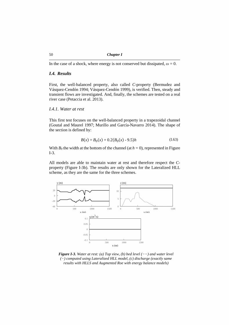
I.4.1. Water at rest This first test focuses on the well-balanced property in a trapezoidal channel (Goutal and Maurel 1997; Murillo and García-Navarro 2014). The shape of the section is defined by: Bx=B0x+0.2B0x-9.5h (I.63)
With B0 the width at the bottom of the channel (at h = 0), represented in Figure I-3. All models are able to maintain water at rest and therefore respect the C- property (Figure I-3b). The results are only shown for the Lateralized HLL scheme, as they are the same for the three schemes.
Figure I-3. Water at rest: (a) Top view, (b) bed level (−−) and water level (−) computed using Lateralized HLL model, (c) discharge (exactly same
results with HLLS and Augmented Roe with energy balance models)
-40
-20
0
20
0 500 1000 1500
x (m)
y (m)
0
5
10
0 500 1000 1500
x (m)
z (m)
-0.1
-0.05
0
0.05
0.1
0 500 1000 1500x (m)
q (m3/s)

Hydrodynamic Modeling 51
I.4.2. Steady flows I.4.2.1. Flows in a convergent-divergent frictionless channel For this test case (Murillo and García-Navarro 2014), the channel is frictionless, 25 m long and flat. The cross-sections are rectangular with the width (Figure I-4) defined by: B= min0.8+0.05x-102,1 (I.64)
Figure I-4. Steady flows in a convergent–
divergent channel: Top view.
First, a smooth transcritical flow without a shock is tested. At the inflow, the discharge is imposed at 4.42 m3/s; the outflow is let free (the flow is then supercritical with the critical section at x = 10 m). The schemes are compared using two different grid sizes: 0.5 m and 0.05 m. The Lateralized HLL predicts accurately the water level with a fine mesh, but with the coarse mesh of 0.5 m, the water level at the critical section is not accurately predicted (Figure I-5a). The discharge within cells is not conserved, with a significant error in the subcritical part of the flow. For the refined mesh, this error is smaller but still important (Figure I-5b). However the discharge across cells, i.e. the mass flux, is conserved (not shown). The Froude number (Figure I-5c) is poorly represented with the coarse mesh, the critical section being located too far downstream. The results for the refined mesh are better but still incorrect as can be observed in Table I-1, which indicates the value of the Froude Number at the narrowest section. At this section, the flow is supposed to be critical (Fr=1); this is not the case when using the Lateralized HLL, even when refining the mesh. Finally, the total head should be constant due to the absence of friction, but it is not the case here, even with the fine mesh.
-0.5
0
0.5
0 5 10 15 20 25
x (m)
y (m)
52 Chapter I
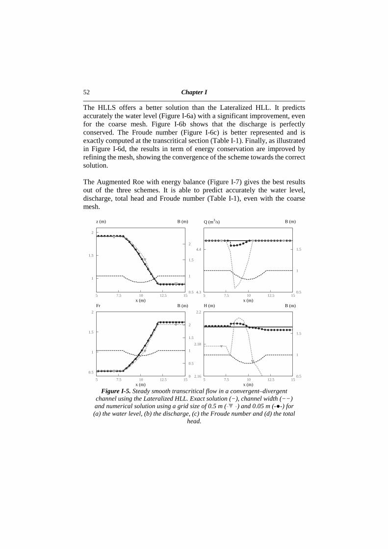
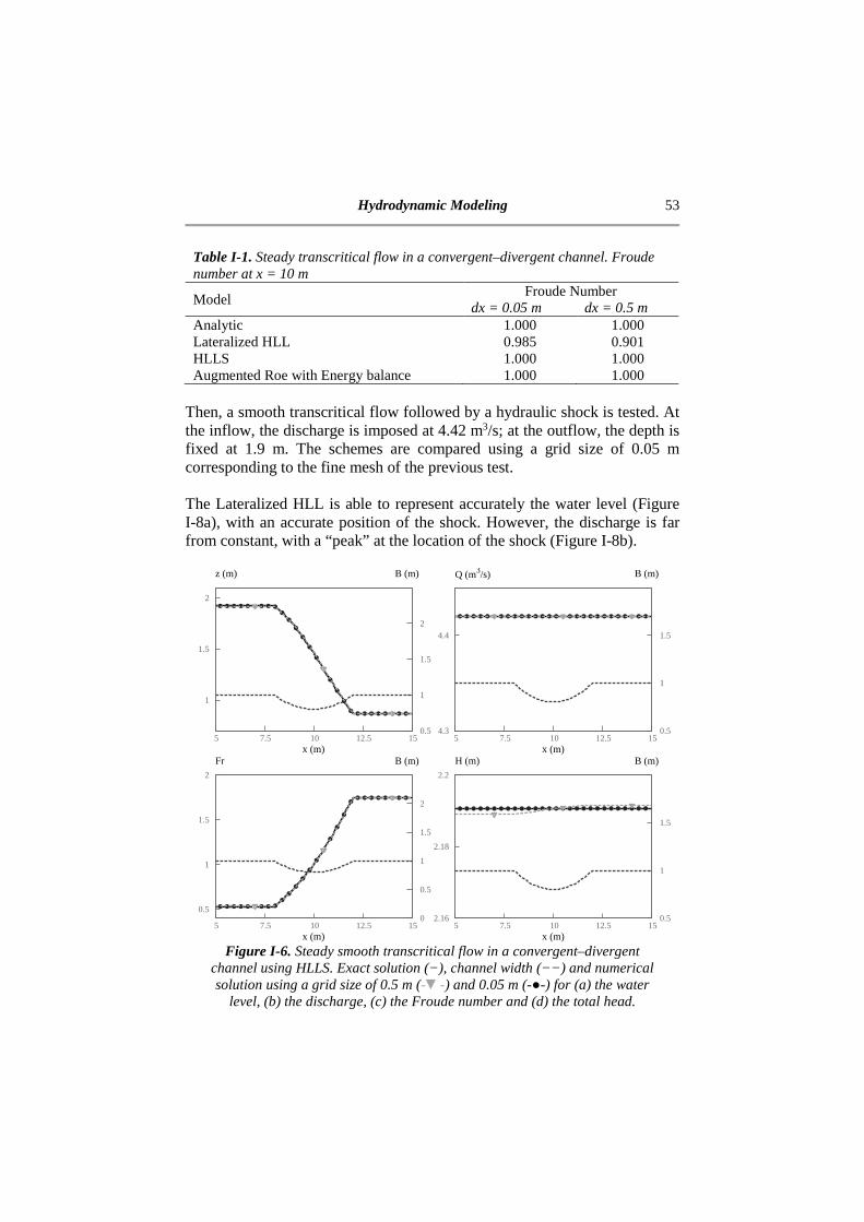
The HLLS offers a better solution than the Lateralized HLL. It predicts accurately the water level (Figure I-6a) with a significant improvement, even for the coarse mesh. Figure I-6b shows that the discharge is perfectly conserved. The Froude number (Figure I-6c) is better represented and is exactly computed at the transcritical section (Table I-1). Finally, as illustrated in Figure I-6d, the results in term of energy conservation are improved by refining the mesh, showing the convergence of the scheme towards the correct solution. The Augmented Roe with energy balance (Figure I-7) gives the best results out of the three schemes. It is able to predict accurately the water level, discharge, total head and Froude number (Table I-1), even with the coarse mesh.
Figure I-5. Steady smooth transcritical flow in a convergent–divergent
channel using the Lateralized HLL. Exact solution (−), channel width (−−) and numerical solution using a grid size of 0.5 m (--) and 0.05 m (--) for (a) the water level, (b) the discharge, (c) the Froude number and (d) the total
head.
1
1.5
2
5 7.5 10 12.5 15 0.5
1
1.5
2
B (m)
x (m)
z (m)
4.3
4.4
5 7.5 10 12.5 15 0.5
1
1.5
B (m)
x (m)
Q (m3/s)
0.5
1
1.5
2
5 7.5 10 12.5 15 0
0.5
1
1.5
2
B (m)
x (m)
Fr
2.16
2.18
2.2
5 7.5 10 12.5 15 0.5
1
1.5
B (m)
x (m)
H (m)
Hydrodynamic Modeling 53
Table I-1. Steady transcritical flow in a convergent–divergent channel. Froude number at x = 10 m
Model Froude Number
dx = 0.05 m dx = 0.5 m Analytic 1.000 1.000 Lateralized HLL 0.985 0.901 HLLS 1.000 1.000 Augmented Roe with Energy balance 1.000 1.000
Then, a smooth transcritical flow followed by a hydraulic shock is tested. At the inflow, the discharge is imposed at 4.42 m3/s; at the outflow, the depth is fixed at 1.9 m. The schemes are compared using a grid size of 0.05 m corresponding to the fine mesh of the previous test. The Lateralized HLL is able to represent accurately the water level (Figure I-8a), with an accurate position of the shock. However, the discharge is far from constant, with a “peak” at the location of the shock (Figure I-8b).
Figure I-6. Steady smooth transcritical flow in a convergent–divergent
channel using HLLS. Exact solution (−), channel width (−−) and numerical solution using a grid size of 0.5 m (--) and 0.05 m (--) for (a) the water
level, (b) the discharge, (c) the Froude number and (d) the total head.
1
1.5
2
5 7.5 10 12.5 15 0.5
1
1.5
2
B (m)
x (m)
z (m)
4.3
4.4
5 7.5 10 12.5 15 0.5
1
1.5
B (m)
x (m)
Q (m3/s)
0.5
1
1.5
2
5 7.5 10 12.5 15 0
0.5
1
1.5
2
B (m)
x (m)
Fr
2.16
2.18
2.2
5 7.5 10 12.5 15 0.5
1
1.5
B (m)
x (m)
H (m)

54 Chapter I
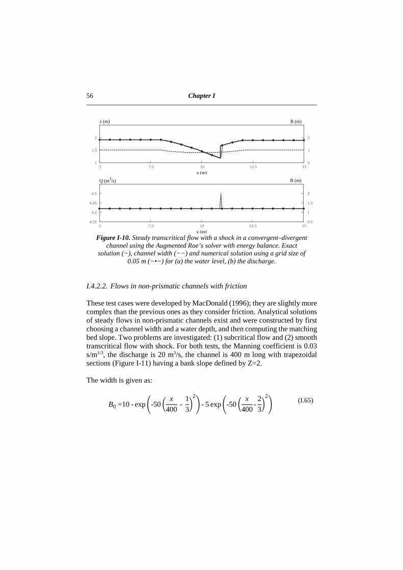
The HLLS is also able to represent accurately the water level and the shock position (Figure I-9a). The discharge is constant in every cell except one, at the location of the shock (Figure I-9b). The Augmented Roe scheme with energy balance is also able to represent accurately the water level. However, the shock position is incorrect as it is located too far downstream (Figure I-10a). This difference is caused by the energy balance computation. The weight coefficient (Equation (I.62)) is set to zero in case of a shock because, by definition, the energy is not conserved at the shock. This, however, creates a change in the treatment of source terms that induces a shift in the shock position. The discharge is constant in every cell except one, at the location of the shock (Figure I-10b).
Figure I-7. Steady smooth transcritical flow in a convergent–divergent channel
using the Augmented Roe’s solver with energy balance. Exact solution (−), channel width (−−) and numerical solution using a grid size of 0.5 m (--) and 0.05 m (--) for (a) the water level, (b) the discharge, (c) the Froude number and
(d) the total head
1
1.5
2
5 7.5 10 12.5 15 0.5
1
1.5
2
B (m)
x (m)
z (m)
4.3
4.4
5 7.5 10 12.5 15 0.5
1
1.5
B (m)
x (m)
Q (m3/s)
0.5
1
1.5
2
5 7.5 10 12.5 15 0
0.5
1
1.5
2
B (m)
x (m)
Fr
2.16
2.18
2.2
5 7.5 10 12.5 15 0.5
1
1.5
B (m)
x (m)
H (m)

Hydrodynamic Modeling 55
Figure I-8. Steady transcritical flow with a shock in a convergent–divergent channel using Lateralized HLL. Exact solution (−), channel width (−−) and numerical solution using a grid size of 0.05 m (−•−) for (a) the water level,
(b) the discharge.
Figure I-9. Steady transcritical flow with a shock in a convergent–divergent channel using HLLS. Exact solution (−), channel width (−−) and numerical
solution using a grid size of 0.05 m (−•−) for (a) the water level, (b) the discharge.
1
1.5
2
5 7.5 10 12.5 15 0
1
2
B (m)
x (m)
z (m)
4.35
4.4
4.45
4.5
5 7.5 10 12.5 15 0.5
1
1.5
2
B (m)
x (m)
Q (m3/s)
1
1.5
2
5 7.5 10 12.5 15 0
1
2
B (m)
x (m)
z (m)
4.35
4.4
4.45
4.5
5 7.5 10 12.5 15 0.5
1
1.5
2
B (m)
x (m)
Q (m3/s)
56 Chapter I
Figure I-10. Steady transcritical flow with a shock in a convergent–divergent
channel using the Augmented Roe’s solver with energy balance. Exact solution (−), channel width (−−) and numerical solution using a grid size of
0.05 m (−•−) for (a) the water level, (b) the discharge.
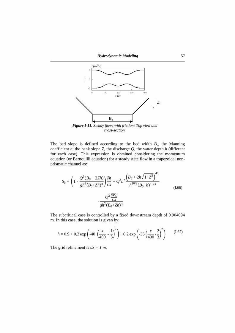
I.4.2.2. Flows in non-prismatic channels with friction These test cases were developed by MacDonald (1996); they are slightly more complex than the previous ones as they consider friction. Analytical solutions of steady flows in non-prismatic channels exist and were constructed by first choosing a channel width and a water depth, and then computing the matching bed slope. Two problems are investigated: (1) subcritical flow and (2) smooth transcritical flow with shock. For both tests, the Manning coefficient is 0.03 s/m1/3, the discharge is 20 m3/s, the channel is 400 m long with trapezoidal sections (Figure I-11) having a bank slope defined by Z=2. The width is given as:
B0=10- exp-50- x
400- 1
3.2 -5 exp-50- x
400-2
3.2
(I.65)
1
1.5
2
5 7.5 10 12.5 15 0
1
2
B (m)
x (m)
z (m)
4.35
4.4
4.45
4.5
5 7.5 10 12.5 15 0.5
1
1.5
2
B (m)
x (m)
Q (m3/s)
Hydrodynamic Modeling 57
Figure I-11. Steady flows with friction: Top view and
cross-section.
The bed slope is defined according to the bed width B0, the Manning coefficient n, the bank slope Z, the discharge Q, the water depth h (different for each case). This expression is obtained considering the momentum equation (or Bernouilli equation) for a steady state flow in a trapezoidal non-prismatic channel as:
S0= 1-Q2B0+2Zhgh3B0+Zh3 ∂h
∂x+Q2n2
B0+2h#1+Z24/3
h10/3B0+h10/3
-Q2 ∂B0
∂xgh2B0+Zh3
(I.66)
The subcritical case is controlled by a fixed downstream depth of 0.904094 m. In this case, the solution is given by: h=0.9+0.3 exp-40 - x
400- 1
3.2+0.2 exp-35- x
400-2
3.2
(I.67)
The grid refinement is dx = 1 m.
-5
0
5
0 100 200 300 400
y (m
)
x (m)
Q (m3/s)
Z
1
B0
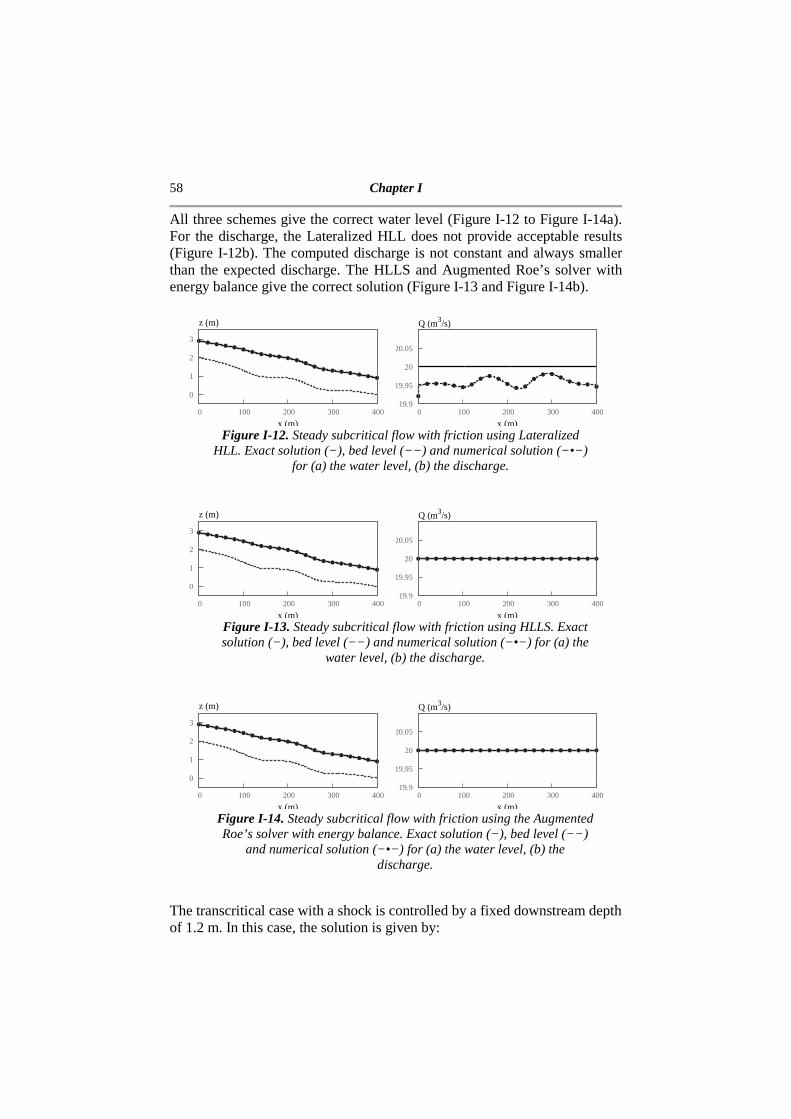
58 Chapter I
All three schemes give the correct water level (Figure I-12 to Figure I-14a). For the discharge, the Lateralized HLL does not provide acceptable results (Figure I-12b). The computed discharge is not constant and always smaller than the expected discharge. The HLLS and Augmented Roe’s solver with energy balance give the correct solution (Figure I-13 and Figure I-14b).
Figure I-12. Steady subcritical flow with friction using Lateralized
HLL. Exact solution (−), bed level (−−) and numerical solution (−•−) for (a) the water level, (b) the discharge.
Figure I-13. Steady subcritical flow with friction using HLLS. Exact solution (−), bed level (−−) and numerical solution (−•−) for (a) the
water level, (b) the discharge.
Figure I-14. Steady subcritical flow with friction using the Augmented Roe’s solver with energy balance. Exact solution (−), bed level (−−)
and numerical solution (−•−) for (a) the water level, (b) the discharge.
The transcritical case with a shock is controlled by a fixed downstream depth of 1.2 m. In this case, the solution is given by:
0
1
2
3
0 100 200 300 400
x (m)
z (m)
19.9
19.95
20
20.05
0 100 200 300 400
x (m)
Q (m3/s)
0
1
2
3
0 100 200 300 400
x (m)
z (m)
19.9
19.95
20
20.05
0 100 200 300 400
x (m)
Q (m3/s)
0
1
2
3
0 100 200 300 400
x (m)
z (m)
19.9
19.95
20
20.05
0 100 200 300 400
x (m)
Q (m3/s)
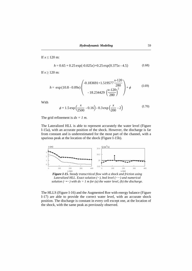
Hydrodynamic Modeling 59
If x≤120 m: h=0.65+0.25 exp-0.025x+0.25 exp0.375x-4.5 (I.68)
If x≥120 m:
h=exp (10.8-0.09x)JK-0.183691+1.519577
x-120
280
-18.234429 -x-120
280.2 L
M+ϕ (I.69)
With ϕ=1.5 exp x
2500-0.16 -0.3 exp x
200-2 (I.70)
The grid refinement is dx = 1 m. The Lateralized HLL is able to represent accurately the water level (Figure I-15a), with an accurate position of the shock. However, the discharge is far from constant and is underestimated for the most part of the channel, with a spurious peak at the location of the shock (Figure I-15b).
Figure I-15. Steady transcritical flow with a shock and friction using Lateralized HLL. Exact solution (−), bed level (−−) and numerical
solution (−•−) with dx = 1 m for (a) the water level, (b) the discharge.
The HLLS (Figure I-16) and the Augmented Roe with energy balance (Figure I-17) are able to provide the correct water level, with an accurate shock position. The discharge is constant in every cell except one, at the location of the shock, with the same peak as previously observed.
0
1
2
3
0 100 200 300 400
x (m)
z (m)
19.8
20
20.2
20.4
0 100 200 300 400
x (m)
Q (m3/s)
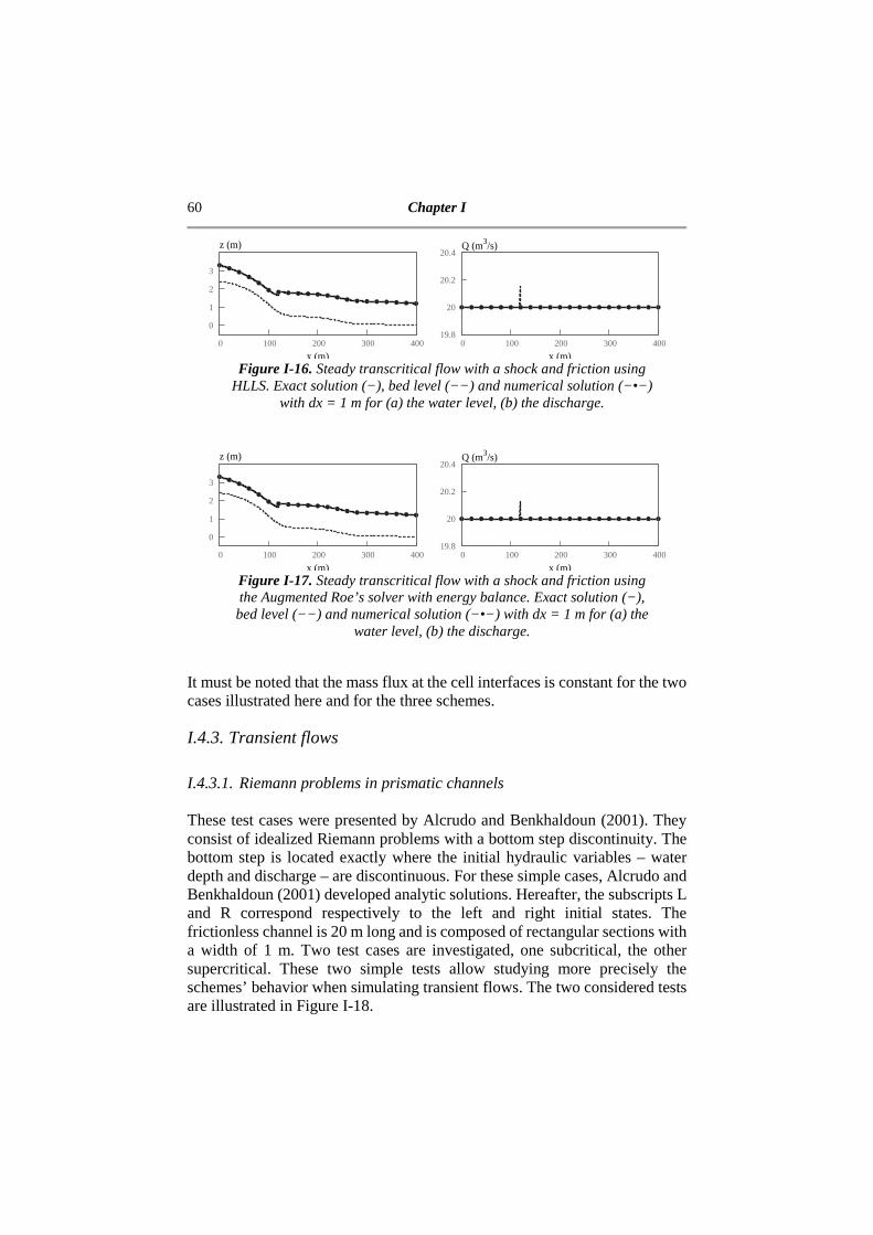
60 Chapter I
Figure I-16. Steady transcritical flow with a shock and friction using
HLLS. Exact solution (−), bed level (−−) and numerical solution (−•−) with dx = 1 m for (a) the water level, (b) the discharge.
Figure I-17. Steady transcritical flow with a shock and friction using the Augmented Roe’s solver with energy balance. Exact solution (−), bed level (−−) and numerical solution (−•−) with dx = 1 m for (a) the
water level, (b) the discharge.
It must be noted that the mass flux at the cell interfaces is constant for the two cases illustrated here and for the three schemes.
I.4.3. Transient flows I.4.3.1. Riemann problems in prismatic channels These test cases were presented by Alcrudo and Benkhaldoun (2001). They consist of idealized Riemann problems with a bottom step discontinuity. The bottom step is located exactly where the initial hydraulic variables – water depth and discharge – are discontinuous. For these simple cases, Alcrudo and Benkhaldoun (2001) developed analytic solutions. Hereafter, the subscripts L and R correspond respectively to the left and right initial states. The frictionless channel is 20 m long and is composed of rectangular sections with a width of 1 m. Two test cases are investigated, one subcritical, the other supercritical. These two simple tests allow studying more precisely the schemes’ behavior when simulating transient flows. The two considered tests are illustrated in Figure I-18.
0
1
2
3
0 100 200 300 400
x (m)
z (m)
19.8
20
20.2
20.4
0 100 200 300 400
x (m)
Q (m3/s)
0
1
2
3
0 100 200 300 400
x (m)
z (m)
19.8
20
20.2
20.4
0 100 200 300 400
x (m)
Q (m3/s)

Hydrodynamic Modeling 61
For the first, subcritical, test (Figure I-18a), the initial left side is characterized by hL = 4 m, QL = 0 m3/s and zbL = 0 m; the right side being hR = 1 m, QR = 0 m3/s and zbL = 1 m. The solution consists of a rarefaction spreading to the left, a subcritical transition and a shock moving to the right. The results are presented after 1 s using a grid refinement of dx = 0.1 m in Figure I-19 and Figure I-20.
Figure I-18. Transient Riemann problems, initial states: (a) subcritical,
(b) supercritical with the bed level (−), the water level (−•−) and the discharge (−×−).
All three schemes provide the correct water level (Figure I-19 and Figure I-20a). The Lateralized HLL predicts a correct discharge except near the step where it is underestimated (Figure I-19b). The small difference in the discharge is also present in the total head but is not as easily visible. The HLLS and the Augmented Roe with energy balance provide the correct discharge (Figure I-20b). As the results using the HLLS and the Augmented Roe’s solver with energy balance are the same, but only the latter is shown. For the second, supercritical, test (Figure I-18b), the initial left side is characterized hL = 1 m, QL = 6 m3/s and zbL = 1 m; the right side being hR = 4 m, QR = 40 m3/s and zbR = 0 m. The solution consists of a supercritical transition, a shock and a rarefaction. The results are presented after 0.5 s using a grid refinement of dx = 1 m in Figure I-21 and Figure I-22. The Lateralized HLL (Figure I-21) gives an accurate prediction of the water level and discharge before the step but presents some differences for the two constant states just after it (between 0 and 5 m). These differences are more easily visible in the total head where the drop occurs too close of the step (Figure I-21c). The HLLS and the Augmented Roe with energy balance provide the correct water level and discharge (Figure I-22). As the results using the HLLS and the Augmented Roe’s solver with energy balance are the same, but only the latter is shown.
0
1
2
3
4
-10 -5 0 5 10 0
2.5
5
Q (m3/s)
x (m)
z (m)
0
1
2
3
4
-10 -5 0 5 10 0
10
20
30
40
Q (m3/s)
x (m)
z (m)

62 Chapter I
Figure I-19. Transient subcritical Riemann problem using Lateralized HLL. Exact solution (−), bed level (−−) and numerical solution (−•−) with dx = 0.1m after 1 s for (a) the water level, (b) the discharge, (c)
the total head.
Figure I-20. Transient subcritical Riemann problem using the
Augmented Roe’s solver with energy balance. Exact solution (−), bed level (−−) and numerical solution (−•−) with dx = 0.1m after 1 s for (a) the water level, (b) the discharge, (c) the total head (same results
with the HLLS).
0
1
2
3
4
-10 -5 0 5 10x (m)
z (m)
0
2.5
5
-10 -5 0 5 10
x (m)
Q (m3/s)
1.5
2.5
3.5
-10 -5 0 5 10
H (m)
0
1
2
3
4
-10 -5 0 5 10
x (m)
z (m)
0
2.5
5
-10 -5 0 5 10
x (m)
Q (m3/s)
1.5
2.5
3.5
-10 -5 0 5 10
H (m)

Hydrodynamic Modeling 63
Figure I-21. Transient supercritical Riemann problem using
Lateralized HLL. Exact solution (−), bed level (−−) and numerical solution (−•−) with dx = 0.1m after 0.5 s for (a) the water level, (b)
the discharge, (c) the total head.
Figure I-22. Transient supercritical Riemann problem using the
Augmented Roe’s solver with energy balance. Exact solution (−), bed level (−−) and numerical solution (−•−) with dx = 0.1m after 0.5 s for (a) the water level, (b) the discharge, (c) the total head (same results
with the HLLS).
0
1
2
3
4
-10 -5 0 5 10
x (m)
z (m)
0
10
20
30
40
-10 -5 0 5 10
x (m)
Q (m3/s)
2.5
4.5
6.5
8.5
-10 -5 0 5 10
H (m)
0
1
2
3
4
-10 -5 0 5 10
x (m)
z (m)
0
10
20
30
40
-10 -5 0 5 10
x (m)
Q (m3/s)
2.5
4.5
6.5
8.5
-10 -5 0 5 10
H (m)

64 Chapter I
I.4.3.2. Dam-break wave over a triangular bottom sill This test is an experiment realized by Soares-Frazão (2007) and was part of the European CADAM project (2004). It is important to compare simulation and experimental data as they are much more complex and realistic than problem with analytic solutions. This case, consisting of a dam-break wave over a triangular sill, is particularly interesting, as it possesses several difficulties for numerical models such as wet-dry front, adverse slopes and water at rest. Figure I-23 shows the channel geometry. It is 5.6 m long and 0.5 m wide with a rectangular cross-section. The upstream and downstream reservoirs are initially filled with 0.111 m and 0.02 m deep water respectively. The gate is located at 2.39 m of the upstream end. The symmetrical sill spans from 4.0 to 4.9 m and is 0.065 m tall. The Manning coefficient was determined under a steady flow as 0.011 s/m1/3. Both extremities are closed by a wall.
Figure I-23. Dam-break wave over a triangular
bottom sill. Channel geometry.
Two types of data are available: water level profiles at different times (deduced from high-speed camera pictures) and water level evolution at three stations along the channel (Figure I-23) measured using water level gauges. The gauges are located at 5.575 m, 4.925 m and 3.935 m. The grid refinement used for this test is dx = 0.005 m. The three schemes give similarly satisfying results for both the water level profiles and evolutions. Therefore, hereafter the results are only shown for the Lateralized HLL. For the first gauge (Figure I-24a), located at the downstream end, the correct water level is predicted, with only a slight delay before 5 s. For the second gauge (Figure I-24b), located just downstream of the sill, the simulation is slightly slower during the initial 5 s then, until 20 s, the results are similar. After, the models give an average water level slightly higher than
2.39 m 1.61 m 0.9 m 0.7 m
z = 0.111 m
z = 0.02 m
3 2 1
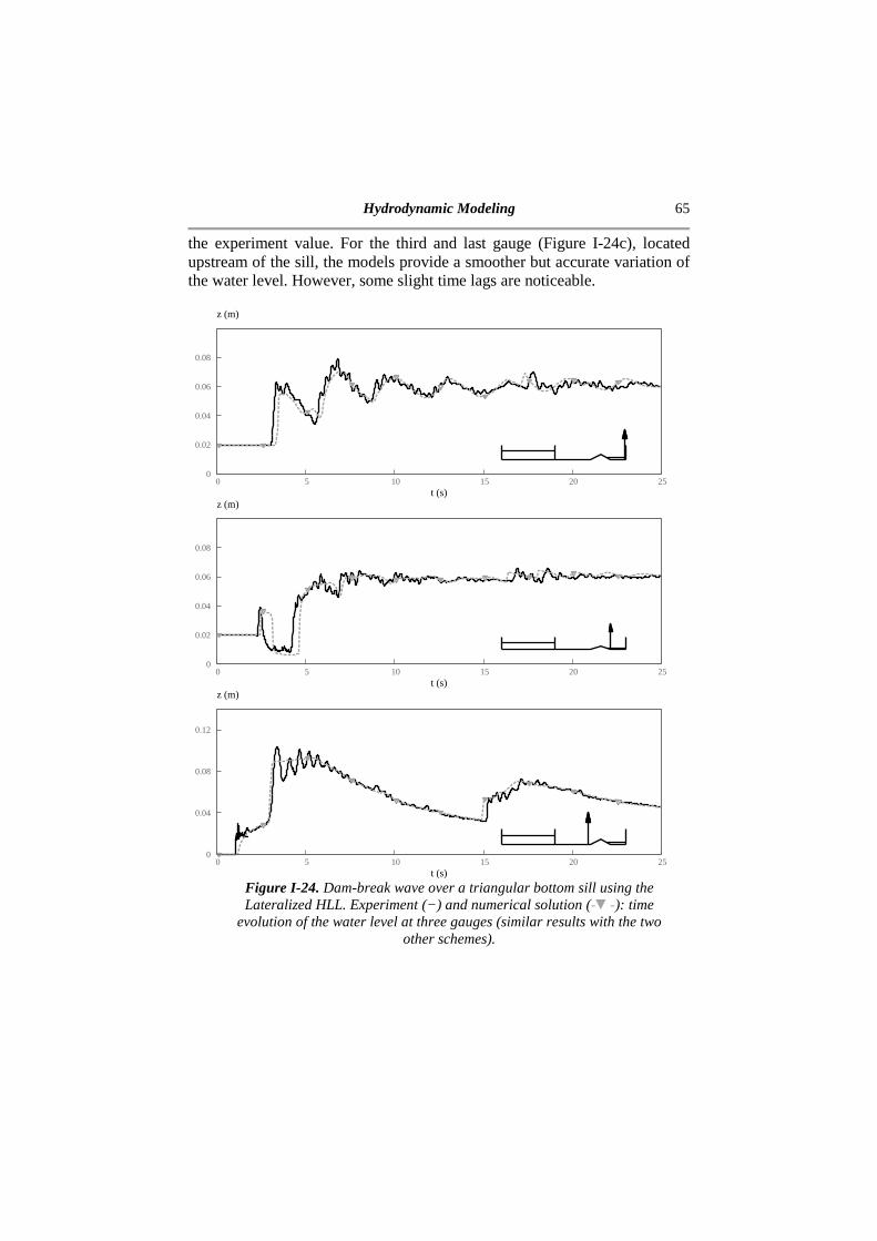
Hydrodynamic Modeling 65
the experiment value. For the third and last gauge (Figure I-24c), located upstream of the sill, the models provide a smoother but accurate variation of the water level. However, some slight time lags are noticeable.
Figure I-24. Dam-break wave over a triangular bottom sill using the Lateralized HLL. Experiment (−) and numerical solution (--): time
evolution of the water level at three gauges (similar results with the two other schemes).
0
0.02
0.04
0.06
0.08
0 5 10 15 20 25t (s)
z (m)
0
0.02
0.04
0.06
0.08
0 5 10 15 20 25t (s)
z (m)
0
0.04
0.08
0.12
0 5 10 15 20 25t (s)
z (m)

66 Chapter I
Concerning the water profiles (Figure I-25), the models provide a smoother but generally correct water profile. However, the water depth just downstream of the sill is lower than the experiment for t = 3 s. This is caused by the definition of the hydraulic jump which is sharper in the numerical model.
Figure I-25. Dam-break wave over a triangular bottom sill using the
Lateralized HLL. Experiment (−), bed level (−−) and numerical solution (--) for the water level after (a) 1.8 s, (b) 3.0 s, (c) 8.4 s (similar results
with the two other schemes).
0
0.04
0.08
0 1 2 3 4 5 6x (m)
z (m)
0
0.04
0.08
0 1 2 3 4 5 6x (m)
z (m)
0
0.04
0.08
0 1 2 3 4 5 6x (m)
z (m)

Hydrodynamic Modeling 67
I.4.4. Brembo River The last test focuses on a flow in a real complex river, the Brembo River (Lombardy Region, Italy) (Petaccia et al. 2013). This river is approximately 50 km long. It is a challenging case because of the high influence of the source terms on the results due to steep slopes and strong width variations (see Figure I-26). A total of 274 cross-sections were obtained by land survey with an average dx of 180 m. The Manning coefficients were estimated to range from 0.018 to 0.1 s/m1/3 (Arcement and Schneider 1989).
Figure I-26. Brembo River: (a) Top view and (b) Bed level.
For this test case, a steady flow of 400 m3/s – 35-year return period flood – is imposed. The model is composed of 1134 cross sections interpolated from the initial 274 (Petaccia et al. 2013). The simulations are compared to the reference solution computed using the steady-state version of HEC-RAS (Brunner 2002; Petaccia et al. 2013). A constant Manning coefficient of 0.04 s/m1/3 is considered. The boundary conditions are an imposed discharge upstream and a weir downstream. In the following analysis, the results are illustrated with two types of plots. First, a portion of the river is presented (between 5 and 10 km). Secondly, the results of the river are summarized by illustrating the percentage of elements that are below a given error limit. The results for the water level (Figure I-27a) and the water depth (Figure I-27b) are similar for the three schemes. However, HLLS and the Augmented Roe’s solver with energy balance give slightly better results than the Lateralized HLL (Figure I-28). The number of cells with an error lower than
-500
-250
0
250
0 10 20 30 40 50
x (km)
y (m)
0
100
200
300
400
500
0 10 20 30 40 50
x (km)
zb (m)
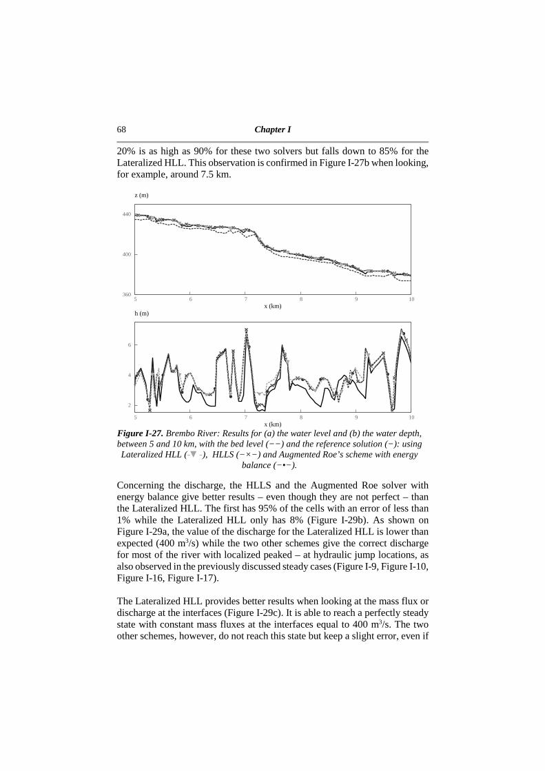
68 Chapter I
20% is as high as 90% for these two solvers but falls down to 85% for the Lateralized HLL. This observation is confirmed in Figure I-27b when looking, for example, around 7.5 km.
Figure I-27. Brembo River: Results for (a) the water level and (b) the water depth, between 5 and 10 km, with the bed level (−−) and the reference solution (−): using Lateralized HLL (--), HLLS (−×−) and Augmented Roe’s scheme with energy
balance (−•−).
Concerning the discharge, the HLLS and the Augmented Roe solver with energy balance give better results – even though they are not perfect – than the Lateralized HLL. The first has 95% of the cells with an error of less than 1% while the Lateralized HLL only has 8% (Figure I-29b). As shown on Figure I-29a, the value of the discharge for the Lateralized HLL is lower than expected (400 m3/s) while the two other schemes give the correct discharge for most of the river with localized peaked – at hydraulic jump locations, as also observed in the previously discussed steady cases (Figure I-9, Figure I-10, Figure I-16, Figure I-17). The Lateralized HLL provides better results when looking at the mass flux or discharge at the interfaces (Figure I-29c). It is able to reach a perfectly steady state with constant mass fluxes at the interfaces equal to 400 m3/s. The two other schemes, however, do not reach this state but keep a slight error, even if
360
400
440
5 6 7 8 9 10x (km)
z (m)
2
4
6
5 6 7 8 9 10x (km)
h (m)
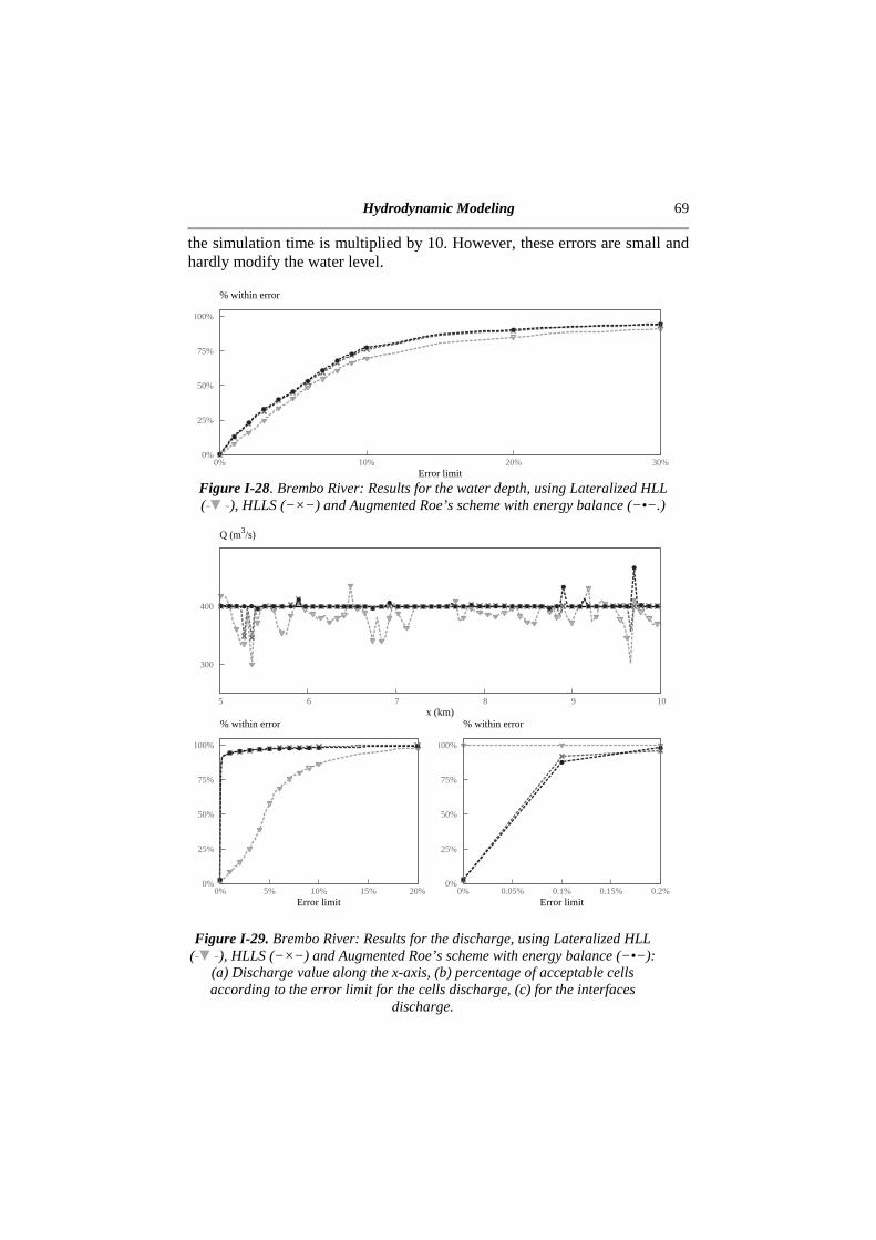
Hydrodynamic Modeling 69
the simulation time is multiplied by 10. However, these errors are small and hardly modify the water level.
Figure I-28. Brembo River: Results for the water depth, using Lateralized HLL (--), HLLS (−×−) and Augmented Roe’s scheme with energy balance (−•−.)
Figure I-29. Brembo River: Results for the discharge, using Lateralized HLL (--), HLLS (−×−) and Augmented Roe’s scheme with energy balance (−•−):
(a) Discharge value along the x-axis, (b) percentage of acceptable cells according to the error limit for the cells discharge, (c) for the interfaces
discharge.
0%
25%
50%
75%
100%
0% 10% 20% 30%Error limit
% within error
300
400
5 6 7 8 9 10x (km)
Q (m3/s)
0%
25%
50%
75%
100%
0% 5% 10% 15% 20%Error limit
% within error
0%
25%
50%
75%
100%
0% 0.05% 0.1% 0.15% 0.2%Error limit
% within error
70 Chapter I
I.5. Discussion and conclusion A set of complementary test cases has been presented to assess the capabilities of three of the most recent 1D finite-volume schemes: the Lateralized HLL (Petaccia et al. 2013), the HLLS (Murillo and García-Navarro 2012) and the Augmented Roe’s solver with energy balance (Murillo and García-Navarro 2014). These tests present different difficulties, such as steady flows, complex topography or friction, which allowed highlighting the limitations of some of the schemes. The LHLL scheme gives generally good results for the water level if the mesh is fine enough – as highlighted by the steady case without friction (Figure I-5 and Figure I-8) – with an exception for the supercritical Riemann problem (Figure I-21). However, the discharge within the cells is not correctly represented. This scheme, which has the advantage of being very simple for the computation of the waves celerities, could thus be used for cases where the water level needs to be known and where an accurate prediction of the discharge is not mandatory. This should be considered when modeling cases with sediment transport, as the transport capacity is determined as a function of the discharge. However, it is interesting to note that this scheme seems to be the most robust in highly complex topographies like the Brembo river, being the only one to give accurate results for the water level and reaching a completely steady state with constant discharge at the interfaces– even though the discharge within the cells is still wrongly computed. The HLLS model and the Augmented Roe’s solver with energy balance provide similar results. They provide good results for all the cases presented here. The HLLS performs better for the position of the shock in the first test case (Figure I-9). The Augmented Roe’s solver with energy balance gives better results with a coarser mesh. Still, they show one limitation concerning the conservation of the discharge at jump locations. However, this problem was also highlighted in the literature using different approaches (Delenne and Guinot 2012; Kesserwani 2013) and is also present for the Lateralized HLL. The major drawback of these improved schemes is that they are also less robust than the LHLL model, failing to reach a perfectly steady state in the Brembo River case – even though the error is localized, relatively small and does not change the water level much. To summarize the previous analysis, a grade has been given to each model regarding the prediction of the water level and the discharge and the robustness. The results are available in Table I-2.
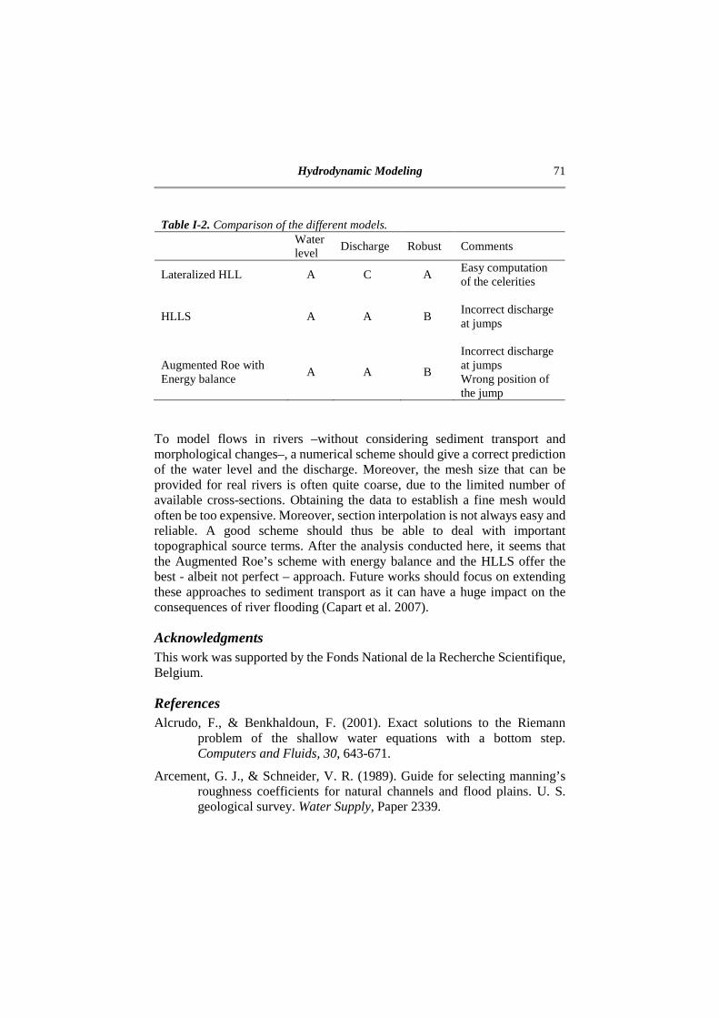
Hydrodynamic Modeling 71
Table I-2. Comparison of the different models.
Water level
Discharge Robust Comments
Lateralized HLL A C A Easy computation of the celerities
HLLS A A B Incorrect discharge at jumps
Augmented Roe with Energy balance
A A B
Incorrect discharge at jumps Wrong position of the jump
To model flows in rivers –without considering sediment transport and morphological changes–, a numerical scheme should give a correct prediction of the water level and the discharge. Moreover, the mesh size that can be provided for real rivers is often quite coarse, due to the limited number of available cross-sections. Obtaining the data to establish a fine mesh would often be too expensive. Moreover, section interpolation is not always easy and reliable. A good scheme should thus be able to deal with important topographical source terms. After the analysis conducted here, it seems that the Augmented Roe’s scheme with energy balance and the HLLS offer the best - albeit not perfect – approach. Future works should focus on extending these approaches to sediment transport as it can have a huge impact on the consequences of river flooding (Capart et al. 2007).
Acknowledgments This work was supported by the Fonds National de la Recherche Scientifique, Belgium.
References Alcrudo, F., & Benkhaldoun, F. (2001). Exact solutions to the Riemann
problem of the shallow water equations with a bottom step. Computers and Fluids, 30, 643-671.
Arcement, G. J., & Schneider, V. R. (1989). Guide for selecting manning’s roughness coefficients for natural channels and flood plains. U. S. geological survey. Water Supply, Paper 2339.

72 Chapter I
Audusse, E. a.-O. (2004). A fast and stable well-balanced scheme with
hydrostatic reconstruction for shallow water flows. Siam journal of science computation, 25, 2050-2065.
Audusse, E., Chalons, C., & Ung, P. (2015). A simple well-balanced and positive numerical scheme for the shallow-water system. Communications in Mathematical Sciences, 13, 1317-1332.
Bermudez, A., & Vázquez-Cendón, M. E. (1994). Upwind methods for hyperbolic conservation laws with source terms. Computers and Fluids, 23, 1049-1071.
Bradford, S. F., & Sanders, B. F. (2002). Finite volume model for shallow water flooding of arbitrary topography. Journal of Hydraulic Engineering, 128, 289-298.
Brunner, G. W. (2002). HEC-RAS River Analysis System Hydraulic Reference Manual, Version 3.1. Davis, CA: Hydrologic Engineering Center, Institute for Water Resources, US Army Corps of Engineers.
Burguete, J., & García-Navarro, P. (2004). Improving simple explicit methods for unsteady open channel and river flow. International Journal for Numerical Methods in Fluids, 45, 125-156.
CADAM Project. (2004). www.cadam-project.net
Capart, H., Eldho, T. I., Huang, S. Y., Young, D. L., & Zech, Y. (2003). Treatment of Natural Geometry in Finite Volume River Flow Computations. Journal of Hydraulic Engineering, 385-393.
Capart, H., Spinewine, B., Young, D. L., Zech, Y., Brooks, G. R., Leclerc, M., & Secretan, Y. (2007). The 1996 Lake Ha!Ha! breakout flood, Québec : test data for geomorphic flood routing methods. Journal of Hydraulics Research, 45, 97-109.
Cunge, J. A., Holly, F. M., & Vervey, A. (1980). Practical Aspects of Computational River Hydraulics. London: Pitman Publ. Inc.
Davis, S. F. (1988). Simplified second-order Godunov-type methods. SIAM Journal on Scientific and Statistical Computing, 9, 445-473.
Delenne, C., & Guinot, V. (2012). Auxiliary Variable-based Balancing (AVB) for source term treatment in open channel simulations. Advances in Water Resources, 44, 85-100.
Fraccarollo, L., Capart , H., & Zech Yves. (2003). A Godunov method for the computation of erosional shallow water transients. International journal for numerical methods in fluids, 41, 951-976.

Hydrodynamic Modeling 73
Godunov, S. K. (1959). A difference method for numerical calculation of
discontinuous solutions of the equations of hydrodynamics. Matematicheskii Sbornik, 47, 271-306.
Goutal, N., & Maurel, F. (1997). Proceedings of the 2nd Workshop on Dam-break Wave Simulation. Technical report EDF/DER HE-43/97/016/B, France.
Goutière, L., Soares-Frazão, S., Savary, C., T, L., & Zech, Y. (2008). One-dimensional model for transient flows involving bed-load sediment transport and changes in flow regimes. Journal of Hydraulic Engineering, 134, 726-735.
Harten, A., Lax, P. D., & Van Leer, B. (1983). On upstream differencing and Godunov type schemes for hyperbolic conservation laws. SIAM review, 25, 35-61.
Kesserwani, G. (2013). Topography discretization techniques for Godunov-type shallow water numerical models: a comparative study. Journal of Hydraulic Research, 51, 351-367.
MacDonald, I. (1996). Analysis and computation of steady open channel flow. University of Reading.
Murillo, J., & Garcìa-Navarro, P. (2012). Augmented versions of the HLL and HLLC Riemann solvers including source terms in one and two dimensions for shallow flow applications. Journal of Computational Physics, 231, 6861-6906.
Murillo, J., & Garcìa-Navarro, P. (2013). Energy balance numerical schemes for shallow water equations with discontinuous topography. Journal of Computational Physics, 236, 119-142.
Murillo, J., & Garcìa-Navarro, P. (2014). Accurate numerical modeling of 1D flow in channels with arbitrary shape. Application of the energy balanced property. Journal of Computational Physics, 231, 222-248.
Nujic, M. (1995). fficient implementation of non-oscillatory schemes for the computation of free surface flows. Journal of Hydraulics Research, 33, 101-111.
Petaccia, G., Natale, L., Savi, F., Velickovic, M., Zech, Y., & Soares-Frazão, S. (2013). Flood wave propagation in steep mountain rivers. Journal of Hydroinformatics, 15(1), 120-137.
Roe, P. (1981). Approximate Riemann solvers, parameter vectors, and difference schemes. Journal of Computational Physics, 43, 357-372.

74 Chapter I
Soares-Frazão, S. (2002) Ph.D. thesis Dam-Break Induced Flows in Complex
Topographies: Theoretical, Numerical and Experimental Approaches, University of Louvain
Soares-Frazão, S. (2007). Experiments of dam-break wave over a triangular bottom sill. Journal of Hydraulic Research, 45, 19-26.
Toro, E. F. (1997). Riemann Solvers and Numerical methods for fluid dynamics. Springer.
Vázquez-Cendón, M. E. (1999). Improved Treatment of Source Terms in Upwind Schemes for the Shallow Water Equations in Channels with Irregular Geometry. Journal of Computational Physics, 148, 497-526.

MODELING THE FLOW AROUND ISLANDS
Extended version of [Franzini F., Hoedenaeken D. and Soares-Frazão S. Modelling the flow around islands in rivers using a one-dimensional approach. Submitted to Simhydro 2017]
The second chapter presents the simulation of the flow around islands. Having a model able to compute the flow around island is important as, for example, Figure II-1 clearly shows that, during the Ha!Ha! River flood the flow was divided in two sub-channels. The approach presented here uses one of the models presented in Chapter I (Augmented Roe with energy balance) to compute the flow in the channel and considers the connections before and after the island as inside boundary conditions.
Figure II-1. Picture taken after the Ha!Ha! River flood (Capart et
al. 2007): during the flood, the flow was divided in two sub-channels.

76 Chapter II
Abstract One-dimensional models are widely used for the simulation of flows in rivers. Around islands, the flow is divided and the discharge is distributed in the different branches. Such a flow in a bifurcation is a typical two-dimensional phenomenon, and representing the accurate partition of discharge might be a challenge in one-dimensional models depending on the flow conditions. In the present paper, a one-dimensional model is presented where the connections between the main river and the sub-channels are modeled as inner boundary conditions. These conditions are defined considering characteristic paths and conservation of the water head. Four flow configurations are considered: (i) a subcritical junction, (ii) a subcritical bifurcation, (iii) a supercritical junction and (iv) a supercritical bifurcation. For the supercritical bifurcation, an additional condition is required and it is proposed here to partition the discharge proportionally to an equivalent cross-section width. The new one-dimensional model has been validated by comparing the results with those from a two-dimensional model for the four configurations. The comparison showed that the one-dimensional model predicts correctly the discharge and the water depth in each branch. Finally, the one-dimensional model was used to simulate the flow in a reach of the Meuse River (Belgium), showing good agreement with field data.
II.1. Introduction One-dimensional models for river flow simulations are still widely used and often constitute the only realistic option when results are expected in a very short time. In addition, in many cases, especially for smaller streams, no detailed two-dimensional bathymetric data are available and the setup of a detailed two-dimensional model is not possible. In these cases, one-dimensional models are often preferred, as they are faster and simpler to build. However, one limit of using 1D models is that they are, of course, unable to capture 2D phenomena that can occur for example at junctions, bifurcations, or around islands where these two cases are combined. There, the channel is divided into two sub-channels around the island before merging again. To represent this behavior in a one-dimensional model, several options are available. First, the island can be simply ignored by either combining the cross-sections on both sides of the island or creating a large section englobing the island and the two sub-channels. In these approaches, the flow velocity is considered as being the same in the two branches around the island, which constitutes a limitation when the flow in each branch is significantly different.

Modeling the flow around islands 77
Secondly, the junction can be modeled using a local 2D model (Soares-Frazão and Zech 2002, Ghostine et al. 2015). This method is also used to model the interactions between flood plains and main channel during a flood (Finaud-Guyot et al. 2011; Morales-Hernández et al. 2013). While using such a local 2D model appears as an efficient method allowing for sharp changes in direction, such a 90° bends for example (Soares-Frazão and Zech, 2002), it might be difficult to set up in natural rivers with arbitrary cross-sections. So, when the main flow can be considered as one-dimensional and the angles between the branches are limited, the junction can be represented using an “internal boundary condition”, which allows staying in a purely one-dimensional framework. In this latter case, corresponding to the approach adopted here, the river reach containing an island is divided into four linked parts: (i) the upstream channel, (ii-iii) the two sub-channels on both sides of the island and (iv) the downstream channel. In such an approach, the local two-dimensional features of the flow are not represented, but the focus is set on accurate discharge distribution in the branches and water levels. This approach has been first used by Chow (1959) for steady subcritical flows: an iterative procedure is developed for the discharge repartition in the sub-channels until an equality of the water level is reached in the upstream channel. Instead of using the water level equality, Wylie (1972) proposed the use of the water head (or energy) equality. His model, also, was developed for steady subcritical flows. For unsteady flows, Garcia-Navarro and Saviron (1992) developed a model to solve the convergence (or junction) in subcritical and supercritical flows using the characteristic paths. The model developed here uses the characteristic paths method and the conservation of water head to represent both subcritical connections (junction and bifurcation) and supercritical junctions. For the supercritical bifurcation, where one equation is missing to close the system, it is proposed to partition the discharge according to the available width of each sub-channel. This is a simpler model than the one proposed by Lhomme (2006) based on the work of Chocat (1997) where several parameter are considered such as width, slope, Froude number, angle between the sub-channels. The research focuses on the flow around islands in a one-dimensional framework such as presented in Figure II-2. Therefore, the bifurcation at the upstream end of the island is represented as in Figure II-3, where only the case with equal and small angles (φ1 = φ2 < < 90°) will be considered. This contrasts with other works presented in the literature focusing on the flow in crossroads (e.g. Mignot et al. 2011; ) where the angles are equal to 90° or in confluences and bifurcations (e.g. Ghostine et al. 2012) where both angles are different. In order words, the approach proposed here focuses on the discharge partition in

78 Chapter II
the branches around an island assuming that the global flow direction is one-dimensional along the river thalweg. Finally, only cases where the main channel and the sub-channels are in the same regime – either subcritical or supercritical – will be studied.
Figure II-2. Islands near Yvoir, Belgium (credits Google)
Figure II-3. Description of the bifurcation upstream of an island
The paper is divided as follows. First, the models are presented, i.e. the one-dimensional model used for the channel flow and the finite-volume solver, and then the approaches developed for the four types of inner boundary conditions: (i) the subcritical junction, (ii) the subcritical bifurcation, (iii) the supercritical junction and (iv) the supercritical bifurcation. Then, test cases aimed at validating these approaches are presented and, for each case, the results are compared to those obtained using a detailed two-dimensional finite-volume model. In addition, the model is used to simulate the flow in a real

Modeling the flow around islands 79
river and the results are compared to field measurements. Finally, conclusions are drawn and perspectives are discussed.
II.2. Governing equations and numerical scheme
II.2.1. One-dimensional Saint-Venant equations in conservative form The one-dimensional Saint-Venant equations are written in conservative form that is best suited for flows in arbitrary topographies featuring sudden changes in the cross-section shape (Petaccia et al., 2013). Therefore, the equations read
∂A
∂t+
∂Q
∂x=0
(II-1)
∂Q
∂t+
∂
∂xQ2
A+gI1 = gI2+AS0-Sf (II-2)
where Q is the discharge, A the wetted area, S0 the bed slope defined by:
S0= -dzb
dx
(II-3)
with zb the bed level, more precisely the thalweg level. The term gI1 represents the hydrostatic pressure thrust while gI2 represents the longitudinal component of the lateral pressure due to the longitudinal width changes. These integrals are written as
gI1 = g + h-ηb dηh
0 (II-4)
gI2 = g+ h-η ∂b
∂xdη
h
0 (II-5)
with η a local variable for the depth integration and b(x, η) the width of the channel at a determined depth (Figure II-4).

80 Chapter II
Figure II-4. Definition of the hydrostatic pressure
The friction is modeled using the Manning equation (II-6), with the Manning roughness coefficient n and the wetted perimeter P.
Sf =n2Q2P 4/3
A10/3 (II-6)
The system of equations (II-1) and (II-2) can be written in vector form as
∂U∂t
+∂F∂x
= S (II-7)
with U the vector of conserved variables, F the vector of fluxes and S the source terms. U = 7AQ9 (II-8)
F= N Q
Q2
A+gI1
O = AQΣG (II-9)
S= 7 0gI2+ QAS0-Sf9 (II-10)

Modeling the flow around islands 81
II.2.2. Finite-volume resolution of the equations The first-order finite-volume discretization of (II-7) is given by
Uin+1=Ui
n+∆t
∆xFi-1/2
* - Fi+1/2* + S ∆t (II-11)
where the superscript n refers to the time step and the subscript i to the spatial step. To compute the fluxes Fi+1/2
* , the Augmented Roe solver with energy balanced (Murillo and Garcia-Navarro, 2014) was used. This model, developed for arbitrary cross-sections, was validated against a series of test cases by Franzini and Soares-Frazão (2016) and showed good results especially in terms of discharge conservation in steady flows. The particular feature of this solver is that all source terms, i.e. topographical and friction terms, are included in the fluxes computation. Equation (II-11) thus becomes:
Uin+1 = Ui
n + ∆t
∆xFi-1/2
*R - Fi+1/2*L (II-12)
where the fluxes are lateralized, in the sense that the flux entering cell R at the right side of the interface is different from the flux exiting cell L at the left side of the interface, the difference being due to the source terms between the two computational cells. These fluxes are written as
Fi+ 1/2*L = Fi + )λα - βe
m,i+1/2
m
λm<0
(II-13)
Fi+1/2*R = Fi+1- )(λα - β)em,i+1/2
m
λm>0
(II-14)
As the solver is based on Roe scheme (Roe, 1981), the wave celerities λ are defined based on the Roe averages, denoted by a ~overbar, as:
λ1 = u:- c: (II-15)
λ2 = u: + c: (II-16)

82 Chapter II
with the Roe averages being calculated as
u: = #Ai ui + #Ai+ 1 ui+1 #Ai + #Ai+1
(II-17)
c: = !g
2-Ai+1
Bi+1+
Ai
Bi. (II-18)
In (17) and (18), u is the velocity along the x-axis defined by Q/A and B is the width of the section at the water surface (Figure II-4). The eigenvectors e to be considered in (II-13) and (II-14) are expressed as
em= 7 1λm9 (II-19)
E = e1 e2 = 71 1λ1 λ2
9 (II-20)
The wave strengths α are obtained using the relations
α1 = λ2∆A - ∆Q
2c: (II-21)
α2= - λ1∆A - ∆Q
2c: (II-22)
Finally, the source terms are included in the fluxes using a stationary wave, as follows:
β1 = - ζ
2c: (II-23)
β2 = ζ
2c: (II-24)
Where ζ represents the combined topographical and friction source terms written as: ζ = 1-ωζga + ωζgb- gA8Sf
8 ∆x (II-25)

Modeling the flow around islands 83
with a weighting coefficient ω used to introduce the water head conservation in the model. Equation (II-25) includes a linear combination of two possible expressions (II-26) and (II-27) of the topographical source terms allowing ensuring energy conservation (Murillo and García-Navarro 2014, Franzini and Soares-Frazão 2016):
ζga= - gA8∆z + c:2∆A (II-26)
ζgb = - gAmin∆z + c:2∆A (II-27)
The weighting coefficient ω is obtained by combining the momentum conservation and the head conservation of (II-26) and (II-27) as
ω =
δQ2
A - A8 δQ2
2A2ζgb- ζga
(II-28)
II.3. Internal boundary conditions This section presents the different internal boundary conditions used to represent the flow at junctions and bifurcations. These boundary conditions are expressed using the characteristics, along which the Saint-Venant equations can be expressed as ordinary differential equations (Mahmood and Yevjevich 1975). The negative and positive characteristics are defined by
C- ≡ dx
dt= u - c (II-29)
C ≡ dx
dt= u + c (II-30)
Along these curves, the Saint-Venant equations become (II-31) and (II-32) on the negative (C -) characteristic and (II-33) and (II-34) on the positive (C +) characteristic. These equations are also known as compatibility equations, written here without source terms.
dQ
dt-u+cdA
dt=0 (II-31)
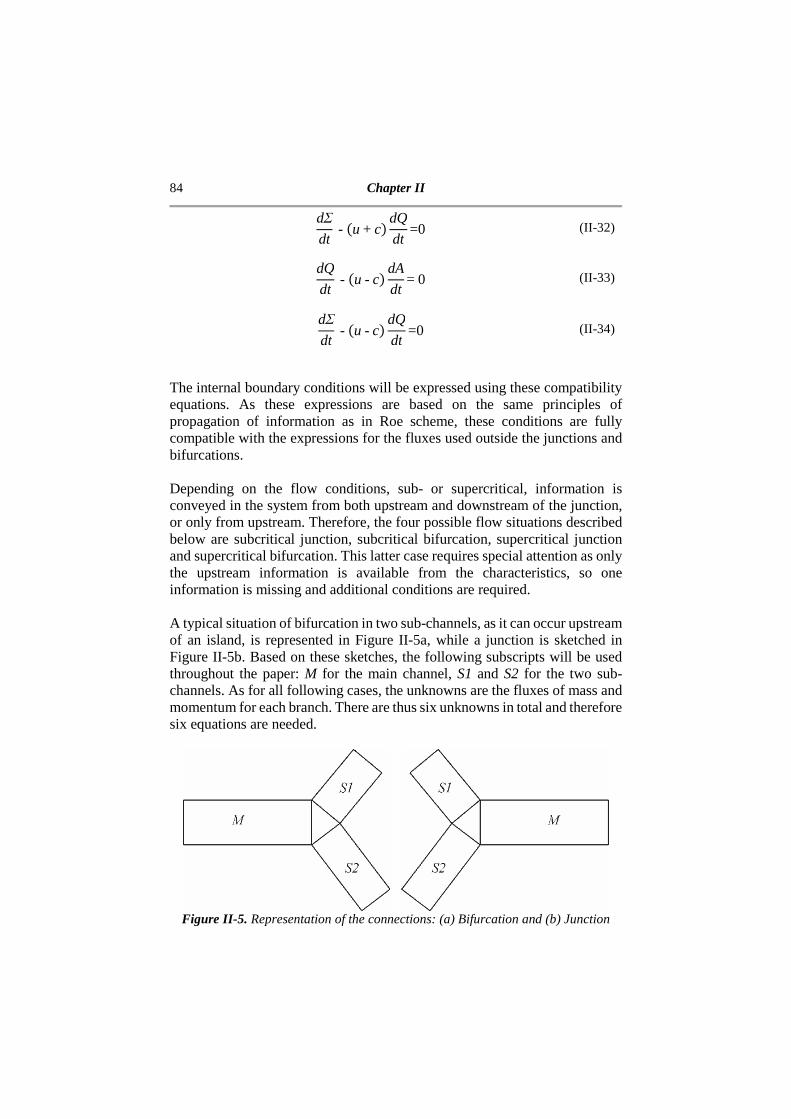
84 Chapter II
dΣ
dt-u+cdQ
dt=0 (II-32)
dQ
dt-u-c dA
dt=0 (II-33)
dΣ
dt-u-c dQ
dt=0 (II-34)
The internal boundary conditions will be expressed using these compatibility equations. As these expressions are based on the same principles of propagation of information as in Roe scheme, these conditions are fully compatible with the expressions for the fluxes used outside the junctions and bifurcations. Depending on the flow conditions, sub- or supercritical, information is conveyed in the system from both upstream and downstream of the junction, or only from upstream. Therefore, the four possible flow situations described below are subcritical junction, subcritical bifurcation, supercritical junction and supercritical bifurcation. This latter case requires special attention as only the upstream information is available from the characteristics, so one information is missing and additional conditions are required. A typical situation of bifurcation in two sub-channels, as it can occur upstream of an island, is represented in Figure II-5a, while a junction is sketched in Figure II-5b. Based on these sketches, the following subscripts will be used throughout the paper: M for the main channel, S1 and S2 for the two sub-channels. As for all following cases, the unknowns are the fluxes of mass and momentum for each branch. There are thus six unknowns in total and therefore six equations are needed.
Figure II-5. Representation of the connections: (a) Bifurcation and (b) Junction

Modeling the flow around islands 85
II.3.1. Subcritical junction For the particular case of the subcritical junction (Figure II-5b), the compatibility equations (II-31) to (II-34) are discretized at the interface using the expressions for the positive characteristic for the sub-channels S1 and S2 and the negative characteristic for the main channel M to convey the information towards the interface (Figure II-6). So, the mass fluxes can be expressed as
QS1* =QS1
n +u0-c0AS1* -AS1
n (II-35)
QS2* =QS2
n +u8-c0AS2* -AS2
n (II-36)
QM* =QM
n +u8+ c0AM* -AM
n (II-37)
The superscript * refers to the value at the interface, the other values being taken in the cells and u0 and c0 are the arithmetic average of the velocities and celerities, respectively.
Figure II-6. Characteristics at the subcritical junction
As only three equations (II-35)-(II-37) are available with the characteristics, three other relations are thus needed to close the system. First, the conservation of discharge at the interface is imposed:
QS1* +QS2
* =QM* (II-38)

86 Chapter II
Then, the last two equations are the conservation of the water head between S1 and M, and between S2 and M. They are written as
zb,S1+ AS1*Be,S1+uS1
2
2g=zb,M+ AM
*Be,M+ uM
2
2g+Sf,S1→M∆x (II-39)
zb,S2+ AS2*Be,S2+uS2
2
2g=zb,M+ AM
*Be,M+ uM
2
2g+Sf,S2→M∆x (II-40)
With Be the equivalent, average width of the channel, defined as A/h, with h the water depth, and Sf,Sj→M∆x the friction loss between the sub-channel j and the main channel. By combining these six equations, the wetted area at the interface of the main channel AM
* can be determined as
AM* = ϕS1+ϕS2+ϕM
ψ (II-41)
With ϕM=QM
n +(u0+c0)AMn (II-42)
ϕS1= QS1n + u0-c0 Be,,S1
2guM2 -uS1
2 +zb,M-zb,S1Be,S1-AS1n
+Sf,S1→M∆xBe,S1
" (II-43)
ϕS2 = QS2n + u 8- c0 Be,S2
2guM
2 - uS22 + zb,M - zb,S2Be,S2 - AS2
n
+ Sf,S2→M ∆x Be,S2
" (II-44)
ψ= u8+c0-Be,S1Be,Mu0-c0-Be,S2Be,M
u8-c0 (II-45)
The other wetted areas AS1
* and AS2* are then simply computed using the energy
balances (II-39) and (II-40).
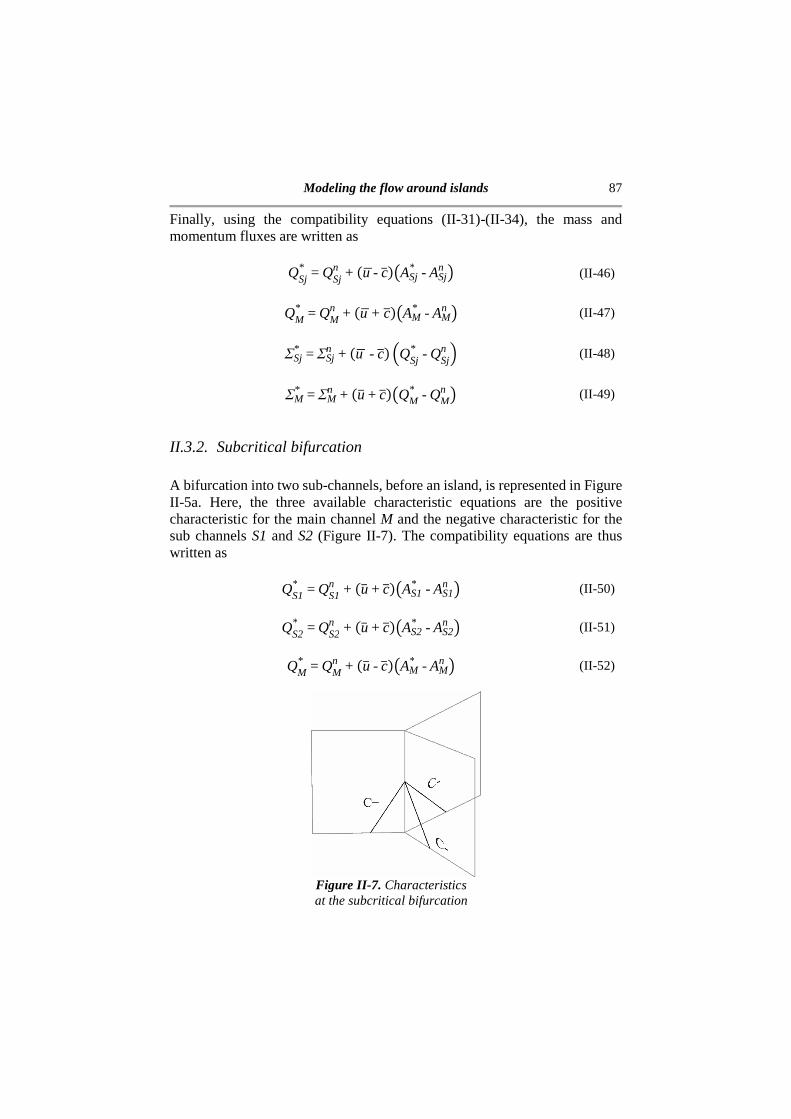
Modeling the flow around islands 87
Finally, using the compatibility equations (II-31)-(II-34), the mass and momentum fluxes are written as
QSj* =QSj
n +u8-c0ASj* -ASj
n (II-46)
QM* =QM
n +u8+ c0AM* -AM
n (II-47)
ΣSj* =ΣSj
n +u8-c0 QSj* -QSj
n (II-48)
ΣM* =ΣM
n +u0+c0QM* -QM
n (II-49)
II.3.2. Subcritical bifurcation A bifurcation into two sub-channels, before an island, is represented in Figure II-5a. Here, the three available characteristic equations are the positive characteristic for the main channel M and the negative characteristic for the sub channels S1 and S2 (Figure II-7). The compatibility equations are thus written as
QS1* =QS1
n +u0+c0AS1* -AS1
n (II-50)
QS2* =QS2
n +u0+c0AS2* -AS2
n (II-51)
QM* =QM
n +u0-c0AM* -AM
n (II-52)
Figure II-7. Characteristics at the subcritical bifurcation
88 Chapter II
To complete the system of equations, the same equations as for the junction are used: discharge conservation (II-38) and water head conservation (II-39) - (II-40), with only a change in sign for the friction terms.
QM * =QS1
* +QS2* (II-53)
zb,M+ AM*
Be,M+uM
2
2g=zb,S1+ AS1
*
Be,S1+ uS1
2
2g+Sf,M→S1∆x+JE (II-54)
zb,M+ AM*
Be,M+uM
2
2g=zb,S2+ AS2
*Se,S2+uS2
2
2g+Sf,M→S1∆x+JE (II-55)
The energy loss JE in (II-54) and (II-55) is due to the expansion of the river that can occur at the bifurcation, where often the total available flow section downstream of the bifurcation is larger than the available section before. This head loss is computed using a modified Borda equation (Guinot and Soares-Frazão, 2006) as
JE= QS1+ QS2AS1+ AS2
2
2gTBe,S1+ Be,S2Se,M
-12
+1
9U (II-56)
By combining these six equations (II-50)-(II-55), the wetted area at the bifurcation seen from the main channel AM
* can be determined as
AM* = ϕS1+ ϕS2+ ϕM
ψ (II-57)
with
ϕM=-QMn +(u0-c0)AM
n (II-58)
ϕS1= QS1n + u0+c0 Be,S1
2guM2 -uS1
2 +zb,M-zb,S1Be,S1-AS1n
-Sf,M→S1∆xBe,S1-JEBe,S1
" (II-59)
ϕS2=QS2n + u8+ c0 Be,S2
2guM
2 -uS22 +zb,M-zb,S2Se.S2-AS2
n -Sf,M→S1∆xSe,S2-JESe,S2
" (II-60)

Modeling the flow around islands 89
ψ= -u8-c0-Be.S1Se,Mu0+c0-Se,S2
Be,Mu0+c0 (II-61)
Finally, the mass and momentum fluxes can be written as
QSj* =QSj
n +u0+c0ASj* -ASj
n (II-62)
QM* =QM
n +u0-c0AM* -AM
n (II-63)
ΣSj* =ΣSj
n +u0+c0 QSj* -QSj
n (II-64)
ΣM* =ΣM
n +u0-c0QM* -QM
n (II-65)
II.3.3. Supercritical junction For the case of the supercritical junction, the characteristics provide four equations, as all the information is coming from upstream (Figure II-8)
QS1* =QS1
n +u0+c0AS1* -AS1
n (II-66)
QS1* =QS1
n +u0-c0AS1* -AS1
n (II-67)
QS2* =QS2
n +u0+c0AS2* -AS2
n (II-68)
QS2* =QS2
n +u0-c0AS2* -AS2
n (II-69)
Figure II-8. Characteristics at the supercritical junction
90 Chapter II
Therefore, only two more equations are needed to close the system. The four equations (II-66)-(II-69) can be solved directly for the mass fluxes towards the two sub-channels QS1
* .and QS2* , yielding (II-70)-(II-71). To determine the
mass flux coming from the main channel, the conservation of the mass fluxes (II-72) is used. Then, using (II-73) – (II-45), the momentum fluxes in the sub-channels and in the main channel can be obtained. The six fluxes are thus
QS1* =QS1
n (II-70)
QS2* =QS2
n (II-71)
QM* =QS1
* +QS2* (II-72)
ΣS1* =ΣS1
n (II-73)
ΣS2* =ΣS2
n (II-74)
ΣM* = ΣS1
* +ΣS2* (II-75)
II.3.4. Supercritical bifurcation This case is the most complex one as the characteristics only provide two useful equations (Figure II-9)
QM* =QM
n +u0+c0AM* -AM
n (II-76)
QM* =QM
n +u0-c0AM* -AM
n (II-77)
Four more conditions are thus needed. Two of them are, as before, the conservation of the water head:
zb,M+ AM*
Be,M+uM
2
2g=zb,S1+ AS1
*Se,S1+uS1
2
2g+Sf,M→S1∆x+JE (II-78)
zb,M+ AM*
Be.M+uM
2
2g=zb,S2+ AS2
*
Be,S2+ uS2
2
2g+Sf,M→S1∆x+JE (II-79)
with JE, the energy loss due to a widening computed using the same modified Borda equation (II-56) as for the subcritical bifurcation.

Modeling the flow around islands 91
Figure II-9. Characteristics at the supercritical bifurcation
The last two equations are provided considering a partition of the discharge (coefficient C) proportional to the sub-channels average widths Be,S1.and Be,S2
QS1 * = QM
* Be,S1
Be,S1 + Be,S2= CQM
* (II-80)
QS2 * =QM
* Be,S2
Be,S1+Be,S2= (1-C )QM
* (II-81)
Other partitions are possible, such as a partition according to the conveyance of each sub-channel. However, comparative tests using a two-dimensional model showed that, for supercritical flows, the main factor was the average width. This choice of partition method is compatible with the partition proposed by Lhomme (2006) and Chocat (1997) in the considered case, under the following assumptions: (1) Large Froude number and (2) small and similar angles between the two sub-channels and the main channel (φ1 = φ2 = φ/2). Using Lhomme (2006) expression for a case with a high Froude Number, for wide channels and with the same slope for both sub-channels, it is possible to highlight the impact of the angle between the two sub-channels on the partition coefficient. Figure II-10 shows the percentage of the discharge flowing in sub-channel S1 calculated according to the proposed partition, and according to Lhomme (2006). It can be observed that, for small angles, the two expressions are highly similar.
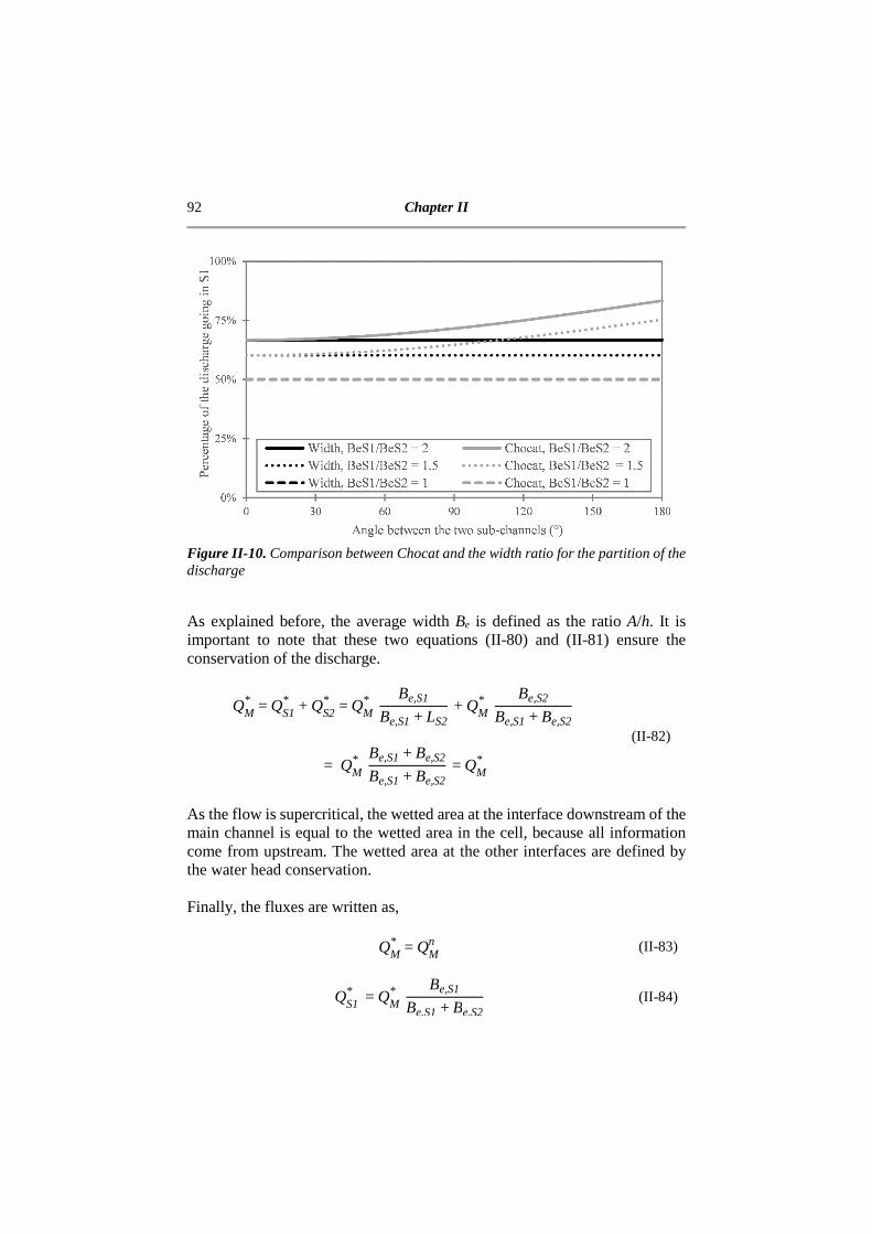
92 Chapter II
Figure II-10. Comparison between Chocat and the width ratio for the partition of the discharge
As explained before, the average width Be is defined as the ratio A/h. It is important to note that these two equations (II-80) and (II-81) ensure the conservation of the discharge.
QM* =QS1
* +QS2* =QM
* Be,S1
Be,S1+LS2+QM
* Be,S2
Be,S1+Be,S2
= QM* Be,S1+Be,S2
Be,S1+Be,S2=QM
*
(II-82)
As the flow is supercritical, the wetted area at the interface downstream of the main channel is equal to the wetted area in the cell, because all information come from upstream. The wetted area at the other interfaces are defined by the water head conservation. Finally, the fluxes are written as,
QM* =QM
n (II-83)
QS1 * =QM
* Be,S1
Be.S1+Be.S2 (II-84)

Modeling the flow around islands 93
QS2 * =QM
* Be,S2
Be,S1+Be.S2 (II-85)
ΣM* =ΣM
n (II-86)
ΣS1* =u0 QS1
* +gI1, S1* (II-87)
ΣS2* =u0 QS2
* +gI1,S2* (II-88)
II.4. Results and discussion First, the results of this one-dimensional model are compared to those of a full two-dimensional model in numerical test cases covering all the types of connections described before, under steady-flow conditions. For each case, the water levels in the different branches and the discharge partition are compared. The two-dimensional model used as reference is the model developed by Soares-Frazão and Zech (2002). Then, the one-dimensional model is used to simulate the flow in the Meuse River in Belgium (Dal Cin et al. 2005) and compared to field measurements. For the numerical cases, different configurations of channels with rectangular cross-sections are tested (R-I to R-VI), as summarized in Table II-1. In addition, one configuration where the cross-sections are trapezoidal (T), yielding more complex junctions and bifurcations, is considered. The trapezoidal cross-sections are defined in the main channel as in Figure II-11 with Z = 0.25. The sub-channels are defined as semi-trapezoidal cross-sections with one vertical wall and one sloping bank (Z = 0.25). For each configuration, the four flow cases corresponding to the four internal boundary conditions are considered. The main channel keeps the same characteristics for all the tests: a bottom width (B0) of 75 m, a Manning coefficient (n) of 0.025 s/m1/3 and a slope of 0.3% and 5% for the subcritical and supercritical, respectively. In the equivalent 2D model, the two branches of the junction or bifurcation make an angle of 60° with the main channel. This choice is arbitrary, as the angle at the connection is not taken into account in the flux expressions of the 1D model. In addition, this angle between the two sub-channels does not have any influence on the discharge partition (Figure II-12) and only extend the area of influence of the local water level peak at the connection (Figure II-13) in the two-dimensional simulations. Finally, for all tests, the connection is located at x = 500 m.

94 Chapter II
Figure II-11. Trapezoid cross-section: definition
Figure II-12. Influence of the sub-channels angle
on the partition of the discharge in the two-dimensional model
For each type of internal boundary condition, the water depths results are shown for configurations R-I, R-III and R-IV. The plots show the comparison between the 1D water depth and the cross-section averaged value of the 2D water depth across the cross-section. The discharges are compared for all the tests.
Figure II-13. Influence of the sub-channels
angle on the water depth in the main channel for a subcritical bifurcation, in the two-dimensional
model

Modeling the flow around islands 95
Table II-1. Key parameters of the different numerical test cases: bottom width (B0), slope (S0) and Manning coefficient (n). The bold number highlight the differences between the test and the classical symmetrical test R-I
Test case Sub-channel S1 Sub-channel S2
B0 (m)
S0 (%)
n (s/m1/3)
B0 (m)
S0 (%)
n (s/m1/3)
R-I Sub 37.5 0.3 0.025 37.5 0.3 0.025
Super 37.5 5 0.025 37.5 5 0.025
R-II Sub 37.5 0.3 0.025 37.5 0.3 0.045
Super 37.5 5 0.025 37.5 5 0.045
R-III Sub 37.5 0.3 0.025 37.5 0.1 0.025
Super 37.5 5 0.025 37.5 8 0.025
R-IV Sub 50 0.3 0.025 25 0.3 0.025
Super 50 5 0.025 25 5 0.025
R-V Sub 60 0.3 0.025 15 0.3 0.025
Super 60 5 0.025 15 5 0.025
R-VI1 Sub 56.25 0.3 0.025 56.25 0.3 0.025 Super 56.25 5 0.025 56.25 5 0.025
T Sub 49.75 0.3 0.025 24.75 0.3 0.025
Super 49.75 5 0.025 24.75 5 0.025
1Only for the bifurcation cases
II.4.1. Subcritical junction For configuration R-I, as shown in Figure II-14, the 1D model is able to provide the correct water depth far from the junction but is not able to capture the increased elevation and the depression at the junction (x = 500 m). These features, that depend on the angle at the connection, can only appear in the 2D model (Figure II-15) as the flows coming from each sub-channel have opposite velocities along the y-axis, and so their mixing results in an area of higher depth at the junction. Also, as the flows are directed towards the center of the main channel, two area of shallow depth appear close to the wall.
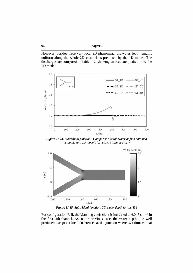
96 Chapter II
However, besides these very local 2D phenomena, the water depth remains uniform along the whole 2D channel as predicted by the 1D model. The discharges are compared in Table II-2, showing an accurate prediction by the 1D model.
Figure II-14. Subcritical junction: Comparison of the water depths obtained
using 1D and 2D models for test R-I (symmetrical)
Figure II-15. Subcritical junction: 2D water depth for test R-I
For configuration R-II, the Manning coefficient is increased to 0.045 s/m1/3 in the first sub-channel. As in the previous case, the water depths are well predicted except for local differences at the junction where two-dimensional

Modeling the flow around islands 97
features appear when the two flows merge. Table II-2 shows that the discharge is also correctly computed. Then, in configuration R-III, the slope in sub-channel S2 is decreased to 0.1 %, with the consequence that the normal depth is higher in this sub-channel than in S1. It can be seen in Figure II-16 that the 1D model correctly predicts the water depths except for the exact position of the connection, in a similar way than for configuration R-I and R-II. Again, the discharge partition is well predicted (Table II-2).
Figure II-16. Subcritical junction: Comparison of the water depths
obtained using 1D and 2D models for test R-III (different slopes: 0.3% for M and S1 and 0.1% for S2)
The sub-channel width is investigated in configurations R-IV (50 m – 25 m) and R-V (60 m – 15 m). Figure II-17 shows the water depth results for R-IV with a subcritical junction. The results for R-V are very similar and are not illustrated. As for the other configurations, the overall water depth and the discharge (Table II-2) are correctly predicted except are the location of the junction.

98 Chapter II
Figure II-17. Subcritical junction: Comparison of the water depths obtained using 1D and 2D models for test R-IV (different width: 75 m for M, 50 m for
S1 and 25 m for S2)
Finally, in configuration T (trapezoidal channel, sketched in Figure II-11), the main channel consists of a full trapezoidal cross-section and the sub-channels are defined with semi-trapezoidal cross-sections, with one vertical wall and one sloping bank. The bank slope is the same for both sub-channels and for the main channel. Each sub-channel has its own, different, bottom width, 49.75 m and 24.75 m, respectively. The results are only shown for the discharge (Table II-2), as the water depth conclusions are similar to the rectangular cases. Table II-2 shows that the one-dimensional model better preserves the constant discharge than the two-dimensional model, due to an imperfect balance of topographical source terms at the limit of the free-surface against the inclined banks.
Table II-2. Subcritical junction: Comparison of the discharges (in m3/s) obtained using the 1D and 2D models
Test QS1, 1D QS1, 2D QS2, 1D QS2, 2D QM, 1D QM, 2D R-I 200 200 200 200 400 400 R-II 200 200 200 200 400 400 R-III 200 200 200 200 400 400 R-IV 266.7 266.7 133.3 133.3 400 400 R-V 320 320 80 80 400 400 T 267.1 267.1 132.9 132.9 400 402.4

Modeling the flow around islands 99
II.4.2. Subcritical bifurcation The same configurations as in the subcritical junctions are tested, the only difference being that the main channel is now located upstream of the two sub-channels instead of downstream. The discharge imposed upstream of the main channel is 400 m3/s. The conclusions for configuration R-I are similar to the one obtained for the convergence: the water depth is correctly predicted far from the bifurcation but the 1D model does not capture the peaks created by the 2D velocity distribution at the bifurcation (Figure II-18 and Figure II-19). The discharge is also accurately predicted (Table II-3). For configurations R-II (influence of Manning coefficient) and R-III (different bed slopes in sub-channels), the 1D model is able to better capture the water depth than for configuration R-I but is still not high enough (Figure II-20 for R-III). In the 2D models, the higher water level at the bifurcation that was clearly marked for R-I (Figure 8) appears less important because of an increase of the water level in one of the sub channels due to the higher Manning coefficient (R-II) or to the lower bed sole (R-III). Due to these effects, the differences between 1D and 2D model results are still observed, but their importance is less than 1 % for the discharge (Table II-3). For configurations R-IV and R-V, the conclusions are similar to what has been observed in the other cases. The water is correctly predicted far from the connection (Figure II-21) and the discharge is correctly predicted with a small difference (less than 1 %).
Figure II-18. Subcritical bifurcation: Comparison of the water depths
obtained using 1D and 2D models for test R-I (symmetrical)

100 Chapter II
Figure II-19. Subcritical bifurcation: 2D water depth for test R-I
Figure II-20. Subcritical bifurcation: Comparison of the water depths
obtained using 1D and 2D models for test R-III (different slopes: 0.3% for M and S1 and 0.1% for S2)

Modeling the flow around islands 101
Figure II-21. Subcritical bifurcation: Comparison of the water depths
obtained using 1D and 2D models for test R-IV (different widths: 75 m for M, 50 m for S1 and 25 m for S2)
For configuration R-VI (Figure II-22), the width of each sub-channel is 56.25 m, their sum being larger than the main channel (75 m). Comparing the results of test R-VI and test R-I (Figure II-18), it can be observed that, as the water depth drops significantly because of the widening, the upstream deep-water area is not present. Therefore, the results obtained by the 1D model agree better with the 2D model. As both sub-channels are symmetrical, their discharge is identical (for the 1D model not for the 2D model due to a rounding error caused by the mesh, Table II-3). For configuration T (trapezoidal channel), the water depth along the flume presents the same evolution as for the rectangular cases, with a correct prediction of the overall values but poor capture of the peak at the connection. Table II-3 shows that the partition of the discharge between the two sub-channels corresponds to the values obtained by the two-dimensional model. Furthermore, the one-dimensional model conserves correctly the discharge (the sum of the discharges in the sub-channels is equal to the discharge in the main channel). In addition, the partition of the discharges between the two sub-channels is proportional to the equivalent width even though this proportionality is not imposed as a condition in the subcritical flux model.

102 Chapter II
Figure II-22. Subcritical bifurcation: Comparison of the water depths
obtained using 1D and 2D models for test R-VI (widening: 75 m for M, 56.25 m for S1 and S2)
Table II-3. Subcritical bifurcation: Comparison of the discharges (in m3/s) obtained using the 1D and 2D models
Test QM, 1D QM, 2D QS1, 1D QS1, 2D QS2, 1D QS2, 2D R-I 400 400 200 200 200 200 R-II 400 400 229.4 225.6 170.6 174.4 R-III 400 400 221.3 217.5 178.7 182.5 R-IV 400 400 266.7 266 133.3 134 R-V 400 400 320 319.2 80 80.8 R-VI 400 400 200 199.9 200 200.1 T 400 400 261.7 262.5 138.3 138.7
II.4.3. Supercritical junction For configuration R-I, as observed in Figure II-23, the water depth is correctly represented far from the convergence. Downstream of the convergence, a peak is observed in the 2D model results because of the velocity distribution when the flows issued from the two sub-channels merge (Figure II-24). However, besides these very local 2D phenomena, the water depth remains uniform along the whole 1D and 2D channel. The discharge is also accurately predicted (Table II-4).
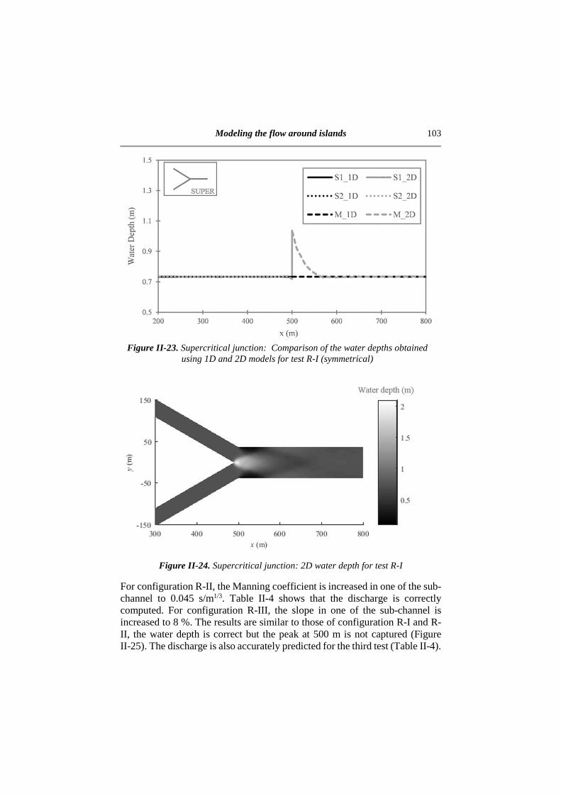
Modeling the flow around islands 103
Figure II-23. Supercritical junction: Comparison of the water depths obtained
using 1D and 2D models for test R-I (symmetrical)
Figure II-24. Supercritical junction: 2D water depth for test R-I
For configuration R-II, the Manning coefficient is increased in one of the sub-channel to 0.045 s/m1/3. Table II-4 shows that the discharge is correctly computed. For configuration R-III, the slope in one of the sub-channel is increased to 8 %. The results are similar to those of configuration R-I and R-II, the water depth is correct but the peak at 500 m is not captured (Figure II-25). The discharge is also accurately predicted for the third test (Table II-4).

104 Chapter II
Figure II-25. Supercritical junction: Comparison of the water depths
obtained using 1D and 2D models for test R-III (different slopes: 5% for M and S1, 8% for S2)
Then, the impact of the sub-channel width is investigated for configurations R-IV (50 m– 25 m) and R-V (60 m – 15 m). The water depth results are only shown for configuration R-IV. As for the previous tests, the water depths and the discharges are correctly predicted, only the local peak being not captured (Figure II-26 and Table II-4). For configuration T (trapezoidal channels), the results for the water depth are similar to the results in the rectangular channels, with an overall good correlation between the 1D and 2D predictions but without capturing the peak at the connection. In addition, the 1D model correctly conserves the discharge (Table II-4) while the 2D model presents some small inaccuracies.
Table II-4. Supercritical junction: Comparison of the discharges (in m3/s) obtained using the 1D and 2D models
Test QS1, 1D QS1, 2D QS2, 1D QS2, 2D QM, 1D QM, 2D R-I 200 200 200 200 400 400 R-II 200 200 200 200 400 400 R-III 200 200 200 200 400 400 R-IV 266.67 266.67 133.33 133.33 400 400 R-V 320 320 80 80 400 400 T 267.1 267.1 132.9 132.9 400 401
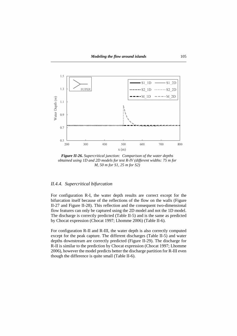
Modeling the flow around islands 105
Figure II-26. Supercritical junction: Comparison of the water depths
obtained using 1D and 2D models for test R-IV (different widths: 75 m for M, 50 m for S1, 25 m for S2)
II.4.4. Supercritical bifurcation For configuration R-I, the water depth results are correct except for the bifurcation itself because of the reflections of the flow on the walls (Figure II-27 and Figure II-28). This reflection and the consequent two-dimensional flow features can only be captured using the 2D model and not the 1D model. The discharge is correctly predicted (Table II-5) and is the same as predicted by Chocat expression (Chocat 1997; Lhomme 2006) (Table II-6). For configuration R-II and R-III, the water depth is also correctly computed except for the peak capture. The different discharges (Table II-5) and water depths downstream are correctly predicted (Figure II-29). The discharge for R-II is similar to the prediction by Chocat expression (Chocat 1997; Lhomme 2006), however the model predicts better the discharge partition for R-III even though the difference is quite small (Table II-6).

106 Chapter II
Figure II-27. Supercritical bifurcation: Comparison of the water depths
obtained using 1D and 2D models for test R-I (symmetrical)
Figure II-28. Supercritical bifurcation: 2D water depth for test I
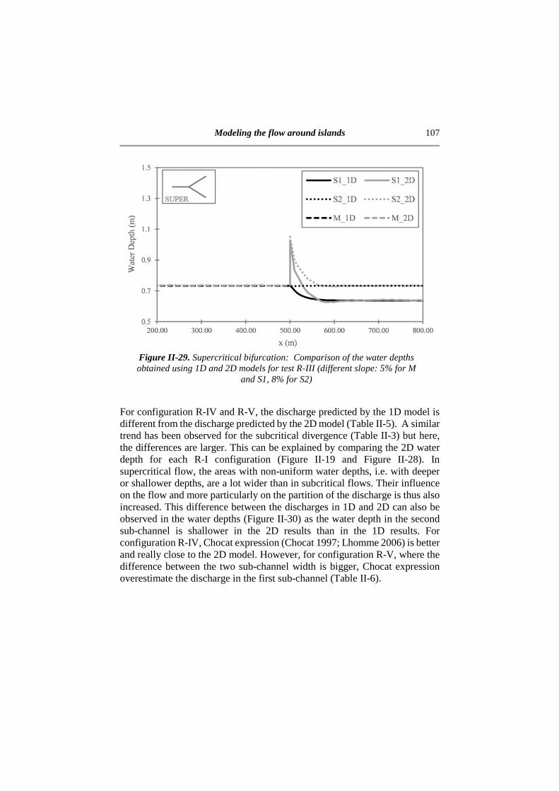
Modeling the flow around islands 107
Figure II-29. Supercritical bifurcation: Comparison of the water depths obtained using 1D and 2D models for test R-III (different slope: 5% for M
and S1, 8% for S2)
For configuration R-IV and R-V, the discharge predicted by the 1D model is different from the discharge predicted by the 2D model (Table II-5). A similar trend has been observed for the subcritical divergence (Table II-3) but here, the differences are larger. This can be explained by comparing the 2D water depth for each R-I configuration (Figure II-19 and Figure II-28). In supercritical flow, the areas with non-uniform water depths, i.e. with deeper or shallower depths, are a lot wider than in subcritical flows. Their influence on the flow and more particularly on the partition of the discharge is thus also increased. This difference between the discharges in 1D and 2D can also be observed in the water depths (Figure II-30) as the water depth in the second sub-channel is shallower in the 2D results than in the 1D results. For configuration R-IV, Chocat expression (Chocat 1997; Lhomme 2006) is better and really close to the 2D model. However, for configuration R-V, where the difference between the two sub-channel width is bigger, Chocat expression overestimate the discharge in the first sub-channel (Table II-6).

108 Chapter II
Figure II-30. Supercritical bifurcation: Comparison of the water depths obtained using 1D and 2D models for test R-IV (different width: 75 m for
M, 50 m for S1 and 25 m for S2)
For configuration R-VI, the widening of the total available width (56.25 m in each of the two sub-channels against 75 m in the main channel) reduces the impact of the peak as it is “absorbed” by the diminution of the water depth downstream. However, the water depth obtained by the 1D model at the bifurcation is still too low compared to the one obtained with the 2D model. As for the other tests with both sub-channels having the same width (tests R-I, R-II and R-III), the discharge partition however is correctly predicted by the 1D model (Table II-5) and is the same as Chocat expression (Chocat 1997; Lhomme 2006) (Table II-6). For configuration T, as for the other configurations, the one-dimensional model predicts correctly the overall water depth. The partition of the discharge is also close to the partition predicted by the two-dimensional model (Table II-5). However, it is important to note that the latter presents important fluctuations of the computed discharge due to an imperfect treatment of the wet-dry interface on the banks of the trapezoidal cross-sections.

Modeling the flow around islands 109
Figure II-31. Supercritical bifurcation: Comparison of the water depths
obtained using 1D and 2D models for test R-VI (widening: 75 m for M and 56.25 m for S1 and S2)
Table II-5. Supercritical bifurcation: Comparison of the discharges (in m3/s) obtained using the 1D and 2D models
Test QM, 1D QM, 2D QS1, 1D QS1, 2D QS2, 1D QS2, 2D R-I 400 400 200 200.2 200 199.8 R-II 400 400 200 200.1 200 199.9 R-III 400 400 200 199.9 200 200.1 R-IV 400 400 266.67 275.4 133.33 124.6 R-V 400 400 320 327.5 80 72.5 R-VI 400 400 200 200.2 200 199.8 T 400 400 264.6 262 135.4 138.1

110 Chapter II
Table II-6. Supercritical bifurcation: Comparison of the discharges (in m3/s) obtained using the 1D, 2D models and Chocat expression Test QS1, 1D QS1, 2D QS1,Chocat R-I 200 200.2 200 R-II 200 200.1 200 R-III 200 199.9 197 R-IV 266.67 275.4 276 R-V 320 327.5 336 R-VI 200 200.2 200 T 264.6 262 -
II.4.5. Application to the Meuse River Finally, the one-dimensional model is compared to a real case, the simulation of the flow in one reach of the Meuse River in Belgium featuring an island surrounded by two sub-reaches of different widths (Figure II-32 and Figure II-33): subreach S1 is much wider than subreach S2 and they present a very different bed elevation. The 4 km reach is located between the cities of Houx and Hun in the south of Belgium. The reach has been divided into 45 cross-sections as represented in Figure II-33. Measurement of the water level 200 m upstream of the city of Houx are compared to the numerical simulations for one almost complete year of measurements, from the 1st of January 2016 to the 22nd of December 2016, computed from the measured hydrograph represented in Figure II-34, with discharges ranging from 30 m3/s to 780 m3/s.
Figure II-32. Bifurcation of the river at the island location: Comparison of the three cross-sections
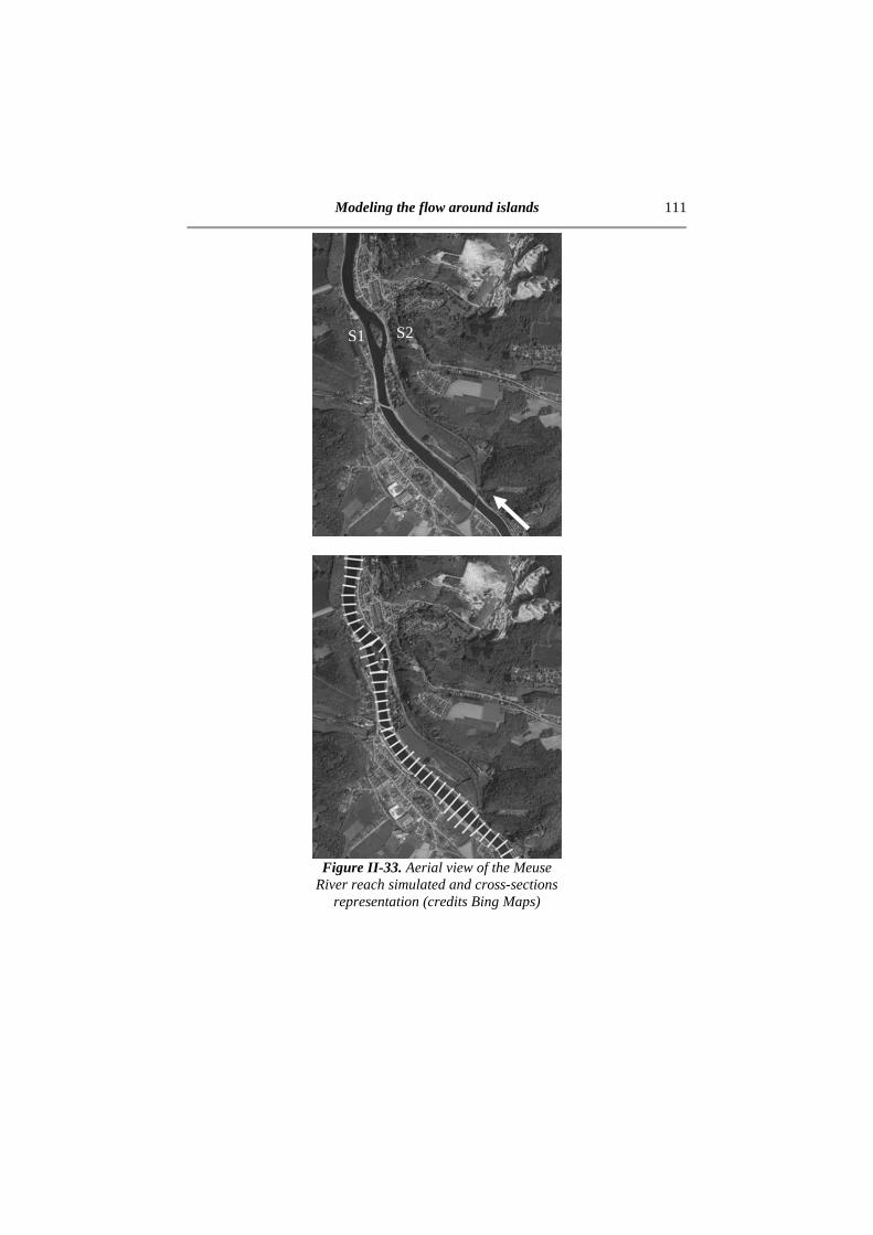
Modeling the flow around islands 111
Figure II-33. Aerial view of the Meuse
River reach simulated and cross-sections representation (credits Bing Maps)
S1 S2

112 Chapter II
Figure II-34. Discharge imposed upstream
Figure II-35 and Figure II-36 illustrate the result of the water level for the 24th of June 2016 at 20:00 (8 PM, local time, corresponding to 6 PM, 18:00 UTC). The dot symbolizes the measured water level. As before, the notation M is used for the main channel and the notations S1 and S2 for the two sub-channels, located on each side of the island. Figure II-35 clearly indicates that the bed level in each of the sub-channel is significantly different resulting in a difference of the water level in the two sub-channels (Figure II-36). The model correctly predicts the measured water level upstream of the island. Figure II-37 summarized the results for the complete test, comparing the hourly measured and computed water depths (more than 8000 points of comparison). It shows that the computed water depth is within 5 cm of the measured water depth for the most of the predictions.

Modeling the flow around islands 113
Figure II-35. Results for the water level (gray) and the bed level (black) for
the reach of the Meuse River for 24 June 2016 20:00.
Figure II-36. Results for the water level for the reach of the Meuse River
for 24 June 2016 20:00.

114 Chapter II
Figure II-37. Comparison between the computed and measured water
depths for the Meuse River. The solid line represent the exact prediction and the dash lines an error of 5 cm
II.5. Conclusion A one-dimensional model to simulate the flow around islands in a river has been presented. The model uses the characteristic equations and the water head balance to compute the fluxes before and after the island, i.e. at bifurcations and junctions. It has been compared to a 2D model for rectangular and trapezoidal cross-sections. It showed good results in predicting the discharge partition according to the equivalent width. However, the water depth at the junction/bifurcation showed some differences between the 1D and 2D models. These differences are caused by the non-consideration of the transversal velocities or the constriction in the one-dimensional model that makes it impossible to capture the reflections on the walls of the channel. Nevertheless, the water depth results provided by the 1D model are correct, when neglecting these local 2D phenomena with, for example, a correct continuity for the symmetrical cases (Figure II-14, Figure II-18, Figure II-23 and Figure II-27). Furthermore, the water depth was correct away from the junction / bifurcation and, in real rivers, the transitions and divisions of the flow are usually smoother than the one tested here, creating a much reduced local peak of the water level. In addition, the computations with the one-dimensional model were substantially faster than the two-dimension model.
Modeling the flow around islands 115
Finally, the one-dimensional model has been used to simulate the flow in a reach of a real river, the Meuse River in the south of Belgium. The results showed good agreement with the measurements for a year of predictions. Future work should focus on the computation of the sediment transport in the connections and should treat the particular issue of wetting/drying of a sub-channel. These improvements would allow the model to be used to predict the flood in river with intense sediment transport.
Acknowledgments This work was supported by the Fonds National de la Recherche Scientifique, Belgium. The authors would also like to thank Xavier Bodart and Quentin Callut for their help during the creation of the model.
References Chocat. 1997. Encyclopédie de l’hydrologie urbaine et de l’assainissement.
Lavoisier. France (in French)
Chow V.T. 1959 Open Channel Hydraulics. McGraw-Hill Book Company, New York
Dal Cin C., Moens L., Dierickx P., Bastin G, Zech Y. 2005. An integrated approach for real-time flood-map forecasting on the Belgian Meuse River, Natural Hazards, 36(1-2): 237-256
Finaud-Guyot, P., Delenne, C., Guinot, V. 2011. Coupling of 1D and 2D models for river flow modelling. Houille Blanche, (3), 23-28.
Franzini F. & Soares-Frazão S. 2016 Efficiency and accuracy of Lateralized HLL, HLLS and Augmented Roe's scheme with energy balance for river flows in irregular channels. Applied Mathematical Modelling. 40 (17-18), 7427-7446.
García-Navarro P. & Savirón J.M. 1992 Numerical simulation of unsteady flow at open channel junctions, Journal of Hydraulic Research, 30 (5), 595-609.
Ghostine R., Vazquez J., Terfous A., & Ghenaim A. 2012. Comparative study of 1D and 2D flow simulations at open-channel junctions. Journal of Hydraulic Research, 50 (2), 164-170.

116 Chapter II
Ghostine R., Hoteit I., Vazquez J., Terfous A., Ghenaim A. & Mose, R.
2015 Comparison between a coupled 1D-2D model and a fully 2D model for supercritical flow simulation in crossroads. Journal of Hydraulic Research, 53 (2), 274-281.
Guinot V. & Soares-Frazão, S. 2006 Flux and source term discretization in two-dimensional shallow water models with porosity on unstructured grids. International Journal for Numerical Methods in Fluids, 50 (3), 309-345.
Lhomme J. 2006. Modélisation des inondations en milieu urbain : approches unidimensionnelle, bidimensionnel et macroscopique. PhD Thesis. Université Montpellier II. France (in French)
Mahmood K. & Yevjevich V. 1975. Unsteady flow in open channels I. Water resources publications, USA.
Mignot E., Rivière N., Paquier A., & Perkins R.J. 2011. Hydraulic Models of the flow distribution in a four branch open channel junction with supercritical flow. Journal of Hydraulic Engineering, 137(3), 289-299.
Morales-Hernández M., García-Navarro P., Burguete J. & Brufau, P. 2013 A conservative strategy to couple 1D and 2D models for shallow water flow simulation. Computers and Fluids, 81, 26-44.
Murillo J. & Garcia-Navarro P. 2014 Accurate numerical modeling of 1d flow in channels with arbitrary shape. Application of the energy balanced property. Journal of Computational Physics. 260, 222–248.
Petaccia, G., Natale, L., Savi, F., Velickovic, M., Zech, Y., & Soares-Frazão, S. 2013 Flood wave propagation in steep mountain rivers. Journal of Hydroinformatics, 15(1), 120-137.
Roe P. 1981 Approximate Riemann solvers, parameter vectors, and difference schemes. Journal of Computational Physics. 43, 357–372.
Soares-Frazão S. & Zech Y. 2002 Dam Break in Channels with 90° Bend. Journal of Hydraulic Engineering, 128, 956-968
Wylie E.B. 2004 Water surface profiles in divided channels. Journal of Hydraulic Research, 10 (3), 325-341.
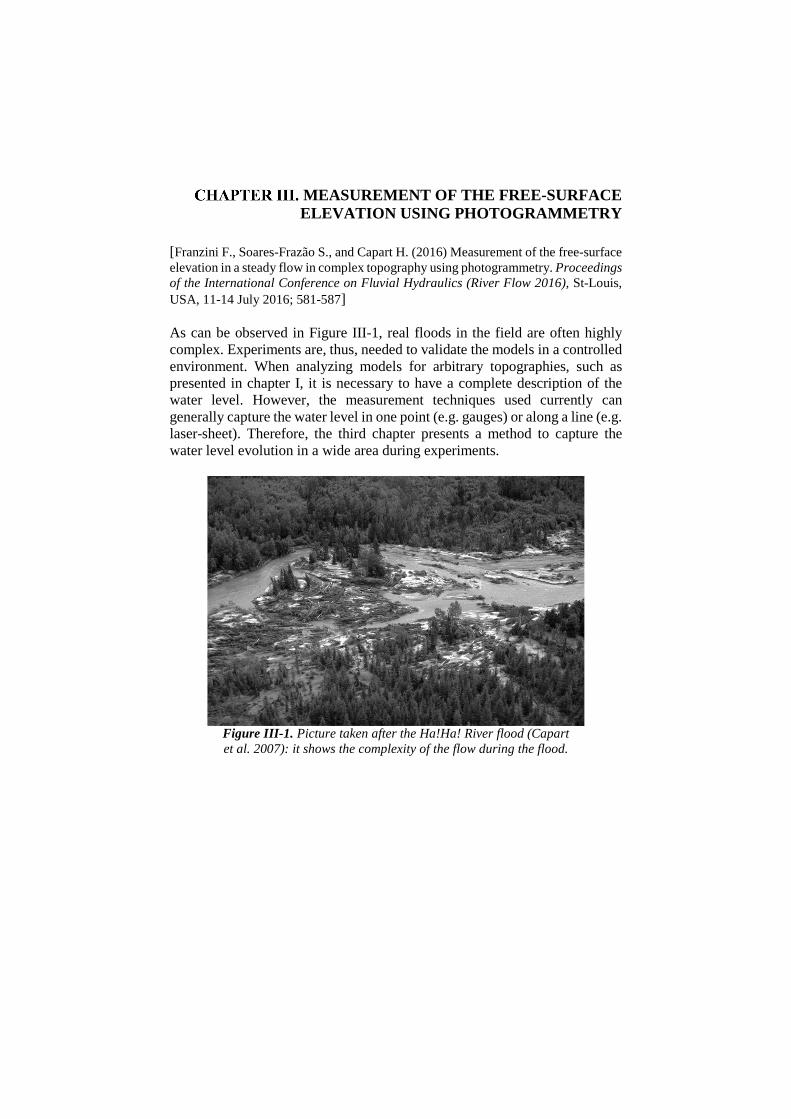
MEASUREMENT OF THE FREE-SURFACE ELEVATION USING PHOTOGRAMMETRY
[Franzini F., Soares-Frazão S., and Capart H. (2016) Measurement of the free-surface elevation in a steady flow in complex topography using photogrammetry. Proceedings of the International Conference on Fluvial Hydraulics (River Flow 2016), St-Louis, USA, 11-14 July 2016; 581-587] As can be observed in Figure III-1, real floods in the field are often highly complex. Experiments are, thus, needed to validate the models in a controlled environment. When analyzing models for arbitrary topographies, such as presented in chapter I, it is necessary to have a complete description of the water level. However, the measurement techniques used currently can generally capture the water level in one point (e.g. gauges) or along a line (e.g. laser-sheet). Therefore, the third chapter presents a method to capture the water level evolution in a wide area during experiments.
Figure III-1. Picture taken after the Ha!Ha! River flood (Capart et al. 2007): it shows the complexity of the flow during the flood.
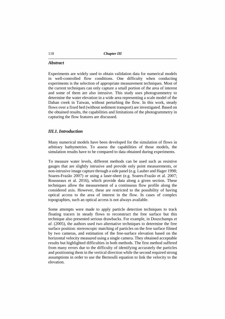
118 Chapter III
Abstract Experiments are widely used to obtain validation data for numerical models in well-controlled flow conditions. One difficulty when conducting experiments is the selection of appropriate measurement techniques. Most of the current techniques can only capture a small portion of the area of interest and some of them are also intrusive. This study uses photogrammetry to determine the water elevation in a wide area representing a scale model of the Dahan creek in Taiwan, without perturbing the flow. In this work, steady flows over a fixed bed (without sediment transport) are investigated. Based on the obtained results, the capabilities and limitations of the photogrammetry in capturing the flow features are discussed.
III.1. Introduction Many numerical models have been developed for the simulation of flows in arbitrary bathymetries. To assess the capabilities of those models, the simulation results have to be compared to data obtained during experiments. To measure water levels, different methods can be used such as resistive gauges that are slightly intrusive and provide only point measurements, or non-intrusive image capture through a side panel (e.g. Lauber and Hager 1998; Soares-Frazão 2007) or using a laser-sheet (e.g. Soares-Frazão et al. 2007; Rousseaux et al. 2016), which provide data along a given section. These techniques allow the measurement of a continuous flow profile along the considered axis. However, these are restricted to the possibility of having optical access to the area of interest in the flow. In cases of complex topographies, such an optical access is not always available. Some attempts were made to apply particle detection techniques to track floating tracers in steady flows to reconstruct the free surface but this technique also presented serious drawbacks. For example, in Douxchamps et al. (2005), the authors used two alternative techniques to determine the free surface position: stereoscopic matching of particles on the free surface filmed by two cameras, and estimation of the free-surface elevation based on the horizontal velocity measured using a single camera. They obtained acceptable results but highlighted difficulties in both methods. The first method suffered from many errors due to the difficulty of identifying accurately the particles and positioning them in the vertical direction while the second required strong assumptions in order to use the Bernoulli equation to link the velocity to the elevation.

Measurement of the free-surface elevation using photogrammetry 119
Aureli et al. (2011) used a light-absorption method to capture the water level during a dam-break on a flat bed. With the combination of a backlighting diffusing light and a colored solution, the authors could determine the water depths from recorded RGB values. The determination is possible because the absorption is a function of the wavelength and the water depth. The method showed promising results. However, it suffers the limitation of being valid only on a flat bed or a smoothly varying bed. The research presented here uses photogrammetry to capture the whole water free-surface elevation. According to Schenk (2005), photogrammetry is defined as the science of obtaining reliable information about the properties of surfaces and objects without physical contact with the objects, and of measuring and interpreting this information. The information is obtained by taking several overlapping pictures (stereopsis) issued from different viewpoints in order to reconstruct a 3D geometry. This method has the advantage of being both non-intrusive and able to capture a wide area. Those two characteristics are interesting for capturing water level while performing experiments, or in the field. Photogrammetry is here applied to an experiment conducted at the National Taiwan University. The case considered is a scale model of the Dahan creek, located upstream of the Shihmen reservoir in the northern part of Taiwan. This creek is characterized by a complex topography, with a main channel and floodplains limited by cliffs and then higher terrain, and featuring abrupt changes in the cross-section shape (Figure III-2). The goal of this experiment is to assess the capabilities of this technique in capturing the water level for a flow in a completely arbitrary topography. The paper is organized as follows: in section III.2, the experiment and measurement technique are detailed. Then, results obtained using photogrammetry are presented and validated in section III.3. Finally, conclusions regarding the capabilities of photogrammetry in the domain of experimental hydraulics are drawn. Several possibilities of improvement are also highlighted.
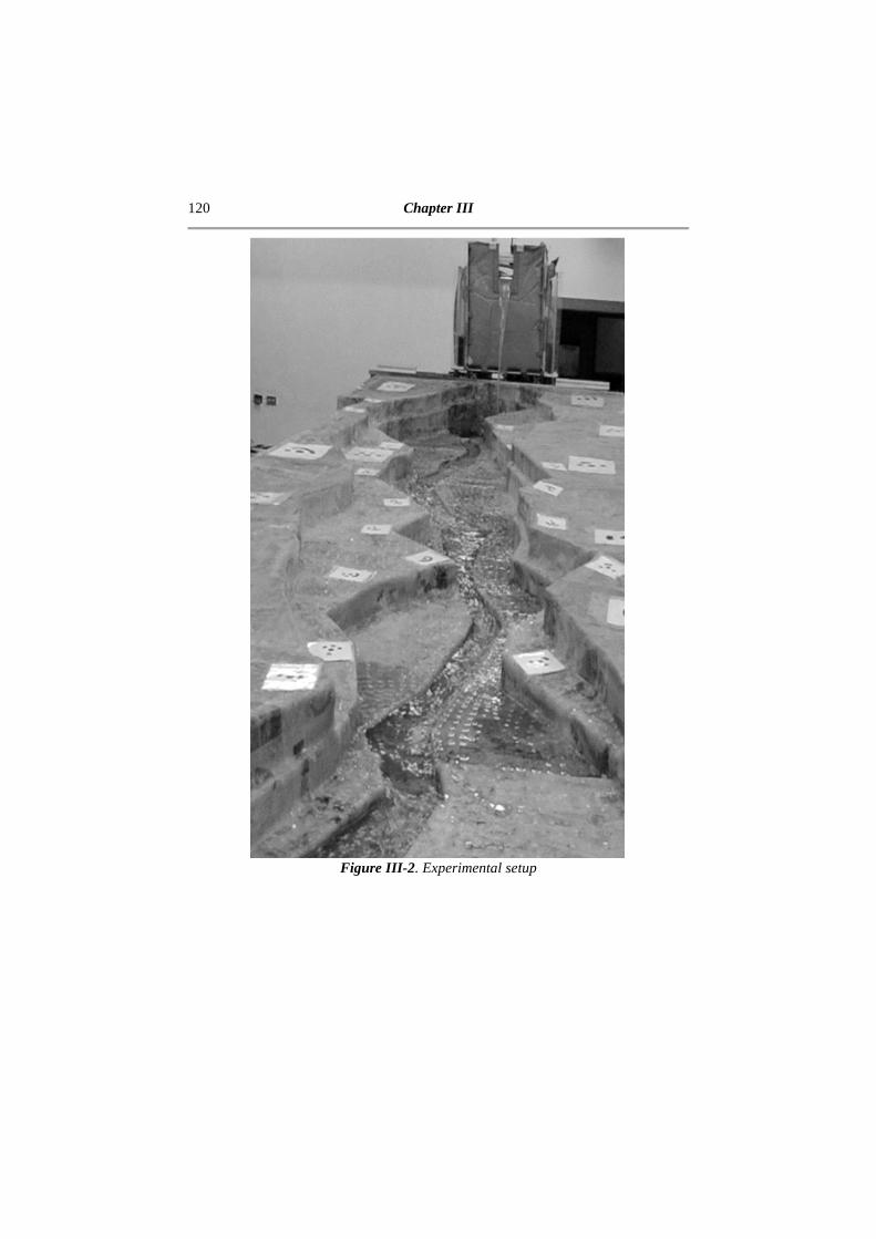
120 Chapter III
Figure III-2 . Experimental setup

Measurement of the free-surface elevation using photogrammetry 121
III.2. Experimental setup The 1/2500 scaled model was constructed in fiberglass reinforced polyester (Figure III-2). The topography was created from field measurements and maps. To obtain an accurate representation of the terrain, a mold was cut out of a block of Styrofoam by a Computer Numerical Controlled Styrofoam Cutter. As Styrofoam is not water tight and highly resistant, a layer of fiberglass-reinforced polyester was added on top of it. Considering the important scale factor, a vertical / horizontal distortion of a factor 7 has been applied in order to obtain measurable water-depths in the model. The vertical scale is thus 7/2500. This distortion is acceptable because the flow is mainly one-dimensional and the width of the channel is much bigger than its depth (Kobus, 1980). The final model, illustrated in Figure III-2, is 12 m long and 2 m wide. In order to reproduce the observed water depths taking into account the distortion factor applied, it is necessary to have an adapted high value of the Manning coefficient. This is not achievable with a channel made of polyester. Therefore, a higher friction is created using small acrylic cubes placed on the riverbed. Their size (3 mm) and distribution were selected to reach the expected water depths without affecting too much the water surface, i.e. without creating a step-pool behavior. The 3 mm roughness height in the model corresponds to approximately 1 m in the prototype; this is non-negligible but the increase of friction is important to reach the correct measured water depth. Three different discharges are considered. The lower one corresponds to a flow restricted to the main channel with Q = 0.93 l/s, corresponding approximately to 16,000 m3/s in the prototype – the ratio between the model and the prototype discharges being 25002.5/71.5 (Kobus, 1980). The largest one corresponds to the peak discharge that could be reasonably expected in case of a dam failure at the Shihmen Reservoir, with Q = 2.37 l/s, i.e. approximately 40,000 m3/s in the prototype. The last one corresponds to intermediary conditions, with Q = 1.48 l/s, i.e. approximately 25,000 m3/s in the prototype. To impose the discharge, a reservoir with a rotating door was built. Inside the reservoir, the water level was kept constant using a system of pumps. Thus, the inclination of the door could control the discharge exiting by overflow.
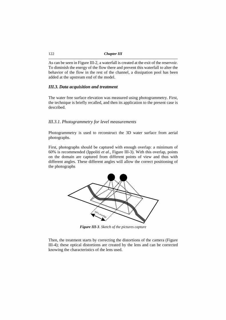
122 Chapter III
As can be seen in Figure III-2, a waterfall is created at the exit of the reservoir. To diminish the energy of the flow there and prevent this waterfall to alter the behavior of the flow in the rest of the channel, a dissipation pool has been added at the upstream end of the model.
III.3. Data acquisition and treatment The water free surface elevation was measured using photogrammetry. First, the technique is briefly recalled, and then its application to the present case is described.
III.3.1. Photogrammetry for level measurements Photogrammetry is used to reconstruct the 3D water surface from aerial photographs. First, photographs should be captured with enough overlap: a minimum of 60% is recommended (Ippoliti et al., Figure III-3). With this overlap, points on the domain are captured from different points of view and thus with different angles. These different angles will allow the correct positioning of the photographs
Figure III-3 . Sketch of the pictures capture
Then, the treatment starts by correcting the distortions of the camera (Figure III-4); these optical distortions are created by the lens and can be corrected knowing the characteristics of the lens used.
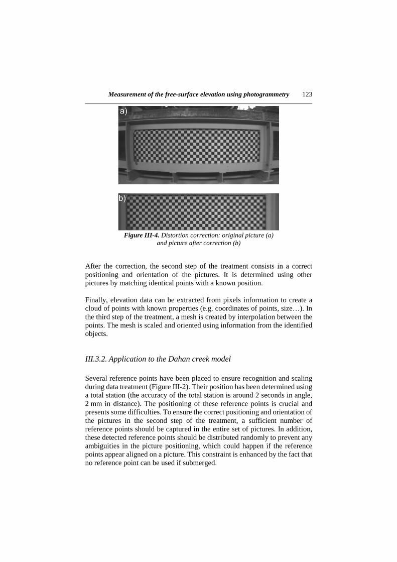
Measurement of the free-surface elevation using photogrammetry 123
Figure III-4. Distortion correction: original picture (a)
and picture after correction (b)
After the correction, the second step of the treatment consists in a correct positioning and orientation of the pictures. It is determined using other pictures by matching identical points with a known position. Finally, elevation data can be extracted from pixels information to create a cloud of points with known properties (e.g. coordinates of points, size…). In the third step of the treatment, a mesh is created by interpolation between the points. The mesh is scaled and oriented using information from the identified objects.
III.3.2. Application to the Dahan creek model Several reference points have been placed to ensure recognition and scaling during data treatment (Figure III-2). Their position has been determined using a total station (the accuracy of the total station is around 2 seconds in angle, 2 mm in distance). The positioning of these reference points is crucial and presents some difficulties. To ensure the correct positioning and orientation of the pictures in the second step of the treatment, a sufficient number of reference points should be captured in the entire set of pictures. In addition, these detected reference points should be distributed randomly to prevent any ambiguities in the picture positioning, which could happen if the reference points appear aligned on a picture. This constraint is enhanced by the fact that no reference point can be used if submerged.

124 Chapter III
To satisfy as much as possible these recommendations, 72 reference points have been placed on the channel, on the small plateaus, out of the reach of the flow and as close as possible to the main channel. The average distance between two consecutive reference points (on the same bank) is thus 0.2 m.
Figure III-5. Example of reference points (12-bit
circular)
Any type of reference points can be used. In this case, 12-bit circular reference points (Figure III-5) have been used, because they can easily be recognized (position and number) by the software used for image treatment. The pictures were captured using four synchronized cameras (see Table III-1). The synchronization was controlled by four independent flashes. It was necessary to use four flashes in order to obtain uniformly bright pictures and a recycling time low enough to be able to take many pictures in a short time. To synchronize correctly the pictures, the room was kept completely dark and the cameras were set in long exposure mode. That way, the flash ensures that all the pictures are taken at exactly the same time. The area covered by one set of pictures is approximately 2 by 2 meters. The set of cameras is thus moved twelve times to cover the complete domain with enough overlap. This is relatively easy for steady flows, as the water surface is considered stable.
Table III-1. Cameras used in the experiments. Camera Type Lens focal length Nikon D3 24 mm Nikon D200 18 mm Nikon D7000 18 mm Nikon D7000 18 mm
Before starting the experiment, pictures of the dry bed have been taken to obtain a reference situation to extract water depths. Then, the flow
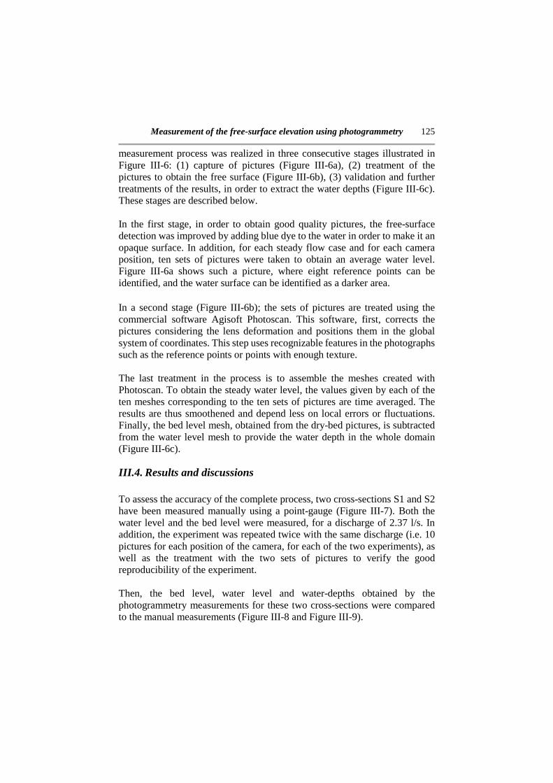
Measurement of the free-surface elevation using photogrammetry 125
measurement process was realized in three consecutive stages illustrated in Figure III-6: (1) capture of pictures (Figure III-6a), (2) treatment of the pictures to obtain the free surface (Figure III-6b), (3) validation and further treatments of the results, in order to extract the water depths (Figure III-6c). These stages are described below. In the first stage, in order to obtain good quality pictures, the free-surface detection was improved by adding blue dye to the water in order to make it an opaque surface. In addition, for each steady flow case and for each camera position, ten sets of pictures were taken to obtain an average water level. Figure III-6a shows such a picture, where eight reference points can be identified, and the water surface can be identified as a darker area. In a second stage (Figure III-6b); the sets of pictures are treated using the commercial software Agisoft Photoscan. This software, first, corrects the pictures considering the lens deformation and positions them in the global system of coordinates. This step uses recognizable features in the photographs such as the reference points or points with enough texture. The last treatment in the process is to assemble the meshes created with Photoscan. To obtain the steady water level, the values given by each of the ten meshes corresponding to the ten sets of pictures are time averaged. The results are thus smoothened and depend less on local errors or fluctuations. Finally, the bed level mesh, obtained from the dry-bed pictures, is subtracted from the water level mesh to provide the water depth in the whole domain (Figure III-6c).
III.4. Results and discussions To assess the accuracy of the complete process, two cross-sections S1 and S2 have been measured manually using a point-gauge (Figure III-7). Both the water level and the bed level were measured, for a discharge of 2.37 l/s. In addition, the experiment was repeated twice with the same discharge (i.e. 10 pictures for each position of the camera, for each of the two experiments), as well as the treatment with the two sets of pictures to verify the good reproducibility of the experiment. Then, the bed level, water level and water-depths obtained by the photogrammetry measurements for these two cross-sections were compared to the manual measurements (Figure III-8 and Figure III-9).

126 Chapter III
Figure III-6. Complete process to obtain results: (a) Sets of
four pictures taken on the flume (only one is represented here), (b) Determination of the level using the commercial
software Photoscan, and (c) Final treatment of the data and extraction of the water depth
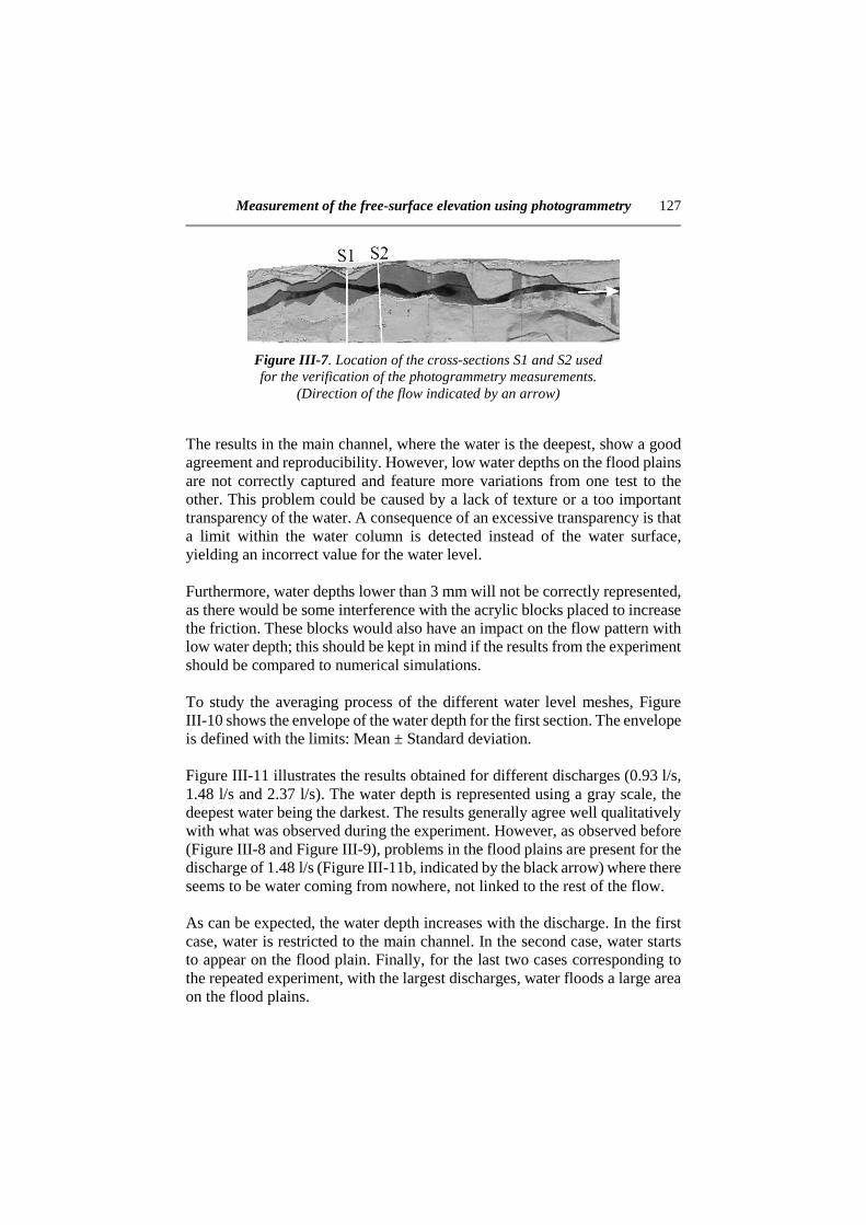
Measurement of the free-surface elevation using photogrammetry 127
Figure III-7 . Location of the cross-sections S1 and S2 used for the verification of the photogrammetry measurements.
(Direction of the flow indicated by an arrow)
The results in the main channel, where the water is the deepest, show a good agreement and reproducibility. However, low water depths on the flood plains are not correctly captured and feature more variations from one test to the other. This problem could be caused by a lack of texture or a too important transparency of the water. A consequence of an excessive transparency is that a limit within the water column is detected instead of the water surface, yielding an incorrect value for the water level. Furthermore, water depths lower than 3 mm will not be correctly represented, as there would be some interference with the acrylic blocks placed to increase the friction. These blocks would also have an impact on the flow pattern with low water depth; this should be kept in mind if the results from the experiment should be compared to numerical simulations. To study the averaging process of the different water level meshes, Figure III-10 shows the envelope of the water depth for the first section. The envelope is defined with the limits: Mean ± Standard deviation. Figure III-11 illustrates the results obtained for different discharges (0.93 l/s, 1.48 l/s and 2.37 l/s). The water depth is represented using a gray scale, the deepest water being the darkest. The results generally agree well qualitatively with what was observed during the experiment. However, as observed before (Figure III-8 and Figure III-9), problems in the flood plains are present for the discharge of 1.48 l/s (Figure III-11b, indicated by the black arrow) where there seems to be water coming from nowhere, not linked to the rest of the flow. As can be expected, the water depth increases with the discharge. In the first case, water is restricted to the main channel. In the second case, water starts to appear on the flood plain. Finally, for the last two cases corresponding to the repeated experiment, with the largest discharges, water floods a large area on the flood plains.

128 Chapter III
The measurement technique was able to capture the hydraulic jump (darkest colors) at the narrowing part of the channel, as observed during the experiments.
Figure III-8 . Comparison of the bed and water levels obtained by photogrammetry (lines) and
measured manually (crosses and dots) for (a) cross-section S1, (b) cross-section S2

Measurement of the free-surface elevation using photogrammetry 129
Figure III-9. Comparisons of the water depth
obtained by photogrammetry for the two repeated experiments (lines) and measured with point-
measurements (crosses) for (a) cross-section S1, (b) cross-section S2
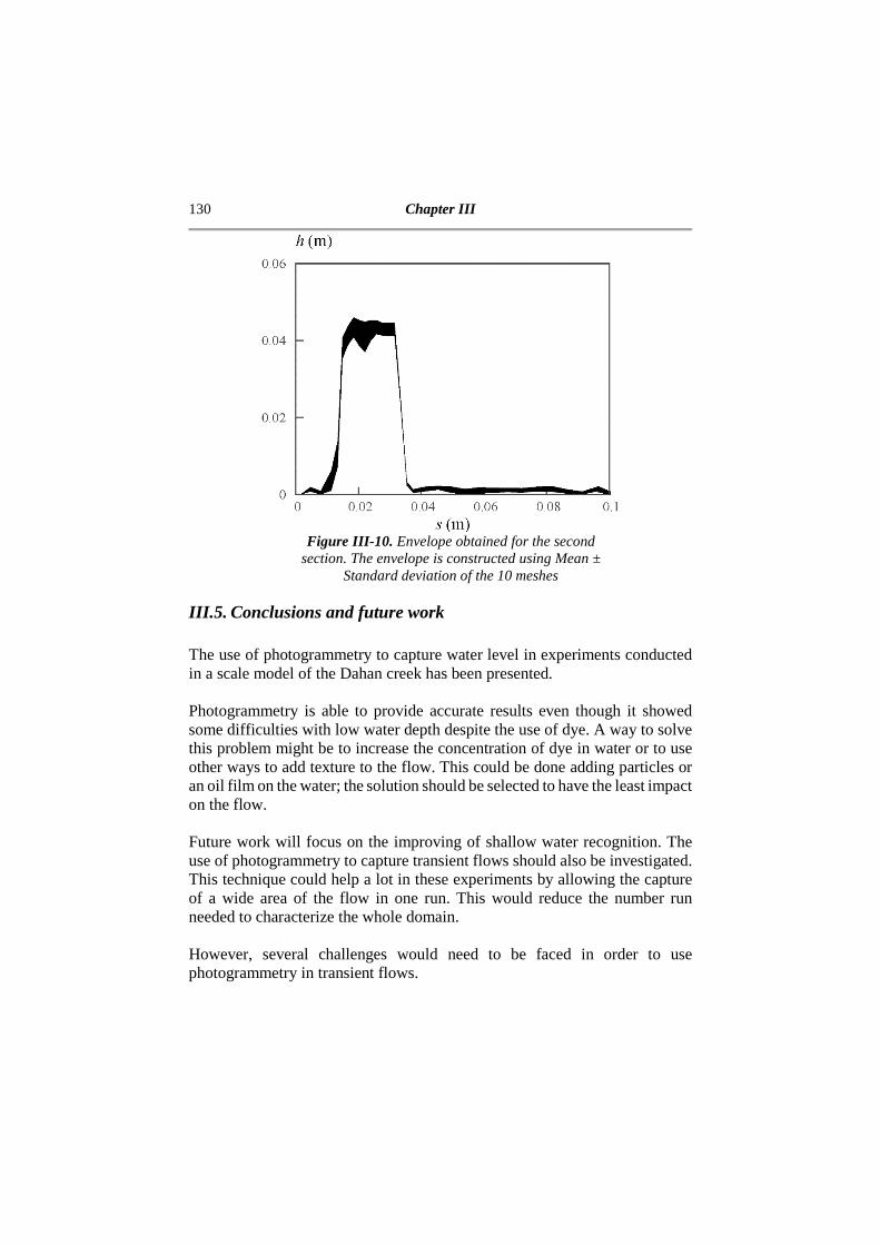
130 Chapter III
Figure III-10. Envelope obtained for the second
section. The envelope is constructed using Mean ± Standard deviation of the 10 meshes
III.5. Conclusions and future work The use of photogrammetry to capture water level in experiments conducted in a scale model of the Dahan creek has been presented. Photogrammetry is able to provide accurate results even though it showed some difficulties with low water depth despite the use of dye. A way to solve this problem might be to increase the concentration of dye in water or to use other ways to add texture to the flow. This could be done adding particles or an oil film on the water; the solution should be selected to have the least impact on the flow. Future work will focus on the improving of shallow water recognition. The use of photogrammetry to capture transient flows should also be investigated. This technique could help a lot in these experiments by allowing the capture of a wide area of the flow in one run. This would reduce the number run needed to characterize the whole domain. However, several challenges would need to be faced in order to use photogrammetry in transient flows.
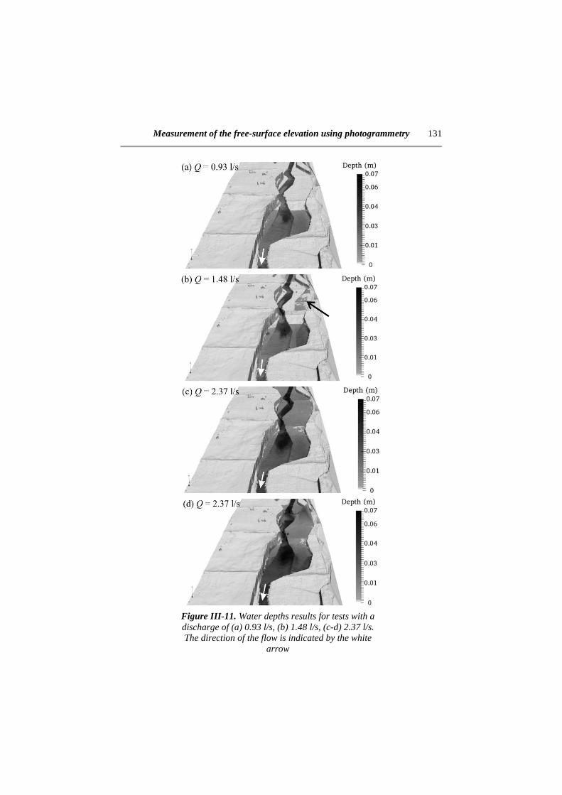
Measurement of the free-surface elevation using photogrammetry 131
Figure III-11. Water depths results for tests with a discharge of (a) 0.93 l/s, (b) 1.48 l/s, (c-d) 2.37 l/s. The direction of the flow is indicated by the white
arrow

132 Chapter III
First, the time elapsed between two consecutive pictures is controlled by the flashes used. In this experiment, the use of four independent flashes, with independent power supplies, allowed to take a set of pictures every second, but not faster without losing quality. This poses a limitation to the type of transient flows that could be captured. Real dam break or transient flows in arbitrary topographies would, currently, be out of reach (with the technique used in this paper). Second, in order to reconstruct the complete domain from different data set, it would be necessary to have pictures taken at the same time but in different positions. This would need a complete automated system to control the beginning of the test (e.g. the starting of the pumps, or, in this case, the opening of the door) and the capture of the pictures. Another solution would be to increase the number of cameras. However, this is not the most practical solution as, for example, 48 pictures were necessary to represent the full domain in the experiments presented here. To improve the results, as in the steady state, every set of pictures should be duplicated to be able to determine an average water level. This increase the importance of a well-timed experiment. This is not as important in the case of a steady flow as it can be assumed that the water level does not change when moving the cameras set. Finally, photogrammetry could be applied to monitor the morphological evolution in flows over movable beds by, for example, projecting a grid on the bed surface (Frank and Hager, 2015)
References Aureli, F., Maranzoni, A,. Mignosa, P., and Ziveri, C. 2011, An image
processing technique for measuring free surface of dam-break flows. Experiments in Fluids 50 (3): 665-675
Douxchamps, D., Devriendt, D., Capart, H., Craeye, C., Macq, B., and Zech, Y. 2005. Stereoscopic and velocimetric reconstructions of the free surface topography of antidune flows. Experiments in Fluids 39: 533–551
Frank P-J, and Hager, W.H. 2015, Spatial Dike Breach: Sediment Surface Topography Using Photogrammetry. E-proceedings of the 36th IAHR World Congress 28 June – 3 July 2015, The Hague, the Netherlands
Ippoliti, E, Meschini, A., and Sicuranza, F. 2015. Structure from Motion Systems for Architectural Heritage. A Survey of the Internal Loggia Courtyard of Palazzo Dei Capitani, Ascoli Piceno, Italy. ISPRS -

Measurement of the free-surface elevation using photogrammetry 133
International Archives of the Photogrammetry, Remote Sensing and Spatial Information Sciences. XL-5/W4: 53-60
Kobus, H. (1980). Hydraulic Modelling. German Association for water resources and land improvement. Stuttgart. Germany
Lauber, G. and Hager, W.H. 1998. Experiments to dambreak wave: Sloping channel. Journal of Hydraulic Research 36 (5): 761-772
Rousseaux, G., Mougenot J-M., Chatellier, L., David L., and Calluaud, D., 2016. A novel method to generate tidal-like bores in the laboratory. European Journal of Mechanics, B/Fluids 55: 31-38
Schenk, T. 2005. Introduction to Photogrammetry. The Ohio State University (course)
Soares-Frazão, S., Le Grelle, N., Spinewine, B., and Zech, Y. 2007. Dam-break induced morphological changes in a channel with uniform sediments: measurements by a laser-sheet imaging technique. Journal of Hydraulic Research 45: 13-16
Soares-Frazão, S. 2007. Experiments of dam-break wave over a triangular bottom sill. Journal of Hydraulic Research 45: 19-26

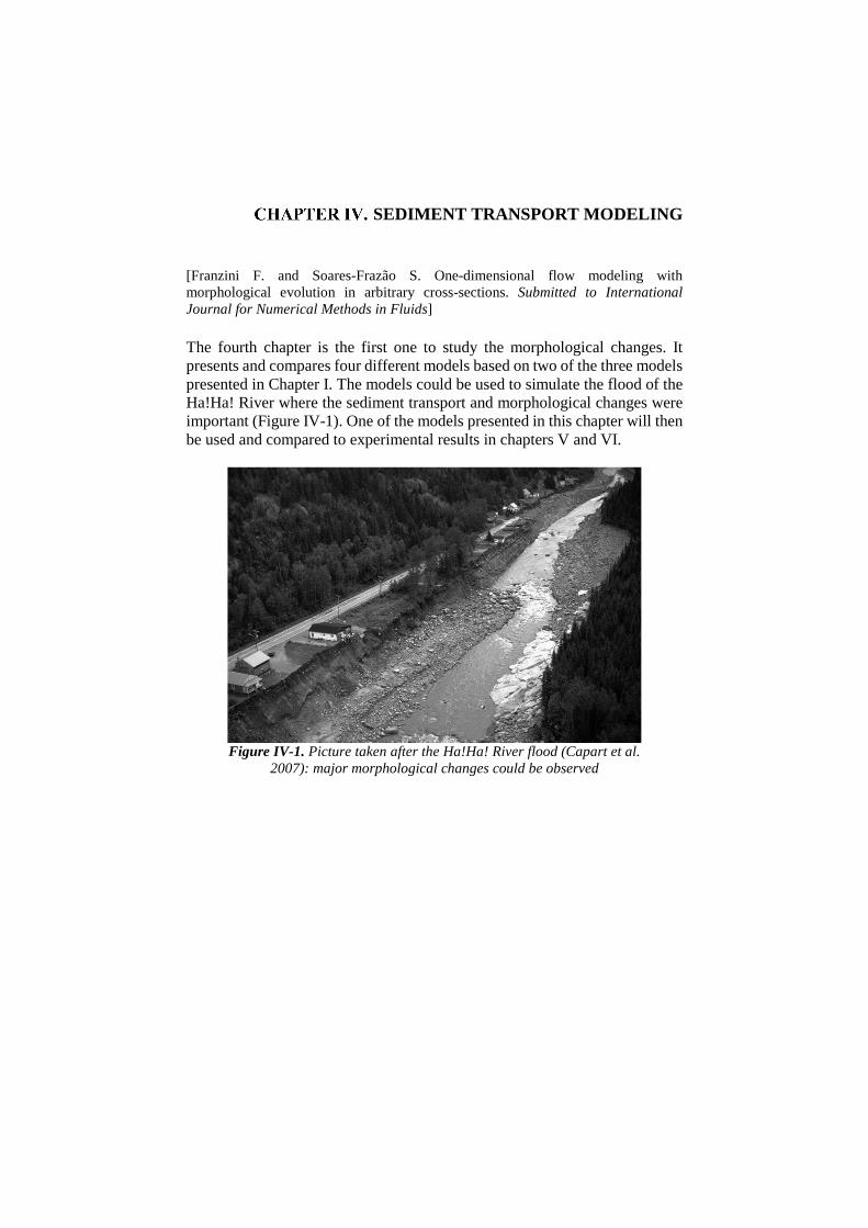
SEDIMENT TRANSPORT MODELING
[Franzini F. and Soares-Frazão S. One-dimensional flow modeling with morphological evolution in arbitrary cross-sections. Submitted to International Journal for Numerical Methods in Fluids]
The fourth chapter is the first one to study the morphological changes. It presents and compares four different models based on two of the three models presented in Chapter I. The models could be used to simulate the flood of the Ha!Ha! River where the sediment transport and morphological changes were important (Figure IV-1). One of the models presented in this chapter will then be used and compared to experimental results in chapters V and VI.
Figure IV-1. Picture taken after the Ha!Ha! River flood (Capart et al.
2007): major morphological changes could be observed

136 Chapter IV
Abstract The performances of four different one-dimensional numerical models are assessed by comparing the results obtained in simulating the morphological changes in a river during a flood. All four models solve the shallow-water-Exner equations but they differ in the finite-volume discretization. Two models solve the set of equations using an uncoupled approach where the shallow-water equations are first solved to compute the hydrodynamics and, then, the Exner equation is solved to compute the morphological changes. The other two models use a coupled approach where all three equations are solved simultaneously. Another distinction between the models is the type of scheme used: HLL- or Roe-based. The four models are thus: uncoupled HLL, uncoupled Roe, coupled HLL and coupled Roe. Numerous test cases were examined, including water at rest, steady flows and transient flows. The results showed that the coupled Roe model provides correct results for steady flows and for water at rest, in a smoother, more natural, way than the other models. The coupled HLL model shows good results for the prediction of a dike overtopping and the consequent erosion. However, the results for the simulation of the progressive evolution of an initially sloping sediment bed towards an equilibrium slope showed the limit of this model as the bed evolves until becoming horizontal. The coupled models performed globally better than their uncoupled counterpart did. However, the uncoupled HLL predicted better the equilibrium slope as it did not become horizontal like the coupled HLL. Finally, test cases in arbitrary cross-sections with steep banks highlighted the importance of including a bank failure mechanism in the model. Without such additional features, none of the models, even the most accurate one, is able to produce reliable results for the case of a dam-break flow in a semi-trapezoidal channel.
IV.1. Introduction Floods can be highly damaging natural disasters and their impact is often increased by the presence of sediments. In such cases, the strong morphological changes following an important flood completely reshape the riverbed and the landscape of the surrounding area (Capart et al. 2007). Predicting such floods and their morphological consequences is thus important to prevent human loses and damages. In solving this problem, 1D models could play a role as they have the advantages of needing less data and being faster than 2D models. Of course, they are not able to capture as many

Sediment transport modeling 137
complex patterns as the 2D models. However, during a flood crisis, time is a key factor, if not the most important factor. In this aspect, 1D models are still much faster than 2D models even with latest developments on the use of GPU to increase the computation speed (Lacasta et al. 2014). In a depth-averaged framework, the shallow-water equations describing the water flow are used together with additional equations describing the morphological evolution of the bed following erosion and deposition of sediments. The links between these sets of equations, and consequently the impact of the presence of sediments on the water flow, are described in the literature using various approaches: (a) only mass conservation is considered for the sediments, and their effect on the flow density is neglected (Cunge and Perdreau 1973, Kassem and Chaudhry 1998, Goutière et al. 2008); (b) the effect of the sediment concentration on the flow is considered by providing some additional, but weak, coupling between the equations (Cao et al. 2004, Wu and Wang 2007, Garegnani et al. 2011); (c) the moving sediments are represented using a transport layer, leading to fully coupled equations, which consider momentum exchanges between layers (Fraccarollo et al. 2003, Zech et al. 2008, Spinewine and Capart 2013); and (d) the moving sediments are considered as a separate and immiscible phase in the water flow with exchanges between the two phase providing a significant level of coupling between the equations (Greco et al. 2012). In the present research, where only bed load transport is considered, the first approach (a) has been favored because in such cases, the concentration of sediment in the water column is low and can be neglected. The considered sediments consist of non-cohesive particles, such as sand, that are more often transported by bed load than suspension load. In this approach, the flow is considered as consisting of a layer of clear water, without sediment, flowing on top of a movable bed. The three main equations in this model are the two shallow-water equations describing mass and momentum conservations of the water layer, and the Exner equation describing the mass conservation of the sediment bed. Two approaches can be considered to solve these equations. In the first approach, called uncoupled (or weakly coupled) approach (Juez and Garcia-Navarro 2014), the equations are solved using a two-step method. First, the shallow water equations are solved without considering the sediment transport. Then, the Exner equation is solved without changing the hydraulic variables. In the second approach, the three equations are solved simultaneously, leading to a coupled solver (Goutière et al. 2008). Both approaches are tested here. This paper is divided as follows. First, the governing equations used to represent the flow and sediment transport in a one-dimensional framework

138 Chapter IV
with arbitrary cross-sections are presented. Then, the different solvers and the erosion process are discussed. Finally, the models are compared and validated using selected test cases from the literature.
IV.2. Governing equations The model used consists of three equations: the one-dimensional shallow-water equations or Saint-Venant equations for the hydrodynamics in arbitrary cross-sections, and the Exner equation for the mass conservation of the sediments. The main assumptions for the Saint-Venant equations are an incompressible fluid, a hydrostatic pressure distribution, and, as stated before, a negligible concentration of sediments in the water. For a cross-section of arbitrary shape, they read
∂A
∂t+
∂Q
∂x=0
(IV-1)
∂Q
∂t+
∂
∂xQ2
A+gI1 =gI2+AS0-Sf (IV-2)
Where Q is the discharge, A the area of water, S0 the bed slope defined by:
S0=- dzb0
dx
(IV-3)
With zb0 the bed level, more precisely the thalweg level.
The integral gI1 represents the hydrostatic pressure thrust while the integral gI2 represents the longitudinal component of the lateral pressure due to the longitudinal width changes. They are integrals written as gI1=g + h-ηb dη
h
0 (IV-4)
gI2=g+ h-η ∂b
∂xdη
h
0 (IV-5)
With η a local variable for the depth integration and b(x, η) the width of the channel at a determined depth (Figure IV-2). It is important to note that these
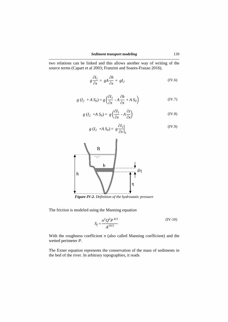
Sediment transport modeling 139
two relations can be linked and this allows another way of writing of the source terms (Capart et al 2003; Franzini and Soares-Frazao 2016).
g∂I1
∂x= gA
∂h
∂x+ gI2 (IV.6)
g (I2 +AS0)= g-∂I1
∂x-A∂h
∂x+AS0. (IV.7)
g (I2 +A S0)= g-∂I1
∂x-A∂z
∂x. (IV.8)
g (I2 +AS0)= g∂I1
∂x/z0 (IV.9)
Figure IV-2. Definition of the hydrostatic pressure
The friction is modeled using the Manning equation
Sf =n2Q2P 4/3
A10/3 (IV-10)
With the roughness coefficient n (also called Manning coefficient) and the wetted perimeter P. The Exner equation represents the conservation of the mass of sediments in the bed of the river. In arbitrary topographies, it reads

140 Chapter IV
∂Ab
∂t+
1
1 - ε0
∂Qs
∂x = 0
(IV-11)
Where Ab is the area of the bed of sediments (Figure IV-3), Qs the sediment transport rate and ε0 the bed porosity.
Figure IV-3. Definition of the area of sediment
In this research, the bed porosity is considered constant in both time and space. The Exner equation can thus be rewritten as
∂Ab
∂t+∂
∂x Qs
1 - ε0= 0
(IV-12)
Finally, it is necessary to add a closure equation to determine the sediment transport (Qs). Several relationships exist in the literature such as Meyer-Peter and Müller, Smart and Jäggi or Camenen and Larson, summarized e.g. in El Kadi Abderrezzak and Paquier (2011). In the present paper, it has been decided to use the equation developed by Meyer-Peter and Müller (1948). This equation is only valid for non-cohesive particles and without suspension or wash load and provides the unit-width sediment transport rate as.
qs=8Vgs-1d50 3 RSfs-1 d50
- θcr1.5
(IV-13)
Where s is the specific gravity of the sediments, d50 the median bed sediment diameter, R the hydraulic radius (defined as R = A/P), and θcr the adimensional
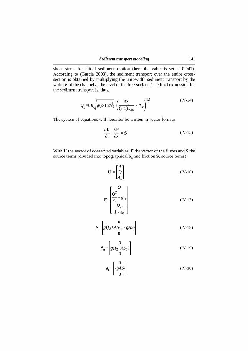
Sediment transport modeling 141
shear stress for initial sediment motion (here the value is set at 0.047). According to (Garcia 2008), the sediment transport over the entire cross-section is obtained by multiplying the unit-width sediment transport by the width B of the channel at the level of the free-surface. The final expression for the sediment transport is, thus,
Qs=8BVgs-1d50 3 RSfs-1d50
- θcr1.5
(IV-14)
The system of equations will hereafter be written in vector form as
∂U∂t
+∂F∂x=S (IV-15)
With U the vector of conserved variables, F the vector of the fluxes and S the source terms (divided into topographical Sg and friction Sτ source terms).
U =T AQAb
U (IV-16)
F=
WXXXXY
Q
Q2
A+gI1
Qs
1 - ε0 Z[[[[\ (IV-17)
S= T 0gI2+AS0-gASf
0U (IV-18)
Sg= T 0gI2+AS0
0U (IV-19)
Sτ= T 0-gASf
0U (IV-20)
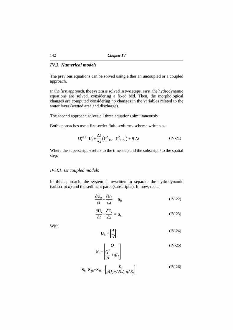
142 Chapter IV
IV.3. Numerical models The previous equations can be solved using either an uncoupled or a coupled approach. In the first approach, the system is solved in two steps. First, the hydrodynamic equations are solved, considering a fixed bed. Then, the morphological changes are computed considering no changes in the variables related to the water layer (wetted area and discharge). The second approach solves all three equations simultaneously. Both approaches use a first-order finite-volumes scheme written as
Uin+1=Ui
n+∆t
∆xFi-1/2
* -Fi+1/2* +S∆t (IV-21)
Where the superscript n refers to the time step and the subscript i to the spatial step.
IV.3.1. Uncoupled models In this approach, the system is rewritten to separate the hydrodynamic (subscript h) and the sediment parts (subscript s). It, now, reads
∂Uh
∂t+
∂Fh
∂x = Sh (IV-22)
∂Us
∂t+
∂Fs
∂x = Ss (IV-23)
With
Uh = 7AQ9 (IV-24)
Fh= N Q
Q2
A+gI1
O (IV-25)
Sh=Sgh+Sτh= 7 0gI2+AS0-gASf
9 (IV-26)

Sediment transport modeling 143
Us =Ab (IV-27)
Fs= ^ Qs
1 - ε0` (IV-28)
Ss=Sgs+Sτs=0 (IV-29)
To solve the hydrodynamic part, several flux calculation schemes can be used. Here, two different schemes are chosen: the Lateralized HLL (Petaccia et al, 2013) and the Augmented Roe solver (Murillo and Garcia-Navarro 2014). Considering only pure hydrodynamic flows, the performances of these schemes were compared by Franzini and Soares-Frazão (2016) on a selection of test cases. The conclusion was that the Augmented Roe scheme is more accurate but less robust than the Lateralized HLL scheme. The key features of these solvers are shortly recalled below. IV.3.1.1. LHLL solver This solver is a variation of the HLL solver (Harten et al. 1983) developed for cross-sections of arbitrary shapes (Petaccia et al. 2013). To compute more accurately the impact of the topography, the topographical sources terms Sgh are included in the fluxes computations while the friction source terms Sτh remain separated, leading to a two-step scheme as
Uh,in+1=Uh,i
n +∆t
∆xFh,i-1/2
*R -Fh,i+1/2*L (IV-30)
Uh,in+1=Uh,i
n+1+Sτh∆t (IV-31)
Where the topographical source terms are included in the fluxes, leading to “left” and “right” fluxes Fh
*R and Fh*L linked by the relationFh
*R-Fh*L =Sgh∆x.
Only the momentum fluxes are influenced by this change, they read: 4i+ 1/2
*L =λ24i - λ14i+1- λ1λ2(Qi - Qi+1)
λ2- λ1+λ1g ∆I1|zi8λ2- λ1
(IV-32)
4i+1/2*R =
λ24i - λ14i+1- λ1λ2(Qi - Qi+1)
λ2- λ1+ λ2g ∆I1|zi+100000
λ2 - λ1
(IV-33)
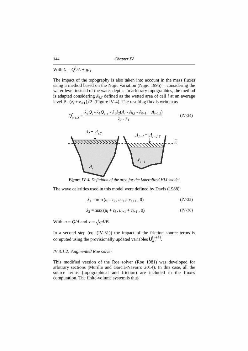
144 Chapter IV
With 4= Q2/A+ gI1 The impact of the topography is also taken into account in the mass fluxes using a method based on the Nujic variation (Nujic 1995) – considering the water level instead of the water depth. In arbitrary topographies, the method is adapted considering a,b defined as the wetted area of cell i at an average levelz= zi + zi+1 2⁄ (Figure IV-4). The resulting flux is written as
Qi+1/2* =
λ2Qi - λ1Qi+1- λ1λ2(Ai - Ai,z - Ai+1 + Ai+1,z)
λ2- λ1 (IV-34)
Figure IV-4. Definition of the area for the Lateralized HLL model
The wave celerities used in this model were defined by Davis (1988):
λ1 =min(ui - ci,ui +1- ci +1 , 0) (IV-35)
λ2=max(ui +ci , ui+1+ci+1 , 0) (IV-36) With u= Q/A and c=#gA/B In a second step (eq. (IV-31)) the impact of the friction source terms is
computed using the provisionally updated variablesUUUUh,in+1. IV.3.1.2. Augmented Roe solver This modified version of the Roe solver (Roe 1981) was developed for arbitrary sections (Murillo and Garcia-Navarro 2014). In this case, all the source terms (topographical and friction) are included in the fluxes computation. The finite-volume system is thus

Sediment transport modeling 145
Uh,in+1=Uh,i
n + ∆t
∆xFh,i-1/2
*R -Fh,i+1/2*L (IV-37)
The fluxes are written as
Fh,i+ 1/2*L =Fh,i + )λα-βe
m,i+1/2
m
λm<0
(IV-38)
Fh,i+1/2*R =Fh,i+1- )(λα-β)em,i+1/2
m
λm>0
(IV-39)
The wave celerities are defined as:
λ1 = u:- c: (IV-40)
λ2 = u: + c: (IV-41) with the Roe averages defined as,
u: = #Ai ui + #Ai+ 1 ui+1 #Ai + #Ai+1
(IV-42)
c: = !g
2-Ai+1
Bi+1+
Ai
Bi. (IV-43)
The eigenvectors are
em= 7 1λm9 (IV-44)
E = e1 e2 = 71 1λ1 λ2
9 (IV-45)
The wave strengths are obtained using
α = E-1 ∆Uh (IV-46)
α1 = λ2∆A - ∆Q
2c: (IV-47)

146 Chapter IV
α2= - λ1∆A - ∆Q
2c: (IV-48)
The source terms are represented using a stationary wave, as follow:
β = E-1 Sh (IV-49)
β1 = - ζ
2c: (IV-50)
β2 = ζ
2c: (IV-51)
With the source terms written as:
ζ = ζg- gA8Sf8 ∆x (IV-52)
The friction terms are written considering the average values:
A8 = Ai + Ai+1
2 (IV-53)
Sf8 = u:|u:|nini+1-Pi + Pi+1
Ai + Ai+1.4/3
(IV-54)
To introduce the energy conservation in the model, the topographical source terms are written as a linear combination of two expressions:
ζga= -gA8∆z+ c:2∆A (IV-55)
ζgb= -gAmin∆z+c:2∆A (IV-56)
These two relations are combined using a weighting coefficient ω: (IV-57)
ζg = 1-ωζga + ωζgb
This weighting coefficient is calculated by imposing the energy conservation.
∆ Q2
2gA2 + z = - Sf8 ∆x (IV-58)
Sediment transport modeling 147
By combining this relation with the momentum conservation equation, the weighting coefficient is obtained:
ω =
∆Q2
A - A8 ∆ Q2
2A2ζgb- ζga
(IV-59)
In a shock, as the energy is not conserved but dissipated, thus ω= 0. IV.3.1.3. Morphological evolution The Exner equation describing the morphological evolution is solved using an upstream-downstream scheme with the following discretization:
∆Ab=∆t
∆xQs,i-1/2
* -Qs,i+1/2* (IV-60)
In this approach, the sediment transport at the interface i-1/2 has the value of either the downstream i-1 or the upstream i sediment transport. The choice is made according to the Froude number, as Savary (2007) showed that the eigenstructure of the Exner equation is such that information comes either from downstream or upstream depending on the Froude number, and on the derivative of the sediment transport with respect to the bed level. Such an approach consists in considering for the sediment transport the celerity of a system of one equation. This yields If Fr>1 or∂Qs/∂zb<0: Qs,i-1/2
∗ = Qs,i1 − h, (IV-61)
Else Qs,i-1/2
∗ = Qs,i-11 − h,i (IV-62)
The sediment discharge in this model can be evaluated using any sediment transport equations using the flow variables at time n in an explicit way.
IV.3.2. Coupled models As stated before, in coupled models, all three equations are solved simultaneously. As for the hydrodynamic part of the uncoupled model, several approaches can be used to solve this system. Here, it has been decided to use
148 Chapter IV
the two approaches described in IV.3.1.1 and IV.3.1.2 (Lateralized HLL and Augmented Roe solver) and to extend them for the third equation, representing the morphological evolution. The system is slightly modified to link the three equations together considering the relation ∆zb0=∆Ab Bs⁄ where Bs is a representative cross-section width that will be defined for each method and depends on the erosion assumptions. The system now reads:
∂U∂t+ ∂F
∂x+H ∂U
∂x=S (IV-63)
With
U =T AQAb
U (IV-64)
F =
WXXXXY
Q
Q2
A + gI1
Qs
1 - ε0 Z[[[[\ (IV-65)
S = T 0gI2- gASf
0U (IV-66)
HHHH = k0 0 0
0 0gA
Bs0 0 0
l (IV-67)
The Jacobian matrix of the new system (IV-63) is
J = ∂F∂U
+ HHHH =
WXXXY 0 1 0
c2- u2 2ugA
Bs
1
1-ε0
∂Qs
∂A
1
1-0
∂Qs
∂Q0 Z[[[\ (IV-68)
The eigenvectors can be found by solving the following equation

Sediment transport modeling 149
|J-Iλ|=0 (IV-69) Resulting in
λ3 + a2λ
2 + a1λ + a0 = 0 (IV-70)
With
a2=-2u (IV-71)
a1 = u2- c2- gA
Bs
1
1 - ε0
∂Qs
∂Q (IV-72)
a0 = - gA
Bs
1
1 - ε0
∂Qs
∂A (IV-73)
The solution to equation (IV-70) is not straightforward and the eigenvalues cannot be expressed analytically in a simple form. The Coupled Lateralized HLL and the Coupled Augmented Roe offer different solutions to this problem that are described below. IV.3.2.1. Coupled Lateralized HLL This model was developed by Goutière et al. (2008) for a rectangular channel. The approach is here extended to arbitrary topographies. As for the Lateralized HLL scheme for the hydrodynamic equations, the topographical source terms are included in the fluxes computation.
Uin+1=Ui
n+∆t
∆xFi-1/2
*R -Fi+ 1/2*L +Sτ∆t (IV-74)
To find the three wave celerities, i.e. the eigenvalues of (IV-68) it is assumed that the largest eigenvalue is not influenced by sediments (Lyn and Altinakar 2002). This gives
λ3,i = ui + ci (IV-75) Then, using the relations (IV-76) and (IV-77) linking the roots λ of a polynomial equation of the third degree and using the definitions in equations (IV-71) to (IV-73) we obtain
λ1,i + λ2,i + λ3,i = - a2 = 2 ui (IV-76)

150 Chapter IV
λ1,iλ2,iλ3,i = - a0 = gAiSs,i
1
1 - ε0∂Qs
∂A
i
(IV-77)
The last two wave celerities can be defined as
λ2,i =
ui - ci + !ui - ci2- 4gAiBs,i
11 - ε0
-∂Qs∂A .i
1ui + ci
2
(IV-78)
λ1,i =
ui - ci - !ui - ci2- 4gAiBs,i
11 - ε0
-∂Qs∂A .i
1ui + ci
2
(IV-79)
With these approximate wave celerities, the fluxes can now be written as follows for the water mass and momentum conservation equations, with two equations for the momentum flux following the lateralized approach
Qi+1/2* =
λ3Qi - λ1Qi+1- λ1λ3(Ai - Ai,z- Ai+1 + Ai+1,z)
λ3 - λ1 (IV-80)
4i+1/2*R =
λ34i - λ14i+1- λ1λ3(Qi - Qi+1)
λ3 - λ1 +
λ3g ∆I1|zi+100000λ3- λ1
(IV-81)
4i+1/2*L =
λ34i - λ14i+1- λ1λ3(Qi - Qi+1)
λ3- λ1 +
λ1g∆I1|zλ3- λ1
(IV-82)
In addition, the sediment transport flux in the Exner equation is defined as
Qs, i+1/2* =
λ2
Qs,i1 - ε0
- λ1
Qs,i+11 - ε0
- λ1λ2 Bs,i+Bs,i+1
2 zb0,i-zb0,i+1λ2-λ1
(IV-83)
where the wave celerities are written, using the definitions (IV-75), (IV-78) and (IV-79).
λ1= minλ1,i ,λ1,i+ 1 , 0 (IV-84)
λ2= maxλ2,i , λ2,i+1 , 0 (IV-85)

Sediment transport modeling 151
λ3= maxλ3,i , λ3,i+ 1 ,0 (IV-86)
It is important to note that, if no transport occurs, the models is the same as the Lateralized HLL for hydrodynamics ((IV-87) to (IV-89)) as λ2 = 0 (for a subcritical flow, u-c<0) according to (IV-78).
λ3,i = ui + ci (IV-87)
λ2,i =
ui - ci + !ui - ci2- 4gAiBs,i
11 - ε0
-∂Qs∂A .i
1ui + ci
2= ui - ci + #ui - ci2 2
= ui - ci + |ui - ci| 2
=ui - ci - ui - ci 2
= 0
(IV-88)
λ1,i =
ui - ci - !ui - ci2- 4gAiBs,i
11 - ε0
-∂Qs∂A .i
1ui + ci
2
= ui - ci - #ui - ci2 2
= ui - ci - |ui - ci| 2
=ui - ci + ui - ci 2
= ui - ci
(IV-89)
IV.3.2.2. Coupled Augmented Roe This model is based on the 2D model developed by Murillo and Garcia-Navarro (2010). It is here developed to one-dimensional cross-sections with arbitrary topographies and includes an adaptation of the concept of energy conservation (Murillo and Garcia-Navarro 2014; Franzini and Soares-Frazão 2016).

152 Chapter IV
In a similar way as in the pure hydrodynamic case, the fluxes of the Augmented Roe scheme are written as
Fi+ 1/2*L =Fi + )λα-βe
m,i+1/2
m
λm<0
(IV-90)
Fi+ 1/2*R =Fi+1- )(λα-β)em,i+1/2
m
λm>0
(IV-91)
Where α is the wave strength and β represents the source terms through a stationary wave. The eigenvalues λ are the solution of eq. (IV-70) and their evaluation thus requires the calculation of derivatives of the sediment transport rate, which can be evaluated using a wide range of sediment transport formula. To obtain simple expressions for these derivatives, the Grass formulation (1981) is used:
Qs= G u3 (IV-92)
The methodology can however be adapted to any sediment transport formula. In the case of the Grass formulation, considering a constant coefficient G, the eigenvalue equation (IV-70) can be rewritten as
λ3 + a2λ
2 + a1λ + a0 = 0 (IV-93)
With
a2=-2u (IV-94)
a1 = u2- c2- gASm 1
1 - ε0
3Gu2
A = u2- c2- gASm kG (IV-95)
a0 = - gA
Bs
1
1 - ε0
- 3 Gu2
Au = gA
BskGu (IV-96)
The Roe averages are estimated at the interface using
u: = #Ai ui + #Ai+1 ui+1 #Ai + #Ai+1
(IV-97)
Sediment transport modeling 153
c: =!g
2-Ai+1
Bi+1+
Ai
Bi. (IV-98)
Smn = Ss,i + Bs,i+1
2 (IV-99)
kgH =
Gi + Gi+1
2
1
1 - ε0
ui2 + uiui+1 + ui+1
2#AiAi+1
(IV-100)
In a similar way as the Augmented Roe scheme for the shallow-water equations, the energy conservation affects the definition of the area AH at the interface with the weighting coefficient ω defined using equation (IV-59).
AH=1-ωAi +Ai+1
2 +ω min(Ai ,Ai+1) (IV-101)
Instead of calculating approximate solutions to the third-order polynomial eigenvalue equation as in the coupled Lateralized HLL, the eigenvalues are obtained directly as
λ1=2#-ϕ cos-θ+2π
3. - a2
3 (IV-102)
λ2=2#-ϕ cos-θ-2π3
. - a2
3 (IV-103)
λ3=2#-ϕ cos-θ3. -
a2
3 (IV-104)
with
θ= acosJK ψ
V-ϕ3LM (IV-105)
ϕ=3a1-a22
9 (IV-106)
ψ= 9a2a1-27a0-2a23
54 (IV-107)

154 Chapter IV
It is important to note that the system (IV-63) is hyperbolic only if ϕ3+ ψ2< 0. This condition is fulfilled in all the types of classical flows. Knowing the eigenvalues, the matrix of eigenvectors can be determined as
em= WXXXY 1
λmλm2 +u:2-c:2-2u:λm
gAH/Smn Z[[[\ (IV-108)
E=[e1 e2 e3] (IV-109)
As for the uncoupled Augmented Roe scheme, the wave strengths and the source terms are obtained using
α=E-1∆U (IV-110)
β= E-1S (IV-111) With the source terms written as:
S= k 0
c:2∆A-gAH∆h -gAi +Ai+1
2Sf8∆x
0
l (IV-112)
As stated before, other sediment transport formulations can be used, such as e.g. the Meyer-Peter and Müller formula. In that case, the model has to be slightly modified to ensure the sediment mass conservation. First, the MPM formula can be expressed in the same form as the Grass formula considering now a variable G coefficient (Murillo and Garcia-Navarro 2010) defined by G= #gn3s-1√R
8B -1-θcr
θ.1.5 (IV-113)
Even though this formulation of the Grass coefficient is a function of the water velocity, it is considered constant in each cell at each time step leading, for interface i+1/2, to the sediment flux written as
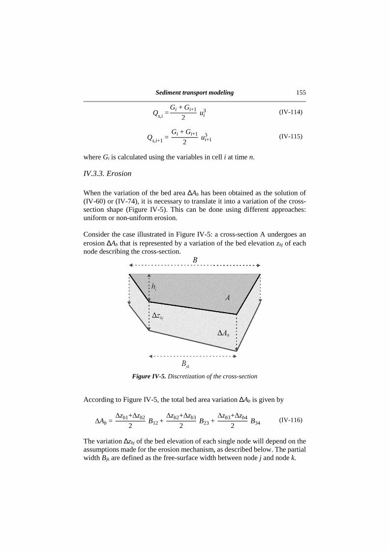
Sediment transport modeling 155
Qs,i= Gi +Gi+1
2 ui
3 (IV-114)
Qs,i+1=Gi +Gi+1
2 ui+1
3 (IV-115)
where Gi is calculated using the variables in cell i at time n.
IV.3.3. Erosion When the variation of the bed area ∆Ab has been obtained as the solution of (IV-60) or (IV-74), it is necessary to translate it into a variation of the cross-section shape (Figure IV-5). This can be done using different approaches: uniform or non-uniform erosion. Consider the case illustrated in Figure IV-5: a cross-section A undergoes an erosion ∆Ab that is represented by a variation of the bed elevation zbj of each node describing the cross-section.
Figure IV-5. Discretization of the cross-section
According to Figure IV-5, the total bed area variation ∆Ab is given by
∆Ab=∆zb1+∆zb2
2 B12+∆zb2+∆zb3
2 B23+∆zb3+∆zb4
2 B34 (IV-116)
The variation ∆zbj of the bed elevation of each single node will depend on the assumptions made for the erosion mechanism, as described below. The partial width Bjk are defined as the free-surface width between node j and node k.

156 Chapter IV
IV.3.3.1. Uniform erosion In this case, the erosion is uniformly distributed over all the immerged bed. The relation linking the bed level variation of two points j and k is
∆zbj =∆zbk (IV-117)
Introducing this relation into the total bed area variation relation for any node j yields
∆Ab= ∆zbj+∆zbj
2 B12+∆zbj+∆zbj
2 B23+∆zbj+∆zbj
2 B34 (IV-118)
ΔAb=ΔzbjB12+B23+B34 (IV-119)
∆Ab=∆zbj B (IV-120)
Finally, the bed level variation of node j is obtained with
∆zbj=∆Ab
B (IV-121)
Showing that in this case, the width Bs of equation (IV-63) is defined as
Bm=B (IV-122) IV.3.3.2. Non-uniform erosion In this second case, which is closer to the reality, the erosion is distributed along the bed according to the water depth, in such a way that no erosion occurs if the water depth is equal to zero. This last characteristic renders the operator smoother as the transition between submerged and emerged material is directly taken into account. Now, the relation linking the bed level variation of two points j and k is
∆zj =∆zk hj
hk n
(IV-123)
More specifically, a linear relation has been selected (n =1).

Sediment transport modeling 157
∆zj =∆zk hj
hk (IV-124)
Introducing this relation into the total bed area variation relation (IV-116) for node j yields
∆Ab=∆zbj h1
hj +∆zbj h2hj
2 B12+
∆zbjh2hj
+∆zbjh3hj
2 B23
+ ∆zbjh3hj
+∆zbjh4hj
2 B34
(IV-125)
∆Ab=∆zbj
hj-h1+h2
2 B12+
h2+h3
2 B23+
h3+h4
2 B34. (IV-126)
∆Ab=A
hj∆zbj (IV-127)
Finally, the level variation of each point is obtained by
∆zbj=hj
A ∆Ab (IV-128)
In this method, the Bs width is defined as Bm= A
zw-zb0 (IV-129)
with zw the water level and zb0 the thalweg level. It can be observed that, in rectangular channels, the non-uniform erosion gives the exact same results has the uniform erosion.
∆zbj=hj
A ∆Ab= hA∆Ab=∆Ab
B (IV-130)
IV.3.4. Bank Failure In nature, when erosion starts at the toe of the bank of a river, the bank slope can become steeper than the stability limits of the constituting material that can result in a failure of the bank. To represent this phenomenon in the model,

158 Chapter IV
a bank failure mechanism has been added. It is based on a tilting of the unstable portion of the bank (Zech et al. 2008, Swartenbroekx et al. 2010). This tilting operator is applied only on the considered cross-section, without any effect on the neighboring cross-sections in the longitudinal direction. The cross-sections are thus treated successively, without interaction. For each cross-sections, the segments are treated one after the other. So, the tilting of one segment can render another one unstable. In Figure IV-6, the segment BC is initially unstable and after the tilting, segment B’C’ is stable but segment AB’ is now unstable. The process thus needs to be iterated until the complete cross-section is stable.
Figure IV-6. Bank failure operator
As for the transport equation, the sediment is considered composed only of non-cohesive particles. Therefore, the slope limit depends solely on the internal friction angle of material. It is important to add that, as the bank failure operator is operated separately from the rest of the model¸ it only changes the shape of the section without affecting the sediment transport Qs. The sediment deposited at the toe of the bank after a failure event will be transported by the flow during the next time step. No dynamical effects are thus taken into account.

Sediment transport modeling 159
IV.4. Results In this section, the results of the different models are compared to several test cases. Here, the models are abbreviated as follows: UH for the uncoupled lateralized HLL, UR for the uncoupled Augmented Roe, CH for the coupled lateralized HLL and CR for the coupled Augmented Roe model.
IV.4.1. Water at rest To assess the well-balancedness of the models, it is important to check if they are able to keep water at rest. The selected tests consider a trapezoidal channel (Murillo and Garcia-Navarro 2014) with a shape defined by Bx=B0x+0.2B0x-9.5h (IV-131) With B0 the width of the channel atℎ = 0, as represented in Figure IV-7 for the CR model. All models are able to maintain the water at rest and, therefore, respect the C-property (Vázquez-Cendón 1999), so only the results for the CR model are illustrated, as they are the same for the four models.
IV.4.2. Equilibrium Slopes This test compares the models results to the analytical solution of a progressive slope aggradation or degradation in a prismatic channel. Both supercritical (slope S0 = 5%) and subcritical (slope S0 = 0.5%) cases are investigated. For each case, three initial configurations are studied (Figure IV-8 and Figure IV-9): (1) starting at the equilibrium slope, (2) starting at a steeper slope (6% and 0.8% for the supercritical and subcritical cases, respectively), (3) starting at a milder slope (4% and 0.25% for the supercritical and subcritical cases, respectively).

160 Chapter IV
Figure IV-7. Results for the water at rest
using the CR model
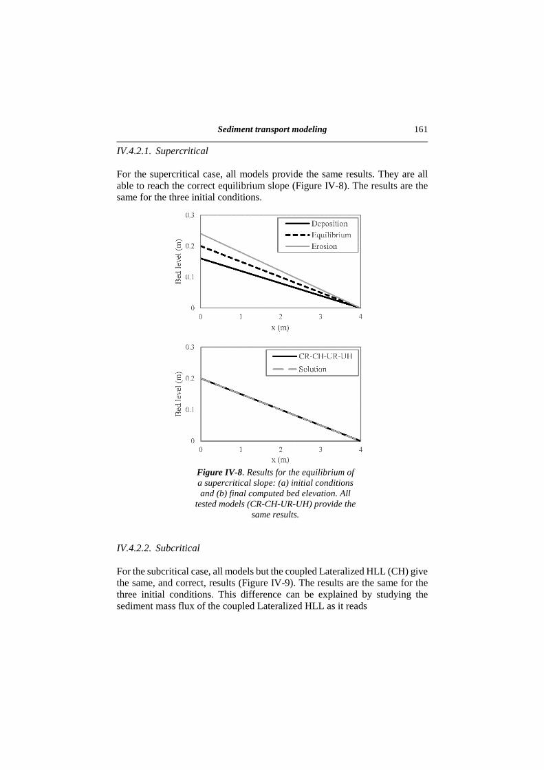
Sediment transport modeling 161
IV.4.2.1. Supercritical For the supercritical case, all models provide the same results. They are all able to reach the correct equilibrium slope (Figure IV-8). The results are the same for the three initial conditions.
Figure IV-8. Results for the equilibrium of a supercritical slope: (a) initial conditions and (b) final computed bed elevation. All
tested models (CR-CH-UR-UH) provide the same results.
IV.4.2.2. Subcritical For the subcritical case, all models but the coupled Lateralized HLL (CH) give the same, and correct, results (Figure IV-9). The results are the same for the three initial conditions. This difference can be explained by studying the sediment mass flux of the coupled Lateralized HLL as it reads

162 Chapter IV
Qs, i+1/2* =
λ2
Qs,i1 - ε0
- λ1
Qs,i+11 - ε0
- λ1λ2 Bs,i+Bs,i+1
2 zb0,i-zb0,i+1λ2-λ1
(IV-132)
The last term of the equation, which constitutes the diffusive part of the flux expression, only cancels out if the bed elevation is constant. This problem, already pointed out by Goutiere et al (2008) for rectangular channels, can be solved by adding a term, which is a function of the equilibrium slope, in the diffusive term. However, this solution proposed by Goutiere et al. (2008) was not adopted here, as it cannot be extended to arbitrary topographies with abruptly changing bed slopes. Therefore, the CH model should not be considered for general applications.
Figure IV-9. Results for the equilibrium of a subcritical slope: (a) initial and (b) final
IV.4.3. Dam break flow on a flat bed This test is an experiment of a dam-break flow on an initially flat mobile bed (Spinewine and Zech 2007). The channel is 6 m long and 0.25 m wide. Upstream, the first 3 m are initially filled with 0.35 m of water. At' = 0, the

Sediment transport modeling 163
dam is removed and the water starts flooding the flume. The sediment bed is composed of PVC particles with a median diameter (d50) of 3.9 mm and a specific mass (s) of 1.58. During the experiment, three flow regions were observed: a layer of pure water, a layer of sediment transport composed of a mixture of water and sediments and the motionless bed. Therefore, two interfaces were captured: the interface between the flow of pure water and the mixture and the interface between the mixture and the motionless bed. However, the models presented in this paper do not compute a layer of moving sediments. They only provide the bed elevation after erosion or deposition. This level is assumed to correspond to an intermediate value between the lower and upper limits of the moving sediment layer. So, numerical results are considered to be in good agreement with the measurements when computed bed elevation is located between the two recorded interfaces. The results are presented for t = 1 s (Figure IV-10 and Figure IV-11). They show that all four models give approximately the same erosion with the coupled Lateralized HLL model eroding less. However, the coupled Roe model shows less variation and a smoother profile than the other three (Figure IV-11). Moreover, as expected, all three models are between the two captured interfaces.
Figure IV-10. Comparison between the different models and the
experimental results of a dam break flow on a flat bed

164 Chapter IV
Figure IV-11. Comparison between the different models for the
simulation of a dam break flow on a flat bed
IV.4.4. Dike failure by overtopping This experiment was conducted at the Hydraulics Laboratory of the Université catholique de Louvain, Belgium (Van Emelen et al. 2015). It studies the erosion and failure of a slice of a sand dike. The dike was built in a 10 m long, 0.2 m wide and 0.3 m high horizontal flume. The dike is of trapezoidal shape, 0.20 m high with slopes of 1V:2H (Figure IV-12) and is made of sand with a mean diameter of 0.61 mm. During the erosion process, both water and bed level evolutions were captured.
Figure IV-12. Dike failure: experimental setup

Sediment transport modeling 165
The results are here shown for four time steps: 8 s, 24 s, 64 s and 200 s (t = 0 s corresponds to the initial overtopping of the dike) for each model in Figure IV-13 to Figure IV-16. These results are then summarized in Figure IV-17 where the evolution of the average absolute error is presented for the bed level, the water level and the water depth. The errors are computed for t = 8, 14, 24, 64 and 200 s. Finally, Figure IV-18 represents the signed error for the bed level, water level and water depth computed as the difference between the predicted and measured values. As observed from Figure IV-13 to Figure IV-16, the results are similar for the coupled and uncoupled version of the Augmented Roe model (CR and UR) for 8 s, 24 s and 64 s. All models also reach similar results at 64 s. However, the intermediary results (at 24 s) show significant differences. The models based on Roe scheme erode the dike faster than the experiment while the uncoupled Lateralized HLL erode slower. Only the coupled Lateralized HLL model is able to capture the correct crest level evolution without reaching a horizontal bed like the equilibrium slope problem because the dike failure is a faster event. However, all models fail to represent the correct behavior of the bed and water level at 64 s when an antidune is formed in the experiment. The errors show that the coupled Roe model (CR) is not able to reduce the error for the bed level prediction for t = 200 s contrarily to the other models. In addition, HLL based model (CH and UH) predicted better the evolution of the bed level while Roe based model (CR and UR) predicted better the evolution of the water depth. Figure IV-18 shows that all models have the same error for the prediction of the dike erosion. First, at 8 s, the models do not transport enough sediments. Then, at 14 and 24 s, they overestimate the erosion of the dike before underestimating it again at 64 s. For the prediction of the volume of water, the coupled Roe model (CR) gives the best prediction with an average error of less than 2 10-4 m after 24 s.
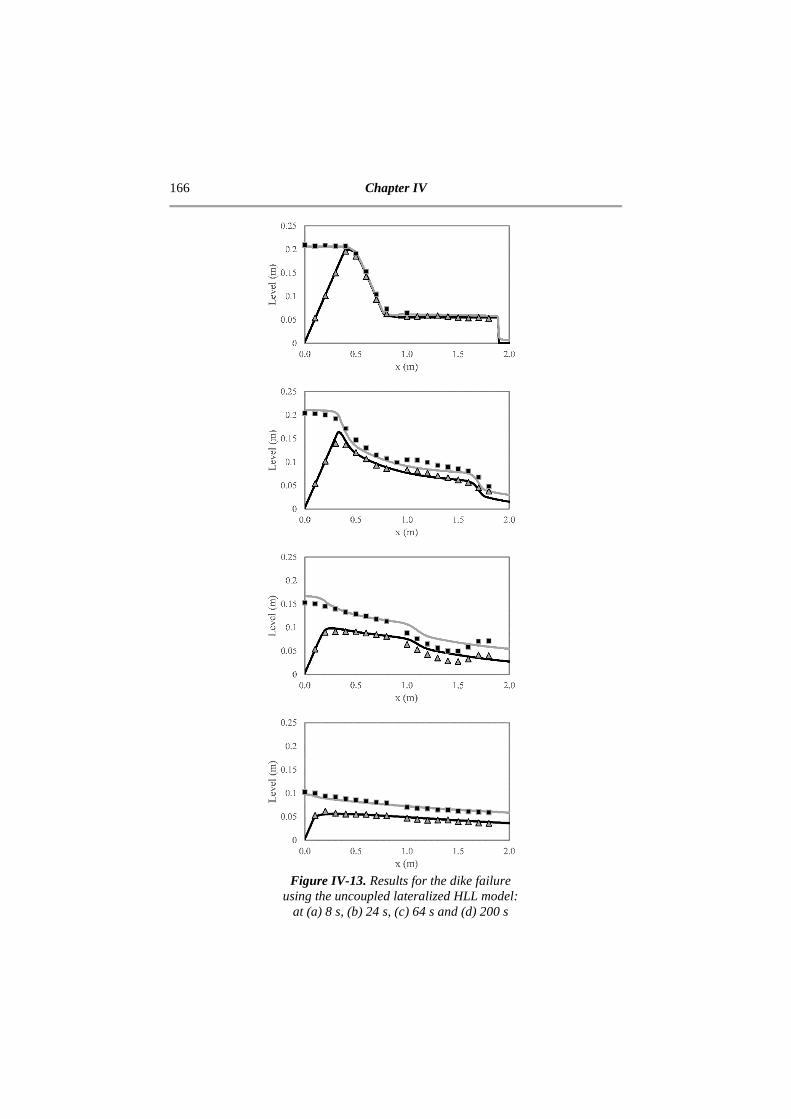
166 Chapter IV
Figure IV-13. Results for the dike failure
using the uncoupled lateralized HLL model: at (a) 8 s, (b) 24 s, (c) 64 s and (d) 200 s
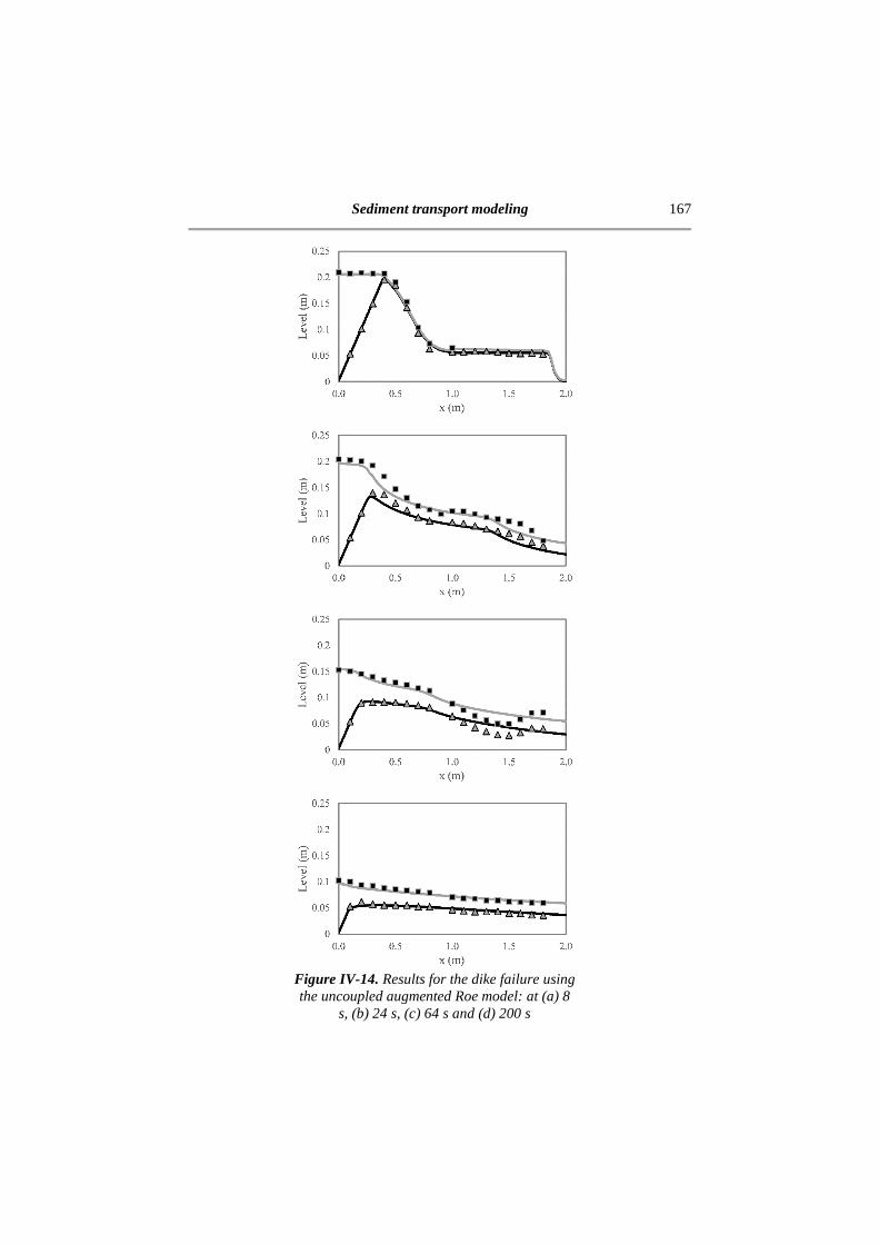
Sediment transport modeling 167
Figure IV-14. Results for the dike failure using the uncoupled augmented Roe model: at (a) 8
s, (b) 24 s, (c) 64 s and (d) 200 s

168 Chapter IV
Figure IV-15. Results for the dike failure using
the coupled lateralized HLL model: at (a) 8 s, (b) 24 s, (c) 64 s and (d) 200 s

Sediment transport modeling 169
Figure IV-16. Results for the dike failure using the coupled augmented Roe model: at (a) 8 s,
(b) 24 s, (c) 64 s and (d) 200 s
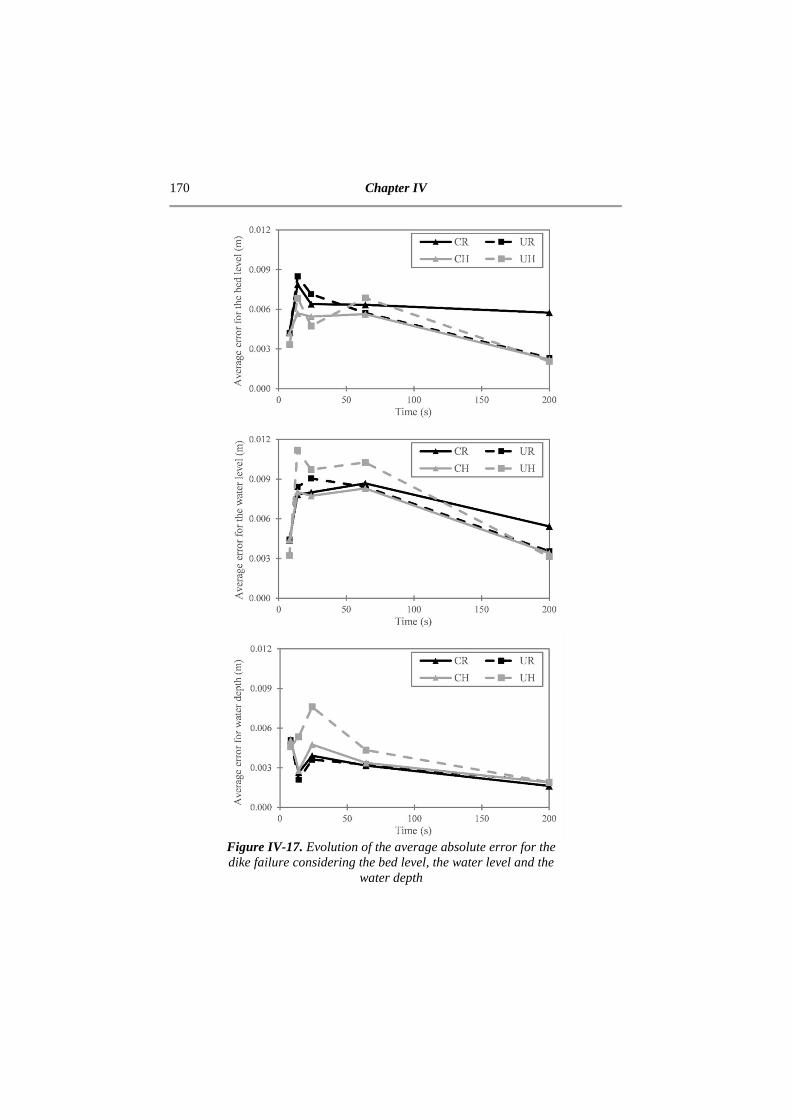
170 Chapter IV
Figure IV-17. Evolution of the average absolute error for the dike failure considering the bed level, the water level and the
water depth
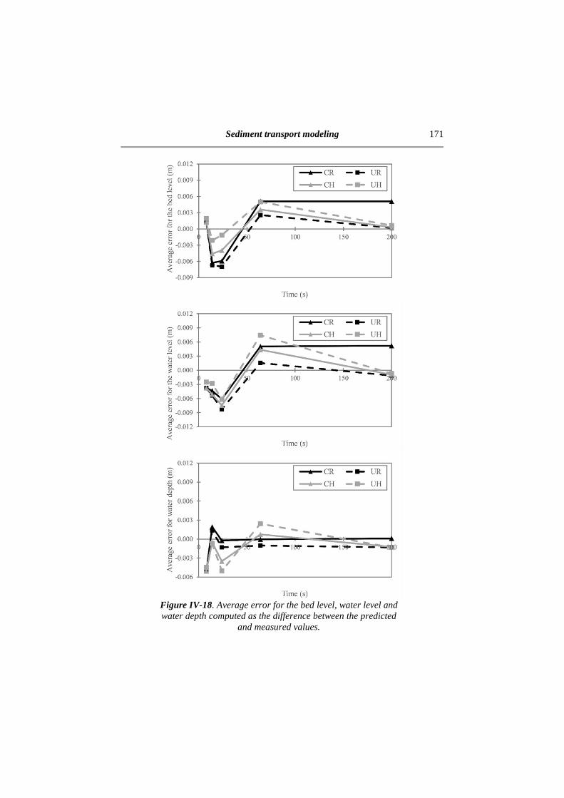
Sediment transport modeling 171
Figure IV-18. Average error for the bed level, water level and water depth computed as the difference between the predicted
and measured values.
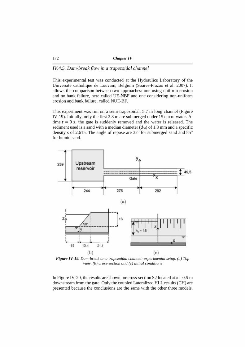
172 Chapter IV
IV.4.5. Dam-break flow in a trapezoidal channel This experimental test was conducted at the Hydraulics Laboratory of the Université catholique de Louvain, Belgium (Soares-Frazão et al. 2007). It allows the comparison between two approaches: one using uniform erosion and no bank failure, here called UE-NBF and one considering non-uniform erosion and bank failure, called NUE-BF. This experiment was run on a semi-trapezoidal, 5.7 m long channel (Figure IV-19). Initially, only the first 2.8 m are submerged under 15 cm of water. At time' = 0w, the gate is suddenly removed and the water is released. The sediment used is a sand with a median diameter (d50) of 1.8 mm and a specific density s of 2.615. The angle of repose are 37° for submerged sand and 85° for humid sand.
Figure IV-19. Dam-break on a trapezoidal channel: experimental setup. (a) Top
view, (b) cross-section and (c) initial conditions
In Figure IV-20, the results are shown for cross-section S2 located at x = 0.5 m downstream from the gate. Only the coupled Lateralized HLL results (CH) are presented because the conclusions are the same with the other three models.
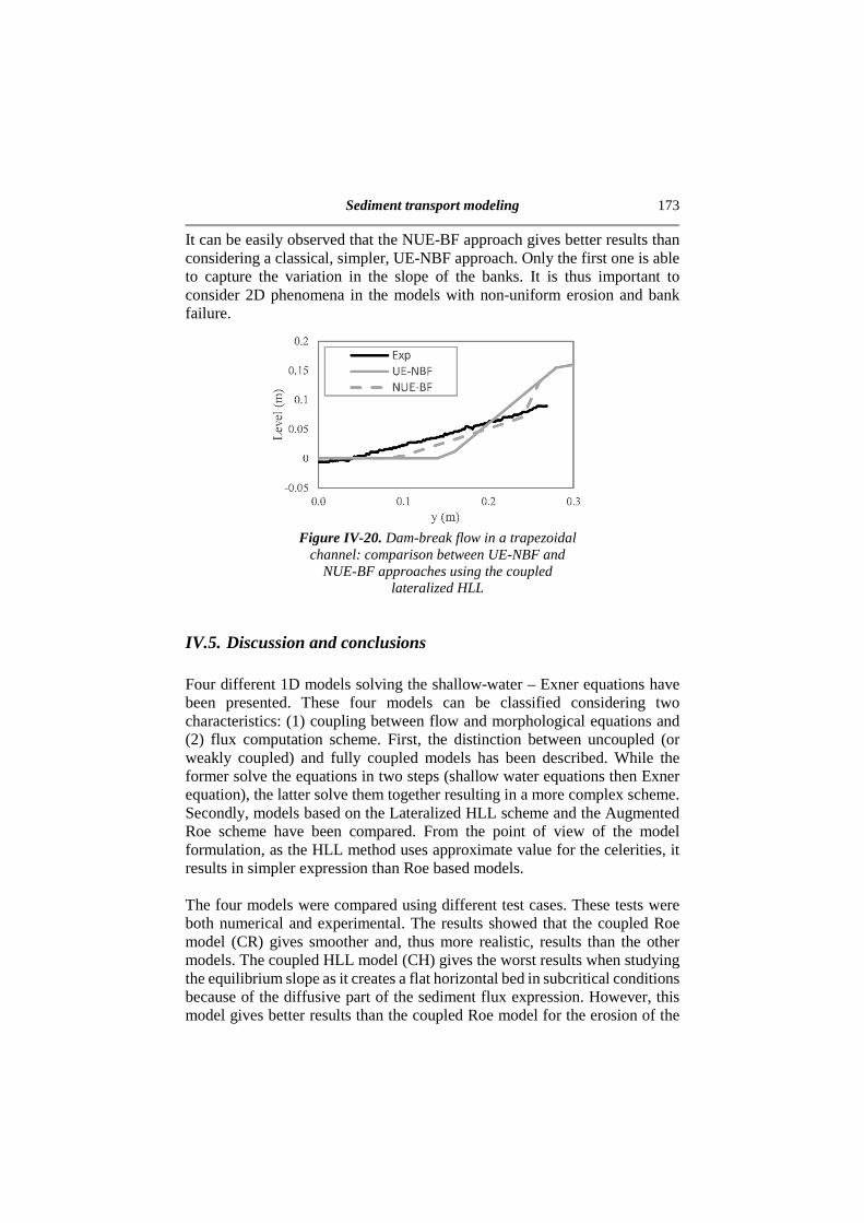
Sediment transport modeling 173
It can be easily observed that the NUE-BF approach gives better results than considering a classical, simpler, UE-NBF approach. Only the first one is able to capture the variation in the slope of the banks. It is thus important to consider 2D phenomena in the models with non-uniform erosion and bank failure.
Figure IV-20. Dam-break flow in a trapezoidal
channel: comparison between UE-NBF and NUE-BF approaches using the coupled
lateralized HLL
IV.5. Discussion and conclusions Four different 1D models solving the shallow-water – Exner equations have been presented. These four models can be classified considering two characteristics: (1) coupling between flow and morphological equations and (2) flux computation scheme. First, the distinction between uncoupled (or weakly coupled) and fully coupled models has been described. While the former solve the equations in two steps (shallow water equations then Exner equation), the latter solve them together resulting in a more complex scheme. Secondly, models based on the Lateralized HLL scheme and the Augmented Roe scheme have been compared. From the point of view of the model formulation, as the HLL method uses approximate value for the celerities, it results in simpler expression than Roe based models. The four models were compared using different test cases. These tests were both numerical and experimental. The results showed that the coupled Roe model (CR) gives smoother and, thus more realistic, results than the other models. The coupled HLL model (CH) gives the worst results when studying the equilibrium slope as it creates a flat horizontal bed in subcritical conditions because of the diffusive part of the sediment flux expression. However, this model gives better results than the coupled Roe model for the erosion of the

174 Chapter IV
dike. Nevertheless, it has been showed by Van Emelen et al. (2015) that the choice of the sediment transport law has an enormous impact on the erosion rate of the dike. Thus, it can be expected that Roe-based models with other well-calibrated sediment transport formulas (El Kadi Abderrezzak and Paquier 2011) would provide better results. However, changing the sediment transport formula would not prevent the coupled HLL (CH) to reach a horizontal bed for the subcritical equilibrium slope (Figure IV-9). Finally, the impact of the bank failure model and non-uniform erosion distribution was highlighted by studying a dam-break flow in a semi-trapezoidal channel. It was shown that these two parameters influence greatly the morphological changes created by a dam-break flow in arbitrary topographies.
Acknowledgments This work was supported by the Fonds National de la Recherche Scientifique, Belgium.
References Cao Z, Pender G, Wallis S, Carling PA. Computational dam-break hydraulics
over erodible sediment bed. J. Hydraul. Eng. 2004; 130(7): 689–703.
Capart H, Eldho T, Huang S, Young D, Zech Y. Treatment of Natural Geometry in Finite Volume River Flow Computations. J. Hydraul. Eng. 2003; 129(5): 385-393.
Capart H, Spinewine B, Young DL, Zech Y, Brooks GR, Leclerc M, Secretan Y. The 1996 Lake Ha! Ha! breakout flood, Quebec: Test data for geomorphic flood routing methods. Journal of Hydraulic Research 2007; 45: 97–109.
Cunge JA, Perdreau N. Mobile bed fluvial mathematical models. Houille Blanche 1973; 28(7): 561–580.
Davis SF, Simplified second-order Godunov-type methods, SIAM Journal on Scientific and Statistical Computing 1988; 9: 445–473.
El Kadi Abderrezzak K, Paquier A. Applicability of sediment transport capacity formulas to dam-break flows over movable beds. Journal of hydraulic engineering 2011; 137(2): 209-221.
Sediment transport modeling 175
Fraccarollo L, Capart H, Zech Y. A Godunov method for the computation of
erosional shallow water transient. Intl. J. Numer. Meth. Fluids 2003; 41: 951–976.
Franzini F, Soares-Frazão S. Efficiency and accuracy of Lateralized HLL, HLLS and Augmented Roe's scheme with energy balance for river flows in irregular channels. Applied Mathematical Modelling 2016; 40 (17-18): 7427-7446.
García MH. Sediment transport and morphodynamics. In Sedimentation engineering processes, measurements, modeling and practice, M.H. García (ed.), ASCE Manuals and Reports on Engineering Practice 110, ASCE, Reston VA, 2008: 21–163.
Garegnani G, Rosatti G, Bonaventura L. Free surface flows over mobile bed: mathematical analysis and numerical modeling of coupled and decoupled approaches. Commun. Appl. Indus. Math. 2011; 3(1): 1–22.
Goutière L, Soares-Frazão S, Savary C, Laraichi T, Zech Y. One-dimensional model for transient flows involving bedload sediment transport and changes in flow regimes. J. Hydraul. Eng. 2008; 134(6): 726–735.
Grass AJ. Sediments transport by waves and currents. SERC London Cent. Mar. Technol. 1981, Report No. FL29.
Greco M, Iervolino M, Vacca A, Leopardi A. Two-phase modelling of total sediment load in fast geomorphic transients. Proc. Int. Conf. on Fluvial Hydraul. - River Flow 2012; 1: 643–648.
Harten A, Lax PD, Van Leer B. On upstream differencing and Godunov type schemes for hyperbolic conservation laws, SIAM review 25 1983: 35–61.
Juez C, Murillo J, García-Navarro P. A 2D weakly-coupled and efficient numerical model for transient shallow flow and movable bed. Advances in Water Resources 2014; 71: 93-109.
Kassem AA, Chaudry MH. Comparison of coupled and semicoupled numerical models for alluvial channels. J. Hydraulic Eng.1998; 124(8): 794–802.
176 Chapter IV
Lacasta A, Morales-Hernández M, Murillo J, García-Navarro P.An optimized GPU implementation of a 2D free surface simulation model on unstructured meshes. Advances in Engineering Software 2014; 78: 1-15.
Lyn DA, Altinakar M. St. Venant–Exner equations for near-critical and transcritical flows. J. Hydraul. Eng. 2002; 128(6): 579– 587.
Meyer-Peter E, Müller R. Formulas for bed load transport. Proc., 2nd Meeting, IAHR, Stockholm, Sweden, 1948: 39–64.
Murillo J, Garcia-Navarro P. An Exner-based coupled model for the two-dimensional transient flow over erodible bed. Journal of computational physics 2010; 229(23): 8704-8732.
Murillo J, Garcia-Navarro P. Accurate numerical modeling of 1d flow in channels with arbitrary shape. Application of the energy balanced property. Journal of Computational Physics 2014; 260: 222–248.
Nujic M. Efficient implementation of non-oscillatory schemes for the computation of free surface flows. Journal of Hydraulics Research 1995; 33: 101–111.
Petaccia G, Natale L, Savi F, Velickovic M, Zech Y, Soares-Frazão S. Flood wave propagation in steep mountain rivers. Journal of Hydroinformatics 2013; 15(1): 120–137.
Roe P. Approximate Riemann solvers, parameter vectors, and difference schemes. Journal of Computational Physics 1981; 43: 357–372.
Savary, Céline. Transcritical transient flow over mobile beds Boundary conditions treatment in a two-layer shallow-water model. PhD Thesis 2007, Université catholique de Louvain, Louvain-la-Neuve, Belgium
Soares-Frazão S, Le Grelle N, Spinewine B, Zech Y. Dam-break induced morphological changes in a channel with uniform sediments: measurements by a laser-sheet imaging technique. Journal of Hydraulic Research 2007; 45: 87-95.
Spinewine B, Capart H. Intense bed-load due to a sudden dam-break. Journal of fluid mechanic 2013; 731: 579-614.
Spinewine B, Zech Y. Small-scale laboratory dam-break waves on movable beds. Journal of Hydraulic Research 2007, 45, 73-86.

Sediment transport modeling 177
Swartenbroekx C, Soares-Frazão S, Staquet R, Zech Y. Two-dimensional
operator for bank failures induced by water-level rise in dam-break flows. Journal of Hydraulic Research 2010; 48(3): 302–314.
Van Emelen S, Zech Y, Soares-Frazão S. Impact of sediment transport formulations on breaching modelling. Journal of Hydraulic Research 2015; 53(1): 60-72.
Vazquez-Cendon ME. Improved treatment of source terms in upwind schemes for the shallow water equations in channels with irregular geometry, Journal of Computational Physics 1999; 148: 497–526.
Wu W, Wang S. One-Dimensional Modeling of Dam-Break Flow over Movable Beds. J. Hydraul. Eng. 2007; 133(1): 48–58.
Zech Y, Soares-Frazão S, Spinewine B, Le Grelle N. Dam-break induced sediment movement: Experimental approaches and numerical modelling. J. Hydraul. Res. 2008; 46(2): 176–190.


DIKE BREACHING
[Franzini F., Van Emelen S., Zech Y. and Soares-Frazão S. (2016) Dike breaching evolution in sand dike: comparison between coarser and finer sand. Submitted to Journal of Hydraulic Research]
The fifth chapter presents an experimental and numerical study of the failure of a sand dike by overtopping. This study is important as the failure of sand dikes or dams are often the root cause of a flood. The Ha!Ha! River flood is still a great example here as it was caused by the failure of a dike (Figure V-1). This chapter is written in two parts. First, an experimental study of the failure of sand dikes is presented. Then, the results of one of the models from the fourth chapter (the coupled Roe model) are compared to the experimental results and to those obtained by a two-dimensional model.
Figure V-1. Picture taken after the Ha!Ha! River flood (Capart et al. 2007). It shows the location of the initial dike that failed during the event, flooding the Ha!Ha! River.
180 Chapter V
Abstract
Dike failures often induce highly damaging floods. Improved understanding of the inherent mechanisms of these failures is important to better predict and prevent dike failures. The research presented in this paper focuses on the failure of sand dike by overtopping. An initial small breach is dug at the dike crest to initiate the failure process. The evolution of nine sections was monitored using laser-sheet while the water level in the upstream reservoir was captured using ultrasonic gauges. The impact of the sand grain was studied by comparing a fine sand of 0.7 mm and a coarser sand of 1.7 mm. Even though both failure mechanisms look similar, some differences could be observed in the evolution of the geometry of the dike. Finally, the failure was simulated with 1D and 2D models. While much simpler, the 1D model shows good results for the initial stage of the dike and in predicting the evolution of the width of the breach. The 2D model predicts the correct shape but slightly overestimated the widening of the breach.
V.1. Introduction Dike failure can induce large floods and greatly damage buildings and infrastructures. In case of earth dike, three causes of failure can be defined: (i) infiltration, (ii) stability failure and (iii) overtopping. The current research focuses on the failure of non-cohesive, sand, dikes by overtopping. This type of failure has been studied extensively over the last decades (Morris et al. 2009). Visser (1998), first, described the failure process for fine sand dikes and Coleman et al. (2002) extended the study to coarse sand dikes. Lately, the experiments focus on the influence of several parameters, such as the sediment nature, dike height and discharge (Schmocker and Hager, 2012), the grain size distribution (Schmocker et al., 2014) or the shape and headwater elevation (Müller et al., 2016). Regarding breaching modeling, the models have evolved from parametric models to more complex physical models (Van Emelen et al., 2015). The research presented here corresponds to these two trends as it compares the failure of two dikes built with sand of different grain sizes. Furthermore, it compares the simulation of these failures using 1D and 2D finite-volume models. The current paper is divided in two part. First, experiments of failure of a breached dike are presented. Then, 1D and 2D models are used to simulate the failure. Their results are compared to the experimental results and to each other. Finally, these differences are analyzed, and the strengths and weaknesses of each model are highlighted.

Dike breaching 181
V.2. Experimental setup The breaching experiments were carried out at the Hydraulics Laboratory of the Institute of Mechanics, Materials and Civil Engineering of the Université catholique de Louvain (Belgium). The set-up is illustrated in Figure V-2 and Figure V-3 and consists of a dike constructed with an initial pilot breach. The flume is 12 m long, 1.2 m wide and 0.32 m high. A pump supplies water to a 2-m long, upstream reservoir. The dike is built 2.88 m downstream of the upstream end. Two types of initial geometry were used, each one corresponding to a size of sand. The first one, used for coarse sand, is of trapezoidal shape, 1.2 m wide and 0.2 m high (Figure V-2). Both downstream and upstream slopes are 1:3 and the crest length is 0.1 m. An initial trapezoidal channel is dug in the dike to initiate the failure mechanisms. This pilot channel has a depth of 0.03m, a base width of 0.03 m and 1:1 slopes. A 1 m long and 0.04 m thick sand layer is set downstream of the dike to minimize the risk of failure by seepage. The coarser sand has a median diameter, d50, of 1.7 mm; a specific gravity, s, of 2.615; and a bed porosity, ε0, of 45% after compaction.
Figure V-2. Experimental setup for the coarse sand dike

182 Chapter V
The second geometry, used for fine sand, is of triangular shape, 1.2 m wide and 0.217 m high (Figure V-3). As for the coarse sand dike, both downstream and upstream slopes are 1:3. A similar pilot channel is dug in the dike and is set at the same level (0.17 m) to improve the comparison between the two tests. The same sand layer is set downstream of the dike. The fine sand has a median diameter, d50, of 0.71 mm; a specific gravity, s, of 2.615; and a bed porosity, ε0, of 44% after compaction.
Figure V-3. Experimental setup for the fine sand dike
Initially the flume upstream of the dike is filled with 0.15 m of water. Then, when the experiment starts, the pumps are activated to provide a discharge of 4 l/s. This discharge is kept constant during the whole experiment.
V.3. Measurement techniques The important parameters studied in the experiments are the water and bed level evolution. These are captured using two types of measurement techniques: ultrasonic probes and laser-sheets. These two techniques have the advantage of being non-intrusive. This prevents any local influence of the measurement on the experiment.

Dike breaching 183
Three ultrasonic probes are used to determine the water level evolution at three locations (see Figure V-4 and Table V-1): just downstream of the reservoir (x = − 0.75 m), at the upstream toe of the dike (x = 0 m) and on the downstream sand layer (x = 2.05 m).
Figure V-4. Water level measurements
Table V-1. Water level measurements
Gauges Position G1 − 0.75 m G2 0.00 m G3 2.05 m
To measure the bed level evolution, a series of laser-sheets are used (Soares-Frazão et al. 2007). Nine cross-sections (Figure V-5 and Table V-2) are captured as well as the longitudinal bed profile of the breach. The cross-sections are measured by a set of three laser-sheets. The flume is set in a completely dark environment. A laser-sheet perpendicular to the flow direction is used to illuminate the flow cross section. This creates a fine red line along the cross-section that can be captured by a camera.

184 Chapter V
Figure V-5. Cross-sections measurements
Table V-2. Cross-sections measurements
Cross-section Location C1 0.60 m C2 0.65 m C3 0.70 m C4 0.80 m C5 0.90 m C6 1.00 m C7 1.10 m C8 C9
1.20 m 1.30 m

Dike breaching 185
Figure V-6 shows a typical result for a set of three laser-sheets (the red lines appear white in this black and white picture).
Figure V-6. Image captured for the three cross-sections
To extract the bed profile from the pictures, they are treated using a Matlab code. First, the pictures are corrected by removing deformations due to the camera lenses and position. These deformations can clearly be seen on Figure V-7 where a checkerboard is placed in the channel. Two types of deformation need to be addressed: (1) barrel distortion and (2) perspective distortion. After the pictures are corrected, the bed level lines are isolated selecting the pixels with the highest contrast. Finally, the results are scaled using the ratio pixel/cm and the bed level is obtained. To be able to use the data collected during the experiment, it is important to assess their repeatability. Figure V-8 shows the comparison between breach level evolutions for three tests with fine sand. For the three locations, the three experiments provide the same results. This shows that the experiment is repeatable. Comparisons for the coarse sand lead to the same conclusion.

186 Chapter V
Figure V-7. Picture corrections: (a) initial, (b) after
barrel correction, (c) after perspective correction
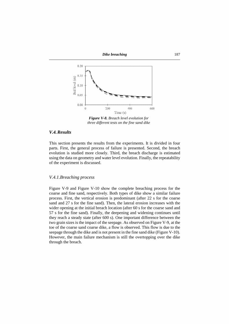
Dike breaching 187
Figure V-8. Breach level evolution for
three different tests on the fine sand dike
V.4. Results This section presents the results from the experiments. It is divided in four parts. First, the general process of failure is presented. Second, the breach evolution is studied more closely. Third, the breach discharge is estimated using the data on geometry and water level evolution. Finally, the repeatability of the experiment is discussed.
V.4.1.Breaching process Figure V-9 and Figure V-10 show the complete breaching process for the coarse and fine sand, respectively. Both types of dike show a similar failure process. First, the vertical erosion is predominant (after 22 s for the coarse sand and 27 s for the fine sand). Then, the lateral erosion increases with the wider opening at the initial breach location (after 60 s for the coarse sand and 57 s for the fine sand). Finally, the deepening and widening continues until they reach a steady state (after 600 s). One important difference between the two grain sizes is the impact of the seepage. As observed on Figure V-9, at the toe of the coarse sand coarse dike, a flow is observed. This flow is due to the seepage through the dike and is not present in the fine sand dike (Figure V-10). However, the main failure mechanism is still the overtopping over the dike through the breach.

188 Chapter V
Figure V-9. Failure process: coarse sand dike
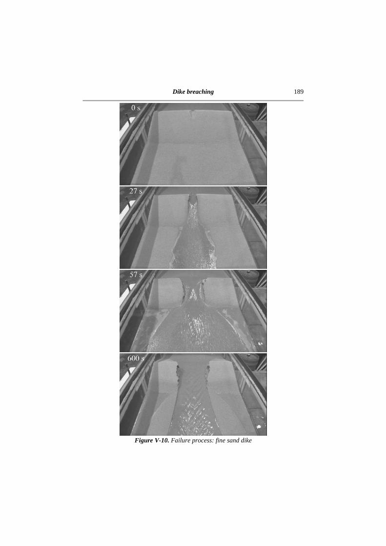
Dike breaching 189
Figure V-10. Failure process: fine sand dike
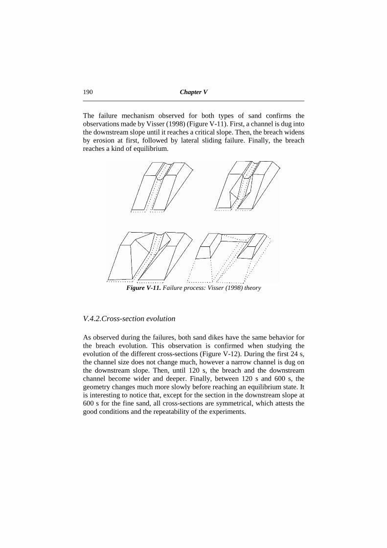
190 Chapter V
The failure mechanism observed for both types of sand confirms the observations made by Visser (1998) (Figure V-11). First, a channel is dug into the downstream slope until it reaches a critical slope. Then, the breach widens by erosion at first, followed by lateral sliding failure. Finally, the breach reaches a kind of equilibrium.
Figure V-11. Failure process: Visser (1998) theory
V.4.2.Cross-section evolution As observed during the failures, both sand dikes have the same behavior for the breach evolution. This observation is confirmed when studying the evolution of the different cross-sections (Figure V-12). During the first 24 s, the channel size does not change much, however a narrow channel is dug on the downstream slope. Then, until 120 s, the breach and the downstream channel become wider and deeper. Finally, between 120 s and 600 s, the geometry changes much more slowly before reaching an equilibrium state. It is interesting to notice that, except for the section in the downstream slope at 600 s for the fine sand, all cross-sections are symmetrical, which attests the good conditions and the repeatability of the experiments.

Dike breaching 191
Figure V-12. Cross-sections evolutions: (a) at the crest (x = 0.65 m, laser-sheet C2) with the coarse sand and
(b) the fine sand; (c) in the slope (x = 0.9 m, laser-sheet C5) with the coarse sand and (d) the fine sand

192 Chapter V
To analyze further the evolution of the cross-sections geometry, the vertical and lateral erosion is studied separately below. Figure V-13 shows the results for the cross-section located at the dike crest (x = 0.65 m) but similar conclusions can be drawn when studying other cross-sections of the dike. Initially, for the first 15 s, the bed level increases. This observation may be explained by the mobilization of the mixture of water and sand that induces some expansion captured by the laser-sheet. After that, the dike is eroded with a decreasing erosion rate. The coarse sand dike is initially eroded faster than the fine one. However, the fine sand dike then catch up this delay and they both stabilize at the same level.
Figure V-13. Breach level evolution
The evolution of the dike along its centerline shows the same bed level increase at the initial stage (Figure V-14, at the upstream end of the crest) as mentioned before. After that, between 24 s and 46 s, the erosion progresses on the downstream slope. Then, the dikes are eroded until they reach a steady slope. Furthermore, the fine sand profiles seem smoother than the coarse sand profiles and present an adverse slope that does not appear in the coarse sand dike. The erosion process presents some similarities with the theory presented by Coleman et al. (2002) with the appearance of a pivot point (Figure V-15). However this pivot point is located further downstream than Coleman’s theory.

Dike breaching 193
Figure V-14. Evolution of the bed level
along the centerline of the flume: (a) coarse sand, (b) fine sand
Figure V-15. Coleman et al. (2002) theory on the bed
level evolution
Both sand dikes present a similar behavior when focusing on the breach width evolution (Figure V-16). Initially, the breach width does not change and a narrow channel forms downstream (24 s). Then, the widening of the breach starts at the upstream and propagates downstream (46 s). Finally, the width does not change much between 120 s and 600 s. Regarding the breach width, the coarse sand dike presents a smoother evolution than the fine sand dike.

194 Chapter V
This can be explained by an apparent cohesion in the fine sand that creates a burst behavior: small blocks of fine sand sliding together.
Figure V-16. Breach width evolution: (a) coarse sand and (b) fine sand

Dike breaching 195
Another important variable in the experiment is the emptying of the upstream reservoir. This information is captured by the first ultrasonic probe (G1). Figure V-17 illustrates the difference between the two dikes material. The water-level peak occurs later and higher for the fine sediment: at 46.5 s with a maximum level of 0.203 m for the fine sand and at 41 s with a level of 0.199 m for the coarse sand. However, the final water level of the coarse sand dike remains higher. These differences are directly linked to the dikes breaching. The water level peak is lower for the coarse dike because of the seepage and the faster breaching initially. The final water level is higher for the coarse dike because the profile is completely different (Figure V-14).
Figure V-17. Evolution of the reservoir
water level (from gauge G1): (a) complete test and (b) zoom near the peak time
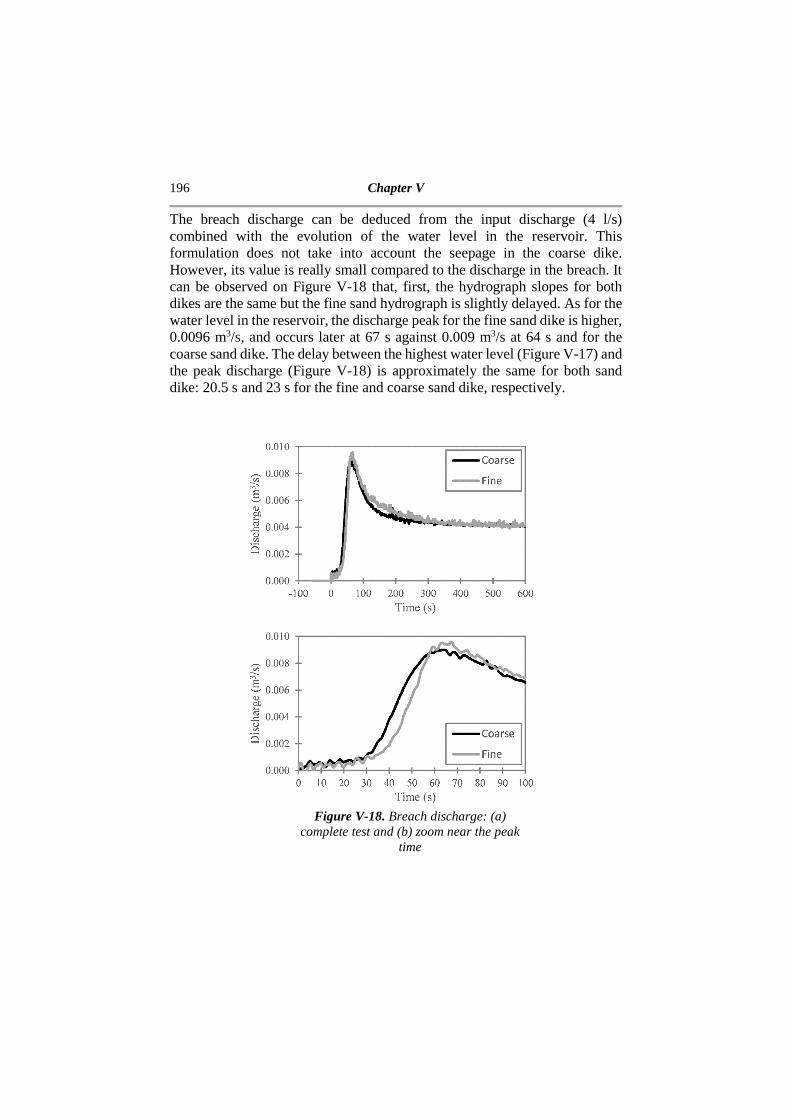
196 Chapter V
The breach discharge can be deduced from the input discharge (4 l/s) combined with the evolution of the water level in the reservoir. This formulation does not take into account the seepage in the coarse dike. However, its value is really small compared to the discharge in the breach. It can be observed on Figure V-18 that, first, the hydrograph slopes for both dikes are the same but the fine sand hydrograph is slightly delayed. As for the water level in the reservoir, the discharge peak for the fine sand dike is higher, 0.0096 m3/s, and occurs later at 67 s against 0.009 m3/s at 64 s and for the coarse sand dike. The delay between the highest water level (Figure V-17) and the peak discharge (Figure V-18) is approximately the same for both sand dike: 20.5 s and 23 s for the fine and coarse sand dike, respectively.
Figure V-18. Breach discharge: (a)
complete test and (b) zoom near the peak time

Dike breaching 197
V.5. Comparison with numerical simulations It is interesting to compare the experimental results to some numerical approaches. Two types of models are used for comparison: on the one hand a 2D finite-volume model and on the other hand a simple 1D approach that revealed surprisingly good regarding some aspects.
V.5.1. Two-dimensional Model V.5.1.1. Model description The 2D finite-volume model solves the Shallow Water & Exner equations on unstructured triangular meshes, using a modify HLLC scheme to determine the fluxes (Soares-Frazão and Zech 2010). The governing equations are written, in two dimensions, as
∂U∂t
+∂F∂x
+∂G∂y
=S (V-1)
U= k huhvhzb
l = k hqxqyzb
l (V-2)
F= WXXY uhu2h+gh2/2
uvhqsx/(1-ε0) Z[[
\ = kqx
σxπxyψx
l (V-3)
G= WXXY vh
uvhv2h+gh2/2qsy/(1-ε0) Z[
[\= kqyπxyσyψy
l (V-4)
S=
WXXXXY
0
gh-- ∂zb∂x-Sfx.
gh-- ∂zb
∂y-Sfy.
0 Z[[[[\ (V-5)
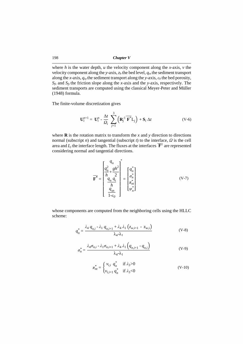
198 Chapter V
where h is the water depth, u the velocity component along the x-axis, v the velocity component along the y-axis, zb the bed level, qsx the sediment transport along the x-axis, qsy the sediment transport along the y-axis, ε0 the bed porosity, Sfx and Sfy the friction slope along the x-axis and the y-axis, respectively. The sediment transports are computed using the classical Meyer-Peter and Müller (1948) formula. The finite-volume discretization gives
Uin+1= Ui
n- ∆t
Ωi )Rj
-1 F*0000L j +Si ∆t
3
j=1
(V-6)
where R is the rotation matrix to transform the x and y direction to directions normal (subscript n) and tangential (subscript t) to the interface, Ω is the cell area and Lj the interface length. The fluxes at the interfaces @∗0000 are represented considering normal and tangential directions.
F*000=WXXXXXY qn
qn2
h+
gh2
2qn qt
hqsn
1-ε0 Z[[[[[\*
=
WXXXYqn
*
σn*
πnt*
ψn* Z[[[\ (V-7)
whose components are computed from the neighboring cells using the HLLC scheme:
qn* = λ4qn,i-λ1qn,i+1+λ4λ1zw,i+1-zw,i
λ4-λ1 (V-8)
σn* = λ4σn,i-λ1σn,i+1+λ4λ1 qn,i+1-qn,i
λ4-λ1 (V-9)
πnt* = x vt,i qn
* if λ3>0
vt,i+1 qn* if λ3<0
(V-10)

Dike breaching 199
ψn* =
λ2ψi - λ1ψi+1 + λ2λ1zb,i+1- zb,iλ2-λ1
(V-11)
where λj are the eigenvectors of the Jacobian matrix ranked from smallest to largest. To account for the bank failure due to an eventual excessive increase of a local slope, a tilting bank-failure operator is also included (Swartenbroekx et al. 2010). The mesh was composed of approximately 200 000 triangles with the smallest at the peak of the dike being 2.5 mm. Such a refined mesh was needed to capture the widening of the breach better as it has a tremendous impact on the bank failure operator.
V.5.1.2. Results Figure V-19 to Figure V-21 show the results obtained using the 2D model on the coarse-sand dike breaching case. Only this case is illustrated here, as the conclusions are similar for both dikes. The failure process can be divided into three parts: (i) the first 50 seconds (illustrated here by the results at 46 s), (ii) between 50 and 120 s (illustrated here by the results at 120 s), and (iii) between 120 s and 600 s. The 2D model gives a good prediction of the overall evolution of the breach. The evolution of the bottom profile is relatively closed to what has been observed during the experiment. During the first phase, the model predicts correctly the widening of the breach although the model yields less symmetrical results than observed ones. The discharge and reservoir water level are also predicted correctly. During the second phase, the breach is widened more than the experiment while the breach level evolution is correctly captured. Moreover, the model is able to predict the breach constriction. The consequence of this breach width overestimation can be observed in Figure V-21. The peak discharge and thus the speed of the reservoir water level descent are both overestimated.
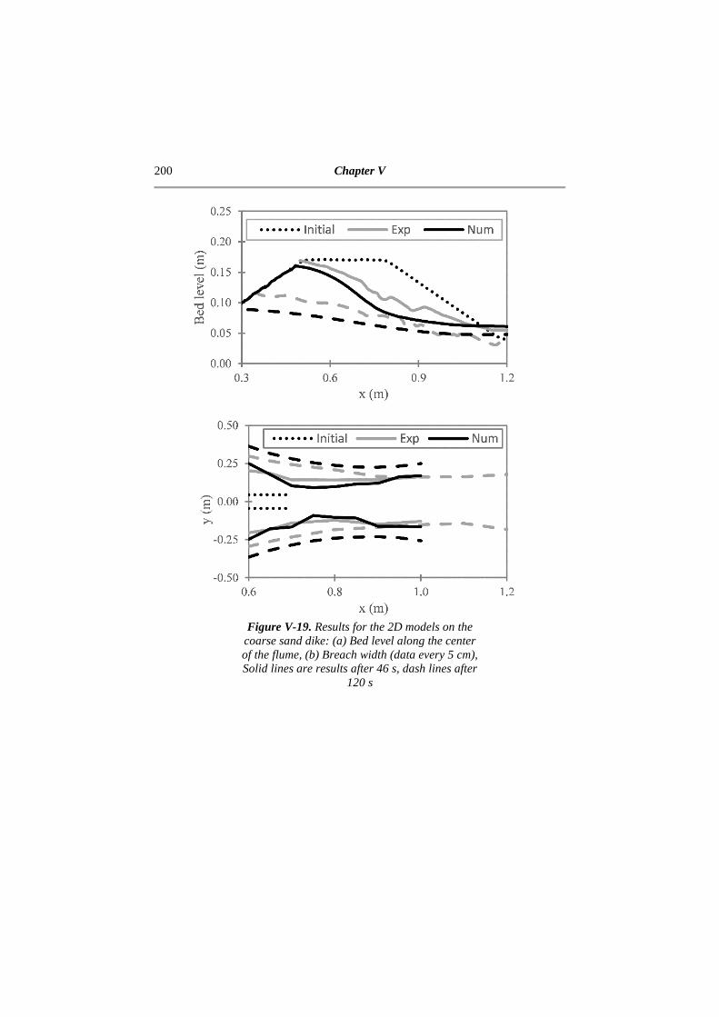
200 Chapter V
Figure V-19. Results for the 2D models on the coarse sand dike: (a) Bed level along the center of the flume, (b) Breach width (data every 5 cm), Solid lines are results after 46 s, dash lines after
120 s

Dike breaching 201
Figure V-20. Results for the 2D models on the
coarse sand dike: (a) Crest cross-section (x = 0.65 m, laser-sheet C2), (b) End of the crest cross-
section (x = 0.7 m, laser-sheet C3). Solid lines are results after 46 s, dash lines after 120 s

202 Chapter V
Figure V-21. Results for the 2D models on the
coarse sand dike: (a) Reservoir level, (b) Breach Discharge.

Dike breaching 203
V.5.2.One-dimensional Model V.5.2.1. Model description The 1D finite-volume model solves the Shallow Water & Exner equations using an Augmented Roe scheme with energy balance to determine the fluxes. The model is presented in Franzini and Soares-Frazão (submitted, chapter IV) and is based on the two-dimensional model presented by Murillo and Garcia-Navarro (2010). It also includes the concept of energy balance (Murillo and Garcia-Navarro 2014; Franzini and Soares-Frazão 2016). The governing equations are written, in one dimension vector form, as
∂U∂t
+ ∂F∂x
+ H∂U∂x
= S (V-12)
U = TAQAb
U (V-13)
F =
WXXXXY
Q
Q2
A + gI1
Qs
1 - ε0 Z[[[[\ (V-14)
S = T 0gI2- gASf
0U (V-15)
H = k0 0 0
0 0gA
Bs0 0 0
l (V-16)
where A is the wetted area, Q the discharge, Ab the area of available sediments (Figure V-22), gI1 the hydrostatic pressure, Bs the ratio to determine the discretization of the area of sediment evolution as ∆zb = ∆Ab/Bs (here equal to A/h, Figure V-22), gI2 the longitudinal component of lateral pressure in case of expansion or constriction of the river, and Sf the friction slope.

204 Chapter V
Figure V-22. Discretization of the erosion
The sediment transport Qs is calculated using the Meyer-Peter and Müller (1948) formula as
Qs=8BVgs-1d50 3 RSfs-1d50
- θcr1.5
(V-17)
where s is the specific gravity of the sediments, d50 the bed sediment median diameter, R the hydraulic radius (defined as R = A/P), and θcr the shear stress for initial sediment motion (here the value is set at 0.047).
The finite-volume discretization is
Uin+1 = Ui
n+∆t
∆xFi-1/2
*R - Fi+ 1/2*L (V-18)
The fluxes with a lateralized treatment of the source terms are written as
Fi+ 1/2*L = Fi + )λα - βe
m,i+1/2
m
λm<0
(V-19)
Fi+ 1/2*R = Fi+1- )(λα - β)em,i+1/2
m
λm>0
(V-20)
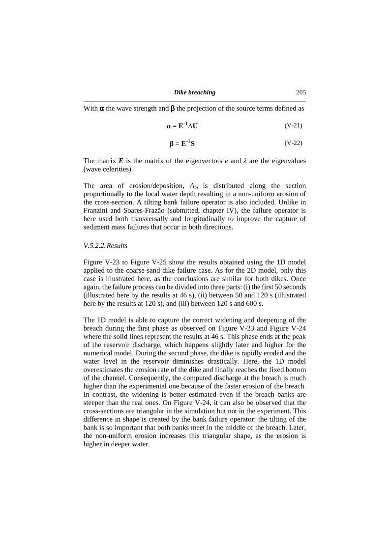
Dike breaching 205
With αααα the wave strength and ββββ the projection of the source terms defined as
α = E-1∆U (V-21)
β = E-1S (V-22)
The matrix E is the matrix of the eigenvectors e and λ are the eigenvalues (wave celerities). The area of erosion/deposition, Ab, is distributed along the section proportionally to the local water depth resulting in a non-uniform erosion of the cross-section. A tilting bank failure operator is also included. Unlike in Franzini and Soares-Frazão (submitted, chapter IV), the failure operator is here used both transversally and longitudinally to improve the capture of sediment mass failures that occur in both directions. V.5.2.2. Results Figure V-23 to Figure V-25 show the results obtained using the 1D model applied to the coarse-sand dike failure case. As for the 2D model, only this case is illustrated here, as the conclusions are similar for both dikes. Once again, the failure process can be divided into three parts: (i) the first 50 seconds (illustrated here by the results at 46 s), (ii) between 50 and 120 s (illustrated here by the results at 120 s), and (iii) between 120 s and 600 s. The 1D model is able to capture the correct widening and deepening of the breach during the first phase as observed on Figure V-23 and Figure V-24 where the solid lines represent the results at 46 s. This phase ends at the peak of the reservoir discharge, which happens slightly later and higher for the numerical model. During the second phase, the dike is rapidly eroded and the water level in the reservoir diminishes drastically. Here, the 1D model overestimates the erosion rate of the dike and finally reaches the fixed bottom of the channel. Consequently, the computed discharge at the breach is much higher than the experimental one because of the faster erosion of the breach. In contrast, the widening is better estimated even if the breach banks are steeper than the real ones. On Figure V-24, it can also be observed that the cross-sections are triangular in the simulation but not in the experiment. This difference in shape is created by the bank failure operator: the tilting of the bank is so important that both banks meet in the middle of the breach. Later, the non-uniform erosion increases this triangular shape, as the erosion is higher in deeper water.

206 Chapter V
Figure V-23. Results for the 1D model on the
coarse sand dike: (a) Bed level along the flume axis, (b) Breach width. Solid lines are results after
46 s, dash lines after 120 s

Dike breaching 207
Figure V-24. Results for the 1D model on the coarse sand dike: (a) Crest cross-section (x = 0.65 m, laser-sheet C2), (b) End of the crest cross-section (x = 0.7 m, laser-sheet C3). Solid lines are results after 46 s,
dash lines after 120 s
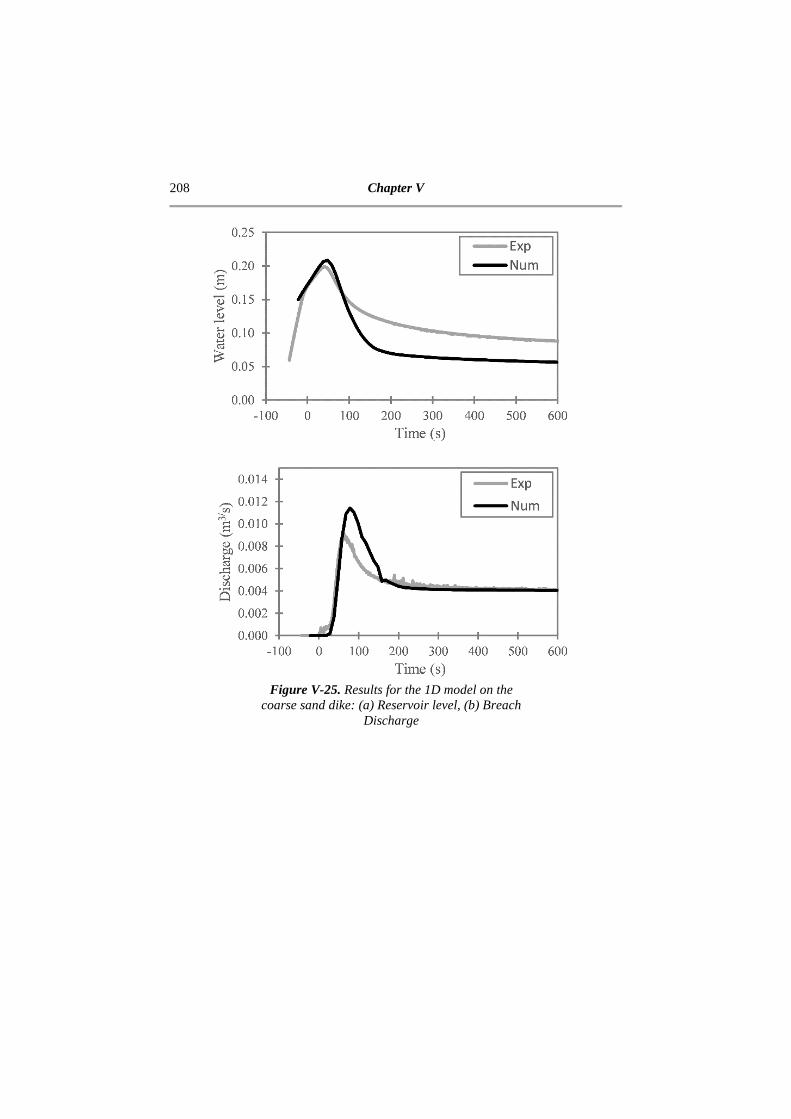
208 Chapter V
Figure V-25. Results for the 1D model on the
coarse sand dike: (a) Reservoir level, (b) Breach Discharge
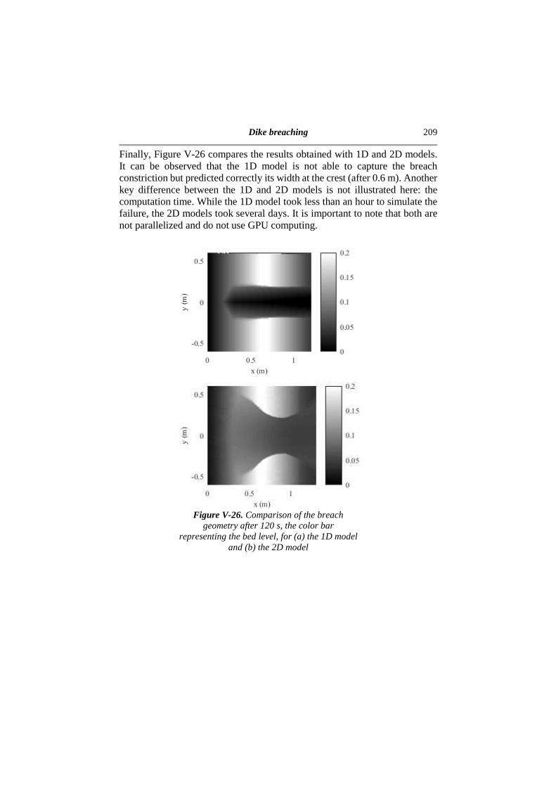
Dike breaching 209
Finally, Figure V-26 compares the results obtained with 1D and 2D models. It can be observed that the 1D model is not able to capture the breach constriction but predicted correctly its width at the crest (after 0.6 m). Another key difference between the 1D and 2D models is not illustrated here: the computation time. While the 1D model took less than an hour to simulate the failure, the 2D models took several days. It is important to note that both are not parallelized and do not use GPU computing.
Figure V-26. Comparison of the breach
geometry after 120 s, the color bar representing the bed level, for (a) the 1D model
and (b) the 2D model
210 Chapter V
V.6. Discussion and conclusions Experiments of dike breaching have been run using two different grain sizes. The general process showed good agreement with the theory from the literature. The differences between fine and coarse grain have been highlighted. First, even though both failures were due to the overtopping of the dike, the fine sand dike is less affected by the water seepage inside the dike. Second, some differences appear between both sand: while the bed level profile was smoother for the fine sand, the width variation was smoother for the coarse sand. Third, the fine sand dike failure exhibits a higher and later peak for both the water level in the upstream reservoir and the breach discharge. It was also observed that the delay between the reservoir level peak and the discharge peak were similar for both sand. Then, the experiment results have been compared to numerical simulation using 2D and 1D models. The 2D model showed good results in predicting the overall evolution of the dike breach. However, the results were not as symmetrical as the experiment and the breach was wider than observed. The simple 1D model showed surprisingly good results for the initial stage of the dike failure for all the monitored parameters even though the width evolution along the breach was straighter than the experiment. However, the results after the discharge peak were not as good, as the 1D model tends to overestimate the erosion rate. Nevertheless, the width evolution along the breach was correctly estimated even if presenting too straight bank slopes.
Acknowledgments This work was supported by the Fonds National de la Recherche Scientifique, Belgium. The authors would also like to thank Charles Descantons and Rémi Dujardin (2014) for their help in designing and running the experiments.
References Coleman, E., Andrews, D.P., Webby, M.G. (2002) Overtopping breaching of
noncohesive homogenous embankments. Journal of Hydraulics Engineering, ASCE, 128(9), 829-838.
Descantons, C., Dujardin, R. (2014). Formation, par débordement, d’une brèche dans une digue en matériau non cohésif. Master Thesis (in French). Université catholique de Louvain.
Dike breaching 211
Franzini F, Soares-Frazão S. (2016) Efficiency and accuracy of Lateralized
HLL, HLLS and Augmented Roe's scheme with energy balance for river flows in irregular channels. Applied Mathematical Modelling; 40 (17-18): 7427-7446.
Morris, M. W., Kortenhaus, A., Visser, P. J., and Hassan, M. A. A. M. (2009). “Breaching processes: A state of the art review.” FLOODsite Rep. T06-06-03, FLOODsite Consortium, ⟨www.floodsite.net⟩.
Müller, C., Frank, P.-J., Hager, W.H. (2016) Dyke overtopping: effects of shape and headwater elevation. Journal of Hydraulic Research, 54 (4), 410-422.
Meyer-Peter E, Müller R (1948). Formulas for bed load transport. Proc., 2nd Meeting, IAHR, Stockholm, Sweden; 39–64.
Murillo J, Garcia-Navarro P (2010). An Exner-based coupled model for the two-dimensional transient flow over erodible bed. Journal of computational physics; 229(23): 8704-8732
Murillo J, Garcia-Navarro P (2014). Accurate numerical modeling of 1d flow in channels with arbitrary shape. Application of the energy balanced property. Journal of Computational Physics; 260 : 222–248.
Schmocker, L., Hager, W.H. (2012). Effect of sediment diameter on plane dike breach shape and on breach discharge. River Flow 2012 - Proceedings of the International Conference on Fluvial Hydraulics, Vol. 2, 1065-1072.
Schmocker, L., Frank, P.-J. , Hager, W.H. (2014) Overtopping dike-breach: Effect of grain size distribution. Journal of Hydraulic Research, 52 (4), 559-564.
Soares-Frazão, S., Le Grelle, N., Spinewine, B., and Zech, Y. (2007) Dam-break induced morphological changes in a channel with uniform sediments: measurements by a laser-sheet imaging technique. Journal of Hydraulic Research 45, 13-16
Soares-Frazão, S., Zech, Y. (2011) HLLC scheme with novel wave-speed estimators appropriate for two-dimensional shallow-water flow on erodible bed. International Journal for Numerical Methods in Fluids, 66 (8), 1019-1036
Swartenbroekx, C., Soares-Frazão, S., Staquet, R., and Zech, Y. (2010) Two-dimensional operator for bank failures induced by water-level rise in dam-break flows. J. Hydraul. Res., 48(3), 302-314.
212 Chapter V
Van Emelen, S., Zech, Y., Soares-Frazaõ, S. (2015) Impact of sediment transport formulations on breaching modelling. Journal of Hydraulic Research, 53 (1), 60-72.
Visser, P.J. (1998). Breach growth in sand-dikes. PhD Thesis and Communications on Hydraulic and Geotechnical Engineering Series, Report 98-1, Delft University of Technology, Delft, The Netherlands.

SCOURING AT THE INTERFACE BETWEEN FIXED AND MOBILE BED
[Franzini F., Chen T., Capart H, and Soares-Frazão S. Scouring at the interface between fixed and mobile bed in steep sloped channel. Submitted to IAHR world congress 2016, Kuala Lumpur] The sixth and last chapter presents an experimental study of the scouring at the transition between fixed and mobile bed. This problem does not only appear around structures but could happen when part of the riverbed are composed of non-erodible bedrock (Figure VI-1). One of the models presented in chapter IV (the coupled Roe model) is validated using experimental results in order to study possible improvements.
Figure VI-1. Picture taken after the Ha!Ha! River flood (Capart et al.
2007): Transition between fixed and mobile bed
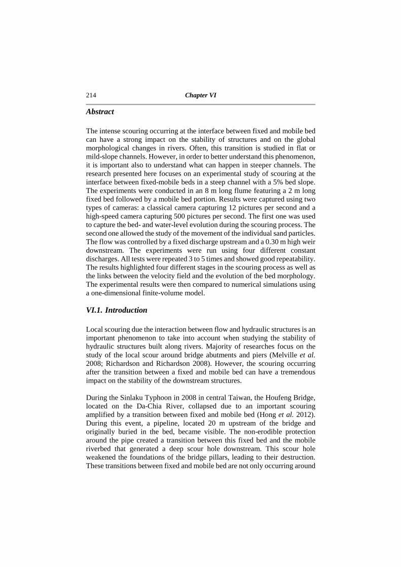
214 Chapter VI
Abstract The intense scouring occurring at the interface between fixed and mobile bed can have a strong impact on the stability of structures and on the global morphological changes in rivers. Often, this transition is studied in flat or mild-slope channels. However, in order to better understand this phenomenon, it is important also to understand what can happen in steeper channels. The research presented here focuses on an experimental study of scouring at the interface between fixed-mobile beds in a steep channel with a 5% bed slope. The experiments were conducted in an 8 m long flume featuring a 2 m long fixed bed followed by a mobile bed portion. Results were captured using two types of cameras: a classical camera capturing 12 pictures per second and a high-speed camera capturing 500 pictures per second. The first one was used to capture the bed- and water-level evolution during the scouring process. The second one allowed the study of the movement of the individual sand particles. The flow was controlled by a fixed discharge upstream and a 0.30 m high weir downstream. The experiments were run using four different constant discharges. All tests were repeated 3 to 5 times and showed good repeatability. The results highlighted four different stages in the scouring process as well as the links between the velocity field and the evolution of the bed morphology. The experimental results were then compared to numerical simulations using a one-dimensional finite-volume model.
VI.1. Introduction Local scouring due the interaction between flow and hydraulic structures is an important phenomenon to take into account when studying the stability of hydraulic structures built along rivers. Majority of researches focus on the study of the local scour around bridge abutments and piers (Melville et al. 2008; Richardson and Richardson 2008). However, the scouring occurring after the transition between a fixed and mobile bed can have a tremendous impact on the stability of the downstream structures. During the Sinlaku Typhoon in 2008 in central Taiwan, the Houfeng Bridge, located on the Da-Chia River, collapsed due to an important scouring amplified by a transition between fixed and mobile bed (Hong et al. 2012). During this event, a pipeline, located 20 m upstream of the bridge and originally buried in the bed, became visible. The non-erodible protection around the pipe created a transition between this fixed bed and the mobile riverbed that generated a deep scour hole downstream. This scour hole weakened the foundations of the bridge pillars, leading to their destruction. These transitions between fixed and mobile bed are not only occurring around
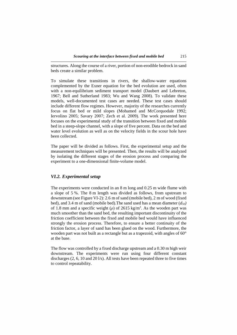
Scouring at the interface between fixed and mobile bed 215
structures. Along the course of a river, portion of non-erodible bedrock in sand beds create a similar problem. To simulate these transitions in rivers, the shallow-water equations complemented by the Exner equation for the bed evolution are used, often with a non-equilibrium sediment transport model (Daubert and Lebreton, 1967; Bell and Sutherland 1983; Wu and Wang 2008). To validate these models, well-documented test cases are needed. These test cases should include different flow regimes. However, majority of the researches currently focus on flat bed or mild slopes (Mohamed and McCorquodale 1992; Iervolino 2005; Savary 2007; Zech et al. 2009). The work presented here focuses on the experimental study of the transition between fixed and mobile bed in a steep-slope channel, with a slope of five percent. Data on the bed and water level evolution as well as on the velocity fields in the scour hole have been collected. The paper will be divided as follows. First, the experimental setup and the measurement techniques will be presented. Then, the results will be analyzed by isolating the different stages of the erosion process and comparing the experiment to a one-dimensional finite-volume model.
VI.2. Experimental setup The experiments were conducted in an 8 m long and 0.25 m wide flume with a slope of 5 %. The 8 m length was divided as follows, from upstream to downstream (see Figure VI-2): 2.6 m of sand (mobile bed), 2 m of wood (fixed bed), and 3.4 m of sand (mobile bed).The sand used has a mean diameter (d50) of 1.8 mm and a specific weight (ρ) of 2615 kg/m3. As the wooden part was much smoother than the sand bed, the resulting important discontinuity of the friction coefficient between the fixed and mobile bed would have influenced strongly the erosion process. Therefore, to ensure a better continuity of the friction factor, a layer of sand has been glued on the wood. Furthermore, the wooden part was not built as a rectangle but as a trapezoid, with angles of 60° at the base. The flow was controlled by a fixed discharge upstream and a 0.30 m high weir downstream. The experiments were run using four different constant discharges (2, 6, 10 and 20 l/s). All tests have been repeated three to five times to control repeatability.
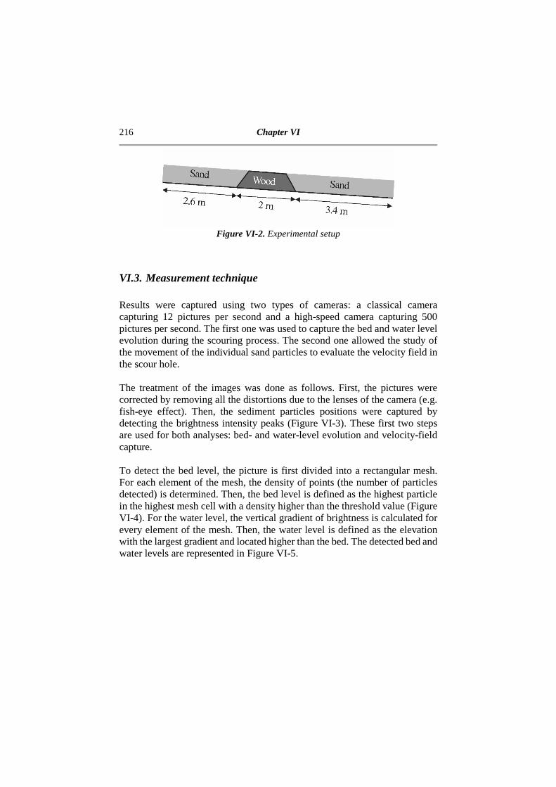
216 Chapter VI
Figure VI-2. Experimental setup
VI.3. Measurement technique Results were captured using two types of cameras: a classical camera capturing 12 pictures per second and a high-speed camera capturing 500 pictures per second. The first one was used to capture the bed and water level evolution during the scouring process. The second one allowed the study of the movement of the individual sand particles to evaluate the velocity field in the scour hole. The treatment of the images was done as follows. First, the pictures were corrected by removing all the distortions due to the lenses of the camera (e.g. fish-eye effect). Then, the sediment particles positions were captured by detecting the brightness intensity peaks (Figure VI-3). These first two steps are used for both analyses: bed- and water-level evolution and velocity-field capture. To detect the bed level, the picture is first divided into a rectangular mesh. For each element of the mesh, the density of points (the number of particles detected) is determined. Then, the bed level is defined as the highest particle in the highest mesh cell with a density higher than the threshold value (Figure VI-4). For the water level, the vertical gradient of brightness is calculated for every element of the mesh. Then, the water level is defined as the elevation with the largest gradient and located higher than the bed. The detected bed and water levels are represented in Figure VI-5.

Scouring at the interface between fixed and mobile bed 217
Figure VI-3. Particles capture
Figure VI-4. Density mesh to capture the bed level

218 Chapter VI
Figure VI-5. Bed level (black dots) and water level (white cross)
The velocity fields are determined using the Particle Tracking Velocimetry, also known as PTV. This method, unlike the Particle Image Velocimetry (PIV), tracks individual particles from one picture to the other. To track one particle, three methods are mainly used in the literature: nearest neighbor, pattern tracking and path tracking. The first method considers that the particle in the next frame is simply the particle nearest to the previous position. It is the simplest method of the three however, in rapid and dense flows, the results are not always accurate. The second method was developed by Capart et al. (2002), Instead of matching individual particles, group of particles, described by their Voronoi diagrams, are matched. The third and last method was first developed by Sethi and Jain (1987). It uses a sequence of pictures to find the trajectories of the particles and then correct the tracking by checking the coherence and the continuity of the calculated trajectories. To check that the results are repeatable, the measured water and bed levels for three different tests at 10 l/s after 40s are compared (Figure VI-6). It can be observed that, even though there are small differences, a good repeatability is obtained.
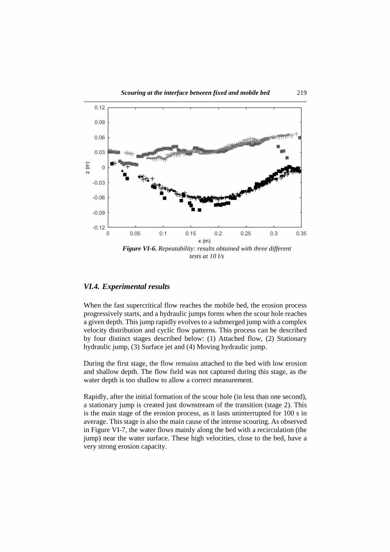
Scouring at the interface between fixed and mobile bed 219
Figure VI-6. Repeatability: results obtained with three different tests at 10 l/s
VI.4. Experimental results When the fast supercritical flow reaches the mobile bed, the erosion process progressively starts, and a hydraulic jumps forms when the scour hole reaches a given depth. This jump rapidly evolves to a submerged jump with a complex velocity distribution and cyclic flow patterns. This process can be described by four distinct stages described below: (1) Attached flow, (2) Stationary hydraulic jump, (3) Surface jet and (4) Moving hydraulic jump.
During the first stage, the flow remains attached to the bed with low erosion and shallow depth. The flow field was not captured during this stage, as the water depth is too shallow to allow a correct measurement. Rapidly, after the initial formation of the scour hole (in less than one second), a stationary jump is created just downstream of the transition (stage 2). This is the main stage of the erosion process, as it lasts uninterrupted for 100 s in average. This stage is also the main cause of the intense scouring. As observed in Figure VI-7, the water flows mainly along the bed with a recirculation (the jump) near the water surface. These high velocities, close to the bed, have a very strong erosion capacity.

220 Chapter VI
When the scour hole becomes too deep, the main velocity vectors detach from the bed and become horizontal, and a recirculation zone appears at the bottom, close to the bed (Stage 3, Figure VI-8). The erosion is greatly reduced during this regime and the upstream slope becomes milder because, due to the recirculation at the bottom, the sand particles are transported upstream. In addition, the length of the scour hole is increased. After 2-3 s, when the upstream slope is sufficiently mild again, the flow reattaches to the bed and a new hydraulic jump is formed at the downstream end of the scour hole (Stage 4, Figure VI-9). The erosion process is similar to Stage 3, with a low erosion rate and sand particles close to the bed moving in the upstream direction. This jump then proceeds to move upstream where it becomes stationary, resulting in the situation of Stage 2 again (Figure VI-7) and the whole process, from Stage 2 to Stage 4, starts again in a cyclic way.
Figure VI-7. Velocity field during stage 2 of the erosion process
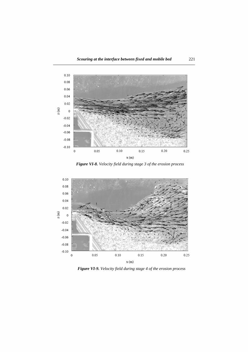
Scouring at the interface between fixed and mobile bed 221
Figure VI-8. Velocity field during stage 3 of the erosion process
Figure VI-9. Velocity field during stage 4 of the erosion process
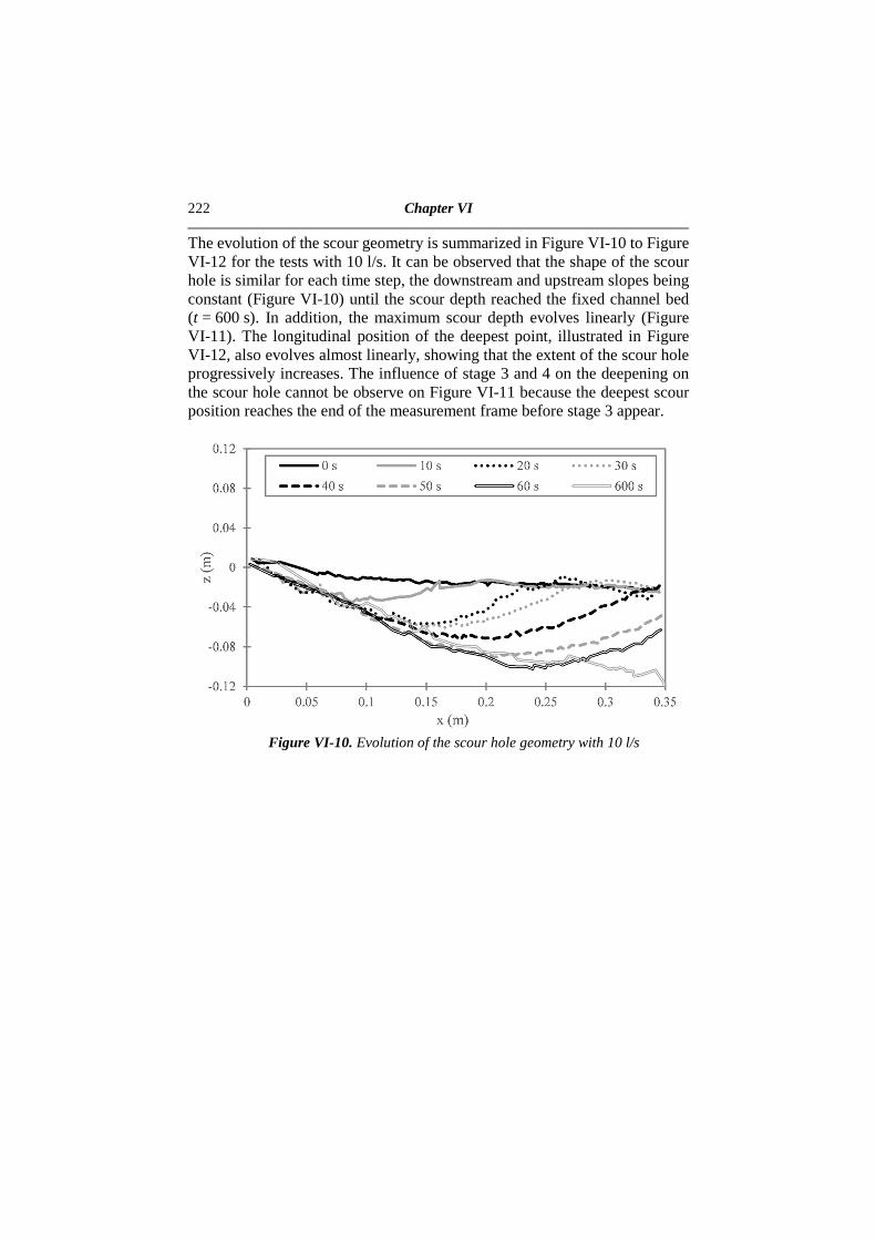
222 Chapter VI
The evolution of the scour geometry is summarized in Figure VI-10 to Figure VI-12 for the tests with 10 l/s. It can be observed that the shape of the scour hole is similar for each time step, the downstream and upstream slopes being constant (Figure VI-10) until the scour depth reached the fixed channel bed (t = 600 s). In addition, the maximum scour depth evolves linearly (Figure VI-11). The longitudinal position of the deepest point, illustrated in Figure VI-12, also evolves almost linearly, showing that the extent of the scour hole progressively increases. The influence of stage 3 and 4 on the deepening on the scour hole cannot be observe on Figure VI-11 because the deepest scour position reaches the end of the measurement frame before stage 3 appear.
Figure VI-10. Evolution of the scour hole geometry with 10 l/s

Scouring at the interface between fixed and mobile bed 223
Figure VI-11. Evolution of the max scour depth for 10 l/s
Figure VI-12. Evolution of the deepest scour position for 10 l/s
224 Chapter VI
VI.5. Comparison with numerical simulations A one-dimensional model based on the Saint-Venant equations and the Exner equation for the bed evolution is used to represent the flow. These equations are
∂A
∂t+
∂Q
∂x=0
(VI-1)
∂Q
∂t+
∂
∂xQ2
A+gI1 = gAS0-Sf (VI-2)
∂Ab
∂t+∂
∂x Qs
1 - ε0= 0 (VI-3)
Where Q is the discharge, A the wetted area, S0 the bed slope, Ab the area of the sediment bed, Qs the sediment transport rate and ε0 the bed porosity. The integral gI1 represents the hydrostatic pressure thrust. The sediment transport rate is determined by the Meyer-Peter and Müller (1948) equation
Qs=8BVgs-1d50 3 RSfs-1d50
- θcr1.5
(VI-4)
Where s is the specific gravity of the sediments, d50 the median bed sediment diameter, R the hydraulic radius (defined as R = A/P), and θcr the non-dimensional shear stress for initial sediment motion (here the value is set at 0.047). According to Garcia (2008), the sediment transport over the entire cross-section is obtained by multiplying the unit-width sediment transport by the width B of the channel at the level of the free surface. The sediment transport is always considered to be at capacity, equal to the value of (VI-4), if sediments are available. The system of equations (VI-1) to (VI-3) is written in vector form as
∂U∂t
+ ∂F∂x
+ H∂U∂x
= S (VI-5)

Scouring at the interface between fixed and mobile bed 225
With
U =TAQAb
U (VI-6)
F =
WXXXXY
Q
Q2
A + gI1
Qs
1 - ε0 Z[[[[\ (VI-7)
S = T 0- gASf
0U (VI-8)
H = k0 0 0
0 0gAS
0 0 0
l (VI-9)
The finite-volume scheme is then solved using a Roe solver with a lateralized treatment of the source terms (Franzini and Soares-Frazao submitted, Chapter IV).
Uin+1 = Ui
n+∆t
∆xFi-1/2
*R - Fi+ 1/2*L (VI-10)
Fi+ 1/2*L = Fi + )λα - βe
m,i+1/2
m
λm<0
(VI-11)
Fi+ 1/2*R = Fi+1- )(λα - β)em,i+1/2
m
λm>0
(VI-12)
With α the wave strength and β the projection of the source terms defined as
α = E-1∆U (VI-13)
β = E-1S (VI-14)
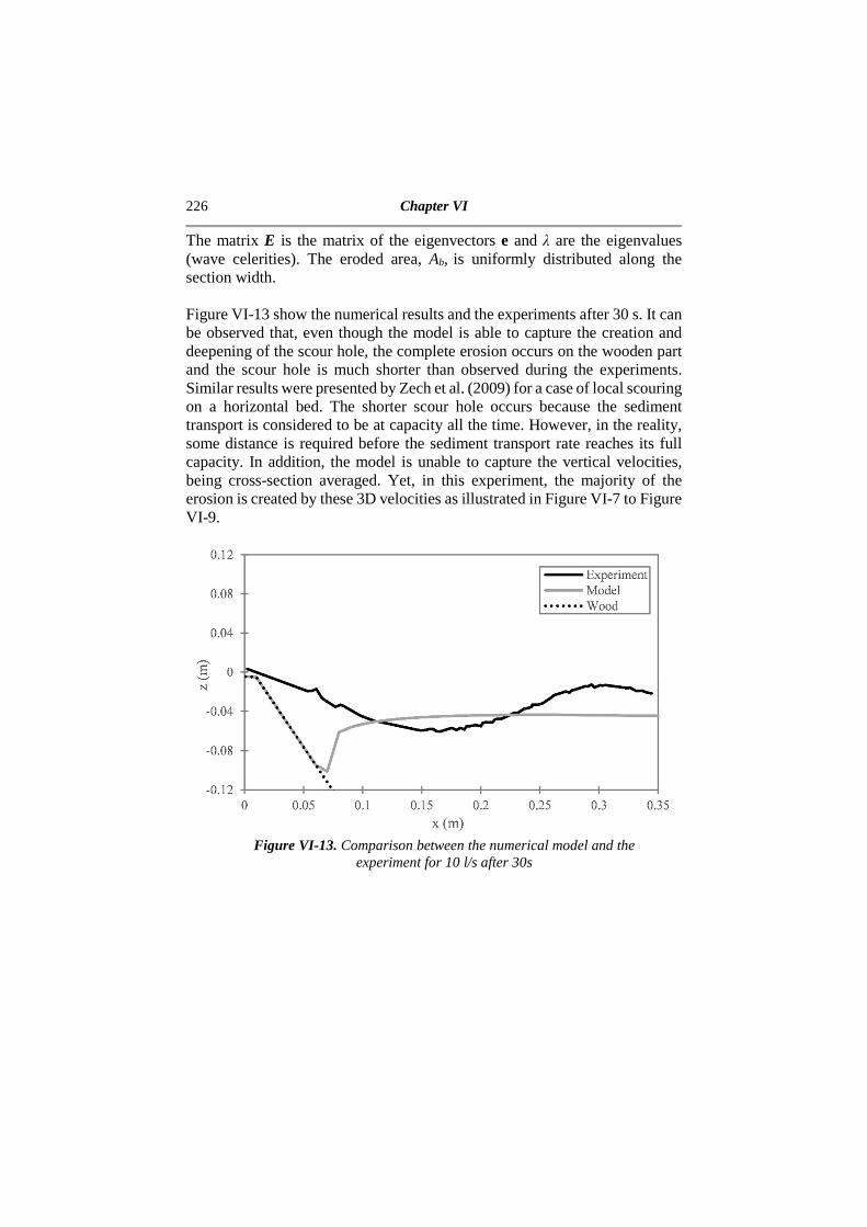
226 Chapter VI
The matrix E is the matrix of the eigenvectors e and λ are the eigenvalues (wave celerities). The eroded area, Ab, is uniformly distributed along the section width. Figure VI-13 show the numerical results and the experiments after 30 s. It can be observed that, even though the model is able to capture the creation and deepening of the scour hole, the complete erosion occurs on the wooden part and the scour hole is much shorter than observed during the experiments. Similar results were presented by Zech et al. (2009) for a case of local scouring on a horizontal bed. The shorter scour hole occurs because the sediment transport is considered to be at capacity all the time. However, in the reality, some distance is required before the sediment transport rate reaches its full capacity. In addition, the model is unable to capture the vertical velocities, being cross-section averaged. Yet, in this experiment, the majority of the erosion is created by these 3D velocities as illustrated in Figure VI-7 to Figure VI-9.
Figure VI-13. Comparison between the numerical model and the
experiment for 10 l/s after 30s
Scouring at the interface between fixed and mobile bed 227
VI.6. Conclusions Experiments of scouring at the transition between fixed and mobile in a steep-sloped channel have been presented. During the experiments, the evolution of the bed and water levels were filmed through a side window using a suitable digital video camera. It was shown that the scour hole progressively evolves during the whole erosion process keeping constant upstream and downstream slopes. The deepest point of the scour hole was tracked and it was observed that both the depth and the position of this point evolved linearly; the position being progressively pushed in the downstream direction. A high-speed camera (500 fps) was used to capture the movement of the sand particles in the scour hole. This tracking achieved using PTV (path tracking) allowed to determine the velocity fields during the erosion process. Four different stages were observed during the experiments: (1) attached flow, (2) stationary hydraulic jump, (3) surface jet and (4) moving hydraulic jump. The first stage, the attached flow, only occurred during the first instants of the experiments as long as the erosion remained limited. The second and most important stage, both in terms of duration and erosion capabilities, presented a stationary hydraulic jump with the main flow field close to the bed surface. Then, the third and fourth stages were relatively short and the main flow field became horizontal before returning to the second stage, starting a new cycle of stages 2-3-4. Finally, the experimental results were compared to a one-dimensional finite-volume model computing the sediment transport using the Meyer-Peter and Müller formula and considering equilibrium sediment transport. The comparison showed that the model was able to capture the creation and deepening of the scour hole. However, the length of the scour hole was not well predicted, the scour hole being too short and located too close to the transition between the fixed and mobile beds. Future work will focus on an appropriate lag formulation for the sediment transport rate in order to better represent the progressive evolution of this transport rate towards the full transport capacity.
Acknowledgments This work was supported by the Fonds National de la Recherche Scientifique, Belgium.
228 Chapter VI
References Bell, R. G., and Sutherland, A. J. (1983) Nonequilibrium bedload transport by
steady flows. J. Hydraul. Eng., 109(3), 351–367.
Capart, H., Young, D.L., and Zech, Y. (2002). Voronoï imaging methods for the measurement of granular flows. Experiments in Fluids, 32, 121-135.
Daubert, A., and Lebreton, J. C. (1967). Etude expérimentale sur modèle mathématique de quelques aspects des processus d’érosion des lits alluvionnaires, en régime permanent et non-permanent. Proc. 12th IAHR Congress, Rotterdam, The Netherlands.
García MH. (2008). Sediment transport and morphodynamics. In Sedimentation engineering processes, measurements, modeling and practice, M.H. García (ed.), ASCE Manuals and Reports on Engineering Practice 110, ASCE, Reston VA, 21–163.
Hong, J.H, Chiew, Y.M., Lu, J.Y, Lai, J.S., & Lin, Y.B. (2012). Houfeng Bridge failure in Taiwan. Journal of hydraulic engineering. 138(2), 186-198.
Iervolino, M. (2005). Transporto solido di fondo in condizioni non stazionare: modellazione onodimensionale. PhD thesis, Università degli Studi di Napoli “Frederico II” , Naples, Italy (in Italian).
Melville, B.W., Parola, A.C., & Coleman, S.E. (2008) Bridge-scour prevention and countermeasures. In Sedimentation engineering processes, measurements, modeling and practice, M.H. García (ed.), ASCE Manuals and Reports on Engineering Practice 110, ASCE, Reston VA, 543–577.
Meyer-Peter E, Müller R. (1948) Formulas for bed load transport. Proc. 2nd Meeting, IAHR, Stockholm, Sweden; 39–64.
Mohamed, M.S., McCorquodale, J.A. (1992) Short-term local scour. Journal of Hydraulic Research, 30 (5), 685-699.
Richardson, J.R., & Richardson, E.V. (2008) Bridge scour evaluation. In Sedimentation engineering processes, measurements, modeling and practice, M.H. García (ed.), ASCE Manuals and Reports on Engineering Practice 110, ASCE, Reston VA, 505–542.
Scouring at the interface between fixed and mobile bed 229
Savary, Céline. (2007) Transcritical transient flow over mobile beds Boundary
conditions treatment in a two-layer shallow-water model. PhD Thesis, Université catholique de Louvain, Louvain-la-Neuve, Belgium
Sethi, I.K., and Jain, R. (1987) Finding trajectories of feature points in monocular image sequence. IEEE Transactions on pattern analysis and machine intelligence, PAMI-9(1), 56-73.
Wu, W., and Wang, S. S. Y. (2008). One-dimensional modeling of dam- break flow over movable beds. Journal of Hydraulic Research, 46(1), 87–98.
Zech, Y., Soares-Frazão, S., Spinewine, B., Savary, C., and Goutière, L. (2009) Inertia effects in bed-load transport models. Canadian Journal of Civil Engineering, 36, 1587-1597.


CONCLUSION As presented in the introduction, the aim of the present thesis consists in developing a one-dimensional finite-volumes model to simulate fast transient flows with morphological changes in a river. Numerical and experimental approaches have both been investigated. First, the research focused on the simulation of pure hydrodynamic flows, without considering the sediment transport or morphological changes. Three key problems have been presented: (1) the computation of hydrodynamic flows with strong source terms and how to include them in the model, (2) the simulation of the flow around islands and (3) how to capture the water level evolution efficiently in the laboratory. Then, the impact of the sediment transport has been studied. Again, three key problems have been investigated: (1) the simulation of the flow and morphological changes, (2) the failure of a sand dike by overtopping and (3) the experimental study of the transition between fixed and movable bed. As each chapter is written in a form suitable for submission in professional journals or conferences, they all contain their own independent conclusions. These conclusions will be briefly summarized here by placing a stronger accent on the limitations of the approaches used in this thesis and the possible improvements and future researches. In the first chapter, three approaches to include the source terms in the computations of fluxes have been compared: one based on the HLL model (Lateralized HLL), one on the Roe model (Augmented Roe with energy balance) and one intermediary (HLLS). Using the Augmented Roe and the HLLS approaches, the correct discharge could be computed for the majority of the tests, with only some errors on the discharge conservation in hydraulic jumps. Furthermore, these approaches were able to predict the correct water level in all elementary cases tested in this work. However, it was observed that the Augmented Roe solver performs better on coarse meshes than the HLLS. Finally, the Lateralized HLL predicts correctly the water level for the majority of the tests but is unable to conserve correctly the discharge. However, when applied to simulate the real river case, it proved to be more robust than the other models, as it was the only model that could reach a perfect steady-state flow. In the second chapter, a method to simulate the flow around island using a one-dimensional model has been presented and tested. The model uses the characteristics path, the conservation of the discharge and the conservation of the water head to compute the fluxes before and after the island. For the supercritical bifurcation, where these relations are not sufficient to solve the problem, the discharge is distributed proportional to the average width of the branches, calculated as A/h. The one-dimensional model has been compared to a two-dimensional model. It predicts correctly the partition of discharge
232 Conclusion
between the two sub-channels. The one-dimensional model also predicts correctly the water depth in the channels even though it is not able to capture the creation of a peak at the connections. The model has also been confronted to measurement of the water level in a real case: the flow in one reach of the Meuse River. The predictions showed great agreement with the measurements. In the third chapter, the use of photogrammetry to capture the water level has been presented. The use of photogrammetry showed promising results in recording the water level in a wide area for a steady state problem. Comparison with gauge measurements showed that photogrammetry is a reliable technique to capture the water level. Moreover, photogrammetry is able to capture the water level much more efficiently than using other measurement techniques such as gauges as the area of capture is much larger. However, this method can still be improved as it showed some limits in recording very shallow water depths. In the fourth chapter, sediment transport is introduced and four different approaches to simulate the morphological changes have been presented. They all solve the shallow water-Exner equations but use different finite-volume discretizations and different schemes to compute the fluxes: coupled versus uncoupled and HLL- versus Roe-based. The models were compared to various test cases including water at rest, steady and unsteady problems. The results showed that the Coupled Roe model provides better results than the other models as it predicted correctly the evolution of the bed morphology and created smoother, thus more realistic, bed profiles. The coupled Lateralized HLL provided good prediction of the erosion of a sand dike. However, it predicted poorly the equilibrium slope in subcritical conditions as it reached a flat bed. In addition, simulations in arbitrary cross-sections with steep banks highlighted the importance of including a bank failure mechanism in the model. In the fifth chapter, experiments on the failure of sand dikes were presented. Dikes built with two grain sizes were compared, one coarser (mean diameter of 1.7 mm) and one finer (mean diameter of 0.7 mm). Differences between the two dikes were highlighted such as a smaller infiltration and a later and higher peak of breach discharge for the finer sand. Then, the experimental results were compared to one- and two-dimensional models. These comparisons showed the capabilities and limits of one of the model developed in the fourth chapter, the coupled Roe model. The one-dimensional model was able to predict correctly the overall widening of the breach even though it did not capture the breach constriction. The erosion was correctly predicted for the first half of the breaching. However, after that, the numerical model eroded a lot faster than observed during the experiment.

Conclusion 233
In the sixth and last chapter, an experimental study of the transition between fixed and mobile beds in steep channels was presented. Two cameras, one recording at 12fps and the other at 500 fps were used to capture the evolution of the bed and water level and the flow fields. Four stages were observed: (1) attached flow, (2) stationary hydraulic jump, (3) surface jet and (4) moving hydraulic jump. The second stage was the most important both in terms of duration and erosion rate as the flow was located mainly close to the bed. Then, the experimental results were compared to one of the model developed in the fourth chapter, the coupled Roe model. It highlighted the limit of the current approach, as the model is not able to capture accurately the geometry of the scour hole. The predicted scour hole was too short and located too close to the transition between the fixed and mobile beds. Future work should focus on three main topics: the simulation of the islands, the sediment transport model and the use of photogrammetry. For the simulation of the flow around islands, several improvements could be made on the model. First, the island simulation could be improved by adding the wetting/drying of the sub-channels. This would allow the model to simulate the creation of an island during a flood. In addition, the model should be able to consider different combinations of upstream and downstream sub-channels. For instance, being able to simulate the flow around two islands side-by-side, meaning that the flow would be divided in three sub-channels instead of two. One last improvement on the simulation of the islands would be to include morphological changes in the model. In addition, experiments of the flow around island, with and without sediments, should be realized. The morphological model could be improved by, first, considering the non-equilibrium transport. It could allow the model to better simulate the scour hole after the transition between fixed and mobile bed. Then, suspension transport could be included in the model. This means changing the governing equations of the model and using a model closer to two-phase models. In addition, the transport of cohesive material should be investigated both experimentally and numerically. Finally, more experiments should be conducted using photogrammetry in order to improve the current method. The focus should be set on the capture of shallow water depth and fast transient flows. The capture of shallow water could be improved, for instance, by increasing the concentration of dye or by adding some particles or oil on the water. For transient flows, the synchronization of the cameras will be a key factor of success and should be investigated further. This is difficult because the synchronization, in chapter

234 Conclusion
III, was realized using flashes, the lag between two successive pictures is thus controlled by the number of flashes available and their loading time. As a final conclusion, a wide range of topics were investigated in this thesis. Most of them open new possible fields of investigation and offer opportunities for future work in this fascinating domain.

NOTATIONS
Roman A wetted area
Ab area of sediments
B width at the free-surface
b width of the channel at a determined depth
B0 width at the bottom of the channel
Be equivalent width
Bs cross-section width for morphological changes
c celerity
C coefficient of partition
C- negative characteristic
C+ positive characteristic
d50 median sediment diameter
e eigenvectors
E matrix of the eigenvectors
F vector of fluxes
Fr Froude number
g gravity
G Grass coefficient
G fluxes in the y direction (2D)
H water head
H alternative flux matrix
h water depth
I identity matrix
I1 cross-section first moment (hydrostatic pressure thrust)
I2 spatial variation of the cross-section width (longitudinal component of the lateral pressure due to the longitudinal width variation)

236 Notations
J Jacobian
JE energy loss due to the expansion
L interface length (2D)
n Manning coefficient
P wetter perimeter
Q discharge
Qs sediment transport
qs sediment transport by unit width
R hydraulic radius
R rotation matrix (2D)
S vector of source terms
s specific gravity of the sediments
S0 bed slope
Sf friction slope
T impact of the stationary wave related to the source terms in the mass flux (HLLS)
t time
U vector of conserved variables
u velocity
v velocity in the y direction (2D)
x longitudinal coordinate along the river thalweg
z water level
Z bank slope ratio
zb bed level
zb0 thalweg level
zw water level

Notations 237
Greek α wave strengths (Roe)
β impact of the stationary source terms wave (Augmented Roe - Chap 2,4, 5, 6)
ε0 porosity
ζ source terms in the cells (Augmented Roe)
η local variable for the integration over the depth
θ impact of the stationary source terms wave (Augmented Roe - Chap 1)
θ adimensional shear stress (Chap 4-6)
θcr adimensional critical shear stress
λ eigenvalues (wave celerities)
π transversal momentum flux (2D)
Σ momentum flux
φ angle between the sub-channel and the main channel
ψ transport flux (2D)
ω weight coefficient (Augmented Roe)
Ω cell area (2D)
Subscripts g relative to the topography
h relative to the hydrodynamic
i cell indices
i-1/2 or i+1/2 interface indices
M relative to the main channel
s relative to the sediments
S1 or S2 relative to the first or second sub-channel
x relative to the x direction (2D)
y relative to the y direction (2D)
τ relative to the friction

238 Notations
Superscripts L relative to the left side
n Time indices
R relative to the right side
* Intermediate time
Overlines - (overline) arithmetic average
~ (tilde) Roe average