On upwind methods for parabolic nite elements in incompressible ows

INTERNATIONAL JOURNAL FOR NUMERICAL METHODS IN ENGINEERINGInt. J. Numer. Meth. Engng. 47, 317–340 (2000)

On upwind methods for parabolic �nite elementsin incompressible ows

Dena Hendriana and Klaus-J�urgen Bathe ∗

Department of Mechanical Engineering; Massachusetts Institute of Technology; 77 Massachusetts Avenue;Cambridge; MA 02139; U.S.A.

SUMMARY

We study the performance of various upwind techniques implemented in parabolic �nite element discretiza-tions for incompressible high Reynolds number ow. The characteristics of an ‘ideal’ upwind procedure are�rst discussed. Then the streamline upwind Petrov=Galerkin method, a simpli�ed version thereof, the Galerkinleast squares technique and a high-order derivative arti�cial di�usion method are evaluated on test problems.We conclude that none of the methods displays the desired solution characteristics. There is still need forthe development of a reliable and e�cient upwind method with characteristics close to those of the ‘ideal’procedure. Copyright ? 2000 John Wiley & Sons, Ltd.

KEY WORDS: incompressible uid; upwinding; parabolic elements

1. INTRODUCTION

In the �nite element method using the standard Galerkin procedure for incompressible ows,there are two major sources of numerical instability. The �rst source of instability is due to aninappropriate combination of element interpolation functions for the velocity and pressure. Thisinstability of the formulation is observed even in very low Reynolds number ows. The othersource of instability is due to the presence of the convective term and is observed when theconvective term is dominant.To remedy the �rst source of numerical instability, the theory of the inf–sup condition for

incompressible media is available, see, e.g. [1; 2]. It is shown that the �nite element methodis optimally convergent if an appropriate combination of �nite element spaces for velocity andpressure are used to satisfy the inf–sup condition for incompressible media. This condition limitsthe combinations of appropriate velocity and pressure interpolation functions. Some methods havealso been proposed to stabilize the �nite element formulation while still using equal-order ofinterpolations for the velocity and pressure, see, e.g. [1; 3–6]. In these methods, a numericalstabilization term is introduced to ‘damp’ the pressure oscillations.To remedy the second source of numerical instability, upwind methods are employed. Various

upwind techniques have been proposed and are employed in �nite element solutions, including

∗ Correspondence to: Klaus-J�urgen Bathe, Department of Mechanical Engineering, Massachusetts Institute of Technology,77 Massachusetts Avenue, Cambridge, MA 02139, U.S.A. E-mail: [email protected]

CCC 0029-5981/2000/020317–24$17.50 Received 12 November 1998Copyright ? 2000 John Wiley & Sons, Ltd.

318 D. HENDRIANA AND K. J. BATHE

the Streamline Upwind=Petrov Galerkin (SUPG) method [7; 8], the Galerkin Least Squares (GLS)method [9], upwinding based upon bubble functions [3; 10; 11], the Taylor–Galerkin based method[12; 13] and the High-order Derivative Arti�cial Di�usion (HDAD) method [14]. A few compar-isons of some of these techniques are available [15], but there is still little understanding as tohow these methods perform comparatively when used in a broad spectrum of solutions.In solving a high Reynolds number problem, an ‘ideal’ solution scheme would have the following

properties.

1. Property of discretization errors: uniform and optimal convergence of the �nite element solu-tions to the solution of the mathematical model, and

2. Property of solution of �nite element equations: fast convergence in the iterations to solve thealgebraic �nite element equations for any mesh and up to very high Reynolds number ows.

The second property is clearly necessary in order to have an e�ective solution scheme. Note theemphasis on obtaining the �nite element solution for any—of course, reasonable—mesh and veryhigh Reynolds number ows.The �rst property entails a number of requirements, namely

(1) For any mesh, the method should give a reasonable solution.(2) The method should give the highest possible (optimal) convergence in discretization errors.(3) The method should not be ‘too sensitive’ to the mesh used.(4) For any mesh, an error indicator should be available to evaluate the quality of the solution.(5) If the error indicator indicates too large an error, re�ning the mesh should result into a good

solution with an acceptable error.(6) The method should converge to the ‘exact’ solution of the mathematical model.

Considering these requirements, a reasonable solution means that the solution does not contradictintuition or physical reasoning; for example the direction of ow should be intuitively correct. Thesolutions should have no oscillations and as the mesh is re�ned, the overall ow �eld shouldcontinuously change to approach the ‘exact’ solution of the mathematical model. Hence, denotingthe solution obtained using a given mesh by U(mesh), we want to have

U(coarse mesh)⊂U(�ne mesh)⊂U(�ner mesh)⊂ · · ·The mathematical model we consider in this study is governed by the Navier–Stokes equations.

Hence, at the scale considered, laminar ow is assumed although high Reynolds number condi-tions are speci�ed. The upwind �nite element solution procedure should be able to solve for thelaminar ow at high Reynolds number for at least two reasons. First, the laminar ow assumptionis generally used in the numerical solution as an initial approximation. Therefore, if the solutioncannot be obtained with this approximation, it is di�cult to continue the iterative solution intro-ducing appropriate turbulence models. Second, at high Reynolds number, the ow is frequentlyonly turbulent in certain areas, and is still laminar in the other parts of the uid domain.When the mesh is very coarse, the method should be able to obtain ‘a reasonable’ solution

even though the actual physical ow might contain instabilities. With a coarse mesh, the solutionwill not be able to represent all the physical phenomena, such as boundary layers, back ows, orinstabilities, but as the mesh is re�ned, increasingly more physical phenomena should be revealedin the solution, while the overall ow should be similar to the coarse mesh solution. Eventually,when the mesh is �ne enough, the method should also be able to solve for an unstable behaviourof the ow in which case a transient analysis need be used.

Copyright ? 2000 John Wiley & Sons, Ltd. Int. J. Numer. Meth. Engng. 47, 317–340 (2000)

ON UPWIND METHODS FOR PARABOLIC FINITE ELEMENTS 319

For example, let us consider the driven ow cavity problem, see Figure 1. The domain isdiscretized initially into a mesh of 10 × 10 elements. The method should be able to solve theproblem when the Reynolds number is low, such as 10 or 100, without too much di�culty. Whenthe Reynolds number is greater than 1000, and then much greater than 1000, the iteration mightconverge more slowly but an ideal method would still obtain a physically reasonable solution.Of course, using the coarse mesh, boundary layers and circulation ows near the corners will notbe revealed, but as the mesh is re�ned, these physical phenomena will be presented.Ideally, the method should be able to solve any Navier–Stokes ow problem as described above

up to a Reynolds number ∼107, because many engineering problems are de�ned at such highReynolds numbers.The objective of this paper is to test some existing upwind methods for parabolic �nite elements

and determine whether the methods satisfy the requirements of the ‘ideal’ scheme discussed above.Simple Galerkin discretizations using parabolic elements are generally more stable than using linearelements; however, upwinding is still needed to solve high Reynolds number ows. The methodsthat we consider here are the high-order derivative arti�cial di�usion method which is similarto upwind methods used in �nite di�erence procedures, the Streamline Upwind Petrov=Galerkin(SUPG) method [7; 8], a simpli�cation thereof, and the Galerkin Least Squares (GLS) technique[9]. We use four test problems to measure the performance of the methods. Of course, our eval-uation is by no means all encompassing in that, for example, we only consider four upwindingprocedures, we only solve a few test problems, we do not measure the solution errors, we donot use specially aligned meshes to minimize these errors, and we solve the problems only withparabolic elements. However, although these shortcomings are severe, we believe that the study isvaluable in contributing to the comparative evaluation of the existing upwind methods, and mightlead towards ideas to improve the solution schemes.

2. GOVERNING EQUATIONS

Let Vol and (0,T ) be the spatial and temporal domains, and let x∈Vol and t ∈ [0; T ] represent theassociated co-ordinates. Using a Cartesian co-ordinate system and indicial notation, the Navier–Stokes equations for incompressible ow can be written as

vi; i=0 in Vol× (0; T )�vi; t + �vi; jvj + p;i − �(vi; j + vj; i);j − fBi =0 in Vol× (0; T )

(1)

where vi; �; p; �, and fBi are the velocity in the xi-direction, uid density, pressure, uid viscosity,and body force per unit volume in the xi-direction, respectively, and ( );t ; ( );i denote partialdi�erentiations with respect to time and xi-coordinate. The Dirichlet and Neumann type boundaryconditions are imposed at di�erent segments of the boundary S

vi = gi on Su

�ijnj = hi on Sf(2)

where gi; hi are given functions; �ij is the stress component; nj is the component of the boundaryunit normal vector and Su; Sf are complementary subsets of S. Note that we do not consider theenergy equation because the �nite element solution of the above equations will already revealsu�ciently the basic characteristics of the solution schemes.



Figure 1. Schematics of solutions of driven ow cavity problem



3. FINITE ELEMENT DISCRETIZATIONS

We want to evaluate the performance of upwind methods when using parabolic element discretiza-tions. For incompressible ow at low Reynolds number the most e�ective nine-node elements arethe 9=3 (linear pressure interpolation) element and the 9=4-c (bilinear continuous pressure interpo-lation) element. These discretizations contain the highest possible order of pressure interpolationwhile satisfying the inf–sup condition for incompressible analysis (without use of a numericalfactor as employed in stabilized �nite element discretizations), and are therefore excellent can-didates for high Reynolds number ow solutions. We use the 9=4-c element for the solution ofhigh Reynolds number ow with the SUPG, simpli�ed SUPG and high-order derivative arti�cialdi�usion upwind methods embedded in the discretizations. On the other hand, for the Galerkinleast squares method we use the usual approach of equal-order interpolations and numerically sta-bilizing the velocity and pressure components [1]. Hence, we use the nine-node element with allnodes employed to interpolate the velocity and pressure variables.

3.1. High-order Derivative Arti�cial Di�usion (HDAD) method

The high-order derivative arti�cial di�usion method is considered because the method is verysimple and computationally e�cient. The method for incompressible ows is an extention of thetechnique used for compressible ows [14]. In the solution, the two-dimensional quadrilateral 9=4-celement is employed to discretize the domain.The solution and weighting functional linear spaces† are

Vh ={vh | vh ∈L2(Vol); @(vh)i@xj

∈L2(Vol); i=1; 2; 3; j=1; 2; (vh)1 ∈Q1(Vol(m));

(vh)2;3 ∈Q2(Vol(m)); (vh)i|Su = gi(t); i=2; 3}

Wh ={wh |wh ∈L2(Vol); @(wh)i@xj

∈L2(Vol); i=1; 2; 3; j=1; 2; (wh)1 ∈Q1(Vol(m));

(wh)2;3 ∈Q2(Vol(m)); (wh)i|Su =0; i=2; 3}

where, as usual, L2(Vol) is the space of square integrable functions in the volume, and Q1(Vol(m))

and Q2(Vol(m)) denote the bilinear and biquadratic functions in the reference element m.

The �nite element formulation for the incompressible ow using the high-order derivative arti-�cial di�usion method is:Find (p; v1; v2)∈Vh such that for all ( �p; �v1; �v2)∈Wh∫

Vol�pvi; i dVol= 0∫

Vol{ �vi(�vi; t + �vi; jvj)− �vi; ip+ �vi; j�(vi; j + vj; i)} dVol

+∑m

∫Vol(m)

�vi; jj�j�|vj|vi; jj dVol(m) =∫Vol�vifBi dVol +

∫Sf

�vSi fSi dS (3)

† Actually, to be precise, Vh is not a linear space, but an a�ne manifold that can be thought of as obtained by translatingthe linear space Wh



Regarding this equation, the boundary traction term in the xi-direction is de�ned as

fSi = {−p�ij + �(vi; j + vj; i)}nj (4)

where nj is the xj-direction cosine of the unit (pointed outward) boundary normal vector. �ij isthe Kronecker delta (i.e. �ij =1 for i= j, and �ij =0 for i 6= j).The value of �j is de�ned as

�j =19

(∣∣∣∣@xj@r∣∣∣∣)3

where r denotes the co-ordinates in the natural co-ordinate system of the element. The characteristiclength is de�ned as ∣∣∣∣@xj@r

∣∣∣∣ =√(

@xj@r1

)2+(@xj@r2

)2

The factor 19 in the �j de�nition is used to obtain full upwinding corresponding to the outer nodesof the element in one-dimensional ow conditions.We note that the form of upwinding used in equation (3) is similar to high-order upwinding in

�nite di�erence methods. The upwinding is proportional to the second derivatives of the velocitycomponents, and is therefore of higher order, but in the form of equation (3), the amount ofupwinding is dependent on the directions of the co-ordinate axes. Our numerical experimentationshowed that this de�ciency appears to be not a serious drawback. However, other forms of HDADupwinding can of course be designed, including a scheme that would only apply arti�cial di�usionin the streamline direction (and perhaps a controlled amount in the cross-direction).

3.2. Streamline Upwind=Petrov–Galerkin (SUPG) method

The SUPG method was originally proposed for the bilinear element [7]. We use the methodhere for the quadratic 9=4-c element. Some authors extended the SUPG technique for use with aquadratic element by using di�erent de�nitions of the SUPG parameter � for corner, mid-face andcentre nodes of the element [12; 16]. However, this approach leads to a complicated formulation.The �nite element formulation that we use with the SUPG upwinding is:Find (p; v1; v2)∈Vh such that for all ( �p; �v1; �v2)∈Wh∫



+∑m

∫Vol(m)

�vi; kvk�{�vi; t + �vi; jvj + p; i − �(vi; j + vj; i); j − fBi } dVol(m)

=∫Vol�vifBi dVol +

∫Sf

�vSi fSi dS (5)

The value of � is de�ned as

�= h�(Ree)=2V



Figure 2. Impinging uid ow over a slip-wall problem

Figure 3. Meshes used for the impinging uid ow over a slip-wall problem: (a) uniform; (b) distorted

where h is the characteristic length of the element, and

Ree = �Vh=�

V =√v21 + v

22

�(Ree) =

{Ree=3; Ree63

1; Ree¿3

3.3. Simpli�ed SUPG (S-SUPG) procedure

In this solution we also use the 9=4-c element. The �nite element formulation for the incom-pressible ow using the simpli�ed SUPG technique is:Find (p; v1; v2)∈Vh such that for all ( �p; �v1; �v2)∈Wh∫



+∑m

∫Vol(m)

�vi; kvk�{�vi; jvj − fBi } dVol(m) =∫Vol�vifBi dVol +

∫Sf

�vSfi fSi dS (6)



The de�nition of � is as for the SUPG method. The reasoning for using this method is that theconvective term in the stabilization is dominant and the pressure and di�usive terms might not beneeded. Also, the transient term should not be needed since the upwinding is used to stabilize thespatial solution variation.

3.4. Galerkin Least Squares (GLS) method

In this method, the 9-node (9=9-c) element is employed to discretize the domain with the usual9-node interpolation of the velocity and the same 9-node interpolation for the pressure. The solutionand weighting functional linear spaces‡ are

Vh ={vh | vh ∈L2(Vol); @(vh)i@xj

∈L2(Vol); i=1; 2; 3; j=1; 2;

(vh)1;2;3 ∈Q2(Vol(m)); (vh)i|Su = gi(t); i=2; 3}

Wh ={wh |wh ∈L2(Vol); @(wh)i@xj

∈L2(Vol); i=1; 2; 3; j=1; 2;

(wh)1;2;3 ∈Q2(Vol(m)); (wh)i|Su =0; i=2; 3}

The �nite element formulation for the incompressible ow using the Galerkin least squaresmethod is:Find (p; v1; v2)∈Vh such that for all ( �p; �v1; �v2)∈Wh∫

Vol�pvi; i dVol +

∑m

∫Vol(m)

�p; i�{�vi; t + �vi; jvj + p; i−�(vi; j + vj; i); j − fBi } dVol(m) = 0∫


+∑m

∫Vol(m)

{� �vi; t + � �vi; kvk − �( �vi; k + �vk; i); k} � {�vi; t + �vi; jvj + p; i

−�(vi; j + vj; i); j − fBi } dVol(m) =∫Vol�vifBi dVol +

∫Sf

�vSi fSi dS (7)

The value of � was de�ned in References [9; 17]

�= h�(Ree)=2�V

where

Ree =mh�Vh=4�

V =√v21 + v

22

�(Ree) ={Ree; Ree¡11; Ree¿1

‡ See footnote 1



Figure 4. Solution of impinging uid ow over a slip-wall using the 9=9-c element with the GLS method: (a) streamlines;(b) pressure in case 1; (c) pressure in case 2

and mh=1=12 for quadratic elements, see [15]. Hence, with this de�nition, maximum upwindingis reached when �Vh=�=36, whereas in the SUPG method when �Vh=�=3.



Figure 5. Convergence curves for the impinging uid ow over a slip-wall problem, case 1: (a) pressure error in L2-norm;(b) velocity error in L2-norm

4. NUMERICAL TESTS

In this section we study the performance of the discretization and upwind methods summarizedin the previous section. First, we apply the methods to the solution of a problem, for whichwe have the exact analytical solution, and we estimate the convergence rates of the methods.Then we consider three problems to solve high Reynolds number ows. To solve the nonlin-ear equations, we use the Newton–Raphson method and allow a maximum of 35 iterations toreach the solution. We report the number of iterations required to solve the problems at di�er-ent Reynolds numbers and report the largest Reynolds number for which the methods yield thesolutions.The problem solutions can of course also be sought using the Galerkin method without up-

winding, and depending on the problem, convergence in the solution of the algebraic equations



Figure 6. Convergence curves for the impinging uid ow over a slip-wall problem, case 2: (a) pressure error in L2-norm;(b) velocity error in L2-norm

is obtained for some reasonably high Reynolds number ows. However, the converged solutionsshow oscillations and we do not include the results in this paper.

4.1. Convergence study problem

We consider the problem described in Figure 2. The problem consists of a jet impinging upona wall with a controlled body force. The uid is assumed to slip on the wall. The body forcefunctions are

fB1 = 5x1x82 + 10x1x

32 + 60�x1x

22

fB2 = 0



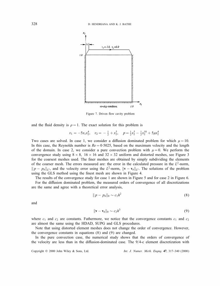
Figure 7. Driven ow cavity problem

and the uid density is �=1. The exact solution for this problem is

v1 = −5x1x42 ; v2 = − 12 + x

52 ; p= 1

2x52 − 1

2x102 + 5�x

42

Two cases are solved. In case 1, we consider a di�usion dominated problem for which �=10.In this case, the Reynolds number is Re=0·5025, based on the maximum velocity and the lengthof the domain. In case 2, we consider a pure convection problem with �=0. We perform theconvergence study using 8× 8; 16× 16 and 32× 32 uniform and distorted meshes, see Figure 3for the coarsest meshes used. The �ner meshes are obtained by simply subdividing the elementsof the coarser mesh. The errors measured are: the error in the calculated pressure in the L2-norm,‖p − ph‖L2 , and the velocity error using the L2-norm, ‖v − vh‖L2 . The solutions of the problemusing the GLS method using the �nest mesh are shown in Figure 4.The results of the convergence study for case 1 are shown in Figure 5 and for case 2 in Figure 6.For the di�usion dominated problem, the measured orders of convergence of all discretizations

are the same and agree with a theoretical error analysis,

‖p− ph‖0 ∼ c1h2 (8)

and

‖v − vh‖0 ∼ c2h3 (9)

where c1 and c2 are constants. Futhermore, we notice that the convergence constants c1 and c2are almost the same using the HDAD, SUPG and GLS procedures.Note that using distorted element meshes does not change the order of convergence. However,

the convergence constants in equations (8) and (9) are changed.In the pure convection case, the numerical study shows that the orders of convergence of

the velocity are less than in the di�usion-dominated case. The 9=4-c element discretization with



Table I. Number of iterations required to solve thedriven ow cavity problem with di�erent Reynolds

numbers using di�erent upwind methods

Re HDAD SUPG S-SUPG GLS

400 8 8 7 81000 7 8 6 82000 6 7 6 63000 5 6 5 54000 4 ∗ 5 65000 4 5 46000 4 4 47000 4 4 48000 4 4 49000 5 4 410 000 ∗ 4 411 000 5 412 000 5 413 000 5 414 000 6 515 000 6 416 000 6 418 000 13 420 000 ∗ 422 000 424 000 426 000 528 000 ∗Note: Newton–Raphson method is used with convergencetolerance= 10−6; the (∗) denotes iteration not converged

Figure 8. Solution of the driven ow cavity problem with Re=5000 using the 9=4-c element with high-order derivativearti�cial di�usion method: (a) pressure contours; (b) velocity vectors



Figure 9. Solution of the driven ow cavity problem with Re=5000 using the 9=4-c element with simpli�ed SUPG method:(a) pressure contours; (b) velocity vectors

Figure 10. Solution of the driven ow cavity problem with Re=5000 using the 9=9-c element with GLS method:(a) pressure contours; (b) velocity vectors

the high-order derivative arti�cial di�usion method gives almost an order of convergence of 3.The SUPG and GLS methods give almost the same orders of convergence, around 2, and thesimpli�ed SUPG method gives less than 2. Notice that, in this case, the use of distorted meshesresults in better convergence rates for all methods because the mesh distortions favour the owsolution.For the pressure variable, the discretizations using the HDAD, SUPG and GLS procedures give

as good orders of convergence as in the di�usion-dominated problem, and in some cases evenbetter values. Using the simpli�ed SUPG method the order of convergence is, however, less thanin the di�usion-dominated problem.



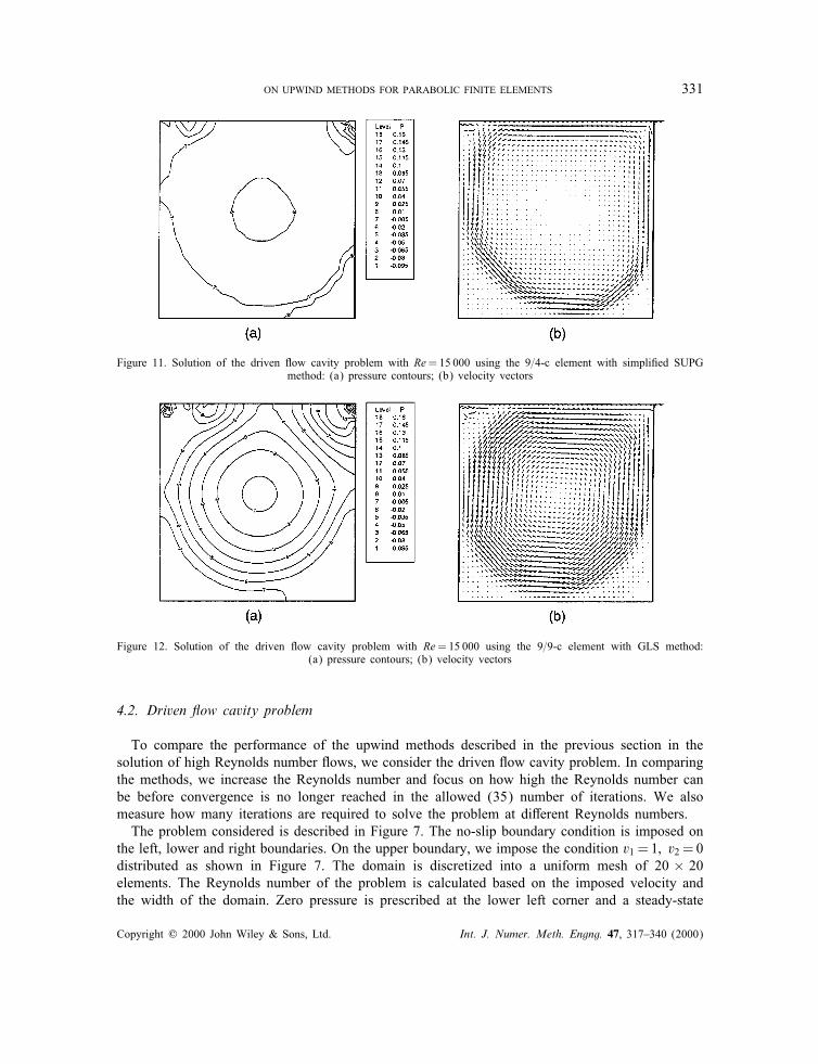
Figure 11. Solution of the driven ow cavity problem with Re=15 000 using the 9=4-c element with simpli�ed SUPGmethod: (a) pressure contours; (b) velocity vectors

Figure 12. Solution of the driven ow cavity problem with Re=15 000 using the 9=9-c element with GLS method:(a) pressure contours; (b) velocity vectors

4.2. Driven ow cavity problem

To compare the performance of the upwind methods described in the previous section in thesolution of high Reynolds number ows, we consider the driven ow cavity problem. In comparingthe methods, we increase the Reynolds number and focus on how high the Reynolds number canbe before convergence is no longer reached in the allowed (35) number of iterations. We alsomeasure how many iterations are required to solve the problem at di�erent Reynolds numbers.The problem considered is described in Figure 7. The no-slip boundary condition is imposed on

the left, lower and right boundaries. On the upper boundary, we impose the condition v1 = 1; v2 = 0distributed as shown in Figure 7. The domain is discretized into a uniform mesh of 20 × 20elements. The Reynolds number of the problem is calculated based on the imposed velocity andthe width of the domain. Zero pressure is prescribed at the lower left corner and a steady-state



Figure 13. The ‘S’-shaped channel ow problem

Figure 14. The mesh used for the ‘S’-shaped channel ow problem

analysis is carried out. We perform runs with increasing Reynolds numbers as given in Table Iand record the number of iterations. The Newton–Raphson method is used to solve the nonlinearequations with the convergence tolerance on the normalized norms of residuals in the velocitiesand pressure (Rv= ‖�vh|=‖vh‖; Rp= ‖�ph|=‖ph‖) equal to 10−6. To reach the solutions for theReynolds numbers listed in Table I, we start from zero pressure and velocities as initial condition,and use the converged solution of the lower Reynolds number case as the initial condition for thenext higher Reynolds number problem.The solutions of the problem for Re=5000 using di�erent upwind methods are shown in

Figures 8–10. In the solutions, the high-order derivative arti�cial di�usion method gives thelargest pressure gradient and the GLS method gives the smallest pressure gradient. This is tobe expected since the GLS method contains an arti�cial di�usion in the pressure term. Fig-ure 8(a) shows that the HDAD method solution contains slight pressure oscillations. The ve-locity solution of the high-order derivative arti�cial di�usion method is similar to the solutionof the GLS method. The simpli�ed SUPG method gives a narrow banded velocity solution,see Figure 9(b).



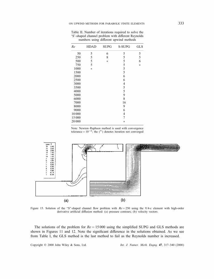
Table II. Number of iterations required to solve the‘S’-shaped channel problem with di�erent Reynolds

numbers using di�erent upwind methods


50 5 6 5 5250 5 8 5 5500 5 ∗ 5 6750 5 5 ∗1000 ∗ 51500 52000 62500 63000 43500 54000 55000 96000 87000 168000 99000 610 000 415 000 720 000 ∗Note: Newton–Raphson method is used with convergencetolerance= 10−6; the (∗) denotes iteration not converged

Figure 15. Solution of the “S”-shaped channel ow problem with Re=250 using the 9=4-c element with high-orderderivative arti�cial di�usion method: (a) pressure contours; (b) velocity vectors

The solutions of the problem for Re=15 000 using the simpli�ed SUPG and GLS methods areshown in Figures 11 and 12. Note the signi�cant di�erence in the solutions obtained. As we seefrom Table I, the GLS method is the last method to fail as the Reynolds number is increased.



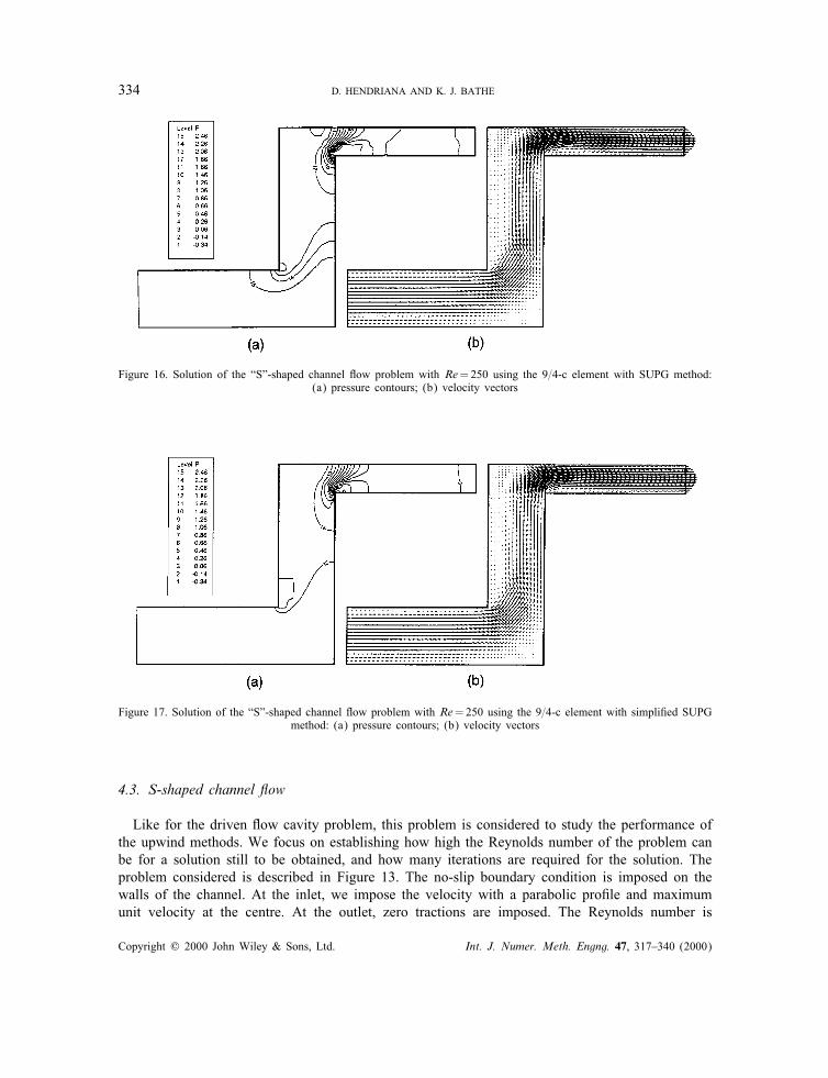
Figure 16. Solution of the “S”-shaped channel ow problem with Re=250 using the 9=4-c element with SUPG method:(a) pressure contours; (b) velocity vectors

Figure 17. Solution of the “S”-shaped channel ow problem with Re=250 using the 9=4-c element with simpli�ed SUPGmethod: (a) pressure contours; (b) velocity vectors

4.3. S-shaped channel ow

Like for the driven ow cavity problem, this problem is considered to study the performance ofthe upwind methods. We focus on establishing how high the Reynolds number of the problem canbe for a solution still to be obtained, and how many iterations are required for the solution. Theproblem considered is described in Figure 13. The no-slip boundary condition is imposed on thewalls of the channel. At the inlet, we impose the velocity with a parabolic pro�le and maximumunit velocity at the centre. At the outlet, zero tractions are imposed. The Reynolds number is



Figure 18. Solution of the “S”-shaped channel ow problem with Re=250 using the 9=9-c element with GLS method: (a)pressure contours; (b) velocity vectors

Figure 19. Solution of the “S”-shaped channel ow problem with Re=15 000 using the 9=4-c element with simpli�edSUPG method: (a) pressure contours; (b) velocity vectors

calculated based on the maximum inlet velocity and the height of the channel at the inlet. Themesh used is shown in Figure 14.A steady-state analysis is performed for each Reynolds number considered. The Reynolds num-

ber is increased as given in Table II. This table also gives the iterations required to solve theproblem using the di�erent upwind methods. The Newton–Raphson method is used to solve thenonlinear �nite element equations and the convergence tolerance on the residual of normalizedvelocities and pressure is 10−6. Like for the driven ow cavity problem, in solving the problemwith a certain Reynolds number, we use the solution of the lower Reynolds number as the initialcondition.



Figure 20. The curved-channel ow problem

Figure 21. The mesh used for the curved-channel ow problem

Table III. Number of iterations required to solvethe curved channel ow problem with di�erentReynolds numbers using di�erent upwind methods


50 4 6 5 4500 4 4 4 45000 4 5 4 550 000 4 ∗ ∗ ∗500 000 35 000 000 3

Note: The Newton–Raphson method is used with conver-gence tolerance=10−6; the (*) denotes iteration not con-verged

The solutions of the problem for Re=250 using di�erent upwind methods are shown inFigures 15–18. Notice that all upwind methods give very similar pressure and velocity solutions.The solutions of the problem for Re=15 000 using the simpli�ed SUPG method is shown in

Figure 19. As we can see from Table II, the simpli�ed SUPG method fails last as the Reynoldsnumber is increased.



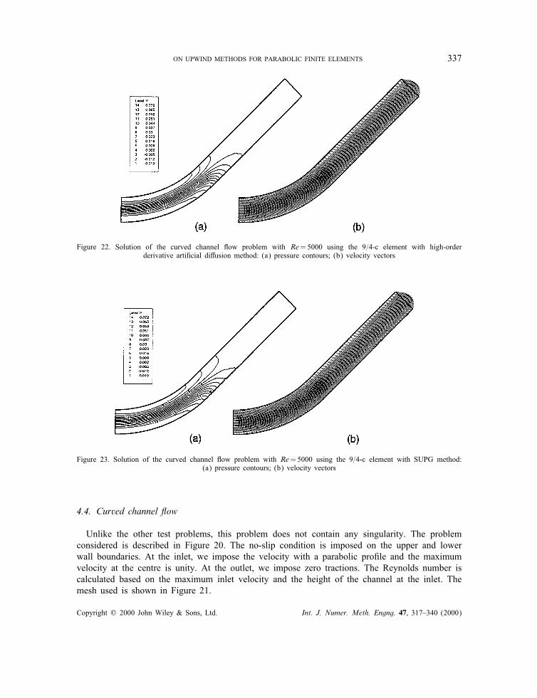
Figure 22. Solution of the curved channel ow problem with Re=5000 using the 9=4-c element with high-orderderivative arti�cial di�usion method: (a) pressure contours; (b) velocity vectors

Figure 23. Solution of the curved channel ow problem with Re=5000 using the 9=4-c element with SUPG method:(a) pressure contours; (b) velocity vectors

4.4. Curved channel ow

Unlike the other test problems, this problem does not contain any singularity. The problemconsidered is described in Figure 20. The no-slip condition is imposed on the upper and lowerwall boundaries. At the inlet, we impose the velocity with a parabolic pro�le and the maximumvelocity at the centre is unity. At the outlet, we impose zero tractions. The Reynolds number iscalculated based on the maximum inlet velocity and the height of the channel at the inlet. Themesh used is shown in Figure 21.



Figure 24. Solution of the curved channel ow problem with Re=5000 using the 9=4-c element with simpli�ed SUPGmethod: (a) pressure contours; (b) velocity vectors

Figure 25. Solution of the curved channel ow problem with Re=5000 using the 9=9-c element with GLS method:(a) pressure contours; (b) velocity vectors

We solve for the steady-state response and increase the Reynolds number as given in Table III,and record the number of iterations.Like for the other problems, the Newton–Raphson method is used to solve the nonlinear equa-

tions with the convergence tolerance on the velocities and pressure equal to 10−6. To reach thesolutions for the Reynolds numbers listed in Table III, we start from zero pressure and velocitiesas initial condition and use the converged solution of the lower Reynolds number case as theinitial condition for the next higher Reynolds number problem.The solutions of the problem with Re=5000 using di�erent upwind methods are shown in

Figures 22–25. Note that all upwind methods give very similar pressure and velocity solutions.The solution of the problem for the Reynolds number 5 000 000 using the high-order deriva-

tive arti�cial di�usion method is shown in Figure 26. As we see from Table III, the high-order



Figure 26. Solution of the curved channel ow problem with Re=5000 000 using the 9=4-c element with high-orderderivative arti�cial di�usion method: (a) pressure contours; (b) velocity vectors

derivative arti�cial di�usion method is the only method to solve the problem when the Reynoldsnumber is very large.

5. CONCLUSIONS

The aim in this study was to evaluate some upwind techniques when used in parabolic �niteelement discretizations. We �rst described the characteristics of an ‘ideal’ upwind procedure andthen reviewed and evaluated four upwind techniques: the high-order derivative arti�cial di�usion(HDAD) method, the SUPG technique, a simpli�cation thereof, and the GLS method.All methods performed quite well in a convergence study using a simple problem for which the

exact solution is available. In the di�usion-dominated case, the L2-norm orders of convergence inpressure and velocity were two and three, respectively. In the convection dominated case, theL2-norm order of convergence in pressure remained two (except using the simpli�ed SUPGmethod), whereas the velocity order of convergence decreased with di�erent amounts for the meth-ods to values between two and three. Of course, di�erent convergence constants were measuredfor the techniques.Three other test problems were solved. In each case the Reynolds number was increased in

steps and we measured how many iterations were required for solution at a given Reynolds num-ber and how high the Reynolds number could be for solution. The methods performed di�erentlyin the problem solutions with no method clearly outperforming the others. None of the methodstested could solve all high Reynolds number problems with the meshes used and hence no methodshowed characteristics close to the ‘ideal’ solution scheme. Indeed, the measured solution char-acteristics were rather far from the desired qualities which underlines the need for further majoradvances in the �eld.

REFERENCES

1. Brezzi F, Fortin M. Mixed and Hybrid Finite Element Methods. Springer: Berlin, 1991.2. Bathe KJ. Finite Element Procedures. Prentice Hall: New Jersey, 1996.



3. Brezzi F, Pitk�aranta J. On the stabilization of �nite element approximations of the Stokes equations. In E�cientSolutions of Elliptic Systems: Proceedings of a GAMM-Seminar, Notes on Numerical Fluid Mechanics, vol. 10,Hackbush W (ed.). Braunschweig, 1984.

4. Tezduyar TE, Mittal S, Ray SE, Shih R. Incompressible ow computations with stabilized bilinear and linear equal-order-interpolation velocity-pressure elements. Computer Methods in Applied Mechanics and Engineering 1992;95:221–242.

5. Storti M, Nigro N, Idelsohn S. Equal-order interpolations: a uni�ed approach to stabilize the incompressible andadvective e�ects. Computer Methods in Applied Mechanics and Engineering 1997; 143:317–331.

6. Codina R, Blasco J. A �nite element formulation for the Stokes problem allowing equal velocity-pressure interpolation.Computer Methods in Applied Mechanics and Engineering 1997; 143:373–391.

7. Brooks AN, Hughes TJR. Streamline upwind=Petrov–Galerkin formulations for convection dominated ows withparticular emphasis on the incompressible Navier–Stokes equations. Computer Methods in Applied Mechanics andEngineering 1982; 32:199–259.

8. Hughes TJR, Mallet M, Mizukami A. A new �nite element formulation for computational uid dynamics: II. BeyondSUPG. Computer Methods in Applied Mechanics and Engineering 1986; 54:341–355.

9. Hughes TJR, Franca LP, Hulbert GM. A new �nite element formulation for computational uid dynamics: VIII.The Galerkin=Least-squares method for advective-di�usive equations. Computer Methods in Applied Mechanics andEngineering 1989; 73:173–189.

10. Brezzi F, Bristeau MO, Franca LP, Mallet M, Roge G. A relationship between stabilized �nite element methods and theGalerkin method with bubble functions. Computer Methods in Applied Mechanics and Engineering 1992; 96:117–129.

11. Brezzi F, Marini D, Russo A. Applications of the pseudo residual-free bubbles to the stabilization of convection-di�usionproblems. Computer Methods in Applied Mechanics and Engineering 1998; 166:51–63.

12. Donea J, Belytschko T, Smolinski P. A generalized Galerkin method for steady convection-di�usion problems withapplication to quadratic shape function elements. Computer Methods in Applied Mechanics and Engineering 1985;48:25–43.

13. Demkowicz L, Oden JT, Rachowicz W, Hardy O. An h-p Taylor–Galerkin �nite element method for compressibleEuler equations. Computer Methods in Applied Mechanics and Engineering 1991; 88:363–396.

14. Hendriana D, Bathe KJ. On a parabolic quadrilateral �nite element for compressible ows. Computer Methods inApplied Mechanics and Engineering, in press.

15. Hannani SK, Stanislas M, Dupont P. Incompressible Navier–Stokes computations with SUPG and GLS formulations—A comparison study. Computer Methods in Applied Mechanics and Engineering 1995; 124:153–170.

16. Codina R, Onate E, Cervera M. The intrinsic time for the streamline upwind=Petrov–Galerkin formulation usingquadratic elements. Computer Methods in Applied Mechanics and Engineering 1992; 94:239–262.

17. Franca LP, Frey SL. Stabilized �nite element methods: II. The incompressible Navier–Stokes equations. ComputerMethods in Applied Mechanics and Engineering 1992; 99:209–233.


On upwind methods for parabolic nite elements in incompressible ows

Documents

Transcript of On upwind methods for parabolic nite elements in incompressible ows