Auton RobotDOI 10.1007/s10514-009-9108-0

On the use of likelihood fields to perform sonar scan matchinglocalization

Antoni Burguera · Yolanda González · Gabriel Oliver

Received: 8 May 2008 / Accepted: 6 January 2009© Springer Science+Business Media, LLC 2009

Abstract Scan matching algorithms have been extensivelyused in the last years to perform mobile robot localization.Although these algorithms require dense and accurate sets ofreadings with which to work, such as the ones provided bylaser range finders, different studies have shown that scanmatching localization is also possible with sonar sensors.Both sonar and laser scan matching algorithms are usuallybased on the ideas introduced in the ICP (Iterative ClosestPoint) approach. In this paper a different approach to scanmatching, the Likelihood Field based approach, is presented.Three scan matching algorithms based on this concept, thenon filtered sNDT (sonar Normal Distributions Transform),the filtered sNDT and the LF/SoG (Likelihood Field/Sum ofGaussians), are introduced and analyzed. These algorithmsare experimentally evaluated and compared to previouslyexisting ICP-based algorithms. The obtained results suggestthat the Likelihood Field based approach compares favor-ably with algorithms from the ICP family in terms of ro-bustness and accuracy. The convergence speed, as well asthe time requirements, are also experimentally evaluated anddiscussed.

Keywords Sonar · Scan matching · Likelihood fields

This work is partially supported by DPI 2005-09001-C03-02 andFEDER funding.

A. Burguera (!) · Y. González · G. OliverDept. Matemàtiques i Informàtica, Universitat de les Illes Balears,Ctra. Valldemossa, Km. 7’5, 07122 Palma de Mallorca, IllesBalears, Spaine-mail: antoni.burguera@uib.es

Y. Gonzáleze-mail: y.gonzalez@uib.es

G. Olivere-mail: goliver@uib.es

1 Introduction

Nowadays an outstanding issue in robotics is mobile robotlocalization. Thrun et al. (2005) define mobile robot local-ization as the problem of determining the pose of a robot rel-ative to a given map of the environment. However, in manyrobotic applications it is not possible to have an a priori mapof the environment. In such situations, the problem may beaddressed by building local maps of the environment whilethe robot is executing a mission and, subsequently, deter-mining the robot pose by matching the local maps.

The choice of a specific map to represent the knowledgeregarding the environment is a difficult task. Maps can beroughly classified in two categories, referred to as Feature-Based Maps and Location-Based Maps.

Feature-based maps, which are composed of a set of fea-tures together with their Cartesian location, are extensivelyused in the localization context. However, these maps in-troduce geometric constraints such as the existence of linesand corners in the environment (Castellanos et al. 2001;Dissanayake et al. 2002; Bosse et al. 2004). Thus, they arenot well suited to model non-structured environments.

Location-based maps, which offer a marker for any lo-cation in the world, usually do not assume geometric con-straints. A classical location-based map is the occupancygrid (Moravec 1988; Elfes 1989). These maps have two ma-jor drawbacks to performing localization. First, it is compu-tationally expensive to match such dense representations ofthe space. Second, the granularity inherent to a grid repre-sentation may produce low resolution estimates of the robotpose.

To deal with those problems, some authors determine therobot displacement by matching up successive sets of rawrange readings, called scans. This technique is known asscan matching (Burguera et al. 2005; Pfister et al. 2002;

Auton Robot

Weiss and Puttkamer 1995). Scan matching neither assumesgeometric constraints nor builds dense, grid-based, repre-sentations of the environment. Thus, it is well suited to local-izing a mobile robot with high precision both in structuredand non-structured environments.

First attempts to perform mobile robot localization bymatching successive range scans were inspired by the com-puter vision community. A standard approach to image reg-istration is the ICP (Iterative Closest Point). Although thename ICP was first presented by Besl and McKay (Besl andMcKay 1992), very similar ideas were presented by otherauthors such as Chen and Medioni (1992) or Zhang (1994).

The ICP concepts were introduced in the mobile robotlocalization context by Lu and Milios (1997). These authorsproposed some changes to the original algorithm to make itmore suitable for robotic applications. As a matter of fact,due to the great success of this approach, many other scanmatching algorithms rely on the same basic structure. In thecontext of this paper, these algorithms will be referred to asICP-based algorithms.

Although different localization strategies have been usedwith a variety of range sensors, such as sonar (Leonard andDurrant-Whyte 1992; Tardós et al. 2002), ICP-based algo-rithms have been mostly used to localize mobile robots en-dowed with laser range finders. Today, off the shelf lasersensors provide thousands of readings per second with a subdegree angular resolution. Other sensors, such as standardPolaroid ultrasonic range finders, are only able to providetenths of readings per second, with angular resolutions oneor two orders of magnitude poorer than laser. Moreover, ef-fects such as multiple reflections or cross-talking are veryfrequent in sonar sensing, producing large amounts of read-ings which do not correspond to real objects in the environ-ment.

However, ultrasonic range finders have interesting prop-erties that make them appealing in the mobile robotics com-munity (Lee 1996). On the one hand, their size, power con-sumption and price are better than those of laser scanners.Consequently, they are well suited for low cost and domes-tic robots, such as automatic vacuum cleaners. On the otherhand, their basic behavior is shared by underwater sonar sen-sors, which are extensively used in underwater and marinerobotics. Thus, typical underwater sonar, although being farmore complex than standard Polaroid ultrasonic range find-ers, can benefit from of those localization techniques thattake into account the sonar limitations.

Recent studies demonstrated that ICP-based algorithmscan be used with sonar sensors (Burguera et al. 2005),especially if an accurate sensor model is defined (Bur-guera et al. 2007c). For instance, in (Burguera et al. 2008),each sonar reading is modeled as a Normal distribution,thus accounting for range and angular uncertainties. Then,

statistical compatibility tests are used to establish read-ing to reading correspondences in an ICP-based frame-work.

In spite of its great success, ICP-based algorithms presentimportant flaws. Other paradigms have been recently intro-duced to avoid such problems. For example, the NDT (Nor-mal Distributions Transform) (Biber and Straßer 2003) de-fines the scan matching concept from a completely differ-ent point of view, which will be described in detail later inthis document. Also, Hähnel et al. (2003) define a proba-bilistic laser scan registration. In this study, hill-climbingstrategies are used to maximize a likelihood function builtfrom a laser range finder model. In order to evaluate thismodel, ray-tracing techniques have to be applied. These newparadigms are strongly related to the concept of LikelihoodField, which is a common and computationally cheap wayto model range sensors and perform localization given an apriori map. Nevertheless, these paradigms rely on accurateand dense sets of laser range readings, and are not suited toworking with sonar sensors.

Our objective is to define new sonar scan matching para-digms which do not rely on the establishment of correspon-dences. This paper focuses on the use of Likelihood Fieldsto perform such a task. Henceforth, the scan matching tech-niques relying on Likelihood Fields will be referred to asLikelihood Field based or LF-based for short. The theoret-ical basis of LF-based scan matching is presented, and twonew variants of Likelihood Fields to be used with sonar read-ings are introduced.

The main contributions of this paper are as follows; first,the theoretical basis of the LF-based scan matching is pro-vided. This theoretical basis is a generalization of the onepresented by Biber et al. (2004), where Likelihood Fieldswere not explicitly taken into account. Then, two novelmethods to achieve robust and accurate scan matching lo-calization, particularly suitable when sonar sensors are used,are introduced. At first, the sNDT (sonar Normal Distrib-utions Transform), which involves important arrangementsto the original NDT concept to cope with the high num-ber of outliers provided by sonar sensors. Secondly, theLF/SoG (Likelihood Field/Sum of Gaussians), which is orig-inally designed to work with sonar sensors but can be di-rectly used with other range sensors. Both methods are eval-uated by means of a complete set of experiments, com-paring them with other well known scan matching algo-rithms.

Although not being the central point of this paper, therequired processes to deal with the sparsity of sonar readingsare also presented as a necessary tool both for sNDT andLF/SoG.

Auton Robot

2 Notation

Scan matching algorithms require two sets of range read-ings called scans. Let Sref = {q1, q2, . . . , qn} be a set of n

points gathered at frame A, which is called the referencescan. Let Scur = {p1,p2, . . . , pm} be a set of m points gath-ered at frame B , which is called the current scan.

The aim of scan matching algorithms is to estimate therobot motion between frames A and B . Let xA

B be thescan matching estimate of the relative position betweenthe frames A and B . Thus, xA

B represents a rototransla-tion in the plane. A common assumption is that the errorin scan matching is Normal. Thus, we will represent thescan matching estimate as a multivariate Normal distributionxAB = N(x̂A

B ,P AB ). Being xA

B a rototranslation in the plane,the mean vector x̂A

B has the form [x, y, ! ]T , where x and y

represents the translation and ! represents the rotation. Ac-cordingly, the covariance P A

B is a 3 ! 3 matrix.To deal with processes corrupted by Gaussian noise, a

common approach in stochastic mapping and SLAM is theuse of the operator " (composition of transformations).This operator is used throughout this paper both for pointsand transformations. A detailed description can be found in(Tardós et al. 2002).

Let S#cur = {p#

1,p#2, . . . , p

#m} be the set of Scur points pro-

jected to the coordinate frame of Sref . That is, p#i = xA

B "pi ,$pi % Scur .

Broadly speaking, the problem of scan matching is one offinding the robot motion xA

B that maximizes the overlap be-tween the parts of the environment represented by Sref andScur . The intuitive concept of overlap turns into very differ-ent mathematical definitions depending on the specific scanmatching algorithm under consideration. For instance, in theICP context, the overlap is a function of the sum of distancesbetween pairs of closest points in Sref and S#

cur . In the Like-lihood Field based approach, the overlap is represented bythe likelihood of having the readings in S#

cur given a like-lihood function constructed according to Sref . The formaldefinitions of overlap for the different approaches to scanmatching presented in this paper are provided in Sects. 3and 5. Finally, Table 1 summarizes the main acronyms usedthroughout this paper.

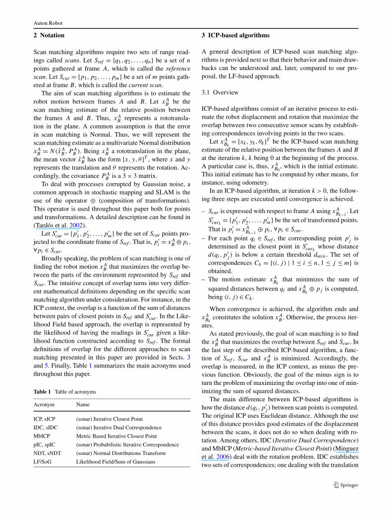
Table 1 Table of acronyms

Acronym Name

ICP, sICP (sonar) Iterative Closest Point

IDC, sIDC (sonar) Iterative Dual Correspondence

MbICP Metric Based Iterative Closest Point

pIC, spIC (sonar) Probabilistic Iterative Correspondence

NDT, sNDT (sonar) Normal Distributions Transform

LF/SoG Likelihood Field/Sum of Gaussians

3 ICP-based algorithms

A general description of ICP-based scan matching algo-rithms is provided next so that their behavior and main draw-backs can be understood and, later, compared to our pro-posal, the LF-based approach.

3.1 Overview

ICP-based algorithms consist of an iterative process to esti-mate the robot displacement and rotation that maximize theoverlap between two consecutive sensor scans by establish-ing correspondences involving points in the two scans.

Let xABk

= [xk, yk, !k]T be the ICP-based scan matchingestimate of the relative position between the frames A and B

at the iteration k, k being 0 at the beginning of the process.A particular case is, thus, xA

B0, which is the initial estimate.

This initial estimate has to be computed by other means, forinstance, using odometry.

In an ICP-based algorithm, at iteration k > 0, the follow-ing three steps are executed until convergence is achieved.

– Scur is expressed with respect to frame A using xABk&1

. LetS#

curk= {p#

1,p#2, . . . , p

#m} be the set of transformed points.

That is p#i = xA

Bk&1" pi , $pi % Scur .

– For each point qi % Sref , the corresponding point p#j is

determined as the closest point in S#curk

whose distanced(qi,p

#j ) is below a certain threshold dmin. The set of

correspondences Ck = {(i, j) | 1 ' i ' n,1 ' j ' m} isobtained.

– The motion estimate xABk

that minimizes the sum ofsquared distances between qi and xA

Bk" pj is computed,

being (i, j) % Ck .

When convergence is achieved, the algorithm ends andxABk

constitutes the solution xAB . Otherwise, the process iter-

ates.As stated previously, the goal of scan matching is to find

the xAB that maximizes the overlap between Sref and Scur . In

the last step of the described ICP-based algorithm, a func-tion of Sref , Scur and xA

B is minimized. Accordingly, theoverlap is measured, in the ICP context, as minus the pre-vious function. Obviously, the goal of the minus sign is toturn the problem of maximizing the overlap into one of min-imizing the sum of squared distances.

The main difference between ICP-based algorithms ishow the distance d(qi,p

#j ) between scan points is computed.

The original ICP uses Euclidean distance. Although the useof this distance provides good estimates of the displacementbetween the scans, it does not do so when dealing with ro-tation. Among others, IDC (Iterative Dual Correspondence)and MbICP (Metric-based Iterative Closest Point) (Minguezet al. 2006) deal with the rotation problem. IDC establishestwo sets of correspondences; one dealing with the translation

Auton Robot

using Euclidean distance and the other with the rotation bymeans of an angular distance. MbICP defines a new distancemeasure that simultaneously accounts for translation and ro-tation errors. However, none of these methods take into ac-count the range sensor imprecisions. Some other methods,such as the research of Pfister et al. (2002) and the pIC(probabilistic Iterative Correspondence) (Montesano et al.2005) deal with this problem. The former, by weighting thecontribution of each scan point according to its uncertainty.The latter defines an interesting framework to deal with un-certainties in scan matching computing statistical compati-bility between the scan points by means of the Mahalanobisdistance.

3.2 Drawbacks

In spite of its high success, ICP-based algorithms have twoimportant drawbacks, which are described next.

Correspondences: What scan matching wants to estimate isa roto-translation between two nearby places in the envi-ronment. However, this estimation is carried out by meansof the partial and noisy projections of the environmentprovided by range sensors. This fact is particularly rele-vant when observing the concept of correspondence. Whenpoint-to-point correspondences are established it is implic-itly assumed that corresponding points have been producedexactly at the same position in the environment. This as-sumption is not correct, not only because of the existenceof spurious readings, but mainly because sensors samplethe environment, providing a discrete view of its surround-ings. Moreover, at a given iteration k, only points belong-ing to Ck are taken into account to compute xA

Bk. Thus,

the problem is not only that sensors provide partial viewsof the environment, but also that the algorithm itself dis-cards information when establishing correspondences. Dif-ferent attempts have been performed to minimize these ef-fects, ranging from point-to-line correspondences (Lu andMilios 1997) to the use of statistical compatibility tests(Montesano et al. 2005; Burguera et al. 2008). However,the problems derived from the establishment of correspon-dences are inherent to the ICP-based approach. Thus, tosolve them, a different scan matching approach is neces-sary.

Poor convergence: ICP-based algorithms do not hold infor-mation to guarantee coherence between iterations. Once aminimization is performed, a new set of correspondencesis established. Moreover, the threshold dmin is context de-pendent and has to be tuned. Depending on the value ofthis parameter, the algorithm can discard too many read-ings when searching corresponding points. In these cases,the set of correspondences changes a lot from one iterationto the next. Thus, the function to be minimized is changingin every iteration due to the different correspondence sets.

Depending on the threshold dmin and, thus, on the specificcontext where the ICP-based algorithm is deployed, thechanges on the function being minimized may result in alarge number of iterations until the algorithm converges. Insome cases, changing correspondences may result in oscil-lations around a minimum and even prevent convergence.

In order to deal with these problems, new approaches toscan matching are necessary. Although the concept of Like-lihood Field is not new, its use in the scan matching contextprevents the establishment of correspondences and, thus,solves the two aforementioned problems. In consequence,the use of Likelihood Fields in scan matching seems to be agood approach to overcome some of the ICP-based limita-tions.

4 Sonar scan matching

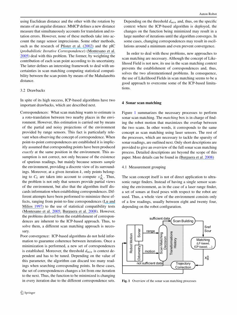
Figure 1 summarizes the necessary processes to performsonar scan matching. The matching box is in charge of find-ing the robot motion that maximizes the overlap betweenthe two scans. In other words, it corresponds to the sameconcept as scan matching using laser sensors. The rest ofthe processes, which are necessary to tackle the sparsity ofsonar readings, are outlined next. Only short descriptions areprovided to give an overview of the full sonar scan matchingprocess. Detailed descriptions are beyond the scope of thispaper. More details can be found in (Burguera et al. 2008)

4.1 Measurement grouping

The scan concept itself is not of direct application to ultra-sonic range finders. Instead of having a single sensor scan-ning the environment, as in the case of a laser range finder,a set of sonars at fixed poses with respect to the robot areused. Thus, a whole view of the environment consists onlyof a few readings, usually between eight and twenty four,depending on the robot configuration.

Fig. 1 Overview of the sonar scan matching processes

Auton Robot

Scan matching algorithms require dense sets of readingswith which to work. Accordingly, to perform sonar scanmatching, some processes to group the sonar readings alongshort robot trajectories are needed. These processes will bereferred to as the Scan Matching Decision and the ScanBuilding.

The Scan Matching Decision is in charge of collectingsonar readings and odometric estimates and storing them inthe so called Transformations History. The Scan MatchingDecision is also in charge of deciding when sufficient datahas been collected so that a scan can be built. When suffi-cient sensor readings have been collected, according to theScan Matching Decision, the Scan Building process is exe-cuted. This process makes use of the Transformations His-tory and builds the sonar scan by representing the storedsonar readings with respect to a common coordinate frame.

When the two scans Scur and Sref have been generated bythe Scan Building, the matching process (either ICP-basedor LF-based) is executed.

4.2 Trajectory correction

After execution of the matching process, the estimate xAB

between the coordinate frames of Sref and Scur is available.However, the scan readings have not only been gathered atframes A and B , but along a much larger set of robot poses.Thus, it is desirable to correct all the motion estimates in-volved in the Scan Building process according to xA

B . Thistask is performed by the Trajectory Correction process.

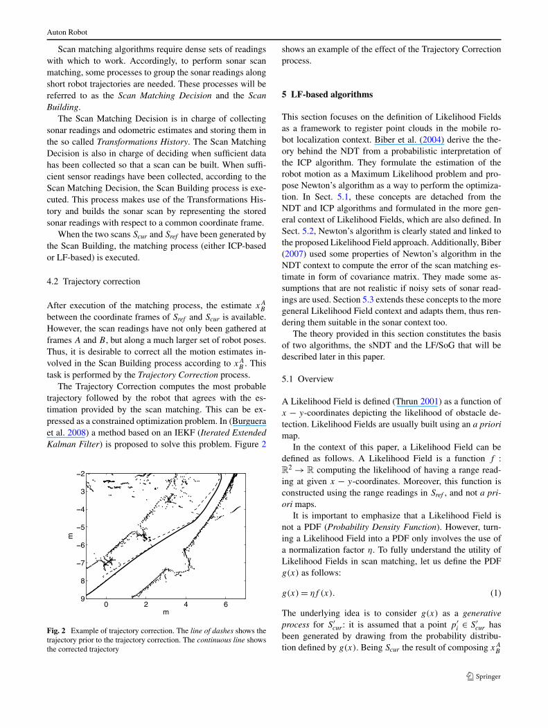
The Trajectory Correction computes the most probabletrajectory followed by the robot that agrees with the es-timation provided by the scan matching. This can be ex-pressed as a constrained optimization problem. In (Burgueraet al. 2008) a method based on an IEKF (Iterated ExtendedKalman Filter) is proposed to solve this problem. Figure 2

Fig. 2 Example of trajectory correction. The line of dashes shows thetrajectory prior to the trajectory correction. The continuous line showsthe corrected trajectory

shows an example of the effect of the Trajectory Correctionprocess.

5 LF-based algorithms

This section focuses on the definition of Likelihood Fieldsas a framework to register point clouds in the mobile ro-bot localization context. Biber et al. (2004) derive the the-ory behind the NDT from a probabilistic interpretation ofthe ICP algorithm. They formulate the estimation of therobot motion as a Maximum Likelihood problem and pro-pose Newton’s algorithm as a way to perform the optimiza-tion. In Sect. 5.1, these concepts are detached from theNDT and ICP algorithms and formulated in the more gen-eral context of Likelihood Fields, which are also defined. InSect. 5.2, Newton’s algorithm is clearly stated and linked tothe proposed Likelihood Field approach. Additionally, Biber(2007) used some properties of Newton’s algorithm in theNDT context to compute the error of the scan matching es-timate in form of covariance matrix. They made some as-sumptions that are not realistic if noisy sets of sonar read-ings are used. Section 5.3 extends these concepts to the moregeneral Likelihood Field context and adapts them, thus ren-dering them suitable in the sonar context too.

The theory provided in this section constitutes the basisof two algorithms, the sNDT and the LF/SoG that will bedescribed later in this paper.

5.1 Overview

A Likelihood Field is defined (Thrun 2001) as a function ofx & y-coordinates depicting the likelihood of obstacle de-tection. Likelihood Fields are usually built using an a priorimap.

In the context of this paper, a Likelihood Field can bedefined as follows. A Likelihood Field is a function f :R2 ( R computing the likelihood of having a range read-ing at given x & y-coordinates. Moreover, this function isconstructed using the range readings in Sref , and not a pri-ori maps.

It is important to emphasize that a Likelihood Field isnot a PDF (Probability Density Function). However, turn-ing a Likelihood Field into a PDF only involves the use ofa normalization factor ". To fully understand the utility ofLikelihood Fields in scan matching, let us define the PDFg(x) as follows:

g(x) = "f (x). (1)

The underlying idea is to consider g(x) as a generativeprocess for S#

cur: it is assumed that a point p#i % S#

cur hasbeen generated by drawing from the probability distribu-tion defined by g(x). Being Scur the result of composing xA

B

Auton Robot

with each point in Scur , the problem of scan matching canbe seen as the one of finding the xA

B that makes the gener-ative process assumption true. From a probabilistic point ofview, this can be expressed as the problem of maximizingthe following likelihood function:

#(x) =!

pi%Scur

g(x " pi) (2)

where x represents a rototranslation between the LikelihoodField and the Scur coordinate frames. The idea behind thisfunction is to project each point in the current scan ontothe PDF g by means of the aforementioned rototranslation.Then, the PDF is evaluated at each of these projected pointsand the results are multiplied. A good rototranslation x willproject the points in Scur onto regions of g with high val-ues (i.e. with high probability of having a sonar reading).Thus, the better the rototranslation x, the higher the valuesof #(x).

The rototranslation x that maximizes this likelihoodfunction constitutes the scan matching estimate xA

B . In con-sequence, the likelihood function #(x) represents the over-lap between the two scans. If the NDT grid is used as theLikelihood Field f (x), the likelihood function #(x) turnsinto the energy function proposed in (Biber et al. 2004).

As it may be computationally expensive to maximizeEq. 2, a usual approach is to use log-likelihood functions.Thus, the problem of scan matching using Likelihood Fieldscan be expressed as one of minimizing the following nega-tive log-likelihood function:

& log(#(x))

= &"

pi%Scur

log(g(x " pi))

= &#

(m log") +"

pi%Scur

log(f (x " pi))

$(3)

where m is the number of points in Scur . " being a constantvalue, it is clear that it will not influence the minimizationprocess. Thus, it is not necessary either to compute it or toturn the Likelihood Field into a PDF.

This approach has some advantages when compared tothe ICP-based approach. On the one hand, no correspon-dences are established. On the other hand, only one func-tion has to be minimized. This is important because, in theICP-based context, since the set of correspondences changesat every iteration, then so too the function to be minimized.Thus, although the ICP-based structure is the same through-out its whole execution, it minimizes a different function atevery iteration. Some problems arise from this issue, as de-scribed in Sect. 3.2. Moreover, the underlying probabilisticapproach to LF-based scan matching makes it easy to esti-mate the error of the matching process in the form of covari-ance matrix, as will be shown later.

The key issue when using Likelihood Fields is how tobuild an accurate Likelihood Field from sensor data. Themain difference between the approaches presented in thisdocument refers to how the Likelihood Field is built.

5.2 Optimization

The optimization process consists of minimizing Eq. 3. Asstated previously, the constant term m log" does not affectthe minimization. Thus, to provide a simpler notation, let thefunction to be minimized be as follows:

h(x) = &"

pi%Scur

log(f (x " pi)). (4)

Newton’s algorithm has proved to be an effective tool inthis context (Biber and Straßer 2003), and has interestingproperties that will be shown later. Newton’s algorithm iscommonly used to find the minima by using the gradientvector and the Hessian matrix instead of the function itselfand the gradient vector. Next, Newton’s method for findinga minimum of the score function is presented.

1. Start with an approximation x0 to the minimum point.This approximation can be obtained using odometry. Setk ) 0.

2. Evaluate the gradient vector *h(xk) and the Hessian ma-trix H(xk).

3. Compute the next estimate xk+1 ) xk +$x, being $x =&(H(xk))

&1*h(xk)

4. If convergence is achieved, the algorithm ends and xk+1constitutes the scan matching estimate xA

B . Otherwise, setk ) k + 1 and iterate.

Newton’s algorithm to find the minima of a function isproposed in this paper to perform the optimization in thecontext of LF-based scan matching. Other minimization al-gorithms could be used and, of course, if a closed form so-lution exists for one specific Likelihood Field definition, isgreatly preferred.

5.3 Estimating the covariance matrix

In (Biber 2007) some properties of Newton’s algorithm wereused to estimate the error of the scan matching estimate.This section outlines the mentioned approach and showshow this approximation of the scan matching error is validin other Likelihood Field approaches providing Newton’s al-gorithm is used to perform the optimization.

At each iteration, Newton’s algorithm approximates thefunction being minimized, h(x), by a quadratic. In particu-lar, when convergence is achieved at the minimum xA

B , thisquadratic has the form:

h(x) + h(xAB ) + 1

2(x & xA

B )T H(xAB )(x & xA

B ). (5)

Auton Robot

A common approach is to model the scan matching erroras a Normal distribution with mean xA

B and covariance P AB .

Thus, the PDF of the error is the following Gaussian:

perror(x) = "# exp#

&12(x & xA

B )T (P AB )&1(x & xA

B )

$(6)

The negative log-likelihood of perror(x) is as follows:

& log(perror(x))

= & log("#) + 12(x & xA

B )T (P AB )&1(x & xA

B ). (7)

It has implicitly been assumed that the quadratic in Eq. 5is a sufficiently good approximation of h(x) when Newton’salgorithm has converged to a minimum. In other words, it isassumed that the higher order terms of the Taylor series aresmall. It can be observed in Eq. 4 that h(x) is constructed byprojecting the points in Scur onto the Likelihood Field. Thus,it is assumed that the range readings are properly modeledby points. This is a reasonable assumption if laser sensorsare used. Due to the very high accuracy of laser, the readingscan be assumed to be points truly located at the detected ob-ject. In consequence, the function h(x) will most likely havea clear minimum around the true robot motion and Newton’salgorithm may converge to a xA

B very close to that minimum.On the contrary, if sonar sensors are used, the point read-

ing assumption is not as good as it was with laser. Mainlybecause of its low angular resolution, an object detected byan ultrasonic range finder may not be located on the pointreading, but in a certain area around the point. Thus, someambiguities may appear, resulting in a minimum of h(x) notbeing as clear as in the case of laser sensors. Thus, Newton’salgorithm may not be able to converge to a solution xA

B asclose to the minimum as in the case of laser.

As stated previously, Eq. 5 approximates h(x) onlyaround a minimum. In other words, the closer xA

B is to thereal minimum, the better the approximation. As the researchin (Biber 2007) is based on laser sensors, it is assumed thatEq. 5 constitutes a very good approximation of h(x). Inconsequence, taking into account Eqs. 5 and 7, and per-forming some additional assumptions, they conclude thatP A

B = H(xAB )&1. In other words, the scan matching error

can be easily computed from the Hessian matrix used byNewton’s algorithm.

However, in the sonar case, although the xAB computed

by Newton’s algorithm may be good enough to localize therobot, it can not guarantee that Eq. 5 is an approximation ofh(x) as good as that of the laser case. In consequence, inthe sonar case we can not conclude that the scan matchingerror is equal to H(xA

B )&1. Nevertheless, looking at Eqs. 5and 7 it is clear that the scan matching error, although beingbigger in the sonar case, has a similar shape to the one of thelaser case. At this point, we have experimentally observed

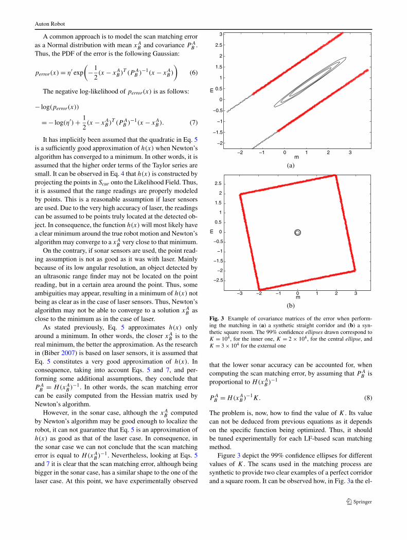
(a)

(b)

Fig. 3 Example of covariance matrices of the error when perform-ing the matching in (a) a synthetic straight corridor and (b) a syn-thetic square room. The 99% confidence ellipses drawn correspond toK = 104, for the inner one, K = 2 ! 104, for the central ellipse, andK = 3 ! 104 for the external one

that the lower sonar accuracy can be accounted for, whencomputing the scan matching error, by assuming that P A

B isproportional to H(xA

B )&1

P AB = H(xA

B )&1K. (8)

The problem is, now, how to find the value of K . Its valuecan not be deduced from previous equations as it dependson the specific function being optimized. Thus, it shouldbe tuned experimentally for each LF-based scan matchingmethod.

Figure 3 depict the 99% confidence ellipses for differentvalues of K . The scans used in the matching process aresynthetic to provide two clear examples of a perfect corridorand a square room. It can be observed how, in Fig. 3a the el-

Auton Robot

lipse spreads out along the corridor, which is the direction ofmaximum uncertainty. In Fig. 3b the uncertainty region hasa circular shape, as in the square room there is no predomi-nant direction for the error. Moreover, the ellipses in Fig. 3bare much smaller than those in Fig. 3a because the matchingwas more accurate.

6 The sonar normal distributions transform (sNDT)

The sNDT constitutes a good example of the LF-based sonarscan matching. Being an improvement of the NDT (Biberand Straßer 2003) to deal with sonar sensors, it demonstrateshow an existing scan matching algorithm can be used withsonar sensors if the real behavior of these sensors is explic-itly taken into account.

The main structure of the sNDT algorithm coincides withthe NDT. First, a grid is built. The idea behind this grid issimilar to the one of Likelihood Field. When the grid hasbeen built, a score function is defined so that optimizingthis function leads to the solution of the scan matching. ThesNDT structure is the same, except that the grid buildingprocess is different and that a filtering procedure is appliedto the scans. For this reason, the NDT approach is first pre-sented, though adapted slightly to the Likelihood Field back-ground. Then, the two improvements that define the sNDTare presented.

6.1 The normal distributions transform (NDT)

Biber and Straßer presented the NDT approach in (Biber andStraßer 2003) as an ad hoc method to register point clouds.The idea was refined and a probabilistic interpretation wasprovided in (Biber et al. 2004). The key idea of the NormalDistributions Transform (NDT) is to model the distributionof a point cloud by a grid of Normal distributions. A descrip-tion of the original NDT is provided in this section, albeitadapted slightly to the approach presented in this paper; theLF-based scan matching.

The NDT grid is built from qi % Sref . It starts dividing thespace containing Sref in N cells of size L!L and searchingthe set of qi points lying inside each cell. In the seminalNDT paper, the value of L was set to 1m. Depending onthe position of the grid’s origin in the range [0,L) ! [0,L),the points of Sref will be divided in different groups. Let usdenote by % a particular position of the grid’s origin. Then,for each cell j containing at least three points, the followingsteps are executed:

1. Let &%,j be the set of n points qi % Sref contained in thiscell.

2. Compute the mean µ%,j and the covariance matrix P%,j

of the points in &%,j .

3. To prevent singular and near singular covariance matri-ces, the smallest eigenvalue of P%,j is tested to be at least0.001 times the biggest eigenvalue. If not, it is set to thisvalue. The parameter 0.001 was experimentally tuned in(Biber and Straßer 2003).

4. Model the probability of having a reading at point x

contained in cell j by the bivariate Normal distributionN(µ%,j ,P%,j ). By dropping the normalization factor offthe PDF (see Eq. 1), the Likelihood Field correspondingto cell j is as follows:

f%,j (x) = exp#

&(x & µ%,j )

T P &1%,j (x & µ%,j )

2

$. (9)

The Likelihood Field f%(x) associated to Sref and thegrid’s origin % is then built using the computed f%,j (x) asfollows:

f%(x) =

%&&&'

&&&(

f%,1(x), x %&%,1,

f%,2(x), x %&%,2,

. . .

f%,N (x) x %&%,N .

(10)

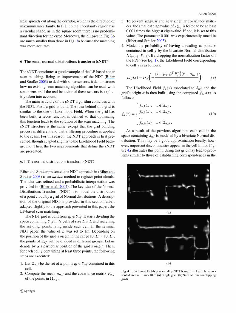
As a result of the previous algorithm, each cell in thespace containing Sref is modeled by a bivariate Normal dis-tribution. This may be a good approximation locally, how-ever, important discontinuities appear in the cell limits. Fig-ure 4a illustrates this point. Using this grid may lead to prob-lems similar to those of establishing correspondences in the

Fig. 4 Likelihood Fields generated by NDT being L = 1 m. The repre-sented area is 18 m!10 m (a) Single grid. (b) Sum of four overlappinggrids

Auton Robot

ICP-based approach. Moreover, the minimization algorithmrequires the Likelihood Field to be continuous and differen-tiable and certainly this is not true in that model.

To reduce the effects of these problems, the original NDTapproach proposes the use of four overlapping grids, insteadof a single one. Now, each point falls into four cells. Thus,four Likelihood Fields are built, each of them consideringa particular position of the grid’s origin. Given a point x,four likelihood values, f1(x), f2(x), f3(x) and f4(x), areavailable. Using this approach, to evaluate the LikelihoodField at position x, the contributions of the four grids areadded up

f (x) ="

1'%'4

f%(x). (11)

Figure 4b shows the result of summing the four overlap-ping grids. Although the function is not continuous, it is, inpractice, usable in Newton’s algorithm context.

When f (x) is defined, the optimization process has to becarried out. According to Eq. 4, the function to be optimizedin the NDT approach should be as follows:

h(x) = &"

pi%Scur

log# "

1'%'4

f%(x " pi)

$. (12)

However, instead of minimizing h(x) as defined in theprevious Equation, the NDT minimizes the following scorefunction, s(x):

s(x) = &"

pi%Scur

"

1'%'4

f%(x " pi). (13)

The main advantage of defining this score function in-stead of the negative log-likelihood is that it makes the opti-mization process easier and faster. Moreover, (Biber et al.2004) shows that s(x) is a good approximation of h(x).Thus, the NDT computes xA

B by minimizing the score func-tion s(x) by means of Newton’s algorithm as described inSect. 5.2.

6.2 Building the sNDT grid

As stated previously, the sNDT follows the same structureas the NDT except that the grid is built taking into accountthe sonar behavior and the scans are filtered. Next, both thesNDT grid building and scan filtering are presented.

The NDT approximates the probability of having a read-ing at a certain position in a given cell j of a particulargrid % by the Normal N(µ%,j ,P%,j ). For clarity purposes,subindexes will be dropped throughout this section and theNormal distribution written as N(µ,P ).

Both µ and P are computed using all the points lyinginside the cell. Computing them in such a way may be prob-lematic in the presence of outliers. If laser sensors are used,

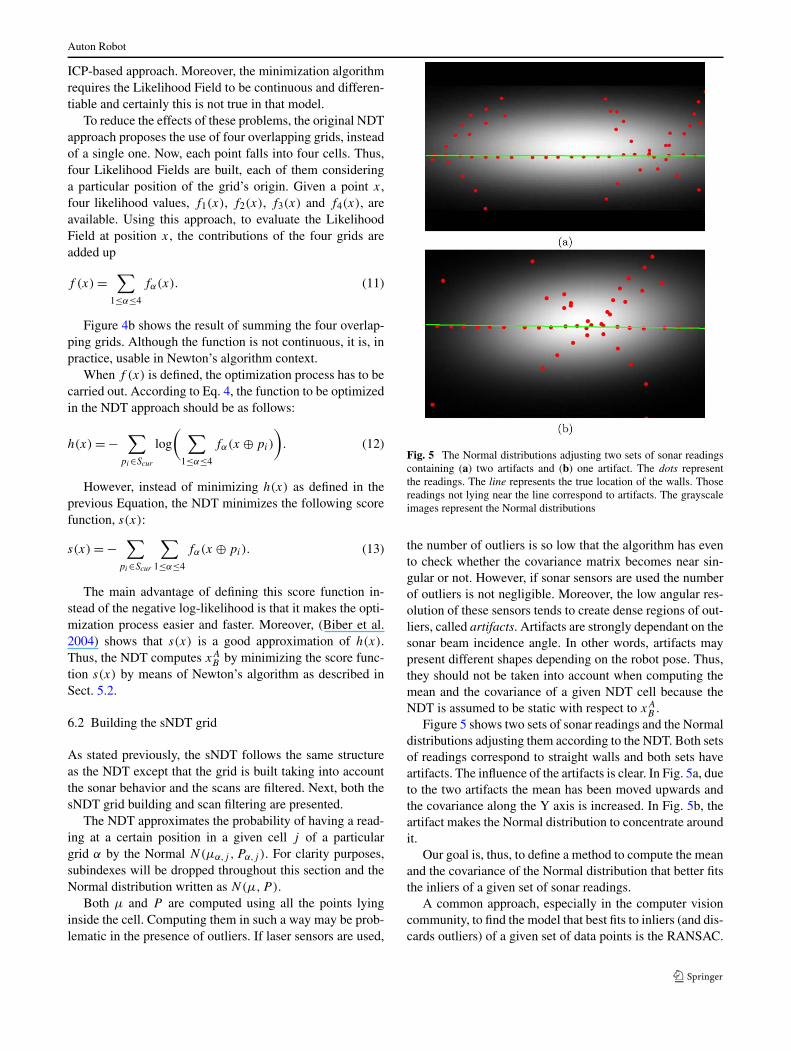
Fig. 5 The Normal distributions adjusting two sets of sonar readingscontaining (a) two artifacts and (b) one artifact. The dots representthe readings. The line represents the true location of the walls. Thosereadings not lying near the line correspond to artifacts. The grayscaleimages represent the Normal distributions

the number of outliers is so low that the algorithm has evento check whether the covariance matrix becomes near sin-gular or not. However, if sonar sensors are used the numberof outliers is not negligible. Moreover, the low angular res-olution of these sensors tends to create dense regions of out-liers, called artifacts. Artifacts are strongly dependant on thesonar beam incidence angle. In other words, artifacts maypresent different shapes depending on the robot pose. Thus,they should not be taken into account when computing themean and the covariance of a given NDT cell because theNDT is assumed to be static with respect to xA

B .Figure 5 shows two sets of sonar readings and the Normal

distributions adjusting them according to the NDT. Both setsof readings correspond to straight walls and both sets haveartifacts. The influence of the artifacts is clear. In Fig. 5a, dueto the two artifacts the mean has been moved upwards andthe covariance along the Y axis is increased. In Fig. 5b, theartifact makes the Normal distribution to concentrate aroundit.

Our goal is, thus, to define a method to compute the meanand the covariance of the Normal distribution that better fitsthe inliers of a given set of sonar readings.

A common approach, especially in the computer visioncommunity, to find the model that best fits to inliers (and dis-cards outliers) of a given set of data points is the RANSAC.

Auton Robot

This method has also been used in the robotics communityto approximate sets of range readings by polygonal models.

RANSAC (Random Sample Consensus) was introducedby Fischler and Bolles (Fischler and Bolles 1981) as a newparadigm for fitting a model to experimental data containinga significant percentage of outliers.

The RANSAC algorithm is an iterative process. In eachiteration, a subset of the original data points is randomly se-lected. These points are used to estimate the model that bestfits them. Then the algorithm determines, for every point ofthe remaining set, how well the point fits to the estimatedmodel. If the number of points that fit well to the estimatedmodel is large enough, the algorithm ends and the modelconstitutes the output of the algorithm. Otherwise, the algo-rithm iterates.

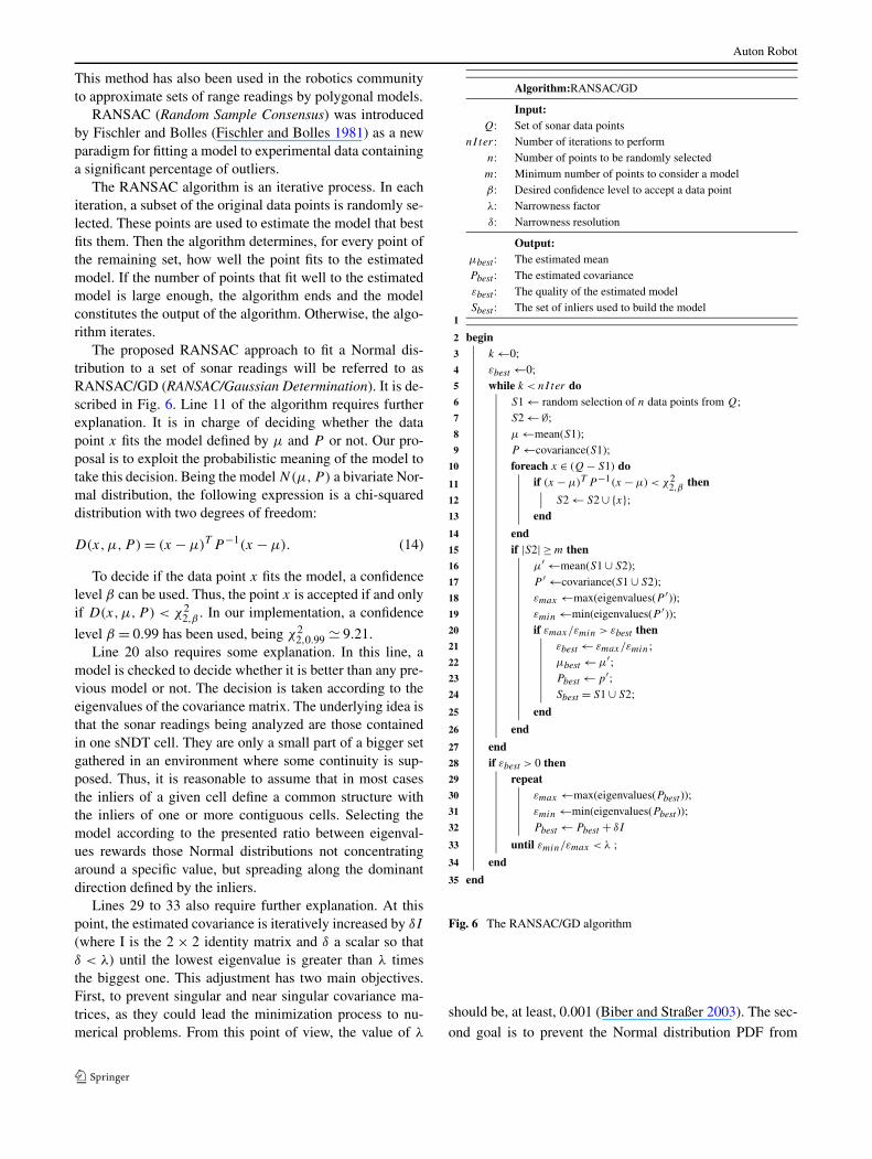
The proposed RANSAC approach to fit a Normal dis-tribution to a set of sonar readings will be referred to asRANSAC/GD (RANSAC/Gaussian Determination). It is de-scribed in Fig. 6. Line 11 of the algorithm requires furtherexplanation. It is in charge of deciding whether the datapoint x fits the model defined by µ and P or not. Our pro-posal is to exploit the probabilistic meaning of the model totake this decision. Being the model N(µ,P ) a bivariate Nor-mal distribution, the following expression is a chi-squareddistribution with two degrees of freedom:

D(x,µ,P ) = (x & µ)T P &1(x & µ). (14)

To decide if the data point x fits the model, a confidencelevel ' can be used. Thus, the point x is accepted if and onlyif D(x,µ,P ) < (2

2,' . In our implementation, a confidencelevel ' = 0.99 has been used, being (2

2,0.99 + 9.21.Line 20 also requires some explanation. In this line, a

model is checked to decide whether it is better than any pre-vious model or not. The decision is taken according to theeigenvalues of the covariance matrix. The underlying idea isthat the sonar readings being analyzed are those containedin one sNDT cell. They are only a small part of a bigger setgathered in an environment where some continuity is sup-posed. Thus, it is reasonable to assume that in most casesthe inliers of a given cell define a common structure withthe inliers of one or more contiguous cells. Selecting themodel according to the presented ratio between eigenval-ues rewards those Normal distributions not concentratingaround a specific value, but spreading along the dominantdirection defined by the inliers.

Lines 29 to 33 also require further explanation. At thispoint, the estimated covariance is iteratively increased by )I(where I is the 2 ! 2 identity matrix and ) a scalar so that) < *) until the lowest eigenvalue is greater than * timesthe biggest one. This adjustment has two main objectives.First, to prevent singular and near singular covariance ma-trices, as they could lead the minimization process to nu-merical problems. From this point of view, the value of *

Algorithm:RANSAC/GD

Input:Q: Set of sonar data points

nI ter: Number of iterations to performn: Number of points to be randomly selectedm: Minimum number of points to consider a model': Desired confidence level to accept a data point*: Narrowness factor): Narrowness resolution

Output:µbest: The estimated meanPbest: The estimated covariance+best: The quality of the estimated modelSbest: The set of inliers used to build the model

1

begin2

k )0;3

+best )0;4

while k < nI ter do5

S1 ) random selection of n data points from Q;6

S2 ) ,;7

µ )mean(S1);8

P )covariance(S1);9

foreach x % (Q & S1) do10

if (x & µ)T P&1(x & µ) < (22,' then11

S2 ) S2 - {x};12

end13

end14

if |S2| . m then15

µ# )mean(S1 - S2);16

P # )covariance(S1 - S2);17

+max )max(eigenvalues(P #));18

+min )min(eigenvalues(P #));19

if +max/+min > +best then20

+best ) +max/+min;21

µbest ) µ#;22

Pbest ) p#;23

Sbest = S1 - S2;24

end25

end26

end27

if +best > 0 then28

repeat29

+max )max(eigenvalues(Pbest));30

+min )min(eigenvalues(Pbest));31

Pbest ) Pbest + )I32

until +min/+max < * ;33

end34

end35

Fig. 6 The RANSAC/GD algorithm

should be, at least, 0.001 (Biber and Straßer 2003). The sec-ond goal is to prevent the Normal distribution PDF from

Auton Robot

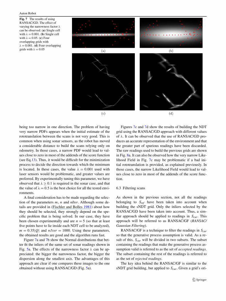
Fig. 7 The results of usingRANSAC/GD. The effect ofvarying the narrowness factor *can be observed. (a) Single cellwith *= 0.001. (b) Single cellwith *= 0.05. (c) Fouroverlapping grids with*= 0.001. (d) Four overlappinggrids with *= 0.05

being too narrow in one direction. The problem of havingvery narrow PDFs appears when the initial estimate of therototranslation between the scans is not very good. This iscommon when using sonar sensors, as the robot has moveda considerable distance to build the scans relying only onodometry. In those cases, a narrow PDF would lead to val-ues close to zero in most of the addends of the score function(see Eq.13). Thus, it would be difficult for the minimizationprocess to decide the direction towards which the minimumis located. In these cases, the value * = 0.001 used withlaser sensors would be problematic, and greater values arepreferred. By experimentally tuning this parameter, we haveobserved that *. 0.1 is required in the sonar case, and thatthe value of *= 0.5 is the best choice for all the tested envi-ronments.

A final consideration has to be made regarding the selec-tion of the parameters m, n and nIter. Although some de-tails are provided in (Fischler and Bolles 1981) about howthey should be selected, they strongly depend on the spe-cific problem that is being solved. In our case, they havebeen chosen experimentally and are n = 5 (so that at leastfive points have to lie inside each NDT cell to be analyzed),m = 0.35|Q| and nI ter = 1000. Using these parameters,the obtained results are good and the algorithm runs fast.

Figure 7a and 7b show the Normal distributions that bet-ter fit the inliers of the same set of sonar readings shown inFig. 5a. The effects of the narrowness factor * can be ap-preciated: the bigger the narrowness factor, the bigger thedispersion along the smallest axis. The advantages of thisapproach are clear if one compares these images to the oneobtained without using RANSAC/GD (Fig. 5a).

Figures 7c and 7d show the results of building the NDTgrid using the RANSAC/GD approach with different valuesof *. It can be observed that the use of RANSAC/GD pro-duces an accurate representation of the environment and thatthe greater part of spurious readings have been discarded.The raw readings used to build the previous grids are shownin Fig. 8a. It can also be observed how the very narrow Like-lihood Field in Fig. 7c may be problematic if a bad ini-tial rototranslation is provided, as explained previously. Inthose cases, the narrow Likelihood Field would lead to val-ues close to zero in most of the addends of the score func-tion.

6.3 Filtering scans

As shown in the previous section, not all the readingsbelonging to Sref have been taken into account whenbuilding the sNDT grid. Only the inliers selected by theRANSAC/GD have been taken into account. Thus, a sim-ilar approach should be applied to readings in Scur . Thisapproach will be referred to as RANSAC/GF (RANSAC/Gaussian Filtering).

RANSAC/GF is a technique to filter the readings in Scurso that the generative process assumption is valid. As a re-sult of this, Scur will be divided in two subsets. The subsetcontaining the readings that make the generative process as-sumption valid is referred to as the set of accepted readings.The subset containing the rest of the readings is referred toas the set of rejected readings.

The key idea behind the RANSAC/GF is similar to thesNDT grid building, but applied to Scur . Given a grid’s ori-

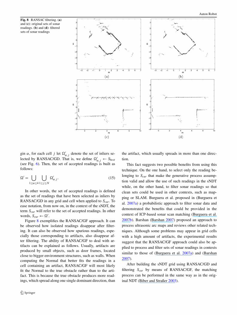
Auton Robot

Fig. 8 RANSAC filtering. (a)and (c): original sets of sonarreadings. (b) and (d): filteredsets of sonar readings

gin %, for each cell j let &#%,j denote the set of inliers se-

lected by RANSAC/GD. That is, we define &#%,j ) Sbest

(see Fig. 6). Then, the set of accepted readings is built asfollows:

&# =)

1'%'4

)

1'j'N

&#%,j . (15)

In other words, the set of accepted readings is definedas the set of readings that have been selected as inliers byRANSAC/GD in any grid and cell when applied to Scur . Toease notation, from now on, in the context of the sNDT, theterm Scur will refer to the set of accepted readings. In otherwords, Scur )&#.

Figure 8 exemplifies the RANSAC/GF approach. It canbe observed how isolated readings disappear after filter-ing. It can also be observed how spurious readings, espe-cially those corresponding to artifacts, also disappear af-ter filtering. The ability of RANSAC/GF to deal with ar-tifacts can be explained as follows. Usually, artifacts areproduced by small objects, such as door frames, locatedclose to bigger environment structures, such as walls. Whencomputing the Normal that better fits the readings in acell containing an artifact, RANSAC/GF will most likelyfit the Normal to the true obstacle rather than to the arti-fact. This is because the true obstacle produces more read-ings, which spread along one single dominant direction, than

the artifact, which usually spreads in more than one direc-tion.

This fact suggests two possible benefits from using thistechnique. On the one hand, to select only the reading be-longing to Scur that make the generative process assump-tion valid and allow the use of such readings in the sNDTwhile, on the other hand, to filter sonar readings so thatclean sets could be used in other contexts, such as map-ping or SLAM. Burguera et al. proposed in (Burguera etal. 2007a) a probabilistic approach to filter sonar data anddemonstrated the benefits that could be provided in thecontext of ICP-based sonar scan matching (Burguera et al.2007b). Barshan (Barshan 2007) proposed an approach toprocess ultrasonic arc maps and reviews other related tech-niques. Although some problems may appear in grid cellswith a high amount of artifacts, the experimental resultssuggest that the RANSAC/GF approach could also be ap-plied to process and filter sets of sonar readings in contextssimilar to those of (Burguera et al. 2007a) and (Barshan2007).

After building the sNDT grid using RANSAC/GD andfiltering Scur by means of RANSAC/GF, the matchingprocess can be performed in the same way as in the orig-inal NDT (Biber and Straßer 2003).

Auton Robot

7 The likelihood field/sum of Gaussians (LF/SoG)

The LF/SoG is an application of the Likelihood Field ap-proach to scan matching. It approximates one of the scansby a sum of Gaussians. Thus, it builds a continuous anddifferentiable Likelihood Field. Although it involves morecomputations than the sNDT, a simplification is proposedto reduce the computational cost. The results provided byLF/SoG are better than those obtained with sNDT and NDT,as will be shown in Sect. 8.

7.1 Building the likelihood field

The Likelihood Field f (p) is defined as follows:

f (p) ="

qj %Sref

exp(&((px & qxj )2 + (py & qyj )

2)) (16)

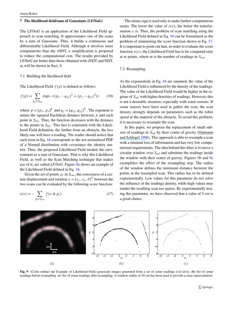
where p = [px,py]T and qj = [qxj , qyj ]T . The exponent isminus the squared Euclidean distance between p and eachpoint in Sref . Thus, the function decreases with the distanceto the points in Sref . This fact is consistent with the Likeli-hood Field definition: the farther from an obstacle, the lesslikely one will have a reading. The reader should notice thateach term in Eq. 16 corresponds to the not normalized PDFof a Normal distribution with covariance the identity ma-trix. Thus, the proposed Likelihood Field models the envi-ronment as a sum of Gaussians. That is why this LikelihoodField, as well as the Scan Matching technique that makesuse of it, are called LF/SoG. Figure 9a shows an example ofthe Likelihood Field defined in Eq. 16.

Given the set of points pi in Scur , the correctness of a cer-tain displacement and rotation x = [xx, xy, ! ]T between thetwo scans can be evaluated by the following score function:

s(x) = &"

pi%Scur

f (x " pi). (17)

The minus sign is used only to make further computationseasier. The lower the value of s(x), the better the transfor-mation x is. Thus, the problem of scan matching using theLikelihood Field defined in Eq. 16 can be formulated as theproblem of minimizing the score function shown in Eq. 17.It is important to point out that, in order to evaluate the scorefunction s(x), the Likelihood Field has to be computed onlyat m points, where m is the number of readings in Scur .

7.2 Resampling

As the exponentials in Eq. 16 are summed, the value of theLikelihood Field is influenced by the density of the readings.The value of the Likelihood Field would be higher in the re-gions of Sref with higher densities of readings. However, thisis not a desirable situation, especially with sonar sensors. Ifsonar sensors have been used to gather the scan, the scandensity strongly depends on parameters such as the robotspeed or the material of the obstacle. To avoid this problem,it is necessary to resample the scan.

In this paper, we propose the replacement of small sub-sets of readings in Sref by their center of gravity (Gutmannand Schlegel 1996). This approach is able to resample a scanwith a minimal loss of information and has very low compu-tational requirements. The idea behind this filter is to move acircular window over Sref and substitute the readings insidethe window with their center of gravity. Figures 9b and 9cexemplifies the effect of the resampling step. The radiusof the window defines the minimum distance between thepoints in the resampled scan. This radius has to be definedexperimentally. Low values for this parameter do not solvethe influence of the readings density, while high values mayrender the resulting scan too sparse. By experimentally test-ing this parameter, we have observed that a value of 5 cm isa good choice.

Fig. 9 (Color online) (a) Example of Likelihood Field (grayscale image) generated from a set of sonar readings (red dots). (b) Set of sonarreadings before resampling. (c) Set of sonar readings after resampling. A window radius of 20 cm has been used to provide a clear representation

Auton Robot

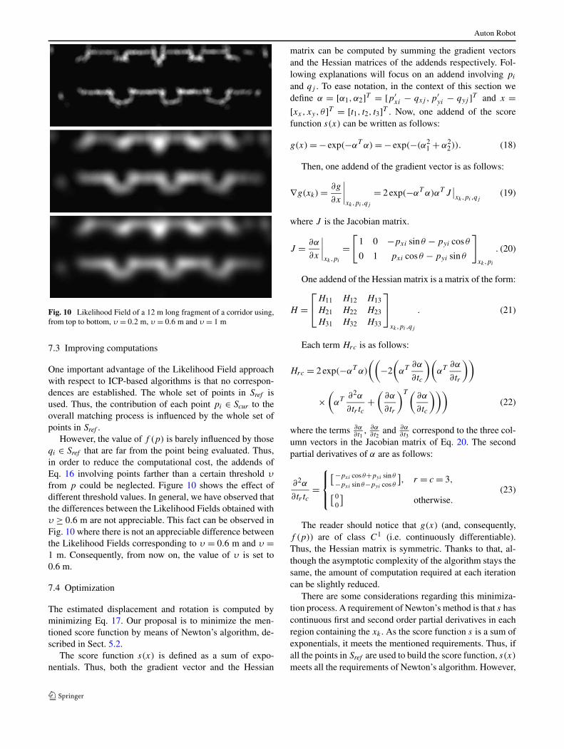
Fig. 10 Likelihood Field of a 12 m long fragment of a corridor using,from top to bottom, , = 0.2 m, , = 0.6 m and , = 1 m

7.3 Improving computations

One important advantage of the Likelihood Field approachwith respect to ICP-based algorithms is that no correspon-dences are established. The whole set of points in Sref isused. Thus, the contribution of each point pi % Scur to theoverall matching process is influenced by the whole set ofpoints in Sref .

However, the value of f (p) is barely influenced by thoseqi % Sref that are far from the point being evaluated. Thus,in order to reduce the computational cost, the addends ofEq. 16 involving points farther than a certain threshold ,

from p could be neglected. Figure 10 shows the effect ofdifferent threshold values. In general, we have observed thatthe differences between the Likelihood Fields obtained with, . 0.6 m are not appreciable. This fact can be observed inFig. 10 where there is not an appreciable difference betweenthe Likelihood Fields corresponding to , = 0.6 m and , =1 m. Consequently, from now on, the value of , is set to0.6 m.

7.4 Optimization

The estimated displacement and rotation is computed byminimizing Eq. 17. Our proposal is to minimize the men-tioned score function by means of Newton’s algorithm, de-scribed in Sect. 5.2.

The score function s(x) is defined as a sum of expo-nentials. Thus, both the gradient vector and the Hessian

matrix can be computed by summing the gradient vectorsand the Hessian matrices of the addends respectively. Fol-lowing explanations will focus on an addend involving pi

and qj . To ease notation, in the context of this section wedefine % = [%1,%2]T = [p#

xi & qxj ,p#yi & qyj ]T and x =

[xx, xy, ! ]T = [t1, t2, t3]T . Now, one addend of the scorefunction s(x) can be written as follows:

g(x) = & exp(&%T %) = & exp(&(%21 + %2

2)). (18)

Then, one addend of the gradient vector is as follows:

*g(xk) = -g

-x

****xk,pi ,qj

= 2 exp(&%T %)%T J**xk,pi ,qj

(19)

where J is the Jacobian matrix.

J = -%

-x

****xk,pi

=+

1 0 &pxi sin ! & pyi cos !

0 1 pxi cos ! & pyi sin !

,

xk,pi

. (20)

One addend of the Hessian matrix is a matrix of the form:

H =

-

.H11 H12 H13H21 H22 H23H31 H32 H33

/

0

xk,pi ,qj

. (21)

Each term Hrc is as follows:

Hrc = 2 exp(&%T %)

##&2

#%T -%

-tc

$#%T -%

-tr

$$

!#%T -2%

-tr tc+

#-%

-tr

$T #-%

-tc

$$$(22)

where the terms -%-t1

, -%-t2

and -%-t3

correspond to the three col-umn vectors in the Jacobian matrix of Eq. 20. The secondpartial derivatives of % are as follows:

-2%

-tr tc=

%&'

&(

1&pxi cos !+pyi sin !&pxi sin !&pyi cos !

2, r = c = 3,

1 00

2otherwise.

(23)

The reader should notice that g(x) (and, consequently,f (p)) are of class C1 (i.e. continuously differentiable).Thus, the Hessian matrix is symmetric. Thanks to that, al-though the asymptotic complexity of the algorithm stays thesame, the amount of computation required at each iterationcan be slightly reduced.

There are some considerations regarding this minimiza-tion process. A requirement of Newton’s method is that s hascontinuous first and second order partial derivatives in eachregion containing the xk . As the score function s is a sum ofexponentials, it meets the mentioned requirements. Thus, ifall the points in Sref are used to build the score function, s(x)

meets all the requirements of Newton’s algorithm. However,

Auton Robot

when using the method described in Sect. 7.3 to reduce thecomputational cost, the number of addends in s(x) dependon the parameter x, rendering the score function non contin-uous. If Newton’s method is applied in this situation, eachiteration of the algorithm may be performed over differentfunctions. This situation, where the function to be mini-mized changes, is similar to the minimization approach ofICP-based algorithms. However, if values of , greater than0.6 m are used as stated in Sect. 7.3, an addend is included orneglected from s(x) only if its value is close to zero. Thus,the functions being minimized in two consecutive iterationswould be similar, making possible in practice, the use ofNewton’s algorithm.

8 Experimental results

8.1 Overview

In this paper, two approaches to LF-based scan matchinghave been described: the sNDT and the LF/SoG. In order toevaluate these approaches, we compare them with other scanmatching algorithms. On the one hand, they are compared tothree ICP-based algorithms: sICP (sonar ICP), sIDC (sonarIDC) and spIC (sonar probabilistic Iterative Correspon-dence). On the other hand, they are also compared to theoriginal NDT because it is a non ICP-based algorithm thathas proved to be very effective when used with laser sensors.

Regarding the ICP-based algorithms, sICP and sIDC arethe sonar versions of the well known and widely tested ICPand IDC algorithms. The only difference between the orig-inal versions and the sonar versions of ICP and IDC is thatthe Measurement Grouping and the Trajectory Correctionsteps, described in Sect. 4, are used.

The spIC is a probabilistic, ICP-based, sonar scan match-ing algorithm, which has proved to be more robust and accu-rate than sICP and sIDC. The main idea behind spIC is thatcorrespondences are established if statistical compatibilityexists between them. Also, spIC makes use of sonar models.To provide a fair comparison, exactly the same implemen-tation of Measurement Grouping and Trajectory Correctionhas been applied to all the algorithms.

All the experiments discussed in this section have beencarried out using real sonar data obtained with a Pioneer3-DX mobile robot endowed with 16 Polaroid ultrasonicrange finders. Data sets gathered in four different environ-ments of our university have been used. The first environ-ment has smooth stone walls, combined with glass walls andmultiple door frames. The second environment has woodenwalls. The NDT grid shown in Fig. 4 corresponds to this en-vironment. The third environment is a corridor with roughwalls and multiple entrances to offices. The Likelihood Fieldshown in Fig. 10 has been built using data gathered in this

environment. Finally, the fourth environment is an unstruc-tured room with cardboard boxes, chairs and tables. In con-sequence, the obtained data sets include structured and un-structured areas, posing different difficulties both to sonarsensing and odometry.

Two scans have been gathered along the same robot tra-jectory in each environment. Therefore, the displacementand rotation between both scans is perfectly known to be[0,0,0]T . In other words, the ground truth is available. It isimportant to point out that although both scans have beengathered in similar conditions, they are not identical. Thus,they constitute a realistic test bench for sonar scan matchingalgorithms. Moreover, by gathering two scans at the samerobot pose, the experiments concentrate specifically on thematching capabilities of the algorithms. In other words, bychoosing a different rototranslation between two scans, theMeasurement Grouping, the Trajectory Correction, and theerrors involved in measuring the ground truth, would all in-fluence the results.

Five experiments have been carried out introducing dif-ferent initial location errors. Each experiment has been per-formed in each of the four described environments. Thementioned initial location errors correspond to the valuesassigned to the initial estimate, both in Newton’s methodand in ICP-based algorithms. These values have been ran-domly selected according to a uniform distribution between&0.05 m and 0.05 m in x and y, and between &9/ and 9/

in ! in Experiment 1. The amount of initial error increaseswith the experiment, up to random errors between &0.25 mand 0.25 m in x and y and between &45/ and 45/ in ! inExperiment 5. The procedure is repeated 1000 times per ex-periment and scan, which means a total of 20000 trials peralgorithm. By analyzing the data obtained from these exper-iments, the algorithms are evaluated in terms of robustness,accuracy and convergence speed.

In all the experiments, the standard parametrization bothfor sNDT and NDT has been used (L = 1 m and * = 0.5).The LF/SoG has been executed with , = 0.6.

8.2 Robustness

In order to evaluate the robustness of the algorithms, the re-sults provided by each algorithm in each of the five experi-ments have been classified in four categories: true positives,false positives, true negatives and false negatives. A truepositive appears when the algorithm converges to the rightsolution. A false positive describes those situations wherethe algorithm converges to a wrong solution. True negativesappear when the algorithm does not converge and the esti-mate generated in their last iteration was wrong. Finally, thesituations where the algorithm does not converge, but wheretheir last estimation was correct is described by false nega-tives. Although some ICP-based algorithms are convergent,

Auton Robot

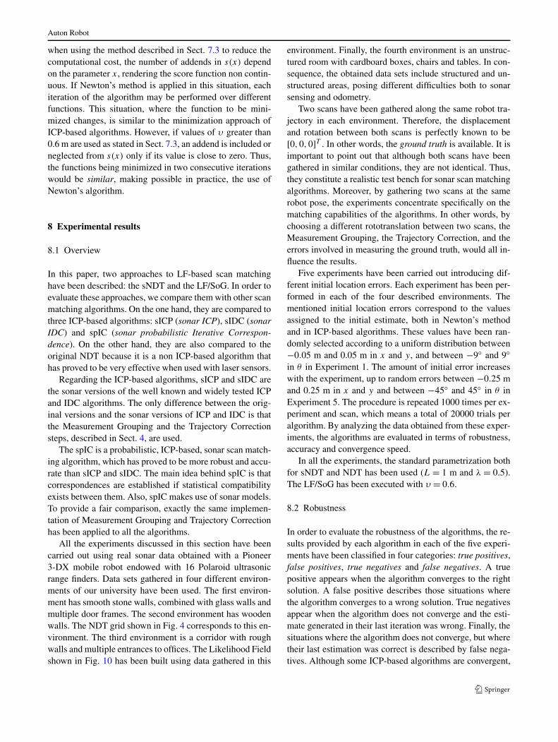
Fig. 11 Robustness of previously existing methods: (a) sICP, (b) sIDC, (c) spIC and (d) NDT. True positives (black), false positives (gray), truenegatives (white) and false negatives (lines) are shown

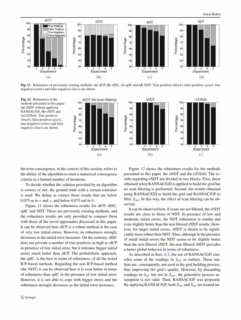
Fig. 12 Robustness of themethods presented in this paper:(a) sNDT without applyingRANSAC/GF, (b) sNDT and(c) LF/SoG. True positives(black), false positives (gray),true negatives (white) and falsenegatives (lines) are shown

the term convergence, in the context of this section, refers tothe ability of the algorithm to meet a numerical convergencecriteria in a limited number of iterations.

To decide whether the solution provided by an algorithmis correct or not, the ground truth with a certain toleranceis used. We define as correct those results that are below0.075 m in x and y, and below 0.075 rad in ! .

Figure 11 shows the robustness results for sICP, sIDC,spIC and NDT. These are previously existing methods, andthe robustness results are only provided to compare themwith those of the novel approaches discussed in this paper.It can be observed how sICP is a robust method in the caseof very low initial errors. However, its robustness stronglydecreases as the initial error increases. On the contrary, sIDCdoes not provide a number of true positives as high as sICPin presence of low initial error, but it tolerates bigger initialerrors much better than sICP. The probabilistic approach,the spIC, is the best in terms of robustness, of all the testedICP-based methods. Regarding the non ICP-based method(the NDT) it can be observed how it is even better in termsof robustness than spIC in the presence of low initial error.However, it is not able to cope with bigger errors and therobustness strongly decreases as the initial error increases.

Figure 12 shows the robustness results for the methodspresented in this paper, the sNDT and the LF/SoG. The re-sults regarding sNDT are divided in two blocks. First, thoseobtained when RANSAC/GD is applied to build the grid butno scan filtering is performed. Second, the results obtainedusing RANSAC/GD to build the grid and RANSAC/GF tofilter Scur . In this way, the effect of scan filtering can be ob-served.

It can be observed how, if scans are not filtered, the sNDTresults are close to those of NDT. In presence of low andmoderate initial errors, the NDT robustness is similar andeven slightly better than the non filtered sNDT results. How-ever, for larger initial errors, sNDT is shown to be signifi-cantly more robust than NDT. Thus, although in the presenceof small initial errors the NDT seems to be slightly betterthan the non filtered sNDT, the non filtered sNDT providesa better global behavior in terms of robustness.

As described in Sect. 6.3, the use of RANSAC/GD clas-sifies some of the readings in Sref as outliers. These out-liers are, consequently, not used in the grid building process,thus improving the grid’s quality. However, by discardingreadings in Sref but not in Scur , the generative process as-sumption is not valid. Then, RANSAC/GF was proposed.By applying RANSAC/GF, both Scur and Sref are treated un-

Auton Robot

der identical conditions. The advantages of performing thementioned filtering are clear when examining Fig. 12b. Thefiltered sNDT is remarkably more robust than the non fil-tered approach and the NDT. Moreover, the sNDT results areslightly better than those produced by spIC. For instance, inExperiment 5, the sNDT achieves a 89.07% of true positiveswhereas the percentage of spIC true positives is 82.07%.

A big advantage of the LF/SoG with respect to the sNDT,is that LF/SoG uses a continuous likelihood field. The effectof this fact on the robustness of the algorithm can be appre-ciated in Fig. 12c. It can be appreciated how LF/SoG is morerobust than any other tested algorithm.

8.3 Accuracy

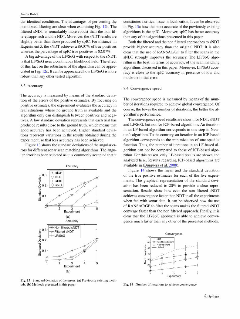
The accuracy is measured by means of the standard devia-tion of the errors of the positive estimates. By focusing onpositive estimates, the experiment evaluates the accuracy inreal situations where no ground truth is available and thealgorithm only can distinguish between positives and nega-tives. A low standard deviation represents that each trial hasproduced results close to the ground truth, which means thatgood accuracy has been achieved. Higher standard devia-tions represent variations in the results obtained during theexperiment, so that less accuracy has been achieved.

Figure 13 shows the standard deviations of the angular er-rors for different sonar scan matching algorithms. The angu-lar error has been selected as it is commonly accepted that it

Fig. 13 Standard deviation of the errors. (a) Previously existing meth-ods. (b) Methods presented in this paper

constitutes a critical issue in localization. It can be observedin Fig. 13a how the most accurate of the previously existingalgorithms is the spIC. Moreover, spIC has better accuracythan any of the algorithms presented in this paper.

Both the filtered and the non filtered approaches to sNDTprovide higher accuracy than the original NDT. It is alsoclear that the use of RANSAC/GF to filter the scans in thesNDT strongly improves the accuracy. The LF/SoG algo-rithm is the best, in terms of accuracy, of the scan matchingalgorithms discussed in this paper. Moreover, LF/SoG accu-racy is close to the spIC accuracy in presence of low andmoderate initial error.

8.4 Convergence speed

The convergence speed is measured by means of the num-ber of iterations required to achieve global convergence. Ofcourse, the lower the number of iterations, the better the al-gorithm’s performance.

The convergence speed results are shown for NDT, sNDTand LF/SoG, but not for ICP-based algorithms. An iterationin an LF-based algorithm corresponds to one step in New-ton’s algorithm. To the contrary, an iteration in an ICP-basedalgorithm corresponds to the minimization of one specificfunction. Thus, the number of iterations in an LF-based al-gorithm can not be compared to those of ICP-based algo-rithm. For this reason, only LF-based results are shown andanalyzed here. Results regarding ICP-based algorithms areavailable in (Burguera et al. 2008).

Figure 14 shows the mean and the standard deviationof the true positive estimates for each of the five experi-ments. The graphical representation of the standard devi-ation has been reduced to 20% to provide a clear repre-sentation. Results show how even the non filtered sNDTachieves convergence faster than NDT in all the experimentswhen fed with sonar data. It can be observed how the useof RANSAC/GF to filter the scans makes the filtered sNDTconverge faster than the non filtered approach. Finally, it isclear that the LF/SoG approach is able to achieve conver-gence much faster than any other of the presented methods.

Fig. 14 Number of iterations to achieve convergence

Auton Robot

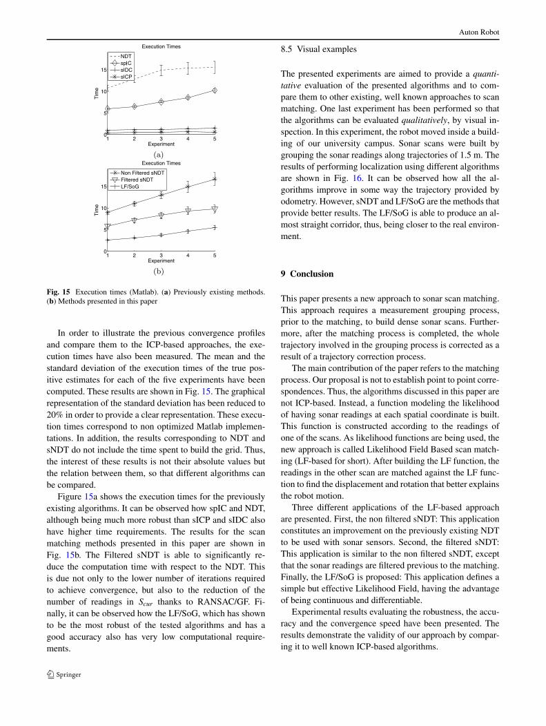
Fig. 15 Execution times (Matlab). (a) Previously existing methods.(b) Methods presented in this paper

In order to illustrate the previous convergence profilesand compare them to the ICP-based approaches, the exe-cution times have also been measured. The mean and thestandard deviation of the execution times of the true pos-itive estimates for each of the five experiments have beencomputed. These results are shown in Fig. 15. The graphicalrepresentation of the standard deviation has been reduced to20% in order to provide a clear representation. These execu-tion times correspond to non optimized Matlab implemen-tations. In addition, the results corresponding to NDT andsNDT do not include the time spent to build the grid. Thus,the interest of these results is not their absolute values butthe relation between them, so that different algorithms canbe compared.

Figure 15a shows the execution times for the previouslyexisting algorithms. It can be observed how spIC and NDT,although being much more robust than sICP and sIDC alsohave higher time requirements. The results for the scanmatching methods presented in this paper are shown inFig. 15b. The Filtered sNDT is able to significantly re-duce the computation time with respect to the NDT. Thisis due not only to the lower number of iterations requiredto achieve convergence, but also to the reduction of thenumber of readings in Scur thanks to RANSAC/GF. Fi-nally, it can be observed how the LF/SoG, which has shownto be the most robust of the tested algorithms and has agood accuracy also has very low computational require-ments.

8.5 Visual examples

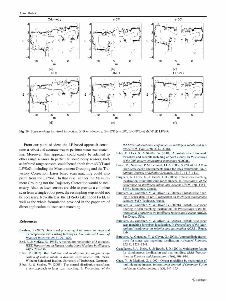
The presented experiments are aimed to provide a quanti-tative evaluation of the presented algorithms and to com-pare them to other existing, well known approaches to scanmatching. One last experiment has been performed so thatthe algorithms can be evaluated qualitatively, by visual in-spection. In this experiment, the robot moved inside a build-ing of our university campus. Sonar scans were built bygrouping the sonar readings along trajectories of 1.5 m. Theresults of performing localization using different algorithmsare shown in Fig. 16. It can be observed how all the al-gorithms improve in some way the trajectory provided byodometry. However, sNDT and LF/SoG are the methods thatprovide better results. The LF/SoG is able to produce an al-most straight corridor, thus, being closer to the real environ-ment.

9 Conclusion

This paper presents a new approach to sonar scan matching.This approach requires a measurement grouping process,prior to the matching, to build dense sonar scans. Further-more, after the matching process is completed, the wholetrajectory involved in the grouping process is corrected as aresult of a trajectory correction process.

The main contribution of the paper refers to the matchingprocess. Our proposal is not to establish point to point corre-spondences. Thus, the algorithms discussed in this paper arenot ICP-based. Instead, a function modeling the likelihoodof having sonar readings at each spatial coordinate is built.This function is constructed according to the readings ofone of the scans. As likelihood functions are being used, thenew approach is called Likelihood Field Based scan match-ing (LF-based for short). After building the LF function, thereadings in the other scan are matched against the LF func-tion to find the displacement and rotation that better explainsthe robot motion.

Three different applications of the LF-based approachare presented. First, the non filtered sNDT: This applicationconstitutes an improvement on the previously existing NDTto be used with sonar sensors. Second, the filtered sNDT:This application is similar to the non filtered sNDT, exceptthat the sonar readings are filtered previous to the matching.Finally, the LF/SoG is proposed: This application defines asimple but effective Likelihood Field, having the advantageof being continuous and differentiable.

Experimental results evaluating the robustness, the accu-racy and the convergence speed have been presented. Theresults demonstrate the validity of our approach by compar-ing it to well known ICP-based algorithms.

Auton Robot

Fig. 16 Sonar readings for visual inspection. (a) Raw odometry, (b) sICP, (c) sIDC, (d) NDT, (e) sNDT, (f) LF/SoG

From our point of view, the LF-based approach consti-tutes a robust and accurate way to perform sonar scan match-ing. Moreover, this approach could easily be adapted toother range sensors. In particular, some noisy sensors, suchas infrared range sensors, could benefit both from sNDT andLF/SoG, including the Measurement Grouping and the Tra-jectory Correction. Laser based scan matching could alsoprofit from the LF/SoG. In that case, neither the Measure-ment Grouping nor the Trajectory Correction would be nec-essary. Also, as laser sensors are able to provide a completescan from a single robot pose, the resampling step would notbe necessary. Nevertheless, the LF/SoG Likelihood Field, aswell as the whole formulation provided in the paper are ofdirect application to laser scan matching.

References

Barshan, B. (2007). Directional processing of ultrasonic arc maps andits comparison with existing techniques. International Journal ofRobotics Research, 26(8), 797–820.

Besl, P., & McKay, N. (1992). A method for registration of 3-d shapes.IEEE Transactions on Pattern Analysis and Machine Intelligence,14(2), 239–256.

Biber, P. (2007). Map building and localization for long-term op-eration of mobile robots in dynamic environments. PhD thesis,Wilhelm-Schickard-Institut, University of Tuebingen, Germany.

Biber, P., & Straßer, W. (2003). The normal distribution transform:a new approach to laser scan matching. In Proceedings of the

IEEE/RSJ international conference on intelligent robots and sys-tems (IROS) (Vol. 3, pp. 2743–2748).

Biber, P., Fleck, S., & Straßer, W. (2004). A probabilistic frameworkfor robust and accurate matching of point clouds. In Proceedingsof the 26th pattern recognition symposium (DAGM).

Bosse, M., Newman, P. M. Leonard, J.J. & Teller, S. (2004). SLAM inlarge-scale cyclic environments using the atlas framework. Inter-national Journal of Robotics Research, 23(12), 1113–1139.

Burguera, A., Oliver, G., & Tardós, J. D. (2005). Robust scan matchinglocalization using ultrasonic range finders. In Proceedings of theconference on intelligent robots and systems (IROS) (pp. 1451–1456), Edmonton, Canada.

Burguera, A., González, Y., & Oliver, G. (2007a), Probabilistic filter-ing of sonar data. In IFAC symposium on intelligent autonomousvehicles (IAV), Toulouse, France.

Burguera, A., González, Y., & Oliver, G. (2007b). Probabilistic sonarfiltering in scan matching localization. In: Proceedings of the In-ternational Conference on Intelligent Robots and Systems (IROS).San Diego, USA.

Burguera, A., González, Y., & Oliver, G. (2007c). Probabilistic sonarscan matching for robust localization. In Proceedings of the inter-national conference on robotics and automation (ICRA), Rome,Italy.

Burguera, A., González, Y., & Oliver, G. (2008). A probabilistic frame-work for sonar scan matching localization. Advanced Robotics,22(11), 1223–1241.

Castellanos, J. A., Neira, J., & Tardós, J. D. (2001). Multisensor fusionfor simultaneous localization and map building. IEEE Transac-tions on Robotics and Automation, 17(6), 908–914.

Chen, Y., & Medioni, G. (1992). Object modelling by registration ofmultiple range images. International Journal of Computer Visionand Image Understanding, 10(3), 145–155.

Auton Robot

Dissanayake, G., Williams, S. B., Durrant-Whyte, H., & Bailey, T.(2002). Map management for efficient simultaneous localizationand mapping (SLAM). Autonomous Robots, (12), 267–286.

Elfes, A. (1989). Occupancy grids: a probabilistic framework for mo-bile robot perception and navigation. PhD thesis, Dept. Electricaland Computer Engineering. Robotics Institute, Carnegie MellonUniversity.

Fischler, M. A., & Bolles, R. C. (1981). Random sample consensus:a paradigm for model fitting with applications to image analysisand automated cartography. Communications of the ACM, 24(6),381–395.

Gutmann, J. S., & Schlegel, C. (1996). AMOS: comparison of scanmatching approaches for self-localization in indoor environments.In Proceedings of the Euromicro workshop in advanced mobilerobotics.

Hähnel, D., Burgard, W., & Thrun, S. (2003). Learning compact 3Dmodels of indoor and outdoor environments with a mobile robot.Robotics and Autonomous Systems, 44(1), 15–27.

Lee, D. (1996). The map-building and exploration strategies of a sim-ple sonar-equipped mobile robot. Cambridge: Cambridge Univer-sity Press.

Leonard, J., & Durrant-Whyte, H. F. (1992). Directed sonar sensingfor mobile robot navigation. Cambridge: Kluwer Academic.

Lu, F., & Milios, E. (1997). Robot pose estimation in unknown envi-ronments by matching 2D range scans. Journal of Intelligent andRobotic Systems, 18(3), 249–275.

Minguez, J., Montesano, L., & Lamiraux, F. (2006). Metric-based iter-ative closest point scan matching for sensor displacement estima-tion. IEEE Transactions on Robotics, 22(5), 1047–1054.

Montesano, L., Minguez, J., & Montano, L. (2005). Probabilistic scanmatching for motion estimation in unstructured environments. InProceedings of the conference on intelligent robots and systems(IROS) (pp. 1445–1450).

Moravec, H. P. (1988). Sensor fusion in certainty grids for mobile ro-bots. AI Magazine, 9, 61–74.

Pfister, S. T., Kreichbaum, K. L., Roumeliotis, S. I., & Burdick, J. W.(2002). Weighted range sensor matching algorithms for mobilerobot displacement estimation. In Proceedings of the IEEE inter-national conference on robotics and automation (ICRA) (Vol. 2,pp. 1667–1674).

Tardós, J. D., Neira, J., Newman, P. M., & Leonard, J. J. (2002). Ro-bust mapping and localization in indoor environments using sonardata. International Journal of Robotics Research, 21(4), 311–330.

Thrun, S. (2001). A probabilistic online mapping algorithm for teamsof mobile robots. International Journal of Robotics Research,20(5), 335–363.

Thrun, S., Burgard, W., & Fox, D. (2005). Probabilistic robotics. Cam-bridge: MIT Press.

Weiss, G., & Puttkamer, E. V. (1995). A map based on laserscanswithout geometric interpretation. In Proceedings of intelligent au-tonomous systems (IAS) (Vol. 4, pp. 403–407).

Zhang, Z. (1994). Iterative point matching for registration of free-formcurves and surfaces. International Journal of Computer Vision,13(2), 119–152.

Antoni Burguera received his de-gree in Computer Science fromthe Universitat de les Illes Balearsin 2000. Since then, he has beenResearch Assistant of the Mathe-matics and Computer Science De-partment of the Universitat de lesIlles Balears and has participatedin projects mainly related with un-derwater robotics. He is currently amember of the Systems, Roboticsand Vision Group, doing his PhDthesis on mobile robot localizationand map building. His research in-terests include mobile robot navi-

gation, localization and map building, focusing on the use of noisysensors such as ultrasonic range finders.

Yolanda González received his MSdegree in Computer Engineeringfrom the Technical University ofDeusto in 1992. From 1992 to 2000he worked at the Open University ofSpain (UNED) as a Research Assis-tant. She received the PhD degreein Electrical Engineering from thisuniversity in 1998. Since 2000 sheis working as a Senior Researchermember of the SRV research groupat the University of Balearic Islands.Her research interests include ScanMatching, SLAM, computer visionand robotics.

Gabriel Oliver received a degree inPhysics from the Autonomous Uni-versity of Barcelona. He earned hisPh.D. in Computer Science fromthe Polytechnic University of Cat-alonia. He is currently a senior lec-turer at the Department of Mathe-matics and Computer Science at theUniversity of the Balearic Islandswhere he is the Director of the Sys-tems, Robotics and Computer Vi-sion Group. His major research in-terests include computer vision andacoustic data processing for robotguidance and navigation. He has

been the leading researcher of projects, related to underwater robot-ics, granted by the Spanish Scientific Council (CICYT).