On the statistical characterization of flows in Internet traffic with application to sampling

On the Statistical Characterization of Flows in Internet

Traffic with Application to Sampling

Yousra Chabchoub, Christine Fricker, Fabrice Guillemin, Philippe Robert

To cite this version:

Yousra Chabchoub, Christine Fricker, Fabrice Guillemin, Philippe Robert. On the StatisticalCharacterization of Flows in Internet Traffic with Application to Sampling. 20 pages. 2009.<hal-00360266v2>

HAL Id: hal-00360266

https://hal.archives-ouvertes.fr/hal-00360266v2

Submitted on 26 Jun 2009

HAL is a multi-disciplinary open accessarchive for the deposit and dissemination of sci-entific research documents, whether they are pub-lished or not. The documents may come fromteaching and research institutions in France orabroad, or from public or private research centers.

L’archive ouverte pluridisciplinaire HAL, estdestinee au depot et a la diffusion de documentsscientifiques de niveau recherche, publies ou non,emanant des etablissements d’enseignement et derecherche francais ou etrangers, des laboratoirespublics ou prives.

https://hal.archives-ouvertes.fr

https://hal.archives-ouvertes.fr/hal-00360266v2

ON THE STATISTICAL CHARACTERIZATION OF FLOWS IN

INTERNET TRAFFIC WITH APPLICATION TO SAMPLING

YOUSRA CHABCHOUB, CHRISTINE FRICKER, FABRICE GUILLEMIN,AND PHILIPPE ROBERT

Abstract. A new method of estimating some statistical characteristics ofTCP flows in the Internet is developed in this paper. For this purpose, a newset of random variables (referred to as observables) is defined. When dealingwith sampled traffic, these observables can easily be computed from sampleddata. By adopting a convenient mouse/elephant dichotomy also dependent ontraffic, it is shown how these variables give a reliable statistical representationof the number of packets transmitted by large flows during successive timeintervals with an appropriate duration. A mathematical framework is devel-oped to estimate the accuracy of the method. As an application, it is shownhow one can estimate the number of large TCP flows when only sampled traf-fic is available. The algorithm proposed is tested against experimental datacollected from different types of IP networks.

Contents

1. Introduction 12. Statistical Properties of Flows 43. Sampled Traffic: Assumptions and Definition of Observables 114. Mathematical Properties of the Observables 135. Applications 176. Conclusion 18References 19

1. Introduction

In Internet traffic a flow is classically defined as the set of those packets withthe same source and destination IP addresses together with the same source anddestination port numbers and the same protocol type. It is well known that if largeTCP flows carry the prevalent part of traffic (in Bytes), most of flows are small (innumber of packets). A formal definition of “large” and “small” will be given laterin the paper. As it will be seen, it may depend on the context; in a first step, thediscussion is kept informal.

We investigate in this paper how to characterize the statistical properties ofthe sizes of large flows (notably their number of packets) in Internet traffic. Itis commonly observed in the technical literature and in real experiments that the

Date: June 26, 2009.Key words and phrases. Flow statistics, Statistical Models, Pareto distribution, Poisson

Approximation.

1

2 CHABCHOUB, FRICKER, GUILLEMIN, AND ROBERT

total size (in packets or bytes) of such flows has a heavy tailed distribution. Inpractice, however, this characterization holds only for very large values of the flowsize. Consequently, in order to accurately estimate the tail of the size probabilitydistribution, a large number of large flows is necessary. To increase the sample sizewhen empirically estimating probability distribution tails, one is led to increase thelength of the observation period. But the counterpart is that the distribution ofthe flow size can no more be described in terms of simple probability distributions,of the Pareto type for example. This is due to the fact that traffic is not stationaryover long time periods, for instance because of daily variations of interactive services(video, web, etc.).

Actually, numerous approaches have been proposed in the technical literature inorder to model large flows as well as their superposition properties. One can roughlyclassify them in two categories: signal processing models and statistical models.Using ideas from signal processing, Abry and Veitch [1], see also Feldman et al. [14,15] and Crovella and Bestravos [8], describe the spectral properties of the time seriesassociated with IP traffic by using wavelets. In this way, a characterization of longrange dependence (the Hurst parameter for example) can be provided. Straight linesin the log-log plot of the power spectrum support some of the “fractal” propertiesof the IP traffic, even if they may simply be due to packet bursts in data flows. SeeRolland et al. [23].

Signal processing tools provide information on aggregated traffic but not on char-acteristics on individual TCP flows, like the number of packets or their transmissiontime. For statistical models, a representation with Poisson shot noise processes (andtherefore some independence properties) has been used to describe the dynamics ofIP traffic, see Hohn and Veitch [17], Duffield et al. [11], Gong et al. [16], Barakatet al. [4] and Krunz and Makowski [18] for example. In Ben Azzouna et al. [3],Loiseau et al. [20, 19] and Gong et al. [16], the distribution of the size of large flowsis represented by a Pareto distribution, i.e. a probability distribution whose taildecays on a polynomial scale. ,

The starting point of some of these analyses is the need for understanding therelation between the distribution of the number S of sampled packets when per-forming packet sampling and the distribution of the flow size S. The problem canbe described as follows: P(S = j) = Q(P(S = ·), j), j ≥ 1, with

Q(φ, i) = pj

+∞∑

ℓ=j

(

ℓ

j

)

(1 − p)ℓ−jφ(ℓ).

The problem then consists of finding a distribution φ0 maximizing some functional

L(φ) so that the relation P(S = j) = Q(φ, j) holds. See Loiseau et al. [19] for anextensive discussion of the current literature where our algorithm is called “stochas-tic counting”. As it will be seen in the following, we will not rely on the maximumlikelihood ratio of distributions in our approach but on estimations of some averagesto estimate some key parameters.

Statistical Characterization Method. We develop in this paper an alternativemethod of obtaining a statistical description of the size of large flows in IP trafficby means of a Pareto distribution: Statistics are collected during successive timewindows of limited length (instead of one single time window for the whole trace). Itmust be emphasized that this characterization in terms of a Pareto distribution does

STATISTICAL CHARACTERIZATION OF FLOWS IN INTERNET TRAFFIC 3

not rely on the asymptotic behavior of the tail distribution but only on statisticson some range of values for the sizes of flows.

The advantage of the proposed method is that with a careful procedure, a simplestatistical characterization is possible and seems to be quite reliable as shown byour experiments for various sets of traffic traces. The intuitive reason for consid-ering short time periods is that on such times scales, flows exhibit only one majorstatistical mode (typically a Pareto behavior). In larger time windows, differentmodes due to the wide variety of flows and non-stationarity in IP traffic necessarilyappear. (See Feldman et al. [15].) This approach allows us to establish a reliablestatistical characterization of flows which is used to infer information from sampledtraffic as it will be seen. The counterpart of that the distribution of the total sizeof a large flow (obtained when considering the complete traffic trace) cannot beobtained directly in this way since the trace is cut into small pieces.

An algorithm is proposed to obtain the statistical representation of large flowswhen all the packets of the trace are available. The constants used in our algo-rithms are explicitly expressed as either universal constants (independent of traffic)or constants depending on traffic : Length of the observation window, definitionof TCP flows referred to as large flows, etc. The procedure invoked to estimateflow statistics should not depend on some hidden pre-processing of the trace. Ouralgorithms determine on-line the constants depending on the traffic. This is, in ourview, one important aspect which is sometimes neglected in the technical literature

Application to Sampled Traffic. The basic motivation for developing a flowcharacterization method is to infer flow characteristics from sampled data. Thisis notably the case for sampling processes such as the 1-out-of-k sampling schemeimplemented by CISCO’s NetFlow [7], which greatly degrades information on flows.What we advocate in this paper is that it is still possible to infer relevant char-acteristics on flows from sampled data if some characteristics of the flow size canbe confidently described by means of a simple Pareto distribution. By using thestatistical representation described above, we propose a method of inferring thenumber of large flows from sampled traffic.

The proposed method relies on a new set of random variables, referred to asobservables and computed in successive time intervals with fixed length. Specif-ically, these random variables count the number of flows sampled once, twice ormore in the successive observation windows. The properties of these variables canbe obtained through simple characteristics, in particular mean values of variablesinstead of remote quantiles of the tail distribution, which are much more difficultto accurately estimate. By developing a convenient mathematical setting (Poissonapproximation methods), it is moreover possible to show that quantities relatedto the observables under consideration are close to Poisson random variables withan explicit bound on the error. This Poisson approximation is the key result toestimate the total number of large flows.

Organization of the paper. The organization of the paper is as follows. A statis-tical description of large TCP flows is presented in Section 2, this representation istested against five exhaustive sets of traffic traces: three from the France Telecom(FT) commercial IP network carrying residential ADSL traffic and two others fromAbilene network. An algorithm is developed in this section to compute the charac-teristics of the Pareto distributions describing flows. In Section 3, some assumptions


on sampled traffic are introduced and the observables for describing traffic are de-fined. The mathematical properties are analyzed in light of Poisson approximationmethods in Section 4. The results developed in this section are crucial to inferthe statistics of an IP traffic from sampled data. Experiments with the five sets ofsampled traces used in this paper are presented and discussed in Section 5. Someconcluding remarks are presented in Section 6.

2. Statistical Properties of Flows

This section is devoted to a statistical study of the size (the number of packets)of flows in a limited time window of duration ∆. The goal of this section is showthat a simple statistical representation of the flow size can be obtained for varioussets of traffic traces.

2.1. Assumptions and Experimental Conditions.

The sets of traces used for testing theoretical results. For the experiments carriedout in the following sections, several sets of traces will be considered: CommercialIP traffic, namely ADSL traces from the France Telecom (FT) IP collect network,and traffic issued from campus networks (Abilene III traces). Their characteristicsare given in Table 1.

Table 1. Characteristics of traffic traces considered in experiments.

Name Nb. IP packets Nb. TCP Flows DurationADSL Trace A 271 455 718 20 949 331 2 hoursADSL Trace B Upstream 54 396 226 2 648 193 2 hoursADSL Trace B Downstream 53 391 874 2 107 379 2 hoursAbilene III Trace A 62 875 146 1 654 410 8 minutesAbilene III Trace B 47 706 252 1 826 380 8 minutes

The Abilene traces 20040601-193121-1.gz (trace A) and 20040601-194000-0.gz(trace B) can be found at the url http://pma.nlanr.net/Traces/Traces/long/ipls/3/.

Time Windows. Traffic will be observed in successive time windows with length∆. In practice, the quantity ∆ can vary from a few seconds to several minutesdepending upon traffic characteristics on the link considered.

The ideal value of ∆ actually depends on the targeted application. For thedesign of network elements considering the flow level (e.g., flow aware routers,measurement devices, etc.), it is necessary to estimate the requirements in termsof memory to store the different flow descriptors. In this context, ∆ may be of theorder of few seconds. The same order of magnitude is also adapted to anomalydetection, for instance for detecting a sudden increase in the number of flows. Forthe computation of traffic matrices, ∆ can be several minutes long (typically 15minutes). In our study, the “adequate” values for ∆ are of the order of severalseconds. See the discussion below.


Mice and Elephants. With regard to the analysis of the composition of traffic, inlight of earlier studies on IP traffic (see Estan and Varghese [13], Papagiannaki et

al. [22] or Ben Azzouna et al. [2]), two types of flows are identified: small flows withfew packets (referred to as mice) and the other flows will be referred to as elephants.In commercial IP traffic, this simple traffic decomposition can be justified by thepredominance of web browsing and peer-to-peer traffic giving rise to either signalingand very small file transfers (mice) or else file downloads (elephants).

This dichotomy may be more delicate to verify in a different context than theone considered in Ben Azzouna et al. [2]. For LAN traffic, for example, there maybe very large amounts of data transferred at very high speed. As it will be seenin the various IP traces used in our analysis, the distinction between mice andelephants has to be handled with care and in our case is dependent on the type oftraffic considered. The distinction between the constants depending on the traceand “universal” constants is, in our view, a crucial issue. It amounts to preciselystating which constants are depend on traffic. This aspect is generally (unduly inour opinion) neglected in traffic measurement studies. In particular, the variable∆ and the dichotomy mice/elephants are dependent on the trace, as explained inthe next section.

2.2. Heavy Tails. The fact that the distribution of the size S of a large TCP flow isheavy tailed is well known. Experiments and theoretical results on the superpositionof ON-OFF heavy tailed traffic have justified the self similar nature of IP traffic,see Crovella and Bestravos [8]. Although the heavy tailed property of the size oflarge flows is commonly admitted, little attention has been paid to identify properlya class of heavy tailed distributions so that the corresponding parameters can beestimated for an arbitrary traffic trace with a significant duration.

One of the reasons for this situation is that the most common heavy taileddistributions G(x) = P(S ≥ x) (e.g., Pareto, i.e., G(x) = C/xα for x ≥ b and someα > 0, or Weibull, i.e., G(x) = exp(−νxβ) for some β > 0 and ν > 0) have avery small number of parameters and consequently a limited of number of possibledegrees of freedom for describing the distribution of the sizes of flows. For thisreason, such a distribution can rarely represent the statistics of the total numberof packets transmitted by a flow in a trace of arbitrary duration.

As a matter of fact, if a traffic trace is sufficiently long, some non stationaryphenomena may arise and the diversity of file sizes may not be captured by one ortwo parameters. For example, with a Pareto distribution, the function x → G(x)in a log-log scale should be a straight line. The statistics of the file sizes in thetraces used in our experiments are depicted in Figure 1 and 2 for an ADSL traffictrace from the France Telecom backbone IP collect network and for a traffic tracefrom Abilene network, respectively.

Figure 1 and 2 clearly show that for the two traffic traces considered, the file sizeexhibits a multimodal behavior: At least several straight lines should be necessaryto properly describe these distributions. These figures also exhibit the (intuitive)fact that has been noticed in earlier experiments: The longer the trace is, themore marked is the multimodal phenomenon. (See Ben Azzouna et al. [3] for adiscussion.)

The key observation when characterizing a traffic trace is the fact that if theduration ∆ of the successive time intervals used for computing traffic parameters isappropriately chosen, then the distribution of the size of the main contributing flows


1

10

100

1000

10000

100000

1 10 100 1000 10000

−lo

gP(S

ize>

x)

log x

Figure 1. Statistics of the number of packets S of a flow for ADSLA (2 hours): the quantity − log(P(S > x)) as a function of log(x).

1

10

100

1000

10000

100000

1 10 100 1000 10000 100000

−lo

gP(S

ize>

x)

log x

Figure 2. Statistics of the number of packets S of a flow forABILENE A trace (8 minutes): the quantity − log(P(S > x)) as afunction of log(x).

in the time interval can be represented by a Pareto distribution. More precisely,there exist ∆, Bmin, Bmax and a > 0 such that if S is the number of packetstransmitted by a flow in ∆ time units, then P(S ≥ x | S ≥ Bmin) ∼ Pα(x) forBmin ≤ x ≤ Bmax with

(1) Pα(x)def.=

(

Bmin

x

)a

, for x ≥ Bmin,

and furthermore the proportion of large flows with size greater than Bmax is lessthan 5%. The parameter Bmin is usually referred to as the location parameter anda as the shape parameter.

In other words, if the time interval is sufficiently small then the distribution ofthe number of packets transmitted by a large flow has one dominant Pareto modeand therefore can confidently be characterized by a unique Pareto distribution. Thealgorithm used to validate this result is described in Table 2. It is run from thebeginning of the trace; in practice a couple of minutes is sufficient to obtain resultsfor the constants ∆, Bmin, Bmax. The algorithm is of course valid when the totaltrace is available for at least an interval of several minutes. In the case of sampled


traffic for which this algorithm cannot be used, another method will be proposedin Section 3.

Table 2. Algorithm for Identifying ∆ and the Pareto Distribution.

— ∆ is fixed so that at least 1000 flows have more than 20 packets.— Bmax is defined as the smallest integer such that less than 5% of the flows

have a size greater than Bmax.— A Least Square Method, see Deuflhard and Hohmann [9] for example, is

performed to get a linear interpolation in a log-log scale of the distributionof sizes between Bmin and Bmax. The constant Bmin is chosen as the small-est integer such that the L2-distance in the sense of least square methodwith the approximating straight line is less than 2.10−3. The slope of theline gives the value of the parameter a.

The quantity Bmin defines the boundary between mice and elephants in thetrace. A mouse is a flow with a number of packets less than Bmin. An elephant isa flow such that its number of packets during a time interval of length ∆ is greaterthan or equal to Bmin. By definition of Bmax, flows whose size is greater thanBmax represent a small fraction of the elephants.

2.3. Experiments with Synthetic and Real Traffic Traces. Some experi-ments have been done using artificial traces with a real Pareto distribution. Forthese traces, the algorithm described in Table 2 has been used without any modi-fication: A time window is defined when at least 1000 flows of size greater than 20packets are detected. As it can be seen, the identification of the exponent a is quitegood. Note that, because only Pareto distributed flows are present the minimalsize Bmin of elephants is smaller than in real traffic.

Experimental results with real traces, for the ADSL A and Abilene A traffictraces, are displayed in Figures 4 and 5, respectively. The same algorithm has beenrun for the ADSL trace B Upstream and Downstream as well as for the AbileneIII B trace. The benefit of the algorithm is that the distribution of the number ofpackets in elephants can always be represented by a unimodal Pareto distributionif the duration of ∆ is adequately chosen by using the algorithm given in Table 2.Results are summarized in Table 3.

Table 3. Statistics of the elephants for the different traffic traces.

ADSL A ADSL B Up ADSL B Down Abilene A Abilene B

∆ (sec) 5 15 15 2 2Bmin 20 29 39 89 79Bmax 94 154 128 324 312a 1.85 1.97 1.50 1.30 1.28

2.4. On the choice of parameters. We discuss in this section the various pa-rameters used by the algorithm.


1e-03

1e-02

0.1

1

10

100

1000

10000

1 10 100 1000

−lo

gP(S

ize>

x)

log x

(a) Pareto a = 1.85. Estimation: a = 1.84,Bmin = 9, Bmax = 100

1e-05

1e-04

1e-03

1e-02

0.1

1

10

100

1000

10000

1 10 100 1000

−lo

gP(S

ize>

x)

log x

(b) Pareto a = 2.5. Estimation: a = 2.48,Bmin = 11, Bmax = 65

Figure 3. Synthetic traces with 106 flows with a Pareto distribution

Fixed parameters and parameters depending on traffic. There are four basic param-eters for the model which are determined by the trace: ∆ (duration of time windowfor statistics), the range of values [Bmin, Bmax] for the Pareto distribution and theexponent a of this distribution. These parameters are discussed below.

Additionally there are “universal” (i.e. independent of the trace): the minimalnumber of flows to make statistics, set to 1000 here, the proportion, 5%, of flows ofsize ≥ Bmax, and the level of accuracy, 2.10−3 here, of the least square method todetermine Bmin and Bmax.

Parameter Bmin. It turns out that for commercial (ADSL) traffic, the value ofBmin is close to 20. This value is fairly common in earlier studies for classifyingADSL traffic. It should be noted that this value is not at all universal since, inour view, it does depend on traffic. The examples with Abilene traces, see below,which contain significantly bigger elephants, shows that the corresponding valuesshould be higher than 20 (around 80 in our example).

The two types of traffic are intrinsically different: ADSL traffic is mainly com-posed of peer to peer traffic (with a huge number of small flows and a few filetransfers of limited size because of the segmentation of large files into chunks),


1

10

100

1000

10000

1 10 100

−lo

gP(S

ize>

x)

log x

Bmax

Bmin

(a) ADSL A trace – ∆ = 5s

1

10

100

1000

10000

1 10 100 1000

−lo

gP(S

ize>

x)

log x

Bmax

Bmin

(b) ADSL B Down trace – ∆ = 15 seconds

1

10

100

1000

10000

1 10 100

−lo

gP(S

ize>

x)

log x

Bmax

Bmin

(c) ADSL B Up trace – ∆ = 15 s

Figure 4. Statistics of the flow size (number of packets) in a timeinterval of length ∆ = 15

while Abilene traffic comprises large file transfers issued from campus networks. Inorder to maximize the range for the Pareto description, the variable Bmin is definedas the smallest value for which the linear representation (in the log scale) holds.

Parameter ∆. This parameter ∆ is determined in a simple way by our algorithm.According to the various experiments, the parameter ∆ can be taken in some rangeof values where the Pareto representation still holds. On the one hand, ∆ has tobe taken large enough so that sufficiently many packets arrive in time intervals of


1

10

100

1000

10000

1 10 100 1000

−lo

gP(S

ize>

x)

log x

Bmax

Bmin

(a) Abilene A trace – ∆ = 2 s

1

10

100

1000

10000

1 10 100 1000

−lo

gP(S

ize>

x)

log x

Bmax

Bmin

(b) Abilene B trace – ∆ = 2 s

Figure 5. Statistics of the flow size (number of packets) in a timeinterval of length ∆ for the Abilene traces.

duration ∆ to derive reliable estimations of the Pareto distribution. An experimentwith ADSL A trace with ∆ = 1s gives only 63 flows of size more than 20 whichis not enough to obtain reliable statistics. A “correct” value in this case is 5s.Experiments show that higher values (like 10s) do not change significantly thePareto property observed in this case.

On the other hand, ∆ should not be too large so that the statistical properties(a Pareto distribution in our case) can be identified, i.e., so that the statistics areunimodal. See Figures 1 and 2 which illustrate situations where statistics are doneon the complete trace, i.e. when ∆ is taken equal to the total duration of the trace.In these examples, the piecewise linear aspect of the curves suggests, for both cases,there is at least a bi-modal Pareto behavior.

2.5. Discussion. As it will be seen in the following, the above statistical modelgives interesting results to extract information from sampled traffic. It has never-theless some shortcomings which are now discussed.

A partial information when ∆ is small. . It should be noted that the parameterscomputed in a time window of length ∆ do not give a complete description of thedistribution of the size of a large flow, since statistics are done over a limited timehorizon. The procedure provides therefore a fragmented information.


To obtain a complete description of the statistics of the size of flows, it wouldbe necessary to relate the statistics from successive time windows of length ∆. Wedo not know how to do that yet. Nevertheless, as it will be seen in the following,this fragmented information can be recovered from sampled traffic and it will beused to give a good estimation on the number of active large flows at a given time.This incomplete but useful description of the statistics is, in some sense, the priceto pay to have a simple estimation of the statistics of flows.

An incomplete description of large flows in a time window of size ∆. The repre-sentation with a Pareto distribution is for elephants (with size greater than Bmin)whose size is less than Bmax. In particular, it does not give any information onthe statistics of flows with size greater than Bmax. But note that, by definition,less that 5% of the total number of flows have a size greater than Bmax. This ishowever a source of errors when, as in Section 4, the Pareto representation is usedon the interval [Bmin, +∞] instead of [Bmin, Bmax]

3. Sampled Traffic: Assumptions and Definition of Observables

In the previous section, an algorithm to describe the distribution of large flowsby means of a unimodal distribution has been introduced. Now, it is shown howto exploit this algorithm in the context of packet sampling in the Internet. Packetsampling is a crucial issue when performing traffic measurements in high speedbackbone networks. As a matter of fact, a fundamental problem related to thecomputation of flow statistics from traffic crossing very high speed transmissionlinks is that, due to the enormous number of packets handled by routers, only areduced amount of information can be available to the network operator.

Packet sampling is in this context an efficient method of reducing the volumeof data to analyze when performing measurements in the Internet. One populartechnique consists of picking up one packet every other κs packets with κs = 100,500, 1000 in practice. (This sampling scheme is referred to as 1-out-of-κs packetsampling in the technical literature.) This method is implemented for instance inCISCO routers, namely NetFlow facility [7] widely deployed in operational net-works today. It suffers from different shortcomings well identified in the technicalliterature, see for instance Estan et al. [12].

We describe in this section the different assumptions made on traffic in order todevelop an analytical evaluation of our method of inferring flow statistics. Through-out this paper, high speed transmission links (at least 1 Gbit/s) will be considered.

3.1. Mixing condition. When observing traffic, packets are assumed to be suffi-ciently interleaved so that those packets of a same flow are not back-to-back butmixed with packets of other flows. This introduces some randomness in the selec-tion of packets when performing sampling. In particular, when K flows are activein a given time window and if the ith flow comprises vi packets during that period,then the probability of selecting a packet of the ith flow is assumed to be equalvi/(v1 + v2 + · · · + vK). This property will be referred to as mixing condition inthe following and is formally defined as follows. A variant of this property is, im-plicitly at least, assumed in the existing literature. See, e.g. Duffield et al. [10] andChabchoub et al. [6].

Definition 1 (Mixing Condition). If K TCP flows are active during a time in-

terval of duration ∆, traffic is said to be mixing if for all i, 1 ≤ i ≤ K, the total


number vi of packets sampled from the ith flow during that time interval has the

same distribution as the analog variable in the following scenario: at each sam-

pling instant a packet of the ith flow is chosen with probability vi/V where vi is the

number of packets of the ith flow and V = v1 + · · · + vK .

This amounts to claim that with regard to sampling, the probability of selectinga packet of a given flow is proportional to the total number of packets of this flow.

One alternative would consist of assuming that the probability of selecting apacket of the ith flow is 1/K, the inverse of the total number of flows. Thisassumption, however, does not take into account the respective contributions ofthe different flows to the total volume and thus may be inaccurate. If all K flowshad the same distribution with a small variance, then this assumption would notmuch differ from the mixing condition. Note however that the variance of Paretodistributions can be infinite if the shape parameter a is less than 2. Hence, thisleads us to suppose that the mixing condition holds and that the probability ofselecting a packet from flow i is indeed vi/V .

3.2. Negligibility assumption. We consider traffic on very high speed links andit then seems reasonable to assume that no flows contribute a significant proportionof global traffic. In other words, we suppose that the contribution of a given flowto global traffic is negligible. In the following, we go one step further by assumingthat in any time window, the number of packets of a given flow is negligible whencompared to the total number of packets in the observation window. By usingthe notation of the previous section, this amounts to assuming that for any flow i,the number of packet vi is much less than V . Furthermore, we even impose thatthe squared value of vi is much less than V . We specifically formulate the aboveassumptions as follows.

Definition 2 (Negligibility condition). In any window of length ∆, the square of

the number of packets of every flow is negligible when compared to the total number

of packets V in the observation window. There specifically exists some 0 < ε ≪ 1such that for all i = 1, . . . , K, v2

i /V ≤ ε.

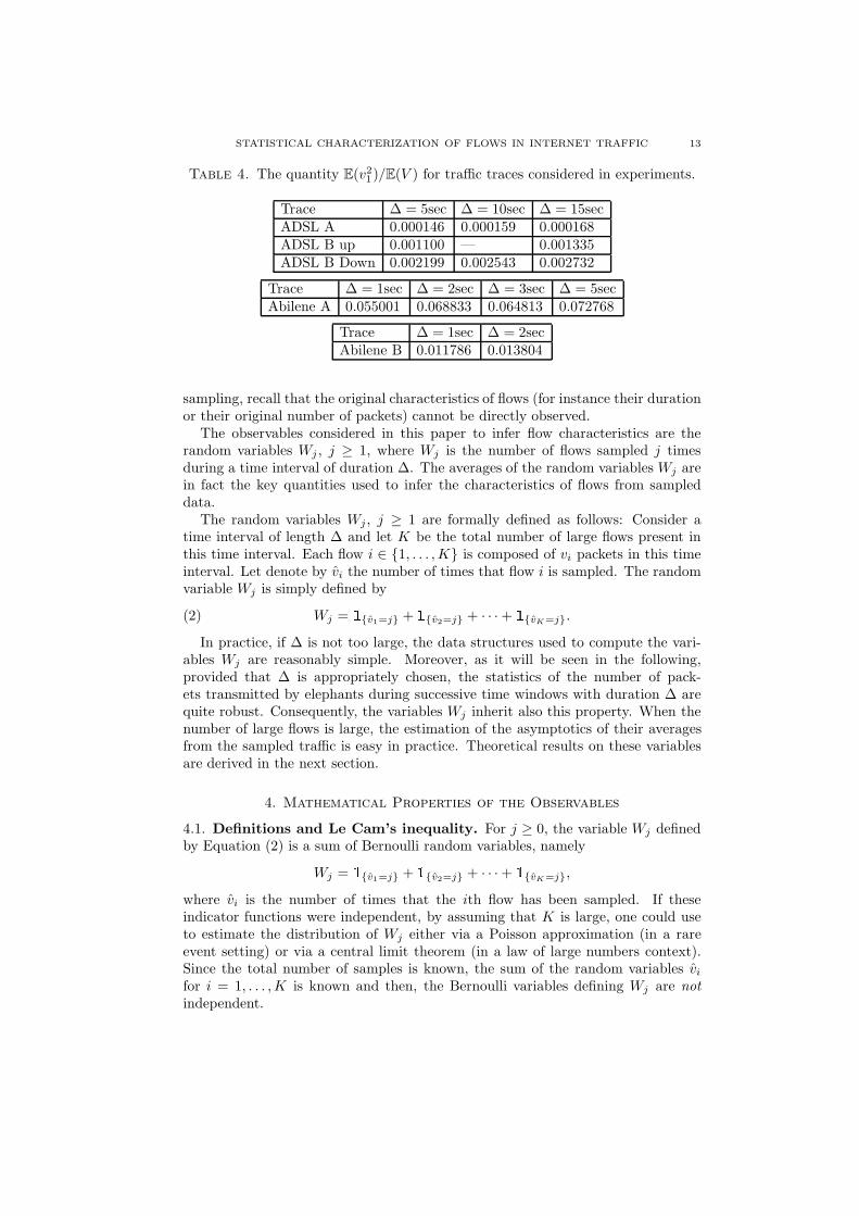
The above assumption implies that no flows are dominating when observingtraffic on a high speed transmission link. Table 4 shows that this is the case forthe traces used in our experiments. There is thus no bias in the sampling process,which may be caused by the fact that some flows are oversampled because theycontribute a significant part of traffic. This assumption is reasonable for commercialADSL traffic because access links are often the bottlenecks in the network. Forinstance, ADSL users may have access rates of a few Mbit/s, which are negligiblewhen compared against backbone links of 1 to 10 Gbit/s. Moreover, the bit rateachievable by an individual flow rarely exceeds a few hundreds of Kbit/s. In thecase of transit networks carrying campus traffic, the above assumption may bemore questionable since bulk data transfers may take place in Ethernet local areanetworks and individual flows may achieve bit rates of several Mbit/s.

3.3. The Observables. We now introduce the different variables used to inferflow characteristics. These variables are based only upon sampled data; they canbe evaluated when analyzing NetFlow records sent by routers of an IP network.For this reason, these variables are referred to as observables. Because of packet


Table 4. The quantity E(v21)/E(V ) for traffic traces considered in experiments.

Trace ∆ = 5sec ∆ = 10sec ∆ = 15secADSL A 0.000146 0.000159 0.000168ADSL B up 0.001100 — 0.001335ADSL B Down 0.002199 0.002543 0.002732

Trace ∆ = 1sec ∆ = 2sec ∆ = 3sec ∆ = 5secAbilene A 0.055001 0.068833 0.064813 0.072768

Trace ∆ = 1sec ∆ = 2secAbilene B 0.011786 0.013804

sampling, recall that the original characteristics of flows (for instance their durationor their original number of packets) cannot be directly observed.

The observables considered in this paper to infer flow characteristics are therandom variables Wj , j ≥ 1, where Wj is the number of flows sampled j timesduring a time interval of duration ∆. The averages of the random variables Wj arein fact the key quantities used to infer the characteristics of flows from sampleddata.

The random variables Wj , j ≥ 1 are formally defined as follows: Consider atime interval of length ∆ and let K be the total number of large flows present inthis time interval. Each flow i ∈ {1, . . . , K} is composed of vi packets in this timeinterval. Let denote by vi the number of times that flow i is sampled. The randomvariable Wj is simply defined by

(2) Wj = 1{v1=j} + 1{v2=j} + · · · + 1{vK=j}.

In practice, if ∆ is not too large, the data structures used to compute the vari-ables Wj are reasonably simple. Moreover, as it will be seen in the following,provided that ∆ is appropriately chosen, the statistics of the number of pack-ets transmitted by elephants during successive time windows with duration ∆ arequite robust. Consequently, the variables Wj inherit also this property. When thenumber of large flows is large, the estimation of the asymptotics of their averagesfrom the sampled traffic is easy in practice. Theoretical results on these variablesare derived in the next section.

4. Mathematical Properties of the Observables

4.1. Definitions and Le Cam’s inequality. For j ≥ 0, the variable Wj definedby Equation (2) is a sum of Bernoulli random variables, namely

Wj = 1{v1=j} + 1{v2=j} + · · · + 1{vK=j},

where vi is the number of times that the ith flow has been sampled. If theseindicator functions were independent, by assuming that K is large, one could useto estimate the distribution of Wj either via a Poisson approximation (in a rareevent setting) or via a central limit theorem (in a law of large numbers context).Since the total number of samples is known, the sum of the random variables vi

for i = 1, . . . , K is known and then, the Bernoulli variables defining Wj are not

independent.


To overcome this problem, we make use of general results on the sum of Bernoullirandom variables. Let us consider a sequence (Ii) of Bernoulli random variables,i.e. Ii ∈ {0, 1}. The distance in total variation between the distribution of X =I1 + · · · + Ii + · · · and a Poisson distribution with parameter δ > 0 is defined by

‖P(X ∈ ·) − P(Qδ ∈ ·)‖tvdef.= sup

A⊂N

|P(X ∈ A) − P(Qδ ∈ A)|

=1

2

∑

n≥0

∣

∣

∣

∣

P(X = n) −δn

n!e−δ

∣

∣

∣

∣

.

The Poisson distribution Qδ with mean δ is such that

P(Qδ = n) =δn

n!exp(−δ).

Note that the total variation distance is a strong distance since it is uniform withrespect to all events, i.e., for all subset s A of N,

|P(X ∈ A) − P(Qδ ∈ A)| ≤ ‖P(X ∈ ·) − P(Qδ ∈ ·)‖tv.

The following result (see Barbour et al. [5]) gives a tight bound on the totalvariation distance between the distribution of X and the Poisson distribution withthe same expected value when the Bernoulli variables are independent. In spite ofthe fact that this result is not directly applicable in our case, we shall show in thefollowing how to use it to obtain information on the distributions of the observablesWj .

Theorem 1 (Le Cam’s Inequality). If the random variables (Ii) are independent

and if X =∑

i Ii, then

(3) ‖P(X ∈ ·) − P(QE(X) ∈ ·)‖tv ≤∑

i

P(Ii = 1)2 = E(X) − Var(X)

If X is a Poisson distribution then Var(X) = E(X), the above relation showsthat to prove the convergence to a Poisson distribution one has only to prove thatthe expectation of the random variable is arbitrarily close to its variance.

4.2. Estimation of the mean value of the observables. We consider the 1-out-of-κs deterministic sampling technique, where one packet is selected every otherκs packets. In addition, we suppose that traffic on the observed link is sufficientlymixed so that the mixing condition given by Definition 1 holds and that there areno dominating flows in traffic so that the negligibility condition (Definition 2) alsopertains.

It is assumed that during a time interval of length ∆, there are K flows composedof at least Bmin packets, where Bmin is defined in Section 2. It has been seenthat the number of packets in these flows follows a Pareto distribution definedby Relation (1) for some exponent a and parameters Bmin and Bmax. Let S bea random variable whose distribution is given by Relation (1) for all x ≥ Bmin.From our experiments, S is the size of a “typical” flow whose size is in the interval[Bmin, Bmax]. See the discussion at the end of Section 2 for the flows of size greaterthan Bmax. Of course the sizes of mice are not represented by this random variable.The variable V denotes the total number of packets in the observation window, notethat it includes not only the elephants but also the mice.


Note that V is the sum of the number of packets in elephants and mice. If vi isthe number of packet in the ith elephant, then vi has the same Pareto distribution

as S (i.e., vidist.= S) and V ≥ v1 +v2+ · · ·+vK . The difference V −v1−v2−· · ·−vK

is the number of packets of mice.

Proposition 1 (Mean Value of the Observables). If K elephants are active in a

time window of length ∆, the mean number E(Wj) of flows sampled j times, j ≥ 1,satisfies the relation

∣

∣

∣

∣

E(Wj)

K− Qj

∣

∣

∣

∣

≤ psE

(

S2

V

)

,(4)

where Q is the probability distribution defined by

P(Q = j)def= Qj = E

(

(psS)j

j!e−psS

)

,

and ps = 1/κs is the sampling rate.

From Equation (4) one gets that the larger the total volume V of packets is, thebetter is the approximation of E(Wj)/K by Qj.

Proof. The number of times vi that the ith flow is sampled in the time interval isgiven by

vi = Bi1 + Bi

2 + · · · + BipsV ,

where, due to the mixing condition, Biℓ is equal to one if the ℓth sampled packet is

from the ith flow, which event occurs with probability vi/V . Note that the totalnumber of sampled packets is psV .

Conditionally on the values of the set F = {v1, . . . , vK}, the variables (Biℓ, ℓ ≥ 1)

are independent Bernoulli variables. For 1 ≤ i ≤ K, Le Cam’s Inequality (3) givestherefore the relation

‖P(vi ∈ · | F) − Qpsvi‖

tv≤ ps

v2i

V.

By integrating with respect to the variables v1, . . . , vK , this gives the relation

‖P(vi ∈ ·) − Q‖tv ≤ psE

(

v2i

V

)

.

In particular, for j ∈ N, |P(vi = j) − Qj | ≤ psE(

S2/V)

. Since

E(Wj) =

K∑

i=1

P(vi = j),

by summing on i = 1, . . . , K, one gets

|E(Wj) − KQj| ≤ psKE

(

S2

V

)

and the result follows. �

If the number of packets per flow were constant, then Q would be a Poissondistribution with parameter psS, the variable S being in this case a constant. Theabove inequality shows that at the first order the expected value of Wj is psE(S).The expression of Q, however, indicates that higher order moments of S play asignificant role. For example, if the variable S has a significant variance, then the


classical rough reduction, which consists of assuming that the size of a sampledelephant is psS, is no longer valid for estimating the original size of the elephant.

Under the negligibility condition, we deduce that∣

∣

∣

∣

E(Wj)

K− Qj

∣

∣

∣

∣

≤ psε,

where ε appears in Definition 2 and is assumed to much less than 1. This impliesthat Inequality (4) is tight and the quantity E(Wj)/K can accurately be approxi-mated by the quantity Qj, when no flows are dominating in traffic.

We are now ready to state the main result needed for estimating the number Kof elephants from sampled data.

Proposition 2 (Asymptotic Mean Values). Under the same assumptions as those

of Proposition 1,

(5) limK→+∞

E(Wj+1)

E(Wj)∼ 1 −

a + 1

j + 1

and

(6) limK→+∞

E(Wj)

K∼ a(psBmin)a Γ(j − a)

j!,

if Bmax >> 1 and psBmin << 1, where Γ is the classical Gamma function defined

by

Γ(x) =

∫ +∞

0

ux−1e−u du, x > 0.

Proof. For j ≥ 1,

Qj = E

(

(psS)j

j!e−psS

)

∼ aBamin

pa+1s

j!

∫ +∞

Bmin

(psu)j−a−1e−psu du

and then

Qj ∼ aBamin

pas

j!

∫ +∞

psBmin

uj−a−1e−u du ∼ a(psBmin)a Γ(j − a)

j!,

since psBmin ∼ 0. Therefore, by using the relation Γ(x + 1) = xΓ(x) we obtain theequivalence

Qj+1

Qj

∼j − a

j + 1.

The proposition follows by using the fact that the upper bound of Equation (4) ofProposition 1 goes to 0 by the law of large numbers. �

As it will be seen later in the next section, Relation (5) is used to estimatethe exponent a of the Pareto distribution of the number of packets of elephants,the quantities E(Wj) and E(Wj+1) being easily derived from sampled traffic. Thequantity K will be estimated from Relation (6). The estimation of the parameterBmin from sampled traffic as well as the correct choice of the integer j will bediscussed in the next section.


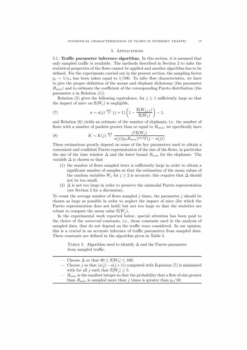
5. Applications

5.1. Traffic parameter inference algorithm. In this section, it is assumed thatonly sampled traffic is available. The methods described in Section 2 to infer thestatistical properties of the flows cannot be applied and another algorithm has to bedefined. For the experiments carried out in the present section, the sampling factorps = 1/κs has been taken equal to 1/100. To infer flow characteristics, we haveto give the proper definition of the mouse and elephant dichotomy (the parameterBmin) and to estimate the coefficient of the corresponding Pareto distribution (theparameter a in Relation (1)).

Relation (5) gives the following equivalence, for j ≥ 1 sufficiently large so thatthe impact of mice on E(Wj) is negligible,

(7) a ∼ a(j)def.= (j + 1)

(

1 −E(Wj+1)

E(Wj)

)

− 1,

and Relation (6) yields an estimate of the number of elephants, i.e. the number offlows with a number of packets greater than or equal to Bmin; we specifically have

(8) K ∼ K(j)def.=

j! E(Wj)

a(j)(psBmin)a(j)Γ(j − a(j)).

These estimations greatly depend on some of the key parameters used to obtain aconvenient and confident Pareto representation of the size of the flows, in particularthe size of the time window ∆ and the lower bound Bmin for the elephants. Thevariable ∆ is chosen so that

(1) the number of flows sampled twice is sufficiently large in order to obtain asignificant number of samples so that the estimation of the mean values ofthe random variables Wj for j ≥ 2 is accurate; this requires that ∆ shouldnot be too small,

(2) ∆ is not too large in order to preserve the unimodal Pareto representation(see Section 2 for a discussion).

To count the average number of flows sampled j times, the parameter j should bechosen as large as possible in order to neglect the impact of mice (for which thePareto representation does not hold) but not too large so that the statistics arerobust to compute the mean value E(Wj).

In the experimental work reported below, special attention has been paid tothe choice of the universal constants, i.e., those constants used in the analysis ofsampled data, that do not depend on the traffic trace considered. In our opinion,this is a crucial in an accurate inference of traffic parameters from sampled data.These constants are defined in the algorithm given in Table 5.

Table 5. Algorithm used to identify ∆ and the Pareto parameterfrom sampled traffic.

— Choose ∆ so that 80 ≤ E[W2] ≤ 100;— Choose j so that |a(j)−a(j+1)| computed with Equation (7) is minimized

with for all j such that E[Wj ] ≥ 5.— Bmin is the smallest integer so that the probability that a flow of size greater

than Bmin is sampled more than j times is greater than ps/10;


5.2. Experimental results. Concerning the estimation of the constants Bmin, thenumerical results obtained by using the algorithm given in Table 5 are presentedin Table 6, where the values of the different Bmin estimated by the algorithmare compared against the values given in Section 2. As it can be observed, theproposed algorithm yields a rather conservative definition of elephants (i.e., flowsof size greater than or equal to Bmin).

Table 6. Elephants for the France Telecom ADSL and the Abilenetraffic traces.

ADSL A ADSL B Up ADSL B Down Abilene A Abilene B

Bmin 20 29 39 89 79estimated Bmin 21 45 45 77 77

The main results are gathered in Table 7 giving the quantities K and a estimatedby using Equations (7) and (8) for different values of the parameters j. Thesevalues are compared against the experimental values aexp and Kexp, referred to asthe “real” a and K obtained from the complete traffic traces in Section 2. Theaccuracy of the estimation of K is generally quite good except for the AbileneA trace where the error is significant although not out of bound. A look at thecorresponding figure in Section 2 gives a plausible explanation for this discrepancy:For this trace, the Pareto representation is not very precise.

Finally, it is worth noting from Table 7 that the estimation of the importantparameter a describing the statistics of flows is also quite accurate. The error inthis table is defined as

K(j) − Kexp

Kexp

.

Table 7. Estimations of the Number of Elephants from Sampled traffic

Trace ∆ j E(Wj) E(Wj+1) aexp a(j) Kexp K(j) ErrorADSL A 5s 3 12.89 3.33 1.85 1.95 943.71 1031.04 9.25%ADSL B Do 15s 4 9.7 4.75 1.49 1.55 414.90 404.13 2.59%ADSL B Up 15s 4 7.46 2.97 1.97 2.00 453.01 462.68 2.13%ABILENE A 1s 5 6.04 3.21 1.38 1.81 217.44 270.79 24.53%ABILENE B 1s 5 6.1 3.7 1.36 1.51 209.12 197.12 5.74%

Remark. As pointed out by Loiseau et al. [19], the determination of ∆ is crucial.Recall it is determined explicitly by the first step of our algorithm, see Table 5.

6. Conclusion

We have developed in this paper one method of characterizing flows in IP trafficby a few parameters and another one of inferring these parameters from sampleddata obtained via deterministic 1-out-of-k sampling. For this purpose, we havemade some restrictive assumptions, which are in our opinion essential in orderto establish an accurate characterization of flows. The basic principle we haveadopted consists of describing flows in successive observation windows of limitedlength, which has to satisfy two contradicting requirements. On the one hand,


observation windows shall not to be too large in order to preserve a description offlow statistics as simple as possible, for instance their size by means of a simplePareto distribution.

On the other hand, a sufficiently large number of packets has to be present ineach observation window in order to be able of computing flow characteristics withsufficient accuracy, in particular the tail of the distribution of the flow size. Byassuming that large flows (elephants) have a size which is Pareto distributed, wehave developed an algorithm to determine the optimal observation window lengthtogether with the parameters of the Pareto distribution. The location parameterBmin (see Equation (1)) leads to a natural division of the total flow populationinto two sets: those flows with at least Bmin packets, referred to as elephants, andthose flows with less than Bmin packets,called mice. This method of characterizingflows has been tested against traffic traces from the France Telecom and Abilenenetworks carrying completely different types of traffic.

For interpreting sampled data, we have made assumptions on the sampling pro-cess. We have specifically supposed that flows are sufficiently interleaved in orderto introduce some randomness in the packet selection process (mixing condition)and that there are no dominating flows so that there is no bias with regard to theprobability of sampling a flow (negligibility condition). These two assumptions al-lows us to establish rigorous results for the number of times an elephant is sampled,in particular for the mean values of the random variables Wj , j ≥ 1.

Of course, when analyzing sampled data, the original flow statistics are notknown. In particular, the length of the observation window necessary to character-ize the flow size by means of a unique Pareto distribution is unknown. To overcomethis problem, we have proposed an algorithm to fix the observation window lengthand the minimal length of elephants. Then, by choosing the index j sufficiently largeso as to neglect the impact of mice, the theoretical results are used to complete theflow parameter inference. This method has been tested against the Abilene and theFrance Telecom traffic traces and yields satisfactory results.

References

[1] P. Abry and D. Veitch, Wavelet analysis of long range dependent traffic, IEEE Trans. Infor-mation Theory 44 (1998), no. 1, 2–15.

[2] N. Ben Azzouna, F. Clerot, C. Fricker, and F. Guillemin, A flow-based approach to modelingADSL traffic on an IP backbone link, Annals of Telecommunications 59 (2004), no. 11-12,1260–1299.

[3] N. Ben Azzouna, F. Guillemin, S. Poisson, P. Robert, C. Fricker, and N. Antunes, Invertingsampled ADSL traffic, Proc. ICC 2005 (Seoul, Korea), May 2005.

[4] C. Barakat, P. Thiran, G. Iannaccone, C. Diot, and P. Owezarski, A flow-based model for in-ternet backbone traffic, Proc. ACM SIGCOMM Internet Measurement Workshop (Marseille),November 2002.

[5] A. D. Barbour, Lars Holst, and Svante Janson, Poisson approximation, The Clarendon PressOxford University Press, New York, 1992, Oxford Science Publications.

[6] Yousra Chabchoub, Christine Fricker, Fabrice Guillemin, and Philippe Robert, Deterministicversus probabilistic packet sampling in the Internet, Proceedings of ITC’20, June 2007.

[7] CISCO, http://www.cisco.com/warp/public/netflow/index.html.

[8] M. Crovella and A. Bestravos, Self-similarity in world wide web. Evidence and possible causes,IEEE/ACM Trans. on Networking (1997), 835–846.

[9] Peter Deuflhard and Andreas Hohmann, Numerical analysis in modern scientific computing:an introduction, Texts in Applied Mathematics, Springer, 2003.


[10] Nick Duffield, Carsten Lund, and Mikkel Thorup, Properties and prediction of flow statisticsproperties and prediction of flow statistics, ACM SIGCOMM Internet Measurement Work-shop, November 2002, pp. 6–8.

[11] , Estimating flow distributions from sampled flow statistics, IEEE/ACM Trans. Netw.13 (2005), no. 5, 933–946.

[12] C. Estan, K. Keys, D. Moore, and G. Varghese, Building a better NetFlow, Proc. ACMSigcomm’04 (Portland, Oregon, USA), August 30 – September 3 2004.

[13] Cristian Estan and George Varghese, New directions in traffic measurement and accounting:Focusing on the elephants, ignoring the mice, ACM Trans. Comput. Syst. 21 (2003), no. 3,270–313.

[14] A. Feldmann, A. C. Gilbert, W. Willinger, and T. G. Kurtz, The changing nature of networktraffic: scaling phenomena, SIGCOMM Comput. Commun. Rev. 28 (1998), no. 2, 5–29.

[15] Anja Feldmann, Jennifer Rexford, and Ramon Caceres, Efficient policies for carrying webtraffic over flow-switched networks, IEEE/ACM Trans. Netw. 6 (1998), no. 6, 673–685.

[16] W. Gong, Y. Liu, V. Misra, and D. Towsley, On the tails of web file size distributions,Proceedings of 39th Allerton Conference on Communication, Control, and Computing, 2001.

[17] Nicolas Hohn and Darryl Veitch, Inverting sampled traffic, IEEE/ACM Trans. Netw. 14

(2006), no. 1, 68–80.[18] M.M. Krunz and A.M. Makowski, Modeling video traffic using m/g/∞ input processes: acom-

promise between markovian and lrd models, IEEE Journal on Selected Areas in Communica-tions 16 (1998), no. 5, 733–748.

[19] Patrick Loiseau and Paulo Goncalves and Stephane Girard and Florence Forbesand PascalePrimet Vicat-Blanc, Maximum likelihood estimation of the flow size distribution tail indexfrom sampled packet data, ACM Sigmetrics Conference (Seattle, WA, USA), June 2009.

[20] Patrick Loiseau, Paulo Goncalves, and Pascale Primet Vicat-Blanc, A comparative studyof different heavy tail index estimators of the flow size from sampled data, GridNets ’07:Proceedings of the first international conference on Networks for grid applications (ICST,Brussels, Belgium, Belgium), ICST (Institute for Computer Sciences, Social-Informatics andTelecommunications Engineering), 2007, pp. 1–8.

[21] Michael Mitzenmacher, Dynamic models for file sizes and double pareto distributions, Inter-net Mathematics 1 (2002), no. 3, 301–33.

[22] Konstantina Papagiannaki, Nina Taft, Supratik Bhattacharyya, Patrick Thiran, Kave Sala-matian, and Christophe Diot, A pragmatic definition of elephants in internet backbone traffic,Internet Measurement Workshop, ACM, 2002, pp. 175–176.

[23] C. Rolland, J. Ridoux, and B. Baynat, Using LitGen, a realistic IP traffic model, to evaluatethe impact of burstiness on performance, Proc. SIMUTools 2008 (Marseille, France), 2008.

(Y. Chabchoub, C. Fricker, Ph. Robert) INRIA Rocquencourt, RAP project, Domaine de

Voluceau, 78153 Le Chesnay, France.

E-mail address: [email protected]



Orange Labs, F-22300 Lannion, France


On the statistical characterization of flows in Internet traffic with application to sampling

Documents

Transcript of On the statistical characterization of flows in Internet traffic with application to sampling